An Analytical Model for Sequential Investment Opportunities

Roger Adkins*

Bradford University School of Management

Dean Paxson**

Manchester Business School

Submitted to Real Options Conference, Japan

26 January, 2013

JEL Classifications: D81, G31, H25

Keywords: Real Options Analysis, Multi-stage Multi-factor Sequential Investment, Perpetual

Compound Option, Catastrophic Risk

Acknowledgements:

We thank Alcino Azevedo, Xianzhi Cao, Michael Flanagan, Afzal Siddiqui and Sigbjørn Sødal

for helpful comments on previous versions of this paper.

*Bradford University School of Management, Emm Lane, Bradford BD9 4JL, UK.

r.adkins@bradford.ac.uk

+44 (0)1274233466.

**Manchester Business School, Booth St West, Manchester, M15 6PB, UK.

dean.paxson@mbs.ac.uk

+44(0)1612756353.

2

An Analytical Model for Sequential Investment Opportunities

Abstract

We provide an analytical solution for American perpetual compound options, that do not rely on

a bivariate or multivariate distribution function. This model is especially applicable for a real

sequential investment opportunity, such as a series of drug development, tests and clinical trials,

where the project can be cancelled at any time, and where the probability of failure declines over

stages of completion. The effect of changing input parameter values can clearly be seen in terms

of resulting overall project process volatility, and the effective mark-up factor which justifies

continuing with each investment stage. In the base case, the effective markup factor increases as

the stage nears completion if the project failure declines, although the absolute threshold of the

project value less the remaining stage investment costs declines. This is consistent with the effect

of decreases in project value volatility. Other results are not always intuitive, with different

signed vegas and chi’s for different investment stages and degrees of moneyness. This study

appears to be a unique approach, which yields the threshold project value relative to investment

costs that justifies investment at each stage, with no timing restrictions.

3

1 Introduction

We extend the result of (Tourinho 1979) for a single investment opportunity to the case of a

project comprising a multiple sequential investment opportunity, while retaining the simplicity of

a closed-form solution. Our solution depends on assuming a probability of catastrophic failure at

each investment stage that declines in value as the project nears completion, which is a

characteristic of many R&D, exploration and infrastructure projects

We conceive a real sequential investment opportunity as a set of distinct, ordered investments

that have to be made before the project can be completed. The project can then be interpreted as

a collection of investment stages, such that no stage investment, except the first, can be started

until the preceding stage has been completed. Success at each stage is not guaranteed because of

the possibility of a catastrophic failure that reduces the option value to zero. The project value is

realized when all the stages have been successfully completed. The following four-stage

opportunity provides an illustration: (i) undertaking basic research. (ii) developing a marketable

product, (iii) testing its viability and (iv) implementing the infrastructure for launch and delivery.

Bearing in mind that a project can be composed of any number of distinct stages, multiple

sequential investment opportunities are common amongst industries as diverse as oil exploration

and mining, aircraft manufacture, pharmaceuticals and consumer electronics.

Schwartz and Moon (2000) illustrate a new drug development process which consists of four

distinct phases, each with a positive probability of failure, although not necessarily declining

over time. Cortazar, Schwartz and Casassus (2003) describe four natural resource exploration

stages of a project with technical success probability increasing over each phase, and then a

production phase which is subject to commodity price uncertainty. Pennings and Sereno (2011)

describe a typical development path of a new medicine over seven phases, with a probability of

failure declining over time.

4

Making an investment at a stage depends on whether the prevailing project value is of sufficient

magnitude to economically justify committing the investment cost, or whether it is more

desirable to wait for more favorable conditions. In our formulation, these conditions are

represented by the prevailing project value and investment cost, which are both treated as

stochastic, and possibly correlated. After making the stage investment, there is no absolute

guarantee that the stage will be successfully completed, because of the presence of irresolvable

difficulties in converting intentions into reality owing to technological, technical or market

impediments. This means that the stage investment opportunity is subject to a catastrophic failure

that causes the option value to be entirely destroyed, and the project as an entity becomes

irredeemably lost. Our aim is to analyze this sequential investment opportunity under the three

sources of uncertainty, the stochastic project value and the investment cost, and the probability of

a catastrophic failure, so to be able to produce a closed-form rule on the investment decision at

each of the project stages.

Although the single-stage investment opportunity model of (Tourinho 1979, or McDonald and

Siegel 1986) yields a closed-form solution, this degree of analytical elegance has not been

achieved for the multi-stage sequential investment opportunity. (Dixit and Pindyck 1994)

identify the rule for a two-stage sequential investment but for fixed investment costs. Their

solution, based on American perpetuity options, is identical to the one-stage model but with

accumulated costs. Nevertheless, it is important to solve the sequential investment problem

because amongst other things, the project value may vary between succeeding stages and the

option value at each stage needs to be evaluated. Their resolution is an appeal to the time-to-

build model of (Majd and Pindyck 1987). In this representation, firms can invest continuously, at

a rate no greater than a specified maximum, until the project has been completed, but investment

may be temporarily halted at any time and subsequently re-started, albeit at a zero cost. The

solution, evaluated by using numerical methods, shows the importance of the project value

volatility in deciding whether or not to suspend investment activities. Even though the

investment levels can be managed, it is essentially a single stage representation. (Schwartz and

Moon 2000) extend the model by including the possibility of a catastrophic failure and the

presence of multiple stages, but their solution again rests on numerical methods.

5

Other authors simplify the multiple investment stage problems for obtaining a meaningful

solution. By assuming a fixed time between stages, (Bar-Ilan and Strange 1998) formulate a two-

stage sequential investment model and obtain a solution by treating the option as European.

Building on the valuation of sequential exchange opportunities by (Carr 1988), (Lee and Paxson

2001) use an element of European style compound options (and approximation of an American

option phase) for formulating a two-stage sequential investment. (Brach and Paxson 2001)

examine a two-stage sequential investment opportunity similar to the formulation currently under

study but they confine their attention more to valuation. (Childs and Triantis 1999) formulate a

multiple sequential investment model with interaction and obtain a solution through using a

trinomial lattice. For all of these expositions, the solution is either not analytical or is restricted to

only two stages.

Agliardi and Agliardi (2003, 2005), Andergassen and Sereno (2012), Gukhal (2004), Huang and

Pi (2009), Lee, Yeh and Chen (2008), Pendharkar (2010) and Pennings and Sereno (2012) and

other authors study N phases for a sequential option, often with a geometric Brownian motion

combined with downward jumps, but typically the options are European, so the optimal timing

for the investment is not computed. Cassimon et al. (2004), Cassimon et al. (2011) and

Cortelezzi and Villani (2009) study American-type investment options, but provide either a

Monte Carlo solution or a solution based on the complex multivariate distribution available in

some mathematical programmes.

The aim of this paper is to revisit the sequential investment model originally specified by (Dixit

and Pindyck 1994). Combinations of three distinct sources of uncertainty associated with project

value, investment cost and catastrophic failure are proposed as possible contenders for reaching a

meaningful solution. Amongst these, we find that the uncertainty, at each stage, regarding the

possibility of a catastrophic failure that causes the “sudden death” for the project is crucial.

Although the uncertain project value is normally an essential ingredient of the real option model,

it alone cannot yield a meaningful solution as established by (Dixit and Pindyck 1994). However,

a meaningful solution does arise when the sequential investment opportunity is considered in

conjunction with the failure probability. The presence of an uncertain investment cost is not

critical to obtaining a meaningful solution, but its inclusion does create a richer representation.

6

The major analytical findings for the sequential investment model are developed in Section 2.

Based on the three sources of uncertainty, the model is presented first for a one-stage

opportunity, and then incrementally developed for a two-, three- and finally (in Appendix C) for

an N -stage sequential investment opportunity. We develop closed-form solutions for whether or

not to commit investment at a particular stage and for the real option value at each stage. In

Section 3, we obtain further insights into the model behavior through numerical illustrations. The

last section summarizes some advantages and limitations of our model and suggests plausible

extensions.

2 Sequential Investment Model

A firm, which can be treated as being a monopolist in its market, is considering an investment

project made up of a discrete number of sequential stages, each involving an individual non-zero

investment cost. The project as an entity is not fully implemented and the project value not

realized until all of the sequential stages have been successfully completed. Each successive

investment stage relies on the successful completion of the investment made at the preceding

stage, but the stage timing is not specified. We order each investment stage by the number J of

remaining stages, including the current one, until project completion. Although it may be more

natural to label the initial stage of the project as 1, a reverse ordering is used since a

backwardation process is used in deriving the solution. First, we examine the decision making

position for the ultimate stage where 1J , and then by replication for the preceding stages,

incrementally. At the ultimate stage, the firm is considering the decision whether or not to make

an investment in a real asset. This is decided by whether or not the option value at 1J fully

compensates the expected net present value of the cash flow stream rendered by the asset. At the

penultimate stage 2J , the firm is considering whether to make an expenditure to obtain the

investment option at 1J . This decision rests on whether or not the option value at 2J fully

compensates the net option value at 1J . This procedure is then replicated incrementally for

stages greater than 2. If the completion of any stage J occurs at time JT , then 1J JT T for all

positive integers J since the stages have to be completed consecutively.

7

A representation of the sequential investments process for a J N stage project is illustrated in

Figure 1. This figure reveals the ordered sequence of stage investments comprising the project. It

also shows that after an investment, the possible outcomes are success and failure. If all the stage

outcomes are successful, then the entire project is successfully completed and its value can be

realized. However, there is a possibility of failure at each stage. Although the investment is

committed, the stage may not be successfully completed owing to fundamental irresolvable

technical or market impediments, in which case, the option value instantly falls to zero and the

project is abandoned without any value. The probability of failure at stage J is denoted by J

where 0 1J J . Situations do arise when an investment can produce an innovative

breakthrough and generate an unanticipated increase in the project value, but we have ignored

this possibility. Also, other forms of optionality, such as terminating a project before completion

for its abandonment value, are not considered.

---- Figure 1 about here ----

The value of the project is defined by V . The investment expenditure made at any stage J is

denoted by JK for all possible values of J . Both the project value and the set of investment

expenditures are treated as stochastic. It is assumed that they are individually well described by

the geometric Brownian motion process1:

d d dX X XX X t X z , (1.1)

for , JX V K J , where X represent the respective drift parameters, X the respective

instantaneous volatility parameter, and d Xz the respective increment of a standard Wiener

process. Dependence between any two of the factors is represented by the covariance term; so,

for example, the covariance between the real asset value and the investment expenditure at stage

J is specified by:

1 Many authors assume a mixed jump diffusion process for the underlying values, but in this case the entire project

fails, perhaps due to a collapse in the project value, or escalation of the investment cost, or other reasons, so the

jump process is not confined to a particular element.

8

Cov d ,d dJ JJ VK V KV K t .

Different stages may have different factor volatilities and correlations. The risk-free rate is r,

and the investment expenditure at each stage K is assumed to be instantaneous.

2.1 One-Stage Model

The stage 1J model represents the investment opportunity for developing a project value V

following the investment cost 1K , given that the research effort may fail totally with probability

1 . We only provide here the main results since the solution is directly obtainable from

(McDonald and Siegel 1986). An alternative solution developed by (Adkins and Paxson 2011)

and applied to the one-stage model is briefly described in Appendix A, since it naturally extends

to dimensions greater than two2.

The value 1F of the investment opportunity at stage 1J depends on the project value and the

investment cost, so 1 1 1,F F V K . By Ito’s lemma, the risk neutral valuation relationship is:

1 1

1

2 2 22 2 2 21 1 11 1

1 12 22 2

1 1

1 11 1 1

1

0

V VK V K

V K

F F FV K VK

V K V K

F FV K r F ,

V K

(1.2)

where the X for , JX V K J denote the respective risk neutral drift rate parameters. The

generic solution to (1.2) is the two-factor power function:

1 11

1 1 1 ,F AV K

(1.3)

where 1 and 11 denote the generic unknown parameters for the two factors, project value and

investment cost, and 1A denotes a generic unknown coefficient. In this notation, the first

subscript for 1A , 1 and 11 refers to the specific stage under consideration, while the second

2 The additional subscripts indicating the relevant quadrant are explained in Appendices A and B.

9

subscript of 10 refers to any feasible successive stage, which only becomes relevant for 1J .

By substituting (1.3) in (1.2), the power function satisfies the valuation relation with

characteristic root function:

1 1 1 1

1 1 11

2 21 11 1 11 11 1 11 1 11 12 2

1 1 0V K VK V K V K

Q ,

r .

(1.4)

Since a justified economic incentive to exercise the stage-one option exists provided that the

project value is sufficiently high and the investment cost is sufficiently low, and the incentive

intensifies for project value increases and investment cost decreases, we conjecture that

1 12 0 and 11 112 0 . Also 1 12 0A A since the option value is positive. Then (1.3)

becomes:

12 112

1 12 1 .F A V K

(1.5)

The threshold levels for the project value and the investment cost signaling the optimal exercise

for the investment option at stage 1J are denoted by 1V̂ and

11K̂ , respectively. The value

matching relationship describes the conservation equality at optimality that the option value

1 1 1 11ˆ ˆ ˆ,F F V K exactly compensates the net asset value

1 11ˆ ˆV K . Then:

12 112

12 1 11 1 11ˆ ˆ ˆ ˆA V K V K

. (1.6)

The first order condition for optimality is characterized by the two associated smooth pasting

conditions, one for each factor, (Samuelson 1965) and (Dixit 1993). These can be expressed as:

12 112 1 1112 1 11

12 102

ˆ ˆˆ ˆ V K

A V K

. (1.7)

Since the option value is always non-negative, 12 0A . Also, (1.7) corroborates our conjecture

that 12 0 and 112 0 . Together, (1.6) and (1.7) demonstrate Euler’s result on homogeneity

10

degree-one functions, (Sydsæter et al. 2005), so 12 112 1 . Replacing 112 by 121 in (1.4)

yields:

1

211 12 12 1 12 12 12 1 12

1 1 0 V K

Q , r , (1.8)

where 1 1 1

2 2 2

12

V K V,K V K. From (1.8), 12 1 is the positive root solution for a

quadratic equation, which is greater than 1. Further, the threshold levels are related by:

121 11

12

ˆ ˆ ,1

V K

(1.9)

with 12121

12 12 12 1A

. The markup factor is simply 12

1 11

12

ˆ ˆ/1

V K

.

Finally, the option threshold value at the 1J stage defined by 1 1 1 11ˆ ˆ ˆF F V ,K is:

11

12

V̂F̂ .

(1.10)

Applying Ito’s lemma to (1.5):

1 1 11 1 1d d d ,F F FF F t F z (1.11)

where

1 1 1 1 1

2 2112 12 12 122

1 2 1 ,F V K VK V K V K

1 1 1 1

22 2 2 2

12 12 12 121 2 1 .F V K VK V K

Under risk neutrality, the expected return on the option equals the risk-free rate adjusted by the

probability of failure, so 1 1F r , which is borne out by 1Q , (1.8).

11

2.2 Two-Stage Model

At the preceding stage, 2J , the firm examines the viability of committing an investment 2K

to acquire the option to invest 1F by comparing the value of the compound option 2F with the

net benefits 1 2F K . Because of (1.3), 2F depends on the three factors V , 1K and 2K , so

2 2 1 2, ,F F V K K . By Ito’s lemma, the risk neutral valuation relationship for 2F is:

1 2

1 1 2 2 1 2 1 2

2 1

2 2 22 2 2 2 2 22 2 21 1 1

1 22 2 22 2 2

1 2

2 2 2

2 2 2, 1 , 2 , 1 2

1 2 1 2

2 2 22 1 2 2

2 1

0.

V K K

V K V K V K V K K K K K

V K K

F F FV K K

V K K

F F FVK VK K K

V K V K K K

F F FV K K r F

V K K

(1.12)

We conjecture that the solution to (1.12) is a product power function, with generic form:

24 21 22

2 2 1 2 ,F A V K K

(1.13)

where 2 , 21 and 22 denote the generic unknown parameters for the three factors, project

value and investment expenditure at stage-one and -two respectively, and 2A denotes an

unknown coefficient. Substitution reveals that (1.13) satisfies (1.12), with characteristic root

equation:

1 2

1 1 2 2 1 2 1 2

1 2

2 2 21 22

2 2 21 1 12 2 21 21 22 222 2 2

2 21 2 22 21 22

2 21 22 2

, ,

1 1 1

0.

V K K

VK V K VK V K K K K K

V K K

Q

r

(1.14)

Since the stage-two option value increases for positive changes in 2V but for negative changes in

12K and 22K , we conjecture in Appendix B that the relevant hyper-quadrant is labeled IV where

2 24 0 , 21 214 0 and 22 224 0 . From (1.13), the option valuation function

becomes:

12

24 214 224

2 24 1 2F A V K K

. (1.15)

We specify that the stage-two threshold levels signaling an optimal exercise are represented by

2V̂ , 21K̂ and

22K̂ for V , 1K and 2K , respectively. The set 2 21 22ˆ ˆ ˆ, ,V K K forms the boundary that

discriminates between the “exercise” decision and the “wait” decision. This boundary is

determined from establishing the relationship amongst 2V̂ ,

21K̂ and 22K̂ , or alternatively, from

identifying the dependence of 2V̂ with respect to 21K̂ and

22K̂ . A stage-two option exercise

occurs for the balance between the stage-two option value 24 214 224

24 2 21 22ˆ ˆ ˆA V K K and the stage-one

option value 12 11

12 1 11ˆ ˆA V K less the investment cost

22K̂ incurred in its acquisition. This equilibrium

amongst the threshold levels is the value matching relation that is expressed as:

24 214 224 12 121

24 2 12 22 12 2 12 22ˆ ˆ ˆ ˆ ˆ ˆ ,A V K K A V K K

(1.16)

where 12A and 12 are known from the evaluation for stage-one. The three smooth pasting

conditions associated with (1.16), one for each of the three factors V , 1K and 2K , respectively,

can be expressed as:

24 214 224 12 121

24 24 2 12 22 12 12 2 12ˆ ˆ ˆ ˆ ˆ ,A V K K A V K

(1.17)

24 214 224 12 121

214 24 2 12 22 12 12 2 12ˆ ˆ ˆ ˆ ˆ1 ,A V K K A V K

(1.18)

24 214 224

224 24 2 12 22 22ˆ ˆ ˆ ˆ .A V K K K (1.19)

Since an option value is non-negative, then 24 0A . This implies that 24 0 from (1.17),

214 0 from (1.18), and 224 0 from (1.19), which justifies our conjecture on the signs of the

power parameters. Moreover, the dependence amongst the parameters can be found from

combining the smooth pasting conditions and the value matching relationship. First, the

comparison of (1.17) and (1.19) with (1.16) yields:

13

24224

12

1 ,

(1.20)

which implies that 24 12 . Second, the comparison of (1.19) with (1.20) yields:

12214 24

12

1.

(1.21)

Third, a comparison of (1.20) with (1.21) yields:

24 214 224 1. (1.22)

The pattern amongst the parameters is highly significant. First, it leads to a simplification in

calculating their solution values. If we specify 24 24 12/ 0 , then by using the substitutions

24 24 12 , 214 12 241 and 224 241 , the quadratic function 2Q (1.14) can be

expressed as:

1 1 2

2

2 12 24 12 24 24

2 21 124 24 2 24 12 12 1 122 2

2

, 1 ,1

1 1

0,

V K K K

K

Q

r

(1.23)

where

1 2

1 1 2 2 1 2 1 2

22 2 2 2 2

2 12 12

12 12 12 12

1

2 1 2 2 1

V K K

VK V K VK V K K K K K .

The value of 24 is evaluated as the positive root of 2 0Q , (1.23), where 12 is the previously

calculated stage-one solution. The values of 24 , 214 and 224 are then obtained from 24 and

12 . Subsequently, we show that 24 is greater than 1, so 24 12 .

The second significant feature is the ease in deriving the solution. Although the solution for 24A

and 2V̂ as a function of 21K̂ and 22K̂ can be derived from the value matching relationship and the

14

smooth pasting conditions, (1.16) - (1.19), a more convenient way is based on the homogeneity

degree-one property for 2F , since the result is easily extendable for deriving the stage-three

solution and beyond. The valuation function 2F (1.13) can be expressed in the form:

22

2 1 11 21 1

2 22 1 2 2 1 1 2 2 1 1 2, , ,F F F K B F V K K B AV K K (1.24)

where 2

2 2 1B A A

. In this formulation, the two-stage option value 2F is a function of two

stochastic factors: (i) the stage-one option value 1F , and (ii) the stage-two investment cost 2K .

Moreover, since 2F is characterized as homogenous degree-one and its form (1.24) exactly

mirrors the stage-one investment option value 1F (1.3), the solution is directly obtainable from

the results for the one-stage model. If the stage-two thresholds for optimal exercise occur at the

levels 12 1 2 12ˆ ˆ ˆF F V ,K and

22K̂ , for the stage-one option and the stage-two investment cost,

respectively, then the stage-two value matching relationship (1.16) can be expressed as:

24 241

24 12 22 12 22ˆ ˆ ˆ ˆ .B F K F K

(1.25)

Except for the change in variable, (1.25) is identical in form to (1.6), so 24 24

1

24 24 241 /B

,

which implies:

2424 12

24 12

1 1

24 12

24

24 12

1 1A

, (1.26)

so the two-stage option value is defined by:

2424 12

12 2412 24 24

24 12

1 1

124 12 1

2 2 1 2 2 1 2

24 12

1 1, ,F V K K V K K

. (1.27)

Also:

12 121 2412 1 2 12 12 2 12 22

24

ˆ ˆ ˆ ˆ ˆ,1

F F V K A V K K

, (1.28)

15

so:

1212

12 12

1212

12 12

11 1

24 12122 12 22

12 24

11 1

24 121212 22

12 24 12

1ˆ ˆ ˆ1 1

1 ˆ ˆ .1

V K K

K K

(1.29)

For an economically meaningful solution to emerge, then from (1.28) 24 has to exceed one. In

(1.29), the threshold level for the stage-two project value 2V̂ is related to the stage-one and stage-

two investment cost levels, 12K̂ and

22K̂ , respectively, and this relationship defines two-stage

compound option and extends the single stage standard result of (McDonald and Siegel 1986).

The two investment cost threshold levels enter the formulation as a weighted geometric average

with weights dependent on only the stage-one parameter. If the levels are specified to be equal,

then the stage-two project value level 2V̂ and the equal investment cost level are linearly related,

just as for 1V̂ and

1K̂ at stage-one. The composite stage-two basic mark-up factor:

12

1

24 1212

12 24

1

1 1

is composed of two components: the stage-one mark-up factor adjusted by a term reflecting the

impact of the second stage. Since 12 24, 1 , the adjusting component 12

1

24 12 241 1

is greater than one provided 12 242 1 , which is always true for 12 24 . However, now

this basic factor is applied to the K powers

12

12 12

1 1

12 22ˆ ˆK K

. So for consistency with the Stage 1

markup factor, we denote the Stage 2 markup effective factor, MEF, as simply 2 12 22ˆ ˆ ˆ/ ( )V K K

.

Standard real-option theory tells us that the underlying volatility has a profound effect on the

solution, (McDonald and Siegel 1986), (Dixit and Pindyck 1994). For a given value of the stage-

one power parameter 12 , a positive change in 2 produces a decrease in the parameter 24 , but

16

an increase in 24 24 1/ and in the adjusting component that yields an increase in the stage-

two mark-up factor. Now, the variance term 2 depends on the parameter 12 as well as the

volatilities for V , 1K and 2K , and their covariances. We first consider the consequences if all

the covariances can be assumed to be zero. High values for 12 , which are caused by low V

and 1K , tend to ratchet up the value of 2 , while a value of 12 closer to 1 due to high V or

1K , tends to diminish the effect of 1K in explaining 2 . The importance of

1K in determining

2 depends on its magnitude relative to V . Further, since the value of 12 depends positively

on the probability of a catastrophic failure at the 1J stage, the importance of 2K relative to

V and 1K in explaining 2 diminishes as the failure probability increases. It is through this

mechanism that the probabilities of catastrophic failures at succeeding stages are translated into

the investment strategy at stage-two.

We now turn our attention to the effects of the covariance terms on 2 . If 1

0VK , 2

0VK , or

1 20K K , then the value of 2 declines while the value of 12 increases relative to the instance

of zero correlations. This can be explained in the following way. A long investment cost acts as a

partial hedge for a long project value whenever 1

0VK and 2

0VK , since a random positive

(negative) movement in the investment cost is partly compensated by a movement in the same

direction in the project value. (A long/short position in the investment cost might be established

through fixed-price/cost-plus construction contracts). This partial hedge reduces the riskiness of

the combined position, which is reflected in a lower value of 2 . In contrast, a long investment

cost and V position becomes more risky whenever 1VK or

2VK is negative. If 1 2

0K K , then a

random movement in the 2J stage investment cost tends to be followed by a movement in the

opposite direction in the 1J stage investment cost, and a long 2J stage investment cost acts

as a hedge against a short 1J stage investment cost. A positive movement in the 2J stage

investment cost that is followed by a negative movement in the 1J stage investment cost can

be interpreted as dynamic learning, since a higher than anticipated preliminary investment cost

leads to a lower investment cost at a subsequent stage, while a negative movement in the 2J

17

stage investment cost that is followed by a positive movement in the 1J stage investment cost

can be interpreted as compensatory. Under-investment is corrected by over-investment at a

subsequent stage. In contrast, when 1 2

0K K , the volatility 2 is inflated. This can arise from a

positive movement in the 2J stage investment cost that is followed by a positive movement in

the 1J stage investment cost, which suggests that errors at the earlier 2J stage are

compounded at the later 1J stage. However, a positive value for 1 2K K can just as well be due

to a negative movement in the 2J stage investment cost followed by a negative movement in

the 1J stage investment cost. This may also represent bad news if low investment levels

presage low project values. Clearly, the sensitivity of the volatility 2 depends on the

magnitudes of the contributory quantities as well as their interactions.

By combining (1.23) with (1.8) in order to eliminate 12 , the 2Q function can be expressed as:

2 2

212 24 24 2 24 1 22

1 0.K KQ r r (1.30)

The parameter 24 , which is required to be greater than one, is evaluated as the positive root of

the quadratic function 2Q (1.30). Given that 2

2 0 , since it is a variance expression, then 24 1

provided that the value of 2Q evaluated at 24 1 is negative, (Dixit and Pindyck 1994). It can

be observed from (1.30) that for 2 0Q at 24 1 , then 2 1 , see also Figure 2.

---- Figure 2 about here ---

The parameter measures the conditional probability of a catastrophic failure at a particular

stage. The existence of a solution to the sequential investment model represented by an

American perpetual compound option depends crucially on the probabilities at the two stages

following a distinct pattern. Although it plays an important role in deciding an acceptable

investment level at each stage, the stochastic nature of the investment expenditures is not critical.

The condition 2 1 for obtaining a meaningful solution continues to hold even if both 1K and

18

2K are zero, so our findings also apply for a deterministic investment cost. The only

requirement for a meaningful solution to exist is that the conditional probability of a failure at the

2J stage has to exceed that for the 1J stage. This condition can be seen simply as a

stipulation imposed by the model structure. Since 2 2 11 , the failure probability at the

2J stage is always greater than that for the 1J stage. Alternatively, this condition could be

interpreted as the presence of dynamic learning. Because of the reduction in the failure

probabilities, the effect of making an investment at the 2J stage is to increase the affordable

amount of investment expenditure made at the subsequent stage. Ceteris paribus, project viability

is able to support a higher level of investment expenditure at the next stage, and this implies

some element of learning.

By applying Ito’s lemma to (1.24), then the return on the option 2F is:

2 2 2

2

2

dd dF F F

Ft z

F , (1.31)

where:

2 1 2 1 2 1 2 1 2

2 2124 24 24 242

1 2 1F F K F K F K F K ,

1 2 1 2 2 2 1 2 1 212 121F K F K VK V K K K K K ,

2 1 2 1 2 1 2

22 2 2 2

24 24 24 241 2 1F F K F K F K .

Under risk neutrality, 2 2F r , which is borne out by the 2Q function.

2.3 Three-Stage Model

Since the extension of the sequential investment model to the 3J stage is achieved by

replication, we only provide the crucial results with only a basic explanation. Then, the

19

comparison of the results for each of the three stages facilitates the formulation of a more general

result for a J N stage project.

The value of the option to invest at the 3J stage 3F depends on the project value V , and the

investment costs at the 1J , 2J and 3J stages, 1K , 2K and 3K , respectively, so

3 3 1 2 3F F V ,K ,K ,K . Using Ito’s lemma, it can be shown that the risk neutral valuation

relationship for 3F is a four-dimensional partial differential equation, whose solution is the

product power function:

3 13 23 33

3 3 1 2 3F A V K K K

, (1.32)

with characteristic root equation:

1 2 3

1 1 2 2 3 3

1 2 1 2 1 3 1 3 2 3 2 3

1 2 3

3 3 13 23 33

2 2 2 21 1 1 13 3 13 13 23 23 33 332 2 2 2

3 13 3 23 3 33

13 23 13 33 23 33

3 13 23 33

1 1 1 1V K K K

VK V K VK V K VK V K

K K K K K K K K K K K K

V K K K

Q , , ,

r

3 0.

(1.33)

The function 3Q specifies a hyper-ellipse that has a presence in all possible quadrants. The

relevant quadrant is where 3 0 , 13 0 , 23 0 and 33 0 , since we expect the stage-three

investment option to become more valuable and its value to rise because of a project value

increase but an investment cost decrease. For convenience, we suppress the subscript

designating the relevant quadrant.

Alternatively, the valuation function 3F can be expressed as:

3

31

3 33 2 3 3 2 1 2 3, , , ,F F F K B F V K K K

(1.34)

20

where 3 3 2 3 2 1 , 13 3 12 3 2 11 , 23 3 22 3 21 , and 33 31 ,

with 1 1. The coefficient 3B is determined as:

3

3

3

3

3 3 2

3 3

11

1B A A

At the stage-three investment decision, the thresholds signaling an optimal exercise for the stage-

three option value 3F , the stage-two option value 2F and the stage-three investment cost 3K are

denoted by 3 13 23 33

3 3 3 13 23 33ˆ ˆ ˆ ˆ ˆF A V K K K ,

23 2 3 13 23

ˆ ˆ ˆ ˆF F V ,K ,K and 33K̂ , respectively. Value

conservation at the stage-three investment holds when the stage-three option value 3F̂ exactly

compensates the stage-two option value 23F̂ less the investment cost

33K̂ . The value matching

relationship becomes:

3 31

3 3 23 33 23 33ˆ ˆ ˆ ˆF B F K F K .

(1.35)

The optimal stage-three investment solution is obtained from the two smooth pasting conditions

associated with the value matching relationship (1.35) and can be expressed as:

323 33

3 1ˆ ˆF K

. (1.36)

Since from (1.27):

22 1

1 21 2 24

2 1

1 1

12 1 1

23 2 3 13 23 3 13 23

2 1

1 1ˆ ˆ ˆ ˆ ˆ ˆ ˆF F V ,K ,K V K K ,

(1.37)

then from (1.36):

1 22

2 1

1 1 2 1 2 1 2

12

1

1 1 13 2 13 13 23 3311

3 121 11

ˆ ˆ ˆ ˆV K K K

(1.38)

21

Clearly, an economically meaningful solution is only obtainable provided 3 exceeds 1, which

implies that 3 2 . If the investment cost threshold levels for the three stages are all equal,

then the project value threshold is a linear relationship of this equal investment cost threshold.

The stage-three mark-up factor in (1.38) can be expressed as:

11 2

1

1

1 1

32 121

2 31

11 11

where the first term is the stage-two mark-up factor and the second term 1 21

2 3 31 1

denotes the adjusting component. The stage-three mark-up factor exceeds the stage-two mark-up

factor provided 2 3 31 1 1 or 2 32 1 , which is true for 2 3 . For consistency

with the Stage 1 markup factor, we denote the Stage 3 markup effective factor, MEF, as simply

3 13 23 33ˆ ˆ ˆ ˆ/ ( )V K K K

.

In (1.38), the solution to the boundary discriminating between investing and not investing at

stage-three requires evaluating only 3 , since 2 and 1 are presumed to have been calculated at

each of the subsequent two stages. By eliminating 13 , 23 and 33 from (1.33) yields after some

simplification:

1 2 3

3

3 3 2 1 3 2 1 3 2 3

213 3 32

2 21 13 2 2 2 2 1 1 1 1 1 22 2

3

1 1 1

1

1 1 1 1

0

V K K K

K

Q , , ,

r ,

where:

1 2 3

1 1 2 2 3 3

1 2 1 2 1 3 1 3 2 3 2 3

2 22 2 2 2 2 2 2 21 1 1 1 13 2 1 2 1 22 2 2 2 2

2

1 1 2 1 2 2 3 23 1 2

1 2 2 1 2 2

1 1

1 1

1 1 1 1

V K K K

VK V K VK V K VK V K

K K K K K K K K K K K K .

22

Then after further simplification, we obtain:

3 3

213 3 3 3 3 2 32

1 0K KQ r r . (1.39)

The value of 3 is the positive root solution to (1.39). By applying a similar argument as before,

its value exceeds one provided that 3 2 . Further, it depends not only on the stage-three

catastrophic failure probability 3 but also the probability 2 at the next stage, as well as on the

composite variance term 2

3 . This variance term is defined as the sum of variance and

covariances amongst the factors, the project value and the stage-three, -two and -one investment

costs, weighted by combinations of 3 , 2 and 1 . Because of this, the stage-three investment

commitment is decided by the properties of both the current and subsequent stages.

2.4 N-Stage Model

The solution to the 1J N stage of the sequential investment model is derived from the

results for the 2J and 3J stages by induction, as shown in Appendix C.

3 Numerical Illustrations

We have presented a general analytical framework for evaluating a sequential investment project

that can be characterized by J N successive investment stages. This framework incorporates

three sources of uncertainty: (i) uncertainty regarding the asset value on completion of the

project, (ii) uncertainty regarding the cost of the investment at each of the stages, and (iii)

uncertainty, at each stage, regarding the possibility of a catastrophic failure that causes the

“sudden death” of the project, by imposing the stage option value to collapse to zero. Further, the

framework allows for the first two types of uncertainty to co-vary. Analysis of the general

framework also yields closed-form solutions for the optimal investment strategy as the maximal

amount of investment allowable at each stage according to the project’s prevailing value, or

23

alternatively the minimal prevailing value that would justify proceeding with the stage

investment, if the investment cost is at the assumed base value.

We establish that for an investment to be economically justified at each stage, the prevailing

project value has to exceed the anticipated investment cost. Also we assumed that the probability

of a catastrophic failure at each stage declines successively as the stage approaches completion.

To obtain additional insights into the behaviour of the analytical framework, we conduct some

numerical evaluations on an illustration involving a 4-stage sequential investment project using

the base case information exhibited in Table 1. The set of probabilities of catastrophic failure at

the stages adheres to the condition 1 2 3 4 . Initially, the variances for the investment

costs at the four stages have been set to be equal and the covariance terms between the five

factors to equal zero.

---- Table 1 about here ----

First, we consider the results for the base case information, and then examine the impact of key

sensitivities.

Table 2 shows the results calculated from the values exhibited in Table 1, using the

backwardation principle so the 1J stage is enumerated first, then the 2J stage, and so on.

The volatilities at each of the 4 stages, 1 , 2 , 3 and 4 , are evaluated from (1.49), the

parameters J for 1J from (1.8) and for 2 3 4J , , from (1.49), and the mark-up factors for

each of the 4 stages from (1.47). Table 2 illustrates that the volatilities at each stage, J for

1,2,3,4J , increase in magnitude as the stage in question becomes more distant from

completion. This finding is in line with expectations, since the volatility depends not only on the

volatilities for the project value and the current stage investment cost but also on the cascading

effect of the investment cost volatilities and parameter values for all possible subsequent stages.

As expected, the parameter values J for 1 2 3 4J , , , are all greater than one. This feature arises

owing to the pattern of failure probabilities specified in Table 1. Even though 4 3 2 1 ,

as required by the model, this does not imply that the J necessarily follow a declining pattern.

24

The values for the J depend not only on the volatility for the stage in question but also on the

failure probability J . These two effects work in opposing directions. While an increase in

volatility for the J stage yields an increase in J , an increase in the failure probability J leads

a decline in J . Although the former is more dominant according (Dixit and Pindyck 1994), it is

conceivable that 1J J . Note that with these parameter values, V̂ increases with the distance

of the stage from completion, and with the stage volatility, but the excess of the V̂ over the

assumed investment cost is variable over each stage. The real option value (ROV), which is the

option to continue the next stages if ˆV V , and otherwise V less the remaining investment costs

also varies by stage. In stages 3 and 4, the ROV is the option value, while in stages 1 and 2 ROV

is the intrinsic value, if V=100 > V̂ .

---- Table 2 about here ----

The middle column in Table 2 presents the mark-up effective factor (MEF). This reveals the

MEFs to be in excess of one, as required. The MEF is a critical element of the investment

strategy, since it stipulates for each stage that for an investment at that stage to be economically

justified, the ratio of the anticipated project value to investment cost has to be at least equal to

the MEF. According to our results, the MEFs decrease in magnitude as the stage becomes more

distant from completion, but the project value that justifies investment less the assumed

remaining investment costs declines, given these parameter values.

3.1 Probability of Failure

We examine how the probability of a catastrophic failure influences the solution initially by

increasing its value, J for 1 2 3 4J , , , by a constant amount of 5%. The results, which are

presented in Table 3, do not necessarily conform with expectations. The increase in probability at

each stage has the consequence of raising the volatility, of lowering the parameter value J and

lowering the MEF, but only for stages 2, 3 and 4. For the 1J stage, since an increase in 1

25

effectively raises the discount rate but leaves the volatility 1 unaffected, there is a

consequential rise in the parameter value J and fall in the MEF reflecting a greater urgency in

exercising the option, (Dixit and Pindyck 1994). However, this feature is not replicated for stages

2 3 4J , , since the effect of the increased discount rate due to the failure probability increase is

dominated by the cascading impact of the failure probability at the stage 1J on the volatility

J at stages 2 3 4J , , . A change in the failure probability J for J I has both a direct effect

on the solution at the stage J I as well as an indirect effect on the solution at the stages J I

due to the cascading impact of I on the volatilities.

The ROV does not change for stages 1 and 2, since ˆV V and the intrinsic option value has not

changed. But the ROV for stages 3 and 4 has increased, consistent with the effect of an increase

in volatility on option value (positive “vega”).

---- Table 3 about here ----

3.2 Volatility

For the single-stage investment opportunity, an increase in project value volatility is normally

accompanied with a fall in the parameter value, a rise in the MEF, a rise in V̂ and a rise in the

ROV (positive “vega”). We obtain this finding for the multi-stage sequential investment

opportunity in stage 2. This can be observed from Table 4, which illustrates the effect of

increasing the project value volatility to 40% on the solution. For the early stages, 3 4J , , while

there is a fall in the parameter value and a rise in the MEF, there is, in contrast, a decrease in the

ROV. This is an instance of a negative “vega” for these parameter values. So high project

volatility and a high probability of failure do not always increase option value in sequential

investments.

A somewhat similar pattern of effects arising from the increase in project value volatility is

shown for an increase in the investment cost volatility. Table 5 illustrates the impact of

increasing all investment cost volatilities to 10% on the solution. It can be seen that this change

26

leads to slightly decreasing the overall volatilities at stages 2,3, and 4, reducing the stage 3 and 4

ROV, indicating a positive overall vega effect.

---- Tables 4 and 5 about here ----

3.3 Correlation

Changes in the correlation coefficients impact on the solution through the relevant stage

volatility, J for 1 2 3 4J , , , , which in turn influences the parameter value. Further, since the

volatility at the preceding stage 1J depends on the volatility at the current stage J , changes in

the correlation coefficient cascade through the volatilities of the preceding stages. Theoretically,

we argue that owing to the hedging effect, a positive change in the correlation between the

project value and the investment cost depresses the stage volatility, which in turn raises the

parameter value, while a negative change in the correlation between value and investment cost

increases the stage volatility. The primary aim of the sensitivity analysis is to corroborate these

finding. We only consider the cases of a project value and investment cost positive or negative

correlation.

For a consistent terminology, when correlation increases and volatility decreases, there is a

negative chi (and negative vega) if ROV increases, and vice versa. There are numerous examples

of negative vegas, and both positive and negative chi’s using this model. Table 6 illustrates the

effects on the solution when the correlation between the project value and all stage investment

costs is increased to 50%. As expected, there is a fall in the volatility in all stages, less in stages

far from completion. Since the investment cost acts as a form of hedge for the project value, a

greater economically justified level in the investment cost is able to be sustained by the project

value. For the stages 3 4J , , the volatility is observed to fall, but there is an increase in the

ROV, indicating a negative chi (and negative vega). For stages 1 and 2, a decline in the volatility

results in a no change in the ROV (reflecting just the intrinsic value).

---- Table 6 about here ----

By setting 1 2 3 4

50VK VK VK VK % , Table 7 illustrates the effects of a correlation

decrease on the solution. This reveals that the correlation decrease is accompanied by a rise in

27

the volatility at all of the stages, 1 2 3 4J , , , , which leads to a fall in the parameter value and a

rise in the effective mark-up factor. For the stages 3 4J , , although the volatility is observed to

rise, there is a decrease in the ROV, indicating a positive chi (and positive vega). For stages 1

and 2, a rise in the volatility results in no change in the ROV (reflecting just the intrinsic value).

---- Table 7 about here-

Many of these results are changed for way out-of-the-money real sequential options, where

ˆV V , so the real option value is always above the intrinsic value (typically zero). Tables 2A,

3A, 4A, 5A, 6A and 7A assume, except for the specified change the base parameter values

except that V=40. It is interesting that in Table 3A increasing 1 results in a decline in the ROV,

although all other ROVs increase. In Tables 4A, 5A, 6A and 7A, while the overall volatilities

and MEF are not changed as V changes, the ROV changes, always consistently with positive

vegas, and positive chi’s.

--- Tables 2A, 3A, 4A, 5A, 6A and 7A about here-

There are many other alternative combinations of changes in value volatility, investment cost

volatility at each stage, and probability of failure at each stage that could be simulated, to

illustrate the power and surprises of viewing sequential investment opportunities (and eventually

investment requirements over stages) using this model.

4 Conclusion

We provide an analytical solution for a multi-factor, multi-phase sequential investment process,

where there is the real option at any stage of continuing, or abandoning the project development.

This model is particularly appropriate for real sequential R&D investment opportunities, such as

geological exploration in natural resources that may be followed by development and then

production, or drug development processes, where after drug discovery there are subsequent tests

28

and trials required before production and marketing is feasible or allowed. Also, in these cases

often there is a decreasing probability of project failure, as more information appears, and the

efficacy and robustness of the original discovery are examined.

Other authors have provided unsatisfactory solutions to similar problems, or relied on bivariate

or multivariate distribution functions, or required complex numerical solutions.

An advantage of our approach is that the effect of changing input parameter values can clearly be

seen in terms of resulting overall project process volatility, and the MEF which justifies

continuing with the investment stages. Some of the results are intuitive. For instance, an

increase in the failure probability by a constant amount for all stages decreases the MEF.

Increasing project value volatility always results in a rise of the MEF (a hurdle for continuing the

investment process). But with zero correlation, increasing the investment cost volatilities

produces mixed results on overall volatilities and the MEF.

So in general, the effect of changes in input parameter values on the real option value and on the

investment process continuance is sometimes surprising, and dependent on the specific input

values and the number and sequence of stages, seen only in the solutions for each case. For

instance, given the base parameter values but increasing the correlation between value and all

investment costs from zero to -50% is accompanied by a fall in the volatility at all of the stages,

1 2 3 4J , , , . But for the stages 3 4J , , although the volatility is observed to fall, there is a

increase in the ROV, indicating a negative chi (and negative vega), when V=100, but not when

V=40, so the degree of moneyness matters in the magnitude (and even sign) of the sensitivity of

real sequential investment options to changes in some critical parameter values.

Our model is not appropriate where the probability of failure increases with completion of each

investment stage. Also we have assumed instantaneous investment completion, constant project

value and investment cost drifts, volatilities and correlation, and no competition. Relaxing these

assumptions are challenging issues for further research.

29

Appendix A: One-Stage Model

The function 1Q (1.4) specifies an ellipse defined over a two-dimensional space spanned by two

unknown parameters, 1 and 10 . Since for a zero value of one parameter, the other parameter

takes on a positive and a negative value, 1Q has a presence in all 4 quadrants, which we label I –

IV. The specification for these four quadrants is:

I: 11 101, 11 1010, 0

II: 12 102, 12 1020, 0

III: 13 103, 13 1030, 0

IV: 14 104, 14 1040, 0

This suggests that (1.3) takes the expanded form:

13 11311 111 12 112 14 114

1 11 1 12 1 13 1 14 1F A V K A V K A V K A V K

(1.40)

Now, (1.40) is simplified by invoking the limiting boundary conditions. A justified economic

incentive to exercise the option 1F exists provided that the project value is sufficiently high and

the investment cost is sufficiently low, and this incentive intensifies for project value increases

and investment cost decreases. This suggests that the relevant quadrant is II, 12 1120, 0

with 12 0A . In contrast, no justified economic incentive exists if the project value is

significantly low or the investment cost is significantly high. This suggests that quadrants I, III

and IV should be ignored, that 11 13 14 0A A A , and the corresponding option value is zero.

This implies that (1.40) becomes:

10212

1 12 1 .F A V K

(1.41)

30

Appendix B: Two-stage Model

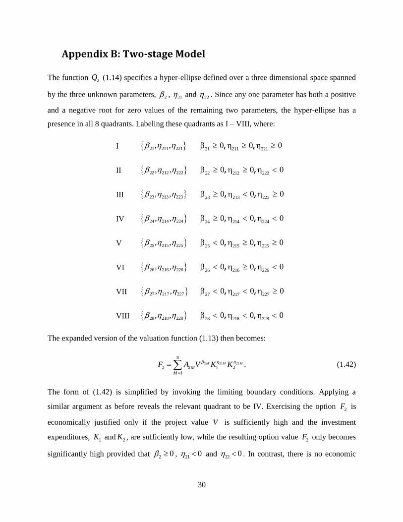
The function 2Q (1.14) specifies a hyper-ellipse defined over a three dimensional space spanned

by the three unknown parameters, 2 , 21 and 22 . Since any one parameter has both a positive

and a negative root for zero values of the remaining two parameters, the hyper-ellipse has a

presence in all 8 quadrants. Labeling these quadrants as I – VIII, where:

I 21 211 221, , 21 211 221

0 0 0 , ,

II 22 212 222, , 22 212 222

0 0 0 , ,

III 23 213 223, , 23 213 223

0 0 0 , ,

IV 24 214 224, , 24 214 224

0 0 0 , ,

V 25 215 225, , 25 215 225

0 0 0 , ,

VI 26 216 226, , 26 216 226

0 0 0 , ,

VII 27 217 227, , 27 217 227

0 0 0 , ,

VIII 28 218 228, , 28 218 228

0 0 0 , ,

The expanded version of the valuation function (1.13) then becomes:

2 21 22

8

2 2 1 2

1

.M M M

M

M

F A V K K

(1.42)

The form of (1.42) is simplified by invoking the limiting boundary conditions. Applying a

similar argument as before reveals the relevant quadrant to be IV. Exercising the option 2F is

economically justified only if the project value V is sufficiently high and the investment

expenditures, 1K and 2K , are sufficiently low, while the resulting option value 2F only becomes

significantly high provided that 2 0 , 21 0 and 22 0 . In contrast, there is no economic

31

justification for exercising the option 2F whenever the project value is sufficiently low, or either

of the two investment expenditures, 1K and 2K , are sufficiently high. This suggests that the

quadrants other than IV are not relevant, and that their coefficients, 21A , 22A , 23A , 25A , 26A ,

27A and 28A , are all set to equal zero. Consequently, (1.42) simplifies to:

24 214 224

2 24 1 2 .F A V K K (1.43)

32

Appendix C: N-Stage Model

The value of the option to invest at the J N stage, denoted by 1N N NF F V ,K , ,K , is

described by a 1N dimensional partial differential equation, whose solution takes the form of a

recursive product power function:

1 2 1

1 2 1N N N NN N N

N N N N N NF A V K K K B F K

, (1.44)

where the power parameters for NF are related to the J according to:

1 3 2 1

1 1 3 2 1

2 1 3 2

1 1

1

1

1

1

N N N

N N N

N N N

N N N N

NN N

,

,

,

,

.

Also, we have 1N

N N NB A A

. The stage- N value matching relationship can now defined as:

1

1 1N N

N N ,N NN N ,N NNˆ ˆ ˆ ˆB F K F K

(1.45)

where 1ˆ ˆ ˆ, , ,N N NNV K K denote the respective optimal threshold levels with

1 1 1 2 1 1 1

1 1 1 1

1 1 2 1N N N N N

N ,N N N N N N

N N N N N N

ˆ ˆ ˆ ˆF F V ,K , ,K

ˆ ˆ ˆ ˆA V K K K .

The stage- N value matching relationship (1.45) is expressed in the form of a two factor

investment opportunity model, the value gained after exercise 1N ,NF

and the investment cost

NNK , so the thresholds can be determined from standard theoretical results. It follows that:

1 1 1 2 1 1 1

1 1 1 2 11

N N N N N NN ,N N N N N N N NN

N

ˆ ˆ ˆ ˆ ˆ ˆF A V K K K K

(1.46)

and

33

0

1 2 1

1 2 1

1 1

N

N N N N NNNN N N N N NN

N N

ˆ ˆ ˆ ˆ ˆV K K K KA

(1.47)

where

0 1 3 2 1

1 1 1

2 2 2 1

3 3 3 2 1

1 1 1 3 2 1

1 3 2 1

1

1

1

1

1

1

N N

N

N

N

N N N N

NN N

,

,

,

,

,

.

The parameter N is evaluated from the characteristic root equation, which can be expressed as:

2112

1 0N NN N N N N N N K N KQ r r . (1.48)

The variance term 2

N is given by:

2 Tw ΩwN (1.49)

where Ω is the 1N dimensional square variance-covariance matrix with its first diagonal

element being 2

V , the second 1

2

K , and so on until 2

NK . The off-diagonal elements denote the

corresponding covariances. The column vector w is given by:

1 3 2 1

1 3 2 1

1 3 2

1 2

1

1

1

w

1

1

1

N

N

N

N N

N

34

The full expression for 2 Tw ΩwN is:

1 2

2 1

1 1 2 2

1 1

2 22 2 2 2 2 2 2 2 2 2 2 2 2 2 21 1 1 11 2 2 1 1 2 2 2 1 1 2 3 22 2 2 2

2 22 2 2 21 1 11 2 12 2 2

2 2 2 2 2

1 3 2 1 1 1 3 2 2 1

1 1

1 1

1 1

N N N

N N

N V N N K N N K N N

K N N K N K

VK V K N VK V K N

VK V K

1 2 1 2

1 3 1 3

1 2 1 2

1 1 1 1

1 1

1 1 2 2 1

1 2 2 1

2 2

1 3 2 2 1

2 2

1 4 3 3 2 1

2

1 2 2 3 2 1

1 1 2 2 1

1

1 1

1 1

1 1

1 1

N N

N N

N N

N N

N N N

VK V K N N

K K K K N

K K K K N

K K K K N N N N

K K K K N N N

K K K K

2 3 2 3

2 4 2 4

2 2 2 2

2 1 2 1

2 2

3 2

1 2 2 1

2 2

1 4 3 3 2

2 2

1 5 4 4 3 2

2

1 2 2 3 3 2

1 1 2 3 2

1 2 3 2

1

1 1

1 1

1 1

1 1

1

N N

N N

N N

N N

N N

K K K K N

K K K K N

K K K K N N N N

K K K K N N N

K K K K N N

K K K

3 2

3 1 3 1

3 3

2 1 2 1

2 2

1 1

2

1 2 3

1 1 2 3

1 2 3

1 1 2

1 2

1

1 1

1 1

1

1 1

1

1

N N

N N N N

N N N N

N N N N

N N N N

N N N N

K N N N

K K K K N N N N

K K K K N N N

K K K K N N N

K K K K N N

K K K K N ,

Because of the homogeneity degree-one property, we have Tw 0i where i is the unit vector.

Note that for 1N , Tw 1 1 , .

Having evaluated N , we can solve for:

35

11

N

N

N

N

N

B

, (1.50)

and then NA is determined from:

1

N

N N NA B A

. (1.51)

The 1 1NA A and 1 1NB B are obtainable by applying (1.50) and (1.51) recursively, starting at

1J and ending at 1J N .

The solution to the stage-N investment decision is obtained through a process of backwardation,

starting from the stage-one decision. This backwardation process yields consecutively the values

of 1 2 1N, , , , 1 2 1NB ,B , ,B and 1 2 1NA ,A , ,A , which are required for evaluating N , NB

and NA . From these values, we can then determine the discriminatory boundary linking the

project value threshold ˆNV with the investment cost thresholds 1 2

ˆ ˆ ˆ, ,N N NNK K K . Further, for a

meaningful solution to the stage-N investment decision to be obtained, the 1 2 1N N, , , , have

to individually exceed 1, which demands because of (1.49) that 1 2 1N N .

36

Figure 1

Sequential Investment Process

37

Figure 2

The 2Q Function for Investment Stage 2

38

Table 1

Base Case Information

Project value drift rate V 0%

Project value volatility V 25%

Investment cost drift rate 1 2 3 4K K K K 0%

Investment cost volatility 1 2 3 4K K K K 5%

Stage 1 failure probability 1 0%

Stage 2 failure probability 2 10%

Stage 3 failure probability 3 20%

Stage 4 failure probability 4 40%

Risk-free probability r 6%

All the correlations between the project value and the investment costs at each stage are set to

equal zero, so the correlation matrix is specified by:

V 1K 2K 3K 4K

V 100%

1K 0% 100%

2K 0% 0% 100%

3K 0% 0% 0% 100%

4K 0% 0% 0% 0% 100%

39

Table 2

Base Case Results

Table 3

The Effect of Increasing the Failure Probability by a Constant Amount of 5%

Table 4

The Effect of Increasing the Project Value Volatility to 40%

STAGE VOLATILITY MEF V^ V^-SKN ROV

1 0.2550 1.9478 2.0551 51.3766 26.3766 75.0000

2 0.4918 1.4294 1.8534 92.6715 42.6715 50.0000

3 0.7015 1.2176 1.6929 126.9680 51.9680 51.1388

4 0.8535 1.2760 1.2720 127.1951 27.1951 32.0015

STAGE VOLATILITY MEF V^ V^-SKN ROV

VOLATILITY

CHANGE

ROV

CHANGE

1 0.2550 2.4065 1.7110 42.7750 17.7750 75.0000 100.00% 100.00%

2 0.6078 1.2875 1.8379 91.8968 41.8968 50.0000 123.58% 100.00%

3 0.7816 1.1757 1.5134 113.5060 38.5060 89.6858 111.42% 175.38%

4 0.9185 1.2401 1.1052 110.5242 10.5242 66.2623 107.62% 207.06%

STAGE VOLATILITY MEF V^ V^-SKN ROV

VOLATILITY

CHANGE

ROV

CHANGE

1 0.4031 1.4942 3.0234 75.5854 50.5854 75.0000 158.11% 100.00%

2 0.6003 1.3331 2.3861 119.3041 69.3041 52.8006 122.06% 105.60%

3 0.7992 1.1856 2.3238 174.2822 99.2822 36.2633 113.93% 70.91%

4 0.9471 1.2445 1.7016 170.1619 70.1619 21.4385 110.97% 66.99%

40

Table 5

The Effect of Increasing all Investment Cost Volatilities to 10%

Table 6

The Effect of Increasing the Correlation between the Project Value

and the Investment Cost at All Stages to 50%

Table 7

The Effect of Decreasing the Correlation between the Project Value

and the Investment Cost at All Stages -50%

STAGE VOLATILITY MEF V^ V^-SKN ROV

VOLATILITY

CHANGE

ROV

CHANGE

1 0.2693 1.8803 2.1360 53.4001 28.4001 75.0000 105.61% 100.00%

2 0.4886 1.4329 1.8862 94.3122 44.3122 50.0000 99.35% 100.00%

3 0.6939 1.2204 1.7395 130.4646 55.4646 47.3204 98.92% 92.53%

4 0.8442 1.2794 1.3083 130.8269 30.8269 28.8968 98.91% 90.30%

STAGE VOLATILITY MEF V^ V^-SKN ROV

VOLATILITY

CHANGE

ROV

CHANGE

1 0.2291 2.0924 1.9154 47.8855 22.8855 75.0000 89.87% 100.00%

2 0.4737 1.4492 1.7485 87.4271 37.4271 50.0000 96.32% 100.00%

3 0.6849 1.2237 1.5680 117.6004 42.6004 61.2297 97.63% 119.73%

4 0.8374 1.2819 1.1815 118.1465 18.1465 40.1191 98.12% 125.37%

STAGE VOLATILITY MEF V^ V^-SKN ROV

VOLATILITY

CHANGE

ROV

CHANGE

1 0.2784 1.8410 2.1890 54.7251 29.7251 75.0000 109.19% 100.00%

2 0.5084 1.4123 1.9445 97.2253 47.2253 50.0000 103.38% 100.00%

3 0.7166 1.2122 1.8022 135.1672 60.1672 45.5708 102.16% 89.11%

4 0.8681 1.2707 1.3500 134.9974 34.9974 27.7605 101.71% 86.75%

41

Table 2A

Alternative Base Case Results

Table 3A

The Effect of Increasing the Failure Probability by a Constant Amount of 5%

Table 4A

The Effect of Increasing the Project Value Volatility to 40%

STAGE VOLATILITY MEF V^ V^-SKN ROV

1 0.2550 1.9478 2.0551 51.3766 26.3766 16.1987

2 0.4918 1.4294 1.8534 92.6715 42.6715 5.6119

3 0.7015 1.2176 1.6929 126.9680 51.9680 2.2892

4 0.8535 1.2760 1.2720 127.1951 27.1951 0.6079

STAGE VOLATILITY MEF V^ V^-SKN ROV

VOLATILITY

CHANGE

ROV

CHANGE

1 0.2550 2.4065 1.7110 42.7750 17.7750 15.1255 100.00% 93.37%

2 0.6078 1.2875 1.8379 91.8968 41.8968 6.6070 123.58% 117.73%

3 0.7816 1.1757 1.5134 113.5060 38.5060 3.1850 111.42% 139.13%

4 0.9185 1.2401 1.1052 110.5242 10.5242 1.0559 107.62% 173.71%

STAGE VOLATILITY MEF V^ V^-SKN ROV

VOLATILITY

CHANGE

ROV

CHANGE

1 0.4031 1.4942 3.0234 75.5854 50.5854 19.5460 158.11% 120.66%

2 0.6003 1.3331 2.3861 119.3041 69.3041 8.5105 122.06% 151.65%

3 0.7992 1.1856 2.3238 174.2822 99.2822 4.1651 113.93% 181.94%

4 0.9471 1.2445 1.7016 170.1619 70.1619 1.4508 110.97% 238.66%

42

Table 5A

The Effect of Increasing all Investment Cost Volatilities to 10%

Table 6A

The Effect of Increasing the Correlation between the Project Value

and the Investment Cost at All Stages to 50%

Table 7A

The Effect of Decreasing the Correlation between the Project Value

and the Investment Cost at All Stages -50%

STAGE VOLATILITY MEF V^ V^-SKN ROV

VOLATILITY

CHANGE

ROV

CHANGE

1 0.2693 1.8803 2.1360 53.4001 28.4001 16.4960 105.61% 101.83%

2 0.4886 1.4329 1.8862 94.3122 44.3122 5.7279 99.35% 102.07%

3 0.6939 1.2204 1.7395 130.4646 55.4646 2.3263 98.92% 101.62%

4 0.8442 1.2794 1.3083 130.8269 30.8269 0.6122 98.91% 100.72%

STAGE VOLATILITY MEF V^ V^-SKN ROV

VOLATILITY

CHANGE

ROV

CHANGE

1 0.2291 2.0924 1.9154 47.8855 22.8855 15.7055 89.87% 96.96%

2 0.4737 1.4492 1.7485 87.4271 37.4271 5.1964 96.32% 92.60%

3 0.6849 1.2237 1.5680 117.6004 42.6004 2.0431 97.63% 89.25%

4 0.8374 1.2819 1.1815 118.1465 18.1465 0.5133 98.12% 84.45%

STAGE VOLATILITY MEF V^ V^-SKN ROV

VOLATILITY

CHANGE

ROV

CHANGE

1 0.2784 1.8410 2.1890 54.7251 29.7251 16.6920 109.19% 103.05%

2 0.5084 1.4123 1.9445 97.2253 47.2253 6.0224 103.38% 107.31%

3 0.7166 1.2122 1.8022 135.1672 60.1672 2.5375 102.16% 110.85%

4 0.8681 1.2707 1.3500 134.9974 34.9974 0.7073 101.71% 116.35%

43

References

Adkins, R., and D. Paxson. "Renewing assets with uncertain revenues and operating costs."

Journal of Financial and Quantitative Analysis 46 (2011), 785-813.

Agliardi, E., and R. Agliardi. "A generalization of Geske formula for compound options".

Mathematical Social Sciences 45 (2003), 75-82.

Agliardi, E., and R. Agliardi. "A closed-form solution for multicompound options". Risk Letters

(2005).

Andergassen, R. and L. Sereno. "Valuation of N-stage investments under jump-diffusion".

Computational Finance (2012).

Bar-Ilan, A., and W. C. Strange. "A model of sequential investment." Journal of Economic

Dynamics and Control 22 (1998), 437-463.

Brach, M. A., and D. A. Paxson. "A gene to drug venture: Poisson options analysis." R&D

Management 31 (2001), 203-214.

Carr, P. "The valuation of sequential exchange opportunities." Journal of Finance 43 (1988),

1235-1256.

Cassimon, D., Engelen, P.J., Thomassen, L., and M. Van Wouwe. "The valuation of a NDA

using a 6-fold compound option". Research Policy 33 (2004), 41-51.

Cassimon, D., Engelen, P.J., and V. Yordanov. "Compound real option valuation with phase-

specific volatility: a multi-phase mobile payments case study". Technovation (2011).

Childs, P. D., and A. J. Triantis. "Dynamic R&D investment policies." Management Science 45

(1999), 1359-1377.

Cortazar, G., Schwartz, E. and J.Casassus. "Optimal exploration investments under price and

geological-technical uncertainty: a real options model". in Real R&D Options, D. Paxson, ed.,

Butterworth-Heinemann, Oxford, (2003), 149-165.

Cortelezzi, F., and G. Villani. "Valuation of R&D sequential exchange options using Monte

Carlo approach". Computational Economics 33 (2009), 209-236.

Dixit, A. "The art of smooth pasting." In Fundamentals of Pure and Applied Economics,55, J.

Lesourne and H. Sonnenschein, eds. Chur (Switzerland): Harwood Academic Press (1993).

Dixit, A. K., and R. S. Pindyck. Investment under Uncertainty. Princeton, NJ: Princeton

University Press (1994).

Gukhal, C.R. "The compound option approach to American option on jump-diffusion". Journal

of Economic Dynamics and Control, 28 (2004), 2035-2074.

Huang, Y.L. and C.C.Pi. "Valuation of multi-stage BOT projects involving dedicated asset

investments: a sequential compound option approach". Construction Management and

Economics (2009).

Lee, J., and D. A. Paxson. "Valuation of R&D real American sequential exchange options."

R&D Management 31 (2001), 191-201.

Lee, M.Y., Yeh, F.B. and A.P. Chen. "The generalized sequential compound options pricing and

sensitivity analysis". Mathematical Social Sciences (2008).

Majd, S., and R. S. Pindyck. "Time to build, option value, and investment decisions." Journal of

Financial Economics 18 (1987), 7-27.

McDonald, R. L., and D. R. Siegel. "The value of waiting to invest." Quarterly Journal of

Economics 101 (1986), 707-728.

Pendharkar. P. "Valuing interdependent multi-stage it investment: a real options approach".

European Journal of Operational Research 201 (2010), 847-859.

44

Pennings, E. and L. Sereno. "Evaluating pharmaceutical R&D under technical and economic

uncertainty". European Journal of Operational Research 212 (2012), 374-385.

Samuelson, P. A. "Rational theory of warrant pricing." Industrial Management Review 6 (1965),

13-32.

Schwartz, E. S., and M. Moon. "Evaluating research and development investments." In Project

Flexibility, Agency, and Competition, M. J. Brennan and L. Trigeorgis, eds. Oxford: Oxford

University Press (2000), 85-106.

Sydsæter, K., Hammond, P., Seierstad, A. and A. Strøm. Further Mathematics for Economic

Analysis. Harlow, England: Prentice-Hall (2005).

Tourinho, O.A.F. The valuation of reserves of natural resources: An option pricing approach.

PhD thesis, University of California, Berkeley, 1979.