An Analysis of the Height of Tries with Random Weights …luc.devroye.org/tries_weighted.pdfAn...

An Analysis of the Height of Tries with

Random Weights on the Edges

N. Broutin L. Devroye∗

September 10, 2007

Abstract

We analyze the weighted height of random tries built from independent stringsof i.i.d. symbols on the finite alphabet 1, . . . , d. The edges receive random weightswhose distribution depends upon the number of strings that visit that edge. Such amodel covers the hybrid tries of de la Briandais (1959) and the TST of Bentley andSedgewick (1997), where the search time for a string can be decomposed as a sum ofprocessing times for each symbol in the string. Our weighted trie model also permitsone to study maximal path imbalance. In all cases, the weighted height is shown beasymptotic to c logn in probability, where c is determined by the behavior of the coreof the trie (the part where all nodes have a full set of children) and the fringe of thetrie (the part of the trie where nodes have only one child and form spaghetti-like trees).It can be found by maximizing a function that is related to the Cramer exponent ofthe distribution of the edge weights.

Keywords: data structure, trie, TST, random tree, height, branching random walk.

1 Introduction

Tries are tree-like data structures that have been introduced by de la Briandais (1959) andFredkin (1960) in order to efficiently store and manipulate strings. They find a multitudeof applications in computer science and telecommunications (see, e.g., Szpankowski, 2001;Flajolet, 2006). Consider n strings, each consisting of an infinite sequence of symbols takenfrom a finite alphabet A. We assume without loss of generality that A = 1, 2, . . . , d. Eachsequence defines an infinite path in an infinite d-ary position tree T∞. If the sequences aredistinct, then the paths are distinct as well. We trim T∞ by cutting every branch belowthe shallowest node that belongs to a single path. The trie is the resulting finite tree, andthe strings are stored in the leaves. In the usual array-based implementation of the datastructure, the worst-case time to answer a search query corresponds to the height of the trie,i.e., the maximum number of edges on a path from the root. The heights of tries have beenstudied by many authors under various model of randomness for the sequences. For moreinformation about general models, see Szpankowski (2001), Clement, Flajolet, and Vallee(2001), Flajolet (2006) and the references found there.

Here, we assume that the sequences are built using a memoryless source: each string isan infinite sequence of independent and identically distributed (i.i.d.) symbols distributedlike X, where P X = i = pi, 1 ≤ i ≤ d. In addition, we assume that the strings are

∗Research of the authors was supported by NSERC Grant A3456 and a James McGill fellowship.Address: School of Computer Science, McGill University, Montreal H3A2K6 Canada. Email: nico-

[email protected], [email protected].

1

independent. It is well-known that the height Hn of a trie built from n such sequencessatisfies (Regnier, 1981; Devroye, 1984; Pittel, 1985; Szpankowski, 1991, 2001)

Hn

log n−−−−→n→∞ − 2

logQ(2)in probability, (1)

where

Q(b) =d∑i=1

pbi (2)

is the probability that b ≥ 1 independent characters are identical. This result holds whenevery leaf contains only one string. If the leaves can store up to b strings, the tree is calleda b-trie (see, e.g., Szpankowski, 2001) and its height Hn,b is such that

Hn,b

log n−−−−→n→∞ − b+ 1

logQ(b+ 1)in probability.

The usual implementation of a trie uses an array for the branching structure of a node(Fredkin, 1960). Although this always ensures constant-time shunting of the words in thesubtrees, the space required may become an issue for large alphabets: many pointers wouldbe left unused. To avoid this, one can replace the array by variable size structures. Thereare essentially two solutions which have been considered. De la Briandais (1959) proposed touse linked-lists, and we shall call the implementation a list-trie. More recently, building onearly ideas of Clampett (1964), Bentley and Sedgewick (1997) developed an elegant structurebased on binary search trees going by the name of bst-trie, ternary search trie or TST forshort.

These alternative implementations aim at a trade-off between storage space and speed,and the access time to children of a node is no longer constant. In particular, the height ofthe tree and the worst-case search time are different in general. List-tries and TST may beseen as high-level tries whose edges are weighted to reflect the internal low-level structureused to organize the children of a node. This point of view has been taken by Clement,Flajolet, and Vallee (1998, 2001) who thoroughly analyzed these hybrid implementations oftries. In particular, they analyzed the average size and average depth. The question of theworst-case search time in hybrid-tries was left open. This paper addresses the latter questionby studying the weighted height of a general model of weighted tries that encompass hybridtries.

The analysis requires the new ideas of Broutin and Devroye (2007a) who distinguish twodifferent regions in the trie. We shall motivate the need for such a distinction and give moreinsight about the model using an example.

Example: randomized list-tries. Assume that the low level structure used to implementthe set of subtrees at a node is a list. Assume for simplicity that the alphabet is 1, 2 andthat, for each node, an independent coin is flipped to decide which subtree will be first in thelist. Then, one can easily see that the nodes do not all behave in the same way with respectto the costs: Towards the top of the tree, the nodes tend to have two children, and the costof going to any of them is 1 or 2, each case occurring with probability 1/2. Towards thebottom of the tree, however, many nodes only have one child and the cost is then always 1.

Even this simple example shows that one should distinguish a region that is close tothe root —the core— from the fringe of the tree —the spaghettis— (precise definitions willfollow). We will see in the following (Lemma 1) that this simple binary distinction suffices toexplain properties of tries such as the height and the profile. The distinction is not necessary

2

to obtain parameters like the average cost of looking up a sequence because the number ofnodes in the spaghettis is negligible compared to that in the core. This partly explains whythe average weighted depth was know already (Clement et al., 1998, 2001). The situationis of course radically different if one is interested in the height for which every single nodeis relevant.

Figure 1. The structure of a trie: the bulk is thecore, then some spaghetti-like trees hang down thecore. Both the core and the spaghettis contributesignificantly to the height of the trie. Observealso that the height may not be explained by aspaghetti born at one of the deepest nodes of thecore. This latter fact will become clear later.

Our main result (Theorem 1) is a law of large numbers for the (weighted) height of ageneral model of random tries. Roughly speaking, we prove that the height of such trieson n sequences is asymptotic to c log n in probability, where c is characterized using largedeviation techniques. The constant c is the sum of the contributions of the core and thespaghettis.

Our method has several advantages. First, it yields the first order asymptotics of theheight of hybrid-tries (see Clement et al., 1998, 2001, for more on this). But it also permitsto shed new light on the family of digital trees. The profile of the core also happens to bethe profile of digital search trees, a related model discussed more precisely later. In thissense, our methods unify the treatment of tries and digital search trees. This similarity goesfurther than the mere case of digital trees, and our methods rely on the branching processestreatment of trees of Broutin et al. (2007).

A detailed plan of the paper can be found at the end of Section 2, where we introduce themodel more precisely and we sketch the key steps explaining our results. An early versionof the results and the case of hybrid tries in particular in an extended abstract (see Broutinand Devroye, 2007b).

2 Random weighted tries

2.1 Constructing tries via an embedding

In this section, we propose an embedding to construct weighted tries. We will see in Section 7that hybrid-tries, like list-tries and TST, can be seen as weighted tries built using thisprocess.

Consider the distribution p1, . . . , pd over the alphabet A = 1, 2, . . . , d. We assumewithout loss of generality that 1 > p1 ≥ p2 ≥ · · · ≥ pd > 0. We are given n independent

3

strings, each consisting of an infinite sequence of i.i.d. characters of A distributed as X,where P X = i = pi, 1 ≤ i ≤ d. A weighted b-trie is built in two steps as follows: firstit is given a shape (unweighted tree), the weights are then assigned to the edges using theshape.

The shape of the trie. Each string defines an infinite path in T∞. For a node u ∈ T∞,let N?

u be the number of strings whose paths in T∞ intersect u. Then, for a natural numberb ≥ 1, the b-trie Tn,b consists of the root together with the nodes whose parent v has N?

v > b:

Tn,b = all nodes u whose parent v has N?v > b ∪ root.

We can then define the cardinality Nu of a node u ∈ T∞ as the number of strings intersectingu within Tn,b. Observe that we have Nu = 0 if u 6∈ Tn,b. The sequences are distinct withprobability one, and the strings define distinct paths in T∞. Therefore, the trie Tn,b isalmost surely finite. The tree Tn,b constitutes the shape of the weighted trie, and may berepresented by the sequence Nu : u ∈ T∞. For the edge e between u and its i-th child welet pe = pi and Ee = − log pe.

Remark. For a specified edge e, Ee is deterministic. The values will later become randomafter some symmetrization process among the child edges of a node.

5

3

2

2

11

1

1

1

1

5

3

2

2

1 00

000

Figure 2. The way cardinalities are defined for a 2-trie. On the left we have represented thesequences and the values of N?

u , u ∈ T∞. On the right, the white nodes are those not in the 2-trie,and the labels are the values of the cardinalities Nu, u ∈ T∞.

As a position tree, Tn,b potentially contains 2d types of nodes, each type being char-acteristic of the subset of children that are present. The type of every node u ∈ Tn,b isrepresented by a d-vector τu: if u1, . . . , ud are the d children of u in T∞, then we define

τu = (1[Nui ≥ 1],1[Nu2 ≥ 1], . . . ,1[Nud ≥ 1]) ,

where 1[A] = 1 if and only if the event A holds. The weights of the edges to u1, . . . , ud areassigned depending on the type τu.

The weights. Consider a collection Z of random vectors Zτ , τ ∈ 0, 1d, where Zτ =(Zτ1 , . . . , Z

τd ). For a fixed type τ ∈ 0, 1d, the components of Zτ may be dependent. Also,

the members of the collection may be dependent. Each node of T∞ is given an independentcopy of Z. We always assume that there is a constant a such that |Zτi | ≤ a for all τ ∈ 0, 1dand i ∈ 1, . . . , d. Consider a node u ∈ T∞, and its sequence Zτ. The weights of thechild edges of u are assigned using the vector Zτu only. In particular, the edge ei betweenu and its i-th child in T∞ is given the weight

Zei = Zτui =∑

τ∈0,1dZτi · 1[τu = τ ].

4

We use the notations Zτi and Ze interchangeably. It should always be clear whether asubscript refers to an index or an edge. The weighted tree obtained in this way is called arandom trie with weight sequence distribution Zτ , τ ∈ 0, 1d and source p1, . . . , pd.

Example. Let d = 2. The collection of weights Z such that Z(0,0) = (0, 0), Z(1,0) =(X, 0), Z(0,1) = (0, X) and Z(1,1) = (X,X) where X is a [0, 1]-uniform random variable isacceptable.

Example: Randomized list-tries. Consider the example of binary list-tries of Section 1.The shape is the regular (unweighted) trie. The weight accounts for the costs to branch tosubtrees. When the subtrees are ordered randomly in the list, we have

Z(1,1) =

(1, 2) w.p. 1/2(2, 1) w.p. 1/2,

and Z(0,1) = Z(1,0) = Z(0,0) = (1, 1). Observe that the weights associated to edges going toempty subtrees are irrelevant.

Remark. Our construction emphasizes an underlying structure consisting of independentrandom vectors associated with the nodes of T∞. However, in the coupled trie built fromthe embedding, the random variables Nu : u ∈ T∞ and Ze associated respectively withthe nodes and the edges of T∞ are dependent: the values of Nu : u ∈ T∞ influence thetypes τu : u ∈ T∞ which in turn influence the weights Ze.

Let π(u) be the set of edges on the path from u to the root of T∞. The weighted depthof a node u ∈ T∞ is defined by Du =

∑e∈π(u) Ze. We are interested in the weighted height

of Tn,b defined byHn,b = maxDu : u ∈ Tn,b.

Surprisingly, if the weights are non-negative and bounded, Hn,b ∼ cb log n in probability,and cb depends only on

• the distribution p1, . . . , pd,

• the capacity b of the leaves,

• the distribution of Z(1,...,1), and

• the distributions of Zτ , for all a permutations τ of (1, 0, . . . , 0).

In particular, the first order asymptotics of Hn,b stay the same if we modify the distributionof Z in such a way that the above parameters remain unchanged. In other words, the onlynodes whose weights affect the first order term of the height are the ones having either dchildren or a single child in Tn,b. This is easily understood by thinking of the structure ofthe shape of a trie.

2.2 Understanding the height using the structure of a trie

The reason why only the nodes with either one single child or d children affect the first orderasymptotics of the height is simply that the other types are negligible when looking at anypath.

Lemma 1. Let Tn,b be a random trie. Let m = m(n)→∞ such that m = o(log n). Thereexists ω = ω(n)→∞, as n→∞ such that:(a) with probability at least 1− n−ω, all the nodes u with Nu ≥ log2 n have τu = (1, . . . , 1),(b) the maximum number of nodes with Nu ≥ m(n) and τu 6= (1, . . . , 1) on a path from the

root is o(log n) with probability at least 1− n−ω, and

5

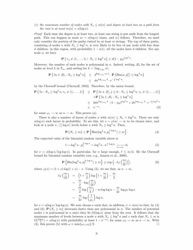
(c) the maximum number of nodes with Nu ≤ m(n) and degree at least two on a path fromthe root is at most m(n) = o(log n).

Proof. Each time the degree is at least two, at least one string is put aside from the longestpath. This can happen at most m = o(log n) times, and (c) follows. Therefore, we needonly consider the portion of the paths visited by at least m strings. The top of these paths,consisting of nodes u with Nu ≥ log2 n, is very likely to be free of any node with less thand children: in this region, with probability 1− o(1), all the nodes have d children. For anynode u, we have

Pτu 6= (1, . . . , 1) | Nu ≥ log2 n

≤ d(1− pd)log2 n.

Moreover, the number of such nodes is polynomial in n. Indeed, writing Lk for the set ofnodes at level k in T∞, and setting for k = dlog1/p1 ne,

P∃u ∈ Lk : Nu ≥ log2 n

≤ dlog1/p1

n+1 ·P

Bin(n, pk1) ≥ log2 n

≤ dnlog1/p1d · e− 1

2 log2 n,

by the Chernoff bound (Chernoff, 1952). Therefore, by the union bound,

P∃u : Nu ≥ log2 n, τu 6= (1, . . . , 1)

≤ P

∃u ∈ Lj , j ≤ k : Nu ≥ log2 n, τu 6= (1, . . . , 1)

+P

∃u ∈ Lk : Nu ≥ log2 n

≤ 2dnlog1/p1

d · (1− pd)log2 n + dnlog1/p1d · e− 1

2 log2 n

≤ n−ω1 , (3)

for some ω1 →∞ as n→∞. This proves (a).There is also a number of layers of nodes u with m(n) ≤ Nu < log2 n. There are only

o(log n) such layers in probability. To see this, let ν = ν(n) → ∞ to be chosen later, andlook at a node v, d 1

ν log ne levels below u with Nu ≤ log2 n. Then,

P Nv ≥ m ≤ P

Bin(log2 n, p1ν logn1 ) ≥ m

. (4)

The expected value of the binomial random variable above is

` = log2 n · p1ν logn1 = log2 n · n 1

ν log p1 −−−−→n→∞ 0, (5)

for ν = o(log n/ log log n). In particular, for n large enough, ` ≤ m/2. By the Chernoffbound for binomial random variables (see, e.g., Janson et al., 2000),

P

Bin(log2 n, pam logn1 ) ≥ m

≤ exp

(−`ϕ

(m2`

)), (6)

where ϕ(x) = (1 + x) log(1 + x)− x. Using (5), we see that, as n→∞,

`ϕ(m

2`

)=

(`+

m

2

)log(

1 +m

2`

)− m

2

∼ m

2· log

(m2`

)∼ m

2log(m

2

)−m log log n− m

2νlog p1 log n

∼ m

2νlog(

1p1

)log n,

for ν = o(log n/ log log n). We now choose ν such that, in addition, ν = o(m) so that, by (4)and (6), P Nv ≥ m decreases faster than any polynomial in n. The number of potentialnodes v is polynomial in n since they lie O(log n) away from the root. It follows that themaximum number of levels between a node u with Nu ≤ log2 n and v such that Nv ≤ m isO( logn

ν ) = o(log n) with probability at least 1 − n−ω2 , for some ω2 → ∞ as n → ∞. With(3), this proves (b) with ω = minω1, ω2/2.

6

Lemma 1 justifies the distinction of two regions in a trie: a so-called core, that essentiallyconsists of the nodes of out degree d, and spaghetti -like trees hanging from the core (seeBroutin and Devroye, 2007a).

The core of a trie. What we call the core here should not be confused with the graph-theoretic core, which happens to be empty for trees (see, e.g., Janson et al., 2000). Thecore of the trie is defined to be the set of nodes u ∈ T∞ for which Nu ≥ m = m(n), form(n)→∞ and m(n) = o(log n). The core is denoted by C. By Lemma 1, on any path fromthe root, the number of nodes in the core which are not of type τ = (1, . . . , 1) is o(log n) inprobability. As a consequence, when looking at a path of length Θ(log n) in a weighted trie,the distribution of weights in the core should be closely approximated by Zc = Z(1,...,1).The core can be described by its logarithmic profile

φ(α, t) = limn→∞

log EPm(t log n, α log n)log n

∀t, α > 0, (7)

where Pm(k, h) denotes the number of nodes u ∈ T∞, k levels away from the root withNu ≥ m and Du ≥ h. In other words, assuming for now that the limit in (7) exists, we haveEPm(t log n, α log n) = nφ(α,t)+o(1), as n→∞. This will be proved, and the function φ(·, ·)will be characterized in Section 4 (Theorem 3).

Hanging spaghettis. The spaghettis are the trees remaining when pulling out the corefrom the trie. They lie in the part of the trie where the nodes do not have d childrenwith high probability anymore: the types of the nodes may take all the values in 0, 1d.However, by Lemma 1, in any spaghetti, the number of nodes with at least two children iso(log n). Since the weights are bounded, these o(log n) terms contribute at most o(log n) tothe height. Therefore, to first order, only the nodes of degree one affect the height. Thisexplains why only Zτ for τ a permutation of (1, 0, . . . , 0) matter in the weighted heights ofspaghettis.

Understanding the height. Both the core and the spaghettis contribute significantlyto the height of a weighted trie. By figuring out what the core looks like, we can determinewhen the spaghettis take over. Roughly speaking, we then know if an edge’s weight can beapproximated by a component of Z(1,...,1), characteristic of the core, or rather Zτ , for τ apermutation of (1, 0, . . . , 0), characteristic of the spaghettis. Each spaghetti is rooted at anode u ∈ ∂C, the external node-boundary of the core C in Tn,b (the nodes u ∈ ∂C are thechildren of some node v in the core, but are not themselves in the core). Recall that Lk

denotes the set of nodes at level k in T∞. Then, if we write Wu for the (weighted) height ofthe subtree rooted at u, we have

Hn,b = maxDu +Wu : u ∈ ∂C = suph,kh+Wu : u ∈ ∂C ∩Lk, Du ≥ h,

where the nodes in ∂C have been split into groups depending on their level k and weighteddepth h. Thus, we can rewrite

Hn,b = suph,kh+ maxWu : u ∈ ∂C, Du ≥ h, u ∈ Lk.

We have separated the contributions of the core and the spaghettis,

h and maxWu : u ∈ ∂C, Du ≥ h, u ∈ Lk,

respectively. The height is simply the maximum value of the sum of these two terms, and weneed to characterize them in order to pin down the asymptotic value of the height. The firstterm is just h ∼ α log n, a parameter. The second one amounts to studying the weighted

7

height of the forest of conditionally independent random tries rooted at the nodes u ∈ Lk

with Du ≥ h. When k ∼ t log n and h ∼ α log n, we have

limn→∞

maxWu : u ∈ ∂C, Du ≥ h, u ∈ Lklog n

= φ(α, t) · γb in probability, (8)

for some constant γb characterizing the depths in spaghettis. This will be proved, andγb will be characterized in Section 5 (Theorem 6) where we study forests of independentrandom tries. The two parameters φ(·, ·) and γb suffice to obtain the first order term of theasymptotic expansion of the height. Our main result is the following theorem.

Theorem 1. Consider Tn,b, a weighted b-trie with non-negative weight sequence Zτ , τ ∈0, 1d built from n independent sequences with distribution p1, . . . , pd. Let Hn,b be itsweighted height. Assume that the weights Zτ are bounded. Let φ(α, t) be the logarithmicweighted profile of the core of Tn,b defined in (7), and γb the constant defined in (8). Let

cb = sup α+ γb · φ(α, t) : α, t > 0 .

Then Hn,b = cb log n+ o(log n) in probability, as n→∞.

Remarks. (a) For Theorem 1 to be useful in applications, we show that φ(·, ·) and γb arecomputable in Theorems 3 and 6, respectively.(b) The definition of cb given makes it clear that, as long as the weights take positive valueswith positive probability, cb > 0 is well and uniquely defined. We will see later that cb <∞.

The rest of the paper is organized as follows. The core and spaghettis are analyzed indetail in Sections 4 and 5, respectively. In Section 6, we prove Theorem 1. Finally, wepresent some applications in Section 7, with in particular, the heights of the trees of de laBriandais (1959) and of the TST of Bentley and Sedgewick (1997). The proofs are basedon large deviations, in particular φ(·, ·) and γb are characterized in terms of large deviationrate functions.

3 Review of large deviations

In this section, we review large deviation theory. For a more complete treatment, see thetextbooks of Deuschel and Stroock (1989), Dembo and Zeitouni (1998), or den Hollander(2000). We are interested in the case of extended random vectors (Z,E), that is, for whichZ = −∞ may happen with positive probability. The reason will become clear when weanalyze the behavior of spaghettis in Section 5. In the following, for a function f takingvalues in (−∞,∞], we define its domain Df = x : f(x) <∞, with interior Dof .

Let Xi, 1 ≤ i ≤ n be a family of i.i.d. extended random vectors distributed like (Z,E).Assume Z ∈ [−∞,∞) and E ∈ [0,∞). Set κ = P Z > −∞. For α and ρ real numbers,we are interested in the tail probability

P

n∑i=1

Zi > αn,

n∑i=1

Ei < ρn

, (9)

whose magnitude is dealt with by Cramer’s theorem (Cramer, 1938). Define the cumulantgenerating function Λ of the (extended) random vector (Z,E) by

Λ(λ, µ) = log E[eλZ+µE

∣∣ Z > −∞]

+ log κ ∀λ, µ ∈ R.

The tail probability in (9) is characterized using Λ?(·, ·), the Fenchel–Legendre or convexdual of Λ (see Rockafellar, 1970): we define

Λ?(α, ρ) = supλ,µλα+ µρ− Λ(λ, µ) ∀α, ρ ∈ R.

8

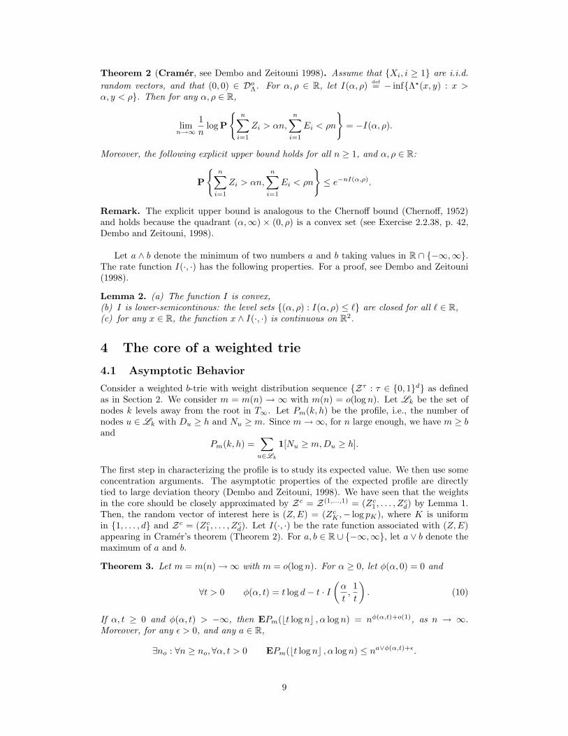
Theorem 2 (Cramer, see Dembo and Zeitouni 1998). Assume that Xi, i ≥ 1 are i.i.d.random vectors, and that (0, 0) ∈ DoΛ. For α, ρ ∈ R, let I(α, ρ) def= − infΛ?(x, y) : x >α, y < ρ. Then for any α, ρ ∈ R,

limn→∞

1n

log P

n∑i=1

Zi > αn,

n∑i=1

Ei < ρn

= −I(α, ρ).

Moreover, the following explicit upper bound holds for all n ≥ 1, and α, ρ ∈ R:

P

n∑i=1

Zi > αn,

n∑i=1

Ei < ρn

≤ e−nI(α,ρ).

Remark. The explicit upper bound is analogous to the Chernoff bound (Chernoff, 1952)and holds because the quadrant (α,∞) × (0, ρ) is a convex set (see Exercise 2.2.38, p. 42,Dembo and Zeitouni, 1998).

Let a ∧ b denote the minimum of two numbers a and b taking values in R ∩ −∞,∞.The rate function I(·, ·) has the following properties. For a proof, see Dembo and Zeitouni(1998).

Lemma 2. (a) The function I is convex,(b) I is lower-semicontinous: the level sets (α, ρ) : I(α, ρ) ≤ ` are closed for all ` ∈ R,(c) for any x ∈ R, the function x ∧ I(·, ·) is continuous on R2.

4 The core of a weighted trie

4.1 Asymptotic Behavior

Consider a weighted b-trie with weight distribution sequence Zτ : τ ∈ 0, 1d as definedas in Section 2. We consider m = m(n) → ∞ with m(n) = o(log n). Let Lk be the set ofnodes k levels away from the root in T∞. Let Pm(k, h) be the profile, i.e., the number ofnodes u ∈ Lk with Du ≥ h and Nu ≥ m. Since m→∞, for n large enough, we have m ≥ band

Pm(k, h) =∑u∈Lk

1[Nu ≥ m,Du ≥ h].

The first step in characterizing the profile is to study its expected value. We then use someconcentration arguments. The asymptotic properties of the expected profile are directlytied to large deviation theory (Dembo and Zeitouni, 1998). We have seen that the weightsin the core should be closely approximated by Zc = Z(1,...,1) = (Zc1, . . . , Z

cd) by Lemma 1.

Then, the random vector of interest here is (Z,E) = (ZcK ,− log pK), where K is uniformin 1, . . . , d and Zc = (Zc1, . . . , Z

cd). Let I(·, ·) be the rate function associated with (Z,E)

appearing in Cramer’s theorem (Theorem 2). For a, b ∈ R ∪ −∞,∞, let a ∨ b denote themaximum of a and b.

Theorem 3. Let m = m(n)→∞ with m = o(log n). For α ≥ 0, let φ(α, 0) = 0 and

∀t > 0 φ(α, t) = t log d− t · I(α

t,

1t

). (10)

If α, t ≥ 0 and φ(α, t) > −∞, then EPm(bt log nc , α log n) = nφ(α,t)+o(1), as n → ∞.Moreover, for any ε > 0, and any a ∈ R,

∃no : ∀n ≥ no,∀α, t > 0 EPm(bt log nc , α log n) ≤ na∨φ(α,t)+ε.

9

Remarks. (a) Observe that Theorem 3 justifies the definition of φ(·, ·) in (7).(b) The constraint that m(n) is o(log n) is only used in the lower bound. However, the mainreason why we choose m = o(log n) is for the spaghettis to contain each only o(log n) nodesof degree at least two.(c) If k ∼ t log n and h ∼ α log n, we also have EPm(k, h) = nφ(α,t)+o(1). The proof isslightly more technical but does not shed any new light.

Unlike the profile of unweighted tries (Devroye, 2002, 2005; Park et al., 2006), that ofweighted tries does not seem concentrated. In regular (unweighted) tries, the modificationof one single sequence may affect Pm(k, 0) by at most one, and contrasts with the case ofweighted tries where Pm(k, h) may potentially change a lot. However, it is log-concentratedin the sense of the following theorem.

Theorem 4. Let m = m(n) → ∞ as n → ∞ such that m = o(log n). Let k ∼ t log n andh ∼ α log n for some positive constants t and α. Then, for all ε > 0, as n→∞,

PPm(k, h) ≤ nφ(α,t)−ε

−−−−→n→∞ 0.

For all a ∈ R, and all ε > 0, there exists no large enough such that

∀n ≥ no supα,t≥0

PPm(bt log nc , α log n) ≥ na∨φ(α,t)+ε

≤ n−ε/2.

Remark. In the upper bound, the use of a∨ φ(α, t), a ∈ R, is necessary since it is possiblethat φ(α, t) = −∞. In such a case nφ(α,t)+ε = 0 for all n ≥ 2, and of course,

PPm(bt log nc , α log n) ≥ nφ(α,t)+ε

= 1.

Lemma 3. Let φ(·, ·) be the logarithmic profile as defined in (10). Then,(a) the domain Dφ

def= (α, t) : α, t > 0, φ(α, t) > −∞ of φ is bounded,(b) φ(·, ·) is concave, and(c) φ(·, ·) is continuous on Dφ, and for all a ∈ R, a ∨ φ(·, ·) is continuous on [0,∞)2.

Proof. We prove (a), the rest follows from Lemma 2. For all x and ρ, we have

Λ?(x, ρ) = supλ,µλx+ µρ− Λ(λ, µ) ≥ sup

λµρ− Λ(0, µ).

We find a lower bound on the cumulant generating function. For all µ < 0,

Λ(0, µ) = log E[eµE

]≥ −µ log p1.

As a consequence, we see that for ρ < − log p1, and all x, taking µ → −∞, Λ?(x, ρ) = ∞.Since φ(α, t) = t log d− Λ?(α/t, 1/t), the result follows.

Example: asymmetric randomized list-tries. Consider asymmetric tries on 1, 2 withp1 = p > 1/2 and p2 = q = 1−p. A fair coin is flipped independently at each node to decidewhether the character 1 or 2 would be first in the list. Therefore, the vector Zc = (Z1, Z2)of search costs is such that Z1 and Z2 take values 1 or 2 with equal probability. In thisexample, the variables E and Z are independent and they are both linear functions ofBernoulli random variables (see Dembo and Zeitouni, 1998, Section 4.2 on transformationsof large deviation functions). If we write f(y) = y log y + (1 − y) log(1 − y) + log 2, thenΛ?(x, ρ) = Λ?Z(x) + Λ?E(ρ), where

Λ?Z(α) = f (α− 1) and Λ?E(ρ) = f

(ρ+ log p

log p− log q

).

The corresponding logarithmic profile φ(·, ·) shown in Figure 3 is taken from this example.

10

α

t

φ(α, t)

−EZlog p1

−1log p1

b

b

Figure 3. A typical logarithmic profile 0 ∨ φ(α, t). The thick black lines represent φ(0, t) andφ(tEZ, t). For to constant, φ(α, to) is constant for α ∈ [0, toEZ].

4.2 The expected profile: Proof of Theorem 3

4.2.1 The upper bound

Lemma 4. Let m = m(n)→∞. Let φ(α, t) be given by (10). Then, for any ε > 0 and anya ∈ R, there exists no large enough such that for all n ≥ no,

∀α, t > 0 EPm(bt log nc , α log n) ≤ na∨φ(α,t)+ε.

Proof. Let ε > 0. When t is small, there are not enough nodes in the k-th level Lk of T∞.For all t < ε/ log d and all α ≥ 0,

EPm(bt log nc , α log n) ≤ dt logn < dε logd n = nε.

Furthermore, if φ(α, t) ≥ 0, ε ≤ φ(α, t) + ε ≤ a ∨ φ(α, t) + ε, and

∀(α, t) ∈ B EPm(bt log nc , α log n) ≤ na∨φ(α,t)+ε, (11)

where B is a small enough ball around the origin. It suffices now to consider the range(α, t) 6∈ B. In particular, in the rest of the proof, t is bounded away from 0. Consider auniformly random path u0, u1, . . . , uk, . . . in T∞: u0 is the root, and for any integer i ≥ 0,ui+1 is a child of ui picked uniformly at random. Note that for k ≥ 0, uk is a uniform nodein Lk, the set of nodes k levels away from the root in T∞. Let

Luk =∏

e∈π(uk)

pe =∏

e∈π(uk)

e−Ee . (12)

By definition of Pm(k, h), we have

EPm(k, h) = dk ·P Bin(n,Luk) ≥ m,Duk ≥ h .

The randomness coming from the binomial random variables is irrelevant for the order ofprecision we are after. Indeed, for any ξ1 ∈ [0, 1], we have

EPm(k, h) ≤ dk ·P Luk ≥ ξ1, Duk ≥ h+ dk · supξ≤ξ1

P Bin(n, ξ) ≥ m . (13)

In particular, if we set

ξ1 =md−k/m

en1+1/√m, (14)

11

the second term of (13) is easily bounded as follows

supξ≤ξ1

P Bin(n, ξ) ≥ m ≤ P Bin(n, ξ1) ≥ m ≤(n

m

)ξ1m ≤

(enξ1m

)m=

d−k

n√m.

As a consequence, by definition of Duk and (12),

EPm(k, h) ≤ dk ·P

∑e∈π(uk)

Ze ≥ h,∑

e∈π(uk)

Ee ≤ − log ξ1

+1

n√m. (15)

There exists a constant A > 0 such that, for all t ≤ to and α ≤ αo, we have, by (14),

− log ξ1 =(

1 +1√m

)log n+ 1− logm+

bt log ncm

log d ≤(

1 +A√m

)log n,

for n large enough. Hence, rewriting (15), we have


∑e∈π(uk)

Ze ≥ h,∑

e∈π(uk)

Ee ≤(

1 +A

m

)log n

+1

n√m, (16)

since m = m(n)→∞. By assumption, Ee, e ∈ π(uk) is a family of i.i.d. random variables.It is not the case for Ze, e ∈ π(uk), and hence, not for (Ze, Ee), e ∈ π(uk) either.However, by Lemma 1, the maximum number of nodes with less than d children lying on apath down the root with N ≥ m(n) is o(log n) with probability 1 − n−ω, for some ω → ∞as n → ∞. Let (Zci , Ei), i ≥ 1, be i.i.d. random vectors distributed like (Zc, E). Then, forany δ > 0, and all n large enough,


k∑i=1

Zci ≥α

t· k,

k∑i=1

Ei ≤(

1t

+ δ

)k

+

1n√m

+dk

nω, (17)

for n large enough. Therefore, by Cramer’s theorem (Theorem 2), we have, for any δ > 0,and n large enough,

EPm(k, h) ≤ exp(k log d− kI

(α

t,

1t

+ δ

))+

1n√m

+dk

nω. (18)

Recall that, by Lemma 3, Dφ = (α, t) : φ(α, t) > −∞ is bounded. It follows that for (α, t)outside a slight compact blow-up S of Dφ, I(α/t, 1/t + δ) = ∞. Then, a ∨ φ(α, t) = a, forany a ∈ R, and

∀(α, t) 6∈ S EPm(bt log nc , α log n) ≤ na∨φ(α,t) +1

n√m

+dk

nω= na∨φ(α,t)+ε, (19)

for n large enough. It only remains to deal with the range (α, t) ∈ S \ B. By (18), for anyx ∈ R,

EPm(k, h) ≤ exp(k log d− k

[x ∧ I

(α

t,

1t

+ δ

)])+

1n√m

+dk

nω.

By Lemma 2, the function x∧I(·, ·) is continuous on R2, and uniformly continuous on S \B.Thus, for any η > 0, there exists n large enough such that for all (α, t) ∈ S \ B,

EPm(bt log nc , α log n) ≤ exp(k log d− k

[x ∧ I

(α

t,

1t

)+ η

])+

1n√m

+dk

nω

≤ exp(k log d− k

[x ∧ I

(α

t,

1t

)]+ε

2log n

)+

1n√m

+dk

nω,

12

for η small enough. Then,

EPm(bt log nc , α log n) ≤ ntx log d∨φ(α,t)+ε/2 +1

n√m

+dk

nω.

Choosing x such that tx log d < a if (α, t) ∈ S \ B, we obtain that, for n large enough(independent of α and t),

∀(α, t) ∈ S \B EPm(bt log nc , α log n) ≤ na∨φ(α,t)+ε. (20)

Putting (11), (19) and (20) together proves the claim. This finishes the proof the lemmaand the upper bound of Theorem 3.

4.2.2 The lower bound

Lemma 5. Let m = m(n) → ∞ with m = o(log n). Let α, t ≥ 0 such that φ(α, t) > −∞,then EPm(bt log nc , α log n) ≥ nφ(α,t)+o(1), as n→∞.

Proof. If t = 0, Pm(bt log nc , α log n) = 1 = no(1) = nφ(α,t)+o(1), by definition of φ. We nowassume that t > 0. We write k = bt log nc and h = α log n. As in the proof of the upperbound, let uk be a random node in Lk, the set of nodes k levels away from the root in T∞.We have

EPm(k, h) = dk ·P Nuk ≥ m,Duk ≥ h .

By definition Nuk is distributed as Bin(n,Luk), where Luk is defined in (12). As a conse-quence, for any ξ2,

EPm(k, h) ≥ dk ·P Luk ≥ ξ2, Duk ≥ h · infξ≥ξ2

P Bin(n, ξ) ≥ n ,

Choosing ξ2 = m/n, we see that

infξ≥ξ2

P Bin(n, ξ) ≥ m = P Bin(n, ξ2) ≥ m

≥ P Bin(n, ξ2) ≥ EBin(n, ξ2) = no(1),

and it follows that

EPm(k, h) ≥ dk ·P Luk ≥ ξ2, Duk ≥ h · no(1)

≥ dk ·P

∑e∈π(uk)

Ee ≤ − log ξ2,∑

e∈π(uk)

Ze ≥ h

· no(1). (21)

The random vectors (Ze, Ee), e ∈ π(uk) are not i.i.d., since the path is likely to containnodes of various types. We write:

EPm(k, h) ≥ dk ·P

∑e∈π(uk)

Ee ≤ − log ξ2,∑

e∈π(uk)

Ze1[Ze = Z(1,...,1)e ] ≥ h

· no(1).

Let (Zci , Ei), i ≥ 1, be i.i.d. vectors distributed like (Z(1,...,1), E). By Lemma 1, there exists` = o(log n) such that the number of nodes along π(uk) with a type different from (1, . . . , 1)is at most ` with probability 1− o(1). Recall that Zc ≥ −a for some a ≥ 0. Thus,

EPm(k, h) ≥ dk · no(1) ·P

k−∑i=1

Zci ≥ h+ a`,

k∑i=1

Ei ≤ − log ξ2

· (1− o(1))

≥ dk · no(1) ·P

k−∑i=1

Zci ≥ h+ a`,

k−∑i=1

Ei ≤ − log ξ2 + ` log pd

,

13

since E ≤ − log pd. Recall that − log ξ2 = (1 + o(1)) log n, k = bt log nc, h = α log n, and` = o(log n). Thus, for any δ > 0, there exists n large enough such that

EPm(k, h) ≥ dk · no(1) ·P

k−∑i=1

Zci ≥(αt

+ δ)

(k − `),k−∑i=1

Ei ≤(

1t− δ)

(k − `)

.

By Cramer’s theorem (Theorem 2) and (21), this yields,

EPm(k, h) ≥ dk · exp(−kI

(α

t+ δ,

1t− δ)

+ o(k))· no(1),

for any δ > 0 and n large enough. Now by assumption, φ(α, t) > −∞ and hence I(α/t, 1/t) <∞. Since δ is arbitrary and I(·, ·) is continuous where it is finite, the claim is proven:

EPm(bt log nc , α log n) ≥ nφ(α,t)+o(1),

where φ(α, t) is given by (10).

4.3 Log-concentration of the profile: Proof of Theorem 4

The upper bound is straightforward if we combine Markov’s inequality and the statementof Theorem 3. Let a ∈ R. By Markov’s inequality, for all α, t > 0,

PPm(bt log nc , α log n) ≥ na∨φ(t,α)+ε

≤ EPm(bt log nc , α log n)

na∨φ(α,t)+ε.

By the uniform upper bound of Theorem 3, there exists no large enough such that for alln ≥ no and for all α, t ≥ 0, we have EPm(bt log nc , α log n) ≤ na∨φ(α,t)+ε/2. It follows that

supα,t≥0

PPm(bt log nc , α log n) ≥ na∨φ(t,α)+ε

≤ n−ε/2,

for such n, independently of t or α. We now focus on the lower bound. We first prove aweaker version that we will boost using standard techniques.

Lemma 6. Let α, t > 0 such that φ(α, t) > 0. Let k ∼ t log n and h ∼ t log n. For anyε > 0,

lim supn→∞


< 1.

Proof. From the previous section, we recall that all but o(log n) nodes have d children onany path down the root in Tn,b. Then, all but the corresponding o(log n) random vectorsare i.i.d.. We use a similar argument to relate the profile Pm(k, h) to a Galton–Watsonprocess. We construct our Galton–Watson tree using the variables (Zc, E) = (Z(1,...,1), E)of the embedding.

Let ε > 0. By assumption, φ(α, t) > 0 and I(α/t, 1/t) < log d. Since the level setsof I(·, ·) are closed (Lemma 2), there exists an open ball B with center (α, t) such thatI(α′/t′, 1/t′) < log d, for all (α′, t′) ∈ B. We enforce further the constraints: α′ > α, t′ > tand α′/t′ > α/t. For a node u ∈ T∞, let Lu =

∏e∈π(u) pe. Let ` be a natural number to be

chosen later. The individuals of our process are some of the nodes of Ls`, s ≥ 0. A node uis called good if either it is the root, or it lies ` levels below a good node v and we have

Dcu > Dc

v +α′`t′

and Lu > Lv · e−`/t′,

where Dcu =

∑e∈π(u) Z

ce . The set of good nodes is a Galton–Watson process. For an integer

s ≥ 0, let Gs be the number of good nodes in the s-th generation (at level s` in T∞). LetY denote the progeny of an individual of the process. Then, the expected progeny is

EY = d`P

∑e∈π(u`)

Zce >α′`t′,∑

e∈π(u`)

Ee <`

t′

.

14

Hence, by Cramer’s theorem (Theorem 2),

EY ≥ d` · exp(−Ì

(α′

t′,

1t′

)+ o(`)

)= exp

(` log d− Ì

(α′

t′,

1t′

)+ o(`)

).

By our choice of α′ and t′, I(α′/t′, 1/t′) < log d. Then, for β > 0 small enough, there is `large enough such that we have

EY ≥ exp(` log d− Ì

(α′

t′,

1t′

)− β`

)> 1. (22)

Thus, the process Gs, s ≥ 0 of good nodes is supercritical.

Let A be the event that all the nodes with Nu ≥ log2 n are of type (1, . . . , 1). Let B bethe event that all the nodes with nLu ≥ 2 log2 n have Nu ≥ log2 n. We have


≤ P

Pm(k, h) ≤ nφ(α,t)−ε, A,B

+ P

A

+ PB,

where A and B are the complements of A and B, respectively. If both A and B occur, then,the nodes with nLu ≥ 2 log2 n all have d children. Writing r = r(n) = log2 n, for n largeenough, we have m(n) ≤ r(n), and

PPm(k, h) ≤ nφ(α,t)−ε, A,B

≤ P

Pr(k, h) ≤ nφ(α,t)−ε, A,B

.

By definition, on the event A, all the variables influencing Pr(k, h) are distributed as (Zc, E).Also, for k = bt log nc, for any good node u at level `bk/`c (in the bk/`c-th generation ofthe process), we have

nLu ≥ n ·(e−`/t

′)bk/`c

≥ n · e−t logn/t′ = n1−t/t′ ≥ 2 log2 n,

for n large enough since t < t′. Hence, if k = 0 mod `, and A ∩ B occurs, Gbk/`c is a lowerbound on Pr(k, `). If k 6= 0 mod `, the subtree of every good node lying at level bk/`ccontains at level k a node with Nu ≥ d−` · n1−t/t′ ≥ r, for n large enough. Moreover, theweights are nonnegative and all the nodes at level k lying in the subtree of a good node atlevel ` bk/`c are such that

Du ≥ bk`c ·α′

t′≥ (t log n− 1) · α

′

t′≥ α log n,

for n large enough, by our choice of α′ and t′. Thus, if A ∩B occurs, for any k ≥ 0, Gbk/`cis a lower bound for Pr(k, h). As a consequence,

PPm(k, h) ≤ nφ(α,t)−ε, A,B

≤ P

Pr(k, h) ≤ nφ(α,t)−ε, A,B

≤ P

Gbk/`c ≤ nφ(α,t)−ε, A,B

≤ P

Gbk/`c ≤ nφ(α,t)−ε

.

Now, by Lemma 1, for n large enough, PA≤ n−ω, for some ω → ∞, as n → ∞. Also,

by the union bound and Chernoff’s bound,

PB≤ dk ·P

Bin

(n,

2n

log2 n

)≤ log2 n

≤ dke− 1

8 log2 n ≤ e− 110 log2 n,

for n large enough. It follows that


≤ P

Gbk/`c ≤ nφ(α,t)−ε

+ o(1), (23)

15

as n→∞. Proving the claim reduces to showing that the first term in the right-hand sideabove is strictly less than one. For this purpose, we take advantage of asymptotic propertiesof supercritical Galton–Watson process.

By Doob’s limit law (see, e.g., Athreya and Ney, 1972), there exists a random variableW such that

GsEGs

−−−→s→∞ W in distribution.

The equation above gives us a handle on Gbk/`c via the limit distribution W . Recall that

EGbk/`c ≥ exp(k log d− kI

(α′

t′,

1t′

+ o(k)))

.

Hence, by continuity of I(·, ·) at (α/t, 1/t), we can choose α′ and t′ satisfying the previousconstraints and close enough to α and t, respectively, that

EGbk/`c ≥ nφ(α,t)−ε/2+o(1),

for n large enough. It follows that

PGbk/`c ≤ nφ(α,t)−ε

= P

Gbk/`c ≤ EGbk/`c · no(1)−ε/2

,

As a consequence, by (23),


≤ P

Gbk/`c

EGbk/`c= o(1)

+ o(1) −−−−→

k→∞P W = 0 .

The random variable W is characterized by the Kesten–Stigum theorem (see, e.g., Athreyaand Ney, 1972). Since the progeny Y is bounded by d`, we have E [Y log(1 + Y )] <∞, andhence, P W = 0 = q, the extinction probability of the Galton–Watson process. Recallingthat the process is supercritical by (22), we have


≤ q + o(1) < 1,

for n large enough. This completes the proof.

We now proceed with the boosting argument. Let ε > 0 be arbitrary. Observe first that,by Lemma 6, for some q < 1, and no large enough,

supn≥no

PPm(k, h) ≤ nφ(t,α)−ε/2

≤ q, (24)

where Pm(k, h) denotes the profile in a trie on n sequences. Consider Ls, the set of nodes slevels away from the root, for s = s(n) = blog log nc. Each one of Nu, u ∈ Ls is distributedas a binomial Bin(n, ξu) with ξu ≥ psd. Let Js be the good event that for each u ∈ Ls,Nu ≥ ns with ns = dnpsd/2e. Using the union bound, and then Chernoff’s bound forbinomial random variables (Chernoff, 1952; Janson et al., 2000), we see that Js happenswith high probability:

PJs

= P

minu∈Ls

Nu < ns

≤ ds ·P Bin(n, psd) < ns ≤ ds · e−ns/8. (25)

Let T∞(u) denote the subtree of T∞ rooted at a node u. Given the values of the first ssymbols of each string, the subtrees T∞(u), u ∈ Ls are independent. Moreover, conditioningon Js, each one of these trees behaves as a weighted trie with at least ns sequences. Let

16

Pun,m(k, h) be the number of nodes v ∈ Lk ∩ T∞(u) such that Nv ≥ m and Dv ≥ h. Sincethe weights are bounded below by −a, say, we have

PPun,m(k, h) ≤ nφ(t,α)−ε

∣∣∣ Js ≤ supu∈Ls

PPNu,m(k − s, h−Du) ≤ nφ(α,t)−ε

≤ sup

N≥nsPPN,m(k − s, h+ as) ≤ nφ(α,t)−ε/2

s

,

for n large enough. Hence, for n large enough, since k − s ∼ t log n and h+ as ∼ α log n,

PPun,m(k, h) ≤ nφ(α,t)−ε

∣∣∣ Js ≤ supN≥ns

PPN,m(k − s, h+ as) ≤ nφ(t,α)−ε/2

s

≤ q,

by (24). However, if Pun,m(k, h) is large for any of the nodes u ∈ Ls, then Pm(k, h) is largeas well:

PPn,m(k, h) ≤ nφ(t,α)−ε

∣∣∣ Js ≤ P∀u ∈ Ls, P

un,m(k, h) ≤ nφ(t,α)−ε

∣∣∣ Js ≤ qds

,

by independence. This finishes the proof of Theorem 4 since,

PPn,m(k, h) ≤ nφ(α,t)−ε

≤ P

Pn,m(k, h) ≤ nφ(α,t)−ε

∣∣∣ Js+ PJs

= o(1),

by (25) and our choice for s.

5 How long is a spaghetti?

5.1 Behavior and geometry

As we have seen in Section 2.2, the behavior of the spaghettis is captured by that of forestsof independent tries. In preparation for the proof of Theorem 1, we aim at characterizingthe maximum weighted height of a trie in such a forest.

Let T 1, T 2, . . . , Tn be n independent b-tries. We assume that T i is a weighted b-trie onmi = mi(n) sequences generated by the memoryless source with distribution p1, . . . , pd.We also assume that for all i, m/d ≤ mi ≤ m. The roots of T i, 1 ≤ i ≤ n, all lie at levelzero. Then, we let P s(k, h) count the number of nodes u at level k with Du ≥ h lying inany component T i of the forest. Since T i is a b-trie, we only count the nodes for whichNu ≥ b+ 1. For now, we are only interested in EP s(k, h), when k ∼ ρ log n and h ∼ γ log n.

The point of view we adopt here is radically different from the one we used for the core:instead of counting the nodes using a uniformly random node among the dk ones in the k-thlevel, we consider here a uniformly random sequence and the corresponding node vk at levelk. In other words, we write:

EP s(k, h) = nP Dvk ≥ h, vk ∈ Tn,b ,

whereas the core was studied using the formula EP (k, h) = dk · P Duk ≥ h, uk ∈ Tn,b ,where uk is uniformly random among the dk nodes in the k-th level of T∞. This approachis very similar to the classical one and relies on the analysis of (b+ 1)-tuples of strings (see,e.g., Szpankowski, 2001).

Let us focus on one single (b+ 1)-tuple. Recall that

Q(b+ 1) =d∑i=1

pb+1i

17

is the probability that (b+ 1) characters generated independently by the source p1, . . . , pdare identical. Assume that the b+ 1 sequences are identical up to the k-th position. So thepaths corresponding to the b+ 1 strings agree at least until the k-th level in T∞. The valuesof the (k + 1)-st characters influence the next step in the paths, and the weights on thecorresponding edges. There are two possible situations: if the b + 1 characters in positionk+ 1 are not identical, the paths split and the (b+ 1)-tuple cannot influence the profile pastlevel k. Otherwise, they are identical and the b+ 1 sequences have followed the same edge.We account for the tuple being split using a weight of −∞, hence the need for extendedrandom variables in Section 3. This case happens with probability 1 − Q(b + 1). On theother hand if the paths did not split, they have followed the same edge i with probabilitypi, the weight is then that of the i-th edge. More precisely, let σ(i) be the permutation of(1, 0, . . . , 0) with the 1 in the i-th position. Then, we define

Zs =−∞ w.p. 1−Q(b+ 1)Zσ(i)i w.p. pi ·Q(b+ 1) ∀i ∈ 1, . . . , d.

(26)

Let Λ?s denote the Fenchel-Legendre transform of the cumulant generating function Λs as-sociated with Zs (see definitions in Section 3). Let Is(·) be the (one-dimensional) ratefunction associated with the variable Zs appearing in Cramer’s theorem (Theorem 2), thatis, Is(γ) = infΛ?s(γ′) : γ′ > γ and

P

k∑i=1

Zsi ≥ γk

= e−kIs(γ)+o(k),

as k →∞, where Zsi , i ≥ 1, are i.i.d. copies of Zs. For γ ≥ 0, define ψ(γ, 0) = 1 and

∀ρ > 0 ψ(γ, ρ) = 1− ρIs(γ

ρ

). (27)

Theorem 5. Let T i, 1 ≤ i ≤ n, be a forest of n independent tries. Let T i store mi = mi(n)sequences. Assume that m/d ≤ mi ≤ m for all 1 ≤ i ≤ n, with m = m(n) → ∞ andm = o(log n). Let ρ, γ ≥ 0 such that ψ(γ, ρ) > −∞, then,

EP s(bρ log nc , γ log n) = nψ(γ,ρ)+o(1).

Moreover, for any natural number k, any δ > 0, and n large enough, we have the explicitupper bound

EP s(k, γ log n) ≤ mb+1 · n · exp(−kIs

((γ − δ) log n

k

)). (28)

A typical logarithmic profile of a forest of tries is shown in Figure 4. Observe in particularthat the logarithmic profile decreases linearly along any fixed direction γ/ρ. In other words,the point (0, 0, 1) casts a cone of projections on the horizontal plane. There is a preferreddirection, corresponding to (γb, ρb, 0), such that

γb = supγ,ρ>0

γ : ψ(γ, ρ) ≥ 0.

This point is especially important since it characterizes the maximum weighted height ofT 1, . . . , Tn. Let H1, . . . ,Hn be the weighted heights of T 1, . . . , Tn, respectively, and define

Sn,b = max1≤i≤n

Hi. (29)

18

γ ρ

ψ(γ, ρ)

1 b

b

γb

ρb

Figure 4. The profile generated by n independent tries on roughly m(n) = o(logn) sequenceseach. The constant γb characterizing the highest component (trie) of the forest is also shown.

Theorem 6. Assume that p1 < 1. Assume that m(n)→∞ and m(n) = o(log n). Let

γbdef= sup

γ,ρ>0γ : ψ(γ, ρ) ≥ 0. (30)

Then, Sn,b ∼ γb log n in probability, as n → ∞. Furthermore, for every ε > 0, there existsδ > 0 such that, for n large enough,

P Sn,b ≥ (γb + ε) log n ≤ n−δ. (31)

Lemma 7. Let Zs be defined by (26). Let Λ?s and Is be the Fenchel-Legendre transform ofthe cumulant generating function Λs and the rate function associated with Zs, respectively.Let γb = supγ,ργ : ψ(γ, ρ) ≥ 0. We have

γb = supγ : ∃ρ Λ?s(ρ) ≤ ρ

γ

= sup

γ,ρ>0γ : ρΛ?s (γ/ρ) ≤ 1

= infγ : ∀ρ Λ?s(ρ) >

ρ

γ

.

Proof. We prove the first equality. Recall that ψ(γ, ρ) = 1− ρIs(γ/ρ). Assume that

supγ,ρ>0

γ : ψ(γ, ρ) ≥ 0 = supγ,ρ>0

γ : Is(ρ) ≤ ρ/γ = γo.

Let ε > 0. Then, there exists γ1 > γo − ε and ρ1 such that Is(ρ1) ≤ ρ1/γ1. By definition ofIs(·), there exists ρ′1 > ρ1 > 0 such that Λ?s(ρ

′1) ≤ I(ρ1) + ε. Therefore,

Λ?s(ρ′1) ≤ ρ′1

γ+ ε ≤ ρ′1

γ − γ1ε/ρ′1,

since ρ′1 > 0. It follows that

supγ,ρ>0

γ : Λ?s(ρ) ≤ ρ

γ

≥ γ1 −

γ1ε

ρ′1≥ γo − ε−

γ1ε

ρ′1−−→ε↓0

γo = supγ,ρ

γ : Is(ρ) ≤ ρ

γ

.

19

Similar arguments prove the second inequality: assume that supγ,ργ : Λ?s(ρ) ≤ ρ/γ = γ2.Then, there exist γ3 > γ2 − ε and ρ3 such that Is(ρ3) ≤ ρ3/γ3. Moreover,

Is(ρ3 − ε) ≤ Λ?s(ρ3 − ε) ≤ρ3 − εγ3

· 11− ε/ρ3

.

Therefore,

supγ,ρ

γ : Is(ρ) ≤ ρ

γ

≥ γ3 −

γ3ε

ρ3−−→ε↓0

γ2 = supγ,ρ

γ : Λ?s(ρ) ≤ ρ

γ

.

The condition on the right-hand side of (30) implies that γb is the largest γ such thatthere exists ρ satisfying Λ?s(ρ) ≤ ρ/γ. In other words, if we plot ρ 7→ Λ?s(ρ), then 1/γb isthe slope of the most gentle line going through the origin and hitting the graph of Λ?s(·),as shown in Figure 5. We have just proved the second equality. The third follows from theminimax principle.

ρ

Λ⋆s(ρ)

0

1

0 1

b

b

Figure 5. The constant 1/γb is the slope of theline going through the origin that is tangent tothe curve (ρ,Λ?

s(ρ)).

Using this alternate definition of γb, we can characterize the value of γb.

Lemma 8. Let Zs and ψ(·, ·) be defined by (26) and (27), respectively. Let γb = supγ,ργ :ψ(γ, ρ) ≥ 0. Assume that Zs is not almost surely null. If Q(b) < 1, then γb ∈ (0,∞).Otherwise, γb =∞.

Proof. We have infρ Λ?s(ρ) = − log P Zs > −∞ (Dembo and Zeitouni, 1998; Broutin,2007). Recall Lemma 7. If Q(b) < 1, then infρ Λ?s(ρ) = − logQ(b) > 0. Moreover theinfimum is reached at ρ = E [ Zs | Zs > −∞ ] > 0. The result follows (see Figure 5). Onthe other hand, if Q(b) = 1, then infρ Λ?s(ρ) = 0 and 1/γb = 0.

5.2 The profile of a forest of tries: Proof of Theorem 5

As we have sketched before, the proof of Theorem 5 relies on the analysis of (b+ 1)-tuplesof sequences. Let γ, ρ > 0 such that ψ(γ, ρ) > −∞. Let k and h be such that h ∼ γ log n,k ∼ ρ log n, as n→∞.

Consider a single sequence X1X2 . . . . Let vk be the node of its associated path in T∞lying at level k. Since the number of sequences lies between nm/d and n/m, we have

nm

d·P

Dvk ≥ h, vk ∈n⋃j=1

T i

≤ EP s(k, h) ≤ nmP

Dvk ≥ h, vk ∈n⋃j=1

T i

. (32)

20

Assume that X1X2 . . . is stored in T i. Then, vk is a node of the forest if there are at least bother sequences also stored in T i whose path intersect vk. For a given set of b extra sequencesstored in T i, let Fj be the event that all the characters in j-th position are identical to Xj .There are mb

i choices for these b sequences, and m/d ≤ mi ≤ m. Therefore,

P

Dvk ≥ h,k⋂j=1

Fj

≤ P

Dvk ≥ h, vk ∈

n⋃i=1

T i

≤ mbP

Dvk ≥ h,k⋂j=1

Fj

, (33)

where the lower bound is obtained by considering a single set of b sequences, and the upperbound follows by the union bound. Putting (32) and (33) together, we obtain, for n largeenough,

n ·P

Dvk ≥ h,k⋂j=1

Fj

≤ EP s(k, h) ≤ nmb+1 ·P

Dvk ≥ h,k⋂j=1

Fj

. (34)

However, Dvk =∑e∈π(vi)

Ze, and at most m = o(log n) nodes of any downward path inthe forest have at least two children (in the forest). So for all but o(log n) levels, the nodevj has type σ(Xj), and the edge between vj and vj+1 has weight

Zσ(Xj)Xj

.

Since the weights are bounded, and for h ∼ γ log n, it follows that

P

Dvk ≥ h,⋂

1≤j≤kFj

= P

k∑j=1

Zσ(Xj)Xj

+ o(log n) ≥ γ log n,⋂

1≤j≤kFj

= P

k∑j=1

(Zσ(Xj)Xj

−∞1[Fj ])

+ o(log n) ≥ γ log n

.

The summands in the probability above are precisely distributed as

Zs =−∞ w.p. 1−Q(b+ 1)Zσ(i)i w.p. pi ·Q(b+ 1) ∀i ∈ 1, . . . , d.

defined in (26). It follows that

P

Dvk ≥ h,⋂

1≤j≤kFj

= P

k∑j=1

Zsj + o(log n) ≥ γ log n

, (35)

where Zsj , 1 ≤ j ≤ k, are i.i.d. copies of Zs. Let δ > 0 be arbitrary. There is n large enoughsuch that γ log n+ o(log n) ≥ (γ − δ) log n. By Chernoff’s bound,

EP s(k, γ log n) ≤ nmb+1 · exp(−kIs

((γ − δ) log n

k

)),

which proves the explicit upper bound (28). Now, if k ∼ ρ log n and h ∼ γ log n, there existsn large enough that,

γ

ρ− δ ≤ γ log n+ o(log n)

k≤ γ

ρ+ δ.

21

Using Cramer’s Theorem in (35), and (34), we obtain

n · e−kIs(γ/ρ+δ)+o(k) ≤ EP s(k, h) ≤ nmb+1 · e−kIs(γ/ρ−δ),

as n → ∞, where Is(x) = infΛ?s(x′) : x′ > x, and Λ?s is the rate function of Zs. Bydefinition of ψ in (27), by continuity of Λ?s and Is at γ/ρ ∈ DoΛ?s (see, e.g., Dembo andZeitouni, 1998), and since k ∼ ρ log n, we have

EP s(k, h) = n1−ρIs(γ/ρ)+o(1) = nψ(γ,ρ)+o(1),

as n→∞, since mb+1 = no(1). This completes the proof of Theorem 5.

5.3 The longest spaghetti: Proof of Theorem 6

The upper bound. We use the first moment method (see, e.g., Alon et al., 2000). Letε > 0 be arbitrary. By the definition of Sn,b in (29) and the union bound,

P Sn,b ≥ (γb + ε) log n ≤∑k≥0

EP s(k, γ′ log n)

≤ nmb∑k≥0

exp(−kIs

((γb + ε/2)

log n

)), (36)

for n large enough, by the explicit upper bound (28) of Theorem 5. We now split the sumin the right-hand side of (36) into two pieces, and then bound each one of them separately.

When k is large, it is unlikely that we find a set of b + 1 sequences in the same triethat all agree on the first k characters. Recall that P Zs > −∞ = Q(b + 1), and henceinfρ Is(ρ) = infρ Λ?s(ρ) = − logQ(b+ 1). Let δ > 0 and define

K = K(n) =1 + δ

− logQ(b+ 1)· log n.

Then, for n large enough, we have

nmb∑k≥K

exp(−kIs

((γb + ε/2) log n

k

))= O

(nmbeK logQ(b+1)

)= O

(n−δ/2

). (37)

For the low values of k, we have to consider the weights. Observe first that, by definitionof γb, there exists β > 0 such that

infk≥K,n≥2

k

log n· Is(γ + ε/2k/ log n

)≥ inf

ρ>0

ρ · Is

(γ + ε/2

ρ

)= 1 + β.

Then, since K = O(log n),

nmb∑k≤K

exp(−kIs

((γ + ε/2) log n

k

))≤ Kmbn−β = O

(n−β/2

), (38)

for n large enough. Plugging both (37) and (38) in (36) proves that

P Sn,b > (γb + ε) log n = O(n−δ/2

)+O

(n−β/2

),

which completes the proof of the upper bound (31).

22

The lower bound. Let ε > 0. By assumption, m(n)→∞, and hence, there exists n largeenough that m(n)/d ≥ b+ 1. We only consider one single tuple from the each of the n triesT i, 1 ≤ i ≤ n. We then have n independent realizations each one being at least

max

k∑j=1

Zsj : k ≥ 0

− o(log n), (39)

where Zsj , j ≤ 1 are i.i.d. copies of Zs defined in (26). The largest of n independent copiesof (39) is a lower bound on Sn,b. Let ξi, 1 ≤ i ≤ n denote the sequence of indicators that thei-th realization is at least (γb − ε) log n. Let M =

∑ni=1 ξi. We intend to prove that M ≥ 1

with probability tending to one as n → ∞. For this purpose, we use the second momentmethod. Since ξi, 1 ≤ i ≤ n are independent, it suffices to prove that EM →∞ (see, e.g.,Alon et al., 2000, Corollary 4.3.4, p. 46). However, we have,

EM = n ·P

∃k :k∑j=1

Zsj − o(log n) ≥ (γb − ε) log n

≥ n ·P

ko∑j=1

Zsj ≥ (γb − ε/2) log n

,

for any ko ≥ 1, and n large enough. By the alternate definition of γb provided by Lemma 7,there exists ρ such that

ρ · Is(γb − ε/2

ρ

)< 1.

In particular, if we set ko = dρ log ne, by Cramer’s theorem,

EM ≥ n ·P

ko∑j=1

Zjs ≥ (γb − ε/2) log n

= n · exp(−koIs

(γb − ε/2

ρ

)+ o(ko)

)−−−−→n→∞ ∞.

This completes the proof of Theorem 6.

6 The height of weighted tries

6.1 Projecting the profile

Recall the definitions of the core and spaghettis. Let m = m(n) → ∞ with m = o(log n).The core C of a b-trie Tn,b is the set of nodes u ∈ Tn,b such that Nu ≥ m. When removingthe core C from Tn,b, we obtain a forest of trees, the spaghettis (see Figure 1). Each one ofthese trees is rooted at a node u ∈ ∂C, the external node-boundary of C in Tn,b. In otherwords, the nodes u ∈ ∂C are the children of some node v in the core, but are not themselvesin the core. Recall that

γb = supγ,ρ>0

γ : ψ(γ, ρ) ≥ 0 and cb = supα,t>0

α+ γbφ(α, t) ,

where ψ(·, ·) and φ(·, ·) denote the logarithmic profiles of a forest of tries and a single trie,respectively (see Sections 4 and 5).

The definition of cb can be interpreted as follows. Consider a point (α, t, φ(α, t)). Thispoint is mapped on the horizontal plane going through the origin via a projection. Thedirection of the projection is given by the vector (1, 0,−1/γb). The direction along the t-axis is actually irrelevant, and any direction (1, x,−1/γb) gives the same α-coordinate for

23

the image of the point (α, t, φ(α, t)). The constant cb is the largest α-coordinate of theseprojections.

The projection is not a mere interpretation of the formula for cb. Indeed, Theorem 5shows that a set of Pm(k, h) tries on about m(n) sequences each has a logarithmic profile thatdecays linearly in every direction. Observe also that the actual profile induces a preferreddirection of projection (1,−1/ρb,−1/γb), as shown in Figure 4. The projection of points(α, t, φ(α, t)) using this preferred direction is depicted in Figure 6.

α

t

φ(α, t)

bbbbbbbbbbbbbbbbbbbbbbbbbbbbbbbbbbbbbbbbbbbbbbbbbbbbbbbbbbbbb

bbb

b

bbbbbbbbbbbbbbbbbbbbbbbbbbbbbbbbbbbbbbbbbbbbbbbbbbbbbbbbb

bbb

bb

b

bbbbbbbbbbbbbbbbbbbbbbbbbbbbbbbbbbbbbbbbbbbbbbbbbbbbbbb

bbb

bb

b

b

b

bbbbbbbbbbbbbbbbbbbbbbbbbbbbbbbbbbbbbbbbbbbbbbbbbbbbb

bbb

bb

bbb

b

b

bbbbbbbbbbbbbbbbbbbbbbbbbbbbbbbbbbbbbbbbbbbbbbbbbbb

bbb

bb

bb

bb

b

b

b

bbbbbbbbbbbbbbbbbbbbbbbbbbbbbbbbbbbbbbbbbbbbbbbbb

bbb

bb

bb

bb

bb

b

b

b

bbbbbbbbbbbbbbbbbbbbbbbbbbbbbbbbbbbbbbbbbbbbbbb

bbb

bb

bb

bb

bbb

b

b

b

b

bbbbbbbbbbbbbbbbbbbbbbbbbbbbbbbbbbbbbbbbbbbbb

bbb

bb

bb

bb

bb

bb

b

b

b

b

b

bbbbbbbbbbbbbbbbbbbbbbbbbbbbbbbbbbbbbbbbbbb

bbb

bb

bb

bb

bb

bb

bb

b

b

b

b

bbbbbbbbbbbbbbbbbbbbbbbbbbbbbbbbbbbbbbbbbb

bbb

bb

bb

bb

bb

bb

bb

b

b

b

b

b

b

bbbbbbbbbbbbbbbbbbbbbbbbbbbbbbbbbbbbbbbb

bbb

bb

bb

bb

bb

bb

bb

bb

b

b

b

b

b

b

bbbbbbbbbbbbbbbbbbbbbbbbbbbbbbbbbbbbbb

bbb

bb

bb

bb

bb

bb

bb

bb

bb

b

b

b

b

b

bbbbbbbbbbbbbbbbbbbbbbbbbbbbbbbbbbbbb

bbb

bb

bb

bb

bb

bb

bb

bb

bb

bb

b

b

b

b

b

bbbbbbbbbbbbbbbbbbbbbbbbbbbbbbbbbbb

bbb

bb

bb

bb

bb

bb

bb

bb

bb

bbb

b

b

b

b

b

b

bbbbbbbbbbbbbbbbbbbbbbbbbbbbbbbbb

bbb

bb

bb

bb

bb

bb

bb

bb

bb

bb

bbb

b

b

b

b

b

bbbbbbbbbbbbbbbbbbbbbbbbbbbbbbbb

bbb

bb

bb

bb

bb

bb

bb

bb

bb

bb

bb

bb

b

b

b

b

b

b

bbbbbbbbbbbbbbbbbbbbbbbbbbbbbb

bbb

bb

bb

bb

bb

bb

bb

bb

bb

bb

bb

bbb

b

b

b

b

b

b

bbbbbbbbbbbbbbbbbbbbbbbbbbbbb

bbb

bb

bb

bb

bb

bb

bb

bb

bb

bb

bb

bb

bbb

b

b

b

b

b

bbbbbbbbbbbbbbbbbbbbbbbbbbbb

bbb

bb

bb

bb

bb

bb

bb

bb

bb

bb

bb

bb

bb

bb

b

b

b

b

b

b

bbbbbbbbbbbbbbbbbbbbbbbbbb

bbb

bb

bb

bb

bb

bb

bb

bb

bb

bb

bb

bb

bb

bbb

b

b

b

b

b

b

bbbbbbbbbbbbbbbbbbbbbbbbb

bbb

bb

bb

bb

bb

bb

bb

bb

bb

bb

bb

bb

bb

bb

bbb

b

b

b

b

b

b

bbbbbbbbbbbbbbbbbbbbbbb

bbb

bb

bb

bb

bb

bb

bb

bb

bb

bb

bb

bb

bb

bb

bb

bbb

b

b

b

b

b

bbbbbbbbbbbbbbbbbbbbbb

bbb

bb

bb

bb

bb

bb

bb

bb

bb

bb

bb

bb

bb

bb

bb

bbb

b

b

b

b

b

b

bbbbbbbbbbbbbbbbbbbbb

bbb

bb

bb

bb

bb

bb

bb

bb

bb

bb

bb

bb

bb

bb

bb

bb

bbb

b

b

b

b

b

bbbbbbbbbbbbbbbbbbbb

bbb

bb

bb

bb

bb

bb

bb

bb

bb

bb

bb

bb

bb

bb

bb

bb

bb

bbb

b

b

b

b

b

bbbbbbbbbbbbbbbbbb

bbb

bb

bb

bb

bb

bb

bb

bb

bb

bb

bb

bb

bb

bb

bb

bb

bb

bbbb

b

b

b

b

b

bbbbbbbbbbbbbbbbb

bbb

bb

bb

bb

bb

bb

bb

bb

bb

bb

bb

bb

bb

bb

bb

bb

bb

bb

bbb

b

b

b

b

b

bbbbbbbbbbbbbbbb

bbb

bb

bb

bb

bb

bb

bb

bb

bb

bb

bb

bb

bb

bb

bb

bb

bb

bb

bb

bbb

b

b

b

b

bbbbbbbbbbbbbbb

bbb

bb

bb

bb

bb

bb

bb

bb

bb

bb

bb

bb

bb

bb

bb

bb

bb

bb

bb

bbbb

b

b

b

bbbbbbbbbbbbbbb

bbb

bb

bb

bb

bb

bb

bb

bb

bb

bb

bb

bb

bb

bb

bb

bb

bb

bb

bb

bb

bbb

b

b

b

bbbbbbbbbbbbbb

bbb

bb

bb

bb

bb

bb

bb

bb

bb

bb

bb

bb

bb

bb

bb

bb

bb

bb

bb

bb

bb

bbbb

b

bbbbbbbbbbbbb

bbb

bb

bb

bb

bb

bb

bb

bb

bb

bb

bb

bb

bb

bb

bb

bb

bb

bb

bb

bb

bb

bbbb

b

bbbbbbbbbbbbbbbbbbbbbbbbbbbbbbbbbbbbbbbbbbbbbbbbbbbbbbbbbbbbbbbbbbbbbbbbbbbbbbbbbbbbbbbbbbbbbbbbbbbbbbbbbbbbbbbbbbbbbbbbbbbbbbbbbbbbbbbbbbbbbbbbbbbbbbbbbbbbbbbbbbbbbbbbbbbbbbbbbbbbbbbbbbbbbbbbbbbbbbbbbbbbbbbbbbbbbbbbbbbbbbbbbbbbbbbbbbbbbbbbbbbbbbbbbbbbbbbbbbbbbbbbbbbbbbbbbbbbbbbbbbbbbbbbbbbbbbbbbbbbbbbbbbbbbbbbbbbbbbbbbbbbbbbbbbbbbbbbbbbbbbbbbbbbbbbbbbbbbbbbbbbbbbbbbbbbbbbbbbbbbbbbbbbbbbbbbbbbbbbbbbbbbbbbbbbbbbbbbbbbbbbbbbbbbbbbbbbbbbbbbbbbbbbbbbbbbbbbbbbbbbbbbbbbbbbbbbbbbbbbbbbbbbbbbbbbbbbbbbbbbbbbbbbbbbbbbbbbbbbbbbbbbbbbbbbbbbbbbbbbbbbbbbbbbbbbbbbbbbbbbbbbbbbbbbbbbbbbbbbbbbbbbbbbbbbbbbbbbbbbbbbbbbbbbbbbbbbbbbbbbbbbbbbbbbbbbbbbbbbbbbbbbbbbbbbbbbbbbbbbbbbbbbbbbbbbbbbbbbbbbbbbbbbbbbbbbbbbbbbbbbbbbbbbbbbbbbbbbbbbbbbbbbbbbbbbbbbbbbbbbbbbbbbbbbbbbbbbbbbbbbbbbbbbbbbbbbbbbbbbbbbbbbbbbbbbbbbbbbbbbbbbbbbbbbbbbbbbbbbbbbbbbbbbbbbbbbbbbbbbbbbbbbbbbbbbbbbbbbbbbbbbbbbbbbbbbbbbbbbbbbbbbbbbbbbbbbbbbbbbbbbbbbbbbbbbbbbbbbbbbbbbbbbbbbbbbbbbbbbbbbbbbbbbbbbbbbbbbbbbbbbbbbbbbbbbbbbbbbbbbbbbbbbbbbbbbbbbbbbbbbbbbbbbbbbbbbbbbbbbbbbbbbbbbbbbbbbbbbbbbbbbbbbbbbbbbbbbbbbbbbbbbbbbbbbbbbbbbbbbbbbbbbbbbbbbbbbbbbbbbbbbbbbbbbbbbbbbbbbbbbbbbbbbbbbbbbbbbbbbbbbbbbbbbbbbbbbbbbbbbbbbbbbbbbbbbbbbbbbbbbbbbbbbbbbbbbbbbbbbbbbbbbbbbbbbbbbbbbbbbbbbbbbbbbbbbbbbbbbbbbbbbbbbbbbbbbbbbbbbbbbbbbbbbbbbbbbbbbbbbbbbbbbbbbbbbbbbbbbbbbbbbbbbbbbbbbbbbbbbbbbbbbbbbbbbbbbbbbbbbbbbbbbbbbbbbbbbbbbbbbbbbbbbbbbbbbbbbbbbbbbbbbbbbbbbbbbbbbbbbbbbbbbbbbbbbbbbbbbbbbbbbbbbbbbbbbbbbbbbbbbbbbbbbbbbbbbbbbbbbbbbbbbbbbbbbbbbbbbbbbbbbbbbbbbbbbbbbbbbbbbbbbbbbbbbbbbbbbbbbbbbbbbbbbbbbbbbbbbbbbbbbbbbbbbbbbbbbbbbbbbbbbbbbbbbbbbbbbbbbbbbbbbbbbbbbbbbbbbbbbbbbbbbbbbbbbbbbbbbbbbbbbbbbbbbbbbbbbbbbbbbbbbbbbbbbbbbbbbb

b

b

b

b

to

cb

αo

αo + γbφ(αo, to)

to + γbφ(αo, to)

Figure 6. A geometric interpretation for the height: each point (α, t, φ(α, t)) of the logarithmicprofile of the core throws a line whose direction is given by (1,−1/ρb,−1/γb). The line intersectsthe plane φ = 0 at (α + γbφ(α, t)), t + ρbφ(α, t), 0). The constant cb is the largest coordinate ofone of these point along the α-axis.

6.2 Proof of Theorem 1

Put together, Lemmas 10 and 9 prove Theorem 1. We start with the lower bound which iseasier.

Lemma 9. Let Tn,b be a b-trie as defined in Section 2. Let Hn,b be its weighted height.Then, for any ε > 0, P Hn,b ≤ (cb − ε) log n → 0, as n→∞.

Proof. Let ε > 0. Recall that, by definition, cb = sup α+ γb · φ(α, t) : t, α > 0 . Therefore,there exists (αo, to) such that

αo + γb · φ(αo, to) ≥ cb − ε/2. (40)

Let αo and to now be fixed. Let k = dto log ne and h = αo log n. Let Fk be the σ-algebragenerated by the first k characters of the n strings. Consider the N ′ = Pm(k, h) nodes uat level k for which Nu ≥ m, Du ≥ h. Conditioning on Fk, the Pm(k, h) trees rooted atthese nodes are independent. Following the setting of Section 5, SN ′,b denotes the weightedheight of the tallest of these trees. We want to show that h+ SN ′,b is a good enough lowerbound on Hn,b. For this purpose, it suffices to lower bound SN ′,b.

As we have sketched before, we are in the situation of a forest of independent random

24

tries, and we intend to apply Theorem 6. Let δ > 0 and n′ = nφ(αo,to)−δ. We have

PSN ′,blog n′

≤ γb − δ∣∣∣∣ Fk ≤ P

SN ′,blog n′

≤ γb − δ∣∣∣∣ Fk, Pm(k, h) ≥ nφ(αo,to)−δ

+1[Pm(k, h) ≤ nφ(αo,to)−δ].

Taking expected values, we obtain

PSN ′,blog n′

≤ γb − δ≤ P

Sn′,blog n′

≤ γb − δ

+ PPm(k, h) ≤ nφ(αo,to)−δ

. (41)

It only remains to bound both terms appearing in the right-hand side of (41). By Theorems 4and 6, respectively, we have, for any δ > 0,

PPm(k, h) ≤ nφ(to,αo)−δ

−−−−→n→∞ 0 and P

Sn′,blog n′

≤ γb − δ−−−−→n→∞ 0.

Therefore, with probability 1− o(1),

Sn′,b ≥ (γb − δ) · log n′

= (γb − δ) · (φ(αo, to)− δ) · log n> (γbφ(αo, to)− ε/2) · log n,

for δ small enough. The weighted height Hn,b of Tn,b is at least h + SN ′,b. It follows that,with probability 1− o(1),

Hn,b

log n≥ αo + γbφ(αo, to)− ε/2 ≥ cb − ε,

by our choice of δ and (40). This completes the proof of the lower bound.

Lemma 10. Let Tn,b be a b-trie as defined in Section 2. Let Hn,b be its weighted height.Then, for any ε > 0, P Hn,b ≥ (cb + ε) log n → 0, as n→∞.

Proof. Let ε > 0. Let Wu denote the weighted height of the subtree of Tn,b rooted at u.Recall that C denotes the set of nodes in the core. We have

P Hn,b ≥ (cb + ε) log n ≤ P ∃u ∈ C : Du +Wu ≥ (cb + ε) log n .

Let Ck = C ∩Lk, where Lk is the set of nodes k levels away from the root in T∞. Then,

P Hn,b ≥ (cb + ε) log n ≤ P ∃k, u ∈ Ck : Du +Wu ≥ (cb + ε) log n .

We can immediately restrict the range of k. Indeed, when k is too large, it is unlikely thatthere is even one node u in Ck. By Lemma 3, (α, t) : φ(α, t) ≥ 0 is contained in a boundedset. Pick t large enough that φ(0, t) ≤ −ε < 0. Let K = K(n) = dt log ne. Then,

P ∃k ≥ K,u ∈ Ck : Du +Wu ≥ (cb + ε) log n ≤ P ∃u ∈ CK≤ EPm(0,K)= n−ε+o(1),

by Theorem 3. Let Ck(h) = u ∈ Ck : Du ≥ h. By the union bound,

P Hn,b ≥ (cb + ε) log n ≤∑k≤K

P ∃u ∈ Ck : Du +Wu ≥ (cb + ε) log n+ o(1) (42)

=∑k≤K

P∃h : Ck(h) 6= ∅, h+ max

u∈Ck(h)Wu ≥ (cb + ε) log n

︸︷︷︸

R(k)

+o(1).

25

The terms R(k), 0 ≤ k ≤ K, are influenced by two parameters: the number of trees in theforest, and the rate at which their weighted depths grow when their number is fixed. Theseparameters depend on the core and the spaghettis, respectively, as studied in Sections 4and 5.Bounding the growth of spaghettis. Let k ≤ K, and consider the corresponding termR(k) in the sum above. Let Fk be the σ-algebra generated by the first k symbols of the nstrings. Then,

R(k) = E[P∃h : Ck(h) 6= ∅, h+ max


∣∣∣∣ Fk] .However, given Fk, the number of trees in the forest is fixed, and only the rate of growth ofthe spaghettis matters. More precisely, given Fk, maxWu : u ∈ Ck(h) is distributed likethe longest of Pm(k, h) independent weighted tries, each on at most m(n) sequences. Webound the rate of growth of the spaghettis: by Theorem 6, for any β > 0 there exists δ > 0such that

P

maxu∈Ck(h)

Wu ≥ (γb + β) logPm(k, h)∣∣∣∣ Fk ≤ e−δ logPm(k,h), (43)

where γb defined by (30). This bound is weak when Pm(k, h) is small. In such a case, weshall rather use

P

maxu∈Ck(h)

Wu ≥ε

2log n

∣∣∣∣ Fk ≤ n−δε/(2γb+2β). (44)

Define the following good event:

Adef=∀h : max

u∈Ck(h)Wu < max

(γb + β) logPm(k, h),

ε

2log n

.

Then, by (44) and (44), since the weights are bounded, we have, and for β ≤ γb, and allk ≤ K,

PA≤ K‖Z‖∞ · n−δε/(4γb) ≤ n−δε/(5γb),

for n large enough. Therefore, by definition of R(k),

R(k) ≤ P∃h : Ck(h) 6= ∅, h+ max


∣∣∣∣ A+ PA

≤ P∃h : h+ (γb + β) logPm(k, h) ≥

(cb +

ε

2

)log n

+ n−δε/(5γb). (45)

Bounding the number of spaghettis. We now bound the first term of (45), for whichonly the core matters. Let η > 0. The full range for k and h is obtained by setting

bt log nc ≤ k ≤ b(t+ η/‖Z‖∞) log ncα log n ≤ h ≤ (α+ η) log n,

and letting t and α vary. For such k and h,

P (k, h) ≤ P (bt log n, (α− η) log nc) · dη logn/‖Z‖∞ . (46)

Recall the definition of cb = supα + γbφ(α, t) = supα + γb [a ∨ φ(α, t)], if a < 0. Ifφ(α− η, t) > −∞, we write

P

logPm(k, h)

log n≥cb − h

logn + ε/2

γb + β

≤ P

logPm(k, h)log n

≥ cb − (α− η) + ε/2− 2ηγb + β

≤ P

logPm(k, h)

log n≥ γb [a ∨ φ(α− η, t)] + ε/2− 2η

γb + β

.

26

Using (46), we can choose η and β small enough that the probability above is bounded by

PPm(bt log nc , (α− η) log n) ≥ na∨φ(α−η,t)+ε/(4γb)

≤ n−ε/(8γb),

for n large enough, by Theorem 4. This implies that

suph≤K,h

P

logPm(k, h)

log n≥cb − h

logn + ε/2

γb + β

≤ n−ε/(8γb).

As a consequence, recalling (42) and (45),

P Hn,b ≥ (cb + ε) log n ≤∑k≤K,h

n−ε/(8γb) +∑k≤K

n−δε/(5γb) + o(1)

≤ O(n−ε/(8γb) log2 n

)+O

(n−δε/(4γb) log n

)+ o(1),

since P (k, h) = 0 for all k ≤ K unless h ≤ K‖Z‖∞. It follows that

P Hn,b ≥ (cb + ε) log n −−−−→n→∞ 0,

which completes the proof of the upper bound.

7 Applications

7.1 Standard b-tries

We shall first consider simple well-known examples. We start with the case of standardunweighted trie. We show that the following theorem follows from Theorem 1.

Theorem 7. Consider an unweighted b-trie Tn,b on n independent sequences of charactersof 1, . . . , d generated by a memoryless source with distribution p1 ≥ · · · ≥ pd > 0. LetHn,b denote the height of Tn,b. Then,

Hn,b

log n−−−−→n→∞

b+ 1− logQ(b+ 1)

in probability, as n→∞.

Theorem 7 is due to Szpankowski (1991). The case b = 1 was proved by Pittel (1985).See also Devroye et al. (1992). It has first been proved by considering the longest prefix of(b+1)-tuples of sequences, which is exactly what we do for the analysis of the spaghettis. Itis interesting to note that for this case, one can obtain tight bounds on the height withoutdistinguishing the core from the spaghettis. One of the reasons is that the weights aredeterministic and identical for all the edges.

Proof. Here, we assume that Z = 1 almost surely. Then, φ(α, t) is just the logarithmicprofile studied by Park et al. (2006) in the binary case, or Broutin and Devroye (2007a). Inthis case, we have functions of one variable.

The core of the trie. For 1 ≤ i ≤ d, we have E = − log pi with probability 1/d. Wecan compute the generating function of the cumulants: for any λ, µ ∈ R,

Λ(λ, µ) = log E[eλZ+µE

]= λ+ log

d∑i=1

p−µi − log d.

27

Then, the associated convex dual Λ? is given by

Λ?(x, y) = supλ,µ

λ(x− 1) + µy − log

d∑i=1

p−µi

+ log d.

It follows that Λ?(x, y) is infinite unless x = 1. Writing µ = µ(y) for the unique solution of

y =∂Λ(λ, µ)∂µ

=∑di=1 log pi · p−µi∑d

i=1 p−µi

, (47)

we have

Λ?(1, y) = µy − logd∑i=1

p−µi + log d.

For the height, the only relevant points of the profile are α ≥ 1/E , where

E = −d∑i=1

pi log pi

is the entropy of the distribution pi, 1 ≤ i ≤ d. In the range of interest, α ≥ 1/EE,I(1, 1/α) = Λ?(1, 1/α), and therefore

φ(α, α) = α log d− αΛ?(

1,1α

)= µ(1/α) + α log

d∑i=1

p−µ(1/α)i . (48)

For details see Broutin (2007) or Broutin and Devroye (2007a).

The behavior of spaghettis. In an unweighted trie, we have

Zs =

1 w.p. Q(b+ 1)−∞ w.p. 1−Q(b+ 1).

Therefore, for all λ,Λs(λ) = log E

[eλ]

+ logQ(b+ 1),

and hence Λ?s(x) is infinite unless x = 1, in which case, we have Λ?s(1) = − logQ(b + 1).Then, by Lemma 7, we have

γb = supγ : ∃ρ Λ?b(ρ) ≤ ρ

γ

=

1− logQ(b+ 1)

.

The overall contribution. Now, by Theorem 1, the height Hn,b of a random b-trie isasymptotic to cb log n in probability, where

cb = supα>0

α+

φ(α, α)− logQ(b+ 1)

.

This reduces to finding αo such that

∂φ(αo, αo)∂α

∣∣∣∣α=αo

= logQ(b+ 1).

This occurs for αo = Q(b+ 1)/E(b+ 1), where

E(b+ 1) = −d∑i=1

pb+1i log pi.

28

Indeed,∂φ(α, α)∂α

= log d− Λ?(

1,1α

)+

1α· ∂Λ?(1, y)

∂y

∣∣∣∣y=1/α

.

Also, Λ?(1, y) = µy − Λ(0, µ), where µ = µ(y) is defined in (47). For α = αo, we haveµ = µ(1/αo) = −b− 1 and

∂φ(α, α)∂α

∣∣∣∣αo

= log d− Λ? (1, 1/α) +1α· ∂Λ?(1, y)

∂y

∣∣∣∣y=1/αo

= log d−(−(b+ 1)

E(b+ 1)Q(b+ 1)

− logdQ(b+ 1))

+E(b+ 1)Q(b+ 1)

(−(b+ 1) +

E(b+ 1)Q(b+ 1)

∂µ(y)∂y

∣∣∣∣y=1/αo

− E(b+ 1)Q(b+ 1)

∂µ(y)∂y

∣∣∣∣y=1/αo

)= logQ(b+ 1).

Now, observe that the line of support of φ(α, α) at αo hits the vertical axis at

φ(αo, αo)− αo∂φ(α, α)∂α

∣∣∣∣α=αo

= − ∂Λ?(1, y)∂y

∣∣∣∣y=1/αo

= b+ 1.

This implies that

cb =b+ 1

− logQ(b+ 1).

This completes the proof of Theorem 7. For an illustration of this case, see Figure 7.

t

φ(t)

1E

1EE

b

Q(b)E(b)

−blog Q(b)

−1log p1

b

b

b

b

b

b

b

Figure 7. The diagram explaining the profile of the core (concave curve) and the behavior of thespaghettis (straight line) for the case of ordinary tries.

Example: symmetric b-tries. When p1 = p2 = · · · = pd = 1/d, the function Λ? isdegenerate in the sense that Λ? is null at one point and infinite otherwise. Then, φ(α, t) is

29

triangular: φ(α, α) = α log d, for α ≤ 1/ log d and −∞ otherwise. In this case, logQ(b+1) =−b log d. It follows that

Hn,b ∼(

1log d

+1

− logQ(b+ 1)

)log n =

(1 +

1b

)logd n

in probability, as n → ∞. In such a case, the contribution of the spaghettis is 1/b timesthat of the core. For instance, with ordinary tries, b = 1 and the contribution of spaghettisis comparable to that of the core. Observe that this example is very special since all thespaghettis are born at the same level, which happens every time p1 = · · · = pd = 1/d. Thisresult was first obtained by Regnier (1981) in the case of a Poisson number of sequences.Flajolet and Steyaert (1982) and Flajolet (1983) obtained the limit distribution. See alsoDevroye (1984) and Pittel (1985).

b 1 2 3 10 50 100

cb(2) 2.88539. . . 2.16404. . . 1.92359. . . 1.58696. . . 1.47154. . . 1.45712. . .cb(3) 1.82047. . . 1.36535. . . 1.21365. . . 1.00126. . . 0.92844. . . 0.91934. . .cb(10) 0.86858. . . 0.65144. . . 0.57905. . . 0.47772. . . 0.44298. . . 0.43863. . .

Table 1. Some numerical values for cb = cb(d) the height of symmetric ordinary tries, as b variesand d ∈ 2, 3, 10.

7.2 Hybrid tries

Let A = 1, . . . , d be the alphabet. Let Xi, 1 ≤ i ≤ n be the n strings. In ordinarytries that use the array implementation, the order of the sequences is irrelevant. This isnot the case any more in either the list-trie or the TST. In the following, we distinguish thenodes that constitute the high-level trie structure from the slots which make the low-levelstructure of a node, whether this latter is a linked-list or a binary search tree.

We now describe the way the internal structure of a node is constructed, in both list-triesand TSTs. Consider a node u. The subtree rooted at u stores a subset of the sequences Xi,1 ≤ i ≤ n. Let Nu ⊂ 1, . . . , n be the set of their indices. So, in particular, the cardinalityof u is Nu = |Nu|. The internal structure of the node is built using the sequences inincreasing order of their index (see Figure 8). For a node u at level k in T∞, only the k-thcharacters of each sequence are used. Only the distinct characters matter. Let Au ⊂ A bethe set of distinct characters appearing at the k-th position in the sequences Xi, i ∈ Nu.The characters in Au are ordered by first appearance. This induces a permutation σu of Au.The internal structure of the node u is built by successive insertions of the elements of σuinto an originally empty linked list, or binary search tree.

Both the list-tries and ternary search trees are built using the process we have justdescribed. We shall now study each one of them more precisely.

7.3 List-tries

In the list-trie of de la Briandais (1959), the cost of branching to a character a is just theindex of a in the permutation σu. For every node u, for which Au = A, σu is distributed asthe sequence (in order) of first appearance of characters in an infinite string generated bythe source. This fully describes the distribution of Z. That is, we have Zi is the index of iin σ, and Z = ZK , where K is uniform in 1, . . . , d. Observe that when |Au| = 1, we haveZ = 1.

30

1 2 3 4 5 6

1 23 45 6

1

2

3

4

5

6

Figure 8. The different node structures used for the standard (top-left), list (bottom-left) andbst-trie (right) when the order of appearance of the characters is 3, 5, 4, 1, 2 and 6. The dashedarrows represent the pointers to further levels of the trie.

Theorem 8. Let Hn,b be the weighted height of a list-trie on n sequences. Let Z be asdescribed above. Then, Hn,b ∼ cb log n in probability, as n→∞, where

cb = supα,t>0

α+

φ(α, t)− logQ(b+ 1)

,

and φ(·, ·) is the logarithmic profile of the trie weighted with Z.

The theorem explains and characterizes the first term of the asymptotic expansion ofthe height for all distributions p1, . . . , pd for d < ∞. For general distributions, it seemsdifficult to obtain a closed form for the height. We shall obtain more concrete values for aspecific example.

Example: symmetric list-tries. In this case, for all i, we have pi = 1/d and Zi is uniformin 1, . . . , d. Equivalently, Z(1,...,1) = (1, 2, . . . , d). Therefore, for any λ, µ ∈ R,

Λ(λ, µ) = log E[eλZ · dµ

]+ µ log d = log

(d∑i=1

eiλ

)+ (µ− 1) log d.

For x ∈ [1, d], there exists λ = λ(x) such that

x =∂Λ(λ, µ)∂λ

∣∣∣∣(λ(x),1)

=∑di=1 ie

iλ∑di=1 e

iλ. (49)

Then, we have

Λ?(x, y) =

λx− log

(∑di=1 e

iλ)

+ log d if x ∈ [1, d], y = log d∞ otherwise.

As for ordinary tries, in the range of interest,

φ

(α,

1log d

)= 1− αλ(α log d) +

Λ(λ(α log d), 1)log d

, (50)

where λ(·) is defined in (49). In essence, φ(α, t) is a function of α only. And we now writeφ(α) = φ(α, t) and Λ(λ) = Λ(λ, 1). By Theorem 8, looking for the constant cb boils downto finding αo such that

dφ(α)dα

∣∣∣∣α=αo

=1

− logQ(b+ 1)=

1b log d

,

31

and for this αo, we have

cb = αo +φ(αo)log d

. (51)

In other words, we have

dφ(α)dα

∣∣∣∣αo

= −λ(αo log d)− α dλ(α log d)dα

∣∣∣∣αo

+1

log d· dΛ(λ(α log d))

dα

∣∣∣∣αo

= −λ(αo log d)− α dλ(α log d)dα

∣∣∣∣αo

+1

log d· dΛ(λ)

dλ

∣∣∣∣λ(αo log d)

· dλ(α log d)dα

∣∣∣∣αo

= −λ(αo log d),

by (49), and hence λ(αo log d) = b log d. Hence, by (50) and (51),

cb =1

b log d+

Λ(b log d)b log2 d

.

Observe that this fully characterizes cb and holds for any symmetric weighted trie. For ourcase of symmetric list-tries, we obtain

cb = cb(d) =log(∑d

i=1 dbi)

b log2 d∼ d

log d,

for large d. Some numerical values can be found in Table 2.

b 1 2 3 10 50 100

cb(2) 3.28661. . . 2.67491. . . 2.52441. . . 2.44289. . . 2.44215. . . 2.44206. . .cb(3) 3.12515. . . 2.86870. . . 2.83088. . . 2.82022. . . 2.81969. . . 2.81963. . .cb(10) 4.92852. . . 4.90959. . . 4.90850. . . 4.90723. . . 4.90680. . . 4.90675. . .

Table 2. Some numerical values of cb = cb(d) characterizing the height of symmetric list-tries.

Remark. Another equivalent description of the trees of de la Briandais is the following. Wecan consider list-tries in which children are added by a first-come-first-serve rule. Then, writ-ing (σ1, . . . , σd) for a uniformly random permutation of 1, . . . , d, we have Zτ = (1, . . . , 1)a.s. for every permutation τ of (1, 0, . . . , 0), and Z(1,...,1) = (σ1, . . . , σd) with probability

pξ1 ·pξ2

1− pξ1· pξ3

1− pξ1 − pξ2· · ·

pξd−1

1− pξ1 − · · · − pξd−2

,

where (ξ1, . . . , ξd) is the inverse permutation of (σ1, . . . , σd), i.e., ξi = j if σj = i.

7.4 Ternary search trees

In the ternary search trees introduced by Bentley and Sedgewick (1997), the implementationof a node uses a binary search tree. Hence, the cost of branching to a character i ∈ A at anode u is the depth of i in the binary search built from the (non-uniform) random permu-tation σu. When the node u is of type τu = (1, . . . , 1), the permutation σu is distributedas the ordered list of first appearances of characters in an infinite string generated by thememoryless source with distribution p1, . . . , pd.

Let Zi be distributed as the depth of i in the binary search tree built from σ. Then, Zis distributed as (Z1, . . . , Zd) and Z = ZK , where K is uniform in 1, . . . , d. When u is anon-branching node, i.e., τu is a permutation of (1, 0, . . . , 0), then the depth of the uniquechild is always one: Zs = 1 almost surely. By Theorem 1, we obtain:

32

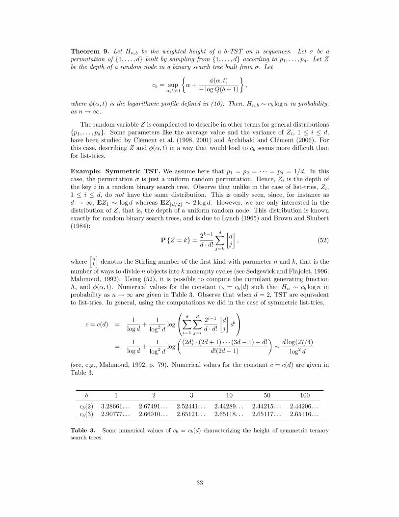
Theorem 9. Let Hn,b be the weighted height of a b-TST on n sequences. Let σ be apermutation of 1, . . . , d built by sampling from 1, . . . , d according to p1, . . . , pd. Let Zbe the depth of a random node in a binary search tree built from σ. Let

cb = supα,t>0

α+

φ(α, t)− logQ(b+ 1)

,

where φ(α, t) is the logarithmic profile defined in (10). Then, Hn,b ∼ cb log n in probability,as n→∞.

The random variable Z is complicated to describe in other terms for general distributionsp1, . . . , pd. Some parameters like the average value and the variance of Zi, 1 ≤ i ≤ d,have been studied by Clement et al. (1998, 2001) and Archibald and Clement (2006). Forthis case, describing Z and φ(α, t) in a way that would lead to cb seems more difficult thanfor list-tries.

Example: Symmetric TST. We assume here that p1 = p2 = · · · = pd = 1/d. In thiscase, the permutation σ is just a uniform random permutation. Hence, Zi is the depth ofthe key i in a random binary search tree. Observe that unlike in the case of list-tries, Zi,1 ≤ i ≤ d, do not have the same distribution. This is easily seen, since, for instance asd → ∞, EZ1 ∼ log d whereas EZbd/2c ∼ 2 log d. However, we are only interested in thedistribution of Z, that is, the depth of a uniform random node. This distribution is knownexactly for random binary search trees, and is due to Lynch (1965) and Brown and Shubert(1984):

P Z = k =2k−1

d · d!

d∑j=k

[dj

], (52)

where[nk

]denotes the Stirling number of the first kind with parameter n and k, that is the

number of ways to divide n objects into k nonempty cycles (see Sedgewick and Flajolet, 1996;Mahmoud, 1992). Using (52), it is possible to compute the cumulant generating functionΛ, and φ(α, t). Numerical values for the constant cb = cb(d) such that Hn ∼ cb log n inprobability as n → ∞ are given in Table 3. Observe that when d = 2, TST are equivalentto list-tries. In general, using the computations we did in the case of symmetric list-tries,

c = c(d) =1

log d+

1log2 d

log

d∑i=1

d∑j=i

2i−1

d · d!

[dj

]di

=

1log d

+1

log2 dlog(

(2d) · (2d+ 1) · · · (3d− 1)− d!d!(2d− 1)

)∼ d log(27/4)

log2 d

(see, e.g., Mahmoud, 1992, p. 79). Numerical values for the constant c = c(d) are given inTable 3.

b 1 2 3 10 50 100

cb(2) 3.28661. . . 2.67491. . . 2.52441. . . 2.44289. . . 2.44215. . . 2.44206. . .cb(3) 2.90777. . . 2.66010. . . 2.65121. . . 2.65118. . . 2.65117. . . 2.65116. . .

Table 3. Some numerical values of cb = cb(d) characterizing the height of symmetric ternarysearch trees.

33

7.5 Path imbalance

The question of path imbalance for random trees has been raised by Knuth in his keynotetalk at the Conference on Analysis of Algorithms in 2004. The imbalance of a node in abinary tree is the difference between the number of left and right edges on its path from theroot. Kuba and Panholzer (2007) have addressed this question and determined the limitdistribution for the imbalance of a specified or randomly chosen node. Mahmoud (2007) andChristophi and Mahmoud (2007) have dealt with similar questions in tries. See also Janson(2006) who treated the related issue of left and right path lengths of random binary trees.We are interested in the maximum path imbalance in trees. The first order asymptoticshave been described by Broutin and Devroye (2006) for binary search trees. Here, we useTheorem 1 to answer the question of the maximum path imbalance in tries. We assume thatthe tries are binary with symbol probabilities p and q = 1 − p. In this case, the averageimbalance is

E∆n = (p− q)(

log nE

+O(1)),

and the rescaled imbalance of a random node has a Gaussian limit law :

∆n − p−qE log n

√log n

d−−−−→n→∞ N

(0,

log2(pq)E3

)(see Christophi and Mahmoud, 2007; Mahmoud, 2007). Observe in particular that whenp = q, the typical range of ∆n is O(

√log n). As we will see in the following, this contrasts

with the behavior of the maximum imbalance in the trie which is Ω(log n) as soon as p > 0.We let Bn be the maximal path imbalance in a random b-trie. Then, as we will outlinebelow, there is a constant cb depending upon b and p only such that

Bnlog n

→ cb in probability

as n→∞.

Remark. A related model involves tries whose edges are weighted with +1 or −1, indepen-dently for each edge using a fair coin flip. The values of the weights are then independentof the direction of the edges and we have

(Z,E) =

(+1,− log p) w.p. 1/4(−1,− log p) w.p. 1/4(+1,− log q) w.p. 1/4(−1,− log q) w.p. 1/4.

For this model, the average weight on the path to a random node has a centered Gaussianlimit law, and the typical range is O(

√log n) for every p ∈ (0, 1).

The core of the trie. In the case of imbalance, the vector of interest in the core is((+1,− log p), (−1,− log q)

)and hence a typical component (after symmetrization) is

(Z,E) =

(+1,− log p) w.p. 1/2(−1,− log q) w.p. 1/2.

Therefore,Λ(λ, µ) = log

(eλ−µ log p + e−λ−µ log q

)− log 2. (53)

By definition, Λ?(x, y) = supλx+ µy − Λ(λ, µ) and Λ(x, y) =∞ unlessx =

∂Λ(λ, µ)∂λ

=e−λ−µ log p − e−λ−µ log q

e−λ−µ log p + e−λ−µ log q

y =∂Λ(λ, µ)∂µ

=−e−λ−µ log p log p− e−λ−µ log q log q

e−λ−µ log p + e−λ−µ log q.

34

Then we have(1− x)eλ−µ log p + (−1− α)e−λ−µ log q = 0

(− log q − y)eλ−µ log p + (− log q − y)e−λ−µ log q = 0.

This leads to the equivalent system2λ+ µ log(q/p) = log

(1 + x

1− x

)x+ 1x− 1

=log q + y

log p+ y.

(54)

For x and y satisfying (54),

Λ?(x, y) = λx+ µy − Λ(λ, µ)= λx+ µy + log 2− log

(eλ−µ log p + e−λ−µ log q

)= λx+ µy + log 2− log

(e2λ+µ log(q/p) + 1

)+ λ+ µ log q

= λ(x+ 1) + µ(y + log q) + log(1− x).

Using the expression for λ in terms of µ, we can express Λ?(x, y) independently of λ or µ.Finally, we obtain

Λ?(x, y) =

x+ 1

2log(x+ 11− x

)+ log(1− x) if

1 + x

x− 1=

log q + y

log p+ y∞ otherwise.

The entire profile φ(α, t) can be obtained from the values on the line where Λ? takes finitevalues.

φ(α, t) = t log 2− α− t2

log(α+ t

t− α

)− t log

(1− α

t

)when

α+ t

α− t=t log q + 1t log p+ 1

or for such α and t = t(α) we have, in terms of α only,

φ(α, t) =α log p+ 1

log pq· log

(1− α log q1 + α log p

)+

2− α log(q/p)log(pq)

· log(

α log p+ 1α log(q/p)− 2

). (55)

The spaghettis. The spaghettis are characterized by the random variable Zs such that

Zs =

−∞ w.p. 1−Q(b+ 1)+1 w.p. pQ(b+ 1)−1 w.p. qQ(b+ 1).

To compute the constant γb, we find the expressions for Λs(·) and Λ?s(·). We have

∀β ∈ R Λs(β) = logQ(b+ 1) + log(peβ + qe−β

).

For every ρ ∈ R, Λ?s(γ) <∞ if and only if there exists β such that

dΛ(β)dβ

=peβ − qe−β

peβ + qe−β= ρ,

and then Λ?s(ρ) = ρβ − Λs(β). This yields

Λ?s(ρ) =

ρ2 log

(qp ·

1+ρ1−ρ)− logQ(b+ 1)− log

(√1+ρ1−ρ +

√1−ρ1+ρ

)− log(pq)

2 if ρ ∈ [−1, 1]+∞ otherwise.

35

α

t

φ(α, t)

Figure 9. The weighted profile of the core for the question of path imbalance for p = .3. Whenlooking at levels deep in the core, the nodes have mostly negative imbalance due to the fact thatp < 1/2.

By Lemma 7 and the remark there, γb is the given by the slope of a line with an end at theorigin and which is tangent to the the curve Λ?s(ρ) : ρ ∈ [−1, 1]. In other words, γ is givenby

dΛ?s(ρ)dρ

=1γ

and Λ?s(ρ) =ρ

γ,

for some ρ ∈ [−1, 1]. This leads to an explicit formula for γb. Indeed,

dΛ?s(ρ)dρ

=ρ

2· log

(q

p· 1 + ρ

1− ρ

),

and hence

1γ b

=Λ?s(ρo)ρo

=dΛ?(ρ)

dρ

∣∣∣∣ρ=ρo

where√

1 + ρo1− ρo

+√

1− ρo1 + ρo

=1

pqQ(b+ 1).

It follows that

ρo =√

1− 4p2q2Q2(b+ 1) and γb = 2/ρo · log

(q

p· 1 + ρo

1− ρo

). (56)

Numerical values are given in Table 4.

Overal contribution. We are in a case where Λ?(·, ·) is degenerate and takes finitevalues on a line only. So we have

cb = supα,tα+ γbφ(α, t) = sup

α+ γbφ(α, t) :

α+ t

α− t=t log q + 1t log p+ 1

.

Therefore, we have

cb = αo + γbαo wheredφ(α, t(α))

dα

∣∣∣∣α=αo

= − 1γb,

where φ(α, t(α)) and γb are given by (55) and (56), respectively. It is this constant cb thatis the weak limit of Bn/ log n. Numerical values can be found in Table 4 below.

36

b 1 2 3 4 5 10

γb 0.66760. . . 0.46085. . . 0.36055. . . 0.29896. . . 0.25664. . . 0.15328. . .cb 1.16161. . . 1.10845. . . 1.09658. . . 1.09313. . . 1.09200. . . 1.09136. . .

Table 4. Numerical values for the constants γb and cb in the example of the path imbalance whenp = 0.4.

8 Concluding remarks

In addition to yielding the asymptotic properties of the height of hybrid tries, our methodsheds some new light on the family of digital trees in general. In particular, the decomposi-tion of the tree into a core and hanging spaghettis yields new connections between tries andthe digital search tree. Coffman and Eve (1970) proposed digital search trees to improvethe search costs in tries that are far from optimal. The main idea is to move the data fromthe external nodes to the internal nodes, which reduces the depth of the data, and hencethe costs. This roughly speaking shaves off the spaghettis, as the weighted profile of digitalsearch trees is identical to that of the core. Observe that the constant that would charac-terize the height of spaghettis in digital search trees would be γb = 0, since the height of adigital search tree on m sequences is bounded by m and digital search tree fits into the modelof trees with bounded height of Broutin, Devroye, and McLeish (2007). So in our formalism,the height Hn,b is asymptotic to cb log n in probability with cb = supα : φ(α, t) ≥ 0.

9 Acknowledgement

We thank Julien Clement for drawing our attention to the problem of the height of ternarysearch trees which lead to this document, and both referees for helping us improve thepresentation.

References

N. Alon, J. Spencer, and P. Erdos. The Probabilitic Method. Wiley, New York, NY, secondedition, 2000.

M. Archibald and J. Clement. Average depth in binary search tree with repeated keys. InFourth Colloquium on Mathematics and Computer Science, pages 309–320, 2006.

K. B. Athreya and P. E. Ney. Branching Processes. Springer, Berlin, 1972.

J. L. Bentley and R. Sedgewick. Fast algorithm for sorting and searching strings. In EighthAnnual ACM-SIAM Symposium on Discrete Algorithms, pages 360–369, 1997.

N. Broutin. Shedding New Light on Random Trees. Phd thesis, McGill University, Montreal,2007.

N. Broutin and L. Devroye. Large deviations for the weighted height of an extended classof trees. Algorithmica, 46:271–297, 2006.

N. Broutin and L. Devroye. The core of a trie. In International Conference on Analysis ofAlgorithms, 2007a. To appear.

N. Broutin and L. Devroye. The height of list tries and TST. In International Conferenceon Analysis of Algorithms, 2007b. (13 pages). To appear.

37

N. Broutin, L. Devroye, and E. McLeish. Weighted height of random trees. Manuscript (46pages), 2007.

G.G. Brown and B.O. Shubert. On random binary trees. Mathematics of Operations Re-search, 9:43–65, 1984.

H. Chernoff. A measure of asymptotic efficiency for tests of a hypothesis based on the sumof observations. Annals of Mathematical Statistics, 23:493–507, 1952.

C.A. Christophi and H. M. Mahmoud. One-sided variations on tries: path imbalance,climbing, and key sampling. In Proceedings of the International Conference on Analysisof Algorithms (AofA), pages 301–310, 2007.

H. A. Clampett. Randomized binary searching with tree structures. Communications of theACM, 7(3):163–165, 1964.

J. Clement, P. Flajolet, and B. Vallee. The analysis of hybrid trie structures. In 9th annualACM-SIAM Symposium on Discrete Algorithms, pages 531–539, Philadelphia, PA, 1998.SIAM Press.

J. Clement, P. Flajolet, and B. Vallee. Dynamical source in information theory: a generalanalysis of trie structures. Algorithmica, 29:307–369, 2001.

E. G. Coffman and J. Eve. File structures using hashing functions. Communications of theACM, 13:427–436, 1970.

H. Cramer. Sur un nouveau theoreme-limite de la theorie des probabilites. In ColloqueConsacre a la Theorie des Probabilites, volume 736, pages 5–23. Hermann, Paris, 1938.

R. de la Briandais. File searching using variable length keys. In Proceedings of the WesternJoint Computer Conference, Montvale, NJ, USA. AFIPS Press, 1959.

A. Dembo and O. Zeitouni. Large Deviation Techniques and Applications. Springer Verlag,second edition, 1998.

F. den Hollander. Large Deviations. American Mathematical Society, Providence, RI, 2000.

J.-D. Deuschel and D.W. Stroock. Large Deviations. American Mathematical Society,Providence, RI, 1989.

L. Devroye. Laws of large numbers and tail inequalities for random tries and patricia trees.Journal of Computational and Applied Mathematics, 142:27–37, 2002.

L. Devroye. Universal asymptotics for random tries and patricia trees. Algorithmica, 42:11–29, 2005.

L. Devroye. A probabilistic analysis of the height of tries and of the complexity of triesort.Acta Informatica, 21:229–237, 1984.

L. Devroye. A note on the height of binary search trees. Journal of the ACM, 33:489–498,1986.

L. Devroye. Branching processes and their application in the analysis of tree structures andtree algorithms. In M. Habib, C. McDiarmid, J. Ramirez-Alfonsin, and B. Reed, editors,Probabilistic Methods for Algorithmic Discrete Mathematics, volume 16 of Springer Serieson Algorithms and Combinatorics, pages 249–314, Berlin, 1998. Springer.

L. Devroye, W. Szpankowski, and B. Rais. A note on the height of suffix trees. SIAMJournal on Computing, 21:48–53, 1992.

38

P. Flajolet. The ubiquitous digital tree. In B. Durand and W. Thomas, editors, STACS2006, Annual Symposium on Theoretical Aspects of Computer Science, volume 3884 ofLecture Notes in Computer Science, pages 1–22, Marseille, February 2006.

P. Flajolet. On the performance evaluation of extendible hashing and trie searching. ActaInformatica, 20:345–369, 1983.

P. Flajolet and J.M. Steyaert. A branching process arising in dynamic hashing, trie search-ing and polynomial factorization. In M. Nielsen and E.M. Schmidt, editors, Automata,Languages and Programming: Proceedings of the 9th ICALP Conference, volume 140 ofLecture Notes in Computer Science, pages 239–251. Springer, 1982.

E. Fredkin. Trie memory. Communications of the ACM, 3(9):490–499, 1960.

S. Janson. Left and right pathlengths in random binary trees. Algorithmica, 46:419–429,2006.

S. Janson, T. Luczak, and A. Rucinski. Random Graphs. Wiley, New York, 2000.

M. Kuba and A. Panholzer. The left-right-imbalance of binary search trees. TheoreticalComputer Science, 370:265–278, 2007. Manuscript.

W.C. Lynch. More combinatorial properties of certain trees. Computing J., 7:299–302, 1965.

H. Mahmoud. Evolution of Random Search Trees. Wiley, New York, 1992.

H. M. Mahmoud. Imbalance in random digital trees. Submitted, 2007.

G. Park, H.K. Hwang, P. Nicodeme, and W. Szpankowski. Profile of tries. Manuscript,2006.

B. Pittel. Asymptotic growth of a class of random trees. The Annals of Probability, 13:414–427, 1985.

M. Regnier. On the average height of trees in digital search and dynamic hashing. Infor-mation Processing Letters, 13:64–66, 1981.

R. Rockafellar. Convex Analysis. Princeton University Press, Princeton, NJ, 1970.

R. Sedgewick and P. Flajolet. An Introduction to the Analysis of Algorithm. Addison-Wesley,Reading, MA, 1996.

W. Szpankowski. Average Case Analysis of Algorithms on Sequences. Wiley, New York,2001.

W. Szpankowski. On the height of digital trees and related problems. Algorithmica, 6:256–277, 1991.

39

An Analysis of the Height of Tries with Random Weights …luc.devroye.org/tries_weighted.pdfAn...

Documents

Transcript of An Analysis of the Height of Tries with Random Weights …luc.devroye.org/tries_weighted.pdfAn...