MICHIGAN JUSTICE STATISTICS CENTER SCHOOL OF CRIMINAL JUSTICE

MICHIGAN STATE UNIVERSITY

DECEMBER 2014

AN ANALYSIS OF PATTERNS IN INTERPERSONAL VIOLENCE USING

MICHIGAN INCIDENT CRIME REPORTING

MICHIGAN JUSTICE STATISTICS CENTER SCHOOL OF CRIMINAL JUSTICE MICHIGAN STATE UNIVERSITY

DECEMBER 2014

AN ANALYSIS OF PATTERNS IN INTERPERSONAL VIOLENCE USING MICHIGAN INCIDENT

CRIME REPORTING DATA

Jason Rydberg, Ph.D.

Edmund F. McGarrell, Ph.D.

Michigan Justice Statistics Center School of Criminal Justice Michigan State University

December 2014

This project was supported by Grant No. 2013-BJ-CX-K032 awarded by Bureau of Justice Statistics, Office of Justice Programs, U.S. Department of Justice. Points of view in this document are those of the authors and do not necessarily represent the official position or policies of the U.S. Department of Justice or the Michigan State Police.

MICHIGAN JUSTICE STATISTICS CENTER SCHOOL OF CRIMINAL JUSTICE MICHIGAN STATE UNIVERSITY

DECEMBER 2014

Michigan Justice Statistics Center The School of Criminal Justice at Michigan State University, through the Michigan Justice Statistics Center, serves as the Statistical Analysis Center (MI-SAC) for the State of Michigan. The mission of the Center is to advance knowledge about crime and justice issues in the state of Michigan while also informing policy and practice. The Center works in partnership with the Michigan State Police, Michigan’s State Administering Agency (SAA), as well as with law enforcement and criminal justice agencies serving the citizens of Michigan. For further information see: http://cj.msu.edu/programs/michigan-justice-statistics-center/ About the Authors Jason Rydberg is an assistant professor of criminology and justice studies at the University of Massachusetts Lowell. Until recently, he served as a research assistant with the Michigan Justice Statistics Center at Michigan State University. His research interests concern the evaluation of criminal justice program and policies, particularly in the areas of prisoner reentry, community supervision, and sex offender management. His research has recently appeared in Criminology and Public Policy, Justice Quarterly, Homicide Studies, and Victims and Offenders. Edmund F. McGarrell is Professor in the School of Criminal Justice at Michigan State University and Director of the Michigan Justice Statistics Center that serves as the Statistical Analysis Center for the state of Michigan. From 2001 to 2014 he served as Director of the School of Criminal Justice. McGarrell's research focuses on communities and crime with a specific focus on violence prevention and control. Recent articles appear in Crime and Delinquency, Criminology and Public Policy, Journal of Criminal Justice and Journal of Experimental Criminology.

REPORT OUTLINE ACKNOWLEDGEMENTS INTRODUCTION Research Questions DATA AND METHODS Data: The Michigan Incident Crime Reporting System (MICR) Analysis Plan ANALYSES Victims of Homicides, Aggravated Assaults, and Robberies Perpetrators of Homicides, Aggravated Assaults, and Robberies Circumstances of Homicides, Aggravated Assaults, and Robberies Regional Variation and Correlates of Homicides, Aggravated Assaults, and Robberies CONCLUSIONS REFERENCES APPENDIX MICR File Linking Process

ACKNOWLEDGEMENTS

Producing this report would not have been possible without the assistance of the Michigan State Police. In particular, we would like to thank Wendy Easterbrook, who provided access to the highly detailed MICR data and provided advice and instruction on the file-linking process. Additionally, she answered an excessive number of e-mails from the research team pertaining to any number of issues or questions, for which we are very appreciative. Additionally, the Michigan Justice Statistics Center works closely with the MSP’s Grants and Community Services Division. Their support for joint research efforts reflected in the current report is greatly appreciated.

1

INTRODUCTION

Despite a steady decrease in national rates of violent victimization since the early 1990s

(Truman & Langton, 2014), the incidence of violence in America remains high. Michigan has

experienced decreases in offending as well, with 2013 data indicating a 7 percent decrease in

homicides, a 4 percent decrease in aggravated assaults, and a 1 percent decrease in robberies

from 2012 (Michigan Incident Crime Reporting, 2014). Although rates of these violent crimes

have decreased statewide, beneath these trends are degrees of uniformity and variation in the

characteristics of victims, offenders, and context of violent crime. That is, criminological

research has suggested that there is a great degree of regional variation in violent offending and

victimization within places (Kposowa, Breault, &, Harrison, 1995; Sampson & Lauritsen, 1994).

Even within geographic regions with high rates of offending, there are groups of people that

experience disproportionately high rates of violence, particularly young, minority males

(Blumstein, 1995, Braga, 2003; McGarrell & Chermak, 2004), especially firearm-related

violence.

The purpose of the current report is to conduct a problem analysis of violent victimization

and offending in the State of Michigan, examining patterns in victim, offender, and circumstance

characteristics, as well as examine regional variation in violence across the State. These analyses

are designed to inform priorities for strategic intervention, highlighting the characteristics of

victims at the highest risk of violent crime, the most prevalent offender characteristics, and the

contexts in which violent offenses are the most prevalent. Additionally, specific attention is

given to differential rates of violent victimization within the counties with the highest rates of

general and firearm violence.

2

Research Questions Towards these ends, this report attempts to provide a thorough descriptive analysis of

violent victimization and offending in Michigan, focusing on homicides, aggravated assaults, and

robberies. Specifically, the research questions informing the analyses presented in this report ask:

1. What is the distribution of victim, offender, and offense characteristics across incidents of

homicides, aggravated assaults, and robberies in Michigan?

2. To what extent does violent victimization and violent victimization by firearms vary

across Michigan counties?

3. Which features of Michigan counties are correlated with variation in homicide,

aggravated assaults, and robbery victimization?

3

DATA AND METHODS Data: The Michigan Incident Crime Reporting System (MICR)

The analyses presented in this report were conducted by utilizing data from the Michigan

Incident Crime Reporting system (MICR). As its name implies, MICR is an incident-based crime

reporting system maintained by the Michigan State Police (MSP). All law enforcement agencies

in the state are required to submit incident-level crime statistics to MSP. Beginning in 1989,

MSP shifted reporting requirements from a summary-based system (i.e., such as the aggregate

data contained Uniform Crime Reports) to an incident-based system, along the lines of the

National Incident-Based Reporting System (NIBRS) (Michigan Department of State Police,

2014). Although Michigan law requires submission of data on a minimum of a monthly basis,

currently local agencies are able to submit data to MSP electronically on a continuous basis.

Eventually Michigan law enforcement agencies will be able to access MICR data through the

MSP Dashboard, allowing these agencies to produce desired reports (Michigan Department of

State Police, 2014). Michigan is one of a small number of states with such complete incident-

based crime data. The availability of the incident-based MICR data covering the entire state

represent a valuable resource for law enforcement, researchers, and policy makers for

understanding crime patterns and planning prevention, intervention, and enforcement strategies

to reduce crime and violence.

The current study demonstrates the utility of MICR data to gain an in-depth

understanding of the nature of violent crime across the State. Given that MICR boasts a high

degree of compliance across Michigan law enforcement agencies, these data provide detailed

insight into violent crimes that come to the attention of the police. Members of the Michigan

Justice Statistics Center research team worked with the Criminal Justice Information Center

4

(CJIC) at MSP to access the MICR data files. The MICR files consisted of numerous segments

which were linked together on the basis of unique incident, victim, offender, and offense

identifiers. Detail on the sequential file linking process is explained in Appendix A.

This report analyzes MICR data for the year 2013. For this year of data, 529 Michigan

law enforcement agencies were equipped to submit incident data to MICR. Of these agencies,

462 (87.3%) submitted a full 12 months of data, while another 36 (4.9%) submitted less than 12

months of data. As such a total of 498 (94.1%) Michigan law enforcement agencies were either

fully or partially represented in the data. In 2013 the MICR contained data on 744,223 unique

criminal incidents across the state, where an incident is defined as “one or more offenses

committed by the same person or group of persons acting in concert, at the same time and place”

(MSP, 2014). Within MICR, each incident is identified by a unique identifier called a ‘MIC1

number.’ In any given incident, there may be a single victim or multiple victims, a single

offender or multiple offenders, and involve the commission of a single offense or multiple

offenses by said offenders against said victims. As such, unique identifiers were created for each

victim, offender, and offense occurring within each incident (see Appendix A).

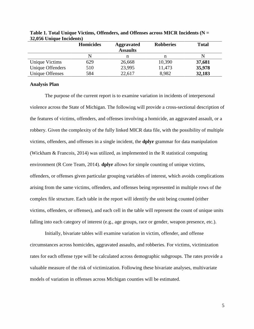
Given this report’s focus on violent crime, the data were reduced to incidents involving a

reported homicide, aggravated assault, or robbery against a victim that was an individual (i.e., a

person, excluding businesses and the government as victims). With these criteria in place, the

current report analyzes 32,056 unique violent incidents, which included 37,681 unique victims,

35,978 unique offenders, and 32,183 unique offenses (see Table 1).1

1 It is important to emphasize that this report uses different incident selection procedures than the overall summary reports filed by MSP. As such, the exact totals and rates reported in this document will not match the totals and rates provided by MSP.

5

Table 1. Total Unique Victims, Offenders, and Offenses across MICR Incidents (N = 32,056 Unique Incidents) Homicides Aggravated

Assaults Robberies Total

N n n N Unique Victims 629 26,668 10,390 37,681 Unique Offenders 510 23,995 11,473 35,978 Unique Offenses 584 22,617 8,982 32,183 Analysis Plan

The purpose of the current report is to examine variation in incidents of interpersonal

violence across the State of Michigan. The following will provide a cross-sectional description of

the features of victims, offenders, and offenses involving a homicide, an aggravated assault, or a

robbery. Given the complexity of the fully linked MICR data file, with the possibility of multiple

victims, offenders, and offenses in a single incident, the dplyr grammar for data manipulation

(Wickham & Francois, 2014) was utilized, as implemented in the R statistical computing

environment (R Core Team, 2014). dplyr allows for simple counting of unique victims,

offenders, or offenses given particular grouping variables of interest, which avoids complications

arising from the same victims, offenders, and offenses being represented in multiple rows of the

complex file structure. Each table in the report will identify the unit being counted (either

victims, offenders, or offenses), and each cell in the table will represent the count of unique units

falling into each category of interest (e.g., age groups, race or gender, weapon presence, etc.).

Initially, bivariate tables will examine variation in victim, offender, and offense

circumstances across homicides, aggravated assaults, and robberies. For victims, victimization

rates for each offense type will be calculated across demographic subgroups. The rates provide a

valuable measure of the risk of victimization. Following these bivariate analyses, multivariate

models of variation in offenses across Michigan counties will be estimated.

6

ANALYSES

Victims of Homicides, Aggravated Assaults, and Robberies

The following tables and figures display the distribution of victims of violent crimes

across different demographic characteristics and offense types. In this portion of 2013 MICR

data there were 37,681 unique victims across 32,056 unique incidents involving a violent crime.

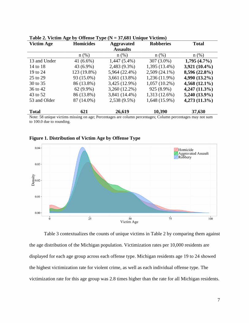
Table 2 displays the distribution of victims by age groupings.2 The modal age category for

victims of violent crime was age 19 to 24, accounting for 23 percent of violent victimizations

within the data. Victims between the ages of 14 and 29 years old accounted for nearly half of all

victimizations (46.4%). There was some variation in the distribution of victim age across offense

types around this modal category, with this information presented both in Table 2 and in Figure

1. For homicides, aggravated assaults, and robberies alike, the modal victim age category was

age 19 to 24. There was a larger proportion of victims of robberies falling towards the younger

side of 19 to 24 (i.e., 14 to 18), relative to homicides and aggravated assaults. There were also

more homicide and aggravated assault victims falling into the 25 to 29 category, relative to

robberies. Additionally, there was a relatively larger proportion of robbery and homicide victims

that were 53 or older, relative to aggravated assaults. However, Figure 2 indicates that there were

more robbery victims between the ages of 50 to 60, and a larger proportion of homicide victims

above age 70, relative to the other offenses.

2 Given the small number of victims missing their age information, no “unknown” or “missing” category is included in the tables.

7

Table 2. Victim Age by Offense Type (N = 37,681 Unique Victims) Victim Age Homicides Aggravated

Assaults Robberies Total

n (%) n (%) n (%) n (%) 13 and Under 41 (6.6%) 1,447 (5.4%) 307 (3.0%) 1,795 (4.7%) 14 to 18 43 (6.9%) 2,483 (9.3%) 1,395 (13.4%) 3,921 (10.4%) 19 to 24 123 (19.8%) 5,964 (22.4%) 2,509 (24.1%) 8,596 (22.8%) 25 to 29 93 (15.0%) 3,661 (13.8%) 1,236 (11.9%) 4,990 (13.2%) 30 to 35 86 (13.8%) 3,425 (12.9%) 1,057 (10.2%) 4,568 (12.1%) 36 to 42 62 (9.9%) 3,260 (12.2%) 925 (8.9%) 4,247 (11.3%) 43 to 52 86 (13.8%) 3,841 (14.4%) 1,313 (12.6%) 5,240 (13.9%) 53 and Older 87 (14.0%) 2,538 (9.5%) 1,648 (15.9%) 4,273 (11.3%) Total 621 26,619 10,390 37,630 Note: 58 unique victims missing on age; Percentages are column percentages; Column percentages may not sum to 100.0 due to rounding. Figure 1. Distribution of Victim Age by Offense Type

Table 3 contextualizes the counts of unique victims in Table 2 by comparing them against

the age distribution of the Michigan population. Victimization rates per 10,000 residents are

displayed for each age group across each offense type. Michigan residents age 19 to 24 showed

the highest victimization rate for violent crime, as well as each individual offense type. The

victimization rate for this age group was 2.8 times higher than the rate for all Michigan residents.

8

Indeed, victimization rates substantially higher than the overall rate for all Michigan residents

were concentrated around residents between the ages of 14 and 35.

Table 3. Victimization Rates per 10,000 Residents: Victim Age by Offense Type (N = 37,681 Unique Victims) Homicides Aggravated

Assaults Robberies Total Violence

Rate Rate Rate Rate 13 and Under 0.2 8.2 1.7 10.1 14 to 18 0.6 34.3 19.3 54.1 19 to 24 1.5 72.6 30.5 104.6 25 to 29 1.6 62.1 21.0 84.6 30 to 35 1.2 49.7 15.3 66.3 36 to 42 0.7 36.4 10.3 47.5 43 to 52 0.6 26.0 8.9 35.5 53 and Older 0.3 8.7 5.7 14.7 Overall 0.6 27.0 10.5 38.1 Consistent with national trends, men were more common among victims of violent crime,

comprising more than half of all violent crime victims (58%) (see Table 4). There was variation

in the distribution of victim gender across the offense types, however, as women were relatively

less frequent as victims of homicides and robberies, but relatively more common as victims of

aggravated assaults.

Table 4. Victim Gender by Offense Type (N = 37,681 Unique Victims) Homicides Aggravated

Assaults Robberies Total

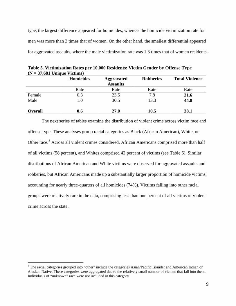
n (%) n (%) n (%) n (%) Female 147 (23.5%) 11,834 (44.4%) 3,923 (37.8%) 15,904 (42.2%) Male 479 (76.5%) 14,799 (55.6%) 6,459 (62.2%) 21,737 (57.7%) Total 626 26,633 10,382 37,641 Note: 47 unique victims missing on gender; Percentages are column percentages; Column percentages may not sum to 100.0 due to rounding. Comparing the victimization counts to population totals, the male violent victimization

rate stood at approximately 1.4 times that of women (see Table 5). Disaggregating by offense

9

type, the largest difference appeared for homicides, whereas the homicide victimization rate for

men was more than 3 times that of women. On the other hand, the smallest differential appeared

for aggravated assaults, where the male victimization rate was 1.3 times that of women residents.

Table 5. Victimization Rates per 10,000 Residents: Victim Gender by Offense Type (N = 37,681 Unique Victims) Homicides Aggravated

Assaults Robberies Total Violence

Rate Rate Rate Rate Female 0.3 23.5 7.8 31.6 Male 1.0 30.5 13.3 44.8 Overall 0.6 27.0 10.5 38.1 The next series of tables examine the distribution of violent crime across victim race and

offense type. These analyses group racial categories as Black (African American), White, or

Other race.3 Across all violent crimes considered, African Americans comprised more than half

of all victims (58 percent), and Whites comprised 42 percent of victims (see Table 6). Similar

distributions of African American and White victims were observed for aggravated assaults and

robberies, but African Americans made up a substantially larger proportion of homicide victims,

accounting for nearly three-quarters of all homicides (74%). Victims falling into other racial

groups were relatively rare in the data, comprising less than one percent of all victims of violent

crime across the state.

3 The racial categories grouped into “other” include the categories Asian/Pacific Islander and American Indian or Alaskan Native. These categories were aggregated due to the relatively small number of victims that fall into them. Individuals of “unknown” race were not included in this category.

10

Table 6. Victim Race by Offense Type (N = 37,681 Unique Victims) Homicides Aggravated

Assaults Robberies Total

n (%) n (%) n (%) n (%) Black 450 (73.9%) 14,613 (56.3%) 6,001 (59.6%) 21,064 (57.5%) White 157 (25.8%) 11,245 (43.3%) 4,017 (39.9%) 15,419 (42.1%) Other 2 (0.3%) 87 (0.3%) 57 (0.5%) 146 (0.4%) Sub-Total 609 25,945 10,075 36,629 Unknown 20 (3.2%) 723 (2.7%) 315 (3.0%) 1,058 (2.8%) Total 629 26,668 10,390 37,687 Note: Percentages are column percentages; Column percentages may not sum to 100.0 due to rounding. Table 7 presents victimization rates across the racial categories of Michigan residents.

Violent crime victimization rates for African Americans were substantially higher than for

Whites or those in other racial categories. Indeed, the total violence victimization rate for Blacks

was 7.5 times that of Whites, attributable to the fact that African Americans comprise 14 percent

of the Michigan population but 58 percent of violent crime victims. The largest ratio difference

between African American and White residents was for homicides, where the Black

victimization rate was 16 times that of White residents.

Table 7. Victimization Rates per 10,000 Residents: Victim Race by Offense Type (N = 37,681 Unique Victims) Homicides Aggravated

Assaults Robberies Total Violence

Rate Rate Rate Rate Black 3.2 104.4 42.9 150.4 White 0.2 14.4 5.1 19.8 Other 0.0 1.3 0.8 2.1 Overall 0.6 27.0 10.5 38.1 Note: Victims with unknown rate excluded from rate calculations. The joint distribution of victim race and gender was also examined (see Table 8). In

considering total counts of violent victimizations, African American males (31%) and African

American females (25%) were the most common. White males accounted for one-quarter (25%)

of violent crime victims. Together, these groups (Black males, Black females, and White males)

11

accounted for 80 percent of all violent crime victims. Across the disaggregated crime types,

several patterns were apparent. Relative to the overall distribution of violent crime victims,

Black males comprised a substantially larger proportion of homicide victims. Additionally,

Black females made up a larger proportion of aggravated assault victims than White males,

which is striking given than men overall comprise a much larger proportion of aggravated assault

victims (see Table 5).

Table 8. Victim Race and Gender by Offense Type (N = 37,681 Unique Victims) Homicides Aggravated

Assaults Robberies Total

n (%) n (%) n (%) n (%) Black Female 77 (12.3%) 6,910 (25.9%) 2,401 (23.1%) 9,388 (24.9%) White Female 63 (10.1%) 4,627 (17.4%) 1,417 (13.6%) 6,107 (16.2%) Other Female 1 (0.2%) 36 (0.1%) 21 (0.2%) 58 (0.2%) Unk. Female 6 (1.0%) 261 (1.0%) 84 (0.8%) 351 (0.9%) Black Male 373 (59.6%) 7,701 (28.9%) 3,600 (34.7%) 11,674 (31.0%) White Male 94 (15.0%) 6,615 (24.8%) 2,600 (25.0%) 9,309 (24.7%) Other Male 1 (0.2%) 51 (0.2%) 36 (0.3%) 88 (0.2%) Unk. Male 11 (1.8%) 432 (1.6%) 223 (2.1%) 666 (1.8%) Total 626 26,633 10,382 37,641 Note: 47 unique victims missing on gender; Percentages are column percentages; Column percentages may not sum to 100.0 due to rounding. Victimization Rates by Subgroup Interactions To further explore the nature of violent victimization in the 2013 MICR data,

victimization rates for age, sex, and race combinations were calculated. For the purposes of these

analyses, “young victims” were defined as those victims between the ages of 15 and 24, when

the risk for violent victimization has been noted to be significantly higher (Truman & Langton,

2014), particularly since the mid-1980s onwards (Dahlberg, 1998). Specifically, a figure is

produced comparing the violent victimization rate for all Michigan residents, young men and

women, race and gender combinations, and then young race and gender combinations. A

12

separate figure is produced for homicides, aggravated assaults, robberies, and total violence –

resulting in four figures in all.

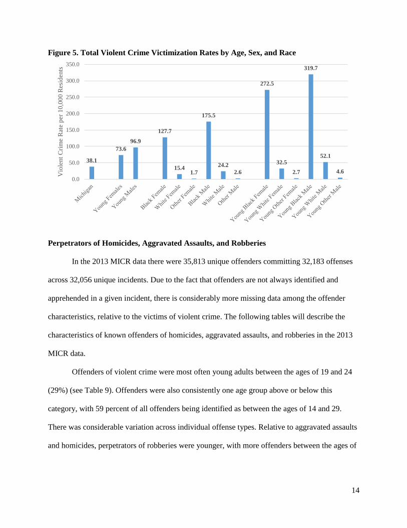
In general, Figures 2 through 5 demonstrate the interaction between age, race, and gender

in producing variation in violent crime victimization rates. For instance, the overall homicide

rate per 10,000 residents for the State of Michigan is 0.6. The homicide victimization rate for

young males is 3 times the rate for all residents (1.8 per 10,000), and the rate for young Black

males is 15.5 times that (9.3 per 10,000). These estimates are consistent with national trends,

placing homicide as the leading cause of death among Black males age 15 to 24 (Centers for

Disease Control, 2014). This pattern manifests across homicides, aggravated assaults, and

robberies. For each of the violent crime types, the victimization rate for young Black males is the

highest among all age, race, and gender combinations. The aggravated assault rate for young

Black women is an exception, as it is nearly equivalent to that of young Black males (197 versus

200 per 10,000).

Figure 2. Homicide Victimization Rates by Age, Sex, and Race

0.6 0.5

1.8 1.0

0.2 0.0

5.6

0.2 0.0

2.0

0.2 0.0

9.3

0.3 0.0 0.0

1.0

2.0

3.0

4.0

5.0

6.0

7.0

8.0

9.0

10.0

Hom

icid

es p

er 1

0,00

0 R

esid

ents

13

Figure 3. Aggravated Assault Victimization Rates by Age, Sex, and Race

Figure 4. Robbery Victimization Rates by Age, Sex, and Race

27.0

53.7 61.6

94.0

11.7 1.0

115.8

17.2 1.5

197.2

24.3

1.4

200.0

34.0

2.5 0.0

50.0

100.0

150.0

200.0

250.0

Agg

rava

ted

Ass

aults

per

10,

000

Res

iden

ts

10.5 19.3

33.6 32.7

3.6 0.6

54.1

6.8 1.1

73.2

8.1 1.4

110.3

17.8

2.1 0.0

20.0

40.0

60.0

80.0

100.0

120.0

Rob

bery

Rat

e pe

r 10,

000

Res

iden

ts

14

Figure 5. Total Violent Crime Victimization Rates by Age, Sex, and Race

Perpetrators of Homicides, Aggravated Assaults, and Robberies In the 2013 MICR data there were 35,813 unique offenders committing 32,183 offenses

across 32,056 unique incidents. Due to the fact that offenders are not always identified and

apprehended in a given incident, there is considerably more missing data among the offender

characteristics, relative to the victims of violent crime. The following tables will describe the

characteristics of known offenders of homicides, aggravated assaults, and robberies in the 2013

MICR data.

Offenders of violent crime were most often young adults between the ages of 19 and 24

(29%) (see Table 9). Offenders were also consistently one age group above or below this

category, with 59 percent of all offenders being identified as between the ages of 14 and 29.

There was considerable variation across individual offense types. Relative to aggravated assaults

and homicides, perpetrators of robberies were younger, with more offenders between the ages of

38.1

73.6 96.9

127.7

15.4 1.7

175.5

24.2 2.6

272.5

32.5 2.7

319.7

52.1

4.6 0.0

50.0

100.0

150.0

200.0

250.0

300.0

350.0V

iole

nt C

rime

Rat

e pe

r 10,

000

Res

iden

ts

15

14 and 18. Additionally, 81 percent of robbery offenders were between the ages of 14 and 29,

relative to 55 percent of homicide offenders, and 50 percent of aggravated assault offenders.

Table 9. Offender Age by Offense Type (N = 35,813 Unique Offenders) Homicides Aggravated

Assaults Robberies Total

n (%) n (%) n (%) n (%) 13 and Under 2 (0.0%) 502 (2.3%) 80 (0.9%) 584 (1.9%) 14 to 18 35 (8.5%) 2,315 (10.4%) 2,360 (26.6%) 4,710 (15.0%) 19 to 24 139 (33.6%) 5,437 (24.5%) 3,661 (41.3%) 9,237 (29.3%) 25 to 29 53 (12.8%) 3,377 (15.2%) 1,165 (13.1%) 4,595 (14.6%) 30 to 35 53 (12.8%) 3,312 (14.9%) 857 (9.7%) 4,222 (13.4%) 36 to 42 42 10.1%) 2,626 (11.8%) 355 (4.0%) 3,023 (9.6%) 43 to 52 47 (11.4%) 2,873 (12.9%) 268 (3.0%) 3,188 (10.1%) 53 and Older 43 (10.4%) 1,744 (7.9%) 126 (1.4%) 1,913 (6.1%) Sub-Total 414 22,186 8,872 31,472 Unknown 96 (18.8%) 1,809 (7.5%) 2,601 (22.7%) 4,506 (12.5%) Total 510 23,995 11,473 35,978 Note: Percentages are column percentages; Column percentages may not sum to 100.0 due to rounding. Identified offenders of violent crime are predominantly male. Men comprise four-fifths

(80%) of all unique offenders. Across the individual offense types, women make up a relatively

smaller proportion of robbery offenders (6%) and a relatively larger proportion of aggravated

assault offenders (26%).

Table 10. Offender Gender by Offense Type (N = 35,813 Unique Offenders) Homicides Aggravated

Assaults Robberies Total

n (%) n (%) n (%) n (%) Female 54 (11.1%) 6,161 (26.1%) 663 (6.0%) 6,878 (19.6%) Male 434 (88.9%) 17,434 (73.9%) 10,376 (94.0%) 28,244 (80.4%) Sub-Total 488 23,595 11,039 35,122 Unknown 21 (4.1%) 399 (1.7%) 432 (3.8%) 852 (2.4%) Total 509 23,994 11,471 35,974 Note: Percentages are column percentages; Column percentages may not sum to 100.0 due to rounding.

16

Table 11 displays the racial characteristics of identified violent crime offenders. African

Americans comprise the majority of identified offenders, making up more than two-thirds (71%).

Robbery offenders were disproportionately African American, as 89 percent of offenders were

identified as being Black. On the other hand, the racial distribution of aggravated assault

offenders was less polarized, as Whites comprised 37 percent of unique offenders.

Table 11. Offender Race by Offense Type (N = 35,813 Unique Offenders) Homicides Aggravated

Assaults Robberies Total

n (%) n (%) n (%) n (%) Black 362 (75.7%) 14,340 (62.6%) 9,572 (88.9%) 24,274 (71.0%) White 110 (23.0%) 8,452 (36.9%) 1,175 (10.9%) 9,737 (28.5%) Other 6 (1.3%) 130 (0.6%) 20 (0.2%) 156 (0.5%) Sub-Total 478 22,922 10,767 34,167 Unknown 32 (6.2%) 1,073 (4.5%) 706 (6.2%) 1,811 (5.0%) Total 510 23,995 11,473 35,978 Note: Percentages are column percentages; Column percentages may not sum to 100.0 due to rounding. The joint distribution of offender race and gender is displayed in Table 12. Unlike violent

crime victim race and gender patterns, where African American males and females, and White

males accounted for similar proportions of victims, the identified offenders of violent crimes are

more tightly concentrated. Black males accounted for more than half (56%) of identified violent

crime offenders. White males represented the second highest total, comprising 22 percent of

unique violent crime offenders. In comparing the racial and gender composition of the individual

offense types, African American males accounted for the majority of robbery offenders (82%),

and for a relatively smaller proportion of aggravated assault offenders (43%), although still

represented the modal category. White males consistently comprised the second most frequent

race/gender combination among offenders.

17

Table 12. Offender Race and Gender by Offense Type (N = 35,813 Unique Offenders) Homicides Aggravated

Assaults Robberies Total

n (%) n (%) n (%) n (%) Black Female 31 (6.4%) 4,164 (17.6%) 455 (4.1%) 4,660 (13.3%) White Female 22 (4.5%) 1,821 (7.7%) 185 (1.7%) 2,028 (5.8%) Other Female 1 (0.2%) 31 (0.1%) 3 (<0.1%) 35 (0.1%) Unk. Female 0 (0.0%) 145 (0.6%) 20 (0.2%) 165 (0.5%) Black Male 331 (67.8%) 10,154 (43.0%) 9,051 (82.0%) 19,536 (55.6%) White Male 88 (18.0%) 6,626 (28.1%) 981 (8.9%) 7,695 (21.9%) Other Male 4 (0.8%) 99 (0.4%) 16 (0.1%) 119 (0.3%) Unk. Male 11 (2.3%) 555 (2.4%) 328 (3.0%) 894 (2.5%) Sub-Total 488 23,595 11,039 35,132 Unk. Race & Gender

22 (4.0%) 400 (1.6%) 434 (3.9%) 856 (2.3%)

Total 510 23,995 11,473 35,998 Note: Percentages are column percentages; Column percentages may not sum to 100.0 due to rounding. Circumstances of Homicides, Aggravated Assaults, and Robberies This section of the report will detail important circumstances of violent offenses. The

information presented will cover joint victim and offender characteristics, such as the

relationship between victim age and offender age, and the relationship between the victims and

offenders of violent offenses. Additionally, patterns in the time and location of offenses will be

examined.

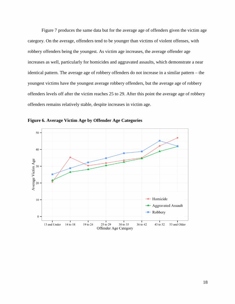
Victim and Offender Age Pairings Figures 6 and 7 display the average ages of victims and offenders given the age

categories of victims and offenders. For instance, Figure 6 shows the average age of homicide,

aggravated assault, and robbery victims for each offender age category. The results in Figure 6

suggest that younger offenders tend to offend against younger victims on the average, and as

offenders become older, the average age of victims increases. Similar patterns are observed for

homicides, aggravated assaults, and robberies.

18

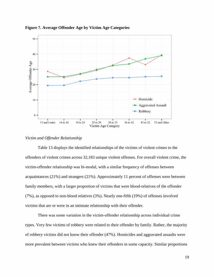
Figure 7 produces the same data but for the average age of offenders given the victim age

category. On the average, offenders tend to be younger than victims of violent offenses, with

robbery offenders being the youngest. As victim age increases, the average offender age

increases as well, particularly for homicides and aggravated assaults, which demonstrate a near

identical pattern. The average age of robbery offenders do not increase in a similar pattern – the

youngest victims have the youngest average robbery offenders, but the average age of robbery

offenders levels off after the victim reaches 25 to 29. After this point the average age of robbery

offenders remains relatively stable, despite increases in victim age.

Figure 6. Average Victim Age by Offender Age Categories

19

Figure 7. Average Offender Age by Victim Age Categories

Victim and Offender Relationship Table 13 displays the identified relationships of the victims of violent crimes to the

offenders of violent crimes across 32,183 unique violent offenses. For overall violent crime, the

victim-offender relationship was bi-modal, with a similar frequency of offenses between

acquaintances (21%) and strangers (21%). Approximately 11 percent of offenses were between

family members, with a larger proportion of victims that were blood-relatives of the offender

(7%), as opposed to non-blood relatives (3%). Nearly one-fifth (19%) of offenses involved

victims that are or were in an intimate relationship with their offender.

There was some variation in the victim-offender relationship across individual crime

types. Very few victims of robbery were related to their offender by family. Rather, the majority

of robbery victims did not know their offender (47%). Homicides and aggravated assaults were

more prevalent between victims who knew their offenders in some capacity. Similar proportions

20

of victims were either murdered or assaulted by acquaintances (28% and 26%, respectively), but

a larger proportion of aggravated assault victims were in or used to be in an intimate relationship

with their offender (25%).

Table 13. Relationship of Victim to the Offender (N = 32,183 Unique Offenses) Homicides Aggravated

Assaults Robberies Total

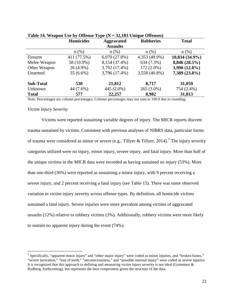
n (%) n (%) n (%) n (%) Family Blood Relative 34 (7.9%) 2,198 (9.8%) 33 (0.4%) 2,265 (7.3%) Non-Blood 12 (2.8%) 968 (4.3%) 35 (0.4%) 1,015 (3.3%) Intimate Partner Current 43 (10.0%) 4,158 (18.5%) 83 (1.0%) 4,284 (13.8%) Former 10 (2.3%) 1,443 (6.4%) 90 (1.1%) 1,543 (5.0%) Acquaintance 118 (27.5%) 5,833 (25.9%) 712 (8.8%) 6,663 (21.5%) Other Known 25 (5.8%) 2,428 (10.8%) 369 (4.6%) 2,822 (9.1%) Stranger 57 (13.3%) 2,731 (12.1%) 3,777 (46.7%) 6,565 (21.2%) Unknown 130 (30.3%) 2,746 (12.2%) 2,992 (37.0%) 5,868 (18.9%) Sub-Total 429 22,505 8,091 31,025 Missing 176 (29.1%) 1,929 (7.9%) 1,285 (13.7%) 3,390 (9.9%) Total 605 24,434 9,376 34,415 Note: Percentages are column percentages; Column percentages may not sum to 100.0 due to rounding. Weapon Use In more than three-quarters (76%) of violent offenses were offenders armed with some

sort of weapon (Table 14). Firearms were the most frequently present in an offense (35%),

followed by melee weapons, such as blades or blunt objects (29%).4 There was considerable

variation in weapon use across the individual violent offense types. Firearms were involved in

more than three-quarters (78%) of homicides, and only in 7 percent of homicides was the

offender unarmed. Firearms were relatively less frequent among aggravated assault offenders,

who were most often armed with a melee weapon (37%). Robbery offenders were evenly split

between the use of a firearm (49%) and being unarmed (41%).

4 Other weapons included the use of motor vehicles, poison, fire, or explosive devices.

21

Table 14. Weapon Use by Offense Type (N = 32,183 Unique Offenses) Homicides Aggravated

Assaults Robberies Total

n (%) n (%) n (%) n (%) Firearm 411 (77.5%) 6,070 (27.8%) 4,353 (49.9%) 10,834 (34.9%) Melee Weapon 58 (10.9%) 8,154 (37.4%) 634 (7.3%) 8,846 (28.5%) Other Weapon 26 (4.9%) 3,792 (17.4%) 172 (2.0%) 3,990 (12.8%) Unarmed 35 (6.6%) 3,796 (17.4%) 3,558 (40.8%) 7,389 (23.8%) Sub-Total 530 21,812 8,717 31,059 Unknown 44 (7.6%) 445 (2.0%) 265 (3.0%) 754 (2.4%) Total 577 22,257 8,982 31,813 Note: Percentages are column percentages; Column percentages may not sum to 100.0 due to rounding. Victim Injury Severity Victims were reported sustaining variable degrees of injury. The MICR reports discrete

trauma sustained by victims. Consistent with previous analyses of NIBRS data, particular forms

of trauma were considered as minor or severe (e.g., Tillyer & Tillyer, 2014).5 The injury severity

categories utilized were no injury, minor injury, severe injury, and fatal injury. More than half of

the unique victims in the MICR data were recorded as having sustained no injury (53%). More

than one-third (36%) were reported as sustaining a minor injury, with 9 percent receiving a

severe injury, and 2 percent receiving a fatal injury (see Table 15). There was some observed

variation in victim injury severity across offense types. By definition, all homicide victims

sustained a fatal injury. Severe injuries were more prevalent among victims of aggravated

assaults (12%) relative to robbery victims (3%). Additionally, robbery victims were more likely

to sustain no apparent injury during the event (74%).

5 Specifically, “apparent minor injury” and “other major injury” were coded as minor injuries, and “broken bones,” “severe laceration,” “loss of teeth,” “unconsciousness,” and “possible internal injury” were coded as severe injuries. It is recognized that this approach to defining and measuring victim injury severity is not ideal (Grommon & Rydberg, forthcoming), but represents the best compromise given the structure of the data.

22

Table 15. Victim Injury Severity by Offense Type (N = 37,681 Unique Victims) Homicides Aggravated

Assaults Robberies Total

n (%) n (%) n (%) n (%) No Injury 0 (0.0%) 12,291 (46.1%) 7,676 (73.9%) 19,967 (53.0%) Minor Injury 0 (0.0%) 11,178 (41.9%) 2,426 (23.4%) 13,604 (36.1%) Severe Injury 0 (0.0%) 3,199 (12.0%) 282 (2.7%) 3481 (9.2%) Fatal Injury 629 (100.0%) 0 (0.0%) 0 (0.0%) 629 (1.7%) Total 629 26,668 10,384 37,681 Note: Percentages are column percentages; Column percentages may not sum to 100.0 due to rounding. Clearance by Arrest Not all offenses resulted in the arrest of a suspect. The clearance rates for homicides,

aggravated assaults, and robberies by arrest are displayed in Table 16.6 In considering the total

violent offenses in these data, 28 percent resulted in the arrest of a suspect. Homicides and

aggravated assaults showed slightly higher clearance rates (34% for each), compared to robberies

which had the lowest clearance rate, at 13 percent.

Table 16. Arrests by Offense Type (N = 32,183 Unique Offenses) Homicides Aggravated

Assaults Robberies Total

n (%) n (%) n (%) n (%) Arrest Made 210 (34.5%) 7,917 (34.1%) 1,242 (13.3%) 9,369 (28.3%) No Arrest 398 (65.5%) 15,299 (65.9%) 8,080 (86.7%) 23,777 (71.7%) Total 608 23,216 9,322 33,146 Note: Percentages are column percentages; Column percentages may not sum to 100.0 due to rounding. Time and Location Patterns in the times and locations of violent offenses are examined in Tables 17 and 18.

Offenses were grouped into time of day categories, including early morning (2:00am to 5:59am),

morning (6:00am to 9:59am), midday (10:00am to 1:59pm), afternoon (2:00pm to 5:59pm),

6 It should be noted that these figures underestimate the clearance rates for each offense type, relative to Michigan State Police statistics. These differences are likely due to the data reduction process in which the subsample of total MICR cases were selected. The authors of this report do not claim that these are the actual arrest rates for each offense type, but simply the arrest rates that were observed within the current subsection of MICR data.

23

evening (6:00pm to 9:59pm), and late night (10:00pm to 1:59am). These time categories are

similar to those used in previous examinations of NIBRS data (Weber, 2012). Violent offenses

were primarily reported in the evening (23%) and late night (24%) (i.e., between 6:00pm and

1:59am). Violent offenses were least likely to be reported in the morning hours (7%). These

patterns were largely consistent across offense types, with the exception of homicides. Slightly

larger proportions of homicides were reported in the early morning (18%) and fewer homicides

were reported in the afternoon (13%), relative to aggravated assaults and robberies.

Table 17. Incident Time by Offense Type (N = 32,183 Unique Offenses) Homicides Aggravated

Assaults Robberies Total

n (%) n (%) n (%) n (%) Early Morning 101 (17.6%) 2,702 (12.6%) 1,016 (11.9%) 3,819 (12.5%) Morning 50 (8.7%) 1,583 (7.4%) 533 (6.2%) 2,166 (7.1%) Midday 83 (14.5%) 3,056 (14.2%) 1,212 (14.2%) 4,351 (14.2%) Afternoon 72 (12.6%) 4,109 (19.1%) 1,783 (20.9%) 5,964 (19.5%) Evening 120 (20.9%) 4,985 (23.2%) 1,964 (23.0%) 7,069 (23.1%) Late Night 147 (25.6%) 5,035 (23.5%) 2,030 (23.8%) 7,212 (23.6%) Sub-Total 573 21,470 8,538 30,581 Unknown 11 (1.9%) 1,147 (5.1%) 444 (4.9%) 1,602 (5.0%) Total 584 22,617 8,982 32,183 Note: Early Morning = 2:00am to 5:59am, Morning = 6:00am to 9:59am, Midday = 10:00am to 1:59pm, Afternoon = 2:00pm to 5:59pm, Evening = 6:00pm to 9:59pm, Late Night = 10:00pm to 1:59am; Percentages are column percentages; Column percentages may not sum to 100.0 due to rounding. Table 18 displays the distribution of violent offenses across particular location types.

These locations are grouped as residence, public-outdoors areas (e.g., offenses occurring in the

street, public areas, or wooded areas), businesses (e.g., offenses occurring within stores),

government buildings, schools, or transportation hubs (e.g., offenses occurring within jails,

public or private schools, bus stops or airports), and other locations (e.g., any known location

that does not fall into any of the aforementioned categories).

24

The most frequent location for violent offenses to be reported is in a residence,

comprising just under half of all violent offenses (46%). The most prevalent location for violent

offenses to occur is in public or outdoors areas (39%), suggesting that the majority of violent

offenses occur either in a home or public areas outside of a home, but not some other building

enclosed location. Across the individual violent offense types, slightly more homicides and

aggravated assaults took place within a residence (51% and 58%, respectively). Robberies were

much more frequent in public/outdoors locations (62%) and businesses (18%), and less frequent

within residences (15%).

Table 18. Incident Location by Offense Type (N = 32,183 Unique Offenses) Homicides Aggravated

Assaults Robberies Total

n (%) n (%) n (%) n (%) Residence 298 (51.3%) 13,099 (58.1%) 1,358 (15.1%) 14,755 (46.0%) Public-Outdoors 211 (36.3%) 6,757 (30.0%) 5,582 (62.2%) 12,550 (39.1%) Business 51 (8.8%) 1,690 (7.5%) 1,605 (17.9%) 3,346 (10.4%) Government / School / Transport Hub

11 (1.9%) 720 (3.2%) 243 (2.7%) 974 (3.0%)

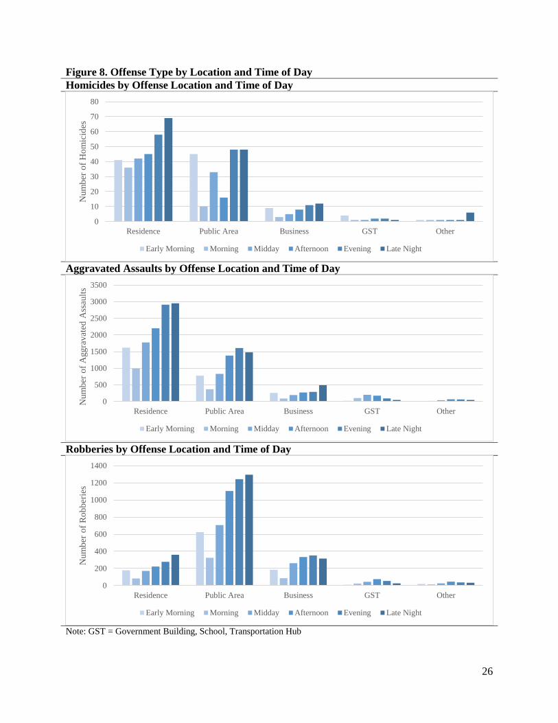
Other Location 10 (1.7%) 289 (1.3%) 186 (2.1%) 485 (1.5%) Sub-Total 581 22,555 8,974 32,110 Unknown 3 (0.5%) 62 (0.2%) 8 (0.1%) 73 (0.2%) Total 584 22,617 8,982 32,183 Note: Percentages are column percentages; Column percentages may not sum to 100.0 due to rounding. Violent offenses were observed to vary jointly across time and location. Figure 8 displays

frequencies of homicides, aggravated assaults, and robberies at each of the location types at the

different times of day. The earliest offenses are displayed in the lightest blue, while the later

offenses are displayed in the darker blue.

Several patterns are apparent in Figure 8. Within residences, homicides increase in

frequency as the time of day progresses, and a similar pattern is observed among homicides at

businesses. Homicides in public areas are most frequent in the late night and early morning

25

hours, and less frequent during daylight hours. Aggravated assaults are reported in similar

patterns across residences and public areas, whereas the frequency of reporting increases moving

into the late night hours. As observed in Table 18 (above), robberies are most frequent in public

areas, and their frequency in this location type increases into the late hours of the night.

Robberies in businesses demonstrate a more uniform distribution, with relatively equivalent

frequencies across the midday to late night hours.

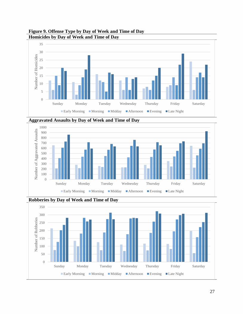
Figure 9 displays similar variation in the temporal nature of violent offending, indicating

the frequency of offenses by time of day and the day of the week. In general across the days of

the week, for each offense type the frequency of reported offenses is the lowest during daylight

hours and increases as time progresses into the late night. The weekends (Saturdays and

Sundays) are an exception to this trend, as there is an increased frequency of offenses in the early

morning hours, possibly following the end of alcohol trading hours. Relative to aggravated

assaults and robberies, homicides also display more variable patterns in offense temporality,

potentially due to the relatively smaller number of total incidents.

26

Figure 8. Offense Type by Location and Time of Day Homicides by Offense Location and Time of Day

Aggravated Assaults by Offense Location and Time of Day

Robberies by Offense Location and Time of Day

Note: GST = Government Building, School, Transportation Hub

0

10

20

30

40

50

60

70

80

Residence Public Area Business GST Other

Num

ber o

f Hom

icid

es

Early Morning Morning Midday Afternoon Evening Late Night

0

500

1000

1500

2000

2500

3000

3500

Residence Public Area Business GST Other

Num

ber o

f Agg

rava

ted

Ass

aults

Early Morning Morning Midday Afternoon Evening Late Night

0

200

400

600

800

1000

1200

1400

Residence Public Area Business GST Other

Num

ber o

f Rob

berie

s

Early Morning Morning Midday Afternoon Evening Late Night

27

Figure 9. Offense Type by Day of Week and Time of Day Homicides by Day of Week and Time of Day

Aggravated Assaults by Day of Week and Time of Day

Robberies by Day of Week and Time of Day

0

5

10

15

20

25

30

35

Sunday Monday Tuesday Wednesday Thursday Friday Saturday

Num

ber o

f Hom

icid

es

Early Morning Morning Midday Afternoon Evening Late Night

0100200300400500600700800900

1000

Sunday Monday Tuesday Wednesday Thursday Friday Saturday

Num

ber o

f Agg

rava

ted

Ass

aults

Early Morning Morning Midday Afternoon Evening Late Night

0

50

100

150

200

250

300

350

Sunday Monday Tuesday Wednesday Thursday Friday Saturday

Num

ber o

f Rob

berie

s

Early Morning Morning Midday Afternoon Evening Late Night

28

Regional Variation and Correlates of Homicides, Aggravated Assaults, and Robberies An explicit purpose of this report is to explore regional variation in violent victimization

and offending across Michigan counties. Using the dplyr package in R, it was possible to easily

group the MICR offenses by the county in which they were reported, counting the number of

unique victims of violent crime across each. It was then possible to pair the victimization totals

in each county to the total population to calculate the victimization rate per 10,000 residents.

Table 19 displays the counties with the top ten highest victimization rates for homicides,

aggravated assaults, and robberies. Concerning homicides, Wayne County had the highest

homicide rate of the Michigan counties in 2013, at 1.96 per 10,000 residents. This is due to the

county containing the city of Detroit, which accounts for a sizable proportion of total homicides.

On the other hand, Saginaw and Genesee have similarly high homicide rates, yet are much

smaller cities, each with a population one-tenth and one-fifth as large, respectively.

It is worth noting that the small relative population of some Michigan counties resulted in

their having a relatively high homicide rate with only a small number of homicides. For instance,

Crawford County reported a single homicide in 2013, resulting in the fourth highest homicide

rate in the state (0.70 homicides per 10,000 residents). In fact, Michigan homicides were

primarily concentrated in Wayne, Saginaw, and Genesee Counties. There were 42 counties

without a single homicide (51%), 20 counties reporting a single homicide (24%), and a total of

51 counties with 5 or fewer homicides (61%).

For aggravated assaults and robberies, Wayne also accounts for the highest relative

victimization rate – particularly for robberies, where it is nearly double the rate of the next

highest county (Genesee). Across all three offense types, there are six counties that appear in the

top 10 for each – Wayne, Saginaw, Genesee, Ingham, Muskegon, and Kalamazoo. Of these

29

counties, Wayne, Genesee, and Saginaw are particularly noteworthy for their historical levels of

violent crime extending back into the 1980s (Matthews, 1997). For instance, in the 2013 MICR

data these three counties comprise 74 percent of all homicides, 54 percent of all aggravated

assaults, and 72 percent of all robberies – further suggesting that violent crime is heavily

concentrated into relatively small geographic areas.

Table 19. Counties with 10 Highest Homicide, Aggravated Assault, and Robbery Victimization Rates per 10,000 Residents. Homicides Aggravated Assaults Robberies Rank County Count Rate County Count Rate County Count Rate 1 Wayne 378 1.96 Wayne 11,543 59.94 Wayne 6,557 34.05 2 Saginaw 31 1.55 Saginaw 1,107 55.34 Genesee 769 18.13 3 Genesee 58 1.37 Mecosta 199 47.64 Ingham 382 13.76 4 Crawford 1 0.70 Genesee 1,833 44.41 Dickinson 34 12.74 5 Ionia 4 0.64 Oscoda 34 39.05 Kalamazoo 280 11.27 6 Gogebic 1 0.63 Calhoun 510 37.61 Saginaw 189 9.45 7 Benzie 1 0.58 Ingham 962 34.65 Muskegon 141 8.11 8 Ingham 15 0.54 Kalamazoo 758 30.51 Berrien 124 7.33 9 Muskegon 8 0.46 Muskegon 481 27.65 Calhoun 89 6.56 10 Kalamazoo 11 0.44 Crawford 38 26.75 Macomb 506 6.09 Table 20 expands on the analysis in Table 19 (above) by examining regional variation in

firearm violence across counties. The results suggest that firearm violence is particularly

concentrated into a small number of counties. As with total homicides, Wayne, Saginaw, and

Genesee Counties showed the highest rates of firearm homicide victimization. There were 58

counties (70%) that had zero firearm homicides, and 75 counties (90%) had 5 or fewer such

homicides during 2013.

Wayne, Genesee, and Saginaw Counties had the top 3 to 4 highest firearm violence

victimization rates across each individual offense type. These three counties accounted for 81

percent of all firearm homicides, 70 percent of firearm aggravated assaults, and 78 percent of

firearm robberies. In this sense, while these three counties already comprised a disproportionate

30

amount of total violent victimizations, firearm violence is even more concentrated within these

three key counties.

Table 20. Counties with 10 Highest Firearm Homicide, Aggravated Assault, and Robbery Rates per 10,000 Residents. Homicides Aggravated Assaults Robberies Rank County Count Rate County Count Rate County Count Rate 1 Wayne 296 1.54 Wayne 4,331 22.49 Wayne 3,709 19.26 2 Saginaw 23 1.15 Saginaw 441 22.04 Genesee 427 10.07 3 Genesee 43 1.01 Genesee 823 19.41 Ingham 157 5.65 4 Ionia 3 0.48 Calhoun 119 8.77 Saginaw 102 5.10 5 Manistee 1 0.41 Muskegon 148 8.51 Kalamazoo 105 4.23 6 Roscommon 1 0.41 Crawford 12 8.45 Muskegon 66 3.79 7 Iosco 1 0.39 Oscoda 7 8.04 Berrien 58 3.61 8 Mason 1 0.35 Ingham 205 7.38 Macomb 228 2.74 9 Muskegon 6 0.34 Kalamazoo 158 6.36 Oakland 318 2.64 10 Clare 1 0.33 Berrien 89 5.55 Baraga 2 2.32 The next section of the report will analyze these three counties more in depth by

examining variation in the violent crime victimization rates among age, race, and gender

subgroups within these counties.

Violent Crime Victimization Rates among Young Men in High Rate Counties – Wayne, Genesee, and Saginaw Analyses of victimization rates earlier in the report suggested that among Michigan

residents, violent crime victimization is more common among young people, African Americans,

and men. Additionally, across all Michigan counties, the violent crime victimization rate was

found to be substantially higher for particular combinations of these subgroups, particularly

young, Black, males. The following Figures examine the victimization rate among young men in

the high victimization rate counties of Wayne, Genesee, and Saginaw, in comparison to

victimization rates for the same groups across the State of Michigan.

31

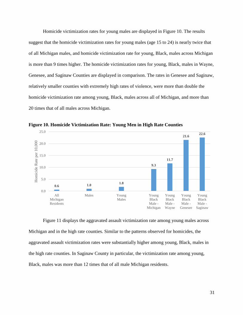
Homicide victimization rates for young males are displayed in Figure 10. The results

suggest that the homicide victimization rates for young males (age 15 to 24) is nearly twice that

of all Michigan males, and homicide victimization rate for young, Black, males across Michigan

is more than 9 times higher. The homicide victimization rates for young, Black, males in Wayne,

Genesee, and Saginaw Counties are displayed in comparison. The rates in Genesee and Saginaw,

relatively smaller counties with extremely high rates of violence, were more than double the

homicide victimization rate among young, Black, males across all of Michigan, and more than

20 times that of all males across Michigan.

Figure 10. Homicide Victimization Rate: Young Men in High Rate Counties

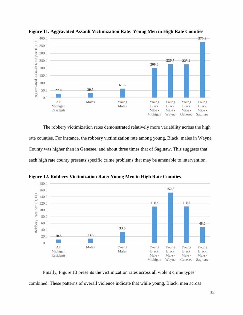
Figure 11 displays the aggravated assault victimization rate among young males across

Michigan and in the high rate counties. Similar to the patterns observed for homicides, the

aggravated assault victimization rates were substantially higher among young, Black, males in

the high rate counties. In Saginaw County in particular, the victimization rate among young,

Black, males was more than 12 times that of all male Michigan residents.

0.6 1.0 1.8

9.3 11.7

21.6 22.6

0.0

5.0

10.0

15.0

20.0

25.0

AllMichiganResidents

Males YoungMales

YoungBlackMale -

Michigan

YoungBlackMale -Wayne

YoungBlackMale -

Genesee

YoungBlackMale -

Saginaw

Hom

icid

e R

ate

per 1

0,00

0

32

Figure 11. Aggravated Assault Victimization Rate: Young Men in High Rate Counties

The robbery victimization rates demonstrated relatively more variability across the high

rate counties. For instance, the robbery victimization rate among young, Black, males in Wayne

County was higher than in Genesee, and about three times that of Saginaw. This suggests that

each high rate county presents specific crime problems that may be amenable to intervention.

Figure 12. Robbery Victimization Rate: Young Men in High Rate Counties

Finally, Figure 13 presents the victimization rates across all violent crime types

combined. These patterns of overall violence indicate that while young, Black, men across

27.0 30.5 61.6

200.0 226.7 225.2

375.3

0.0

50.0

100.0

150.0

200.0

250.0

300.0

350.0

400.0

AllMichiganResidents

Males YoungMales

YoungBlackMale -

Michigan

YoungBlackMale -Wayne

YoungBlackMale -

Genesee

YoungBlackMale -

Saginaw

Agg

rava

ted

Ass

ault

Rat

e pe

r 10,

000

10.5 13.3

33.6

110.3

152.8

110.6

48.0

0.0

20.0

40.0

60.0

80.0

100.0

120.0

140.0

160.0

180.0

AllMichiganResidents

Males YoungMales

YoungBlackMale -

Michigan

YoungBlackMale -Wayne

YoungBlackMale -

Genesee

YoungBlackMale -

Saginaw

Rob

bery

Rat

e pe

r 10,

000

33

Michigan are at a substantially higher risk of violent victimization, the rates within Wayne,

Genesee, and Saginaw Counties present particularly problematic rates of violent victimization.

Figure 13. Total Violent Crime Victimization Rate: Young Men in High Rate Counties

Multivariate Models of Violent Crime Victimizations across Michigan Counties The previous analyses suggest that violent offending and victimization are highly

concentrated within several high rate counties. In order to gain a better understanding of factors

which contribute to variation in violent victimization across the all counties a series of

multivariate negative binomial regression models were estimated. These models examine the

relationship between counts of violent victimizations and the distributions of a set of covariates

in order to state how those covariates contribute the expected count of violent victimizations in a

given county (Gardner, Mulvey, & Shaw, 1995).

The several county-level covariates were constructed using data from the 2010 U.S.

Census and the Uniform Crime Reports (UCR). These covariates are described in Table 21. The

variables population density and metropolitan county were included to capture variation violent

victimizations across urban and rural locations. The variables ethnic heterogeneity, concentrated

38.1 44.8

96.9

319.7

391.2 357.4

445.8

0.0

50.0

100.0

150.0

200.0

250.0

300.0

350.0

400.0

450.0

500.0

AllMichiganResidents

Males YoungMales

YoungBlackMale -

Michigan

YoungBlackMale -Wayne

YoungBlackMale -

Genesee

YoungBlackMale -

Saginaw

Vio

lent

Crim

e R

ate

per 1

0,00

0

34

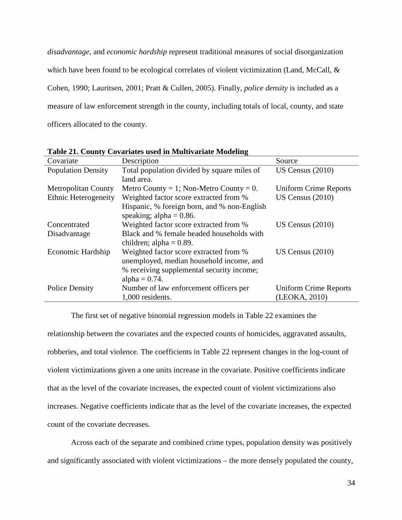
disadvantage, and economic hardship represent traditional measures of social disorganization

which have been found to be ecological correlates of violent victimization (Land, McCall, &

Cohen, 1990; Lauritsen, 2001; Pratt & Cullen, 2005). Finally, police density is included as a

measure of law enforcement strength in the county, including totals of local, county, and state

officers allocated to the county.

Table 21. County Covariates used in Multivariate Modeling Covariate Description Source Population Density Total population divided by square miles of

land area. US Census (2010)

Metropolitan County Metro County = 1; Non-Metro County = 0. Uniform Crime Reports Ethnic Heterogeneity Weighted factor score extracted from %

Hispanic, % foreign born, and % non-English speaking; alpha = 0.86.

US Census (2010)

Concentrated Disadvantage

Weighted factor score extracted from % Black and % female headed households with children; alpha = 0.89.

US Census (2010)

Economic Hardship Weighted factor score extracted from % unemployed, median household income, and % receiving supplemental security income; alpha = 0.74.

US Census (2010)

Police Density Number of law enforcement officers per 1,000 residents.

Uniform Crime Reports (LEOKA, 2010)

The first set of negative binomial regression models in Table 22 examines the

relationship between the covariates and the expected counts of homicides, aggravated assaults,

robberies, and total violence. The coefficients in Table 22 represent changes in the log-count of

violent victimizations given a one units increase in the covariate. Positive coefficients indicate

that as the level of the covariate increases, the expected count of violent victimizations also

increases. Negative coefficients indicate that as the level of the covariate increases, the expected

count of the covariate decreases.

Across each of the separate and combined crime types, population density was positively

and significantly associated with violent victimizations – the more densely populated the county,

35

the higher the expected count of violent victimizations. Other covariates were not significantly

associated with variation in violent victimizations across all crime types. Contrary to

expectations counties with higher levels of concentrated disadvantage had lower expected counts

of aggravated assault victimizations. Counties with higher levels of economic hardship saw

significantly higher expected counts of homicides and aggravated assaults. Police density was

positively associated with aggravated assault and robbery victimization, suggesting that more

police officers are present in counties with relatively high counts of violent victimizations. This

likely reflects a greater relative investment in police resources in counties with higher levels of

violent crime.

Table 22. Negative Binomial Regression Models for Homicides, Aggravated Assaults, and Robberies on County Covariates (N = 83) Covariates Model 1:

Homicides Model 2:

Aggravated Assaults

Model 3: Robberies

Model 4: Total Violence

Est. (SE) Est. (SE) Est. (SE) Est. (SE) Population Densitya 0.43 (0.19)* 0.29 (0.08)*** 0.86 (0.18)*** 0.35 (0.09)*** Metro County 0.04 (0.38) 0.28 (0.17) 0.67 (0.33)* 0.55 (0.18)** Ethnic Heterogeneity -0.22 (0.14) 0.01 (0.06) -0.11 (0.13) -0.03 (0.07) Conc. Disadvantage 0.04 (0.16) -0.29 (0.08)*** -0.21 (0.16) -0.33 (0.09)*** Econ. Hardship 0.46 (0.10)*** 0.31 (0.05)*** 0.36 (0.10) 0.22 (0.06)*** Police Densitya 0.34 (0.27) 0.38 (0.15)* 0.72 (0.29)* 0.60 (0.17)*** Intercept -13.1 (0.84)*** -8.20 (0.36)*** -13.6 (0.80)*** -8.48 (0.40)*** -2 Log Likelihood -225.98 -769.13 -443.14 -807.36 Resid. Deviance (df) 75.96 (76) 87.70 (76) 98.03 (76) 84.81 (76) LR Test χ2 8.04** 921.41*** 393.63*** 2,366.30*** Note: * p < .05, ** p < .01, *** p < .001; Counts represent total victims in each county; Total county population used as offset; LR = Likelihood Ratio a Indicates that the predictor has been logged. The second set of regression models estimate the contribution of the county-level

covariates to counts of violent victimizations by firearms (see Table 23).7 Similar to the findings

7 A model for firearm homicides was not estimated. This is due to the large number of counties with zero firearm homicides (78%), which necessitates the use of a zero-inflated negative binomial regression model. These models

36

for the overall violent victimizations models, population density, the county falling in a

metropolitan area, economic hardship, and police density were all positively associated with

counts of firearm aggravated assaults and robberies.8

Table 23. Negative Binomial Regression Models for Firearm Homicides, Aggravated Assaults, and Robberies on County Covariates (N = 83) Covariates Model 1:

Homicides Model 2:

Aggravated Assaults

Model 3: Robberies

Model 4: Total Violence

Est. (SE) Est. (SE) Est. (SE) Est. (SE) Population Densitya -- 0.31 (0.13)* 0.97 (0.25)*** 0.40 (0.13)** Metro County -- 0.61 (0.26)* 0.58 (0.44)* 0.66 (0.25)** Ethnic Heterogeneity -- -0.08 (0.10) -0.16 (0.18) -0.08 (0.10) Conc. Disadvantage -- -0.21 (0.13) -0.14 (0.21) -0.21 (0.12) Econ. Hardship -- 0.45 (0.45)*** 0.36 (0.14)* 0.43 (0.07)*** Police Densitya -- 0.73 (0.24)** 0.58 (0.38) 0.81 (0.23)*** Intercept -- 10.3 (0.58)*** -15.4 (1.13)*** -10.6 (0.56)*** -2 Log Likelihood -- -544.00 -321.10 -572.10 Resid. Deviance (df) -- 96.10 (76) 84.67 (76) 96.41 (76) LR Test χ2 -- 282.15*** 149.35*** 391.60*** Note: * p < .05, ** p < .01, *** p < .001; Counts represent total victims in each county; Total county population used as offset; LR = Likelihood Ratio a Indicates that the predictor has been logged.

are generally inappropriate for small sample sizes, such as the current sample of Michigan counties (“R Data Analysis Examples: Zero-Inflated Negative Binomial Regression”, 2014). As such, the model for firearm homicides is not estimated. 8 Additional sensitivity analyses (not shown) were conducted to assess the robustness of the associations in Tables 22 and 23. These analyses estimated alternative models in which adjustments were made for multi-collinearity and outlier violence rates. It was observed that the significant relationship for police density and the different overall violence measures disappeared when multi-collinearity was reduced. A similar change was not observed for firearm violence.

37

CONCLUSIONS Limitations The descriptive analyses in the current report are not without limitation. It is worth noting

again that the violent offense totals and rates presented here will differ slightly from official

Michigan State Police publications. The current report uses a subset of the overall MICR data

and differences in the data reduction process can result in different totals being produced. It is

not claimed here that the totals generated in the report are the true offense totals.

Second, the estimation of victimization and offense rates will be subject to some error

due to non-reporting by active law enforcement agencies. However, 87 percent of Michigan law

enforcement agencies submitted a full 12 years of data, and 94 percent submitted at least partial

data, lending validity to the claim that the rates estimated here at least represent relative

differences between victim demographic subgroups and counties.

Finally, because of the process through which MICR data are generated, these analyses

can only claim to represent violent crimes that are reported to the police, excluding offenses that

never came to the attention of law enforcement. Fortunately, violent offenses, particularly the

serious violent offenses here have tended to be reported to the police more reliably than other

offenses. The most recent data from the National Crime Victimization survey suggests that 68

percent of robbery victims nationally report the incident to the police, as do 64 percent of

aggravated assault victims (Truman & Langton, 2014). These figures stand in comparison to 36

percent of all property crime victims nationally reporting their victimization to the police

(Truman & Langton, 2014).

38

Summary and Policy Considerations Determining how to allocate scarce resources, at local, state and federal levels, towards

reducing violent crime remains a paramount issue for law enforcement. Particularly in Michigan,

over the last decade law enforcement agencies increasingly faced relatively high rates of general

and firearm violence in spite of declining budgets and declining numbers of sworn personnel. As

such, the systematic analysis of MICR data can be utilized to suggest areas of enforcement,

prevention and intervention. The analyses in the current report suggest that the risk of violent

victimization is strongly concentrated among demographic subgroups and across geographic

regions of the state. In Michigan in 2013, young, Black males were at a substantially higher risk

for violent victimization – especially for homicides and robberies. Young, Black females made

up a disproportionate number of aggravated assault victims – experiencing a victimization rate

on par with that of Black males.

These victimization rates were observed to vary considerably across Michigan counties.

Wayne, Saginaw, Genesee, Ingham, Muskegon, and Kalamazoo Counties all had top 10

victimization rates for homicides, aggravated assaults, and robberies. In particular, Wayne,

Genesee, and Saginaw counties comprised the top 3-4 counties for rates of firearm violence.

The concentration of victimization risk is particularly striking when combining

demographic characteristics and geography. Specifically within these subareas (Wayne, Genesee,

and Saginaw Counties), young, Black males already at a high rate of violent victimization

statewide were at an even higher risk of such victimization. Indeed, young, Black males in

Wayne, Genesee, and Saginaw Counties had a violent victimization risk in excess of 10 times

that of all male Michigan residents. The homicide victimization rate was even more striking as

young, Black males in these three counties experienced rates 19 to 37 times that of other

39

Michigan residents. If this were a discussion of another type of disease, these rates of

victimization would be considered a public health epidemic.

These disproportionately high rates of violent victimization within already high violent

crime rate counties suggest an appropriate focus for law enforcement intervention and related

prevention efforts. Research evidence demonstrates that enforcement, intervention, and

prevention, using data-driven, evidence-based strategies hold considerable promise for reducing

violence. Specifically, highly focused and targeted interventions have been shown to be the key

for crime and violence reduction (National Research Council, 2004). The findings of the current

analysis support such highly focused and targeted efforts.9

Fortunately, such efforts are underway. The Governor’s Secure Cities initiative dedicates

enforcement and related resources to Detroit, Flint, and Saginaw (Wayne, Genesee, and Saginaw

Counties) along with Pontiac (Oakland County). The U.S. Attorney’s Offices in the Eastern and

Western Districts have coordinated Project Safe Neighborhoods (PSN) initiatives focused on gun

and gang violence in the Counties suggested in this study. Various federally supported

initiatives such as Detroit Ceasefire and Detroit PSN, Byrne Criminal Justice Innovation (Detroit

and Flint), the Michigan Youth Violence Prevention Center (Flint), Detroit’s participation in the

Violence Reduction Network, among others, focus on the cities and neighborhoods within these

cities suffering high rates of violent victimization.

The operation of DDACTS (Data Driven Approaches to Crime and Traffic Safety) by the

Michigan State Police in Flint (Genesee County) already represents one such enforcement-

9 The School of Criminal Justice at Michigan State University, with the support of the U.S. Department of Justice, Bureau of Justice Assistance, is developing the Violence Reduction Assessment Tool. Known as the VRAT, it is a planning and assessment tool to support local communities in the identification and effective implementation of evidence-based violence reduction practices. Although currently in development, the School is happy to assist local communities in piloting the use of VRAT to assist their efforts. Please contact Ms. Heather Perez (perezh@msu.edu) for additional information.

40

guided effort to reduce violence. Part of the Secure Cities initiative, a prior evaluation found

reductions of 14 percent in violent crime and 30 percent in robbery in the target locations of Flint

(Rydberg, McGarrell, and Norris, 2014).

The DDACTS approach is suggested by prior research on the use of directed police patrol

in gun crime hotspots. Studies conducted in Kansas City, Indianapolis, and Pittsburgh found that

such directed patrols focused on illegal firearms in gun crime hotspots resulted in significant

reductions in firearms violence (Sherman and Rogan, 1995; McGarrell et al. 2001; Cohen and

Ludwig, 2003). More recent experimental evidence from St. Louis suggests that directed police

patrols combined with officer self-initiated enforcement activity within tightly defined hotspots

significantly reduced firearm aggravated assaults over a nine-month period (Rosenfeld, Deckard,

& Blackburn, 2014).

In addition to directed patrol at violent crime hotspots, problem solving initiatives

focused on specific places and foot patrol have demonstrated promise for reducing violent crime

(Braga and Weisburd, 2010; Braga, Papachristos, and Hureau, 2012; Ratcliffe et al., 2011).

Yet, there are questions about the long-term impact of focused enforcement efforts alone

(e.g., Sorg et al., 2013). Consequently a broader set of prevention and intervention strategies can

complement these enforcement strategies. These include the Ceasefire focused deterrence model

that addresses group-based violence (Braga et al. 2001; McGarrell et al. 2006; Corsaro and

McGarrell, 2010) and the drug market intervention focused on closing down violence-generating

drug markets (McGarrell 2014; McGarrell et al., 2013). Similar promising strategies include

parolee forums with high risk parolees returning to high violent crime locations (Braga, Piehl,

and Hureau, 2009; Papachristos et al., 2013) and the High Point, North Carolina focused

deterrence approach to intimate partner violence.

41

Many other evidence-based and evidence-informed interventions are available ranging

from primary prevention (e.g., nurse-family partnerships, pre-school), to offender-based

interventions (cognitive-behavioral), and community-focused interventions (e.g., crime

prevention through environmental design; blight elimination and greening). More information is

available at crimesolutions.gov. The common ingredient across these interventions is developing

highly focused and targeted interventions based on data-driven problem assessments. Though

possible options exist, any Michigan evidence-based approach should consider using detailed

MICR data to inform the allocation of resources towards those at the highest risk in the areas

with the highest risk of violent crime.

Finally, when considering focusing enforcement, prevention and intervention strategies in

the counties, cities, and neighborhoods suffering from the highest rates of violence, it is

important to remember that while violence is highly concentrated, it is still a sub-set of people

and places that drive the violence problem. Within the high violent crime cities of Detroit, Flint,

and Saginaw, most young, African-American men are not carrying and using illegal firearms;

most citizens are law abiding; and many street segments, even in high crime areas, do not

experience violent crime. This reality calls for careful analysis, highly focused interventions,

police-citizen collaboration, balanced enforcement and prevention strategies, economic

development and neighborhood revitalization efforts, and fair and respectful policing.

42

REFERENCES

Blumstein, A. (1995). Youth violence, guns, and the illicit-drug industry. Journal of Criminal Law & Criminology, 86(1), 10-36.

Braga, A. A. (2003). Serious youth gun offenders and the epidemic of youth violence in Boston.

Journal of Quantitative Criminology, 19(1), 33-54. Braga, A.A., Papachristos, A.V., & Hureau, D.M. (2012). The effects of hotspots policing on

crime: An updated systematic review and meta-analysis. Justice Quarterly Braga A.A. & Weisburd, D.L... (2010). Policing Problem Places: Crime Hot Spots and Effective

Prevention. Oxford University Press, New York. Braga, A.A., Piehl, A.M, & Hureau, D. (2009). “Controlling Violent Offenders Released to the

Community: An Evaluation of the Boston Reentry Initiative.” Journal of Research in Crime and Delinquency 46:411-436.

Braga A.A., Kennedy, D.M., Waring, E.J., & Piehl, A.M. (2001). Problem-oriented policing,

deterrence, and youth violence: An evaluation of Boston's Operation Ceasefire. Journal of Research in Crime and Delinquency, 38: 195-225.

Center for Disease Control (2014). Top 10 leading causes of death, Black Males, 2012. Retrieved

from http://webappa.cdc.gov/cgi-bin/broker.exe, December 18th, 2014. Cohen, J. & Ludwig, J. 2003. Policing crime guns. In (P.J. Cook and J. Ludwig,

eds.), Evaluating gun policy: Effects on crime and violence (pp. 217-239). Washington, DC: Brookings Institution Press.

Corsaro, N. & McGarrell, E.F. (2010). “Reducing homicide risk in Indianapolis between 1997

and 2000.” Journal of Urban Health 87, 5: 851-64. Dahlberg, L. L. (1998). Youth violence in the United States: Major trends, risk factors, and

prevention approaches. American Journal of Preventative Medicine, 14(4), 259-272. Gardner, W., Mulvey, E. P., & Shaw, E. C. (1995). Regression analyses of counts and rates:

Poisson, overdispersed Poisson, and negative binomial models. Psychological Bulletin, 118(3), 392-404.

Grommon, E., & Rydberg, J. (Forthcoming). Elaborating the correlates of firearm injury

severity: Combining criminological and public health concerns. Victims & Offenders. doi: 10.1080/15564886.2014.952472

Kposowa, A. J., Breault, K. D., & Harrison, B. M. (1995). Reassessing the structural covariates

of violent and property crimes in the USA: A county level analysis. British Journal of Criminology, 46(1), 79-105.

43

Lauritsen, J. (2001). The social ecology of violent victimization: Individual and contextual

effects in the NCVS. Journal of Quantitative Criminology, 17(1), 3-32. Land, K. C., McCall, P. L., & Cohen, L. E. (1990). Structural covariates of homicide rates: Are

there any invariances across time and social space? American Journal of Sociology, 95(4), 922-963.

Matthews, R. (1997). What’s good for GM…: Deindustrialization and crime in four Michigan

cities, 1975-1993. Dissertation: Western Michigan University, Department of Sociology. McGarrell, E.F. (2014). “Offender-oriented Strategies: The focused deterrence ‘pulling levers’

strategy.” In G.J.N. Bruinsma, D.L. Weisburd (eds.), Encyclopedia of Criminology and Criminal Justice, New York: Springer.

McGarrell, E.F., Hipple, N.K. Bynum, T.S., Perez, H., Gregory, K., Kane, C.M., & Ransford, C. (2013). Promising strategies for violence reduction: Lessons from two

decades of innovation. Project Safe Neighborhoods Case Study Report #13. Washington, DC: U.S. Department of Justice, Bureau of Justice Assistance.

McGarrell, E.F., Corsaro, N., Hipple, N.K. & Bynum, T.S. (2010). Project safe neighborhoods

and violent crime trends in U.S. cities: Assessing violent crime impact. Journal of Quantitative Criminology, 26: 165-190.

McGarrell, E.F., Chermak, S.,Wilson, J.M. & Corsaro, N. (2006). Reducing homicide through a

"lever-pulling" strategy. Justice Quarterly, 23:214-231. McGarrell, E. F., & Chermak, S. (2004). Strategic approaches to reducing firearms violence:

Final report on the Indianapolis violence reduction partnership. Report submitted to the U.S. Department of Justice.

McGarrell, E.F., Chermak, S., Weiss, A. & Wilson, J.M.. (2001). Reducing firearms violence

through directed police patrol. Criminology and Public Policy, 1: 119-148. Michigan Incident Crime Reporting (2014). 2013 Crimes at a glance: Group “A” crimes.

Lansing, MI: Michigan State Police. National Research Council. (2004). Fairness and effectiveness in policing: the evidence. (W.

Skogan & K. Frydl, eds.) Washington, DC. National Academies Press. Papachristos, A.V., Wallace, D., Meares, T., and Fagan, J. (2013). Desistance and legitimacy:

The impact of offender notification meetings on recidivism among high risk offenders. Columbia Public Law Research Paper #13-343, Yale Law and Economics Research Paper #469.

44

Pratt, T. C., & Cullen, F. T. (2005). Assessing macro-level predictors and theories of crime: A meta-analysis. In M. H. Tonry (ed.) Crime and Justice: A Review of Research, Vol. 32. Chicago: University of Chicago Press.

R Core Team. (2014). R: A language and environment for statistical computing. R Foundation

for Statistical Computing, Vienna, Austria. http://R-project.org. R Data Analysis Examples: Zero-Inflated Negative Binomial Regression. UCLA: Statistical

Consulting Group. Retrieved from http://www.ats.ucla.edu/stat/r/dae/zinbreg.htm, December 1st, 2014.

Ratcliffe, J.H, Taniguchi, T., Groff, E.R., & Wood, J. (2011). The Philadelphia Foot Patrol

Experiment: A randomized controlled trial. Criminology, 49(4),795-831. Rosenfeld, R., Deckard, M. J., & Blackburn, E. (2014). The effects of directed patrol and self-

initiated enforcement on firearm violence: A randomized controlled study of hot spot policing. Criminology, 52(3), 428-449.

Rydberg, J., McGarrell, E.F., & Norris, A. (2014). Flint DDACTS pilot evaluation. East Lansing,

MI: Michigan Justice Statistics Center, School of Criminal Justice, Michigan State University.

Sampson, R. J., & Lauritsen, J. L. (1994). Violent victimization and offending: Individual-,

situational-, and community-level risk factors. In A. J. Reiss, Jr. & J. A. Roth (eds.), Understanding and preventing violence: Social influences on violence, Vol. 3. Committee on Law and Justice, National Research Council. Washington, D.C.: National Academy Press.

Sherman, L.W. and Rogan, D.P. (1995). Deterrent Effects of Police Raids on Crack Houses: A

Randomized, Controlled Experiment. Justice Quarterly, 12(4), 755-781. Sorg, E.T., Haberman, C.P., Ratcliffe, J.H. & Groff, E. (2013). Foot patrol in violent crime hot

spots. Criminology 5(1), 65-102. Tillyer, M. S., & Tillyer, R. (2014). Violence in context: A multi-level analysis of victim injury

in robbery incidents. Justice Quarterly, 31(4), 767-791. Truman, J. L., & Langton, L. (2014). Criminal victimization, 2013. Washington, DC: U.S.

Department of Justice, Office of Justice Programs, Bureau of Justice Statistics. Weber, R. (2012). An analysis of domestic violence and arrest patterns in Vermont using NIBRS

data. Northfield Falls, VT: The Vermont Center for Justice Research. Wickham, H., & Francois, R. (2014). dplyr: A grammar of data manipulation. R package version

0.3.0.2. http://CRAN.R-project.org/package=dplyr.

45

APPENDIX

46

APPENDIX A

MICR FILE LINKING PROCESS

Table A.1: Initial Files Received and Utilized

File Name File Description

MICR1 Administrative look-up table; Includes date and time

MICRADDRS Location table

MICR3 Offender table

MICROUSED Offender used table

MICR5 Victim table

MICRVOFNS Offense against victim table

MICRVOR Victim-Offender relationship table

MICR7 Arrestee table

MICRARMED Arrestee armed table

MICROFFNS Offense table

MICRATYPE Activity type table

Table A.2: Unique Identifier Creation

Identifier (File Name) Components

Victim ID (MICR5) MIC1_NUMBER + MICR5_VICTIMNO

Victim ID (MICRVOFNS) MIC1_NUMBER + VOFNS_VICTIMNO

Victim ID (MICRVOR) MIC1_NUMBER + VOR_VICTIMNO

Offender ID (MICR3) MIC1_NUMBER + MICR3_OFFENDERNO

Offender ID (MICRVOR) MIC1_NUMBER + VOR_OFFEDERNO

Offender ID (MICR7) MIC1_NUMBER + MICR7_ARRESTNO

Offender ID (MICRARMED) MIC1_NUMBER + ARMED_ARRESTNO

Offense ID (MICROUSED) MIC1_NUMBER + OUSED_OFFENSE_CO

Offense ID (MICROFFNS) MIC1_NUMBER + OFFNS_OFFENSE_CO

Offense ID (MICRATYPE) MIC1_NUMBER + ATYPE_OFFENSE_CO

Offense ID (MICRVOFNS) MIC1_NUMBER + VOFNS_OFFENSE_CO

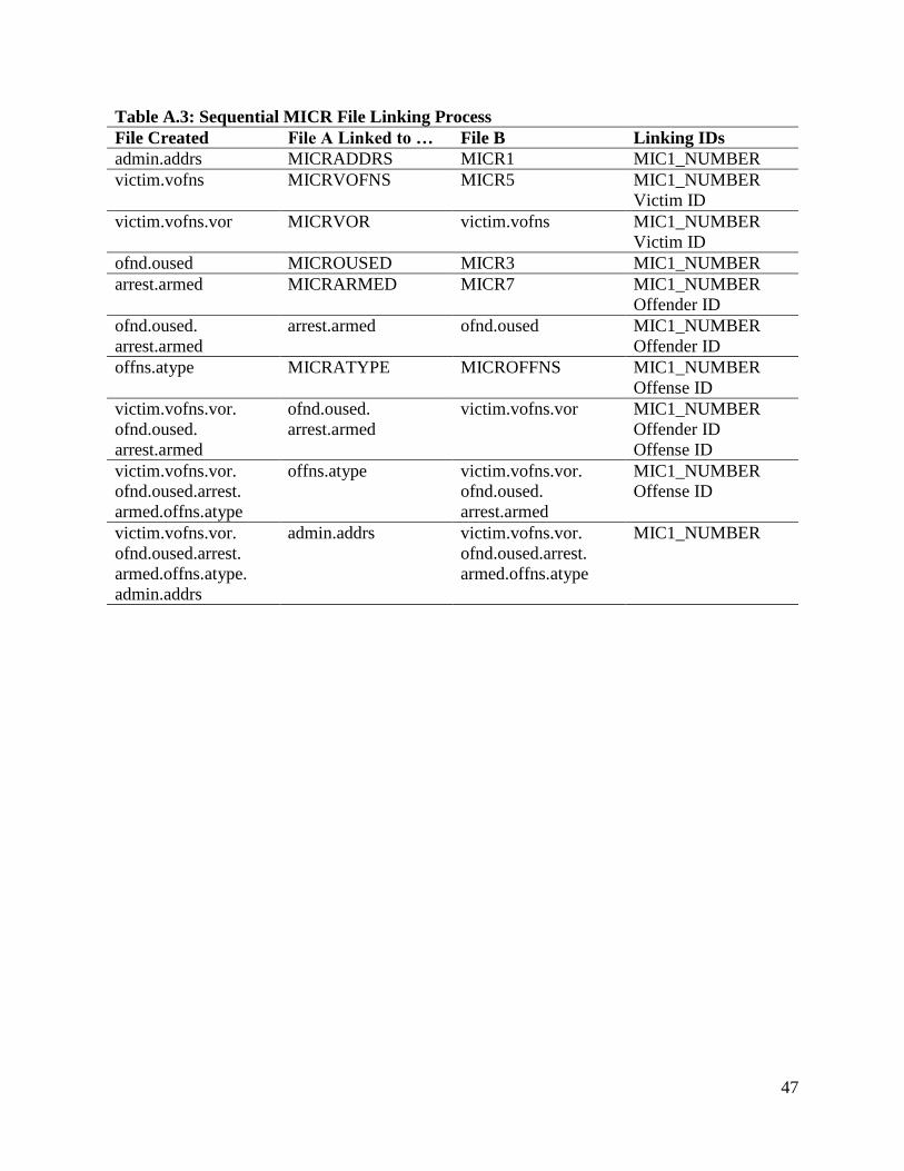
47

Table A.3: Sequential MICR File Linking Process

File Created File A Linked to … File B Linking IDs

admin.addrs MICRADDRS MICR1 MIC1_NUMBER

victim.vofns MICRVOFNS MICR5 MIC1_NUMBER

Victim ID

victim.vofns.vor MICRVOR victim.vofns MIC1_NUMBER

Victim ID

ofnd.oused MICROUSED MICR3 MIC1_NUMBER

arrest.armed MICRARMED MICR7 MIC1_NUMBER

Offender ID

ofnd.oused.

arrest.armed

arrest.armed ofnd.oused MIC1_NUMBER

Offender ID

offns.atype MICRATYPE MICROFFNS MIC1_NUMBER

Offense ID

victim.vofns.vor.

ofnd.oused.

arrest.armed

ofnd.oused.

arrest.armed

victim.vofns.vor MIC1_NUMBER

Offender ID

Offense ID

victim.vofns.vor.

ofnd.oused.arrest.

armed.offns.atype

offns.atype victim.vofns.vor.

ofnd.oused.

arrest.armed

MIC1_NUMBER

Offense ID

victim.vofns.vor.

ofnd.oused.arrest.

armed.offns.atype.

admin.addrs

admin.addrs victim.vofns.vor.

ofnd.oused.arrest.

armed.offns.atype

MIC1_NUMBER