An Additional Application of the Space Interferometry

Mission to Gravitational Microlensing Experiments

Cheongho Han

Department of Astronomy & Space Science,Chungbuk National University, Chongju, Korea 361-763

cheongho@astronomy.chungbuk.ac.kr

Tu-Whan Kim

Department of Astronomy,Yonsei University, Seoul, Korea 120-749

Received ; accepted

– 2 –

ABSTRACT

Despite the detection of a large number of gravitational microlensing events,the nature of Galactic dark matter remains very uncertain. This uncertaintyis due to two major reasons: the lens parameter degeneracy in the measuredEinstein timescale and the blending problem in dense field photometry. Recently,consideration has been given to routine astrometric followup observations oflensing events using the Space Interferometry Mission (SIM) as a means ofbreaking the lens parameter degeneracy in microlensing events. In this paper,we show that in addition to breaking the lens parameter degeneracy, SIMobservations can also be used to correct for nearly all types of blending.Therefore, by resolving both the problems of the lens parameter degeneracyand blending, SIM observations of gravitational lensing events will significantlybetter constrain the nature of Galactic dark matter.

Subject headings: gravitational lensing – dark matter – astrometry – photometry

resubmitted to Monthly Notices of the Royal Astronomy Society: Dec. 28, 1998Preprint: CNU-A&SS-09/98

– 3 –

1. Introduction

Surveys to detect Galactic dark matter by monitoring light variations of source starscaused by gravitational microlensing are being carried out by several groups and ∼ 300events have been detected (MACHO: Alcock et al. 1997a, 1997b; EROS: Ansari et al. 1996;OGLE: Udalski et al. 1997). The light curve of a lensing event is represented by

Aabs =u2 + 2

u(u2 + 4)1/2; u =

[β2 +

(t − t0

tE

)2]1/2

, (1.1)

where the lensing parameters β, t0, and tE represent the lens-source impact parameter,the time of maximum amplification, and the Einstein ring radius crossing time (Einsteintimescale), respectively. Once the light curve of an event is observed, these lensingparameters are obtained by fitting the theoretical light curves of equation (1.1) to theobservations. One can obtain information about individual lenses because the Einsteintimescale is related to the physical lens parameters by

tE =rE

v, rE =

(4GM

c2

DolDls

Dos

)1/2

, (1.2)

where rE is the Einstein ring radius, v is the lens-source transverse speed, M is the lensmass, and Dol, Dls, and Dos are the separations between the observer, lens, and source star.However, since the Einstein timescale depends on a combination of the lens parameters, thevalues of the lens parameters determined from it suffer from large uncertainties.

The lens parameters suffer from additional uncertainties due to blending. Theprobability for a single source star to be in the state of gravitational amplification, i.e., theoptical depth τ , is very low; from (O)10−7 to (O)10−6 depending on the observed field.To increase the event rate, therefore, experiments are being conducted toward very densestar fields such as the Galactic bulge and Magellanic Clouds. However, photometry of suchdense star fields is affected by the flux from stars not participating in the gravitationallensing, the “blending problem.” Depending on the origin of the blended light, blending isclassified into regular, amplification-bias, binary-source, and bright-lens blending (see § 2).When an event is affected by blending, the observed light curve is represented by

Aobs = Aabs(1− f) + f ; f =B

F0 + B, (1.3)

where F0 is the unblended flux of the source star before (or after) gravitational amplification,B is the amount of blended flux, and thus f represents the fraction of the blended lightto the total observed flux. Therefore, when fitting a blended lensing event light curve,an additional lensing parameter f must be included. As a result, the determined lensparameters become even more uncertain.

Efforts to improve the results of gravitational microlensing experiments are thereforefocused on breaking the lens parameter degeneracy and correcting for the blending effect.

– 4 –

Various methods have been proposed to do this. The methods for removing the degeneracyin the lens parameters are summarized by Jeong, Han, & Park (1999). Here we discussthe methods proposed to correct for various types of blending (see § 2). However, thesemethods are either applicable to only in a few rare cases or impractical due to the largeuncertainty in the determined value of f . Therefore, to gain improved results from the nextgeneration of lensing experiments, it is essential to devise practical methods that can resolvethe problems of the lens parameter degeneracy and blending in general microlensing events.

Recently, routine astrometric followup observations of lensing events with high precisioninstruments such as the Space Interferometry Mission (hereafter SIM, Allen, Shao, &Peterson 1998) are being discussed as a method to break the lens parameter degeneracyof general microlensing events. When a source star is gravitationally lensed, it is splitinto two images. The image separation is too small for direct observation. However, thedisplacements of the light centroid of the two images can be measured with SIM. Thetrajectory of the centroid shifts is an ellipse (astrometric ellipse) whose shape depends onthe lens-source impact parameter (see § 4.2). The usefulness of astrometric measurementsof lensing events is that one can determine the angular Einstein ring radius, θE = rE/Dol,from the measured centroid shifts because the size of the astrometric ellipse is directlyproportional to θE. While the Einstein timescale depends on three lens parameters (M ,Dos, and v), the angular Einstein ring radius depends only on two parameters (M and Dol).Therefore, by measuring θE, the uncertainties in the determined lens parameters can besignificantly reduced (Walker 1995; Paczynski 1998; Boden, Shao, & Van Buren 1998; Han& Chang 1998).

In this paper, we show that in addition to breaking the lens parameter degeneracy,observations with SIM can be used to correct for the blending effect in general microlensingevents. Due to the high resolution, ∼< 0.′′5, from the diffraction-limited space observations,a significant fraction of events blended by field stars, i.e., regular and amplification-biasblended events, are automatically resolved by a single mirror of SIM. For events affectedby very close blends with separations ∆θ ∼< 10 mas, including a large fraction of binarycompanions and all bright lenses, one can also identify the lensed source star by detectingthe distortions of the astrometric centroid trajectory caused by the blended star. For eventsaffected by medium range separation blends, 10 mas ∼< ∆θ ∼< 0.′′5, the blending effect can becorrected for by either detecting the shift of the broad envelope centroid between the pointspread functions (PSFs) of lensed and blended stars caused by gravitational amplificationor by examining the narrow fringe patterns observed at multi-wavelengths. Therefore, byresolving both the problems of lens parameter degeneracy and blending, SIM observationsof gravitational lensing events will significantly better constrain the nature of Galactic darkmatter.

– 5 –

2. Types of Blending

Depending on the origin of the blended light, blending is classified into several types.First, “regular blending” occurs when a star brighter than the detection limit, which isset by crowding, is lensed and the measured flux is affected by the residual flux fromother blended stars fainter than the detection limit. Due to regular blending, the apparentamplification of the event is lower than its intrinsic value. As a result, the apparent Einsteintimescale is shorter than its true value, resulting in systematic underestimation of lensmasses (Di Stefano & Esin 1995; Wozniak & Paczynski 1997; Han 1998b). Since the opticaldepth is directly proportional to the timescale, the value of τ determined without properlycorrecting for regular blending is also underestimated.

The observed light curve is also affected by blending when one of several unresolvedfaint stars below the detection limit is lensed and its flux is associated with the flux fromother field stars in the effective seeing disk of a monitored bright source star. This isknown as “amplification-bias blending” (Bouquet 1993; Nemiroff 1994). The effects ofamplification-bias blending for the determination of individual lens parameters are similarto those of regular blending, but the effects are more severe due to the much larger amountof blended light. However, the most important effect of amplification bias blending is thatwhen not accounted for, the optical depth might be significantly overestimated (Alard1997). This is because τ is determined based only on the number of monitored stars brighterthan the detection limit, while events are actually detected among a larger number of stars,including fainter stars. Han (1997) estimated that the increase in τ caused by the miscountof effectively monitored stars is large enough to compensate the decrease in τ due to thedecrease in timescales and make the observed optical depth overestimated by a factor ∼ 1.7.

In addition to background stars the lens itself can cause blending known as “brightlens blending” (Kamionkowski 1995; Buchalter & Kamionkowski 1997; Nemiroff 1997;Han 1998a). Bright lens blending causes the measured timescale and optical depth tobe underestimated in the same manner as regular blending. In addition to the effects ofregular blending, lens blending causes the determined optical depth to depend on the lenslocation. This is because detecting events caused by bright lenses close to the observeris comparatively more difficult than detecting events produced by lenses near the source.Additionally, since the brighter the lens is, the more massive it tends to be, and thus themore likely it is to be affected by lens blending. As a result, the decrease in optical depthfor massive lenses is relatively bigger than the decrease for low-mass lenses, making themeasured optical depth dependent on the lens mass function.

Finally, the last type of blending, known as “binary star blending” occurs when thesource is a binary. In general, the typical separation between the component stars in abinary system is larger than the typical size of the Einstein ring radius. In this case onlyone star is significantly amplified, and the flux from the other star simply contributes asblended light (Dominik 1998). For some binaries with small component separations, on the

– 6 –

other hand, both component stars can be amplified. However, even in these cases it is noteasy to detect the binarity of the source because the light curve mimics that of a singlesource event with a longer timescale and larger impact parameter than the true values(Griest & Hu 1992; Han & Jeong 1998).

3. Limitations of Current Blending-Correction Methods

There have been various methods proposed to correct for the blending problem.However, these methods are either applicable to only a few specific types of blending orimpractical due to the large uncertainty in the determined value of f . In this section, welist these proposed methods and discuss their performance in correcting blending effects.

Because a blended event light curve is not exactly the same as that of an unblendedevent, ideally the effects are detectable using photometry. However, due to the limits onphotometric precision of the current lensing experiments, blending has been photometricallydetected only in a small number of events. Nevertheless, photometry is still being discussedbecause of the rapidly increasing photometric precision made possible through the operationof early warning systems (MACHO: Alcock et al. 1996; OGLE: Udalski et al. 1994) andsubsequent effective followup observations (PLANET: Albrow et al. 1998; GMAN: Alcocket al. 1997c). However, we still find that even with this higher precision photometry, theuncertainties in the derived lensing parameters are very large, making it difficult to properlycorrect for blending effects. To demonstrate this, we simulate model events that are affectedby various amounts of blended light and estimate the uncertainties of the recovered lensingparameters. The events are assumed to have β = 0.3, and tE,0 = 15 days, which are themost common values for the Galactic bulge events, and are affected by blending with variousblended light fractions of f = 0.3, 0.5, 0.7, and 0.9. The events are assumed to be observed5 times/day during −0.5tE ≤ tobs ≤ 3tE with a high photometric precision of p = 1%. Thelight curves are then fit with a theoretical blended light curve as given by equation (1.3).We estimate the uncertainties of the recovered lensing parameters by computing the valuesof χ2 by

χ2 =Ndat∑i=1

(AO − AT

pAT

)2

, (3.1)

where Ndat is the number of data points and AO and AT represent the simulatedand theoretical model light curves, respectively. In Figure 1, we present the resultingvalues of χ2 as functions of tE/tE,0 and f . The degrees of freedom are determined bydof = Ndat − Npar − 1, where Npar = 4 is the number of lensing parameters for theblended light curve fit. The contours are drawn at the levels of ∆χ2 = 1.0, 4.0, and 9.0(i.e., 1 σ, 2 σ, and 3 σ levels) from inside to outside. From the figure, one finds that theuncertainties in both the derived values of tE and f are large. One also finds that theuncertainty ranges of the blended light fraction measured at all levels include f = 0 (i.e.,

– 7 –

no blended light), implying that it will be difficult to detect blending effect even with highprecision photometry. In addition, since the uncertainties increase rapidly with increasingvalues of f , correcting for blending effects using this method will be especially difficult foramplification-bias events which are severely affected by blending.

Another method of correcting for blending effects is to detect color shifts during anevent with high precision, multi-band photometry (Buchalter, Kamionkowski, & Rich 1996).This method might be applicable if the lensed source star has a very different color fromthat of the integrated light of the blended stars. However, the expected amount of colorshift is generally very small because most Galactic bulge stars have similar colors (Goldberg1998). In addition, even when the color shift is detected, the determined lens parameterssuffer from the same degeneracy as in the case of single-band photometry, making it difficultto properly correct for the blending effect (Wozniak & Paczynski 1997).

A more general method of correcting for blending effects is by detecting the shifts ofa source star’s image centroid, δx, during an event (Alard, Mao, & Guibert 1995; Alard1996). If one of many stars in a blended seeing disk is gravitationally amplified, the positionof the center of light will shift toward the lensed star by an amount

δx = η |〈~x〉 − ~x0| ; η =Aobs − 1

Aobs

=(1− f)(Aabs − 1)

Aabs(1− f) + f, (3.2)

where 〈~x〉 is the position of the center of light before gravitational amplification and ~x0 is thelocation of the lensed star. Goldberg & Wozniak (1997) actually applied this method to theOGLE data base and found that 7 out of 15 tested events showed significant centroid shiftsof δx ∼> 0′′.2, demonstrating the usefulness of this method. However, not all blended eventsproduce large centroid shifts. If the amplification of an event is very low, i.e., Aabs ∼ 1, theexpected centroid shift is small since η ∼ 0. In addition, if the lensed star is the brightestone in the blended seeing disk and its flux dominates that from the other blended stars, theexpected amount of centroid shift is very small even for a high amplification event becausethe position of the center of light before gravitational amplification will be very close tothat of the lensed star, i.e., |〈~x〉 − ~x0| ∼ 0. For large centroid shifts, therefore, the lensedstar should be one of the faint stars in the seeing disk so that it has a negligible effect onthe position of the center of light (Han, Jeong, & Kim 1998). For amplification-biasedevents, source stars are generally very faint. Because they are faint, the fact that theyare detectable implies that the source stars are highly amplified. Since the conditions fordetecting amplification-biased events agree well with those for large centroid shifts, thecentroid shift measurement is an efficient method for detecting amplification-bias blending.However, this method is not efficient for detecting other types of blending. First, becauseof a relatively small amount of blended light, regular blended events do not need to behighly amplified to be detected. Although they can be highly amplified, the dominance ofthe source flux over that from other faint blended stars will result in small centroid shifts.This method is also inefficient for an event affected by the light from very closely located

– 8 –

blends such as binary companions and bright lenses due to the small amount of expectedcentroid shift.

4. Correction of Blending Effect by SIM

In the previous section, we showed that correcting for blending effects for generalmicrolensing events is difficult by using the previously proposed methods. In this section weshow that with diffraction-limited, single-mirror images and the high astrometric precisionof SIM, one can correct for the effects of nearly all types of blending.

The optics of SIM can be modeled by a diffraction-limited telescope with two circularmirrors. Then the expected PSF is given by the classical double circular-aperture diffractionpattern formula of

I(θ) = I0

[2J1(πθD/λ)

πθD/λ

]2

cos2

(πθd

λ

), (4.1)

where I0 is the intensity of the central peak, d is the separation between the two mirrorswith an aperture diameter D, λ is the observed wavelength, θ is the angle measured fromthe central fringe, and J1 is the 1st-order Bessel function (Hecht 1998). According to thespecification of SIM, d = 10 m and D = 0.3 m. The upper left two panels of Figure 2 showthe expected PSF when a single (unblended) source star is observed by SIM. When observedat λ ∼ 5500 A, the PSF has a “broad envelope” of a width 1.22λ/D ∼ 0.′′5 modulated by“narrow fringes” of a width λ/d ∼ 10 mas.

When the source star is blended, however, the PSF takes a different form fromthat in equation (4.1). The blended source star PSF can be classified into three regimesdepending on the separation ∆θ between the lensed source and the blended star: regime1 (∆θ ∼> 1.22λ/D), regime 2 (∆θ < λ/d), and regime 3 (λ/d ≤ ∆θ < 1.22λ/D). In thefollowing subsections, we investigate how the blends with various separations affect the PSFand their effects can be corrected for individual cases.

4.1. Regime 1 (∆θ ∼> 1.22λ/D ∼ 0.′′5)

In this regime the broad envelopes of the two sources do not overlap (see the lower leftpanels of Figure 2), and thus the blended source is easily distinguished. In Baade’s Windowthe density of stars with V < 23, which are the major sources of blending, is less than1 arcsec−2 according to the luminosity function determined from the Hubble Space Telescopeobservations by Holtzman et al. (1998). The stellar density in LMC field is even smaller.This implies that a significant fraction of sources blended by field stars, i.e., regular andamplification-bias blended events, are automatically resolved by a single mirror of SIM.

– 9 –

4.2. Regime 2 (∆θ < λ/d ∼ 10 mas)

In this case the narrow fringes from the two images overlap (the upper right panelsof Figure 2). The position of the centroid of the central fringe, which is the position tobe astrometrically measured by SIM, reflects the flux-weighted average of the two sourcesseparately. Two classes of blending sources belong to this regime: a large fraction of binarycompanions to the source and all bright lenses. Of these two types of blending, Jeong,Han, & Park (1999) discussed in detail the effects of bright lenses on SIM observations andhow to correct for blending effects caused by bright lenses. Here we focus on the effects ofblending on events affected by binary star blending.

When a source star is gravitationally amplified, it is split into two images located onthe same and opposite sides of the lens, respectively (see Figure 2 of Paczynski 1996).Due to the changes in position and amplification of the individual images caused by thelens-source transverse motion (see Figure 3 of Paczynski 1996), the light centroid betweenthe images changes its location during the event. The location of the image centroid relativeto the source star is related to the lensing parameters by

~δθc =θE

u2 + 2(T x + βy), (4.2.1)

where T = (t − t0)/tE and x and y are the unit vectors toward the directions whichare parallel and normal to the lens-source transverse motion, respectively. If we let(x, y) = (δθc,x, δθc,y − b) and b = βθE/2(β2 + 2)1/2, the coordinates are related by

x2 +y2

q2= a2, (4.2.2)

where a = θE/2(β2 + 2)1/2 and q = b/a = β/(β2 + 2)1/2. Therefore, during the event thetrajectory of the source star image centroid traces out an astrometric ellipse (Walker 1995;Boden et al. 1998; Jeong et al. 1999).

However, when an event is affected by binary star blending, the centroid shift is affectedby the light from the companion star and its trajectory deviates from an ellipse. Therefore,by detecting the distortion of the astrometric shift trajectory, it is possible to identify theblend and thus correct for the blending effect. In Figure 3, we illustrate the distortion ofthe astrometric shift trajectory when an event is blended by a binary companion with alight fraction of f = 0.3. In the figure, the dotted line represents the unperturbed trajectoryof the centroid shift with respect to the position of the lensed source star located at theorigin. As mentioned, the trajectory is an ellipse. On the other hand, when the event isblended by a companion star, located at ~δθB with respect to the lensed star, the positionof the light centroid will shift toward the companion. In addition, the reference position ofthe astrometric measurements is not the position of the lensed source star but the centerof light between the binary components before amplification. Due to these two effects, the

– 10 –

resulting trajectory (represented by a solid line) of the astrometric shifts is no longer anellipse. Note that since the majority of binaries in this regime have long orbital periods, forexample P ∼ 30 yrs for a Galactic bulge binary system with ∆θ ∼ 1 mas, the motion of theblend is not important. Assuming that the distribution of separations for binaries in thesolar neighborhood determined by Duquennoy & Mayor (1991) can be applied to bulge andLMC populations, ∼> 60% of Galactic and ∼> 70% of LMC binaries belong to this regime.

The trajectory of the centroid shift for a blended, binary event takes various formsdepending on the fraction of blended light and the location of the blended star with respectto the lensed star. The centroid shift for an event blended by a binary companion isrepresented by

~δθc,obs =1− f

f + Aabs(1− f)

[Aabs

~δθc − f ~δθB(Aabs − 1)]. (4.2.3)

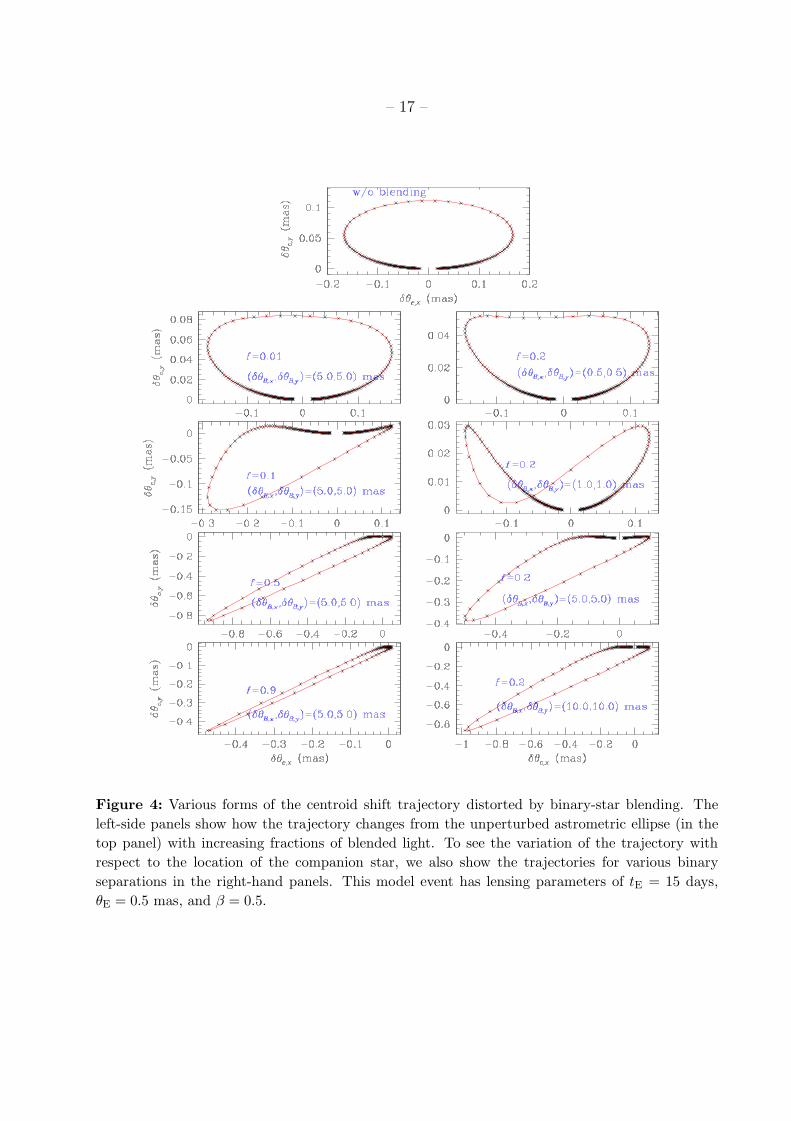
In the equation, the term including ~δθc describes the elliptical motion of the centroid shiftwith respect to the lensed star (the elliptical term). On the other hand, the term including~δθB describes the linear shift caused by the light from the blended star (the linear term).Therefore, the shape of the astrometric shift trajectory for a blended event results fromthe combination of the elliptical displacement caused by gravitational lensing and thelinear displacement toward the blended star. In Figure 4, we present various forms of thecentroid shift trajectory as distorted by binary star blending. The left panels show howthe trajectory changes from the unperturbed astrometric ellipse (in the top panel) withincreasing fractions of blended light. To see the variation in the trajectory with respectto the location of the companion star, we also present the trajectories for various binaryseparations in the right panels.

4.3. (Regime 3 λ/d ≤ ∆θ < 1.22λ/D)

In this case both the broad envelopes and fringes of the two PSFs are not matched(the lower right panels of Figure 1), and thus both centroids are shifted. The position ofthe centroid between the central broad envelopes is the flux-weighted average of the twosources and the amount of the shift is given by equation (3.2). One way to detect andcorrect for blending in this regime, therefore, is to measure the shift of the broad envelopecentroid. However, the situation is slightly more complex for the position of the centroid ofthe narrow fringes. If the separation between two source is exactly the same as n times thewidth of the narrow fringe, i.e., ∆θ = nλ/d, the 0th fringe of the blend coincide exactlywith the nth fringe of the lensed source. However, this is true only at a specific wavelength.If the blended source is observed at twice as long a wavelength, for example, the 0th fringeof the blend coincides exactly with the 1st null of the lensed source. Therefore, from thedifference in the interference patterns observed at multiple wavelengths, one can deduce theposition and brightness of the blend even if the observer chooses to examine the central

– 11 –

fringe rather than the whole interference pattern. The sources of blending belonging to thisregime include large-separation binary companions to the lensed source and very closelylocated field stars.

5. Summary

By observing gravitational microlensing events with SIM, one can correct for the effectsof nearly all types of blending. With its diffraction-limited, ∼< 0.′′5 imaging, a single mirrorof SIM can resolve blended stars for a significant fraction of the events blended by fieldstars, such as regular and amplification-bias blended events. For events affected by veryclose blends with separations ∆θ ∼< 10 mas, such as a large fraction of binary-star blendedevents, it is also possible to identify the blend by detecting a distortion in the astrometricshift trajectory. For events affected by blends with medium range separations, such asclosely located field stars and wide binary companions, one can correct for the effects ofblending by either detecting the shift of the broad envelope centroid between the PSFs oflensed and blended stars or by examining the narrow fringe patterns observed at multiplewavelengths.

We would like to thank to M. Everett and P. Martini for a careful reading of themanuscript. We also would like to thank the referee (A. Gould) for useful suggestions thatimproved the paper.

– 12 –

REFERENCES

Alard, C. 1996, in IAU Symp. 173, Astrophysical Applications of Gravitational Lensing, ed.C. S. Kochanek & J. N. Hewitt (Dordrecht: Kluwer), 215

Alard, C. 1997, A&A, 321, 424

Alard, C., Mao, S., & Guibert, J. 1995, A&A, 300, L17

Albrow, M., et al. 1998, ApJ, 509, 000

Alcock, C., et al. 1996, ApJ, 463, L67

Alcock, C., et al. 1997a, ApJ, 479, 119

Alcock, C., et al. 1997b, ApJ, 486, 697

Alcock, C., et al. 1997c, ApJ, 491, 436

Allen, R., Shao, M., & Peterson, D. 1998, Proc. SPIE, 2871, 504

Ansari, R., et al. 1996, A&A, 314, 94

Boden, A. F., Shao, M., & Van Buren, D. 1998, ApJ, 502, 538

Bouquet, A. 1993, A&A, 280, 1

Buchalter, A., Kamionkowski, M., & Rich, M. R. 1996, ApJ, 469, 676

Buchalter, A., & Kamionkowski, M. 1997, ApJ, 482, 782

Di Stefano, R., & Esin, A. A. 1995, ApJ, 448, L1

Dominik, M. 1998, A&A, 333, 893

Duquennoy, A., & Mayor, M. 1991, A&A, 248, 485

Goldberg, D. M. 1998, ApJ, 489, 156

Goldberg, D. M., & Wozniak, P. R. 1998, Acta Astron., 48, 19

Griest, K., & Hu, W. 1992, ApJ, 397, 362

Han, C. 1997, ApJ, 484, 555

Han, C. 1998a, ApJ, 500, 569

Han, C. 1998b, MNRAS, submitted

Han, C., & Chang, K. 1998, MNRAS, submitted

Han, C., & Jeong, Y. 1998, MNRAS, 301, 231

Han, C., Jeong, Y., & Kim, H.-I. 1998, ApJ, 507, 102

Hecht, E. 1998, Optics (Rending: Addison-Wesley Longman), 461

Holtzman, J. A., et al. 1998, AJ, 115, 1946

Jeong, Y., Han, C., & Park, S.-H. 1999, ApJ, 511, 000

– 13 –

Kamionkowski, M. 1995, ApJ, 442, L9

Nemiroff, R. J. 1994, ApJ, 435, 682

Nemiroff, R. J. 1997, ApJ, 486, 693

Paczynski, B. 1996, ARA&A, 34, 419

Paczynski, B. 1998, ApJ, 404, L23

Udalski, A., et al. 1994, Acta Astron., 44, 227

Udalski, A., et al. 1997, Acta Astron., 47, 169

Walker, M. A. 1995, ApJ, 453, 37

Wozniak, P., & Paczynski, B. 1997, ApJ, 487, 55.

This manuscript was prepared with the AAS LATEX macros v4.0.

– 14 –

Figure 1: The uncertainties in the lensing parameters for events whose high precision light curvesare fit with models. The events are assumed to have tE = 15 days and β = 0.3, and are affectedby blending with blended light factions of f = 0.3, 0.5, 0.7, and 0.9. The events are assumed tobe observed 5 times/day during −0.5tE ≤ tobs ≤ 3tE with a photometric precision of p = 1%. Theuncertainties in the lensing parameters are determined by computing χ2, and the resulting χ2 asfunctions of tE/tE,0 and f are presented as contour maps. In each panel, the contours are drawnat 1σ, 2σ, and 3σ levels from inside to outside.

– 15 –

Figure 2: The expected fringe patterns when a source star affected by a blended star with variousseparations is observed by SIM. To better show the centroid shift of the narrow fringe pattern, theregion around the position of the central fringe of the lensed star is expanded in the lower panelof each PSF. For all of these model events, we assume a blended light fraction of f = 0.5 andarbitrarily normalize the intensity.

– 16 –

Figure 3: Illustration of the distortion of the astrometric shift trajectory by a binary companion.In the figure, the dotted line represents the trajectory of the centroid shifts with respect to theposition of the source star located at the origin when the star is not affected by the binary-starblending. On the other hand, when the event is blended by a companion star, located at (θB,x, θB,y),the position of the light centroid will shift toward the companion. In addition, the reference positionof the astrometric measurements is not the position of the lensed source star, but the center of lightbetween the component stars. Due to these combined effects, the resulting trajectory (representedby a solid line) of the astrometric shifts is no longer an ellipse. This model event has lensingparameters of tE = 15 days, θE = 0.5 mas, and β = 0.5. The light fraction of the blended star isf = 0.3.

– 17 –

Figure 4: Various forms of the centroid shift trajectory distorted by binary-star blending. Theleft-side panels show how the trajectory changes from the unperturbed astrometric ellipse (in thetop panel) with increasing fractions of blended light. To see the variation of the trajectory withrespect to the location of the companion star, we also show the trajectories for various binaryseparations in the right-hand panels. This model event has lensing parameters of tE = 15 days,θE = 0.5 mas, and β = 0.5.