AN ADAPTED MODULATION TRANSFER FUNCTION FOR...
111
1 AN ADAPTED MODULATION TRANSFER FUNCTION FOR X-RAY BACKSCATTER RADIOGRAPHY BY SELECTIVE DETECTION By NISSIA SABRI A THESIS PRESENTED TO THE GRADUATE SCHOOL OF THE UNIVERSITY OF FLORIDA IN PARTIAL FULFILLMENT OF THE REQUIREMENTS FOR THE DEGREE OF MASTER OF SCIENCE UNIVERSITY OF FLORIDA 2007
Transcript of AN ADAPTED MODULATION TRANSFER FUNCTION FOR...

1
AN ADAPTED MODULATION TRANSFER FUNCTION FOR X-RAY BACKSCATTER RADIOGRAPHY BY SELECTIVE DETECTION
By
NISSIA SABRI
A THESIS PRESENTED TO THE GRADUATE SCHOOL OF THE UNIVERSITY OF FLORIDA IN PARTIAL FULFILLMENT
OF THE REQUIREMENTS FOR THE DEGREE OF MASTER OF SCIENCE
UNIVERSITY OF FLORIDA
2007

2
© 2007 Nissia Sabri

3
To my mother

4
ACKNOWLEDGMENTS
I would like to thank Dr. Edward Dugan and Dr. Alan Jacobs for their guidance, constant
enthusiasm and help. I would like also to thank Dr. James Baciack for being on the committee.
I would like to give a special thanks to my family and friends who were a great source of
motivation. I need to especially thank my husband Julien, for his help support, and endless
patience; my sister and mother, for their constant support; and my friends, especially Benoit
Dionne, Anne Charmeau and Colleen Politt, for their encouragement.
I would like to thank Warren Ussery for the financial funding and my research group,
especially Daniel Shedlock for the invaluable learning experience. Thanks to Ines Aviles-
Spadoni for her help.
I would like to thank Dr.Sjoden for accepting me in his research group to pursue my Ph.D.
Finally, I would like to thank Lockheed Martin Space Systems Co, NASA, Langley Research
Center, NASA, Marshall Space Flight Center and The University of Florida, Department of
Nuclear and Radiological Engineering, for the financial support.

5
TABLE OF CONTENTS page
ACKNOWLEDGMENTS ...............................................................................................................4
LIST OF TABLES...........................................................................................................................7
LIST OF FIGURES .........................................................................................................................8
ABSTRACT...................................................................................................................................12
CHAPTER
1 INTRODUCTION ..................................................................................................................14
Compton Backscattering Imaging (CBI) ................................................................................14 Backscatter Radiography by Selective Detection (RSD) .......................................................16
Overview of Previous Work............................................................................................16 Project Objectives............................................................................................................17
RSD Scanning System............................................................................................................17 Moving Table: X-Ray Source and Detectors ..................................................................17 Image Acquisition :Signal Flow and Software................................................................18
2 PROBLEM STATEMENT.....................................................................................................24
General Physics of Photon Interaction ...................................................................................24 Compton Effect ...............................................................................................................25 Kinematics.......................................................................................................................26 Cross Section ...................................................................................................................26
Theoretical Approach of the Modulation Transfer Function (MTF)......................................27 The Fourier Transform Applied to Image Processing ............................................................30 MTF Applied to the RSD Scanning System...........................................................................31
3 PRELIMINARY EXPERIMENTS: PULSE AND STEP FUNCTIONS SIMULATION.....36
RSD System Experimental Responses ...................................................................................36 Pulse Input Experiment ...................................................................................................36 Step Function Experiment ...............................................................................................37
Principles of Statistics and Curve Fitting Applied to MTF Calculation.................................37 Results and Analysis...............................................................................................................39
Pulse Function Experiment..............................................................................................39 The Step Function Experiment ........................................................................................41
4 MTF CALCULATION BASED ON A SINUSOIDAL INPUT FUNCTION.......................44
MTF Sinusoidal Pattern Design..............................................................................................44 System Response to the Input Modulation Function..............................................................44

6
Digital Output Profile ......................................................................................................44 Comparison of Detection Properties Between NaI and YSO Crystals............................45
A Model of the Sinusoidal Input Function Using MCNP5 and Variance Reduction Techniques ..........................................................................................................................46
Input Function from a 2D Model of the MTF Sine Target..............................................46 Input Function from a 3D Model of the MTF Sine Target..............................................50
Volumetric Normalization of the MTF...................................................................................51 Geometric Normalization ................................................................................................52 Volume Calculation Based on an MCNP5 Model ..........................................................54
Actual MTF Curves Based on a Sine Input Pattern................................................................56
5 AN IMPROVED TECHNIQUE FOR THE MTF CALCULATION BASED ON A STEP FUNCTION..................................................................................................................71
Step Function Target Design for MTF Calculation................................................................71 A Model of the Step Function Target Using MCNP5 and Variance Reduction
Techniques. .........................................................................................................................72
6 PROPOSED TECHNIQUES FOR IMAGE QUALITY ASSESMENT................................79
Multiple Derivatives and Inflection Points as a Mathematical Criterion for Image Quality Assessment.............................................................................................................79
Correlation Between the Different Methods of Calculating the MTF....................................82 Resolution Assessment from a Step Function Input...............................................................82
7 COMPUTATIONAL PROCESSING WITH MATLAB. ALGORITHM ARCHITECTURE FOR MTF CALCULATION (MATLAB)..............................................95
Modulation Transfer Function Based on the Sine Target.......................................................95 Modulation Transfer Function Based on a Step Function Target...........................................96
8 CONCLUSION.....................................................................................................................103
APPENDIX
A ENERGY FILTERING USING PAPER..............................................................................105
B MTF FRAME STRUCTURE...............................................................................................107
LIST OF REFERENCES.............................................................................................................109
BIOGRAPHICAL SKETCH .......................................................................................................111

7
LIST OF TABLES
Table page 4-1 Number of counts at the detector surface. .........................................................................60
4-2 Comparison between the Analog and Non-Analog MCNP5.............................................61
4-3 Summary of the line diameters and the associated number of line position......................62
4-4 MCNP5 run condition for Analog versus Non-Analog .....................................................62
4-5 Comparison between Analog and Non-Analog results in MCNP5 ...................................64
6-1 Coefficients used in the fitting function formula for each MTF curve..............................88
6-2 Statistical measures of the fitting accuracy........................................................................88
6-3 Roots value of the MTF second derivatives curves ...........................................................89
6-4 Different methods of the MTF derivation..........................................................................92

8
LIST OF FIGURES
Figure page 1-1 Schematic illustrating X-ray production............................................................................19
1-2 Typical spectrum obtained from an X-ray tube with a tungsten anode4............................19
1-3 Compton Backscattering Imaging (CBI) ...........................................................................20
1-4 Lateral Migration Radiography (LMR) .............................................................................20
1-5 Photograph of RSD System with 4 NaI Detectors.............................................................21
1-6 Photograph of RSD System showing YSO detectors mounted to NaI Detectors..............21
1-7 RSD scanning system mounted on a fixed frame ..............................................................22
1-8 Flow chart of the image acquisition process20 ...................................................................23
2-1 Photoelectric, Compton and Pair Production5. ..................................................................34
2-2 Kinematics of the Compton Effect ....................................................................................34
2-3 Transmission model ...........................................................................................................35
2-4 Backscatter model..............................................................................................................35
3-1 Scanning system output two line pairs placed at 45°with respect to the vertical axis.......42
3-2 High exposure scanning output, one sweep of a nylon line (Dirac Simulation)................43
3-3 Scan of a cubic plastic sample: 17.5 mm width, 1 mm beam, 0.5 mm pixels ...................43
4-1 Scheme for simulating a sinusoidal input ..........................................................................57
4-2 MTF frame plate ................................................................................................................58
4-3 MTF frame plate detailed design .......................................................................................58
4-4 Output profile from the scan of the MTF Sine target (detector 1 NaI)..............................59
4-5 Scattering-to-absorption ratios for NaI and Y5Si2O crystals. ............................................59
4-6 MCNP5 model for input profile calculation ......................................................................60
4-7 Energy spectrum distribution used in the MCNP5 model based on Kramers spectrum....60
4-8 The input sine profile obtained from running MCNP5......................................................62

9
4-9 Sine profile obtained from modeling 10 nylon lines of different diameters in MCNP5 ...63
4-10 The complete input profile from an MCNP5 simulation as recorded at the detector. .......63
4-11 MCNP5 model for input profile calculation ......................................................................64
4-12 Average energy and fraction of the detected signal in each of the six collision bins. .......65
4-13 Intersection volume of two cylinders.................................................................................65
4-14 Two cylinder intersection volume .....................................................................................65
4-15 Integrated profile data ........................................................................................................66
4-16 Equivalence between peaks and steps profiles. .................................................................66
4-17 Normalization methodology scheme. ................................................................................66
4-18 Experimental and normalized data profile.........................................................................67
4-19 A representation of the MCNP5 setup for volume intersection calculations.....................67
4-20 Line and beam intersection volume values........................................................................68
4-21 A plot of the volumetric normalization of half peaks obtained from MCNP model. ........68
4-22 Visual editor view of the new MCNP setup for volume calculations................................69
4-23 Normalization of the MTF sine profile over the intersection volume ...............................69
4-24 Statistical smoothing of the normalized profile .................................................................70
4-25 MTF function from detector 5 ...........................................................................................70
5-1 Edge target made from a junction of lead (absorber) and nylon (scatterer) ......................74
5-2 Scanning system response to an edge. ...............................................................................74
5-3 Fourier transform of the line spread function (black curve) and fitting function (red) .....75
5-4 Geometry of the MTF step target in MCNP5 ....................................................................75
5-5 Data profile obtained from the first MTF step target design in MCNP5...........................76
5-6 Geometry of the second design of the MTF step target.....................................................76
5-7 Profile data obtained from the second design of the MTF step target ...............................77
5-8 Data profile obtained from the third target design; nylon block on top of lead.................77

10
5-9 Final design profile proposed for the MTF step target ......................................................78
6-1 MTF comparison between NaI and Y5Si2O detectors at 45 kVp, 0.5 mm aperture ..........86
6-2 MTF comparison for 3 different aperture diameters..........................................................86
6-3 MTF comparison for different pixel sizes and beam apertures at 45 kVp-45 mA ............87
6-4 MTF Boltzmann model fitting function comparison .........................................................87
6-5 MTF fitting function first derivative, scan at 45 kVp-45 mA............................................88
6-6 MTF fitting function second derivative, scan at 45 kVp-45mA........................................89
6-7 1 MTF 0.1 mm pixel, 0.5 mm aperture..............................................................................89
6-8 2 MTF 0.05 mm pixel, 0.5 mm aperture............................................................................90
6-9 3 MTF 0.1 mm pixel, 1.0 mm aperture..............................................................................90
6-10 4 MTF 0.05 mm pixel, 1.0 mm aperture............................................................................90
6-11 5 MTF 0.05 mm pixel, 1.5 mm aperture............................................................................91
6-12 YSO image of MTF Target on a tile panel ........................................................................91
6-13 Selection and smoothing steps for the MTF calculation from a step function ..................92
6-14 An example of the edge profile and its first derivative......................................................93
6-15 Edge function width estimation .........................................................................................93
6-16 Numerical evaluation of the first derivative of the edge function .....................................94
7-1 Matlab user interface..........................................................................................................97
7-2 MTF menu and data profile ...............................................................................................98
7-3 Data profile ........................................................................................................................98
7-4 User interface for information entries................................................................................99
7-5 Maximum search................................................................................................................99
7-6 Saving files.......................................................................................................................100
7-7 Data profile from an edge function and its first derivative..............................................100
7-8 Selection of a region of interest in the edge function profile...........................................101

11
7-9 The selected region of interest and the first derivative of the edge function...................101
7-10 MTF curves with frequencies expressed in line pairs/pixel and line pairs/mm...............102
A-1 Comparison between two backscatter images .................................................................105
A-2 Line profile evaluation of the paper filtering...................................................................106
B-1 MTF frame plate top view ...............................................................................................107
B-2 MTF cover plate top view................................................................................................108

12
Abstract of Thesis Presented to the Graduate School of the University of Florida in Partial Fulfillment of the
Requirements for the Degree of Master of Science
AN ADAPTED MODULATION TRANSFER FUNCTION FOR X-RAY BACKSCATTER RADIOGRAPHY BY SELECTIVE DETECTION
By
Nissia Sabri
August 2007
Chair: Edward T. Dugan Major: Nuclear Engineering Sciences
The Modulation Transfer Function (MTF) is a quantitative function based on frequency
resolution that characterizes imaging system performance. In this study, a new MTF
methodology is investigated for application to Radiography by Selective Detection (RSD). RSD
is an enhanced, single-side x-ray Compton backscatter imaging (CBI) technique which
preferentially detects selected scatter components to enhance image contrast through a set of
finned and sleeve collimators. Radiography by selective detection imaging has been successfully
applied in many non-destructive evaluation (NDE) applications. RSD imaging systems were
designed and built at the University of Florida for use on the external tank of the space shuttle for
NDE of the spray-on foam insulation (SOFI) inspection. The x-ray backscatter RSD imaging
system has been successfully used for cracks and corrosion spot detection in a variety of
materials.
The conventional transmission x-ray image quality characterization tools do not apply for
RSD because of the different physical process involved. Thus, the main objective of this project
is to provide an adapted tool for dynamic range evaluation of RSD system image quality. For this
purpose, an analytical model of the RSD imaging system response is developed and supported.

13
Using the Fourier transform and Monte Carlo methods, two approaches are taken for the
MTF calculations: one using a line spread function and the other one using a sine function
pattern. Calibration and test targets are then designed according to this proposed model. A
customized Matlab code using image contrast and digital curve recognition is developed to
support the experimental data and provide the Modulation Transfer Functions for RSD.
14
CHAPTER 1 INTRODUCTION
The purpose of this investigation is to present and explain the different approaches that
have been taken to develop a Modulation Transfer Function adapted to the Radiography by
Selective Detection RSD imaging system1-3 for the purpose of defining a process to measure
system response by evaluating the image quality.
The first objective of the MTF calculations was to give a complete specification of the
RSD scanning system properties. Therefore a frequency characterization of the output/input
linking was desired. However, the backscattered field is highly dependent on the scanned object
meaning that a complete description of the imaging process for all applications is not possible
with a unique transfer function.
After an overview of the physical process involved in this type of imaging, the
experimental results are presented. The major sections treated are: the preliminary impulse and
step functions responses, the design of an MTF plate to simulate a sinusoidal input function, the
use of MCNP5 and variance reduction techniques to model the input function, the fitting process
to associate mathematical functions to the experimental data, two proposed models for the MTF
measurements (the sinusoidal and the step functions) and finally, the Matlab codes for practical
calculations.
Compton Backscattering Imaging (CBI)
In this section X-ray production is described for imaging applications. The physics of the
photon interactions with matter is treated in detail in Chapter 2 For a standard transmission
process, X-ray images are maps of the x-ray attenuation coefficient. To a large extent the
attenuation depends on the chemical composition and physical state of the attenuating medium.
In Compton Backscattering Imaging (CBI), images are maps of X-ray photon backscattering4.

15
X-rays are produced by focusing a beam of high energy electrons into a small focal spot on
an anode.
The rapid deceleration of the electrons after they enter the metal of the anode produces a
broad continuous spectrum of X- rays called Bremsstrahlung. Figure 1-1 shows the basic
principle of X-ray production.
There is also a probability for electrons to ionize the atoms in the anode, creating vacancies
in the inner electrons shells. These vacancies are rapidly filled by transitions from outer electron
shells, with the emission of characteristic X-rays5.
The energies of these discrete line spectra are characteristic of the anode chemical element.
The total spectrum obtained from a typical X-ray tube with a tungsten anode is shown in Figure
1-2.
As the X-rays traverse the object being scanned, they may be scattered, either elastically or
inelastically, or they may be totally absorbed in a photoionzation process. More details on these
physical processes and their dependence on photon energy can be found in Chapter 2.
A transmission imaging system consists of an X-ray source, the object being radiographed,
and a detector.
From an imaging standpoint there is an important distinction between absorption and
scattering. Usual X-ray scanning systems use transmission (i.e., forward scattered ) photons
while CBI uses backscattered photons. The reason for employing a CBI system is simple; for
some applications it is impossible to have film or a detector behind the scanned object.
By illuminating a single point on the target and having a set of detectors collecting the
backscattered photons, it is possible to reconstruct the image with a spatial mapping. The image
is thus a two-dimensional projection of a three-dimensional object; many planes are collapsed

16
into one. The information is not given by photons which pass throw the sample like in
transmission radiography, but is given by photons which are scattered back on the same side as
the source.
The detector senses photons coming back from the sample. These photons have interacted
with the medium (Compton interaction) and are scattered back with a different energy. The
energies and angles of backscattered photons depend on the energy of the incident photons and
the medium with which they interact. By counting the number of photons coming back,
information about the target can be deduced.
Backscatter Radiography by Selective Detection (RSD)
Overview of Previous Work
The technique developed at the Nuclear Engineering Department at the University of
Florida, called Lateral Migration Radiography6-14 (Figure 1-4) is similar to the CBI technique
(Figure 1-3), but instead of counting only single-collision backscattered photons, the LMR
technique counts both single- and multiple-collision backscattered photons that have laterally
spread out from the illumination beam entry point.
At the detector surface, signals from single- and multiple-collision backscattered photons
overlap. Therefore, they cannot be expected to cast a sharp shadow image. Instead, the
backscattered radiations form a broad, diffuse distribution on the detector, severely impairing the
distinction between deep and shallow objects.
This technique, with some modifications, later led to the Backscatter Radiography by
Selective Detection RSD. By adding adjustable collimators to the detectors it was possible to
select the backscattered photons being counted, especially the depth of the counted photons. By
preferentially selecting specific components of a scattered photon field, information relating to
specific locations and properties of an imaged sample can be extracted.

17
Project Objectives
The components that form the RSD scanning system are different and complex. Four
major parts can be identified: X-ray generator, detectors, the electronics and the image
acquisition and processing.
The objective of this study is to characterize the system response depending on different
setups and components. Since the development of the first RSD scanning system, there has not
been an experimental methodology to measure system performance. The global response of the
system depends on the individual performance of each component. The purpose of this project is
to define a process to measure the system response by evaluating the image quality. Since the
image is the system output, it gives an indication on how all the components are performing
together.
From a physical system point of view, the characterization of the response must be defined
through the input/output relationship. Then the challenge is to develop an expression for this
relationship which provides a basis for evaluating the performance of the imaging device and
understanding the nature of its evaluated image properties.
From the image processing standpoint, contrast and resolution characterize the image
quality. Therefore, the calculation of the Modulation Transfer Function (MTF) would be a better
characterization parameter if it is related to the contrast and resolution.
RSD Scanning System
Detector response and image acquisition observed throughout this study are generated
using the RSD scanning system developed for Lockheed.
Moving Table: X-Ray Source and Detectors
The system used in this study consists of four sodium iodide [NaI (Tl)] scintillation
detectors, one YSO detector and a Yxlon MCG41 X-ray generator mounted onto a scanning

18
table with X – Y scan motion capabilities. The [NaI (Tl)] detectors are positioned at the corners
of an eighteen by eighteen centimeter square, centred on the X-ray beam. The YSO detector
orbits on an aluminium ring around NaI detector two.
YSO images are usually comparable to the NaI images in image contrast. Although the
YSO detector has much less detection surface area (5.06 cm2 vs. 20.3 cm2), it has a slightly
higher quantum efficiency compared to the NaI for low energy X-rays (10-55keV). The detector
is also much lighter and smaller than the NaI detector so it can easily be positioned to obtain
better images. Each [NaI (Tl)] detector comprises a two inch diameter by two inch thick NaI
scintillation crystal mounted onto a photomultiplier tube (PMT) and a fast preamplifier
specifically designed to handle high count rates.
A schematic of the RSD [NaI (Tl)] detectors components and their configurations is
presented below in Figure 1-5. In Figure 1-6, the YSO is mounted on detector 2 using an
aluminium ring. In Figure 1-7 the RSD system is mounted on a fixed frame.
The 230 ns constant decay time of the NaI(T1) crystal (230ns) allows sufficient light and
charge collection time from the NaI and PMT, while allowing the detectors to measure
backscatter fields up to 800,000 counts per second, without experiencing statistically significant
pulse pile-up19.
Image Acquisition :Signal Flow and Software
The signal recorded from the scanning system is processed and displayed through a
Labview code.
The following flow chart (Figure 1-8) presents the entire image acquisition process from
detection to display.

19
Figure 1-1. Schematic illustrating X-ray production
Figure 1-2. Typical spectrum obtained from an X-ray tube with a tungsten anode4
High voltage
-
+
X-ray tube
Anode
Electron gun
X-rays
Electron beam
Sample

20
Figure 1-3. Compton Backscattering Imaging (CBI)
Figure 1-4. Lateral Migration Radiography (LMR)
Land mine
Collimated detector
NoiseSignal
X-ray generator
Earth
Uncollimated detector
X-Ray Generator
Object
Detector
Signal
Noise

21
Figure 1-5. Photograph of RSD System with 4 NaI Detectors
Figure 1-6. Photograph of RSD System showing YSO detectors mounted to NaI Detectors
Aluminium ring
YSO detector
NaI detector
2
A set of YSO
detectors
NaI detector Sleeve
collimator extended
X-ray beam tube Finned
Collimator Angle at 90 (degrees)

22
Figure 1-7. RSD scanning system mounted on a fixed frame

23
Figure 1-8. Flow chart of the image acquisition process20
Dir Active
Step
Dir
Step
Step
X-axis
Complete Pulse train
Complete Pulse train
Complete Pulse train
Y-axis
Y-axis
X-axis
X-axis
Visible light
X-Ray
Current
Analog pulse
Analog pulse
Analog pulse
Digital pulse
Analog pulse
Yes
X-ray scattered toward detector
Na I
Photo-Cathode
PMT
PreAmp
FastAmp
oscilloscope
MCA
SCA is the pulse in the
voltage window
Counter/Timer
Pulse train BNC 2121
NI-Daq PCI 6602
Labview/computer
Y axis Y-Motor Y-Motor Amps
or
image
NI-Motion PCI 7344
NI-Motion breakout box
Limit/Home Switches
X-Motor
X-Motor Amps

24
CHAPTER 2 PROBLEM STATEMENT
General Physics of Photon Interaction
When considering an X-ray based scanning system, it is highly important to understand
how the photons interact with matter4. There are five types of interactions with matter by X-ray
photons which must be taken into account.
• Compton effect • Photoelectric effect • Pair production • Rayleigh (coherent) scattering • Photonuclear interactions
Since the importance of an interaction for the purpose of this study is being measured by
the energy released in the medium, the three first interactions are the most important. The photon
energy is transferred to electrons, which then impart that energy to matter in many Coulomb-
force interactions along their tracks. Rayleigh scattering is elastic (total energy conserved, and
kinetic energy conserved), meaning that the photon is merely redirected within a small solid
angle with nearly no energy loss. Photonuclear interactions are only significant for photon
energies above a few Mev, where they may create radiation-protection problems through the
(γ,n) production of neutrons and consequent radioactivation.
The relative importance of the Compton Effect, photoelectric effect, and pair production
depends on both the photon quantum energy ( υγ hE = ) and the atomic number Z of the
absorbing medium.
Figure 2-1 indicates the regions of Z and γE in which each interaction predominates.
The photoelectric effect is dominant at the lower photon energies, the Compton effect takes
over at medium energies, and pair production dominates at the higher energies (with a threshold
of at least 1.02 Mev because the photon energy must exceed twice the rest mass of an electron).

25
For low-Z (e.g., carbon, air, aluminum, Spray-on Foam Insulation) media the region of
Compton-effect dominance is very broad, extending from approximately 20 keV to 20 Mev. This
gradually narrows with increasing Z. However, for Al, the PE effect is dominant up to about 50
keV.
According to the previous description it is easily understandable why the Compton Effect
is the one that characterizes the photon interactions in an RSD scanning system. The following
description deals with some aspects of the Compton Effect that are essential to understanding
how the image is formed in the RSD scanning system.
Compton Effect
A complete description of the Compton Effect must cover two major aspects: kinematics
and cross sections. The first one relates to the energies and angles of the participating particles
when a Compton event occurs; the second predicts the probability that a Compton interaction
will occur.
Two major assumptions are made in the following theoretical approach: the electron struck
by the incoming photon is initially unbound and stationary. These assumptions are not rigorous
since the electrons occupy different energy levels and, thus, are in motion and bound to the
nucleus. However, for low Z materials the binding effect does not introduce that much
modification in the cross section value.
As presented in Figure 2-2, a photon of quantum energy E incident from the left strikes an
unbound stationary electron, scattering it at angle θ relative to the incident photon’s direction,
with kinetic energy T.
The scattered photon E’ departs at angle φ on the opposite side of the electron direction, in
the same scattering plane. Energy and momentum are each conserved. The assumption of an

26
unbound electron means that the above kinematics relationships are independent of the atomic
number of the medium.
Kinematics
The relationships between angles and energies are given in Equation 2-1
⎪⎪⎪⎪
⎩
⎪⎪⎪⎪
⎨
⎧
+=
−=
−+=
)2
tan()1()cos(
))cos(1)((1
20
'
20
'
ϕυθ
υυ
ϕυυυ
cmh
hhT
cmh
hh
(2-1)
Where 20cm , the rest energy of the electron, is 0.511 Mev, and ', υυ hh and T are
expressed in Mev. There is a one-to-one relation between 'υh and angle φ of the scattered photon
for a given energy of the incident photon.
The photon transfers a portion of its energy to the electron. All scattering angles θ for the
photon (between 0 to 180°) are possible and the energy transferred can vary from zero to a large
fraction of the photon energy.
Cross Section
The microscopic cross section is the effective target area presented to an incident photon.
The earliest theoretical description of the process was provided by J.J. Thomson. In this theory
the electron that scatters the incident photon is assumed to be free to oscillate under the influence
of the electric vector.
The Thomson differential cross section per electron for a photon scattered at angleϕ , per
unit solid angle is based upon classical mechanics/electrodynamics and is expressed as:

27
)cos1(2
22
00 ϕσ
ϕ
+=Ω
rdde
(2-2)
Later on, Klein-Nishina developed (based upon quantum mechanics) a new definition for
the Compton Effect cross section15. This treatment was more successful in predicting the correct
experimental value, even though the electron was still assumed unbound and initially at rest.
The Klein-Nishina differential cross section for photon scattering at angleϕ , per unit solid
angle and per electron may be written in the form
)sin()(2
2'
'2
'200 ϕ
υυ
υυ
υυσ
ϕ
−+=Ω h
hhh
hhr
dde
(2-3)
Equation 2-3 is the one usually used for standard calculation of the cross sections, 20r is
squared value of the classical electron radius. In the low-energy limit of Compton scatter (hυ less
than about 10 keV), hυ’ ≈ hυ regardless of the photon scatter angle and Equation 2-3 reduces to
Equation 2-2.
Theoretical Approach of the Modulation Transfer Function (MTF)
There are several ways to measure the MTF. Some of them are largely applicable to
different recording systems; either the image is recorded on a film or it is processed to be
displayed on a screen. The two major techniques are the Sine Wave Method and the Spread
Function Method16.
The main problem associated with the first method lies in the production of a spatially-
sinusoidal exposure of known modulation.
A relatively straight forward method is to photograph a variable area test chart for an input
exposure that is a one-dimensional sinusoidal distribution defined by:

28
)2cos()( επω ++= xbaxf where ω is the one-dimensional spatial frequency (or line
frequency), and ε is a measure of the phase.
The output is also sinusoidal with the same spatial frequency as the input, but with a
change of amplitude, or modulation. The ratio of the output modulation to the input modulation
depends on the spatial frequency, and turns out to be equal to the modulus of the Fourier
transform of the line spread function.
The modulus of the Fourier transform of the line spread function l(x) is defined by:
⎪⎪
⎩
⎪⎪
⎨
⎧
=−=
=
∫∫ ∫
∫∞
∞−
∞
∞−
+∞
∞−
−
1111111
2
),(),()()(
)()(
dyyxhdydxyxhxxxlwith
dxexlM xi
δ
ω ωπ
(2-4)
Note that the line spread function of an imaging system is defined as the response of the
system to a line input. A line input may be represented by a single delta function, )( 1xδ , which
lies along the y1 axis. It is the ratio of output to input modulation that is called the Modulation
Transfer Function, or MTF. The input modulation is defined by: ab
ffff
Min =+−
=minmax
minmax .
Since the system response is a convolution of the input and the point spread function of the
system, the output can be written as:
∫ ∫
∫ ∫∞
∞−
∞
∞−
+−+=
−−=
11111
111111
),()))(2cos((
),(),()(
dydxyxhxxba
dydxyxhyyxxfxg
επω (2-5)
Integration with respect to y1 using (2.4) gives:
∫∞
∞−
+−+= 111 )()))(2cos(()( dxxlxxbaxg επω (2-6)

29
where )( 1xl is the line spread function defined earlier. Using the expansion:
)sin()sin()cos()cos()cos( BABABA +=− (2-7)
)( 1xl is normalized such that its area is unity, i.e. ∫∞
∞−
= 1)( 11 dxxl , then
∫
∫∞
∞−
∞
∞−
++
++=
111
111
)2sin()()2sin(
)2cos()()2cos()(
dxxxlxb
dxxxlxbaxg
πωεπω
πωεπω (2-8)
or
)()2sin()()2cos()( ωεπωωεπω SxbCxbaxg ++++= (2-9)
where
∫∞
∞−
−==− 111 )2exp()()()()( dxxixlTSiC ωπωωω (2-10)
The function )(ωT is the optical transfer function, and )(ωC and )(ωS− are its real and
imaginary parts. The optical transfer function is the Fourier transform of the line spread function.
Defining )()( ωφω andM as the modulus and phase of the optical transfer function, they
can be expressed as:
)(sin)()()(cos)()()()(tan)()()( 122
ωφωωωφωωωωφωωω
MSandMCCSandSCM
−==
⎟⎟⎠
⎞⎜⎜⎝
⎛ −=+= −
(2-11)
And by using these, then Equation 2-9 reduces to:
))(2cos()()( ωφεπωω +++= xbMaxg . (2-12)
Equation 2-12 shows that the output is sinusoidal and has the same frequency as the input.
The output modulation is defined as:

30
abM
gggg
M OUT )(minmax
minmax ω=+−
= (2-13)
Thus, the ratio of the output modulation to the input modulation is simply equal to )(ωM ,
the modulus of the Fourier Transform of the line spread function.
Since the area under the spread function has been defined as unity, the MTF will be
normalized to unity at zero spatial frequency:
1)()0( 11 == ∫∞
∞−
dxxlM (2-13)
Given a sinusoidal input of constant modulationab , the system frequency response can be
deduced from the output image contrast minmax
minmax
gggg
+− after dividing by
ab .
Due to the general non-linearity of the scanning process and the uncertainty in
characterizing the input function, the MTF deduced from spread function measurements will not
generally be exactly the same as that obtained from the sine-wave method.
The line spread function method could be performed either by simulating an experimental
pulse with a “Dirac function” or by scanning an edge and differentiating. The last step then is
performing a Fourier Transform calculation.
The Fourier Transform Applied to Image Processing
The general definition of the Fourier Transform of a function f(t) in one dimension is
dttftitfFG )()2exp())(()( 1 ∫+∞
∞−
−== νπν (2-14)

31
Two conditions are assumed to be satisfied for f(t) : continuity and periodicity . The
extension of this definition to two or three dimensions is straightforward with the spatial
exponential function written as )(2exp( zyxi ξημπ ++− ).
The real utility of the Fourier Transform is that it has a simple inverse.
νννπν dGtiGFtf )()2exp())(()( 11 ∫
+∞
∞−
− +== (2-15)
For a linear system a Fourier Transform of the input is defined as follows
duuwukikW inin )()2exp()( ∫+∞
∞−
−= π (2-16)
With the linearity condition, the system output is a superposition of individual outputs.
''' )()()()()( dttwttptwtptw ininout ∫+∞
∞−
−=⊗= . This type of integral is known as a convolution
product where p(t) is the spatial system response function.
The main utility of the Fourier Transform is to give an equivalent expression of the
function in frequency space.
In frequency space the convolution product is equivalent to the usual multiplication. Thus,
in frequency space the output is the multiplication of the input function by the system response
function.
The last important property of the convolution product is that the unit function is Dirac’s
function. Thus, the response to an impulse input is the system response function.
MTF Applied to the RSD Scanning System
The Modulation Transfer Function - from a scanning system characterization standpoint -
is the spatial frequency response of an imaging system or a component defined by the contrast,
C, at a given spatial frequency relative to low frequencies.

32
Spatial frequency is typically measured in cycles or line pairs per millimeter. High spatial
frequencies correspond to fine image details. The more extended the response, the finer the
detail.
Two methods were used to perform the MTF calculation. The first one is based on the
response to a sinusoidal input illumination. The second one uses the magnitude of the Fourier
Transform of the point or line spread function which is the response of an imaging system to a
pulse input such as a point or a line.
Due to technical issues the experiments were performed using sine patterns of various
frequencies and various diameters. A more adapted pattern would have been achieved by
keeping the diameters constant to have a constant modulation. However, the drilling process is
technically difficult for holes of large diameters and small separation. The patterns were
produced using nylon lines (cylindrical shape) of different diameters and spacing.
The following definitions were used
)0()(*%100)(
ContrastfContrastfMTF = (2-17)
where ( )minmax
minmax
VVVV
fC+−
= is the contrast at the spatial frequency f and ( )Bw
Bw
VVVV
C+−
=0 is
the low frequency contrast (the largest line pair). The above contrast values are the immediate
applications of the theory detailed previously.
maxmin ,,, VVVV Bw represent the luminescence for a pattern at the associated frequency.
wV , BV are maximum (white) and minimum (black) luminescences, respectively, at zero
frequency.
maxmin ,VV are maximum and minimum luminescences, respectively, at any frequency f.

33
It is important to notice that in the case of X-ray backscattering, an MTF calculation based
on the output image contrast depends on the spectrum, the target material and geometrical set up
of the system if not properly normalized.
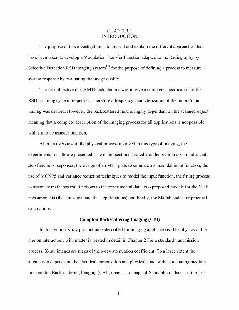
In usual transmission imaging the MTF is a projection on a 2D plane (Figure 2-3.3). The
signal recorded through the target does not interact with the target pattern. The photons counted
are those that have not been absorbed by the pattern. Thus, the actual volume of the target is not
a critical parameter.
When performing X-ray backscatter imaging, the signal measured is formed by the
photons that interacted with the target pattern (Figure 2-4). Thus, the amplitude of the signal
depends on the volume intersection of the pattern and the beam or the reaction rate.
The use of cylindrical lines in the pattern is to minimize the errors when generating a
sinusoidal input. The lines in the pattern are made of nylon, which has the best ratio of scatter-
to-absorption cross section in the energy range of interest: 5.1 at 35 keV and 26 at 60 keV.
The choice of varying the cylinder diameter with the frequencies introduced an additional
challenge when dealing with the volumetric normalization. The intersection volume of two
cylinders at 90° is easily represented by an integral function. However, because the beam sweeps
continuously over the cylindrical line, a summation of integrals is needed. This aspect will be
treated later on.

34
Figure 2-1. Photoelectric, Compton and Pair Production5.
Figure 2-2. Kinematics of the Compton Effect
υγ hE =
Momentum=c
hυ
θ
ϕ
−e
°0
'' υγ hE = Momentum=c
h 'υ
KE =T
Momentum=P
35
Figure 2-3. Transmission model
Figure 2-4. Backscatter model
X-ray generator
Detector 1 Detector 2
Backscattered photons Cylindrical
shape pattern
Nylon lines
X-ray generator
Rectangular shape pattern
Detector 1 Detector 2
Transmitted photons

36
CHAPTER 3 PRELIMINARY EXPERIMENTS: PULSE AND STEP FUNCTIONS SIMULATION
RSD System Experimental Responses
One of the first objectives was to vary one parameter at a time. The spacing was varied
using a limited number of lines due to the lack of precision in the spacing setup in preliminary
experiments. Experimental results presented in Figures 3-1 show a scanning output of two pairs
of nylon lines with the associated Line Spread Function profile. The two sets of line pairs were
of the same diameter 0.3 mm at 45 degrees with respect to the vertical axis with 3 mm and 1 mm
spacing respectively from left to right on the line profile.
The Line Spread Function (Figure 3-1) shows a typical loss of contrast with increasing
spatial frequency of the line pairs. The decrease of the amplitude between maxima and minima is
the indication of the contrast loss. This experiment was only meant to demonstrate the relation
between the frequency increase and the loss of contrast.
Pulse Input Experiment
Relative to the dimensions of the system, a pulse input can be approximated by a single
thin nylon line (0.3 mm diameter) with a 1 mm beam.
Since the system response depends on the intersection volume of the beam and the line, the
use of a small source beam aperture with a thin line simulates a “Finite” Dirac function. Figure
3-2 is a high resolution, single-line scan of a nylon line (0.3 mm diameter) with 0.02 mm pixel
size.
A convolution product shows that in the ideal case, the system output for a Dirac input
gives the Transfer Function.
)()()( xresponseSystemxInputxOutput ⊗= (3-1)

37
Since the Dirac function is the convolution product unit operator, the output is the system
response. By fitting the experimental data, a mathematical expression for the system response to
a line can be derived.
Step Function Experiment
This experiment simulates an edge function. The Fourier transform of the edge function
should give the same Modulation Transfer Function (MTF) as the line spread function. In the
frequency domain the output is defined as follows:
)()()( fresponseSystemfInputfOutput ∗= (3-2)
With * indicating regular multiplication.
For modeling an edge function the target is a plastic piece of 17.5 mm width as shown at
the bottom part of Figure 3-3.
Principles of Statistics and Curve Fitting Applied to MTF Calculation
Figure 3-2 and Figure 3-3 show experimental data profiles and the fitting functions
associated with them. To be valid the fitting function must be statistically equal to the
experimental profile. Thus, this section covers the basics of statistics applied to data samples and
more precisely applied to fitting functions.
In order to evaluate the fitting efficiency of a given function, some statistical tests are
performed for each data set. One of these tests is the determination of R, the Correlation
Coefficient. The closer the determination coefficient 2R is to 1, the better is the fit. A correlation
measures the strength of the predicted relation between the experimental data and the fitting
function. The stronger the correlation the better the fitted function approaches the experimental
data.

38
Given n pairs of observations ( ii yx , ),with x the experimental data and y the fitting
function value, the sample correlation is computed as
yyxx
xy
yyxx
ii
SS
S
SS
yyxxR =
−−= ∑ ))((
(3-3)
Where the sums of squared residuals are defined as
∑ −=i
iyy yyS 2)( =SS(Total) (3-4)
The Chi-square test is a different measure of the goodness-of-fit. The test−2χ measures
the deviation between the sample and the assumed probability distribution (i.e., hypothesis). The
value of Chi-square is calculated according to the following formula,
∑ −=
n
i i
ii
NpNpN 2
2 )(χ (3-5)
Where { }npppp ,...,,, 321 is a set of hypothetical probabilities associated with N events
falling into n categories with observed relative frequencies of{ }NNNNNN n /,...,/,/ 21 . For
large values of N, the random variable 2χ approximately follows the 2χ -distribution density
function with n-1 degrees of freedom.
The F-test is another statistical tool that can be used, for example, to test if different MTF
curves are statistically equal. Here are some explanations on how the F-test is performed.
First the two data sets (the measured data and the data from the library) are individually
fitted using the fitting function. Then the two data sets are combined (appending one to the
other), and then a fit is performed on the combined data set with the same function. From these
three fits, the values for the SSR (sum of squares of the difference between the data and fit
values) and the DOF (number of degrees of freedom) are obtained.

39
Then, SSR1, DOF1, SSR2, and DOF2 are obtained from the individual fits, and
SSRcombined and DOFcombined are obtained from the fit of the combined data.
The following values are computed: SSRseparate = SSR1 + SSR2 and DOFseparate =
DOF1 + DOF2 .
The last step is performed by computing the F value.
eSSRseparateDOFseparat
eDOFseparatdDOFcombineeSSRseparatdSSRcombineF *
)()(
−−
= (3-6)
Once the F value is computed, the p-value is computed using the formula:
)),(,(1 eDOFseparateDOFseparatdDOFcombineFinvfp −−= (3-7)
This p-value is then used to make a statistical statement as to whether the data (not the
parameter values) are significantly different or not. If the p-value is greater than 0.05, we can say
that the data sets are not significantly different at the 95% confidence level.
Results and Analysis
Pulse Function Experiment
In order to obtain the MTF from experimental data, it is necessary to obtain a mathematical
function from a data fit. Once the fitting function is obtained, the Fourier Transform of the
profile gives the system response function in the case of a pulse input. To perform the fitting, a
Lorentz’s model was used with the following equation:
))(*4(**2
220 wxxwAyy
c +−+=
π (3-8)
where
⎪⎪⎩
⎪⎪⎨
⎧
±=±=±=
±=
69682.1240838.4590139.037763.000462.062368.4
60653.257969.21350
Awxy
c with statistical tests on the data ⎪⎩
⎪⎨
⎧
=
=
39739.26666
85644.02
2
Dof
Rχ

40
The data profile used in the Pulse function experiment has been obtained from a scan at 45
kVp, 45 mA with a beam aperture size of 0.5 mm and a pixel size 0.02mm x 1mm. The line was
0.050 mm width.
Once the mathematical formulation was established, the next step was to calculate the
Fourier Transform of the obtained function (Equation 3-8). Since the exact formula depends on
different constants that change according to the experimental conditions, it is more valuable to
determine the general shape of the Fourier Transform than the precise mathematical expression.
By using Equation 3-9
XXFT πωωαωα
αα 2)exp())(exp(2
22 =−=−−⎯→⎯+ (3-9)
letting )(2 0xxX −= and using the following formulas )(1)(
)exp()()( 00
αω
αα
ωω
fxf
xjfxxf
FT
FT
⎯→⎯
−⎯→⎯−
The Fourier Transform of Equation 3-8 is obtained as
)2(*)4
exp(*)4exp(*4*
*2))(*4(
*)2(*)2(*
*20
0220 x
yxx
jx
wAwxx
wAyy FT
c
πδππ
ππ+−−⎯→⎯
+−+=
(3-10)
The Fourier Transform modulus gives the Modulation Transfer Function:
MTF_dirac_function )*8*exp(*4*
*2)16
exp(*4*
*2 22
02
zwAx
xwA
−≈−≈π
ππ
(3-11)
with )(2 1−= mmx
z π
The above formula gives the general behavior.

41
The Step Function Experiment
When the step function is treated, the best fitting function for this shape is provided by the
Bolzmann’s model
)exp(1
)(0
212
dxxx
AAAy−
+
−+= (3-12)
Where
⎪⎪⎩
⎪⎪⎨
⎧
±=±=
±=±=
05193.00441.00304.07751.3
17543.269652.97135331.542214.495
0
2
1
dxxAA
and ⎪⎩
⎪⎨
⎧
=
=
87267.397
98645.02
2
Dof
Rχ for the statistical tests
When using a step function to define the MTF an additional step is needed before the
Fourier Transform. A first derivative is performed.
20
0
)1(
*)12()(
dXXX
dXXX
e
eAAdX
XdY−
−
+
−= (3-13)
Due to the complex form of the above function, a straight forward calculation of the
Fourier transform is not possible.
An alternative approach was to perform the derivative and its Fourier Transform
numerically. Then by fitting the function a mathematical formulation was established.
MTF_edge_function ))(*2exp(*
2*
20 w
zz
w
Ay c−−+=
π (3-14)
with )(2 1−= mmx
z π

42
⎪⎪⎩
⎪⎪⎨
⎧
±=±=
±=
±−=−
01373.557833.43800568.065586.0
00177.07481.1
66317.265077.1416
0
Aw
Ez
y
C with statistical test on data ⎪⎩
⎪⎨
⎧
=
=
95055.76
99794.02
2
Dof
Rχ
The data profile used in the Pulse function experiment has been obtained from a scan at 45
kVp, 45 mA with a beam aperture size of 1 mm and a pixel size 0.5mm x 0.5mm. The line was
0.050 mm width.
Even though the mathematical expressions for the pulse based MTF and the step function
MTF are not exactly the same, the general behavior follows )exp( 2zα− , with α a constant.
Figure 3-1. Scanning system output two line pairs placed at 45°with respect to the vertical axis
0 10 20 30 40 50
1450
1500
1550
1600
1650
1700
Num
ber o
f cou
nts/
pixe
l
Distance x (cm)
Line profile
High contrast
Low contrast

43
0 2 4 6 8 10
2000
2200
2400
2600
2800
3000
line spread function(1) Lorentz fitting function(2)
Num
ber o
f cou
nts/
pixe
l
Distance x in (mm) Figure 3-2. High exposure scanning output, one sweep of a nylon line (Dirac Simulation)
0 5 10 15 20 25 30 352000
4000
6000
8000
10000
12000
14000
16000
Num
ber o
f cou
nts/
pixe
l
Distance x in (mm)
B Boltzmann fit of Data33_B
Figure 3-3. Scan of a cubic plastic sample: 17.5 mm width, 1 mm beam, 0.5 mm pixels
Line profile
Line profile

44
CHAPTER 4 MTF CALCULATION BASED ON A SINUSOIDAL INPUT FUNCTION
MTF Sinusoidal Pattern Design
The first idea was to generate a sinusoidal input pattern using nylon line of different
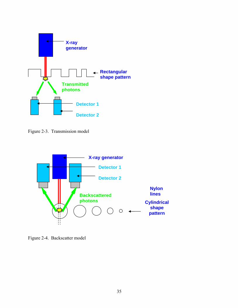
diameters and spacing. Figure 4-1, showing five nylon lines, an x-ray generator and two
detectors, illustrates the scheme for simulating a sinusoidal input. As the scanning system sweeps
over the lines, a sinusoidal signal is formed at the detector face
The actual MTF target contains 5 lines for each diameter. This is to ensure good statistics
in the results. The actual MTF target consists of an aluminum frame to hold different diameter
nylon lines with varying spatial frequencies. Figures 4-2 and 4-3 show the MTF plate design.
The target frame is 25.4 cm x 12.7 cm (10 x 5 inches) and 0.3 cm (1/8 inch) thick. The
nylon lines are strung across the 7.6 cm (3 inch) air gap in the center of the frame. A cover plate
was designed to be attached to the back of the frame to protect the nylon lines connections and
provide a flat surface on which the target sits. The cover plate is 0.6 cm (1/4 inch) thick.
Twelve sets of holes were initially designed. Two additional levels of holes sets were
included in the design to vary the frequency while the diameters are kept constant.
System Response to the Input Modulation Function
Digital Output Profile
Figure 4-4 shows the output profile obtained from scanning the MTF Sine target at an X-
ray energy of 45 kVp and a current of 45 mA. This profile was obtained from detector 1 (NaI).
For this particular set up, the decrease in contrast started at the sixth set of lines corresponding to
a diameter of 1.28 mm (0.39 line pairs/mm). The loss of contrast is noticeable when there is an
increase in the minimum values of the profile, i.e. a shift in the baseline.

45
After the eighth set of lines, the five peaks of each new set are not distinguishable. Thus,
the loss of resolution starts at a line diameter of 0.52 mm (0.96 line pairs/mm). The loss of
resolution is defined with respect to the Full Width at Half Max (FWHM). If the separation
between two maxima is smaller than the width of the individual peak at half its maximum value
than the resolution between the two peaks is lost.
Comparison of Detection Properties Between NaI and YSO Crystals
In the previous section, the output profile was treated from a digital imaging point of view
and no special care was taken to evaluate the best detector configurations. However, since the
detectors themselves have limited efficiencies, it is necessary to quantify their responses with
respect to the backscattered spectrum.
Two types of detectors were used in the MTF experiments: NaI and YSO. Figure 4-5
shows the scattering-to-absorption ratios for both NaI and YSO. The values obtained are for NaI
and Y5SI2O crystals17.
The lower the scattering-to-absorption ratio the better the detection capabilities. In the
energy range of interest (below 50 keV) the Y5Si2O crystal has a more favorable scattering-to-
absorption ratio than the NaI from about 16 keV to 33 keV. At about 16.4 keV, the ratio achieves
a maximum value of 0.0796 for the Y5Si2O. The NaI crystal is a much better detector at energies
higher than 33 keV.
Since the Y5Si2O was the most frequently used detector for the MTF experiments, the
following study will concentrate on characterizing the Y5Si2O detection performance with
respect to detected energies. First, it is necessary to calculate the average energy of the
backscattered spectrum using a Monte Carlo simulation. The model used is based on MCNP5
analog simulations and the layout is described in detail in the following section.

46
The average energy of the incident X-ray beam is 22.73 keV and its maximum energy is 50 kVp.
The average energy of the backscattered spectrum given in Table 4-1 is 26.74 keV. This value
was obtained by averaging over the five energy bins with the number of particles used as
weighting functions. A non-analog run gives essentially the same result with an average detected
energy of 26.75 keV and a relative error of 0.021%. A more detailed analysis on the Analog
versus Non-Analog results will be given in the following section.
A Model of the Sinusoidal Input Function Using MCNP5 and Variance Reduction Techniques
As shown in the previous section, the output profile is easily obtained from scanning the
MTF Sine target. However, there is no experimental way to precisely determine the input profile.
Thus a Monte Carlo model is necessary to correctly determine the input function, to
correlate the output profile to the system response.
Input Function from a 2D Model of the MTF Sine Target
Figure 4-6 shows the MCNP5 model for a 2D input profile calculation. The profile
obtained from the model presented in Figure 4-6 is not strictly 2D. Actually the entire line (3D
volume) is modeled but only the contribution from the mid-plane region is used to generate the
profile. This is to be compared with the profile obtained from the contribution of the entire line.
Only one line per set is modeled up to the 10th set of holes. The last two sets did not give
good experimental results. Then using the problem symmetry only one half of the line is
modeled.
In the actual experimental design, the X-ray generator and the detector move over the
target. For each mesh cell defined by (x+Δx, y+Δy) the number of photons recorded is used to
display one pixel. To simplify the model in MCNP5 the detector and X-ray beam are kept at the
same position while the line position is varied.

47
The start position is where the beam and the line axis intercept. Then an offset of 0.01 cm
is added between the two axes for each new simulation. The final position of the line axis is such
that it does not intersect with the beam any more.
The detector is a cylinder of 2.54 cm diameter with 0.635 cm thickness centered at (0,
5.08, 4.317).
The plane source is defined at the bottom surface of the detector. Note that it is not
recommended to use a plane that is a physical boundary in a system as a source plane. This can
cause problems. A “source plane” that can be very slightly offset (e.g., by 0.001 cm) from the
physical plane should be used instead. From which the x-ray beam is sampled using a disc of
0.05 cm diameter along the z axis.
The nylon line is centered for the first position at 3.8 cm along the x axis as is the X-ray
beam. The line is represented by a cylinder along the y axis lying on the xy plane.
To model the experimental set up as closely as possible a sheet of paper underneath the
nylon line and a concrete floor are modeled.
There are ten different diameters to simulate. For each diameter the number of line
positions is equal to the ratio of the radius and the modeled pixel size (constant 0.01 cm).
Two Variance Reduction Techniques are used: DXTRAN sphere and forced collisions for
modeling the input profile.
The DXTRAN sphere enables the simulation to obtain many particles in a small region of
interest that would otherwise be difficult to sample. Because the solid angle that sees the detector
surface from the interaction volume in the line is small, a transport of particle to the surface of
interest is necessary.

48
Upon sampling a collision, DXTRAN estimates the correct weight fraction that should
scatter toward the detector surface, and arrive without collision at the surface of the sphere. The
DXTRAN method then puts this correct weight on the sphere.
The collision event is sampled in the usual manner, except that the particle is killed if it
tries to enter the sphere because all particles entering the sphere have already been accounted for
deterministically. The DXTRAN sphere is centred on the YSO detector.
Forced collisions are used to increase the frequency of random walk collisions within the
small intersection volume of the beam and the entire nylon line.
A particle can be forced to undergo a collision each time it enters a designated cell that is
almost transparent to it. The particle and its weight are appropriately split into two parts, collided
and uncollided. Forced collisions are often used to generate contributions to point detectors, ring
detectors, or DXTRAN spheres.
Here forced collisions are used as a complementary method to the DXTRAN sphere. The
forced collision card is set such that only the particles entering the cell undergo forced collisions.
The run used a 0.5 mm diameter beam, a 0.1 mm pixel and the beam was centered over the
pixel. The number of runs necessary for this input profile calculation is 132.
The energy card uses a distribution of energies with the associated probabilities at 50kVp.
The distribution is based on the Kramers spectrum5 modified for tungsten target attenuation and
beryllium window and aluminum filter attenuation.
Figure 4-7 shows the energy distribution used at 50kVp as a maximum energy of the
incident particles in the MCNP5 model based on the Kramers spectrum. The spectrum is
distributed between 0 and 50 kVp with 74 interpolation points.

49
Two tallies are used; they are based on the current entering the bottom surface of the
detector. The first tally records the partial and total currents and based on the number of particle
collisions from 1 up to 6. The second tally does not distinguish the particles according to the
number of collisions experienced before reaching the detector but it counts particles coming
from a specific cell in the mid-plane of the nylon lines. Table 4-2 summarizes the number of
simulations needed for modeling the input profile, taking into account the number of different
diameters and for each diameter the number of runs.
In addition to the 132 runs necessary for the line profiles, there is one simulation for
modeling the air separation between the lines. Figure 4-8 shows the data profile obtained from a
mid-plane contribution only.
The errors associated with the data profile shown in Figure 4-8 are on the order of a tenth
of a percent. Table 4-3 shows a comparison between an Analog MCNP5 run without any
variance reduction technique and a Non-Analog run using the two indicated variance reduction
techniques. The numbers of counts are given for a single source particle and for a positive
current with respect to the detector entrance surface. Table 4-3 shows that up to 40 keV the
errors associated to both Analog and Non-Analog techniques are below 1%. The last energy bin
from 40 to 50 keV corresponds to the incident beam maximum energy; this is why very few
particles are counted. As explained in Chapter 1, the energy of the backscattered particle is a
fraction of the incident energy.
Also according to Figure 4-5 the fraction of scatter/absorption in the YSO detector
increases continuously above 20 keV and reaches a value of 0.1 between 45 keV and 50 keV.
This means that a fraction of the positive current is scattered back out of the detector and even
less particles are counted in this energy region leading to an increase in the error.

50
In a Non-analog Monte Carlo method, the physics is biased such that the quantities to be
calculated are estimated in a shorter time or with a smaller variance. To preserve an unbiased
sample mean, each particle is given a statistical weight which is defined based on the unbiased
and biased density functions.
The effectiveness of the Non-Analog techniques is measured by a quantity called “Figure
of Merit”, FOM, defined by:
2*(min)1
errortimeFOM = (4-1)
Where “error” is the relative error. The higher the FOM, the more efficient the calculation.
Table 4-4 presents the number of particles and calculation time for both Analog and Non-
Analog runs. The Non-Analog run is more than 3 times faster and needs less than 16 times the
number of particles to achieve the same order of accuracy on the results.
As discussed previously another aspect of the Non-Analog technique is to introduce a shift
in number of particles with respect to the energy bins. This is mostly due to the DXTRAN
sphere. Some variance reduction techniques do not preserve the energy spectrum information.
Input Function from a 3D Model of the MTF Sine Target
The 3D input profile was obtained using the same layout as the one used in the previous
section for the 2D profile. The only difference is that the entire volume of the nylon line was
sampled instead of sampling only the mid-plane contribution. Figure 4-9 shows the MCNP5
model used for the calculation of the 3D input profile from a nylon line.
The same variance reduction techniques were used and the detector coordinates were (0, 0,
4.317). The profile was obtained using 1000000 particles for each of the 132 runs.
Nine of the ten statistical tests were passed in MCNP5. The last test; the pdf slope was not
passed.

51
However, the relative errors associated with the obtained profile were between0.32% and
2.35%. Figure 4-10 and Figure 4-11 show the partial and complete profiles obtained from
modeling the MTF sine target using MCNP5.
Figure 4-10 shows the reconstructed input profile with only one line for a given diameter.
Each peak corresponds to one line and was obtained from the MCNP5 simulation. Then knowing
the actual separation distances between the lines, the complete profile has been reconstructed and
is shown in Figure 4-11.
Table 4-5 shows a comparison between the Analog and Non-Analog results for the 3D
model of the input Sine Target.
Figure 4-12 shows the fraction of the contribution of the particles to the detected signal
according to their number of collisions and the average energy of each collision bin. The signal
is dominated by the first scatter signal up to 94.156%. The sixth collisions component is almost
0%. In order for a particle to have undergone multiple collisions and get back to the detector, it
must have come from the higher end of the source spectrum.
Volumetric Normalization of the MTF
The previous section treated the sine function profile at the detector face. Since the MTF
target used nylon lines of different diameters and spacing, the amplitude of the sine profile varies
with the line pair frequency. This variation is due to the variation line diameters and more
specifically, to the variation in the intersection volumes of the X-ray beam with the nylon line.
The volumetric normalization attempts to normalize over the intersection volume to obtain
a profile with constant amplitude. Two methods used are: a geometric normalization based on
integrals and an MCNP5 model to estimate the volume from the particles path.

52
Geometric Normalization
It is important to notice that the conventional MTF calculation (e.g., as employed with
transmission X-ray imaging) is performed using a multiple step data profile. This model gives a
constant amplitude of the input signal distribution after normalization per unit volume. The
intersection volume of the cylindrical beam and the target (MTF Sine pattern) sample is easily
calculated in this case and remains constant at a given frequency.
In order to introduce equivalence between the step model and the actual Sine MTF, some
definitions are given below:
First, consider the intersection volume of two cylinders of the same radius in Figure 4-13.
One of the cross sections is a square of side half-length 22 zr − , the volume is given by
∫−
=−=r
r
rdzzrrrV 32222 3
16)2(),( (4-2)
Figure 4-14 shows the intersection volume of two cylinders.
If the two right cylinders are of different radii BeamLine randr with BeamLine rr > , then the
volume common to them is :
)]()()()[(38),( 2222
2 kKrrkErrrrrV BeamLineBeamLineLineBeamLine −−+= (4-3)
Where K(k) is the complete elliptic integral of the first kind, E(k) is the complete elliptic
integral of the second kind, and Line
Beam
rr
k = is the elliptic modulus.

53
However, even with a formula to calculate the intersection volume, the complete physical
process is not covered. The beam sweeps over the lines in a continuous mode. For a given beam
size, the actual intersection volume is related to the number of counts through the exposure time
and the pixel size. This means that at each step a fraction of the volume is covered several times.
The resulting overlapping contributes to the signal (counts per peak) in different
proportions depending on the cylinders’ radii.
As a preliminary model, only the intersection at the center is considered to give the most
significant response. Although this is a restrictive approach, it gives an idea of the intersection
volume contribution versus the diameter for the large line diameters.
As previously explained, the data profile has to be redistributed for each given diameter.
Thus, using the integral of the data and the line widths as they appear in the image, the number
of counts is redistributed to flatten the maximum of each peak. Figure 4-15 presents the
integrated profile.
The idea is to obtain an equivalent of the step profile from a peak profile as shown in
Figure 4-16.This is to avoid two competing factors of signal amplitude and frequency variations.
The method consists of transforming the peak shape profile to a step shape profile and
normalizing the number of counts per unit volume.
The first step is performed using the integral under each peak shown in Figure 4-15. The
second step requires knowing the value of the intersection volume (X-ray beam and nylon line).
This volume has been calculated using Equation 4-3 assuming an intersection of the X-ray beam
and the line at the center axis only. Figure 4-18 shows the experimental data and the normalized
profile. From right to left each set of lines of a given diameter is shown in a specific color.

54
Also from right to left the line diameter decreases. At about 2.5 inches the peak data are
not represented because of mismatch between the line diameter and the drilled hole diameter.
This was fixed on the MTF sine plate for later experiments. Note that up to the ninth set of
lines, the normalized profile is decreasing, and the slope is matching the contrast loss. Up to the
ninth line set, the beam diameter is less than the line diameter. In the tenth set the beam and the
lines are of the same diameter. The two last line sets, 11 and 12, have smaller diameters than the
beam diameter.
Figure 4-18 shows that the employed model is well adapted to the first nine line sets. For
line sets 11 and 12, the signals from two different lines overlap. This overlapping gives an
artificially high response. In fact for each line in these sets, the signal includes the response of
several lines. Recall that the equivalence between cylindrical lines and the multiple step target is
performed using the integral and the width. For these sets the normalization is more challenging
since the number of counts recorded and the intersection volume are related in a more complex
manner.
Volume Calculation Based on an MCNP5 Model
In order to perform the volume intersection calculations the input model used to obtain the
input profile is modified. A spherical source is set to enclose the problem with a radius of 12 cm.
Figure 4-19 shows a sketch representing the MCNP5 input model, the two cylinders
intersecting, detector, paper and concrete. However the figure does not show that the source
sphere is centered at the origin.
Note that the input set up described in Figure 4-19 is not the optimum way for doing
volume calculations. However, because of the large number of input files needed, it was a quick
start method since the inputs did not need major modifications.

55
A more efficient configuration would be achieved by suppressing everything in the model
but the two cylinders and centering a much smaller spherical source on them. Then by setting the
material card to void, the volume is obtained by tallying the flux in the intersection region.
The line radii are the ones used in the previous MCNP5 models (for the input profile
calculations). Figure 4-20 shows a plot of the intersection volume values versus the line radii.
The absolute errors are also plotted. The intersection volume increases with the line radius as
expected and the relative errors are higher for small radii. The plot in Figure 4-20 is given as an
indication of the volume trend versus line radius. The values shown are not exact since MCNP5
scales the flux inside the cell of interest to an unknown volume.
Note that for the very small volume intersections there were zero particles in the volume of
interest after running 7,000,000 histories. From these poor statistics, the volume values are
obviously not reliable for small lines radii and small intersection volumes.
Figure 4-21 shows a normalization based on the volume values calculated from the above
model. It is expected to not have constant amplitude since the volume values over which the
normalization is performed are not expected to be correct.
Either a new model is necessary or a higher number of histories. Figure 4-21 is obtained by
taking half of each peak plotted in Figure 4-10 and then normalizing by the intersection volume
from the above results.
Figure 4-22 shows a new input set up that is proposed to enhance the volume calculation.
As previously mentioned, by modeling only the two cylinders and the spherical source, better
statistics are achieved.
This new set up was done using 7,000,000 histories. Figure 4-23 and Figure 4-24 show the
normalization of the input sine profile over the intersection volume of two cylinders.

56
The two cylinders have the same dimensions as the nylon line and the X-ray beam. The
figures show that a more effective normalization is achieved when it is performed over the
individual pixels.
Note that in Figure 4-23 the extreme values correspond to 10σ the average value of the
normalized profile for each line. This is due to the small intersection volume on the line’s edges.
Thus a statistical smoothing is performed over these values and the resulting normalization is
shown in Figure 4-24.
This last plot shows the feasibility of a volumetric normalization to obtain a profile of
constant amplitude.
Even if the volumetric MTF couples the volumetric distribution of the target to the
scanning system response, it offers a basis for the system relative evaluation.
This integrated 3-D MTF allows comparison between detectors and gives a basis on which
to test a global improvement in the system. By using the same target, the volume and material
parameters are kept constant in the different scans.
Actual MTF Curves Based on a Sine Input Pattern
An example of the MTF curves obtained from the Sine target is given in Figure 4-25, this
profile is obtained from detector 5 (Y5Si2O).
The MTF presented here does not include any normalization processing. Thus, the MTF is
sensitive to the change in the volume intersection of the beam and the lines. The drop in the MTF
values is related to a loss of contrast and a volume variation. The relative difference in MTF
values indicates the quality of the images when using the same target.
The Boltzmann fitting model is given by the following formula:
MTF_experimental=dX
XX
e
AAAY 0
1
212 −
+
−+= (4-3)
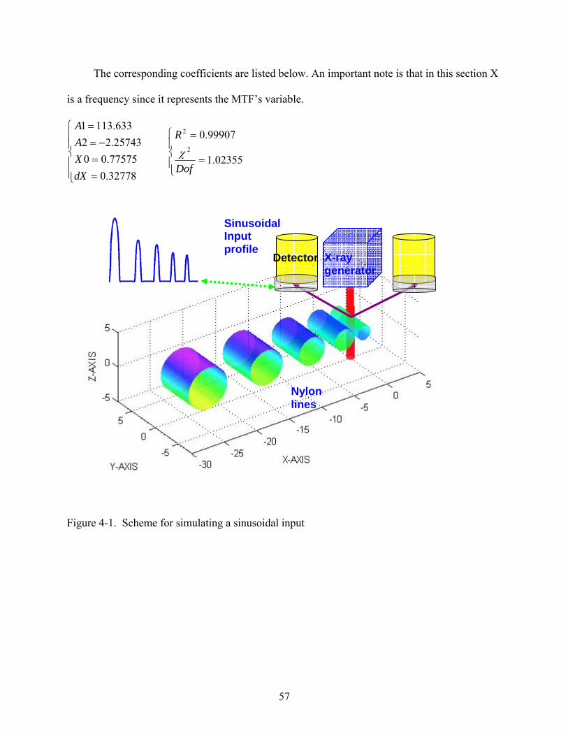
57
The corresponding coefficients are listed below. An important note is that in this section X
is a frequency since it represents the MTF’s variable.
⎪⎪⎩
⎪⎪⎨
⎧
==
−==
32778.077575.0025743.22633.1131
dXXAA
⎪⎩
⎪⎨
⎧
=
=
02355.1
99907.02
2
Dof
Rχ
Figure 4-1. Scheme for simulating a sinusoidal input
Sinusoidal Input profile
X-ray generator
Detector
Nylon lines

58
Figure 4-2. MTF frame plate
Figure 4-3. MTF frame plate detailed design
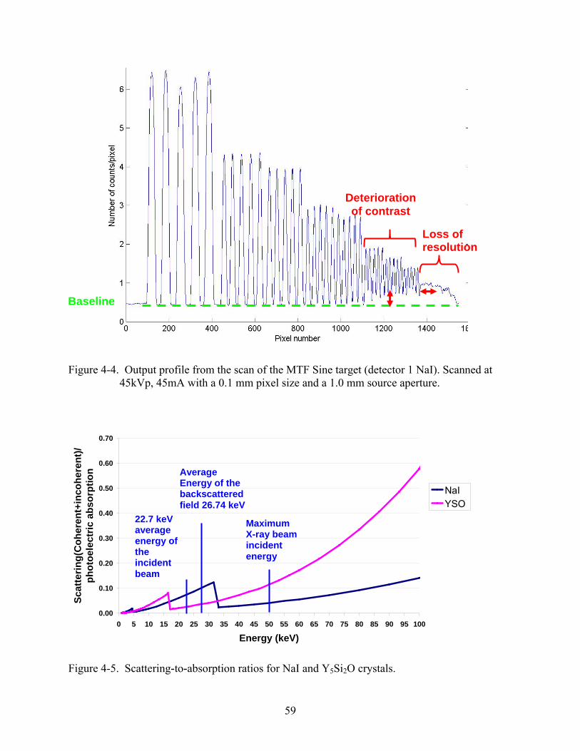
59
Figure 4-4. Output profile from the scan of the MTF Sine target (detector 1 NaI). Scanned at
45kVp, 45mA with a 0.1 mm pixel size and a 1.0 mm source aperture.
0.00
0.10
0.20
0.30
0.40
0.50
0.60
0.70
0 5 10 15 20 25 30 35 40 45 50 55 60 65 70 75 80 85 90 95 100
Energy (keV)
Scat
terin
g(C
oher
ent+
inco
here
nt)/
phot
oele
ctric
abs
orpt
ion
NaIYSO
Figure 4-5. Scattering-to-absorption ratios for NaI and Y5Si2O crystals.
Deterioration of contrast
Loss of resolution
Baseline
Average Energy of the backscattered field 26.74 keV
22.7 keV average energy of the incident beam
Maximum X-ray beam incident energy

60
Table 4-1. Number of counts at the detector surface for each energy bin and the average energy of the backscattered spectrum.
Energy bins Mev Counts Error % 2.00E-02 1.08466E-02 0.1300%3.00E-02 8.65223E-03 0.1500%4.00E-02 3.15683E-03 0.2500%5.00E-02 1.34348E-04 1.2200%
total 2.27900E-02 0.0900%Average energy Mev 2.67437E-02 1.2989%
Figure 4-6. MCNP5 model for input profile calculation. 2D profile calculated from mid-plane
contribution
Figure 4-7. Energy spectrum distribution used in the MCNP5 model based on Kramers spectrum
Pb shield
z
x
YSO detector, R=1.27cm
Plane source
X-Ray beam
Paper
Concrete
Nylon line R=0.1665cm
+
DXTRAN sphere Outer radius 4.635 cm Inner radius 4 cm Flagged tally from mid-plane interactions
Forced Collisions
Photons

61
Table 4-2. Comparison between the Analog and Non-Analog MCNP5 Flagged mid-plane surface Analog Non-Analog positive current
Energy bins Mev
Counts Error %
Counts Error %
Error % Analog vs Non-Analog
J+ 2.00E-02 4.77980E-03 0.2000% 4.79438E-03 0.3400% -0.3050% 3.00E-02 4.31184E-03 0.2100% 4.34073E-03 0.3600% -0.6700% 4.00E-02 1.60421E-03 0.3600% 1.60496E-03 0.6700% -0.0468% 5.00E-02 6.81481E-05 1.7500% 6.80647E-05 3.6700% 0.1224% total 1.07640E-02 0.1300% 1.08081E-02 0.2300% -0.4097%
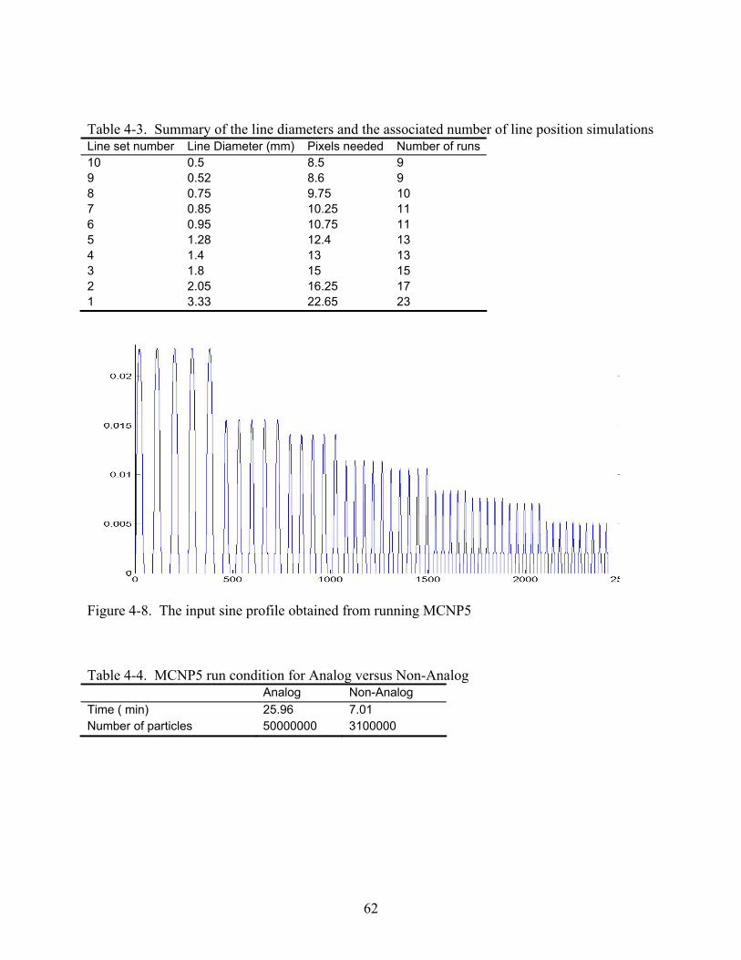
62
Table 4-3. Summary of the line diameters and the associated number of line position simulations Line set number Line Diameter (mm) Pixels needed Number of runs10 0.5 8.5 9 9 0.52 8.6 9 8 0.75 9.75 10 7 0.85 10.25 11 6 0.95 10.75 11 5 1.28 12.4 13 4 1.4 13 13 3 1.8 15 15 2 2.05 16.25 17 1 3.33 22.65 23
Figure 4-8. The input sine profile obtained from running MCNP5
Table 4-4. MCNP5 run condition for Analog versus Non-Analog Analog Non-Analog Time ( min) 25.96 7.01 Number of particles 50000000 3100000
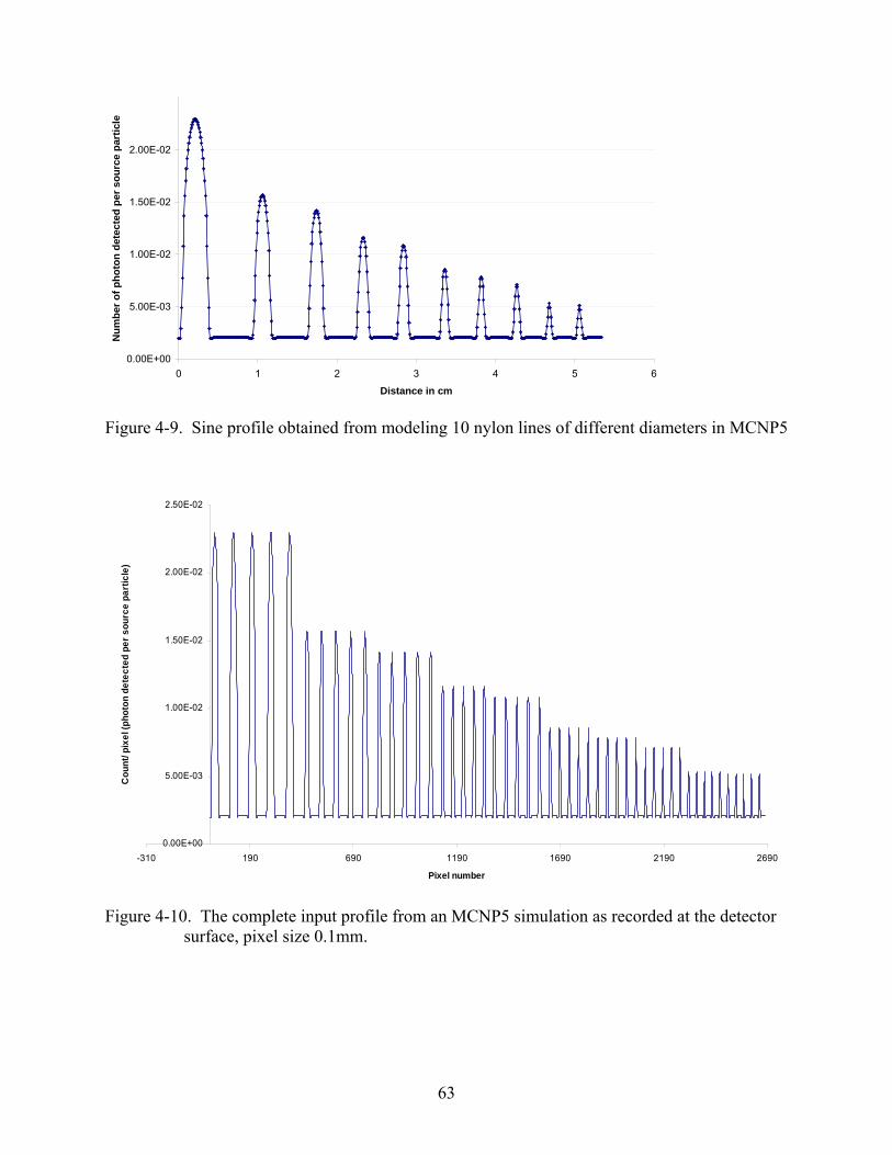
63
0.00E+00
5.00E-03
1.00E-02
1.50E-02
2.00E-02
0 1 2 3 4 5 6
Distance in cm
Num
ber o
f pho
ton
dete
cted
per
sou
rce
part
icle
Figure 4-9. Sine profile obtained from modeling 10 nylon lines of different diameters in MCNP5
0.00E+00
5.00E-03
1.00E-02
1.50E-02
2.00E-02
2.50E-02
-310 190 690 1190 1690 2190 2690
Pixel number
Cou
nt/ p
ixel
(pho
ton
dete
cted
per
sou
rce
part
icle
)
Figure 4-10. The complete input profile from an MCNP5 simulation as recorded at the detector
surface, pixel size 0.1mm.

64
Figure 4-11. MCNP5 model for input profile calculation. 3D profile calculated from a volume
contribution
Table 4-5. Comparison between Analog and Non-Analog results in MCNP5 Response from the entire line volume Analog Non-Analog positive current
Energy bins Mev Counts Error % Counts Error %
Error % Analog vs Non-Analog
J+ 2.00E-02 1.08466E-02 0.1300% 1.08436E-02 0.2300% 0.0277% 3.00E-02 8.65223E-03 0.1500% 8.71375E-03 0.2300% -0.7110% 4.00E-02 3.15683E-03 0.2500% 3.14837E-03 0.4000% 0.2680% 5.00E-02 1.34348E-04 1.2200% 1.35106E-04 2.1000% -0.5642% total 2.27900E-02 0.0900% 2.28408E-02 0.1400% -0.2229%
Pb shield
z
x
YSO detector, R=1.27cm
Plane source
X-Ray beam
Paper
Concrete
Nylon line R=0.1665cm
+
DXTRAN sphere Outer radius 4.635 cm Inner radius 4 cm
Forced Collisions
Photons

65
1 2 3 4 5 6
Fraction of detected signaAvarage energy
Number of collisions Figure 4-12. Average energy and fraction of the detected signal in each of the six collision bins.
Figure 4-13. Intersection volume of two cylinders
Figure 4-14. Two cylinder intersection volume
Energy in keV 26.77 26.26 25.82 30.87 36.51 25.37
94.145% 5.512% 0.297% 0.03% 0.005% 0.0%

66
0
20000
40000
60000
0 500 1000 1500Pixel number
coun
t/pix
el
Figure 4-15. Integrated profile data
Figure 4-16. Equivalence between peaks and steps profiles.
Figure 4-17. Normalization methodology scheme.
Equivalence
Obtain the number of counts per unit volume
of nylon.
Step 2
Normalize the new profile by
the intersection
volume of the X-ray beam and the line
Step 1 Redistribute
to have a constant
number of counts along
the line
Obtain the data profile

67
010000200003000040000500006000070000
0 1 2 3 4 5 6
X position in inches
Num
ber o
f cou
nts/
pixe
l
Data profile from the image Baseline Normalised data
Figure 4-18. Experimental and normalized data profile
Figure 4-19. A representation of the MCNP5 setup for volume intersection calculations
Source z
x Paper Concrete
Flux tally
YSO detector
12 1110 9 8 7 6 5 4 3 2 1

68
0.00
0.50
1.00
1.50
2.00
2.50
0 0.02 0.04 0.06 0.08 0.1 0.12 0.14 0.16 0.18Nylon line radius in cm
Volu
me
valu
es fr
om fl
ux ta
llies
in c
m3
Figure 4-20. Line and beam intersection volume values. Beam radius 0.025 cm and line radii
from 0.1665 cm to 0.025 cm
0
0.02
0.04
0.06
0.08
0.1
0.12
0.14
0.16
0.18
0 1 2 3 4 5 6Distance in (cm )
Volu
met
ric n
orm
aliz
atio
n of
the
inpu
t pro
file
Figure 4-21. A plot of the volumetric normalization of half peaks obtained from MCNP model.
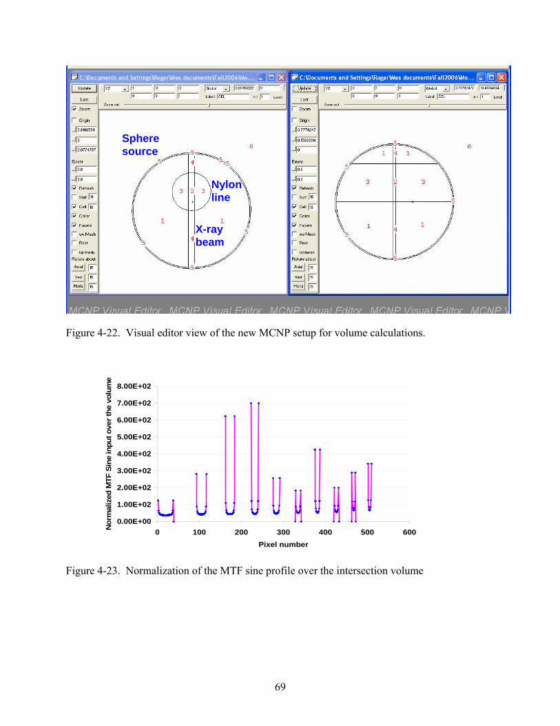
69
Figure 4-22. Visual editor view of the new MCNP setup for volume calculations.
0.00E+00
1.00E+02
2.00E+02
3.00E+02
4.00E+02
5.00E+02
6.00E+02
7.00E+02
8.00E+02
0 100 200 300 400 500 600Pixel number
Nor
mal
ized
MTF
Sin
e in
put o
ver t
he v
olum
e
Figure 4-23. Normalization of the MTF sine profile over the intersection volume
Sphere source
Nylon line
X-ray beam

70
0.00E+00
1.00E+02
2.00E+02
3.00E+02
4.00E+02
5.00E+02
6.00E+02
7.00E+02
8.00E+02
0 100 200 300 400 500 600Pixel number
Nor
mal
ized
MTF
Sin
e in
put o
ver t
he v
olum
e
Figure 4-24. Statistical smoothing of the normalized profile
0
20
40
60
80
100
120
0 0.5 1 1.5 2 2.5
Frequency line pairs per mm
Nor
mal
ized
MTF
(%)
Figure 4-25. MTF function from detector 5, pixel size 0.05mm and beam aperture 0.5mm at 45
kVp-45 mA

71
CHAPTER 5 AN IMPROVED TECHNIQUE FOR THE MTF CALCULATION BASED ON A STEP
FUNCTION
Step Function Target Design for MTF Calculation
Figure 5-1 is a calibration target which can be used for the Modulation Transfer Function
calculation based on the edge function method. The left side of the target is lead (absorber) and
the right side of the target is nylon (scatterer).
Figure 5-2 is the measured experimental response (black line) of the RSD scanning system
to an edge in units of number of counts/pixel as the scanning system moves across an edge; the
fitting function is shown in red.
The relation and the parameters used in the fitting process are:
)1
exp(*1function fitting Step 0 tzAy += (5-1)
⎪⎩
⎪⎨
⎧
±=±=
±=
0.000016-2.3019E10.076150.25157
368.69193149.89047
1
0
Aty
⎪⎩
⎪⎨
⎧
=
=
25663638.531
0.816712
2
Dof
Rχ
The line spread function is obtained by differentiating the step response function
formulated from Figure 5-2. Figure 5-3 shows the Fourier transform of the differentiated step
function. Both amplitude and phase are given; the resulting data are then fitted to give an MTF
function.
The Modulation Transfer Function is given by:
))(*2exp(*
2*
unctionMTF_edge_f 20 w
zz
w
Ay c−−+=
π (5-2)
)(2 1−= mmx
z π

72
with the following parameters
⎪⎪⎩
⎪⎪⎨
⎧
±=±=
±=±=
236.34524722048.33170.036995.59145
0.0071116-9.8466E16.80154-214.139740
Awzy
C
⎪⎩
⎪⎨
⎧
=
=
395.45637
0.999662
2
Dof
Rχ
There are two important features to notice. First, the Modulation Transfer Function
obtained from this latest experiment is in agreement with the preliminary experiments performed
with the edge function. Second, the MTF based on the edge function includes the effect of a
geometric edge. Although the nylon and lead are at the same height, the X-rays easily penetrate
the nylon compared to lead and as a result the lead/nylon interface appears as an edge to X-rays.
As expected, the MTF obtained using this method is not exactly the one obtained from a
sine input modeling (with the MTF Sine target) due to amplitude variation. However, the
behavior still follows an exponential decrease. For the sine wave modeling with the MTF target,
the MTF follows an asymptotic behavior proportional to exp(-x), and according to this study the
asymptotic behavior is proportional to exp(-x2).
Finally, for calibration purposes and relative comparison of image quality both methods
are valid. However, for simplicity and efficiency in general calibration procedures the edge
response would provide a much faster tool. Obviously the MTF based on a Sine input is more
accurate in predicting the system response versus frequency.
The MTF Sine target is more sensitive to small variations in contrast and resolution than
the step target.
A Model of the Step Function Target Using MCNP5 and Variance Reduction Techniques.
To achieve the optimum design of the MTF step target, the system response is modeled in
MCNP5. Different configurations were tested to obtain a system response as sharp as possible to

73
approach the ideal step function. In all MCNP5 runs the same detector set up as in Chapter 4 was
used. Forced collisions and DXTRAN sphere were also used as accelerations techniques. The
maximum error achieved on the number of counts was 1.05%.
The first target design was a cubic plastic piece enclosed in a lead frame of the same
height. Figure 5-4 shows the geometry of the target.
The lead frame is 0.5 cm thick and 2 cm height, the cubic nylon piece is 2 cm by 2 cm by 2
cm. According to the MCNP5 run the mean free path of particles in the nylon piece is 1.9806 cm
and about 0.00263 cm in lead.
This configuration gave the data profile shown in Figure 5-5. The beam source scanned the
target from edge to edge; the detector is on the left hand side at a negative x. This first
configuration did not provide a satisfactory profile shape to model an edge function.
A modified design of the MTF step target was tested by setting the nylon piece 1 cm
higher than the lead frame. Figure 5-6 shows the geometry of the second design of the step
target. This design was chosen to reduce the geometric lead shielding on the edges of the nylon
piece.
Figure 5-7 shows the data profile obtained from the second MTF step target design. The
profile is closer to a sharp edge function than the first design in the central top region, however
the drop near the lead frame is more important than in the first design
A third design was tested where the nylon block (2cm by 2 cm by 2cm) was laid down on a
lead sheet (3 cm by 3 cm by 0.5 cm). The data profile (Figure 5-8) shows an increase on the
nylon block edges that is slightly larger on the detector side (left hand side). This is due to a 2 cm
nylon edge that is contributing to the total signal in addition to the flat top surface.

74
The contribution of the top center part of the target appears as a dip in the center of the
profile due to the relatively high contribution of the edges. This design gives a sharper profile at
the plastic/edge junction but the high contribution of the plastic step induces a distortion of the
center part of the profile. A better target would be achieved using a thinner plastic piece on a
lead sheet.
The final design proposed for the step target is given in Figure 5-9, it includes aluminum
and lead base sheets and a junction of lead and plastic pieces of the same height.
The lead and plastic pieces are sitting on the lead sheet enabling to obtain the two
configurations presented in the first and third designs on the same line profile.
Figure 5-1. Edge target made from a junction of lead (absorber) and nylon (scatterer)
4,00 4,25 4,50 4,75 5,00 5,25 5,50 5,75
0
2000
4000
Y A
Figure 5-2. Scanning system response to an edge.
ScattererAbsorber
Distance in cm
Number of counts
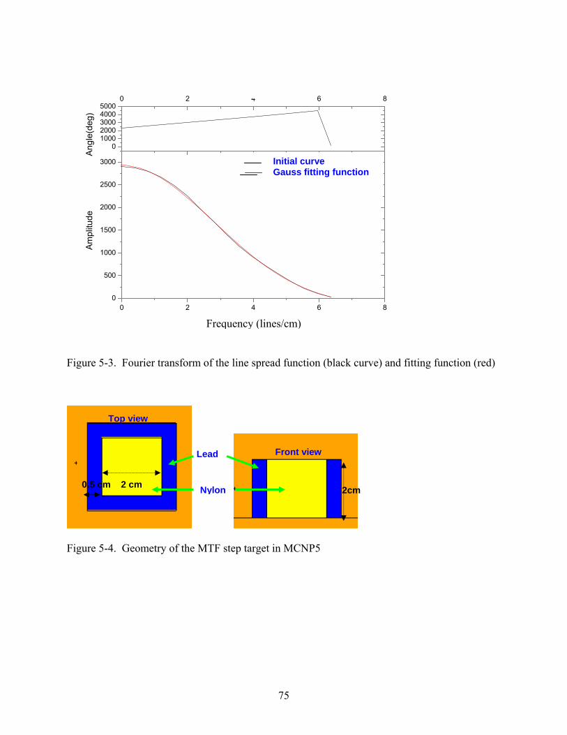
75
0 2 4 6 80
500
1000
1500
2000
2500
3000 r Gauss fit of FFT1_r ###
Frequency (Hz)
Am
plitu
de
010002000300040005000
0 2 4 6 8Frequency (Hz)
Ang
le(d
eg)
Figure 5-3. Fourier transform of the line spread function (black curve) and fitting function (red)
Figure 5-4. Geometry of the MTF step target in MCNP5
Initial curve Gauss fitting function
Frequency (lines/cm)
0.5 cm 2 cm
Top view
Nylon
Lead Front view
2cm

76
0.00E+00
1.00E-02
2.00E-02
3.00E-02
4.00E-02
5.00E-02
6.00E-02
0 0.5 1 1.5 2 2.5 3 3.5 4Distance (cm)
Cou
nts/
pixe
l
Figure 5-5. Data profile obtained from the first MTF step target design in MCNP5
Figure 5-6. Geometry of the second design of the MTF step target
PlasticLead Lead
Detector
Air
Top view
2cm
Front view
Lead
Nylon
0.5 cm 2 cm 1cm

77
0.00E+00
1.00E-02
2.00E-02
3.00E-02
4.00E-02
5.00E-02
6.00E-02
7.00E-02
8.00E-02
0 0.5 1 1.5 2 2.5 3 3.5 4Distance (cm)
Cou
nts/
pixe
l
Figure 5-7. Profile data obtained from the second design of the MTF step target
0.00E+00
1.00E-02
2.00E-02
3.00E-02
4.00E-02
5.00E-02
6.00E-02
7.00E-02
8.00E-02
9.00E-02
1.00E-01
0 0.5 1 1.5 2 2.5 3 3.5 4Distance (cm)
Cou
nts/
pixe
l
Figure 5-8. Data profile obtained from the third target design; nylon block on top of lead
PlasticLead Lead

78
Figure 5-9. Final design profile proposed for the MTF step target
2 inch1/16 inch 1/16 inch 0.5 inch
0.5 inch 0.5 inch
0.5 inch 1 inch
Nylon 6/6
Aluminium
Lead
First step design
Second step design

79
CHAPTER 6 PROPOSED TECHNIQUES FOR IMAGE QUALITY ASSESMENT
Multiple Derivatives and Inflection Points as a Mathematical Criterion for Image Quality Assessment
Even if the volumetric Sine MTF couples the target specific variations to the scanning
system response, it offers a basis for relative evaluation of system performance. It is an
integrated 3-D MTF over the vertical direction. This MTF allows comparison between detectors
and gives a basis on which to test a global improvement in the system.
Figure 6-1 presents a comparison between the MTF from Detector 1 (NaI) and Detector 5
(Y5Si2O). These results show that over a frequency range between 0.2 line pairs/mm and 2 line
pairs /mm, the performance of the Y5Si2O detector is superior to that of the NaI detector.
In Figure 6-2 the MTF plots are compared for three different aperture diameters of 0.5 mm,
1.0 mm and 1.5 mm.
Over the whole range of frequencies the MTF curve is higher for the smallest aperture. The
higher the MTF, the better the image with respect to the contrast and resolution.
The MTF presented here does not include any volumetric normalization processing. The
MTF is sensitive to the change in the volume intersection of the beam and the lines. The drop in
the MTF values is related to a loss of contrast and a volume variation. The relative difference in
MTF values indicates the quality of the images when using the same target.
Since the main purpose of the MTF plate is X-ray imaging system calibration, the main
objective is to provide a comparison of image quality.
Figure 6-3 shows several MTF plots for different conditions. In addition to the MTF value
at a given frequency, the curvature and the inflection point characterize the contrast and
resolution losses.

80
In Figure 6-3 the comparison is done over three aperture sizes of 0.5 mm, 1.0 mm, 1.5 mm
and two pixel sizes of 0.05 mm and 0.1 mm.
For a given aperture, the larger pixel size has a higher MTF and hence a better image
quality.
In order to use mathematical properties as a criterion to sort the MTF curves, a
mathematical model is established. The plots in Figure 6-4 were generated by fitting the MTF
curves using Boltzmann functions.
The formula used for the fitting process is MTF_experimental=dX
XX
e
AAAY 0
1
212 −
+
−+= . The
corresponding coefficients are listed in Table 6-1 for each curve. Note that in this section X is a
frequency since it represents the MTF’s variable.
In order to evaluate the fitting efficiency some statistical test results are given in Table 6-3.
The 2R values are close to 1 indicating a very good fitting function, the DoFChi 2
are the reduced
2Chi values obtained from the Nonlinear Least squares fitting and are given as an example
As previously explained, the curvatures and inflection points are of great interest when
comparing images from different set ups. Equation 6-1 gives the first derivative with respect to
the frequency (line pairs per mm). The coefficients are given in Table 6-2 and the plots are
shown in Figure 6-5.
20
0
)1(
*)12()(
dXXX
dXXX
e
eAAdX
XdY−
−
+
−= (6-1)
The second derivative is given by Equation 6-2:
32
2
)1(
1**)12(0
00
+
−−= −
−−
dXXX
dXXX
dXXX
e
edX
eAAdX
Yd (6-2)

81
The inflection points are given by the second derivatives’ zeros. By sorting the
corresponding frequencies, the images are compared with respect to their contrasts. The plots are
shown in Figure 6-6.
The zero values of the second derivative are presented in Table 6-4. The higher zero values
characterize better image quality according to criteria developed in this study.
The images corresponding to the MTF curves shown in Figure 6-3 are sorted and presented
in Figure 6-7 to Figure 6-11. The images are sorted using a scale from 1 to 5; 1 is the best
relative quality and 5 the relatively poorest quality.
The proposed MTF target is to be used in large scans for calibration purposes. Figure 6-12
is an image from an uncollimated YSO detector.
The number of counts needs to be increased to achieve a lower statistical error.
The image is shown to give an idea of how a calibration scan would be done. The MTF
target was laid on the sample being scanned. The heterogeneity of the sample (Tile Test Panel
VT70-191037-005) offered a good test to evaluate the MTF target response in a real
environment. However the background is of the same order of magnitude as the MTF target
response (approximately one third). This shows the limit of this MTF target design which is
highly affected by the material background.
The objective is to design an optimized small MTF target, such as the effect of the
background material is minimized.
The proposed image assessment techniques used the MTF curves obtained from the MTF
Sine target. However the same techniques can be applied to the MTF curves obtained from the
MTF step target.

82
Correlation Between the Different Methods of Calculating the MTF
The correlation between the Step function and the Sine function for MTF determination
needs to be done under the same experimental conditions. Once a relation is established between
the two methods one can be used knowing its limitations and advantages.
As previously explained, the Sine function based MTF uses more experimental
interpolation points over the frequency domain than the Step function MTF. This makes the Sine
MTF target more adapted for precise measurements of the contrast and resolution for given
frequencies. Also comparison between different MTF curves is finer and extends over a larger
frequency domain. For these reasons the Sine MTF target will be used as a reference for MTF
calculations.
A comparison between the MTF curves obtained experimentally from the Sine target and
the step target are not of high interest, unless the profiles are normalized over the target
interaction volume. This is because the MTF obtained from the Sine target contains information
on the change in volume. Recall from Chapter 4 that the Sine based MTF decreases less rapidly
(exp(-x)) compared to the Step function based MTF (exp(-x2)).
The Sine based MTF uses the output modulation of the Sine input function whereas the
Step function MTF is derived through the Line Spread function.
Resolution Assessment from a Step Function Input
To demonstrate the equivalence between the MTF calculations based on the edge function
and the line spread function the definition of the step function is needed.
⎩⎨⎧
<>
=0001
),(xx
yxwedgein (6-3)
Also

83
'''''''' ),())()(()(),( dxyxwdxdyyxdxxyxwx
Linein
x xedgein ∫∫ ∫ ∫
∞−∞− ∞−
∞
∞−
=== δδδ (6-4)
Since the system is assumed in first approximation as linear, the output must be:
∫∫∞−∞−
===xx
Lineout
edgeout dxxldxyxwyxwxe '''' )(),(),()( (6-5)
Hence, the edge spread function is the indefinite integral of the line spread function:
dxxdexl )()( = (6-6)
Figure 6-13 shows the 3 steps needed to perform an MTF calculation based on the edge
function. First the data profile is obtained from the experiment then the profile is truncated to
only use one edge, finally the profile is smoothed using the averaged values of the lower and
higher regions of the profile. This smoothing procedure is necessary because the derivation is a
high pass filter; meaning that the high frequency noise will have a high contribution to the signal.
Another possibility is to apply a Gaussian frequency window to the first derivative of the profile
to discriminate against the high frequency noise.
Once this smoothing step is performed the first derivative is obtained numerically as
shown in Figure 6-14.
The width of the rising edge between 10% and 90% corresponds to the width of the first
derivative at 10% of its maximum. This distance x in pixel or mm can be used as a quick criteria
to compare different scan conditions and to perform resolution assessment using a step function.
There are many advantages to using the edge response for measuring resolution. In fact,
the main reason for wanting to know the resolution of a system is to understand how the edges in
an image are blurred.

84
The first advantage is that the edge response is simple to measure because edges are easy
to generate in images. If needed, the Line Spread Function can easily be found by taking the first
derivative of the edge response.
The second advantage is that all common edges responses have a similar shape, even
though they may originate from different Point Spread Functions20. Since the shapes are similar,
the 10%-90% distance is an excellent single parameter measure of resolution. The third
advantage is that the MTF can be directly found by taking the one-dimensional Fourier
Transform of the Line Spread Function (unlike the PSF to MTF calculation that must use a two-
dimensional Fourier transform).
For example the step function presented in Figure 6-13 is used to calculate the resolution
associated to the 10%-90% edge response. Figure 6-15 shows how the width x of the 10%-90%
edge is calculated.
For the particular conditions of the above edge scan the system has a 10%-90% edge
response of 1.94 mm.
The limiting resolution is a vague term indicating the frequency where the MTF amplitude
has a value of 3% to 10%.
In fact the edge width measured between 10% and 90% can be related to a frequency at
which the MTF is 10% of its maximum value.
Assuming the LSF can be fitted by a Gaussian function, which is the case for most imaging
systems. Then the Fourier Transform is also a Gaussian function as shown in Equation 6-7.
))2(21exp(*2))(()
21exp()( 2
2
2
σπσπσ
ffLSFFTxxLSF −=→−= (6-7)
The width of the LSF at 10% of its maximum is given by
widthedgex _)10ln(22%10 == σ (6-8)

85
This distance can also be measured directly from the edge width between 10% and 90%.
Now considering the MTF given by the Fourier Transform of the LSF, it has a value of
about 10% of its maximum at a frequency
πσ2)10ln(2
%10 =f (6-9)
Combining Equations 6-8 and 6-9 gives
widthedgewidthedgef
_46.1
_*)10ln(*2
%10 ==π
(lp/mm or lp/pixel) (6-10)
The 10% contrast level on the corresponding MTF curves will occur at about: 0.75 lp/mm
or lp/pixel for an edge width of 1.94 mm. This is a very convenient method to asses the system
limiting resolution between 10% and to compare different images using a single number.
Figure 6-16 shows an example of a numerical calculation of the first derivative and the
Fourier Transform of the edge function used in Figure 6-15. The amplitude of the Fourier
Transform gives the MTF. The predicted frequency at which the MTF value is 10% from the
edge width method gives 0.75 lp/mm the measured value from the MTF curve gives 0.665
lp/mm. The error associated to the measured value with respect to the predicted value is about
11.3%.
This is due to the errors associated to the numerical evaluations of the first derivative and
the Fourier Transform but also the initial assumption of the Gaussian fitting.
As a conclusion the edge width between 10 % and 90% is a convenient single number for
relative comparison of different images. The same edge function can be used to generate an MTF
curve. The theoretical relationship between the edge width and the frequency at which the MTF
value is 10% can be used as an indication of the experimental frequency. In the previous
example an error of 11.3% was calculated between the two frequencies.

86
0
20
40
60
80
100
120
0 0.5 1 1.5 2 2.5frequency line pairs/mm
MTF
% detector1-NaIdetector5-YSO
Figure 6-1. MTF comparison between NaI and Y5Si2O detectors at 45 kVp, 0.5 mm aperture
0
20
40
60
80
100
120
0 0.5 1 1.5 2 2.5
Frequency line pairs per mm
Nor
mal
ized
MTF
(%) mtf-1.5mmaperture
mtf-1.0mmaperture
mtf-0.5mmaperture
Figure 6-2. MTF comparison for 3 different aperture diameters at 45kVp-45mA-0.05mm pixel
size.

87
0
20
40
60
80
100
0 0.5 1 1.5 2 2.5
Frequency line pairs per mm
Nor
mal
ized
MTF
(%)
mtf-0.1mm pix-1mm ap
mtf-0.1mm pix-0.5mm ap
mtf-0.05mm pix-1.5mm ap
mtf-0.05mm pix-1.0mm ap
mtf-0.05mm pix-0.5mm ap
Figure 6-3. MTF comparison for different pixel sizes and beam apertures at 45 kVp-45 mA
0
20
40
60
80
100
120
0 0.5 1 1.5 2 2.5
Frequency line pairs per mm
Nor
mal
ized
MTF
(%) f it-mtf-0.1mm pix-
1mm ap
fit-mtf-0.1mm pix-0.5mm ap
fit-mtf-0.05mmpix-1.5mm ap
fit-mtf-0.05mmpix-1.0mm ap
fit-mtf-0.05mmpix-0.5mm ap
Figure 6-4. MTF Boltzmann model fitting function comparison for different pixel sizes and
beam apertures at 45 kVp-45 mA
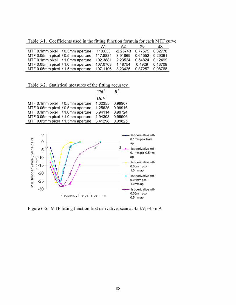
88
Table 6-1. Coefficients used in the fitting function formula for each MTF curve A1 A2 X0 dX
MTF 0.1mm pixel / 0.5mm aperture 113.633 -2.25743 0.77575 0.32778 MTF 0.05mm pixel / 0.5mm aperture 117.8884 3.91869 0.61552 0.29361 MTF 0.1mm pixel / 1.0mm aperture 102.3881 2.23524 0.54824 0.12499 MTF 0.05mm pixel / 1.0mm aperture 107.0763 1.48754 0.4929 0.13709 MTF 0.05mm pixel / 1.5mm aperture 107.1106 3.23425 0.37257 0.08768
Table 6-2. Statistical measures of the fitting accuracy
DoFChi 2
2R
MTF 0.1mm pixel / 0.5mm aperture 1.02355 0.99907MTF 0.05mm pixel / 0.5mm aperture 1.25625 0.99916MTF 0.1mm pixel / 1.0mm aperture 5.94114 0.99724MTF 0.05mm pixel / 1.0mm aperture 1.94303 0.99906MTF 0.05mm pixel / 1.5mm aperture 3.41298 0.99825
-30
-25
-20
-15
-10
-5
0
5
0 1 2 3
Frequency line pairs per mm
MTF
firs
t der
ivat
ive
(%/li
ne p
airs
pe
r mm
)
1st derivative mtf-0.1mm pix-1mmap
1st derivative mtf-0.1mm pix-0.5mmap
1st derivative mtf-0.05mm pix-1.5mm ap
1st derivative mtf-0.05mm pix-1.0mm ap
1st derivative mtf-0.05mm pix-0.5mm ap
Figure 6-5. MTF fitting function first derivative, scan at 45 kVp-45 mA
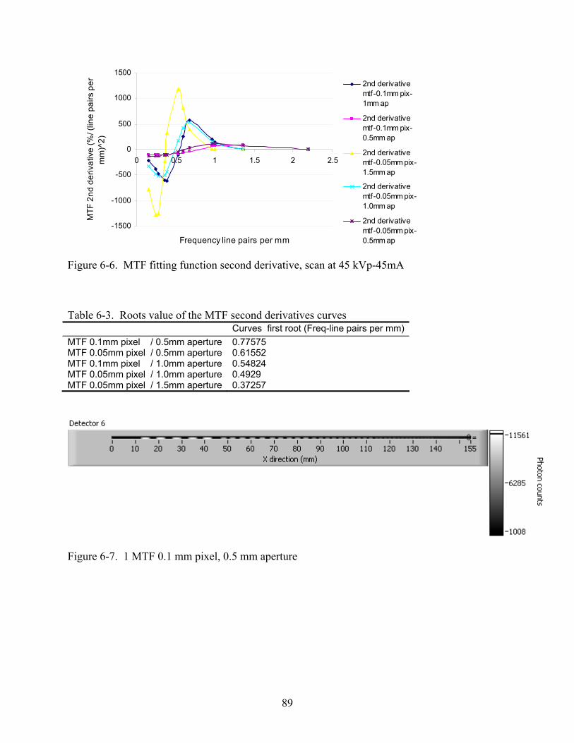
89
-1500
-1000
-500
0
500
1000
1500
0 0.5 1 1.5 2 2.5
Frequency line pairs per mm
MTF
2nd
der
ivat
ive
(%/ (
line
pairs
per
mm
)^2)
2nd derivativemtf-0.1mm pix-1mm ap
2nd derivativemtf-0.1mm pix-0.5mm ap
2nd derivativemtf-0.05mm pix-1.5mm ap
2nd derivativemtf-0.05mm pix-1.0mm ap
2nd derivativemtf-0.05mm pix-0.5mm ap
Figure 6-6. MTF fitting function second derivative, scan at 45 kVp-45mA
Table 6-3. Roots value of the MTF second derivatives curves Curves first root (Freq-line pairs per mm) MTF 0.1mm pixel / 0.5mm aperture 0.77575 MTF 0.05mm pixel / 0.5mm aperture 0.61552 MTF 0.1mm pixel / 1.0mm aperture 0.54824 MTF 0.05mm pixel / 1.0mm aperture 0.4929 MTF 0.05mm pixel / 1.5mm aperture 0.37257
Figure 6-7. 1 MTF 0.1 mm pixel, 0.5 mm aperture

90
Figure 6-8. 2 MTF 0.05 mm pixel, 0.5 mm aperture
Figure 6-9. 3 MTF 0.1 mm pixel, 1.0 mm aperture
Figure 6-10. 4 MTF 0.05 mm pixel, 1.0 mm aperture

91
Figure 6-11. 5 MTF 0.05 mm pixel, 1.5 mm aperture
Figure 6-12. YSO image of MTF Target on a tile panel
Nylon lines
from the MTF target
Aluminium edge of the MTF frame
Tile Test Panel

92
Table 6-4. Different methods of the MTF derivation Input function Output function Intermediate steps MTF
Point source (x,y) Point spread function (x,y)
2D FT MTF (ξ,η)
Line source (x)= ∫ Point source (x,y)
Line spread function (x)
1D FT MTF (ξ,0)
Edge function (x) Edge spread function (x)
d(Edge(x)) /dx = Line spread function (x) and 1D FT
MTF (ξ,0)
Sine input(x) Sine output (x) Contrat(ξ)/Contrast(0)=α*MTF MTF(ξ,0)
Figure 6-13. Selection and smoothing steps for the MTF calculation from a step function
0
5000
10000
15000
20000
25000
30000
0 10 20 30 40 50 60 70Distance (mm)
Nor
mal
ized
cou
nts
/pix
el
0
5000
10000
15000
20000
25000
30000
0 10 20 30 40 50 60 70Distance (mm)
Nor
mal
ized
cou
nts
/pix
el
0
5000
10000
15000
20000
25000
30000
0 10 20 30 40 50 60 7Distance (mm)
Nor
mal
ized
cou
nts
/pix
el
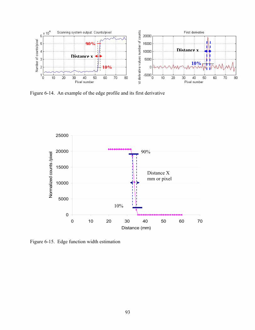
93
Figure 6-14. An example of the edge profile and its first derivative
Figure 6-15. Edge function width estimation
0
5000
10000
15000
20000
25000
0 10 20 30 40 50 60 70Distance (mm)
Nor
mal
ized
cou
nts
/pix
el
10%
90%
Distance X mm or pixel
90%
10%10%
Distance xDistance x

94
Figure 6-16. Numerical evaluation of the first derivative of the edge function used in the
example and its Fourier Transform
8 10 12 14 16 18 20 22 24 26 28 30 32
7000
6000
5000
4000
3000
2000
1000
0 Data: Derivative1_Data33BModel: GaussEquation: y=y0 + (A/(w*sqrt(PI/2)))*exp(-2*((x-xc)/w)^2)Weighting: y No weighting Chi^2/DoF = 9422.64067R^2 = 0.9963 y0 -1.76655 ±16.04368xc 25.76397 ±0.00675w 1.01068 ±0.01394A -9715.58996 ±120.72925X Axis Title
0 5 10 15 20 25 30 350
2000
4000
6000
8000
10000
12000
14000
X A i Ti l
0.0 0.2 0.4 0.6 0.8 1.0 1.20
10
20
30
40
50
60
70 r Gauss fit of FFT7_r
Data: FFT7_rModel: GaussEquation: y=y0 + (A/(w*sqrt(PI/2)))*exp(-2*((x-xc)/w) 2)Weighting: y No weighting Chi 2/DoF = 7.01484R2 = 0.98518 y0 -1.71357 ±0.41015xc -1.9351E-16 ±0.00232w 0.65329 ±0.00754A 50.06194 ±0.76622
F (H)
Ampl
itude
05000
100001500020000
0.0 0.2 0.4 0.6 0.8 1.0 1.2
Ang
le(d
eg)

95
CHAPTER 7 COMPUTATIONAL PROCESSING WITH MATLAB. ALGORITHM ARCHITECTURE FOR
MTF CALCULATION (MATLAB)
Modulation Transfer Function Based on the Sine Target
The main result of this task was a code that integrates all the calculations for the MTF
process. The code was written in the MATLAB 7.0.4 programming language. The code was to
be implemented in an image processing tool previously used by the Lockheed-Martin Space
Systems Company.
Figure 7-1 shows the Matlab interface for the profile data generation and the MTF
calculation. The interface is analogous to the code used currently to process the output images
from the system and draw the profiles.
After scanning the MTF plate, a couple lines are generated. When saving the profile
(Figure 7-2), the MTF menu appears to enable the MTF processing.
Once the profile is saved in a text format, the code generates a *.dat file using the same
name. This file will be used in Matlab to generate MTF curves.
The conventional profile used for the MTF calculation should have the maximum peaks on
the left, since they are used to generate the low frequencies. The code is essentially written
following this model. There is an option to reverse the profile data to make user entries easier
(Figure 7-3).
Figure 7-4 shows the user interface for entering the Sine MTF plate information. Default
values are already entered for the Sine MTF target.
The first step is to locate the maxima and minima in the image. Based on these values the
contrast and the MTF are calculated. Figure 7-5 shows how the preliminary peak selection is
displayed.

96
The local maximums are designated using red crosses. Because of the fluctuations in the
data, it is nearly impossible to pick up one maximum per peak, unless using the Full Width at
Half Maximum (FWHM) for each set of holes. This part is performed in the “Automatic” option
available in the code.
Currently, the MTF calculation requires that the user select for each peak a region of
interest. The region of interest (ROI) does not have to be precisely selected. The code extracts
the x-ordinates from the image to recalculate the overall maximum in the ROI.
After all the peaks have been selected, the MTF plot is generated (Figure 7-6). When
saving the plot, the same name is used to create a new folder that contains the data profile and
the MTF plots in PDF format in addition to a text file that contains the values of the MTF versus
frequencies.
Modulation Transfer Function Based on a Step Function Target
Figure 7-7 shows a step function profile obtained from the preliminary experiment
(Chapter 3) of an edge function. The first derivative is also given since the derivation is the first
step in using the edge function. Note that the data is noisy and a statistical smoothing would
provide a better data profile to start with.
A discrete Fourier transform is then performed on the first derivative and the modulus is
estimated to give the MTF. Figure 7-8 shows the MTF curve and its first and second derivatives.
As expected, the numerical treatment without any smoothing on the data introduces high
fluctuations in the MTF calculation. These large fluctuations made it nearly impossible to use the
zeros of the second derivative as a criterion for image quality assessment.
Either a denoising algorithm or an iterative least squares estimate fitting of the data using
∑ =−
j j
xitMeasuremenxictionFittingFun min))()((2
2
σ is needed.

97
The more convenient choice for automated use would be using the fitting tools provided
with the Matlab7.0.4 version.
Figures from 7-8 to 7-10 show the different steps in the Matlab code used to generate MTF
curves from an edge function. Figure 7-8 shows how a region of interest can be selected, Figure
7-9 and 7-10 show the selected region of the edge function its first derivative and the MTF
curves with the frequencies expressed in line pairs/pixel and line pairs/mm.
Figure 7-1. Matlab user interface

98
Figure 7-2. MTF menu and data profile
Figure 7-3. Data profile
Line profile

99
Figure 7-4. User interface for information entries
Figure 7-5. Maximum search

100
Figure 7-6. Saving files
Figure 7-7. Data profile from an edge function and its first derivative

101
Figure 7-8. Selection of a region of interest in the edge function profile
Figure 7-9. The selected region of interest and the first derivative of the edge function

102
Figure 7-10. MTF curves with frequencies expressed in line pairs/pixel and line pairs/mm

103
CHAPTER 8 CONCLUSION
In order to properly characterize the X-ray backscattering system several definitions of the
Modulation Transfer Function have been introduced. These definitions and the methodology for
calculating the MTF depend on the input function to the system. Several input functions have
been tested: Point Function, Line Function, Step Function and Sine Function. The relationship
between the different functions and the resulting MTF was treated to understand the benefits and
limitations of each input type function for practical use. The preliminary experiments for an
impulse and step functions showed the expected responses from mathematical derivations. The
key step for a complete analysis was the ability to accurately fit the curves according to statistical
tests and obtain mathematical expressions that were used later for curve recognition.
A Sine target pattern was proposed for precise evaluation of the MTF as a function of
frequency. The design was based on nylon lines of different diameters and separation. This MTF
Sine target was used for major comparisons and relative image quality assessment. The
experiments were performed mostly with the new compact system using Y5SI2O detectors, but
some experiments used NaI detectors. The large dimensions of the MTF Sine target made it less
desirable for practical use on small scans areas. Also this Sine MTF target was highly dependent
on the background material. Instead, an improved Step target design was proposed to meet a size
constraint of approximately a cube of 0.5 inch by 2 inch by 5/8 inch.
The different designs were supported by MCNP5 models using two variance reduction
techniques; forced collisions and DXTRAN sphere. These models enabled to understand the
different contributions to the signal and their relationships with the target own volume.
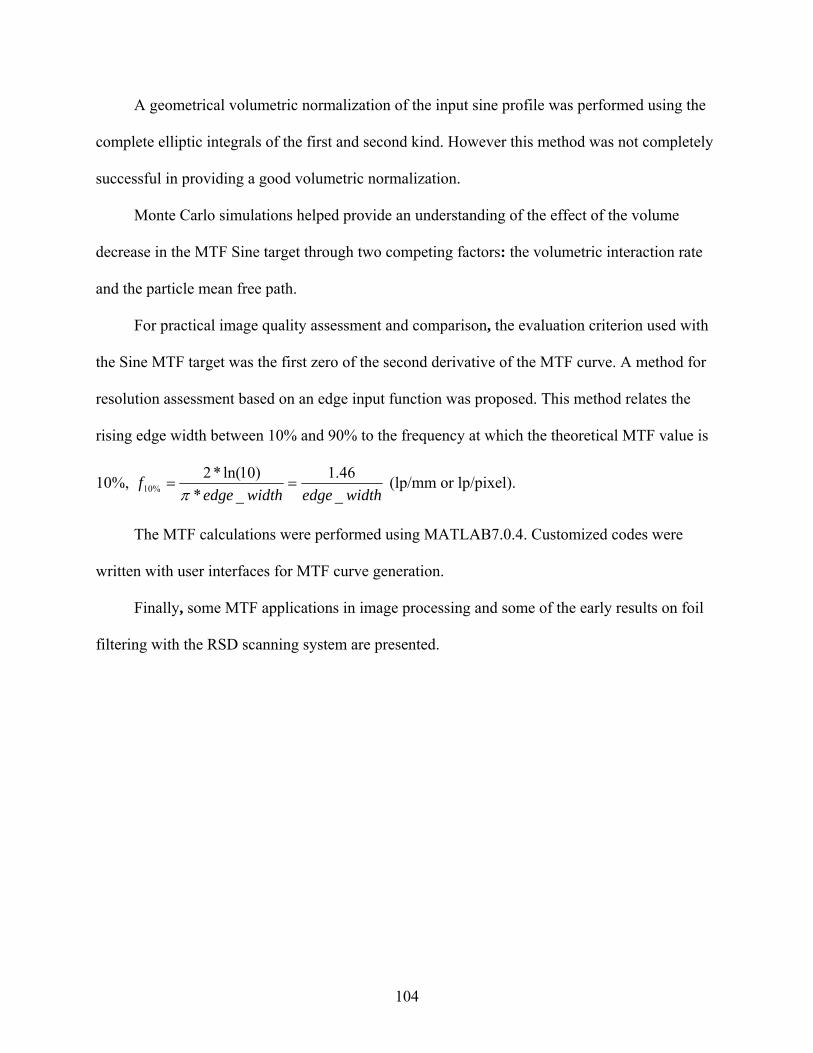
104
A geometrical volumetric normalization of the input sine profile was performed using the
complete elliptic integrals of the first and second kind. However this method was not completely
successful in providing a good volumetric normalization.
Monte Carlo simulations helped provide an understanding of the effect of the volume
decrease in the MTF Sine target through two competing factors: the volumetric interaction rate
and the particle mean free path.
For practical image quality assessment and comparison, the evaluation criterion used with
the Sine MTF target was the first zero of the second derivative of the MTF curve. A method for
resolution assessment based on an edge input function was proposed. This method relates the
rising edge width between 10% and 90% to the frequency at which the theoretical MTF value is
10%, widthedgewidthedge
f_46.1
_*)10ln(*2
%10 ==π
(lp/mm or lp/pixel).
The MTF calculations were performed using MATLAB7.0.4. Customized codes were
written with user interfaces for MTF curve generation.
Finally, some MTF applications in image processing and some of the early results on foil
filtering with the RSD scanning system are presented.

105
APPENDIX A ENERGY FILTERING USING PAPER
While setting up the experiments for the MTF measurements, placing a regular sheet of
paper under the nylon lines, in addition to the lead on the floor, drops the background noise by
400 counts/pixel.
Figure A-1 shows a comparison between two backscatter images, one with and one
without paper. The maximum intensities are about the same order, while the background
contribution drops off by half.
Note that for case b in Figure A-1 the bright line on the image is above the sheet of paper
while the 3 lines on the left of the image are right under the paper. All of the lines are equally
distant from the paper.
Figure A-2 shows a line profile across image b in Figure A-1. The lines under the paper
show with near half intensity of that of the line above the paper.
a b Figure A-1. Comparison between two backscatter images. a) Scan without paper underneath the
nylon line. b) Scan with paper underneath the nylon line

106
Figure A-2. Line profile evaluation of the paper filtering

107
APPENDIX B MTF FRAME STRUCTURE
Figure B-1. MTF frame plate top view

108
Figure B-2. MTF cover plate top view

109
LIST OF REFERENCES
1. E. Dugan, A. Jacobs, S. Keshavmurthy, and J. Wehlburg," Lateral Migration Radiography," Research in Nondestructive Evaluation, 10(2) p. 75-108 (1998).
2. A. Jacobs, E. Dugan, S. Brygoo, D. Ekdahl, L. Houssay, and Z. Su, “Lateral Migration Radiography: A New X-ray Backscatter Imaging Technique,” Proceeding of SPIE, 4786 p. 1-16 (2002).
3. E. Dugan, A. Jacobs, L. Houssay, and D. Ekdahl, “Detection of Flaws and Defects Using Lateral Migration X-ray Radiography,” Proceeding of SPIE, 5199 p. 47-61 (2004).
4. H. Barrett, and W.Swindell, Radiological Imaging, The Theory of Image Formation, Detection, and Processing, Academic Press, Inc San Diego, California 1981.
5. F. Attix, Introduction to Radiological Physics and Radiation Dosimetry, John Wiley & sons, Inc New York, New York (1986).
6. A. Jacobs, and J. Campbell, “Landmine Detection by Scatter Radiation Radiography,” Scientific and Technical Final Report, Contract DAAK 70-86-K-0016, U.S. Army Belvoir Research, Development and Engineering Center, (1987).
7. J. Campbell, and A. Jacobs, “Detection of Buried Land Mines by Compton Backscatter Imaging,” Nuclear Science and Engineering, 110 p. 417-424 (1992).
8. Y. Watanabe, J. Monroe., S. Keshavmurthy, A. Jacobs, and E. Dugan, “Computational Methods for Shape Restoration of Buried Objects in Compton Backscatter Imaging,” Nuclear Science and Engineering, 122 p. 55-67 (1996).
9. J. Wehlburg, S. Keshavmurthy, E. Dugan, and A. Jacobs, “Geometric Considerations Relating to Lateral Migration Backscatter Radiography (LMBR) as Applied to the Detection of Landmines," Proceeding of SPIE, 3079 p. 384-393 (1997).
10. Z. Su, J. Howley, J. Jacobs, E. Dugan, and A. Jacobs., “The Discernibility of Landmines Using Lateral Migration Radiography,” Proceeding of SPIE, 3392 p. 878-887 (1998).
11. C. Wells, Z. Su, J. Moore, E. Dugan, and A. Jacobs, "Lateral Migration Radiography Measured Image Signatures for the Detection and Identification of Buried Landmines”, Proceeding of SPIE, 3710 p. 906-916 (1999).
12. C. Wells, Z. Su, A. Allard, S. Salazar, E. Dugan, and A. Jacobs, “Suitability of Simulated Landmines for Detection Measurements Using X-ray Lateral Migration Radiography”, Proceeding of SPIE, 4038 p. 578-589 (2000).
13. Z. Su, A. Jacobs, E. Dugan, J. Howley, and J. Jacobs, “Lateral Migration Radiography Application to Land Mine Detection, Confirmation and Classification,” Optical Engineering, 39(9) p. 2472-2479 (2000).

110
14. E. Dugan, A. Jacobs, Z. Su, L. Houssay, D. Ekdahl, and S. Brygoo, “Development and Field Testing of a Mobile Backscatter X-ray Lateral Migration Radiography Land Mine Detection System,” Proceeding of SPIE, 4742 p. 120-131 (2002).
15. R. Evans, The Atomic Nucleus, McGraw Hill Boo, Inc. New York, New York (1955).
16. J. Dainty, and R.Shaw, Image Science Principles, Analysis and Evaluation of Photographic-Type Imaging Processes, Academic Press, London (1974).
17. M.J. Berger, J.H. Hubbell, S.M. Seltzer, J. Chang, J.S. Coursey, R. Sukumar, and D.S. Zucker, “XCOM: Photon Cross Section Database (version 1.3) http://physics.nist.gov/xcom”, National Institute of Standards and Technology (May 2007).
18. D. Shedlock, “X-ray Backscatter Imaging for Radiography by Selective Detection and Snapshot Evolution, Development, and Optimization”, Ph.D. Dissertation, University of Florida (2007).
19. B.T. Addicott, “Characterization and Optimization of Radiography by Selective Detection Backscatter X-ray Imaging Modality”, M.S. Thesis, University of Florida (2006).
20. S. Smith, The Scientist and Engineer’s Guide to Digital Signal Processing California Technical Publishing, San Diego, California (1997).

111
BIOGRAPHICAL SKETCH
Nissia Sabri is a graduate assistant at the University of Florida. She joined the Scatter x-ray
laboratory in the Nuclear and Radiological Engineering Department in August of 2005 to
complete a Master of Science in nuclear engineering. She obtained a Master of Science in
applied physics engineering in September 2006 and a Bachelor of Science in physics in May
2005 at The Grenoble National Engineering School for Physics–France.