“Mean Field Theory And Computer

Simulations On Non-Equilibrium

Phenomena In Complex Chemical

Systems.”

Thesis submitted for the degree of

Doctor of philosophy (Sc.)

in

Chemistry (Physical)

by

Amit Das

University of Calcutta

2013

2

To My Family

3

Acknowledgements

I would start thanking my supervisor Jaydeb Chakrabarti for his constant support and

invaluable guidance over the years which not only enriched my understanding of the subjects,

but also was the key to develop myself as a good scientist. His incredible belief in me helped

me to pursue diverse problems simultaneously which was very important for my development.

I would also thank Dr. Ranjit Biswas who has been a wonderful mentor and collaborator. My

special thanks go to Dr. Mahua Ghosh, our collaborator in the works on biomacromolecules,

for introducing me to the world of biology. Her contributions as a mentor have been

enormous in my development at later stages of my PhD. Thanks also to my thesis and PhD

committee members Dr. Sanjoy Bandopadhyay, Indian Institute of Technology Kharagpur,

and Professor Debshankar Ray, Indian Association for Cultivation of Sciences, Kolkata,

respectively, for helpful comments and suggestions.

I have been really lucky to come across several brilliant minds during my days at St.

Xavier’s College (SXC), Kolkata, Rajabazar Science College (RSC), Kolkata, and S. N. Bose

National Centre for Basic Sciences (SNBNCBS), Kolkata. I would always remember the

statistical physics courses taken by Professor Jayanta K. Bhattacharjee and Professor Arup

K. Raychaudhuri, the Director, SNBNCBS. I thank all of my teachers at the undergraduate

and master’s level, in particular, Dr. Ashish Nag (SXC) for transforming my views on

physical chemistry and Dr. Swapan Chakrabarty (RSC) for a sound introduction to the world

of statistical mechanics. Thanks to Professor Kamal Bhattacharya and Dr. Nikhil Guchhait

(RSC) also for constant help and encouragement.

Great friends always make days fun and fruitful. I thank my fellow group-members,

present and past: Samapan Sikdar, Paramita Saha, Suman Dutta and Arup Bhowmik. I would

also thank my other friends who were part of my days of PhD in Chemical, Biological and

Macromolecular Sciences department, SNBNCBS. Specifically, I would thank Snehasis

Daschakrabarty who was my batch-mate and Hemanata Kashyap, a senior in the department

with whom I shared my work-cubicle at early stages. Kinshuk Banerjee and Biswajit Das

require special mention, who were my other cubicle-mates from the department later. Thanks

to both of them for some great and memorable moments of both fun and serious scientific

discussions. Tapas Sahoo, Neetik Mukherjee and Mithun Chaudhury have been wonderful

friends over the years from my days at RSC. Finally, I would thank my close friends from

4

college days: Avisek Dutta, Kaustav Goswami, Shauvik De, Subhradip Paul, Debjit Roy,

Sambit Gan, Saswata Chakrabarty, and Deep Sengupta.

My journey could not have sailed so far without the love and support of my family. No

degree of thanks would be sufficient for my parents, Swapna and Banamali Das, to ensure

that I get a great education. I also thank my younger brother Shubhajit, a budding physical

chemist, for his constant support, comments and enticing discussions to disseminate my views

onto various arenas, including, science, literature and of course music.

Finally, I would thank SNBNCBS for providing me a wonderful research environment

and facilities. I also thank Council of Scientific and Industrial Research, India for a research

fellowship.

Amit Das

S. N. Bose National Centre for Basic Sciences,

Block JD, Sector III, Salt Lake,

Kolkata-700098, West Bengal, India.

5

Table of Contents Chapter 1 Introduction ............................................................................................................... 8

1.1 Dipolar solute rotation in different media ........................................................................ 9

1.2 Solvation dynamics in nanoconfined fluids ................................................................... 12

1.3 Conformational fluctuations in biomacromolecules ...................................................... 15

1.4 Outline of the thesis ....................................................................................................... 19

Chapter 2 Dipolar solute rotation in a supercritical polar fluid ............................................... 20

2.1 Introduction .................................................................................................................... 20

2.2 Wave vector dependent viscosity ................................................................................... 22

2.2.1 Molecular hydrodynamic description for normal liquid .......................................................22

2.2.2 Molecular dynamics simulation............................................................................................24

2.2.3 Extension to SC CHF3 ..........................................................................................................25

2.3 Generalization of SED model: Molecular hydrodynamic R ......................................... 27

2.4 Inclusion of solute-solvent interaction ........................................................................... 28

2.5 Conclusion ..................................................................................................................... 30

Appendices ........................................................................................................................... 31

Chapter 3 Dipolar solute rotation in liquid media: effect of electrostatic solute-solvent

interaction ................................................................................................................................ 37

3.1 Introduction .................................................................................................................... 37

3.2 Common dipolar liquids ................................................................................................ 40

3.2.1 Molecular hydrodynamic friction and hydrodynamic rotation times ...................................40

3.2.2 Friction due to long-ranged solute-solvent interaction .........................................................41

3.2.3 Rotation times including DF ................................................................................................46

3.2.4 Comparison with earlier theories ..........................................................................................47

3.3 Generalization for ionic media....................................................................................... 48

3.3.1 Wave vector dependent viscosity and molecular hydrodynamic R .....................................49

3.3.2 Electrostatic contribution to R in ionic media .....................................................................53

3.4 Quasi-universality of solute rotation in liquid solvents ................................................. 56

3.5 Conclusion ..................................................................................................................... 59

Appendices ........................................................................................................................... 60

Chapter 4 Solvation dynamics in fluids under nano-meter scale confinement ........................ 72

4.1 Introduction .................................................................................................................... 72

4.2 Dimensional crossover ................................................................................................... 77

4.2.1 Simulation details .................................................................................................................77

4.2.2 Characterization of fluid structure under confinement .........................................................78

4.2.3 Crossover in equilibrium density fluctuations: Reflecting and repulsive walls ...................80

4.2.4 Crossover in dynamic density fluctuations: Reflecting and repulsive walls ........................81

6

4.2.5 Dependence of crossover on wall-fluid potential .................................................................83

4.3 Solvation dynamics under confinement ......................................................................... 84

4.3.1 Simulation details .................................................................................................................84

4.3.2 Mechanisms of confinement-induced slowing down ...........................................................85

4.3.3 Effects of drying-wetting competition on SD .......................................................................87

4.3.4 Implications of the results ....................................................................................................90

4.4 Conclusion ..................................................................................................................... 91

Chapter 5 Conformational fluctuations in biomacromolecules ............................................... 93

5.1 Introduction .................................................................................................................... 93

5.2 The histogram based method for conformational thermodynamics .............................. 99

5.2.1 Protein-ligand binding ..........................................................................................................99

5.2.2 Metal-ion binding to protein ...............................................................................................103

5.3 Conformational thermodynamics of CaM-peptide complexes .................................... 104

5.3.1 Simulation details ...............................................................................................................105

5.3.2 Methyl order parameters .....................................................................................................105

5.3.3 Equilibrium correlations among dihedral angles ................................................................106

5.3.4 Histograms of dihedrals and convergence of thermodynamics ..........................................107

5.3.5 Conformational entropy ......................................................................................................109

5.3.6 Conformational free energy ................................................................................................110

5.3.7 Thermodynamics at individual binding regions .................................................................111

5.3.8 Scaling of conformational entropy with methyl order parameters .....................................113

5.3.9 Prediction ............................................................................................................................114

5.3.10 The HBM: merits, demerits and extensions .....................................................................115

5.4 Conformational thermodynamics for Ca2+

-ion binding to CaM .................................. 116

5.4.1 Dihedral correlations and histograms .................................................................................117

5.4.2 Overall thermodynamics data .............................................................................................118

5.4.3 Conformational changes of the Ca2+

binding loops ............................................................118

5.4.4 Changes in linker ................................................................................................................121

5.4.5 Generalization of results on metal-ion binding to protein ..................................................122

5.5 Allosteric regulations in Ca2+

binding to CaM ............................................................ 122

5.5.1 Dynamic correlations between dihedral angles ..................................................................122

5.5.2 Dihedral auto- and cross correlations in CaM ....................................................................123

5.5.3 Dynamic dihedral correlations and allosteric regulations ..................................................127

5.6 Conclusion ................................................................................................................... 129

Appendices ......................................................................................................................... 131

Chapter 6 Thermodynamics of interfacial changes in a protein-protein complex ................. 136

6.1 Introduction .................................................................................................................. 136

7

6.2 Methods........................................................................................................................ 138

6.2.1 Simulation details ...............................................................................................................138

6.2.2 Thermodynamics from HBM .............................................................................................138

6.2.3 HBM for interfacial water molecules .................................................................................139

6.2.4 Dynamics of Interfacial water molecules ...........................................................................139

6.3 Results .......................................................................................................................... 140

6.4 Interpretation of results ................................................................................................ 147

6.5 Conclusion ................................................................................................................... 149

References…………………………………………………………………………………..150

List of Publications………………………………………………………………………… 165

Chapter 1 8

Chapter 1 Introduction

Exploration of non-equilibrium phenomena in complex chemical systems lies at the

heart of research in physical chemistry. The phrase ‘complex chemical systems’ applies for

any multicomponent atomic or molecular system1, 2

containing interacting particles. Such

systems are ubiquitous in nature, for instance, fluid-media in living systems host several

dissolved or dispersed organic and inorganic molecules. The air surrounding us, which is a

vast reservoir of various molecules of different species, also falls into this category. Solutions

of fluorescent dyes, electrolytes, biomacromolecules, like protein, DNA, different interfaces

and micelles all form instances of complex chemical systems. Development of such complex

materials with specific physical and chemical properties constitutes an important branch of

science and technology3.

In scientific literature the complex chemical systems are recognized by characteristic

static and dynamic properties observed over broad range of length and timescales2. Such

characteristic properties often lead to highly specific and unique chemical phenomena,

controlled by the diverse coupling among the different length and timescales. With increasing

number of emergent complex chemical systems, molecular level understanding of their

properties and these phenomena is becoming exceedingly important. Experiments allow

direct exploration of structure and dynamics over different space and time windows. The

theoretical approaches aided by computational techniques offer scope to procure knowledge

essential for fundamental understanding of complex systems. Various experimental

techniques have been employed in this regard, in conjunction with theory and computation2, 4

to extract structural and functional information about numerous emergent complex chemical

systems during the past few decades.

The connection between the equilibrium structure and the underlying dynamics is an

important feature of the complex chemical systems. The dynamics of constituent molecules

in a system is determined by their spatial arrangements which are very important for their

functional properties. Here lies the motivation for the studies of non-equilibrium processes in

these complex materials which ultimately help to characterize the relationship between

structure and functions. Different processes reveal different aspects of this relationship, of

which three main classes of non-equilibrium phenomena are discussed in the present thesis:

(i) solute rotation in different complex media, (ii) effects of nanometer scale confinement on

dynamics of solvation in fluids and (iii) conformational dynamics in biomacromolecules.

Chapter 1 9

We pursue the understanding of the above classes of non-equilibrium phenomena

using theoretical and computational approaches. For the analytical calculations we work

within the frame-work of mean field theory5. As the name suggests, Mean field theory

5, 6 is a

theoretical framework which approximates the many-body interactions in a system by an

effective interaction so that any molecule feels a ‘mean field’ due to the other molecules.

Thus, it reduces a many-body problem into an effective one-body problem and hence is

enormously advantageous for the mathematical simplicity it brings in. Mean field theory is

almost invariably the first approach adopted to explore any complex system. It is quite a

useful description if the spatial fluctuations in the system are not significant. Such

approximation leads to quantitative results when the range of interactions is infinite. For our

purpose, we use the mean field theory to treat the long-ranged forces in the system. We

perform several computer simulations to support our analytical results. The simulations on

biomacromolecular systems are based on atomistic force-field based methods. All the

theoretical and simulation methods are described in the relevant chapters where they have

been employed.

In the three subsequent sections 1.1-1.3 of this chapter, we describe the backgrounds

and unresolved aspects of these processes in the relevant complex chemical systems. We also

briefly state our results and discuss the implications. The final section of this chapter gives an

outline of the remaining part of the thesis.

1.1 Dipolar solute rotation in different media

Rotation of dissolved solute molecules in a fluid medium is a motion of fundamental

category. Such rotation depends directly on the ability of the immediate surroundings of the

solute to accommodate its new orientations. Any heterogeneity in the environment of the

solute is captured by these rotational motions. Thus the dynamics of solute rotation has been

one very important class of non-equilibrium process that supply valuable information

regarding the nature of solute-solvent coupling7-9

and local environment of the solute. The

rotational dynamics of a molecular rotor is typically expressed in terms of the rate of angular

displacement around a specific molecular axis. For a spherical molecule one finds a unique

rate of rotation, inverse of which gives the timescale of rotation. However, multiple

timescales also are observed if the molecule itself possesses different rotational degrees of

freedom, applicable for highly anisotropic molecules10

and biomacromolecules11

. The

timescales can be lengthened if there is any specific interaction or complex formation

between the solute and the solvent molecules12, 13

. Thus, these rotational rates or the

associated timescales have proved useful tools to understand the local compactness of a

Chapter 1 10

medium at a length scale of the order of the solute size. In addition such timescales often give

valuable idea about mechanisms of certain reactions, especially in biomolecules, since

binding can significantly retard these rotations.

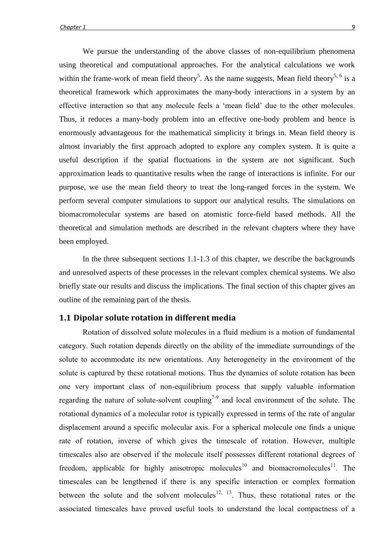
Figure 1.1: Rotation of a dipole. It is initially aligned to z-axis and then rotates about the

y-axis. represents the angular displacement with respect to its initial orientation.

Figure 1.1 schematically shows the rotation of a dipole where the angular

displacement is marked as a time-dependent quantity, rate of change of which describes the

rate of rotation. Measurements of the time dependent fluorescence anisotropy11

r(t) provides

a method to track the rotation of a fluorescent solute. In such experiments the solute is

excited using laser to create a dipole in a higher electronic state. This excited solute dipole

then gradually relaxes to equilibrium via diffusive rotational motion. The time-dependent

fluorescence emission intensity for such a dipole is anisotropic which is expressed in terms of

r(t). The conventional probes used in these experiments are aromatic fluorescent molecules,

like coumarins, oxazines, anthracenes and many more. The observed r(t) generally follows an

exponential decay, given by )/exp( Rt , with a characteristic time scale R for the solute

rotation. This is called the rotational correlation time, conventionally known as the rotation

time. Sometimes multi-exponential decays are observed when one obtains via the time-

integration of the normalized r(t), an average R , dominated by the longer time scale of the

decay.

There are three major classes of well-studied solvent systems. In the first class fall the

common liquid solvents having critical points much higher than ambient temperature (AT).

These are the conventional solvents including the dipolar liquids, both protic (water and

alcohols) and aprotic (acetone, acetonitrile, chloroform, formamide etc.), and the non-dipolar

ones, like, the hydrocarbons (cyclohexane, benzene, toluene etc.)8, 14

. The observed R in

these solvents are a few tens of picoseconds (ps). Next class comprises of the supercritical

Chapter 1 11

fluids15

with the fluid critical temperature near AT. Some examples are fluoroform, ethane,

carbon-dioxide and nitrous oxide16-19

. Average R in these media are typically 5-10 ps.

Finally, there are ionic media which are multicomponent systems themselves, namely, the

ionic liquids20

where the observed R are about few nanoseconds (ns), electrolyte solutions12,

13, 21 with R about few hundreds of ps and so on. The most popular fluorescent probe

molecules have been the coumarin dyes, among which coumarin 153 is the one used mostly

due to its non-reactive nature. It does not undergo any complexation with the solvent

molecules in any of the above three varieties of solvent systems, thus providing reliable

information about the local solvent structure and dynamics.

The average R of a solute is conventionally understood by the Stokes-Einstein-

Debye (SED) model8, 22

. It is a purely hydrodynamic model according to which the average

R for a spherical rotor, with volume pV in a medium of viscosity , is given under the stick

boundary condition by

Tk

V

B

p

R

, (1.1)

where TkB , the Boltzmann constant ( Bk ) times the absolute temperature. The conventional

SED model has received enormous success in describing solute rotation in common polar

solvents8, ionic liquids

23, electrolyte solutions

13 and for biologically relevant moieties

24. In

particular, increases with increasing solvent density Thus, R gets longer as increases.

Figure 1.2: Phase diagram of a fluid. The supercritical and sub-critical regions are shown.

The experimentally observed solvent density dependence of R in the supercritical

fluids (Figure 1.2) is highly non-trivial. For instance, the observed R for Coumarin 153, a

dipolar solute, in supercritical fluoroform, a dipolar solvent, exhibit a non-monotonic

Chapter 1 12

variation passing through a maximum around = 0.6c and a minimum at = c, the critical

density, followed by a monotonic increase for > c . The SED model fails to explain this

complex density dependence of R . Our recent work25

, incorporating the solvent structural

effects and solute-solvent interactions in the friction experienced by the rotating solute,

satisfactorily describes the anomalous density-dependence of solute rotation within the SED-

framework. The formulation and results are presented in chapter 2.

We extend26, 27

the above generalization of the SED model to answer the long-

standing controversy on the decoupling of electrical part of rotational friction, termed as the

dielectric friction28

, from dipolar solute rotation in various liquid systems. The controversy

stems from the experimental finding for the common dipolar liquids8, the ionic liquids

23 and

electrolyte solutions13

that hydrodynamic timescale matches the measured average rotation

times in these complex media. This is surprising, for these experimental observations, suggest

negligible dielectric friction even in presence of strong electrostatic solute-solvent

interactions. This cannot be explained by the existing theories29

which predict appreciably

large dielectric friction. Our theory predicts a minimal contribution from the dielectric

friction, and thus provides a microscopic explanation of how the dielectric friction gets

decoupled from dipolar solute rotation in above liquid systems26, 27

. More importantly, our

analyses suggest27

the existence of a quasi-universality in solute rotation for a wide variety of

solute-solvent combinations. We derive a macro-micro relation connecting a set of

experimentally measurable quantities to the molecular arrangement of the solvent around a

dissolved solute, and demonstrate that both the quasi-universality and the domination of

hydrodynamics originate from one single source, that is, packing at liquid-like density. These

calculations and results are given in chapter 3.

1.2 Solvation dynamics in nanoconfined fluids

Fluids under confinement represent a very important class of system relevant in

various branches of science and technology, from biology30

to tribology31

. With increasing

importance of physical and chemical processes in confined geometry32-43

, fundamental

understanding of confinement-induced effects on fluid properties has drawn considerable

attention44, 45

. If the confinement is comparable to molecular size, measuring a few

nanometers, the confined fluid undergoes drastic changes in static and dynamic properties46,

47, while the dimensionality of the system crosses from three to two. In strong solvophilic

confinements particle-movements become sluggish33, 47, 48

compared to the bulk, while strong

solvophobic confinements tend to make particles to move faster than in the bulk46, 49

. The

Chapter 1 13

understanding of this crossover in fluid properties is one of the most challenging problems.

All the phenomena in nanoconfined fluids affect a broad range of physical and chemical

processes in confined media32-43

, ranging from extraction to catalysis in nanopores. Thus,

study of the confinement-induced changes in fluid properties is both pedagogically and

technologically important.

In a complex chemical system a fundamental step for most of the physical or chemical

process is the solvation of the participating solute45, 50

by the solvent molecules. Any

stabilizing interaction between a solute and surrounding solvent molecules is conventionally

termed as solvation. The organization of the solvent molecules around the solute is a non-

equilibrium process governed by the instantaneous solvent distribution and diffusion of the

solvent molecules. Confinement affects both the fluid distribution as well as the diffusion

significantly. Thus, solvation dynamics experience such confinement effects when the solute

gets solvated in a confined fluid. Knowledge on modifications in solvation dynamics under

confinement would supply valuable information on the possible changes in rates of various

solvation-dependent processes, e.g. catalysis in nanoscale pores, charge- or proton-transfer

reactions and associations of biomolecules.

Figure 1.3: Schematic representation of solvation dynamics. The solute (larger circle) is

perturbed from its (a) initial equilibrium solvated state via suddenly increasing its size

or changing the dipole moment (vertical arrows inside circles) to create a (b) non-

equilibrium situation. From this state the solvent molecules (smaller circles) move to

reorganize themselves to reach a (c) new equilibrium state. Inset shows a schematic

solvent response function S(t).

Solvation dynamics is typically studied (Figure 1.3) via perturbing an equilibrated

state of the solute and then measuring the time required for the solvent to reach a new

equilibrium state from the initial equilibrium distribution. This time required, termed as the

solvation time , is obtained in terms of the decay time-scale(s) of the time (t) dependent

solvent response function45

S(t) which typically behaves like )/exp( t in the long-time

limit. Dynamics of solvation of many fluorescent dyes have been widely studied in confined

Chapter 1 14

fluids. The general picture emerging out of the observations from both experiments45

and

computer simulations51-53

is as follows: In a bulk fluid the solvation is typically complete

within tens of ps with one or two decay timescales in S(t). In nanoconfined solvents, the

solvation may extend from hundreds of ps to even ns. Recent computer simulations51-53

also

show such slowing of the solvation dynamics in various confined systems compared to the

bulk. The most striking feature of this slowing down of solvation is that it happens in both

solvophilic as well as solvophobic confinements. There has been no molecular-level

understanding of this slowing down of solvation dynamics due to geometrical constraints

imposed by the confinement.

The effects of confinement become more severe when the thermodynamic condition

of the bulk-fluid phase surrounding the confined media is in the sub-critical region (Figure

1.2) near liquid-gas coexistence. The nature of surface becomes vital here which leads to

changes in fluid phase behaviour54, 55

. Although, there exist many applications56-58

of the sub-

critical liquids along with several studies on the surface induced phenomena55, 59-63

, not many

studies have been performed to elucidate the roles of sub-critical solvents in solvation

process. However, a simulation study64

has shown that the density of the sub-critical solvent

controls the solvation behaviour.

Our studies highlight several aspects of confinement-induced changes in solvent

properties in absence and presence of solute to address above two classes of phenomena:

1. Dimensional crossover in fluids:

In a recent work we have studied65

using extensive computer simulations the effects

of nanoscale confinement on a fluid in a slit geometry far away from any coexistence point.

We explain the dimensional crossover, observed in experiments46, 47

, in terms of modification

in the long-wavelength behaviour of density response of the fluid due to geometrical

constraints. We also show that the confining potential significantly affects the crossover

behaviour. In a solvophobic slit the fluctuations increase as the confinement is made stronger.

On the other hand, in a solvophilic confinement the fluctuation decreases significantly due to

large attraction of the attractive walls under strong confinement.

2. Solvation dynamics under nanoconfinement:

We also study the solvation dynamics in a confined geometry where the bulk fluid-

phase surrounding the confinement is specified. Two different phase-points are considered:

(a) Far away from phase-transition We study66

via computer simulations the

dynamics of solvation of a large solute in a fluid under nanometer scale confinement to

provide microscopic mechanisms of the slowing down observed earlier. We find a single-

Chapter 1 15

exponential S(t) both in bulk and confinement to show that two fundamentally different

aspects of the crossover is responsible for the slowing down in the presence of two kinds of

walls. We show a sharp slowing down of solvation dynamics in solvophilic confinements due

to suppression of fluid diffusion in the presence of solvophilic walls, along with slow solvent

dynamics due to geometrical constraints. The solvation becomes slower than in the bulk in

strong solvophobic confinements as well, but not as sharply as in the solvophilic case. This is

due to the competition between reduction of dimensionality in solvent dynamics and faster

in-plane solvent diffusion.

(b) Near the liquid-gas phase-coexistence We further carry out computer simulations

to study67

the dynamics of solvation of a solvophilic solute in a solvophobic confinement, the

confined solvent being in equilibrium with bulk liquid close to liquid-gas phase coexistence,

far below the critical point. Under these circumstances evaporation takes place inside the

pore, commonly known as capillary drying61

. If a solvophilic solute particle is now inserted

in such a dried solvophobic pore the solute tends to wet the pore via capillary condensation68

posing a competition62

with the wall-mediated drying effect. This competition decides the

fluid diffusion in the pore to affect solvation dynamics. We find that the solvent response

inside the solvophobic confinement for the solvophilic solute is bi-exponential as in the bulk

sub-critical liquid. The observed solvation timescales are significantly smaller under strong

confinement compared to the bulk timescale indicating faster solvation in the pores. This is

due to a low density fluid phase created via the competition between the drying by

solvophobic walls and the surface-mediated wetting by solvophilic solute. The solvation

timescale increases linearly with slit separation to approach the bulk value.

Details of all the calculations and results on dimensional crossover and solvation

dynamics are included in chapter 4.

1.3 Conformational fluctuations in biomacromolecules

The biomacromolecules are highly flexible systems, with a huge number of internal

degrees of freedom, having the capability to adopt numerous conformations. The fluctuations

from one conformation to another plays very important role in various biological processes

including molecular recognition, signal transduction, gene expression and so on69-72

.

Reversible conformational switching of different biomacromolecules are important even

technologically, for their application in several biosensing devices73, 74

. Nuclear Magnetic

Resonance (NMR) relaxation experiments75

, fluorescence correlation spectroscopy coupled

with Forster resonance energy transfer76

, multiphoton microscopy77

and paramagnetic

relaxation experiments78

have been employed to explore conformational dynamics of

Chapter 1 16

biomacromolecules. Molecular simulations79-83

have been important in this regard yielding

microscopic information about conformational changes.

The primary focus of studies on conformations of biomacromolecules has been

identification of a set of suitable variables to capture the conformational fluctuations. When a

biomacromolecule participates in a binding event with another molecule, both the binding

partners experience conformational changes84

which stabilize the complex85

. These changes

take place simultaneously at several pockets distributed over the entire surface of the

biomacromolecules. The handling of such a large number of variables is extremely difficult.

Moreover, the interactions in the system are also diverse, like van der Waals forces,

electrostatic and hydrophobic interactions. These factors render the full characterization of

the conformational fluctuations in biomacromolecules at microscopic level quite

challenging86, 87

.

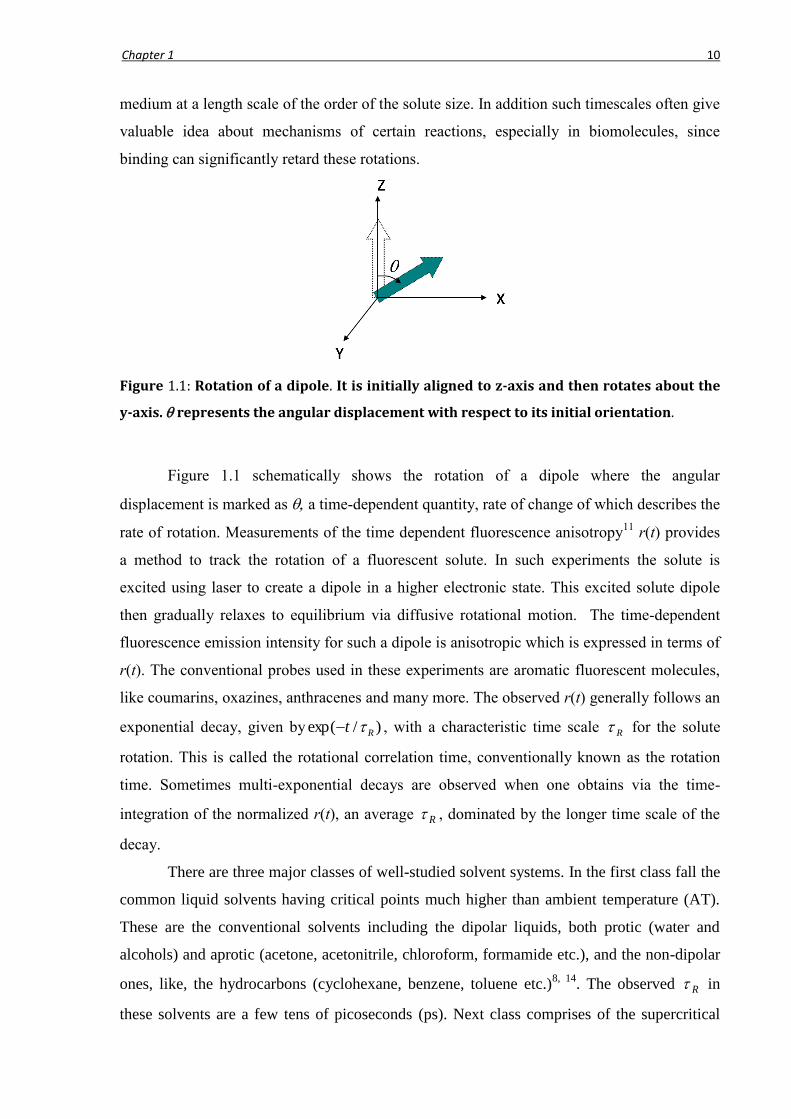
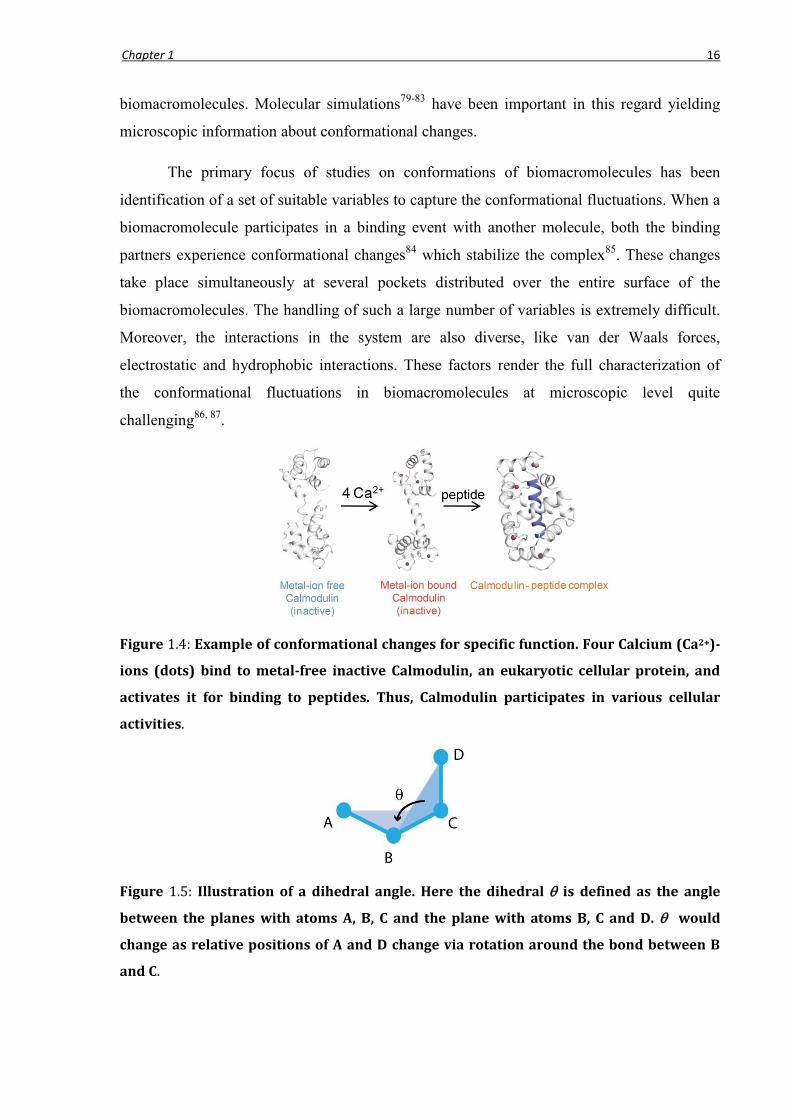
Figure 1.4: Example of conformational changes for specific function. Four Calcium (Ca2+)-

ions (dots) bind to metal-free inactive Calmodulin, an eukaryotic cellular protein, and

activates it for binding to peptides. Thus, Calmodulin participates in various cellular

activities.

Figure 1.5: Illustration of a dihedral angle. Here the dihedral is defined as the angle

between the planes with atoms A, B, C and the plane with atoms B, C and D. would

change as relative positions of A and D change via rotation around the bond between B

and C.

Chapter 1 17

Proteins are important biomacromolecules with a huge diversity of their structures

and functions. They often form complexes with metal-ions, ligands and other

macromolecules88

to adopt specific conformations for certain biological function (Figure 1.4).

Importance of various backbone and side-chain dihedral angles89

as suitable conformational

variables have recently been highlighted90

to describe protein conformations. A dihedral

angle is given by the angle between two atomic planes constituted by four consecutive atoms

as illustrated in Figure 1.5. By definition the dihedral angles are designed to trace the changes

in rotational degrees of freedom which govern the conformational fluctuations. Moreover, the

dihedrals are coarse-grained variables which give an advantage over the normal mode

analyses with a significant reduction of number of working variables. We use the dihedral

angles to describe following equilibrium and non-equilibrium aspects:

1. Conformational thermodynamics:

One significant aspect of the equilibrium conformational fluctuations is the estimation

of thermodynamics of conformational changes upon complexation. This involves changes in

both conformational entropy ( confS ) and free energy ( confG ) associated with the binding

event91

. The experimental methods, like, isothermal titration calorimetry (ITC)69

providing

the standard free energy and entropy changes of binding, can neither yield the conformational

contributions nor resolve the changes at the level of individual variables or binding regions.

NMR relaxation experiments92-95

provide an estimate of confS . However, there has been no

established experimental means of extracting confG as yet, except UV resonance Raman

measurements of conformational free energy landscapes96

. Histograms of the dihedral angles,

obtained from all-atom molecular dynamics simulation trajectories have been used to

estimate the confS for proteins97

. Several computational techniques exist to estimate the

confG as well81, 82

. However, all these methods have been computationally very demanding

and hence limited to small and medium sized biomacromolecules only.

We have recently developed83

a theoretical approach, based on one dimensional

histogram of dihedral angles, to estimate confG and confS for biomacromolecular

complexes. These histograms are generated from all-atom molecular dynamics simulations of

the binding molecules in explicit solvent in their free and bound states. Our approach is

simple and computationally efficient compared to existing methods for its ability to provide

both confG and confS simultaneously from the same histogram. confG is obtained from the

ratio of histogram maxima (equilibrium populations) in free and bound states, whereas confS

is estimated using the Gibbs formula98

. Moreover, our method allows us to estimate the

thermodynamic changes in the individual binding regions.

Chapter 1 18

We first illustrate our studies for protein-peptide binding where we show that the

equilibrium fluctuations of dihedral angle represent the conformational thermodynamics

obtained from NMR relaxation experiments75

. Next we consider99

the case of a protein

undergoing conformational changes upon binding to metal-ions100, 101

. We find different

thermodynamic changes in different metal-binding sites where the ligands coordinating to the

metal-ions play different roles in stabilizing the metal-ion bound protein-structure. Metal-ion

binding induce large thermodynamic changes in distant part of the protein also via

modification of secondary structural elements. The details of above method and the results

are presented in chapter 5.

2. Dynamic fluctuations of dihedral angles:

Apart from the equilibrium aspects, we explore102

a very important non-equilibrium

process allosteric regulation103

in biomacromolecular systems. Allosteric regulation is defined

as communication among distant sites in biomacromolecules which governs fundamental

cellular processes, ranging from metabolism to gene expression. Such communication is an

inherent capability of nearly all proteins104

to regulate structural and dynamical changes at

some part upon binding events at a distant part. Understanding such long-distance

communication is a formidable experimental challenge, while the current theoretical

explanation utilizes simplified models105

. We show that the distant site communications can

be probed directly from the time-dependent correlations among the dihedral angles at

different sites. We illustrate this for binding of multiple metal-ions to a protein where

modifications in the dynamical correlation pattern upon the binding of metal-ions are

interpreted in terms of allosteric regulations which explain experimental observations. We

also discuss the connections between our observations and the existing understanding of

allosteric regulation based on shift of populations among various conformational states103

. All

these calculations and results are also included in chapter 5.

3. Changes at biomacromolecular Interface:

Another very important issue regarding biomacromolecular complexes is the changes

at the interface. Recent experiments106, 107

suggest that structural modifications at the

interfaces are vital for stability of the complexes and functions of the associated

biomacromolecules. Although several qualitative aspects about such interfaces are known

from structural data, quantification of the interfacial changes is lacking. In chapter 6 we

study108

in close detail the thermodynamics of conformational changes at the interface of a

Chapter 1 19

protein-protein complex. confG and confS are calculated from the histograms of dihedral

angles to show that the binding at interface is dominated by strong electrostatic interactions.

We also show that the changes in the distribution of interfacial water molecules give rise to a

substantial entropy contribution in binding of the proteins. The dynamics of the interfacial

water molecules get arrested which demonstrates tight binding at the interface.

1.4 Outline of the thesis

The organization of the rest of this thesis is as follows: In chapter 2 we develop the

molecular theory on dipolar solute rotation in a supercritical polar fluid to explain the

experimentally observed non-monotonic solvent density dependence of average rotation

times. We extend this theory in chapter 3 for dipolar solute rotation in various complex

media, including common dipolar liquids, ionic liquids and electrolyte solutions to resolve

the long-standing question regarding the role of dielectric friction in solute rotation.

In chapter 4 we provide a generic understanding for the experimentally observed

confinement-induced dimensional crossover in various fluid properties. We also consider the

dynamics of solvation of a large solute in a nanoconfined fluid to explore microscopic

mechanisms of experimentally observed slowing down of solvation dynamics under

confinement. Further we predict the solvation behaviour in a solvophobic pore placed in a

sub-critical bulk fluid near liquid-gas coexistence, to capture the effects of competition

between drying by the solvophobic walls and wetting by the solvophilic solute.

Chapters 5 and 6 consider conformational fluctuations in biomacromolecular systems.

In chapter 5 we present our histogram-based method for estimation of entire conformational

thermodynamics of biomacromolecular complexation from histogram of dihedral angles. We

illustrate this method first for protein-peptide binding to show that dihedral histograms indeed

provide the conformational thermodynamics obtained from NMR relaxation experiments.

Further, we consider metal-ion binding to a protein where, apart from the thermodynamics,

we also provide a route for direct probe of allosteric regulations via dynamic correlations

among dihedral angles. Chapter 6 describes a study on biomacromolecular interface where

we extend the histogram-based method for a protein-protein complex to highlight the

important interactions dominating the binding at the interface. We generalize the histogram

based method to compute interfacial water contributions to the thermodynamics. Estimation

of the changes in dynamics of interfacial water molecules demonstrates tight binding at the

biomacromolecular interface.

Chapter 2 20

Chapter 2 Dipolar solute rotation in a supercritical polar fluid

2.1 Introduction

A fluid phase slightly above the gas-liquid critical temperature (see Figure 1.2) is

broadly regarded as a supercritical (SC) fluid15

. They are highly compressible offering large

tunability of density by mild pressure variations. Pedagogically, the solvent-density

dependence of several non-equilibrium rate processes near room temperature, can be studied

in SC fluids like carbon dioxide, fluoroform, ethane etc. having critical temperature (Tc) close

to the room temperature109

. Specifically, rotational dynamics of aromatic solutes in a SC fluid

can supply valuable information regarding the nature of solute-solvent coupling7-9

and local

environment of the solute.

The )(tr -decay of Coumarin 153 (C153) in SC CHF3 (Tc=299 K)109

is single-

exponential18

for all solvent densities. The observed R is nearly temperature-insensitive with

a non-monotonic variation between 5-9 ps as the fluid density () increases. In spite of large

uncertainties, there is a clear maximum near ccr ,( being the critical density of the

fluid) = 0.6 with R ~ 8 ps and a minimum around 0.1r with R ~ 5 ps. Since for a

fluid, including the SC fluids, in general monotonically increases110

with density, the

conventional SED model (Eq. 1.1) fails to explain the above complex density dependence.

The SED model has two major drawbacks: (1) Being based on purely continuum

description of the molecular solvent, it does not consider the effects of solvent structure. The

SC fluids have large compressibility. In a fluid composed of spherical molecules of diameter

, the spatial arrangement of molecules can be described by the wave vector )(k dependent

static structure factor5, 111, 112

, )( kS . Note that the compressibility is the long-wavelength

limit of )( kS . Therefore, )( kS may have a crucial role in the observed complex density

dependence of R . (2) The solute-solvent interaction has not been included in the above

model. Several workers attempted7-9, 29, 113-115

to incorporate the effects of solute-solvent

interaction on solute rotation. Especially, the concept of dielectric friction28

has been invoked

to address the change in the friction experienced by a rotating polar solute, due to

electrostatic interactions. However, none of the above works conclusively support this

picture. Relatively recent work114

suggests that the additional friction due to solute-solvent

interaction is attributable to a static „electrostriction‟ effect. This is believed to originate from

the enhanced solvent-structure in the first solvation shell116

around the solute due to electrical

interaction between the solute and the solvent molecules. Another interesting factor

Chapter 2 21

encouraging the inclusion of solute-solvent interaction is the „local density augmentation‟

(LDA)16, 117-121

observed during solvation in a SC solvent. As one approaches the critical

density from low r , the solvent density around a dissolved solute becomes much larger than

the bulk density of the SC solvent. This unusual enhancement of local density is termed as

the LDA. For C153 in SC CHF3, the maximum in R and LDA occurs109

around the same r.

This LDA is an outcome of strong solute-solvent coupling overcoming large length scale

density fluctuations near critical point. Therefore, the solute-solvent interaction may have a

significant role in solute rotation in a SC polar fluid. Note a modified SED model8, 22

includes

the effects of solute-solvent interaction via two phenomenological parameters: a boundary

condition factor and a solute shape-factor.

Figure 2.1: Pictorial description of solute-solvent interaction effects on solute rotation.

Smaller circles with smaller arrows denote the solvent dipoles whereas larger circles

with larger arrows denote the solute dipole. (A) The equilibrium condition with solute in

its excited state. (B) After an angular displacement ( ) of the solute dipole in the

background of solvent molecules.

In this chapter we introduce a molecular level theoretical framework25

to calculate the

R of a dipolar solute in a dipolar fluid incorporating the contributions of both solvent

structure and the solute-solvent dipolar interaction. Basically, the conventional SED theory is

used with a couple of ramifications: (1) The hydrodynamic viscosity is replaced with the

wave vector dependent viscosity )( k of the fluid which brings in )( kS directly into the

picture. This is done based on molecular hydrodynamic arguments leading to an analytical

expression of )( k which is verified via MD simulations. We also show how to extract the

experimental for a SC fluid from )( k . This modification to SED model captures

qualitatively the experimentally observed non-trivial density dependence of R in SC CHF3.

(2) The effect of the solute-solvent interaction is included by considering the rotational

Chapter 2 22

relaxation of the excited solute in fluorescence depolarization experiments. In such

experiments, anisotropy in polarization is created by photo-exciting a dissolved solute. This

anisotropy in polarization subsequently relaxes to a new equilibrium via rotational diffusion

of the solute. Let us consider a small angular displacement of the solute dipole from its final

solvent-equilibrated orientation in the background of the solvent dipoles (shown

schematically in Figure 2.1). The solute dipole would then tend to relax back to its

equilibrium orientation by rotational diffusion under the action of torque generated via the

solute-solvent interaction.

The organization of this chapter is as follows: In section 2.2 we describe the

theoretical formulations of )( k for SC fluid. Section 2.3 shows the calculation of molecular

hydrodynamic R of C153 in SC CHF3 from )( k . The effects of solute-solvent electrostatic

interactions in R are included in section 2.4. We conclude in section 2.5. At the end of the

chapter the appendices are given which include the details of theoretical calculations.

2.2 Wave vector dependent viscosity

In this section we introduce the molecular hydrodynamic description of )( k and

then illustrate the calculation for a normal liquid. The theory is verified by MD simulations

on a Lennard-Jones liquid. Finally, we calculate )( k for SC CHF3.

2.2.1 Molecular hydrodynamic description for normal liquid

According to molecular hydrodynamics, the transverse current autocorrelation

function tkC , is defined for a normal liquid as 0, 2 kk jtjktkC where tjk

is the Fourier component of the transverse current. tkC , is known to be related to the

shear viscosity of the fluid111

:

tketkC2 2

0,

(2.1)

where t denotes the time, mTkk B

22

0 , m and m , the mass of a fluid molecule.

Integrating both sides of Eq. 2.1 over the entire time range we get the wave vector dependent

viscosity given by122

1

02

0

2td,

1

tkC

k

mk

(2.2)

Fick‟s law111

for diffusive motion states that the current:

Chapter 2 23

)(r)j(r tDt ,, (2.3)

where )(r t, is the time dependent microscopic solvent density at position r, D being the

self-diffusion coefficient of the fluid. Now, Eq. 2.3 yields in the Fourier space for the

transverse current, tDiktj kk , k being the transverse component of k (parallel to z

axis). Multiplying both sides by 0kj and taking average over initial conditions111

, we

obtain

00 22

kk

kk tDkjtj

. (2.4)

It is known111

that: tDkkk et

2 , k being the Fourier component of the

microscopic solvent density. Inserting this in Eq. 2.4 leads to, 0kk jtj

tDkekSDk222

, where static structure factor111

, kkkS . Thus, we reach at a

molecular hydrodynamic expression of tkC , , following its definition111

tDkkk ekSDkkjtjktkC22222 0,

(2.5)

Putting Eq. 2.5 in Eq. 2.2 and performing the integration one obtains,

kDSk

Tkk B

2

. (2.6)

We set 0

2 6 rk ( being the bulk density and 0r , the molecular radius of the fluid) to

arrive at the final expression of wave vector dependent viscosity,

kSDr

Tkk B

06 (2.7)

We can also derive the weakly interacting limit of diffusion5, from the expression of k :

The isothermal compressibility of the fluid111

is given by 1 TkBT kSk 0lim . So,

0~6/0~ 0 kDSrTkk B )6/(1 0 TDr . Rearranging this we get TdD 2

where 06 rd , a density dependent dissipative coefficient5.

Note that Eq. 2.7 yields

kSkSkk (2.8)

for wave vectors k and k . In the long-wavelength 0~k limit where kS has a

minimum111

(inset, Figure 2.2a), an expansion yields, 221 bkk where b depends

Chapter 2 24

on the curvature of kS near 0~k . Such small k behaviour of k has been

reported earlier24, 122

.

2.2.2 Molecular dynamics simulation

Both sides of Eq. 2.8 can be computed from Molecular Dynamics simulations which

can provide direct test of the wave vector dependent viscosity. We consider to this end, for

simplicity, a Lennard-Jones (LJ) system at normal liquid condition. The interaction potential

between a pair of LJ liquid molecules at separation r is given by ][4612

rr ,

being the interaction strength parameter111

. Our simulation system involves 216 LJ particles

using the argon units111

[ = 120 K in Bk unit, diameter = 3.4 Å and molecular mass 40

a.m.u], adopting microcanonical (fixed number of particles N, volume V and total energy E)

ensemble111

. A simple cubic simulation box is used of side 46.6L with the periodic

boundary condition on all sides. The density of the system is taken at 8.03 and the

average temperature at 8.0~TkB (96 K). The equations of motion are integrated using the

Verlet algorithm123

, the time-step for integration being 0.028 ps.

We calculate k from the simulation by Eq. 2.2, with tkC , 02 kk jtjk

and

i

tikzi

k ietvtj , tvi

being the transverse component of the velocity of the ith

particle at time t and tzi , its z-coordinate at time t. Finally, we can write: tkC ,

j

tikz

j

i

ikz

iji etvevk

02 0 . Here, the angular brackets represent an average over

1000 independent initial configurations. kS has been calculated from the Fourier

transform (FT) of the pair correlation function111, 123

obtained via the simulations.

Figure 2.2: Wave vector dependent viscosity and structure factors. (a) minkk

(filled circles with error bars) and kSkS min (open triangles, the solid line is

drawn only as a guide to the eyes) as a function of k , both calculated from MD

simulation, for LJ liquid for 8.03 at 96K. Inset: kS of the same system calculated

from our simulation. (b) kS as function of k for SC CHF3 at 310 K at two densities,

Chapter 2 25

74.0r (the solid line) and at 0.2r (the dotted line). Inset: Scaled compressibility

𝝌𝑻∗

of SC CHF3 at 310 K as a function of r .

The finiteness of the simulated system-size restricts us to explore the 0~k limit122

.

The minimum accessible wave vector in our simulation is Lk 2min , L being the side-

length of the simple-cubic simulation box. The inset in Figure 2.2a shows kS from the

simulations. Figure 2.2a shows a comparison between minkk (circles with error

bars) and kSkS min (open triangles), both computed from the simulations. Both the

plots are similar in appearance with almost the same rate of decrease from the maximum

value of unity at the smallest wave vector, which is consistent to the low wave vector

expansion. The discrepancy between the two plots is more pronounced for low wave vector

region which could be due to finite size effects in the simulations123

.

2.2.3 Extension to SC CHF3

Hydrodynamic results being insensitive to the detailed molecular interactions, we

expect the hydrodynamic description of k in terms of kS to be valid for SC polar

fluids also. We calculate kS using the standard liquid state theory111

and obtain its

0~k limit as a theoretical estimate of T . Here, kS is computed using the Ornstein-

Zernike (OZ)111, 112

relation: 11

kCkS , kC being the Fourier transform (FT)

of rC , the spatial direct correlation function of the fluid. In our calculation we assume that

the solvent-solvent interaction consists of hard core part of diameter and a long-ranged

dipolar contribution due to a dipole moment of magnitude located at the centre of a solvent

molecule. rC is expressed as a combination of the short-ranged and long-ranged part for

the polar fluid. For the former, we use the Percus-Yevick (PY)111, 112

form rCPY for hard

sphere potential. The long-ranged part rCLR is considered within mean-field approximation

where the many-body correlations are replaced by a simple form based on the pair-potentials.

Here we derive rCLR from angle averaged Mayer‟s function111, 112

based on standard dipolar

potential. Thus,

rCrCrC LRPY (2.9)

where 3310 rcrccrC PY for r

0 for r (2.10)

and 624 )(92 rTkrC B

LR (2.11)

Chapter 2 26

The three coefficients c0, c1 and c3 in rCPY , are functions of the packing-fraction

36 p , and given by: 42

0 )1/()21( ppc , 421 15.016 pppc and

03 5.0 pcc . Inset of Figure 2.2b shows )( 62 TT for a typical isotherm. Our

estimate for the critical point from the divergence of T is: 29.0)( 23 cBc TkT and

25.0

c which are in good agreement with the experimental numbers110

. The details of all

these calculations are given in Appendix A.

Subsequently, we perform calculations at a supercritical temperature124

. We show the

calculated kS of SC CHF3 ( = 3.5 Å)110

in Figure 2.2b at two densities above and below

c . In general, two peaks can be observed in kS : one around 0~k in a region

dominated by fluid compressibility and another around 2~k , dictated by the molecular

packing. For low r , the peak at 0~k predominates which gradually disappears with

increasing r along with the concomitant enhancement of the packing-driven peak.

Figure 2.3: Shear viscosity of SC CHF3. Experimental (circles) and theoretical (triangles)

at 310 K as a function of r .

We use this kS and experimentally observed110

D to obtain k for SC CHF3.

It is found that the experimentally observed shear viscosity of SC CHF3 is well reproduced

(see Figure 2.3) by an integration of k over the entire range of wave vectors:

kk dd4/1 k where, the factor 4/1 takes care of the degeneracy of the

choice of the transverse direction. Here, for numerical purpose, the integration range was

taken from 0k up to 10k . We note that a larger upper limit does not alter the value

of . The experimentally observed viscosity110

is thus an average momentum transfer in a

given layer of fluid over all possible length scales. This rationalizes the extension of the

molecular hydrodynamic expression for the k for SC CHF3.

Chapter 2 27

2.3 Generalization of SED model: Molecular hydrodynamic R

Let us now consider the generalization of the SED theory via replacement of by

k . Recalling the SED expression (Eq. 1.1): TkV BpR , we can define the rate of

rotational relaxation pBR VTk 1 . Introducing k we get the wave vector

dependent rate, pB VkTkk . Now, the different peaks in kS for SC CHF3,

both sharp and broad, appearing at different regions of wave vectors, create different wave

vector-windows for k . We average the k over the wave vectors under a given

structure factor peak to produce an average rate: kk ddkav )(~

, for the th

peak. The rotation time for the th peak is then, ,,~/1~

avR . Here, each of the structure

factor peaks (Figure 2.2b) will give rise to a time scale implying an over-all multi-

exponential rotational relaxation. For example, at low density region 1r , kS has a

single prominent peak around 0~k but no such peak at larger wave vectors. This implies a

single-exponential relaxation, R being governed by the single peak. In the higher density

region 1r , the relaxation would be bi-exponential with two time scales because of two

peaks in kS , R being a weighted average of the two. However, the present formalism

does not allow calculating the weights of these separate time scales.

Figure 2.4a shows both 1,~

R and 2,~

R of C153 (Vp = 246 Å3 and excited state dipole

moment 0 = 13.4 D)125

in SC CHF3 at 310 K as a function of r while the experimental data

at two temperatures 302 K and 310 K are shown in inset. At very low densities, 0~k being

the only peak of kS , 1,~

R is the only relevant time scale. Interestingly, it shows all the

features of the experimental density dependence of rotation time with the maximum at

59.0r , agreeing qualitatively with the experimental data. Appearance of this maximum

can be explained by a minimum in compressibility (see inset of Figure 2.2b). Such a

minimum also justifies the LDA becoming maximum near 6.0r . 1,~

R becomes minimum

at 03.1r , with good agreement with the experimental finding. This minimum is explained

by the maximum in compressibility at 03.1r .

Chapter 2 28

Figure 2.4: Estimated rotation time data. (a) Molecular hydrodynamic rotation times of

C153 in SC CHF3 at 310 K as a function of r : Filled and open triangles represent the 1,~

R

(from 0~k peak) and 2,~

R ( 2~k peak) respectively. Inset: The experimentally

observed time scales with error bars at 302K (filled) and 310 K (diamonds), respectively.

(b) Rotation times after inclusion of solute-solvent polar interaction: Filled and open

circles represent the 1,R and 2,R respectively. Inset: the lower time scale of 1,R and

2,R , the symbols being identical as before.

The packing dominated peak appears for densities above 1r , giving rise to 2,~

R

that increases linearly with r . In this regime the packing dominated contribution of kS

remains almost unchanged with density implying DR 1~2, . According to the Enskog's

description111

, 2/12 ))](8/(3[ )( mTkgD B for a fluid where g is the radial

distribution function at contact, m being the mass of a molecule. g being weakly sensitive

to r in this density regime, we get rR D 1~2, . Note that in the density range

6.10 r , 1,~

R and 2,~

R do not differ significantly from each other, although 2,1,~~

RR .

However, 1,~

R increases rapidly at very high densities ( r > 1.6) where the fluid becomes

highly incompressible. The experimental R in these densities does not show such rapid

increase, rather is comparable in trend with 2,~

R .

2.4 Inclusion of solute-solvent interaction

It is evident from the earlier section that although the molecular hydrodynamic

timescales successfully capture the experimentally observed non-monotonic density

dependence, the timescale values are only qualitative. Therefore, we next include the

contributions from solute-solvent electrostatic interactions which could contribute

significantly. The torque on the solute dipole undergoing rotational relaxation, as shown in

Figure 2.1, is determined by the electrostatic interaction energy, U of the rotating photo-

Chapter 2 29

excited dipolar solute as a function of its orientation (with respect to the laboratory frame z

-axis), due to the solvent dipoles in the first solvation shell (see Appendix B). U depends

on two factors: (1) the solute-solvent dipolar interaction potential† and (2) the solvent

orientation distribution in the first solvation shell. The solvent orientation is characterized by

t10 , the projection of the solvent orientation distribution for spherical harmonic 1l .

Since we are considering the perturbation from the final equilibrium orientation of the solute

and relaxation back to the same equilibrium state, we use over-damped equation of motion

for all the relevant dynamical variables. Note that the solvent orientation distribution

undergoes relaxation as well, the rate being dictated by the solvent rotational diffusion RD .

The fluctuating torque is then given by U , where cos0100 tuU (see

Appendix B) where 410 , the bulk value of the orientation profile. The over-damped

equation of motion (EOM) of the solute dipole:

Urot where rot is the

rotational frictional coefficient126, 127

. For small angular displacement from the final

equilibrium state and 1 RDt , the solution is tet 0 . Here rotu 01000 , the

angular frequency of rotation which is the relaxation rate of the orientational correlation

function. Hence, we identify TkMV BpR 1 where‡

)9/21()/6( 22

0

3 TkTRkM BB , R being the solute-solvent interaction length in the

first solvation shell (see Appendix B). This expression is similar to the SED-expression, with

the friction experienced by the solute dipole being modified by a factor of M over the

hydrodynamic friction. Therefore, the solute-solvent interaction contributes non-additively to

the hydrodynamic friction. Now, inserting the k -dependence we get the modified wave

vector dependent rotational relaxation frequency: MVkTkk pB , and follow the

similar averaging over peaks of kS to calculate the new time scales 1,R and 2,R . To

calculate M we use 00 rRR , 0R and 0r being the solute and solvent radii respectively.

† Note that the total solute-solvent interaction contains an orientation independent short-

ranged component in addition to the asymmetric (dipolar) component given by. However, the short-ranged component does not contribute to the torque acting on the solute because the latter (torque) is determined by the angle-dependent interaction alone.

‡ Here an obvious restriction arises, out of the mean field approximations we imposed in our

formulation, to allow only positive values of the factor M that, 2𝜇2𝜌/9kBT < 1.

Chapter 2 30

Figure 2.4b shows the 1,R and 2,R . The maximum in 1,R is now at 4 ps at

59.0r and the minimum is at 3.24 ps at 03.1r . The 2,R values ranges between 9 ps

and 16 ps for 6.1r . Interestingly, the experimental R of C153 compares well to the

lower of the two calculated time scales. In particular the large time scale given by 1,R has

not been reported in the experiments for 6.1r . Thus identification of R with 1,R for

low density and that with 2,R at high density produce semi-quantitative agreement with the

experimental data, shown in inset of Figure 2.4b.

2.5 Conclusion

In conclusion, we have developed a theoretical understanding of the rotational

relaxation, for large polar solutes in polar SC solvents, incorporating the solvent structure via

wave vector dependent shear viscosity and then the solute-solvent interaction. Here we

extend the SED picture to incorporate the molecular interactions explicitly. The SED model,

in its conventional form can qualitatively produce the experimental data with the simple

replacement of by k . However, for a semi-quantitative agreement one needs to include

the solute-solvent interaction. Apart from extracting the time scales that compare well with

the experimental data, the present theory explains the possible causes behind this remarkable

density dependence of rotation of a polar solute in a SC polar fluid. In particular, the

rotational relaxation of the solute at low solvent densities is essentially governed by fluid

compressibility. We predict that at very high densities, where the packing dominates the

solvent structure, the time scales increase linearly. We expect that a more explicit treatment7

of the solute-solvent interaction would yield a better agreement to the experimental rotation

times. Even though we restrict our discussion to rotation of C153 in SC fluoroform for the

availability of experimental data, the present theoretical framework is applicable to rotation

of a polar solute in a polar solvent in general. Moreover, such framework can be used to find

the rotation time in other systems having different solute-solvent interactions and different

solvent structures, like electrolytes, ionic liquids, to name only a few.

Chapter 2 31

Appendices

A. Determination of critical point of fluid and calculation of S(k) of the SC fluid.

The critical point of the fluid is determined124

by the divergence of 𝜒𝑇∗ defined as

(1/𝜌𝑘𝐵𝑇)lim𝑘𝜎→0 𝑆(𝑘𝜎). Therefore, the inverse compressibility 𝐵𝑇∗ = 1/𝜒𝑇

∗ = 0 at the

critical point. S(k) has been calculated from C(k), the Fourier transform of C(r). The short-

ranged part of C(r) is CPY

(r), defined in 2.2.3, and the long-ranged attractive part CLR

(r) for

the polar fluid is derived by angle-averaging the Mayer‟s function111, 112

:

]1[,, ',, rvLR erC , where, ,,rv is the potential energy of interaction between

two fluid dipoles with orientations and in the laboratory frame. We derive ,,rv from

the standard dipole-dipole potential128

, the potential energy of interaction between two fluid

dipoles given by,

rμrμμμr, ˆˆ31

3

rv , (2.12)

where, Ωμ , ,Ω being the unitary vector pointing along the direction of a fluid

dipole in the laboratory frame; ,r is the unit vector along r, the separation vector

between two dipoles. We carry out the dot products and integrate over all the angular

coordinates, and of the separation r. We integrate over the azimuthal coordinates, &

of the dipoles also, retain only the polar coordinates '& , to get '&

32 'coscos',, rrv . We expand the exponential in ',, rC LR under mean field

theory2 approximation, retaining up to the quadratic term:

2',,',,',, rvrvrC LR , (2.13)

Finally, integrating ',, rC LRover and ' we find 642 92 rrC LR .

Figure A1: Estimation of critical point of a polar fluid. Plot of 𝑩𝑻∗ as a function of * at

three different temperatures, T* = 0.28 (the dash-dot curve) below the 𝑻𝑪∗ , T* = 0.30 (the

Chapter 2 32

dotted curve) above the 𝑻𝑪∗ , and at 𝑻∗ = 𝑻𝑪

∗ = 0.29 (the solid curve). Note that, *

TB at 𝑻𝑪∗ ,

becomes zero for 25.0* .

To calculate the S(k) of SC CHF3 ( cT =299 K)110

, we use 47.2 D, higher than its

gas phase value of 1.65 D (such high value is reported110

) and 5.3 Å, also taken from

Song et al110

. The 0~k mode is calculated analytically by integration of C(r) over the

entire space. In Figure A1, we show the plot of 𝐵𝑇∗ as a function of fluid density,

3* at

three different temperatures, 23* TkT B : one above (T* = 0.30) and one below (T* =

0.28) the critical temperature 𝑇𝐶∗ and another at 𝑇𝐶

∗ = 0.29. We get the critical density, 𝜌𝐶∗ =

0.25 which is fairly comparable with the corresponding experimental value110

of 0.2. The

other non-zero k modes of C(k) has been calculated numerically.

B. Calculation of the interaction energy U() of the rotating solute.

Following similar treatment as described above, we can write down the dipolar

interaction potential ',, RVdip , between the solute dipole ( 0 ) with polar orientation

and a solvent dipole ( ) with polar orientation ' (both in the laboratory frame) with a

separation R , as

'coscos',, 0 uRVdip , (2.14)

where 3

00 Ru .

As the solute relaxes back to its final equilibrium orientation, the solvent also relaxes.

The solvent relaxation is given by the equation of continuity111

for the solvent orientation

profile t,' :

0

'

,'

j

t

t (2.15)

j being the current associated with the rotational diffusion of the solvent, defined as:

',' tDj R (2.16)

where is the chemical potential and RD , the coefficient of rotational diffusion of the

solvent. We use the following definition for :

t

tF

,'

,'

, (2.17)

Chapter 2 33

F being the density functional free energy111

as a functional of t,' . Also, we define

t10 , the projection of the solvent orientation distribution for spherical harmonic 1l as

010 ,''cos'cos tdt (2.18)

where 0 is the bulk value of the orientation profile given by 410 .

In the calculation of from Eq. 2.17, we generalize the equilibrium density

functional111

F for non-equilibrium fluctuations in the solvent orientation distribution. The

equilibrium free energy that describes equilibrium changes in the solvent orientation

distribution ' from its bulk value 0 is:

00

0

''''','''cos'cos2

11

'ln''cos'

CdddF

',''cos RVd dip (2.19)

where, TkB1 and '',' C is the two particle direct orientational correlation function

between solvent molecules having orientations ' and '' . Note that the solvent molecules

also possess spherically symmetric interaction potential. However, the correlations due to

spherically symmetric potential are irrelevant for ' . We simply replace ' by t,'

in Eq. 2.19.

We use the mean field111

expression for '',''',' vC where '',' v is the

long-ranged dipolar interaction potential between solvent molecules with separation r , given

by

3

2 ''cos'cos'','

rv

(2.20)

The solvent-solvent correlation is truncated at the mean interparticle separation sa defined as

13

4 3 sa (2.21)

where denotes bulk solvent density. Using Eqs. 2.16, 2.17 and 2.19 we get

'

',,''sin,'

'

,'10

RVtDttD

tDj

dip

RRR (2.22)

where 32

0 sa . From Eq. 2.22 we can easily arrive at,

Chapter 2 34

2cos)(cos)( 0100100 utDtD

jRR

(2.23)

where we have used 'cos,' 100 tt . Inserting Eq. 2.23 in 2.15 we finally find a

solution for

tDRet

01010 . (2.24)

We now calculate the angle dependent interaction energy. Considering only the

solvent molecules in the first solvation shell, the angle-dependent interaction energy is given

by:

'cos,''coscos'cos,'',, 0 dtudtRVU dip (2.25)

Inserting Eq. 2.18 in Eq. 2.25 we can write

cos0100 tuU (2.26)

The fluctuating torque on the solute dipole is then given by U . We recall the over-

damped EOM of the solute dipole5:

Urot

(2.27)

which with the help of Eq. 2.26 becomes in small limit,

rot

tu

1000

(2.28)

Therefore we find the solution:

t

rot

dttu

t0

10

00 ' ' exp0

. (2.29)

Inserting Eq. 2.24 in 2.29 we get

tD

Rrot

ReD

ut 1

0exp0 1000

(2.30)

As long as 1 RDt , we can linearize the second exponential in Eq. 2.30 to get

tt exp0 , where rotu 01000 . The rotational relaxation of the solute can

be characterized by the correlation function: 0 ttCr where denotes an average

over initial angular orientations of the solute dipole in the laboratory frame. Insertion of the

Chapter 2 35

solution of t here, gives: tr etC 2

0 . Now, comparing the relaxation of this

correlation function with the fluorescence depolarization, we identify the rotation time of the

solute as 01 1000 urotR .

We now define 1010 0 which is calculated by minimizing 'F in Eq. 2.19

with respect to ' . The minimization condition 0'' F yields within the

framework of classical density functional theory111

(DFT):

0

',

0

'''','''cosexp'

Cde

RVdip (2.31)

Note that we are working at a temperature few percent (1~3%) above the critical point of the

solvent, where the fluctuations of solvent orientation is much less pronounced than those at

the critical point. In addition, the presence of moderate solute-solvent dipolar interaction

(u0~kBT) further reduces the orientation fluctuations. In this limit of small solvent orientation

fluctuations, implying 1' 00 , we expand the second exponential in the right

hand side of Eq. 2.31 and retain only the linear term to obtain

0

',

0

'''','''cos1'

Cde

RVdip (2.32)

Using the mean field expression of '',''',' vC again in Eq. 2.32 we arrive at

0

',

0

'''','''cos1'

vde

RVdip (2.33)

We now multiply both sides in Eq.2.33 by 'cos , integrate and use Eqs.2.18 and 2.19

yielding

',2

3

2

100 ',

10 'cos'cos'cos'cos

RV

s

RV dipdip eda

ed

(2.34)

Rearranging Eq. 2.34 we get

',2

3

2

0

',

10

'cos'cos1

'cos'cos

RV

s

RV

dip

dip

eda

ed

(2.35)

Chapter 2 36

Eq. 2.14 is then inserted in Eq. 2.35. After this, linearization with respect to 0u , subsequent

integrations and use of Eq. 2.21 lead to the final expression of the required orientation

distribution

921

322

010

u. (2.36)

Chapter 3 37

Chapter 3 Dipolar solute rotation in liquid media: effect of electrostatic solute-solvent interaction

3.1 Introduction

The SED model8, 22

in Eq. 1.1 can be recast as

TkB

hyd

rot

R6

, (3.1)

where the hydrodynamic rotational friction127, 129

p

hyd

rot V6 . Even though the conventional

SED model has received enormous success in describing solute rotation in common polar

solvents8, ionic liquids

23, electrolyte solutions

13 and for biologically relevant moieties

24, it

completely breaks down while explaining the non-monotonic density dependence of R

observed in supercritical fluids. Our generalization25

of the SED model, described in the

previous chapter, incorporating the solvent structural effects in the friction experienced by the

rotating solute rather satisfactorily describes the non-monotonic density-dependence.

Following this approach25

, the generalized expression of the hydrodynamic friction becomes:

phydrot Vkk 6 involving the wave vector dependent viscosity

25 kS which contains

the molecular information of the solvent via the static structure factor kS 111. The success

of the generalized SED model naturally raises the following question: Why does the simple

and purely hydrodynamic SED model works so well for complex media? khydrot takes into

account the solvent-solvent interactions in kS , while the solute-solvent interactions enter

only through pV , the excluded volume of the solvent due to the presence of the solute. Since

the friction arises due to the solute-solvent coupling at the molecular level, the total rotational

friction rot should contain the effects from both the short-ranged and long-ranged solute-

solvent interactions.

The solute-solvent long-ranged electrostatic interactions become operational when the

solute and the solvent are charged or having permanent electrical moment. Nee and

Zwanzig28

explored, within a continuum model description, the connection between the

rotational friction and the dielectric response of a liquid. When a polar solute rotates in a

polar medium, there is a redistribution of the polarization field generated by the solute in its

surrounding solvent. This redistribution is not instantaneous, rather takes time, thus imparting

a friction on the solute against the motion, termed as the “dielectric friction (DF)”. The early

theoretical approaches28, 29, 130-133

addressing DF included the solvent effects through

continuum dielectric constant and dielectric relaxation time. The solute in all these theories

Chapter 3 38

has been a point dipole in a spherical cavity. Recent works7, 115, 134-136

consider an extended

charge distribution model (ECDM) of a solute molecule where the constituent atoms with

individual partial charges are distributed in an asymmetric ellipsoidal cavity. In spite of

realistic elements, the ECDM received limited applications for two principal reasons: the

high sensitivity on the cavity radius134

and the somewhat arbitrary truncation of the number

of terms used in the expression of DF113, 134

. Both these factors are highly system specific,

varying for different solute-solvent combinations. Moreover, the solvent is still considered as

a dielectric continuum without any microscopic details.

Although the concept of DF has been a key to understand ion-transport137-142

and

other non-equilibrium phenomena in polar media in general29

, its role in solute rotation is still

a matter of considerable debate8. r(t) measurements of C153 in various polar liquids show

8

that R increases linearly with the solvation time s and consequently, viscosity of the

solvent. SED model is found to works quite well in most of these cases. R in a polar

medium is observed to be slightly larger than that in a non-polar medium of similar viscosity.

It is tempting to interpret the additional slowing down of R in terms of extra DF operating in

the system. The conventional van der Zwan and Hynes (VZH) theory132

, used widely to

estimate the dielectric contributions towards the rotational friction, shows that DF depends

linearly on s. Calculations for C153 in the aprotic solvents using this model yield8 dielectric

contributions around 10-20% of the total friction. Similar estimation for the monohydroxy

alcohols indicates even larger contributions of DF due to larger s for the alcohols compared

to those for the aprotic solvents of similar polarity. However, the enhancement of

experimental R is not as large as predicted by the existing DF theories28, 132

. Such

discrepancy calls for a proper microscopic theory of DF on solute rotation.

The observations on dipolar solute rotation in ionic media, namely, ionic liquids (IL)

and the electrolyte solutions (ES) possessing interactions even long-ranged than dipolar

interactions, render the situation even more interesting. ILs are highly viscous and often has

ions containing large alkyl chains143

and permanent dipole moment144

. The dipolar solute

rotation in ILs is then expected to be controlled by coupling between the medium viscosity

and solute-IL dipole-dipole and dipole-ion interactions. r(t)-measurements using fluorescent

probes report R ~ a few ns23, 145-148

, one or two order of magnitude larger than that in regular

liquid solvents8. The electrical interactions in an ES are very similar as in dipolar ILs. They

are more viscous compared to the neat liquid component13

. Consequently, much slower solute

rotation ( R ~ hundreds of ps) is observed in an ES13

than in regular liquids.

Chapter 3 39

Systematic investigations on dipolar probe C153 show23

that in the dipolar ILs the R

is well explained by the SED model. In case of ES, the concentration dependent R values, as

observed13

using coumarin 334 (C334, another dipolar solute) in solutions of LiNO3 in

dimethyl sulphoxide (DMSO), are exactly reproduced by Eq. 1.1 with solution viscosities as

inputs. These observations seem to suggest insignificant DF even in these ionic media. Given

the validity of the SED description for solute rotation in common dipolar solvents, the

question then naturally arises: Is there a common mechanism that decouples the solute

rotation from the friction due to electrostatic solute-medium interactions?

Recent computer simulations29, 114

reveal that the enhancement in rot on a solute in a

dipolar medium can be attributed to a static “electrostriction” effect, arising from enhanced

structure in the first solvation shell via solute-solvent electrostatic interactions. Keeping this

in mind, in the present chapter, we develop a theoretical formalism26

to estimate the DF in a

polar medium due to increased solvent ordering around the solute via the long-ranged solute-

solvent interactions. The hydrodynamic friction has been taken into account via k

introduced in the previous chapter. We derive an expression for R of a dipolar solute in a

dipolar solvent, where the relevant parameters have been obtained from microscopic

considerations. Both the solute and the solvent are treated as point dipoles embedded in the

centre of hard spheres to keep the calculation analytically tractable. Our main finding is that

the DF have marginal effects on solute rotation, allowing an overwhelming dominance of

hyd

rot in R . In this way, we provide a molecular level explanation for the validity of the well-

known SED description for solute rotation in common dipolar solvents. We generalize the

molecular theory to ILs and ES, with an emphasis on a possible common mechanism for the

decoupling between solute rotation and DF. Our calculations27

show that viscosity and R are

dominated by the packing driven peak of the experimental kS . This motivates us to

consider only the packing driven peaks of kS for different media, obtained from

analytical liquid state theories111

. Our results agree well with the experimental data. Here we

again find negligible DF contributions to solute rotation.

This interesting similarity of DF for solute rotation in all the liquid media of varying

interaction could be attributed to the short-range repulsive interaction that governs the solvent

packing around the solute at liquid density. This leads us to construct a quantity which

reflects the insensitivity of solute rotation to the details of solute-solvent interaction. This

factor, we term, the quasi-universality factor and is defined as pR VDr /0 where 0r and

D are respectively the molecular radius and the translational self-diffusion coefficient of the

solvent. Note here, R and D are experimentally accessible quantities, while 0r and pV can

be obtained from molecular modelling. is further connected to the microscopic solvent

Chapter 3 40

structure and thereby constitute a macro-micro relation. We find that remains very similar

for a wide variation of solute-solvent interactions which confirms the quasi-universality. The

reason behind this universality can be traced to the fact that solute rotation is governed by the

local friction which in turn is dominated by the packing-driven interactions.

The rest of chapter is organized as follows: Section 3.2 includes the calculations of

hyd

rot , the DF and finally R for a dipolar solute in common dipolar solvents. The calculations

are extended in section 3.3 for the ionic media. Section 3.4 describes the quasi-universality of

solute rotation in various liquid media. We conclude in section 3.5 and then present the

appendices containing the details of various calculations.

3.2 Common dipolar liquids

In this section we formulate our theory for common dipolar liquids. First, the

calculations on hyd

rot and hydrodynamic contributions to R are described. Next we show how

the DF can be included in the theory to calculate rot . Finally the R are estimated with both

hydrodynamic and electrostatic contributions. The obtained theoretical R are compared with

the experimental data on C153 in common dipolar solvents.

3.2.1 Molecular hydrodynamic friction and hydrodynamic rotation times

Let us first calculate the rotation time for a dipolar solute in a dipolar liquid from the

molecular hydrodynamic friction khydrot . We consider the case of C153 in acetonitrile at

ambient condition as a representative example. From Eq. 2.7, the wave vector dependent

viscosity for a liquid solvent25

in the limit of slip boundary condition111

, appropriate for

normal liquids, is: kDSrTkk B 04 . Here, we model acetonitrile as a fluid

consisting of hard spheres of diameter with central point dipole, of dipole moment

5.3 D125

. kS could be obtained experimentally via neutron or x-ray scattering

experiments, computer simulations or liquid state theories111

as shown in the previous

chapter. Our calculated kS from liquid state theories, shown in Figure 3.1, reveals the only

peak (nearest-neighbour) around the wave vector 2k which according to molecular

hydrodynamics, represent the governing wave vector modes for shear waves in a liquid149-151

.

Therefore, the average viscosity is given by25

, kk ddk , integrating over the

wave vectors spanning the nearest-neighbour peak. Using the values of 0r and D for

acetonitrile8, 152

, we find 29.0 cP at 300 K, which is close to the experimental shear

viscosity8, 0.34 cP.

Chapter 3 41

Figure 3.1: Representative static structure factor of a common dipolar liquid acetonitrile.

One can use in place of in the SED expression to estimate the hydrodynamic

rotation time: TkV Bp

hyd

R . hyd

R can also be estimated from the wave vector dependent

rate of rotational relaxation25

: pB VkTkk ~ , as in the previous chapter. The

average rate of rotational relaxation is defined by integrating over the wave vectors under the

k≈ 2 peak of kS : kk ddkav )(~~. The average rotation time can then be

identified as: av

hyd

R ~1 . Using 246pV Å3 for C153, we find 17

hydR ps and 19 ps from

the above two descriptions respectively, which are faster by ~ 20% from that measured (22

ps) in experiments8. Since the two descriptions produce results differing so little, for

simplicity, onwards we use the first one.

3.2.2 Friction due to long-ranged solute-solvent interaction

Let us now include the long-ranged solute-solvent interactions in the total rotational

friction. The torque acting on a rotating dipolar solute, as shown in chapter 2,

Utf where is the time-dependent solute-orientation with respect to the

laboratory frame z -axis, U being the solvent-orientation averaged solute-solvent dipolar

interaction potential energy25

. For simplicity, we consider first the solvent molecules in the

first solvation shell. The interaction potential ,,sdip RV between the dipolar solute and a

dipolar solvent molecule at separation 00 RrRs , integrated over all possible solvent

orientation and weighted by the solvent orientational density t,' in the first solvation

shell, provides

'cos,'',, dtRVU sdip (3.2)

Chapter 3 42

where 0R is the solute radius. Note, U has got implicit time dependence via the time-

dependent solvent density t,' . ,,sdip RV , for the photo-excited solute dipole

becomes25

'coscos',, 0 uRV sdip , (3.3)

where 3

00 sRu , the solute-solvent interaction strength. The normalized projection of

t,' for spherical harmonics 1l and 0m is given by

00

110 ,'cos'cos tYdt (3.4)

where 410 , the bulk orientational solvent density. Here, t10 approximately

determines the solvent response towards the photo-excitation of the solute dipole, which is

proportional to the solvent polarization. Using Eqs. 3.2-2.18, one obtains

cos0100 tuU (3.5)

The microscopic expression for the time dependent total torque, in the limit of small angular

displacements, then becomes

01000100 sin tututf . (3.6)

The DF rot due to long-ranged solute-solvent interaction is subsequently determined by the

memory function111, 153 tM , the auto-correlation function of the time-dependent fluctuating

torque which is the orthogonal projection111, 153

of the total torque tf . tM is related to the

auto-correlation function of the total torque, 000 2 Iftft , by the Mori-

Zwanzig formalism111, 153

:

sssM

1~1

~1

(3.7)

where sM~

and s~

denote the Laplace transforms of tM and t respectively, at a

complex frequency s . Here, I denotes the moment of inertia of the rotating body about the

axis of rotation. Using the equipartition theorem we obtain

TIk

ftft

B

0 , (3.8)

which, after using Eq. 3.6, takes the following form

Chapter 3 43

001010

20

20

ttTIk

ut

B

. (3.9)

Note that t has coupling between the fast mode t10 , describing the orientational

relaxation of the solvent and slow mode t , describing the rotational motion of the solute.

For rotation of a massive and large polar solute in fast polar solvents, the relaxation time

scales of t10 and t are widely separated. Hence, under decoupling approximation154

one can write

001010

20

20

ttTIk

ut

B

, (3.10)

Now, the lag in solvent response towards solute rotation can be linked to the solvent

reorganization time via the following approximate relation: stet

01010 . Considering

the equation of motion for we find (Appendix A):

tBet (3.11)

where

TIk

uB

B

210

20

20 0

and

srot

u

101000 .

Insertion of the Laplace transform of Eq. 3.11: sBs~

, in Eq. 3.7 leads to

Bss

BssM

~. (3.12)

which can further be expressed as

ss

s

ss

s

B

BsM

4

~

2, (3.13)

s and s being the roots of the equation, 02 Bss , given by 242 Bs .

Here s gives a divergent exponential in t limit, implying an unphysical situation.

Therefore, integrating around the pole at s , we have the inverse Laplace transform

tses

B

BtM

42 (3.14)

Now, we calculate rot by the time-integral of the memory function tM :

Chapter 3 44

B

BIdttM

Irot

422 20

, (3.15)

In the limit of weak solute-solvent coupling (i.e., B2 ), insertion of the expressions of B

and in Eq. 3.15 produces

1

10002

1000 10

2

0

srotB

rot

u

Tk

u

. (3.16)

Eq. 3.16 is a self-consistent expression for rot since rothydrotrot with solution given

by

s

B

hydrots

shydrot

Brot

Tk

uu

Tk

u

2

00

2

0

21000

1000

21000

. (3.17)

Note Eq. 3.17 connects rot to the orientational static solvent structure around the solute,

10 and the average solvation time, s . The total friction now becomes

1

1000

21000

02

01

shydrotB

shydrotrot

uTk

u

. (3.18)

Expansion of Eq. 3.18 in the weak solute-solvent coupling limit produces the following first

order term:

shydrotB

shydrotrot

uTk

u

02

01

1000

21000 (3.19)

where 12

010 ]921)[32(0 TkTku BbB , obtained in the Appendix B in the previous

chapter from a equilibrium DFT for the classical systems, b being the bulk solvent density.

Now, we recast Eq. 3.19 as

Jhydrotrot 1 (3.20)

where 1

1000

2

1000 ]02[0 s

hyd

rotBs uTkuJ , the solute-solvent dipolar coupling

factor. Note that, J is essentially the ratio hydrotrot , diminishing with increasing

hydrodynamic friction.

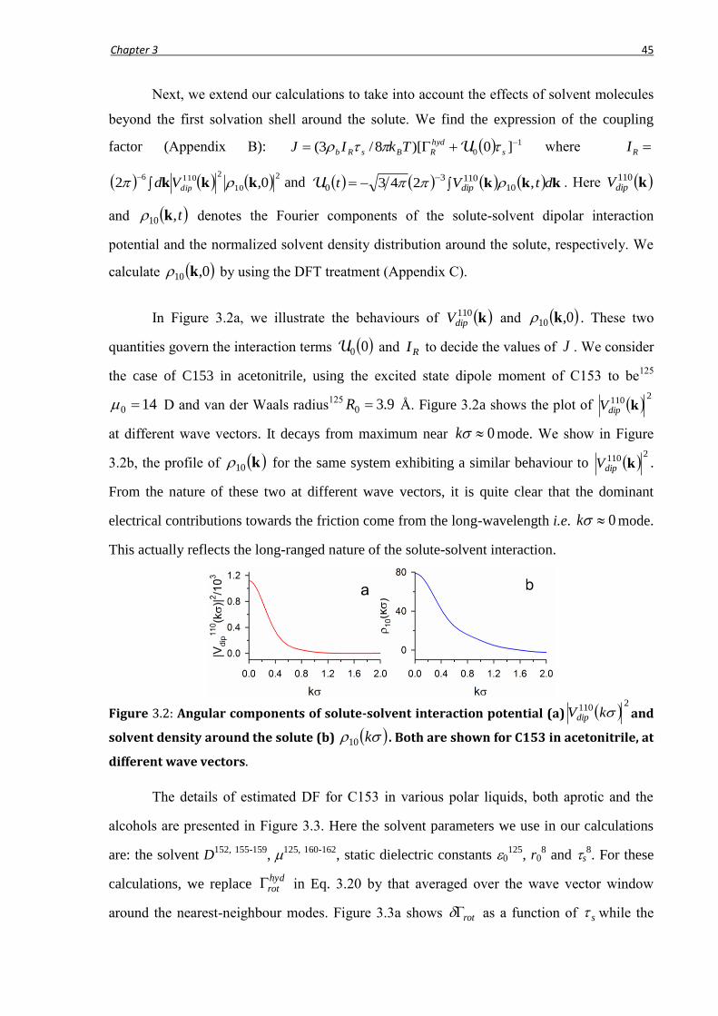
Chapter 3 45

Next, we extend our calculations to take into account the effects of solvent molecules

beyond the first solvation shell around the solute. We find the expression of the coupling

factor (Appendix B): 1

0 ]0)[8/3( s

hyd

RBsRb TkIJ U where RI

2

10

21106

0,2 kkk dipVd and

kkk dtVt dip ,243 101103

0 U . Here k110dipV

and t,10 k denotes the Fourier components of the solute-solvent dipolar interaction

potential and the normalized solvent density distribution around the solute, respectively. We

calculate 0,10 k by using the DFT treatment (Appendix C).

In Figure 3.2a, we illustrate the behaviours of k110dipV and 0,10 k . These two

quantities govern the interaction terms 00U and RI to decide the values of J . We consider

the case of C153 in acetonitrile, using the excited state dipole moment of C153 to be125

140 D and van der Waals radius

125 9.30 R Å. Figure 3.2a shows the plot of

2110

kdipV

at different wave vectors. It decays from maximum near 0k mode. We show in Figure

3.2b, the profile of k10 for the same system exhibiting a similar behaviour to 2

110kdipV .

From the nature of these two at different wave vectors, it is quite clear that the dominant

electrical contributions towards the friction come from the long-wavelength i.e. 0k mode.

This actually reflects the long-ranged nature of the solute-solvent interaction.

Figure 3.2: Angular components of solute-solvent interaction potential (a) 2

110 kVdip and

solvent density around the solute (b) k10 . Both are shown for C153 in acetonitrile, at

different wave vectors.

The details of estimated DF for C153 in various polar liquids, both aprotic and the

alcohols are presented in Figure 3.3. Here the solvent parameters we use in our calculations

are: the solvent D152, 155-159

, 125, 160-162, static dielectric constants 0

125, r0

8 and s

8. For these

calculations, we replace hydrot in Eq. 3.20 by that averaged over the wave vector window

around the nearest-neighbour modes. Figure 3.3a shows rot as a function of s while the

Chapter 3 46

hydrodynamic part hydrot is shown in Figure 3.3b. Note the difference in scales of the vertical

axes in these two panels. We find that for most of the aprotic solvents DF is nearly zero

barring the cases of DMSO and propylene carbonate (PC) both of which have dipole

moments larger than 4 D. The alcohols also exhibit comparatively larger DF. In Figure 3.3c

we show the ratio hydrotrot = J which turn out to be too small in all the cases to generate

any considerable dielectric contribution. J accounts for at most ~1-2% of the total friction,

even for solvents like the alcohols supporting observations of Horng et al8. A closer

inspection reveals that hydrot is always very large compared to the product sRI in the

numerator of J , rendering it small.

Figure 3.3: Friction data for common dipolar liquids. (a) rot and (b) hydrot and (c)

hydrotrot , all as functions of s for C153 in aprotic polar liquids and in alcohol solvents.

The solvation times have been taken from Horng et al8.

Figure 3.4: Experimental8 (circles) and calculated (triangles) R of C153 in aprotic polar

solvents and alcohols, as a function of experimental8 s. Colour codes same as Figure 3.3.

The best linear fit through the experimental points are shown by the dotted straight line.

3.2.3 Rotation times including DF

Let us now discuss the rotation times. We can rewrite Eq. 3.20 as

Chapter 3 47

JhydRR 1 . (3.21)

Figure 3.4 shows the experimental8 (circles) and calculated (triangles) R of C153 in the

polar liquids depicted in Figure 3.3, as a function of experimental s . From the data in Figure

3.4, it is clear that the calculated R agree reasonably well with the experimental values.

Further, Figure 3.4 indicates a linear dependence163-165

between R and s , shown by the best

fit line through the experimental data. Such behaviour can be rationalized by noting that in

general we have shydrot 00U , true for all the liquids we study here. Under these

circumstances, Eq. 3.21 can be approximated as

s

B

RbhydRR

Tk

I

248

3 , (3.22)

showing a linear dependence between R and s . Typically in dipolar solvents s is

proportional to solvent viscosity . So the linear dependence in Eq. 3.22 implies that R is

also proportional to which is observed in experiments. In most of the dipolar solvents, the

pre-factor of the term containing s is too small to contribute significantly to R . However,

if the pre-factor is large due to large solute-solvent coupling this additional dependence could

be observed.

3.2.4 Comparison with earlier theories

Our estimated values of DF are smaller in magnitude than those obtained from the

VZH theory. The differences between the VZH and our results are more significant for the

alcohol solvents. Interestingly, a common point of both the frameworks lies in the inclusion

of the solute-solvent interaction and s to determine the DF. In the VZH approach, the

solute-solvent interaction is incorporated in terms of experimentally observed fluorescence

stokes shift125

. It has been experimentally observed that C153 exhibits larger s in alcohol

solvents compared to the same in aprotic solvents of equivalent polarity, probably due to

solute-solvent specific interactions and/or solvent-solvent interactions. It is to be mentioned

here that computer simulation studies166

have indicated presence of such interactions, even

though effects of these interactions have not been reflected strongly in the solvatochromic

shift125

of C153 in protic polar solvents. Therefore, the VZH description, based directly on

the Stokes shift values and s , predicts larger friction for alcohols than aprotic solvents. In

the present theory, the solute-solvent interactions are considered using a microscopic model

Chapter 3 48

of the interactions where in principle the Stokes shift values can also be used. It is indeed true

that in common to the VZH approach the DF in the present theory is related to the s .

However, the difference here is that the dependence on s is non-linear and enters through a

self-consistent manner (Eq. 3.17). This non-linear dependence on s reduces the magnitude of

DF significantly compared to that predicted by the VZH approach. Even in the linearized

version (Eq. 3.22), the pre-factor of s for these solute-solvent systems is rather small.

Figure 3.5: Solute-solvent correlation for ionic solutes in dipolar solvent. 2

10 kcid as a

function of k , for ionic solutes in acetonitrile. The solute here is modelled as a hard

sphere with a unit positive charge embedded at the centre. We show the data for three

values of the solute radius with insignificant dependence for solutes larger than solvents.

Similar self-consistent treatment of DF, as in our calculation, done in the context of

ion-transport in a polar medium to obtain the DF137-142

shows substantial contribution of the

long-ranged forces. The solute-solvent long-ranged interaction in those cases is of ion-dipole

type, much stronger compared to the dipole-dipole interaction. Figure 3.5 shows the

longitudinal component of wave vector dependent direct correlation function142, 167

, kcid10

plotted for an ionic solute placed in acetonitrile. For a univalent cationic solute of size

comparable to C153, the value of 2

10 kcid is about 1000 times larger than 2

110 kVdip

(Figure 3.2a) at 0k . Since the principal electrical contribution to friction arises from the

0k mode, clearly the DF would be important for ion translation but not so significant for

solute rotation in a dipolar solvent.

3.3 Generalization for ionic media

Here we generalize the theory developed in the previous section for the ionic solvents,

namely the IL and the ES to compute the DF. We follow similar steps as in section 3.2: First

we consider the hydrodynamic contributions from k and then extend the equations 3.2.2

Chapter 3 49

for IL and ES. Finally, the rotation times are calculated and compared with the experimental

data.

3.3.1 Wave vector dependent viscosity and molecular hydrodynamic R

We present our analyses based on k for ILs and ES in this section.

(a) Ionic liquids

To calculate k for the ILs we need the structure factors. The total structure factor

kStot of an IL is obtained combining the partial structure factors168

, kSij :

ji

ijjitot kSxxkS,

where xi is the mole fraction of the ith ion (i, j = 1 (cation) and 2

(anion)). The experimental kStot of different ILs, measured via small angle x-ray

scattering experiments168, 169

, are different from the kS of normal liquids111

due to pre-

peaks at lower wave vectors ( 20 k ) apart from the packing driven 2k peak.

These pre-peaks have also been observed in several simulation studies170-173

and are believed

to be manifestations of long-range charge-ordering in ILs172

. The pre-peak intensities vary

with alkyl chain-length as shown by studies on ILs with [Imn1+] and [Prn1

+] cations (see

Tables for names168, 169

). For n<8 typically one pre-peak is present, whereas another pre-peak

appears only for n 8 and becomes stronger even than the other pre-peak for n=10.

We calculate k for three pyrollidinium ILs (n = 4, 6 and 10) using the

experimental168

kStot , for which the experimental viscosities and R are known23

.

Considering the similarities of the experimentally observed ionic partial structure factors168

,

radii23

and self-diffusivities144, 174

, we define an average molecular radius 2)( 210 rrr and

average self-diffusion coefficient 2)( 21 DDD for each IL, ir and iD denoting the

radius and self-diffusion coefficient of ith ion. Therefore, for an IL

kSDrTkk totB 04 . The viscosity contribution from the th peak in kStot is

calculated as25

, kk ddk integrating from

)( Lkk to )( Rkk , covering

the entire peak. For instance, in case of [Pr41+][Tf2N

], we set 1.5)1( Lk and 4.7)1( Rk for the

pre-peak, while 4.7)2( Lk and 0.11)2( Rk for the 2k peak.

The overall average viscosity is obtained as

c where

hhc / , the

combining weight factors and h , the height of the th peak. Table 3.1 shows that for the

Chapter 3 50

above three ILs agree reasonably well with their experimental viscosities. For n=4 and 6, we

find that the 2k peak contributions are dominating (>85% of the ), while it is the

major contributor (~50%) for n=10. These clearly show the dominance of the nearest-

neighbour peak over the pre-peaks which is not surprising, for the viscosity is determined by

the momentum transfer between the adjacent layers. The molecular hydrodynamic friction,

)(6 kVk p

hyd

rot , defines the wave vector dependent rate of rotational relaxation25

:

pB VkTkk ~ . The corresponding average rate is defined as25

:

kk ddkav )(~~ . The molecular hydrodynamic rotation time is then given by

TkV Bpav

hyd

R ~1 . The calculated hyd

R of C153 in these three ILs (Table 3.1) agree

well with the experimental data23

.

The dominance of the 2k peak contributions in calculated from the

experimental kStot indicates that the viscosity can be extracted from a model of the

2k peak in kStot . To this end, we theoretically calculate the kStot , using the

known Percus-Yevik form111

for short-ranged repulsive interactions and treating the long-

ranged electrostatic interactions at the mean-field level25, 26

(Appendix C) that is known to

capture the 2k peak111

reasonably well. We consider the ILs to be composed of hard

spheres with unit point charges at centres, a dipolar ion having an additional central point

dipole. Further, we assume only dipolar cations and choose ILs having no specific interaction

with C153. Table 3.1 shows that the and hyd

R values for the three pyrrolidinium ILs

discussed above, calculated from the 2k peak of the theoretical kStot (numbers in

parenthesis), agree well with the experimental data.

Next we consider the ILs for which no experimental kStot are available, focusing

only on the 2k peak. In Figure 3.6a, we illustrate the theoretical kSij and kStot

for [Im41][PF6

]. The calculated values of these dipolar ILs (Table 3.2) from the 2k

peak of kStot agree quite well with the experimental23

which justify our model

calculations. The hyd

R values (Table 3.2) too are quite close to the respective experimental R .

Chapter 3 51

Table 3.1: Viscosities and hyd

R of C153 in three N-methyl(N-alkyl)pyrrolidinium ([Prn1+])

ILs with anion bis(trifluoromethylsulfonyl)imide ([Tf2N]) at 298 K, whose experimental

structure factors are known.

Name of ILs (cP)

(calc.) (cP)

from k 2 peak

(cP)

(expt)

a hyd

R(ns) (calc.)

R(ns) (expt.)

Rb J

[Pr41+][Tf2N] 50 43(64)c 70 29(9) 3.0(3.8) 3.4 12(12) 0.0002

[Pr61+][Tf2N] 57 49(66) 93 39(29) 3.4(3.9) 5.7 40(32) 0.0031

[Pr10,1+][Tf2N]d 155 78(111) 145 7(23) 9.2(6.6) 9.0 2(27) -

a 100

exp

exp

t

t

b 100

exp

exp

t

R

hyd

R

t

R

R

.

c The results in the parenthesis are from the theoretically calculated structure factors. In addition, we use the dipole moments144, static dielectric constants175, ionic radii23 and self-diffusivities174, 176 of the ILs for calculations.

d In this case, the dipole moment of the cation is too high (~ 16 D)144 for the mean-field approximation to be valid.

Table 3.2: Viscosities and hyd

R of C153 in other ILs at 298 K.

Name of ILsa (cP)

(calc.)

(cP)

(expt)

hyd

R (ns)

(calc.)

R (ns)

(expt.)

R J

[Im41+][Tf2N] 33 41 20 2.0 2.6 23 0.0010

[Pr31+][Tf2N] 42 53 21 2.5 2.6 4 0.0002

[Im41+][BF4

] 52 75 31 3.1 4.3 28 0.0068

[Nip311+][Tf2N] 71 105 32 4.2 4.4 5 0.0002

[Nip411+][Tf2N] 99 130 24 5.9 7.9 25 0.0002

[Nip611+][Tf2N] 129 139 7 7.7 7.8 1 0.0021

[Im41+][PF6

] 149 187 20 8.9 12.0 26 0.0024

a The cation [Im41+] is 1-Butyl-3-methylimidazolium and [Nipn11

+] is (dimethyl)(isopropyl)(alkylammonium); the anion [BF4

] is tetrafluoroborate and ([PF6] is

hexafluorophosphate.

Chapter 3 52

Figure 3.6: The theoretical static structure factors. For (a) IL [Im41][PF6

] and (b) 0.5 M

LiNO3 in DMSO at 298 K. In both cases we show the total as well as partial structure

factors. In panel a, the range over which we carry out the integrations on total structure

factor for calculation of viscosities is marked by the quantities kL and kR. In panel b, such

integration ranges are marked, for the ionic components by kI and for the dipolar

component by kL and kR. In case of the electrolyte solutions the calculations are done

using the ionic radii116 r1, r2 and molecular radius8 r3, dipole moment125 and static

dielectric constant125 0 of DMSO.

(b) Electrolyte Solutions

Here we focus on the LiNO3-DMSO solution since a systematic experimental

investigation on rotation of a neutral dipolar solute C334 in this ES, is available13

. Moreover,

C334 does not show any solute-solvent specific interaction in this ES. However, no

experimental or simulated structure factor of this ES system is known. Therefore, we model

this ES as a ternary mixture177

of oppositely charged hard spheres representing the ions and

dipolar hard spheres representing the dipolar solvent to calculate the kSij (Appendix D).

Here also the long-ranged interactions are treated at the mean-field level. The ionic

components (Figure 3.6b) have only one significant mode around 0k with no structure

near 2k . This compressibility mode25

can be attributed to weak screening at low

concentrations (c ~ 0.1-1 M here) leading to a small inverse Debye screening length111

1~D . The dipolar component in Figure 3.6b is similar to the kS for normal liquids.

The cross-terms nearly vanish (Figure 3.6b) rendering only the self terms significant.

The partial viscosity i due to the ith component is defined as

σdσdkσ= ii kk / where kσSDπrTk=kσ iiiiBi 4/ . We fix ≡ 0k mode for

the ionic components ( 2 ,1i ) and ≡ 2k mode for the dipolar solvent ( 3i ).

Chapter 3 53

Integrating over the different ranges depicted in Figure 3.6b ( 0k to Ikk for 2 ,1i

and from Lkk to Rkk for 3i ), the average viscosity of the ES: i

iix where

ix is the mole fraction of the i th species. The calculated (Figure 3.7a) at several

concentrations agree quite well with the experimental viscosities13

. The hyd

R of a solute in an

ES can be obtained as: i

iavi

hyd

R x , where σddkωiiav kk /, , defined for the

i th species in solution. The agreement of the calculated hyd

R values of C334 to the

experimental13

R (Figure 3.7b) is also quite well. Both and deviate from the experimental

data at large c values which can be attributed to formation of of ion-pairs, triple-ions etc178

,

modifying the average solvent structure.

Figure 3.7: Viscosities and rotation times in ES. Comparison of (a) experimental and

calculated of solutions of LiNO3 in DMSO and (b) experimental R and calculated hyd

R of

C334 ( 252pV

Å3)13 in the solutions of LiNO3 in DMSO, both at 298 K. For these

calculations we calculate the concentration dependent ionic self-diffusivities iD using

Onsager equation179 with ionic conductivities at infinite dilution180 as inputs.

3.3.2 Electrostatic contribution to R in ionic media

According to section 3.2.2, the DF ( rot ) acting on a rotating dipolar solute can be

expressed as26

]0[8

3

0 s

hyd

rotB

sRbhyd

rot

hyd

rot

hyd

rotrotrotTk

IJ

U. (3.23)

The solute-solvent interaction has been treated here at the mean-field level replacing the

solute-solvent correlation simply by the interaction potential111

. Equation 3.23 clearly reveals

the non-linear coupling between DF and hyd

rot . In addition, rot possesses complex

dependence on s , showing an implicit connection to solvent dielectric response. This is

Chapter 3 54

important because nowhere in this theory we explicitly connect rot with solvent polarization

relaxation. 00U incorporates all the important medium-interactions in rot . The overall

rotation time is given by Eq. 3.21 in terms of J.

In order to use the above formalism (Eq. 3.21, 3.23), developed above for a dipolar

liquid, in case of IL and ES, we calculate 00U and RI for these media and determine J. For

dipolar solute rotation in an IL we find (see Appendix E),

kkkkkkIL

0 dtVdtVt sds ,,243 10

1

110

0

10

1

110

10

3U

kkk dtVs ,2 10

2

110

2 (3.24)

where 4/10 . k110

siV denotes the Fourier component of the interaction potential

between the solute and the ith ionic species; ti ,k10 , the normalized projection of the local

density of the ith species around the solute for spherical harmonics 1l and 0m ; and

k110

sdV , the Fourier component of the dipole-dipole part of the solute-IL interaction potential.

Similarly, for an ES (Appendix F)

k,kkk,kk2243 10

3

110

0

2,1

101103ES

0 dtnVdtnVt sd

i

isi U (3.25)

where the local ionic densities are denoted by ni (i=1 for cation and 2 for anion) and density

of the dipolar solvent by n3. Here k110

siV and k110

sdV correspond to solute-ion and solute-

dipolar solvent interactions respectively.

Figure 3.8: The wave vector dependent solvent density profiles around the solute. (a) IL

[Im41][PF6

] and (b) 1M LiNO3 in DMSO at 298 K.

We calculate the equilibrium solvent local densities using the classical DFT

(Appendix G). Figure 3.8 illustrates representative density profiles in IL and ES. The panel a

Chapter 3 55

shows the behaviour of the dipolar cation density 0,k10

1 for [Im41][PF6

] around C153

(solute radius R0 = 3.9 Å and excited state dipole moment 140 D)

125. In panel b we show

the cationic density profile 0,k10

1n for 1M LiNO3 in DMSO around C334 (R0 = 4.1 Å and

130 D)

13, 181.

We show the ratio J= hyd

rotrot for C153 in dipolar-ILs in Tables 3.1 and 3.2,

calculated using experimental23, 125

s , 0 and R0. J does not exceed 1%, suggesting complete

domination of hyd

rot . Due to unavailability of experimental s for C334 in LiNO3-DMSO, we

use the s (2.1 ns) observed21

for C334 in 1M NaClO4-DMSO solution with similar viscosity

(4.7 cP)21

to that of 1M LiNO3-DMSO (4.35 cP)13

. Here we find a very similar J ~ 1% as in

the ILs. The calculated R s of C153 in ILs (Figure 3.9) are within 1% of the corresponding

hyd

R . Both the calculated and experimental R depend linearly on s indicating a viscosity-

scaling of these average inverse rates, as observed for common dipolar solvents26

. In case of

ES, for C334 in 1M LiNO3-DMSO we calculate R =328 ps, ~1% larger than the

corresponding hyd

R =325 ps.

Figure 3.9: Rotation time data in ILs. The experimental (circles) R with error bars and

calculated (triangles) R of C153 in nine ionic liquids as functions of s . The dotted line

represents the best linear fit through the experimental data.

In dipolar liquids also we observe very small J (~1%) for dipolar solute rotation26

.

Here we find in IL and ES, even long-ranged solute-solvent electrostatic interactions fail to

generate appreciable DF. The reason can be demonstrated from Eq. 30. The criterion for

significant J is: hyd

rots 0IL

0U . Although in ILs we get ~10-100 times larger 0IL

0U than

its analogue 00U in dipolar liquids26

and much higher s than that in dipolar solvents, the

Chapter 3 56

product s0IL

0U (Figure 3.10a) is never comparable to hyd

rot (Figure 3.10b) which is also

very large (~1000 times of that in dipolar liquids) due to high medium viscosity. This

analysis also provides a microscopic explanation for the experimental observation that

dipolar solute rotation in ILs follow essentially the same dependence on the temperature-

reduced viscosity ( T ) as in the common dipolar solvents23

. For an ES at low electrolyte

concentration, the ion-ordering around the solute is smaller than that in an IL (Figure 3.8)

because of ion solvation by the dipolar medium. Consequently, 0ES

0U is quite small so that

even subsequent multiplication by a large s fails to make the product dominate over hyd

rot .

Consequently, the rot for a dipolar solute in an ES appears to be similar to that in a neat

dipolar medium but viscosity-scaled.

Figure 3.10: Components of friction in ILs. (a) The product TkBs0IL

0U and (b)

TkB

hyd

rot for C153 in nine ILs (marked in the figure by colours).

3.4 Quasi-universality of solute rotation in liquid solvents

The present calculations clearly show that the solute-solvent excluded volume and the

hydrodynamic viscosity are enough to understand the rotation of a spherical solute as the

long-ranged interactions get decoupled. This decoupling leads us to write, av

hyd

RR ~1 ,

where kk ddkav )(~~ . Using pB VkTkk ~ and

kDSrTkk B 04 one can write

avpR S=VDr 41/0 (3.26)

where kk ddkSSav . This integral will be dominated by the peak in kS .

Equation 3.26 relates experimental quantities to the microscopic solvent structure and thus

constitutes a macro-micro relationship. Note, a similar relation as Eq. 3.26 can be derived

from the SED expression: TkV BpR / and Stokes-Einstein relation111

for self-diffusion

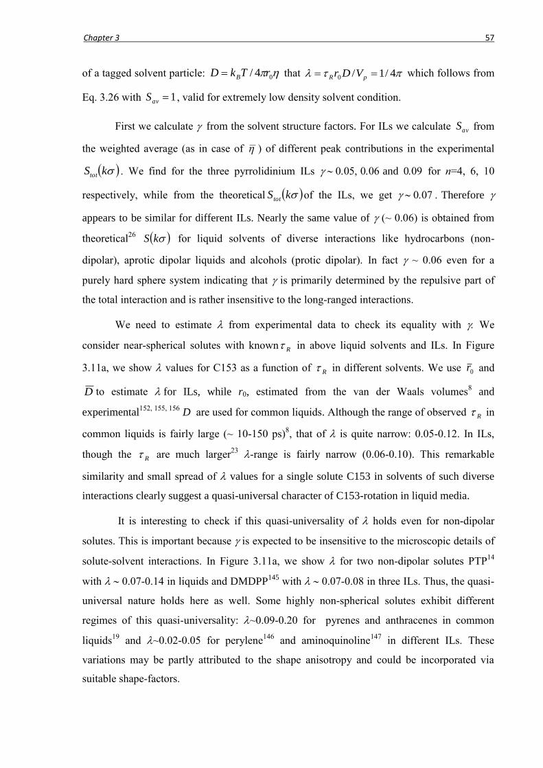
Chapter 3 57

of a tagged solvent particle: 04/ rTkD B that 4/1/0 pR VDr which follows from

Eq. 3.26 with 1avS , valid for extremely low density solvent condition.

First we calculate from the solvent structure factors. For ILs we calculate avS from

the weighted average (as in case of ) of different peak contributions in the experimental

kStot . We find for the three pyrrolidinium ILs and 0 for n=4, 6, 10

respectively, while from the theoretical kStot of the ILs, we get Therefore

appears to be similar for different ILs. Nearly the same value of (~ 0.06) is obtained from

theoretical26

kS for liquid solvents of diverse interactions like hydrocarbons (non-

dipolar), aprotic dipolar liquids and alcohols (protic dipolar). In fact ~ 0.06 even for a

purely hard sphere system indicating that is primarily determined by the repulsive part of

the total interaction and is rather insensitive to the long-ranged interactions.

We need to estimate from experimental data to check its equality with We

consider near-spherical solutes with known R in above liquid solvents and ILs. In Figure

3.11a, we show values for C153 as a function of R in different solvents. We use 0r and

D to estimate for ILs, while r0, estimated from the van der Waals volumes8 and

experimental152, 155, 156

D are used for common liquids. Although the range of observed R in

common liquids is fairly large (~ 10-150 ps)8, that of is quite narrow: 0.05-0.12. In ILs,

though the R are much larger23

-range is fairly narrow (0.06-0.10). This remarkable

similarity and small spread of values for a single solute C153 in solvents of such diverse

interactions clearly suggest a quasi-universal character of C153-rotation in liquid media.

It is interesting to check if this quasi-universality of holds even for non-dipolar

solutes. This is important because is expected to be insensitive to the microscopic details of

solute-solvent interactions. In Figure 3.11a, we show for two non-dipolar solutes PTP14

with 0.07-0.14 in liquids and DMDPP145

with 0.07-0.08 in three ILs. Thus, the quasi-

universal nature holds here as well. Some highly non-spherical solutes exhibit different

regimes of this quasi-universality: ~0.09-0.20 for pyrenes and anthracenes in common

liquids19

and ~0.02-0.05 for perylene146

and aminoquinoline147

in different ILs. These

variations may be partly attributed to the shape anisotropy and could be incorporated via

suitable shape-factors.

Chapter 3 58

Due to the difference in partial structure factors of different components in an ES one

needs to further generalize the calculations of and . Here Rτ is given by: i

iaviR xτ ,

where σddkωiiav kk /, , for the i th component in the medium. Using

piBi VkσTk=kσω / and kσSDπrTk=kσ iiiiBi 4/ we find

i

iiaviiipR SDrxV ,41 . (3.27)

which connects solute properties ( R and pV ) to the medium properties: structure factors and

self-diffusion coefficients. Figure 3.11b shows the values for C334, DMDPP and DPP12

,

in LiNO3-DMSO solutions at different concentrations c along with computed for the ES at

each c. As c increases from 0.1 to 1M, the observed R of all three solutes12, 13

increases, the

same trend being present in . Here again, at c < 1M agree quite well with , while the

agreement worsens at higher concentrations presumably for changes in average solvent

structure for the ion-pairs, triple-ions etc178

appearing at such concentrations.

Figure 3.11: Data on for various solute-solvent combinations. (a) vs. R plot for five

solutes: C153, PTP (p-terphenyl) and DMDPP (2,5-dimethyl-1,4-dioxo-3,6-

diphenylpyrrolo[3,4-c]pyrrole) in various liquid solvents: hydrocarbons (black), polar

aprotic (red), alcohols (green) and ionic liquids (blue). (b) Plot of for three solutes

C334, DMDPP and DPP (1,4-dioxo-3,6-diphenylpyrrolo[3,4-c]pyrrole) as a function of c in

solutions of LiNO3 in DMSO at 298K along with the values of for the solvent. Here and

defined by Eq. 3.27 are made dimensionless by multiplying both with 3D where 3D is

the self-diffusion coefficient of the dipolar solvent and , the average molecular diameter

of the components in ES.

Chapter 3 59

3.5 Conclusion

In conclusion, in this chapter, we have developed a microscopic theory that

systematically includes the effects of solute-solvent dipole-dipole interactions and solvent

structure on average rotation time of a polar solute in a polar solvent. We find that the

rotational relaxation of a dipolar solute in a polar medium is governed by the hydrodynamics,

having little dependence on the long-ranged solute-solvent interaction. We thus provide a

molecular basis for the SED model which has been obtained from purely hydrodynamic

consideration.

We generalize our theory for ionic liquids and electrolyte solutions to show that

decoupling of DF from solute rotation occurs even in ionic media via the non-linear

dependence of DF on hyd

rot and an overwhelming domination of hyd

rot . The fact that repulsive

part of the interaction largely determines the liquid structure makes solute rotation insensitive

to the mean-field effect generated via the solute-solvent long-ranged interactions. This

insensitivity leads to quasi-universality in solute rotation and thus provides a microscopic

explanation for the experimental observation that dipolar solute rotation in ILs and ES follow

the same correlation as established for common dipolar solvents. Note, the present theory

considers only the solute-solvent combinations with no specific interaction (such as H-

bonding). The effects of shape anisotropies of solute and solvent molecules or solution

inhomogeneity are also ignored. Despite these lacunae, the present analytical scheme

provides a resolution to the debate regarding the role of DF in solute rotation.

Finally, the approach described in this chapter can be extended to rotation of realistic

solutes in any solvent in general. One needs to this end, a proper description of the solvent

static structure factor and an appropriate solute-solvent interaction model. Generally, the

solute-solvent interaction can be expressed as: ',, RrV

coscos21

21

21

,,

m

l

m

lmll

mllYYV Rr . Inclusion of the higher harmonics (l1, l2 > 1) will take

care of the contributions from the finite charge distributions over the solute and the solvent

molecules systematically. Similar expressions can be written for the fluctuating solvent

density and the solvent-solvent static correlations. This kind of modelling would be very

similar to the extended charge distribution model134

considered earlier. Note that the coupling

parameter J depends on a competition between hydrot and the product s00U . The modified

treatment will affect the solute-solvent interaction strength 00U , resulting in very different

value of the DF. However, the calculation scheme will be numerically quite intensive, loosing

Chapter 3 60

analytical simplicity of the present one. The scenario could be simplified for an uncharged

multipolar solute in a non-dipolar solvent having only higher multipole moments. The solute-

solvent interaction term Rr mll

V 21 in such cases will fall off quite fast as a function of

Rr . In such cases, the rotational friction will be dominated by the packing of the solvent

around the solute.

Appendices

A. Equation of motion and orientational correlation function for solute rotation

The EOM for solute rotation can be written as

t

Urot

(3.28)

where t denotes the fluctuating torque arising out of all possible sources including short-

ranged and long-ranged forces and the terms non-linear in . Here5, 111 0t and

tTkt Brot 20 . Considering the initial equilibrium distribution of the solvent

around the rotating solute, we can write Eq. 3.28 in Fourier space:

0100 0ui rot , (3.29)

and subsequently

2

10002 0

2

rotrot

B

u

Tk

, (3.30)

which, upon inverse Fourier transformation, becomes

t

u

u

Tkt

rot

B 0exp

00 1000

1000

. (3.31)

Therefore, the normalized profile for orientational correlation function for solute

t

ut

rot

0exp

00

01000

(3.32)

Chapter 3 61

B. Calculation of the solute-solvent dipolar coupling factor J including

contributions from beyond the first solvation shell

Here we calculate the coupling factor after considering the solvent molecules in the

immediate neighbourhood and beyond. To this end, we write the average dipolar solute-

solvent interaction energy as

'cos,,',, ddtVU dip rrRr (3.33)

where ',, Rr dipV is space-dependent form of dipolar interaction potential between the

photo-excited solute dipole and a solvent dipole, with a separation Rr . t,, r denotes

the time dependent solvent density distribution. Here, r and R denote the position vectors

of the solvent molecule and the solute molecule, respectively. Now, ',, Rr dipV can be

written as25

'coscos',,3

0

Rr

Rr

dipV . (3.34)

One can expand ',, Rr dipV as a function of spherical harmonics182

coscos',,21

21

21

,,

ml

ml

mll

mlldipdip YYVV RrRr (3.35)

where

coscoscoscos',,21

21 ddYYVV ml

mldip

mlldip RrRr . (3.36)

As it turns out, Rr 110dipV is the leading component of ',, Rr dipV that couples with

t,10 r . Therefore, we obtain for the interaction energy

rrRr dtVU dip ,cos43 10110 (3.37)

using182

cos43cos01 Y . Setting, 0R , implying the solute being located at the

origin, we can write Eq. 3.37 in Fourier space using the Parseval‟s relation182

:

kkk dtVU dip ,cos243 101103

(3.38)

Eq. 3.38 can be rewritten as

cos0 tU U (3.39)

Chapter 3 62

where

kkk dtVt dip ,243 101103

0 U , (3.40)

the solute-solvent interaction strength, weighted by the solvent distribution. Therefore, the

torque on the rotating solute becomes

tttf 0U (3.41)

in small limit. The autocorrelation function of tf , under the decoupling approximation:

00,,24

31010

21106

ttVd

TIkt dip

B

b

k-kkk (3.42)

Here, for the solvent density modes we use stet

0,, 1010 kk . For the auto-correlation

of the angular variable, through analysis of the equation of motion (Appendix A), we get

t

t

t

rot

0exp

0

00U

(3.43)

where

kqk dVdip 0,2430 101103

0 U . Using this normalized profile in Eq. 3.42,

we arrive at

tBet (3.44)

where 2

10

21106

0,24

3kkk

dip

B

b VdTIk

B and

srot

100U

. Finally, we

calculate the memory function as described earlier, using Eq. 3.44 and derive the long-range

part of the rotational friction:

1

02

10

21106 10

0,28

3

srot

dip

B

brot Vd

Tk

Ukkk . (3.45)

This leads to the following expression of total friction

shydrotB

sRbhydrotrot

Tk

I

08

31

0U (3.46)

where 2

10

21106

0,2 kkk dipR VdI . Therefore, the modified dipolar coupling

parameter J becomes:

Chapter 3 63

shydrotB

sRb

Tk

IJ

08

3

0U (3.47)

C. Calculation of 10(k) for a dipolar liquid around the dipolar solute

To evaluate k10 we evaluate r10

using equilibrium DFT as described in

Appendix B of the previous chapter. The density functional free energy ', rF is given

by:

1

4

',rln',r'cosr ',r

b

ddF

4'',r4',r'',',rr''cos'cos rr 2

1bbCdddd

',0,Rr',r'cosr dipVdd (3.48)

where, '',', rr C is the two particle direct correlation function (DCF) between solvent

molecules at positions r and rhaving orientations ' and '' . Minimization of ', rF ,

with respect to the constraint for N solvent molecules

Ndd ','cos rr , (3.49)

yields 0','cos rrddF , being the Lagrange‟s multiplier. The

differentiations give

4'',r'',',rr''cosr

4

',rln b

b

Cdd

',RrdipV (3.50)

For small fluctuations: 14',44', bbb rr , Eq. 3.50 yields

4'',r'',',rr''cosr

4

',rb

b

Cdd

',RrdipV (3.51)

Multiplying both sides of Eq. 3.51 by cos01Y , integrating over cos we obtain using

Eq.2.18

Chapter 3 64

'',r'',',rrcoscos'cosr

4

r 0

1

010

CYddd

b

',Rrcos'cos 0

1 dipVYd (3.52)

Again, multiplying both sides of Eq. 3.52 by rk.ie , integrating over r and using the

convolution theorem182

'',k'',',kcoscos'cos

4

k 0

1

010

CYdd

b

',kcos'cos 0

1 dipVYd (3.53)

Here the surviving component of the Fourier mode of the DCF, '',', kC is given by

coscoscoscos,, 01

01

.110 dddYYerCC irk

rk . We can write within

mean-field approximation25

: rCrCrC LRPY ,, as in Appendix A of chapter 2.

rCLR is obtained by angle-averaging of coscos,, 32 rrC LR , denoting

the long-ranged part25

. Finally, we get from Eq. 3.53,

k - kk

k 1010

1100

010 24

dip

b

VC

(3.54)

where kk11010 3 dipdip VV . Rearrangement of Eq. 3.54 leads to

2110

10

1081

k

kk

C

V

b

dipb

(3.55)

D. Calculation of the Static structure factors

(i) Ionic liquid

We model an IL as a binary mixture of hard spheres (HS)183

, each with a charge

embedded at the centre. For a dipolar ion, there is an additional dipole at the centre of the HS.

The spatial direct correlation function111, 112

(SDCF) between the ith and jth ion (i=1 for

cation, 2 for anion) can be written as: rCrCrCLR

ij

PY

ijij , where rCPY

ij is the hard

core part given by the Percus-Yevick form for binary mixture of hard spheres183

and

jir rr . The long-ranged part rCLR

ij is treated at the mean-field level111

. For simple

Chapter 3 65

ions: rqqrC ji

LR

ij , the standard Coulombic form. For the dipolar ions with dipole

moment we write 642 92 rrqqrC ji

LR

ij , qi, the charge on the ith ion and

, the dielectric constant of the medium. Here the second term denotes the dipolar part

calculated as in Appendix A of chapter 2. For the ion-dipole interactions

23 rqrC i

LR

ij , the projections of standard ion-dipole interaction potential184

coscos)( 2rqrv iij between the ith ion with polar angle and jth dipolar ion

with orientation (both in the laboratory frame) for spherical harmonics 11 l , 12 l and

0m . From rCij we calculate kCij and hence kSij , the partial structure factors

using the OZ relation2,3

. The total static structure factor is then obtained as:

ji

ijjitot kSxxkS,

where xi is the mole fraction of the ith ion.

(ii) Electrolyte solution

We model the solution of a 1:1 electrolyte to be a ternary mixture, the components

being the cations, the anions and the dipolar solvent molecules. The mole-fractions of the

ions are the same to maintain electro-neutrality. We label the components in the following

fashion: the cations as 1, the anions as 2 and the dipoles as 3. For salt concentrations 0.1M to

1M, the ionic mole-fractions turn out to be ~0.001-0.01. As a result, the hard core

contributions are negligible to ionic SDCFs rCij 2,1, ji , owing to very small packing

fraction p. Here we use the hypernetted chain closure by Attard et al185

to calculate the ionic

SDCFs, via solving the OZ relation. We use the asymptotic form185

of total correlation

function reqqrh r

jiij . Here, 2132

621

DDD , the modified

screening length in terms of the inverse Debye screening length111

21

24

i

iiD qc

where is the average molecular diameter of the components in ES and ci, the concentration

of the ith ion. The SDCFs for ion-dipole 3,1, ji and the dipole-dipole interactions

3, ji are calculated as described in previous section. The hard sphere part rC HSij are

adopted from the work by Hoshino et al177

on structure factors for a ternary mixture of hard

spheres. kSij s are calculated using the method for ternary mixtures described in Hoshino

et al177

.

Chapter 3 66

E. Calculation of dielectric friction

(i) Ionic liquid

For an IL made of dipolar cation (i=1) and simple anion (i=2), the average solute-

solvent interaction energy can be written, via an extension of Eq.3.37, as,

rrRrrrRr dtVdtVU sds ,,cos43 10

1

110

0

10

1

110

10

rrRr dtVs ,2 10

2

110

2 (3.56)

where Rr 110

siV denotes the leading component of the interaction potential between the

dipolar solute and the ith ionic species in the medium; and Rr 110

sdV , the same between

dipolar solute and a dipolar ion. Setting, 0R , we can write Eq. 3.56 in Fourier space:

kkkkkk dtVdtVU sds ,,cos243 10

1

110

0

10

1

110

10

3

kkk dtVs ,2 10

2

110

2 (3.57)

Eq. 3.57 can be expressed as

costU IL

0U (3.58)

where

kkkkkkIL dtVdtVt sds ,,243 10

1

110

0

10

1

110

10

3

0 U,

kkk dtVs ,2 10

2

110

2 (3.59)

the time dependent solute-solvent interaction strength, weighted by the solvent distribution.

Therefore, the torque on the rotating solute given by Utf becomes

tttf IL

0U (3.60)

in small limit. The autocorrelation function of tf , under the decoupling approximation:

TkI

ttt

B

00IL

0

IL

0

UU (3.61)

where I denotes the moment of inertia of the rotating body about the axis of rotation. We

now calculate 0IL

0

IL

0 UU t and 0 t separately. We write

Chapter 3 67

6IL

0

IL

0 )2( 4

30

TkIt

B

bUU

tVtVtVd ssds ,kk2,kk,kkk 10

2

110

2

10

1

110

0

10

1

110

10

kkkkkkk tVtVtVd ssds ,2,, 10

2

110

2

10

1

110

0

10

1

110

10 (3.62)

Here, for the solvent density modes we use st

ii et

0,, 1010kk to get

st

B

Rb eTkI

It

/IL

0

IL

0 4

30

UU (3.63)

where IR contains all the self- and cross-terms in Eq. 3.62 resulting from the multiplication.

Using the EOM (Eq.3.28) we arrive at

t

t

rot

0exp

00

0 IL

0U

(3.64)

The rest of the treatment is similar to that for the dipolar liquids26

once all the

multicomponent contributions are accounted for in IR. We get the DF

1

0 10

8

3

srotB

Rb

rotTk

I

ILU (3.65)

Eq. 3.65 portrays the self-consistency for rot as rothydrotrot . Solution of Eq. 3.65

leads to the following expression of total friction

1

IL

0 08

31

s

hyd

rotB

sRbhyd

rotrotTk

I

U (3.66)

We find that 1

0 ]0)[8/3( s

hyd

RBsRb TkIJ ILU << 1 for all the ILs and hence we can

linearize Eq. 3.66 to write

Jhyd

rotrot 1 . (3.67)

Hence, hyd

rot

hyd

rotrotrot J .

(ii) Electrolyte solution

In this case, we have three components: cation, anion and the dipolar liquid.

Therefore, the average solute-solvent interaction energy is given in Fourier space by

Chapter 3 68

kkkkkk dtnVdtnVU ss ,2,2cos243 10

2

110

2

10

1

110

1

3

kkk dtnVsd ,10

3

110

0 (3.68)

Here k110

siV and k110

sdV denote the Fourier components of the dipole-ion part and dipole-

dipole part of the solute-solvent interactions, respectively. Note, here we use ni instead of i

to denote the densities of the components. Equation 3.68 can readily be written as

cosES

0 tU U (3.69)

where

kkkkkk

ES dtnVdtnVt sd

i

isi ,,2243 10

3

110

0

2,1

101103

0 U (3.70)

The rest of the calculation is similar to that for IL to arrive at the same expression of DF as

Eq. 3.65 where the quantities that would be different are tES

0U and IR.

E. Calculation of equilibrium solvent density profiles around solute

(i) Ionic liquid

We get r10

i from DFT treatment similar as Appendix B. The free energy

', riF , is given by

1ln'cos1

4

',ln','cos', 2

21

1

bb

i ddddF

r,r,r

rrr r

',','',',''cos'cos2

11111

rrrr rr ddCdddd

iji

ji

ii

ijCdddd,

',','',',''cos'cos2

1 rrrr rr

',','',',''cos'cos2

11111

rrrr rr diCdddd

',','',',''cos'cos2

12112

rrrr rr diCdddd

Rrrr ',0,','cos 11 sVdd Rrrr ',0,','cos 22 sVdd

Rrrr ',0,','cos 1 sdVdd (3.71)

Chapter 3 69

where 4',', 11 b rr and b ',', 22 rr , the superscripts

denoting the solvent-solvent interaction types: d-d (dipole-dipole), i-i (ion-ion) and i-d (ion-

dipole). Note, for i=2, the polar angle =0 since it has no dipole where r10

i is defined by

the polar angle associated with the radius vector. Minimization of ', riF , with respect

to the constraints

ii Ndd ','cos rr , (3.72)

where Ni is the number of ith ion type in medium (N1=N2 for electroneutrality) yields two

separate equations for two species. For the dipolar cation:

0','cos 1111 rrddF , (3.73)

1 being the Lagrange‟s multiplier for species 1, which in limit 14', br yields

','',',''cos

4

',

4

',ln 111

11

rrrrrr dd

bb

Cdd

','',',''cos2

1','',',''cos 212111

rrrrrrrriiii CddCdd

','',',''cos2

1','',',''cos 212111

rrrrrrrrdidi CddCdd

11 ',0,',0, Rr Rr sds VV . (3.74)

Using the definitions in Eq. 2.18 for r10 and Eq. 3.36 for Rr 110C in Eq. 3.74 we

obtain:

rrrrrrrrr

10

1

110,

11

10

1

110,

11

10

1 433

2 didd

b CdCd

Rr Rrrrrr 1010

1

10

2

110,

122

1sds

di VVCd (3.75)

Next, in a similar fashion from Eq. 3.71 and 3.72 we can write for the anion

0','cos 2222 rrddF , (3.76)

2 being the Lagrange‟s multiplier for the anionic species. Equation 3.76 gives us, through

the same analysis as described above for the cation that

Chapter 3 70

Rrrrrrr 10

2

10

1

110,

12

10

22

143

3

2s

di

b VCd (3.77)

Now, Eq. 3.75 and 3.77 are self-consistent equations for r10

1 and r10

2 respectively

which are solved iteratively using the appropriate DCFs. Finally, Fourier transform gives the

k10

i s.

(ii) Electrolyte solution

For an ES, we can write down the free energy functional as

14/

ln'cos1',

ln','cos',3

3

3

2,1

bi

b

i

i

iin

nndd

n

nnddnF

r,r,r

rrr r

)(2,1,

',','',',''cos'cos2

1

ijji

ji

ii

ij nnCdddd rrrr rr

',','',',''cos'cos2

13333

rrrr rr nnCdddd dd

2,1

33 ',','',',''cos'cos2

1

i

i

di

i nnCdddd rrrr rr

Rrrr

2,1

',0,','cosi

sii Vndd

Rrrr ',0,','cos 3 sdVndd (3.78)

where b

iii nnn ',', rr for the ions (i=1,2) and 4',', 333

bnnn rr for

the dipolar solvent with b

in being the bulk density for the ith species. The minimization

conditions:

ii Ndd ','cos rr , for the ions where N1=N2 (3.79)

and, dNndd ','cos 3 rr for the dipolar solvent (3.80)

Minimization of free energy with respect to the constraints in Eq. 3.79 and 3.80 gives:

0','cos rr iiii nddnnF , for i = 1, 2, 3 (3.81)

i being the Lagrange‟s multiplier for ith species. Rest of the treatment is very similar to the

IL case. We finally arrive at the following self-consistent expressions for the local densities:

Chapter 3 71

Rrrrrrr 1010

3

110,

3

10

2

143

3

2si

di

i

b

ii VnCdnn for i = 1, 2 (3.82)

and

2,1

10110,

3

10

3

110,

333

10

32

143

3

2

i

i

di

i

ddb nCdnCdnn rrrrrrrrr

Rr 10

sdV (3.83)

Using DCFs obtained in Appendix C-(ii), we solve Eq. 3.82 and 3.83 in iterative manner to

obtain the spatial r10

in and the Fourier components k10

in . Here we have used an average

molecular diameter for all the components for simplicity.

Chapter 4 72

Chapter 4 Solvation dynamics in fluids under nano-meter scale confinement

4.1 Introduction

Recently fluids in nanometer (nm) scale confinements have drawn considerable

attention as important media in various branches of science and technology37, 38, 40-43

. Several

experiments focus on the dimensional crossover from 3D to 2D behaviour, observed when a

fluid is kept under a confinement of about a nm. In an enclosed environment many static and

dynamic properties of the fluid alter dramatically44

compared to the bulk, like self-diffusion,

refractive index, mechanical relaxation and so on. Such changes lead to confinement-induced

effects on physical and chemical processes in fluid phase.

Confined water has been quite extensively studied in the recent past: Surface force

measurements show that water molecules confined to a film of three to four molecular

diameters (~ a nm) thickness, undergo ordering similar to a solid47

. The mechanical

relaxation timescale, for dissipating the stress against an external strain, becomes almost an

order of magnitude larger47

compared to the corresponding bulk value under a confinement

less than a nm. The melting temperature of water drops significantly when confined in silica

nano-pores of diameter ~ 3 nm as revealed by Raman scattering measurements186

. Water

confined in reverse micelles (RM) of diameter ~ nm has a static dielectric constant (0) 3-4

times lower187

than the bulk value (~ 80)35

. Sudden jumps in the viscosity and diffusion

coefficient D have been observed33

in case of linear alkanes and alcohols in organosilicate

nano-pores of diameter less than 2 nm. Measurements of refractive index (n) and the

equilibrium film-thickness of cyclohexane confined within two mica plates have shown a

sudden transition from a 3D bulk fluid to a 2D adsorbate for plate separation around couple

of nm. This transition is accompanied with significant enhancement in fluctuations of n,

changes in phase-transition temperatures and normalized enthalpies, lowering of critical

temperature and anomalous fast self diffusion46

. However, the changes in fluid properties

under confinement depend on the nature of the confining potential. Li et al48

have studied

water in sub-nanometer confinements where the viscosity increases substantially in a

hydrophilic environment but having not so much effect in a hydrophobic confinement. There

have been a number of theoretical studies on confinement induced effects. Schoen and co-

workers188

have reported on extensive grand-canonical Monte-Carlo (GCMC) simulation123

to calculate static properties of confined fluid and shows their sensitivity to the wall structure.

A weighted density functional theory of a 2D fluid has also been derived189

as a limiting case

Chapter 4 73

of the corresponding functional for an inhomogeneous 3D fluid within linearized

approximation. The 3D to 2D crossover under confinement has been studied extensively near

the critical point190-192

. However, the question how the confinement-induced crossover takes

place in various fluid properties, even far from critical point, has remained largely

unaddressed.

The rates of various non-equilibrium processes are also highly affected in confined

media. Solvation is one such process which governs nearly all chemical reactions in fluid-

phase45, 50

. Any stabilizing interaction leading to the organization of the solvent molecules

around a solute is conventionally termed as solvation. Therefore, study of solvation dynamics

(SD) under confinement is extremely important for understanding chemical reactions in

confined media, ranging from catalysis in nanopores37

to charge-transfer in biomolecules193

.

Conventionally, SD is studied via monitoring the relaxation of solvent distribution

around the solute after a perturbation of the solute-solvent interaction30, 45, 53, 194

from an

existing equilibrium solvated state. The solvent response to the perturbation is given by124

)(tS )()0(

)()(

UU

UtU. (4.1)

Here

)(tU)]0()(),()([3 tUtUrd unpertpert r,RrrRr . (4.2)

where )( Rr unpertU and )( Rr pertU are the interaction potentials between the solute at

position R and a solvent molecule at position r before and after the perturbation. ),( tr is

the time-dependent local solvent density124

around the solute particle. Eq. 4.2 can be rewritten

as:

)(tU = )]0(),()[({3 ttUrd pert r,rRr

)}0()]()([ tUU pertunpert r,RrRr . (4.3)

Simple hydrodynamic results111

show that the Fourier components of )]0(),([ tt r,r

decay as ]exp[ 2tDk for wave vector k. Consequently, the solvent relaxation represented by

)(tS shows typical exponential dependence124

, ]/exp[ t , being the solvation timescale,

governed primarily by D. Since D is dramatically altered in confinement, SD also is affected

by confinement. Several studies exist on SD of fluorescent dyes in confined fluids. The

confining frameworks have been diverse30, 45, 195, 196

, for instance, solvophilic lipid vesicles

Chapter 4 74

and RM194

; and solvophobic carbon nanotubes37

, sol-gel glasses197

and silica nano-pores52

. In

a bulk fluid is generally tens of ps45

, whereas in solvophilic nanoconfinements30, 45

, may

extend from hundreds of ps to even ns. For instance, the longest timescale for a dye coumarin

480 turns out to be about 10 ns in spherical water-pools of aqueous AOT (dioctyl sodium

sulfosuccinate) RMs (solvophilic) of 1-10 nm diameter198

, in sharp contrast to a sub-ps

solvation timescale observed for the same dye in bulk water199

. The solvation time for

coumarin dyes increase typically by factor of 2 to 3 in solvophobic nanopores196, 200

. Recent

computer simulations51-53

also show such slowing of the SD in various confined systems

compared to the bulk. Although these studies bring out various aspects of solvation in

confinement in details, there is, as yet, no general understanding of how the confinement-

induced changes in solvent properties bring about the slowing down of SD under

confinement.

The effects of confinement become severe when the thermodynamic condition of the

surrounding bulk fluid falls in the sub-critical region of the phase diagram (Figure 1.2). It is

well known that presence of any surface drastically alters the phase behaviour of a sub-

critical fluid62

. If a solvophobic surface is placed in a bulk sub-critical liquid, close to the

liquid-gas phase coexistence, it stabilizes the coexisting low density gas-phase in vicinity of

the surface. This surface-mediated evaporation in a solvophobic pore is commonly known as

capillary drying61

. The diffusion of the fluid molecules becomes much faster in a dried

solvophobic pore compared to the surrounding bulk liquid. On the other hand, a solvophilic

surface, placed in the bulk gas, induces the high density coexisting liquid phase near the

surface. This surface-mediated wetting inside a pore is called the capillary condensation68

which slows down the fluid diffusion. The typical interfacial width between the gas and the

liquid phases induced by surfaces near the bulk phase-coexistence extends to several nms201,

202 that becomes comparable to the size of the nanoconfinement. If a solvophilic solute

particle is inserted in a dried solvophobic nanoscale pore, the solute tends to wet the pore,

posing a competition62, 203, 204

with the wall-mediated drying. This competition decides the

fluid diffusion in the pore which in turn affects the SD. Therefore, the studies on how the SD

responds to this competition would throw light on surface-induced effects on various physical

and chemical processes in a sub-critical nanoconfined solvent. Despite many applications56-58

of the sub-critical liquids and several studies on capillary drying and condensation

phenomena55, 59-63

, there have not been many attempts to elucidate the roles of sub-critical

solvents in solvation process. Recent MD simulations64

on SD in a bulk Stockmayer fluid

show that the density of the sub-critical fluid phase controls the solvation behaviour. Thus,

Chapter 4 75

SD under confinement near bulk phase-coexistence has remained largely unexplored to the

best of our knowledge.

In this chapter we study the three different aspects of nanoconfined fluids. First we

study, using computer simulations, the dimensional crossover in fluids under nanoscale

confinements where the surrounding bulk fluid is far away from any phase transition point.

The wave vector (k) dependent fluctuations in density govern majority of properties of a fluid

including static quantities like 0 and n††

, as well as long-time dynamic quantities like , D

and so forth111

. Hence, the crossover in all such properties should be generically related to

that in density fluctuations. We calculate65

the fluctuation in number of particles N in a slit of

parallel walls with a fixed volume V at absolute temperature T at the same chemical potential

as in the bulk shown schematically in Figure 4.1. The fluctuation is defined as:

NNN 2)( , (4.4)

the angular brackets representing ensemble averages generated by GCMC simulations123, 205

.

The generality of experimentally observed crossover, independent of system specific

details, leads us to consider a model LJ fluid with model wall-fluid potential to capture

qualitatively the generic effect of confinement. We show65

that undergoes a crossover from

3D to 2D behaviour without any accompanying phase-transition below a confinement

extending only a few molecular diameters, measuring about a nm, the same length scale of

crossover observed in the experiments. The crossover in can be understood from the

suppression of the density fluctuations in the system in direction perpendicular to the slit,

beyond the wavelength given by the length scale of the confinement. The dynamic density

fluctuations, given in terms of the Van Hove correlation function (VHCF), computed from

MD simulations with initial conditions chosen from the GCMC configurations, also exhibit65

similar crossover in the in-plane diffusivity D||. However, the crossover is dependent on the

confining potential: 3D to 2D crossover in and D|| for a fluid in solvophobic slit is

significantly different from that in solvophilic pore due to strong layering of the fluid-

particles near the wall by large wall attraction in the later case. We relate our observations to

experimental observations on different fluid properties dependent on density fluctuations.

††

For instance, 0 of a dipolar fluid is related to the long-wavelength limit of the dipole moment

density M(k) of the system = Ltk0 Mk M-k / NkBT. Now, M(k) (k)

which connects 0 with the long-wavelength limit of density fluctuation. The refractive index n is also related to density fluctuations.

Chapter 4 76

Next we consider SD of a spherical non-polar solute in the confined LJ fluid.

Although SD in general gets slower under confinement30, 45

there is a caveat in the existing

interpretation of the data. The surrounding equilibrium bulk-phases have not been clearly

specified in all these cases. This leads us to consider the SD when the bulk is well-specified.

Moreover, we observe that ||D suddenly exceeds the bulk-value in strong solvophobic

confinement, while ||D becomes very small compared to bulk under strong solvophilic

confinements65

. This prompts us to examine any subtle interplay between the heterogeneous

solvent distribution and ||D leading to slowing down of SD in confined geometry,

irrespective of the nature of the confining potential. The choice of a non-polar system to

study SD is not so restrictive, for the long-time SD is primarily governed by non-polar

interactions in the system124

. The model system also offers a scope to single out the effects of

confinement avoiding the various complicating factors of realistic systems. At a phase point,

far away from any phase transition, we show66

that two fundamentally different aspects of the

dimensional crossover are responsible for the confinement-induced slowing down of SD in

presence of two kinds of walls. The confined geometry reduces the solvent relaxation due to

restricted dynamics which alone slows down the SD. The reduced dimension of solvent

dynamics adds up to slower ||D in a solvophilic confinement to result in a sharp increase in

solvation timescale. On the other hand, slowing down of the dynamics due to reduced

dimensionality competes with the faster diffusion in a solvophobic slit, resulting in marginal

slowing down in solvation time.

Another phase point is taken67

at a sub-critical temperature where the fluid is confined

in a solvophobic slit in equilibrium with the bulk sub-critical liquid, close to liquid-gas phase

coexistence. Here SD in confinement becomes faster compared to the bulk liquid, but not

driven by the gas-like diffusion in the dried solvophobic pore. This can be explained as an

outcome of the competition between the wall-induced evaporation effect trying to make

diffusion faster and condensation in the pore due the solvophilic solute increasing the density

creating an opposite effect. SD slows down linearly as the slit separation increases. Finally,

we discuss the implications of our results in the light of confinement effects on various

chemical processes in confined geometry.

The rest of the chapter is organized as follows: In section 4.2 we consider the

dimensional crossover in nanoscale confinements. Section 4.3 includes the studies on SD

under confinement. Then we conclude in section 4.4.

Chapter 4 77

Figure 4.1: System details and phase diagram. (a) Schematic diagram of the simulated slit

placed in bulk fluid. (b) *(=) vs. * plots for bulk fluid at T*=2.0. The working phase-

point is point ‘A’ (*=0.4, *=0.67).

4.2 Dimensional crossover

In this section, we first present the details of the simulations. Then we discuss the

structure of the confined fluids in terms of density profiles and in-plane radial distribution

functions. Next, we consider the crossover behaviour of in different type of slits which is

followed by the results of crossover in ||D .

4.2.1 Simulation details

For the studies on dimensional crossover, the model fluid is taken in a rectangular

simulation box with two parallel plates placed at a separation H on the z -axis at z = -H/2 and

z = H/2 (Figure 4.1a), with fixed box lengths along x and y axes (Lx = Ly = 20, being the

particle diameter). Here, the periodic boundary condition is applied along x and y directions

only. We consider a truncated LJ potential with a cut-off radius Lx/2 as the interparticle

interaction: 612 )()(4)( rrruLJ , being the interaction strength and r, the

interparticle separation. Due to large cut-off we have not added any corrections due to

truncation. The confining potential type is varied: hard walls only reflecting the colliding

particles; repulsive walls with wall-fluid interaction for a particle at z :

10)2/(4)2/( HzHzu fw and attractive walls: )2/( Hzu fw

39 )2/()2/(4 HzHz where 10 .

We calculate the fluid density profiles in the direction normal to the slits (z-axis)

given by (z)* N(z)3/AΔz where N(z) is the number of particles in a particular fluid-

segment of width Δz located at z and A, the area of the x-y plane. We calculate the radial

a

Chapter 4 78

distributions functions (RDF) 111

, describing the probability of finding two particles at a given

separation. The in-plane 2D RDF188

is defined as nzrrrNrg lD )(2/)()( 2|||||||| for a layer

at z of width z () with n particles where 22|| yxr , layer-density Anzl

D /)(2 .

For a wider layer (z), we compute the 3D nrrrNrg lD3

24/)()( where

222 zyxr , layer-density zAnlD /3 .

In the MD simulations, we adopt NVE ensemble (constant N, volume V and total

energy E) using the Verlet algorithm123

to integrate the equations of motion with time-step

0.005 LJ units (0 = (m2/ ~ 2.8 10

-12 s for Argon where m is the mass of Argon

atom)111

. We calculate T from fluctuations of kinetic energy and by inserting test

particles123

. The mean values of the T and in MD runs agree to those of the GCMC

simulations. Furthermore, these quantities remain similar also for different initial conditions

chosen from equilibrated GCMC configurations. The self part of in-plane VHCF206

are

computed:

i

ii

s tNtrG ))()0(()/1(),( |||||||| rrr , (4.5)

where ||r is the space variable parallel to the walls (along x-y plane) and )(|| tir , the position of

the ith particle along x-y plane at time t. In the long-time limit, the VHCF is Gaussian:

]4/exp[)4/1(),( ||2

|||||| tDrtDtrGs .

4.2.2 Characterization of fluid structure under confinement

Figure 4.1b shows the - diagram obtained from GCMC simulations for the bulk

fluid in absence of any solute. The diagram confirms that there is no phase transition207

at LJ

temperature T*(= TkB )=2.0 where the point „A‟, with chemical potential123

)(* TkB

= 0.4, represent the phase point of our interest for dimensional crossover. The behaviour of

(z)* is shown in Figure 4.2 for different wall types which exhibit layering similar to those in

earlier studies48, 188, 189

. We characterize the structure of different layers from the RDFs.

Structurally, the wall-adjacent layers for any type of wall assume 2D behaviour as suggested

by g(r||), shown in Figure 4.3a. For reflecting walls, at H = 4, the central region is a fluid-

segment of one diameter width, the corresponding g(r||) revealing 2D structure (Figure 4.3b).

For H > 4, central region of uniform density appears which gets extended as confinement is

relaxed. We calculate the 3D g(r) in that region, for instance, 3z in Figure 4.2c and 6z

Chapter 4 79

in Figure 4.2e. Unlike the bulk 3D g(r), the g(r) for the central region drops off to small

values at large r till H = 10 (Figure 4.3c), characterizing a finite spatial extent

(perpendicular to the wall). At sufficiently large H (H 12), the central region approaches

the 3D limit with proper asymptotic behaviour, g(r) ~ 1 for large r. These features of the

central region are qualitatively same for the other wall types as well. The well-formed central

region resembles the bulk-like inner-core of water inside large reverse micelles194

. The other

layers formed in between the central region and the wall-adjacent layers behave quite

similarly as a 2D fluid.

Figure 4.2: Density profile in the slits: (z)* in reflecting (solid), repulsive (dotted) and

attractive (dashed) slits for different H: (a), (b) 4, (c), (d) 10 and (e), (f) 20. Dash-dot

lines mark the bulk density. Profiles shown here are for the half-slit width along z and

they are symmetric about z axis.

Figure 4.3: Structure of fluid in confinement. (a) g(r||) for wall-adjacent layers at H = 10

for reflecting (solid), repulsive (dashed), attractive (dash-dot) slits and the pure 2D case

(dotted). g(r)s for the central region in a reflecting slit at (b) H = 4, along with pure 2D

g(r||) (dotted), (c) H = 8 (dotted), 10 (dashed), 12dash-dotdash-dot-dotand

20dash-dash-dashhe solid line represents the bulk 3D g(r).

Chapter 4 80

4.2.3 Crossover in equilibrium density fluctuations: Reflecting and repulsive walls

The bulk 3D and 2D limits of shown in Figure 4.4a are evaluated from the bulk

simulations of a 3D fluid and 2D disks respectively at the same and T. Figure 4.4a shows

as a function of H for reflecting and repulsive walls. exhibits a clear 3D to 2D crossover in

case of reflecting walls: A steep rise in takes place around a critical separation 4cH

where the structural crossover takes place in the central region as well. Similar crossover is

observed for the repulsive walls also. The intimate connection of crossover in and the

structural changes at the central region is illustrated by Figure 4.4b, showing the behaviour of

calculated over the central regions. The striking similarity of these plots with those in

Figure 4.4a confirms that the central fluid layer holds the key to this crossover. The constant

volume specific heat123, 205

CV as a function of H are featureless for both kind of walls (Figure

4.4c), ruling out any thermodynamic phase-transition associated with the crossover. This

crossover in qualitatively matches the sudden increase in fluctuations in refractive index of

cyclohexane confined between solvophobic mica plates with separation just below 2 nm (~

Hc), measured from surface force experiments46

. Thus, Hc matches with the length scale at

which the jumps in , 0, , D and n are observed in experiments33, 35, 46, 47

.

Figure 4.4: Different quantities in slits as functions of H: (a) , reflecting (triangles:

simulation; dotted line: theory) and repulsive (circles: simulation; dashed line: theory);

(b) in the central region, reflecting (triangles) and repulsive (circles). (c) CV, reflecting

(triangles) and repulsive (circles).

The crossover in around Hc can be made more explicit within a simple theoretical

treatment focusing on the long-wavelength cut-off due to the confinement. is given by the

long-wavelength ( 0k ) limit of the static structure factor S(k) in bulk111

. S(k) can be

calculated from the liquid direct correlation function c(r) via the OZ relation111

. Within mean-

Chapter 4 81

field approximations for LJ fluids, the c(r) is split into correlations due to the short-ranged

hard core, given by the Percus-Yevick form111

CPY

(r) for r< and an attractive tail, CLR

(r) =

4(k(/r)6 for r. In a slit geometry, we integrate over ||r in c(r) to yield c(z). We

compute zkS , zk being the transverse component of wave vector, using the OZ relation:

1)](1[ zz kckS where is the average fluid density in the slit obtained from GCMC

simulations. We ignore the density inhomogeneity near the walls which is a good

approximation here, since the homogeneous central region, showing the crossover,

encompasses majority of the slit. The spatial integration for the Fourier Transform of c(z) to

calculate zkc becomes restricted as z runs from zero to H/2 corresponding to a minimum

wave vector Hk z /2min . Here, is defined by the value of min

zkS . The comparison of

simulation and theoretical results for reflecting walls (Figure 4.4a) reveals nearly quantitative

agreement. This indicates that the crossover is a manifestation of cut-off in long-wavelength

density fluctuations due to geometrical constraint. The repulsive slit results also show good

qualitative agreement between simulations and the theoretical estimate (Figure 4.4a). This is

because the fluid layers in this case are formed away from the walls due to their repulsive

nature, creating geometrical constraint similar to reflecting walls.

4.2.4 Crossover in dynamic density fluctuations: Reflecting and repulsive walls

The crossover shows up in the dynamic density fluctuations as well, as demonstrated

in Figure 4.5a by the long-time (t ~ 100 times larger than the diffusion time scale required for

a tagged particle to traverse the length of its diameter) behaviour of ),(ln || trGs as a

function of 2||r for different values of H. The plots, shown for the reflecting slits, are straight

lines with slopes changing from 2D to 3D limit with a sudden change above H = 4. Note

that the crossover in )]/[( 2/12

||

*

|| mDD almost coincides with that in . *||D , for both the

reflecting and repulsive walls (Figure 4.5b), become maximum at the smallest value of H and

drops around H = 6 to meet the bulk 3D value. Physically, under maximum confinement,

there is only one fluid layer resembling 2D fluid where the self-diffusion is faster compared

to the 3D situation. The in-plane diffusivity drops, as the confinement is relaxed to

accommodate multiple fluid layers, due to contributions from inter-layer diffusion. Figure

4.5c shows *||D for the central layer which indicates that the crossover in

*||D is primarily is

due to the central region. Similar faster diffusion than bulk have been observed for

cyclohexane in mica pores of a few nm width from NMR measurements208

, for water in

Chapter 4 82

carbon nanotubes using flow measurements49

and in earlier simulations209

. This trend,

however, is absent in the shear viscosity data of water from Atomic Force Microscopy

(AFM) experiments with a hydrophobic graphite substrate48

. This could be due to the fact

that the geometry of a spherical tip sliding close to a planar solid does not represent the

strong confinement limit.

Figure 4.5: Dynamic density fluctuations in solvophobic slits. (a) long-time limit of

),(ln || trGs vs. 2||r in reflecting slits for H = 3.5triangles 4 (circles), 6 (dotted),

8solid), dashed16dash-dotand 20dash-dot-dotalong with the

corresponding 2D (diamonds) and 3D (squares) limits. (b) *||D for reflecting (triangles)

and repulsive (circles) slits. (c) *||D of only the central region in a slit with reflecting

(triangles) and repulsive (circles) walls. (d) Layer wise value of *||D in a slit of H=14 with

reflecting (triangles) and repulsive (circles) walls. The left-most layer is the central

region and the right-most one is for the wall-adjacent layer. The middle one is for a layer

in between the two.

We extract the in-plane diffusion coefficient for different layers as well. In Figure

4.5d we show the *||D data for different layers for a reflecting and repulsive slit with H=14

There are only three different layers present in the slits with these walls: the central region,

the wall-adjacent layer and the layer in between. Nearly 3D bulk like diffusion is observed in

the central region. The relatively faster in-plane diffusion observed in the wall adjacent layer

compared to the other layers is probably due to the fact that unlike other layers, the particles

Chapter 4 83

in this layer are in contact with the smooth wall in one side which makes the particles to

move faster compared to those which are in between two layers of particles.

Figure 4.6: Different variables for the attractive slits as functions of H: (a) , (b) *||D and

(c) calculated )(/)( *

||min

*

|| HDHD (squares) with a similar quantity )(/)( minHH for

confined water48 (diamonds). (d) Layer wise value of *||D in a slit of H=14 with attractive

walls. The left-most layer is the central region and the right-most one is for the wall-

adjacent layer. The data in between are for the middle layers.

4.2.5 Dependence of crossover on wall-fluid potential

Let us now consider the effect of different wall-particle interaction on the crossover.

The case of the attractive walls is different compared to the reflecting and repulsive walls.

Due to attractive nature of the walls, the density in the fluid layers close to the wall becomes

very high. This suppresses the fluctuation in the system which is reflected in very low values

of in the extreme confinement limit (H~3) far from the bulk 2D value (Figure 4.6a).

Unlike the reflecting and repulsive slits, here gradually approaches the 3D limit for large H

from low values. The dependence of on H (Figure 4.6a) agrees qualitatively with the

observed trends in 0 for the water pool confined inside hydrophilic cavities of RMs35

. Under

the strong confinements, *||D is about an order of magnitude smaller for the attractive slit

(Figure 4.6b), compared to those for the reflecting and repulsive walls. Variation of *||D is in

agreement with the earlier simulation reports on water in hydrophilic silica pores48, 210

. Figure

4.6c shows the trends of the inverse of *||D , qualitatively in agreement with the observations

of estimated viscosity ( of water confined between an AFM tip and hydrophilic surfaces48

.

Chapter 4 84

The layer-wise diffusion is shown in Figure 4.6d for H=14 Note, here we get five distinct

layers in total. *||D gradually decreases from the central to the wall-adjacent layer. The

diffusivity in the central region is near the 3D bulk value while the particles in the high-

density layer close to the wall are almost immobilized due to the attractive wall-fluid

potential resulting in almost zero diffusivity.

Figure 4.7: Schematic diagram of the simulated slit with solute. The LJ solute particle is

placed at the centre of the slit. The dotted line around solute marks its change in size as

the perturbation. (b) * vs. * plots for bulk fluid at T*=0.9 (triangles). The working

phase-point is B (*=3.7 and *=0.79).

4.3 Solvation dynamics under confinement

First we summarize the details of simulations and calculations. Then the results on

confinement effects on SD in solvophilic and solvophilic slits are presented to highlight

different mechanisms of slowing down. Afterwards, we show how SD is modified from that

in a bulk sub-critical solvent, in presence of competition between drying effect of

solvophobic slit and wetting effect of solvophilic solute. Finally, we compare our results with

various realistic systems to discuss some future implications of the observations.

4.3.1 Simulation details

The simulated system for SD (Figure 4.7a) is very similar to that in Figure 4.1a with

the additional solute particle with diameter 3 fixed at the middle of the box. The solute is

solvophilic interacting with the solvent particles via ),;(|)(| bauU LJ |Rr|Rr where

2a and 2b , determined from the Lorentz-Berthelot mixing rules211

. For the high

temperature studies we use same parameters as above for wall-fluid interactions. For the low

temperature studies (Figure 4.7b) we set 5 where our simulations are stable with the

solvophobic slits.

B

Chapter 4 85

To calculate the S(t) we first run equilibrium MD from stored GCMC configurations

at the average and T same as that of the respective GCMC runs65

. After equilibration of the

dynamics we increase the solute diameter by 5% (shown by dotted circle in Figure 4.7a)

which acts as the perturbation to study the SD using Eq. 4.1. Such change in solute-size is

fundamental in any solute-excitation process leading to chemical reactions212-215

. The solvent

is in equilibrium before the perturbation and relaxes to the new equilibrium after the

perturbation. The averages represented by the overhead lines in Eq. 4.1, equivalent to the

averages over solvent density as in Eq. 4.2, are performed in simulation by averaging over

400 trajectories. Each such trajectory is generated from an equilibrium snapshot chosen from

the GCMC runs. In general, S(t) contains a short-time Gaussian part45

followed by multi-

exponential decay given by i

ii ta ]/exp[ where the ia s are the amplitudes and i s are the

associated decay timescales, obtained by suitable fitting procedure. The error in has been

estimated from the error of the fitting parameters.

4.3.2 Mechanisms of confinement-induced slowing down

Let us now consider effects of confinement on SD when the bulk fluid surrounding

the slits is at point „A‟ on Figure 4.1b. We observe two different regions in S(t) in bulk fluid

(solid line in Figure 4.8a): A short-time (<1ps) Gaussian component is followed by a single-

exponential decay of S(t), as shown in the inset of Figure 4.8a, having a time-scale ~ 5 ps

within the error bars (Figure 4.8b). We ensure, as a check of consistency, that in all cases we

get back the bulk-behaviour as the walls are removed far apart (H=20.

The single exponential behaviour of S(t) remains similar in confined fluid as in the

bulk, shown in Figure 4.8a by the dashed (solvophilic) and dotted (solvophobic) lines.

However, the effects of the confinement on the values of are significant particularly in

solvophilic slits compared to those in solvophobic ones. Figure 4.8b shows -data along with

the error bars. As the solvophilic confinement is made stronger by reducing H from H=20

remains similar to that in the bulk up to H=5We observe a sharp jump in around

H~4(circles in Figure 4.8b)At the strongest confinement (H=4we find ps which

is about four times slower than the bulk. This qualitatively matches with earlier observations

of SD45, 51

. At the strongest confinement the solute experiences the sharp layers with liquid

structure. The fluid diffusion in these layers would govern the SD. We have shown in

4.2.5that such strong layering in presence of the attractive walls (Figure 4.2b) leads to slower

D|| compared to the bulk diffusion. The slowing down of is similar to that in D||. However,

Chapter 4 86

the detailed features show qualitative differences: D|| decreases gradually

from the bulk 3D

behavior with decrease in H from 20(Figure 4.6b), whereas values show a sharp jump

under strong confinement conditions.

Figure 4.8: Solvation data at point A: (a) S(t), in bulk (solid) and in solvophobic (dotted)

and solvophilic (dashed) slits with H=12. (b) as function of H, with the error bars, in

solvophobic (triangles) and solvophilic (circles) slits. The bulk timescale marked by

dashed line through the open circle with error bar.

Although the increase in in solvophobic slits is marginal (triangles in Figure 4.8b), it

occurs around H=5 similar length scale where dimensional crossover has been shown in

4.2.3 in solvophobic slits. We find ps at the strongest confinement (H=5) which is

slightly slower than the bulk in agreement qualitatively with earlier results51, 196, 200

on SD in

solvophobic confinements. Unlike the solvophilic case there is no jump in the values for

small H. Such marginal slowing down of SD in the solvophobic slits is interesting for our

earlier results show that under similar condition D|| gets faster than the bulk diffusion by a

factor of two (Figure 4.5b) with a sharp jump at H=5

The contrasting qualitative behaviors of and D|| indicate that further confinement-

induced effects are important to understand SD under strong confinements. The confinement

restricts the solvent motion in the z-direction, hindering the solvent relaxation in that

direction. For instance, the solvent forms distinct layers in the strongest solvophilic

confinement (Figure 4.2a). Under strongest solvophobic confinement, the solvent forms a

single layer of about two diameter thickness inside the pore (Figure 4.2b). All these layers

exhibit the fluid properties resembling a quasi-2D system

. Thus, the solvation of solute of

diameter 3 is due to solvent response from these strong layers of restricted z-motion. To

assess the possible effects of this reduced dimensionality on SD we simulate the SD from the

GCMC equilibrated snapshots of the quasi-2D system at without the solvophobic

Chapter 4 87

walls. The system is shown schematically in Figure 4.9. The solvophobic walls are removed

(Figure 4.9) so that the particles do not feel any effect of wall. We update the x and y

coordinates of the particles, but keep the z-coordinates fixed. Thus, we completely cut off the

z-component of the solvent response. Then we ensure proper equilibration of the system in

the MD run with these restrictions and calculate S(t) as usual by averaging over hundreds of

trajectories. We find slower (~ 3-times) SD here than the bulk 3D case. This observation

confirms that reduction of solvent response along z-direction alone leads to the slower

solvation than bulk. In presence of solvophobic walls this slowing effect competes with the

higher in-plane diffusivity resulting in marginal increase in . In solvophilic slits this effect

adds up with slower diffusion resulting in much sharper change in .

Figure 4.9: Scheme for the system simulated to understand the effects of walls.

Figure 4.10: S(t) and density profiles at point B. (a) Solvent response functions S(t), in

bulk (solid) and in solvophobic (dotted) slit with H=8. Bi-exponential fits to both data

are shown: dash-dot line for the bulk S(t) and the dashed line for the S(t) in slit. The zero

line is highlighted in the figure. Inset, comparison of the logarithm of the fitted S(t) data

for the two cases. (b) Density profiles z* in the same slit in presence (dotted) and

absence (solid) of solute.

4.3.3 Effects of drying-wetting competition on SD

Our studies on SD in solvophobic slits placed in a bulk sub-critical fluid near liquid-

gas coexistence are performed at a sub-critical isotherm at T*= 0.9 (Figure 4.7b) which is

well below the critical temperature of LJ fluids (Tc*=1.3)124

. The liquid-gas phase-

coexistence accompanies a sharp change in density around the coexistence chemical

Chapter 4 88

potential207

9.3* coex . We consider 7.3* , just above

coex (marked „B‟ in Figure

4.7b), corresponding to liquid bulk phase.

Next we discuss the behaviour of bulk SD. S(t) for the bulk liquid phase has three

regions: the Gaussian component, followed by a bi-exponential decay (the solid line in Figure

4.10a), with timescales 1 = 3.2 ps and 2 = 40 ps. Such behaviour of S(t) has been observed

earlier for ambient non-polar solvents216

. 1 has been interpreted as the timescale originated

from the solvent-cage expansion217

following the initial Gaussian response and 2 as the

longer diffusive relaxation timescale.

.

Figure 4.11: Solvation Data at point B. (a) solvation timescale 2 in solvophobic slits

placed in bulk sub-critical liquid. The dotted lines indicate the linear fit to the data. (b)

*

||D at different H. A fit line is shown to highlight the 1/H dependence. The bulk limits are

marked in both panels by dashed line.

Let us now consider the SD data in a solvophobic slit. The observed S(t) show bi-

exponential decay as in the bulk liquid with which the slit is in equilibrium. We show one

such representative case for the strongest confined situation Hmin=8 by the dotted line in

Figure 4.10a. Here SD is somewhat faster than the bulk as is evident from the zero line in the

figure. This is also clear from the comparison of logarithm of the fitted S(t) data in the inset

of Figure 4.10a. The initial slopes in the inset reflect the smaller timescale which are similar

in the two cases. Here 1 ~ 2 ps and 2 ~ 14 ps which is about 1/3-rd of the value in the bulk

liquid. Interestingly, this 2 is considerably longer compared to the diffusive timescale in the

coexisting bulk gas-phase (~ 1 ps) which is stabilized by the solvophobic slit in absence of

the solvophilic solute. This longer 2 occurs due to formation of a meta-stable fluid phase

(Figure 4.7b) in the slit, with a density profile as shown by the dotted line in Figure 4.10b, via

Chapter 4 89

competition between the wetting effect around the solvophilic solute and the drying effects

by the solvophobic walls. This competition enhances the mean density inside the slit up to ~

0.45, much higher than the density at dried condition (~ 0.03) in the solvophobic slit without

the solute (solid line in Figure 4.10b), but much less than the coexisting bulk liquid density.

We now look at the effect of changing H on the timescales. Out of the two timescales

observed in the S(t), 1 is nearly unaffected by confinement, as observed in earlier

experiments45

. It remains about 2-3 ps which is very similar to that in the bulk S(t). However,

2 rises almost linearly with H, approaching the bulk-behaviour beyond H=16(Figure

4.11a) Figure 4.11b shows that the ||D in solvophobic slits, estimated in presence of the

solute, attains maximum at the strongest confinement where the mean-density in the slit is

minimum. With increasing H, ||D linearly decreases as 1/H (fit shown in Figure 4.11b) to

approach the bulk value beyond H=16he observations of larger ||D in solvophobic

confinement compared to that in bulk liquid is qualitatively similar to our earlier

observations65

.

The dependences of ||D and

2 on H can be understood from simple qualitative

arguments. The diffusion of fluid molecules in weak interaction limit is given by D0/ T

where the T is the isothermal compressibility and D0 is the Stoke diffusion of a tagged

particle5. By definition TT VPV )/)(/1( where P is the pressure and V is the volume of

the system. If two walls are at separation H=2, no solvent particle can enter the slit. For H >

2, the available volume for the solvent particles in the pore V= )2(2 HL . For low H the

density in the pore is much smaller than the bulk liquid where we ignore the effect of

correlations. In such a case, TNkHL BT /)2(2 . Therefore, we can write

)2(/ 2

0|| HLTNkDD B which indicates a 1/H-dependence of ||D , as shown by the fitted

line in Figure 4.11b. Comparing the exponential behaviours of )]0(),([ tt r,r and S(t),

given in section 4.1, we can write )/(1 2Dk . Since, the majority of the solvent response

comes from the solvent movements in the first few coordination spheres of the solute

corresponding to 1k , we get in slit geometry where the relevant diffusion is in planes

parallel65, 210

to the walls of the slit: ||

2 / D . Thus we can write here ||

2

2 / D

TNkDHL B0

22 /)2( . This clearly indicates a linear relation between 2 and H as we

observe in Figure 4.11a.

Chapter 4 90

4.3.4 Implications of the results

Let us now discuss various perspectives of our observations on confinement induced

changes in SD. The mechanisms of slowing of SD we bring out here would control various

chemical reactions in confined geometry. One important class of chemical reaction, for

instance, is charge-transfer (CT) or proton-coupled electron-transfer in biological systems193

.

Effects of SD on rates of CT reactions have been studied widely in biomimetic systems, like,

RMs which show45

qualitatively similar slowing of rate as confinement becomes stronger.

Although such systems, for instance, the fluorescent dyes in an associative solvent like water,

are very complex with complicated interactions, both the RM and the reacting species are

solvophilic. Our results on the solvophilic confinement show that one contribution to the

observed slowing down in the rates of CT reactions in these systems is due to slow SD in

response to the suppression of fluid diffusion under strong confinement. Interestingly,

considering the four times slowing of SD in a slit geometry, one would expect ~12 times

slowing down in a confining framework in all directions, like that in a spherical RM which is

qualitatively similar to the experimentally observed (10 to 100 times) slowing down45

. Fluid-

phase reactions in carbon nanotubes37

using metal nanoparticles as catalysts in alcohol

solvents, like, methanol have drawn lot of attention recently where the confining frameworks

are solvophobic. The reaction rates and the yields are found to be enhanced significantly in

the nanotubes37

compared to the bulk. This phenomenon can be qualitatively explained from

our observations with solvophobic slits. Here SD is slower, but the in-plane fluid diffusion is

faster than the bulk case. As a result the reacting particles encounter each other at a faster

rate, even before they are solvated by the medium.

It would be interesting to discuss our results of 4.3.3 in light of the earlier

observations with sub-critical water confined in solvophobic environment. Several studies204,

218 on the phase behaviour and fluctuations of water molecules near hydrophobic surfaces in

nanoscale slits to show similar evaporation effects as we have seen here. However, the

presence of a single hydrophilic site resists204

the evaporation and leads to similar

competition we have observed. This competition has been interpreted203, 219

in terms of

changes in density fluctuation behaviour of water molecules near a hydrophobic surface via

the hydrophilic interaction which plays very important part in deciding the phase behaviour

of water at a biomolecular interface. Our simplified model captures all these essential

physics. Our results reflect the dynamical aspects of solvation affected by such competing

interactions. In general biomolecular surfaces are heterogeneous having both types of

interactions. Solvation plays very important role in associations of biomolecules203

where two

Chapter 4 91

such surfaces with competing interactions come in close vicinity. Our results on solvation

dynamics may be helpful to understand the kinetics of such biomolecular and

macromolecular associations. Moreover, the fixed solute approximation would be useful for

large solutes212

, like the biomolecules and different macromolecules in general where the

movement of solute is much slower compared to the solvent molecules. The perturbation

chosen here in terms of change in solute size also would be applicable for the

macromolecular solutes, since any perturbations leading to chemical reactions always

accompany changes in shape and conformation of the participating solvated species.

The most interesting aspect of our results on SD under solvophobic confinement, in

equilibrium with a sub-critical bulk liquid, is the faster SD under strong confinement and its

linear approach to bulk behaviour with increasing H. This behaviour is in sharp contrast to

the confinement induced slowing down where the confined fluid is far away from any phase-

transition. Our results also clearly show that experimental observation of this slowing of SD

cannot be rationalized without precise specification of the surrounding equilibrium bulk fluid.

More interestingly, the solvation of solvophilic solute in a solvophobic pore in equilibrium

sub-critical liquid near phase-coexistence offers a wonderful scope for tuning of solvation

timescales which may be useful in controlling chemical and physical processes in the

confined media. In particular, the sub-critical liquid in solvophobic confinements, like,

carbon nanotubes, graphene nanochannels, sol-gel matrix, could be attractive media for

controlling the chemical reactions, namely, large scale catalysis, charge-transfer, nanoparticle

synthesis and physical processes, for instance, industrial scale separations and extractions,

and so on.

4.4 Conclusion

In conclusion, we have shown that the dimensional crossover in static density

fluctuations for a confined fluid can be understood from the modifications in long-

wavelength response of the fluid due to confinement-induced geometrical constraints. The

dynamic density fluctuations also show the signature of this crossover. Our results provide a

clear relation between the crossover of different physical properties and the length scale of

confinement although the detailed nature of the crossover is sensitive to the confining

potential. Thus, we suggest a possible general mechanism for the crossover in large number

of diverse static and long-time dynamical quantities under confinement.

We also show that the SD of a solute in a nanoconfined fluid is affected by the

dimensional crossover in fluid properties. In fact, two different aspects of crossover in

Chapter 4 92

solvophilic and solvophobic slits lead to different mechanisms of slowing down of SD

observed in several confined systems. There is sharp slowing down of solvation timescale in

solvophilic slits due to suppression of fluid diffusion by the attractive walls, in addition to the

restricted solvent dynamics in confining direction. The slowing down of SD is marginal in

solvophobic slits which can be explained via a competition between two opposite effects:

reduction of dimensionality in solvent dynamics and faster solvent diffusion in narrow

repulsive slits. Experiments and further theoretical investigations are required to verify the

suggested mechanisms which could shed important light on solvation dominated chemical

processes under confinement.

Finally we examine the effects on surface-induced phase transition on the SD of a

solute in a fluid confined in solvophobic environment when the bulk is a sub-critical liquid

close to the liquid-gas phase coexistence. The solvent response is bi-exponential as in the

bulk liquid. This happens due to the formation of a meta-stable high density phase by the

wetting induced by the solvophilic solute in competition with the drying effects of the

solvophobic walls. However, SD slows down linearly to approach the bulk character as the

confinement becomes weaker. Thus, we bring out clearly how geometric constraints, in

combination with the influences of the confining potential, nature of solute and the

thermodynamic state of the surrounding bulk fluid lead to a dramatic behavior of the SD in a

nanoconfined fluid. Our results would help in further theoretical and experimental

investigations on nanoconfined fluids with well-specified surrounding bulk fluid phase.

Chapter 5 93

Chapter 5 Conformational fluctuations in biomacromolecules

5.1 Introduction

Biomacromolecules are large flexible molecules which exist in numerous possible

conformations in biological environments. Fluctuations among these conformations are of

fundamental importance from various perspectives, like, structure, function and applications.

Specific conformations are required for thermodynamic stability of biomacromolecules. One

classic example of such conformational fluctuation is the folding of proteins into its native

conformation220

. The biomacromolecules need to adopt suitable conformations in general to

participate in molecular recognition, signal transduction, gene expression and so on69-72

.

Furthermore, subtle conformational changes of different biomacromolecules have been

utilized in various nano-biotechnological applications73, 74, 221

. Thus, microscopic

understanding of conformational changes in biomacromolecules is important from both

biological and technological standpoints.

The biomacromolecules, like proteins, are characterized by a large number of internal

degrees of freedom which specify the conformations. When a biomacromolecule binds with a

binding partner, these large molecules themselves experience conformational changes, to

stabilize the complex85

, along with the changes in surrounding solvent84

. Not only that these

changes take place simultaneously over different binding regions consisting of large number

of conformational variables, but also the interactions between different groups of atoms are

diverse. A microscopic understanding of biomacromolecular binding at the level of the

binding regions, essential for understanding most of the biophysical and biochemical

processes in detail, is thus one of the most challenging problems86, 87

.

The most important equilibrium aspect of conformational fluctuations is the

thermodynamic characterization including both entropy and free energy contributions91

.

Experimentally, the binding entropy and the binding free energy for biomacromolecular

complexes have been measured by isothermal titration calorimetry (ITC)69

. However, this

macroscopic method cannot yield the information on the changes of individual binding

regions. With the advent of NMR relaxation experiments92-95

to measure the conformational

entropy costs in biomacromolecular complexes, the role of conformational changes in the

binding regions has been emphasized. Computer simulations provide a useful route to extract

thermodynamic data at the microscopic level in controlled manner81

. The computer

simulations222-225

to estimate the conformational entropy from the normal modes226

associated

Chapter 5 94

with atomic vibrations or quasi-harmonic (QH) analyses227

have been numerically very

challenging, while the approaches based on purely statistical scoring functions from the

crystal structure databases228, 229

are devoid of microscopic details. Atomic Cartesian

coordinates often are not suitable to capture all possible bond rotations, thus providing poor

estimates230

of conformational entropy. Furthermore these methods are often limited due to

huge collective motional correlations inherent to changes in atomic Cartesian coordinates.

Recently, the protein dihedral angles have been widely used as the conformational

variables. Multidimensional histograms of the dihedral angle distributions have been

constructed to estimate the conformational entropy97

. However, such calculations are

computationally demanding thus limiting the applicability to small systems only. A detailed

approach79

incorporating correlations among the dihedral angles up to different order (pair-

wise correlations, three-point correlations and beyond) has shown that ~80% of the

conformational entropy for different small molecules could be recovered by neglecting all

sorts of correlations. In biomacromolecules, the long-ranged dihedral correlations have been

found90, 231

to be negligible except some short-ranged correlations among the side-chain

torsions. These observations practically illustrate the importance of completely reduced one-

dimensional histograms80, 232

based on a single dihedral angle. A recent Monte-Carlo based

approach98

has considered a fixed-backbone implicit solvent model to probe the contributions

of side-chain entropies towards the binding entropy for protein-ligand interactions. Their

estimates correlate quite well with the ITC data233

for several Calmodulin-target peptide

complexes.

Accurate and efficient estimation of conformational free energy is quite challenging

till date. The conformational states of a small biomacromolecule have been explored via UV

resonance Raman measurements96

where the free energy difference between two states has

been calculated by the population ratios of those two states. Computational methodologies for

calculation of conformational free energies are of two types: 1) estimating the absolute free

energies of a conformational state; and 2) evaluating the free energy differences between two

states. One recent example of the former class is the reference system method234

. It is an

implicit solvent model based on the description of a reference system for a biomacromolecule

using the internal or Cartesian coordinates. Though this method gives good measures of

conformational free energies for dipeptides, application to larger systems is computationally

very costly. There are a number of methods belonging to the latter class. For instance, the

confinement method235

, a variation of the normal mode analyses and the deactivated

morphing method236

, based on non-physical transformations between two conformational

Chapter 5 95

states where all the interactions are turned off before the change. Non-equilibrium MD

simulations82

have been employed, based on differential fluctuation theorem237

, to evaluate

free energy differences with implicit solvent contributions. Explicit solvent MD

simulations238

have also been used to calculate the free energy differences between two

conformational states of a polymer chain, using a path variable connecting two states on the

configurational phase space. A Common limitation of all these approaches is their

inefficiency to study medium to large biomacromolecular systems and focus on individual

binding regions.

The dynamic conformational fluctuations control various fundamental non-

equilibrium processes in biological systems including allosteric regulations239

. The

remarkable ability of biomacromolecules to transmit responses over large distances is known

as allosteric regulation which governs a host of cellular processes, ranging from signal

transduction to gene expression240-243

. For example, binding of a ligand at one sub-unit of a

protein affects the subsequent ligand binding at another sub-unit through propagation of

change in protein shape or conformation far away from the first ligand binding site103

. Recent

experiments244-249

indicate that even in absence of any structural changes, the ligand-induced

modifications of dynamic fluctuations of a protein can link two sites via allosteric regulation.

The current understanding of allosteric regulation is based on population shift

experienced by the biomacromolecule into different conformational states104, 105, 250

upon

ligand binding. This shift occurs through the participation of a large number of dynamically

coupled conformational degrees of freedom. The simplest system showing dynamical

coupling are a set of coupled harmonic oscillators. However, the conformational degrees of

freedom are much more complex in nature. In fact, experimental characterization of the

dynamic coupling among conformational degrees of freedom has been quite challenging,

despite several techniques to probe conformational dynamics of biomacromolecules75-78

.

NMR experiments have been widely used to probe allostery251

. Changes in intrinsic dynamics

at allosteric sites, observed via measurement of NMR relaxation rates of backbone motions,

have been a good marker of dynamic-driven allostery in proteins244, 245

. A solution-NMR

residual dipolar coupling analysis have shown that significant rotational motions of different

sub-domains control the allosteric regulation in a heat-shock protein252

. Covariance analysis

of NMR chemical shifts has been used253

to study the coupling between residues which

participate in allosteric regulation in a protein during ligand binding events. Using this

method, other dynamics-driven allosteric networks have also been identified from the inter-

residue chemical shift correlations. However, the nature of dynamic coupling among

Chapter 5 96

allosteric degrees of freedom revealing a complete molecular picture has remained elusive. A

microscopic characterization of dynamics of the conformational variables is thus of primary

importance to understand the allosteric events.

In the absence of detailed knowledge on dynamic coupling among the conformational

degrees of freedom, the processes responsible for population shift are taken to be Markovian

so that the transition to a conformational state depends only on the previous one254

. Although

the Markovian model has been tested for few biomacromolecules in the long-time limit using

a Master equation approach105

, its validity needs the knowledge of all the dynamical variables

associated with the processes254

which is a really difficult task. Apart from the Markovian

model of population shift, various other techniques have been employed to understand the

mechanism of allosteric regulation in biomacromolecules. Many of the approaches255-262

are

based on different network-models of biomacromolecules to highlight allosteric pathways for

conformational transitions. Such models have also formed the basis of normal-mode

analyses257

to describe allosterically regulated large domain motions, induced by ligand-

binding, in biomacromolecules. Despite revealing important insight to allosteric regulation256,

260, the coarse-grained network models lack any atomistic detail. However, there are a

number of atomistic approaches, like models263, 264

based on fluctuations of distances between

different parts in a biomacromolecule; structure-based statistical mechanical model265

based

on large backbone and side-chain entropic contributions as driving factors of allosteric

transitions in proteins; statistical coupling analysis266

to map the equilibrium correlations

among parts of biomacromolecules; cross-correlation matrices267

between position vectors of

C atoms of different residues; force distribution analysis241

; and investigation268

of

evolutionarily conserved pathways of allosteric signal transmission via energy propagation.

The distance fluctuation matrices and the correlation maps, although point at key allosteric

sites or correlated regions in biomacromolecules, cannot reveal the nature of dynamic

correlation between allosterically coupled dynamical variables. Since the biomacromolecules

feature a wide distribution of timescales of various kinds of motions, the temporal behaviour

of such correlations could be very important for specific allosteric events occurring in a given

time-domain. Recent studies79-83, 90, 105, 269, 270

have shown that the dihedral angles are

convenient variables to microscopically describe conformations of biomacromolecules,

including the conformational thermodynamics83

and allosteric regulation in proteins105, 269, 270

.

However, these studies do not directly address the dynamic coupling of the dihedral angles.

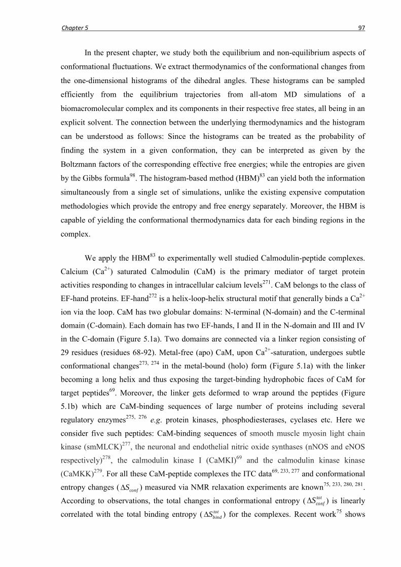
Chapter 5 97

In the present chapter, we study both the equilibrium and non-equilibrium aspects of

conformational fluctuations. We extract thermodynamics of the conformational changes from

the one-dimensional histograms of the dihedral angles. These histograms can be sampled

efficiently from the equilibrium trajectories from all-atom MD simulations of a

biomacromolecular complex and its components in their respective free states, all being in an

explicit solvent. The connection between the underlying thermodynamics and the histogram

can be understood as follows: Since the histograms can be treated as the probability of

finding the system in a given conformation, they can be interpreted as given by the

Boltzmann factors of the corresponding effective free energies; while the entropies are given

by the Gibbs formula98

. The histogram-based method (HBM)83

can yield both the information

simultaneously from a single set of simulations, unlike the existing expensive computation

methodologies which provide the entropy and free energy separately. Moreover, the HBM is

capable of yielding the conformational thermodynamics data for each binding regions in the

complex.

We apply the HBM83

to experimentally well studied Calmodulin-peptide complexes.

Calcium (Ca2+

) saturated Calmodulin (CaM) is the primary mediator of target protein

activities responding to changes in intracellular calcium levels271

. CaM belongs to the class of

EF-hand proteins. EF-hand272

is a helix-loop-helix structural motif that generally binds a Ca2+

ion via the loop. CaM has two globular domains: N-terminal (N-domain) and the C-terminal

domain (C-domain). Each domain has two EF-hands, I and II in the N-domain and III and IV

in the C-domain (Figure 5.1a). Two domains are connected via a linker region consisting of

29 residues (residues 68-92). Metal-free (apo) CaM, upon Ca2+

-saturation, undergoes subtle

conformational changes273, 274

in the metal-bound (holo) form (Figure 5.1a) with the linker

becoming a long helix and thus exposing the target-binding hydrophobic faces of CaM for

target peptides69

. Moreover, the linker gets deformed to wrap around the peptides (Figure

5.1b) which are CaM-binding sequences of large number of proteins including several

regulatory enzymes275, 276

e.g. protein kinases, phosphodiesterases, cyclases etc. Here we

consider five such peptides: CaM-binding sequences of smooth muscle myosin light chain

kinase (smMLCK)277

, the neuronal and endothelial nitric oxide synthases (nNOS and eNOS

respectively)278

, the calmodulin kinase I (CaMKI)69

and the calmodulin kinase kinase

(CaMKK)279

. For all these CaM-peptide complexes the ITC data69, 233, 277

and conformational

entropy changes ( confS ) measured via NMR relaxation experiments are known75, 233, 280, 281

.

According to observations, the total changes in conformational entropy (tot

confS ) is linearly

correlated with the total binding entropy ( tot

bindS ) for the complexes. Recent work75

shows

Chapter 5 98

that confS for CaM and the target peptides are linearly related to 2

MeS , the average

changes in residue-weighted methyl group order-parameters 2

MeS which describes the

rotational freedom of the methyl group. We estimate confS of the complexes and the

components correctly and recover the experimental observations. Further, we estimate the

conformational free energy cost of binding to predict different contributions of the individual

binding regions of CaM. Our calculations show that the deformations in linker helix to wrap

around the peptides cost huge free energy and entropy. The unfavourable changes are

outweighed by the favourable changes at different binding regions dominated by the

interactions among the charged residues and the hydrophobic residues.

Figure 5.1: Binding events of CaM. (a) Apo- to holo- transition of CaM using cartoon

representations. The EF-hand loops are coloured: I (purple), II (yellow), III (pink) and IV

(cyan). The part of linker that undergo loop to helix transformation is marked by circle.

(b) CaM bound to a target peptide (blue), smMLCK.

We also consider the Ca2+

-ion binding to apo-CaM. Despite several experimental100,

101, 282 and theoretical studies

283, 284 on such binding events, the conformational

thermodynamics of CaM upon Ca2+

-ion binding is largely unexplored. Using the HBM we

estimate the contributions from individual metal-binding sites to the conformational

thermodynamics along with the role of the individual residues in bringing about the

thermodynamic changes in the conformation space. We find four metal-ion binding sites in

CaM have different conformational free energy and entropy changes with the major share of

the changes due to the coordinating residues to the Ca2+

-ions. The non-coordinating residues

in the vicinity of the binding sites also undergo thermodynamic changes. We find substantial

thermodynamic changes in the linker where modification of the secondary structural element

takes place (Figure 5.1a). Finally, we correlate these results with the experimentally

measured binding data and discuss the broad implications of our studies.

The dynamic correlation between the non-equilibrium fluctuations of different

degrees of freedom have been studied in great detail via time-dependent correlation functions

Chapter 5 99

(TDCF) for various non-equilibrium systems65, 111, 254, 285

. The TDCF between two variables

describes how the changes in a physical quantity affect the other quantities after certain time.

The TDCF remains non-zero till a timescale called dynamic correlation time (). Such TDCF

has not been explored in details in the context of dynamical variables associated with the

biomacromolecules. We extract the TDCF of the dihedral angles in a protein from the

temporal evolution of all-atom MD trajectories. Our primary objective is to probe directly the

dynamic correlation among the conformational variables participating in allosteric regulation.

We illustrate the TDCFs of the dihedral angles in the case of Ca2+

ion binding to apo-CaM

which is known to involve certain allosteric events. We show that a number of dihedrals

exhibit long-ranged temporal correlation with non-exponential behaviour. Further, a sub-set

of dynamically cross-correlated dihedrals of distant residues is affected via binding of Ca2+

ions to CaM, indicating their involvement in allosteric regulation. Our approach, based on

dynamic correlations, provides a significant advancement to understand allosteric regulation

of biomacromolecules without any assumption on the underlying dynamical processes.

The rest of the present chapter is organized as follows: We describe the HBM for a

protein-ligand binding and its extensions in Section 5.2. The results on conformational

thermodynamics for CaM-peptide complexes are presented, along with a prediction and

discussions on merits and demerits of HBM in 5.3. Conformational thermodynamics for

binding of Ca2+

ions to CaM is considered in 5.4. Section 5.5 deals with the allosteric

regulations in CaM. We conclude in 5.6.

5.2 The histogram based method for conformational thermodynamics

In this section we illustrate the theoretical basis of HBM for protein-ligand binding

and its extensions.

5.2.1 Protein-ligand binding

For a system with conformational variable set i , the normalized probability

distribution is given by:

TkZ

P Bii H exp1

(5.1)

where kB is the Boltzmann constant, T the absolute temperature, iH , the Hamiltonian

and Z, the partition function of the system. The reduced probability distribution for a given

conformational variable can be obtained by integrating over the other variables in Eq. 5.1:

Chapter 5 100

iP ii

iBi dTkZ Hexp1 TkGZ B exp1 (5.2)

which defines the effective free energy G(ξ) or the potential of mean force111

associated with

.

We consider ≡ where and are the dihedral angles for protein p and ligand l

respectively. Subsequently, we use the subscripts p+l, p and l to indicate quantities associated

with the complex, the protein and the ligand respectively, while the superscripts c and f to

denote the bound and free state respectively. We define the following effective free energies

from Eq. 5.2:

TkGZ

P B

c

lp

c

lp /exp1

, TkGZ

P B

f

p

f

p /exp1

and TkGZ

P B

f

l

f

l /exp1

(5.3)

Therefore, the free energy change for due to complexation is

.ln)(

f

l

f

p

c

lp

BconfPP

PTkG (5.4)

The correlation between any two dihedral angles i of ith residue and j of jth residue

is defined as80

jijisC coscoscoscos (5.5)

where the jis and the angular brackets denote ensemble average. If correlations are

negligibly small, the conformational variables can be considered independent. Then we write,

c

l

c

p

c

lp GGG and c

l

c

p

c

lp PPP to give us from Eq. 5.4:

f

l

c

l

Bf

p

c

p

BconfP

PTk

P

PTkG lnln)( (5.6)

so that the thermodynamics is given separately in terms of the individual dihedrals. If we sum

over all the dihedral angles of protein and ligand we get the total conformational free energy

change:

lig

conf

prot

conff

l

c

l

Bf

p

c

p

B

tot

conf GGP

PTk

P

PTkG

)(

)(ln

)(

)(ln

. (5.7)

Chapter 5 101

We can expresstot

confG differently to illustrate the nature of approximations in our

calculations. Let z() be the partition function corresponding to effective free energy G() =

kBT ln z(). Therefore, z() = exp(G()/kBT) = P()Z, from Eq. 5.3, P() being the

probability distribution for . Defining z() for the protein variables and ligand variables

in free and complex states we can write

)(

)(ln

)(

)(ln

)(

)(ln

)(

)(ln

f

l

c

l

Bf

p

c

p

Bf

l

c

l

Bf

p

c

p

BP

PTk

P

PTk

z

zTk

z

zTk

(5.8)

which, using Eq. 5.7, simplifies to

)(

)(

)(

)(ln

f

l

c

l

f

p

c

p

B

tot

confZ

Z

Z

ZTkG (5.9)

where )()(

c

p

c

p zZ and so on. The term in square brackets in Eq. 5.9 is the conformational

contribution to the equilibrium binding constant. Here we assume that the other degrees of

freedom like bond angles and bond vibrations change very little in the complex compared to

the free states and they are decoupled from the dihedral angles, thus cancelling out from the

ratio in Eq. 5.9. The ratio of partition functions in Eq. 5.9 resembles that used earlier286

to

define the standard free energy of binding of a receptor to a ligand. However, we consider

here only a restricted set of internal degrees of freedom associated with equilibrium

fluctuations of the dihedrals. Since we focus only on the conformational part of the

thermodynamics we do not consider the solvation components, although the effects of solvent

on dihedral distributions have been taken into account through explicit solvent molecules. We

also ignore the external contributions to the thermodynamics as in Marlow et al75

.

The normalized probability distribution of a protein dihedral is given by the

histograms )(c

pH and )(f

pH and that for a ligand dihedral by )(c

lH and )(f

lH in the bound

and the free state, respectively. They can be generated from equilibrium trajectories obtained

by molecular simulations. The peak of the histogram defines the equilibrium value of the

relevant dihedrals. Then the equilibrium conformational free energy cost associated with any

protein dihedral is

)](/)(ln[)( max,max, f

p

c

pB

eq

conf HHTkG (5.10)

Chapter 5 102

where the subscript „max‟ denotes the maximum of histogram. Such a treatment is sufficient

since the population at the base of a peak is insignificant (1-10%) compared to that at the

maximum for a typical histogram.

The free energy contributions from the neighbourhood of the maximum can be

accounted for within a QH expansion about the maximum. We expand a histogram )(H

about the maximum at 0 up to the quadratic term: 2

00 ))(()2/1()( HHH mox

where )()( 00 CH , the curvature near the maximum. Therefore, the effective free energy

for can be written using Eq. 5.3 as:

ZCHTkG B ln]))(()2/1(ln[/)( 2

00max . (5.11)

Equation 5.11 can be rearranged to give ]1[ln/)( 2

max BxZHTkG B where 0 x

and moxHCB 2/)( 0 . For 12 Bx , we get 2

maxln/)( BxZHTkG B . This can be

further approximated as 1]exp[ln/)( 2

max BxZHTkG B to yield

]exp[ln/)( 2

max BxeZHTkG B (5.12)

Considering contributions from all x, Eq. 5.12 can be written as: TkG B/)(~ ]ln[ maxeZH

dxBx

]exp[ 2 . This integration essentially implies that the contributions around the peak

have been taken into account at QH level. The integration gives the modified free energy

)]1)/exp(ln[/)(~

max BZHTkG B . (5.13)

The corresponding free energy difference is then

f

p

c

p

f

p

c

pBconf BBHHTkG //)](/)(ln[/)(~

max,max, . (5.14)

Similar expressions like Eq. 5.10 and 5.14 can be written for the ligand dihedrals as well.

For multi-modal histograms we compute the free energies by taking average,

weighted by the maximum values of the peaks. For a particular dihedral with multi-modal

histograms in both free and complex states, the free energy cost is given by ji

ijij Gc,

where

)/ln( max,max,

f

i

c

jBij HHTkG representing the free energy cost for transition from ith peak

in free state to jth peak in the complex state and )/( max,max,max,max, j

c

ji

f

i

c

j

f

iij HHHHc , the

respective weights.

Chapter 5 103

The conformational entropy for a particular dihedral can be estimated directly using

the Gibbs entropy formula, given for a dihedral by

)(ln)()( i

iiBconf HHkS (5.15)

where the sum is taken over the histogram bins i with a non-zero value of Hi(). Therefore,

the conformational entropy change for the dihedral is

)(ln)()(ln)()(

i

f

i

f

i

i

c

i

c

iBconf HHHHkS . (5.16)

In the QH-limit, the entropy associated with the histogram of any dihedral can be

expressed in terms of the entropy of a harmonic oscillator fitted to the peak. The frequency of

the oscillator of mass and force constant k is given by // Ck . So, entropy is

given by )]//2ln(1[)( ChTkkS BBconf , h being the Planck‟s constant. If Cf and Cc

are the curvatures near maxima for the dihedral-histogram in free and complexed states

respectively, we have

)/ln()2/1()( cfBconf CCkS (5.17)

For multi-peak histograms QH entropies are obtained by weighted average over the peaks

with finite curvature around the maxima.

The thermodynamics of conformational changes of a given residue are finally

obtained by adding all the associated dihedral contributions. confG and confS of a given

region are computed by adding the contributions of all residues in that region. Similarly, the

total changes are calculated by adding all residue contributions.

5.2.2 Metal-ion binding to protein

We can write down the free energy cost for dihedral for apo- to holo-transition of

the protein as

)(confG )()( apoholo GG ]/ln[ apoholoB PPTk , (5.18)

where the respective states are indicated by the appropriate subscripts. To arrive at Eq. 5.18

we assume the total partition function Z of the system to remain unchanged in the apo- and

the holo-state. These two states differ only by (i) the Ca2+

ions and (ii) a few added counter

ions that replace some water molecules to maintain constant N. The replacement of water

molecules with ions may lead to difference in Z between apo- and holo-state. However, this

Chapter 5 104

difference is proportional to the ratio of fugacities111

of the added ions (including Ca2+

) and

replaced waters, given by )/exp()/exp( TkTkz BwaterBion where ‟s are chemical

potentials of the respective species. Since the densities of the ions ( ion ) are too small, we

have ionion ln~ and hence z ~ 0, indicating that the difference in Z between the two

states can be safely neglected. This is further supported by very small difference in ionic

strengths between the apo-CaM system (0.26) and the holo-CaM system (0.29) simulated

here. The total free energy change is then

]/[ln

apoholoB

tot

conf PPTkG . (5.19)

Here, the contributions from other variables like bond angles, bond vibrations etc. are

considered to remain similar in apo- and holo-states since metal-ion binding only alters the

secondary and/or tertiary structure of the protein. Consequently, they get decoupled from the

dihedrals and their distributions cancel from the ratio in Eq. 5.19. Thermodynamics of

solvation are not considered as we focus only on the conformational changes. However, the

solvent-effects on conformation have been incorporated via the explicit solvent. The total

equilibrium conformational free energy difference in terms of histograms is given from Eq.

5.19 by

)](/)([ln maxmax

apoholoB

tot

conf HHTkG , (5.20)

The conformational entropy change for any dihedral is obtained from Eq. 5.16:

)(ln)()(ln)()(

i

apo

i

apo

i

i

holo

i

holo

iBconf HHHHkS . (5.21)

5.3 Conformational thermodynamics of CaM-peptide complexes

In this section we discuss the conformational thermodynamics of CaM-peptide

complexes. First we describe the details of the simulations. Then the results in the following

order are presented on methyl order parameters, dihedral correlations, histograms,

conformational entropy and conformational free energy. Then we discuss changes at different

binding regions, scaling between methyl order parameters and conformational entropy and

predictions using HBM. Finally we discuss different merits, demerits and possible routes to

extend the HBM.

Chapter 5 105

5.3.1 Simulation details

For CaM-peptide complexes, we perform all atom MD simulation of the free protein,

free peptide and the complex in explicit water. Simulations are done with the NAMD

program287

at 308K and 1 atm pressure in isothermal-isobaric (NPT) ensemble under standard

protocols288

, using the CHARMM force-field289

, periodic boundary conditions and 1

femtosecond time-step. TIP3P model is used for solvent water molecules. Electroneutrality is

maintained via addition of counter-ions (Na+ or Cl

). The particle-mesh Ewald method

290 is

used to treat the long-ranged electrostatic forces. The initial configurations are chosen from

following protein data bank (PDB) entries: 1CDL (smMLCK), 1NIW (eNOS), 2O60 (nNOS),

2L7L (CaMKI), 1CKK (CaMKK) and 1CLL (free CaM). The peptide coordinates in the

complexes are taken as the initial configurations of the free peptide simulations. We keep the

number of total particles including water, pressure and temperature fixed for each case to

make the simulated ensembles equivalent. We run 50 ns long simulations to capture most of

the protein motions and peptide motions relevant for binding. The equilibration is ensured in

any run by monitoring the root mean square deviation of the biomacromolecules, shown in

the Figure A1 in Appendix. We analyze the data at two levels: First, we consider the

trajectories up to 10 ns since the conformational entropy is dominated primarily by sub-ns

side-chain motions75, 233

, and calculate the histograms for the dihedral angles from

equilibrated configurations sampled beyond 2 ns. Subsequently, we consider the longer 50 ns

trajectory and compare data with the shorter run. The dihedral angles are calculated from

angle between the relevant atomic planes89

given by the Cartesian coordinates of the

associated atoms.

5.3.2 Methyl order parameters

By definition 2

MeS of a methyl group increases from zero to unity as its rotation about

the long-axis gets restricted indicating lowering of entropy. We compare our calculated

methyl group (Figure A2) order-parameters 2

MeS (calc) (method in Appendix A) to the

experimental data 2

MeS (exp)75

in Figure 5.2a (CaM) and 5.2b (peptide) for a representative

case: eNOS-complex. Most of the Ala, Met, Val and Thr methyls are close to the perfect

correlation line ( 2

MeS (exp)= 2

MeS (calc)) or within the 2

MeS (exp)= 2

MeS (calc)0.2 region,

indicating reasonable agreement between the theoretical and experimental values. There are

some overestimations, mostly for the Leu methyls, as expected for force-field based MD

simulations291, 292

. Results of other complexes are shown in Figure A3 and A4.

Chapter 5 106

Figure 5.2: Methyl order parameter data. 2

MeS are shown for different types of methyls (a)

CaM and (b) peptide in the eNOS-complex. Here, the experimental data (exp)2

MeS are

plotted against the theoretical )calc(2

MeS values. The straight lines show (exp)2

MeS =

)calc(2

MeS (solid), (exp)2

MeS = )calc(2

MeS +0.2 (dotted) and (exp)2

MeS = )calc(2

MeS 0.2

(dashed) situations.

5.3.3 Equilibrium correlations among dihedral angles

We choose the backbone dihedrals , and the side-chain dihedrals 1, 2, 3, 4 and

5. Figure 5.3a-c show the equilibrium correlations (Eq. 5.5) among different dihedrals. The

correlation data among different dihedrals in CaM (Figure 5.3a) and peptides (Figure 5.3b) in

various complexes and the cross-correlations between CaM and peptide dihedrals (Figure

5.3c) indicate nearly zero correlations among the dihedrals which is consistent with the

earlier observations80, 231

.

Figure 5.3: Equilibrium dihedral correlations and histograms. (a-c) - correlations

sC (Eq. 5.5) where and are dihedral angles from two residues and s is the

Chapter 5 107

difference between their locations. (a) Dihedrals of CaM in different complexes:

in the eNOS-complex (solid line), in smMLCK-complex (dashed), 1 angles in

nNOS-complex (dotted) and 2 in CaMKI-complex (dash-dot). (b) Dihedrals of peptides in

different complexes: in the eNOS-complex (solid line), in CaMKI-complex

(dashed), 1 angles in smMLCK-complex (dotted) and 2 in CaMKK-complex (dash-dot).

(b) Cross-correlations among side-chain dihedrals from protein and from peptide:

1 in nNOS-complex (solid), 2 in eNOS-complex (dashed), 1 in CaMKI-complex

(dotted) and 2 in CaMKK-complex (dash-dot). Representative histograms of (d) of

Glu45 of CaM in free and bound form in smMLCK-complex. The inset shows the near-peak

region for the free case. In each case three convergent histograms are shown in solid,

dashed and dotted lines sampled from different parts of the MD-trajectory; (e) of

Lys802 of smMLCK peptide in free (dotted) and CaM-bound form (solid). Multi-modal

histograms are shown for (f) 2 of CaM residue Leu69 in free and bound form in CaMKK

complex and (g)2 of CaM residue Asp118 in free and bound form in CaMKI complex.

Figure 5.4: The convergence of conformational entropy during the simulation. A

representative case of smMLCK complex is shown. The CaM and peptide contributions

individually remain almost invariant with time demonstrating the robustness of the

histogram technique. The errors in calculated Sconf for free CaM (0.05 kJ K-1mol-1) and for

CaM in the complex (0.04 kJ K-1mol-1) are quite small. The errors in the peptide-data are

nearly zero.

5.3.4 Histograms of dihedrals and convergence of thermodynamics

In absence of significant correlations, we consider the histograms of the individual

dihedrals for the calculation of thermodynamics. The histograms are calculated over 10 sets

of equilibrated configurations each having 1000 samples from different parts of the

trajectory. Figure 5.3d shows three such histograms in free and complex states for the

Chapter 5 108

dihedral angle of CaM-residue Glu45 in smMLCK-complex. The similarities of these

histograms indicate the convergence of thermodynamic quantities calculated based on them,

for instance, conformational entropies (Figure 5.4). Due to equivalence of the samples we

compute the overall changes in entropy and free energy via a flat average over the entire

equilibrium trajectory. All the backbone dihedrals exhibit sharply single-peaked histograms

with the maxima around the equilibrium values in the initial configuration (PDB

coordinates). Histograms of dihedral of a peptide residue Lys802 of smMLCK peptide are

shown in Figure 5.3e. Multi-modal histograms have been mostly observed for the side-chain

dihedrals, as illustrated in Figure 5.3f for 2 of CaM residue Leu69 and Figure 5.3g for 2 of

CaM residue Asp118, indicating different rotameric states.

Figure 5.5: Conformational entropy data. (a-b) Comparison of theoretical and

experimental tot

confS for CaM-peptide binding plotted against the experimental tot

bindS

from ITC measurements233: (a) Calculated tot

confS (Gibbs formula) from the 10 ns runs

(filled circles), the 50 ns runs (open circles) along with the experimental tot

confS (Marlow

et al75) (filled triangles). The lines represent the best linear fits: 10 ns (dashed), 50 ns

(dash-dot) and the experimental data (dotted). The stars represent the 50 ns tot

confS data

in QH-limit. (b) Calculated tot

confS from 10 ns simulations (filled circles) and 50 ns

simulations (open circles) using QH approximation. The best linear fits: 10 ns (dashed,

Chapter 5 109

m=0.39, R2=0.53) and 50 ns (dash-dot, m=0.47, R2=0.32). (c) The conformational entropy

contributions of the components from 50 ns run plotted against tot

bindS : CaM contributions

(open squares) with the best fit line (dashed) and peptide contributions (open diamonds)

with the best fit line (dash-dot). The corresponding experimental data75 are also shown

for CaM contributions (filled squares) with the best fit line (solid) and peptides (filled

diamonds) with best fit line (dotted).

5.3.5 Conformational entropy

In Figure 5.5, we compare our calculated total conformational entropiestot

confS of the

complex with the available experimental results. First we consider the results calculated using

the Gibbs formula (Eq. 5.16) (Figure 5.5a). Here we compare the 10 ns and 50 ns data with

the experimental tot

confS (filled triangles) reported in Marlow et al75

. Both the theoretical and

experimental tot

confS are plotted against the corresponding tot

bindS from ITC233

, showing linear

correlations between tot

confS and tot

bindS . The 10 ns data (filled circles) can account for the

experimental trend (filled triangles) except for CaMKI and CaMKK. However, the best fit

correlation line has slope m = 0.3 and linear correlation coefficient R = 0.3 which are far

from the experimental data (m = 0.95 and R = 0.75). The 50 ns data (open circles) provide an

overall better estimate for all cases where the correlation line (m = 1.3 and R = 0.95) agree

quite well with the experimental data. One reason of the underestimation by the 10 ns data for

CaMKI and CaMKK could be the fact that the initial configurations for simulations in these

two cases are NMR determined structures. For other complexes the initial structures are from

crystallographic data where the 10 ns and 50 ns data hardly make any difference. NMR-data

generate an ensemble of structures, unlike the only structure obtained from crystallography.

Therefore, equilibration of the solution-NMR structures may not have been completed

properly in the 10 ns simulation run. Figure 5.5a further shows that tot

confS from QH

approximation (Eq. 5.17) (open stars) leads to underestimation, although the linear

correlation between tot

confS and tot

bindS is observed here as well (Figure 5.5b).

The confS (in kJ K-1

mol-1

) for all the side-chain dihedrals in the complexes showing

multi-peak histograms are 0.43 (nNOS), 0.23 (eNOS), 0.57 (CaMKI), 0.56 (smMLCK)

and 0.58 (CaMKK) obtained using the Gibbs formula. Such multi-modal histograms

contribute more than 60% of the total conformational entropy stabilizations of the complexes,

indicating the importance of the redistributions of populations among various side-chain

rotamers in the binding. In Figure 5.5c, we report the contributions of the CaM and peptide

separately in the complexes, estimated from the 50 ns runs. The CaM contributions show

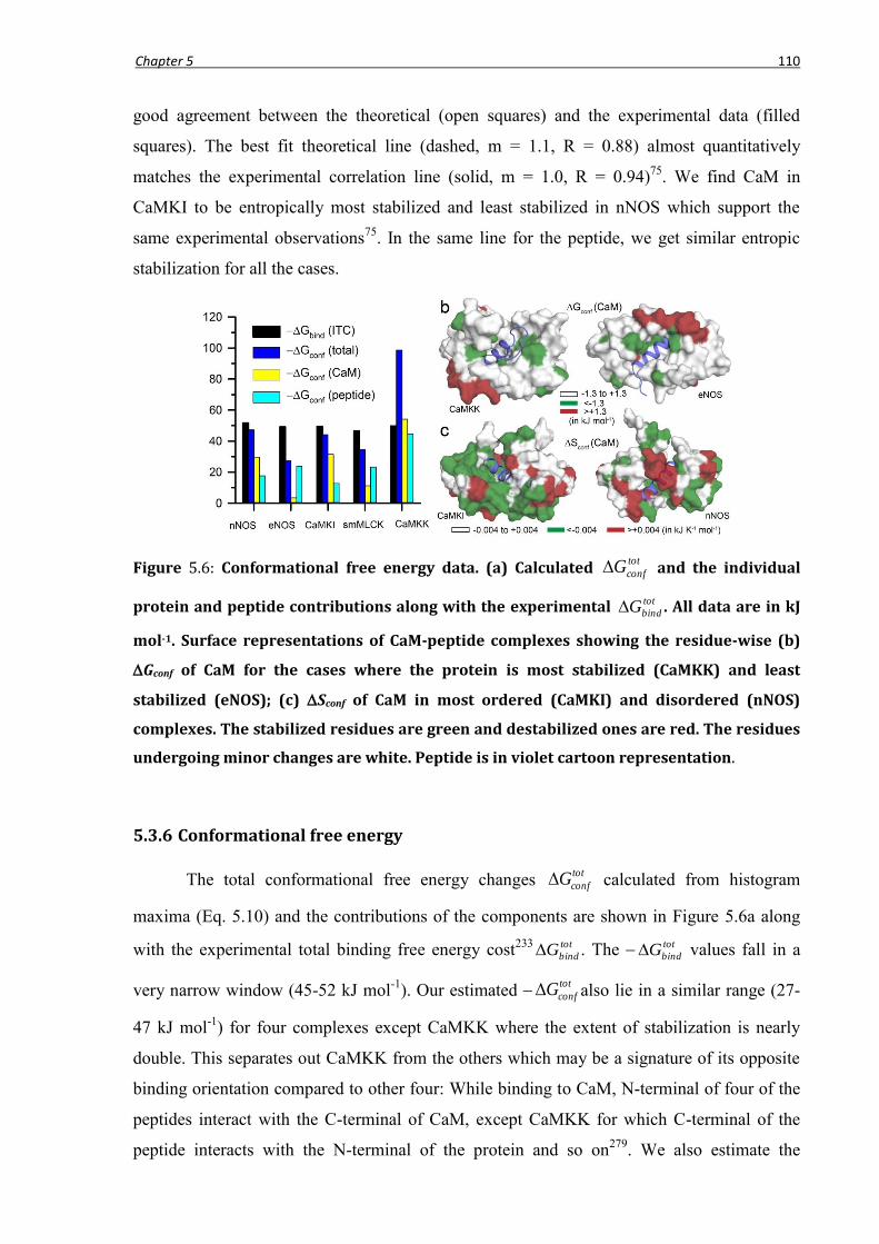
Chapter 5 110

good agreement between the theoretical (open squares) and the experimental data (filled

squares). The best fit theoretical line (dashed, m = 1.1, R = 0.88) almost quantitatively

matches the experimental correlation line (solid, m = 1.0, R = 0.94)75

. We find CaM in

CaMKI to be entropically most stabilized and least stabilized in nNOS which support the

same experimental observations75

. In the same line for the peptide, we get similar entropic

stabilization for all the cases.

Figure 5.6: Conformational free energy data. (a) Calculated tot

confG and the individual

protein and peptide contributions along with the experimental tot

bindG . All data are in kJ

mol-1. Surface representations of CaM-peptide complexes showing the residue-wise (b)

Gconf of CaM for the cases where the protein is most stabilized (CaMKK) and least

stabilized (eNOS); (c) Sconf of CaM in most ordered (CaMKI) and disordered (nNOS)

complexes. The stabilized residues are green and destabilized ones are red. The residues

undergoing minor changes are white. Peptide is in violet cartoon representation.

5.3.6 Conformational free energy

The total conformational free energy changes tot

confG

calculated from histogram

maxima (Eq. 5.10) and the contributions of the components are shown in Figure 5.6a along

with the experimental total binding free energy cost233 tot

bindG . The tot

bindG values fall in a

very narrow window (45-52 kJ mol-1

). Our estimated tot

confG also lie in a similar range (27-

47 kJ mol-1

) for four complexes except CaMKK where the extent of stabilization is nearly

double. This separates out CaMKK from the others which may be a signature of its opposite

binding orientation compared to other four: While binding to CaM, N-terminal of four of the

peptides interact with the C-terminal of CaM, except CaMKK for which C-terminal of the

peptide interacts with the N-terminal of the protein and so on279

. We also estimate the

Chapter 5 111

contributions to tot

confG due to finite width of the histograms using Eq. 5.14, to be only 1-5%

of the estimate from histogram maxima for all the complexes except smMLCK for which this

difference is ~15%. Although it seems from tot

bindG -data that all the peptides exhibit similar

affinity to CaM, the conformational contributions of the components bring out a different

picture. The protein is conformationally most stabilized in CaMKK-complex, while least

stabilized in eNOS-complex. The peptide, on the other hand, is stabilized similarly in all the

cases except in CaMKK-complex.

Table 5.1: Conformational thermodynamics of different highly stabilized peptide binding

regions of CaM in the complexes. The residue numbers according to the PDB indices are

listed. The conformational free energy and entropy contributions of these binding

regions are shown along with their percentages of charged and polar residue

contributions (CPRC) and hydrophobic residue contributions (HRC).

peptide CaM residues

Gconf (kJ mol-1) Sconf (kJ K-1 mol-1)

Total CPRC (%)

HRC (%)

Total CPRC (%)

HRC (%)

nNOS 11-19, 36-41, 42-50, 84-92 31 29

eNOS 11-19, 117-123 76 4

CaMKI 7-10,36-41, 42-50, 52-55, 71-76, 84-

92, 105-116 68 15

smMLCK 11-19, 36-41, 52-55, 84-92, 105-116,

117-123 65 12

CaMKK 7-10, 11-19. 36-41, 42-50, 52-55, 84-

92, 105-116, 124-128 49 22

DAPK2 11-19, 35, 36-41, 42-50,124-128 55 23

5.3.7 Thermodynamics at individual binding regions

The thermodynamic changes at each protein residue are shown by surface

representations in Figure 5.6b-c for the most and least stabilized complexes, both free-

energetically and entropically. In Figure 5.6b, CaMKK and eNOS complexes are shown,

where the green residues are stabilized, the red residues are destabilized and the white

residues undergo a marginal change in conformational free energy. In Figure 5.6c we show

Chapter 5 112

the entropy changes for CaMKI and nNOS complexes where the green residues are ordered

while the red residues are disordered in the bound protein compared to the free state. Similar

surface representations showing residue-level changes of the other complexes are included in

Figure A5.

Next we examine closely the changes in the peptide binding regions (PBR) of CaM. If

any atom of a protein residue comes within a distance of 5Å of a peptide atom, we consider

the corresponding residue to be part of the PBR. The thermodynamic contribution of a PBR is

obtained by summing over the contributions of the residues that are part of the PBR.

Different PBRs show different degree of thermodynamic stabilizations. The residues in linker

helix responsible for the wrapping the peptide, constitute the most destabilized PBRs. The

deformation of linker helix occurs for different peptides at slightly different locations where a

coiled region is formed due to loss of secondary structure element. For instance, in nNOS-

complex the coil is produced over the residues 77-83 (Gconf = +19.8 kJ mol-1

and Sconf =

+0.07 kJ K-1

mol-1

), whereas it is 73-76 for smMLCK (Gconf = +11.7 kJ mol-1

and Sconf =

0.0 kJ K-1

mol-1

) and 76-81 for CaMKK (Gconf = +20.6 kJ mol-1

and Sconf = +0.08 kJ K-1

mol-1

). For the other two complexes these regions are residues 77-83 with the changes being

for eNOS (Gconf = +15.6 kJ mol-1

and Sconf = +0.08 kJ K-1

mol-1

) and CaMKI (Gconf =

+12.8 kJ mol-1

and Sconf = +0.12 kJ K-1

mol-1

).

The huge free energy cost at the destabilized PBR is compensated by the favourable

changes at the other PBRs and the peptides. The changes at the most stabilized PBRs for

different complexes are shown in Table 5.1. Furthermore, CaM being an acidic protein

interacting with all these peptides rich with basic residues, the electrostatic contributions are

also expected to play an important role. We analyze from our calculations the contributions

of these protein-peptide interactions in some highly stabilized PBRs. It is quite apparent from

Table 5.1 that the charged and polar residue contributions dominate in all the cases, for both

conformational free energy as well as entropy. The highly stabilized common binding regions

in all the complexes are CaM-residues 11-19 (EFKEAFSLF), 36-41 (MRSLGQ), 42-50

(NPTEAELQD), 52-55 (INEV), 84-92 (EIREAFRVF) and 105-116 (LRHVMHNLGEKL).

Evidently, these PBRs are rich in charged (E, D, R, K, H) and polar (S, Q, N, T) residues

making it the dominating stabilizing factor in CaM-peptide complexes. Table 5.1 also shows

that there are stabilized residues with hydrophobic side-chains (F, A, L, I, V, M) as well,

undergoing substantial conformational stability in the binding, as pointed out earlier from

structural analyses69

and recent NMR studies280

.

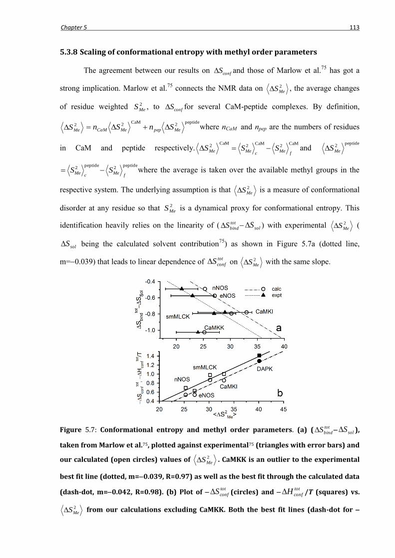
Chapter 5 113

5.3.8 Scaling of conformational entropy with methyl order parameters

The agreement between our results on confS and those of Marlow et al.75

has got a

strong implication. Marlow et al.75

connects the NMR data on 2

MeS , the average changes

of residue weighted 2

MeS , to confS for several CaM-peptide complexes. By definition,

2

MeSpeptide

2CaM

2

MepepMeCaM SnSn where nCaM and npep are the numbers of residues

in CaM and peptide respectively.CaM

2

MeSCaM

2CaM

2

fMe

cMe SS and

peptide2

MeS

peptide2

peptide2

fMe

cMe SS where the average is taken over the available methyl groups in the

respective system. The underlying assumption is that 2

MeS is a measure of conformational

disorder at any residue so that 2

MeS is a dynamical proxy for conformational entropy. This

identification heavily relies on the linearity of ( tot

bindS solS ) with experimental 2

MeS (

solS being the calculated solvent contribution75

) as shown in Figure 5.7a (dotted line,

m=0.039) that leads to linear dependence of tot

confS on 2

MeS with the same slope.

Figure 5.7: Conformational entropy and methyl order parameters. (a) ( tot

bindS solS ),

taken from Marlow et al.75, plotted against experimental75 (triangles with error bars) and

our calculated (open circles) values of 2

MeS . CaMKK is an outlier to the experimental

best fit line (dotted, m=0.039, R=0.97) as well as the best fit through the calculated data

(dash-dot, m=0.042, R=0.98). (b) Plot of tot

confS (circles) and tot

confH /T (squares) vs.

2

MeS from our calculations excluding CaMKK. Both the best fit lines (dash-dot for

Chapter 5 114

tot

confS and solid for tot

confH /T) have m=0.05. The solid symbols represent the data for

the CaM-DAPK2 complex.

We calculate 2

MeS from our simulation data on 2

MeS in order to check whether we

could recover the experimentally observed linearity between ( tot

bindS solS ) and 2

MeS . The

estimation of 2

MeS from simulation is somewhat tricky. Although CaM

2

cMeS and

CaM2

fMeS

remain very similar over the entire equilibrium trajectory, peptide

2

cMeS and

peptide2

fMeS converge

slowly with convergence achieved typically beyond 12 ns (Figure A6). Such slow

convergence is probably due to the presence of fewer methyl groups than in protein. The

convergence for smMLCK is the poorest, for it has the least number (8) of methyl groups.

This slow convergence for peptides leads to pronounced variations in 2

MeS arising due to

large multiplicative factors (nCaM = 148 and npep ~20). Therefore, we consider only the long-

time part of the trajectory to estimate 2

MeS . The ( tot

bindS solS ) from Marlow et al75

is

linear with our calculated 2

MeS (dash-dot line in Figure 5.7a, m = 0.042) excluding the

data for CaMKK which is an outlier in the experimental plot as well. A microscopic

justification for the use of 2

MeS as a dynamical proxy of conformational entropy in Marlow et

al75

is provided by Figure 5.7b showing the linearity between our estimated tot

confS (open

circles) from dihedral distributions and simulated 2

MeS (dash-dot line) with very similar

slope (m = 0.050). Since, our calculated tot

confG values are very similar for different

complexes except CaMKK, the conformational enthalpy changes )( tot

conf

tot

conf

tot

conf STGH

should also have the same linearity with 2

MeS as tot

confS for thermodynamic consistency.

We find this indeed is the case in Figure 5.7b, also showing the plot of TH tot

conf / values

(open squares) of the complexes, excluding the outlier CaMKK.

5.3.9 Prediction

We apply our approach to make predictions on the conformational thermodynamics of

binding of a target peptide from death associated protein kinase (DAPK2)293

to CaM. Here,

the S308D mutant of DAPK2 has been considered with a high resolution crystal structure

Chapter 5 115

(PDB ID 1ZUZ) and known ITC data ( 5.39 tot

bindG kJ mol-1

and 28.0 tot

bindS kJ K-1

mol-1

at 300K)293

. However, nothing is known regarding the conformational entropies of this

system to the best of our knowledge. We perform 20 ns runs for this complex and the free

peptide as we have seen earlier that shorter runs are sufficient to capture the conformational

thermodynamics if crystal structures are employed as starting configurations. The residue-

wise 2

MeS data are given in Figure A7. We find 29.1 tot

confS kJ K-1

mol-1

using the Gibbs

formula where the CaM and peptide contributions are 0.98 and 0.31 kJ K-1

mol-1

respectively. The tot

confS value follow the same linear scaling with 2

MeS as the other

complexes as shown by the closed circle in Figure 5.7b. We get 1.38 tot

confG kJ mol-1

with

CaM and peptide contributions being 15.4 and 22.7 kJ mol-1

, respectively. These free

energy values are very similar to the case of smMLCK. The calculated tot

confH (filled square)

falls, just like tot

confS , on the line drawn for other complexes in Figure 5.7b. Residues 77-83

constitute the maximum destabilized PBR in DAPK2-complex with very similar changes as

earlier: Gconf = +21.2 kJ mol-1

and Sconf = +0.02 kJ K-1

mol-1

. Surface representations of

CaM-DAPK2-complex are included in Figure A5 where contributions of different CaM-

residues are shown. The changes of highly stabilized PBRs are listed in Table 5.1 along with

the associated contributions of charged and hydrophobic residues.

5.3.10 The HBM: merits, demerits and extensions

Efficiency of any computational method depends on the simulation length to generate

a convergent thermodynamics. The present method is highly advantageous from that point of

view as indicated by the convergence of the histograms and conformational entropy (Figure

5.4) obtained from different parts of trajectory. The convergence has been achieved with

shorter runs (10 ns) where initial configurations are taken from available crystal structures,

while longer runs (50 ns) are required for the solution-NMR derived initial structures. The

reduced histograms can also be generated from suitable model initial structures in the absence

of PDB structure. However, the equilibration may depend on how the initial conditions are

constructed.

As far as the efficiency of the method used to extract confS from the histograms is

concerned, both the Gibbs formula and QH-approximation are computationally comparable

when the dihedrals are uncorrelated. Although the Gibbs formula is more accurate, the QH

approximation is often used for its simplicity and as a benchmark-tool for analyses with

Chapter 5 116

probability distributions of conformational variables. However, the QH approximation

underestimates confS in our studies. It may be stressed that we use the QH approximation to

incorporate the free energy contributions for conformations away from the equilibrium value

marked by histogram maxima. Such treatment is meaningful due to low weightage of those

conformations compared to the equilibrium conformation.

Experimentally, large amplitude rigid body domain motions have been observed for

CaM in time scales much longer than 50 ns78

. Due to high conservation of the compact

structures among all the complexes these domain motions are not expected to vary much

from one to another. Such motions of time scale ~milliseconds78

, in both free and complex

states, would be decoupled from the sub-ns highly localized side-chain motions75

that control

the conformational thermodynamics. Even if we consider the entropy change associated with

such motions, given by the logarithm of the ratio of two high-frequencies in free and complex

states, the contribution would be insignificant.

The uncorrelated dihedral angles reduce the computation-cost enormously. However,

when the correlations of the conformational variables cannot be neglected, the correlation

matrix can be diagonalized to obtain the uncorrelated basis and used for the calculations. For

any two conformational variables i and j the covariance matrix is symmetric since

jiij CC . Therefore, one can determine a set of uncorrelated variables }~

{ i by diagonalizing

the covariance matrix, j

jiji ~

where ][ ij is the transformation matrix found by the

eigenvalues. The maximum of a sharp histogram of a given variable is essentially equal to its

mean and the curvature given by the variance. The mean of the transformed variable,

j

jiji ~

, the variance: Var( i~

) = .)),

2 kj

kjjkijiii Cov(Var(

5.4 Conformational thermodynamics for Ca2+-ion binding to CaM

In this section we consider the thermodynamics of conformational changes for Ca2+

-

ion binding to apo-CaM. The equilibrium dihedral correlations and histograms in apo- and

holo-CaM are shown in section 5.4.1. Overall thermodynamics and domain contributions are

discussed in 5.4.2. Then we present the contributions of the Ca2+

binding loops in detail in

5.4.3. Changes in the linker in CaM are discussed in 5.4.4. We comment on generalization of

our observations for other proteins in section 5.4.5.

Chapter 5 117

5.4.1 Dihedral correlations and histograms

To study metal-ion binding to apo-CaM we simulate from the PDB structure 1CFD

for apo-state of CaM. The equilibrium correlations (Figure 5.8a-b) among different side-

chain dihedrals in both apo- and holo-CaM turn out to be negligible (Figure 5.8a), although

the backbone dihedrals show short-ranged correlations (Figure 5.8b). In section 5.3.3 we have

shown that one can ignore such correlations in the calculations of the thermodynamic

quantities. Accordingly, we treat the dihedrals as independent conformational variables80, 83

.

Some sample histograms of apo- and holo-CaM dihedral angles are shown in Figure

5.8c-f. The backbone dihedral histograms generally have one sharp peak typically around the

values in PDB structure. This is illustrated in Figure 5.8c-d for of a loop I residue Glu31

(Figure 5.8c) and of Thr79, residue in the linker (Figure 5.8d). We find significant increase

in the histogram peak value with reduction of width from apo- to holo-state indicating

increase in rigidity of the protein backbone due to binding to Ca2+

. The Ca2+

-coordinating

side-chains are more prone to changes induced by metal-ions. For instance, the 2-histogram

of Ca2+

binding residue Asp133 (loop IV) exhibits two broad peaks in apo-state (Figure 5.8e)

each indicating a rotamer, while there is one sharp peak in holo-state. For Ser81 in the loop

region of the linker helix in apo-CaM (marked in Figure 5.1), the 1-histogram (Figure 5.8f)

shows a very similar behaviour as in Figure 5.8e. This observation demonstrates the

suppression of side-chain fluctuations induced by the binding of metal-ions.

Figure 5.8: Equilibrium dihedral correlations and histograms in apo- and holo-CaM.

)(sC (Eq. 5.5) for (a) and (b) 1 in apo- and holo-CaM. Histograms

for dihedrals (c) (Glu31), (d) (Thr79), (e) 2 (Asp133) and (f) 1 (Ser81) in apo and

holo-CaM. Line description for all panels is same as in panel a.

Chapter 5 118

5.4.2 Overall thermodynamics data

The conformational thermodynamic changes have been calculated for the holo-state

with respect to the apo-state. A negative value of Gconf means stabilization in holo-state than

in apo-state, while positive values indicate destabilization. As far as Sconf is concerned, a

negative value means ordering in holo-state with respect to apo, while positive Sconf suggest

disordering. We find tot

confG = 54.9 kJ mol-1

for binding of four Ca2+

, nearly 30% of the

experimentally measured binding free energy282

. The correspondingtot

confST = 128.7 kJ mol-1

indicating substantial drop in conformational flexibility due to Ca2+

binding. In absence of

any experimental data, we provide an alternative verification of our estimated tot

confST from

2

MeS

calculated from the simulations83

. We estimate 2

MeS =10.95 (detailed order

parameter data shown in Figure A8-A10 in Appendix). Using the theoretical value of the

slope83

(0.05) of the linear dependence between tot

confST and 2

MeS , we find tot

confST

=169 kJ mol-1

which is close to the estimated tot

confST from dihedral histograms.

As far as the domain-specific data are concerned, we find the N-domain of CaM

conformationally more stabilized ( confG = 26.5 kJ mol-1

) in presence of Ca2+

ions

compared to the C-domain ( confG = kJ mol-1

). This observation matches with the

trend of domain-wise binding free energies in earlier grafting experiment100

and isothermal

titration calorimetry measurement101

. Entropically both domains get ordered when bound to

metal-ions, N-domain being more ordered ( confST = kJ mol-1

) compared to the C-

domain ( confST = kJ mol-1

).

5.4.3 Conformational changes of the Ca2+ binding loops

Figure 5.9 summarizes the loop-wise data on conformational entropy change L

confST

(L=I, II, III and IV) (Figure 5.9a) and free energy change L

confG (Figure 5.9b) of the Ca2+

-

ion binding to CaM. Loop I, II and IV undergo conformational ordering and stabilization

upon Ca2+

binding as indicated by negative values of both L

confST and L

confG . Loop III,

however, shows a different trend. The L

confST -value of loop III shows slight disordering

upon the metal-ion binding, while the L

confG value indicates marginal stabilization,. The

finding of different L

confG values for the four loops is consistent with the earlier experimental

observations100, 101

of four different Ca2+

binding constants for CaM, indicating different

affinities of the four EF-hands.

Figure 5.9 also shows the contributions of different type of residues in these loops

towards the respective L

confST (Figure 5.9a) and L

confG (Figure 5.9b). The trends are very

similar in both the panels for all the loops. In all cases except loop III, the main change comes

Chapter 5 119

from the acidic residues, nearly all coordinating to Ca2+

. However, the ordering and

stabilization of the acidic residues in loop III is nearly half of those observed in loops I and

IV. The basic residues in loops I are ordered and stabilized, while that in loop III remains

almost unchanged. The residues with hydrophobic side-chains and those with polar side-

chains order and stabilize amply in loops I, II and IV.

Figure 5.9: Data of the four EF-hand loops. (a) confST and (b) confG , showing the total

changes and contributions of different types of residues. The loop descriptions are: loop I

- residues 20-31 (amino acid sequence DKDGDGTITTKE), loop II - residues 56-67

(sequence DADGNGTIDFPE), loop III - residues 93-104 (sequence DKDGNGYISAAE) and

loop IV - residues 129-140 (sequence DIDGDGQVNYEE).

Figure 5.10 presents the residue-wise conformational entropy changes i

confST (Figure

5.10a), i being the residue-index, and conformational free energy changes i

confG (Figure

5.10b) of the four EF-hand loops using cartoon representations. Earlier studies have shown100,

284 that the stabilities of these loops depend heavily on their amino acid compositions and the

charge of the binding cation. Although the four Ca2+

binding loops of CaM are structurally

very similar and all of them show strong sequence conservation at three loop positions 1, 6

and 12, their conformational stabilizations upon binding of Ca2+

are different as revealed on

closer inspection.

All of the four acidic residues in loop I: Asp20, Asp22, Asp24 and Glu31, coordinate

to Ca2+

, get ordered and stabilized. The only uncharged Ca2+

coordinating residue Thr26 also

undergoes high ordering and good stabilization. There are several non-coordinating loops

residues as well which show thermodynamic changes. The basic residue Lys21, located

between acidic Asp20 and Asp22, also undergo favourable changes. The backbone between

Asp20 and Asp22 closes up somewhat upon Ca2+

binding. This brings the side-chain of

Lys21, projecting outward perpendicularly to the loop-backbone in the apo-state, within the

range of electrostatic interactions with the negatively charged side-chains of Asp20 and

Chapter 5 120

Asp22 in the holo-state. The other basic residue Lys30 is also ordered and stabilized, with its

side-chain drawn near the polar residue Thr29 undergoing favourable charge-dipole

interaction. Among the hydrophobic residues Ile27, the structural linker with loop II100

, gets

ordered with a high stabilization.

Figure 5.10: Cartoon representations of the EF-hand loops in holo-CaM to show the

residue-wise data. (a) i

confST and (b) i

confG (in kJ mol-1). The colours are described in

the figure.

In case of Loop II, the Ca2+

coordinating ligands are acidic residues Asp56, Asp58,

Glu67 and the polar residues Asn60 and Thr62. All become ordered upon metal-ion binding,

but the extent of ordering is less compared to the Ca2+

coordinating residues in loop I.

Maximum ordering is observed for Glu67, a bidentate Ca2+

coordinating ligand like Glu31 in

loop I. The smaller i

confST of Asp56 and Asp58, compared to their analogue Asp20 and

Asp22 in loop I, is probably due to absence of any basic residue in between them.

Interestingly, this is evident from the fact that i

confST values of Lys21 and Lys30 and the

excess i

confST of Asp20 and Asp22 over their analogues in loop II add up to ~ 8.0 kJ mol-1

,

comparable to the difference in L

confST between loop II and loop I. The fourth acidic residue

Asp64 though does not coordinate to Ca2+

, gets ordered highly because of the negative charge

on its side-chain pointing towards the Ca2+

. Among other non-coordinating residues, Ala57,

Ile63 and Phe65, all of which are hydrophobic, also become conformationally more ordered

and stable compared to the apo-state (Figure 5.10).

The L

confST (~ +0.2 kJ mol-1

) and L

confG (~ 2.4 kJ mol-1

) values of loop III (Figure

5.9) suggest very different Ca2+

binding behaviour compared to loops I and II. One reason

could be the lack of any fourth negatively charged residue in this loop. This trend is

Chapter 5 121

supported by the enhanced Ca2+

binding affinities observed by mutational studies294

via

increasing the number acidic residues in loop III. Flexibility of this loop increases upon Ca2+

binding, indicated by the high disordering of Ca2+

coordinating residues Asp93, Tyr99 and

Glu104. Most ordered residue in this loop is Ca2+

coordinating Asn97 which occupies the

same loop position as Asp24 in loop I and Asn60 in loop II. The other Ca2+

coordinating

residue Asp95 also undergoes ordering and stabilization which is reflected in the movement

of its side-chain, for coordinating to Ca2+

, closer to the side-chain of Lys94 for favourable

interactions. The ordering of non-coordinating residue I100, the structural link to loop IV, is

very small (Figure 5.10a), while its stabilization is significant (Figure 5.10b).

The loop IV, on the other hand, shows similar changes as loops I and II. It has five

acidic residues, maximum among the loops. Four of them: Asp129, Asp131, Asp133 and

Glu140, coordinate to Ca2+

and become highly ordered and stabilized. The disordering and

instability of the fifth acidic residue Glu139, which is non-coordinating, is due to the local

repulsive strain its side-chain experiences with that of Glu140. Such repulsions lead to

somewhat less stabilization of Glu140 compared to its N-domain analogues Glu31 and

Glu67. Among other non-coordinating residues in this loop, ordering and stabilization of

Gln135 and that of Val136, the structural link to loop III are also significant. The most

ordered residue here is Tyr138 (Figure 5.10a) whose stabilization is also high (Figure 5.10b).

The ordering factors here are: the reorientation of its side-chain brining it near Phe89 gaining

substantial stacking interaction and favourable charge-dipole interactions with Glu82 and

Glu140.

5.4.4 Changes in linker

The most striking conformational change upon Ca2+

binding to apo-CaM occurs in the

linker (residues 64-92), connecting the two domains, where a loop (the encircled region in

Figure 5.1a) becomes helical in holo-state helping CaM to expose its hydrophobic surface for

target-binding. The metal-induced changes of the linker helix in CaM are quite substantial:

confST = and confG = 13.3 kJ mol-1

for all 29 residues in the linker. These values

account for ~34% of tot

confST and ~25% of tot

confG for the whole protein. The majority of the

changes in linker helix come from the loop region that becomes helical upon Ca2+

-binding.

confST = 20.5 and confG = 10.2 kJ mol-1

for these six residues 76-81 account for ~46% of

confST and ~77% of confG estimated for linker helix.

Chapter 5 122

5.4.5 Generalization of results on metal-ion binding to protein

Due to appreciable similarity in sequence, structure and mode of function among

different EF-hand proteins with CaM, our results on CaM can be useful to understand the

Ca2+

binding activities of the EF-hand proteins in general. It is well known that the EF-hand

proteins, just like CaM, possess distinct domains containing EF-hand pairs with different

Ca2+

binding affinities. For instance, Calbindin D9k has295

two EF-hands, one of which,

having higher Ca2+

binding affinity than the other, is similar in composition and structure to

one of the EF-hands in CaM. The other one is an unconventional EF-hand with the loop

containing 14 residues. Both the EF-hands in Parvalbumin296

are homologous to those in

CaM and therefore, could be expected to exhibit similar affinities. Calbindin D28k has297

six

EF-hands out of which four are high affinity sites for Ca2+

. Troponin-C and Centrin both have

four EF-hands298, 299

distributed over the N- and C- globular domains with a helix linking

them, just like CaM. They all undergo conformational changes upon Ca2+

binding which are

very similar to CaM. Another EF-hand protein S100A1 is, even, known to compete with

CaM for binding to the same target300

. The conformational entropy and free energy costs of

different key residues in CaM for Ca2+

induced conformational changes would be helpful for

understanding the stabilities and target related activities of analogous residues in these EF-

hand proteins.

5.5 Allosteric regulations in Ca2+ binding to CaM

In this section we consider the allosteric regulations in apo- to holo-transition of CaM

upon binding of Ca2+

ions, via the TDCFs of dihedral angles which describe the dynamic

correlations. First, we describe in section 5.51 the calculations of the TDCFs. The results on

TDCFs are presented in 5.5.2. Then we interpret the changes of TDCF pattern in terms of

allosteric regulations and connect our method to existing understanding of allostery in 5.5.3.

5.5.1 Dynamic correlations between dihedral angles

We compute the dynamic fluctuations of dihedral angles of the residues in CaM in

both the apo- and the holo-states. The dihedral auto-correlation function (DACF) of a

dihedral of one residue is defined via the TDCF80

:

)cos)]0()(cos[cos)]((cos[)( ttC (5.22)

where tand are the values of the dihedral at time t and at time t 0, respectively. The

dihedral cross-correlation function (DCCF) )(tC corresponds to the case when and are

dihedral angles of two different residues. The single angular brackets denote ensemble

Chapter 5 123

average, while double angular brackets represent average over 10000 independent initial

conditions111

chosen from the equilibrated part of the MD trajectories.

5.5.2 Dihedral auto- and cross correlations in CaM

First, we characterize the nature of fluctuations of the dihedral angles over the

simulated MD trajectories with respect to their mean values in the simulated ensemble.

Figure 5.11a shows a couple of sample distributions )(cosH vs. cos for the dihedral of

Ile27 and of Met76 in apo-(metal-ion free) CaM. Such plots clearly show that the

fluctuations about the mean value are Gaussian. The mean values agree to the values of these

dihedral angles in the PDB structure.

Figure 5.11: Statistics and correlations of dihedral angles. (a) The histograms )(cosH for

the dihedral of Ile27 and of Met76 in apo-CaM. (b) DACFs )(tC for dihedral of

Ile27 and that for of Met76, along with their exponential fits, all in apo-CaM. DCCFs

)(tC for dihedrals of different pairs of CaM residues in apo (solid) and holo-states

(dotted): (a) of Asp20 and Asp56, (b) of Ile 27 and Ile63, (c) 1-1 of Ser101 and

Asn137 and (d) 2-2 of Glu104 and Glu140. All the correlation functions are shown after

division with their values at t=0

The majority of the dynamic correlation functions of the dihedrals show usual

exponential decay111, 254, 285

with short (~ less than 1 ns) which we designate as the absence

of dynamic correlation. There are, however, a number of cases where there are large

deviations from such behaviour. We show in Figure 5.11b a couple of such cases, namely,

Chapter 5 124

DACF for the same dihedrals for which the fluctuations have Gaussian distributions. The

for these cases are as long as about 15 ns. The solid lines in this plot exhibit the exponential

fits which makes it evident that these DACFs deviate from exponential decay. In particular,

both of them show anti-correlations which cannot be captured by the exponential functions.

The non-exponential character is exhibited by several DCCFs as can be seen from

Figure 5.11c-f and Figure 5.12. The typical for the DCCFs is around 3-4 ns. Although these

values are smaller than those for the DACFs, they are much larger compared to the timescales

of side-chain motions which are predominantly in the sub-ns regime.

It is interesting to compare the DCCFs in the apo- and the holo-states. Probing into the

domain-wise behaviour, we first consider the N-domain. Figure 5.11c shows the DCCF

between Asp20 (loop I) and Asp56 (loop II) for which ~ 3 ns in apo-state, but the dynamic

cross-correlation is absent in holo-form. The DCCF between the structurally linked

residues100

Ile27 (loop I) and Ile63 (loop II) in the apo-state also has ~ 3 ns which vanishes

in holo-state (Figure 5.11d). In C-domain, only side-chain dihedrals show significant DCCFs.

In Figure 5.11e we show the DCCF of one such case: 1-1 DCCF between Ser101 (loop III)

and Asn137 (loop IV) with similar in apo-state, and dynamically uncorrelated in holo-form.

However, opposite trend is shown in Figure 5.11f by 2-2 DCCF between Glu104 (loop III)

and Glu140 (loop IV) which is significant in holo, but not in apo.

Figure 5.12: Cross-correlations between dihedrals of linker and loops. DCCFs )(tC for

dihedrals of different pairs of CaM residues in apo (solid) and holo-states (dotted): (a)

of Met76 and Gly25, (b) - of Lys77 and Lys94 (c) of Asp78 and Gly59, (d) of

Asp80 and Ile63.

Chapter 5 125

Figure 5.13: Dynamic cross-correlation patterns in the loops. N-domain: (a) backbone and

(b) side-chain dihedrals. C-domain: (c) backbone and (d) side-chain dihedrals. Class A

(green) includes pairs of dihedrals correlated in apo-state, but not in holo. Class B (red)

includes correlated dihedral pairs in holo, but not in apo-state. One residue pair show

‘mixed’ (yellow) behaviour. The dashes, coloured according to the classes, connect the

residues correlated to each other. In panels (a) and (c) the distances between the

residues in each pair are shown beside the connecting dashes.

Figure 5.14: Dynamic cross-correlation patterns between the dihedrals of linker and loop

residues. (a) Backbone and (b) side-chain dihedrals. The classification and colouring

schemes are similar to Figure 5.13.

Next we consider the DCCFs between the dihedrals of the Ca2+

binding loop residues

and those from residues 76-81 of the linker helix in CaM which undergoes loop to helix

transition upon binding of Ca2+

ions to CaM (Figure 5.1a). A few typical such DCCFs are

shown in Figure 5.12 where is a dihedral of one of the six residues 76-81 and is a

Chapter 5 126

dihedral of a loop residue. In Figure 5.12a, we show the DCCF between Met76 and

Gly25 (loop I) which is non-trivial in apo-state, but is negligible in holo-form. Similar

behaviour is observed for all other cases: DCCF between Lys77 and Lys94 (loop III) in

Figure 5.12b, Asp78 and Gly59 (loop II) in Figure 5.12c and Asp80 and Ile63 (loop II) in

Figure 5.12d.

We compare the overall dynamic cross-correlation patterns in N- and C-domains in

Figure 5.13 in the apo and the holo states. We find two major classes of dihedral-pairs. Some

pair shows non-trivial dynamical cross-correlation in the apo-state which vanish in the holo

state, marked as class A (green coloured residues connected by green dots). There is another

group of dihedral pairs with opposite behaviour, namely, significant dynamical cross-

correlation in the holo state, but not in the apo state, which we mark as class B (collared red

and joined by red dots). Apart from the classes A and B there are cases where the dihedrals

show similar or negligible dynamical correlation in both the apo- and the holo-state

(uncoloured residues). Figure 5.13a shows the dynamical correlations between backbone

dihedrals of loop-residues in the N-domain. We observe the dominance of class A with

several pairs of residues, separated by long-distances (5-20Å) and cross-correlated

dynamically via backbone. For instance, the distance between the C atoms of Asp20 in loop

I and Asp56 in loop II are 18 Å, yet they show non-trivial DCCF in apo-state. Similarly,

significant DCCF is shown in apo-state by Thr28 in loop I and Asp64 in loop II,

although C distance of these residues is as large as 20 Å. However, among the side-chains in

N-domains (Figure 5.13b), there are very few dynamical cross-correlations with two pairs in

class A (Asp22 in loop I with Asp58 in loop II and Ile27 in loop I with Ile63 in loop II) and

one pair in class B (Thr29 in loop I with Phe65 in loop II). In C-domain, backbones are

totally uncorrelated in apo-state shown in Figure 5.13c. In contrast, some long-ranged holo-

state dynamical cross-correlations build up here on the backbone (class B): Lys94 in loop III

and Ile130 in loop IV with C distance 19 Å; and Asp95 in loop III and Asp131 in loop IV

with C distance 20 Å. Among the side-chain dihedrals in C-domain (Figure 5.13d), we find

only two class A pairs: Tyr99 (loop III) and Gln135 (loop IV) with C distance 9 Å; and

Ser101 (loop III) and Asn137 (loop IV) with C distance 11 Å. A good number of side-chain

dihedrals belong to class B. The behaviour of side-chains of N97 and Asp133 are mixed,

since 1-1 DCCF falls in class A, but 2-2 DCCF in class B.

This linker region is about 20-30 Å away from each of the four loops as shown in

Figure 5.14a. We find that most of the backbone dihedrals and of the residues of this

Chapter 5 127

loop-segment are dynamically cross-correlated in apo-state with the backbone dihedrals of

the loop residues, but these correlations are absent in holo CaM (class A). This is clearly

shown in Figure 5.14a for the linker residue Thr79 as a representative case. Only a few loop

residues show side-chain dynamical correlations with those of Thr79 (Figure 5.14b) of both

class A and B types. The situation is very similar for most of the other linker residues as well,

except the dihedrals of Ser81 which do not show dynamical cross-correlation at all.

5.5.3 Dynamic dihedral correlations and allosteric regulations

The autocorrelation functions of dynamical variables are known to show exponential

decay with time for a stationary, Gaussian and Markovian process according to the Doob‟s

theorem254

. Since we construct the DACFs for the dihedral angles from equilibrated MD

trajectories the stationarity condition holds good. The histogram of the fluctuations of the

cosine of the dihedral angles (Figure 5.11a) shows that these fluctuations obey Gaussian

statistics. Thus, the non-exponential character of the DACFs (Figure 5.11b) indicates non-

Markovian dynamical process of the dihedral fluctuations. The non-Markovian behaviour

indicates persistent memory in the dynamical processes governing the dihedral fluctuations.

This should lead to persistence in any dynamically coupled processes, as reflected in the

temporally non-exponential and long-ranged DCCFs. In general slower DACFs than the

DCCFs would imply the participation of dynamical variables of different timescales in the

system.

Our calculations clearly highlight a dynamically coupled network of residues in apo-

CaM: the N-domain loops which are primarily correlated via the backbone, the C-domain

loops, correlated via side-chains and the linker, correlated with the four loops through the

backbone. The estimated for different cases of cross correlations, compares well to the

signal transmission time of allosteric control105

. Unlike short-ranged correlations building up

the long-range correlations269

, we find in this network, that there are several cross-correlated

residues which are separated by large spatial distances (Figure 5.13 and 5.14). This indicates

long-ranged dynamic communication among different regions in the protein. Therefore, if

one part of the network is perturbed, other distant parts could be dynamically affected103

.

Some of the known allosteric events in CaM can be rationalized from the changes in

dynamical coupling pattern between distant sites in class A. The consecutive binding of two

Ca2+

ions to a pair of EF-hands in general show positive cooperativity,272, 282, 301

such that

Ca2+

binding to one EF-hand loop assists the binding on the other. The cooperativity301

of

consecutive binding of Ca2+

ions to a pair of EF-hands is thus an example of allosteric

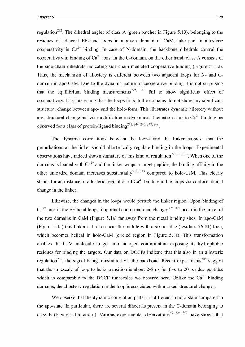
Chapter 5 128

regulation272

. The dihedral angles of class A (green patches in Figure 5.13), belonging to the

residues of adjacent EF-hand loops in a given domain of CaM, take part in allosteric

cooperativity in Ca2+

binding. In case of N-domain, the backbone dihedrals control the

cooperativity in binding of Ca2+

ions. In the C-domain, on the other hand, class A consists of

the side-chain dihedrals indicating side-chain mediated cooperative binding (Figure 5.13d).

Thus, the mechanism of allostery is different between two adjacent loops for N- and C-

domain in apo-CaM. Due to the dynamic nature of cooperative binding it is not surprising

that the equilibrium binding measurements282, 301

fail to show significant effect of

cooperativity. It is interesting that the loops in both the domains do not show any significant

structural change between apo- and the holo-form. This illustrates dynamic allostery without

any structural change but via modification in dynamical fluctuations due to Ca2+

binding, as

observed for a class of protein-ligand binding241, 244, 245, 248, 249

.

The dynamic correlations between the loops and the linker suggest that the

perturbations at the linker should allosterically regulate binding in the loops. Experimental

observations have indeed shown signature of this kind of regulation77, 302, 303

. When one of the

domains is loaded with Ca2+

and the linker wraps a target peptide, the binding affinity in the

other unloaded domain increases substantially302, 303

compared to holo-CaM. This clearly

stands for an instance of allosteric regulation of Ca2+

binding in the loops via conformational

change in the linker.

Likewise, the changes in the loops would perturb the linker region. Upon binding of

Ca2+

ions in the EF-hand loops, important conformational changes274, 304

occur in the linker of

the two domains in CaM (Figure 5.1a) far away from the metal binding sites. In apo-CaM

(Figure 5.1a) this linker is broken near the middle with a six-residue (residues 76-81) loop,

which becomes helical in holo-CaM (circled region in Figure 5.1a). This transformation

enables the CaM molecule to get into an open conformation exposing its hydrophobic

residues for binding the targets. Our data on DCCFs indicate that this also in an allosteric

regulation265

, the signal being transmitted via the backbone. Recent experiments305

suggest

that the timescale of loop to helix transition is about 2-5 ns for five to 20 residue peptides

which is comparable to the DCCF timescales we observe here. Unlike the Ca2+

binding

domains, the allosteric regulation in the loop is associated with marked structural changes.

We observe that the dynamic correlation pattern is different in holo-state compared to

the apo-state. In particular, there are several dihedrals present in the C-domain belonging to

class B (Figure 5.13c and d). Various experimental observations69, 306, 307

have shown that

Chapter 5 129

several target peptides, binding to a particular domain of holo-CaM, prefer the C-domain to

the N-domain which indicates greater activity of the C-domain. Therefore, the class B

dihedrals in C-domain may be signature of its higher-target binding activity compared to the

N-domain. This idea is substantiated by the fact that this communication is formed mainly

between the dihedrals of side-chains which control the binding processes. The dynamically

cross-correlated side-chains in the C-domain loops would have role in any allostery

associated with the peptide binding process.

Our studies indicate that the changes in dynamical correlation patterns reflect the

allosteric regulations, albeit via non-Markovian processes. The conventional Markovian

behaviour may be retrieved only in the large time limit105

after the dynamical correlations

have decayed sufficiently. This clearly shows the limitation of Markovian models to explain

allosteric regulation. In particular, the long-time Markovian behaviour of dihedral

fluctuations assumed in earlier works105, 308

is not necessarily valid as shown by the DACFs

in our studies. The allosteric signalling timescale is much shorter (< 10 ns)105

, indicating that

the non-Markovian dynamical behaviours, observed in our studies at these timescales, should

also be relevant in allosteric regulation. Such non-Markovian dynamics would be ubiquitous

in biomacromolecular systems where a host of complex and heterogeneous dynamical

processes309

take place. The treatment of non-Markovian dynamics is one of the most

challenging problems in non-equilibrium statistical mechanics254

. However, since we probe

directly the dynamical correlation among the conformational variables, our studies yield a

very general picture of allosteric regulation based on the changes of dynamical correlation

pattern, even if the underlying dynamical fluctuations may be non-Markovian. Moreover,

unlike very long simulation trajectories required to ensure the Markovian process, the non-

equilibrium fluctuation of the dihedral angles can be captured with much shorter simulation

runs. The novelty of our method lies in the fact that we liberate the microscopic picture of

allosteric regulation, with modest computational efforts, from the current Markovian

assumptions105

. However, to study the allostery associated with slow domain motions one

would require very long simulations, although our method of analysis should hold good in

such situations as well. Direct identification of allosterically regulated conformational

variables represents significant advancement in microscopic understanding of allostery in

biomacromolecules.

5.6 Conclusion

To summarize, we have shown that the entire thermodynamic changes in

biomacromolecular conformations can be extracted from the distributions of the dihedral

Chapter 5 130

angles using the HBM. We reproduce the experimentally observed correlation between the

conformational and binding entropies and quantify the thermodynamic contributions of

different binding regions for a number of CaM-peptide complexes. The histograms would be

sensitive to any quantity that undergoes changes upon binding. Hence the present analysis

can suitably be extended to calculate thermodynamic changes in the solvent and any other

macromolecular complex like protein-protein, protein-DNA or protein-ligand complexes. The

detailed thermodynamic information of the binding regions would enable us to identify the

prime spots of binding, facilitating the manipulation of the macromolecules required for

various applications such as drug design, drug delivery and so forth.

We employed the HBM83

to also study the conformational thermodynamic for Ca2+

ion binding to CaM. We estimate the quantitative information of conformational changes at

each residue including the different metal binding domains. The N-domain undergoes a

higher conformational ordering and stabilization compared to the C-domain. The Ca2+

ion

binding loops I, II and IV are qualitatively similar with respect to conformational changes,

while loop III is significantly different from them undergoing only nominal stabilization and

enhanced disorder due to the metal-ion binding. Our results at the level of individual residues

indicate that the loop residues including those coordinating to the metal-ions dominate the

overall changes in the loops. Apart from the loops, the linker, far away from the metal

binding sites, undergoes substantial stabilization and ordering as it becomes a long helix in

holo-state. One can readily apply the HBM to understand the microscopic picture of metal-

ion binding induced changes in any protein to characterize different metal binding regions.

Finally, we show that the cosine of the dihedral angles for successive equilibrium

configurations sampled from MD runs forms a convenient time-series for calculations of the

dynamic correlations between the dihedral angles80

. The dynamical correlation functions

yield the microscopic nature of coupling among different degrees of freedom belonging to

distant sites in biomacromolecules, highlighting their roles in allosteric regulations. The

extraction of dynamical correlation depends on the computation of convenient time-series of

the associated dynamical variable. Such correlation functions can be extended to any set of

dynamical variables which may provide a unified microscopic insight into non-equilibrium

phenomena in biological systems.

Chapter 5 131

Appendices

Calculation of order parameters

In order to calculate the long-axis order parameters 2

MeS of the side-chain methyl

groups in CaM-peptide complexes we follow the methods described in Yang et al93

and

Krishnan et al291

. One such methyl group is schematically shown in Figure A2. First, all the

backbone CA (-carbon) atoms in the equilibrium configurations of the complex are fitted to

the backbone CA atoms in the average structure calculated over the equilibrium trajectory.

This way the effect of rotation of the whole complex is removed. This is done using the VMD

program288

. The resultant aligned configurations are then subjected to the calculation of 2

MeS

values. The generalized order parameter for the methyl long-axis is given by 291

the following

expression:

2/12222/32222

22

22

22

zxyzxyzyxSMe

where cos)sin( x , sin)sin( y and )cos( z , being the polar angle

and , the dihedral angle as shown in Figure A2. The angular brackets represent ensemble

averages over 10000 equilibrium configurations.

Figure A1: Root mean square deviation (RMSD) during simulations. Free CaM and two

representative cases of the nNOS and smMLCK complex. Note the larger fluctuations in

case of free CaM as it is free to move in the solution. Fluctuations are suppressed a lot in

the complexes due to binding of the peptide which is evident from the RMSDs of the

complexes.

Chapter 5 132

Figure A2: Schematic representation of a side-chain methyl group. The associated polar

angle and dihedral angle are shown. Here A is the methyl carbon atom (A = CB for Ala,

CG or CD for Ile, CD1 or CD2 for Leu, CE for Met, CG2 for Thr and CG1 or CG2 for Val). The

other atoms B, C and D represent other heavy atoms which are determined by the residue

identity.

Figure A3: Methyl order parameter data. 2

MeS for nNOS complex and smMLCK complex are

shown (a,c) for CaM and (b,d) for the peptide. The symbol and line descriptions are the

same as those in Figure 5.2.

Chapter 5 133

Figure A4: Methyl order parameter data. 2

MeS for CaMKI complex and CaMKK complex are

shown (a,c) for CaM and (b,d) for the peptide. The symbol and line descriptions are the

same as those in Figure 5.2.

Figure A5: Surface representations of six CaM-peptide complexes showing the residue-

wise (a) Gconf; (b) Sconf of CaM. Two views separated by 180 rotation about vertical axis

are shown in each case. The stabilized residues are green and destabilized ones are red.

The residues undergoing minor changes are white. Peptide is in violet cartoon

representation.

Chapter 5 134

Figure A6: The time-variation of methyl order parameters. CaM

cMeS 2 and peptide

cMeS 2

(average over available methyl groups) during the simulations for CaM and peptide in

several complexes. (a) For CaM in eNOS and smMLCK complexes. These values remain

similar throughout the entire equilibrium trajectory in both cases. (b) For the peptides in

eNOS and smMLCK complexes. Here convergence is slower than for protein. The

convergence in smMLCK is poorer than eNOS. This could be attributed to the fact that this

peptide has only 8 methyls, which is fewest among all the peptides considered here. (c)

Data for DAPK2-complex. Here, the CaM-data are similar throughout the trajectory, while

the peptide-data converge beyond 12 ns.

Figure A7: The methyl order parameters of CaM-DAPK2 complex. (a) CaM and the (b)

peptide data, predicted from our simulations. The different types of methyl groups are

represented by different colours as shown in the legend.

Chapter 5 135

Figure A8: Comparison of methyl order parameters of holo-CaM. The experimental 2

MeS

(expt)281 vs. calculated 2

MeS (calc) from our simulation. Few overestimations in S2 are

observed due to limitations of the force fields291, 292.

Figure A9: Methyl order parameters in apo- and holo-CaM. Residues (a) 5-75, (b) 76-146.

.

Figure A10: Change in methyl order parameters from apo- to holo-CaM.

)apo()holo( 222

MeMeMe SSS values for different CaM residues.

Chapter 6 136

Chapter 6 Thermodynamics of interfacial changes in a protein-protein complex

6.1 Introduction

Biomacromolecules often share large interfacial area310

to facilitate formation of

stable complexes. Recent experiments75, 106, 311

suggest that structural modifications at the

interface play pivotal role at times both in the stability of such complexes and functional

activities106

of the associated biomacromolecules. From structural studies311-313

several

qualitative aspects, like formation of salt bridges and water-mediated contacts, changes in

secondary-structure elements and so on, associated with the biomacromolecular interfaces

have been determined. However, there is hardly any quantification of the thermodynamics of

these interfacial changes. Quantitative information about the interface at the microscopic

level is of immense importance, not only for understanding the binding mechanism, but also

for development of functionally potent biomacromolecules via manipulation of the interfacial

interactions314, 315

.

The interfacial changes in biomacromolecular complexes are primarily derived from

the conformational changes of the binding partners. The advancements with NMR relaxation

experiments92-95

provide a scope of estimating the conformational entropy change for

biomacromolecular complexation. These measurements highlight the importance of

conformational changes in the binding interface75

. Similarly, computer simulations offer a

very powerful tool to study the microscopic details of the biomacromolecules79-81, 83, 86

. In

chapter 5, we have shown that the conformational thermodynamics can be extracted from

various backbone and side-chain dihedral angles of the amino acid residues in a protein. The

equilibrium distributions of different dihedral angles in the complex and the free components

are calculated from all-atom MD simulations. Comparing these distributions in the free and

the complexed states, one can estimate the changes in conformational entropy ( confS ) as

well as the conformational free energy ( confG ) for binding. Via this histogram based method

(HBM)83

a comparable confS as derived from the NMR experiments, can easily be

calculated. The additional advantage of this methodology enables us to quantitative

estimation83

of the conformational changes at different binding regions for a number of

protein-peptide complexes.

Other than the proteins or nucleic acids, the biomacromolecular interface quite often

contains water molecules. These water molecules which could be integral parts of the

Chapter 6 137

interfaces316

, not only help in the formation of the hydrogen bonding between the

biomacromolecular chains106

, but also modulate the specificity and the affinities of

binding317-320

. Sometimes even a small number of water molecules are found to play key role

in driving the whole binding process321

. The thermodynamics for displacement of waters in a

model cavity with specific electrical property by an incoming ligand has been studied in

detail321-323

to reveal significant contribution of these interfacial water molecules in the

overall binding thermodynamics. In practice the situation in biomacromolecular interfaces are

very complex, with competition between the hydrophobic and hydrophilic interactions.

In the present chapter we apply the HBM83

to quantify the thermodynamics of

interfacial conformational changes in a protein-protein complex between an enzyme Nuclease

A (NucA) 324

and its specific inhibitor325

NuiA, a protein (Figure 6.1). NucA, a sugar non-

specific nuclease from Anabaena sp., is one of the most active nucleases known326, 327

from a

class of nucleases containing DRGH structure motif. These nucleases, having the capacity to

hydrolyze nucleic acids without any base-preference327

, are very important for their roles in

host defence mechanisms328

providing nutrients to host, DNA-drug binding329

, RNA

sequencing330

, cellular apoptosis331

and so on. NuiA, an intrinsic inhibitor, deactivates NucA

specifically326

via formation of a 1:1 complex332

with a high stability constant (> 109 M

-1)326,

333. These enzymes require divalent metal-ion cofactor (like Mn

2+, Mg

2+) at the active-site to

function. The crystal structure data of the NucA-NuiA complex106

reveals the conformational

changes of NucA and NuiA compared to their free forms107, 334

. The crystal structure also

indicates the presence of water molecule mediated interactions at the interface, accompanied

by changes in tertiary structural fold of NuiA. We extend the HBM to estimate the

thermodynamic contributions due to the interfacial water molecules present in the NucA-

NuiA complex. Here the relevant probability distribution is the pair distribution function111

g(r) for the water molecules which gives the probability of finding the centres of mass of a

pair of molecules at given separation r.

Our data on confS and confG corroborate well with the known structural

information106, 333

on the enzyme-inhibitor interfacial region (Figure 6.1). The binding is

primarily dominated by electrostatic interactions at the interface, as indicated106

by the high

ordering and stabilizations of the basic interfacial residues of NucA and acidic interfacial

residues of NuiA. From the generalization of the HBM for interfacial waters we also find that

the entropy cost due to the water molecules is substantial. These water molecules are

dynamically arrested at the locked jaw interface in NucA-NuiA complex which demonstrates

the tight binding of the inhibitor to the enzyme. Our results quantitatively bring out the local

Chapter 6 138

order and stabilities of the enzyme-inhibitor interaction sites due to complexation which has

been hitherto known only qualitatively from structural data. Moreover, the complete

microscopic picture from our calculation predicts some more residues which could be

important in the inhibitor binding to the enzyme.

Figure 6.1: Cartoon representation of the NucA (white) – NuiA (violet) complex. The side-

chains of the interfacial residues, coluored in purple, are shown using stick

representation. The region enclosed by dashed line, representing the interface, is

zoomed where the important basic NucA residues (regular labels) and acidic NuiA

residues (italicized labels) are shown.

6.2 Methods

6.2.1 Simulation details

MD simulations of free NucA (PDB 1ZM8), free NuiA (PDB 1J57) and the NucA-

NuiA complex (PDB 2O3B) are performed with explicit water and counter ions at 300 K

using same methods and protocols as described in the previous chapter. The active-site

divalent metal-ion of NucA in 1ZM8 is Mn2+

, while that in 2O3B is Mg2+

. However, hardly

any difference is observed107

in the residue arrangements and coordination geometry around

Mg2+

or Mn2+

. Therefore, we proceed with these available structures. We use 50 ns

trajectories for our analyses to compute the normalized histograms of the dihedral angles

from equilibrated configurations sampled beyond 10 ns.

6.2.2 Thermodynamics from HBM

Extending Eq. 5.7 for NucA (N) and NuiA (I), the total conformational free energy

change for complexation can be written as:

)()( I

conf

N

conf

tot

conf GGG , (6.1)

Chapter 6 139

where )](/)(ln[)( max,max, f

N

c

NB

N

conf HHTkG and

)](/)(ln[)( max,max, f

I

c

IB

I

conf HHTkG , and are the dihedral angles of N and I

respectively. Here the summations are over all dihedrals and the subscript „max‟ denotes

maximum of histogram. Similarly, the conformational entropy change83

, using the Gibbs

formula,

)](ln)()(ln)([)( i

f

i

f

i

i

c

i

c

iBconf HHHHkS (6.2)

i being the bin-index of the histograms.

6.2.3 HBM for interfacial water molecules

Next we extend the HBM to estimate the free energy and entropy costs associated

with the changes of interfacial water distribution. We calculate g(r) for the interfacial water

(iw) molecules within 5 Å of the interfacial residues in the complex ( )(rg c), and those within

5 Å of the binding regions of the free enzyme ( )(rg f

N ) and inhibitor ( )(rg f

I ). Here r is the

separation between the O-atoms of two water molecules. The free energy cost is given by

straightforward extension of Eq. 6.1:

)}]()(/{)(ln[ max,max,max rgrgrgTkG f

I

f

N

c

Biw

(6.3)

where the peak values in the respective g(r) are used. The corresponding entropy cost ( iwST

) is obtained using the Gibbs formula as in Eq. 6.2:

]lnlnln[ ,,,, i

f

iI

f

iI

i

f

iN

f

iN

i

c

i

c

iBiw ggggggkS (6.4)

where the the sum has been taken over non-zero bins marked by the index i.

6.2.4 Dynamics of Interfacial water molecules

To capture any change in the dynamics of the active-site waters (asw) we determine

their diffusion behavior from the self-part of Van-Hove correlation function (VHCF)111

defined at time t as:

i

iiasws tNtrG ))()0(()/1(),( rrr , (6.5)

where Nasw is the total number of active-site waters and )(tir represents the position vector of

the oxygen atom of the ith water molecule. The angular brackets here designate average over

10000 initial configurations. At long-times (t ~ 100 times larger than the diffusion time scale

required for a tagged water to traverse the length of its diameter) the self-VHCF behaves like

Chapter 6 140

a Gaussian111

: ])(exp[)/)((),( 22/3 rtttrGs where the time-dependent parameter (t)

~ 1/4Daswt, Dasw being the self-diffusion coefficient of the water molecules. We plot 1/(t) as

a function of t and Dasw is obtained from the slope of the best linear fit.

6.3 Results

The RMSD are followed in each simulation to ensure the equilibration (Figure 6.2).

The equilibrium correlations among different dihedral angles in the NucA-NuiA complex

turn out to be negligible (Figure 6.3) as in the previous chapter, so that we consider them as

independent conformational variables for the calculation of thermodynamics.

Figure 6.2: RMSD of free NucA, NuiA and the complex as function of simulation time (t).

Figure 6.3: Simulation data on NucA-NuiA complex. (a) Variation of RMSD of free NucA,

free NuiA and the complex as functions of simulation time (t). (b) Equilibrium -

correlations among dihedral angles given by sC where s denotes the separation

between the locations of the residues having dihedrals and .

Few sample histograms of dihedral angles are shown in Figure 6.4 showing similar

behaviour, as in the previous chapter, for both backbone (Figure 6.4a-b) and side-chain

(Figure 6.4c-d) dihedral angles. The peak values of the histograms generally increases upon

binding, indicating decrease in fluctuations of the dihedrals from free to the bound state.

Chapter 6 141

Multi-modal histograms are observed here also as illustrated in Figure 6.4d for of Thr135

of NuiA which shows two broad peaks in free state, indicating two rotamers, reduce to one

sharp peak in the bound state after binding to active-site metal-ion.

Figure 6.4: Sample histograms of dihedrals of different residues in free and bound states.

Histogram of (a) in NucA residue Arg93, (b) in NuiA residue Glu24, (c) in NucA

residue Asn155 and (d) histogram of in NuiA residue Thr135.

After taking a close look at our data on histograms we elaborate different aspects of

the thermodynamic changes in the NucA-NuiA complex. Decrease in free energy indicates

gain in stability, whereas drop in entropy suggests ordering.

Overall conformational changesWe estimate the total conformational free energy

cost of NucA-NuiA complexation tot

confG = 138.2 kJ mol-1

. NuiA gets stabilized by kJ

mol-1

which is about double the contribution of NucA towardstot

confG . Similarly, the total

conformational entropy cost for the NucA-NuiA complexation tot

confST = kJ mol-1

.

The individual contribution by NucA is 148.3 kJ mol-1

and that by NuiA is 323.3 kJ mol-1

,

again almost twice that of NucA as in conformational free energy contributions. The 240

residue protein NucA experiences a very small confG or confST value per residue (< 1 kJ

mol-1

) which quantifies the experimentally observed 106

little conformational change of NucA

upon inhibitor binding. On the other hand, for the 135 residue inhibitor protein NuiA, the

confG value per residue is small (< 1 kJ mol-1

) but the confST per residue is quite large (~

2.4 kJ mol-1

).

Chapter 6 142

A large contribution to the tot

confST in NuiA is due to the striking difference between

the tertiary structures of bound NuiA (Figure 6.5a) and free NuiA (Figure 6.5b), reflected in

the lowered spatial separation across the hinge-like structure of the molecule in the bound

state. This occurs via rotation of the longest helix in NuiA around the normal to its helical

axis to facilitate (i) coordination with the active-site of NucA via one end of the hinge and (ii)

formation of a salt-bridge with NucA at the other end. The two helices constituting the hinge-

like structure become heavily ordered in the enzyme-bound form (Figure 6.5a): confST

19.7 kJ mol-1

for the 12-residue shorter helix (residues 5-16) and confST 74.5 kJ mol-1

for the 20-residue longer helix containing residues 79-98. This stabilization is because of the

formation of a hydrophobic core in the space between these two helices in bound NuiA by the

side-chains of six residues as shown in Figure 6.5a. Each of these six residues participating in

this hydrophobic region undergoes huge ordering ( i

confST 4 to 11 kJ mol-1

) to result in a

total entropy change of confST 48.3 kJ mol-1

, further stabilizing the hinge.

Figure 6.5: Cartoon representations of bound and free NuiA. (a) Enzyme bound NuiA and

(b) free NuiA showing the changes in the hinge-like region. The side-chains of the

residues forming a hydrophobic core between the two helices in the hinge are also shown

using stick representations.

Conformational changes at interfaceIf we now consider the conformational changes

associated with complexation, the region which will definitely require attention is the

interface (Figure 6.1). The enzyme-inhibitor interface consists of the residues of NucA and

NuiA within 5Å separations. This is an open-jaw like interface, consisting of: (i) the active-

site of NucA, (ii) the second interaction-site containing the salt-bridge and (iii) other NucA

and NuiA residues in contact through either direct or water-bridged hydrogen bonding

Chapter 6 143

interactions106

. The conformational entropy and free energy changes of all interfacial residues

are shown in Figure 6.6a-b.

Figure 6.6: Surface representations of the complex showing the interfacial

thermodynamics data and contributions of different types of residues. (a)

conformational entropy and (b) free energy costs of all the interfacial residues (only

side-chains shown via sticks). Colour description: residues coloured green if i

confST or

i

confG < kJ mol-1, cyan for ~ 1.3 to 3.8 kJ mol-1, yellow for ~ +1.3 to +3.8 kJ mol-1,

red for > +3.8 kJ mol-1 and left uncoloured for negligible changes. (c) The conformational

entropy and (d) free energy changes of different types of residues at NucA-NuiA interface

are shown along with the total interfacial contributions of the respective system.

The conformational entropy and free energy contributions of the different types of

residues in the interfacial region are shown in Figure 6.6c and d. The basic residues of NucA

and acidic residues of NuiA undergo maximum stabilization and ordering out of all

interfacial residues. In Table 6.1, we list the i

confST and

i

confG of these interfacial charged

residues whose locations are shown in Figure 6.1. The stabilizations and ordering of the polar

side-chain containing residues at the interface are also significant, while the changes in any

other type of interfacial residues are negligible. All these observations quantitatively confirm

that the enzyme-inhibitor interaction is predominantly electrostatic as suggested from the

crystal structure of the complex106

. We now take a close look at the interface.

The active-site region is shown in Figure 6.7a-b where the side-chains of different

metal-ion coordinating and neighbouring residues are labelled according to their i

confST

(Figure 6.7a) and i

confG (Figure 6.7b) values. Here, four water molecules coordinate to the

Chapter 6 144

metal-ion Mg2+

along with the side-chain of Asn155 (i

confST = kJ mol-1

and i

confG =

kJ mol-1

) of NucA and the terminal residue of NuiA, Thr135 (i

confST = kJ mol-1

and i

confG = kJ mol-1

). A neighbouring NucA residue Arg93, believed to participate in

transition state stabilization, undergoes a significant rearrangement of its side-chain106

and

experiences high ordering and stabilization. A few more highly stabilized and ordered

residues in the active-site are tabulated in Table 6.1. They are mostly the hydrogen bonded

residues involved in nucleolytic activity or its inhibition such as His124, Arg156, Glu163 of

NucA and Glu24 of the inhibitor. The roles of Arg93, His124 and Glu163 in substrate

binding to NucA have already been emphasized earlier via mutational studies333

where

significant decrease in enzymatic activity have been observed upon mutation of any of these

residues. Furthermore, Glu24 (NuiA) induced decrease in inhibition has also been reported

earlier106

.

Table 6.1: The conformational entropy and free energy changes (in kJ mol-1) of interfacial

basic residues of NucA and acidic residues of NuiA. Lys202 is a non-interface residue, but

included here for its large entropy change.

NucA residue i

confST i

confG NuiA residue i

confST i

confG

Arg93 Glu24

Arg98 Glu26

Lys101 Asp75

Arg122 Glu80

His124 Glu81

Arg156 Glu109

Arg167 Glu111

Lys202 Glu134

The second interaction-site in the open-jaw type NucA-NuiA interfacial structure is

shown in Figure 6.7c-d. The side-chains of the salt-bridge forming Lys101 (NucA) and

Asp75 (NuiA) are marked along with those of some neighbouring residues. Both of these

residues are highly ordered (Table 6.1) indicating the strong attractive interaction. Several

neighbouring residues in NuiA Gln74 (i

confST = kJ mol-1

), Trp76 (i

confST = kJ

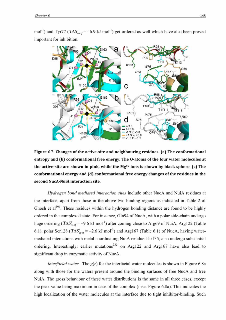
Chapter 6 145

mol-1

) and Tyr77 (i

confST = kJ mol-1

) get ordered as well which have also been proved

important for inhibition.

Figure 6.7: Changes of the active-site and neighbouring residues. (a) The conformational

entropy and (b) conformational free energy. The O-atoms of the four water molecules at

the active-site are shown in pink, while the Mg2+ ions is shown by black sphere. (c) The

conformational energy and (d) conformational free energy changes of the residues in the

second NucA-NuiA interaction site.

Hydrogen bond mediated interaction sites include other NucA and NuiA residues at

the interface, apart from those in the above two binding regions as indicated in Table 2 of

Ghosh et al106

. These residues within the hydrogen bonding distance are found to be highly

ordered in the complexed state. For instance, Gln94 of NucA, with a polar side-chain undergo

huge ordering (i

confST = kJ mol-1

) after coming close to Arg69 of NuiA. Arg122 (Table

6.1), polar Ser128 (i

confST = kJ mol-1

) and Arg167 (Table 6.1) of NucA, having water-

mediated interactions with metal coordinating NuiA residue Thr135, also undergo substantial

ordering. Interestingly, earlier mutations333

on Arg122 and Arg167 have also lead to

significant drop in enzymatic activity of NucA.

Interfacial waterThe g(r) for the interfacial water molecules is shown in Figure 6.8a

along with those for the waters present around the binding surfaces of free NucA and free

NuiA. The gross behaviour of these water distributions is the same in all three cases, except

the peak value being maximum in case of the complex (inset Figure 6.8a). This indicates the

high localization of the water molecules at the interface due to tight inhibitor-binding. Such

Chapter 6 146

localization leads to a substantial drop of entropy ( iwST ~ kJ mol-1

for about 300

interfacial waters) with respect to the free components. However, the free energy cost turns

out to be negligible ( iwG ~ kJ mol-1

). It is interesting to compare our results to those of

an earlier study322

where the thermodynamics of cavity-ligand association for different

systems has been reported with particular emphasis on water contributions. The free energy

associated with the water molecules depends very sensitively on the property of the cavity

and the ligand. For instance, neutral ligand in positively charged cavity shows a marginal

decrease in water free energy, whereas a negatively charged ligand in a positively charged

cavity shows a large change in the water free energy322

. In our system, the electrical

properties of different residues are highly non-uniform having both positively and negatively

charged as well as polar side-chains. Such a complicated interfacial environment brings in

compensatory changes in the water free energy leading to only a marginal change.

Figure 6.8: Data on interfacial water molecules. (a) The oxygen-oxygen pair distribution

function g(r)s of the water molecules at the protein-protein interface of the complex and

around the binding regions of NucA and NuiA are shown. Inset, a close view of the peaks

in g(r)-plots. (b) The plot of 1/ as a function of time t along with the best fit line through

the points for the active-site water in complex and free NucA.

The immobilization of the water molecules at the active site of NucA in the inhibitor-

bound state is reflected in the VHCFs as well. In Figure 6.8b, we show the long-time-

behaviour of 1/ for the active-site waters in free (the filled circles) and inhibitor-bound

NucA (the open circles). Clearly, the metal-ion coordinating water molecules move away

from the active-site of free NucA as indicated by the increase in 1/. The slope of the best

linear fit through the filled circles gives us the self-diffusion coefficient Dasw of the active-site

waters. We find Dasw ~ 0.4 cm2 s

-1 which is 5 times smaller compared to the self-diffusion

coefficient in bulk water335

, but resembles the values reported for water diffusion near a

protein or a biomolecular surface335-337

. On the other hand, we observe no change of the value

Chapter 6 147

of for the active-site waters in the complex, indicating that they are arrested dynamically

with practically no diffusion.

6.4 Interpretation of results

Our results on the thermodynamic changes at the biomolecular interface of NucA-

NuiA complex shed lights on several microscopic aspects of NucA-NuiA binding:

Importance of interfacial changesIt is known106

from experimental observations that

enzymatic activity of NucA diminishes dramatically upon binding to NuiA. Therefore, it is

expected that NuiA binds either exactly or adjacent to the substrate binding sites, blocking

the binding of the substrate to the enzyme. However, isolation of substrate-bound NucA has

been unsuccessful so far due to its high activity106

. Consequently, comparison of inhibitor-

bound NucA structure has been done earlier106

with a DNA-bound NucA model structure.

The comparison reveals106

that several atoms of Glu24 and Thr135 of NuiA occupy the

positions where key atoms of DNA could have been. In our calculations, we find large

ordering and stabilization for both these NuiA residues Glu24 (Table 6.1) and Thr135.

More importantly, the fact that NucA hardly shows any activity in inhibitor-bound

form indicates that the inhibitor binding to NucA is tighter compared to the substrate binding.

Both DNA and RNA carry high negative charges. Therefore, they would prefer to interact

with the positively charged basic residues of the enzyme. From the structure106, 107

it turns out

that the binding surface of NucA offers at least seven basic residues (Table 6.1). In The

NucA-NuiA complex there are eight interfacial acidic residues of NuiA (Table 6.1) which

could satisfy all the interfacial positive charges of NucA. A DNA substrate, on the other

hand, is unlikely to satisfy all the seven positive charges on NucA interface. This is because

of the fact that in order to access the phosphate groups the DNA would have bound to the

enzyme surface through its minor groove. The space covered by NuiA at the NucA-NuiA

interface, about 31 Å in width, could be accessed at most by 4-5 phosphates present on the

approaching minor groove of the DNA, as seen from a docking of a DNA double helix on

NucA using HADDOCK338

. Similar situation also has been observed earlier in the DNA-

bound structure of Vvn nuclease (PDB 1OUP)339

where only 4 phosphates bind with the

enzyme. Thus, it is quite possible that the better electrostatic stabilization factor is

responsible for the preferential binding of the NuiA to NucA in presence of nucleic acid

molecules.

Chapter 6 148

Second interaction siteAnother very important interaction site, other than the active

site, between NucA and NuiA is the possible salt-bridge interaction106

between Lys101

(NucA)-Asp75 (NuiA) shown in Figure 6.7c and d. Measurements of the inhibition constants

with several NuiA-mutants have shown106

that the looser binding is observed when Asp75 is

replaced by an Asn or even Glu. This may be indicating that the salt-bridge is formed

possibly at an optimum separation between Lys101 (NucA) and Asp75 (NuiA) which is

altered by the mutations. Interestingly, a very similar effect is observed when there is a

double mutation106

at two adjacent residues of Asp75 (NuiA) to replace both Gln74 and

Trp76 by Ala. From our results, we find that both Lys101 (NucA) and Asp75 (NuiA) are well

ordered indicating strong attractive interaction between their side-chains. We find that several

neighbouring residues of Asp 75 (NuiA) undergo substantial ordering as well via van der

Waals interaction among their side-chains, as shown in Fig, 6.7c-d, to stabilize the loop

structure around this region. Such stabilization may lead to proper orientation of Asp75

(NuiA) to be at the optimum distance to form the salt-bridge with Lys101 (NucA).

Conformational entropy and methyl order parametersIt has been observed via NMR

relaxation experiments75

and detailed molecular simulations83

that the generalized order

parameters for methyl groups ( 2

MeS ) can provide a measure of total conformational entropy

cost of complexation tot

confST . For several calmodulin-peptide complexes75

, tot

confS has been

observed to vary linearly with the residue weighted average changes in methyl order

parameter75, 83

given by 2

MeS . Here we check whether the same linear scaling is present

here. The plot of individual conformational entropy changes of NucA (N

confS = 0.49 kJ K-1

mol-1

) and NuiA (I

confS = kJ K-1

mol-1

) against their respective 2

MeS , computed from

our simulations using earlier methods83

, yields a slope m = 0.06 which is close to the m

calculated earlier75, 83

.

Contribution of interfacial watersThe immobilization of the active-site water

molecules in the inhibitor-bound form during the entire simulation clearly demonstrates the

extent of tight-binding of the inhibitor to NucA and hence justifies the drop in interfacial

water-entropy. The binding of inhibitor leads to sufficiently heavy packing of the side-chains

at the interface of NucA and NuiA, so that the water molecules cannot escape from within or

come in from outside. These observations also support the proposed catalytic mechanism of

NucA to hydrolyze a DNA or RNA molecule 107

that the water required for hydrolysis is

provided from the coordination sphere of the active-site metal-ion, not from the bulk or the

hydration shells around the protein surface.

Chapter 6 149

Predictions on possible mutationsWe have already pointed out several interfacial

residues of NucA and NuiA which undergo large ordering and stabilization upon

complexation. Roles of many of them, like, Arg93, Arg122, His124 and Arg167 have already

been explored 333

by studying the changes in enzymatic activity of NucA after mutations of

those residues. In addition to these we predict some other interfacial residues whose roles

have not been explored via mutational studies. These are basic residue Arg98 of NucA and

acidic residues of NuiA, like, Glu109, Glu111 and Glu134. All of these residues, shown in

Figure 6.1, undergo heavy ordering upon complexation (Table 6.1). According to Table 6.1

ordering of Lys202 is also very large. This is a non-interfacial residue which is part of the six

stranded -sheet of NucA (Figure 6.1), making it an interesting candidate for such mutational

studies. Here Arg98 can have very important role in substrate binding to NucA and others

may be important in the inhibition mechanism.

6.5 Conclusion

Our studies might be the first report on the quantitative thermodynamics data of the

interfacial changes, highlighting both the conformational contributions as well as the water

contributions, due to binding of inhibitor protein NuiA to the enzyme NucA using the

HBM83

. We show that the interfacial changes are governed by the electrostatic interactions.

This supports quantitatively the idea that the inhibitor mimics the way different nucleic acid

substrates bind to NucA. The tight inhibitor binding to the enzyme leads to a heavily packed

interface with bound water molecules undergoing a large change in entropy. The HBM

depends on the shift in distributions of different degrees of freedom upon binding and should

be applicable to any biomacromolecular interface. Our study thus provides a novel route to

microscopic understanding of biomacromolecular interfaces which would help the

manipulations of interfacial properties to regulate biomacromolecular activities in general.

References 150

References

1. J. Ross and A. P. Arkin, Proc. Nat. Acad. Sci., USA 106, 6433 (2009).

2. B. Bagchi and C. Chakravarty, J. Chem. Sci. 122, 459 (2010).

3. C. J. Mundy, S. M. Kathmann, R. Rousseau, G. K. Schenter, J. VandeVondele and J.

Hutter, in SciDAC Review (USA, 2010), pp. 10-21.

4. D. G. Truhlar, J. Am. chem. Soc 130, 16824 (2008).

5. P. M. Chaikin and T. C. Lubensky, Principles of Condensed Matter Physics.

(Cambridge University Press, Cambridge, 1995).

6. M. Plischke and B. Bergersen, Equilibrium statistical physics, 3 ed. (World Scientific,

Singapore, 2006).

7. M. G. Kurnikova, N. Balabai, D. H. Waldeck and R. D. Coalson, J. Am. Chem. Soc.

120, 6121 (1998).

8. M. L. Horng, J. A. Gardecki and M. Maroncelli, J. Phys. Chem. A 101, 1030 (1997).

9. M. Maroncelli, J. Chem. Phys. 106, 1545 (1997).

10. G. S. Jas, Y. Wang, S. W. Pauls, C. K. Johnson and K. Kuczera, J. Chem. Phys. 107,

8800 (1997).

11. J. R. Lakowicz, Principles of Fluorescence Spectroscopy. (Kluwar Academic/Plenum

Publishers, New York, USA, 1999).

12. G. B. Dutt and T. K. Ghanty, J. Chem. Phys. 116, 6687 (2002).

13. G. B. Dutt and T. K. Ghanty, J. Phys. Chem. B 107, 3257 (2003).

14. L. A. Philips, S. P. Webb and J. H. Clark, J. Chem. Phys. 83, 5810 (1985).

15. R. Noyori, in Chem. Rev. (1999), Vol. 99, pp. 353-634.

16. M. P. Heitz and F. V. Bright, J. Phys. Chem. 100 (1996).

17. R. Biswas, K. Dahl and M. Maroncelli, J. Phys. Chem. B 106 (2002).

18. N. Kometani, Y. Hoshihara, Y. Yonezawa, O. Kajimoto, K. Hara and N. Ito, J. Phys.

Chem. A 108 (2004).

19. M. P. Heitz and M. Maroncelli, J. Phys. Chem. A 101, 5852 (1997).

20. R. D. Rogers and K. R. Seddon, Science 302, 792 (2003).

21. C. F. Chapman and M. Maroncelli, J. Phys. Chem. 95, 9095 (1991).

22. J. L. Dote, D. Kivelson and R. N. Schwartz, J. Phys. Chem. 85, 2169 (1981).

23. H. Jin, G. A. Baker, S. Arzhantsev, J. Dong and M. Maroncelli, J. Phys. Chem. B 111,

7291 (2007).

24. B. Halle and M. Davidovic, Proc. Natl. Acad. Sci. USA 100 (2003).

25. A. Das, R. Biswas and J. Chakrabarti, J. Phys. Chem. A 115, 973 (2011).

References 151

26. A. Das, R. Biswas and J. Chakrabarti, J. Chem. Phys. 136, 014505 (2012).

27. A. Das, R. Biswas and J. Chakrabarti, Chem. Phys. Lett. 558, 36 (2013).

28. T. W. Nee and R. Zwanzig, J. Chem. Phys. 52, 6353 (1970).

29. A. Papazyan and M. Maroncelli, J. Chem. Phys. 102, 2888 (1995).

30. K. Bhattacharyya, Chem. Commun. 2008, 2848 (2008).

31. B. Bhushan, J. N. Israelachvilli and U. Landman, Nature , 374, 607 (1995).

32. L. Bureau, Phys. rev. lett 104, 218302 (2010).

33. T.-S. Kim and R. H. Dauskardt, Nano Lett. 10, 1955 (2010).

34. T. K. Nielsen, U. Bosenberg, R. Gosalawit, M. Dornheim, Y. Cerenius, F.

Besenbacher and T. R. Jensen, ACS Nano 4, 3903 (2010).

35. R. Biswas, N. Rohman, T. Pradhan and R. Buchner, J. Phys. Chem. B 112, 9379

(2008).

36. L. Jiang, Y. Sun and X. Chen, Small 8, 333 (2012).

37. X. Pan and X. Bao, Acc. Chem. Res. 44 553 (2011).

38. C. Li, H. Zhang, D. Jiang and Q. Yang, Chem. Commun., 547 (2007).

39. P. K. Verma, A. Makhal, R. K. Mitra and S. K. Pal, Phys. Chem. Chem. Phys. 11,

8467 (2009).

40. K. Ishikawa, N. Kameta, M. Aoyagi, M. Asakawa and T. Shimizu, Adv. Funct. Mater.

23, 1677 (2013).

41. C. F. Lopez, S. O. Nielsen, P. B. Moore and M. L. Klein, Proc. Natl. Acad. Sci. USA

101, 4431 (2004).

42. A. Calvo, M. C. Fuertes, B. Yameen, F. J. Williams, O. Azzaroni and G. J. A. A.

Soler-Illia, Langmuir 26, 5559 (2010).

43. M. Fichtner, Phys. Chem. Chem. Phys. 13, 21186 (2011).

44. S. Granick, S. C. Bae, S. Kumar and C. Yu, Physics 3, 73 (2010).

45. W. H. Thompson, Annu. Rev. Phys. Chem. 62, 599 (2011).

46. M. Heuberger, M. Zach and N. D. Spencer, Science 292, 905 (2001).

47. S. H. Khan, G. Matei, S. Patil and P. M. Hoffmann, Phys. Rev. Lett 105, 106101

(2010).

48. T.-D. Li, J. Gao, R. Szoszkiewicz, U. Landman and E. Riedo, Phys. Rev. B 75,

115415 (2007).

49. J. K. Holt, H. G. Park, Y. Wang, M. Stadermann, A. B. Artyukhin, C. P.

Grigoropoulos, A. Noy and O. Bakajin, Science 312, 1034 (2006).

50. J. D. Simon, Pure & Appl. Chem. 62, 2243 (1990).

References 152

51. M. D. Elola, J. Rodriguez and D. Laria, J. Phys. Chem. B 115, 12859 (2011).

52. A. A. Vartia and W. H. Thompson, J. Phys. Chem. B 116, 5414 (2012).

53. W. H. Thompson, J. Chem. Phys. 120, 8125 (2004).

54. Z. Gemici, P. I. Schwachulla, E. H. Williamson, M. F. Rubner and R. E. Cohen, Nano

Lett. 9 1064 (2009).

55. E. Shahraeeni and D. Or, Phys. Rev. E 85, 016317 (2012).

56. P. P. Singh and M. D. A. Saldaña, Food Res. Int. 44, 2452 (2011).

57. X. Amashukeli, C. C. Pelletier, J. P. Kirby and F. J. Grunthaner, J. Geophys. Res.

112, G04S16 (2007).

58. I. Rodríguez-Meizoso, L. Jaime, S. Santoyo, F. J. Señoráns, A. Cifuentes and E.

Ibáñez, J. Pharm. Biomed. Anal. 51, 456 (2010).

59. I. Brovchenko and A. Oleinikova, J. Phys. Chem. B 115, 9990 (2011).

60. D. R. Bérard, P. Attard and G. N. Patey, J. Chem. Phys. 98, 7236 (1993).

61. K. Leung, A. Luzar and D. Bratko, Phys. Rev. Lett. 90, 065502 (2003).

62. M. C. Stewart and R. Evans, Phys. Rev. E 86, 031601 (2012).

63. R. Evans, U. M. B. Marconi and P. Tarazona, J. Chem. Phys. 84, 2376 (1986).

64. P. Graf and A. Nitzan, Chem. Phys. 235, 297 (1998).

65. A. Das and J. Chakrabarti, Phys. Rev. E 85, 050601(R) (2012).

66. A. Das and J. Chakrabarti, Microscopic mechanisms of confinement induced slow

solvation Communicated (2013).

67. A. Das and J. Chakrabarti, Solvation in nanoscale solvophobic confinement near

liquid-gas phase coexistence Communicated (2013).

68. E. Charlaix and M. Ciccotti, in Handbook of Nanophysics, edited by K. D. Sattler

(CRC Press, USA, 2011), Vol. 1.

69. R. D. Brokx, M. M. Lopez, H. J. Vogel and G. I. Makhatadze, J. Biol. Chem. 276,

14083 (2001).

70. I. Andre, T. Kesvatera, B. Jonsson, K. S. Akerfeldt and S. Linse, Biophys. J. 87, 1929

(2004).

71. S. W. Vetter and E. Leclerc, Eur. J. Biochem. 270, 404 (2003).

72. J. K. Soukup and G. A. Soukup, Curr. Opin. Struct. Biol. 14, 344 (2004).

73. W. P. Hall, J. Modica, J. Anker, Y. Lin, M. Mrksich and R. P. V. Duyne, Nano Lett.

11, 1098 (2011).

74. D. Dell’Orco, S. Sulmann, S. Linse and K.-W. Koch, Anal. Chem. 84, 2982 (2012).

References 153

75. M. S. Marlow, J. Dogan, K. K. Frederick, K. G. Valentine and A. J. Wand, Nature

Chem. Biol. 6, 352 (2010).

76. E. S. Price, M. Aleksiejew and C. K. Johnson, J. Phys. Chem. B 115, 9320 (2011).

77. H. Y. Park, S. A. Kim, J. Korlach, E. Rhoades, L. W. Kwok, W. R. Zipfel, M. N.

Waxham, W. W. Webb and L. Pollack, Proc. Natl. Acad. Sci., USA 105, 542 (2008).

78. N. J. Anthis, M. Doucleff and G. M. Clore, J. Am. Chem. Soc. 133, 18966 (2011).

79. B. J. Killian, J. Y. Kravitz and M. K. Gilson, J. Chem. Phys. 127 (2007).

80. D.-W. Li, S. A. Showalter and R. Bru¨schweiler, J. Phys. Chem. B 114, 16036 (2010).

81. H. Meirovitch, Curr. Opin. Struct. Biol. 17, 181 (2007).

82. M. Spichty, M. Cecchini) and M. Karplus, J. Phys. Chem. Lett. 1, 1922 (2010).

83. A. Das, J. Chakrabarti and M. Ghosh, Biophys. J. 104, 1274 (2013).

84. B. Jayaram, K. J. McConnell, S. B. Dixit and D. L. Beveridge, J. Comp. Phys. 151,

333 (1999).

85. M. Ghosh, G. Meiss, A. M. Pingoud, R. E. London and L. C. Pedersen, J. Biol. Chem.

282, 5682 (2007).

86. J. Wereszczynski and J. A. McCammon, Quarterly Reviews of Biophysics 45, 1

(2012).

87. W. L. Jorgensen, Nature 466, 42 (2010).

88. T. Dudev and C. Lim, Ann. Rev. Biophys. 37, 97 (2008).

89. C. Branden and J. Tooze, Introduction to Protein Structure, 2 ed. (Garland

Publishing, Inc., New York, 1999).

90. R. Mendez and U. Bastolla, Phys. Rev. Lett. 104, 228103 (2010).

91. P. Atkins and J. d. Paula, Atkins' Physical Chemistry, 8 ed. (Oxford University Press,

New York, 2006).

92. M. Akke, R. Bruschweiler and A. G. Palmer, J. Am. Chem. Soc. 115, 9832 (1993).

93. D. Yang and L. E. Kay, J. Mol. Biol. 263, 369 (1996).

94. Z. Li, S. Raychaudhuri and A. J. Wand, Protein Sci. 5, 2647 (1996).

95. T. I. Igumenova, K. K. Frederick and A. J. Wand, Chem. Rev. 106, 1672 (2006).

96. L. Ma, Z. Ahmed, A. V. Mikhonin and S. A. Asher, J. Phys. Chem. B 111, 7675

(2007).

97. N. Trbovic, J.-H. Cho, R. Abel, R. A. Friesner, M. Rance and A. G. Palmer, J. Am.

Chem. Soc. 131, 615 (2009).

98. K. H. DuBay and P. L. Geissler, J. Mol. Biol. 391, 484 (2009).

99. A. Das, J. Chakrabarti and M. Ghosh, Chem. Phys. Lett. In Press (2013).

References 154

100. Y. Ye, H.-W. Lee, W. Yang, S. Shealy and J. J. Yang, J. Am. Chem. Soc. 127, 3743

(2005).

101. G. Wu, Z. Gao, A. Dong and S. Yu, Int. J. Biol. Macromol. 50 1011 (2012).

102. A. Das, M. Ghosh and J. Chakrabarti, Dynamic correlation among allosterically

regulated conformational variables in biomacromolecules Communicated (2013).

103. V. J. Hilser, J. O.Wrabl and H. N. Motlagh, Annu. Rev. Biophys. 41, 585 (2012).

104. K. Gunasekaran, B. Ma and R. Nussinov, Prot. Struct. Func. Bioinf. 57, 433 (2004).

105. D. Long and R. Bruschweiler, J. Am. Chem. Soc. 133, 18999 (2011).

106. M. Ghosh, G. Meiss, A. Pingoud, R. E. London and L. C. Pedersen, J. Biol. Chem.

282, 5682 (2007).

107. M. Ghosh, G. Meiss, A. Pingoud, R. E. London and L. C. Pedersen, J. Biol. Chem.

280, 27990 (2005).

108. A. Das, J. Chakrabarti and M. Ghosh, Thermodynamics of interfacial changes in a

protein-protein complex Communicated (2013).

109. R. Biswas, J. E. Lewis and M. Maroncelli, Chem. Phys. Lett. 310 (1999).

110. W. Song, N. Patel and M. Maroncelli, J. Phys. Chem. B 106 (2002).

111. J. P. Hansen and I. R. McDonald, Theory of Simple Liquids, 3 ed. (Academic, San

Diego, 2006).

112. C. G. Gray and K. E. Gubbins, Theory of Molecular Fluids. (Oxford University Press,

New York, 1984).

113. N. Balabai, A. Sukharevsky, I. Read, B. Strazisar, M. Kurnikova, R. S. Hartman, R.

D. Coalson and D. H. Waldeck, J. Mol. Liq. 77, 37 (1998).

114. P. V. Kumar and M. Maroncelli, J. Chem. Phys. 112 (2000).

115. M. G. Kurnikova, D. H. Waldeck and R. D. Coalson, J. Chem. Phys. 105, 628 (1996).

116. Y. Marcus, Chem. Rev. 88, 1475 (1988).

117. J. L. deGrazia, T. W. Randolph and J. A. O'Brien, J. Phys. Chem. A 102 (1998).

118. T. A. Betts, J. Zagrobelny and F. V. Bright, J. Am. Chem. Soc. 114 (1992).

119. F. Ingrosso, B. M. Ladanyi, B. Mennucci and G. Scalmani, J. Phys. Chem. B 110

(2006).

120. N. Kometani, S. Arzhantsev and M. Maroncelli, J. Phys. Chem. A 110 (2006).

121. J. E. Lewis, R. Biswas, A. G. Robinson and M. Maroncelli, J. Phys. Chem. B 105

(2001).

122. T. Gaskell, U. Balucani, M. Gori and R. Vallauri, Phys. Scr. 35 (1987).

References 155

123. M. P. Allen and D. J. Tildsley, Computer Simulation of Liquids. (Clarendon Press,

Oxford, 1987).

124. R. Biswas and J. Chakrabarti, Journal of Physical Chemistry B 111, 13743 (2007).

125. M. L. Horng, J. A. Gardecki, A. Papazyan and M. Maroncelli, J. Phys. Chem. 99,

17311 (1995).

126. C. R. Cantor and P. R. Schimmel, Biophysical Chemistry. (W. H. Freeman, New

York, 1980).

127. A. Mukherjee and B. Bagchi, Curr. Sci. 91 (2006).

128. R. Ramirez, R. Gebauer, M. Mareschal and D. Borgis, Physical Review E 66 (2002).

129. A. Mukherjee and B. Bagchi, Chem. Phys. Lett. 404, 409 (2005).

130. J. B. Hubbard and P. G. Wolynes, J. Chem. Phys. 69, 998 (1978).

131. P. Madden and D. Kivelson, J. Phys. Chem. 86, 4244 (1982).

132. G. v. d. Zwan and J. T. Hynes, J. Phys. Chem. 89, 4181 (1985).

133. P. Brito and P. Bordewijk, Mol. Phys. 39, 217 (1980).

134. D. S. Alavi and D. H. Waldeck, J. Chem. Phys. 94, 6196 (1991).

135. D. S. Alavi, R. S. Hartman and D. H. Waldeck, J. Chem. Phys. 94, 4509 (1991).

136. D. S. Alavi, R. S. Hartman and D. H. Waldeck, J. Chem. Phys. 95, 6770 (1991).

137. B. Bagchi and R. Biswas, Adv. Chem. Phys. 109 (1999).

138. R. Biswas, S. Roy and B. Bagchi, Phys. Rev. Lett. 75, 1098 (1995).

139. R. Biswas and B. Bagchi, J. Chem. Phys. 106, 5587 (1997).

140. R. Biswas and B. Bagchi, J. Am. Chem. Soc. 119, 5946 (1997).

141. B. Bagchi and R. Biswas, Acc. Chem. Res. 31, 181 (1998).

142. H. K. Kashyap, T. Pradhan and R. Biswas, J. Chem. Phys. 125, 174506 (2006).

143. S. Daschakraborty and R. Biswas, Chem. Phys. Lett. 510, 202 (2011).

144. H. Jin, B. O'Hare, J. Dong, S. Arzhantsev, G. A. Baker, J. F. Wishart, A. J. Benesi and

M. Maroncelli, J. Phys. Chem. B 112, 81 (2008).

145. L. Karve and G. B. Dutt, J. Phys. Chem. B 115, 725 (2011).

146. K. Fruchey and M. D. Fayer, J. Phys. Chem. B 114, 2840 (2010).

147. K. Iwata, M. Kakita and H. Hamaguchi, J. Phys. Chem. B 111, 4914 (2007).

148. D. C. Khara and A. Samanta, PCCP 12, 7671 (2010).

149. T. R. Kirkpatrick, Phys. Rev. Lett. 53, 1735 (1984).

150. T. R. Kirkpatrick, J. Non. Cryst. Solids 75 () 437 (1985).

151. E. G. D. Cohen, B. Kamgar-Parsi and I. M. D. Schepper, Phys. Lett. 114, 241 (1986).

152. H. Kovacs, J. Kowalewski, A. Maliniak and P. Stilbs, J. Phys. Chem. 93, 962 (1989).

References 156

153. D. J. Evans and G. P. Morriss, Statistical Mechanics of Nonequilibrium Liquids.

(Academic Press, London London, 1990).

154. A. Lagendijk, Physica B 83, 283 (1976).

155. L. X. Dang, J. Chem. Phys. 110, 10113 (1999).

156. D. W. McCall, D. C. Douglass and E. W. Anderson, J. Chem. Phys. 31, 1555 (1959).

157. G. Guevara-Carrion, C. Nieto-Draghi, J. Vrabec and H. Hasse, J. Phys. Chem. B 112,

16664 (2008).

158. S. Girard and F. Muller-Plathe, Mol. Phys. 101, 779 (2003).

159. Y. Marcus, The Properties of Solvents. (John Wiley & Sons Ltd, Chichester, England,

1999).

160. L. X. Dang and T.-M. Chang, J. Chem. Phys. 119, 9851 (2003).

161. S. Patel and C. L. BrooksIII, J. Chem. Phys. 123, 164502-1 (2005).

162. A. B. Roney, B. Space, E. W. Castner, R. L. Napoleon and P. B. Moore, J. Phys.

Chem. B 108, 7389 (2004).

163. L.-M. Wang and R. Richert, J. Chem. Phys. 120, 11082 (2004).

164. J. A. Ingram, R. S. Moog, N. Ito, R. Biswas and M. Maroncelli, J. Phys. Chem. B 107,

5926 (2003).

165. N. Ito, S. Arzhantsev, M. Heitz and M. Maroncelli, J. Phys. Chem. B 108, 5771

(2004).

166. P. V. Kumar and M. Maroncelli, J. Chem. Phys. 103 (1995).

167. D. Y. C. Chan, D. J. Mitchell and B. W. Ninham, J. Chem. Phys. 70, 2946 (1979).

168. C. S. Santos, N. S. Murthy, G. A. Baker and E. W. Castner-Jr, J. Chem. Phys. 134,

121101 (2011).

169. O. Russina, A. Triolo, L. Gontrani, R. Caminiti, D. Xiao, L. G. Hines, R. A. Bartsch,

E. L. Quitevis, N. Plechkova and K. R. Seddon, J. Phys.: Condens. Matter 21 424121

(2009).

170. O. Borodin and G. D. Smith, J. Phys. Chem. B 110, 11481 (2006).

171. L. J. A. Siqueira and M. C. C. Ribeiro, J. Phys. Chem. B 111, 11776 (2007).

172. H. K. Kashyap, C. S. Santos, H. V. R. Annapureddy, N. S. Murthy, C. J. Margulis and

E. W. Castner-Jr, Faraday Discuss. 154, 133 (2012).

173. S. Li, J. L. Banuelos, J. Guo, L. Anovitz, G. Rother, R. W. Shaw, P. C. Hillesheim, S.

Dai, G. A. Baker and P. T. Cummings, J. Phys. Chem.Lett. 3, 125 (2012).

174. H. Tokuda, K. Ishii, M. A. B. H. Susan, S. Tsuzuki, K. Hayamizu and M. Watanabe,

J. Phys. Chem. B 110, 2833 (2006).

References 157

175. M.-M. Huang, Y. Jiang, P. Sasisanker, G. W. Driver and H. Weingartner, J. Chem.

Eng. Data 56, 1494 (2011).

176. H. Tokuda, K. Hayamizu, K. Ishii, M. A. B. H. Susan and M. Watanabe, J. Phys.

Chem. B 108, 16593 (2004).

177. K. Hoshino, J. Phys. F: Metal Physics 13, 1981 (1983).

178. T. Pradhan and R. Biswas, J. Phys. Chem. A 111, 11514 (2007).

179. H. J. Wang and S. Miller, Journal of American Chemical Society 74, 1611 (1952).

180. R. Gopal and S. J. Jha, J. Phys. Chem. 78, 2405 (1974).

181. P. K. McCarthy and G. J. Blanchard, J. Phys. Chem. 97, 12205 (1993).

182. G. B. Arfken and H. J. Weber, Mathematical Methods for Physicsts, 5 ed. (Academic

Press: A Harcourt Science and Technology Company, San Diego, 2001).

183. N. W. Ashcroft and D. C. Langreth, Phys. Rev. 156, 685 (1967).

184. J. N. Israelachvili, Intermolecular and Surface forces, 2 ed. (Academic Press, 1998).

185. A. McBride, M. Kohonen and P. Attard, J. Chem. Phys. 109 (1998).

186. M. Erko, G. H. Findenegg, N. Cade, A. G. Michette and O. Paris, Phys. Rev. B 84,

104205 (2011).

187. N. E. Levinger, Science 298, 1722 (2002).

188. M. Schoen, D. J. Diestler and J. H. Cushman, J. Chem. Phys. 87, 5464 (1987).

189. B. Go¨tzelmann and S. Dietrich, Phys. Rev. E 55, 2994 (1997).

190. Y. Liu, A. Z. Panagiotopoulos and P. G. Debenedetti, J. Chem. Phys. 132, 144107

(2010).

191. S. K. Singh, J. K. Singh, S. K. Kwak and G. Deo, Chem. Phys. Lett. 494, 182 (2010).

192. R. L. C. Vink, K. Binder and J. Horbach, Phys. Rev. E 73, 056118 (2006).

193. S. Y. Reece and D. G. Nocera, Annu. Rev. Biochem. 78, 673 (2009).

194. N. E. Levinger and L. A. Swafford, Annu. Rev. Phys. Chem. 60, 385 (2009).

195. H. Shirota and H. Segawa, Langmuir 20, 329 (2004).

196. R. Baumann, C. Ferrante, E. Kneuper, F.-W. Deeg and C. Brauchle, J. Phys. Chem. A

107, 2422 (2003).

197. S. K. Pal, D. Sukul, D. Mandal, S. Sen and K. Bhattacharyya, J. Phys. Chem. B 104,

2613 (2000).

198. N. Sarkar, K. Das, A. Datta, S. Das and K. Bhattacharyya, J. Phys. Chem. 100, 10523

(1996).

199. R. Jimenez, G. R. Fleming, P. V. Kumar and M. Maroncelli, Nature 369, 471 (1994).

References 158

200. R. Baumann, C. Ferrante, F. W. Deeg and C. Bräuchle, J. Chem. Phys. 114, 5781

(2001).

201. J. Chakrabarti, S. Chakrabarti and H. Lowen, J. Phys.: Condens. Matter 18, L81

(2006).

202. J. Chakrabarti and H. Lowen, J. Chem. Phys. 129, 134507 (2008).

203. A. J. Patel, P. Varilly, S. N. Jamadagni, M. F. Hagan, D. Chandler and S. Garde, J.

Phys. Chem. B 116, 2498 (2012).

204. N. Giovambattista, P. J. Rossky and P. G. Debenedetti, J. Phys. Chem. B 113, 13723

(2009).

205. D. J. Adams, Mol. Phys. 29, 307 (1975).

206. T. Fehr and H. Lowen, Phys. Rev. E 52, 4016 (1995).

207. N. B. Wilding, Am. J. Phys. 69, 1147 (2001).

208. S. Stapf, R. Kimmich and T. Zavada, Appl. Magn. Reson. 12, 199 (1997).

209. O. Beckstein and M. S. P. Sansom, Proc. Natl. Acad. Sci. USA 100, 7063 (2003).

210. S. R.-V. Castrillón, N. s. Giovambattista, I. A. Aksay and P. G. Debenedetti, J. Phys.

Chem. B 113, 7973 (2009).

211. L. Zarkova, U. Hohm and M. Damyanova, Int. J. Thermophys 25, 1775 (2004).

212. V. Tran and B. J. Schwartz, J. Phys. Chem. B 103, 5570 (1999).

213. M. M. Martins and H. Stassen, J. Chem. Phys. 118, 5558 (2003).

214. E. Bernardi, M. M. Martins and H. Stassen, Chem. Phys. Lett. 407, 171 (2005).

215. P. Larre´garay, A. Cavina and M. Chergui, Chem. Phys. 308 13 (2005).

216. L. Reynolds, J. A. Gardecki, S. J. V. Frankland, M. L. Horng and M. Maroncelli, J.

Phys. Chem. 100, 10337 (1996).

217. S. L. Chang and T.-M. Wu, Chem. Phys. Lett. 324 381 (2000).

218. H. Kim, J. K. Saha and J. Jang, J. Phys. Chem. C 116, 19233 (2012).

219. R. Godawat, S. N. Jamadagni and S. Garde, Proc. Natl. Acad. Sci. USA 106, 15119

(2009).

220. D. Thirumalai, Z. Liu, E. P. O’Brien and G. Reddy, Curr. Opin. Struct. Biol. 23, 22

(2013).

221. J. Min, T. Lee, S.-M. Oh, H. Kim and J.-W. Choi, Biotechnol. Bioprocess Eng. 15, 30

(2010).

222. J. J. Prompers and R. Bruschweiler, J. Phys. Chem. B 104, 11416 (2000).

223. H. Schafer, A. E. Mark and W. F. v. Gunsteren, J. Chem. Phys. 113, 7809 (2000).

References 159

224. R. Baron, P. H. Hu¨nenberger and J. A. McCammon, J. Chem. Theory Comput. 5,

3150 (2009).

225. E. Suarez, N. Díaz and D. Suarez, J. Chem. Theory Comput. 7, 2638 (2011).

226. B. Brooks and M. Karplus, Proc. Natl. Acad. Sci. USA 80, 6571 (1983).

227. M. Karplus and J. N. Kushick, Macromolecules 14, 325 (1981).

228. M. M. Gromiha and K. Fukui, J. Chem. Inf. Model. 51, 721 (2011).

229. S. Samanta, J. Chakrabarti and D. Bhattacharyya, J. Biomol. Struct. Dyn. 27, 429

(2010 ).

230. C.-E. Chang, W. Chen and M. K. Gilson, J. Chem. Theory Comput. 1, 1017 (2005).

231. D.-W. Li, D. Meng and R. Bru¨schweiler, J. Am. Chem. Soc. 131, 14610 (2009).

232. D.-W. Li and R. Bru¨schweiler, Phys. Rev. Lett. 102, 118108 (2009).

233. K. K. Frederick, M. S. Marlow, K. G. Valentine and A. J. Wand, Nature 448, 325

(2007).

234. F. M. Ytreberg and D. M. Zuckerman, J. Chem. Phys. 124, 104105 (2006).

235. M. Cecchini, S. V. Krivov, M. Spichty and M. Karplus, J. Phys. Chem. B 113, 9728

(2009).

236. S. Park, A. Y. Lau and B. Roux, J. Chem. Phys. 129, 134102 (2008).

237. P. Maragakis, M. Spichty and M. Karplus, J. Phys. Chem. B 112, 6168 (2008).

238. P. I. Zhuravlev, S. Wu, D. A. Potoyan, M. Rubinstein and G. A. Papoian, Methods 52

115 (2010).

239. P. Weinkama, J. Ponsb and A. Sali, Proc. Natl. Acad. Sci., USA 109, 4875 (2012).

240. J. L. Vinkenborg, N. Karnowski and M. Famulok, Nat. Chem. Biol. 7, 519 (2011).

241. W. Stacklies, F. Xia and F. Grater, PLoS Comput. Biol. 5, e1000574 (2009).

242. S. Kim, E. Broströmer, D. Xing, J. Jin, S. Chong, H. Ge, S. Wang, C. Gu, L. Yang, Y.

Q. Gao, X.-d. Su, Y. Sun and X. S. Xie, Science 339, 816 (2013).

243. I. R. Kleckner, P. Gollnick and M. P. Foster, J. Mol. Biol. 415, 372 (2012).

244. N. Popovych, S. Sun, R. H. Ebright and C. G. Kalodimos, Nat. Struct. Mol. Biol. 13,

831 (2006).

245. C. G. Kalodimos, Ann. N.Y. Acad. Sci. 1260 81 (2012).

246. B. F. Volkman, D. Lipson, D. E. Wemmer and K. D., Science 291, 2429 (2001).

247. V. A. Jarymowycz and M. J. Stone, Biochemistry 47, 13371 (2008).

248. A. Zhuravleva, D. M. Korzhnev, S. B. Nolde, L. E. Kay, A. S. Arseniev, M. Billeter

and V. Y. Orekhov, J. Mol. Biol. 367, 1079 (2007).

References 160

249. C. M. Petit, J. Zhang, P. J. Sapienza, E. J. Fuentes and A. L. Lee, Proc. Natl. Acad.

Sci., USA 106, 18249 (2009).

250. C.-J. Tsai, A. d. Sol and R. Nussinov, Mol. BioSyst. 5, 207 (2009).

251. G. Manley and J. P. Loria, Archives of Biochemistry and Biophysics 519 223 (2012).

252. A. Bhattacharya, A. V. Kurochkin, G. N. B. Yip, Y. Zhang, E. B. Bertelsen and E. R.

P. Zuiderweg, J. Mol. Biol. 388, 475 (2009).

253. R. Selvaratnam, S. Chowdhury, B. VanSchouwen and G. Melacini, Proc. Natl. Acad.

Sci., USA 108, 6133 (2011).

254. N. G. V. Kampen, Stochastic Processes in Physics and Chemistry, third ed. (Elsevier,

Amsterdam, The Netherlands, 2007).

255. A. Pandini, A. Fornili, F. Fraternali and J. Kleinjung, FASEB J. 26, 868 (2012).

256. C. Chennubhotla and I. Bahar, PLoS Comput. Biol. 3, 1716 (2007).

257. W. Zheng, B. R. Brooks and D. Thirumalai, Proc. Natl. Acad. Sci., USA 103, 7664

(2006).

258. A. T. VanWart, J. Eargle, Z. Luthey-Schulten and R. E. Amaro, J. Chem. Theory

Comput. 8, 2949 (2012).

259. Z. Yang, P. Majek and I. Bahar, PLoS Comput. Biol. 5, e1000360 (2009).

260. E. Laine, C. Auclair and L. Tchertanov, PLoS Comput. Biol. 8, e1002661 (2012).

261. A. Ghosh, R. Sakaguchi, C. Liu, S. Vishveshwara and Y.-M. Hou, J. Biol. Chem. 286,

37721 (2011).

262. E. Marcos, R. Crehuet and I. Bahar, PLoS Comput. Biol. 7, e1002201 (2011).

263. F. Chiappori, I. Merelli, G. Colombo, L. Milanesi and G. Morra, PLoS Comput. Biol.

8, e1002844 (2012).

264. G. Morra, G. Verkhivker and G. Colombo, PLoS Comput. Biol. 5, e1000323 (2009).

265. K. Itoh and M. Sasai, J. Chem. Phys. 134, 125102 (2011).

266. R. A. Estabrook, J. Luo, M. M. Purdy, V. Sharma, P. Weakliem, T. C. Bruice and N.

O. Reich, Proc. Natl. Acad. Sci., USA 102, 994 (2005).

267. A. Cembran, L. R. Masterson, C. L. McClendon, S. S. Taylor, J. Gao and G. Veglia,

Biochemistry 51, 10186 (2012).

268. S. W. Lockless and R. Ranganathan, Science 286, 295 (1999).

269. D. Long and R. Bruschweiler, J. Phys. Chem. Lett. 3, 1722 (2012).

270. K. H. DuBay, J. P. Bothma and P. L. Geissler, PLoS Comput. Biol. 7, e1002168

(2011).

References 161

271. Y. S. Babu, J. S. Sack, T. J. Greenhough, C. E. Bugg, A. R. Means and W. J. Cook,

Nature 315, 37 (1985).

272. M. R. Nelson, E. Thulin, P. A. Fagan, S. Forsén and W. J. Chazin, Protein Sci. 11,

198 (2002 ).

273. H. Kuboniwa, N. Tjandra, S. Grzesiek, H. Ren, C. Klee and A. Bax, Nat Struct Biol.

2, 768 (1995 ).

274. M. Zhang, T. Tanaka and M. Ikura, Nature Struct. Biol. 2, 758 (1995).

275. K. T. O'Neil, H. R. Wolfe-Jr, S. Ericksen-Vitanen and W. F. Degrado, Science 236,

1454 (1987).

276. C. R. Kahl and A. R. Means, Endocr. Rev. 24, 719 (2003).

277. P. L. Wintrode and P. L. Privalov, J. Mol. Biol. 266, 1050 (1997).

278. M. Zhang and H. J. Vogel, J. Biol. Chem. 269, 981 (1994).

279. M. Osawa, H. Tokumitsu, M. B. Swindells, H. Kurihara, M. Orita, T. Shibanuma, T.

Furuya and M. Ikura, Nature struct. Mol. Biol. 6, 819 (1999).

280. J. L. Gifford, H. Ishida and H. J. Vogel, J. Biomol. NMR 50, 71 (2011).

281. A. L. Lee, S. A. Kinnear and A. J. Wand, Nature Struct. Biol. 7, 72 (2000).

282. S. Linse, A. Helmersson and S. Forsen, J. Biol. Chem 266, 8050 (1991).

283. C. Kobayashi and S. Takada, Biophys. J. 90, 3043 (2006).

284. M. Lepsik and M. J. Field, J. Phys. Chem. B 111, 10012 (2007).

285. D. A. McQuarrie, Statistical Mechanics. (University Science Books, Sausalito,

California, USA, 2000).

286. M. K. Gilson, J. A. Given, B. L. Bush and J. A. McCammon, Biophys. J. 72, 1047

(1997).

287. J. C. Phillips, R. Braun, W. Wang, J. Gumbart, E. Tajkhorshid, E. Villa, C. Chipot, R.

D. Skeel, L. Kale and K. Schulten, J. Comp. Chem. 26, 1781 (2005).

288. W. Humphrey, A. Dalke and K. Schulten, J. Molec. Graphics 14, 33 (1996).

289. B. R. Brooks, C. L. B. III, A. D. Mackerell, L. Nilsson, R. J. Petrella, Y. W. B. Roux,

G. Archontis, C. Bartels, S. Boresch, A. Caflisch, L. Caves, Q. Cui, A. R. Dinner, M.

Feig, S. Fischer, J. Gao, M. Hodoscek, K. K. W. Im, T. Lazaridis, J. Ma, V.

Ovchinnikov, E. Paci, R. W. Pastor, C. B. Post, J. Z. Pu, M. Schaefer, B. Tidor, R. M.

Venable, H. L. Woodcock, X. Wu, W. Yang, D. M. York and M. Karplus., J. Comp.

Chem. 30, 1545 (2009).

290. U. Essmann, L. Perera, M. L. Berkowitz, T. Darden, H. Lee and L. G. Pedersen, J.

Chem. Phys. 103, 8577 (1995).

References 162

291. M. Krishnan and J. C. Smith, J. Phys. Chem. B 116, 4124 (2012).

292. R. B. Best, J. Clarke and M. Karplus, J. Mol. Biol. 349 (2005).

293. K. Kuczera and P. Kursula, J. Biomol. Struct. Dyn. 30, 45 (2012).

294. X. Wu and R. E. Reid, Biochemistry 36, 8649 (1997).

295. M. andersson, A. malmendal, S. linse, I. ivarsson, S. forsen and L. A. svensson, Prot.

Sci. 6, 1139 (1997).

296. M. S. Cates, M. B. Berry, E. L. Ho, Q. Li, J. D. Potter and G. N. Phillips, Structure 7,

1269 (1999).

297. U. V. Nagerl, D. Novo, I. Mody and J. L. Vergara, Biophys. J. 79, 3009 (2000).

298. J. Gulati, A. Babu, H. Su and Y. u.-F. Zhang, J. Biol. Chem 268, 11685 (1993).

299. H. Hu, J. H. Sheehan and W. J. Chazin, J. Biol. Chem 279, 50895 (2004).

300. N. T. Wright, B. L. Prosser, K. M. Varney, D. B. Zimmer, M. F. Schneider and D. J.

Weber, J. Biol. Chem 283, 26676 (2008).

301. W. S. VanScyoc, R. A. Newman, B. R. Sorensen and M. A. Shea, Biochemistry 45,

14311 (2006).

302. Z. Xia and D. R. Storm, Nat Rev Neurosci 6 (2005).

303. J. M. Shifman, M. H. Choi, S. Mihalas, S. L. Mayo and M. B. Kennedy, Proc. Natl.

Acad. Sci., USA 103, 13968 (2006).

304. Z. Qin and T. C. Squier, Biophys. J. 81, 2908 (2001).

305. O. F. Mohammed, G. S. Jas, M. M. Lin and A. H. Zewail, Angew. Chem. Int. Ed. 48,

5628 (2009).

306. B. Elshorst, M. Hennig, H. Försterling, A. Diener, M. Maurer, P. Schulte, H.

Schwalbe, C. Griesinger, J. Krebs, H. Schmid, T. Vorherr and E. Carafoli,

Biochemistry 38, 12320 (1999).

307. Y. Liu, X. Zheng, G. A. Mueller, M. Sobhany, E. F. DeRose, Y. Zhang, R. E. London

and L. Birnbaumer, J. Biol. Chem. 287, 43030 (2012).

308. N.-V. Buchete and G. Hummer, J. Phys. Chem. B 112, 6057 (2008).

309. F. Demmel and C. Morkel, Phys. Rev. E 85, 051204 (2012).

310. S. J. d. Vries and A. M. J. J. Bonvin, Curr. Prot. Pept. Sci. 9, 394 (2008).

311. R. B. Russell, F. Alber, P. Aloy, F. P. Davis, D. Korkin, M. Pichaud, M. Topf and A.

Sali, Curr. Opin. Struct. Biol. 14, 313 (2004).

312. F. Ferrage, K. Dutta, A. Shekhtman and D. Cowburn, J. Biomol. NMR 47, 41 (2010).

313. M. J. Hartl, B. M. Burmann, S. J. Prasch, C. Schwarzinger, K. Schweimer, B. M.

Wöhrl, P. Rösch and S. Schwarzinger, J. Biomol. Struct. Dyn. 29, 793 (2012).

References 163

314. L. S. Wong, C. V. Karthikeyan, D. J. Eichelsdoerfer, J. Micklefield and C. A. Mirkin,

Nanoscale 4, 659 (2012).

315. F. Rechfeld, P. Gruber, J. Hofmann and J. Kirchmair, Curr. Top. Med. Chem. ;(11):.

11, 1305-1319 (2011).

316. Z. Li, Y. He, L. Cao, L. Wong and J. Li, Int. J. Bioinform. Res. Appl. 8, 228 (2012).

317. F. A. Quiocho, D. K. Wilson and N. K. Vyas, Nature 340, 404 (1989).

318. N. A. G. Meenan, A. Sharma, S. J. Fleishman, C. J. MacDonald, B. Morel, R.

Boetzel, G. R. Moore, D. Baker and C. Kleanthous, Proc. Natl. Acad. Sci., USA 107,

10080 (2010).

319. C. K. Reddy, A. Das and B. Jayaram, J. Mol. Biol. 314, 619 (2001).

320. S. B. A. d. Beer, N. P. E. Vermeulen and C. Oostenbrink, Curr. Top. Med. Chem. 10,

55 (2010).

321. G. Hummer, Nature Chem. 2, 906 (2010).

322. R. Baron, P. Setny and J. A. McCammon, J. Am. Chem. Soc. 132, 12091 (2010).

323. R. Baron and V. Molinero, J. Chem. Theory Comput. 8, 3696−3704 (2012).

324. A. M. Muro-Pastor, Flores, E., Herrero, A. & Wolk, C. P., Mol. Microbiol. 6, 3021

(1992).

325. A. M. Muro-Pastor, Herrero, A., Flores, E., J. Mol. Biol. 268, 589 (1997).

326. G. Meiss, Franke, I., Gimadutdinow, O., Urbanke, C., and Pingoud, A., Eur. J.

Biochem. 251, 924 (1998).

327. E. S. Rangarajan and V. Shankar, FEMS Microbiol. Rev. 25, 583 (2001).

328. K.-C. Hsia, C.-L. Li and H. S. Yuan, Curr. Opin. Struct. Biol. 15, 126 (2055).

329. K. R. Fox and M. J. Waring, Biochim. Biophys. Acta. 909, 145 (1987).

330. G. Krupp and H. J. Gross, Nucleic Acids Res. 6, 3481 (1979).

331. M. Varecha, J. Amrichova, M. Zimmermann, V. ı. Ulman, E. Lukasova and M.

Kozubek, Apoptosis 12, 1155 (2007).

332. C. Korn, G. Meiss, F.-U. Gast, O. Gimadutdinow, C. Urbanke and A. Pingoud, Gene

253, 221 (2000).

333. G. Meiss, Gimadutdinow, O., Haberland, B., Pingoud, A., J. Mol. Biol. 297, 521

(2000).

334. T. W. Kirby, G. A. Mueller, E. F. DeRose, M. S. Lebetkin, G. Meiss, A. Pingoud and

R. E. London, J. Mol. Biol. 320, 771 (2002).

335. C. D. Eccles, P. T. Callaghan and C. F. Jenner, Biophys. J. 53, 77 (1988).

336. J. Fitter, R. E. Lechner and N. A. Dencher, J. Phys. Chem. B 103, 8036 (1999).

References 164

337. J. H. Ortony, C.-Y. Cheng, J. M. Franck, R. Kausik, A. Pavlova, J. Hunt and S. Han,

New J. Phys. 13 015006 (2011).

338. S. J. d. Vries, M. v. Dijk and A. M. J. J. Bonvin, Nature Protocols 5, 883 (2010).

339. C.-L. Li, L.-I. Hor, Z.-F. Chang, L.-C. Tsai, W.-Z. Yang and H. S. Yuan, Embo J. 22,

4014 (2003).

Publications 165

List of Publications

1. A. Das, R. Biswas and J. Chakrabarti, Dipolar Solute Rotation in a Supercritical Polar

Fluid, J. Phys. Chem. A 115, 973 (2011).

2. A. Das, R. Biswas and J. Chakrabarti, Solute rotation in polar liquids: Microscopic

basis for the Stokes-Einstein-Debye model, J. Chem. Phys. 136, 014505 (2012).

3. A. Das, R. Biswas and J. Chakrabarti, Dipolar solute rotation in ionic liquids,

electrolyte solutions and common polar solvents: Emergence of universality, Chem.

Phys. Lett. 558, 36 (2013).

4. A. Das and J. Chakrabarti, Dimensional crossover in fluids under nanometer-scale

confinement, Phys. Rev. E 85, 050601(R) (2012).

5. A. Das, J. Chakrabarti and M. Ghosh, Conformational contribution to

thermodynamics of binding in protein-peptide complexes through microscopic

simulation, Biophys. J. 104, 1274 (2013).

6. A. Das, J. Chakrabarti and M. Ghosh, Conformational thermodynamics of metal-ion

binding to a protein, Chem. Phys. Lett. In Press (2013).

7. A. Das and J. Chakrabarti, Microscopic mechanisms of confinement induced slow

solvation. Communicated (2013).

8. A. Das and J. Chakrabarti, Solvation in nanoscale solvophobic confinement near

liquid-gas phase coexistence. Communicated (2013).

9. A. Das, M. Ghosh and J. Chakrabarti, Dynamic correlations among allosterically

regulated conformational variables in biomacromolecules, Communicated (2013).

10. A. Das, J. Chakrabarti and M. Ghosh, Thermodynamics of interfacial changes in a

protein-protein complex, Communicated (2013).