Ambiguity, Monetary Policy and Trend Inflation∗

Riccardo M. Masolo Francesca Monti

Bank of England and CfM

February 6, 2017

Abstract

Allowing for ambiguity, or Knightian uncertainty, about the behavior of the policy-maker helps explain the evolution of trend inflation in the US in a simple new-Keynesianmodel, without resorting to exogenous changes in the inflation target. Using Blue Chipsurvey data to gauge the degree of private sector confidence, our model helps reconcilethe difference between target inflation and the inflation trend measured in the data.We also show how, in the presence of ambiguity, it is optimal for policymakers to leanagainst the private sectors pessimistic expectations.

JEL Classification: D84, E31, E43, E52, E58Keywords: Ambiguity aversion, monetary policy, trend inflation

1 Introduction

It is common practice to assume that the private sector has full knowledge of, and confidence

in, the monetary policy rule. Under this assumption, in standard new-Keynesian models,

inflation converges in the long run to its target, so long as the Taylor principle is satisfied. We

show that, when agents have Knightian uncertainty about the conduct of monetary policy,

∗We are grateful to our discussants Cosmin Ilut, Peter Karadi and Argia Sbordone, and to Guido Ascari,Carlos Carvalho, Ferre DeGraeve, Wouter Den Haan, Jesus Fernandez-Villaverde, Richard Harrison, RolandMeeks, Ricardo Reis and Paulo Santos Monteiro for insightful comments and suggestions. We would alsolike to thank the participants to various seminars and conferences, including: Oxford University, Bank ofCanada, the Fed Board, the 2015 NAWM of the Econometric Society, the 2015 Barcelona GSE SummerForum, the Cleveland Fed 2016 Inflation Conference, and the 2016 Mid-Year NBER-EFSF Workshop at theChicago Fed. Any views expressed are solely those of the authors and so cannot be taken to represent thoseof the Bank of England or to state Bank of England policy.

1

this result no longer holds. Using survey data to quantify the degree of ambiguity we can

explain the evolution of the trend component of US inflation over the last three decades: in

particular we relate the decline in trend inflation to the increase in confidence spurred by

greater transparency.

Though several decades have past from the times in which monetary policy was perceived

as an arcane undertaking best practiced out of public view,1 and transparency has become

a key tenet of modern central banking, events like the 2013 “taper tantrum” show that the

markets are not fully certain about the conduct of monetary policy. As the quote below notes,

transparency can go a long way in dispelling uncertainty, but it is impossible to eliminate it

completely.

... the faulty estimate [of the federal funds rate] was largely attributable to misapprehen-

sions about the Fed’s intentions. [...] Such misapprehensions can never be eliminated, but

they can be reduced by a central bank that offers markets a clearer vision of its goals, its

‘model’ of the economy, and its general strategy.

Blinder (1998)

Our model explicitly allows the private sector agents to entertain multiple priors on

the monetary policy rule, as a way of formalizing the misapprehensions discussed above in

Blinder (1998). We augment a prototypical new-Keynesian model by introducing ambiguity

about the monetary policy rule and assuming that agents are averse to ambiguity. We

introduce ambiguity aversion in the model using a recursive version of the multiple prior

preferences (see Gilboa and Schmeidler, 1989, and Epstein and Schneider, 2003), pioneered

in business cycle models by Ilut and Schneider (2014). The multiple-priors assumption allows

us to model agents that have a set of multiple beliefs and also captures a strict preference

for knowing probabilities (or an aversion to not knowing the probabilities of outcomes), as

discussed in Ilut and Schneider (2014)2.

The assumption that agents are not fully confident about the conduct of monetary policy

helps explain features of the data that are otherwise difficult to make sense of, even in state-

of-the-art macroeconomic models. We focus on two of these features. First, our model,

despite its simplicity, provides a rationale for the observed low-frequency component in the

series for inflation. Second, it allows us to study the monetary policy implications of the

presence of Knightian uncertainty about the conduct of monetary policy. We show that some

1As Bernanke pointed out in a 2007 speech: Montagu Norman, the Governor of the Bank of Englandfrom 1921 to 1944, reputedly took as his personal motto “Never explain, never excuse.”

2More details and axiomatic foundations for such preferences are in Epstein and Schneider (2003).

2

policy, such as the “overly tight” policy stance that Chairman Volcker followed in 1982 (see

Goodfriend 2005, p. 248), can be better appreciated from the viewpoint of our model, than

with standard models.

Trend inflation. The dynamics of inflation and, in particular, its persistence are driven in

large part by a low-frequency, or trend, component, as documented for example in Stock and

Watson (2007) and Cogley and Sbordone (2008). Most of the macroeconomic literature relies,

however, on models that are approximated around a zero-inflation steady state3 and that,

consequently, cannot capture the persistent dynamic properties of inflation. Recently Del

Negro and Eusepi (2011) and Del Negro, Giannoni and Schorfheide (2015) have advocated

the introduction in the model of a very persistent shock to target inflation4 as a way to match

the inflation dynamics. Evidence from the Fed’s Blue Book and other sources, discussed in

Section 3, suggests that target inflation has been relatively stable and that this is not a

compelling explanation of the persistent dynamics of inflation.

Our model, instead, can match the dynamics of trend inflation in the data without

resorting to a persistent inflation target shock. The key driver of the wedge between target

and trend inflation is the time-varying degree of confidence the private sector has in the

conduct of monetary policy. Ambiguity-averse agents will base their decisions on the worst-

case scenario consistent with their belief set. This means that, in our model, agents act on a

distorted belief about the policy rate, which differs from the one actually set by the central

bank. As a result, inflation in steady state will not necessarily coincide with the target.

Our model delivers a characterization of the relationship between inflation trend and

target, which depends on the degree of ambiguity about monetary policy – i.e. on how wide

the private sector’s set of beliefs about the interest rate is – and the responsiveness of the

policy rate to inflation. With a very standard calibration and using data on forecasters’

disagreement5 about their policy rate nowcasts (available in the Blue Chip Financial Fore-

casts dataset) as a measure for ambiguity about monetary policy, our model explains quite

well the dynamics of trend inflation in the US since the early 1980s, the beginning of our

sample. The model can match the dynamics of trend inflation in the period before the Great

Recession, when trend inflation was mostly above target but falling, as well as the low trend

inflation of the post-crisis period.

3Or alternatively, and equivalently from this perspective, a full indexation steady-state.4The use of the term target inflation rather that inflation target in Del Negro, Giannoni and Schorheide

(2015) is intended to highlight that the explicit inflation target has been announced by the Fed only in 2012.5Forecasters disagreement is often used as a measure for ambiguity (see, for example, Ilut and Schneider,

2014).

3

This is because, before the crisis, the worst-case scenario was one in which the private

sector feared that the interest rate would be lower than the one that would prevail with

no ambiguity, thus resulting in above-target inflation. The observed fall in trend inflation

since the early 1980s can be explained by an increase in private sector confidence, which in

turn can be traced back to the great increase in transparency and communications enacted

by the Fed, as highlighted by Lindsey (2003). Transparency boosted the private sector’s

confidence in the conduct of monetary policy, reducing ambiguity and thus reducing trend

inflation. Swanson (2006) shows that, since the late 1980s, U.S. financial markets and private

sector forecasters have become better able to forecast the federal funds rate at horizons out to

several months. Moreover, his work shows that the cross-sectional dispersion of their interest

rate forecasts – i.e. their disagreement – shrank over the same period and, importantly, also

provides evidence that these phenomena can be traced back to increases in central bank

transparency. Also Ehrmann et al. (2012) find that increased central bank transparency

lowers disagreement among professional forecasters. This seems natural. For a given degree

of uncertainty about the state of the economy, improved knowledge about the policymakers’

objectives and model will help the private sector anticipate policy responses more accurately,

therefore increasing their confidence.

Our model explains the recent low level of trend inflation as a consequence of the prox-

imity of the policy rate to the zero lower bound, which sets a floor to the distortion of the

beliefs about the interest rate. In these circumstances agents will make their consumption-

saving decision based on the worst-case distorted belief that the interest rate is above the

one actually set by the central bank, and this will generate lower inflation.

Monetary Policy Implications. If the policymaker could dispel ambiguity completely,

it would be optimal to do so. It is however natural to imagine that there is a limit to the

possibility of reducing Knightian uncertainty. For example, the changing composition of the

policymaking committee might introduce some uncertainty about the conduct of monetary

policy in the future; or the policymaker’s assessment of variables of interest, like the natural

rate of interest, are not in the public domain. Our model generates interesting prescriptions

for monetary policy in the presence of ambiguity and can help make sense of policy actions,

such as the perceived excessive tightening in the Volker era (Goodfriend, 2005), which seem

at odds with the policy prescriptions of standard set-ups.

Our model implies that, in the presence of ambiguity that determines higher than target

inflation, the policymakers should be more hawkish than what implied by their policy rule.

4

The policymakers should achieve this in two ways. First, they should increase its respon-

siveness to inflation. On top of that, they should set the intercept of their policy rule above

the natural rate of interest, imposing an interest rate that is higher than the one implied by

the rule. If, instead, ambiguity were to drive trend inflation below the target, then it would

be optimal for policymakers to aim for a rate below the natural rate of interest.

Our set-up is related to Ilut and Schneider (2014), whose model features agents that

have multiple priors on the TFP process, and to Baqaee (2015), who uses the multiple priors

approach to model how asymmetric responses to news can explain downward wage rigidity.

We instead focus on the ambiguity about the conduct of monetary policy, to explain trend

inflation and study its policy implications. Our paper also relates to work by Benigno and

Paciello (2012), who consider optimal monetary policy in a model in which agents have a

desire for robustness to misspecification about the state of the economy, in the spirit of

Hansen and Sargent (2007). The advantage of the multiple-priors approach is that can

characterize the effects of ambiguity on the steady state.

The rest of the paper is organized as follows. Section 2 provides a description of the model

we use for our analysis and characterizes the steady state of our economy as a function of the

degree of ambiguity. In Section 3 we show how our simple model can match the dynamics

of trend inflation, while in Section 4 we discuss the implications for monetary policy of

the presence of some unavoidable Knightian uncertainty about monetary policy. Section 5

concludes.

2 The Model

We augment a simple New-Keynesian model (see Yun, 2005 or Galı, 2008) by assuming that

private agents face ambiguity about the expected future policy rate. To isolate the effects

of ambiguity, we set up our model so that, absent ambiguity, the first-best steady state

would be attained, thanks to a government subsidy that corrects the distortion introduced

by monopolistic competition. Ambiguity, however, will cause steady-state, or trend, inflation

to deviate from its target. For expositional simplicity, the derivation of the model is carried

out assuming the inflation target is zero, so the steady-state level of inflation we find should

be interpreted as a deviation from the target. The model is equivalent to one in which the

central bank targets a positive constant level of inflation, to which firms index their prices.

We present the model’s building blocks starting with a description of the monetary policy

rule, which is critical for our analysis.

5

Monetary policy. In our economy the only disturbance unrelated to the policymaker’s

behavior is a technology process At. A policy rule responding more than one for one to

inflation and including the natural rate of interest, Rnt = Et

(At+1

βAt

), would thus be optimal

(Galı, 2008). Indeed, together with the optimal production subsidy, this policy rule would

attain the first-best allocation at all times.

However, we augment the policy rule to account for the possibility that the policymaker

might deviate from the rule and/or might follow a poorly measured estimate of the natural

rate of interest:

Rt = (Rnt e

εt) (Πt)φ , (1)

where εt is characterized by the following law of motion:

εt = ρεεt−1 + uεt + µ∗t . (2)

We follow Ilut and Schneider (2014) and posit that the two terms that make up the inno-

vations to εt, zt ≡ εt − ρεεt−1, are a sequence of iid Gaussian innovations uεt ∼ N (0, σu),

and a deterministic sequence µ∗t . By assumption, the empirical moments of µ∗t converge in

the long run to those of an iid zero-mean Gaussian process, independent of uεt , and with

variance σ2z − σ2

u > 0. These assumptions result in µ∗t being extremely hard to recover.

Agents thus treat it as ambiguous. The information at their disposal only enables them put

bounds on their conditional expectations for policy rates6, which we parametrize with the

interval [µt, µt]. Throughout the paper, we will maintain the assumption that µ

t< 0 and

µt > 0, so that the interval contains zero. The width of the interval −µt+ µt measures the

agents’ confidence, a smaller interval capturing the idea that agents are more confident in

their prediction of the policy rate.

Households. The representative household’s felicity function is:

u(−→C t) = log(Ct)−

N1+ψt

1 + ψ.

6Given our timing convention, the realization of εt only becomes known after decisions are made, as weexplain below.

6

Utility can be written recursively as:

Ut(−→C ; st) = min

p∈Pt(st)Ep[u(−→C t) + βUt+1(

−→C ; st, st+1)

], (3)

where Pt(st) is a set of conditional probabilities about next period’s state st+1 ∈ S, the

standard rational expectations model being a special case in which the belief set contains only

the correct belief. The conditional probability p is drawn to minimize expected continuation

utility, subject to the constraint that p must lie in the set Pt(st). The minimization of

the expected continuation utility captures a strict preference for knowing probabilities, as

detailed in Gilboa and Schmeidler (1989) and Epstein and Schneider (2003).

We parametrize the belief set with an interval[µt, µt

]of conditional mean distortions

for εt, so we can rewrite the utility function as:

Ut(−→C ; st) = min

µt∈[µt, µt]Eµt[u(−→C t) + βUt+1(

−→C ; st, st+1)

], (4)

which the agents maximize subject to their budget constraint:

PtCt +Bt = Rt−1Bt−1 +WtNt + Tt. (5)

Tt includes government transfers as well as a profits, Wt is the nominal wage, Pt is the price

of the final good, and Bt are bonds with a one-period nominal return Rt which are in zero

net supply. There is no heterogeneity across households, because they all earn the same wage

in the competitive labor market, they own a diversified portfolio of firms, they consume the

same Dixit-Stiglitz consumption bundle and face the same level of ambiguity. We assume

that households make their decisions before the current value of Rt is realized, along the lines

of Christiano, Eichenbaum and Evans (2005) – this also captures the fact that it is common

for policymakers to meet multiple times during a quarter to set policy rates. This timing

assumption and the zero-net supply of bonds imply that:

1. At the beginning of time t, when decisions are made, the realization of εt is not yet

known, so the household’s expected policy rate (in logs) is:

Eµtt rt = rnt + ρεεt−1 + µt + φπt.

2. Consumption will be pinned down so that desired savings are zero, given this expecta-

tion for the policy rate (which is common across all households).

7

3. When the actual policy rate is set it will not affect the household’s wealth, because

bonds holdings are zero.

The household’s intertemporal and intratemporal Euler equations are:

1

Ct= Eµtt

[βRt

Ct+1Πt+1

](6)

Nψt Ct =

Wt

Pt. (7)

We can rewrite the intertemporal Euler equation substituting in the distorted expectations

for the policy rate:

1

Ct= Et

[βRn

t eρεεt−1+µt (Πt)

φ

Ct+1Πt+1

], (8)

where Et is the rational expectations operator. Equations (7) and (8) characterize the

maximization problem of the household.

The state of the economy is st = (∆t−1, εt−1, at, µt, µt), that is, the level of price disper-

sion, the past level of the monetary disturbance, the level of technology and the degree of

ambiguity. The first element evolves endogenously according to the law of motion in equation

(15), depending on the level of inflation, while the latter four are exogenous processes.

Firms. The final good Yt is produced by perfectly competitive producers using a continuum

of intermediate goods Yt(i) and the standard CES production function

Yt =

[∫ 1

0

Yt(i)ε−1ε di

] εε−1

. (9)

Taking prices as given, the final good producers choose intermediate good quantities Yt(i) to

maximize profits, resulting in the usual Dixit-Stiglitz demand function for the intermediate

goods

Yt(i) =

(Pt(i)

Pt

)−εYt (10)

and in the aggregate price index

Pt =

[∫ 1

0

Pt(i)1−εdi

] 11−ε

.

Intermediate goods are produced by a continuum of monopolistically competitive firms

8

with the following linear technology:

Yt(i) = AtNt(i), (11)

where At is a stationary technology process. Prices are sticky in the sense of Calvo (1983):

only a random fraction of firms (1− θ) can re-optimize their price at any given period, while

the others must keep the nominal price unchanged7. Whenever a firm can re-optimize, it

sets its price maximizing the expected present discounted value of future profits

maxP ∗t (i)

∞∑s=0

θjβjE

[C−1t+j

Pt+j

[P ∗t Yt+j(i)− Pt+jMCt+jYt+j(i)

]], (12)

where MCt = (1 − τ) Wt

AtPtis the real marginal cost, net of the subsidy τ = 1/ε and the

stochastic discount factor reflects log-preferences in consumption.

The firm’s price-setting decision, which is the same for all the firms setting prices in given

period, can be characterised by the firms’ first-order condition:

P ∗t (i)

Pt=

εε−1

Et∑∞

j=0 βjθjMCt+j

(PtPt+j

)−εEt∑∞

j=0 βjθj(

PtPt+j

)1−ε (13)

together with the following equation derived from the law of motion for the price index:

P ∗t (i)

Pt=

(1− θΠε−1

t

1− θ

) 11−ε

. (14)

Government and Market Clearing. The Government runs a balanced budget and fi-

nances the production subsidy with a lump-sum tax. Out of notational convenience, we

include the firms’ aggregate profits in the lump-sum transfer:

Tt = Pt

(−τ Wt

PtNt + Yt

(1− (1− τ)

Wt∆t

PtAt

))= PtYt

(1− Wt∆t

PtAt

),

where ∆ is the price dispersion term, which we define below. The first expression explicitly

shows that we include in Tt the financing of the subsidy, the second refers to the economy-

7Or indexed to the inflation target when we consider it to be non-zero.

9

wide profits, which include the price-dispersion term.

Market clearing in the goods markets requires that Yt(i) = Ct(i) for all firms i ∈ [0, 1]

and all t, which implies

Yt = Ct.

Market clearing on the labor market implies that

Nt =

∫ 1

0

Nt(i)di =

∫ 1

0

Yt(i)

Atdi =

YtAt

∫ 1

0

(Pt(i)

Pt

)−εdi,

where we define ∆t ≡∫ 1

0

(Pt(i)Pt

)−εdi as the relative price dispersion across intermediate firms

(Yun, 2005). This quantity represents the inefficiency loss due to relative price dispersion.

Finally, it can be established that the relative price dispersion evolves as follows:

∆t = θΠεt∆t−1 + (1− θ)

(1− θΠε−1

t

1− θ

) εε−1

. (15)

2.1 The Worst-Case Steady State

We study our model economy around the worst-case steady state, since agents act as if the

economy converges there in the long run (see Ilut and Schneider, 2014).8 We derive the

steady state of the agents’ first-order conditions as a function of a generic constant level of

the belief distortion induced by ambiguity, µ, and we then rank the different steady states,

indexed by µ, to characterize the worst-case steady state – some expressions are reported in

the Appendix.

To keep notation to a minimum, we will define steady-state variables as having no sub-

script, even though we will later on give an anticipated-utility (Kreps, 1998 and Cogley and

Sargent, 2008) interpretation to these quantities, in the tradition of Cogley and Sbordone

(2008).

Steady-State Inflation. It is useful to pin down steady-state inflation as a function of

µ, because it delivers the very tightly parametrized expression linking ambiguity to trend

inflation that we will bring to the data. Moreover, all other steady state variables can be

expressed as a function of steady state inflation and, indeed, even the log-linearized version

8In the Appendix we show that the worst case, indeed, corresponds to the one we find in this section,even when we log-linearize the equilibrium conditions.

10

of the model mimics that of models with non-zero but exogenous trend inflation (e.g. Ascari

and Ropele, 2009).

Result 2.1. Steady-state inflation depends on ambiguity as follows:

Π(µ, ·) = e−µφ−1 . (16)

Hence, φ > 1 implies that for any µ > 0:

Π(µ, ·) < Π(0, ·) = 1

and the opposite for µ < 0.

Proof. Proof in Appendix A.

Result 2.1 clearly shows that inflation is a decreasing function of belief distortion µ, as

long as φ > 1. To build some intuition, let us consider the case in which household decisions

are based on an expected level of the interest rate that is systematically lower than the

true policy rate (µ < 0). Other things being equal, agents will want to bring consumption

forward, thus causing high demand pressure and driving up inflation.

Result 2.1 also hints at how the cost of ambiguity is decreasing in φ. Intuitively, this

follows from the fact that for a given µ, a more aggressive response to inflation deviations

will keep inflation closer to target thus reducing the adverse effects on welfare.9

Characterization of the Worst Case. To pin down the worst-case steady state we then

need to consider how the agents’ welfare is affected by different values of the belief distortion

µ and find the µ that minimizes it.

In our simple model, the presence of the production subsidy ensures that the first-best

steady state is attained in the absence of ambiguity. Therefore, any belief distortion µ 6= 0

will generate a welfare loss. However, it is not a priori clear if a negative µ is worse than a

positive one of the same magnitude, i.e. if underestimating the interest rate is worse than

overestimating it by the same amount.

The following proposition characterizes the properties of steady-state welfare, which we

refer to as V(µ, ·), in detail.

9This claim can be established formally by noting that the second derivative of the welfare function withrespect to µ, which we present in the proof of Proposition 2.1 and governs the curvature of welfare as afunction of µ, is decreasing in φ.

11

Figure 1: Steady-state welfare as a function of µ (measured in annualized percentage points).

-1.5 -1.0 -0.5 0.5 1.0 1.5Μ

-104

-103

-102

-101

-100V

Proposition 2.1. For β ∈ [0, 1), ε ∈ (1,∞), θ ∈ [0, 1), φ ∈ (1,∞), ψ ∈ [0,∞), V(µ, ·) is

continuously differentiable around µ = 0 and:

i. attains a maximum at µ = 0

ii. is strictly concave in µ

iii. under symmetry of the bounds (µ = −µ), for β sufficiently close to one, attains its

minimum on [−µ, µ] at µ = −µ.

Proof. See Appendix A

Proposition 2.1 states that for any economically viable calibration, welfare is maximized

when µ = 0 – indeed we know it attains first best – and that welfare is strictly concave, which

rules out interior minima. Not only the welfare function is concave, it is also asymmetric,

as shown in Figure 1: welfare decreases faster with negative values of µ than it does with

positive values of µ. The last part of our Proposition shows that this asymmetry is not

calibration-specific. For any symmetric bounds – which we will show to be a reasonable

description of the data for most of our sample – the minimum over the interval is attained

at µ = −µ.10 Together, with Result 2.1, this result implies that, under symmetry, the

worst-case steady state is characterized by inflation exceeding target, whenever ambiguity is

present, and declining towards the target with any reduction in ambiguity.

10The condition that β be close to one is required to derive the results analytically but it is easy to verifynumerically that it is practically not restrictive.

12

The intuition for the result rests on the fact that, while the effect of µ on inflation is

symmetric (in logs) around the zero,11 the impact of inflation on welfare is not. Positive

steady-state inflation – associated with negative levels of µ, as shown in Result 2.1 - leads

to a bigger welfare loss than the corresponding level of negative inflation. That is because

positive inflation tends to lower the relative price of firms which do not get a chance to

re-optimize. These firms will face a very high demand, which, in turn, will push up their

labor demand. In the limit, as their relative price goes to zero, these firms will incur huge

production costs while their unitary revenues shrink.

On the other hand, negative trend inflation will reduce the demand for firms which do

not re-optimize and this will reduce their demand for labor. In the limit, demand for their

goods will tend to zero, but so will their production costs.

3 Trend Inflation

The introduction of ambiguity about the behavior of the monetary policymaker is a relatively

small variation to an otherwise standard model, but it provides an assessment of the private

agents’ understanding of the conduct of monetary policy that is more in line with the observed

disagreement about the policy rate. And it can help make sense of some features of data,

like the evolution of trend inflation in the US in the last 30 years, that are otherwise difficult

to reconcile with state-the-art macroeconomic models. We take the key implication of our

model to the data, and show that it can – with a very standard calibration and using the

dispersion in the individual Blue chip nowcasts of the federal funds rate as a measure of

ambiguity about monetary policy – explain the observed decline in trend inflation over the

80s and 90s, as well as the low trend inflation of the last few years.

There is a great number of estimates of trend inflation: see for example Clark and Doh

(2014) for a review of the main models in use and their relative forecasting performance.

And, invariably, they have all declined since the early 1980s, as a result of the fall in headline

inflation. We take as benchmark the estimate of trend inflation we obtain with a Bayesian

vector autoregression model with drifting coefficients, along the lines of Cogley and Sargent

(2002). In particular we use the specification presented in Cogley and Sbordone (2008),

using the following data series: real GDP growth, unit labor cost, the federal funds rate,

and a series for inflation. We estimate trend inflation based on three different measures of

11Note that the derivation of the model is carried out assuming the inflation target is zero, but the modelis equivalent to one in which the central bank targets a positive constant level of inflation, to which firmsindex their prices.

13

Figure 2: Trend inflation

1960 1970 1980 1990 2000 2010

−5

0

5

10

Trend inflation based on different measures of inflationPe

rcen

t

PCE inflationPCE trend inflationGDPDEF trend inflationCPI trend inflation2%

inflation: the GDP deflator, the PCE deflator and CPI. Figure 2 reports Personal Consump-

tion Expenditure inflation and the trend inflation series implied by this model, when using

as inflation measure the implicit GDP deflator (green line), the PCE deflator (blue line)

and CPI price index (red line). For the PCE-based trend inflation we also show the 90%

confidence bands. We focus our attention on the PCE inflation, because that is the measure

of inflation targeted by the Federal Reserve. Clearly, inflation is characterized by a trend

component, which has fallen since the early 1980s and is currently estimated to be slightly

below the FOMC’s 2% target.

In order to capture the dynamics of inflation, Del Negro and Eusepi (2011) and Del Negro,

Giannoni and Schorfheide (2015) propose replacing the constant inflation target with a time-

varying very persistent but otherwise exogenous inflation target process. This assumption

helps match the data, but seems at odds with evidence from various sources, including the

Blue Book, a document about monetary policy alternatives presented to the committee by

Fed staff before each FOMC meeting. While the Federal Reserve officially did not have

an explicit numerical target for inflation until 2012, the Blue Book simulations have been

produced assuming long-run inflation levels of 1.5% and 2% since at least 2000. Lindsey

(2003) states that, as early as July 1996, numerous FOMC members had indicated at least an

informal preference for an inflation rate in the neighborhood of 2%, as indicated by FOMC

transcripts.12 Goodfriend (2005) provides detailed evidence that the Fed had implicitly

12See transcripts of the July 2-3, 1996, FOMC meeting for a statement by Chairman Greenspan.

14

Figure 3: A measure of disagreement about the federal funds rate

1985 1990 1995 2000 2005 2010 20150

0.1

0.2

0.3

0.4

0.5

0.6

0.7

0.8

Annu

alize

d Pe

rcen

tage

Poin

ts

The solid line is the interdecile dispersion of Blue Chip nowcasts of the federal funds rate in the secondmonth of the quarter.

adopted an inflation target in the 1980s. In sum, it seems clear that the concept of inflation

trend differs from that of inflation target. We see the latter as changing, if at all, at few and

relatively distant points in time, while the former moves, albeit slowly, with every change in

headline inflation.

Our simple model can help explain the dynamics of trend inflation as a function of the

changes in the private sector’s confidence about the conduct of monetary policy. The changes

in confidence, often measured with the forecasters’ disagreement (see for example, Ilut and

Schneider, 2014), are plausibly related to the evolution of the Fed’s communication and

the growing emphasis on transparency. Both Swanson (2006) and Ehrmann et al. (2012)

present evidence of a clear link between increased central bank transparency and forecasters’

disagreement about the policy rate.

Our headline measure of ambiguity about the conduct of monetary policy is the interdecile

dispersion of the individual nowcasts of the current quarter’s federal funds rate from the Blue

Chip Financial Forecasts dataset, which are available from 1983 onwards. The Blue Chip

nowcasts of the federal funds rate are collected on a monthly basis. Since we want to isolate

the uncertainty relating to monetary policy, rather than macro uncertainty in general, we

compare the Blue Chip release dates with the FOMC meeting dates. We find that the

nowcasts produced on the second month of the quarter are the most likely to capture the

15

type of uncertainty we are modelling. FOMC meetings mostly happened before the third

month’s survey was administered, dispelling most of the uncertainty relating to policy for

those nowcasts. The nowcasts produced for the first month of the quarter, instead, also reflect

uncertainty about the incoming macro data, while on the second month of the quarter most

of the relevant information available to the FOMC at the time of their meeting has already

been released. Therefore we choose the nowcasts produced for the second month. We take

a 4-quarter moving average to smooth out very high-frequency variations which would have

not much to say about trends. But, clearly, the scale of the numbers, which is really what

we are primarily concerned with, is unaffected.

Figure 3 shows the 4-quarter moving-average of our preferred measure of ambiguity. It is

obvious that the degree of dispersion was much larger in the early 1980s than it is now. From

the mid-1990s onwards, the dispersion is on average below 25 basis points, which means that

the usual disagreement among the hawkish and dovish ends of the professional forecasters’

pool amounts to situations like the former expecting a 25bp tightening and the latter no

change – a very reasonable scenario in the late 1990s and early 2000s. In the early 80s,

however, that number was 3-4 times larger.

Our model implies the following relationship between trend inflation π, target inflation

π∗ and ambiguity, which is simply the log-linear representation of equation (16) when the

ambiguity interval is symmetric (as shown in Proposition 2.1):

πt = π∗t −µt

φ− 1= π∗t +

µtφ− 1

, (17)

where the second equality follows from the symmetry of the interval, which implies µt

= −µt.The anticipated-utility approximation we exploit implies that agents treat µ

tand µt as

constants for the purpose of computing expectations, an assumption commonly adopted in

the study of trend inflation (see for example Ascari and Sbordone, 2014).

This very stark relation implied by our model can be brought to the data in a very simple

way. We only need to calibrate φ, which we set to 1.5 as advocated by Taylor (1993), and

the target, which we set to 2% – the value announced by the FOMC in 2012. We then

use the Blue Chip interdecile dispersion measure described above to calibrate µt. When the

dispersion is roughly symmetric, it makes sense to set µt to half the measured dispersion.

To verify this assumption, we test for the symmetry in the dispersion of short-term rate

nowcasts using a test developed by Premaratne and Bera (2015).13 Figure 4 shows that

13This test adjusts the standard√b1 test of symmetry of a distribution, which assumes no excess kurtosis,

for possible distributional misspecifications.

16

Figure 4: Test for the null that the distribution of the individual Blue Chip nowcasts issymmetric.

1985 1990 1995 2000 2005 2010 20150

2

4

6

8

10

12

14

16

18

20

skewness statisticα = 1%

We test for the symmetry of the distribution of the individual Blue Chip nowcasts of the federal funds rate.We use the Premaratne and Bera (2015) test for symmetry of the distribution and perform it period perperiod from 1983 to 2015. The test is χ2-distributed. The points above the black line are those in which thenull of symmetry is rejected with 99% confidence.

the null of symmetry of the distribution of individual Blue Chip nowcasts of the federal funds

rate is only occasionally rejected, and never for several subsequent quarters, up to 2010.14

After 2010/2011, the dispersion started to display a noticeable and persistent upward skew,

as the zero lower bound provides a natural limit to the extent that agents can forecast low

rates, and this determines a persistent rejection of the null hypothesis of symmetry. Indeed,

it is plausible that, in the proximity of the ZLB, agents would expect the worst-case scenario

to be one in which rates are too high, resulting in a low level of inflation, as our theory

predicts.

We can draw a first implication from our model, simply based on this observed change

in the features of the dispersion series. Under symmetry, our model predicts trend inflation

to exceed target, while, in the presence of a sufficiently high positive skew, the worst-case

scenario switches to being one in which inflation is below target. This is consistent with

the idea that, in the past, high inflation was the public’s main concern, while in the last

few years it has been low inflation instead. And it is also consistent with the decline in the

14We perform the test on the cross-section of nowcasts at each date in our sample.

17

Figure 5: Trend inflation implied by our measure of forecasters’ disagreement

1985 1990 1995 2000 2005 2010 2015−2

−1

0

1

2

3

4

5

6

7

Annu

alize

d per

centa

ge P

oints

PCE inflationTrend inflationModel−implied trend inflation (Blue Chip)Model−implied trend inflation (SPF)

Level of annualized trend inflation implied by the Blue Chip measure of forecasters’ disagreement in red andthe SPF measure of forecasters’ disagreement in green, assuming φ = 1.5 and π∗ = 2pc. The thick blue lineis the measure of trend inflation from the time-varying-parameters VAR, will the dotted lines are is 90%confidence bands, while the thin black line is actual PCE deflator inflation.

inflation trend. A more accurate assessment can be obtained by plugging our measure of

ambiguity in equation (17) and comparing the resulting measure of trend inflation with our

estimates where, as the distribution becomes asymmetric, the worst-case scenario switches

and trend inflation becomes:

πt = π∗t −µt

φ− 1.

Figure 5 overlays the measure of trend inflation implied by our model and our baseline

estimate for the PCE inflation trend depicted in Figure 2. The ambiguity-based estimate

of trend inflation captures the decline in the secular component of inflation in the data.

It can also explain why, over recent years, inflation trend fell below the 2% mark. The

ambiguity-based trend in Figure 5 is obtained under the assumption that the worst-case

scenario switches only after 2010/2011, because it is from then onwards that the distribution

of the Blue Chip nowcasts of the federal funds rate has been consistently skewed upwards.

However, the estimated trend inflation series, as Figure 5 shows, temporarily dips below 2%

also around the later part of the 1990s and around 2005: these dates match the dates in

which the symmetry test is rejected. So, if we would let the worst-case scenario switch in

18

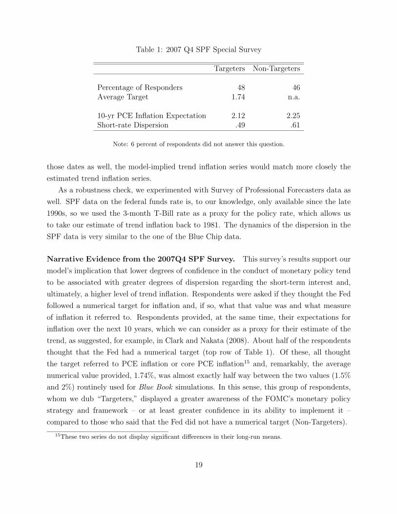
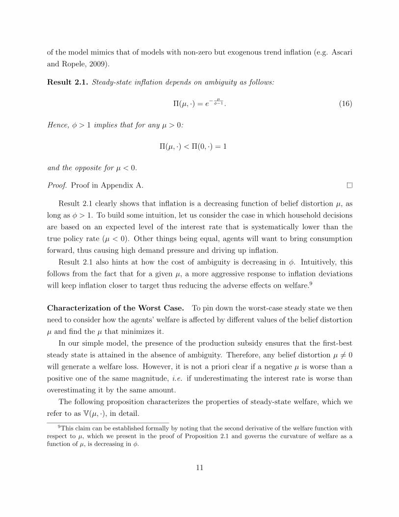
Table 1: 2007 Q4 SPF Special Survey

Targeters Non-Targeters

Percentage of Responders 48 46Average Target 1.74 n.a.

10-yr PCE Inflation Expectation 2.12 2.25Short-rate Dispersion .49 .61

Note: 6 percent of respondents did not answer this question.

those dates as well, the model-implied trend inflation series would match more closely the

estimated trend inflation series.

As a robustness check, we experimented with Survey of Professional Forecasters data as

well. SPF data on the federal funds rate is, to our knowledge, only available since the late

1990s, so we used the 3-month T-Bill rate as a proxy for the policy rate, which allows us

to take our estimate of trend inflation back to 1981. The dynamics of the dispersion in the

SPF data is very similar to the one of the Blue Chip data.

Narrative Evidence from the 2007Q4 SPF Survey. This survey’s results support our

model’s implication that lower degrees of confidence in the conduct of monetary policy tend

to be associated with greater degrees of dispersion regarding the short-term interest and,

ultimately, a higher level of trend inflation. Respondents were asked if they thought the Fed

followed a numerical target for inflation and, if so, what that value was and what measure

of inflation it referred to. Respondents provided, at the same time, their expectations for

inflation over the next 10 years, which we can consider as a proxy for their estimate of the

trend, as suggested, for example, in Clark and Nakata (2008). About half of the respondents

thought that the Fed had a numerical target (top row of Table 1). Of these, all thought

the target referred to PCE inflation or core PCE inflation15 and, remarkably, the average

numerical value provided, 1.74%, was almost exactly half way between the two values (1.5%

and 2%) routinely used for Blue Book simulations. In this sense, this group of respondents,

whom we dub “Targeters,” displayed a greater awareness of the FOMC’s monetary policy

strategy and framework – or at least greater confidence in its ability to implement it –

compared to those who said that the Fed did not have a numerical target (Non-Targeters).

15These two series do not display significant differences in their long-run means.

19

Based also on the respondents’ comments, it seems fair to conclude that, while the fact

that policymakers aimed at low and stable inflation was well understood, there emerged

varying degrees of confidence in the extent to which this goal could be achieved. Targeters

expected inflation over the next 10 years to be on average .4 percent above their stated

target. It is interesting to notice that Non-Targeters expected inflation to be even higher

than Targeters (third row of Table 1) over the next ten years, and also displayed a higher

degree of disagreement on the short rate than Targeters (bottom row of Table 1).

Even though the 2007Q4 set of special questions was a one-off event16 and the limited

number of respondents makes it difficult to find statistically significant differences, the ev-

idence from this survey stacks up nicely with our model. In particular, lower confidence

in the conduct of monetary policy is clearly related to higher dispersion of the short-term

forecasts, as well as a higher expectated long-run inflation.

4 Optimal Monetary Policy

In our simple economy the policy implemented by equation (1) would be optimal, if the

policymaker measured the natural rate accurately (σu → 0) and if the private sector had full

confidence in this happening (µ = µ = 0).

It is out of question that optimizing policymakers would want to reduce the error com-

ponent in their measure of the natural rate as much as possible and increase the degree

of confidence as much as possible. The interesting question is: what happens if, despite

the obvious advances in transparency and communication that occurred over the last few

decades, there are limits to the degree to which ambiguity regarding the policy rule can be

reduced? The natural rate, for instance, is inherently unobserved and, as Hachem and Wu

(2016) point out, a degree of heterogeneity in expectations can survive even in the face of

increased transparency. Here we explore optimal rules for these scenarios.

Our first set of results characterizes, under relatively general conditions, policy rules that

attain the best of possible worst-case steady-state welfare levels – a concept we will refer to

as steady-state optimality. Steady-state optimality is very often disregarded in the analysis

of optimal policy set-ups because, in the absence of ambiguity, zero inflation and the optimal

subsidy deliver the first-best allocation, independent of the values of the other parameters.

16Another one-off set of questions were included in a 2012 SPF survey, which was administered right afterthe announcement of the target. The questions do not map exactly into those we discuss here, but the ideathat different agents display varying degrees of confidence in the conduct of monetary policy emerges fromthat survey as well.

20

We will show how, in our setting, the degree of policy responsiveness to deviations of inflation

from target plays a critical role, instead.

More common (Schmitt-Grohe and Uribe, 2007, providing one of the earliest examples)

are, on the other hand, rankings of monetary policy rules based on their cyclical performance

- we refer to this as dynamic optimality. Extensive numerical exercises are typically the only

way to rank a host of alternative policy rules. Here we will, rather, focus on a particular

parametrization for which a precise characterization can be derived.

Steady-State Optimality. Our main optimal policy result characterizes the optimal mon-

etary policy rule when ambiguity cannot be completely eliminated. As can be seen in equa-

tion (16), as φ → ∞, steady state approaches first best. However, as Schmitt-Grohe and

Uribe (2007) point out, values of φ above around 3 are impractical. Hence, we will work

under the assumption that values φ can take are bounded.

Proposition 4.1. Given the economy described in Section 2, a small µ > 0, µ = −µ and

φ ≤ φ ≤ φ, the following rule

Rt = R∗tΠφt (18)

where R∗t = Rnt e

δ∗(µ,φ,·) and 0 < δ∗(µ, φ; ·) < µ, is steady-state optimal in its class.

Proof. See Appendix B.4

We can summarize the result by saying that the central bank needs to be more hawkish,

because it is optimal respond as strongly as it possibly can to inflation and to increase

the monetary policy rule’s intercept. The overly tight policy stance that Chairman Volcker

followed in 1982 (see Goodfriend 2005, p. 248) can be better appreciated from the perspective

of this result. In an economy in which ambiguity about policy was rampant, it was optimal

to tighten above and beyond what the business cycle conditions (captured by the natural

rate and inflation in our model economy) would seem to dictate.

To understand our result it is important to note that both high φ and positive δ reduce

the wedge between steady-state inflation and the target, thus increasing welfare. The slope

coefficient φ reduces the effects of ambiguity on inflation, because, even if the worst-case

interest rate tends to drive inflation away from target, this effect is mitigated by a more

forceful response by the policymaker to any deviation from the target.

The optimal intercept is higher than the natural rate, because, as inflation is inefficiently

high in the presence of ambiguity, the central bank would like to tighten more. The only

21

other way it can do so, given the upper bound on φ, is by increasing the intercept of its

policy rule. In doing so, though, it faces a limit. If it increases the intercept too much the

worst case will switch. In particular, consider a naıve policymaker who realizes the private

sector is systematically underestimating its policy rate by µ. Its response could amount to

systematically setting rates higher than its standard policy rule would predict by the same

amount µ. If agents did not evaluate welfare in the worst-case scenario when making their

decisions, this policy action would implement first best. In our setting, though, ambiguity-

averse agents would realize that the worst-case scenario has become one in which interest

rates are too high and steady state inflation would end up falling below target. The level

of δ that maximizes worst-case welfare is positive but strictly smaller than µ. This captures

the idea that the policymaker can do better than blindly following the policy rule that would

be optimal in the absence of ambiguity, yet he or she has to ensure that the policy is not as

tight so as to make agents fear excessive tightening more than a looser than optimal policy.

The previous result applies under the assumption that the interval over which agents are

ambiguous is symmetric (µ = −µ). The data suggests symmetry is a reasonable approxima-

tion at most times, yet it is worth asking ourselves what would happen if the interval was

not symmetric, in particular if |µ| << |µ| to the point where V(µ, ·)> V (µ, ·), as in recent

years.

Corollary 4.1. Given the setup in Proposition 4.1 except for the fact that |µ| << |µ|, so

that V(µ, ·)> V (µ, ·), then

Rt = R∗tΠφt (19)

where R∗t = Rnt e

δ∗(µ,µ,φ,·) and −µ < δ∗(µ, µ, φ; ·) < 0, is steady-state optimal in its class.

Proof. See Appendix B.3

This corollary highlights the different roles played by φ and δ. Higher φ always tends

to bring trend inflation closer to target, so it is always optimal to increase φ as much as

possible, irrespective of whether trend inflation is above or below target. As for the policy

rule intercept, however, when the worst-case level of inflation is below target, it is optimal

for R∗t to be lower than the natural rate to generate inflationary pressures that would push

inflation up towards its target.

Dynamic Optimality. Evaluating the dynamic properties of alternative policy functions

requires a policy-rule independent welfare criterion. Coibion, Gorodnichenko and Wieland

22

(2012) showed that reducing the variance of inflation and the output gap enhances welfare

even in an economy with trend inflation17.

Under a particular calibration, we can analytically prove that the policy rule in equation

(18) is also dynamically optimal.

Result 4.1. If leisure enters the felicity function linearly, the degree of ambiguity is suffi-

ciently small and shocks to its level are i.i.d., it can be proven that equation (18) is:

i. dynamically optimal in its class

ii. can reduce the variability of the output gap and inflation around their worst-case steady-

state as much as any other generic rule for a suitably high level of φ.

Proof. See Appendix B.4

The restrictions on the parametrization enable us to show analytically that the coefficients

governing the responses of the output gap and inflation are decreasing (in absolute value) in

φ. Hence, setting φ = φ minimizes the variability of inflation and the output gap to shocks

to ε and to µ, while the presence of the natural rate in the monetary policy rule prevents

TFP shocks from having any effect on deviations of inflation and the output gap from their

worst-case steady state levels. Moreover, as φ grows, the response coefficients tend to zero.

Numerical exercises (Schmitt-Grohe and Uribe, 2007) show that setting φ to the highest

possible value is optimal under a variety of rule configurations, so the applicability of our

result is in practice much wider than the simple case for which we can demonstrate the result

analytically.18

The main message is that, for a given steady state, the dynamic implications of our model

mimic those found in the literature. Selecting the best possible stead-state, however, is not

trivial. In particular, the fact that the private sector does not have full confidence in the

conduct of monetary policy makes blindly tracking the natural rate of interest suboptimal.

It calls, instead, for an intercept of the policy rule that leans against the private sectors

distorted expectations.

17The main differences relative to standard quadratic loss function (Woodford, 2003) are 1) that a constantterm, capturing steady state welfare losses, enters the welfare criterion and 2) that the level of trend inflationaffects the weights at which inflation and output gap stabilization are optimally traded off.

18Schmitt-Grohe and Uribe (2007), find that if they removed the upper limit on the coefficient on inflationin their optimal-rule experiment, they would end up with and inflation coefficient in excess of 300, althoughthe welfare implications are not much different from those derived under φ = 3 according to their analysis.

23

5 Conclusions

We develop a model that features ambiguity-averse agents and ambiguity regarding the con-

duct of monetary policy, but is otherwise standard. We show that the presence of ambiguity

has far-reaching effects, also in steady state. In particular, the model can generate trend

inflation endogenously. Trend inflation has three determinants in our model: the inflation

target, the strength with which the central bank responds to deviation from the target and

the degree of private sector confidence about the monetary policy rule.

Based on a calibration of ambiguity that matches the interdecile dispersion of the Blue

Chip nowcasts of the current quarter’s federal funds rate, our model can explain the disin-

flation of the 80s and 90s as resulting from an increase in the private sector’s confidence in

their understanding of monetary policy, rather than from changes in target inflation. We

can also match the fall in trend inflation since 2009-2010 as an effect of the zero lower bound

on interest rates. The bound sets a floor to the distortion of the interest rate and makes the

worst-case scenario shift from one in which agents fear that the interest rate will be set too

low, to one in which they fear it will be set to high. Agents base their consumptions-saving

decisions on a distorted rate that is too high and will therefore end up facing low inflation.

We also study the optimal monetary policy implications of operating in a world where

some Knightian uncertainty is unavoidable. In our model economy, the parameter governing

the response of the policy rate to inflation deviations from target (φ) reduces the effects and

the cost of ambiguity and we can show it is optimal for policymakers to set it to the highest

feasible value. Moreover, it is optimal for policymakers to lean against the agents’ pessimistic

expectations by increasing the policy rule intercept when the agents’ worst-case expectation

corresponds to overly loose policy. Viceversa, when the worst-case policy scenario is one in

which policy might turn out to be too tight, it is optimal for the policymaker to set a policy

rate that is lower than the one the rule would dictate in thee absency of ambiguity. In so

doing, though, policymakers face a limit which can be ultimately traced back to the private

sector’s lack of full confidence. As a result the first-best steady state cannot be attained for

a finite level of φ in the presence of ambiguity.

24

References

[1] Ascari, G. and T. Ropele, 2009. “Trend Inflation, Taylor Principle, and Indeterminacy,”

Journal of Money, Credit and Banking, vol. 41(8), 1557-1584.

[2] Ascari, G. and A. Sbordone, 2014. “The Macroeconomics of Trend Inflation,” Journal

of Economic Literature, vol. 52(3), 679-739.

[3] Baqaee, D.R., 2015.“Asymmetric Inflation Expectations, Downward Rigidity of Wages

and Asymmetric Business Cycles,” Discussion Papers 1601, Centre for Macroeconomics

(CFM).

[4] Benigno, P. and L. Paciello, 2014. “Monetary policy, doubts and asset prices,” Journal

of Monetary Economics, 64(2014), 85-98.

[5] Bernanke B.S., 2007. “Federal Reserve Communications.” Speech at the Cato Institute

25th Annual Monetary Conference, Washington, D.C.

[6] Blinder, A.S. 1998. Central Banking in Theory and Practice. The MIT Press, Cambridge

MA.

[7] Calvo, G. A., 1983. “Staggered prices in a utility-maximizing framework,” Journal of

Monetary Economics, Elsevier, vol. 12(3), pages 383-398.

[8] Clark, T.E. and T. Doh, 2014. “Evaluating Alternative models of Trend Inflation.”

International Journal of Forecasting 30 (3), 426-448

[9] Clark, T.E. and T. Nakata, 2008. ”Has the behavior of inflation and long-term inflation

expectations changed?,” Economic Review, Federal Reserve Bank of Kansas City, issue

Q I, pages 17-50.

[10] Cogley, T. and T.J. Sargent, 2008. ”Anticipated Utility And Rational Expectations As

Approximations Of Bayesian Decision Making,” International Economic Review, vol.

49(1), pages 185-221, 02.

[11] Cogley, T. and T.J. Sargent, 2002. “Evolving Post World War II U.S. Inflation Dynam-

ics.” In NBER Macroeconomics annual 2001, edited by B.S. Bernanke and K. Rogoff,

331-338, MIT press.

[12] Cogley, T. and A. Sbordone, 2008. “Trend Inflation, Indexation, and Inflation Persis-

tence in the New Keynesian Phillips Curve.” American Economic Review, 98(5):2101-26.

[13] Coibion, O., Y. Gorodnichenko and J. Wieland, 2012. “The Optimal Inflation Rate in

New Keynesian Models: Should Central Banks Raise Their Inflation Targets in Light

25

of the Zero Lower Bound?,” Review of Economic Studies, Oxford University Press, vol.

79(4), pages 1371-1406

[14] Del Negro, M., M.P. Giannoni and F. Schorfheide, 2015. ”Inflation in the Great Re-

cession and New Keynesian Models,” American Economic Journal: Macroeconomics,

American Economic Association, vol. 7(1), pages 168-96, January

[15] Del Negro, M. and S. Eusepi, 2011. “Fitting observed inflation expectations,” Journal

of Economic Dynamics and Control, Elsevier, vol. 35(12), pages 2105-2131.

[16] Ehrmann, M., S. Eijffinger and M. Fratzscher, 2012. “The Role of Central Bank Trans-

parency for Guiding private Sector Forecasts,” Scandinavian Journal of Economics,

114(3),1018-1052.

[17] Epstein, L.G. and M. Schneider, 2003. “Recursive multiple-priors,” Journal of Economic

Theory, Elsevier, vol. 113(1), pages 1-31.

[18] Galı, J. 2008. Monetary Policy, Inflation, and the Business Cycle: An Introduction to

the New Keynesian Framework, Princeton University Press.

[19] Gilboa, I. and D. Schmeidler, 1989. “Maxmin expected utility with non-unique prior,”

Journal of Mathematical Economics, Elsevier, vol. 18(2), pp. 141-153

[20] Goodfriend, M., 2005. “The Monetary Policy Debate Since October 1979: Lessons for

Theory and Practice.” Federal Reserve Bank of St. Louis Review, March/April 2005,

87(2, Part 2), pp. 243-62.

[21] Hachem, K. and J.C. Wu, 2016. “Inflation Announcements and Social Dynamics.”

Chicago Booth Research Paper No. 13-76.

[22] Hansen, L.P. and T. J. Sargent, 2007. Robustness. Princeton University Press.

[23] Ilut, C. and M. Schneider, 2014. “Ambiguous Business Cycles,” American Economic

Review, American Economic Association, Vol. 104(8), pp. 2368-99.

[24] Kreps, D.M., 1998. “Anticipated Utility and Dynamics Choice.” In Frontiers of Research

in Economic Theory: The Nancy L. Schwartz Memorial Lectures 1983-1997, edited by

D.P. Jacobs, E. Kalai and M.I. Kamien, 242-74. Cambridge University Press

[25] Lindsey, D.E., 2003. A Modern History of FOMC Communication: 1975-2002, Board

of Governors of the Federal Reserve System.

[26] Premaratne, G. and A.K. Bera, 2015. “Adjusting the tests for skewness and kurtosis

for distributional misspecifications,” Communications in Statistics – Simulation and

Computation, http://dx.doi.org/10.1080/03610918.2014.988254

26

[27] Schmitt-Grohe, S. and M. Uribe, 2007. “Optimal simple and implementable monetary

and fiscal rules,” Journal of Monetary Economics, Elsevier, vol. 54(6), pages 1702-1725.

[28] Stock, J.H. and M.W. Watson, 2007. “Why Has U.S. Inflation Become Harder to Fore-

cast?,” Journal of Money, Banking and Credit, Vol. 39, No. 1.

[29] Swanson, E.T., 2006. “Have Increases in Federal Reserve Transparency Improved Pri-

vate Sector Interest Rate Forecasts?,” Journal of Money Credit and Banking, vol. 38(3),

pp. 791-81.

[30] Taylor, J.B., 1993. “Discretion versus Policy Rules in Practice,” Carnegie-Rochester

Conference Series on Public Policy 39: 195214.

[31] Woodford, M., 2003. Interest and Prices: Foundations of a Theory of Monetary Policy.

Princeton University Press.

[32] Yun, T. 2005. “Optimal Monetary Policy with Relative Price Distortions,”American

Economic Review, American Economic Association, vol. 95(1), pages 89-109.

27

Appendix

A Proofs of Steady State Results

Proof of Result 2.1. In steady state, equation 8 becomes:

1

C=

β 1βeµΠφ

CΠ(20)

where 1β

is the steady state value for the natural rate of interest. Simplifying and rearranging

delivers equation (16). The second part follows immediately.

Proof of Proposition 2.1. V (µ, ·), as defined in equation (35), is continuously differen-

tiable around zero. Direct computation, or noting that the first-best allocation is attained

in our model when µ = 0, shows that ∂V(µ,·)∂µ

= 0.

Direct computation also delivers:

∂2V (µ, ·)∂µ2

∣∣∣∣µ=0

= − θ ((β − 1)2θ + ε(βθ − 1)2(1 + ψ))

(1− β)(θ − 1)2(βθ − 1)2(φ− 1)2(1 + ψ)(21)

All the terms are positive given the minimal theoretical restrictions we impose, hence the

second derivative is strictly negative, which completes the proof of parts i. and ii..

Direct computation shows that the third derivative evaluated at µ = 0 can be expressed as:

∂3V (µ, ·)∂µ3

∣∣∣∣µ=0

=ε(2ε− 1)θ(1 + θ)

(1− β)(1− θ)3(φ− 1)3+R(β) (22)

Where, given our parameter restrictions, the first term on the RHS is positive and R(β) is

a term in β such that limβ→1−R(β) = 0. Hence, limβ→1−∂3V(µ,·)∂µ3

∣∣∣∣µ=0

= +∞.

Moreover, ∂

(∂3V(µ,·)∂µ3

∣∣∣∣µ=0

)/∂β exists, which ensures continuity of the third derivative in β.

Hence the third derivative is positive for any β sufficiently close to but below unity.

A third-order Taylor expansion around zero can be used to show that, for a generic small

28

but positive µ0:

V (µ0, ·)− V (−µ0, ·) =∂3V (µ, ·)∂µ3

∣∣∣∣µ=0

2µ30

6+ o(µ4

0) > 0, (23)

So the steady state value function attains a lower value at −µ0 than it does at at +µ0.

This, combined with the absence of internal minima, delivers our result under symmetry

(µ = −µ).

B Optimal Policy

We start off by proving two lemmas which we will then use to prove the main optimal-policy

results.

B.1 Two Useful Lemmas

Lemma B.1. While parameter values are in the intervals defined in Proposition 2.1 and µ

is a small positive number, given any pair (µ, φ) ∈ [−µ, 0)× (1,∞), for any µ′ ∈ [µ, 0) there

exists φ′ ∈ (1, ∞) such that:

V(µ, φ′) = V(µ′, φ)

And φ′ ≥ φ iff µ′ ≥ µ.

A corresponding equivalence holds for µ ∈ (0, µ].

Proof. Inspection reveals that µ and φ only enter steady-state welfare through the steady-

state inflation term Π(µ, ·) = eµ

1−φ . It follows immediately that, for a given µ′, φ′ = 1+ (φ−1)µµ′

implies that (µ, φ′) is welfare equivalent to (µ′, φ). (µ, µ′) ∈ [µ, 0)×[µ, 0) ensures that µ′·µ > 0

and so φ′ ∈ (1,∞) for any φ > 1. The inequalities follow immediately from the definition of

φ′ given above and the fact that both µ and µ′ are both negative.

A similar argument would go through for (µ, µ′) ∈ (0, µ]× (0, µ].

Lemma B.2. Assuming that V(µ, ·) takes only real values over some interval (m,m), is con-

tinuously differentiable, strictly concave and attains a finite maximum at µ = µ0 ∈ (m,m);

if φ is fixed and m > µ > 0 > µ > −m, then the level of δ (entering the economy as a

29

constant in the log-linear version of the policy rule) that maximizes worst-case steady-state

welfare is implicitly defined as:

δ∗(µ, µ) : V(µ+ δ∗(µ, µ), ·

)= V

(µ+ δ∗(µ, µ), ·

)(24)

Proof. Computing the steady state of the model, it is easy to verify that the only effect of

adding a term eδ to the policy rule is that steady state inflation becomes:

Π (µ, δ, ·) = e−µ+δφ−1 (25)

while all the other steady-state expressions, most notably consumption and hours, as a func-

tion of inflation, remain unchanged. Hence, two policy rules delivering the same level of

steady state inflation also deliver the same level of steady state welfare. If Vδ is the welfare

function for this economy, equation (25) shows that Vδ(µ, δ, ·) = V(µ+ δ, ·), where the latter

is the welfare in our original economy. So we can proceed using V, whose properties we have

estalished.

Having established that, note that strict concavity ensures µ0 is the unique maximum.

A number of different cases then arise:

1. µ0 ∈ (µ, µ): then V′(µ, ·) > 0 > V′(µ, ·)

a. V(µ, ·) < V(µ, ·). Together with strict concavity this implies that the minimum (or

worst-case) over [µ, µ] is µ. Then there exists a small δ > 0 such that

V(µ, ·) < V(µ+ δ, ·) < V(µ+ δ, ·) < V(µ, ·).

So now the worst case µ + δ generates a higher level of welfare. The worst-case

welfare can be improved until the second inequality above holds with equality.

Continuity ensures such a level of δ∗ exists. Our assumptions also ensure that

µ0−µ > δ∗19, because if µ+ δ = µ0, V(µ+ δ) = V(µ0) which is a unique maximum

so the equality cannot hold. This, in turn ensures that V′(µ+ δ∗) > 0 > V′(µ+ δ∗).

Hence, any further increase in δ would make µ + δ the worst case and welfare at

the worst-case would fall.

b. V(µ, ·) > V(µ, ·). Together with strict concavity, this implies that the minimum is

19Clearly µ0 − µ > 0, since µ0 > µ in this case.

30

attained at µ. Then there exists a small enough δ < 0 such that:

V(µ, ·) < V(µ+ δ, ·) < V(µ+ δ, ·) < V(µ, ·)

By the same arguments as above µ0−µ < δ∗ < 0 makes the second inequality hold

with equality and attains the higher level of welfare.

c. V(µ, ·) = V(µ, ·). Any δ 6= 0 would lower the worst-case welfare: δ∗ = 0.

2. µ0 ∈ [µ,m). Strict concavity implies that welfare is strictly increasing over [µ, µ] and µ

mimizes welfare over that range. For all 0 ≤ δ ≤ µ0 − µ

V(µ, ·) ≤ V(µ+ δ, ·) < V(µ+ δ, ·) ≤ V(µ0, ·)

The second inequality will always be strict. For δ just above µ0 − µ we fall in case 1a

above and δ∗ can be determined accordingly.

3. µ0 ∈ (m,µ]. Strict concavity implies that welfare is strictly decreasing over [µ, µ] and

µ mimizes welfare over that range. For all 0 ≥ δ ≥ µ0 − µ

V(µ0, ·) ≥ V(µ+ δ, ·) > V(µ+ δ, ·) ≥ V(µ, ·)

The second inequality will always be strict. For δ just below µ0 − µ we fall in case 1b

above and δ∗ can be determined accordingly.

B.2 Proof of Proposition 4.1

The first part of the proof of Lemma B.2 applies here as well, in particular the fact that

if we define welfare in the economy in which we allow for δ in the Taylor rule Vδ, then

Vδ(µ, δ, ·) = V(µ+ δ, ·), where the latter is the welfare in the original economy.

Having established this, the proof of static optimality proceeds in two steps by first

findind the optimal value of φ given assumptions on the welfare function and on δ and then

verifying that for φ, the conjectures made in the previous point hold.

i. Suppose that V(−µ + δ, ·) corresponds to the worst-case steady-state welfare for some

δ ∈ (0, µ), then φ = φ maximizes worst-case welfare over [φ, φ].

31

Following the same logic as in Lemma B.1, but using the expression in equation (25)

for inflation, it is easy to verify that for any 1 < φ′ < φ, there exists a µ′ s.t.:

V (µ′ + δ, φ′, ·) = V(−µ+ δ, φ, ·

)(26)

In particular:

µ′ = −µ(φ′ − 1

φ− 1

)− δ

(1− φ′ − 1

φ− 1

)(27)

Given our restrictions, this implies that 0 > −δ > µ′ > −µ.

In our economy V(0, ·) corresponds to the maximum, so the argmax µ = −δ (the level

of µ delivering Π (µ, δ, ·) = 1). Together with strict concavity (Proposition 2.1), this

implies that V() strictly increasing for µ < −δ, hence:

V(−µ+ δ, φ, ·

)= V (µ′ + δ, φ′, ·) > V (−µ+ δ, φ′, ·) (28)

ii. 0 < δ∗ < µ defined by V (−µ+ δ∗, ·) = V (µ+ δ∗, ·) maximizes worst-case welfare for

φ = φ.

Proposition 2.1 guarantees that our welfare function satisfies the assumptions of Lemma

B.2 in a neighborhood of zero.

To find the bounds on δ∗, note that for µ > 0 and µ = −µ, Proposition 2.1 also implies

that the maximum µ0 = 0 is interior and that V(µ, ·) < V(µ, ·). So, case 1a of the proof

of Lemma B.2 applies, which implies that µ0 − µ = µ > δ∗ > 0. These considerations

apply for any φ > 1, thus also for φ.

B.3 Proof of Corollary 4.1

Following the same approach as for Proposition 4.1

i. Suppose that V(µ + δ, ·) corresponds to the worst-case steady-state welfare for some

δ ∈ (−µ, 0), then φ = φ maximizes worst-case welfare over [φ, φ].

For any 1 < φ′ < φ, there exists a µ′ s.t.:

V (µ′ + δ, φ′, ·) = V(µ+ δ, φ, ·

)(29)

32

In particular:

µ′ = µ

(φ′ − 1

φ− 1

)− δ

(1− φ′ − 1

φ− 1

)(30)

Given our restrictions, this implies that 0 < −δ < µ′ < µ.

V() is strictly decreasing for µ > −δ, hence:

V(µ+ δ, φ, ·

)= V (µ′ + δ, φ′, ·) > V (µ+ δ, φ′, ·) (31)

ii. 0 > δ∗ > −µ defined by V(µ+ δ∗, ·

)= V (µ+ δ∗, ·) maximizes worst-case welfare for

φ = φ.

V(µ, ·) > V(µ, ·) and for µ < 0 and µ > 0 the welfare maximum µ0 = 0 is in the

interior. This corresponds to case 1b of the proof of Lemma B.2, which implies that

µ0 − µ = −µ < δ∗ < 0.

B.4 Proof or Result 4.1

In another section of the Appendix we present the solution of the log-linearized version

of our model using the method of undetermined coefficients. Those coefficients simplify

substantially when we consider the limit µ → 0 - which simplifies the expressions for the

κ’s log-linear coefficients - and ρµ = 0. In particular, we get λπε = −ρε(1−θ)(1−βθ)Ξ

, λyε =

−ρεθ(1−βρε)Ξ

, λπµ = (1−θ)(1−βθ)Ξ

, λyµ = θ(1−βρε)Ξ

, where Ξ ≡ (θ−ρε)(1−βθρε)+(1−θ)(1−βθ)φ.

Ξ is strictly positive since Ξ > (θ − ρε)(1 − βθρε) − (θ − 1)(1 − βθ) > 0. This can be seen

considering that (θ − ρε)(1 − βθρε) − (θ − 1)(1 − βθ), as a second-order polynomial in ρε

is strictly positive for small values of ρε and has two roots at 1 and −1 + 1βθ

+ θ > 1 ,if

β < 1. Hence it is strictly positive for 0 < ρε < 1. So Ξ is strictly positive and increasing

in φ. Hence, as φ increases all the coefficients decrease (in absolute value) thus reducing

the variability of the output gap and inflation around their worst-case steady state values.

Which proves the first part of our result because φ = φ attains the lowest degree of variability

given our constraint.

Moreover, as φ tends to ∞ all the λ’s tend to zero, which proves the second part of the

result.

33

C Steady State

Pricing. In our model firms index their prices based on the first-best inflation, which

corresponds to the inflation target and is zero in the case presented in the main body of the

paper. Because of ambiguity, however, steady-state inflation will not be zero and therefore

there will be price dispersion in steady state:

∆(µ, ·) =(1− θ)

(1−θΠ(µ,·)ε−1

1−θ

) εε−1

1− θΠ(µ, ·)ε(32)

∆ is minimised for Π = 1 - or, equivalently, µ = 0 - and is larger than unity for any other

value of µ. As in Yun (2005), the presence of price dispersion reduces labour productivity

and ultimately welfare.

Hours, Consumption and Welfare. In a steady state with no real growth, steady-state

hours are the following function of µ:

N(µ, ·) =

((1− θΠ(µ, ·)ε−1) (1− βθΠ(µ, ·)ε)(1− βθΠ(µ, ·)ε−1) (1− θΠ(µ, ·)ε)

) 11+ψ

, (33)

while consumption is:

C(µ, ·) =A

∆(µ, ·)N(µ, ·) (34)

Hence the steady state welfare function takes a very simple form:

V(µ, ·) =1

1− β

(log (C(µ, ·))− N(µ, ·)1+ψ

1 + ψ

). (35)

Bound on µ. Equation (33) delivers the upper bound on steady-state inflation that is

commonly found in this class of models (e.g. Ascari and Sbordone (2014)). As inflation

grows, the denominator goes to zero faster than the numerator, so it has to be that Π (µ, ·) <θ−

1ε for steady state hours to be finite20. Given our formula for steady-state inflation, we

can then derive the following restriction on the range of values µ can take on, given our

20Indeed, the same condition could be derived from the formula for price dispersion in equation (32).

34

parameters:

µ >φ− 1

εlog (θ) , (36)

where the right-hand side is negative since ε > 1, φ > 1 and 0 < θ < 1. To put things in

perspective, note that under our baseline calibration, the bound would require µ to be not

lower than −2.48 annualized percentage points. Our measure of forecasters disagreement

for the Survey of Professional Forecasters peaks at 2.26 percent, which implies a calibration

for µ of 1.13 percent at most (i.e. half the measure of dispersion under symmetry), which is

clearly well within the acceptable range.

D Model Dynamics

To study the dynamic properties of our model, we log-linearize the equlibrium conditions

around the worst-case steady state in the usual way. As explained in Ascari and Ropele

(2007), having price dispersion in steady state essentially results in an additional term in

the Phillips Curve. Appendix D.1 presents the log-linear approximation around a generic

steady state indexed by µ. By setting µ = −µ, we obtain the log-linear approximation to

the worst-case steady state (under symmetry).

Armed with the solution of the log-linearized model, we can verify if the worst-case indeed

corresponds to our conjecture not only in steady state but also around it.

Once we have verified our conjecture about the worst-case steady state, we turn our

attention to the implications of changes in the agents’ confidence in their understanding of

the monetary policy rule on the determinacy region and we then study the effects of shocks

to ambiguity.

D.1 Log-linearized Equations and Solution

The following equations describe the dynamics of the variables of interest around a generic

steady state indexed by µ21. Setting µ to its worst-case steady state value, one obtains the

21Where we refer to the numerator of equation (13) as F1 and to the denominator as F2 and express bothin recursive form as F1t = ε

ε−1MCt + βθEtΠεt+1F1t+1 and F2t = 1 + βθEtΠε−1

t+1F2t+1 respectively.

35

log-linear approximation around the worst-case steady state:

ct = Et [ct+1 − (rt − πt+1)] (37)

πt = κ0 (µ, ·)mct + κ1 (µ, ·)EtF2t+1 + κ2 (µ, ·)Etπt+1 (38)

rt = (rnt + εt) + φπt (39)

∆t = κ3 (µ, ·) ∆t−1 + κ4 (µ, ·) πt (40)

F2t = κ5 (µ, ·)Etπt+1 + κ6 (µ, ·)EtF2t+1 (41)

mct = wt − at (42)

wt = ct + ψnt (43)

yt = at − ∆t + nt (44)

ct = yt (45)

rnt = Etat+1 − at (46)

ynt = at (47)

εt = ρεεt−1 + uεt (48)

at = ρaat−1 + uat (49)

Where κ’s are known convultions of deep parameters defined as:

κ0 (µ, ·) ≡

((1

Π(µ,·)

)ε−1

− θ)

(1− βθΠ (µ, ·)ε)

θ(50)

κ1 (µ, ·) ≡ β

((1

Π (µ, ·)

)ε−1

− θ

)(Π (µ, ·)− 1) Π (µ, ·)ε−1 (51)

κ2 (µ, ·) ≡ βΠ (µ, ·)ε−1

(θ(ε− 1)(Π (µ, ·)− 1) + (1− ε+ εΠ (µ, ·))

(1

Π (µ, ·)

)ε−1)

(52)

κ3 (µ, ·) ≡ Π(µ, ·)εθ (53)

κ4 (µ, ·) ≡ θε (Π (µ, ·)− 1)(1

Π(µ,·)

)ε−1

− θ(54)

κ5 (µ, ·) ≡ (ε− 1)βθΠ(µ, ·)ε−1 (55)

κ6 (µ, ·) ≡ βθΠ(µ, ·)ε−1 (56)

36

The equations above can be summarized in the following system of four equations:

yt = Et [yt+1 − (φπt + εt − Etπt+1)] (57)

πt = κ0 (µ, ·)(

(1 + ψ)yt + ψ∆t

)+ κ1 (µ, ·)EtF2t+1 + κ2 (µ, ·)Etπt+1 (58)

∆t = κ3 (µ, ·) ∆t−1 + κ4 (µ, ·)πt (59)

F2t = Et(κ5 (µ, ·) πt+1 + κ6 (µ, ·) F2t+1

)(60)

Where yt ≡ yt−ynt = yt−at is the output gap. Moreover, Et[εt] = ρεεt−1 +µt and, assuming

symmetric bounds, µt = −µt. µt = µt−(1−ρµ)µ is the degree of ambiguity in deviation from

its mean, and µt = (1−ρµ)µ+ρµµt−1+uµt governs the cyclical variations of ambiguity around

its steady state. In words, a positive shock uµt implies that ambiguity will be higher than

usual which, under our worst-case steady state results22, means that agents will ”increase

their underestimation of the policy rate”.

These equation make it transparent that technological shocks do not affect any of the

four variables in this system and, in particular, the output gap and inflation. This is common

in models in which the natural rate enters the policy rule but it useful to verify that this

property extends to the case in which we log-linearize the model around the worst-case steady

state. at will still play a role, though, in that consumption, and thus utility, respond to it.

D.2 Worst-Case around the Steady State

We now need to study welfare around the worst-case steady state. In particular, we study a

case that lends itself well to an anlytical solution and provides the intuition. We will follow

a similar approach to that in Ilut and Scheider (2014), section II. Namely:

i. Based on Result 2.1 we determine the worst-case steady state, i.e. µ = −µ under

symmetry.

ii. We then solve for the linear policy functions, thus getting a mapping from the state

of the economy (∆t−1, εt−1, at, µt)23 onto all the endogenous variables of interest, most

notably ct and nt, which determine welfare.

iii. We then verify whether welfare is increasing in εt−1, consistent with the guess that the

worst-case scenario is that in which its expectation takes the lower value on the range

22The next section explores how it holds around the worst-case steady state.23Under symmetry, we do not need to keep track of variations in µ and µ separately, hence the state of

the economy is smaller.

37

(−µ).

If hours enter felicity linearly (ψ = 0)24, the price dispersion term drops out of equation

(58). Hence inflation, the output gap and consumption will not depend on price dispersion,

which, however, will still affect welfare as the number of hours worked will depend on it.

We can thus solve equations (57)-(60) with the method of undetermined coefficients and be

able to obtain analytical expression for the coefficients.

The policy functions for the four variables in equations (57)-(60):

πt = λπεεt−1 + λπµµt λπε ≡−κ0ρ

ε

(1− ρε)(

1 + (φ−ρε)κ01−ρε − ρε

(κ2 + ρεκ1κ5

1−ρεκ6

))(61)

yt = λyεεt−1 + λyµµt λyε ≡ −ρε

1− ρε− (φ− ρε)λπε

1− ρε(62)

F2t = λFεεt−1 + λFµµt λFε ≡ρεκ5λπε1− ρεκ6

(63)

∆t = κ3∆t−1 + κ4

(λπεεt−1 + λπµµt

)(64)

Where λπε is zero when ρε = 0 and negative for positve values of ρε: if the current state

εt−1 signals tighter policy in the future ρε > 0 then inflation falls. Indeed λπε → − 1φ−1

as

ρε → 1−, consistent with our steady-state analysis. λyε and generally negative and larger

(in absolute value) than λπε25. λFε simply reflects the fact that F2t is a discounted sum of

future expected inflation.

As for λπµ, λyµ, λFµ, they can also be expressed as functions of the underlying parameters

and they have the opposite sign relative to the corresponding coefficients for ε, which is to

be expected given the way the two terms enter the Euler equation.26

24The results in our paper are not specific to any calibrated values (with the exception of those pertainingto the policy rule) so we prefer to higlight the first-order effect of a monetary policy shock on welfare in oursetting in the most transparent way, rather than performing a battery of numerical exercises for differentcalibrations.

25λyε is zero when ρε = 0 and negative for 0 < ρε < ρε, where ρε is generally very close to unity forreasonable calibrations. λyε is larger (in absolute values) than λπε, except for values of ρε very close to unity,so long as κ0 (”the slope of the Phillips Curve”) is relatively small, which, in turn, depends on the degreeof price stickiness. Moreover only the signal of λπε matters for our result as we will show, while λyε cancelsout.

26Their values are not directly relevant for the point we are addressing here (i.e. whether welfare isincreasing in varepsilont−1 around the worst-case steady state) so we don’t report them but they areavailable from the authors upon request.

38

Using the expressions in Section D.1 we can back out the policy functions for consumption

and hours:

ct = yt + at = λyεεt−1 + +λπµµt + at (65)

nt = ct − at + ∆t = yt + ∆t

= λyεεt−1 + λπµµt + κ3∆t−1 + κ4

(λπεεt−1 + λπµµt

)(66)

The value function for the problem, using the linear policy functions, can be expressed as:

V(

∆t−1, εt−1, at, µt

)= log ((1 + ct)C(−µ, ·))− (1 + nt)N (−µ, ·) + βEtV

(∆t, εt, at+1, µt+1

)(67)

V(

∆t−1, εt−1, at, µt

)= u

(−→C (−µ, ·)

)+ log (1 + ct)− ntN (−µ, ·) + βEtV

(∆t, εt, at+1, µt+1

)(68)

We can then define dV(

∆t−1, εt−1, at, µt

)≡ V

(∆t−1, εt−1, at, µt

)−V (−µ, ·), which can be

expressed as:

dV(

∆t−1, εt−1, at, µt

)= log (1 + ct)− ntN (−µ, ·) + βEtdV

(∆t, εt, at+1, µt+1

)(69)

dV(

∆t−1, εt−1, at, µt

)= ct − nt + βEtdV

(∆t, εt, at+1, µt+1

)(70)

dV(

∆t−1, εt−1, at, µt

)= at − ∆t + βEtdV

(∆t, εt, at+1, µt+1

)(71)

dV(

∆t−1, εt−1, at, µt

)= at − κ3∆t−1 − κ4λπεεt−1 − κ4λπµµt + βEtdV

(∆t, εt, at+1, µt+1

)(72)

The result27 is very intuitive and shows that εt−1 has a positive (κ4 > 0 and λπε < 0) first-

order effect on welfare around the worst-case steady state, which confirms our conjecture.

More generally, equation (71) shows that, in this model, TFP and price dispersion are

the key determinants of welfare as they drive a wedge (in opposite directions) between

consumption and hours, as can be clearly seen from the resource constraint Ct = At∆tNt. It is

thus natural that welfare be increasing in at and decreasing in ∆t. The former is completely

exogenous while the second is not.

A monetary policy tightening reduces consumption by a factor of λyε. Hours fall because,

as in the standard case, production falls (λyε) but also because there is an efficiency gain

brought about by the reduction in price disperion (κ4λπε). The first two effects net out and

the efficiency gain dominates and ultimately determines the first-order effect of a monetary

27We use the Taylor approximation for log(1 + ct) and the fact that N (−µ, ·), as defined in (33), isextremely close to one (within about 10−4 for some calibrations we tried and reasonable values for µ).

39

policy shock on welfare.

From an economic standpoint, the result is intuitive. Inflation is inefficiently high at the

worst-case steady state, so tightening is beneficial. If there was no ambiguity and steady-

state inflation coincided with the target, κ4 = 0 (see equation (54)), hence a monetary policy

shock would have no first-order effect on welfare as expected.

Also notice that, as expected, welfare is decreasing in the degree of ambiguity (κ4 > 0

and λπµ > 0) even in deviations from steady state.

Finally, notice that in situations in which the worst case corresponds to µ = µ, gross

inflation falls below target, κ4 becomes negative28 and welfare would increase with monetary

policy loosening, thus verifying the steady-state conjecture that, in that case, the worst-case

is one in which policy is overly tight.

28The sign of λπε does not change as can be generally verified numerically. This is more transparent inthe limit case above in which it takes value − 1

φ−1 which is completely independent of the κ coefficients,which depend on the worst-case steady state inflation.

40