FEDERAL RESERVE BANK OF SAN FRANCISCO

WORKING PAPER SERIES

Monetary Policy Mistakes and the Evolution of Inflation Expectations

Athanasios Orphanides Central Bank of Cyprus

and

John C. Williams

Federal Reserve Bank of San Francisco

May 2011

Working Paper 2010-12 http://www.frbsf.org/publications/economics/papers/2010/wp10-12bk.pdf

The views in this paper are solely the responsibility of the authors and should not be interpreted as reflecting the views of the Federal Reserve Bank of San Francisco or the Board of Governors of the Federal Reserve System.

Monetary Policy Mistakesand the Evolution of Inflation Expectations

Athanasios OrphanidesCentral Bank of Cyprus

andJohn C. Williams∗

Federal Reserve Bank of San Francisco

May 2011

Abstract

What monetary policy framework, if adopted by the Federal Reserve, would have avoidedthe Great Inflation of the 1960s and 1970s? We use counterfactual simulations of an esti-mated model of the U.S. economy to evaluate alternative monetary policy strategies. Weshow that policies constructed using modern optimal control techniques aimed at stabilizinginflation, economic activity, and interest rates would have succeeded in achieving a high de-gree of economic stability as well as price stability only if the Federal Reserve had possessedexcellent information regarding the structure of the economy or if it had acted as if it placedrelatively low weight on stabilizing the real economy. Neither condition held true. We doc-ument that policymakers at the time both had an overly optimistic view of the natural rateof unemployment and put a high priority on achieving full employment. We show that inthe presence of realistic informational imperfections and with an emphasis on stabilizingeconomic activity, an optimal control approach would have failed to keep inflation expecta-tions well anchored, resulting in high and highly volatile inflation during the 1970s. Finally,we show that a strategy of following a robust first-difference policy rule would have beenhighly effective at stabilizing inflation and unemployment in the presence of informationalimperfections. This robust monetary policy rule yields simulated outcomes that are closeto those seen during the period of the Great Moderation starting in the mid-1980s.

Keywords: Great Inflation, rational expectations, robust control, model uncertainty, nat-

ural rate of unemployment.

JEL Classification System: E52

∗We thank Nick Bloom, Bob Hall, Seppo Honkapohja, Andy Levin, John Taylor, Bharat Trehan, and

participants at the NBER Conference on the “Great Inflation” and other presentations for helpful comments

and suggestions. We also thank Justin Weidner for excellent research assistance. The opinions expressed are

those of the authors and do not necessarily reflect the views of the Central Bank of Cyprus, the Governing

Council of the European Central Bank, the Federal Reserve Bank of San Francisco, or the Board of Governors

of the Federal Reserve System. Correspondence: Orphanides: Central Bank of Cyprus, 80 Kennedy Avenue,

1076 Nicosia, Cyprus, Tel: +357-22714471, email: Athanasios.Orphanides@centralbank.gov.cy. Williams:

Federal Reserve Bank of San Francisco, 101 Market Street, San Francisco, CA 94105, Tel.: (415) 974-2240,

e-mail: John.C.Williams@sf.frb.org.

In monetary policy central bankers have a potent means for fostering stability in

the general price level. By training, if not also by temperament, they are inclined

to lay great stress on price stability. . . . And yet, despite their antipathy to

inflation and the powerful weapons they could yield against it, central bankers

have failed so utterly in this mission in recent years. In this paradox lies the

anguish of central banking. (Arthur Burns, 1979, p. 7)

1 Introduction

Numerous explanations have been put forward for the causes of the Great Inflation of the

late 1960s and 1970s in the United States. But one explanation that may be the most

worrisome for the future is that policy mistakes made by otherwise well-informed and well-

intentioned policymakers, free of institutional and political constraints, were responsible

for these outcomes. The epigraph quoted above, from the 1979 Per Jacobsson Lecture

delivered by Arthur Burns shortly after the end of his tenure as Chairman of the Federal

Reserve, exemplifies this concern. In this paper, we provide a historical account of the Great

Inflation and subsequent evolution of the economy in the United States using an estimated

model with a benevolent and sophisticated policymaker. We examine how the economy

would have fared if the Federal Reserve had applied modern optimal control techniques—of

the type recommended by many academic researchers today—to reach its policy decisions

from the middle of the 1960s on.1 We then compare the resulting simulated outcomes to

those obtained under alternative monetary policy strategies designed to be robust to model

misspecification.

The main thesis of this paper is that the modern optimal control approach to monetary

policy is prone to inviting policy errors that lead to instability in inflation and inflation

expectations like those that occurred during the Great Inflation, while alternative robust1Optimal control methods were first developed in the 1960s and have gained popularity in the academic

literature during the past 10 years. See Svensson and Woodford, 2003; Woodford, 2003; Giannoni andWoodford, 2005; and Svensson and Tetlow, 2005, for modern derivations and applications of optimal controltechniques to monetary policy. See Levin and Williams (2003) and Orphanides and Williams (2008, 2009)for analysis of the optimal control approach to realistic degrees of uncertainty.

1

policy strategies could have been more effective at stabilizing inflation and unemployment.

Our reading of the narrative evidence highlights three critical factors that contributed to

the unmooring of inflation expectations and the resulting runaway inflation of the Great

Inflation. First, policymakers placed a high priority on stabilizing real economic activity

relative to price stability. Second, they severely overestimated the productive capacity of

the economy during the critical period of 1965 to 1975. In particular, contemporaneous

measures of the unemployment rate corresponding to full employment were significantly

lower than retrospective estimates. Third, they were overly confident of their understanding

of the precise linkage between measures of utilization gaps and inflation. The modern

optimal control approach is not designed to protect against any of these factors.

This paper provides a “stress test” of optimal control policies and other policy strategies

to see how they would have fared in times of particular macroeconomic turmoil and when the

central bank faced imperfect information. The 1960s and 1970s provide an ideal laboratory

for such an experiment. The U.S. economy was buffeted by large shocks, providing severe

stress to the economy, and the realized macroeconomic performance was abysmal. Our

analysis is related to that of Orphanides (2002) and Orphanides and Williams (2005a), who

show that a strong response to flawed measures of economic slack can help explain the

very high inflation and unemployment that developed during the 1960s and 1970s and that

policies that reacted less aggressively to slack would have been more effective at stabilizing

both inflation and unemployment during that period. The contribution of the current

paper is to analyze the stabilization properties of optimal control policies and alternative

policy approaches using counterfactual simulations of the U.S. economy over the past several

decades. In so doing, we aim to use the experiences of the past to glean lessons for the

design of robust monetary policy for the future.

Our model respects the natural rate hypothesis and shares key features with modern

models used for monetary policy analysis. We investigate what would have happened over

history had policymakers implemented state-of-the-art optimal control methods under the

assumption of rational expectations. We focus on the difficulties associated with anchoring

2

inflation expectations when policymakers attempt to maintain a high degree of employment

stability relative to price stability in an environment where the central bank has imperfect

information about the economy. The estimated model confirms the presence of adverse

supply shocks and natural rate misperceptions during the 1970s, which caused policy to

become overly expansionary. However, we find that these shocks alone cannot account for

the Great Inflation experience.

Using counterfactual simulations, we show that in the absence of informational im-

perfections, following the optimal control policy during the 1960s and 1970s would have

maintained reasonably well-anchored inflation expectations and succeeded in achieving a

relatively high degree of economic and price stability. Under these assumptions, monetary

policy could have offset the shocks that buffeted the economy during this period.

However, our model simulations also show that informational imperfections, such as

policymakers’ misperceptions of the natural rate of unemployment, significantly reduce the

effectiveness of this approach to policy. The presence of imperfect knowledge amplifies the

effects of the underlying shocks, and optimal control monetary policies designed assuming

complete information would have failed to keep inflation expectations well anchored. Indeed,

optimal control policies would have avoided the Great Inflation only if the weight given to

stabilizing the real economy were relatively modest—with the best results achieved if the

most weight were placed on stabilizing prices.

We also examine an alternative policy strategy that could have been more robust and

avoided this experience, even in the presence of supply shocks and natural rate mispercep-

tions. We show that such a strategy would have been very effective at stabilizing inflation

and economic activity, despite the large shocks of the 1970s. A striking result is that this

policy rule yields simulated outcomes close to the realized behavior of the economy dur-

ing the Great Moderation starting in the mid-1980s, suggesting that the actual practice of

monetary policy during this period changed in ways that incorporated the key properties

of the robust monetary policy rule.

The remainder of the paper is organized as follows. Section 2 examines the narrative

3

evidence of policymakers’ views on the natural rate of unemployment and the importance

of stabilizing economic activity during the 1960s and 1970s. Our model of the U.S. economy

and its estimation are described in Section 3. Section 4 describes the optimal control mon-

etary policy and its implementation in the model simulations. The models of expectations

formation and the simulation methods are described in Sections 5 and 6, respectively. Sec-

tion 7 examines the performance of the optimal control policy using counterfactual model

simulations. Section 8 analyzes the performance of a simple robust monetary policy rule,

and Section 9 concludes.

2 A Narrative History

In this section, we examine the narrative evidence regarding the views of policymakers

regarding the natural rate of unemployment and the role of stabilizing real activity at “full

employment” before, during, and after the Great Inflation.2 We use this narrative evidence

to inform the specification of monetary policy in the model simulations reported in the

subsequent sections of the paper.

To set the stage for later events, it is useful to recall the evolution of the policy debate in

the post-World War II period. In the Employment Act of 1946, Congress declared that “it

is the continuing policy and responsibility of the Federal Government to use all practicable

means ... to promote maximum employment, production and purchasing power” (quoted in

Council of Economic Advisers, 1966, p. 170).3 Until the 1960s, policymakers interpreted the

Employment Act of 1946 to be a broad mandate to protect price stability, that is, to promote

“purchasing power” and growth and to dampen business cycle fluctuations. In congressional

testimony in August 1957, for example, Federal Reserve Chairman William McChesney

Martin stated that “[t]he objective of the System is always the same—to promote monetary

and credit conditions that will foster sustained economic growth together with stability in2See, Mayer (1999), Meltzer (2003) and Hetzel (2008a), among others, for detailed histories of Federal

Reserve policy during this period.3Chapter 7 of the 1966 Economic Report of the President was devoted to the 20 years of experience with

the Act since it became law on February 20, 1946. This edition of the report, published in early 1966,provides a useful snapshot of policy thinking at the start of the Great Inflation.

4

the value of the dollar.” To this end, he stressed the importance of price stability: “Price

stability is essential to sustainable growth. Inflation fosters maladjustments” (Martin, 1957,

p. 8).

During the 1960s, an increasing number of economists argued that fiscal and monetary

policy should play a more active role in managing aggregate demand with the goal of achiev-

ing and maintaining full employment. In 1961, the incoming Council of Economic Advisers

(CEA) adopted what became known as the “New Economics,” which was highlighted in

the 1962 Economic Report of the President (Council of Economic Advisers, 1962). The new

strategy was eloquently summarized by Walter Heller, who, according to Time Magazine,

as “Chief Economic Adviser of the Kennedy Council, presided over the birth of the New

Economics as a practical policy” (Time Magazine, 1965, p. 67A). Heller said:

The promise of modern economic policy, managed with an eye to maintain-

ing prosperity, subduing inflation, and raising the quality of life, is indeed great.

And although we have made no startling conceptual breakthroughs in economics

in recent years, we have, more effectively than ever before, harnessed the ex-

isting economics—the economics that has been taught in the nation’s college

classrooms for some twenty years—to the purposes of prosperity, stability, and

growth. (Heller, 1966, p. 116, emphasis in the original)

A key aspect of the New Economics was a heightened focus on achieving a desired

level of economic activity, as measured by the unemployment rate or the level of GDP,

rather than the less demanding goal of economic expansion. This focus on achieving the

economy’s potential level of activity necessitated the measurement of potential output and

the unemployment rate corresponding to full employment. Arthur Okun, Chairman of the

CEA in the late 1960s, later summarized the implications of the new strategy for economic

policy as follows:

The revised strategy emphasized, as the standard for judging economic perfor-

mance, whether the economy was living up to its potential rather than merely

whether it was advancing. Ideally, total demand should be in balance with the

5

nation’s supply capabilities. When the balance is achieved, there is neither the

waste of idle resources nor the strain of inflationary pressure. The nation is then

actually producing its potential output. (Okun, 1970, p. 40)

Okun explained that the New Economics reflected a “shift in emphasis from the achievement

of expansion to the realization of potential” (p. 41) and explained how this implied greater

policy activism:

[T]he focus on the gap between potential and actual output provided a new

scale for the evaluation of economic performance, replacing the dichotomized

business cycle standard which viewed expansion as satisfactory and recession

as unsatisfactory. This new scale of evaluation, in turn, led to greater activism

in economic policy: As long as the economy was not realizing its potential,

improvement was needed and government had a responsibility to promote it.

(p. 41)

The shift in emphasis towards more explicit targets for employment and the level of eco-

nomic activity was not intended to downplay the need to preserve price stability. The twin

policy objectives of full employment and price stability were stressed repeatedly, starting

with the very first study that provided the quantitative definitions of full employment that

would shape policy throughout the 1960s: “The full employment goal must be understood

as striving for maximum production without inflation pressure” (Okun, 1962, p. 82).

The New Economics also emphasized the importance of monetary policy in achieving

these goals. Indeed, the essence of monetary policy was seen in a rather conventional

manner not inconsistent with current views. According to the 1962 Economic Report of the

President: “The proper degree of ‘tightness’ or ‘easiness’ of monetary policy . . . depend[s]

on the state of the domestic economy, on the fiscal policies of the Government, and on

the international economic position. When the economy is in recession or beset by high

unemployment and excess capacity, monetary policy should clearly be expansionary. . . .

When demand is threatening to outrun the economy’s production potential, monetary policy

6

should be restrictive” (Council of Economic Advisers, 1962, p. 85). As this quote makes

clear, such a policy depends crucially on measuring the economy’s capacity accurately.

The critical test for the New Economics would begin in 1965, when the economy was

nearing what was perceived at the time to be full employment. The apparent success of

economic policy up to that point was the topic of the cover story of the December 1965

Time magazine. The story noted that “[e]conomists have descended in force from their

ivory towers and now sit confidently at the elbow of almost every important leader in

Government and business, where they are increasingly called upon to forecast, plan and

decide” (p. 65). Indeed, Okun later remarked, “The high-water mark of the economists

prestige in Washington was probably reached late in 1965” (1970, p. 59).

Although the New Economics held sway at the CEA and at many academic institutions,

Federal Reserve Chairman Martin remained skeptical that policymakers would ever possess

the precise knowledge of the economy demanded by the policies of the New Economics.

Although Martin’s attitude was interpreted by some as a mistrust of economists, it would

be more accurate to describe his views as reflecting a mistrust of the fine-tuning approach

advocated by some economists who were gaining influence at the time. As Sherman Maisel,

an economist who joined the Board of Governors in 1965, later recounted: “The press

frequently reported Martin’s dismay over the number of economists appointed to the Board.

He felt that the economy was too complex to explain in detail; intuition would be lost and

false leads followed if too much stress were put on measurement” (Maisel 1973, p. 114).

Nonetheless, by 1965, the center of gravity at the Federal Reserve was shifting away from

what we would describe as Martin’s robust policy approach toward a fine-tuning approach

that sought to achieve a quantitative full-employment goal as well as price stability.

By July 1965 the unemployment rate had fallen to about 4-1/2 percent and the balance of

payments was deteriorating. Martin believed that policy needed to be tightened to restrain

inflationary pressures. During the second half of 1965, he attempted to forge a consensus

at the Federal Reserve towards policy tightening. But the Council of Economic Advisers

and like-minded economists at the Federal Reserve argued against such a preemptive move.

7

In their view, a 4 percent unemployment rate corresponded to full employment. Therefore,

the economy was operating below its full-employment level and inflationary pressures were

unlikely to emerge.4

Martin postponed proposing a policy tightening until December 1965, when, despite

significant opposition from members of the Board of Governors, he felt it was no longer

prudent to wait. On December 3, 1965, the Federal Reserve Board increased the discount

rate from 4.0 to 4.5 percent with four members of the Board voting in favor of and three

voting against the rate hike. The published announcement explained: “With slack in man-

power and productive capacity now reduced to narrow proportions, with the economy closer

to full potential than at any time in nearly a decade ... it was felt that excessive additions

to money and credit availability in an effort to hold present levels of interest rates would

spill over into further price increases. Such price rises would endanger the sustainable na-

ture of the present business expansion” (Board of Governors of the Federal Reserve System,

1965, p. 1668). Governors Robertson, Mitchell, and Maisel dissented from the discount

rate action “on the ground that it was at least premature in the absence of more compelling

evidence of inflationary dangers” (Board of Governors of the Federal Reserve System, 1965,

p. 1668).

In remarks that were delivered a few days later, on December 8, Chairman Martin had

an opportunity to explain his reasoning for the rate hike:

The Federal Reserve, in all its actions, aims always at the same goal: to help the

economy move forward at the fastest sustainable pace. We reach our destination

most rapidly as well as more assuredly when we travel at maximum safe speed—

and this speed cannot be the same under all conditions and at all times. . . .

To me, the effective time to act against inflationary pressures is when they are4The CEA (1962) put the unemployment rate corresponding to full employment at 4 percent. The 1962

Economic Report of the President indicated that “in the existing economic circumstances, an unemploymentrate of about 4 percent is a reasonable and prudent full employment target for stabilization policy” (p. 46).Although this goal of a 4 percent unemployment rate may appear overly ambitious in retrospect, it did notappear so at the time. Indeed, many considered the 4 percent goal for the unemployment rate insufficientlyambitious. For them, 4 percent was seen to be an interim goal, with the ultimate objective being even lowerunemployment.

8

in the development stage—before they have become full-blown and the damage

has been done. Precautionary measures are more likely to be effective than

remedial action: the old proverb that an ounce of prevention is worth a pound

of cure applies to monetary policy as well as to anything else. . . .

[S]o long as inflation is merely a threat rather than a reality, it is enough to

prevent the pace of economic expansion from accelerating dangerously. But

once that pace has become unsustainably fast, then it becomes necessary to

reduce the speed, and once such a reduction is started, there is no assurance it

can be stopped in time to avoid an actual downswing (Martin, 1965, emphasis

in original).

The discount rate increase prompted a bruising congressional hearing the following week,

on December 13-14, 1965. The hearing on “Recent Federal Reserve Action and Economic

Policy Coordination” (U.S. Congress, 1966) served as a forum for criticizing Chairman

Martin for tightening policy. It provides an invaluable glimpse into the policy debate at the

time and highlights the crucial role that perceptions about full employment had acquired.

Martin represented the majority view and Governors Mitchell and Maisel, who opposed the

tightening, represented the dissenting view at the hearing on December 13, 1965. At the

hearing, it was confirmed that a crucial reason for the disagreement on the tightening was

a disagreement about the risks to the inflation outlook. Furthermore, details emerged as

to the assessments of the Chairman and dissenting members of the Board regarding what

constituted full employment.

The discussion centered on whether a 4 percent unemployment rate was the appropriate

definition of full employment. Martin remarked, “As long as unemployment of manpower

and plant capacity was greater than could be considered acceptable or normal, we had

every reason to lean on the side of monetary stimulus.” Senator Jacob Javits asked, “Do

you consider a 4 percent unemployment acceptable and normal and is that the basis for

your decision?” (U.S. Congress, 1966, p. 116). Noting that this is a long-standing debate

among experts, Martin replied that, although the Federal Reserve Board would want “as

9

low a level as it is possible to have,” he did not know what the right level ought to be.

Responding to subsequent questions he added, “We [the Board of Governors] have never

addressed ourselves to a definitive discussion of the 3 or 4 or 5 percent.” But he admitted

that in making the policy decision the Board deemed that “we were approaching a state

of full employment” (pp. 116-117). The unemployment rate had fallen to 4.2 percent in

November 1965.

Those arguing against a policy tightening pointed to the fact that unemployment was

still above 4 percent and therefore inflationary pressures should be absent, despite the fact

that inflation, as measured by the consumer price index, had been edging up for some time.

In his prepared statement at the hearing, Governor Mitchell explained that the challenge

to policy at the end of 1965 was to “ease the economy onto a steady growth path at full

employment,” adding, “I believe this can be done with reasonably stable prices” (United

States Congress, 1966, p. 21). But, with the unemployment rate exceeding 4 percent, he

disagreed that a policy tightening was necessary. “[T]he evidence on prices does not, in my

view, now call for more monetary restraint than is already being applied” (p. 22). The

crux of his argument evolved around the definition of full employment: “Those who regard

4 percent unemployment ... as the approximate total of the frictionally unemployed ... may

feel that we have achieved our employment goals and that any further progress in reducing

unemployment cannot come from aggregate demand. ... I am not yet ready to agree that

there is no further room for compression of the unemployment rate” (pp. 22-23).

Indeed, Governor Maisel argued that 4 percent may have been too high a target for the

unemployment rate. He explained that he disagreed with the policy decision because he

felt that policy tightening was premature. In his prepared remarks, he noted, “Raising the

discount rate would be interpreted as a view by the Board that because full employment

increases inflationary problems, restrictive monetary policy must be invoked at its mere

approach” (p. 31). Asked about his views on full employment, in the light of the various

efforts to reduce frictional unemployment he replied, “My assumption is that the retraining

enables us to say that 4 percent unemployment was only an interim goal. ... As a result

10

4 percent might have been a proper goal five years ago. ... Now we need to think of these

retraining programs you have cited and see what our present goal should be. Should it be

3 percent or what?” (p. 181). The view that the interim goal for unemployment could

perhaps be adjusted downwards was also shared by the Council of Economic Advisers. As

noted in the Economic Report of the President published in early 1966, “The unemployment

rate has now virtually reached the interim target and is projected to fall below 4 percent

in 1966. There is strong evidence that the conditions originally set for lowering the target

are in fact being met, and that the economy can operate efficiently at lower unemployment

rates” (Council of Economic Advisers, 1966, p. 75).

This debate centered on estimates of the unemployment rate consistent with price sta-

bility and the proper policy response to movements in inflation and unemployment. Im-

portantly, the participants did not possess fundamentally divergent views of the inflation

process. Indeed, both sides used a relatively conventional understanding of the process of

inflation and the effect of “gaps” on inflation. In particular, policymakers clearly believed

that they had the power to control inflation through monetary policy. The 1966 Economic

Report of the President provides a view of inflation that relates well to models used today:

As a first approximation, the classical law of supply and demand leads one

to expect that the change in the price level will depend mainly on the size of

the gap between capacity and actual output. The more production falls short

of potential—i.e., the greater is excess productive capacity—the further prices

should drop. Conversely, when demand outruns aggregate supply, the imbalance

should raise prices. ...

Expectations and attitudes also affect price changes. An economy accustomed

to price stability is less vulnerable to inflation” (Council of Economic Advisers,

1966, pp. 63-65).

Note the explicit recognition of the role of expectations in the determination of inflation.5

5To be sure, there are differences between the reasoning in the 1960s and modern models. One importantdifference is that the models of the New Economics era typically implied a long-term trade-off between infla-

11

Even when inflation got noticeably higher in the second half of the 1960s, the mistaken

belief that the full-employment unemployment rate was very low continued to distort policy

decisions, exacerbating inflationary pressures. Although the rise in inflation during 1966

and thereafter vindicated Martin’s position, this evidence proved insufficient to stem the

tide toward greater fine-tuning with an emphasis on achieving what was believed to be full

employment. Later, Herbert Stein went so far as to call the belief that the natural rate of

unemployment was 4 percent “the most serious error of the Nixon CEA” (Stein, 1996, p.

19). As he explained, “fascinated by the idea of ‘the natural rate of unemployment,’ which

we thought to be 4 percent, we thought it necessary only to let the unemployment rate rise

slightly above that to hold down inflation” (pp. 19-20). The resulting policy actions would

have been the “optimum feasible path,” except that they built upon a fatally flawed view

of the productive capacity of the economy. Instead of restoring stability, they led to further

increases in inflation.

The inflation rate rose from below 2 percent in the early 1960s to over 5 percent by

1970. Figure 1 shows the four-quarter average of the U.S. inflation rate, measured by

the GDP price deflator, from 1955 to 2003. (Note that throughout this paper, unless

otherwise indicated, the figures show the four-quarter moving average of the inflation rate

to reduce the visual clutter caused by quarterly volatility in this series.) For comparison, the

horizontal line shows the 2 percent inflation target that we assume reflects the policymaker’s

price stability objective for our counterfactual simulations reported in later sections. The

inflation rate was around this level before the Great Inflation and returned once again to

this level in the last decade of our sample. Inflation expectations became unmoored during

the Great Inflation (see Levin and Taylor, 2009, for further discussion of the evidence on

inflation expectations) and only in the 1990s did they become anchored again. By the

beginning of the 1980s, survey measures of long-run inflation expectations had risen to over

tion and unemployment, whereas modern models such as ours typically respect the natural rate hypothesis.But this difference is not key for explaining the Great Inflation in our view. As explained by Modiglianiand Papademos (1975), in both types of models, there exists a rate of unemployment (the NAIRU) that isconsistent with the policymaker’s definition of reasonable price stability. In our model, this corresponds tothe natural rate of unemployment. What is critical is that in both types of models, misperceptions aboutthe NAIRU (or natural rate) have inflationary consequences under the optimal control approach to policy.

12

8 percent.

Under Arthur Burns, who became Fed Chairman in 1970, the Federal Reserve continued

the activist bent with even greater force (Hetzel, 1998, Orphanides, 2003). The high degree

of confidence that economists had regarding their ability to measure the capacity of the

economy and to gauge inflationary pressures is nicely illustrated by the staff briefing to the

Board of Governors from August 1970 presented by John Charles Partee (who become a

Governor in 1976): “there is substantial underutilization of resources, as evidenced by a

5 per cent unemployment rate and an operating rate in manufacturing estimated at well

under 80 per cent of capacity. In these circumstances, there is virtually no risk that economic

recovery over the year ahead would add to the inflationary problem through stimulation of

excess—or even robust—demand in product or labor markets” (Board of Governors, 1970,

p. 19).

In his Anguish lecture, Burns admitted that the Federal Reserve was slow to recognize

the upward drift in the natural rate of unemployment, thus adding to inflation (Burns, 1979).

Figure 2 plots real-time estimates of the natural rate of unemployment and a retrospective

measure of the natural rate equal to the Congressional Budget Office (CBO) estimates

available at the time that this paper was written. The actual unemployment rate is plotted

as well. The real-time series for the natural rate is taken from Orphanides and Williams

(2005a), extended to include more recent data. These real-time estimates were constructed

drawing on a number of sources (see Orphanides and Williams, 2002, for details). As seen in

the figure, differences between real-time estimates of the natural rate of unemployment and

current retrospective estimates were especially large and persistent during the second half

of the 1960s and the 1970s. The mean absolute difference between the real-time and current

estimates was 1.2 percentage points over this period. But such natural rate “misperceptions”

are not merely a historical curiosity, with the mean absolute difference between the two

measures equaling 0.6 percentage points over the period of 1980-2003.6

6Note that this measure of natural rate misperceptions does not take into account uncertainty regardingthe CBO’s estimates of the natural rate. Instead, it merely measures changes in the estimates that reflectchanges in methodology and the effects of new data.

13

The overly optimistic estimates of the economy’s capacity was of particular importance

in light of the high value placed on achieving full employment relative to price stability.

Despite the upward trend in inflation since 1965, the Federal Reserve remained focused on

stabilizing real activity, with the hope that inflationary pressures would subside. At the

May 1975 meeting of the Federal Open Market Committee, the Board staff argued that

“there is such a large amount of slack in the economy now that real growth would have to

exceed our projection by a wide margin, and for an extended period, before excess aggregate

demand once again emerged as a significant problem.” (Board of Governors of the Federal

Reserve, 1975, p. 26). Furthermore, “Simulations using the econometric model suggested

that a considerably faster rate of expansion could be stimulated without having a significant

effect on the rate of increase in prices–that a considerably more rapid rate of increase in

real GNP would still be consistent with a further winding down of inflationary pressures”

(p. 27). The inflation rate in fact did come down from its 1975 peak of about 10 percent

over the next few years, but bottomed out above 5 percent, well in excess of conventional

views of price stability.

Monetary policy moved away from the policy activism of the earlier period and towards

an approach focused more on inflation stabilization only after Paul Volcker became Chair-

man in 1979. Volcker eschewed the fine-tuning approach and concentrated instead on the

goal of price stability, seeing this as the only way to effectively reanchor inflation expec-

tations and restore broader stability to the economy (Goodfriend and King, 2005, Hetzel,

2008b, Lindsey et al., 2005, Orphanides and Williams, 2005a). He explained his rationale

in his first Humphrey-Hawkins testimony on February 19, 1980.

In the past, at critical junctures for economic stabilization policy, we have usu-

ally been more preoccupied with the possibility of near-term weakness in eco-

nomic activity or other objectives than with the implications of our actions for

future inflation. To some degree, that has been true even during the long pe-

riod of expansion since 1975. As a consequence, fiscal and monetary policies

alike too often have been prematurely or excessively stimulative or insufficiently

14

restrictive. The result has been our now chronic inflationary problem, with a

growing conviction on the part of many that this process is likely to continue.

Anticipations of higher prices themselves help speed the inflationary process. ...

The broad objective of policy must be to break that ominous pattern. That

is why dealing with inflation has properly been elevated to a position of high

national priority. Success will require that policy be consistently and persistently

oriented to that end. Vacillation and procrastination, out of fears of recession

or otherwise, would run grave risks. Amid the present uncertainties, stimulative

policies could well be misdirected in the short run. More importantly, far from

assuring more growth over time, by aggravating the inflationary process and

psychology, they would threaten more instability and unemployment.

(Volcker, 1980, pp. 2-3)

3 An Estimated Model of the U.S. Economy

We now turn to the evaluation of alternative monetary policy strategies. We use coun-

terfactual simulations of the estimated quarterly model of the U.S. economy described in

Orphanides and Williams (2008). The specification of the model is motivated by the recent

literature on micro-founded models incorporating some inertia in inflation and output (see

Woodford, 2003, for a fuller discussion). The main difference from other monetary policy

models is that the unemployment gap is substituted for the output gap in the model to

facilitate estimation using real-time data. The two concepts are closely related in practice

by Okun’s law, and the key properties of the model are largely unaffected by this choice.

3.1 The Model

The structural model consists of two equations that describe the behavior of the unemploy-

ment rate and the inflation rate and equations describing the time-series properties of the

exogenous shocks. To close the model, the short-term interest rate is set by the central

bank, as described in the next section.

15

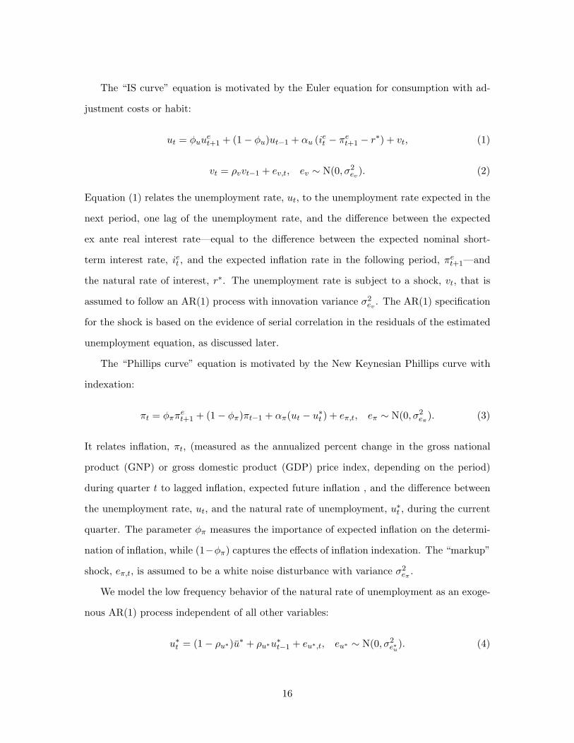
The “IS curve” equation is motivated by the Euler equation for consumption with ad-

justment costs or habit:

ut = φuuet+1 + (1− φu)ut−1 + αu (iet − πe

t+1 − r∗) + vt, (1)

vt = ρvvt−1 + ev,t, ev ∼ N(0, σ2ev

). (2)

Equation (1) relates the unemployment rate, ut, to the unemployment rate expected in the

next period, one lag of the unemployment rate, and the difference between the expected

ex ante real interest rate—equal to the difference between the expected nominal short-

term interest rate, iet , and the expected inflation rate in the following period, πet+1—and

the natural rate of interest, r∗. The unemployment rate is subject to a shock, vt, that is

assumed to follow an AR(1) process with innovation variance σ2ev

. The AR(1) specification

for the shock is based on the evidence of serial correlation in the residuals of the estimated

unemployment equation, as discussed later.

The “Phillips curve” equation is motivated by the New Keynesian Phillips curve with

indexation:

πt = φππet+1 + (1− φπ)πt−1 + απ(ut − u∗t ) + eπ,t, eπ ∼ N(0, σ2

eπ). (3)

It relates inflation, πt, (measured as the annualized percent change in the gross national

product (GNP) or gross domestic product (GDP) price index, depending on the period)

during quarter t to lagged inflation, expected future inflation , and the difference between

the unemployment rate, ut, and the natural rate of unemployment, u∗t , during the current

quarter. The parameter φπ measures the importance of expected inflation on the determi-

nation of inflation, while (1−φπ) captures the effects of inflation indexation. The “markup”

shock, eπ,t, is assumed to be a white noise disturbance with variance σ2eπ

.

We model the low frequency behavior of the natural rate of unemployment as an exoge-

nous AR(1) process independent of all other variables:

u∗t = (1− ρu∗)u∗ + ρu∗u∗t−1 + eu∗,t, eu∗ ∼ N(0, σ2

e∗u). (4)

16

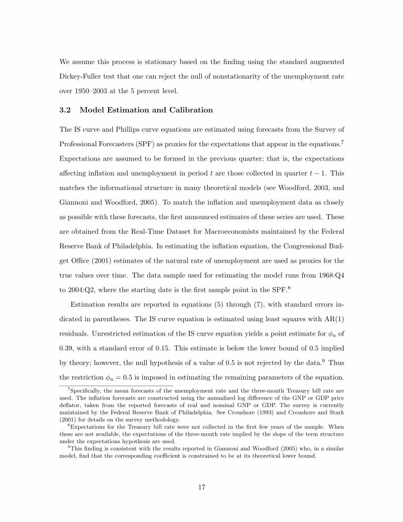
We assume this process is stationary based on the finding using the standard augmented

Dickey-Fuller test that one can reject the null of nonstationarity of the unemployment rate

over 1950–2003 at the 5 percent level.

3.2 Model Estimation and Calibration

The IS curve and Phillips curve equations are estimated using forecasts from the Survey of

Professional Forecasters (SPF) as proxies for the expectations that appear in the equations.7

Expectations are assumed to be formed in the previous quarter; that is, the expectations

affecting inflation and unemployment in period t are those collected in quarter t− 1. This

matches the informational structure in many theoretical models (see Woodford, 2003, and

Giannoni and Woodford, 2005). To match the inflation and unemployment data as closely

as possible with these forecasts, the first announced estimates of these series are used. These

are obtained from the Real-Time Dataset for Macroeconomists maintained by the Federal

Reserve Bank of Philadelphia. In estimating the inflation equation, the Congressional Bud-

get Office (2001) estimates of the natural rate of unemployment are used as proxies for the

true values over time. The data sample used for estimating the model runs from 1968:Q4

to 2004:Q2, where the starting date is the first sample point in the SPF.8

Estimation results are reported in equations (5) through (7), with standard errors in-

dicated in parentheses. The IS curve equation is estimated using least squares with AR(1)

residuals. Unrestricted estimation of the IS curve equation yields a point estimate for φu of

0.39, with a standard error of 0.15. This estimate is below the lower bound of 0.5 implied

by theory; however, the null hypothesis of a value of 0.5 is not rejected by the data.9 Thus

the restriction φu = 0.5 is imposed in estimating the remaining parameters of the equation.7Specifically, the mean forecasts of the unemployment rate and the three-month Treasury bill rate are

used. The inflation forecasts are constructed using the annualized log difference of the GNP or GDP pricedeflator, taken from the reported forecasts of real and nominal GNP or GDP. The survey is currentlymaintained by the Federal Reserve Bank of Philadelphia. See Croushore (1993) and Croushore and Stark(2001) for details on the survey methodology.

8Expectations for the Treasury bill rate were not collected in the first few years of the sample. Whenthese are not available, the expectations of the three-month rate implied by the slope of the term structureunder the expectations hypothesis are used.

9This finding is consistent with the results reported in Giannoni and Woodford (2005) who, in a similarmodel, find that the corresponding coefficient is constrained to be at its theoretical lower bound.

17

Note that the estimated equation also includes a constant term (not shown) that provides

an estimate of the natural real interest rate, which is assumed to be constant:

ut = 0.5uet+1 + 0.5ut−1 +0.056

(0.022)

(iet − πet+1 − r∗) + vt, (5)

vt = 0.513(0.085)

vt−1 + ev,t, σev = 0.30, (6)

πt = 0.5πet+1 + 0.5πt−1 − 0.294

(0.087)

(ut − u∗t ) + eπ,t, σeπ = 1.35. (7)

Unrestricted estimation of the Phillips curve equation yields a point estimate for φπ

of 0.51, just barely above the lower bound implied by theory.10 For symmetry with the

treatment of the IS curve, the restriction φπ = 0.5 is imposed and the remaining parameters

are estimated using ordinary least squares. The estimated residuals for this equation show

no signs of serial correlation in the price equation, consistent with the assumption of the

model.

We do not estimate the model of the natural rate of unemployment; instead, we set

the autocorrelation parameter, ρr∗ , to 0.99 and set the unconditional mean to the sample

average of the unemployment rate.

4 Monetary Policy

We focus on two alternative approaches to monetary policy. The first is the optimal control

approach. The second is a simple monetary policy that is closely related to nominal income

growth targeting. In both cases, the policy instrument is the nominal short-term interest

rate. We assume that the central bank observes all variables from previous periods when

making the current-period policy decision. We further assume that policy is conducted

under commitment.10For comparison, Giannoni and Woodford (2005) find that the corresponding coefficient is constrained

to be at its theoretical lower bound of 0.5.

18

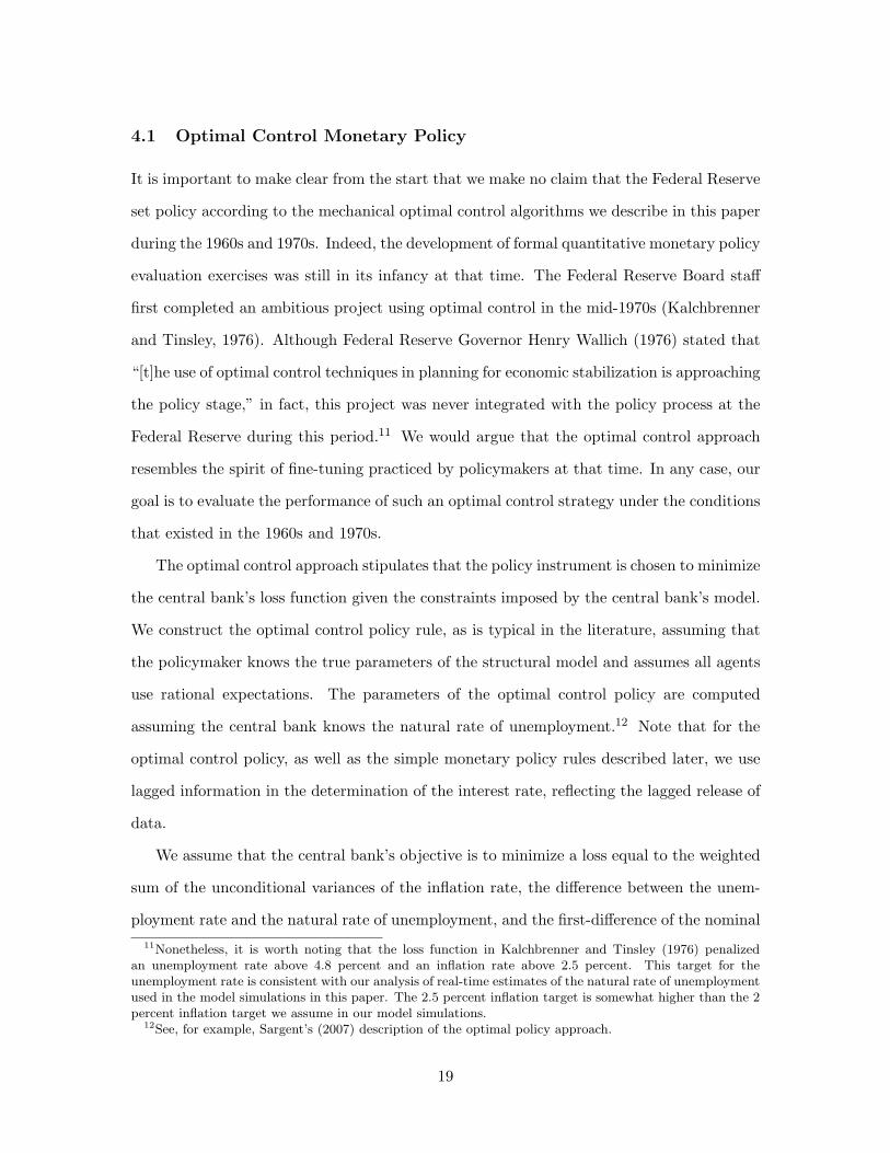
4.1 Optimal Control Monetary Policy

It is important to make clear from the start that we make no claim that the Federal Reserve

set policy according to the mechanical optimal control algorithms we describe in this paper

during the 1960s and 1970s. Indeed, the development of formal quantitative monetary policy

evaluation exercises was still in its infancy at that time. The Federal Reserve Board staff

first completed an ambitious project using optimal control in the mid-1970s (Kalchbrenner

and Tinsley, 1976). Although Federal Reserve Governor Henry Wallich (1976) stated that

“[t]he use of optimal control techniques in planning for economic stabilization is approaching

the policy stage,” in fact, this project was never integrated with the policy process at the

Federal Reserve during this period.11 We would argue that the optimal control approach

resembles the spirit of fine-tuning practiced by policymakers at that time. In any case, our

goal is to evaluate the performance of such an optimal control strategy under the conditions

that existed in the 1960s and 1970s.

The optimal control approach stipulates that the policy instrument is chosen to minimize

the central bank’s loss function given the constraints imposed by the central bank’s model.

We construct the optimal control policy rule, as is typical in the literature, assuming that

the policymaker knows the true parameters of the structural model and assumes all agents

use rational expectations. The parameters of the optimal control policy are computed

assuming the central bank knows the natural rate of unemployment.12 Note that for the

optimal control policy, as well as the simple monetary policy rules described later, we use

lagged information in the determination of the interest rate, reflecting the lagged release of

data.

We assume that the central bank’s objective is to minimize a loss equal to the weighted

sum of the unconditional variances of the inflation rate, the difference between the unem-

ployment rate and the natural rate of unemployment, and the first-difference of the nominal11Nonetheless, it is worth noting that the loss function in Kalchbrenner and Tinsley (1976) penalized

an unemployment rate above 4.8 percent and an inflation rate above 2.5 percent. This target for theunemployment rate is consistent with our analysis of real-time estimates of the natural rate of unemploymentused in the model simulations in this paper. The 2.5 percent inflation target is somewhat higher than the 2percent inflation target we assume in our model simulations.

12See, for example, Sargent’s (2007) description of the optimal policy approach.

19

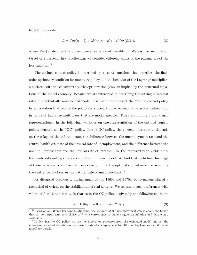
federal funds rate:

L = V ar(π − 2) + λV ar(u− u∗) + νV ar(∆(i)), (8)

where V ar(x) denotes the unconditional variance of variable x. We assume an inflation

target of 2 percent. In the following, we consider different values of the parameters of the

loss function.13

The optimal control policy is described by a set of equations that describes the first-

order optimality condition for monetary policy and the behavior of the Lagrange multipliers

associated with the constraints on the optimization problem implied by the structural equa-

tions of the model economy. Because we are interested in describing the setting of interest

rates in a potentially misspecified model, it is useful to represent the optimal control policy

by an equation that relates the policy instrument to macroeconomic variables, rather than

in terms of Lagrange multipliers that are model specific. There are infinitely many such

representations. In the following, we focus on one representation of the optimal control

policy, denoted as the “OC” policy. In the OC policy, the current interest rate depends

on three lags of the inflation rate, the difference between the unemployment rate and the

central bank’s estimate of the natural rate of unemployment, and the difference between the

nominal interest rate and the natural rate of interest. The OC representation yields a de-

terminate rational expectations equilibrium in our model. We find that including three lags

of these variables is sufficient to very closely mimic the optimal control outcome assuming

the central bank observes the natural rate of unemployment.14

As discussed previously, during much of the 1960s and 1970s, policymakers placed a

great deal of weight on the stabilization of real activity. We represent such preferences with

values of λ = 16 and ν = 1. In that case, the OC policy is given by the following equation:

it = 1.16it−1 − 0.05it−2 − 0.21it−3 (9)13Based on an Okun’s law type relationship, the variance of the unemployment gap is about one-fourth

that of the output gap, so a choice of λ = 4 corresponds to equal weights on inflation and output gapvariability.

14In deriving the OC policy, we use the innovation processes from the estimated model and set theinnovation standard deviation of the natural rate of unemployment to 0.07. See Orphanides and Williams(2009) for details.

20

+0.23πt−1 − 0.07πt−2 + 0.05πt−3

−3.70(ut−1 − u∗t−1) + 2.81(ut−2 − u∗t−1)− 0.15(ut−3 − u∗t−1),

plus a constant reflecting the constant natural rate of interest and inflation target, where

u∗t denotes the central bank’s estimate of the natural rate of unemployment.

In the following, we also examine the performance of the OC policy derived for alter-

native values of λ. The resulting OC policy for λ = 4 and ν = 1 is given by the following

equation:

it = 1.17it−1 + 0.02it−2 − 0.28it−3 (10)

+0.18πt−1 + 0.03πt−2 + 0.01πt−3

−2.47(ut−1 − u∗t−1) + 2.11(ut−2 − u∗t−1)− 0.33(ut−3 − u∗t−1).

Compared to the OC policy derived with λ = 16, this policy is characterized by a stronger

response to inflation and a much smaller response to the unemployment rate. Finally, the

OC policy derived for λ = 0 and ν = 1 is given by:

it = 1.12it−1 + 0.13it−2 − 0.34it−3 (11)

+0.17πt−1 + 0.09πt−2 − 0.01πt−3

−1.63(ut−1 − u∗t−1) + 1.53(ut−2 − u∗t−1)− 0.38(ut−3 − u∗t−1).

As expected, this policy is characterized by a stronger response to inflation and a much

smaller response to the unemployment rate than the OC policy derived for λ = 4.

4.2 Central Bank Natural Rate Estimates

As seen in these equations, a key input into the setting of OC policies is the central bank’s

estimate of the natural rate of unemployment. In deriving the OC policy, we assume that the

central bank knows the true structure of the economy, including the value of the natural

rate of unemployment. In the model simulations, however, we also examine alternative

assumptions regarding the central bank’s knowledge of the natural rate. One alternative

is that the central bank’s estimates of the natural rate follow the historical pattern of the

21

real-time estimates reported in Figure 2. We refer to this case as “historical natural rate

misperceptions.” A second alternative is that the central bank estimates the natural rate

based on the Kalman filter applied to the Phillips curve equation for inflation. We refer to

this case as “Kalman filter estimates.” In each case, we assume that the true values of the

natural rate of unemployment follow the current CBO estimates shown in Figure 2.

In the case of Kalman filter estimation of the natural rate of unemployment, we as-

sume that the central bank uses an appropriate Kalman filter consistent with the data.

In particular, the central bank’s real-time Kalman filter estimate of the natural rate of

unemployment, u∗t , is given by

u∗t = a1u∗t−1 + a2(u∗t − eπ,t/απ), (12)

where a1 and a2 are the Kalman gain parameters. The term within the parentheses is the

current-period “shock” to inflation that incorporates the effects of the transitory inflation

disturbance and the deviation of the natural rate of unemployment from its unconditional

mean, scaled in units of the unemployment rate. Note that the central bank only observes

this “surprise” and not the decomposition into its two components.

The optimal values of the gain parameters depend on the variances of the various shocks

in the model. Based on a calibrated Kalman filter model, we assume that the central bank

uses the following values: a1 = 0.982 and a2 = 0.008 (see Orphanides and Williams, 2009,

for the derivation of these values). We assume that the central bank starts the simulation

with the value of 4 percent, consistent with the evidence from real-time estimates reported

earlier.

5 Expectations and Simulation Methods

We assume that private agents and, in some cases, the central bank form expectations

using an estimated reduced-form forecasting model. Specifically, following Orphanides and

Williams (2005b), we posit that private agents engage in perpetual learning, that is, they

reestimate their forecasting model using a constant-gain least squares algorithm that weights

recent data more heavily than past data. (See Sargent, 1999; Cogley and Sargent, 2001; and

22

Evans and Honkapohja, 2001 for related treatments of learning.) This approach to modeling

learning allows for the possible presence of time variation in the economy, including the

natural rates of interest and unemployment. It also implies that agents’ estimates are

always subject to sampling variation, that is, the estimates do not eventually converge to

fixed values.

Private agents forecast inflation, the unemployment rate, and the short-term interest

rate using an unrestricted vector autoregression (VAR) model containing three lags of these

three variables and a constant. Note that we assume that private agents do not observe or

estimate the natural rate of unemployment directly in forming expectations. The effects of

time variation in the natural rate on forecasts are reflected in the forecasting VAR by the

lags of the interest rate, inflation rate, and unemployment rate. As discussed in Orphanides

and Williams (2008), this VAR forecasting model provides accurate forecasts in model

simulations.

At the end of each period, agents update their estimates of their forecasting model

using data through the current period. Let Yt denote the 1 × 3 vector consisting of the

inflation rate, the unemployment rate, and the interest rate, each measured at time t:

Yt = (πt, ut, it). Further, let Xt be the 10 × 1 vector of regressors in the forecast model:

Xt = (1, πt−1, ut−1, it−1, . . . , πt−3, ut−3, it−3). Also, let ct be the 10× 3 vector of coefficients

of the forecasting model. Using data through period t, the coefficients of the forecasting

model can be written in recursive form as follows:

ct = ct−1 + κR−1t Xt(Yt −X ′

tct−1), (13)

Rt = Rt−1 + κ(XtX′t −Rt−1), (14)

where κ is the gain. Agents construct the multiperiod forecasts that appear in the inflation

and unemployment equations in the model using the estimated VAR.

The matrix Rt may not be full rank at times. To circumvent this problem, in each

period of the model simulations, we check the rank of Rt. If it is less than full rank, we

assume that agents apply a standard Ridge regression (Hoerl and Kennard, 1970), where

Rt is replaced by Rt + 0.00001 ∗ I(10) and I(10) is a 10× 10 identity matrix.

23

5.1 Calibrating the Learning Rate

A key parameter in the learning model is the private-agent updating parameter, κ. Esti-

mates of this parameter tend to be imprecise and sensitive to model specification, but tend

to lie between 0 and 0.04.15 We take 0.02 to be a reasonable benchmark value for κ.

6 Model Simulations

We examine a set of alternative counterfactual simulations to investigate the implications

of alternative monetary policy frameworks on macroeconomic developments over the past

40 years. We start our simulations in the first quarter of 1966, which corresponds to what

we and many observers consider to be the beginning of the Great Inflation in the United

States.

6.1 Initial Conditions

The state variables of the model economy with learning are as follows: the current and

lagged values of the inflation rate, the federal funds rate, the unemployment rate, the true

natural rate of unemployment, the real-time estimate of the natural rate, the shocks to the

structural equations, and the matrices C and R for the forecasting model. We initialize the

C and R matrices using the values implied by the reduced-form solution of the model under

rational expectations for the stipulated monetary policy rule. In so doing, we are implicitly

assuming that the initial conditions for the agents’ learning model are consistent with the

policy rule in place. That is, we assume that at the start of the simulation, expectations are

well aligned with the monetary policy regime under consideration. Over time, expectations

then evolve as described above. This assumption implies that the initial conditions for these

state variables are different across the counterfactual simulations. As a result, the simulated

paths will often differ significantly from the historical patterns.

To compute the history of equation residuals, we first compute the implied forecasts

from our forecasting model of inflation, the unemployment rate, and the federal funds rate

over the period 1966–2003. We treat the forecasts generated by the learning model as15See Sheridan (2003), Orphanides and Williams (2005a), Branch and Evans (2006), and Milani (2007).

24

the true data for agents’ expectations and then compute tracking residuals, that is, the

values of the historical residuals for the equations for the unemployment rate, the inflation

rate, and the natural rate of unemployment. Thus, given these residuals and the historical

path for the nominal interest rate, the model’s predictions will exactly match the historical

paths for all endogenous variables. We then conduct counterfactual experiments in which

we modify assumptions regarding monetary policy, but do not change the paths for the

equation residuals for unemployment, inflation, and the natural rate of unemployment,

which we assume are exogenous. Each counterfactual simulation starts in the first quarter

of 1966 and ends in the fourth quarter of 2003.

7 Performance of Optimal Control Policies

If the Federal Reserve had accurate estimates of the natural rate of unemployment, then

the OC policy derived assuming a moderately large weight on unemployment stabilization

would have avoided the Great Inflation. Figure 3 shows the simulated paths for key variables

assuming that the Fed follows the OC policy derived under λ = 16 and ν = 1. The

left column of the figure shows the outcomes assuming the Fed knew the true values of

the natural rate of unemployment. Inflation would have been somewhat volatile during

the 1970s, reflecting the effects of the large shocks hitting the economy at the time, but

the deviation of the four-quarter inflation rate from target would not have exceeded three

percentage points during that period.

In the absence of natural rate misperceptions, inflation expectations would have re-

mained reasonably contained during the 1970s. The middle left panel shows the simulated

four-quarter-ahead inflation expectations under the OC policy. For comparison, the fig-

ure also shows the corresponding SPF inflation forecasts, which rose dramatically in the

1970s.16 As seen in Figure 3, the OC policy acts to raise the unemployment rate up to the

natural rate by 1967 and holds the unemployment rate moderately above the natural rate

through most of the 1970s, offsetting the inflationary effects of the supply shocks of that16For this figure and those that follow, the SPF three-quarter-ahead inflation forecast is substituted for

the four-quarter-ahead forecast in the periods when the latter is missing from the survey.

25

period. These policy actions help stabilize inflation and inflation expectations and avoid

the need of a disinflationary policy at the end of the decade.

According to our model simulation, this same OC policy performs dismally in the face

of the historical natural rate misperceptions, leading to a Great Inflation outcome in the

1970s. The panels in the right column of Figure 3 show the outcomes when the Fed uses

the historical real-time natural rate estimates. The simulated path of inflation during the

1970s is similar to that seen in the actual data. But, unlike the actual data, the high

volatility of inflation continues through to the end of the sample. Owing to the low real-

time estimate of the natural rate of unemployment, in this simulation the Fed does not

act to raise unemployment during the latter part of the 1960s and early 1970s, as seen in

the right panel of Figure 3. This extended period of easy policy leads to a sustained rise

in inflation and inflation expectations. By the time the supply shocks of the 1970s strike,

inflation expectations are completely untethered from the assumed 2 percent target.

Could the high inflation of the late 1970s have been mitigated by following an optimal

control policy predicated on placing a much lower weight on unemployment stabilization?

Orphanides and Williams (2008, 2009) show that “robust optimal control” policies derived

assuming downward biased values of λ and ν can be robust to imperfect knowledge of

the type studied in the present paper. We examine the effectiveness of such an approach

by evaluating the performance of the OC policies derived assuming alternative weights on

unemployment in the central bank loss of 4 and 0.

The OC policy derived assuming λ = 4 avoids the worst of the Great Inflation during

the 1970s, even with natural rate misperceptions. The left column in Figure 4 shows the

simulation results when the natural rate is known by the Fed. The results are similar to the

case of the OC policy derived assuming λ = 16. In the case of natural rate misperceptions,

monetary policy is too easy during the late 1960s and early 1970s and, as a result, inflation

and inflation expectations trend upwards. But, the rise in inflation during this period is

not as extreme as seen in the actual data.

In the absence of natural rate misperceptions, the OC policy that places no weight on

26

unemployment stabilization, λ = 0, is effective at stabilizing inflation during the 1970s (and

indeed for the entire sample period). The left column panels in Figure 5 show the simulated

paths of inflation, inflation expectations, and unemployment under this policy in the case

of no natural rate misperceptions. Under this policy, fluctuations in inflation and inflation

expectations are far more muted than under the OC policy derived assuming λ = 4 or 16.

This greater stabilization of inflation comes at the cost of only somewhat greater variability

in the unemployment rate.

With the historical natural rate misperceptions, the OC policy derived with a zero

weight placed on the stabilization of unemployment in the loss function avoids the Great

Inflation, but still allows some inflation volatility to develop. The panels in the right column

of Figure 5 show the simulated paths of inflation, inflation expectations, and unemployment

under this policy in the case of historical natural rate misperceptions. Given the incorrect

low estimate of the natural rate of unemployment at the start of the simulation, this policy

keeps unemployment too low for too long. As a result, in the simulation, the inflation rate

rises and inflation expectations become untethered. Note that the policy error does not

stem from a concern for stabilizing unemployment for its own good, but instead reflects

the importance of deviations of unemployment from its natural rate for the future path of

inflation. With inflation reaching 6 percent by mid-decade, policy acts aggressively to bring

inflation back down to target by the end of the 1970s and a major stagflation is averted.

Table 1 quantifies the performance of the various OC policies during the late 1960s and

1970s. The first three columns report the root mean squared differences of the inflation

rate from its target value of 2 percent, the unemployment rate from it natural rate, and the

first difference of the short-term interest rate, respectively. The final three columns report

the implied values of the central bank loss for three different values of λ, the weight placed

on the squared deviations of the unemployment rate from the natural rate. Table 2 reports

the same set of statistics for the full sample of 1966-2003.

The first row of Table 1 reports key summary statistics for the actual data over the

period of the Great Inflation from 1966 to 1979. Corresponding results for the full sample are

27

reported in Table 2. Rows 2-4 of each table report the simulated outcomes under OC policies

in the case of no natural rate misperceptions. All three of these policies yield fluctuations

in inflation and the unemployment rate over 1966-1979 that are broadly comparable to

those experienced during the period of the Great Moderation and nothing like the horrible

performance that actually occurred during the Great Inflation.

The magnitude of simulated inflation fluctuations under the OC policies with histori-

cal natural rate misperceptions depends crucially on the weight placed on unemployment

stabilization in the objective function. Rows 5-7 of Tables 1 and 2 report the results for

OC policies with historical natural rate misperceptions. The policy designed assuming no

weight on unemployment stabilization performs the best of the three, even if the true value

of λ is 16. The OC policy designed for λ = 16 yields much larger central bank losses over

this period.

Interestingly, given the presence of natural rate misperceptions, the OC policies derived

with a nonnegligible weight on stabilizing unemployment yield much greater inflation vari-

ability in the final 20 years of our sample than is seen in the data. Although these policies

describe the Great Inflation period reasonably well, they do not match the experience since

the disinflation of the early 1980s. In contrast, the OC policy derived assuming no weight

on unemployment stabilization does a much better job of describing inflation during the

latter part of the sample.

The performance of OC policies is significantly improved if the central bank uses an

appropriate Kalman filter to estimate the natural rate of unemployment, rather than using

the historical estimates. Rows 8-10 of Tables 1 and 2 report the summary statistics in

the case of Kalman filter estimation of natural rates. The simulated outcomes lie between

those of the two cases previously considered of no misperceptions and historical mispercep-

tions. As in the case of historical misperceptions, the OC policy designed for no weight

on unemployment stabilization performs the best. We also experimented with alternative

values of the Kalman gain (not shown). A higher gain applied to the inflation surprise,

a2, implies a quicker adjustment of the central bank’s estimate of the natural rate from 4

28

percent toward its true value of roughly 6 percent early in the sample. As a result, the OC

policies using higher gains perform somewhat better than the results reported in Tables 1

and 2. Conversely, a lower value of a2 than our benchmark value implies worse performance

during this period than reported.

In summary, this analysis suggests that a benevolent policymaker striving to achieve

full employment and price stability using modern optimal control methods could well have

made policy decisions during the 1960s and 1970s that would have led to unmoored inflation

expectations and highly volatile inflation. The magnitude of these problems depends on the

weight that the policymaker places on the stabilization of real activity. Only if that weight

is relatively small or if the policymaker has excellent information about the economy does

the optimal control policy perform reasonably well in terms of stabilizing inflation and

unemployment.

8 Performance of a Simple Policy Rule

We now examine the performance of an alternative monetary policy rule that has proven

to be robust to various forms of model uncertainty in other contexts (see Tetlow, 2006, and

Orphanides and Williams, 2008, 2009). The rule was proposed by Orphanides and Williams

(2007) and takes the form:

it = it−1 + θπ(πet+3 − π∗) + θ∆u(ut−1 − ut−2). (15)

A key feature of this policy is the absence of any measures of natural rates in the determi-

nation of policy. This policy rule is related to the elastic price standard proposed by Hall

(1984), whereby the central bank aims to maintain a stipulated relationship between the

forecast of the unemployment rate and the price level. It is also closely related to the first

difference of a modified Taylor-type policy rule in which the forecast of the price level is

substituted for the forecast of the inflation rate.

We choose the parameters of these simple rules to minimize the central bank loss for

λ = 4 and ν = 1, under the assumptions of rational expectations and constant natural

29

rates.17 The resulting optimized simple rule is given by:

it = it−1 + 1.74 (πet+3 − π∗)− 1.19 (ut−1 − ut−2). (16)

This is the same rule as analyzed in Orphanides and Williams (2008, 2009), where it was

shown to be effective at stabilizing inflation and unemployment in model simulations with

imperfect knowledge.

According to the model simulation, if the Fed had followed this simple rule over the past

40 years, inflation would have been relatively stable and the Great Inflation would never

have occurred. Figure 6 compares the simulated paths of inflation, inflation expectations,

the real interest rate, and the unemployment rate under this simple robust policy rule to

the actual data. Because this simple policy rule does not respond to the natural rate of

unemployment, the simulations are invariant to the assumed path of central bank natural

rate estimates. Inflation does fluctuate a bit during the 1970s, reflecting the large shocks of

that period, but the deviations from target are short-lived. The simulated path for inflation

is very stable since the mid-1980s.

This simple policy rule is extremely effective at keeping inflation expectations well an-

chored. Although the inflation rate itself fluctuates under the simple policy rule, inflation

is expected to return to near its target rate of 2 percent within one year. As discussed

in Orphanides and Williams (2008), the anchoring of inflation expectations is key to the

success of this rule in stabilizing inflation and unemployment. A striking result is that this

simple rule does better at stabilizing inflation and inflation expectations than the OC policy

derived for λ = 0. The anchoring of inflation expectations implies that the gap between

the unemployment rate and the natural rate is considerably smaller throughout the sample

than in the actual data.

Interestingly, the simulated behavior of inflation, inflation expectations, and unemploy-

ment over the latter part of our sample is very close to that of the actual data. This

finding suggests that the actual policy framework during this period may not have been17If we allow for time-varying natural rates that are known by all agents, the optimized parameters of this

simple rule under rational expectations are nearly unchanged. The relative performance of this policy is alsounaffected.

30

very different from that prescribed by this robust simple rule.

The simple robust policy rule performs as well as or better than the best OC policy where

the central bank uses the Kalman filter to estimate the natural rate of unemployment. The

final rows of Tables 1 and 2 report the summary statistics for the robust policy rule. This

holds for any of the three values of the central bank loss considered here.

The anchoring of long-run inflation expectations under the simple robust policy rule

is illustrated by the small variance in the simulated path for inflation expectations over

the next 10 years. The thin solid line in Figure 7 shows the simulated path for 10-year

inflation expectations when monetary policy follows the simple robust policy rule. This line

fluctuates very little over the entire sample. By comparison, surveys of 10-year consumer

price index inflation expectations (not shown) reached around 8 percent at the start of the

1980s, and then gradually fell to around 2-1/2 percent in the late 1990s. Since that time,

these long-run inflation expectations have fluctuated very little.

In contrast, the OC policy derived assuming λ = 16 does a poor job of anchoring long-

run inflation expectations. The thick solid line in the chart shows the path of 10-year

inflation expectations under the OC policy optimized for λ = 16 and assuming historical

natural rate misperceptions. This line fluctuates considerably over the sample, reflecting the

relatively poor anchoring of inflation expectations under this regime. The dashed line shows

the corresponding outcomes under the OC policy optimized for λ = 16 and assuming no

natural rate misperceptions. Not surprisingly, long-run inflation expectations are generally

reasonably well anchored in this case. However, even in this case, there are extended

episodes during the 1970s and early 2000s when long-run inflation expectations fluctuate

significantly.

9 Conclusion

Our narrative account and counterfactual simulations squarely attribute the Great Inflation

to policy actions that were viewed by many at the time to reflect the latest advances in

macroeconomics as embodied in the New Economics. The fine-tuning approach to monetary

31

policy, with its emphasis on stabilizing the level of real activity, might have succeeded in

stabilizing the economy if policymakers had possessed accurate real-time assessments of

the natural rate of unemployment. In the event, they did not and they failed to account

for their imperfect information regarding the economy’s potential and the effects of these

misperceptions on the evolution of inflation expectations and inflation. Price and economic

stability were only restored after the Federal Reserve, under Chairman Volcker, refocused

policy on establishing and maintaining price stability.

This paper shows that, even if the Federal Reserve had applied modern optimal control

techniques in conducting monetary policy, it would not have been more effective at stabiliz-

ing inflation during the 1970s owing to the presence of realistic informational imperfections

such as misperceptions of the natural rate of unemployment. Such optimal control policies

would likely have failed to keep inflation expectations well anchored, resulting in highly

volatile inflation. An optimal control policy would have succeeded only if the weight placed

on stabilizing the real economy were relatively modest—with the best results achieved if

virtually all the weight were placed on stabilizing prices. Finally, we show that a strategy

of following a simple first-difference policy rule would have been more successful than opti-

mal control policies in maintaining price stability and employment stability in the presence

of realistic informational imperfections. In addition, this policy rule yields simulated out-

comes close to the realized behavior of the economy during the Great Moderation starting

in the mid-1980s, suggesting that the actual practice of monetary policy during this period

changed in ways that incorporated the key properties of the robust monetary policy rule.

32

References

Board of Governors of the Federal Reserve System (1965), “Federal Reserve Policy Actions”,Federal Reserve Bulletin, December, 1667-1668.

Board of Governors of the Federal Reserve System (1970), “Minutes of Action for theMeeting of Federal Open Market Committee,” August 18, 1970.

Board of Governors of the Federal Reserve System (1975), “FOMC Memorandum of Dis-cussion,” May 1975.

Branch, William A. and George W. Evans (2006), “A Simple Recursive Forecasting Model,”Economics Letters 91, 158-166.

Burns, Arthur (1979), The Anguish of Central Banking The 1979 Per Jacobsson Lecture,Belgrade, September 30.

Cogley, Timothy and Thomas Sargent (2001), “Evolving Post-World War II U.S. InflationDynamics,” In: Bernanke, B.S., Rogoff, K.S. (Eds.), NBER Macroeconomics Annual2001. Cambridge, MA: The MIT Press, 331–373.

Congressional Budget Office (2001), “CBO’s Method for Estimating Potential Output: AnUpdate,” Washington, DC: Government Printing Office (August).

Council of Economic Advisers (1962), Economic Report of the President, U.S. GovernmentPrinting Office, Washington, DC.

Council of Economic Advisers (1966), Economic Report of the President, U.S. GovernmentPrinting Office, Washington, DC.

Croushore, Dean (1993), “Introducing: The Survey of Professional Forecasters,” FederalReserve Bank of Philadelphia Business Review, November/December, 3–13.

Croushore, Dean and Tom Stark (2001), ”A Real-Time Data Set for Macroeconomists,”Journal of Econometrics 105, November, 111–130.

Evans, George and Seppo Honkapohja (2001), Learning and Expectations in Macroeco-nomics, Princeton: Princeton University Press.

Giannoni, Marc P. and Michael Woodford (2005), “Optimal Inflation Targeting Rules,”In: Bernanke, B.S., Woodford, M. (Eds.), The Inflation Targeting Debate, Chicago:University of Chicago Press, 93–162.

Goodfriend, Marvin and Robert G. King (2005), “The Incredible Volcker Disinflation,”Journal of Monetary Economics, 52(5), 981-1015.

Hall, Robert E. (1984), “Monetary strategy with an elastic price standard,” Price Stabilityand Public Policy: A Symposium Sponsored by the Federal Reserve Bank of KansasCity, Kansas City: Federal Reserve Bank of Kansas City, 137–159.

Heller, Walter W. (1966), New Dimensions of Political Economy, Cambridge, MA: HarvardUniversity.

Hetzel, Robert (1998), “Arthur Burns and Inflation,” Federal Reserve Bank of Richmond,Economic Quarterly, 84, Winter, 21-44.

Hetzel, Robert (2008a), The Monetary Policy of the Federal Reserve: A History, Cambridge:Cambridge University Press.

33

Hetzel, Robert (2008b), “What is the Monetary Standard, Or, How Did the Volcker-Greenspan Fed Tame Inflation,” Federal Reserve Bank of Richmond Economic Quarterly94, Spring, 147-171.

Hoerl, A.E. and R.W. Kennard (1970), “Ridge Regression: Biased Estimation of Nonorthog-onal Problems,” Tecnometrics, 12, 69–82.

Kalchbrenner, J.H. and Peter. A. Tinsley (1976), “On the Use of Feedback Control inthe Design of Aggregate Monetary Policy,” American Economic Review, 66(2), May,349-355

Levin, Andrew T., and John B. Taylor (2009), “Falling Behind the Curve: A PositiveAnalysis of Stop-Start Monetary Policies and the Great Inflation,” Stanford University,December.

Levin, Andrew T. and John C. Williams (2003), Robust Monetary Policy with CompetingReference Models. Journal of Monetary Economics, 50, 945–975.

Lindsey, David E., Athanasios Orphanides and Robert H. Rasche (2005), “The Reform of1979: How It Happened and Why,” In Reflections on Monetary Policy 25 Years AfterOctober 1979, Federal Reserve Bank of St. Louis Review, 87 (March/April): 187-235.

Maisel, Sherman J. (1973), Managing the Dollar, New York: Norton.

Martin, William M. (1957), “Statement” before the Committee of Finance, United StatesSenate, August 13.

Martin, William M. (1965), “Remarks before the 59th annual meeting of the Life InsuranceAssociation of America,” New York City, December 8.

Mayer, Thomas (1999), Monetary Policy and the Great Inflation in the United States:The Federal Reserve and the Failure of Macroeconomic Policy, 1965–1979, Cheltenham:Edward Elgar.

Meltzer, Allan H. (2003), A History of the Federal Reserve: Volume 1, University of ChicagoPress, Chicago.

Milani, Fabio (2007), “Expectations, Learning, and Macroeconomic Persistence,” Journalof Monetary Economics, 54, 2065–2082.

Modigliani, Franco and Lucas Papademos (1975), “Targets for Monetary Policy in theComing Year,” Brookings Papers for Economic Activity 1, 141-63.

Okun, Arthur (1962), “Potential Output: Its Measurement and Significance,” in Amer-ican Statistical Association 1962 Proceedings of the Business and Economic Section,American Statistical Association, Washington DC.

Okun, Arthur (1970), The Political Economy of Prosperity, Brookings Institution, Wash-ington DC.

Orphanides, Athanasios (2002), “Monetary Policy Rules and the Great Inflation,” AmericanEconomic Review, 92(2), May, 115–120.

Orphanides, Athanasios (2003), “The Quest for Prosperity without Inflation.” Journal ofMonetary Economics, 50(3), 633–663.

Orphanides, Athanasios and John C. Williams (2002), “Robust Monetary Policy Rules withUnknown Natural Rates,” Brookings Papers on Economic Activity, 2:2002, 63–118.

34

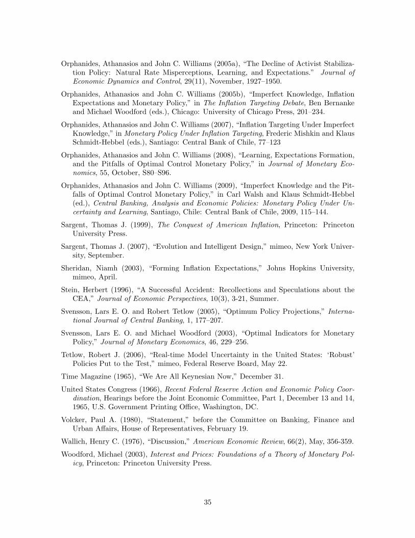
Orphanides, Athanasios and John C. Williams (2005a), “The Decline of Activist Stabiliza-tion Policy: Natural Rate Misperceptions, Learning, and Expectations.” Journal ofEconomic Dynamics and Control, 29(11), November, 1927–1950.

Orphanides, Athanasios and John C. Williams (2005b), “Imperfect Knowledge, InflationExpectations and Monetary Policy,” in The Inflation Targeting Debate, Ben Bernankeand Michael Woodford (eds.), Chicago: University of Chicago Press, 201–234.

Orphanides, Athanasios and John C. Williams (2007), “Inflation Targeting Under ImperfectKnowledge,” in Monetary Policy Under Inflation Targeting, Frederic Mishkin and KlausSchmidt-Hebbel (eds.), Santiago: Central Bank of Chile, 77–123

Orphanides, Athanasios and John C. Williams (2008), “Learning, Expectations Formation,and the Pitfalls of Optimal Control Monetary Policy,” in Journal of Monetary Eco-nomics, 55, October, S80–S96.

Orphanides, Athanasios and John C. Williams (2009), “Imperfect Knowledge and the Pit-falls of Optimal Control Monetary Policy,” in Carl Walsh and Klaus Schmidt-Hebbel(ed.), Central Banking, Analysis and Economic Policies: Monetary Policy Under Un-certainty and Learning, Santiago, Chile: Central Bank of Chile, 2009, 115–144.

Sargent, Thomas J. (1999), The Conquest of American Inflation, Princeton: PrincetonUniversity Press.

Sargent, Thomas J. (2007), “Evolution and Intelligent Design,” mimeo, New York Univer-sity, September.

Sheridan, Niamh (2003), “Forming Inflation Expectations,” Johns Hopkins University,mimeo, April.

Stein, Herbert (1996), “A Successful Accident: Recollections and Speculations about theCEA,” Journal of Economic Perspectives, 10(3), 3-21, Summer.

Svensson, Lars E. O. and Robert Tetlow (2005), “Optimum Policy Projections,” Interna-tional Journal of Central Banking, 1, 177–207.

Svensson, Lars E. O. and Michael Woodford (2003), “Optimal Indicators for MonetaryPolicy,” Journal of Monetary Economics, 46, 229–256.

Tetlow, Robert J. (2006), “Real-time Model Uncertainty in the United States: ‘Robust’Policies Put to the Test,” mimeo, Federal Reserve Board, May 22.

Time Magazine (1965), “We Are All Keynesian Now,” December 31.

United States Congress (1966), Recent Federal Reserve Action and Economic Policy Coor-dination, Hearings before the Joint Economic Committee, Part 1, December 13 and 14,1965, U.S. Government Printing Office, Washington, DC.

Volcker, Paul A. (1980), “Statement,” before the Committee on Banking, Finance andUrban Affairs, House of Representatives, February 19.

Wallich, Henry C. (1976), “Discussion,” American Economic Review, 66(2), May, 356-359.

Woodford, Michael (2003), Interest and Prices: Foundations of a Theory of Monetary Pol-icy, Princeton: Princeton University Press.

35

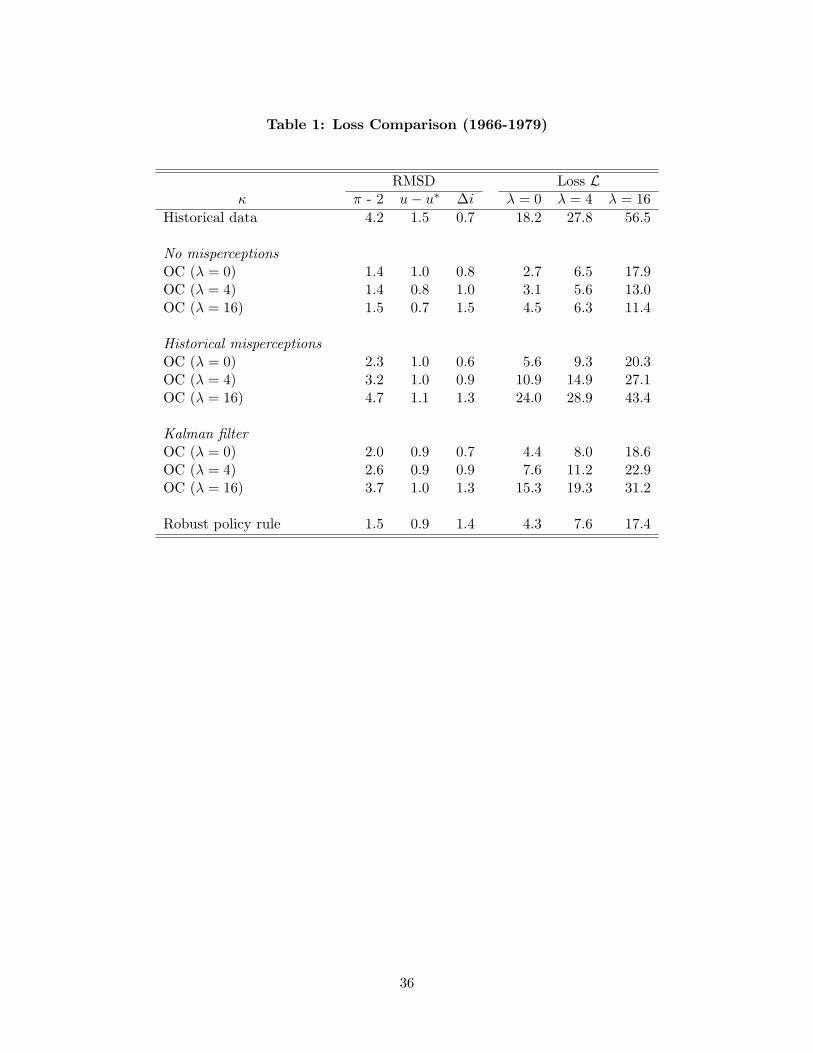
Table 1: Loss Comparison (1966-1979)

RMSD Loss Lκ π - 2 u− u∗ ∆i λ = 0 λ = 4 λ = 16

Historical data 4.2 1.5 0.7 18.2 27.8 56.5

No misperceptionsOC (λ = 0) 1.4 1.0 0.8 2.7 6.5 17.9OC (λ = 4) 1.4 0.8 1.0 3.1 5.6 13.0OC (λ = 16) 1.5 0.7 1.5 4.5 6.3 11.4

Historical misperceptionsOC (λ = 0) 2.3 1.0 0.6 5.6 9.3 20.3OC (λ = 4) 3.2 1.0 0.9 10.9 14.9 27.1OC (λ = 16) 4.7 1.1 1.3 24.0 28.9 43.4

Kalman filterOC (λ = 0) 2.0 0.9 0.7 4.4 8.0 18.6OC (λ = 4) 2.6 0.9 0.9 7.6 11.2 22.9OC (λ = 16) 3.7 1.0 1.3 15.3 19.3 31.2

Robust policy rule 1.5 0.9 1.4 4.3 7.6 17.4

36

Table 2: Loss Comparison (1966-2003)

RMSD Loss Lκ π - 2 u− u∗ ∆i λ = 0 λ = 4 λ = 16

Historical data 3.3 1.4 1.0 11.6 19.6 43.8

No misperceptionsOC (λ = 0) 1.2 0.7 0.6 2.0 4.0 10.0OC (λ = 4) 1.3 0.6 0.9 2.5 3.8 7.7OC (λ = 16) 1.5 0.5 1.2 3.7 4.6 7.3

Historical misperceptionsOC (λ = 0) 1.7 0.8 0.6 3.4 5.7 12.9OC (λ = 4) 2.3 0.8 0.8 6.0 8.4 15.5OC (λ = 16) 3.3 0.8 1.2 12.4 14.9 22.5

Kalman filterOC (λ = 0) 1.6 0.8 0.6 2.9 5.3 12.6OC (λ = 4) 2.0 0.8 0.8 4.8 7.0 13.9OC (λ = 16) 2.7 0.8 1.2 8.8 11.1 18.0

Robust policy rule 1.3 0.8 1.0 2.7 5.2 12.6

37

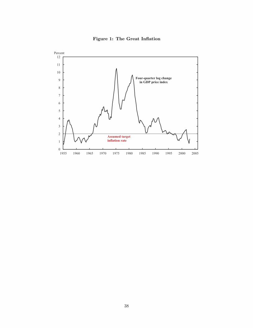
Figure 1: The Great Inflation

0

1

2

3

4

5

6

7

8

9

10

11

12

1955 1960 1965 1970 1975 1980 1985 1990 1995 2000 2005

Percent

Four-quarter log change

in GDP price index

Assumed target

inflation rate

38

Figure 2: Estimates of the Natural Rate of Unemployment

3

4

5

6

7

8

9

10

11

1955 1960 1965 1970 1975 1980 1985 1990 1995 2000 2005

Percent

Real-time estimates

Retrospective

CBO estimates

Unemployment rate

39

Figure 3: Counterfactual Simulations under OC Policy with λ = 16

Absent Misperceptions With Historical Misperceptions

Inflation Inflation

-2

0

2

4

6

8

10

12

1965 1970 1975 1980 1985 1990 1995 2000 2005

Percent

OC policy (� � ��� � � ��

Data

-2

0

2

4

6

8

10

12

1965 1970 1975 1980 1985 1990 1995 2000 2005

Percent

OC policy (� � ��� � � ��

Data

Inflation Expectations Inflation Expectations

0

1

2

3

4

5

6

7

8

9

10

1965 1970 1975 1980 1985 1990 1995 2000 2005

Percent

OC policy (� � ��� � � ��

SPF

0

1

2

3

4

5

6

7

8

9

10

1965 1970 1975 1980 1985 1990 1995 2000 2005

Percent

OC policy (� � ��� � � ��SPF

Unemployment Rate Unemployment Rate

3

4

5

6

7

8

9

10

11

1965 1970 1975 1980 1985 1990 1995 2000 2005

Percent

OC policy

(� � ��� � � ��

Data

Natural rate

3

4

5

6

7

8

9

10

11

1965 1970 1975 1980 1985 1990 1995 2000 2005

Percent

OC policy

(� � ��� � � ��

Data

Natural rate

40

Figure 4: Counterfactual Simulations under OC Policy with λ = 4

Absent Misperceptions With Historical Misperceptions

Inflation Inflation

-2

0

2

4

6

8

10

12

1965 1970 1975 1980 1985 1990 1995 2000 2005

Percent

Data

OC Policy (� � �� � � ��

-2

0

2

4

6

8

10

12

1965 1970 1975 1980 1985 1990 1995 2000 2005

Percent

Data

OC Policy

(� � ��� � ��

Inflation Expectations Inflation Expectations

0

1

2

3

4

5

6

7

8

9

10

1965 1970 1975 1980 1985 1990 1995 2000 2005

Percent

SPF

OC Policy (� � �� � � ��

0

1

2

3

4

5

6

7

8

9

10

1965 1970 1975 1980 1985 1990 1995 2000 2005

Percent

SPF

OC Policy (� � �� � � ��

Unemployment Rate Unemployment Rate

3

4

5

6

7

8

9

10

11

1965 1970 1975 1980 1985 1990 1995 2000 2005

Percent

Data

Natural rate

OC Policy

(� � ��� � ��

3

4

5

6

7

8

9

10

11

1965 1970 1975 1980 1985 1990 1995 2000 2005

Percent

Data

Natural rateOC Policy

(� � �� � � ��

41

Figure 5: Counterfactual Simulations under OC Policy with λ = 0

Absent Misperceptions With Historical Misperceptions

Inflation Inflation

-2

0

2

4

6

8

10

12

1965 1970 1975 1980 1985 1990 1995 2000 2005

Percent

Data

OC Policy (� �

0� � � ��-2

0

2

4

6

8

10

12

1965 1970 1975 1980 1985 1990 1995 2000 2005

Percent

Data

OC Policy

(� �

0� � � ��Inflation Expectations Inflation Expectations

0

1

2

3

4

5

6

7

8

9

10

1965 1970 1975 1980 1985 1990 1995 2000 2005

Percent

SPF

OC Policy (� �

0� � � ��0

1

2

3

4

5

6

7

8

9

10

1965 1970 1975 1980 1985 1990 1995 2000 2005

Percent

SPF

OC Policy (� �

0� � � ��Unemployment Rate Unemployment Rate

3

4

5

6

7

8

9

10

11

1965 1970 1975 1980 1985 1990 1995 2000 2005

Percent

Data

Natural rate

OC Policy

(� �

0� � � ��3

4

5

6

7

8

9

10

11

1965 1970 1975 1980 1985 1990 1995 2000 2005

Percent

Data

Natural rateOC Policy

(� �

0� � � ��

42

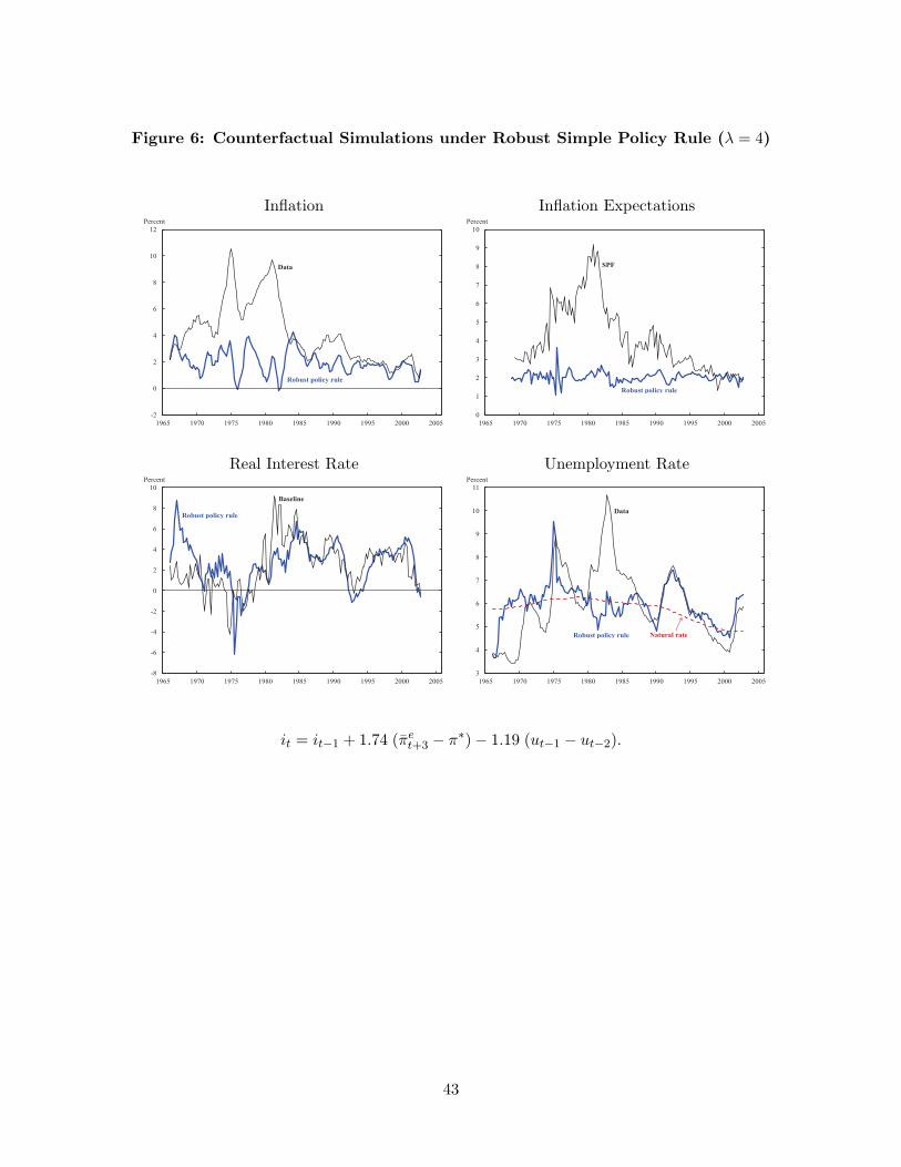
Figure 6: Counterfactual Simulations under Robust Simple Policy Rule (λ = 4)

Inflation Inflation Expectations

-2

0

2

4

6

8

10

12

1965 1970 1975 1980 1985 1990 1995 2000 2005

Percent

Data

Robust policy rule

0

1

2

3

4

5

6

7

8

9

10

1965 1970 1975 1980 1985 1990 1995 2000 2005

Percent

Robust policy rule

SPF

Real Interest Rate Unemployment Rate

-8

-6

-4

-2

0

2

4

6

8

10

1965 1970 1975 1980 1985 1990 1995 2000 2005

Percent

Robust policy rule

Baseline

3

4

5

6

7

8

9

10

11

1965 1970 1975 1980 1985 1990 1995 2000 2005

Percent

Data

Natural rateRobust policy rule

it = it−1 + 1.74 (πet+3 − π∗)− 1.19 (ut−1 − ut−2).

43

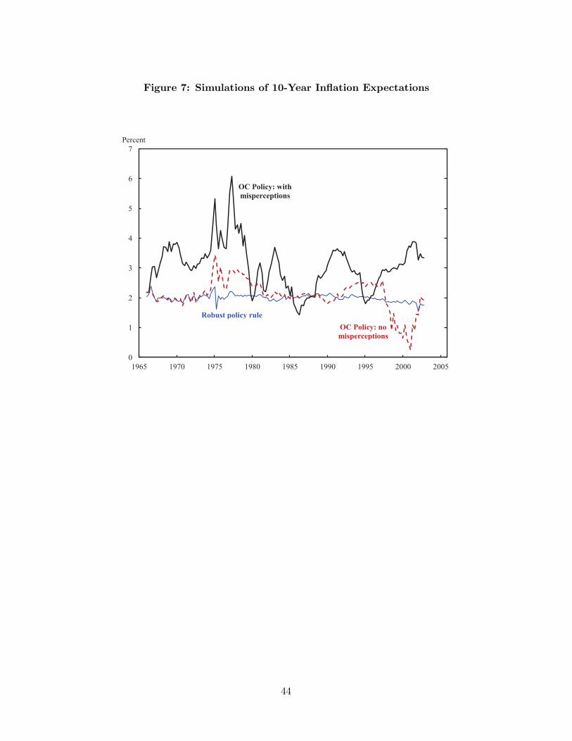
Figure 7: Simulations of 10-Year Inflation Expectations

0

1

2

3

4

5

6

7

1965 1970 1975 1980 1985 1990 1995 2000 2005

Percent

Robust policy rule

OC Policy: with

misperceptions

OC Policy: no

misperceptions

44