APPLICATIONS OF SHORTEST PATH ALGORITHMS TO VLSI

LAYOUT PROBLEMS

BY

ASHOK JAGANNATHANB�E�� Computer Science and Engineering� Regional Engineering College� Trichy� India� ����

THESIS

Submitted as partial ful�llment of the requirementsfor the degree of Master of Science in Electrical Engineering and Computer Science

in the Graduate College of theUniversity of Illinois at Chicago� ����

Chicago� Illinois

To my parents���

iii

ACKNOWLEDGMENTS

I express my profound gratitude to my advisor Dr�John Lillis for his constant guidance�

support and encouragement throughout the course of this work� His friendly behavior with

students has made working with him a wonderful experience� As his student� I have learnt a

lot of things from him� both technically and as a person�

I also thank my committee members Dr�Shantanu Dutt and Dr�Peter Nelson for spending

their precious time on reviewing my thesis and providing valuable comments on this work�

As colleagues in the same lab� I sincerely thank SungWoo Hur for all the help he extended

without any reservations� I also thank Milos Hrkic for the time he spent on reviewing my thesis�

I cannot forget the various technically enriching discussions we had during the course of our

work� It was really a pleasure working with both of them�

Of course� I thank all my roommates for making my stay at UIC absolutely unforgettable�

Finally� I am very thankful to my parents� brother and sisters for having given me this

opportunity and for constantly backing me on all my pursuits�

iv

TABLE OF CONTENTS

CHAPTER PAGE

� INTRODUCTION � � � � � � � � � � � � � � � � � � � � � � � � � � � � � � � � ���� Intrarow Optimization Of StandardCell Placement � � � � � � ���� Context Aware Buer Insertion � � � � � � � � � � � � � � � � � � �

� INTRA�ROW OPTIMIZATION OF STANDARD�CELL LAY�

OUT � � � � � � � � � � � � � � � � � � � � � � � � � � � � � � � � � � � � � � � � � ���� StandardCell Design � � � � � � � � � � � � � � � � � � � � � � � � ���� Preliminaries � � � � � � � � � � � � � � � � � � � � � � � � � � � � � ������ Wirelength Estimation � � � � � � � � � � � � � � � � � � � � � � � ��� Problem Formulation � � � � � � � � � � � � � � � � � � � � � � � � ��� �� Previous Work � � � � � � � � � � � � � � � � � � � � � � � � � � � � ���� Optimal Arrangement By Dynamic Programming � � � � � � � ������� Dynamic Programming Recurrence � � � � � � � � � � � � � � � � ������� Computing Incremental Cost � � � � � � � � � � � � � � � � � � � � � ���� DPAlgorithm � � � � � � � � � � � � � � � � � � � � � � � � � � � � � ������� Complexity � � � � � � � � � � � � � � � � � � � � � � � � � � � � � � ����� GraphTheoretic Interpretation � � � � � � � � � � � � � � � � � � ����� Accelerating ShortestPath Search � � � � � � � � � � � � � � � � � ������� Relaxation Based Lower Bound � � � � � � � � � � � � � � � � � � ������� Faster Lower Bound Computation � � � � � � � � � � � � � � � � � ������ SPAlgorithm � � � � � � � � � � � � � � � � � � � � � � � � � � � � � ��� Experimental Results � � � � � � � � � � � � � � � � � � � � � � � � ��� Comments and Conclusion � � � � � � � � � � � � � � � � � � � � � �

� CONTEXT�AWARE BUFFER INSERTION � � � � � � � � � � � � � � �� Introduction � � � � � � � � � � � � � � � � � � � � � � � � � � � � � � � �� Background � � � � � � � � � � � � � � � � � � � � � � � � � � � � � � �� ���� Delay Models � � � � � � � � � � � � � � � � � � � � � � � � � � � � � �� ���� Dominance Property � � � � � � � � � � � � � � � � � � � � � � � � � � � Buer Graph � � � � � � � � � � � � � � � � � � � � � � � � � � � � � � �� Problem Formulations � � � � � � � � � � � � � � � � � � � � � � � � �� ���� Labeling Algorithm � � � � � � � � � � � � � � � � � � � � � � � � � �� �� DRCR Algorithm � � � � � � � � � � � � � � � � � � � � � � � � � � � �� ���� Complexity � � � � � � � � � � � � � � � � � � � � � � � � � � � � � � �� �� Properties � � � � � � � � � � � � � � � � � � � � � � � � � � � � � � � �� ���� Lower Convex Hull � � � � � � � � � � � � � � � � � � � � � � � � � � �� �� Experimental Results � � � � � � � � � � � � � � � � � � � � � � � � �

v

TABLE OF CONTENTS �Continued�

CHAPTER PAGE

�� Comments and Conclusion � � � � � � � � � � � � � � � � � � � � � ��

CITED LITERATURE � � � � � � � � � � � � � � � � � � � � � � � � � � � � ��

VITA � � � � � � � � � � � � � � � � � � � � � � � � � � � � � � � � � � � � � � � � � ��

vi

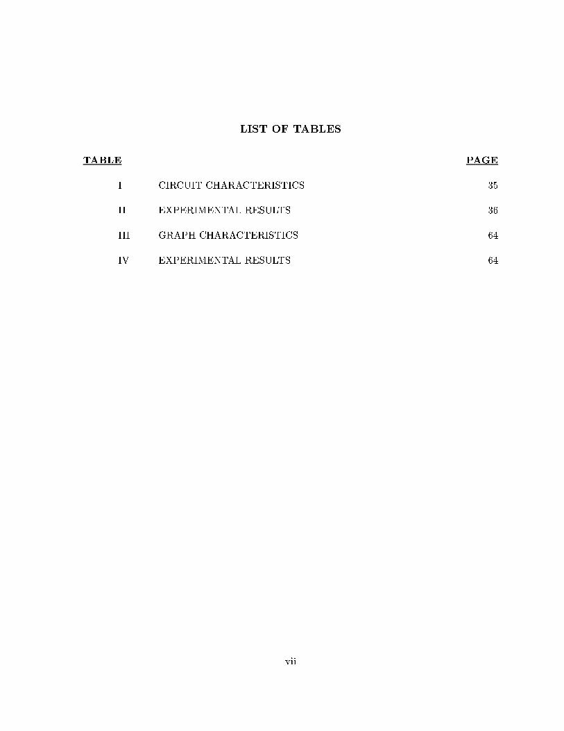
LIST OF TABLES

TABLE PAGE

I CIRCUIT CHARACTERISTICS � � � � � � � � � � � � � � � � � � � � � �

II EXPERIMENTAL RESULTS � � � � � � � � � � � � � � � � � � � � � � � �

III GRAPH CHARACTERISTICS � � � � � � � � � � � � � � � � � � � � � � ��

IV EXPERIMENTAL RESULTS � � � � � � � � � � � � � � � � � � � � � � � ��

vii

LIST OF FIGURES

FIGURE PAGE

� Illustration of a typical standard cell placement where cells are dis�tributed over a set of rows� � � � � � � � � � � � � � � � � � � � � � � � � � � � �

� Estimation of wirelength using Half�Perimeter metric� The wirelength

of the net is the sum of the length and width of the smallest rectangle

enclosing all the pins in the net as shown by the dark lines� � � � � � � � �

Example of a window of � cells from a single�row of a standard�cell

placement� � � � � � � � � � � � � � � � � � � � � � � � � � � � � � � � � � � � � � �

� Illustration of the notion of incremental wirelength of a cell with respect

to a subset of cells� � � � � � � � � � � � � � � � � � � � � � � � � � � � � � � � � ��

� Illustration of the extension of an arrangement of a subset of cells� � � � �

� Outline of the dynamic programming approach for �nding the optimal

linear arrangement of cells� � � � � � � � � � � � � � � � � � � � � � � � � � � � ��

� Illustration of the graph implied by the DP�algorithm for an instance of

three cells fa� b� cg inside the window� � � � � � � � � � � � � � � � � � � � � ��

� Illustration of A� approach� � � � � � � � � � � � � � � � � � � � � � � � � � � ��

� Example of a sub�circuit projected on the x�axis� � � � � � � � � � � � � � ��

�� Instance of an output generated by the network��ow algorithm� Many

mobile cells can be associated with a single �xed cell� � � � � � � � � � � � �

�� Computing lower bounds from the information on the minimum number

of nets cut between pair of adjacent �xed cells� � � � � � � � � � � � � � � � �

�� Computing lower bounds for subsets based on the information obtained

from a pre�processing step� � � � � � � � � � � � � � � � � � � � � � � � � � � � �

� Outline of the algorithm using lower bounding to �nd optimal linear

arrangement� � � � � � � � � � � � � � � � � � � � � � � � � � � � � � � � � � � � �

viii

LIST OF FIGURES �Continued�

FIGURE PAGE

�� An illustration of bu�er insertion taking pre�placed macro cells into con�

sideration� the black boxes represent portions of the routing area where

neither bu�ering nor wiring is possible� the grey boxes represent areaswhere wires can be routed� but bu�ers cannot be inserted� � � � � � � � �

�� RC delay modeling for a wire� � � � � � � � � � � � � � � � � � � � � � � � � ��

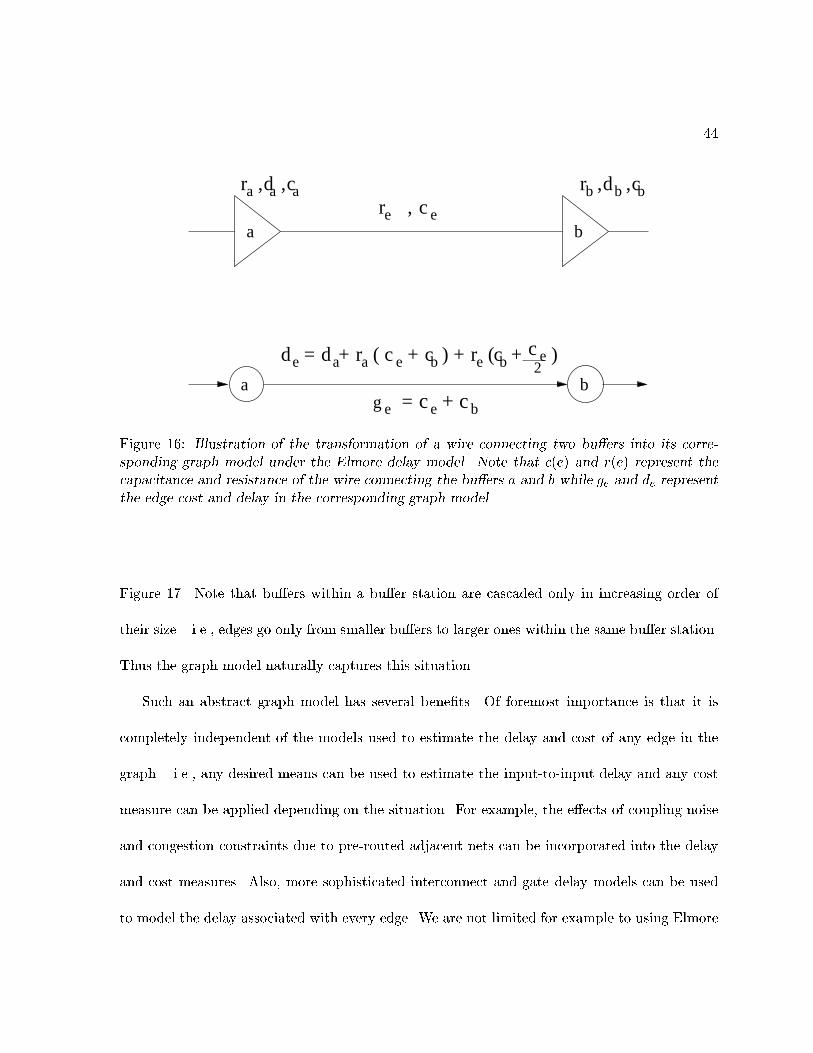
�� Illustration of the transformation of a wire connecting two bu�ers into

its corresponding graph model under the Elmore delay model� Note

that c�e� and r�e� represent the capacitance and resistance of the wire

connecting the bu�ers a and b while ge and de represent the edge cost

and delay in the corresponding graph model� � � � � � � � � � � � � � � � ��

�� Illustration of cascading bu�ers within a bu�er station� solid lines rep�resent connections within the bu�er station and broken lines represent

edges to and from outside the bu�er station� a A bu�er station with

bu�ers of di�erent sizes and b the corresponding graph model� � � � � ��

�� Illustration of a set of bu�er stations modeled as a graph � all lines

represent edges while the solid lines represent source�to�sink paths� a

instance of a set of bu�er stations with �nite bu�ering resources b a

simple s � t path passing though various bu�er stations c a s � tpath in which bu�ers are cascaded at the intermediate bu�er station A� ��

�� DRCR algorithm to solve the ratio maximization problem� � � � � � � � ��

�� Illustration of the Lower Convex Hull property� All circles represent the

set of all non�dominated paths� the shaded circles represent points on

the LCH� � � � � � � � � � � � � � � � � � � � � � � � � � � � � � � � � � � � � � ��

�� Figure illustrating the existence of a Dref for every �g� d� on the LCH� ��

�� Examples of LCH of the cost vs� delay trade o� curve for two di�erent

graphs G� and G�� � � � � � � � � � � � � � � � � � � � � � � � � � � � � � � � ��

ix

SUMMARY

Due to the natural interpretation of a circuit as a graph model� a lot of research has been

done on e�ciently applying graphtheoretic algorithms to VLSI layout problems� In this thesis�

we study two such applications of classical shortestpath algorithms in the context of VLSI

layout synthesis�

The �rst problem deals with minimizing the wirelength of a given standardcell layout by

rearranging the cells within a given window in a row� We study the modeling of this problem

as a shortestpath problem and apply the A� algorithm for e�ciently �nding the shortest path�

A powerful network�ow based technique is proposed to �nd lower bounds on wirelength which

is used to accelerate the A� search�

The second problem deals with minimizing interconnect delay via buer insertion in the

context of a given layout� where there are typically restrictions on where buers can be placed�

We model this problem with a buer graph and formulate a new problem called Delay Reduction

to Cost Ratio Maximization� which is aware of the tradeo between cost and delay� We also

propose a fast algorithm for probing the tradeo curve e�ciently�

Our experimental results show the viability of the approaches suggested in this work�

x

CHAPTER �

INTRODUCTION

The progressively increasing number of devices in modern highperformance circuits have

made the use of CAD tools for layout synthesis inevitable� Moreover� due to the scaling down

VLSI process technology� interconnect delay has become the bottleneck in designing modern

circuits� Clearly� techniques which consider minimizing the interconnect delay directly �by

inserting buers� sizing wires etc�� or indirectly �by minimizing total wirelength etc�� have

become necessary and important� Toward this end� a lot of work has been done in recent years�

opening new avenues for potential research�

Due to the natural interpretation of a circuit representation as a graph model� applications of

a variety of graph theoretic algorithms have been studied with respect to VLSI layout synthesis�

For example� graph partitioning algorithms are extensively used to partition a large circuit into

smaller components such that the number of interconnections between components is minimized�

which is a very crucial problem in the layout domain� It is important to note that most of the

layout problems are NP�hard��� and hence there has been continued interest in exploring new

applications of graphbased algorithms to these problems�

In this thesis� we study the applications of the classical shortest�path algorithm in a graph

in the context of two dierent VLSI layout problems which are very important during layout

optimization of any chip� Abstracts of these two applications are presented below�

�

�

��� Intra�row Optimization Of Standard�Cell Placement

Minimizing the total wirelength of a standardcell placement by optimally placing cells

within a row is a fundamental problem in CAD� Given a window of n adjacent cells in a row� the

problem is to �nd the optimal arrangement of these cells within the window such that the total

wirelength of all nets incident on these cells is minimized� In this work� we study a dynamic

programming �DP� based algorithm which �nds the minimum wirelength arrangement of cells

by incrementally constructing all �n subsets of the given cells� The idea is based on the fact

that the optimal arrangement of a subset S of placed cells within the window is independent

of the arrangement of the unplaced cells �within the window�� The DP algorithm implies a

con�guration graph with �n vertices� where each vertex represents a subset of cells within the

window� In the traditional DP algorithm� this graph is exhaustively explored levelbylevel� To

speed up this process� we apply the A� algorithm��� to this con�guration graph� By using A�

along with e�cient lower bounding techniques using network �ows� only a small percentage of

the vertices are visited and hence the problem size which can be solved eectively is increased�

��� Context Aware Bu�er Insertion

Buer insertion has been proven to be a very powerful technique in optimizing interconnect

delay� We study the problem of inserting buers in the context of a given layout with possibly

some restrictions on the location of buers� Due to the presence of such restrictions on where

buers can be placed� it sometimes becomes necessary to detour just to �pick up� a buer�

Due to this reason� it is necessary to perform routing and buer insertion simultaneously� Also�

it is important that such algorithms are aware of the tradeo between cost �eg� routing cost�

total capacitance etc�� and delay� In this context� we propose the Delay Reduction to Cost

Ratio Maximization problem �which is similar to the shortest weightconstrained path problem

���� and propose a fast algorithm for the same� Some interesting properties of the solutions

generated by the algorithm have also been studied�

Chapter � deals with the linear arrangement problem and its application to standardcell

layout while chapter discusses the problem of buer insertion in the context of a given layout�

CHAPTER �

INTRA�ROW OPTIMIZATION OF STANDARD�CELL LAYOUT

��� Standard�Cell Design

In a Standardcell design methodology� the designer is provided with a library of e�ciently

designed basic logic cells such as NAND gates� Multiplexers� Decoders etc� Additionally� all

logic cells in the library are implemented so that the height of the blocks is the same while the

widths vary� In such a scenario� any logic function on the designer�s side can be implemented

in terms of a set of basic blocks taken from the standardcell library� The advantage of such a

design methodology is that designs can be completed rapidly� Also� as the layout for the cells

from the library is readily available� the layout tool is only concerned about assigning locations

to these cells and �nding interconnections between these cells� Although the predesigned cell

library considerably reduces the complexity of the design process� there can be as much as

hundreds of thousands of cells in a single circuit these days� and hence the physical design

process has to be e�ciently automated�

The Standard�cell Placement problem is related to �nding locations for all the cells in the

circuit such that no two cells overlap and the placement optimizes some objectives� Most com

mon objectives for the placement problem are timing optimization� chip area minimization�

wirelength minimization etc� or a composite function of these objectives� Irrespective of the

objective function� most of the placement problems belong to the class of NP�hard ��� prob

�

�

lems� The placement problem is one of the crucial problems in VLSI physical design� and it

has a direct impact on the performance� area� routability and yield of the circuit�

Since all the cells in a standardcell design have the same height� such a design is typically

placed in rows of cells� as shown in Figure ��

Figure �� Illustration of a typical standard cell placement where cells are distributed over a set

of rows�

Once the cells are distributed across rows� a variety of intrarow optimization techniques

are applied to further improve the placement by optimizing certain objectives� The focus of

this work is also on performing intrarow optimization by �nding optimal linear arrangement

�

of cells within a row� where the cost of any arrangement is the sum of the wirelengths of the

nets incident on the cells under consideration�

��� Preliminaries

A netlist is a representation of a circuit which speci�es the components contained in the

circuit along with the respective interconnecting signals� Such a netlist of any circuit can be

modeled as a hypergraph G � �V�E�� where the vertex set V represents the set of cells �or

modules� and the hyperedge set E represents the set of all signal nets that interconnect the

cells� Each edge e � E connects a subset of two or more vertices from V � i�e�� e � V �

Since each cell in the circuit has a nonzero length and width� the pins on each cell can be

located anywhere on the cell� However� for simplicity reasons� we approximate the pin locations

on any cell to be the center of that cell� Based on such an assumption� there are several methods

to estimate the wirelength of any signal net in a given placement of a circuit� Of these� we use

the halfperimeter�HP� metric explained below to estimate the wirelength of the nets�

����� Wirelength Estimation

Basically� the HPestimator �nds the smallest rectangle enclosing all the pins on the net�

and takes the sum of the length and width of this rectangle to be an estimate of the wirelength

of the corresponding net� Figure � shows an example where the HPestimator is used to �nd the

wirelength of a �pin net� The dark lines in the �gure show the length and width of the smallest

rectangle enclosing all the pins� and the sum of these two values is the estimated wirelength of

this net�

�

Figure �� Estimation of wirelength using Half�Perimeter metric� The wirelength of the net is

the sum of the length and width of the smallest rectangle enclosing all the pins in the net asshown by the dark lines�

The HPestimator is widely used because of its simplicity in implementation� More impor

tantly� the metric provides an exact estimate of the wirelength for �pin and pin nets and a

lower bound on the wirelength of nets with four or more pins�

In the following section� we formally introduce the linear arrangement problem in the context

of a given standardcell layout and discuss some previous work relevant to the problem�

��� Problem Formulation

Given a standardcell layout with cells distributed over dierent rows� the optimal linear

arrangement problem can be stated as follows�

Formulation � Given� A set W of n cells in a row of a given standard�cell placement along

with their connectivity information�

�

Objective� Find an optimal linear arrangement of the n cells within the window such that the

sum of the wirelength of the nets incident on these cells is minimized�

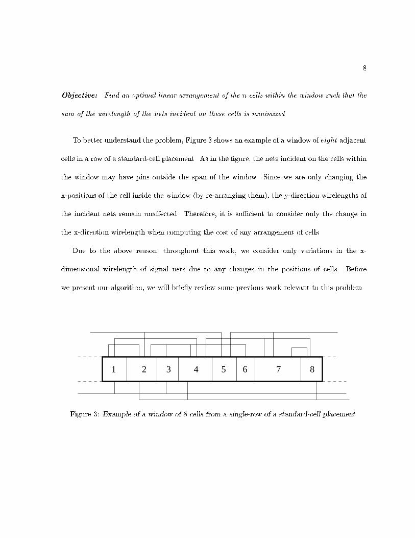
To better understand the problem� Figure shows an example of a window of eight adjacent

cells in a row of a standardcell placement� As in the �gure� the nets incident on the cells within

the window may have pins outside the span of the window� Since we are only changing the

xpositions of the cell inside the window �by rearranging them�� the ydirection wirelengths of

the incident nets remain unaected� Therefore� it is su�cient to consider only the change in

the xdirection wirelength when computing the cost of any arrangement of cells�

Due to the above reason� throughout this work� we consider only variations in the x

dimensional wirelength of signal nets due to any changes in the positions of cells� Before

we present our algorithm� we will brie�y review some previous work relevant to this problem�

1 2 3 4 5 6 7 8

Figure � Example of a window of � cells from a single�row of a standard�cell placement�

�

����� Previous Work

The optimal linear arrangement problem naturally lends itself to enumeration and branch�

and�bound based approaches� Enumeration based methods evaluate all n� permutations of

the given cells and choose the minimum wirelength arrangement of the cells� However� as

stated before� such techniques become extremely slow in practice for even modest problem sizes

�windows containing � or more cells� � ��

On the other hand� branchandbound based methods have been proposed to �nd the min

imum wirelength arrangement of the cells � �� In such a branchandbound placer� starting

from an empty initial arrangement� cells are added one at a time to the arrangement� and the

bounding box of the incident nets are extended to include the the new pin locations intro

duced by the newly added cell� The e�ciency of this approach largely relies on computing�

from a given partial arrangement� a lower bound on the wirelength of any completion of this

arrangement� Extensions of the current partial arrangement are considered only as long as this

lower bound is smaller than the cost of the best complete arrangement seen so far� Though

the branchandbound algorithms can be e�cient depending on the lower bounding technique�

they explore all n� permutations in the worst case�

The techniques presented in this work are based on the fact that the optimal arrangement

of a subset S of cells in W is independent of the arrangement of the cells in �W �S� � i�e�� any

pre�x of the minimum wirelength arrangement of all the cells in W is the minimum wirelength

arrangement of the cells contained in that pre�x� This observation was earlier applied to the

problem of backboard ordering by Cederbaum ���� In this work� we study this property in the

��

context of a standardcell placement and present an algorithm based on a dynamic programming

framework to compute the minimum wirelength linear arrangement of the cells in W �

��� Optimal Arrangement By Dynamic Programming

Consider any possible linear arrangement L of all n cells� This linear arrangement can be

obtained by placing one cell at a time starting from the left boundary of the window till all the

n cells are placed� Since each cell v has some signal nets associated with it� each cell contributes

some wirelength to the total wirelength of the arrangement L� We now introduce the notion

of incremental wirelength contributed by any cell to the total wirelength of an existing partial

arrangement�

Let N represent the set of all nets which are incident on at least one cell in the window �

i�e�� these are exactly those nets whose wirelength is aected by any rearrangement of the cells

within the window� Then� if S is any subset of cells in W � for each v � �W � S�� we de�ne the

incremental cost I�S� v� of the cell v with respect to the subset S as the total wirelength of all

the nets in N within the region spanned by the width of cell v� when v is placed immediately

to the right of any arrangement of the cells only in S�

To clearly illustrate the notion of incremental wirelength� Figure � shows an example of a

window W � fa� b� c� d� e� f� g� hg of eight cells� As shown� x� and x� mark the left and right

boundaries of the window respectively� The subset S � fa� b� c� dg of cells has already been

placed as shown in the �gure� We now want to place the cell e to the right of the cells only in S

as shown� The incremental wirelength I�S� e� is exactly the wirelength of the nets in the region

between x� and x� which is the xregion spanned by the width of cell e� The portion of the nets

��

a b c d e f hg

xx1 2x x0 3

Figure �� Illustration of the notion of incremental wirelength of a cell with respect to a subset

of cells�

which contribute to I�S� e� is shown in dark lines in the �gure� The sum of the xdimensional

span of all the dark lines is the incremental wirelength for cell e with respect to subset S�

An interesting property of I�S� v� is that it is independent of the arrangement of cells in S

and in �W � S � fvg�� It is only dependent on the cells in S and the corresponding xregion

that is spanned by the width of cell v� Also� note that if � represents the empty set� then I��� v�

gives the incremental wirelength of placing cell v at the left boundary of the window�

Thus� the total wirelength of any linear arrangement L of all n cells can be computed as the

sum of the incremental wirelengths contributed when each cell was added� The arrangement

for which this sum is a minimum is the solution to the problem�

��

Based on this incremental wirelength computation� we now present a dynamic programming

recurrence for �nding the minimum wirelength arrangement of the cells in W �

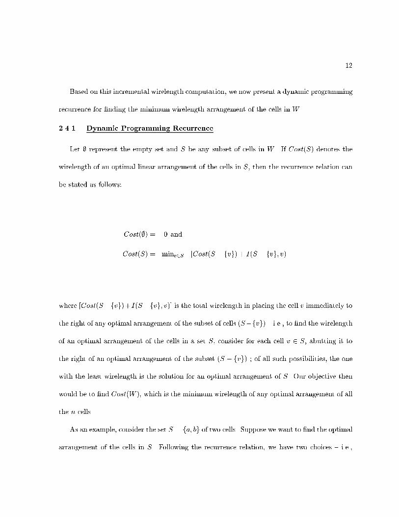
����� Dynamic Programming Recurrence

Let � represent the empty set and S be any subset of cells in W � If Cost�S� denotes the

wirelength of an optimal linear arrangement of the cells in S� then the recurrence relation can

be stated as follows�

Cost��� � � and

Cost�S� � minv�S �Cost�S � fvg� � I�S � fvg� v��

where �Cost�S�fvg��I�S�fvg� v�� is the total wirelength in placing the cell v immediately to

the right of any optimal arrangement of the subset of cells �S�fvg� � i�e�� to �nd the wirelength

of an optimal arrangement of the cells in a set S� consider for each cell v � S� abutting it to

the right of an optimal arrangement of the subset �S � fvg� � of all such possibilities� the one

with the least wirelength is the solution for an optimal arrangement of S� Our objective then

would be to �nd Cost�W �� which is the minimum wirelength of any optimal arrangement of all

the n cells�

As an example� consider the set S � fa� bg of two cells� Suppose we want to �nd the optimal

arrangement of the cells in S� Following the recurrence relation� we have two choices � i�e��

�

�Cost�fag� � I�fag� b�� which is the cost of the arrangement ab and �Cost�fbg� � I�fbg� a���

which is the cost of the arrangement ba� The one with the least cost of these two choices is

the solution� However� to compute these values� we should have computed the minimum cost

arrangement of sets fag and fbg� which is basically the cost of placing cell a or b at the left

boundary of the window�

Observe that for any net in N � the dynamic programming recurrence covers only the wire

length that is within the xrange spanned by the entire window � i�e�� it does not take into

account the wirelength of any net in N beyond the left and right boundaries of the window�

For example� in Figure � the portion of the nets to the left of x� and right of x� is not taken

into account by the dynamic programming recurrence� In the following section� we detail the

procedure to compute the incremental cost of a cell v with respect to a subset S of cells�

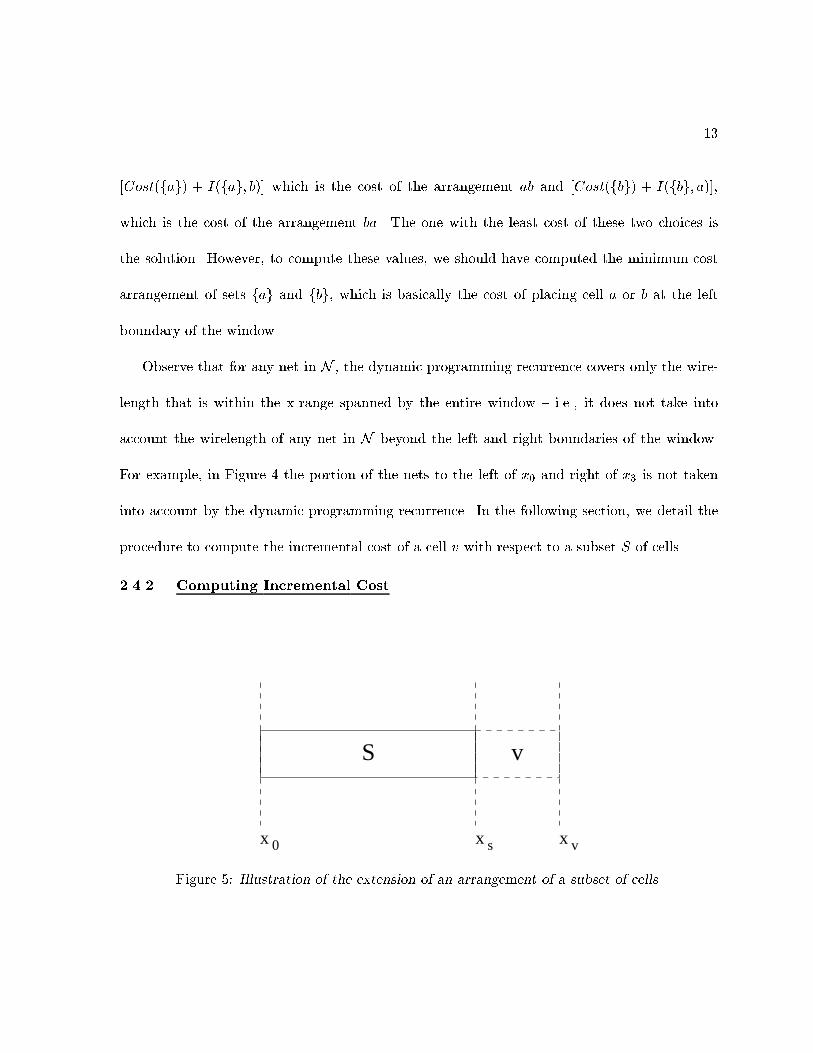
����� Computing Incremental Cost

x

S v

xs vx 0

Figure �� Illustration of the extension of an arrangement of a subset of cells�

��

Suppose we have already constructed a linear arrangement of a subset S of cells in W and

we consider expanding S by placing one more cell v � �W � S� to its right� As shown in

Figure �� let x� be the left boundary of the window W and xs represent the right boundary

of the subset S� We will now show how to compute the incremental cost I�S� v� of cell v with

respect to S�

Assume that the cell v � �W � S� is placed to the right of S� If width�v� represents the

width of the cell v� then let xv � xs � width�v� represent the right boundary of �S � fvg� as

shown in Figure �� As mentioned earlier� let N represent the set of nets which are incident

at least on one cell in W � With respect to S� the subset of nets in N which contribute to the

incremental wirelength of cell v can be classi�ed as follows�

� Terminating nets �Tv These are the nets in N which have at least one pin to the

left of xs and have no pins to the right of xv� Intuitively� these are the set of nets that

start before xs and terminate before xv�

� Continuing nets �Cv These are the nets in N which have pins both to the left of

xs and right of xv� Basically� these are the nets which start before xs� continue over the

region covered by the width of v and terminate somewhere to the right of xv�

� Starting nets �Sv These are the nets in N which have no pin to the left of xs�

have atleast one pin between xs and xv and have at least one pin to the right of xv�

Alternatively� these are the nets which start between xs and xv and terminate somewhere

to the right of xv�

��

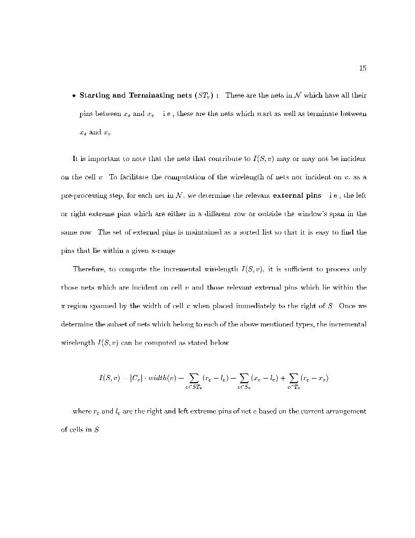
� Starting and Terminating nets �STv These are the nets in N which have all their

pins between xs and xv � i�e�� these are the nets which start as well as terminate between

xs and xv�

It is important to note that the nets that contribute to I�S� v� may or may not be incident

on the cell v� To facilitate the computation of the wirelength of nets not incident on v� as a

preprocessing step� for each net in N � we determine the relevant external pins � i�e�� the left

or right extreme pins which are either in a dierent row or outside the window�s span in the

same row� The set of external pins is maintained as a sorted list so that it is easy to �nd the

pins that lie within a given xrange�

Therefore� to compute the incremental wirelength I�S� v�� it is su�cient to process only

those nets which are incident on cell v and those relevant external pins which lie within the

xregion spanned by the width of cell v when placed immediately to the right of S� Once we

determine the subset of nets which belong to each of the above mentioned types� the incremental

wirelength I�S� v� can be computed as stated below�

I�S� v� � jCvj � width�v� �X

e�STv�re � le� �

Xe�Sv

�xv � le� �Xe�Tv

�re � xs�

where re and le are the right and left extreme pins of net e based on the current arrangement

of cells in S�

��

����� DP�Algorithm

The outline of an algorithm named DP�Algorithm based on the dynamic programming

recurrence presented earlier is given in Figure �� The algorithm starts from the left boundary of

the window and incrementally computes optimal arrangement of all �n subsets until it �nds the

best arrangement of all n cells� The dynamic programming recurrence to compute the optimal

arrangement for any subset is used in line ���� of the algorithm� Since the algorithm generates

subsets in increasing sizes� it ensures that no subset is expanded before its optimal arrangement

is determined�

DP�Algorithm

Given A set W of n adjacent cellsObjective Min wirelength linear arrangement of cells

�� Wi � set of all subsets of size i�� x� is the left boundary of the window

��� W� � ���� for i � � to n do� � begin��� for each subset S �Wi do��� begin��� Cost�S�� minv�S �Cost�S � fvg� � I�S � fvg� v����� end��� end��� �� all �n subsets generated��� Output Cost�W �

Figure �� Outline of the dynamic programming approach for �nding the optimal linear arrange�

ment of cells�

��

It is important to note that when we �nd the minimum wirelength arrangement of a subset

S of cells using the dynamic programming recurrence presented before� we also �nd the cor

responding optimal arrangement of the cells in S� The recurrence ensures that no subset S

is expanded � i�e�� by adding another cell v from �W � S�� until the optimal arrangement for

S is determined� The information on the arrangement of the cells in S is actually encoded in

the last cell v that was added to S based on the recurrence � i�e�� the cell v which corresponds

to the minimum cost of S is the last cell added to S and appears as the rightmost cell in the

optimal ordering of S� Thus we immediately have the information on the subset �S�fvg� from

which we obtained the optimal arrangement for S� following which we can obtain the linear

arrangement of cells which led to this minimum cost of S� Hence� when we reach the set W � we

can backtrack based on the last cell added toW to obtain the corresponding linear arrangement

of all n cells�

����� Complexity

The running time of the algorithm depends on the total time spent on computing the in

cremental wirelengths throughout the algorithm� As stated before� to compute the incremental

wirelength I�S� v�� it is su�cient to examine all nets incident on cell v and all external pins

which lie within the xregion covered by the width of cell v immediately preceded by S� Hence

the total running time of the algorithm can be represented as Ti�Te� where Ti is the total time

to process incident nets during all incremental wirelength computations and Te corresponds to

the total time spent on external pins during all incremental wirelength computations� These

two running times are analyzed separately below�

��

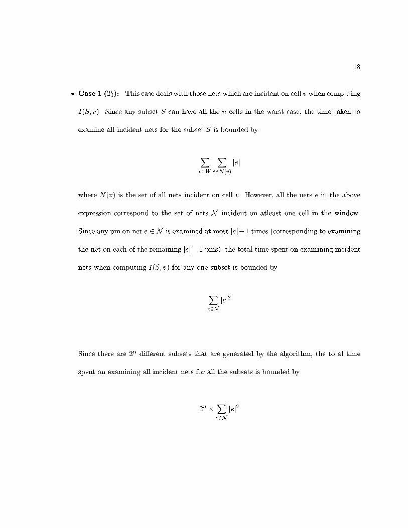
� Case � �Ti This case deals with those nets which are incident on cell v when computing

I�S� v�� Since any subset S can have all the n cells in the worst case� the time taken to

examine all incident nets for the subset S is bounded by

Xv�W

Xe�N�v�

jej

where N�v� is the set of all nets incident on cell v� However� all the nets e in the above

expression correspond to the set of nets N incident on atleast one cell in the window�

Since any pin on net e � N is examined at most jej�� times �corresponding to examining

the net on each of the remaining jej � � pins�� the total time spent on examining incident

nets when computing I�S� v� for any one subset is bounded by

Xe�N

jej�

�

Since there are �n dierent subsets that are generated by the algorithm� the total time

spent on examining all incident nets for all the subsets is bounded by

�n Xe�N

jej�

�

��

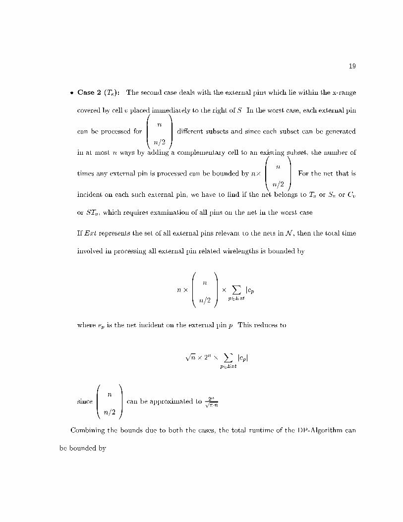
� Case � �Te The second case deals with the external pins which lie within the xrange

covered by cell v placed immediately to the right of S� In the worst case� each external pin

can be processed for

�BBB�

n

n��

�CCCA dierent subsets and since each subset can be generated

in at most n ways by adding a complementary cell to an existing subset� the number of

times any external pin is processed can be bounded by n

�BBB�

n

n��

�CCCA� For the net that is

incident on each such external pin� we have to �nd if the net belongs to Tv or Sv or Cv

or STv� which requires examination of all pins on the net in the worst case�

If Ext represents the set of all external pins relevant to the nets in N � then the total time

involved in processing all external pin related wirelengths is bounded by

n

�BBB�

n

n��

�CCCA

Xp�Ext

jepj

where ep is the net incident on the external pin p� This reduces to

pn �n

Xp�Ext

jepj

since

�BBB�

n

n��

�CCCA can be approximated to �np

��n �

Combining the bounds due to both the cases� the total runtime of the DPAlgorithm can

be bounded by

��

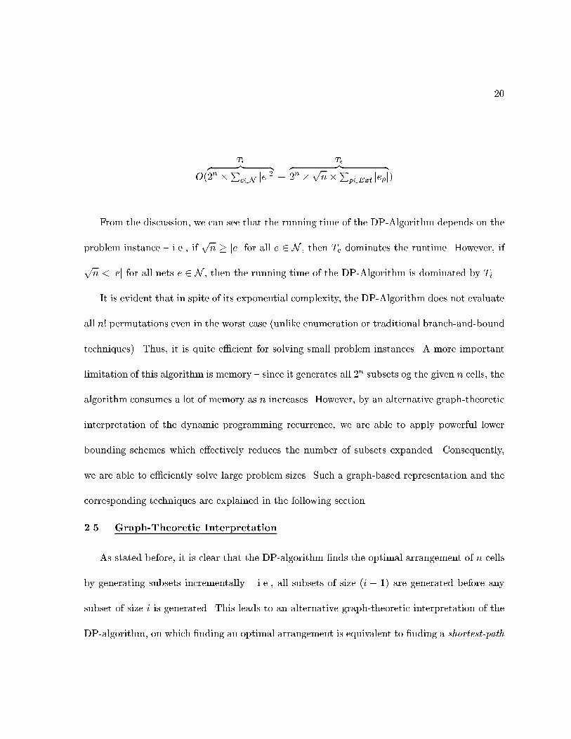
O�

Tiz �� ��n Pe�N jej� �

Tez �� ��n p

nPp�Ext jepj�

From the discussion� we can see that the running time of the DPAlgorithm depends on the

problem instance � i�e�� ifpn jej for all e � N � then Te dominates the runtime� However� if

pn � jej for all nets e � N � then the running time of the DPAlgorithm is dominated by Ti�

It is evident that in spite of its exponential complexity� the DPAlgorithm does not evaluate

all n� permutations even in the worst case �unlike enumeration or traditional branchandbound

techniques�� Thus� it is quite e�cient for solving small problem instances� A more important

limitation of this algorithm is memory � since it generates all �n subsets og the given n cells� the

algorithm consumes a lot of memory as n increases� However� by an alternative graphtheoretic

interpretation of the dynamic programming recurrence� we are able to apply powerful lower

bounding schemes which eectively reduces the number of subsets expanded� Consequently�

we are able to e�ciently solve large problem sizes� Such a graphbased representation and the

corresponding techniques are explained in the following section�

��� Graph�Theoretic Interpretation

As stated before� it is clear that the DPalgorithm �nds the optimal arrangement of n cells

by generating subsets incrementally � i�e�� all subsets of size �i � �� are generated before any

subset of size i is generated� This leads to an alternative graphtheoretic interpretation of the

DPalgorithm� on which �nding an optimal arrangement is equivalent to �nding a shortest�path

��

between two vertices in the graph� This abstraction was earlier studied by Cederbaum ��� in the

context of �nding optimal backboard ordering for minimizing the total interconnection length

and was later used by Auer ��� in applying linear placement algorithm for cell generation�

To clearly understand the graphbased representation� we present the construction of a

directed� acyclic graph G � �V�E�� The vertices vi � V of this graph correspond to all the �n

subsetsWi for all i � �� �� �� ���� �n�� of the set W � including the empty set � andW itself� The

vertex v� corresponding to the � is connected by edges e�i to n vertices vi � fwig� i � �� �� ��� n

corresponding to the singleton subsets containing just one cell� In general� a vertex vi �Wi� is

connected by an edge eij to all vertices vj � Wj� where Wj � Wi � fwg� �w � �W �Wi�� An

example of such a graph for a window of three cells fa� b� cg is shown in Figure ��

For a vertex vk corresponding to a subset Wk with m dierent cells �m n�� there are m

edges incident into vk and �n�m� edges incident out of vk� together making n edges incident

on vk� Therefore� the graph G is a regular graph of degree n and the total number of edges in

G is jEj � �n � �n��� � n � �n���

In this graph� v� � � will be the source vertex and is the only vertex with n outgoing edges�

Similarly� vt � W is the sink vertex and is also the only vertex in the graph with n incoming

edges� Along any directed path v� � vt� the order of the corresponding subsets of cells always

increases� Consequently� no directed sourcetosink path can pass through the same vertex

twice� and hence G is cycle free� Starting from the source vertex v�� one can continue along a

number of dierent directed paths� each of which contain exactly n edges� and terminate at the

sink vt�

��

{}

{c}

{b}

{a} {a,b}

{a,c}

{b,c}

{a,b,c}

a

a

b

b

b

b

cc

c

a

c

a

Figure �� Illustration of the graph implied by the DP�algorithm for an instance of three cells

fa� b� cg inside the window�

An important property of the graph is that there exists a onetoone correspondence between

the linear arrangements of the cells in W and the directed sourcetosink paths in the graph G�

To observe this� let L � fwi� � wi� � ���� wing be some linear arrangement of the cells in W � Thus

L can be represented by a sequence of subsets of cells as

SL � ��� fwi�g� fwi� � wi�g� ���� fwi� � wi� � ���� win��g�W �

�

which starts with the empty set �� terminates with the complete set of cells W � and whose

jth term� � j n� is the subset fwi� � wi� � ���� wij��g formed by the �rst j � � elements of L�

If the set SL is projected on the graph G� its image will be a sequence of vertices in G�

starting from v� � �� Since each element in the set SL but for the �rst one �� is obtained

by appending one complementary cell to the previous set of cells� the image vertices will be

joined by edges of G� eventually forming a directed path PL from v� to vt� Thus� through the

medium of the sequence set SL of cells� the path PL can be seen as the unique image of the

linear arrangement L of cells on the graph G�

Since this argument is valid in both directions� the correspondence between any linear

arrangement of cells in W and the directed sourcetosink paths in G is onetoone�

Also� along any directed sourcetosink path� the outdegrees of the consecutive vertices in

G �starting from v�� follows the sequence n� n� �� n� ������ �� �� Hence the number of dierent

sourcetosink directed paths in G is equal to

�n��n� ���n� ����������� � n�

which is the number of dierent permutations of the n cells�

To see that the optimal linear arrangement problem is equivalent to �nding a shortestpath

in this graph� let us introduce the notion of �length� for each edge� Consider any edge eij

directed from vertex vi � Wi to vertex vj � Wj � By the construction of the graph� we know

that Wj � Wi � fvg for some cell v � �W �Wi�� Then� the length of the edge eij is given by

��

I�Wi� v�� which is the incremental cost of placing cell v to the right of any arrangement of cells

inWi� Based on this notion� all the edges edges in E can be annotated with their corresponding

length values�

Now� consider any path P in the graph between vertices v� � � and vt � W � The total

length of this path is equal to the sum of the lengths of its constituent edges� However� as

discussed before� the path P corresponds to some linear arrangement L of the cells in W �

Following the way the edge lengths are computed� it is clear that the length of P is equal

to the total wirelength corresponding to arrangement L� Since the optimal linear arrangement

problem is to �nd the linear arrangement with the least wirelength� this translates to �nding the

path between v� and vt with shortest length � i�e�� the shortest path between the two vertices�

It is interesting to note that the con�guration graph need not be generated beforehand� In

fact� the graph is implicitly constructed levelbylevel � i�e� � all vertices �or subsets� at level i

are generated before any vertex �or subset� at level i�� is generated �as presented in Figure ���

Similarly� the edges going out of vertices at level i are also generated only during the expansion

of vertices �or subsets� at level i by adding a complementary cell to the right of any arrangement

of the cells in that subset� However� the optimal linear arrangement cannot be found until all

the �n vertices are generated�

��� Accelerating Shortest�Path Search

The technique presented in this section for speedingup the search for shortest path is based

on the A� approach ������ which is a goaloriented search paradigm� The approach relies on

��

x x x

S S

s0 1

Figure �� Illustration of A� approach�

computing lower bounds on the wirelength of the �unplaced� cells with respect to any subset

S�

Let Cinit represent the total wirelength of the initial arrangement of the cells in W � As

shown in Figure �� assume that we have already computed the cost of an optimal arrangement

of a subset S of cells in the window and we consider expanding S to include more cells from

S � W � S� Let Cost�S� represent the wirelength of an optimal arrangement of cells in S�

Note that Cost�S� covers the wirelength of all nets in N between x� and xs as shown in the

Figure ��

Let lb�S� represent a lower bound on the wirelength of the nets in N within the xregion

covered by cells in S � i�e�� the region between xs and x� in Figure ��

Then Cost�S� � lb�S� gives a lower bound on the total wirelength of any arrangement of

the n cells� whose pre�x is an optimal arrangement of cells in S� Let h�S� � Cost�S� � lb�S�

represent this heuristic lower bound�

��

Then� if h�S� Cinit� it means that any ordering of the cells in W � whose pre�x is an

optimal ordering of S will not produce a solution with a better cost than the initial cost Cinit�

Hence we do not have to expand the subset S� This way� we can suppress the expansion of

many intermediate subsets� This heuristic h�S� also captures the estimated path length from

v� to vt which passes through vs � S� Therefore� a subset S with a lower value for h�S� means

that the path through the corresponding vertex vs has more chances of being the shortest

path� Hence� among all candidate subsets for expansion at any stage� the subset with lowest

h value is expanded �rst� For this reason� the con�guration graph is not necessarily expanded

levelbylevel�

However� the eectiveness of such a technique largely depends on how tight lower bounds can

we compute for the wirelength of the cells in S� In this section� we present an e�cient network

�ow based method for computing lower bounds on wirelength� which helps in accelerating the

shortestpath search�

����� Relaxation Based Lower Bound

The lower bounding technique that we use is based on a relaxation based approach as

discussed in ���� The idea is to �nd optimal relaxed locations for all the �unplaced� cells in the

given window W and use this information to obtain lower bounds on the wirelength�

Suppose that we want to �nd a lower bound on the wirelength of any arrangement of a

subset S of cells within the window W � The set S of cells inside the window form the set of

mobile cells � i�e�� these cells can be moved from their current position in the placement� All

nets which are incident on any mobile cell are termed as �active nets� E� � i�e�� these are the

��

nets whose lengths are aected if we change the arrangement of the mobile cells� We then

determine the set of �xed cells F as follows�

F � fv j v � �ei � S�� where ei � E�� and v is either the left or right extreme cell of ei g�

The primary role of the �xed cells is to aid in establishing a lower bound on the wirelength

of nets in E� � i�e�� no matter where the mobile cells are placed� the total wirelength of nets in

E� is at least as much as that determined by the positions of the relevant �xed cells in F �

When �nding the optimal relaxed xcoordinates for the mobile cells� we consider only those

�xed cells which aect the xdirection wirelength of the active nets� Since we are only re

arranging cell locations within a row� we will consider only �nding relaxed locations along the

xdirection�

To �nd relaxed xpositions for the set of mobile cells� we project the set of �xed cells on

the xaxis� Note that we are concerned only about the location of the �xed cells� Hence if

more than one �xed cell is projected to the same xlocation� only one cell is considered for each

associated xlocation�

Figure � shows an example of a projected subcircuit on the xaxis� The �xed cells� mobile

cells and the corresponding interconnections are shown in the �gure�

We now derive a LP�formulation for optimally placing the mobile cells� By following a

LPformulation� we are able to model hyperedges exactly � i�e�� there is no need to use a

clique model as in other analytical methods� Similarly� the LPformulation captures true linear

wirelength objective�

��

f3 4f f5 f6 f7f1 f2

Mobile Cell Fixed Cell

Figure �� Example of a sub�circuit projected on the x�axis�

��

Such a linear program will produce an xcoordinate xv for each mobile cell v � S� The LP

is of course in�uenced by the locations of the �xed cells F � Let Xv be the location of a cell

v � F in a given placement� Then the LP relaxation for xcoordinate can be stated as follows�

minXe�E�

�re � le� subject to

le xv re� �v � e�

xv � Xv� �v � F

The dummy variables re and le in the formulation give the leftmost and rightmost ends of

net e�

This formulation can be solved using any standard LPsolver� However� we use the network

�ow based algorithm outlined in ��� to solve this problem as this approach has been found to

be e�cient in practice� The algorithm iteratively �nds minimum cuts from left to right which

assign mobile cells to bins formed by each of the �xed cells� The resulting relaxed placement is

an optimal solution to the LP formulation�

Based on the relaxed xlocations obtained for all the cells in the set S� we can compute the

lower bound on the wirelength of the corresponding active nets�

����� Faster Lower Bound Computation

Though a single run of the network�ow algorithm explained in the previous section is fast in

practice� due to the large number of subsets ��n in the worst case� for which we may want to �nd

�

f3 4f f5 f6 f7f1 f2

Mobile Cell Fixed Cell

Figure ��� Instance of an output generated by the network��ow algorithm� Many mobile cells

can be associated with a single �xed cell�

lower bounds� using the network�ow algorithm for each subset turns out be computationally

expensive as n increases� In this section� we suggest a faster method for computing lower

bounds� which uses information generated by a single run of the network�ow algorithm done

as a preprocessing step�

Assume that we choose all the cells in the window W as mobile cells and run the network

�ow algorithm to �nd optimal relaxed locations for all mobile cells� Figure �� shows an example

of the output of the network�ow algorithm� As expected� there may be more than one mobile

cell associated with each �xed cell�

An alternative interpretation of the output of the network�ow algorithm is that it gives

the minimum number of nets cut between every pair of adjacent �xed cells� no matter how the

mobile cells are arranged�

�

f3 4f f5 f6 f7f1 f2

D D D D D D1,2 2,3 3,4 4,5 5,6 6,7

Figure ��� Computing lower bounds from the information on the minimum number of nets cut

between pair of adjacent �xed cells�

Suppose� as shown in Figure ��� we have information on the minimum number of nets cut

between every pair of adjacent �xed cells � i�e�� let Di�j represent the minimum number of nets

cut between �xed cells fi and fj� Then the lower bound on the wirelength of the active nets is

given by

jF jXi��

Di���i � �Xfi �Xfi���

where Xfi gives the xlocation of the �xed cell fi and jF j is the total number of relevant �xed

nodes�

Given any window of cells� this information on the minimum number of nets cut between

adjacent �xed cells can be obtained using the network�ow algorithm as a preprocessing step�

Once we have obtained this information� computing lower bounds on the wirelength for any

subset of cells S can be done quickly as shown below�

As shown in Figure ��� assume that we already have an arrangement of a subset of cells

S and we want to compute a lower bound on the wirelength of the nets corresponding to the

�

f3 4f f5 f6 f7f1 f2

D D D D D D1,2 2,3 3,4 4,5 5,6 6,7

W-S

x s

S

Figure ��� Computing lower bounds for subsets based on the information obtained from a

pre�processing step�

unplaced cells in S �W � S� Let xs be the right boundary of S along the xdirection� Then if

fi and fj are two adjacent �xed cells such that Xfi xs Xfj � then the lower bound on the

wirelength of the unplaced cells is given by

lb�S� � Di�j � �Xfj � xs� �

jF j��Xk�j

Dk�k�� � �Xfk�� �Xfk�

However� it is to be noted that though this method to �nd a lower bound is faster than

using the network�ow algorithm on S� it may not be as tight as the lower bound provided

by the network�ow algorithm� Nevertheless� this simpli�ed approach has been proven to be

powerful in practice�

����� SP�Algorithm

An algorithm named SP�Algorithm �SP for shortestpath� which is based on the A�

paradigm and uses the above mentioned lower bounding technique is shown in Figure � � The

algorithm uses a priority queue to hold the subsets that are to be expanded� The subsets are

prioritized based on the heuristic path length h through the corresponding vertex in the graph

� i�e�� the vertex with the lowest h value is the �rst one to be expanded�

Note that this algorithm does not explore the con�guration graph levelbylevel� Also� it

does not generate all �n subsets unless necessary� the tighter the lower bound is� the lesser

is the number of subsets generated by this algorithm� The SPAlgorithm has improvement

both in terms of memory and runtime when compared to the DPAlgorithm� as shown in our

experiments results�

�� Experimental Results

We have implemented both the dynamic programming based DP�Algorithm and the A�

based SP�Algorithm in C� Table I shows a list of circuits with their characteristics that we used

for our experiments� The initial reference placements for these circuits were generated using

the placement tool Mongrel����

The goal of the experiments was to evaluate the reduction in runtime produced by the

SPAlgorithm over the DPAlgorithm for various window sizes� Also� we wanted to see the

�

SP�Algorithm

Given A window W of n adjacent cells

Output Minimum wirelength ordering of the n cells

�� Q is a priority queue of sets S�� ordered by Cost�S� � lb�S���� Cinit is the wirelength of the initial�� arrangement of cells in the window W ��� x� is the left boundary of the window

��� Run network�ow algorithm on W to �ndmincut information between �xed cells�

��� EnQueue�Q���� � while �Q �� Empty� do��� begin��� S � DeQueue�Q���� if �jSj �� n� goto step ����� for each v � �W � S� do��� S� � �S � fvg���� Cost�S��� Cost�S� � I�S� v�

��� S� � �W � S����� Compute lowerbound lb�S����� if Cost�S�� � lb�S�� � Cinit ��feasible path� � EnQueue�Q�S����� end��� �� Shortest path to W �� S found��� Output Cost�S��

Figure � � Outline of the algorithm using lower bounding to �nd optimal linear arrangement�

�

TABLE I

CIRCUIT CHARACTERISTICS

Circuit cells nets

industry� ��� � � ���

industry ��� �����

avq�small ����� �����

avq�large ����� �� ��

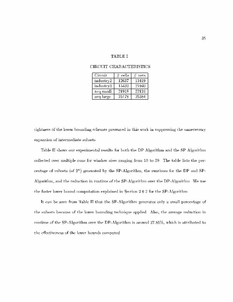
tightness of the lower bounding schemes presented in this work in suppressing the unnecessary

expansion of intermediate subsets�

Table II shows our experimental results for both the DPAlgorithm and the SPAlgorithm

collected over multiple runs for window sizes ranging from �� to ��� The table lists the per

centage of subsets �of �n� generated by the SPAlgorithm� the runtimes for the DP and SP

Algorithm� and the reduction in runtime of the SPAlgorithm over the DPAlgorithm� We use

the faster lower bound computation explained in Section ����� for the SPAlgorithm�

It can be seen from Table II that the SPAlgorithm generates only a small percentage of

the subsets because of the lower bounding technique applied� Also� the average reduction in

runtime of the SPAlgorithm over the DPAlgorithm is around ����!� which is attributed to

the eectiveness of the lower bounds computed�

�

TABLE II

EXPERIMENTAL RESULTS

DPAlgorithm SPAlgorithm

cells Time�s� !subsets Time�s� Reductionin Time�!�

�� ����� ���� ��� � �����

�� �� �� ���� ����� ����

�� ����� ���� ����� ���

� ����� ����� ����� �����

�� ����� ����� ����� �����

�� ������ ����� ����� � ���

�� ������ ����� ����� �����

�� ��� �� ����� ������ �����

�� ����� � ����� ��� � ��� �

�� ������ ����� � ���� � ���

�� ���� �� ����� ������� �����

Average ����

��� Comments and Conclusion

We studied the problem of mincost linear arrangement in the context of intrarow opti

mization of a standardcell placement� A dynamic programming approach was suggested to

solve the problem optimally�

Also� it was shown that the dynamic programming approach implies a con�guration graph�

where the vertices represent all �n subsets of the given cells� Moreover� on this con�gura

tion graph� the problem of �nding an optimal linear arrangement reduces to that of �nding a

shortestpath between two vertices�

�

A powerful network�ow based algorithm was suggested to �nd lower bounds on the wire

length of any arrangement of a set of cells� Using this lower bounding technique� an algorithm

based on the goal oriented A� framework was presented�

Our experimental results show the tightness of the lower bounds generated by the network

�ow based approach� The results also show that by using such tight bounding techniques with

the A� approach� the size of the problem that can be e�ciently solved increases�

CHAPTER �

CONTEXT�AWARE BUFFER INSERTION

��� Introduction

In Chapter �� we presented the application of the shortest path algorithm to �nd the optimal

linear arrangement of cells within a given window in a placement� By using such intrarow

optimization techniques� the wirelength of the given placement can be further optimized� Once

we have an optimized placement� we perform routing of the signal nets to interconnect the cells

in the circuit� At this stage� a variety of interconnect delay optimization techniques are applied

to ensure that the signal nets meet the corresponding timing requirements� In this chapter� we

study the application of the shortest path algorithm in the context of optimizing interconnect

delay which is very crucial in practice�

In the Deep Submicron era� delay optimization for high performance interconnects has

become of fundamental interest� In this context� buer insertion has been proven to be a very

powerful technique� Much of the past work �e�g������ on buer insertion� while of fundamental

interest� has focused on idealized situations where buers can be inserted at arbitrary positions

on the routing area� However� as pointed out in the recent work of Zhou and Wong ����� in

practice such optimizations must occur in the context of� for example� a �oorplan where there

may be preplaced macro cells which can be routed over� but which preclude the insertion of

buers in that region�

�

�

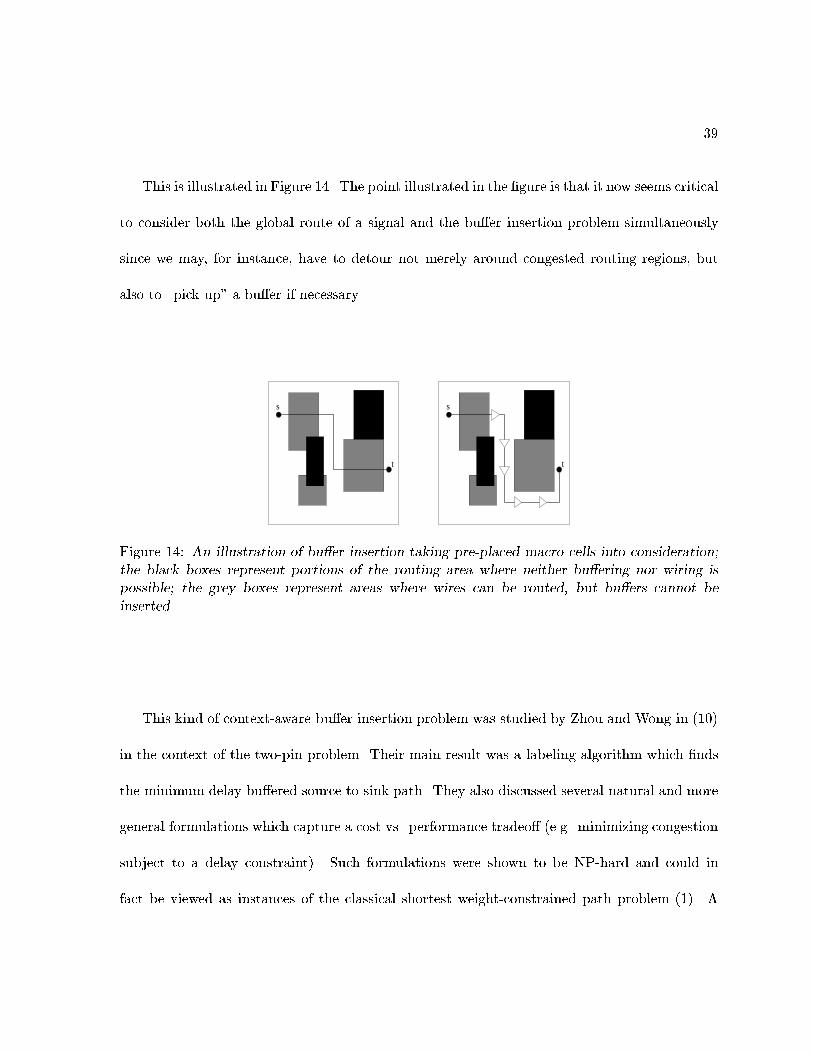
This is illustrated in Figure ��� The point illustrated in the �gure is that it now seems critical

to consider both the global route of a signal and the buer insertion problem simultaneously

since we may� for instance� have to detour not merely around congested routing regions� but

also to �pick up� a buer if necessary�

s s

tt

Figure ��� An illustration of bu�er insertion taking pre�placed macro cells into consideration�

the black boxes represent portions of the routing area where neither bu�ering nor wiring is

possible� the grey boxes represent areas where wires can be routed� but bu�ers cannot be

inserted�

This kind of contextaware buer insertion problem was studied by Zhou and Wong in ����

in the context of the twopin problem� Their main result was a labeling algorithm which �nds

the minimum delay buered source to sink path� They also discussed several natural and more

general formulations which capture a cost vs� performance tradeo �e�g� minimizing congestion

subject to a delay constraint�� Such formulations were shown to be NPhard and could in

fact be viewed as instances of the classical shortest weightconstrained path problem ���� A

��

pseudopolynomial algorithm for such formulations was also presented� which �nds the set of all

sourcetosink paths that lie on the cost vs� delay tradeo curve �a similar algorithm appears

in ������

This thesis also focuses on the twopin problem with an emphasis on the tradeos between

cost �e�g�� total capacitance� and delay� The ability to capture such tradeos is crucial in

practice since the cost overhead of �fastest� solutions tends to be excessive�

Toward this end we propose and characterize a new formulation� called the Delay Reduction

to Cost Ratio Maximization �DRCR problem� Given a set of candidate buer insertion

locations and their candidate connections modeled as a directed graph� and a reference delay

value Dref � we wish to maximize the ratioDref�d

gover all sourcetosink paths� where g and d

are the path cost and delay respectively � i�e�� we maximize the ratio of the reduction in delay

to the corresponding cost�

A nice property of this formulation is that it is completely independent of the cost and delay

models used to estimate the cost and delay associated with the candidate edges interconnecting

the buers� For example� we are not restricted to using the total capacitance as the cost and

Elmore delay model ���� for the interconnect delay �though for simplicity in our experiments

we have used Elmore�� By the same token� the cost associated with a particular candidate

connection and buer is also �exible� while total estimated capacitance is a natural measure�

heuristic measures relating to congestion and buer availability are also plausible�

It is suggested that the DRCR is a natural composite objective function capturing the

tradeo between cost and delay� Our main contribution is a fast polynomial time algorithm for

��

this problem� It is then natural to consider the relation between solutions of the DRCR problem

and other formulations �in particular cost minimization subject to a delay constraint�� Toward

this end the problem is characterized with respect to all sourcetosink paths that lie on the cost

vs� delay tradeo curve �i�e�� nondominated paths�� A subset of these paths forms the Lower

Convex Hull �LCH�� the LCH is essentially the points on the lowerleft of the convex hull� It is

shown that a variant of the algorithm can e�ciently identify any point on the LCH� Thus we

have a tradeo� the expense of using the fast algorithm presented is that we are no longer able

to identify paths which lie o� the LCH while a comparatively slow pseudopolynomial algorithm

is able to identify such points� We argue that in practice this is not a major sacri�ce since paths

o the LCH tend to make less sound engineering choices� Computational experiments show

the algorithms to be extremely e�cient� Thus we believe the proposed algorithm will become

a valuable tool in the early stages of design where buers must be allocated and topological

buertobuer routes determined�

��� Background

The algorithm that we present in this work is independent of the delay models that are used

to model the interconnect delay� However� in this section� we brie�y review some background

material on delay models which are used in our experiments�

����� Delay Models

Though the graph model we utilize allows any desired technique to estimate the delay from

the input of a buer to the input of the next� we review some of the basic RC delay models for

the purpose of discussion�

��

Let r� and c� represent the unit length resistance and capacitance respectively of a wire�

Then for a wire e of length l�e�� the resistance r�e� and the capacitance c�e� are given by

r�e� � r� � l�e� and c�e� � c� � l�e�

r

2 2ec ec

e

Figure ��� RC delay modeling for a wire�

Figure �� shows the common RC model of a wire� Recall that according to the Elmore

delay model ����� the delay De of a wire e driving a load C is given by

De � r�e� ��c�e�

�� C

�

Similarly� if b is a buer with intrinsic delay db� output resistance rb and a loading capaci

tance C� then the delay of the buer Db is given by

Db � db � rb � C

�

����� Dominance Property

Since paths are characterized by two parameters g and d� they may be compared with a

partial order� A path p � s� t is said to be nondominated� if all other paths p� � s � t� have

g� g or d� d� � i�e�� the set of nondominated paths are those on the cost vs� delay tradeo

curve intrinsic in the problem�

��� Bu�er Graph

We model the contextaware buer insertion problem by a directed graph in which nodes

represent buers and edges represent the candidate connections between buers� A path in

such a graph represents a sequence of buers inserted by virtue of the nodes on the path� To

avoid confusion� we emphasize that the buer selection is implicit in the node � there is no need

to explicitly determine the type of buer inserted at a node� this is determined by the graph

itself �see below��

Each edge e is annotated with two labels� ge is the cost associated with taking the edge

�including the routing cost and the cost of the destination buer� and de is the delay from the

input of the source buer to the input of the destination� Figure �� shows two buers a and

b and their candidate interconnection modeled as a graph� where the cost and the delay of the

edges are computed under the Elmore delay model� Recall that the cost and delay of the edge

are computed from the input of buer a to the input of buer b�

It is often the case that each buer station has a set of buers of dierent sizes to facilitate

cascading of buers within the buer station for improved performance� An illustration of a

buer station with multiple buer sizes and its corresponding graph model is shown in Figure

��

ra ad

de = da + c +2

=e

ac rb db,

bc, , , ,

a b

a b

(+ ra

r c

b ) )

g c e + c b

c e + rec e

ee

(cb

Figure ��� Illustration of the transformation of a wire connecting two bu�ers into its corre�

sponding graph model under the Elmore delay model� Note that c�e� and r�e� represent thecapacitance and resistance of the wire connecting the bu�ers a and b while ge and de representthe edge cost and delay in the corresponding graph model�

Figure ��� Note that buers within a buer station are cascaded only in increasing order of

their size � i�e�� edges go only from smaller buers to larger ones within the same buer station�

Thus the graph model naturally captures this situation�

Such an abstract graph model has several bene�ts� Of foremost importance is that it is

completely independent of the models used to estimate the delay and cost of any edge in the

graph � i�e�� any desired means can be used to estimate the inputtoinput delay and any cost

measure can be applied depending on the situation� For example� the eects of coupling noise

and congestion constraints due to prerouted adjacent nets can be incorporated into the delay

and cost measures� Also� more sophisticated interconnect and gate delay models can be used

to model the delay associated with every edge� We are not limited for example to using Elmore

��

(a)

(b)

Figure ��� Illustration of cascading bu�ers within a bu�er station� solid lines represent connec�

tions within the bu�er station and broken lines represent edges to and from outside the bu�erstation� a A bu�er station with bu�ers of di�erent sizes and b the corresponding graph

model�

delay or considering only the total capacitance as our cost measure�� Moreover� this graph

model points out the intimate relationship between the contextaware buer insertion problem

and the shortest weightconstrained path problem in ����

�As presented� we do require that the delay be independent of the previous stage � however� if this isa serious issue� it can be modeled via a further transformation of the graph �at the expense of a largegraph��

��

As stated earlier� a path in such a graph represents not only the wiring route to be taken�

but by virtue of the vertices on the path� the buers to be inserted� Figure Figure �� presents

a complete example of a set of buer stations� the corresponding graph model� and two s� t

paths in the graph�

A naive graph construction method results in a complete graph � i�e�� there is one vertex

for each size of buer inside every buer station and an edge connecting every pair of vertices�

However� in practice there is a threshold on the interconnect length beyond which a buer

must be inserted and thus it is su�cient if a buer is connected to only its neighbors which lie

within a speci�c technology dependent distance� By taking this factor into account during the

construction process� the graph size can be reduced considerably�

��� Problem Formulations

Given such a graph theoretic interpretation of the problem� the traditional constrained

optimization problem can be stated as follows �recall this problem is NPhard��

Formulation � Given� A directed graph G � �V�E�� where V represents the set of candidate

bu�er insertion locations� a bu�er library B� each e � E is annotated with a cost g and delay

d� a source terminal s with a driving resistance Rs� a sink terminal t with load Ct� and a delay

bound dspec�

Objective� Find a bu�ered path connecting s and t such that the total cost of the path is

minimized subject to the delay not exceeding dspec�

The Delay Reduction to Cost Ratio Maximization problem is stated as follows�

��

s

A

t

B C

A

s

B

t

C

A

ts

B C

(a)

(b) (c)

Figure ��� Illustration of a set of bu�er stations modeled as a graph � all lines represent edges

while the solid lines represent source�to�sink paths� a instance of a set of bu�er stations with

�nite bu�ering resources b a simple s � t path passing though various bu�er stations c a

s� t path in which bu�ers are cascaded at the intermediate bu�er station A�

��

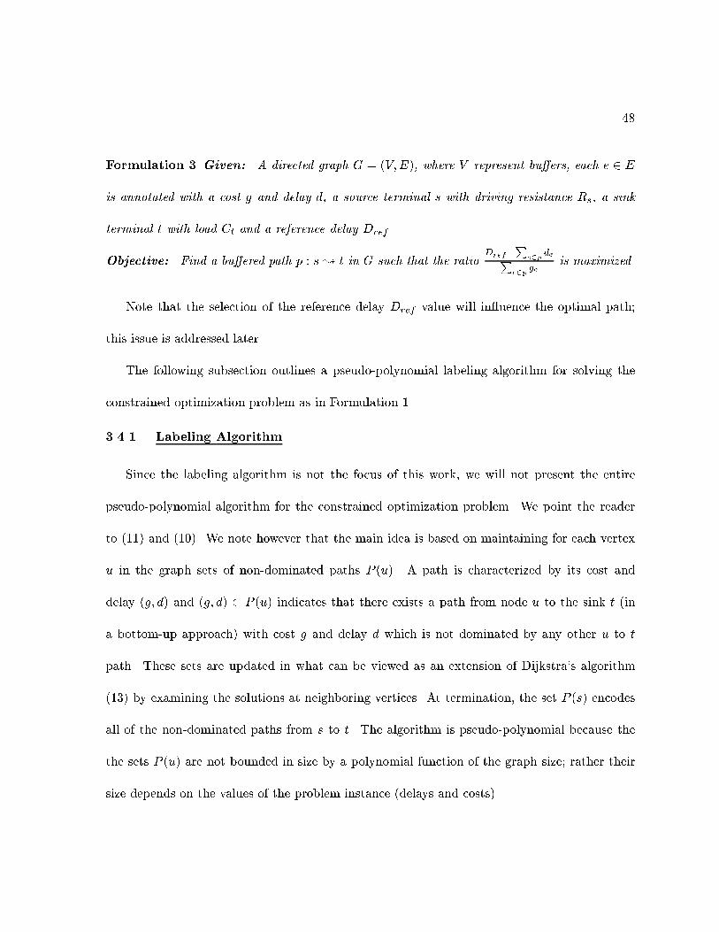
Formulation � Given� A directed graph G � �V�E�� where V represent bu�ers� each e � E

is annotated with a cost g and delay d� a source terminal s with driving resistance Rs� a sink

terminal t with load Ct and a reference delay Dref �

Objective� Find a bu�ered path p � s� t in G such that the ratioDref�

Pe�p

dePe�p

geis maximized�

Note that the selection of the reference delay Dref value will in�uence the optimal path�

this issue is addressed later�

The following subsection outlines a pseudopolynomial labeling algorithm for solving the

constrained optimization problem as in Formulation ��

����� Labeling Algorithm

Since the labeling algorithm is not the focus of this work� we will not present the entire

pseudopolynomial algorithm for the constrained optimization problem� We point the reader

to ���� and ����� We note however that the main idea is based on maintaining for each vertex

u in the graph sets of nondominated paths P �u�� A path is characterized by its cost and

delay �g� d� and �g� d� � P �u� indicates that there exists a path from node u to the sink t �in

a bottomup approach� with cost g and delay d which is not dominated by any other u to t

path� These sets are updated in what can be viewed as an extension of Dijkstra�s algorithm

�� � by examining the solutions at neighboring vertices� At termination� the set P �s� encodes

all of the nondominated paths from s to t� The algorithm is pseudopolynomial because the

the sets P �u� are not bounded in size by a polynomial function of the graph size� rather their

size depends on the values of the problem instance �delays and costs��

��

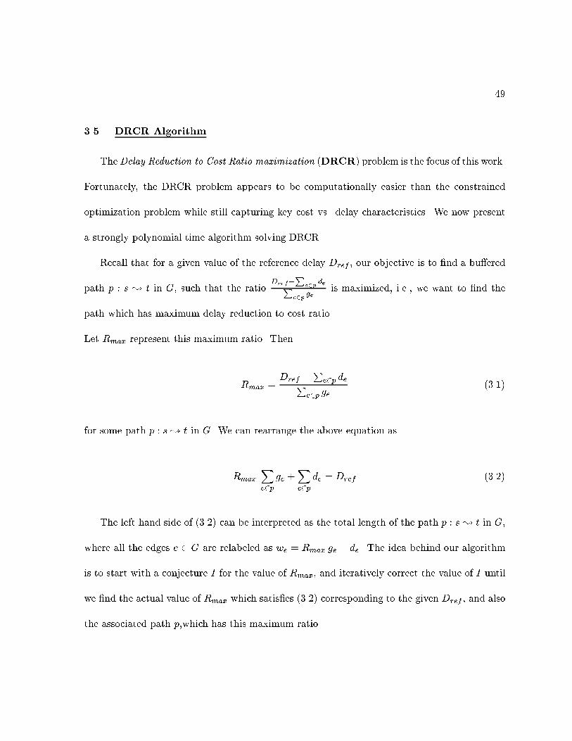
��� DRCR Algorithm

TheDelay Reduction to Cost Ratio maximization �DRCR� problem is the focus of this work�

Fortunately� the DRCR problem appears to be computationally easier than the constrained

optimization problem while still capturing key cost vs� delay characteristics� We now present

a strongly polynomial time algorithm solving DRCR�

Recall that for a given value of the reference delay Dref � our objective is to �nd a buered

path p � s � t in G� such that the ratioDref�

Pe�p

dePe�p

geis maximized� i�e�� we want to �nd the

path which has maximum delay reduction to cost ratio�

Let Rmax represent this maximum ratio� Then

Rmax �Dref �Pe�p deP

e�p ge� ���

for some path p � s� t in G� We can rearrange the above equation as

Rmax

Xe�p

ge �Xe�p

de � Dref � ���

The left hand side of � ��� can be interpreted as the total length of the path p � s� t in G�

where all the edges e � G are relabeled as we � Rmax ge � de� The idea behind our algorithm

is to start with a conjecture I for the value of Rmax� and iteratively correct the value of I until

we �nd the actual value of Rmax which satis�es � ��� corresponding to the given Dref � and also

the associated path p�which has this maximum ratio�

��

Starting with the initial conjecture I� for each edge e � G� we assign edge weights we �

I ge � de� where ge and de are the original cost and delay values associated with edge e� With

this relabeled graph� we �nd the shortest path p from s to t� Clearly� the length of the path

p is given byPwe � I

Pge �

Pde� where e � p��i�e�� the sum of the cost and delay values

associated with all the edges in the path� One of the following three situations is possible�

� If the length of the path p is equal to Dref � then � ��� is satis�ed and we have the current

I � Rmax and also the corresponding path p� and we are done�

� If the length of the path is less than Dref � then we increase the value of I� relabel the

graph with the new I value and repeat the algorithm until we reach a value of I for which

equation � ��� is satis�ed�

� If the length of the path is greater than Dref � then we decrease the value of I� relabel

the graph with the new I value and repeat the algorithm until we reach a value of I for

which equation � ��� is satis�ed�

Since we do not know how I should be increased or decreased during any iteration of the

algorithm� we suggest a binary search technique to optimize the number of iterations �The

algorithm employs binary search on the optimal ratio and is similar in spirit to algorithms for

the minimum timetopro�t cycle problem presented in ������

The idea is to �nd two values of I� namely Ilow and Ihigh such that

IlowX

e�plowge �

Xe�plow

de Dref � � �

��

and

IhighX

e�phighge �

Xe�phigh

de Dref � ���

where plow and phigh are the shortest s to t paths in the graphs relabeled with Ilow and Ihigh

respectively�

Identifying Ilow and Ihigh can be done as follows� For the initial value of the conjecture I� if

the length of the shortest path in the relabeled graph is less than Dref � then we repeatedly keep

doubling I� till we �nd the two successive values Ilow and Ihigh such that equations � � � and

� ��� are satis�ed� On the other hand� if starting from the initial I� the length of the shortest

path is greater than Dref � we keep halving I until we �nd Ilow and Ihigh�

Once we �nd Ilow and Ihigh� we can do a binary search in the range �Ilow��Ihigh� to identify

the �nal value of I which maximizes the delay reduction to cost ratio� The DRCR algorithm

which is based on such a binary search technique is shown in Figure Figure ���

The correctness of the iterative search algorithm in identifying the path with maximum

delay reduction to cost ratio is justi�ed by the following lemma�

Lemma � Given Dref � the iterative search technique �nds the path for which

I �Dref � d

g

is a maximum� where g is the cost and d is the delay of the path�

��

Algorithm DRCR

Subroutine AssignWeights �G� I�

For each e � G�we � I ge � de

Main Routine

� Find Ilow and Ihigh� I � �Ilow � Ihigh��� AssignWeights�G� I�� P � shortest s� t path in G�� while �Dref �� length�P ��� if �length�P � � Dref �� Ihigh � I� else

� Ilow � I�� endif�� I � �Ilow � Ihigh����� AssignWeights�G� I�� P � shortest s� t path in G��� endwhile

�� return P

Figure ��� DRCR algorithm to solve the ratio maximization problem�

Proof Let p be the shortest path between s and t found during any stage of the algorithm�

Following assignment of weights to edges� the length of p is given by IP

e�p ge �P

e�p de� At

any stage� we need to deal with one of the following three cases�

� Case � IP

e�p ge �P

e�p de � Dref � Then�

I �Dref �Pe�p deP

e�p ge�

�

i�e��the ratio for the path p is clearly better than the conjecture I�

So� I is increased�

� Case � IP

e�p ge �P

e�p de � Dref �

Since p is the shortest path� for all other paths p��

IXe�p�

ge �Xe�p�

de � Dref �

Also�

I �Dref �Pe�p� deP

e�p� ge� p��

So� I is decreased�

� Case � IP

e�p ge �P

e�p de � Dref �

Therefore�

I �Dref �Pe�p deP

e�p ge�

Since p is the shortest path� all other paths p� have

IXe�p�

ge �Xe�p�

de Dref �

��

and

I Dref �Pe�p� dePe�p� ge

�

i�e� all those paths p� have smaller ratios�

The algorithm terminates with the maximum ratio path� ��

����� Complexity

Observation If D is the delay of the path with minimum cost� then the number of

invocations of Dijkstra�s algorithm is bounded by O�logD��

The running time of theDRCR algorithm is given by �number of invocations of the shortest

path algorithm� �time to �nd the shortest path� i�e� O�logD E log jV j��

��� Properties

In this section� we explain some interesting properties of the solutions generated by the

DRCR algorithm�

Lemma � For any value of Dref � the optimal ratio solution is not dominated by any other

solution�

��

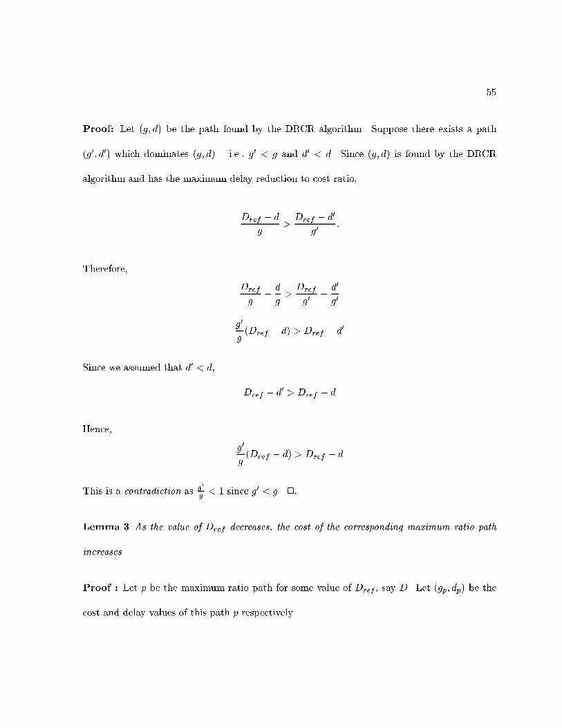
Proof Let �g� d� be the path found by the DRCR algorithm� Suppose there exists a path

�g�� d�� which dominates �g� d� � i�e�� g� � g and d� � d� Since �g� d� is found by the DRCR

algorithm and has the maximum delay reduction to cost ratio�

Dref � d

g�Dref � d�

g��

Therefore�

Dref

g� d

g�Dref

g�� d�

g�

g�

g�Dref � d� � Dref � d�

Since we assumed that d� � d�

Dref � d� � Dref � d

Hence�

g�

g�Dref � d� � Dref � d

This is a contradiction as g�

g� � since g� � g ��

Lemma � As the value of Dref decreases� the cost of the corresponding maximum ratio path

increases�

Proof Let p be the maximum ratio path for some value of Dref � say D� Let �gp� dp� be the

cost and delay values of this path p respectively�

��

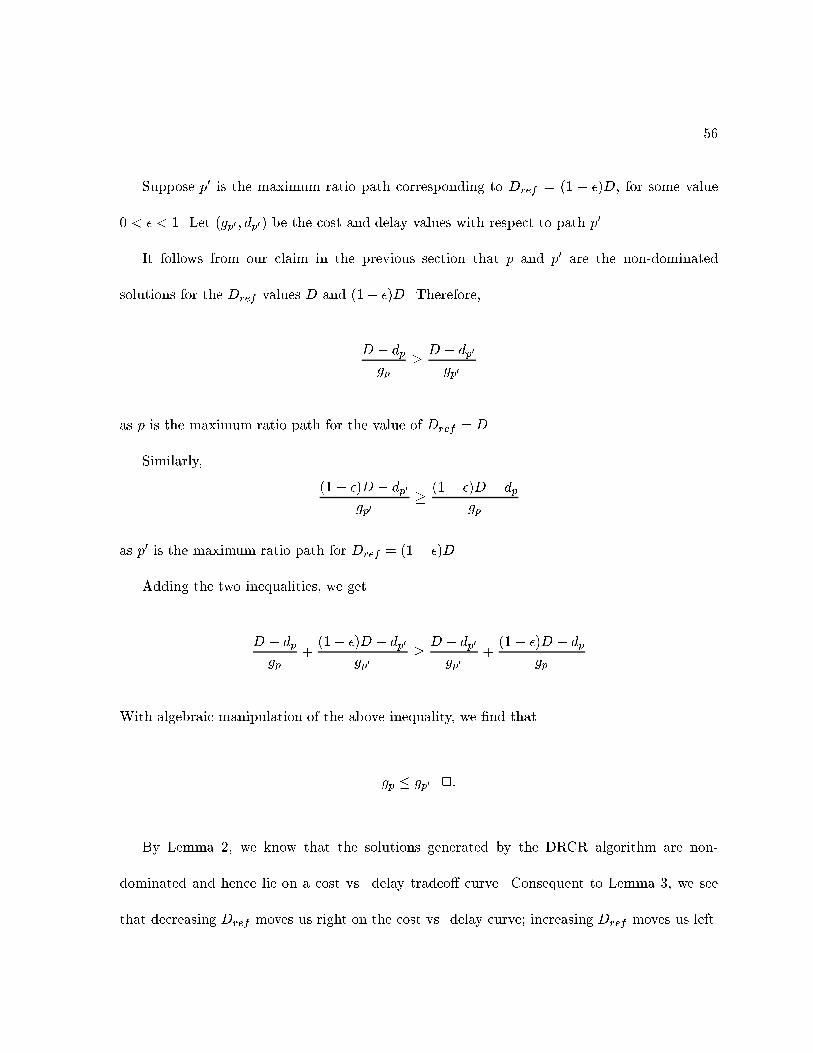
Suppose p� is the maximum ratio path corresponding to Dref � �� � ��D� for some value

� � � � �� Let �gp� � dp�� be the cost and delay values with respect to path p��

It follows from our claim in the previous section that p and p� are the nondominated

solutions for the Dref values D and ��� ��D� Therefore�

D � dpgp

D � dp�

gp�

as p is the maximum ratio path for the value of Dref � D�

Similarly�

��� ��D � dp�

gp� ��� ��D � dp

gp

as p� is the maximum ratio path for Dref � ��� ��D�

Adding the two inequalities� we get

D � dpgp

���� ��D � dp�

gp� D � dp�

gp����� ��D � dp

gp

With algebraic manipulation of the above inequality� we �nd that

gp gp� ��

By Lemma �� we know that the solutions generated by the DRCR algorithm are non

dominated and hence lie on a cost vs� delay tradeo curve� Consequent to Lemma � we see

that decreasing Dref moves us right on the cost vs� delay curve� increasing Dref moves us left�

��

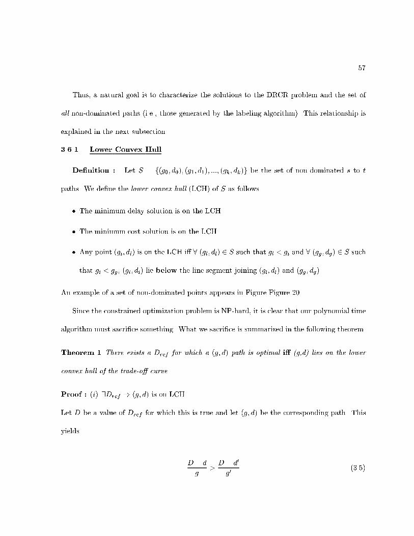
Thus� a natural goal is to characterize the solutions to the DRCR problem and the set of

all nondominated paths �i�e�� those generated by the labeling algorithm�� This relationship is

explained in the next subsection�

����� Lower Convex Hull

De�nition Let S � f�g�� d��� �g�� d��� ���� �gk � dk�g be the set of nondominated s to t

paths� We de�ne the lower convex hull �LCH� of S as follows�

� The minimum delay solution is on the LCH�

� The minimum cost solution is on the LCH�

� Any point �gi� di� is on the LCH i � �gl� dl� � S such that gl � gi and � �gg� dg� � S such

that gi � gg� �gi� di� lie below the line segment joining �gl� dl� and �gg� dg��

An example of a set of nondominated points appears in Figure Figure ���

Since the constrained optimization problem is NPhard� it is clear that our polynomial time

algorithm must sacri�ce something� What we sacri�ce is summarized in the following theorem�

Theorem � There exists a Dref for which a �g� d� path is optimal i� �g�d� lies on the lower

convex hull of the trade�o� curve�

Proof �i� �Dref � �g� d� is on LCH�

Let D be a value of Dref for which this is true and let �g� d� be the corresponding path� This

yields

D � d

g�D � d�

g�� ���

��

Cost

Del

ay

Figure ��� Illustration of the Lower Convex Hull property� All circles represent the set of all

non�dominated paths� the shaded circles represent points on the LCH�

for all other nondominated paths �g�� d��� If �g� d� is the mincost or the mindelay solution�

then the proof is trivial �these paths are always on the lower convex hull��

Hence we only need to prove that for any pair of solutions �g�� d�� and �g�� d�� such that

g� � g � g� �as in Figure Figure ����

d� d�g � g�

�d� � d�g� � g�

� ���

i�e�� the slope of the line joining �g� d� and �g�� d�� should be less that the slope of the line

joining �g�� d�� and �g�� d���

��

Rearranging inequality � ����

d � d� � �g � g��d� � d�g� � g�

and hence � ���

d �g�d� � gd� � gd� � g�d�

g� � g�� ���

Hence our goal is to prove inequality � ��� holds�

Since D is the value of Dref for which the path �g� d� has a maximum ratio�

D � d

g�D � d�g�

and � ���

D � d

g�D � d�g�

� � ����

Rearranging inequality � ���� we have

d � D � g

g�D �

g

g�d�� � ����

Multiplying � ���� by g��

g�d� gd� � D�g� � g��

Since the term �g� � g� is negative� we have

��

g�d� gd�g� � g

� D� � ����

Rearranging inequality � ���� and multiplying g� yields

g�d� gd�g� � g

� D� � �� �

Combining � ���� and � �� � � we have

g�d� gd�g� � g

�g�d� gd�g� � g

�

Multiplying both sides by �g� � g��g� � g�� which is negative�

�g� � g��g�d� gd�� � �g� � g��g�d� gd���

By algebraic manipulation� we see that this reduces to

�g� � g��d � g�d� � gd� � gd� � g�d�

which is the same as inequality � ����

��

( g1 )1d,

(g2,d2

(g,d) (g’,d)

)

(g’’,d’’)

Cost

Del

ay

Figure ��� Figure illustrating the existence of a Dref for every �g� d� on the LCH�

�ii� To prove the other way �i�e�� �g� d� is on the LCH � �Dref which has the maximum ratio

at �g� d�� set

Dref �g�d� � g�d�g� � g�

which makes the ratio

r �Dref � d�

g��Dref � d�

g��

As in Figure Figure ��� for any point �g��� d��� on the line joining �g�� d�� and �g�� d���

Dref � d��

g��� r�

��

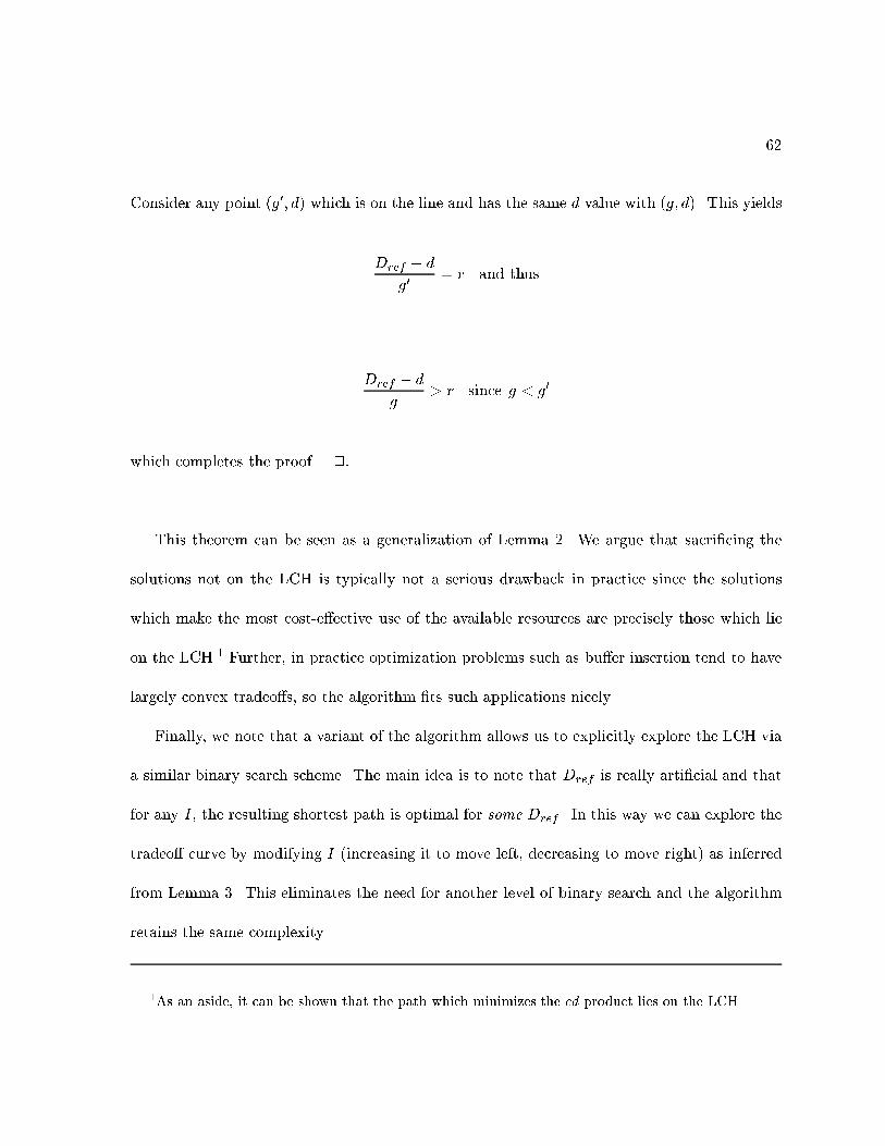
Consider any point �g�� d� which is on the line and has the same d value with �g� d�� This yields

Dref � d

g�� r and thus

Dref � d

g� r since g � g�

which completes the proof� ��

This theorem can be seen as a generalization of Lemma �� We argue that sacri�cing the

solutions not on the LCH is typically not a serious drawback in practice since the solutions

which make the most costeective use of the available resources are precisely those which lie

on the LCH�� Further� in practice optimization problems such as buer insertion tend to have

largely convex tradeos� so the algorithm �ts such applications nicely�

Finally� we note that a variant of the algorithm allows us to explicitly explore the LCH via

a similar binary search scheme� The main idea is to note that Dref is really arti�cial and that

for any I� the resulting shortest path is optimal for some Dref � In this way we can explore the

tradeo curve by modifying I �increasing it to move left� decreasing to move right� as inferred

from Lemma � This eliminates the need for another level of binary search and the algorithm

retains the same complexity�

�As an aside� it can be shown that the path which minimizes the cd product lies on the LCH�

�

�� Experimental Results

We implemented the pseudopolynomial algorithm and our DRCR algorithm in C and tested

on dierent test cases on a ���MHz Sun UltraSparc �� The main objective of our experiments

was to evaluate the computational feasibility of the DRCR algorithm and compare it with the

pseudopolynomial algorithm�

Test graphs were generated by randomly placing some macro blocks inside a rectangular

routing region� Candidate buer locations are then chosen randomly from the area that is not

covered by the blocks and two buers are considered as candidate neighbors �i�e�� there is an edge

between the corresponding nodes� only if they lie within a threshold distance �e�g�� �����m��

The routing regions vary from �cm �cm to �cm �cm� From existing literature� we use

the following values for the technology parameters � unit length capacitance c� � ����fF��m�

unit length resistance r� � ����"��m� driver resistance Rs � ���" � loading capacitance Ct

� ��fF � We use a single buer with the following parameters and build the buer library by

scaling these parameters� rb � ���"� cb � ��fF � db � ���ps� We use the Elmore model ����

to compute the delay of the interconnect in our test cases�

Table III shows the characteristics of the graphs that were used for the experiments� The

table lists the number of buer locations in each graph� the dierent sizes of buers used� total

number of nodes in the graph and the corresponding number of edges�

Table IV shows the running times for the pseudopolynomial and DRCR algorithms on all

the test graphs� The running time shown for the pseudopolynomial algorithm is for generating

all the solutions on the tradeo curve while for the DRCR� the running time reported is to

��

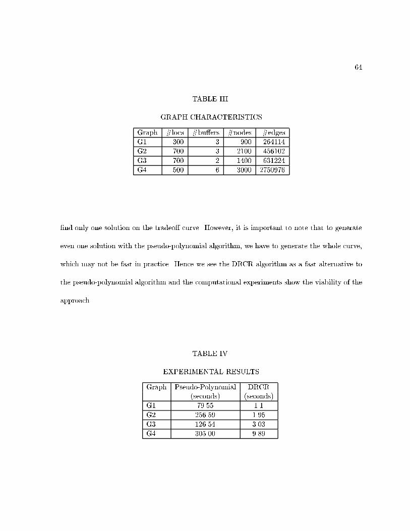
TABLE III

GRAPH CHARACTERISTICS

Graph locs buers nodes edges

G� �� ��� ������

G� ��� ���� ������

G ��� � ���� � ����

G� ��� � ��� �������

�nd only one solution on the tradeo curve� However� it is important to note that to generate

even one solution with the pseudopolynomial algorithm� we have to generate the whole curve�

which may not be fast in practice� Hence we see the DRCR algorithm as a fast alternative to

the pseudopolynomial algorithm and the computational experiments show the viability of the

approach�

TABLE IV

EXPERIMENTAL RESULTS

Graph PseudoPolynomial DRCR�seconds� �seconds�

G� ����� ���

G� ������ ����

G ������ ��

G� ����� ����

��

1500

2000

2500

3000

3500

4000

4500

3 3.5 4 4.5 5 5.5 6

Dela

y

Cost

G1G2

Figure ��� Examples of LCH of the cost vs� delay trade o� curve for two di�erent graphs G�

and G��

Figure Figure �� shows the plot of the solutions which can be found the DRCR algorithm

for two dierent graphs G� and G�� The graph shows the minimum delay solution� the delay

of the minimum cost solution� and the solutions that lie on the LCH of the tradeo curve� Our

experiments show that on the average� around ���solutions lie on the LCH�

��

��� Comments and Conclusion

In this work� we have studied the problem of buer insertion in the context of a given layout

where there are typically restrictions on the buer locations�

We have proposed the Delay Reduction to Cost Ratio Maximization problem in this context

that captures the cost vs� delay tradeo which is very crucial in practice� We also presented

a fast algorithm for solving the problem� which can be considered as an application of the

traditional shortestpath algorithm� The experimental results show the practicability of our

approach� Hence� we see the DRCR algorithm to be a possible alternative to slow pseudo

polynomial algorithms�

An important note is that we have assumed in this work that the delay of an interconnect

between two buers is independent of the input slew at the source buer� Though this as

sumption is not valid in practice� such varying input slews can be taken into account in our

graph model at the expense of more vertices � i�e�� one vertex for each possible input slew at

every buer input� But using such modeling� it is possible that we capture more realistic and

accurate delay modeling�

Though the DRCR problem in this work focuses on the �pin nets in a circuit� a possible

extension of this work would be to explore if a similar approach is possible for multipin nets�

which we hope would be of great practical value�

Finally� this algorithm �ts problems with largely convex tradeo �like buer insertion��

Hence we hope that this algorithm has a broad range of practical applications�

CITED LITERATURE

�� Garey� M� R� and Johnson� D� S�� Computers and Intractablility� A Guide to the Theoryof NPCompleteness� W�H�Freeman and Company� �����

�� Hart� P� E�� Nilsson� N� J�� and Raphael� B�� A Formal Basis for the Heuristic Determinationof Minimum Cost Paths� IEEE Transations on Systems� Science and Cybernetics�SCC������������� �����

� A� E� Caldwell� A� B� K� and Markov� I� L�� Optimal Partitioners and EndCase Placersfor StandardCell Layout� In Proc� of Intl� Symposium on Physical Design� pages������ �����

�� Cederbaum� I�� Optimal Backboard Ordering Through The Shortest Path Algorithm� InIEEE Trans� on Circuits and Systems� volume ��� pages ����� �� �����

�� E� Auer� W� S� and Sigl� G�� A New Linear Placement Algorithm for Cell Generation� InProc� of IEEE Intl� Conference on ComputerAided Design� pages �������� �����

�� Shirai� Y� and Tsujii� J�� Arti�cial Intelligence� Concepts� Techniques� and Applications�John Wiley # Sons� �����

�� Hur� S�W� and Lillis� J�� Relaxation and Clustering in a Local Search Framework� Application to Linear Placement� In Technical Report UICEECS���� �����

�� Hur� S�W� and Lillis� J�� Hybrid Techniques for StandardCell Placement� In To appearin Proc� of International Conference on ComputerAided Design� Nov� �����

�� Chu� C� C� N� and Wong� D� F�� Greedy Wire�Sizing is Linear Time� In Proc� of Intl�Symposium on Physical Design� pages ����� �����

��� Zhou� H�� Wong� D� F�� Liu� I�M�� and Aziz� A�� Simultaneous Routing and Buer Insertionwith Restrictions on Buer Locations� In Proc� of ACM�IEEE Design AutomationConference� pages ������ �����

��� Joksch� H� C�� The Shortest Route Problem With Constraints� J� Math Anal� Appl������������� �����

��

��

��� Elmore� W� C�� The Transient Response of Damped Linear Network with Particular Regardto Wideband Ampli�ers� J� Applied Physics� ������� � �����

� � Dijkstra� E� W�� A Discipline of Programming� PrenticeHall� Englewood Clis� N�J�� �����

��� Lawler� E�� Combinatorial Optimization � Networks and Matroids� Holt� Rinehart andWinston� �����

VITA

NAME� Ashok Jagannathan

EDUCATION� B�E�� Computer Science and Engineering� Regional Engineering College�Trichy� India� �����

M�S�� Electrical Engineering and Computer Science� University of Illinois at Chcicago� Illinois� USA� �����

TEACHINGEXPERIENCE�

Department of EECS� University of Illinois� Chicago� January ���� �May �����

HONORS� DAC Graduate Scholarship� Design Automation Conference� August���� � June �����

PROFESSIONAL Association for Computing MachineryMEMBERSHIP�

PUBLICATIONS� Ashok Jagannathan� SungWoo Hur and John Lillis� A Fast Algorithm for ContextAware Buer Insertion� in ACM�IEEE Proc�of Design Automation Conference� June ����� Los Angeles� CA� pages

�� � �

SungWoo Hur� Ashok Jagannathan and John Lillis� Timing DrivenMaze Routing� in ACM Proc�of International Symposium on Physical

Design� April ����� Monterey� CA� pages ����� �

SungWoo Hur� Ashok Jagannathan and John Lillis� Timing DrivenMaze Routing� in IEEE Transactions on ComputerAided Design ofIntegrated Circuits and Systems� Vol� ��� No� �� pages � ����� Feb��

�����

��