Prentice Hall: Pre-Algebra © 2001, Algebra I, Algebra II ...
Upload
david-tothCategory
view
31download
0description
M2P2Algebra 2
as lectured by Prof. Liebeck
MathematicsImperial College London
ii
These notes are based on a course of lectures given by Professor Liebeck during Spring Term 2006 atImperial College London. In general the notes follow the lectures very closely and only few changeswere made mostly to make the typesetting easier.These notes have not been checked by Professor Liebeck and should not be regarded as official notesfor the course. In particular, all the errors are made by me. However, I don’t take any responsibility fortheir consequences; use at your own risk (and attend lectures, they are fun).Please email me at [email protected] with any comments or corrections.
Anton StefanekOctober 2008
CONTENTS iii
Contents
I Groups 1
1 Introduction 3
2 Symmetry groups 52.1 Symmetry groups . . . . . . . . . . . . . . . . . . . . . . . . . . . . . . . . . . . . . . . . . . . . 52.2 More on D8 . . . . . . . . . . . . . . . . . . . . . . . . . . . . . . . . . . . . . . . . . . . . . . . 7
3 Isomorphism 93.1 Cyclic groups . . . . . . . . . . . . . . . . . . . . . . . . . . . . . . . . . . . . . . . . . . . . . . 12
4 Even and odd permutations 134.1 Alternating groups . . . . . . . . . . . . . . . . . . . . . . . . . . . . . . . . . . . . . . . . . . . 15
5 Direct Products 17
6 Groups of small size 216.1 Remarks on larger sizes . . . . . . . . . . . . . . . . . . . . . . . . . . . . . . . . . . . . . . . . 236.2 Quaternian group Q8 . . . . . . . . . . . . . . . . . . . . . . . . . . . . . . . . . . . . . . . . . . 23
7 Homomorphisms, normal subgroups and factor groups 257.1 Kernels . . . . . . . . . . . . . . . . . . . . . . . . . . . . . . . . . . . . . . . . . . . . . . . . . . 277.2 Normal subgroups . . . . . . . . . . . . . . . . . . . . . . . . . . . . . . . . . . . . . . . . . . . 287.3 Factor groups . . . . . . . . . . . . . . . . . . . . . . . . . . . . . . . . . . . . . . . . . . . . . . 30
8 Symmetry groups in 3 dimensions 35
9 Counting using groups 37
II Linear Algebra 39
10 Some revision 41
11 Determinants 4311.1 Basic properties . . . . . . . . . . . . . . . . . . . . . . . . . . . . . . . . . . . . . . . . . . . . . 4411.2 Expansions of determinants . . . . . . . . . . . . . . . . . . . . . . . . . . . . . . . . . . . . . . 4611.3 Major properties of determinants . . . . . . . . . . . . . . . . . . . . . . . . . . . . . . . . . . 47
11.3.1 Elementary matrices . . . . . . . . . . . . . . . . . . . . . . . . . . . . . . . . . . . . . . 48
12 Matrices and linear transformations 5312.0.2 Consequences of 12.1 . . . . . . . . . . . . . . . . . . . . . . . . . . . . . . . . . . . . . 55
12.1 Change of basis . . . . . . . . . . . . . . . . . . . . . . . . . . . . . . . . . . . . . . . . . . . . . 5612.2 Determinant of a linear transformation . . . . . . . . . . . . . . . . . . . . . . . . . . . . . . . 57
iv CONTENTS
13 Characteristic polynomials 5913.1 Diagonalisation . . . . . . . . . . . . . . . . . . . . . . . . . . . . . . . . . . . . . . . . . . . . . 6013.2 Algebraic & geometric multiplicities . . . . . . . . . . . . . . . . . . . . . . . . . . . . . . . . . 61
14 The Cayley-Hamilton theorem 6514.1 Proof of Cayley-Hamilton . . . . . . . . . . . . . . . . . . . . . . . . . . . . . . . . . . . . . . . 66
15 Inner product Spaces 6915.1 Geometry . . . . . . . . . . . . . . . . . . . . . . . . . . . . . . . . . . . . . . . . . . . . . . . . . 7015.2 Orthogonality . . . . . . . . . . . . . . . . . . . . . . . . . . . . . . . . . . . . . . . . . . . . . . 7115.3 Gram Schmidt . . . . . . . . . . . . . . . . . . . . . . . . . . . . . . . . . . . . . . . . . . . . . . 7215.4 Direct Sums . . . . . . . . . . . . . . . . . . . . . . . . . . . . . . . . . . . . . . . . . . . . . . . 7215.5 Orthogonal matrices . . . . . . . . . . . . . . . . . . . . . . . . . . . . . . . . . . . . . . . . . . 7315.6 Diagonalisation of Symmetric Matrices . . . . . . . . . . . . . . . . . . . . . . . . . . . . . . . 73

1
Part I
Groups


1. INTRODUCTION 3
Chapter 1
Introduction

4 1. INTRODUCTION
2. SYMMETRY GROUPS 5
Chapter 2
More examples of groups – symmetrygroups
Definition. Group of all isometries of R2 is I (R2).
2.1 Symmetry groups
LetΠ be a subset of R2. For a function g :R2 →R2, define
g (Π) = {g (x) | x ∈Π}
Example. Π=square with centre in the origin and aligned with axes, g = ρπ/4. Then g (Π) is the originalsquare rotated by π/4.
Definition. The symmetry group ofΠ to be G(Π) – set of isometries g such that g (Π) =Π, i.e. symmetry group
G(Π) = {g ∈ I (R2) | g (Π) =Π}
.
Example. For the square from the previous example, G(Π) contains ρπ/2, σx . . .
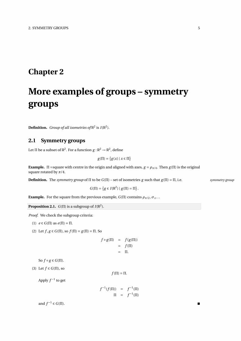
Proposition 2.1. G(Π) is a subgroup of I (R2).
Proof. We check the subgroup criteria:
(1) e ∈G(Π) as e(Π) =Π.
(2) Let f , g ∈G(Π), so f (Π) = g (Π) =Π. So
f ◦ g (Π) = f (g (Π))
= f (Π)
= Π.
So f ◦ g ∈G(Π).
(3) Let f ∈G(Π), sof (Π) =Π.
Apply f −1 to get
f −1( f (Π)) = f −1(Π)
Π = f −1(Π)
and f −1 ∈G(Π). �
6 2. SYMMETRY GROUPS
So we have a wast collection of new examples of groups G(Π).
Example.
1. Equilateral triangle (=Π)Here G(Π) contains
3 rotations: e = ρ0, ρ = ρ2π/3, ρ2 = ρ4π/3,
3 reflections: σ1 =σl1 , σ2 =σl2 , σ3 =σl3 .
Each of these corresponds to a permutation of the corners 1, 2, 3:
e ∼ e,
ρ ∼ (1 2 3),
ρ2 ∼ (1 3 2),
σ1 ∼ (2 3),
σ2 ∼ (1 3),
σ3 ∼ (1 2).
Any isometry in G(Π) permutes the corners. Since all the permutations of the corners are alreadypresent, there can’t be any more isometries in G(Π). So the Symmetry group of equilateral triangleis {
e,ρ,ρ2,σ1,σ2,σ3}
,
called the dihedral group D6.dihedral group
Note. Easy to work out products in D6: e.g.
ρσ3 ∼ (1 2 3)(1 2) = (1 3)
∼ σ2.
2. The squareHere G =G(Π) contains
4 rotations: e,ρ,ρ2,ρ3 where ρ = ρπ/2,
4 reflections: σ1,σ2,σ3,σ4 where σi =σli .
So |G| ≥ 8. We claim that |G| = 8: Any g ∈G permutes the corners 1,2,3,4 (as g preserves distance).So g sends
1 → i , (4 choices of i )
2 → j, neighbour of i , (2 choices for j )
3 → opposite of i ,
4 → opposite of j .
So |G| ≤ (num. of choices for i )× (for j ) = 4×2 = 8. So |G| = 8.Symmetry group of the square is {
e,ρ,ρ2,ρ3,σ1,σ2,σ3,σ4}
,
called the dihedral group D8.
2. SYMMETRY GROUPS 7
Note. Can work out products using the corresponding permutations of the corners.
e ∼ e,
ρ ∼ (1 2 3 4),
ρ2 ∼ (1 3)(2 4),
ρ3 ∼ (1 4 3 2),
σ1 ∼ (1 4)(2 3),
σ2 ∼ (1 3),
σ3 ∼ (1 2)(3 4),
σ4 ∼ (2 4).
For example
ρ3σ1 → (1 4 3 2)(1 4)(2 3) = (1 3)
→ σ2.
Note. Not all permutations of the corners are present in D8, e.g. (1 2).
2.2 More on D8
Define H to be the cyclic subgroup of D8 generated by ρ, so
H = ⟨ρ⟩ = {e,ρ,ρ2,ρ3} .
Write σ=σ1. The right coset
Hσ= {σ,ρσ,ρ2σ,ρ3σ
}is different from H .
H Hσ
So the two distinct right cosets of H in D8 are H and Hσ, and
D8 = H ∪Hσ.
Hence
Hσ = {ρ,ρσ,ρ2σ,ρ3σ
}= {σ1,σ2,σ3,σ4} .
So the elements of D8 are
e,ρ,ρ2,ρ3,σ,ρσ,ρ2σ,ρ3σ.
To work out products, use the “magic equation” (see Sheet 1, Question 2)
σρ = ρ−1σ.
Example.
3. Regular n-gonLetΠ be the regular polygon with n sides. Symmetry group G =G(Π) contains
n rotations: e,ρ,ρ2, . . . ,ρn−1 where ρ = ρ2π/n ,
n reflections σ1,σ2, . . . ,σn where σi =σli .
8 2. SYMMETRY GROUPS
So |G| ≥ 2n. We claim that |G| = 2n.
Any g ∈G sends corners to corners, say
1 → i , (n choices for i)
2 → j neighbour of i . (2 choices for j )
Then g sends n to the other neighbour of i and n −1 to the remaining neighbour of g (n) and soon. So once i , j are known, there is only one possibility for g . Hence
|G| ≤ number of choices for i , j = 2n.
Therefore |G| = 2n.
Symmetry group of regular n-gon is
D2n = {e,ρ,ρ2, . . . ,ρn ,σ1, . . . ,σn
},
the dihedral group of size 2n.
Note. Again can work in D2n using permutations
ρ → (1 2 3 · · · n)
σ1 → (2 n)(3 n −1) · · ·
4. Benzene moleculeC6H6. Symmetry group is D12.
5. Infinite strip of F’s. . . F F F . . .
−1 0 1
What is symmetry group G(Π)?
G(Π) contains translationτ(1,0) : v 7→ v + (1,0).
Write τ = τ(1,0). Then G(Π) contains all translations τn = τ(n,0). Note G(Π) is infinite. We claimthat
G(Π) = {τn | n ∈Z}
= ⟨τ⟩ ,
infinite cyclic group.
Let g ∈G(Π). Must show that g = τn for some n. Say g sends
F at 0 → F at n.
Note that τ−n sends F at n to F at 0. So τ−n g sends F at 0 to F at 0. So τ−n g is a symmetry of the Fat 0. It is easy to observe that F has only symmetry e. Hence
τ−n g = e
τnτ−n g = τn
g = τn .
Note. Various other figures have more interesting symmetry groups, e.g. infinite strip of E’s, squaretiling of a plane, octagons and squares tiling of the plane, 3 dimensions – platonic solids. . . later.
3. ISOMORPHISM 9
Chapter 3
Isomorphism
Let
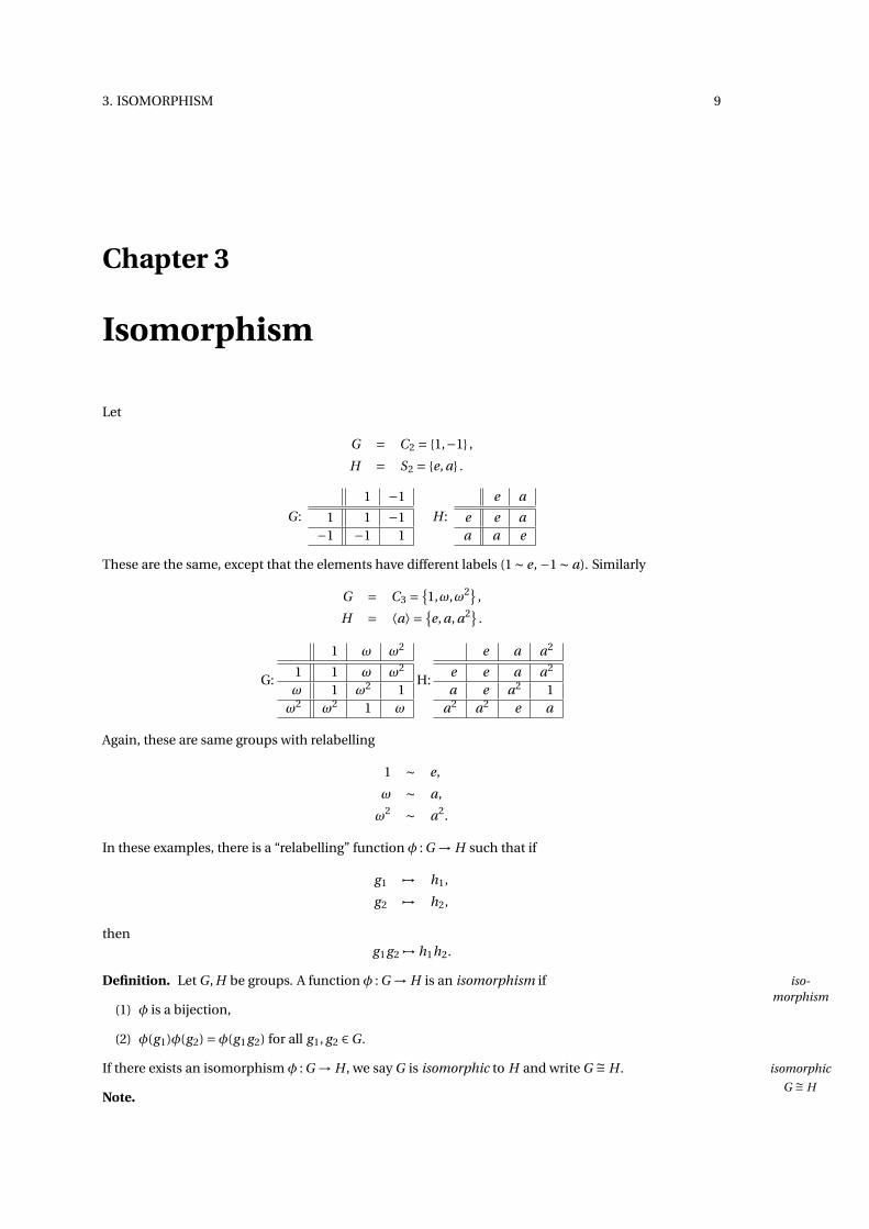
G = C2 = {1,−1} ,
H = S2 = {e, a} .
G :
1 −1
1 1 −1−1 −1 1
H :
e a
e e aa a e
These are the same, except that the elements have different labels (1 ∼ e, −1 ∼ a). Similarly
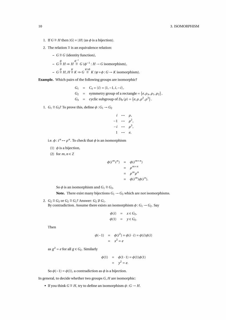
G = C3 ={1,ω,ω2} ,
H = ⟨a⟩ = {e, a, a2} .
G:
1 ω ω2
1 1 ω ω2
ω 1 ω2 1ω2 ω2 1 ω
H:
e a a2
e e a a2
a e a2 1a2 a2 e a
Again, these are same groups with relabelling
1 ∼ e,
ω ∼ a,
ω2 ∼ a2.
In these examples, there is a “relabelling” function φ : G → H such that if
g1 7→ h1,
g2 7→ h2,
theng1g2 7→ h1h2.
Definition. Let G , H be groups. A function φ : G → H is an isomorphism if iso-morphism
(1) φ is a bijection,
(2) φ(g1)φ(g2) =φ(g1g2) for all g1, g2 ∈G .
If there exists an isomorphism φ : G → H , we say G is isomorphic to H and write G ∼= H . isomorphic
G ∼= HNote.
10 3. ISOMORPHISM
1. If G ∼= H then |G| = |H | (as φ is a bijection).
2. The relation ∼= is an equivalence relation:
– G ∼=G (identity function),
– Gφ∼= H ⇒ H
φ−1
∼= G (φ−1 : H →G isomorphism),
– Gφ∼= H , H
ψ∼= K ⇒Gψ◦φ∼= K (ψ◦φ : G → K isomorphism).
Example. Which pairs of the following groups are isomorphic?
G1 = C4 = ⟨i ⟩ = {1,−1, i ,−i } ,
G2 = symmetry group of a rectangle = {e,ρπ,ρ1,ρ2
},
G3 = cyclic subgroup of D8 ⟨ρ⟩ ={e,ρ,ρ2,ρ3} .
1. G1∼=G3? To prove this, define φ : G1 →G2
i 7→ ρ,
−1 7→ ρ2,
−i 7→ ρ3,
1 7→ e,
i.e. φ : i n 7→ ρn . To check that φ is an isomorphism
(1) φ is a bijection,
(2) for m,n ∈Z
φ(i m i n) = φ(i m+n)
= ρm+n
= ρmρn
= φ(i m)φ(i n).
So φ is an isomorphism and G1∼=G3.
Note. There exist many bijections G1 →G3 which are not isomorphisms.
2. G2∼=G3 or G2
∼=G1? Answer: G2 6∼=G1.By contradiction. Assume there exists an isomorphism φ : G1 →G2. Say
φ(i ) = x ∈G2,
φ(1) = y ∈G2.
Then
φ(−1) = φ(i 2) =φ(i · i ) =φ(i )φ(i )
= x2 = e
as g 2 = e for all g ∈G2. Similarly
φ(1) = φ(1 ·1) =φ(1)φ(1)
= y2 = e.
So φ(−1) =φ(1), a contradiction as φ is a bijection.
In general, to decide whether two groups G , H are isomorphic:
• If you think G ∼= H , try to define an isomorphism φ : G → H .
3. ISOMORPHISM 11
• If you think G 6∼= H , try to use the following proposition.
Proposition 3.1. Let G , H be groups.
(1) If |G| 6= |H | then G 6∼= H .
(2) If G is abelian and H is not abelian, then G 6∼= H .
(3) If there is an integer k such that G and H have different number of elements of order k, thenG 6∼= H .
Proof.
(1) Obvious.
(2) We show that if G is abelian and G ∼= H , then H is abelian (this gives (2)). Suppose G is abelian andφ : G → H is an isomorphism. Let h1,h2 ∈ H . As φ is a bijection, there exist g1, g2 ∈ G such thath1 =φ(g1) and h2 =φ(g2). So
h2h1 = φ(g2)φ(g1)
= φ(g2g1)
= φ(g1)φ(g2)
= h1h2.
(3) Let
Gk = {g ∈G | ord(g ) = k
},
Hk = {h ∈ H | ord(h) = k} .
We show that G ∼= H implies |Gk | = |Hk | for all k (this gives (3)).Suppose G ∼= H and let φ : G → H be an isomorphism. We show that φ sends Gk to Hk : Let g ∈Gk ,so ord(g ) = k, i.e.
g k = eG , ( )
g i 6= eG for 1 ≤ i ≤ k −1.
Now φ(eG ) = eH , since
φ(eG ) = φ(eG eG )
= φ(eG )φ(eG )
φ(eG )−1φ(eG ) = φ(eG )
eH = φ(eG ).
Also
φ(g i ) = φ(g g · · ·g︸ ︷︷ ︸i times
)
= φ(g )φ(g ) · · ·φ(g )︸ ︷︷ ︸i times
= φ(g )i .
Applying this to ( ) gives
φ(g )k = φ(eG ) = eH ,
φ(g )i 6= eH for 1 ≤ i ≤ k −1.
12 3. ISOMORPHISM
In other words, φ(g ) has order k, so φ(g ) ∈ Hk .
So φ sends Gk to Hk . As φ is 1-1, this implies
|Gk | ≤ |Hk |.Also φ−1 : H →G is an isomorphism and similarly sends Hk to Gk , hence
|Hk | ≤ |Gk |.Therefore |Gk | = |Hk |. �
Example.
1. Let G = S4, H = D8. Then |G| = 24, |H | = 8, so G 6∼= H .
2. Let G = S3, H =C6. Then G is non-abelian, H is abelian, so G 6∼= H .
3. Let G = C4, H = symmetry group of the rectangle = {e,ρπ,ρ1,ρ2
}. Then G has 1 element of order
2, H has 3 elements of order 2, so G 6∼= H .
4. Question: (R,+) ∼= (R∗,×)? Answer: No, since (R,+) has 0 elements of order 2, (R∗,×) has 1 elementof order 2.
3.1 Cyclic groups
Proposition 3.2.
(1) If G is a cyclic group of size n, then G ∼=Cn .
(2) If G is an infinite cyclic group, then G ∼= (Z,+).
Proof.
(1) Let G = ⟨x⟩, |G| = n, so ord(x) = n and therefore
G = {e, x, x2, . . . , xn−1} .
RecallCn = {
1,ω,ω2, . . . ,ωn−1} ,
where ω= e2πi /n . Define φ : G →G byφ(xr ) =ωr
for all r . Then φ is a bijection, and
φ(xr xs ) = φ(xr+s )
= ωr+s
= ωrωs
= φ(xr )φ(xs ).
So φ is an isomorphism, and G ∼=Cn .
(2) Let G = ⟨x⟩ be infinite cyclic, so ord(x) =∞ and
G = {. . . , x−2, x−1,e, x, x2, x3, . . .
},
all distinct. Define φ : G → (Z,+) byφ(xr ) = r
for all r . Then φ is an isomorphism, so G ∼= (Z,+). �
Note. This proposition says that if we think of isomorphic groups as being “the same”, then there is onlyone cyclic group of each size. We say: “up to isomorphism”, the only cyclic groups are Cn and (Z,+).
Example. Cyclic subgroup ⟨3⟩ of (Z,+) is {3n | n ∈Z}, infinite, so by the proposition
⟨3⟩ ∼= (Z,+).

4. EVEN AND ODD PERMUTATIONS 13
Chapter 4
Even and odd permutations
We’ll classify each permutation in Sn as either “even” or “odd” (reason given later).
Example. For n = 3. Consider the expression
∆= (x1 −x2)(x1 −x3)(x2 −x3),
a polynomial in 3 variables x1, x2, x3. Take each permutation in S3 to permute x1, x2, x3 in the same wayit permutes 1,2,3. Then each g ∈ S3 sends ∆ to ±∆ (∆ 7→
(1 3)−∆, ∆ 7→
(1 2 3)+∆). For example
for e, (1 2 3), (1 3 2) : ∆ 7→ +∆,
for (1 2), (1 3), (2 3) : ∆ 7→ −∆.
Generalize this:
Definition. For arbitrary n ≥ 2, define ∆
∆= ∏i< j
(xi −x j
),
a polynomial in n variables x1, . . . , xn .
If we let each permutation g ∈ Sn permute the variables x1, . . . , xn just as it permutes 1, . . . ,n then gsends ∆ to ±∆.
Definition. For g ∈ Sn , define the signature sgn(g ) to be +1 if g (∆) =∆ and −1 if g (∆) =−∆. So signaturesgn
g (∆) = sgn(g )∆.
The function sgn : Sn → {+1,−1} is the signature function on Sn .Call g an even permutation if sgn(g ) = 1, and odd permutation if sgn(g ) =−1. even
oddperm.Example. In S3 e, (1 2 3), (1 3 2) are even and (1 2), (1 3), (2 3) are odd.
Example. Given (1 2 3 5)(6 7 9)(8 4 10) ∈ S10, what’s its signature?
Aim: To answer such questions instantaneously.This is the key:
Proposition 4.1.
(a) sgn(x y) = sgn(x)sgn(y) for all x, y ∈ Sn
(b) sgn(e) = 1, sgn(x−1) = sgn(x).
(c) If t = (i j ) is a 2-cycle then sgn(t ) =−1.
Proof.
14 4. EVEN AND ODD PERMUTATIONS
(a) By definition
x(∆) = sgn(x)∆,
y(∆) = sgn(y)∆.
So
x y(∆) = x(y(∆))
= x(sgn(y)∆)
= sgn(y)x(∆) = sgn(y)sgn(x)∆.
Hencesgn(x y) = sgn(x)sgn(y).
(b) We havee(∆) =∆,
so sgn(e) = 1. So
1 = sgn(e) = sgn(xx−1)(a)= sgn(x)sgn(x−1)
and hence sgn(x) = sgn(x−1).
(c) Let t = (i j ), i < j . We count the number of brackets in ∆ that are sent to brackets (xr − xs ), r > s.These are
(xi −x j ),(xi −xi+1), . . . , (xi −x j−1),(xi+1 −x j ), . . . , (x j−1 −x j ).
Total number of these is 2( j − i −1)+1, an odd number. Hence t (∆) =−∆ and sgn(t ) =−1. �
To work out sgn(x), x ∈ Sn :
• express x as a product of 2-cycles
• use proposition 4.1
Proposition 4.2. Let c = (a1a2 . . . ar ), an r -cycle. Then c can be expressed as a product of (r −1) 2-cycles.
Proof. Consider the product(a1ar )(a1ar−1) · · · (a1a3)(a1a2).
This product sendsa1 7→ a2 7→ a3 7→ · · · 7→ ar−1 7→ a1.
Hence the product is equal to c. �
Corollary 4.3.
sgn(r -c ycle) = (−1)r−1
={
1 if r is odd−1 if r is even.
Proof. Let c = (a1 · · ·ar ), an r -cycle. By 4.2, c = (a1ar ) · · · (a1a2). So
sgn(c)4.1(a)= sgn(a1ar ) · · ·sgn(a1a2)4.1(c)= (−1)r−1.
�
4. EVEN AND ODD PERMUTATIONS 15
Corollary 4.4. Every x ∈ Sn can be expressed as a product of 2-cycles.
Proof. From first year, we know thatx = c1 · · ·cm ,
a product of disjoint cycles ci . Each ci is a product of 2-cycles by 4.2. Hence so is x. �
Proposition 4.5. Let x = c1 · · ·cm a product of disjoint cycles c1, . . . ,cm of lengths r1, . . . ,rm . Then
sgn(x) = (−1)r1−1 · · · (−1)rm−1.
Proof.
sgn(x)4.1(a)= sgn(c1) · · ·sgn(cm)
4.3= (−1)r1−1 · · · (−1)rm−1.
�
Example. (1 2 5 7)(3 4 6)(8 9)(10 12 83)(79 11 26 15) has sgn =−1.
Importance of signature
1. We’ll use it to define a new family of groups.
2. Fundamental in the theory of determinants.
4.1 Alternating groups
Definition. Define An
An = {x ∈ Sn | sgn(x) = 1
},
the set of even permutations in Sn . Call An the alternating group (after showing that it is a group). alternating group
Theorem 4.6. An is a subgroup of Sn , of size 12 n!.
Proof.
• An is a subgroup:
(1) e ∈ An as sgn(e) = 1.
(2) for x, y ∈ An ,
sgn(x) = sgn(y) = 1,
sgn(x y)4.1(a)= sgn(x)sgn(y) = 1,
i.e. x y ∈ An ,
(3) x ∈ An , so sgn(x) = 1. Then by 4.1(b), sgn(x−1) = 1, i.e. x−1 ∈ An .
• |An | = 12 n!: Recall that there are right cosets of An ,
An = Ane,
An(1 2) = {x(1 2) | x ∈ An} .
These cosets are distinct (as (1 2) ∈ An(1 2) but (1 2) ∉ An), and have equal size (i.e. |An | = |An(1 2)|).We show that Sn = An ∪An(1 2): Let g ∈ Sn . If g is even, then g ∈ An . If g is odd, then g (1 2) is even(as sgn(g (1 2)) = sgn(g )sgn(1 2) = 1), so g (1 2) = x ∈ An . Then g = x(1 2) ∈ An(1 2).
So |An | = 12 |Sn | = 1
2 n!. �
16 4. EVEN AND ODD PERMUTATIONS
Example.
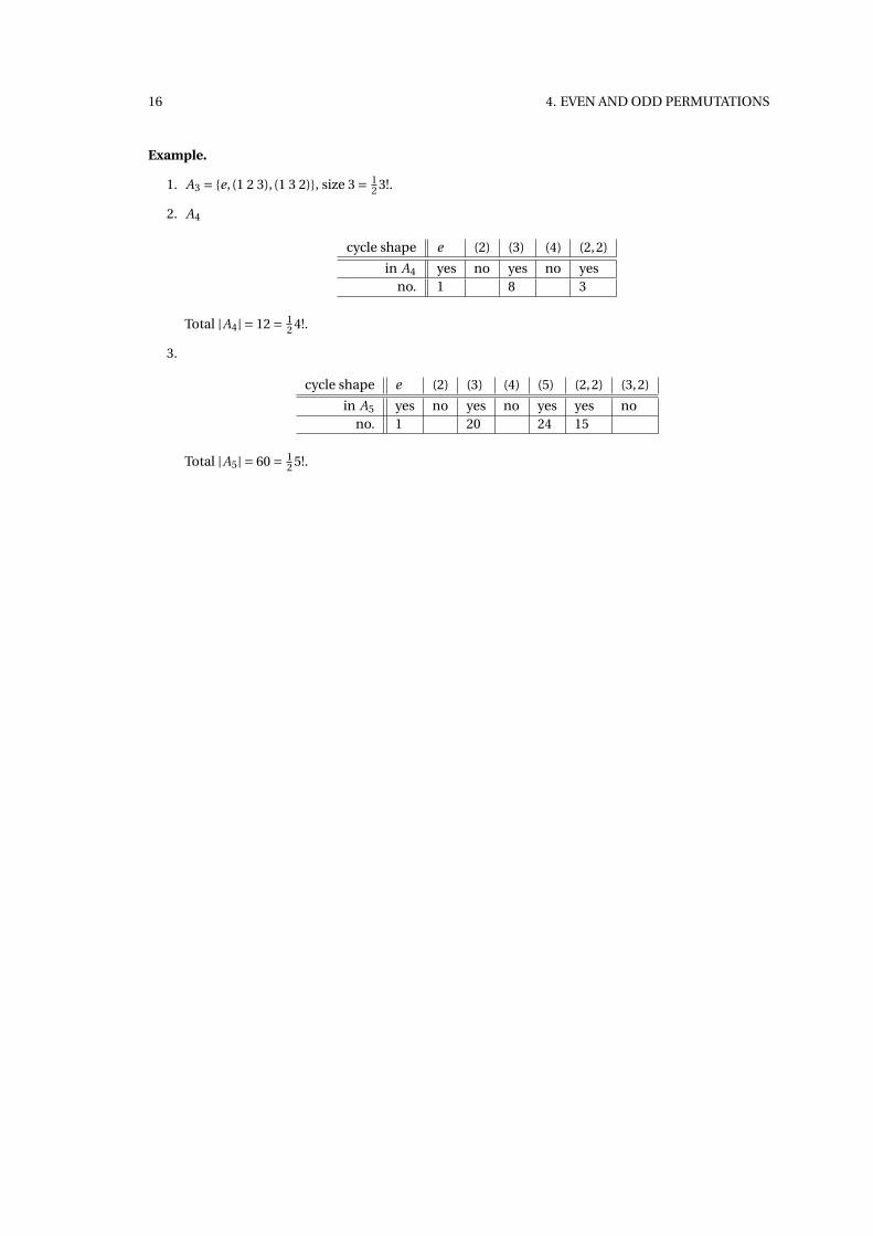
1. A3 = {e, (1 2 3), (1 3 2)}, size 3 = 12 3!.
2. A4
cycle shape e (2) (3) (4) (2,2)
in A4 yes no yes no yesno. 1 8 3
Total |A4| = 12 = 12 4!.
3.
cycle shape e (2) (3) (4) (5) (2,2) (3,2)
in A5 yes no yes no yes yes nono. 1 20 24 15
Total |A5| = 60 = 12 5!.
5. DIRECT PRODUCTS 17
Chapter 5
Direct Products
So far, we’ve seen the following examples of finite groups: Cn ,D2n ,Sn , An . We’ll get many more usingthe following construction.Recall: if T1,T2, . . . ,Tn are sets, the Cartesian product T1×T2×·· ·×Tn is the set consisting of all n-tuples
(t1, t2, . . . , tn) (ti ∈ Ti ).
Now let G1,G2, . . . ,Gn be groups. Form the Cartesian product G1×G2×·· ·×Gn and define multiplicationon this set by
(x1, . . . , xn)(y1, . . . , yn) = (x1 ·G1 y1, . . . , xn ·Gn yn)
for xi , yi ∈Gi .
Definition. Call G1 ×·· ·×Gn the direct product of the groups G1, . . . ,Gn . direct product
Proposition 5.1. Under above defined multiplication, G1 ×·· ·×Gn is a group.
Proof.
• Closure True by closure in each Gi .
• Associativity Using associativity in each Gi ,[(x1, . . . , xn)(y1, . . . , yn)
](z1, . . . , zn) = (x1 y1, . . . , xn yn)(z1, . . . , zn)
= ((x1 y1)z1, . . . , (xn yn)zn
)= (
x1(y1z1), . . . , xn(yn zn))
= (x1, . . . , xn)(y1z1, . . . , yn zn)
= (x1, . . . , xn)[(y1, . . . , yn)(z1, . . . , zn)
].
• Identity is (e1, . . . ,en), where ei is the identity of Gi .
• Inverse of (x1, . . . , xn) is (x−11 , . . . , x−1
n ).
�
Example.
1. Some new groups: C2 ×C2,C2 ×C2 ×C2,S4 ×D36, A5 × A6 ×S297, . . . ,Z×Q×S13, . . . .
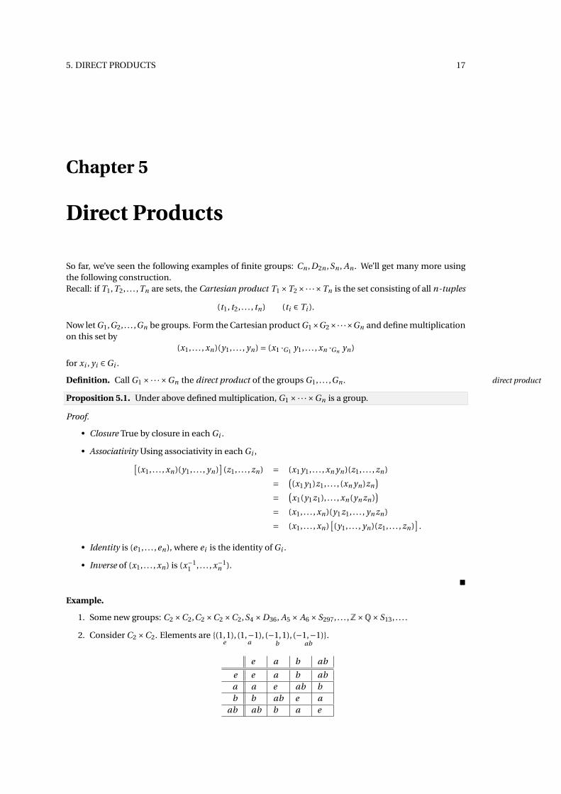
2. Consider C2 ×C2. Elements are {(1,1)e
, (1,−1)a
, (−1,1)b
, (−1,−1)ab
}.
e a b ab
e e a b aba a e ab bb b ab e a
ab ab b a e
18 5. DIRECT PRODUCTS
G =C2 ×C2 is abelian and x2 = e for all x ∈G .
3. Similarly C2 ×C2 ×C2 has elements (±1,±1,±1), size 8, abelian, x2 = e for all x.
Proposition 5.2.
(a) Size of G1 ×·· ·×Gn is |G1||G2| · · · |Gn |.(b) If all Gi are abelian so is G1 ×·· ·×Gn .
(c) If x = (x1, . . . , xn) ∈G1×·· ·×Gn , then order of x is the least common multiple of ord(x1), . . . ,ord(xn),i.e.
o(x) = lcm(ord(x1), . . . ,ord(xn)).
Proof.
(a) Clear.
(b) Suppose all Gi are abelian. Then
(x1, . . . , xn)(y1, . . . , yn) = (x1 y1, . . . , xn yn)
= (y1x1, . . . , yn xn)
= (y1, . . . , yn)(x1, . . . , xn).
(c) Let ri = ord(xi ). Recall that
xki = e ⇔ ri |k.
Let r = lcm(r1, . . . ,rn). Then
xr = (xr1 , . . . , xr
n)
= (e1, . . . ,en) = e.
For 1 ≤ s < r , ri 6 |s for some i . So xsi 6= e. So
xs = (. . . , xsi , . . . ) 6= (e1, . . . ,en).
Hence r = ord(x). �
Example.
1. Since cyclic groups Cr are abelian, so are all direct products
Cr1 ×Cr2 ×·· ·×Crk .
2. C4 ×C2 and C2 ×C2 ×C2 are abelian of size 8. Are they isomorphic?Claim: NO.
Proof. Count the number of elements of order 2 :
In C4 ×C2 these are (±i ,±1) except for (1,1), so there are 3.
In C2 ×C2 ×C2, all the elements except e have order 2, so there are 7.
So C4 ×C2 6∼=C2 ×C2 ×C2. �
Proposition 5.3. If hcf(m,n) = 1, then Cm ×Cn∼=Cmn .
5. DIRECT PRODUCTS 19
Proof. Let Cm = ⟨α⟩, Cn = ⟨β⟩. So ord(α) = m, ord(β) = n. Consider
x = (α,β) ∈Cm ×Cn .
By 5.2(c)ord(x) = lcm(m,n) = mn.
Hence cyclic subgroup ⟨x⟩ of Cm ×Cn has size mn, so is whole of Cm ×Cn . So Cm ×Cn = ⟨x⟩ is cyclic andhence Cm ×Cn
∼=Cmn by 3.2. �
Direct products are fundamental to the theory of abelian groups.
Theorem 5.4. Every finite abelian group is isomorphic to a direct product of cyclic groups.
Proof. Won’t give one here. Reference: [Allenby, p. 254]. �
Example.
1. Abelian groups of size 6: by theorem 5.4, possibilities are C6,C3×C2. By 5.3, these are isomorphic,so there is only one abelian group of size 6 (up to isomorphism).
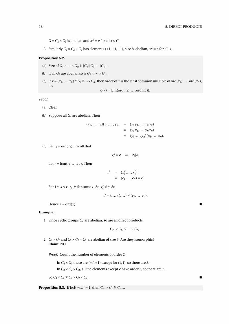
2. By 5.4, the abelian groups of size 8 are: C8, C4 ×C2,C2 ×C2 ×C2.Claim: No two of these are isomorphic.
Proof.
Group C2 ×C2 ×C2 C4 ×C2 C8
| {x | ord(x) = 2} | 7 3 1
So up to isomorphism, there are 3 abelian groups of size 8. �

20 5. DIRECT PRODUCTS
6. GROUPS OF SMALL SIZE 21
Chapter 6
Groups of small size
We’ll find all groups of size ≤ 7 (up to isomorphism). Useful results:
Lemma 6.1. If |G| = p, a prime, then G ∼=Cp .
Proof. By corollary of Lagrange, G is cyclic. Hence G ∼=Cp by 3.2. �
Lemma 6.2. If |G| is even, then G contains an element of order 2.
Proof. Suppose |G| is even and G has no element of order 2. List the elements of G as follows:
e, x1, x−11 , x2, x−1
2 , . . . , xk , x−1k .
Note that xi 6= x−1i since ord(xi ) 6= 2. Hence |G| = 2k +1, a contradiction. �
Groups of size 1,2,3,5,7
By 6.1, only such groups are C1,C2,C3,C5,C7.
Groups of size 4
Proposition 6.3. The only groups of size 4 are C4 and C2 ×C2.
Proof. Let |G| = 4. By Lagrange, every element of G has order 1,2 or 4. If there exists x ∈ G of order 4,then ⟨x⟩ is cyclic, so G ∼=C4. Now suppose ord(x) = 2 for all x 6= e, x ∈G . So x2 = e for all x ∈G . Let e, x, ybe 3 distinct elements of G . Now suppose
x y = e,
x = y−1 = y,
a contradiction. So suppose
x y = x,
y = e,
a contradiction. Similarly for x y = y . So x y 6= e, x, y , hence
G = {e, x, y, x y
}.
Now y x 6= e, x, y hence y x = x y . So multiplication table of G is
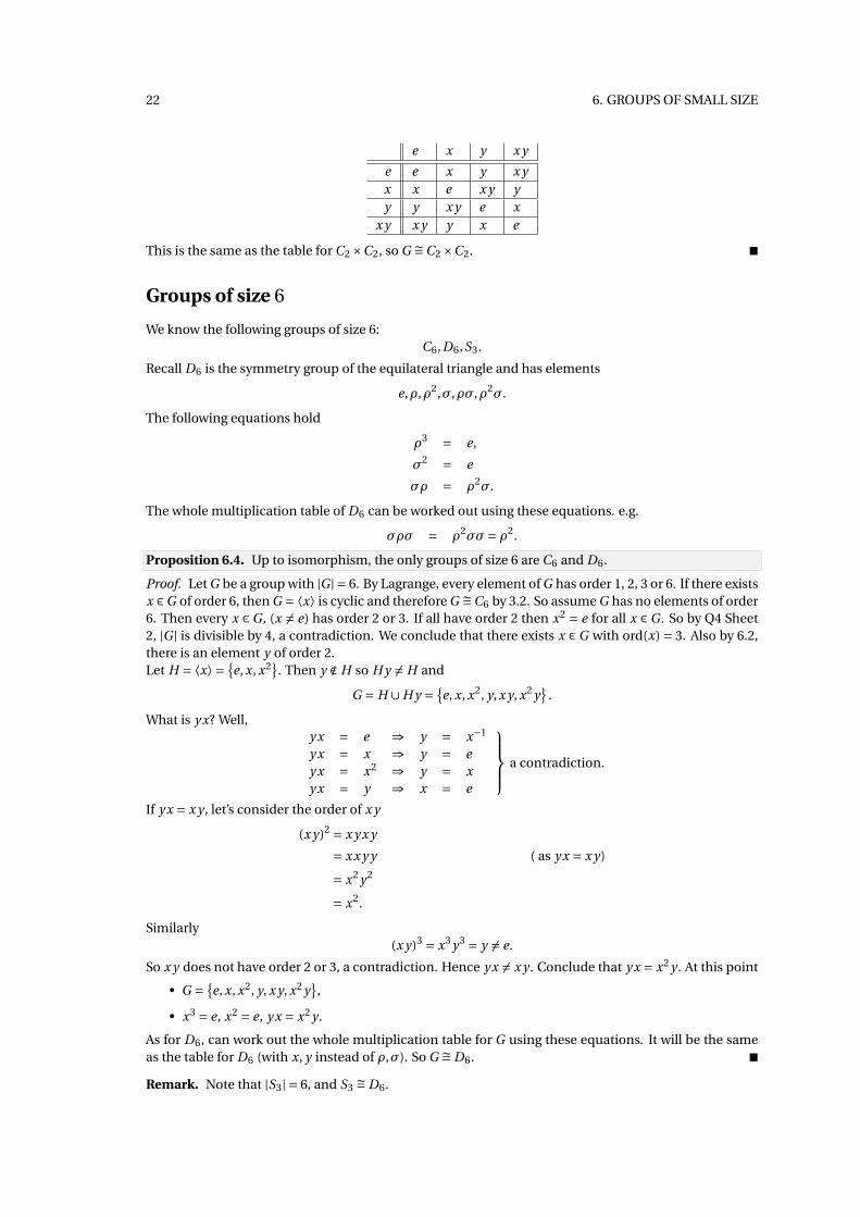
22 6. GROUPS OF SMALL SIZE
e x y x y
e e x y x yx x e x y yy y x y e x
x y x y y x e
This is the same as the table for C2 ×C2, so G ∼=C2 ×C2. �
Groups of size 6
We know the following groups of size 6:C6,D6,S3.
Recall D6 is the symmetry group of the equilateral triangle and has elements
e,ρ,ρ2,σ,ρσ,ρ2σ.
The following equations hold
ρ3 = e,
σ2 = e
σρ = ρ2σ.
The whole multiplication table of D6 can be worked out using these equations. e.g.
σρσ = ρ2σσ= ρ2.
Proposition 6.4. Up to isomorphism, the only groups of size 6 are C6 and D6.
Proof. Let G be a group with |G| = 6. By Lagrange, every element of G has order 1, 2, 3 or 6. If there existsx ∈G of order 6, then G = ⟨x⟩ is cyclic and therefore G ∼=C6 by 3.2. So assume G has no elements of order6. Then every x ∈G , (x 6= e) has order 2 or 3. If all have order 2 then x2 = e for all x ∈G . So by Q4 Sheet2, |G| is divisible by 4, a contradiction. We conclude that there exists x ∈G with ord(x) = 3. Also by 6.2,there is an element y of order 2.Let H = ⟨x⟩ = {
e, x, x2}. Then y ∉ H so H y 6= H and
G = H ∪H y = {e, x, x2, y, x y, x2 y
}.
What is y x? Well,y x = e ⇒ y = x−1
y x = x ⇒ y = ey x = x2 ⇒ y = xy x = y ⇒ x = e
a contradiction.
If y x = x y , let’s consider the order of x y
(x y)2 = x y x y
= xx y y ( as y x = x y)
= x2 y2
= x2.
Similarly(x y)3 = x3 y3 = y 6= e.
So x y does not have order 2 or 3, a contradiction. Hence y x 6= x y . Conclude that y x = x2 y . At this point
• G = {e, x, x2, y, x y, x2 y
},
• x3 = e, x2 = e, y x = x2 y .
As for D6, can work out the whole multiplication table for G using these equations. It will be the sameas the table for D6 (with x, y instead of ρ,σ). So G ∼= D6. �
Remark. Note that |S3| = 6, and S3∼= D6.
6. GROUPS OF SMALL SIZE 23
Summary
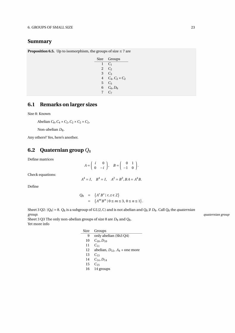
Proposition 6.5. Up to isomorphism, the groups of size ≤ 7 are
Size Groups1 C1
2 C2
3 C3
4 C4, C2 ×C2
5 C5
6 C6,D6
7 C7
6.1 Remarks on larger sizes
Size 8: Known
Abelian C8,C4 ×C2,C2 ×C2 ×C2,
Non-abelian D8.
Any others? Yes, here’s another.
6.2 Quaternian group Q8
Define matrices
A =(
i 00 −i
), B =
(0 1
−1 0
).
Check equations:A4 = I , B 4 = I , A2 = B 2,B A = A4B.
Define
Q8 = {Ar B s | r, z ∈Z}
= {AmB n | 0 ≤ m ≤ 3, 0 ≤ n ≤ 1
}.
Sheet 3 Q2: |Q8| = 8. Q8 is a subgroup of GL(2,C) and is not abelian and Q8 6∼= D8. Call Q8 the quaterniangroup. quaternian group
Sheet 3 Q3 The only non-abelian groups of size 8 are D8 and Q8.Yet more info
Size Groups9 only abelian (Sh3 Q4)
10 C10,D10
11 C11
12 abelian, D12, A4 + one more13 C13
14 C14,D14
15 C15
16 14 groups

24 6. GROUPS OF SMALL SIZE
7. HOMOMORPHISMS, NORMAL SUBGROUPS AND FACTOR GROUPS 25
Chapter 7
Homomorphisms, normal subgroupsand factor groups
Homomorphisms are functions between groups which “preserve multiplication”.
Definition. Let G , H be groups. A function φ : G → H is a homomorphism if homomorphism
φ(x y) =φ(x)φ(y)
for x, y ∈G .
Note. An isomorphism is a homomorphism which is a bijection.
Example.
1. G , H any groups. Define φ : G → H byφ(x) = eH
for all x ∈G . Then φ is a homomorphism since φ(x y) = eH = eH eH =φ(x)φ(y).
2. Recall the signature function sgn : Sn →C2. By 4.1(a),
sgn(x y) = sgn(x)sgn(y),
so sgn is a homomorphism.
3. Define φ : (R,+) → (C∗,×) byφ(x) = e2πi x
for all x ∈R. Then
φ(x + y) = e2πi (x+y)
= e2πi x e2πi y
= φ(x)φ(y),
so φ is a homomorphism.
4. Define φ : D2n →C2 (writing D2n = {e,ρ, . . . ,ρn−1,σ,ρσ, . . . ,ρn−1σ
})
φ(ρrσs ) = (−1)s .
(so φ sends rotations to +1 and reflections to −1). Then φ is a homomorphism:
φ((ρrσs )(ρtσu)
) = φ(ρr±tσs+u)
= (−1)s+u =φ(ρrσs )φ(ρrσu)
since
σsρt ={
ρt s = 0,ρ−tσ s = 1.
26 7. HOMOMORPHISMS, NORMAL SUBGROUPS AND FACTOR GROUPS
Proposition 7.1. Let φ : G → H be a homomorphism
(a) φ(eG ) = eH
(b) φ(x−1) =φ(x)−1 for all x ∈G .
(c) ord(φ(x)) divides ord(x) for all x ∈G .
Proof.
(a) Noteφ(eG ) =φ(eG eG ) =φ(eG )φ(eG ).
Multiply by φ(eG )−1 to geteH =φ(eG ).
(b) By (a),
eH = φ(eG ) =φ(xx−1)
= φ(x)φ(x−1).
So φ(x−1) =φ(x)−1.
(c) Let r = ord(x). Then
φ(x)r = φ(x) · · ·φ(x)
= φ(x · · ·x)
= φ(xr ) =φ(eG ) = eH .
Hence ord(φ(x)) divides r . �
Definition. Let φ : G → H be homomorphism. The image of φ isimage
ImImφ=φ(G) = {
φ(x) | x ∈G}⊆ H .
Proposition 7.2. If φ : G → H is a homomorphism, then Imφ is a subgroup of H .
Proof.
(1) eH ∈ Imφ since eH =φ(eG ).
(2) g ,h ∈ Imφ then g =φ(x) and h =φ(y) for some x, y ∈G .
g h = φ(x)φ(y) =φ(x y),
so g h ∈ Imφ.
(3) g ∈ Imφ then g =φ(x) for some x ∈G . So
g−1 =φ(x)−1 =φ(x−1)
(7.1(b)) so g−1 ∈ Imφ.
Hence Imφ is a subgroup of H . �
Example.
1. Is there a homomorphism φ : S3 → C3? Yes, φ(x) = 1 for all x ∈ S3. For this homomorphism,Imφ= {1}.
7. HOMOMORPHISMS, NORMAL SUBGROUPS AND FACTOR GROUPS 27
2. Is there a homomorphism φ : S3 → C3 such that Imφ = C3? Suppose φ : S3 → C3 is a homomor-phism Considerφ(1 2). By 7.1(c),φ(1 2) has order dividing ord(1 2) = 2. Asφ(1 2) ∈C3, this impliesthat
φ(1 2) = 1.
Similarly φ(1 3) =φ(2 3) = 1. Hence
φ(1 2 3) = φ ((1 3)(1 2))
= φ(1 3)φ(1 2) = 1
and similarly φ(1 3 2) = 1. We’ve shown that
φ(x) = 1
for all x ∈ S3. So there is no surjective homomorphism φ : S3 →C3.
7.1 Kernels
Definition. Let φ : G → H be a homomorphism. Then kernel of φ is kernelKer
Kerφ= {x ∈G |φ(x) = eH
}.
Example.
1. If φ : G → H isφ(x) = eH
for all x ∈G then Kerφ=G .
2. For sgn : Sn →C2,
Ker(sgn) = {x ∈ Sn | sgn(x) = 1
}= An , the alternating group.
3. If φ : (R,+) → (C∗,×) isφ(x) = e2πi x
for all x ∈R. Then
Kerφ ={
x ∈R | e2πi x = 1}
= Z.
4. Let φ : D2n →C2,φ(ρrσs ) = (−1)s .
ThenKerφ= ⟨ρ⟩ .
Proposition 7.3. If φ : G → H is a homomorphism, then Kerφ is a subgroup of G .
Proof.
(1) eG ∈ Kerφ as φ(eG ) = eH by 7.1.
(2) x, y ∈ Kerφ then φ(x) =φ(y) = eH , so φ(x y) =φ(x)φ(y) = eH ; i.e. x y ∈ Kerφ.
(3) x ∈ Kerφ then φ(x) = eH , so φ(x)−1 =φ(x−1) = eH , so x−1 ∈ Kerφ. �
In fact, Kerφ is a very special type of subgroup of G known as a normal subgroup.
28 7. HOMOMORPHISMS, NORMAL SUBGROUPS AND FACTOR GROUPS
7.2 Normal subgroups
Definition. Let G be a group, and N ⊆G . We say N is a normal subgroup of G ifnormalsubgroup
(1) N is a subgroup of G ,
(2) g−1N g = N for all g ∈G , where g−1N g = {g−1ng | n ∈ N
}.
If N is a normal subgroup of G , write�
N �G .
Example.
1. G any group. Subgroup ⟨e⟩ = {e}�G asg−1eg = e
for all g ∈G . Also subgroup G itself is normal, i.e. G �G , as
g−1Gg =G
for all g ∈G .
Next lemma makes condition (2) a bit easier to check.
Lemma 7.4. Let N be a subgroup of G . Then
N �G ⇔ g−1N g ⊆ N
for all g ∈G .
Proof.
⇒ Clear.
⇐ Suppose g−1N g ⊆ N for all g ∈G . Let g ∈G . Then
g−1N g ⊆ N .
Using g−1 instead, we get
(g−1)−1N g−1 ⊆ N
g N g−1 ⊆ N .
Hence N ⊆ g−1N g . Therefore g−1N g = N . �
Example. Claim An �Sn . Need to show that
g−1 An g ⊆ An
for all g ∈ Sn (this will show An �Sn by 7.4).For x ∈ An ,
sgn(g−1xg )4.1= sgn(g−1)sgn(x)sgn(g )
= sgn(g−1) ·1 · sgn(g )4.1= 1.
So g−1xg ∈ An for all x ∈ An . Henceg−1 An g ⊆ An .
So An �Sn .
7. HOMOMORPHISMS, NORMAL SUBGROUPS AND FACTOR GROUPS 29
Example. Let G = S3, N = ⟨(1 2)⟩ = {e, (1 2)}. Is N �G? Well,
(1 3)−1
g−1(1 2)
n(1 3)
g= (1 3)(1 2)(1 3)
= (2 3) ∉ N .
So (1 3)N (1 3) 6= N and N 6�S3.
Example. If G is abelian, then all subgroups N of G are normal since for g ∈G , n ∈ N ,
g n = ng
n = g−1ng .
Hence g−1N g = N .
Example. Let D2n = {e,ρ, . . . ,ρn−1,σ,ρσ, . . . ,ρn−1σ
}. Fix an integer r . Then
⟨ρr ⟩�D2n .
Proof – sheet 4. (key: magic equation σρ = ρ−1σ, . . . ,σρn = ρ−nσ).
Proposition 7.5. If φ : G → H is a homomorphism, then Kerφ�G .
Proof. Let K = Kerφ. By 7.3 K is a subgroup of G . Let g ∈G , x ∈ K . Then
φ(g−1xg ) = φ(g−1)φ(x)φ(g )
= φ(g )−1eHφ(g )
= eH .
So g−1xg ∈ Kerφ= K . This shows g−1K g ⊆ K . So K �G . �
Example.
1. We know that sgn : Sn →C2 is a homomorphism, with kernel An . So An �Sn by 7.5.
2. Know φ : D2n →C2 defined byφ(ρrσs ) = (−1)s
is a homomorphism with kernel ⟨ρ⟩. So ⟨ρ⟩�D2n .
3. Here’s a different homomorphism α : D8 →C2 where
α(ρrσs ) = (−1)r .
This is a homomorphism, as
α((ρrσs )(ρtσu)) = α(ρr±tσs+u)
= (−1)r±t = (−1)r · (−1)t
= α(ρrσs )α(ρtσu).
The kernel of α is
Kerα = {ρrσs | r even
}= {
e,ρ2,σ,ρ2σ}
.
Hence {e,ρ2,σ,ρ2σ
}�D8.

30 7. HOMOMORPHISMS, NORMAL SUBGROUPS AND FACTOR GROUPS
7.3 Factor groups
Let G be a group, N a subgroup of G . Recall that there are exactly |G||N | different right cosets N x (x ∈ G).
SayN x1, N x2, . . . , N xr
where r = |G||N | . Aim is to make the set
{N x1, . . . , N xr }
into a group in a natural way. Here is a “natural” definition of multiplication of these cosets:
(N x)(N y) = N (x y). ( )
Does this definition make sense? To make sense, we need:
N x = N x ′N y = N y ′
}⇒ N x y = N x ′y ′
for all x, y, x ′, y ′ ∈G . This property may or may not hold.
Example. G = S3, N = ⟨(1 2)⟩ = {e, (1 2)}. The 3 right cosets of N in G are
N = Ne, N (1 2 3), N (1 3 2).
Also
N = N (1 2)
N (1 2 3) = N (1 2)(1 2 3) = N (2 3)
N (1 3 2) = N (1 2)(1 3 2) = N (1 3).
According to ( ),
(N (1 2 3))(N (1 3 2)) = N (1 2 3)(1 2 3) = N (1 3 2).
But ( ) also says that
(N (2 3))(N (2 3)) = N (2 3)(2 3) = Ne.
So ( ) makes no sense in this example.
How do we make that ( ) makes sense? The condition is that N �G . Key is to prove the following:
Proposition 7.6. Let N �G . Then for x1, x2, y1, y2 ∈G
N x1 = N x2
N y1 = N y2
}⇒ N x1 y1 = N x2 y2.
(Hence definition of multiplication of cosets ( ) makes sense when N �G .)
Proof. Assume that N x1 = N x2, N y1 = N y2. Then (for n ∈ N )
x1 = nx2
so x1x−12 ∈ N . Similarly y1 y−1
2 ∈ N . Observe
N x1 y1 = N x2 y2 ⇔ x1 y1(x2 y2)−1 ∈ N
⇔ x1 y1 y−12 x−1
2 ∈ N . ( )
So aim to prove x1 y1 y−12 x−1
2 ∈ N . Now
x1 y1 y−12 x−1
2 = (x1x−12 )︸ ︷︷ ︸
∈N
(x2 y1 y−12︸ ︷︷ ︸
∈N
x−12 )
Now y1 y−12 ∈ N and N �G , so x2N x−1
2 = N , so
x2 y1 y−12 x−1
2 ∈ N .
Therefore x1x−12 , x2 y1 y−1
2 x−12 ∈ N so their product x1 y1 y−1
2 x−12 ∈ N . Hence N x1 y1 = N x2 y2 by ( ). �
7. HOMOMORPHISMS, NORMAL SUBGROUPS AND FACTOR GROUPS 31
So when N �G then the definition of multiplication of cosets
(N x)(N y) = N x y
for x, y ∈G makes sense.
Theorem 7.7. Let N �G . Define G/N to be the set of all right cosets N x (x ∈ G). Define multiplicationon G/N by
(N x)(N y) = N x y.
Then G/N is a group under this multiplication.
Proof.
Closure obvious.
Associativity Using associativity in G
(N xN y)N z = (N x y)N z
= N (x y)z
= N x(y z)
= (N x)(N y z)
= N x(N y N z).
Identity is Ne = N , since
N xNe = N xe = N x
NeN x = Nex = N x.
Inverse of N x is N x−1 asN xN x−1 = N xx−1 = Ne,
the identity.
�
Definition. The group G/N is called the factor group of G by N . G/N
factorgroupNote. |G/N | = |G|
|N | .
Example.
1. An �Sn . Since |Sn ||An | = 2, the factor group Sn/An has 2 elements
An , An(1 2).
So Sn/An∼= C2. Note: in the group Sn/An identity is the coset An and the non identity element
An(1 2) has order 2 as
(An(1 2))2 = An(1 2)An(1 2)
= An(1 2)(1 2) = An .
2. G any group. We know that G �G . What is G/G? Ans: G/G has 1 element, the identity coset G . SoG/G ∼=C1.
Also ⟨e⟩ = {e}�G . What is G/⟨e⟩? Coset ⟨e⟩g = {g}, and multiplication(⟨e⟩g
)(⟨e⟩h) = ⟨e⟩g h.
So G/⟨e⟩∼=G (isomorphism g 7→ ⟨e⟩g ).
32 7. HOMOMORPHISMS, NORMAL SUBGROUPS AND FACTOR GROUPS
3. G = D12 ={e,ρ, . . . ,ρ5,σ,σρ, . . . ,σρ5
}where ρ6 =σ2 = e, σρ = ρ−1σ.
(a) Know that ⟨ρ⟩�D12. Factor group D12/⟨ρ⟩ has 2 elements ⟨ρ⟩ ,⟨ρ⟩σ so D12/⟨ρ⟩ ∼=C2.
(b) Know also that ⟨ρ2⟩ = {e,ρ2,ρ4
}�D12. So D12/⟨ρ2⟩ has 4 elements, so
D12/⟨ρ2⟩ ∼=C4 or C2 ×C2.
Which? Well, let N = ⟨ρ2⟩. The 4 elements of D12/N are
N , Nρ, Nσ, Nρσ.
We work out the order of each of these elements of D12/N :
(Nρ)2 = NρNρ = Nρ2
= N ,
(Nσ)2 = NσNσ= Nσ2
= N ,
(Nρσ)2 = N (ρσ)2
= N .
So all non-identity elements of D12/N have order 2, hence D12/⟨ρ⟩ ∼=C2 ×C2.
(c) Also ⟨ρ3⟩ = {e,ρ3
}� D12. Factor group D12/⟨ρ3⟩ has 6 elements so is ∼= C6 or D6. Which? Let
M = ⟨ρ3⟩. The 6 elements of D12/M are
M , Mρ, Mρ2, Mσ, Mρσ, Mρ2σ.
Let x = Mρ and y = Mσ. Then
x3 = (Mρ)3 = MρMρMρ = Mρ3
= M ,
y2 = (Mσ02 = Mσ2
= M ,
y x = MσMρ = Mσρ = Mρ−1σ= Mρ−1Mσ
= x−1 y.
So D12/M = {identity, x, x2, y, x y, x2 y
}and x3 = y2 = identity,y x = x−1 y . So D12/⟨ρ3⟩ ∼= D6.
Here’s a result tying all these topics together:
Theorem 7.8 (First Isomorphism Theorem). Let φ : G → H be a homomorphism. Then
G/Kerφ∼= Imφ.
Proof. Let K = Kerφ. So G/K is the group consisting of the cosets K x (x ∈G) with multiplication (K x)(K y) =K x y . We want to define a “natural” function G/K → Imφ. Obvious choice is the function K x 7→φ(x) forx ∈G . To show this is a function, need to prove:Claim 1. If K x = K y , then φ(x) =φ(y).
Proof. Suppose K x = K y . Then x y−1 ∈ K (as x ∈ K x ⇒ x = k y for some k ∈ K ⇒ x y−1 = k ∈ K ). Hencex y−1 ∈ K = Kerφ, so
φ(x y−1) = e
φ(x)φ(y−1) = e
φ(x)φ(y)−1 = e
φ(x) = φ(y).
�
7. HOMOMORPHISMS, NORMAL SUBGROUPS AND FACTOR GROUPS 33
By Claim 1, we can define a function α : G/K → Imφ by
α(K x) =φ(x)
for all x ∈G .Claim 2. α is an isomorphism.
Proof.
(1) α is surjective: if φ(x) ∈ Imφ then φ(x) =α(K x).
(2) α is injective:
α(K x) = α(K y)
φ(x) = φ(y)
φ(x)φ(y)−1 = e
φ(x y−1) = e,
so x y−1 ∈ Kerφ= K and so K x = K y .
(3) Finally
α((K x)(K y)) = α(K x y)
= φ(x y)
= φ(x)φ(y)
= α(K x)α(K y).
Hence α is an isomorphism. �
Hence G/K ∼= Imφ. �
Corollary 7.9. If φ : G → H is a homomorphism, then
|G| = |Kerφ| · | Imφ|.
[Group theory version of the rank-nullity theorem]
Example.
1. Homomorphism sgn : Sn →C2. By 7.8
Sn/Ker(sgn) ∼= Im(sgn),
soSn/An
∼=C2.
2. Homomorphism φ : (R,+) → (C∗,×)φ(x) = e2πi x .
Here
Kerφ ={
x ∈R | e2πi x = 1}
= Z,
Imφ ={
e2πi x | x ∈R}
= T the unit circle.
34 7. HOMOMORPHISMS, NORMAL SUBGROUPS AND FACTOR GROUPS
3. Is there a surjective homomorphism φ from S3 onto C3? Shown previously – No.A better way: suppose there exist such φ. Then Imφ=C3, so by 7.8,
S3/Kerφ∼=C3.
So Kerφ is a normal subgroup of S3 of size 2. But S3 has no normal subgroups of size 2 (they are⟨(1 2)⟩, ⟨(1 3)⟩, ⟨(2 3)⟩).
Given a homomorphism φ : G → H , we know Kerφ�G . Converse question: Given a normal subgroupN �G , does there exist a homomorphism with kernel N ? Answer is YES:
Proposition 7.10. Let G be a group and N �G . Define H =G/N . Let φ : G → H be defined by
φ(x) = N x
for all x ∈G . Then φ is a homomorphism and Kerφ= N .
Proof.
φ(x y) = N x y
= (N x)(N y)
= φ(x)φ(y)
so φ is a homomorphism. Also x ∈ Kerφ iff
φ(x) = eH
N x = N
iff x ∈ N . Hence Kerφ= N . �
Example. From a previous example, we know ⟨ρ2⟩ = {e,ρ2,ρ4
}�D12. We showed that D12/⟨ρ2⟩ ∼=C2×C2.
So by 7.10, the functionφ(x) = ⟨ρ2⟩x
(x ∈ D12) is a homomorphism D12 →C2 ×C2 which is surjective, with kernel ⟨ρ2⟩.
Summary
There is a correspondence{normal subgroups of G
}∼ {homomorphisms of G
}.
For N there is a homomorphism φ : G →G/N with Kerφ= N .For a homomorphism φ, Kerφ is a normal subgroup of G .Given G , to find all H such that there exist a surjective homomorphism G → H :
(1) Find all normal subgroups of G .
(2) The possible H are the factor groups G/N for N �G .
Example. G = S3.
(1) Normal subgroups of G are⟨e⟩ ,G , A3 = ⟨(1 2 3)⟩
(cyclic subgroups of size 2 ⟨(1 2)⟩ are not normal).
(2) Factor groups:S3/⟨e⟩∼= S3, S3/S3
∼=C1, S3/A3∼=C2/
8. SYMMETRY GROUPS IN 3 DIMENSIONS 35
Chapter 8
Symmetry groups in 3 dimensions
These are defined similarly to symmetry groups in 2 dimensions, see chapter 2. An isometry of R3 is abijection f :R3 →R3 such that
d(x, y) = d( f (x), f (y))
for all x, y ∈R3.
Example. Rotation about an axis, Reflection in a plane. Translation.
As in ??, the set of all isometries ofR3, under composition, forms a group I (R3). ForΠ⊆R3, the symmetrygroup of Π is G(Π) = {
g ∈ I (R3) | g (Π) =Π}. There exist many interesting symmetry groups in R3. Some
of the most interesting are the symmetry groups of the Platonic solids: tetrahedron, cube, . . .
Example (The regular tetrahedron). LetΠ be regular tetrahedron in R3, and let G =G(Π).
• Rotations in G : Let R be the set of rotations in G . Some elements of R:
(1) e,
(2) rotations of order 3 fixing one corner: these are
ρ1,ρ21,ρ2,ρ2
2,ρ3,ρ23,ρ4,ρ2
4
(where ρi fixes corner i ),
(3) rotations of order 2 about an axis joining the mid-points of opposite sides
ρ12,34,ρ13,24,ρ14,23.
So |R| ≥ 12. Also |R| ≤ 12: can rotate to get any face i on bottom (4 choices). If i is on the bottom,only 3 possible configurations. Hence |R| ≤ 4 ·3 = 12. Hence |R| = 12.Claim 1. R ∼= A4.
Proof. Each rotation r ∈ R gives a permutation of the corners 1,2,3,4, call it πr :
e → πe = identity permutation
ρi ,ρ2i → all 8 3-cycles in S4 (1 2 3), (1 3 2), . . .
ρ12,34 → (1 2)(3 4)
ρ13,24 → (1 3)(2 4).
Notice that {πr | r ∈ R} consists of all the 12 even permutations in S4, i.e. A4. The map r 7→πr is anisomorphism R → A4. So R ∼= A4. �
Claim 2. The symmetry group G is S4.
36 8. SYMMETRY GROUPS IN 3 DIMENSIONS
Proof. Obviously G contains a reflection σwith corresponding permutation πσ = (1 2). So G con-tains
R ∪Rσ.
So |G| ≥ |R| + |Rσ| = 24. On the other hand, each g ∈ G gives a unique permutation πg ∈ S4, so|G| ≤ |S4| = 24. So |G| = 24 and the map g 7→πg is an isomorphism G → S4. �
9. COUNTING USING GROUPS 37
Chapter 9
Counting using groups
Problem. Colour edges of an equilateral triangle with 2 colours R,B . How many distinguishable colour-ings are there? Answer: There are 8 colourings altogether:
(1) all the edges red – 1,
(2) all the edges blue – 1,
(3) two reds and a blue – 3,
(4) two blues and a red – 3.
Clearly there are 4 distinguishable colourings. Point: Two colourings are not distinguishable iff thereexists a symmetry of the triangle sending one to the other.Groups: Call C the set of all 8 colorings. So
C = {RRR, . . . ,RBR} .
Let G be the symmetry group of the equilateral triangle, D6 = {e,ρ,ρ2,σ,ρσ,ρ2σ
}. Each element of D6
gives a permutation of C , e.g.(RRB) →
ρ(RBR) →
ρ(BRB) →
ρ
(BBR) →ρ
(BRB) →ρ
(RBB).
Divide the set C into subsets called orbits of G : two colourings c,d are in the same orbit if there exists orbit
g ∈ D6 sending c to d . The orbits are the sets (1) - (4) above. The number of distinguishable colouringsis equal to the number of orbits of G .
General situation
Suppose we have a set S and a group G consisting of its permutations (e.g. S = C , G = D6 above). Par-tition S into orbits of G , by saying that two elements s, t ∈ S are in the same orbit iff there exists a g ∈Gsuch that g (s) = t . How many orbits are there?
Lemma 9.1 (Burnside’s Counting Lemma). For g ∈G , define
fix(g ) = number of elements of S fixed by g
= ∣∣{s ∈ S | g (s) = s}∣∣ .
Then
number of orbits of G = 1
|G|∑
g∈Gfix(g ).
fix
Proof. See Fraleigh book. �
38 9. COUNTING USING GROUPS
Example.
(1) C = set of 8 colourings of the equilateral triangle. G = D6. Here are the values of fix(g ):
g e ρ ρ2 σ ρσ ρ2σ
fix(g ) 8 2 2 4 4 4
By 9.1, number of orbits is 16 (8+2+2+4+4+4) = 4.
(2) 6 beads coloured R, R, W, W, Y, Y are strung on a necklace. How many distinguishable necklaces arethere? Each necklace is a colouring of the hexagon. The necklaces are indistinguishable if there isa rotation or reflection sending one to the other. Let D be the set of colourings of a hexagon andG = D12.
g e ρ ρ2 ρ3 ρ4 ρ5
fix(g )(6
2
)× (42
)0 0 6 0 0
g σ ρσ ρ2σ ρ3σ ρ4σ ρ5σ
fix(g ) 6 6 6 6 6 6
So by 9.1
number of orbits = 1
12(90+42) = 11.
So the number of distinguishable necklaces is 11.
(3) Make a tetrahedral die by putting 1, 2, 3, 4 on the faces. How many distinguishable dice are there?Each die is a colouring (colours 1, 2, 3, 4) of the tetrahedron. Two such colourings are indistin-guishable if there exists a rotation of the tetrahedron sending one to the other. Let E be the setof colourings, and G = rotation group of tetrahedron (so |G| = 12, G ∼= A4 by Chapter 8). Here forg ∈G
fix(g ) ={
24 if g = e,0 if g 6= e.
So by 9.1, number of orbits is 112 (24) = 2. So there are 2 distinguishable tetrahedral dice.
39
Part II
Linear Algebra

10. SOME REVISION 41
Chapter 10
Some revision
From M1GLA:
• Matrices, Linear equations; Row operations; echelon form; Gaussian elimination; Finding in-verses; 2×2, 3×3 determinants; Eigenvalues & eigenvectors; Diagonalization.
From M1P2:
• Vector spaces; Subspaces; Spanning sets; Linear independence; Basis, dimension; Rank, col-rank= row-rank; Linear transformations; Kernel, image, rank-nullity theorem; Matrix [T ]B of a lineartransformation with respect to a basis B ; Diagonalization, change of basis .

42 10. SOME REVISION
11. DETERMINANTS 43
Chapter 11
Determinants
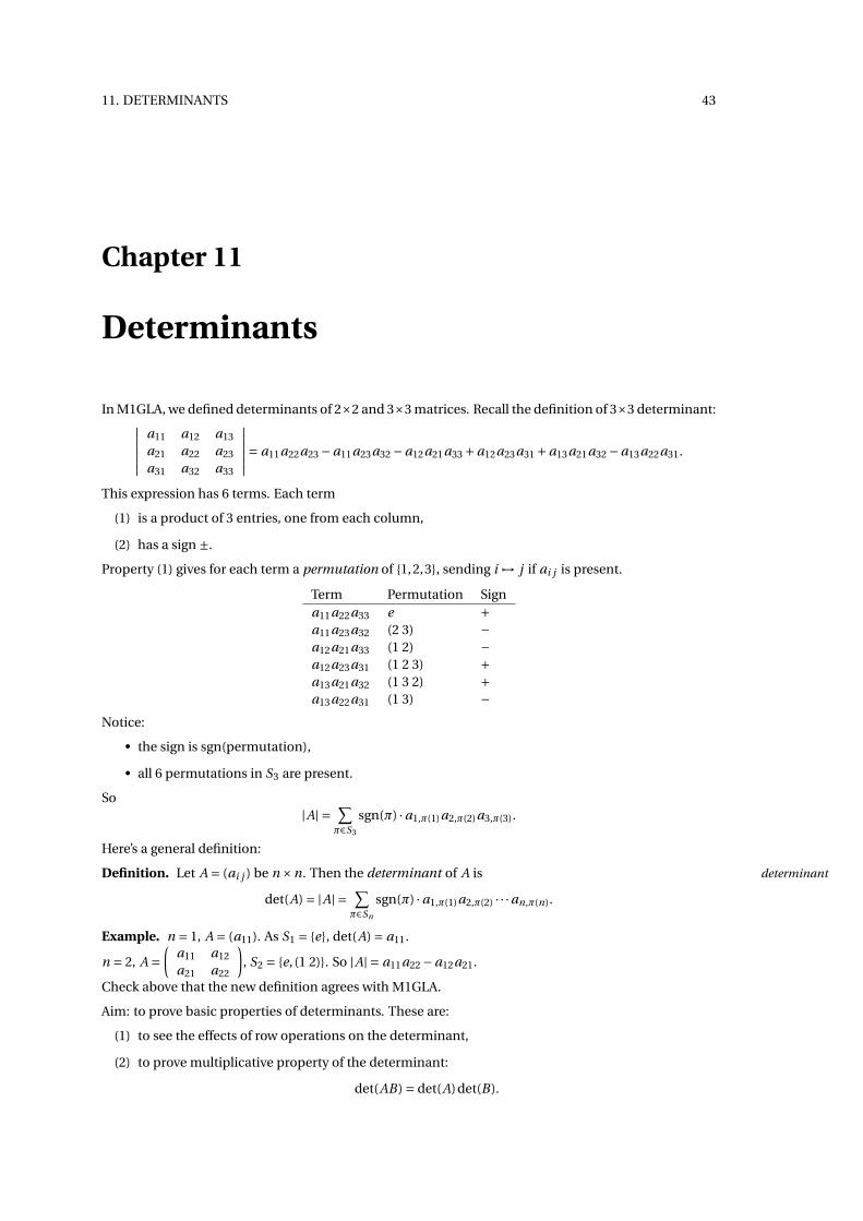
In M1GLA, we defined determinants of 2×2 and 3×3 matrices. Recall the definition of 3×3 determinant:∣∣∣∣∣∣a11 a12 a13
a21 a22 a23
a31 a32 a33
∣∣∣∣∣∣= a11a22a23 −a11a23a32 −a12a21a33 +a12a23a31 +a13a21a32 −a13a22a31.
This expression has 6 terms. Each term
(1) is a product of 3 entries, one from each column,
(2) has a sign ±.
Property (1) gives for each term a permutation of {1,2,3}, sending i 7→ j if ai j is present.
Term Permutation Signa11a22a33 e +a11a23a32 (2 3) −a12a21a33 (1 2) −a12a23a31 (1 2 3) +a13a21a32 (1 3 2) +a13a22a31 (1 3) −
Notice:
• the sign is sgn(permutation),
• all 6 permutations in S3 are present.
So|A| = ∑
π∈S3
sgn(π) ·a1,π(1)a2,π(2)a3,π(3).
Here’s a general definition:
Definition. Let A = (ai j ) be n ×n. Then the determinant of A is determinant
det(A) = |A| = ∑π∈Sn
sgn(π) ·a1,π(1)a2,π(2) · · ·an,π(n).
Example. n = 1, A = (a11). As S1 = {e}, det(A) = a11.
n = 2, A =(
a11 a12
a21 a22
), S2 = {e, (1 2)}. So |A| = a11a22 −a12a21.
Check above that the new definition agrees with M1GLA.
Aim: to prove basic properties of determinants. These are:
(1) to see the effects of row operations on the determinant,
(2) to prove multiplicative property of the determinant:
det(AB) = det(A)det(B).
44 11. DETERMINANTS
11.1 Basic properties
Let A = (ai j ) be n ×n. Recall the transpose of A is
AT = (a j i ).
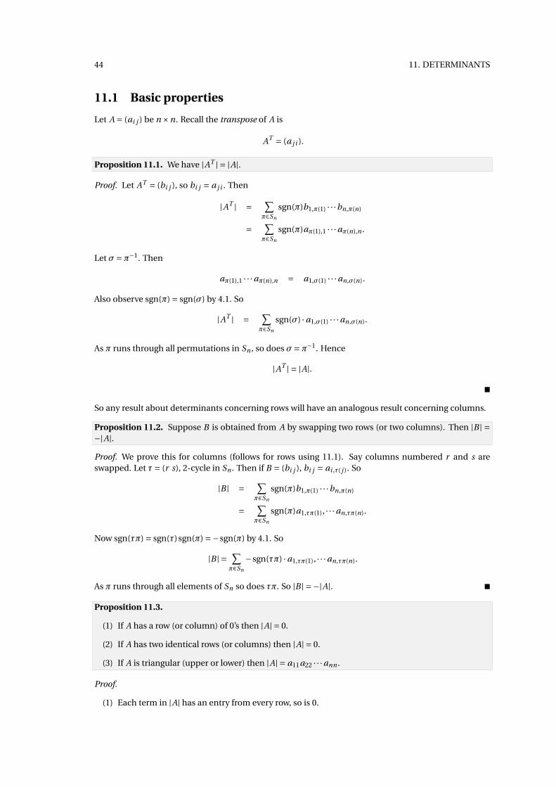
Proposition 11.1. We have |AT | = |A|.
Proof. Let AT = (bi j ), so bi j = a j i . Then
|AT | = ∑π∈Sn
sgn(π)b1,π(1) · · ·bn,π(n)
= ∑π∈Sn
sgn(π)aπ(1),1 · · ·aπ(n),n .
Let σ=π−1. Then
aπ(1),1 · · ·aπ(n),n = a1,σ(1) · · ·an,σ(n).
Also observe sgn(π) = sgn(σ) by 4.1. So
|AT | = ∑π∈Sn
sgn(σ) ·a1,σ(1) · · ·an,σ(n).
As π runs through all permutations in Sn , so does σ=π−1. Hence
|AT | = |A|.
�
So any result about determinants concerning rows will have an analogous result concerning columns.
Proposition 11.2. Suppose B is obtained from A by swapping two rows (or two columns). Then |B | =−|A|.Proof. We prove this for columns (follows for rows using 11.1). Say columns numbered r and s areswapped. Let τ= (r s), 2-cycle in Sn . Then if B = (bi j ), bi j = ai ,τ( j ). So
|B | = ∑π∈Sn
sgn(π)b1,π(1) · · ·bn,π(n)
= ∑π∈Sn
sgn(π)a1,τπ(1), · · ·an,τπ(n).
Now sgn(τπ) = sgn(τ)sgn(π) =−sgn(π) by 4.1. So
|B | = ∑π∈Sn
−sgn(τπ) ·a1,τπ(1), · · ·an,τπ(n).
As π runs through all elements of Sn so does τπ. So |B | = −|A|. �
Proposition 11.3.
(1) If A has a row (or column) of 0’s then |A| = 0.
(2) If A has two identical rows (or columns) then |A| = 0.
(3) If A is triangular (upper or lower) then |A| = a11a22 · · ·ann .
Proof.
(1) Each term in |A| has an entry from every row, so is 0.
11. DETERMINANTS 45
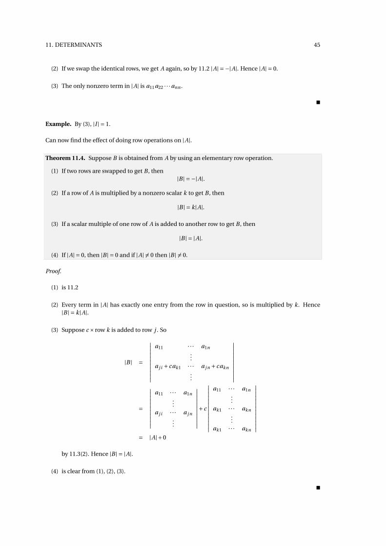
(2) If we swap the identical rows, we get A again, so by 11.2 |A| = −|A|. Hence |A| = 0.
(3) The only nonzero term in |A| is a11a22 · · ·ann .
�
Example. By (3), |I | = 1.
Can now find the effect of doing row operations on |A|.
Theorem 11.4. Suppose B is obtained from A by using an elementary row operation.
(1) If two rows are swapped to get B , then|B | = −|A|.
(2) If a row of A is multiplied by a nonzero scalar k to get B , then
|B | = k|A|.
(3) If a scalar multiple of one row of A is added to another row to get B , then
|B | = |A|.
(4) If |A| = 0, then |B | = 0 and if |A| 6= 0 then |B | 6= 0.
Proof.
(1) is 11.2
(2) Every term in |A| has exactly one entry from the row in question, so is multiplied by k. Hence|B | = k|A|.
(3) Suppose c × row k is added to row j . So
|B | =
∣∣∣∣∣∣∣∣∣∣∣
a11 · · · a1n...
a j i + cak1 · · · a j n + cakn...
∣∣∣∣∣∣∣∣∣∣∣
=
∣∣∣∣∣∣∣∣∣∣∣
a11 · · · a1n...
a j i · · · a j n...
∣∣∣∣∣∣∣∣∣∣∣+ c
∣∣∣∣∣∣∣∣∣∣∣∣∣
a11 · · · a1n...
ak1 · · · akn...
ak1 · · · akn
∣∣∣∣∣∣∣∣∣∣∣∣∣= |A|+0
by 11.3(2). Hence |B | = |A|.
(4) is clear from (1), (2), (3).
�
46 11. DETERMINANTS
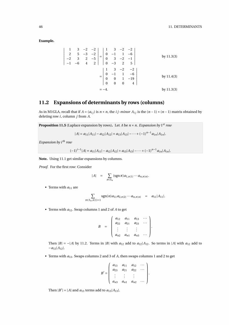
Example. ∣∣∣∣∣∣∣∣1 3 −2 −22 5 −3 −2
−2 3 2 −5−1 −6 4 2
∣∣∣∣∣∣∣∣=∣∣∣∣∣∣∣∣
1 3 −2 −20 −1 1 −60 3 −2 −10 −3 2 5
∣∣∣∣∣∣∣∣ by 11.3(3)
=
∣∣∣∣∣∣∣∣1 3 −2 −20 −1 1 −60 0 1 −190 0 0 4
∣∣∣∣∣∣∣∣ by 11.4(3)
=−4. by 11.3(3)
11.2 Expansions of determinants by rows (columns)
As in M1GLA, recall that if A = (ai j ) is n ×n, the i j -minor Ai j is the (n −1)× (n −1) matrix obtained bydeleting row i , column j from A.
Proposition 11.5 (Laplace expansion by rows). Let A be n ×n. Expansion by 1st row
|A| = a11|A11|−a12|A12|+a13|A13|− · · ·+ (−1)n−1a1n |A1n |.
Expansion by i th row
(−1)i−1|A| = ai 1|Ai 1|−ai 2|Ai 2|+ai 3|Ai 3|− · · ·+ (−1)n−1ai n |Ai n |.
Note. Using 11.1 get similar expansions by columns.
Proof. For the first row: Consider
|A| = ∑π∈Sn
(sgnπ)a1,π(1) · · ·an,π(n).
• Terms with a11 are ∑π∈Sn ,π(1)=1
sgn(n)a11a2,π(2) · · ·an,π(n) = a11|A11|.
• Terms with a12. Swap columns 1 and 2 of A to get
B =
a12 a11 a13 · · ·a22 a21 a23 · · ·
......
...an2 an1 an3 · · ·
.
Then |B | = −|A| by 11.2. Terms in |B | with a12 add to a12|A12. So terms in |A| with a12 add to−a12|A12|.
• Terms with a13. Swaps columns 2 and 3 of A, then swaps columns 1 and 2 to get
B ′ =
a13 a11 a12 · · ·a23 a21 a22 · · ·
......
...an3 an1 an2 · · ·
.
Then |B ′| = |A| and a13 terms add to a13|A13|.
11. DETERMINANTS 47
Continuing like this, see that |A| = a11|A11|−a12|A12 +·· · which is expansion by the first row.
For expansion by i th row: Do i −1 row swaps in A to get
B ′′ =
ai 1 · · · ai n
a11 · · · a1n
a21 · · · a2n...
.
Then |B ′′| = (−1)i−1|A|. Now use expansion of B ′′ by 1st row. �
11.3 Major properties of determinants
Two major results. First was proved in M1GLA for 2×2 and 3×3 cases.
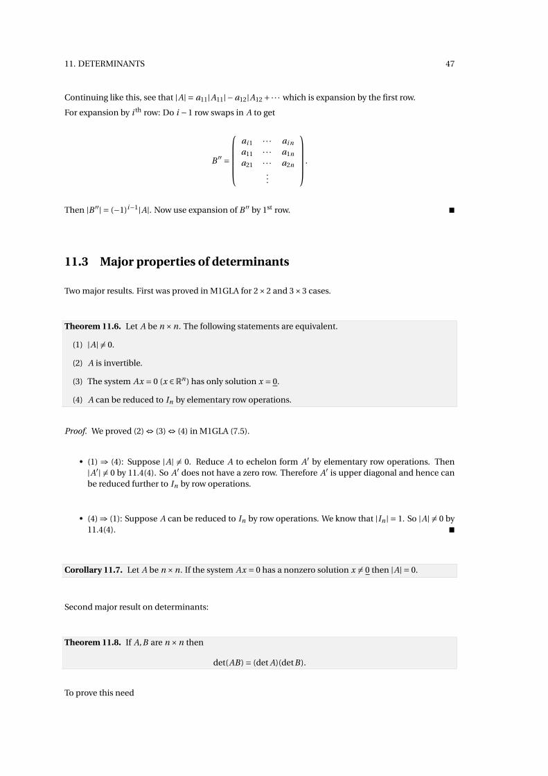
Theorem 11.6. Let A be n ×n. The following statements are equivalent.
(1) |A| 6= 0.
(2) A is invertible.
(3) The system Ax = 0 (x ∈Rn) has only solution x = 0.
(4) A can be reduced to In by elementary row operations.
Proof. We proved (2) ⇔ (3) ⇔ (4) in M1GLA (7.5).
• (1) ⇒ (4): Suppose |A| 6= 0. Reduce A to echelon form A′ by elementary row operations. Then|A′| 6= 0 by 11.4(4). So A′ does not have a zero row. Therefore A′ is upper diagonal and hence canbe reduced further to In by row operations.
• (4) ⇒ (1): Suppose A can be reduced to In by row operations. We know that |In | = 1. So |A| 6= 0 by11.4(4). �
Corollary 11.7. Let A be n ×n. If the system Ax = 0 has a nonzero solution x 6= 0 then |A| = 0.
Second major result on determinants:
Theorem 11.8. If A,B are n ×n then
det(AB) = (det A)(detB).
To prove this need
48 11. DETERMINANTS
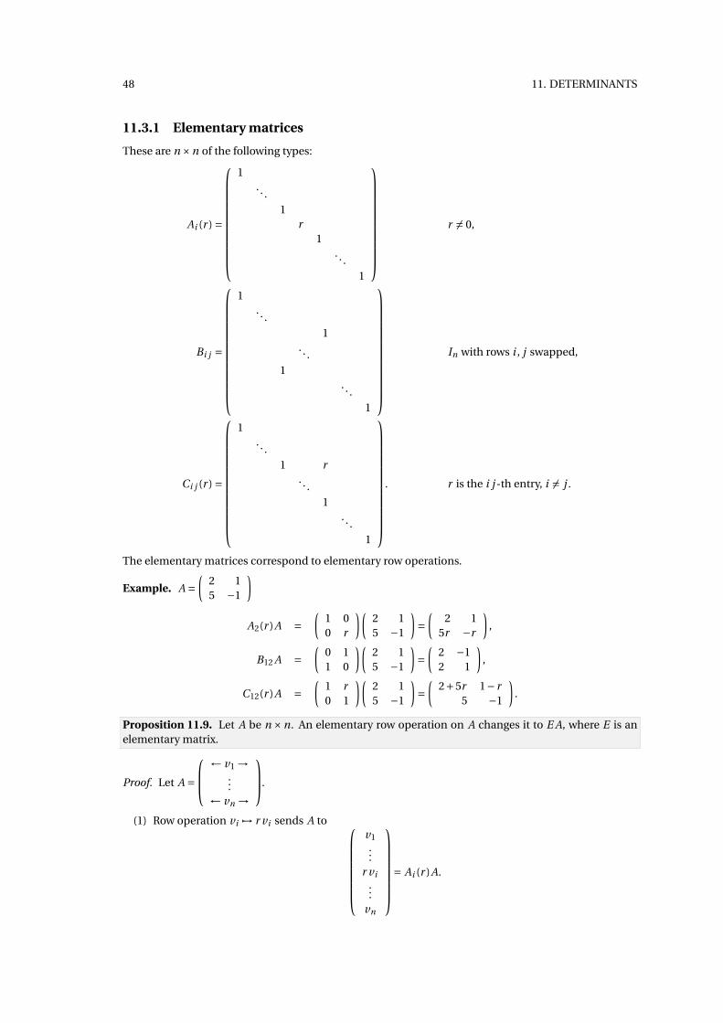
11.3.1 Elementary matrices
These are n ×n of the following types:
Ai (r ) =
1. . .
1r
1. . .
1
r 6= 0,
Bi j =
1. . .
1. . .
1. . .
1
In with rows i , j swapped,
Ci j (r ) =
1. . .
1 r. . .
1. . .
1
. r is the i j -th entry, i 6= j .
The elementary matrices correspond to elementary row operations.
Example. A =(
2 15 −1
)
A2(r )A =(
1 00 r
)(2 15 −1
)=
(2 1
5r −r
),
B12 A =(
0 11 0
)(2 15 −1
)=
(2 −12 1
),
C12(r )A =(
1 r0 1
)(2 15 −1
)=
(2+5r 1− r
5 −1
).
Proposition 11.9. Let A be n ×n. An elementary row operation on A changes it to E A, where E is anelementary matrix.
Proof. Let A =
← v1 →...
← vn →
.
(1) Row operation vi 7→ r vi sends A to
v1...
r vi...
vn
= Ai (r )A.

11. DETERMINANTS 49
(2) Row operation vi ↔ v j sends A to Bi j A.
(3) Row operation vi 7→ vi + r v j sends A to Ci j (r )A. �
Proposition 11.10.
(1) The determinant of an elementary matrix is nonzero and
|Ai (r )| = r, |Bi j | = −1, |Ci j (r )| = 1.
(2) The inverse of an elementary matrix is also an elementary matrix:
Ai (r )−1 = Ai (r−1), B−1i j = Bi j , Ci j (r )−1 =Ci j (−r ).
Proposition 11.11. Let A be n×n, and suppose A is invertible. Then A is equal to a product of elemen-tary matrices, i.e. A = E1 · · ·Ek where each Ei is an elementary matrix.
Proof. By 11.6, A can be reduced to I by elementary row operations. By 11.9 first row operations changesA to E1 A with E1 elementary matrix. Second changes E1 A to E2E1 A, E2 elementary matrix . . . and so on,until we end up with I . Hence
I = Ek Ek−1 · · ·E1 A,
where each Ei is elementary. Multiply both sides on left by E−11 · · ·E−1
k−1E−1k to get
E−11 · · ·E−1
k = A.
Each E−1i is elementary by 11.10(2). �
Remark. The proof shows how to find the elementary matrices Ei of which A is the product.
Example. A =(
1 2−1 0
)Express A as a product of elementary matrices.
(1 2
−1 0
)→
(1 20 2
)=C21(1)A,
→(
1 00 2
)=C12(−1)C21(1)A,
→(
1 00 1
). = A2(1/2)C12(−1)C21(1)A.
So
A =(
1 01 1
)−1 (1 −10 1
)−1 (1 00 1/2
)−1
=(
1 0−1 1
)(1 10 1
)(1 00 2
).
Towards 11.8:
Proposition 11.12. If E is an elementary n ×n matrix, and A is n ×n, then
det(E A) = (detE)(det A).
Proof. Let A =
← v1 →...
← vn →
.
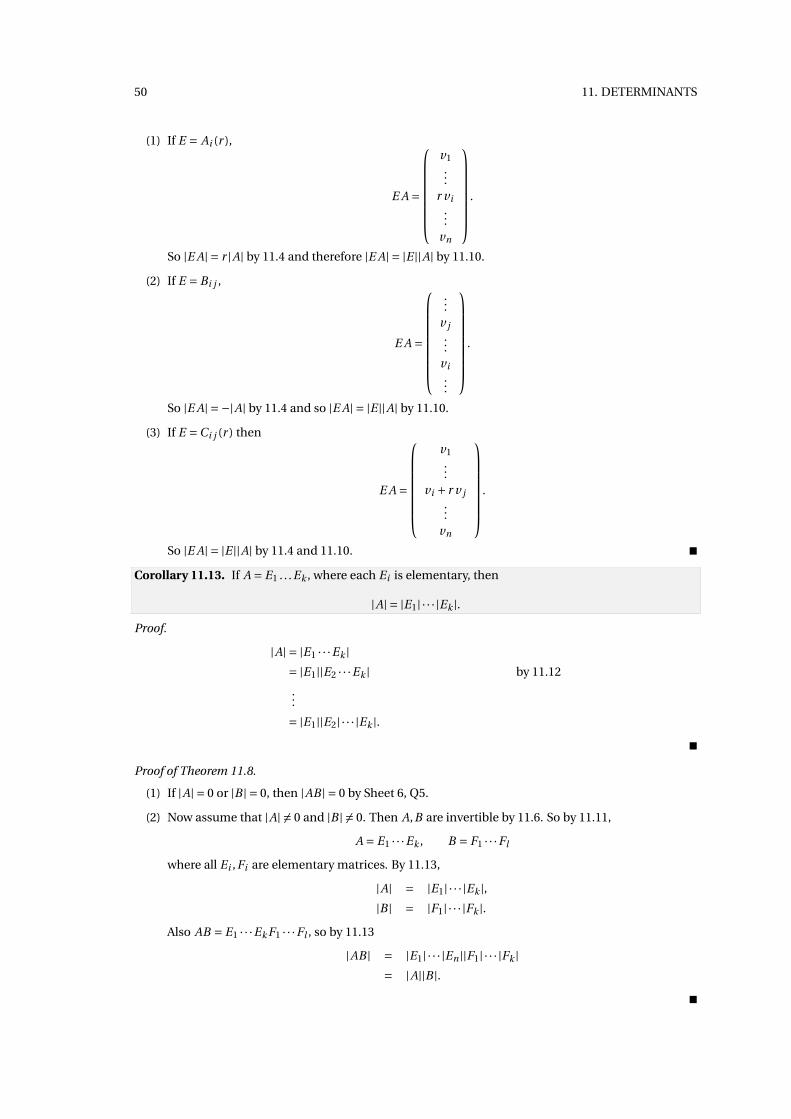
50 11. DETERMINANTS
(1) If E = Ai (r ),
E A =
v1...
r vi...
vn
.
So |E A| = r |A| by 11.4 and therefore |E A| = |E ||A| by 11.10.
(2) If E = Bi j ,
E A =
...v j...
vi...
.
So |E A| = −|A| by 11.4 and so |E A| = |E ||A| by 11.10.
(3) If E =Ci j (r ) then
E A =
v1...
vi + r v j...
vn
.
So |E A| = |E ||A| by 11.4 and 11.10. �
Corollary 11.13. If A = E1 . . .Ek , where each Ei is elementary, then
|A| = |E1| · · · |Ek |.Proof.
|A| = |E1 · · ·Ek |= |E1||E2 · · ·Ek | by 11.12
...
= |E1||E2| · · · |Ek |.�
Proof of Theorem 11.8.
(1) If |A| = 0 or |B | = 0, then |AB | = 0 by Sheet 6, Q5.
(2) Now assume that |A| 6= 0 and |B | 6= 0. Then A,B are invertible by 11.6. So by 11.11,
A = E1 · · ·Ek , B = F1 · · ·Fl
where all Ei ,Fi are elementary matrices. By 11.13,
|A| = |E1| · · · |Ek |,|B | = |F1| · · · |Fk |.
Also AB = E1 · · ·Ek F1 · · ·Fl , so by 11.13
|AB | = |E1| · · · |En ||F1| · · · |Fk |= |A||B |.
�
11. DETERMINANTS 51
Immediate consequence:
Proposition 11.14. Let P be an invertible n ×n matrix.
(1) det(P−1) = 1det(P ) ,
(2) det(P−1 AP ) = det(A) for all n ×n matrices A.
Proof.
(1) det(P )(det(P−1)
)= detPP−1 = det I = 1 by 11.8.
(2) det(P−1 AP ) = det(P−1)det A detP = det A by 11.8 and (1). �

52 11. DETERMINANTS
12. MATRICES AND LINEAR TRANSFORMATIONS 53
Chapter 12
Matrices and linear transformations
Recall from M1P2:Let V be a finite dimensional vector space and T : V →V a linear transformation. If B = {v1, . . . , vn} is abasis of V , write
T (v1) = a11v1 +·· ·+an1vn ,...
T (vn) = a1n v1 +·· ·+ann vn .
The matrix of T with respect to B is [T ]B
[T ]B =
a11 · · · a1n...
...an1 · · · ann
.
Example. T :R2 →R2 ,
T
(x1
x2
)=
(2x1 −x2
x1 +2x2
)=
(2 −11 2
)(x1
x2
).
If E = {e1,e2}, e1 =(
10
),e2 =
(01
)then
T (e1) = 2e1 +e2,
T (e2) = −e1 +2e2,
so
[T ]E =(
2 −11 2
).
If F = {f1, f2
}, f1 =
(11
), f2 =
(01
)then
T ( f1) = f1 +2 f2,
T ( f2) = − f1 +3 f2,
so
[T ]F =(
1 −12 3
).
Proposition 12.1. Let S : V →V and T : V →V be linear transformations and let B be a basis of V . Then
[ST ]B = [S]B [T ]B ,
where ST is the composition of S and T .
54 12. MATRICES AND LINEAR TRANSFORMATIONS
Before proof, recall from M1P2: If B = {v1, . . . , vn} is a basis of V , and v ∈V , can write v = r1v1 +·· ·rn vn
(ri scalars in F =R or C) and define[v]B
[v]B =
r1...
rn
∈ F n .
4.8 of M1P2 says that: if T : V →V is a linear transformation, then
[T (v)]B = [T ]B [v]B . ( )
Example. V = polynomials of degree ≤ 2, T (p(x)) = p ′(x), B = {1, x, x2
}. Then
[T ]B = 0 1 0
0 0 20 0 0
.
Let p(x) = 1−x +x2. Then
[p(x)]B = 1
−11
.
So by ( ),
[T (p(x))]B = 0 1 0
0 0 20 0 0
1−1
1
= −1
20
.
So T (p(x)) =−1+2x.
Proof of 12.1. Let S,T : V →V and B a basis of V . For v ∈V ,
[ST (v)]B = [ST ]B [v]B .
Also
[ST (v)]B = [S(T (v))] = [S]B [T (v)]B
= [S]B [T ]B [v]B .
Hence
[ST ]B [v]B = [S]B [T ]B [v]B
for every column vector [v]B . Applying this for [v]B =
10...
0
, . . . ,
0...
01
we see that [ST ]B = [S]B [T ]B . �
Note. Proposition 12.1 actually proves the associativity of matrix multiplication in a natural way. Here’show. Take 3 linear transformations S,T,U : V →V . We know that
(ST )U = S(TU )
since
(ST )U (v) = S(T (U (v))),
S(TU )(v) = S(T (U (v)))
for all v ∈V . So by 12.1, if B is a basis of V ,
([S]B [T ]B )[U ]B = [S]B ([T ]B [U ]B ).
These matrices are arbitrary n ×n since given any n ×n matrix A, the linear transformation T : v 7→ Av(Rn →Rn) has [T ]B = A where B is the standard basis.
12. MATRICES AND LINEAR TRANSFORMATIONS 55
Example. V = polynomials of degree ≤ 2 over R
S(p(x)) = p ′(x)
T (p(x)) = p(1−x).
Then ST (p(x)) = S(p(1−x)) =−p ′(1−x). If B = {1, x, x2
},
[S]B = 0 1 0
0 0 20 0 0
,
[T ]B = 1 1 1
0 −1 −20 0 1
.
So
[S]B [T ]B = 0 −1 −2
0 0 20 0 0
.
12.0.2 Consequences of 12.1
As in 12.1, let V be n-dimensional over F =R or C, basis B . The map T 7→ [T ]B gives a correspondence
{linear transformations V →V } ∼ {n ×n matrices over F } .
This has many nice properties.
1. If [T ]B = A then [T 2]
B12.1= [T ]B [T ]B = A2
and similarly[T k
]B = Ak .
Ifq(x) = ar xr +·· ·+a1x +a0
is a polynomial, defineq(A) = ar Ar +·· ·+a1 A+a0I
andq(T ) = ar T r +·· ·+a1T +a01
where 1 : V →V is the identity map. Then 12.1 implies that[q(T )
]B = q(A).
Example. V = polynomials of degree ≤ 2, T (p(x)) = p ′(x). Then
(T 2 −T )(p(x)) = p ′′(x)−p ′(x)
and
[T 2 −T
]B =
0 1 00 0 20 0 0
2
− 0 1 0
0 0 20 0 0
=
0 −1 20 0 −20 0 0
.
2. Define GL(V )
GL(V ) = {all invertible linear transformations V →V } .
Then
– GL(V ) is a group under composition,
– T 7→ [T ]B is an isomorphism from GL(V ) to GL(n,F ) (the group of all n ×n invertible matri- GL(n,F )
ces).
56 12. MATRICES AND LINEAR TRANSFORMATIONS
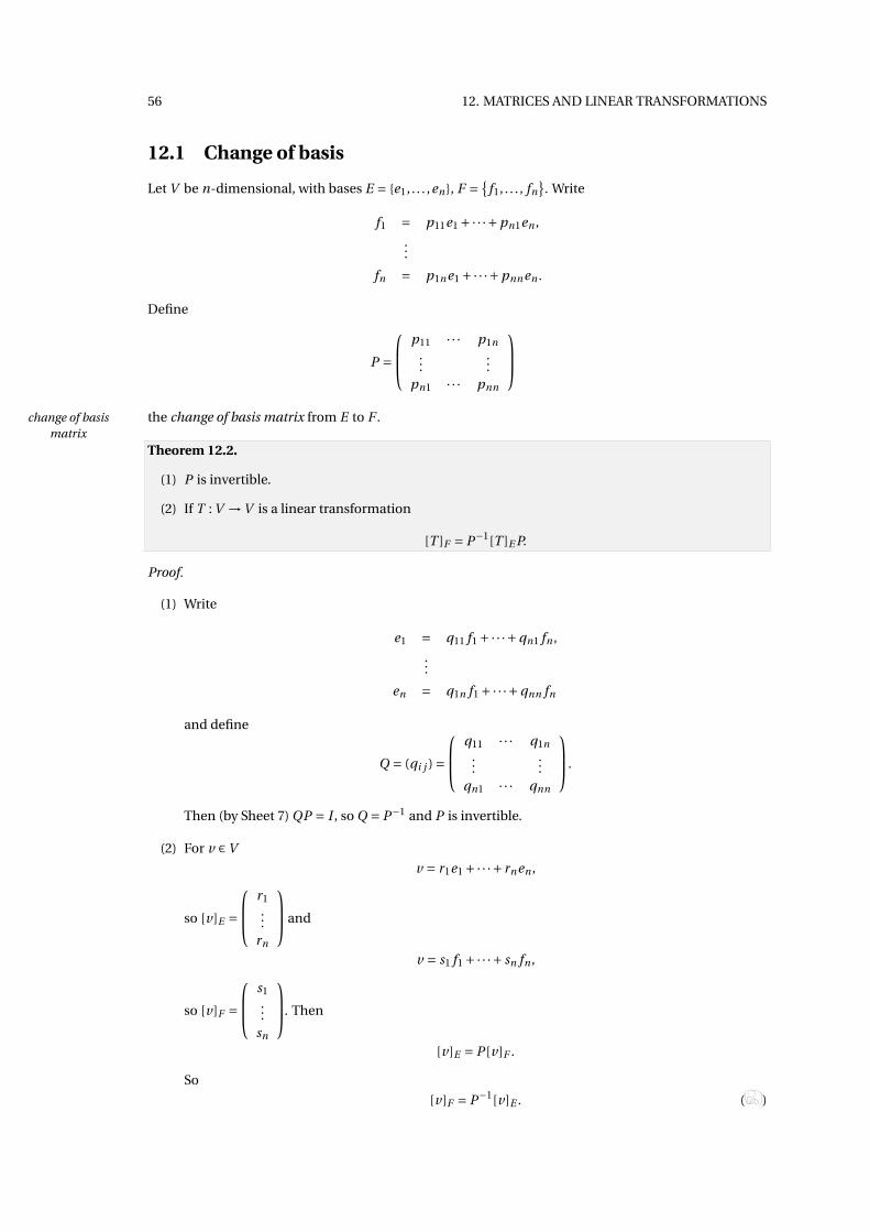
12.1 Change of basis
Let V be n-dimensional, with bases E = {e1, . . . ,en}, F = {f1, . . . , fn
}. Write
f1 = p11e1 +·· ·+pn1en ,
...
fn = p1ne1 +·· ·+pnnen .
Define
P =
p11 · · · p1n...
...pn1 · · · pnn
the change of basis matrix from E to F .change of basis
matrix
Theorem 12.2.
(1) P is invertible.
(2) If T : V →V is a linear transformation
[T ]F = P−1[T ]E P.
Proof.
(1) Write
e1 = q11 f1 +·· ·+qn1 fn ,
...
en = q1n f1 +·· ·+qnn fn
and define
Q = (qi j ) =
q11 · · · q1n...
...qn1 · · · qnn
.
Then (by Sheet 7) QP = I , so Q = P−1 and P is invertible.
(2) For v ∈V
v = r1e1 +·· ·+ rnen ,
so [v]E =
r1...
rn
and
v = s1 f1 +·· ·+ sn fn ,
so [v]F =
s1...
sn
. Then
[v]E = P [v]F .
So
[v]F = P−1[v]E . ( )
12. MATRICES AND LINEAR TRANSFORMATIONS 57
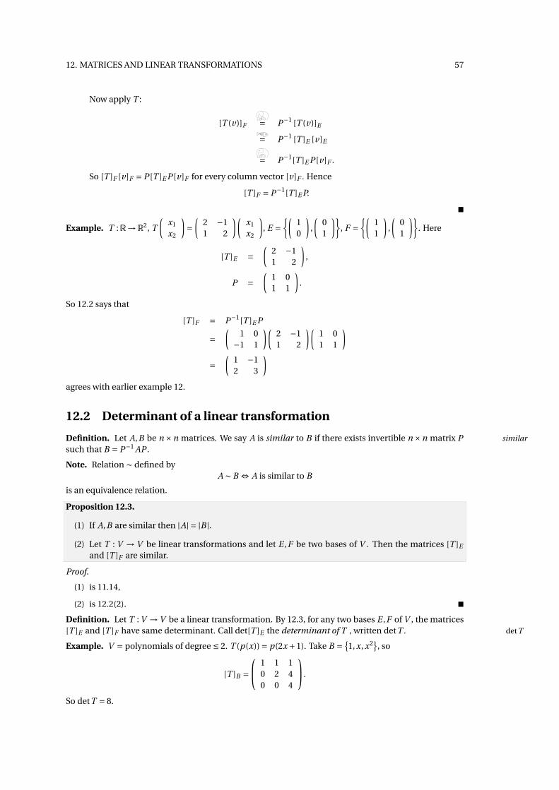
Now apply T :
[T (v)]F = P−1 [T (v)]E
= P−1 [T ]E [v]E
= P−1[T ]E P [v]F .
So [T ]F [v]F = P [T ]E P [v]F for every column vector [v]F . Hence
[T ]F = P−1[T ]E P.
�
Example. T :R→R2, T
(x1
x2
)=
(2 −11 2
)(x1
x2
), E =
{(10
),
(01
)}, F =
{(11
),
(01
)}. Here
[T ]E =(
2 −11 2
),
P =(
1 01 1
).
So 12.2 says that
[T ]F = P−1[T ]E P
=(
1 0−1 1
)(2 −11 2
)(1 01 1
)=
(1 −12 3
)agrees with earlier example 12.
12.2 Determinant of a linear transformation
Definition. Let A,B be n ×n matrices. We say A is similar to B if there exists invertible n ×n matrix P similar
such that B = P−1 AP .
Note. Relation ∼ defined byA ∼ B ⇔ A is similar to B
is an equivalence relation.
Proposition 12.3.
(1) If A,B are similar then |A| = |B |.(2) Let T : V → V be linear transformations and let E ,F be two bases of V . Then the matrices [T ]E
and [T ]F are similar.
Proof.
(1) is 11.14,
(2) is 12.2(2). �
Definition. Let T : V →V be a linear transformation. By 12.3, for any two bases E ,F of V , the matrices[T ]E and [T ]F have same determinant. Call det[T ]E the determinant of T , written detT . detT
Example. V = polynomials of degree ≤ 2. T (p(x)) = p(2x +1). Take B = {1, x, x2
}, so
[T ]B = 1 1 1
0 2 40 0 4
.
So detT = 8.

58 12. MATRICES AND LINEAR TRANSFORMATIONS
13. CHARACTERISTIC POLYNOMIALS 59
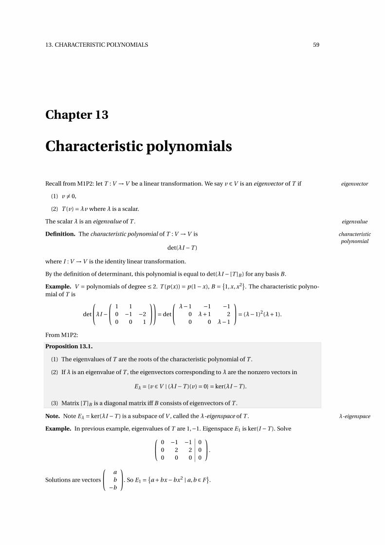
Chapter 13
Characteristic polynomials
Recall from M1P2: let T : V →V be a linear transformation. We say v ∈V is an eigenvector of T if eigenvector
(1) v 6= 0,
(2) T (v) =λv where λ is a scalar.
The scalar λ is an eigenvalue of T . eigenvalue
Definition. The characteristic polynomial of T : V →V is characteristicpolynomial
det(λI −T )
where I : V →V is the identity linear transformation.
By the definition of determinant, this polynomial is equal to det(λI − [T ]B ) for any basis B .
Example. V = polynomials of degree ≤ 2. T (p(x)) = p(1− x), B = {1, x, x2
}. The characteristic polyno-
mial of T is
det
λI − 1 1
0 −1 −20 0 1
= det
λ−1 −1 −10 λ+1 20 0 λ−1
= (λ−1)2(λ+1).
From M1P2:
Proposition 13.1.
(1) The eigenvalues of T are the roots of the characteristic polynomial of T .
(2) If λ is an eigenvalue of T , the eigenvectors corresponding to λ are the nonzero vectors in
Eλ = {v ∈V | (λI −T )(v) = 0} = ker(λI −T ).
(3) Matrix [T ]B is a diagonal matrix iff B consists of eigenvectors of T .
Note. Note Eλ = ker(λI −T ) is a subspace of V , called the λ-eigenspace of T . λ-eigenspace
Example. In previous example, eigenvalues of T are 1,−1. Eigenspace E1 is ker(I −T ). Solve 0 −1 −1 00 2 2 00 0 0 0
.
Solutions are vectors
ab
−b
. So E1 ={
a +bx −bx2 | a,b ∈ F}.
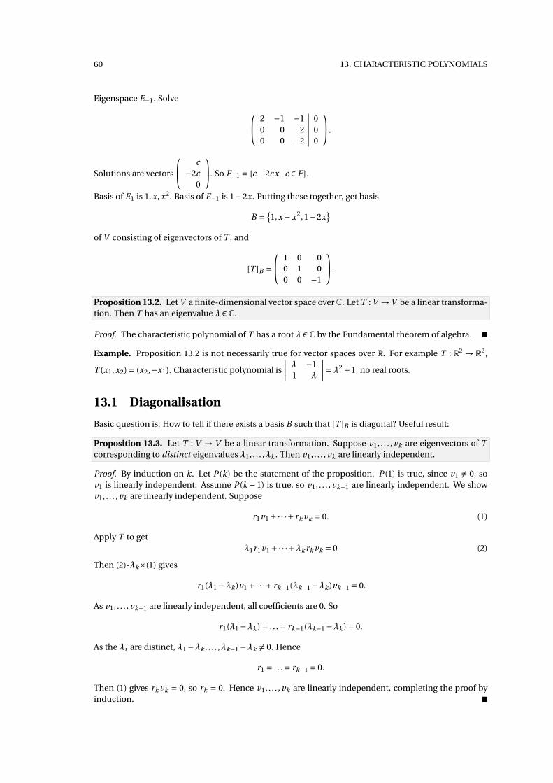
60 13. CHARACTERISTIC POLYNOMIALS
Eigenspace E−1. Solve 2 −1 −1 00 0 2 00 0 −2 0
.
Solutions are vectors
c−2c
0
. So E−1 = {c −2cx | c ∈ F }.
Basis of E1 is 1, x, x2. Basis of E−1 is 1−2x. Putting these together, get basis
B = {1, x −x2,1−2x
}of V consisting of eigenvectors of T , and
[T ]B = 1 0 0
0 1 00 0 −1
.
Proposition 13.2. Let V a finite-dimensional vector space over C. Let T : V →V be a linear transforma-tion. Then T has an eigenvalue λ ∈C.
Proof. The characteristic polynomial of T has a root λ ∈C by the Fundamental theorem of algebra. �
Example. Proposition 13.2 is not necessarily true for vector spaces over R. For example T : R2 → R2,
T (x1, x2) = (x2,−x1). Characteristic polynomial is
∣∣∣∣ λ −11 λ
∣∣∣∣=λ2 +1, no real roots.
13.1 Diagonalisation
Basic question is: How to tell if there exists a basis B such that [T ]B is diagonal? Useful result:
Proposition 13.3. Let T : V → V be a linear transformation. Suppose v1, . . . , vk are eigenvectors of Tcorresponding to distinct eigenvalues λ1, . . . ,λk . Then v1, . . . , vk are linearly independent.
Proof. By induction on k. Let P (k) be the statement of the proposition. P (1) is true, since v1 6= 0, sov1 is linearly independent. Assume P (k −1) is true, so v1, . . . , vk−1 are linearly independent. We showv1, . . . , vk are linearly independent. Suppose
r1v1 +·· ·+ rk vk = 0. (1)
Apply T to getλ1r1v1 +·· ·+λk rk vk = 0 (2)
Then (2)-λk×(1) gives
r1(λ1 −λk )v1 +·· ·+ rk−1(λk−1 −λk )vk−1 = 0.
As v1, . . . , vk−1 are linearly independent, all coefficients are 0. So
r1(λ1 −λk ) = . . . = rk−1(λk−1 −λk ) = 0.
As the λi are distinct, λ1 −λk , . . . ,λk−1 −λk 6= 0. Hence
r1 = . . . = rk−1 = 0.
Then (1) gives rk vk = 0, so rk = 0. Hence v1, . . . , vk are linearly independent, completing the proof byinduction. �
13. CHARACTERISTIC POLYNOMIALS 61
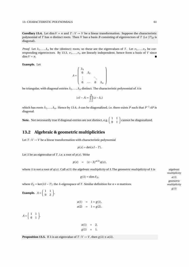
Corollary 13.4. Let dimV = n and T : V → V be a linear transformation. Suppose the characteristicpolynomial of T has n distinct roots. Then V has a basis B consisting of eigenvectors of T (i.e [T ]B isdiagonal).
Proof. Let λ1, . . . ,λn be the (distinct) roots, so these are the eigenvalues of T . Let v1, . . . , vn be cor-responding eigenvectors. By 13.3, v1, . . . , vn are linearly independent, hence form a basis of V sincedimV = n. �
Example. Let
A =
λ1
0 λ2...
. . .0 · · · 0 λn
be triangular, with diagonal entries λ1, . . . ,λn distinct. The characteristic polynomial of A is
|xI − A| =n∏
i=1(x −λi )
which has roots λ1, . . . ,λn . Hence by 13.4, A can be diagonalized, i.e. there exists P such that P−1 AP isdiagonal.
Note. Not necessarily true if diagonal entries are not distinct, e.g.
(1 10 1
)cannot be diagonalized.
13.2 Algebraic & geometric multiplicities
Let T : V →V be a linear transformation with characteristic polynomial
p(x) = det(xI −T ).
Let λ be an eigenvalue of T , i.e. a root of p(x). Write
p(x) = (x −λ)a(λ)q(x),
where λ is not a root of q(x). Call a(λ) the algebraic multiplicity of λ.The geometric multiplicity of λ is algebraicmultiplicity
a(λ)
geometricmultiplicity
g (λ)
g (λ) = dimEλ,
where Eλ = ker(λI −T ), the λ-eigenspace of T . Similar definition for n ×n matrices.
Example. A =(
1 10 2
),
a(1) = 1 = g (1),
a(2) = 1 = g (2).
A =(
1 10 1
),
a(1) = 2,
g (1) = 1.
Proposition 13.5. If λ is an eigenvalue of T : V →V , then g (λ) ≤ a(λ).
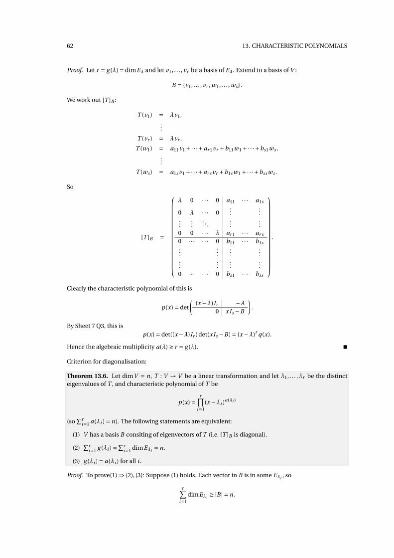
62 13. CHARACTERISTIC POLYNOMIALS
Proof. Let r = g (λ) = dimEλ and let v1, . . . , vr be a basis of Eλ. Extend to a basis of V :
B = {v1, . . . , vr , w1, . . . , ws } .
We work out [T ]B :
T (v1) = λv1,...
T (vr ) = λvr ,
T (w1) = a11v1 +·· ·+ar 1vr +b11w1 +·· ·+bs1ws ,...
T (ws ) = a1s v1 +·· ·+ar s vr +b1s w1 +·· ·+bss ws .
So
[T ]B =
λ 0 · · · 0 a11 · · · a1s
0 λ · · · 0...
......
.... . .
......
0 0 · · · λ ar 1 · · · ar s
0 · · · · · · 0 b11 · · · b1s...
......
......
......
...0 · · · · · · 0 bs1 · · · bss
.
Clearly the characteristic polynomial of this is
p(x) = det
((x −λ)Ir −A
0 xIs −B
).
By Sheet 7 Q3, this isp(x) = det((x −λ)Ir )det(xIs −B) = (x −λ)r q(x).
Hence the algebraic multiplicity a(λ) ≥ r = g (λ). �
Criterion for diagonalisation:
Theorem 13.6. Let dimV = n, T : V → V be a linear transformation and let λ1, . . . ,λr be the distincteigenvalues of T , and characteristic polynomial of T be
p(x) =r∏
i=1(x −λi )a(λi )
(so∑r
i=1 a(λi ) = n). The following statements are equivalent:
(1) V has a basis B consiting of eigenvectors of T (i.e. [T ]B is diagonal).
(2)∑r
i=1 g (λi ) =∑ri=1 dimEλi = n.
(3) g (λi ) = a(λi ) for all i .
Proof. To prove(1) ⇒ (2), (3): Suppose (1) holds. Each vector in B is in some Eλi , so
r∑i=1
dimEλi ≥ |B | = n.
13. CHARACTERISTIC POLYNOMIALS 63
By 13.5
r∑i=1
dimEλi =r∑
i=1g (λi ) ≤
r∑i=1
a(λi ) = n.
Hence∑r
i=1 dimEλi = n and g (λi ) = a(λi ) for all i .Evidently (2) ⇔ (3), so it is enough to show that (2) ⇒ (1). Suppose
∑ri=1 dimEλi = n. Let Bi be a basis of
Eλi and let B =⋃ri=1 Bi , so |B | = n (the following shows that Bi ’s are disjoint). We claim B is a basis of V ,
hence (1) holds:It’s enough to show that B is linearly independent (since |B | = n = dimV ). Suppose there is a linearrelation ∑
v∈B1
αv v +·· ·+ ∑z∈Br
αz z = 0.
Write
v1 = ∑v∈B1
αv v,
...
vr = ∑z∈Br
αz z,
so vi ∈ Eλi and v1 +·· ·+ vr = 0. As λ1, . . . ,λr are distinct, the set of nonzero vi ’s is linearly independentby 13.3. Hence vi = 0 for all i . So
vi = ∑v∈Bi
αv v = 0.
As Bi is linearly independent (basis of Eλi ) this forcesαv = 0 for all v ∈ Bi . This completes the proof thatB is linearly independent, hence a basis of V . �
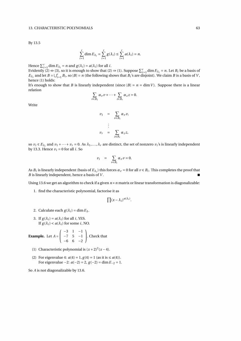
Using 13.6 we get an algorithm to check if a given n×n matrix or linear transformation is diagonalizable:
1. find the characteristic polynomial, factorise it as∏(x −λi )a(λi ).
2. Calculate each g (λi ) = dimEλ.
3. If g (λi ) = a(λi ) for all i , YES.If g (λi ) < a(λi ) for some i , NO.
Example. Let A =
−3 1 −1−7 5 −1−6 6 −2
. Check that
(1) Characteristic polynomial is (x +2)2(x −4).
(2) For eigenvalue 4: a(4) = 1, g (4) = 1 (as it is ≤ a(4)).For eigenvalue −2: a(−2) = 2, g (−2) = dimE−2 = 1.
So A is not diagonalizable by 13.6.

64 13. CHARACTERISTIC POLYNOMIALS
14. THE CAYLEY-HAMILTON THEOREM 65
Chapter 14
The Cayley-Hamilton theorem
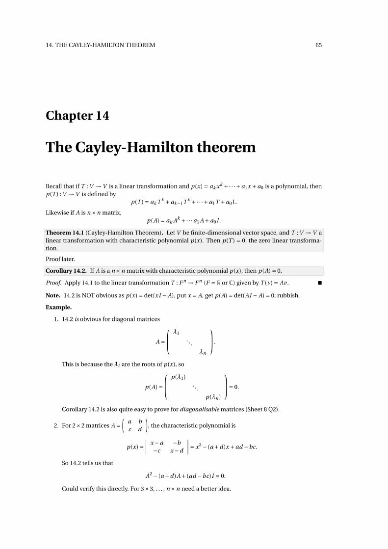
Recall that if T : V →V is a linear transformation and p(x) = ak xk +·· ·+a1x +a0 is a polynomial, thenp(T ) : V →V is defined by
p(T ) = ak T k +ak−1T k +·· ·+a1T +a01.
Likewise if A is n ×n matrix,p(A) = ak Ak +·· ·a1 A+a0I .
Theorem 14.1 (Cayley-Hamilton Theorem). Let V be finite-dimensional vector space, and T : V →V alinear transformation with characteristic polynomial p(x). Then p(T ) = 0, the zero linear transforma-tion.
Proof later.
Corollary 14.2. If A is a n ×n matrix with characteristic polynomial p(x), then p(A) = 0.
Proof. Apply 14.1 to the linear transformation T : F n → F n (F =R or C) given by T (v) = Av . �
Note. 14.2 is NOT obvious as p(x) = det(xI − A), put x = A, get p(A) = det(AI − A) = 0; rubbish.
Example.
1. 14.2 is obvious for diagonal matrices
A =
λ1
. . .λn
.
This is because the λi are the roots of p(x), so
p(A) =
p(λ1). . .
p(λn)
= 0.
Corollary 14.2 is also quite easy to prove for diagonalisable matrices (Sheet 8 Q2).
2. For 2×2 matrices A =(
a bc d
), the characteristic polynomial is
p(x) =∣∣∣∣ x −a −b
−c x −d
∣∣∣∣= x2 − (a +d)x +ad −bc.
So 14.2 tells us that
A2 − (a +d)A+ (ad −bc)I = 0.
Could verify this directly. For 3×3, . . . , n ×n need a better idea.
66 14. THE CAYLEY-HAMILTON THEOREM
14.1 Proof of Cayley-Hamilton
Let T : V →V be a linear transformation with characteristic polynomial p(x). Aim: for v ∈V , show thatp(T )(v) = 0. Strategy: Study the subspacevT
vT = Span(v,T (v),T 2(v), . . . )
= Span(T i (v) | i ≥ 0).
Definition. A subspace W of V is T -invariant if T (W ) ⊆W , i.e. T (w) ∈W for all w ∈W .T -invariant
Proposition 14.3. Pick v ∈V and let
W = vT = Span(T i (v) | i ≥ 0).
Then W is T -invariant.
Proof. Let w ∈W , so
w = a1T i1 (v)+·· ·+ar T ir (v).
ThenT (w) = a1T i1+1(v)+·· ·+ar T ir +1(v),
so T (w) ∈W . �
Example. V = polynomials of deg ≤ 2, T (p(x)) = p(x +1). Then
xT = Span(x,T (x),T 2(x), . . .)
= Span(x, x +1) = subspace of polynomials of deg ≤ 1.
Clearly this is T -invariant.
Definition. Let W be a T -invariant subspace of V . Define TW : W →W byTW
TW (w) = T (w)
for all w ∈W . Then TW is a linear transformation, the restriction of T to W .restriction
Proposition 14.4. If W is a T -invariant subspace of V , then the characteristic polynomial of TW dividesthe characteristic polynomial of T .
Proof. LetBW = {w1, . . . , wk }
be a basis of W and extend it to a basis
B = {w1, . . . , wk , x1, . . . , xl }
of V . As W is T -invariant,
T (w1) = a11w1 +·· ·+ak1wk ,...
T (wk ) = a1k w1 +·· ·+akk wk .
Then
[TW ]BW =
a11 · · · a1k...
...ak1 · · · akk
= A
14. THE CAYLEY-HAMILTON THEOREM 67
and
[T ]B =(
A X0 Y
).
The characteristic polynomial of TW is
pW (x) = det(xIk − A)
and characteristic polynomial of T is
p(x) = det
(xIk − A −X
0 xIl −Y
)= det(xIk − A) ·det(xIl −Y )
= pW (x) ·q(x).
So pW (x) divides p(x). �
Example. V = polynomials of deg ≤ 2, T (p(x)) = p(x + 1), W = xT = Span(x, x +1). Take basis BW ={1, x}, B = {
1, x, x2}. Then
[T ]BW =(
1 10 1
),
[T ]B = 1 1 1
0 1 20 0 1
.
Characteristic polynomial of TW is (x −1)2, characteristic polynomial of T is (x −1)3.
Proposition 14.5. Let T : V →V be a linear transformation. Let v ∈V , v 6= 0, and
W = vT = Span(T i (v) | i ≥ 0
).
Let k = dimW . Then {v,T (v),T 2(v), . . . ,T k−1(v)
}is a basis of W .
Proof. We show that{
v,T (v), . . . ,T k−1(v)}
is linearly independent, hence a basis of W . Let j be thelargest integer such that the set
{v,T (v), . . . ,T j−1(v)
}is linearly independent. So 1 ≤ j ≤ k. Aim to show
that j = k. Let
S ={
v,T (v), . . . ,T j−1(v)}
andX = Span(S).
Then X ⊆W and dim X = j . By the choice of j , the set{v,T (v), . . . ,T j−1(v),T j (v)
}is linearly dependent. This implies that T j (v) ∈ Span(S) = X . Say
T j (v) = b0v +b1T (v)+·· ·+b j−1T j−1(v).
SoT j+1(v) = b0T (v)+b1T 2(v)+·· ·+b j−1T j (v) ∈ X .
Similarly T j+2(v) ∈ X , T j+3(v) ∈ X and so on. Hence
T i (v) ∈ X
68 14. THE CAYLEY-HAMILTON THEOREM
for all i ≥ 0. This impliesW = Span(T i (v) | i ≥ 0) ⊆ X .
As X ⊆ W this means X = W , so j = dim X = dimW = k. Hence{
v,T (v), . . . ,T k−1(v)}
is linearly inde-pendent. �
Proposition 14.6. Let T : V → V , let v ∈ V and W = vT = Span(T i (v) | i ≥ 0
), with basis BW ={
v,T (v), . . . ,T k−1(v)}
as in 14.5. Then
(1) there exist scalars ai such that
a0v +a1T (v)+·· ·+ak−1T k−1(v)+T k (v) = 0,
(2) the characteristic polynomial of TW is
pW (x) = xk +ak−1xk−1 +·· ·+a1x +a0,
(3) pW (T )(v) = 0.
Proof.
(1) Clear, since T k (v) ∈W and BW is a basis of W .
(2) Clearly
[TW ]BW =
0 0 · · · 0 −a0
1 0 · · · 0 −a1
0 1 · · · 0 −a2...
.... . .
......
0 0 · · · 1 −ak−1
(for the last column T (T k−1(v)) = T k (v) =−a0v −a1T (v)−·· ·−ak−1T k−1(v)). By the Sheet 8, thecharacteristic polynomial of this matrix is
pW (x) = xk +ak−1xk−1 +·· ·+a0.
(3) Clear from (1) and (2). �
Completion of the proof of Cayley-Hamilton 14.1. Have T : V → V with characteristic polynomial p(x),let v ∈ V , let W = vT with basis
{v,T (v), . . . ,T k−1(v)
}. Let pW (x) = xk + ak−1xk−1 + ·· · + a0 to be the
characteristic polynomial of TW . By 14.6(3),
pW (T )(v) = 0.
By 14.4, pW (x) divides p(x), say p(x) = q(x)pW (x), so
p(T ) = q(T )pW (T ).
Then
p(T )(v) = (q(T )pW (T ))(v)
= q(T )(pW (T )(v))
= q(T )(0) = 0.
Repeat for all v ∈V (and corresponding W ’s) to get p(T )(v) = 0 for all v ∈V , i.e. p(T ) = 0. �
15. INNER PRODUCT SPACES 69
Chapter 15
Inner product Spaces
On Rn we have the dot product x.y = x1 y1 +·· ·+xn yn , where x = (x1, . . . , xn), y = (y1, . . . , yn). Enables usto do geometry – length ‖x‖2 = x.x, . . . . Likewise, Cn has dot product
x.y = x1 y1 +·· ·+xn yn .
Then ‖x‖2 = x.x =∑n1 |xi |2, etc. Generalisation of these:
Definition. Let F = R or C and let V be a vector space over F . Suppose that to each pair x, y ∈ V weassign a scalar (x, y) ∈ F . This mapping is an inner product on V if, for all x, y, z ∈ V and α,β ∈ F , the (x, y)
inner productfollowing axioms hold:
(1) (αx +βy, z) =α(x, z)+β(y, z).
(2) (y, x) = (x, y) (complex conjugate)
(3) (x, x) > 0 if x 6= 0.
Call V equipped with an inner product ( , ), an inner product space (real if F =R, complex if F =C). inner productspace
Note.
• (x, x) ∈R by (2), hence (3) makes sense.
• (0, y) = (0x, y) = 0(x, y) = 0 for all y ∈V .
• If F =R then (2) says (y, x) = (x, y).
• (x,αy +βz) =α(x, y)+β(x, z).
Example.
1. V =Rn , (x, y) = x.y is an inner product: (1), (2) clear, for (3),(x, x) = x.x =∑x2
i > 0 if x 6= 0.
2. V = Cn , (x, y) = x.y =∑xi yi is an inner product: (1) clear; for (2), (y, x) =∑
yi xi =∑xi yi = (x, y);
for (3) (x, x) =∑xi xi =∑ |xi |2 > 0 if x 6= 0.
3. Let V be the vector space of all continuous functions f : [a,b] →R. Define
( f , g ) =∫ b
af (x)g (x)d x.
This is a (real) inner product:
(1) (α f +βg ,h) = ∫ ba (α f (x)+βg (x))h(x)d x =α∫ b
a f (x)h(x)+β∫ ba g (x)h(x) =α( f ,h)+β(g ,h).
(2) ( f , g ) = (g , f ).
70 15. INNER PRODUCT SPACES
(3) ( f , f ) = ∫ ba f (x)2d x > 0 if f 6= 0.
4. V =R2. For x, y ∈R2 define
(x, y) = x1 y1 −x1 y2 −x2 y2 +3x2 y2
= xT(
1 −1−1 3
)y.
where x =(
x1
x2
), y =
(y1
y2
). This is an inner product: (1),(2) clear. For (3),
(x, x) = x21 −2x1x2 +3x2
2
= (x1 −x2)2 +2x22 > 0
if x 6= 0.
15.1 Geometry
Let V be an inner product space with inner product ( , ). Define the length of x ∈V bylength
‖x‖ ‖x‖ =√
(x, x).
Say x is a unit if ‖x‖ = 1. Distance d(x, y) = ‖x − y‖. .unitvector
distanced
Theorem 15.1 (Cauchy-Schwarz inequality). For any x, y ∈V ,
|(x, y)| ≤ ‖x‖‖y‖.
Proof. Clear if y = 0. So assume that y 6= 0. Write λ= (x, y). For t ∈R consider the vector x − tλy . Now
0 ≤ ‖x − tλy‖2 = (x − tλy, x − tλy)(1)= (x, x − tλy)− tλ(y, x − tλy)
= (x, x)− tλ(x, y)− tλ[
(y, x)− tλ(y, y)]
= (x, x)− tλλ− tλλ+ t 2λλ(y, y)
= t 2|λ|2‖y‖2 − t2|λ|2 +‖x‖2.
This is a quadratic in t which is always ≥ 0. Hence “b2 ≤ 4ac”, so
|λ|4 ≤ |λ|2‖y‖2‖x‖2.
Hence
|(x, y)|2 = |λ|2 ≤ ‖x‖2‖y‖2.
�
Example.
1. Apply the Cauchy-Schwartz inequality to Cn with(x, y
) = ∑xi y i . For any complex numbers
x1, . . . , xn , y1, . . . , yn
(x1 y1 +·· ·+xn yn)2 ≤ (|x1|2 +·· ·+ |xn |2)(|y1|2 +·· ·+ |yn |2).
2. Let V be the space of continuous functions [0,1] → R with(
f , g) = ∫ 1
0 f (x)g (x)d x. By Cauchy-Schwartz (∫ 1
0f (x)g (x)d x
)2
≤(∫ 1
0f (x)2d x
)(∫ 1
0g (x)2d x
).
3. Take(x, y
)= x1 y1 −x1 y2 −x2 y1 +3x2 y2 ∈R2. By Cauchy-Schwartz
(x1 y1 −x1 y2 −x2 y1 +3x2 y2)2 ≤ (x21 −2x1x2 +3x2
2)(y21 −2y1 y2 +3y2
2 )
15. INNER PRODUCT SPACES 71
15.2 Orthogonality
Definition. Let V be an inner product space. Then the vectors x, y ∈V are orthogonal if(x, y
)= 0. orthogonal
For W ⊆V , the orthogonal complement of W is orthogonal complement
W ⊥ = {v ∈V | (v, w) = 0 for all w ∈W } .
Example. For V =R3 with dot product as the inner product, let W = {(1,1,1,1)}. Then
W ⊥ = {x ∈R3 | x(1,1,1,1) = 0
}= the plane x1 +x2 +x3 = 0.
Proposition 15.2. For W ⊂V , W ⊥ is a subspace of V .
Proof.
(1) 0 ∈W ⊥ as (0, v) = 0 for all v ∈V .
(2) For x, y ∈ W ⊥, (x, w) = (y, w
) = 0 for all w ∈ W ⊥. Therefore(x + y, w
) = (x, w)+ (y, w
) = 0; hencex + y ∈W ⊥.
(3) For x ∈W ⊥, λ ∈ F , (λx, w) =λ (x, w) = 0; λx ∈W ⊥. �
Definition. A set {v1, . . . , vn} is orthogonal if(vi , v j
)= 0 for all i 6= j . It is orthonormal if orthogonal
orthonormal(vi , v j
)= {0 if j 6= i ,1 if j = i .
Example.
1. For V =Rn with dot product, The standard basis e1, . . . ,en is an orthonormal basis of V .
2. For V = set of continuous functions, f : [−π,π] →R with inner product(
f , g)= ∫ π
−π f (x)g (x)d x, aset of orthogonal functions in V is{1,cos x,cos2x, . . . , sin x, sin2x, . . . }.
Proposition 15.3. Let {u1, . . . ,ur } be an orthonormal set of vectors. Then
(1) {u1, . . . ,ur } is linearly independent,
(2) for v ∈V , the vector w = v − (v,u1)u1 − (v,u2)u2 −·· ·− (v,ur )ur is orthogonal to every ui .
Proof.
(1) Let λ1, . . . ,λr ∈ F be such thatλ1u1 +·· ·+λr ur = 0.
Take inner product with ui
(λ1u1 +·· ·+λr ur ,ui ) = (0,ui )
λ1 (u1,ui )+·· ·+λr (ur ,ui ) = 0
λi (ui ,ui ) = 0
as the set is orthogonal. Hence (repeating for all ui ) all λi = 0 and so {u1, . . . ,ur } is linearly inde-pendent.
(2)
(w,ui ) = (v,ui )− (v,ui ) (v,u1) (u1,ui )−·· · (v,ur ) (ur ,ui )
= (v,ui )− (v,ui ) (ui ,ui )
= 0.
�
72 15. INNER PRODUCT SPACES
Example. V = R3 with dot product, u1 = 1p2
(1,1,0), u2 = 1p2
(1,−1,1) so that {u1,u2} is orthonormal.
Want to find a vector orthogonal to both u1 and u2. Let v = (1,0,0). Then
w = v − (v,u1)u1 − (v,u2)u2
= (1,0,0)− 1p2
u1 − 1p3
u2
=(
1
6,−1
6,−1
3
)is orthogonal to both u1 and u2.
15.3 Gram Schmidt
Theorem 15.4. If V is finite dimensional inner product space, then V has an orthonormal basis.
Proof. Let v1, . . . , vn be a basis of V . Let u1 = v1‖u1‖ so that {u1} is orthonormal. Let w2 = v2 − (v2,u1)u1
and u2 = w2‖w2‖ . By 15.2, (u1,u2) = 0 so {u1,u2} are orthonormal. Continue and end up with an orthonor-
mal set {u1, . . . ,un}. By 15.1, this is linearly independent, therefore a basis of V . �
Example. Let V = R2 with(x, y
) = x1 y1 − x1 y2 − x2 y1 +3x2 y2. Find an orthonormal basis. Use Gram-Schmidt to get
u1 = (1,0)
‖(1,0)‖ = (1,0),
w2 = (0,1)− ((0,1),u1)u1
= (0,1)+u1
= (1,1),
u2 = 1p2
(1,1).
Therefore the orthonormal basis is{
(1,0), 1p2(1,1)
}.
Proposition 15.5. Let V be a finite dimensional inner product space and {u1, . . . ,ur } an orthonormalset of vectors in V . Then there exists an orthonormal basis of V containing u1, . . . ,ur .
Proof. By 15.3, u1, . . . ,ur are linearly independent. Therefore they can be extended to a basis of V .Applying Gram-Schmidt, an orthonormal basis can be obtained containing u1, . . . ,ur . �
15.4 Direct Sums
Definition. Let V be a vector space with subspaces U and W . If
(1) V =U +W and
(2) U ∩W = {0}
then we write V =U ⊕W and say that V is a direct sum of U and W .⊕direct sum
Example. V =R3. If U = Span(1,0,0) and W = Span{(0,1,0), (0,0,1)} then V =U ⊕W . Note that dimV =dimU +dimW .
Proposition 15.6. The following statements are equivalent:
(1) V =U ⊕W .
(2) dimV = dimU +dimW and U ∩W = {0}.
(3) If BU is a basis of U and BW a basis of W then B = BU ∪BW is a basis of V .

15. INNER PRODUCT SPACES 73
Proposition 15.7. Let V be a finite dimensional inner product space and let W be a subspace of V .Then V =W ⊕W ⊥ and therefore dimW ⊥ = dimV −dimW .
Proof. By 15.4, W has an orthonormal basis {w1, . . . , wr }. By 15.5, there exists an orthonormal basis ofV {w1, . . . , wr , v1, . . . , vs }. Each vi is orthogonal to w1, . . . , wr , so vi ∈W ⊥. Let v ∈V . Then
v =λ1w1 +·· ·+λr wr +µ1v1 +·· ·+µs vs ,
so v = w + x for w ∈ W , x ∈ W ⊥. If v ∈ W ∩W ⊥, then (v, v) = 0 and so v = 0. Hence W ∩W ⊥ = {0} andtherefore V =W ⊕W ⊥. �
15.5 Orthogonal matrices
Definition. A matrix A ∈Rn×n is orthogonal if AT A = I . orthogonalmatrix
Proposition 15.8. A matrix A ∈ Rn×n is orthogonal iff the columns of A form an orthonormal basis ofRn .
Proof. The i j -th entry of AT A is
(AT A)i j = (row i of AT )(column j of A)
= (column i of A)(column j of A).
So AT A = I iff
(column i of A)(column j of A) ={
1 if i = j ,0 otherwise.
�
Note.
1. If A is orthogonal, then for x ∈Rn , ‖Ax‖ = ‖x‖ since ‖Ax‖2 = (Ax)T (Ax) = xT AT Ax = xT I x = ‖x‖2.
2. Analogous definition for complex matrices: B ∈Cn×n is Hermitean if B T B = I . Hermitean
15.6 Diagonalisation of Symmetric Matrices
Theorem 15.9 (Principal Axis Theorem). Let A ∈Rn×n be symmetric. Then:
(1) The eigenvalues of A are all real.
(2) Rn has an orthonormal basis consisting of eigenvectors of A.
(3) There is an orthogonal matrix P such that P−1 AP is diagonal.
Proof. (2) ⇒ (3):If u1, . . . ,un is an orthonormal basis of eigenvectors, then P = (u1, . . . ,un) is orthogonal by 15.8 andP−1 AP is diagonal.(1) ⇒ (2) and (1) is true:Apply 15.10 to T (x) = Ax, x ∈Rn . �
V =Cn with usual dot product(x, y
)= x.y =∑xi y i = xT y where
x =
x1...
xn
, y =
y1...
yn
∈Cn .
Then (T (x), y
)= (x,T (y)
)for all x, y ∈V ( )
74 15. INNER PRODUCT SPACES
for T : V → V with T (x) = Ax for all x ∈ V . Let A ∈ Rn×n be symmetric and T : V → V , T (x) = Ax for allx ∈V . Then (
T (x), y) = (
Ax, y)
= (Ax)T y
= xT AT y
= xT Ay
since A is symmetric. Since A is real we have(T (x), y
) = xT (Ay)
= (x,T (y)
).
In general, a linear transformation T : V → V on an inner product space V satisfying ( ) is called asymmetric operator on V .symmetric operator
Theorem 15.10. Let V be an inner product space and T : V → V be a linear transformation such that(T (x), y
)= (x,T (y)
)for all x, y ∈V . Then
(1) the eigenvalues of T are real,
(2) V has an orthonormal basis consisting of eigenvectors of T .
Remark. Applying 15.10 to the linear transformation T (x) = Ax proves 15.9 for x ∈Rn .
Proof of 15.10.
(1) Let λ ∈C be an eigenvalue of T and v a corresponding eigenvector; so T (v) =λv . Then
(T (v), v) = (λv, v)
= λ(v, v)
= λ‖v‖2.
By ( ), this is equal to (v,T (v)) =λ‖v‖2. Since v is an eigenvector it cannot be zero so λ=λ andtherefore λ ∈R.
(2) We prove that V has a basis of eigenvectors of T by induction on dimV = n. If n = 1, result isclear. Now assume result for all inner product spaces of dimension ≤ n − 1. Let dimV = n > 1.By 13.2, T has an eigenvalue λ ∈ C and by (1), λ ∈ R. Let v1 be a corresponding eigenvector, soT (v1) = λv1. Define unit vector u1 = v1
‖v1‖ . Let W = Span(u1). By 15.7, V = W ⊕W ⊥. We claim
that W ⊥ is T -invariant, i.e. T (w) ∈ W ⊥ for all w ∈ W ⊥:Let w ∈ W ⊥. Then (u1, w) = 0 and so(u1,T (w)) = (T (u1), w) = (λu1, w) =λ(u1, w) = 0 and therefore T (w) ∈W ⊥.
Thus we can define the restriction TW ⊥ : W ⊥ → W ⊥, TW ⊥ (w) = T (w) for all w ∈ W ⊥. Space W ⊥is an n − 1 dimensional inner product space and linear transformation TW ⊥ satisfies ( ). Byinduction, W ⊥ has an orthonormal basis u2, . . . ,un of eigenvectors of TW ⊥ , hence also of T . Thesevectors are orthonormal to u1. Hence u1, . . . ,un is an orthonormal set of vectors. It is linearlyindependent by 15.3 and hence a basis of V consisting of eigenvectors of T .
�