Preprint typeset in JHEP style - PAPER VERSION

Resumming the string perturbation series

Alba Grassi, Marcos Marino and Szabolcs Zakany

Departement de Physique Theorique et Section de Mathematiques,Universite de Geneve, Geneve, CH-1211 Switzerland

alba.grassi@unige.ch, marcos.marino@unige.ch, szabolcs.zakany@unige.ch

Abstract: We use the AdS/CFT correspondence to study the resummation of a perturbativegenus expansion appearing in the type II superstring dual of ABJM theory. Although the series isBorel summable, its Borel resummation does not agree with the exact non-perturbative answerdue to the presence of complex instantons. The same type of behavior appears in the WKBquantization of the quartic oscillator in Quantum Mechanics, which we analyze in detail asa toy model for the string perturbation series. We conclude that, in these examples, Borelsummability is not enough for extracting non-perturbative information, due to non-perturbativeeffects associated to complex instantons. We also analyze the resummation of the genus expansionfor topological string theory on local P1 × P1, which is closely related to ABJM theory. Inthis case, the non-perturbative answer involves membrane instantons computed by the refinedtopological string, which are crucial to produce a well-defined result. We give evidence that theBorel resummation of the perturbative series requires such a non-perturbative sector.

arX

iv:1

405.

4214

v3 [

hep-

th]

7 M

ay 2

015

Contents

1. Introduction 1

2. Borel resummation, non-perturbative effects, and the quartic oscillator 32.1 Borel resummation 32.2 The pure quartic oscillator 6

3. Resumming the 1/N expansion in ABJM theory 12

4. Resumming the genus expansion in topological string theory 20

5. Conclusions and prospects 27

1. Introduction

Most of the perturbative series appearing in quantum theory are asymptotic rather than conver-gent. Therefore, the question arises of how to make sense of the information that they encodein order to reconstruct the underlying physical quantities. A powerful technique to handle thisproblem is the theory of Borel transforms and Borel resummation (see [1, 2] for reviews). Infavorable situations, this procedure makes sense of the original perturbative series and leads toa well-defined result, at least for some values of the coupling constant. In practice, it can beoften combined with the theory of Pade approximants into what we will call the Borel–Paderesummation method. Using this method, one can in principle obtain precise numerical valuesfrom the asymptotic series, and increase the accuracy of the calculation by incorporating moreand more terms, exactly as one would do with a convergent series.

The procedure of Borel resummation has been applied successfully in many problems inQuantum Mechanics and in Quantum Field Theory. For example, the perturbative series for theenergy levels of the quartic anharmonic oscillator is known to be divergent for all values of thecoupling [3, 4], yet its Borel resummation can be performed and it agrees with the exact valuesobtained from the Schrodinger equation [5] (see [1] for a review). In this case, the series has theproperty of being Borel summable, which means roughly that no singularities are encounteredin the process of Borel resummation. However, in many cases of interest, the divergent seriesis not Borel summable: singularities are encountered, and they lead to ambiguities in the Borelresummation. These ambiguities are exponentially small and invisible in perturbation theory,and they signal the existence of non-perturbative effects. In order to cure these ambiguities, oneneeds to include instanton sectors (or other type of non-perturbative information) to reconstructthe exact answer. The canonical example of this situation is the double-well potential in QuantumMechanics [6, 7], although there are simpler examples in the theory of Painleve equations [8, 2].

The perturbative series appearing in the 1/N expansion and in string theory have beencomparatively less studied than their counterparts in Quantum Mechanics and Quantum FieldTheory. One reason for this is the additional complexity of the problem, which involves anadditional parameter: in the 1/N expansion, the coefficients are themselves functions of the

– 1 –

’t Hooft coupling, while in the genus expansion of string theory, they are functions of α′. Inboth cases the series are known to be asymptotic and to diverge factorially, like (2g)! [9], butnot much more is known about them. In some examples, like the bosonic string, it has beenargued that the genus expansion is in general not Borel summable [10]. Limiting values of somescattering amplitudes of the bosonic string can be however resummed using the techniques ofBorel resummation [11]. In some models of non-critical superstrings, the genus expansion is notBorel summable but there is a known non-perturbative completion [12], and the structure onefinds is similar to that of the double-well potential in Quantum Mechanics [8]. A recent attemptto resum the string perturbation series, by exploiting strong-weak coupling dualities, can befound in [13].

Large N dualities make it possible to relate the genus expansion of a string theory to the’t Hooft expansion of a gauge theory, and more importantly, they provide the non-perturbativeobjects behind these expansions. A particularly interesting example is the free energy of ABJMtheory [14] on a three-sphere, which depends on the rank N of the gauge group and on thecoupling constant k. It can be computed by localization [15] and reduced to a matrix modelwhich provides a concrete and relatively simple non-perturbative definition. The 1/N expansionof this matrix model is known in complete detail [16] and can be generated in a recursive way.This gives us a unique opportunity to compare the asymptotic 1/N expansion of the gauge theory,as well as its Borel resummation, to the exact answer. By the AdS/CFT correspondence, theresulting 1/N series can be also regarded as the string perturbation series for the free energy ofthe type IIA superstring on AdS4×CP3 [14], and therefore we can address longstanding questionson the nature of the string perturbation series by looking at this example.

In this paper we initiate a systematic investigation of these issues by using the techniques ofBorel–Pade resummation. As pointed out in [17], and in contrast to many previous examples, theperturbative genus expansion of the free energy of ABJM theory seems to be Borel summable.Hence, one can obtain accurate numerical values for the Borel–Pade resummation of the series.However, we find strong evidence that the Borel resummation is not equal to the exact non-perturbative answer. This mismatch is controlled by complex instantons, which are known toexist in this theory and have been interpreted in terms of D2-brane instantons. This means that,in order to recover the exact answer, one should explicitly add to the Borel resummation of theperturbative series, the contributions due to these instantons.

This result is somewhat surprising. On the one hand, there is no guarantee that the Borelresummation of a Borel summable series reconstructs the non-perturbative answer. There aresufficient conditions for this to be the case, like Watson’s theorem and its refinements (see [1]),which typically require strong analyticity conditions on the underlying non-perturbative function.On the other hand, in most of the examples of Borel summable series in quantum theories, Borelresummation does reconstruct the correct answer, as in [5]. As we will explain in this paper,the theory of resurgence suggests that this mismatch between the Borel resummation and thenon-perturbative answer can be expected to happen in situations involving complex instantons.Indeed, an example of such a situation is the WKB series for the energies of the pure quarticoscillator, studied in [18]. This series is asymptotic and oscillatory, and the leading singularityin the Borel plane is a complex instanton associated to complex trajectories in phase space. Asalready pointed out in [18] (albeit in the context of a simpler resummation scheme known asoptimal truncation), the contribution of this complex instanton has to be added explicitly, as inour string theory models. In this paper, in order to clarify the role of complex instantons, werevisit the quartic oscillator of [18] in the context of Borel–Pade resummation. We verify that,indeed, the difference between the Borel–Pade resummation of the perturbative series and the

– 2 –

exact answer is controlled by the complex instanton identified in [18].

Our results lead to an important qualification concerning the non-perturbative structure ofstring theory. The standard lore is that string perturbation theory is not Borel summable, andtherefore important non-perturbative effects have to be included [10]. Our results suggest that,even when string perturbation theory is Borel summable, additional non-perturbative correctionsdue to complex instantons might be required.

In this paper we also study a different, but closely related string perturbation series. Thefree energy of ABJM theory turns out to be related to the free energy of topological string theoryon a toric Calabi–Yau manifold called local P1 × P1 [16, 19, 20]. In [21] this relationship wasused to find a natural non-perturbative completion of the topological string free energy: theperturbative series of the topological string can be partially resummed by using the Gopakumar–Vafa representation [22], which has poles for an infinite number of values of the string couplingconstant. In the non-perturbative completion of [21], one adds to the Gopakumar–Vafa resultnon-perturbative corrections due to membrane instantons. It turns out that these correctionshave poles which cancel precisely the divergences in the Gopakumar–Vafa resummation, and thefinal answer is finite (this is a consequence of the HMO cancellation mechanism of [23]).

One could then ask at which extent the standard perturbative series of the topological string“knows” about the non-perturbative completion proposed in [21]. It turns out that the Borel–Pade resummation of the perturbative series does not reproduce the full non-perturbative answer,and the difference is due again to the presence of complex instantons in the theory. However, theBorel–Pade resummation is smooth and does not display the singular behavior at the poles ofthe Gopakumar–Vafa representation. This indicates that the pole cancellation mechanism foundin [23] and built in the proposal of [21] should be present in a non-perturbative completion oftopological string theory.

This paper is organized as follows. In section 2 we review the basic ideas and techniquesof Borel resummation and the theory of resurgence used in this paper. We explain why com-plex instantons, although they do not obstruct Borel summability, might lead to relevant non-perturbative effects. We then show that this is exactly what happens in the example of thequantum-mechanical quartic oscillator studied in [18, 24]. In section 3, we consider the resum-mation of the 1/N expansion in ABJM theory, and we compare in detail the results obtained inthis way to the exact results. In section 4, we do a similar analysis for the genus expansion of asimple topological string model. Finally, in section 5 we list some conclusions and prospects forfuture explorations of this problem.

2. Borel resummation, non-perturbative effects, and the quartic oscillator

2.1 Borel resummation

Our starting point is a formal power series of the form,

ϕ(z) =∞∑n=0

anzn. (2.1)

We will assume that the coefficients of this series diverge factorially, as

an ∼ A−nn!. (2.2)

– 3 –

In this case, the Borel transform of ϕ, which we will denote by ϕ(ζ), is defined as the series

ϕ(ζ) =∞∑n=0

ann!ζn, (2.3)

and it has a finite radius of convergence |A| at ζ = 0. We will sometimes refer to the complexplane of the variable ζ as the Borel plane. In some situations, we can analytically extend ϕ(ζ)to a function on the complex ζ-plane. The resulting function will have singularities and branchcuts, but if it is analytic in a neighborhood of the positive real axis, and if it grows sufficientlyslowly at infinity, we can define its Laplace transform

s(ϕ)(z) =

∫ ∞0

e−ζϕ(zζ) dζ = z−1

∫ ∞0

e−ζ/zϕ(ζ) dζ, (2.4)

which will exist in some region of the complex z-plane. In this case, we say that the series ϕ(z)is Borel summable and s(ϕ)(z) is called the Borel sum or Borel resummation of ϕ(z).

In practice one only knows a few coefficients in the expansion of ϕ(z), and this makes itvery difficult to analytically continue the Borel transform to a neighbourhood of the positive realaxis. A practical way to find accurate approximations to the resulting function is to use Padeapproximants. Given a series

g(z) =∞∑k=0

akzk (2.5)

its Pade approximant [l/m]g, where l,m are positive integers, is the rational function

[l/m]g(z) =p0 + p1z + · · ·+ plz

l

q0 + q1z + · · ·+ qmzm, (2.6)

where q0 is fixed to 1, and one requires that

g(z)− [l/m]g(z) = O(zl+m+1). (2.7)

This fixes the coefficients involved in (2.6).The method of Pade approximants can be combined with the theory of Borel transforms in

the so-called Borel–Pade method, which gives a very powerful tool to resum series. First, we usePade approximants to reconstruct the analytic continuation of the Borel transform ϕ(z). Thereare various methods to do this, but one simple approach is to use the following Pade approximant,

Pϕn (ζ) =[[n/2]/[(n+ 1)/2]

]ϕ(ζ) (2.8)

which requires knowledge of the first n+ 1 coefficients of the original series. The integral

s(ϕ)n(z) = z−1

∫ ∞0

dζ e−ζ/zPϕn (ζ) (2.9)

gives an approximation to the Borel resummation of the series (2.4), which can be systematicallyimproved by increasing n.

Usually, the original asymptotic series is only the first term in what is called a trans-series,which takes into account all the non-perturbative sectors (see [25, 2] for reviews, [26, 8, 27] fordevelopments of the general theory with applications to differential equations, [28, 29] for recent

– 4 –

C+

C!

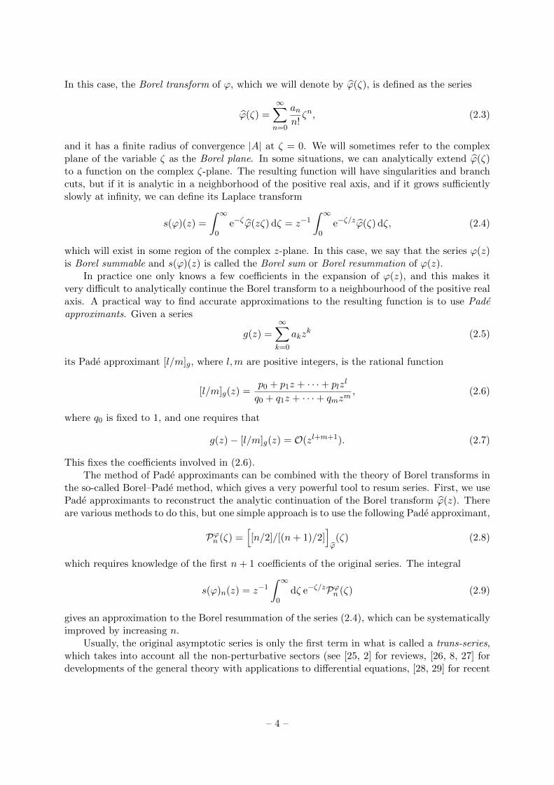
Figure 1: The paths C± avoiding the singularities of the Borel transform from above (respectively, below).

applications in Quantum Field Theory, and [30, 31] for recent applications in string theory andmatrix models). In its simplest incarnation, trans-series involve both the small parameter z aswell as the small exponentials

e−Sα/z, α ∈ A. (2.10)

Here α ∈ A labels the different non-perturbative sectors of the theory. The trans-series is aformal infinite sum over all these sectors, of the form,

Σ(z) = ϕ(z) +∑α∈A

Cαe−Sα/zϕα(z), (2.11)

where the ϕα(z) are themselves formal power series in z, and Cα (in general complex numbers)are the weights of the instanton sectors. When the non-perturbative effects are associated toinstantons, the quantities Sα are interpreted as instanton actions, and they usually appear assingularities in the complex plane of the Borel transform of ϕ(z) (in simple cases, these actions areinteger multiples of a single instanton action A). In principle, the non-perturbative answer for theproblem at hand can be obtained by performing a Borel resummation of the series ϕ(z), ϕα(z),and then plugging in the result in (2.11) with an appropriate choice of the Cα. The resultingsum of trans-series is usually well-defined if z is small enough. Since the Borel transforms of theformal power series appearing in (2.11) might in general have singularities along the positive realaxis, one has to consider as well lateral Borel resummations,

s±(ϕ)(z) = z−1

∫C±

e−ζ/zϕ(ζ) dζ, (2.12)

where the contours C± avoid the singularities and branch cuts by following paths slightly aboveor below the positive real axis, as in Fig. 1.

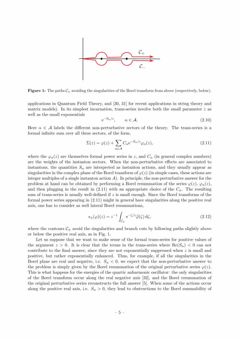
Let us suppose that we want to make sense of the formal trans-series for positive values ofthe argument z > 0. It is clear that the terms in the trans-series where Re(Sα) < 0 can notcontribute to the final answer, since they are not exponentially suppressed when z is small andpositive, but rather exponentially enhanced. Thus, for example, if all the singularities in theBorel plane are real and negative, i.e. Sα < 0, we expect that the non-perturbative answer tothe problem is simply given by the Borel resummation of the original perturbative series ϕ(z).This is what happens for the energies of the quartic anharmonic oscillator: the only singularitiesof the Borel transform occur along the real negative axis [32], and the Borel resummation ofthe original perturbative series reconstructs the full answer [5]. When some of the actions occuralong the positive real axis, i.e. Sα > 0, they lead to obstructions to the Borel summability of

– 5 –

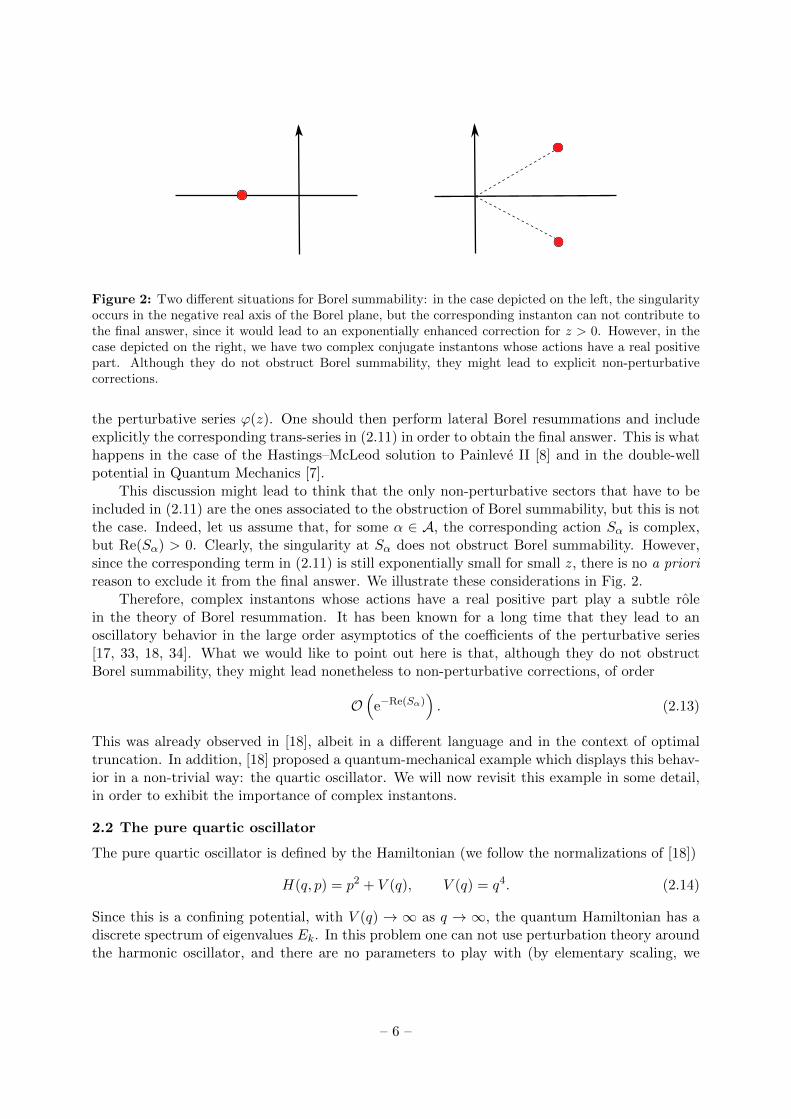
Figure 2: Two different situations for Borel summability: in the case depicted on the left, the singularityoccurs in the negative real axis of the Borel plane, but the corresponding instanton can not contribute tothe final answer, since it would lead to an exponentially enhanced correction for z > 0. However, in thecase depicted on the right, we have two complex conjugate instantons whose actions have a real positivepart. Although they do not obstruct Borel summability, they might lead to explicit non-perturbativecorrections.

the perturbative series ϕ(z). One should then perform lateral Borel resummations and includeexplicitly the corresponding trans-series in (2.11) in order to obtain the final answer. This is whathappens in the case of the Hastings–McLeod solution to Painleve II [8] and in the double-wellpotential in Quantum Mechanics [7].

This discussion might lead to think that the only non-perturbative sectors that have to beincluded in (2.11) are the ones associated to the obstruction of Borel summability, but this is notthe case. Indeed, let us assume that, for some α ∈ A, the corresponding action Sα is complex,but Re(Sα) > 0. Clearly, the singularity at Sα does not obstruct Borel summability. However,since the corresponding term in (2.11) is still exponentially small for small z, there is no a priorireason to exclude it from the final answer. We illustrate these considerations in Fig. 2.

Therefore, complex instantons whose actions have a real positive part play a subtle rolein the theory of Borel resummation. It has been known for a long time that they lead to anoscillatory behavior in the large order asymptotics of the coefficients of the perturbative series[17, 33, 18, 34]. What we would like to point out here is that, although they do not obstructBorel summability, they might lead nonetheless to non-perturbative corrections, of order

O(

e−Re(Sα)). (2.13)

This was already observed in [18], albeit in a different language and in the context of optimaltruncation. In addition, [18] proposed a quantum-mechanical example which displays this behav-ior in a non-trivial way: the quartic oscillator. We will now revisit this example in some detail,in order to exhibit the importance of complex instantons.

2.2 The pure quartic oscillator

The pure quartic oscillator is defined by the Hamiltonian (we follow the normalizations of [18])

H(q, p) = p2 + V (q), V (q) = q4. (2.14)

Since this is a confining potential, with V (q) → ∞ as q → ∞, the quantum Hamiltonian has adiscrete spectrum of eigenvalues Ek. In this problem one can not use perturbation theory aroundthe harmonic oscillator, and there are no parameters to play with (by elementary scaling, we

– 6 –

have that Ek(~) = ~4/3Ek(1)). This suggests using the WKB expansion to find the energy levels,which is an asymptotic expansion for large quantum numbers. The starting point for this methodis the well-known Bohr–Sommerfeld quantization condition,

vol0(E) = 2π~(k +

1

2

), k ≥ 0. (2.15)

In this equation,

vol0(E) =

∮γλ(q), (2.16)

where γ is a contour around the two real turning points defined by V (q) = E, and

λ(q) = p(q, E)dq, p(q, E) =√E − q4 (2.17)

is a differential on the curve of constant energy defined by

H(q, p) = E. (2.18)

The notation (2.16) is due to the fact that the above integral computes the volume of phase spaceenclosed inside the curve (2.18).

As it is well-known, the Bohr–Sommerfeld condition is just the leading term in a system-atic ~ expansion. The quantum-corrected quantization condition, due to Dunham [35], can beformulated in a more geometric language as follows. We can solve the Schrodinger equation(

−~2 d2

dq2+ q4 − E

)ψ(q) = 0 (2.19)

in terms of a function p(q, E; ~) as

ψ(q) =1√

p(q, E; ~)exp

(i

~

∫ q

p(q′, E; ~)dq′). (2.20)

We then define the “quantum” differential by

λ(q; ~) = p(q, E; ~)dq. (2.21)

This has an expansion in powers of ~ whose first term is the “classical” differential λ(q). In termsof the “quantum” differential λ(q; ~) we define a quantum-corrected volume as

volp(E) =

∮γλ(q; ~), (2.22)

which reduces to vol0(E) as ~→ 0. The Dunham quantization condition reads now,

volp(E) = 2π~(k +

1

2

), k ≥ 0. (2.23)

In the case of the pure quartic oscillator, one can write

volp(E) =

∞∑n=0

~2n

∮γu2n(q)dq, (2.24)

– 7 –

where u0(q) = p(q, E) and the higher order terms are given by the following recursion relation:

u2n = (−1)nv2n, n ≥ 0,

vn =1

2p

(v′n−1 −

n−1∑k=1

vkvn−k

).

(2.25)

This implies that all the u2n(q) are sums of rational functions of the form qn/pm, and the contourintegrals can be explicitly evaluated. By using the variable

σ =Γ(1/4)2

3~

√2

πE3/4, (2.26)

one finds that1

~volp(E) =

∑n≥0

bnσ1−2n, (2.27)

where the coefficients bn can be computed in closed form, and b0 = 1.

The series appearing in (2.27) has zero radius of convergence, therefore we should expecta rich non-perturbative structure in the theory. Such a structure has been studied in detail in[18, 24]. The first step in understanding non-perturbative aspects of this model is to look for allpossible saddle-points of the path integral. Since the quartic potential has a single minimum,one could think that the only saddle-point is the classical trajectory of energy E between theturning points ±E1/4, which corresponds to the cycle γ in (2.16). However, one should look forgeneral, complex saddle-points1. The curve (2.18), once it is complexified, describes a Riemannsurface of genus one with a lattice of one-cycles. The perturbative quantization condition (2.23)involves the cycle going around the two real turning points, but there are other one-cycles relatedto non-trivial, complex saddle-points. The existence of these cycles can be seen very explicitlyby looking at complexified classical trajectories. The classical solution to the EOM with energyE is given by the trajectory

q(t) = E1/4cn

(2√

2E1/4t,1√2

), (2.28)

where we have fixed one integration constant due to time translation invariance. Here, cn(u, k)is a Jacobi elliptic function. As noticed in [18], this function has a complex lattice Λ of periodsin the t plane, generated by

T1 =T + iT

2, T2 = −T − iT

2, (2.29)

where

T =√

2E−1/4K(

1/√

2)

(2.30)

is the real period of the classical trajectory (2.28), and K(k) is the elliptic integral of the firstkind. Any period in Λ leads to a complex, periodic trajectory. The trajectories with periods T1,

1Strictly speaking, instantons are just a particular class of such saddle-points, describing a trajectory in realspace but in imaginary or Euclidean time. However, we will refer to a general saddle-point of the complexifiedtheory also as an instanton configuration.

– 8 –

T2 go around the real turning point −E1/4 and the complex turning points ±iE1/4, respectively.They have actions σS1,2, where

S1 =1 + i

2, S2 = −1− i

2. (2.31)

Therefore, the actions of the complex trajectories associated to the periods in Λ are given by σ,times

nS1 +mS2, n,m ∈ Z. (2.32)

The cycle γ appearing in (2.16) corresponds to the real trajectory (2.28) with period T , and it isassociated to the point S1−S2 = 1, with action σ. The lattice of points (2.32) gives the possiblesingularities of the Borel transform of the series (2.27), which we define as follows: we write theperturbative series (2.27) as

1

~volp(E) = σ +

1

σϕ(σ), ϕ(σ) =

∑n≥0

bn+1σ−2n. (2.33)

The Borel transform is then defined by

ϕ(ζ) =∑n≥0

bn+1

(2n)!ζ2n. (2.34)

This definition is slightly different from the one used in [24], but leads to the same structure ofsingularities in the Borel plane. However, not all the instanton actions in (2.32) lead to actualsingularities in the Borel transform. These have been determined in [24], and they are given bythe points nS1 and nS2, where n ∈ Z\{0}, as well as by the points

n(S1 − S2), n ∈ Z\{0}. (2.35)

The singularities which are closest to the origin are ±S1 and ±S2, and they correspond to complexsaddles with actions ±1± i

2σ. (2.36)

Through the standard connection to the large order behavior of the perturbative series, they leadto an oscillatory behavior for the coefficients bn [18]. Note as well that there is an infinite numberof singularities along the positive real axis, and the closest one to the origin occurs at S1−S2 = 1.This clearly leads to an obstruction to Borel summability. However, this obstruction comes froma sub-dominant singularity, and it is only seen in exponentially small, subleading corrections tothe large order behavior of the coefficients bn [24].

We would like to compare the results for the energy spectrum obtained by Borel–Paderesummation of the series (2.27), to the values obtained by solving the Schrodinger equation, asin [36, 37]. Since there is a singularity in the positive real axis of the Borel plane, we have toconsider lateral Borel–Pade resummations. In order to do this, we have first generated a largenumber of terms in the series (2.27), and then computed Pade approximants (2.8) of the Boreltransform (2.34), for different values of n.

The first piece of information that can be extracted from the Pade approximants is thestructure of singularities in the Borel plane. The Pade approximants are by construction rationalfunctions, therefore their only singularities are poles. However, the accumulation of their polesalong segments signals the presence of branch cut singularities in the Borel transform. The pole

– 9 –

ΓΕ

-3 -2 -1 1 2 3

-2

-1

1

2

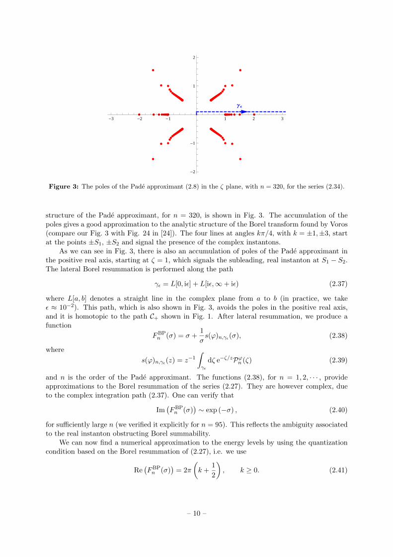
Figure 3: The poles of the Pade approximant (2.8) in the ζ plane, with n = 320, for the series (2.34).

structure of the Pade approximant, for n = 320, is shown in Fig. 3. The accumulation of thepoles gives a good approximation to the analytic structure of the Borel transform found by Voros(compare our Fig. 3 with Fig. 24 in [24]). The four lines at angles kπ/4, with k = ±1,±3, startat the points ±S1, ±S2 and signal the presence of the complex instantons.

As we can see in Fig. 3, there is also an accumulation of poles of the Pade approximant inthe positive real axis, starting at ζ = 1, which signals the subleading, real instanton at S1 − S2.The lateral Borel resummation is performed along the path

γε = L[0, iε] + L[iε,∞+ iε) (2.37)

where L[a, b] denotes a straight line in the complex plane from a to b (in practice, we takeε ≈ 10−2). This path, which is also shown in Fig. 3, avoids the poles in the positive real axis,and it is homotopic to the path C+ shown in Fig. 1. After lateral resummation, we produce afunction

FBPn (σ) = σ +

1

σs(ϕ)n,γε(σ), (2.38)

where

s(ϕ)n,γε(z) = z−1

∫γε

dζ e−ζ/zPϕn (ζ) (2.39)

and n is the order of the Pade approximant. The functions (2.38), for n = 1, 2, · · · , provideapproximations to the Borel resummation of the series (2.27). They are however complex, dueto the complex integration path (2.37). One can verify that

Im(FBPn (σ)

)∼ exp (−σ) , (2.40)

for sufficiently large n (we verified it explicitly for n = 95). This reflects the ambiguity associatedto the real instanton obstructing Borel summability.

We can now find a numerical approximation to the energy levels by using the quantizationcondition based on the Borel resummation of (2.27), i.e. we use

Re(FBPn (σ)

)= 2π

(k +

1

2

), k ≥ 0. (2.41)

– 10 –

We will denote by E(0)n (k) the energy levels obtained from this quantization condition (the su-

perscript (0) indicates that we are not considering instanton contributions explicitly). Some ofthe results of our calculation are displayed in Table 1.

k E(k) E(0)320(k)

6 26.528 471 183 682 518 191 8 26.528 471 181 399 704 803

3 11.644 745 511 378 11.644 768 005 3

0 1.060 0.96

Table 1: Energies of the levels k = 0, 3, 6 of the quartic oscillator with ~ = 1. The first column showsthe value obtained numerically in [36] for k = 0, 6 and [37] for k = 3, while the second column shows thevalue of the energy obtained by using the quantization condition (2.41) with n = 320. All the given digitsare stable.

Since we are not including the effects of the real instanton, we know that the energy levelsobtained with the above procedure will have an accuracy not better than e−σ, where σ is givenby (2.26)2. However, by comparing the real part of the Borel–Pade resummation to the energylevels calculated numerically, one notices that the disagreement is not of order e−σ, but ratherof order e−σ/2. This was already pointed out in [18], in the context of optimal truncation. Inthat paper, Balian, Parisi and Voros argued that one should correct the perturbative WKBquantization condition (2.23) by adding explicit, non-perturbative contributions to the volumeof phase space, which incorporate the effect of complex instantons. These corrections are due tothe complex instantons associated to the points S1, −S2, whose action has a real part given byσ/2. The leading term of their contribution was determined in [18], and it is given by

volnp(E) = ∓2 arctan

[exp

(i

2~

∮γ′λ(q; ~)

)]+ · · · , (2.42)

where the ∓ sign corresponds to wavefunctions with even (respectively, odd) parity, and γ′

is a contour in the complex q-plane around the two imaginary turning points iE1/4, −iE1/4.Note that (2.42) is just the leading non-perturbative correction to the volume of phase space.There should be additional non-perturbative corrections coming from higher instantons, whichare exponentially suppressed as compared to (2.42).

We can now incorporate the above non-perturbative correction to the quantization condition

vol(E) = volp(E) + volnp(E) = 2π~(k +

1

2

). (2.43)

This correction involves an additional asymptotic series, coming from the integration along thecycle γ′. It turns out that this series can be expressed in terms of the same coefficients bn [18],namely,

i

2~

∮γ′λ(q; ~) = −1

2

∑n≥0

(−1)nbnσ1−2n, (2.44)

and it can be also analyzed with the Borel–Pade resummation method. In this case there are nosingularities in the positive real axis [24], and we can do a standard Borel–Pade resummation.If we proceed exactly as we did for (2.27), we obtain, from the formal series (2.44), a functionGBPn (σ), where n is again the order of the Pade approximant as defined in (2.8).

2Since we are imposing the quantization condition (2.23), σ is, for large k, of order 2πk.

– 11 –

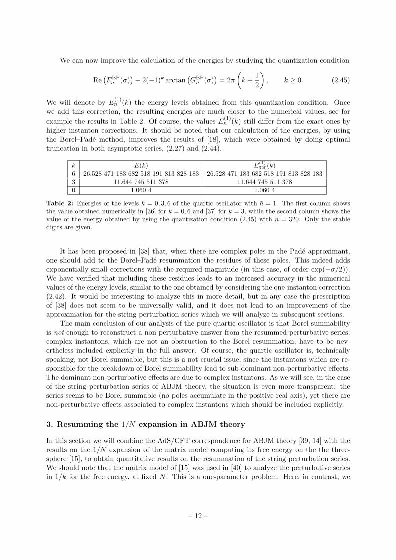
We can now improve the calculation of the energies by studying the quantization condition

Re(FBPn (σ)

)− 2(−1)k arctan

(GBPn (σ)

)= 2π

(k +

1

2

), k ≥ 0. (2.45)

We will denote by E(1)n (k) the energy levels obtained from this quantization condition. Once

we add this correction, the resulting energies are much closer to the numerical values, see for

example the results in Table 2. Of course, the values E(1)n (k) still differ from the exact ones by

higher instanton corrections. It should be noted that our calculation of the energies, by usingthe Borel–Pade method, improves the results of [18], which were obtained by doing optimaltruncation in both asymptotic series, (2.27) and (2.44).

k E(k) E(1)320(k)

6 26.528 471 183 682 518 191 813 828 183 26.528 471 183 682 518 191 813 828 1833 11.644 745 511 378 11.644 745 511 3780 1.060 4 1.060 4

Table 2: Energies of the levels k = 0, 3, 6 of the quartic oscillator with ~ = 1. The first column showsthe value obtained numerically in [36] for k = 0, 6 and [37] for k = 3, while the second column shows thevalue of the energy obtained by using the quantization condition (2.45) with n = 320. Only the stabledigits are given.

It has been proposed in [38] that, when there are complex poles in the Pade approximant,one should add to the Borel–Pade resummation the residues of these poles. This indeed addsexponentially small corrections with the required magnitude (in this case, of order exp(−σ/2)).We have verified that including these residues leads to an increased accuracy in the numericalvalues of the energy levels, similar to the one obtained by considering the one-instanton correction(2.42). It would be interesting to analyze this in more detail, but in any case the prescriptionof [38] does not seem to be universally valid, and it does not lead to an improvement of theapproximation for the string perturbation series which we will analyze in subsequent sections.

The main conclusion of our analysis of the pure quartic oscillator is that Borel summabilityis not enough to reconstruct a non-perturbative answer from the resummed perturbative series:complex instantons, which are not an obstruction to the Borel resummation, have to be nev-ertheless included explicitly in the full answer. Of course, the quartic oscillator is, technicallyspeaking, not Borel summable, but this is a not crucial issue, since the instantons which are re-sponsible for the breakdown of Borel summability lead to sub-dominant non-perturbative effects.The dominant non-perturbative effects are due to complex instantons. As we will see, in the caseof the string perturbation series of ABJM theory, the situation is even more transparent: theseries seems to be Borel summable (no poles accumulate in the positive real axis), yet there arenon-perturbative effects associated to complex instantons which should be included explicitly.

3. Resumming the 1/N expansion in ABJM theory

In this section we will combine the AdS/CFT correspondence for ABJM theory [39, 14] with theresults on the 1/N expansion of the matrix model computing its free energy on the the three-sphere [15], to obtain quantitative results on the resummation of the string perturbation series.We should note that the matrix model of [15] was used in [40] to analyze the perturbative seriesin 1/k for the free energy, at fixed N . This is a one-parameter problem. Here, in contrast, we

– 12 –

study the 1/N expansion, in which each coefficient is itself a non-trivial function of the ’t Hooftparameter.

ABJM theory [14, 41] is a conformally invariant, Chern–Simons–matter theory in threedimensions with gauge group U(N)k × U(N)−k and N = 6 supersymmetry. The Chern–Simonsactions for the gauge groups have couplings k and −k, respectively. The theory contains aswell four hypermultiplets in the bifundamental representation of the gauge group. The ’t Hooftparameter of this theory is defined as

λ =N

k. (3.1)

In [15] it was shown, through a beautiful application of localization techniques, that the partitionfunction of ABJM theory on the three-sphere can be computed by a matrix model (see [42] fora pedagogical review). This matrix model is given by

Z(N, k) =1

N !2

∫ N∏i=1

dµidνj(2π)2

∏i<j sinh2

(µi−µj

2

)sinh2

(νi−νj

2

)∏i,j cosh2

(µi−νj

2

) eik4π (

∑i µ

2i−

∑j ν

2j ). (3.2)

The free energy, defined as F (N, k) = logZ(N, k), has a 1/N expansion of the form

F (λ, k) =

∞∑g=0

(2π

k

)2g−2

Fg(λ). (3.3)

ABJM theory has been conjectured to be dual to type IIA superstring theory on AdS4 × CP3.This theory has two parameters, the string coupling constant gst and the radius L of the AdSspace, and they are related to the parameters λ, k of ABJM theory by

k2 = g−2st

(L

`s

)2

,

λ− 1

24=

1

32π2

(L

`s

)4(

1− 4π2g2st

3

(`sL

)6),

(3.4)

where `s is the string length. Here, we have used the corrected dictionary proposed in [43, 44],although our results will not depend on its details. According to the AdS/CFT correspondence,the free energy (3.3) is the free energy of type IIA superstring theory on the AdS background,and its 1/N expansion (3.3) corresponds to the genus expansion of the superstring.

The genus g free energies appearing in (3.3) were determined in [16] by using various tech-niques. The strong coupling regime of the free energies at genus zero and one reproduces theexpected answer from supergravity [16, 45]. We will now review the structure of these free en-ergies. Their natural variable is the parameter κ, which is related to the ’t Hooft coupling by[19, 16]

λ(κ) =κ

8π3F2

(1

2,1

2,1

2; 1,

3

2;−κ

2

16

). (3.5)

The genus zero free energy is determined by the equation,

−∂λF0 =κ

4G2,3

3,3

(12 ,

12 ,

12

0, 0, −12

∣∣∣∣−κ2

16

)+π2iκ

23F2

(1

2,1

2,1

2; 1,

3

2;−κ

2

16

), (3.6)

– 13 –

where G2,33,3 is a Meijer function3. The integration constant can be fixed by looking at the weak

coupling limit [16, 46]. For g ≥ 1, the free energies are quasi-modular forms with modularparameter

τ = iK ′(

iκ4

)K(

iκ4

) . (3.7)

For g = 1, one has

F1 = − log η(τ) + 2ζ ′(−1) +1

6log

(iπ

2k

), (3.8)

where η is the usual Dedekind eta function. For g ≥ 2, the Fgs can be written in terms of E2(τ)(the standard Eisenstein series), b(τ) and d(τ), where

b(τ) = ϑ42(τ), d(τ) = ϑ4

4(τ), (3.9)

are standard Jacobi theta functions. More precisely, they have the general structure

Fg(λ) =1

(b(τ)d2(τ))g−1

3g−3∑k=0

Ek2 (τ)p(g)k (b(τ), d(τ)) , g ≥ 2, (3.10)

where p(g)k (b(τ), d(τ)) are polynomials in b(τ), d(τ) of modular weight 6g − 6− 2k. The genus g

free energies Fg(λ) obtained in this way are exact functions of the ’t Hooft parameter, and theyprovide interpolating functions between the weak and the strong coupling regimes.

The nature of the series (3.3) was investigated in [17]. As usual in string theory and in the1/N expansion, at fixed λ, the genus g free energies diverge factorially [9],

Fg(λ) ∼ (A(λ))−2g(2g)!. (3.11)

A first question one can ask is: what are the possible instanton actions appearing in the non-perturbative sector, and how do they manifest themselves in the large order behavior of the freeenergies? In [17], based on previous work on instantons in matrix models (reviewed in for example[2]), a proposal was made for the instanton actions. The large N limit of the matrix model (3.2)is controlled by a spectral curve of genus one, and there is a lattice of periods, just as in thecase of the quartic oscillator analyzed in the previous section. In addition, there is a constantperiod. The conjecture of [17] is that the instanton actions are linear integer combinations of thetwo independent periods of the spectral curve, and of the constant period. This proposal is verymuch along the lines of [18], since they both involve the periods of a complexified curve.

The proposal of [17] can be checked by looking at the large order behavior of the series (3.3).At large λ, the leading behavior of Fg is dominated by the so-called constant map contribution,

Fg(λ) = cg +O(λ3/2−2g

), g ≥ 2, (3.12)

where

cg =4g−1(−1)g|B2gB2g−2|g(2g − 2)(2g − 2)!

, (3.13)

and B2g are Bernoulli numbers. The large order behavior of these coefficients is controlled bythe constant period [47, 2]

A = 2π2i, (3.14)

3The free energies used in this paper have an overall factor (−1)g−1 w.r.t. the ones used in [16, 17].

– 14 –

together with its complex conjugate. They lead to a pair of complex conjugate singularities inthe Borel plane. However, this gives the “trivial” part of the asymptotic behavior. Much moreinteresting is the subleading singularity, which can be obtained from the study of the large orderbehavior of the sequence Fg(λ)− cg at sufficiently large λ (in practice, λ & 0.75). It is controlledby the action

As(λ) = − 1

π∂λF0 + iπ2, (3.15)

which is one of the periods of the spectral curve. Since this action is complex, it can be writtenas

As(λ) = |As(λ)| eiθs(λ), (3.16)

and it leads to an oscillatory behavior in the sequence Fg(λ)− cg:

Fg(λ)− cg ∼ |As(λ)|−2g cos (2gθs(λ) + δs(λ)) (2g)!, (3.17)

where δs(λ) is an unknown function of λ. The behavior (3.17) was tested numerically in [17]. Asexplained in [17], for smaller values of λ, the dominant action is no longer (3.15), but

Aw(λ) = 4iπ2λ. (3.18)

In addition, a study of the lattice of the periods in [17] led to the conclusion that there areno singularities on the positive real axis of the Borel plane. As we will see in a moment, ournumerical results for the Borel–Pade transform seem to confirm the Borel summability of theasymptotic series (3.3).

The results of [17] open the window to an analysis of the Borel–Pade resummation of (3.3).Using the techniques of [16], we can generate the free energies in (3.3) up to genus 30. As wewill see, this gives already good numerical results. On the other hand, since (3.3) is the 1/Nexpansion of the matrix model (3.2), we know what is the non-perturbative object that we shouldcompare to this resummation: the free energy of the matrix model F (N, k) for finite values of Nand k4. It turns out that the partition function Z(N, k) has been computed analytically with theTBA equations of [48, 49] in [50, 51, 23], for various integer values of N and k. In particular, [23]gives results for k = 1, 2, 3, 4, 6 and N = 1, 2, ..., Nmax,k where Nmax,(1,2,3,4,6) = (44, 20, 18, 16, 14).

To proceed with the Borel–Pade resummation, we write (3.3) as

F (λ, z) = z−2F0(λ) + F1(λ) +∑g≥2

z2g−2Fg(λ), (3.19)

where

z =2π

k. (3.20)

Then we consider the Borel transform of

ϕ(z) =∑g≥2

Fg(λ)z2g−2, (3.21)

which is given by

ϕ(ζ) =∑g≥2

Fg(λ)

(2g − 2)!ζ2g−2, (3.22)

– 15 –

-100 -50 50 100

-100

-50

50

100

-100 -50 50 100

-100

-50

50

100

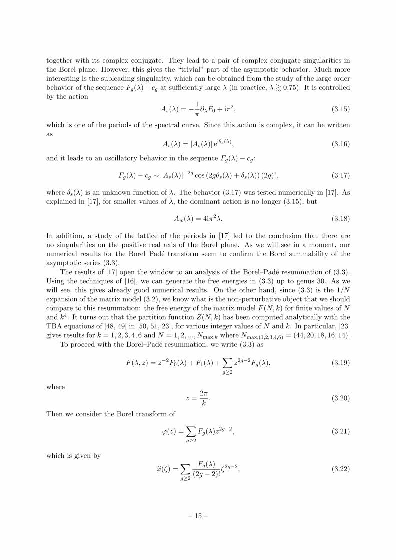
Figure 4: The red dots signal the location of the poles of the Pade approximant (2.8), for the series(3.22) with λ ≈ 2.61. In the figure on the left we have included the full Fg(λ), while in the figure on theright we have subtracted the contribution of constant maps. The blue circle corresponds to the numericalvalue of the complex instanton action As(λ). The degree of the Pade approximant is n = 54 (left) andn = 60 (right).

and we fix the value of λ to obtain a numerical series. We consider Pade approximants of ordern for the Borel transform, as in (2.8).

As we explained in the example of the quartic oscillator, the first information we can obtainfrom the Borel–Pade transform is the singularity structure in the Borel plane of the ζ variable.This can be studied by looking at the poles of the Pade approximants. We show the location ofthese poles in Fig. 4 for λ ≈ 2.61, where we consider both the Pade approximant of the series(3.22) associated to Fg(λ), on the left, and of the series where we removed the constant mapcontribution Fg(λ) − cg, on the right. When the constant map contribution is included, theleading singularity in the Borel plane takes place in the imaginary axis, near ±2π2i, as expectedfrom (3.14). The subleading singularity, which we have indicated by a blue circle, correspondsprecisely to the value of the instanton action (3.15),

As(λ ≈ 2.61) ≈ 44.73 + 9.87i. (3.23)

When the constant map contribution is removed, this becomes the leading singularity. Finally,the singularities display a periodicity of 2π2 in the imaginary direction, corresponding to multiplesof the constant period. Note as well that all singularities come in groups of four, A, −A, A∗ and−A∗. This is due to the fact that the perturbative series only has even powers (hence the paritysymmetry A→ −A) and it is real (hence the conjugation symmetry A→ A∗). In overall, thesenumerical results are in good agreement with the analytic results conjectured in [17].

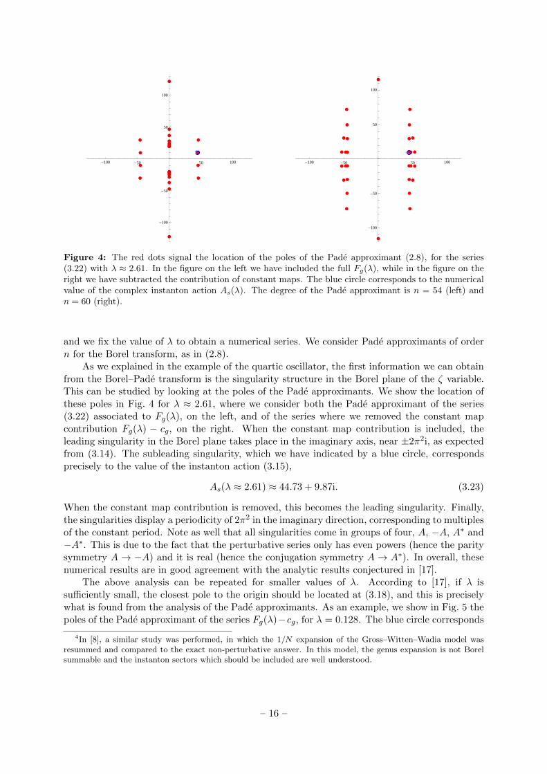
The above analysis can be repeated for smaller values of λ. According to [17], if λ issufficiently small, the closest pole to the origin should be located at (3.18), and this is preciselywhat is found from the analysis of the Pade approximants. As an example, we show in Fig. 5 thepoles of the Pade approximant of the series Fg(λ)−cg, for λ = 0.128. The blue circle corresponds

4In [8], a similar study was performed, in which the 1/N expansion of the Gross–Witten–Wadia model wasresummed and compared to the exact non-perturbative answer. In this model, the genus expansion is not Borelsummable and the instanton sectors which should be included are well understood.

– 16 –

-20 -10 10 20

-20

-10

10

20

Figure 5: The red dots signal the location of the poles of the Pade approximant (2.8), for the seriesFg(λ) − cg and λ ≈ 0.128. The blue circle corresponds to the numerical value of the purely imaginaryinstanton action Aw(λ) in (3.18). The degree of the Pade approximant is n = 54.

precisely to the value of Aw(λ), and gives the location of the leading singularity. We concludethat the structure of the poles in the Borel plane agrees with the analysis in [17]: when λ is small(weak coupling regime), the leading singularity in the Borel plane for the sequence Fg(λ) − cgis given by the instanton action (3.18). As we increase the ’t Hooft coupling and we enter thestrong coupling regime, the singularities move in the plane and the one corresponding to As(λ)becomes dominant (i.e. smaller in absolute value).

One important aspect of the numerical structure of the poles of the Pade approximantsis that no singularities appear along the positive real axis5. This is again consistent with theanalysis in [17]. It indicates that the series is likely to be Borel summable, and therefore wecan perform a standard Borel–Pade resummation (2.4): we do the integral (2.9) for the Padeapproximant of (3.22), and we add at the end the terms of genus zero and one. We will denoteby

FBPn (N, k) (3.24)

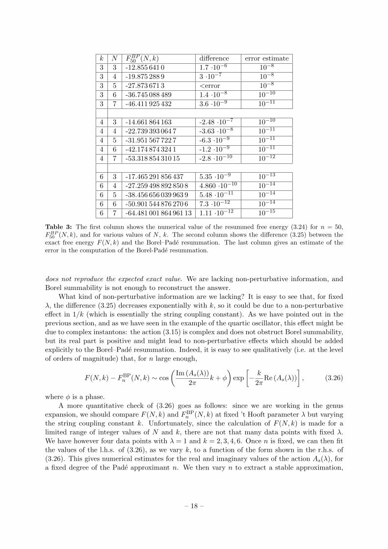
the final result, where the subindex n refers to the degree of the Pade approximant in (2.8).In Table 3 we present some of our numerical results, for various values of N and k (this also

fixes the value of λ), and for n = 50. The first column shows the numerical value of FBPn (N, k).

The second column shows the difference between the exact results for the free energy listed in[23] and the Borel–Pade resummation, i.e

F (N, k)− FBPn (N, k). (3.25)

The third column gives an estimate of the error incurred in the Borel–Pade resummation (sincethe values of F (N, k) for the chosen N , k are known analytically, the error in their numerical valuecan be made arbitrarily small.) We see that the difference (3.25) is systematically bigger thanthe error estimate. One is forced to conclude that the Borel resummation of the 1/N expansion

5One might find poles in the positive real axis for some of the Pade approximants, but they are not stable andthey should be regarded as artifacts of the numerical approximation. When these accidental poles are present, weperform the Borel resummation by deforming the contour slightly above the real axis.

– 17 –

k N FBP50 (N, k) difference error estimate

3 3 -12.855 641 0 1.7 ·10−6 10−8

3 4 -19.875 288 9 3 ·10−7 10−8

3 5 -27.873 671 3 <error 10−8

3 6 -36.745 088 489 1.4 ·10−8 10−10

3 7 -46.411 925 432 3.6 ·10−9 10−11

4 3 -14.661 864 163 -2.48 ·10−7 10−10

4 4 -22.739 393 064 7 -3.63 ·10−8 10−11

4 5 -31.951 567 722 7 -6.3 ·10−9 10−11

4 6 -42.174 874 324 1 -1.2 ·10−9 10−11

4 7 -53.318 854 310 15 -2.8 ·10−10 10−12

6 3 -17.465 291 856 437 5.35 ·10−9 10−13

6 4 -27.259 498 892 850 8 4.860 ·10−10 10−14

6 5 -38.456 656 039 963 9 5.48 ·10−11 10−14

6 6 -50.901 544 876 270 6 7.3 ·10−12 10−14

6 7 -64.481 001 864 961 13 1.11 ·10−12 10−15

Table 3: The first column shows the numerical value of the resummed free energy (3.24) for n = 50,FBP50 (N, k), and for various values of N , k. The second column shows the difference (3.25) between the

exact free energy F (N, k) and the Borel–Pade resummation. The last column gives an estimate of theerror in the computation of the Borel-Pade resummation.

does not reproduce the expected exact value. We are lacking non-perturbative information, andBorel summability is not enough to reconstruct the answer.

What kind of non-perturbative information are we lacking? It is easy to see that, for fixedλ, the difference (3.25) decreases exponentially with k, so it could be due to a non-perturbativeeffect in 1/k (which is essentially the string coupling constant). As we have pointed out in theprevious section, and as we have seen in the example of the quartic oscillator, this effect might bedue to complex instantons: the action (3.15) is complex and does not obstruct Borel summability,but its real part is positive and might lead to non-perturbative effects which should be addedexplicitly to the Borel–Pade resummation. Indeed, it is easy to see qualitatively (i.e. at the levelof orders of magnitude) that, for n large enough,

F (N, k)− FBPn (N, k) ∼ cos

(Im (As(λ))

2πk + φ

)exp

[− k

2πRe (As(λ))

], (3.26)

where φ is a phase.A more quantitative check of (3.26) goes as follows: since we are working in the genus

expansion, we should compare F (N, k) and FBPn (N, k) at fixed ’t Hooft parameter λ but varying

the string coupling constant k. Unfortunately, since the calculation of F (N, k) is made for alimited range of integer values of N and k, there are not that many data points with fixed λ.We have however four data points with λ = 1 and k = 2, 3, 4, 6. Once n is fixed, we can then fitthe values of the l.h.s. of (3.26), as we vary k, to a function of the form shown in the r.h.s. of(3.26). This gives numerical estimates for the real and imaginary values of the action As(λ), fora fixed degree of the Pade approximant n. We then vary n to extract a stable approximation,

– 18 –

1 2 3 4 5 6 7

-30

-25

-20

-15

-10

-5

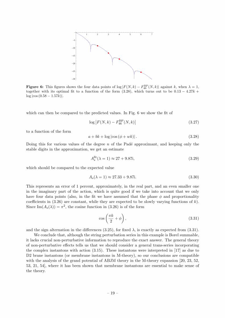
Figure 6: This figures shows the four data points of log |F (N, k) − FBP46 (N, k)| against k, when λ = 1,

together with its optimal fit to a function of the form (3.28), which turns out to be 0.13 − 4.27k +log |cos (0.58− 1.57k)|.

which can then be compared to the predicted values. In Fig. 6 we show the fit of

log∣∣F (N, k)− FBP

46 (N, k)∣∣ (3.27)

to a function of the forma+ bk + log |cos (φ+ wk)| . (3.28)

Doing this for various values of the degree n of the Pade approximant, and keeping only thestable digits in the approximation, we get an estimate

Afits (λ = 1) ≈ 27 + 9.87i, (3.29)

which should be compared to the expected value

As(λ = 1) ≈ 27.33 + 9.87i. (3.30)

This represents an error of 1 percent, approximately, in the real part, and an even smaller onein the imaginary part of the action, which is quite good if we take into account that we onlyhave four data points (also, in the fit we have assumed that the phase φ and proportionalitycoefficients in (3.26) are constant, while they are expected to be slowly varying functions of k).Since Im(As(λ)) = π2, the cosine function in (3.26) is of the form

cos

(πk

2+ φ

), (3.31)

and the sign alternation in the differences (3.25), for fixed λ, is exactly as expected from (3.31).We conclude that, although the string perturbation series in this example is Borel summable,

it lacks crucial non-perturbative information to reproduce the exact answer. The general theoryof non-perturbative effects tells us that we should consider a general trans-series incorporatingthe complex instantons with action (3.15). These instantons were interpreted in [17] as due toD2 brane instantons (or membrane instantons in M-theory), so our conclusions are compatiblewith the analysis of the grand potential of ABJM theory in the M-theory expansion [20, 23, 52,53, 21, 54], where it has been shown that membrane instantons are essential to make sense ofthe theory.

– 19 –

4. Resumming the genus expansion in topological string theory

In this section we will consider a different, but related string perturbation series: the genusexpansion of topological string theory on a particular local Calabi–Yau manifold, known as localP1 × P1. This topological string theory has been studied in much detail, due to its relationshipto Seiberg–Witten theory [55], to Chern–Simons theory on lens spaces [56], and to ABJM theory[19, 16]. In this section we will focus on the genus g free energies Fg in the so-called large radiusframe. In this frame, the Fgs count holomorphic curves of genus g in the Calabi–Yau target andthey depend on two Kahler parameters, T1 and T2, which correspond to the (complexified) sizesof the P1s. They have the structure

Fg(T1, T2) =∑d1,d2

Ngd1,d2

e−d1T1−d2T2 , (4.1)

where Ngd1,d2

are the Gromov–Witten invariants of local P1 × P1 at genus g and for the degreesd1, d2. For g ≥ 2 there is also a contribution due to constant maps, as in (3.12), but this is muchsimpler to analyze and not relevant for our analysis. In the cases g = 0 and g = 1 there are alsosome additional contributions (which are cubic and linear polynomials in T1,2, respectively), butthese are also inessential to our purposes and will not be included in our definition of the Fgs.

The free energies Fg(T1, T2) can be computed in closed form by using the holomorphicanomaly equations of [57], adapted to the local case as in for example [58]. However, theirexplicit calculation becomes difficult at higher genus. Therefore, we will consider them in the“slice” of moduli space where

T1 = T2 = T. (4.2)

In that case, the functions Fg(T ) have the structure

Fg(T ) =∑d≥1

NgdQ

d, (4.3)

whereNgd =

∑d1+d2=d

Ngd1,d2

, Q = e−T , (4.4)

and they can be computed in a much simpler way6. They are in fact modular transformationsof the functions Fg(λ) which we considered in the previous section [16]. It will then be useful touse a parametrization related to the one we used there. Namely, we will use the mirror map

T = −4z 4F3

(1, 1,

3

2,3

2; 2, 2, 2; 16z

)− log(z), (4.5)

where z is related to the parameter κ appearing in (3.5) by [19, 16]

z = − 1

κ2. (4.6)

We will often parametrize the Kahler moduli space by

q = eiπτlr , (4.7)

6The Fgs we will use have an additional factor of 4g−1 as compared to the standard ones in the topologicalstring literature. This is equivalent to a rescaling gs → 2gs of the string coupling constant.

– 20 –

where

τlr = iK ′(

4iκ

)K(

4iκ

) . (4.8)

This large radius τlr is related to the τ in (3.7) through

τlr − 1 = − 1

τ − 1. (4.9)

The parametrization in terms of (4.7) is more convenient since the Fgs are quasi-modular formsin the variable τ . Of course, a given value of q corresponds to a value of the Kahler parameterthrough the equations (4.5), (4.6), (4.8) and (4.7).

We would like to study the total topological string free energy

F (T, gs) =∑g≥0

g2g−2s Fg(T ), (4.10)

where gs is the topological string coupling constant. This is again an asymptotic series, for fixedT , and it behaves as

Fg(T ) ∼ |Alr(T )|−2g cos (2gθlr(T ) + δlr(T )) (2g)!, (4.11)

whereAlr(T ) = πT + 2π2i, (4.12)

and we have written it asAlr(T ) = |Alr(T )| eiθlr(T ). (4.13)

It turns out that the total string free energy has a very different representation due toGopakumar and Vafa [22]. In this representation, one fixes the order of e−T and resums thegenus expansion. It has the structure

FGV(T, gs) =∑g≥0

∑w,d≥1

ndg (2 sin (gsw))2g−2 1

wQdw, (4.14)

where ndg are integers called Gopakumar–Vafa invariants. It is crucial to notice that the twoseries (4.10) and (4.14) are very different. The first series should be understood as an asymptoticseries in gs at fixed T . The series (4.14) should be understood as a series in Q = e−T , withcoefficients depending on gs. Of course, when one expands the Fgs appearing in (4.10) in powerseries in Q, and when one expands the trigonometric functions in (4.14) in powers of gs, oneobtains the same formal, double power series∑

g,d

NgdQ

dg2g−2s . (4.15)

One crucial question is then: what is the nature of the series appearing in the Gopakumar–Vafarepresentation? In [21], numerical evidence was given that, surprisingly, if gs is real, the series(4.14) has a finite radius of convergence in Q. However, the price to pay for this is the presenceof an infinite number of poles in the real line: in fact, if we write

gs =2π

k, (4.16)

– 21 –

then the series (4.14) has double poles for any rational value of k. Since this is a dense set in R,the Gopakumar–Vafa representation does not seem to be very useful in the way of providing anon-perturbative definition of the theory, at least for real gs.

In the context of ABJM theory, one can relate the topological string free energy to the grandpotential of the theory J(µ, k), which is defined by regarding Z(N, k) as a canonical partitionfunction, i.e.

J(µ, k) = log

1 +∑N≥1

zNZ(N, k)

. (4.17)

As usual in Statistical Mechanics, the grand potential is a function of the chemical potential µ,and we have also introduced the fugacity,

z = eµ. (4.18)

The function FGV(T, gs) can be interpreted as the contribution from worldsheet instantons tothe grand potential J(µ, k) [23], where the relationship between gs and k is given in (4.16), and

T =4µ

k− iπ. (4.19)

In [23] it was pointed out that, since Z(N, k) is well-defined for any value of k, there mustbe some additional contributions to J(µ, k) which cancel the divergences at rational k. Thesecontributions are due to membrane instantons and they can be partially computed by using theFermi gas approach of [20]. They were determined in the series of works [23, 52, 53, 21, 54].In particular, in [21] it was conjectured that they can be obtained from the refined topologicalstring partition function [59], in the Nekrasov–Shatashvili limit [60]. In [54] some aspects of thisconjecture were derived from an analysis of the spectral problem appearing in the Fermi gasformulation.

In order to set up the result for the non-perturbative completion of FGV(T, gs), we introducethe quantum-corrected Kahler parameter,

Teff = T + 2π2∑`≥1

a`(k) exp

(−k`

2(T + iπ)

). (4.20)

In this equation, the a`(k) are closely related to the coefficients of the quantum A-period ofthe local Calabi–Yau, which was introduced in [61, 62] (see [63] for recent extensions). Moredetails on these coefficients, as well as detailed values for the very first orders, can be found infor example [21]. We also introduce the membrane partition function,

FM2(T, gs) =∑`≥1

(a`(k)µ2 + b`(k)µ+ c`(k)

)e−2`µ. (4.21)

Here, the relationship between T, gs and µ, k is the one expressed in (4.16) and (4.19). Thecoefficients b`(k) are closely related to the quantum B-periods of the local Calabi–Yau, and thecoefficients c`(k) can be obtained from the coefficients a`(k), b`(k) [52, 54]. We then define thenon-perturbative topological string free energy as

FNP(T, gs) = FGV(Teff , gs) + FM2(T, gs). (4.22)

– 22 –

-40 -20 20 40

-40

-20

20

40

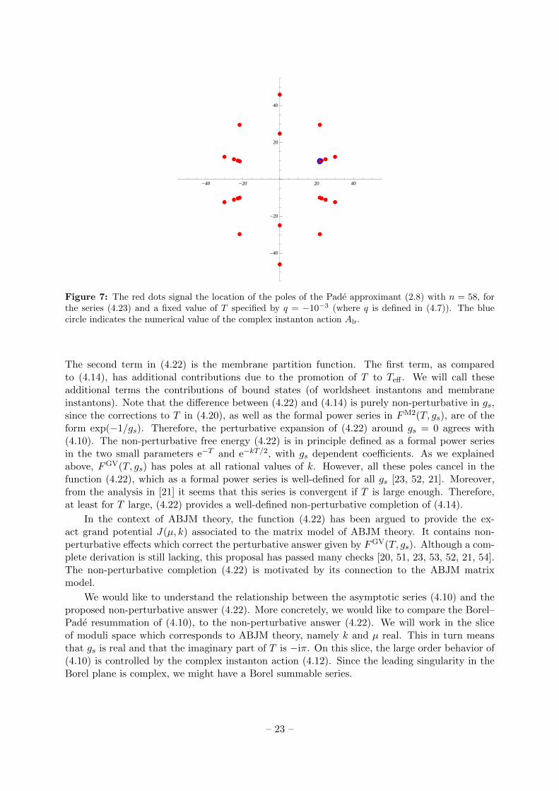
Figure 7: The red dots signal the location of the poles of the Pade approximant (2.8) with n = 58, forthe series (4.23) and a fixed value of T specified by q = −10−3 (where q is defined in (4.7)). The bluecircle indicates the numerical value of the complex instanton action Alr.

The second term in (4.22) is the membrane partition function. The first term, as comparedto (4.14), has additional contributions due to the promotion of T to Teff . We will call theseadditional terms the contributions of bound states (of worldsheet instantons and membraneinstantons). Note that the difference between (4.22) and (4.14) is purely non-perturbative in gs,since the corrections to T in (4.20), as well as the formal power series in FM2(T, gs), are of theform exp(−1/gs). Therefore, the perturbative expansion of (4.22) around gs = 0 agrees with(4.10). The non-perturbative free energy (4.22) is in principle defined as a formal power seriesin the two small parameters e−T and e−kT/2, with gs dependent coefficients. As we explainedabove, FGV(T, gs) has poles at all rational values of k. However, all these poles cancel in thefunction (4.22), which as a formal power series is well-defined for all gs [23, 52, 21]. Moreover,from the analysis in [21] it seems that this series is convergent if T is large enough. Therefore,at least for T large, (4.22) provides a well-defined non-perturbative completion of (4.14).

In the context of ABJM theory, the function (4.22) has been argued to provide the ex-act grand potential J(µ, k) associated to the matrix model of ABJM theory. It contains non-perturbative effects which correct the perturbative answer given by FGV(T, gs). Although a com-plete derivation is still lacking, this proposal has passed many checks [20, 51, 23, 53, 52, 21, 54].The non-perturbative completion (4.22) is motivated by its connection to the ABJM matrixmodel.

We would like to understand the relationship between the asymptotic series (4.10) and theproposed non-perturbative answer (4.22). More concretely, we would like to compare the Borel–Pade resummation of (4.10), to the non-perturbative answer (4.22). We will work in the sliceof moduli space which corresponds to ABJM theory, namely k and µ real. This in turn meansthat gs is real and that the imaginary part of T is −iπ. On this slice, the large order behavior of(4.10) is controlled by the complex instanton action (4.12). Since the leading singularity in theBorel plane is complex, we might have a Borel summable series.

– 23 –

k FBP54 (T, gs) error FNP(T, gs) error difference

2 0.0037 10−5 0.0056228650 10−11 0.0019

4 0.000996873 10−10 0.000993519297616245561182089 10−28 - 3.354 ·10−6

6 0.0013366713318 10−14 0.0013366762433924625954836366 10−29 4.9116 ·10−9

8 0.00200549863390460 10−18 0.0020054986273950134496944117 10−29 -6.50958 ·10−12

10 0.00290255648876704552 10−21 0.002902556488775177021081745 10−28 8.13151 ·10−15

12 0.00401133227863213883147 10−24 0.00401133227863212905949245 10−27 -9.77197 ·10−18

14 0.0053270579960529530912943 10−26 0.00532705799605295310272304 10−27 1.14287 ·10−20

16 0.0068479115274744906938481552 10−29 0.00684791152747449069383505 10−27 -1.310 ·10−23

Table 4: In this table we show the values for the Borel-Pade resummation of the series (4.10), for differentintegers k and q = −10−3, as well as the values of FNP up to order Q10. In both cases we give an estimateof the numerical error. The last column shows the numerical value of the difference (4.25).

We then proceed as in the previous section: we define the Borel–Pade transform as

ϕ(ζ) =∑g≥2

ζ2g−2 Fg(T )

(2g − 2)!, (4.23)

and we consider its Pade approximants. The first thing we can do is to examine their poles in theBorel plane. The results are shown in Fig. 7, for the point in the moduli space with q = −10−3

and for an approximant (2.8) with n = 58. We notice that indeed, the pole which is closest tothe origin agrees with the analytic value

Alr ≈ 21.69 + 9.87i. (4.24)

There are no stable poles on the positive real axis, so the series seems to be Borel summable,and we can perform a Borel–Pade resummation of the series (4.10). Like before, we will denoteby FBP

n (T, gs) the result of the resummation by using a Pade approximant of order n.We can also compute the proposed non-perturbative answer (4.22) for different values of

T , gs. In this case, this answer is only known in the form of a conjecturally convergent series,therefore there is a numerical error associated to the truncation of this series. We estimate theerror in FNP(T, gs) as follows: we first consider the series (4.22), where the Gopakumar–Vafaseries is truncated at order Q10, and the series involving the non-perturbative effects is truncatedat order ` =

[20k

]. Then we consider the sames series with truncation at Q12 and ` =

[24k

]. The

difference between these two results will be taken as a reliable error estimate7.We can now compare both results, the Borel–Pade resummation and the non-perturbative

result (4.22). Our numerical results show conclusively that they are different. This is shown intable 4, where we consider a value of the Kahler parameter corresponding to q = −10−3. Asin the situation of the previous section, and in the case of the quartic oscillator, we interpretthis difference as due to non-perturbative effects associated to complex instantons. The leadingcomplex instanton has action given by (4.12), and we expect, for n large enough,

FNP(T, gs)− FBPn (T, gs) ∼ cos

(Im (Alr(T ))

k

2π+ φ

)exp

[− k

2πRe (Alr(T ))

]. (4.25)

where φ is a phase. In order to test this expectation, we can fix T , produce a sequence with thevalues of the l.h.s. of (4.25) as a function of k, and fit it to a function of the form shown in ther.h.s. In Fig. 8 we show the fit of

log∣∣FNP(T, gs)− FBP

54 (T, gs)∣∣ (4.26)

7For k = 2 we estimated the error by truncating the series at Q6 and at Q4

– 24 –

ææ

ææ

ææ

æ

ææææææææ

ææ

ææ

ææ

æ

æ

æ

æææææææ

ææ

ææ

ææ

æ

æ

æææææææ

ææ

ææ

ææ

æ

æ

æææææææ

ææ

ææ

ææ

æ

æ

æææææææ

ææ

ææ

ææ

æ

æ

æææææææ

ææ

ææ

ææ

æ

æ

æææææææ

ææ

ææ

ææ

æ

æ

æææææææ

ææ

ææ

ææ

æ

æ

æææææææ

ææ

ææ

ææ

æ

æ

æææææ

5 10 15 20k

-80

-60

-40

-20

0

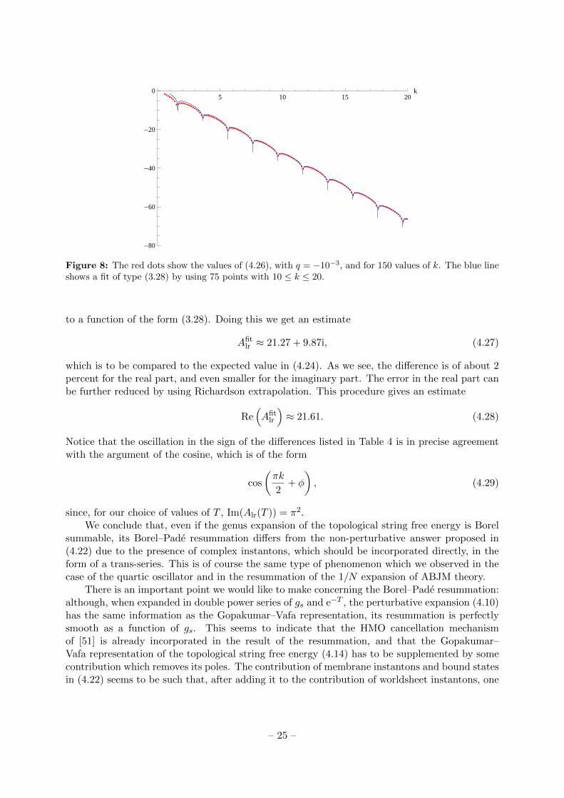
Figure 8: The red dots show the values of (4.26), with q = −10−3, and for 150 values of k. The blue lineshows a fit of type (3.28) by using 75 points with 10 ≤ k ≤ 20.

to a function of the form (3.28). Doing this we get an estimate

Afitlr ≈ 21.27 + 9.87i, (4.27)

which is to be compared to the expected value in (4.24). As we see, the difference is of about 2percent for the real part, and even smaller for the imaginary part. The error in the real part canbe further reduced by using Richardson extrapolation. This procedure gives an estimate

Re(Afit

lr

)≈ 21.61. (4.28)

Notice that the oscillation in the sign of the differences listed in Table 4 is in precise agreementwith the argument of the cosine, which is of the form

cos

(πk

2+ φ

), (4.29)

since, for our choice of values of T , Im(Alr(T )) = π2.We conclude that, even if the genus expansion of the topological string free energy is Borel

summable, its Borel–Pade resummation differs from the non-perturbative answer proposed in(4.22) due to the presence of complex instantons, which should be incorporated directly, in theform of a trans-series. This is of course the same type of phenomenon which we observed in thecase of the quartic oscillator and in the resummation of the 1/N expansion of ABJM theory.

There is an important point we would like to make concerning the Borel–Pade resummation:although, when expanded in double power series of gs and e−T , the perturbative expansion (4.10)has the same information as the Gopakumar–Vafa representation, its resummation is perfectlysmooth as a function of gs. This seems to indicate that the HMO cancellation mechanismof [51] is already incorporated in the result of the resummation, and that the Gopakumar–Vafa representation of the topological string free energy (4.14) has to be supplemented by somecontribution which removes its poles. The contribution of membrane instantons and bound statesin (4.22) seems to be such that, after adding it to the contribution of worldsheet instantons, one

– 25 –

4.02 4.04 4.06 4.08 4.10 4.12 4.14k

-0.0010

-0.0005

0.0005

0.0010

0.0015

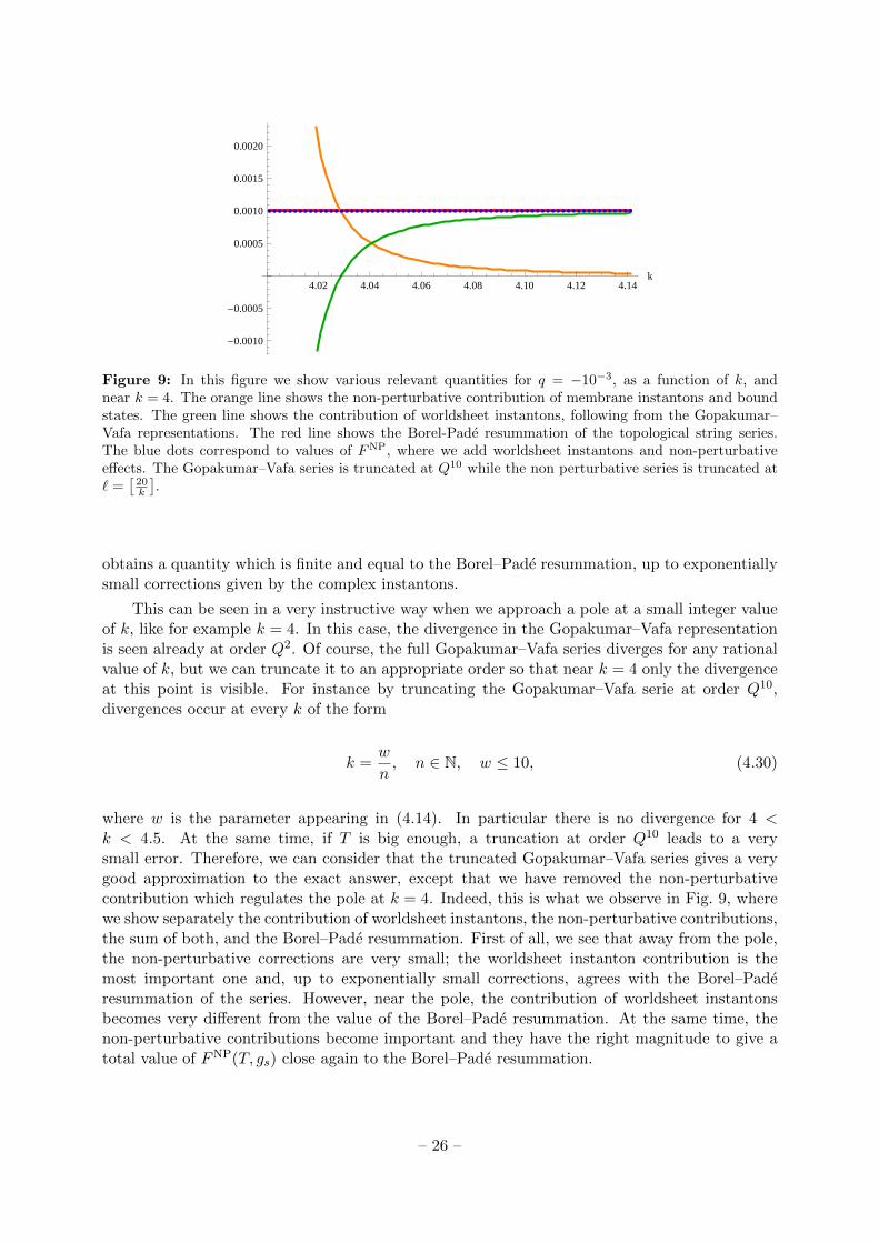
0.0020

Figure 9: In this figure we show various relevant quantities for q = −10−3, as a function of k, andnear k = 4. The orange line shows the non-perturbative contribution of membrane instantons and boundstates. The green line shows the contribution of worldsheet instantons, following from the Gopakumar–Vafa representations. The red line shows the Borel-Pade resummation of the topological string series.The blue dots correspond to values of FNP, where we add worldsheet instantons and non-perturbativeeffects. The Gopakumar–Vafa series is truncated at Q10 while the non perturbative series is truncated at` =

[20k

].

obtains a quantity which is finite and equal to the Borel–Pade resummation, up to exponentiallysmall corrections given by the complex instantons.

This can be seen in a very instructive way when we approach a pole at a small integer valueof k, like for example k = 4. In this case, the divergence in the Gopakumar–Vafa representationis seen already at order Q2. Of course, the full Gopakumar–Vafa series diverges for any rationalvalue of k, but we can truncate it to an appropriate order so that near k = 4 only the divergenceat this point is visible. For instance by truncating the Gopakumar–Vafa serie at order Q10,divergences occur at every k of the form

k =w

n, n ∈ N, w ≤ 10, (4.30)

where w is the parameter appearing in (4.14). In particular there is no divergence for 4 <k < 4.5. At the same time, if T is big enough, a truncation at order Q10 leads to a verysmall error. Therefore, we can consider that the truncated Gopakumar–Vafa series gives a verygood approximation to the exact answer, except that we have removed the non-perturbativecontribution which regulates the pole at k = 4. Indeed, this is what we observe in Fig. 9, wherewe show separately the contribution of worldsheet instantons, the non-perturbative contributions,the sum of both, and the Borel–Pade resummation. First of all, we see that away from the pole,the non-perturbative corrections are very small; the worldsheet instanton contribution is themost important one and, up to exponentially small corrections, agrees with the Borel–Paderesummation of the series. However, near the pole, the contribution of worldsheet instantonsbecomes very different from the value of the Borel–Pade resummation. At the same time, thenon-perturbative contributions become important and they have the right magnitude to give atotal value of FNP(T, gs) close again to the Borel–Pade resummation.

– 26 –

5. Conclusions and prospects

In this paper, by combining the AdS/CFT correspondence with results on the localization ofABJM theory and its 1/N expansion, we have been able to study the resummation of the stringperturbation series in some examples, and compare it with the non-perturbative answer. Ourmain result is that, although the series seems to be Borel summable, it lacks explicit non-perturbative information due to the presence of complex instantons. This type of behaviorappears in a much simpler model, first studied from this point of view by Balian, Parisi and Voros[18], namely the WKB series for the pure quartic oscillator in Quantum Mechanics. Although thisWKB series is technically non-Borel summable, the leading, exponentially small error obtainedin performing lateral Borel resummations is not due to the poles in the positive real axis, but tothe poles associated to complex instantons.

The results of this paper confirm that Borel summability is not a crucial property of asymp-totic series. The key issue when faced with a perturbative scheme is whether we can extractthe exact answer from just the perturbative series, or we have to include additional informa-tion. It is well-known that Borel summability is a necessary condition for this extraction, sincewhen the series is not Borel summable one is forced to add non-perturbative sectors. However,being Borel summable is not a sufficient condition, since additional requirements are needed inorder to reconstruct the original exact answer (like those appearing in Watson’s theorem andits extensions). As we have argued in section 2, the mismatch between the Borel resummationof a Borel summable series and the exact answer is made possible by the presence of complexinstantons. For this reason, this mismatch is not found in examples where complex instantonsare absent, like the anharmonic quartic oscillator, where the Borel resummation agrees with thenon-perturbative result [5].

It would be interesting to see in which cases the presence of complex instantons in a Borel-summable theory leads to a mismatch between Borel resummation and the non-perturbativeresult. Complex instantons seem to be necessary for this mismatch to occur, but they are notsufficient, and we know of an explicit example where this can be seen: in the N vector modelstudied in [64], we have verified that the Borel–Pade resummation of the 1/N expansion of thefree energy agrees with the exact result, in spite of the presence of complex instantons. A rich setof examples to study could come from non-unitary 2d CFTs coupled to 2d gravity. For example,the Yang–Lee singularity coupled to two-dimensional gravity leads to a Borel summable seriesfor the specific heat, yet it contains complex instantons, and a non-perturbative definition hasbeen proposed (see for example [65] for a review and relevant references). To our knowledge,the Borel resummation of the series has not been compared in detail to the non-perturbativeanswer. Of course, beyond a list of examples and counter-examples, we would like to know ifthere is a simple criterium to determine in advance what is the relationship between the Borelresummation of the perturbative series and the exact answer.

The next step in our research program would be to incorporate the complex instantons inan explicit way, through a trans-series ansatz. By the general theory of non-perturbative effects,we expect the exact answer to be given by the Borel resummation of a formal power series ofthe form (2.11). This is given by the Borel resummation of the perturbative series, plus theBorel resummation of multi-instanton series, with certain weights which have to be determined.In the case of ABJM theory and topological strings, the most promising avenue for computingthis formal trans-series is the formalism of [31], based on the holomorphic anomaly equations of[57], suitably extended to the non-perturbative sector. This would provide, in the context of thegenus expansion, a detailed understanding of the non-perturbative effects in these theories. It

– 27 –

would also make it possible to test some aspects of the proposal of [21] in models with no knownlarge N dual, like local P2. We hope to report on these and related problems in the near future.

Acknowledgements

We would like to thank Ricardo Couso-Santamarıa, Jean–Pierre Eckmann, Pavel Putrov, RicardoSchiappa and Peter Wittwer for useful conversations. We are particularly grateful to RicardoSchiappa for a detailed reading of the manuscript. This work is supported by the Fonds NationalSuisse, subsidies 200020-141329 and 200020-137523.

References

[1] E. Caliceti, M. Meyer-Hermann, P. Ribeca, A. Surzhykov and U. D. Jentschura, “From usefulalgorithms for slowly convergent series to physical predictions based on divergent perturbativeexpansions,” Phys. Rept. 446, 1 (2007) [arXiv:0707.1596 [physics.comp-ph]].

[2] M. Marino, “Lectures on non-perturbative effects in large N gauge theories, matrix models andstrings,” Fortsch. Phys. 62, 455 (2014) [arXiv:1206.6272 [hep-th]].

[3] C. M. Bender and T. T. Wu, “Anharmonic oscillator,” Phys. Rev. 184, 1231 (1969).

[4] C. M. Bender and T. T. Wu, “Anharmonic oscillator. 2: A Study of perturbation theory in largeorder,” Phys. Rev. D 7, 1620 (1973).

[5] S. Graffi, V. Grecchi and B. Simon, “Borel summability: Application to the anharmonic oscillator,”Phys. Lett. B 32, 631 (1970).

[6] J. Zinn-Justin, “Multi - Instanton Contributions In Quantum Mechanics,” Nucl. Phys. B 192, 125(1981); “Multi - Instanton Contributions In Quantum Mechanics. 2.,” Nucl. Phys. B 218, 333(1983).

[7] J. Zinn-Justin and U. D. Jentschura, “Multi-instantons and exact results I: Conjectures, WKBexpansions, and instanton interactions,” Annals Phys. 313, 197 (2004) [arXiv:quant-ph/0501136];“Multi-Instantons And Exact Results II: Specific Cases, Higher-Order Effects, And NumericalCalculations,” Annals Phys. 313, 269 (2004) [arXiv:quant-ph/0501137].

[8] M. Marino, “Non-perturbative effects and non-perturbative definitions in matrix models andtopological strings,” JHEP 0812, 114 (2008) [arXiv:0805.3033 [hep-th]].

[9] S.H. Shenker, “The strength of nonperturbative effects in string theory,” in O. Alvarez, E. Marinariand P. Windey (eds.), Random Surfaces and Quantum Gravity, Plenum, New York 1992.

[10] D. J. Gross and V. Periwal, “String Perturbation Theory Diverges,” Phys. Rev. Lett. 60, 2105(1988).

[11] P. F. Mende and H. Ooguri, “Borel Summation of String Theory for Planck Scale Scattering,” Nucl.Phys. B 339, 641 (1990).

[12] I. R. Klebanov, J. M. Maldacena and N. Seiberg, “Unitary and complex matrix models as 1-d type0 strings,” Commun. Math. Phys. 252, 275 (2004) [hep-th/0309168].

[13] A. Sen, “S-duality Improved Superstring Perturbation Theory,” JHEP 1311, 029 (2013)[arXiv:1304.0458 [hep-th]].

[14] O. Aharony, O. Bergman, D. L. Jafferis and J. Maldacena, “N=6 superconformalChern-Simons-matter theories, M2-branes and their gravity duals,” JHEP 0810, 091 (2008)[arXiv:0806.1218 [hep-th]].

– 28 –

[15] A. Kapustin, B. Willett and I. Yaakov, “Exact Results for Wilson Loops in SuperconformalChern-Simons Theories with Matter,” JHEP 1003, 089 (2010) [arXiv:0909.4559 [hep-th]].

[16] N. Drukker, M. Marino, P. Putrov, “From weak to strong coupling in ABJM theory,” Commun.Math. Phys. 306, 511-563 (2011). [arXiv:1007.3837 [hep-th]].

[17] N. Drukker, M. Marino and P. Putrov, “Nonperturbative aspects of ABJM theory,” JHEP 1111,141 (2011) [arXiv:1103.4844 [hep-th]].

[18] R. Balian, G. Parisi and A. Voros, “Discrepancies from asymptotic series and their relation tocomplex classical trajectories,” Phys. Rev. Lett. 41, 1141 (1978); “Quartic Oscillator,” in FeynmanPath Integrals, Lecture Notes in Physics 106, 337 (1979).

[19] M. Marino and P. Putrov, “Exact Results in ABJM Theory from Topological Strings,” JHEP 1006,011 (2010) [arXiv:0912.3074 [hep-th]].

[20] M. Marino and P. Putrov, “ABJM theory as a Fermi gas,” J. Stat. Mech. 1203, P03001 (2012)[arXiv:1110.4066 [hep-th]].

[21] Y. Hatsuda, M. Marino, S. Moriyama and K. Okuyama, “Non-perturbative effects and the refinedtopological string,” JHEP 1409, 168 (2014) [arXiv:1306.1734 [hep-th]].

[22] R. Gopakumar and C. Vafa, “M theory and topological strings. 2.,” hep-th/9812127.

[23] Y. Hatsuda, S. Moriyama and K. Okuyama, “Instanton Effects in ABJM Theory from Fermi GasApproach,” JHEP 1301, 158 (2013) [arXiv:1211.1251 [hep-th]].

[24] A. Voros, “The return of the quartic oscillator. The complex WKB method,” Ann. Inst. H. PoincareA 39, 211 (1983).

[25] T. M. Seara and D. Sauzin, “Ressumacio de Borel i teoria de la ressurgencia,” Bull. Soc. Cat. deMat. 18 (2003) 19.

[26] S. Garoufalidis, A. Its, A. Kapaev and M. Marino, “Asymptotics of the instantons of Painleve I,”Int. Math. Res. Notices 2012 (2012) 561 [arXiv:1002.3634].

[27] I. Aniceto and R. Schiappa, “Nonperturbative Ambiguities and the Reality of ResurgentTransseries,” Commun. Math. Phys. 335, no. 1, 183 (2015) [arXiv:1308.1115 [hep-th]].

[28] G. V. Dunne and M. Unsal, “Resurgence and Trans-series in Quantum Field Theory: The CP(N-1)Model,” JHEP 1211, 170 (2012) [arXiv:1210.2423 [hep-th]].

[29] A. Cherman, D. Dorigoni, G. V. Dunne and M. Unsal, “Resurgence in QFT: Unitons, Fractons andRenormalons in the Principal Chiral Model,” Phys. Rev. Lett. 112, 021601 (2014) [arXiv:1308.0127[hep-th]].

[30] I. Aniceto, R. Schiappa and M. Vonk, “The Resurgence of Instantons in String Theory,” Commun.Num. Theor. Phys. 6, 339 (2012) [arXiv:1106.5922 [hep-th]].

[31] R. C. Santamarıa, J. D. Edelstein, R. Schiappa and M. Vonk, “Resurgent Transseries and theHolomorphic Anomaly,” arXiv:1308.1695 [hep-th].

[32] E. Delabaere, H. Dillinger and F. Pham, “Exact semiclassical expansions for one-dimensionalquantum oscillators,” J. Math. Phys. 38, 6126 (1997).

[33] E. Brezin, J. -C. Le Guillou and J. Zinn-Justin, “Perturbation Theory at Large Order. 2. Role ofthe Vacuum Instability,” Phys. Rev. D 15, 1558 (1977).

[34] G. Basar, G. V. Dunne and M. Unsal, “Resurgence theory, ghost-instantons, and analyticcontinuation of path integrals,” JHEP 1310, 041 (2013) [arXiv:1308.1108 [hep-th]].

[35] J. L. Dunham, “The Wentzel–Brillouin–Kramers method of solving the wave equation,” Phys. Rev.41, 713 (1932).

– 29 –

[36] H. Taseli, “Accurate computation of the energy spectrum for potentials with multiminima”,International Journal of Quantum Chemistry, Vol. 46, pp. 319-334, 1993.

[37] K. Banerjee, S. P. Bhatnagar, V. Choudhry, S. S. Kanwal, “The Anharmonic Oscillator”,Proceedings of the Royal Society of London. Series A, Mathematical and Physical Sciences, 1703(1978) 360.

[38] U. D. Jentschura, “The Resummation of nonalternating divergent perturbative expansions,” Phys.Rev. D 62, 076001 (2000) [hep-ph/0001135].

[39] J. M. Maldacena, “The Large N limit of superconformal field theories and supergravity,” Adv.Theor. Math. Phys. 2, 231 (1998) [hep-th/9711200].

[40] J. G. Russo, “A Note on perturbation series in supersymmetric gauge theories,” JHEP 1206, 038(2012) [arXiv:1203.5061 [hep-th]].

[41] J. Bagger, N. Lambert, S. Mukhi and C. Papageorgakis, “Multiple Membranes in M-theory,” Phys.Rept. 527, 1 (2013) [arXiv:1203.3546 [hep-th]].

[42] M. Marino, “Lectures on localization and matrix models in supersymmetric Chern-Simons-mattertheories,” J. Phys. A 44, 463001 (2011) [arXiv:1104.0783 [hep-th]].

[43] O. Bergman and S. Hirano, “Anomalous radius shift in AdS4/CFT3,” JHEP 0907, 016 (2009)[arXiv:0902.1743].

[44] O. Aharony, A. Hashimoto, S. Hirano, P. Ouyang, “D-brane charges in gravitational duals of 2+1dimensional gauge theories and duality cascades,” JHEP 1001, 072 (2010). [arXiv:0906.2390].

[45] S. Bhattacharyya, A. Grassi, M. Marino and A. Sen, “A One-Loop Test of Quantum Supergravity,”Class. Quant. Grav. 31, 015012 (2014) [arXiv:1210.6057 [hep-th]].

[46] M. Hanada, M. Honda, Y. Honma, J. Nishimura, S. Shiba and Y. Yoshida, “Numerical studies ofthe ABJM theory for arbitrary N at arbitrary coupling constant,” JHEP 1205, 121 (2012)[arXiv:1202.5300 [hep-th]].

[47] S. Pasquetti and R. Schiappa, “Borel and Stokes Nonperturbative Phenomena in Topological StringTheory and c=1 Matrix Models,” Annales Henri Poincare 11, 351 (2010) [arXiv:0907.4082 [hep-th]].

[48] A. B. Zamolodchikov, “Painleve III and 2-d polymers,” Nucl. Phys. B 432, 427 (1994)[hep-th/9409108].

[49] C. A. Tracy and H. Widom, “Proofs of two conjectures related to the thermodynamic Betheansatz,” Commun. Math. Phys. 179, 667 (1996) [solv-int/9509003].

[50] P. Putrov and M. Yamazaki, “Exact ABJM Partition Function from TBA,” Mod. Phys. Lett. A 27,1250200 (2012) [arXiv:1207.5066 [hep-th]].

[51] Y. Hatsuda, S. Moriyama and K. Okuyama, “Exact Results on the ABJM Fermi Gas,” JHEP1210, 020 (2012) [arXiv:1207.4283 [hep-th]].

[52] Y. Hatsuda, S. Moriyama and K. Okuyama, “Instanton Bound States in ABJM Theory,” JHEP1305, 054 (2013) [arXiv:1301.5184 [hep-th]].

[53] F. Calvo and M. Marino, “Membrane instantons from a semiclassical TBA,” JHEP 1305, 006(2013) [arXiv:1212.5118 [hep-th]].

[54] J. Kallen and M. Marino, “Instanton effects and quantum spectral curves,” arXiv:1308.6485[hep-th].

[55] S. H. Katz, A. Klemm and C. Vafa, “Geometric engineering of quantum field theories,” Nucl. Phys.B 497, 173 (1997) [hep-th/9609239].

[56] M. Aganagic, A. Klemm, M. Marino and C. Vafa, “Matrix model as a mirror of Chern-Simonstheory,” JHEP 0402, 010 (2004) [hep-th/0211098].

– 30 –

[57] M. Bershadsky, S. Cecotti, H. Ooguri and C. Vafa, “Kodaira-Spencer theory of gravity and exactresults for quantum string amplitudes,” Commun. Math. Phys. 165, 311 (1994) [hep-th/9309140].

[58] B. Haghighat, A. Klemm and M. Rauch, “Integrability of the holomorphic anomaly equations,”JHEP 0810, 097 (2008) [arXiv:0809.1674 [hep-th]].

[59] A. Iqbal, C. Kozcaz and C. Vafa, “The Refined topological vertex,” JHEP 0910, 069 (2009)[hep-th/0701156].

[60] N. A. Nekrasov and S. L. Shatashvili, “Quantization of Integrable Systems and Four DimensionalGauge Theories,” arXiv:0908.4052 [hep-th].

[61] A. Mironov and A. Morozov, “Nekrasov Functions and Exact Bohr-Sommerfeld Integrals,” JHEP1004, 040 (2010) [arXiv:0910.5670 [hep-th]].

[62] M. Aganagic, M. C. N. Cheng, R. Dijkgraaf, D. Krefl and C. Vafa, “Quantum Geometry of RefinedTopological Strings,” JHEP 1211, 019 (2012) [arXiv:1105.0630 [hep-th]].

[63] M. -x. Huang, A. Klemm, J. Reuter and M. Schiereck, “Quantum geometry of del Pezzo surfaces inthe Nekrasov-Shatashvili limit,” JHEP 1502, 031 (2015) [arXiv:1401.4723 [hep-th]].

[64] S. Hikami and E. Brezin, “Large Order Behavior of the 1/N Expansion in Zero-dimensions andOne-dimensions,” J. Phys. A 12 (1979) 759.

[65] P. Di Francesco, P. H. Ginsparg and J. Zinn-Justin, “2-D Gravity and random matrices,” Phys.Rept. 254, 1 (1995) [hep-th/9306153].

– 31 –