AIRY WAVE PACKETS AS QUANTUM SOLUTIONS FOR …
88
AIRY WAVE PACKETS AS QUANTUM SOLUTIONS FOR RECOVERING CLASSICAL TRAJECTORIES by Vern Philip Hart II A senior thesis submitted to the faculty of Brigham Young University in partial fulfillment of the requirements for the degree of Bachelor of Science Department of Physics and Astronomy Brigham Young University August 2006
Transcript of AIRY WAVE PACKETS AS QUANTUM SOLUTIONS FOR …
AIRY WAVE PACKETS AS QUANTUM SOLUTIONS FOR RECOVERING
CLASSICAL TRAJECTORIES
by
Vern Philip Hart II
A senior thesis submitted to the faculty of
Brigham Young University
in partial fulfillment of the requirements for the degree of
Bachelor of Science
Department of Physics and Astronomy
Brigham Young University
August 2006

Copyright c© 2006 Vern Philip Hart II
All Rights Reserved
BRIGHAM YOUNG UNIVERSITY
DEPARTMENT APPROVAL
of a senior thesis submitted by
Vern Philip Hart II
This thesis has been reviewed by the research advisor, research coordinator,and department chair and has been found to be satisfactory.
Date Jean-Francois S. Van Huele, Advisor
Date Eric G. Hintz, Research Coordinator
Date Scott D. Sommerfeldt, Chair

ABSTRACT
AIRY WAVE PACKETS AS QUANTUM SOLUTIONS FOR RECOVERING
CLASSICAL TRAJECTORIES
Vern Philip Hart II
Department of Physics and Astronomy
Bachelor of Science
We use quantum mechanics to describe J.J. Thomson’s experiment for deter-
mining the mass-to-charge ratio me
of the electron. We review the derivation
of Thomson’s classical trajectories in the electrostatic and magnetic fields.
We model Thomson’s capacitor and obtain the stationary wave mechanical
solutions. We construct wave packets representing the transverse probability
amplitude of the beam. We allow this packet to evolve in time to observe
the motion of the peak and compare it with the classical trajectory. As time
progresses the packet disperses and the peak delocalizes. We discuss physical
and numerical causes for this phenomenon. We also use the analytic solution
in momentum space to characterize the wave packets. We consider the prob-
lem in the Heisenberg representation and confirm the correspondence between
quantum expectation values and classical trajectories. The uncertainties of
the Thomson trajectories are identical to those of the undeflected beam.

ACKNOWLEDGMENTS
I would like to thank my family and friends for their invaluable support
and encouragement during the entirety of this project. I would like to thank
Jacque Jackson for the help and support she gave me. I would also like to thank
Dr. Jean-Francois Van Huele for the countless hours he spent assisting and
guiding me throughout the course of my research and for his valued suggestions
while writing my thesis. I would especially like to thank my Mother for the
irreplaceable source of strength and encouragement she has been during the
entire course of my life and for always being there for me when I needed her
to be. Thank you again to all those who assisted me in this endeavor.

Contents
Table of Contents vii
List of Figures ix
1 Introduction 1
2 The Thomson Experiment 32.1 J. J. Thomson’s e
mmeasurements . . . . . . . . . . . . . . . . . . . . 3
2.2 J. J. Thomson’s equations . . . . . . . . . . . . . . . . . . . . . . . . 42.3 The capacitor model and sloped wells . . . . . . . . . . . . . . . . . . 6
3 Trajectories as Classical Solutions 93.1 The electric field . . . . . . . . . . . . . . . . . . . . . . . . . . . . . 93.2 The magnetic field . . . . . . . . . . . . . . . . . . . . . . . . . . . . 143.3 The electromagnetic field . . . . . . . . . . . . . . . . . . . . . . . . . 23
4 Wave Packets as Quantum Solutions 274.1 Constant potentials . . . . . . . . . . . . . . . . . . . . . . . . . . . . 284.2 Linear potentials and Airy functions . . . . . . . . . . . . . . . . . . 294.3 Airy wave packets . . . . . . . . . . . . . . . . . . . . . . . . . . . . . 324.4 Normalization . . . . . . . . . . . . . . . . . . . . . . . . . . . . . . . 36
5 Deflection from Wave Packet Evolution 395.1 Dispersion . . . . . . . . . . . . . . . . . . . . . . . . . . . . . . . . . 395.2 Dispersion-controlling techniques . . . . . . . . . . . . . . . . . . . . 40
5.2.1 Expectation values . . . . . . . . . . . . . . . . . . . . . . . . 405.2.2 Energy level selection . . . . . . . . . . . . . . . . . . . . . . . 47
5.3 Robinett’s analytic solution . . . . . . . . . . . . . . . . . . . . . . . 485.4 Dispersion times comparison . . . . . . . . . . . . . . . . . . . . . . . 535.5 Discussion . . . . . . . . . . . . . . . . . . . . . . . . . . . . . . . . . 53
6 Conclusion 57
Bibliography 59
vii
viii CONTENTS
A Another Approach to the E-B Relationship 61
B Maple Code for the Construction of the Wave Packet 63
C Further Localization of the Probability Amplitude 67
D Quantum Mechanical Justification Based on the Heisenberg Picture 71
Index 77
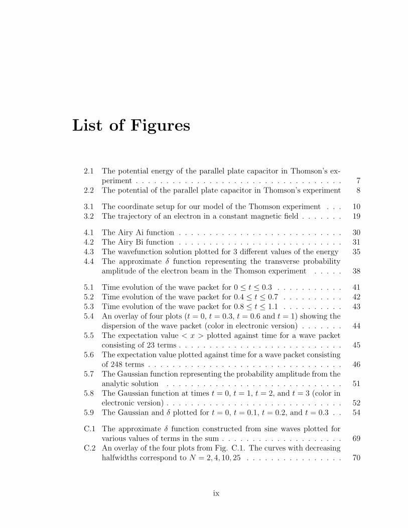
List of Figures
2.1 The potential energy of the parallel plate capacitor in Thomson’s ex-periment . . . . . . . . . . . . . . . . . . . . . . . . . . . . . . . . . . 7
2.2 The potential of the parallel plate capacitor in Thomson’s experiment 8
3.1 The coordinate setup for our model of the Thomson experiment . . . 103.2 The trajectory of an electron in a constant magnetic field . . . . . . . 19
4.1 The Airy Ai function . . . . . . . . . . . . . . . . . . . . . . . . . . . 304.2 The Airy Bi function . . . . . . . . . . . . . . . . . . . . . . . . . . . 314.3 The wavefunction solution plotted for 3 different values of the energy 354.4 The approximate δ function representing the transverse probability
amplitude of the electron beam in the Thomson experiment . . . . . 38
5.1 Time evolution of the wave packet for 0 ≤ t ≤ 0.3 . . . . . . . . . . . 415.2 Time evolution of the wave packet for 0.4 ≤ t ≤ 0.7 . . . . . . . . . . 425.3 Time evolution of the wave packet for 0.8 ≤ t ≤ 1.1 . . . . . . . . . . 435.4 An overlay of four plots (t = 0, t = 0.3, t = 0.6 and t = 1) showing the
dispersion of the wave packet (color in electronic version) . . . . . . . 445.5 The expectation value < x > plotted against time for a wave packet
consisting of 23 terms . . . . . . . . . . . . . . . . . . . . . . . . . . . 455.6 The expectation value plotted against time for a wave packet consisting
of 248 terms . . . . . . . . . . . . . . . . . . . . . . . . . . . . . . . . 465.7 The Gaussian function representing the probability amplitude from the
analytic solution . . . . . . . . . . . . . . . . . . . . . . . . . . . . . 515.8 The Gaussian function at times t = 0, t = 1, t = 2, and t = 3 (color in
electronic version) . . . . . . . . . . . . . . . . . . . . . . . . . . . . . 525.9 The Gaussian and δ plotted for t = 0, t = 0.1, t = 0.2, and t = 0.3 . . 54
C.1 The approximate δ function constructed from sine waves plotted forvarious values of terms in the sum . . . . . . . . . . . . . . . . . . . . 69
C.2 An overlay of the four plots from Fig. C.1. The curves with decreasinghalfwidths correspond to N = 2, 4, 10, 25 . . . . . . . . . . . . . . . . 70
ix

Chapter 1
Introduction
Classical mechanics is an approximate description of physical reality. Quantum me-
chanics was developed to improve it and to provide a more complete representation of
physical phenomena. It also explains and predicts new phenomena like the stability
of matter and its interaction with radiation.
There exist several fundamental differences between these two theories. Their
application domains are typically vastly different. As a result, systems are commonly
treated in the literature as either quantum or classical. Specific systems that exhibit
strong classical or quantum behavior are better understood in their respective theory.
Quantum theory, however, claims to be the more accurate theory for describing all
physical systems. We should thus be able to describe any physical system using a
quantum approach, even those where the classical description is typically sufficient.
Achieving an agreement between these two descriptions of the same system is the
goal of this project.
Quantum mechanics was also assisted in its development by some of the early
experiments of the 20th century. One such experiment was the determination of the
charge-to-mass ratio em
of the electron by J. J. Thomson in 1897. This discovery of the
1
2 Chapter 1 Introduction
electron was crucial in understanding the nature of the atom as well as in achieving
the ability to view the universe from a quantized perspective. It is this experiment
that we choose to study.
Our goal is to apply quantum theory to the Thomson experiment and give its
purely quantum mechanical description. Our survey of descriptions of the Thomson
experiment in the literature has led us to classical models exclusively. We have been
unable to find a quantum mechanical treatment of this experiment.
Our research is exploring to what extent quantum mechanics can be used to
understand the Thomson experiment. We model the capacitor through a potential
and use the time-independent Schrodinger equation to find stationary solutions. We
then superpose those solutions to construct wave packets. We use the wave packets to
represent the cathode ray beam in Thomson’s experiment and allow them to evolve in
time. We deal with quantum effects such as dispersion and localization. We compare
our results with the classical solutions, namely, the trajectories of the electron beam
in the electric field.
In Chapter 2 we give the history of the Thomson experiment and describe the
quantum mechanical model of the capacitor. In Chapter 3 we derive the classical tra-
jectories from the force law. Chapter 4 explores the nature of the quantum solutions
and describes the construction of the wave packet and its normalization. Chapter
5 addresses the time evolution of the packet, discusses methods for analyzing and
controlling dispersion, and gives an analytic solution based on momentum space for
comparison to the numeric results. We conclude in Chapter 6. Appendix A derives
another method for obtaining the E − B relationship. Appendix B gives the Maple
code for the construction of the wave packet. Appendix C discusses methods for lo-
calizing the wave packet and Appendix D gives the quantum mechanical justification
for treating the Thomson experiment as a quantum rather than a classical system.

Chapter 2
The Thomson Experiment
In this chapter we review some of Thomson’s work. We discuss the electric and
magnetic fields and their potentials and we comment on the extent that we will be
modeling Thomson’s setup.
2.1 J. J. Thomson’s em measurements
Thomson had been experimenting with the electrostatic discharge properties of vari-
ous gases. For each different gas the velocity of the electrons would vary slightly. This
would change the way that the ray was affected by the field because it would increase
or decrease the exposure time. In turn it would change the amount of deflection that
was observed. The length of the field would also change the exposure time and would
therefore affect the deflection.1
Thomson conducted his experiment numerous times using different tubes and
different gases. Although the field length and initial velocity would vary with each
experiment, they would remain constant during a given experiment.1 Thomson needed
something that could be controlled during each experiment and would lead to the ratio
3
4 Chapter 2 The Thomson Experiment
he was looking for. This was the purpose of the two critical variables E and B. By
changing the amount of current flowing through the coil, Thomson could control the
strength of the magnetic field B. Thomson could also vary the voltage between the
plates and could then adjust the electric field strength E.1
Once a given system had been established, Thomson could make the adjustments
he needed in order to balance the forces. He would obtain slightly different values
each time and would eventually average his results in order to obtain the most accu-
rate value for em
.1 The equations for the electrostatic and electrodynamic forces are
different and are affected by different physical stipulations. They would be adjusted
in different ways during the course of the experiment. The question could then be
raised as to what type of relationship exists between these two field strengths. We
are concerned with creating a balanced force and it might be helpful to understand
this relationship in detail.
2.2 J. J. Thomson’s equations
In conducting his experiment for the determination of the charge-to-mass ratio ( em
)
for an electron, Thomson introduced both electric and magnetic fields. His objective
was to obtain two different forces that would cancel. This cancelation leads to a lack
of deflection in a cathode ray. Electrons feel an electric force from two oppositely
charged conducting plates. The ray bends toward the positive and away from the
negative. Electrons also feel a magnetic force. If the two forces are equal, they cancel
and the cathode ray travels undisturbed.
Let us consider the point where the forces are balanced. This means that the
electric and magnetic forces are equal in magnitude. We can then set the two forces
2.2 J. J. Thomson’s equations 5
on the particle equal to each other and solve. Starting from the Lorentz force law2
~F = q( ~E + ~v × ~B) (2.1)
we specialize in the electric
~F1 = ~Eq (2.2)
and magnetic forces
~F2 = q(~v × ~B). (2.3)
The forces are equal in magnitude.
| ~F1| = | ~F2| (2.4)
| ~E|q = q|~v × ~B| (2.5)
| ~E| = |~v × ~B| (2.6)
Recall that the force vectors are actually opposing each other. Thomson chose the
initial velocity to be perpendicular to the magnetic field. The resultant force is
perpendicular to both. The magnitude of the cross product of two orthogonal vectors
gives us the product of their magnitudes.
|~v × ~B| = |~v||B| sin θ = |~v|| ~B| (2.7)
since
θ =π
2. (2.8)
We now have a simple expression for the relationship between the two field strengths.
It is a function of the velocity of the particle (a very simple one)
E
B= v. (2.9)
Thomson used this result to find the velocity of the electrons in his cathode ray. He
was able to measure the strengths of the E and B fields when there was no deflection
6 Chapter 2 The Thomson Experiment
of the beam and could thus find a value for v. This value was important because he
needed it to determine the value of em
. Thomson measured the radius of curvature R
of the electrons in a magnetic field.1 In section (3.2) we will show that the radius of
this circular trajectory is given by3
R =mv
eB. (2.10)
Thus
m
e=BR
v. (2.11)
Thomson had measured the values of B and R and obtained v through the ratio of
the two fields, Eq. (2.9). He thus was able to determine a value for em
which he
averaged to be 1.6× 10⁻⁷ in c.g.s units.1
2.3 The capacitor model and sloped wells
In classical physics we deal with forces. Particles or objects in a field experience a
force. We can use Newton’s equations to find the motion of these particles as they
travel through space. In quantum mechanics we don’t deal with forces, we deal with
potentials. As such we must model the environment as a potential well rather than
through a force diagram. If we consider the Thomson experiment we have an electric
field being generated by a parallel plate capacitor. Neglecting edge effects at the edge
of the plates, this field is uniform throughout the capacitor itself. Recall the relation
between field and potential2
~E = −~∇V. (2.12)
We can solve for the potential by integrating. Constant fields correspond to linear
potentials. We have a linear potential in the region inside the capacitor. The potential
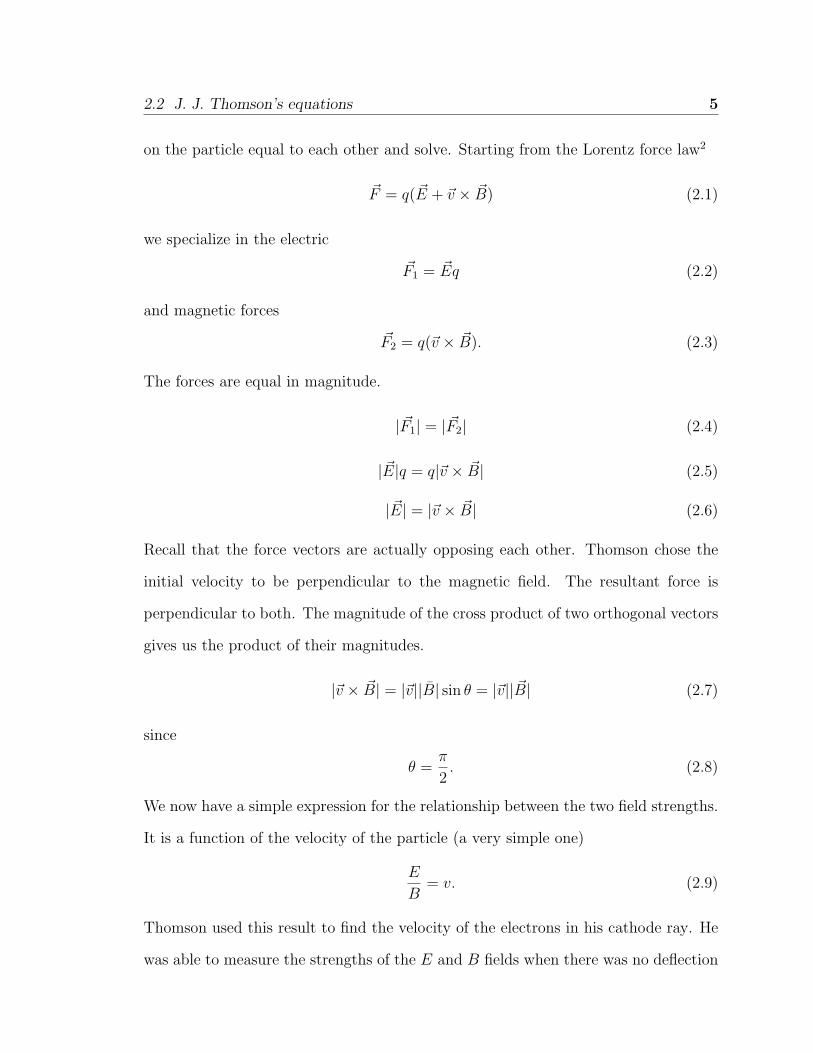
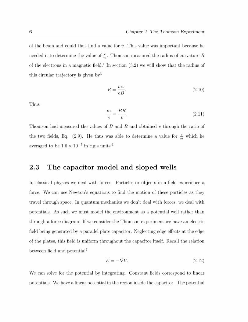
2.3 The capacitor model and sloped wells 7
Figure 2.1 The potential energy of the parallel plate capacitor in Thomson’s
experiment
decreases in the direction in which the field is pointing. It is not the direction the
beam is traveling in but is actually perpendicular to it.
What happens outside of the capacitor? Again, neglecting edge effects, the field
outside is zero. The potential energy is zero in the region below the capacitor. Once
we have traversed the field to the other side, we again have a constant potential but it
is no longer zero. The potential on this side is some non-zero constant. This analysis
of the potential allows us to create a model potential well for our capacitor. The
capacitor can be constructed as shown in Figs. 2.1 and 2.2.
8 Chapter 2 The Thomson Experiment
Figure 2.2 The potential of the parallel plate capacitor in Thomson’s ex-
periment
Chapter 3
Trajectories as Classical Solutions
In this chapter we obtain the trajectories of the particles based on Newtonian theory.
It is important to have these trajectories as a guide for our quantum results. The
electrons in this apparatus experience both an electric and a magnetic force. We
model the system by considering the two fields separately, beginning with the electric
field.
3.1 The electric field
To begin we select appropriate coordinates. For the case of the electric field, the
trajectory will be parabolic rather than circular. I will choose to work in Cartesian
coordinates because a polar coordinate system will not be of any particular advantage.
The initial velocity v0, E, and B are orthogonal in Thomson’s setup. Let us consider
the capacitor to be parallel to the xz plane. Neglecting edge effects we only have a
force in the y direction. A real capacitor is finite and has skewed field lines around
the edges. This creates forces in the xz plane. For our purposes, however, we treat
the capacitor as ideal (see Fig. 3.1).
9

10 Chapter 3 Trajectories as Classical Solutions
Figure 3.1 The coordinate setup for our model of the Thomson experiment
3.1 The electric field 11
The electric force
~F = ~Eq (3.1)
can be inserted into Newton’s second law and expanded as three differential equations
describing the force in each direction.
mx = 0 (3.2)
my = Eq (3.3)
mz = 0 (3.4)
Introducing the acceleration ω, where
ω =Eq
m(3.5)
we obtain
x = 0 (3.6)
y = ω (3.7)
z = 0. (3.8)
Our equation set contains second-order differential equations. The general solutions
of these equations as functions of time are
x(t) = At+B (3.9)
y(t) =1
2ωt2 + Ct+D (3.10)
z(t) = Gt+H, (3.11)
where A, B, C, D, G and H are constants of integration. To find particular solu-
tions we specify boundary conditions for the functions and their first derivatives.
Differentiating our general solutions gives
x = A (3.12)
12 Chapter 3 Trajectories as Classical Solutions
y = ωt+ C (3.13)
z = E. (3.14)
By considering the initial conditions we find a physical meaning for the integration
constants
x(0) = B (3.15)
y(0) = D (3.16)
z(0) = H (3.17)
x0 = x(0) = A (3.18)
y0 = y(0) = C (3.19)
z0 = z(0) = G. (3.20)
We can now rewrite our general solutions using the interpretation of the constants
that we just discovered
x(t) = x0t+ x0 (3.21)
y(t) =1
2ωt2 + y0t+ y0 (3.22)
z(t) = z0t+ z0. (3.23)
We have a quadratic relation perpendicular to the capacitor axis and linear relations
along the capacitor. We can combine the two linear equations
t =z − z0
z0
(3.24)
t =x− x0
x0
(3.25)
to eliminate the time from our solution. The resulting equation describes the parabolic
trajectory as it is projected onto the xz plane. The relation is linear because it is an
overhead view of the parabola
z − z0
z0
=x− x0
x0
. (3.26)
3.1 The electric field 13
We can also eliminate t to create spatial representations of the trajectory in y as
functions of either x or z. These equations describe the projection of the parabola on
either the xy or the yz planes
y(x) =1
2ω(x− x0
x0
)2 + y0(x− x0
x0
) + y0 (3.27)
y(z) =1
2ω(z − z0
z0
)2 + y0(z − z0
z0
) + y0. (3.28)
If we allow the initial x and z coordinates to be zero we can find an equation for the
parabola in terms of an r axis. This r axis lies in the xz plane and is the horizontal
distance the particle has traveled
x0 = 0 z0 = 0
r =√x2 + z2 =
√x0
2t2 + z02t2 = t
√x0
2 + z02 = tv0. (3.29)
From the Pythagorean relation we can solve for r in terms of x and z. We can then
use our earlier values for t to relate t and r
t =r
v0
(3.30)
y(r) =1
2ω
(r2
v20
)+ y0
(r
v0
)+ y0. (3.31)
Let us find an expression for the angle at which the beam is deflected after passing
through the capacitor. The particle enters the capacitor at the origin. For simplicity
the initial velocities in the y and z directions are also chosen to vanish. After making
these assumptions we can simplify the equation for y in terms of x
y(x) =1
2ωx2
x02 . (3.32)
When the particle leaves the field, it follows a straight line that is tangent to its
trajectory
y′(x) ≡ dy(x)
dx=ωx
x02 . (3.33)
14 Chapter 3 Trajectories as Classical Solutions
This derivative gives the slope of the parabola. We are interested in the slope when
the particle exits the field, namely x = L
y′(L) =ωL
x02 . (3.34)
We know that the slope of a line is equal to the tangent of the angle it forms with
the x axis
y′(L) = tan θ. (3.35)
If θ is small, as is the case in Thomson’s experiment, we can approximate the tangent
with its argument3
θ � π
2=⇒ tan θ ≈ θ. (3.36)
The deflection angle can then be written as
θ ≈ EqL
mx02 . (3.37)
3.2 The magnetic field
Now we turn our attention to the magnetic field. Taking an approach similar to the
electric field case, we begin by considering the forces acting on the particle. We again
approximate our system to be ideal. We will consider a constant, uniform magnetic
field acting in the positive z direction
Bx = 0 By = 0 Bz = B. (3.38)
This means that the Lorentz force will be in the xy plane,
~F = q(~v × ~B). (3.39)
We again use Newton’s second law to model the force in each direction
mx = q(~v × ~B)x (3.40)
3.2 The magnetic field 15
my = q(~v × ~B)y (3.41)
mz = 0. (3.42)
Working out the cross product we obtain the components in the force equation,
mx = yBq (3.43)
my = −Bxq (3.44)
mz = 0. (3.45)
Introducing
ω =qB
m(3.46)
the differential equations simplify further,
x = ωy (3.47)
y = −ωx (3.48)
z = 0. (3.49)
It would be easier for us to solve this system if it were uncoupled, meaning each
equation contained only one variable. We introduce variables for the first derivatives
of x and y:
χ = x (3.50)
Υ = y (3.51)
as well as
χ = x, (3.52)
Υ = y. (3.53)
Combining Eqs. (3.47)-(3.51) we obtain
χ = ωΥ Υ = −ωχ (3.54)
16 Chapter 3 Trajectories as Classical Solutions
and finally
χ = −ω2χ (3.55)
Υ = −ω2Υ. (3.56)
We now have differential equations with constant coefficients that can be solved di-
rectly for χ and Υ as functions of t,
χ(t) = A cosωt+B sinωt (3.57)
Υ(t) = C cosωt+D sinωt. (3.58)
We must remember, however, that χ and Υ were the first derivatives of x and y. We
are really interested in finding x(t) and y(t) so we must integrate Eqs. (3.57), (3.58),
and (3.49)
x(t) =A
ωsinωt− B
ωcosωt+ C1 (3.59)
y(t) =C
ωsinωt− D
ωcosωt+ C2 (3.60)
z(t) = Gt+H. (3.61)
We notice that the motion describes a periodic closed trajectory. Let us consider
first the two constants, C1 and C2. With some foresight we can consider the average
value of integrating the functions over one period. The average value is obtained by
integrating over the period and dividing by its length
x =1
2π
∫ 2π
0x(t)dt =
1
2π
∫ 2π
0
(A
ωsinωt− B
ωcosωt+ C1
)dt = C1 (3.62)
y =1
2π
∫ 2π
0y(t)dt =
1
2π
∫ 2π
0
(C
ωsinωt− D
ωcosωt+ C2
)dt = C2 (3.63)
leading to
x = C1, y = C2. (3.64)
Indeed we have found the average values of these functions. Let us try now to
interpret the physical nature of these constants. Equations (3.59) and (3.60) are
3.2 The magnetic field 17
parametric equations that suggest elliptical motion. Since the magnetic field is per-
pendicular to the velocity at all times, the speed is constant and the motion is circular.
The magnetic field does no work.2 When we consider an orbiting particle, the average
position of that particle is the center of the circle. This is what we have solved for.
We have found two coordinates (C1,C2) for the center of the circle that the electron
describes in the plane orthogonal to the magnetic field.
We look for the physical significance of the integration constants A, B, C, D, G,
and H that remain in our equation. This information comes from the initial conditions
of the system. We will need the functions and their first derivatives. The motion is
completely described by the following set of equations
x(t) =A
ωsinωt− B
ωcosωt+ C1 (3.65)
y(t) =C
ωsinωt− D
ωcosωt+ C2 (3.66)
z(t) = Gt+H (3.67)
x(t) = A cosωt+B sinωt (3.68)
y(t) = C cosωt+D sinωt (3.69)
z(t) = G (3.70)
which at the initial time become another set
x0 = −Bω
+ C1 (3.71)
y0 = −Dω
+ C2 (3.72)
z0 = H (3.73)
x0 = A (3.74)
y0 = C (3.75)
18 Chapter 3 Trajectories as Classical Solutions
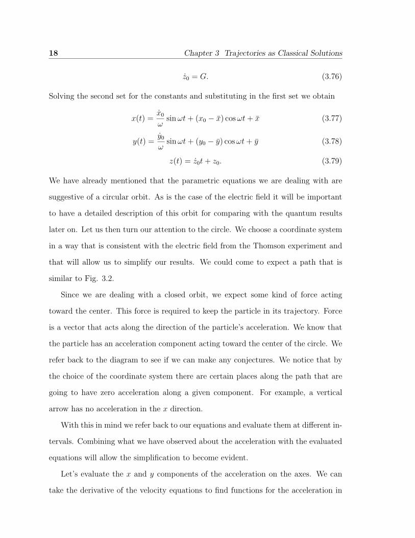
z0 = G. (3.76)
Solving the second set for the constants and substituting in the first set we obtain
x(t) =x0
ωsinωt+ (x0 − x) cosωt+ x (3.77)
y(t) =y0
ωsinωt+ (y0 − y) cosωt+ y (3.78)
z(t) = z0t+ z0. (3.79)
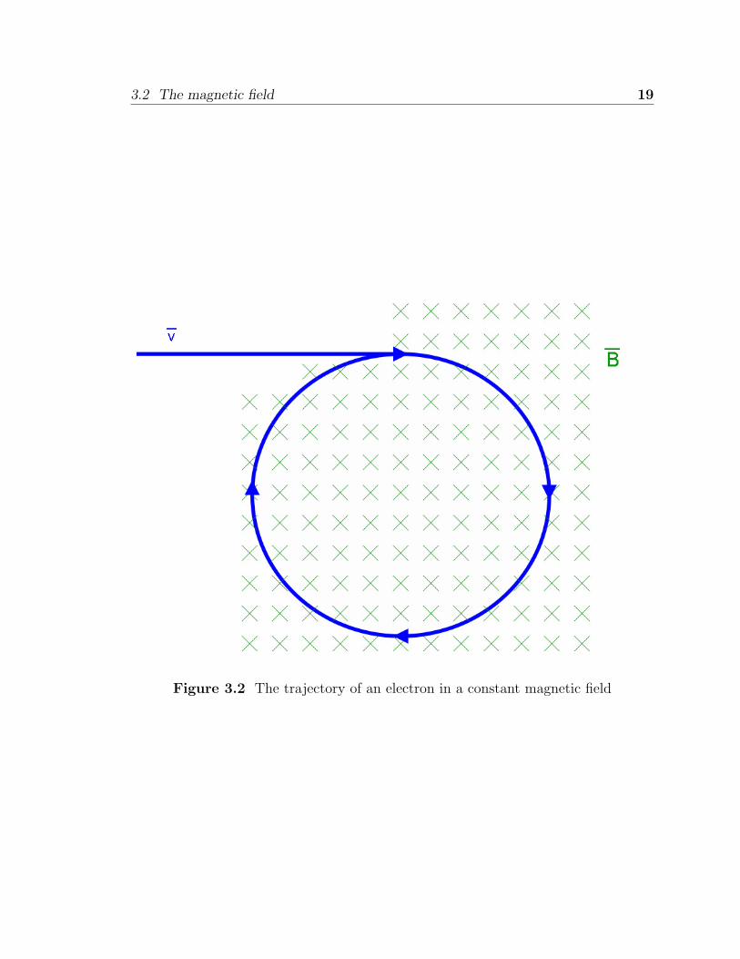
We have already mentioned that the parametric equations we are dealing with are
suggestive of a circular orbit. As is the case of the electric field it will be important
to have a detailed description of this orbit for comparing with the quantum results
later on. Let us then turn our attention to the circle. We choose a coordinate system
in a way that is consistent with the electric field from the Thomson experiment and
that will allow us to simplify our results. We could come to expect a path that is
similar to Fig. 3.2.
Since we are dealing with a closed orbit, we expect some kind of force acting
toward the center. This force is required to keep the particle in its trajectory. Force
is a vector that acts along the direction of the particle’s acceleration. We know that
the particle has an acceleration component acting toward the center of the circle. We
refer back to the diagram to see if we can make any conjectures. We notice that by
the choice of the coordinate system there are certain places along the path that are
going to have zero acceleration along a given component. For example, a vertical
arrow has no acceleration in the x direction.
With this in mind we refer back to our equations and evaluate them at different in-
tervals. Combining what we have observed about the acceleration with the evaluated
equations will allow the simplification to become evident.
Let’s evaluate the x and y components of the acceleration on the axes. We can
take the derivative of the velocity equations to find functions for the acceleration in
3.2 The magnetic field 19
Figure 3.2 The trajectory of an electron in a constant magnetic field
20 Chapter 3 Trajectories as Classical Solutions
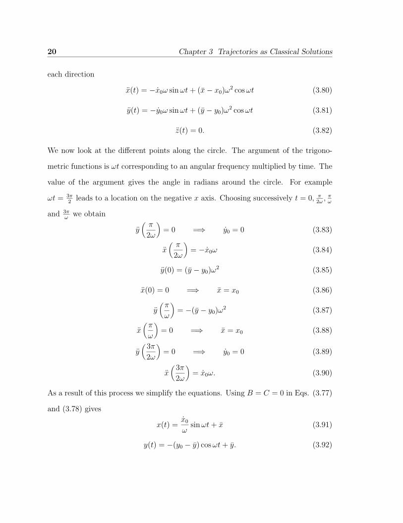
each direction
x(t) = −x0ω sinωt+ (x− x0)ω2 cosωt (3.80)
y(t) = −y0ω sinωt+ (y − y0)ω2 cosωt (3.81)
z(t) = 0. (3.82)
We now look at the different points along the circle. The argument of the trigono-
metric functions is ωt corresponding to an angular frequency multiplied by time. The
value of the argument gives the angle in radians around the circle. For example
ωt = 3π2
leads to a location on the negative x axis. Choosing successively t = 0, π2ω, π
ω
and 3πω
we obtain
y(π
2ω
)= 0 =⇒ y0 = 0 (3.83)
x(π
2ω
)= −x0ω (3.84)
y(0) = (y − y0)ω2 (3.85)
x(0) = 0 =⇒ x = x0 (3.86)
y(π
ω
)= −(y − y0)ω
2 (3.87)
x(π
ω
)= 0 =⇒ x = x0 (3.88)
y(
3π
2ω
)= 0 =⇒ y0 = 0 (3.89)
x(
3π
2ω
)= x0ω. (3.90)
As a result of this process we simplify the equations. Using B = C = 0 in Eqs. (3.77)
and (3.78) gives
x(t) =x0
ωsinωt+ x (3.91)
y(t) = −(y0 − y) cosωt+ y. (3.92)
3.2 The magnetic field 21
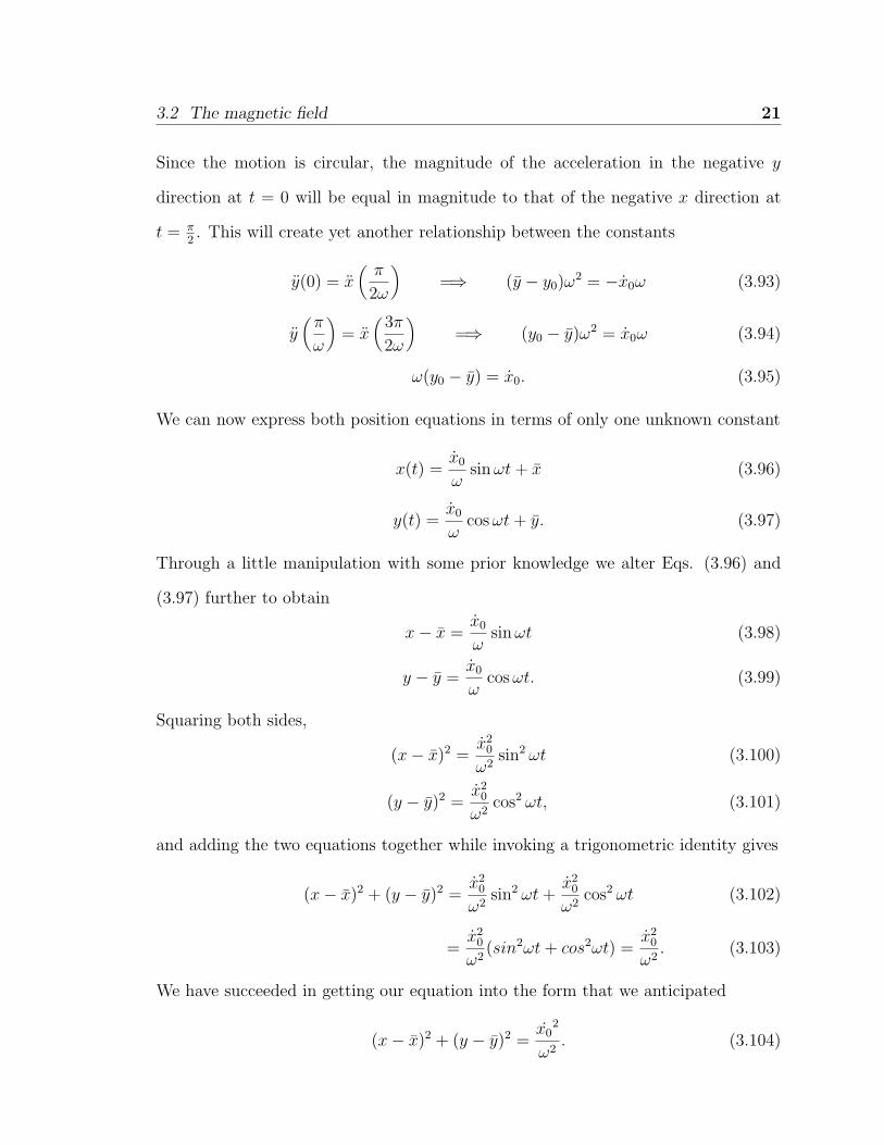
Since the motion is circular, the magnitude of the acceleration in the negative y
direction at t = 0 will be equal in magnitude to that of the negative x direction at
t = π2. This will create yet another relationship between the constants
y(0) = x(π
2ω
)=⇒ (y − y0)ω
2 = −x0ω (3.93)
y(π
ω
)= x
(3π
2ω
)=⇒ (y0 − y)ω2 = x0ω (3.94)
ω(y0 − y) = x0. (3.95)
We can now express both position equations in terms of only one unknown constant
x(t) =x0
ωsinωt+ x (3.96)
y(t) =x0
ωcosωt+ y. (3.97)
Through a little manipulation with some prior knowledge we alter Eqs. (3.96) and
(3.97) further to obtain
x− x =x0
ωsinωt (3.98)
y − y =x0
ωcosωt. (3.99)
Squaring both sides,
(x− x)2 =x2
0
ω2sin2 ωt (3.100)
(y − y)2 =x2
0
ω2cos2 ωt, (3.101)
and adding the two equations together while invoking a trigonometric identity gives
(x− x)2 + (y − y)2 =x2
0
ω2sin2 ωt+
x20
ω2cos2 ωt (3.102)
=x2
0
ω2(sin2ωt+ cos2ωt) =
x20
ω2. (3.103)
We have succeeded in getting our equation into the form that we anticipated
(x− x)2 + (y − y)2 =x0
2
ω2. (3.104)
22 Chapter 3 Trajectories as Classical Solutions
Equation (3.104) describes a circle centered at (x, y). The term on the right corre-
sponds to the radius R squared
R =x0
ω(3.105)
or in terms of the physical parameters
R =mx0
qB(3.106)
and
(x− x)2 + (y − y)2 =m2x2
0
q2B2. (3.107)
The constant ω has a well-defined physical significance. We first determine the SI
units
[ω] =C
Kg
Kg
Cs=
1
s= 1Hz (3.108)
corresponding to a frequency. Indeed it is a frequency, often called the cyclotron
frequency, or the frequency at which the particle cycles through one revolution around
the circle just found.3
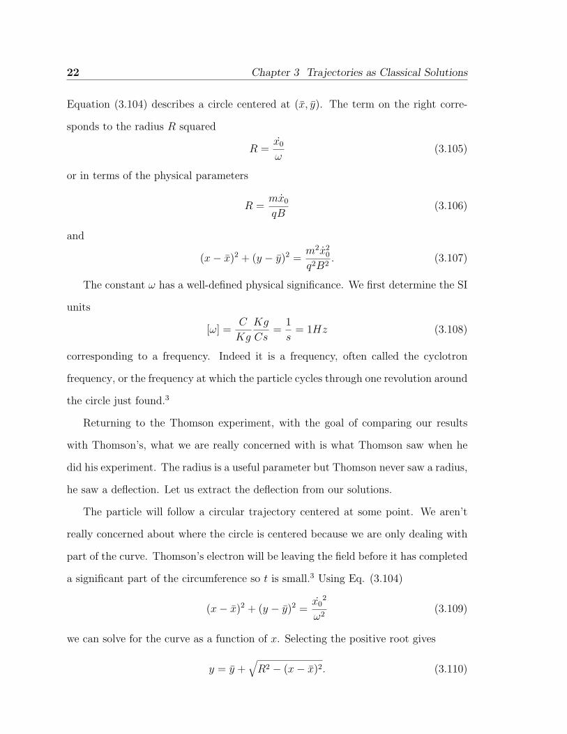
Returning to the Thomson experiment, with the goal of comparing our results
with Thomson’s, what we are really concerned with is what Thomson saw when he
did his experiment. The radius is a useful parameter but Thomson never saw a radius,
he saw a deflection. Let us extract the deflection from our solutions.
The particle will follow a circular trajectory centered at some point. We aren’t
really concerned about where the circle is centered because we are only dealing with
part of the curve. Thomson’s electron will be leaving the field before it has completed
a significant part of the circumference so t is small.3 Using Eq. (3.104)
(x− x)2 + (y − y)2 =x0
2
ω2(3.109)
we can solve for the curve as a function of x. Selecting the positive root gives
y = y +√R2 − (x− x)2. (3.110)
3.3 The electromagnetic field 23
We are dealing with a situation where the particle travels tangent to the curve of the
circle. This would lead us to believe that we will be needing the derivative.
y′ =−(x− x)√R2 − (x− x)2
(3.111)
This expression gives us the slope of the curve at that point. Since the slope is equal to
the tangent of the angle, we would have to take the inverse tangent of this expression
in order to find θ. Thomson, however, was only concerned with small angles for the
most part. As a result, we are probably safe to use the small angle approximation for
tangents.
θ ≈ tan θ (3.112)
This approximation will then give us a final result that we can use to find the angle.
If we relabel (x− x0) as L then we can write
θ ≈ −L√R2 − L2
. (3.113)
At this point we can make another approximation. L is small compared to R so we
can eliminate the L2 term and we are left with:
θ ≈ −L√R2
=−LR. (3.114)
Recall that
R =mv
qB, (3.115)
which results in our final expression for the deflection angle
θ ≈ −qBLmv
= −qBLmx0
. (3.116)
3.3 The electromagnetic field
In order to remain consistent with the Thomson experiment we consider the classical
description of the case in which both fields are acting on the electron. In section
24 Chapter 3 Trajectories as Classical Solutions
3.1 we found that the force from the electric field acting on the electron could be
described by Eq. (3.3). It is a differential equation describing the force in the y
direction,
my = Eq. (3.117)
Using the right-hand rule confirms that when the electron first enters the magnetic
field it experiences a force in the y direction. In section 3.2 we found that this force
could be described by Eq. (3.44)
my = −Bxq. (3.118)
The net force acting on the electron in the y direction is then the sum of the two
forces
my = Eq −Bxq. (3.119)
Thomson, however, arranged his setup so there would not be any deflection of the
beam.1 This means that the net force on the particle is zero and Eq. (3.119) becomes
0 = Eq −Bxq. (3.120)
Which gives
Eq = Bxq (3.121)
E = Bx (3.122)
x =E
B. (3.123)
Substituting this result back into Eq. (3.119) gives
my = Eq − Eq = 0, (3.124)
as we established by assuming no deflection. We found in section 3.1 that the force
from the electric field acts only in the y direction and since the velocity remains solely
3.3 The electromagnetic field 25
along x in this case, there is no force from the magnetic field in the x or z directions.
This means
mx = 0 (3.125)
my = 0 (3.126)
mz = 0 (3.127)
and
x(t) = x0t+ x0 (3.128)
y(t) = y0t+ y0 (3.129)
z(t) = z0t+ z0. (3.130)
Knowing that y0 = 0 and z0 = 0 gives
x(t) = x0t+ x0 (3.131)
y(t) = y0 (3.132)
z(t) = z0 (3.133)
which is the straight line trajectory we expected.

26 Chapter 3 Trajectories as Classical Solutions
Chapter 4
Wave Packets as Quantum
Solutions
When we consider the classical version of the Thomson experiment, we rely upon
Newton’s equations to obtain trajectories. Newton’s equations deal with forces but
the quantum treatment is interested in potentials. We use an equation that re-
flects the wave nature of our quantum solutions Ψ(x). The foundation for the quan-
tum description comes from the equation governing nonrelativistic wave mechanics,
the Schrodinger equation. For time-independent potentials we can use the time-
independent Schrodinger equation4
− h2
2m
d2Ψ(x)
dx2= (E − U(x))Ψ(x). (4.1)
This equation is a second-order differential equation in one dimension. Here E
stands for the total energy of the system. The term U(x) represents the potential
energy of the particle in its environment. The term in parentheses (E − U(x)) can
therefore be considered as the kinetic energy of the particle. We solve for the wave-
function Ψ(x).
27
28 Chapter 4 Wave Packets as Quantum Solutions
4.1 Constant potentials
The term in the Schrodinger equation that governs the behavior of the wavefunction
is the potential energy term U(x). We consider some relevant potentials. In the
simplest possible case U(x) = 0 and there is no external influence
− h2
2m
d2Ψ(x)
dx2= EΨ(x). (4.2)
Using k =√
2mEh2 we get
d2Ψ(x)
dx2= −k2Ψ(x). (4.3)
This Ordinary Differential Equation (ODE) says that the second derivative of a func-
tion is equal to itself multiplied by a negative constant. This is in very different
circumstances the same equation as that encountered in Eq. (3.56). The solution
to this equation consists of sines and cosines. We know from superposition that any
linear combination of these solutions will also be a solution.3 This gives us a generic
form for the wavefunction in a zero-potential region
Ψ(x) = A sin kx+B cos kx. (4.4)
It is a stationary solution and its time dependence has been removed. We can express
it as a complex exponential or a cosine term with a phase shift
Ψ(x) =(A+B
2
)eikx +
(−A+B
2
)e−ikx (4.5)
Ψ(x) = B cos(kx+ φ). (4.6)
Another simple case is a constant potential V0 different from zero. Suppose also that
the potential V0 is greater than the total energy E of the particle. If this is the case,
it changes the sign in front of Ψ(x) in Eq. (4.1)
d2Ψ(x)
dx2= κ2Ψ(x) (4.7)

4.2 Linear potentials and Airy functions 29
where κ =√
2m(E−V0)
−h2 . Again, we have a simple differential equation but the solution
has a different form now. Rather than trigonometric functions we obtain exponentials.
The generic solution from superposition is
Ψ(x) = Aeκx +Be−κx. (4.8)
These solutions apply to the two domains outside of the capacitor.
4.2 Linear potentials and Airy functions
If we refer back to our model for the capacitor from section 2.3 we notice that in the
central region the potential is linear. We can set up the Schrodinger equation to solve
for solutions in this region. For U(x) = αx, a linear potential energy, we obtain
d2
dx2Ψ (x) = (αx− E) Ψ (x) (4.9)
where the constant slope α depends on the strength of the applied electric field. This
equation is not as easy to solve because we no longer have a constant multiplying the
wavefunction. Solving this equation using Maple we find
Ψ (x) = C1 AiryAi
(αx− E
(−α)2/3
)+ C2 AiryBi
(αx− E
(−α)2/3
), (4.10)
where C1 and C2 are integration constants. AiryAi and AiryBi are Maple’s way
of expressing a special class of functions called Airy functions. These functions are
related to the more familiar Bessel functions and they come in two types, Ai and Bi.5
A plot of AiryAi is displayed in Fig. 4.1. We can make a few observations about
the behavior of this function. Towards the right the function decays to zero once it
crosses into the positive x values after reaching a final maximal peak. Towards the
left the function oscillates at an increasing pace as it dies off. This oscillation makes
sense physically if we consider what is happening to the electron. As the electron
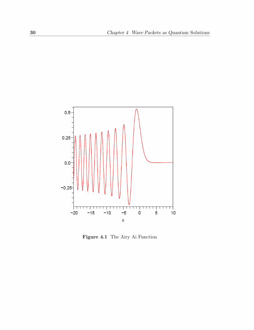
30 Chapter 4 Wave Packets as Quantum Solutions
Figure 4.1 The Airy Ai Function
4.2 Linear potentials and Airy functions 31
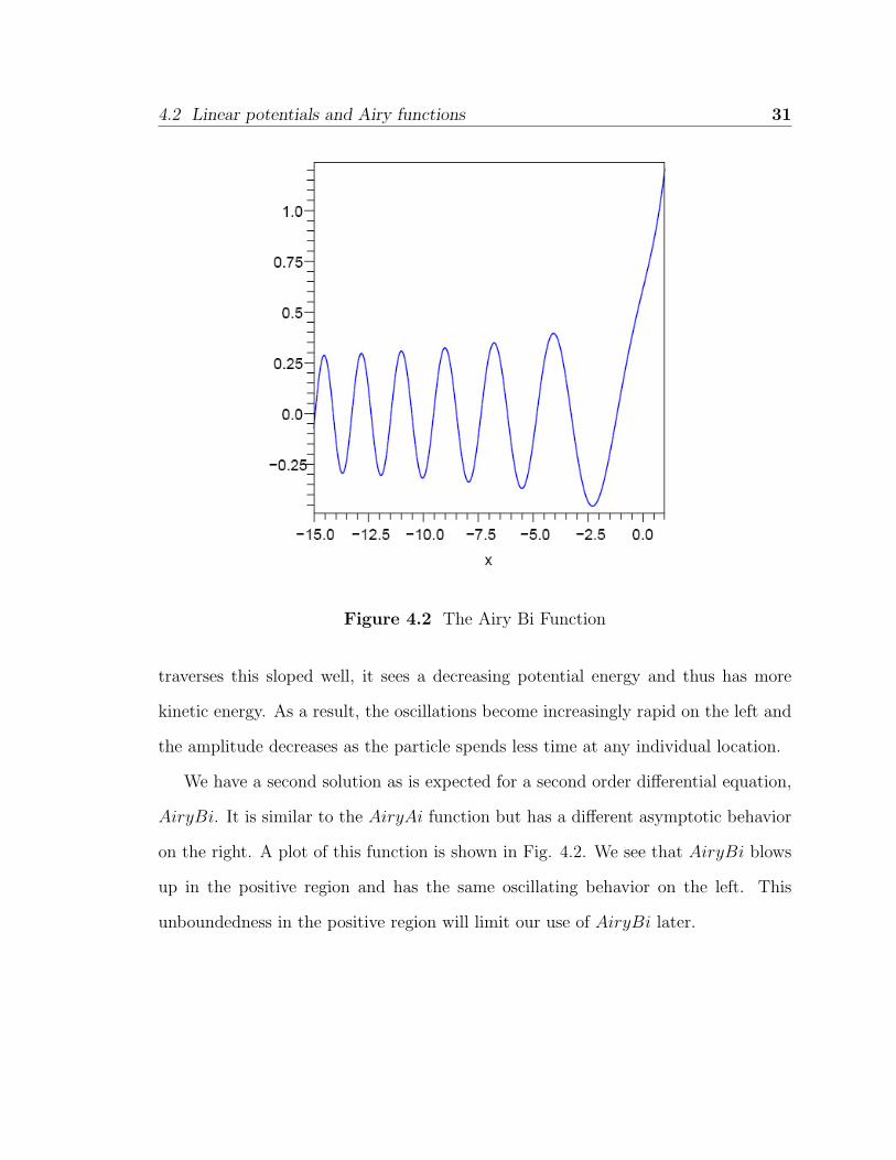
Figure 4.2 The Airy Bi Function
traverses this sloped well, it sees a decreasing potential energy and thus has more
kinetic energy. As a result, the oscillations become increasingly rapid on the left and
the amplitude decreases as the particle spends less time at any individual location.
We have a second solution as is expected for a second order differential equation,
AiryBi. It is similar to the AiryAi function but has a different asymptotic behavior
on the right. A plot of this function is shown in Fig. 4.2. We see that AiryBi blows
up in the positive region and has the same oscillating behavior on the left. This
unboundedness in the positive region will limit our use of AiryBi later.
32 Chapter 4 Wave Packets as Quantum Solutions
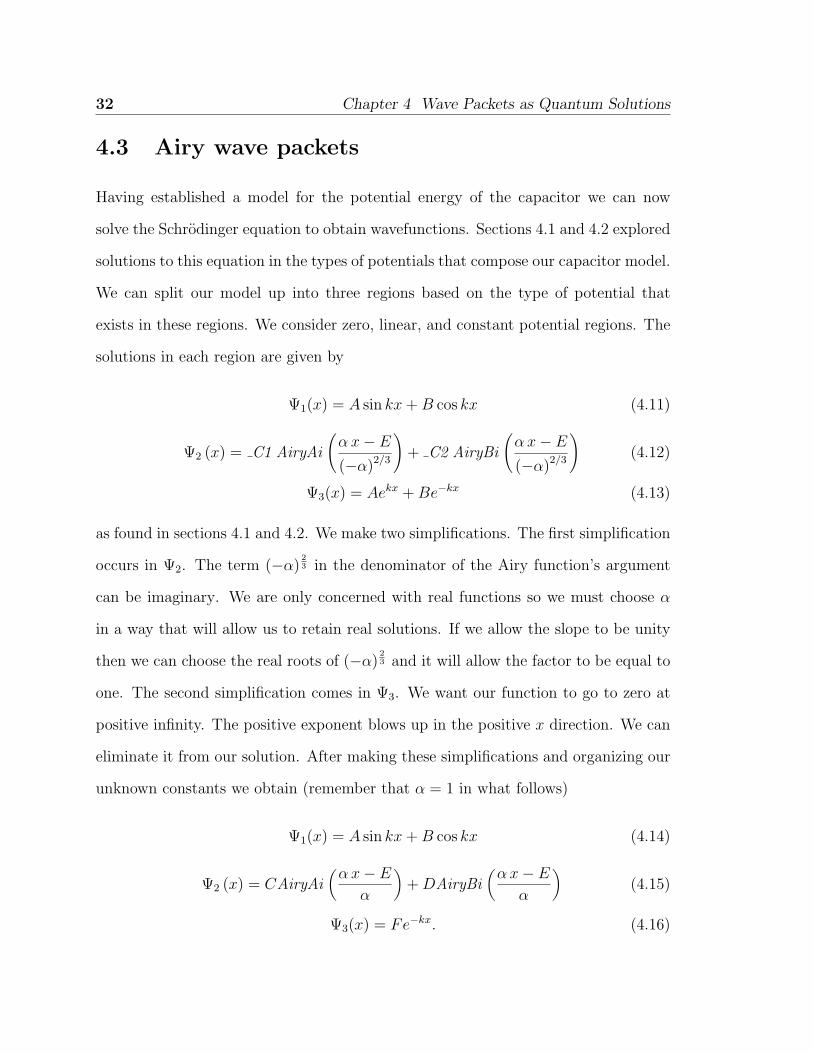
4.3 Airy wave packets
Having established a model for the potential energy of the capacitor we can now
solve the Schrodinger equation to obtain wavefunctions. Sections 4.1 and 4.2 explored
solutions to this equation in the types of potentials that compose our capacitor model.
We can split our model up into three regions based on the type of potential that
exists in these regions. We consider zero, linear, and constant potential regions. The
solutions in each region are given by
Ψ1(x) = A sin kx+B cos kx (4.11)
Ψ2 (x) = C1 AiryAi
(αx− E
(−α)2/3
)+ C2 AiryBi
(αx− E
(−α)2/3
)(4.12)
Ψ3(x) = Aekx +Be−kx (4.13)
as found in sections 4.1 and 4.2. We make two simplifications. The first simplification
occurs in Ψ2. The term (−α)23 in the denominator of the Airy function’s argument
can be imaginary. We are only concerned with real functions so we must choose α
in a way that will allow us to retain real solutions. If we allow the slope to be unity
then we can choose the real roots of (−α)23 and it will allow the factor to be equal to
one. The second simplification comes in Ψ3. We want our function to go to zero at
positive infinity. The positive exponent blows up in the positive x direction. We can
eliminate it from our solution. After making these simplifications and organizing our
unknown constants we obtain (remember that α = 1 in what follows)
Ψ1(x) = A sin kx+B cos kx (4.14)
Ψ2 (x) = CAiryAi(αx− E
α
)+DAiryBi
(αx− E
α
)(4.15)
Ψ3(x) = Fe−kx. (4.16)

4.3 Airy wave packets 33
At this point we make a numeric simplification. It was mentioned in section 4.1 that
k =√
2mEh2 . We establish our system with natural units such that 2m
h2 = 1. This
implies that k =√E.
We must now apply boundary conditions to our functions in order to obtain a
solution for the entire system. The boundary condition on the left requires that the
function and its derivative be continuous at the boundary between Ψ1 and Ψ2.4 Using
the functions with adjusted units gives
B = CAiryAi(− E
α
)+DAiryBi
(− E
α
), (4.17)
having evaluated Ψ1 at x = 0 to obtain B on the left side of Eq. (4.17). We also use
the condition that the derivatives of Ψ1 and Ψ2 must be equal at x = 0. Taking the
derivative of these functions and evaluating them at x = 0 gives
A√E = CAiryAi
(1,− E
α
)+DAiryBi
(1,− E
α
)(4.18)
where the number 1 in the argument of the AiryAi and AiryBi functions,(1,−E
α
),
refers to the first derivatives of AiryAi(−E
α
)and AiryBi
(−E
α
)respectively. We
divide one equation by the other and get
B
A√E
=
(CAiryAi
(− E
α
)+DAiryBi
(− E
α
))(CAiryAi
(1,− E
α
)+DAiryBi
(1,− E
α
)) . (4.19)
We also have a boundary condition on the right at x = d where d is the length of the
capacitor. The symbol L has been used for the same quantity. We have already taken
care of the end behavior by choosing the exponential term that decays rather than
blowing up, so we are left with conditions at x = d. We have the same conditions
at x = d for Ψ2 and Ψ3 as we do at x = 0 for Ψ1 and Ψ2. The functions and
their derivatives must be equal when evaluated at the boundary point. Setting the
functions equal to each other gives
CAiryAi
(α d− E
α
)+DAiryBi
(α d− E
α
)= Fe−
√α d−Ed. (4.20)
34 Chapter 4 Wave Packets as Quantum Solutions
Setting their derivatives equal gives
CAiryAi
(1,α d− E
α
)+DAiryBi
(1,α d− E
α
)= −F
√α d− Ee−
√α d−Ed. (4.21)
Dividing the two equations produces(CAiryAi
(α d−E
α
)+DAiryBi
(α d−E
α
))(CAiryAi
(1, α d−E
α
)+DAiryBi
(1, α d−E
α
)) = − 1√α d− E
. (4.22)
We now have two equations Eq. (4.19) and Eq. (4.22) and four unknowns A, C, D,
and F. We reduce this system to two unknowns by simplifying down to a ratio of
constants. In Eq. (4.19) we already have a ratio of BA. We can obtain a ratio for C
D.
The way we accomplished this in Maple was to set D = 1 and solve Eq. (4.22) for C.
This result was really equal to the ratio of CD
. We did the same with Eq. (4.19) by
setting B = 1 and solving for A, obtaining the ratio for AB
. We set D = 1 and C = CD
and solve Eq. (4.20) for FD
. We set the same conditions and solve Eq. (4.17) for BD
.
We take the expressions for each of these combinations of constants and substitute
them into Ψ1, Ψ2 and Ψ3 as follows,
Ψ1(x) =B
D
(A
Bsin kx+ cos kx
)= A sin kx+B cos kx (4.23)
Ψ2 (x) =C
DAiryAi
(αx− E
α
)+ AiryBi
(αx− E
α
)(4.24)
= CAiryAi(αx− E
α
)+DAiryBi
(αx− E
α
)(4.25)
Ψ3(x) =F
D(e−kx) = Fe−kx. (4.26)
This method works because we set D = 1 and we found expressions for BD
, AB
, CD
and
FD
.
We now have the correct boundary conditions applied to our wavefunctions in
each region. We construct a piecewise function in Maple consisting of each of these
solutions in their respective domain. This piecewise solution is a function of x and

4.3 Airy wave packets 35
Figure 4.3 The wavefunction solution plotted for 3 different values of theenergy

36 Chapter 4 Wave Packets as Quantum Solutions
also a function of E, the energy of the particle. Figure 4.3 displays plots of this
piecewise function for different values of the energy E. The wavefunction behaves as
expected in each of the three regions. The behavior is also affected by the value of
the energy.
We have found the wavefunction that is the solution to our model of the capacitor
in the Thomson experiment. We must now use this wavefunction to construct a local-
ized wave packet. We construct our wave packet as a δ function. The wavefunction
is multiplied by a weight factor and integrated,4
δ(x− a) =∫ ∞0
ΨE(x)ΨE(a)dE. (4.27)
Maple is not able to analytically integrate the complicated combination of Airy func-
tions that exists in the expression for our wavefunction. Therefore we must approxi-
mate the integral with a finite sum. We also want to localize our wave packet around
a specific point. The wavefunction squared is going to correspond to the probability
density for the cathode ray. We localize the beam in the center of the capacitor
which, according to our model in Fig. 2.1, is equivalent to x = 12.5. Thus we have
δ(x− 12.5) =n∑
E=0
ΨE(x)ΨE(12.5). (4.28)
We substitute this value of x into ΨE in our Maple code and sum over a range
of energies. This finite sum may actually have benefits because of the Heisenberg
uncertainty. The less localized our wave packet is, the less dispersive it will be.
4.4 Normalization
Once we had completed the necessary steps for constructing our wave packet, there
remained a plaguing error that prevented us from obtaining a localized peak. We had
summed the Airy terms and constructed a wave packet but it was not localized as
4.4 Normalization 37
we had expected it to be. We noticed in the plots of our wavefunction that changing
the value of the energy was also changing the amplitude. We made a table of values
corresponding to the different energies and the amplitudes they corresponded to.
There did not seem to be a pattern and some of the amplitudes were several orders
of magnitude larger than others. This was an interesting result and it was important
because it helped us to realize that even though our wave packet was normalized in
the end, we had neglected to normalize the wavefunctions from which the packet was
constructed. The relation Eq. (4.27) holds for normalized ΨE.
We returned to the beginning of our Maple code where we had first composed our
piecewise wavefunction from the individual wavefunctions in each region. A term was
added to the code which summed the squares of Ψ(x)1, Ψ(x)2 and Ψ(x)3 over their
respective regions. Again we had to approximate the integral with a sum because
of Maple’s inability to analytically integrate the expressions. This approximation
accounts for the reason that some of the curves in the plots don’t appear to enclose
an area of exactly one. Summing each wavefunction over a sufficiently large region
gives
n21E =
0∑x=−25
ΨE(x)21 (4.29)
n22E =
25∑x=0
ΨE(x)22 (4.30)
n23E =
35∑x=25
ΨE(x)23. (4.31)
We then obtain the normalization constant
NE =1√
n21E + n2
2E + n23E
. (4.32)
We multiplied our wavefunction by this normalization constant and constructed the
approximate δ function again
δ(x− 12.5)N =25∑
E=0
NEΨE(x)ΨE(12.5) (4.33)
38 Chapter 4 Wave Packets as Quantum Solutions
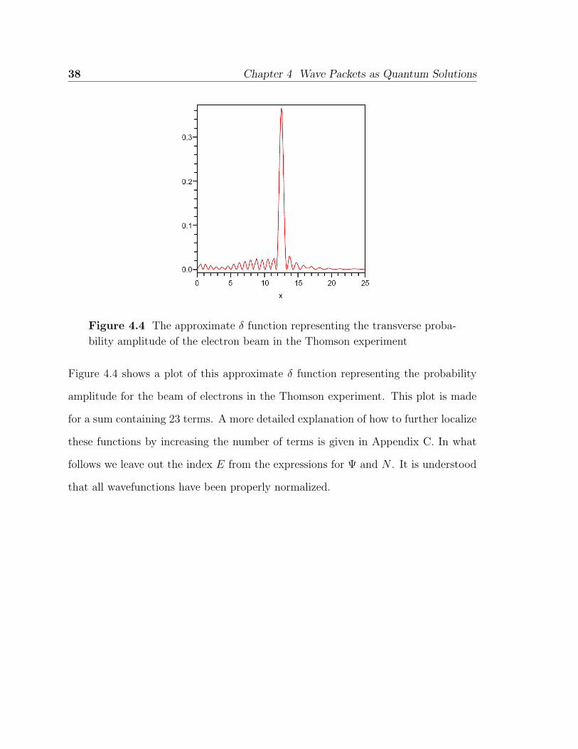
Figure 4.4 The approximate δ function representing the transverse proba-
bility amplitude of the electron beam in the Thomson experiment
Figure 4.4 shows a plot of this approximate δ function representing the probability
amplitude for the beam of electrons in the Thomson experiment. This plot is made
for a sum containing 23 terms. A more detailed explanation of how to further localize
these functions by increasing the number of terms is given in Appendix C. In what
follows we leave out the index E from the expressions for Ψ and N . It is understood
that all wavefunctions have been properly normalized.
Chapter 5
Deflection from Wave Packet
Evolution
Now that we have constructed a wave packet we follow its behavior in the poten-
tial region as time progresses. We include the time dependence by multiplying the
stationary states by the factor e−iωt in the expression for the δ function4
δ(x− xc, t)N =n∑
E=0
NΨ(x)Ψ(xc)e−iωt (5.1)
where ω = Eh
and xc is the center of the capacitor. In our setup xc = 12.5. Based on
the results of the Thomson experiment and our classical derivations we can make some
assumptions about the wave packet evolution. We should obtain a packet that moves
to the left at an accelerating rate. This corresponds to the probability amplitude of
the electron as it is accelerated through the electric field.
5.1 Dispersion
Once we have obtained an expression for the time-dependent wave packet we animate
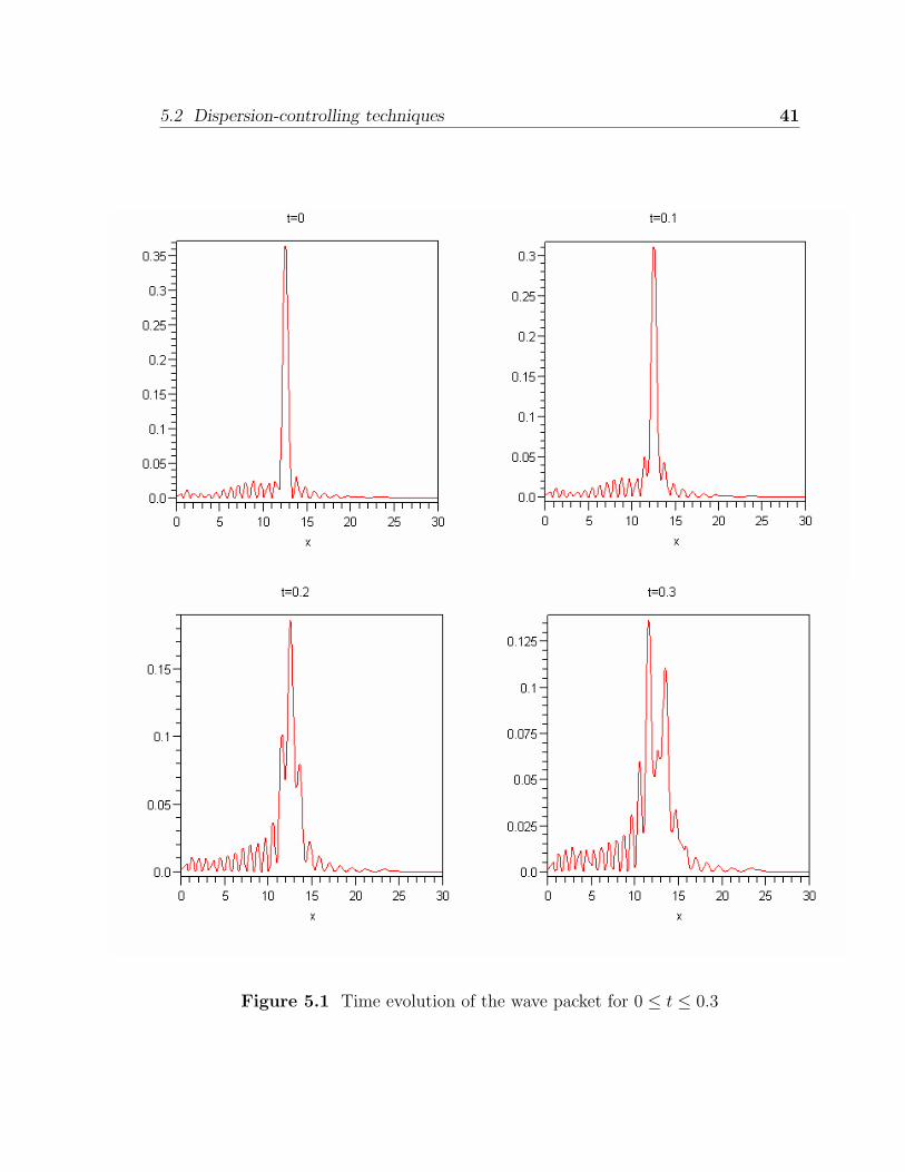
it in Maple to see how it behaves. The surprising results illustrated in Fig. 5.1
39
40 Chapter 5 Deflection from Wave Packet Evolution
show that the peak starts out localized at t = 0 as constructed. As time progresses,
however, the packet rapidly disperses and we lose any information about the motion
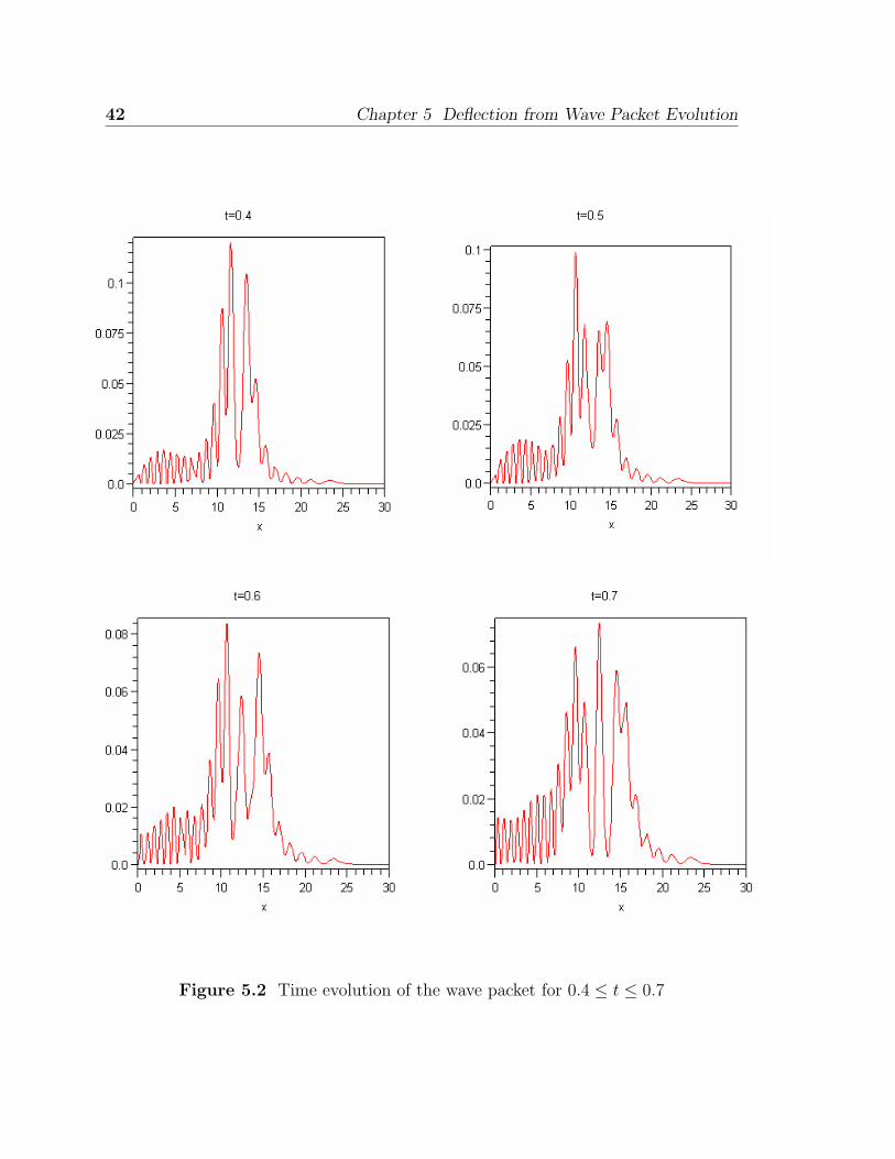
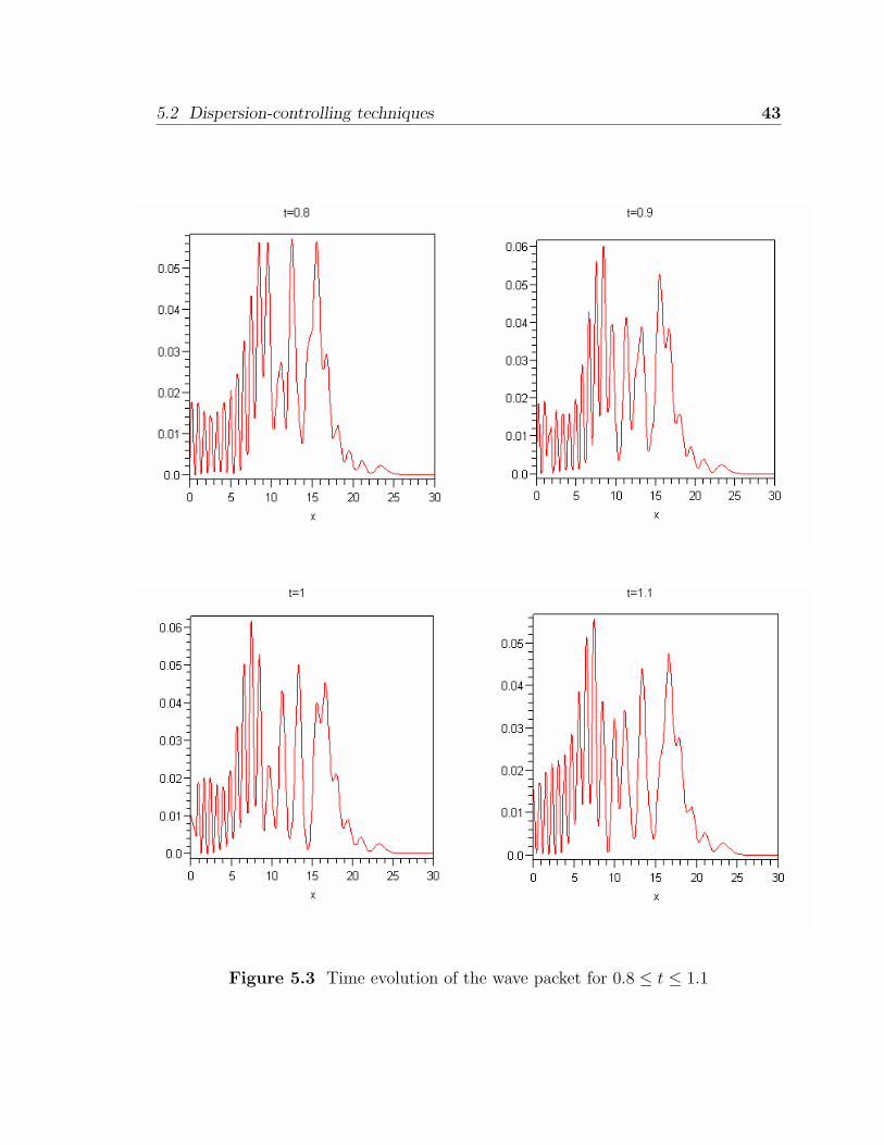
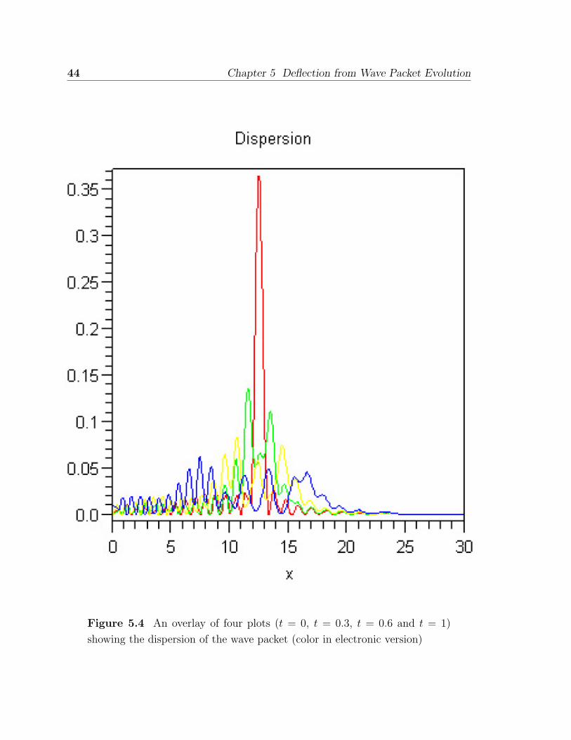
of the packet. This is seen in Figs. 5.2 and 5.3. Figure 5.4 is an overlay of times
t = 0, t = 0.3, t = 0.6, and t = 1.
Dispersion is a quantum effect that happens to wave packets as time progresses.
We expect to see some dispersion in our packet as it moves through time but it is
quite surprising to see it dominating the motion of the peak. We investigate this
dispersion thoroughly and attempt several techniques to understand its origins.
5.2 Dispersion-controlling techniques
5.2.1 Expectation values
One of the techniques is to look at the expectation value for the wave packet as it
moves through time. To compute the expectation value we use its general definition:4
< x >=
∫∞−∞ x|ψ(x)|2dx∫∞−∞ |ψ(x)|2dx
. (5.2)
Again we approximate the integral in Maple using a sum,
< x >=
∑30x=0 x|ψ(x)|2dx∑30x=0 |ψ(x)|2dx
. (5.3)
The Maple code for this operation is given below
exp:=sum(subs(t=0,x*shift),x=0..30)/sum(subs(t=0,shift),x=0..30);.
The Maple function shift stands for the solution ψ(x) or δ(x−xc)N . We construct
an array in Maple that takes the expectation value and pairs it with the corresponding
value of t that it was created from. This creates a scatter plot of expectation values
plotted against time. We want to see how the expectation value changes relative to
5.2 Dispersion-controlling techniques 41
Figure 5.1 Time evolution of the wave packet for 0 ≤ t ≤ 0.3
42 Chapter 5 Deflection from Wave Packet Evolution
Figure 5.2 Time evolution of the wave packet for 0.4 ≤ t ≤ 0.7
5.2 Dispersion-controlling techniques 43
Figure 5.3 Time evolution of the wave packet for 0.8 ≤ t ≤ 1.1
44 Chapter 5 Deflection from Wave Packet Evolution
Figure 5.4 An overlay of four plots (t = 0, t = 0.3, t = 0.6 and t = 1)
showing the dispersion of the wave packet (color in electronic version)
5.2 Dispersion-controlling techniques 45
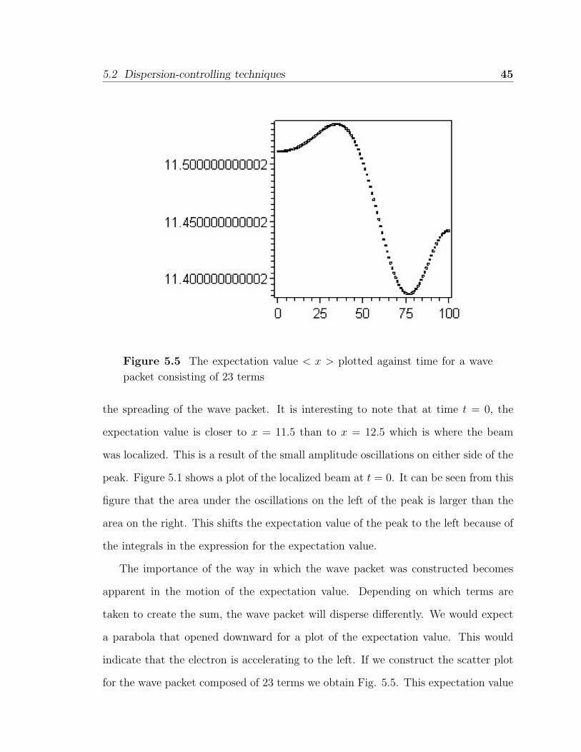
Figure 5.5 The expectation value < x > plotted against time for a wave
packet consisting of 23 terms
the spreading of the wave packet. It is interesting to note that at time t = 0, the
expectation value is closer to x = 11.5 than to x = 12.5 which is where the beam
was localized. This is a result of the small amplitude oscillations on either side of the
peak. Figure 5.1 shows a plot of the localized beam at t = 0. It can be seen from this
figure that the area under the oscillations on the left of the peak is larger than the
area on the right. This shifts the expectation value of the peak to the left because of
the integrals in the expression for the expectation value.
The importance of the way in which the wave packet was constructed becomes
apparent in the motion of the expectation value. Depending on which terms are
taken to create the sum, the wave packet will disperse differently. We would expect
a parabola that opened downward for a plot of the expectation value. This would
indicate that the electron is accelerating to the left. If we construct the scatter plot
for the wave packet composed of 23 terms we obtain Fig. 5.5. This expectation value
46 Chapter 5 Deflection from Wave Packet Evolution
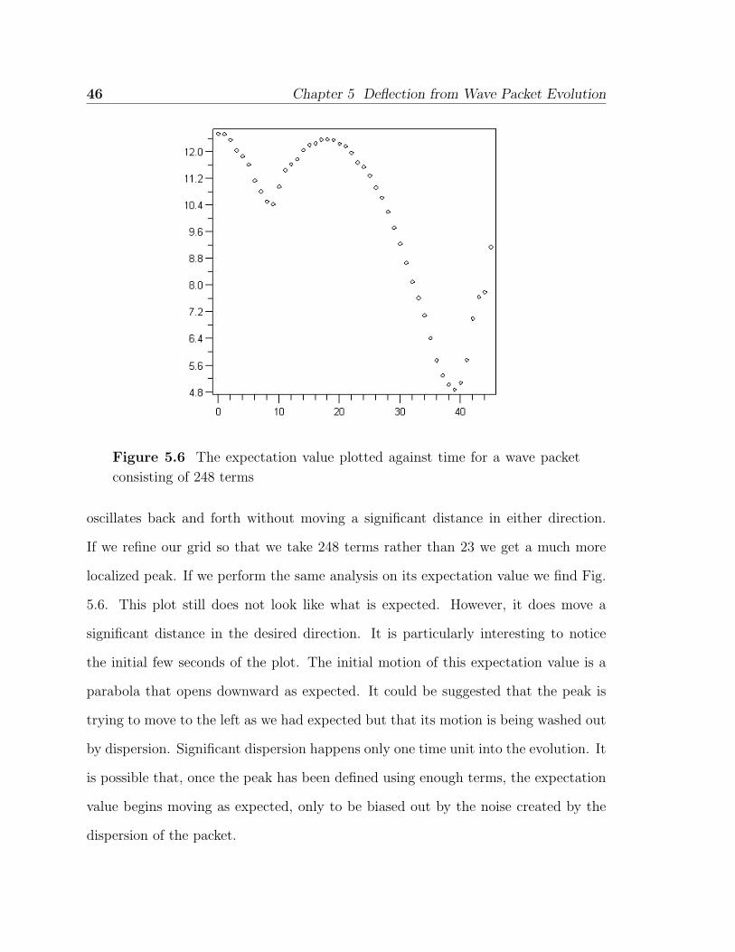
Figure 5.6 The expectation value plotted against time for a wave packet
consisting of 248 terms
oscillates back and forth without moving a significant distance in either direction.
If we refine our grid so that we take 248 terms rather than 23 we get a much more
localized peak. If we perform the same analysis on its expectation value we find Fig.
5.6. This plot still does not look like what is expected. However, it does move a
significant distance in the desired direction. It is particularly interesting to notice
the initial few seconds of the plot. The initial motion of this expectation value is a
parabola that opens downward as expected. It could be suggested that the peak is
trying to move to the left as we had expected but that its motion is being washed out
by dispersion. Significant dispersion happens only one time unit into the evolution. It
is possible that, once the peak has been defined using enough terms, the expectation
value begins moving as expected, only to be biased out by the noise created by the
dispersion of the packet.
5.2 Dispersion-controlling techniques 47
We tried several other techniques to understand the nature of the spreading in-
cluding an analysis using sine waves instead of Airy functions. We did measurements
of the time required for significant dispersion and compared those times for different
parameters. Section 5.4 will discuss our findings.
While conducting the investigation into the nature of the dispersion, we were
able to learn about the behavior of the wave packet. We tried changing the slope
of the potential region, changing the relative dimensions of the capacitor and other
alterations to our model. We also tested several ways of selecting which energy values
to take when we were creating our sum.
5.2.2 Energy level selection
We take more terms to create a finer grid in the sum in Eq. (4.33). We do this to
improve the approximation made in expressing the integral as a sum. Taking more
terms leads to more localized wave packets initially but does not remove the dispersion
in time.
Another method consists of changing the selection of the terms. Rather than
spacing them evenly over the entire range we select them by hand. We do this
to avoid coincidences from the existing periodicity in the frequency of the energy.
Otherwise it might lead to resonances that would be misleading and falsely represent
the data over the entire range. Again this method does affect the packets but does
not remove the dispersion.
As mentioned in the discussion of expectation values, the way in which the packet
is constructed affects its behavior. Taking more terms creates a more localized peak.
Because of the Heisenberg uncertainty relation, a more localized wave packet will
disperse more quickly.4 Our packet disperses much faster when it is composed of
more terms. However, it does lead to a more accurate expectation value plot.
48 Chapter 5 Deflection from Wave Packet Evolution
Taking different combinations of values and trying to stagger the energy terms
affects the packet and the way the packet disperses. Each method seems to have its
own unique effect leading to slightly different dispersion in each case.
5.3 Robinett’s analytic solution
To avoid the difficulties of the numerical analysis of the wave packet we follow a
description of this problem found in Robinett.6 An analytic solution can be found
in momentum space and then Fourier transformed back into position representation.
Rather than modeling the wave packet with δ functions, Gaussian distributions model
the probability amplitude for the electron. We will discuss this selection in detail in
the current and following sections.
The discussion below follows Robinett.6 He begins with the time-dependant Schrodinger
equation in momentum space,
p2
2mφ(p, t)− F
[ih∂
∂p
]φ(p, t) = ih
∂φ(p, t)
∂t(5.4)
or
ih
(F∂φ(p, t)
∂p+∂φ(p, t)
∂t
)=
p2
2mφ(p, t) (5.5)
where F plays the role of our slope, −F = α. Assume a solution of the form φ(p, t) =
Φ(p− Ft)φ(p). With this form, Eq. (5.5) reduces to
∂φ(p)
∂p= − ip2
2mhFφ(p) (5.6)
with the solution
φ(p) = e−ip3
6mFh . (5.7)
The general solution can then be written as
φ(p, t) = Φ(p− Ft)e−ip3
6mFh (5.8)
5.3 Robinett’s analytic solution 49
or, using the arbitrariness of Φ(p), as
φ(p, t) = φ0(p− Ft)ei((p−Ft)3−p3)
6mFh (5.9)
where φ0(p) is some initial momentum distribution since φ(p, 0) = φ0(p). It is interest-
ing to note that if the initial momentum distribution is characterized by < p >0= p0,
then using a change of variables gives
< p >t=∫ ∞−∞
p|φ(p, t)|2dp (5.10)
=∫ ∞−∞
p|φ0(p− Ft)|2dp. (5.11)
Using q = p− Ft gives
∫ ∞−∞
q|φ0(q)|2dq + Ft∫ ∞−∞|φ0(q)|2dq (5.12)
=< p >0 +Ft. (5.13)
Thus
< p >t=< p >0 +Ft (5.14)
which is a result comparable to Eq. (D.5). This equation states that the average
momentum value increases linearly with time, consistent with the classical result for
a constant force, F = dpdt
. The momentum distribution translates uniformly to the
right with no change in shape since
|φ(p, t)|2 = |φ0(p− Ft)|2. (5.15)
The corresponding position space wavefunction can then be obtained through a
Fourier transform
ψ(x, t) =1√2πh
∫ ∞−∞
φ0(p− Ft)ei((p−Ft)3−p3)
6mFh eipxh dp. (5.16)
50 Chapter 5 Deflection from Wave Packet Evolution
Since the p3 terms cancel in the exponent this transform can be done analytically for
a Gaussian momentum distribution characterized by a parameter γ. In that case, we
have
φ0(p) =
√γ√πe−γ2p2
2 (5.17)
so that
ψ(x, t) =1√
γh√π(1 + it
t0)e
iFth
(x−Ft2
6m)e−
(x−Ft2
2m )2
2h2γ2(1+ itt0
) (5.18)
where the spreading time is defined by t0 ≡ mhγ2. The corresponding probability
density is then
|ψ(x, t)|2 =1
βt
√πe−
(x−Ft2
2m )2
β2t (5.19)
where βt = hγ√
1 + t2
t20. This analytic solution has produced a Gaussian distribution
as the description of the probability amplitude. We modify Eq. (5.19) slightly by
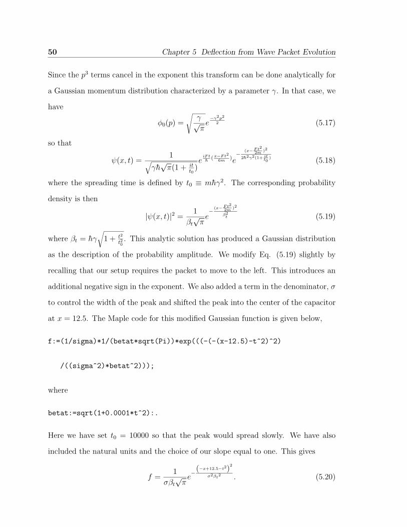
recalling that our setup requires the packet to move to the left. This introduces an
additional negative sign in the exponent. We also added a term in the denominator, σ
to control the width of the peak and shifted the peak into the center of the capacitor
at x = 12.5. The Maple code for this modified Gaussian function is given below,
f:=(1/sigma)*1/(betat*sqrt(Pi))*exp(((-(-(x-12.5)-t^2)^2)
/((sigma^2)*betat^2)));
where
betat:=sqrt(1+0.0001*t^2):.
Here we have set t0 = 10000 so that the peak would spread slowly. We have also
included the natural units and the choice of our slope equal to one. This gives
f =1
σβt
√πe−(−x+12.5−t2)
2
σ2βt2 . (5.20)
5.3 Robinett’s analytic solution 51
Figure 5.7 The Gaussian function representing the probability amplitude
from the analytic solution
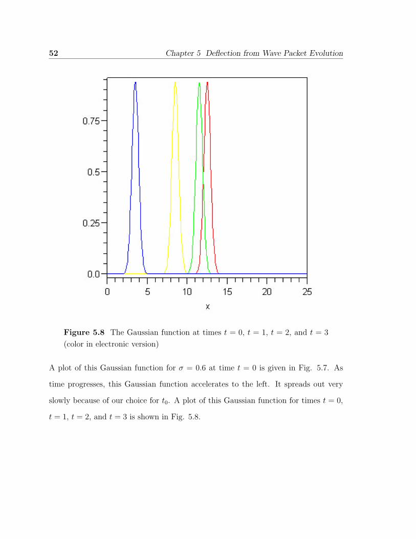
52 Chapter 5 Deflection from Wave Packet Evolution
Figure 5.8 The Gaussian function at times t = 0, t = 1, t = 2, and t = 3
(color in electronic version)
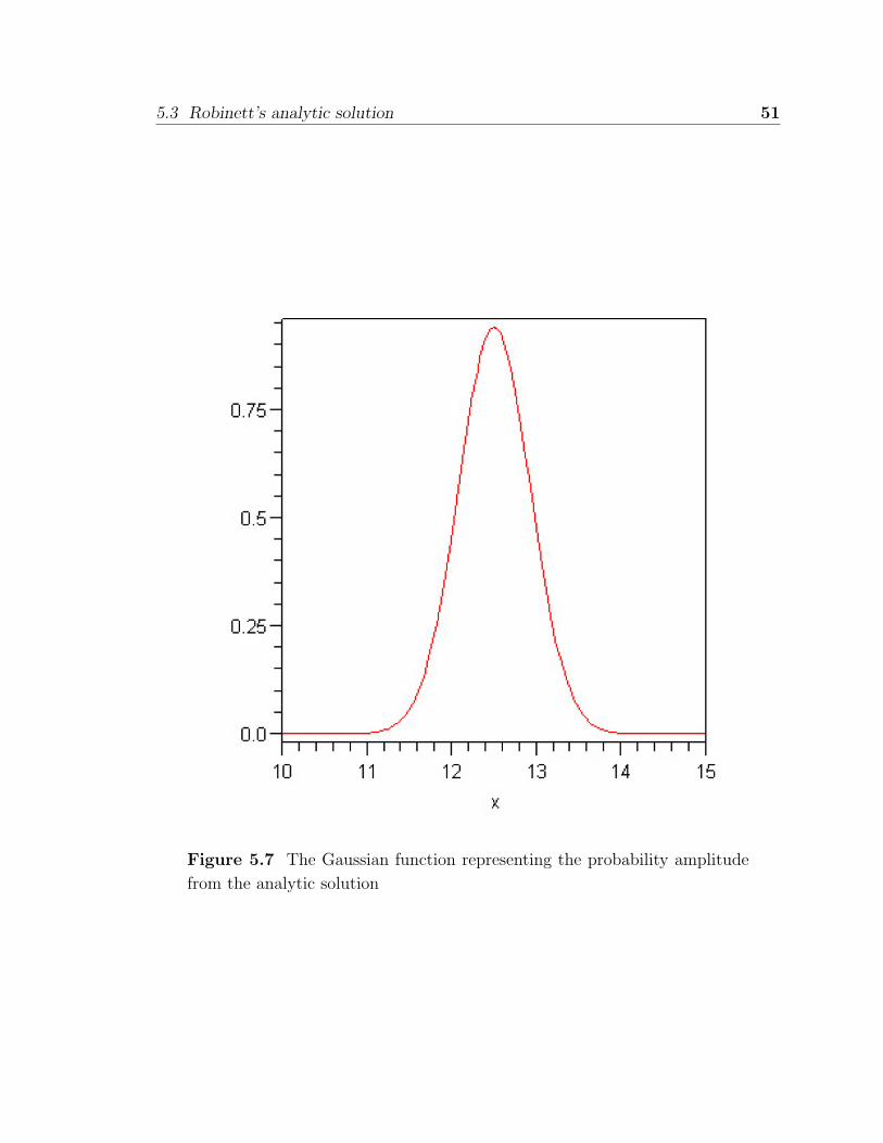
A plot of this Gaussian function for σ = 0.6 at time t = 0 is given in Fig. 5.7. As
time progresses, this Gaussian function accelerates to the left. It spreads out very
slowly because of our choice for t0. A plot of this Gaussian function for times t = 0,
t = 1, t = 2, and t = 3 is shown in Fig. 5.8.
5.4 Dispersion times comparison 53
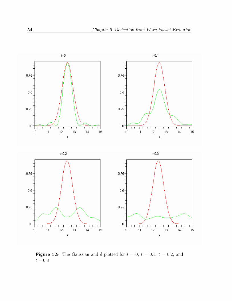
5.4 Dispersion times comparison
One of the interesting features that comes from the analytic solutions is the ability
to compare them with the numerical solutions. We are particularly interested in the
dispersion time of each packet. This is the amount of time required before significant
dispersion or spreading is observed in either case. In the case of the δ function,
significant dispersion occurs after only a fraction of a time unit. We are interested
in comparing the dispersion of this δ packet with the motion of the Gaussian packet.
We are also interested in any similarities that exist between the motion of the two
peaks. A plot of the two peaks is shown in Fig. 5.9 for t = 0, t = 0.1, t = 0.2, and
t = 0.3.
We know that the Gaussian function is accelerating but it starts from rest and
thus moves very slowly during the first few fractions of a time unit. The δ function
disperses before the Gaussian has moved a significant distance. We had suspected
that the dispersion we were seeing was related to the numeric issues of the problem
rather than any actual specific quantum phenomenon. This comparison helped to
support our beliefs about the nature of the dispersion.
5.5 Discussion
When initially considering the model for the wave packet we did consider the idea of
using a Gaussian distribution. We decided that either method should work, because
of the relationship showing that δ functions can be written as the limit of infinitely
narrow Gaussians,2
δ(x) = limε→0+
1
2√πεe−x2
4ε . (5.21)
Thus our approach of using an approximate δ function seems to be mathematically
sound.
54 Chapter 5 Deflection from Wave Packet Evolution
Figure 5.9 The Gaussian and δ plotted for t = 0, t = 0.1, t = 0.2, and
t = 0.3
5.5 Discussion 55
It is interesting to note that while we were studying the dispersion of our wave
packet we encountered an article addressing a similar problem.7 We ultimately found
the solution in Robinett’s text6 which, as previously mentioned, was derived using a
Gaussian packet in momentum space. In Churchill’s paper7 we found a description of
our problem with a statement about the nature of its difficulties. Churchill states that
modeling this problem from a numeric approach as we did was ”extremely difficult
and numerically intensive.”7
The combination of Robinett’s Gaussian solution in momentum space and the
numeric description by Churchill leads us to a few conclusions about the nature of
our project.6,7 From a mathematical standpoint, we are unaware of any mistakes that
were made in our derivations and expressions. We believe that we have correctly
modeled the wave packet.
The first conclusion we can make comes from the analytic solution. Since the
derivation was carried out in momentum space with a Gaussian function, we can
assume certain special properties about the wavefunctions. The first observation is
that the Gaussian distribution seems to be a more stable solution for this particular
problem. Airy functions are difficult to work with because of their complexity and
the math seems to be simpler with a Gaussian function.
Another observation we can make comes from comparing the dispersion times
for the two peaks. Since the δ function disperses so quickly when compared to the
Gaussian, we are lead to believe that the dispersion is not a purely quantum effect.
The numeric setup we are dealing with in Maple seems to have some complications.
It is possible that we made too many approximations or that Maple is unable to
obtain a stable solution. Modeling the system numerically does not work as well as
the analytic setup.

56 Chapter 5 Deflection from Wave Packet Evolution
Chapter 6
Conclusion
In this project we sought to find a quantum mechanical description of Thomson’s
determination of the charge-to-mass ratio em
for the electron. After modeling the sys-
tem and finding stationary solutions in the capacitor we combined them to construct
approximate δ function packets. We allowed these wave packets to evolve in time and
found the packets dispersing before we could observe their deflection. This compli-
cation prevented us from comparing the quantum results to the classical results with
the accuracy that we had expected.
We also found that the problem can be solved analytically in momentum space if
the peak is modeled with a Gaussian function. The apparent lack of dispersion in the
Gaussian packet would indicate that it is a better model for the probability amplitude
than the approximate δ function. The Gaussian and the δ function can be related
mathematically through the limiting relationship between the two functions. This
leads us to believe that there are problems with modeling the probability amplitude
with a δ function that are not inherent in the functions themselves.
This discrepancy was only one of the reasons that we had to question our numeric
approach using Maple. We also compared dispersion times between the two peaks,
57
58 Chapter 6 Conclusion
one being a Gaussian and the other a δ function. The dispersion in the δ function
happened far more quickly than it should have for the system involved. It also
dispersed long before any quantum mechanical dispersion or physical deflection was
observed in the Gaussian distribution. This leads us to believe that the dispersion we
are seeing is related to the numeric approach using Maple as opposed to any actual
physical quantum dispersion.
We can thus form some conclusions about our numeric approach. Although Maple
was an exceptionally useful aid during this research project, it struggled towards the
end with the time evolution. The primary reason for this was the analytic manip-
ulation of Airy functions. Maple is not able to perform important operations such
as integration when dealing with complicated expressions involving Airy functions.
There were several integrals we had to approximate with finite sums for this reason.
It is possible that our level of accuracy was just not adequate for the calculations
involved. It is also possible that Maple was not accurate enough to describe the time
evolution graphically. Maple was helpful but may not have been the best choice for
this project.
We also discovered an interesting property of Airy functions. The analytic deriva-
tion was carried out in momentum space to take advantage of the fact that Gaussian
wave packets of Airy functions can be integrated analytically.
In conclusion, we were able to model the Thomson experiment with the analytic
solution. The numeric approach in modeling the peak with an approximate δ function
was not as successful as we had hoped for. We could not avoid the occurrence of
dispersion in the peak. Our recommendation for any future study of the problem is
to better understand the nature of this dispersion. This might be accomplished by
systematically studying dispersion in different potentials. Also a systematic study of
wave packets of different shapes should give insights into the dispersion issue.
Bibliography
1E.A. Davis and I.J. Falconer, J. J. Thomson and the Discovery of the Electron
(Taylor and Francis, Bristol, Pennsylvania, 1997).
2D.J. Griffiths, Introduction to Electrodynamics, 3rd Ed. (Prentice Hall, Upper
Saddle River, New Jersey, 1999).
3J.R. Taylor, C.D. Zafiratos, and M.A. Dubson, Modern Physics for Scientists
and Engineers, 2nd Ed. (Prentice Hall, Upper Saddle River, New Jersey, 2004).
4J.S. Townsend, A Modern Approach to Quantum Mechanics (University Science
Books, Sausalito, California, 2000).
5O. Vallee and M. Soares, Airy Functions and Applications to Physics (World
Scientific, Hackensack, New Jersey, 2004).
6R.W. Robinett, Quantum Mechanics: Classical Results, Modern Systems, and
Visualized Examples (Oxford University Press, New York, 1997).
7J.N. Churchill, Am. J. Phys. 46(5), 537 (1978).
59

60 BIBLIOGRAPHY
Appendix A
Another Approach to the E-B
Relationship
It is interesting to note that there is a second way to obtain a mathematical link
between the fields from our original definition. We know that we are considering the
case where the forces are balanced and we have already used this to find a common
ratio. We can also consider that if the forces are balanced, there will be no deflection
of the ray and θ will be zero. We can set our two angle functions equal and opposite
to each other:
EqL
mv2=qBL
mv. (A.1)
We can cancel some variables
E
v= B (A.2)
and we obtain
E = Bv (A.3)
v =E
B(A.4)
which is the same relationship found in Eq. (3.123) using another method involving
forces.
61

62 Chapter A Another Approach to the E-B Relationship
Appendix B
Maple Code for the Construction
of the Wave Packet
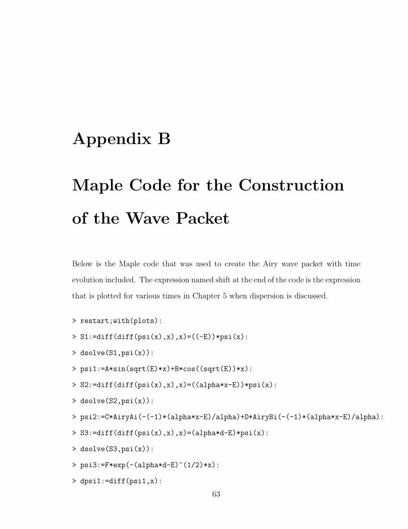
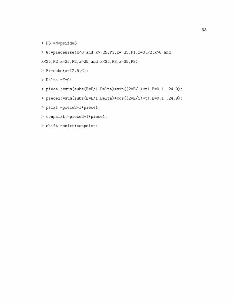
Below is the Maple code that was used to create the Airy wave packet with time
evolution included. The expression named shift at the end of the code is the expression
that is plotted for various times in Chapter 5 when dispersion is discussed.
> restart;with(plots):
> S1:=diff(diff(psi(x),x),x)=((-E))*psi(x):
> dsolve(S1,psi(x)):
> psi1:=A*sin(sqrt(E)*x)+B*cos((sqrt(E))*x):
> S2:=diff(diff(psi(x),x),x)=((alpha*x-E))*psi(x):
> dsolve(S2,psi(x)):
> psi2:=C*AiryAi(-(-1)*(alpha*x-E)/alpha)+D*AiryBi(-(-1)*(alpha*x-E)/alpha):
> S3:=diff(diff(psi(x),x),x)=(alpha*d-E)*psi(x):
> dsolve(S3,psi(x)):
> psi3:=F*exp(-(alpha*d-E)^(1/2)*x):
> dpsi1:=diff(psi1,x):
63

64 Chapter B Maple Code for the Construction of the Wave Packet
> dpsi2:=diff(psi2,x):
> dpsi3:=diff(psi3,x):
> LBC:=evalf(subs(x=0,psi1)=subs(x=0,psi2)):
> LBCP:=evalf(subs(x=0,dpsi1)=subs(x=0,dpsi2)):
> LBCR:=evalf(subs(x=0,psi1))/evalf(subs(x=0,dpsi1))
=evalf(subs(x=0,psi2))/evalf(subs(x=0,dpsi2)):
> RBC:=evalf(subs(x=d,psi2)=subs(x=d,psi3)):
> RBCP:=evalf(subs(x=d,dpsi2)=subs(x=d,dpsi3)):
> RBCR:=evalf(subs(x=d,psi2))/evalf(subs(x=d,dpsi2))
=evalf(subs(x=d,psi3))/evalf(subs(x=d,dpsi3)):
> CoD:=solve(subs(D=1,RBCR),C):
> AoB:=solve(subs(B=1,C=CoD,D=1,LBCR),A):
> FoD:=solve(subs(D=1,C=CoD,RBC),F):
> BoD:=subs(D=1,C=CoD,rhs(LBC)):
> psi1:=BoD*(subs(A=AoB,B=1,psi1)):
> psi2:=subs(C=CoD,D=1,psi2):
> psi3:=FoD*(subs(F=1,psi3)):
> psifda1:=subs([alpha=1,d=25],psi1):
> psifda2:=subs([alpha=1,d=25],psi2):
> psifda3:=subs([alpha=1,d=25],psi3):
> n1:=sum(psifda1*psifda1,x=-25..0):
> n2:=sum(psifda2*psifda2,x=0..25):
> n3:=sum(psifda3*psifda3,x=25..35):
> N:=sqrt(1/(n1+n2+n3)):
> P1:=N*psifda1:
> P2:=N*psifda2:
65
> P3:=N*psifda3:
> G:=piecewise(x<0 and x>-25,P1,x=-25,P1,x=0,P2,x>0 and
x<25,P2,x=25,P2,x>25 and x<35,P3,x=35,P3):
> F:=subs(x=12.5,G):
> Delta:=F*G:
> piece1:=sum(subs(E=E/1,Delta)*sin((2*E/1)*t),E=0.1..24.9):
> piece2:=sum(subs(E=E/1,Delta)*cos((2*E/1)*t),E=0.1..24.9):
> psixt:=piece2+I*piece1:
> conpsixt:=piece2-I*piece1:
> shift:=psixt*conpsixt:

66 Chapter B Maple Code for the Construction of the Wave Packet
Appendix C
Further Localization of the
Probability Amplitude
The sum command in Maple is designed to add the terms of a series that differ by
integer increments. Chapter 4 describes the need for the integrals in our calculations
to be replaced by finite sums. We summed the terms in Maple using the sum command
but were then limited by the size of our interval. We used a change of variables method
in which the variables we were summing over were replaced by a smaller fraction of
the same variable. For example, summing E from 1 to 25,
25∑E=1
E (C.1)
gives 25 terms from E = 1 to E = 25. This includes E = 1, 2, 3...etc. If we replace E
with another variable G such that G = E10
, then summing G from G = 10 to G = 250
gives 241 terms in E from E = 1 to E = 25
250∑G=10
G =⇒25∑
E=1
E. (C.2)
This includes E = 1, 1.1, 1.2, 1.3...etc. We are summing over the same region but we
now have a much finer grid. The Maple code for this substitution is
67
68 Chapter C Further Localization of the Probability Amplitude
>Sum:=sum(subs(E=E/10,Delta),E=10..250);
where Delta is a function of the energy E. Adding more terms creates a more localized
peak in our probability distribution. This inherently carries with it certain quantum
effects such as dispersion that come from uncertainty.
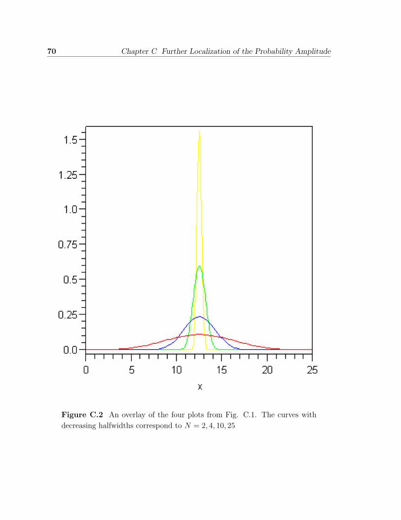
Figure C.1 shows plots of similar wave packets that were constructed using sine
waves instead of Airy functions. They were constructed in the same way but represent
a different situation such as a particle in a rigid box with a flat potential. They
are plotted for different numbers of terms in the sum and show the effect on the
localization of the packet. In the plots, N is the number of terms in the sum used to
create the packet. Figure C.2 displays the four plots overlayed.

69
Figure C.1 The approximate δ function constructed from sine waves plotted
for various values of terms in the sum
70 Chapter C Further Localization of the Probability Amplitude
Figure C.2 An overlay of the four plots from Fig. C.1. The curves with
decreasing halfwidths correspond to N = 2, 4, 10, 25
Appendix D
Quantum Mechanical Justification
Based on the Heisenberg Picture
In this project we took an approach to the Thomson experiment that was based on
the quantum mechanical description of the system involved. We sought to recover
the same results that we found in the classical case. The Thomson experiment is
most frequently treated as a classical system. Viewing it from a purely quantum
mechanical standpoint is not nearly as common. It makes sense to solve this system
using classical physics because everything works nicely. The claim of quantum theory,
however, is that it is a better description of how the physical world operates than
classical mechanics. We should thus be able to do anything with quantum mechanics
that we can do with classical physics. In this section I give some justification for the
treatment of the Thomson experiment, which is traditionally classical, as a quantum
mechanical system. This justification is based on the Heisenberg representation.
When working with constant state vectors, we are using the Heisenberg picture.
The time dependence of the operators is given by the Heisenberg equation.4 This
71
72 Chapter D Quantum Mechanical Justification Based on the Heisenberg Picture
equation states that for any operator A, its time evolution is given by
A =1
ih[A,H]. (D.1)
The Hamiltonian for an electron in the electric field of the Thomson experiment is3
H =P 2
2m+ αx (D.2)
where α is the slope of the potential energy in the capacitor model of section 2.3.
Since α is positive the electron is expected to accelerate towards the left. When we
substitute the Hamiltonian into the Heisenberg equation and use [x, P ] = ih we get4
P =1
ih[P,H] =
1
ih[P, αx] = − α
ihih = −α. (D.3)
Thus
P = −α (D.4)
which is the constant force we expect from the electric field. Integrating to find P (t)
gives
P (t) = P0 − αt. (D.5)
We can do the same thing for the position operator. Applying the Heisenberg equation
gives
x =1
ih[x,
P 2
2m+ αx] =
2ih
ih2mP =
P
m. (D.6)
Therefore
x =1
ih[x, H] =
1
ih[P
m,P 2
2m+ αx] = − α
m. (D.7)
We can integrate to solve for x(t),
x = − αm
(D.8)
x =P0
m− α
mt (D.9)
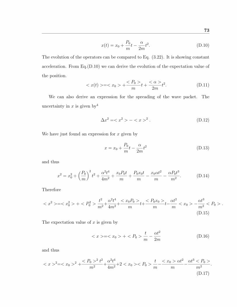
73
x(t) = x0 +P0
mt− α
2mt2. (D.10)
The evolution of the operators can be compared to Eq. (3.22). It is showing constant
acceleration. From Eq.(D.10) we can derive the evolution of the expectation value of
the position.
< x(t) >=< x0 > +< P0 >
mt+
< α >
2mt2. (D.11)
We can also derive an expression for the spreading of the wave packet. The
uncertainty in x is given by4
∆x2 =< x2 > − < x >2 . (D.12)
We have just found an expression for x given by
x = x0 +P0
mt− α
2mt2 (D.13)
and thus
x2 = x20 +
(P0
m
)2
t2 +α2t4
4m2+x0P0t
m+P0x0t
m− x0αt
2
m− αP0t
3
m2. (D.14)
Therefore
< x2 >=< x20 > + < P 2
0 >t2
m2+α2t4
4m2+< x0P0 >
mt+< P0x0 >
mt−αt
2
m< x0 > −
αt3
m2< P0 > .
(D.15)
The expectation value of x is given by
< x >=< x0 > + < P0 >t
m− αt2
2m(D.16)
and thus
< x >2=< x0 >2 +
< P0 >2 t2
m2+α2t4
4m2+2 < x0 >< P0 >
t
m−< x0 > αt2
m−αt
3 < P0 >
m2.
(D.17)
74 Chapter D Quantum Mechanical Justification Based on the Heisenberg Picture
The spreading is then given by
∆x2 =< x2 > − < x >2 (D.18)
=< x20 > − < x0 >
2 +(< P 20 > − < P0 >
2)t2
m2+
2t
m
(< P0x0 + x0P0 >
2− < x0 >< P0 >
).
(D.19)
Thus
∆x2 = ∆x20 + ∆P 2
0
t2
m2+
2t
m
(< P0x0 + x0P0 >
2− < x0 >< P0 >
). (D.20)
It is interesting to note that α is not contained in the expression. This means that
the spreading is independent of the slope of the potential. It is also interesting to
note that the uncertainty in x is identical to that of the free particle. We can use the
same method for the momentum. We begin with
P (t) = P0 − αt (D.21)
and
< P >=< P0 > −αt. (D.22)
We then proceed to find the values we need for the uncertainty. We find the square
of the momentum
P 2 = P 20 + α2t2 − 2αP0t. (D.23)
Thus
< P >2=< P0 >2 +α2t2 − 2α < P0 > t (D.24)
and
< P 2 >=< P 20 > +α2t2 − 2α < P0 > t. (D.25)
We can then find the uncertainty,
∆P 2 =< P 2 > − < P >2= ∆P 20 (D.26)
75
∆P 2(t) = ∆P 20 . (D.27)
If we minimize the uncertainty between these two quantities by setting their product
equal to h,
∆x∆P =h
2(D.28)
then we can assign values as
∆x0 =
√h
2(D.29)
and
∆P0 =
√h
2. (D.30)
This results in the following expression for the square of the uncertainty in x,
∆x2 =h
2
(1 +
t2
m2
)+
2t
m
(< P0x0 + x0P0 >
2− < x0 >< P0 >
). (D.31)

76 Chapter D Quantum Mechanical Justification Based on the Heisenberg Picture
Index
Airy functions, 29, 31–34, 36, 47, 55, 58,63, 68
Ai, 29Bi, 31
Analysisnumerical, 48
Angular frequency, 20Approximations, 14, 23, 36–38, 40, 47, 53,
55, 57, 58Average value, 16
Bessel functions, 29
Capacitor, iv, 2, 6, 7, 9, 12, 13, 29, 32, 36,47, 57, 72
Cathode ray, 2, 4, 5, 36Circular orbit, 17, 18, 22Classical, iv, 1, 2, 6, 23, 27, 39, 49, 57, 71Conditions
boundary, 11, 33, 34initial, 12, 17
Constant force, 49, 72Coordinates, 9, 17, 18Cross product, 5, 15Cyclotron frequency, 22
Deflection, iv, 3–5, 22, 24, 57, 58, 61angle, 13, 14, 23
Delta function, 36, 53, 55, 57, 58, 68Differential equation, 15, 16, 24, 27, 29
ordinary, 28Dispersion, 2, 36, 40, 45–48, 53, 55, 57,
58, 63, 68Distribution
Gaussian, 48, 50, 53, 55, 58momentum, 49
probability, 68
Edge effects, 6, 7Electron, iv, 1–6, 9, 17, 22–24, 29, 38, 39,
45, 48, 57, 72Elliptical motion, 17Energy, 27, 36, 37, 47, 48, 68Expectation value, iv, 40, 45–47, 73
Fieldelectric, iv, 2–4, 9, 18, 24, 29, 61, 72magnetic, iv, 3, 4, 6, 9, 14, 17, 24, 25,
61Fourier transform, 48, 49Free particle, 74
Gaussian, 48, 58function, 50, 52, 53, 55, 57packet, 53
Hamiltonian, 72Heisenberg, iv, 36, 47, 71, 72
Imaginary, 32
Linear combination, 28Localization, iv, 2, 36, 38, 45–47, 68Lorentz, 5, 14
Magnetic field, 11Maple, 2, 34, 36, 37, 39, 40, 55, 57, 58,
63, 67Minimize, 75Momentum, 49, 74Momentum space, 2, 48, 55, 57, 58
Newton, 6, 9, 27second law, 11, 14
77
78 INDEX
Normalization, 2, 37, 38constant, 37
Orthogonal, 5, 9, 17
Parabola, 45, 46Parametric equations, 17, 18Peak width, 50Piecewise function, 34, 37Position space, 48, 49Potential, 2, 27, 47, 58, 68, 74
constant, 7, 28, 32energy, 7, 27, 28, 72linear, 6, 29, 32well, 6, 7, 31zero, 7, 32
Probabilityamplitude, iv, 38, 39, 48, 50, 57density, 36, 50distribution, 68
Pythagorean, 13
Quadratic relation, 12Quantum, 1, 2, 9, 18, 27
effect, 2, 40, 55, 68mechanics, iv, 1, 2, 57, 58, 71
Relativistic, 27Right-hand rule, 24Robinett, 48, 55
Schrodinger, 2, 27–29, 32, 48Selection, 47Slope, 14, 23, 29, 32, 47, 48, 50, 72, 74Small angle approximation, 23Spreading, 45, 47, 50, 53, 73, 74Summation, 36–38, 45, 47, 58, 67, 68
Thomson, iv, 1–6, 9, 14, 22–24, 27, 36, 38,39, 57, 58, 71, 72
Timedependence, 39, 71evolution, iv, 2, 58, 63, 72function of, 11, 16independent, 27
initial, 17Trajectory, iv, 2, 13
circular, 6, 17, 18, 21, 22parabolic, 12straight line, 25
Trigonometricfunctions, 20identity, 21
Uncertainty, iv, 36, 47, 68, 73–75Uncoupled, 15Units
natural, 33, 50SI, 22
Velocity, 3, 5, 13, 17, 18, 24Voltage, 4
Wave packets, iv, 2, 36, 37, 39, 40, 45, 47,48, 50, 53, 55, 57, 58, 63, 68, 73
Wavefunction, 27–29, 32, 34, 36–38, 49,55