AIR FORCE INSTITUTE OF TECHNOLOGY - apps.dtic.mil · existing free-space pathloss model used by...
102
DEVELOPMENT OF A WIRELESS MODEL INCORPORATING LARGE- SCALE FADING IN A RURAL, URBAN AND SUBURBAN ENVIRONMENT THESIS Roger A. Illari, Captain, USAF AFIT/GE/ENG/06-25 DEPARTMENT OF THE AIR FORCE AIR UNIVERSITY AIR FORCE INSTITUTE OF TECHNOLOGY Wright-Patterson Air Force Base, Ohio APPROVED FOR PUBLIC RELEASE; DISTRIBUTION UNLIMITED
Transcript of AIR FORCE INSTITUTE OF TECHNOLOGY - apps.dtic.mil · existing free-space pathloss model used by...

DEVELOPMENT OF A WIRELESS MODEL INCORPORATING LARGE-SCALE FADING IN A RURAL, URBAN AND SUBURBAN ENVIRONMENT
THESIS
Roger A. Illari, Captain, USAF
AFIT/GE/ENG/06-25
DEPARTMENT OF THE AIR FORCE AIR UNIVERSITY
AIR FORCE INSTITUTE OF TECHNOLOGY
Wright-Patterson Air Force Base, Ohio
APPROVED FOR PUBLIC RELEASE; DISTRIBUTION UNLIMITED

The views expressed in this thesis are those of the author and do not reflect the official
policy or position of the United States Air Force, Department of Defense, or the U.S.
Government.

AFIT/GE/ENG/06-25
DEVELOPMENT OF A WIRELESS MODEL INCORPORATING LARGE-SCALE FADING IN A RURAL, URBAN AND SUBURBAN ENVIRONMENT
THESIS
Presented to the Faculty
Department of Electrical and Computer Engineering
Graduate School of Engineering and Management
Air Force Institute of Technology
Air University
Air Education and Training Command
In Partial Fulfillment of the Requirements for the
Degree of Master of Science in Electrical Engineering
Roger A. Illari, BS
Captain, USAF
March 2006
APPROVED FOR PUBLIC RELEASE; DISTRIBUTION UNLIMITED

AFIT/GE/ENG/06-25
DEVELOPMENT OF A WIRELESS MODEL INCORPORATING LARGE-SCALE FADING IN A RURAL, URBAN AND SUBURBAN ENVIRONMENT
Roger A. Illari, BS
Captain, USAF
Approved: __________//Signed//______________ ________ Barry E. Mullins, Ph.D. (Chairman) Date __________//Signed//______________ Rusty O. Baldwin, Ph.D. (Member) Date
__________//Signed//______________ ________ Michael A. Temple, Ph.D. (Member) Date

iv
Acknowledgments
First, I would like to thank my family because without them I would never have
been able to make it through the program. I would like to express my sincere
appreciation to my thesis advisor, Dr. Barry E. Mullins, for his guidance and support
throughout the course of this thesis effort. I would also like to thank my committee
members Dr. Rusty O. Baldwin and Dr. Michael A. Temple for their guidance and help
in answering my questions. I would also like to thank my sponsor, Mr. Scott Gardner,
from the Air Force Communications Agency for the support provided to me in this
endeavor. Finally, I would like to thank my fellow students Kevin Morris and LeRoy
Willemsen. Kevin was my local OPNET deity and LeRoy provided me with help and
advice on everything else.
Roger A. Illari
.

v
Table of Contents
Page
ACKNOWLEDGMENTS.......................................................................................................................... IV
TABLE OF CONTENTS.............................................................................................................................V
LIST OF FIGURES.................................................................................................................................VIII
LIST OF TABLES........................................................................................................................................X
ABSTRACT ................................................................................................................................................ XI
I. INTRODUCTION............................................................................................................................... 1 1.1 BACKGROUND.............................................................................................................................. 1 1.2 MOTIVATION AND GOAL.............................................................................................................. 2 1.3 THESIS LAYOUT ........................................................................................................................... 3
II. LITERATURE REVIEW................................................................................................................... 4 2.1 CHAPTER OVERVIEW ................................................................................................................... 4 2.2 BACKGROUND.............................................................................................................................. 5
2.2.1 History .................................................................................................................................... 5 2.3 CURRENT ISSUES.......................................................................................................................... 6 2.4 MOBILE RADIO PROPAGATION FACTORS ..................................................................................... 8
2.4.1 Reflection................................................................................................................................ 8 2.4.2 Diffraction .............................................................................................................................. 9 2.4.3 Scattering.............................................................................................................................. 10
2.5 LARGE-SCALE FADING............................................................................................................... 10 2.6 SMALL–SCALE FADING.............................................................................................................. 11
2.6.1 Multipath Propagation ......................................................................................................... 11 2.6.2 Speed of the Mobile .............................................................................................................. 12 2.6.3 Speed of the Surrounding Objects ........................................................................................ 12 2.6.4 Transmission Bandwidth of the Signal ................................................................................. 12
2.7 PROPAGATION MODELS ............................................................................................................. 13 2.7.1 Outdoor Propagation Models............................................................................................... 13 2.7.2 Free Space Propagation Model............................................................................................ 13 2.7.3 Okumura Model.................................................................................................................... 14 2.7.4 Hata Model ........................................................................................................................... 17 2.7.5 COST-231 Model.................................................................................................................. 19
2.8 OPNET WIRELESS MODULE...................................................................................................... 19 2.8.1 Receiver Group..................................................................................................................... 21 2.8.2 Transmission Delay .............................................................................................................. 21 2.8.3 Link Closure ......................................................................................................................... 21 2.8.4 Channel Match ..................................................................................................................... 22

vi
2.8.5 TX Antenna Gain .................................................................................................................. 22 2.8.6 Propagation Delay ............................................................................................................... 22 2.8.7 RX Antenna Gain .................................................................................................................. 22 2.8.8 Received Power .................................................................................................................... 23 2.8.9 Background Noise................................................................................................................. 23 2.8.10 Interference Noise................................................................................................................. 23 2.8.11 Signal-to-Noise Ratio ........................................................................................................... 24 2.8.12 Bit Error Rate ....................................................................................................................... 24 2.8.13 Error Allocation ................................................................................................................... 25 2.8.14 Error correction ................................................................................................................... 25
2.9 RELEVANT RESEARCH................................................................................................................ 25 2.9.1 IEEE 802.16 Pathloss Replacement ..................................................................................... 26 2.9.2 Rayleigh Fading Incorporation ............................................................................................ 26 2.9.3 Ricean and Rayleigh Fading Incorporation in NS Network Simulator ................................ 26
2.10 SUMMARY.................................................................................................................................. 27
III. METHODOLOGY....................................................................................................................... 28 3.1 PROBLEM DEFINITION ................................................................................................................ 28
3.1.1 Goals and Hypothesis ........................................................................................................... 28 3.1.2 Approach .............................................................................................................................. 28
3.2 SYSTEM BOUNDARIES................................................................................................................. 29 3.3 SYSTEM SERVICES...................................................................................................................... 29 3.4 WORKLOAD ............................................................................................................................... 30 3.5 PERFORMANCE METRICS............................................................................................................ 30 3.6 PARAMETERS ............................................................................................................................. 30
3.6.1 System................................................................................................................................... 30 3.7 FACTORS .................................................................................................................................... 31 3.8 EVALUATION TECHNIQUE .......................................................................................................... 33 3.9 EXPERIMENTAL DESIGN............................................................................................................. 33 3.10 ANALYSIS AND INTERPRETATION OF RESULTS........................................................................... 38 3.11 SUMMARY.................................................................................................................................. 39
IV. ANALYSIS AND RESULTS....................................................................................................... 40 4.1 PATHLOSS CALCULATION COMPARISON .................................................................................... 40 4.2 PIPELINE STAGE COMPARISON ................................................................................................... 42 4.3 MEASURED RECEIVED POWER COMPARISON ............................................................................. 49 4.4 SUMMARY.................................................................................................................................. 52
V. CONCLUSIONS AND RECOMMENDATIONS .......................................................................... 54 5.1 CHAPTER OVERVIEW ................................................................................................................. 54 5.2 CONCLUSIONS AND SIGNIFICANCE OF RESEARCH ...................................................................... 54 5.3 RECOMMENDATIONS FOR FUTURE RESEARCH ........................................................................... 55

vii
APPENDIX A: MODIFIED PIPELINE CODE ...................................................................................... 56
APPENDIX B: OPNET DEBUGGER OUTPUT .................................................................................... 70
APPENDIX C: SUBURBAN SIMULATION RESULTS ...................................................................... 74
BIBLIOGRAPHY ...................................................................................................................................... 87
viii
List of Figures
Figure Page
1. Consumer Market Percentage of Mobile Telephony [Rap96]....................................... 5
2. Frequency Range Allocated in 1974 [Lee97] ................................................................ 6
3. Basic Cell Block [Rap02] .............................................................................................. 7
4. Reflection of an Incoming Wave [Wir06] ..................................................................... 9
5. Effects of Diffraction [Wid06]....................................................................................... 9
6. Measured Signal Strength [NNP00] ............................................................................ 11
7. Median Attenuation Relative to Free Space [Oku68].................................................. 15
8. AREAG Graph................................................................................................................. 17
9. Radio Transceiver Pipeline Execution [Opn05] .......................................................... 20
10. Rayleigh Fading in Radar System [Wif06]................................................................ 26
11. Experiment Scenario Setup........................................................................................ 34
12. Initial Node Location and Speed................................................................................ 35
13. Node Models.............................................................................................................. 36
14. C/C++ Pipeline Stage Used ....................................................................................... 37
15. Urban Large City and Free-Space Comparison .......................................................... 43
16. Urban Large City Received Signal Strength Comparison .......................................... 44
17. Urban Medium City and Free-Space Comparison...................................................... 45
18. Urban Medium City Received Signal Strength Comparison...................................... 46
19. Suburban and Free Space Comparison ....................................................................... 47
20. Suburban Received Signal Strength Comparison ....................................................... 47

ix
21. Rural and Free-Space Comparison ............................................................................. 48
22. Rural Received Signal Strength Comparison ............................................................. 49
23. Pathloss Slopes for 894 MHz and 1922 MHz [HTJ93] .............................................. 52

x
List of Tables
Table Page
1. List of Factors and Values Used .................................................................................. 32
2. Simulation Parameters ................................................................................................. 38
3. Urban Large City Pathloss Calculation........................................................................ 40
4. Urban Medium City Pathloss Calculation ................................................................... 41
5. Suburban Pathloss Calculation .................................................................................... 41
6. Rural Pathloss Calculation........................................................................................... 41
7. Measured Pathloss Slope [HTJ93]............................................................................... 50
8. Simulation Pathloss Slopes for Hata / COST-231 Model (dB/decade) ....................... 50

xi
AFIT/GE/ENG/06-25
Abstract
The goal of this research is to develop a more realistic estimate of received signal
strength level as calculated by OPNET. The goal is accomplished by replacing the
existing free-space pathloss model used by OPNET with the Hata and COST-231
pathloss models. The calculated received signal strength using the new models behaves
similarly to the measured values, with a 0.245 dB difference for 880 MHz and a 1.365 dB
difference for 1922 MHz between the pathloss slopes. There is an 11.3 dBm difference
between the initial starting signal strength from the calculated values and the measured
values.
An important aspect of a wireless communication system is the planning process.
The planning phase of a wireless communication system will determine the number of
necessary transmitting antennas, the frequency to be used for communications, and
ultimately the cost of the entire project. Because of the possible expense of these factors
it is important that the planning stage of any wireless communications project produce an
accurate calculation of the coverage area.

1
DEVELOPMENT OF A WIRELESS MODEL INCORPORATING LARGE-SCALE FADING IN A RURAL, URBAN AND SUBURBAN ENVIRONMENT
I. Introduction
1.1 Background
The propagation of a radio signal is affected by three main factors; reflection,
scattering and diffraction [Rap02]. Reflection occurs when the signal impinges upon an
object much larger than the signal wavelength, e.g., the earth or a large building.
Scattering occurs when the traveling wave front encounters objects much smaller than the
wavelength with sharp edges, e.g., lampposts and stop signs. The result is multiple
smaller wave fronts are created. Diffraction is the apparent bending or spreading of a
signal/wave when it impinges upon an object [Rap02].
Due to these factors, a received radio signal level is subject to fading. Large-scale
fading is mainly due to the transmitter receiver pair (T-R) separation. The further a
receiver gets from a transmitter, the more the received signal will decrease. Small-scale
fading is also known as multipath fading because the main cause is the arrival of multiple
copies of the same signal at the receiver. If the copies are in phase they will have an
additive effect on the average signal strength; if the signals are out of phase, there will be
a destructive effect on the signal strength [Rap02]. Over a small distance such as a 25 m
T-R separation, the value of a received signal fluctuates very little due to large-scale
fading. On the other hand, small-scale fading can cause the signal to fluctuate by as
much as 30 dB over the same distance [Skl97].

2
The need for accurate signal strength prediction spurred the creation of radio
signal propagation models. Propagation models are either empirical, theoretical or a mix
of the two. The empirical model is based on measurements and takes into account all
factors that affect radio propagation. Theoretical models are based on the fundamental
principles of the radio wave phenomenon [NNP00].
OPNET modeler is a comprehensive network research and development tool used
to plan and design wireless communications networks. The wireless module for OPNET
has a radio transceiver pipeline that accounts for radio communications link such as
transmit (TX) and receive (RX) antenna gain, signal to noise ratio (SNR) and received
power.
1.2 Motivation and Goal
Military bases all over the world have wireless communication systems located on
each of them. The limited resources available to organizations such as the Air Force
Communications Agency (AFCA) mean they rely heavily on computer simulators to plan
any changes to existing systems or create new ones. Therefore, the models should be as
accurate as possible. This means the pathloss model used by OPNET should model the
environment the system will operate in with maximum fidelity.
The goal of this research is to replace the free space pathloss model used by
OPNET to calculate wireless links characteristics with a pathloss model that more
accurately accounts for the different types of environments that a signal will travel
through.

3
1.3 Thesis Layout
This chapter introduces the factors which can interfere with wireless
communications; it also discusses the goals and motivation for the research. Chapter II
discusses the different factors that affect radio signal propagation in detail as well as
some different outdoor pathloss models. Chapter II discusses the operation of OPNET’s
transceiver pipeline. Chapter III discusses the methodology used to conduct the research
and the factors and parameters being used in the research, the number of simulations
being performed, how the simulations are setup and what data is being collected from
each simulations. Chapter IV presents the analysis of the results and Chapter V presents
conclusions drawn from the research and provides ideas for future research.

4
II. Literature Review
2.1 Chapter Overview
This chapter illustrates the complications and tools associated with planning a
wireless communication system. It also discusses current research into effective and
realistic planning of a wireless communication system.
One of the main obstacles encountered when planning a wireless communication
system are factors that reduce the received signal strength such as large-scale fading and
small-scale fading [Rap96]. Aiding the planner of a wireless communication system is a
research and development tool called OPNET. OPNET Modeler is an environment for
network modeling and simulation, which supports the design and study of
communication networks, devices, protocols, and applications. [Opn05]. Current
research illustrates the need to incorporate the fading factors into modern network
modelers such as OPNET and NS to provide a more realistic assessment of the
performance of a proposed wireless communication system [Acl03], [Acr03] and
[Pun00]. The research in [Acl03], [Acr03] and [Pun00] each attempt to replace the
original pathloss model used by OPNET and NS with pathloss models that more
accurately reflect real world conditions.
Section 2 provides background and current issues in wireless communications.
Section 3 discusses the factors that affect radio signal propagation. Section 4 and 5
discusses the details of large-scale and small-scale fading of the radio signal. Section 6
discusses some of the outdoor propagation models currently being used to predict

5
wireless signal coverage. Section 7 explains each stage of the radio transceiver pipeline
of OPNET. Section 8 discusses relevant research concerning wireless signal propagation.
2.2 Background
2.2.1 History
In 1897, Guglielmo Marconi demonstrated the importance of radio by
maintaining constant contact with a ship as it crossed the English Channel [Rap96].
What Marconi did not realize at the time was how rapidly wireless communication
system would pervade modern society. With the advancements in technology, wireless
communication has become a part of modern society faster than any other invention of
the 20th century as seen in Figure 1 [Rap96].
Figure 1. Consumer Market Percentage of Mobile Telephony [Rap96]

6
Figure 1 shows that Mobile Telephony which does not include paging systems, amateur
radio, dispatch radio, citizens band (CB) radio, public service radio, cordless phones, or
terrestrial microwave radio systems have become increasingly popular in the consumer
sector. For 35 years following their introduction, mobile telephones were not prevalent
in modern society due to the expense of the service and equipment. But during the
1980’s, there is a marked increase in mobile telephones acceptance in modern society
compared to the television and the videocassette recorder. The increased acceptance of
mobile telephones is attributed to the increase in technological advances, which reduced
the expense associated with the service and equipment, and in turn made mobile
telephones more affordable for consumers [Rap96].
2.3 Current Issues
With the popularity of mobile telephone came issues inherent in the planning of a
wireless communication system. In 1974 the Federal Communications Commission
(FCC) allocated a 40 MHz of bandwidth in the 800 to 900 MHz frequency range which
was divided into a total of 666 duplex channels for mobile telephone use [Lee97] as
shown in Figure 2.
Figure 2. Frequency Range Allocated in 1974 [Lee97]
In 1989, the FCC granted an additional 166 channels (10 MHz) to accommodate the rapid
growth and demand. The rapid growth coupled with the limited number of channels
available (832 total) caused wireless communications system planners to develop

7
schemes for frequency reuse and allocation. To meet the demand with the limited
amount of frequency channels available, wireless system planners developed a technique
for frequency reuse by allocating a group of radio channels to be used within a small
geographic area called a cell [Rap02]. The cell is a hexagonal-shaped geographic area as
seen in Figure 3.
Figure 3. Basic Cell Block [Rap02]
The different numbered individual cells seen in Figure 3 are allocated a different group of
frequencies for use in that cell, and cells with the same numbers are using the same group
of frequencies. The number of cells in each block K is calculated from Equation (2.1).
( )2
3D R
K = (2.1)
where D is the distance between two adjacent frequency-reuse cells and R is the radius of
each cell. For a D/R equal to 4.6, K is equal to 7. For the number of cells in the block in
Figure 3 this means the frequencies can be divided into 7 groups (cells).

8
2.4 Mobile Radio Propagation Factors
Predicting the received signal strength at a mobile receiver from a stationary
transmitter has become one of the most difficult aspects of planning for a wireless
communication system [Rap02]. The varied environments in which wireless
communications systems are used pose different challenges that hinder wireless signal
propagation. To predict the average signal strength at a receiver, planners must account
for obstacles between the transmitter and mobile receiver that affect radio wave
propagation. The signal can travel over a path that can vary from a line of sight (no
obstacles), to mountains, to buildings. The three mechanisms that influence signal
propagation in a mobile communication system are reflection, diffraction, and scattering.
2.4.1 Reflection
Reflection occurs when a propagating electromagnetic wave impinges upon an
object that has very large dimensions compared to the wavelength of the incident wave
[Rap02]. A reflected wave can either increase or decrease a signal level at the reception
point [NNP00]. Figure 4, below, illustrates the phenomenon of refection as it pertains to
radio signal propagation. The signal level can be increased if a large proportion of the
reflected waves are reflected toward the receiver and decreased if the reflected wave is
directed away from the receiver. Buildings, walls and the surface of the earth are causes
of reflection.

9
Figure 4. Reflection of an Incoming Wave [Wir06]
2.4.2 Diffraction
Diffraction occurs when a large opaque body whose dimensions are considerably
larger than the signal wavelength obstructs the signal path between the transmitter and
receiver. Diffraction occurs at the obstacle’s edges where some scattering may also occur
as well as additional attenuation [NNP00]. Figure 5 below illustrates the phenomenon of
diffraction.
Figure 5. Effects of Diffraction [Wid06]
When a crest, the section of a wave that rises above an undisturbed position, overlaps
with another crest or a trough, the low point of the wave, overlaps with another trough
constructive interference occurs, and the signal strength will increase. If a crest overlaps
with a trough, then they cancel each out, and the interference is destructive. [Wid06] The
creation of the secondary wave front allows the receiver to receive a signal even though

10
the line-of-sight (LOS) path is obstructed; this phenomenon is sometimes called
shadowing [Skl97].
2.4.3 Scattering
Scattering occurs when the medium in which the signal is propagating has many
objects that are smaller than or comparable to the wavelength of the radio signal. This
phenomenon is similar to diffraction except the radio wave is scattered in a greater
number of directions [NNP00]. In urban settings foliage, stop signs and lampposts are
examples of objects that cause scattering [Skl97].
2.5 Large-Scale Fading
The factors affecting wireless communication can be categorized into two main
categories; large-scale fading and small-scale fading [Skl97]. Large-scale fading is
useful in determining a transmit antenna coverage area. Large-scale fading or large-scale
pathloss is useful for predicting the average received signal strength at a given distance
from the transmit antenna. In Figure 6, the effects of large-scale fading are shown as the
distance between the transmitter and receiver increases.

11
Figure 6. Measured Signal Strength [NNP00]
The graph shows as the separation of the receiver from the transmitter increases, the
average signal level i.e., (solid dark line) decreases. The measured signal level at 50
meters is approximately 62dBμ; at the ending distance of 200 meters, the received
average signal strength is approximately 40dBμ.
2.6 Small–Scale Fading
Unlike large-scale fading that measures the average received signal strength,
small-scale fading is a rapid fluctuation in signal strength measured over a small distance
or period of time [Rap02]. The effects of small-scale fading are shown in Figure 6 by the
gray line. It can be seen in Figure 6 the transmitter and receiver distances of 100-150
meters shows great fluctuation in the received signal strength, from a maximum value of
approximately 52dBμ to a minimum value of 15dBμ. The four main physical factors
which influence small-scale fading in the radio propagation channel are multipath
propagation, speed of the mobile receivers, speed of surrounding objects and
transmission bandwidth of the signal [Rap02].
2.6.1 Multipath Propagation
Multipath propagation results from the presence of reflectors and scatterers in the
propagation channel that cause multiple versions of the transmitted signal to arrive at the
receiver, each distorted in amplitude, phase and angle of arrival. Small-scale fading is
also known as multipath fading [Mat05]. Due to the increased time required to receive
the baseband portion of the signal, intersymbol interference can occur resulting in signal
smearing [Rap02]. Intersymbol interference is a disturbance caused by extraneous

12
energy from the signal in one or more keying intervals that interferes with the reception
of the signal in another keying interval [Wii06].
2.6.2 Speed of the Mobile
The relative motion between a base station and a mobile receiver results in
random frequency modulation due to the different Doppler shifts on each of the multipath
components (waves arriving at the receiver). The Doppler shifts can be either negative or
positive depending on whether the mobile receiver is moving towards or away from the
base station [Rap02].
2.6.3 Speed of the Surrounding Objects
This phenomenon occurs if the objects surrounding a mobile receiver are moving
much faster in relation to the mobile receiver. For example, if a mobile receiver is
adjacent to a highway, the speed and multitude of the vehicles near the mobile receiver
will induce a Doppler shift upon the signals being received [Rap02].
2.6.4 Signal Transmission Bandwidth
This physical factor is concerned with the transmitted signal bandwidth compared
to the “bandwidth” of the multipath channel. If the transmitted signal bandwidth is much
greater than the “bandwidth” of the multipath channel, then the received signal strength
will not fade much over the local area because of small-scale fading factors. Otherwise,
if the transmitted signal bandwidth is narrow relative to the “bandwidth” of the multipath
channel, then the signal amplitude can change rapidly while the signal structure is not
itself distorted in time [Rap02].

13
2.7 Propagation Models
Because of the numerous factors involved in the radio signal propagation and the
difficulty in predicting short-term fading, nearly all propagation models estimate either
the average or median values of the signal level [NNP00]. A propagation model is a set
of mathematical expressions, diagrams and/or algorithms used to represent the
environment a radio signal will travel through [NNP00]. These models can be either
empirical (statistical) or theoretical (deterministic) or a combination of the two. The
empirical model is based on measurements while theoretical models use the fundamental
principles of radio wave propagation phenomena [NNP00].
2.7.1 Outdoor Propagation Models
Radio transmissions in a mobile communication system often take place over
irregular terrain. The terrain profile must be taken into account to determine the pathloss
and will vary from an unobstructed line of sight (LOS) to a simple curvature of the earth
to a highly mountainous profile. The presence of trees, buildings and other obstacles
must all be taken into account when predicting signal strength coverage. A few of the
more commonly used outdoor propagation models are discussed.
2.7.2 Free Space Propagation Model
The free-space propagation model is used when the transmitter-receiver (T-R)
pair have an unobstructed clear LOS between them. Satellite communications and
microwave LOS radio communication typically experience free-space pathloss [Rap02].
When the receive antenna gain is isotropic, the power received is given by the Friis free-
space equation (equation (2.2)).

14
2
2 2( )(4 )
t t rr
PG GP d
d Lλ
π= (2.2)
where d in equation 2.2 is the T-R distance in meters, Pt is the transmitted power which is
a function of the T-R seperation, Gt is the gain of the transmit antenna, Gr is the gain of
the receive antenna, λ is the free-space wavelength in meters and L accounts for all
system losses not related to propagation (L ≥ 1) [Rap02]. This model assumes that the
path between the T-R pair is free of obstructions that might reflect or absorb any radio
frequency (RF) energy and is mainly a function of the transmitter and receiver separation
[Skl96].
2.7.3 Okumura Model
The Okumura model is one of the most widely used models for signal prediction
in urban areas [Rap02]. The Okumura model is the result of empirical data collected in
detailed propagation tests over various situations of an irregular terrain and
environmental clutter [NNP00]. Okumura developed a set of curves which describe
median attenuation denoted as 50 ( )L dB , relative to free-space in an urban area over a
quasi-smooth terrain with a base station effective antenna height of 200 m and mobile
antenna height of 3 m. To determine pathloss with Okumura’s model, free-space
pathloss is first calculated between the points of interest. The value of median
attenuation relative to free-space ( ( , )muA f d ) is then read from curves in Figure 7.
Finally, the correction factors for the type of terrain and the height of the receive and
transmit antennas is added [Oku68]. The resultant model is shown in equation (2.3).

15
50 ( ) ( , ) ( ) ( )F mu te re AREAL dB L A f d G h G h G= + − − − (2.3)
where FL is the free-space propagation loss in decibels, ( , )muA f d is the median
attenuation relative to free-space obtained from the graph in Figure 7 in decibels, ( )teG h
is the base station antenna height gain factor in decibels, ( )reG h is the mobile antenna
height gain factor in decibels and AREAG is the gain due to the type of environment
[Oku68].
Figure 7. Median Attenuation Relative to Free Space [Oku68]
16
For transmit antenna heights teh from 30 m to 1000 m, ( )teG h is obtained from equation
(2.4).
( ) 20 log200
tete
hG h ⎛ ⎞= ⎜ ⎟
⎝ ⎠ (2.4)
If the antenna height is less than or equal to 3 m, ( )reG h is obtained from equation (2.5).
( ) 10 log3re
reh
G h ⎛ ⎞= ⎜ ⎟⎝ ⎠
(2.5)
where reh is the receiver antenna height in meters. If the antenna height is greater than 3
m and less than 10 m ( )reG h is obtained using equation (2.6).
( ) 20 log3re
reh
G h ⎛ ⎞= ⎜ ⎟⎝ ⎠
. (2.6)
AREAG is obtained from Figure 8. AREAG is dependent on the type of environment and the
frequency being used. Okumura’s model is considered to be among the simplest and best
in terms of accuracy for pathloss prediction for a mature cellular and land mobile radio
system in cluttered environments [Rap02]. The model developed by Okumura is solely
based on measured data and does not provide any analytical explanation. The model is
valid for the frequencies in the range of 150 MHz to 1920 MHz, T-R distances of 1 km to
100 km, base station antenna heights of 30 m to 1000 m and receiver antenna heights of 3
m to 10 m [Rap02].

17
Figure 8. AREAG Graph
2.7.4 Hata Model
The Hata model is an empirical formulation of the graphical pathloss data
provided by Okumura. The model is valid for frequencies between 150 MHz to 1500
MHz, transmit antenna heights of 30 m to 200 m, receiver antenna heights of 1 m to 10 m
and distances of 1 km to 100 km. Hata developed a standard formula for propagation
loss in an urban environment (see equation (2.7)).
50( )( ) 69.55 26.16log 13.82log( ) (44.9 6.55log ) log
c te
re te
L urban dB f ha h h d
= + −− + −
(2.7)

18
where cf is the frequency in MHz, teh is the transmit antenna height in meters, reh is the
receiver antenna height in meters, d is the T-R separation in km and ( )rea h is the
correction factor for effective mobile antenna height which is a function of the size of the
coverage area. ( )rea h is calculated for a large city using equations (2.8) and (2.9).
2( ) 8.29(log1.54 ) 1.1 300re re ca h h dB for f MHz= − ≤ , or (2.8)
2( ) 3.2(log11.75 ) 4.97 300re re ca h h dB for f MHz= − ≥ . (2.9)
Medium to small sized cities have a smaller number of tall buildings i.e. skyscrapers.
Manhattan would be characterized as a large city where as downtown Dayton, OH would
be characterized as a small city. Equation (2.10) is used to calculate ( )rea h for small to
medium sized cities.
( )( ) (1.1log 0.7) 1.56 log 0.8re c re ca h f h f dB= − − − (2.10)
To obtain the pathloss in a suburban area the Hata formula becomes equation (2.11).
( )( )250 50( )( ) ( ) 2 log / 28 5.4cL suburban dB L urban f= − − (2.11)
where the ( )rea h is calculated using the equation (2.10). The pathloss in a rural area is
obtained using equation (2.12).
( )250 50( )( ) ( ) 4.78 log 18.33log 40.94c cL rural dB L urban f f= − + − (2.12)
where ( )rea h is calculated using equation (2.10). The prediction’s of Hata’s model are
very close to the graphs of Okumura’s model, with both providing a practical means to
planning for large cell mobile systems [Hat90].

19
2.7.5 COST-231 Model
The COST-231 model is an empirical formula that was proposed by the European
Cooperative for Scientific and Technical research to extend Hata’s model to 2 GHz
[Rap02]. The COST-231 pathloss model given by equation (2.13).
( )
( ) ( )50 46.3 33.9 log 13.82log
44.9 6.55log logc te
re e M
L urban f h
a h h d C
= + −
− + − + (2.13)
where cf is the frequency in MHz, teh is the transmit antenna height in meters, d is the
T-R separation in km and ( )rea h is the correction factor for effective mobile antenna
height which is a function of the size of the coverage area and reh which is the receiver
antenna height in meters. ( )rea h is defined in equations (2.8), (2.9) and (2.10). MC is
equal to 0 dB for a medium sized city and suburban area or 3 dB for a metropolitan
center. The COST-231 model is valid for frequencies between 1500 MHz to 2000 MHz,
transmit antenna heights of 30 m to 200 m, receiver antenna heights of 1 m to 10 m and
distances of 1 km to 20 km [EUR91].
2.8 OPNET Wireless Module
The OPNET wireless module is model that allows realistic and accurate modeling
of wireless networks. The wireless module uses a Radio Transceiver Pipeline (RTP) to
model wireless transmissions of packets. An “execution” of the pipeline is performed for
each eligible receiver. Figure 9 depicts the 14 stages of the Radio Transceiver Pipeline.

20
Figure 9. Radio Transceiver Pipeline Execution [Opn05]
Because radio links are carried over a broadcast medium, one transmission can have
multiple receivers or one receiver can receive multiple transmissions. Thus some
receivers can require multiple executions of various stages of the pipeline because they
are part of multiple transmission-receiver channels. The following subsections describe
OPNET’s Radio Transceiver pipeline stages.

21
2.8.1 Receiver Group
During a radio transmission, this stage calculates the possible transmission
channel - receiver channel pairs that form the receiver groups. This information forms an
initial list of possible receivers for the transmission object. This is not actually a part of
the dynamic pipeline but it is included because the results of this pipeline stage will
influence the behavior of the radio transmissions. This stage is only executed once at the
start of a simulation for each transmitter and receiver channels.
2.8.2 Transmission Delay
This is the only stage for which a single execution is performed to support all
subsequent pipeline stages. This stage calculates the time an entire packet takes to
complete transmission. The result is the simulation difference between the transmission
of the first bit of a packet and the last bit of a packet. The result of this stage is used in
conjunction with the propagation delay stage to determine the time for the last bit of a
packet arrived at a link’s destination (receiver).
2.8.3 Link Closure
This stage is invoked once per receiver channel for each transmitter channel. The
goal of this stage is to determine if a receiver can be affected by the transmitter signal by
determining if transmission signal can physically reach the receiver. Physical
considerations such as occlusion by obstacles and/or the surface of the earth are used to
make this determination.

22
2.8.4 Channel Match
This stage is invoked once per receiver channel to classify the transmission with
respect to the receiver. This stage uses the result from the Link Closure stage to assign
one of three possible categories to the packet. “Valid” means that the packets will be
accepted and possibly forwarded to other modules. “Noise” identifies these packets as
having data content that cannot be received. The “Ignored” category means that a
transmission will have no effect on a receiver channels performance or state.
2.8.5 TX Antenna Gain
This stage is executed separately for each destination channel. This stage
computes the gain of the transmitter’s associated antenna based on a directional vector
from the transmitter to the receiver [Opn05]. The antenna gain is used in stage 7 of the
pipeline to calculate the received power.
2.8.6 Propagation Delay
This stage is invoked for each receiver channel that has successfully passed the
previous two stages. This stage calculates the time required for a packet’s signal to travel
from the radio transmitter to the radio receiver. The result is distance dependent and is
used by the simulation kernel to schedule the beginning of reception event for the
receiver channel. Additionally, the result is used in conjunction with the transmission
delay result to determine the time the packet completes reception.
2.8.7 RX Antenna Gain
This is the earliest stage executed that is associated with the receiver and is
executed separately for eligible destination channels as determined by the link closure

23
stage. The purpose of this stage is to calculate the gain provided by the receiver antenna.
This stage’s operation is similar to that of the TX antenna gain stage and the result of this
stage is used in stage 7 to calculate the received power.
2.8.8 Received Power
This stage is executed separately for each eligible destination channel. This stage
calculates the received power of the arriving packet’s signal (in watts). For a “valid”
packet, the received power is used to determine if a receiver can correctly capture all the
information contained within a packet. The received power is used to determine the
relative strengths of a packet marked as either “valid” or “noise” which is used by later
stages (Signal-to-Noise Ratio) of the pipeline.
2.8.9 Background Noise
This stage represents the effect of all noise sources on the receiver except for
other concurrently arriving transmissions. The result is the sum of power (in watts) of
noise sources measured at the receiver’s location and in the receiver channel bandwidth.
This quantity is stored for later use in stage 10 where it is added to other noise sources to
compute a total noise level.
2.8.10 Interference Noise
This stage may be invoked for a packet if either of two conditions occurs, either
the packet is valid and other packets arrive at a destination at the same time, or the packet
is valid and is already being received when another packet occur at the destination. The
pipelines of the two packets share the results of this stage if the packets are both “valid”.
This stage tries to account for the interactions between transmissions that arrive

24
concurrently at the same receiver channel. The result of this stage determines the current
level of noise from all interfering transmissions.
2.8.11 Signal-to-Noise Ratio (SNR)
This stage is executed for a valid packet under three circumstances: the packet
arrives at a destination; a packet is being received when another packet arrives at the
destination, or a packet is being received when another packet is being completed. The
purpose of this stage is to compute the current average signal power to average noise
power ratio (SNR) result for the arriving packet. It takes into account values obtained
from the previous stages, received power, background noise and interference noise, to
determine if the receiver can correctly receive the packet contents. The result is used by
the kernel to update standard output results of receiver channels and by the Bit Error Rate
stage of the pipeline.
2.8.12 Bit Error Rate (BER)
The three circumstances in which this stage is executed are: the packet completes
reception at its destination channel, the packet is already being received and another
packet (valid or invalid) arrives, the packet is already being received and another packet
(valid or invalid) completes reception. This stage derives the probability of bit error
during the previous interval of constant SNR. This is an expected rate, not an empirical
rate as it is usually based on the SNR, and is a function of the type of modulation used by
the transmitted signal. The result from this stage is a computed bit error rate (BER)
which is a double-precision floating-point number between zero and one (inclusive).

25
2.8.13 Error Allocation
This stage is always executed and estimates the number of bit errors in a packet
segment where the bit error probability has been calculated and is constant. Bit error
count estimation is based on the bit error probability from the previous stage and the
length of the affected segment. The result from this stage is the number of new errors
added to the total number of errors found per packet. The value should be between zero
and the number of bits in the packet.
2.8.14 Error correction
This stage is invoked when a packet completes reception. Only one invocation of
this stage occurs per valid packet. The purpose of this stage is to determine if the arriving
packet can be forwarded via the channel’s corresponding output stream to one of the
receiver’s neighboring modules in the destination node. This is usually dependent upon
whether the packet has experienced collisions, the result computed in the error allocation
stage, and the ability of the receiver to correct the errors affecting the packet [Opn05].
The kernel will either destroy the packet or allow it to proceed based upon the result from
this stage.
2.9 Relevant Research
In the past few years there has been some research done on modifying OPNET’s
transceiver pipeline by incorporating new standards [Acl03] or by adding a more realistic
fading model [Acr03]. Research incorporated Ricean and Rayleigh fading into the ns
network simulator [Pun00].
26
2.9.1 IEEE 802.16 Pathloss Replacement
In [Acl03], The free-space pathloss model used by OPNET’s received power
stage is modified. The original pathloss formula is replaced with the IEEE 802.16
pathloss formula obtained from [Erc01]. The new formula accounts for large-scale
pathloss [Acl03].
2.9.2 Rayleigh Fading Incorporation
The received power stage of the wireless module of OPNET is modified to
account for wireless fading in addition to the original calculation of distance attenuation
[Acr03]. Time correlated flat Rayleigh fading is incorporated into the pipeline stage.
Rayleigh fading is caused by the effects of multipath include constructive and destructive
interference, and phase shifting of the signal [Wif06]. Figure 10 below illustrates the
effects of Rayleigh fading on a radar system. Rayleigh fading can cause the appearance
of multiple ghost targets in a radar system [Wif06].
Figure 10. Rayleigh Fading in Radar System [Wif06]
2.9.3 Ricean and Rayleigh Fading Incorporation in NS Network Simulator
27
In [Pun00] Ratish J. Punnoose, Pavel V. Nikitin, and Daniel D. Stancil model the
effects of small-scale fading within the ns network simulator. Their model accounted for
time-correlation when computing packet error probability without adding to the
complexity of the computation. The model uses a simple table lookup for an efficient
implementation. The fading models statistics and time correlation properties are obtained
from the Doppler spectrum. This method of implementation allows for the faithful
simulation of a complete fading envelope [Pun00].
2.10 Summary
This chapter introduces some of the history of wireless communications and it
shows how quickly wireless communication devices have become popular. It also
describes some of the characteristics of the mobile propagation channel. Radio
propagation models that exist and are used to plan wireless communication systems are
described. The chapter discusses the OPNET network simulator used to plan wireless
communication systems. The chapter concludes with a discussion of relevant research
done on the subject of modeling radio propagations.

28
III. Methodology
3.1 Problem Definition
3.1.1 Goals and Hypothesis
The goal of this research is to develop a more accurate received signal strength
model for a wireless communication network using a more realistic outdoor propagation
model.
OPNET calculates the pathloss PL between a T-R pair using the free-space
pathloss formula
2
4LPd
λπ
⎛ ⎞= ⎜ ⎟⎝ ⎠
(3.1)
where d is the distance between the T-R pair in meters and λ is the wavelength of the
center frequency in meters. This formula is accurate for calculations of pathloss between
a T-R pair under line-of-sight (LOS) conditions. However, this formula does not account
for environments with a large number of reflectors, scatterers and/or diffractors. By
replacing the free-space pathloss formula with an empirical pathloss formula, which
provides accurate pathloss calculations in urban, suburban and rural environments, the
calculation of received signal strength should more accurately reflect measured values.
3.1.2 Approach
OPNET calculates the pathloss in the received power stage of the radio
transceiver pipeline. The default receiver power pipeline stage, dra_power, uses the free-
space pathloss formula. Replacing the formula used by the radio transceiver pipeline
stage with a more realistic empirical formula should result in a more realistic and
29
accurate prediction for received signal strength levels. The default empirical formulas for
free-space pathloss are replaced with the Hata formula [Hat90] and the COST-231
extension to the Hata model [Eur91]. Hata models are empirical formulas derived from
the tables used in the Okumura outdoor propagation model [Oku68]. The Okumura
models are widely used for signal prediction in urban areas [Rap02]. Hata models reduce
the complexity of calculating pathloss and the COST-231 extends the range of
frequencies for which the Hata model is valid [Rap02].
3.2 System boundaries
The System under Test (SUT) is the radio transceiver pipeline of OPNET’s
wireless module which consists of 14 stages. Each stage performs a specific wireless
communications link function. Each of the stages is executed once for a receiver and
may be executed a number of times depending on the situation. The Component under
Test (CUT) is the received power stage, stage 7 because it calculates the received power
of the arriving packet. The pathloss is calculated in this stage.
3.3 System Services
The services provided by the radio transceiver pipeline is the characterization of a
wireless communications link incorporating TX/RX antenna gain, propagation delay,
interference noise, bit error rate, signal to noise ratio and received power. Pathloss is the
inverse of received power. Therefore, if OPNET provides accurate prediction of
pathloss, it can provide a realistic and accurate value for received signal strength.

30
3.4 Workload
The system workload are the packets transmitted from transmitter to receiver.
OPNET calculates the pathloss for each packet arriving at the receiver. The calculation
of pathloss is independent of the quantity or type of traffic being received by receiver.
That is, the system invokes the same radio transceiver pipeline every time a packet is
received independent of the quantity or type of traffic. An increase in packets may affect
interference calculations and result in the Bit Error Rate (BER) of the packet increasing.
An increase in the BER reduces the throughput of the wireless link. However, an
examination of the throughput of the system is outside of the scope of this research.
3.5 Performance Metrics
The performance metric for the research is received signal power level in
decibels. Pathloss is defined as the attenuation undergone by an electromagnetic wave in
transit between a transmitter and a receiver. Pathloss is one factor that affects the signal
strength at a receiver. For validation, the calculated received signal strength is compared
to actual measured received signal strength levels found in [HTJ93].
3.6 Parameters
A parameter is a characteristic of a system that affects performance if changed or
a user request to the system that if changed affects the performance. The parameters
below impact system performance.
3.6.1 System
• Antenna Characteristics

31
o Antenna Gain – Antenna gain determines how much of a signal level
will be received. It also allows a signal to be received at greater
distances from the transmitter.
o Antenna Type – An Omni directional antenna transmits in a circular
pattern, while a directional antenna is an antenna, which transmits or
receives maximum power in a particular direction [Wia06].
• Transmitted Traffic Level – The number of packets being transmitted to a
receiver can increase the interference at a receiver. This increases the background and
noise interference which, in turn, increase the BER and SNR.
• Transmitter and Receiver Separation – The distance between the
transmitter and receiver inversely affects the received signal level. The further a receiver
is from the transmitter, the less power it receives.
• Signal Propagation Environment – The number of reflectors, diffractors
and scatterers in the path between the transmitter and receiver effects the amount of
received power at the receiver.
• Signal Frequency – The frequency of the signal determines how much of
the signal is absorbed into different types of material, and it also determines how far the
signal propagates.
3.7 Factors
Factors are parameters that are varied during the simulations for analysis
purposes.

32
Table 1. List of Factors and Values Used Factor Values Used Signal Frequency 880 MHz for Hata model, except for Suburban environment 894 MHz is
used 1922 MHz, for COST-231 model
Signal Propagation Environment
Large City Urban, Urban, Suburban and Rural for Hata model only
Antenna Gain 6.5 dBi Large City and Urban TX antennas 9 dBi Suburban and Rural TX antennas 5.2 dBi RX antenna
Antenna Height 136 meters for Large City Urban TX antenna 34 meters for Urban TX antenna 57 meters for Suburban TX antenna 37 meters for Rural TX antenna 3.35 meters for RX antenna (0.61 meters for actual antenna height and 2.74 meters for van height)
• Signal Frequency – The frequencies of 880 and 894 MHz is used to test the Hata
model and 1922 MHz is used to test the COST-231 model.
• Signal Propagation Environment – The environment in which a signal travels is
classified into four categories; Urban Large City, Urban Medium City, Suburban and
Rural for the Hata and three categories; Urban Large City, Urban Medium City and
Suburban for the COST-231 models. Each category is characterized by the number of
reflectors, diffractors and scatterers found in the environment. The Large City Urban
environment contains the most obstructions (large number of skyscrapers). The Urban
environment is characterized by mainly having 3 to 4 story buildings. The Suburban
environment contains residential and small business buildings. The Rural or Open Space
environment is characterized by open spaces and farmland. All four environments are
tested for both propagation models [HTJ93].

33
• Antenna Height – The models are valid for TX antenna heights of 30 m to 200 m
and RX antenna heights of 1 m to 10 m. The antenna heights listed in Table 1 were
obtained from [HTJ93] and these are the values tested.
3.8 Evaluation Technique
The evaluation of the SUT is performed in three steps. The factors listed in Table
1 are used to evaluate the system during each step. The first step ensures that OPNET is
correctly calculating the pathloss using the Hata model and the COST-231 model. The
pathloss calculated by OPNET is compared to a manual calculation of the pathloss using
the model formulas. There should be no difference between the two calculated
pathlosses. The second evaluation compares the received signal strength manually
calculated using the free-space pathloss and using the original pipeline stage, dra_power,
against the modified versions of dra_power_urban_large, dra_power_urban,
dra_power_suburban and dra_power_rural. The final step in the evaluation compares the
received signal strength calculated using the “modified” pipeline stages with measured
received signal strength levels obtained from [HTJ93].
3.9 Experimental Design
The simulations are performed using OPNET Modeler 10.5. There are four
different scenarios including Large City Urban, Urban, Suburban and Rural. Each
scenario consists of a stationary base station, two mobile nodes and a mobility
configuration component. Figure 11 below shows the experiment setup for the Large
City Urban scenario.

34
Figure 11. Experiment Scenario Setup
The mobile nodes travel in a straight line along the arrow at a rate of 60 km/hr, which
means that after 20 minutes the nodes will have traversed 20 km. At the beginning of
each simulation, the mobile nodes are placed at the same location as the base transmitter.
Figure 12 depicts the initial node placement, speed of the mobile nodes and the direction
of travel.
35
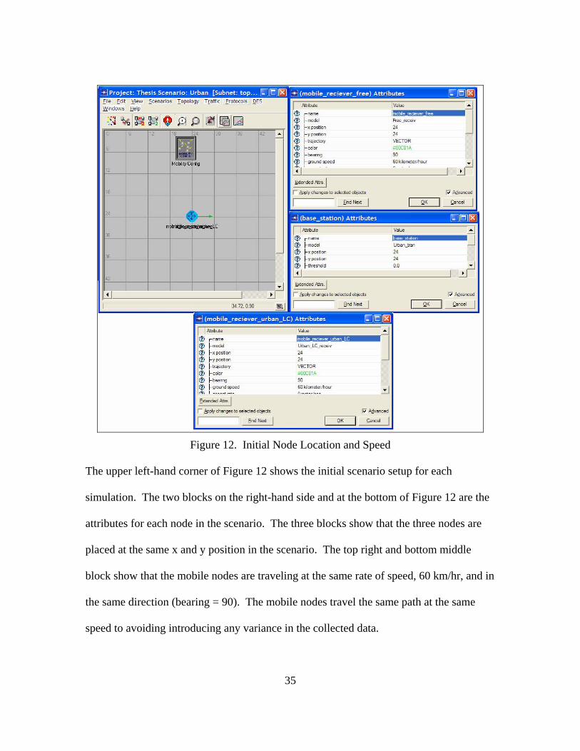
Figure 12. Initial Node Location and Speed
The upper left-hand corner of Figure 12 shows the initial scenario setup for each
simulation. The two blocks on the right-hand side and at the bottom of Figure 12 are the
attributes for each node in the scenario. The three blocks show that the three nodes are
placed at the same x and y position in the scenario. The top right and bottom middle
block show that the mobile nodes are traveling at the same rate of speed, 60 km/hr, and in
the same direction (bearing = 90). The mobile nodes travel the same path at the same
speed to avoiding introducing any variance in the collected data.

36
Each node consists of a processor component, a point-to-point
transmitter/receiver, an antenna component and a packet stream connecting all three
components together as seen in Figure 13.
Figure 13. Node Models
In Figure 13 the processor component for the transmitter in the upper right hand corner is
a simple source, labeled tx_gen, outputting packets 1024 bits long every 0.025 seconds.
The packets are sent to the radio transmitter, labeled radio_tx, via the packet stream. The
packets are passed to transmitting antenna, labeled ant_tx, via the packet stream for
broadcast to the receiver. The receiver nodes are in the blocks located in the upper left
and bottom center of Figure 13. The packets are received through the receiver antennas

37
then the packets are passed via the packet stream to the radio receiver, radio_rx. The
packets are then sent to the sink processors, rx_sink_free and rx_sink_urban_LC where
the statistical information from the packets is collected and the packets are destroyed.
To implement the pathloss changes in the transceiver pipeline, the original C/C++
code for the received power stage (dra_power) is modified. The modified pipeline stages
are located in Appendix A. The pipeline stages are modified to use the new formulas in
equation 2.7 and 2.13 for pathloss calculation and to calculate the statistic of received
power in decibels. The mobile node in each simulation using the original free-space
pathloss model has its’ dra_power pipeline code modified to calculate received power in
decibels and in watts. The C/C++ pipeline code being utilized by the mobile nodes is
changed in the attributes for each radio_rx in Figure 13.
Figure 14. C/C++ Pipeline Stage Used
Figure 14 shows the attributes for the free-space mobile receiver on the left and the
mobile receiver with the “modified” pipeline code on the right. The value for the power
38
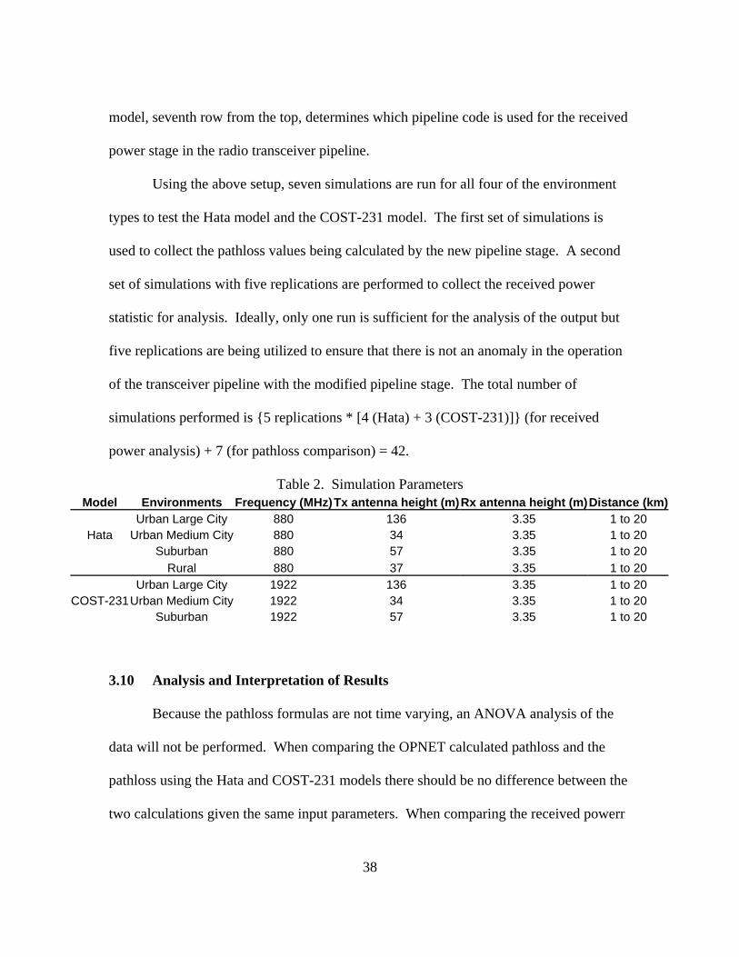
model, seventh row from the top, determines which pipeline code is used for the received
power stage in the radio transceiver pipeline.
Using the above setup, seven simulations are run for all four of the environment
types to test the Hata model and the COST-231 model. The first set of simulations is
used to collect the pathloss values being calculated by the new pipeline stage. A second
set of simulations with five replications are performed to collect the received power
statistic for analysis. Ideally, only one run is sufficient for the analysis of the output but
five replications are being utilized to ensure that there is not an anomaly in the operation
of the transceiver pipeline with the modified pipeline stage. The total number of
simulations performed is {5 replications * [4 (Hata) + 3 (COST-231)]} (for received
power analysis) + 7 (for pathloss comparison) = 42.
Table 2. Simulation Parameters Model Environments Frequency (MHz)Tx antenna height (m)Rx antenna height (m) Distance (km)
Urban Large City 880 136 3.35 1 to 20 Hata Urban Medium City 880 34 3.35 1 to 20
Suburban 880 57 3.35 1 to 20 Rural 880 37 3.35 1 to 20 Urban Large City 1922 136 3.35 1 to 20
COST-231 Urban Medium City 1922 34 3.35 1 to 20 Suburban 1922 57 3.35 1 to 20
3.10 Analysis and Interpretation of Results
Because the pathloss formulas are not time varying, an ANOVA analysis of the
data will not be performed. When comparing the OPNET calculated pathloss and the
pathloss using the Hata and COST-231 models there should be no difference between the
two calculations given the same input parameters. When comparing the received powerr

39
using the original pipeline C/C++ code and the modified code there should be significant
difference between the two calculations. The final analysis compares the signal strength
calculated from the modified pipeline code and the measured received signal strength
data obtained from [HTJ93]. The modified results should more closely resemble the
actual data than the original pipeline code.
3.11 Summary
The frequency, distance, TX/RX antenna heights and the propagation
environment will be set to specified values to analyze the data. An ANOVA approach
will not be used because the formulas are not time varying.

40
IV. Analysis and Results
4.1 Pathloss Calculation Comparison
The first step in evaluating the modifications is to ensure OPNET calculates the
correct pathloss. The actual output from the OPNET debugger is listed is Appendix B.
Table 3 lists the results and factors being used for the Urban Large City simulation.
Table 3. Urban Large City Pathloss Calculation OPNET PL Distance (km) Formula PL Difference Parameter Settings
114.066 1.011 114.066 0.000 Fc (MHz)= 880 114.288 1.028 114.288 0.000 ht (m)= 136 114.506 1.045 114.506 0.000 hr (m)= 3.35 114.721 1.061 114.721 0.000 a(hr)= 114.721
OPNET PL Distance (km) Formula PL Difference Parameter Settings
128.107 1.011 128.107 0.000 Fc (MHz)= 1922 128.329 1.028 128.329 0.000 ht (m)= 136 128.548 1.045 128.548 0.000 hr (m)= 3.35 128.763 1.061 128.763 0.000 a(hr)= 3.172
The first column shows the pathloss calculated by OPNET and obtained from the
debugger output. The third column shows the value calculated by the formula from
Chapter 2. The parameters being used are listed in the last column. The fourth column
shows that there is no difference between the two calculated values.
Table 4 lists the pathloss values calculated during the Urban Medium City
simulation.
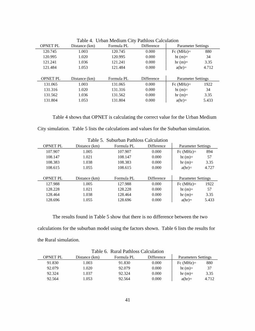
41
Table 4. Urban Medium City Pathloss Calculation OPNET PL Distance (km) Formula PL Difference Parameter Settings
120.745 1.003 120.745 0.000 Fc (MHz)= 880 120.995 1.020 120.995 0.000 ht (m)= 34 121.241 1.036 121.241 0.000 hr (m)= 3.35 121.484 1.053 121.484 0.000 a(hr)= 4.712
OPNET PL Distance (km) Formula PL Difference Parameter Settings
131.065 1.003 131.065 0.000 Fc (MHz)= 1922 131.316 1.020 131.316 0.000 ht (m)= 34 131.562 1.036 131.562 0.000 hr (m)= 3.35 131.804 1.053 131.804 0.000 a(hr)= 5.433
Table 4 shows that OPNET is calculating the correct value for the Urban Medium
City simulation. Table 5 lists the calculations and values for the Suburban simulation.
Table 5. Suburban Pathloss Calculation OPNET PL Distance (km) Formula PL Difference Parameter Settings
107.907 1.005 107.907 0.000 Fc (MHz)= 894 108.147 1.021 108.147 0.000 ht (m)= 57 108.383 1.038 108.383 0.000 hr (m)= 3.35 108.615 1.055 108.615 0.000 a(hr)= 4.727
OPNET PL Distance (km) Formula PL Difference Parameter Settings
127.988 1.005 127.988 0.000 Fc (MHz)= 1922 128.228 1.021 128.228 0.000 ht (m)= 57 128.464 1.038 128.464 0.000 hr (m)= 3.35 128.696 1.055 128.696 0.000 a(hr)= 5.433
The results found in Table 5 show that there is no difference between the two
calculations for the suburban model using the factors shown. Table 6 lists the results for
the Rural simulation.
Table 6. Rural Pathloss Calculation OPNET PL Distance (km) Formula PL Difference Parameters Settings
91.830 1.003 91.830 0.000 Fc (MHz)= 880 92.079 1.020 92.079 0.000 ht (m)= 37 92.324 1.037 92.324 0.000 hr (m)= 3.35 92.564 1.053 92.564 0.000 a(hr)= 4.712

42
Table 6 shows that there is no difference between the two calculated pathloss
values.
4.2 Pipeline Stage Comparison
The second comparison is between the original pipeline code using the OPNET
implementation of the free-space pathloss formula and the “modified” pipeline code. The
goal is to show that the “modified” pipeline code results are different from the original
pipeline code. The received signal strength obtained from the simulations using the two
different models is compared. The values are collected for T-R separation distances of 1
km to 20 km. The received signal strength in dBm is plotted verses the log distance in
kilometers. The data from all five repetitions is plotted to ensure that OPNET does not
produce any anomalies during calculations. If there were, any anomalies in the data
collected, more than one line would appear in the graphs.
The manual calculation of the received signal strength using equation 2.2 with the
pathloss obtained from the free-space model is compared with the Urban Large City
signal strength values calculated from OPNET in Figure 15. The Friis free-space
equation implies that the received power will decrease as the square of the T-R separation
distance increases. This implies that the power drops off at a rate of 20 dB/decade
[Rap02]. The graphs on the left in Figure 15 behave as predicted at d = 1 km the initial
signal strength is – 32.7 dBm and at d = 10 km the value is – 52.7 dBm for 880 MHz.
The initial signal strength level for 1922 MHz is – 39.5 dBm at d = 1 km and – 59.5 dBm
at d = 10 km. The free-space model and Hata/COST-231 models have calculated signal
strength values that behave logarithmic.

43
10 20-100
-90
-80
-70
-60
-50
-40
-30
Distance (km)
dBm
880 MHz Free Space Calculation
10 20-100
-90
-80
-70
-60
-50
-40
-30
Distance (km)
dBm
880 MHz Hata OPNET Calculation
10 20-110
-100
-90
-80
-70
-60
-50
-40
Distance (km)
dBm
1922 MHz Free Space Calculation
10 20-110
-100
-90
-80
-70
-60
-50
-40
Distance (km)dB
m
1922 MHz COST 231 OPNET Calculation
data1data2data3data4
Figure 15. Urban Large City and Free-Space Comparison
The main difference between the values calculated using the free-space model and the
Hata/COST-231 models is the signal strength at d = 1 km. The Hata has an initial signal
strength of -55.4 dBm at d = 1 km and the COST-231 has an initial signal strength of –
69.4 dBm.
The graphs in Figure 16 compare the received signal strength calculated by
OPNET using the free-space pathloss model. The graphs on the left side of Figure 16 are
using the original pipeline code and on the right side are the graphs from the “modified”
Urban Large City pipeline code. One difference between the two pipeline codes is that
the signal strength calculated using the “modified” pipeline code decreases in a
logarithmic fashion, consistent with (2.7) for the Hata model and (2.13) for the COST-
231 model.

44
10 20-100
-80
-60
-40
Distance (km)
dBm
880 MHz OPNET Free Space Model Calculation
10 20-100
-80
-60
-40
Distance (km)
dBm
880 MHz Hata OPNET Calculation
10 20-120
-100
-80
-60
Distance (km)
dBm
1922 MHz OPNET Free Space Model Calculation
10 20-120
-100
-80
-60
Distance (km)dB
m
1922 MHz COST-231 OPNET Calculation
data1data2data3data4data5
Figure 16. Urban Large City Received Signal Strength Comparison
Whereas the signal strength from the original pipeline code is almost constant
until the ten kilometer mark at which point it begins to decrease. Another difference
between the two pipeline codes is the initial signal strengths at d = 1 km. The signal
strength using the original pipeline code starts at approximately -75.1 dBm and -81.9
dBm for 880 MHz and 1922 MHz, respectively. The simulation results using the Hata
and COST-231 models have a starting signal strength level of -55.37 dBm and -69.41
dBm respectively. In Figures 18, 20 and 22 similar trends can be seen for the Urban
Medium City, Suburban and Rural cases, respectively.
Figure 17 compares the Friis calculation using the Urban Medium City
parameters with the OPNET calculation using the Hata/COST-231 models. The same
differences can be seen in Figure 17 that is evident in Figure 15. The two models behave
in a logarithmic manner and have different initial signal strengths at d = 1 km.

45
10 20-110
-100
-90
-80
-70
-60
-50
-40
-30
Distance (km)
dBm
880 MHz Free Space Calculation
101-110
-100
-90
-80
-70
-60
-50
-40
-30
Distance (km)
dBm
880 MHz Hata OPNET Calculation
10 20-120
-110
-100
-90
-80
-70
-60
-50
-40
Distance (km)
dBm
1922 MHz Free Space Calculation
10 20-120
-110
-100
-90
-80
-70
-60
-50
-40
Distance (km)dB
m
1922 MHz COST 231 OPNET Calculation
data1data2data3data4data5
Figure 17. Urban Medium City and Free-Space Comparison
There is – 29.4 dBm difference between the free-space model calculation and the Hata
model and a – 33.0 dBm difference at the 1922 MHz.
The results from the Urban Medium City Received Signal Strength Comparison
are seen in Figure 16. The simulation results from the free-space model and Hata/COST-
231 models show similar characteristics to the results found in Figure 15. The free-space
model is almost constant until the ten kilometer mark and the “modified” pipeline code is
logarithmic in appearance. The initial signal strength values for d = 1 km are similar for
the free-space model at 880 MHz and the Hata model, approximately -62.4 dBm and -
62.05 dBm respectively.

46
10 20-120
-100
-80
-60
Distance (km)
dBm
880 MHz OPNET Free Space Model Calculation
10 20-120
-100
-80
-60
Distance (km)
880 MHz Hata OPNET Calculation
10 20-120
-100
-80
-60
Distance (km)
dBm
1922 MHz OPNET Free Space Model Calculation
10 20-120
-100
-80
-60
Distance (km)dB
m
1922 MHz COST-231 OPNET Calculation
data1data2data3data4data5
Figure 18. Urban Medium City Received Signal Strength Comparison
But the starting signal strengths are different for the 1922 MHz results,
approximately -69.2 dBm for the Free-space model and -72.37 dBm for the COST-231
model.
In Figure 19 the free-space model and the Hata/COST-231 models are compared
using the suburban environment settings. The free-space model and Hata/COST-231
models behave logarithmic manner. The initial signal strength at d = 1 km is different
between the two models for the different frequencies. At 894 MHz the difference is –
16.4 dBm and at 1922 MHz the difference is – 29.8 dBm.
The results for the Suburban Received Signal Strength Comparison are seen in
Figure 20. The trend continues with the received signal strength levels calculated by the
Free-space model appearing almost constant and then decreasing at the ten kilometer
point.
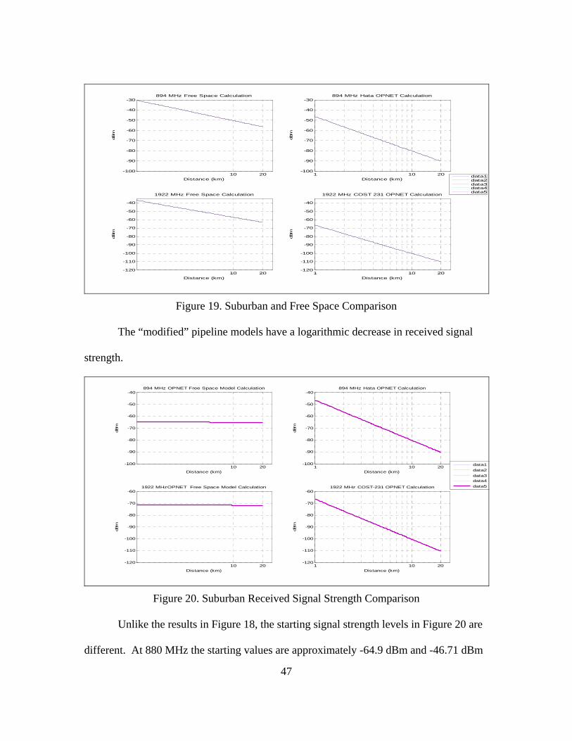
47
10 20-100
-90
-80
-70
-60
-50
-40
-30
Distance (km)
dBm
894 MHz Free Space Calculation
1 10 20-100
-90
-80
-70
-60
-50
-40
-30
Distance (km)
dBm
894 MHz Hata OPNET Calculation
10 20-120
-110
-100
-90
-80
-70
-60
-50
-40
Distance (km)
dBm
1922 MHz Free Space Calculation
1 10 20-120
-110
-100
-90
-80
-70
-60
-50
-40
Distance (km)
dBm
1922 MHz COST 231 OPNET Calculation
data1data2data3data4data5
Figure 19. Suburban and Free Space Comparison
The “modified” pipeline models have a logarithmic decrease in received signal
strength.
10 20-100
-90
-80
-70
-60
-50
-40
Distance (km)
dBm
894 MHz OPNET Free Space Model Calculation
1 10 20-100
-90
-80
-70
-60
-50
-40
Distance (km)
dBm
894 MHz Hata OPNET Calculation
10 20-120
-110
-100
-90
-80
-70
-60
Distance (km)
dBm
1922 MHzOPNET Free Space Model Calculation
1 10 20-120
-110
-100
-90
-80
-70
-60
Distance (km)
dBm
1922 MHz COST-231 OPNET Calculation
data1data2data3data4data5
Figure 20. Suburban Received Signal Strength Comparison
Unlike the results in Figure 18, the starting signal strength levels in Figure 20 are
different. At 880 MHz the starting values are approximately -64.9 dBm and -46.71 dBm

48
for the Free-space model and Hata model respectively. At 1922 MHz the values are
approximately -71.5 dBm and -66.79 dBm for the Free-space model and COST-231
models respectively.
The parameters for the Rural environment are used to compare the free-space
model with the Hata/COST-231 models in Figure 21.
10 20-80
-75
-70
-65
-60
-55
-50
-45
-40
-35
-30
Distance (km)
dBm
880 MHz Free Space Calculation
10 20-80
-75
-70
-65
-60
-55
-50
-45
-40
-35
-30
Distance (km)
dBm
880 MHz Hata OPNET Calculation
data1data2data3data4data5
Figure 21. Rural and Free-Space Comparison
Both models behave in a logarithmic manner but, they have very similar initial signal
strength levels. The free-space model has a signal strength value of – 30.2 dBm at d = 1
km and the Hata model has a – 30.6 dBm at d = 1 km, a – 0.4 dBm difference.
The graphs in Figure 22 are for the Rural Received Signal Strength Comparison
using the Hata model and the Free-space model. The free-space model has a received
signal strength level of approximately -60.5 dBm; where as the Hata model has a
received signal strength level of approximately -31 dBm.

49
10 20-80
-75
-70
-65
-60
-55
-50
-45
-40
-35
-30
Distance (km)dB
m
880 MHz Hata OPNET Calculation
10 20-80
-75
-70
-65
-60
-55
-50
-45
-40
-35
-30
Distance (km)
dBm
880 MHz OPNET Free Space Model Calculation
data1data2data3data4data5
Figure 22. Rural Received Signal Strength Comparison
As with the previous results, the signal strength levels are almost constant until
the d = 10 km point for the Free-space model and are logarithmic for the Hata model.
In Figures 16, 18, 20 and 22 the signal strength levels for the free-space model are
minimally impacted by the increase in T-R separation. This is observed by the small
decrease in signal strength from 1 km to 20 km. Yet the Hata model and COST-231
exhibit a logarithmic decrease as the T-R separation increases.
4.3 Measured Received Signal Strength Comparison
The final comparison is between the measured received power levels that are
obtained using the new models and measured received signal strength levels obtained
from [HTJ93]. The pathloss slope of all seven simulations will be compared and the
measured received signal strength values for the suburban environment will be compared

50
with the suburban simulation results. The measured slopes for the pathloss of [HTJ93]
are shown in Table 7.
Table 7. Measured Pathloss Slope [HTJ93]
Site Pathloss Slope (dB/decade) 880 MHz 1922 MHz Cell 13 (semi rural) -30.5 -26.7 Cell 5 (suburban) -38.2 -34.4 Cell 100 (urban) -37.4 -36.3 Cell 19 (heavy urban) -28.7 -29.4 Average -33.7 -31.7
The pathloss slopes for each simulation are shown in Table 7. The pathloss slope for the
simulations is calculated by converting the time axis that is used by OPNET to a distance
in kilometers. The mobile nodes are traveling at 60 km/hr therefore the time in seconds
is divided by sixty to obtain the distance in km. The log of the distance is calculated by
taking the common log of the distance in kilometers. Then the slope is calculated by
subtracting the received signal strength value at the zero log starting distance (1 km) from
the one log ending distance (10 km) to obtain a dB/decade pathloss slope.
Table 8. Simulation Pathloss Slopes for Hata / COST-231 Model (dB/decade)
Sim. Environment 880 MHz 1922 MHz Rural - 34.628 N/A Suburban - 33.399 - 33.399 Urban Med. - 34.868 - 34.869 Urban LC - 30.926 - 30.926 Average - 33.455 - 33.065
The pathloss slopes from the simulations are similar to the measured slopes
presented in Table 7 with the average simulation pathloss being nearly identical to the
measured pathloss slope. The 880 MHz has a 0.245 dB difference and the 1922 MHz has
a 1.365 dB difference between averages. The pathloss slopes for each individual

51
environment: Suburban, Urban Medium and Urban Large City is identical for both
frequencies. Using the graphs in Figure 23, the signal strengths from the suburban
simulation are compared with the measured signal strength at 1 km. The measured signal
strength data of the suburban simulation is found in Appendix C.
The value of the average received signal strength at 1 km is estimated from the
graphs in Figure 23 [HTJ93] as -58 dBm for 894 MHz and -78 MHz for 1922 MHz. The
simulated values from Figure 17 at 1 km are -46.7 dBm at 880 MHz (Hata Model) and -
66.7 dBm at 1922 MHz (COST-231 Model). Therefore, there is a difference (simulated-
measured) of + 11.3 dBm for both the 880 MHz and 1922 MHz cases. The significance
of this is that the average received signal strength calculated by the Hata and COST-231
models are going to behave similar to an actual received signal because pathloss slopes
are identical. However, the simulated signal strength is going to be greater than an actual
received signal.
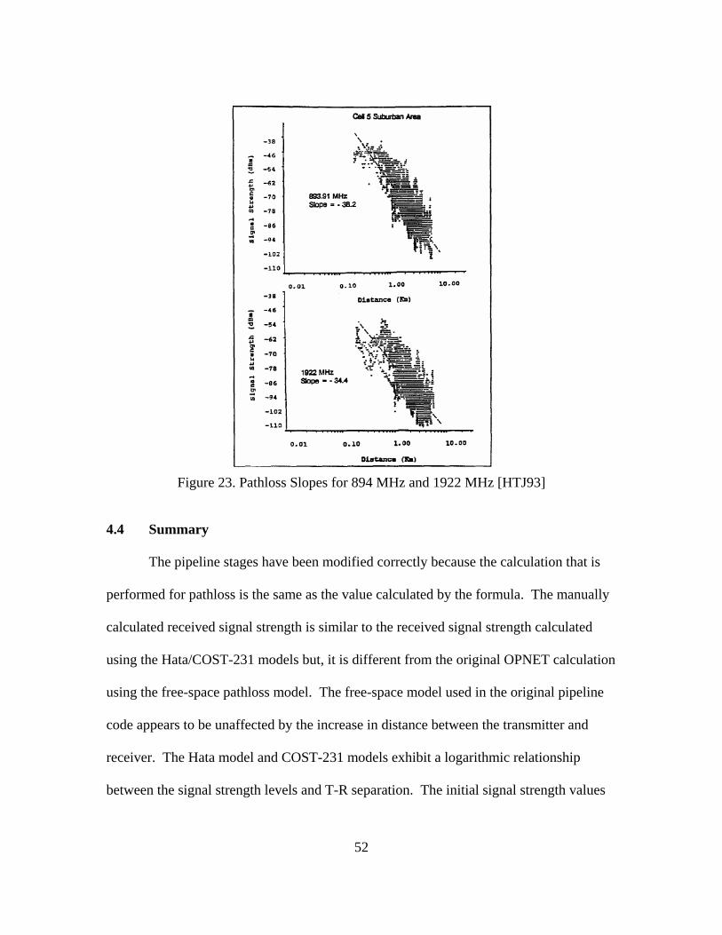
52
Figure 23. Pathloss Slopes for 894 MHz and 1922 MHz [HTJ93]
4.4 Summary
The pipeline stages have been modified correctly because the calculation that is
performed for pathloss is the same as the value calculated by the formula. The manually
calculated received signal strength is similar to the received signal strength calculated
using the Hata/COST-231 models but, it is different from the original OPNET calculation
using the free-space pathloss model. The free-space model used in the original pipeline
code appears to be unaffected by the increase in distance between the transmitter and
receiver. The Hata model and COST-231 models exhibit a logarithmic relationship
between the signal strength levels and T-R separation. The initial signal strength values

53
differ from the free-space model and the Hata and COST-231 models. When compared
to measured data, the values for the pathloss slope are similar to the simulation results.
The signal strength value at 1 km for the suburban environment simulation was greater
than the measured value by approximately 11 dBm. The results produced by the
modified pipeline stages are more similar to the actual measured values than the original
pipeline stages.

54
V. Conclusions and Recommendations
5.1 Chapter Overview
This chapter provides a summary of the research conclusions, the significance of
the research and recommendations for future research.
5.2 Conclusions and Significance of Research
Altering the pathloss model being used by OPNET produces results that are more
realistic than the original OPNET implementation. The original pathloss model does not
account for the diffractors, scatterers and reflectors found in typical communication
environments. In addition, the implementation of the free-space model by OPNET
produce results that do not reflect the decay associated with using the free-space pathloss
model. The OPNET implementation of the free-space model uses the propagation
distance between the transmitter and receiver. The propagation distance is the three
dimensional distance or vector distance between the transmitter and receiver (LOS). The
propagation distance is appropriate for non-terrestrial calculations but produce results that
are depicted in Figures 16, 18, 20 and 22, which are insensitive (to the T-R separation)
and inaccurate for terrestrial communications systems in OPNET. The additions of the
new pathloss models (Hata and COST 321) produces signal strength results that are
similar to actual measured values.
With the modification of the OPNET pipeline stage, dra_power, the output from
the wireless model can now be trusted to produce a more accurate/realistic result.

55
5.3 Recommendations for Future Research
In this research, the models used produced realistic results; unfortunately, the
models were not completely accurate when compared to actual measured data. In
addition, the models were limited to a certain range of frequencies, transmitter-receiver
separation and antenna heights.
For future research, modifications can be made to the current pathloss model to
account for the -11 dBm difference between the calculated signal strength and the
measured signal strength. Additional models can be incorporated which will overcome
the limits imposed by the frequency range, transmitter-reciever separation, and antenna
heights on the current model.

56
Appendix A: Modified Pipeline Code
Modified dra_power pipeline stage for Urban Large City environment:
/* dra_power_large.ps.c */ /* Default received power model for radio link Transceiver */ /* Pipeline. This model uses the receiver channel state */ /* information to check and update the signal lock status */ /* of the channel. It relies on the rxgroup stage model for */ /* the creation and initialization of the channel state */ /* information. */ /****************************************/ /* Copyright (c) 1993-2003 */ /* by OPNET Technologies, Inc. */ /* (A Delaware Corporation) */ /* 7255 Woodmont Av., Suite 250 */ /* Bethesda, MD 20814, U.S.A. */ /* All Rights Reserved. */ /****************************************/ #include "opnet.h" #include "dra.h" #include <math.h> #include <stdlib.h> #include <stdio.h> /***** constants *****/ #define C 3.0E+08 /* speed of light (m/s) */ #define SIXTEEN_PI_SQ 157.91367 /* 16 times pi-squared */ /***** pipeline procedure *****/ #if defined (__cplusplus) extern "C" #endif void dra_power_urban_large_mt (OP_SIM_CONTEXT_ARG_OPT_COMMA Packet * pkptr) { double prop_distance, rcvd_power, path_loss; double tx_power, tx_base_freq, tx_bandwidth, tx_center_freq; double lambda, rx_ant_gain, tx_ant_gain; Objid rx_ch_obid; double in_band_tx_power, band_max, band_min; double rx_base_freq, rx_bandwidth; DraT_Rxch_State_Info* rxch_state_ptr; double tx_ant_height, rx_ant_height; /* Antenna heights for TX,RX*/ double tx_MHz_freq; /* TX freq in Mega Hertz*/ double km_distance; /* Distance converted to Kilometers*/ double a_hm, rcvd_power_dbm; /* Correction factor for mobile antenna*/ double path_loss_db = 0, in_band_tx_power_db; /* decible value of pathloss and in band transmission power*/ int prop_model = 0; /* determines which pathloss formula to use*/ double rx_ant_gain_db, tx_ant_gain_db; /* db values of the ant. gains */ /** Compute the average power in Watts of the **/ /** signal associated with a transmitted packet. **/ FIN_MT (dra_power_urban_large_mt (pkptr)); /* If the incoming packet is 'valid', it may cause the receiver to */ /* lock onto it. However, if the receiving node is disabled, then */ /* the channel match should be set to noise. */ if (op_td_get_int (pkptr, OPC_TDA_RA_MATCH_STATUS) == OPC_TDA_RA_MATCH_VALID) { if (op_td_is_set (pkptr, OPC_TDA_RA_ND_FAIL)) { /* The receiving node is disabled. Change */ /* the channel match status to noise. */ op_td_set_int (pkptr, OPC_TDA_RA_MATCH_STATUS, OPC_TDA_RA_MATCH_NOISE); } else { /* The receiving node is enabled. Get */ /* the address of the receiver channel. */ rx_ch_obid = op_td_get_int (pkptr, OPC_TDA_RA_RX_CH_OBJID); /* Access receiver channels state information. */ rxch_state_ptr = (DraT_Rxch_State_Info *) op_ima_obj_state_get (rx_ch_obid); /* If the receiver channel is already locked, */ /* the packet will now be considered to be noise. */ /* This prevents simultaneous reception of multiple */ /* valid packets on any given radio channel. */ if (rxch_state_ptr->signal_lock) op_td_set_int (pkptr, OPC_TDA_RA_MATCH_STATUS, OPC_TDA_RA_MATCH_NOISE); else {

57
/* Otherwise, the receiver channel will become */ /* locked until the packet reception ends. */ rxch_state_ptr->signal_lock = OPC_TRUE; } } } /* Get power allotted to transmitter channel. */ tx_power = op_td_get_dbl (pkptr, OPC_TDA_RA_TX_POWER); /* Get transmission frequency in Hz. */ tx_base_freq = op_td_get_dbl (pkptr, OPC_TDA_RA_TX_FREQ); tx_bandwidth = op_td_get_dbl (pkptr, OPC_TDA_RA_TX_BW); tx_center_freq = tx_base_freq + (tx_bandwidth / 2.0); /*Convert the transmit frequency to Mega Hertz*/ tx_MHz_freq = tx_center_freq/1000000; printf("freq = %f\n",tx_MHz_freq); /* Caclculate wavelength (in meters). */ lambda = C / tx_center_freq; /*printf("lambda = %f\n",lambda);*/ /* Get distance between transmitter and receiver (in meters). */ prop_distance = op_td_get_dbl (pkptr, OPC_TDA_RA_START_DIST); m_distance = (km_distance * 1000); /*printf("prop = %f\n",prop_distance);*/ /* Get the height of the transmit and recieve antennas.*/ tx_ant_height = (op_td_get_dbl (pkptr, OPC_TDA_RA_TX_ALT))/1000; rx_ant_height = (op_td_get_dbl (pkptr, OPC_TDA_RA_RX_ALT))/1000; printf("tx_height = %f\n",tx_ant_height); printf("rx_height = %f\n",rx_ant_height); /* Calculate the distance using the TDA sart_dist*/ km_distance = sqrt(pow((prop_distance/1000),2)- pow((tx_ant_height-rx_ant_height),2)); printf("dist_z = %f\n",km_distance); // Calculate a_hm for Hata and COST-231 if (tx_MHz_freq <= 300) { a_hm = 8.29*(pow(log10(1.54*rx_ant_height),2)) - 1.1; } else { a_hm = 3.2*(pow(log10(11.75*rx_ant_height),2)) - 4.97; } /* When using TMM, the TDA OPC_TDA_RA_RCVD_POWER will already */ /* have a raw value for the path loss. */ if (op_td_is_set (pkptr, OPC_TDA_RA_RCVD_POWER)) { path_loss = op_td_get_dbl (pkptr, OPC_TDA_RA_RCVD_POWER); } else { /* Compute the path loss for this distance and wavelength. */ if (prop_distance > 0.0) { /* Determine which propagation model to use and use value in the db form*/ if ((tx_MHz_freq >= 150 && tx_MHz_freq <= 2000) && (km_distance >= 1 && km_distance <= 100) && (tx_ant_height >= 30 && tx_ant_height <= 200) && (rx_ant_height >= 1 && rx_ant_height <= 10)) { if ((tx_MHz_freq >= 150 && tx_MHz_freq <= 1500) && (km_distance >= 1 && km_distance <= 100)) { path_loss_db = 69.55 + 26.16*log10(tx_MHz_freq) - 13.82*log10(tx_ant_height) - a_hm + (44.9 - 6.55*log10(tx_ant_height))*log10(km_distance); prop_model = 1; } else if ((tx_MHz_freq > 1500 && tx_MHz_freq <= 2000) && (km_distance >= 1 && km_distance <= 20)) { path_loss_db = 46.3 + 33.9*log10(tx_MHz_freq) - 13.82*log10(tx_ant_height) - a_hm + (44.9 - 6.55*log10(tx_ant_height))*log10(km_distance) + 3; prop_model = 1; }
else if ((tx_MHz_freq > 1500 && tx_MHz_freq <= 2000) && (km_distance > 20))
{ path_loss = (lambda * lambda) / (SIXTEEN_PI_SQ * m_distance * m_distance); prop_model = 0; printf("Using Free-space PL\n\n",path_loss); }
printf("Hata/COST_PL = %f\n\n",path_loss_db); } else { path_loss = (lambda * lambda) / (SIXTEEN_PI_SQ * m_distance * m_distance); prop_model = 0; printf("Using Free Space PL\n\n",path_loss); } } else {

58
if (prop_model == 1)path_loss_db = 0.0; else path_loss = 1; } } printf("prop_model = %i\n",prop_model); /* Determine the receiver bandwidth and base frequency. */ rx_base_freq = op_td_get_dbl (pkptr, OPC_TDA_RA_RX_FREQ); rx_bandwidth = op_td_get_dbl (pkptr, OPC_TDA_RA_RX_BW); /* Use these values to determine the band overlap with the transmitter. */ /* Note that if there were no overlap at all, the packet would already */ /* have been filtered by the channel match stage. */ /* The base of the overlap band is the highest base frequency. */ if (rx_base_freq > tx_base_freq) band_min = rx_base_freq; else band_min = tx_base_freq; /* The top of the overlap band is the lowest end frequency. */ if (rx_base_freq + rx_bandwidth > tx_base_freq + tx_bandwidth) band_max = tx_base_freq + tx_bandwidth; else band_max = rx_base_freq + rx_bandwidth; /* Compute the amount of in-band transmitter power. */ in_band_tx_power = tx_power * (band_max - band_min) / tx_bandwidth; in_band_tx_power_db = 10*log10(in_band_tx_power); /* Get antenna gains. */ tx_ant_gain = pow (10.0, op_td_get_dbl (pkptr, OPC_TDA_RA_TX_GAIN) / 10.0); rx_ant_gain = pow (10.0, op_td_get_dbl (pkptr, OPC_TDA_RA_RX_GAIN) / 10.0); tx_ant_gain_db = op_td_get_dbl (pkptr, OPC_TDA_RA_TX_GAIN); rx_ant_gain_db = op_td_get_dbl (pkptr, OPC_TDA_RA_RX_GAIN); printf("tx gain = %f\n",tx_ant_gain_db); printf("rx_gain = %f\n",rx_ant_gain_db); /* Calculate received power level (in db). */ if(prop_model == 1) rcvd_power = pow(10.0, ((in_band_tx_power_db + tx_ant_gain_db + rx_ant_gain_db - path_loss_db) / 10.0)); else { rcvd_power = in_band_tx_power * tx_ant_gain * path_loss * rx_ant_gain; printf("using normal rcvd power \n"); } /* The received power is stored in the packet as a decible value*/ rcvd_power_dbm = 10*log10(rcvd_power/.001); op_td_set_dbl (pkptr, OPC_TDA_RA_RCVD_POWER_DBM, rcvd_power_dbm); printf("rcvd_power_dbm = %f\n",rcvd_power_dbm); printf("rcvd_power = %f\n",rcvd_power); /* Assign the received power level (in Watts) */ /* to the packet transmission data attribute. */ op_td_set_dbl (pkptr, OPC_TDA_RA_RCVD_POWER, rcvd_power); FOUT }

59
Modified dra_power pipeline stage for Urban Medium City environment:
/* dra_power.ps.c */ /* Default received power model for radio link Transceiver */ /* Pipeline. This model uses the receiver channel state */ /* information to check and update the signal lock status */ /* of the channel. It relies on the rxgroup stage model for */ /* the creation and initialization of the channel state */ /* information. */ /****************************************/ /* Copyright (c) 1993-2003 */ /* by OPNET Technologies, Inc. */ /* (A Delaware Corporation) */ /* 7255 Woodmont Av., Suite 250 */ /* Bethesda, MD 20814, U.S.A. */ /* All Rights Reserved. */ /****************************************/ #include "opnet.h" #include "dra.h" #include <math.h> /***** constants *****/ #define C 3.0E+08 /* speed of light (m/s) */ #define SIXTEEN_PI_SQ 157.91367 /* 16 times pi-squared */ /***** pipeline procedure *****/ #if defined (__cplusplus) extern "C" #endif void dra_power_urban_mt (OP_SIM_CONTEXT_ARG_OPT_COMMA Packet * pkptr) { double prop_distance, rcvd_power, path_loss; double tx_power, tx_base_freq, tx_bandwidth, tx_center_freq; double lambda, rx_ant_gain, tx_ant_gain; Objid rx_ch_obid; double in_band_tx_power, band_max, band_min; double rx_base_freq, rx_bandwidth; DraT_Rxch_State_Info* rxch_state_ptr; double tx_ant_height, rx_ant_height; /* Antenna heights for TX,RX*/ double tx_MHz_freq; /* TX freq in Mega Hertz*/ double km_distance; /* Distance converted to Kilometers*/ double a_hm; /* Correction factor for mobile antenna*/ double path_loss_db = 0, in_band_tx_power_db; /* decible value of pathloss and in band transmission power*/ int prop_model = 0; /* determines which pathloss formula to use*/ double rx_ant_gain_db, rcvd_power_dbm, tx_ant_gain_db; /* db values of the ant. gains */ /** Compute the average power in Watts of the **/ /** signal associated with a transmitted packet. **/ FIN_MT (dra_power_urban_large_mt (pkptr)); /* If the incoming packet is 'valid', it may cause the receiver to */ /* lock onto it. However, if the receiving node is disabled, then */ /* the channel match should be set to noise. */ if (op_td_get_int (pkptr, OPC_TDA_RA_MATCH_STATUS) == OPC_TDA_RA_MATCH_VALID) { if (op_td_is_set (pkptr, OPC_TDA_RA_ND_FAIL)) { /* The receiving node is disabled. Change */ /* the channel match status to noise. */ op_td_set_int (pkptr, OPC_TDA_RA_MATCH_STATUS, OPC_TDA_RA_MATCH_NOISE); } else { /* The receiving node is enabled. Get */ /* the address of the receiver channel. */ rx_ch_obid = op_td_get_int (pkptr, OPC_TDA_RA_RX_CH_OBJID); /* Access receiver channels state information. */ rxch_state_ptr = (DraT_Rxch_State_Info *) op_ima_obj_state_get (rx_ch_obid); /* If the receiver channel is already locked, */ /* the packet will now be considered to be noise. */ /* This prevents simultaneous reception of multiple */ /* valid packets on any given radio channel. */ if (rxch_state_ptr->signal_lock) op_td_set_int (pkptr, OPC_TDA_RA_MATCH_STATUS, OPC_TDA_RA_MATCH_NOISE); else { /* Otherwise, the receiver channel will become */ /* locked until the packet reception ends. */ rxch_state_ptr->signal_lock = OPC_TRUE; } } } /* Get power allotted to transmitter channel. */ tx_power = op_td_get_dbl (pkptr, OPC_TDA_RA_TX_POWER);

60
/* Get transmission frequency in Hz. */ tx_base_freq = op_td_get_dbl (pkptr, OPC_TDA_RA_TX_FREQ); tx_bandwidth = op_td_get_dbl (pkptr, OPC_TDA_RA_TX_BW); tx_center_freq = tx_base_freq + (tx_bandwidth / 2.0); /*Convert the transmit frequency to Mega Hertz*/ tx_MHz_freq = tx_center_freq/1000000; /*printf("freq = %f\n",tx_MHz_freq);*/ /* Caclculate wavelength (in meters). */ lambda = C / tx_center_freq; /*printf("lambda = %f\n",lambda);*/ /* Get distance between transmitter and receiver (in meters). */ prop_distance = op_td_get_dbl (pkptr, OPC_TDA_RA_START_DIST); m_distance = (km_distance * 1000); /*printf("prop = %f\n",prop_distance);*/ /* Get the height of the transmit and recieve antennas.*/ tx_ant_height = (op_td_get_dbl (pkptr, OPC_TDA_RA_TX_ALT))/1000; rx_ant_height = (op_td_get_dbl (pkptr, OPC_TDA_RA_RX_ALT))/1000; printf("tx_height = %f\n",tx_ant_height); printf("rx_height = %f\n",rx_ant_height); /* Calculate the distance using the TDA start_dist*/ km_distance = sqrt(pow((prop_distance/1000),2)- pow((tx_ant_height-rx_ant_height),2)); printf("dist_z = %f\n",km_distance); // Calculate a_hm for Hata and COST-231 a_hm = (1.1*log10(tx_MHz_freq) - 0.7)*rx_ant_height - (1.56*log10(tx_MHz_freq) - 0.8); /* When using TMM, the TDA OPC_TDA_RA_RCVD_POWER will already */ /* have a raw value for the path loss. */ if (op_td_is_set (pkptr, OPC_TDA_RA_RCVD_POWER)) { path_loss = op_td_get_dbl (pkptr, OPC_TDA_RA_RCVD_POWER); } else { /* Compute the path loss for this distance and wavelength. */ if (prop_distance > 0.0) { /* Determine which propagation model to use and use value in the db form*/ if ((tx_MHz_freq >= 150 && tx_MHz_freq <= 2000) && (km_distance >= 1 && km_distance <= 100) && (tx_ant_height >= 30 && tx_ant_height <= 200) && (rx_ant_height >= 1 && rx_ant_height <= 10)) { if ((tx_MHz_freq >= 150 && tx_MHz_freq <= 1500) && (km_distance >= 1 && km_distance <= 100)) { path_loss_db = 69.55 + 26.16*log10(tx_MHz_freq) - 13.82*log10(tx_ant_height) - a_hm + (44.9 - 6.55*log10(tx_ant_height))*log10(km_distance); prop_model = 1; } else if ((tx_MHz_freq > 1500 && tx_MHz_freq <= 2000) && (km_distance >= 1 && km_distance <= 20)) { path_loss_db = 46.3 + 33.9*log10(tx_MHz_freq) - 13.82*log10(tx_ant_height) - a_hm + (44.9 - 6.55*log10(tx_ant_height))*log10(km_distance); prop_model = 1; }
else if ((tx_MHz_freq > 1500 && tx_MHz_freq <= 2000) && (km_distance > 20)) { path_loss = (lambda * lambda) / (SIXTEEN_PI_SQ * m_distance * m_distance); prop_model = 0; printf("Using Free Space PL\n\n",path_loss); }
printf("Hata/COST_PL = %f\n\n",path_loss_db); } else { path_loss = (lambda * lambda) / (SIXTEEN_PI_SQ * m_distance * m_distance); prop_model = 0; printf("Using Free Space PL\n\n",path_loss); } } else { if (prop_model == 1)path_loss_db = 0.0; else path_loss = 1; } } /* Determine the receiver bandwidth and base frequency. */ rx_base_freq = op_td_get_dbl (pkptr, OPC_TDA_RA_RX_FREQ); rx_bandwidth = op_td_get_dbl (pkptr, OPC_TDA_RA_RX_BW); /* Use these values to determine the band overlap with the transmitter. */ /* Note that if there were no overlap at all, the packet would already */ /* have been filtered by the channel match stage. */

61
/* The base of the overlap band is the highest base frequency. */ if (rx_base_freq > tx_base_freq) band_min = rx_base_freq; else band_min = tx_base_freq; /* The top of the overlap band is the lowest end frequency. */ if (rx_base_freq + rx_bandwidth > tx_base_freq + tx_bandwidth) band_max = tx_base_freq + tx_bandwidth; else band_max = rx_base_freq + rx_bandwidth; /* Compute the amount of in-band transmitter power. */ in_band_tx_power = tx_power * (band_max - band_min) / tx_bandwidth; in_band_tx_power_db = 10*log10(in_band_tx_power); /* Get antenna gains. */ tx_ant_gain = pow (10.0, op_td_get_dbl (pkptr, OPC_TDA_RA_TX_GAIN) / 10.0); rx_ant_gain = pow (10.0, op_td_get_dbl (pkptr, OPC_TDA_RA_RX_GAIN) / 10.0); tx_ant_gain_db = op_td_get_dbl (pkptr, OPC_TDA_RA_TX_GAIN); rx_ant_gain_db = op_td_get_dbl (pkptr, OPC_TDA_RA_RX_GAIN); /* Calculate received power level (in db). */ if(prop_model == 1) rcvd_power = pow(10.0, ((in_band_tx_power_db + tx_ant_gain_db + rx_ant_gain_db - path_loss_db) / 10.0)); else rcvd_power = in_band_tx_power * tx_ant_gain * path_loss * rx_ant_gain; printf("rcvd_power = %f\n",rcvd_power); /* The received power is stored in the packet as a decible value*/ rcvd_power_dbm = 10*log10(rcvd_power/.001); op_td_set_dbl (pkptr, OPC_TDA_RA_RCVD_POWER_DBM, rcvd_power_dbm); printf("rcvd_power_dbm = %f\n",rcvd_power_dbm); /* Assign the received power level (in Watts) */ /* to the packet transmission data attribute. */ op_td_set_dbl (pkptr, OPC_TDA_RA_RCVD_POWER, rcvd_power); FOUT }
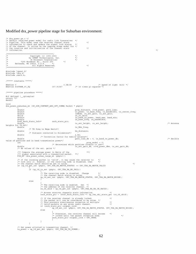
62
Modified dra_power pipeline stage for Suburban environment:
/* dra_power.ps.c */ /* Default received power model for radio link Transceiver */ /* Pipeline. This model uses the receiver channel state */ /* information to check and update the signal lock status */ /* of the channel. It relies on the rxgroup stage model for */ /* the creation and initialization of the channel state */ /* information. */ /****************************************/ /* Copyright (c) 1993-2003 */ /* by OPNET Technologies, Inc. */ /* (A Delaware Corporation) */ /* 7255 Woodmont Av., Suite 250 */ /* Bethesda, MD 20814, U.S.A. */ /* All Rights Reserved. */ /****************************************/ #include "opnet.h" #include "dra.h" #include <math.h> /***** constants *****/ #define C 3.0E+08 /* speed of light (m/s) */ #define SIXTEEN_PI_SQ 157.91367 /* 16 times pi-squared */ /***** pipeline procedure *****/ #if defined (__cplusplus) extern "C" #endif void dra_power_suburban_mt (OP_SIM_CONTEXT_ARG_OPT_COMMA Packet * pkptr) { double prop_distance, rcvd_power, path_loss; double tx_power, tx_base_freq, tx_bandwidth, tx_center_freq; double lambda, rx_ant_gain, tx_ant_gain; Objid rx_ch_obid; double in_band_tx_power, band_max, band_min; double rx_base_freq, rx_bandwidth; DraT_Rxch_State_Info* rxch_state_ptr; double tx_ant_height, rx_ant_height; /* Antenna heights for TX,RX*/ double tx_MHz_freq; /* TX freq in Mega Hertz*/ double km_distance; /* Distance converted to Kilometers*/ double a_hm; /* Correction factor for mobile antenna*/ double path_loss_db = 0, in_band_tx_power_db; /* decible value of pathloss and in band transmission power*/ int prop_model = 0; /* determines which pathloss formula to use*/ double rx_ant_gain_db, rcvd_power_dbm, tx_ant_gain_db; /* db values of the ant. gains */ /** Compute the average power in Watts of the **/ /** signal associated with a transmitted packet. **/ FIN_MT (dra_power_urban_large_mt (pkptr)); /* If the incoming packet is 'valid', it may cause the receiver to */ /* lock onto it. However, if the receiving node is disabled, then */ /* the channel match should be set to noise. */ if (op_td_get_int (pkptr, OPC_TDA_RA_MATCH_STATUS) == OPC_TDA_RA_MATCH_VALID) { if (op_td_is_set (pkptr, OPC_TDA_RA_ND_FAIL)) { /* The receiving node is disabled. Change */ /* the channel match status to noise. */ op_td_set_int (pkptr, OPC_TDA_RA_MATCH_STATUS, OPC_TDA_RA_MATCH_NOISE); } else { /* The receiving node is enabled. Get */ /* the address of the receiver channel. */ rx_ch_obid = op_td_get_int (pkptr, OPC_TDA_RA_RX_CH_OBJID); /* Access receiver channels state information. */ rxch_state_ptr = (DraT_Rxch_State_Info *) op_ima_obj_state_get (rx_ch_obid); /* If the receiver channel is already locked, */ /* the packet will now be considered to be noise. */ /* This prevents simultaneous reception of multiple */ /* valid packets on any given radio channel. */ if (rxch_state_ptr->signal_lock) op_td_set_int (pkptr, OPC_TDA_RA_MATCH_STATUS, OPC_TDA_RA_MATCH_NOISE); else { /* Otherwise, the receiver channel will become */ /* locked until the packet reception ends. */ rxch_state_ptr->signal_lock = OPC_TRUE; } } } /* Get power allotted to transmitter channel. */ tx_power = op_td_get_dbl (pkptr, OPC_TDA_RA_TX_POWER);

63
/* Get transmission frequency in Hz. */ tx_base_freq = op_td_get_dbl (pkptr, OPC_TDA_RA_TX_FREQ); tx_bandwidth = op_td_get_dbl (pkptr, OPC_TDA_RA_TX_BW); tx_center_freq = tx_base_freq + (tx_bandwidth / 2.0); /*Convert the transmit frequency to Mega Hertz*/ tx_MHz_freq = tx_center_freq/1000000; /*printf("freq = %f\n",tx_MHz_freq);*/ /* Caclculate wavelength (in meters). */ lambda = C / tx_center_freq; /*printf("lambda = %f\n",lambda);*/ /* Get distance between transmitter and receiver (in meters). */ prop_distance = op_td_get_dbl (pkptr, OPC_TDA_RA_START_DIST); /*printf("prop = %f\n",prop_distance);*/ /* Get the height of the transmit and recieve antennas.*/ tx_ant_height = (op_td_get_dbl (pkptr, OPC_TDA_RA_TX_ALT))/1000; rx_ant_height = (op_td_get_dbl (pkptr, OPC_TDA_RA_RX_ALT))/1000; printf("tx_height = %f\n",tx_ant_height); printf("rx_height = %f\n",rx_ant_height); /* Calculate the distance using the TDA sart_dist*/ km_distance = sqrt(pow((prop_distance/1000),2)- pow((tx_ant_height-rx_ant_height),2)); m_distance = (km_distance * 1000); printf("dist_z = %f\n",km_distance); // Calculate a_hm for Hata and COST-231 a_hm = (1.1*log10(tx_MHz_freq) - 0.7)*rx_ant_height - (1.56*log10(tx_MHz_freq) - 0.8); /* When using TMM, the TDA OPC_TDA_RA_RCVD_POWER will already */ /* have a raw value for the path loss. */ if (op_td_is_set (pkptr, OPC_TDA_RA_RCVD_POWER)) { path_loss = op_td_get_dbl (pkptr, OPC_TDA_RA_RCVD_POWER); } else { /* Compute the path loss for this distance and wavelength. */ if (prop_distance > 0.0) { /* Determine which propagation model to use and use value in the db form*/ if ((tx_MHz_freq >= 150 && tx_MHz_freq <= 2000) && (km_distance >= 1 && km_distance <= 100) && (tx_ant_height >= 30 && tx_ant_height <= 200) && (rx_ant_height >= 1 && rx_ant_height <= 10)) { if ((tx_MHz_freq >= 150 && tx_MHz_freq <= 1500) && (km_distance >= 1 && km_distance <= 100)) { path_loss_db = 69.55 + 26.16*log10(tx_MHz_freq) - 13.82*log10(tx_ant_height) - a_hm + (44.9 - 6.55*log10(tx_ant_height))*log10(km_distance) - 2*pow(log10(tx_MHz_freq/28),2) - 5.4; prop_model = 1; } else if ((tx_MHz_freq > 1500 && tx_MHz_freq <= 2000) && (km_distance >= 1 && km_distance <= 20)) { path_loss_db = 46.3 + 33.9*log10(tx_MHz_freq) - 13.82*log10(tx_ant_height) - a_hm + (44.9 - 6.55*log10(tx_ant_height))*log10(km_distance); prop_model = 1; }
else if ((tx_MHz_freq > 1500 && tx_MHz_freq <= 2000) && (km_distance > 20)) { path_loss = (lambda * lambda) / (SIXTEEN_PI_SQ * m_distance * m_distance); prop_model = 0; printf("Using Free Space PL\n\n",path_loss); }
printf("Hata/COST_PL = %f\n\n",path_loss_db); } else { path_loss = (lambda * lambda) / (SIXTEEN_PI_SQ * m_distance * m_distance); prop_model = 0; printf("Using Free Space PL\n\n",path_loss); } } else { if (prop_model == 1)path_loss_db = 0.0; else path_loss = 1; } } /* Determine the receiver bandwidth and base frequency. */ rx_base_freq = op_td_get_dbl (pkptr, OPC_TDA_RA_RX_FREQ); rx_bandwidth = op_td_get_dbl (pkptr, OPC_TDA_RA_RX_BW); /* Use these values to determine the band overlap with the transmitter. */ /* Note that if there were no overlap at all, the packet would already */
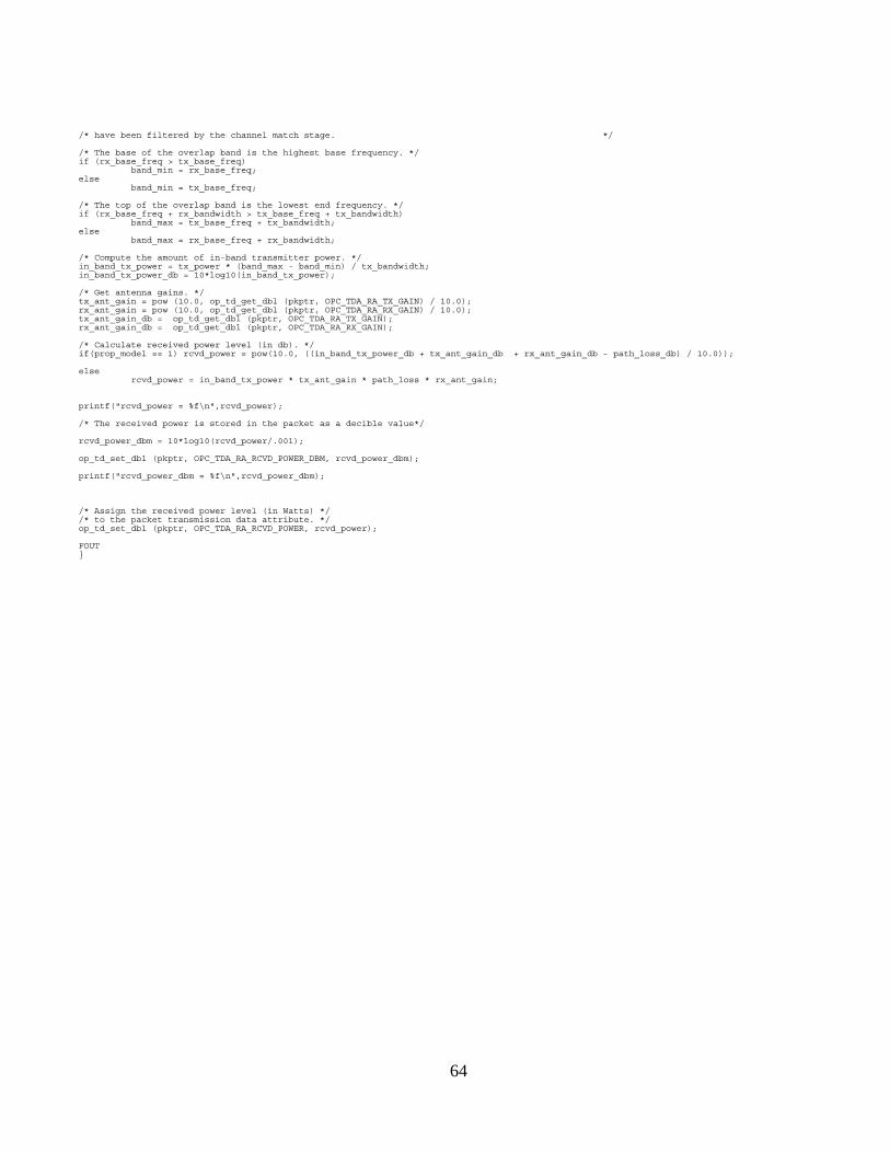
64
/* have been filtered by the channel match stage. */ /* The base of the overlap band is the highest base frequency. */ if (rx_base_freq > tx_base_freq) band_min = rx_base_freq; else band_min = tx_base_freq; /* The top of the overlap band is the lowest end frequency. */ if (rx_base_freq + rx_bandwidth > tx_base_freq + tx_bandwidth) band_max = tx_base_freq + tx_bandwidth; else band_max = rx_base_freq + rx_bandwidth; /* Compute the amount of in-band transmitter power. */ in_band_tx_power = tx_power * (band_max - band_min) / tx_bandwidth; in_band_tx_power_db = 10*log10(in_band_tx_power); /* Get antenna gains. */ tx_ant_gain = pow (10.0, op_td_get_dbl (pkptr, OPC_TDA_RA_TX_GAIN) / 10.0); rx_ant_gain = pow (10.0, op_td_get_dbl (pkptr, OPC_TDA_RA_RX_GAIN) / 10.0); tx_ant_gain_db = op_td_get_dbl (pkptr, OPC_TDA_RA_TX_GAIN); rx_ant_gain_db = op_td_get_dbl (pkptr, OPC_TDA_RA_RX_GAIN); /* Calculate received power level (in db). */ if(prop_model == 1) rcvd_power = pow(10.0, ((in_band_tx_power_db + tx_ant_gain_db + rx_ant_gain_db - path_loss_db) / 10.0)); else rcvd_power = in_band_tx_power * tx_ant_gain * path_loss * rx_ant_gain; printf("rcvd_power = %f\n",rcvd_power); /* The received power is stored in the packet as a decible value*/ rcvd_power_dbm = 10*log10(rcvd_power/.001); op_td_set_dbl (pkptr, OPC_TDA_RA_RCVD_POWER_DBM, rcvd_power_dbm); printf("rcvd_power_dbm = %f\n",rcvd_power_dbm); /* Assign the received power level (in Watts) */ /* to the packet transmission data attribute. */ op_td_set_dbl (pkptr, OPC_TDA_RA_RCVD_POWER, rcvd_power); FOUT }

65
Modified dra_power pipeline stage for Rural environment:
/* dra_power.ps.c */ /* Default received power model for radio link Transceiver */ /* Pipeline. This model uses the receiver channel state */ /* information to check and update the signal lock status */ /* of the channel. It relies on the rxgroup stage model for */ /* the creation and initialization of the channel state */ /* information. */ /****************************************/ /* Copyright (c) 1993-2003 */ /* by OPNET Technologies, Inc. */ /* (A Delaware Corporation) */ /* 7255 Woodmont Av., Suite 250 */ /* Bethesda, MD 20814, U.S.A. */ /* All Rights Reserved. */ /****************************************/ #include "opnet.h" #include "dra.h" #include <math.h> /***** constants *****/ #define C 3.0E+08 /* speed of light (m/s) */ #define SIXTEEN_PI_SQ 157.91367 /* 16 times pi-squared */ /***** pipeline procedure *****/ #if defined (__cplusplus) extern "C" #endif void dra_power_rural_mt (OP_SIM_CONTEXT_ARG_OPT_COMMA Packet * pkptr) { double prop_distance, rcvd_power, path_loss; double tx_power, tx_base_freq, tx_bandwidth, tx_center_freq; double lambda, rx_ant_gain, tx_ant_gain; Objid rx_ch_obid; double in_band_tx_power, band_max, band_min; double rx_base_freq, rx_bandwidth; DraT_Rxch_State_Info* rxch_state_ptr; double tx_ant_height, rx_ant_height; /* Antenna heights for TX,RX*/ double tx_MHz_freq; /* TX freq in Mega Hertz*/ double km_distance; /* Distance converted to Kilometers*/ double a_hm; /* Correction factor for mobile antenna*/ double path_loss_db = 0, in_band_tx_power_db; /* decible value of pathloss and in band transmission power*/ int prop_model = 0; /* determines which pathloss formula to use*/ double rx_ant_gain_db, rcvd_power_dbm, tx_ant_gain_db; /* db values of the ant. gains */ /** Compute the average power in Watts of the **/ /** signal associated with a transmitted packet. **/ FIN_MT (dra_power_urban_large_mt (pkptr)); /* If the incoming packet is 'valid', it may cause the receiver to */ /* lock onto it. However, if the receiving node is disabled, then */ /* the channel match should be set to noise. */ if (op_td_get_int (pkptr, OPC_TDA_RA_MATCH_STATUS) == OPC_TDA_RA_MATCH_VALID) { if (op_td_is_set (pkptr, OPC_TDA_RA_ND_FAIL)) { /* The receiving node is disabled. Change */ /* the channel match status to noise. */ op_td_set_int (pkptr, OPC_TDA_RA_MATCH_STATUS, OPC_TDA_RA_MATCH_NOISE); } else { /* The receiving node is enabled. Get */ /* the address of the receiver channel. */ rx_ch_obid = op_td_get_int (pkptr, OPC_TDA_RA_RX_CH_OBJID); /* Access receiver channels state information. */ rxch_state_ptr = (DraT_Rxch_State_Info *) op_ima_obj_state_get (rx_ch_obid); /* If the receiver channel is already locked, */ /* the packet will now be considered to be noise. */ /* This prevents simultaneous reception of multiple */ /* valid packets on any given radio channel. */ if (rxch_state_ptr->signal_lock) op_td_set_int (pkptr, OPC_TDA_RA_MATCH_STATUS, OPC_TDA_RA_MATCH_NOISE); else { /* Otherwise, the receiver channel will become */ /* locked until the packet reception ends. */ rxch_state_ptr->signal_lock = OPC_TRUE; } } } /* Get power allotted to transmitter channel. */ tx_power = op_td_get_dbl (pkptr, OPC_TDA_RA_TX_POWER);

66
/* Get transmission frequency in Hz. */ tx_base_freq = op_td_get_dbl (pkptr, OPC_TDA_RA_TX_FREQ); tx_bandwidth = op_td_get_dbl (pkptr, OPC_TDA_RA_TX_BW); tx_center_freq = tx_base_freq + (tx_bandwidth / 2.0); /*Convert the transmit frequency to Mega Hertz*/ tx_MHz_freq = tx_center_freq/1000000; /*printf("freq = %f\n",tx_MHz_freq);*/ /* Caclculate wavelength (in meters). */ lambda = C / tx_center_freq; /*printf("lambda = %f\n",lambda);*/ /* Get distance between transmitter and receiver (in meters). */ prop_distance = op_td_get_dbl (pkptr, OPC_TDA_RA_START_DIST); m_distance = (km_distance * 1000); /*printf("prop = %f\n",prop_distance);*/ /* Get the height of the transmit and recieve antennas.*/ tx_ant_height = (op_td_get_dbl (pkptr, OPC_TDA_RA_TX_ALT))/1000; rx_ant_height = (op_td_get_dbl (pkptr, OPC_TDA_RA_RX_ALT))/1000; printf("tx_height = %f\n",tx_ant_height); printf("rx_height = %f\n",rx_ant_height); /* Calculate the distance using the TDA sart_dist*/ km_distance = sqrt(pow((prop_distance/1000),2)- pow((tx_ant_height-rx_ant_height),2)); printf("dist_z = %f\n",km_distance); /* When using TMM, the TDA OPC_TDA_RA_RCVD_POWER will already */ /* have a raw value for the pathloss. */ if (op_td_is_set (pkptr, OPC_TDA_RA_RCVD_POWER)) { path_loss = op_td_get_dbl (pkptr, OPC_TDA_RA_RCVD_POWER); } else { /* Compute the pathloss for this distance and wavelength. */ if (prop_distance > 0.0) { /* Determine which propagation model to use and use value in the db form*/ if ((tx_MHz_freq >= 150 && tx_MHz_freq <= 1500) && (km_distance >= 1 && km_distance <= 100) && (tx_ant_height >= 30 && tx_ant_height <= 200) && (rx_ant_height >= 1 && rx_ant_height <= 10)) { a_hm = (1.1*log10(tx_MHz_freq) - 0.7)*rx_ant_height - (1.56*log10(tx_MHz_freq) - 0.8); path_loss_db = 69.55 + 26.16*log10(tx_MHz_freq) - 13.82*log10(tx_ant_height) - a_hm + (44.9 - 6.55*log10(tx_ant_height))*log10(km_distance) - (4.78*pow(log10(tx_MHz_freq),2) + 18.33*log10(tx_MHz_freq) - 40.94); prop_model = 1; printf("HataPL = %f\n",path_loss_db); } else { path_loss = (lambda * lambda) / (SIXTEEN_PI_SQ * m_distance * m_distance); prop_model = 0; printf("path_loss = %f\n",path_loss); } } else { if (prop_model == 1)path_loss_db = 0.0; else path_loss = 1; } } /* Determine the receiver bandwidth and base frequency. */ rx_base_freq = op_td_get_dbl (pkptr, OPC_TDA_RA_RX_FREQ); rx_bandwidth = op_td_get_dbl (pkptr, OPC_TDA_RA_RX_BW); /* Use these values to determine the band overlap with the transmitter. */ /* Note that if there were no overlap at all, the packet would already */ /* have been filtered by the channel match stage. */ /* The base of the overlap band is the highest base frequency. */ if (rx_base_freq > tx_base_freq) band_min = rx_base_freq; else band_min = tx_base_freq; /* The top of the overlap band is the lowest end frequency. */ if (rx_base_freq + rx_bandwidth > tx_base_freq + tx_bandwidth) band_max = tx_base_freq + tx_bandwidth; else band_max = rx_base_freq + rx_bandwidth; /* Compute the amount of in-band transmitter power. */ in_band_tx_power = tx_power * (band_max - band_min) / tx_bandwidth; in_band_tx_power_db = 10*log10(in_band_tx_power); /* Get antenna gains. */ tx_ant_gain = pow (10.0, op_td_get_dbl (pkptr, OPC_TDA_RA_TX_GAIN) / 10.0); rx_ant_gain = pow (10.0, op_td_get_dbl (pkptr, OPC_TDA_RA_RX_GAIN) / 10.0);

67
tx_ant_gain_db = op_td_get_dbl (pkptr, OPC_TDA_RA_TX_GAIN); rx_ant_gain_db = op_td_get_dbl (pkptr, OPC_TDA_RA_RX_GAIN); /* Calculate received power level (in db). */ if(prop_model == 1) rcvd_power = pow(10.0, ((in_band_tx_power_db + tx_ant_gain_db + rx_ant_gain_db - path_loss_db) / 10.0)); else rcvd_power = in_band_tx_power * tx_ant_gain * path_loss * rx_ant_gain; printf("rcvd_power = %f\n",rcvd_power); /* The received power is stored in the packet as a decible value*/ rcvd_power_dbm = 10*log10(rcvd_power/.001); op_td_set_dbl (pkptr, OPC_TDA_RA_RCVD_POWER_DBM, rcvd_power_dbm); printf("rcvd_power_dbm = %f\n",rcvd_power_dbm); /* Assign the received power level (in Watts) */ /* to the packet transmission data attribute. */ op_td_set_dbl (pkptr, OPC_TDA_RA_RCVD_POWER, rcvd_power); FOUT }

68
Modified dra_power pipeline stage for dB collection:
/* dra_power_db.ps.c */ /* Default received power model for radio link Transceiver */ /* Pipeline. This model uses the receiver channel state */ /* information to check and update the signal lock status */ /* of the channel. It relies on the rxgroup stage model for */ /* the creation and initialization of the channel state */ /* information. */ /****************************************/ /* Copyright (c) 1993-2003 */ /* by OPNET Technologies, Inc. */ /* (A Delaware Corporation) */ /* 7255 Woodmont Av., Suite 250 */ /* Bethesda, MD 20814, U.S.A. */ /* All Rights Reserved. */ /****************************************/ #include "opnet.h" #include "dra.h" #include <math.h> /***** constants *****/ #define C 3.0E+08 /* speed of light (m/s) */ #define SIXTEEN_PI_SQ 157.91367 /* 16 times pi-squared */ /***** pipeline procedure *****/ #if defined (__cplusplus) extern "C" #endif void dra_power_db_mt (OP_SIM_CONTEXT_ARG_OPT_COMMA Packet * pkptr) { double prop_distance, rcvd_power, path_loss; double tx_power, tx_base_freq, tx_bandwidth, tx_center_freq; double lambda, rx_ant_gain, tx_ant_gain; Objid rx_ch_obid; double in_band_tx_power, band_max, band_min; double rx_base_freq, rx_bandwidth; DraT_Rxch_State_Info* rxch_state_ptr; double rcvd_power_dbm; /* Correction factor for mobile antenna*/ /** Compute the average power in Watts of the **/ /** signal associated with a transmitted packet. **/ FIN_MT (dra_power (pkptr)); /* If the incoming packet is 'valid', it may cause the receiver to */ /* lock onto it. However, if the receiving node is disabled, then */ /* the channel match should be set to noise. */ if (op_td_get_int (pkptr, OPC_TDA_RA_MATCH_STATUS) == OPC_TDA_RA_MATCH_VALID) { if (op_td_is_set (pkptr, OPC_TDA_RA_ND_FAIL)) { /* The receiving node is disabled. Change */ /* the channel match status to noise. */ op_td_set_int (pkptr, OPC_TDA_RA_MATCH_STATUS, OPC_TDA_RA_MATCH_NOISE); } else { /* The receiving node is enabled. Get */ /* the address of the receiver channel. */ rx_ch_obid = op_td_get_int (pkptr, OPC_TDA_RA_RX_CH_OBJID); /* Access receiver channels state information. */ rxch_state_ptr = (DraT_Rxch_State_Info *) op_ima_obj_state_get (rx_ch_obid); /* If the receiver channel is already locked, */ /* the packet will now be considered to be noise. */ /* This prevents simultaneous reception of multiple */ /* valid packets on any given radio channel. */ if (rxch_state_ptr->signal_lock) op_td_set_int (pkptr, OPC_TDA_RA_MATCH_STATUS, OPC_TDA_RA_MATCH_NOISE); else { /* Otherwise, the receiver channel will become */ /* locked until the packet reception ends. */ rxch_state_ptr->signal_lock = OPC_TRUE; } } } /* Get power allotted to transmitter channel. */ tx_power = op_td_get_dbl (pkptr, OPC_TDA_RA_TX_POWER); /* Get transmission frequency in Hz. */ tx_base_freq = op_td_get_dbl (pkptr, OPC_TDA_RA_TX_FREQ); tx_bandwidth = op_td_get_dbl (pkptr, OPC_TDA_RA_TX_BW); tx_center_freq = tx_base_freq + (tx_bandwidth / 2.0); /* Caclculate wavelength (in meters). */ lambda = C / tx_center_freq; /* Get distance between transmitter and receiver (in meters). */ prop_distance = op_td_get_dbl (pkptr, OPC_TDA_RA_START_DIST); m_distance = (km_distance * 1000);

69
/* When using TMM, the TDA OPC_TDA_RA_RCVD_POWER will already */ /* have a raw value for the pathloss. */ if (op_td_is_set (pkptr, OPC_TDA_RA_RCVD_POWER)) { path_loss = op_td_get_dbl (pkptr, OPC_TDA_RA_RCVD_POWER); } else { /* Compute the pathloss for this distance and wavelength. */ if (prop_distance > 0.0) { path_loss = (lambda * lambda) / (SIXTEEN_PI_SQ * m_distance * m_distance); } else path_loss = 1.0; } /* Determine the receiver bandwidth and base frequency. */ rx_base_freq = op_td_get_dbl (pkptr, OPC_TDA_RA_RX_FREQ); rx_bandwidth = op_td_get_dbl (pkptr, OPC_TDA_RA_RX_BW); /* Use these values to determine the band overlap with the transmitter. */ /* Note that if there were no overlap at all, the packet would already */ /* have been filtered by the channel match stage. */ /* The base of the overlap band is the highest base frequency. */ if (rx_base_freq > tx_base_freq) band_min = rx_base_freq; else band_min = tx_base_freq; /* The top of the overlap band is the lowest end frequency. */ if (rx_base_freq + rx_bandwidth > tx_base_freq + tx_bandwidth) band_max = tx_base_freq + tx_bandwidth; else band_max = rx_base_freq + rx_bandwidth; /* Compute the amount of in-band transmitter power. */ in_band_tx_power = tx_power * (band_max - band_min) / tx_bandwidth; /* Get antenna gains (raw form, not in dB). */ tx_ant_gain = pow (10.0, op_td_get_dbl (pkptr, OPC_TDA_RA_TX_GAIN) / 10.0); rx_ant_gain = pow (10.0, op_td_get_dbl (pkptr, OPC_TDA_RA_RX_GAIN) / 10.0); /* Calculate received power level. */ rcvd_power = in_band_tx_power * tx_ant_gain * path_loss * rx_ant_gain; /* The received power is stored in the packet as a decible value*/ rcvd_power_dbm = 10*log10(rcvd_power/.001); op_td_set_dbl (pkptr, OPC_TDA_RA_RCVD_POWER_DBM, rcvd_power_dbm); /* Assign the received power level (in Watts) */ /* to the packet transmission data attribute. */ op_td_set_dbl (pkptr, OPC_TDA_RA_RCVD_POWER, rcvd_power); FOUT }

70
Appendix B: OPNET Debugger Output
Urban Large City output using the Hata and COST-231 model:
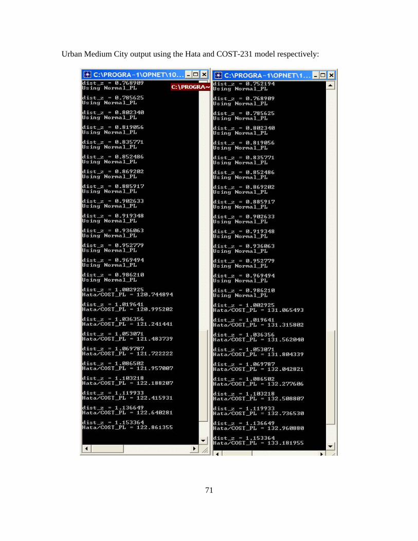
71
Urban Medium City output using the Hata and COST-231 model respectively:

72
Suburban output using the Hata and COST-231 model respectively:

73
Rural output using the Hata model respectively:

74
Appendix C: Suburban Simulation Results
Suburban simulation results obtained from OPNET at 880 MHz using the
parameters found in Table 4. The data is an average of all values collected from a two
second bucket.
time (sec) Distance (Km)60 -46.717 -46.717 -46.717 -46.717 -46.717 1.000 62 -46.718 -46.718 -46.718 -46.718 -46.718 1.033 64 -47.193 -47.193 -47.193 -47.193 -47.193 1.067 66 -47.654 -47.654 -47.654 -47.654 -47.654 1.100 68 -48.100 -48.100 -48.100 -48.100 -48.100 1.133 70 -48.533 -48.533 -48.533 -48.533 -48.533 1.167 72 -48.954 -48.954 -48.954 -48.954 -48.954 1.200 74 -49.362 -49.362 -49.362 -49.362 -49.362 1.233 76 -49.760 -49.760 -49.760 -49.760 -49.760 1.267 78 -50.147 -50.147 -50.147 -50.147 -50.147 1.300 80 -50.523 -50.523 -50.523 -50.523 -50.523 1.333 82 -50.891 -50.891 -50.891 -50.891 -50.891 1.367 84 -51.249 -51.249 -51.249 -51.249 -51.249 1.400 86 -51.598 -51.598 -51.598 -51.598 -51.598 1.433 88 -51.940 -51.940 -51.940 -51.940 -51.940 1.467 90 -52.273 -52.273 -52.273 -52.273 -52.273 1.500 92 -52.599 -52.599 -52.599 -52.599 -52.599 1.533 94 -52.918 -52.918 -52.918 -52.918 -52.918 1.567 96 -53.230 -53.230 -53.230 -53.230 -53.230 1.600 98 -53.535 -53.535 -53.535 -53.535 -53.535 1.633 100 -53.834 -53.834 -53.834 -53.834 -53.834 1.667 102 -54.127 -54.127 -54.127 -54.127 -54.127 1.700 104 -54.415 -54.415 -54.415 -54.415 -54.415 1.733 106 -54.696 -54.696 -54.696 -54.696 -54.696 1.767 108 -54.972 -54.972 -54.972 -54.972 -54.972 1.800 110 -55.244 -55.244 -55.244 -55.244 -55.244 1.833 112 -55.510 -55.510 -55.510 -55.510 -55.510 1.867 114 -55.771 -55.771 -55.771 -55.771 -55.771 1.900 116 -56.028 -56.028 -56.028 -56.028 -56.028 1.933 118 -56.280 -56.280 -56.280 -56.280 -56.280 1.967 120 -56.528 -56.528 -56.528 -56.528 -56.528 2.000 122 -56.772 -56.772 -56.772 -56.772 -56.772 2.033 124 -57.012 -57.012 -57.012 -57.012 -57.012 2.067 126 -57.247 -57.247 -57.247 -57.247 -57.247 2.100 128 -57.480 -57.480 -57.480 -57.480 -57.480 2.133 130 -57.708 -57.708 -57.708 -57.708 -57.708 2.167

75
132 -57.933 -57.933 -57.933 -57.933 -57.933 2.200 134 -58.154 -58.154 -58.154 -58.154 -58.154 2.233 136 -58.372 -58.372 -58.372 -58.372 -58.372 2.267 138 -58.587 -58.587 -58.587 -58.587 -58.587 2.300 140 -58.799 -58.799 -58.799 -58.799 -58.799 2.333 142 -59.008 -59.008 -59.008 -59.008 -59.008 2.367 144 -59.214 -59.214 -59.214 -59.214 -59.214 2.400 146 -59.416 -59.416 -59.416 -59.416 -59.416 2.433 148 -59.617 -59.617 -59.617 -59.617 -59.617 2.467 150 -59.814 -59.814 -59.814 -59.814 -59.814 2.500 152 -60.009 -60.009 -60.009 -60.009 -60.009 2.533 154 -60.201 -60.201 -60.201 -60.201 -60.201 2.567 156 -60.390 -60.390 -60.390 -60.390 -60.390 2.600 158 -60.577 -60.577 -60.577 -60.577 -60.577 2.633 160 -60.762 -60.762 -60.762 -60.762 -60.762 2.667 162 -60.945 -60.945 -60.945 -60.945 -60.945 2.700 164 -61.125 -61.125 -61.125 -61.125 -61.125 2.733 166 -61.303 -61.303 -61.303 -61.303 -61.303 2.767 168 -61.479 -61.479 -61.479 -61.479 -61.479 2.800 170 -61.652 -61.652 -61.652 -61.652 -61.652 2.833 172 -61.824 -61.824 -61.824 -61.824 -61.824 2.867 174 -61.994 -61.994 -61.994 -61.994 -61.994 2.900 176 -62.161 -62.161 -62.161 -62.161 -62.161 2.933 178 -62.327 -62.327 -62.327 -62.327 -62.327 2.967 180 -62.491 -62.491 -62.491 -62.491 -62.491 3.000 182 -62.653 -62.653 -62.653 -62.653 -62.653 3.033 184 -62.813 -62.813 -62.813 -62.813 -62.813 3.067 186 -62.972 -62.972 -62.972 -62.972 -62.972 3.100 188 -63.129 -63.129 -63.129 -63.129 -63.129 3.133 190 -63.284 -63.284 -63.284 -63.284 -63.284 3.167 192 -63.437 -63.437 -63.437 -63.437 -63.437 3.200 194 -63.589 -63.589 -63.589 -63.589 -63.589 3.233 196 -63.740 -63.740 -63.740 -63.740 -63.740 3.267 198 -63.888 -63.888 -63.888 -63.888 -63.888 3.300 200 -64.036 -64.036 -64.036 -64.036 -64.036 3.333 202 -64.181 -64.181 -64.181 -64.181 -64.181 3.367 204 -64.326 -64.326 -64.326 -64.326 -64.326 3.400 206 -64.469 -64.469 -64.469 -64.469 -64.469 3.433 208 -64.610 -64.610 -64.610 -64.610 -64.610 3.467 210 -64.750 -64.750 -64.750 -64.750 -64.750 3.500 212 -64.889 -64.889 -64.889 -64.889 -64.889 3.533 214 -65.027 -65.027 -65.027 -65.027 -65.027 3.567 216 -65.163 -65.163 -65.163 -65.163 -65.163 3.600 218 -65.298 -65.298 -65.298 -65.298 -65.298 3.633 220 -65.431 -65.431 -65.431 -65.431 -65.431 3.667 222 -65.564 -65.564 -65.564 -65.564 -65.564 3.700 224 -65.695 -65.695 -65.695 -65.695 -65.695 3.733 226 -65.825 -65.825 -65.825 -65.825 -65.825 3.767 228 -65.954 -65.954 -65.954 -65.954 -65.954 3.800 230 -66.082 -66.082 -66.082 -66.082 -66.082 3.833

76
232 -66.209 -66.209 -66.209 -66.209 -66.209 3.867 234 -66.334 -66.334 -66.334 -66.334 -66.334 3.900 236 -66.459 -66.459 -66.459 -66.459 -66.459 3.933 238 -66.582 -66.582 -66.582 -66.582 -66.582 3.967 240 -66.705 -66.705 -66.705 -66.705 -66.705 4.000 242 -66.826 -66.826 -66.826 -66.826 -66.826 4.033 244 -66.946 -66.946 -66.946 -66.946 -66.946 4.067 246 -67.066 -67.066 -67.066 -67.066 -67.066 4.100 248 -67.184 -67.184 -67.184 -67.184 -67.184 4.133 250 -67.302 -67.302 -67.302 -67.302 -67.302 4.167 252 -67.418 -67.418 -67.418 -67.418 -67.418 4.200 254 -67.534 -67.534 -67.534 -67.534 -67.534 4.233 256 -67.648 -67.648 -67.648 -67.648 -67.648 4.267 258 -67.762 -67.762 -67.762 -67.762 -67.762 4.300 260 -67.875 -67.875 -67.875 -67.875 -67.875 4.333 262 -67.987 -67.987 -67.987 -67.987 -67.987 4.367 264 -68.098 -68.098 -68.098 -68.098 -68.098 4.400 266 -68.208 -68.208 -68.208 -68.208 -68.208 4.433 268 -68.318 -68.318 -68.318 -68.318 -68.318 4.467 270 -68.427 -68.427 -68.427 -68.427 -68.427 4.500 272 -68.534 -68.534 -68.534 -68.534 -68.534 4.533 274 -68.641 -68.641 -68.641 -68.641 -68.641 4.567 276 -68.748 -68.748 -68.748 -68.748 -68.748 4.600 278 -68.853 -68.853 -68.853 -68.853 -68.853 4.633 280 -68.958 -68.958 -68.958 -68.958 -68.958 4.667 282 -69.062 -69.062 -69.062 -69.062 -69.062 4.700 284 -69.165 -69.165 -69.165 -69.165 -69.165 4.733 286 -69.268 -69.268 -69.268 -69.268 -69.268 4.767 288 -69.369 -69.369 -69.369 -69.369 -69.369 4.800 290 -69.471 -69.471 -69.471 -69.471 -69.471 4.833 292 -69.571 -69.571 -69.571 -69.571 -69.571 4.867 294 -69.671 -69.671 -69.671 -69.671 -69.671 4.900 296 -69.770 -69.770 -69.770 -69.770 -69.770 4.933 298 -69.868 -69.868 -69.868 -69.868 -69.868 4.967 300 -69.966 -69.966 -69.966 -69.966 -69.966 5.000 302 -70.063 -70.063 -70.063 -70.063 -70.063 5.033 304 -70.159 -70.159 -70.159 -70.159 -70.159 5.067 306 -70.255 -70.255 -70.255 -70.255 -70.255 5.100 308 -70.350 -70.350 -70.350 -70.350 -70.350 5.133 310 -70.444 -70.444 -70.444 -70.444 -70.444 5.167 312 -70.538 -70.538 -70.538 -70.538 -70.538 5.200 314 -70.632 -70.632 -70.632 -70.632 -70.632 5.233 316 -70.724 -70.724 -70.724 -70.724 -70.724 5.267 318 -70.816 -70.816 -70.816 -70.816 -70.816 5.300 320 -70.908 -70.908 -70.908 -70.908 -70.908 5.333 322 -70.999 -70.999 -70.999 -70.999 -70.999 5.367 324 -71.089 -71.089 -71.089 -71.089 -71.089 5.400 326 -71.179 -71.179 -71.179 -71.179 -71.179 5.433 328 -71.268 -71.268 -71.268 -71.268 -71.268 5.467 330 -71.357 -71.357 -71.357 -71.357 -71.357 5.500

77
332 -71.445 -71.445 -71.445 -71.445 -71.445 5.533 334 -71.533 -71.533 -71.533 -71.533 -71.533 5.567 336 -71.620 -71.620 -71.620 -71.620 -71.620 5.600 338 -71.707 -71.707 -71.707 -71.707 -71.707 5.633 340 -71.793 -71.793 -71.793 -71.793 -71.793 5.667 342 -71.878 -71.878 -71.878 -71.878 -71.878 5.700 344 -71.963 -71.963 -71.963 -71.963 -71.963 5.733 346 -72.048 -72.048 -72.048 -72.048 -72.048 5.767 348 -72.132 -72.132 -72.132 -72.132 -72.132 5.800 350 -72.216 -72.216 -72.216 -72.216 -72.216 5.833 352 -72.299 -72.299 -72.299 -72.299 -72.299 5.867 354 -72.381 -72.381 -72.381 -72.381 -72.381 5.900 356 -72.463 -72.463 -72.463 -72.463 -72.463 5.933 358 -72.545 -72.545 -72.545 -72.545 -72.545 5.967 360 -72.626 -72.626 -72.626 -72.626 -72.626 6.000 362 -72.707 -72.707 -72.707 -72.707 -72.707 6.033 364 -72.788 -72.788 -72.788 -72.788 -72.788 6.067 366 -72.868 -72.868 -72.868 -72.868 -72.868 6.100 368 -72.947 -72.947 -72.947 -72.947 -72.947 6.133 370 -73.026 -73.026 -73.026 -73.026 -73.026 6.167 372 -73.105 -73.105 -73.105 -73.105 -73.105 6.200 374 -73.183 -73.183 -73.183 -73.183 -73.183 6.233 376 -73.261 -73.261 -73.261 -73.261 -73.261 6.267 378 -73.338 -73.338 -73.338 -73.338 -73.338 6.300 380 -73.415 -73.415 -73.415 -73.415 -73.415 6.333 382 -73.492 -73.492 -73.492 -73.492 -73.492 6.367 384 -73.568 -73.568 -73.568 -73.568 -73.568 6.400 386 -73.643 -73.643 -73.643 -73.643 -73.643 6.433 388 -73.719 -73.719 -73.719 -73.719 -73.719 6.467 390 -73.794 -73.794 -73.794 -73.794 -73.794 6.500 392 -73.868 -73.868 -73.868 -73.868 -73.868 6.533 394 -73.942 -73.942 -73.942 -73.942 -73.942 6.567 396 -74.016 -74.016 -74.016 -74.016 -74.016 6.600 398 -74.090 -74.090 -74.090 -74.090 -74.090 6.633 400 -74.163 -74.163 -74.163 -74.163 -74.163 6.667 402 -74.236 -74.236 -74.236 -74.236 -74.236 6.700 404 -74.308 -74.308 -74.308 -74.308 -74.308 6.733 406 -74.380 -74.380 -74.380 -74.380 -74.380 6.767 408 -74.451 -74.451 -74.451 -74.451 -74.451 6.800 410 -74.523 -74.523 -74.523 -74.523 -74.523 6.833 412 -74.594 -74.594 -74.594 -74.594 -74.594 6.867 414 -74.664 -74.664 -74.664 -74.664 -74.664 6.900 416 -74.735 -74.735 -74.735 -74.735 -74.735 6.933 418 -74.804 -74.804 -74.804 -74.804 -74.804 6.967 420 -74.874 -74.874 -74.874 -74.874 -74.874 7.000 422 -74.943 -74.943 -74.943 -74.943 -74.943 7.033 424 -75.012 -75.012 -75.012 -75.012 -75.012 7.067 426 -75.081 -75.081 -75.081 -75.081 -75.081 7.100 428 -75.149 -75.149 -75.149 -75.149 -75.149 7.133 430 -75.217 -75.217 -75.217 -75.217 -75.217 7.167

78
432 -75.285 -75.285 -75.285 -75.285 -75.285 7.200 434 -75.352 -75.352 -75.352 -75.352 -75.352 7.233 436 -75.419 -75.419 -75.419 -75.419 -75.419 7.267 438 -75.486 -75.486 -75.486 -75.486 -75.486 7.300 440 -75.552 -75.552 -75.552 -75.552 -75.552 7.333 442 -75.618 -75.618 -75.618 -75.618 -75.618 7.367 444 -75.684 -75.684 -75.684 -75.684 -75.684 7.400 446 -75.749 -75.749 -75.749 -75.749 -75.749 7.433 448 -75.814 -75.814 -75.814 -75.814 -75.814 7.467 450 -75.879 -75.879 -75.879 -75.879 -75.879 7.500 452 -75.944 -75.944 -75.944 -75.944 -75.944 7.533 454 -76.008 -76.008 -76.008 -76.008 -76.008 7.567 456 -76.072 -76.072 -76.072 -76.072 -76.072 7.600 458 -76.136 -76.136 -76.136 -76.136 -76.136 7.633 460 -76.200 -76.200 -76.200 -76.200 -76.200 7.667 462 -76.263 -76.263 -76.263 -76.263 -76.263 7.700 464 -76.326 -76.326 -76.326 -76.326 -76.326 7.733 466 -76.388 -76.388 -76.388 -76.388 -76.388 7.767 468 -76.451 -76.451 -76.451 -76.451 -76.451 7.800 470 -76.513 -76.513 -76.513 -76.513 -76.513 7.833 472 -76.575 -76.575 -76.575 -76.575 -76.575 7.867 474 -76.636 -76.636 -76.636 -76.636 -76.636 7.900 476 -76.698 -76.698 -76.698 -76.698 -76.698 7.933 478 -76.759 -76.759 -76.759 -76.759 -76.759 7.967 480 -76.820 -76.820 -76.820 -76.820 -76.820 8.000 482 -76.880 -76.880 -76.880 -76.880 -76.880 8.033 484 -76.940 -76.940 -76.940 -76.940 -76.940 8.067 486 -77.000 -77.000 -77.000 -77.000 -77.000 8.100 488 -77.060 -77.060 -77.060 -77.060 -77.060 8.133 490 -77.120 -77.120 -77.120 -77.120 -77.120 8.167 492 -77.179 -77.179 -77.179 -77.179 -77.179 8.200 494 -77.238 -77.238 -77.238 -77.238 -77.238 8.233 496 -77.297 -77.297 -77.297 -77.297 -77.297 8.267 498 -77.356 -77.356 -77.356 -77.356 -77.356 8.300 500 -77.414 -77.414 -77.414 -77.414 -77.414 8.333 502 -77.472 -77.472 -77.472 -77.472 -77.472 8.367 504 -77.530 -77.530 -77.530 -77.530 -77.530 8.400 506 -77.588 -77.588 -77.588 -77.588 -77.588 8.433 508 -77.645 -77.645 -77.645 -77.645 -77.645 8.467 510 -77.702 -77.702 -77.702 -77.702 -77.702 8.500 512 -77.759 -77.759 -77.759 -77.759 -77.759 8.533 514 -77.816 -77.816 -77.816 -77.816 -77.816 8.567 516 -77.873 -77.873 -77.873 -77.873 -77.873 8.600 518 -77.929 -77.929 -77.929 -77.929 -77.929 8.633 520 -77.985 -77.985 -77.985 -77.985 -77.985 8.667 522 -78.041 -78.041 -78.041 -78.041 -78.041 8.700 524 -78.097 -78.097 -78.097 -78.097 -78.097 8.733 526 -78.152 -78.152 -78.152 -78.152 -78.152 8.767 528 -78.208 -78.208 -78.208 -78.208 -78.208 8.800 530 -78.263 -78.263 -78.263 -78.263 -78.263 8.833

79
532 -78.317 -78.317 -78.317 -78.317 -78.317 8.867 534 -78.372 -78.372 -78.372 -78.372 -78.372 8.900 536 -78.426 -78.426 -78.426 -78.426 -78.426 8.933 538 -78.481 -78.481 -78.481 -78.481 -78.481 8.967 540 -78.535 -78.535 -78.535 -78.535 -78.535 9.000 542 -78.589 -78.589 -78.589 -78.589 -78.589 9.033 544 -78.642 -78.642 -78.642 -78.642 -78.642 9.067 546 -78.696 -78.696 -78.696 -78.696 -78.696 9.100 548 -78.749 -78.749 -78.749 -78.749 -78.749 9.133 550 -78.802 -78.802 -78.802 -78.802 -78.802 9.167 552 -78.855 -78.855 -78.855 -78.855 -78.855 9.200 554 -78.907 -78.907 -78.907 -78.907 -78.907 9.233 556 -78.960 -78.960 -78.960 -78.960 -78.960 9.267 558 -79.012 -79.012 -79.012 -79.012 -79.012 9.300 560 -79.064 -79.064 -79.064 -79.064 -79.064 9.333 562 -79.116 -79.116 -79.116 -79.116 -79.116 9.367 564 -79.168 -79.168 -79.168 -79.168 -79.168 9.400 566 -79.219 -79.219 -79.219 -79.219 -79.219 9.433 568 -79.271 -79.271 -79.271 -79.271 -79.271 9.467 570 -79.322 -79.322 -79.322 -79.322 -79.322 9.500 572 -79.373 -79.373 -79.373 -79.373 -79.373 9.533 574 -79.424 -79.424 -79.424 -79.424 -79.424 9.567 576 -79.474 -79.474 -79.474 -79.474 -79.474 9.600 578 -79.525 -79.525 -79.525 -79.525 -79.525 9.633 580 -79.575 -79.575 -79.575 -79.575 -79.575 9.667 582 -79.625 -79.625 -79.625 -79.625 -79.625 9.700 584 -79.675 -79.675 -79.675 -79.675 -79.675 9.733 586 -79.725 -79.725 -79.725 -79.725 -79.725 9.767 588 -79.774 -79.774 -79.774 -79.774 -79.774 9.800 590 -79.824 -79.824 -79.824 -79.824 -79.824 9.833 592 -79.873 -79.873 -79.873 -79.873 -79.873 9.867 594 -79.922 -79.922 -79.922 -79.922 -79.922 9.900 596 -79.971 -79.971 -79.971 -79.971 -79.971 9.933 598 -80.020 -80.020 -80.020 -80.020 -80.020 9.967 600 -80.068 -80.068 -80.068 -80.068 -80.068 10.000

80
Suburban simulation results obtained from OPNET at 1922 MHz using the
parameters found in Table 4. The data is an average of all values collected from a two
second bucket.
time (sec) Distance (Km) 60 -66.798 -66.798 -66.798 -66.798 -66.798 1.00 62 -66.799 -66.799 -66.799 -66.799 -66.799 1.03 64 -67.274 -67.274 -67.274 -67.274 -67.274 1.07 66 -67.735 -67.735 -67.735 -67.735 -67.735 1.10 68 -68.181 -68.181 -68.181 -68.181 -68.181 1.13 70 -68.614 -68.614 -68.614 -68.614 -68.614 1.17 72 -69.035 -69.035 -69.035 -69.035 -69.035 1.20 74 -69.443 -69.443 -69.443 -69.443 -69.443 1.23 76 -69.841 -69.841 -69.841 -69.841 -69.841 1.27 78 -70.228 -70.228 -70.228 -70.228 -70.228 1.30 80 -70.604 -70.604 -70.604 -70.604 -70.604 1.33 82 -70.972 -70.972 -70.972 -70.972 -70.972 1.37 84 -71.330 -71.330 -71.330 -71.330 -71.330 1.40 86 -71.679 -71.679 -71.679 -71.679 -71.679 1.43 88 -72.021 -72.021 -72.021 -72.021 -72.021 1.47 90 -72.354 -72.354 -72.354 -72.354 -72.354 1.50 92 -72.680 -72.680 -72.680 -72.680 -72.680 1.53 94 -72.999 -72.999 -72.999 -72.999 -72.999 1.57 96 -73.311 -73.311 -73.311 -73.311 -73.311 1.60 98 -73.616 -73.616 -73.616 -73.616 -73.616 1.63 100 -73.915 -73.915 -73.915 -73.915 -73.915 1.67 102 -74.208 -74.208 -74.208 -74.208 -74.208 1.70 104 -74.496 -74.496 -74.496 -74.496 -74.496 1.73 106 -74.777 -74.777 -74.777 -74.777 -74.777 1.77 108 -75.053 -75.053 -75.053 -75.053 -75.053 1.80 110 -75.325 -75.325 -75.325 -75.325 -75.325 1.83 112 -75.591 -75.591 -75.591 -75.591 -75.591 1.87 114 -75.852 -75.852 -75.852 -75.852 -75.852 1.90 116 -76.109 -76.109 -76.109 -76.109 -76.109 1.93 118 -76.361 -76.361 -76.361 -76.361 -76.361 1.97 120 -76.609 -76.609 -76.609 -76.609 -76.609 2.00 122 -76.853 -76.853 -76.853 -76.853 -76.853 2.03 124 -77.093 -77.093 -77.093 -77.093 -77.093 2.07 126 -77.328 -77.328 -77.328 -77.328 -77.328 2.10 128 -77.561 -77.561 -77.561 -77.561 -77.561 2.13 130 -77.789 -77.789 -77.789 -77.789 -77.789 2.17

81
132 -78.014 -78.014 -78.014 -78.014 -78.014 2.20 134 -78.235 -78.235 -78.235 -78.235 -78.235 2.23 136 -78.453 -78.453 -78.453 -78.453 -78.453 2.27 138 -78.668 -78.668 -78.668 -78.668 -78.668 2.30 140 -78.880 -78.880 -78.880 -78.880 -78.880 2.33 142 -79.089 -79.089 -79.089 -79.089 -79.089 2.37 144 -79.295 -79.295 -79.295 -79.295 -79.295 2.40 146 -79.497 -79.497 -79.497 -79.497 -79.497 2.43 148 -79.697 -79.697 -79.697 -79.697 -79.697 2.47 150 -79.895 -79.895 -79.895 -79.895 -79.895 2.50 152 -80.090 -80.090 -80.090 -80.090 -80.090 2.53 154 -80.282 -80.282 -80.282 -80.282 -80.282 2.57 156 -80.471 -80.471 -80.471 -80.471 -80.471 2.60 158 -80.658 -80.658 -80.658 -80.658 -80.658 2.63 160 -80.843 -80.843 -80.843 -80.843 -80.843 2.67 162 -81.026 -81.026 -81.026 -81.026 -81.026 2.70 164 -81.206 -81.206 -81.206 -81.206 -81.206 2.73 166 -81.384 -81.384 -81.384 -81.384 -81.384 2.77 168 -81.560 -81.560 -81.560 -81.560 -81.560 2.80 170 -81.733 -81.733 -81.733 -81.733 -81.733 2.83 172 -81.905 -81.905 -81.905 -81.905 -81.905 2.87 174 -82.075 -82.075 -82.075 -82.075 -82.075 2.90 176 -82.242 -82.242 -82.242 -82.242 -82.242 2.93 178 -82.408 -82.408 -82.408 -82.408 -82.408 2.97 180 -82.572 -82.572 -82.572 -82.572 -82.572 3.00 182 -82.734 -82.734 -82.734 -82.734 -82.734 3.03 184 -82.894 -82.894 -82.894 -82.894 -82.894 3.07 186 -83.053 -83.053 -83.053 -83.053 -83.053 3.10 188 -83.210 -83.210 -83.210 -83.210 -83.210 3.13 190 -83.365 -83.365 -83.365 -83.365 -83.365 3.17 192 -83.518 -83.518 -83.518 -83.518 -83.518 3.20 194 -83.670 -83.670 -83.670 -83.670 -83.670 3.23 196 -83.821 -83.821 -83.821 -83.821 -83.821 3.27 198 -83.969 -83.969 -83.969 -83.969 -83.969 3.30 200 -84.117 -84.117 -84.117 -84.117 -84.117 3.33 202 -84.262 -84.262 -84.262 -84.262 -84.262 3.37 204 -84.407 -84.407 -84.407 -84.407 -84.407 3.40 206 -84.550 -84.550 -84.550 -84.550 -84.550 3.43 208 -84.691 -84.691 -84.691 -84.691 -84.691 3.47 210 -84.831 -84.831 -84.831 -84.831 -84.831 3.50 212 -84.970 -84.970 -84.970 -84.970 -84.970 3.53 214 -85.108 -85.108 -85.108 -85.108 -85.108 3.57 216 -85.244 -85.244 -85.244 -85.244 -85.244 3.60 218 -85.379 -85.379 -85.379 -85.379 -85.379 3.63 220 -85.512 -85.512 -85.512 -85.512 -85.512 3.67

82
222 -85.645 -85.645 -85.645 -85.645 -85.645 3.70 224 -85.776 -85.776 -85.776 -85.776 -85.776 3.73 226 -85.906 -85.906 -85.906 -85.906 -85.906 3.77 228 -86.035 -86.035 -86.035 -86.035 -86.035 3.80 230 -86.163 -86.163 -86.163 -86.163 -86.163 3.83 232 -86.290 -86.290 -86.290 -86.290 -86.290 3.87 234 -86.415 -86.415 -86.415 -86.415 -86.415 3.90 236 -86.540 -86.540 -86.540 -86.540 -86.540 3.93 238 -86.663 -86.663 -86.663 -86.663 -86.663 3.97 240 -86.786 -86.786 -86.786 -86.786 -86.786 4.00 242 -86.907 -86.907 -86.907 -86.907 -86.907 4.03 244 -87.027 -87.027 -87.027 -87.027 -87.027 4.07 246 -87.147 -87.147 -87.147 -87.147 -87.147 4.10 248 -87.265 -87.265 -87.265 -87.265 -87.265 4.13 250 -87.383 -87.383 -87.383 -87.383 -87.383 4.17 252 -87.499 -87.499 -87.499 -87.499 -87.499 4.20 254 -87.615 -87.615 -87.615 -87.615 -87.615 4.23 256 -87.729 -87.729 -87.729 -87.729 -87.729 4.27 258 -87.843 -87.843 -87.843 -87.843 -87.843 4.30 260 -87.956 -87.956 -87.956 -87.956 -87.956 4.33 262 -88.068 -88.068 -88.068 -88.068 -88.068 4.37 264 -88.179 -88.179 -88.179 -88.179 -88.179 4.40 266 -88.289 -88.289 -88.289 -88.289 -88.289 4.43 268 -88.399 -88.399 -88.399 -88.399 -88.399 4.47 270 -88.508 -88.508 -88.508 -88.508 -88.508 4.50 272 -88.615 -88.615 -88.615 -88.615 -88.615 4.53 274 -88.722 -88.722 -88.722 -88.722 -88.722 4.57 276 -88.829 -88.829 -88.829 -88.829 -88.829 4.60 278 -88.934 -88.934 -88.934 -88.934 -88.934 4.63 280 -89.039 -89.039 -89.039 -89.039 -89.039 4.67 282 -89.143 -89.143 -89.143 -89.143 -89.143 4.70 284 -89.246 -89.246 -89.246 -89.246 -89.246 4.73 286 -89.349 -89.349 -89.349 -89.349 -89.349 4.77 288 -89.450 -89.450 -89.450 -89.450 -89.450 4.80 290 -89.552 -89.552 -89.552 -89.552 -89.552 4.83 292 -89.652 -89.652 -89.652 -89.652 -89.652 4.87 294 -89.752 -89.752 -89.752 -89.752 -89.752 4.90 296 -89.851 -89.851 -89.851 -89.851 -89.851 4.93 298 -89.949 -89.949 -89.949 -89.949 -89.949 4.97 300 -90.047 -90.047 -90.047 -90.047 -90.047 5.00 302 -90.144 -90.144 -90.144 -90.144 -90.144 5.03 304 -90.240 -90.240 -90.240 -90.240 -90.240 5.07 306 -90.336 -90.336 -90.336 -90.336 -90.336 5.10 308 -90.431 -90.431 -90.431 -90.431 -90.431 5.13 310 -90.525 -90.525 -90.525 -90.525 -90.525 5.17
83
312 -90.619 -90.619 -90.619 -90.619 -90.619 5.20 314 -90.713 -90.713 -90.713 -90.713 -90.713 5.23 316 -90.805 -90.805 -90.805 -90.805 -90.805 5.27 318 -90.897 -90.897 -90.897 -90.897 -90.897 5.30 320 -90.989 -90.989 -90.989 -90.989 -90.989 5.33 322 -91.080 -91.080 -91.080 -91.080 -91.080 5.37 324 -91.170 -91.170 -91.170 -91.170 -91.170 5.40 326 -91.260 -91.260 -91.260 -91.260 -91.260 5.43 328 -91.349 -91.349 -91.349 -91.349 -91.349 5.47 330 -91.438 -91.438 -91.438 -91.438 -91.438 5.50 332 -91.526 -91.526 -91.526 -91.526 -91.526 5.53 334 -91.614 -91.614 -91.614 -91.614 -91.614 5.57 336 -91.701 -91.701 -91.701 -91.701 -91.701 5.60 338 -91.787 -91.787 -91.787 -91.787 -91.787 5.63 340 -91.874 -91.874 -91.874 -91.874 -91.874 5.67 342 -91.959 -91.959 -91.959 -91.959 -91.959 5.70 344 -92.044 -92.044 -92.044 -92.044 -92.044 5.73 346 -92.129 -92.129 -92.129 -92.129 -92.129 5.77 348 -92.213 -92.213 -92.213 -92.213 -92.213 5.80 350 -92.296 -92.296 -92.296 -92.296 -92.296 5.83 352 -92.380 -92.380 -92.380 -92.380 -92.380 5.87 354 -92.462 -92.462 -92.462 -92.462 -92.462 5.90 356 -92.544 -92.544 -92.544 -92.544 -92.544 5.93 358 -92.626 -92.626 -92.626 -92.626 -92.626 5.97 360 -92.707 -92.707 -92.707 -92.707 -92.707 6.00 362 -92.788 -92.788 -92.788 -92.788 -92.788 6.03 364 -92.869 -92.869 -92.869 -92.869 -92.869 6.07 366 -92.949 -92.949 -92.949 -92.949 -92.949 6.10 368 -93.028 -93.028 -93.028 -93.028 -93.028 6.13 370 -93.107 -93.107 -93.107 -93.107 -93.107 6.17 372 -93.186 -93.186 -93.186 -93.186 -93.186 6.20 374 -93.264 -93.264 -93.264 -93.264 -93.264 6.23 376 -93.342 -93.342 -93.342 -93.342 -93.342 6.27 378 -93.419 -93.419 -93.419 -93.419 -93.419 6.30 380 -93.496 -93.496 -93.496 -93.496 -93.496 6.33 382 -93.572 -93.572 -93.572 -93.572 -93.572 6.37 384 -93.649 -93.649 -93.649 -93.649 -93.649 6.40 386 -93.724 -93.724 -93.724 -93.724 -93.724 6.43 388 -93.800 -93.800 -93.800 -93.800 -93.800 6.47 390 -93.875 -93.875 -93.875 -93.875 -93.875 6.50 392 -93.949 -93.949 -93.949 -93.949 -93.949 6.53 394 -94.023 -94.023 -94.023 -94.023 -94.023 6.57 396 -94.097 -94.097 -94.097 -94.097 -94.097 6.60 398 -94.171 -94.171 -94.171 -94.171 -94.171 6.63 400 -94.244 -94.244 -94.244 -94.244 -94.244 6.67

84
402 -94.316 -94.316 -94.316 -94.316 -94.316 6.70 404 -94.389 -94.389 -94.389 -94.389 -94.389 6.73 406 -94.461 -94.461 -94.461 -94.461 -94.461 6.77 408 -94.532 -94.532 -94.532 -94.532 -94.532 6.80 410 -94.604 -94.604 -94.604 -94.604 -94.604 6.83 412 -94.675 -94.675 -94.675 -94.675 -94.675 6.87 414 -94.745 -94.745 -94.745 -94.745 -94.745 6.90 416 -94.815 -94.815 -94.815 -94.815 -94.815 6.93 418 -94.885 -94.885 -94.885 -94.885 -94.885 6.97 420 -94.955 -94.955 -94.955 -94.955 -94.955 7.00 422 -95.024 -95.024 -95.024 -95.024 -95.024 7.03 424 -95.093 -95.093 -95.093 -95.093 -95.093 7.07 426 -95.162 -95.162 -95.162 -95.162 -95.162 7.10 428 -95.230 -95.230 -95.230 -95.230 -95.230 7.13 430 -95.298 -95.298 -95.298 -95.298 -95.298 7.17 432 -95.366 -95.366 -95.366 -95.366 -95.366 7.20 434 -95.433 -95.433 -95.433 -95.433 -95.433 7.23 436 -95.500 -95.500 -95.500 -95.500 -95.500 7.27 438 -95.566 -95.566 -95.566 -95.566 -95.566 7.30 440 -95.633 -95.633 -95.633 -95.633 -95.633 7.33 442 -95.699 -95.699 -95.699 -95.699 -95.699 7.37 444 -95.765 -95.765 -95.765 -95.765 -95.765 7.40 446 -95.830 -95.830 -95.830 -95.830 -95.830 7.43 448 -95.895 -95.895 -95.895 -95.895 -95.895 7.47 450 -95.960 -95.960 -95.960 -95.960 -95.960 7.50 452 -96.025 -96.025 -96.025 -96.025 -96.025 7.53 454 -96.089 -96.089 -96.089 -96.089 -96.089 7.57 456 -96.153 -96.153 -96.153 -96.153 -96.153 7.60 458 -96.217 -96.217 -96.217 -96.217 -96.217 7.63 460 -96.281 -96.281 -96.281 -96.281 -96.281 7.67 462 -96.344 -96.344 -96.344 -96.344 -96.344 7.70 464 -96.407 -96.407 -96.407 -96.407 -96.407 7.73 466 -96.469 -96.469 -96.469 -96.469 -96.469 7.77 468 -96.532 -96.532 -96.532 -96.532 -96.532 7.80 470 -96.594 -96.594 -96.594 -96.594 -96.594 7.83 472 -96.656 -96.656 -96.656 -96.656 -96.656 7.87 474 -96.717 -96.717 -96.717 -96.717 -96.717 7.90 476 -96.779 -96.779 -96.779 -96.779 -96.779 7.93 478 -96.840 -96.840 -96.840 -96.840 -96.840 7.97 480 -96.901 -96.901 -96.901 -96.901 -96.901 8.00 482 -96.961 -96.961 -96.961 -96.961 -96.961 8.03 484 -97.021 -97.021 -97.021 -97.021 -97.021 8.07 486 -97.081 -97.081 -97.081 -97.081 -97.081 8.10 488 -97.141 -97.141 -97.141 -97.141 -97.141 8.13 490 -97.201 -97.201 -97.201 -97.201 -97.201 8.17

85
492 -97.260 -97.260 -97.260 -97.260 -97.260 8.20 494 -97.319 -97.319 -97.319 -97.319 -97.319 8.23 496 -97.378 -97.378 -97.378 -97.378 -97.378 8.27 498 -97.437 -97.437 -97.437 -97.437 -97.437 8.30 500 -97.495 -97.495 -97.495 -97.495 -97.495 8.33 502 -97.553 -97.553 -97.553 -97.553 -97.553 8.37 504 -97.611 -97.611 -97.611 -97.611 -97.611 8.40 506 -97.669 -97.669 -97.669 -97.669 -97.669 8.43 508 -97.726 -97.726 -97.726 -97.726 -97.726 8.47 510 -97.783 -97.783 -97.783 -97.783 -97.783 8.50 512 -97.840 -97.840 -97.840 -97.840 -97.840 8.53 514 -97.897 -97.897 -97.897 -97.897 -97.897 8.57 516 -97.954 -97.954 -97.954 -97.954 -97.954 8.60 518 -98.010 -98.010 -98.010 -98.010 -98.010 8.63 520 -98.066 -98.066 -98.066 -98.066 -98.066 8.67 522 -98.122 -98.122 -98.122 -98.122 -98.122 8.70 524 -98.178 -98.178 -98.178 -98.178 -98.178 8.73 526 -98.233 -98.233 -98.233 -98.233 -98.233 8.77 528 -98.288 -98.288 -98.288 -98.288 -98.288 8.80 530 -98.344 -98.344 -98.344 -98.344 -98.344 8.83 532 -98.398 -98.398 -98.398 -98.398 -98.398 8.87 534 -98.453 -98.453 -98.453 -98.453 -98.453 8.90 536 -98.507 -98.507 -98.507 -98.507 -98.507 8.93 538 -98.562 -98.562 -98.562 -98.562 -98.562 8.97 540 -98.616 -98.616 -98.616 -98.616 -98.616 9.00 542 -98.670 -98.670 -98.670 -98.670 -98.670 9.03 544 -98.723 -98.723 -98.723 -98.723 -98.723 9.07 546 -98.777 -98.777 -98.777 -98.777 -98.777 9.10 548 -98.830 -98.830 -98.830 -98.830 -98.830 9.13 550 -98.883 -98.883 -98.883 -98.883 -98.883 9.17 552 -98.936 -98.936 -98.936 -98.936 -98.936 9.20 554 -98.988 -98.988 -98.988 -98.988 -98.988 9.23 556 -99.041 -99.041 -99.041 -99.041 -99.041 9.27 558 -99.093 -99.093 -99.093 -99.093 -99.093 9.30 560 -99.145 -99.145 -99.145 -99.145 -99.145 9.33 562 -99.197 -99.197 -99.197 -99.197 -99.197 9.37 564 -99.249 -99.249 -99.249 -99.249 -99.249 9.40 566 -99.300 -99.300 -99.300 -99.300 -99.300 9.43 568 -99.352 -99.352 -99.352 -99.352 -99.352 9.47 570 -99.403 -99.403 -99.403 -99.403 -99.403 9.50 572 -99.454 -99.454 -99.454 -99.454 -99.454 9.53 574 -99.505 -99.505 -99.505 -99.505 -99.505 9.57 576 -99.555 -99.555 -99.555 -99.555 -99.555 9.60 578 -99.606 -99.606 -99.606 -99.606 -99.606 9.63 580 -99.656 -99.656 -99.656 -99.656 -99.656 9.67
86
582 -99.706 -99.706 -99.706 -99.706 -99.706 9.70 584 -99.756 -99.756 -99.756 -99.756 -99.756 9.73 586 -99.806 -99.806 -99.806 -99.806 -99.806 9.77 588 -99.855 -99.855 -99.855 -99.855 -99.855 9.80 590 -99.905 -99.905 -99.905 -99.905 -99.905 9.83 592 -99.954 -99.954 -99.954 -99.954 -99.954 9.87 594 -100.003 -100.003 -100.003 -100.003 -100.003 9.90 596 -100.052 -100.052 -100.052 -100.052 -100.052 9.93 598 -100.101 -100.101 -100.101 -100.101 -100.101 9.97 600 -100.149 -100.149 -100.149 -100.149 -100.149 10.00
87
Bibliography
[Acl03] Academic OPNET Research and Educational Projects, “Incorporating
IEEE 802.16a large-scale path-loss model in OPNET”,
http://www.sce.carleton.ca/~mmrahman/research_using_opnet.htm 2003.
[Acr03] Academic OPNET Research and Educational Projects, “Simulation of
Flat Raleigh Fading in OPNET”,
http://www.sce.carleton.ca/~mmrahman/research_using_opnet.htm 2003.
[Ara04] Arauz, Julio, “On the effect of the channel model in packet transmissions
over wireless links”, 2004.
[Erc01] V. Erceg et. al, “Channel Models for Fixed Wireless Applications”, IEEE
802.16 work-in-progress document, July 2001.
[EUR91] European Cooperation in the Field of Scientific and Technical Research
EURO-COST-231, “Urban Transmission Loss Models for Mobile Radio
in the 900 and 1800 MHz Bands,” Revision 2, The Hague, September
1991.
[Hat90] Hata, Masaharu, “Empirical Formula for Propagation Loss in Land Mobile
Radio Services,” IEEE Transactions on Vehicular Technology, Vol. VT-
29, No. 3, pp. 317-325, August 1980
[HTJ93] Michael E. Hughes, and William J. Tanis II, Arun Jalan, and Masud
Kibria, “Narrowband Propagation Characteristics of 880 MHz and 1922
MHz Radio Waves in Macrocellular Environments” Universal Personal
Communications, 1993.
88
[Lee97] William C. Y. Lee, Mobile communications Engineering: Theory and
Applications Second Edition. New York: McGraw-Hill, Inc., 1997.
[Mat05] Suhas Mathur, “Small-scale Fading in Radio Propagation” 2005.
[NNP00] Aleksandar Neskovic, Natasa Neskovic, and George Paunovic, “Modern
Approaches in Modeling of Mobile Radio Systems Propagation
Environment” IEEE Communications Surveys 2000.
[Oku68] T. Okumura, E. Ohmori, and K. Fukuda, “Field Strength and Its
Variability in VHF and UHF Land Mobile Services,” Review Electrical
Communication Laboratory, Vol. 16, No. 9-10, pp. 825-873, September-
October 1968.
[Opn05] OPNET Wireless Module User Guide for Modeler. http://www.opnet.com
[Pun00] Ratish J. Punnoose, Nikitin V. Pavel, and Daniel D. Stancil. “Efficient
Simulation of Ricean Fading within a Packet Simulator”. IEEE Vehicular
Technology Conference, Sept 2000.
[Rap96] Theodore S. Rappaport, Wireless Communications: Principles & Practice.
Upper Saddle River, New Jersey: Prentice-Hall, Inc., 1996.
[Rap02] Theodore S. Rappaport, Wireless Communications: Principles & Practice
Second Edition. Upper Saddle River, New Jersey: Prentice-Hall, Inc.,
2002.
[Skl97] Bernard Sklar, “Rayleigh Fading Channels in Mobile Digital
Communication Systems Part I: Characterization” IEEE communications
Magazine, (July 1997).

89
[Wia06] Wikipedia.com “Directional Antenna”
http://en.wikipedia.org/wiki/Directional_antenna (2006).
[Wid06] Wikipedia.com “Image:Doubleslitdiffraction.PNG”
http://en.wikipedia.org/wiki/Diffraction (2006).
[Wir06] Wikipedia.com “Image:Diffuse Reflection.PNG”
http://en.wikipedia.org/wiki/Image:Diffuse_reflection.PNG (2006).
[Wif06] Wikipedia.com “Multipath” http://en.wikipedia.org/wiki/Rayleigh_fading
(2006).
[Wii06] Wikipedia.com “Intersymbol Interference”
http://en.wikipedia.org/wiki/Intersymbol_interference (2006).

REPORT DOCUMENTATION PAGE Form Approved OMB No. 074-0188
The public reporting burden for this collection of information is estimated to average 1 hour per response, including the time for reviewing instructions, searching existing data sources, gathering and maintaining the data needed, and completing and reviewing the collection of information. Send comments regarding this burden estimate or any other aspect of the collection of information, including suggestions for reducing this burden to Department of Defense, Washington Headquarters Services, Directorate for Information Operations and Reports (0704-0188), 1215 Jefferson Davis Highway, Suite 1204, Arlington, VA 22202-4302. Respondents should be aware that notwithstanding any other provision of law, no person shall be subject to an penalty for failing to comply with a collection of information if it does not display a currently valid OMB control number. PLEASE DO NOT RETURN YOUR FORM TO THE ABOVE ADDRESS. 1. REPORT DATE (DD-MM-YYYY)
23-03-2006 2. REPORT TYPE
Master’s Thesis 3. DATES COVERED (From – To)
March 2005 – March 2006 5a. CONTRACT NUMBER
5b. GRANT NUMBER
4. TITLE AND SUBTITLE DEVELOPMENT OF A WIRELESS MODEL INCORPORATING LARGE-SCALE FADING IN A RURAL, URBAN AND SUBURBAN ENVIRONMENT
5c. PROGRAM ELEMENT NUMBER
5d. PROJECT NUMBER 5e. TASK NUMBER
6. AUTHOR(S) Illari, Roger A., Captain, USAF 5f. WORK UNIT NUMBER
7. PERFORMING ORGANIZATION NAMES(S) AND ADDRESS(S) Air Force Institute of Technology Graduate School of Engineering and Management (AFIT/EN) 2950 Hobson Way, Building 640 WPAFB OH 45433-8865
8. PERFORMING ORGANIZATION REPORT NUMBER AFIT/GE/ENG/06-25
10. SPONSOR/MONITOR’S ACRONYM(S)
9. SPONSORING/MONITORING AGENCY NAME(S) AND ADDRESS(ES) Air Force Communications Agency 203 W. Losey St. Scott AFB, IL 62225 POC. Mr. Scott Gardner AFCA/ENAN (DSN 779-6794) 11. SPONSOR/MONITOR’S REPORT
NUMBER(S)
12. DISTRIBUTION/AVAILABILITY STATEMENT APPROVED FOR PUBLIC RELEASE; DISTRIBUTION UNLIMITED.
13. SUPPLEMENTARY NOTES 14. ABSTRACT
The goal of this research is to develop a more realistic estimate of received signal strength level as calculated by OPNET. The goal is accomplished by replacing the existing free-space pathloss model used by OPNET with the Hata and COST-231 pathloss models.
An important aspect of a wireless communication system is the planning process. The planning phase of a wireless communication system will determine the number of necessary transmitting antennas, the frequency to be used for communications, and ultimately the cost of the entire project. Because of the possible expense of these factors it is important that the planning stage of any wireless communications project produce an accurate calculation of the coverage area.
15. SUBJECT TERMS
16. SECURITY CLASSIFICATION OF:
19a. NAME OF RESPONSIBLE PERSON Barry E. Mullins, Ph.D. (ENG)
a. REPORT
U
b. ABSTRACT
U
c. THIS PAGE
U
17. LIMITATION OF ABSTRACT
UU
18. NUMBER OF PAGES
102
19b. TELEPHONE NUMBER (Include area code) ((937) 255-3636, ext 7979 ([email protected])
Standard Form 298 (Rev. 8-98) Prescribed by ANSI Std. Z39-18


![Analysis of Addax-Sinopec Outdoor Pathloss Behavior … · Keywords pathloss issues owing to location techniques used [5],[6]. In Wifi, WiMax, Mobility, Pathloss, QoS, Signal Degradation,](https://static.fdocuments.us/doc/165x107/5b5e63247f8b9aa3048cf02e/analysis-of-addax-sinopec-outdoor-pathloss-behavior-keywords-pathloss-issues.jpg)