Air Emissions in Texas

7/27/2019 Air Emissions in Texas

http://slidepdf.com/reader/full/air-emissions-in-texas 1/19

L B J S c h o o l o f P u b l i c A f f a i r s - A d v a n c e d E m p i r i c a l M e t h o d s

Air Emissions in TexasMaxwell, John PShalin, Ariel S

The purpose of this study is to analyze Texas’s effort to curb air emissions. Texas is a state of interest because it is the heart of the traditional fossil fuel energy industry, but it is also a

leader in renewable power generation, wind in particular. Our research will answer thefollowing question: As utilities in Texas switch to a cleaner fuel mix, are emissions of SO2, NOx and CO2 in significant decline? To answer this question, we will analyze therelationship between several explanatory variables and air emissions, including SO2, NOx and CO2. We will use data from the Energy Information Administration that ranges from1990 to 2010 to complete this study.

Spring 12



2

Table o f Contents

Introduction ................... ............. ............. ............. ........... ............. .............. . 3

Discussion of Variables ................ .............. .......... ............. ........... ............. ... 5

Statistical Research Methods ............. ............. ........... ............. ............. .......... 9

Statistical Results Discussion ............ ............. .......... .............. ............. .......... 9 Carbon Dioxide ....................................................................................................................................... 9 Sulfur Dioxide ....................................................................................................................................... 11 Nitrogen Oxide ...................................................................................................................................... 13

Conclusions ............ .............. .......... .............. ............. .......... .............. ........ 15

Works Cited............................................................................................... 16



3

IntroductionSulfur dioxide (SO2), nitrogen oxide (NOx) and carbon dioxide (CO2) are byproducts of

fossil fuel power generation. These air emissions negatively affect public health, the environment

and contribute to global climate change. According to the National Oceanic and Atmospheric

Administration (NOAA), as of 2007, the worldwide temperature is approximately half a degree

Celsius warmer than it was at the beginning of the 20 th century, and this rate has accelerated

since the 1970s.1 Consequently, the last 25 years have grown increasingly warm, which NOAA

calls “unprecedented.”2

Sea levels have already increased by an average of 150 millimeters over

the course of the previous century, and thermal expansion is the cause of nearly 40 percent of the

explainable rise witnessed to date.3

Climate change could increase water levels to the point

where 75 to 250 million people will feel the negative effects, and “if coupled with increased

demand, this will adversely affect livelihoods and exacerbate water-related problems.”4

Problems

resulting from increased water levels are expected to occur by 2020.5 Experts predict that if

global temperatures were to rise by two to three degrees Celsius by the end of the 21st century, a

plausible scenario, world GDP could contract by zero to three percent.6 The most recent

Intergovernmental Panel on Climate Change (IPCC) report states, “Disasters associated with

climate extremes influence population mobility and relocation, affecting host and origin

communities.”7 Areas that are disproportionately prone to natural disasters will find it

progressively more difficult to maintain their lifestyles as climate change continues. Moreover,

“migration and displacement could become permanent and could introduce new [economic and

social] pressures in areas of relocation.”8

Clearly there are disastrous negative externalities associated with climate change that

must be addressed by policymakers. U.S. policymakers have taken some steps to combat these

negative externalities caused by air emissions. “The Clean Air Act Amendments of 1990

(CAAA) augment the significant progress made in improving the nation’s air quality through the

original Clean Air Act of 1970 and its 1977 amendments.”9 On SO2 reduction, the CAAA

instituted a market-based environmental policy—tradable emissions allowances. “In Phase I,

allowances were allocated to allow each affected utility to emit 2.5 lbs./MMBtu per year. Firms

that were not able to meet this requirement could emit more if they purchased additional permits

from a plant that was able to reduce emissions by more than the required amount.”10 Over 2000

power plants nationwide are included in the tradable allowances program, and aggregate annual



4

emissions cannot exceed 8.95 million tons, which is approximately 50 percent of 1980 levels by

the year 2000.11 The SO2 trading program became binding for certain regions in 1995.12 In phase

II of the program, “beginning January 1, 2000, nearly all fossil fuel electric power plants [were

brought] within the system.”13 Policymakers agree that these regulations have been successful in

reducing SO2 emissions.14

On NOx emissions, regulation has been implemented on a regional basis. The CAAA

required major stationary sources of NOx, including coal-fired power plants, to use reasonably

available control technology (RACT) by 1995.15 The most widely cited regional NOx programs

have reduced emissions in the Eastern United States. “All of the New England States have

developed and implemented NOx RACT regulations. Region-wide, these regulations have

reduced NOx from stationary sources by more than 50 [percent] from 1990 levels.”16

The Ozone

Transport Commission (OTC) is another successful example of regional NOx regulation

implementation. Maine, New Hampshire, Vermont, Massachusetts, Connecticut, Rhode Island,

New York, New Jersey, Pennsylvania, Maryland, Delaware, the northern counties of Virginia

and the District of Columbia have developed a regional NOx cap-and-trade program to address

NOx emissions caused by regional transport.17

“Beginning in the ozone season of 2003, the OTC

program [became] more stringent requiring sources in southern New England to meet a cap

equivalent to the sources reducing seasonal emissions by 65 [percent] – 75 [percent] from a 1990

baseline, or emitting NOx

at a rate no greater than 0.15 lb. NOx/MMBtu of heat input.” Texas has

yet to join a regional trading program, but has been regulated under the NOx provisions of the

CAAA.

National CO2 emissions reduction remains far more elusive. President Obama unveiled a

cap-and-trade proposal in 2009, projected to cut greenhouse gas emissions by 14 percent from

2005 levels before 2020.18 The program would have auctioned off emissions permits to

industries, and about $80 billion of revenue generated would have gone toward middle-class tax

cuts each year beginning in 2012; $15 billion would have gone to developing clean energy

technologies.19 The White House Office of Management and Budget insisted that increased

energy costs were taken into account and that taxpayers would receive “direct payments to help

them cope with higher energy prices.”20 But this assurance was not enough, and the proposal was

“done in by the weak economy, the Wall Street meltdown, determined industry opposition and

its own complexity.”21



5

The discussion above sums up some of the key nationwide initiatives, both successful and

unsuccessful, that the U.S. government has undertaken to reduce emissions. However, our study

is concerned with an individual state’s efforts to curb emissions. The state we chose to analyze,

Texas, is at the heart of the traditional fossil fuel energy industry, but it is also a leader in

renewable power generation, mainly wind. While Texas may lead the nation in wind power, we

wonder if the current share of alternative energy in the power generation mix is enough to

significantly curb emissions. Therefore, our study will attempt to answer the following question:

As utilities in Texas switch to a cleaner fuel mix, are emissions of SO2, NOx and

CO2 in significant decline?

Disc ussion of VariablesIn order to answer the research question posed above, we will analyze the relationship

between several variables that could impact emissions and SO2, NOx and CO2. This study will

include 20 years of data for each variable—from 1990 to 2010. Data was collected from the

Energy Information Administration.

The first variable of interest is natural gas generation as a share of the electricity fuel mix.

The recent shale gas boom in the United States has made natural gas a cheap and cleaner

alternative to coal for power generation. The technologies that make shale gas exploration and

production possible—horizontal drilling and hydraulic fracturing—now promise nearly half of all U.S. natural gas production to come from shale by 2035 (13.6 trillion cubic feet), up from 23

percent in 2010 (5 trillion cubic feet).22 While natural gas is a fossil fuel, the carbon dioxide

emissions it generates are estimated to be about 45 percent lower per Btu than coal and 30

percent lower than oil.23 When used efficiently, “natural gas combustion can emit less than half

as much CO2 as coal combustion...”24 Natural gas prices are also extremely low. “Between 2000

and 2008, the natural gas price at Henry Hub averaged $6.73 per MMBtu in constant 2010

dollars. But as shale production started to ramp up in significant volumes in 2009 and 2010, the

price dropped to an average of $4.17 per MMBtu (constant 2010 dollars). By October 2011, it

had declined further to $3.50 per MMBtu (constant 2010 dollars). From 2011 through 2035, IHS

Global Insight projects that the price will average $4.79 MMBtu (constant 2010 dollars).”25 As

natural gas prices go down, we might see more switching to natural gas from coal by power

plants, and if utilities switch to a relatively clean fuel source, we would expect to see emissions



6

go down. Natural gas’s low price may provide a compelling incentive to shift away from coal.

Thus, we will be interested to see if Texas has seen a significant reduction in emissions in recent

years due in part to more and cheaper natural gas. Data for natural gas generation in the fuel mix

in Texas was obtained from the Energy Information Administration from 1990 to 2010.

The second explanatory variable relates to Texas’s wind energy use in electric power

generation. Americans have become increasingly aware of the negative externalities caused by

climate change, some of which were discussed in the introduction. In response, many states have

implemented a Renewable Portfolio Standard (RPS), which “ensures that the public benefits of

renewable energy, such as wind and solar, continue to be recognized as electricity markets

become more competitive.”26 Texas’s RPS was implemented in 1999, and the state prides itself

on having “one of the most effective and successful [programs] in the nation, widely considered

a model RPS.”27 Electricity providers were required to together generate 2,000 megawatts of

additional renewable energy by 2009, and this target will increase to 5,880 megawatts by 2015

and 10,000 megawatts by 2025.28 The standard was met in 2010. Therefore, we would expect to

see a significant decline in emissions as wind energy generation increases. If we do not see this

effect, it might indicate that renewable energy does not yet make up a significant portion of the

electricity generation fuel mix to displace emissions from fossil fuels.

Recent literature has focused on the impact of renewable portfolio standards and similar

state policies that integrate renewable energy sources into the electricity fuel mix, specifically

wind power. The first empirical study of CO2 reduction with respect to one of these policies was

recently completed. This study suggests that certain renewable portfolio standards may in fact

significantly reduce carbon dioxide emissions.29 In addition, four previous studies analyzed the

effect on CO2 from instituting a RPS. The main finding of these studies is as follows: Wind

power is intermittent and will largely displace variable generation from natural gas-fired power

plants. Coal will continue to generate base load power.30 31 32 33 These studies took a high natural

gas price into account, and they do not fully reflect either the recent decline in gas prices or cost

of capital decline from a more certain supply of natural gas. We would expect studies that

consider lower natural gas price data to assume natural gas base-load power, leading to a

significant decline in emissions.



7

Since wind was by far and away the largest source of renewable energy in Texas, we

decided to examine wind generation. Data for wind energy generation in the fuel mix in Texas

was obtained from the Energy Information Administration 1990 to 2010.

The third explanatory variable that we will test is coal generation in the electricity fuel

mix. In 2010, coal supplied 39.5 percent of electricity in Texas.34 As noted in the introduction,

the CAAA put measures in place to decrease emissions. Since coal is the “dirtiest” of the fossil

fuels, the Act ultimately required power plants that burn coal to either switch to a cleaner fuel

source or adopt technology that would reduce emissions associated with burning coal. The

amount of coal included in the electricity generation mix has fluctuated since 1990, but if the

overall trend indicates a rise in coal generation with a decline in emissions, this could indicate

that power generators have adopted technologies to reduce emissions in response to the CAAA.

Data for coal energy generation in the fuel mix in Texas was obtained from the Energy

Information Administration from 1990 to 2010.

Measuring coal generation alone is not enough to capture changes in technology or

regulations that may have impacted the fuel mix in the wake of the Clean Air Act Amendments

of 1990. We will take two steps to approximate the effect of newer, more efficient coal

generation plants and new emissions capturing technologies: Our fourth variable, the number of

coal plants in service in any given year during the study period, and the fifth variable, time trend.

If on average, a new plant was added in any given year yet emissions did not increase, this would

indicate that the new plant was engineered to be cleaner in response to the CAAA. Since we are

unable to find specific data on technologies added to existing coal plants in Texas to make them

cleaner, we will include a time trend variable. The time trend variable measures changes in

emissions that cannot be accounted for by the other variables included in our study. Time trend is

a catchall variable intended to capture changes in regulations and technology that affected coal

generation from 1990 to 2010 as a result of the Clean Air Act Amendments of 1990.

Our endogenous variables, NOx, SO2, and CO2, and the regulation of these emissions in

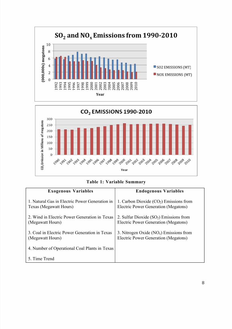
Texas, will be addressed in the statistical results discussion. The following charts display

emissions in Texas from electric power generation over the 20-year study period.



8

Table 1: Variable Summary

Exogenous Variables

1. Natural Gas in Electric Power Generation inTexas (Megawatt Hours)

2. Wind in Electric Power Generation in Texas(Megawatt Hours)

3. Coal in Electric Power Generation in Texas(Megawatt Hours)

4. Number of Operational Coal Plants in Texas

5. Time Trend

Endogenous Variables

1. Carbon Dioxide (CO2) Emissions fromElectric Power Generation (Megatons)

2. Sulfur Dioxide (SO2) Emissions fromElectric Power Generation (Megatons)

3. Nitrogen Oxide (NOx) Emissions fromElectric Power Generation (Megatons)

0

2

4

6

8

10

1 9 9 2

1 9 9 3

1 9 9 4

1 9 9 5

1 9 9 6

1 9 9 7

1 9 9 8

1 9 9 9

2 0 0 0

2 0 0 1

2 0 0 2

2 0 0 3

2 0 0 4

2 0 0 5

2 0 0 6

2 0 0 7

2 0 0 8

2 0 0 9

2 0 1 0

( 0 0 0 , 0

0 0 s ) m e g a t o n s

Year

SO2

and NOx

Emissions from 1990‐2010

SO2 EMISSIONS (MT)

NOX EMISSIONS (MT)



9

Statistical Research MethodsIn order to analyze the relationship between the exogenous and endogenous variables

discussed above, our first inclination was to run three Ordinary Least Squared (OLS) regression

models—one for each endogenous variable. However, discovering multiple patterns in the

residual plots encouraged us to use an alternative regression model.1 We ultimately decided on

Zellner’s Seemingly Unrelated Regressors Model (ZSURM). This regression model first runs

OLS, looks for common patterns in the residuals and makes adjustments to the coefficient

estimates accordingly. Therefore, our discussion of the results below uses ZSURM. We left

nuclear generation out of our model to avoid running into multi-collinearity. By leaving nuclear

power generation out, we created a reference group that has zero emissions.

Statistical Results Dis cussion

Carbon Dioxide

On average, holding all other variables constant, as natural gas generation increased by

one megawatt hour (MWh), CO2 emissions increased by .576 megatons (MT). This variable is

significant since the p value (.0001) is smaller than the significance level (.05). On average,

holding all other variables constant, as coal generation increased by one MWh, CO2 emissions

increase by .848 MT. This variable is significant since the p value (.0004) is smaller than the

significance level (.05). Overall, these coefficients are in line with what we expected. While

today we would expect natural gas to emit half as much CO2 as coal, we see approximately 32 percent less CO2 in our model. This could be explained by the fact that historically natural gas

was not used for base-load power since natural gas fuel price was higher in real terms compared

1 The following warning appeared in SAS when we first attempted to run an OLS model, solidifying the need to use

ZSURM: “The model is not of full rank. Least Squares solutions for the parameters are not unique. Certain statistics

will be misleading. A reported degree of freedom of 0 or B means the estimate is biased.”

Intercept 0 . . . Intercept

NGgen 0.576307 0.10109 5.7 <.0001 Natural Gas

WINDgen -0.56773 0.265832 -2.14 0.0485 Wind Energy

COALgen 0.848323 0.188167 4.51 0.0004 Coal Energy

COALpn 1009919 669281.8 1.51 0.1508 Number of Coal

Timetrnd -488319 578084.7 -0.84 0.4107 Time Trend

Pr > |t| Variable LabelVariable

Parameter

Estimate

Standard

Error t Value



10

to today. Instead, natural gas was used for peak generation, which is more emissions-intensive

than base-load power generation.

On average, holding all other variables constant, when the number of coal plants in

operation increased by one, CO2 emissions increased by 1,009,919 MT. This variable is not

significant, since the p value (.1508) is larger than the significance level (.05). This result is

surprising; we would have expected to see a significant increase in CO2 emissions with an

additional power plant coming online since the CAAA did not target CO2 reductions.

On average, holding all other variables constant, as wind energy generation increased by

one MWh, CO2 emissions decreased by .568 MT. This variable is significant since the p value

(.0485) is smaller than the significance level (.05). We are not surprised to see a relatively small,

yet significant decrease in carbon emissions due to increased wind generation as a part of

Texas’s RPS. Perhaps Texas could consider its RPS a success in terms of CO2 emissions

reductions.

Lastly, with each additional year, emissions decreased by 488,319 MWh, yet this

decrease is insignificant. The p value (.4107) is higher than the significance level (.05). The

purpose of including the time trend variable was to capture any significant decreases in

emissions resulting from cleaner power plants and technological improvements to existing plants,

in response to the CAAA. However, the CAAA did not target carbon emissions, so it is not

surprising to see that this time trend variable was insignificant. The chart below indicates

relatively flat CO2 levels from 1990 to 2010.



11

Sulfur Dioxide

On average, holding all other variables constant, when natural gas generation increased

by one MWh, SO2 emissions decreased by .0023 megatons. This variable is not significant since

the p value (.2455) is larger than the significance level (.05). This result was not surprising

because natural gas emits a minimal amount of sulfur dioxide when used in electricity generation.

Therefore, we would not expect any reported decline in natural gas SO2 emissions to be

significant. On average, holding all other variables constant, when wind energy increased by one

MWh, SO2 emissions decreased by .0138 megatons. This variable is significant since the p value

(.0101) is smaller than the significance level (.05). The fact that this was the only significant

variable shows that dispatching wind generation can have a meaningful impact on sulfur dioxide.

Perhaps policymakers should keep this in mind in future efforts to reduce SO2.

On average, holding all other variables constant, when coal generation increased by one

MWh, SO2 emissions increased by .0042 megatons. This variable is not significant since the pvalue (.2214) is larger than the significance level (.05). On average, holding all other variables

constant, when the number of coal plants increased by one in any given year, SO2 emissions

increased by 17,430.42 megatons. This variable is not significant since the p value (.2817) is

larger than the significance level (.05). We were surprised by these results, as coal generation has

the highest sulfur content of any fossil fuel. Perhaps we saw this result because coal plants in

Texas began to use Powder River Basin coal, which has lower sulfur content, beginning in the

mid-2000s.35 Also, four out of the six new coal plants brought online between 1990 and 2000

utilized a form of coal technology that increased efficiency by measure of the higher heating

value. These technologies include the use of pulverized coal in ultra-supercritical steam plants

and fluidized bed combustion.36 These technologies may have prevented the increases in SO2

emissions from being significant.

Intercept -195373 642454.2 -0.3 0.7652 Intercept

NGgen -0.00232 0.001916 -1.21 0.2455 Natural Gas

WINDgen -0.01375 0.004671 -2.94 0.0101 Wind Energy


COALpn 17430.42 15610.75 1.12 0.2817 Number of Coal

Timetrnd 4447.365 12139.6 0.37 0.7192 Time Trend

Variable

Parameter

Estimate

Standard

Error t Value Pr > |t| Variable Label



12

On average, holding all other variables constant, with each additional year, SO2

emissions increased by 4447.37 megatons. This variable is not significant since the p value

(.7192) is larger than the significance level (.05). It does not appear that emissions reduction

technology or the CAAA has had a significant impact on SO2 emissions in Texas. Phase I of the

CAAA mainly impacted states in the Northeast and Midwest until the turn of the century, when

other states were included in Phase II and required to comply with the CAAA’s more stringent

regulations.

The first phase, effective January 1, 1995, required 110 specific power plantslisted in the statute—predominantly Midwestern coal-burning units—to reducetheir SO2 emissions to a rate of 2.5 pounds per million British thermal units (SO2 lbs./MMBtu) multiplied by the unit’s average 1985-1987 baseline heat input tothe combustion units. This creates a cap on aggregate emissions from the affected

sources. In Phase II…the cap is expanded to apply to a wider range of sources andis based on a lower rate (a “declining cap”).37

Plus, electricity generation has experienced a greater rate of increase in natural gas generation

over coal generation by a factor of 4. Perhaps an increase in natural gas, as indicated by the

charts below, led the sulfur increase to be insignificant. “SO2 emission reductions in the region

were found to be largely attributable to fuel switching.”38



13

Nitrogen Oxide

On average, holding all other variables constant, as natural gas generation increased by

one MWh, NOx emissions increased by .0024 MT. This variable is not significant since the p

value (.0882) is larger than the significance level (.05). On average, holding all other variables

constant, as coal generation increased by one MWh, NOx emissions increased by .0003 MT. This

variable is not significant since the p value (.8955) is higher than the significance level (.05). On

average, holding all other variables constant, with each additional coal plant, emissions increased

by 14,865.87 MT. This variable is not significant since the p value (.1891) is higher than the

significance level (.05). It is not surprising that natural gas is not significant since it does not

have a high NOx content. But we would have expected to see a significant relationship between

coal generation, the number of coal plants and NOx emissions. The explanation for these results

is likely captured in the time trend variable. On average, holding all other variables constant,

with each additional year, emissions decreased by 42,107.5. This variable is significant since the

p value (.0001) is smaller than the significance level (.05). “…[W]ith the 1990 CAA

Intercept -126178 453429.9 -0.28 0.7846 Intercept

NGgen 0.002395 0.001313 1.82 0.0882 Natural Gas

WINDgen 0.005263 0.003185 1.65 0.1192 Wind Energy


COALpn 14865.87 10806.51 1.38 0.1891 Number of Coal

Timetrnd -42107.5 8364.76 -5.03 0.0001 Time Trend

Pr > |t| Variable LabelVariable

Parameter

Estimate

Standard

Error t Value



14

Amendments, Congress made its first serious effort to regulate NOx as an ozone precursor. As a

result of this change, combustion sources such as utility boilers and industrial furnaces for the

first time face significant emission reduction obligations under the ozone nonattainment

program.”39 Therefore, this variable captures the various regulations and technologies that

impacted NOx emissions at power plants in Texas as a result of the CAAA.

The CAAA targeted SO2 and NOx, yet only the NOx regulation time trend variable was

significant. “…[O]ver the 1995 to 2006 period, while NOx and SO2 emissions decreased 60

percent and 22 percent, respectively,…SO2 emissions have been generally stable since 2000,

while NOx emissions have decreased each year since 1998.”40 Emissions reductions mainly

declined due to the expansion of NOx emissions control technology.41 This fact could explain

why the NOx regulation time trend variable was significant, while the SO2 time trend variable

was not.

On average, holding all other variables constant, as wind energy increased by one MWh,

NOx emissions increased by .0052 megatons. This variable is not significant since the p value

(.1192) is larger than the significance level (.05). This result was also surprising; we would have

expected a similar relationship between wind energy and NOx as observed between wind and the

other endogenous variables. The mechanisms from the CAAA may somehow muddle the effect

of wind energy on NOx.



15

ConclusionsTwo of our research findings stand out. First, wind energy had a significant impact on

emissions reductions for CO2 and SO2, whereas this relationship was not present with NOx. This

indicates that Texas should continue to invest in renewable energy to replace carbon and sulfur

intensive fuel sources. Wind energy is intermittent, so there may be a floor on emissions

reductions due to back-up fuel resources. Further analysis could explore the relationship between

back-up fossil fuel resources and the variability of emissions due to generation fluctuations in

Texas. Second, the time trend variable did not have a significant relationship with CO2 and SO2,

yet it did with NOx. As mentioned above, this could be explained by the fact that: a) the CAAA

did not target carbon emissions; b) the CAAA targeted SO2, yet these regulations did not

immediately affect Texas; c) the CAAA’s main impact on Texas was in terms of NOx reductions.

Future study could expand upon these time trend variables to determine which technologies

helped existing and new power plants reduce emissions, as well as the role that costs play on

technology adoption.



16

Works Cited

“2010 Census: Texas’ Population Growth is Highest.” Govpro. Modified January 4, 2011. Accessed February 19,

2012. http://govpro.com/news/census-population-growth-20110104/.

Brown, Stephen P.A., Alan J Krupnick and Margaret A Walls. Natural Gas: A Bridge to a Low-carbon Future?

Resources for the Future and National Energy Policy Institute, 09-11, 3. Accessed March 25, 2011.http://www.ocgi.okstate.edu/OREC/NAT_GAS.pdf.

"Cap and Trade." New York Times. Modified March 26, 2010. Accessed March 17, 2012.http://topics.nytimes.com/topics/reference/timestopics/subjects/g/greenhouse_gas_emissions/

cap_and_trade/index.html.

“Coal Prices, Back to 1949.” Energy Information Administration. Data from Annual Energy Review. Accessed

March 26, 2012. http://205.254.135.7/coal/data.cfm#prices.

“Contribution of Working Group I to the Fourth Assessment Report.” Intergovernmental Panel on Climate Change

(IPCC). 2007a. Geneva, Switzerland. Page 7.

“Contribution of Working Group II to the Fourth Assessment Report.” Intergovernmental Panel on Climate Change(IPCC). 2007b. Geneva, Switzerland. Page 8.

“Demographics.” Texas Comptroller of Public Accounts. Accessed February 19, 2012.http://www.window.state.tx.us/specialrpt/tif/population.html.

“Domestic Coal Distribution, by Destination State, 2010.” 2010. U.S. Energy Information Administration.

"Energy in Brief." Energy Information Administration. Modified August 4, 2011. Accessed March 23, 2012.

http://www.eia.gov/energy_in_brief/about_shale_gas.cfm.

Galbraith, Kate. “Why Texas is Using More Coal, Wind and Less Gas.” The Texas Tribune. Modified January 25,

2011. Accessed February 12, 2012. http://www.texastribune.org/texas-energy/electric-reliability-council-texas/why-

texas-is-using-more-coal-wind-and-less-gas/.

Hogan, Michael T. “Running in place: renewable portfolio standards and Climate change.” M.S. Thesis.Massachusetts Institute of Technology. Department of Urban Studies and Planning. 2008.

IHS Global Insight. The Economic and Employment Contributions of Shale Gas in the United States. 7. Modified

December 2011. Accessed February 11, 2012. http://www.ihs.com/images/Shale-Gas-Economic-Impact-Dec-2011.pdf.

Kydes, Andy S. “Impacts of a Renewable Portfolio Generation Standard on US Energy Markets.” Energy Policy. 2007. 35 (2). 809–814.

Michaels, Robert J. “National Renewable Portfolio Standard: Smart Policy or Misguided Gesture?” Energy Law

Journal. 2008. 29. 79–119.

“Nitrogen Oxides (NOx) Control Regulations.” Environmental Protection Agency. Modified February 10, 2012.

Accessed February 19, 2012. http://www.epa.gov/region1/airquality/nox.html.

“NOAA Reports 2006 Warmest Year on Record for U.S.” National Oceanic and Atmospheric Administration.

Modified January 9, 2007. Accessed on November 4, 2011. http://www.noaanews.noaa.gov/stories2007/s2772.htm.

Palmer, Karen and Burtraw, Dallas. “Cost-Effectiveness of Renewable Electricity Policies.” Energy Economics.

2005. 27 (6). 873–894.



17

“Pechan Report No. 09.02.001/9461.000.” E.H. Pechan & Associates, Inc. March 2009. Page IX. Accessed April 17,

2012.

Popp, David. “Pollution Control Innovations and the Clean Air Act of 1990.” NBER Working Paper 8593. National

Bureau of Economic Research. November 2001.

Prasad, Monica and Munch, Steven. “State-Level Renewable Electricity Policies and Reductions in Carbon

Emissions.” Energy Policy. 2012. Vol. 45. 237-242.

Samuelsohn, Darren and Robin Bravender. "Obama's Draft Budget Projects Cap-and-Trade Revenue." Scientific

American. February 26, 2009. Accessed April 5, 2012.

http://www.scientificamerican.com/article.cfm?id=cap-and-trade-obama-budget.

Smith, Christopher A. “Producing Natural Gas from Shale.” January 26, 2012. Accessed February 8, 2012.

http://energy.gov/articles/producing-natural-gas-shale.

“Special Report: Managing the Risks of Extreme Events and Disasters to Advance Climate Change Adaptation

(SREX).” Intergovernmental Panel on Climate Change (IPCC). Modified November 1, 2011. Accessed March 19,2012. Page 13. http://www.ipcc-wg2.gov/SREX/images/uploads/SREX-SPM_Approved-HiRes_opt.pdf.

Stavins, Robert N. “What Can We Learn From the Grand Policy Experiment? Lessons From SO2 AllowanceTrading.” The Journal of Economic Perspectives. 1998. 12(3): 69-88.

Stern, Nicholas. The Economics of Climate Change. 2007. Cambridge, UK: Cambridge University Press.

Texas Department of State Health Services. “Texas Population.” DSHS Center for Health Statistics. Accessed

February 4, 2012. http://www.dshs.state.tx.us/chs/popdat/ST1990.shtm.

“Texas Renewable Portfolio Standard.” State Energy Conservation Office, Accessed February 19, 2012.http://seco.cpa.state.tx.us/re_rps-portfolio.htm.

United States Department of Energy. “U.S. Natural Gas Wellhead Price (Dollars per Thousand Cubic Feet).” Energy

Information Administration. Modified January 30, 2012. Accessed February 4, 2012.

http://www.eia.gov/dnav/ng/hist/n9190us3A.htm.

United States Energy Information Administration, Form EIA-923, "Power Plant Operations Report" and predecessor

forms.

United States Environmental Protection Agency. The Benefits and Costs of the Clean Air Act 1990 to 2010 .

November 1999. Accessed April 5, 2012. http://www.epa.gov/oar/sect812/1990-2010/chap1130.pdf.

United States Government. “Annual 1990 - 2009 U.S. Electric Power Industry Estimated Emissions by State.”

Data.gov. Accessed February 4, 2012. http://explore.data.gov/Energy-and-Utilities/Annual-1990-2009-U-S-Electric-

Power-Industry-Estim/t6sb-8txz.

Wooley, D.R. and E.M Morss. “The Clean Air Act Amendments of 1990: Opportunities for Promoting Renewable

Energy.” December 11, 2000. Accessed April 17, 2012.



18

1 “NOAA Reports 2006 Warmest Year on Record for U.S,” National Oceanic and Atmospheric Administration,

accessed on November 4, 2011, last modified January 9, 2007,http://www.noaanews.noaa.gov/stories2007/s2772.htm.2 Ibid.3 “Contribution of Working Group I to the Fourth Assessment Report,” Intergovernmental Panel on Climate Change

(IPCC), 2007a, Geneva, Switzerland. Page 7.4“Contribution of Working Group II to the Fourth Assessment Report,” Intergovernmental Panel on Climate Change

(IPCC), 2007b, Geneva, Switzerland. Page 8.5 Ibid.6 Nicholas Stern, The Economics of Climate Change, 2007, Cambridge, UK: Cambridge University Press.7 “Special Report: Managing the Risks of Extreme Events and Disasters to Advance Climate Change Adaptation(SREX),” Intergovernmental Panel on Climate Change (IPCC), November 1, 2011, accessed November 19, 2011,

Page 13, http://www.ipcc-wg2.gov/SREX/images/uploads/SREX-SPM_Approved-HiRes_opt.pdf.8 Ibid.9 United States Environmental Protection Agency, The Benefits and Costs of the Clean Air Act

1990 to 2010, November 1999, page 1, accessed April 5, 2012, http://www.epa.gov/oar/sect812/

1990-2010/chap1130.pdf. 10 David Popp, “Pollution Control Innovations and the Clean Air Act of 1990,” NBER Working Paper 8593,

National Bureau of Economic Research. November 2001.11 Ibid.12 Robert N. Stavins, “What Can We Learn From the Grand Policy Experiment? Lessons From SO2 Allowance

Trading,” The Journal of Economic Perspectives, 1998, 12(3): 70.13 Ibid.14 Ibid. 15 “Nitrogen Oxides (NOx) Control Regulations, Environmental Protection Agency, February 10, 2012, accessed

February 19, 2012, http://www.epa.gov/region1/airquality/nox.html.16 Ibid17 Ibid18 Darren Samuelsohn and Robin Bravender, "Obama's Draft Budget Projects Cap-and-Trade Revenue," Scientific

American, February 26, 2009, accessed November 17, 2011,

http://www.scientificamerican.com/article.cfm?id=cap-and-trade-obama-budget.19 Ibid.20 Ibid.21 "Cap and Trade," New York Times, March 26, 2010, accessed November 17, 2011,

http://topics.nytimes.com/topics/reference/timestopics/subjects/g/greenhouse_gas_emissions/

cap_and_trade/index.html.22 Christopher A. Smith, “Producing Natural Gas from Shale,” January 26, 2012, accessed February 8, 2012,

http://energy.gov/articles/producing-natural-gas-shale.23 Stephen P.A. Brown, Alan J Krupnick, and Margaret A Walls, Natural Gas: A Bridge to a

Low-carbon Future? Resources for the Future and National Energy Policy Institute, 09-11, 3, accessed September

23, 2011, http://www.ocgi.okstate.edu/OREC/NAT_GAS.pdf.24 "Energy in Brief," Energy Information Administration, August 4, 2011, accessed September 23, 2012,

http://www.eia.gov/energy_in_brief/about_shale_gas.cfm.25 IHS Global Insight, The Economic and Employment Contributions of Shale Gas in the United States, 7, accessed

February 11, 2012, http://www.ihs.com/images/

Shale-Gas-Economic-Impact-Dec-2011.pdf.26 “Texas Renewable Portfolio Standard,” State Energy Conservation Office, accessed February 19, 2012,

http://seco.cpa.state.tx.us/re_rps-portfolio.htm.27 Ibid.28 Ibid.29 Monica Prasad and Munch, Steven, “State-Level Renewable Electricity Policies and Reductions in Carbon

Emissions,” Energy Policy, 2012, Vol. 45, 237-242.30 Michael T. Hogan, “Running in Place: Renewable Portfolio Standards and Climate Change,” M.S. Thesis,Massachusetts Institute of Technology, Department of Urban Studies and Planning, 2008.



19

31 Andy S. Kydes, “Impacts of a Renewable Portfolio Generation Standard on US Energy Markets,” Energy Policy,2007, 35(2), 809–814.32 Robert J. Michaels, “National Renewable Portfolio Standard: Smart Policy or Misguided Gesture?” Energy Law

Journal , 2008, 29, 79–119.33 Karen Palmer and Burtraw, Dallas, “Cost-effectiveness of renewable electricity policies,” Energy Economics ,

2005, 27(6), 873–894. 34 Kate Galbraith, “Why Texas is Using More Coal, Wind and Less Gas,” The Texas Tribune, January 25, 2011,

accessed February 12, 2012, http://www.texastribune.org/texas-energy/electric-reliability-council-texas/why-texas-

is-using-more-coal-wind-and-less-gas/.35 “Domestic Coal Distribution, by Destination State, 2010,” 2010, U.S. Energy Information Administration.36

Ibid.

37 D.R. Wooley and E.M Morss, “The Clean Air Act Amendments of 1990: Opportunities for Promoting Renewable

Energy,” December 11, 2000, page 16, accessed April 17, 2012.38 “Pechan Report No. 09.02.001/9461.000,” E.H. Pechan & Associates, Inc, March 2009, page IX, accessed April17, 2012.39 D.R. Wooley and E.M Morss, “The Clean Air Act Amendments of 1990: Opportunities for Promoting Renewable

Energy,” December 11, 2000, page 21, accessed April 17, 2012.40 “Pechan Report No. 09.02.001/9461.000,” E.H. Pechan & Associates, Inc, March 2009, page IX, accessed April

17, 2012.41 Ibid.

Air Emissions in Texas

Documents

Transcript of Air Emissions in Texas