Agile Flight Control Techniques for a Fixed-Wing

Aircraft

by

Frantisek Michal Sobolic

B.S., Aerospace EngineeringUniversity of Michigan (2006)

Submitted to the Department of Aeronautics and Astronauticsin partial fulfillment of the requirements for the degree of

Master of Science in Aeronautics and Astronautics

at the

MASSACHUSETTS INSTITUTE OF TECHNOLOGY

June 2009

c© Massachusetts Institute of Technology 2009. All rights reserved.

Author . . . . . . . . . . . . . . . . . . . . . . . . . . . . . . . . . . . . . . . . . . . . . . . . . . . . . . . . . . . . . .Department of Aeronautics and Astronautics

May 22, 2009

Certified by. . . . . . . . . . . . . . . . . . . . . . . . . . . . . . . . . . . . . . . . . . . . . . . . . . . . . . . . . .Jonathan P. How

ProfessorThesis Supervisor

Accepted by . . . . . . . . . . . . . . . . . . . . . . . . . . . . . . . . . . . . . . . . . . . . . . . . . . . . . . . . .Prof. David L. Darmofal

Associate Department HeadChair, Committee on Graduate Students

2

Agile Flight Control Techniques for a Fixed-Wing Aircraft

by

Frantisek Michal Sobolic

Submitted to the Department of Aeronautics and Astronauticson May 22, 2009, in partial fulfillment of the

requirements for the degree ofMaster of Science in Aeronautics and Astronautics

Abstract

As unmanned aerial vehicles (UAVs) become more involved in challenging missionobjectives, the need for agility controlled flight becomes more of a necessity. Theability to navigate through constrained environments as well as quickly maneuver toeach mission target is essential. Currently, individual vehicles are developed with aparticular mission objective, whether it be persistent surveillance or fly-by reconnais-sance. Fixed-wing vehicles with a high thrust-to-weight ratio are capable of perform-ing maneuvers such as take-off or perch style landing and switch between hover andconventional flight modes. Agile flight controllers enable a single vehicle to achievemultiple mission objectives. By utilizing the knowledge of the flight dynamics throughall flight regimes, nonlinear controllers can be developed that control the aircraft ina single design.

This thesis develops a full six-degree-of-freedom model for a fixed-wing propeller-driven aircraft along with methods of control through nonconventional flight regimes.In particular, these controllers focus on transitioning into and out of hover to levelflight modes. This maneuver poses hardships for conventional linear control archi-tectures because these flights involve regions of the post-stall regime, which is highlynonlinear due to separation of flow over the lifting surfaces. Using Lyapunov back-stepping control stability theory as well as quaternion-based control methods, controlstrategies are developed that stabilize the aircraft through these flight regimes with-out the need to switch control schemes. The effectiveness of each control strategy isdemonstrated in both simulation and flight experiments.

Thesis Supervisor: Jonathan P. HowTitle: Professor

3

4

Acknowledgments

First, I would like to thank Raytheon Missile Systems for their support during my

graduate school experience in which I am able to advance both my education and my

career.

Secondly, I would like to thank Professor How for his guidance and wisdom during

my research pursuits at MIT. His constant curiosity with the challenges that I faced

and his helpful notions gave me the direction to successfully complete my research.

The members of the Aerospace Controls Laboratory have been extremely support-

ive throughout my work on this thesis. I would like to offer a special thanks to Buddy

Michini, who offered continual guidance throughout my work, especially with soft-

ware and hardware issues. I would also like to thank Cameron Fraser, Josh Redding,

Karl Kulling, Sergio Cafarelli, Frank Fan, Samera Ponda, Dan Levine, Brett Bethke,

Brandon Luders, Andrew Whitten and Kenneth Lee for the specific ways in which

they have assisted me. I would also like to thank Kathryn Fischer for her support

and resourcefulness throughout my time here.

During the dynamic modeling phase of my project, I received invaluable technical

support from Dave Robertson, Richard Perdichizzi and Todd Billings. I would like

to thank them for guidance and technical advice.

Finally, my family and friends have been a constant source of love, support and

inspiration for me throughout my education. My parents, Frank and Maryanne have

always been there in many ways to support my aspirations as well as my Aunt Diane

and Uncle Tom who supported me and have always been interested in my educational

pursuits.

5

6

Contents

1 Introduction 13

1.1 Motivation . . . . . . . . . . . . . . . . . . . . . . . . . . . . . . . . . 14

1.2 Background . . . . . . . . . . . . . . . . . . . . . . . . . . . . . . . . 16

1.2.1 Quaternion . . . . . . . . . . . . . . . . . . . . . . . . . . . . 16

1.2.2 Lyapunov Backstepping Design . . . . . . . . . . . . . . . . . 16

1.3 Literature Review . . . . . . . . . . . . . . . . . . . . . . . . . . . . . 17

1.4 Contributions . . . . . . . . . . . . . . . . . . . . . . . . . . . . . . . 19

1.5 Approach . . . . . . . . . . . . . . . . . . . . . . . . . . . . . . . . . 20

2 Modeling 21

2.1 Introduction . . . . . . . . . . . . . . . . . . . . . . . . . . . . . . . . 21

2.2 Preliminaries . . . . . . . . . . . . . . . . . . . . . . . . . . . . . . . 22

2.2.1 Nomenclature . . . . . . . . . . . . . . . . . . . . . . . . . . . 22

2.2.2 Vehicle Description . . . . . . . . . . . . . . . . . . . . . . . . 23

2.2.3 RAVEN Testbed . . . . . . . . . . . . . . . . . . . . . . . . . 24

2.3 Tests Performed . . . . . . . . . . . . . . . . . . . . . . . . . . . . . . 25

2.3.1 Introduction . . . . . . . . . . . . . . . . . . . . . . . . . . . . 25

2.3.2 Prop-Hang Test . . . . . . . . . . . . . . . . . . . . . . . . . . 26

2.3.3 Quasi-Steady State Wind Tunnel Test . . . . . . . . . . . . . 29

2.4 Equations of Motion . . . . . . . . . . . . . . . . . . . . . . . . . . . 31

2.4.1 System Identification . . . . . . . . . . . . . . . . . . . . . . . 35

3 Quaternion Based Control 41

3.1 Introduction . . . . . . . . . . . . . . . . . . . . . . . . . . . . . . . . 41

3.1.1 Notation . . . . . . . . . . . . . . . . . . . . . . . . . . . . . . 42

3.2 Inner Attitude Loop . . . . . . . . . . . . . . . . . . . . . . . . . . . 42

3.3 Outer Velocity Loop . . . . . . . . . . . . . . . . . . . . . . . . . . . 44

3.4 Thrust Controller . . . . . . . . . . . . . . . . . . . . . . . . . . . . . 46

7

3.5 Results . . . . . . . . . . . . . . . . . . . . . . . . . . . . . . . . . . . 47

3.5.1 Simulation . . . . . . . . . . . . . . . . . . . . . . . . . . . . . 47

3.5.2 Decoupled Roll Control . . . . . . . . . . . . . . . . . . . . . . 47

3.5.3 Transition to Level-Flight . . . . . . . . . . . . . . . . . . . . 49

4 Nonlinear Lyapunov Backstepping Controller 53

4.1 Introduction . . . . . . . . . . . . . . . . . . . . . . . . . . . . . . . . 53

4.2 Controller Outline . . . . . . . . . . . . . . . . . . . . . . . . . . . . 54

4.2.1 Simulation . . . . . . . . . . . . . . . . . . . . . . . . . . . . . 59

4.3 Linearized Hover Controller . . . . . . . . . . . . . . . . . . . . . . . 61

4.3.1 Flight Test . . . . . . . . . . . . . . . . . . . . . . . . . . . . . 65

4.4 Lyapunov Quaternion Control . . . . . . . . . . . . . . . . . . . . . . 67

4.4.1 Introduction . . . . . . . . . . . . . . . . . . . . . . . . . . . . 67

4.4.2 Simulation . . . . . . . . . . . . . . . . . . . . . . . . . . . . . 70

4.4.3 Hardware Implementation . . . . . . . . . . . . . . . . . . . . 72

5 Conclusion 81

5.1 Future Work . . . . . . . . . . . . . . . . . . . . . . . . . . . . . . . . 83

5.1.1 Improved Dynamic Model . . . . . . . . . . . . . . . . . . . . 83

5.1.2 Trajectory Linearized Control . . . . . . . . . . . . . . . . . . 83

5.1.3 Path Feasibility Planner . . . . . . . . . . . . . . . . . . . . . 84

A Quaternion Based Method for the Determination of Body Rates

using a Motion Capture System 85

A.1 Introduction . . . . . . . . . . . . . . . . . . . . . . . . . . . . . . . . 85

A.2 Extracting the Axis Angle . . . . . . . . . . . . . . . . . . . . . . . . 86

8

List of Figures

1-1 General Atomics Aeronautical Systems Predator B . . . . . . . . . . 14

1-2 AeroVironment Raven B UAV . . . . . . . . . . . . . . . . . . . . . . 14

1-3 Bell Boeing V-22 Osprey . . . . . . . . . . . . . . . . . . . . . . . . . 15

1-4 Lockheed Martin X-35B Joint Strike Fighter . . . . . . . . . . . . . . 15

2-1 Vehicle and hardware used for controller implementation . . . . . . . 23

2-2 Modeling test setup and load cell placement . . . . . . . . . . . . . . 25

2-3 Aircraft mounted with tinsel hung around control surfaces to determine

propeller downwash diameter . . . . . . . . . . . . . . . . . . . . . . 27

2-4 Linear least square fit of the radius of the cone produced by propeller

downwash . . . . . . . . . . . . . . . . . . . . . . . . . . . . . . . . . 27

2-5 Estimated and actual propeller downwash flow located at the respective

control surfaces . . . . . . . . . . . . . . . . . . . . . . . . . . . . . . 28

2-6 Moment coefficient as a function of respective control surface deflection

angle . . . . . . . . . . . . . . . . . . . . . . . . . . . . . . . . . . . . 29

2-7 Wind tunnel test setup - mounted upside down due to maneuverability

constraints . . . . . . . . . . . . . . . . . . . . . . . . . . . . . . . . . 29

2-8 Sample wind tunnel moment data taken at 30◦ angle-of-attack . . . . 30

2-9 Effect of propeller downwash combined with the free-stream velocity . 31

2-10 Aircraft body and inertial coordinate frames . . . . . . . . . . . . . . 31

2-11 Measured versus theoretical force coefficients for various free-stream

velocities . . . . . . . . . . . . . . . . . . . . . . . . . . . . . . . . . . 34

2-12 System Identification: compared state outputs for the sinusoidal ve-

locity test . . . . . . . . . . . . . . . . . . . . . . . . . . . . . . . . . 37

2-13 Stills from the Clik transition maneuver . . . . . . . . . . . . . . . . 39

2-14 System Identification: compared state outputs for the hover to transi-

tion test . . . . . . . . . . . . . . . . . . . . . . . . . . . . . . . . . . 40

3-1 Quaternion-based control system architecture . . . . . . . . . . . . . 42

9

3-2 Vector description of additional body x-velocity necessary to obtain

desired inertial velocity . . . . . . . . . . . . . . . . . . . . . . . . . . 46

3-3 Roll decoupling maneuver state output . . . . . . . . . . . . . . . . . 50

3-4 3-D visualization of the quaternion controlled transition maneuver . . 51

3-5 Position output for the quaternion-based control transition maneuver 51

3-6 Various state results for the quaternion-based controlled transition to

level-flight . . . . . . . . . . . . . . . . . . . . . . . . . . . . . . . . . 52

4-1 Lyapunov-based backstepping control architecture . . . . . . . . . . . 53

4-2 Simulated Lyapunov-based backstepping control in hover with initial

condition offsets . . . . . . . . . . . . . . . . . . . . . . . . . . . . . . 60

4-3 Lyapunov-based backstepping take-off to hover simulation . . . . . . 61

4-4 Experimental linearized Lyapunov-based controller position data about

hover. . . . . . . . . . . . . . . . . . . . . . . . . . . . . . . . . . . . 66

4-5 Lyapunov quaternion control architecture . . . . . . . . . . . . . . . . 68

4-6 Sample transition trajectory data with radial basis least square fit . . 70

4-7 Simulated Lyapunov quaternion controlled hover to hover state data . 73

4-8 Simulated Lyapunov quaternion controlled hover to hover control effort 74

4-9 Hardware implemented Lyapunov quaternion controlled hover to hover

state data . . . . . . . . . . . . . . . . . . . . . . . . . . . . . . . . . 75

4-10 Hardware Lyapunov quaternion controlled hover to hover control effort 76

4-11 Measured y-position output for the hover to hover maneuver varying

the feed-forward predictive gains . . . . . . . . . . . . . . . . . . . . . 76

4-12 Elevator deflection output for the hover to hover maneuver varying the

model feed-forward gains . . . . . . . . . . . . . . . . . . . . . . . . . 76

4-13 Hardware implemented Lyapunov quaternion controlled take-off to hover

maneuver . . . . . . . . . . . . . . . . . . . . . . . . . . . . . . . . . 77

4-14 Lyapunov quaternion controlled take-off to hover state data . . . . . 78

4-15 Lyapunov quaternion controlled take-off to hover control effort . . . . 79

5-1 Trajectory linearized control architecture . . . . . . . . . . . . . . . . 83

A-1 Quaternion data due to a pure rotation about the reference z-axis. . . 87

A-2 Pure body z-rotation illustrating axis flip . . . . . . . . . . . . . . . . 88

A-3 Continuous quaternion data due to a pure rotation about the reference

z-axis. . . . . . . . . . . . . . . . . . . . . . . . . . . . . . . . . . . . 89

10

List of Tables

2.1 Clik aircraft parameters . . . . . . . . . . . . . . . . . . . . . . . . . 24

2.2 Clik aerodynamic parameters . . . . . . . . . . . . . . . . . . . . . . 34

3.1 Simulation quaternion attitude loop gains . . . . . . . . . . . . . . . 47

4.1 Algorithm to convert from DCM to quaternion . . . . . . . . . . . . . 69

4.2 Radial basis function values: σ = 1.2 . . . . . . . . . . . . . . . . . . 71

A.1 Smooth quaternion signal data algorithm . . . . . . . . . . . . . . . . 89

11

12

Chapter 1

Introduction

Unmanned aerial vehicles (UAVs) are becoming increasingly involved in challenging

mission objectives including search and rescue, reconnaissance and other intelligence-

gathering roles. The advantage of these vehicles is not only the absence of human

presence in a volatile scenario, but also their production value relative to manned

vehicles. In general, two types of UAVs are produced, remote piloted and self-piloted.

Remote piloted UAVs allow an operator to control the vehicle to perform a mission

objective while a self-piloted UAV performs a mission autonomously based on a set

of rules preprogrammed prior to flight. Autonomous UAVs are much more complex

system, however, emerging technologies would allow them to address much more

complex missions.

Even under the categroy of technologically advanced aircraft, classes of UAVs are

built to perform tasks based on specific mission scenarios. For instance, the General

Atomics Aeronautical Systems Predator, shown in Figure 1-1, is a very common and

very well known UAV designed for long-endurance, medium altitude remotely con-

trolled surveillance and reconnaissance operations. With a wingspan of 66ft, weight

of 10,000lbs and operational duration of more than 40 hours, this aircraft is able to

provide both a front line soldier and operational commander real-time footage with

its on-board vision system [1]. The AeroVironment Raven (Figure 1-2), also used for

surveillance and reconnaissance but at low altitude, is a highly mobile, light weight

aircraft that can be operated manually or programmed for autonomous operation [2].

13

Figure 1-1: General Atomics Aero-nautical Systems Predator B

Figure 1-2: AeroVironment RavenB UAV

Each of these UAV classifications have an important role in their aerial missions.

For a particular mission, multiple UAVs may be used to provide feedback on related

issues from different perspectives. With these various specified aircraft systems, clas-

sifications have been made to separate vehicles by the roles which they fulfill yet

vehicles that are able to perform multiple missions could declare UAV dominance.

An individual UAV is only limited by the user, the amount of autonomy it is granted

and the overall capabilities of the aircraft. By advancing the capabilities, thus ex-

panding the range of mission qualifications, a single UAV may be used for multiple

mission scenarios.

1.1 Motivation

An aircraft with short take-off and landing (STOL) and vertical take-off and landing

(VTOL) capabilities has been an active area of research for many reasons. One of

the main interests is their ability to maneuver and land in a constrained environment

and still have the fuel efficiency and quickness to proceed to another location. One

such vehicle is the Bell Boeing V-22 Osprey shown in Figure 1-3. It is a tiltrotor

aircraft with the combined STOL and VTOL capabilities. The vehicle can take-off

and land similar to a helicopter and hover at a single position above ground. Once

airborne, its engine nacelles can be rotated to convert the aircraft to a turboprop

airplane, capable of high-speed, high-altitude flight [3]. There are many reasons

14

Figure 1-3: Bell Boeing V-22 Os-prey

Figure 1-4: Lockheed Martin X-35B Joint Strike Fighter

why this aircraft seems so attractive for multiple missions. Its capabilities include:

transporting troops and cargo, air-to-air refueling and landing aboard an aircraft

carrier compacting its storage area by retracting its rotors. Another type of vehicle

is the X-35B Joint Strike Fighter produced by Lockheed Martin shown in Figure 1-4.

This vehicle also has combined ability features that allow it to proceed in a short take-

off and vertical landing (STOVL) manner. The nozzle, which is supplemented by two

roll control ducts on the inboard section of the wing, together with the vertical lift

fan provide the military required STOVL capability [1]. These combined capabilities

allows the aircraft to carry a larger payload during take-off and land in constrained

environments. Versatile aircraft such as these are in high demand, and it seems

therefore fitting to develop UAVs with similar capabilities. UAVs have the potential

to maneuver much more aggressively due to the lack of a human pilot, yet controlling

them through such maneuvers remains a challenge, even today.

The UAVs that have been designed thus far are built for a mission specific scenario.

For a reconnaissance mission, fixed wing vehicles are constrained to fly at speeds above

stall limiting them to perform a loitering pattern for persistent surveillance. On the

other hand, vehicles such as quadrotors and helicopters have a hovering ability but

are hindered by their efficiency in translating from one mission location to the next.

However, a vehicle designed to capture the strengths of both a fixed and rotary wing

aircraft could be used in either situations and provide this sought-after versatility.

The objective of this thesis is to design a agile flight controller for a fixed wing

aircraft, enabling it to follow a desired trajectory through multiple regimes of flight,

15

including post-stall. Such a controller will enable the aircraft to hover as well as safely

transition to steady-level flight. It will also inhabit the capabilities of conventional

take-off and landing as well as a perch style landing. With these combined abilities,

the agile flight controller gives an aircraft the desirable characteristics of the versatile,

manned vehicles mentioned previously.

1.2 Background

1.2.1 Quaternion

A quaternion is a 4-dimensional vector used to describe the transformation of a vehicle

in 3-dimensions. The use of quaternions are sometimes favored over other descriptors

due to their non-singularity properties at any aircraft attitude. Traditional aeronautic

transformations (Euler angles), are hindered by a phenomenon known as gimbal lock.

Gimbal lock causes a loss of degree of freedom (DOF) which could lead to controller

instability. Since this thesis explores aggressive flight regimes, a quaternion attitude

descriptor was chosen to provide a singularity-free rotation from hover to horizontal

flight.

1.2.2 Lyapunov Backstepping Design

Lyapunov backstepping control provides a stable controller by developing a promi-

nent functional candidate that satisfies the Lyapunov criteria, known as the control

Lyapunov function. The backstepping technique can be summarized as follows:

1. Start with the state furthest from influential control actuators.

2. Introduce a virtual state and a control.

3. Define a control Lyapunov function.

4. Choose the virtual controller such that the control Lyapunov function satisfies

the Lyapunov criteria.

16

5. If the virtual controller involves a control actuator, this is the control law, if

not repeat Step 2 with the new virtual state.

These control Lyapunov functions “step” through the dynamics of a system leading

to a control methodology that can be used to produce a desired response.

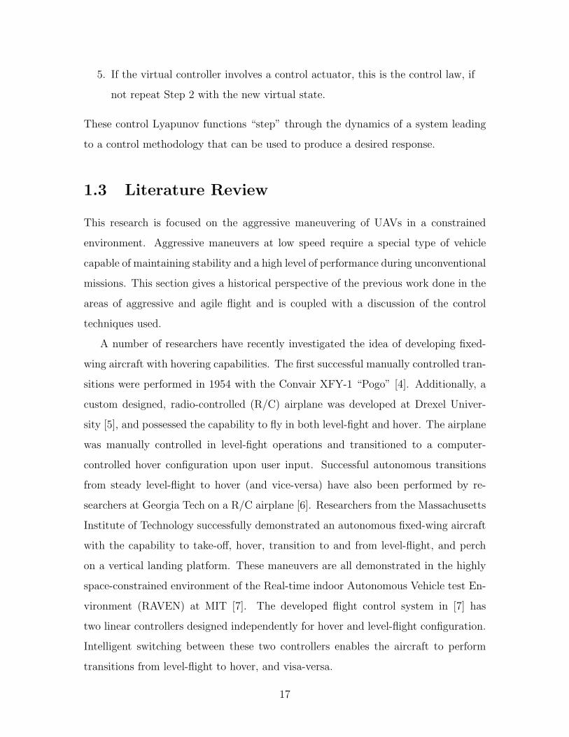
1.3 Literature Review

This research is focused on the aggressive maneuvering of UAVs in a constrained

environment. Aggressive maneuvers at low speed require a special type of vehicle

capable of maintaining stability and a high level of performance during unconventional

missions. This section gives a historical perspective of the previous work done in the

areas of aggressive and agile flight and is coupled with a discussion of the control

techniques used.

A number of researchers have recently investigated the idea of developing fixed-

wing aircraft with hovering capabilities. The first successful manually controlled tran-

sitions were performed in 1954 with the Convair XFY-1 “Pogo” [4]. Additionally, a

custom designed, radio-controlled (R/C) airplane was developed at Drexel Univer-

sity [5], and possessed the capability to fly in both level-fight and hover. The airplane

was manually controlled in level-fight operations and transitioned to a computer-

controlled hover configuration upon user input. Successful autonomous transitions

from steady level-flight to hover (and vice-versa) have also been performed by re-

searchers at Georgia Tech on a R/C airplane [6]. Researchers from the Massachusetts

Institute of Technology successfully demonstrated an autonomous fixed-wing aircraft

with the capability to take-off, hover, transition to and from level-flight, and perch

on a vertical landing platform. These maneuvers are all demonstrated in the highly

space-constrained environment of the Real-time indoor Autonomous Vehicle test En-

vironment (RAVEN) at MIT [7]. The developed flight control system in [7] has

two linear controllers designed independently for hover and level-flight configuration.

Intelligent switching between these two controllers enables the aircraft to perform

transitions from level-flight to hover, and visa-versa.

17

The control techniques mentioned above are limited to performing in a region pre-

scribed by the linearization method used. Full knowledge of the aircraft’s dynamics,

including nonlinearities, could solve potential issues of needing multiple controllers

in different flight modes and a single control design could be realized. The use of

nonlinear controllers provide means of control at all possible flight regimes so, non-

linear decoupling theory and dynamic inversion approaches have been applied to

flight control systems [8], [9]. Unfortunately, it was shown that an inverse dynamic

approach, even when the dynamics are very well known, may result in the desired lin-

ear input/output response but may also include undesirable unstable zero dynamics.

Nonlinear Lyapunov-based controllers have the ability to overcome some of these is-

sues [10–13]. In particular, the backstepping approach is used when a vehicles states

are influenced through other states. This technique is demonstrated in [14] for a

6-DOF mid-altitude unmanned airship, where a simulated airship tracks a desired

trajectory. They prove that the tracking error will converge exponentially to zero

since the proposed controller is globally asymptotically stable. Also, [13] demon-

strates the same type of trajectory-tracking capability in simulation for a hovercraft

moving on a planar surface and an underwater vehicle moving in 3-D space. It is

important to note that this control law assumes no parametric uncertainty, there-

fore an onboard estimator is implemented to predict the values of the states used for

feedback in the Lyapunov control algorithm.

The work presented in this thesis follows the work of [13] and [15] to control

an aircraft from hover to translational flight. In [15], Knoebel uses an adaptive

quaternion-based attitude controller to maintain aircraft performance through poorly

known regions of the vehicle dynamics during a transition from hover to level-flight.

Gain scheduling was used based on the sensed airspeed over the control surfaces.

On the other hand, [13] forms a Lyapunov backstepping controller such that all the

closed-loop signals are bounded and the tracking error converges to a neighborhood

of the origin that can be made arbitrarily small. It has the capability of following a

prescribed trajectory solely based on the vehicles dynamics. Therefore, an accurate

and complete model of the system dynamics must be known through all regions of

18

movement.

1.4 Contributions

Each of the following chapters provide a unique contribution to the overall goal of a

transition controller, which are summarized below.

• Chapter 2: A full nonlinear dynamic model is derived for a specific vehicle

which serves as a testbed for all controllers through simulation and hardware

implementation. The process of achieving this high-fidelity model is presented

through extensive wind-tunnel and static experimentation. A full system iden-

tification is performed to verify the input/output response through the use of

an off-board motion capture system which provides the necessary vehicle state

information.

• Chapter 3: A quaternion-based attitude controller is presented following the

work of Ref. [15], but is modified for reference velocity tracking. The velocity

error is used to provide the quaternion controller with the desired attitude in

order to decrease the velocity error. Controller results are presented in simula-

tion as well as hardware implementation. A full transition from hover to level

flight and back to hover is shown.

• Chapter 4: A general Lyapunov backstepping technique is introduced with

trajectory tracking capabilities. This technique is then applied in simulation to

the derived dynamics and the results are shown. To implement this design on

hardware, a modified version of Ref. [13] is used that combines the rotational

rate tracking capabilities of the quaternion attitude controller, with the state

to state influential approach of the backstepping design. Both simulation and

hardware results are shown for various trajectories.

19

1.5 Approach

This thesis is structured as follows. Chapter 2 introduces the fixed-wing aircraft which

serves as the vehicle testbed for all of the controllers developed. Here the equations

of motion are derived and a full system identification is performed. In Chapter 3, a

quaternion-based attitude controller with the ability to follow user defined velocity

commands is derived. Chapter 4 introduces a Lyapunov backstepping controller with

the ability to follow a user defined position trajectory modified with the quaternion

controller and implemented in hardware. Finally, Chapter 5 provides concluding

remarks as well as suggested future work.

20

Chapter 2

Modeling

2.1 Introduction

In order to control a system effectively, a good understanding of the dynamics and

its effects on the environment must be modeled. The more that is known about

the system, the more affective the controller can be. Controllers developed about

linearized models are often used but limit the vehicles ability to the neighborhood

encompassing this linear region. One of the most challenging parts in designing a

control system for most vehicles is the complexities and interrelated dynamics present,

thus a lot of time and effort is contributed to the modeling process.

For fixed-wing aircraft, the dynamics associated with pre-stall configurations

are well known and have been studied since early flight. However, performing agile

aggressive flight requires an aircraft go beyond the pre-stall configuration and into

the poorly understood post-stall flight regime. In the following chapter, a detailed

description of the tests that were performed in order to obtain these equations of mo-

tion (EOM) is given. Multiple tests are compared to theoretical findings, in particular

predictions made using flat plate theory which describes the entire flight regime par-

ticularly well at low Reynolds numbers (< 104). Finally, the EOM are compared to

actual flight test data recorded in the Real-time indoor Autonomous Vehicle test EN-

vironment (RAVEN) concluding that the system identification validates the models

accuracy.

21

2.2 Preliminaries

In the following sections the experimental aircraft as well as the notation and nomen-

clature are introduced. This aircraft is used throughout the rest of the controller

implementation in this thesis. Due to the complexities of modeling, standard aero-

dynamic notations presented in [16] and [17] are used.

2.2.1 Nomenclature

p = Vehicle position vector, m

v = Velocity vector, m/s

w = Angular rate vector, radians/sec

q = 4-Dimensional unit quaternion

RIB = Rotation matrix from vehicle body to inertial frame

uw = Control surface deflection input vector, radians

m = Mass of the aircraft, kg

α = Angle-of-attack of the wing, radians

ρ = Density of air, kg/m3

δt = Thrust, N

(·)d = Desired value

(·)e = Error value

(·)a = Measured value

(·)p = Details pertaining to the propeller

(·)w = Area affected by propeller downwash

(·)nw = Area not affected by propeller downwash

(·)ref = Reference

(·)I = Inertial frame

(·)B = Body frame

22

2.2.2 Vehicle Description

To facilitate the implementation of various controllers, a slightly modified version

of the high performance Clik [18] indoor aerobatic plane designed by RC Factory is

being used, shown in Figure 2-1(a). This aircraft is extremely maneuverable due to its

large control surfaces and high thrust-to-weight ratio. The vehicle is equipped with

an Axi Brushless Out-Runner 2203/52 motor with a 20cm Grapner Slowfly Propeller

which provides a thrust-to-weight ratio in excess of 1.4. Control deflection actuation

is provided by three GWS pico standard servo motors and receives commands on a

GWS four-channel micro receiver. The aircraft is also equipped with a 400mAh 2-

cell lithium polymer battery which delivers power to an 8-amp JETI electronic speed

controller shown in Figure 2-1(b).

(a) Indoor aerobatic Clik air-craft

(b) Vehicle hardware components

Figure 2-1: Vehicle and hardware used for controller implementation

The vehicle is extremely light for its size, weighing approximately 170 grams due

to the use of 2.8mm thick Dapron foam material for its body and carbon fiber strips to

reinforce structurally weak areas. The aircraft is symmetric about body x-z axes (see

Figure 2-10) and made up of flat plates. The total length of the vehicle is 90cm with

a wingspan of 84cm and the inertial as well as the surface area estimation is provided

through the use of SolidWorks CAD modeling software. More vehicle parameters and

details are given in Table 2.1.

23

Table 2.1: Clik aircraft parameters

Parameter Description Value Units

AR Aspect Ratio 4.2d Propeller diameter 20.0 cmAap Area of aileron induced by propeller downwash 0.00150 m2

Ae Area of the elevator 0.03226 m2

Ar Area of the rudder 0.03123 m2

Aanw Area of the aileron in the free-stream 0.024 m2

Ixx x-Moment of Inertia 0.00143 kg· m2

Iyy y-Moment of Inertia 0.00610 kg· m2

Izz z-Moment of Inertia 0.00737 kg· m2

Lap Moment arm of the aileron 0.080 maffected by prop-wash

Lep Moment arm of the elevator 0.533 m(cg to center of pressure)

Lrp Moment arm of the rudder 0.631 m(cg to center of pressure)

Lanw Moment arm of the aileron 0.23 mfree-stream induced

2.2.3 RAVEN Testbed

Vehicle position and attitude sensing is done off-board through the Real-time indoor

Autonomous Vehicle test ENvironment (RAVEN), eliminating the need for onboard

sensors which typically are expensive and add unwanted weight. RAVEN provides

a well equipped, robust platform for the rapid prototyping of controllers applicable

to many different vehicles. This testing environment uses a position and orientation

tracking system with an update rate of 120 Hz, minimal delay (20-30msec) and sub-

millimeter accuracy with the use of Vicon motion capture camera system [19]. A

single camera can be seen at the top of Figure 2-1(a) as the black object with the red

ring. The only requirement is that the vehicle be equipped with reflective dots which

the cameras use for object recognition.

Since only position and attitude data are directly measured by the system, the

states time rate of change must be taken to acquire rate data. This is done by the

process of a Kalman filter to attenuate noise produced by differentiating. The filter

requires that smooth continuous data is used as the input. Quaternion data however,

24

is not a smooth continuous signal by the process of extraction, so a special algorithm

is implemented to ensure smoothness which is outlined in Appendix A. From this

tracking system, state data such as position, velocity, attitude and rotational rate

is computed and used for full-state feedback. The state data is then routed to a

computer which processes the desired control commands. These control commands

are then sent to the R/C transmitter which relays the respective commands to the

vehicle, closing the control loop.

2.3 Tests Performed

2.3.1 Introduction

To accurately identify the dynamic model, a JR3 6-axis load cell is placed at the center

of gravity which allowed steady-state force and moment data to be taken for all 3

axes (load cell configuration shown in Figure 2-2). With the aid of a low pass filter

Figure 2-2: Modeling test setup and load cell placement

to attenuate high frequency noise, the multi-axis load cell is able to measure forces

within 10−3 Newtons and moments within 10−2 Newton meters. Two main types

of tests were performed, prop-hang and wind tunnel tests. A prop-hang is when the

force used to balance out the vehicles weight is solely provided by the propeller thrust.

25

These tests were performed with the intent of determining the specifics of the vehicles

dynamics at high angles-of-attack during a hover to level-flight transition.

2.3.2 Prop-Hang Test

The prop-hang was the first test done and was primarily used to determine the

specifics of individual axis moment data and propeller downwash velocity. The pro-

peller downwash velocity is defined as the induced velocity created by the spinning

blade and is found by using aspects of propeller momentum theory and conservation

of mass as in [7] and [20] and based on inviscid, incompressible flow assumptions. A

similar approach is used here but modified experimentally under the assumption that

the flow created is in a uniform conical form as a function of the thrust command and

distance from the propeller blades instead of a stream tube that extends infinitely and

uniformly far downstream. This is an approximation for attempting to capture the

loss of efficiency due to the slipstream rotation of the fluid within and outwards from

the stream tube, which is one of the major objectives propeller momentum theory.

The approximation assumes that the conical formation, in the limit, will approach

a pure cylindrical shape as the thrust is increased. In order to measure the radius

of the assumed cone shape as a function of distance and thrust, pieces of tinsel were

pieced along both the aileron and rudder/elevator control surfaces as shown in Fig-

ure 2-3. The thrust is varied to determine the granularity spacing of the tinsel which

is necessary to produce an accurate measurement. Figure 2-4 shows a linear least

squares fit to the measured radius as a function of thrust. With the cross-sectional

area estimated, the flow created is approximated by [20]

up(δt, l) =

√u2∞4

+δt

2ρAdisk(δt, l)− u∞

2(2.1)

where u∞ is the magnitude of the free-stream velocity given as

u∞ = ‖v‖2. (2.2)

26

Figure 2-3: Aircraft mounted with tin-sel hung around control surfaces to de-termine propeller downwash diameter

Figure 2-4: Linear least square fit of theradius of the cone produced by propellerdownwash

Assuming that during a prop-hang their is no free-stream velocity present, Equa-

tion 2.1 reduces to

up(δt, l) =

√δt

2ρAdisk(δt, l)(2.3)

where Adisk(δt, l) is determined experimentally and represents the cross-section of the

conical region as a function of thrust (δt) and distance (l) from the propeller. The

propeller downwash velocity is presented as upa or upr , depending on whether the

aileron (a) or rudder/elevator (r) is the particular aerodynamic region of interest.

The rudder and elevator calculations are done together due to very similar measure-

ments and distance from the propeller. Actual measurements were taken using an

anemometer and comparisons are shown in Figure 2-5.

The prop-hang test provides means to estimate the moment coefficients for the

control surfaces by using the combination of thin airfoil theory and Prandtl’s lift-line

theory [17] by

M =1

2ρu2

pCle/rAe/rLe/r. (2.4)

The coefficient of lift is the last parameter to be estimated. Prandtl’s lift-line the-

27

Figure 2-5: Estimated and actual propeller downwash flow located at the respectivecontrol surfaces

ory predicts that for an infinite flat plate, Cl is approximated by a value of 2π. A

correction accounting for a finite aspect ratio for each surface must be taken into

account [21] by

CLα =Clα

1 + Clα/πAR. (2.5)

With the load cell placed at the center of gravity of the vehicle and thrust approx-

imately equal to the weight, measurements were taken to determine the moment

created with each control surface deflection. Figure 2-6 shows a comparison between

the theoretical and measured moment data about an individual aircraft body axis.

Aileron control authority is limited during a prop-hang due to the lack of down-

wash over these control surfaces. Measurements taken were primarily in the noise

of this particular instrument and could not be physically determined. An estimate

28

(a) Elevator moment coefficient (b) Rudder moment coefficient

Figure 2-6: Moment coefficient as a function of respective control surface deflectionangle

Figure 2-7: Wind tunnel test setup - mounted upside down due to maneuverabilityconstraints

of the propeller drag and moment contribution of the ailerons are discussed more in

Section 2.4.

2.3.3 Quasi-Steady State Wind Tunnel Test

The vehicle was tested at multiple free-stream conditions in the wind tunnel (see

Figure 2-7). The first set of tests were done at 5 degree increments of angle-of-attack

without the propeller on to obtain nominal aerodynamic coefficients. The primary ob-

jective was to gain insight on the moments produced by the body/elevator deflection

combination. Since elevator coefficient data has been determined in Section 2.3.2, the

29

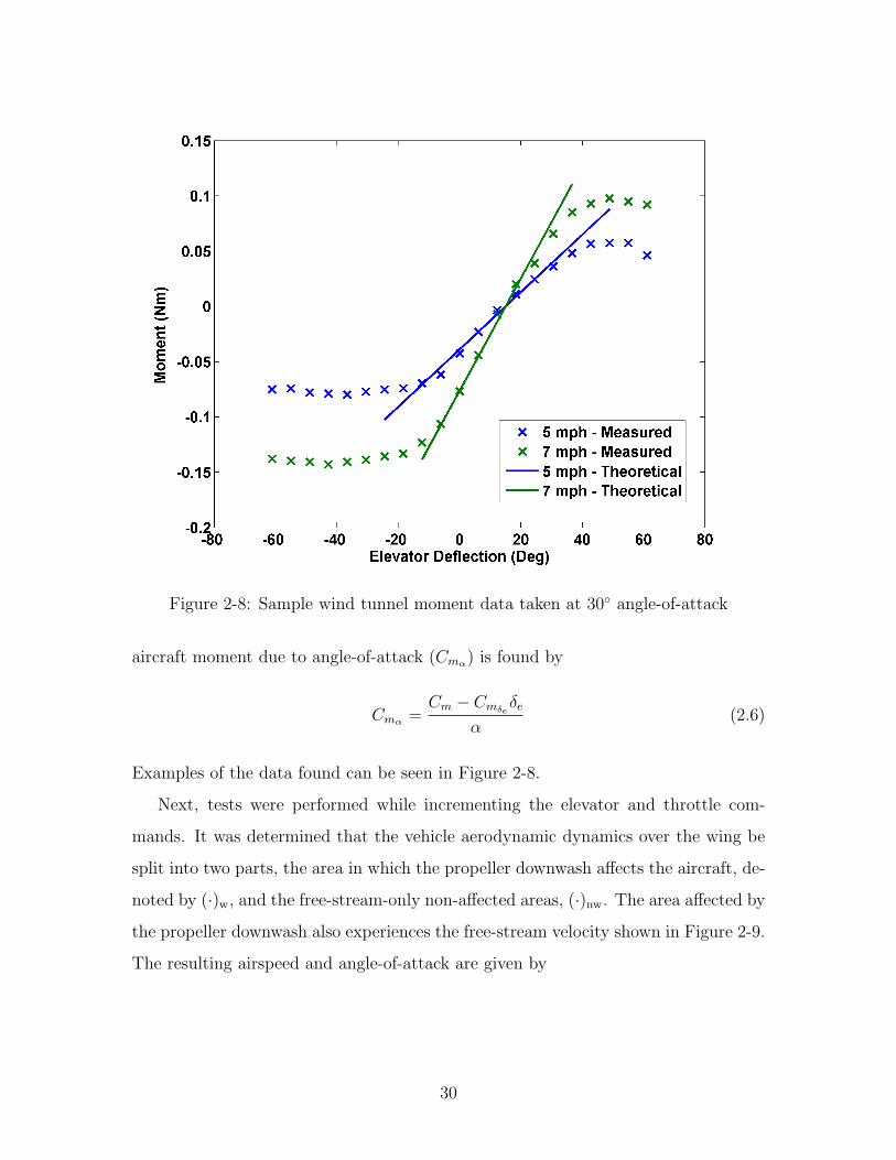
Figure 2-8: Sample wind tunnel moment data taken at 30◦ angle-of-attack

aircraft moment due to angle-of-attack (Cmα) is found by

Cmα =Cm − Cmδeδe

α(2.6)

Examples of the data found can be seen in Figure 2-8.

Next, tests were performed while incrementing the elevator and throttle com-

mands. It was determined that the vehicle aerodynamic dynamics over the wing be

split into two parts, the area in which the propeller downwash affects the aircraft, de-

noted by (·)w, and the free-stream-only non-affected areas, (·)nw. The area affected by

the propeller downwash also experiences the free-stream velocity shown in Figure 2-9.

The resulting airspeed and angle-of-attack are given by

30

Figure 2-9: Effect of propeller downwash combined with the free-stream velocity

uwa/r=√u2∞ + u2

pa/r+ 2u∞upa/r cos(α) (2.7)

αwa/r= arctan

vzvx + upa/r

. (2.8)

The rest of the wind tunnel aerodynamic data is presented in the next section.

2.4 Equations of Motion

Figure 2-10: Aircraft body and inertial coordinate frames

The set of nonlinear differential equations follows the baseline model described

in [16] using Newton’s second law for rigid-body dynamics but modified for this

particular aircraft’s kinematics and dynamics. Equations are in the aircraft body

31

frame (shown in Figure 2-10) given by

pI = RIBvB, (2.9)

RIB = RI

BS(wB), (2.10)

JwB = −S(wB)JwB + fw +Gwuw, (2.11)

M vB = −S(wB)MvB + fv + gvδt. (2.12)

where the mass, inertia and thrust force directional matrices are respectively,

M =

m 0 0

0 m 0

0 0 m

, J =

Ixx 0 0

0 Iyy 0

0 0 Izz

, gv =

1

0

0

.

Due to the symmetrical build of the aircraft, the cross-coupled inertia tensor terms

Ixy, Ixz and Iyz are considerably smaller than the coupled terms and are disregarded.

The angular velocity cross-product matrix, moment decoupling matrix and control

surface deflections are

S(w) =

0 −wz wy

wz 0 −wx−wy wx 0

, Gw =

g11 0 0

0 g22 0

0 0 g33

, uw =

δa

δe

δr

where

g11

g22

g33

=

12ρ(u2

waCLδawAapLap + u2

∞CLδanwAanwLanw)

12ρu2

wrCLδeAeLep

12ρu2

wrCLδrArLrp

. (2.13)

The constant parameters (Aanw , Aap, Ae, Ar) and (Lanw , Lap, Lep, Lrp) are the respec-

tive aileron, elevator and rudder areas and moment arms given in Table 2.1. In

Equation 2.13, the difference in the form of g11 is due to the fact that only part of

the wing area is affected by the propeller downwash while the rudder and elevator

control surfaces are always engulfed. Although the propeller downwash conical area

32

changes as a function of thrust and distance, it deviates very little over the wings and

is modeled as a constant (see Figure 2-4). Development of the remaining force and

moment terms will be based on this assumption. This assumption is a major contrib-

utor to the total force and moments created because of the low Reynolds number in

which the aircraft is flying through, ∼ 104.

The force vector fv is the sum of the gravitational and aerodynamic forces in the

body frame, given in Equation 2.14.

fv = RBI

0

0

−mg

−− cos(α) 0 sin(α)

0 1 0

− sin(α) 0 cos(α)

Drag

0

Lift

−CDxvx

CDyvy

CDzvz

. (2.14)

The first term involves the transformation of weight from the inertial to body frame.

The second term comprises the aerodynamic contribution of lift and drag forces.

Since these are in the wind frame a rotation matrix pre-multiplies the aerodynamic

terms to obtain the desired forces in the body frame. The last term in Equation 2.14

represents the viscous drag that is induced by translating through the air. Drag and

lift forces are divided into two sections and are described as

Drag =1

2ρ(u2

waCDwSw + u2

∞CDSnw

)(2.15)

Lift =1

2ρ(u2

waCLwSw + u2

∞CLSnw

). (2.16)

Figure 2-11 shows the coefficients of lift (CL) and drag (CD) for the free-stream

section. Since this aircrafts main lifting surface is without camber, the coefficient

of lift is symmetric about the body x-y axes. Note that the measured data is in

agreement with flat plate theory [22], where

CL = 2 sin(α) cos(α) CD = 2 sin2(α). (2.17)

The areas affected by the prop-wash experience an angle-of-attack ≤ 20 degrees (de-

termined by measuring flows then using Equation 2.8) due to the contribution of

33

(a) Coefficient of lift (b) Coefficient of drag

Figure 2-11: Measured versus theoretical force coefficients for various free-streamvelocities

the additive propeller flow, and thus Prandtl’s classical lifting-line theory [17] can be

used:

CLw = CLαwαwa CDw = CDow +

C2Lw

πeAR(2.18)

These also need to be corrected for a finite wing by Equation 2.5. Descriptions of the

various parameters are given in Table 2.2. The term fw in Eq. 2.11 represents the

Table 2.2: Clik aerodynamic parameters

Parameter Description

e Oswald efficiency factorCLδa Aileron coefficient of liftCLδe Elevator coefficient of liftCLδr Rudder coefficient of liftCDαwa

Effective drag coefficientCLαwa

Effective lift coefficientCmαw

Moment coefficient from effected propeller downwashCmαnw

Moment coefficient from free-stream velocityc Moment arm from effected propeller downwashlnw Moment arm from free-stream velocitySw Wing area effected by propeller downwashSnw Wing area not effected by propeller downwash

34

rest of the net torque acting about the aircraft center of gravity (cg),

fw =

−Macc −Mdrag + 1

2ρLaLa,pAaupawx

12ρLeLe,pAeuprwy − 1

2ρ(u2

wrCmαw

αwrSwc+ u2∞Cmαnw

αSnwlnw

)12ρLrLr,pAruprwz

. (2.19)

Macc and Mdrag are moment contributions from the acceleration and drag of the

propeller, respectively, calculated as [7]

Macc =Ipωp (2.20)

Mdrag =δtdCp2πCT

. (2.21)

Equation 2.20 is a function of both the inertia of the propeller about the spinning

axis and the rotational acceleration denoted as Ip and ωp respectively. Due to the

relative size of the propeller compared to the vehicles x inertial body tensor, this

term is negligible and is not used in the model formulation. Equation 2.21 however,

is not negligible and its contribution can be seen during hover when the ailerons

deflect in order to counteract its moment, which can be seen Section 3.5.2. The

thrust and power coefficients CT and CP are estimated for the given propeller using

a NACA-standardized table as in [7].

2.4.1 System Identification

The following results compare the measured and simulated states for two types of ma-

neuvers. These maneuvers include sinusoidal inertial y-velocity commands in hover

causing the vehicle to oscillate about the body y-axis and the full transition to level-

flight and back to hover which uses the controller outlined in Chapter 3. The simula-

tion is given the initial conditions of each state and the input to each of the control

surfaces for processing. In order to provide manual control of the vehicle, an ex-

ternal joystick is programmed that commands desired velocity in both the x and

y-inertial frame. This allows the user to define a suitable starting position within the

35

constrained environment. A trigger switch, when executed, commands the desired

autonomous maneuver. For each executed maneuver, the body velocities and rota-

tional rate are of interest and are compared in the following plots. It is important to

note that the modeling is done primarily to support the transition maneuver on the

body x and z forces and the y-axis moment.

Sinusoidal Velocity Inputs

For this test, a sinusoidal input to the y-inertial velocity is commanded and used to

determine the accuracy in hover and high angles-of-attack with slight transition to

level-flight mode properties. The sinusoidal input is commanded as

vIyd = 2 sin(πt).

This is an important test that is used to determine the accuracy of the model that

was accomplished through the prop-hang test. It verifies how well the propeller

downwash velocity is modeled as well as moments created by control surface actuation.

Since the aircraft is primarily in a hover position, the body x-axis is mainly testing

the modeling of the thrust force created by the propeller shown in Figure 2-12(a).

Due to inaccuracies in the power supply and un-modeled motor lag dynamics, slight

deviations are present. Most of the sinusoidal command can be seen in Figure 2-12(e).

For this inertial velocity command, the body z-velocity will mainly experience drag

at a very high angle-of-attack. Most of the moment is generated about the y-body

axis which is evident in Figure 2-12(d). Deviations occur after peak inputs which are

distinctly due to the quasi-steady state modeling.

Transition to Hover and Back

The main test is to compare the output during a transition from hover to level-

flight and back to hover. To obtain this desired maneuver, an exponential decaying

y-velocity,

vIyd = −5.0(1− e−3.0t)

36

(a) Body x velocity which for this test is mostlythrust

(b) Roll rotational rate compensating for pro-peller drag

(c) Body y velocity (d) Pitch rotational rate

(e) Body z velocity which mainly experiencesdrag

(f) Yaw rotational rate

Figure 2-12: System Identification: compared state outputs for the sinusoidal velocitytest

37

is commanded due to the spatial limitation of a horizontal distance of 9.5 meters.

This command allowed the vehicle to transition from hover to steady-level flight as

can be seen in Figure 2-13.

A comparison of the measured to simulated state data is provided in Figure 2-14.

This data shows two takes of this maneuver which is apparent by the two large spikes

in Figure 2-14(a). Larger deviations are noticeable and are due to the very quick

control surface actuation necessary to perform the transitions. The largest deviation

in force is shown in Figure 2-14(e) at the point where the aircraft transitions from

level to hover flight regimes. At this point the aircraft is essentially performing a skid

stop, moving considerably quick at this high angle-of-attack. Flow separation makes

the drag calculation a bit more obscure and the model over predicts these forces.

However, trends in the data are similar and show that even with some un-modeled

dynamics, the model can predict a response sufficiently well.

38

Fig

ure

2-13

:Sti

lls

from

the

Clik

tran

siti

onm

aneu

ver

39

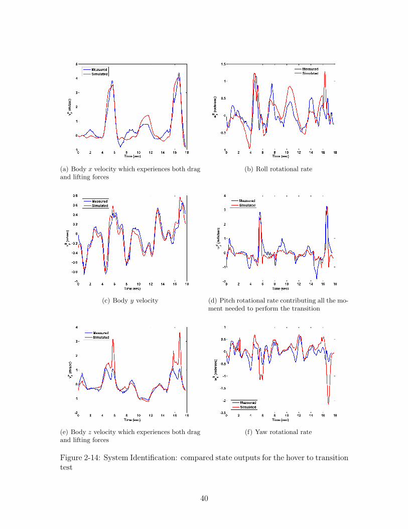
(a) Body x velocity which experiences both dragand lifting forces

(b) Roll rotational rate

(c) Body y velocity (d) Pitch rotational rate contributing all the mo-ment needed to perform the transition

(e) Body z velocity which experiences both dragand lifting forces

(f) Yaw rotational rate

Figure 2-14: System Identification: compared state outputs for the hover to transitiontest

40

Chapter 3

Quaternion Based Control

3.1 Introduction

One of the most recognizable issues when designing a controller to perform aggressive

flight maneuvers is the concern over which attitude descriptor to use. The stan-

dard aerodynamic Euler angles suffer from singularity problems due to gimbal lock,

a point in which a degree of freedom is lost. Therefore, other descriptors such as the

quaternion and direction cosine matrix (DCM) are used, each with its own distinct

advantage. In Chapter 2, the aircraft model was pieced together using a DCM, an

orthogonal matrix whose inverse (and consequently the transpose due to the proper-

ties of orthogonal matrices) represents the reverse transformation. One of the caveats

of using this descriptor is the amount of computation that must be done in order to

complete a single transformation, 9 multiplications and 6 summations per transforma-

tion. Quaternion descriptors are less computationally intensive and, in this chapter,

the use of a quaternion based controller is presented. Figure 3-1 shows the controller’s

inner and outer loop architecture. Section 3.2 explains how the inner loop stabilizes

the attitude of the aircraft based on a nominal desired quaternion and rotational rate

by utilizing many of the properties of quaternion mathematics. The inner controller

also regulates the amount of thrust necessary to perform a maneuver based on veloc-

ity errors while attempting to maintain its vertical position. The velocity controller

provides the inner loop with an updated desired quaternion based on the error be-

41

VelocityController

Att/AltController

AircraftDynamics

ViconSensing

vIrefqxy,v

Izref δt,uw

qa,wBa ,v

Ia,pa,v

Ba

Figure 3-1: Quaternion-based control system architecture

tween commanded and measured velocity, and also an update on vertical position

loss. Again, the RAVEN testbed is used to provide all the state data necessary to

close the loop.

3.1.1 Notation

Quaternions are defined using a four-element vector, q = (qo, qx, qy, qz) = (qo,q),

representing a rotation in R3 space. The basic algebraic form of a quaternion is:

q = qo + qxi+ qy j + qzk. (3.1)

These four elements have the unit magnitude property in the usual 3-dimensional vec-

tor space. The symbol⊗ implies a quaternion multiplication while q∗ is the quaternion

conjugate defined as

q∗ = qo − qxi− qy j − qzk. (3.2)

The subscripts in this chapter follow the same nomenclature presented at the begin-

ning of Chapter 2.

3.2 Inner Attitude Loop

This inner attitude loop is a PD controller based on a desired attitude quaternion error

and body rates [15]. The controller is developed to maintain a nominal prop-hang

orientation. For the sake of avoiding confusion of multiple frame transformations, a

42

hover orientation is define as

qrefd =

1.0

0.0

0.0

0.0

. (3.3)

In this orientation, the body z and x-axes are aligned with the inertial y and z-axes

respectively. RAVEN provides the measured vehicle quaternion orientation data,

and the error deviated from the reference quaternion is calculated using quaternion

multiplication as

qe =qrefd ⊗ q∗a (3.4)

where (·)∗ represents the quaternion conjugate. The individual rotational error about

the reference quaternion is found by calculating the axis angle interpretation, defined

by:

[axis, angle] =

ax

ay

az

, γrotation

.

To find the rotational error for an individual axis, the total rotation error must first

be defined by

γrotation = 2 cos(qeo)

and the axis vector error asax

ay

az

=1

sin(γrotation/2)

qex

qey

qez

.

43

The axis angle vector is a unit vector by definition and multiplying each component

by the total error rotation yields the individual axis errors given byφe

θe

ψe

= γrotation

az

ax

ay

.

Each one of these axis angular errors are defined from the desired attitude. It is

important to note that in this orientation, the commonly viewed roll error, labeled

φe, is about the z-axis. This is consistent with having the body x and inertial z-

axes aligned, and similar arguments are made for the other axis errors. The control

command that maintain a hover orientation is defined as uw

uw =

Kpδa

0 0

0 Kpδe0

0 0 Kpδr

φe

θe

ψe

+

Kdδa

0 0

0 Kdδe0

0 0 Kdδr

wB (3.5)

which is a PD controller on attitude.

3.3 Outer Velocity Loop

The outer velocity loop is a PI controller on the velocity error in the inertial frame.

This control command manipulates the desired quaternion to produce an attitude

in the direction of decreasing velocity error. One of the goals in performing this

transition maneuver is to maintain a desired altitude, therefore the controller will

limit the amount of control authority as a function of altitude loss.

In order to redefine a new attitude, a transformation that manipulates the desired

quaternion based on the error of the inertial velocity command is developed. Since

the objective of this controller is to translate the aircraft in the inertial x and y di-

rection while maintaining altitude, errors between commanded and measured inertial

velocities will be used to affect the transformation. Start by defining the inertial

44

velocity error as vxe

vye

vze

I

=

vxd − vxavyd − vyavzd − vza

I

(3.6)

and inertial z-error as

zIe =zId − zIa. (3.7)

These errors can be used to define the final quaternion transformation

qxy =

1.0

Kpyvelvye +Kiyvel

∫vyedt+Kpzsign(vya)z

Ie +Kvzsign(vya)v

Izd

Kpxvelvxe +Kixvel

∫vxedt+Kpzsign(vxa)z

Ie +Kvzsign(vxa)v

Izd

0.0

. (3.8)

So from an intuitive perspective, to obtain a desired velocity in the inertial y-direction,

a rotation about the inertial x (second element of qxy) must be performed. The same

reasoning is applied to the third element of qxy. The vehicle will need to change

its attitude, which is proportional to the error, but if a loss of altitude is sensed,

the velocity controller will attenuate the attitude command based on the inertial z-

velocity and position error which are the final two terms in Equation (3.8). Note that

this is not a unit quaternion and needs to be normalized before performing quaternion

multiplication. Quaternion multiplication is a transformation [23], so the new desired

quaternion based on an inertial velocity command is

qd = qrefd ⊗ qxy. (3.9)

This new desired quaternion is what the inner loop will now act on, deflecting control

surfaces in a manner that decreases the inertial velocity error and maintains altitude.

45

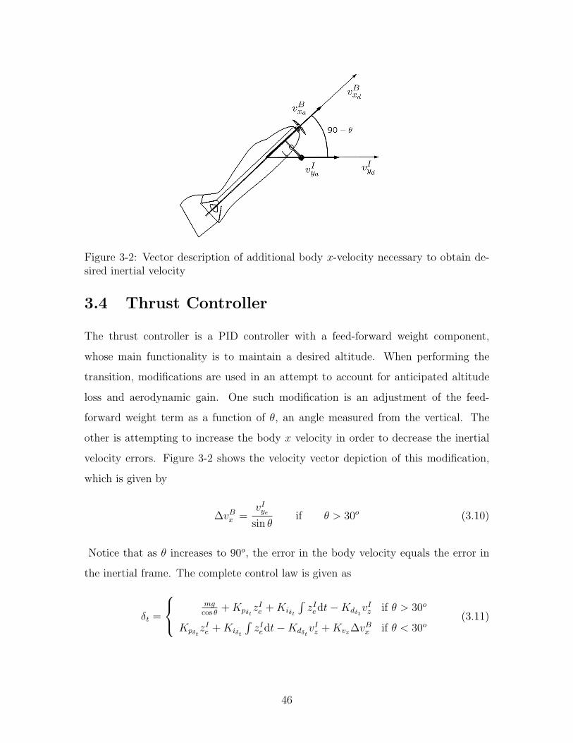
Figure 3-2: Vector description of additional body x-velocity necessary to obtain de-sired inertial velocity

3.4 Thrust Controller

The thrust controller is a PID controller with a feed-forward weight component,

whose main functionality is to maintain a desired altitude. When performing the

transition, modifications are used in an attempt to account for anticipated altitude

loss and aerodynamic gain. One such modification is an adjustment of the feed-

forward weight term as a function of θ, an angle measured from the vertical. The

other is attempting to increase the body x velocity in order to decrease the inertial

velocity errors. Figure 3-2 shows the velocity vector depiction of this modification,

which is given by

∆vBx =vIye

sin θif θ > 30o (3.10)

Notice that as θ increases to 90o, the error in the body velocity equals the error in

the inertial frame. The complete control law is given as

δt =

mg

cos θ+Kpδt

zIe +Kiδt

∫zIedt−Kdδt

vIz if θ > 30o

KpδtzIe +Kiδt

∫zIedt−Kdδt

vIz +Kvx∆vBx if θ < 30o

(3.11)

46

In hover the controller is a regular PID controller where vIz provides the damping

in the body frame. As the translation occurs, the modifications regulate the thrust,

attempting to maintain the desired altitude and decrease the inertial velocity errors.

3.5 Results

3.5.1 Simulation

A simulation was developed to test the capabilities of the controller and to find the

gains necessary to stabilize the system in a prop-hang orientation. To make the

model more realistic, an ensemble of state data was taken to determine the mean and

variance of the measurement noise. Saturators were added to the control actuators

as well as time delays to limit their performance to a realistic range. Table 3.1 shows

the gains that are used in the model as well as on the actual flight hardware.

Table 3.1: Simulation quaternion attitude loop gains

Gains Aileron Elevator Rudder ThrustKp 1.4 2.0 1.7 0.8Ki 0.0 0.0 0.0 0.2Kd 0.2 0.25 0.1 0.33

3.5.2 Decoupled Roll Control

Since the velocity commands are given in an inertial frame, the controller has an

additive feature that will track the velocity commands decoupled from the aircraft

roll orientation. For instance, if the aircraft is at a roll angle that does not correspond

to a single control surface deflection (e.g. elevator) to obtain the desired velocity, the

controller will couple the commands from the elevator and rudder.

To produce this roll decoupling feature, a transformation from the reference to

the current roll angle quaternion must be calculated. A problem arises since the

measurement of the current roll angle is not accurate, due to gimbal lock, and therefore

47

an intermediate derivation must be computed. This derivation involves the same

computation as the inner loop controller but only the roll information is used.

To proceed, transform the measured quaternion into this new intermediate orien-

tation (qint) by defining

qint = qa ⊗ qref . (3.12)

The conversion from quaternion to roll Euler angle is found by

φ = arctan2(qoint

qxint+ qyint

qzint)

1− 2(q2xint

+ q2yint

)(3.13)

which is the roll angle defined from hover.

Since the desired quaternion (Eq. 3.3) is a transformation in itself (level-flight to

hover), the roll transformation has to take place on the z-element of the quaternion,

therefore defining the roll decoupling transformation as

qroll =

cos φ

2

0.0

0.0

sin φ2

(3.14)

which is a unit quaternion by definition. Now Equation (3.9) can be re-written as

qd = qrefd ⊗ qroll ⊗ qxy. (3.15)

This redefined desired quaternion is now independent of the roll angle of the aircraft.

With this decoupling feature, a roll rate controller can be used to perform the rolling

hover. This is a PI controller on the roll rate error defined as

δa = Kprollwxerr +Kiroll

∫wxerrdt (3.16)

where

wBxerr= wBxd − w

Bxa . (3.17)

48

Performing a rolling hover requires that the body x-axis remains aligned with the

inertial z-axis. Therefore, the aircraft is able to roll (or rotate) about its body x-axis

in a controlled manner. Note that in hover, the effective airflow over the aileron

control surfaces are limited to a smaller finite area, Aap. During this maneuver, the

thrust may be varying due to the added drag caused by the control surface deflections,

causing uneven flow over the control surfaces which is solely provided by the propeller.

Since the propeller induces drag (another bounded random process) when spinning

about this axis, it is expected that the aircraft will rotate quicker in the direction

of the motor. This effect can be seen in Figure 3-3(a) which is rotating with the

propeller and has a slightly faster rise time than that of Figure 3-3(c) which is rotating

against the motor direction. Also, notice that Figure 3-3(c) has a significantly higher

overshoot. This is due to the integrator wind-up of the rotational rate and the added

amount of control that is necessary to track the desired rate. Figure 3-3(d) and 3-3(b)

both show the amount of aileron deflection necessary to perform these commands.

Just to maintain a non-rotating aircraft, the aileron must deflect approximately −15

degrees. Note the very large difference in the amount of control authority necessary

to rotate against the propeller than with. Since the same controller is used to perform

both rotations, there is a tradeoff between the response rate and lack of damping.

The quicker the desired response (characteristics of rise time), the higher the integral

gain, which causes more oscillation at constant commands.

3.5.3 Transition to Level-Flight

Since inertial velocity serves as the reference command for the outer loop of the

quaternion based controller, a joystick is used to manually provide a desired input. A

3-D visualization of the maneuver is shown in Figure 3-4. The goal for this controller

is to maintain a commanded inertial z-position while translating from hover to level-

flight. Figure 3-5 shows both the desired and measured output of the z position. As

expected, a loss in altitude is present during the transition but recovers over time

as the velocity command remains constant. Also, since the desired velocity can be

viewed as a user defined step input (Figure 3-6(b)), the y-position is a ramp function.

49

(a) Rotational rate spinning in the same directionas the propeller

(b) Aileron deflection to rotate the aircraft in thesame direction as the propeller

(c) Rotational rate spinning in the opposite di-rection of the propeller

(d) Aileron deflection to rotate the aircraft in theopposite direction of the propeller

Figure 3-3: Roll decoupling maneuver state output

Figure 3-6(a) shows how the body velocities over time, with constant pitch angle

(Figure 3-6(c)), stabilize to an equilibrium.

The control commands for this maneuver are shown in Figure 3-6(e) and Figure 3-

6(f). Notice that during the transition, the lift dynamics become more influential,

and therefore the thrust is used less for supporting the weight and more towards

translating the aircraft, which is seen in the dramatic decrease in thrust usage. The

elevator is used extensively for the initial rotation, but as the velocity command

remains constant, it tends back to a steady-state equilibrium.

50

Figure 3-4: 3-D visualization of the quaternion controlled transition maneuver

Figure 3-5: Position output for the quaternion-based control transition maneuver

51

(a) Resultant output body velocities (b) Reference and measured inertial velocity sig-nals

(c) Aircraft pitch angle over time (d) Measured rotational y body rate

(e) Actuated aircraft thrust (f) Elevator deflection over time

Figure 3-6: Various state results for the quaternion-based controlled transition tolevel-flight

52

Chapter 4

Nonlinear Lyapunov Backstepping

Controller

4.1 Introduction

This chapter presents the design of a Lyapunov-based backstepping controller extend-

ing the work of [13] to track any feasible smooth time-varying position commands,

including the case of constant position commands. Backstepping controllers are use-

ful when states are controlled through other states as is the case with aircraft. The

velocity vector is used to control the position, while the aircraft angular velocity and

thrust are used to control the velocity vector. To close the loop on the controller,

the aerodynamic control surfaces are used to control the angular velocity. The pro-

posed control architecture is shown in Figure 4-1, showing how stepping through the

dynamics of the system, the actuators can influence the response of the aircraft.

Position

Control

Kinematic

Eqs.

Force

Control

Translational

Dynamics

Moment

Control

Rotational

Dynamicsδaδeδrwd

δt

pd vd

Figure 4-1: Lyapunov-based backstepping control architecture

53

4.2 Controller Outline

In this section, a brief overview of the Lyapunov back-stepping control scheme de-

veloped in [13] is presented. This controller is the core formulation for the control

scheme presented in the following sections. For further understanding of the controller

development and insight, please see the referenced source.

The position tracking error in the body-fixed frame is defined as

e = RBI (pa − pd)

I . (4.1)

By taking the derivative, the dynamic equation for the body-fixed tracking error e is

e = RBI (pa − pd)

I +RBI pIa −RB

I pId

= −S(wB)e + vBa −RBI pd (4.2)

which uses Equation 2.10 and properties of skew-symmetric matrices.

The first control Lyapunov function is defined as

V1 =1

2eTe (4.3)

which is positive definite. Computing the time derivative of (4.3) and applying (4.2),

yields

V1 = eT e

= eT (−S(wB)e + vBa −RBI pId)

= −eTS(wB)e + eT (vBa −RBI pId)

= eT (vBa −RBI pId). (4.4)

To achieve stabiltiy in the sense of Lyapunov, V1 must be negative definite, which

54

can be accomplished in (4.4) by setting the desired velocity as

vBd = RBI pd −KeM

−1e. (4.5)

This cancels the dynamics and by choosing Ke as a diagonal positive definite matrix,

since M is the diagonal mass matrix, the Lyapunov criteria is satisfied.

Since the desired velocity needs to follow Equation (4.5), the error between the

desired and actual velocities must be forced to zero. Define the velocity error

z1 = vBa − vBd = vBa −RBI pId +KeM

−1e. (4.6)

Equation (4.4) can then be re-written as

V1 = −KeeTM−1e + eTz1 (4.7)

and the time derivative of z1 can be calculated as

M z1 = M vBa −MRBI pId −MRB

I pId +Kee

= −S(wB)Mv + fv + gvδt +MS(wB)RBI pd −MRB

I pd −KeS(wB)e +Kev −KeRBI pd

= −S(wB)Mv + fv + gvδt +MS(wB)RBI pd −MRB

I pd −KeS(wB)e +Kez1 −K2eM

−1e

= −S(wB)M [z1 +RBI pd −KeM

−1e] + fv + gvδt +MS(wB)RBI pd −MRB

I pd −KeS(wB)e

+Kez1 −K2eM

−1e

= S(Mz1)wB + [S(MRBI pd)−MS(RB

I pd)]wB + gvδt + fv −MRB

I pd +Kez1 −K2eM

−1e

= S(Mz1)wB + gvδt + h (4.8)

where,

h = fv −MRBI pd +Kez1 −K2

eM−1e. (4.9)

Note that

v = z1 +RBI pd −KeM

−1e

55

and because of diagonal M

S(MRBI pd)−MS(RB

I pd) = MS(RBI pd)−MS(RB

I pd) = 0

In compact notation

M z1 = S(Mz1)wB + gvδt + h. (4.10)

The last term in Equation (4.7) works against the need for negative definiteness

of V1 to meet the Lyapunov criteria. Unfortunately, it is not always possible to

make z1 zero since it eliminates the direct coupling between the translational and the

rotational dynamics. This can be seen by setting z1 to zero which also implies z1 is

zero, and in Equation (4.10), gvδt = h which implies no coupling since h is a function

of force terms. However, z1 can be made a constant vector δ ∈ R3 such that the error

ϕ = z1 − δ (4.11)

is forced to zero. Based on Equation (4.11), a second control-Lyapunov function

defined as

V2 = V1 +1

2ϕTM2ϕ (4.12)

is defined. The time derivative of V2 can be written as

V2 = V1 + ϕTM(M z1)

= −KeeTM−1e + eT δ + ϕT (M [gv S(Mδ)][δt wB]T +Mh + e). (4.13)

which uses the fact that

ϕTMS(Mϕ) = 0 and eTϕ = ϕTe.

56

For simplicity, define

B = [gv S(Mδ)] ∈ R3×4 (4.14)

ζ = [δt wB]T ∈ R4 (4.15)

and thus Equation (4.13) in this compact notation becomes

V2 = −KeeTM−1e + eT δ + ϕT (MBζ +Mh + e). (4.16)

Equation (4.15) harbors the first control actuation ability in this control design. The

next step extracts this control variable by satisfying the Lyapunov criteria for V2.

Note that one can choose δ = M−1gv ε, where ε is a positive constant such that the

matrix BBT is invertible,

BBT =

1 0 0 0

0 0 0 −ε

0 0 ε 0

1 0 0

0 0 0

0 0 ε

0 −ε 0

=

1 0 0

0 ε2 0

0 0 ε2

. (4.17)

The vector ζ, which consists of the desired thrust and rotational rate, serves as a

virtual control that forces V2 to satisfy the Lyapunov condition. This is achieved by

setting ζ as

ζd = BT (BBT )−1(−h−M−1e−M−1Kϕϕ) (4.18)

where Kϕ ∈ R3×3 is a diagonal symmetric positive definite matrix. To obtain the first

control input δt, extract the first entry of ζd as

δt = [1 01×3]ζd. (4.19)

57

Now, the final error variable that must be forced to zero is

z2 = wB − [03×1 I3×3]ζd. (4.20)

By combining Equation (4.15) and (4.20) to form ζ = [0 z2]T+I4×4ζd and noting that

ϕTMB[0 z2]T = ϕTMS(Mδ)z2, we can rewrite Eq. 4.16 with δt given by Eq. 4.19

as

V2 = −KeeTM−1e + eT δ − ϕTKϕϕ+ ϕTMS(Mδ)z2. (4.21)

The third and final control-Lyapunov functions is

V3 = V2 +1

2zT2 Jz2 =

1

2eTe +

1

2ϕTM2ϕ+

1

2zT2 Jz2. (4.22)

The time derivative of V3 is computed as

V3 = −KeeTM−1e + eT δ − ϕTKϕϕ+ zT2 (Gwuw − S(wB)JwB + fw

− [03×1 J ]ζd − S(Mδ)Mϕ), (4.23)

where the last term is due to the fact ϕTMS(Mδ)z2 = −zT2 S(Mδ)Mϕ. In order to

satisfy the Lyapunov criteria, uw is chosen as

uw = G−1w (S(wB)JwB − fw + [ 03×1 J ]ζd + S(Mδ)Mϕ−Kz2z2). (4.24)

where Kz2 ∈ R3×3 is a diagonal symmetric positive definite matrix. Note that Gw is

never singular, even at hover due to the control authority produced by the propeller

airflow over the control surfaces. Substituting in uw from (4.24), the time derivatives

of V3 is then

V3 = −KeeTM−1e + eT δ − ϕTKϕϕ− zT2Kz2z2. (4.25)

By selecting appropriate positive definite matrices Ke, Kφ, Kz2 , the user is able

58

to produce a control scheme with stable trajectory tracking capabilities. As can be

seen from Equation (4.25), the Lyapunov function is not always negative definite

because of the δ term introduced in Equation (4.11). Hence, maintaining this term to

a sufficiently small value will aid in stability, with the trade-off of having decreased

coupling between the rotational and translational dynamics. It is important to note

that the above control design approach can not guarantee the stability results during

implementation because it assumes no parametric uncertainty between the model and

actual vehicle.

4.2.1 Simulation

This control design is tested with the aircraft model outlined in Chapter 2. Two

types of tests are performed. The first test demonstrates the controller’s capability

to stabilize the aircraft in hover, while the second demonstrates its take-off to hover

capabilities.

For the hover test, the aircraft was given a commanded vector position (in meters)

of

pd =

10

0

6

. (4.26)

To test this controller’s robustness to initial conditions, a small offset is placed in

the x and z-axes, and its correction can be seen in Figure 4-2. There are a few

things to note from this test. First, the controller corrects the aircraft’s position in

the x-direction. Second, there is a very noticeable error in the z-axis which will be

explained further in Section 4.3. The controller, however, seems to be very dependent

on the error constant that is chosen in Equation (4.17). It created a coupling between

the rotational and translational dynamics and the larger the constant is made, the

simulation converges to a result faster, but a larger steady state error is induced.

59

Figure 4-2: Simulated Lyapunov-based backstepping control in hover with initialcondition offsets

For the take-off to hover test, the following trajectory is commanded:

pd(t) =

10(1− e−0.3t)

0

6(1− e−0.5t)

0 ≤ t < 10

10

0

6

10 ≤ t < 20.

(4.27)

Results from the simulation are shown in Figure 4-3. Note that a similar behavior can

be seen here as in the hover test: there is a significant difference between the actual z

and desired output, and the x-error converges to zero as t→∞. For this particular

maneuver, the value of ε from Equation (4.17) had to be increased compared to the

hover test. This is expected since there is more interaction between the rotational

and translational dynamics for such a desired trajectory.

When attempting to place this control design on the actual Clik aircraft, issues

arise with the stability of the vehicle starting at hover. In Section 4.3, a linearization

is performed in order to gain more insight and intuition on the control needed at

60

(a) Desired and actual parametric position out-put as a function of time

(b) 3-D visualization of the take-off to hover ma-neuver

Figure 4-3: Lyapunov-based backstepping take-off to hover simulation

hover. The key questions that are answered during this linearization process are the

nature of steady-state errors and the controller’s sensitivity to the ε term.

4.3 Linearized Hover Controller

This section outlines a linearization of the nonlinear controller near hover to study

the behavior in the linear domain about hover. By performing this linearization, a

simplistic view of this controller concept can be understood and analyzed.

Near the hover orientation, u∞ ≈ 0, up ≈√

mg2ρAd

from Equation (2.3) and the

direction cosine matrix (DCM) at a +90 degree pitch angle (the body x and inertial

frame z axis are aligned) is

RIB =

0 0 −1

0 1 0

1 0 0

,

61

which transforms the equations of motion (2.9), (2.14) and (2.10) respectively into

phover≈

−vzvy

vx

, fvhover≈

−mg

0

0

,

RIB

hover≈

wy −wx 0

wz 0 −wx0 −wz wy

.

Starting with the nonlinear thrust command from Equation 4.19 and noting that

ζd = BT (BBT )−1(−h−M−1e−M−1Kϕϕ)

≡ BT (BBT )−1W

with

BT (BBT )−1 =

1 0 0

0 0 0

0 0 1ε

0 −1ε

0

,

the thrust is the first entry of W ∈ R3×1. Noting that the general vector form of h(1)

denotes the first entry in the vector, and the thrust command can be reformulated as

δt = −h(1)−M−1e(1)−M−1Kϕϕ(1).

Applying the near hover approximations, the term-by-term linearization of W be-

62

comes

−h(1) = mg − kevx,

−M−1e(1) =pz − pdzm

,

−M−1Kϕϕ(1) = −kϕ(vx +

ke(pz − pdz)m

− ε

m

),

yielding the linearized thrust term

δthover≈ mg − (ke + kϕ)vx −

(1 + kekϕ

m

)(pz − pdz)−

kϕε

m, (4.28)

which is a Proportional/Derivative (PD) controller, given by the two inner terms,

with a feed-forward weight term. Note that the last term in Equation (4.28) is both a

function of kϕ and ε. This is the explanation to why, in the body x axis, the controller

fails to eliminate the steady-state error. The larger ε is, the larger this steady-state

error will be.

The aircraft control surface law is given in Equation 4.24 and rewritten here as

uw = G−1w T where T ∈ R3×1 is given as

T = S(wB)JwB − fw +[

03×1 J]ζd + S(Mδ)Mϕ−Kz2z2.

With the hover assumptions, the moment decoupling matrix terms areg11

g22

g33

=

12ρu2

paCLδawAapLap

12ρu2

prCLδeAeLep

12ρu2

prCLδrArLrp

.

The following performs a term-by-term expansion on T using the hover conditions

and assumptions:

63

S(wB)JwB =

wywz(Izz − Iyy)

wxwz(Ixx − Izz)

wxwy(Iyy − Ixx

hover≈

0

0

0

(4.29)

fwhover≈

−Macc −Mdrag

−12ρLeLe,pAeuprwy

−12ρLrLr,pAruprwz

(4.30)

[03×1 J

]ζd

hover≈

0

Iyyε

(−wymg − vz 1+kϕke

m

)− Izz

ε

(−wzmg − vy 1+kϕke

m

) (4.31)

MS(δ)Mϕhover≈

0

−εm(vz − ke

m(px − pdx)

)εm(vy + ke

m(py − pdy)

) (4.32)

Kz2z2hover≈ Kz2

ε

0

vz(−ke − kϕm

) + m+kekϕm2 (px − pdx)

vy(ke + kϕm

) + m+kekϕm2 (py − pdy)

(4.33)

Combining terms Eq.( 4.29-4.33) yields

Thover≈

Macc +Mdrag

wy(Aepupr +Bep) + vz(Cep) + (px − pdx)Dep

wz(Aryupr +Bry) + vy(Cry) + (py − pdy)Dry

(4.34)

64

where,

Aep =1

2ρLeLe,pAe Ary =

1

2ρLrLr,pAr

Bep = −Iyyεmg Bry = −Izz

εmg

Dep =ε2m2ke − kekϕ −m

m2εDry =

ε2m2ke − kekϕ −mm2ε

Cep =kz2(mke + kϕ)− Iyy(1 + kϕke)− ε2m2

εm

Cry =mkz2ke + kϕkz2 + Izz(1 + kϕke)− ε2m2

εm

Therefore the total deflection control in a linearized hover condition is

uw =

δa

δe

δr

hover≈ Gw

Macc +Mdrag

wy(Aepup +Bep) + vz(Cep) + (px − pdx)Dep

wz(Aryup +Bry) + vy(Cry) + (py − pdy)Dry

. (4.35)

Equation (4.35) shows that, when linearized about hover, the controller is similar to

what might be expected. In particular, the deflection of the aileron is a function

of the thrust and cancels the moment caused by the rotation of the propeller. The

rudder and elevator control surfaces have similar feedback strategies that use a PD

controller for position along with a rate attitude term.

4.3.1 Flight Test

This linearized version of the nonlinear controller has been implemented on the Clik

indoor aerobatic aircraft. In this linearized controller test, the attitude controller

presented in Chapter 3 is used prior to the linearized controller to attain a desired

hover attitude and position in flight to ensure proper initial conditions. Once this

attitude is obtained, the controllers are interchanged, and the last inertial position

vector becomes the linearized controller’s commanded position, shown in Figure 4-

4. The switch becomes apparent when the reference command becomes constant.

65

Figure 4-4: Experimental linearized Lyapunov-based controller position data abouthover.

Since the controller is a PD controller, some steady-state error is seen. The z-axis

behavior is due to the drop in battery voltage over time. In the Lyapunov sense of

linearized stability at an equilibria, the equilibrium point is asymptotically stable for

the actual nonlinear system [24]. Thus, the conclusion can be drawn that the aircraft

will maintain stability with the nonlinear controller while at hover.

The above implementation of the linearized controller only takes the form of the

controller found in Section 4.3. The reason for this is to acquire an envelope of gains

that will stabilze the aircraft. Once this envelope is found, a system of equations is

developed and a feasibility check is done to verify whether the form of Equations (4.28)

and (4.35) can be satisfied. For instance, in Eq. (4.28), the gains that stabilized the

66

system take the form

δthover≈ mg − 0.34vx − 0.95(pz − pdz). (4.36)

To satisfy this criteria, the gains above would have to satisfy

0.34 = (ke + kϕ) (4.37)

0.95 =

(1 + kekϕ

m

)(4.38)

along with the other gains used for the control surfaces as well as satisfying the

Lyapunov criteria by remaining positive definite. Unfortunately, the criteria above

could not be met. In order to satisfy the system of equations, the Lyapunov criteria

had to be relaxed (meaning allow some values to take on negative values occasionally

allowing V > 0), which led to an unstable system in other flight regimes. In the next

section, a controller is devised that utilizes part of the controller properties outlined

in Section 4.2 to obtain the desired state values, but uses the quaternion controller

to reach these states.

4.4 Lyapunov Quaternion Control

4.4.1 Introduction

In this section, a Lyapunov-based quaternion controller with state feed-back is pre-

sented. This control design combines the Lyapunov algorithm developed in [13] with

the quaternion based controller from [15] and is shown in Figure 4-5. The user inputs a

desired smoothly time-varying continuous trajectory (including constant commands),

assumed to be twice differentiable, which will be used in both the attitude and thrust

actuation.

Beginning with the attitude controller, the Lyapunov algorithm dictates the de-

sired rotational velocities through Equation (4.20) as wBd = [03×1 I3×3]ζd. To main-

tain the same notation from above, the rotational update from Equation (2.10) pro-

67

Lyapunov

Algorithm

Attitude

Update

Attitude

Conversion

Quaternion

Control

Aircraft

Dynamics

qa

pa,vBa , Ra,wBa

Thrust

Control+

PD

Throttle pa,vBa

δt

pIdvIdaId

wBd Rd qd uw

δt δt

Figure 4-5: Lyapunov quaternion control architecture

duces the desired DCM which represents the desired attitude. This DCM then needs

to be converted to a desired quaternion. The relationship between these two attitude

descriptors is given in [25] as

RBI =

r11 r12 r13

r21 r22 r23

r31 r32 r33

=

q2o + q2

x − q2y − q2

z 2(qxqy + qzqo) 2(qxqz − qyqo)

2(qxqy − qzqo) q2o − q2

x + q2y − q2

z 2(qyqz + qxqo)

2(qxqz + qyqo) 2(qyqz − qxqo) q2o − q2

x − q2y + q2

z

.(4.39)

By using the diagonal elements alone, one may determine the magnitudes of the

individual quaternion elements. The other six off-diagonal elements determine the

signs.

Many algorithms have been developed to convert from DCM to quaternion. For

this design approach Shepperd’s algorithm is used [26] and proceeds as outlined in

Table 4.1. The reason Shepperd’s algorithm is used is not only to provide the correct

signs for the quaternion, but also to avoid dividing by a very small number, creating

a singularity in the solution for qd. This desired quaternion is used as the reference

desired quaternion in the quaternion-based controller as given in Equation (3.4).

The thrust controller predicts a thrust feed-forward term, denoted as δt,based on

the user defined desired state inputs which are inserted in the model. The primary

goal for this design is to transition from hover to level flight by rotating about the

68

Table 4.1: Algorithm to convert from DCM to quaternion

Algorithm 4.1. Shepperd’s Algorithm1: Compute the trace of RB

I

2: Define r44:r44 = trace{RB

I } = T3: Define the elements p2

i

p2i = 1 + 2dii − T i = 1, 2, 3, 4

4: Based on Eq. 4.39 write the relations between pi and elements in RBI

5: Find the largest of the dii:|dii,max| = Max{|d11|, |d22|, |d33|, |d44|}

6: For that dii, compute the corresponding pi using Step 3pi =

√1 + 2dii − T

7: With this pi, use Step 4 to obtain the rest of the p′is8: Divide all four p′is by 2 to obtain the individual quaternion components

body-fixed y-axis. The main control actuation is performed by the thrust and elevator,

and thus the S(wB)MvB term may be omitted resulting in

gvδt = M vB − fv. (4.40)

The first entry of (4.40) is the feed-forward thrust term. A feedback law is used to

help correct the thrust controller if there is an error between the commanded and

desired states. This feedback law uses the error in the state variables defined in

Equation (4.6) for the velocity and Equation (4.1) for the position in the body frame

but modified by the desired DCM in the following manner:

eBv = vBa −RBIdvId (4.41)

eBp = RBId

(pa − pd). (4.42)

So for this thrust controller formulation, the errors are defined about the desired

trajectory error through the use of the desired orientation. The final thrust controller

is given as,

δt = δt +KpeBp +Kde

Bv . (4.43)

69

Figure 4-6: Sample transition trajectory data with radial basis least square fit

The major difference between this controller and the quaternion controller described

in Chapter 3 is that the rotational and translational dynamics are cognisant of each

other through the desired DCM. This is done by providing the thrust controller with

the desired DCM and the control surfaces with the velocity and position errors in the

body frame.

In the following sections, simulation and hardware implementation of this con-

troller are presented. Since the quaternion-based controller has been successfully

implemented, it serves as a guideline for the type of trajectory that is feasible for the

aircraft to follow.

4.4.2 Simulation

Data taken from multiple trials of the transition maneuver are all quite similar and is

shown in Figure 4-6. For the ease of computation when taking multiple derivatives,

a normally distributed gaussian radial basis function is used to fit this curve and is

70

Table 4.2: Radial basis function values: σ = 1.2

i ti αi1 0.0 7.78172 1.0 -5.25573 2.0 10.90594 3.0 -8.29355 4.0 2.5327

given by

pdy =N∑i=1

αie−(t−ti)

2

2σ2 . (4.44)

The ti values represent the center of the normal gaussian distributed function and

are placed discretely along the length of the maneuver time-line. The αi’s represent

the weighting functions and are determined using the matrix methods of linear least

squares [27]. The variances of the exponential functions is a function of the number

of sample points; the denser the sample points, the smaller the variance. For this

function, five basis functions are used (values shown in Table 4.2) and a comparison

is shown in Figure 4-6. This function provides continuous both first and second order

derivatives and is used as the desired inertial position function in the simulation and

implementation of the Lyapunov quaternion controller.

In this simulation, the goal is to gain insight on the expected reaction of the vehicle

with the Lyapunov quaternion controller implemented. It also provides a basis of how

well the quaternion controller can track the type of desired rotational rates required

to perform this maneuver. The desired position for the trajectory is denoted as given

in Eq. (4.44), pdy , and the total desired position in R3 is given as

pd =

0.0

pdy

1.2

(4.45)

Since it was determined that the transition maneuver will be done about the body

71

y-axis, the above control design is only placed on the thrust and elevator control

actuators so that the body x-z plane is parallel to the inertial y-z axis. The other

surfaces are controlled through the quaternion based controller to maintain the above

desired position.

Some trade-offs are apparent between the “quickness” of the desired rotational

rate and the overall performance of the vehicle. Figure 4-7(f) shows that there is

some lag between the desired and measured y-rotational velocity. This is due to

several reasons. Their is a modeled lag in the actuators in an attempt to bring more

realism to the system, and the attitude update equation is actually running a time

step (50Hz) behind the actual system. It is also apparent that the more aggressive

the desired rotational rate is (a product of the selective gain choice being close to the

point of instability), the more of a ”wiggling” phenomenon takes place during the

transition seen between 1-3 seconds.

This phenomenon is also captured in the body velocity output shown in Figure 4-

7(c) and Figure 4-7(d) between the same time range. The most substantial advantage

to this system design is the controllers ability to track the desired trajectory. Figure 4-

7(a) and Figure 4-7(a) shows the output of both the y and z-positions which are

followed very well. Position in the z-axis is more apparent but the error is less than

0.2 meters.

4.4.3 Hardware Implementation

Hover to Hover Maneuver

The same trajectory used in simulation also provided a reference command for hard-

ware implementation. All the resultant state data for this experiment are shown in

Figure 4-9. The first figure of merit of these plots is the similarities to the simulated

data. The position tracking, in particular, in Figure 4-9(a) and Figure 4-9(b) are

remarkably similar to that in the simulation. The body velocities in Figures 4-9(c)

exhibit a bit of lag due to possible un-modeled delays in the motor and/or actuator

dynamics.

72

(a) Simulated y position output (b) Simulated z position output

(c) Simulated vBx velocity output (d) Simulated vB

z velocity output

(e) Simulated pitch output (f) Simulated wBy rotational rate output

Figure 4-7: Simulated Lyapunov quaternion controlled hover to hover state data

The pitch is similar to the simulation (Figure 4-9(e)), but the amount of control

effort by the elevator (Figure 4-10(b)) and consequently the rotational rate (Figure 4-

73

(a) Simulated thrust command (b) Simulated elevator deflection control

Figure 4-8: Simulated Lyapunov quaternion controlled hover to hover control effort

9(f)) differ. This is due to the difference in initial conditions and user-defined gain

inputs. When tuning the gains for the desired rotational rate variable, the user

is able to give a weighting factor to either error or modeled feed-forward output,

similar to a linear quadratic estimator (LQE) design. This is also directly related

to how anticipatory the desired rate will be. Since the trajectory is predefined, the

desired control laws, if weighed heavily on the feed-forward term, will anticipate

future movements and dampen the response. Therefore, the user is able to design

the response to a given trajectory within the control limits. In this experiment,

the measured error and the model based controls are weighed equally providing the

authority necessary for tracking (Figure 4-10).

An additional experiment was done to determine the affects of weighing the mod-

els feed-forward control strategy for the elevator more heavily than the state error.

As the model feed-forward control gains are increased, the system becomes more con-

servative yielding larger control deflections earlier in the maneuver which can be seen

in Figure 4-12. As a result, the tracking about the y-position undershoots as seen in

Figure 4-11. From this example, it is apparent that there is a trade-off in this control

strategy between weighing the feed-forward controls calculated by the model and the

error-based control signals.

74

(a) y position outputs (b) z position outputs

(c) vBx velocity outputs (d) vB

z velocity outputs

(e) Pitch output (f) wBy rotational rate output

Figure 4-9: Hardware implemented Lyapunov quaternion controlled hover to hoverstate data

75

(a) Hardware implemented thrust command (b) Hardware implemented elevator deflectioncontrol

Figure 4-10: Hardware Lyapunov quaternion controlled hover to hover control effort

Figure 4-11: Measured y-position output for the hover to hover maneuver varying thefeed-forward predictive gains

Figure 4-12: Elevator deflection output for the hover to hover maneuver varying themodel feed-forward gains

76

Figure 4-13: Hardware implemented Lyapunov quaternion controlled take-off to hovermaneuver

Take-off to Hover Maneuver

For the previous maneuver, the quaternion controller is used as insight to produce a

feasible path. This type of trajectory insight is not available for a take-off to hover

maneuver, so an educated ad hoc estimate was performed which involved manually

directing the aircraft in the environment to develop a path, shown in Figure 4-14(a)

and Figure 4-14(b). The same type of data fitting done in the previous section

is done to provide the controller with a smooth, continuous path. The controller

provides sufficient tracking given the uncertainty in the ad hoc trajectory planned.

The elevator control inputs are intentionally made extra aggressive to ensure path

following which can be seen in Figure 4-15(c) as the pitch angle dramatically decreases

desperately attempting to track both the desired y and z-positions.

Since the aircraft is taking-off from the ground, the dynamics are considerably

different than during flight because of drag from the floor and various other reasons

including ground effect. These effects hinder the initial take-off portion of the maneu-

ver as can been seen during the initial 2 seconds in Figure 4-14(a). The thrust term,

77

(a) y position outputs (b) z position outputs

(c) vBx velocity outputs (d) vB

z velocity outputs

Figure 4-14: Lyapunov quaternion controlled take-off to hover state data

since anticipating aerial flight, only provides enough thrust to maintain the desired

velocity and position for this instance in time. The error terms are building up, which

can be seen in Figure 4-15(a) between 0.5-1.2 seconds as a linear increase in measured

thrust output, and is providing the additional thrust necessary to compensate for the

non-modeled effects. This lack of thrust can also be seen in Figure 4-14(c), by the

measured velocity lagging behind the desired velocity then creating a massive over-

shoot in attempt to decrease error. Given how arbitrary this trajectory was produced,

the controller performs well showing great potential for high-bandwith capability.

78

(a) Hardware implemented thrust command (b) Hardware implemented elevator deflectioncontrol

(c) Pitch output (d) wBy rotational rate output

Figure 4-15: Lyapunov quaternion controlled take-off to hover control effort

79

80

Chapter 5

Conclusion

This thesis presents multiple techniques for controlling a fixed-wing aircraft during

aggressive, agile flight. Each controller offers its own unique approach to the reference

command tracking problem. The quaternion-based attitude controller provides the

ability to track a desired attitude sufficiently well using a linear control scheme. The

Lyapunov controller uses derived equations of motion of the vehicle to accurately track

feasible, sufficiently smooth, continuous position commands in a inertial-based frame.

Each of these control designs are demonstrated, both in simulation and in actual

hardware implementation using a small scale, indoor aerobatic fixed-wing aircraft.

Each chapter explored a specific component of the agile flight control problem

which contribute to the overall goal of this thesis. In Chapter 2, a six-degree-of-

freedom model of a fixed wing aircraft was derived and tested to ensure an accurate

system identification. This was accomplished through the use of a load cell placed

at the center of gravity of the aircraft which measured both forces and moments

about the body fixed frame. Two main types of tests were performed to determine

the aerodynamic properties of the vehicle, which included hover and multiple wind-

tunnel tests. The hover tests were performed to determine the aircraft’s response

to propeller downwash, which solely provided the dynamic pressure used to control

the aircraft. The wind tunnel tests were done at several different angles-of-attack,

both with and without the propeller active. With these tests, the interaction of

the propeller downwash and the free-stream velocity was determined as well as the

81

induced angle-of-attack in the region of the prop flow. The aircraft dynamics about

the major lifting surface were split into two regions in order to differentiate this

combined flow (or effective flow) from the pure free-stream flow. From these tests, a

complete set of equations of motion were developed to form a high fidelity model. To

ensure model accuracy, a system identification was done using the RAVEN motion

capture system, which provided all the state data necessary for comparison. This

model was then able to serve as the testbed for all simulation experiments and for

the development of the nonlinear controller.

Chapter 3 presents a quaternion based attitude controller with velocity error based

thrust correction. This controller has the ability to prescribe a desired attitude in

the direction of decreasing error based on the error between a user-defined inertial

velocity command and the actual measured velocity. The thrust command also uses

the velocity command as a correction term for error minimization. The design was

formulated to perform a desired transition from hover to level-flight mode. During

this maneuver, the minimization of the loss of altitude as well as sufficient velocity

tracking were priorities. The implementation of this controller was demonstrated on

the testbed aircraft and the results confirmed desired performance.

Finally, Chapter 4 introduces a Lyapunov backstepping control technique that

tracks reference input position commands. This design is highly model based and

relies on the accuracy of the model presented in Chapter 2. Stability is proven under

the Lyapunov criteria, and the linearization of the control law is provided to gain

insight into the inner workings of the controller and to give aid to potential hazards

of the design. Based on the research done in [13], a modified version of this controller

has been created based on the lessons learned from the linearization technique, and

combines the quaternion based control scheme outlined in Chapter 3. This controller

is then implemented on actual hardware to obtain desired performance results.

In summary, the controllers developed in this thesis allow a fixed wing aircraft to

perform some aggressive, agile flight maneuvers which show the potential of combining

abilities of the desired flight regimes into one single design.

82

5.1 Future Work

During the course of this work, several key topics and issues have emerged which

merit further research. These items are discussed below.

5.1.1 Improved Dynamic Model

The modeling done in this thesis, though extensive, was done primarily about the

body y-axis focusing on a specific maneuver. The inclusion of a even higher fidelity

model for the rest of the aircraft’s axes would dramatically increase the capabilities

of the control schemes mentioned. Given a three-dimensional, time-varying, para-

metric trajectory, the Lyapunov quaternion controller would be able to generate the

necessary control commands for sufficient tracking. This additional modeling would

include the motor dynamics with attached propeller and thus the effect they have on

the thrust and moment in the aircraft’s body x-direction.

5.1.2 Trajectory Linearized Control

Trajectory linearized control (TLC) is an advanced nonlinear control technique that

linearizes the tracking error of a nonlinear system along a desired reference trajec-

tory [28]. The TLC control configuration is shown in Figure 5-1.

+ Stability Controller + Aircraft Dynamics

Inverse Dynamics

pd u

−

u

Figure 5-1: Trajectory linearized control architecture

This control technique is also a highly model-based control technique, but given an

accurate model, would dramatically increase the tracking capability, thus increasing

83

the controllers bandwidth. The inverse dynamics are used to develop the desired (or

nominal) control, u, necessary to perform the prescribed path. A linear time-varying,

controller is then used to stabilize the nominal trajectory based on the state feedback.

This design can be viewed as an ideal gain-scheduled controller at every point along

the commanded trajectory and can be very robust given the accuracy and fidelity

of the reference model. Computing the nominal control involves solving an optimal

control problem. For a tracking problem, the definition of the cost function [29] is

minuJ =

∫ tf

to

[∥∥p(t)− pd(t)∥∥2

Q(t)+∥∥u(t)

∥∥2

R(t)

]dt (5.1)

where Q and R represent symmetric n×n weighting matrices. The goal is to minimize

the above cost function subject to the dynamics of the aircraft given as

s.t. pI = RvB (5.2)

R = RS(wB) (5.3)

JwB = −S(wB)JwB + fw +Gwuw (5.4)

M vB = −S(wB)MvB + fv + gvδt (5.5)

u(t) ∈ U . (5.6)

These control commands can be computed either a priori on an off-board computation

system, or during the flight, which would require quick computational power.

5.1.3 Path Feasibility Planner

One of the major issues when planning a desired path, especially within a constrained

environment, is ensuring that the commanded path is feasible. The paths given in

this thesis were defined using feedback from manually maneuvering the aircraft in

an educated adhoc manner, or an actual flight path that was either flown manually

or from another controller. With a path feasibility planner, the control techniques

mentioned in this thesis would be able to track a path, eliminating this as one of the

control variabilities.

84

Appendix A

Quaternion Based Method for the

Determination of Body Rates using

a Motion Capture System

A.1 Introduction

The Vicon motion capture system used for vehicle sensing provides position and

orientation data about a local inertial reference frame. The reference frame is an

East North Up (ENU) frame in which position is given in millimeters and orientation

in a three vector axis-angle representation with an embedded angle. When performing

aggressive, agile flight in a nonconventional manner, attitude representation without

singularities is essential. Convenient and typical forms of attitude representation,

such as the use of Euler angles, suffer from the loss of at least one or more degrees of

freedom resulting in what is known as “gimbal lock”. Since the sensor only provides

orientation data, the extraction of rate data must be done by means of a derivative.

Issues arise with the continuity of the orientation data due to the embedded angle

information and precautionary steps are made to ensure smooth, continuous data

extraction.

85

A.2 Extracting the Axis Angle

An axis angle representation parameterizes a single rotation of a rigid body through

an angle θ and a reference axis,

(angle, axis) =

θ,ax

ay

az

(A.1)

commonly referred to as Euler axis or eigenaxis [25]. The three axis components and

total rotational angle describe a vector and an object’s pure rotation about this vector

in a single fixed reference frame. The axis vector’s magnitude produces an additional

degree of freedom which is constrained to a unit magnitude given by

a2x + a2

y + a2z ≡ 1. (A.2)

The motion capture system provides object orientation in the form (axis with em-

bedded angle)

Ax

Ay

Az

=

ax

ay

az

θ. (A.3)

The angle θ can be extracted using Equations [A.2] and [A.3],

A2x + A2

y + A2z =

(a2x + a2

y + a2z

)θ2 = θ2

⇒ θ = ±√A2x + A2

y + A2z (A.4)

which can be substituted into Eq.[A.3] to find the axis vector components. Initially,

the sign of θ can be arbitrarily chosen to be positive which leads to a bounded angle,

θ ∈ [0, π] . (A.5)

86

These axis angle components can then be transformed into their respective quaternion

representations by qo

qx

qy

qz

=

cos(θ2

)axsin

(θ2

)aysin

(θ2

)azsin

(θ2

)

. (A.6)

It is then possible to relate this quaternion and its respective component time rate of

change to an object’s rotational body rate, denoted by w, using

w

wx

wy

wz

=

2(qoqx + qz qy − qy qz − qxqo)

2(−qz qx + qoqy + qxqz − qy qo)

2(qy qx − qxqy + qoqz − qz qo)

. (A.7)

This is equivalent to the nominal aerospace nomenclature of p, q and r which are the

rotational body rates. Cusps and discontinuities arise in the functions due to the am-

biguous sign allocation of θ and is shown in Figure A-1. This figure shows the output

Figure A-1: Quaternion data due to a pure rotation about the reference z-axis.

quaternion of a pure rotation about the z-axis. Only the scalar and z components are

shown because the rotation axis is strictly a unit z-axis rotation. The reason for these

cusps and discontinuities can be explained by the following: since the rotation angle

is chosen to be positive for all rotations, the axis must flip in order to agree with the

87

right-hand-rule, illustrated in Figure A-2. Taking the derivatives of these functions

(a) Positive rotation with axis pointingout of the page

(b) Positive rotation with axis pointinginto the page

Figure A-2: Pure body z-rotation illustrating axis flip

leads to large errors at the point of the cusp or discontinuity. Therefore, a method

for tracking when a flip occurs has been developed to maintain smooth continuous

functions so that their derivatives are also continuous. This method uses the unit

magnitude property of Equation A.2 by taking the dot product of an update axis

angle (k + 1) with the previous update (k). This point can be shown by evaluating

the dot product of an axis angle at each side of the discontinuity or cusp using the

pure z rotation example as follows:ax

ay

az

k+1

≈

0

0

−1

&

ax

ay

az

k

≈

0

0

1

(A.8)

ax

ay

az

k

·

ax

ay

az

k+1

≈ −1 (A.9)

The dot product of the these axis angle terms yields a −1 which is in violation of

Equation A.2. Thus, the conclusion that a flip has occurred can be realized and the

negative sign can be placed on the angle to maintain q as a continuous function of θ.

88

Table A.1: Smooth quaternion signal data algorithm

Algorithm A.11: Initialize: sign = 1.0Loop2: if (ak · ak−1 < 0.0)

sign = -1.0·sign3: qo = sign · cos

(θ2

)qx = sign · ax sin

(θ2

)qy = sign · ay sin

(θ2

)qz = sign · az sin

(θ2

)

Figure A-3: Continuous quaternion data due to a pure rotation about the referencez-axis.

With this algorithm implemented (Table A.1), the output in Figure A-1 from before

becomes a smooth time varying function, now shownn in Figure A-3. This data

can now be differentiated and the quaternion rates are calculated. Then, by using

Equation A.7, the body rates can be found.

89

90

Bibliography

[1] SPG Media. Airforce-technology.com. http://www.airforce-

technology.com/projects/predator/, 2009. 13, 15

[2] AeroVironment, Inc. AeroVironment Unmanned Aircraft Systems. Available at

http://www.avinc.com/uas/, 2009. 13

[3] Boeing. Boeing Integrated Defense Systems - V-22 Osprey. Available at

http://www.boeing.com/rotorcraft/military/v22/index.htm, 2009. 14

[4] W. F. Chana and J. F. Coleman. World’s first VTOL airplane Convair/Navy

XFY-1 Pogo. In Proceedings of the International Powered Lift Conference, pages

99–104, Jupiter, FL, November 1996. 17

[5] W.E. Green and P.Y. Oh. A MAV That Flies Like an Airplane and Hovers Like

a Helicopter. In Proceedings of the 2005 IEEE/ASME International Conference

on Advanced Intelligent Mechatronics, Monterey, CA, July 2005. 17

[6] E. N. Johnson, M. A. Turbe, A. D. Wu, S. K. Kannan, and J. C. Neidhoefer.

Flight Test Results of Autonomous Fixed-Wing UAV Transitions to and from

Stationary Hover. In Proceedings of the AIAA Guidance, Navigation, and Control

Conference and Exhibit, Keystone, CO, August 2006. 17

[7] A. Frank, J. McGrew, M. Valenti, D. Levine, and J. How. Hover, Transition, and

Level Flight Control Design for a Single-Propeller Indoor Airplane. In Proceed-

ings of the AIAA Guidance, Navigation, and Control Conference and Exhibit,

Hilton Head, SC, August 2007. 17, 26, 35

91

[8] G. Meyer and R. Su and L. R. Hunt. Application of nonlinear transformations

to automatic flight control. Automatica, 1(20), 1984. 18

[9] S. H. Lane and R. F. Stengle. Flight control using nonlinear inverse dynamics.

Automatica, 24:471–483, 1988. 18

[10] S. N. Singh and M. Steinberg. Adaptive Control of Feedback Linearizable Non-

linear Systems with Application to Flight Control. Journal of Guidance, Control,

and Dynamics, 19(4):871–877, 1996. 18

[11] D. Angeli and E. Mosca. Lyapunov-Based Switching Supervisory Control of Non-

linear Uncertain Systems. IEEE Transactions on Automatic Control, 47(3):500–

505, 2002. 18

[12] Z.P. Jiang. Global Tracking Control of Underactuated Ships by Lyapunovs Direct

Method. Automatica, 38:301–309, 2002. 18

[13] A. Pedro Aguiar and J. P. Hespanha. Trajectory-Tracking and Path-Following

of Underactuated Autonomous Vehicles With Parametric Modeling Uncertainty.

IEEE Transactions on Automatic Control, 52(8):1362–1379, August 2007. 18,

19, 53, 54, 67, 82

[14] S. Lee, H. Lee, D. Won and H. Bang. Backstepping Approach of Trajectory

Tracking Control for the Mid-Altitude Unmanned Airship. AIAA Guidance,

Navigation, and Control Conference and Exhibit, 20-23 August 2007. 18

[15] N. Knoebel. Adaptive Quaternion Control of a Miniature Tailsitter UAV. Mas-

ter’s thesis, Brigham Young University, 2007. 18, 19, 42, 67

[16] B.L. Stevens and F.L. Lewis. Aircraft Control and Simulation. John Wiley &

Sons, Inc., 1992. 22, 31

[17] J.D. Anderson, Jr. Fundamentals of Aerodynamics. McGraw-Hill, 2001. 22, 27,

34

92

[18] RC Factory. High Performance Indoor Aerobatic Models. Available at

http://www.rc-factory.eu/, 2008. 23

[19] J. How, B. Bethke, A. Frank, D. Dale, and J. Vian. Real-Time Indoor Au-

tonomous Vehicle Test Environment. IEEE Control Systems Magazine, April

2008. 24

[20] W.F. Phillips. Mechanics of Flight. John Wiley & Sons, Hoboken, NJ, 2004. 26

[21] R.C. Nelson. Flight Stability and Automatic Control. McGraw-Hill, 1998. 28

[22] J.L. Tangler and J.D. Kocurek. Wind Turbine Post-Stall Airfoil Performance

Characteristics Guidelines for Blade-Element Momentum Methods. In Proceed-

ings of the 43rd AIAA Aerospace Sciences Meeting and Exhibit, Reno, NV, Jan-

uary 2005. 33

[23] A.J. Hanson. Visualizing Quaternions. Morgan Kaufmann Publishers, San Fran-

cisco, CA, 2006. 45

[24] J. E. Slotine and W. Li. Applied Nonlinear Control. Prentice Hall, 1991. 66

[25] W.F. Phillips, C.E. Hailey and G.A. Gebert. Review of Attitude Representations

Used for Aircraft Kinematics. AIAA Journal of Aircraft, 38(4):718–737, July-

August 2001. 68, 86

[26] I.Y. Bar-Itzhack. An Algorithm For Computing the Quaternion from the Ro-

tation Matrix. AIAA/AAS Astrodynamics Specialist Conference, August 2000.

68

[27] G. Strang. Computational Science and Engineering. Wellesley-Cambridge Press,

Wellesley, MA, 2007. 71

[28] T. Bevacqua, E. Best, A. Huizenga, D. Cooper, and J. Zhu. Improved Trajectory

Linearization Flight Controller for Reusable Launch Vehicles. In Proceedings of

the 42nd AIAA Aerospace Sciences Meeting and Exhibit, Reno, NV, January

2004. 83

93

[29] D.E. Kirk. Optimal Control Theory: An Introduction. Dover Publications, Inc.,

Mineola, NY, 1998. 84

94