Aeroelastic analysis of a typical section using Euler and...

Scientia Iranica B (2016) 23(1), 194{205

Sharif University of TechnologyScientia Iranica

Transactions B: Mechanical Engineeringwww.scientiairanica.com

Aeroelastic analysis of a typical section using Euler andNavier-Stokes mesh-less method

S. Sattarzadeh, A. Jahangirian� and H. Shahverdi

Department of Aerospace Engineering, Amirkabir University of Technology, 424 Hafez Avenue, Tehran, P.O. Box 15875-4413, Iran.

Received 23 April 2014; received in revised form 2 August 2014; accepted 13 April 2015

KEYWORDSAeroelastic instability;Compressible ow;Flutter speed;Mesh-less method;Navier-Stokesequations;Transonic ow.

Abstract. The main aim of this paper is to develop an e�cient aeroelastic tool forpredicting the utter speed of a typical section in transonic regime. An implicit mesh-less method, based on Euler and Navier-Stokes equations, is conducted to simulate thetransonic uid ow around an airfoil. This technique is applied directly to the di�erentialform of the aerodynamic governing equations and the time integration is carried out using adual-time implicit time discretization scheme. The capabilities of the ow solution methodare demonstrated by ow computations around NACA0012 airfoil under di�erent owconditions. For structural dynamics simulation, a typical section model with pitchingand plunging motion capability is considered. Finally, the aeroelastic analysis of the 2Dmodel is performed by the consecutive simulation of both structural and aerodynamicdomains. Also, the e�ect of viscosity and time interval choice between two structural andaerodynamic solvers on utter instability is studied. A comparison between the obtainedresults and those available in the literature shows the good accuracy of the present method.© 2016 Sharif University of Technology. All rights reserved.

1. Introduction

There is no escaping the fact that aeroelastic stabilityinvestigations play an important role in the design-ing process of an air vehicle. The most performedactivities and research in the aeroelastic �eld havebeen determination of critical utter speed. In thisregard, �nding a suitable and powerful method forsolving structural and uid ow �elds has always beenan attractive subject for researchers [1,2]. Speci�cally,from a uid computational aspect, some well-knownanalytical models, such as Theodorsen's theory forunsteady subsonic incompressible ow and the pistontheory for supersonic applications, are reachable (ofcourse with some limitations) [3]. Moreover, theComputational Fluid Dynamics (CFD) method can be

*. Corresponding author. Tel.: +98 21 64543223E-mail addresses: [email protected] (S. Sattarzadeh);[email protected] (A. Jahangirian); h [email protected](H. Shahverdi)

put into use to study the complex phenomena of a uid ow (e.g. ow separation, compressibility, shock, etc.).Using these methods may increase solution complexityand computational e�ort, and, thus, solution of anespecial case, such as a transonic ow regime, with asuitable tool, is an important challenge in aeroelasticanalysis. Transonic aeroelasticity is more complex incomparison with subsonic and supersonic regimes dueto the existence of shock waves across the airfoil. Inthese regimes, the uid ow equations can be usedin the linear form, which could be incorporated intoaeroelastic equations. However, transonic ow has anonlinear nature that is not easy to be solved withthe same techniques. One way to overcome thesedi�culties is to use numerical methods (CFD) whichmay be implemented through time-marching schemes.

Finite element or �nite volume methods are ex-tensively applied to address the computational aeroe-lasticity �eld problems [4-6]. However, most of thesestudies have some restrictions in transonic ow. The�rst aeroelastic study in the transonic regime was

S. Sattarzadeh et al./Scientia Iranica, Transactions B: Mechanical Engineering 23 (2016) 194{205 195

performed by Edwards et al. [2]. In this paper, anonlinear time-marching aeroelastic model was solvedusing Transonic Small Disturbance (TSD). Bendiksenand Kousen achieved the utter boundaries for aNACA 64A010 airfoil using an explicit method basedon the convolution integral. They found that the large-amplitude limit cycles could be achieved in unsteadymotion [7]. Lee studied the e�ect of viscosity using theFinite Volume (FV) method [8]. Kholodar et al. [9]applied a novel Harmonic Balance (HB) technique tosolve the utter boundary in the presence of Eulerequations. In other work by Thomas et al. [10,11],this method was developed for N-S equations to predict utter velocity. The e�ect of viscosity on uttervelocity in the transonic regime, based on the HBmethod, was investigated by Schwarz et al. [12].

Guruswamy [13] attained acceptable results usingdi�erent equations for 2D and 3D geometries, includingvertical ow. To capture valid results in these methods,a re�ned mesh is required. Indeed, the problem of thesemethods will be initiated when the complexity of themodel and its operational conditions are increased.

Compared to mesh-based methods, mesh-lessmethods have some advantages. For example, the mainproblem of Computational Fluid Dynamics (CFD) inmesh-based methods is their di�culties in generationof a practical mesh [14]. But, in mesh-less methods,only computational points (instead of elements) areused in the solution process. One of the majordisadvantages of all mesh-based methods (especially inaero-elastic analysis) is their di�culty in the solutionof unsteady ow because of element deformation. Thisobstacle could be resolved using mesh-less methods,which employ computational points that are easilyreplaced and moved in comparison with mesh-basedalgorithms. This privilege can be useful especially inunsteady conditions (because of a large number of timesteps in unsteady computations). These advantagesencourage the use of mesh-less method in aero-elasticapplications. Di�erent mesh-less methods have beenpresented in the literature [15,16]. A very e�cientimplicit mesh-less method is applied to solve steadycompressible ows by Jahangirian and Hashemi [17].In that paper, the least square method, based on theTaylor series, was applied to calculate the derivatives.The results indicated that the computational timeis decreased by 50% in comparison with the similarControl Volume (CV) method using the same pointdistribution [18]. In this paper, implicit and explicitmethods were developed to solve unsteady stationary ows. The unsteady mesh-less method, based on pointreplacement, has been provided by Wang et al. [19] andOrtega et al. [20]. In another work, Wang et al. [21]used Delaunay triangle principles to solve unsteady ow.

Several mesh-less methods have been applied for

uid-solid interaction problems [22-25]. For instance,Hu et al. [22] applied the Pure Particle Method (PPM)to complex geometries, along with large deformationcapability. In another work, a staggered algorithm,based on the mesh-less method, has been extended for uid-structural interaction [23]. However, only a fewworks have been performed based on the least squaremethod.

The main objective of the present work is tofurther extend the application of the least square mesh-less method to aeroelastic moving boundary unsteadyproblems under transonic ow conditions. At the�rst stage, the ability of the ow solution method isdemonstrated. It is shown that the convergence rate ofthis method is higher than the similar Control Volume(CV) method with the same discretization and initialdata [18]. In the next step, the ability of the method isshown regarding the solution of unsteady ow. Then,the provided computational aerodynamic model isincorporated into the system of aeroelastic equations ofa typical section model to perform aeroelastic analysis.Also, the e�ect of viscosity on utter instability isstudied.

2. Computational models

2.1. Aerodynamic modelThe uid ow around a moving, two-dimensional airfoilis governed by Navier-Stokes (N-S) equations, whichcan be written in the di�erential form as [17]:�

@w@t

+ wr �ws

�+�@f I

@x+@gI

@y

�=

Ma1Re1

�@fV

@x+@gV

@y

�; (1)

where:

w =

0BB@ ��u�v�E

1CCA ; ws =�xtyt

�f I =

0BB@ �U�uU + P�vU

�EU + Pu

1CCA ;

gl =

0BB@ �V�uV

�vV + P�EV + Pv

1CCA ; fV =

0BB@ 0�xx�xy

u�xx + v�xy � qx

1CCA ;

gV =

0BB@ 0�xy�yy

u�xy + v�yy � qy

1CCA : (2)

U and V represent the x and y components of relativevelocity and are evaluated as:

U = x� xt; V = v � yt: (3)

196 S. Sattarzadeh et al./Scientia Iranica, Transactions B: Mechanical Engineering 23 (2016) 194{205

Figure 1. A sample point and its neighbors.

For a perfect gas, the following equation can be writtenas:

P = ( � 1)��E � �(u2 + v2)

2

�: (4)

In this study, for applying the mesh-less method,equations are used in a conservation form. In thismethod, the di�erential form of governing equationsis implemented, and a least-square approximation isused to calculate the derivatives [26]. Accordingto Figure 1, Ci is the set of computational points,which are neighbors for point i, and the value of anyparameter, �, is de�ned at the mid-point between twoadjacent points [27]. The amount of function �ij isassumed to change linearly along line ij. Using Taylor'sformula for point i and its neighboring points, thefollowing equation is achieved [17]:�

@�@x

��xij +

�@�@y

��yij = ��ij ;�xij = xj � xi;

�yij = yj � yi; ��ij = �j � �i: (5)

Similar equations are achieved for all cloud pointswhich are neighbors with point i by considering anarbitrary weighting factor, !i. This may result in thefollowing matrix for point i [26]:0@ !i1�xi1 !i1�yi1� � � � � �

!im�xim !im�yim

1A24@�@x ji@�@y ji

35 =

24 !i1��i1� � �!im��im

35 ;!ij =

1dij

: (6)

By considering Eq. (5) and using the least-squaresmethod, the derivatives of each parameter can beestimated as follows [26]:

@�@x

��i=

mXj=1

aij��ij ;@�@y

��i

=mXj=1

bij��ij : (7)

The coe�cients in Eq. (7) can be computed throughsolving Eq. (6) [16]:

aij =

!ij�xijPmk=1 !ik�y2

ik�!ij�yijPmk=1 !ik�xik�yikPm

k=1 !ik�x2ijPmk=1 !ik�y2

ik � (Pmk=1 !ik�xik�yik)

2

bij =

!ij�yijPmk=1 !ik�x2

ik�!ij�xijPmk=1 !ik�xik�yikPm

k=1 !ik�x2ijPmk=1 !ik�y2

ik�(Pmk=1!ik�xik�yik)

2 :(8)

To achieve a semi-discrete form of the Navier-Stokesequations (Eq. (1)) at point i, using Eq. (7), thefollowing equation is obtained [16]:24@wi

@t+ wi

0@ mXj=1

aij�xt;ij +mXj=1

bij�yt;ij

1A35+

24 mXj=1

aij�f Iij +mXj=1

bij�gIij

35=

Ma1Re1

24 mXj=1

aij�fVij +mXj=1

bij�gVij

35 ;i = 1:::N: (9)

In this equation, �fij and �gij are:

�fij = fj � fi; �gij = gj � gi: (10)

By de�ning H = aF + bG (which is de�ned as uxin the direction of the least square coe�cients and issimilar to ux which is calculated in the mesh-basedmethods [17]) in Eq. (9), the following equation can beachieved:�

@wi

@t+ wi

� mXj=1

aij�xt;ij +mXj=1

bij�yt;ij��

+mXj=1

�HIij =

Ma1Re1

24 mXj=1

�HVij

35 ;�Hij = Hj �Hi: (11)

By applying the central di�erence method to theNavier-Stokes equations, the following equation can beachieved:�

@wi

@t+ wi

� mXj=1

aij�xt;ij +mXj=1

bij�yt;ij��

+ 2mXj=1

�HIi j+1=2 =

2Ma1Re1

24 mXj=1

�HVi j+1=2

35Hj+1=2 =

Hi + Hj

2: (12)

Due to the use of the central di�erence method,


unstable results are achieved. In order to overcomethis problem, stabilizing terms are used in Eq. (9) byadding damping terms. In this dissipation model, inorder to prevent oscillations, especially in critical zones,an aggregation of the second and fourth di�erences ofconserved variables (W ) is added to Eq. (11) [17], whichis denoted by the D symbol in the following relation:

@wi

@t+ 2� mXj=1

�HIi j+1=2 � Ma1

Re1

� mXj=1

�HVi j+1=2

��Di = 0: (13)

These dissipation terms are de�ned by:

Di =�r("(2)�)rW �r2("(4)�)r2W

�i;

r("(2)�)rW =nXj=1

h("(2)�)i;j=2(Wj �Wi)

i;

r2W =nXj=1

(Wj �Wi); (14)

where "(2) and "(4) can be formulated as:

"(2)ij = k2vij ;

"4ij = max

�0; k4 � "(2)

ij

�;

vij =jPj � PijjPj + Pij : (15)

The values of constant k2 and k4 are in the range0 < k2 < 1 and 1

256 < k4 < 132 [28]. Eq. (11) is

applied to each node in the computational domain anda set of ordinary di�erential equations are obtained asfollows [28]:

@Wi

@t+R(Wi) = 0;

Ri(W ) =Wi

� mXj=1

aij�xt;ij +mXj=1

bij�yt;ij�

+mXj=1

�HIij � Ma1

Re1

24 mXj=1

�HVij

35�Di;

dWdt

+R(Wn+1i ) = 0: (16)

An implicit time discretization is applied in Eq. (16),which can be written as [17]:

@wn+1i@t

+ Ri(wn+1) = 0: (17)

In this equation, the superscript n+1 is applied for timelevel (n + 1). For d

dt , by using the implicit backwarddi�erence, by considering the order of accuracy of k,the following equation is achieved:

ddt� 1

�t

kXq=1

1q

[��]q; (18)

where:

��wn+1 = wn+1 �wn: (19)

Considering the second order accuracy, the followingequation can be obtained:

3wn+1i

2�ti� 4wn

i2�ti

+wn�1i

2�ti+ Ri(wn+1) = 0; (20)

where wn+1i is nonlinear and, so, cannot be solved by

analytical methods. To overcome this problem, a newresidual, R�, is de�ned and referred to the unsteadyresidual:

R�i (wn+1) =3wn+1

i2�ti

� 4wni

2�ti+

wn�1i

2�ti

+ wn+1i

� mXj=1

aij�xt;ij +mXj=1

bij�yt;ij�

+mXj=1

�HIij(w

n+1)

� Ma1Re1

24 mXj=1

�HVij(w

n+1)

35�Di(wn+1): (21)

This equation can be used to solve steady-state prob-lems by considering a new pseudo time (�).

@wn+1i@�

+ R�i (wn+1) = 0: (22)

To solve the steady-state problem, one can have:

@wn+1i@�

= 0: (23)

By comparing two equations, we can have R�i (wn+1) =0, which can be used to solve Eq. (24). By consideringtime marching methods, such as the Runge-Kuttamethod [23], the solution can be found.

In this research, implicit and explicit CFLnumbers are assumed to be 100000 and 5, respec-tively [17,28]. To solve Euler and Navier-Stokesequations at a solid boundary, it is assumed that the


Figure 2. Schematic of boundary zone.

boundary is re ective and impenetrable [17], which canlead to the following assumption for a solid boundary:

un= 0;@ut@n

=0;@H@n

= 0;@�@n

=0;@P@n

= 0:(24)

To achieve a better result, especially in the solid bound-ary region, the Ghost point method [17] is employed.In this method, some new points are added to improvethe accuracy of the mesh-less method in the solidboundary (Figure 2). For the new points, the velocitycomponents are calculated as the following:

ug = �(uj � 2 _xb); vg = �(vj � 2 _yb);

For viscous ow;

ug = uj � 2jVnjnx; vg = vj � 2jVnjny;For inviscid ow: (25)

Also, in the far �eld, characteristic analysis based onRiemann invariants are exploited [17]. The pointsneighbouring stencils inside the boundary layer regionand outside this area are shown in Figure 3.

2.2. Structural modelA NACA 0012 airfoil section model with plungingand pitching motion has been considered as a two-dimensional test case of the structural model. Asshown in Figure 4, the exibility of each degree offreedom has been shown using two discretized springmodels.

Figure 3. Neighboring stencils.

Figure 4. Typical section model.

The structural dynamics equations of motion canbe written as follows [3]:

m�h+ S��+Khh = Qh;

S��h+ I��+K�� = Q�: (26)

Since the aerodynamic equations are developed indimensionless form, it is better to use the non-dimensional form of the structural equations. Thus,they can be written as [3]:

�h+12x��+ 4

!2r

~u2�h =

cl��

; (27)

x��h+12r2��+

2r2�

~u2 � =4cm��

; (28)

where �h is de�ned by the following relation:

�h =hc; (29)

� is de�ned as:

� =��b2

m: (30)

Also, !r can be explained as:

!r =!h!�

: (31)

Finally, the above equations, along with the aero-dynamic equations, could be incorporated into theframework of aero-elastic analysis.

2.3. Solution methodologyTo perform aero-elastic analysis, structural and aero-dynamic equations are solved sequentially. In this way,the unsteady aerodynamic loads are �rstly determinedusing the mesh-less method for certain free-streamconditions. In the next step, these computed loads are


applied to the structural model and they are solvedby a transient dynamic analysis. Then, the obtainedresults, including deformations (structural dynamicresponse) and induced velocities, are applied to theaerodynamic model in order to update its geometry andboundary conditions for the next unsteady solution.This process continues until the user de�ned endcondition of the problem is met. In this situation, thesolution is repeated until the di�erence between theamplitudes of two successive picks of the alpha anddisplacement response become less than 0.001. For theaerodynamic solver, it is notable that at each time step,the average error should reach the level of less than0.0001. It must be noted that for transient dynamicanalysis, the 4th order Runge-Kutta scheme is used.The owchart of this aeroelastic solution algorithmis shown in Figure 5. Using the above mentionedmethodology, an investigation is carried out about thee�ects of di�erent parameters using the complete CFD-structural system.

3. Results

To validate the present method and show its capabilityfor aeroelastic computations, several numerical inves-tigations are carried out which are explained in thefollowing subsections.

Figure 5. The owchart of the aeroelastic analysis.

Figure 6. Point distribution around NACA0012 (viscouscase).

3.1. Viscous caseTo show the e�ect of viscosity and to show the ability ofthe method in comparison with the control volume, the�rst case is considered with ow conditions of Ma = 0:8and Re = 500. The generated point distribution aroundthe airfoil is shown in Figure 6, which includes 13233points in total, 72 points of which are located onthe outer boundary and 364 nodes lie on the solidboundary. In this case, both Euler and Navier-Stokessolutions are obtained, and the related results areshown in Figures 7 and 8, respectively. It is notablethat in this case, the amounts of dissipation terms, "(2)

and "(4), are 0.5 and 0.015, respectively.In these �gures, Mach number contours for dif-

ferent angles of attacks are shown. As illustrated,there are considerable di�erences between the inviscidand viscous results, which clearly show the viscositye�ect in this problem. Surface pressure distributions indi�erent situations are shown in Figure 9. As is clear,viscous terms play an important role in shock involvedproblems. To show the ability of the method, the con-vergence rate and the pressure coe�cient distributionof the method at Ma = 0:8 and AOA=2.5 are comparedwith similar CV methods with the same discretizationand the same initial data [18]. Figure 10(a) illustratesthat good results are achieved in comparison with theCV method. The convergence history is shown inFigure 10(b). As is obvious, the mesh-less methodhas better convergence in comparison with the CVmethod. The computations are performed on a Dualcore PC with 2.00 GHz speed. This bene�t can be morehelpful in aeroelastic analysis, especially in saving CPUtime.

3.2. Unsteady caseThe next case is chosen to simulate the unsteady owsolution around an oscillating NACA0012 airfoil at


Figure 7. Mach contours around NACA0012 using Euler equations at Ma = 0:8: (a) AOA=0; (b) AOA=2.5; and (c)AOA=5.0.

Figure 8. Mach number contours around airfoil using N-S equations at Ma = 0:8: (a) AOA=0; (b) AOA=2.5; and (c)AOA=5.0.

Figure 9. Surface pressure distributions at di�erent times at Ma = 0:8: a) AOA=0; b) AOA=2.5; and c) AOA=5.0.

Figure 10. (a) The pressure coe�cient distribution. (b) The convergence rate for NACA 0012. Ma = 0.8, AOA = 2.5, Re= 500


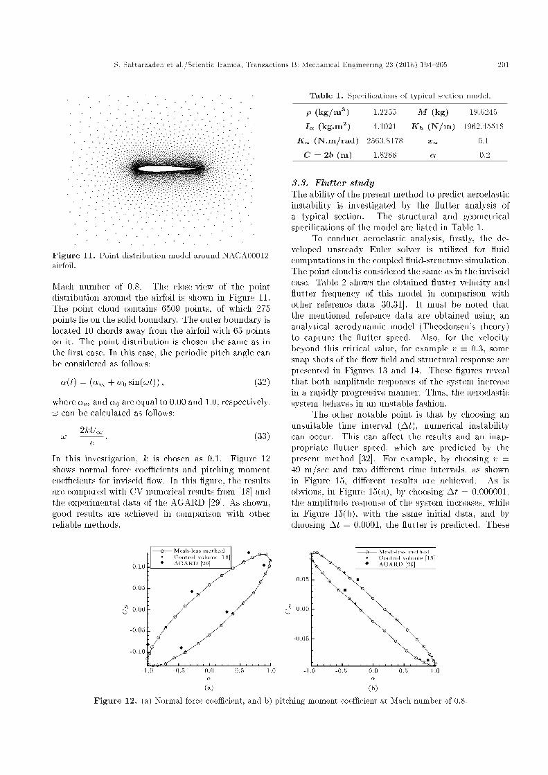
Figure 11. Point distribution model around NACA00012airfoil.

Mach number of 0.8. The close-view of the pointdistribution around the airfoil is shown in Figure 11.The point cloud contains 6509 points, of which 275points lie on the solid boundary. The outer boundary islocated 10 chords away from the airfoil with 65 pointson it. The point distribution is chosen the same as inthe �rst case. In this case, the periodic pitch angle canbe considered as follows:

�(t) = (�m + �0 sin(!t)) ; (32)

where �m and �0 are equal to 0.00 and 1.0, respectively.! can be calculated as follows:

! =2kU1c

: (33)

In this investigation, k is chosen as 0.1. Figure 12shows normal force coe�cients and pitching momentcoe�cients for inviscid ow. In this �gure, the resultsare compared with CV numerical results from [18] andthe experimental data of the AGARD [29]. As shown,good results are achieved in comparison with otherreliable methods.

Table 1. Speci�cations of typical section model.

� (kg/m3) 1.2255 M (kg) 19.6245

I� (kg.m2) 4.1021 Kh (N/m) 1962.45518

K� (N.m/rad) 2563.8178 x� 0.1

C = 2b (m) 1.8288 � -0.2

3.3. Flutter studyThe ability of the present method to predict aeroelasticinstability is investigated by the utter analysis ofa typical section. The structural and geometricalspeci�cations of the model are listed in Table 1.

To conduct aeroelastic analysis, �rstly, the de-veloped unsteady Euler solver is utilized for uidcomputations in the coupled uid-structure simulation.The point cloud is considered the same as in the inviscidcase. Table 2 shows the obtained utter velocity and utter frequency of this model in comparison withother reference data [30,31]. It must be noted thatthe mentioned reference data are obtained using ananalytical aerodynamic model (Theodorsen's theory)to capture the utter speed. Also, for the velocitybeyond this critical value, for example v = 0:3, somesnap shots of the ow �eld and structural response arepresented in Figures 13 and 14. These �gures revealthat both amplitude responses of the system increasein a rapidly progressive manner. Thus, the aeroelasticsystem behaves in an unstable fashion.

The other notable point is that by choosing anunsuitable time interval (�t), numerical instabilitycan occur. This can a�ect the results and an inap-propriate utter speed, which are predicted by thepresent method [32]. For example, by choosing v =49 m/sec and two di�erent time intervals, as shownin Figure 15, di�erent results are achieved. As isobvious, in Figure 15(a), by choosing �t = 0:000001,the amplitude response of the system increases, whilein Figure 15(b), with the same initial data, and bychoosing �t = 0:0001, the utter is predicted. These

Figure 12. (a) Normal force coe�cient, and b) pitching moment coe�cient at Mach number of 0.8.


Figure 13. A few snap shots of the ow �eld for v = 0:3 at (a) 1 min, (b) 2 min, (c) 3 min, (d) 4 min, (e) 4:30 min, and(f) 5 min.

Figure 14. (a) � vs. time, and (b) �h vs. time at v = 0:3.

Table 2. Flutter speed of typical section model.

Present result Ref. [30] Ref. [31]

Flutter velocity 49.164 m/sec 50.5968 m/sec 52.42 m/sec

Flutter frequency 96.345 rad/sec 100.19 rad/sec 104.34 rad/sec

results show that a proper time interval should bechosen to prevent numerical instability.

For investigation of the ability of the presentmethod to analyze aeroelasticity under a compress-ibility e�ect, especi�cally in the transonic regime,an aeroelastic analysis of the previous model, underdi�erent Mach numbers, is conducted, and the obtainedresults are shown in Figure 16. This �gure showsthat the present method, based on the Euler equation,

has good agreement with Ref. [4], and con�rms theacceptable accuracy of the presented mesh-less methodin aeroelastic computations. It must be noted that inRef. [4], Euler equations are applied using interpolationtechniques, such as kriging and Arti�cial Neural Net-works (ANN), to predict utter speed in the transonicregime.

For comparing the results of di�erent studies, the utter index (VF ) is de�ned as:


Figure 15. The e�ect of time interval on utter speed predicting at (a) �t = 0:000001, and (b) �t = 0:0001.

Figure 16. VF vs. Mach number.

VF =~up� (34)

Figure 16 shows that the utter index decreases withincreasing the Mach number until critical Mach num-ber. However, after this value, the utter indexincreases sharply with increasing Mach number. Thetransonic dip [33] can be seen in this �gure, which isbecause of the compressibility e�ects [34]. Also, theobtained results show that considering the viscosityin aeroelastic computations has little e�ect on thestability results if the ight Mach number is less thancritical. Thus, for this ight condition, the Eulerequation can be considered to overcome numericalcomplexity [9]. For higher Mach number, the N-S curvedi�erences become large because, in this region, theviscous e�ect cannot be neglected. In this zone, theviscosity can replace the position of the shock, whichhas an important role to play in separation of theboundary layer. Thus, the utter index can be a�ectedby boundary layer separation [34]. The di�erencesbetween the position of separations and shock wavesin Euler and N-S equations after Ma = 0.76 createsenormous variations between the two results.

4. Conclusions

In this paper, a numerical aeroelastic model for atypical section (two-dimensional wing) via a mesh-lessmodel is developed. For utilizing the time-marchingtechnique, a dual-time implicit time discretizationscheme was applied and the computational e�ciencywas enhanced by adopting accelerating techniques.The obtained results showed the validity of the devel-oped solver for the uid ow computations in compari-son with available data. In addition, it was found thatthe time of convergence in this method is better thanin the CV method. The ability of the method wasshown by simulating the unsteady ow solution aroundan oscillating NACA0012 airfoil. Also, the capability ofthe present method to conduct aeroelastic analysis wasshown using two di�erent test cases in subsonic andcompressible regimes (up to transonic regime). Theresults show the ability and accuracy of the presentmethod to perform transonic aeroelastic analysis. Also,it has been shown that the viscosity e�ect can beneglected in transonic aeroelastic analysis when the ight Mach number is less than critical. It was shownthat the choice of time interval has a signi�cant e�ecton the proper prediction of utter speed.

Nomenclature

u Velocity component in x directionv Velocity component in y directionU Relative velocity in x directionV Relative velocity in y directionun Normal velocityut Tangential velocityxt Nodal velocity in x directionyt Nodal velocity in y directionVv Nodal velocityP Pressure


E Total energydij Distance between points i and jaij Least square coe�cient in x directionbij Least square coe�cient in y directionD Arti�cial dissipationMa1 Mach number in far �eldRe1 Reynolds number in far �eldh Plunging motion�h Dimensionless form of hm Mass of the airfoilc Chord lengthk Reduced frequencyU1 Free-stream velocityVF Flutter indexS� Static mass unbalanceI� Mass moment of inertia about the

elastic centerKh plunge spring constantK� Pitch spring constantQh Lift forceQ� Aerodynamic pitching moment about

the elastic center~sij Unit vector between i and jS� Static mass unbalanceI� Mass moment of inertia about the

elastic center~u Dimensionless reduced velocityr� Dimensionless radius of gyration about

the elastic centerx� A scale of distance between the center

of gravity and the elastic centervij Pressure sensor shock at any edges (ij)

"(2) Local adaptive coe�cients in criticalzones

"(4) Local adaptive coe�cients innon-critical zones

!i Weighting factor� Pitching angle�m Mean angle�0 Oscillation amplitude! Frequency of the system� Non-dimensional mass Ratio of the speci�c heats!r Ratio of uncoupled natural frequencies!h Uncoupled plunge natural frequency!� Uncoupled pitch natural frequency� Densityr'j+1=2 The average of gradients of any

variable at midpoint

References

1. Garrick, I.E. and Reed, W.H. \Historical developmentof aircraft utter", Journal of Aircraft, 18(11), pp.897-912 (1981).

2. Edwards, J.W., Bennett, R.J. and Seidel, D. \Timemarching transonic utter solutions including angle ofattack e�ects", AIAA Journal, 20(11), pp. 899-906(1982).

3. Clark, R., Cox, D., Curtiss, H., Edwards, J., Hall,K., Peters, D., Scanlan, R., Simiu, E., Sisto, F.,Strganac, T. and Dowell, E.H., A Modern Course inAeroelasticity (Solid Mechanics and Its Applications),Springer, 4th Rev. Ed. (2004).

4. Timme, S., Rampurawala, A. and Badcock, K.J. \Ap-plying interpolation techniques to search for transonicaeroelastic instability: ANN vs kriging", The RAESAerodynamics Conference, Bristol, United Kindom(2010).

5. Mariem, J.B. and Hamdi, M.A. \A new boundary�nite element method for uid-structure interactionproblems", Int. J. for Numerical Methods in Engineer-ing, 24(9), pp. 1251-1267 (1987).

6. Wang, X. and Bathe, K.J. \Displacement/pressurebased mixed �nite element formulations for acoustic uid-structure interaction problems", Int. J. for Nu-merical Methods in Engineering, 40 (11), pp. 2001-2017 (1997).

7. Kousen, K.A. and Bendiksen, O.O. \Nonlinear aspectsof the transonic aeroelastic stability problem", Pre-sented at the AIAA/ASME/ASCE/AHS29th Struc-tures, Structural Dynamics, and Materials Confer-ence, Williamsburg, Virginia, DOI: 10.2514/6.1988-2306 (1988).

8. Lee, S. \Viscosity in uence on utter boundary andlimit cycle oscillation in transonic regime", Journal ofFluid Science and Technology, 3(1) pp. 195-206 (2008).

9. Kholodar, D.B., Dowell, E.H. and Thomas, J.P. \Limitcycle oscillations of a typical section airfoil in transonic ow", Journal of Aircraft, 41(5), pp. 1067-1072 (2004).

10. Thomas, J.P., Dowell, E.H. and Hall, K.C. \Nonlinearinviscid aerodynamic e�ects on transonic divergence, utter and limit cycle oscillations", AIAA Journal,40(4), pp. 638-646 (2002).

11. Thomas, J., Dowell, E. and Hall, K. \Modeling viscoustransonic limit-cycle oscillation behavior using a har-monic balance approach", Journal of Aircraft, 41(6),pp. 1266-1274 (2004).

12. Schwarz, J.B., Dowell, E.H. and Thomas, J.P. \Im-proved utter boundary prediction for an isolated two-degree-of freedom airfoil", Journal of Aircraft, 46(6),pp. 2069-2076 (2009).

13. Guruswamy, G.P. \Vertical ow computations onswept exible wings using Navier-Stokes equations",AIAA Journal, 28(12) pp. 2077-2133 (1990).


14. Aftosmis, M.J. \Solution adaptive Cartesian gridmethods for aerodynamic ows with complex geome-tries", von Karman Institute for Fluid Dynamics, 28thComputational Fluid Dynamics Lecture Series, 1997-02, Chauss�ee de Waterloo 72, B-1640 Rhode-Saint-Gen�ese, Belgium (1997).

15. Liu, G.R. and Gu, Y.T., An Introduction to Meshfree Methods and Their Programming, Springer, TheNetherlands (2005).

16. Katz, A. and Jameson, A. \A comparison of variousmeshless schemes within a uni�ed algorithm", 47thAIAA Aerospace Sciences Meeting and Exhibit, Or-lando, Florida, AIAA paper 2009-0596 (2009).

17. Jahangirian, A. and Hashemi, Y. \An e�cient implicitmesh-less method for compressible ow calculations",International Journal for Numerical Methods in Flu-ids, 67(6) pp. 754-770 (2011).

18. Jahangirian, A. and Hadidoolabi, M. \Unstructuredmoving grids for implicit calculation of unsteady com-pressible viscous ows", Int. J. for Num. Methods inFluids, 47(10-11) pp. 1107-1113 (2005).

19. Wang, G., SUN, Y. and YE, Z. \Gridless solutionmethod for two-dimensional unsteady ow", ChineseJournal of Aeronautics, 18(1), pp. 8-14 (2005).

20. Ortega, E., O~nate, E., Idelsohn, S. and Flores, R.\A meshless �nite point method for three-dimensionalanalysis of compressible ow problems involving mov-ing boundaries and adaptivity", Int. J. Numer. Meth.Fluids, 73(4) pp. 323-343 (2013).

21. Wang, H., Chen, H.Q. and Periaux, J. \A study ofgridless method with dynamic clouds of points forsolving unsteady CFD problems in aerodynamics", Int.J. Numer. Meth. Fluids, 64(1), pp. 98-118 (2010).

22. Hu, P., Kamakoti, R., Xue, L., Wang, Z. and Li,Q. \A meshless method for aeroelastic applicationsin ASTE-P toolset", AIAA Modeling and SimulationTechnologies Conference, Toronto, Canada (2010).

23. Wendland, H. \Spatial coupling in aeroelasticity bymesh-less kernel-based methods", European Confer-ence on Computational Fluid Dynamics ECCOMAS,(2006).

24. Sarigul-Klijn, N. \E�cient interfacing of uid andstructure for aeroelastic instability predictions", Int.J. for Num. Meth. in Eng., 47(1), pp. 705-728 (2000).

25. Lesoinne, M. and Kaila, V. \Meshless aeroelasticsimulations of aircraft with large control surface de ec-tions", AIAA paper 2005-1089, AIAA 43rd AerospaceSciences Meeting and Exhibit, Reno, NV (2005).

26. Sattarzadeh, S. and Jahangirian, A. \3D implicitmesh-less method for compressible ow calculations",Journal of Scientia Iranica, 19(3), pp. 503-512 (2012).

27. Katz, A. and Jameson, A. \Edge-based meshlessmethods for compressible ow simulations", 46thAIAA Aerospace Sciences Meeting and Exhibit, Reno,Nevada, AIAA Paper 2008-699 (2008).

28. Jameson, A. \Time dependent calculations usingmultigrid, with applications to unsteady ows pastairfoils and wings", AIAA Paper 91-1596, AIAA 10thComputational Fluid Dynamics Conference, Honolulu(1991).

29. AGARD Fluid Dynamics Panel \Compendium of Un-steady Aerodynamic Measurements", AGARD, R -702(1982).

30. \MSC/NASTRAN veri�cation problem manual", TheMaclean-Schwendler Corporation (1988).

31. Haddadpour, H. and Firouz-Abadi, R.D. \Evaluationof quasi-steady aerodynamic modeling for utter pre-diction of aircraft wings in incompressible ow", Thin-Walled Structures, 44(9), pp. 931-936 (2006).

32. Benini, G.R., Belo, E.M. and Marques, F.D. \Numer-ical model for the simulation of �xed wings aeroelasticresponse", J. Braz. Soc. Mech. Sci. & Eng., 26(2), pp.129-136 (2004).

33. Isogai, K. \Transonic-dip mechanism of utter of asweptback wing", AIAA Journal, 17(7), pp. 793-795(1979).

34. Pradeepa, T.K. and Venkatraman, K. \Shock-boundary layer interaction and transonic utter", Bul-letin of the American Physical Society, 65th AnnualMeeting of the APS Division of Fluid Dynamics, SanDiego, California, 57(17), pp. 22-28 (2012).

Biographies

Samad Sattarzadeh received his MS degree inAerospace Engineering from Amirkabir University ofTechnology (AUT), Tehran, Iran, where he is currently,a PhD degree student. His research interests includemesh-less methods.

Alireza Jahangirian received a BS degree in Mechan-ical Engineering from Amirkabir University of Tech-nology (AUT), Tehran, Iran, in 1988, his MS degreein Mechanical Engineering from Sharif University ofTechnology, Tehran, Iran, in 1992, and a PhD degreefrom Manchester University, England, in 1997. Heis currently Associate Professor in the Department ofAerospace Engineering at AUT. His research interestsinclude: computational uid dynamics, grid generationand evolutionary aerodynamic optimization.

Hossein Shahverdi received BS, MS and PhD degreesin Aerospace Engineering from Amirkabir Universityof Technology (AUT), Tehran, Iran, in 1997, 2000and 2006. He is currently Assistant Professor inthe Department of Aerospace Engineering at AUT.His research interests include aeroelasticity, structuraldynamics and structural analysis.

Aeroelastic analysis of a typical section using Euler and...

Documents

Transcript of Aeroelastic analysis of a typical section using Euler and...