
An integrated lot-sizing model for imperfect production...
16
Transcript of An integrated lot-sizing model for imperfect production...

Scientia Iranica E (2018) 25(2), 852{867
Sharif University of TechnologyScientia Iranica
Transactions E: Industrial Engineeringhttp://scientiairanica.sharif.edu
An integrated lot-sizing model for imperfect productionwith multiple disposals of defective items
Y.-L. Chenga;�, W.-T. Wanga, C.-C. Weia, and K.-L. Leeb
a. Department of Marketing and Distribution Management, Chien Hsin University of Science and Technology, Jungli 32097,Taiwan, R.O.C.
b. Department of Industrial Management, Chien Hsin University of Science and Technology, Jungli 32097, Taiwan, R.O.C.
Received 29 February 2016; received in revised form 5 November 2016; accepted 10 December 2016
KEYWORDSInventory;Integrated lot-sizingmodel;Defective items;Multiple disposals.
Abstract. In this study, an optimal integrated vendor-buyer inventory model withdefective items is proposed. Most researches on defective items assumed that an inspectionprocess was carried out by the buyer. We consider that the vendor conducts the inspectionprocess and disposes defective items in multiple batches. We prove that the function ofannual cost is convex, and obtain closed-form expressions. A solution procedure is used toderive the optimal order quantity, the number of shipments, and the number of defectiveitem disposals. Numerical examples are provided to illustrate our model. Setting thefraction of defective items to zero, the numerical examples indicate that the proposedmodel can result in the solutions to the existing models without considering defectiveitems. Moreover, a sensitivity analysis is used to reveal the e�ects of cost parameters onthe optimal solution. We show that when the disposal cost is relatively low, a multipledisposals strategy may perform better than a single disposal strategy.© 2018 Sharif University of Technology. All rights reserved.
1. Introduction
The problem of vendor-buyer integration is consideredas the foundational research topic in supply chain man-agement. The objective is to minimize the total systemcost or maximize the entire system pro�t. One of the�rst integrated inventory models consisting of singlevendor and single buyer was proposed by Goyal [1].Banerjee [2] modi�ed Goyal's [1] model considering a�nite production rate for the vendor who followed alot-for-lot shipment policy. Goyal [3] relaxed the lot-for-lot policy and proposed an integer multiple of equal-
*. Corresponding author. Tel.: +886-3-4581196;Fax: +886-3-2503032E-mail addresses: [email protected] (Y.-L. Cheng);[email protected] (W.-T. Wang);[email protected] (C.-C. Wei); [email protected] (K.-L.Lee)
doi: 10.24200/sci.2017.4414
size vendor production quantity shipments. Lu [4] thengeneralized Goyal's [3] model by relaxing the assump-tion that the supplier could supply the retailer aftercompleting a production batch. Goyal [5] developeda policy with which the shipment sizes increased bya �xed factor, which was equal to the productionrate divided by the demand rate. Hill [6] proposed ageneralized policy for shipment batches increasing by ageometric growth factor. Several researchers (e.g., [7-9]). proposed di�erent batching and shipping policiesfor the integrated inventory models.
Since then, many extensions have been madeto the basic integrated production inventory models.Huang [10] investigated the e�ect of quality on lotsizes for a single-vendor single-buyer inventory sys-tem. Nieuwenhuyse and Vandaele [11] proved thatlot splitting policies would bene�t both the supplierand the buyer. Ertogral et al. [12] developed anintegrated vendor-buyer model under equal-size ship-ment and added transportation cost to the model.

Y.-L. Cheng et al./Scientia Iranica, Transactions E: Industrial Engineering 25 (2018) 852{867 853
Lin [13] proposed an integrated single-vendor single-buyer inventory model with backorder price discountand variable lead time. Sajadieh et al. [14] discussedan integrated model where the demand was dependenton the amount of goods displayed on the shelf. Sari etal. [15] considered an integrated vendor-buyer problemwhere the supplier o�ered temporary price discountsto the buyer during a sale period. Readers are referredto Glock [16] for a comprehensive review of integratedsystems. Rad et al. [17] suggested a joint economiclot sizing model of a single-vendor single-buyer supplychain for items with imperfect quality and shortagesunder price-sensitive demand. Lee and Fu [18] ana-lyzed an integrated production and delivery quantitymodel in a make-to-order producer-buyer supply chain.Sarakhsi et al. [19] studied a joint economic lot-sizingproblem for a single-vendor single-buyer system wherethe demand was dependent on selling price. Somerecent works on integrated vendor-buyer models havebeen done by many researchers, such as Lin [20], Yi &Sarker [21], Wee & Widyadana [22], Ouyang et al. [23],Giri & Sharma [24], and Chung et al. [25].
Rosenblatt and Lee [26] was one of the �rstmodels to consider imperfect production inventorymodels. Salameh and Jaber [27] presented a classiceconomic order quantity model in which the order lotcontained a random proportion of imperfect qualityitems. Many extensions and modi�cations regardingquality issues have been researched recently. Weeet al. [28] and Eroglu and Ozdemir [29] extendedSalameh and Jaber's [27] inventory model to considershortages with complete backorders. Subsequently,Chang and Ho [30] revisited the inventory modelof Wee et al. [28] and derived closed-form optimalsolutions by applying Renewal Reward Theory. Hsuand Yu [31] studied a one-time-only discount policyfor an economic order quantity model that consideredimperfect quality items. Maddah et al. [32] presentedan approach to avoid shortages during the screeningperiod. Khan et al. [33] provided a detailed andcomplete review for economic order quantity modelswith imperfect quality items. Chang et al. [34] andYassine et al. [35] developed an economic productionquantity model for imperfect quality items. Rezaeiand Davoodi [36,37] provided inventory models thatconsidered supplier selection and imperfect quality.Moussawi-Haidar et al. [38] and Rezaei [39] investigatedeconomic order quantity models where imperfect itemswere screened with sampling inspection plans. Hsuand Hsu [40] provided economic production quantitymodels to determine the optimal lot size and backorderquantity under imperfect productions. Taleizadehet al. [41] proposed an extension to economic orderquantity model with partial backordering and repara-ble products. Some other recent inventory modelsthat considered imperfect quality items are Wahab et
al. [42], Sarkar [43], Hsu & Hsu [44], Chang [45], Jaberet al. [46], Rezaei & Salimi [47], and Taleizadeh etal. [48].
This paper extends Salameh and Jaber [27] modelto an integrated production inventory model withdefective items. We assume that the integrated policyfor the proposed model is accepted by the vendorand the buyer. To maintain a long-term cooperation,the vendor would deliver 100% good products to thebuyer. In addition, as shown in Rezaei and Salimi [47],conducting the inspection process by the buyer maynot be a cost-e�cient strategy. We investigate thatthe products are screened by the vendor while someliterature such as Huang [10] and Wu et al. [49]assumed that the buyer conducted inspection processwhenever receiving products. We relax the assumptionof defective items removed from stock after screeningto allow the defective items be scrapped by multipledisposals during the production period.
The paper is organized into �ve sections. Sec-tion 1 provided an introduction. The notation andassumptions for this study are stated in Section 2. Themodel description, formulation, and solution procedureare presented in Section 3. Section 4 provides thenumerical examples to illustrate the solution procedurefor determining the optimum. Conclusions and sugges-tions for future research are given in Section 5.
2. Notation and assumptions
We summarize the notation used in this study asfollows:T Order cycle timeP Annual constant production rateD Annual constant demand rateQ Lot size of good quality items per
shipment (decision variable)n Number of good quality items
shipments per order cycle (decisionvariable)
nM Number of defective item disposalsover a production period (decisionvariable)
� Random fraction of defective items,a random variable with a knownprobability density function; 0 � � < 1
SV Fixed production setup cost perproduction batch
SB Fixed ordering cost per orderhV Stock-holding cost for the vendor per
unit per yearhB Stock-holding cost for the buyer per
unit per year

854 Y.-L. Cheng et al./Scientia Iranica, Transactions E: Industrial Engineering 25 (2018) 852{867
u Fixed cost of each disposal for defectiveitems
g Fixed cost of each shipment for goodquality items
TCM (n;Q) Annual total relevant inventory costfor the vendor
TCR(n;Q) annual total relevant inventory cost forthe buyer
TC(N;Q) Annual total relevant inventory costfor both parties
We make the following assumptions for this study:
1. Consider single vendor and single buyer;2. The demand rate is known and �nite;3. The production rate is known and �nite;4. All products are 100% inspected by the vendor.
We assume that the inspection is included in pro-duction process. The vendor conducts multipledisposals of the defective items without salvagevalue;
5. The good items are delivered to the buyer while thedefective ones are disposed from the vendor's stock.Thus, to meet the demand, it is constrained by: (1��)P > D, i.e. P > D
1�� (Taking the expectation, ityields P > E( 1
1�� )D);6. The cost for facilitating multiple deliveries is the
responsibility of the buyer;7. We assume that the buyer's holding cost is greater
than the vendor's holding cost, i.e. hB > hV ;8. Shortages are not allowed.
3. Model formulation
We consider a single-vendor single-buyer integratedmodel where the buyer's order quantity is manufac-tured and delivered in multiple equal-batch shipments.From the buyer's order quantity, the vendor plans theirproduction batch and conducts the inspection process.During the production run, the defective items arescrapped by multiple disposals from the stock. Thedisposal cost for the defective items is paid by thevendor. The good quality products are spited intosmall lot sizes that are delivered to the buyer over aninventory cycle. The buyer incurs the shipment cost inthe multiple deliveries.
Figure 1 depicts the behavior of inventory levelsfor the vendor and the buyer. Since the fraction ofdefective items is � (or the fraction of good qualityitems is 1 � �), the vendor would produce nQ
1�� unitsto meet the demand of nQ units during an ordercycle. The vendor delivers good items to the buyerwho receives n shipments with each lot size Q. Sincethe demand rate is D, the shipment interval is Q
D
Figure 1. Vendor's and buyer's inventory levels withn = 8 and nM = 3.
and the order cycle is nQD . During the production
period, the nQ�1�� defective item units are scrapped with
multiple disposals (or removals). Since the number ofthe disposals per cycle is nM , the defective items unitin each disposal is nQ�
nM (1��) .The total relevant inventory cost for an integrated
inventory system includes the inventory costs from thevendor and the buyer. The vendor's cost comprisessetup cost, holding cost, and disposal costs. Thebuyer's cost consists of ordering cost, holding cost,and shipment costs. Our purpose is to minimize theannual total relevant inventory cost for both parties,which contains the annual vendor's and buyer's costs.Subsequently, we derive di�erent inventory costs for thevendor and the buyer.
3.1. Vendor's inventory holding cost:Figure 2 shows that the vendor's holding inventory(time-weighted inventory) per order cycle can be de-rived by subtracting the shaded area from the boldarea. The bold area includes the areas above intervalT1 and above interval T2. Referring to Figure 2, wehave:
T1 =nQ
(1� �)P; (1)
T2 =nQD� nQ
(1� �)P��QD� Q
(1� �)P
�= (n� 1)Q
�1D� 1
(1� �)P
�: (2)
The bold area is derived as:

Y.-L. Cheng et al./Scientia Iranica, Transactions E: Industrial Engineering 25 (2018) 852{867 855
Eq:(5)T
hV =nQ2
2D
h(n� 1) + 2D
P (1��) � nDP (1��) + nD
nMP
�1
(1��)2 � 1(1��)
�inQD
hV
=Q2
"(n� 1) +
2DP (1� �)
� nDP (1� �)
+nDnMP
1
(1� �)2 � 1(1� �)
!#hV : (6)
Box I
Figure 2. Vendor's accumulated inventory and buyer'saccumulated inventory with n = 8 and nM = 3.
12T1
nM
nMXi=1
��(i� 1)
T1
nMP � (i� 1)
T1
nMP��
+�iT1
nMP � (i� 1)
T1
nMP���
+ nQT2
=n2Q2 (nM (1� �) + �)
2(1� �)2nMP
+ n (n� 1)Q2�
1D� 1
(1� �)P
�: (3)
Subsequently, the shaded area is calculated from:
QDfQ+ 2Q+ 3Q+ � � �+ (n� 1)Qg =
QD
n�1Xi=1
iQ
!=n (n� 1)Q2
2D: (4)
Subtracting shades area, Eq. (4), from bold area,
Eq. (3), we yield the vendor's holding inventory perorder cycle as:
n2Q2 (nM (1��)+�)2(1� �)2nMP
+n (n�1)Q2�
1D� 1
(1� �)P
�
�n (n� 1)Q2
2D=nQ2
2D
�(n� 1) +
2DP (1� �)
� nDP (1� �)
+nDnMP
1
(1� �)2 � 1(1� �)
!�:(5)
Thus, we can obtain the vendor's inventory holding costper year as shown in Box I.
3.2. Vendor's setup costSince the vendor has one production per cycle time andthe setup cost per production is sV , the vendor's setupcost per year is:
sVnQ=D
=DnQ
sV : (7)
3.3. Vendor's disposal costThe number of disposals of the defective items is nM ,the cost per disposal is u, and the cycle time is nQ=D.Therefore, the disposal cost per year is:
nMunQ=D
=nMDnQ
u: (8)
Summing costs in Eqs. (6) to (8), we derive the annualtotal relevant inventory cost for the vendor:
TCM (Q;n; nM ) =Q2
�(n� 1) +
2DP (1� �)
� nDP (1� �)
+nDnMP
1
(1� �)2� 1(1� �)
!�hV
+DnQ
sV +nMDnQ
u: (9)
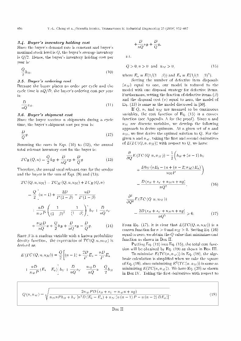
856 Y.-L. Cheng et al./Scientia Iranica, Transactions E: Industrial Engineering 25 (2018) 852{867
3.4. Buyer's inventory holding costSince the buyer's demand rate is constant and buyer'smaximal stock level is Q, the buyer's average inventoryis Q=2. Hence, the buyer's inventory holding cost peryear is:
Q2hB : (10)
3.5. Buyer's ordering costBecause the buyer places an order per cycle and thecycle time is nQ=D, the buyer's ordering cost per yearis:
DnQ
sB : (11)
3.6. Buyer's shipment costSince the buyer receives n shipments during a cycletime, the buyer's shipment cost per year is:
DQg: (12)
Summing the costs in Eqs. (10) to (12), the annualtotal relevant inventory cost for the buyer is:
TCR (Q;n) =Q2hB +
DnQ
sB +DQg: (13)
Therefore, the annual total relevant cost for the vendorand the buyer is the sum of Eqs. (9) and (13):
TC (Q;n; nM ) = TCM (Q;n; nM ) + TCR (Q;n)
=Q2
�(n� 1) +
2DP (1� �)
� nDP (1� �)
+nDnMP
1
(1� �)2 � 1(1� �)
!�hV +
DnQ
sV
+nMDnQ
u+Q2hB +
DnQ
sB +DQg: (14)
Since � is a random variable with a known probabilitydensity function, the expectation of TC(Q;n;mM ) isderived as:
E (TC (Q;n; nM )) =Q2
�(n� 1) +
2DPEa � nD
PEa
+nDnMP
(Eb � Ea)�hV +
DnQ
sV +nMDnQ
u+Q2hB
+DnQ
sB +DQg;
s.t.
Q > 0; n > 0 and nM > 0; (15)
where Ea = E(1=(1� �)) and Eb = E(1=(1� �)2).Setting the number of defective item disposals
(nM ) equal to one, our model is reduced to themodel with one disposal strategy for defective items.Furthermore, setting the fraction of defective items (�)and the disposal cost (u) equal to zero, the model ofEq. (15) is same as the model discussed in [50].
If Q, n, and nM are assumed to be continuousvariables, the cost function of Eq. (15) is a convexfunction (see Appendix A for the proof). Since n andnM are discrete variables, we develop the followingapproach to derive optimum. At a given set of n andnM , we �rst derive the optimal solution to Q. For thegiven n and nM , taking the �rst and second derivativesof E(TC(Q;n; nM )) with respect to Q, we have:
@@Q
E (TC (Q jn; nM )) =12
�hB + (n� 1)hV
+DhV (nEb � (n+ (n� 2)nM )Ea)
nMP
�� D (sB + sV + nMu+ ng)
nQ2 ; (16)
@2
@Q2E (TC (Q jn; nM ))
=2D (sB + sV + nMu+ ng)
nQ3 > 0: (17)
From Eq. (17), it is clear that E(TC(Q;n; nM )) is aconvex function for n > 0 and nM > 0. Setting Eq. (16)equal to zero, we obtain theQ value that minimizes costfunction as shown in Box II.
Putting Eq. (18) into Eq. (15), the total cost func-tion will be obtained by Eq. (19) as shown in Box III.
To minimize E(TC(n; nM )) in Eq. (19), the alge-braic calculation is simpli�ed when we take the squareof Eq. (19), since minimizing E2(TC(n; nM )) is same asminimizing E(TC(n; nM )). We have Eq. (20) as shownin Box IV. Taking the �rst derivatives with respect to
Q (n; nM ) =
s2nMPD (sB + sV + nMu+ ng)
nMnPhB + hV [n2D (Eb � Ea) + nM (n (n� 1)P � n (n� 2)DEa)]: (18)
Box II

Y.-L. Cheng et al./Scientia Iranica, Transactions E: Industrial Engineering 25 (2018) 852{867 857
E (TC (n; nM ))=np2pnMnPhB+hV (n2D (Eb�Ea)+nM (n (n�1)P�n (n�2)DEa))�pnMPD (sB+sV +nMu+ng)
onMnP
:(19)
Box III
E2 (TC (n; nM )) =�2 [nMPhB + hV (nD (Eb � Ea) + nM ((n� 1)P � (n� 2)DEa))]� [D (sB + sV + nMu+ ng)]
nMnP
: (20)
Box IV
n and nM , we get:
@@n
E2 (TC (n; nM )) = 2DghV
�2D2ghV ((nM + 1)Ea � Eb)nMP
�2D (2DEahV + P (hB � hV ))(sB + sV + nMu)n2P
;(21)
@@nM
E2 (TC (n; nM )) =
2Du (P (hB + (n� 1)hV )� (n� 2)DEahV )nP
�2D2 (Eb � Ea) (sB + sV + ng)hVn2MP
: (22)
Let n# and n#M be the solutions to @
@nE2(TC(n;
nM )) = 0 and @@nM E
2(TC(n; nM )) = 0, respectively;we have:
n# =vuuutn#M (2DEahV + P (hB � hV ))
�sB + sV + n#
Mu�
ghV�D (Eb � Ea) + n#
M (P �DEa)� ;
(23)
n#M =s
n#DhV (Eb � Ea) (sB + sV + n#g)u (PhB + hV ((n# � 1)P � (n# � 2)DEa))
: (24)
We can employ numerical search methods to solve
Eqs. (23) and (24). Alternatively, applying mathemat-ical software such as Mathematica or Maple, we derivethe following closed-form expressions of n#
M and n#.Substituting n# in Eq. (24) into Eq. (23) yields:
n#M =
sD (Eb � Ea) (sB + sV )
(P �DEa)u> 0: (25)
It can be seen that n#M decreases as u increases.
Subsequently, substituting n#M in Eq. (25) into Eq. (23)
gives:
n# =
s(2DEahV + P (hB � hV )) (sB + sV )
(P �DEa) ghV> 0:
(26)
In Appendix B, we prove the convexity of E2(TC(n; nM )). It implies that E(TC(n; nM )) is also aconvex function because E2(TC(n; nM )) is derivedfrom E(TC(n; nM )). We demonstrate that n#
M andn# are, respectively, equal to n�MC in Eq. (A.7) and n�Cin Eq. (A.10) since E(TC(n; nM )) is the cost functionwith the optimal Q shown in Eq. (18). Due to theassumptions of hB > hV and P �DEa > 0, Eqs. (25)and (26) show that n# and n#
M are positive numbersminimizing E2(TC(n; nM )) and E(TC(n; nM )).
Since the optimal n and nM should be integers,although n# and n#
M are positive and not alwaysinteger numbers, optimal n and nM values should bethe integers around n# and n#
M . Let n#�(n#�M ) and
n#+(n#+M ), respectively, denote the minimal integers
less than and greater than n#(n#M ). Note that if
n#(n#M ) is less than one, we let n#� = n#+ = 1
(n#�M = n#+
M = 1) because zero is not feasible.Let (n�; n�M ) be the optimal integer solution
to E(TC(n; nM )). If E(TC(n; nM )) in Eq. (19) is

858 Y.-L. Cheng et al./Scientia Iranica, Transactions E: Industrial Engineering 25 (2018) 852{867
minimized, we have:
E (TC (n�; n�M )) = Min�E�TC
�n#�; n#�
M
��;
E�TC
�n#�; n#+
M
��; E�TC
�n#+; n#�
M
��;
E�TC
�n#+; n#+
M
���; (27)
where:
(n�; n�M ) 2��
n#�; n#�M
�;�n#�; n#+
M
�;�
n#+; n#�M
�;�n#+; n#+
M
��:
Substituting (n�; n�M ) for (n; nM ) in Eq. (18), theoptimal shipment quantity is derived by Eq. (28) asshown in Box V.
The following solution procedure is provided toderive the optimal solution.
1. Compute n#M and n# from Eqs. (25) and (26),
respectively. The values of n#�, n#+, n#�M , and
n#+M are obtained. If n#
M (n#) is less than one, thenn#�M = n#+
M = 1 (n#� = n#+ = 1);
2. Derive the optimal solution to (n; nM ):
(n�; n�M ) 2��
n#�; n#�M
�;�n#�; n#+
M
�;
�n#+; n#�
M
�;�n#+; n#+
M
��;
which results in the lowest cost decided fromEq. (27);
3. From Eq. (18) or (28), the optimal shipment quan-tity is derived, i.e. Q� = Q(n�; n�M ).
4. Numerical example
To illustrate the proposed model, we provide thefollowing examples:
Example 1. The imperfect fraction in each pro-
duction batch follows a uniform distribution with thefollowing probability density function:
f(�) =
(25; 0 � � � 0:04;0; otherwise
The parameter values are as follows:
� Production rate: P = 48; 000 (unit/year)� Demand rate: D = 12; 000 (unit/year)� Vendor's setup cost: SV = 500 ($/setup)� Vendor's holding cost: hV = 10 ($/unit/year)� Vendor's disposal cost: u = 50 ($/disposal)� Buyer's order cost: SB = 25 ($/order)� Buyer's holding cost: hB = 12 ($/unit/year)� Buyer's shipment cost: g = 25 ($/shipment)
Compute the expectation values:
Ea = E�
11� �
�= 1:0206;
Eb = E
1
(1� �)2
!= 1:0417:
In Figure 3, we �rst illustrate that Eq. (19) isa convex function. The optimal solutions are derivedthrough the following procedures.
Figure 3. The graphic diagram for the integrated totalrelevant cost in Example 1.
Q (n�; n�M ) =
s2n�MPD (sB + sV + n�Mu+ n�g)
n�Mn�PhB + hV�n�2D (Eb � Ea) + n�M (n� (n� � 1)P � n� (n� � 2)DEa)
� : (28)
Box V
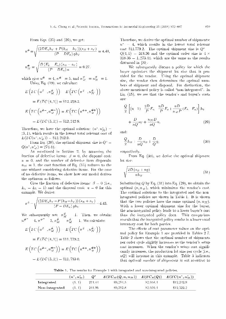
Y.-L. Cheng et al./Scientia Iranica, Transactions E: Industrial Engineering 25 (2018) 852{867 859
From Eqs. (25) and (26), we get:
n# =
s(2DEahV + P (hB � hV ))(sB + sV )
(P �DEa) ghV= 4:48;
n#M =
sD (Eb � Ea) (sB + sV )
(P �DEa)u= 0:27;
which give n#� = 4, n#+= 5, and n#�
M = n#+M = 1.
Using Eq. (19), we calculate:
E�TC
�n#�; n#�
M
��= E
�TC
�n#�; n#+
M
��= E (TC (4; 1)) = $12; 259:2;
E�TC
�n#+; n#�
M
��= E
�TC
�n#+; n#+
M
��= E (TC (5; 1)) = $12; 242:9:
Therefore, we have the optimal solution: (n�; n�M ) =(5; 1), which results in the lowest total relevant cost ofE(TC(n�; n�M )) = $12; 242:9.
From Eq. (28), the optimal shipment size is Q� =Q(n�; n�M ) = 274:44.
As mentioned in Section 2, by assuming thefraction of defective items: � = 0, the disposal cost:u = 0, and the number of defective item disposals:nM = 1, the cost function of Eq. (15) reduces to theone without considering defective items. For the caseof no defective items, we show how our model derivesthe optimum as follows.
Give the fraction of defective items: � = 0 (i.e.,Ea = Eb = 1) and the disposal cost: u = 0 for thisexample. We derive:
n# =
s(2DEahV +P (hB�hV )) (sB + sV )
(P �DEa) ghV=4:43:
We subsequently set: n#M = 1. Then, we obtain:
n#� = 4, n#+= 5, n#�
M = n#+
M = 1. We calculate:
E�TC
�n#�; n#�
M
��= E
�TC
�n#�; n#+
M
��= E (TC (4; 1)) = $11; 779:2;
E�TC
�n#+; n#�
M
��= E
�TC
�n#+; n#+
M
��= E (TC (5; 1)) = $11; 783:0:
Therefore, we derive the optimal number of shipments:n� = 4, which results in the lowest total relevantcost $11,779.2. The optimal shipment size is Q� =Q(4; 1) = 318:36 and the optimal order size is 4 �318:36 = 1; 273:44, which are the same as the resultsdiscussed in [50].
We subsequently discuss a policy for which thebuyer optimizes the shipment lot size that is pro-vided for the vendor. Using the optimal shipmentsize, the vendor then determines the optimal num-bers of shipment and disposal. For distinction, theabove-mentioned policy is called \non-integrated". InEq. (15), we see that the vendor's and buyer's costsare:
Q2
�(n�1)+
2DPEa�nDP Ea+
nDnMP
(Eb�Ea)�hV
+DnQ
sV +nMDnQ
u; (29)
and:
Q2hB +
DnQ
sB +DQg; (30)
respectively.From Eq. (30), we derive the optimal shipment
lot size:s2D (sB + ng)
nhB: (31)
Substituting Q by Eq. (31) into Eq. (29), we obtain theoptimal (n; nM ), which minimizes the vendor's cost.The optimal solutions to the integrated and the non-integrated policies are shown in Table 1. It is shownthat the two policies have the same optimal (n; nM ).With a lower optimal shipment size for the buyer,the non-integrated policy leads to a lower buyer's costthan the integrated policy does. This comparisonreveals that the integrated policy results in a lower totalinventory cost for both parties.
The e�ects of cost parameter values on the opti-mal policy for Example 1 are provided in Tables 2-7.Table 2 shows that the optimal number of shipmentsper order cycle slightly increases as the vendor's setupcost increases. When the vendor's setup cost signi�-cantly increases, the production lot size per cycle (i.e.,nQ) will increase in this example. Table 3 indicatesthat optimal number of shipments is not sensitive to
Table 1. The results for Example 1 with integrated and non-integrated policies.
(n�; n�M) Q� E(TCM(Q;n; nM)) E(TCR(Q)) E(TC(n�; n�M))
Integrated (5, 1) 274.44 $9,284.5 $2,958.4 $12,242.9Non-integrated (5, 1) 244.95 $9,382.8 $2,939.4 $12,322.2

860 Y.-L. Cheng et al./Scientia Iranica, Transactions E: Industrial Engineering 25 (2018) 852{867
Table 2. The optimal solutions for Example 1 with di�erent SV values.
P = 48; 000, D = 12; 000, hV = 10, u = 50, SB = 25, hB = 12, g = 25Vendor's setup cost (SV ) 300 400 500 600 700
(n�; n�M ) (4,1) (4,1) (5, 1) (5, 1) (5,1)Q� 277.13 304.91 274.44 293.39 311.19
E(TC(n�; n�M )) 10283.9 $11,314.8 $12,242.9 $13,088.2 $13,882.2
Table 3. The optimal solutions for Example 1 with di�erent SB values.
P = 48; 000, D = 12; 000, hV = 10, u = 50, SB = 25, hB = 12, g = 25Buyer's order cost (SB) 15 20 25 30 35
(n�; n�M ) (5, 1) (5, 1) (5, 1) (5, 1) (5, 1)Q� 272.48 273.46 274.44 275.42 276.40
E(TC(n�; n�M )) $12,155.2 $12,199.1 $12,242.9 $12,286.6 $12,330.1
Table 4. The optimal solutions for Example 1 with di�erent hV values.
P = 48; 000, D = 12; 000, u = 50, SV = 500, SB = 25 hB = 12, g = 25Vendor's holding cost (hV ) 8 9 10 11 12
(n�; n�M ) (6, 1) (5, 1) (5, 1) (4, 1) (4, 1)Q� 256.47 285.06 274.44 319.72 310.05
E(TC(n�; n�M )) $11,307.4 $11,786.9 $12,242.9 $12,667.2 $13,062.4
Table 5. The optimal solutions for Example 1 with di�erent hB values.
P = 48; 000, D = 12; 000, u = 50, hV = 10, u = 50, SV = 500 SB = 25, g = 25Buyer's holding cost (hB) 10 11 12 13 14
(n�; n�M ) (4, 1) (4, 1) (5, 1) (5, 1) (5, 1)Q� 339.64 334.91 274.44 271.42 268.49
E(TC(n�; n�M )) $11,924.3 $12,092.9 $12,242.9 $12,379.4 $12,514.4
Table 6. The optimal solutions for Example 1 with di�erent u values.
P = 48; 000, D = 12; 000, hV = 10, SV = 500 SB = 25, hB = 12, g = 25Vendor's disposal cost (u) 0.1 1 50 100 200
(n�; n�M ) (5, 6) (5, 2) (5, 1) (5, 1) (5, 1)Q� 265.24 265.26 274.44 284.08 302.42
E(TC(n�; n�M )) $11,773.9 $11,798.2 $12,242.9 $12,672.6 $13,491.0
Table 7. The optimal solutions for Example 1 with di�erent g values.
P = 48; 000, D = 12; 000, hV = 10, u = 50, SV = 500 SB = 25, hB = 12Buyer's shipment cost (g) 5 15 25 35 45
(n�; n�M ) (10, 1) (6, 1) (5, 1) (4, 1) (4, 1)Q� 135.15 225.93 274.44 340.01 349.39
E(TC(n�; n�M )) $11,098.4 $11,773.5 $12,242.9 $12,617.3 $12,965.4
the buyer's ordering cost. It is obvious that the optimalnumber of shipments will increase when the buyer'sordering cost (the vendor's setup cost) increases. InTable 4, one can see that a larger vendor's holdingcost results in a smaller optimal number of shipments.
Table 5 reveals that the buyer would like a largernumber of shipments when the buyer's holding costis larger. From Table 6, it can be seen that whenthe disposal cost is low, the vendor will bene�t fromincreasing the number of disposals. Table 7 concludes

Y.-L. Cheng et al./Scientia Iranica, Transactions E: Industrial Engineering 25 (2018) 852{867 861
that the optimal number of shipments decreases as thebuyer's shipment cost increases.
Example 2. The imperfect fraction in each produc-tion batch is same as that in Example 1. The parametervalues are as follows:
� Production rate: P = 3; 200 (unit/year)
� Demand rate: D = 1; 000 (unit/year)
� Vendor's setup cost: SV = 400 ($/setup)
� Vendor's holding cost: hV = 4 ($/unit/year)
� Vendor's disposal cost: u = 14 ($/disposal)
� Buyer's order cost: SB = 0 ($/order)
� Buyer's holding cost: hB = 5 ($/unit/year)
� Buyer's shipment cost: g = 25 ($/shipment)
We have Ea = 1:0206 and Eb = 1:0417, like thosein Example 1.
From Eqs. (25) and (26), we obtain: n# = 4:57and n#
M = 1:97, which give n#� = 4, n#+= 5, n#�
M =1, and n#+
M = 2.From Eq. (19), we calculate:
E�TC
�n#�; n#�
M
��= E (TC (4; 1)) = $1; 909:4;
E�TC
�n#�; n#+
M
��= E (TC (4; 2)) = $1; 907:8;
E�TC
�n#+; n#�
M
��= E (TC (5; 1)) = $1; 908:1;
E�TC
�n#+; n#+
M
��= E (TC (5; 2)) = $1; 906:3:
Therefore, we derive the optimal solution: (n�; n�M ) =(5; 2), which results in the lowest total relevant costof E(TC(n�; n�M )) = $1; 906:3. From Eq. (28), theoptimal shipment size is derived as: Q� = Q(n�; n�M ) =110:58.
We subsequently consider this example withoutdefective items. Setting the fraction of defective items:� = 0 (i.e., Ea = Eb = 1) and the disposal cost: u = 0,we derive:
n# =
s(2DEahV +P (hB�hV )) (sB+sV )
(P�DEa) ghV=4:51:
Set n#M = 1. Therefore, we have: n#� = 4, n#+
=5, n#�
M n#+M = 1. Then, we calculate:
E�TC
�n#�; n#�
M
��= E
�TC
�n#�; n#+
M
��= E (TC (4; 1)) = $1; 903:94;
E�TC
�n#+; n#�
M
��= E
�TC
�n#+; n#+
M
��= E (TC (5; 1)) = $1; 903:29:
The optimal number of shipments, which results in thelowest total relevant cost $1,903.29, is n� = 5. Theoptimal shipment size is Q� = Q(5; 1) = 110:34 andthe optimal order size is 5 � 110:34 = 551:70. Ourresult is same as the result using the equal-size batchpolicy in Hill [7].
5. Conclusions
This study presents an integrated vendor-buyer in-ventory model with defective items. While someliterature assumed products screened by the buyerand defective items removed after inspection process,our proposed model considered the vendor responsibleto conduct quality inspection. A random fractionof defective items was produced by the vendor whoimplemented a 100% inspection to screen the defectiveunits, which were scrapped by multiple disposals duringthe screening period. The multiple disposals strategyprovides the vendor with a exible treatment to scrapdefective items. To minimize the integrated cost,the mathematical model was formulated to derive theclosed-form optimal solutions to the order quantity, thenumber of shipments, and the number of defective itemdisposals. We proved that the function of annual costwas convex. The examples illustrated the solution pro-cedure and compared our results with related modelsin the literature. The sensitivity analysis was providedto show how the cost parameters a�ected the optimalsolution. If the disposal cost is relatively low, it may bebetter to scrap defective items by the multiple disposalsstrategy.
Future research directions are open to considerunequal-size shipment policies and to incorporatequantity discount or return policy. Moreover, our studycan be extended to models in which the screening rateis di�erent from the production rate, and the defectiveitems are reworked during the same production cycle.
References
1. Goyal, S.K. \An integrated inventory model for asingle supplier-single customer problem", InternationalJournal of Production Research, 14, pp. 107-111(1976).
2. Banerjee, A. \A joint economic-lot-size model forpurchaser and vendor", Decision Science, 17, pp. 292-311 (1986).
3. Goyal, S.K. \A joint economic-lot-size model for pur-chaser and vendor: a comment", Decision Science, 19,pp. 236-241 (1988).

862 Y.-L. Cheng et al./Scientia Iranica, Transactions E: Industrial Engineering 25 (2018) 852{867
4. Lu, L. \A one-vendor multi-buyer integrated inventorymodel", European Journal of Operational Research,81, pp. 312-323 (1995).
5. Goyal, S.K. \A one vendor multi-buyer integratedinventory model: a comment", European Journal ofOperational Research, 82, pp. 209-210 (1995).
6. Hill, R.M. \The single-vendor single-buyer integratedproduction-inventory model with a generalized policy",European Journal of Operational Research, 97, pp.493-499 (1997).
7. Hill, R.M. \The optimal production and shipmentpolicy for the single-vendor single-buyer integratedproduction-inventory problem", International Journalof Production Research, 37, pp. 2463-2475 (1999).
8. Goyal, S.K. and Nebebe, F. \Determination of eco-nomic production-shipment policy for a single-vendor-single-buyer system", European Journal of OperationalResearch, 121, pp. 175-178 (2000).
9. Hill, R.M. and Omar, M. \Another look at the single-vendor single-buyer integrated inventory production-inventory problem", International Journal of Produc-tion Research, 44, pp. 791-800 (2006).
10. Huang, C.K. \An optimal policy for a single-vendorsingle-buyer integrated production-inventory problemwith process unreliability consideration", InternationalJournal of Production Economics, 91, pp. 91-98(2004).
11. Nieuwenhuyse, I.V. and Vandaele, N. \The impact ofdelivery lot splitting on delivery reliability in a two-stage supply chain", International Journal of Produc-tion Economics, 104, pp. 694-708 (2006).
12. Ertogral, K., Darwish, M., and Ben-Daya, M. \Pro-duction and shipment lot sizing in a vendor-buyer sup-ply chain with transportation cost", European Journalof Operational Research, 176, pp. 1592-1606 (2007).
13. Lin, Y.J. \An integrated vendor-buyer inventory modelwith backorder price discount and e�ective investmentto reduce ordering cost", Computers and IndustrialEngineering, 56, pp. 1597-1606 (2009).
14. Sajadieh, M.S., Thorstenson, A., and Jokar, M.R.A.\An integrated vendor-buyer model with stock-dependent demand", Transportation Research: Part E:Logistics and Transporation Review, 46(6), pp. 963-974(2010).
15. Sari, D.P., Rusdiansyah, A., and Huang, L. \Modelsof joint economic lot-sizing problem with time-basedtemporary price discounts", International Journal ofProduction Economics, 139, pp. 145-154 (2012).
16. Glock, C.H. \The joint economic lot size problem:A review", International Journal of Production Eco-nomics, 135(2), pp. 671-686 (2012).
17. Rad, M.A., Khoshalhan, F., and Glock, C.H. \Opti-mizing inventory and sales decisions in a two-stage sup-ply chain with imperfect production and backorders",Computers and Industrial Engineering, 74, pp. 219-227 (2014).
18. Lee, S.D. and Fu, Y.C. \Joint production and deliverylot sizing for a make-to-order producer-buyer supplychain with transportation cost", Transportation Re-search Part E: Logistics and Transportation Review,66, pp. 23-35 (2014).
19. Sarakhsi, M.K., Ghomi, S.F., and Karimi, B. \Jointeconomic lot-sizing problem for a two-stage supplychain with price-sensitive demand", Scientia Iranica.Transaction E, Industrial Engineering, 23(3), pp.1474-1487 (2016).
20. Lin, T.Y. \Coordination policy for a two-stage supplychain considering quantity discounts and overlappeddelivery with imperfect quality", Computers & Indus-trial Engineering, 66(1), pp. 53-62 (2013).
21. Yi, H. and Sarker, B.R. \An operational policy for anintegrated inventory system under consignment stockpolicy with controllable lead time and buyers' spacelimitation", Computers & Operations Research, 40,pp. 2632-2645 (2013).
22. Wee, H.M. and Widyadana, G.A. \Single-vendorsingle-buyer inventory model with discrete deliveryorder, random machine unavailability time and lostsales", International Journal of Production Economics,143(2), pp. 574-579 (2013).
23. Ouyang, L.-Y., Chen, L.-Y., and Yang, C.-T. \Impactsof collaborative investment and inspection policies onthe integrated inventory model with defective items",International Journal of Production Research, 51(19),pp. 5789-5802 (2013).
24. Giri, B.C. and Sharma, S. \Lot sizing and unequal-sized shipment policy for an integrated production-inventory system", International Journal of SystemsScience, 45(5), pp. 888-901 (2014).
25. Chung, K.J., Lin, T.Y., and Srivastava, H.M. \Analternative solution technique of the JIT lot-splittingmodel for supply chain management", Applied Math-ematics & Information Sciences, 9(2), pp. 583-591(2015).
26. Rosenblatt, M.J. and Lee, H.L. \Economic produc-tion cycles with imperfect production processes", IIETransactions, 18, pp. 48-55 (1986).
27. Salameh, M.K. and Jaber, M.Y. \Economic produc-tion quantity model for items with imperfect quality",International Journal of Production Economics, 64,pp. 59-64 (2000).
28. Wee, H.M., Yu, J., and Chen, M.C. \Optimal in-ventory model for items with imperfect quality andshortage backordering", Omega, 35, pp. 7-11 (2007).
29. Eroglu, A. and Ozdemir, G. \An economic orderquantity model with defective items and shortages",International Journal of Production Economics, 106,pp. 544-549 (2007).
30. Chang, H.C. and Ho, C.H. \Exact closed-form so-lutions for optimal inventory model for items withimperfect quality and shortage backordering", Omega,38(3-4), pp. 233-237 (2010).

Y.-L. Cheng et al./Scientia Iranica, Transactions E: Industrial Engineering 25 (2018) 852{867 863
31. Hsu, W.K.K. and Yu, H.F. \EOQ model for imper-fective items under a one-time-only discount", Omega,37(5), pp. 1018-1026 (2009).
32. Maddah, B., Salameh, M.K., and Moussawi, L. \Or-der overlapping: a practical approach for preventingshortages during screening", Computers and IndustrialEngineering, 58(4), pp. 691-695 (2010).
33. Khan, M., Jaber, M.Y., Gui�rida, A.L., andZolfaghari, S. \A review of the extensions of a modi�edEOQ model for imperfect quality items", Interna-tional Journal of Production Economics, 132, pp. 1-12(2011).
34. Chang, H.J., Su, R.H., Yang, C.T., and Weng, M.W.\An economic manufacturing quantity model for atwo-stage assembly system with imperfect processesand variable production rate", Computers & IndustrialEngineering, 63(1), pp. 285-293 (2012).
35. Yassine, A., Maddah, B., and Salameh, M. \Dis-aggregation and consolidation of imperfect qualityshipments in an extended EPQ model", InternationalJournal of Production Economics, 135, pp. 345-352(2012).
36. Rezaei, J. and Davoodi, M. \A deterministic, multi-item inventory model with supplier selection andimperfect quality", Applied Mathematical Modelling,32(10), pp. 2106-2116 (2008).
37. Rezaei, J. and Davoodi, M. \A joint pricing, lot-sizing,and supplier selection model", International Journal ofProduction Research, 50(16), pp. 4524-4542 (2012).
38. Moussawi-Haidar, L., Salameh, M., and Nasr, W. \Aninstantaneous replenishment model under the e�ectof a sampling policy for defective items", AppliedMathematical Modelling, 37(3), pp. 719-727 (2013).
39. Rezaei, J. \Economic order quantity and samplinginspection plans for imperfect items", Computers &Industrial Engineering, 96, pp. 1-7 (2016).
40. Hsu, L.F. and Hsu, J.T. \Economic production quan-tity (EPQ) models under an imperfect productionprocess with shortages backordered", InternationalJournal of Systems Science, 47(4), pp. 852-867 (2016).
41. Taleizadeh, A.A., Khanbaglo, M.P.S., and C�ardenas-Barr�on, L.E. \An EOQ inventory model with partialbackordering and reparation of imperfect products",International Journal of Production Economics, 182,pp. 418-434 (2016).
42. Wahab, M.I.M., Mamun, S.M.H., and Ongkunaruk, P.\EOQ models for a coordinated two-level internationalsupply chain considering imperfect items and environ-mental impact", International Journal of ProductionEconomics, 134(1), pp. 151-158 (2011).
43. Sarkar, B. \An EOQ model with delay in payments andstock dependent demand in the presence of imperfectproduction", Applied Mathematics and Computation,218(17), pp. 8295-8308 (2012).
44. Hsu, J.-T. and Hsu, L.-F. \An EOQ model withimperfect quality items, inspection errors, shortagebackordering, and sales returns", International Jour-
nal of Production Economics, 143(1), pp. 162-170(2013).
45. Chang, H.-C. \An economic production quantitymodel with consolidating shipments of imperfect qual-ity items: A note", International Journal of Produc-tion Economics, 144(2), pp. 507-509 (2013).
46. Jaber, M.Y., Zanoni, S., and Zavanella, L.E. \Eco-nomic order quantity models for imperfect items withbuy and repair options", International Journal ofProduction Economics, 155, pp. 126-131 (2014).
47. Rezaei, J. and Salimi, N. \Economic order quantityand purchasing price for items with imperfect qualitywhen inspection shifts from buyer to supplier", Inter-national Journal of Production Economics, 137(1), pp.11-18 (2012).
48. Taleizadeh, A.A., Kalantari, S.S., and Cardenas-Barron, L.E. \Determining optimal price, replenish-ment lot size and number of shipments for an EPQmodel with rework and multiple shipments", Journalof Industrial and Management Optimization, 11(4),pp. 1059-1071 (2015).
49. Wu, K.-S., Ouyang, L.-Y., and Ho, C.-H.\Integratedvendor-buyerinventory system with sublotsampling inspection policy and controllable leadtime", International Journal of Systems Science, 38,pp. 339-350 (2007).
50. Ha, D. and Kim, S.L. \Implementation of JIT purchas-ing: an integrated approach", Production Planningand Control, 8(2), pp. 152-157 (1997).
Appendix A
When Q, n, and nM are continuous variables, we provethat Eq. (15) is a convex function.
Taking the �rst partial derivatives of E(TC(Q;n; nM )) with respect to Q, n, and nM , we have:
@@Q
E (TC (Q;n; nM )) =12
�hB + (n� 1)hV
+DhV (nEb � (n+ (n� 2)nM )Ea)
nMP
�� D (sB + sV + nMu+ ng)
nQ2 ; (A.1)
@@n
E (TC (Q;n; nM )) =Q2
�hV
� DhV ((nM + 1)Ea � Eb)nMP
�� D (sB + sV + nMu)
n2Q; (A.2)
@@nM
E (TC (Q;n; nM )) =DunQ�nQD (Eb�Ea)hV
2n2MP
:(A.3)

864 Y.-L. Cheng et al./Scientia Iranica, Transactions E: Industrial Engineering 25 (2018) 852{867
Q�C =
s2n�MCPD (sB + sV + n�MCu+ n�Cg)
n�Cn�MCPhB + hV�n�C2D (Eb � Ea) + n�MC (n�C (n�C � 1)P � n�C (n�C � 2)DEa)
� : (A.4)
n�C =1Q�C
s2n�MCPD (sB+sV +n�MCu)
hV [D (Eb � Ea)+n�MC (P�DEa)]; (A.5)
n�MC = n�CQ�CrhV (Eb � Ea)
2Pu: (A.6)
Box A.I
Setting Q�C , n�C , and n�MC as the solutions with whichthe �rst partial derivatives in Eqs. (A.1)-(A.3) are equalto zero, respectively, we obtain Eqs. (A.4) to (A.6) asshown in Box A.I. Substituting n�C in Eq. (A.5) intoEq. (A.6), we get:
n�MC =
sD (Eb � Ea) (sB + sV )
(P �DEa)u: (A.7)
Putting Eq. (A.7) into Eq. (A.5), we have:
n�C =1Q�C
s2PD (sB + sV )hV (P �DEa)
: (A.8)
Replacing n�C and n�MC in Eq. (A.4) with Eqs. (A.7)and (A.8) gives:
Q�C =
s2PDg
2DEahV + P (hB � hV ): (A.9)
Substituting Q�C in Eq. (A.9) into Eq. (A.8), n�Cbecomes:
n�C =
s(2DEahV + P (hB � hV )) (sB + sV )
(P �DEa) ghV:(A.10)
We subsequently take the second partial derivatives forE(TC(Q;n; nM )):
@2
@Q2E (TC (Q;n; nM ))
=2D (sB + sV + nMu+ ng)
nQ3 > 0; (A.11)
@2
@Q@nE (TC (Q;n; nM ))
=(D (Eb � Ea � nMEa) + nMP )hV
2nMP
+D (sB + sV + nMu)
n2Q2 ; (A.12)
@2
@Q@nME (TC (Q;n; nM )) = �nD (Eb � Ea)hV
2n2MP
� DunQ2 ; (A.13)
@2
@n@QE (TC (Q;n; nM ))
=(D (Eb � Ea � nMEa) + nMP )hV
2nMP
+D (sB + sV + nMu)
n2Q2 ; (A.14)
@2
@n2E (TC (Q;n; nM )) =2D (sB + sV + nMu)
n3Q> 0;
(A.15)
@2
@n@nME (TC (Q;n; nM )) = �QD (Eb � Ea)hV
2n2MP
� Dun2Q
; (A.16)
@2
@nM@QE (TC (Q;n; nM )) = �nD (Eb � Ea)hV
2n2MP
� DunQ2 ; (A.17)
@2
@nM@nE (TC (Q;n; nM )) = �QD (Eb � Ea)hV
2n2MP
� Dun2Q
; (A.18)

Y.-L. Cheng et al./Scientia Iranica, Transactions E: Industrial Engineering 25 (2018) 852{867 865
@2
@n2ME (TC (Q;n; nM )) =
nQD (Eb � Ea)hVn3MP
> 0:(A.19)
If Q�C , n�C , and n�MC are the optimal solutions ofE(TC(Q;n; nM )), the following conditions are satis-�ed:
jH1j = h11 > 0; jH2j = h11h22 � h12h21 > 0;
jH3j =������ h11 h12 h13h21 h22 h23h31 h32 h33
������ > 0; (A.20)
where hij (i; j = 1; 2; 3) are the second par-tial derivatives, i.e. h11 = @2
@Q2E (TC (Q;n; nM )),h12 = @2=@Q@nE (TC (Q;n; nM )) and h13 = @2=@Q@nME (TC (Q;n; nM )). From Eq. (A.11), it isobvious that jH1j = h11 > 0.
To further simplify expressions, let:
a1 = 2DEahV + P (hB � hV ) > 0; (A.21)
a2 = sB + sV > 0; (A.22)
a3 = P �DEa > 0; (A.23)
a4 = Eb � Ea � 0: (A.24)
Because P > E(1=(1 � �))D = EaD (see the as-sumptions in Section 2) and Eb = E(1=(1 � �)2) �E(1=(1 � �)) = Ea, it implies a3 > 0 and a4 � 0. Toprove jH2j = h11h22�h12h21 > 0 on Q�C , n�C , and n�MC ,we rewrite the related equations by using ai shown inEqs. (A.21)-(A.24). We have:
Q�C =r
2PDga1
; (A.25)
n�C =r
a1a2
a3ghV; (A.26)
n�MC =rDa4a2
a3u; (A.27)
h11 =@2
@Q2E (TC (Q;n; nM ))
=2D (a2 + nMu+ ng)
nQ3 > 0; (A.28)
h12 =@2
@Q@nE (TC (Q;n; nM ))
=(D (a4 � nMEa) + nMP )hV
2nMP
+D (a2 + nMu)
n2Q2 ; (A.29)
h21 =@2
@n@QE (TC (Q;n; nM ))
=(D (a4 � nMEa) + nMP )hV
2nMP
+D (a2 + nMu)
n2Q2 ; (A.30)
h22 =@2
@n2E (TC (Q;n; nM )) =2D (a2 + nMu)
n3Q:
(A.31)
We apply Eqs. (A.28)-(A.31) to calculate jH2j =h11h22 � h12h21.
Then, substituting Eqs. (A.25)-(A.27) for Q, n,and nM in jH2j, we take jH2j > 0. Applyingmathematical software for simpli�cation of equations,we can obtain jH3j > 0.
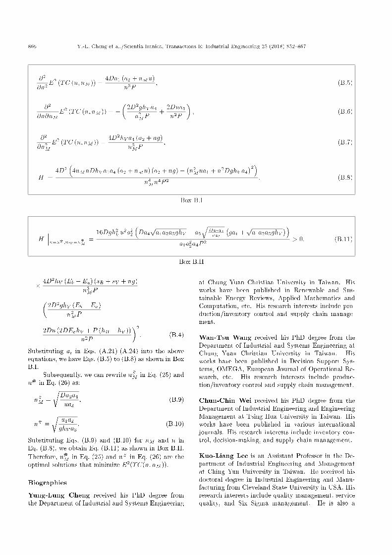
Appendix B
Taking the second partial derivatives of E2(TC(n;nM )) with respect to n and nM , we have:
@2
@n2E2 (TC (n; nM ))
=4D (2DEahV +P (hB�hV )) (sB+sV +nMu)
n3P;
(B.1)
@2
@n2ME2 (TC (n; nM ))
=4D2hV (Eb � Ea) (sB + sV + ng)
n3MP
; (B.2)
@2
@n@nME2 (TC (n; nM )) = �
�2D2ghV (Eb � Ea)
n2MP
+2Du (2DEahV + P (hB � hV ))
n2P
�: (B.3)
Letting:
jHj = @2
@n2E (TC (n; nM )) � @2
@n2ME (TC (n; nM ))
��
@2
@n@nME (TC (n; nM ))
�2
;
we get:
jHj =4D (2DEahV + P (hB � hV )) (sB + sV + nMu)
n3P
866 Y.-L. Cheng et al./Scientia Iranica, Transactions E: Industrial Engineering 25 (2018) 852{867
@2
@n2E2 (TC (n; nM )) =
4Da1 (a2 + nMu)n3P
; (B.5)
@2
@n@nME2 (TC (n; nM )) = �
�2D2ghV a4
n2MP
+2Dua1
n2P
�; (B.6)
@2
@n2ME2 (TC (n; nM )) =
4D2hV a4 (a2 + ng)n3MP
; (B.7)
jHj = 4D2�
4nMnDhV a1a4 (a2 + nMu) (a2 + ng)� �n2Mua1 + n2DghV a4
�2�n4Mn4P 2 : (B.8)
Box B.I
jHj���n=n#;nM=n#
M=
16Dgh2V u2a2
3
�Da4pa1a2a3ghV + a3
qDa2a4ua3
�ga1 +
pa1a2a3ghV
��a1a2
2a4P 2 > 0: (B.11)
Box B.II
� 4D2hV (Eb � Ea) (sB + sV + ng)n3MP
��
2D2ghV (Eb � Ea)n2MP
+2Du (2DEahV + P (hB � hV ))
n2P
�2
: (B.4)
Substituting ai in Eqs. (A.21)-(A.24) into the aboveequations, we have Eqs. (B.5) to (B.8) as shown in BoxB.I.
Subsequently, we can rewrite n#M in Eq. (25) and
n# in Eq. (26) as:
n#M =
rDa2a4
ua3; (B.9)
n# =r
a1a2
ghV a3: (B.10)
Substituting Eqs. (B.9) and (B.10) for nM and n inEq. (B.8), we obtain Eq. (B.11) as shown in Box B.II.Therefore, n#
M in Eq. (25) and n# in Eq. (26) are theoptimal solutions that minimize E2(TC(n; nM )).
Biographies
Yung-Lung Cheng received his PhD degree fromthe Department of Industrial and Systems Engineering
at Chung Yuan Christian University in Taiwan. Hisworks have been published in Renewable and Sus-tainable Energy Reviews, Applied Mathematics andComputation, etc. His research interests include pro-duction/inventory control and supply chain manage-ment.
Wan-Tsu Wang received his PhD degree from theDepartment of Industrial and Systems Engineering atChung Yuan Christian University in Taiwan. Hisworks have been published in Decision Support Sys-tems, OMEGA, European Journal of Operational Re-search, etc. His research interests include produc-tion/inventory control and supply chain management.
Chun-Chin Wei received his PhD degree from theDepartment of Industrial Engineering and EngineeringManagement at Tsing Hua University in Taiwan. Hisworks have been published in various internationaljournals. His research interests include inventory con-trol, decision-making, and supply chain management.
Kuo-Liang Lee is an Assistant Professor in the De-partment of Industrial Engineering and Managementat Ching Yun University in Taiwan. He received hisdoctoral degree in Industrial Engineering and Manu-facturing from Cleveland State University in USA. Hisresearch interests include quality management, servicequality, and Six Sigma management. He is also a

Y.-L. Cheng et al./Scientia Iranica, Transactions E: Industrial Engineering 25 (2018) 852{867 867
Six Sigma consultant and an ISO 9001 Lead Auditor.There are many �rms that have bene�ted from his help.Dr. Lee is an Associate Professor and the Chairmanof the Department of Industrial Management at ChienHsin University of Science and Technology in Taiwan.He received his PhD degree in Industrial Engineering
and Manufacturing from Cleveland State University inUSA. His research interests include quality manage-ment, service quality, and Six Sigma management andLean Six Sigma. He is also a Six Sigma consultant andan ISO 9001:2015 Lead Auditor. There are many �rmsthat have bene�ted from his help.