Aerodynamics of Low Reynolds Number Rigid Flapping Wing Under ...

Aerodynamics of Low Reynolds Number Rigid Flapping Wing Under Hover and

Freestream Conditions

by

Patrick Clark Trizila

A dissertation submitted in partial fulfillment

of the requirements for the degree of

Doctor of Philosophy

(Aerospace Engineering)

in The University of Michigan

2011

Doctoral Committee:

Professor Wei Shyy, Chair

Professor Carlos E. Cesnik

Professor Peretz P. Friedmann

Associate Professor Luis P. Bernal

Assistant Professor Samantha H. Daly

Assistant Professor Anouck R. Girard

ii

Dedication

To my family and friends

iii

Acknowledgements

The work supported here has been supported in part by the Air Force

Office of Scientific Research‟s Multidisciplinary University Research Initiative

(MURI) grant and by the Michigan/AFRL (Air Force Research

Laboratory)/Boeing Collaborative Center in Aeronautical Sciences.

I would like to thank my advisor Prof. Wei Shyy for his patience and

guidance and for the atmosphere which he fostered within the group. The open

discussion between members on a daily basis, perhaps hourly basis, was infinitely

helpful in problem shooting, expanding horizons, and just getting a look from

another perspective.

I would like to thank my committee Dr. Bernal, Dr. Cesnik, Dr. Daly, Dr.

Friedmann, and Dr. Girard for their role in helping finalize the last step of this

journey.

I would like to thank my group members and office mates for the rich

interactions on a daily basis. This work was not the contribution of an individual

in isolation, but instead greatly benefitted from the, sometimes quite lively,

discussions. I would like to thank Chang-kwon Kang and Dr. Hikaru Aono for the

close collaborations and constant dynamic feedback that allowed this work to

iv

happen. I would like to thank Dr. Emre Sozer, Dr. Xiangchun Zhang, Dr. Dragos

Viieru, Dr. Eric Gustafson, Dr. Amor Menezes, Dr. Erin Farbar, Dr. Nick Bisek,

Dr. Chien-Chou Tseng, (soon to be Dr.) Young Chang Cho for the constant

barrage of material which always resulted in new fangled knowledge.

I would like to thank the professors and teachers from my earliest days

through graduate school. I find myself fortunate to have been able to have been in

the right place at the right time to have had such devoted and approachable

mentors. I look at where I am today and my previous incarnations are nowhere

near as capable in no small part due to the expectations and efforts put forth by

these fantastic individuals. I wish I could name everyone but I feel accidentally

leaving one out would be an injustice and I will instead thank you personally

when we next meet.

I would like to thank Dr. Jeff Wright and Dr. ST Thakur of Streamline

Numerics for help with quite possibly the most unintentionally obfuscated CFD

code in Loci-STREAM. I had a bad habit of breaking pieces of the code and do

not blame you if you do not answer when you see me calling.

I would like to thank AFRL for the invaluable experience of being able to

work so closely with the research labs for three consecutive summers and take

advantage of their expertise and experience. I would like to thank Dr. Visbal for

the enlightening discussions pertaining to higher order numerical methods and

their applications to the flapping wing research area. I would also like to thank the

v

regular conversations with Dr. Don Rizzetta, Dr. Scott Sherer, Dr. Jon Poggie

regarding the methodology and applications during my stay.

I would like to thank Dr. Tushar, Dr. Felipe Viana, and Dr. Haftka for

their instruction and patience while developing my understanding of surrogate

models and how to make use of them.

I would like to thank the support staff in the department for which they

perhaps get too little recognition in keeping the wheels turning of this great

department. Particularly I would like to thank Denise Phelps, Lisa Szuma, Dave

McLean, and Brock Palen for their part in making this degree happen.

Last but not least I would like to thank my family and friends. I have

perhaps been a bit scarce the last few years, but will be redoubling my efforts to

compensate shortly. Thank you for your continued reassurances and support.

vi

Table of Contents

Dedication ............................................................................................................... ii

Acknowledgements ................................................................................................ iii

List of Figures ......................................................................................................... x

List of Tables ...................................................................................................... xvii

List of Abbreviations ......................................................................................... xviii

Abstract ................................................................................................................ xix

Chapter

1 Introduction ..................................................................................................... 1

1.1 Unsteady Flight Mechanisms ................................................................... 5

1.1.1 Clap and fling .................................................................................... 5

1.1.2 Rapid Pitch Mechanism .................................................................... 7

1.1.3 Wake Capture.................................................................................... 8

1.1.4 Delayed Stall of a Leading Edge Vortex (LEV) ............................. 10

1.1.5 Tip vortex ........................................................................................ 14

1.1.6 Induced Jet ...................................................................................... 15

1.1.7 Passive Pitching Mechanism ........................................................... 17

vii

1.1.8 Vortex Dynamics ............................................................................ 18

1.2 Kinematics, Geometry, Flexibility, and Re Effects in Flapping Wing

Aerodynamics ................................................................................................... 19

1.2.1 Single Wing in Forward Flight Conditions ..................................... 22

1.2.2 Single Wing in Hovering Flight Conditions ................................... 29

1.2.3 Tandem Wings in Forward/Hoving Flight Conditions ................... 33

1.2.4 Implications of Wing Geometry ..................................................... 37

1.2.5 Implications of Wing Kinematics ................................................... 39

1.2.6 Reynolds Number Effects ............................................................... 41

1.2.7 Wing Flexibility and Aerodynamic Consequences ......................... 43

1.2.8 Reduced Order Models ................................................................... 50

2 Approach and Methods ................................................................................. 53

2.1 CFD Modeling........................................................................................ 54

2.2 Surrogate Modeling ................................................................................ 59

2.2.1 Design Space ................................................................................... 61

2.2.2 Design of Experiments .................................................................... 62

2.2.3 Prediction Error Sum of Squares (PRESS) ..................................... 63

2.2.4 Polynomial Response Surface (PRS) .............................................. 64

2.2.5 Kriging ............................................................................................ 65

viii

2.2.6 Radial Basis Neural Network (RBNN) ........................................... 66

2.2.7 Weighted Average Surrogate Models (WAS) ................................ 67

2.2.8 Global Sensitivity Analysis (GSA) ................................................. 68

3 Hovering Aerodynamics of a Rigid Flat Plate .............................................. 70

3.1 Interpreting Force Histories and Flow Features ..................................... 70

3.1.1 Impact of a Persistent Jet in 2D Hovering ...................................... 73

3.1.2 Instantaneous Lift and Drag as Design Variables are Varied ......... 77

3.2 Time-Averaged Lift................................................................................ 82

3.3 Region 1; Synchronized Hovering, High AoA ...................................... 86

3.4 Region 2; Advanced Rotation, Low AoA .............................................. 89

3.5 Region 3; Delayed Rotation, High AoA, Low Plunging Amplitude ..... 90

3.6 Region 4; Delayed Rotation, Low AoA, Low Plunging Amplitude ...... 95

3.7 Region of similarity ................................................................................ 97

3.8 Power Requirements ............................................................................ 100

3.9 Pareto Front .......................................................................................... 102

4 Effect of Gust and Freestream on Flapping Wing Aerodynamics .............. 105

4.1 Two Dimensional or Infinite Aspect Ratio Wings in a Gust ............... 106

4.2 Finite Aspect Ratio Wings in a Gust .................................................... 111

4.3 Surrogate Trends .................................................................................. 114

ix

4.4 On the Applicability of Effective Angle of Attack in Reduced Order

Models............................................................................................................. 117

5 Summary, Conclusions, and Recommendations for Future Work ............. 120

Appendix ............................................................................................................. 131

Bibliography ....................................................................................................... 133

x

List of Figures

Figure 1. Sectional schematic of wings approaching each other to clap (A-C) and fling apart (D-

F) adopted from Sane (2003) and originally described in Weis-Fogh (1973). Black lines

show flow lines and dark blue arrows show induced velocity. Light blue arrows show net

forces acting on the airfoil. (A-C) Clap. As the wing approach each other dorsally (A), their

leading edges touch initially (B), and the wing rotates around the leading edge. As the

trailing edges approach each other, vorticity shed from the trailing edge rolls up in the

form of stopping vortices (C), which dissipate into the wake. The leading edge vortices

also lose strength. The closing gap between the two wings pushes fluid out, giving and

additional thrust. (D-F) Fling. The wings fling apart by rotating around the trailing edge

(D). The leading edge translates away and fluid rushes in to fill the gap between the two

wing sections, giving an initial boost in circulation around the wing system (E). (F) A

leading edge vortex forms anew but the trailing edge starting vortices are mutually

annihilated as they are of opposite circulation. 6

Figure 2. Illustrations of wake capture mechanism [Shyy et al. (2008a, 2009)]. (a) Supination,(b)

beginning of upstroke, and (c) early of upstroke. At the end of the stroke, (a), the wake

shed in the previous stroke denoted by CWV is en route of the flat plate. As the flat plate

moves into the wake (b-c) the effective flow velocity increases and additional

aerodynamic force is generated. The color of contour indicates spanwise-component of

vorticity. CWV and CCWV indicate clock-wise and counter clock-wise vortex. 8

xi

Figure 3. Leading edge suction analogy adopted from Sane (2003). (A) Flow around the blunt

wing. The sharp diversion of flow around the leading edge results in a leading edge

suction force (dark blue arrow), causing the resultant force vector (light blue arrow) to

tilt towards the leading edge and perpendicular to free stream. (B) Flow around a thin

airfoil. The presence of a leading edge vortex causes a diversion of flow analogous to the

flow around the blunt leading edge in (A) but in a direction normal to the surface of the

airfoil. This results in an enhancement of the force normal to the wing section. 11

Figure 4. Illustration of the shed vortices reinforcing the downward momentum created as the

wing flaps. 16

Figure 5. Vertical velocity (left) and vorticity (right) contours of a two-dimensional case at

Re=100 hovering case governed by 2ha/c=3.0, αa= 45°, ϕ=90. The persistent jet is

expressed as the darker blue region in the v-velocity plots. 17

Figure 6. Illustration of the kinematic parameters for normal hovering. 56

Figure 7. (Left) : Grid distribution on the flat plate, and on the symmetry plane. (Right):

Boundary conditions assigned on the computational domain. The outer boundary plane

opposite to the symmetry plane has not been shown due to visibility and also has the

incompressibleInlet boundary condition. 58

Figure 8. Cross-validation of Loci-Stream and FDL3DI for a two-dimensional ellipse with 15%

thickness during normal hovering computation with for Re = 100, 2ha/c = 3.0, αa = 45°, φ

= 90°. 59

Figure 9. Outline of the surrogate process. 61

Figure 10. Illustration of the lift and drag coefficients for a two-dimensional ellipse normal

hovering case with 2ha/c = 3.0, αa = 45°, and ϕ=90° and the corresponding airfoil

positions. Three flowfield shots illustrating the unsteady aerodynamics are emphasized.

71

xii

Figure 11. Vertical velocity (top) and vorticity (bottom) contours of the normal, reverse, and

delay starting conditions after 25 periods for a two-dimensional case at Re=100 hovering

case governed by 2ha/c=3.0, αa= 45°, ϕ=90. The persistent jet, expressed as a blue region

in the u2 velocity plots, exhibits a slight preference to the left and right for the normal

and reverse cases respectively, whereas the delay case is roughly centered about the

mid-stroke. 74

Figure 12. The lift coefficients of two-dimensional computation at Re=100 for the three starting

conditions after 25 periods (left) and 40 periods (right). The centered jet created by the

delay case moves to a stable configuration to one side. For the cases studied the eventual

preference was dictated by the initial direction of motion of the wing. After 40 periods

the normal and delay cases overlap completely while still differing from the reverse case

noticeably. 76

Figure 13. Time histories of the lift coefficients for selected cases (a) as is increases

from 2.0 (left) to 4.0 (right) holding = 62.5° and =90° (b) as is increased from 45°

(left) to 80° (right) while holding =3.0 and =90° (c) examining delayed rotation

=60° (left) and andvanced rotation =120° (right) while holding =4.0 = 80°

(d) examining delayed rotation =60° (left) and andvanced rotation =120° (right) while

holding =2.0 = 45°. 78

Figure 14. Time histories of the drag coefficients for selected cases (a) as is increases

from 2.0 (left) to 4.0 (right) holding = 62.5° and =90° (b) as is increased from 45°

(left) to 80° (right) while holding =3.0 and =90° (c) examining delayed rotation

=60° (left) and andvanced rotation =120° (right) while holding =4.0 = 80°

(d) examining delayed rotation =60° (left) and andvanced rotation =120° (right) while

holding =2.0 = 45° 81

xiii

Figure 15. Surrogate modeling results for lift. Left: two-dimensional, Middle: three-

dimensional, Right: three-dimensional minus the two-dimensional time averaged lift. 84

Figure 16. Global sensitivity analysis (GSA) of lift for two-dimensional and three-dimensional

hovering kinematics. 85

Figure 17. Iso-sufaces of 2D lift (a), 3D lift (b), 3D minus 2D lift (c), and (d) where the absolute

difference between the 2D and 3D lift equals 0.10. The symbols denote training points in

those regions for which detailed force histories and flow field quantities are available;

brown octahedra (region 1), circles (region 2), black quarter sphere (region 3), and a blue

cube (region 4). 86

Figure 18. Instantaneous force history (2D: red, 3D: black) and vertical velocity contour plots at

three time instants in the forward stroke for the case 11 (h_a=3.0,α_a=45°,ϕ=90°): (a)

from two-dimensional computation; (b) in the symmetry plane of three-dimensional

computation; (c) near the wingtip (z/c = 1.8). 88

Figure 19 Time history of lift coefficients in a representative case in region 1, 2ha/c = 4.0, αa=

80°, and ϕ = 120°, with the associated flow features. (A) Lift, (C_L), during a motion cycle.

Red-solid, two-dimensional computation; black-dashed, three-dimensional computation.

(B) kinematic schema of the flat plate motion. (C) Representative flow features at 1) t/T =

0.9, u2 contours; 2) t/T = 1.0, vorticity contours; 3) t/T=1.2, u2 contours. 90

Figure 20 Force history (2D: red, 3D: black) for a flapping cycle and z-vorticity contour plots at

three time instants in the forward stroke for the case 1 ( ):

(a) from two-dimensional computation; (b) in the symmetry plane of three-dimensional

computation; (c) near the wingtip (z/c = 1.8). 92

Figure 21. The lift per unit span and iso-Q surfaces (Q=0.75) colored by z-vorticity over half of

the wing using the kinematic parameters 2ha/c =2.0,αa=45°,ϕ=60° (case 1) at Re = 100 at

t/T= 0.8, 1.0, 1.2. The spanwise variation in forces is examined with the two-dimensional

xiv

equivalent marked for reference. Time averaged lift coefficient for i) two-dimensional:

0.13, ii) three-dimensional: 0.22. 93

Figure 22. Force history (2D: red, 3D: black) for a flapping cycle and z-vorticity contour plots at

three time instants in the forward stroke for the case 3 (h_a=2.0,α_a=80°,ϕ=60°): (a)

from 2D computation; (b) in the symmetry plane of 3D computation; (c) near the wingtip

(z/c = 1.8) plane. 96

Figure 23. Force history over a flapping cycle (solid red=2D, dashed black=3D) and z-vorticity

contour plots at three time instants in the forward stroke for the case 12

(2ha/c=3.0,α_a=80°,ϕ=90°): (a) from 2D computation; (b) in the symmetry plane of 3D

computation; (c) near the wingtip (z/c = 1.8) plane. 98

Figure 24. Surrogate modeling results for power required. Left- two-dimensional, Middle-three-

dimensional, Right- three-dimensional minus two-dimensional time averaged power

requirement approximations. 101

Figure 25. Global sensitivity analysis (GSA) of power for two-dimensional and three-

dimensional hovering kinematics. 101

Figure 26. Pareto fronts illustrating the competing objectives of lift and power requirements in

two-dimensions (left) and three-dimensions (right) and the design variable combinations

which provide those fronts. The dashed line is for reference. 104

Figure 27. Representative high lift (left: 2ha/c = 2.7, αa= 45°, and ϕ = 120°) and low power

(right: 2ha/c = 4.0, αa= 80°, and ϕ = 90°) kinematics. 104

Figure 28. Force history and vorticity contours illustrating the vortex formation and

interactions during the LEV dominated portion of the stroke (a-c) or wake capture

dominated portion of the stroke (d-f)at their respective maximal lift for a 20% strength

headwind hover scenario with no freestream. The 3D LEV dominated portion of the

xv

stroke is highlighted with z-vorticity contours at two spanwise locations with a 20%

freestream in g), h), and i. 107

Figure 29. Force history (2D) and vorticity contours illustrating the vortex formation between

stroke reversal and their respective maximums in lift for b) 20% downward freestream c)

20% upward freestream. 109

Figure 30. 2D (a-c) and 3D (d-f) CL in response to a freestream with a magnitude of 20% of the

maximum plunging velocity heading in three distinct directions (down: red, right: green,

and up: blue) for three hovering kinematics (g-i). The black dotted line is the reference

hovering case. 111

Figure 31. Vorticity contours during beginning, mid, and end-stroke for a 2D flatplate and at

mid-span (z/c=0) and wingtip (z/c=1.95) for a 3D flatplate with AR=4 with a 20%

freetream tailwind The 3D perspective shots show iso-Q surfaces colored by z-vorticity.

The blue arrow denotes freestream direction. 112

Figure 32. Surrogate models illustrating the trends in lift in the presence of a 20% horizontal

freestream [a) 2D, c) 3D], the differences between freestream and hover [b) 2D, d) 3D],

and the difference between 3D and 2D [e]. 116

Figure 33. Illustration cautioning the use of effective angle of attack as measure of lift in the

hovering context. The lift coefficients of the three kinematic patterns studied in this

section have been plotted versus the effective angle of attack for freestream strengths of

5%, 10%, and 20% with orientations heading down, right, and up. 119

FIGURE 26. Time histories of the lift and drag coefficients between a two-dimensional

ellipse of 15% thickness and two-dimensional flatplate for selected cases (a) as is

increases from 2.0 (left) to 4.0 (right) holding = 62.5° and =90° (b) as is increased

from 45° (left) to 80° (right) while holding =3.0 and =90° (c) examining delayed

rotation =60° (left) and andvanced rotation =120° (right) while holding =4.0

xvi

= 80° (d) examining delayed rotation =60° (left) and andvanced rotation =120°

(right) while holding =2.0 = 45°. 132

xvii

List of Tables

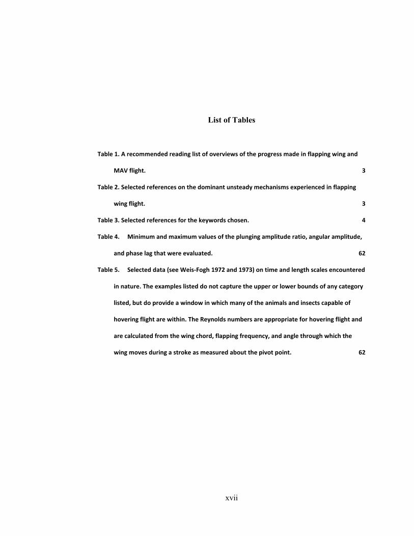
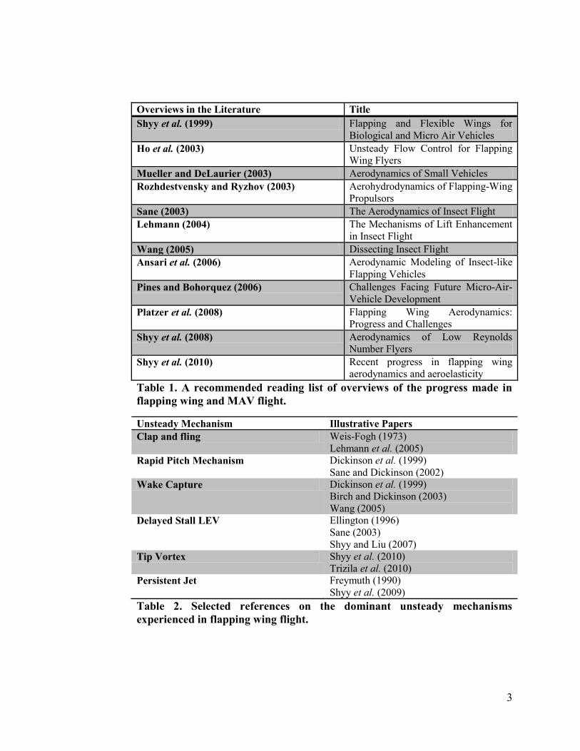
Table 1. A recommended reading list of overviews of the progress made in flapping wing and

MAV flight. 3

Table 2. Selected references on the dominant unsteady mechanisms experienced in flapping

wing flight. 3

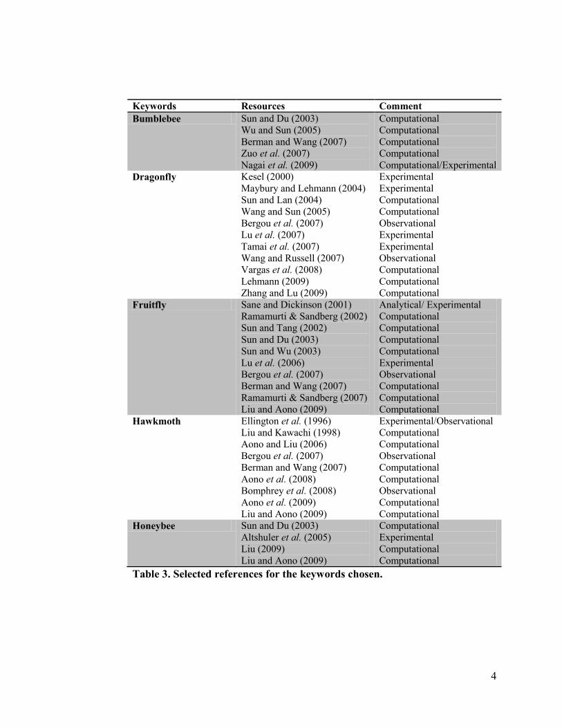
Table 3. Selected references for the keywords chosen. 4

Table 4. Minimum and maximum values of the plunging amplitude ratio, angular amplitude,

and phase lag that were evaluated. 62

Table 5. Selected data (see Weis-Fogh 1972 and 1973) on time and length scales encountered

in nature. The examples listed do not capture the upper or lower bounds of any category

listed, but do provide a window in which many of the animals and insects capable of

hovering flight are within. The Reynolds numbers are appropriate for hovering flight and

are calculated from the wing chord, flapping frequency, and angle through which the

wing moves during a stroke as measured about the pivot point. 62

xviii

List of Abbreviations

AoA- angle of attack

AR- aspect ratio

CFD- computational fluid dynamics

k- reduced frequency

LEV- leading edge vortex

MAV- micro air vehicle

NS- Navier-Stokes

PIV- particle image velocimetry

PRS- polynomial response surface

RBNN- radial basis neural network

Re- Reynolds number

SVR- support vector regression

WAS- weighted average surrogate

xix

Abstract

Micro-air-vehicles (MAVs) are constrained by spatial dimensions less

than 15cm. Equipped with a camera or sensor, these vehicles could perform

surveillance and reconnaissance with low probability of detection, or

environmental and bio-chemical sensing at remote or otherwise hazardous

locations. Its size makes the MAV easily transported and deployed as well as

inexpensive and more expendable than alternatives, e.g. an airplane, a satellite, or

a human.

The ability to hover for an MAV is highly desirable in these contexts. The

approach taken in this thesis was to numerically simulate the aerodynamics about

flapping wings while controlling the kinematic motions and environmental

conditions. Two complementary sets of tools were used in the investigations. i)

Navier-Stokes solvers were used to obtain detailed fluid physics information,

instantaneous force data, and to train the surrogate models. ii) The surrogate

models were used to estimate the time-averaged lift and power required over a

flapping cycle while also providing information on the sensitivity of the kinematic

variables, to identify trends in lift and power required as a function of the

kinematic variables, and to construct a Pareto front showing the trade-offs

between the competing objectives.

xx

The roles of the unsteady mechanisms are discussed as well as their

influence on the forces felt. Findings include i) the competing influences

introduced by tip vortices, and it was seen that they could increase lift compared

to their analogous 2D cases, counter to classical steady state theory. ii) The

highest time averaged lift values were found during kinematics with high angles

of attack during advanced rotation as they promoted LEV generation and

subsequently took advantage of them during wake capture. iii) Kinematics with

synchronized rotation and low angles of attack had similar 2D and low-aspect-

ratio force histories. iv) Modest environmental perturbations were shown to

increase the instantaneous 2D forces up to 200%, and though the 3D simulations

were less sensitive some felt an increase of 50%. v) The surrogate models proved

useful in analysis by identifying local/global sensitivities and trends of the

kinematic variables as well as zeroing in on regions for further examination. The

kinematics yielding highest lift, lowest power, or where 3D effects became most

influential were quickly identifiable.

1

Chapter 1 Introduction

Micro Air Vehicles (MAVs) have the potential to revolutionize our sensing

and information gathering capabilities in areas such as environmental monitoring

and homeland security. Numerous aspects relating to potential vehicle concepts,

including fixed wing, rotary wing, and flapping wing, have been addressed [see

summaries by Shyy et al. 2010, Platzer et al. 2008, Shyy et al. 2008a, Ansari et

al. 2006, Wang 2005, Dalton 2006, Pines and Bohorquez 2006, Ho et al. 2003,

Mueller and DeLaurier 2003, Rozhdestvensky and Ryzhov 2003, Norberg 2002,

Ellington 1999, Shyy et al 1999, Spedding and Lissaman 1998]. As the size of a

vehicle becomes smaller than a few centimeters, fixed wing designs encounter

fundamental challenges in lift generation and flight control. There are merits and

challenges associated with rotary and flapping wing designs. Fundamentally, due

to the Reynolds number effect, the aerodynamic characteristics such as the lift,

drag and thrust of a flight vehicle change considerably between MAVs and

conventional manned air vehicles. And, since MAVs are light weight and fly at

low speeds, they are sensitive to wind gusts. Because of the common

characteristics shared by MAVs and biological flyers, the aerospace and

biological science communities are now actively communicating and

collaborating. Much can be shared between researchers with different training and

2

background including biological insight, mathematical models, physical

interpretation, experimental techniques, and design concepts.

MAVs are defined by having a maximal dimension of 15 cm or less and a

flight speed of 10 m/s, and are interests for both military and civilian applications.

Equipped with a video camera or a sensor, these vehicles can perform

surveillance and reconnaissance, and environmental and bio-chemical sensing at

remote or otherwise hazardous locations. In addition, from the scaling laws [Shyy

et al. 2008a], a MAV‟s payload is very limited; sensors, batteries,

communications equipment, and means of sustained propulsion will have to

compete for precious cargo space only in as much as that they will directly help

defined mission statements. Research regarding MAVs is growing as there are

still many open challenges in theory and in practice. Tables 1-3 attempt to

characterize select references in an easily readable and more palatable form while

favoring conciseness over completeness or comprehensiveness.

3

Overviews in the Literature Title

Shyy et al. (1999) Flapping and Flexible Wings for

Biological and Micro Air Vehicles

Ho et al. (2003) Unsteady Flow Control for Flapping

Wing Flyers

Mueller and DeLaurier (2003) Aerodynamics of Small Vehicles

Rozhdestvensky and Ryzhov (2003) Aerohydrodynamics of Flapping-Wing

Propulsors

Sane (2003) The Aerodynamics of Insect Flight

Lehmann (2004) The Mechanisms of Lift Enhancement

in Insect Flight

Wang (2005) Dissecting Insect Flight

Ansari et al. (2006) Aerodynamic Modeling of Insect-like

Flapping Vehicles

Pines and Bohorquez (2006) Challenges Facing Future Micro-Air-

Vehicle Development

Platzer et al. (2008) Flapping Wing Aerodynamics:

Progress and Challenges

Shyy et al. (2008) Aerodynamics of Low Reynolds

Number Flyers

Shyy et al. (2010) Recent progress in flapping wing

aerodynamics and aeroelasticity

Table 1. A recommended reading list of overviews of the progress made in

flapping wing and MAV flight.

Unsteady Mechanism Illustrative Papers

Clap and fling Weis-Fogh (1973)

Lehmann et al. (2005)

Rapid Pitch Mechanism Dickinson et al. (1999)

Sane and Dickinson (2002)

Wake Capture Dickinson et al. (1999)

Birch and Dickinson (2003)

Wang (2005)

Delayed Stall LEV Ellington (1996)

Sane (2003)

Shyy and Liu (2007)

Tip Vortex Shyy et al. (2010)

Trizila et al. (2010)

Persistent Jet Freymuth (1990)

Shyy et al. (2009)

Table 2. Selected references on the dominant unsteady mechanisms

experienced in flapping wing flight.

4

Keywords Resources Comment

Bumblebee Sun and Du (2003)

Wu and Sun (2005)

Berman and Wang (2007)

Zuo et al. (2007)

Nagai et al. (2009)

Computational

Computational

Computational

Computational

Computational/Experimental

Dragonfly Kesel (2000)

Maybury and Lehmann (2004)

Sun and Lan (2004)

Wang and Sun (2005)

Bergou et al. (2007)

Lu et al. (2007)

Tamai et al. (2007)

Wang and Russell (2007)

Vargas et al. (2008)

Lehmann (2009)

Zhang and Lu (2009)

Experimental

Experimental

Computational

Computational

Observational

Experimental

Experimental

Observational

Computational

Computational

Computational

Fruitfly Sane and Dickinson (2001)

Ramamurti & Sandberg (2002)

Sun and Tang (2002)

Sun and Du (2003)

Sun and Wu (2003)

Lu et al. (2006)



Ramamurti & Sandberg (2007)

Liu and Aono (2009)

Analytical/ Experimental

Computational

Computational

Computational

Computational

Experimental

Observational

Computational

Computational

Computational

Hawkmoth Ellington et al. (1996)

Liu and Kawachi (1998)

Aono and Liu (2006)



Aono et al. (2008)

Bomphrey et al. (2008)

Aono et al. (2009)

Liu and Aono (2009)

Experimental/Observational

Computational

Computational

Observational

Computational

Computational

Observational

Computational

Computational

Honeybee Sun and Du (2003)

Altshuler et al. (2005)

Liu (2009)

Liu and Aono (2009)

Computational

Experimental

Computational

Computational

Table 3. Selected references for the keywords chosen.

5

1.1 Unsteady Flight Mechanisms

The flapping wing variety of MAVs [Shyy et al. 2010, Shyy et al. 2008,

Shyy et al. 1999], of interest in the current study, take a cue from nature and

attempt to mimic the success achieved by insects, birds, and bats [Fearing et al

2000, Lentink et al. 2007, Pornsin-Sirirak et al. 2000]. The study of flapping wing

flyers with all of their intricacies is challenging. However significant progress has

been made in both engineering and biological communities. Natural flyers utilize

flapping mechanisms to generate lift and thrust. These mechanisms are related to

formation and shedding of the vortices into the flow, varied wing shape, and

structural flexibility. Therefore, understanding the vortex dynamics, the vortex-

wing interaction, and the fluid-structure interaction is important. A brief

introduction to some of the key unsteady mechanisms associated with flapping

wings which are frequently encountered in the literature is given next.

1.1.1 Clap and fling

The earliest unsteady lift generation mechanism to explain how insects fly,

found by Weis-Fogh (1973), was the clap-and-fling motion of a chalcid wasp,

Encarsia Formosa. Based on the steady-state approximation, the lift generated by

the chalcid wasp was insufficient to stay aloft. To explain this, he observed that a

chalcid wasp claps two wings together and then flings them open about the

horizontal line of contact to fill the gap with air. During the fling motion, the air

around each wing acquires circulation in the correct direction to generate

additional lift. A schematic of this procedure is shown in Fig. 1.

6

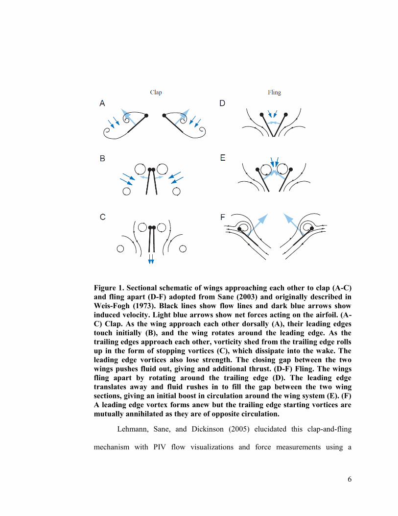
Figure 1. Sectional schematic of wings approaching each other to clap (A-C)

and fling apart (D-F) adopted from Sane (2003) and originally described in

Weis-Fogh (1973). Black lines show flow lines and dark blue arrows show

induced velocity. Light blue arrows show net forces acting on the airfoil. (A-

C) Clap. As the wing approach each other dorsally (A), their leading edges

touch initially (B), and the wing rotates around the leading edge. As the

trailing edges approach each other, vorticity shed from the trailing edge rolls

up in the form of stopping vortices (C), which dissipate into the wake. The

leading edge vortices also lose strength. The closing gap between the two

wings pushes fluid out, giving and additional thrust. (D-F) Fling. The wings

fling apart by rotating around the trailing edge (D). The leading edge

translates away and fluid rushes in to fill the gap between the two wing

sections, giving an initial boost in circulation around the wing system (E). (F)

A leading edge vortex forms anew but the trailing edge starting vortices are

mutually annihilated as they are of opposite circulation.

Lehmann, Sane, and Dickinson (2005) elucidated this clap-and-fling

mechanism with PIV flow visualizations and force measurements using a

7

dynamically-scaled robotic wing model. Also numerical investigations further

demonstrated lift enhancement due to the clap-and-fling mechanisms at low

Reynolds numbers [Sun and Yu 2003, Sun and Yu 2006, Miller and Peskin 2004,

Miller and Peskin 2005, Liu and Aono 2009]. The relative benefit of clap-and-

fling lift enhancement strongly depended on stroke kinematics and could

potentially increase the performance by reducing the power requirements

[Lehmann and Pick 2007, Lehmann 2009]. The clap-and-fling mechanism is

beneficial in producing a mean lift coefficient to keep a low weight flyer aloft:

numerous natural flyers, such as hawkmoths, butterflies, fruitflies, wasps, and

thrips enhance their aerodynamic force production with the clap-and-fling

mechanism [Weis-Fogh 1973, Cooter and Baker 1977, Brodsky 1991,

Brachenbury 1990, Srygley and Thomas 2002].

1.1.2 Rapid Pitch Mechanism

At the end of each stroke, flapping wings can experience rapid pitching

rotation, which can enhance the aerodynamic force generation [Dickinson et al.

1999]. The phase difference between the translation and the rotation can be

utilized as a lift controlling parameter: similar to the Magnus effect where the

rotating body‟s no-slip surface will drag surrounding air, accelerating the fluid in

the direction of motion on one side and impeding it on the other side of the body

thereby creating a pressure difference and sideways force. If the wing flips before

the stroke ends, then the wing undergoes rapid pitch-up rotation in the correct

translational direction enhancing the lift. This is called the advanced rotation. On

8

the other hand, in delayed rotations, if a wing rotates back after the stroke

reversal, then when the wing starts to accelerate it pitches down resulting in

reduced lift [Dickinson et al. 1999]. In a follow-up study Sane and Dickinson

(2002) related the lift peak at the stroke ends to be proportional to the angular

velocity of the wing using the quasi-steady theory. The numerical studies [Shyy et

al. 2008, Sun and Tang 2002] showed an increase in the vorticity around the wing

due to rapid pitch-up rotation of the wing led to augmentation of the lift

generation.

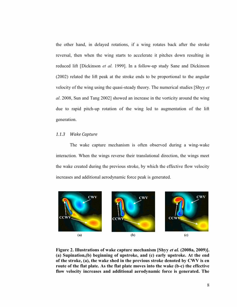
1.1.3 Wake Capture

The wake capture mechanism is often observed during a wing-wake

interaction. When the wings reverse their translational direction, the wings meet

the wake created during the previous stroke, by which the effective flow velocity

increases and additional aerodynamic force peak is generated.

Figure 2. Illustrations of wake capture mechanism [Shyy et al. (2008a, 2009)].

(a) Supination,(b) beginning of upstroke, and (c) early upstroke. At the end

of the stroke, (a), the wake shed in the previous stroke denoted by CWV is en

route of the flat plate. As the flat plate moves into the wake (b-c) the effective

flow velocity increases and additional aerodynamic force is generated. The

9

color of contour indicates spanwise-component of vorticity. CWV and

CCWV indicate clock-wise and counter clock-wise vortex.

Lehmann, Sane and Dickinson (2005), Dickinson et al. (1999), and Birch

and Dickinson (2003) examined the effect of wake capturing of several simplified

fruit fly-like wing kinematics using a dynamically-scaled robotic fruit fly wing

model at Re= 1.0-2.0×102. They compared the force measurement data with the

quasi-steady approximation, then isolated the aerodynamic influence of the wake.

Results demonstrated that wake capture force represented a truly unsteady

phenomenon dependent on temporal changes in the distribution and magnitude of

vorticity during stroke reversal. The sequence of the wake capture mechanism is

illustrated in Fig. 2. Wang (2005) and Shyy et al. (2008, 2009) further elucidated

the wake capture mechanism and lift augmentation of the instantaneous lift peak

using 2-D numerical simulations. The effectiveness of the wake capture

mechanism was a function of wing kinematics and flow structures around the

flapping wings [Shyy et al. 2008, Lehmann et al. 2005, Dickinson et al. 1999,

Birch and Dickinson 2003]. A different view on the effect of wake capture existed

as well. Jardin et al. (2009) used a NACA0012 airfoil under asymmetric flapping

wing kinematics such that in the downstroke the interaction of the previously shed

wake with the leading edge vortex (LEV) formation was reduced. In most cases

they considered this reduced effect of wake capture led to a closely attached

downstroke LEVs. Compared to a synchronized wing rotation they saw enhanced

downstroke aerodynamic loading.

10

1.1.4 Delayed Stall of a Leading Edge Vortex (LEV)

Ellington et al. [(1996), van den Berg and Ellington (1997a,b), Willmott et

al. 1997] suggested that the delayed stall of LEV can significantly promote lift

associated with a flapping wing. The LEV created a region of lower pressure

above the wing and hence it would enhance lift. Multiple follow-up investigations

[Liu and Kawachi (1997), Liu et al. (1998), Liu (2002, 2005)] were conducted for

different insect models, resulting in a better understanding of the role played by

the LEV and its implications on lift generation. When a flapping wing travels

several chord lengths, the flow separates from the leading and trailing edges, as

well as at the wing tip, and forms large organized vortices known as a leading

edge vortex (LEV), a trailing edge vortex (TEV), and a tip vortex (TiV). In

flapping wing flight, the presence of LEVs is essential to delay stall and to

augment aerodynamic force production during the translation of the flapping

wings as shown in Fig. 3 [Sane 2003]. Fundamentally, the LEV is generated and

sustained from the balance between the pressure-gradient, the centripetal force,

and the Coriolis force in the Navier-Stokes (NS) equations. The LEV generates a

lower pressure area in its core, which results in an increased suction force on the

upper surface. Employing 3-D NS computations, Liu and Aono (2009) and Shyy

and Liu (2007) demonstrated that a LEV is a common flow feature in flapping

wing aerodynamics at Reynolds numbers O(100) and lower, which correspond to

the flight regime of insects and flapping wing MAVs. However, main

characteristics and implications of the LEV on the lift generation varied with

11

changes in the Reynolds number, the reduced frequency, the Strouhal number, the

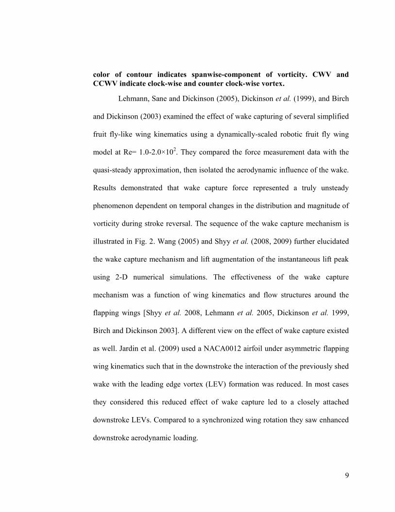
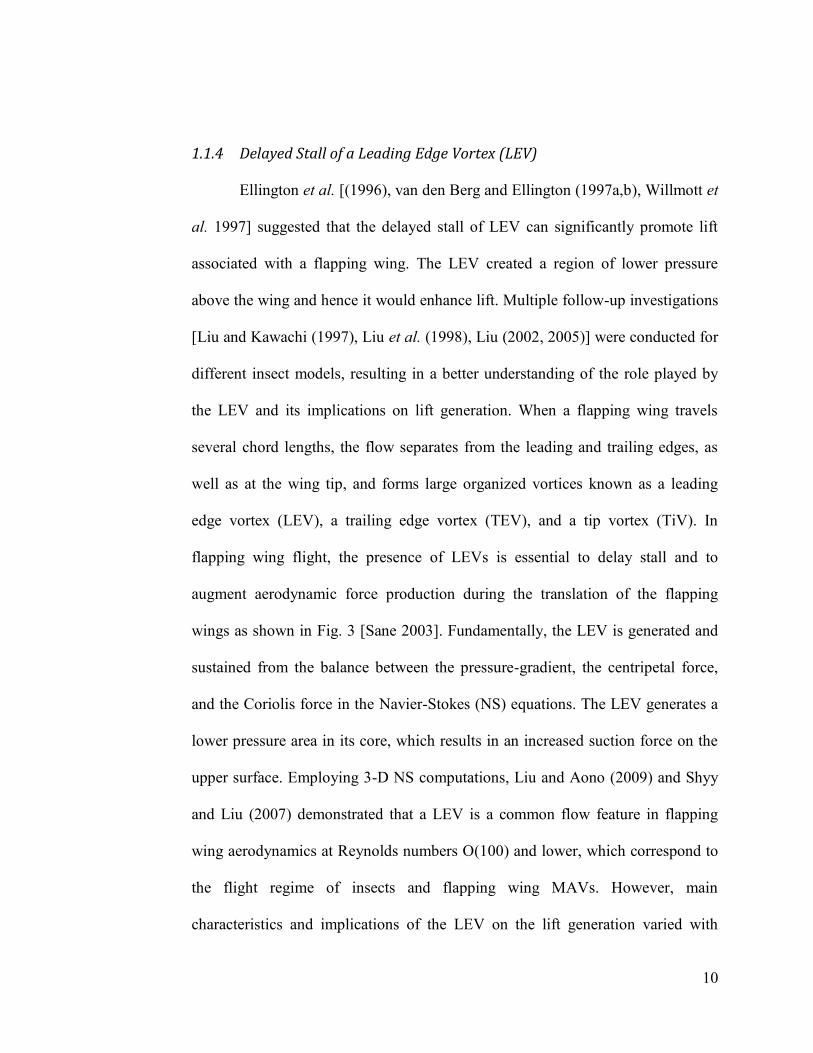
wing flexibility, and flapping wing kinematics.

Figure 3. Leading edge suction analogy adopted from Sane (2003). (A) Flow

around the blunt wing. The sharp diversion of flow around the leading edge

results in a leading edge suction force (dark blue arrow), causing the

resultant force vector (light blue arrow) to tilt towards the leading edge and

perpendicular to free stream. (B) Flow around a thin airfoil. The presence of

a leading edge vortex causes a diversion of flow analogous to the flow around

the blunt leading edge in (A) but in a direction normal to the surface of the

airfoil. This results in an enhancement of the force normal to the wing

section.

12

Milano and Gharib (2005) measured the forces generated by a pitching

rectangular flat plate at approximately Re= O(103) and observed the trajectories

yielding maximum average lift based on a genetic algorithm. Results showed the

optimal flapping produces LEVs of maximum circulation and that a dynamic

formation time that described the vortex formation process of about 4 is

associated with production of a maximum-circulation vortex [Gharib et al. (1998),

Dabiri (2009)]. Rival et al. (2009) investigated experimentally the formation

process of LEVs associated with several combinations of pitching and plunging

SD7003 airfoils in forward flight using PIV at Re= O(104). Results suggested that

by carefully tuning the airfoil kinematics, thus gradually feeding the LEV over the

downstroke, it was to some extent possible to stabilize the LEV without the

necessity of a spanwise flow.

Tarascio et al. (2005) and Ramasamy and Leishman (2006) visualized the

flow fields around a biologically-inspired flapping wing at Re= O(104) by a

mineral oil fog strobed with a laser sheet and PIV. They presented the presence of

a shed dynamic stall vortex that spans across most of the wing span and multiple

shedding LEVs on the top surface of the wing during each wing stroke. Also they

provided several observations related to the role of turbulence at low Reynolds

numbers. Poelma et al. (2006) measured the time-dependent 3-D velocity field

around a flapping wing at Re= O(104) based on maximum chord. A dynamically-

scaled fruitfly wing in mineral oil with hovering kinematics extracted from real

insect movements was used. They presented refined 3-D structures of LEVs and

13

suggested including the counter-rotating TEVs to get a complete picture for

production of circulation. Lu and Shen (2008) highlighted the detailed structures

of LEVs for a flapping wing in hover at Re = O(103). They used phase-lock based

multi-slice digital stereoscopic PIV to show that the spanwise variation along the

LEV was time-dependent. Their results demonstrated that the observed LEV

systems were a collection of four vortical elements: one primary vortex and three

minor vortices, instead of a single conical or tube-like vortex as reported or

hypothesized in previous studies [Dickinson et al. (1999), Ellington et al. (1996)].

Recently, Pick and Lehmann (2009) used 3-D three-components Multiple-Color-

Plane Stereo PIV techniques to obtain a 3-D velocity field around a flapping

wing. The need for 3-D PIV is evident since the critical flow features in

understanding flapping wing aerodynamics, such as LEVs and unsteady wakes

behind an insect body, are inherently 3-D in nature. Compared to the previous

findings, they reported similar structure of the LEV but stronger outward axial

flow inside the LEV of up to 80% of the maximum in-plane velocity. On the other

hand, Liang et al. (2010) presented results based on direct numerical simulation to

investigate wake structures of hummingbird hovering flight and associated

aerodynamic performance. They reported that the amount of lift produced during

downstroke is about 2.95 times of that produced in upstroke. Two parallel vortex

rings were formed at the end of the upstrokes. There is no obvious leading edge

vortex that can be observed at the beginning of the upstroke. Although only rigid

wing structures were considered, the results were claimed to be in good

14

agreement with PIV measurements of Warrick et al. (2005) and Altshuler et al.

(2009).

1.1.5 Tip vortex

Tip vortices (TiVs) associated with fixed finite wings are seen to decrease

lift and induce drag [Anderson (2006)]. However, in unsteady flows, TiVs have

been seen to influence the total force exerted on the wing in three ways: i)

creating a low pressure area near the wing tip [Shyy et al. (2009), Aono et al.

(2008, 2009), Ramamurti and Sandberg (2007), Ringuette et al. (2007)], ii) an

interaction between the LEV and the TiV [Shyy et al. (2009), Aono et al. (2008,

2009), Ramamurti and Sandberg (2007), Ringuette et al. (2007)], and iii)

constructing wake structures by interactions from the downward and radial

influence of the root vortex and TiV [Ramasamy and Leishmann (2006)]. The

first two mechanisms ((i) and (ii)) also were observed for impulsively started flat

plates normal to the motion with low aspect ratios: Riguette et al. (2007)

presented experimentally that the TiVs contributed substantially to the overall

plate force by interacting with the LEVs at Re = O(103). Taira and Colonius

(2009) utilized the immersed boundary method (IBM) to highlight the 3-D

separated flow and vortex dynamics for a number of low aspect ratio flat plates at

different angles of attacks at Re of O(102). They showed that the TiVs could

stabilize the flow and exhibited nonlinear interaction with the shed vortices.

Stronger influence of downwash from the TiVs resulted in reduced lift for lower

aspect ratio plates.

15

For flapping motion in hover, however, depending on the specific

kinematics, the TiVs could either promote or make little impact on the

aerodynamics of a low aspect ratio flapping wing. Shyy et al. [55] demonstrated

that for a flat plate with AR = 4 at Re = 64 with delayed rotation kinematics, the

TiV anchored the vortex shed from the leading edge increasing the lift compared

to a 2-D computation under the same kinematics. On the other hand, under

different kinematics with small angle of attack and synchronized rotation, the

generation of TiVs was small and the aerodynamic loading was well

approximated by the analogous 2-D computation. They concluded that the TiVs

could either promote or make little impact on the aerodynamics of a low aspect

ratio flapping wing by varying the kinematic motions [Shyy et al. 2009].

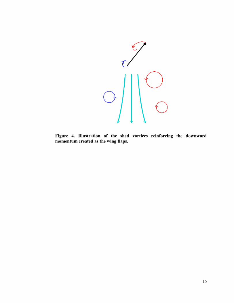
1.1.6 Induced Jet

As a high aspect ratio wing repeats a periodic hovering motion, the shed

vortices may sustain a pocket of downward momentum initiated by the wing as it

pitches and plunges, illustrated in Fig. 4. This has been seen experimentally by

Freymuth (1990) and numerically by Trizila et al. (2008a,b). Figure 5 illustrates a

representative vertical velocity and vorticity field and unpublished results will be

shown in the appendix as to the magnitude of impact it can have on the flowfield

and force histories. The wing encounters the persistent jet which accelerates the

flow along its underside. This decreases the lift of the wing and can introduce or

accentuate asymmetries in the force history, despite symmetric kinematics, as the

jet evolves a bias either behind or in front of the center of stroke position.

16

Figure 4. Illustration of the shed vortices reinforcing the downward

momentum created as the wing flaps.

17

v-velocity

z-vorticity

Figure 5. Vertical velocity (left) and vorticity (right) contours of a two-

dimensional case at Re=100 hovering case governed by 2ha/c=3.0, αa= 45°,

ϕ=90. The persistent jet is expressed as the darker blue region in the v-

velocity plots.

1.1.7 Passive Pitching Mechanism

Wing torsional flexibility can allow for a passive pitching motion due to

the inertial forces during wing rotation at stroke reversals [Ennos (1987, 1988a,

1988b, 1999), Ishihara et al. (2009)]. There were three modes of passive pitching

motions which were similar to those suggested by rigid robotic wing model

experiments [Dickinson et al. (1999)]; 1) delayed pitching, 2) synchronized

18

pitching, and 3) advanced pitching. It was found that the ratio of flapping

frequency and the natural frequency of the wing were important to determine the

modes of passive pitching motions of the wing [Ishihara et al. (2009), Vanella et

al. (2009)]. If the flapping frequency was less than the natural frequency of the

wing, then the wing experienced an advanced pitching motion, which led to lift

enhancement by intercepting the stronger wake generated during the previous

stroke [Vanella et al. (2009)]. Moreover, it was shown for 2-D flows, the LEVs

produced by the airfoil motion with passive pitching seemed to attach longer on

the flexible airfoil than on a rigid airfoil [Ishihara et al. (2009)].

1.1.8 Vortex Dynamics

The above discussion show that vortex dynamics play an important role in

the force generation during flapping wing flight. The act of quantifying the vortex

dynamics is an area of study unto itself. A common way of illustrating vortex

dynamics, and used extensively in the present document, is through vorticity, the

curl of velocity [Anderson (2006)]:

(1)

In certain circumstances vorticity in and of itself, while useful, is not conclusive.

Particularly in regions of sheer flow vorticity may be significant but streamline

curvature negligible. Another quantity used in the present document is the second

invariant of the velocity gradient tensor referred to as the Q criterion [Hunt et al.

(1988)]:

19

(2)

Here S is the rate of strain tensor, and ω is the vorticity vector, both in indicial

notation. One advantage of using this criterion over the vorticity is that the shear

and rotational components are separated, e.g. a boundary layer will exhibit high

vorticity but lacks coherent vortices. This in turn allows for additional

possibilities in following the vortex dynamics as a vortex can be better quantified.

Another popular approach in fluid dynamics for studying time dependent

flows is through the calculation of Lagrangian Coherent Structures (LCS). One

strength is the ability to discern transport properties not immediately evident in

the Eulerian frame. One potential drawback is that the computational cost can be

significant as either many points or a method for surface tracking which is

advected in time must be resolved. This technique is not used in the current study,

but the interested reader is referred to Shadden et al. (2005), Green et al. (2007),

Lipinski and Mohseni (2009), and Wilson et al. (2009) for theoretical

formulation, numerical implementation, and practical applications.

1.2 Kinematics, Geometry, Flexibility, and Re Effects in Flapping Wing

Aerodynamics

This section presents a literature survey on flapping wing aerodynamics

using experimental, theoretical, and computational approaches.

Experimentally, numerous previous efforts on flow visualization around

biological flyers have been made, including smoke visualizations [Brodsky

20

(1991), Srygley and Thomas (2002), Willmott et al.(1997), Thomas et al. (2004),

Bomphrey et al. (2009)] and PIV measurements [Warrick et al. (2005,2009),

Altshuler et al. (2009), Hubel et al. (2009), Tobalske et al. (2009), Videler et al.

(2004), Bomphrey et al. (2005), Bomphrey (2006), Hedenstrom et al. (2007,

2009), Muijres et al. (2008)]. The advance of such technologies has enabled

researchers to obtain not only 2-D but also 3-D flow structures around biological

flyers [Hubel et al. (2009), Warrick et al. (2009), Hedenstrom et al. (2007, 2009),

Muijres et al. (2008)] and/or scaled models [Poelma et al. (2006), Lu and Shen

(2008), Pick and Lehmann (2009)] with reasonable resolution in space. At the

same time, measurements of wing and body kinematics have been conducted

using high-speed cameras [Wakeling and Ellington (1997), Willmott and

Ellington (1997a,b), Fry et al. (2003), Tian et al.(2006), Riskin et al. (2008),

Wallance et al. (2006), Hedrick (2008), Ristroph et al. (2009)], laser techniques (a

scanning projected line method [Zeng et al. (2000)], a reflection beam method

[Zeng et al. (2001)], a fringe shadow method [Zeng et al. (1996)], and a projected

comb fringe method [Song et al. (2001)]), and a combination of high-speed

cameras and a projected comb-fringe technique with the Landmarks procedure

[Wang et al. (2003)]. Advancement in measurement techniques also enabled

quantification of flapping wing and body kinematics along with the 3-D

deformation of the flapping wing. Recently, data on the instantaneous wing

kinematics involving camber along the span, twisting, and flapping motion have

been reported (a hovering honeybee [Zhang et al. (2008)]; a hovering hover fly

21

and a tethered locust [Walker et al. (2008, 2009)], a free-flying hawkmoth [Wu

and Zeng (2009)]). These efforts help in establishing more complex and useful

computational models [Zheng et al. (2009), Young et al. (2009)]. Furthermore,

the in-vivo measurement of aerodynamic forces generated by biological flyers in

free-flight is a challenging research topic.

Various models have been developed in an effort to understand flapping

wing phenomena where the variables and ambient conditions are known,

controllable, and repeatable. Detailed discussion regarding the experimental and

numerical methodologies utilized to examine flapping wing related studies is

beyond the scope of the current effort. Suffice it to say, numerous computational

techniques based on moving meshes [Shyy et al. (2006), Tezduyar et al. (1992),

Lesoinne and Farhat (1996)] or stationary meshes (cut cell or immersed

boundary) [Shyy (1994), Mittal et al. (2005)] have been developed. The physical

models include NS as well as simplified treatments [Katz and Plotkin (2001),

Ansari et al. (2006)]. Some of the experimental methods employed are introduced

in the paragraph above.

In the following section recent progress regarding rigid flapping wing

aerodynamics is presented. First, studies for forward flight will be described.

Then studies for hovering flight will be presented. Explorations on the

implications of wing kinematics and wing shape will be touched upon after that.

This will be followed by a highlight focusing on the unsteady aerodynamics of 2-

22

D and 3-D hovering flat plates, Re = O(102), based on a surrogate modeling

approach. Finally, the fluid dynamics related to the LEV, the TEV, and the TiV

will be presented, including the authors‟ computational efforts to highlight the

vortex dynamics of a hovering hawkmoth at Re = O(103) and the effect of

Reynolds number (size of flyers) on the LEV structures and spanwise flow.

1.2.1 Single Wing in Forward Flight Conditions

Von Ellenrieder et al. (2003) studied the impact of variation of Strouhal

number (0.2< St< 0.4), pitch amplitude (0° < αa< 10°), and phase angle (65° < ϕ<

120°) between pitching and plunging motion on 3-D flow structures behind a

plunging/pitching finite-span NACA0012 wing using dye flow visualization at

Re= O(100). The results demonstrated that the variation of these parameters had

observable effects on the wake structure. However, they observed a representative

pattern of the most commonly seen flow structures and proposed a 3-D model of

the vortex structure behind a plunging/pitching wing in forward flight. Godoy-

Diana et al. (2009) investigated the vortex dynamics associated with a pitching 2-

D teardrop shaped airfoil (2.2°< αa< 16.9°, 0.1< St< 0.5) in forward flight at Re =

O(103) using PIV measurements. Their results illustrated the transition from the

von Kármán vortex streets to the reverse von Kármán vortex streets that

characterize propulsive wakes. Furthermore, the symmetry breaking of this

reverse von Kármán vortex pattern gave rise to an asymmetric wake which was

intimately related to the time-averaged aerodynamic force production. Lee et al.

(2008) numerically investigated aerodynamic characteristics of unsteady force

23

generation by a 2-D pitching and plunging 5% thick elliptic airfoil with inclined

stroke plane at Re= O(100). They showed that the thrust was generated due to

correct alignment of the vortices at the end of the upstroke and there was a

monotonic decrease in thrust as the rotational center of the pitching motion was

moved from the leading edge towards the trailing edge (0.1 < X< 0.5).

Anderson et al. (1998) considered harmonically oscillating NACA0012

airfoils in a water tunnel to measure the thrust. After a parametric study (0°< αa<

60°, 0.25 < ha/c < 1.0, 30° < ϕ < 110°) to find the optimum flow condition for

the thrust generation (αa= 30°, ha/c = 0.75 , ϕ = 75°) at Re= O(104) and St= 0.05-

0.6, they proceeded to show the presence of a reverse von Kármán vortex street

formed by the vortices shed from the leading and trailing edges for St in the range

of 0.3 and 0.4 at Re= O(103). Triantafyllou and co-workers [Read et al. (2003),

Hover et al. (2004), Schouveiler et al. (2005)] performed parametric

investigations using experiments on the performance of a pitching/plunging

NACA0012 airfoil in forward flight at Re O(104), and St between 0.1 and 0.45.

Systematic measurements of the fluid loading showed a unique peak efficiency of

more than 70% for optimal combinations of the parameters (e.g. ha/c = 0.75, αa =

15°, and ϕ = 90° at St = 0.25 gives an efficiency of 73%) and observed that higher

thrust can be expected when increasing the Strouhal number and/or the maximum

of the angle of attack. Then a parametric range where the efficiency and high

thrust conditions were achieved together would fall in the parameter domain they

considered. Lai and Platzer (1999) used LDV and dye injection techniques to

24

visualize the velocity field and the wake structures of an oscillating NACA0012

airfoil in water at Re O(102) to O(10

4). The transition from drag to thrust was seen

to depend on the non-dimensional plunge velocity (kha which is proportional to

St), i.e. for kha>0.4 the considered airfoil was thrust-producing. Cleaver et al.

(2010) performed force and supporting PIV measurements on a plunging

NACA0012 airfoil at a Reynolds number of O(104), at pre-stall, stall, and post-

stall angles of attack. The lift coefficient for pre-stall and stall angles of attack at

larger plunge amplitudes showed abrupt bifurcations with the branch determined

by initial conditions. With the frequency gradually increasing, high positive lift

coefficients were observed, this was termed mode A. At the same frequency with

the airfoil impulsively started, negative lift coefficients were observed, this was

termed mode B. The mode A flow field is associated with trailing edge vortex

pairing near the bottom of the plunging motion causing an upwards deflected jet,

and a resultant strong upper surface leading edge vortex. The mode B flow field is

associated with trailing edge vortex pairing near the top of the plunging motion

causing a downwards deflected jet, and a resultant weak upper surface leading

edge vortex. The bifurcation was not observed for plunge small amplitudes due to

insufficient trailing edge vortex strength, nor at post-stall angles of attack due to

greater asymmetry in the strength of the trailing-edge vortices, which creates a

natural preference for a downward deflected mode B wake.

Lewin and Haj-Hariri (2003) conducted 2-D numerical investigations for

fluid dynamics associated with elliptic-like plunging airfoils at Re O(102) and

25

compared and contrasted the findings with ideal flow theories. They mentioned

that for high-frequency plunging, the vorticity was shed primarily from the

trailing edge, and therefore better matched the inviscid models. However, for high

kha the LEV and its secondary vortices were occasionally shed into the wake,

which would differentiate the physics from those found in inviscid models. The

monotonic trend found in ideal fluid models of efficiency decreasing as reduced

frequency increases, was not seen in the numerical models where the maximum

efficiency was found for an intermediate range of reduced frequencies. Lua et al.

(2007) experimentally examined the wake structure formation of a 2-D elliptic

airfoil undergoing a sinusoidal plunging motion at Re = O(103) and k = 0.1 to 2.0.

The results showed the type of wake structure produced depends on not only the

reduced frequency, but also on the normalized stroke amplitude. Bohl and

Koochesfahani (2009) focused on quantifying, via MTV, the vortical structures in

the wakes of a sinusoidally pitching NACA0012 airfoil with low pitching

amplitude, αa = 2°, at Re = O(104). The reduced frequency was set to a relatively

high range, between 4.1 and 11.5, to generate thrust. They found that the

transverse alignment of the vortices switched at k = 5.7, i.e. the vortices of

positive circulation switched from below to above the vortices of negative

circulation. The mean streamwise velocity profile herewith changed from velocity

deficit (wake) to velocity excess (jet). However this switch from the vortex array

orientation could not be used to determine the crossover from drag to thrust. Von

Ellenrieder and Pothos (2008) conducted PIV measurements behind a 2-D

26

plunging NACA0012 airfoil, operating at St between 0.17-0.78 and Re= O(104).

Their results showed that for Strouhal numbers larger than 0.43, the wake became

deflected such that the average velocity profile was asymmetric about the mean

heave position of the airfoil. Jones and Babinsky (2010) studied the fluid

dynamics associated with a three-dimensional 2.5% thick waving flat plate. The

spanwise velocity gradient and wing starting and stopping acceleration that exist

on an insect-like flapping wing are generated by rotational motion of a finite span

wing. The flow development around a waving wing at Re = O(104) was studied

using high speed PIV to capture the unsteady velocity field. Vorticity field

computations and a vortex identification scheme reveal the structure of the 3-D

flow-field, characterized by strong leading edge and tip vortices. A transient high

lift peak approximately 1.5 times the quasi-steady value occurred in the first

chord-length of travel, caused by the formation of a strong attached leading edge

vortex. This vortex then separated from the leading edge, resulting in a sharp drop

in lift. As weaker leading edge vortices continued to form and shed, lift values

recovered to an intermediate value. They also reported that the wing kinematics

had only a small effect on the aerodynamic forces produced by the waving wing if

the acceleration is sufficiently high. Calderon et al. (2010) presented an

experimental study on a plunging rectangular wing with aspect ratio of 4, at low

Re O(104). Time-averaged force measurements were presented as a function of

non-dimensional frequency, alongside PIV measurements at the mid-span plane.

In particular, they focused on the effect of oscillations at low amplitudes and

27

various angles of attack. The presence of multiple peaks in lift was identified for

this 3-D wing, thought to be related to the natural shedding frequency of the

stationary wing. Wing/vortex and vortex/vortex interactions were identified which

may also contribute to the selection of optimal frequencies. Lift enhancement was

observed to become more notable with increasing plunging amplitude, to lower

reduced frequencies, with increasing angle of attack. Despite the highly 3-D

nature of the flow, lift enhancements up to 180% were possible.

Under the Research and Technology Organization (RTO) arrangement of

the North Atlantic Treaty Organization (NATO) there was a community-wide

effort organized, which offered a wide range of experimental and computational

data for both the SD7003 airfoil and flat plate, with kinematics promoting

different degrees of flow separation. The detailed information can be found in [Ol

et al. (2009a)]. Here we present samples of the information collected in this group

endeavor. Ol et al. (2009b) compared PIV flow field measurements of a pitching

and plunging SD7003 airfoil at Re = O(104), k = 0.25, and St = 0.08 with

computed results by Kang et al. (2009). They considered two kinematic motions,

a shallow-stall case and a deep-stall case where the maximum effective angle of

attack was larger than the former case. In the shallow-stall case where the flow

was moderately attached overall, the computed result was able to approximate the

flow field measured using PIV well. For the deep-stall case the flow separated just

before the middle of the downstroke (i.e. maximum effective angle of attack). The

numerical solution showed vortical structures similar to the PIV, but at a later

28

phase of motion. However, the instantaneous lift over a motion cycle obtained

from both methods compared well, indicating that the differences in details of the

flow structures do not necessarily lead to large differences in the forces integrated

over the airfoil, as long as the large scale flow structures remain similar.

For Re (104) and higher, turbulence influences the development of the

flow structures and forces. Ol et al. (2009a), Baik et al. (2009) investigated the

fluid physics at Re = O(104) of a pitching and plunging SD7003 airfoil and flat

plate, experimentally using PIV focusing on the second order turbulence statistics.

They observed laminar boundary layer and laminar-to-turbulence transition. In a

companion paper Kang et al. (2009) used RANS computations with the SST

turbulence model [Menter (1993)] to simulate the same cases [146] to investigate

the implications of the turbulence modeling. By limiting the production of

turbulence kinetic energy they observed that leading edge separation was

dependent on the level of eddy viscosity for the SD7003 airfoil, and hence

turbulence, in the flow. Regarding the computed lift, they concluded that the large

scale vortical structures in the flow were the contributing factors. Baik et al.

(2010) conducted an experimental study of a pitching and plunging flat plate at

Re = O(104) constrained to motions enforcing a pure sinusoidal effective angle of

attack. The effect of non-dimensional parameters governing pitching and plunging

motion including Strouhal number (St), reduced frequency (k), and the plunge

amplitude (ha) was investigated for the same effective angle of attack kinematics.

The formation phase of the LEV was found to be dependent on k: the LEV

29

formation is delayed for higher k value. It was found that for cases with the same

k the velocity profiles normal to the airfoil surface closely follow each other in all

cases independent of pitch rate and pivot point effect. Of course, even though the

flow structures with constant k seemed little affected by Strouhal number and

plunging amplitude, the time history of forces along the horizontal (thrust) and

normal (lift) directions can be substantially altered because the geometric angle-

of-attack, viewed from the ground.

Visbal et al. (2009) computed the unsteady transitional flow over a

plunging 2-D and 3-D SD7003 airfoil with high reduced frequency (k= 3.93) and

low plunge amplitude (ha/c= 0.05) using implicit Large Eddy Simulations at Re =

O(104). The results showed that the generation of dynamic-stall-like vortices near

the leading edge was promoted due to motion-induced high angles of attack and

3-D effects in vortex formation around the wing. Radespiel et al. (2007) compared

the flow field over a SD7003 airfoil with and without plunging motion at Re=

6.0×104. Using a NS solver along with the linear stability analysis to predict

transition from laminar-to-turbulent flow, they concluded that transition and

turbulence can play an important role in the unsteady fluid dynamics of flapping

airfoils and wings at the investigated Reynolds numbers.

1.2.2 Single Wing in Hovering Flight Conditions

Ellington and co-workers [Ellington et al. (1996), van den Berg et al.

(1997a,b), Willmott et al. (1997), Liu et al. (1998), Willmott and Ellington

30

(1997a,b)] did pioneering research on flapping wing aerodynamics at Re= O(103).

They built a scaled-up robotic hawkmoth wing model and visualized the flow

field of hovering hawkmoth wing movements [Ellington et al. (1996), van den

Berg et al. (1997a,b), Willmott et al. (1997), Liu et al. (1998), Willmott and

Ellington (1997a,b)] using smoke visualization techniques. They observed that the

presence of the LEV at high angle of attack during the downstroke, and suggested

that „delayed stall‟ of the LEV was responsible for high lift production by

hovering hawkmoths. Dickinson and co-workers [Dickinson (1994, 2005, 2006),

Lehmann et al. (2005), Dickinson et al. (1999), Sane and Dickinson (2001, 2002),

Poelma et al. (2006), Birch and Dickinson (2001, 2004), Dickson and Dickinson

(2004), Fry et al. (2005), Altshuler et al. (2005)] made original contributions to

the understanding of the flapping wing aerodynamics at lower Reynolds number

regimes (Re= O(102) – O(10

3)). They utilized a dynamically-scaled robotic fruit

fly model wing in an oil tank and conducted systematic experiments to relate the

prescribed simplified fly-like kinematics to the resulting aerodynamic forces.

They categorized the aerodynamic loading into three parts: forces due to i)

translation (delayed stall of the LEV [Dickinson et al. (1999), Poelma et al.

(2006), Sane and Dickinson (2001), Birch and Dickinson (2001), Birch et al.

(2004)], ii) rotation [Dickinson et al. (1999), Sane and Dickinson (2002),

Dickinson (1994), Dickson and Dickinson (2004)], and iii) interaction with the

wakes (wake capture [Dickinson et al. (1999), Shyy et al. (2009)]). Furthermore,

Fry et al. (2005) investigated the aerodynamics of hovering/tethered fruit flies

31

using a dynamically-scaled robotic fruit fly wing model at Re =O(102). Altshuler

et al. (2005) studied the aerodynamics of a hovering honeybee using a

dynamically-scaled robotic honeybee wing model at Re = O(103). Their results

showed that aerodynamic force enhancement due to wake capturing and rotational

forces were important in both fruit fly and honeybee hovering. Sunada et al.

(2002) measured fluid dynamic forces generated by a bristled wing model with

four different wing kinematics using scaled-up robotic wings at Re = O(10). The

results demonstrated that fluid dynamic forces acting on the bristled wing were a

little smaller than those on the solid wings.

Nagai et al. (2009) used a mechanical bumblebee wing model and

measured the resulting forces with strain gauges and flow structures using PIV for

a hovering and forward flight at Re= O(103). The comparison between the

experimental results and the numerical solutions, computed using a 3-D NS code,

showed good agreement quantitatively in forces and qualitatively in flow

structures. For the forward flight the relevance of the delayed stall mechanism

depended on the advance ratio. They observed that the LEV hardly appeared

during upstroke at high advance ratios (over 0.5).

Comparisons of 2-D computational simulations of an elliptic airfoil in

hover against 3-D experimental data of the fruit fly model [Dickinson et al.

(1999)] were performed by Wang et al. (2004). They concluded that 2-D

computed aerodynamic forces were good approximations of 3-D experiments for

32

the advanced and symmetrical rotation cases considered in their study. Lua et al.

(2008) experimentally investigated the aerodynamics of a plunging 2-D elliptic

airfoil at Re between O(102) and O(10

3). The results showed that the fluid inertia

and the LEVs played dominant roles in the aerodynamic force generation, and

time-resolved force coefficients during plunging motion were found to be more

sensitive to changes in pitching angular amplitude than to Reynolds number.

Wang [(2000a,b), (2004)] carried out 2-D numerical investigations on the vortex

dynamics associated with a plunging/pitching elliptic airfoil at Re= O(102) –

O(104). The result showed a downward jet of counter rotating vortices which were

formed from LEVs and TEVs. Bos et al. (2008) performed 2-D computational

studies examining different hovering kinematics: simple harmonic, experimental

model [Dickinson et al. (1999)], realistic fruit fly [Fry et al. (2005)], and modified

fruit fly. The results showed that the realistic fruit fly kinematics lead to the

optimal mean lift-to-drag ratio compared to other kinematics. Also they

concluded that in the case of realistic fruit fly wing kinematics, the angle of attack

variation increases the aerodynamic performance, whereas the deviation levels the

forces over the flapping cycle. Kurtulus et al. (2008) obtained a flow field over a

pitching/plunging NACA0012 airfoil in hover at Re = O(103) experimentally and

numerically. A 2-D computation was compared to a pitching and plunging airfoil

in a water tank. They found that the more energetic vortices, which were the most

influential flow features on the resulting forces, were visible.

33

Hong and Altman [Hong and Altman (2007, 2008)] investigated

experimentally the lift generation from spanwise flow associated with a simple

flapping wing at Re between O(103) and O(10

4). The results suggested that the

presence of streamwise vorticity in the vicinity of the wing tip contributed to the

lift on a thin flat plate flapping with zero pitching angle in quiescent air. Isaac et

al. (2008) used both experimental and numerical methods to investigate the

unsteady flow features of a flapping wing at Re between O(102) and O(10

3). They

showed a feasible application of the water treading kinematics for hovering using

insect/bird like cambered wings.

1.2.3 Tandem Wings in Forward/Hovering Flight Conditions

Aerodynamics associated with dragonflies differs from other two-winged

insects because forewing and hindwing interactions generate distinct flow features

[Azuma (2006)]. Sun and Lan (2004) studied the lift requirements for a hovering

dragonfly using a 3-D NS solver with overset grid methods. They showed that the

interaction between the two wings was not strong and reduced the lift compared

to single wing configuration, however it was large enough to stay aloft.

Yamamoto and Isogai (2005) conducted a study on the aerodynamics of a

hovering dragonfly using a mechanical flapping apparatus with a tandem wing

configuration and compared the time history of forces obtained from a 3-D NS

solver. The force comparison showed a good agreement and the results suggested

that the phase difference between the flapping motions of the fore- and hind-

wings only had a small influence on the time averaged forces.

34

Lehmann (2009) and Maybury and Lehmann (2004) investigated the

effect of changing the fore- and hindwing stroke-phase relationship in hover on

the aerodynamic performance of each flapping wing by using a dynamically

scaled electromechanical insect wing model at Re of O(102). They measured the

aerodynamic forces generated by the wings and visualized flow fields around the

wings using PIV. Their results showed that wing phasing determined both mean

force production and power expenditures for flight, in particular, hindwing lift

production might be varied by a factor of two due to LEV destruction and changes

in the strength and the orientation of the local flow vector. Lu et al. (2007)

showed physical images revealing the flow structures, their evolution, and their

interactions during dragonfly hovering using an electromechanical model in water

based on the dye flow visualization. Their results showed a delayed development

of the LEV in the translational motion of the wing. Furthermore, in most cases,

forewing-hindwing interactions were detrimental to the LEVs and were weakened

with increase of the wing-root spacing. For a dragonfly in forward flight, the

conclusions from Wang and Sun (2005) were similar in that the forewing-

hindwing interaction was detrimental for the lift, but sufficient to support its

weight. They suggested that the downward induced velocity from each wing

would decrease the lift on other wings.

Dong and Liang (2010) modeled dragonfly in slow flight by varying the

phase difference between the forewing and hindwing and investigated the changes

of aerodynamic performance of hindwings. They found that the performance of

35

forewings is not affected by the existence of hindwings; however, hindwings have

obvious thrust enhancement and lift reduction due to the existence of forewings.

For slow flight, by decreasing the phase angle difference, hindwings will have

larger thrust production, slight reduction of lift production, and larger oscillation

of force production. Independently, Warkentin and DeLaurier (2007) did a series

of wind-tunnel tests on an ornithopter configuration consisting of two sets of

symmetrically flapping wings of batten-stiffened membrane structures, located

one behind the other in tandem. It was discovered that the tandem arrangement

can give thrust and efficiency increases over a single set of flapping wings for

certain relative phase angles and longitudinal spacing between the wing sets. In

particular, close spacing on the order of 1 chord length is generally best, and

phase angles of approximately 0 +/- 50 deg give the highest thrusts and propulsive

efficiencies. Again, referring to other reported studies involving rigid and flexible

wings, the aerodynamics and aeroelasticity associated with wing-wing

interactions need to be further studied. In another study, Broering et al. (2010)

numerically studied the aerodynamics of two flapping airfoils in tandem

configuration in forward flight at a Reynolds number of O(104). The relationship

between the phase angle and force production was studied over a range of

Strouhal numbers and three different phase angles, 0, 90 and 180 degrees. In

general, they found that the lift, thrust and resultant force of the forewing

increased compared to those of the single wing. The lift and resultant force of the

hindwing was decreased, while the thrust was increased for the 0 phase hindwing

36

and decreased for the 90 and 180 phase hindwings. The lift, thrust and resultant

force of the combined fore and hindwings was also compared to the case of two

isolated single wings. In general, the 0 phase case did not noticeably change the

magnitude of the resultant force, but it inclined the resultant forward due to the

decreased lift and increased thrust. The 90 and 180 phase cases significantly

decreased the resultant force as well as the lift and thrust. Clearly, more work is

needed to help unify our understanding of the wing-wing interactions as a

function of the individual and relative kinematics and dimensionless flow and

structure parameters.

Wang and Russell (2007) investigated the role of phase lag between the

forewing and the hindwing further by filming a tethered dragonfly and computing

the aerodynamic forces and power. They found that the out-of-phase motion in

hovering uses almost minimal power to generate sufficient lift to stay aloft and

the in-phase motion produce additional force to accelerate in takeoffs. Young et

al. (2008) investigated aerodynamics of the flapping hindwing of the Aeschana

juncea dragonfly using 3-D computations at Re between O(102) to O(10

4). The

flapping amplitude observed, 34.5°, for the dragonfly maximized the ratio of

mean vertical force produced to power required. Zhang and Lu (2009) studied a

dragonfly gliding and asserted that the forewing-hindwing interaction improved

the aerodynamic performance for Re= O(102) – O(10

3).

37

1.2.4 Implications of Wing Geometry

Lentink and Gerritsma (2003) considered different airfoil shapes

numerically to investigate the role of shapes in forward flight on the aerodynamic

performance. They computed flow around plunging airfoils at Re of O(102) and

concluded that the thin airfoil with aft camber outperformed other airfoils

including the more conventional airfoil shapes with thick and blunt leading edges.

One exception was the plunging N0010 which due to its highest frontal area had

good performance. Usherwood and Ellington (2002a) examined experimentally

the effect of detailed shapes of a revolving wing with planform based on

hawkmoth wings at Re O(103). The results showed that detailed leading edge

shapes, twist, and camber did not have substantial influence on the aerodynamic

performance. In a companion paper Usherwood and Ellington (2002b) examined

experimentally the effect of aspect ratio of a revolving wing with the same

hawkmoth planform [(2002a)] adjusted to aspect ratios ranging from 4.53 to

15.84 with corresponding Re O(103) to O(10

4). The results showed that the

influence of the aspect ratio was relatively minor, especially at angle of attack

below 50°. Luo and Sun (2005) investigated numerically the effects of

corrugation and wing planform (shape and aspect ratio) on the aerodynamic force

production of model insect wings in sweeping motion at Re O(102) and O(10

3) at

angle of attack of 40°. The results showed that the variation of the wing shape

almost unaffected the force generation and the effect of aspect ratio was also

remarkably small. Moreover, the effects of corrugated wing sections in forward

38

flight were studied in numerical simulations [Vargas et al. (2008), Kim et al.

(2009)] and a numerical-experimental approach [Levy and Seifert (2009)]. The

results demonstrated that the pleated airfoil produced comparable and at times

higher lift than the profiled airfoil, with a drag comparable to that of its profiled

counterpart [Vargas et al. (2008)].

Altshuler et al. (2004) tested experimentally the effect of wing shape (i.e.

with sharpened leading edges and with substantial camber) of a revolving wing at

Re between O(103) and O(10

4). Their results demonstrated that lift tended to

increase as wing models become more realistic, as did the lift-to-drag ratios.

Ansari et al. (2008) used an inviscid model for hovering flapping wings to show

that increasing the aspect ratio, wing length, and wing area enhances lift.

Furthermore, they suggested that for a flapping wing MAV, the best design

configuration would have high aspect ratio, straight leading edge, and large wing

area outboard. The pitching axis would then be located near the center of the area

in the chordwise direction to provide the best compromise for shedding vortices

from the leading and trailing edges during the stroke reversal. Green and Smith

(2008) examined experimentally the effect of aspect ratio and pitching amplitude

of a pitching flat plate in forward flight at Re between O(103) and O(10

4) and

aspect ratios of 0.54 and 2.25. They measured unsteady pressure distributions on

the wing, and compared to the PIV measurements of the same setup

[Buchholzand Smits (2008)]. They concluded that the 3-D effects increased with

decreasing aspect ratio, or when the pitching amplitude increased.

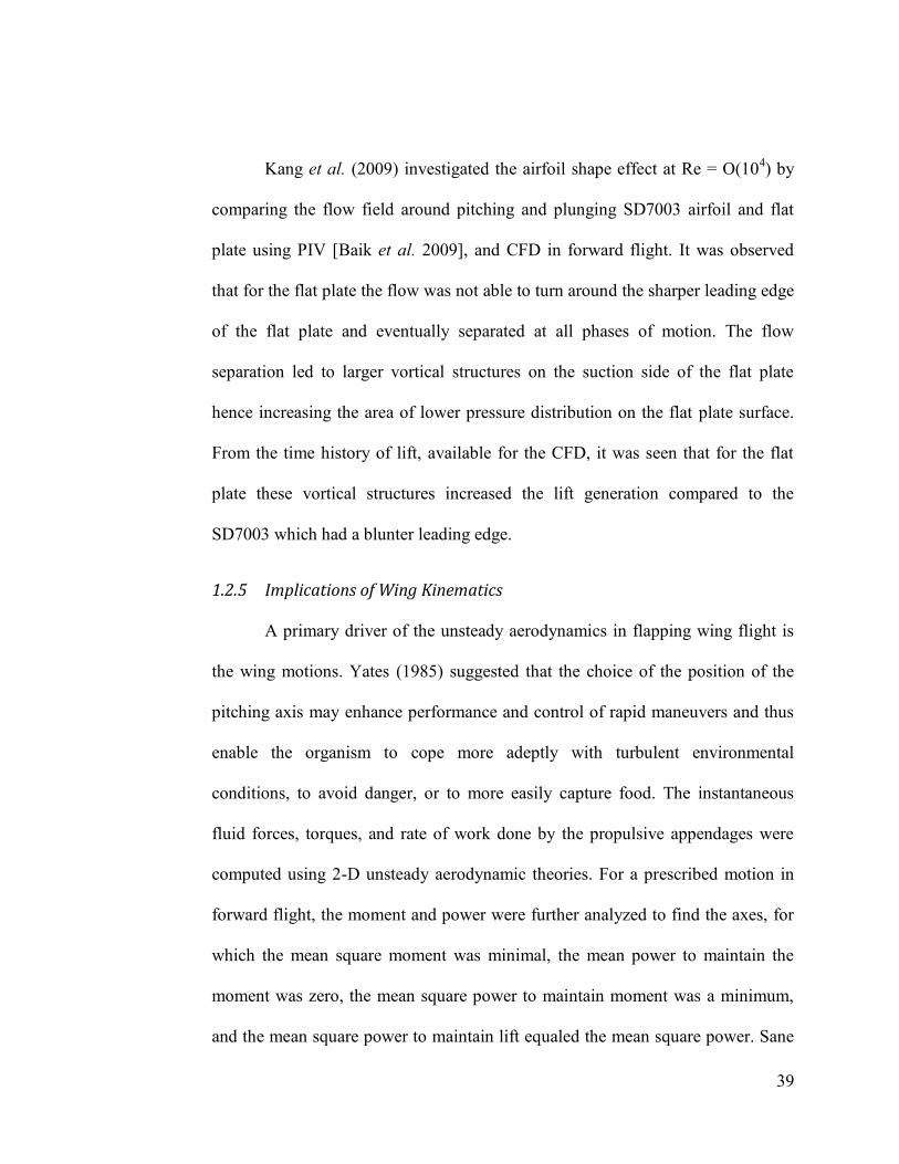
39

Kang et al. (2009) investigated the airfoil shape effect at Re = O(104) by

comparing the flow field around pitching and plunging SD7003 airfoil and flat

plate using PIV [Baik et al. 2009], and CFD in forward flight. It was observed

that for the flat plate the flow was not able to turn around the sharper leading edge

of the flat plate and eventually separated at all phases of motion. The flow

separation led to larger vortical structures on the suction side of the flat plate

hence increasing the area of lower pressure distribution on the flat plate surface.

From the time history of lift, available for the CFD, it was seen that for the flat

plate these vortical structures increased the lift generation compared to the

SD7003 which had a blunter leading edge.

1.2.5 Implications of Wing Kinematics

A primary driver of the unsteady aerodynamics in flapping wing flight is

the wing motions. Yates (1985) suggested that the choice of the position of the

pitching axis may enhance performance and control of rapid maneuvers and thus

enable the organism to cope more adeptly with turbulent environmental

conditions, to avoid danger, or to more easily capture food. The instantaneous

fluid forces, torques, and rate of work done by the propulsive appendages were

computed using 2-D unsteady aerodynamic theories. For a prescribed motion in

forward flight, the moment and power were further analyzed to find the axes, for

which the mean square moment was minimal, the mean power to maintain the

moment was zero, the mean square power to maintain moment was a minimum,

and the mean square power to maintain lift equaled the mean square power. Sane

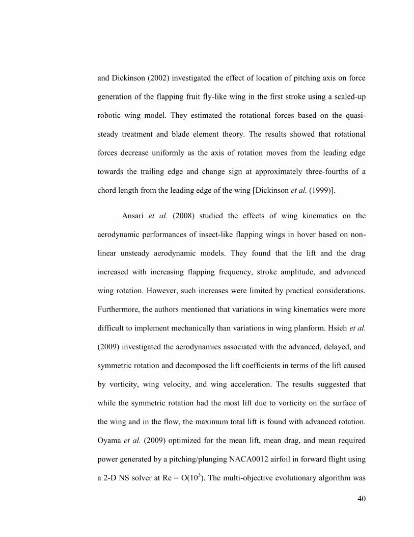
40

and Dickinson (2002) investigated the effect of location of pitching axis on force

generation of the flapping fruit fly-like wing in the first stroke using a scaled-up

robotic wing model. They estimated the rotational forces based on the quasi-

steady treatment and blade element theory. The results showed that rotational

forces decrease uniformly as the axis of rotation moves from the leading edge

towards the trailing edge and change sign at approximately three-fourths of a

chord length from the leading edge of the wing [Dickinson et al. (1999)].

Ansari et al. (2008) studied the effects of wing kinematics on the

aerodynamic performances of insect-like flapping wings in hover based on non-

linear unsteady aerodynamic models. They found that the lift and the drag

increased with increasing flapping frequency, stroke amplitude, and advanced

wing rotation. However, such increases were limited by practical considerations.

Furthermore, the authors mentioned that variations in wing kinematics were more

difficult to implement mechanically than variations in wing planform. Hsieh et al.

(2009) investigated the aerodynamics associated with the advanced, delayed, and

symmetric rotation and decomposed the lift coefficients in terms of the lift caused

by vorticity, wing velocity, and wing acceleration. The results suggested that

while the symmetric rotation had the most lift due to vorticity on the surface of

the wing and in the flow, the maximum total lift is found with advanced rotation.

Oyama et al. (2009) optimized for the mean lift, mean drag, and mean required

power generated by a pitching/plunging NACA0012 airfoil in forward flight using

a 2-D NS solver at Re = O(103). The multi-objective evolutionary algorithm was

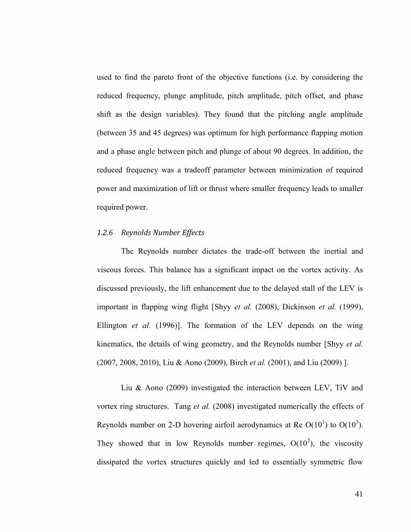
41

used to find the pareto front of the objective functions (i.e. by considering the

reduced frequency, plunge amplitude, pitch amplitude, pitch offset, and phase

shift as the design variables). They found that the pitching angle amplitude

(between 35 and 45 degrees) was optimum for high performance flapping motion

and a phase angle between pitch and plunge of about 90 degrees. In addition, the

reduced frequency was a tradeoff parameter between minimization of required

power and maximization of lift or thrust where smaller frequency leads to smaller

required power.

1.2.6 Reynolds Number Effects

The Reynolds number dictates the trade-off between the inertial and

viscous forces. This balance has a significant impact on the vortex activity. As

discussed previously, the lift enhancement due to the delayed stall of the LEV is

important in flapping wing flight [Shyy et al. (2008), Dickinson et al. (1999),

Ellington et al. (1996)]. The formation of the LEV depends on the wing

kinematics, the details of wing geometry, and the Reynolds number [Shyy et al.

(2007, 2008, 2010), Liu & Aono (2009), Birch et al. (2001), and Liu (2009) ].

Liu & Aono (2009) investigated the interaction between LEV, TiV and

vortex ring structures. Tang et al. (2008) investigated numerically the effects of

Reynolds number on 2-D hovering airfoil aerodynamics at Re O(101) to O(10

3).

They showed that in low Reynolds number regimes, O(102), the viscosity

dissipated the vortex structures quickly and led to essentially symmetric flow

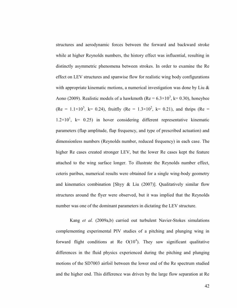
42

structures and aerodynamic forces between the forward and backward stroke

while at higher Reynolds numbers, the history effect was influential, resulting in

distinctly asymmetric phenomena between strokes. In order to examine the Re

effect on LEV structures and spanwise flow for realistic wing body configurations

with appropriate kinematic motions, a numerical investigation was done by Liu &

Aono (2009). Realistic models of a hawkmoth (Re = 6.3×103, k= 0.30), honeybee

(Re = 1.1×103, k= 0.24), fruitfly (Re = 1.3×10

2, k= 0.21), and thrips (Re =

1.2×101, k= 0.25) in hover considering different representative kinematic

parameters (flap amplitude, flap frequency, and type of prescribed actuation) and

dimensionless numbers (Reynolds number, reduced frequency) in each case. The

higher Re cases created stronger LEV, but the lower Re cases kept the feature

attached to the wing surface longer. To illustrate the Reynolds number effect,

ceteris paribus, numerical results were obtained for a single wing-body geometry

and kinematics combination [Shyy & Liu (2007)]. Qualitatively similar flow

structures around the flyer were observed, but it was implied that the Reynolds

number was one of the dominant parameters in dictating the LEV structure.

Kang et al. (2009a,b) carried out turbulent Navier-Stokes simulations

complementing experimental PIV studies of a pitching and plunging wing in

forward flight conditions at Re O(104). They saw significant qualitative

differences in the fluid physics experienced during the pitching and plunging

motions of the SD7003 airfoil between the lower end of the Re spectrum studied

and the higher end. This difference was driven by the large flow separation at Re

43

~1x104 whereas the flow at Re > 3x10

4 was largely attached. The pure plunging

case, which was meant to elicit deep stall, saw separation at all Re with the main

difference being whether or not the flow would be able to reattach. It was able to

for cases Re > 1x104. The flatplate was much less sensitive to the Re due to the

fact that the flow separation dominated the fluid physics. They also found

Theodorson‟s (1935) theory applicable despite the large separation regions

experienced in their studies.

1.2.7 Wing Flexibility and Aerodynamic Consequences

While the content of the original work documented in this thesis focuses

exclusively on rigid wing aerodynamics, natural flyers will have some degree of

flexibility in their wings. Some animals, like bats, have a membrane wing that is

predominantly flexible and the fluid-structure interactions become tightly

interdependent. The consequences of aeroelasticity in flapping wings is actively

being studied, but a full picture of aeroelastic impact is still not clear. Selected

studies from the literature are highlighted below to illustrate the potential for

manipulating the aerodynamic response.

Analytical investigations by Daniel and Combes (2002) suggested that

aerodynamic loads were relatively unimportant in determining the bending

patterns in oscillating wings. Subsequently, experimental investigations by

Combes (2002) and Combes and Daniel (2003a) found that the overall bending

patterns of a Hawkmoth wing were quite similar when flapped (single degree-of-

44

freedom flap rotation) in air and helium, despite a 85% reduction in fluid density

in the latter, suggesting that the contribution of aerodynamic forces was relatively

small compared to the contribution of inertial-elastic forces doing flapping

motion. However, they mentioned that realistic wing kinematics might include

rapid rotation at the stroke reversal that may lead to increased aerodynamic forces

due to unsteady aerodynamic mechanisms. Furthermore, static bending tests by

Combes and Daniel (2003b,c) showed anisotropy of wing structures in a variety

of insect species. More recently, Mountcastle and Daniel (2009) investigated the

influence of wing compliance on the mean advective flows (indicative of induced

flow velocity) using PIV techniques. Their results demonstrated that flexible

wings yield mean advective flows with substantially greater magnitudes and

orientations more beneficial to lift than those of stiff wings.

Vanella et al. (2009) conducted numerical investigations on a similar

structure found that the best performance (up to approximately 30% increase in

lift) was realized when the wing was excited by a non-linear resonance at 1/3rd of

its natural frequency. For all Reynolds numbers considered, the wake capture

mechanism was enhanced due to a stronger flow around the wing at stroke

reversal, resulting from a stronger vortex at the trailing edge. Heathcote et al.

(2004) investigated the effect of chordwise flexibility on aerodynamic

performance of an airfoil in pure plunge under hovering conditions. Because the

trailing edge was a major source of shedding of vorticity at zero freestream

velocity, they showed that the amplitude and phase angle of the motion of the

45

trailing edge affected the strength and spacing of the vortices, and the time

averaged velocity of the induced jet. Direct force measurements confirmed that at

high plunge frequencies, the thrust coefficient of the airfoil with intermediate

stiffness was highest, although the least stiff airfoil can generate larger thrust at

low frequencies. It was suggested that there was an optimum airfoil stiffness for a

given plunge frequency and amplitude. Similar conclusions were made in another

study [Michelin & Smith (2009)], wherein the influence of resonance on the

performance of a chordwise flexible airfoil prescribed with pure plunge motion at

its leading edge was studied. It was shown that while the mean thrust could

increase with an increase in flexibility, below a certain threshold the wing is too

flexible to communicate momentum to the flow. On the other hand, too much

flexibility led to a net drag and hence, only a suitable amount of flexibility was

desirable for thrust generation.

Du and Sun (2008) numerically investigated the effect of prescribed time-

varying twist and chordwise deformation on the aerodynamic force production of

a fruitfly in hover. The results showed that aerodynamic forces on the flapping

wing were not affected much by the twist, but by the camber deformation. The

effect of combined camber and twist deformation was found to be similar to that

of camber deformation alone. With a deformation of 6% camber and 20° twist

(typical values observed for wings of many insects), the lift increased by 10% -

20% compared to the case of a rigid flat plate wing. It was therefore shown that

46

chordwise deformation could increase the maximum lift coefficient of a fruit fly

wing model and reduce its power requirement for flight.

While most of the recent computational and experimental studies explored

the role of wing flexibility in augmenting aerodynamic performance while

focusing on single wings at relatively higher Reynolds numbers, Miller and

Peskin (2009) numerically investigated the effect of wing flexibility on the forces

produced during clap and fling/peel motion [Ellington (1984)] of a small insect

(Re ≈ 10) focusing on wing-wing interactions. They prescribed both clap and

fling kinematics separately to a rigid and a chordwise flexible wing and showed

that while lift coefficients produced during the rigid and flexible clap strokes were

comparable, the peak lift forces in the flexible cases were higher than in the

corresponding rigid cases. This was due to the peel motion which delayed the

formation of the trailing edge vortices, thereby maintaining vortical asymmetry

and augmenting lift for longer periods.

Hui et al. (2009) examined various flexible wing structures to evaluate

their implications on flapping wing aerodynamics. They showed that the flexible

membrane wings were found to have better overall aerodynamic performance

(i.e., lift-to-drag ratio) over the rigid wing for soaring flight, especially for high

speed soaring flight or at relatively high angle of attack. The rigid wing was found

to have better lift production performance for flapping flight in general. The latex

wing, which was the most flexible among the three tested wings, was found to

47

have the best thrust generation performance for flapping flight. The less flexible

nylon wing, which has the best overall aerodynamic performance for soaring

flight, was found to be the worst for flapping flight applications. Shkarayev et al.

(2010) investigated the aerodynamics of cambered membrane flapping wings.

Specifically, a cambered airfoil was introduced into the wing by shaping metal

ribs attached to the membrane skin of the 25 cm-wing-span model. The thrust

force generated by a 9% camber wing was found to be 30% higher than that of the

same size flat wing. Adding a dihedral angle to the wings and keeping the

flapping amplitude constant improved the cambered wing‟s performance even

further.

Kim et al. (2009) developed a biomimetic flexible flapping wing using

micro-fiber composite actuators and experimentally investigated the aerodynamic

performance of the wing under flapping and non-flapping motion in a wind

tunnel. Results showed that the camber due to wing flexibility could produce

positive effects (i.e. stall delay, drag reduction, and stabilization of the LEV) on

flapping wing aerodynamics in quasi-steady and unsteady region. Mueller et al.

(2009) presented a new versatile experimental test for measuring the thrust and

lift of a flapping wing MAV. They showed increase in average thrust due to

increased wing compliance and detrimental influence of excessive compliance on

drag forces during high frequency operation. Also they observed the useful effect

of compliance on the generation of extra thrust at the beginning and end of

flapping motions.

48

Hamamoto et al. (2007) conducted a fluid-structure interaction analysis on

a deformable dragonfly wing in hover and examined the advantages and

disadvantages of flexibility. They tested three types of flapping flight: a flexible

wing driven by dragonfly flapping motion, a rigid wing (stiffened version of the

original flexible dragonfly wing) driven by dragonfly flapping motion, and a rigid

wing driven by modified flapping based on tip motion of the flexible wing. They

found that the flexible wing, with nearly the same average energy consumption,

generated almost the same amount of lift force as the rigid wing with modified

flapping motion, which realized the same angle of attack at the aerodynamically

dominant sections of the wing. However, the rigid wing required 19% more peak

torque and 34% more peak power, indicating the usefulness of wing flexibility.

Aono et al. (2010) reported a combined computational and experimental study of

a flapping wing structure. An aluminum wing was prescribed with single degree-

of-freedom flapping at 10 Hz frequency and ±21º amplitude. Flow velocities and

deformation were measured using digital image correlation and digital PIV

techniques, respectively. In the most flexible flapping wing case, the elastic

twisting of the wing was shown to produce substantially larger mean and

instantaneous thrust due to shape deformation-induced changes in effective angle

of attack. Relevant fluid physics were documented including the counter-rotating

vortices at the leading and the trailing edge which interacted with the tip vortex

during the wing motion.

49

Agrawal and Agrawal (2009) investigated the benefits of insect wing

flexibility on flapping wing aerodynamics based on experiments and numerical

simulations. They compared the performance of two synthetic wings: (i) a flexible

wing based on a bio-inspired design of the hawkmoth (Manduca Sexta) wing and

(ii) a rigid wing of similar geometry. The results demonstrated that more thrust

was generated by the bio-inspired flexible wing compared to the rigid wing in all

wing kinematic patterns considered. They emphasized that the results provided

motivation for exploring the advantages of passive deformation through wing

flexibility and that coupled fluid-structure simulations of flexible flapping wings

were required to gain a fundamental understanding of the physics and to guide

optimal flapping wing MAV designs.

As summarized in Shyy et al. (2010), it seems like the spanwise flexibility

increases aerodynamic forces by creating higher effective angles of attack via

spanwise deformation. However, apart from affecting the overall aerodynamic

force generation, the chordwise flexibility can redistribute lift versus thrust by

changing the angle of the wing with respect to the freestream or the camber of the

wing itself. Overall, an understanding of the structural response and its interplay

with the unsteady aerodynamics has the potential to exceed rigid wing

performance in the context of flapping wing flight. Optimizing the process of

assigning the material properties of the wing based off their impact on the

unsteady flight mechanisms, and thus performance, is still an open area of

research.

50

1.2.8 Reduced Order Models

Before the advent of readily available computational resources and the

methods to utilize them, researchers had to rely on combinations of empirical data

and analytical models. These methods find use today as they have the potential to

provide insight as the governing equations are modified and/or simplified, and as

a quick estimate to be used in a design tool for which on-demand Navier-Stokes

solutions are too computationally expensive or unrealistic.

One approach used in flapping wing aerodynamics are variations of quasi-

steady theories. Flapping wing movements inherently have a time-dependent

nature to them; what quasi-steady theory does is to assume the solution is

instantaneously steady-state and that equivalent forces are felt for a wing with the

same velocity and angle of attack. One of the strengths is having an analytical

solution which is ideal in terms of computational expense. Theodorsen (1935) and

Osborne (1951) modified the blade-element theory of Drzewiecki for flapping

flight applications. While Jensen (1956) saw promise when applying the

principles to tethered locusts, Cloupeau et al. (1979) showed that the forces felt

by the tethered locust were in clear excess of those predicted by quasi-steady

theory. Ellington (1984) found the validity of applying quasi-steady theory to

flapping wing applications ambiguous. Dudley and Ellington (1990) showed that

the fast forward flight of bumblebees was incompatible with quasi-steady

51

aerodynamics. Sane and Dickinson (2002) made further modifications and found

that quasi-steady theory could meaningfully approximate lift and drag values

away from the wake-capture region. Because the models they built did not include

this time history effect they were able to show how much of an impact wake-

capture had on the force history which could be quite significant. Kang et al.

(2009a), as discussed above in section 1.2.6, found applicability in quasi-steady

models for forward flight conditions at Re O(104) despite large regions of

separated flow. The applicability of such models would appear to be highly

context dependent.

Another approach being adopted is numerical in nature, but significantly

less expensive than solving the Navier-Stokes equations. This branch of

investigations is based of inviscid theory and vortex-lattice methods [Anderson

(2006)]. Modifications to the classical theory have been made to allow for the

moving boundary and the shedding of vortices from the leading edge in addition

to the trailing edge. Gogulapati et al. (2008, 2010) showed promising results in

hovering and forward flight conditions for rigid and flexible wings capturing the

overall trends in the force histories for the cases studied and in some situations

closely approximating the instantaneous forces quite closely.

This thesis aims to 1) explore and illuminate the relevant fluid physics in

flapping wing flight as a function of kinematic wing motions 2) provide a method

52

for quickly and accurately predicting the aerodynamic performance in such a way

to be potentially useful for control algorithm implementation.

In regard to point 1, some influences are well documented, e.g. the LEV.

Its role is examined as function of the kinematic motions, and in concert with the

literature is found to be a dominant lift enhancing mechanism at Re = 100. Other

phenomena are recognized but not well documented in the flapping wing

community. The tip vortices found in steady state aerodynamic theory are sources

of performance penalties. It is shown that certain kinematic motions in flapping

wing flight can utilize these tip vortices as a lift enhancement mechanism which

departs from the behavior expressed by the steady state theories. Another

phenomena examined in the following work is the downward jet, which was

observed to exist experimentally, but whose impact was otherwise entirely

ignored. This is work examines the impact on the aerodynamic loading when the

downward jet is present.

The fluid physics exploration used a combination of CFD simulations of

the Navier-Stokes equations and relevant to point 2, a computationally cheap

reduced order model. To be addressed in the following chapter is the reduced

order model technique employed in the current studies, surrogate models. These

need to be trained, e.g. from experimental data or computational simulations, but

then offer predictions at some combination of variables away from the training

data and can be used in a variety of ways to probe the desired phenomena.

53

Chapter 2 Approach and Methods

Due to the complexity of the aerodynamics associated with bio-mimicking

kinematics, building a description of the fundamental factors involved can benefit

from simplified models. As previously addressed, the aerodynamics associated

with flapping wing flight during hover can be dominated by the interactions

between the wing and generated vortices and these interactions can make it

difficult for approximate models to correctly predict quantities of interest. To

capture the appropriate phenomena, solutions to the full governing equations are

solved. This takes the form of computational fluid dynamics simulations (CFD)

that numerically solve the Navier-Stokes equations. From a vehicle development

perspective, since 3D Navier-Stokes simulations are expensive to generate, if 2D

simplifications or other approximations can adequately reproduce the main

aerodynamic features of 3D flapping wing, then the needed data can be generated

much more economically. The simplified models in this study are surrogate

modeling tools that are used in a complementary fashion to systematically

examine the design space while linking the instantaneous force histories and fluid

physics from the Navier-Stokes solutions to the general trends in performance as

kinematic variables are varied.

54

2.1 CFD Modeling

The governing equations are the laminar, unsteady, Navier-Stokes

equations with constant density and transport properties; the incompressible

versions are shown in Eqs. (1) and (2) written in indicial form.

(3)

(4)

Here ui is the velocity vector, xi is the Cartesian position vector, t is time, ρ

is the density of the fluid, p is the pressure, and ν is the kinematic viscosity of the

fluid. Even during the solution of identical equations, the numerical methods

employed can have implications on the stability and accuracy of the solution. Two

codes with vastly different methodologies are used in this study, Loci-STREAM

and FDL3DI and are briefly discussed below.

A rule-based software (see Luke and George 2005), Loci-STREAM (see

Kamakoti et al. 2006) is used to calculate the solutions. Loci-STREAM is a three-

dimensional, unstructured, pressure based finite volume solver. The present

calculations use implicit first or second order time stepping (the first order

technique is adopted in this study). The convection terms are treated using the

second order upwind scheme (see Shyy 1985; Shyy 1994) while pressure and

viscous terms are treated using second order schemes. The system of equations

resulting from the linearized momentum equations are fast to converge (see Shyy

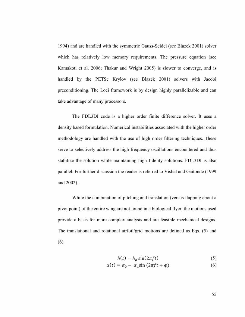
55

1994) and are handled with the symmetric Gauss-Seidel (see Blazek 2001) solver

which has relatively low memory requirements. The pressure equation (see

Kamakoti et al. 2006; Thakur and Wright 2005) is slower to converge, and is

handled by the PETSc Krylov (see Blazek 2001) solvers with Jacobi

preconditioning. The Loci framework is by design highly parallelizable and can

take advantage of many processors.

The FDL3DI code is a higher order finite difference solver. It uses a

density based formulation. Numerical instabilities associated with the higher order

methodology are handled with the use of high order filtering techniques. These

serve to selectively address the high frequency oscillations encountered and thus

stabilize the solution while maintaining high fidelity solutions. FDL3DI is also

parallel. For further discussion the reader is referred to Visbal and Gaitonde (1999

and 2002).

While the combination of pitching and translation (versus flapping about a

pivot point) of the entire wing are not found in a biological flyer, the motions used

provide a basis for more complex analysis and are feasible mechanical designs.

The translational and rotational airfoil/grid motions are defined as Eqs. (5) and

(6).

(5)

(6)

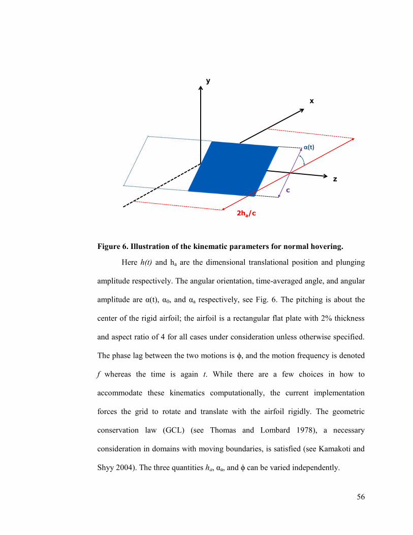
56

Figure 6. Illustration of the kinematic parameters for normal hovering.

Here h(t) and ha are the dimensional translational position and plunging

amplitude respectively. The angular orientation, time-averaged angle, and angular

amplitude are α(t), α0, and αa respectively, see Fig. 6. The pitching is about the

center of the rigid airfoil; the airfoil is a rectangular flat plate with 2% thickness

and aspect ratio of 4 for all cases under consideration unless otherwise specified.

The phase lag between the two motions is ϕ, and the motion frequency is denoted

f whereas the time is again t. While there are a few choices in how to

accommodate these kinematics computationally, the current implementation

forces the grid to rotate and translate with the airfoil rigidly. The geometric

conservation law (GCL) (see Thomas and Lombard 1978), a necessary

consideration in domains with moving boundaries, is satisfied (see Kamakoti and

Shyy 2004). The three quantities ha, αa, and ϕ can be varied independently.

x

y

z

c

2ha/c

α(t)

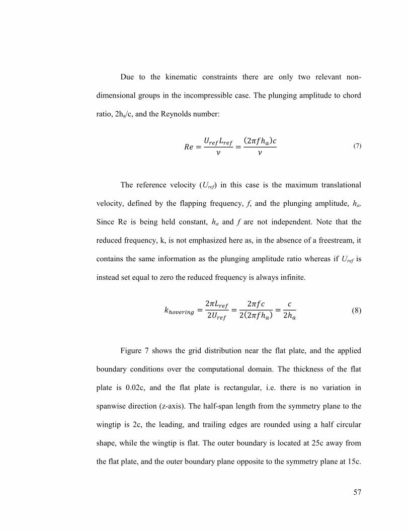
57

Due to the kinematic constraints there are only two relevant non-

dimensional groups in the incompressible case. The plunging amplitude to chord

ratio, 2ha/c, and the Reynolds number:

(7)

The reference velocity (Uref) in this case is the maximum translational

velocity, defined by the flapping frequency, f, and the plunging amplitude, ha.

Since Re is being held constant, ha and f are not independent. Note that the

reduced frequency, k, is not emphasized here as, in the absence of a freestream, it

contains the same information as the plunging amplitude ratio whereas if Uref is

instead set equal to zero the reduced frequency is always infinite.

(8)

Figure 7 shows the grid distribution near the flat plate, and the applied

boundary conditions over the computational domain. The thickness of the flat

plate is 0.02c, and the flat plate is rectangular, i.e. there is no variation in

spanwise direction (z-axis). The half-span length from the symmetry plane to the

wingtip is 2c, the leading, and trailing edges are rounded using a half circular

shape, while the wingtip is flat. The outer boundary is located at 25c away from

the flat plate, and the outer boundary plane opposite to the symmetry plane at 15c.

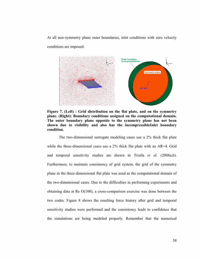
58

At all non-symmetry plane outer boundaries, inlet conditions with zero velocity

conditions are imposed.

Figure 7. (Left) : Grid distribution on the flat plate, and on the symmetry

plane. (Right): Boundary conditions assigned on the computational domain.

The outer boundary plane opposite to the symmetry plane has not been

shown due to visibility and also has the incompressibleInlet boundary

condition.

The two-dimensional surrogate modeling cases use a 2% thick flat plate

while the three-dimensional cases use a 2% thick flat plate with an AR=4. Grid

and temporal sensitivity studies are shown in Trizila et al. (2008a,b).

Furthermore, to maintain consistency of grid system, the grid of the symmetry

plane in the three-dimensional flat plate was used as the computational domain of

the two-dimensional cases. Due to the difficulties in performing experiments and

obtaining data at Re O(100), a cross-comparison exercise was done between the

two codes. Figure 8 shows the resulting force history after grid and temporal

sensitivity studies were performed and the consistency leads to confidence that

the simulations are being modeled properly. Remember that the numerical

59

methods involved are very different and any error or inconsistency in

methodology in one would be hard to reproduce in the other framework.

Figure 8. Cross-validation of Loci-Stream and FDL3DI for a two-

dimensional ellipse with 15% thickness during normal hovering computation

with for Re = 100, 2ha/c = 3.0, αa = 45°, φ = 90°.

2.2 Surrogate Modeling

The motivation behind surrogate models is to replace costly objective

function evaluations, a quantity of interest such as time averaged lift obtained via

detailed CFD solutions or substantial experimental setups, with inexpensive

approximations of sufficient fidelity. Overview of surrogate modeling techniques

and selected applications can be found in reference Queipo et al. (2005) and is

illustrated in Fig. 9. The process starts with choosing number and locations of

training points in the “design space” (here meaning the three-dimensional space

encompassing the three kinematic parameters); this is known as constructing the

60

design of experiment (DOE). Once the training points are chosen, the objective

functions must be evaluated; depending on the context this can be done

computationally, analytically, and/or experimentally. After the objective functions

have been obtained for the selected training points, the surrogate models can be

built. Popular models are polynomial response surfaces (PRS) [Myers and

Montgomery (2002)], Kriging [Sacks, Schiller, and Welch (1989)], radial basis

neural networks (RBNN) [Cheng and Titterington (1994)], support vector

regression (SVR) models [Smola and Scholkopf (2004)] and various

combinations thereof. After the models are constructed, appropriate error

measures can be adopted to construct a weighted average surrogate (WAS) [Goel

et al. (2007), Viana et al. (2008)]. Based on the surrogate approximation, the

global sensitivity evaluations can be performed to evaluate the individual and

collective influence of the kinematic parameters (design variables) and to order

their relative importance in determining the aerodynamic outcome.

Note: In the following surrogate modeling sections the variable “x” is not

used to refer to spatial dimensions, but rather the design variables; in the current

studies this would be the plunging amplitude, angular amplitude, or phase lag.

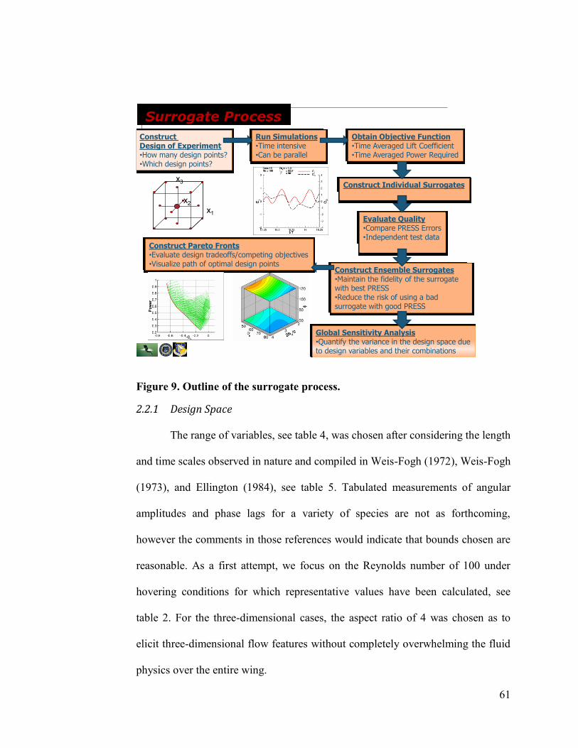
61

Surrogate Process

Construct Design of Experiment•How many design points?•Which design points?

Evaluate Quality•Compare PRESS Errors•Independent test data

Construct Individual Surrogates

Run Simulations•Time intensive•Can be parallel

Construct Ensemble Surrogates•Maintain the fidelity of the surrogate with best PRESS•Reduce the risk of using a bad surrogate with good PRESS

Global Sensitivity Analysis•Quantify the variance in the design space dueto design variables and their combinations

Obtain Objective Function•Time Averaged Lift Coefficient•Time Averaged Power Required

x1

x2

x3

Construct Pareto Fronts•Evaluate design tradeoffs/competing objectives•Visualize path of optimal design points

Figure 9. Outline of the surrogate process.

2.2.1 Design Space

The range of variables, see table 4, was chosen after considering the length

and time scales observed in nature and compiled in Weis-Fogh (1972), Weis-Fogh

(1973), and Ellington (1984), see table 5. Tabulated measurements of angular

amplitudes and phase lags for a variety of species are not as forthcoming,

however the comments in those references would indicate that bounds chosen are

reasonable. As a first attempt, we focus on the Reynolds number of 100 under

hovering conditions for which representative values have been calculated, see

table 2. For the three-dimensional cases, the aspect ratio of 4 was chosen as to

elicit three-dimensional flow features without completely overwhelming the fluid

physics over the entire wing.

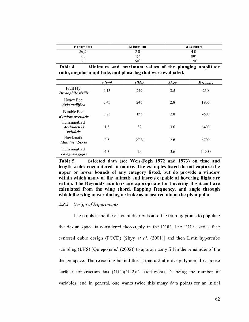
62

Parameter Minimum Maximum

2ha/c 2.0 4.0

αa 45˚ 80˚

φ 60˚ 120˚

Table 4. Minimum and maximum values of the plunging amplitude

ratio, angular amplitude, and phase lag that were evaluated.

c (cm) f(Hz) 2ha/c Rehovering

Fruit Fly:

Drosophila virilis 0.15 240 3.5 250

Honey Bee:

Apis mellifica 0.43 240 2.8 1900

Bumble Bee:

Bombus terrestris 0.73 156 2.8 4800

Hummingbird:

Archilochus

colubris

1.5 52 3.6 6400

Hawkmoth:

Manduca Sexta 2.5 27.3 2.6 6700

Hummingbird:

Patagona gigas 4.3 15 3.6 15000

Table 5. Selected data (see Weis-Fogh 1972 and 1973) on time and

length scales encountered in nature. The examples listed do not capture the

upper or lower bounds of any category listed, but do provide a window

within which many of the animals and insects capable of hovering flight are

within. The Reynolds numbers are appropriate for hovering flight and are

calculated from the wing chord, flapping frequency, and angle through

which the wing moves during a stroke as measured about the pivot point.

2.2.2 Design of Experiments

The number and the efficient distribution of the training points to populate

the design space is considered thoroughly in the DOE. The DOE used a face

centered cubic design (FCCD) [Shyy et al. (2001)] and then Latin hypercube

sampling (LHS) [Quiepo et al. (2005)] to appropriately fill in the remainder of the

design space. The reasoning behind this is that a 2nd order polynomial response

surface construction has (N+1)(N+2)/2 coefficients, N being the number of

variables, and in general, one wants twice this many data points for an initial

63

curve fit which would try and reconcile the computational cost (fewer training

points desired) with the resulting fidelity (more training points desired). A FCCD

design provides 2N+2N+1 points: 2

N corner points, 2N face points, and one center

point. Thus for three design variables, FCCD provides 15 of the 20 points

required. The LHS then provides a method for efficiently choosing the rest of the

points by maximizing the distance between the added points. A tabulation of the

two-dimensional and three-dimensional simulations run and their respective

outcomes, as well as quantitative measures of merit for the surrogate models, are

found in Trizila et al. (2008a).

2.2.3 Prediction Error Sum of Squares (PRESS)

PRESS is one of the quantities used to evaluate the quality of a surrogate

model after it has been constructed, i.e. it is not known a priori. It should be

emphasized that a good PRESS value (low) is not a guarantee of a good surrogate

fit, but that a bad PRESS value (high) is an indication that the surrogate model

does not accurately predict the training data. The idea behind PRESS is to use the

training data to evaluate the quality of the surrogate. Creating surrogates is

inexpensive compared to the time needed for full Navier-Stokes solutions. While

data independent of the training data is needed for validation purposes these are

expensive and minimized. PRESS takes the N training points and uses N-1 to

create the surrogate model. The error is then calculated between the surrogate and

the training point left out. This process is repeated for all N training points (there

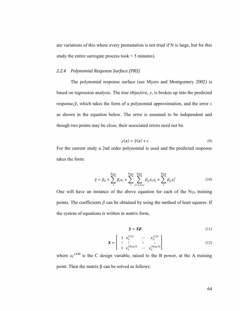
64

are variations of this where every permutation is not tried if N is large, but for this

study the entire surrogate process took < 5 minutes).

2.2.4 Polynomial Response Surface (PRS)

The polynomial response surface (see Myers and Montgomery 2002) is

based on regression analysis. The true objective, y, is broken up into the predicted

response, , which takes the form of a polynomial approximation, and the error ϵ

as shown in the equation below. The error is assumed to be independent and

though two points may be close, their associated errors need not be.

(9)

For the current study a 2nd order polynomial is used and the predicted response

takes the form:

(10)

One will have an instance of the above equation for each of the NTP training

points. The coefficients β can be obtained by using the method of least squares. If

the system of equations is written in matrix form,

(11)

(12)

where xC(A)B

is the C design variable, raised to the B power, at the A training

point. Then the matrix β can be solved as follows:

65

(13)

2.2.5 Kriging

The Kriging (see Sacks et al. 1989) methodology predicts the objective

function as the sum of a polynomial trend, f(x), and a systematic departure, Z(x)

as expressed below.

(14)

The polynomial trend, usually a polynomial of degree 0,1,or 2, accounts

for the low frequency general response of the objective function(s) where the

systematic departure is relatively localized and catches the higher frequency

variation from the trend line but also has a zero mean. Whereas the PRS models

assume independent error, Kriging models are built with the assumption the errors

are correlated. The Gaussian correlation structure used (see Sacks et al. 1989)

takes the form of

(15)

One cycles through and evaluates the kth

design variable x at the ith

and jth

training

points. The standard deviation of the design space is denoted by σ, and θk is a

fitting parameter measuring the degree of correlation in the k direction. Thus,

given NTP training points, f(x), σ, and θk, are chosen such that the likelihood

function is maximized (see Sacks et al. 1989). As two points move closer,

(‖xki-xk

j ‖)→0 , and the correlation function reaches a maximum. Note that at the

66

training points (x) = y(x), and the predicted response matches that of the true

response used to train the models.

2.2.6 Radial Basis Neural Network (RBNN)

Like the Kriging models, the radial basis neural networks use localized

correlation functions. However, unlike Kriging, RBNN do not use a global

approximation term. The predicted response at the design point x is given below.

The weighting factors are denoted wi, and response of the ith

radial basis function

is ai which depends on the distance between two design points. The influence of

all NRBF are summed to get the total response. A popular choice for the basis

function is a Gaussian correlation. The parameter b is the bias and inversely

related to an input parameter that controls the spread, or radius of influence for

the neurons. A spread constant, usually between 0 and 1, that is higher will cause

a smoother transition between neurons‟ regions of influence and result in a more

non-linear response. Too large a spread constant will diffuse the neurons‟

sensitivity, and thus a balance must be met.

(16)

(17)

(18)

Neurons are added one at a time until a user specified tolerance is achieved. A

tolerance that is arbitrarily low is not desirable as this may lead to over-fitting and

responses which are not accurate away from the training points. Five percent of

67

the mean data is a common goal tolerance. The number of radial basis functions

and their associated weights are solved in a “leave one out” procedure similar to

that used in PRESS where parameter combinations are tested until meeting the

desired tolerance. Each point is systematically left out and the models

constructed, and the fitting parameters resulting in the minimum error as summed

from the predicted response to the left out points determine the model used.

2.2.7 Weighted Average Surrogate Models (WAS)

Surrogate models may fit the training data well, however this does not

guarantee a decent fit throughout the design space. Different weighting strategies

are employed to minimize the risk of including one of these surrogates, which

based on certain error measures may seem acceptable, but in reality gives bad

predictions in other parts of the design space. The weighted average surrogates

currently employed use constant weights, meaning that a certain surrogate will

have the same importance throughout the design space. Equation (19) expresses

that the (WAS) is a function of the M candidate surrogates, i.e. those with

acceptable PRESS values. (Bad PRESS values = bad surrogate models, good

PRESS values do NOT guarantee good surrogate models)

(19)

The method proposed by Viana et al.(2008), minimizes the least square error over

the domain where wi is the weighting vector, eWAS is the error associated with the

prediction of the WAS model, and the elements of C, cij are given as functions of

68

the error of the ith

and jth

surrogate models. The weights can then be solved for as

shown.

(20)

(21)

(22)

The method proposed by Goel et al. (2007), instead uses two parameters to

control the weighting strategy αw (recommended value of 0.05) and βw

(recommended value of -1) used to control the influence of the average, eavg, and

the individual PRESS errors, ei, respectively.

(23)

(24)

(25)

2.2.8 Global Sensitivity Analysis (GSA)

The global sensitivity analysis (GSA) is in general useful for: (i)

determining if a variable is particularly influential in the design space, if not

perhaps the variable can be fixed and the degrees of freedom and complexity of

the problem reduced; (ii) ranking the importance of the design variables; (iii)

quantifying the degree of coupling between design variables. For example, is the

69

influence on the design space mostly an individual effort, or is there an effect

caused by the interaction of variables?

Sobol‟s method (see Quiepo et al. 2005) is used for the global sensitivity

evaluations. The surrogate model can be written as:

(26)

Once this decomposition has been calculated the total variance,

(27)

and partial variances, e.g.,

(28)

can be calculated. In this fashion, individual contributions, such as D1/D, or

combinations of variables, e.g., D12/D, can be quantified, effectively capturing the

sensitivity of the variable(s) under consideration.

70

Chapter 3 Hovering Aerodynamics of a Rigid Flat Plate

In this section, we use the surrogate modeling technique, utilizing the

weight-averaged surrogate model [Viana et al. 2008, Goel et al. 2007] to establish

the relationship between lift generated and power required as the three flapping

kinematic parameters vary. The purpose is to gain a global perspective of a multi-

dimensional design space and this is done by combining the detailed fluid physics

and force histories from the Navier-Stokes solutions and combining it with

surrogate modeling trends.

3.1 Interpreting Force Histories and Flow Features

To better understand the implications and limitations of the surrogate

modeling results an example is presented of a representative normal hovering case

of a two-dimensional flat plate at a Re of 100, see figure 10. In the flapping wing

aerodynamics the unsteady mechanisms such as wake capturing and delayed stall

have been established in the literature (see section 1.1).

The discussion following is generally applicable to the synchronized

hovering cases, where phase lag ϕ = 90°. For cases where the phase lag dictates

advanced rotation (ϕ > 90°) or delayed rotation (ϕ < 90°), the same ideas can be

extended though as the parameter suggests, the translation and rotation will be out

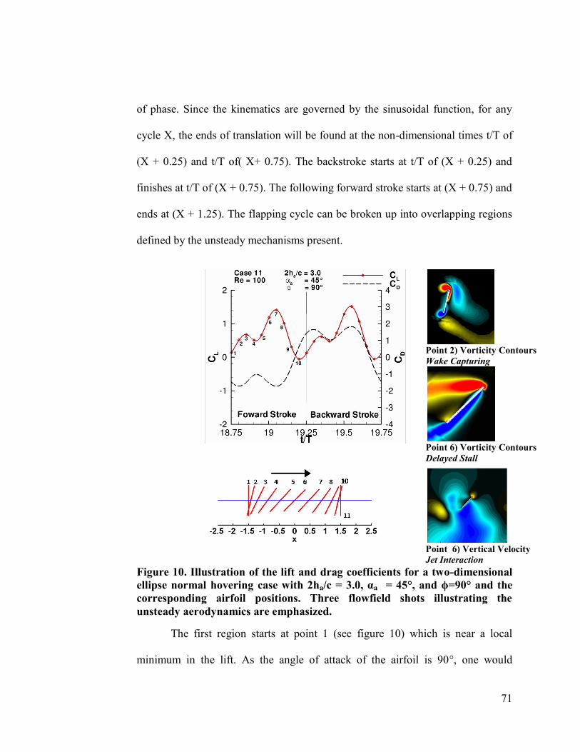
71

of phase. Since the kinematics are governed by the sinusoidal function, for any

cycle X, the ends of translation will be found at the non-dimensional times t/T of

(X + 0.25) and t/T of( X+ 0.75). The backstroke starts at t/T of (X + 0.25) and

finishes at t/T of (X + 0.75). The following forward stroke starts at (X + 0.75) and

ends at (X + 1.25). The flapping cycle can be broken up into overlapping regions

defined by the unsteady mechanisms present.

Point 2) Vorticity Contours

Wake Capturing

Point 6) Vorticity Contours

Delayed Stall

Point 6) Vertical Velocity

Jet Interaction

Figure 10. Illustration of the lift and drag coefficients for a two-dimensional

ellipse normal hovering case with 2ha/c = 3.0, αa = 45°, and ϕ=90° and the

corresponding airfoil positions. Three flowfield shots illustrating the

unsteady aerodynamics are emphasized.

The first region starts at point 1 (see figure 10) which is near a local

minimum in the lift. As the angle of attack of the airfoil is 90°, one would

72

generally expect zero lift. As time continues the airfoil turns back into its previous

wake which is the well-known wake capturing, points 1, 2, and 3. The peak seen

at point 3 will be referred to as the wake capturing peak.

The second unsteady mechanism is due to the angular velocity and the

change in circulation about the flat plate, i.e. the Kramer effect. In the literature

(see 1.1.2), one version of this is referred to as rapid pitch-up. In the present study

it is seen to both aid and take away from the lift production. When ϕ = 90°, as in

the example, the maximum angular velocities are found at the ends of translation.

In two-dimensional case this negative angular velocity at the start of the stroke is

one of the reasons, the other is a contribution of the persistent jet interaction that

degrades the lift as the flow is accelerated on the bottom of the flat plate.

Depending on the kinematic parameters, this unsteady mechanism may interact

with any or all of the other unsteady mechanisms.

The third and fourth unsteady flow features overlap significantly. The

most commonly known is the delayed stall phenomena here resulting from a LEV

at mid-stroke (see figure 10). Specifically, a vortex forms behind the leading edge

of the flat plate producing a low pressure region and enhancing lift. Note that in

the case illustrated, higher lift is achieved at angles of attack of 45°, an angle well

beyond the steady state stall. In cases with higher angular amplitudes, and

therefore lower angles of attack, the peak at points 7 and 8 can be reduced

significantly because the orientation of the airfoil is not able to promote LEV

73

formation. The fourth unsteady feature is the persistent jet which will be

discussed in detail next.

3.1.1 Impact of a Persistent Jet in 2D Hovering

Despite the fact that the specified kinematics are similar during forward

and backstrokes, a substantial asymmetry can sometimes be seen in the resulting

force history. This phenomenon can occur in part due to the formation of a

persistent jet seen to develop as a result of a reverse Karman vortex street

interacting with the downward momentum created by the wing as it translates (see

figure 4). As the wing passes the jet, vortices are shed with an orientation which

reinforces the downward momentum previously created by the wing. These

vortices sustain the downward momentum, and further entrain surrounding fluid,

as to create a flow feature which the wing then interacts with during subsequent

stroke. The details in the initiation of the jet may present a slight bias serving to

off-center the jet. The consequence is that during a forward stroke, the wing will

encounter the jet earlier/later than during the backstroke.

The impact of the jet interaction is more influential in two-dimensional

fluid dynamics. A brief study of wing startup conditions reveals that the evolution

of the jet can impact the aerodynamic loading significantly.

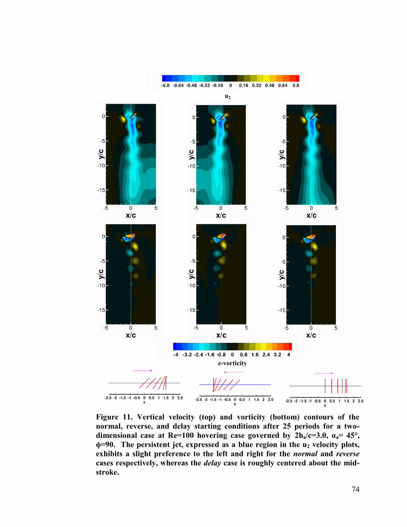
74

u2

z-vorticity

Figure 11. Vertical velocity (top) and vorticity (bottom) contours of the

normal, reverse, and delay starting conditions after 25 periods for a two-

dimensional case at Re=100 hovering case governed by 2ha/c=3.0, αa= 45°,

ϕ=90. The persistent jet, expressed as a blue region in the u2 velocity plots,

exhibits a slight preference to the left and right for the normal and reverse

cases respectively, whereas the delay case is roughly centered about the mid-

stroke.

75

Three startup conditions were evaluated. Normal: start the computation

with the appropriate angle of attack at mid-stroke. Reverse: start the computation

in the opposite direction with the appropriate angle of attack at mid-stroke. Delay:

start the simulation at mid-stroke with the wing vertical and do not start rotating

until after the first end of translation. The resulting vertical velocity and vorticity

contours as well as their respective kinematics are shown after 25 cycles, see

figure 11. The magnitude of the velocity found within the jet reaches 80% of the

maximum translational velocity at a time when the airfoil is at the end of

translation and as far from the jet as possible.

It is also worth noting that the persistent jet was not a phenomena

encountered for all kinematic motions. Not all kinematic combinations yield a jet

in the two-dimensional simulations. The conditions which tend to suppress the jet

formation are a combination of low angles of attack (higher angular amplitudes),

coupled with synchronized rotation. The lower angles of attack cause a smaller

pocket of downward momentum to start with, and coupled with the

weaker/nonexistent vortices due to the flow no longer separating, leads to a

situation which is not able to sustain a persistent downward jet. One consequence

of this is symmetric force histories during the forward and back strokes.

The lift coefficients experienced by the various starting conditions, see

figure 12, further serve to illustrate the consequence of the jet interaction. Note:

force histories are compared when the airfoil is in the same position, i.e. the phase

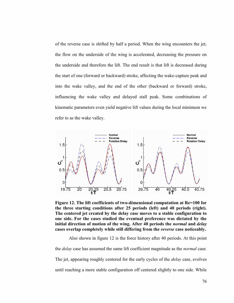
76

of the reverse case is shifted by half a period. When the wing encounters the jet,

the flow on the underside of the wing is accelerated, decreasing the pressure on

the underside and therefore the lift. The end result is that lift is decreased during

the start of one (forward or backward) stroke, affecting the wake-capture peak and

into the wake valley, and the end of the other (backward or forward) stroke,

influencing the wake valley and delayed stall peak. Some combinations of

kinematic parameters even yield negative lift values during the local minimum we

refer to as the wake valley.

Figure 12. The lift coefficients of two-dimensional computation at Re=100 for

the three starting conditions after 25 periods (left) and 40 periods (right).

The centered jet created by the delay case moves to a stable configuration to

one side. For the cases studied the eventual preference was dictated by the

initial direction of motion of the wing. After 40 periods the normal and delay

cases overlap completely while still differing from the reverse case noticeably.

Also shown in figure 12 is the force history after 40 periods. At this point

the delay case has assumed the same lift coefficient magnitude as the normal case.

The jet, appearing roughly centered for the early cycles of the delay case, evolves

until reaching a more stable configuration off centered slightly to one side. While

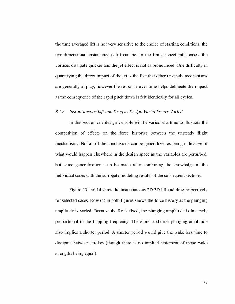
77

the time averaged lift is not very sensitive to the choice of starting conditions, the

two-dimensional instantaneous lift can be. In the finite aspect ratio cases, the

vortices dissipate quicker and the jet effect is not as pronounced. One difficulty in

quantifying the direct impact of the jet is the fact that other unsteady mechanisms

are generally at play, however the response over time helps delineate the impact

as the consequence of the rapid pitch down is felt identically for all cycles.

3.1.2 Instantaneous Lift and Drag as Design Variables are Varied

In this section one design variable will be varied at a time to illustrate the

competition of effects on the force histories between the unsteady flight

mechanisms. Not all of the conclusions can be generalized as being indicative of

what would happen elsewhere in the design space as the variables are perturbed,

but some generalizations can be made after combining the knowledge of the

individual cases with the surrogate modeling results of the subsequent sections.

Figure 13 and 14 show the instantaneous 2D/3D lift and drag respectively

for selected cases. Row (a) in both figures shows the force history as the plunging

amplitude is varied. Because the Re is fixed, the plunging amplitude is inversely

proportional to the flapping frequency. Therefore, a shorter plunging amplitude

also implies a shorter period. A shorter period would give the wake less time to

dissipate between strokes (though there is no implied statement of those wake

strengths being equal).

78

(a)

(b)

(c)

(d)

Figure 13. Time histories of the lift coefficients for selected cases (a) as

is increases from 2.0 (left) to 4.0 (right) holding = 62.5° and =90° (b) as

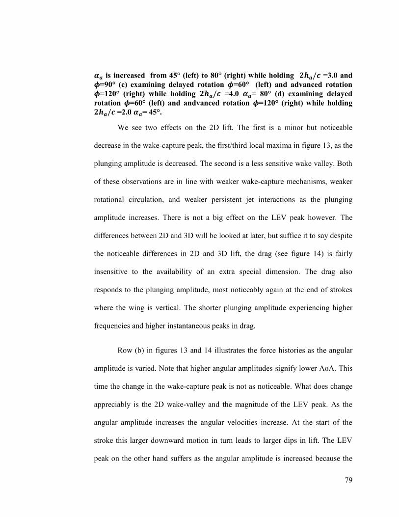
79

is increased from 45° (left) to 80° (right) while holding =3.0 and

=90° (c) examining delayed rotation =60° (left) and advanced rotation

=120° (right) while holding =4.0 = 80° (d) examining delayed

rotation =60° (left) and andvanced rotation =120° (right) while holding

=2.0 = 45°.

We see two effects on the 2D lift. The first is a minor but noticeable

decrease in the wake-capture peak, the first/third local maxima in figure 13, as the

plunging amplitude is decreased. The second is a less sensitive wake valley. Both

of these observations are in line with weaker wake-capture mechanisms, weaker

rotational circulation, and weaker persistent jet interactions as the plunging

amplitude increases. There is not a big effect on the LEV peak however. The

differences between 2D and 3D will be looked at later, but suffice it to say despite

the noticeable differences in 2D and 3D lift, the drag (see figure 14) is fairly

insensitive to the availability of an extra special dimension. The drag also

responds to the plunging amplitude, most noticeably again at the end of strokes

where the wing is vertical. The shorter plunging amplitude experiencing higher

frequencies and higher instantaneous peaks in drag.

Row (b) in figures 13 and 14 illustrates the force histories as the angular

amplitude is varied. Note that higher angular amplitudes signify lower AoA. This

time the change in the wake-capture peak is not as noticeable. What does change

appreciably is the 2D wake-valley and the magnitude of the LEV peak. As the

angular amplitude increases the angular velocities increase. At the start of the

stroke this larger downward motion in turn leads to larger dips in lift. The LEV

peak on the other hand suffers as the angular amplitude is increased because the

80

AoA is decreased which serves to suppress the LEV growth. The weaker LEV

then leads to a less substantial LEV peak. While the higher AoA leads to more

lift, the wing also accrues more drag (see figure 14) as the AoA increases.

Rows (c) and (d) in figures 13 and 14, illustrate two instances as the phase

lag changes as the influence is slightly more complex. The delayed rotation cases

both start off with negative lift, as the kinematic illustration points out the wing is

flying upside-down at this point. After that however (c) shows a secondary lift

peak as the larger angular amplitude now serves in a pitch up fashion to increase

the lift. Row (d) on the other hand shows a highly asymmetric force history whose

kinematics will be focused on later. There is a price to pay on the drag side

however; as the wing is near vertical as it accelerates horizontally, this results in

the largest instantaneous peak drag values of the cases studied.

On the advanced rotation side of the spectrum, again figure 13 and 14

rows (c) and (d), there are a few noticeable phenomena as well. One of the first

things that should be noted is the higher LEV lift peaks associated with the

advanced rotation. These kinematics benefit from increasing angles of attack

during maximum translational velocity. This moves the timing of the pitch down

motion and is also responsible for the exaggerated wake valleys experienced for

these same kinematics.

81

(a)

(b)

(c)

(d)

Figure 14. Time histories of the drag coefficients for selected cases (a) as

is increases from 2.0 (left) to 4.0 (right) holding = 62.5° and =90°

82

(b) as is increased from 45° (left) to 80° (right) while holding =3.0

and =90° (c) examining delayed rotation =60° (left) and advanced

rotation =120° (right) while holding =4.0 = 80° (d) examining

delayed rotation =60° (left) and andvanced rotation =120° (right) while

holding =2.0 = 45°

One point it is worth emphasizing here is that it would appear possible to

keep most of the desirable flow features while minimizing the less desirable ones,

e.g. the deep wake valley, by confining the downward rotation to the end of stroke

and then finding a balance between the desire for high AoA and increasing AoA.

Looking at the drag illustrations in rows (c) and (d) of figures 13 and 14 it is seen

that, while the maximum LEV lift peak values are similar, the same cannot be

said for the drag maxima. Once again the higher AoA as the airfoil is decelerating

causes higher drag values. The competition of effects is important to keep in mind

as one wants to extend the application of the context presented here, e.g. not

confining oneself to sinusoidal motions.

While specific examples have been chosen to illustrate key concepts, what

kind of general trends can be extracted from the data?

3.2 Time-Averaged Lift

Figure 15 shows the surrogate models of the time-averaged lift, including

those based on the two-dimensional and three-dimensional results, as well as their

differences. Each axis corresponds to one of the design variables while the color

contours illustrate the objective function of interest (e.g. time averaged lift or

power). Qualitatively, the general trends found in two- and three-dimensional

cases are consistent. As the angular amplitude is increased, a lower angle of attack

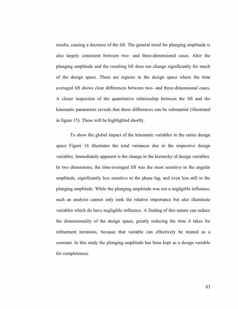
83

results, causing a decrease of the lift. The general trend for plunging amplitude is

also largely consistent between two- and three-dimensional cases. Alter the

plunging amplitude and the resulting lift does not change significantly for much

of the design space. There are regions in the design space where the time

averaged lift shows clear differences between two- and three-dimensional cases.

A closer inspection of the quantitative relationship between the lift and the

kinematic parameters reveals that these differences can be substantial (illustrated

in figure 15). These will be highlighted shortly.

To show the global impact of the kinematic variables in the entire design

space Figure 16 illustrates the total variances due to the respective design

variables. Immediately apparent is the change in the hierarchy of design variables.

In two dimensions, the time-averaged lift was the most sensitive to the angular

amplitude, significantly less sensitive to the phase lag, and even less still to the

plunging amplitude. While the plunging amplitude was not a negligible influence,

such an analysis cannot only rank the relative importance but also illuminate

variables which do have negligible influence. A finding of this nature can reduce

the dimensionality of the design space, greatly reducing the time it takes for

refinement iterations, because that variable can effectively be treated as a

constant. In this study the plunging amplitude has been kept as a design variable

for completeness.

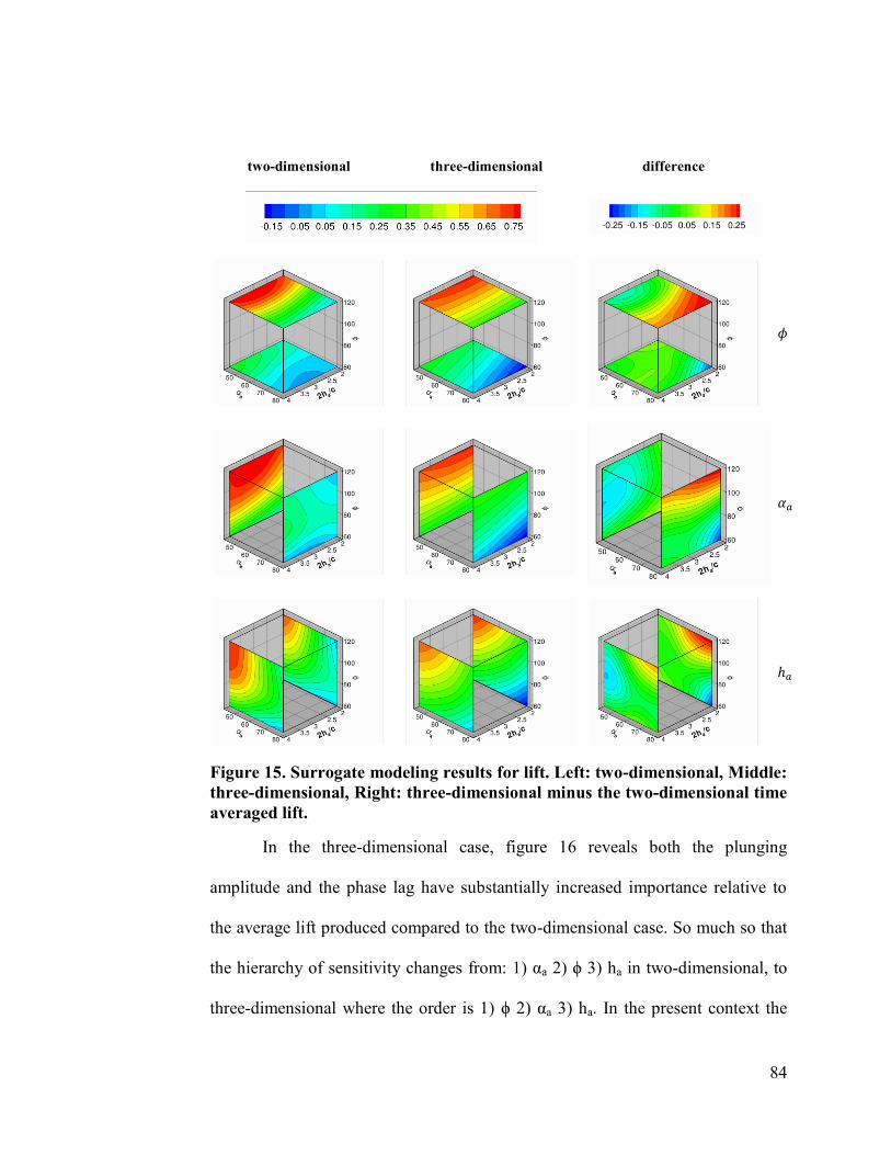
84

two-dimensional three-dimensional difference

Figure 15. Surrogate modeling results for lift. Left: two-dimensional, Middle:

three-dimensional, Right: three-dimensional minus the two-dimensional time

averaged lift.

In the three-dimensional case, figure 16 reveals both the plunging

amplitude and the phase lag have substantially increased importance relative to

the average lift produced compared to the two-dimensional case. So much so that

the hierarchy of sensitivity changes from: 1) αa 2) ϕ 3) ha in two-dimensional, to

three-dimensional where the order is 1) ϕ 2) αa 3) ha. In the present context the

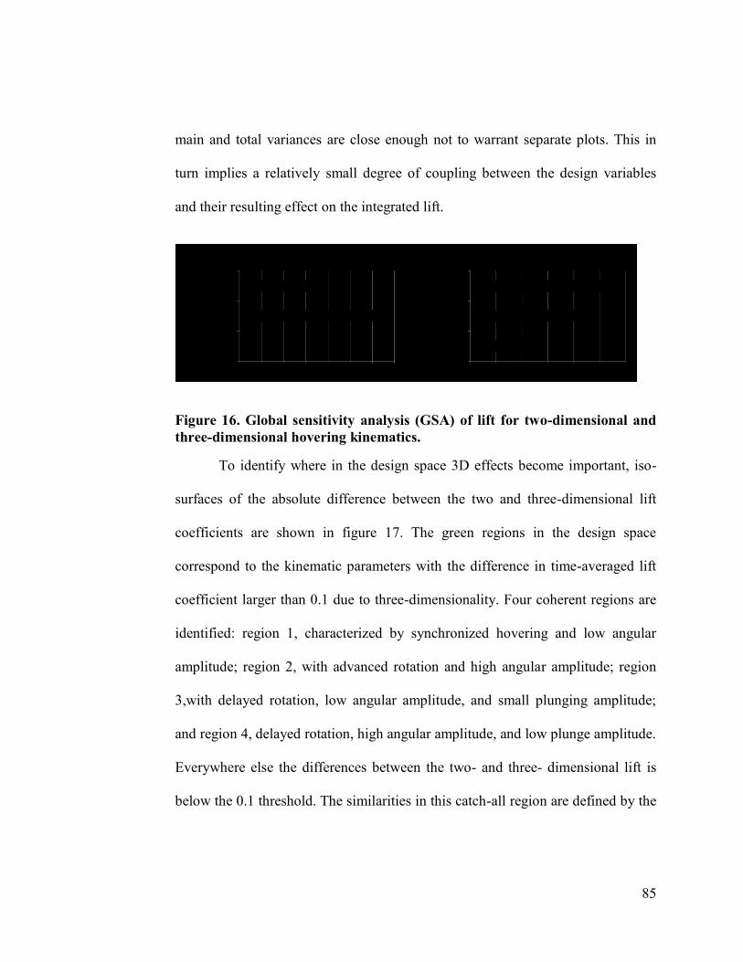
85

main and total variances are close enough not to warrant separate plots. This in

turn implies a relatively small degree of coupling between the design variables

and their resulting effect on the integrated lift.

Figure 16. Global sensitivity analysis (GSA) of lift for two-dimensional and

three-dimensional hovering kinematics.

To identify where in the design space 3D effects become important, iso-

surfaces of the absolute difference between the two and three-dimensional lift

coefficients are shown in figure 17. The green regions in the design space

correspond to the kinematic parameters with the difference in time-averaged lift

coefficient larger than 0.1 due to three-dimensionality. Four coherent regions are

identified: region 1, characterized by synchronized hovering and low angular

amplitude; region 2, with advanced rotation and high angular amplitude; region

3,with delayed rotation, low angular amplitude, and small plunging amplitude;

and region 4, delayed rotation, high angular amplitude, and low plunge amplitude.

Everywhere else the differences between the two- and three- dimensional lift is

below the 0.1 threshold. The similarities in this catch-all region are defined by the

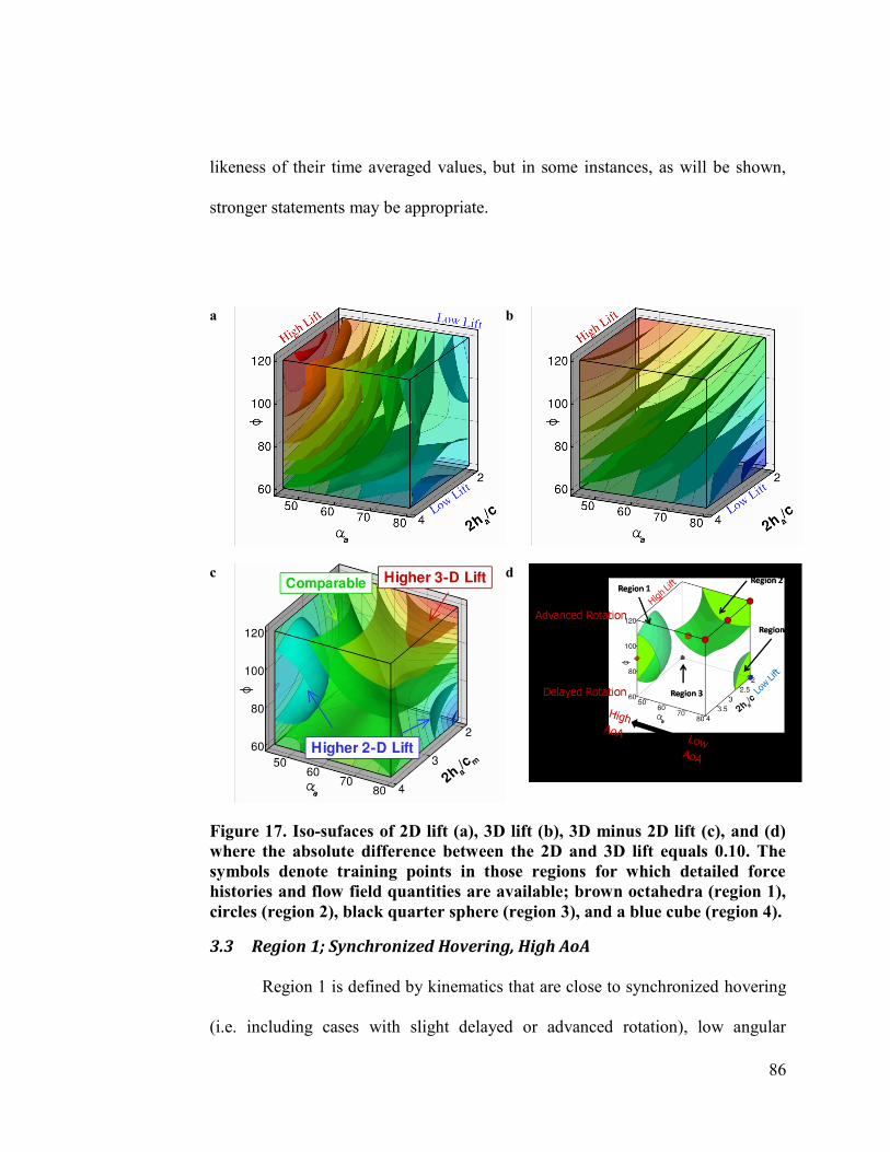
86

likeness of their time averaged values, but in some instances, as will be shown,

stronger statements may be appropriate.

a

b

c

d

Figure 17. Iso-sufaces of 2D lift (a), 3D lift (b), 3D minus 2D lift (c), and (d)

where the absolute difference between the 2D and 3D lift equals 0.10. The

symbols denote training points in those regions for which detailed force

histories and flow field quantities are available; brown octahedra (region 1),

circles (region 2), black quarter sphere (region 3), and a blue cube (region 4).

3.3 Region 1; Synchronized Hovering, High AoA

Region 1 is defined by kinematics that are close to synchronized hovering

(i.e. including cases with slight delayed or advanced rotation), low angular

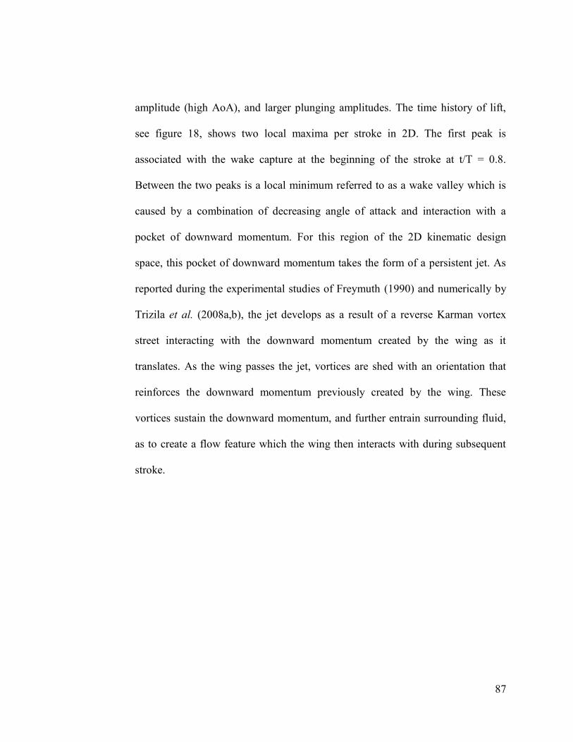
87

amplitude (high AoA), and larger plunging amplitudes. The time history of lift,

see figure 18, shows two local maxima per stroke in 2D. The first peak is

associated with the wake capture at the beginning of the stroke at t/T = 0.8.

Between the two peaks is a local minimum referred to as a wake valley which is

caused by a combination of decreasing angle of attack and interaction with a

pocket of downward momentum. For this region of the 2D kinematic design

space, this pocket of downward momentum takes the form of a persistent jet. As

reported during the experimental studies of Freymuth (1990) and numerically by

Trizila et al. (2008a,b), the jet develops as a result of a reverse Karman vortex

street interacting with the downward momentum created by the wing as it

translates. As the wing passes the jet, vortices are shed with an orientation that

reinforces the downward momentum previously created by the wing. These

vortices sustain the downward momentum, and further entrain surrounding fluid,

as to create a flow feature which the wing then interacts with during subsequent

stroke.

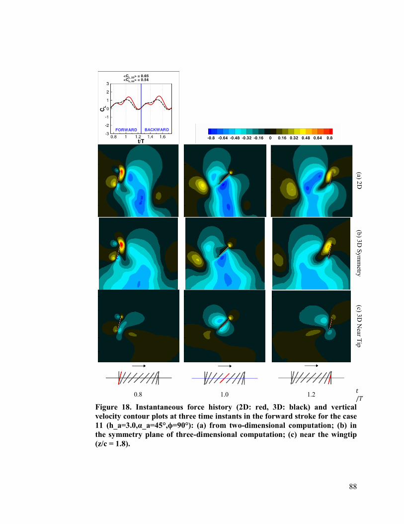
88

(a) 2D

(b) 3

D S

ym

metry

(c) 3D

Near T

ip

0.8 1.0 1.2

Figure 18. Instantaneous force history (2D: red, 3D: black) and vertical

velocity contour plots at three time instants in the forward stroke for the case

11 (h_a=3.0,α_a=45°,ϕ=90°): (a) from two-dimensional computation; (b) in

the symmetry plane of three-dimensional computation; (c) near the wingtip

(z/c = 1.8).

89

In general the tip vortices are found to have four prominent competing

effects: TE1) Enhancement of lift due to the proximity of the associated low

pressure region of the tip vortex next to the airfoil, TE2) Induced downwash

acting to reduce the effective angle of attack along the span weakening the LEV

hence reducing the instantaneous lift, TE3) Interaction with the vortices shed from

the leading and trailing edges anchoring them from shedding near the wing tips

enhancing the lift (region 3), TE4) Due to the tip vortices pulling fluid from the

underside of the wing to the upper side, the wing leaves behind a weaker pocket

of downward momentum in the flow. Upon interaction with this downward

momentum, a loss in lift is seen and so weaker wake-valley means higher lift.

The overall impact for this case is that the two-dimensional lift, <CL,2D>=

0.65, is better than the three-dimensional counterpart, <CL,3D>= 0.54. More

generally, cases with kinematics in region 1 have larger lift in 2D.

3.4 Region 2; Advanced Rotation, Low AoA

In region 2 the kinematics are characterized by advanced rotation, and

high angular amplitude. Figure 19 shows the time histories of lift and the

associated flow features from case 8 (2ha/c = 4.0, αa= 80°, and ϕ = 120°) which is

representative for the other cases in region 2.

Right after the stroke reversal, the flat plate moves into the wake

generated in the previous stroke. Due to the downwash in this wake, see figure

19C1, and low and decreasing angle of attack (figure 19B), lift drops. Note: the

90

pocket of downward momentum encountered for these kinematics is not a

persistent jet. The three-dimensional case does not suffer the same drop in lift as

the two-dimensional case.

Figure 19 Time history of lift coefficients in a representative case in region 1,

2ha/c = 4.0, αa= 80°, and ϕ = 120°, with the associated flow features. (A) Lift,

(C_L), during a motion cycle. Red-solid, two-dimensional computation;

black-dashed, three-dimensional computation. (B) kinematic schema of the

flat plate motion. (C) Representative flow features at 1) t/T = 0.9, u2

contours; 2) t/T = 1.0, vorticity contours; 3) t/T=1.2, u2 contours.

3.5 Region 3; Delayed Rotation, High AoA, Low Plunging Amplitude

In classical steady state theory the presence of wing tip vortices is

attributed to a loss of lift and increase in drag when comparing the two-

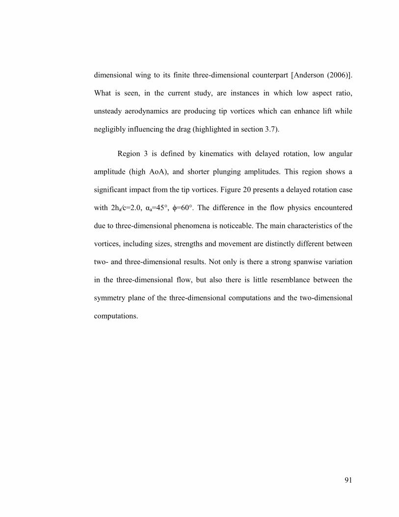
91

dimensional wing to its finite three-dimensional counterpart [Anderson (2006)].

What is seen, in the current study, are instances in which low aspect ratio,

unsteady aerodynamics are producing tip vortices which can enhance lift while

negligibly influencing the drag (highlighted in section 3.7).

Region 3 is defined by kinematics with delayed rotation, low angular

amplitude (high AoA), and shorter plunging amplitudes. This region shows a

significant impact from the tip vortices. Figure 20 presents a delayed rotation case

with 2ha⁄c=2.0, αa=45°, ϕ=60°. The difference in the flow physics encountered

due to three-dimensional phenomena is noticeable. The main characteristics of the

vortices, including sizes, strengths and movement are distinctly different between

two- and three-dimensional results. Not only is there a strong spanwise variation

in the three-dimensional flow, but also there is little resemblance between the

symmetry plane of the three-dimensional computations and the two-dimensional

computations.

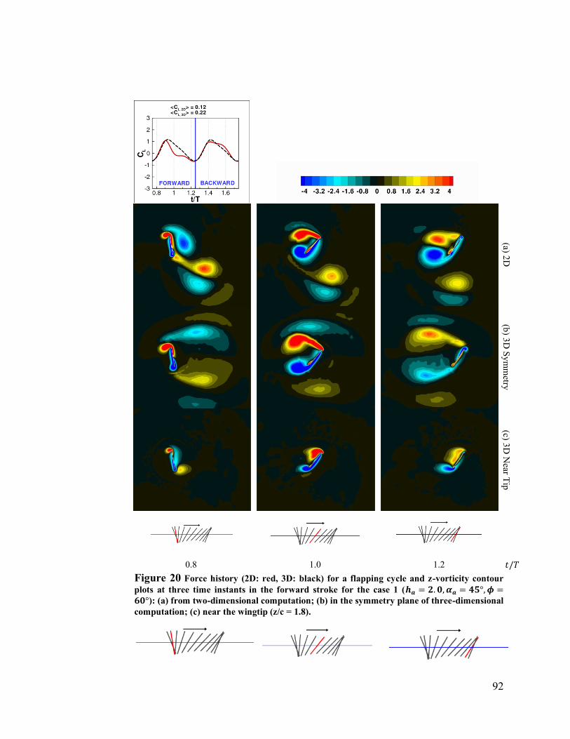
92

(a) 2D

(b) 3

D S

ym

metry

(c) 3D

Near T

ip

0.8 1.0 1.2

Figure 20 Force history (2D: red, 3D: black) for a flapping cycle and z-vorticity contour

plots at three time instants in the forward stroke for the case 1 ( ): (a) from two-dimensional computation; (b) in the symmetry plane of three-dimensional

computation; (c) near the wingtip (z/c = 1.8).

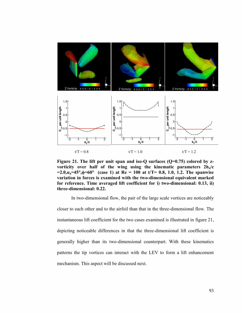
93

t/T = 0.8 t/T = 1.0 t/T = 1.2

Figure 21. The lift per unit span and iso-Q surfaces (Q=0.75) colored by z-

vorticity over half of the wing using the kinematic parameters 2ha/c

=2.0,αa=45°,ϕ=60° (case 1) at Re = 100 at t/T= 0.8, 1.0, 1.2. The spanwise

variation in forces is examined with the two-dimensional equivalent marked

for reference. Time averaged lift coefficient for i) two-dimensional: 0.13, ii)

three-dimensional: 0.22.

In two-dimensional flow, the pair of the large scale vortices are noticeably

closer to each other and to the airfoil than that in the three-dimensional flow. The

instantaneous lift coefficient for the two cases examined is illustrated in figure 21,

depicting noticeable differences in that the three-dimensional lift coefficient is

generally higher than its two-dimensional counterpart. With these kinematics

patterns the tip vortices can interact with the LEV to form a lift enhancement

mechanism. This aspect will be discussed next.

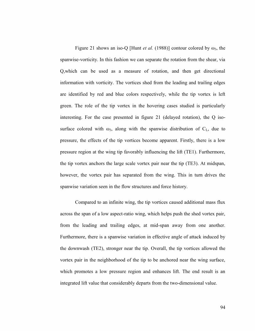
94

Figure 21 shows an iso-Q [Hunt et al. (1988)] contour colored by ω3, the

spanwise-vorticity. In this fashion we can separate the rotation from the shear, via

Q,which can be used as a measure of rotation, and then get directional

information with vorticity. The vortices shed from the leading and trailing edges

are identified by red and blue colors respectively, while the tip vortex is left

green. The role of the tip vortex in the hovering cases studied is particularly

interesting. For the case presented in figure 21 (delayed rotation), the Q iso-

surface colored with ω3, along with the spanwise distribution of CL, due to

pressure, the effects of the tip vortices become apparent. Firstly, there is a low

pressure region at the wing tip favorably influencing the lift (TE1). Furthermore,

the tip vortex anchors the large scale vortex pair near the tip (TE3). At midspan,

however, the vortex pair has separated from the wing. This in turn drives the

spanwise variation seen in the flow structures and force history.

Compared to an infinite wing, the tip vortices caused additional mass flux

across the span of a low aspect-ratio wing, which helps push the shed vortex pair,

from the leading and trailing edges, at mid-span away from one another.

Furthermore, there is a spanwise variation in effective angle of attack induced by

the downwash (TE2), stronger near the tip. Overall, the tip vortices allowed the

vortex pair in the neighborhood of the tip to be anchored near the wing surface,

which promotes a low pressure region and enhances lift. The end result is an

integrated lift value that considerably departs from the two-dimensional value.

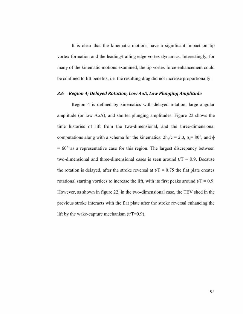
95

It is clear that the kinematic motions have a significant impact on tip

vortex formation and the leading/trailing edge vortex dynamics. Interestingly, for

many of the kinematic motions examined, the tip vortex force enhancement could

be confined to lift benefits, i.e. the resulting drag did not increase proportionally!

3.6 Region 4; Delayed Rotation, Low AoA, Low Plunging Amplitude

Region 4 is defined by kinematics with delayed rotation, large angular

amplitude (or low AoA), and shorter plunging amplitudes. Figure 22 shows the

time histories of lift from the two-dimensional, and the three-dimensional

computations along with a schema for the kinematics: 2ha/c = 2.0, αa= 80°, and ϕ

= 60° as a representative case for this region. The largest discrepancy between

two-dimensional and three-dimensional cases is seen around t/T = 0.9. Because

the rotation is delayed, after the stroke reversal at t/T = 0.75 the flat plate creates

rotational starting vortices to increase the lift, with its first peaks around t/T = 0.9.

However, as shown in figure 22, in the two-dimensional case, the TEV shed in the

previous stroke interacts with the flat plate after the stroke reversal enhancing the

lift by the wake-capture mechanism (t/T=0.9).

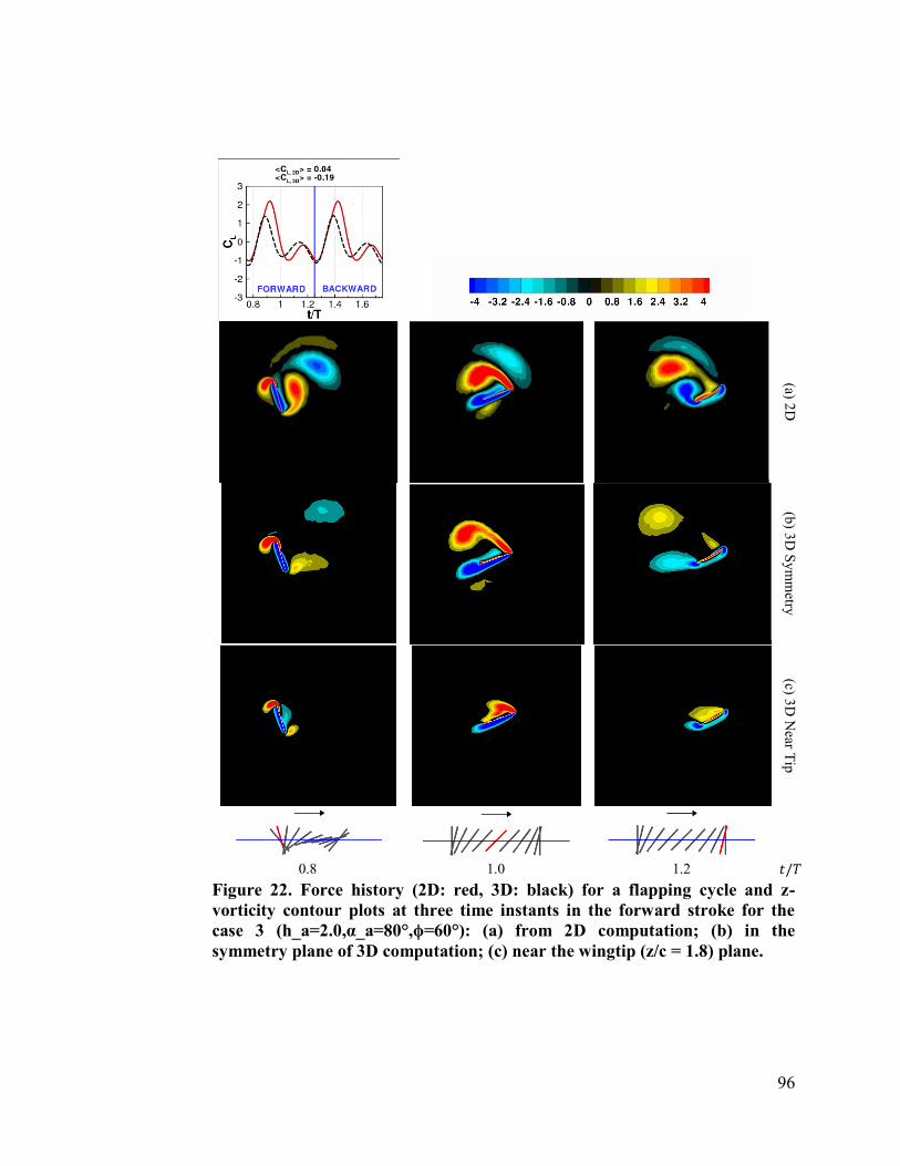
96

(a) 2D

(b) 3

D S

ym

metry

(c) 3D

Near T

ip

0.8 1.0 1.2

Figure 22. Force history (2D: red, 3D: black) for a flapping cycle and z-

vorticity contour plots at three time instants in the forward stroke for the

case 3 (h_a=2.0,α_a=80°,ϕ=60°): (a) from 2D computation; (b) in the

symmetry plane of 3D computation; (c) near the wingtip (z/c = 1.8) plane.

97

On the other hand, for the three-dimensional case, the shed LEV and the

TEV repel from each other and the path of the flat plate, such that after the stroke

reversal, the wake-capturing is absent. The first lift peak in the time history in

figure 22 is then only due to the rotational effects. So the diverging behavior of

the vortices, observed for all delayed rotation cases, and the interaction of the

vortices from the LE, and TE with the wing tip vortex, play a central role as

important three-dimensional effects as described in Region 3.

3.7 Region of similarity

For other kinematic combinations, the integrated forces over time match

reasonably, i.e. the difference between the two-dimensional, and the three-

dimensional time averaged lift is less than 0.1. For some cases even the

instantaneous forces agree closely: a synchronized rotation case with low angles

of attack is remarkably similar when examining two-dimensional and three-

dimensional force histories, see figure 23.

Figure 23 shows the flow fields corresponding to the parameters: 2ha/c

=3.0, αa=80°,ϕ=90°. The variation along the spanwise direction is modest, making

the two-dimensional and three-dimensional simulations substantially similar. The

two-dimensional flow field and the corresponding three-dimensional flow on the

symmetry plane are strikingly consistent.

98

(a) 2D

(b) 3

D S

ym

metry

(c) 3D

Near T

ip

0.8 1.0 1.2

Figure 23. Force history over a flapping cycle (solid red=2D, dashed

black=3D) and z-vorticity contour plots at three time instants in the forward

stroke for case 12 (2ha/c=3.0,α_a=80°,ϕ=90°): (a) from 2D computation; (b)

in the symmetry plane of 3D computation; (c) near the wingtip (z/c = 1.8)

plane.

99

The high angular amplitudes lead to low angles of attack, and coupled

with the timing of the rotation, lead to a flow that does not experience delayed

stall as the formation of the LEV is not promoted. The timing of the rotation for

this example puts the flat plate at its minimum angle of attack, approximately 10°,

at maximum translational velocity, while the translational velocity is zero when

the flat plate is vertical. It is seen from the flowfield that the tip vortex as well as

the leading and trailing edge vortex formation is largely suppressed. The net

effect is a fairly uniform spanwise lift distribution closely resembling the two-

dimensional case with the same kinematics.

Neither the two-dimensional or three-dimensional results in this case

promote downward induced jet formation. As summarized in figure 23, the two-

dimensional and three-dimensional lift coefficients of this case are similar in the

instantaneous as well as the time averaged sense. One implication illustrated is the

usefulness of two-dimensional simulations for quantitative data on a three-

dimensional counterpart. However, not all cases in this region display this similar

instantaneous behavior, and the time-averaged lift comparison is due to

integrating effects which partially cancel out. For instance, the LEV strength may

diminish, however the lift valley during the downward rotation may not be as

severe in three dimensions.

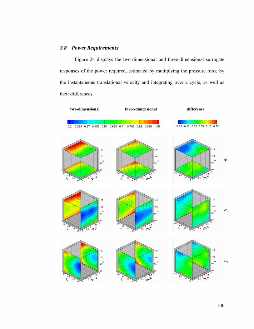
100

3.8 Power Requirements

Figure 24 displays the two-dimensional and three-dimensional surrogate

responses of the power required, estimated by multiplying the pressure force by

the instantaneous translational velocity and integrating over a cycle, as well as

their differences.

two-dimensional three-dimensional difference

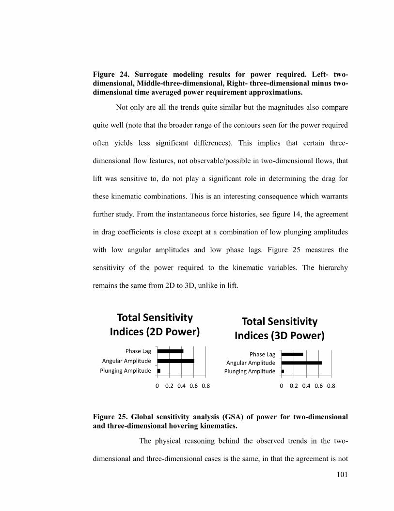
101

Figure 24. Surrogate modeling results for power required. Left- two-

dimensional, Middle-three-dimensional, Right- three-dimensional minus two-

dimensional time averaged power requirement approximations.

Not only are all the trends quite similar but the magnitudes also compare

quite well (note that the broader range of the contours seen for the power required

often yields less significant differences). This implies that certain three-

dimensional flow features, not observable/possible in two-dimensional flows, that

lift was sensitive to, do not play a significant role in determining the drag for

these kinematic combinations. This is an interesting consequence which warrants

further study. From the instantaneous force histories, see figure 14, the agreement

in drag coefficients is close except at a combination of low plunging amplitudes

with low angular amplitudes and low phase lags. Figure 25 measures the

sensitivity of the power required to the kinematic variables. The hierarchy

remains the same from 2D to 3D, unlike in lift.

Figure 25. Global sensitivity analysis (GSA) of power for two-dimensional

and three-dimensional hovering kinematics.

The physical reasoning behind the observed trends in the two-

dimensional and three-dimensional cases is the same, in that the agreement is not

0 0.2 0.4 0.6 0.8

Plunging Amplitude

Angular Amplitude

Phase Lag

Total Sensitivity Indices (2D Power)

0 0.2 0.4 0.6 0.8

Plunging Amplitude

Angular Amplitude

Phase Lag

Total Sensitivity Indices (3D Power)

102

merely a consequence of integration. During normal hovering, ϕ = 90°, the

airfoil/wing is perpendicular to the direction of motion at the ends of translation

but has little translational velocity. As the phase lag is perturbed in either

direction the airfoil can have an appreciable velocity, while perpendicular to the

direction of motion and whether the body is accelerating when perpendicular, as

in delayed rotation cases, or decelerating, as in advanced rotation cases has a

sizable impact on the instantaneous drag that is felt (see figure 14), and

consequently the power required for the maneuver. Compared to the differences

between surrogates for lift, the differences for power between two- and three-

dimensional cases are smaller overall.

3.9 Pareto Front

In a multi-objective investigation, it is often the case that different goals

are in competition regarding suitable selections of design variables. One tool used

to evaluate the trade-offs between objective functions is called the Pareto front

[Miettinen (1999)]. The Pareto front consists of non-dominated points and can be

thought of as the set of best possibilities, as illustrated in figure 26. Non-

dominated points can be thought of as points for which one could not improve all

objective functions simultaneously. The current objectives are to maximize lift

and minimize power requirement. Points on the Pareto front therefore involve

those for which increases in lift are accompanied by increases in power, and vice

versa. To pose all objectives as minimization expressions, any objective which is

maximized, like lift, is multiplied by a negative sign. Note that the Pareto front

103

itself is comparable between two and three dimensions. The primary differences

are the peak lift values attained in two-dimensional flow exceeding their three-

dimensional counterparts, and the fact that the density of design variable

combinations near the front is higher in the three dimensional case. The paths

through the design space are plotted below their respective Pareto fronts in figure

26. Note: the jaggedness of the path is due to the resolution of the tested points

and is seen because of the fine balance in objective functions for design variables

in that region. It is seen that the high lift region follows the lower bound of the

angular amplitude suggesting that future iterations should decrease the lower

bound for higher lift solutions. Overall the design variable combinations on the

optimal front are consistent qualitatively.

As shown in figure 15, and a representative case illustrated in figure 27,

the highest time-averaged lift values are obtained by a combination of advanced

rotation and low angular amplitude in two and three dimensions. The general

trends present, i.e. when holding two of the input variables constant and varying

the last one, remained largely the same. For power required, figure 24 shows that

the synchronized rotation cases with high angular amplitude consume the least

power for both two-dimensional as well as three-dimensional hovering. The

combination of lower angle of attack during the mid-stroke when the translational

velocity is at maximum and small translational velocities at the ends of the strokes

when the flat plate is vertical minimizes the power. These trends not only

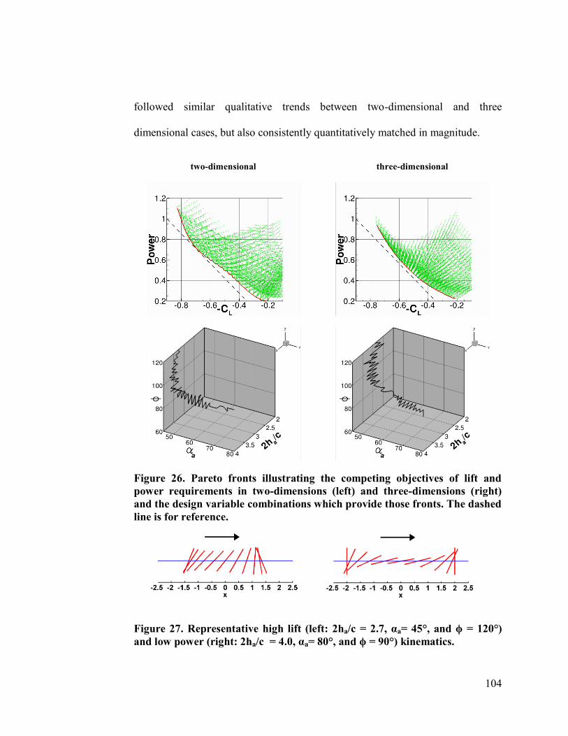
104

followed similar qualitative trends between two-dimensional and three

dimensional cases, but also consistently quantitatively matched in magnitude.

two-dimensional three-dimensional

Figure 26. Pareto fronts illustrating the competing objectives of lift and

power requirements in two-dimensions (left) and three-dimensions (right)

and the design variable combinations which provide those fronts. The dashed

line is for reference.

Figure 27. Representative high lift (left: 2ha/c = 2.7, αa= 45°, and ϕ = 120°)

and low power (right: 2ha/c = 4.0, αa= 80°, and ϕ = 90°) kinematics.

105

Chapter 4 Effect of Gust and Freestream on Flapping Wing

Aerodynamics

One of the main difficulties in realizing a functional MAV is its inherent

sensitivity to the operating environment due to its size and weight. While the

vehicle dynamics are going to be sensitive to the environmental perturbations, due

to the fact that the flapping frequencies are an order of magnitude or two greater

than the wind gusts, O(10) Hz to O(100) Hz versus wind at O(1) Hz, the

aerodynamics associated with flapping wings can be pragmatically modeled by a

constant freestream. In the current study, environmental sensitivity is looked at

using different kinematic schemes, freestream strengths, and freestream

orientations. The three kinematic patterns chosen were those of sections 3.3, 3.5,

and 3.7. These patterns were chosen due to having pronounced LEVs (section

3.3), beneficial tip vortices (section 3.5), and negligible 2D vs 3D differences

(section 3.7) respectively. The freestream strength was fixed at 20% of the

maximum translational velocity of the wing. If one were comparing this to

fruitflies, (Re O(100) and wingspeed ~3.1 m/s) the freestream would be

approximately 0.6 m/s, a relatively light wind or mild disturbance. The directions

of the freestream varied between heading down, right, or up.

106

4.1 Two Dimensional or Infinite Aspect Ratio Wings in a Gust

The 2D cases were much more sensitive to the freestream than their 3D

counterparts. Instantaneous lift associated with all three kinematic patterns was

very sensitive to the horizontal freestream and much less sensitive to the

downward heading freestream. The downward freestream generally decreased lift,

by suppressing vortex generation, while making the forward and backstrokes

more symmetric as the vortical activity was washed away from the airfoil more

quickly. Overall the general nature of the force history was kept intact. On the

other hand the upward freestream had the opposite effect. Namely the vortex

interactions were sustained for a longer period of time as the freestream held the

wake closer to the airfoil and the increased angle of attack also served to

accentuate the unsteady aerodynamics. This upward freestream may or may not

have had a significant impact on the force history which was dependent on the

kinematics. The horizontal freestream had the largest impact over the range of

kinematic motions studied, sometimes more than doubling the lift felt for

freestream strength of 20% of the maximum translational velocity, a relatively

tame environmental situation leading to a significant change in hovering

performance.

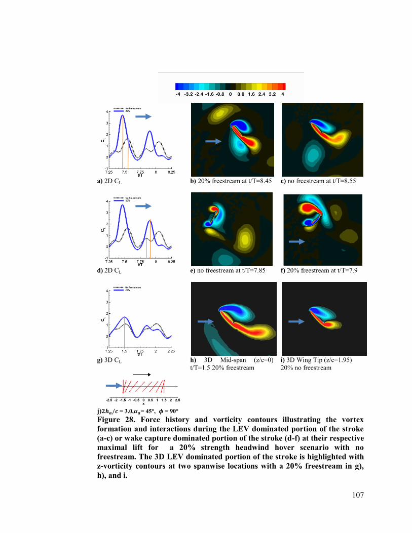
107

a) 2D CL b) 20% freestream at t/T=8.45

c) no freestream at t/T=8.55

d) 2D CL

e) no freestream at t/T=7.85

f) 20% freestream at t/T=7.9

g) 3D CL h) 3D Mid-span (z/c=0)

t/T=1.5 20% freestream

i) 3D Wing Tip (z/c=1.95)

20% no freestream

j) = 3.0, = 45°, = 90°

Figure 28. Force history and vorticity contours illustrating the vortex

formation and interactions during the LEV dominated portion of the stroke

(a-c) or wake capture dominated portion of the stroke (d-f) at their respective

maximal lift for a 20% strength headwind hover scenario with no

freestream. The 3D LEV dominated portion of the stroke is highlighted with

z-vorticity contours at two spanwise locations with a 20% freestream in g),

h), and i.

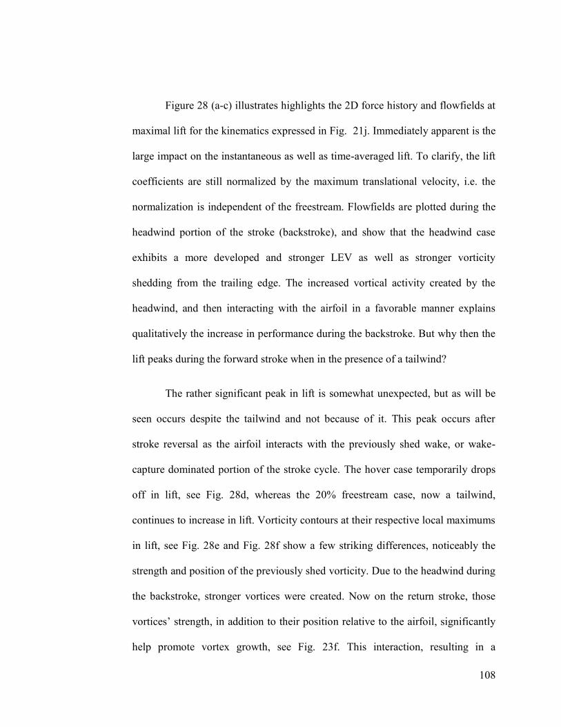
108

Figure 28 (a-c) illustrates highlights the 2D force history and flowfields at

maximal lift for the kinematics expressed in Fig. 21j. Immediately apparent is the

large impact on the instantaneous as well as time-averaged lift. To clarify, the lift

coefficients are still normalized by the maximum translational velocity, i.e. the

normalization is independent of the freestream. Flowfields are plotted during the

headwind portion of the stroke (backstroke), and show that the headwind case

exhibits a more developed and stronger LEV as well as stronger vorticity

shedding from the trailing edge. The increased vortical activity created by the

headwind, and then interacting with the airfoil in a favorable manner explains

qualitatively the increase in performance during the backstroke. But why then the

lift peaks during the forward stroke when in the presence of a tailwind?

The rather significant peak in lift is somewhat unexpected, but as will be

seen occurs despite the tailwind and not because of it. This peak occurs after

stroke reversal as the airfoil interacts with the previously shed wake, or wake-

capture dominated portion of the stroke cycle. The hover case temporarily drops

off in lift, see Fig. 28d, whereas the 20% freestream case, now a tailwind,

continues to increase in lift. Vorticity contours at their respective local maximums

in lift, see Fig. 28e and Fig. 28f show a few striking differences, noticeably the

strength and position of the previously shed vorticity. Due to the headwind during

the backstroke, stronger vortices were created. Now on the return stroke, those

vortices‟ strength, in addition to their position relative to the airfoil, significantly

help promote vortex growth, see Fig. 23f. This interaction, resulting in a

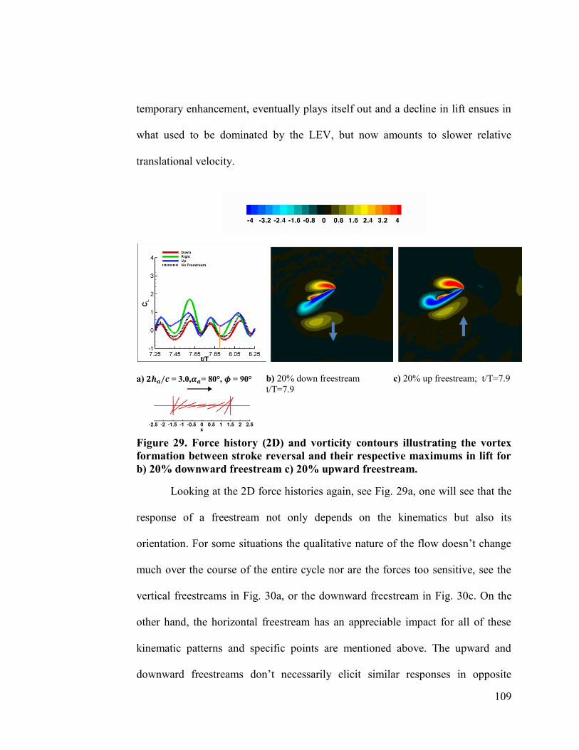
109

temporary enhancement, eventually plays itself out and a decline in lift ensues in

what used to be dominated by the LEV, but now amounts to slower relative

translational velocity.

a) = 3.0, = 80°, = 90°

b) 20% down freestream

t/T=7.9

c) 20% up freestream; t/T=7.9

Figure 29. Force history (2D) and vorticity contours illustrating the vortex

formation between stroke reversal and their respective maximums in lift for

b) 20% downward freestream c) 20% upward freestream.

Looking at the 2D force histories again, see Fig. 29a, one will see that the

response of a freestream not only depends on the kinematics but also its

orientation. For some situations the qualitative nature of the flow doesn‟t change

much over the course of the entire cycle nor are the forces too sensitive, see the

vertical freestreams in Fig. 30a, or the downward freestream in Fig. 30c. On the

other hand, the horizontal freestream has an appreciable impact for all of these

kinematic patterns and specific points are mentioned above. The upward and

downward freestreams don‟t necessarily elicit similar responses in opposite

110

directions, highlighted in figure 29. This in turn brings into question the relevance

of using effective angle of attack in these situations as the nature of the force

history may respond more noticeably to the upward freestream than the

downward freestream. See figure 30 (a-c) where a 20% freestream imposed from

different directions changes the qualitative behavior of the resulting force history

significantly.

For all of the synchronized rotation cases (which have positive angles of

attack at all times), a 20% downward freestream does indeed decrease the lift and

follows from the suppressed vortical activity as the effective angle of attack is

lowered. On the other hand some cases have a much more pronounced sensitivity

to the upward freestream. Figure 29a illustrates again the force histories for a 20%

freestream at various orientations relative to the hover case, as well as the

vorticity flowfield, 30b and 30c, for the 20% upward and downward freestream

cases at a time where the difference in force history between the two is

pronounced. What is seen in Fig. 29b (20% downward freesteam) and Fig. 29c

(20% upward freestream) is the increase in LEV and TEV formation as well as a

more pronounced interaction with the wake as the upward freestream promotes

the growth of the vortex structures and holds the wake in the vicinity for a longer

period of time. The non-linear response in lift as the freestream lowers or raises

the effective angle of attack is a product of these factors.

111

a) 2D CL b) 2D CL c) 2D CL

d) 3D CL e) 3D CL f) 3D CL

g) = 3.0, = 45°, and =

90°

h) = 2.0, = 45°, and =

60°

i) = 3.0, = 80°, and =

90°

Figure 30. 2D (a-c) and 3D (d-f) CL in response to a freestream with a

magnitude of 20% of the maximum plunging velocity heading in three

distinct directions (down: red, right: green, and up: blue) for three hovering

kinematics (g-i). The black dotted line is the reference hovering case.

4.2 Finite Aspect Ratio Wings in a Gust

The 3D cases on the other hand were much less sensitive to the freestream,

see figure 30 (d-f). Note however that the scale for the force histories was chosen

such that they could be directly compared with the 2D cases and the freestream

could be quite influential. The impact was non-negligible for a 20% strength

freestream, but overall the nature of the flow was very similar for most cases. The

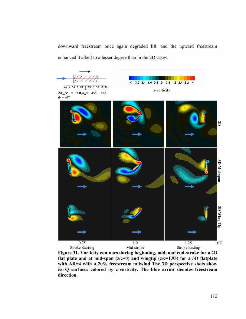
112

downward freestream once again degraded lift, and the upward freestream

enhanced it albeit to a lesser degree than in the 2D cases.

= 3.0, = 45°, and

= 90°

z-vorticity

2D

3D

Mid

-spa

n

3D

Win

g T

ip

0.75

Stroke Starting

1.0

Mid-stroke

1.25

Stroke Ending t/T

Figure 31. Vorticity contours during beginning, mid, and end-stroke for a 2D

flat plate and at mid-span (z/c=0) and wingtip (z/c=1.95) for a 3D flatplate

with AR=4 with a 20% freestream tailwind The 3D perspective shots show

iso-Q surfaces colored by z-vorticity. The blue arrow denotes freestream

direction.

113

Figure 31 highlights beginning, mid, and end stroke vorticity contours for

a 20% freestream tailwind for 2D and at midspan and at the wing tips for 3D. The

three-dimensional wing is unable to generate vortices of the same magnitude as

the analogous 2D counterparts. This in turn directly impacts the wing‟s benefit

from LEV interactions as well as subsequent interactions with the previously shed

wake. The spanwise variation of vorticity exhibited shows a decrease in LEV

generation from mid-span to tip, and while the tip vortices are prominent, they do

not make up for the weakened LEV formation and wake interaction as

experienced in 2D. Figure 28 illustrates the vorticity flowfields during maximal

lift, during the headwind, resulting in a 2D lift, figure 28a, almost twice as large

as its 3D counterpart, figure 28g.

This discrepancy in sensitivity to freestream between 2D and 3D shows up

across the range of kinematic motions. A limited subset of kinematic motions

showed very similar force histories in the time averaged sense as well as

instantaneously, see section 3.7, when not under the influence of an external

freestream. Kinematics in this region of the design space shared low angles of

attack across much of the flapping cycle and synchronized rotation, limiting the

high angular velocities and angles of attack to the end of the stroke where

translational velocity was minimized. This in turn tended to limit vortex size,

strength, formation, and influence. As the freestream is introduced, see figure 30c

and figure 30f for 2D and 3D force histories in the presence of a 20% freestream,

the response is not uniform across the span of the finite wing. The downward

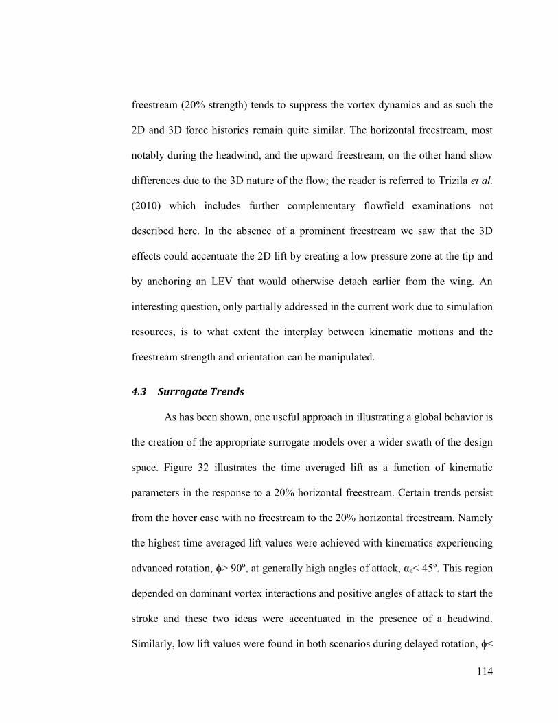
114

freestream (20% strength) tends to suppress the vortex dynamics and as such the

2D and 3D force histories remain quite similar. The horizontal freestream, most

notably during the headwind, and the upward freestream, on the other hand show

differences due to the 3D nature of the flow; the reader is referred to Trizila et al.

(2010) which includes further complementary flowfield examinations not

described here. In the absence of a prominent freestream we saw that the 3D

effects could accentuate the 2D lift by creating a low pressure zone at the tip and

by anchoring an LEV that would otherwise detach earlier from the wing. An

interesting question, only partially addressed in the current work due to simulation

resources, is to what extent the interplay between kinematic motions and the

freestream strength and orientation can be manipulated.

4.3 Surrogate Trends

As has been shown, one useful approach in illustrating a global behavior is

the creation of the appropriate surrogate models over a wider swath of the design

space. Figure 32 illustrates the time averaged lift as a function of kinematic

parameters in the response to a 20% horizontal freestream. Certain trends persist

from the hover case with no freestream to the 20% horizontal freestream. Namely

the highest time averaged lift values were achieved with kinematics experiencing

advanced rotation, ϕ> 90º, at generally high angles of attack, αa< 45º. This region

depended on dominant vortex interactions and positive angles of attack to start the

stroke and these two ideas were accentuated in the presence of a headwind.

Similarly, low lift values were found in both scenarios during delayed rotation, ϕ<

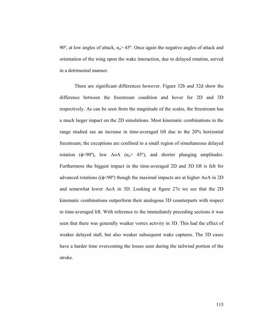
115

90º, at low angles of attack, αa> 45º. Once again the negative angles of attack and

orientation of the wing upon the wake interaction, due to delayed rotation, served

in a detrimental manner.

There are significant differences however. Figure 32b and 32d show the

difference between the freestream condition and hover for 2D and 3D

respectively. As can be seen from the magnitude of the scales, the freestream has

a much larger impact on the 2D simulations. Most kinematic combinations in the

range studied see an increase in time-averaged lift due to the 20% horizontal

freestream; the exceptions are confined to a small region of simultaneous delayed

rotation (ϕ<90º), low AoA (αa> 45º), and shorter plunging amplitudes.

Furthermore the biggest impact in the time-averaged 2D and 3D lift is felt for

advanced rotations ((ϕ<90º) though the maximal impacts are at higher AoA in 2D

and somewhat lower AoA in 3D. Looking at figure 27e we see that the 2D

kinematic combinations outperform their analogous 3D counterparts with respect

to time-averaged lift. With reference to the immediately preceding sections it was

seen that there was generally weaker vortex activity in 3D. This had the effect of

weaker delayed stall, but also weaker subsequent wake captures. The 3D cases

have a harder time overcoming the losses seen during the tailwind portion of the

stroke.

116

a) 2D lift: 20% horizontal freestream b) 2D lift: 20% freestream - hover

c) 3D lift: 20% horizontal freestream d) 3D lift: 20% freestream - hover

e) Freestream lift: 3D-2D

Figure 32. Surrogate models illustrating the trends in lift in the presence of a

20% horizontal freestream [a) 2D, c) 3D], the differences between freestream

and hover [b) 2D, d) 3D], and the difference between 3D and 2D [e].

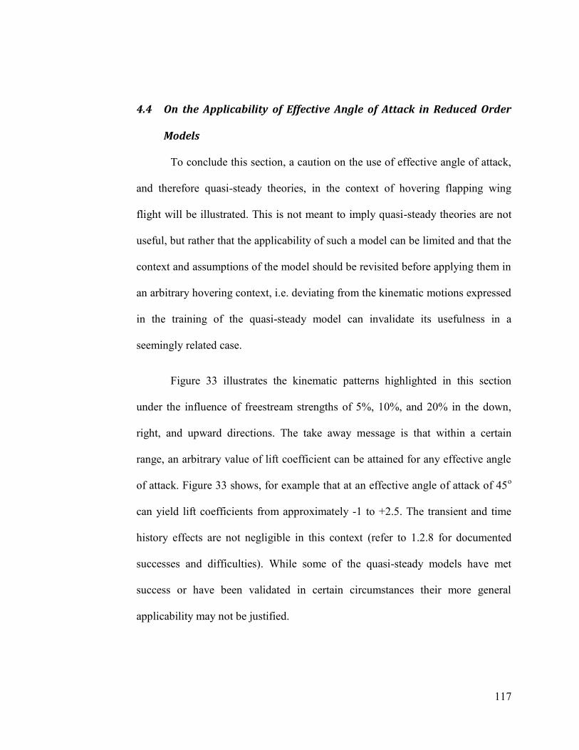
117

4.4 On the Applicability of Effective Angle of Attack in Reduced Order

Models

To conclude this section, a caution on the use of effective angle of attack,

and therefore quasi-steady theories, in the context of hovering flapping wing

flight will be illustrated. This is not meant to imply quasi-steady theories are not

useful, but rather that the applicability of such a model can be limited and that the

context and assumptions of the model should be revisited before applying them in

an arbitrary hovering context, i.e. deviating from the kinematic motions expressed

in the training of the quasi-steady model can invalidate its usefulness in a

seemingly related case.

Figure 33 illustrates the kinematic patterns highlighted in this section

under the influence of freestream strengths of 5%, 10%, and 20% in the down,

right, and upward directions. The take away message is that within a certain

range, an arbitrary value of lift coefficient can be attained for any effective angle

of attack. Figure 33 shows, for example that at an effective angle of attack of 45o

can yield lift coefficients from approximately -1 to +2.5. The transient and time

history effects are not negligible in this context (refer to 1.2.8 for documented

successes and difficulties). While some of the quasi-steady models have met

success or have been validated in certain circumstances their more general

applicability may not be justified.

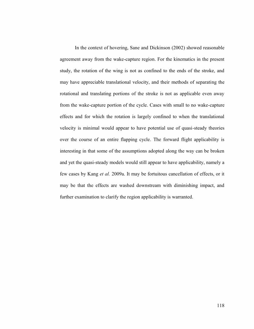
118

In the context of hovering, Sane and Dickinson (2002) showed reasonable

agreement away from the wake-capture region. For the kinematics in the present

study, the rotation of the wing is not as confined to the ends of the stroke, and

may have appreciable translational velocity, and their methods of separating the

rotational and translating portions of the stroke is not as applicable even away

from the wake-capture portion of the cycle. Cases with small to no wake-capture

effects and for which the rotation is largely confined to when the translational

velocity is minimal would appear to have potential use of quasi-steady theories

over the course of an entire flapping cycle. The forward flight applicability is

interesting in that some of the assumptions adopted along the way can be broken

and yet the quasi-steady models would still appear to have applicability, namely a

few cases by Kang et al. 2009a. It may be fortuitous cancellation of effects, or it

may be that the effects are washed downstream with diminishing impact, and

further examination to clarify the region applicability is warranted.

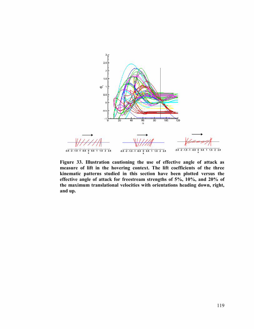
119

Figure 33. Illustration cautioning the use of effective angle of attack as

measure of lift in the hovering context. The lift coefficients of the three

kinematic patterns studied in this section have been plotted versus the

effective angle of attack for freestream strengths of 5%, 10%, and 20% of

the maximum translational velocities with orientations heading down, right,

and up.

120

Chapter 5 Summary, Conclusions, and Recommendations for Future

Work

In this study we examined the hovering kinematics of a two-dimensional

and three-dimensional flat plate (AR=4) with the aid of surrogate models at a

Reynolds number of 100. The analysis of the fluid physics highlighted well

known phenomena such as the LEV, as well as identified novel roles for the tip

vortices and sustained downward jet that were previously unexplored. The

complementary uses of the Navier-Stokes and surrogate models led to the

development of a tool that was helpful in the physical analysis of the fluid physics

by identifying trends in aerodynamic performance as a function of wing motion,

and the quality of the surrogate modeling methodology proved successful in

providing computationally cheap and accurate approximations to the time-

averaged forces. Different methodologies have been employed previously in the

literature to try and achieve this goal in the context of hovering flight with mixed

success and applicability. While the computational expense of the Navier-Stokes

solutions were O(10-100) cpu hours for each combination of kinematic variables,

this data could then be used to train the surrogate models which could predict

performance in a fraction of a second and therefore potentially be used in real

time calculations for control algorithms. Details are expanded below.

121

Hover:

Regarding the fluid physics and aerodynamic implications during hover, we

observed:

(i) The role of the LEV and associated delayed stall plays a dominant role in

the determination of lift in both two- and three-dimensional cases and this

is in consensus with the literature (see section 1.1.4). Angle of attack,

angular velocity, translational velocity, and translational acceleration all

impact the formation and evolution of the LEV. For one of the delayed

cases shown, the two-dimensional starting vortices detach causing a

weaker LEV during mid-stroke. In the corresponding three-dimensional

case, the tip vortices served to anchor the LEV and in the process

increased the time-averaged lift. The surrogate models show that this is

not a general recipe for higher three-dimensional lift though as most

delayed rotation cases at high AoA exhibit higher two-dimensional lift. In

general, the advanced rotation cases, especially those with low AoA, were

able to benefit from the three-dimensional effects as the lift valley

associated with strong downward rotation was much weaker in three

dimensions.

(ii) The manifestation of the wake-capture mechanism in the three-

dimensional case has been seen to change as the behavior of the shed

vortices may differ between two- and three-dimensional cases. This is

122

illustrated by one case where the shed two-dimensional vortices would

remain in the plane of the plunging motion. The three-dimensional

counterparts are shed at angles such that they leave plane of the plunging

wing and do not collide with the wing upon its return affecting the

resulting force histories. This mechanism is also seen to change in relative

importance to the LEV impact with changes in kinematics. When the LEV

and wake-capture pieces of the cycle were separate, the current sinusoidal

pitch-plunge motions showed a larger impact on the force histories from

the LEV. On the other hand, Sane and Dickinson (2001, 2002) illustrate

similar kinematics about which there is also a flapping about a joint

component, and for which the rotation times are localized around the end

of the stroke, for which the wake-capture has a noticeably larger impact

than the subsequent LEV.

(iii) In two-dimensional cases with higher angles of attack, i.e., lower pitching

amplitudes, a persistent downward jet like flow feature was seen to form

in the wake sustained by the influence of shed vortices. This was seen

experimentally by Freymuth (1990) as well. The jet was absent in the two-

dimensional cases with lowest angles of attack as there was also no large

scale vortex shedding. In the low aspect ratio three-dimensional case at Re

= 100, the presence and influence of an induced jet is not as clear cut.

There are pockets of momentum encountered on return strokes, but there

is no coherent reverse Karman vortex street reinforcing the jet due to the

123

more complex three-dimensional vortex interactions. The impact on the

instantaneous force history can be significant as demonstrated in section

3.1.1.

(iv) There was significant variance in the spanwise distribution of forces in the

three-dimensional cases. Cases which suppressed the LEV and tip

vortices, those with the highest angular amplitudes and thus low angles of

attack, and small velocity when vertical (e.g. near synchronized hovering)

appeared to have a relatively constant response along the span. In contrast,

three-dimensional cases with prominent tip vortices exhibited significant

variations along the span which did not have a strong correlation to the

instantaneous two-dimensional lift values experienced.

(v) At the present Reynolds number (100) the three-dimensional flow physics

and tip effects can augment the lift by: a) the presence of a low pressure

region near the tip, b) the anchoring of an otherwise shed vortex (in 2D)

near the tip, and c) weakening the pocket of downward momentum

encountered on a return stroke. A competing effect is the induced

downwash of tip vortex and the reduced effective angle of attack along the

span, serving to reduce lift.

(vi) The competition of effects between rapid pitching motions, their timing,

and subsequent LEV generation would suggest that (non-sinusoidal)

kinematics achieving better lift performance may be achieved by

confining the downward rotation to the end of the stroke while balancing

124

the desire for high AoA and increasing AoA during the stroke cycle to

generate and sustain LEVs. Lift and drag will still compete as higher

angles of attack will increase the drag and the generation of the vortices,

but the trade-offs between the two can be modified.

Environmental Sensitivity:

As flapping wing frequencies are typically an order of magnitude or two faster

than that of environmental perturbations, gusts can be modeled as a constant

freestream for many practical applications.

(i) The sensitivity to the gust for selected kinematic parameters was largely

determined by how much influence it had on the vortex dynamics.

Headwinds with a modest 20% strength could significantly enhance the

LEV generation and this in turn provided stronger wake interactions on

the return stroke. For most kinematic motions, within the ranges studied, a

20% horizontal freestream increased the 2D lift despite half of the stroke

experiencing a tailwind.

(ii) The 3D cases, while still affected appreciably, were noticeably less

sensitive to gusts than their 2D counterparts due to the weakened vortex

dynamics generally occurring in 3D.

(iii)The impact of a gust was tied to its strength, orientation, and what

kinematics it encountered. Those flows affected by the gust saw the

manifestation through its role in LEV, tip vortex, and wake generation and

125

interaction. Those kinematics with little of the aforementioned vortex

dynamics saw the smallest sensitivity to the gust.

(iv) By changing the effective angle of attack on select kinematic motions with

various freestream orientations and strengths, different values at the same

effective angle of attacks were obtained. Hence a cautionary note on the

application of quasi-steady models in the hovering context is warranted.

Surrogate Modelling:

Often as case studies in the literature are performed, or independent

variables varied in a parametric study, it can become difficult to place the findings

in the proper context thus making it difficult to glean the relevant information and

compare with findings of other researchers. The surrogate process more readily

illuminates the global perspective of variables‟ impact as well as the limitations of

the findings, making identification of the applicability much more apparent. The

surrogate modeling techniques provided a useful method for approximating

otherwise computationally expensive simulations without sacrificing fidelity.

Meanwhile they proved an efficient method for analyzing trends seen throughout

the design space and possible points of interest. Coupled with instantaneous force

histories and flow field measurements they can provide insight to the complex

interplay of the physical mechanisms involved. The surrogate modeling

techniques further revealed that:

126

(i) The weighted average surrogate agreed well at the independent test points.

While the number of independent test points was limited, the error was

often less than a few percent. The maximum error, based on time-averaged

lift values, that was found was less than 15%. The agreement shows

promise for using surrogates, namely weighted average surrogates, as a

reduced order model for complex engineering design in the MAV context.

(ii) The hierarchy of variable sensitivity in the time averaged lift changed

between two-dimensional and three-dimensional hover. In two-dimensions

the importance was 1) angular amplitude 2) phase lag and 3) plunging

amplitude. In three-dimensions the hierarchy switches to 1) phase lag 2)

angular amplitude and 3) plunging amplitude. This is in large part from

the tip vortices in three-dimensional simulations not suffering as large a

penalty from the lift valley that would occur between wake-capture and

delayed stall. This difference in two-dimensions and three-dimensions is

partially attributed to the reduced influence of the jet interaction in three-

dimensional simulations.

(iii)Interestingly, the approximation to the power required remained largely

the same between two-dimensional and three-dimensional design spaces.

This implies that the unsteady effects which influence the drag can in

some contexts be reduced down to their two-dimensional counterparts.

Note that the pressure force, and not the viscous force, was still the

dominant component of the drag felt.

127

(iv) Regions for which 2D kinematics outperformed 3D in hover and vice-

versa were identified. Furthermore the density of points near the Pareto

front was higher in three dimensions implying more design variable

combinations that are close to optimal in terms of power and lift trade-

offs. In the study of Sane and Dickinson (2001), consistent conclusions are

reached for obtaining optimal lift, e.g., keep fairly high angles of attack for

as much of the stroke as possible. There are differences though in the

sensitivity to plunging amplitude, which was small in the current study,

but was relevant in the flapping about a joint method employed in their

study.

Further Work:

A few closely related topics which would prove valuable in the understanding of

flapping wing flight:

(i) How can the shape of the wing be constructed to elicit favorable fluid

dynamics? There has been some effort to look at corrugated cross-sections

(often cited as motivated by dragonflies) and a small study in the appendix

on ellipse versus flatplate. Perhaps more importantly, in light of the

findings in the current studies, how can the wing planform be manipulated

to increase performance? It was seen that certain combinations of

kinematic parameters could utilize the 3D effects, namely the tip vortices.

For instance could the trailing edge be tapered as to elicit a vortex which

would not only create a low pressure region, but not interfere with LEV

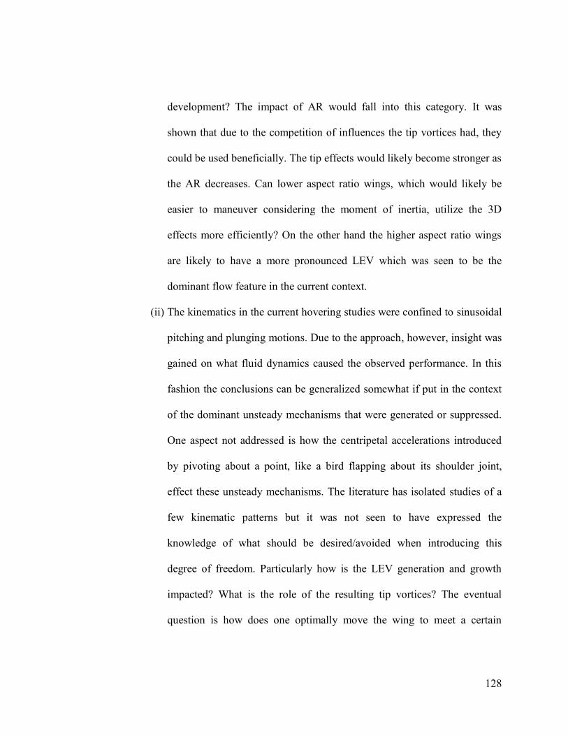
128

development? The impact of AR would fall into this category. It was

shown that due to the competition of influences the tip vortices had, they

could be used beneficially. The tip effects would likely become stronger as

the AR decreases. Can lower aspect ratio wings, which would likely be

easier to maneuver considering the moment of inertia, utilize the 3D

effects more efficiently? On the other hand the higher aspect ratio wings

are likely to have a more pronounced LEV which was seen to be the

dominant flow feature in the current context.

(ii) The kinematics in the current hovering studies were confined to sinusoidal

pitching and plunging motions. Due to the approach, however, insight was

gained on what fluid dynamics caused the observed performance. In this

fashion the conclusions can be generalized somewhat if put in the context

of the dominant unsteady mechanisms that were generated or suppressed.

One aspect not addressed is how the centripetal accelerations introduced

by pivoting about a point, like a bird flapping about its shoulder joint,

effect these unsteady mechanisms. The literature has isolated studies of a

few kinematic patterns but it was not seen to have expressed the

knowledge of what should be desired/avoided when introducing this

degree of freedom. Particularly how is the LEV generation and growth

impacted? What is the role of the resulting tip vortices? The eventual

question is how does one optimally move the wing to meet a certain

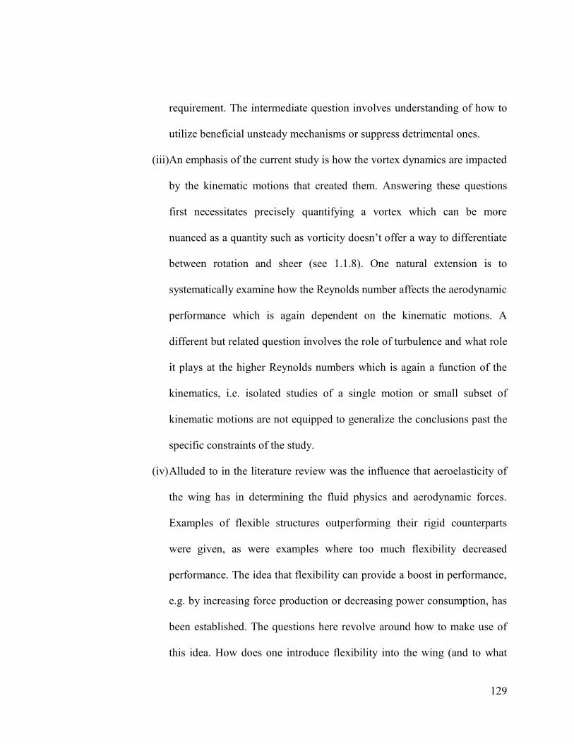
129

requirement. The intermediate question involves understanding of how to

utilize beneficial unsteady mechanisms or suppress detrimental ones.

(iii)An emphasis of the current study is how the vortex dynamics are impacted

by the kinematic motions that created them. Answering these questions

first necessitates precisely quantifying a vortex which can be more

nuanced as a quantity such as vorticity doesn‟t offer a way to differentiate

between rotation and sheer (see 1.1.8). One natural extension is to

systematically examine how the Reynolds number affects the aerodynamic

performance which is again dependent on the kinematic motions. A

different but related question involves the role of turbulence and what role

it plays at the higher Reynolds numbers which is again a function of the

kinematics, i.e. isolated studies of a single motion or small subset of

kinematic motions are not equipped to generalize the conclusions past the

specific constraints of the study.

(iv) Alluded to in the literature review was the influence that aeroelasticity of

the wing has in determining the fluid physics and aerodynamic forces.

Examples of flexible structures outperforming their rigid counterparts

were given, as were examples where too much flexibility decreased

performance. The idea that flexibility can provide a boost in performance,

e.g. by increasing force production or decreasing power consumption, has

been established. The questions here revolve around how to make use of

this idea. How does one introduce flexibility into the wing (and to what

130

degree) such that the unsteady mechanisms are controlled, e.g. keeping the

flow attached, generating stronger LEVs, shedding vortices at the time and

orientation of the designer‟s choosing, etc.?

131

Appendix

(a)

(b)

(c)

132

(d)

FIGURE 34. Time histories of the lift and drag coefficients between a two-dimensional ellipse of

15% thickness and two-dimensional flatplate for selected cases (a) as is increases from 2.0 (left)

to 4.0 (right) holding = 62.5° and =90° (b) as is increased from 45° (left) to 80° (right) while

holding =3.0 and =90° (c) examining delayed rotation =60° (left) and andvanced rotation

=120° (right) while holding =4.0 = 80° (d) examining delayed rotation =60° (left) and

andvanced rotation =120° (right) while holding =2.0 = 45°.

133

Bibliography

Agrawal A, Agrawal SK. 2009 Design of bio-inspired flexible wings for

flapping wing micro-sized air vehicle applications. Adv Robot 23, 979-

1002.

Altshuler DL, Princevac M, Pan H, Lozano J. 2009 Wake patterns of the

wings and tail of hovering hummingbirds. Exp Fluids 46, 835-846.

Altshuler DL, Dickson WB, Vance JT, Roberts SP, Dickinson MH. 2005

Short-amplitude high-frequency wing strokes determine the aerodynamics

of honeybee flight. Proc Natl Acad Sci 102, No. 50, 18213-18218.

Althsuler DL, Dudley R, Ellington CP. 2004 Aerodynamic forces of

revolving hummingbird wings and wing models. J Zool Lond 264, 327-

332.

Anderson JD. 2006 Fundamentals of aerodynamics. 4th ed. New York

McGraw Hill Higher Education.

Anderson JM, Streitlin K, Barrett DS, Triantafyllou MS. 1998 Oscillating

foils of high propulsive efficiency. J Fluid Mech 360, 41-72.

134

Ansari SA, Knowles K, Zbikowski R. 2008 Insectlike flapping wings in

the hover part 2 effect of wing geometry. J Aircraft 45, No. 6, 1976-1990.

Ansari, S.A., Zbikowski, R. & Knowles, K. 2006 Aerodynamic Modeling

of Insect-like Flapping Flight for Micro Air Vehicles. Progress in

Aerospace Sciences 42, 129-172.

Aono H, Chimakurthi SK, Wu P, Sallstrom E, Stanford BK, Cesnik CES,

et al. 2010 A computational and experimental study of flexible flapping

wing aerodynamics. AIAA-Paper 2010-554.

Aono H, Shyy W, Liu H. 2009 Near wake vortex dynamics of a hovering

hawkmoth. Acta Mech Sin 25, 23-36.

Baik YS, Raush J, Bernal L, Shyy W, Ol M. 2010 Experimental Study of

Governing Parameters in Pitching and Plunging Airfoil at Low Reynolds

Number. 48th AIAA Aerospace Sciences Meeting Including the New

Horizons Forum and Aerospace Exposition, AIAA 2010-388.

Baik YS, Rausch JM, Bernal LP, Ol MV. 2009 Experimental investigation

of pitching and plunging airfoils at Reynolds number between 1×104 and

6×104. 39th AIAA Fluid Dynamics Conference, AIAA 2009-4030.

Birch JM, Dickson WB, Dickinson MH. 2004 Force production and flow

structure of the leading edge vortex on flapping wings. J Exp Biol 207,

1063-1072.

135

Birch JM, Dickinson MH. 2003 The influence of wing-wake interactions

on the production of aerodynamic forces in flapping flight. J Exp Biol,

2257-2272.

Birch JM, Dickinson MH. 2001 Spanwise flow and the attachment of the

leading-edge vortex on insect wings. Nature 412, 729-733.

Blazek, J. 2001 Computational Fluid Dynamics: Principles and

Applications. Elsevier.

Bohl DG, Koochesfahani MM. 2009 MTV measurements of the vortical

field in the wake of an airfoil oscillating at high reduced frequency. J

Fluid Mech 620, 63-88.

Bomphrey RJ, Taylor GK, Thomas ALR. 2009 Smoke visualization of

free-flying bumblebees indicates independent leading-edge vortices on

each wing pair. Exp Fluids 46, 811-821.

Bomphrey RJ. 2006 Insects in flight direct visualization and flow

measurements. Bioinsp Biomim 1, 1-9.

Bomphrey RJ, Lawson NJ, Harding NJ, Taylor GK, Thomas ALR. 2005

The aerodynamic of Manduca sexta digital particle image velocimetry

analysis of the leading-edge vortex. J Exp Biol 208, 1079-1094.

136

Bos FM, Lentik D, van Oudheusden BW, Bijl H. 2008 Influence of wing

kinematics on aerodynamic performance in hovering insect flight. J Fluid

Mech 594, 341-368.

Brachenbury J. 1990 Wing movements in the bush cricket Tettigonia

viridissima and the mantis Ameles spallanziana during natural leaping. J

Zoology Long 220, 593-602.

Brodsky AK. 1991 Vortex formation in the tethered flight of the peacock

butterfly Inachis Io L and some aspects of insect flight evolution. J Exp

Biol 161, 77-95.

Broering TM, Lian Y. 2010 Numerical study of two flapping airfoils in

tandem configuration. 48th AIAA Aerospace Sciences Meeting Including

the New Horizons Forum and Aerospace Exposition, AIAA 2010-865.

Buchholz JH, Smits AJ. 2008 The wake structure and thrust performance

of a rigid low-aspect-ratio pitching panel. J Fluid Mech 603, 331-365.

Calderon DE, Wang Z, Gursul I. 2010 Lift enhancement of a rectangular

wing undergoing a small amplitude plunging motion. 48th AIAA

Aerospace Sciences Meeting Including the New Horizons Forum and

Aerospace Exposition, AIAA 2010-386.

Cheng, B. & Titterington, D.M. 1994 Neural Networks: a Review from a

Statistical Perspective. Statistical Science 9, 2-54.

137

Cleaver DJ, Wang Z, Gursul I. 2010 Vortex mode bifurcation and lift

force of a plunging airfoil at low Reynolds Numbers. 48th AIAA



Cloupeau M, Devilliers JF, Devezeaux D. 1979 Direct measurements of

instantaneous lift in desert locust; comparison with Jensen‟s experiments

on detached wings. J Exp Biol 80, 1-15.

Cooter RJ, Baker PS. 1977 Weis-Fogh clap and fling mechanisms in

Locusta. Nature 269, 53-54.

Combes SA. 2002 Wing flexibility and design for animal flight. Ph.D.

Dissertation, University of Washington, 2002.

Combes SA & Daniel TL. 2003a Into thin air: contributions of

aerodynamic and inertial-elastic forces to wing bending in the hawkmoth

Manduca sexta. J Exp Biol 23, 2999-3006.

Combes SA & Daniel TL. 2003b Flexural stiffness in insect wings I.

Scaling and the influenceof wing venation. J Exp Biol 206, 2979-87.

Combes SA & Daniel TL, 2003c Flexural stiffness in insect wings II.

Spatial distribution and dynamic wing bending. J Exp Biol 206, 2989-97.

138

Dabiri JO. 2009 Optimal vortex formation as a unifying principle in

biological propulsion. Ann Rev Fluid Mech 41, No. 1, 17-33.

Dalton S. 2006 The miracle of flight. London: Merrell.

Daniel TL, Combes SA. 2002 Flexible wings and fins: bending by intertial

or fluid-dynamic forces? integr Comp Biol 42, 1044-9.

Dickinson MH, Lehmann F-O, Sane SP. 1999 Wing rotation and the

aerodynamic basis of insect flight. Science 284, No. 5422, 1954-1960.

Dickinson MH. 1994 The effects of wing rotation on unsteady

aerodynamic performance at low Reynolds numbers. JEB 192, 179-206.

Dickson WB, Dickinson MH. 2004 The effect of advance ratio on the

aerodynamics of revolving wings. J Exp Biol 207, 4269-4281.

Dong H, Liang Z. 2010 Effects of ipsilateral wing-wing interactions on

aerodynamic performance of flapping wings. Proceedings of 48th AIAA



Drzewiecki S. 1920 Theorie generale de l'helice.

Du G & Sun M. 2008 Effects of unsteady deformation of flapping wing on

its aerodynamic forces. Appl Math Mech 29, No. 6, 196-204.

139

Dudley R, Ellington CP. 1990 Mechanics of Forward Flight in

Bumblebees II. Quasi-Steady Lift and Power Requirements. J Exp Biol

148, 53-88.

Ellington, C.P 1999 Novel Aerodynamics of Insect Flight: Applications to

Micro-Air Vehicles. Jornal of Experimental Biology 202, 3439-3448.

Ellington CP, van den Berg C, Willmott AP, Thomas ALR. 1996 Leading-

edge vortices in insect flight. Nature 384, 626-630.

Ellingtong CP. 1984 The aerodynamics of hovering insect flight. I. The

quasi-steady analysis. Phil Trans R Soc Lond B 305, 1-15.

Ellington CP. 1984 The aerodynamics of hovering insect flight. IV.

Aerodynamic mechanics. Phil Trans R Soc Lond B 305, 113.

Ennos AR. 1989 Inertial and aerodynamic torques on the wings of Diptera

in flight. J Exp Biol 142, 87-95.

Ennos AR. 1988a The importance of torsion in the design of insect wings.

J. Exp Biol 140, 137-160.

Ennos AR. 1988b The inertial cause of the wing rotation in Diptera. J Exp

Biol 140, 161-169.

Ennos AR. 1987 A comparative study of the flight mechanism of Diptera.

J Exp Biol 127, 355-372.

140

Fearing R.S., Chiang, K.H., Dickinson M., Pick, D.L, Sitti, M. & Yan, J.

2000 Wing Transmission for a Micromechanical Flying Insect. IEEE

International Conference on Robotics and Automation, 1509-1515.

Freymuth P. 1990 Thurst generation by an airfoil in hovermodes.

Experiments in Fluids 9, 17-24.

Fry SN, Sayaman R, Dickinson MH. 2005 The aerodynamics of hovering

flight in Drosophila. J Exp Biol 208, 2303-2318.

Fry SN, Sayaman R, Dickinson MH. 2003 The aerodynamics of free-flight

Maneuvers in Drosophila. J. Exp. Biol. 300, 495-498.

Garland K, Ol M, Bernal L, Kast S. 2010 Experiments on Free-to-Pivot

Hover Motions of a Flat Plate. AIAA-Paper 2010-4456.

Gharib M, Rambod E, Shariff K. 1998 A universal time scale for vortex

ring formation. J Fluid Mech 360, 121-140.

Godoy-Diana R, Marias C, Aider J-L, Wesfried JE. 2009 A model for the

symmetry breaking of the reverse Benard-von Karman vortex street

produced by a flapping foil. J Fluid Mech 622, 23-32.

Godoy-Diana R, Aider J-L, Wesfried JE. 2008 Transitions in the wake of

a flapping foil. Phys Rev E 77, 016308-1-016308-5.

141

Goel, T., Haftka, R.T., Shyy, W. & Queipo, N.V. 2007 Ensemble of

Surrogates. Structural and Multidisciplinary Optimization 33, No. 3.

Gogulapati A, Friedmann P, Kheng E, Shyy W. 2010 Approximate

Aeroelastic Modeling of Flapping Wings: Comparisons with CFD and

Experimental Data. AIAA-Paper 2010-2707.

Gogulapati A, Friedmann P, Shyy . 2008 Nonlinear Aeroelastic Effects in

Flapping Wing Micro Air Vehicles AIAA-Paper 2008-1817

Green MA, Smith AJ. 2008 Effects of three-dimensionality on thrust

production by a pitching panel. J Fluid Mech 615, 211-220.

Green MA, Rowley CW, Haller G. 2007 Detection of Lagrangian coherent

structures in three-dimensional turbulence. J Fluid Mech. 572, 111-120.

Hamamoto M, Ohta Y, Hara K, Hisada T. 2007 Application of fluid-

structure interaction analysis to flapping flight of insects with deformable

wings. Adv Robot 21, 1-21.

Heathcote S, Martin D, Gursul I. 2004 Flexible flapping airfoil propulsion

at zero freestream velocity. AIAA J 42, No. 11, 2196-204.

Hedenström A, Muijres FT, von Busse R, Johansson LC, Winter Y,

Spedding GR. 2009 High-speed stereo PIV measurement of wakes of two

bat species flying freely in a wind tunnel. Exp Fluids 46, 923-932.

142

Hedenström A, Johansson LC, Wolf M, von Busse R, Winter Y, Spedding

GR. 2007 Bat flight generates complex aerodynamic tracks. Science 316,

894-897.

Hedrick TL. 2008 Software techniques for two- and three-dimensional

kinematic measurements of biological and biomimetic systems. Bioinsp

Biomim 3, 1-6.

Ho, S., Nassef, H., Pornsin-Sirirak, N., Tai, Y.C. & Ho, C.M. 2003

Unsteady Aerodynamics and Flow Control for Flapping Wing Flyers.

Progress in Aerospace Sciences 39, No. 8, 635-681.

Hong YS, Altman A. 2008 Lift from spanwise flow in simple flapping

wings. J Aircraft 45, No. 4, 1206-1216.

Hong YS, Altman A. 2007 Streamwise vorticity in simple mechanical

flapping wings. J Aircraft 44 , No. 5, 1588-1597.

Hover FS, Haugsdal Ø. Triantafyllou MS. 2004 Effect of angle of attack

profiles in flapping foil propulsion. J Fluid Struct 19, 37-47.

Hsieh CT, Chang CC, Chu CC. 2009 Revisiting the aerodynamics of

hovering flight using simple models. J Fluid Mech 623, 121-148.

Hubel TY, Hristov NI, Swart SM, Breuer KS. 2009 Time-resolved wake

structure and kinematics of bat flight. Exp Fluids 46, 933-943.

143

Hui H, Kumar AG, Abate G, Albertani R. 2009 An experimental study of

flexible membrane wings in flapping flight AIAA-Paper 2009-876

Hunt, J.C.R., Wray, A.A. & Moin, P. 1988 Eddies, Streams, and

Convergence Zones in Turbulent Flows. Report CTR-S88 Center for

Turbulence Research.

Isaac KM, Rolwes J, Colozza A. 2008 Aerodynamic of a flapping and

pitching wing using simulations and experiments. AIAA J 46, No. 6, 1505-

1515.

Ishihara D, Horie T, Denda M. 2009 A two-dimensional computational

study on the fluid-structure interaction cause of wing pitch changes in

dipteran flapping flight. J Exp Biol 212, 1-10.

Jardin T, David L, Farcy 2009 A. Characterization of vortical structures

and loads based on time-resolved PIV for asymmetric hovering flapping

flight. Exp Fluids 46, 847-857.

Jensen M. 1956 Biology and physics of locust flight. III. The

aerodynamisof locust flight Phil. Trans. R. Soc. Lond. B 239, 511-552.

Jones AR, Babinsky H. 2010 Three-dimensional effects of a waving wing.

48th AIAA Aerospace Sciences Meeting Including the New Horizons

Forum and Aerospace Exposition, AIAA 2010-551.

144

Kamakoti, R., Thakur, S., Wright, J., and Shyy, W. 2006 Validation of a

new parallel all-speed CFD code in a rule-based framework for

multidisciplinary applications. AIAA 2006-3063.

Kang C, Baik Y, Bernal L, Ol MV, Shyy W. 2009a Fluid Dynamics of

Pitching and Plunging Airfoils of Reynolds Number between 1x104 and

6x104. AIAA-Paper 2009-536

Kang C, Aono H, Trizila P, Baik YS, Rausch JM, Bernal LP, Ol MV,

Shyy W. 2009b Modeling of pitching and plunging airfoils at Reynolds

number between 1×104 and 6×104. Proceeding of 39th AIAA Fluid

Dynamics Conference, AIAA 2009-4100.

Katz J, Plotkin A. 2001 Low-speed aerodynamics. 2nd ed. New York.

Cambridge University Press.

Kim D-K, Han J-H, Kwon K-J. 2009 Wind tunnel tests for a flapping wing

model with a changeable camber using macro-fiber composite actuators.

Smart Mater Struct 18, 024008-1-8.

Kim W-K, Ko JH, Park HC, Byun D. 2009 Effects of corrugation of the

dragonfly wing on gliding performance. J Theor Biol 260, 523-530.

Kurtulus DF, David L, Farcy A, Alemdaroglu N. 2008 Aerodynamic

characteristics of flapping motion in hover. Exp Fluids 44, 23-36.

145

Lai JCS, Platzer MF. 1999 Jet characteristics of a plunging airfoil. AIAA J

37, No. 12, 1529-1537.

Lee J-S, Kim J-H, Kim C. 2008 Numerical study on the unsteady-force-

generation mechanism of insect flapping motion. AIAA J 46, No. 7, 1835-

1848.

Lehmann F-O. 2009 Wing-wake interaction reduces power consumption

in insect tandem wings. Exp Fluids 46, 765-775.

Lehmann F-O, Pick S. 2007 The aerodynamic benefit of wing-wing

interaction depends on stroke trajectory in flapping insect wings. J Exp

Biol 210, 1362-1377.

Lehmann F-O, Sane SP, Dickinson MH. 2005 The aerodynamic effects of

wing-wing interaction in flapping insect wings. J Exp Biol 208, 3075-

3092.

Lehmann FO. 2004 The mechanisms and lift enhancement in insect flight

Naturwisenschafen.

Lentink, D., Bradshaw, N. & Jongerius, S.R. 2007 Novel Micro Aircraft

Inspired by Insect Flight. Comparitive Biochemistry and Physiology A-

Molecular & Integrative Physiology 146, No. 4, 133-134.

146

Lentink D, Gerritsma M. 2003 Influence of airfoil shape of performance in

insect flight. Proceeding of 33rd AIAA Fluid Dynamics Conference and

Exhibit, AIAA 2003-3447.

Lesoinne M, Farhat C. 1996 Geometric conservation laws for flow

problems with moving boundaries and deformable meshes, and their

impact on aeroelastic computations. Comput Method Appl M 134, 71-90.

Levy D-E, Seifert A. 2009 Simplified dragonfly airfoil aerodynamics at

Reynolds numbers below 8000. Phys Fluids 21, 071901-1-071901-17.

Lewing GC, Haj-Hariri H. 2003 Modeling thrust generation of a two-

dimensional heaving airfoil in a viscous flow. J Fluid Mech 492, 339-362.

Liang Z, Dong H, Wei M. 2010 Computational Analysis of Hovering

Hummingbird Flight. 48th AIAA Aerospace Sciences Meeting Including

the New Horizons Forum and Aerospace Exposition, AIAA 2010-555.

Lipinski D, Mohseni K. 2009 Flow structures and fluid transport for the

hydromedusae Sarsia tubules and Aequorea Victoria. J Exp Biol 212,

2436-2447.

Liu H, Aono H. 2009 Size effects on insect hovering aerodynamics: an

integrated computational study. Bioinsp Biomim 4, 1-13.

147

Liu H. 2009 Integrated modeling of insect flight: from morphology,

kinematics to aerodynamics J. Comput Phys 228, No. 2, 439-59.

Liu H. 2005 Simulation-based biological fluid dynamics in animal

locomotion. Appl Mech Rev 58, 269-282.

Liu H. 2002 Computational biological fluid dynamics: digitizing and

visualizing animal swimming and flying. 42, No. 5, 1050-1059.

Liu H, Kawachi K. 1997 A numerical study of insect flight. J Comput

Phys 146, No. 1, 124-156.

Lu Y, Shen GX. 2008 Three-dimensional flow structure and evolution of

the leading-edge vortices on a flapping wing. J Exp Biol 211, 1221-1230.

Lua KB, Lim TT, Yeo KS. 2008 Aerodynamic forces and flow fields of a

two-dimensional hovering wing. Exp Fluids 45, 1047-1065.

Lu Y, Shen GX, Su WH. 2007 Flow visualization of dragonfly hovering

via an electromechanical model. AIAA J 45, No. 3, 615-623.

Lua KB, Lim TT, Yeo KS, Oo GY. 2007 Wake-structure formation of a

heaving two-dimensional elliptic airfoil. AIAA J 45, No. 7, 1571-1583.

Luke, E.A. & George, T. 2005 Loci: A Rule-Based Framework for

Parallel Multi-Disciplinary Simulation Synthesis. Journal of Functional

Programming 15, No. 3, 477-502.

148

Luo G, Sun M. 2005 The effects of corrugation and wing planform on the

aerodynamic force production of sweeping model insect wings. Acta Mech

Sin 21, 531-541.

Maybury WJ, Lehmann F-O. 2004 The fluid dynamics of flight control by

kinematic phase lag variation between two robotic insect wings. J Exp

Biol 207, 4707-4726.

Menter FR. 1993 Two equation eddy-viscosity turbulence models for

engineering applications. AIAA J 32, 269-289.

Michelin S & Smith SGL. 2009 Resonance and propulsion performance of

a heaving flexible wing. Phys Fluids 21, 071902-1-15.

Miettinen KM. 1999 Nonlinear Multiobjective Optimization, Kluwer

Academic Publisher, Boston.

Milano M, Gharib M. 2005 Uncovering the physics of flapping flat plates

with artificial evolution. J Fluid Mech 534, 403-409.

Miller LA, Peskin CS. 2009 Flexible clap and fling in tiny insect flight. J

Exp Biol 212, 3076-90.

Miller LA, Peskin CS. 2005 A computational fluid dynamics of „clap and

fling‟ in the smallest insects. J Exp Biol 208, 195-212.

149

Miller LA, Peskin CS. 2004 When vortices stick: an aerodynamic

transition in tiny insect flight. J Exp Biol 207, 3073-3088.

Muijres FT, Johansson LC, Barfield R, Wolf M, Spedding GR,

Hedenström 2008 A. Leading-edge vortex improves lift in slow-flying

bats. Science 319, 1250-1253.

Mueller D, Bruck HA, Gupta SK. 2009 Measurement of thrust and lift

forces associated with the drag of compliant flapping wing for micro air

vehicles using a new test stand design. Exp Mech, 1-11.

Mueller, T.J. & DeLaurier, J.D. 2003 Aerodynamics of Small Vehicles.

Annual Review of Fluid Mechanics 35, 89-111.

Myers, R.H. & Montgomery, D.C. 2002 Response Surface Methodology:

Process and Product Optimization Using Designed Experiments. Wiley.

Nagai H, Isogai K, Fujimoto T, Hayase T. 2009 Experimental and

numerical study of forward flight aerodynamics of insect flapping wing.

AIAA J 47, No. 3, 730-742.

Norberg, U.M.L. 2002 Structure, Form, and Function of Flight in

Engineering and the Living World. Journal of Morphology 252, No. 1, 52-

81.

150

Ol et al. 2009a Unsteady aerodynamics for micro air vehicles. RTO AVT-

149 report, 1-145.

Ol MV, Bernal L, Kang C, Shyy W. 2009b Shallow and deep dynamic

stall for flapping low Reynolds number airfoils. Exp Fluids 46, 883-901.

Osborne MFM. 1951 Aerodynamics of flapping flight with application to

insects. . Exp Biol 28, 221-245.

Oyama A, Okabe Y, Shimoyama K, Fujii K. 2009 Aerodynamic multi-

objective design exploration of a flapping airfoil using a Navier-Stokes

solver. J Aerospace Comput Inf Commun 6, 256-270.

Pines, D. & Bohorquez, F. 2006 Challenges Facing Future Micro-Air-

Vehicle Development. Journal of Aircraft 43, No. 2, 290-305.

Platzer M, Jones K, Young J, Lai J. 2008 Flapping wing aerodynamics:

Progress and challenges. AIAA J 46, No. 9, 2136-2149.

Pick S, Lehmann F-O. Stereoscopic 2009 PIV on multiple color-coded

light sheets and its application to axial flow in flapping robotic insect

wings. Exp Fluids doi 10.1007/s00348-009-0687-5.

Poelma C, Dickinson WB, Dickinson MH. 2006 Time-resolved

reconstruction of the full velocity field around a dynamically-scaled

flapping wing. Exp Fluids 41, 213-225.

151

Pornsin-Sirirak, T.N., Keenon, M., Lee, S.W., Tai, Y.C., Grasmeyer, J.,

Nassef, H. & Ho, C.M. 2000 MEMS Wing Technology for a Battery-

Powered Ornithopter. 13th

IEEE International Conference on Micro

Electro Mechanical Systems, 799-804.

Queipo, N., Haftka, R.T., Shyy, W., Goel, T. Vaidyanathan, R. & Tucker,

P.K. 2005 Surrogate-Based Analysis and Optimization. Progress in

Aerospace Sciences 41, 1-25.

Radespiel R, Windte J, Scholz U. 2007 Numerical and experimental flow

analysis of moving airfoils with laminar separation bubbles. AIAA J 45,

No. 6, 1346-1356.

Ramasamy M, Leishmann JG. 2006 Phase-locked particle image

velocimetry measurements of a flapping wing. J Aircraft 43, No. 6, 1867-

1875.

Read DA, Hover FS, Triantafyllou MS. 2003 Forces on oscillating foils

for propulsion and maneuvering. J Fluid Struct 17, 163-183.

Ringuette MJ, Milano M, Gharib M. 2007 Role of the tip vortex in the

force generation of low-aspect-ratio normal flat plates. J Fluid Mech 581,

453-468.

152

Riskin DK, Willis DJ, Iriarte-Diaz J, Hedrick TL, Kostandov M, Chen J,

Laidlaw DH, Breuer KS, Swartz SM. 2008 Quantifying the complexity of

bat wing kinematics. J Theor Biol 254, 604-615.

Ristroph L, Berman GJ, Bergou AJ, Wang ZJ, Cohen I. 2009 Automated

hull reconstruction motion tracking (HRWT) applied to sideways

maneuvers of free-flying insects. J Exp Biol 212, 1324-1335.

Rival D, Prangemeier T, Tropea C. 2009 The influence of airfoil

kinematics on the formation of leading-edge vortices in bio-inspired flight.

Exp Fluids 46, 823-833.

Rozhdestvensky, K.V. & Ryzhov, V.A. 2003 Aerohydrodynamics of

Flapping-Wing Propulsors. Progress in Aerospace Sciences 39, 585-633.

Sacks, J., Schiller, S.B. & Welch, W.J. 2008 Design for Computer

Experiments. Technometrics 31, No. 1, 41-47.

Sane SP. 2003 The aerodynamics of insect flight. J Exp Biol.

Sane SP, Dickinson MH. 2002 The aerodynamic effects of wing rotation

and a revised quasi-steady model of flapping flight. J Exp Biol 205, 1087-

1096.

Sane SP, Dickinson MH. 2001 The control of flight force by a flapping

wing lift and drag production. J Exp Biol 204, 2607-2626.

153

Schouveiler L, Hover FS, Triantafyllou MS. 2005 Performance of flapping

foil propulsion. J Fluid Struct 20, 949-959.

Shadden SC, Lekien F, and Marsden JE. 2005 Definition and properties of

Lagrangian coherent structures from finite-time Lyapunov exponents in

two-dimensional aperiodic flows. Physica D 212, 271-304.

Shkarayev S, Silin D, Abate G, Albertani R. Aerodynamics of cambered

membrane flapping wing AIAA-Paper 2010-58.

Shyy W., Aono H., Chimakurthi S.K., Trizila P., Kang C.-K., Cesnik

C.E.S., & Liu H. 2010 Recent Progress in Flapping Wing Aerodynamics

and Aeroelasticity. Progress in Aerospace Sciences.

Shyy W, Trizila P, Kang C, Aono H. 2009 Can tip vortices enhance lift of

a flapping wing? AIAA J 47, No. 2, 289-293.

Shyy, W., Lian, Y., Tang, J., Viieru, D. & Liu, H. 2008 Aerodynamics of

Low Reynolds Number Flyers. Cambridge University Press.

Shyy W, Liu H. 2007 Flapping wings and aerodynamics lift. The role of

leading-edge vortices. AIAA J 45, No. 12, 2817-2819.

Shyy W, Udaykumar HS, Rao MM, Smith RW. 2006 Computational fluid

dynamics with moving boundaries. New York. Dover Publications, Inc.

154

Shyy, W., Papila, N., Vaidyanathan, R. & Tucker, P.K. 2001 Global

Design Optimization for Aerodynamics and Rocket Propulsion

Components. Progress in Aerospace Sciences 37, 59-118.

Shyy, W., Berg, M. & Ljungqvist, D. 1999 Flapping and Flexible Wings

for Biological and Micro Air Vehicles. Progress in Aerospace Sciences

35, 455-505.

Shyy W. 1994 Computational modeling for fluid flow and interface

transport. Amsterdam. Elsevier Science Publisher.

Shyy, W. 1985 A Study of Finite Difference Approximations to Steady-

State, Convection-Dominated Flow Problems. Journal of Computational

Physics 57, No. 3, 415-438.

Smola, A.J. & Scholkopf, B. 2004 A Tutorial on Support Vector

Regression. Statistics and Computing 14, 199-222.

Song D, Wang H, Zen L, Yin C. 2001 Measuring the camber deformation

of a dragonfly wing using projected comb fringe. Rev Sci Instrum 72, No.

5, 2450-2454.

Spedding, G.R. & Lissaman, P.B.S. 1998 Technical Aspects of Microscale

Flight Systems. Journal of Avian Biology 29, No. 4, 458-468.

155

Srygley RB, Thomas ALR. 2002 Unconventional lift-generating

mechanisms in free-flying butterflies. Nature 420, 660-664.

Sun M, Yu X. 2006 Aerodynamic force generation in hovering flight in a

tiny insect. AIAA J 44, No. 7, 1532-1540.

Sun M, Lan SL. 2004 A computational study of the aerodynamic forces

and power requirements of dragonfly hovering. J Exp Biol 207,1887-1901.

Sun M, Yu X. 2003 Flows around two airfoils performing fling and

subsequent translation and translation and subsequent clap. Acta Mecha

Sin; 19, No. 2, 103-117.

Sun M, Tang J. 2002 Unsteady aerodynamic force generation by a model

fruit fly wing in flapping motion. J Exp Biol 205, 55-70.

Sunada S, Takahashi H, Hattori T, Yasuda K, Kawachi K. 2002 Fluid-

dynamic characteristics of a bristled wing. J Exp Biol 205, 2737-2744.

Taira K, Colonius T. 2009 Three-dimensional flows around low-aspect-

ratio flat-plate wings at low Reynolds numbers. J Fluid Mech 623, 187-

207.

Tang J, Viieru D, Shyy W. 2008 Effect of Reynolds number and flapping

kinematics on hovering aerodynamics. AIAA J 46, No. 4, 967-76.

156

Tarascio M, Ramasamy M, Chopra I, Leishman JG. 2005 Flow

visualization of MAV scaled insect based flapping wings in hover. J

Aircraft 42, No. 2, 355-360.

Tezduyar TE, Behr M, Mittal S, Liou J. 1992 A new strategy for finite

element computations involving moving boundaries and interfaces- The

deforming-spatial-domain/space-time procedure II. Computation of free-

liquid flows, and flows with drifting cylinders. Comput Method Appl M

94, 353-371.

Thakur,S.T. & Wright, J. 2005 Loci-STREAM: All-Speed CFD Solver for

Arbitrary Polygonal Meshes in the Loci Framework. Streamline Numerics

Inc., Gainesville, Florida (unpublished).

Theodorsen T. 1935 General Theory of Aerodynamic Instability and the

Mechanism of Flutter. NACA Report 496.

Thomas ALR, Taylor GK, Srygley RB, Nudds RL, Bomphrey RJ. 2004

Dragonfly flight free-flight and tethered flow visualzations reveal a

diverse array of unsteady lift-generating mechanisms, controlled primarily

via angle of attack. J Exp Biol 207, 4299-4323.

Thomas, P.D. & Lombard, K. 1978 The Geometric Conservation Law – A

Link between Finite-Difference and Finite-Volume Methods of Flow

Computation on Moving Grids. AIAA Paper 1978-1208.

157

Tian X, Iriate-Diaz J, Middleton K, Galvao R, Israeli E, Roemer A,

Sullivan A, Song A, Swartz S, Breuer K. 2006 Direct measurements of the

kinematics and dynamics of bat flight. Bioinsp Biomim 1, S10-S18.

Tobalske BW, Hearn JWD, Warrick DR. 2009 Aerodynamics of

intermittent bounds in flying birds. Exp Fluids 46, 963-973.

Usherwood JR, Ellington CP. 2002 The aerodynamics of revolving wings

I. Model hawkmoth wings. J Exp Biol 205, 1547-1564.

Trizila P, Kang C, Aono H.,Visbal MR, & Shyy W. 2010 Fluid Physics

and Surrogate Modeling of Low Re Flapping Rigid Flat Plate. AIAA

Paper 2008-5081.

Trizila P, Kang C, Visbal MR, & Shyy W. 2008a A Surrogate Model

Approach in 2D versus 3D Flapping Wing Aerodynamic Analysis. AIAA

Paper 2008-5914.

Trizila P, Kang C, Visbal MR & Shyy W. 2008b Unsteady Fluid Physics

and Surrogate Modeling of Low Reynolds Number, Flapping Airfoils.

AIAA Paper 2008-3821.

Usherwood JR, Ellington CP. 2002 The aerodynamics of revolving wings

II. Propeller force coefficients from mayfly to quail. J Exp Biol 205, 1565-

1576.

158

van den Berg C, Ellington CP. 1997a The three-dimensional leading-edge

vortex of a „hovering‟ model hawkmoth. . Phil. Trans R Soc Lond B 352,

329-340.

van den Berg C, Ellington CP. 1997b The vortex wake of a „hovering‟

model hawkmoth. Phil. Trans R Soc Lond B 352, 317-328.

Vanella M, Fitzgerald T, Preidikman S, Balaras E, Balachandran B. 2009

Influence of flexibility on the aerodynamic performance of a hovering

wing. J Exp Biol 212, 95-105.

Vargas A, Mittal R, Don H. 2008 A computational study of the

aerodynamic performance of a dragonfly wing section in gliding flight.

Bioinsp Biomim 3, (026004) 1-13.

Viana, F.A.C., Haftka, R.T., Valder, S., Butkewitsch, S. & Leal, M. 2008

Ensemble of Surrogates: a Framework based on Minimization of the Mean

Integrated Square Error. AIAA Paper 2008-1885.

Videler JJ, Stamhuis EJ, Povel GDE. 2004 Leading-edge vortex lifts

swifts. Science 306, 1960-1962.

Visbal MR, Gordiner RE, Galbraith MC. 2009 High-fidelity simulations

of moving and flexible airfoils at low Reynolds numbers. Exp Fluids 46,

903-922.

159

Visbal, M.R. & Gaitonde, D.V. 1999 High-Order-Accurate Methods for

Complex Unsteady Subsonic Flows. AIAA Journal 37, No. 10, 1231-1239.

Visbal, M.R. & Gaitonde, D.V. 2002 On the Use of Higher-Order Finite-

Difference schemes on Curvilinear and Deforming Meshes. Journal of

Computational Physics 181, No. 1, 155-185.

von Ellenrieder KD, Pothos S. 2008 PIV measurements of the asymmetric

wake of a two dimensional heaving hydrofoil. Exp Fluids 44, 733-745.

von Ellenrieder KD, Parker K, Soria J. 2003 Flow structures behind a

heaving and pitching finite-span wing. J Fluid Mech 490, 129-138.

Wakeling JM, Ellington CP. 1997 Dragonfly flight II. Velocities,

accelerations and kinematics of flapping flight. J Exp Biol 200, 557-582.

Walker SM, Thomas ALR, Taylor GK. 2009 Deformable wing kinematics

in free-flying hoverflies. J R Soc Interface doi 10. 1098/rsif.2009.0120

Walker SM, Thomas ALR, Taylor GK. 2008 Deformable wing kinematics

in the desert locust how and why do camber, twist and topography vary

through the stroke? J R Soc Interface 6, No. 38, 735-747.

Wallance ID, Lawson NJ, Harvey AR, Jones JDC, Moore AJ. 2006 High-

speed photogrammetry system for measuing the kinematics of insect

wings. Appl Opt 45,No. 7, 4165-4173.

160

Wang H, Zeng L, Liu H, Yin C. 2003 Measuring wing kinematics, flight

trajectory and body attitude during forward flight and turning maneuvers

in dragonflies. J Exp Biol 206, 745-757.

Wang JK, Sun M. 2005 A computational study of the aerodynamic and

forewing-hindwing interaction of a model dragonfly in forward flight. J

Exp Biol 208, 3785-3804.

Wang ZJ, Russell D. 2007 Effect of forewing and hindwing interactions

on aerodynamic forces and power in hovering dragonfly flight. Phys Rev

Lett 99,14801.1-14801.4.

Wang ZJ. 2005 Dissecting Insect Flight, Annual Review of Fluid

Mechanics 37, 183-210.

Wang ZJ. 2004 The role of drag in insect hovering. J Exp Biol 207, 4147-

4155.

Wang ZJ, Birch MB, Dickinson MH. 2004 Unsteady forces and flows in

low Reynolds number hovering flight two-dimensional computations vs

robotic wing experiments. J Exp Biol 207, 461-474.

Wang ZJ. 2000a Two dimensional mechanism for insect hovering. Phys

Rev Lett 85, No. 10, 2216-2219

161

Wang ZJ. 2000b Vortex shedding and frequency selection in flapping

flight. J Fluid Mech 410, 323-341.

Warkentin J, DeLaurier J. 2007 Experimental aerodynamic study of

tandem flapping membrane wings. J Aircraft 44, No. 5, 1653-1661

Warrick DR, Tobalske BW, Powers DR. 2009 Lift production in the

hovering hummingbird. Proc R Soc Lond B 276, No. 1674, 3747-3752.

Warrick DR, Tobalske BW, Powers DR. 2005 Aerodynamics of the

hovering hummingbird. Nature 435, 1094-1097.

Weis-Fogh, T. 1973 Quick Estimates of Flight Fitness in Hovering

Animals, Including Novel Mechanisms for Lift Production. Journal of

Experimental Biology 59, 169-230.

Weis-Fogh, T. 1972 Energentics of Flight in Hummingbirds and in

Drosophila. Journal of Experimental Biology 56, 79-104.

Willmott AP, Ellington CP. 1997a The mechanics of flight in the

hawkmoth Manduca sexta I. Kinematics of hovering and forward flight. J

Exp Biol 200, 2705-2722.

Willmott AP, Ellington CP. 1997b The mechanics of flight in the

hawkmoth Manduca sexta II. Aerodynamic consequences of kinematic

and morphological variation. J Exp Biol 200, 2723-2745.

162

Willmott AP, Ellington CP, Thomas ALR. 1997 Flow visualization and

unsteady aerodymamics in the flight of the hawkmoth, Manduca sexta.

Phil Trans R Soc Lond B 352, 303-316.

Wilson MW, Peng J, Dabiri JO, and Eldredge JD. 2009 Lagrangian

coherent structures in low Reynolds number swimming. J Phys Condens

Matter 21.

Wu G, Zeng L. 2009 Measuring the kinematics of a free-flying hawkmoth

(Macroglossum stellatarum) by a comb-fringe projected method. Acta

Mech Sin doi 10.1007/s10409-009-0306-y.

Yamamoto M, Isogai K. 2005 Measurement of unsteady fluid dynamic

forces for a mechanical dragonfly model. AIAA J 43, No. 12, 2475-2480.

Yates GT. 1985 Optimum pitching axes in flapping wing propulsion. J

Theor Biol 120, 255-276.

Young J, Lai JCS, 2008 Germain C. Simulation and parameter variation of

flapping-wing motion based on dragonfly hovering. AIAA J 46, No. 4,

918-924.

Young J, Walker SM, Bomphrey RJ, Taylor GK, Thomas ALR. 2009

Details of insect wing design and deformation enhance aerodynamic

function and flight efficiency. Science 325, 1549-1552.

163

Zeng L, Hao Q, Kawachi K. 2001 Measuring the body vector of a free

flight bumblebee by the reflection beam method. Meas Sci Technol 12,

1886-1890.

Zeng L, Hao Q, Kawachi K. 2000 A scanning projected line method for

measuring a beating bumblebee wing. Opt Commun 183, 37-43.

Zeng L, Matsumoto H, Kawachi K. 1996 A fringe shadow method for

measuring flapping angle and torsional angle of a dragonfly wing. Meas

Sci Technol 7, 776-781.

Zhang J, Lu X-Y. 2009 Aerodynamic performance due to forewing and

hindwing interaction in gliding dragonfly flight. Phys Rev E 80, 017302.1-

017302.4.

Zhang G, Sun J, Chen D, Wang Y. 2008 Flapping motion measurement of

honeybee bilateral wings using four virtual structured-light sensors. Sens

Actuators A 148, 19-27.

Zheng L, Wang X, Khan A, Vallance RR, Mittal R. 2009 A combined

experimental-numerical study of the role of wing flexibility in insect

flight. 47th AIAA Aerospace Sciences Meeting Including The New

Horizons Forum and Aerospace Exposition AIAA 2009-382.

Aerodynamics of Low Reynolds Number Rigid Flapping Wing Under ...

Documents

Transcript of Aerodynamics of Low Reynolds Number Rigid Flapping Wing Under ...