AERO 422: Active Controls for Aerospace Vehicles - Root ... Root Locus.pdf · Root Locus Plotting...
39
AERO 422: Active Controls for Aerospace Vehicles Root Locus Design Method Raktim Bhattacharya Laboratory For Uncertainty Quantification Aerospace Engineering, Texas A&M University.
Transcript of AERO 422: Active Controls for Aerospace Vehicles - Root ... Root Locus.pdf · Root Locus Plotting...
AERO 422: Active Controls for Aerospace VehiclesRoot Locus Design Method
Raktim Bhattacharya
Laboratory For Uncertainty QuantificationAerospace Engineering, Texas A&M University.

Root Locus
Root Locus Plotting Guidelines Dynamic Compensator Design Example
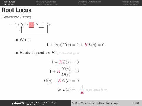
Root LocusGeneralized Setting
C Pu+r e y
−y
Write1 + P (s)C(s) = 1 +KL(s) = 0
Roots depend on K generalized gain
1 +KL(s) = 0
1 +KN(s)
D(s)= 0
D(s) +KN(s) = 0
or L(s) = − 1
Kroot-locus form
AERO 422, Instructor: Raktim Bhattacharya 3 / 39

Root Locus Plotting Guidelines Dynamic Compensator Design Example
Simple ExampleC Pu+r e y
−y
P (s) =A
s(s+ c), C(s) = 1
Two rootsDepends on parameters A and c
r1, r2 =1
2±
√1− 4A
2r1, r2 =
c
2±
√c2 − 4
2
RL studies variation of r1, r2 with respect to A, c one at a time
MATLAB command rlocus(...) is used to generate theseplotshelp rlocus for more details
AERO 422, Instructor: Raktim Bhattacharya 4 / 39

Root Locus Plotting Guidelines Dynamic Compensator Design Example
Simple ExampleVariation w.r.t A
C Pu+r e y
−y
Study variation w.r.t A, set c = 1
P (s) =A
s(s+ c), C(s) = 1
Root-locus form
1 + PC = 0 =⇒ 1 +A1
s(s+ 1)= 0
or 1
s(s+ 1)= − 1
A
AERO 422, Instructor: Raktim Bhattacharya 5 / 39

Root Locus Plotting Guidelines Dynamic Compensator Design Example
Simple ExampleVariation w.r.t A (contd.)
1 +A1
s(s+ 1)= 0
−1.2 −1 −0.8 −0.6 −0.4 −0.2 0 0.2−0.8
−0.6
−0.4
−0.2
0
0.2
0.4
0.6
0.8
Root Locus
Real Axis (seconds−1)
Imag
inar
y A
xis
(sec
onds
−1 )
MATLAB Code
s = tf(’s’);
sys = 1/s/(s+1);
rlocus(sys);
r1, r2 =1
2±
√1− 4A
2
AERO 422, Instructor: Raktim Bhattacharya 6 / 39
Root Locus Plotting Guidelines Dynamic Compensator Design Example
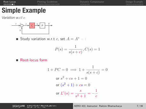
Simple ExampleVariation w.r.t c
C Pu+r e y
−y
Study variation w.r.t c, set A = A∗ = 1
P (s) =1
s(s+ c), C(s) = 1
Root-locus form
1 + PC = 0 =⇒ 1 +1
s(s+ c)= 0
or s2 + cs+ 1 = 0
or (s2 + 1) + cs = 0
or L′(s) =s
s2 + 1= −1
c
AERO 422, Instructor: Raktim Bhattacharya 7 / 39
Root Locus Plotting Guidelines Dynamic Compensator Design Example
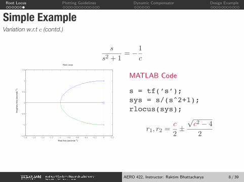
Simple ExampleVariation w.r.t c (contd.)
s
s2 + 1= −1
c
−1.8 −1.6 −1.4 −1.2 −1 −0.8 −0.6 −0.4 −0.2 0 0.2−1.5
−1
−0.5
0
0.5
1
1.5
Root Locus
Real Axis (seconds−1)
Imag
inar
y A
xis
(sec
onds
−1 )
MATLAB Code
s = tf(’s’);
sys = s/(s^2+1);
rlocus(sys);
r1, r2 =c
2±
√c2 − 4
2
AERO 422, Instructor: Raktim Bhattacharya 8 / 39

Guidelines for PlottingRoot Locus

Root Locus Plotting Guidelines Dynamic Compensator Design Example
Guidelines for Drawing Root LocusDefinition 1Root locus of L(s) is the set of values of s for which1 +KL(s) = 0 for values of 0 ≤ K <∞.
Definition 2Root locus is the set of values of s for which phase of L(s) is 180◦.Let the angle from a zero be ψi and angle from a pole be ϕi. Then∑
j
ψj −∑i
ϕi = 180◦ + 360◦(l − 1)
for integer l.
AERO 422, Instructor: Raktim Bhattacharya 10 / 39

Root Locus Plotting Guidelines Dynamic Compensator Design Example
Step 1Draw poles and zeros of L(s)
C Pu+r e y
−y
Plot poles with ×0,−4± 4j for this examplePlot zeros with ONone for this example
Given P (s) = 1s[(s+4)2+16]
,C(s) = K.
Im
Re
x
x
x
AERO 422, Instructor: Raktim Bhattacharya 11 / 39

Root Locus Plotting Guidelines Dynamic Compensator Design Example
Step 2Real axis portions of the locus
Im
Re
x
x
xs0
If we take s0 on the real-axiscontributions from complexpoles and zeros disappearAngle criterion :∑j
ψj −∑i
ϕi = 180◦ +360◦(l− 1)
ϕ1 = −ϕ2
−4 + 4j = − −4− 4j
s0 must lie to the left of oddnumber of real poles & zeros
AERO 422, Instructor: Raktim Bhattacharya 12 / 39
Root Locus Plotting Guidelines Dynamic Compensator Design Example
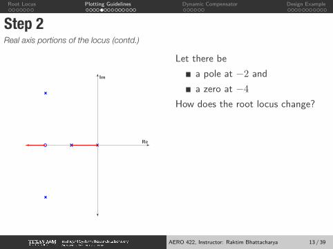
Step 2Real axis portions of the locus (contd.)
Im
Re
x
x
xx
Let there bea pole at −2 anda zero at −4
How does the root locus change?
AERO 422, Instructor: Raktim Bhattacharya 13 / 39
Root Locus Plotting Guidelines Dynamic Compensator Design Example
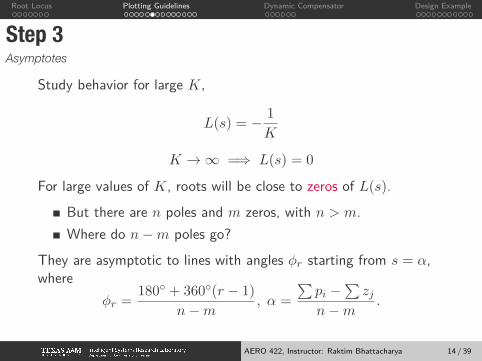
Step 3Asymptotes
Study behavior for large K,
L(s) = − 1
K
K → ∞ =⇒ L(s) = 0
For large values of K, roots will be close to zeros of L(s).But there are n poles and m zeros, with n > m.Where do n−m poles go?
They are asymptotic to lines with angles ϕr starting from s = α,where
ϕr =180◦ + 360◦(r − 1)
n−m, α =
∑pi −
∑zj
n−m.
AERO 422, Instructor: Raktim Bhattacharya 14 / 39
Root Locus Plotting Guidelines Dynamic Compensator Design Example
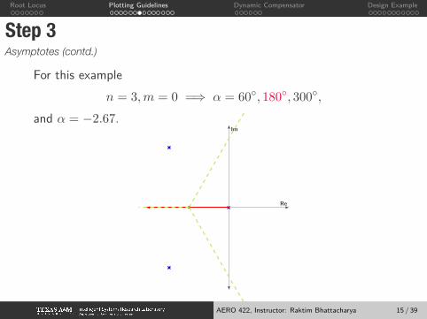
Step 3Asymptotes (contd.)
For this examplen = 3,m = 0 =⇒ α = 60◦, 180◦, 300◦,
and α = −2.67.Im
Re
x
x
x
AERO 422, Instructor: Raktim Bhattacharya 15 / 39

Root Locus Plotting Guidelines Dynamic Compensator Design Example
Step 4Departure Angles
Angle at which a branch of locus departs from one of the poles
rϕdep =∑
ψi −∑
ϕj − 180◦ − 360◦r,
where∑ϕj is over the other poles.
We assume there multiple poles of order q under consideration,and r = 1, · · · , q.
Summation∑ψj is over all zeros.
AERO 422, Instructor: Raktim Bhattacharya 16 / 39

Root Locus Plotting Guidelines Dynamic Compensator Design Example
Step 4Arrival Angles
Angle at which a branch of locus arrives at one of the zeros
rψarr =∑
ϕj −∑
ψi + 180◦ + 360◦r,
where∑ψj is over the other zeros.
We assume there multiple zeros of order q under consideration,and r = 1, · · · , q.
Summation∑ϕj is over all poles.
AERO 422, Instructor: Raktim Bhattacharya 17 / 39

Root Locus Plotting Guidelines Dynamic Compensator Design Example
Step 4Example
Im
Re
x
x
x
AERO 422, Instructor: Raktim Bhattacharya 18 / 39

Root Locus Plotting Guidelines Dynamic Compensator Design Example
Step 5Imaginary axis crossing
Use Routh’s table to determine K for stability for
s3 + 8s2 + 32s+K = 0,
s3 1 32s2 8 Ks1 32−K/8 0s0 K 0
K > 0 and 32−K/8 > 0 =⇒ K > 256
Root locus crosses imaginary axis for K = 256.Substitute K = 256 and s = jω0 in characteristic equation,and solve for ω0.
(jω0)3 + 8(jω0)
2 + 32(jω0) + 256 = 0
AERO 422, Instructor: Raktim Bhattacharya 19 / 39

Root Locus Plotting Guidelines Dynamic Compensator Design Example
Step 5Imaginary axis crossing (contd.)
Solve for ω0
(jω0)3 + 8(jω0)
2 + 32(jω0) + 256 = 0
=⇒ −8ω20 + 256 = 0, and − ω3
0 + 32ω0 = 0.
or ω0 = ±√32.
Im
Re
x
x
x
AERO 422, Instructor: Raktim Bhattacharya 20 / 39
Root Locus Plotting Guidelines Dynamic Compensator Design Example
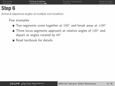
Step 6Arrival & departure angles at multiple root locations
Few examplesTwo segments come together at 180◦ and break away at ±90◦
Three locus segments approach at relative angles of 120◦ anddepart at angles rotated by 60◦
Read textbook for details
AERO 422, Instructor: Raktim Bhattacharya 21 / 39
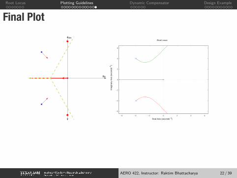
Root Locus Plotting Guidelines Dynamic Compensator Design Example
Final PlotIm
Re
x
x
x
−6 −4 −2 0 2 4 6
−6
−4
−2
0
2
4
6
Root Locus
Real Axis (seconds−1)
Imag
inar
y A
xis
(sec
onds
−1 )
AERO 422, Instructor: Raktim Bhattacharya 22 / 39

Dynamic Compensators
Root Locus Plotting Guidelines Dynamic Compensator Design Example
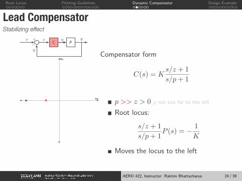
Lead CompensatorStabilizing effect
C Pu+r e y
−y
Re
Imx
Compensator form
C(s) = Ks/z + 1
s/p+ 1
p >> z > 0 p not too far to the left
Root locus:
s/z + 1
s/p+ 1P (s) = − 1
K
Moves the locus to the left
AERO 422, Instructor: Raktim Bhattacharya 24 / 39
Root Locus Plotting Guidelines Dynamic Compensator Design Example
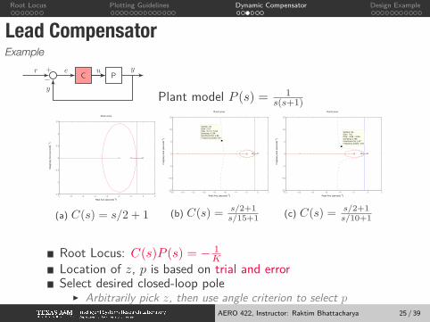
Lead CompensatorExample
C Pu+r e y
−y
Plant model P (s) = 1s(s+1)
−7 −6 −5 −4 −3 −2 −1 0 1−1.5
−1
−0.5
0
0.5
1
1.5
Root Locus
Real Axis (seconds−1)
Imag
inar
y A
xis
(sec
onds
−1 )
(a) C(s) = s/2 + 1
Root Locus
Real Axis (seconds−1)
Imag
inar
y A
xis
(sec
onds
−1 )
−16 −14 −12 −10 −8 −6 −4 −2 0 2−15
−10
−5
0
5
10
15
System: G2Gain: 12.4Pole: −6.74 + 5.34iDamping: 0.784Overshoot (%): 1.89Frequency (rad/s): 8.6
(b) C(s) = s/2+1s/15+1
−12 −10 −8 −6 −4 −2 0 2−15
−10
−5
0
5
10
15
System: G2Gain: 7.91Pole: −3.88 + 3.06iDamping: 0.785Overshoot (%): 1.87Frequency (rad/s): 4.94
Root Locus
Real Axis (seconds−1)
Imag
inar
y A
xis
(sec
onds
−1 )
(c) C(s) = s/2+1s/10+1
Root Locus: C(s)P (s) = − 1K
Location of z, p is based on trial and errorSelect desired closed-loop pole
▶ Arbitrarily pick z, then use angle criterion to select pAERO 422, Instructor: Raktim Bhattacharya 25 / 39

Root Locus Plotting Guidelines Dynamic Compensator Design Example
Lag CompensatorImproves steady state performance
C Pu+r e y
−y
Re
Imx
Compensator form
C(s) = Ks+ z
s+ p
z > p > 0 low frequency, near the origin
z is close to pRoot locus:
s+ z
s+ pP (s) = − 1
K
Boosts steady-state gain: z/p > 1.
AERO 422, Instructor: Raktim Bhattacharya 26 / 39
Root Locus Plotting Guidelines Dynamic Compensator Design Example
Lag CompensatorExample
Plant : 1s(s+1) , Lead Compensator: K(s+2)
s+15
Kv := lims→0 sK(s+2)s+15
1s(s+1) = 90× 2/15 = 12.
Steady-state to ramp input = 1/Kv = 1/12 = 0.0833
How to increase Kv? reduce ess to ramp
Introduce a lag compensator: s+0.05s+0.01
Kv := lims→0 sK(s+0.05)s+0.01
s+2s+15
1s(s+1) = 5× 12 = 60
Steady-state to ramp input = 1/Kv = 1/60 = 0.0166
Lag compensators amplify gain at low frequencyHave no effect at high-frequency
AERO 422, Instructor: Raktim Bhattacharya 27 / 39
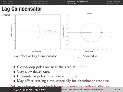
Root Locus Plotting Guidelines Dynamic Compensator Design Example
Lag CompensatorCaution
−16 −14 −12 −10 −8 −6 −4 −2 0 2−20
−15
−10
−5
0
5
10
15
20
Root Locus
Real Axis (seconds−1)
Imag
inar
y A
xis
(sec
onds
−1 )
(a) Effect of Lag Compensator
−0.14 −0.12 −0.1 −0.08 −0.06 −0.04 −0.02 0 0.02 0.04−0.08
−0.06
−0.04
−0.02
0
0.02
0.04
0.06
0.08
Root Locus
Real Axis (seconds−1)
Imag
inar
y A
xis
(sec
onds
−1 )
(b) Zoomed in
Closed-loop poles are near the zero at −0.05Very slow decay rate.Proximity of poles =⇒ low amplitudeMay affect settling time, especially for disturbance response
Put lag pole-zero at as high frequency possible, without affectingtransients AERO 422, Instructor: Raktim Bhattacharya 28 / 39

Design Example

Root Locus Plotting Guidelines Dynamic Compensator Design Example
Control of a Small AirplanePiper Dakota (from text book)
SystemTransfer function from δe (elevator angle) to θ (pitch angle) is
P (s) =θ(s)
δe(s)=
160(s+ 2.5)(s+ 0.7)
(s2 + 5s+ 40)(s2 + 0.03s+ 0.06)
Control Objective 1Design an autopilot so that the step response to elevator input hastr < 1 and Mp < 10% =⇒ ωn > 1.8 rad/s and ζ > 0.6 2nd order
AERO 422, Instructor: Raktim Bhattacharya 30 / 39

Root Locus Plotting Guidelines Dynamic Compensator Design Example
Control of a Small AirplaneOpen Loop Poles: −2.5± 5.81j,−0.015± 0.244j (stable)Open Loop Zeros: −2.5,−0.7 (no RHS zeros)
−3 −2.5 −2 −1.5 −1 −0.5 0 0.5 1−10
−8
−6
−4
−2
0
2
4
6
8
10
Root Locus
Real Axis (seconds−1)
Imag
inar
y A
xis
(sec
onds
−1 )
Figure: Root locus with proportional feedback
AERO 422, Instructor: Raktim Bhattacharya 31 / 39
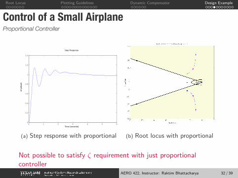
Root Locus Plotting Guidelines Dynamic Compensator Design Example
Control of a Small AirplaneProportional Controller
0 1 2 3 4 5 60
0.2
0.4
0.6
0.8
1
1.2
1.4
Step Response
Time (seconds)
Am
plitu
de
(a) Step response with proportional (b) Root locus with proportional
Not possible to satisfy ζ requirement with just proportionalcontroller
AERO 422, Instructor: Raktim Bhattacharya 32 / 39
Root Locus Plotting Guidelines Dynamic Compensator Design Example
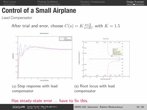
Control of a Small AirplaneLead Compensator
After trial and error, choose C(s) = K s+3s+25 , with K = 1.5
0 1 2 3 4 5 6 7 80
0.2
0.4
0.6
0.8
1
1.2
1.4
Step Response
Time (seconds)
Am
plitu
de
LeadProportional
(a) Step response with leadcompensator
−30 −25 −20 −15 −10 −5 0 5−60
−40
−20
0
20
40
60
0.10.160.230.320.44
0.62
0.84
10
20
30
40
50
60
10
20
30
40
50
60
0.050.10.160.230.320.44
0.62
0.84
0.05
System: G1Gain: 1.5Pole: −8.42 + 9.9iDamping: 0.648Overshoot (%): 6.92Frequency (rad/s): 13
Root Locus
Real Axis (seconds−1)Im
agin
ary
Axi
s (s
econ
ds−
1 )
(b) Root locus with leadcompensator
Has steady-state error ... have to fix this.AERO 422, Instructor: Raktim Bhattacharya 33 / 39

Root Locus Plotting Guidelines Dynamic Compensator Design Example
Control of a Small AirplaneLead Compensator + Integral Control
Fix Steady-State Errorintroduce integral control
C(s) = KDc(s)(1 +KI/s)
tune KI to get desired behaviourstudy root locus w.r.t KI
Characteristic Equation
1 +KDc(s)P (s) +KI
sKDc(s)P (s) = 0
Write this in L(s) = − 1KI
form
AERO 422, Instructor: Raktim Bhattacharya 34 / 39
Root Locus Plotting Guidelines Dynamic Compensator Design Example
Control of a Small AirplaneLead Compensator + Integral Control (contd.)
Characteristic Equation
1 +KDc(s)P (s) +KI
sKDc(s)P (s) = 0
Write this in L(s) = − 1KI
form
L(s) =1
s
KDcP
1 +KDcP
AERO 422, Instructor: Raktim Bhattacharya 35 / 39

Root Locus Plotting Guidelines Dynamic Compensator Design Example
Control of a Small AirplaneLead Compensator + Integral Control (contd.)
−20 −15 −10 −5 0 5−15
−10
−5
0
5
10
15
Root Locus
Real Axis (seconds−1)
Imag
inar
y A
xis
(sec
onds
−1 )
(a) Root locus with PI
−4 −3.5 −3 −2.5 −2 −1.5 −1 −0.5 0 0.5 1−1.5
−1
−0.5
0
0.5
1
1.5
Root Locus
Real Axis (seconds−1)Im
agin
ary
Axi
s (s
econ
ds−
1 )
(b) Root locus with PI (zoomed)
For KI > 0, ζ ↓ =⇒ Mp ↑
AERO 422, Instructor: Raktim Bhattacharya 36 / 39
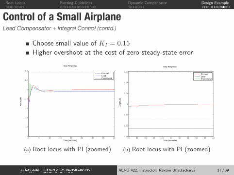
Root Locus Plotting Guidelines Dynamic Compensator Design Example
Control of a Small AirplaneLead Compensator + Integral Control (contd.)
Choose small value of KI = 0.15
Higher overshoot at the cost of zero steady-state error
0 5 10 15 20 25 30 35 400
0.2
0.4
0.6
0.8
1
1.2
1.4
Step Response
Time (seconds)
Am
plitu
de
PI+LeadLeadProportional
(a) Root locus with PI (zoomed)
20 22 24 26 28 30 32 34 36 38 400.94
0.96
0.98
1
1.02
1.04
1.06
Step Response
Time (seconds)
Am
plitu
de
PI+LeadLeadProportional
(b) Root locus with PI (zoomed)
AERO 422, Instructor: Raktim Bhattacharya 37 / 39
Root Locus Plotting Guidelines Dynamic Compensator Design Example
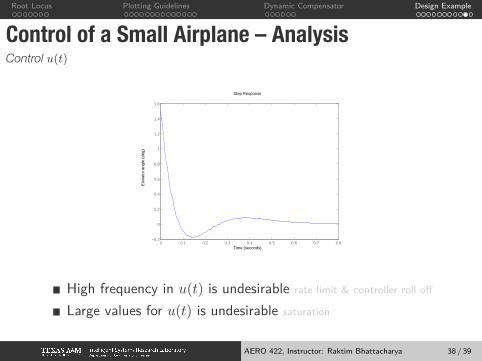
Control of a Small Airplane – AnalysisControl u(t)
0 0.1 0.2 0.3 0.4 0.5 0.6 0.7 0.8−0.2
0
0.2
0.4
0.6
0.8
1
1.2
1.4
1.6
Step Response
Time (seconds)
Ele
vato
r an
gle
(deg
)
High frequency in u(t) is undesirable rate limit & controller roll off
Large values for u(t) is undesirable saturation
AERO 422, Instructor: Raktim Bhattacharya 38 / 39
Root Locus Plotting Guidelines Dynamic Compensator Design Example
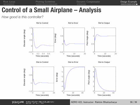
Control of a Small Airplane – AnalysisHow good is this controller?
0 0.2 0.4 0.6−0.5
0
0.5
1
1.5
Ref to Control
Time (seconds)
Ele
vato
r an
gle
(deg
)
0 10 20−0.5
0
0.5
1
Ref to Error
Time (seconds)E
rror
(de
g)0 10 20
0
0.5
1
1.5
Ref to Output
Time (seconds)
Pitc
h A
ngle
(de
g)
0 20 40−5
−4
−3
−2
−1
0
Dist to Error
Time (seconds)
Err
or (
deg)
0 10 20−1.5
−1
−0.5
0
Dist to Control
Time (seconds)
Ele
vato
r an
gle
(deg
)
0 20 400
1
2
3
4
5
Dist to Output
Time (seconds)
Pitc
h an
gle
(deg
)
AERO 422, Instructor: Raktim Bhattacharya 39 / 39