
Ady Stern- Anyons and the quantum Hall effect— A pedagogical review
47
Anyons and the quantum Hall effect— A pedagogical review Ady Stern * Department of Condensed Matter Physics, Weizmann Institute of Science, Rehovot 76100, Israel Received 21 October 2007; accepted 24 October 2007 Available online 17 November 2007 Abstract The dichotomy between fermions and bosons is at the root of many physical phenomena, from metallic conduction of electricity to super-fluidity, and from the periodic table to coherent propaga- tion of light. The dichotomy originates from the symmetry of the quantum mechanical wave function to the interchange of two identical particles. In systems that are confined to two spatial dimensions partic les that are neither fermions nor boson s, coined ‘‘anyons’’, may exist. The fractional quantu m Hall effect offers an experimental system where this possibility is realized. In this paper we present the concept of anyons, we explain why the observation of the fractional quantum Hall effect almost forces the notion of anyons upon us, and we review several possible ways for a direct observation of the physics of anyons. Furthermore, we devote a large part of the paper to non-abelian anyons, motivating their existence from the point of view of trial wave functions, giving a simple exposition of thei r relatio n to conf or mal fie ld theori es, and reviewing several pr oposals for their di rect observation. Ó 2007 Elsevier Inc. All rights reserved. Keywords: Anyons; Quantum Hall effect 1. Introduction There are two basic principles on which the entire formidable world of non-relativistic quantum mechanics resides. First, the world is described in terms of wave functions that 0003-4916/$ - see front matter Ó 2007 Elsevier Inc. All rights reserved. doi:10.1016/j.aop.2005.03.001 * Fax: +972 89344477. E-mail address: [email protected] Available online at www.scien cedirect.com Annals of Physics 323 (2008) 204–249 www.elsevier.com/locate/aop
Transcript of Ady Stern- Anyons and the quantum Hall effect— A pedagogical review

8/3/2019 Ady Stern- Anyons and the quantum Hall effect— A pedagogical review
http://slidepdf.com/reader/full/ady-stern-anyons-and-the-quantum-hall-effect-a-pedagogical-review 1/46
Anyons and the quantum Hall effect— A pedagogical review
Ady Stern *
Department of Condensed Matter Physics, Weizmann Institute of Science, Rehovot 76100, Israel
Received 21 October 2007; accepted 24 October 2007Available online 17 November 2007
Abstract
The dichotomy between fermions and bosons is at the root of many physical phenomena, frommetallic conduction of electricity to super-fluidity, and from the periodic table to coherent propaga-tion of light. The dichotomy originates from the symmetry of the quantum mechanical wave function
to the interchange of two identical particles. In systems that are confined to two spatial dimensionsparticles that are neither fermions nor bosons, coined ‘‘anyons’’, may exist. The fractional quantumHall effect offers an experimental system where this possibility is realized. In this paper we present theconcept of anyons, we explain why the observation of the fractional quantum Hall effect almostforces the notion of anyons upon us, and we review several possible ways for a direct observationof the physics of anyons. Furthermore, we devote a large part of the paper to non-abelian anyons,motivating their existence from the point of view of trial wave functions, giving a simple expositionof their relation to conformal field theories, and reviewing several proposals for their directobservation.Ó 2007 Elsevier Inc. All rights reserved.
Keywords: Anyons; Quantum Hall effect
1. Introduction
There are two basic principles on which the entire formidable world of non-relativisticquantum mechanics resides. First, the world is described in terms of wave functions that
0003-4916/$ - see front matter Ó 2007 Elsevier Inc. All rights reserved.
doi:10.1016/j.aop.2005.03.001
*
Fax: +972 89344477.E-mail address: [email protected]
Available online at www.sciencedirect.com
Annals of Physics 323 (2008) 204–249
www.elsevier.com/locate/aop

8/3/2019 Ady Stern- Anyons and the quantum Hall effect— A pedagogical review
http://slidepdf.com/reader/full/ady-stern-anyons-and-the-quantum-hall-effect-a-pedagogical-review 2/46
satisfy Schroedinger’s wave equation. And second, these wave functions should satisfy cer-tain symmetry properties with respect to the exchange of identical particles. For fermionsthe wave function should be anti-symmetric, for bosons it should be symmetric. It isimpossible to overrate the importance of these symmetries in determining the properties
of quantum systems made of many identical particles. Bosons form superfluids, fermionsform Fermi liquids. The former may carry current without dissipating energy, the latterdissipate energy. The periodic table of elements, and with it chemistry and biology, looksthe way it does because electrons are fermions. And radiation may propagate in a coherentway since photons are bosons.
Given this set of reminders, it should be clear that finding particles that are neitherfermions nor bosons is an exciting development. Finding them as a theoretical constructis exciting enough, as realized by Leinaas and Myrheim [1] and by Wilczek [2]. Havingthem in the laboratory, open for experimental investigation with an Amperemeter and aVoltmeter is plain wonderful. Luckily, two dimensional electronic systems subjected toa strong magnetic field provide both the theoretical and experimental playground for suchan investigation, all through the Quantum Hall effect [3–6].
This paper is aimed at reviewing the physics of Anyons, particles whose statistics is nei-ther fermionic not bosonic, and the way it is manifested in the quantum Hall effect. Wewill start with introducing the basic characters of this play—the Quantum Hall effect,the Aharonov–Bohm effect [7] and (more briefly) the Berry phase [8]. We will then showwhy the mere experimental observation of the quantum Hall effect, coupled with verybasic principles of physics, forces us to accept the existence of excitations that effectivelyare Anyons, and how it raises the distinction between abelian and non-abelian anyons.
Following that, we will explore what the experimental consequences of anyonic quantumstatistics may be, with a strong emphasis on interference phenomena. After this subject iscovered, we will raise one level in complexity, and introduce non-abelian anyons [9], look-ing first at the general concept, then at the simplest example, that of the m ¼ 5=2 quantumHall state, and finally at the more complicated example of the Read–Rezayi states [10].
Some subjects will be left out. In particular, the relation of anyons to topological quan-tum computation [11], to topological quantum field theories and to group theory are allcovered at great length in a recent review article whose list of authors has some overlapwith the corresponding list of the present paper [12]. These subjects will not be repeatedhere. Left out are also realizations of anyons in systems out of the realm of the quantum
Hall effect, the relation of anyons to exclusion statistics (a generalized Pauli principle foranyons [13–17]) and studies of statistical physics of anyons in abstract models.
The paper attempts to be pedagogical, and should be accessible to graduate students,both theorists and experimentalists.
2. The quantum Hall effect
Let us think of electrons on an infinite conducting strip of width w on the x À y plane,subjected to a perpendicular magnetic field B z . If an electronic current is flowing in the ^ x-direction, and the strip is confined in the ^ y -direction, a Hall voltage V H develops in the ^ y -
direction. Classically, this voltage is calculated by a seemingly bullet-proof argument: forthe current to flow in a straight line, the Lorenz force originating from the magnetic fieldshould be cancelled by the force originating from the gradient of the Hall voltage. Thus,one expects,
A. Stern / Annals of Physics 323 (2008) 204–249 205

8/3/2019 Ady Stern- Anyons and the quantum Hall effect— A pedagogical review
http://slidepdf.com/reader/full/ady-stern-anyons-and-the-quantum-hall-effect-a-pedagogical-review 3/46
e
cvB ¼ V H
wð1Þ
where v is the electron’s velocity, e is the electron charge and c is the speed of light. Sincethe current is I
¼nevw, with n being the electron’s density, we get
V H
I ¼ B
necð2Þ
This ratio of the Hall voltage to the current is known as the Hall resistance, denoted by R yx ¼ À R xy or RH. The simple-minded line of thoughts goes even further: once the forcethat results from the Hall voltage cancels the force that results from the magnetic field,there will be no other effect of the magnetic field. Thus, the longitudinal voltage, the volt-age drop parallel to the current, will be independent of the magnetic field. The ratio of thisvoltage to the current is the longitudinal resistance R xx.
Classical arguments are not the whole story. There are two other things to add: real-lifeexperiments and quantum mechanics. Both contradict the classical arguments in a veryfundamental way. Before we get to the quantum Hall effect, we should pay homage toan even earlier contradiction—the sign of the Hall voltage. Indeed, while classical physicsrelates this sign to the direction of the Lorentz force that acts on the negatively chargedelectrons, experiments show a different sign in different materials. Quantum mechanics,in one of its greatest triumphs in solid state physics, explains this varying sign in termsof the theory of bands, and the notion of holes.
Several decades after band theory introduced the holes, the quantum Hall effect wasdiscovered [3–6]. Look at Fig. 1: when the Hall effect is measured in high mobility two
dimensional electronic systems at low temperatures, the Hall resistance is not linear inmagnetic field, in contrast to what Eq. (2) suggests. Rather, it shows steps. The magneticfield at which a step starts or ends varies between samples, but the value of RH at the stepsis universal. At the steps,
RH ¼ h
e2
1
mð3Þ
Here h=e2 is the quantum of resistance, equals to about 25.813 kX. The dimensionlessnumber m has, in the observed steps, either integer values m ¼ 1; 2; 3 . . . going up to severaltens, or ‘‘simple’’ fractions p =q. Most of the simple fractions are of odd denominators (one
of the exceptions to that rule will be later discussed), usually smaller than about 15. Of those the most prominent fractions are of the series m ¼ p =ð2 p þ 1Þ, with p an integer. Gen-erally speaking, the lower is the temperature and the cleaner is the sample, the more stepsare observed. Integer values of m go under the name Integer Quantum Hall effect (IQHE)while fractional values go under the name Fractional Quantum Hall effect (FQHE).
Let us pause to emphasize—these steps are astonishing. First, they are amazingly pre-cise. Eq. (3) is satisfied to a level of one part in 109! Second, their value is independent of any properties of the material being measured. Rather, they are determined by the ratio of two of the four universal constants, the charge of the electron and Planck’s constant.
At the same magnetic field in which R xy is on a step, the longitudinal resistance R xx van-
ishes. Current flows without local dissipation of energy. Ohm’s law may then be put inlocal terms, as a ratio between the gradient of the electro-chemical potential E (looselyspeaking, the electric field) and the current density j as,
206 A. Stern / Annals of Physics 323 (2008) 204–249

8/3/2019 Ady Stern- Anyons and the quantum Hall effect— A pedagogical review
http://slidepdf.com/reader/full/ady-stern-anyons-and-the-quantum-hall-effect-a-pedagogical-review 4/46
E ¼h
e2m z  j ð4Þwhere both vectors lie in the x À y plane. As the electric field and the current are perpen-dicular to one another, the vanishing longitudinal resistivity (commonly denoted by q xx)implies also a vanishing longitudinal conductivity r xx, and the quantized Hall resistivityq xy ¼ h=e2m implies a quantized Hall conductivity r xy ¼ e2m=h.
These universal values are the zero temperature limit of the experimental observations.The deviations at finite temperatures are a rich issue by itself, which we touch only briefly:at least within a certain range of temperatures, the deviation of r xx; r xy from their zero tem-perature value follows an activation law, i.e., is proportional to eÀT 0
T , with T being the
temperature and T 0 being a temperature scale that depends on many details. This temper-ature dependence, which is familiar also from other contexts, such as low temperature con-ductance of intrinsic semi-conductors or low temperature dependence of the heat capacityof super-conductors, indicates the existence of an energy gap between the ground state and
0 5 10 15
0
1
0
1
2
3
4
2/7
2/5
6/2510
19
10
21
1
5/2
1/4
6/23
3/2
MAGNETIC FIELD [T]
T ~ 35 mK
n=1.0×1011 cm-2
μ=10×106 cm2/Vs
2/3
1/2
1/3
R x x
( k Ω )
3/4
2
1
2/3
2/5
1/3
R x y
( h / e 2 )
2/7
Fig. 1. The quantum Hall effect. When the Hall resistance is measured as a function of magnetic field plateaus atquantized values are observed. In regions of the magnetic field where the Hall resistance is in a plateau, thelongitudinal resistance vanishes (Sample grown by L.N. Pfeiffer (Lucent-Alcatel) and measured by W. Pan(Sandia)).
A. Stern / Annals of Physics 323 (2008) 204–249 207

8/3/2019 Ady Stern- Anyons and the quantum Hall effect— A pedagogical review
http://slidepdf.com/reader/full/ady-stern-anyons-and-the-quantum-hall-effect-a-pedagogical-review 5/46
the first excited states. The deviations from the activation law, which are observed at lowtemperatures, probably indicate that the gap is not a ‘‘true’’ gap (a finite range of energiesat which there are no electronic states) but rather a mobility gap (a finite range of energiesat which there are no extended electronic states).
Faced with these dramatic experimental observations, one naturally asks ‘‘why does theeffect happen?’’. We will address this question very partially later. At the moment, how-ever, we are more interested in a different question, namely, ‘‘given that the effect isobserved, what does it teach us?’’ As we will see, the very observation of a fractional quan-tized Hall conductivity, a vanishing longitudinal conductivity and a mobility gap betweenthe ground state and the first excited states, when combined with general principles of physics, will force us to accept the notion of Anyons.
But for going along that route, we first need to review the Aharonov–Bohm effect [7].
3. The Aharonov–Bohm effect
Let us start by digressing a bit, and reminding ourselves a few basic facts on the physicsof electrons in a magnetic field. High school physics tells us that an electron in a magneticfield B and an electric field E is subjected to a force
F ¼ eE þ e
cv  B ð5Þ
Undergraduate classical physics tells us that this force may be derived out of an action.In particular, if we choose a gauge in which the scalar potential vanishes, this force resultsfrom one term in the action,
e
c
Z dt vðtÞ Á Aðx; t Þ ð6Þ
Here A is the vector potential whose various derivatives constitute the electric and mag-netic fields.
Quantum mechanics tells us that an action is not only a device to generate an equationof motion. Rather, when divided by h it gives the phase of the contribution of the trajec-tory xðt Þ to the propagator of the particle. If we look at the case in which the vector poten-tial is independent of time, we see that the term (6) becomes geometric, i.e., independent of the velocity the trajectory is traversed by,
e
c
Z dt vðtÞ Á AðxÞ ¼ e
c
Z d l Á AðxÞ ð7Þ
where the integral is taken along the trajectory. Gauge invariant quantities always involveclosed trajectories (loops). For those, Stokes theorem tells us that the integral (7) becomes2pU=U0, where U is the flux enclosed in the trajectory, and U0 hc=e is the flux quantum.This is the Aharonov–Bohm phase.
A particularly important case is the case of the vector potential created by a solenoid thatcannot be penetrated. In that case, the trajectories of an electron may be topologically clas-sified by nw, the number of times they wind the solenoid. The phase that corresponds to a tra-
jectory is then 2pnwUs=U0, where Us is the flux enclosed by the solenoid. For all trajectories,then, this phase is periodic in the flux, with the period being the flux quantum U0.
There are two useful experimental set-ups to think about in the context of the Aharo-nov–Bohm effect (see Fig. 2). The first is the famous double slit interference experiment.
208 A. Stern / Annals of Physics 323 (2008) 204–249

8/3/2019 Ady Stern- Anyons and the quantum Hall effect— A pedagogical review
http://slidepdf.com/reader/full/ady-stern-anyons-and-the-quantum-hall-effect-a-pedagogical-review 6/46
When a solenoid is put in between the two slits, it shifts the interference patter due to thephase shift it induces. Note that this shift in the interference pattern is very surprising froma classical point of view, as the electron, which cannot penetrate the solenoid, does not feelany Lorenz force when it moves.
The second set-up is that of a ring, or an annulus, with a magnetic flux U going throughthe hole. The electron is now confined to the annulus and again does not experience any
Lorenz force due to the magnetic field in the solenoid. However, due to the Aharonov– Bohm effect its spectrum does depend on the magnetic flux, with a period of U0. And sincethis is true for the spectrum, it is true for all thermodynamic properties, that may all beexpressed as derivatives of the partition function.
The dependence of various thermodynamical quantities on the magnetic flux through thehole, despite the absence of any force exerted on the electron by the magnetic field in thesolenoid, may be understood in the following way: suppose that we look at a ring where ini-tially, at time t ¼ À1, no flux penetrates the hole. Then a fluxU is turned on adiabatically intime. Classically, the process of turning the flux on involves the application of an electricfield on the electron, and hence its acceleration. While there is a freedom of the position
at which the electric field would operate, the condition of adiabaticity implies that the timeperiod at which the electric field operates is much longer than the time it takes an electron toencircle the ring, and thus the electron cannot avoid the effect of the field. As long as the elec-tron is not prevented by a trapping potential from encircling the ring, it will experience aforce due to the electric field, and will absorb (kinetic) momentum and angular momentum.Due to the adiabaticity, the electron stays in an eigen-state throughout the process in whichthe flux is turned on. Thus, the eigen-state evolves in such a way that it absorbs kineticmomentum and angular momentum. As long as this momentum is not fully transferredto static degrees of freedom (impurities etc.), the eigenstate will have the electron encirclingthe ring in a non-zero velocity. This is the source of the persistent current, or thermodynamic
orbital magnetization, observed in normal mesoscopic rings [18].There is a subtle point that needs to be understood in this argument: consider first an
electron in a ballistic circular ring, subjected to a magnetic flux that is adiabatically turnedon. As we said, classically the electron is accelerated by the field. Its velocity is e
mcU
2p L, with
a b
Fig. 2. The Aharonov–Bohm effect. Two realizations of the Aharonov–Bohm effect. In the first, shown in (a), themagnetic flux induces a shift in the interference pattern of a double slit experiment. An analog effect is to be seen
in the quantum Hall interferometers discussed in Sections 7 and 12. In the second, shown in (b), the magnetic fluxaffects the thermodynamic properties of the annulus around it. This realization is very useful in the analysis of thefractional charge and fractional statistics of quasi-particles in the quantum Hall effect, see Section 4.
A. Stern / Annals of Physics 323 (2008) 204–249 209
8/3/2019 Ady Stern- Anyons and the quantum Hall effect— A pedagogical review
http://slidepdf.com/reader/full/ady-stern-anyons-and-the-quantum-hall-effect-a-pedagogical-review 7/46
L being the circumference of the ring and m the electron mass. Quantum mechanically, if the electron was initially in the ground state it stays in an eigenstate, due to adiabaticity. Itdoes not necessarily stay in the ground state, however. As the flux is being turned on, thereare points of time in which the gap in the spectrum closes, and two eigenstates, one whose
energy increases with flux and one whose energy decreases with flux, become degenerate inenergy. Even when these states are degenerate, there is no matrix element that allows for atransition between them, and thus the electron does not go through such a transition. Thereason for that is that the two states have different (canonical) angular momenta, and therotational symmetry of the problem dictates a conservation of angular momentum. Anydeviation from these perfect conditions, however, for example by the ring being imper-fectly circular or imperfectly ballistic, introduces transitions between the two states,removes the degeneracy, and leads to the electron staying, in the adiabatic limit, in thelowest energy state. This subtle point will be of importance later.
4. Fractionally charged excitations: combining the Aharonov–Bohm effect and the quantum
Hall effect
With very little detailed modelling, we are now able to conclude, following Laughlin’soriginal arguments, that a two dimensional system that shows the fractional quantum Halleffect must have quasi-particles that carry a fraction of an electron charge [19]. Followingthat, we will add in a few basic observations about the dynamics of vortices in fluids, andconclude that the fractional charge of the quasi-particles in the fractional quantum Halleffect implies also that the quasi-particles are anyons. While the anyonic nature of the
quasi-particles was first realized by Halperin [20], based on the sequence of observed frac-tional quantum Hall states, the derivation we will follow here is closer to that of Arovas,Schrieffer and Wilczek [21].
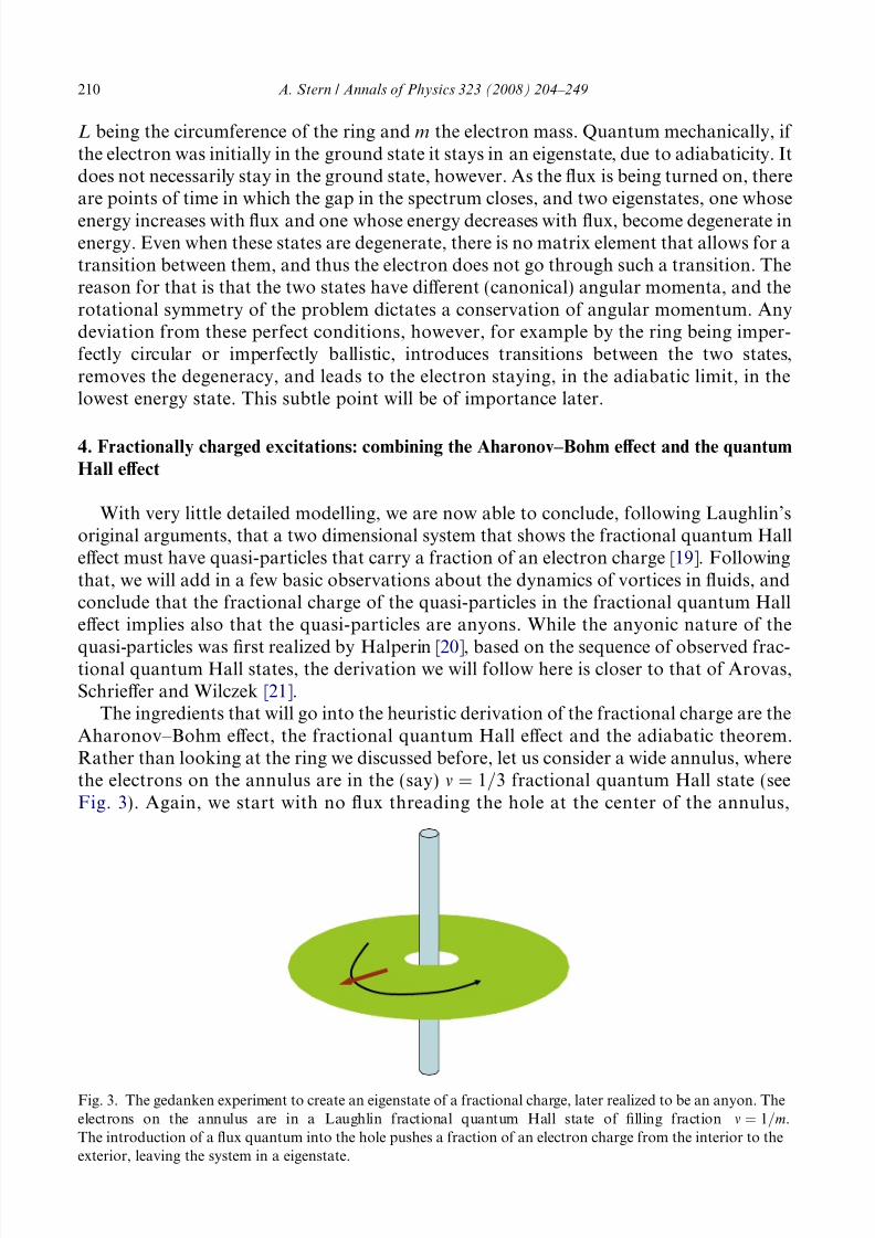
The ingredients that will go into the heuristic derivation of the fractional charge are theAharonov–Bohm effect, the fractional quantum Hall effect and the adiabatic theorem.Rather than looking at the ring we discussed before, let us consider a wide annulus, wherethe electrons on the annulus are in the (say) m ¼ 1=3 fractional quantum Hall state (seeFig. 3). Again, we start with no flux threading the hole at the center of the annulus,
Fig. 3. The gedanken experiment to create an eigenstate of a fractional charge, later realized to be an anyon. Theelectrons on the annulus are in a Laughlin fractional quantum Hall state of filling fraction m ¼ 1=m.The introduction of a flux quantum into the hole pushes a fraction of an electron charge from the interior to theexterior, leaving the system in a eigenstate.
210 A. Stern / Annals of Physics 323 (2008) 204–249

8/3/2019 Ady Stern- Anyons and the quantum Hall effect— A pedagogical review
http://slidepdf.com/reader/full/ady-stern-anyons-and-the-quantum-hall-effect-a-pedagogical-review 8/46
and turn the flux on adiabatically. Again, an electric field is exerted on the electrons, andfor simplicity we assume this electric field to be azimuthally symmetric. Let us analyzewhat happens when the flux is increased.
First, with the electrons being in a fractional quantum Hall state, the azimuthal electric
field leads to a purely radial current flow, according to Eq. (4). At a distance r from theorigin the electric field is E ¼ 1
2prcoUot h, and the resulting radial current density is
jr ¼ e2mh
E . Integrating the current density that goes through a circle of radius r to get thetotal current, we find that the current does not depend on r. Thus, it leaves behind a chargelump at the interior edge of the annulus. Integrating the current over time, starting whenthere was no flux at the ring and ending at a time t when the flux is Uðt Þ, we find that theamount of charge in that lump is
Qðt Þ ¼ e2m
hcUðt Þ ð8Þ
Second, in the quantum Hall effect there is an energy gap between the ground state andthe first excited state. Thus, we can apply the adiabatic theorem, and conclude that the sys-tem, that started in a ground state when there was no flux, remains in an eigenstatethroughout the process.
Third, what happens when the flux isU0?Then,Eq. (8) givesachargeof em.Thesystemisatan eigenstate. The spectrum at U ¼ U0 is the same as the spectrum at U ¼ 0 and the eigen-states at U ¼ U0 are the same as those at U ¼ 0, up to the phase factor exp i
Pi/i (where
/i is the azimuthal coordinate of the i th electron), which does not affect the charge density.Thus, we found that the annulus withU ¼ 0 has an eigenstate in which a lump of charge of em
is localized on its interior edge. The assignments of energies to eigenstates may have inter-changed, as in the case of a ballistic circular ring, so this is not necessarily the ground state.Clearly, an eigenstate in which a charge em has been transferred from the interior of the annu-lus to its exterior is physically different from the ground state the system started in. We callthis state a quasi-particle when it carries a negative charge and a quasi-hole when it carries apositive charge. In much of the following the sign of the charge will not be of our concern, andwe will use the terms quasi-hole and quasi-particle interchangeably.
As in the case of a ring, if the ground state at U ¼ 0 evolves into an excited state atU ¼ U0 then for some intermediate value of U two states must have been degenerate inenergy, with no transition between them taking place as the flux is varied. The absence
of such a transition may be due to the absence of any matrix element connecting them(due to symmetries of the problem), or due to that matrix element being so small such thatthe rate at which Uðt Þ would need to be changed becomes so slow to be impractical.Indeed, for the fractional quantum Hall annulus the latter is the case—the matrix elementbetween the states is exponentially small in the size of the annulus (in the units of the mag-netic length), and thus the two states are effectively uncoupled.
That this is the case may be understood in the following manner: the applied electricfield acting in the azimuthal direction pushes a current to flow radially. If the system endsat U ¼ U0 in the initial state of U ¼ 0, then the charge that was driven from the interior tothe exterior must have tunnelled back. This process of tunneling requires a breaking of
rotational invariance, e.g., by impurities, but being a tunneling process, its amplitude isexponentially small [22].
In the thought experiment we described above the quasi-particle/quasi-hole were exci-tations above the ground state. It is, however, easy to imagine the energetics to change in
A. Stern / Annals of Physics 323 (2008) 204–249 211

8/3/2019 Ady Stern- Anyons and the quantum Hall effect— A pedagogical review
http://slidepdf.com/reader/full/ady-stern-anyons-and-the-quantum-hall-effect-a-pedagogical-review 9/46
such a way that a state with such ‘‘excitations’’ becomes lower in energy than a state with-out them. That happens when electrostatic considerations force the density to deviate froma ‘‘magic’’ m ¼ 1=m filling fraction. For example, imagine that rather than turning a fluxquantum at the center of the annulus we would turn on a potential that would repel elec-
trons away. If the potential is very small, it would have no effect, since the quantum Hallfluid is incompressible, due to its energy gap. But if the potential is strong enough it wouldlead to a ground state that includes one or more quasi-holes. Fractional charges of quasi-holes and quasi-particles have been observed in various types of measurements, such asresonant tunnelling through antidots [23], shot noise [24,25] and local compressibility [26].
The argument we presented so far for the existence of fractionally charged quasi-parti-cles and quasi-holes has been very general, being based on the existence of the fractionalquantum Hall effect as a gapped ground state, and on general principles such as the adi-abatic theorem and the Aharonov–Bohm effect. Historically, these quasi-particles werefirst understood through the use of trial wave functions. As Laughlin discovered [19], if the ground state for a m ¼ 1=3 fractional quantum Hall state is assumed to be made solelyof lowest Landau level wave functions, the following is a very good variational wave func-tion for it (using complex coordinates z i ¼ xi þ iy i for the two Cartesian coordinates of thei th particle):
w g : s:ðf z ig; f z igÞ ¼Yi< j
ð z i À z jÞ3Y
i
exp Àj z ij2=4l2
h ð9Þ
The virtues of this wave function will be explained later on (see Section 13). At themoment we just say that it minimizes the kinetic energy by placing all the electrons in
the lowest Landau level, and minimizes the potential energy by efficiently keeping elec-trons away from one another. To generate a quasi-hole at the origin, Laughlin proposedthe wave function
Yi
z iw g : s: ¼Y
i
j z ij
eiP
i
/i
w g : s: ð10Þ
Indeed, the operatorQ
i z i does exactly what we expect the adiabatic introduction of aflux tube to do: the phase exp i
Pi/i gives each electron an angular momentum h, while the
product Qij z ij moves each electron radially outwards, thus generating the radial current
and the lump of charge at the interior. Over all, the operator does not introduce transitionsbetween different Landau levels, and thus keep the wave function purely within the lowestLandau level.
The angular momentum carried by the quasi-hole (10) is there not only for the Laughlinwave function of the quasi-hole. In fact, it is introduced also in the thought experimentthat we described: as the flux is turned on, a radial current flows, with no introductionof angular momentum. However, when the wavefunction for U ¼ U0 is multiplied byexpi
Pi/i in order to get the wave function for the quasi-hole at U ¼ 0, an angular
momentum of h is given to every electron. The quasi-hole then carries a quantum of vorticity.
To summarize, the process we just described generates an eigenstate that carries a frac-tional charge em and a single quantum of vorticity, both localized at the interior edge of theannulus. By shrinking the size of the hole we can localize this charge to a size of the mag-netic length (below that size the relation (4) does not hold). The state being an eigenstate
212 A. Stern / Annals of Physics 323 (2008) 204–249

8/3/2019 Ady Stern- Anyons and the quantum Hall effect— A pedagogical review
http://slidepdf.com/reader/full/ady-stern-anyons-and-the-quantum-hall-effect-a-pedagogical-review 10/46
implies that both the lump of charge and the vorticity do not decay in time. They are thereto stay.
5. Charges and vortices—Lorenz and Magnus forces in super-fluids and super-conductors
The vorticity carried by the quasi-holes in the fractional quantum Hall effect will turnout to be crucial for their quantum statistics. Thus, let us remind ourselves of a few basicfacts regarding the motion of vortices in two dimensions. In a Galilean invariant system, avortex always moves at the speed of the fluid. In the absence of such symmetry, however,there may be a relative velocity between the vortex and the fluid. Under these conditions,Magnus force operates on the vortex. With this force being relevant for what comes next,we now review its basic features, and draw its similarity to the Lorenz force acting oncharged particles in a magnetic field. We start by considering a vortex in a neutral super-
fluid, say superfluid Helium.The origin of the Magnus force lies in the consideration of the vortex as a collectivedegree of freedom. Having a vortex centered at the point R implies that each fluid particlehas an angular momentum l z relative to the point R. When the vortex is static, there is a
velocity field of the fluid, of vðrÞ ¼ lm
z ÂðrÀRÞjrÀRj2 . When the vortex moves the velocity field of the
fluid is the sum of this motion and the velocity of the vortex’ center relative to the fluid, _R.
If the vortex’ velocity _R is in the ^ x direction, the velocity difference along the ^ y -axis leads toa pressure difference, and hence to a force in the ^ y direction. The force is
F Mag
¼2pnl z
Âv
ð11
Þwhere n is the number density of the fluid. This force is proportional to the product nlv
since the pressure difference between the two sides of the vortex is proportional tonððv þ _RÞ2 À ðv À _RÞ2Þ.
Like the Lorenz force, the Magnus force is proportional and perpendicular to the veloc-ity. Comparing Eq. (11) to Eq. (5) we see that the role played by the product eB=c in Lor-enz force is played by the product 2pnl in Magnus force. As in the Lorenz force, thetransition from classical to quantum mechanics of vortices is best understood when inter-ference effects are considered. The classical Lorenz force gives rise to the quantummechanical Aharonov–Bohm phase accumulated by the wave function when an electron
is moving, which then leads to the definition of the flux quantum. Similarly, the classicalMagnus force gives rise in quantum mechanics to a phase that is accumulated by the wavefunction when a vortex is moving. The Aharonov–Bohm phase is e
hc
R d s Á B. The analo-
gous phase should then be
2pl
h
Z ds n ð12Þ
For a vortex with a single quantum of vorticity (and all those we are interested in are of thistype) l ¼ h and thus the phase accumulated by a vortex traversing a closed loop is 2p timesthe integral R ds n which is nothing but 2p times the number of fluid particles encircled by the
vortex as it goes around the loop. The analog of the flux quantum is a single fluid particle.We limited ourselves to a neutral fluid when we took the velocity field of the vortex to
decay as 1=jr À Rj, but, as we now argue, both the classical force and the quantummechanical phase we obtained hold more generally. When the superfluid is charged, as
A. Stern / Annals of Physics 323 (2008) 204–249 213

8/3/2019 Ady Stern- Anyons and the quantum Hall effect— A pedagogical review
http://slidepdf.com/reader/full/ady-stern-anyons-and-the-quantum-hall-effect-a-pedagogical-review 11/46
is a two-dimensional super-conductor, a vortex still amounts to an angular momentum h
given to each particle fluid (in this case a Cooper pair), but the velocity field decays as1=jr À Rj only for distances smaller than the London penetration length, and decays expo-nentially for larger distance. The reason for that difference is the magnetic field created by
the current that circulates around the center of the vortex. The velocity of the i th Cooperpair is 1
mðpi À e
cAðriÞÞ, and at large distance r, the contribution of the canonical momentum
pi and the vector potential AðriÞ mutually cancel. Despite this decay of the velocity field,the force that acts on the vortex as it moves relative to the fluid does not change. Whatchanges is the source of the force: rather than being the hydrodynamical Magnus force,it is now the Lorenz force. The vortex is a solenoid of charge current enclosing a magneticflux. When it moves relative to a fixed background of charge, it exerts an electric field onthe charges, and a mutual force occurs. The force is
1
cZ ds
ðJ
ÂB
Þ $1
c
2neU0
2v
 z
$2pnlv
 z
ð13
ÞThe first estimate is based on the current density being J ¼ 2nev (the factor of 2 orig-
inates from the charge of the Cooper pair), the magnetic field being B % U0=2k2 L z (k L is the
size of the vortex, and the factor of 2 originates from the flux of the vortex being half theflux quantum, hc=2e), and the integral being confined to a region of k2
L.How is the analog of the Aharonov–Bohm effect realized for vortices? It is easiest to
think of that in the context of a ring. As we saw, a flux piercing the ring affects the spec-trum of a particle residing on it, and may induce a persistent current of the particle aroundthe ring. Imagine now a vortex that is confined to move on a ring. Such a confinement may
be realized by a Josephson junction made of two thin concentric super-conducting cylin-ders [27,28], or by a two dimensional super-conductor in which a circular trench is etched,such that it is energetically costly for a vortex to reside out of the trench. Now let us posi-tion the origin at the center of that circle and imagine a radial current flowing into the cir-cle. In close analogy to the electron on a mesoscopic ring in which a magnetic flux isadiabatically turned on, in the present case the radial current exerts a force on the vortexand accelerates it. When the current stops flowing the vortex is left with angular momen-tum, and keeps on moving in a persistent way. The energy becomes a function of thecharge that flew from one side of the ring to another, in quite the same way that it wasa function of the flux that was inserted to the ring in the previous problem.
A question now arises: the velocity field near the core of a vortex diverges, and hencethe density there must be depleted so that the energy stays finite. Since we found that thephase accumulated by a vortex wave function as the vortex traverses a loop counts thenumber of fluid particles enclosed in that loop, could there be a topological phase associ-ated with one vortex encircling another? That is, could it be that the insertion of vortex 2into the loop traversed by vortex 1 would change the phase that the wave function accu-mulates by a fixed amount, preferably some exotic fraction of 2p? We will now answer thisquestion negatively for vortices in neutral superfluids and charged super-conductors andthen proceed and see that the answer is positive for quasi-holes in the quantum Hall effect.
In neutral super-fluids the density depletion at the core of the vortex decays surprisingly
slowly as a function of the distance from the core. In fact, the decay is proportional to r À2,which leads to a diverging number of fluid particles pushed away from the core of the vor-tex. Thus, no topological phase may emerge [29]. Furthermore, both for neutral andcharged superfluids, there is no energy gap, as the collective charge density mode (that
214 A. Stern / Annals of Physics 323 (2008) 204–249
8/3/2019 Ady Stern- Anyons and the quantum Hall effect— A pedagogical review
http://slidepdf.com/reader/full/ady-stern-anyons-and-the-quantum-hall-effect-a-pedagogical-review 12/46
may be called a plasmon, a phonon, or a Goldstone mode, depending on taste) is gapless.Thus, when a vortex encircles another vortex in an infinite system, and when disorderremoves the conservation of momentum, adiabaticity will never hold—the process willnecessarily involve a radiation of energy to that mode, and that radiation will invalidate
the calculation of the phase.Before we turn to the the quasi-particles and quasi-holes of the quantum Hall effect, we
discuss how our semi-heuristic arguments for the transition from the classical Magnusforce to the accumulation of a phase by the vortex wave function can be made more rig-orous. The main ingredient we need for that is the geometric phase, better known as Ber-ry’s phase [8]. Let us briefly review what that phase is and how it comes into play in thecontext we deal with.
Generally, the systems we consider are composed of identical electrons whose coordi-nates are ri, and collective excitations, the vortices/quasi-particles/quasi-holes, whosecoordinates are Ri. We are interested in the effective Hamiltonians for the latter. Thatis, we are interested in turning the Ri’s from parameters in the system’s wave functions intodynamical degrees of freedom. The vortex is a macroscopic degree of freedom, so thedynamics of R is slower than the dynamics of the fluid particles. In order to calculatethe dynamics of R it is instructive to think of it as an external degree of freedom. Forexample, we think of the vortex as pinned to an impurity at the point R, and the impurityas having a mass M (this situation may naturally arise if the impurity repels the particles of the fluid. Since at the core of the vortex the density is depleted, the vortex would find itenergetically favorable to be pinned on the impurity). Note that we assume the impurityto interact only with the fluid particles, and not with any external fields exerted on the sys-
tem. Any effect it feels of these fields must then arise from the effect of the fields on thefluid particles.The question we ask is this: what is the effect of the vorticity carried around the point R
on the dynamics of R. The answer to that is given within an extension of the Born-Oppen-heimer approximation. If the wave function of the system with a vortex at R is denoted byjwðRÞi, then the kinetic energy that dictates the dynamics of R includes a Berry vectorpotential
A B ¼ ImhwðRÞj$RjwðRÞi ð14ÞThis vector potential depends on R. When it has a curl with respect to R, there is a Lor-
enz force, both in classical and in quantum mechanics. When the quantum mechanics of the vortex is considered, the vector potential leads to an Aharonov–Bohm like effect. Theeffective Hamiltonian of R includes also an induced scalar potential, which is not of ourconcern here [8].
The precise wave function of the vortex depends on many details. Two basic propertiesare rather general, however: each fluid particle gets an angular momentum h relative to thepoint R, and the density close to R must be depleted, to avoid a divergence of the kineticenergy. An operator that achieves both is
V Yi
ei/ðriÀRÞG ðjri À RjÞ ð15Þ
with /ðrÞ arctanð y
xÞ being the angle conjugate to the angular momentum, and with the
real function G ðr Þ vanishing at r ¼ 0. This operator creates a circularly symmetric vortex,but that simplification is not crucial. When it is applied to a featureless state, which is
A. Stern / Annals of Physics 323 (2008) 204–249 215

8/3/2019 Ady Stern- Anyons and the quantum Hall effect— A pedagogical review
http://slidepdf.com/reader/full/ady-stern-anyons-and-the-quantum-hall-effect-a-pedagogical-review 13/46
independent of R, the geometric vector potential (14) is, with qðrÞ being the fluid density atthe point R,
A B
ðR
Þ ¼ Z drq
ðr
Þ z  ðr À RÞ
jr À Rj2
ð16
ÞThis is precisely what our semi-heuristic analysis has led us to believe: the vortex, whose
coordinate is R, sees the fluid particles as an electron sees flux tubes. When it moves rel-ative to the fluid, it experiences a force perpendicular and proportional to its velocity rel-ative to the fluid, and the magnitude of that force is exactly that given by the Magnusforce. Eqs. (14) and (16) also explain why the magnitude of the force is the same for neu-tral and charged vortices: it is determined by derivatives of the wave function with respectto R, and the wave functions for vortices in neutral and super-conducting vortices sharethe same crucial property: the canonical angular momentum of h given to each fluid par-
ticle relative to the vortex’ center. The magnetic field created by the currents that form thevortex in a super-conductor affects the kinetic angular momentum mv  r of the Cooper-pairs around the center of the vortex, but does not affect their canonical angular momen-tum p  r. Finally, the phase accumulated by the quantum mechanical wave functionwhen the vortex traverses a closed loop is 2p times the expectation value of the numberof fluid particles enclosed in the loop [21].
6. Quasi-holes in the fractional quantum Hall effect follow fractional statistics
So we finally got to the quasi-holes in the fractional quantum Hall effect. As we saw,these quasi-holes, at the Laughlin fractions of m ¼ 1=m, carry a fraction 1=m of the electroncharge and one quantum of vorticity. What can we say about their dynamics, using thetwo other types of vortices as references?
The phase factors in the operator (15) create the vorticity carried by the quasi-hole, andwith the proper choice of G ðr Þ this operator will create also the correct depletion of charge.While there are many choices that would satisfy this condition, the most natural one, assuggested by Laughlin, is G ðr Þ ¼ r , making the quasi-hole operator
Qi z i [19]. Under this
choice, the operator that creates the quasi-hole does not introduce mixing of Landau lev-els. When it is applied to the Laughlin wave function (9), the resulting quasi-hole state is
still purely within the lowest Landau level.Similar to the case of a vortex in a charged super-conductor, the velocity field of the
vortex created by the quasi-hole creation operator does not decay inversely with the dis-tance from the center of the quasi-hole. Within the Laughlin picture, the charge densityand azimuthal current associated with the quasi-hole both fall off exponentially at dis-tances larger than the magnetic length. A more elaborate analysis [30] realizes that the azi-muthal currents must be proportional to 1=r 2 (with r being the distance from the quasi-hole), since the charge of the quasi-hole creates a radial electric field that decays as1=r 2, and that field generates an azimuthal Hall current. Furthermore, the charge densityis found to decay as 1=r 3. Independent of these details, however, as the quasi-hole moves
relative to the quantum Hall fluid, it experiences a force proportional and perpendicular toits velocity, given by 2pnlv  z , resulting from the vector potential (16). This is the sameMagnus force experienced by a vortex in a neutral super-fluid, and the same Lorenz forcethat the vortex in a charged super-conductor experienced due to its interaction with the
216 A. Stern / Annals of Physics 323 (2008) 204–249
8/3/2019 Ady Stern- Anyons and the quantum Hall effect— A pedagogical review
http://slidepdf.com/reader/full/ady-stern-anyons-and-the-quantum-hall-effect-a-pedagogical-review 14/46
current. Here this force has a rather simple description: noting that the angular momen-tum is h and that nU0= B ¼ m we see that the force acting on the quasi-hole is em
cv  B,
i.e., it is the Lorenz force acting on a charge em as it moves in a magnetic field B. Viewedas such, this is not too surprising—if we accept the quasi-hole as a collective degree of free-
dom that carries a fractional charge, it should be subjected to the Lorenz force that cor-responds to that charge.
But the story gets more interesting when we think of a quasi-hole as a quantummechanical degree of freedom, i.e., when we consider the phase it accumulates due tothe vector potential (16). The quantum Hall fluid is incompressible. Thus, when the den-sity is such that the local filling factor deviates from 1=m, the deviation is accommodatedin integer number of quasi-particles or quasi-holes. Given the charge em of each quasi-hole,when a quasi-hole goes around a closed loop, every quasi-hole it encircles contributes a phase
of 2pm to its wave function. And since a winding of one quasi-hole around another is just two
interchanges, we find that an interchange of the position of two quasi-holes multiplies the
wave function by a phase of pm, which makes the quasi-holes anyons [21].Note again that what gives the quasi-holes their anyonic character is a combination of
two ingredients—the fractional charge and the vorticity they carry. Both are essential forthe quasi-hole to exist, as we described here in detail.
7. Interferometry as a way to observe anyons
If anyons are defined by the quantum mechanical phase that they accumulate when theyencircle one another, it makes sense to design experimental devices in which quantum
mechanical phases are observables and quasi-particles encircle one another. The observa-tion of phases accumulated by waves is the essence of interferometry. We thus turn tointerferometers as the devices for the observation of anyons, dealing with the Fabry–Perotand Mach–Zehnder interferometers.
7.1. Fabry–Perot interferometer
In the context of the quantum Hall effect, the Fabry–Perot interferometer, discussed indetails first by Chamon et al. [31], is a Hall bar (for concreteness, lying along the x-axis,between 0 < y < w) perturbed by two constrictions, known as quantum point contacts
(say, at x ¼ Æd =2). Current flows chirally along the edges, towards the left along the y ¼ w edge and towards the right along the y ¼ 0 edge. The right moving edge is put ata chemical potential difference V relative to the left moving one. In the absence of the pointcontacts there is no back scattering of current, and thus when the bulk is in a quantumHall state the two-terminal conductance (the ratio of the current difference to the voltagedifference between the two edges) is quantized. The point contacts introduce an amplitudefor inter-edge tunnelling, which makes some of the current flowing along the right movingedge back-scattered. The probability for back-scattering is directly reflected in the voltagebetween the edges, i.e., in the two terminal conductance. Fig. 4b folds the Hall bar into anannulus, for the purpose of comparison with the Mach–Zehnder interferometer, to be dis-
cussed later. In this setting, the point contacts introduce a flow of tunnelling from thesource at the exterior to the drain in the interior.
The presence of two point contacts makes the probability for back-scattering the quan-tum Hall analog of ‘‘the interference screen’’. If the tunnelling amplitudes introduced by
A. Stern / Annals of Physics 323 (2008) 204–249 217

8/3/2019 Ady Stern- Anyons and the quantum Hall effect— A pedagogical review
http://slidepdf.com/reader/full/ady-stern-anyons-and-the-quantum-hall-effect-a-pedagogical-review 15/46
the two point contacts are t 1; t 2 respectively, then the back-scattered current is, to lowestorder in these amplitudes, proportional to jt 1 þ t 2j2. To this lowest order, the Fabry–Perotinterferometer is the QHE analog of the two slit experiment. The relative phase between
the two amplitudes may be varied in three principal ways: by varying the magnetic field,by varying the electron density and by varying the area of the ‘‘cell’’ defined by the twoedges and two point contacts. The latter is implemented by a side gate that ‘‘moves thewalls’’ of the cell in the region it operates on. Within the crudest approximation, a varia-tion of the area of the cell does not vary the filling factor in the bulk. Thus, it varies thenumber of electrons in the cell (which is the product of density and area), but does notintroduce quasi-particles into the bulk. The variation of the electron density and/or mag-netic field lead to a more complicated effect. Electrostatic interaction tends to fix the elec-tronic charge density to be such that it exactly neutralizes the positive background. Whenthis interaction dominates, a variation of the bulk Landau filling from that of the quantum
Hall state (say, a variation from an integer m or from m ¼ 1=m) leads to the introduction of localized quasi-holes or quasi-particles. Such a variation may be created either by varyingthe magnetic field or by varying the positive background density (usually done by applyinga voltage to a gate).
Given this picture, the Fabry–Perot interferometer gives us a device in which quasi-holes that are flowing on the edge split into partial waves that interfere, the interferencepattern is measured by measuring the backscattered current as a function of three possibleparameters, and the area enclosed by the interfering trajectories enclose localized quasi-holes. It then makes sense to expect the dependence of the back-scattered current onthe area of the cell, the magnetic field and the density to reflect the statistics of the
quasi-particles. Let us see how that happens.We start with the simplest toy model, non-interacting electrons at m ¼ 1, and consider
how the back-scattered current depends on the area of the cell and the magnetic field. Bythe Aharonov–Bohm effect, the relative phase between the two interfering waves is 2p
Fig. 4. The Fabry–Perot (a and b) and Mach–Zehnder (c) interferometers. The second drawing is meant toemphasize the difference between the two interferometers. The interior edge is a part of the interference loop in theMach–Zehnder interferometer, while it is not part of that loop in the Fabry–Perot interferometer. Furthermore,in the former only single tunnelling events take place, while the latter allows for multiple reflections and theformation of resonances.
218 A. Stern / Annals of Physics 323 (2008) 204–249

8/3/2019 Ady Stern- Anyons and the quantum Hall effect— A pedagogical review
http://slidepdf.com/reader/full/ady-stern-anyons-and-the-quantum-hall-effect-a-pedagogical-review 16/46
times the number of flux quanta enclosed in the cell between the two interfering waves.That number is BS =U0, with S being the area of the cell. As S is varied, then, we expecta sinusoidal variation of the back-scattered current. The period of this variation isDS
¼e=n0, with n0 being the density of electrons. In other words, the number of electrons
in the cell changes by one for each period of the oscillations.As B is varied the picture might be slightly more complicated, since the variation of B
might also lead to a variation of S , by changing the occupation of states at the edge. Theseedge effects are important when the back-scattering probability is close to one, such thatthe cell becomes a quantum dot. Deferring this limit to a later stage, we assume the area of the cell to be independent of the magnetic field, and thus the dependence of the back-scat-tering current on the magnetic field to be sinusoidal as well. The period for these oscilla-tions is D B ¼ U0=S .
It is important to note that as the magnetic field varies and the bulk filling factorbecomes, say, 1
À, a density n of quasi-holes, which for m
¼1 are just missing electrons,
appears in the bulk. On average, a variation of the magnetic flux through the cell by oneflux quantum introduces one quasi-hole into the bulk of the cell. The precise values of magnetic field in which a quasi-hole is introduced into the bulk depends on the detailedgeometry and the disorder potential within the cell. While for m ¼ 1 the introduction of quasi-holes into the bulk does not affect the back-scattered current, this is not the casefor the fractional quantum Hall states, as we now see.
When the filling factor is the fraction m ¼ 1=m several factors should be taken intoaccount. First, several objects may be tunnelling across the point contacts, starting fromquasi-particles of charge em and ending with electrons of charge e. For several reasons,
we expect the tunnelling of em-charged quasi-particles to be the strongest: being the objectwith the smallest charge, its bare tunnelling matrix elements are likely to be the largest.And under renormalization at low temperatures and low voltage, it has the fastest growthrate. We therefore focus on this type of tunnelling. Second, the phase accumulated by aquasi-particle encircling the cell between the two point contacts is
/ ¼ 2pm½ BS =U0 À N qh ð17ÞThis phase could be thought in two ways: it is the sum of the Aharonov–Bohm phase
accumulated by a charge em going around a flux BS and the statistical phase of a quasi-particle going around N qh others. Alternatively, it is the geometric phase we calculated
above, a phase of 2p per every fluid particle encircled. In any case, when the area S is var-ied, the period of the oscillations of back-scattering is DS ¼ e=n0, as before. When themagnetic field is varied, on the other hand, there is a continuous evolution of the Aharo-nov–Bohm part of the phase, accompanied by occasional jumps of the statistical phase,taking place whenever the number N qh increases by one. These jumps are the manifestations
of the statistical interaction of the quasi-holes flowing along the edge with those that are
localized in the bulk.
When the amplitude for tunnelling across the two point contacts is not very small, mul-tiple reflections should be taken into account. Waves that are back-scattered at the secondpoint-contact wind the cell several times before leaving the cell towards one of the con-
tacts. The electronic Fabry–Perot interferometer develops resonances: rather than havingthe backscattered current oscillate sinusoidally as a function of magnetic field and area,most of the current is backscattered, except in certain lines in the magnetic field-area planein which constructive interference of the waves that are transmitted through the cell build
A. Stern / Annals of Physics 323 (2008) 204–249 219

8/3/2019 Ady Stern- Anyons and the quantum Hall effect— A pedagogical review
http://slidepdf.com/reader/full/ady-stern-anyons-and-the-quantum-hall-effect-a-pedagogical-review 17/46
up the probability of the current not to be back-scattered. Generally, the transmitted cur-rent takes the form:
I bs
¼ X1
n¼0
I n cos n
ð/
þa0
Þ ð18
Þwhere the phase / is given in (17) and a0 is a phase that originates from the phases of thetunnelling amplitudes of the two point contacts. The phase a0 is independent of the mag-netic field and the area. Resonances take place when /À 2p N qh
m¼ 2p‘, with ‘ an integer. The
area between the resonances is then e=n0.This state of affairs can be rephrased in a different language: in the limit of strong back-
scattering the cell becomes a quantum dot, in which the number of electrons is quantized.For most values of the area and the magnetic field, the dot’s energy is minimized with aunique number of electrons N ðS ; BÞ. Current through the dot is then blocked by the energy
cost associated with adding the flowing electron to the dot. Resonances take place at thosevalue of S and B for which the energies of the dot with N electrons and with N þ 1 elec-trons are degenerate. One expects these degeneracy points to appear at an area separationof e=n0.
The picture we described is based on a sharp distinction between edge quasi-holes,which are flowing from one contact to another, and bulk quasi-holes, which are localized.If this distinction is realized experimentally, the Fabry–Perot interferometer takes quasi-holes to encircle one another in a way that realizes the gedanken experiments rather faith-fully. Practically, however, it is difficult to avoid the number of quasi-particles enclosed inthe cell, N qh, to fluctuate during the experimental time scale. When such fluctuations take
place on a characteristic time scale s0 in which many quasi-holes are being back-scattered,they result in two effects: first, for a given value of S and B the back-scattered currentbecomes time dependent, and hence noisy. In the limit of weak backsttering the noise
h I 2bsi À h I bsi2h i
x¼0/ h I bsi2
s0 ð19Þ
Second, as seen from (18), certain harmonics, those for which nm is an integer, survivethe averaging over temporal fluctuations of N qh. The time averaged back-scattered currentthen becomes U0 –periodic. Furthermore, in the limit of weak back-scattering, the Aharo-nov–Bohm oscillations of the back-scattered current would originate primarily from the
nm ¼ 1 term in (18). Since I m / I mÀ1
0 ; ð20Þthe visibility of the Aharonov–Bohm oscillations, for a fixed voltage and varying back-scattering strength, would scale like the average current to the m À 1 power.
7.2. The Mach–Zehnder interferometer
The Mach–Zehnder interferometer is another device that allows for an interference of tra- jectories of particles that are back-scattered through two point contacts. The two important
differences between the Fabry–Perot and Mach–Zehnder interferometers may be conve-niently viewed when they are depicted as in Fig. 4. First, while the former allows for multiplereflections and the formation of resonances, the latter interferes only two waves, each onegoing through one tunnelling event. The structure is built in such a way that each quasi-hole
220 A. Stern / Annals of Physics 323 (2008) 204–249

8/3/2019 Ady Stern- Anyons and the quantum Hall effect— A pedagogical review
http://slidepdf.com/reader/full/ady-stern-anyons-and-the-quantum-hall-effect-a-pedagogical-review 18/46
may tunnel between edges at most once before being collected at the contact. Second, while inthe former the interference loop encloses only the cell between the two point contacts, in thelatter the entire internal edge is part of the interference loop.
The inclusion of one of the edges in the interference loop has a profound effect on the
interference pattern that the interferometer shows, as analyzed by Law et al. [32,33] (seealso [34,35]). The reason for that is that N qh now includes the number of quasi-holes onthat edge, and this number changes by one with every tunnelling quasi-hole. Rather thandiscussing the back-scattered current directly it is then instructive to analyze the tunnellingrate of quasi-holes between the two edges. This rate depends on the number N qh:
1
s¼ C0 þ C1 cos /þ 2p N qh
m
ð21Þ
Here C0 is the classical term, of tunnelling either at the first or at the second point contact,and C
1is the interference contribution. The latter has m possible values, determined by
N qhmod m. At any given time, then, the system is in a state in which, say, j quasi-holes havetunnelled from the exterior edge to the interior one. The transition rates from that state to thestate with j Æ 1 quasi-holes depend on j mod m. A transition from the state j to the state j Æ 1implies a transfer of Æ1 quasi-hole from one edge to another, i.e., a current.
The flow of current through the interferometer is a statistical process, and the currentaverage and noise may be calculated by means of rate equations. At zero temperature tran-sitions are allowed only in one direction, determined by the difference of chemical poten-tials between the edges. The probability of the system being in a state where j quasi-holeshave tunnelled by time t, denoted by P jðt Þ, then satisfies,
d P jðt Þdt
¼ P jÀ1
s jÀ1
À P j
s j
ð22Þ
where 1=s j is the rate for a transition from the state j to the state j þ 1. The initial condi-
tion is P jðt ¼ 0Þ ¼ d j;0. The average current is h I iheà d j
dt i ¼ eà h jðT ÞÀ jð0Þi
T for a very long time T ,
and the zero-frequency noise is S x¼0 ¼ ðeÃÞ2hd j
dt
d j
dt ix¼0. Here eà ¼ e=m is the charge of the
tunnelling quasi-particle. A standard calculation shows that
d j
dt ( )¼ m
Pm
i
¼1si
ð23Þ
and
d j
dt
d j
dt
( )x¼0
¼ 2m2
Pm
i¼1s2iPm
i¼1si
À Á3ð24Þ
Substituting the rates Eq. (21) into these expressions, we find that both the average cur-rent and the current noise depend periodically on the flux, with a period of U0. The ratioS =2h I i, the Fano factor, that is frequently interpreted as the effective charge q, is
q ¼ e Pm
i¼1s2i
Pm
i¼1
siÀ Á2ð25Þ
For m ¼ 1, where quasi-holes are fermions, the effective charge is just the electroncharge. While both the current and the noise depend on the flux, their ratio does not.In contrast, for the Laughlin fractions, with an odd m > 1, the effective charge generally
A. Stern / Annals of Physics 323 (2008) 204–249 221

8/3/2019 Ady Stern- Anyons and the quantum Hall effect— A pedagogical review
http://slidepdf.com/reader/full/ady-stern-anyons-and-the-quantum-hall-effect-a-pedagogical-review 19/46
depends on flux. This dependence is a direct consequence of the fractional statistics of thequasi-holes. It originates from the fact that the tunnelling rate of a quasi-hole from oneedge to another depends periodically on the number of quasi-holes that have already tun-nelled, and that dependence is a direct consequence of the geometric phase that a quasi-
hole accumulates when it encircles another one.The effective charge in a Mach–Zehnder interferometer, Eq. (25) may be rather easily
understood in two cases. In the case where all the tunnelling rates are the same, the effec-tive charge is the charge of the quasi-particle, e=m. In the case where the rate to tunnel outof one state is significantly smaller than all others, the system will spend most of its timewaiting to tunnel out of that state. Once it does so, it very quickly goes through the m stepsuntil it gets back to that state. In that case, then, the effective charge will be m times largerthan the quasi-particle charge, and that would amount to the charge of the electron. Allother cases yield an effective charge between e=m and e. As we will see later, values of the charge that are larger than e are indicative of non-abelian anyons.
The Mach–Zehnder interferometer exhibits also a relation between the visibility of theAharonov–Bohm oscillations, similar to that of (20), as verified by using Eqs. (23) and(21). The current depends on the flux through I ðUÞ ¼ I 0 þ I 1 cosð2p U
U0þ a0Þ, with a power
law relation between I 1 and I 0 [32].On a practical note it is worth mentioning that the increase of the visibility of the oscil-
lations with increasing current, which we find both for a noisy Fabry–Perot interferometerand for a Mach–Zehnder interferometer, is opposite to the dependence one would expectfrom the obvious effect of heating. The latter increases with increased current, and sup-presses the visibility due to loss of coherence.
A different scheme for observing subtle signs of non-abelian statistics in current noisewas suggested in [36].
8. Anyons, composite fermions and the m ¼ p=ð2 p þ 1Þ states
So far we dealt with anyons in the m ¼ 1=m states, basing our analysis on little morethan the experimental input of the fractional quantum Hall effect and general physics prin-ciples. In this section we show how anyons emerge from composite fermion theory, whichis the most commonly used theoretical method to deal with the fractional quantum Halleffect [4,37–42]. There are some reasons to do that. First, the name composite fermion the-
ory seems to suggest that one can understand the quantum Hall effect without ever wor-rying about fractional statistics. Here we explain how quasi-particles are anyons also inthis theory. And second, composite fermion theory gives a theoretical tool for the treat-ment of fractional quantum Hall states not from the m ¼ 1=m type. We will use this toolto analyze the statistics of quasi-particles in these states [43].
So, in brief, what is composite fermion theory? The concept was first introduced by Jainin a first-quantized way, suitable for use in numerical work ([40] and see Section 13). Inthis Section we present it in a field theoretical way [39,41]. The starting point is the wellaccepted Hamiltonian
H ¼ Z d
2
r
1
2m jði$À AÞwðr Þj2
þ H int ð26Þwhere H int is the Coulomb interaction part of the Hamiltonian, and AðrÞ ¼ e
2cB Â r. In this
Hamiltonian wðrÞ is the electronic annihilation operator. The goal of the theory is to
222 A. Stern / Annals of Physics 323 (2008) 204–249

8/3/2019 Ady Stern- Anyons and the quantum Hall effect— A pedagogical review
http://slidepdf.com/reader/full/ady-stern-anyons-and-the-quantum-hall-effect-a-pedagogical-review 20/46
formulate a transformed Hamiltonian in which a natural approximation leads to the phe-nomenology of the quantum Hall effect, including an energy gap and a quantization of theHall resistivity.
The Chern-Simons transformation, which is the cornerstone of composite fermion the-
ory, introduces the composite fermion annihilation operator
wcf ðrÞ ¼ wðrÞe2iR
d2r 0qðr0Þ argðrÀr0Þ ð27Þwhere qðrÞ ¼ w
yðrÞwðrÞ ¼ wycf ðrÞwcf ðrÞ is the density operator. In terms of this operator the
kinetic part of the Hamiltonian acquires a new vector potential and becomes,
H ¼Z
d2r
1
2mjði$À A þ aÞwðr Þj2 þ H int ð28Þ
with $
Âa
¼2U0q
ðrÞ. Figuratively, the transformation attaches two flux quanta to each
electron, transforming it to a composite particle that carries a charge e and two flux quan-ta, and follows fermionic statistics. While this description is correct, it should be used withcaution, as we will shortly see.
On the face of it, the introduction of this vector potential just makes the problemharder, since on top of their electrostatic interaction, the particles now interact also withthe flux tubes of one another. However, the transformation also opens the way for thedesired approximation, a Hartree mean field approximation. Replacing the dynamical vec-tor potential aðrÞ by its expectation value maps the problem of electrons at a magnetic fieldB to composite fermions at a magnetic field b ¼ B À 2U0n, with n the average density. That
mapping also introduces a correspondence between Landau level filling factors: the elec-tronic filling factor me translates to a composite fermion filling factor mcf according tomÀ1
e ¼ mÀ1cf þ 2. In particular, the prominently observed series of fractional quantum Hall
states at filling fractions of me ¼ p
2 p þ1maps onto an integer quantum Hall effect for the com-
posite fermions, with mcf ¼ p (Note that the number 2 in the exponent in Eq. (27) may bereplaced by any other even number for the description of states that do not belong to thisseries, such as m ¼ 1=5 or m ¼ 2=3). The energy gap then becomes a natural consequence of the filling of an integer number of composite fermions Landau levels. The Hall resistivityof the composite fermions is quantized to be h= pe2. Since a current of the composite ferm-ions involves also a motion of their flux tubes, which creates a Chern-Simons transverse
electric field, the resistivity of the electrons and that of the composite fermions are relatedby qe
xx ¼ qcf xx and qe
xy ¼ qcf xy þ 2h=e2. This relation reproduces the correct qe
xy ¼ h=e2m value.With the featureless fractional quantum Hall liquid of m ¼ p =ð2 p þ 1Þ being described as p
filled Landau levels of composite fermions, what would be the quasi-particles and quasi-holes? The procedure we described above for creating a quasi-hole in a m ¼ 1=m state, bythe adiabatic turning on of a U0 flux tube, can be applied here as well, and will create aquasi-hole with a charge of em ¼ ep =ð2 p þ 1Þ. It is possible, however, to create a quasi-holewith a smaller charge. That should come as no surprise: In the m ¼ n integer quantum Halleffect, in a model where electron-electron interaction is neglected, the charge of the quasi-par-ticle is clearly the charge of the electron. It is created by adding an electron to an otherwise
empty Landau level, or —for a quasi-hole—by removing an electron from an otherwise fulllevel. In contrast, the introduction of a flux quantum expels a charge larger by a factor of n.
To identify the charge of the quasi-hole or quasi-particle for the m ¼ p =ð2 p þ 1Þ stateswe repeat the same process, for composite fermions. Let us imagine adiabatically annihi-
A. Stern / Annals of Physics 323 (2008) 204–249 223

8/3/2019 Ady Stern- Anyons and the quantum Hall effect— A pedagogical review
http://slidepdf.com/reader/full/ady-stern-anyons-and-the-quantum-hall-effect-a-pedagogical-review 21/46
lating a composite fermion at the origin, at the lowest angular momentum state of one of the filled Landau levels. This process of annihilation is done in two steps. First, the chargeis taken out, a charge of e. Then, a flux tube carrying 2U0 parallel to the external magneticfield is introduced. Its adiabatic introduction introduces an azimuthal electric field, which
drives away a charge of 2 pe=ð2 p þ 1Þ, leaving a net charge of magnitude Àe=ð2 p þ 1Þ asthe charge of the quasi-hole.
This process may look confusing at first sight: if the charge of a composite fermion isthe charge of the electron, how come that by annihilating a composite fermion we create alump of a fractional charge? The answer is that by adiabatically annihilating a compositefermion in one Landau level we also affect the wave functions of composite fermions in theother Landau levels. Let us look at this carefully: the annihilation of the composite fer-mion takes away a charge q (which we are now set to determine again). Thus, it also variesthe mean-field effective magnetic field b ¼ B À 2U0n in the region from which the chargewas taken. Since a charge is taken out, b grows, and the magnetic flux in the region growsby 2U0q, making the charge in each of the filled Landau levels grow by 2q, since a filledLandau level has a fermion per flux quantum. Altogether, then, one Landau level lostthe composite fermion that was taken out, but got an extra charge 2q because of the mag-netic flux growing. The other p À 1 levels got a charge of 2q each. The total charge thensatisfies
q ¼ 1 À 2q À 2qð p À 1Þ ¼ 1 À 2 pq ð29Þleading to q ¼ 1=ð2 p þ 1Þ.
As we saw for the m ¼ 1=m states, the statistics of the quasi-particles is closely linked
with the vorticity they carry. In the process we described above, in which a composite fer-mion is taken out of one of the filled Landau levels, the Landau level from which it is takenout acquires a vorticity in exactly the same way that the quasi-hole introduced a vortexinto the m ¼ 1=m state. The other Landau levels, however, do not acquire any vorticity.When the quasi-particle goes around a closed trajectory, a phase is accumulated by thevortex that encircles a charge, but the the charge is only the charge in the Landau levelin which the vortex resides. Consequently, if we consider two quasi-holes, one createdby taking a composite fermions off the filled i th Landau level, and the other created bytaking a quasi-hole off the filled j th Landau level, then the phase accumulated when oneencircles the other is
2pð1 À 2qÞ ¼ 2p 1 À 2
2 p þ 1
when i ¼ j ð30Þ
2pðÀ2qÞ ¼ À4p=ð2 p þ 1Þ when i 6¼ j ð31Þ
9. From theory to experiments—present status and inherent difficulties
There has recently been a surge of experimental activity in the field of mesoscopic quan-tum Hall devices in general, and interferometry in particular (see for example [44–52]).
Interesting and only partially explained phenomena were seen in Mach–Zehnder interfer-ometers of integer filling factors [51], but those presumably do not involve anyons. In aseries of beautiful experiments of Camino et al., devices of the Fabry–Perot type were fab-ricated, and were measured in the integer and fractional quantum Hall regime. The results
224 A. Stern / Annals of Physics 323 (2008) 204–249

8/3/2019 Ady Stern- Anyons and the quantum Hall effect— A pedagogical review
http://slidepdf.com/reader/full/ady-stern-anyons-and-the-quantum-hall-effect-a-pedagogical-review 22/46
of these experiments are not yet fully understood, and several interpretations have beenput forward in subsequent theoretical works [36,53–57]. While we will not get into adetailed discussion of these experiments here, we will describe the main results and com-ment on several factors that are crucial for their interpretation.
Naturally, the place to start is with the integer quantum Hall effect. The experimentmeasured the dependence of the back-scattered current on the magnetic field and theelectronic density, which was varied by means of a back-gate. Both dependencies wereoscillatory. The period of the oscillations with respect to the back-gate voltage wasindependent of the integer filling factor f at which the measurement was carried out.In contrast, the period with respect to the magnetic field was inversely proportionalto f .
These measurements reveal a major difference between the theoretical construct weintroduced above and its experimental realization: unlike in the theoretical construct,the ‘‘cell’’ of the interferometer is confined by a smooth potential, and therefore maybreak into several regions of different phases. One example to that is the center of thecell being an ‘‘island’’ of a quantum Hall state of one filling factor surrounded by aquantum Hall state of a different (typically lower) filling factor. Another example isone in which the center of the cell is a compressible island, surrounded by a quantumHall state. Yet another is one in which the bulk both outside and inside the cell is inone quantized Hall state but the region of the point contacts is in another. In all cases,the bulk of the cell has a compressible region, either as an edge separating an island of one quantized state from a bulk of another, or as a compressible island within a quan-tized region. These compressible regions complicate the experiment in several ways.
First, being confined by insulating quantized Hall regions, their charge is quantized. Sec-ond, they add indirect paths for tunnelling from one edge to another. And third, theirsize is a degree of freedom that may vary as the magnetic field or back-gate voltageare varied.
Both the flux and the charge periodicity of the back-scattered current in the integerquantum Hall regime are understood in terms of Coulomb blockade physics of the com-pressible region within the interferometer’s cell. As the flux within the island is varied by1= f flux quanta, the occupation of the highest occupied Landau level (the one that is occu-pied only within the island) changes by one electron, hence giving rise to a Coulomb block-ade periodicity of 1= f . The periodicity in gate voltage is then naturally independent of the
filling factor.Further measurements were carried out in the fractional regime, when the filling frac-
tion at the constrictions was m ¼ 1=3 and that at the island between the constrictions wasm ¼ 2=5. Oscillations of the conductance were observed again, with a flux period of fiveflux quanta through the estimated area of the m ¼ 2=5 island and a charge period of two electronic charges. It must be noted that the estimate of the size of the m ¼ 2=5 islandhas a certain dependence on modelling, and is not directly measured. In any case, the any-onic nature of the quasi-particles is probably involved in the determination of the periodsof the oscillations, but the precise way, and the role of the other factors, are not fullyunderstood yet. In fact, different models of the experimental system yield different period-
icities [54–56], none of which is presently able to fully account for the experimental obser-vations. The models differ from one another in their identification of the dominant inter-edge tunnelling route and by the way they account for the relative roles of Coulomb block-ade physics and interference effects.
A. Stern / Annals of Physics 323 (2008) 204–249 225
8/3/2019 Ady Stern- Anyons and the quantum Hall effect— A pedagogical review
http://slidepdf.com/reader/full/ady-stern-anyons-and-the-quantum-hall-effect-a-pedagogical-review 23/46
10. Non-abelian anyons
10.1. General description
So far we reviewed how the two-dimensional fractional quantum Hall effect extends thenotion of quantum statistics and introduces anyons, particles whose interchange phasesare between the zero of bosons and p of fermions. From now on we will present the nextlevel of extension, of particles satisfying non-abelian statistics, or non-abelian anyons[9,12,58–65]. The first quantum Hall state suspected of being non-abelian is the m ¼ 5=2state [9,66]. The study of this state has then led to the introduction of the Read–Rezayiseries, the series of spin polarized m ¼ 2 þ k =ðk þ 2Þ states, for which non-abelian theorieshave been proposed [10]), and to other non-abelian states, including states that are spin-singlets [67–69]. Numerical works indicate that the m ¼ 5=2 and m ¼ 12=5 ground state areindeed non-abelian for a wide range of interaction parameters [70–74].
We will start this Section with the m ¼ 5=2 state, both because of its relative simplicityand because of it being the most relevant to present days experiments, and will continuewith the way Conformal Field Theories are used to reason and analyze the more compli-cated non-abelian states, taking the Read–Rezayi series as an example.
Let us start by expanding on the statement we made regarding the effect of the quasi-hole’s vorticity on the dynamics of its coordinate. As we said, if the wave function of thesystem with a quasi-hole at a coordinate R is jwðRÞi, then the kinetic energy that dictatesthe dynamics of R includes a Berry vector potential
AB
¼Im
hw
ðR
Þj$R
jw
ðR
Þi ð32
ÞThen, when the vortex traverses a closed loop the wave function accumulates a Berry
phase of R
AB Á dl.There was an assumption in this statement, and its violation is the source of non-abe-
lian quasi-particles. The assumption was that once the positions of the quasi-holes arefixed, there is just one ground state to the system. Under this assumption, when the param-eters in that ground state, the positions Rs, adiabatically traverse a closed loop, the state of the system must evolve from its initial ground state jwðRÞi to a final state that differs fromthe original one by a phase factor only. This is the adiabatic theorem. A calculation thenshows that the phase factor is just the Berry phase mentioned above.
What if the assumption does not hold, and rather than having one ground state pereach configuration of quasi-holes we have several ground states that differ by some inter-nal quantum numbers? Such a degeneracy may in principle appear accidentally, but herewe are interested in the case where the degeneracy originates from deep properties of thequantum states.
At any rate, with such a degeneracy, if the initial state is a ground state the adiabatictheorem guarantees that the final state will be a ground state as well, but it does not guar-antee that it would be the initial state multiplied by a phase factor. Rather, under theseconditions, the geometric vector potential AðRÞ becomes a matrix,
ABij ¼ ImhwiðRÞj$Rjw jðRÞi ð33Þwith the jwii being the various degenerate ground states. Then, the effect of a motion of theparameters Rs along a closed loop is not a phase factor, but rather a unitary transforma-
226 A. Stern / Annals of Physics 323 (2008) 204–249

8/3/2019 Ady Stern- Anyons and the quantum Hall effect— A pedagogical review
http://slidepdf.com/reader/full/ady-stern-anyons-and-the-quantum-hall-effect-a-pedagogical-review 24/46
tion that acts within the subspace of degenerate ground states. This unitary transformationis,
^ P eiR ABÁd l
ð34
Þwith ^ P the path ordering operator.A degenerate subspace of ground states is just one condition for non-abelian anyons to
occur. The second condition is that, up to an abelian phase, the unitary transformation(34) will depend only on the topology of the closed trajectory taken by the parametersR. When that happens an interchange of particles is associated with a unitary transforma-tion. Different unitary transformations do not necessarily commute and the state of thesystem after a series of interchanges of positions of particles may depend on the orderat which these interchanges were carried out, hence the name non-abelian statistics.
10.2. The m ¼ 5= 2 state
This description was very abstract, and an example would probably help to clarify theidea. The most prominent example for non-abelian anyons are believed to be the quasi-holes and quasi-particles of the m ¼ 5=2 fractional quantum Hall state, as realized firstby Moore and Read [9]. This state is also the easiest to analyze, using its mapping ontoa p-wave super-conductor of composite fermions [75–78]. Let us see how this comes about,following closely the work of Read and Green [75]:
In the m ¼ 5=2 state two Landau levels are full and one is half full. The two full levels
are inert and for our discussion have no effect. The half filled Landau level may bemapped, by means of the Chern-Simons transformation (27), onto a system of compositefermions at an average of zero magnetic field, since the external field is cancelled by theChern-Simons field. At very low temperatures it then becomes energetically favorablefor the composite fermions, at least in some regime of interaction parameters, to formCooper-pairs and have them condense to form a super-conductor. If the electrons areassumed to be spin polarized (which is definitely the case in the limit of infinite magneticfield and density, and perhaps also for the experimentally relevant values) so are also thecomposite fermions. Then they cannot form s-wave Cooper-pairs, and the simplest pairingthey may undergo is that of p-wave symmetry. In the absence of a spontaneous breaking of
rotational symmetry, the two possible p-wave types of pairing would be p x Æ i p y . To givean intermediate summary of this line of argument, then, the m ¼ 5=2 quantum Hall state isto be thought of as a p x Æ i p y super-conductor of composite fermions.
With that in mind, note the important difference between the effect of a slight increaseof the magnetic field (or a slight decrease of the density) on the m ¼ p =ð2 p þ 1Þ and them ¼ 5=2 states: while for the former this change introduces vacancies in an otherwise fullLandau level, for the m ¼ 5=2 the residual magnetic field is accommodated by the super-conductor in the form of vortices. These vortices are the non-abelian quasi-holes andquasi-particles of the m ¼ 5=2 state, as we now see.
As seen in Eq. (28), the composite fermions are subjected to the vector potential A
Àa.
The electromagnetic part of that vector potential is externally applied. The tiny currentsthat flow in a two dimensional electronic system do not produce a significant magneticfield. In contrast, the Chern-Simons vector potential is dynamical, i.e., created by the sys-tem itself. As in a super-conductor the vortex currents are screened by one half of a flux
A. Stern / Annals of Physics 323 (2008) 204–249 227
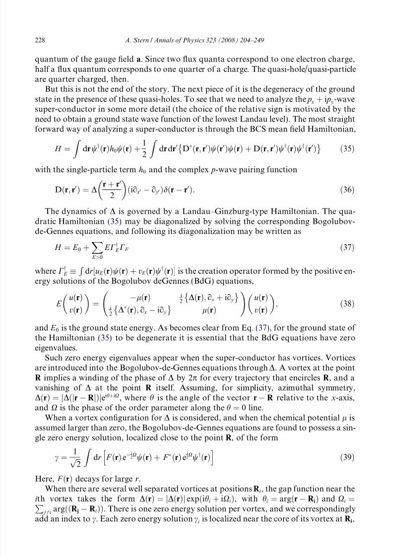
8/3/2019 Ady Stern- Anyons and the quantum Hall effect— A pedagogical review
http://slidepdf.com/reader/full/ady-stern-anyons-and-the-quantum-hall-effect-a-pedagogical-review 25/46
quantum of the gauge field a. Since two flux quanta correspond to one electron charge,half a flux quantum corresponds to one quarter of a charge. The quasi-hole/quasi-particleare quarter charged, then.
But this is not the end of the story. The next piece of it is the degeneracy of the ground
state in the presence of these quasi-holes. To see that we need to analyze the p x þ i p y -wavesuper-conductor in some more detail (the choice of the relative sign is motivated by theneed to obtain a ground state wave function of the lowest Landau level). The most straightforward way of analyzing a super-conductor is through the BCS mean field Hamiltonian,
H ¼Z
drwyðrÞh0wðrÞ þ 1
2
Z dr dr0 DÃðr; r0Þwðr0ÞwðrÞ þ Dðr; r0ÞwyðrÞwyðr0ÞÈ É ð35Þ
with the single-particle term h0 and the complex p-wave pairing function
Dð
r; r0
Þ ¼D
r þ r0
2 ð
io x0 À
o y 0Þdð
rÀ
r0
Þ:
ð36
ÞThe dynamics of D is governed by a Landau–Ginzburg-type Hamiltonian. The qua-
dratic Hamiltonian (35) may be diagonalized by solving the corresponding Bogolubov-de-Gennes equations, and following its diagonalization may be written as
H ¼ E 0 þX E >0
E Cy E C E ð37Þ
where Cy E
R dr ½u E ðrÞwðrÞ þ v E ðrÞwyðrÞ is the creation operator formed by the positive en-
ergy solutions of the Bogolubov deGennes (BdG) equations,
E uðrÞvðrÞ
¼ ÀlðrÞ i
2DðrÞ; o x þ io y
È Éi2D
ÃðrÞ; o x À io y
È ÉlðrÞ
uðrÞvðrÞ
; ð38Þ
and E 0 is the ground state energy. As becomes clear from Eq. (37), for the ground state of the Hamiltonian (35) to be degenerate it is essential that the BdG equations have zeroeigenvalues.
Such zero energy eigenvalues appear when the super-conductor has vortices. Vorticesare introduced into the Bogolubov-de-Gennes equations through D. A vortex at the pointR implies a winding of the phase of D by 2p for every trajectory that encircles R, and a
vanishing of D at the point R itself. Assuming, for simplicity, azimuthal symmetry,DðrÞ ¼ jDðjr À RjÞjeihþiX, where h is the angle of the vector r À R relative to the x-axis,and X is the phase of the order parameter along the h ¼ 0 line.
When a vortex configuration for D is considered, and when the chemical potential l isassumed larger than zero, the Bogolubov-de-Gennes equations are found to possess a sin-gle zero energy solution, localized close to the point R, of the form
c ¼ 1 ffiffiffi2
p Z
dr F ðrÞeÀ i2XwðrÞ þ F ÃðrÞe
i2XwyðrÞ
h ið39Þ
Here, F
ðr
Þdecays for large r.
When there are several well separated vortices at positions Ri, the gap function near thei th vortex takes the form DðrÞ ¼ jDðrÞj expðihi þ iXiÞ, with hi ¼ argðr À RiÞ and Xi ¼P
j6¼i argððR j À RiÞÞ. There is one zero energy solution per vortex, and we correspondinglyadd an index to c. Each zero energy solution ci is localized near the core of its vortex at Ri,
228 A. Stern / Annals of Physics 323 (2008) 204–249

8/3/2019 Ady Stern- Anyons and the quantum Hall effect— A pedagogical review
http://slidepdf.com/reader/full/ady-stern-anyons-and-the-quantum-hall-effect-a-pedagogical-review 26/46
but the phase Xi that replaces X in (39) depends on the position of all vortices. Moreover,the dependence of ci on the positions Ri is not single valued. If the angle of the vectorRi À R j with respect to the x-axis is changed by 2p then ci acquires a minus sign. Theseminus signs will play an important role later.
The operators ci have a few properties that we need to dwell on. First, as is obviousfrom (39), these operators are hermitian, ci ¼ c
yi . Second, they mutually anti-commute.
With the proper normalization, fci; c jg ¼ 2dij. These two properties make the ci’s Major-ana fermions. Since c2
i 6¼ 0 and ðcyi Þ2 6¼ 0, we cannot talk about the ci’s as being ‘‘empty’’
or ‘‘full’’ as we are so used to when talking about fermions. We need to be more carefulwhen counting the dimensionality of the Fock space that is spanned by these fermions. Tothat end, we first note that the number of zero energy states must be even: for a compactgeometry, Dirac’s quantization of the monopole enforces the number of vortices goingthrough the boundary-less surface to be even. For a non-compact geometry, if the bulkof the system has an odd number of vortices, the edge will have a zero mode. If the bulkhas an even number of vortices, the edge will not have one of its own [75]. Thus, there isalways an even number of ci’s, with i ¼ 1 . . . 2 N . To properly count the dimensionality of the Hilbert space they span, it is convenient to define complex fermionic operators,
C j c j À ic jþ N ð40ÞC
y j c j þ ic jþ N ð41Þ
with j ¼ 1 . . . N . The N pairs of fermionic operators C j;Cy j satisfy the anticommutation rela-
tions we are used to from ‘‘conventional’’ fermionic operators, and hence define N fermionicmodes. In particular, each of these modes satisfy C2
j ¼ ðCy jÞ2 ¼ 0, and hence may be referred
to as ‘‘empty’’ and ‘‘full’’. The dimension of the Hilbert space they span is therefore 2
N
,andabasis that spans it can be described in terms of binary numbers of N digits, with 0 denoting an‘‘empty’’ mode, and 1 denoting a ‘‘full’’ one. Note that the BCS mean field Hamiltonian doesnot commute with the particle number operator, but does commute with the parity of thatnumber. Thus, its eigenstates may be characterized by the parity of the number of particlesthey contain. Since the operatorsC j and C
y j change that parity (each is a superposition of cre-
ating and annihilating a particle), half of the 2 N ground states have an even number of par-ticles, and the other half have an odd number of particles.
This subspace of ground states is an interesting Hilbert space. The basis we chose isobviously arbitrary, being based on an arbitrary enumeration of the vortices. A different
enumeration is just a different basis spanning the same subspace. But note how uniquethese states are: suppose that we look at a ground state jwi where all fermionic modesare ‘‘empty’’, C jjwi ¼ 0 for all j . From Eq. (41) we find that,
c jjwi ¼ ic jþ N jwi ð42ÞNoting the structure (39) of the c operators, this relation tells us something interesting
about the ground state jwi. The vortices j and j þ N may be arbitrarily far from one another.Yet, when we operate on jwi with c j, which is an operator that creates and annihilates a par-ticle at the neighborhood of the vortex j , we get essentially the same state (up to an eip=2 phase)that we get when we operate withc j
þ N , which is an operator that creates and annihilates a par-
ticle at the neighborhood of the vortex j þ N . Clearly, this state involves some long range cor-relations between the local occupation of single particle states near the cores of the vortices.
How can we move around within this subspace of degenerate ground states? Can wedesign some kind of a perturbation to the Hamiltonian that, if tuned properly, will take
A. Stern / Annals of Physics 323 (2008) 204–249 229

8/3/2019 Ady Stern- Anyons and the quantum Hall effect— A pedagogical review
http://slidepdf.com/reader/full/ady-stern-anyons-and-the-quantum-hall-effect-a-pedagogical-review 27/46
us from one ground state to another? That is a very subtle question. Generally speaking,we could think of several types of perturbations. The first is a perturbation that takes oneof the particles in the super-conductor and moves it from one single-particle state toanother. An example to that would be an interaction of the composite fermion with an
externally applied electro-magnetic field that does not involve a flip of the spin. The secondis a perturbation that scatters a composite fermion (or an electron) out of the super-con-ductor, for example by a spin-flip. And the third, the most interesting one, involves an adi-abatic motion of the vortices. Remarkably, a perturbation of the first type would have noeffect on the ground state subspace. Typically, a perturbation of this sort looks like,
H pert ¼Z
dx
Z dx0 F ðx À x0ÞwyðxÞwðx0Þbðx; x0Þ ð43Þ
with the range of F ðx À x0Þ being very short and with b being some kind of a bosonic oper-
ator (e.g., creation and annihilation of a photon or a phonon). Most generally, the projec-tion of H pert onto the ground state subspace is
H gspert ¼
Xij
hijcic j ð44Þ
When the wyðxÞ and wðx0Þ are expressed as a superposition of C E and Cy E of Eq. (37),
the proximity of the points x; x0 to one another implies that both will have a significantoverlap with the same Majorana operator ci. As a consequence, in Eq. (44), as long asthe vortices are well separated from one another, hij / dij, making Eq. (44) nothing but
a c-number (remember that c2
i ¼ 1 for all i s). Thus, as long as it is local, the perturbationdoes not induce transitions from one ground state to another and does not remove thedegeneracy of the ground states.
The stability of the degeneracy of the ground state with respect to local perturbationsmay also be understood from the point of view of the Bogolubov-deGennes equations.Since the spectrum of Eq. (38) is symmetric with respect to E ¼ 0, for a perturbation toaffect the degeneracy of the ground states it must mix two E ¼ 0 solutions of the BdGequations into two solutions of non-zero energiesÆ E . For that to happen, however, theperturbation must have matrix elements that couple the two zero energy solutions. Sincethose are localized within vortex cores, as long as vortices are well separated the removal
of the degeneracy will be exponentially small.Having the super-conductor shift from one ground state to another by a perturbation
that changes the parity of the number of particles in the super-conductor is easier to do.For example, consider a perturbation of the type (43) in which the spin state that is createdby wy is opposite to that annihilated by the w. Such a perturbation, when translated to theBdG operator, would involve only a single BdG operator, and thus would not assume theform (44). Note, however, that if the spin polarized super-conductor is the ground state of the system, taking a particle out of it may involve an energy cost, and thus put the entiresystem in an excited state.
The most interesting way to evolve the super-conductor from one ground state to
another is through braiding of vortices [79–81]. Look first at the case where vortex i encir-cles vortex j : independent of the geometry of the trajectory taken by the vortices, whenthat happens argðri À r jÞ changes by 2p. Hence both Xi and X j change by p, and bothci and c j are multiplied by À1. Note, these are changes in operators. The unitary transfor-
230 A. Stern / Annals of Physics 323 (2008) 204–249

8/3/2019 Ady Stern- Anyons and the quantum Hall effect— A pedagogical review
http://slidepdf.com/reader/full/ady-stern-anyons-and-the-quantum-hall-effect-a-pedagogical-review 28/46
mation that operates on the ground state when vortex i encircles vortex j , call it U ij, can beregarded as transforming the operators ck according to
ck ! U yijck U ij ð45Þ
The requirement that this transformation multiplies ci and c j by À1 while leaving allother c’s unaltered is enough to fix U ij up to an abelian phase to be,
U ij ¼ cic j ¼ exp pcic j=2 ¼ cic j ð46ÞThe effect of vortex i going around vortex j must be identical to the effect of two inter-
changes of vortices i and j , and thus it is not surprising that (up to an abelian phase again)the unitary transformation that corresponds to an interchange is the square root of U ij
namely, exp Æpcic j=4, where the sign is determined by the sense of the interchange. Uni-tary transformations that correspond to different interchanges do not necessarily commute
(in fact, two such transformations do not commute if they share one vortex), and hence thevortices satisfy a non-abelian statistics.So to summarize this section, the combination of a degenerate ground state subspace
and a topological unitary transformation that is applied to the state of the super-con-ductor whenever vortices braid makes the vortices satisfy a non-abelian statistics.Remember that the super-conductor we think of is the m ¼ 5=2 state and the vorticesare the quasi-particles and quasi-holes of that state. Would similar phenomena occurin two dimensional superfluid He-3 of the p x Æ i p y pairing, or in two dimensionalsuper-conductors of that symmetry? We will not get into a detailed discussion of thisquestion here, but merely comment on two important differences between the quantum
Hall m ¼ 5=2 state and the latter two examples: first, as we commented earlier, twodimensional super-fluids and super-conductors have a gapless bulk mode in the formof a charge density wave. And second, their vortices do not carry electrical chargeand therefore cannot be manipulated with the help of a magnetic or electric field.The Majorana intra-vortex states and the ground state degeneracy they create are boththere and have measurable consequences, but the question of the statistics of the vorti-ces is more subtle.
11. The geometric phases and quantum entanglement behind the non-abelian statistics
Before we look into the way non-abelian statistics may be observed through interferom-etry, we will dwell a little bit on the meaning of the unitary transformations that areapplied when vortices interchange, or encircle one another. These transformations werefirst worked out using Conformal Field Theory by Nayak and Wilczek [80], and then usingthe p-wave super-conductor description described above by Ivanov [79] (see also [81–84]).Look again on the unitary transformation that results from vortex j encircling vortex j þ 1(Eq. (46)). Written in full detail, it is
c jei2X j þ c
y j eÀ i
2X j
c jþ1e
i2X jþ1 þ c
y jþ1eÀ i
2X jþ1
; ð47Þ
where the operators cðyÞ j ; cðyÞ jþ1 annihilate (create) a composite fermion localized veryclose to the cores of the j th and ð j þ 1Þth vortex, respectively. Eq. (47) seemingly im-plies that the motion of the j th vortex around the ð j þ 1Þth vortex affects the occupa-tions of states very close to the cores of the two vortices. This is in contrast, however,
A. Stern / Annals of Physics 323 (2008) 204–249 231

8/3/2019 Ady Stern- Anyons and the quantum Hall effect— A pedagogical review
http://slidepdf.com/reader/full/ady-stern-anyons-and-the-quantum-hall-effect-a-pedagogical-review 29/46
to the derivation leading to Eq. (47), which explicitly assumes that vortices are kept farenough from one another so that tunneling between vortex cores may be disregarded.How can that happen [81]?
In fact, no tunnelling takes place. Rather, as we now explain, two ingredients are essen-
tial for the nonabelian statistics of the vortices. The first is the quantum entanglement of theoccupation of states near the cores of distant vortices. The second ingredient is familiarfrom our discussion of abelian anyons: the geometric phase accumulated by a vortex tra-versing a closed loop.
As we saw, the anyonic statistics in the m ¼ 1=m state is related to the geometric phaseaccumulated by a vortex traversing a close trajectory. Roughly speaking, the vortex accu-mulates a phase of 2p per fluid particle which it encircles. When another vortex with itsfractional charge is introduced to the encircled area, this phase changes by a fraction of 2p, due to the fractional charge carried by the vortex. Upon adapting the argument tointerchanging of vortices, one finds that this fraction of 2p translates into fractionalstatistics.
Similarly, the Moore-Read theory of the m ¼ 5=2 state describes it also as a superfluid,with the quasiparticles being vortices in that superfluid. However, the ‘‘effective bosons’’forming the superfluid are Cooper pairs of composite fermions. Consequently, the super-fluid has excitation modes associated with the breaking of Cooper-pairs. In the presence of vortices, a Cooper-pair may be broken such that one or two of its constituents are local-ized in the cores of vortices. For p Àwave superconductors, the existence of zero-energyintra-vortex modes leads, first, to a multitude of ground states, and, second, to a parti-cle-hole symmetric occupation of the vortex cores in all ground states. When represented
in occupation-number basis, each of the ground states we deal with is a superpositionwhich has equal probability for the vortex core being empty or occupied by one compositefermion. What distinguishes ground states from one another is the relative phases betweenthe different components of the super-position.
When a vortex traverses a trajectory that encircles another vortex, the phase it accu-mulates depends again on the number of fluid particles that it encircles. Since a fluidparticle is in this case a Cooper pair, the occupation of a vortex core by a fermion, half a pair, leads to an accumulation of a phase of p relative to the case when the core is notoccupied. It is this relative phase of p that the encircling introduces between the differentcomponents of the wave function that might transform the system from one ground
state to another.This line of thoughts leads to the following distinction between three types of fractional
quantum Hall states. The Laughlin m ¼ 1=m fractions are condensates of one type of par-ticle, the composite bosons formed by the attachment of m flux quanta to each electron[85]. The Jain states are several condensates living in parallel, each condensate beingformed of a different type of composite boson. The non-abelian states are bosons madeup of several electrons with flux attached to them. The most prominent example of thethird type is the m ¼ 5=2 state, but this state is followed by a whole series, the Read–Rezayiseries. In Section 13 we will use this line of thoughts to describe the Read–Rezayi series.
12. Interferometry of non-abelian anyons
As we described above for abelian anyons, interferometers seem to be the most directprobe of the topological interaction between anyons, since it is a geometry where winding
232 A. Stern / Annals of Physics 323 (2008) 204–249

8/3/2019 Ady Stern- Anyons and the quantum Hall effect— A pedagogical review
http://slidepdf.com/reader/full/ady-stern-anyons-and-the-quantum-hall-effect-a-pedagogical-review 30/46
of particles around one another is inherent in the way transport takes place. Moreover, ithas recently been shown that, if realized, a Fabry–Perot interferometer of non-abeliananyons may be used as a topologically-protected qubit [86], with an astonishingly lowerror rate. In this section we revisit the two geometries we discussed above with the goal
of analyzing how they manifest the unique properties of the non-abelian m ¼ 5=2 state.
12.1. Fabry–Perot interferometer
Again, we consider the Fabry–Perot geometry and analyze the dependence of the back-scattered current on the area of the cell between the two point contacts and on the mag-netic field. The magnetic field determines the number of quasi-holes localized within theisland and the area of the cell determines the number of fluid particles encircled by theinterference loop. The effect of the localized quasi-particles in the non-abelian case is more
subtle than in the abelian one, since the edge quasi-hole that encircles them may modifythe quantum state they are in [87–92].Let us see how this happens: suppose that N qp quasi-particles are localized in the cell in
between the two point contacts of Fig. 4a, and that their quantum state is jwii. Transportcurrent flows rightwards on the lower edge, and may be back-scattered to flow leftward onthe upper edge. To lowest order, the back-scattering probability is the interference of twoamplitudes, of back-scattering by the left and by the right quantum point contact. Thepartial wave that is back-scattered by the left point contact does not encircle the celland thus does not modify the state jwii. By Eq. (46) the partial wave that is back-scatteredby the right point contact applies a unitary transformation on jwii, whose form is, up to a
phase, c N
qpaQ N
qp j¼1c j, where c j ( j ¼ 1 . . . N qp) are the Majorana modes associated with thelocalized quasi-holes and ca is the Majorana mode of the quasi-hole that is being back-scattered. Clearly, there is a difference between even and odd N qp. When N qp is even,the interfering waves take the form,
t 1jwii þ t 2ccelljwii ð48Þwhere ccell Qnis
j¼1c j; and t 1; t 2 are again the amplitudes for tunnelling at the two pointcontacts. The interference term is then
2Re
½t Ã1t 2
hwi
jccell
jwi
i ð49
ÞThere are two possible eigenvalues to ccell, either Æ1 or Æi, depending on whether N qp is
divisible by four. Thus, as the area of the cell is varied, there are two possible interferencepatterns, that differ by a p phase shift. If jwii is an eigenvector of ccell the observed inter-ference pattern would follow the corresponding eigenvalue. If that is not the case, theback-scattered current would measure the value of ccell and one of the two interference pat-tern would emerge. For an even N qp there are 2 N qp=2 ground states, characterized by N qp=2quantum numbers, each taking one of two possible values. The Fabry–Perot interferom-eter measures just one of these numbers.
As shown by Das Sarma et al. [86], the Fabry–Perot interferometer, if brought to work
for the m ¼ 5=2 state with an even N qp, may be used as a qubit, with the two possible valuesof ccell being the two states of the qubit. To flip the qubit from one value of ccell to another,a quasi-hole should tunnel through the cell, encircling an odd numbered subset of the N qp
localized quasi-holes. This qubit is protected from the sources of dephasing that are so
A. Stern / Annals of Physics 323 (2008) 204–249 233

8/3/2019 Ady Stern- Anyons and the quantum Hall effect— A pedagogical review
http://slidepdf.com/reader/full/ady-stern-anyons-and-the-quantum-hall-effect-a-pedagogical-review 31/46
harmful to other types of qubits. Perturbations such as an external RF noise, hyperfinecoupling with nuclear spins etc. do not affect its behavior at all, as long as their frequenciesare too low to overcome the energy gap.
When N qp is odd, the unitary transformation applied by the partial wave that encircles
the cell depends on the operator ca of the edge quasi-particle. As current is flowing, theunitary transformations applied by that partial wave are caccell followed by cbccell followedby ccccell etc., with ca; cb; cc being the Majorana operators associated with the quasiparticlesthat flow along the edge. As these unitary transformations do not commute with oneanother, their expectation values will be a series of random numbers of magnitude equalor smaller to one. Consequently, no interference pattern will be observed. Rather thanhaving phase jumps as the magnetic field is varied and N qp is changed, as we saw forthe abelian case, the m ¼ 5=2 case is characterized by regions of magnetic field where nointerference is to be seen and regions where the interference assumes one of two possiblepatterns.
As the back-scattering amplitudes get bigger, higher-order reflection amplitudes shouldbe summed up. By the argument above, for an even N qp all orders contribute, while for anodd N qp the odd harmonics, in which the interference loop winds the N qp quasi-particles anodd number of times, do not interfere coherently. The back reflected current then takes theform,
I ¼X1m¼0
I m cos2 mN qp
p
2
h icos m /þ N qpp
4þ vmð N qpÞ
!ð50Þ
when N qp is even vm
ð N qp
Þ ¼ Æmp2
according to the eigenvalue of ccell. When N qp
¼2 j
þ1
(with j an integer) then vm ¼ jp. The calculation of the prefactors I m becomes complicatedfor large m, but is not needed for our purpose.
Similar to the abelian case, when the number N qp fluctuates in time the visibility of theAharonov–Bohm oscillations develops a power-law relation with the average current, dueto the averaging of the harmonics m in (50) that do not divide by 4. In that case the vis-ibility increases with the increase of the average current, and the fluctuations in N qp resultin a current noise [93].
12.2. Mach–Zehnder interferometer
Again, as for the abelian case, the main difference between the Fabry–Perot and Mach– Zehnder interferometers is in the fact that for the former N qp is a parameter whose dynam-ics is (at least as a matter of principle) independent of the current flowing in the interfer-ometer, while for the latter N qp changes by one with each tunnelling quasi-hole. Similar tothe abelian case, the time evolution of the system is a stochastic process, but now the stateof the system is not characterized only by the number of quasi-holes that have tunnelledfrom the exterior to the interior, but also by the state of the system: when N qp is even thereare two possible states, and a different transition rate corresponds to each one of them.This state of affairs can be diagrammatically expressed by means of Brattelli diagrams,
see Fig. 5. The x-axis of the diagram is N qp. The y-axis is the state of the cell, i.e., the inter-ference pattern it shows (this is a rather careless definition of the y-axis. A more elaborateone will be given in the Section 13). For reasons that have to do with conformal field the-ory, and will be explained below, the state of odd N qp is commonly called r, while the two
234 A. Stern / Annals of Physics 323 (2008) 204–249

8/3/2019 Ady Stern- Anyons and the quantum Hall effect— A pedagogical review
http://slidepdf.com/reader/full/ady-stern-anyons-and-the-quantum-hall-effect-a-pedagogical-review 32/46
states of even N qp are called 1 and w (or sometimes 1 and ). When N qp is odd, the system is
in the state w and may go to either 1 or w. The transition rates to these states differ fromone another since the relative phase of the two interfering waves depends on the final state.When N qp is even, there are two possible states the system may be in (1 and w), and onestate to which it may go. Again, two different scattering rates. It turns out that altogetherthere are four transition rates, which depend on the number N qpmod4 also due to the abe-lian phase accumulated around the interference loop. The detailed calculation of the var-ious transition rates is easiest to carry out using the techniques that will be explainedbelow, in Section 13 [94].
The evolution of the state of the system is determined by a set of equations similar to(22), with results that are similar in spirit, but different in important details: the current is
periodic in the flux through the interferometer, with a period of U0. The visibility scales asa power law of the average current, with the power being unique to the m ¼ 5=2 state. Andthe effective charge (Fano factor) measured in a shot noise measurement depends on theflux as well [33].
The range of effective charges (Fano factors) to be seen in various values of the flux is asignature of the m ¼ 5=2 state. The dependence of the effective charge on the flux is, as wesaw for the abelian case, a consequence of the existence of several scattering rates. Similarto the abelian case, two cases are rather easy to analyze. When all transition rates are thesame, the effective charge is that of the quasi-hole, namely e=4. When one transition rate issignificantly smaller than all others, again the effective charge will be larger, since the sys-
tem will be stuck for long times in the state from which it is hard to move on, and thenmove with a burst of steps until the next time it gets stuck. The structure of the Brattellidiagram allows the system to ‘‘bypass’’ the state from which the transition rate is small if that rate happens on a transition out of r, and thus does not limit the number of steps in
Fig. 5. A Brattelli diagram as a way to describe interference at m ¼ 5=2. The x-axis counts the number of quasi-particles in the interference loop. The y-axis describes the state of the quasi-particles. For an even N qp there aretwo possible interference patterns, mutually shifted by p, and the interferometer may be utilized as a qubit [86].For N qp there is zero amplitude of interference in lowest order of tunnelling. An ideal Fabry–Perot interferometerstays on one of the nodes indefinitely. A noisy Fabry–Perot interferometer, where N qp fluctuates, diffuses on theBrattelli diagram. A Mach–Zehder interferometer propagates on the diagram: each tunnelling quasi-particlechanges N qp by one. The notation 1;w;r is explained in the text.
A. Stern / Annals of Physics 323 (2008) 204–249 235

8/3/2019 Ady Stern- Anyons and the quantum Hall effect— A pedagogical review
http://slidepdf.com/reader/full/ady-stern-anyons-and-the-quantum-hall-effect-a-pedagogical-review 33/46
the ‘‘burst’’. This structure allows for an effective charge that is larger than the electroniccharge. In fact, in the case of the m ¼ 5=2 state the largest Fano factor should be higherthan three electronic charges.
Another scheme that uses current noise for the observation of signs of non-abelian sta-
tistics was suggested in [95].
12.3. Resonant tunnelling through a quantum dot
When the two quantum point contacts in a Fabry–Perot interferometer (Fig. 4a aretuned to strong back-scattering, the cell between the point contacts becomes effectivelya quantum dot, where the number of electrons is quantized. Equivalently, in this regimethe conductance of the interferometer may be viewed as determined by multiple windingsof the cell, induced by multiple reflections by the point contacts. Rather than having asinusoidal dependence of the back-scattered current on the area of the dot, we then expectto have most of the current back-scattered by the point contacts, except in those values of the area where resonant tunnelling takes place and all the current is transmitted throughthe dot. Those values correspond to area where the ground state energy of the dot with N
and with N þ 1 electrons is degenerate.In view of this condition, both for integer quantum Hall states and for abelian frac-
tional quantum Hall states we expect the difference in area between two consecutiveresonances to be 1=n0, where n0 is the electronic density in the dot. This predictionis little more than the observation that when the dot has several thousand electrons,the physics of the degeneracy point between the different nearby values of N is identi-
cal. One needs to increase the area of the dot by 1=n0 in order for it to accommodateanother electron.The non-abelian m ¼ 5=2 state is different, since in that state electrons are paired. Thus,
we may wonder whether the periodicity of the peaks on the area axis would be the areaneeded for accomodating another pair, or that needed for accommodating another elec-tron, 2=n0 or 1=n0 (here n0 is the density of electrons in the half filled uppermost Landaulevel). A similar question arises, of course, for super-conductors, where the peaks arescanned on the axis of a gate voltage rather than area. For super-conductors, the spacingbetween peaks indeed alternate, depending on whether the added electron has an electronin the dot to pair with, or whether it remains unpaired. The spacings in the two cases differ
by the energy gap of the super-conductor.In the m ¼ 5=2 case, the answer depends on N qp [88]. If N qp is odd, there is a zero
energy mode on the edge of the dot. This is, in the language of a super-conductor, amid-gap state that is available for the tunnelling electron, since it lies at the edge. Thus,in this case the spacing between transmission peaks will not alternate, and the periodicityin area will be 1=n0. In contrast, this zero energy state is absent from the edge when N qp
is even. As long as there is no edge-bulk coupling the tunnelling electron cannot makeuse of the zero energy states in the bulk, and the resonant peaks alternate: an odd elec-tron must reside on the edge, occupying the lowest energy edge mode, while an even elec-tron forms a Cooper-pair and is absorbed by the bulk. Thus, when N qp is even, the
periodicity in area becomes 2=n0. Even when the measurement is of a transmissionthrough a quantum dot, where the number of electrons is quantized, the combineddependence on area and magnetic field carries a signature of the non-abelian nature of the quasi-holes.
236 A. Stern / Annals of Physics 323 (2008) 204–249

8/3/2019 Ady Stern- Anyons and the quantum Hall effect— A pedagogical review
http://slidepdf.com/reader/full/ady-stern-anyons-and-the-quantum-hall-effect-a-pedagogical-review 34/46
13. Other non-abelian states
The m ¼ 5=2 state is the simplest example of a non-abelian quantum Hall state. Thereare several ways to approach the others. A possible starting point, which we choose here,
is that of trial wave functions. Despite the obvious difficulty in constructing a goodapproximation for an eigenstate wave function of a system of about 10 8 interacting elec-trons, trial wave functions led to enormous progress in the study of the fractional quantumHall effect, as we will review. Other starting points, originating from the non-abelianChern-Simons theories and from quantum groups, are covered extensively in [12] and [96].
Our journey towards non-abelian quantum Hall states on the trial wave function routestarts early, with the construction of the ground state wave function for a system of non-interacting electrons at m ¼ 1. These electrons would fill up the lowest Landau level, withall spins polarized, and would form a many-body wave function that is just the Slaterdeterminant of all single particle lowest Landau level states. In the symmetric gauge thesingle particle states are characterized by their angular momentum m. When the i th elec-tron occupies the mth state its single particle wave function is z mi exp À j z ij2
4l2H
and the many-body Slater determinant becomes,
wm¼1 f z igð Þ ¼Det z mi exp Àj z ij2=4l2
H ð51Þ¼Yi< j
ð z i À z jÞY
i
exp Àj z ij2=4l2H ð52Þ
where in the first equality i; m are the indices of the matrix.This wave function has some properties built into it by construction: it is purely within
the lowest Landau level, it describes a m ¼ 1 droplet, and it is fermionic (anti-symmetric tothe exchange of two of its coordinates). The wave function is exact for non-interactingelectrons, and is expected to be a good approximation when the inter-electron interactionenergy is much smaller than the cyclotron energy.
The next stop on our journey are the celebrated Laughlin wave functions. Let us gen-eralize Eq. (52) by defining
waðf z igÞ ¼Yi< j
ð z i À z jÞaY
i
exp Àj z ij2=4l2
H ð53Þ
When a is an odd integer, this is a Laughlin wave function, but we will think here of a asa parameter to be varied. Generally, the value of a determines the filling factor. This maybe understood either by observing that the probability distribution for finding a singleelectron at a distance j z j very far from the origin scales like j z j2að N À1Þ
eÀj z j2=2l2H , with N being
the number of electrons, thus making the effective area of the droplet scale like a N and thefilling factor scale as 1=a, or by means of the plasma analogy. Writing jwðf z igÞj2 exp ÀH, with
H ¼ 2aX
i< j
logð z i À z jÞ ÀX
i
j z ij2=2l2
H; ð54Þ
the function H can be regarded as the classical Hamiltonian of a fictitious two dimensionalplasma, and the electronic probability distribution as the partition function correspondingto that plasma. In this two-dimensional plasma the fictitious particles, whose coordinatesare z i, mutually interact through a a logð z Þ interaction, and interact with a uniform back-
A. Stern / Annals of Physics 323 (2008) 204–249 237

8/3/2019 Ady Stern- Anyons and the quantum Hall effect— A pedagogical review
http://slidepdf.com/reader/full/ady-stern-anyons-and-the-quantum-hall-effect-a-pedagogical-review 35/46
ground density (that in two dimensions creates a quadratic potential). The condition of charge neutrality then fixes the density to be 1=2pal2
H and the filling factor to be 1=a.If we combine together: (a). the derivation of Eq. (52) as the exact ground state for
non-interacting electrons at m
¼1, (b). the observations made above regarding the wave
function (53), and (c) the requirement that for filling factors smaller than one, in the limitof a very large cyclotron energy, the ground state wave function should be constructed of states of the lowest Landau level only; And if we add to this list a lot of Laughlin–inspiredhindsight, then it becomes almost natural to use the wave function (53) with a ¼ 3; 5 astrial wave functions for the m ¼ 1=3; 1=5 ground states. As long as a is an odd number,the wave function (53) is of fermionic symmetry and describes—as seen above using theplasma analogy—a droplet of filling factor m ¼ 1=a. Its exceptional success in describingthe actual m ¼ 1
3; 1
5states may be ascribed to the clever use it makes in its zeroes. Other than
the exponential factors, this wave function is a polynomial in the z i’s. The largest power ithas for each z i is determined by the filling factor to be of order of a N . Thus, this is also thenumber of zeroes for each z i’s. Surely, there must be a zero whenever two electrons are inthe same position, due to the Pauli principle of Fermions. That forces the position of
N À 1 zeroes per each coordinate, but does not force the position of the otherðaÀ 1Þð N À 1Þ zeroes per coordinate. The Laughlin wave function devotes all its zeroesto keeping electrons away from one another, and thus minimizes their probability forbeing close to one another. As the distance d z between two electrons gets smaller and smal-ler, the probability to find them at that distance decreases as jd z j2a, faster than the jd z j2
forced by the Pauli principle.What happens, however, when m ¼ 1=a and a is not an odd integer? There are two
approaches that have been taken for constructing wave functions for this case: Jain’s com-posite fermions approach and Read–Rezayi’s clustering approach. The composite ferm-ions approach leads to a series of abelian quantum Hall states, while the clusteringapproach leads to a series of non-abelian states. For those filling fractions for which bothabelian and non-abelian trial wave functions may be constructed, the details of electron-electron interaction determine whether one of the two, and which one, is indeed the phaseof lowest energy.
Jain’s approach, which has been the impetus for the development of the compositefermions field theory described above in Section (8), starts from the following decomposi-tion of wa for any odd a and m ¼ 1=a:
wa ¼ Yi< j
ð z i À z jÞaÀ1Y
i
exp À2pnj z ij2ðaÀ 1Þ ÂYi< j
ð z i À z jÞ exp À2pnj z ij2 ð55Þ
Given that À2 H ¼ 2pna, where n is the electronic density, this breaks the wave function
into two factors. The first one, to the left of theÂsign, attaches an even number ðaÀ 1Þof flux quanta to each electron, transforming it into a composite fermion. The filling factorof the composite fermions is 1 and the second factor describes their occupation of a singleLandau level of a reduced magnetic field. Based on this observation, Jain constructed thewave function for p filled Landau levels of composite fermions, corresponding to a fillingfactor of p
ða
À1
Þ p
þ1
by replacing the single Landau level wave function, the second line in (55),
by the wave function for p filled Landau levels, and then projecting the resulting wavefunction into the lowest Landau level. The resulting wave functions are identical in theirtopological properties to those obtained from the field theoretical approach for compositefermions. Specifically, the quasi-particles and quasi-holes follow abelian statistics.
238 A. Stern / Annals of Physics 323 (2008) 204–249
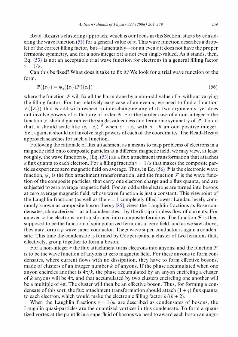
8/3/2019 Ady Stern- Anyons and the quantum Hall effect— A pedagogical review
http://slidepdf.com/reader/full/ady-stern-anyons-and-the-quantum-hall-effect-a-pedagogical-review 36/46
Read–Rezayi’s clustering approach, which is our focus in this Section, starts by consid-ering the wave function (53) for a general value of a. This wave function describes a drop-let of the correct filling factor, but—lamentably—for an even a it does not have the properfermionic symmetry, and for a non-integer a it is not even single-valued. As it stands, then,
Eq. (53) is not an acceptable trial wave function for electrons in a general filling factorm ¼ 1=a.
Can this be fixed? What does it take to fix it? We look for a trial wave function of theform,
Wðf z igÞ ¼ waðf z igÞF ðf z igÞ ð56Þwhere the function F will fix all the harm done by a non-odd value of a, without varyingthe filling factor. For the relatively easy case of an even a, we need to find a functionF ðfZ igÞ that is odd with respect to interchanging any of its two arguments, yet doesnot involve powers of z i that are of order N . For the harder case of a non-integer a thefunction F should guarantee the single-valuedness and fermionic symmetry of W. To dothat, it should scale like ð z i À z jÞÀb when z i ! z j, with aÀ b an odd positive integer.Yet, again, it should not involve high powers of each of the coordinates. The Read–Rezayiapproach searches for such a function.
Following the rationale of flux attachment as a means to map problems of electrons in amagnetic field onto composite particles at a different magnetic field, we may view, at leastroughly, the wave function wa (Eq. (53)) as a flux attachment transformation that attachesa flux quanta to each electron. For a filling fraction m ¼ 1=a that makes the composite par-ticles experience zero magnetic field on average. Thus, in Eq. (56) W is the electronic wave
function, wa is the flux attachment transformation, and the functionF
is the wave func-tion of the composite particles, that carry one electron charge and a flux quanta, and aresubjected to zero average magnetic field. For an odd a the electrons are turned into bosonsat zero average magnetic field, whose wave function is just a constant. This viewpoint of the Laughlin fractions (as well as the m ¼ 1 completely filled lowest Landau level), com-monly known as composite boson theory [85], views the Laughlin fractions as Bose con-densates, characterized—as all condensates—by the dissipationless flow of currents. Foran even a the electrons are transformed into composite fermions. The function F is thensupposed to be the function of spin polarized fermions at zero field, and as we saw above,they may form a p-wave super-conductor. The p-wave super-conductor is again a conden-
sate. This time the condensate is formed by Cooper-pairs, a cluster of two fermions that,effectively, group together to form a boson.
For a non-integer a the flux attachment turns electrons into anyons, and the function F
is to be the wave function of anyons at zero magnetic field. For these anyons to form con-densates, where current flows with no dissipation, they have to form effective bosons,made of clusters of an integer number k of anyons. If the phase accumulated when oneanyon encircles another is 4p=k , the phase accumulated by an anyon encircling a clusterof k anyons will be 4p, and that accumulated by two clusters encircling one another willbe a multiple of 4p. The cluster will then be an effective boson. Thus, for forming a con-densate of this sort, the flux attachment transformation should attach
ð1
þ2k
Þflux quanta
to each electron, which would make the electronic filling factor k =ðk þ 2Þ.When the Laughlin fractions m ¼ 1=m are described as condensates of bosons, the
Laughlin quasi-particles are the quantized vortices in this condensate. To form a quan-tized vortex at the point R in a superfluid of bosons we need to award each boson an angu-
A. Stern / Annals of Physics 323 (2008) 204–249 239

8/3/2019 Ady Stern- Anyons and the quantum Hall effect— A pedagogical review
http://slidepdf.com/reader/full/ady-stern-anyons-and-the-quantum-hall-effect-a-pedagogical-review 37/46
lar momentum of h relative to the point R. When the boson is made of two fermions, therelative angular momentum per fermion is h=2. When the fermion goes around the vortex,then, it accumulates a phase of p. In analogy, when the boson is made of k anyons, eachanyon gets, on average, an angular momentum of h=k and an anyon that goes around a
vortex accumulates a phase of 2p=k .The arguments of the last two paragraphs tell us that there should be a description of
the m ¼ k =ðk þ 2Þ fractional quantum Hall state as a condensate of effective bosons madeof clusters of k anyons. Within this description an anyon that goes around another wouldaccumulate a phase of 4p=k while an anyon that goes around a vortex in the condensatewould accumulate a phase of 2p=k . Our considerations do not tell us, however, the infor-mation we need about a collection of vortices: what is the phase accumulated when vor-tices go around one another, what are the degenerate ground states, if any, that manyvortices form when they are distant from one another, and how these degenerate groundstates lead to non-abelian statistics, if at all. Indeed, for the case of m
¼5=2, described in
details earlier, we needed the machinery of super-conductivity, particularly the Bogo-lubov-deGennes equations for a p-wave super-conductor, to give us that information.The tool that will help us to analyze the clustering of anyons into effective bosons andthe states formed by vortices in the condensate of these bosons will be parafermionic Con-formal Field Theories. As we now review, these theories provide a tool for constructing thefunction F both in the absence and in the presence of quasi-particles in the ground state.
We start with an introduction to the Conformal Field Theories we will use (Our intro-duction is very short and very incomplete. Useful references for a more comprehensivestudy of the subject are [97–104]. Following that, we show how the Ising CFT reproduces
our analysis of the m ¼ 5=2 state, and finally we show how a certain set of parafermionicCFTs generate the Read–Rezayi states for m ¼ 2 þ k =ðk þ 2Þ. When analyzing conformalfield theories, general considerations of symmetries and internal consistency go a long waytowards the calculation of certain properties of correlation functions. Here these correla-tion functions will construct the trial wave functions for the ground state and the quasi-particles. What is needed for these calculations are three inputs. The first is the list of fieldsin the theory. Some of these fields we may anticipate: the field of the anyon, which we willdenote by w1 (this field is called a parafermion in the CFT context), the field of the vortex,which we will denote by r1 and the field of the boson that is formed by k anyons. As wewill see below, at m ¼ 5=2 these are the only three fields, while in the more complicated
CFTs there are more fields. The second input we need is the conformal dimension of eachfield. The third is the list of operator product expansion rules. The operator productexpansion rules tell us that when two fields Uað z 1Þ and Ubð z 2Þ appear together in a corre-lation function, and when the coordinates z 1 and z 2 approach one another, the followingsubstitution may be carried out:
Uað z 1ÞUbð z 2Þ !Xc
C abcð z 1 À z 2ÞÀdUc ð57Þ
where C abc are constants and d ¼ hc À ha À hb with the hs being the conformal dimensionsof the respective fields. The fields Ua and Ub are then said to be ‘‘fused’’ to the field(s) Uc.
These rules for fusion are very important for us, in several contexts. First, we will use themto ‘‘create’’ clusters of anyons. Indeed, we will see that when k w1’s are fused together, theresulting field is the identity. The identity field is an ‘‘invisible’’ one: when it is fused withany field, d ¼ 0, and the right hand side of (57) does not have the ð z 1 À z 2Þ factor. Second,
240 A. Stern / Annals of Physics 323 (2008) 204–249

8/3/2019 Ady Stern- Anyons and the quantum Hall effect— A pedagogical review
http://slidepdf.com/reader/full/ady-stern-anyons-and-the-quantum-hall-effect-a-pedagogical-review 38/46
we will use the fusion rules to figure out the phase accumulated when one field encirclesanother. This phase is simply 2pd, with the d that correspond to the fusion of the twofields. And third, we will use the rules to figure out the structure of the ground state sub-space created when several quasi-particles (vortices) are fused together.
So here is how it will go [9,10]: we will have a description of the electron as a product of two conformal fields,
weð z Þ ¼ ei ffiffiffiffiffi
k þ2k
p /ð z Þw1ð z Þ ð58Þ
In the first piece, ei ffiffiffiffiffi
k þ2k
p /ð z Þ, commonly called a ‘‘vertex operator’’, the field /ð z Þ is a free
chiral boson. The ground state wave function will be a correlator of many electron fields
Wðf z igÞ ¼ hweð z 1Þ . . .weð z nÞi: ð59ÞThe correlation functions of the bosonic vertex operators produce Eq. (53). The corre-
lation function of the w1ð z Þ’s will produce the function F . There are two important prop-erties that will make it happen. Firstly, the fusion of a finite number k of w1’s will producethe identity field. That will guarantee that the power of each z i in the function F will scalelike k , and not like N . Second, the conformal dimension of w1 will guarantee that the entirecorrelator will create a fermionic wave function. Generally, the operator product expan-sion for the bosonic fields is,
eia/ð z Þ Â eib/ð z 0Þ ! eiðaþbÞ/ð z Þð z À z 0Þab ð60ÞElectrons must accumulate a phase of 2p when they encircle one another. They will
accumulate a phase of 2pð
k
þ2Þ=k from the bosonic factors, and will therefore need to
accumulate À4p=k from the parafermionic fields. This will make the combined wave func-tion single-valued and anti-symmetric with respect to interchanging the coordinates of twoelectrons.
To generate vortices, we will introduce terms of r1eib/ into the correlators. The value of b will be chosen as the minimal value for which the correlators will remain single valuedwith respect to the electronic coordinates. As we will see, the fusion rule of two r1’s will befundamentally different from the fusion rule of two w1’s. While two w1’s fuse to a singlefusion product, two r1’s will have two fusion channels to go into. This multiplicity of pos-sible outcomes will be the source of the ground state degeneracy and the non-abelian
statistics.This description looks complicated at first reading, and—to be honest—also at laterreadings. It will hopefully get simpler after we see how it works for the m ¼ 5=2 state,and then how it works for the more complicated Read–Rezayi states.
13.1. The CFT way of analyzing the m ¼ 5= 2 state
The simplest parafermionic theory to be mentioned here is known as the Z 2 (or Ising)theory. It is the CFT method of dealing with the m ¼ 5=2 state. Let us see how it works: thetheory has three fields: w1, r1 and the identity field. In view of that, we will omit the sub-
script from w and r. The identity field corresponds to the Cooper pair. The w is a fermion.The r corresponds to a vortex. The conformal dimensions of these fields are 0, 1/2 and 1/16 respectively. What makes the Z 2 theory simple is the fact that the action for the w isknown to be that of a free chiral Majorana fermion [101]. As explained above, the electron
A. Stern / Annals of Physics 323 (2008) 204–249 241

8/3/2019 Ady Stern- Anyons and the quantum Hall effect— A pedagogical review
http://slidepdf.com/reader/full/ady-stern-anyons-and-the-quantum-hall-effect-a-pedagogical-review 39/46
and quasi-particle fields are composed of the parafermionic fields together with the boson-ic factors.
There are three rules for operator product expansion. For creating the wave functionwith no vortices we need only the following:
wð z Þwð z 0Þ ! ð z À z 0ÞÀ1 ð61ÞIn the language of super-conductivity, this says that two composite fermions may form aCooper-pair whose wave function is ð z À z 0ÞÀ1. Let us put:
Wðf z igÞ ¼Y N
i¼1
ei ffiffi
2p
/ð z iÞwð z iÞeÀi N ffiffi
2p
/ð z 1Þ* +
ð62Þ
with z 1 an arbitrary point at infinity, and the the last factor guarantees that the correlator
of the free boson factor does not vanish. The free action for both w and the boson / en-ables the use of Wick’s theorem, and the rule (61) allows for the explicit calculation of thiscorrelator. The result is
waðf z igÞ ¼Yi< j
ð z i À z jÞ2Y
i
eÀj z i j2
4l2HA
1
z 1 À z 2
1
z 3 À z 4. . .
1
z N À1 À z N
ð63Þ
where A is the anti-symmetrizer.The part F of the wave function we obtain through these correlators, which is the Pfaf-
fian of the matrix M ij ¼ 1=ð z i À z jÞ, is, in fact, the wave function for a p x þ i p y super-con-
ductor with no vortices. Now let us look at the role of the r’s. The operator productexpansion for r with w is
rð z Þwð z 0Þ ! rð z Þð z À z 0ÞÀ1=2 ð64ÞThus, r is an object that gives the fermion w a minus sign when the fermion goes
around it. Sounds like a vortex in the super-conductor, and indeed it is. The quasi-holewould be rð z Þeib/ð z Þ; and b is fixed in such a way that when the electron goes around aquasi-hole (or a quasi-particle) it accumulates a phase of 2p such that the wave functionremains single valued. For that to happen, Eqs. (60) and (64) tell us that we needb
¼ Æ1=2 ffiffiffi2p
, a value that fixes the charge of the quasi-hole/particle to be a quarterof the electron charge.
When two r’s fuse, the Z 2 theory has,
rð z Þrð z 0Þ ! ð z À z 0ÞÀ1=8½1 þ wð z Þð z À z 0Þ1=2 ð65ÞTwo r’s may then be fused either to 1 or to w, which is the CFT way of saying that two
vortices in a p x þ i p y super-conductor introduce a two-fold degeneracy of the ground state,and that the two degenerate states differ by the parity of the total number of fermions.
The only remaining piece of information about operator product expansion that weneed is that the 1 field fuses trivially with the w and the r, leaving them unchanged,
and with no factors of ð z À z 0Þ.Finally for the Z 2 theory, how do we understand the interferometry in the language of
the CFT? Let us look at the Fabry–Perot geometry. The encircling of the bulk quasi-par-ticles by the interference loop amounts to a trajectory in which an edge quasi-particle
242 A. Stern / Annals of Physics 323 (2008) 204–249

8/3/2019 Ady Stern- Anyons and the quantum Hall effect— A pedagogical review
http://slidepdf.com/reader/full/ady-stern-anyons-and-the-quantum-hall-effect-a-pedagogical-review 40/46
rð z Þei/ð z Þ=2 ffiffi
2p
goes around the bulk, whose N qp quasi-particles fuse to eiN qp/ð z 0Þ=2 ffiffi
2p nð z 0Þ where
nð z 0Þ is rð z 0Þ when N qp is odd, and may be either the identity or wð z 0Þ when N qp is even.Now, the phase accumulated when an edge quasi-particle goes around the bulk one can
be obtained from their fusion rules. First, the bosonic fields yield a factor of
ð z
À z 0
Þ N qp=8.
Second, by (65) and (64), the fusion of r with n gives no extra phase when the bulk fuses tothe identity, and an extra phase of p when it fuses to w. Thus, when the bulk quasi-par-ticles fuse to the identity the edge quasi-particles accumulates only the abelian phase. Thisphase is just that of a vortex of a super-conductor going around 1/8 of a Cooper-pair,namely a quarter of a charge. When the bulk quasi-particles fuse to w an extra phase of p is added to the phase accumulated in the previous case. Furthermore, when the bulkfuses to r, the fusion of the edge r with the bulk r gives, according to (65) a sum of two interference patterns of equal magnitude, with a mutual phase shift of p. Obviously,these two terms cancel one another and no interference is to be seen, exactly as predictedby the p x
þi p y superconductor picture.
Before we turn to discuss the other non-abelian states, for which we do not have but theCFT description, let us summarize what use we made of CFT for understanding them ¼ 5=2 state, since similar steps will be useful for the understanding of the other non-abe-lian states:
(1) We carried out a Chern-Simons transformation that is not necessarily single valued,aimed at cancelling the external magnetic field within mean field approximation. Thistransformation effectively maps the problem of electrons in a magnetic field onto aproblem of composite particles at zero magnetic field. For m ¼ 5=2 those particles
were fermions. For other filling fractions, they will be anyons.(2) As the wave function F for the composite particles we looked for a function that willhave the needed power laws when any two particles approach one another, but willbe rather low in the degree of its polynomials. We then introduced the parafermionicCFT’s, that happen to have exactly the needed properties.
(3) We studied the Z 2 CFT, and used it to identify the field for the electron, the field forthe quasi-hole, the degeneracy of the ground state subspace, and the phases accumu-lated when one type of particle goes around another.
Note that this line of thought cannot but offer the possibility of a non-abelian phase at a
particular filling fraction and analyze its properties. It cannot judge if, and at what condi-tions, this phase is energetically favorable to competing phases. This question may beanswered either through experiments or through numerical exact diagonalization studies.
13.2. The Read–Rezayi series
Let us now apply these ideas to other filling fractions, and obtain the Read–Rezayi ser-ies. Consider a filling fraction of k =ðk þ 2Þ. The cases k ¼ 1; 2 are relatively easy, and werediscussed at length above (True, we discussed the m ¼ 5=2 as the k ¼ 2, and not m ¼ 1=2. Itturns out that details of the electron-electron interaction in the N
¼1 Landau level are
more favorable for composite fermion pairing than those of the lowest, N ¼ 0, Landaulevel. That is apluasibly the case for the higher values of k [72]). Now we look at higherintegers. The Chern-Simons transformation (53) is now multiply valued, and we resortagain to the CFTs to fix this problem. Thus, we are looking for a CFT whose correlators
A. Stern / Annals of Physics 323 (2008) 204–249 243

8/3/2019 Ady Stern- Anyons and the quantum Hall effect— A pedagogical review
http://slidepdf.com/reader/full/ady-stern-anyons-and-the-quantum-hall-effect-a-pedagogical-review 41/46
for one of its fields scales like ð z À z 0ÞÀ2=k . Luckily, as we will now see, the parafermionicCFTs do just that.
Similar to the m ¼ 5=2 case, we will combine two CFTs, a free chiral boson /ð z Þ and a‘‘parafermionic’’ one. The parafermionic CFT will have more than the three fields we had
in the Z 2 case. This should come as no surprise: it takes the fusion of k anyons to get to theidentity, so we need to have k fields w jð j ¼ 1 . . . k Þ where w j is just j anyons fused together,and wk is the identity. Since a vortex carries a flux of 1=k , we would also require that k
vortices are allowed to fuse to the identity (but are not forced to do so. Remember thatvortices have several fusion channels). That requires k fields r j which would be j vorticesfused together (the field rk ¼ wk would be the identity field). But even that is not all: let uscall rk À1 the anti-vortex. If the vortex and anti-vortex do not necessarily fuse to the iden-tity, then a collection of j vortices and l anti-vortices does not necessarily fuse to r jÀl, butmay fuse to another state. That state will accumulate the same phase when encircling aparafermion, but a different phase when encircling a vortex.
Altogether, a more elaborate analysis along these lines leads to the following picture: itturns out to be convenient to label the fields by two quantum numbers, Ul
m. The integer m
is called ‘‘the topological charge’’. Fusion processes conserve the topological charge mod-ulo 2k , and it is the topological charge that determines the phase accumulated when aparafermion encircle the field Ul
m. The integer index l satisfies l 2 f0; 1; . . . ; k g, and thefields Ul
m satisfy Ulm ¼ Ul
mþ2k ¼ Uk ÀlmÀk and l þ m 0ðmod2Þ. These fields include all the
fields anticipated in the paragraphs above: w1 U02 is the parafermion, which will play
the role of w in the Z 2 case; The fields w j U02 j are collections of j parafermions; The field
r1 U11 is the vortex (called also the spin field); The field U2
0 is the field that may be
obtained (side by side with the identity) when a vortex and and an anti-vortex fusetogether; And finally Uk k ¼ U0
0 which is the identity.The conformal dimension of the field Ul
m is given by (for Àl 6 m 6 l)
hlm ¼ lðl þ 2Þ
4ðk þ 2Þ À m2
4k : ð66Þ
The operator product expansion (OPE), is given by UiðwÞ Â U jð z Þ ¼Pk C ijk ð z À wÞhk ÀhiÀh jUk , where the fields appearing on the right hand side are determined
by the equation [97,99]:
Ulama
 Ulbmb
!Xminflaþlb;2k ÀlaÀlbg
l¼ laÀlbjjUl
maþmb; ð67Þ
What does this tell us? First, that
w1ð z Þw1ð z 0Þ ! w2ð z Þð z À z 0ÞÀ2=k ð68Þ
as we need. Second, that when we fuse k parafermions w1 we get the unity. Thus, the statewe will construct this way will be a condensate of clusters, each cluster having k paraferm-
ions.As we said above, dissipationless transport is a property of a bosonic system at zero
magnetic field. At m ¼ 1=m the flux attachment term (53) turned the electrons into compos-ite bosons. At m ¼ 1=2 the attachment of flux turned electrons into composite fermions and
244 A. Stern / Annals of Physics 323 (2008) 204–249

8/3/2019 Ady Stern- Anyons and the quantum Hall effect— A pedagogical review
http://slidepdf.com/reader/full/ady-stern-anyons-and-the-quantum-hall-effect-a-pedagogical-review 42/46
pairs of composite fermions acted like bosons. At k ¼ 3 . . . the electrons were turned intoanyons, and the grouping of k anyons creates the bosons that condense.
The identification of the electron creation operator is done as for the m ¼ 5=2 case. It is
w1e
i / ffiffik p ffiffiffiffiffiffik þ2
p . Similarly, the quasi-particle creation operator is r
1e
i u ffiffik p 1 ffiffiffiffiffik
þ2
p . Their charge is e
k þ2and they carry an average angular momentum of h=k per particle.
In the absence of quasi-particles this scheme creates a single ground state, which is thecorrelation function of many electron operators. For each z i, the polynomial part of thewave function has a maximal power of about N ðk þ 2Þ=k , and hence about that numberof zeroes (the word ‘‘about’’ stands for the neglect of numbers of order one, and forthe neglect of the question of whether N divides by k ). Out of these zeroes for, say,
z 1; N À 1 zeroes coincide with the positions of the other electrons, as required by the Pauliprinciple. The other 2=k zeroes are not attached to other electrons. Rather, it can be shownthat if the electronic wave function W in Eq. (56) is written as W ¼ Qi< jð z i À z jÞvðf z igÞ(separating out the zeroes that are dictated by the Pauli principle) then the function v van-ishes quadratically when k þ 1 of the coordinates approach one another [10,102,103] .Thus, when k of the coordinates are close together around the point z 0, we expect the elec-tronic wave function W to vanish like ð z 1 À z 0Þ2, attaching two zeroes—figuratively speak-ing—to k electrons.
The fusion rules Eq. (67) introduce the non-abelian side of these quasi-particles, since aswe fuse many r1’s together, we get a number of fusion channels that increases exponen-tially with the number of fused r’s. Each of these channels corresponds to a ground state.For keeping track of this number it is useful to use again the Brattelli diagram, see Fig. (6).In the Brattelli diagrams that are useful to us the x-axis counts the number of quasi-par-
ticles (which, when divided modulo 2k , gives the topological charge). The y axis is theindex l . A fusion with r1 increases or decreases l by one, and l is limited between 0 andk , and hence the structure reflected in the figure: the diagram has k þ 1 ‘‘floors’’ and eachsteps towards the right or left takes you one floor up or down. A trajectory that starts atthe origin and ends at some node of a particular number of quasi-particles corresponds to
Fig. 6. A Brattelli diagram for a Read–Rezayi state. Each node on the diagram describes the state that the quasi-particles fuse to. Each trajectory on the diagram is a ground state.
A. Stern / Annals of Physics 323 (2008) 204–249 245

8/3/2019 Ady Stern- Anyons and the quantum Hall effect— A pedagogical review
http://slidepdf.com/reader/full/ady-stern-anyons-and-the-quantum-hall-effect-a-pedagogical-review 43/46
a ground state with that number of quasi-particles. Each node in the diagram correspondsto a field Ul
m. The node at which a trajectory ends corresponds to the state to which thequasi-particles fuse in that particular ground state.
The Brattelli diagram makes the counting of the number of ground states relatively sim-
ple—it becomes the counting of trajectories on a graph. For a large number N of quasi-particles, it scales like
2cosp
k þ 2
! N
ð69Þ
To propagate horizontally on the diagram, we need to fuse a state with r1’s. To propagatevertically, we need to fuse with the field U2
0.The information we gave here on the CFT formulation of the Read–Rezayi gives most
of the background needed for generalizing the analysis of interferometry, described abovein detail for the m
¼5=2 state, to these states. We will not carry out this generalization
here, but rather refer the reader to [105–109]. As shown in these works, lowest order inter-ference in the Fabry–Perot interferometer and Couomb blockade peak spacings in a quan-tum dot reflect the number and state of the localized quasi-particles in the cell of theinterferometer, and the effective charge in a shot noise measurement in a Mach–Zehnderinterferometer may identify the Z 3 nature of the m ¼ 12=5 state.
14. Summary
Much of physics is about setting rules, and then looking for ways to break them. Any-
ons were the breaking of the rule that the wave function of identical particles must followfermionic or bosonic symmetry. The breaking of this rule signaled the door to a rich andfascinating part of physics, in which ohmic contacts and semi-conductors mingle withtopology and CFT’s, and the immensely complicated nature of the first two convergesin certain limits to the pure simplicity of the last two. Much is presently understood aboutthat part of physics, as we tried to describe. Much more is awaiting for future research, webelieve.
Acknowledgements
I am indebted to Merav Dolev, Eytan Grosfeld, Roni Ilan and Gil Tayar for their helpin preparing this manuscript. This work was partially funded by the US-Israel BinationalScience Foundation, the Minerva Foundation and the Israel Science Foundation.
References
[1] J.M. Leinaas, J. Myrheim, Nuovo Cimento 37B (1977) 1.[2] F. Wilczek, Phys. Rev. Lett. 48 (17) (1982) 1144.[3] R. Prange, S.M. Girvin (Eds.), The Quantum Hall Effect, Springer-Verlag, New York, 1990.[4] S. Das Sarma, A. Pinczuk (Eds.), Perspectives in Quantum Hall Effects : Novel Quantum Liquids in Low-
dimensional Semiconductor Structures, Wiley, New York, 1997.[5] K.v. Klitzing, G. Dorda, M. Pepper, Phys. Rev. Lett. 45 (6) (1980) 494.[6] D.C. Tsui, H.L. Stormer, A.C. Gossard, Phys. Rev. Lett. 48 (22) (1982) 1559.[7] Y. Aharonov, D. Bohm, Phys. Rev. 115 (3) (1959) 485.[8] M.V. Berry, Proc. Roy. Soc. Lond. A392 (1984) 45.
246 A. Stern / Annals of Physics 323 (2008) 204–249

8/3/2019 Ady Stern- Anyons and the quantum Hall effect— A pedagogical review
http://slidepdf.com/reader/full/ady-stern-anyons-and-the-quantum-hall-effect-a-pedagogical-review 44/46
[9] G. Moore, N. Read, Nucl. Phys. B 360 (1991) 362.[10] N. Read, E. Rezayi, Phys. Rev. B 59 (12) (1999) 8084.[11] A.Y. Kitaev, Ann. Phys. (NY) 303 (2003) 2.[12] S. Das Sarma, M. Freedman, C. Nayak, S. Simon, A. Stern, Non-abelian anyons and topological quantum
computation, (2007) arXiv:0707.1889.
[13] F.D.M. Haldane, Phys. Rev. Lett. 67 (8) (1991) 937.[14] P. Jacob, P. Mathieu, Nucl. Phys. B 620 (2002) 351.[15] E. Ardonne, P. Bouwknegt, K. Schoutens, J. Statistical Phys. 102 (2001a) 421, URL doi:10.1023/
A:1004878231034.;V. Gurarie, M. Flohr and C. Nayak (ITP), Nucl. Phys. B498 (1997) 513–538.
[16] P. Bouwknegt, K. Schoutens, Nucl. Phys. B 547 (1999) 501.[17] K. Schoutens, Phys. Rev. Lett. 81 (9) (1998) 1929.[18] Y. Imry, Introduction to Mesoscopic Physics, Oxford University Press, New York, 2002.[19] R.B. Laughlin, Phys. Rev. Lett. 50 (18) (1983) 1395.[20] B.I. Halperin, Phys. Rev. Lett. 52 (18) (1984) 1583.[21] D. Arovas, J.R. Schrieffer, F. Wilczek, Phys. Rev. Lett. 53 (7) (1987) 722.
[22] D.J. Thouless, Y. Gefen, Phys. Rev. Lett. 66 (6) (1991) 806.[23] V.J. Goldman, B. Su, Science 267(5200) (1995) 1010, URL http://www.sciencemag.org/cgi/content/abstract/267/5200/1010.
[24] R. De Picciotto, M. Reznikov, M. Heiblum, V. Umansky, G. Bunin, D. Mahalu, Nature 389 (1997) 162.[25] L. Saminadayar, D.C. Glattli, Y. Jin, B. Etienne, Phys. Rev. Lett. 79 (1997) 2526.[26] Jens Martin et al., Science 305 (2004) 980.[27] W.J. Elion, J.J. Wachters, L.L. Sohn, J.E. Mooij, Phys. Rev. Lett. 71 (14) (1993) 2311.[28] Z. Hermon, A. Stern, E. Ben-Jacob, Phys. Rev. B 49 (14) (1994) 9757.[29] F.D.M. Haldane, Y.-S. Wu, Phys. Rev. Lett. 55 (26) (1985) 2887.[30] S.L. Sondhi, S.A. Kivelson, Phys. Rev. B 46 (20) (1992) 13319.[31] C. Chamon, D.E. Freed, S.A. Kivelson, S.L. Sondhi, X.G. Wen, Phys. Rev. B 55 (4) (1997) 2331.[32] K.T. Law, D.E. Feldman, Y. Gefen, 2006, Phys. Rev. B (Condensed Matter and Materials Physics) 74(4),
045319 (pages 16), URL http://link.aps.org/abstract/PRB/v74/e045319 .[33] D.E. Feldman, Y. Gefen, A. Kitaev, K. T. Law, A. Stern, Phys. Rev. B (Condensed Matter and Materials
Physics) 76(8) (2007) 085333 (pages 9), URL http://link.aps.org/abstract/PRB/v76/e085333.[34] Vadim V. Ponomarenko, Dmitri V. Averin, Phys. Rev. Lett. 99 (2007) 066803.[35] C.L. Kane, Phys. Rev. Lett. 90 (22) (2003) 226802.[36] E.-A. Kim, 2006, Phys. Rev. Lett. 97(21), 216404 (pages 4), URL http://link.aps.org/abstract/PRL/v97/
e216404.[37] J. Jain, Composite Fermions, Cambridge University Press, United Kingdom, 2007.[38] O. Heinonen, Composite Fermions, World Scientific, 1998.[39] B.I. Halperin, P.A. Lee, N. Read, Phys. Rev. B 47 (12) (1993) 7312.[40] J.K. Jain, Phys. Rev. Lett. 63 (2) (1989) 199.[41] A. Lopez, E. Fradkin, Phys. Rev. B 47 (12) (1993) 7080.
[42] A. Lopez, E. Fradkin, Phys. Rev. B 44 (10) (1991) 5246.[43] B. Blok, X.G. Wen, Phys. Rev. B 42 (13) (1990) 8145.[44] F.E. Camino, W. Zhou, V.J. Goldman, Phys. Rev. B 72 (2005) 075342.[45] F.E. Camino, W. Zhou, V.J. Goldman, Phys. Rev. Lett. 95 (2005) 246802.[46] F.E. Camino, W. Zhou, V.J. Goldman, Phys. Rev. B 74 (2006) 115301.[47] F.E. Camino, W. Zhou, V.J. Goldman, Phys. Rev. Lett. 98 (2007) 076805.[48] M.D. Godfrey, P. Jiang, W. Kang, S. H. Simon, K. W. Baldwin, L. N. Pfeiffer, K. W. West, 2007,
Aharonov–Bohm-like oscillations in quantum hall corrals, URL arXiv.org:0708.2448.[49] J.B. Miller, I.P. Radu, D.M. Zumbuhl, E.M. Levenson-Falk, M.A. Kastner, C.M. Marcus, L.N. Pfeiffer,
K.W. West, 2007, Fractional quantum Hall effect in a quantum point contact at filling fraction 5/2, cond-mat/0703161.
[50] R.L. Willett, M.J. Manfra, L.N. Pfeiffer, K.W. West, 2007, arXiv.org:cond-mat/0703197.[51] Neder, M. Heiblum, Y. Levinson, D. Mahalu, V. Umansky, Phys. Rev. Lett. 96 (1) (2006) 016804,
pages 4.[52] Y. Ji, Y. Chung, D. Sprinzak, M. Heiblum, D. Mahalu, H. Shtrikman, Nature 422 (2003) 415.[53] D.V. Averin, J.A. Nesteroff, Phys. Rev. Lett. 99 (9) (2007) 096801, pages.
A. Stern / Annals of Physics 323 (2008) 204–249 247

8/3/2019 Ady Stern- Anyons and the quantum Hall effect— A pedagogical review
http://slidepdf.com/reader/full/ady-stern-anyons-and-the-quantum-hall-effect-a-pedagogical-review 45/46
[54] B. Rosenow, B.I. Halperin, Phys. Rev. Lett. 98(10) (2007) 106801, URL http://link.aps.org/abstract/PRL/v98/e106801.
[55] J.K. Jain, C. Shi, Phys. Rev. Lett. 96 (13) (2006) 136802, pages 4.[56] V.J. Goldman, Phys. Rev. B 75 (2007) 045334.[57] G.A. Fiete, Refael Gil, Fisher M.P.A., arXiv.org:0705.1543 (2007).
[58] B. Blok, X.-G. Wen, Nuc. Phys. B 374 (1992) 615.[59] H.-K. Lo, J. Preskill, Phys. Rev. D 48 (10) (1993) 4821.[60] X.G. Wen, Phys. Rev. Lett. 66 (6) (1991) 802.[61] J. Frohlich, P.A. Marchetti, Commun. Math. Phys. 121 (1989) 177.[62] J. Frohlich, F. Gabbiani, Rev. Math. Phys. 2 (1990) 251.[63] X.-G. Wen, A. Zee, Phys. Rev. B 58 (23) (1998) 15717.[64] X.-G. Wen, Phys. Rev. B 60 (12) (1999) 8827.[65] F.A. Bais, Nucl. Phys. B170 (1980) 32.[66] R. Willett, J.P. Eisenstein, H.L. Stormer, D.C. Tsui, A.C. Gossard, J.H. English, Phys. Rev. Lett. 59 (15)
(1987) 1776.[67] E. Ardonne, K. Schoutens, Phys. Rev. Lett. 82 (25) (1999) 5096.
[68] E. Ardonne, N. Read, E. Rezayi, K. Schoutens, Nucl. Phys. B 607 (2001) 549.[69] S.H. Simon, E.H. Rezayi, N. R. Cooper, I. Berdnikov, Phys. Rev. B 75(7) (2007) 075317,http://link.aps.org/abstract/PRB/v75/e075317 .
[70] R.H. Morf, Phys. Rev. Lett. 80 (7) (1998) 1505.[71] R. Morf, N. d’Ambrumenil, Phys. Rev. B 68 (2003) 113309/1.[72] E. H. Rezayi, N. Read, 2006, Non-Abelian quantized Hall states of electrons at filling factors 12/5 and 13/5
in the first excited Landau level, cond-mat/0608346.[73] V.W. Scarola, J.K. Jain, E.H. Rezayi, Phys. Rev. Lett. 88 (21) (2002) 216804.[74] X. Wan, K. Yang, E.H. Rezayi, Phys. Rev. Lett. 97 (25) (2006) 256804.[75] N. Read, D. Green, Phys. Rev. B 61 (15) (2006) 10267.[76] M. Greiter, X.-G. Wen, F. Wilczek, Phys. Rev. Lett. 66 (24) (1991) 3205.[77] M. Greiter, X.G. Wen, F. Wilczek, Nucl. Phys. B 374 (3) (1992) 567.
[78] N. Read, E. Rezayi, Phys. Rev. B 54 (23) (1996) 16864.[79] D.A. Ivanov, Phys. Rev. Lett. 86 (2) (2001) 268.[80] C. Nayak, F. Wilczek, Nucl. Phys. B 479 (3) (1996) 529, cond-mat/9605145.[81] A. Stern, F. von Oppen, E. Mariani, Phys. Rev. B 70 (20) (2004) 205338.[82] S.B. Chung, M. Stone, J. Physics A: Math. Theor. 40(19) (2007) 4923, URL http://stacks.iop.org/
1751-8121/40/4923.[83] M. Stone, S.-B. Chung, 2006, Phys. Rev. B 73(1), 014505, URL http://link.aps.org/abstract/PRB/v73/
e014505.[84] Y. Tserkovnyak, S.H. Simon, Phys. Rev. Lett. 90 (1) (2003) 016802.[85] S.C. Zhang, T.H. Hansson, S. Kivelson, Phys. Rev. Lett. 62 (1) (1989) 82.[86] S. Das Sarma, M. Freedman, C. Nayak, Phys. Rev. Lett. 94 (16) (2005) 166802.[87] E. Fradkin, C. Nayak, A. Tsvelik, F. Wilczek, Nucl. Phys. B 516 (3) (1998) 704, cond-mat/9711087.
[88] A. Stern, B.I. Halperin, Phys. Rev. Lett. 96 (1) (2006) 016802.[89] P. Bonderson, A. Kitaev, K. Shtengel, Phys. Rev. Lett. 96 (1) (2006) 016803.[90] C.-Y. Hou, C. Chamon, Phys. Rev. Lett. 97 (2006) 146802.[91] B.J. Overbosch, F.A. Bais, Phys. Rev. A 64 (6) (2001) 062107.[92] L.S. Georgiev, M.R. Geller, Phys. Rev. B 73 (20) (2006) 205310.[93] E. Grosfeld, S.H. Simon, A. Stern, Phys. Rev. Lett. 96 (22) (2006) 226803.[94] D.E. Feldman, A. Kitaev, Phys. Rev. Lett. 97 (2006) 186803.[95] C. Bena, C. Nayak, Phys. Rev. B 73 (2006) 155335.[96] J.K. Slingerland, F.A. Bais, 2001, Nuc. Phys. B 612, 229, URL http://www.citebase.org/abstract?
id=oai:arXiv.org:cond-mat/01 04035.[97] A.B. Zamolodchikov, V.A. Fateev, Zh. Eksp. Teor. Fiz. 89 (1985) 380.[98] D. Gepner, Nucl. Phys. B290 (1987) 10.[99] D. Gepner, E. Witten, Nucl. Phys. B278 (1986) 493.
[100] D. Gepner, Z.-a. Qiu, Nucl. Phys. B285 (1987) 423.[101] P. Di Francesco, P. Mathieu, D. Senechal, Conformal Field Theory, Springer, New York, 1997.[102] A. Cappelli, L.S. Georgiev, I.T. Todorov, Comm. Math. Phys. 205 (1999) 657.
248 A. Stern / Annals of Physics 323 (2008) 204–249

8/3/2019 Ady Stern- Anyons and the quantum Hall effect— A pedagogical review
http://slidepdf.com/reader/full/ady-stern-anyons-and-the-quantum-hall-effect-a-pedagogical-review 46/46
[103] A. Cappelli, L.S. Georgiev, I.T. Todorov, Nuc. Phys. B 599 (3) (2001) 499.[104] E. Verlinde, Nuc. Phys. B 300 (1988) 360.[105] P. Bonderson, K. Shtengel, J.K. Slingerland, Phys. Rev. Lett. 97 (1) (2006) 016401.[106] P. Bonderson, K. Shtengel, J.K. Slingerland, Phys. Rev. Lett. 98(7) (2007) 070401, URL http://link.aps.org/
abstract/PRL/v98/e070401 .
[107] K.T. Law, 2007, Probing non-abelian statistics in nu = 12/5 quantum hall state, URL arXiv.org:0707.3995.[108] R. Ilan, E. Grosfeld, A. Stern, 2007, Coulomb blockade as a probe for non-Abelian statistics in Read–
Rezayi states, arXiv:0705.2187.[109] L. Fidkowski, 2007, Double point contact in the k=3 read-rezayi state, arXiv:0704.3291.
A. Stern / Annals of Physics 323 (2008) 204–249 249


![Anyons in an exactly solved model and beyond …arXiv:cond-mat/0506438v3 [cond-mat.mes-hall] 1 Jan 2008 Anyons in an exactly solved model and beyond Alexei Kitaev California Institute](https://static.fdocuments.us/doc/165x107/5e385f7af119de5653077d70/anyons-in-an-exactly-solved-model-and-beyond-arxivcond-mat0506438v3-cond-matmes-hall.jpg)

![arXiv:1705.04103v4 [cond-mat.mes-hall] 12 Sep 20171.1 Topology, stability and anyons 3 2 Topological order and anyons in condensed matter systems 6 2.1 Topological states that support](https://static.fdocuments.us/doc/165x107/602530c8c95e0501353964d9/arxiv170504103v4-cond-matmes-hall-12-sep-2017-11-topology-stability-and-anyons.jpg)