Advanced Performance Analysis of GSM and UMTS … · To Ericsson, especially to Eng. Hugo Esteves...
200
Advanced Performance Analysis of GSM and UMTS Radio Networks Vasco Miguel Romão Fradinho Dissertation submitted for obtaining the degree of Master in Electrical and Computer Engineering Jury Supervisor: Prof. Luís M. Correia Co-Supervisor: Eng. Hugo Esteves President: Prof. José Bioucas Dias Members: Prof. António Rodrigues September 2011
Transcript of Advanced Performance Analysis of GSM and UMTS … · To Ericsson, especially to Eng. Hugo Esteves...

Advanced Performance Analysis of GSM and UMTS Radio
Networks
Vasco Miguel Romão Fradinho
Dissertation submitted for obtaining the degree of
Master in Electrical and Computer Engineering
Jury
Supervisor: Prof. Luís M. Correia
Co-Supervisor: Eng. Hugo Esteves
President: Prof. José Bioucas Dias
Members: Prof. António Rodrigues
September 2011

ii

iii
To my parents, sister, girlfriend and friends
“Without hard work, nothing grows but weeds.”
(Gordon B. Hinckley)

iv

v
Acknowledgements
Acknowledgements First, I would like to thank to Professor Luís M. Correia for giving me the opportunity to write this thesis
and for the constant knowledge and experience sharing that were of extreme importance throughout
this work. I am thankful for his valuable time during our weekly meetings, where, from the beginning,
he helped me with the schedule of my work and gave a lot of valuable hints, which will also be useful
in my professional life. His orientation, discipline, availability, constant support, and guidelines, were a
key factor to finish this work with the demanded and desired quality.
To Ericsson, especially to Eng. Hugo Esteves and Eng. João Gomes, for all the constructive
criticisms, technical support, suggestions, advice, and their precious time to answer all my doubts.
Their knowledge and experience were very helpful throughout this journey.
To all GROW members for the clarifications, all the support and the contact with several other areas of
wireless mobile communications through the participation in the GROW meetings.
I owe many thanks to my family, especially my parents and my sister for their enormous patience,
understanding and unconditional love, and to my girlfriend Ana Catarina Lopes for all the support,
encouragement and unconditional love, and for giving me the strength and motivation, without which,
the completion of this work would have been a more difficult task.
At last, but not least important, I would like to thank all my friends, to whom I am very grateful for their
friendship, understanding, and support, which kept me going in the hardest times.

vi

vii
Abstract
Abstract The main purpose of this thesis was to study and analyse a mobile operator radio network, GSM and
UMTS, in order to optimise it in terms of performance on coverage, quality of service and capacity, in
collaboration with Ericsson. For this purpose, a list of Key Performance Indicators (KPIs) was
provided. Algorithms were developed in order to process the data collected from the database and the
output results, in order to evaluate the KPIs with the ultimate goal of establishing a correlation
between them. The results from January 2010, show that the throughput KPIs are those that have a
more unsatisfactory performance. EDGE DL throughput has an average value of 27.77 kbps, a
standard deviation of 36.93 kbps, and a ratio of total number of problematic BSs multiplied by the
number of problematic hours over the total number of BSs multiplied by the total number of hours of
6.74%. The correlation between CDR and HSR is a good example of the successful application of the
developed models, with a value of 91.24% in BS 2. The process of establishing correlations had better
results in GSM due to the technical specifications related to the UMTS that hinder this type of analysis.
Keywords GSM, UMTS, KPI, Correlation, Capacity, Interference

viii
Resumo
Resumo O principal objectivo desta tese foi estudar e analisar a rede rádio de um operador móvel, GSM e
UMTS, com o intuito de optimizar a sua performance ao nível de cobertura, qualidade de serviço e
capacidade, em colaboração com a Ericsson. Para isso, uma lista de Key Performance Indicators
(KPIs) foi fornecida. Foram desenvolvidos algoritmos de modo a processar os dados recolhidos de
uma base de dados e os resultados obtidos, de modo a avaliar os KPIs, com o objectivo final de
estabelecer uma correlação entre eles. Os resultados de Janeiro de 2010, mostram que os KPIs de
throughput são aqueles cuja performance é mais insatisfatória. EDGE DL throughput tem um valor
médio de 27.77 kbps, um desvio padrão de 36.93 kbps e um valor de número total de EBs
problemáticas multiplicado pelo número de horas problemáticas sobre o número total de EBs
multiplicado pelo número total de horas de 6.74%. A correlação entre CDR e HSR é um bom exemplo
da aplicação bem sucedida dos modelos desenvolvidos, com um valor de 91.24% na EB 2. O
processo de estabelecimento de correlações entre KPIs teve melhores resultados em GSM devido às
especificações técnicas relacionadas com UMTS que dificultam este tipo de análise.
Palavras-chave GSM, UMTS, KPI, Correlação, Capacidade, Interferência
ix
Table of Contents
Table of Contents
Acknowledgements ................................................................................................................ v
Abstract ................................................................................................................................ vii
Resumo ............................................................................................................................... viii
Table of Contents .................................................................................................................. ix
List of Figures ........................................................................................................................ xi
List of Tables ...................................................................................................................... xvii
List of Acronyms .................................................................................................................. xix
List of Symbols ................................................................................................................... xxii
List of Software.................................................................................................................. xxvi
1 Introduction .................................................................................................................1
1.1 Overview and Motivation ...............................................................................................2
1.2 Structure of the Dissertation ..........................................................................................5
2 Basic Concepts ...........................................................................................................7
2.1 Network Architecture.....................................................................................................8
2.2 Radio Interface .............................................................................................................9
2.2.1 GSM ........................................................................................................................9
2.2.2 UMTS ............................................................................................................................... 10
2.3 Services and Applications ........................................................................................... 13
2.4 GSM Performance Indicators ...................................................................................... 15
2.4.1 Performance Monitoring .................................................................................................... 15
2.4.2 Voice Call Performance Indicators ..................................................................................... 17
2.4.3 Data Performance Indicators ............................................................................................. 18
2.5 UMTS Performance Parameters ................................................................................. 21
2.5.1 Performance Monitoring .................................................................................................... 21
x
2.5.2 Voice Call Performance Indicators ..................................................................................... 23
2.5.3 Data Performance Indicators ............................................................................................. 23
2.6 GSM and UMTS Handover Performance Parameters.................................................. 25
2.7 State of the Art ............................................................................................................ 26
3 Model Development and Implementation ..................................................................29
3.1 Database Search Algorithm ........................................................................................ 30
3.2 GSM Network Analysis ............................................................................................... 31
3.3 UMTS Network Analysis ............................................................................................. 41
4 Results Analysis ........................................................................................................49
4.1 GSM Analysis ............................................................................................................. 50
4.1.1 Voice Call Performance ..................................................................................................... 50
4.1.2 Data Performance ............................................................................................................. 58
4.2 UMTS Analysis ........................................................................................................... 63
4.2.1 Voice Call Performance ..................................................................................................... 63
4.2.2 Data Performance ............................................................................................................. 66
5 Conclusions ..............................................................................................................81
Annex A.................................................................................................................................................89
Annex B.................................................................................................................................................97
Annex C...............................................................................................................................................111
Annex D...............................................................................................................................................119
Annex E...............................................................................................................................................165
References ......................................................................................................................... 173
xi
List of Figures
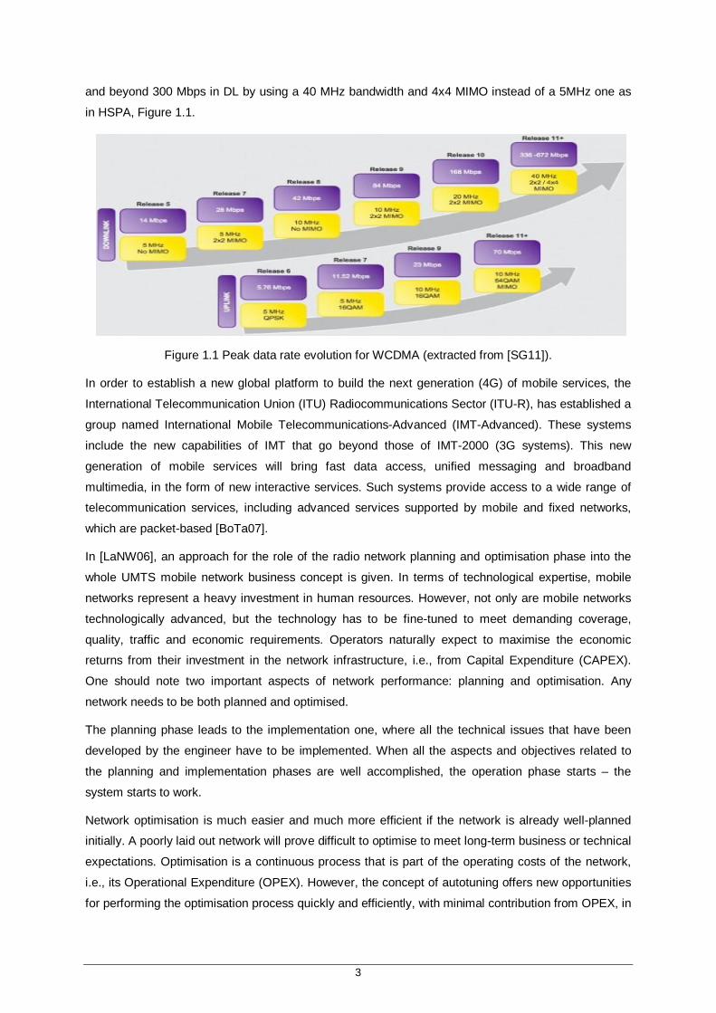
List of Figures Figure 1.1 Peak data rate evolution for WCDMA (extracted from [SG11]). ........................................... 3
Figure 2.1 UMTS network architecture (extracted from [Corr10]). ........................................................ 8
Figure 2.3 The structure for GPRS/EGPRS counters with object types (extracted from [Eric06]). ....... 16
Figure 2.2 Factors that can affect the GPRS/EGPRS user perceived performance perception (adapted from [Eric06]). .................................................................................................................... 17
Figure 2.4 UTRAN observability model (extracted from [Eric08])........................................................ 22
Figure 3.1 Database search algorithm. .............................................................................................. 30
Figure 3.2 Analysis flow chart (adapted from [Eric98]). ...................................................................... 32
Figure 3.3 Analysis algorithm of 푅퐶퐷. ................................................................................................ 33
Figure 3.4 Analysis algorithm of 푅푆퐷퐶퐶퐻퐷. ....................................................................................... 33
Figure 3.5 Call establishment process. .............................................................................................. 34
Figure 3.6 Analysis algorithm of 푅퐶푆푆. .............................................................................................. 34
Figure 3.7 Low TCH Assignment Success Rate analysis (adapted from [Eric98]). ............................. 35
Figure 3.8 HO performance analysis (adapted from [Eric98]). ............................................................ 36
Figure 3.9 Few HO attempts (adapted from [Eric98]). ........................................................................ 37
Figure 3.10 Unsuccessful HOs analysis – part I (adapted from [Eric98]). ........................................... 38
Figure 3.11 Unsuccessful HOs analysis – part II (adapted from [Eric98]). .......................................... 39
Figure 3.12 Analysis algorithm of GSM IP throughput KPIs. .............................................................. 40
Figure 3.13 Analysis algorithm of 푅푃퐷퐶퐻푆. ....................................................................................... 41
Figure 3.14 RRC/RAB connection/establishment scenario algorithm – part I (adapted from [Eric09]). ........................................................................................................................................ 42
Figure 3.15 RRC/RAB connection/establishment scenario algorithm – part II (adapted from [Eric09]). ........................................................................................................................................ 43
Figure 3.16 Speech Call Drop Rate algorithm. ................................................................................... 44
Figure 3.17 Data call drop rate analysis algorithm. ............................................................................ 46
Figure 3.18 PS/HS Throughput analysis algorithm............................................................................. 46
xii
Figure 3.19 Soft HO analysis algorithm. ............................................................................................ 47
Figure 4.1 BS 2 – 푅퐶퐷 and 푅퐻푂푆 performance analysis: correlation value of -91.24%. ..................... 52
Figure 4.2 TCH Drops analysis.......................................................................................................... 53
Figure 4.3 Type of interference (adapted from [Eric98]). .................................................................... 53
Figure 4.4 BS 17 – 푅퐶퐷 and 푅푆퐷퐶퐶퐻퐷 performance analysis: correlation value of -52.03%. ............. 54
Figure 4.5 BS 6 – 푅퐶퐷 and 푅퐶푆푆 performance analysis: correlation value of 53.38%. ........................ 55
Figure 4.6 BS 13 – 푅퐶퐷 and 푅퐶푆푆 performance analysis: correlation value of -81.49%...................... 55
Figure 4.7 BS 36 – 푅푆퐷퐶퐶퐻퐷 and 푅퐶푆푆 performance analysis: correlation value of -96.68%. ............ 56
Figure 4.8 BS 21 – HO relation.......................................................................................................... 57
Figure 4.9 BS 21 – Unsuccessful HOs............................................................................................... 57
Figure 4.10 BS 49 - 푇퐺푃푅푆퐷퐿and 푅푃퐷퐶퐻푆 performance analysis: correlation value of 42.65%. ........ 58
Figure 4.11 BS 49 - 푇퐺푃푅푆푈퐿and 푅푃퐷퐶퐻푆 performance analysis: correlation value of -10.41%. ....... 59
Figure 4.12 BS 49 – DL Radio Link Quality analysis. ......................................................................... 59
Figure 4.13 BS 20 - 푇퐸퐷퐺퐸퐷퐿and 푅푃퐷퐶퐻푆 performance analysis: correlation value of -41.28%. ...... 61
Figure 4.14 BS 20 - 푇퐸퐷퐺퐸푈퐿and 푅푃퐷퐶퐻푆 performance analysis: correlation value of -65.37%. ...... 61
Figure 4.15 DL Radio link quality analysis. ........................................................................................ 62
Figure 4.16 UL Radio link quality analysis. ........................................................................................ 62
Figure 4.17 BS 8 – 푅푆퐶푆푆and 푅푆퐶퐷 performance analysis: correlation value of -51.31%. ................. 65
Figure 4.18 BS 8 – Total number of failures after admission control versus “RRC success rate”. ....... 66
Figure 4.19 BS 58 – 푅푃푆푅99_퐼퐶푆푆and 푅푃푆푅99_퐼퐶퐷 performance analysis: correlation value of -65.00%. ........................................................................................................................................ 67
Figure 4.20 Channel Upswitch Failure Rate DL. ................................................................................ 67
Figure 4.21 Channel Upswitch Failure Rate UL. ................................................................................ 68
Figure 4.22 BS 58 – Total number of failures after admission control versus “RRC success rate”. ..... 68
Figure 4.23 BS 58 – Abnormal RAB PS DCH/FACH releases and normal RAB speech releases. ...... 69
Figure 4.24 BS 51 – 푅퐻푆퐷푃퐴_퐼퐶푆푆 and 푅퐻푆퐷푃퐴_퐼퐶퐷 performance analysis: correlation value of -28.31%. ........................................................................................................................................ 70
Figure 4.25 BS 51 – Channel Upswitch Failure Rate DL. ................................................................... 70
Figure 4.26 BS 51 – Channel Upswitch Failure Rate UL. ................................................................... 70
Figure 4.27 BS 51 – Total number of failures after admission control versus “RRC success rate”. ..... 71
Figure 4.28 BS 51 – Abnormal RAB PS HSDPA releases and normal RAB speech releases. ............ 72
xiii
Figure 4.29 BS 6 – 푅푆퐶퐷 and 푅푆퐻푂푆 performance analysis: correlation value of -68.55%. ................ 73
Figure 4.30 DL cell traffic volume. ..................................................................................................... 75
Figure 4.31 UL cell traffic volume. ..................................................................................................... 76
Figure 4.32 BS 11 – Throughput versus number of users. ................................................................. 76
Figure 4.33 Channel upswitch failure rate DL. ................................................................................... 77
Figure 4.34 Channel upswitch failure rate UL. ................................................................................... 77
Figure 4.35 HS user throughput and number of HS users.. ................................................................ 78
Figure 4.36 Channel upswitch failure rate DL. ................................................................................... 78
Figure 4.37 Channel upswitch failure rate UL. ................................................................................... 78
Figure B.1 Call Drop Rate. ................................................................................................................ 98
Figure B.2 Speech Call Drop Rate..................................................................................................... 99
Figure B.3 Handover Success Rate................................................................................................... 99
Figure B.4 Soft Handover Success Rate. ........................................................................................ 100
Figure B.5 R99 Downlink User Throughput...................................................................................... 100
Figure B.6 GPRS Downlink Throughput. ......................................................................................... 101
Figure B.7 Call Setup Success Rate. ............................................................................................... 101
Figure B.8 Edge Downlink Throughput. ........................................................................................... 102
Figure B.9 Edge Uplink Throughput................................................................................................. 102
Figure B.10 GPRS Uplink Throughput. ............................................................................................ 103
Figure B.11 PDCH Assignment Success Rate. ................................................................................ 103
Figure B.12 SDCCH Drop Rate. ...................................................................................................... 104
Figure B.13 CS64 Call Drop Rate. ................................................................................................... 104
Figure B.14 CS64 Call Setup Success Rate. ................................................................................... 105
Figure B.15 HSDPA Interactive Call Setup Success Rate. ............................................................... 105
Figure B.16 PS R99 Interactive Call Setup Success Rate. ............................................................... 106
Figure B.17 Speech Call Setup Success Rate. ................................................................................ 106
Figure B.18 HSDPA Interactive Call Drop Rate. .............................................................................. 107
Figure B.19 HSDPA Interactive User Throughput. ........................................................................... 107
Figure B.20 IRAT HO Success Rate Incoming................................................................................. 108
Figure B.21 IRAT HO Success Rate Outgoing................................................................................. 108

xiv
Figure B.22 PS R99 Interactive Call Drop Rate. .............................................................................. 109
Figure B.23 PS R99 Interactive Uplink User Throughput.................................................................. 109
Figure C.1 TCH Drops analysis. ...................................................................................................... 112
Figure C.2 Comparing 푅퐶퐷 and 푅퐻푂푆 performance. ....................................................................... 113
Figure C.3 SDCCH Drops analysis. ................................................................................................. 113
Figure C.4 SDCCH Drop Rate. ........................................................................................................ 114
Figure C.5 Call Setup Success Rate. .............................................................................................. 114
Figure C.6 푅퐶푆푆 results if 푅퐶푆푆 = 1 −푅푆퐷퐶퐶퐻퐷. ........................................................................... 115
Figure C.7 HO success rate performance. ....................................................................................... 116
Figure C.8 Unsuccessful HOs. ........................................................................................................ 116
Figure C.9 Radio Link Quality analysis (GPRS). .............................................................................. 117
Figure C.10 Radio Link Quality analysis (EDGE). ............................................................................ 117
Figure D.1 BS 6 – 푅퐶퐷 and 푅퐻푂푆 performance analysis: correlation value of -69.80%. ................... 120
Figure D.2 BS 3 – 푅퐶퐷 and 푅푆퐷퐶퐶퐻퐷 performance analysis: correlation value of 7.62%. ............... 121
Figure D.3 BS 11 – 푅퐶퐷 and 푅푆퐷퐶퐶퐻퐷 performance analysis: correlation value of 51.71%. ........... 121
Figure D.4 BS 12 – 푅퐶퐷 and 푅푆퐷퐶퐶퐻퐷 performance analysis: correlation value of 38.59%. ........... 122
Figure D.5 BS 13 – 푅퐶퐷 and 푅푆퐷퐶퐶퐻퐷 performance analysis: correlation value of 12.44%. ........... 122
Figure D.6 BS 7 – 푅푆퐷퐶퐶퐻퐷 and 푅퐶푆푆 performance analysis: correlation value of 12.48%. ............ 124
Figure D.7 BS 6 – 푅푆퐷퐶퐶퐻퐷 and 푅퐶푆푆 performance analysis: correlation value of -90.17%. ........... 124
Figure D.8 BS 19 – 푅푆퐷퐶퐶퐻퐷 and 푅퐶푆푆 performance analysis: correlation value of -99.30%. ......... 125
Figure D.9 BS 40 – 푅푆퐷퐶퐶퐻퐷 and 푅퐶푆푆 performance analysis: correlation value of -96.31%. ......... 125
Figure D.10 BS 17 – 푅푆퐷퐶퐶퐻퐷 and 푅퐶푆푆 performance analysis: correlation value of -98.35%. ....... 126
Figure D.11 BS 25 – 푅푆퐷퐶퐶퐻퐷 and 푅퐶푆푆 performance analysis: correlation value of -97.89%. ....... 126
Figure D.12 BS 44 – 푅푆퐷퐶퐶퐻퐷 and 푅퐶푆푆 performance analysis: correlation value of 11.34%. ........ 127
Figure D.13 BS 8 – 푅푆퐷퐶퐶퐻퐷 and 푅퐶푆푆 performance analysis: correlation value of -85.03%. ......... 127
Figure D.14 BS 43 – 푅푆퐷퐶퐶퐻퐷 and 푅퐶푆푆 performance analysis: correlation value of -92.55%. ....... 128
Figure D.15 BS 45 - 푇퐺푃푅푆퐷퐿and 푅푃퐷퐶퐻푆 performance analysis: correlation value of -11.37%. .... 133
Figure D.16 BS 45 - 푇퐺푃푅푆푈퐿and 푅푃퐷퐶퐻푆 performance analysis: correlation value of -11.04%. .... 134
Figure D.17 BS 41 - 푇퐺푃푅푆퐷퐿and 푅푃퐷퐶퐻푆 performance analysis: correlation value of 5.61%......... 134
Figure D.18 BS 41 - 푇퐺푃푅푆푈퐿and 푅푃퐷퐶퐻푆 performance analysis: correlation value of 13.56%. ...... 135
xv
Figure D.19 BS 40 - 푇퐺푃푅푆퐷퐿and 푅푃퐷퐶퐻푆 performance analysis: correlation value of -5.81%. ...... 135
Figure D.20 BS 40 - 푇퐺푃푅푆푈퐿and 푅푃퐷퐶퐻푆 performance analysis: correlation value of -0.64%. ...... 136
Figure D.21 BS 24 - 푇퐺푃푅푆퐷퐿and 푅푃퐷퐶퐻푆 performance analysis: correlation value of 0.38%......... 136
Figure D.22 BS 24 - 푇퐺푃푅푆푈퐿and 푅푃퐷퐶퐻푆 performance analysis: correlation value of -2.74%. ...... 137
Figure D.23 BS 37 - 푇퐺푃푅푆퐷퐿and 푅푃퐷퐶퐻푆 performance analysis: correlation value of -22.53%. .... 137
Figure D.24 BS 37 - 푇퐺푃푅푆푈퐿and 푅푃퐷퐶퐻푆 performance analysis: correlation value of -4.18%. ...... 138
Figure D.25 BS 23 - 푇퐺푃푅푆퐷퐿and 푅푃퐷퐶퐻푆 performance analysis: correlation value of -2.18%. ...... 138
Figure D.26 BS 23 - 푇퐺푃푅푆푈퐿and 푅푃퐷퐶퐻푆 performance analysis: correlation value of -32.66%. .... 139
Figure D.27 BS 34 - 푇퐸퐷퐺퐸퐷퐿and 푅푃퐷퐶퐻푆 performance analysis: correlation value of -1.91%. ...... 141
Figure D.28 BS 34 - 푇퐸퐷퐺퐸푈퐿and 푅푃퐷퐶퐻푆 performance analysis: correlation value of -14.20%. .... 141
Figure D.29 BS 71 - 푇퐸퐷퐺퐸퐷퐿and 푅푃퐷퐶퐻푆 performance analysis: correlation value of -18.82%. .... 142
Figure D.30 BS 71 - 푇퐸퐷퐺퐸푈퐿and 푅푃퐷퐶퐻푆 performance analysis: correlation value of -6.15%. ...... 142
Figure D.31 BS 87 - 푇퐸퐷퐺퐸퐷퐿and 푅푃퐷퐶퐻푆 performance analysis: correlation value of -32.10%. .... 143
Figure D.32 BS 87 - 푇퐸퐷퐺퐸푈퐿and 푅푃퐷퐶퐻푆 performance analysis: correlation value of -34.66%. .... 143
Figure D.33 BS 80 - 푇퐸퐷퐺퐸퐷퐿and 푅푃퐷퐶퐻푆 performance analysis: correlation value of -25.08%. .... 144
Figure D.34 BS 80 - 푇퐸퐷퐺퐸푈퐿and 푅푃퐷퐶퐻푆 performance analysis: correlation value of -39.91%. .... 144
Figure D.35 BS 51 - 푇퐸퐷퐺퐸퐷퐿and 푅푃퐷퐶퐻푆 performance analysis: correlation value of -31.41%. .... 145
Figure D.36 BS 51 - 푇퐸퐷퐺퐸푈퐿and 푅푃퐷퐶퐻푆 performance analysis: correlation value of -50.61%. .... 145
Figure D.37 BS 83 - 푇퐸퐷퐺퐸퐷퐿and 푅푃퐷퐶퐻푆 performance analysis: correlation value of -4.50%. ...... 146
Figure D.38 BS 83 - 푇퐸퐷퐺퐸푈퐿and 푅푃퐷퐶퐻푆 performance analysis: correlation value of -3.25%. ...... 146
Figure D.39 BS 10 – 푅푆퐶푆푆and 푅푆퐶퐷 performance analysis: correlation value of -36.84%. ............. 147
Figure D.40 BS 10 – Total number of failures after admission control versus “RRC success rate”. ... 148
Figure D.41 BS 67 – 푅퐻푆퐷푃퐴_퐼퐶푆푆 and 푅퐻푆퐷푃퐴_퐼퐶퐷 performance analysis: correlation value of -0.80%. ........................................................................................................................................ 150
Figure D.42 BS 42 – 푅퐻푆퐷푃퐴_퐼퐶푆푆 and 푅퐻푆퐷푃퐴_퐼퐶퐷 performance analysis: correlation value of -18.39%. ........................................................................................................................................ 150
Figure D.43 BS 55 – 푅퐻푆퐷푃퐴_퐼퐶푆푆 and 푅퐻푆퐷푃퐴_퐼퐶퐷 performance analysis: correlation value of -18.63%. ........................................................................................................................................ 151
Figure D.44 BS 39 – 푅퐻푆퐷푃퐴_퐼퐶푆푆 and 푅퐻푆퐷푃퐴_퐼퐶퐷 performance analysis: correlation value of -7.23%. ........................................................................................................................................ 151
Figure D.45 BS 8 – 푅퐻푆퐷푃퐴_퐼퐶푆푆 and 푅퐻푆퐷푃퐴_퐼퐶퐷 performance analysis: correlation value of -0.85%. ........................................................................................................................................ 152

xvi
Figure D.46 BS 67 – Channel Upswitch Failure Rate DL. ................................................................ 152
Figure D.47 BS 67 – Channel Upswitch Failure Rate UL. ................................................................ 152
Figure D.48 BS 67 – Total number of failures after admission control versus “RAB success rate”. ... 153
Figure D.49 BS 67 – Abnormal RAB PS HSDPA releases and normal RAB speech releases. ......... 154
Figure D.50 BS 42 – Channel Upswitch Failure Rate DL. ................................................................ 154
Figure D.51 BS 42 – Channel Upswitch Failure Rate UL. ................................................................ 154
Figure D.52 BS 42 – Total number of failures after admission control versus “RAB success rate”. ... 155
Figure D.53 Abnormal RAB PS HSDPA releases and normal RAB speech releases. ....................... 156
Figure D.54 BS 55 – Channel Upswitch Failure Rate DL. ................................................................ 156
Figure D.55 BS 55 – Channel Upswitch Failure Rate UL. ................................................................ 156
Figure D.56 BS 55 – Total number of failures after admission control versus “RAB success rate”. ... 157
Figure D.57 BS 55 – Abnormal RAB PS HSDPA releases and normal RAB speech releases. ......... 158
Figure D.58 BS 39 – Channel Upswitch Failure Rate DL. ................................................................ 158
Figure D.59 BS 39 – Channel Upswitch Failure Rate UL. ................................................................ 158
Figure D.60 BS 39 – Total number of failures after admission control versus “RAB success rate”. ... 159
Figure D.61 BS 39 – Abnormal RAB PS HSDPA releases and normal RAB speech releases. ......... 160
Figure D.62 BS 8 – Channel Upswitch Failure Rate DL. .................................................................. 160
Figure D.63 BS 8 – Channel Upswitch Failure Rate UL. .................................................................. 160
Figure D.64 BS 8 – Total number of failures after admission control versus “RAB success rate”. ..... 161
Figure D.65 BS 8 – Abnormal RAB PS HSDPA releases and normal RAB speech releases. ........... 162

xvii
List of Tables
List of Tables Table 2.1 GSM/GPRS transmission rate with different coding schemes (extracted from [LeMa01]). ... 10
Table 2.2 UMTS transmission rate (extracted from [Corr10]). ............................................................ 11
Table 2.3 R99 and HSDPA comparison Table (adapted from [HoTo06]). ........................................... 12
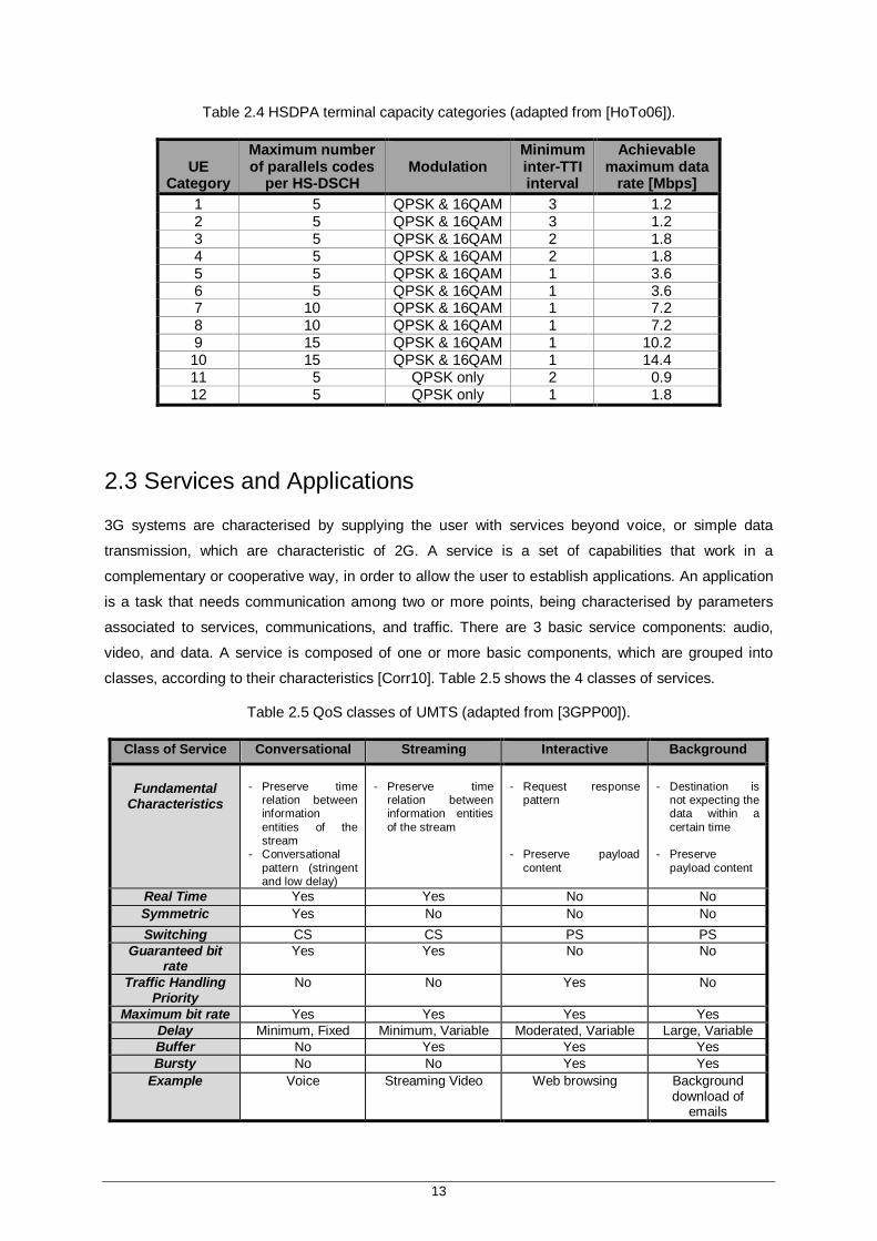
Table 2.4 HSDPA terminal capacity categories (adapted from [HoTo06]). .......................................... 13
Table 2.5 QoS classes of UMTS (adapted from [3GPP00]). ............................................................... 13
Table 2.6 Bit rates and applications of different services (adapted from [Lope08] and [3GPP05]). ...... 14
Table 2.7 GSM KPIs Target and Range of Values. ............................................................................ 17
Table 2.8 UMTS KPIs Target and Range of Values ........................................................................... 22
Table 4.1 Monthly KPIs performance. ................................................................................................ 50
Table 4.2 KPIs analysis after filtering. ................................................................................................ 51
Table 4.3 푅퐶퐷 correlation analysis. ................................................................................................... 52
Table 4.4 푅푆퐷퐶퐶퐻퐷 correlation analysis. .......................................................................................... 56
Table 4.5 HO performance results. .................................................................................................... 57
Table 4.6 푇퐺푃푅푆퐷퐿, 푇퐺푃푅푆푈퐿and 푅푃퐷퐶퐻푆 correlation values. ......................................................... 58
Table 4.7 푇퐸퐷퐺퐸퐷퐿, 푇퐸퐷퐺퐸푈퐿and 푅푃퐷퐶퐻푆 correlation analysis. ..................................................... 60
Table 4.8 Monthly KPIs. .................................................................................................................... 63
Table 4.9 KPIs analysis after filtering. ................................................................................................ 64
Table 4.10 푅푆퐶푆푆 correlation analysis. .............................................................................................. 64
Table 4.11 푅푃푆푅99_퐼퐶푆푆 correlation analysis. ................................................................................... 67
Table 4.12 푅퐻푆퐷푃퐴_퐼퐶푆푆 correlation analysis. ................................................................................. 69
Table 4.13 푅푆퐶퐷 and 푅푆퐻푂푆 correlation analysis. ............................................................................. 73
Table 4.14 푅푃푆푅99_퐼퐶퐷 and 푅푆퐻푂푆 correlation analysis. .................................................................. 74
Table 4.15 푅퐻푆퐷푃퐴_퐼퐶퐷 and 푅푆퐻푂푆 correlation analysis. ................................................................. 74
Table 4.16 푇푃푆푅99퐷퐿and 푇푃푆푅99푈퐿 analysis................................................................................... 75
Table D.1 푅퐶퐷 analysis. .................................................................................................................. 120
xviii
Table D.2 푅푆퐷퐶퐶퐻퐷 analysis. ......................................................................................................... 123
Table D.3 HO performance results. ................................................................................................. 130
Table D.4 GPRS throughput performance results. ........................................................................... 132
Table D.5 EDGE throughput performance results. ........................................................................... 140
Table D.6 푅푆퐶푆푆 analysis. ............................................................................................................... 147
Table D.7 푅푃푆푅99_퐼퐶푆푆 analysis. .................................................................................................... 149
Table D.8 푅퐻푆퐷푃퐴_퐼퐶푆푆 analysis. ................................................................................................... 149
Table D.9 푅푆퐶퐷 and 푅푆퐻푂푆 analysis. ............................................................................................. 162
Table D.10 푅푃푆푅99_퐼퐶퐷 and 푅푆퐻푂푆 analysis.................................................................................. 163
Table D.11 푅퐻푆퐷푃퐴_퐼퐶퐷 and 푅푆퐻푂푆 analysis. ............................................................................... 163
Table E.1 Site Names. .................................................................................................................... 166

xix
List of Acronyms
List of Acronyms 3G Third Generation
3GPP ASE
Third Generation Partnership Project Air Speech Equivalent
BCCH Broadcast Control Channel
BS Base Station
BSC Base Station Controller
BSS Base Station Subsystem
BTS CIR
Base Transceiver Station Carrier to Interference
CN Core Network
CP Central Processor
CS Circuit Switch
DL Downlink
DS-CDMA Direct-Sequence CDMA
DTX Discontinuous Transmission
E-AGCH E-DCH Absolute Grant Channel
E-DCH Enhanced Dedicated Channel
EDGE Enhanced Data for GSM Evolution
E-DPCCH Enhanced DPCCH
E-DPDCH E-DCH Dedicated Physical Data Channel
E-HICH E-DCH HARQ Indicator Channel
E-RGCH E-DCH Relative Grant Channel
FACH Forward Access Channel
FDD Frequency Division Duplex
FDMA Frequency Division Multiple Access
FER Frame Error Ratio
GGSN Gateway GPRS Support Node
GMSC Gateway MSC
GMSK Gaussian Minimum Shift Keying
GPRS General Packet Radio Service
GSM Global System for Mobile Communications
HARQ Hybrid Automatic Repeat Request
HLR Home Location Register
HO Handover

xx
HS High Speed
HSys Home System
HSDPA High Speed Downlink Packet Access
HS-DPCCH High-Speed Dedicated Physical Control Channel
HS-DSCH High-Speed Downlink Shared Channel
HSPA High Speed Packet Access
HS-PDSCH High-Speed Physical Downlink Shared Channel
HS-SCCH High-Speed Shared Control Channel
HSUPA High Speed Uplink Packet Access
HW Hardware
IRAT HO Inter-Radio Access Technology HO
KPI Key Performance Indicator
LLC Logical Link Control
MAC Medium Access Control
MDB Measurement Database
ME Mobile Equipment
MO Managed Objects
MS Mobile Station
MSC Mobile Switching Centre
MT Mobile Terminal
O&M Operation and Maintenance
OSS Operation and Support System
OVSF Orthogonal Variable Spreading Factor
PDCH Packet Data Channel
PDU Protocol Data Unit
PLMN Public Land Mobile Network
PS Packet Switch
QAM Quadrature Amplitude Modulation
QoS Quality of Service
RAB Radio Access Bearer
RAN Radio Access Network
RL Radio Link
RLC Radio Link Control
RNC Radio Network Controller
RRC Radio Resource Control
RRM Radio Resource Management
RSSI Received Signal Strenght Indicator
RXQUAL Received Quality of Speech
SC Scrambling Code
SDCCH Stand-Alone Dedicated Control Channel

xxi
SF Spreading Factor
SGSN Serving GPRS Support Node
SHO Soft HO
SMS Short Message Service
SQL Structured Query Language
SQS Speech Quality Supervision
SRB Signalling Radio Bearer
STS Statistics and Traffic Measurement Subsystem
SW Software
TA Timing Advance
TCH Traffic Channel
TCP Transmission Control Protocol
TDD Time Division Duplex
TDMA Time Division Multiple Access
THP Traffic Handling Priority
TN Transport Network
TS Time Slot
TTI Transmission Time Interval
UE User Equipment
UL Uplink

xxii
List of Symbols
List of Symbols 퐷 Accumulated total LLC data received on the downlink in EDGE
mode transfers for QoS class Background
퐷 Accumulated total LLC data received on the uplink in EDGE mode transfers for QoS class Background
퐷 Amount of IP data for all downlink EDGE mode transfers for QoS class Interactive THP1
퐷 Amount of IP data for all uplink EDGE mode transfers for QoS class Interactive THP1
퐷 Amount of IP data for all downlink EDGE mode transfers for QoS class Interactive THP2
퐷 Amount of IP data for all uplink EDGE mode transfers for QoS class Interactive THP2
퐷 Amount of IP data for all downlink EDGE mode transfers for QoS class Interactive THP3
퐷 Amount of IP data for all uplink EDGE mode transfers for QoS class Interactive THP3
퐷 Accumulated total LLC data received on the downlink in GPRS mode transfers for QoS class Background
퐷 Accumulated total LLC data received on the uplink in GPRS mode transfers for QoS class Background
퐷 Amount of IP data for all downlink GPRS mode transfers for QoS class Interactive THP1
퐷 Amount of IP data for all uplink GPRS mode transfers for QoS class Interactive THP1
퐷 Amount of IP data for all downlink GPRS mode transfers for QoS class Interactive THP2
퐷 Amount of IP data for all uplink GPRS mode transfers for QoS class Interactive THP2
퐷 Amount of IP data for all downlink GPRS mode transfers for QoS class Interactive THP3
퐷 Amount of IP data for all uplink GPRS mode transfers for QoS class Interactive THP3
푁 Successful Mobile Station channel establishments on SDCCH
푁 Number of RLC Downlink Samples
푁 Number of RLC Uplink Samples
푁 _ Number of Abnormal RAB speech releases
푁 Total number of BSs
푁 _ Number of Abnormal RAB CS64 releases.
xxiii
푁 Total number of all the RAB CS64 releases
푁 Minimum number of calls
푁 Number of intra cell handover attempts (decisions) at bad downlink quality
푁_
Number of intra cell handover attempts (decisions) for both links with bad quality
푁 Number of intra cell handover attempts (decisions) at bad uplink quality
푁 Number of successful intra cell handovers
푁 Number of handover commands sent to the MS
푁 Number of successful handover to the neighbouring cell
푁 Total number of hours
푁 __ Number of all the success of outgoing (to GSM) IRAT for RAB Speech and Multi RAB
푁 _ Number of total of incoming IRAT Handover Successful attempts for CS RAB total attempts
푁 _ Number of total of outgoing (to GSM) IRAT for RAB Speech and Multi RAB attempts
푁 _ Number of incoming IRAT Handover Successful attempts for CS RAB
푁 Number of first assignment attempts on TCH for all MS power classes
푁 Number of assignment complete messages for all MS power classes in underlaid subcell, full-rate
푁 Number of assignment complete messages for all MS power classes in underlaid subcell, half-rate
푁 Number of packet channel allocation attempts
푁 Number of packet channel allocation failures
푁 _ Number of problematic hours per BS
푁 _ _ _ Total number of all the RAB PS DCH/FACH releases
푁 _ _ Total number of all the RAB PS HSDPA releases
푁 _ _ _ Number of all the abnormal RAB PS DCH/FACH releases
푁 _ _ Number of all the abnormal RAB PS HSDPA releases
푁 Total number of all the RAB speech releases
푁 Total number of RL addition attempts
푁 Total number of RL addition success
푁 Total number of dropped SDCCH channels in a cell
푁 Total amount of TCH drops
푁 Number of RLC HS Samples
푁 Total number of terminated calls in a cell
푁 _ Total number of problematic BSs

xxiv
푅 Call Drop Rate
푅 _ RAB Establishment Success Rate for CS64
푅 CS64 Call Drop Rate
푅 CS64 Call Setup Success Rate
푅 CS RRC Success Rate
푅 Call Setup Success Rate
푅 Handover Success Rate
푅 _ HSDPA Interactive Call Drop Rate
푅 _ HSDPA Interactive Call Setup Success Rate
푅 _ IRAT CS Handover Success Rate Incoming
푅 _ IRAT CS Handover Success Rate Outgoing
푅 Packet Data Channel Assignment Success Rate
푅 _ PS R99 Interactive Call Drop Rate
푅 _ PS R99 Interactive Call Setup Success Rate
푅 PS RRC Success Rate
푅 _ _ _ RAB Establishment Success Rate PS DCH/FACH
푅 _ _ RAB Establishment Success Rate PS HS
푅 RAB Establishment Success Rate Speech
푅 Speech Call Drop Rate
푅 Speech Call Setup Success Rate
푅 SDCCH Drop Rate
푅 Percentage for drop on SDCCH
푅 Soft Handover Success Rate
푅 TCH Assignment Failure Rate
푇 EDGE Downlink Throughput
푇 EDGE Uplink Throughput
푇 GPRS Downlink Throughput
푇 GPRS Uplink Throughput
푇 RLC HSDPA Throughput
푇 HSDPA Interactive User Throughput
푇 PS R99 Interactive Downlink User Throughput
푇 PS R99 Interactive Uplink User Throughput
푇 RLC Downlink Throughput
푇 RLC Uplink Throughput
푇퐷 Accumulation of (LLC throughout x LLC data volume) for all uplink EDGE mode transfers for QoS class Background
xxv
푇퐷 Accumulation of (LLC throughout x LLC data volume) for all downlink EDGE mode transfers for QoS class Background
푇퐷 Accumulation of (LLC throughput x LLC data volume) for all downlink EDGE mode transfers for QoS class Interactive THP1
푇퐷 Accumulation of (LLC throughput x LLC data volume) for all uplink EDGE mode transfers for QoS class Interactive THP1
푇퐷 Accumulation of (LLC throughput x LLC data volume) for all downlink EDGE mode transfers for QoS class Interactive THP2
푇퐷 Accumulation of (LLC throughput x LLC data volume) for all uplink EDGE mode transfers for QoS class Interactive THP2
푇퐷 Accumulation of (LLC throughput x LLC data volume) for all downlink EDGE mode transfers for QoS class Interactive THP3
푇퐷 Accumulation of (LLC throughput x LLC data volume) for all uplink EDGE mode transfers for QoS class Interactive THP3
푇퐷 Accumulation of (LLC throughout x LLC data volume) for all downlink GPRS mode transfers for QoS class Background
푇퐷 Accumulation of (LLC throughout x LLC data volume) for all uplink GPRS mode transfers for QoS class Background
푇퐷 Accumulation of (LLC throughput x LLC data volume) for all downlink GPRS mode transfers for QoS class Interactive THP1
푇퐷 Accumulation of (LLC throughput x LLC data volume) for all uplink GPRS mode transfers for QoS class Interactive THP1
푇퐷 Accumulation of (LLC throughput x LLC data volume) for all downlink GPRS mode transfers for QoS class Interactive THP2
푇퐷 Accumulation of (LLC throughput x LLC data volume) for all uplink GPRS mode transfers for QoS class Interactive THP2
푇퐷 Accumulation of (LLC throughput x LLC data volume) for all downlink GPRS mode transfers for QoS class Interactive THP3
푇퐷 Accumulation of (LLC throughput x LLC data volume) for all uplink GPRS mode transfers for QoS class Interactive THP3

xxvi
List of
List of Software Microsoft Word Text editor tool
Microsoft Excel Calculation tool
Microsoft Visio Design tool (e.g., flowcharts, diagrams, etc.)
MySQL Relational database management tool
Matlab Computational math tool
MapInfo Geographic Information Systems (GIS) software

1
Chapter 1
Introduction 1 Introduction
This chapter gives a brief overview of the work. Before establishing work targets and original
contributions, the scope and motivations are brought up. At the end of the chapter, the layout of the
work is presented.
2
1.1 Overview and Motivation
Wireless communications is, by any measure, the fastest growing segment of the communications
industry. As such, it has captured the attention of the media and the imagination of the public. Cellular
networks have experienced an exponential growth for many years. Indeed, mobile phones have
become a critical business tool and part of everyday life in most developed countries, as they are
rapidly supplanting the old wire line systems. The explosive growth of wireless systems, coupled with
the proliferation of laptop and palmtop computers, indicate a bright future for wireless networks, both
as stand-alone systems and as part of the larger networking infrastructure. However, many technical
challenges remain in designing robust wireless networks that deliver the performance necessary to
support emerging applications [Gold05].
Second-generation (2G) telecommunication systems, such as the Global System for Mobile
Communications (GSM), enabled voice traffic to go wireless, with the number of mobile phones
exceeding the number of landline ones, and the mobile phone penetration going beyond 100% in
several markets. However, the data-handling capabilities of 2G systems are limited, and third-
generation (3G) ones were needed to provide the high bit-rate services that enable high-quality
images and video to be transmitted, and to provide access to the Internet with higher data rates.
In 1999, the 3rd Generation Partnership Project (3GPP) launched Universal Mobile
Telecommunication System (UMTS), one of the 3G systems, also called Release ’99, as a response
to the needs of higher data rates, being usually deployed on top of GSM networks. The air interface is
Wideband Code Division Multiple Access (WCDMA), featuring a data up to 384 kbps for the Downlink
(DL) and Uplink (UL), despite having a theoretical maximum for DL of 2 Mbps. Although packet-data
communications were already supported in this first release of the standard, an evolution emerged in
2002, Release 5, introducing the High Speed DL Packet Access (HSDPA) and bringing further
enhancements to the provisioning of packet-data services, both in terms of system and end-user
performance. This release enables a more realistic 2 Mbps and even beyond, with data rates up to
14Mbps. The DL packet-data enhancements of HSDPA are complemented by Enhanced UL,
introduced in Release 6, also known as High Speed UL Packet Access (HSUPA). HSDPA and
HSUPA are often jointly referred to as High-Speed Packet Access (HSPA), being build upon the basic
structure, and with a requirement on backwards compatibility, since it is implemented on already
deployed networks.
3GPP is also working to specify a new radio system called Long-Term Evolution (LTE). Release 7 and
8, solutions for HSPA evolution, will be worked in parallel with LTE development, and some aspects of
LTE work are also expected to reflect on HSPA evolution. HSPA evolution in Release 7 brings a
maximum throughput of 28 Mbps in DL and 11 Mbps in UL, [HoTo07]. LTE will then push further the
peak rates beyond 100 Mbps in DL and 50 Mbps in UL by using a 20 MHz bandwidth and 2x2 MIMO,
3
and beyond 300 Mbps in DL by using a 40 MHz bandwidth and 4x4 MIMO instead of a 5MHz one as
in HSPA, Figure 1.1.
Figure 1.1 Peak data rate evolution for WCDMA (extracted from [SG11]).
In order to establish a new global platform to build the next generation (4G) of mobile services, the
International Telecommunication Union (ITU) Radiocommunications Sector (ITU-R), has established a
group named International Mobile Telecommunications-Advanced (IMT-Advanced). These systems
include the new capabilities of IMT that go beyond those of IMT-2000 (3G systems). This new
generation of mobile services will bring fast data access, unified messaging and broadband
multimedia, in the form of new interactive services. Such systems provide access to a wide range of
telecommunication services, including advanced services supported by mobile and fixed networks,
which are packet-based [BoTa07].
In [LaNW06], an approach for the role of the radio network planning and optimisation phase into the
whole UMTS mobile network business concept is given. In terms of technological expertise, mobile
networks represent a heavy investment in human resources. However, not only are mobile networks
technologically advanced, but the technology has to be fine-tuned to meet demanding coverage,
quality, traffic and economic requirements. Operators naturally expect to maximise the economic
returns from their investment in the network infrastructure, i.e., from Capital Expenditure (CAPEX).
One should note two important aspects of network performance: planning and optimisation. Any
network needs to be both planned and optimised.
The planning phase leads to the implementation one, where all the technical issues that have been
developed by the engineer have to be implemented. When all the aspects and objectives related to
the planning and implementation phases are well accomplished, the operation phase starts – the
system starts to work.
Network optimisation is much easier and much more efficient if the network is already well-planned
initially. A poorly laid out network will prove difficult to optimise to meet long-term business or technical
expectations. Optimisation is a continuous process that is part of the operating costs of the network,
i.e., its Operational Expenditure (OPEX). However, the concept of autotuning offers new opportunities
for performing the optimisation process quickly and efficiently, with minimal contribution from OPEX, in

4
order to maximise network revenues.
Operators face the following challenges in the planning of 3G networks:
Planning means not only meeting current standards and demands, but also complying with
future requirements in the sense of an acceptable development path.
There is much uncertainty about future traffic growth and the expected proportions of different
kinds of traffic and different data rates.
New and demanding higher bit rate services require the knowledge of coverage and capacity
enhancement methods, and advanced site solutions.
Network planning faces real constraints. Operators with existing networks may have to co-
locate future sites for either economic, technical or planning reasons. Greenfield operators are
subject to more and more environmental and land use considerations, in acquiring and
developing new sites.
In general, all 3G systems show a certain relation between capacity and coverage, so the
network planning process itself depends not only on propagation but also on cell load. Thus,
the results of network planning are sensitive to capacity requirements, which makes the
process less straightforward. Ideally, sites should be selected based on network analysis with
the planned load and traffic/service portfolio. This requires more analysis with the planning
tools and immediate feedback from the operating network. The 3G revolution forced operators
to abandon the ‘coverage first, capacity later’ philosophy. Furthermore, because of the
potential for mutual interference, sites need to be selected in groups.
The optimisation of a radio network can only be done by using performance analysis reports of the
network itself. This thesis addresses this issue, in order to provide optimisation solutions to the
operator.
The main purpose of this thesis is to study a way to establish an algorithm for the tuning of radio
parameters in GSM/UMTS networks, in order to optimise the radio network performance on coverage,
quality of service and capacity in a defined region. These objectives are accomplished through the
development of a model that considers the provided Key Performance Indicators (KPIs) responsible
for evaluating the radio network performance, and collects and analyses the information from the
operator’s database. A list of nine GSM KPIs and fourteen UMTS KPIs was provided by the operator:
Call Drop Rate, SDCCH Drop Rate, Call Setup Success Rate, Handover Success Rate, GPRS DL
User Throughput, GPRS UL User Throughput, EDGE DL User Throughput, EDGE UL User
Throughput and PDCH Assignment Success Rate for GSM; Speech Call Setup Success Rate, CS64
Call Setup Success Rate, PS R99 Interactive Call Setup Success Rate, HSDPA Interactive Call Setup
Success Rate, Speech Call Drop Rate, CS64 Call Drop Rate, PS R99 Interactive Call Drop Rate,
HSDPA Interactive Call Drop Rate, Soft Handover Success Rate, IRAT HO Success Rate Outgoing,
IRAT HO Success Rate Incoming, PS R99 Interactive DL User Throughput, PS R99 Interactive UL
User Throughput and HSDPA Interactive User Throughput for UMTS. These KPIs were grouped
according to the type of service (voice and data).

5
Besides the possibility of identifying the reasons that may lead the KPIs to be above/below the pre-
defined threshold values, such as, bad quality, low signal strength and sudden loss of connection, the
main results of the model are the establishment of correlations between different KPIs – the model
enables the identification of the cases where a KPI has a poor performance due to the fact that a
different KPI has also a poor performance. This means, e.g., that besides the possibility of assigning
percentages to the different reasons that may lead to a voice call drop (through the combination and
comparison of different radio network counters), it is also possible to identify the percentage of voice
call drops due to handover (HO) issues or to control channel drops. The data parameters are also
taken into account by the throughput KPIs analysis.
This thesis was made in collaboration with Ericsson. Several aspects were discussed together,
including suggested values for several parameters that have been used throughout this thesis; the
type and content of the results analysis had also been discussed, the presented analyses being the
ones that fit better the aim of this work, therefore, providing the most relevant results.
The main contribution of this thesis is the analysis of a radio network, the identification of its problems
and the possibility of providing solutions to the operator in order to improve its performance. Several
algorithms were implemented in order to analyse KPIs performance and to correlate them. The
models allow to analyse several radio network counters variation, enabling the identification of some
critical Base Stations (BSs), as well as the associated reasons that may lead to a poor performance.
1.2 Structure of the Dissertation
This work is composed by 5 Chapters, followed by a set of Annexes.
In Chapter 2, an introduction to GSM, UMTS and HSDPA is performed. UMTS basic aspects are
explained, and afterwards HSDPA new features are presented. Following this, the QoS classes of
UMTS are presented as well as bit rates and applications of different services. In the last two sections,
one presents the list of performance parameters that is analysed, distinguishing 2G and 3G KPIs, and
the type of service, and giving a brief explanation of the counters involved in the calculation. The
chapter ends with a brief state of the art.
Chapter 3 starts by presenting the database search algorithm, useful to know the precise location of
the counters involved in the KPIs calculation. An algorithm to address the network analysis issues is
presented next. The idea is to create an algorithm that allows facing the problem in a generalised way
– identify the problem and try to offer solutions in order to fix it. The last section of the chapter
provides the description of the developed models to analyse GSM and UMTS KPIs. All issues related
to the implementation of the models are also in this chapter, as well as the description of the scenarios
that were taken for simulations.
In Chapter 4, the query’s output results are described. The results concerning January 2010 are
presented, starting with the GSM analysis where the KPIs average value, standard deviation, monthly

6
weight and the percentage of problematic BSs are identified. In the following parts of the chapter, the
correlation process is implemented according to the models and algorithms developed in Chapter 3.
The results are presented with some useful graphic representations and the properly explanation. The
chapter ends with the results presentation and explanation of UMTS analysis.
This thesis concludes with Chapter 5, where the main conclusions of the work are drawn and
suggestions for future work are pointed out.
A set of Annexes with auxiliary information and results is also included. In Annex A, Ericsson’s KPIs
definition is given, according to the User Description. Annex B contains the graphic results obtained
from the database algorithm application. It consists of the illustration of the KPIs performance
throughout seven specific days. In Annex C, the results related to the daily analysis are presented,
being an introduction to the monthly analysis presented in Annex D, which contains the results
presentation and explanation related to the BSs identified as problematic that were not analysed in
Chapter 4.

7
Chapter 2
Basic Concepts 2 Basic Concepts
This chapter provides a brief overview of the main technologies that are related with the scope of this
thesis. A brief introduction of GSM and UMTS network architecture is given, supplemented by the
main characteristics of the GSM/UMTS radio interface. Later, HSDPA main features and
characteristics are introduced, and current services and application in GSM/UMTS are approached. At
the end of the chapter, the performance parameters that are discussed throughout this thesis are
presented and described, as well as the current State-of-the-Art concerning the scope of the work.
8
2.1 Network Architecture
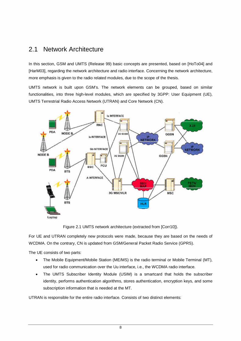
In this section, GSM and UMTS (Release 99) basic concepts are presented, based on [HoTo04] and
[HarM03], regarding the network architecture and radio interface. Concerning the network architecture,
more emphasis is given to the radio related modules, due to the scope of the thesis.
UMTS network is built upon GSM’s. The network elements can be grouped, based on similar
functionalities, into three high-level modules, which are specified by 3GPP: User Equipment (UE),
UMTS Terrestrial Radio Access Network (UTRAN) and Core Network (CN).
Figure 2.1 UMTS network architecture (extracted from [Corr10]).
For UE and UTRAN completely new protocols were made, because they are based on the needs of
WCDMA. On the contrary, CN is updated from GSM/General Packet Radio Service (GPRS).
The UE consists of two parts:
The Mobile Equipment/Mobile Station (ME/MS) is the radio terminal or Mobile Terminal (MT),
used for radio communication over the Uu interface, i.e., the WCDMA radio interface.
The UMTS Subscriber Identity Module (USIM) is a smartcard that holds the subscriber
identity, performs authentication algorithms, stores authentication, encryption keys, and some
subscription information that is needed at the MT.
UTRAN is responsible for the entire radio interface. Consists of two distinct elements:

9
The Node B (i.e., the Base Station (BS)) converts the data flow between the Iub and Uu
interfaces. It also participates in Radio Resource Management (RRM). In GSM the BTS has
the same role.
The Radio Network Controller (RNC) owns and controls the radio resources in its domain (the
Node Bs connected to it). The RNC carries out the RRM, e.g., outer loop power control,
packet scheduling and handover control. In GSM, the Base Station Controller (BSC) handles
the allocation of radio channels, receives measurements from the MTs, and controls
handovers from BTS to BTS.
In UTRAN, all RNCs are connected by the Iur interface with each other.
The CN, upgraded from GSM, is responsible for switching and routing calls and data to external
networks, like the Internet (Packet Switch (PS) network) and public switched telephone network
(Circuit Switch (CS) network). CN main elements are:
Home Location Register (HLR) is a database where the operator subscriber’s information is
stored, such as allowed services, user location for routing calls, and preferences.
Mobile Switching Centre/Visitor Location Register (MSC/VLR) is the switch (MSC) and
database (VLR) that serves the UE in its location.
Gateway MSC (GMSC) is the switch at the point where UMTS Public Land Mobile Network
(PLMN) is connected to external CS networks. All incoming and outgoing CS connections go
through GMSC.
Serving GPRS Support Node (SGSN) has similar functionalities to the MSC, but for PS.
Gateway GPRS Support Node (GGSN) is analogous to that of GMSC, for PS.
The innovations made on UE and UTRAN make possible to Release ’99 support soft handover,
opposite to GSM, where only hard handover is possible. At hard handover the connection between the
old BS and the MT is interrupted before the MT establishes a connection to the new BS. In UMTS,
hard handover can be inter-frequency or inter-system. In the former, the BSs have different carriers
and in the latter it is a handover to another system, e.g., GSM [Molis04]. Soft and softer handovers are
very similar: at soft handover the MT is connected to more than one BS at the same time, while at
softer the MT is transferred from one sector to another of the same cell.
2.2 Radio Interface
2.2.1 GSM Physically, the information flow takes place between the MS and the BTS, but, logically, MSs are
communicating with the BSC, the MSC and the SGSN. The gross transmission rate over the radio
interface is 270.833 kbps, due to the efficient modulation technique (Gaussian Minimum Shift Keying
(GMSK), a variant of Minimum Shift Keying). Separate 200 kHz carrier frequencies are used for UL
10
and DL. Different channel access methods are used:
Frequency Division Duplex (FDD): currently, there are several frequency bands defined, and
operators may implement networks that operate in a combination of these bands to support
multi band MSs. The band for Europe, Africa, Asia and some Latin American countries is [890,
915] MHz for UL and [935, 960] MHz for DL in the 900 MHz band and [1710, 1785] MHz for
UL and [1805, 1880] MHz for DL in the 1800 MHz band.
Frequency Division Multiple Access (FDMA): both available frequency bands are partitioned
into a 200 kHz grid.
Time Division Multiple Access (TDMA): the physical channels are associated to a Time-Slot
(TS), with a duration of 0.57692 ms (156.25 bits). A set of eight timeslots forms the frame, with
a duration of 4.615 ms.
GSM radio interface channels are classified as radio (channel associated to a carrier frequency),
physical (channel transporting any kind of system information, associated to a time-slot) and logical
(channel transporting a specific kind of system information), being TCH and SDCCH part of the last
group. Concerning addressing, one distinguishes common channels (exchange of information
between the BS and MTs in general) and dedicated channels (exchange of information between the
BS and one or several specific MTs). Concerning content, one distinguishes traffic channels (contain
users’ information, e.g., voice, data, and video) and control channels (contain system’s information,
e.g., signaling, synchronism, control and identity).
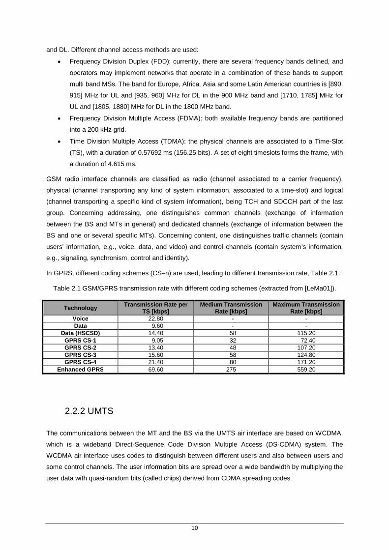
In GPRS, different coding schemes (CS–n) are used, leading to different transmission rate, Table 2.1.
Table 2.1 GSM/GPRS transmission rate with different coding schemes (extracted from [LeMa01]).
Technology Transmission Rate per TS [kbps]
Medium Transmission Rate [kbps]
Maximum Transmission Rate [kbps]
Voice 22.80 - - Data 9.60 - -
Data (HSCSD) 14.40 58 115.20 GPRS CS-1 9.05 32 72.40 GPRS CS-2 13.40 48 107.20 GPRS CS-3 15.60 58 124.80 GPRS CS-4 21.40 80 171.20
Enhanced GPRS 69.60 275 559.20
2.2.2 UMTS
The communications between the MT and the BS via the UMTS air interface are based on WCDMA,
which is a wideband Direct-Sequence Code Division Multiple Access (DS-CDMA) system. The
WCDMA air interface uses codes to distinguish between different users and also between users and
some control channels. The user information bits are spread over a wide bandwidth by multiplying the
user data with quasi-random bits (called chips) derived from CDMA spreading codes.
11
The chip rate of 3.84 Mcps leads to a carrier bandwidth of approximately 4.4 MHz. The carrier spacing
can be selected on a 200 kHz grid between approximately 4.4 and 5 MHz, depending on interference
between the carriers. The data capacity among users can change from frame to frame, which allows
to support highly variable user data rates in PS data services. It uses FDD and the band for Europe,
Africa, Asia and some Latin American countries is [1920, 1980] MHz for UL and [2110, 2170] MHz for
DL.
The spreading operation, known as channelisation, results on spreading data with the same random
appearance as the spreading code. The channelisation code increases the transmission bandwidth,
using the Orthogonal Variable Spreading Factor (OVSF) technique to change the Spreading Factor
(SF). The orthogonality between different spreading codes of different length is maintained.
Scrambling codes are mainly used to distinguish signals from MTs and/or BSs. Scrambling is used on
top of spreading so that the signal bandwidth is not changed and the symbol rate just makes signals
from different sources separable from each other. This allows the use of identical spreading codes for
several transmitters. In DL, it differentiates the sectors of the cell, and in UL, it separates MTs from
each other. The scrambling code (SC) can be either a short or a long one, the latter being a 10 ms
code based on the Gold family, and the former being based on the extended S(2) family. UL
scrambling uses both short and long codes, while DL employs only long ones.
UMTS radio interface channels are classified as logical, transport and physical. Logical channels are
mapped onto transport channels, which are again mapped onto physical ones. Logical to Transport
channel conversion happens in the Medium Access Control (MAC) layer, which is a lower sublayer in
Data Link Layer (Layer 2).
Power control is an essential part of any CDMA system, as it is necessary to control mutual
interference. Without power control, a single MT could block a whole cell, giving rise to the so-called
near-far problem of CDMA. There are two different types of power control, open and closed-loops. The
former is used to supply the initial power to the MT that is initiating a connection, and the latter
performs the continuous adjustements.
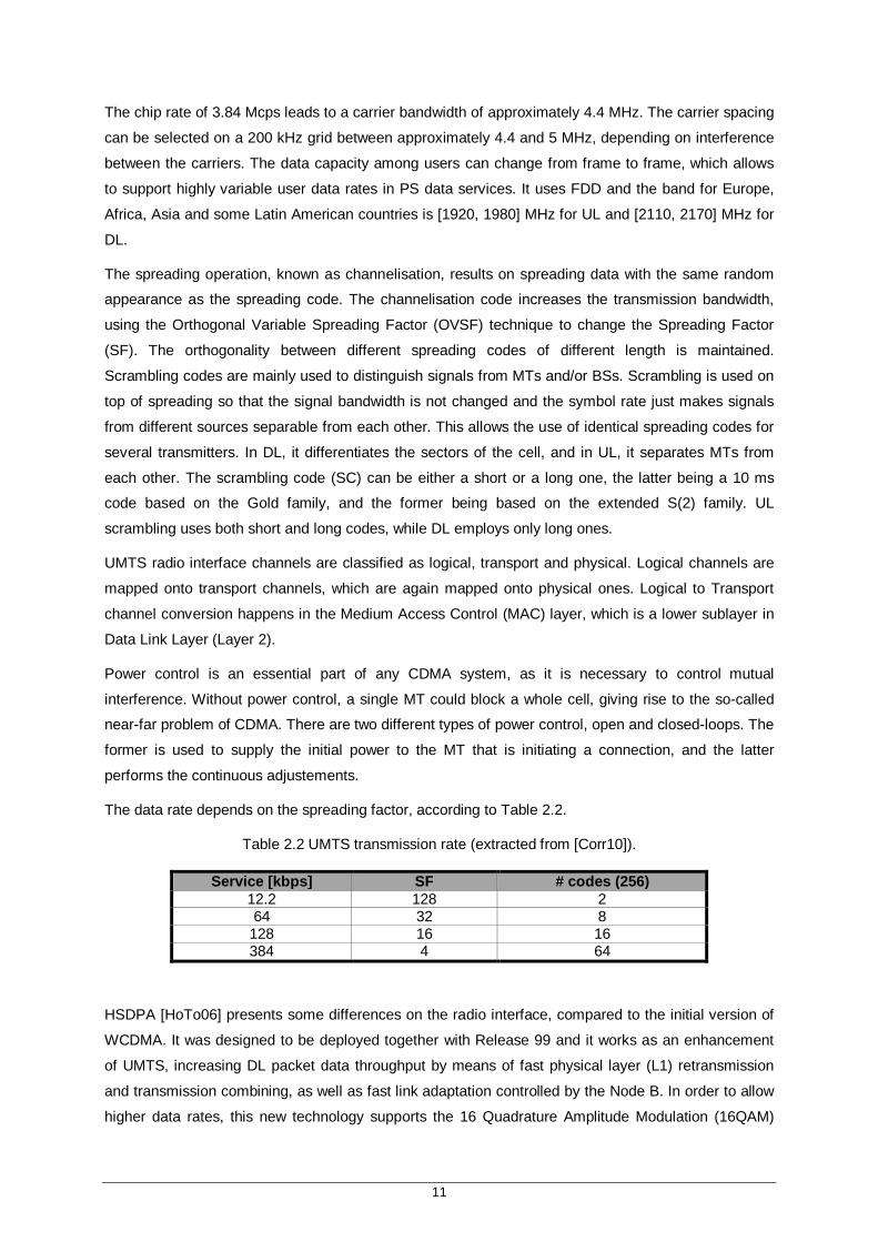
The data rate depends on the spreading factor, according to Table 2.2.
Table 2.2 UMTS transmission rate (extracted from [Corr10]).
Service [kbps] SF # codes (256) 12.2 128 2 64 32 8
128 16 16 384 4 64
HSDPA [HoTo06] presents some differences on the radio interface, compared to the initial version of
WCDMA. It was designed to be deployed together with Release 99 and it works as an enhancement
of UMTS, increasing DL packet data throughput by means of fast physical layer (L1) retransmission
and transmission combining, as well as fast link adaptation controlled by the Node B. In order to allow
higher data rates, this new technology supports the 16 Quadrature Amplitude Modulation (16QAM)
12
with 4 bits per symbol, which can only be used under good radio signal quality, due to additional
decision boundaries.
While in Release 99, the scheduling is based on the RNC and Node B has power control
functionalities, in HSDPA, the BS has a buffer that first receives the packet and keeps it after sending
it to the user, allowing the BS to retransmit the packet, if needed, without RNC intervention, this way
minimising latency. RNC-based retransmission can still be applied on top in case of physical layer
failure, using a Radio Link Control (RLC) acknowledged mode of operation. Concerning scheduling
and link adaptation, these operations take place after the BS estimates the channel quality of each
active user, based on the physical layer feedback in UL.
With these new functionalities, the need to introduce new channels emerged. A new user data channel
was created, and two others were added for signalling purposes. HSDPA is always operated with
Release ’99 in parallel, which can be used to carry CS services and the Signalling Radio Bearer
(SRB), but does not support features like power control and soft handover. The new channels are
High-Speed Downlink Shared Channel (HS-DSCH), for data, which is mapped onto the High-Speed
Physical Downlink Shared Channel (HS-PDSCH), and for signalling, the High-Speed Shared Control
Channel (HS-SCCH) and the High-Speed Dedicated Physical Control Channel (HS-DPCCH), for DL
and UL, respectively. When only packet services are active in DL, other than the SRB, for lower rates,
the DL DCH introduces too much overhead, and can also consume too much code space (if looking
for a large number of users using a low data rate service, like Voice over IP (VoIP)), so the system
uses the Fractional-DPCH (F-DPCH), that handles power control.
The HS-DSCH is the transport channel used to carry the user data in HSDPA. This channel supports
16QAM, besides QPSK, which is used to maximise coverage and robustness, and it has a dynamic
resource sharing based on the BS scheduling with a Transmission Time Interval (TTI) of 2 ms. During
the TTI there is no Discontinuous Transmission (DTX). It uses a fixed SF of 16 for multicode
operation, with a maximum of 15 codes per MT one is needed for HS-SCCH and common channels,
and only turbo-coding is used, since it outperforms the convolutional one for higher data rates.
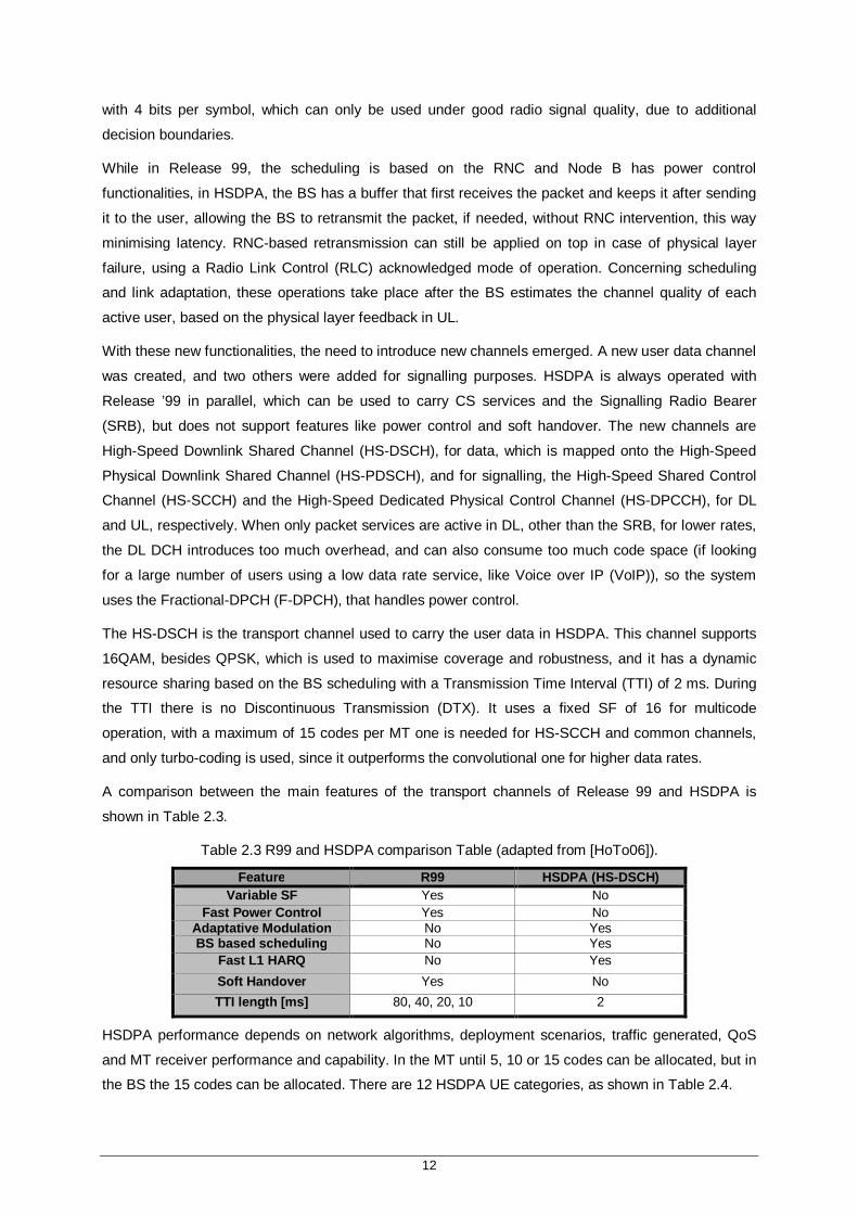
A comparison between the main features of the transport channels of Release 99 and HSDPA is
shown in Table 2.3.
Table 2.3 R99 and HSDPA comparison Table (adapted from [HoTo06]).
Feature R99 HSDPA (HS-DSCH) Variable SF Yes No
Fast Power Control Yes No Adaptative Modulation No Yes BS based scheduling No Yes
Fast L1 HARQ No Yes Soft Handover Yes No TTI length [ms] 80, 40, 20, 10 2
HSDPA performance depends on network algorithms, deployment scenarios, traffic generated, QoS
and MT receiver performance and capability. In the MT until 5, 10 or 15 codes can be allocated, but in
the BS the 15 codes can be allocated. There are 12 HSDPA UE categories, as shown in Table 2.4.
13
Table 2.4 HSDPA terminal capacity categories (adapted from [HoTo06]).
UE
Category
Maximum number of parallels codes
per HS-DSCH
Modulation
Minimum inter-TTI interval
Achievable maximum data
rate [Mbps] 1 5 QPSK & 16QAM 3 1.2 2 5 QPSK & 16QAM 3 1.2 3 5 QPSK & 16QAM 2 1.8 4 5 QPSK & 16QAM 2 1.8 5 5 QPSK & 16QAM 1 3.6 6 5 QPSK & 16QAM 1 3.6 7 10 QPSK & 16QAM 1 7.2 8 10 QPSK & 16QAM 1 7.2 9 15 QPSK & 16QAM 1 10.2 10 15 QPSK & 16QAM 1 14.4 11 5 QPSK only 2 0.9 12 5 QPSK only 1 1.8
2.3 Services and Applications
3G systems are characterised by supplying the user with services beyond voice, or simple data
transmission, which are characteristic of 2G. A service is a set of capabilities that work in a
complementary or cooperative way, in order to allow the user to establish applications. An application
is a task that needs communication among two or more points, being characterised by parameters
associated to services, communications, and traffic. There are 3 basic service components: audio,
video, and data. A service is composed of one or more basic components, which are grouped into
classes, according to their characteristics [Corr10]. Table 2.5 shows the 4 classes of services.
Table 2.5 QoS classes of UMTS (adapted from [3GPP00]).
Class of Service Conversational Streaming Interactive Background
Fundamental
Characteristics
- Preserve time
relation between information entities of the stream
- Conversational pattern (stringent and low delay)
- Preserve time
relation between information entities of the stream
- Request response
pattern
- Preserve payload content
- Destination is
not expecting the data within a certain time
- Preserve payload content
Real Time Yes Yes No No Symmetric Yes No No No Switching CS CS PS PS
Guaranteed bit rate
Yes Yes No No
Traffic Handling Priority
No No Yes No
Maximum bit rate Yes Yes Yes Yes Delay Minimum, Fixed Minimum, Variable Moderated, Variable Large, Variable Buffer No Yes Yes Yes Bursty No No Yes Yes
Example Voice Streaming Video Web browsing Background download of
emails

14
The Conversational class is the one that raises the strongest and most stringent QoS requirements, as
it is the only one where the required characteristics are strictly given by human perception. Therefore,
the maximum end-to-end delay has to be less than 400 ms [HoTo04]. Although the most well known
use of this scheme is telephony speech over CS, there are a number of other applications that fit this
scheme, e.g., VoIP and video conferencing.
The Streaming class includes real-time audio and video sharing, and is one of the newcomers in data
communications. Like the Conversational class, it requires bandwidth to be maintained, but tolerates
some delay variations that are hidden by a buffer in the receiver.
The Interactive class includes, e.g., web browsing, and is characterised by the request response
pattern of the end user. At the message destination, there is an entity expecting the message
(response) within a certain time. Round trip delay time is therefore one of the key attributes. Also, the
content of the packets must be transparently transferred, i.e., with low bit error rate.
The Backgroung class assumes that the destination is not expecting the data within a certain time;
therefore, it is the least delay sensitive class (there is no special requirement for delay). Like in the
Interactive class, the content of the packets must be transparently transferred. Examples are the
delivery of e-mails or Short Message Service (SMS).
UMTS QoS classes are not mandatory for the introduction of any low delay service. It is possible to
support streaming video or conversational VoIP from an end-to-end performance view point by using
just the Background class. QoS differentiation becomes useful for the network efficiency during high
load, when there are services with different delay requirements.
It is also important to know the usual bit rates and typical file dimensions associated to the different
services. Table 2.6. shows some examples, which also includes the QoS priority list. If data rates
reduction strategies are applied, the first services to be reduced are the ones with the lower QoS
priority (that corresponds to a higher priority value), according to the traffic classes shown in Table 2.5.
Table 2.6 Bit rates and applications of different services (adapted from [Lope08] and [3GPP05]).
Service
Bit rate [kbps] QoS
priority
Characteristics DL UL Average volume/duration DL UL
Voice 12.2 1 Call duration [s] 120
Web [512, 1536] [128, 512] 2 Page size [kB] 300 20
Streaming [512, 1024] [64, 384] 3 Video size [MB] 9.60 0.02
Email [384, 1536] [128, 512] 4 File size [kB] 100
FTP [384, 2048] [128, 512] 5 File size [MB] 10
Chat [64, 384] 6 MSN message size [B] 50
P2P [128, 1024] [64, 384] 7 File size [MB] 12.5
15
2.4 GSM Performance Indicators
2.4.1 Performance Monitoring
Monitoring and statistical measures is a very important part of the Operation and Maintenance (O&M)
of a radio network. The radio network statistic and recording functions can be used for monitoring and
optimisation of the radio network performance, evaluation and optimisation of the radio network
features, dimensioning of the radio network, and troubleshooting.
In an Ericsson GSM network, different events occur being counted and collected by a subsystem
called Statistics and Traffic Measurement Subsystem (STS), which is implemented in the BSC and
MSC, and gives statistics about events in different parts of the network, such as cells and equipment.
By continuously supervising the results from STS, the operator can obtain a very good overview of the
radio network performance. The central part in STS is the Measurement Database (MDB), where all
measurements are collected from different blocks in the Central Processor (CP). The contents of the
MDB are written to STS report files defined by the user. These STS files are then fetched from the
BSC and processed by OSS (Operation and Support System) or a user defined external tool.
Due to the scope of this thesis, Key Performance Indicators (KPIs) related to statistical results about
GSM and UMTS radio network performance are analised. In this section, the performance parameters
are identified and a brief description is given. In the following sections, the main objective is to find a
correlation between the parameters, in order to optimise the radio network performance.
The main focus is on how to monitor the GSM radio network performance in areas of accessibility,
retainability and speech quality, taking the subscriber perceived quality into account.
Acessibility: the accessibility area in a radio network covers random access, congestion on
SDCCH (Stand-alone Dedicated Control Channel) and TCH (Traffic Channel) and call setup.
Retainability: covers the ability to keep up a call; call drop rate, handover performance and
interference are included in this area.
Speech Quality: although it is very difficult to measure the speech quality, the Speech Quality
Supervision function (SQS) provides STS with counters, giving an objective measure of it.
A special reference is given to GPRS/EGPRS radio network performance monitoring. The terms
accessibility, retainability and integrity work well for CS networks; accessibility relates to blocked calls,
retainability to dropped calls and integrity to speech quality. All of these can be measured in the BSS
and roughly translated into a user perception of service quality. For PS networks, it is much more
difficult to define STS counters in the BSS and relate this to the users perception of service quality.
There are two main reasons for this:
The GPRS/EGPRS system has many layers of protocols. A session where a TBF (a PS
connection, that can be either UL or DL) is dropped for some reason, a retainability problem
on BSS (Base Station Subsystem) level will normally be kept alive by TCP (Transmission
Control Protocol) until a new TBF is established. To the user, this seems like an integrity
problem, one session that included a short delay.

16
The GPRS/EGPRS network is a bearer for a number of different applications. These are
affected by events in the radio network in different ways, e.g., if the BSS failed to transfer any
data for 5 s this would appear as a serious performance problem to a WAP user but it would
hardly be noticed by a user performing downloading of e-mails in the background.
Accessibility, retainability and integrity can be applied also to GPRS/EGPRS, but only on higher
layers, and by considering events that are invisible to the BSS. A full set of end-to-end KPIs have
been defined, but cannot be fully measured in the BSS. Basically all IP service KPIs in BSS are
experienced as integrity problems to the end user. Rather, the counters focus on the main task of the
BSS, which is the transfer of IP packets between the core network and the terminals. The counters are
grouped into three performance indicators:
Level one: These counters are directly related to the ability of the BSS to transport IP packets.
Typically, they are sets of counters that focus on one area of BSS performance (which could
usually be affected by a number of different factors), which impacts on the user perception of
the service. For example, the IP throughput counters on cell level measure the speed with
which the BSS can transfer IP packets.
Level two: These counters are indirectly related to the ability of the BSS to transport IP
packets. They should be used for trouble-shooting purposes to identify the specific factors that
are causing the level one indicators to show poor performance. For example, the GPRS traffic
load counters show how the number of users sharing the available PDCHs is affecting the
measured IP throughput. They should not be used on their own for any dimensioning
purposes.
Additional: Are usual for monitoring of specific features and impacts.
Figure 2.2 indicates the factors that can affect the users perception of the GPRS/EGPRS service. The
KPIs that are analysed are listed below, Tables 2.7 and 2.8, and Figure 2.3 illustrates how the STS
counters are grouped into the three areas (along with the object type names).
Figure 2.2 The structure for GPRS/EGPRS counters with object types (extracted from [Eric06]).
It is also important to mention that the mobile operator establishes a target value and a range of
values considered valid in order to evaluate the behavior of the KPIs. The data collection is done with
a ∆t = 1 h for GSM and UMTS.

17
Figure 2.3 Factors that can affect the GPRS/EGPRS user perceived performance perception (adapted
from [Eric06]).
Table 2.7 GSM KPIs Target and Range of Values.
GSM Target Value Range of Values 푅 [%] 1 [0, 3]
푅 [%] 1 [0, 3] 푅 [%] 98.5 [95, 100]
푇 [kbps] 25 [20, 45] 푇 [kbps] - [10, 25] 푇 [kbps] 80 [40, 260] 푇 [kbps] - [30, 60] 푅 [%] - [70, 100] 푅 [%] 98 [95, 100]
2.4.2 Voice Call Performance Indicators
The expression for subscriber perceived drop on TCH can be written as:
푅 = × 100[%] (2.1)
where:
푁 is the total amount of TCH drops (including the total number of dropped full and half-
rate TCH in underlaid and overlaid subcells).

18
푁 is the total number of terminated calls in a cell (including the number of initiated calls in a
cell and the sum of all incoming and outgoing handovers to a cell from all its neighbours
(successful assignments to worse and better cell)).
This parameter shows the ratio of drops due to low signal strength on either DL, UL or both links on
TCH compared to the total number of TCH drops.
The expression for drop on SDCCH, drop due to TCH congestion excluded, is:
푅 = × 100[%] (2.2)
where:
푁 is the total number of dropped SDCCH channels in a cell.
푁푀푆푆퐷퐶퐶퐻푆 is the successful Mobile Station (MS) channel establishments on SDCCH.
The different drop reasons are ranked in the order excessive Timing Advance (TA), low signal
strength, bad quality or sudden loss of connection. This means that if the connection suffers from
excessive TA and low signal strength, and drops, the drop reason will be registered as excessive TA.
The urgency condition bad quality is triggered by a high bit error rate on UL or DL.
The expression for Call Setup Success Rate is given by:
푅 = 1− 푅 × 1− 푅 × 100[%] =
1− 푁푆퐷퐶퐶퐻퐷푁푀푆푆퐷퐶퐶퐻푆
× 1− 1− × 100[%] (2.3)
where:
푅 is the TCH Assignment Failure Rate.
푅 indicates the percentage for drop on SDCCH.
푁 is the number of assignment complete messages for all MS power classes in underlaid
subcell, full-rate.
푁 is the number of assignment complete messages for all MS power classes in underlaid
subcell, half-rate.
푁 is the number of first assignment attempts on TCH for all MS power classes.
푅 is very important in the call establishment, being commonly used by operators due to its
importance in terms of performance and system availability.
2.4.3 Data Performance Indicators
The expression used to calculate the weighted average DL IP throughput for QoS classes Interactive
and Background for GPRS is given by:
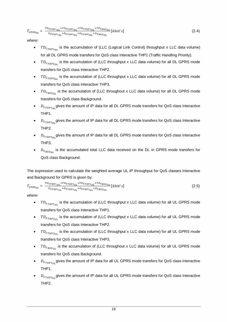
19
푇 = [푘푏푖푡/푠] (2.4)
where:
푇퐷 is the accumulation of (LLC (Logical Link Control) throughput x LLC data volume)
for all DL GPRS mode transfers for QoS class Interactive THP1 (Traffic Handling Priority).
푇퐷 is the accumulation of (LLC throughput x LLC data volume) for all DL GPRS mode
transfers for QoS class Interactive THP2.
푇퐷 is the accumulation of (LLC throughput x LLC data volume) for all DL GPRS mode
transfers for QoS class Interactive THP3.
푇퐷 is the accumulation of (LLC throughout x LLC data volume) for all DL GPRS mode
transfers for QoS class Background.
퐷 gives the amount of IP data for all DL GPRS mode transfers for QoS class Interactive
THP1.
퐷 gives the amount of IP data for all DL GPRS mode transfers for QoS class Interactive
THP2.
퐷 gives the amount of IP data for all DL GPRS mode transfers for QoS class Interactive
THP3.
퐷 is the accumulated total LLC data received on the DL in GPRS mode transfers for
QoS class Background.
The expression used to calculate the weighted average UL IP throughput for QoS classes Interactive
and Background for GPRS is given by:
푇 = [푘푏푖푡/푠] (2.5)
where:
푇퐷 is the accumulation of (LLC throughput x LLC data volume) for all UL GPRS mode
transfers for QoS class Interactive THP1.
푇퐷 is the accumulation of (LLC throughput x LLC data volume) for all UL GPRS mode
transfers for QoS class Interactive THP2.
푇퐷 is the accumulation of (LLC throughput x LLC data volume) for all UL GPRS mode
transfers for QoS class Interactive THP3.
푇퐷 is the accumulation of (LLC throughout x LLC data volume) for all UL GPRS mode
transfers for QoS class Background.
퐷 gives the amount of IP data for all UL GPRS mode transfers for QoS class Interactive
THP1.
퐷 gives the amount of IP data for all UL GPRS mode transfers for QoS class Interactive
THP2.
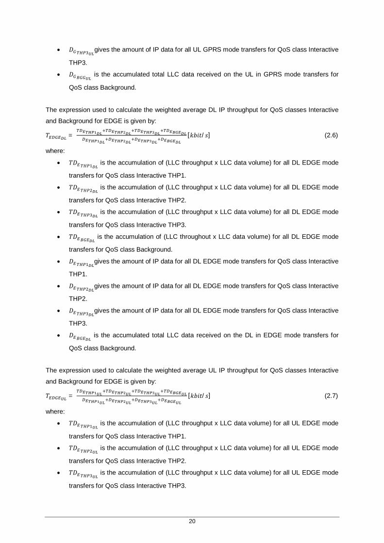
20
퐷 gives the amount of IP data for all UL GPRS mode transfers for QoS class Interactive
THP3.
퐷 is the accumulated total LLC data received on the UL in GPRS mode transfers for
QoS class Background.
The expression used to calculate the weighted average DL IP throughput for QoS classes Interactive
and Background for EDGE is given by:
푇 = [푘푏푖푡/푠] (2.6)
where:
푇퐷 is the accumulation of (LLC throughput x LLC data volume) for all DL EDGE mode
transfers for QoS class Interactive THP1.
푇퐷 is the accumulation of (LLC throughput x LLC data volume) for all DL EDGE mode
transfers for QoS class Interactive THP2.
푇퐷 is the accumulation of (LLC throughput x LLC data volume) for all DL EDGE mode
transfers for QoS class Interactive THP3.
푇퐷 is the accumulation of (LLC throughout x LLC data volume) for all DL EDGE mode
transfers for QoS class Background.
퐷 gives the amount of IP data for all DL EDGE mode transfers for QoS class Interactive
THP1.
퐷 gives the amount of IP data for all DL EDGE mode transfers for QoS class Interactive
THP2.
퐷 gives the amount of IP data for all DL EDGE mode transfers for QoS class Interactive
THP3.
퐷 is the accumulated total LLC data received on the DL in EDGE mode transfers for
QoS class Background.
The expression used to calculate the weighted average UL IP throughput for QoS classes Interactive
and Background for EDGE is given by:
푇 = [푘푏푖푡/푠] (2.7)
where:
푇퐷 is the accumulation of (LLC throughput x LLC data volume) for all UL EDGE mode
transfers for QoS class Interactive THP1.
푇퐷 is the accumulation of (LLC throughput x LLC data volume) for all UL EDGE mode
transfers for QoS class Interactive THP2.
푇퐷 is the accumulation of (LLC throughput x LLC data volume) for all UL EDGE mode
transfers for QoS class Interactive THP3.

21
푇퐷 is the accumulation of (LLC throughout x LLC data volume) for all UL EDGE mode
transfers for QoS class Background.
퐷 gives the amount of IP data for all UL EDGE mode transfers for QoS class Interactive
THP1.
퐷 gives the amount of IP data for all UL EDGE mode transfers for QoS class Interactive
THP2.
퐷 gives the amount of IP data for all UL EDGE mode transfers for QoS class Interactive
THP3.
퐷 is the accumulated total LLC data received on the UL in EDGE mode transfers for
QoS class Background.
The packet data channel assignment success rate can be calculated as:
푅 = 1− × 100[%] (2.8)
where:
푁 is the number of packet channel allocation failures. A failure is when zero PDCH could
be allocated due to the lack of basic physical channels over the air interface. The failure
relates to the inability of the system to allocate resources and, in most cases, not to any failure
to reserve channels experienced by the user. “Failures” are normal, frequent, occurrences in a
situation where PS traffic must compete with CS traffic for basic physical channels.
푁 is the number of packet channel allocation attempts. The counter value is incremented
at each request to allocate PDCHs in the cell. The counter value is incremented by one
independently of the number of channels requested and the result of the request. Requests to
allocate PDCHs occur when the operator increases the number of dedicated PDCHs and
when the packet data traffic demands on-demand PDCHs. No request to allocate PDCHs is
done if there are no deblocked traffic channels in the cell.
2.5 UMTS Performance Parameters
2.5.1 Performance Monitoring
This section provides the KPIs that are studied for UMTS, taking in consideration that observability in
Ericsson UTRAN covers all functions that serve to monitor and analyse the performance and
characteristics of the system. Figure 2.4 illustrates the observability model:
The KPIs represents the end-user perception of a network on a macro level, being typical of
interest for top-level management within an operator. They are typically used to detect
problem areas.
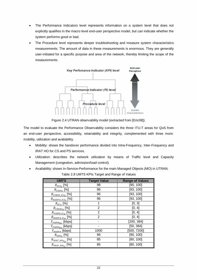
22
The Performance Indicators level represents information on a system level that does not
explicitly qualifies in the macro level end-user perspective model, but can indicate whether the
system performs good or bad.
The Procedure level represents deeper troubleshooting and measure system characteristics
measurements. The amount of data in these measurements is enormous. They are generally
user-initiated for a specific purpose and area of the network, thereby limiting the scope of the
measurements.
Figure 2.4 UTRAN observability model (extracted from [Eric08]).
The model to evaluate the Performance Observability considers the three ITU-T areas for QoS from
an end-user perspective, accessibility, retainability and integrity, complemented with three more:
mobility, utilization and availability.
Mobility: shows the handover performance divided into Intra-Frequency, Inter-Frequency and
IRAT HO for CS and PS services.
Utilization: describes the network utilization by means of Traffic level and Capacity
Management (congestion, admission/load control).
Availability: shows In-Service-Performance for the main Managed Objects (MO) in UTRAN.
Table 2.8 UMTS KPIs Target and Range of Values
UMTS Target Value Range of Values 푅 [%] 98 [95, 100] 푅 [%] 96 [93, 100]
푅 _ [%] 96 [93, 100] 푅 _ [%] 96 [93, 100]
푅 [%] 1 [0, 3] 푅 [%] 2 [0, 4] 푅 _ [%] 2 [0, 4] 푅 _ [%] 2 [0, 4] 푇 [kbps] - [200, 384] 푇 [kbps] - [50, 384] 푇 [kbps] 1000 [500, 7200] 푅 [%] 96 [90, 100]
푅 _ [%] 85 [80, 100] 푅 _ [%] 85 [80, 100]
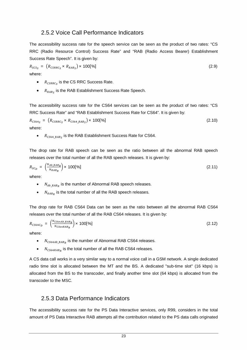
23
2.5.2 Voice Call Performance Indicators
The accessibility success rate for the speech service can be seen as the product of two rates: “CS
RRC (Radio Resource Control) Success Rate” and “RAB (Radio Access Bearer) Establishment
Success Rate Speech”. It is given by:
푅 = 푅 × 푅 × 100[%] (2.9)
where:
푅 is the CS RRC Success Rate.
푅 is the RAB Establishment Success Rate Speech.
The accessibility success rate for the CS64 services can be seen as the product of two rates: “CS
RRC Success Rate” and “RAB Establishment Success Rate for CS64”. It is given by:
푅 = 푅 × 푅 _ × 100[%] (2.10)
where:
푅 _ is the RAB Establishment Success Rate for CS64.
The drop rate for RAB speech can be seen as the ratio between all the abnormal RAB speech
releases over the total number of all the RAB speech releases. It is given by:
푅 = _ × 100[%] (2.11)
where:
푁 _ is the number of Abnormal RAB speech releases.
푁 is the total number of all the RAB speech releases.
The drop rate for RAB CS64 Data can be seen as the ratio between all the abnormal RAB CS64
releases over the total number of all the RAB CS64 releases. It is given by:
푅 = _ × 100[%] (2.12)
where:
푁 _ is the number of Abnormal RAB CS64 releases.
푁 is the total number of all the RAB CS64 releases.
A CS data call works in a very similar way to a normal voice call in a GSM network. A single dedicated
radio time slot is allocated between the MT and the BS. A dedicated "sub-time slot" (16 kbps) is
allocated from the BS to the transcoder, and finally another time slot (64 kbps) is allocated from the
transcoder to the MSC.
2.5.3 Data Performance Indicators
The accessibility success rate for the PS Data Interactive services, only R99, considers in the total
amount of PS Data Interactive RAB attempts all the contribution related to the PS data calls originated
24
on R99 only. It can be seen as the product of two rates: “PS RRC Success Rate” and “RAB
Establishment Success Rate PS DCH/FACH (Dedicated Channel/Forward Access Channel)”. It is
given by:
푅 _ = 푅 × 푅 _ _ _ × 100[%] (2.13)
where:
푅 is the PS RRC Success Rate.
푅 _ _ _ is the RAB Establishment Success Rate PS DCH/FACH.
The accessibility success rate for the PS Data Interactive services, HSDPA only, considers in the total
amount of PS Data Interactive RAB attempts all the contribution related to the PS data calls originated
on HSDPA. It can be seen as the product of two rates: “PS RRC Success Rate” and RAB
Establishment Success Rate PS HS, which indicates the success rate of RAB establishments for PS
HS calls. It is given by:
푅 _ = 푅 × 푅 _ _ × 100[%] (2.14)
where:
푅 _ _ = “RAB Establishment Success Rate PS HS”.
In PS HS RAB, establishments attempts and success have been counted also relatively PS EUL RAB
establishment ones.
The drop rate for all the PS RAB’s only R99 on Cell basis (all counters defined in MO class
“UtranCell”) can be seen as the ratio between all the abnormal RAB PS DCH/FACH releases over the
total number of all the RAB PS DCH/FACH releases (including all the normal releases due to all the
upswitchs from DCH/FACH state to HS). It is given by:
푅 _ = _ _ _
_ _ _× 100[%] (2.15)
where:
푁 _ _ _ is the number of all the abnormal RAB PS DCH/FACH releases.
푁 _ _ _ is the total number of all the RAB PS DCH/FACH releases.
This KPI defines the drop rate for RAB PS HSDPA on Cell basis (all counters defined in MO class
“UtranCell”). It can be seen as the ratio between all the abnormal RAB PS HSDPA releases over the
total number of all the RAB PS HSDPA releases. The expression is given by:
푅 _ = _ _
_ _× 100[%] (2.16)
where:
푁 _ _ is the number of all the abnormal RAB PS HSDPA releases.
푁 _ _ is the total number of all the RAB PS HSDPA releases.
In PS, HS RAB releases have been counted also relatively PS EUL ones.
푇 = [푘푏푖푡/푠] (2.17)
25
This expression evaluates the average user throughput for PS Data in DL (kbps). It includes user data,
excluding retransmissions, padding bits, data PDU (Protocol Data Unit) headers and RLC control
PDU’s. It is measured in the best cell in the active set.
푇 = [푘푏푖푡/푠] (2.18)
This expression evaluates the average user throughput for R 99 PS Data in UL (kbps). It includes user
data, excluding retransmissions, padding bits, data PDU headers and RLC control PDU’s. It is
measured in the best cell in the active set.
The PS Interactive HS user DL throughput is given by:
푇 = [푘푏푖푡/푠] (2.19)
2.6 GSM and UMTS Handover Performance Parameters
Handover parameters are independent of the type of service. These KPIs are composed of counters
which task is to count the number of radio link establishments between the MT and the BS.
The expression for Handover Success Rate is given by:
푅 =
_
× 100[%] (2.20)
where:
푁 is the number of successful handover to the neighbouring cell.
푁 is the number of successful intra cell handovers.
푁 is the number of handover commands sent to the MS.
푁 is the number of intra-cell handover attempts (decisions) at bad DL quality.
푁 is the number of intra-cell handover attempts (decisions) at bad UL quality.
푁_
is the number of intra-cell handover attempts (decisions) for both links with bad
quality.
The intra-cell handover feature can be triggered by bad quality (if the signal strength is above
predefined levels), which in most cases means a high level of interference. If the number of intra-cell
handovers due to bad quality becomes too high, the cell and/or frequency planning needs to be
improved. In cells with congestion, intra-cell handover should be switched off, as two TCHs are seized
during the handover process.
The rate of successful RL addition for the target cell, computed for RL addition or replacement, can be
seen as the rate between the total number of RL addition success and the total number of RL addition
attempts, defined as the sum of success and failures. It is given by:

26
푅 = × 100[%] (2.21)
where:
푁 is the total number of RL addition success.
푁 is the total number of RL addition attempts.
The success rate for IRAT (Inter Radio Access Technology) HO for RAB Speech and MultiRAB can be
seen as the rate between all the success of outgoing (to GSM) IRAT for RAB Speech and Multi RAB
and the total of attempts. It is given by:
푅 _ = __
_× 100[%] (2.22)
where:
푁 __ is the number of all the success of outgoing (to GSM) IRAT for RAB Speech and
Multi RAB.
푁 _ is the number of total attempts.
The following KPI defines the percentage of incoming IRAT Handover Successful attempts for CS
RAB, over the total attempts. Its expression is given by:
푅 _ = _
_× 100[%] (2.23)
where:
푁 _ is the number of incoming IRAT Handover Successful attempts for CS RAB.
푁 _ is the number of total attempts.
Note that all the KPIs can be computed on a per RNC basis, as well as on a per cell one. When
computing the RNC result, individual cell counters should be summed on a RNC basis before applying
KPI calculation. This is in contrast to applying the KPI equation to each cell and then taking an
average across the RNC. The latter can give poor performances.
Being the establishment of correlations between different KPIs one of the main goals of this work, it is
necessary to present the correlation expression.
퐶표푟푟푒푙(푋,푌) = ∑( ̅)( )∑( ̅) ∑( )
(2.24)
where x and y are the sample means of the analysed parameters.
2.7 State of the Art
A brief overview of the state of the art is presented in this section, in order to show what has been
done in this field up to now, thus, emphasising the importance of this work.
In wireless communication systems, QoS is one of the most important issues from both users and
operators point of view. Not all the parameters related to QoS have the same importance for all users
27
and applications. However, to meet QoS requirements accurately, all the parameters of a service
should work properly, and network resources must be used more efficiently.
All mobile operators use KPIs to judge their network performance and evaluate the QoS. In [Seyt10],
GSM network RF performance evaluation is done based on some major KPIs, such as call setup
success rate (CSSR), call drop rate (CDR), handover success rate (HSR) and Traffic Channel
Congestion Rate. Issues that might affect and degrade the KPIs are presented, and the authors also
present methods that can be employed in order to improve the performance of the KPIs in a live
network, analytically proving that it is possible to optimise an existing cellular network using different
methodologies and fine parameter tuning.
In order to characterise QoS parameters for 3G Wireless Networks, [CISL08] assume that CDR is the
most important QoS parameter for all types of services. A soft-QoS scheme is proposed to reduce
CDR: the call will be accepted by a network only when the required bandwidth for that call is less than
or equal to this releasable bandwidth. The results show that the proposed soft-QoS scheme can
reduce not only dropped call rate but also blocked call rate for medium traffic condition.
In [VaHN03], five key UMTS radio network parameters were simultaneously optimised with an
automatic control method, guided by heuristic expert-defined rules, which apply specific trade-off
policies and statistics of poor quality calls, blocking rates, power and interference levels and terminal
measurements to qualify the parameter values. The method was validated using a dynamic WCDMA
system simulator with a deployment of 17 cells in the Helsinki city centre. The simulations were carried
out with four different loadings that were produced with 1000, 2000, 3000 or 4000 subscribers in the
network. Each one of them made 11 calls or call attempts in an hour on the average, and 70% of the
calls used 8 kbps speech service and 30% used 64 kbps CS data service. The average length of
speech calls was 30 s and that of CS data calls 20 s. With 1000 subscribers, the average number of
simultaneous calls in a cell was about five, assuming that no calls were blocked. The simulated time
was 2 h and the parameter control was performed every 100 s. The results show that the number of
started calls was increased significantly with control, the ratio of poor quality calls was at most 1% with
the initial parameters and 2.2% with control, call quality was regarded as poor if over 2% of the frames
were received incorrectly during the whole converse time. The blocking ratio was significantly reduced
with control. Requiring that at most 5% of the calls are either blocked or suffer from poor quality then
the number of subscribers that the network tolerated was between 1000 and 2000 with the initial
parameters, while with control the number was increased to between 2000 and 3000. The capacity
was much improved by trading off quality for reduced blocking and the combined improvement of
capacity was 9% with 2000, 17% with 3000 and 19% with 4000 subscribers – the capacity of the
network was improved close to 20% with slightly decreased but still acceptable quality of calls.
In [ABGC03], soft handover performance for UMTS operations was studied. It consists of a sensitivity
analysis for determining the optimum setting of parameters controlling the performance of the soft
handover procedure. The final results show that the parameters involved in the handover algorithm
had a major bearing on the network traffic handling capacity and their optimisation was considered
essential, in order to improve some aspects such as dropped calls and failed handovers.

28
In [Siom05] and [SiVY06], the authors studied other ways of addressing the optimisation issues that
could be seen, due to the scope of this thesis, as possible solutions for implementation – the Primary
Common Pilot Channel (P-CPICH) Power and antenna tilt optimisation. The P-CPICH is a fixed rate
DL physical channel that carries a pre-defined bit/symbol sequence and the measurements are used
in the cell search and handover procedures. The MTs scan for the CPICH signals continuously and
measure the Carrier-Interference Ratio (CIR) of all pilot signals they can detect. If a MT is unable to
clearly receive one dominant CPICH signal, due to interference or coverage problems, the result is
likely to be dropped calls, failed initiations, poor voice quality and/or poor data throughput. The BS
antenna height, azimuth, and tilt are the important configuration parameters that have a strong impact
on network coverage and system capacity thus, they must be carefully planned in the topology
planning phase. The antenna configuration can be also changed in the network operation and
optimisation phase, but these changes require additional site visits, which is expansive and therefore
least desirable. So, antenna tilting is the easiest and the most practical way of changing the antenna
configuration in order to improve network performance. In [SiVY06], the results show that for a UMTS
planning scenario in Lisbon, automated optimisation saves up to 70% of the CPICH power used in the
network configuration, offering significant performance improvement in terms of fewer overloaded cells
and lower downlink load factor. In [Siom05], the results show that the effect of electrical tilt on
interference reduction is greater than that of mechanical tilt, suggesting that mechanical tilt can be
used in addition to electrical tilting, e.g., when a further increase of the electrical antenna tilt is
impossible.
It is important to note that this is a theme whose information is usually confidential and restricted to the
mobile operators. So the available information is scarce, which is understandable since it is unnatural
companies make available something that might be useful to its development and performance
improvement.
29
Chapter 3
Model Development and
Implementation 3 Model Development and Implementation
This chapter provides an overview of the models that are related to the scope of this thesis. First the
database search algorithm is described, followed by its application with some results presentation.
The development and application of the radio network analysis algorithms are presented,
distinguishing 2G from 3G models.
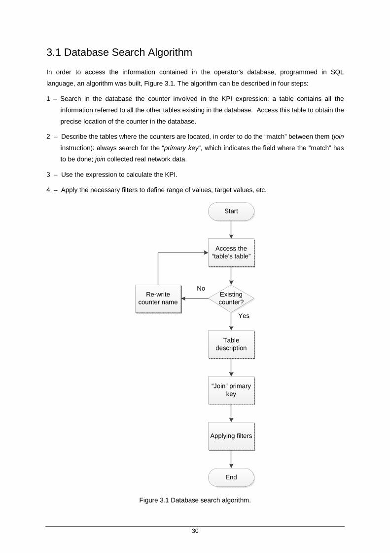
30
3.1 Database Search Algorithm
In order to access the information contained in the operator’s database, programmed in SQL
language, an algorithm was built, Figure 3.1. The algorithm can be described in four steps:
1 – Search in the database the counter involved in the KPI expression: a table contains all the
information referred to all the other tables existing in the database. Access this table to obtain the
precise location of the counter in the database.
2 – Describe the tables where the counters are located, in order to do the “match” between them (join
instruction): always search for the “primary key”, which indicates the field where the “match” has
to be done; join collected real network data.
3 – Use the expression to calculate the KPI.
4 – Apply the necessary filters to define range of values, target values, etc.
Start
Access the “table’s table”
Existing counter?
Table description
“Join” primary key
Applying filters
End
Re-write counter name
Yes
No
Figure 3.1 Database search algorithm.

31
Based on this algorithm, it is possible to access the counters involved in the KPIs calculation, as
shown in the previous chapter. For example, to calculate call drop rate, the first step is to find the
counters that represent the total amount of traffic channel drops (푁 ) and the total number of
terminated calls in a cell (푁 ). The second step is to program a query in order to turn possible to the
programmer know the precise location of the table that contains the counter information. After that, it is
just math, applying the call drop rate expression, as shown in (2.1). The output of the program gives
all the information needed to move on: the area where the cell is located, the name of the cell, the
date, the hour and the value of the KPI for the specified conditions. A list of nine GSM KPIs and
fourteen UMTS KPIs was provided by the operator.
The operator sets 푁 (minimum number of calls) as 10% of the maximum daily value for a site
place, which is important to know in order to evaluate a KPI that uses the counter with the information
related to all the terminated calls in a cell. The region in study is covered by 328 GSM 900 BSs, 306
GSM 1800 BSs and 224 UMTS BSs, as shown in Table E.1. The results obtained from the database
search algorithm application are shown in Annex B.
3.2 GSM Network Analysis
The main goal is try to explain the network performance analysing the KPIs performance throughout
time. A strategy has to be defined in order to adress the KPIs performance issues. Initially the KPIs
are analysed in a total radio network perspective, which means selecting a random day (the chosen
one was the September 2nd 2010) and analyse the network performance in all BSs. An algorithm has
to be built to define the way of “attacking” KPIs performance, providing solutions to solve future
problems, introducing the performance comparison between the different parameters, in order to
detect any kind of correlation between them. The final step is the generalisation of results considering
larger time intervals.
The proposed analysis flow is given in Figure 3.2, applicable to both GSM and UMTS. The objective is
to apply the ideas inherent to the algorithm of Figure 3.2 in the performance analysis of all KPIs. After
the characteristics of the problem being identified, it is necessary to think about what to do next. The
benchmarking process consists of the evaluation of the overall KPI performance and compare it with
the desired performance established by the pre-defined thresholds. If the analysed results do not
match with the desired ones, there is a need to develop specific algorithms to analyse the KPIs
individually based on detailed statistics of the problem areas. The ultimate goal is to identify the
problem reason and if possible to give recommendations to the operator in order to solve it.
Dropped calls show the number of abnormal disconnections during call setup or during conversation.
In [Eric98], three steps to provide a good dropped call analysis are presented:
1) Check dropped calls per cell. Select cells with high dropped call rate.
2) Check reason to dropped calls for selected cells.

32
3) Check ratio of lost handovers to dropped calls. The reason is to determine if the high dropped
call rate is related to handover performance. Check also which cell relations that have more
dropped calls than the average neighbour relation.
Figure 3.2 Analysis flow chart (adapted from [Eric98]).
In order to get an indication of the reason for possible bad performance and according to [Eric06], both
call drop rate on TCH and on SDCCH will be above the threshold level due to excessive TA, low
signal strength, bad quality and sudden loss of connection. 푅 can also be above the threshold level
due to high Frame Error Ratio (FER) and 푅 can also be above the threshold level due to TCH
congestion. Figures 3.3 and 3.4 show the procedure to address the problem on TCH and SDCCH,
respectively, with the properly identification of the counters associated to the reasons that may lead to
a poor performance of the KPI.
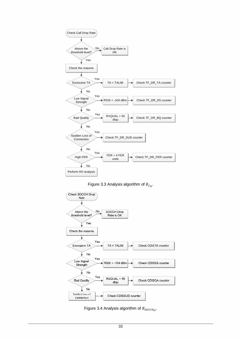
33
Check Call Drop Rate
Above the threshold level?
Check the reasons
Excessive TA
Low Signal Strength
Bad Quality
Sudden Loss of Connection
High FER
Perform HO analysis
TA > TALIM Check TF_DR_TA counter
RSSI < -104 dBm Check TF_DR_SS counter
RXQUAL > 55 dtqu Check TF_DR_BQ counter
Check TF_DR_SUD counter
FER > 4 FER units Check TF_DR_FER counter
Call Drop Rate is OK
No
No
No
No
No
No
Yes
Yes
Yes
Yes
Yes
Yes
Figure 3.3 Analysis algorithm of 푅 .
Figure 3.4 Analysis algorithm of 푅 .

34
푅 is related to 푅 , which is easily understandable when analysing the call establishment
process. Figure 3.5 illustrates it in a very simplistic way.
Figure 3.5 Call establishment process.
Thus, (2.3) is now understandable. The two KPIs are almost symmetric. The difference is in the
1−푅 factor, 푅 being the TCH assignment failure. In perfect conditions the TCH assignment
failure rate is equal 0, which never happens in real radio networks. Figures 3.6 and 3.7 illustrate the
algorithm to address the problems related to푅 . Analysing Figure 3.6, the reasons identified that
may lead to a poor performance of the call setup success rate KPI are a low TCH assignment success
rate or a high SDCCH drop rate. In case of high SDCCH drop rate, the analysis to be made is equal to
the developed model in Figure 3.4. In case of low TCH assignment success rate, Figure 3.7 suggests
actions to the operator that may lead to the problem solution. Those actions can only be implemented
by the operator, many of them only on the field.
Figure 3.6 Analysis algorithm of 푅 .
Start
Set-up
End
Call Duration
SDCCH Assignment TCH Assignment

35
Figure 3.7 Low TCH Assignment Success Rate analysis (adapted from [Eric98]).
Handover is a key function in a network. If the handover performance is poor, the subscriber will
perceive the quality of the network as bad. The 푹푯푶푺 parameter will be below the threshold value due
to intra-cell handover (normally performed in cells with high signal strength and bad quality) or
handover to the neighbouring cell problems. The HO performance analysis is illustrated in Figure 3.8.
The first decision to be taken is related to the HO activity. When analysing the HO performance it is
imperative to define if there are few HO attempts, by checking the HOVERCNT counter. This decision
will guide future decisions, since it will be given a greater importance to a cell with many HO attempts
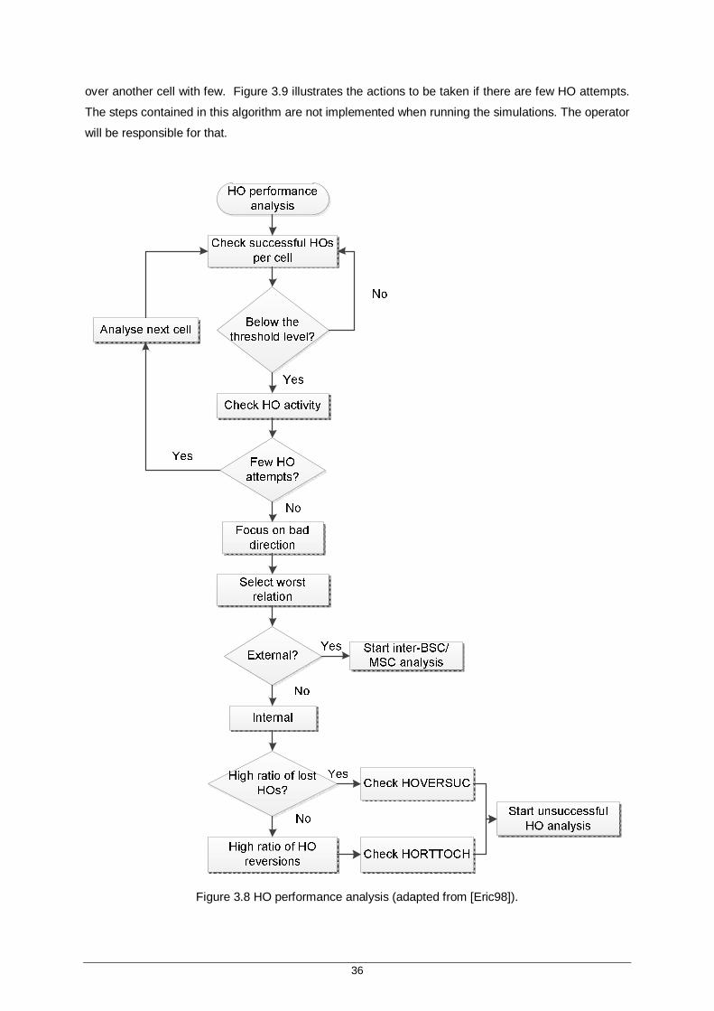
36
over another cell with few. Figure 3.9 illustrates the actions to be taken if there are few HO attempts.
The steps contained in this algorithm are not implemented when running the simulations. The operator
will be responsible for that.
Figure 3.8 HO performance analysis (adapted from [Eric98]).
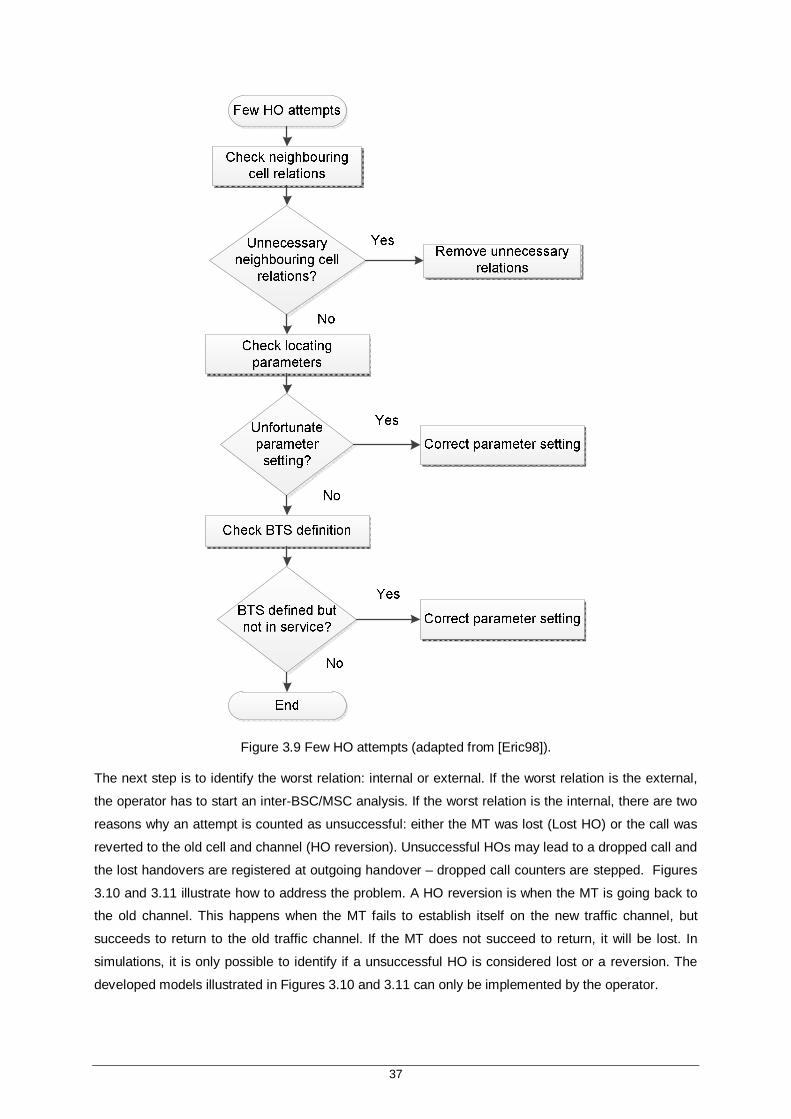
37
Figure 3.9 Few HO attempts (adapted from [Eric98]).
The next step is to identify the worst relation: internal or external. If the worst relation is the external,
the operator has to start an inter-BSC/MSC analysis. If the worst relation is the internal, there are two
reasons why an attempt is counted as unsuccessful: either the MT was lost (Lost HO) or the call was
reverted to the old cell and channel (HO reversion). Unsuccessful HOs may lead to a dropped call and
the lost handovers are registered at outgoing handover – dropped call counters are stepped. Figures
3.10 and 3.11 illustrate how to address the problem. A HO reversion is when the MT is going back to
the old channel. This happens when the MT fails to establish itself on the new traffic channel, but
succeeds to return to the old traffic channel. If the MT does not succeed to return, it will be lost. In
simulations, it is only possible to identify if a unsuccessful HO is considered lost or a reversion. The
developed models illustrated in Figures 3.10 and 3.11 can only be implemented by the operator.
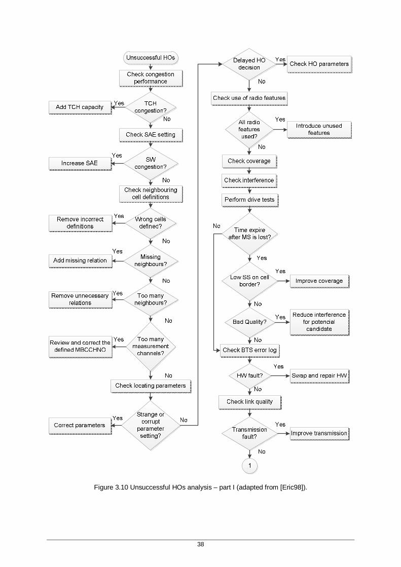
38
Figure 3.10 Unsuccessful HOs analysis – part I (adapted from [Eric98]).
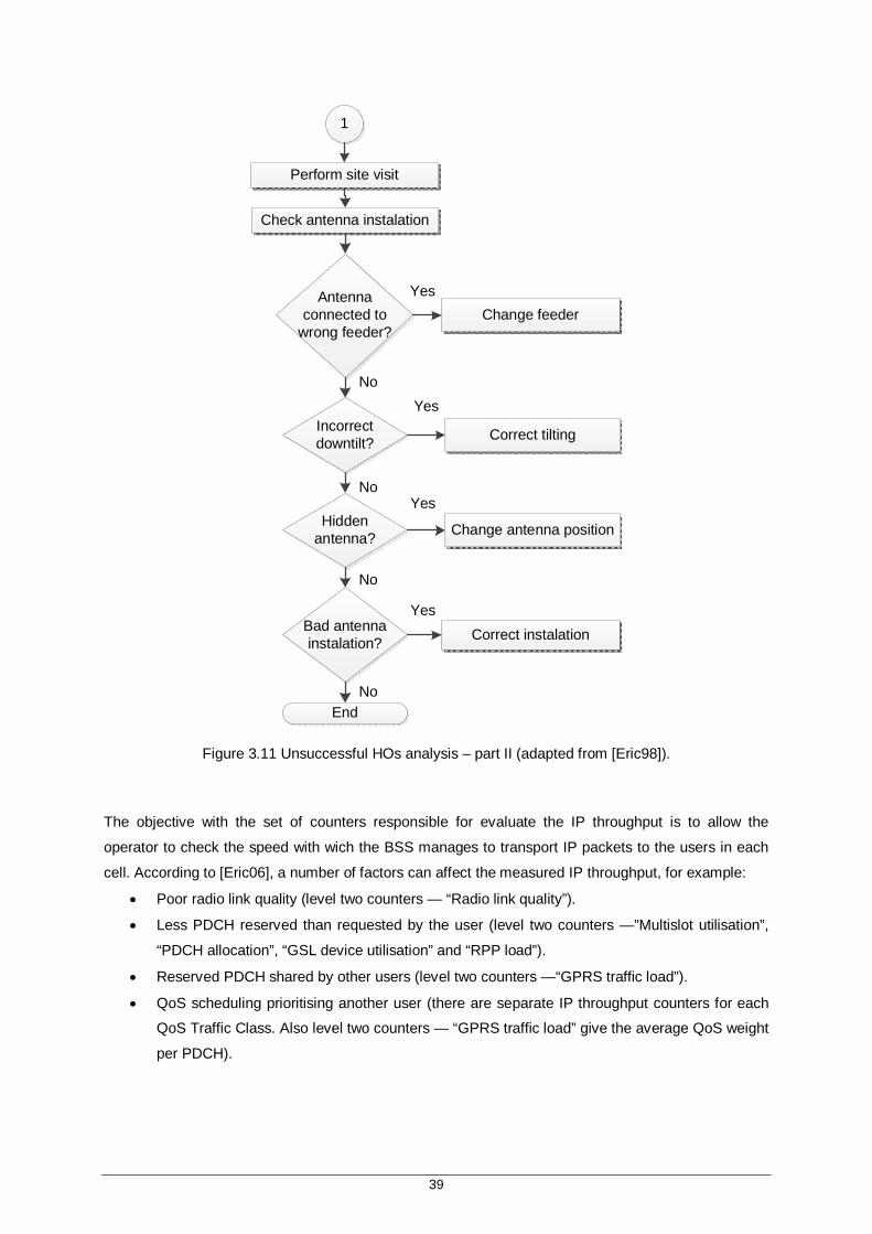
39
Perform site visit
Check antenna instalation
Antenna connected to
wrong feeder?
Incorrect downtilt?
Hidden antenna?
Bad antenna instalation?
End
Change feeder
Correct tilting
Change antenna position
Correct instalation
1
Yes
Yes
Yes
Yes
No
No
No
No
Figure 3.11 Unsuccessful HOs analysis – part II (adapted from [Eric98]).
The objective with the set of counters responsible for evaluate the IP throughput is to allow the
operator to check the speed with wich the BSS manages to transport IP packets to the users in each
cell. According to [Eric06], a number of factors can affect the measured IP throughput, for example:
Poor radio link quality (level two counters — “Radio link quality”).
Less PDCH reserved than requested by the user (level two counters —”Multislot utilisation”,
“PDCH allocation”, “GSL device utilisation” and “RPP load”).
Reserved PDCH shared by other users (level two counters —“GPRS traffic load”).
QoS scheduling prioritising another user (there are separate IP throughput counters for each
QoS Traffic Class. Also level two counters — “GPRS traffic load” give the average QoS weight
per PDCH).
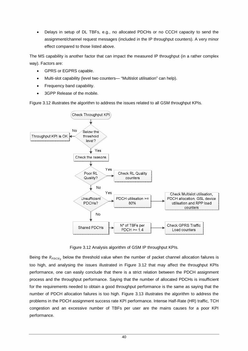
40
Delays in setup of DL TBFs, e.g., no allocated PDCHs or no CCCH capacity to send the
assignment/channel request messages (included in the IP throughput counters). A very minor
effect compared to those listed above.
The MS capability is another factor that can impact the measured IP throughput (in a rather complex
way). Factors are:
GPRS or EGPRS capable.
Multi-slot capability (level two counters— “Multislot utilisation” can help).
Frequency band capability.
3GPP Release of the mobile.
Figure 3.12 illustrates the algorithm to address the issues related to all GSM throughput KPIs.
Figure 3.12 Analysis algorithm of GSM IP throughput KPIs.
Being the 푅 below the threshold value when the number of packet channel allocation failures is
too high, and analysing the issues illustrated in Figure 3.12 that may affect the throughput KPIs
performance, one can easily conclude that there is a strict relation between the PDCH assignment
process and the throughput performance. Saying that the number of allocated PDCHs is insufficient
for the requirements needed to obtain a good throughput performance is the same as saying that the
number of PDCH allocation failures is too high. Figure 3.13 illustrates the algorithm to address the
problems in the PDCH assignment success rate KPI performance. Intense Half-Rate (HR) traffic, TCH
congestion and an excessive number of TBFs per user are the mains causes for a poor KPI
performance.

41
Figure 3.13 Analysis algorithm of 푅 .
3.3 UMTS Network Analysis
In the 3G analysis, the list of provided KPIs contains two major groups: the group of the call setup
success rate KPIs and the group of the call drop rate KPIs. In the first, the analysis is focused on the
“RRC&RAB Success Rate”, taking into account the RRC/RAB connection/establishment scenario. It is
possible to identify two main reasons for the performance degradation: failures after admission and
requests denied due to admission. The counter pmNoFailedAfterAdm is responsible for counting the
number of rejected RRC connections and RAB establishment requests failed after being admitted by
admission control, respectively, and the counter pmNoReqDeniedAdm is responsible for counting the
number of RAB establishment and RRC connections requests denied due to admission. The idea is to
identify the cases where the failures are associated to radio reasons, because they are the one that
really matter, due to the scope of the thesis. The reasons associated to failures after admission are
usually due to Iub configuration problems and are not analysed. The call setup success rate KPIs

42
(Speech, CS64, R99 and HSDPA) can be seen as the product of two rates: the “RRC Success Rate”
and the “RAB Establishment Success Rate”, varying only the type of service. Figures 3.14 and 3.15
illustrate the developed algorithm for evaluate those type of KPIs, addressing the RRC connection
setup and RAB establishment scenarios. The difference between the KPIs analysis is only the
counters involved in the process. The counter associated to node blocking also considers cases that
are not related to radio reasons, which helps to understand some apparently inconsistent results.
Figure 3.14 RRC/RAB connection/establishment scenario algorithm – part I (adapted from [Eric09]).
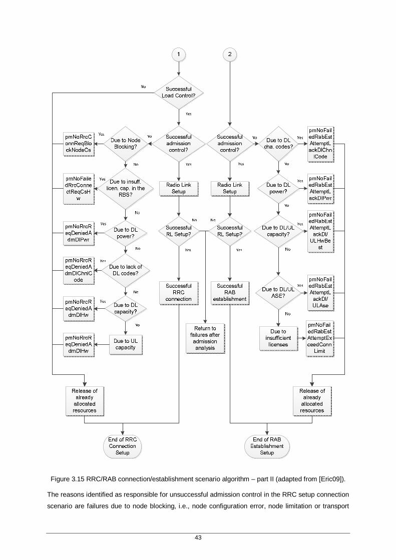
43
Figure 3.15 RRC/RAB connection/establishment scenario algorithm – part II (adapted from [Eric09]).
The reasons identified as responsible for unsuccessful admission control in the RRC setup connection
scenario are failures due to node blocking, i.e., node configuration error, node limitation or transport

44
network layer service unavailability, to insufficient licensed capacity in the RBS, to insufficient DL
power, to lack of DL channelisation codes and to DL/UL lack of capacity. The reasons identified as
responsible for unsuccessful admission control in the RAB establishment scenario are failures due to
insufficient licensed capacity, to insufficient DL power, to lack of DL channelisation codes, to DL/UL
lack of capacity and to lack of DL/UL Air Speech Equivalent (ASE), which is a measure of air-interface
utilisation relative to the utilisation of one speech user (for instance, a connection using 3 ASEs in DL
generates the same interference level as the one generated by three voice users).
In the second group of KPIs, the RAB drop performance is the analysis starting point, since all the
KPIs can be seen as the ratio between the abnormal RAB releases over the total number of RAB
releases. The algorithm to address the speech call drop rate problems is shown in Figure 3.16. The
reasons that may lead to call drops are cell congestion, lost of UL synchronism, missing cell
neighbours and soft HO action.
Figure 3.16 Speech Call Drop Rate algorithm.

45
When analysing call drop rate KPI for data services, the approach has to be a little different. Since
there are no counters directly associated to the reasons that may lead to a poor performance, during
optimisation activity, and especially in case of parameter changes, it is recommended to monitor other
KPIs, since the absolute value of RAB or RRC call drop rate can give a partial vision of the
performances, because it is not taken into consideration service time length. The KPI “Minutes per
Drop” plays an important role in this matter: it gives the average time length (in minutes) between 2
consecutive drops of data calls. It is very useful to report real end user perception of drop call because
it gives the idea how often a user is experiencing a drop call. The pre-defined thresholds are 12
minutes for PS connections and 9 minutes for HS connections. Per example, an user can connect to
the data network in the morning (1 establishment), stay connected for 8 h with multiple transitions
between cell FACH and cell DCH (0 establishments) and 1 drop is counted – this means a call drop
rate of 100% and a call completion success rate of 0%. However, the number of minutes between
drops will be 480. This means that in addiction of analysing the CDR for PS or HS the KPI “Minutes
per Drop” has to be analysed as well as the transitions that occur between different states.
When dealing with the channel switching issues, two KPIs are taken into account: the Channel
Downswitch Failure Rate, which evaluates the probability that the channel downswitch transitions fail
during the channel switching procedure, and the Channel Upswitch Failure Rate, which evaluates the
probability that the channel upswitch transitions fail due to admission control reject or failures during
the channel switching procedure. The last one can be analysed according to the type of transition and
the traffic direction (DL/UL). The Channel Upswitch Failure Rate DL/UL Low Rate is analysed, which
evaluates the failure probability of the transitions in DL between FACH and CELL DCH with DL/UL
rate up to 64 kbps, the Channel Upswitch Failure Rate DL/UL Medium Rate, which evaluates the
failure probability of the channel upswitching transitions due to throughput in DL/UL CELL DCH to
CELL DCH with DL/UL target rate between 64 and 256 kbps, the Channel Upswitch Failure Rate
DL/UL High Rate, which evaluates the failure probability of the channel upswitching transitions due to
throughput in DL/UL CELL DCH to CELL DCH with DL/UL target rate higher than or equal to 256 kbps
(not including HS in DL and excluding EUL in UL), the Channel Upswitch Failure Rate DL HS, which
evaluates the failure probability of the channel upswitching transitions due to throughput in DL from
CELL FACH or CELL DCH R99 to any HS state, and the Channel Upswitch Failure Rate FACH-HS,
which evaluates the failure probability of the transitions in UL between FACH and HSDPA.
Figure 3.17 illustrates the procedures to analyse the performance of the data call drop rate KPIs.
Besides this, the call setup success rate performance has also to be analysed according to Figures
3.10 and 3.11 as well as the speech call drop rate performance, since when a speech call request
arrives the data call will be in preemption.
Throughput problems are usually associated to capacity problems. In the 3G throughput analysis, the
PS/HS throughout performance is compared to parameters, such as the average cell traffic volume,
the number of users, in order to analyse the variations in the throughput data rate with the variations in
the number of users, and the PS/HS call drop rate performance, in order to analyse the effect of a
data call drop in the throughput performance. Figure 3.18 illustrates the process.

46
Figure 3.17 Data call drop rate analysis algorithm.
PS/HS Throughput
Above the threshold
level?
PS/HS Throughput is OK
Compare with other parameters
Cell Traffic Volume Nº of users Analyse PS/HS CDR performance
Analyse the variations in the nº of users with throughput
High channel switching failure rate in HS-FACH or FACH-HS transitions leads
to high values of interference
Analyse channel switching performance
No
Yes
Figure 3.18 PS/HS Throughput analysis algorithm.
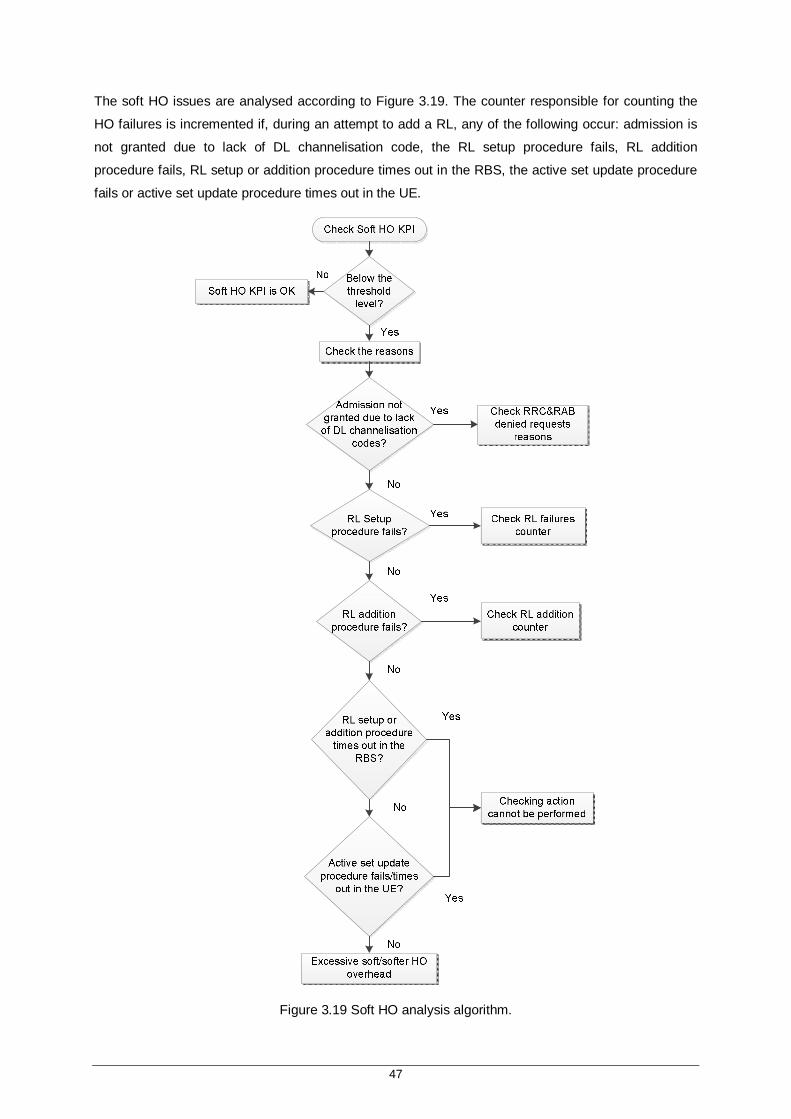
47
The soft HO issues are analysed according to Figure 3.19. The counter responsible for counting the
HO failures is incremented if, during an attempt to add a RL, any of the following occur: admission is
not granted due to lack of DL channelisation code, the RL setup procedure fails, RL addition
procedure fails, RL setup or addition procedure times out in the RBS, the active set update procedure
fails or active set update procedure times out in the UE.
Figure 3.19 Soft HO analysis algorithm.

48
49
Chapter 4
Results Analysis 4 Results Analysis
This chapter contains the descriptions of the used scenarios and the results analysis. First the
simulation scenarios are presented, followed by the simulation output results. The results concerning
the correlation between different KPIs are presented in this chapter.
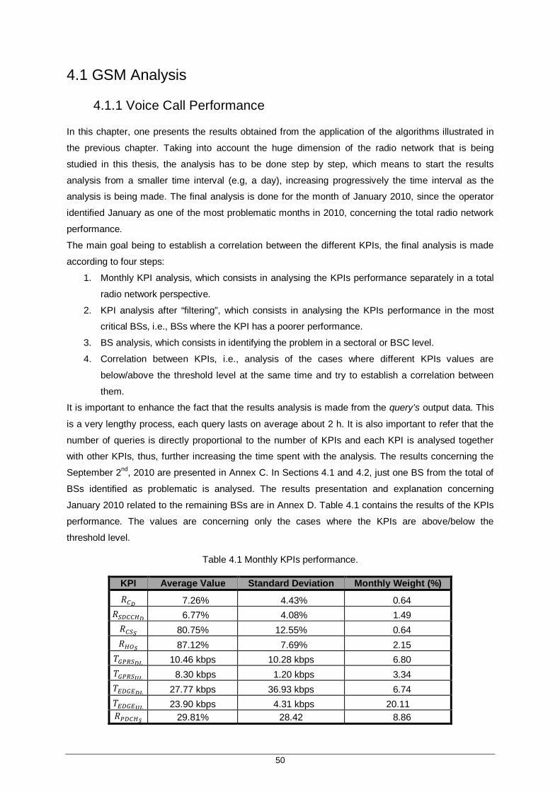
50
4.1 GSM Analysis
4.1.1 Voice Call Performance
In this chapter, one presents the results obtained from the application of the algorithms illustrated in
the previous chapter. Taking into account the huge dimension of the radio network that is being
studied in this thesis, the analysis has to be done step by step, which means to start the results
analysis from a smaller time interval (e.g, a day), increasing progressively the time interval as the
analysis is being made. The final analysis is done for the month of January 2010, since the operator
identified January as one of the most problematic months in 2010, concerning the total radio network
performance.
The main goal being to establish a correlation between the different KPIs, the final analysis is made
according to four steps: 1. Monthly KPI analysis, which consists in analysing the KPIs performance separately in a total
radio network perspective.
2. KPI analysis after “filtering”, which consists in analysing the KPIs performance in the most
critical BSs, i.e., BSs where the KPI has a poorer performance.
3. BS analysis, which consists in identifying the problem in a sectoral or BSC level.
4. Correlation between KPIs, i.e., analysis of the cases where different KPIs values are
below/above the threshold level at the same time and try to establish a correlation between
them.
It is important to enhance the fact that the results analysis is made from the query’s output data. This
is a very lengthy process, each query lasts on average about 2 h. It is also important to refer that the
number of queries is directly proportional to the number of KPIs and each KPI is analysed together
with other KPIs, thus, further increasing the time spent with the analysis. The results concerning the
September 2nd, 2010 are presented in Annex C. In Sections 4.1 and 4.2, just one BS from the total of
BSs identified as problematic is analysed. The results presentation and explanation concerning
January 2010 related to the remaining BSs are in Annex D. Table 4.1 contains the results of the KPIs
performance. The values are concerning only the cases where the KPIs are above/below the
threshold level.
Table 4.1 Monthly KPIs performance.
KPI Average Value Standard Deviation Monthly Weight (%) 푅 7.26% 4.43% 0.64
푅 6.77% 4.08% 1.49 푅 80.75% 12.55% 0.64 푅 87.12% 7.69% 2.15 푇 10.46 kbps 10.28 kbps 6.80 푇 8.30 kbps 1.20 kbps 3.34 푇 27.77 kbps 36.93 kbps 6.74 푇 23.90 kbps 4.31 kbps 20.11 푅 29.81% 28.42 8.86
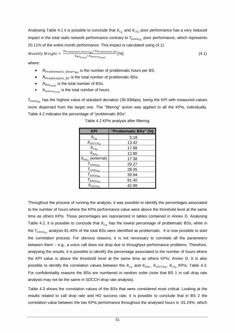
51
Analysing Table 4.1 it is possible to conclude that 푅 and 푅 poor performance has a very reduced
impact in the total radio network performance contrary to 푇 poor performance, which represents
20.11% of the entire month performance. This impact is calculated using (4.1):
푀표푛푡ℎ푙푦푊푒푖푔ℎ푡 = _ × _
×[%] (4.1)
where:
푁 _ is the number of problematic hours per BS. 푁 _ is the total number of problematic BSs. 푁 is the total number of BSs. 푁 is the total number of hours.
푇 has the highest value of standard deviation (36.93kbps), being the KPI with measured values
more dispersed from the target one. The “filtering” action was applied to all the KPIs, individually.
Table 4.2 indicates the percentage of “problematic BSs”.
Table 4.2 KPIs analysis after filtering.
KPI “Problematic BSs” (%) 푅 5.18
푅 13.42 푅 17.68 푅 12.80
푅 (external) 17.38 푇 29.27 푇 28.05 푇 39.94 푇 81.40 푅 42.99
Throughout the process of running the analysis, it was possible to identify the percentages associated
to the number of hours where the KPIs performance value were above the threshold level at the same
time as others KPIs. Those percentages are represented in tables contained in Annex D. Analysing
Table 4.2, it is possible to conclude that 푅 has the lowest percentage of problematic BSs, while in
the 푇 analysis 81.40% of the total BSs were identified as problematic. It is now possible to start
the correlation process. For obvious reasons, it is not necessary to correlate all the parameters
between them – e.g., a voice call does not drop due to throughput performance problems. Therefore,
analysing the results, it is possible to identify the percentage associated to the number of hours where
the KPI value is above the threshold level at the same time as others KPIs, Annex D. It is also
possible to identify the correlation values between the 푅 and 푅 , 푅 , 푅 KPIs, Table 4.3.
For confidentiality reasons the BSs are numbered in random order (note that BS 1 in call drop rate
analysis may not be the same in SDCCH drop rate analysis).
Table 4.3 shows the correlation values of the BSs that were considered most critical. Looking at the
results related to call drop rate and HO success rate, it is possible to conclude that in BS 2 the
correlation value between the two KPIs performance throughout the analysed hours is -91.24%, which

52
indicates a high dependence between them. Figure 4.1 shows 푅 and 푅 performance evolution in
that period.
Table 4.3 푅 correlation analysis.
BS 푅 and 푅 (%) 푅 and 푅 (%) 푅 and 푅 (%) 6 -69.80 -50.92 53.38 2 -91.24 45.16 - 3 -100.00 7.62 -15.66 11 100.00 51.71 -46.85 12 2.72 38.59 -78.70 13 -48.28 12.44 -81.49 17 - -52.03 28.19
Figure 4.1 BS 2 – 푅 and 푅 performance analysis: correlation value of -91.24%.
In BS 2, only sector A in GSM 1800 is affected. Call drop rate has an average value of 30.93% and
HO success rate has an average value of 62.44%. 99.38% of the HO failures are Lost HOs and 0.62%
are HO reversions. According to Figure 3.8, the HO performance analysis has to be done. The first
step is to analyse the number of HO attempts. There are 283 HO attempts, which is considered a low
number. According to the HO algorithm, the analysis stops here, and so another cell will be analysed.
However, just to check where the source of the problem could be, the call drop rate performance is
analysed. A total sample of 819 terminated calls with 72 TCH drops. Figure 4.2 illustrates the
“contribution” given by each call drop reasons.
It allows to conclude that poor quality on DL or UL is the major reason for TCH drops. Poor signal
quality or bad quality of a call are triggered by a high bit error rate on UL or DL – CIR or intersymbol
interference (ISI). It is closely related to the interference between BSs and sometimes it can be due to
bad cellular planning. The type of interference should be identified:
Internal: Internal interference, co-channel or adjacent channel interference means that the
problem exists within the own network due to a bad frequency plan, bad site location,
congestion or too high antenna location.
1 2 3 4 5 6 7 8 9 10 11 12 13 14 15 16 17 18 19 20 21 22 23 24 25 26 27 28 29 30 31 320
10
20
30
40
50
60
70
80
90
100
Number of hours
CD
R a
nd H
SR
[%]
CDR [%]HSR [%]CDR ThresholdHSR Threshold
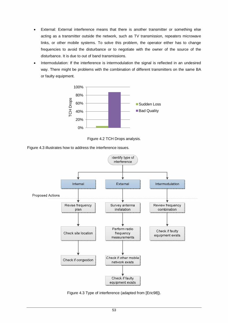
53
External: External interference means that there is another transmitter or something else
acting as a transmitter outside the network, such as TV transmission, repeaters microwave
links, or other mobile systems. To solve this problem, the operator either has to change
frequencies to avoid the disturbance or to negotiate with the owner of the source of the
disturbance. It is due to out of band transmissions.
Intermodulation: If the interference is intermodulation the signal is reflected in an undesired
way. There might be problems with the combination of different transmitters on the same BA
or faulty equipment.
Figure 4.2 TCH Drops analysis.
Figure 4.3 illustrates how to address the interference issues.
Figure 4.3 Type of interference (adapted from [Eric98]).
0%
20%
40%
60%
80%
100%
TCH
Dro
ps
Sudden Loss
Bad Quality
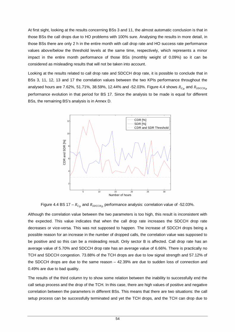
54
At first sight, looking at the results concerning BSs 3 and 11, the almost automatic conclusion is that in
those BSs the call drops due to HO problems with 100% sure. Analysing the results in more detail, in
those BSs there are only 2 h in the entire month with call drop rate and HO success rate performance
values above/below the threshold levels at the same time, respectively, which represents a minor
impact in the entire month performance of those BSs (monthly weight of 0.09%) so it can be
considered as misleading results that will not be taken into account.
Looking at the results related to call drop rate and SDCCH drop rate, it is possible to conclude that in
BSs 3, 11, 12, 13 and 17 the correlation values between the two KPIs performance throughout the
analysed hours are 7.62%, 51.71%, 38.59%, 12.44% and -52.03%. Figure 4.4 shows 푅 and 푅
performance evolution in that period for BS 17. Since the analysis to be made is equal for different
BSs, the remaining BS’s analysis is in Annex D.
Figure 4.4 BS 17 – 푅 and 푅 performance analysis: correlation value of -52.03%.
Although the correlation value between the two parameters is too high, this result is inconsistent with
the expected. This value indicates that when the call drop rate increases the SDCCH drop rate
decreases or vice-versa. This was not supposed to happen. The increase of SDCCH drops being a
possible reason for an increase in the number of dropped calls, the correlation value was supposed to
be positive and so this can be a misleading result. Only sector B is affected. Call drop rate has an
average value of 5.70% and SDCCH drop rate has an average value of 6.66%. There is practically no
TCH and SDCCH congestion. 73.88% of the TCH drops are due to low signal strength and 57.12% of
the SDCCH drops are due to the same reason – 42.39% are due to sudden loss of connection and
0.49% are due to bad quality.
The results of the third column try to show some relation between the inability to successfully end the
call setup process and the drop of the TCH. In this case, there are high values of positive and negative
correlation between the parameters in different BSs. This means that there are two situations: the call
setup process can be successfully terminated and yet the TCH drops, and the TCH can drop due to
5 10 15 20 25 30
2
4
6
8
10
12
Number of hours
CD
R a
nd S
DR
[%]
CDR [%]SDR [%]CDR and SDR Threshold

55
the fact that the call setup process was unsuccessfully terminated. BS 6 performance is a case of
positive correlation and BS 13 is a case of negative correlation. Figures 4.5 and 4.6 show the
performance of the two KPIs. Analysing Figure 4.6, it is easily identifiable the correlation between the
two KPIs. However, the number of problematic hours only represents 4.08% of the entire month
performance of that BS. The call setup success rate has an average value of 93.09%, which does not
represent a high difference compared to the threshold level. With a total of 1236 TCH drops, the call
drop rate has an average value of 5.23%. 60.74% of the drops are due to low signal strength, 18.07%
due to sudden loss of connection and 21.19% are due to bad quality. There is practically no TCH
congestion, and the SDCCH congestion has an average value of 3.61%. In BS 6, the number of
problematic hours only represents 1.34% of the entire month performance of that BS. The call setup
success rate has an average value of 85.07%. With a total of 27095 TCH drops, the call drop rate has
an average value of 27.20%, which is a high value. 0.68% of the drops are due to low signal strength,
82.39% due to sudden loss of connection and 16.93% are due to bad quality. There is no TCH or
SDCCH congestion.
Figure 4.5 BS 6 – 푅 and 푅 performance analysis: correlation value of 53.38%.
Figure 4.6 BS 13 – 푅 and 푅 performance analysis: correlation value of -81.49%.
5 10 15 20 25 300
10
20
30
40
50
60
70
80
90
100
Number of hours
CD
R a
nd C
SS
R [%
]
CDR [%]CSSR [%]CDR ThresholdCSSR Threshold
10 20 30 40 50 60 70 80 900
10
20
30
40
50
60
70
80
90
100
Number of hours
CD
R a
nd C
SS
R [%
]
CDR [%]CSSR [%]CDR ThresholdCSSR Threshold
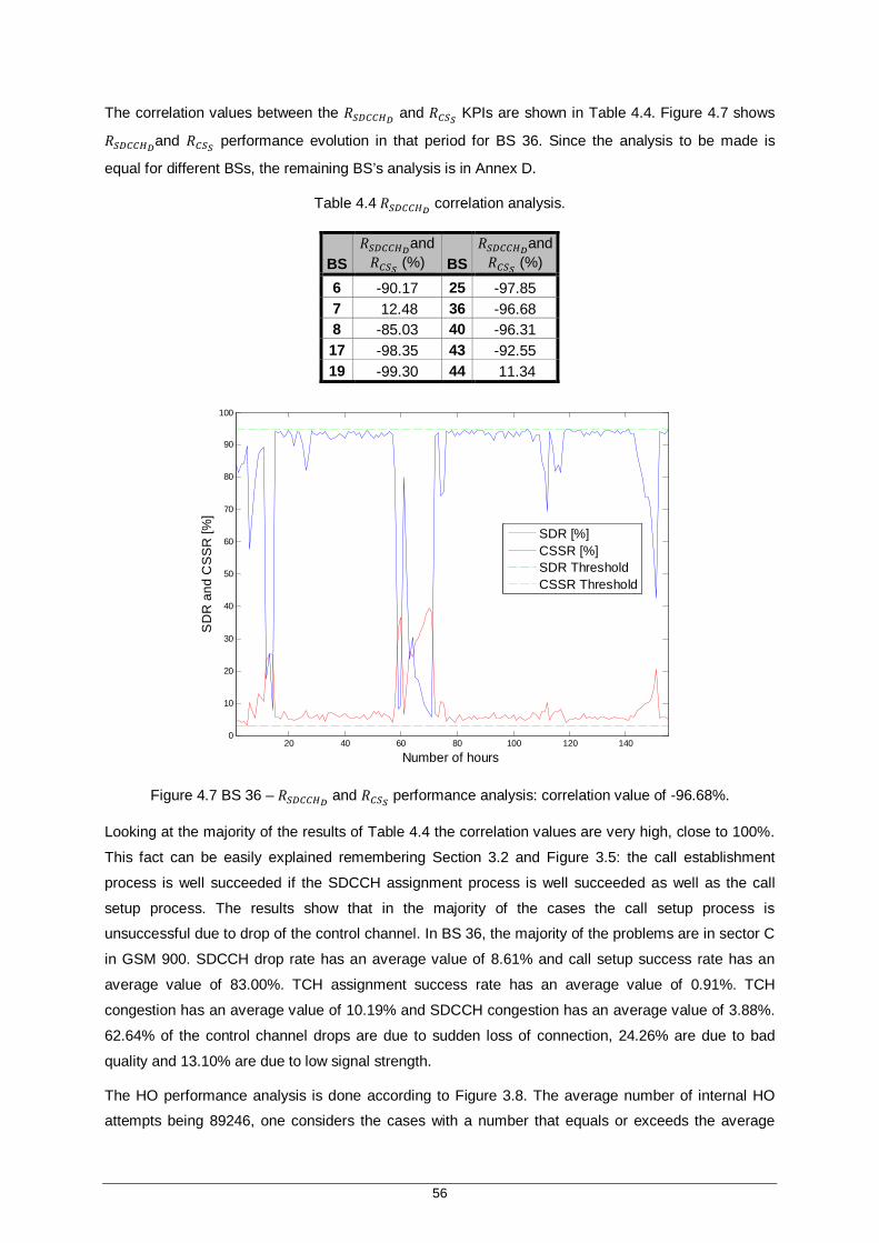
56
The correlation values between the 푅 and 푅 KPIs are shown in Table 4.4. Figure 4.7 shows
푅 and 푅 performance evolution in that period for BS 36. Since the analysis to be made is
equal for different BSs, the remaining BS’s analysis is in Annex D.
Table 4.4 푅 correlation analysis.
BS 푅 and 푅 (%) BS
푅 and 푅 (%)
6 -90.17 25 -97.85 7 12.48 36 -96.68 8 -85.03 40 -96.31 17 -98.35 43 -92.55 19 -99.30 44 11.34
Figure 4.7 BS 36 – 푅 and 푅 performance analysis: correlation value of -96.68%.
Looking at the majority of the results of Table 4.4 the correlation values are very high, close to 100%.
This fact can be easily explained remembering Section 3.2 and Figure 3.5: the call establishment
process is well succeeded if the SDCCH assignment process is well succeeded as well as the call
setup process. The results show that in the majority of the cases the call setup process is
unsuccessful due to drop of the control channel. In BS 36, the majority of the problems are in sector C
in GSM 900. SDCCH drop rate has an average value of 8.61% and call setup success rate has an
average value of 83.00%. TCH assignment success rate has an average value of 0.91%. TCH
congestion has an average value of 10.19% and SDCCH congestion has an average value of 3.88%.
62.64% of the control channel drops are due to sudden loss of connection, 24.26% are due to bad
quality and 13.10% are due to low signal strength.
The HO performance analysis is done according to Figure 3.8. The average number of internal HO
attempts being 89246, one considers the cases with a number that equals or exceeds the average
20 40 60 80 100 120 1400
10
20
30
40
50
60
70
80
90
100
Number of hours
SD
R a
nd C
SS
R [%
]
SDR [%]CSSR [%]SDR ThresholdCSSR Threshold
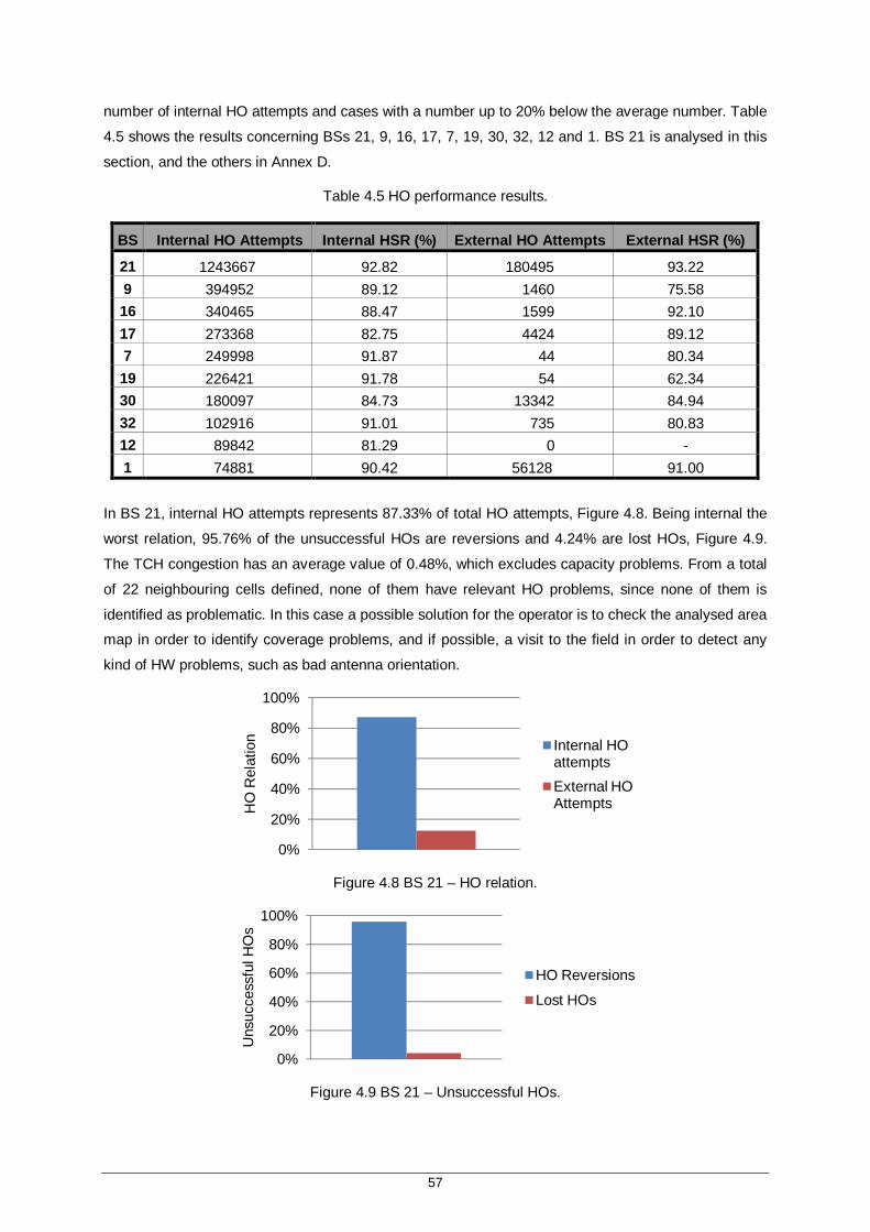
57
number of internal HO attempts and cases with a number up to 20% below the average number. Table
4.5 shows the results concerning BSs 21, 9, 16, 17, 7, 19, 30, 32, 12 and 1. BS 21 is analysed in this
section, and the others in Annex D.
Table 4.5 HO performance results.
BS Internal HO Attempts Internal HSR (%) External HO Attempts External HSR (%)
21 1243667 92.82 180495 93.22 9 394952 89.12 1460 75.58 16 340465 88.47 1599 92.10 17 273368 82.75 4424 89.12 7 249998 91.87 44 80.34 19 226421 91.78 54 62.34 30 180097 84.73 13342 84.94 32 102916 91.01 735 80.83 12 89842 81.29 0 - 1 74881 90.42 56128 91.00
In BS 21, internal HO attempts represents 87.33% of total HO attempts, Figure 4.8. Being internal the
worst relation, 95.76% of the unsuccessful HOs are reversions and 4.24% are lost HOs, Figure 4.9.
The TCH congestion has an average value of 0.48%, which excludes capacity problems. From a total
of 22 neighbouring cells defined, none of them have relevant HO problems, since none of them is
identified as problematic. In this case a possible solution for the operator is to check the analysed area
map in order to identify coverage problems, and if possible, a visit to the field in order to detect any
kind of HW problems, such as bad antenna orientation.
Figure 4.8 BS 21 – HO relation.
Figure 4.9 BS 21 – Unsuccessful HOs.
0%
20%
40%
60%
80%
100%
HO
Rel
atio
n Internal HO attemptsExternal HO Attempts
0%
20%
40%
60%
80%
100%
Uns
ucce
ssfu
l HO
s
HO Reversions
Lost HOs
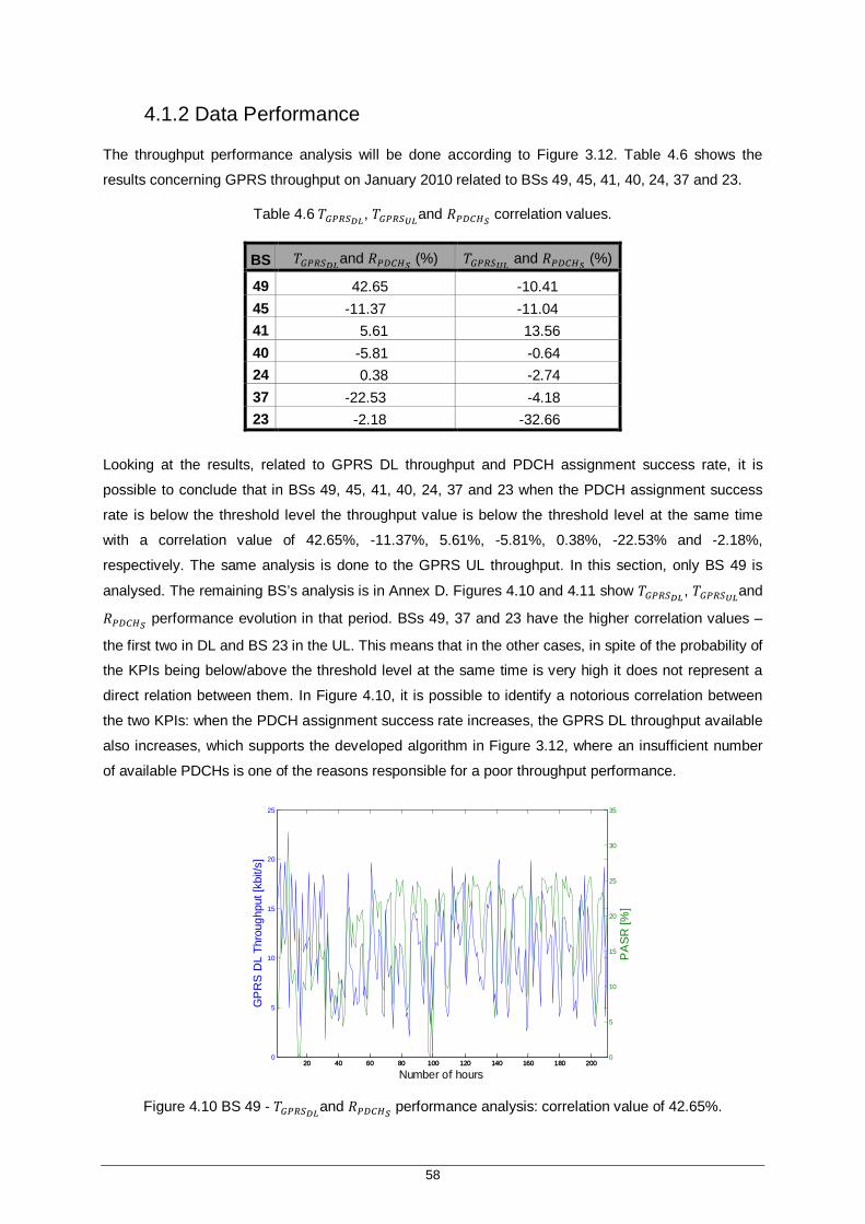
58
4.1.2 Data Performance
The throughput performance analysis will be done according to Figure 3.12. Table 4.6 shows the
results concerning GPRS throughput on January 2010 related to BSs 49, 45, 41, 40, 24, 37 and 23.
Table 4.6 푇 , 푇 and 푅 correlation values.
BS 푇 and 푅 (%) 푇 and 푅 (%)
49 42.65 -10.41 45 -11.37 -11.04 41 5.61 13.56 40 -5.81 -0.64 24 0.38 -2.74 37 -22.53 -4.18 23 -2.18 -32.66
Looking at the results, related to GPRS DL throughput and PDCH assignment success rate, it is
possible to conclude that in BSs 49, 45, 41, 40, 24, 37 and 23 when the PDCH assignment success
rate is below the threshold level the throughput value is below the threshold level at the same time
with a correlation value of 42.65%, -11.37%, 5.61%, -5.81%, 0.38%, -22.53% and -2.18%,
respectively. The same analysis is done to the GPRS UL throughput. In this section, only BS 49 is
analysed. The remaining BS’s analysis is in Annex D. Figures 4.10 and 4.11 show 푇 , 푇 and
푅 performance evolution in that period. BSs 49, 37 and 23 have the higher correlation values –
the first two in DL and BS 23 in the UL. This means that in the other cases, in spite of the probability of
the KPIs being below/above the threshold level at the same time is very high it does not represent a
direct relation between them. In Figure 4.10, it is possible to identify a notorious correlation between
the two KPIs: when the PDCH assignment success rate increases, the GPRS DL throughput available
also increases, which supports the developed algorithm in Figure 3.12, where an insufficient number
of available PDCHs is one of the reasons responsible for a poor throughput performance.
Figure 4.10 BS 49 - 푇 and 푅 performance analysis: correlation value of 42.65%.
20 40 60 80 100 120 140 160 180 2000
5
10
15
20
25
GP
RS
DL
Thro
ughp
ut [k
bit/s
]
Number of hours20 40 60 80 100 120 140 160 180 200
0
5
10
15
20
25
30
35
PA
SR [%
]

59
Figure 4.11 BS 49 - 푇 and 푅 performance analysis: correlation value of -10.41%.
Analysing the PDCH assignment success rate performance, it has an average value of 17.65%, which
is a very low value. TCH congestion has an average value of 2.41%, which is a low value compared to
the pre-defined threshold. The HR traffic represents 95.41% of the total traffic, which means that the
HR traffic can be one of the reasons to have a high number of PDCH fails. Figure 4.12 illustrates the
RLC data volume distribution of this BS.
Figure 4.12 BS 49 – DL Radio Link Quality analysis.
Analysing the GPRS DL throughput (average value of 10.47 kbps), the GPRS RLC average data
volume is distributed in this way: 0.050 kbits in the 8 kbps interval, 0.080 kbits in the 10 kbps interval,
0.278 kbits in the 12 kbps interval, 0.207 kbits in the 14 kbps interval, 0.174 kbits in the 16 kbps
interval and 0.261 kbits in the 18 kbps interval. Looking at the results the major “slice” of the traffic is in
the higher bit rate intervals (61.13% of the total traffic is in the three higher bite rate intervals), which
means good radio link quality. The average PDCH utilisation ratio is 85.73% (above the 80% threshold
value) and there are 5.24 simultaneous users per active PDCH, which is clearly superior compared to
the 1.4 threshold value, which proves there is in fact a high capacity problem. In the UL direction,
20 40 60 80 100 120 1400
5
10
15
20
25
GP
RS
UL
Thro
ughp
ut [k
bit/s
]
Number of hours20 40 60 80 100 120 140
0
10
20
30
40
50
60
70
PA
SR
[%]
0%10%20%30%40%50%60%70%80%90%
100%
RLC
Dat
a V
olum
e [k
bits
]
18 kbps
16 kbps
14 kbps
12 kbps
10 kbps
8 kbps
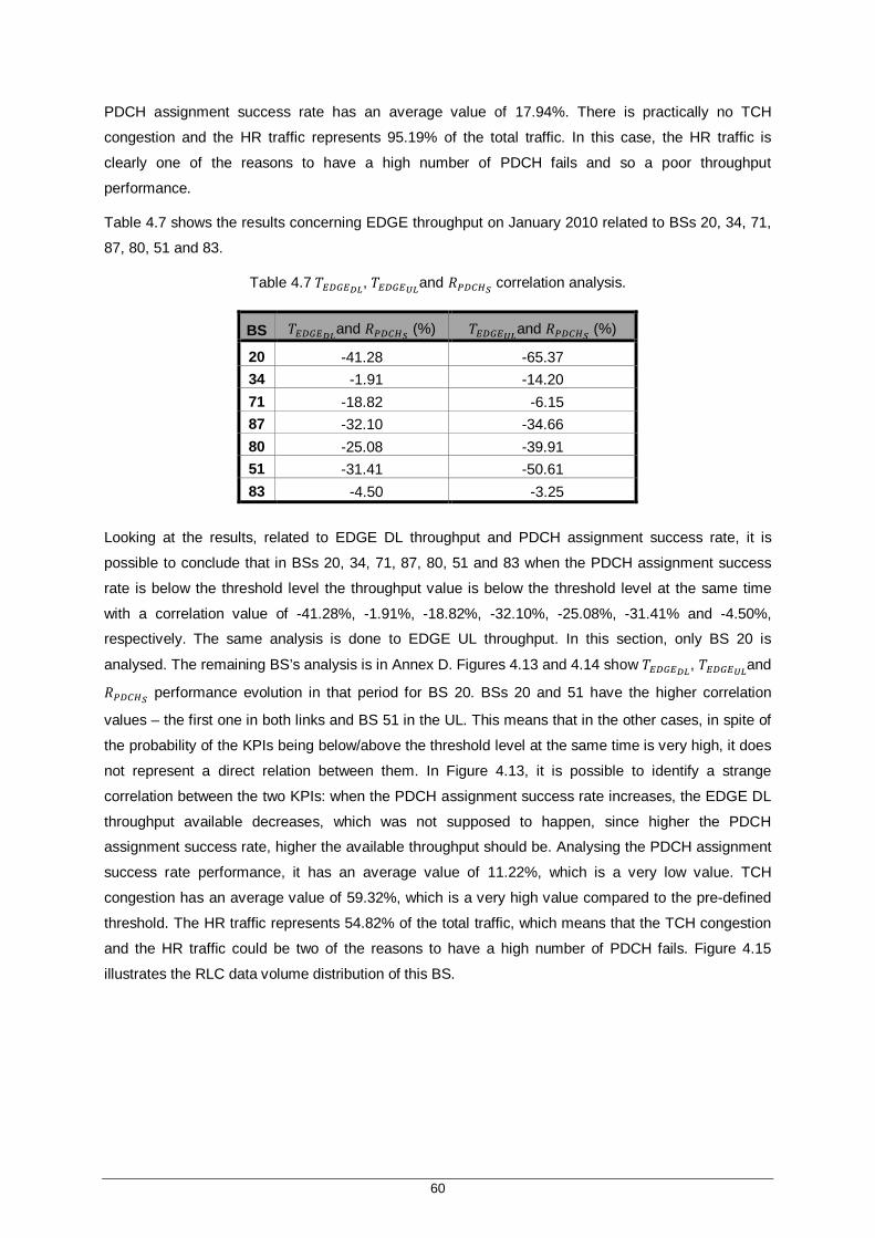
60
PDCH assignment success rate has an average value of 17.94%. There is practically no TCH
congestion and the HR traffic represents 95.19% of the total traffic. In this case, the HR traffic is
clearly one of the reasons to have a high number of PDCH fails and so a poor throughput
performance.
Table 4.7 shows the results concerning EDGE throughput on January 2010 related to BSs 20, 34, 71,
87, 80, 51 and 83.
Table 4.7 푇 , 푇 and 푅 correlation analysis.
BS 푇 and 푅 (%) 푇 and 푅 (%)
20 -41.28 -65.37 34 -1.91 -14.20 71 -18.82 -6.15 87 -32.10 -34.66 80 -25.08 -39.91 51 -31.41 -50.61 83 -4.50 -3.25
Looking at the results, related to EDGE DL throughput and PDCH assignment success rate, it is
possible to conclude that in BSs 20, 34, 71, 87, 80, 51 and 83 when the PDCH assignment success
rate is below the threshold level the throughput value is below the threshold level at the same time
with a correlation value of -41.28%, -1.91%, -18.82%, -32.10%, -25.08%, -31.41% and -4.50%,
respectively. The same analysis is done to EDGE UL throughput. In this section, only BS 20 is
analysed. The remaining BS’s analysis is in Annex D. Figures 4.13 and 4.14 show 푇 , 푇 and
푅 performance evolution in that period for BS 20. BSs 20 and 51 have the higher correlation
values – the first one in both links and BS 51 in the UL. This means that in the other cases, in spite of
the probability of the KPIs being below/above the threshold level at the same time is very high, it does
not represent a direct relation between them. In Figure 4.13, it is possible to identify a strange
correlation between the two KPIs: when the PDCH assignment success rate increases, the EDGE DL
throughput available decreases, which was not supposed to happen, since higher the PDCH
assignment success rate, higher the available throughput should be. Analysing the PDCH assignment
success rate performance, it has an average value of 11.22%, which is a very low value. TCH
congestion has an average value of 59.32%, which is a very high value compared to the pre-defined
threshold. The HR traffic represents 54.82% of the total traffic, which means that the TCH congestion
and the HR traffic could be two of the reasons to have a high number of PDCH fails. Figure 4.15
illustrates the RLC data volume distribution of this BS.
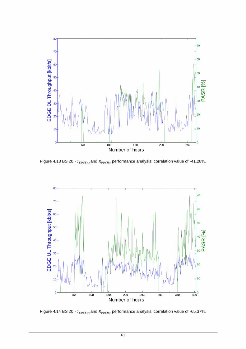
61
Figure 4.13 BS 20 - 푇 and 푅 performance analysis: correlation value of -41.28%.
Figure 4.14 BS 20 - 푇 and 푅 performance analysis: correlation value of -65.37%.
50 100 150 200 2500
10
20
30
40
50
60
70
80
ED
GE
DL
Thro
ughp
ut [k
bit/s
]
Number of hours50 100 150 200 250
0
10
20
30
40
50
60
70
PA
SR
[%]
50 100 150 200 250 300 350 4000
10
20
30
40
50
60
70
80
ED
GE
UL
Thro
ughp
ut [k
bit/s
]
Number of hours50 100 150 200 250 300 350 400
0
10
20
30
40
50
60
70
PA
SR
[%]

62
Figure 4.15 DL Radio link quality analysis.
Analysing the EDGE DL throughput (average value of 20.77 kbps), the EDGE RLC average data
volume is distributed in this way: 0.0058 kbits in the 10 kbps interval, 0.2702 kbits in the 15 kbps
interval, 0.0420 kbits in the 20 kbps interval, 0.0180 kbits in the 25 kbps interval, 0.0260 kbits in the 30
kbps interval, 0.0338 kbits in the 35 kbps interval, 0.0518 kbits in the 40 kbps interval, 0.0816 kbits in
the 45 kbps interval, 0.1190 kbits in the 50 kbps interval and 0.5951 kbits in the 55 kbps interval.
Looking at the results the major “slice” of the traffic is in the higher bit rate intervals (84.74% of the
total traffic is in the four higher bite rate intervals), which means good radio link quality. The average
PDCH utilisation ratio is 87.55% (above the 80% threshold value) and there are 4.77 simultaneous
users per active DL PDCH – above the 1.4 threshold value, which proves there is in fact a high
capacity problem. In UL, PDCH assignment success rate has an average value of 20.37%. The TCH
congestion has an average value of 40.19% and the HR traffic represents 48.63% of the total traffic. In
this case, TCH congestion is very high so it is possible to have here a capacity problem. Figure 4.16
illustrates the analysis of the UL radio link quality.
Figure 4.16 UL Radio link quality analysis.
Analysing the EDGE UL throughput (average value of 15.90 kbps), the EDGE RLC average data
volume is distributed in this way: 0.0056 kbits in the 10 kbps interval, 0.0238 kbits in the 15 kbps
0%10%20%30%40%50%60%70%80%90%
100%
RLC
Dat
a V
olum
e [k
bits
]
55 kbps
50 kbps
45 kbps
40 kbps
35 kbps
30 kbps
25 kbps
20 kbps
15 kbps
0%
10%
20%
30%
40%
50%
60%
70%
80%
90%
100%
RLC
Dat
a V
olum
e [k
bits
]
55 kbps
50 kbps
45 kbps
40 kbps
35 kbps
30 kbps
25 kbps
20 kbps
15 kbps
10 kbps

63
interval, 0.0398 kbits in the 20 kbps interval, 0.0167 kbits in the 25 kbps interval, 0.0249 kbits in the 30
kbps interval, 0.0339 kbits in the 35 kbps interval, 0.0519 kbits in the 40 kbps interval, 0.0818 kbits in
the 45 kbps interval, 0.1272 kbits in the 50 kbps interval and 0.5945 kbits in the 55 kbps interval.
Looking at the results the major “slice” of the traffic is in the higher bit rate intervals (85.54% of the
total traffic is in the four higher bite rate intervals), which means good radio link quality. The average
PDCH utilisation ratio is 80.49% (above the 80% threshold value) and there are 2.92 simultaneous
users per active DL PDCH – above the 1.4 threshold value, which proves there is in fact a capacity
problem.
4.2 UMTS Analysis
4.2.1 Voice Call Performance
Table 4.8 contains the results of the KPIs performance during January 2010. The values are
concerning only the cases where the KPI is above/below the threshold level.
Table 4.8 Monthly KPIs.
KPI Average Value Standard Deviation Monthly Weight (%) 푅 71.79% 18.53% 0.84 푅 46.36% 35.10% 0.06
푅 _ 64.31% 22.41% 4.06 푅 _ 71.34% 17.44% 3.41
푅 13.33% 8.72% 1.80 푅 44.39% 29.97% 0.01 푅 _ 16.48% 10.24% 1.51 푅 _ 47.49% 32.17% 18.74 푅 54.10% 29.63% 0.18 푇 17.41 kbps 129.11 kbps 56.65 푇 13.84 kbps 25.57 kbps 56.25 푇 186.06 kbps 575.54 kbps 51.69
푅 _ 3.16% 57.87% 0.01 푅 _ 52.02% 23.32% 0.38
Analysing Table 4.8, it is possible to conclude that 푅 , 푅 , 푅 , 푅 , 푅 _ and
푅 _ poor performance has a very reduced impact in the total radio network performance
contrary to 푇 , 푇 and 푇 poor performance, which represents 56.65%, 56.25% and
51.69% of the entire month performance, respectively. 푇 has the highest value of standard
deviation (575.54 kbps), being the KPI with measured values more dispersed from the target value.
Analysing Table 4.9, it is possible to conclude that 푅 has the lower percentage of problematic
BSs, while in the 푇 , 푇 and 푇 analysis 58.48%, 59.38% and 56.25% of the total BSs
were identified as problematic, respectively. The “filtering” action was applied to all the KPIs,
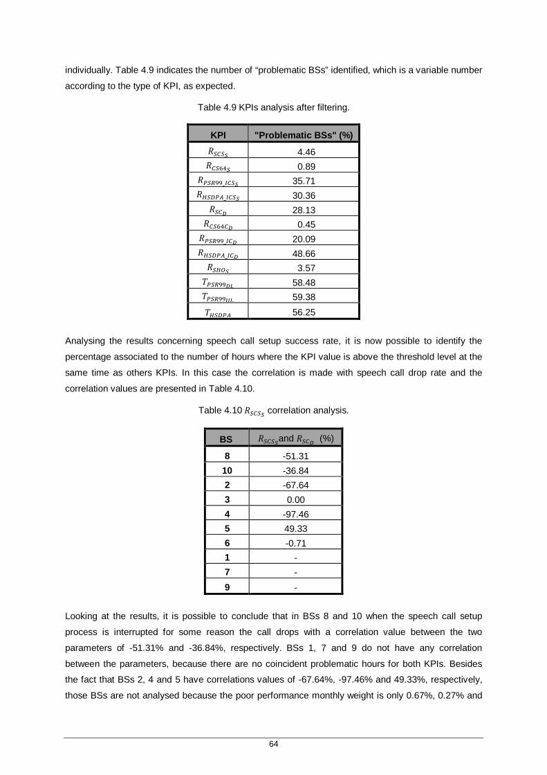
64
individually. Table 4.9 indicates the number of “problematic BSs” identified, which is a variable number
according to the type of KPI, as expected.
Table 4.9 KPIs analysis after filtering.
KPI "Problematic BSs" (%) 푅 4.46 푅 0.89
푅 _ 35.71 푅 _ 30.36
푅 28.13 푅 0.45 푅 _ 20.09 푅 _ 48.66 푅 3.57 푇 58.48 푇 59.38 푇 56.25
Analysing the results concerning speech call setup success rate, it is now possible to identify the
percentage associated to the number of hours where the KPI value is above the threshold level at the
same time as others KPIs. In this case the correlation is made with speech call drop rate and the
correlation values are presented in Table 4.10.
Table 4.10 푅 correlation analysis.
BS 푅 and 푅 (%)
8 -51.31 10 -36.84 2 -67.64 3 0.00 4 -97.46 5 49.33 6 -0.71 1 - 7 - 9 -
Looking at the results, it is possible to conclude that in BSs 8 and 10 when the speech call setup
process is interrupted for some reason the call drops with a correlation value between the two
parameters of -51.31% and -36.84%, respectively. BSs 1, 7 and 9 do not have any correlation
between the parameters, because there are no coincident problematic hours for both KPIs. Besides
the fact that BSs 2, 4 and 5 have correlations values of -67.64%, -97.46% and 49.33%, respectively,
those BSs are not analysed because the poor performance monthly weight is only 0.67%, 0.27% and
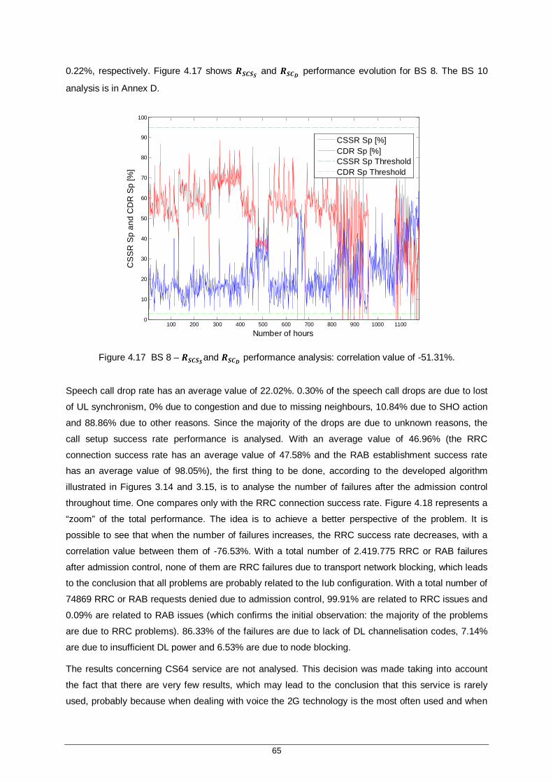
65
0.22%, respectively. Figure 4.17 shows 푹푺푪푺푺 and 푹푺푪푫 performance evolution for BS 8. The BS 10
analysis is in Annex D.
Figure 4.17 BS 8 – 푹푺푪푺푺and 푹푺푪푫 performance analysis: correlation value of -51.31%.
Speech call drop rate has an average value of 22.02%. 0.30% of the speech call drops are due to lost
of UL synchronism, 0% due to congestion and due to missing neighbours, 10.84% due to SHO action
and 88.86% due to other reasons. Since the majority of the drops are due to unknown reasons, the
call setup success rate performance is analysed. With an average value of 46.96% (the RRC
connection success rate has an average value of 47.58% and the RAB establishment success rate
has an average value of 98.05%), the first thing to be done, according to the developed algorithm
illustrated in Figures 3.14 and 3.15, is to analyse the number of failures after the admission control
throughout time. One compares only with the RRC connection success rate. Figure 4.18 represents a
“zoom” of the total performance. The idea is to achieve a better perspective of the problem. It is
possible to see that when the number of failures increases, the RRC success rate decreases, with a
correlation value between them of -76.53%. With a total number of 2.419.775 RRC or RAB failures
after admission control, none of them are RRC failures due to transport network blocking, which leads
to the conclusion that all problems are probably related to the Iub configuration. With a total number of
74869 RRC or RAB requests denied due to admission control, 99.91% are related to RRC issues and
0.09% are related to RAB issues (which confirms the initial observation: the majority of the problems
are due to RRC problems). 86.33% of the failures are due to lack of DL channelisation codes, 7.14%
are due to insufficient DL power and 6.53% are due to node blocking.
The results concerning CS64 service are not analysed. This decision was made taking into account
the fact that there are very few results, which may lead to the conclusion that this service is rarely
used, probably because when dealing with voice the 2G technology is the most often used and when
100 200 300 400 500 600 700 800 900 1000 11000
10
20
30
40
50
60
70
80
90
100
Number of hours
CS
SR
Sp
and
CD
R S
p [%
]
CSSR Sp [%]CDR Sp [%]CSSR Sp ThresholdCDR Sp Threshold

66
dealing with data it is all reported to 3G.
Figure 4.18 BS 8 – Total number of failures after admission control versus “RRC success rate”.
4.2.2 Data Performance
Analysing the results concerning 푅 _ parameter, it is possible to identify the percentage
associated to the number of hours where the KPI value is above the threshold level at the same time
as others KPIs. In this case, the correlation is made with PS R99 Interactive call drop rate and the
correlation values are presented in Table 4.11. BS 58 is the only BS that is analysed, since all the
others have a poor performance monthly weight with low impact. Looking at the results, it is possible
to conclude that in BS 58 when the PS R99 Interactive call setup success rate is below the threshold
level the PS R99 Interactive call drop rate is also below the threshold level with a correlation value
between the two cases of -65.00%.
Figure 4.19 shows 푅 _ and 푅 _ performance evolution. PS R99 interactive call drop rate
has an average value of 33.73%. With a number of 10154 abnormal RAB PS DCH/FACH releases
and according to the “Minutes per Drop” KPI, a user experiences a drop call, in average, in every
5min58s, which exceeds the predefined threshold of 12min, allowing to verify the KPI poor
performance. The channel downswitch failure rate has an average value of 12.09%. Figures 4.20 and
4.21 represent the percentage distribution of the channel upswitch failure rate. Analysing the results, it
is possible to conclude that the DL/UL PS transitions fail very few times, with average values of 0% in
medium and high rate and around 1.50% in low rate, which may lead to the conclusion that the
channel upswitch issues do not contribute for the KPI poor performance. Analysing the call setup
success rate performance, with an average value of 39.14%, the RRC connection success rate has an
600 700 800 900 1000 1100 12000
2000
4000
6000
8000
10000
12000
14000
16000
18000
Num
ber o
f fai
lure
s af
ter t
he a
dmis
sion
con
trol
Number of hours600 700 800 900 1000 1100 1200
0
10
20
30
40
50
60
70
80
90
100
RR
C s
ucce
ss ra
te [%
]
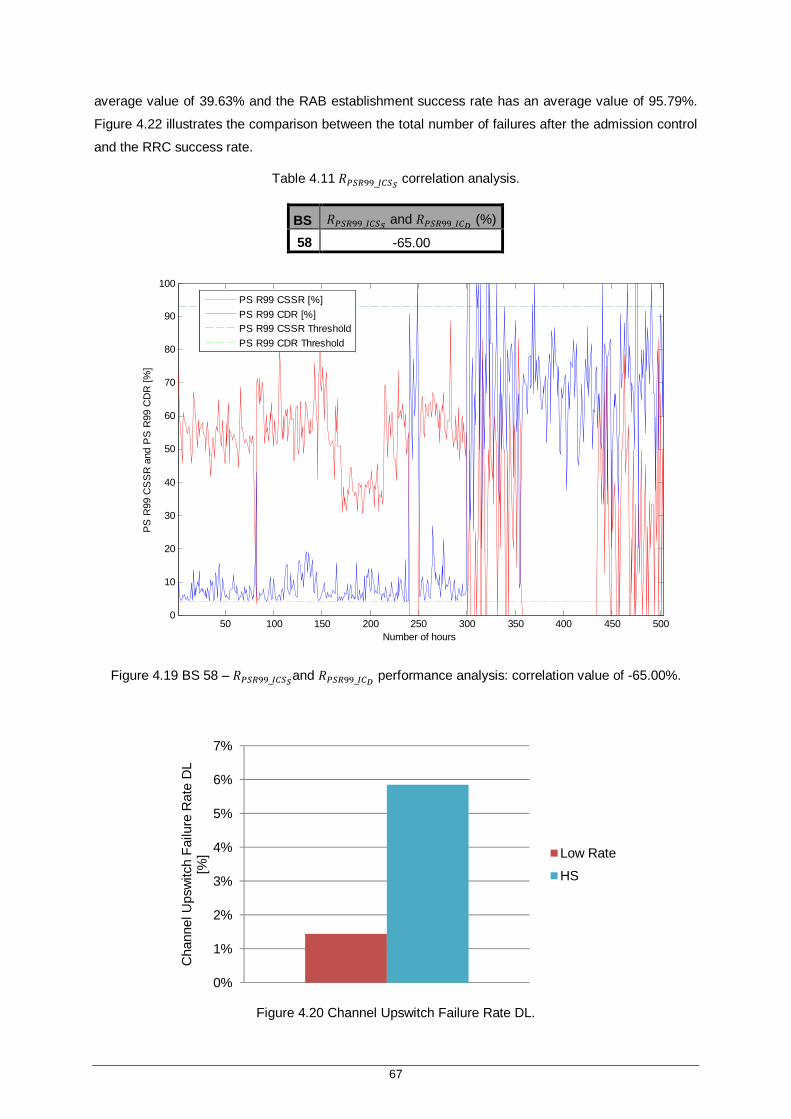
67
average value of 39.63% and the RAB establishment success rate has an average value of 95.79%.
Figure 4.22 illustrates the comparison between the total number of failures after the admission control
and the RRC success rate.
Table 4.11 푅 _ correlation analysis.
BS 푅 _ and 푅 _ (%)
58 -65.00
Figure 4.19 BS 58 – 푅 _ and 푅 _ performance analysis: correlation value of -65.00%.
Figure 4.20 Channel Upswitch Failure Rate DL.
50 100 150 200 250 300 350 400 450 5000
10
20
30
40
50
60
70
80
90
100
Number of hours
PS
R99
CS
SR
and
PS
R99
CD
R [%
]
PS R99 CSSR [%]PS R99 CDR [%]PS R99 CSSR ThresholdPS R99 CDR Threshold
0%
1%
2%
3%
4%
5%
6%
7%
Cha
nnel
Ups
witc
h Fa
ilure
Rat
e D
L [%
] Low Rate
HS
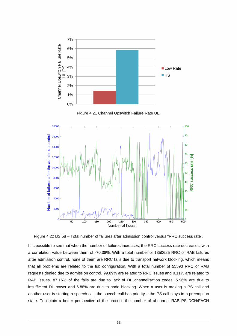
68
Figure 4.21 Channel Upswitch Failure Rate UL.
Figure 4.22 BS 58 – Total number of failures after admission control versus “RRC success rate”.
It is possible to see that when the number of failures increases, the RRC success rate decreases, with
a correlation value between them of -70.38%. With a total number of 1350625 RRC or RAB failures
after admission control, none of them are RRC fails due to transport network blocking, which means
that all problems are related to the Iub configuration. With a total number of 55590 RRC or RAB
requests denied due to admission control, 99.89% are related to RRC issues and 0.11% are related to
RAB issues. 87.16% of the fails are due to lack of DL channelisation codes, 5.96% are due to
insufficient DL power and 6.88% are due to node blocking. When a user is making a PS call and
another user is starting a speech call, the speech call has priority – the PS call stays in a preemption
state. To obtain a better perspective of the process the number of abnormal RAB PS DCH/FACH
0%
1%
2%
3%
4%
5%
6%
7%
Cha
nnel
Ups
witc
h Fa
ilure
Rat
e U
L [%
]Low Rate
HS
50 100 150 200 250 300 350 400 450 5000
2000
4000
6000
8000
10000
12000
14000
16000
18000
Num
ber o
f fai
lure
s af
ter t
he a
dmis
sion
con
trol
Number of hours50 100 150 200 250 300 350 400 450 500
0
10
20
30
40
50
60
70
80
90
100
RR
C s
ucce
ss ra
te [%
]
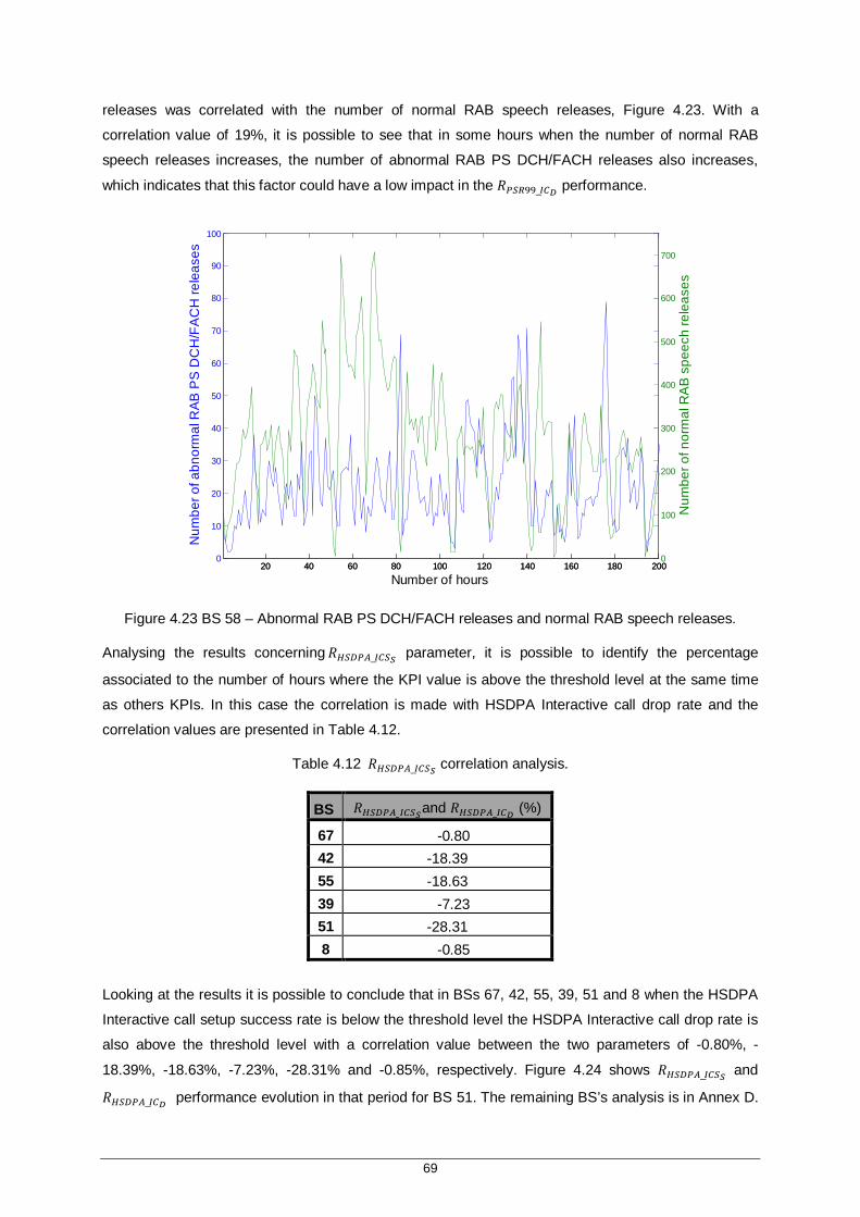
69
releases was correlated with the number of normal RAB speech releases, Figure 4.23. With a
correlation value of 19%, it is possible to see that in some hours when the number of normal RAB
speech releases increases, the number of abnormal RAB PS DCH/FACH releases also increases,
which indicates that this factor could have a low impact in the 푅 _ performance.
Figure 4.23 BS 58 – Abnormal RAB PS DCH/FACH releases and normal RAB speech releases.
Analysing the results concerning푅 _ parameter, it is possible to identify the percentage
associated to the number of hours where the KPI value is above the threshold level at the same time
as others KPIs. In this case the correlation is made with HSDPA Interactive call drop rate and the
correlation values are presented in Table 4.12.
Table 4.12 푅 _ correlation analysis.
BS 푅 _ and 푅 _ (%)
67 -0.80 42 -18.39 55 -18.63 39 -7.23 51 -28.31 8 -0.85
Looking at the results it is possible to conclude that in BSs 67, 42, 55, 39, 51 and 8 when the HSDPA
Interactive call setup success rate is below the threshold level the HSDPA Interactive call drop rate is
also above the threshold level with a correlation value between the two parameters of -0.80%, -
18.39%, -18.63%, -7.23%, -28.31% and -0.85%, respectively. Figure 4.24 shows 푅 _ and
푅 _ performance evolution in that period for BS 51. The remaining BS’s analysis is in Annex D.
20 40 60 80 100 120 140 160 180 2000
10
20
30
40
50
60
70
80
90
100
Num
ber o
f abn
orm
al R
AB P
S D
CH
/FA
CH
rele
ases
Number of hours20 40 60 80 100 120 140 160 180 200
0
100
200
300
400
500
600
700
Num
ber o
f nor
mal
RA
B s
peec
h re
leas
es
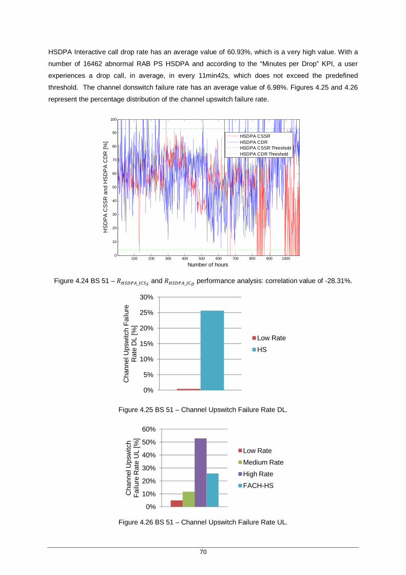
70
HSDPA Interactive call drop rate has an average value of 60.93%, which is a very high value. With a
number of 16462 abnormal RAB PS HSDPA and according to the “Minutes per Drop” KPI, a user
experiences a drop call, in average, in every 11min42s, which does not exceed the predefined
threshold. The channel donswitch failure rate has an average value of 6.98%. Figures 4.25 and 4.26
represent the percentage distribution of the channel upswitch failure rate.
Figure 4.24 BS 51 – 푅 _ and 푅 _ performance analysis: correlation value of -28.31%.
Figure 4.25 BS 51 – Channel Upswitch Failure Rate DL.
Figure 4.26 BS 51 – Channel Upswitch Failure Rate UL.
100 200 300 400 500 600 700 800 900 10000
10
20
30
40
50
60
70
80
90
100
Number of hours
HS
DP
A C
SS
R a
nd H
SD
PA
CD
R [%
]
HSDPA CSSRHSDPA CDRHSDPA CSSR ThresholdHSDPA CDR Threshold
0%
5%
10%
15%
20%
25%
30%
Cha
nnel
Ups
witc
h Fa
ilure
R
ate
DL
[%]
Low Rate
HS
0%
10%
20%
30%
40%
50%
60%
Cha
nnel
Ups
witc
h Fa
ilure
Rat
e U
L [%
]
Low Rate
Medium Rate
High Rate
FACH-HS
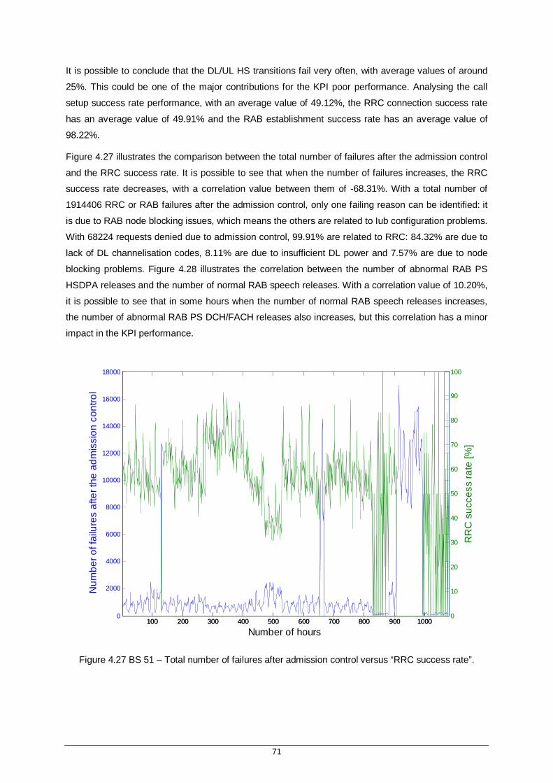
71
It is possible to conclude that the DL/UL HS transitions fail very often, with average values of around
25%. This could be one of the major contributions for the KPI poor performance. Analysing the call
setup success rate performance, with an average value of 49.12%, the RRC connection success rate
has an average value of 49.91% and the RAB establishment success rate has an average value of
98.22%.
Figure 4.27 illustrates the comparison between the total number of failures after the admission control
and the RRC success rate. It is possible to see that when the number of failures increases, the RRC
success rate decreases, with a correlation value between them of -68.31%. With a total number of
1914406 RRC or RAB failures after the admission control, only one failing reason can be identified: it
is due to RAB node blocking issues, which means the others are related to Iub configuration problems.
With 68224 requests denied due to admission control, 99.91% are related to RRC: 84.32% are due to
lack of DL channelisation codes, 8.11% are due to insufficient DL power and 7.57% are due to node
blocking problems. Figure 4.28 illustrates the correlation between the number of abnormal RAB PS
HSDPA releases and the number of normal RAB speech releases. With a correlation value of 10.20%,
it is possible to see that in some hours when the number of normal RAB speech releases increases,
the number of abnormal RAB PS DCH/FACH releases also increases, but this correlation has a minor
impact in the KPI performance.
Figure 4.27 BS 51 – Total number of failures after admission control versus “RRC success rate”.
100 200 300 400 500 600 700 800 900 10000
2000
4000
6000
8000
10000
12000
14000
16000
18000
Num
ber o
f fai
lure
s af
ter t
he a
dmis
sion
con
trol
Number of hours100 200 300 400 500 600 700 800 900 1000
0
10
20
30
40
50
60
70
80
90
100
RR
C s
ucce
ss ra
te [%
]

72
Figure 4.28 BS 51 – Abnormal RAB PS HSDPA releases and normal RAB speech releases.
Similar to what is done in the 2G analysis, the existence of any kind of correlation between a drop call
and HO issues is checked. Analysing the results concerning 푅 and 푅 parameter, it is possible
to identify the percentage associated to the number of hours where the KPI value is above the
threshold level at the same time as others KPIs. In this case, the correlation is made with Speech call
drop rate and the correlation values are presented in Table 4.13. Looking at the results, it is possible
to conclude that in BS 6 when the speech call drop rate KPI is above the threshold level the soft HO
KPI is below the threshold level with a correlation value between the two parameters of -68.55%.
Figure 4.29 shows 푅 and 푅 performance evolution in that period. Soft HO success rate has an
average value of 52.70%. This KPI is calculated as the rate between the total number of RL addition
success and the total number of RL addition attempts, defined as the sum of success and failures.
The counter responsible for counting the failures is incremented if, during an attempt to add a RL, any
of the following occur: admission is not granted due to lack of DL channelisation code, the RL setup
procedure fails, RL addition procedure fails, RL setup or addition procedure times out in the RBS, the
active set update procedure fails or active set update procedure times out in the UE. Analysing the
query’s output results, there is no RRC or RAB requests denied due to admission control procedure,
and so the problem is not related to the lack of DL channelisation codes. There are no RL failures due
to admission and the KPI that defines the success rate for speech RL addition, defined for the source
best cell in the active set has no value, which means this is not the best cell in the active set. The
soft/softer HO overhead speech has an average value of 43.38%. According to [HoTo07], soft HO
overhead can be regarded as a measure of the additional hardware/transmission resources required
50 100 150 200 250 3000
20
40
60
80
100
120
140
Num
ber o
f abn
orm
al R
AB
PS
HS
DP
A re
leas
es
Number of hours50 100 150 200 250 300
0
100
200
300
400
500
600
Num
ber o
f nor
mal
RA
B s
peec
h re
leas
es

73
for implementation of soft HO, planned to be in the order of 20 – 40% for a standard hexagonal cell
grid with three sector sites. So, in BS 6, the value of soft/softer HO overhead speech can be
considered excessive, which could decrease the DL capacity by the increasing of the transmitted
interference to the network. An action that has to be taken into account is the increase of the active set
update rate because they are related: smaller overhead can be obtained at the expense of a higher
active set update rate.
Table 4.13 푅 and 푅 correlation analysis.
BS 푅 and 푅 (%)
6 -68.55
Figure 4.29 BS 6 – 푅 and 푅 performance analysis: correlation value of -68.55%.
The CS64 analysis is not done due to the reduced impact of this parameter in the network
performance.
Analysing the results concerning 푹푷푺푹ퟗퟗ_푰푪푫 parameter, it is possible to identify the percentage
associated to the number of hours where the KPI value is above the threshold level at the same time
as others KPIs. In this case the correlation is made with PS R99 call drop rate and the correlation
values are presented in Table 4.14. There is a considerable number of BSs with problems associated
to PS R99 call drop rate KPI but that problems are not related to SHO problems, e.g., in BS 15, which
is the BS with more critical hours in the entire month when compared with the others identified as
critical, when the PS R99 call drop rate KPI is above the threshold level the soft HO KPI is below the
threshold level only in 2.14% of the cases and the correlation value between the two parameters is -
9.07%. A more exhaustive analysis is not needed in this case.
10 20 30 40 50 60 70 80 900
10
20
30
40
50
60
70
80
90
100
Number of hours
CD
R S
p an
d S
HO
[%]
CDR SpSHOCDR Sp ThresholdSHO Threshold

74
Table 4.14 푅 _ and 푅 correlation analysis.
BS 푅 _ and 푅 (%)
15 -9.07
Analysing the results concerning 푅 _ parameter, it is possible to identify the percentage
associated to the number of hours where the KPI value is above the threshold level at the same time
as others KPIs. In this case the correlation is made with HSDPA call drop rate and the correlation
values are presented in Table 4.15. Although there is a considerable number of BSs with problems
associated to HSDPA call drop rate KPI, that problems are not related to SHO problems, e.g., in BS 9,
when the HSDPA call drop rate KPI is above the threshold level the soft HO KPI is below the threshold
level only in 13.39% of the cases and the correlation value between the two parameters is -38.47%.
This correlation value indicates that the problems concerning RAB PS HSDPA call drop rate have to
be analysed. However, the maximum number of RAB PS HSDPA releases is 73, which is a very low
value, and so a more exhaustive analysis is not needed in this case.
Table 4.15 푅 _ and 푅 correlation analysis.
BS 푅 _ and 푅 (%)
9 -38.47
The R99 throughput analysis is made only to identify possible bidirectional problems, since the
correlation between throughput KPIs and the all the others from the provided list is unnecessary.
Analysing the results concerning 푇 and 푇 parameters, it is possible to identify the
percentage associated to the number of hours where the KPI value is above the threshold level at the
same time as others KPIs, Table 4.16. Easily conclude that in all the BSs identified as problematic in
the 푇 performance analysis there are problems in both DL and UL, which does not necessary
mean a correlation between the two different KPIs. As said before, the idea is not to identify a
correlation between the two KPIs, but just conclude if there is a bidirectional problem. The analysis is
made according to the one made in 2G. Only BS 11 is analysed, since the procedure is the same for
the others BSs.
With a total of 91798 users the average cell traffic volume in DL and UL is illustrated in Figures 30 and
31. It is possible to conclude that in DL the majority of the traffic volume is in the 384 kbps range and
in UL the majority of the traffic volume is in the 16 kbps range. With an average number of maximum
PS Interactive, PS Interactive DCH and PS Interactive FACH users of 19.61, 1.90 and 12.04,
respectively, Figure 4.32 illustrates the variation of the throughout in the cell with the variation of the
number of users. This comparison is made with the objective of identify possible capacity problems.

75
Table 4.16 푇 and 푇 analysis.
BS 푇 and 푇 (%) BS
푇 and 푇 (%) BS
푇 and 푇 (%) BS
푇 and 푇 (%)
11 99.90 75 98.60 47 97.66 81 96.41 20 99.76 49 98.59 105 97.62 112 96.34 94 99.66 33 98.58 25 97.60 69 96.24 28 99.49 73 98.50 98 97.55 30 96.21 44 99.47 95 98.49 10 97.53 120 96.17 52 99.41 114 98.48 61 97.48 57 96.04
101 99.37 107 98.37 43 97.47 19 95.94 39 99.24 85 98.35 40 97.46 124 95.78 7 99.24 32 98.33 67 97.42 90 95.76
100 99.23 23 98.31 5 97.40 118 95.73 72 99.18 53 98.29 126 97.37 87 95.69 93 99.14 66 98.28 128 97.37 89 95.47 65 99.10 18 98.28 92 97.30 50 95.29 99 99.00 123 98.16 36 97.29 122 95.16
106 98.95 2 98.16 6 97.29 24 95.09 1 98.93 78 98.13 108 97.29 79 95.01 58 98.92 46 98.10 117 97.28 9 94.98
103 98.91 60 98.10 37 97.27 21 94.97 27 98.90 13 98.08 41 97.21 26 94.84 86 98.88 35 98.02 16 97.18 12 94.72 3 98.87 51 98.00 83 97.13 115 94.67
119 98.82 74 97.98 64 97.11 110 94.48 91 98.77 62 97.83 82 97.01 59 94.44
116 98.77 113 97.81 76 97.00 127 94.07 125 98.75 29 97.77 54 96.95 104 93.66 96 98.74 14 97.77 38 96.87 84 93.33 42 98.73 8 97.77 71 96.80 34 93.30 56 98.67 68 97.75 22 96.75 80 93.21 70 98.67 48 97.73 88 96.72 109 92.74
121 98.65 45 97.73 63 96.71 102 91.40 55 98.64 111 97.67 31 96.61 17 90.64 15 98.61 97 97.67 77 96.55 4 90.60
Figure 4.30 DL cell traffic volume.
00,20,40,60,8
11,21,41,61,8
DL
Cel
l Tra
ffic
Vol
ume
[MB
] 16 kbps
128 kbps
384 kbps

76
Figure 4.31 UL cell traffic volume.
Figure 4.32 BS 11 – Throughput versus number of users.
Figure 4.33 represents a “zoom” from the total 2026 problematic hours. With a correlation value of
8.47%, it appears to be no correlation between the two parameters. Analysing the performance of the
PS R99 call drop rate KPI, with an average value of 0.37% it can be considered a very good
performance. “Minutes per Drop” KPI average value is 47min31s which means a user experiences a
drop call in almost every 47min which is a very good parameter performance. Channel downswitch
failure rate has an average value of 0.97%, which is a very low value, and Figures 4.33 and 4.34
illustrate the channel upswitch performance. It is possible to conclude that in DL the PS transitions fail
very few times, with a maximum value of 0.25% in the low rate range and in UL the transitions fail in
almost 27.50% of the cases in the high rate range, which is a very high percentage. This means that
the channel upswitching transitions due to throughput in UL CELL_DCH to CELL_DCH with UL target
rate higher than or equal to 256 kbps (excluding EUL) fail due to admission control reject or failures
during the channel switching procedure with a probably of 27.50%.
0
2
4
6
8
10
12
UL
Cel
l Tra
ffic
Vol
ume
[MB
] 16 kbps
64 kbps
128 kbps
20 40 60 80 100 120 140 160 180 200 2200
10
20
30
40
50
60
70
80
90
100
110
PS
R99
DL
Use
r Thr
ough
put
Number of hours20 40 60 80 100 120 140 160 180 200 220
0
20
40
60
80
100
120
140
Num
ber o
f PS
R99
Use
rs

77
Figure 4.33 Channel upswitch failure rate DL.
Figure 4.34 Channel upswitch failure rate UL.
In the case of 푇 parameter, none correlation with other KPI has been made. An analysis will be
performed for the BS with the highest number of problematic hours (2073 hours = 92.88% of the entire
month). With a 푇 average value of 144.78kbps and a total number of 277428 users, the
transmitted bits are all in the spi03 (scheduling priority indicator 03), which is the one associated to the
RAB PS Interactive. 9.30% of the total bits are “non acked”, which means 9.30% of the total bits are
received but non acknowledged by the UE. Analysing the performance of the HSDPA call drop rate
KPI, with an average value of 17.69% it is clearly above the threshold level. “Minutes per Drop” KPI
average value is 28min53s which means a user experiences a drop call in almost every 29min which
is a very good parameter performance. Channel downswitch failure rate has an average value of
1.08% and the channel upswitch performance is represented in Figures 4.36 and 4.37. It is possible to
conclude that in DL and UL the HS transitions fail very few times, with a maximum value of 2.43% in
the DL and 2.53% in the UL. This means that the channel down/upswitch transistion do not have a
significant impact in the throughput performance.
0%
1%
1%
2%
2%
3%
3%
4%
4%
Cha
nnel
Ups
witc
h Fa
ilure
Rat
e D
L [%
]
Low Rate
Medium Rate
High Rate
HS
0%
5%
10%
15%
20%
25%
30%
Cha
nnel
Ups
witc
h Fa
ilure
Rat
e U
L [%
]
Low Rate
Medium Rate
High Rate
FACH-HS

78
Figure 4.35 HS user throughput and number of HS users..
Figure 4.36 Channel upswitch failure rate DL.
Figure 4.37 Channel upswitch failure rate UL.
50 100 150 200 2500
100
200
300
400
500
PS H
SD
PA
Use
r Thr
ough
put
Number of hours50 100 150 200 250
0
10
20
30
40
50
Num
ber o
f PS
HS
Use
rs
0%
1%
1%
2%
2%
3%
3%
Cha
nnel
Ups
witc
h Fa
ilure
R
ate
DL
[%] Low Rate
Medium Rate
High Rate
HS
0%
5%
10%
15%
20%
25%
30%
35%
Cha
nnel
Ups
witc
h Fa
ilure
R
ate
UL
[%] Low Rate
Medium Rate
High Rate
FACH-HS

79
When the reason that leads to a throughput poor performance is not easily identifiable, an action that
has to be taken into account is the licensing process analysis. The variation of the number of users
per cell has to be analysed as well as the number of defined codes in the network. The comparison
between the total of licensed users and the available user throughput allows to identify any kind of
correlation between the parameters. The comparison between the number of HS users and the
number of PS R99 users is also important, since when the lincesed users in HS increases the number
of R99 users decreases leading to a decrease in the codes utilisation. This means that the available
resources increases, leading to a decrease in the number of RAB failures due to lack of DL
channelisation codes.
In this BS, the number of HSDPA codes per cell is 5 and the maximum number of HSDPA users is 16
throughout the entire month. Being a zoom from the total 2073 problematic hours, Figure 4.35
illustrates the comparison between the variation of the HS user throughput and the number of HS
users. The average number of maximum PS HS users is 11.62 which means that the average monthly
value of the maximum number of HSDPA users is below the defined one. Analysing Figure 4.35, with
a correlation value of -17.63% between the two parameters, it is possible to see that in some of the
problematic hours when the number of users increases the available HS throughput decreases. In the
cases of throughput analysis a trade-off relation has to be established, since the decision to increase
the total number of allowed users has to be taken according to the variation of the average user
throughput – this solution is well taken if the expected decrease in the average user throughput is not
significant compared to the number of new allowed users.

80

81
Chapter 5
Conclusions 5 Conclusions
In this chapter, the main conclusions of this thesis are pointed out, as well as some future work
suggestions.

82
The aim of this work was to perform advanced analysis to GSM and UMTS radio networks in order to
establish an algorithm for the tuning of the radio parameters. The main purpose was to optimise the
radio network performance in terms of coverage, quality of service and capacity in a defined region.
Bearing this in mind, a great amount of information (around 400 GB) was gathered in order to develop
a model that considers the provided Key Performance Indicators (KPIs) responsible for evaluate the
radio network performance, and through collecting and analysing the information from the operator’s
database that turns possible the model implementation.
An introduction to GSM, UMTS and HSDPA is performed. UMTS basic aspects are explained, and
afterwards HSDPA new features are presented. Following this, the QoS classes of UMTS are
presented as well as bit rates and applications of different services. A list of nine GSM KPIs and
fourteen UMTS KPIs was provided by the operator, giving a brief explanation of the counters involved
in the calculation. The developed model enables to identify the reasons that lead to the KPIs poor
performance as well as all the cases were a KPI poor performance is directly related with other KPI
poor performance.
Parallel to the model development and implementation, information was gathered concerning radio
network opimisation aspects, i.e., several approaches and literature results were chosen and
analysed, with the objective to provide information regarding the changes and/or improvements that
have to be performed in order to implement the proposed optimisation actions. However, this is a
theme whose information is confidential and restricted to the mobile operators and so the available
information is scarce, which is understandable since it is unnatural companies make available
something that might be useful to its development and performance improvement, which constraints
the search about this scope.
The model development and implementantion chapter was the bulk of the work since the obtained
results and their further analysis is nothing less than a consequence of the designed algorithms
application. The main thought was to create something that would allow to analyse all the KPIs
performance at the same time and correlate all that information. If the KPI performance was not the
desired one there was a problem.
The developed algorithms allowed to analyse the KPIs individually based on detailed statistics of the
problematic areas. In order to access the information contained in the mobile’s operator database,
programmed in SQL language, an algorithm was built. It allowed searching in the database the
counter involved in the KPI expression and using that expression to calculate the KPI, applying all the
necessary filters to define range of values and target values defined by the operator.
Six algorithms were developed to analyse the GSM KPIs although the list provided by the operator
included nine GSM KPIs. This fact can be easily explained, since there are four throughput KPIs in the
list and the procedures to address the throughput performance problems are the same for all of them.
Five algorithms were developed to analyse UMTS KPIs although the list provived by the operator
included fourteen UMTS KPIs. This fact can be easily explained, since the KPIs were divided into two
major groups: the group of the call setup success rate KPIs and the group of the call drop rate KPIs. In
the first the analysis is focused on the “RRC&RAB Success Rate”, taking into account the RRC/RAB
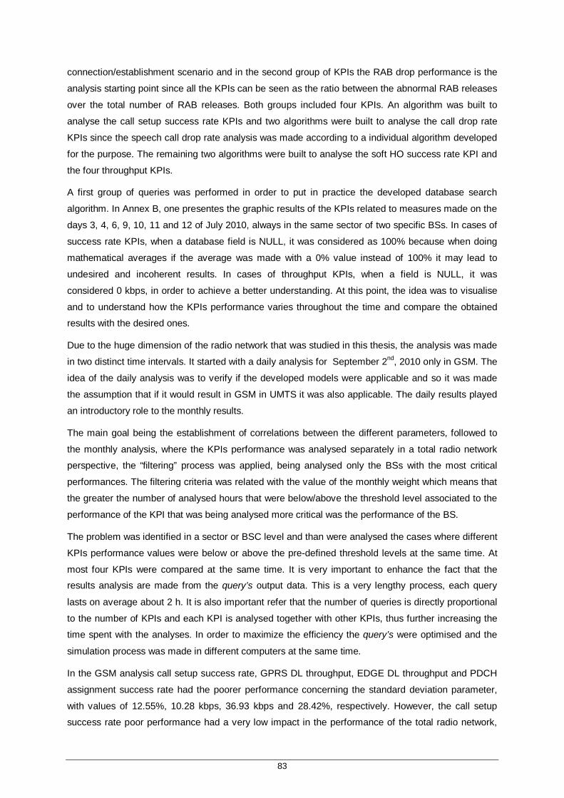
83
connection/establishment scenario and in the second group of KPIs the RAB drop performance is the
analysis starting point since all the KPIs can be seen as the ratio between the abnormal RAB releases
over the total number of RAB releases. Both groups included four KPIs. An algorithm was built to
analyse the call setup success rate KPIs and two algorithms were built to analyse the call drop rate
KPIs since the speech call drop rate analysis was made according to a individual algorithm developed
for the purpose. The remaining two algorithms were built to analyse the soft HO success rate KPI and
the four throughput KPIs.
A first group of queries was performed in order to put in practice the developed database search
algorithm. In Annex B, one presentes the graphic results of the KPIs related to measures made on the
days 3, 4, 6, 9, 10, 11 and 12 of July 2010, always in the same sector of two specific BSs. In cases of
success rate KPIs, when a database field is NULL, it was considered as 100% because when doing
mathematical averages if the average was made with a 0% value instead of 100% it may lead to
undesired and incoherent results. In cases of throughput KPIs, when a field is NULL, it was
considered 0 kbps, in order to achieve a better understanding. At this point, the idea was to visualise
and to understand how the KPIs performance varies throughout the time and compare the obtained
results with the desired ones.
Due to the huge dimension of the radio network that was studied in this thesis, the analysis was made
in two distinct time intervals. It started with a daily analysis for September 2nd, 2010 only in GSM. The
idea of the daily analysis was to verify if the developed models were applicable and so it was made
the assumption that if it would result in GSM in UMTS it was also applicable. The daily results played
an introductory role to the monthly results.
The main goal being the establishment of correlations between the different parameters, followed to
the monthly analysis, where the KPIs performance was analysed separately in a total radio network
perspective, the “filtering” process was applied, being analysed only the BSs with the most critical
performances. The filtering criteria was related with the value of the monthly weight which means that
the greater the number of analysed hours that were below/above the threshold level associated to the
performance of the KPI that was being analysed more critical was the performance of the BS.
The problem was identified in a sector or BSC level and than were analysed the cases where different
KPIs performance values were below or above the pre-defined threshold levels at the same time. At
most four KPIs were compared at the same time. It is very important to enhance the fact that the
results analysis are made from the query’s output data. This is a very lengthy process, each query
lasts on average about 2 h. It is also important refer that the number of queries is directly proportional
to the number of KPIs and each KPI is analysed together with other KPIs, thus further increasing the
time spent with the analyses. In order to maximize the efficiency the query’s were optimised and the
simulation process was made in different computers at the same time.
In the GSM analysis call setup success rate, GPRS DL throughput, EDGE DL throughput and PDCH
assignment success rate had the poorer performance concerning the standard deviation parameter,
with values of 12.55%, 10.28 kbps, 36.93 kbps and 28.42%, respectively. However, the call setup
success rate poor performance had a very low impact in the performance of the total radio network,

84
with a monthly weight of 0.64%. The other three KPIs had a monthly weight value of 6.80%, 6.74%
and 8.86%, respectively. EDGE UL throughput being the KPI with the highest value of monthly weight
(20.11%) it was also the KPI with the highest percentage of problematic BSs after the filtering process.
81.40% of the total radio network BSs were considered critical only considering the performance of
this KPI.
The call drop rate correlation process was very efficient. The correlations were made between this KPI
and HO success rate, SDCCH drop rate and call setup success rate. The results concerning BS 2
showed a correlation between the dropped calls and the HO process of -91.24%, which means that in
the majority of the cases the reasons for a dropped call in this BS were related to HO issues. It was
also concluded that the main reason associated to the drops and consequently to the HO issues was
the bad quality, which is associated to interference. A proposed action in this type of problems was the
identification of the type of interference in order to the operator to be able to know the solution to be
adopted in such cases. In some BSs, the results were misleading since the almost automatic
conclusion in those BSs was that the call drops due to HO problems with 100% sure. However those
BSs poor performance had a very minor impact, in the total radio network performance perspective,
with a monthly weight value of 0.09% and so the results were not taken into account.
The increase of SDCCH drops being a possible reason for an increase in the number of dropped calls,
the correlation value was supposed to be positive and so the negative correlation results were
considered misleading.
The correlation process between the call drop rate and the call setup success rate tried to show some
relation between the inability to successfully end the call setup process and the drop of the TCH, two
possible cases were identified: the call setup process can be successfully terminated and yet the TCH
drops, and the TCH can drop due to the fact that the call setup process was unsuccessfully
terminated. In BSs 6 and 13 the correlation values were 53.38% and -81.49%, respectively, which
could be considered an excellent value in the correlations establishment process. However in BSs 13
and 6 the number of problematic hours only represented 4.08% and 1.34% of the entire month
performance and the call setup success rate had an average value close to the pre-defined threshold.
This means that in those BSs although the correlation results were very satisfactory, leading to the
conclusion that in the majority of the case BS 6 call setup process is successfully terminated and yet
the TCH drops and in BS 13 the TCH drops due to the fact that the call setup process is
unsuccessfully terminated, the performance of those BSs can be considered satisfactory.
The correlation made between the SDCCH drop rate and the call setup success rate corresponded to
what was expected. The call establishment process is well succeeded if the SDCCH assignment
process is well succeeded as well as the call setup process. The results show that in the majority of
the cases the call setup process was unsuccessful due to drop of the control channel with correlation
values close to 100%.
The correlation process in the throughput KPIs analysis was made by the comparison with the PDCH
assignment success rate. The logical thought is that if the PDCH is successfully assigned the
probability of an increase in the available troughput increases. The results show that the correlation

85
values between GPRS DL throughput and PDCH assignment success rate in BSs 49, 37 and 23 had
the highest values – the first two in DL direction and BS 23 in the UL direction. This means that in the
other cases, in spite of the probability of the KPIs being below/above the threshold level at the same
time is very high it does not represent a direct relation between them. In BS 49 it was possible to
identify a notorious correlation between the two KPIs: when the PDCH assignment success rate
increased, the GPRS DL throughput available also increased, which supported the statement that an
insufficient number of available PDCHs is one of the reasons responsible for a poor throughput
performance. The HR traffic have been identified as one of the possible reasons for having a high
number of PDCH assignment fails, since it represented 95.41% of the total traffic, clearly above the
threshold level of 50%. The average PDCH utilisation ratio was 85.73% (above the 80% threshold
value) and there were 5.24 simultaneous users per active PDCH which was clearly superior compared
to the 1.4 threshold value, which proved that there was in fact a high capacity problem. The HR traffic
represented 95.19% of the total traffic, clearly above of the threshold level and affecting the
throughput performance.
In the UMTS analysis CS64 call setup success rate, HSDPA Interactive call drop rate, PS R99
Interactive DL user throughput and HSDPA Interactive user throughput had the poorer performance
concerning the standard deviation parameter, with values of 35.10%, 32.17%, 129.11 kbps and
575.54 kbps, respectively. However, the CS64 call setup success rate poor performance had a very
low impact in the performance of the total radio network due to the low traffic, with a monthly weight of
0.06%. The other three KPIs had a monthly weight value of 18.74%, 56.65% and 51.69%,
respectively. Being PS R99 Interactive DL user throughput the KPI with the highest value of monthly
weight it was the second KPI with the highest percentage of problematic BSs after the filtering
process. 58.48% of the total radio network BSs were considered critical. The KPI with the highest
value of problematic cells was the PS R99 Interactive UL user throughput with a value of 59.38%.
The Speech Call Setup Success Rate correlation process was also very efficient. The correlation was
made between this KPI and speech call drop rate. In BS 8, 88.86% of the speech call drops were due
to unknown reasons, which excludes lost of UL synchronism, congestion, missing neighbours and
SHO action. Analysing the call setup success rate performance it was possible to conclude that there
were problems in the establishment of the RRC connection. There were no fails associated to
transport network blocking, which leads to the conclusion that the majority of the problems that were
detected after the admission process are associated to the Iub configuration. 86.33% of the fails in the
establishment of the RRC connection are due to lack of DL channelisation codes.
The results concerning CS64 service were not analysed. This decision was made taking into account
the fact that the traffic was residual and therefore not statistically significant in the total network traffic.
When dealing with voice the 2G technology is the most often used and when dealing with data it was
all reported to 3G.
The correlation results concerning PS R99 Interactive call setup success rate show that BS 58 was
the only BS with a significant poor performance impact in the total radio network perspective. The
correlation between this KPI and PS R99 Interactive call drop rate in this BS had a value of -65.00%.

86
A user experienced a drop call, in average, in every 5min58s. The channel downswitch failure rate had
a value of 12.09% which could be considered a high value, leading the operator to review the
transistions to lower bit rates. There were no significant problems in the upswitch transitions and the
majority of the denied requests during the admission control process were due to RRC problems and
87.16% of those fails were due to lack of DL channelisation codes.
In the soft HO correlation process, the KPI was correlated with the call drop rate KPIs in order to
continue the process initiated in the GSM analysis. The obtained results allowed to conclude that in
BS 6 the correlation between this KPI and speech call drop rate had a value of -68.55%. The value of
soft/softer HO overhead was identified as the major reason that contributed to the KPI poor
performance since a value of 43.38% could decrease the DL capacity by the increasing of the
transmitted interference to the network. An action that has to be taken into account by the operator is
the increase of the active set update rate because they are related: smaller overhead can be obtained
at the expense of a higher active set update rate.
There were not identified significant correlations between soft HO success rate and PS R99 or
HSDPA Interactive call drop rate, which lead to the conclusion that the HO problems did not contribute
significantly to those KPIs poor performance.
Since the problems associated to user throughput poor performance are most of the times related to
capacity issues, it was not established any correlation between the throughput KPIs and other KPIs
because that was considered unnecessary. The analysis was similar to the one made on GSM.
Analysing PS R99 DL/UL user throughput in BS 11 the channel upswitch transitions due to throughput
in UL CELL_DCH to CELL_DCH with UL target rate higher than or equal to 256 kbps (excluding EUL)
failed due to admission control reject or failed during the channel switching procedure in 27.50% of the
analysed cases. This is a very high value and so the operator has to review the upswitch transitions in
this range of bit rates.
When the reason that leads to a throughput poor performance is not easily identifiable, an action that
have to be taken into account is the licensing process analysis. The variation of the number of users
per cell has to be analysed, as well as the number of defined codes in the network. In the BS with
most problematic hours during the analysis of HSDPA Interactive user throughput the number of
HSDPA codes per cell was 5 and the maximum number of HSDPA users was 16 throughout the entire
month. In the cases of throughput analysis a trade-off relation has to be established since the decision
to increase the total number of allowed users has to be taken according to the variation of the average
user throughput – this solution is well taken if the expected decrease in the average user throughput is
not significant compared to the number of new allowed users.
The correlation establishment process between KPIs revealed to be very useful and efficient. In GSM,
the correlation between dropped voice calls and HO issues is very high, as well as between dropped
voice calls and the drop of the control channel. In BS 2, call drop rate and HO success rate has a
correlation value of -91.24% and in BS 17 call drop rate and SDCCH drop rate has a correlation value
of -52.03%. In UMTS, the correlation between dropped calls and the call setup success rate is also
very high, e.g., in BS 58, PS R99 call drop rate and call setup success rate has a correlation value of -
87
65.00%.
This work allowed the operator to easily identify the call drop reasons due to HO issues and due to
unsucceeded call setup establishment process as well as the major reasons that lead to the
throughput KPIs performance in both GSM and UMTS technologies. This work can represent a high
contribution in terms of economical impact in the performance optimisation and development of a
mobile operator in two different levels. In the network operation level, since it provides to the operator
models and algorithms that allows him to optimise the troubleshooting process in terms of time, and in
this business saving time means making money. In the service to the user level, since the problems
can be more easily and more quickly identified, which means that can also be more easily and quickly
solved and the user experience and QoS to the user will be more satisfactory, reducing the
complaints.
Underlying the variety of still possible studies that can be performed for this subject, it can be
concluded that this is not a finalised work at all. For future work, it is suggested that the IRAT CS HO
success rate incoming and outgoing has to be studied. Although it was part of this work the time
turned out to be a key aspect in the work development and it was not possible to analyse those KPIs
performance. The data collection with ∆t = 0h15 min will provide a different kind of data processing
allowing to identify future problems in smaller time intervals. In the HO analysis the site availabily can
be checked in the analysis of the neighbouring cells which allows to save time in the problems search.
In the 3G throughput analysis, recommendations can be established for the increase of the number of
maximum HS licensed users: cells with a number of HSDPA users more than 80% of the license in
use during 5% of the day and an average value of HS RAB establishments rejected by admission
control throughout the week higher than 100 during two consecutive weeks have to see their license
expanded.

88
89
Annex A
Ericsson’s KPIs Definition A. Annex A
In Annex A, one gives the definition of the Key Performance Indicators and of the counters involved in
the process, according to the Ericsson’s User Description.
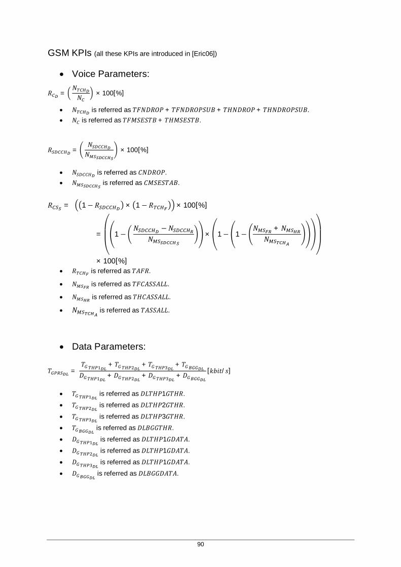
90
GSM KPIs (all these KPIs are introduced in [Eric06])
Voice Parameters:
푅 = 푁푁 × 100[%]
푁 is referred as 푇퐹푁퐷푅푂푃 + 푇퐹푁퐷푅푂푃푆푈퐵 + 푇퐻푁퐷푅푂푃 + 푇퐻푁퐷푅푂푃푆푈퐵. 푁 is referred as 푇퐹푀푆퐸푆푇퐵+ 푇퐻푀푆퐸푆푇퐵.
푅 = 푁푁 × 100[%]
푁 is referred as 퐶푁퐷푅푂푃. 푁 is referred as 퐶푀푆퐸푆푇퐴퐵.
푅 = 1− 푅 × 1 − 푅 × 100[%]
=
⎝
⎜⎛
1 − 푁 −푁
푁× 1− 1−
푁 + 푁푁
⎠
⎟⎞
× 100[%] 푅 is referred as 푇퐴퐹푅.
푁 is referred as 푇퐹퐶퐴푆푆퐴퐿퐿.
푁 is referred as 푇퐻퐶퐴푆푆퐴퐿퐿.
푁 is referred as 푇퐴푆푆퐴퐿퐿.
Data Parameters:
푇 = 푇 + 푇 + 푇 + 푇퐷 +퐷 +퐷 +퐷
[푘푏푖푡/푠]
푇 is referred as 퐷퐿푇퐻푃1퐺푇퐻푅.
푇 is referred as 퐷퐿푇퐻푃2퐺푇퐻푅.
푇 is referred as 퐷퐿푇퐻푃3퐺푇퐻푅.
푇 is referred as 퐷퐿퐵퐺퐺푇퐻푅.
퐷 is referred as 퐷퐿푇퐻푃1퐺퐷퐴푇퐴.
퐷 is referred as 퐷퐿푇퐻푃1퐺퐷퐴푇퐴.
퐷 is referred as 퐷퐿푇퐻푃1퐺퐷퐴푇퐴.
퐷 is referred as 퐷퐿퐵퐺퐺퐷퐴푇퐴.

91
푇 = 푇 + 푇 + 푇 + 푇퐷 +퐷 + 퐷 +퐷
[푘푏푖푡/푠]
푇 is referred as 푈퐿푇퐻푃1퐺푇퐻푅.
푇 is referred as 푈퐿푇퐻푃2퐺푇퐻푅.
푇 is referred as 푈퐿푇퐻푃3퐺푇퐻푅.
푇 is referred as 푈퐿퐵퐺퐺푇퐻푅.
퐷 is referred as 푈퐿푇퐻푃1퐺퐷퐴푇퐴.
퐷 is referred as 푈퐿푇퐻푃1퐺퐷퐴푇퐴.
퐷 is referred as 푈퐿푇퐻푃1퐺퐷퐴푇퐴.
퐷 is referred as 푈퐿퐵퐺퐺퐷퐴푇퐴.
푇 = [푘푏푖푡/푠]
푇 is referred as 퐷퐿푇퐻푃1퐸퐺푇퐻푅.
푇 is referred as 퐷퐿푇퐻푃2퐸퐺푇퐻푅.
푇 is referred as 퐷퐿푇퐻푃3퐸퐺푇퐻푅.
푇 is referred as 퐷퐿퐵퐺퐸퐺푇퐻푅.
퐷 is referred as 퐷퐿푇퐻푃1퐸퐺퐷퐴푇퐴.
퐷 is referred as 퐷퐿푇퐻푃2퐸퐺퐷퐴푇퐴.
퐷 is referred as 퐷퐿푇퐻푃3퐸퐺퐷퐴푇퐴. 퐷 is referred as 퐷퐿퐵퐺퐸퐺퐷퐴푇퐴.
푇 = 푇 + 푇 + 푇 + 푇퐷 +퐷 + 퐷 + 퐷
[푘푏푖푡/푠]
푇 is referred as 푈퐿푇퐻푃1퐸퐺푇퐻푅.
푇 is referred as 푈퐿푇퐻푃2퐸퐺푇퐻푅.
푇 is referred as 푈퐿푇퐻푃3퐸퐺푇퐻푅.
푇 is referred as 푈퐿퐵퐺퐸퐺푇퐻푅.
퐷 is referred as 푈퐿푇퐻푃1퐸퐺퐷퐴푇퐴.
퐷 is referred as 푈퐿푇퐻푃2퐸퐺퐷퐴푇퐴.
퐷 is referred as 푈퐿푇퐻푃3퐸퐺퐷퐴푇퐴.
퐷 is referred as 푈퐿퐵퐺퐸퐺퐷퐴푇퐴.
푅 = 1−푁푁 × 100[%]
푁 is referred as 푃퐶퐻퐴퐿퐿퐹퐴퐼퐿.
푁 is referred as 푃퐶퐻퐴퐿퐿퐴푇푇.

92
UMTS KPIs (all these KPIs are introduced in [Eric08])
Voice Parameters: 푅 = 푅 × 푅 × 100[%]
푅 is referred as .
푅 is referred as .
Note that de counter 푝푚푁표퐿표푎푑푆ℎ푎푟푖푛푔푅푟푐퐶표푛푛퐶푠 allows distinguish load sharing events for CS
RAB’s in case Load Sharing feature is enabled.
푅 = 푅 × 푅 _ × 100[%]
푅 _ is referred as .
푅 = 푁 _
푁 × 100[%]
푁 _ is referred as 푝푚푁표푆푦푠푡푒푚푅푎푏푅푒푙푒푎푠푒푆푝푒푒푐ℎ.
푁 is referred as 푝푚푁표푁표푟푚푎푙푅푎푏푅푒푙푒푎푠푒푆푝푒푒푐ℎ + 푝푚푁표푆푦푠푡푒푚푅푎푏푅푒푙푒푎푠푒푆푝푒푒푐ℎ.
Note that the 푝푚푁표푁표푟푚푎푙푅푎푏푅푒푙푒푎푠푒푆푝푒푒푐ℎ and 푝푚푁표푆푦푠푡푒푚푅푎푏푅푒푙푒푎푠푒푆푝푒푒푐ℎ counters are only
increased due to a RANAP (Radio Access Network Application Part) Iu Release Command or RAB
Assignment Request message for RAB speech respectively with “release cause” = ‘Normal Release’,
‘Successful Relocation’, ‘Resource Optimisation Relocation’, ‘User Inactivity’ or ‘release-due-to-UE-
generated-signaling-connection-release’ for the first one or anything except the previous causes for
the second one. For UtranCell class these counters are incremented for the best cell in the Active Set
in the SRNC (Serving Radio Network Controller).
푅 = 푁 _
푁 × 100[%]
푁 _ is referred as 푝푚푁표푆푦푠푡푒푚푅푎푏푅푒푙푒푎푠푒퐶푆64. 푁 is referred as 푝푚푁표푁표푟푚푎푙푅푎푏푅푒푙푒푎푠푒퐶푆64+ 푝푚푁표푆푦푠푡푒푚푅푎푏푅푒푙푒푎푠푒퐶푆64.
Note that the 푝푚푁표푁표푟푚푎푙푅푎푏푅푒푙푒푎푠푒퐶푆64 and 푝푚푁표푆푦푠푡푒푚푅푎푏푅푒푙푒푎푠푒퐶푆64 counters are only
increased due to a RANAP Iu Release Command or RAB Assignment Request message for a
conversational 64 kbps RAB, respectively with “release cause” = ‘Normal Release’, ‘Successful
Relocation’, ‘Resource Optimisation Relocation’, ‘User Inactivity’ or ‘release-due-to-UE-generated-
signaling-connection-release’ for the first one or anything except the previous causes for the second
one. For UtranCell MO, these counters are incremented for the best cell in the Active Set in the
SRNC.
93
Data Parameters:
푅 _ = 푅 × 푅 _ _ _ × 100[%]
푅 is referred as .
푅 _ _ _ is referred as .
푅 _ = 푅 × 푅 _ _ × 100[%]
푅 _ _ is referred as .
푅 _ = 푁 _ _ _
푁 _ _ _× 100[%]
푁 _ _ _ is referred as 푝푚푁표푆푦푠푡푒푚푅푎푏푅푒푙푒푎푠푒푃푎푐푘푒푡 − 푝푚푁표푆푦푠푡푒푚푅푏푅푒푙푒푎푠푒퐻푠 −푝푚푁표푆푦푠푡푒푚푅푎푏푅푒푙푒푎푠푒푃푎푐푘푒푡푈푟푎.
푁 _ _ _ is referred as 푝푚푁표푁표푟푚푎푙푅푎푏푅푒푙푒푎푠푒푃푎푐푘푒푡 − 푝푚푁표푁표푟푚푎푙푅푎푏푅푒푙푒푎푠푒푃푎푐푘푒푡푈푟푎 −푝푚푁표푁표푟푚푎푙푅푏푅푒푙푒푎푠푒퐻푠 + 푝푚푁표푆푦푠푡푒푚푅푎푏푅푒푙푒푎푠푒푃푎푐푘푒푡 −푝푚푁표푆푦푠푡푒푚푅푎푏푅푒푙푒푎푠푒푃푎푐푘푒푡푈푟푎 − 푝푚푁표푆푦푠푡푒푚푅푏푅푒푙푒푎푠푒퐻푠+푝푚푈푝푠푤푖푡푐ℎ퐹푎푐ℎ퐻푠푆푢푐푐푒푠푠 + 푝푚퐷푙푈푝푠푤푖푡푐ℎ푆푢푐푐푒푠푠퐻푠.
The 푝푚푁표푁표푟푚푎푙푅푎푏푅푒푙푒푎푠푒푃푎푐푘푒푡 and 푝푚푁표푆푦푠푡푒푚푅푎푏푅푒푙푒푎푠푒푃푎푐푘푒푡 counters are only
increased due to a RANAP Iu Release Command or RAB Assignment Request message for all PS
RAB’s respectively with “release cause” = ‘Normal Release’, ‘Successful Relocation’, ‘Resource
Optimisation Relocation’, ‘User Inactivity’ or ‘release-due-to-UE-generated-signaling-connection-
release’ for the first one or anything except the previous causes for the second one. The
푝푚푁표푆푦푠푡푒푚푅푎푏푅푒푙푒푎푠푒푃푎푐푘푒푡푈푟푎 counter represents the number of system release of packet
RAB’s while on URA (Utran Registration Area) state. The 푝푚푁표푆푦푠푡푒푚푅푏푅푒푙푒푎푠푒퐻푠 counter is
stepped for the Serving HS-DSCH (Home System – Downlink Shared Channel) cell at RAB/RB
combination transition from PS Interactive 64/HS (or 384/HS or EUL/HS) – HS-DSCH to SRB-DCH or
to Idle mode due to the same reasons as for stepping the existing counter
푝푚푁표푆푦푠푡푒푚푅푎푏푅푒푙푒푎푠푒푃푎푐푘푒푡.
For UtranCell class, this counter is stepped for the Serving HS-DSCH cell. The same counter has not
been released on Iur link level. The 푝푚푁표푁표푟푚푎푙푅푏푅푒푙푒푎푠푒퐻푠 counter is only increased at RAB/RB
combination transition from PS Interactive 64/HS – HS-DSCH to SRB-DCH or to Idle mode, due to a
RANAP Iu Release Command or RAB Assignment Request message for RAB Speech respectively
with “release cause” = ‘Normal Release’, ‘Successful Relocation’, ‘Resource Optimisation Relocation’,
‘User Inactivity’ or ‘release-due-to-UE-generated-signaling-connection-release’. The
푝푚푈푝푠푤푖푡푐ℎ퐹푎푐ℎ퐻푠푆푢푐푐푒푠푠 counter provides the number of successful upswitches from FACH to any
HS state. The counter is stepped for successful upswitch from CELL_FACH to a RB combination
94
containing HS. The counter is only incremented in all cells of the active set. The
푝푚퐷푙푈푝푠푤푖푡푐ℎ푆푢푐푐푒푠푠퐻푠 counter provides the number of successful DL upswitches to any HS state.
The counter is stepped for successful DL upswitch to a RB combination containing HS. The counter is
only incremented in all cells of the active set.
푅 _ = 푁 _ _
푁 _ _× 100[%]
푁 _ _ is referred as 푝푚푁표푆푦푠푡푒푚푅푏푅푒푙푒푎푠푒퐻푠. 푁 _ _ is referred as 푝푚푁표푁표푟푚푎푙푅푏푅푒푙푒푎푠푒퐻푠+ 푝푚푁표푆푦푠푡푒푚푅푏푅푒푙푒푎푠푒퐻푠.
푇 = 푇
푁 [푘푏푖푡/푠]
푇 is referred as 푝푚푆푢푚퐷푐ℎ퐷푙푅푙푐푈푠푒푟푃푎푐푘푒푡푇ℎ푝. The counter values are read
periodically from an internal level counter and added to this counter. The level counter
maintains the current DL RLC throughput for PS Interactive on R99 DCH, including user data
only. This counter is not incremented when the throughput is 0 kbps. For a multiRAB
combination containing more than one PS Interactive RB, this counter is incremented for only
one of the R99 PS Interactive RB’s in the combination. It has a sample rate of 0.5 s.
푁 is referred as 푝푚푆푎푚푝푙푒푠퐷푐ℎ퐷푙푅푙푐푈푠푒푟푃푎푐푘푒푡푇ℎ푝. This counter represents the
number of samples in 푝푚푆푢푚퐷푐ℎ퐷푙푅푙푐푈푠푒푟푃푎푐푘푒푡푇ℎ푝 (that is,
푝푚푆푎푚푝푙푒푠퐷푐ℎ퐷푙푅푙푐푈푠푒푟푃푎푐푘푒푡푇ℎ푝 = 푝푚푆푎푚푝푙푒푠퐷푐ℎ퐷푙푅푙푐푈푠푒푟푃푎푐푘푒푡푇ℎ푝 +1, whenever
푝푚푆푢푚퐷푐ℎ퐷푙푅푙푐푈푠푒푟푃푎푐푘푒푡푇ℎ푝 is to be updated). It is measured two times/second and
incremented by one if 푝푚푆푢푚퐷푐ℎ퐷푙푅푙푐푈푠푒푟푃푎푐푘푒푡푇ℎ푝 > 0 for the same polling time duration.
푇 = 푇
푁 [푘푏푖푡/푠]
푇 is referred as 푝푚푆푢푚퐷푐ℎ푈푙푅푙푐푈푠푒푟푃푎푐푘푒푡푇ℎ푝. The counter values are read
periodically from an internal level counter and added to this counter. The level counter
maintains the current UL RLC throughput for PS Interactive on R99 DCH, including user data
only. This counter is not incremented when the throughput is 0 kbps. For a multiRAB
combination containing more than one PS Interactive RB, this counter is incremented for only
one of the R99 PS Interactive RB’s in the combination. It has a sample rate of 0.5 s.
푁 is referred as 푝푚푆푎푚푝푙푒푠퐷푐ℎ푈푙푅푙푐푈푠푒푟푃푎푐푘푒푡푇ℎ푝. This counter represents
the number of samples in 푝푚푆푢푚퐷푐ℎ푈푙푅푙푐푈푠푒푟푃푎푐푘푒푡푇ℎ푝 (that is,
푝푚푆푎푚푝푙푒푠퐷푐ℎ푈푙푅푙푐푈푠푒푟푃푎푐푘푒푡푇ℎ푝 = 푝푚푆푎푚푝푙푒푠퐷푐ℎ푈푙푅푙푐푈푠푒푟푃푎푐푘푒푡푇ℎ푝 +1, whenever
푝푚푆푢푚퐷푐ℎ푈푙푅푙푐푈푠푒푟푃푎푐푘푒푡푇ℎ푝 is to be updated). It is measured two times/second and
incremented by one if 푝푚푆푢푚퐷푐ℎ푈푙푅푙푐푈푠푒푟푃푎푐푘푒푡푇ℎ푝 > 0 for the same polling time duration.

95
푇 = 푇
푁 [푘푏푖푡/푠]
푇 is referred as 푝푚푆푢푚퐻푠퐷푙푅푙푐푈푠푒푟푃푎푐푘푒푡푇ℎ푝. The counter sums all values recorded
during a ROP for HS-DSCH RLC throughput measurements, excluding retransmissions. It is
reported on the best cell in the active set. Values are read periodically from an interval level
counter and added to this counter. The level counter maintains the current HS-DSCH RLC
throughput, excluding retransmissions. It has a sample rate of 0.1 seconds.
푁 is referred as 푝푚푆푎푚푝푙푒푠퐻푠퐷푙푅푙푐푈푠푒푟푃푎푐푘푒푡푇ℎ푝. This counter represents the
number of samples in 푝푚푆푢푚퐻푠퐷푙푅푙푐푈푠푒푟푃푎푐푘푒푡푇ℎ푝 (that is,
푝푚푆푎푚푝푙푒푠퐻푠퐷푙푅푙푐푈푠푒푟푃푎푐푘푒푡푇ℎ푝 = 푝푚푆푎푚푝푙푒푠퐻푠퐷푙푅푙푐푈푠푒푟푃푎푐푘푒푡푇ℎ푝 +1, whenever
푝푚푆푢푚퐻푠퐷푙푅푙푐푈푠푒푟푃푎푐푘푒푡푇ℎ푝 is to be updated, this means if no data is transmitted the
counter is not incremented).
GSM and UMTS Handover Parameters (all these KPIs are introduced in [Eric06] and
[Eric08])
푅 = 푁 + 푁
푁 +푁 +푁 +푁_
× 100[%]
푁 is referred as 퐻푂푉퐸푅푆푈퐶.
푁 is referred as 퐻푂퐼푁푆푈퐶.
푁 is referred as 퐻푂푉퐸푅퐶푁푇.
푁 is referred as 퐻푂퐼푁퐷푄퐴.
푁 is referred as 퐻푂퐼푁푈푄퐴.
푁_
is referred as 퐻푂퐼푁퐵푄퐴.
푅 = 푁푁 × 100[%]
푁 is referred as 푝푚푁표푇푖푚푒푠푅푙퐴푑푑푇표퐴푐푡푆푒푡.
푁 is referred as 푝푚푁표푇푖푚푒푠푅푙퐴푑푑푇표퐴푐푡푆푒푡+ 푝푚푁표푇푖푚푒푠퐶푒푙푙퐹푎푖푙퐴푑푑푇표퐴푐푡푆푒푡.
The 푝푚푁표푇푖푚푒푠푅푙퐴푑푑푇표퐴푐푡푆푒푡 counter is increased when a new RL is successfully added to an
active set. The counter is increased after a handover proposal has been received from the handover
evaluation function, admission control has been granted, DL channelisation code has been allocated
for the new cell, RL Setup or RL Addition procedure is successfully completed with the RBS (NBAP
(Node B Application Part) RL Setup Response or RL Addition Response received), the Active Set
Update procedure is successfully completed with the UE (RRC Active Set Update Complete received),
96
and the appropriate parameters are available. If an RL is replaced in an active set, this counter is
increased for the cell which is added. The 푝푚푁표푇푖푚푒푠퐶푒푙푙퐹푎푖푙퐴푑푑푇표퐴푐푡푆푒푡 is increased if, during an
attempt to add an RL, any of the following occur: admission is not granted, no DL channelisation code
is allocated, the RL Setup procedure fails (NBAP RL Setup Failure received), RL Addition procedure
fails (NBAP RL Addition Failure received), RL Setup or Addition procedure times out in the RBS, the
Active Set Update procedure fails (RRC Active Set Update Failure received) or Active Set Update
procedure fails (RRC Active Set Update Failure received) or Active Set Update procedure times out in
the UE. If affects cells which can not enter into the active set. Both counters only monitor UEs in the
SRNC.
푅 _ = 푁 __
푁 _× 100[%]
푁 __ is referred as 푝푚푁표푆푢푐푐푒푠푠푂푢푡퐼푟푎푡퐻표푆푝푒푒푐ℎ + +푝푚푁표푆푢푐푐푒푠푠푂푢푡퐼푟푎푡퐻표푀푢푙푡푖.
푁 _ is referred as 푝푚푁표퐴푡푡푂푢푡퐼푟푎푡퐻표푆푝푒푒푐ℎ+ 푝푚푁표퐴푡푡푂푢푡퐼푟푎푡퐻표푀푢푙푡푖.
The 푝푚푁표퐴푡푡푂푢푡퐼푟푎푡퐻표푆푝푒푒푐ℎ and 푝푚푁표퐴푡푡푂푢푡퐼푟푎푡퐻표푀푢푙푡푖 counters are increased when RNC has
received “HANDOVER FROM UTRAN COMMAND” respectively for RAB speech and MultiRAB.
These counters will only be incremented in the SRNC and for the best cell in active set. The trigger
푝푚푁표푆푢푐푐푒푠푠푂푢푡퐼푟푎푡퐻표푆푝푒푒푐ℎ is when IU RELEASE COMMAND is received with cause ‘Normal
release’ or ‘Successful relocation’ and based on the CS RAB state. This counter will only be
incremented in the SRNC and for the best cell in the active set. The trigger of the
counter푝푚푁표푆푢푐푐푒푠푠푂푢푡퐼푟푎푡퐻표푀푢푙푡푖 is reception of “HANDOVER FROM UTRAN COMMAND”. This
counter will only be incremented in the SRNC and for the best cell in the active set.
푅 _ = 푁 _
푁 _× 100[%]
푁 _ is referred as 푝푚푁표퐼푛퐶푠퐼푟푎푡퐻표푆푢푐푐푒푠푠.
푁 _ is referred as 푝푚푁표퐼푛퐶푠퐼푟푎푡퐻표퐴푡푡.
The 푝푚푁표퐼푛퐶푠퐼푟푎푡퐻표푆푢푐푐푒푠푠 counter provides the number of successful CS incoming Inter System
Handovers. The counter is increased after reception of both RRC message “handover to UTRAN
complete” (UE responds after completed RANAP procedure for Relocation Request) and NBAP
message “RL restore ind” (RBS has received UL synchronisation with the UE). The
푝푚푁표퐼푛퐶푠퐼푟푎푡퐻표퐴푡 counter provides the number of attempted CS incoming Inter System Handovers
(counted before module and central MP load control, after SCCP (Signaling Connection Control Part)
MP if the cell is recognised as being controlled by this RNC (after the stepping also central MP and
module MP is checked for overload).

97
Annex B
Database Algorithm Application B. Annex B
In Annex B, one presentes the graphic results related to the database algorithm application mentioned
in Section 3.1.
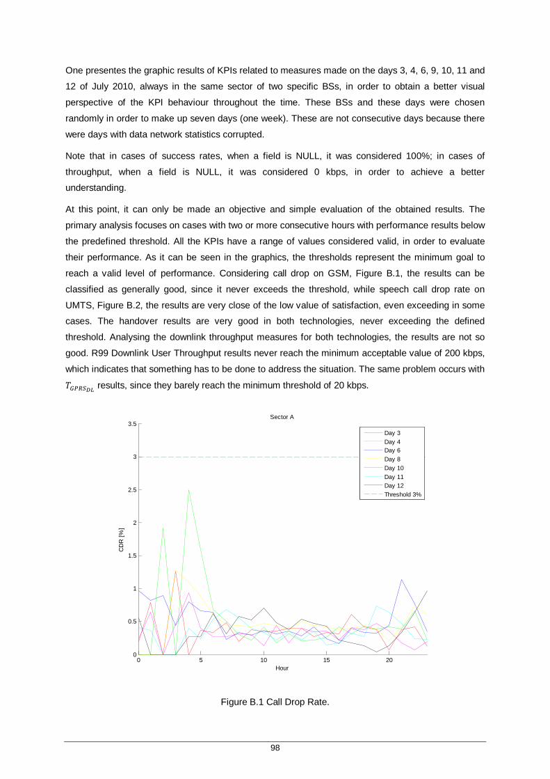
98
One presentes the graphic results of KPIs related to measures made on the days 3, 4, 6, 9, 10, 11 and
12 of July 2010, always in the same sector of two specific BSs, in order to obtain a better visual
perspective of the KPI behaviour throughout the time. These BSs and these days were chosen
randomly in order to make up seven days (one week). These are not consecutive days because there
were days with data network statistics corrupted.
Note that in cases of success rates, when a field is NULL, it was considered 100%; in cases of
throughput, when a field is NULL, it was considered 0 kbps, in order to achieve a better
understanding.
At this point, it can only be made an objective and simple evaluation of the obtained results. The
primary analysis focuses on cases with two or more consecutive hours with performance results below
the predefined threshold. All the KPIs have a range of values considered valid, in order to evaluate
their performance. As it can be seen in the graphics, the thresholds represent the minimum goal to
reach a valid level of performance. Considering call drop on GSM, Figure B.1, the results can be
classified as generally good, since it never exceeds the threshold, while speech call drop rate on
UMTS, Figure B.2, the results are very close of the low value of satisfaction, even exceeding in some
cases. The handover results are very good in both technologies, never exceeding the defined
threshold. Analysing the downlink throughput measures for both technologies, the results are not so
good. R99 Downlink User Throughput results never reach the minimum acceptable value of 200 kbps,
which indicates that something has to be done to address the situation. The same problem occurs with
푇 results, since they barely reach the minimum threshold of 20 kbps.
Figure B.1 Call Drop Rate.
0 5 10 15 200
0.5
1
1.5
2
2.5
3
3.5
Hour
CD
R [%
]
Sector A
Day 3Day 4Day 6Day 8Day 10Day 11Day 12Threshold 3%
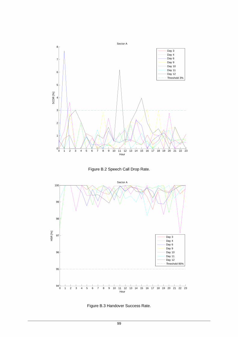
99
Figure B.2 Speech Call Drop Rate.
Figure B.3 Handover Success Rate.
0 1 2 3 4 5 6 7 8 9 10 11 12 13 14 15 16 17 18 19 20 21 22 230
1
2
3
4
5
6
7
8
Hour
SC
DR
[%]
Sector A
Day 3Day 4Day 6Day 9Day 10Day 11Day 12Threshold 3%
0 1 2 3 4 5 6 7 8 9 10 11 12 13 14 15 16 17 18 19 20 21 22 2394
95
96
97
98
99
100
Hour
HS
R [%
]
Sector A
Day 3Day 4Day 6Day 9Day 10Day 11Day 12Threshold 95%

100
Figure B.4 Soft Handover Success Rate.
Figure B.5 R99 Downlink User Throughput.
0 1 2 3 4 5 6 7 8 9 10 11 12 13 14 15 16 17 18 19 20 21 22 2389
90
91
92
93
94
95
96
97
98
99
100
Hour
SH
O S
R [%
]
Sector A
Day 3Day 4Day 6Day 9Day 10Day 11Day 12Threshold 90%
0 5 10 15 200
50
100
150
200
250
300
350
400
Hour
R99
DL
Use
r Thr
[kbi
t/s]
Sector A
Day 3Day 4Day 6Day 9Day 10Day 11Day 12Threshold 200 kbit/sThreshold 384 kbit/s
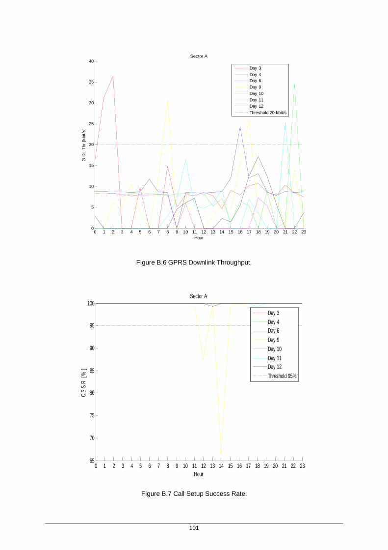
101
Figure B.6 GPRS Downlink Throughput.
Figure B.7 Call Setup Success Rate.
0 1 2 3 4 5 6 7 8 9 10 11 12 13 14 15 16 17 18 19 20 21 22 230
5
10
15
20
25
30
35
40
Hour
G D
L Th
r [kb
it/s]
Sector A
Day 3Day 4Day 6Day 9Day 10Day 11Day 12Threshold 20 kbit/s
0 1 2 3 4 5 6 7 8 9 10 11 12 13 14 15 16 17 18 19 20 21 22 2365
70
75
80
85
90
95
100
Hour
CS
SR
[%]
Sector A
Day 3Day 4Day 6Day 9Day 10Day 11Day 12Threshold 95%
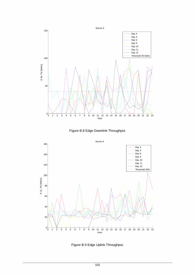
102
Figure B.8 Edge Downlink Throughput.
Figure B.9 Edge Uplink Throughput.
0 1 2 3 4 5 6 7 8 9 10 11 12 13 14 15 16 17 18 19 20 21 22 230
50
100
150
Hour
E D
L Th
r [kb
it/s]
Sector A
Day 3Day 4Day 6Day 9Day 10Day 11Day 12Threshold 40 kbit/s
0 1 2 3 4 5 6 7 8 9 10 11 12 13 14 15 16 17 18 19 20 21 22 230
20
40
60
80
100
120
140
160
Hour
E U
L Th
r [kb
it/s]
Sector A
Day 3Day 4Day 6Day 9Day 10Day 11Day 12Threshold 30%

103
Figure B.10 GPRS Uplink Throughput.
Figure B.11 PDCH Assignment Success Rate.
0 1 2 3 4 5 6 7 8 9 10 11 12 13 14 15 16 17 18 19 20 21 22 230
5
10
15
20
25
30
35
40
45
50
Hour
G D
L Th
r [kb
it/s]
Sector A
Day 3Day 4Day 6Day 9Day 10Day 11Day 12Threshold 10 kbit/s
0 1 2 3 4 5 6 7 8 9 10 11 12 13 14 15 16 17 18 19 20 21 22 230
10
20
30
40
50
60
70
80
90
100
Hour
PA
SR
[%]
Sector A
Day 3Day 4Day 6Day 9Day 10Day 11Day 12Threshold 70%
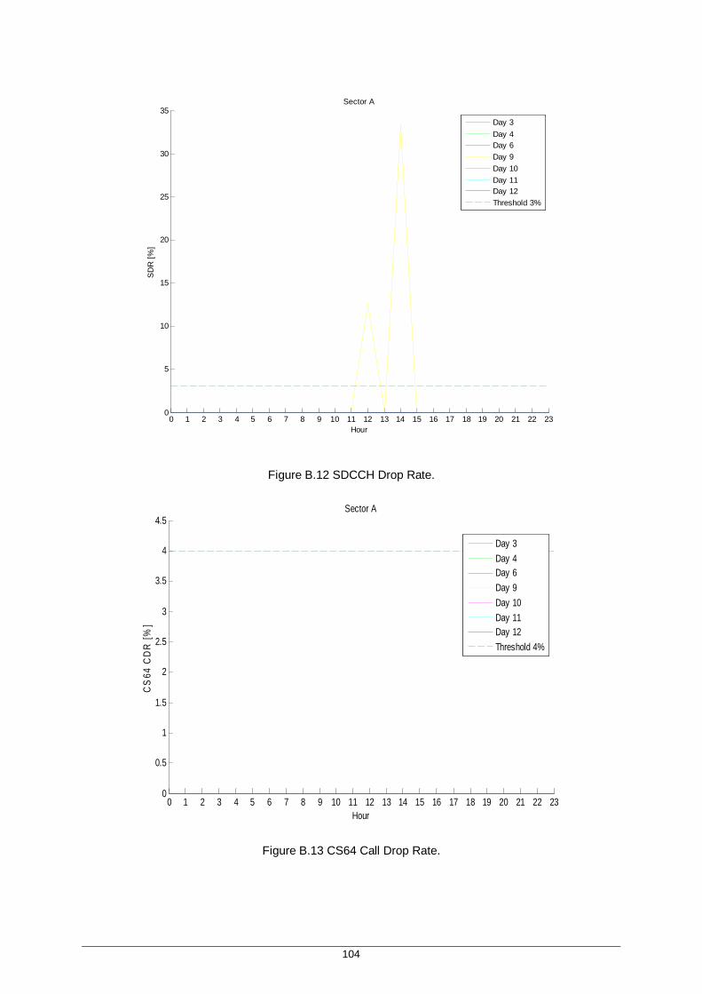
104
Figure B.12 SDCCH Drop Rate.
Figure B.13 CS64 Call Drop Rate.
0 1 2 3 4 5 6 7 8 9 10 11 12 13 14 15 16 17 18 19 20 21 22 230
5
10
15
20
25
30
35
Hour
SD
R [%
]
Sector A
Day 3Day 4Day 6Day 9Day 10Day 11Day 12Threshold 3%
0 1 2 3 4 5 6 7 8 9 10 11 12 13 14 15 16 17 18 19 20 21 22 230
0.5
1
1.5
2
2.5
3
3.5
4
4.5
Hour
CS
64 C
DR
[%]
Sector A
Day 3Day 4Day 6Day 9Day 10Day 11Day 12Threshold 4%

105
Figure B.14 CS64 Call Setup Success Rate.
Figure B.15 HSDPA Interactive Call Setup Success Rate.
0 1 2 3 4 5 6 7 8 9 10 11 12 13 14 15 16 17 18 19 20 21 22 230
10
20
30
40
50
60
70
80
90
100
Hour
CS
SR
CS
64 [%
]
Sector A
Day 3Day 4Day 6Day 9Day 10Day 11Day 12Threshold 93%
0 1 2 3 4 5 6 7 8 9 10 11 12 13 14 15 16 17 18 19 20 21 22 2386
88
90
92
94
96
98
100
Hour
CS
SR
HS
I [%
]
Sector A
Day 3Day 4Day 6Day 9Day 10Day 11Day 12Threshold 93%
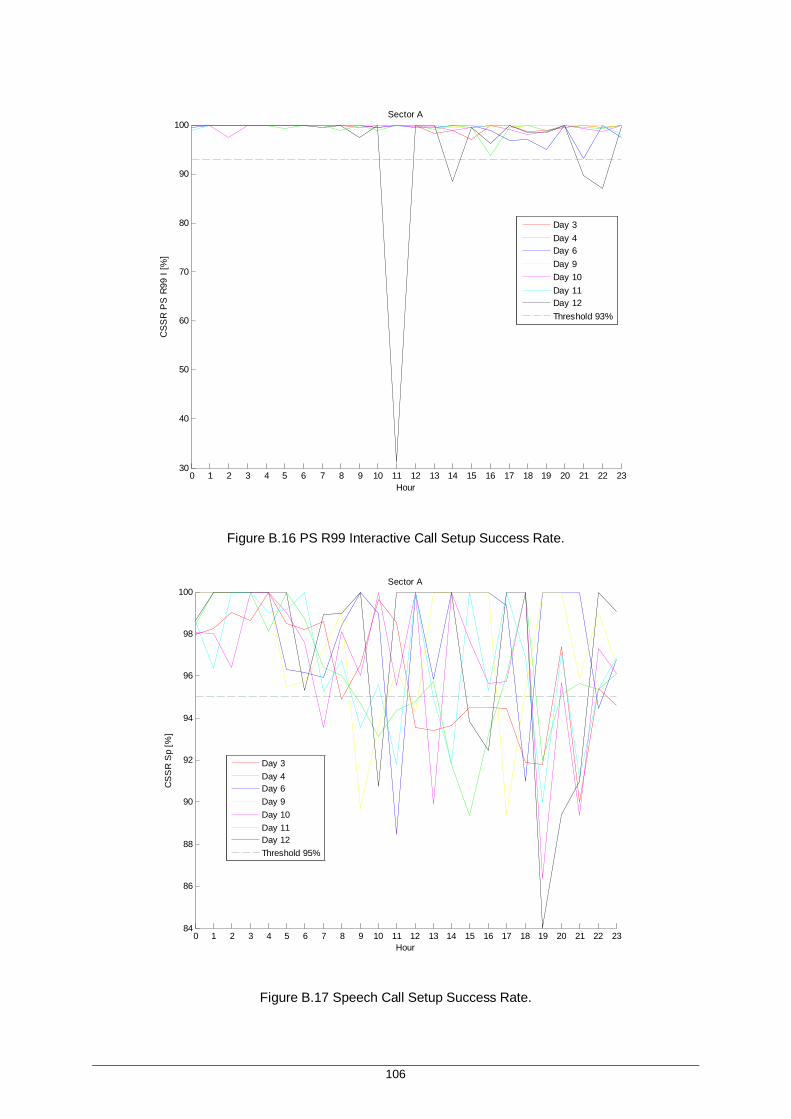
106
Figure B.16 PS R99 Interactive Call Setup Success Rate.
Figure B.17 Speech Call Setup Success Rate.
0 1 2 3 4 5 6 7 8 9 10 11 12 13 14 15 16 17 18 19 20 21 22 2330
40
50
60
70
80
90
100
Hour
CS
SR
PS
R99
I [%
]
Sector A
Day 3Day 4Day 6Day 9Day 10Day 11Day 12Threshold 93%
0 1 2 3 4 5 6 7 8 9 10 11 12 13 14 15 16 17 18 19 20 21 22 2384
86
88
90
92
94
96
98
100
Hour
CS
SR
Sp
[%]
Sector A
Day 3Day 4Day 6Day 9Day 10Day 11Day 12Threshold 95%
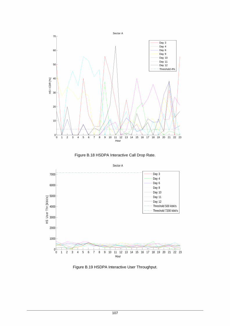
107
Figure B.18 HSDPA Interactive Call Drop Rate.
Figure B.19 HSDPA Interactive User Throughput.
0 1 2 3 4 5 6 7 8 9 10 11 12 13 14 15 16 17 18 19 20 21 22 230
10
20
30
40
50
60
70
Hour
HS
I C
DR
[%]
Sector A
Day 3Day 4Day 6Day 9Day 10Day 11Day 12Threshold 4%
0 1 2 3 4 5 6 7 8 9 10 11 12 13 14 15 16 17 18 19 20 21 22 230
1000
2000
3000
4000
5000
6000
7000
Hour
HS
Use
r Thr
[kbi
t/s]
Sector A
Day 3Day 4Day 6Day 8Day 10Day 11Day 12Threshold 500 kbit/sThreshold 7200 kbit/s

108
Figure B.20 IRAT HO Success Rate Incoming.
Figure B.21 IRAT HO Success Rate Outgoing.
0 1 2 3 4 5 6 7 8 9 10 11 12 13 14 15 16 17 18 19 20 21 22 2375
80
85
90
95
100
Hour
IRA
T H
O C
S S
R In
[%]
Sector A
Day 3Day 4Day 6Day 9Day 10Day 11Day 12Threshold 80%
0 1 2 3 4 5 6 7 8 9 10 11 12 13 14 15 16 17 18 19 20 21 22 2370
75
80
85
90
95
100
Hour
IRA
T H
O C
S S
R O
ut [%
]
Sector A
Day 3Day 4Day 6Day9Day 10Day 11Day 12Threshold 80%

109
Figure B.22 PS R99 Interactive Call Drop Rate.
Figure B.23 PS R99 Interactive Uplink User Throughput.
0 1 2 3 4 5 6 7 8 9 10 11 12 13 14 15 16 17 18 19 20 21 22 230
0.5
1
1.5
2
2.5
3
3.5
4
4.5
Hour
PS
R99
I C
DR
[%]
Sector A
Day 3Day 4Day 6Day 9Day 10Day 11Day 12Threshold 4%
0 1 2 3 4 5 6 7 8 9 10 11 12 13 14 15 16 17 18 19 20 21 22 230
50
100
150
200
250
300
350
400
Hour
R99
UL
Use
r Thr
[kbi
t/s]
Sector A
Day 3Day 4Day 6 Day 9Day 10Day 11Day 12Threshold 50 kbit/sThreshold 384 kbit/s

110

111
Annex C
Daily Analysis Results C. Annex C
In Annex C, one presentes the results related to a single day, September 2nd, 2010, for GSM and
UMTS.
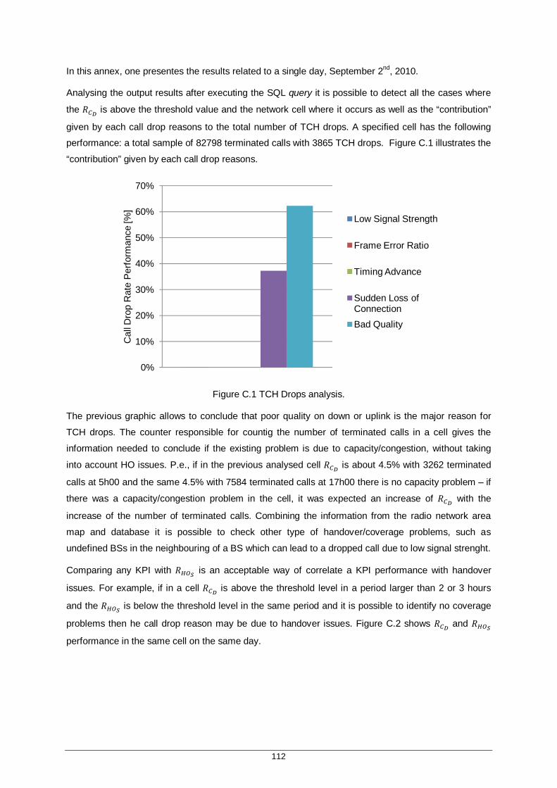
112
In this annex, one presentes the results related to a single day, September 2nd, 2010.
Analysing the output results after executing the SQL query it is possible to detect all the cases where
the 푅 is above the threshold value and the network cell where it occurs as well as the “contribution”
given by each call drop reasons to the total number of TCH drops. A specified cell has the following
performance: a total sample of 82798 terminated calls with 3865 TCH drops. Figure C.1 illustrates the
“contribution” given by each call drop reasons.
Figure C.1 TCH Drops analysis.
The previous graphic allows to conclude that poor quality on down or uplink is the major reason for
TCH drops. The counter responsible for countig the number of terminated calls in a cell gives the
information needed to conclude if the existing problem is due to capacity/congestion, without taking
into account HO issues. P.e., if in the previous analysed cell 푅 is about 4.5% with 3262 terminated
calls at 5h00 and the same 4.5% with 7584 terminated calls at 17h00 there is no capacity problem – if
there was a capacity/congestion problem in the cell, it was expected an increase of 푅 with the
increase of the number of terminated calls. Combining the information from the radio network area
map and database it is possible to check other type of handover/coverage problems, such as
undefined BSs in the neighbouring of a BS which can lead to a dropped call due to low signal strenght.
Comparing any KPI with 푅 is an acceptable way of correlate a KPI performance with handover
issues. For example, if in a cell 푅 is above the threshold level in a period larger than 2 or 3 hours
and the 푅 is below the threshold level in the same period and it is possible to identify no coverage
problems then he call drop reason may be due to handover issues. Figure C.2 shows 푅 and 푅
performance in the same cell on the same day.
0%
10%
20%
30%
40%
50%
60%
70%
Cal
l Dro
p R
ate
Per
form
ance
[%]
Low Signal Strength
Frame Error Ratio
Timing Advance
Sudden Loss of ConnectionBad Quality
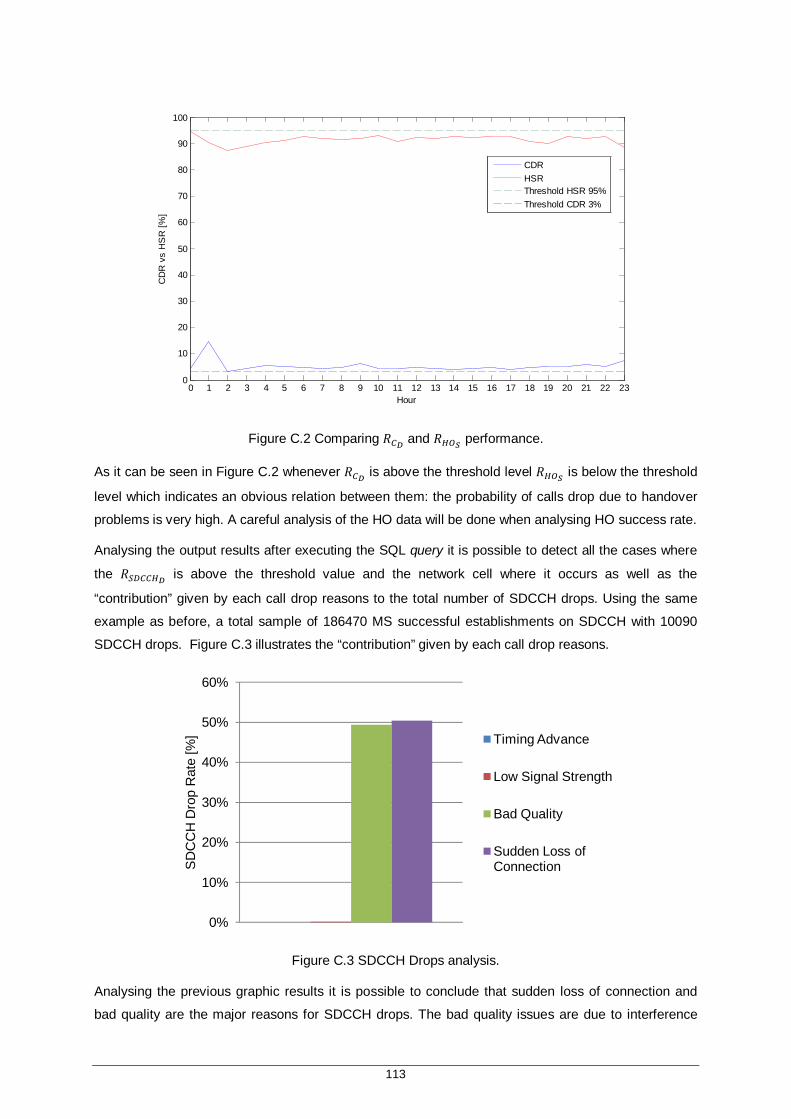
113
Figure C.2 Comparing 푅 and 푅 performance.
As it can be seen in Figure C.2 whenever 푅 is above the threshold level 푅 is below the threshold
level which indicates an obvious relation between them: the probability of calls drop due to handover
problems is very high. A careful analysis of the HO data will be done when analysing HO success rate.
Analysing the output results after executing the SQL query it is possible to detect all the cases where
the 푅 is above the threshold value and the network cell where it occurs as well as the
“contribution” given by each call drop reasons to the total number of SDCCH drops. Using the same
example as before, a total sample of 186470 MS successful establishments on SDCCH with 10090
SDCCH drops. Figure C.3 illustrates the “contribution” given by each call drop reasons.
Figure C.3 SDCCH Drops analysis.
Analysing the previous graphic results it is possible to conclude that sudden loss of connection and
bad quality are the major reasons for SDCCH drops. The bad quality issues are due to interference
0 1 2 3 4 5 6 7 8 9 10 11 12 13 14 15 16 17 18 19 20 21 22 230
10
20
30
40
50
60
70
80
90
100
Hour
CD
R v
s H
SR
[%]
CDRHSRThreshold HSR 95%Threshold CDR 3%
0%
10%
20%
30%
40%
50%
60%
SD
CC
H D
rop
Rat
e [%
] Timing Advance
Low Signal Strength
Bad Quality
Sudden Loss of Connection
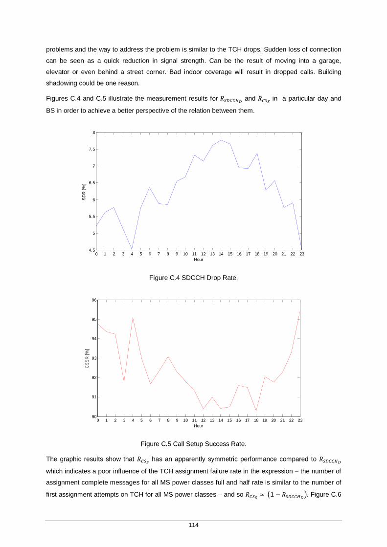
114
problems and the way to address the problem is similar to the TCH drops. Sudden loss of connection
can be seen as a quick reduction in signal strength. Can be the result of moving into a garage,
elevator or even behind a street corner. Bad indoor coverage will result in dropped calls. Building
shadowing could be one reason.
Figures C.4 and C.5 illustrate the measurement results for 푅 and 푅 in a particular day and
BS in order to achieve a better perspective of the relation between them.
Figure C.4 SDCCH Drop Rate.
Figure C.5 Call Setup Success Rate.
The graphic results show that 푅 has an apparently symmetric performance compared to 푅
which indicates a poor influence of the TCH assignment failure rate in the expression – the number of
assignment complete messages for all MS power classes full and half rate is similar to the number of
first assignment attempts on TCH for all MS power classes – and so 푅 ≈ 1 −푅 . Figure C.6
0 1 2 3 4 5 6 7 8 9 10 11 12 13 14 15 16 17 18 19 20 21 22 234.5
5
5.5
6
6.5
7
7.5
8
Hour
SD
R [%
]
0 1 2 3 4 5 6 7 8 9 10 11 12 13 14 15 16 17 18 19 20 21 22 2390
91
92
93
94
95
96
Hour
CS
SR
[%]
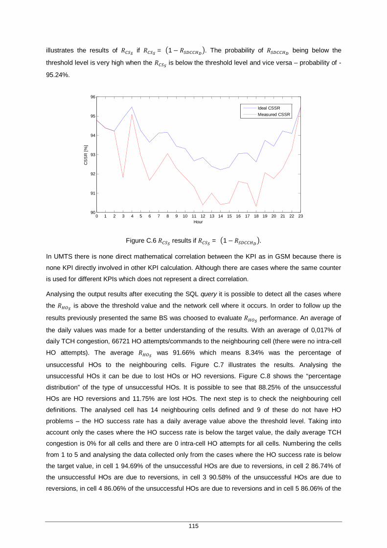
115
illustrates the results of 푅 if 푅 = 1− 푅 . The probability of 푅 being below the
threshold level is very high when the 푅 is below the threshold level and vice versa – probability of -
95.24%.
Figure C.6 푅 results if 푅 = 1−푅 .
In UMTS there is none direct mathematical correlation between the KPI as in GSM because there is
none KPI directly involved in other KPI calculation. Although there are cases where the same counter
is used for different KPIs which does not represent a direct correlation.
Analysing the output results after executing the SQL query it is possible to detect all the cases where
the 푅 is above the threshold value and the network cell where it occurs. In order to follow up the
results previously presented the same BS was choosed to evaluate 푅 performance. An average of
the daily values was made for a better understanding of the results. With an average of 0,017% of
daily TCH congestion, 66721 HO attempts/commands to the neighbouring cell (there were no intra-cell
HO attempts). The average 푅 was 91.66% which means 8.34% was the percentage of
unsuccessful HOs to the neighbouring cells. Figure C.7 illustrates the results. Analysing the
unsuccessful HOs it can be due to lost HOs or HO reversions. Figure C.8 shows the “percentage
distribution” of the type of unsuccessful HOs. It is possible to see that 88.25% of the unsuccessful
HOs are HO reversions and 11.75% are lost HOs. The next step is to check the neighbouring cell
definitions. The analysed cell has 14 neighbouring cells defined and 9 of these do not have HO
problems – the HO success rate has a daily average value above the threshold level. Taking into
account only the cases where the HO success rate is below the target value, the daily average TCH
congestion is 0% for all cells and there are 0 intra-cell HO attempts for all cells. Numbering the cells
from 1 to 5 and analysing the data collected only from the cases where the HO success rate is below
the target value, in cell 1 94.69% of the unsuccessful HOs are due to reversions, in cell 2 86.74% of
the unsuccessful HOs are due to reversions, in cell 3 90.58% of the unsuccessful HOs are due to
reversions, in cell 4 86.06% of the unsuccessful HOs are due to reversions and in cell 5 86.06% of the
0 1 2 3 4 5 6 7 8 9 10 11 12 13 14 15 16 17 18 19 20 21 22 2390
91
92
93
94
95
96
Hour
CS
SR
[%]
Ideal CSSRMeasured CSSR

116
unsuccessful HOs are due to reversions. Since the daily average TCH congestion is 0% there is no
capacity problem.
Figure C.7 HO success rate performance.
Figure C.8 Unsuccessful HOs.
As it can be seen in Figure 3.12 the measured throughput will be below the threshold level due to poor
radio link quality, less PDCH reserved than requested by the users and reserved PDCH shared by
other users. To evaluate radio link quality, there are counters that provide the measure of radio link bit
rate and RLC data volume. It will be analysed the distributions of the radio link bit rate versus RLC
data volume in the whole cell for downlink CS-1/2/3/4 and downlink EGPRS transfers. These are
interval counters (the INTx counters) that count the downlink RLC data volume in certain bit rate
intervals, allowing a distribution of the radio link bit rate to be presented. This gives an excellent
picture of the distribution of the radio link quality in the cell.
To evaluate the number of PDCH’s reserved and requested by the users, the PDCH utilisation ratio as
to be analysed. This means that if the number of used channels over the number of allocated
channels is higher than 80% (this threshold value is defined by Ericsson), there is a capacity problem.
To evaluate the number of reserved PDCH shared by other users the number of TBFs (a PS
0%10%20%30%40%50%60%70%80%90%
100%
HO
Suc
cess
Rat
e P
erfo
rman
ce [%
]
Successful HOs
Unsuccessful HOs
0%10%20%30%40%50%60%70%80%90%
100%
Uns
ucce
ssfu
l HO
s [%
]
HO Reversions
Lost HOs
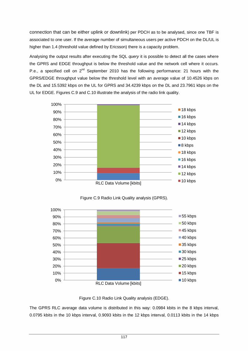
117
connection that can be either uplink or downlink) per PDCH as to be analysed, since one TBF is
associated to one user. If the average number of simultaneous users per active PDCH on the DL/UL is
higher than 1.4 (threshold value defined by Ericsson) there is a capacity problem.
Analysing the output results after executing the SQL query it is possible to detect all the cases where
the GPRS and EDGE throughput is below the threshold value and the network cell where it occurs.
P.e., a specified cell on 2nd September 2010 has the following performance: 21 hours with the
GPRS/EDGE throughput value below the threshold level with an average value of 10.4526 kbps on
the DL and 15.5392 kbps on the UL for GPRS and 34.4239 kbps on the DL and 23.7961 kbps on the
UL for EDGE. Figures C.9 and C.10 illustrate the analysis of the radio link quality.
Figure C.9 Radio Link Quality analysis (GPRS).
Figure C.10 Radio Link Quality analysis (EDGE).
The GPRS RLC average data volume is distributed in this way: 0.0984 kbits in the 8 kbps interval,
0.0795 kbits in the 10 kbps interval, 0.9093 kbits in the 12 kbps interval, 0.0113 kbits in the 14 kbps
0%
10%
20%
30%
40%
50%
60%
70%
80%
90%
100%
RLC Data Volume [kbits]
18 kbps
16 kbps
14 kbps
12 kbps
10 kbps
8 kbps
18 kbps
16 kbps
14 kbps
12 kbps
10 kbps
0%
10%
20%
30%
40%
50%
60%
70%
80%
90%
100%
RLC Data Volume [kbits]
55 kbps
50 kbps
45 kbps
40 kbps
35 kbps
30 kbps
25 kbps
20 kbps
15 kbps
10 kbps

118
interval and 0 kbits in the 16 and 18 kbps interval. Looking at the results the major “slice” of the traffic
is in the lower bit rate intervals (98.97% of the total traffic is in the three lower bite rate intervals) which
means poor radio link quality – the larger the bit rate range in which data are processed, the better the
quality of radio link. At this point, the reason for poor GPRS DL Throughput is identified. Yet the other
possibilities have to be checked. The average PDCH utilisation ratio is 39.85% (below the 80%
threshold value) and there are 1.034 simultaneous users per active B-PDCH (there are no active G-
PDCH) – below the 1.4 threshold value.
The EDGE RLC average data volume is distributed in this way: 0.1715 kbits in the 10 kbps interval,
0.3581 kbits in the 15 kbps interval, 0.2398 kbits in the 20 kbps interval, 0.0094 kbits in the 25 kbps
interval, 0.0260 kbits in the 30 kbps interval, 0.0179 kbits in the 35 kbps interval, 0.0561 kbits in the 40
kbps interval, 0.0476 kbits in the 45 kbps interval, 0.0542 kbits in the 50 kbps interval and 0.0194 kbits
in the 55 kbps interval. Looking at the results the major “slice” of the traffic is in the lower bit rate
intervals (76.94% of the total traffic is in the three lower bite rate intervals) which means poor radio link
quality. The average PDCH utilisation ratio is 40.07% (below the 80% threshold value) and there are
1.035 simultaneous users per active B-PDCH (there are no active G-PDCH) and 1.1721 simultaneous
users per active E-PDCH – below the 1.4 threshold value.
Analysing the output results after executing the SQL query it is possible to detect all the cases where
the 푅 is below the threshold value and the network cell where it occurs. The main reason for
PDCH allocation failures is when zero PDCH could be allocated due to lack of basic physical channels
over the air interface. The failure relates to the inability of the system to allocate resources since
requests to allocate PDCHs occur when the operator increases the number of dedicated PDCHs and
when the packet data traffic demands on-demand PDCHs. If the system cannot respond properly to
traffic demands there is a capacity problem. A good way to find the reasons that leads to failures on
the PDCH assignment is to compare the performance of the KPI with the TCH congestion and the
total traffic in half-rate. If the TCH congestion values are very high it is expected that there are
problems in the PDCH assignment and if the total traffic percentage in HR is higher than 50%
(Ericsson’s threshold) it is also expected that there are problems in the PDCH assignment. P.e., a
specified cell on 2nd September 2010 has the following performance: 18 hours with the PDCH
Assignment Success Rate value below the threshold level with an average value of 39.83%. 48.05%
of PDCH utilization, a TCH congestion of 0.001% and a HR traffic of 81.42% – the failures in PDCH
assignment are due to the high percentage of HR traffic.

119
Annex D
Monthly Analysis Results D. Annex D
In Annex D, one presentes the results concerning January 2010 related to the remaining BSs that are
not analysed in chapter 4.

120
D.1 GSM KPI Analysis
Table D.1 indicates the percentage associated to the number of hours where the KPI value is above
the threshold level at the same time as others analysed KPIs. The BSs were analysed according to
the monthly weight criteria.
Table D.1 푅 analysis.
BS 푅 and 푅 (%)
푅 and 푅 (%)
푅 and 푅 (%) BS
푅 and 푅 (%)
푅 and 푅 (%)
푅 and 푅 (%)
6 83.87 35.48 32.26 7 16.22 10.81 0.00 2 76.19 9.52 9.52 9 15.87 15.87 6.35 15 36.67 0.00 0.00 10 14.29 7.14 7.14 13 34.91 64.57 23.88 3 9.52 61.90 61.90 5 31.82 40.91 47.73 16 5.13 17.95 28.21 8 30.00 25.00 13.33 11 4.26 78.72 57.45 14 20.06 20.34 16.95 12 2.86 65.00 17.86 4 17.33 22.67 25.33 17 0.00 100.00 84.38
Looking at the results it is possible to conclude that in BS 6 83.87% of the total analysed hours do not
meet the minimum criteria required for both 푅 as for 푅 . Figure D.1 shows 푅 and 푅
performance evolution in that period.
Figure D.1 BS 6 – 푅 and 푅 performance analysis: correlation value of -69.80%.
In BS 6, only sector A in GSM 1800 is affected. Call drop rate has an average value of 25.47% and
HO success rate has an average value of 85.24%. 95.66% of the HO failures are Lost HOs and 4.34%
are HO reversions. There are 65143 internal HO attempts, which is the worst relation. There is no
10 20 30 40 50 60 700
10
20
30
40
50
60
70
80
90
100
Number of hours
CD
R a
nd H
SR
[%]
CDR [%]HSR [%]CDR ThresholdHSR Threshold

121
TCH congestion and 82.08% of the TCH drops are due to sudden loss of connection. None of the
defined neighbouring cells has HO problems.
Looking at the results of call drop rate and SDCCH drop rate, it is possible to conclude that in BSs 3,
11, 12 and 13 a call drops in 61.90%, 78.72%, 65.00% and 64.57% of the cases due to control
channel drop reasons, respectively. Figures D.2 to D.5 shows 푅 and 푅 performance evolution
in that period.
Figure D.2 BS 3 – 푅 and 푅 performance analysis: correlation value of 7.62%.
Figure D.3 BS 11 – 푅 and 푅 performance analysis: correlation value of 51.71%.
2 4 6 8 10 122
3
4
5
6
7
8
9
10
11
Number of hours
CD
R a
nd S
DR
[%]
CDR [%]SDR [%]CDR and SDR Threshold
5 10 15 20 25 30 35
5
10
15
20
25
Number of hours
CD
R a
nd S
DR
[%]
CDR [%]SDR[%]CDR and SDR Threshold
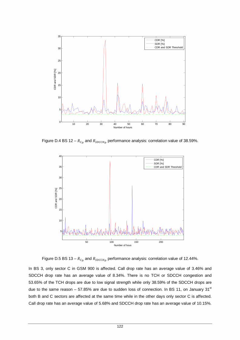
122
Figure D.4 BS 12 – 푅 and 푅 performance analysis: correlation value of 38.59%.
Figure D.5 BS 13 – 푅 and 푅 performance analysis: correlation value of 12.44%.
In BS 3, only sector C in GSM 900 is affected. Call drop rate has an average value of 3.46% and
SDCCH drop rate has an average value of 8.34%. There is no TCH or SDCCH congestion and
53.65% of the TCH drops are due to low signal strength while only 38.59% of the SDCCH drops are
due to the same reason – 57.85% are due to sudden loss of connection. In BS 11, on January 31st
both B and C sectors are affected at the same time while in the other days only sector C is affected.
Call drop rate has an average value of 5.68% and SDCCH drop rate has an average value of 10.15%.
10 20 30 40 50 60 70 80 900
5
10
15
20
25
30
35
Number of hours
CD
R a
nd S
DR
[%]
CDR [%]SDR [%]CDR and SDR Threshold
50 100 150 200
5
10
15
20
25
30
35
40
Number of hous
CD
R a
nd S
DR
[%]
CDR [%]SDR [%]CDR and SDR Threshold
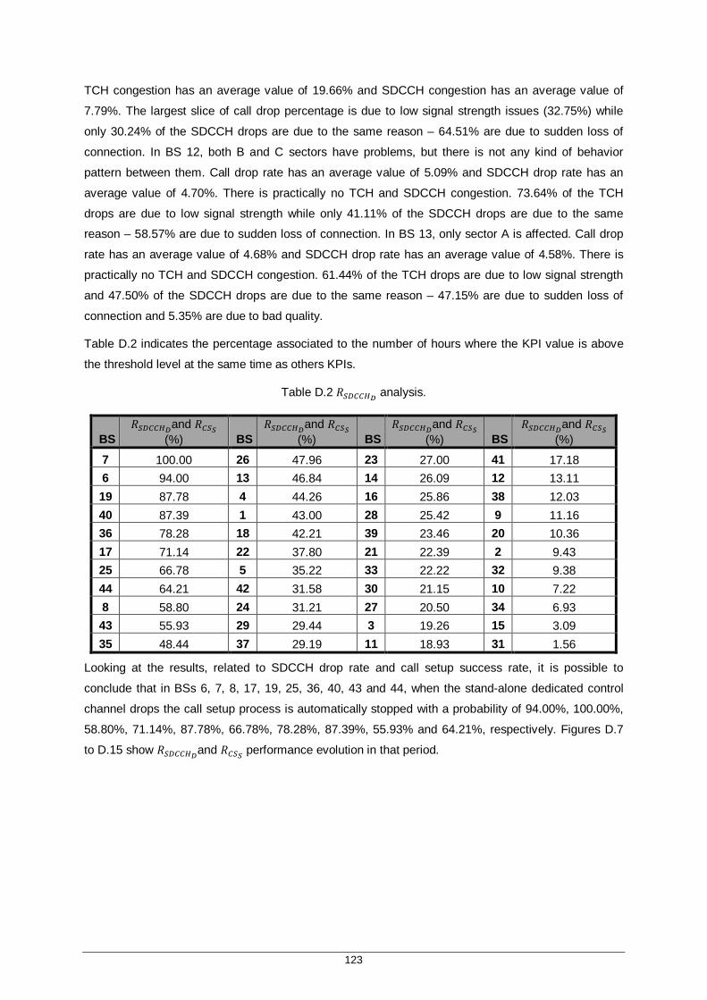
123
TCH congestion has an average value of 19.66% and SDCCH congestion has an average value of
7.79%. The largest slice of call drop percentage is due to low signal strength issues (32.75%) while
only 30.24% of the SDCCH drops are due to the same reason – 64.51% are due to sudden loss of
connection. In BS 12, both B and C sectors have problems, but there is not any kind of behavior
pattern between them. Call drop rate has an average value of 5.09% and SDCCH drop rate has an
average value of 4.70%. There is practically no TCH and SDCCH congestion. 73.64% of the TCH
drops are due to low signal strength while only 41.11% of the SDCCH drops are due to the same
reason – 58.57% are due to sudden loss of connection. In BS 13, only sector A is affected. Call drop
rate has an average value of 4.68% and SDCCH drop rate has an average value of 4.58%. There is
practically no TCH and SDCCH congestion. 61.44% of the TCH drops are due to low signal strength
and 47.50% of the SDCCH drops are due to the same reason – 47.15% are due to sudden loss of
connection and 5.35% are due to bad quality.
Table D.2 indicates the percentage associated to the number of hours where the KPI value is above
the threshold level at the same time as others KPIs.
Table D.2 푅 analysis.
BS 푅 and 푅
(%) BS 푅 and 푅
(%) BS 푅 and 푅
(%) BS 푅 and 푅
(%) 7 100.00 26 47.96 23 27.00 41 17.18 6 94.00 13 46.84 14 26.09 12 13.11 19 87.78 4 44.26 16 25.86 38 12.03 40 87.39 1 43.00 28 25.42 9 11.16 36 78.28 18 42.21 39 23.46 20 10.36 17 71.14 22 37.80 21 22.39 2 9.43 25 66.78 5 35.22 33 22.22 32 9.38 44 64.21 42 31.58 30 21.15 10 7.22 8 58.80 24 31.21 27 20.50 34 6.93 43 55.93 29 29.44 3 19.26 15 3.09 35 48.44 37 29.19 11 18.93 31 1.56
Looking at the results, related to SDCCH drop rate and call setup success rate, it is possible to
conclude that in BSs 6, 7, 8, 17, 19, 25, 36, 40, 43 and 44, when the stand-alone dedicated control
channel drops the call setup process is automatically stopped with a probability of 94.00%, 100.00%,
58.80%, 71.14%, 87.78%, 66.78%, 78.28%, 87.39%, 55.93% and 64.21%, respectively. Figures D.7
to D.15 show 푅 and 푅 performance evolution in that period.
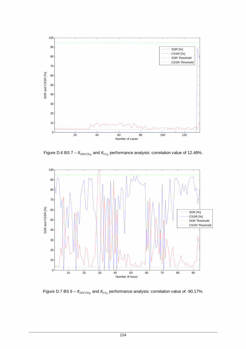
124
Figure D.6 BS 7 – 푅 and 푅 performance analysis: correlation value of 12.48%.
Figure D.7 BS 6 – 푅 and 푅 performance analysis: correlation value of -90.17%.
20 40 60 80 100 1200
10
20
30
40
50
60
70
80
90
100
Number of cases
SD
R a
nd C
SS
R [%
]
SDR [%]CSSR [%]SDR ThresholdCSSR Threshold
10 20 30 40 50 60 70 80 900
10
20
30
40
50
60
70
80
90
100
Number of hours
SD
R a
nd C
SS
R [%
]
SDR [%]CSSR [%]SDR ThresholdCSSR Threshold
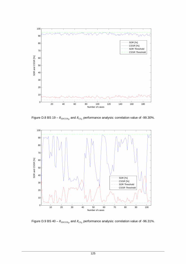
125
Figure D.8 BS 19 – 푅 and 푅 performance analysis: correlation value of -99.30%.
Figure D.9 BS 40 – 푅 and 푅 performance analysis: correlation value of -96.31%.
20 40 60 80 100 120 140 160 1800
10
20
30
40
50
60
70
80
90
100
Number of cases
SD
R a
nd C
SS
R [%
]
SDR [%]CSSR [%]SDR ThresholdCSSR Threshold
10 20 30 40 50 60 70 80 90 1000
10
20
30
40
50
60
70
80
90
100
Number of cases
SD
R a
nd C
SS
R [%
]
SDR [%]CSSR [%]SDR ThresholdCSSR Threshold

126
Figure D.10 BS 17 – 푅 and 푅 performance analysis: correlation value of -98.35%.
Figure D.11 BS 25 – 푅 and 푅 performance analysis: correlation value of -97.89%.
20 40 60 80 100 120 1400
10
20
30
40
50
60
70
80
90
100
SD
R a
nd C
SS
R [%
]
SDR [%]CSSR [%]SDR ThresholdCSSR Threshold
20 40 60 80 100 120 140 160 1800
10
20
30
40
50
60
70
80
90
100
Number of cases
SD
R a
nd C
SS
R [%
]
SDR [%]CSSR [%]SDR ThresholdCSSR Threshold
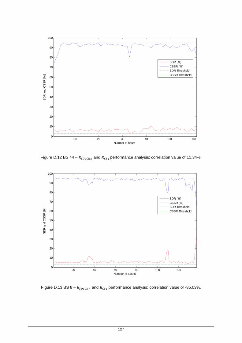
127
Figure D.12 BS 44 – 푅 and 푅 performance analysis: correlation value of 11.34%.
Figure D.13 BS 8 – 푅 and 푅 performance analysis: correlation value of -85.03%.
10 20 30 40 50 600
10
20
30
40
50
60
70
80
90
100
Number of hours
SD
R a
nd C
SS
R [%
]
SDR [%]CSSR [%]SDR ThresholdCSSR Threshold
20 40 60 80 100 1200
10
20
30
40
50
60
70
80
90
100
Number of cases
SDR
and
CS
SR
[%]
SDR [%]CSSR [%]SDR ThresholdCSSR Threshold

128
Figure D.14 BS 43 – 푅 and 푅 performance analysis: correlation value of -92.55%.
In BS 6, the sectors A, B and C are affected at the same time in GSM 900. SDCCH drop rate has an
average value of 20.79%% and call setup success rate has an average value of 63.49%. According to
Figures 3.10 and 3.12 an analysis to “high SDCCH drop rate” and “low TCH assignment success rate”
has to be done. Analysing the remaining output results, TCH assignment success rate has an average
value of 0.8%. TCH congestion has an average value of 11.02% and SDCCH congestion has an
average value of 23.25%. 93.94% of the control channel drops are due to sudden loss of connection.
In BS 7, the sectors A, B and C are affected at the same time in GSM 900. SDCCH drop rate has an
average value of 5.45% and call setup success rate has an average value of 1.87%. TCH assignment
success rate has an average value of 0.02%. TCH congestion has an average value of 94.19% and
SDCCH congestion has an average value of 0.47%. 90.65% of the control channel drops are due to
sudden loss of connection.
In BS 8, the majority of the problems are in sector B in GSM 900. SDCCH drop rate has an average
value of 6.26% and call setup success rate has an average value of 92.89%. TCH assignment
success rate has an average value of 0.99%. TCH congestion has an average value of 0.47% and
SDCCH congestion has an average value of 0.01%. 51.97% of the control channel drops are due to
sudden loss of connection and 36.67% are due to bad quality.
In BS 17, sector B in GSM 1800 is the only sector affected with problems. SDCCH drop rate has an
average value of 7.20% and call setup success rate has an average value of 92.42%. TCH
assignment success rate has an average value of 1.00%. There is no TCH congestion and SDCCH
congestion has an average value of 0.18%. 53.93% of the control channel drops are due to sudden
5 10 15 20 25 300
10
20
30
40
50
60
70
80
90
100
Number of cases
SD
R a
nd C
SS
R [%
]
SDR [%]CSSR [%]SDR ThresholdCSSR Threshold
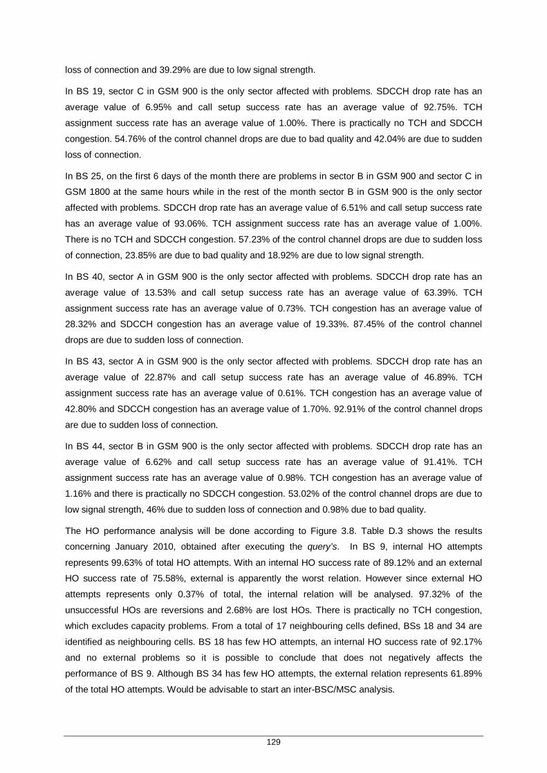
129
loss of connection and 39.29% are due to low signal strength.
In BS 19, sector C in GSM 900 is the only sector affected with problems. SDCCH drop rate has an
average value of 6.95% and call setup success rate has an average value of 92.75%. TCH
assignment success rate has an average value of 1.00%. There is practically no TCH and SDCCH
congestion. 54.76% of the control channel drops are due to bad quality and 42.04% are due to sudden
loss of connection.
In BS 25, on the first 6 days of the month there are problems in sector B in GSM 900 and sector C in
GSM 1800 at the same hours while in the rest of the month sector B in GSM 900 is the only sector
affected with problems. SDCCH drop rate has an average value of 6.51% and call setup success rate
has an average value of 93.06%. TCH assignment success rate has an average value of 1.00%.
There is no TCH and SDCCH congestion. 57.23% of the control channel drops are due to sudden loss
of connection, 23.85% are due to bad quality and 18.92% are due to low signal strength.
In BS 40, sector A in GSM 900 is the only sector affected with problems. SDCCH drop rate has an
average value of 13.53% and call setup success rate has an average value of 63.39%. TCH
assignment success rate has an average value of 0.73%. TCH congestion has an average value of
28.32% and SDCCH congestion has an average value of 19.33%. 87.45% of the control channel
drops are due to sudden loss of connection.
In BS 43, sector A in GSM 900 is the only sector affected with problems. SDCCH drop rate has an
average value of 22.87% and call setup success rate has an average value of 46.89%. TCH
assignment success rate has an average value of 0.61%. TCH congestion has an average value of
42.80% and SDCCH congestion has an average value of 1.70%. 92.91% of the control channel drops
are due to sudden loss of connection.
In BS 44, sector B in GSM 900 is the only sector affected with problems. SDCCH drop rate has an
average value of 6.62% and call setup success rate has an average value of 91.41%. TCH
assignment success rate has an average value of 0.98%. TCH congestion has an average value of
1.16% and there is practically no SDCCH congestion. 53.02% of the control channel drops are due to
low signal strength, 46% due to sudden loss of connection and 0.98% due to bad quality.
The HO performance analysis will be done according to Figure 3.8. Table D.3 shows the results
concerning January 2010, obtained after executing the query’s. In BS 9, internal HO attempts
represents 99.63% of total HO attempts. With an internal HO success rate of 89.12% and an external
HO success rate of 75.58%, external is apparently the worst relation. However since external HO
attempts represents only 0.37% of total, the internal relation will be analysed. 97.32% of the
unsuccessful HOs are reversions and 2.68% are lost HOs. There is practically no TCH congestion,
which excludes capacity problems. From a total of 17 neighbouring cells defined, BSs 18 and 34 are
identified as neighbouring cells. BS 18 has few HO attempts, an internal HO success rate of 92.17%
and no external problems so it is possible to conclude that does not negatively affects the
performance of BS 9. Although BS 34 has few HO attempts, the external relation represents 61.89%
of the total HO attempts. Would be advisable to start an inter-BSC/MSC analysis.

130
Table D.3 HO performance results.
BS
Internal HO
Attempts
Internal HSR (%)
External HO
Attempts
External HSR (%) BS
Internal HO
Attempts
Internal HSR (%)
External HO
Attempts
External HSR (%)
21 1243667 92.82 180495 93.22 2 18416 91.27 30214 87.63 9 394952 89.12 1460 75.58 38 18240 90.92 2134 89.35
16 340465 88.47 1599 92.10 24 17243 91.55 16516 86.83 17 273368 82.75 4424 89.12 35 16894 90.69 2571 60.66 7 249998 91.87 44 80.34 26 13532 87.35 0 -
19 226421 91.78 54 62.34 28 12994 89.65 0 - 30 180097 84.73 13342 84.94 13 11012 78.62 5061 84.75 32 102916 91.01 735 80.83 42 10504 87.13 4981 79.22 12 89842 81.29 0 - 36 9137 84.57 0 - 1 74881 90.42 56128 91.00 18 9074 92.17 0 -
15 63778 92.80 3086 90.84 10 7245 88.54 4239 89.89 3 59669 94.02 0 - 4 6104 90.79 6864 90.42 8 59508 88.35 5247 92.78 41 5999 86.69 2265 89.18
29 40798 91.18 38 75.91 27 5986 92.41 17 74.75 33 36794 91.90 1042 76.35 37 4665 85.46 11050 86.37 22 25555 86.44 3859 87.48 20 3253 89.11 0 - 5 22997 91.20 11236 88.44 11 3169 91.15 7132 85.32
23 22021 89.54 46308 93.24 25 3002 91.54 0 - 34 21837 68.26 35466 75.52 40 1590 90.08 145 89.06 14 20432 88.81 158193 93.09 6 955 73.44 0 - 31 18921 89.62 30337 90.03 39 403 77.47 0 -
In BS 16, internal HO attempts represents 99.53% of total HO attempts. Being internal the worst
relation, 57.97% of the unsuccessful HOs are reversions and 42.03% are lost HOs. There is practically
no TCH congestion, which excludes capacity problems. From a total of 12 neighbouring cells defined,
BSs 27 and 5 are identified as neighbouring cells. BS 27 has few HO attempts, an internal HO
success rate of 92.41% and an external HO success rate of 74.75%, but with only 17 external HO
attempts. It is possible to conclude that does not negatively affect the performance of BS 16. BS 5 has
few HO attempts and has no TCH congestion so also does not affect the performance of BS 16.
In BS 17, internal HO attempts represents 98.41% of total HO attempts. Being internal the worst
relation, 95.60% of the unsuccessful HOs are reversions and 4.40% are lost HOs. There is practically
no TCH congestion, which excludes capacity problems. From a total of 16 neighbouring cells defined,
BSs 8, 4, 12, 29, 33 and 30 are identified as neighbouring cells. BS 8 has an internal HO success rate
of 88.35% (worst relation) with 91.90% of the total HO attempts being internal. 91.52% of the
unsuccessful HOs are due to reversions and there is no TCH congestion. BS 4 has an internal HO
success rate of 90.79% and an external HO success rate of 90.42% but both with few HO attempts,
and so does not affect the performance of BS 17. BS 12 has an internal HO success rate of 81.29%
(worst relation) with 100.00% of the total HO attempts being internal. 92.05% of the unsuccessful HOs
are due to reversions and TCH congestion has an average value of 0.02%. BS 29 has an internal HO

131
success rate of 91.18% with 97.25% of the total HO attempts being internal. 95.03% of the
unsuccessful HOs are due to reversions and TCH congestion has an average value of 0.09%. BS 33
has an internal HO success rate of 91.90% with 97.25% of the total HO attempts being internal.
67.18% of the unsuccessful HOs are due to reversions and 32.82% are due to lost HOs. TCH
congestion has an average value of 0.78%. BS 30 has an internal HO success rate of 84.73% with
93.10% of the total HO attempts being internal. 95.71% of the unsuccessful HOs are due to reversions
and TCH congestion has an average value of 0.26%.
In BS 7, internal HO attempts represents 99.98% of total HO attempts. 97.50% of the unsuccessful
HOs are reversions and 2.50% are lost HOs. There is practically no TCH congestion, which excludes
capacity problems. From a total of 17 neighbouring cells defined, BSs 22, 31, 32, 35 and 34 are
identified as neighbouring cells. BS 8 has an internal HO success rate of 88.35% (worst relation) with
91.90% of the total HO attempts being internal. 91.52% of the unsuccessful HOs are due to reversions
and there is no TCH congestion. BS 22 has an internal HO success rate of 86.44% with 86.88% of the
total HO attempts being internal. 97.61% of the unsuccessful HOs are due to reversions and there is
no TCH. BS 31 has an internal HO success rate of 89.62% and an external HO success rate of
90.03% with 61.59% of the total HO attempts being external. This difference advises an inter-
BSC/MSC analysis. 92.68% of the unsuccessful HOs are due to reversions and there is no TCH
congestion. BS 32 has an internal HO success rate of 91.01% with 99.29% of the total HO attempts
being internal. 96.65% of the unsuccessful HOs are due to reversions and TCH congestion has an
average value of 1.66%. BS 35 has an internal HO success rate of 90.69% with 86.79% of the total
HO attempts being internal. 98.80% of the unsuccessful HOs are due to reversions and there is
practically no TCH congestion. BS 34 has been already analysed.
In BS 19, internal HO attempts represents 99.98% of total HO attempts. Internal HO success rate has
an average value of 91.78%. The number of external HO attempts is very low and so the external
relation is not taken into account. 94.17% of the unsuccessful HOs are reversions and 5.83% are lost
HOs. TCH congestion has an average value of 0.11%, which excludes capacity problems. From a
total of 20 neighbouring cells defined none of them is identified as a problematic BS.
In BS 12, internal HO attempts represents 100.00% of total HO attempts since there is no external HO
attempts. Internal HO success rate has an average value of 81.28%. 92.05% of the unsuccessful HOs
are reversions and 7.95% are lost HOs. TCH congestion has an average value of 0.02%, which
excludes capacity problems. From a total of 12 neighbouring cells defined, BSs 4, 8, 17, 29 and 30 are
identified as neighbouring cells. All of them have been already analysed.
Table D.4 shows the results concerning GPRS throughput on January 2010, obtained after executing
the query’s. Looking at the results it is possible to conclude that in BSs 45, 41, 40, 24, 37 and 23 when
the assignment of the PDCH assignment success rate is below the threshold level the throughput
value is also below the threshold level with a probability of 84.77%, 81.75%, 80.76%, 65.43%, 61.37%
and 50.52%, respectively. The same analysis is done to the GPRS UL throughput. Figures D.16 to
D.27 show 푇 , 푇 and 푅 performance evolution in that period. Only BS 37 will be
analysed since the analysis to the other BSs is made in a similar way.

132
Table D.4 GPRS throughput performance results.
BS 푇 and 푅
푇 and 푅
푇 and 푇 and 푅 BS
푇 and 푅
푇 and 푅
푇 and 푇 and 푅
49 90.13 78.42 60.52 15 18.30 24.24 0.86 45 84.77 97.92 2.87 11 16.58 11.58 0.00 41 81.75 76.96 38.32 17 16.18 0.00 5.43 40 80.76 96.89 12.76 7 15.40 0.00 0.00 24 65.43 66.67 6.32 21 14.97 18.42 4.19 37 61.37 62.63 21.68 36 14.37 9.30 2.35 23 50.52 78.57 3.09 25 13.85 9.41 2.05 51 41.09 33.06 11.39 19 12.44 39.29 7.83 31 37.57 51.50 17.13 12 11.15 0.00 0.00 1 34.82 28.57 15.18 20 9.09 58.33 2.16 34 33.60 26.03 7.80 39 8.19 16.34 6.41 48 32.08 52.91 20.75 29 6.87 9.76 3.00 54 30.55 58.64 7.68 35 6.25 8.74 0.66 46 30.21 37.50 5.14 6 6.08 43.88 2.59 52 29.61 24.70 8.15 27 5.73 6.59 0.00 43 28.44 46.88 9.63 14 5.08 35.07 3.79 53 28.32 40.83 4.30 2 4.52 14.06 5.98 32 27.50 45.83 10.50 4 3.57 34.85 0.00 5 25.59 0.00 0.95 47 3.57 21.79 1.79 44 25.32 36.28 9.74 30 3.40 12.00 0.85 22 24.59 23.00 6.89 16 3.00 20.45 3.76 18 23.47 38.10 5.61 13 1.26 7.22 1.44 50 21.93 20.79 6.14 9 1.21 32.14 4.90 42 21.64 0.00 0.00 10 0.66 6.25 1.01 33 20.14 36.14 7.07 3 0.57 15.71 0.00 38 19.57 45.83 13.62 8 0.00 32.14 0.00 26 18.92 0.00 6.08 28 0.00 16.67 0.00
In BS 37, PDCH assignment success rate has an average value of 36.00%. The TCH congestion has
an average value of 0.22% and the HR traffic represents 18.27% of the total traffic. In this case, since
the two verifiable conditions of PDCH assignment success rate are not above the threshold value, it is
not possible to establish a direct correlation between the two KPIs. Analysing the GPRS DL
throughput (average value of 11.62 kbps) the GPRS RLC average data volume is distributed in this
way: 0.0490 kbits in the 8 kbps interval, 0.0435 kbits in the 10 kbps interval, 0.8774 kbits in the 12
kbps interval, 0.0342 kbits in the 14 kbps interval, 0.0183 kbits in the 16 and 0.0266kbits in the 18
kbps interval. Looking at the results the major “slice” of the traffic is in the lower bit rate intervals
(88.39% of the total traffic is in the three lower bite rate intervals) which means poor radio link quality –
the larger the bit rate range in which data are processed, the better the quality of radio link. At this
point, one of the possible reasons for poor GPRS DL throughput is identified. Yet the other
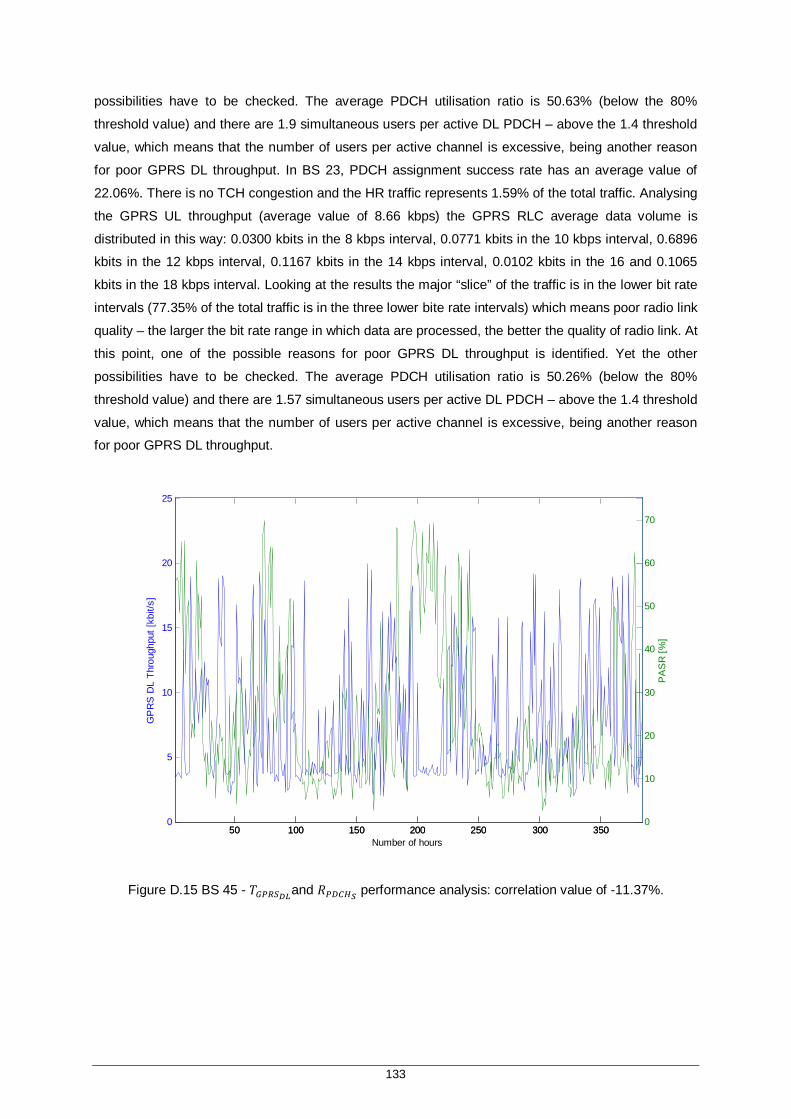
133
possibilities have to be checked. The average PDCH utilisation ratio is 50.63% (below the 80%
threshold value) and there are 1.9 simultaneous users per active DL PDCH – above the 1.4 threshold
value, which means that the number of users per active channel is excessive, being another reason
for poor GPRS DL throughput. In BS 23, PDCH assignment success rate has an average value of
22.06%. There is no TCH congestion and the HR traffic represents 1.59% of the total traffic. Analysing
the GPRS UL throughput (average value of 8.66 kbps) the GPRS RLC average data volume is
distributed in this way: 0.0300 kbits in the 8 kbps interval, 0.0771 kbits in the 10 kbps interval, 0.6896
kbits in the 12 kbps interval, 0.1167 kbits in the 14 kbps interval, 0.0102 kbits in the 16 and 0.1065
kbits in the 18 kbps interval. Looking at the results the major “slice” of the traffic is in the lower bit rate
intervals (77.35% of the total traffic is in the three lower bite rate intervals) which means poor radio link
quality – the larger the bit rate range in which data are processed, the better the quality of radio link. At
this point, one of the possible reasons for poor GPRS DL throughput is identified. Yet the other
possibilities have to be checked. The average PDCH utilisation ratio is 50.26% (below the 80%
threshold value) and there are 1.57 simultaneous users per active DL PDCH – above the 1.4 threshold
value, which means that the number of users per active channel is excessive, being another reason
for poor GPRS DL throughput.
Figure D.15 BS 45 - 푇 and 푅 performance analysis: correlation value of -11.37%.
50 100 150 200 250 300 3500
5
10
15
20
25
GP
RS
DL
Thro
ughp
ut [k
bit/s
]
Number of hours50 100 150 200 250 300 350
0
10
20
30
40
50
60
70
PA
SR
[%]
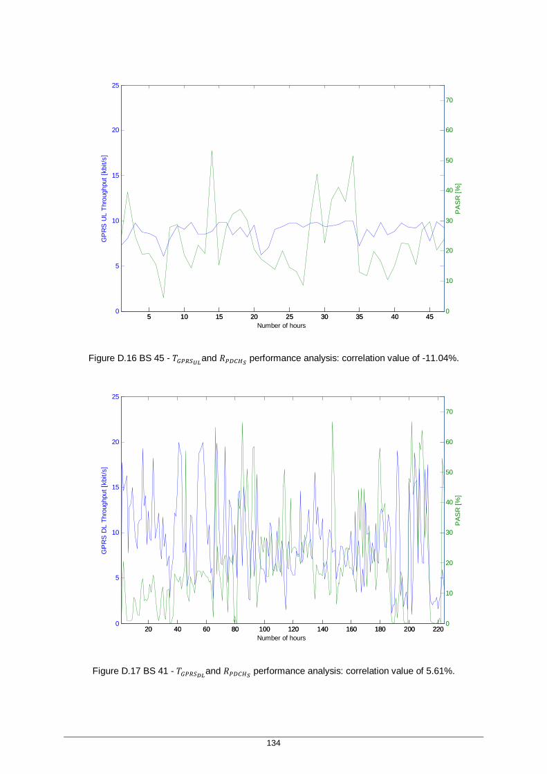
134
Figure D.16 BS 45 - 푇 and 푅 performance analysis: correlation value of -11.04%.
Figure D.17 BS 41 - 푇 and 푅 performance analysis: correlation value of 5.61%.
5 10 15 20 25 30 35 40 450
5
10
15
20
25
GP
RS
UL
Thro
ughp
ut [k
bit/s
]
Number of hours5 10 15 20 25 30 35 40 45
0
10
20
30
40
50
60
70
PA
SR
[%]
20 40 60 80 100 120 140 160 180 200 2200
5
10
15
20
25
GP
RS
DL
Thro
ughp
ut [k
bit/s
]
Number of hours20 40 60 80 100 120 140 160 180 200 220
0
10
20
30
40
50
60
70
PAS
R [%
]
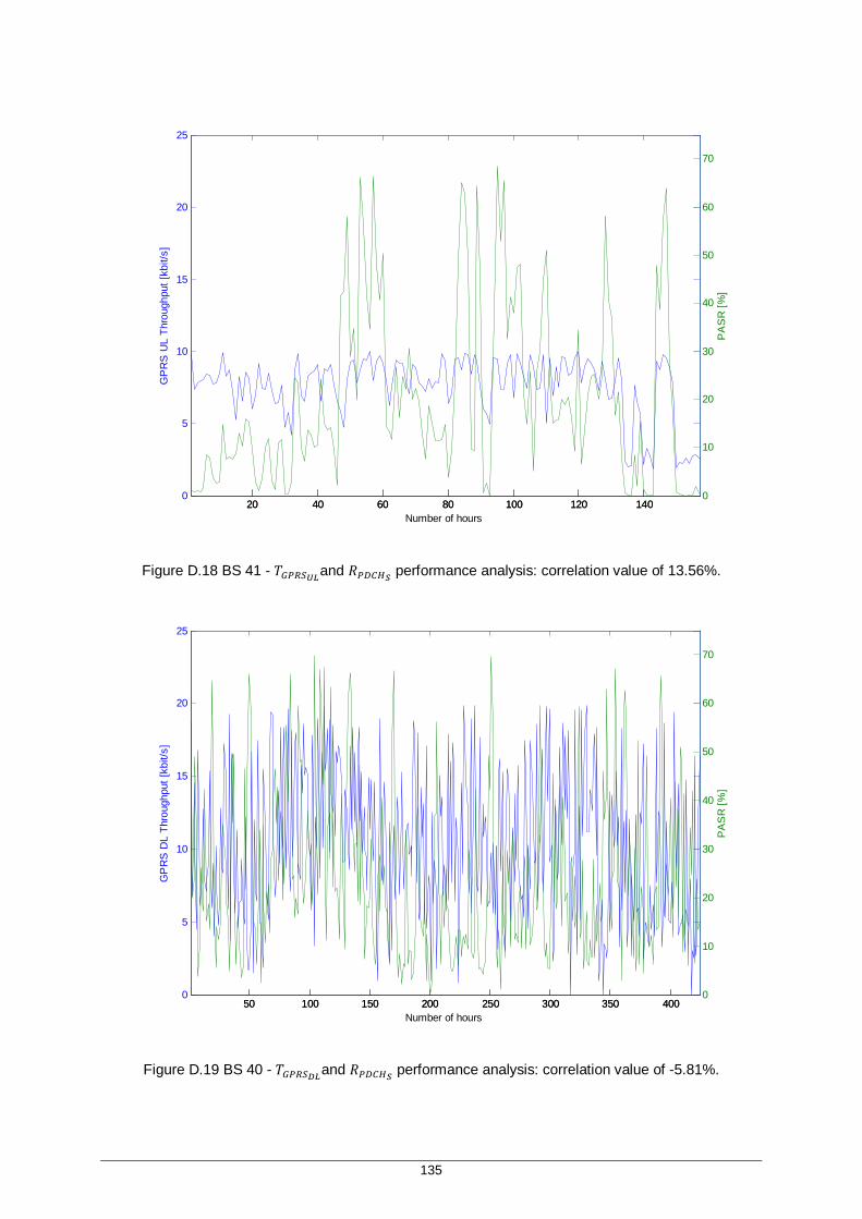
135
Figure D.18 BS 41 - 푇 and 푅 performance analysis: correlation value of 13.56%.
Figure D.19 BS 40 - 푇 and 푅 performance analysis: correlation value of -5.81%.
20 40 60 80 100 120 1400
5
10
15
20
25
GP
RS
UL
Thro
ughp
ut [k
bit/s
]
Number of hours20 40 60 80 100 120 140
0
10
20
30
40
50
60
70
PA
SR
[%]
50 100 150 200 250 300 350 4000
5
10
15
20
25
GP
RS
DL
Thro
ughp
ut [k
bit/s
]
Number of hours50 100 150 200 250 300 350 400
0
10
20
30
40
50
60
70
PA
SR
[%]
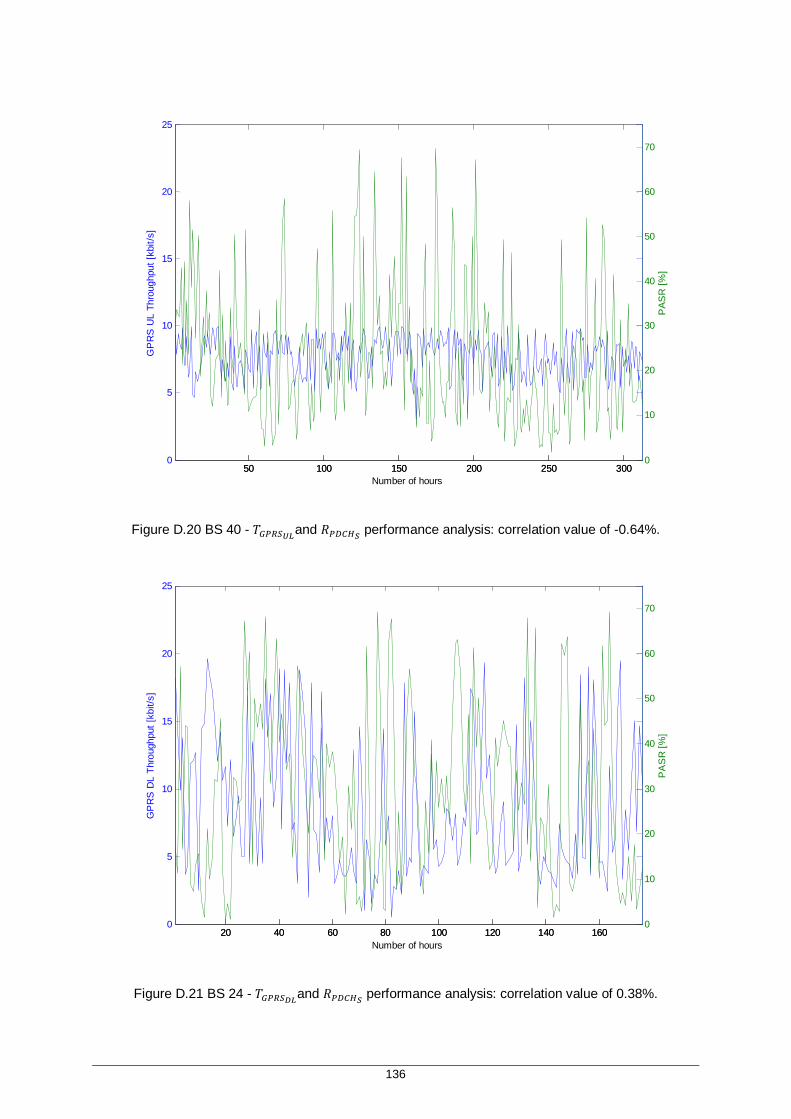
136
Figure D.20 BS 40 - 푇 and 푅 performance analysis: correlation value of -0.64%.
Figure D.21 BS 24 - 푇 and 푅 performance analysis: correlation value of 0.38%.
50 100 150 200 250 3000
5
10
15
20
25
GP
RS
UL
Thro
ughp
ut [k
bit/s
]
Number of hours50 100 150 200 250 300
0
10
20
30
40
50
60
70
PAS
R [%
]
20 40 60 80 100 120 140 1600
5
10
15
20
25
GP
RS
DL
Thro
ughp
ut [k
bit/s
]
Number of hours20 40 60 80 100 120 140 160
0
10
20
30
40
50
60
70
PA
SR
[%]
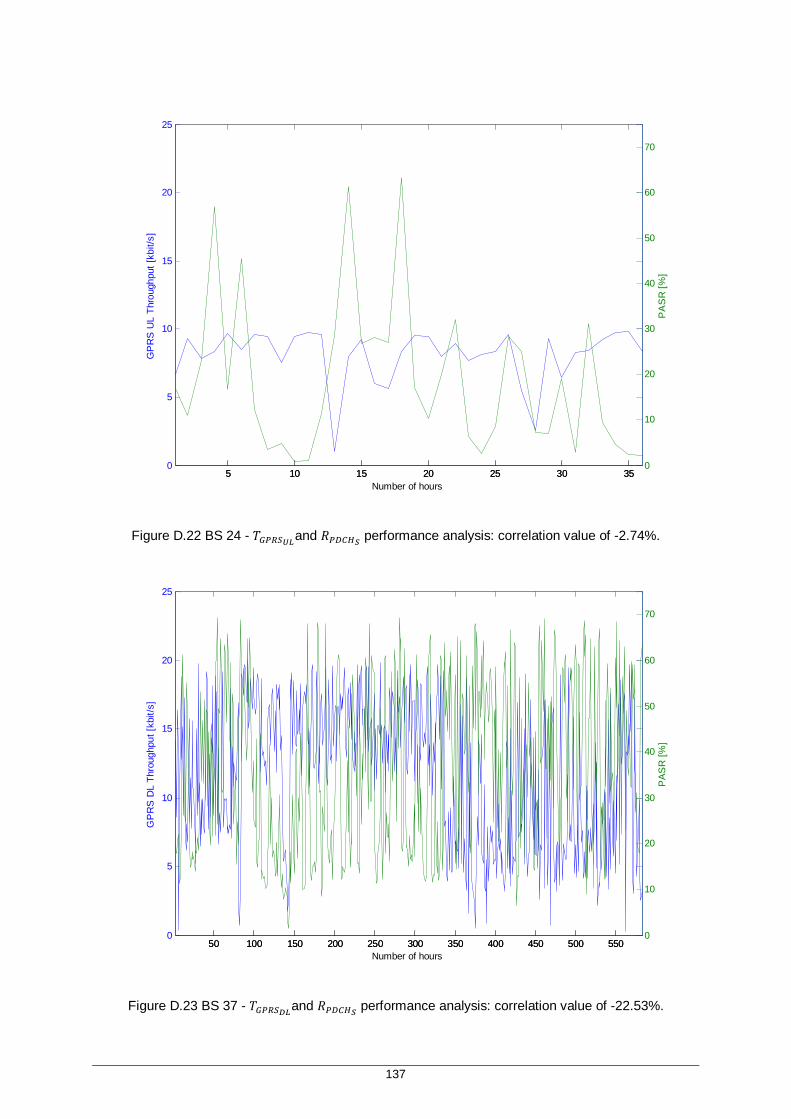
137
Figure D.22 BS 24 - 푇 and 푅 performance analysis: correlation value of -2.74%.
Figure D.23 BS 37 - 푇 and 푅 performance analysis: correlation value of -22.53%.
5 10 15 20 25 30 350
5
10
15
20
25
GP
RS
UL
Thro
ughp
ut [k
bit/s
]
Number of hours5 10 15 20 25 30 35
0
10
20
30
40
50
60
70
PA
SR
[%]
50 100 150 200 250 300 350 400 450 500 5500
5
10
15
20
25
GP
RS
DL
Thro
ughp
ut [k
bit/s
]
Number of hours50 100 150 200 250 300 350 400 450 500 550
0
10
20
30
40
50
60
70
PAS
R [%
]

138
Figure D.24 BS 37 - 푇 and 푅 performance analysis: correlation value of -4.18%.
Figure D.25 BS 23 - 푇 and 푅 performance analysis: correlation value of -2.18%.
50 100 150 200 250 300 350 4000
5
10
15
20
25
GP
RS
UL
Thro
ughp
ut [k
bit/s
]
Number of hours50 100 150 200 250 300 350 400
0
10
20
30
40
50
60
70
PA
SR
[%]
10 20 30 40 50 60 70 80 900
5
10
15
20
25
GP
RS
DL
Thro
ughp
ut [k
bit/s
]
Number of hours10 20 30 40 50 60 70 80 90
0
10
20
30
40
50
60
70
PA
SR
[%]

139
Figure D.26 BS 23 - 푇 and 푅 performance analysis: correlation value of -32.66%.
Table D.5 shows the results concerning EDGE throughput on January 2010, obtained after executing
the query’s. Looking at the results it is possible to conclude that in BSs 20, 34, 71, 87, 80, 51 and 83
when the assignment of the PDCH assignment success rate is below the threshold level the
throughput value is also below the threshold level with a probability of 98.15%, 98.01%, 94.30%,
90.18%, 89.89%, 89.00% and 88.68%, respectively. The same analysis is done to EDGE UL
throughput. Figures D.28 to D.39 show 푻푬푫푮푬푫푳 , 푻푬푫푮푬푼푳and 푹푷푫푪푯푺 performance evolution in that
period. Only BS 51 will be analysed since the analysis to the other BSs in made in a similar way. In BS
51 UL direction, PDCH assignment success rate has an average value of 35.24%. The TCH
congestion has an average value of 0.45% and the HR traffic represents 47.57% of the total traffic.
None of the criteria is exceeded. Analysing the EDGE UL throughput (average value of 20.67 kbps)
the EDGE RLC average data volume is distributed in this way: 0.0189 kbits in the 10 kbps interval,
0.0389 kbits in the 15 kbps interval, 0.0402 kbits in the 20 kbps interval, 0.0516 kbits in the 25 kbps
interval, 0.0580 kbits in the 30 kbps interval, 0.0663 kbits in the 35 kbps interval, 0.0853 kbits in the 40
kbps interval, 0.0936 kbits in the 45 kbps interval, 0.1222 kbits in the 50 kbps interval and 0.4252 kbits
in the 55 kbps interval. Looking at the results the major “slice” of the traffic is in the higher bit rate
intervals (72.63% of the total traffic is in the four higher bite rate intervals) which means good radio link
quality. The average PDCH utilisation ratio is 50.42% (below the 80% threshold value) and there are
2.03 simultaneous users per active DL PDCH – above the 1.4 threshold value, which can mean less
PDCH reserved than requested by the users.
2 4 6 8 10 12 14 16 18 20 220
5
10
15
20
25
GP
RS
UL
Thro
ughp
ut [k
bit/s
]
Number of hours2 4 6 8 10 12 14 16 18 20 22
0
10
20
30
40
50
60
70
PA
SR
[%]

140
Table D.5 EDGE throughput performance results.
BS 푇 and 푅
푇 and 푅
푇 and 푇 and 푅 BS
푇 and 푅
푇 and 푅
푇 and 푇 and 푅
20 98.15 72.84 98.15 1 52.53 48.56 48.48 34 98.01 93.91 92.69 35 50.00 31.08 48.58 71 94.30 84.81 80.42 21 48.07 29.17 47.21 87 90.18 71.98 89.73 59 46.87 49.85 45.85 80 89.89 69.93 79.78 103 45.09 39.64 43.46 51 89.00 46.67 72.00 68 45.00 12.88 44.00 83 88.68 87.56 78.16 30 42.74 38.49 35.48 77 87.53 81.18 79.65 8 42.55 33.84 36.88 44 85.12 10.16 73.55 66 41.41 26.21 37.63 92 84.41 52.26 83.27 24 41.41 4.44 40.23 10 83.15 64.73 81.54 49 41.36 53.23 28.64 39 81.82 60.92 76.42 82 40.64 23.95 37.44 75 77.63 76.40 75.39 12 40.11 19.39 31.07 41 76.47 64.94 57.01 63 38.22 24.35 35.47 67 74.59 69.37 64.29 70 38.04 11.83 36.20 52 74.39 45.27 73.78 56 37.87 23.49 33.73 76 73.78 48.80 69.33 13 36.77 26.01 32.26 7 73.36 51.40 70.93 18 34.55 26.24 31.82
100 69.86 59.42 66.31 15 34.19 26.48 28.06 50 68.65 44.54 65.95 27 33.56 24.14 31.88 26 68.22 69.57 53.39 86 33.19 28.10 30.44 84 68.16 70.41 58.71 85 33.06 22.65 29.03 60 66.33 41.53 65.32 101 32.81 30.36 24.61 88 65.43 38.46 65.43 58 31.01 19.26 25.32 25 63.96 0.00 54.82 94 30.69 26.84 24.48 90 63.92 46.13 57.22 29 30.00 12.18 26.32 74 63.40 56.29 60.95 28 29.97 0.00 28.01 5 62.54 27.97 59.87 97 29.80 29.19 26.67 79 62.02 39.40 56.59 93 29.20 29.05 25.91 95 61.73 59.04 57.54 43 28.14 12.30 24.55 99 61.01 54.64 59.75 104 27.82 19.39 27.07
102 60.91 50.00 56.68 37 25.87 12.55 24.48 69 60.69 11.17 55.94 22 24.76 21.86 22.46 98 60.28 44.99 59.81 23 24.58 47.77 22.88 45 60.25 24.75 57.14 47 24.16 19.27 23.49 2 57.52 29.78 53.98 54 24.03 10.95 23.26
105 56.68 40.20 49.05 73 23.90 12.01 22.93 38 55.43 55.37 47.43 9 23.81 14.35 15.87 17 54.77 45.27 52.05 32 22.49 28.98 22.01 96 53.73 30.64 51.49 55 53.31 31.39 43.01
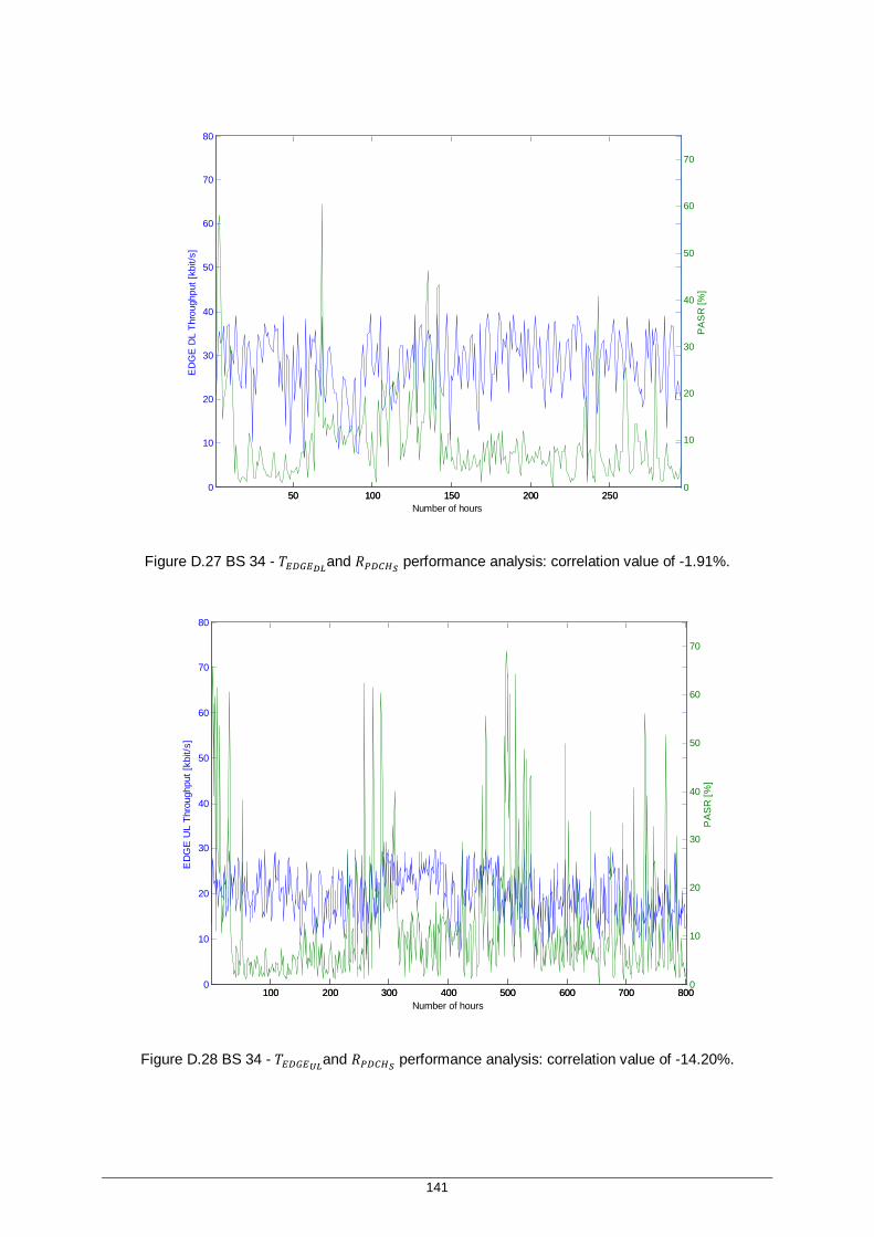
141
Figure D.27 BS 34 - 푇 and 푅 performance analysis: correlation value of -1.91%.
Figure D.28 BS 34 - 푇 and 푅 performance analysis: correlation value of -14.20%.
50 100 150 200 2500
10
20
30
40
50
60
70
80
ED
GE
DL
Thro
ughp
ut [k
bit/s
]
Number of hours50 100 150 200 250
0
10
20
30
40
50
60
70
PA
SR
[%]
100 200 300 400 500 600 700 8000
10
20
30
40
50
60
70
80
ED
GE
UL
Thro
ughp
ut [k
bit/s
]
Number of hours100 200 300 400 500 600 700 800
0
10
20
30
40
50
60
70
PA
SR
[%]

142
Figure D.29 BS 71 - 푇 and 푅 performance analysis: correlation value of -18.82%.
Figure D.30 BS 71 - 푇 and 푅 performance analysis: correlation value of -6.15%.
100 200 300 400 500 600 7000
10
20
30
40
50
60
70
80
ED
GE
DL
Thro
ughp
ut [k
bit/s
]
Number of hours100 200 300 400 500 600 700
0
10
20
30
40
50
60
70
PA
SR
[%]
100 200 300 400 500 600 700 800 9000
10
20
30
40
50
60
70
80
ED
GE
UL
Thro
ughp
ut [k
bit/s
]
Number of hours100 200 300 400 500 600 700 800 900
0
10
20
30
40
50
60
70
PA
SR
[%]

143
Figure D.31 BS 87 - 푇 and 푅 performance analysis: correlation value of -32.10%.
Figure D.32 BS 87 - 푇 and 푅 performance analysis: correlation value of -34.66%.
50 100 150 200 250 300 350 4000
10
20
30
40
50
60
70
80
ED
GE
DL
Thro
ughp
ut [k
bit/s
]
Number of hours50 100 150 200 250 300 350 400
0
10
20
30
40
50
60
70
PA
SR
[%]
50 100 150 200 250 300 350 400 450 5000
10
20
30
40
50
60
70
80
ED
GE
UL
Thro
ughp
ut [k
bit/s
]
Number of hours50 100 150 200 250 300 350 400 450 500
0
10
20
30
40
50
60
70
PA
SR
[%]

144
Figure D.33 BS 80 - 푇 and 푅 performance analysis: correlation value of -25.08%.
Figure D.34 BS 80 - 푇 and 푅 performance analysis: correlation value of -39.91%.
20 40 60 80 100 120 140 1600
10
20
30
40
50
60
70
80
ED
GE
DL
Thro
ughp
ut [k
bit/s
]
Number of hours20 40 60 80 100 120 140 160
0
10
20
30
40
50
60
70
PA
SR
[%]
50 100 150 200 250 300 350 400
8
10
12
14
16
18
20
22
24
26
28
ED
GE
UL
Thro
ughp
ut [k
bit/s
]
Number of hours50 100 150 200 250 300 350 400
15
20
25
30
35
40
45
50
55
60
65P
AS
R [%
]

145
Figure D.35 BS 51 - 푇 and 푅 performance analysis: correlation value of -31.41%.
Figure D.36 BS 51 - 푇 and 푅 performance analysis: correlation value of -50.61%.
10 20 30 40 50 60 70 800
10
20
30
40
50
60
70
80
ED
GE
DL
Thro
ughp
ut [k
bit/s
]
Number of hours10 20 30 40 50 60 70 80
0
10
20
30
40
50
60
70
PA
SR
[%]
20 40 60 80 100 120 140 1600
10
20
30
40
50
60
70
80
ED
GE
UL
Thro
ughp
ut [k
bit/s
]
Number of hours20 40 60 80 100 120 140 160
0
10
20
30
40
50
60
70
PA
SR
[%]

146
Figure D.37 BS 83 - 푇 and 푅 performance analysis: correlation value of -4.50%.
Figure D.38 BS 83 - 푇 and 푅 performance analysis: correlation value of -3.25%.
50 100 150 200 250 3000
10
20
30
40
50
60
70
80
ED
GE
DL
Thro
ughp
ut [k
bit/s
]
Number of hours50 100 150 200 250 300
0
10
20
30
40
50
60
70
PA
SR
[%]
50 100 150 200 250 300 3500
10
20
30
40
50
60
70
80
ED
GE
UL
Thro
ughp
ut [k
bit/s
]
Number of hours50 100 150 200 250 300 350
0
10
20
30
40
50
60
70
PA
SR
[%]

147
D.2 UMTS KPI Analysis
Analysing the results concerning speech call setup success rate, it is now possible to identify the
percentage associated to the number of hours where the KPI value is above the threshold level at the
same time as others KPIs, Table D.6.
Table D.6 푅 analysis.
BS 푅 and 푅 (%)
8 94.03 10 92.31 2 45.45 3 41.18 4 15.79 5 12.50 6 4.76 1 0 7 0 9 0
Looking at the results, it is possible to conclude that in BSs 8 and 10 when the speech call setup
success rate is below the threshold level the speech call drop rate is also above the threshold level
with a probability of 94.03% and 92.31%, respectively. Figure D.40 shows 푹푺푪푺푺 and 푹푺푪푫
performance evolution in that period in BS 10.
Figure D.39 BS 10 – 푅 and 푅 performance analysis: correlation value of -36.84%.
In BS 10, speech call drop rate has an average value of 26.93%. 0.13% of the speech call drops are
due to lost of UL synchronism, 0% due to congestion and due to missing neighbours, 9.68% due to
SHO action and 90.19% due to other reasons. Since the majority of the drops are due to unknown
50 100 150 200 250 3000
10
20
30
40
50
60
70
80
90
100
Number of hours
CSS
R S
p an
d C
DR
Sp
[%]
CSSR Sp [%]CDR Sp [%]CSSR Sp ThresholdCDR Sp Threshold

148
reasons, the call setup success rate performance will be analysed. With an average value of 57.51%,
the RRC connection success rate has an average value of 58.33% and the RAB establishment
success rate has an average value of 98.56%. Figure D.41 illustrates the total number of failures after
admission control and the RRC success rate.
Figure D.40 BS 10 – Total number of failures after admission control versus “RRC success rate”.
The two parameters have a correlation value between them of -6.99% which appears to be a very low
value. In this specific BS there are 466 fails due to MP load control (before the admission control
process). With a total number of 63116 RRC or RAB failures after admission control, none of them are
RRC fails due to transport network blocking, which means that all problems are related to the Iub
configuration. There are no RRC or RAB requests denied due to admission control, which means
there are no radio problems.
Analysing the results concerning 푅 _ parameter, it is possible to identify the percentage
associated to the number of hours where the KPI value is above the threshold level at the same time
as others KPIs, Table D.7.
Analysing the results concerning푅 _ parameter, it is possible to identify the percentage
associated to the number of hours where the KPI value is above the threshold level at the same time
as others KPIs, Table D.8. Looking at the results it is possible to conclude that in BSs 67, 42, 55, 39
and 8 when the HSDPA interactive call setup success rate is below the threshold level the HSDPA
Interactive call drop rate is also above the threshold level with a probability of 94.32%, 93.69%,
92.11%, 91.82% and 90.96%, respectively. Figures D.42 to D.46 show 푅 _ and 푅 _
performance evolution in that period.
50 100 150 200 250 3000
200
400
600
800
1000
Num
ber o
f fai
lure
s af
ter t
he a
dmis
sion
con
trol
Number of hours50 100 150 200 250 300
0
20
40
60
80
100
RR
C s
ucce
ss ra
te [%
]
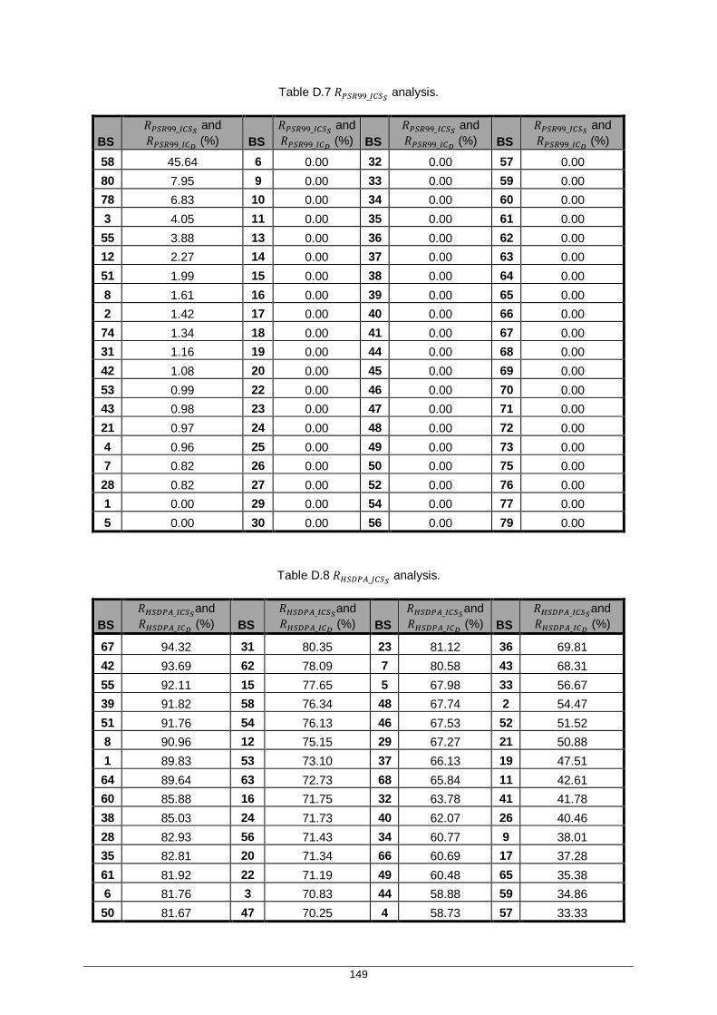
149
Table D.7 푅 _ analysis.
BS 푅 _ and 푅 _ (%) BS
푅 _ and 푅 _ (%) BS
푅 _ and 푅 _ (%) BS
푅 _ and 푅 _ (%)
58 45.64 6 0.00 32 0.00 57 0.00 80 7.95 9 0.00 33 0.00 59 0.00 78 6.83 10 0.00 34 0.00 60 0.00 3 4.05 11 0.00 35 0.00 61 0.00 55 3.88 13 0.00 36 0.00 62 0.00 12 2.27 14 0.00 37 0.00 63 0.00 51 1.99 15 0.00 38 0.00 64 0.00 8 1.61 16 0.00 39 0.00 65 0.00 2 1.42 17 0.00 40 0.00 66 0.00 74 1.34 18 0.00 41 0.00 67 0.00 31 1.16 19 0.00 44 0.00 68 0.00 42 1.08 20 0.00 45 0.00 69 0.00 53 0.99 22 0.00 46 0.00 70 0.00 43 0.98 23 0.00 47 0.00 71 0.00 21 0.97 24 0.00 48 0.00 72 0.00 4 0.96 25 0.00 49 0.00 73 0.00 7 0.82 26 0.00 50 0.00 75 0.00 28 0.82 27 0.00 52 0.00 76 0.00 1 0.00 29 0.00 54 0.00 77 0.00 5 0.00 30 0.00 56 0.00 79 0.00
Table D.8 푅 _ analysis.
BS 푅 _ and 푅 _ (%) BS
푅 _ and 푅 _ (%) BS
푅 _ and 푅 _ (%) BS
푅 _ and 푅 _ (%)
67 94.32 31 80.35 23 81.12 36 69.81 42 93.69 62 78.09 7 80.58 43 68.31 55 92.11 15 77.65 5 67.98 33 56.67 39 91.82 58 76.34 48 67.74 2 54.47 51 91.76 54 76.13 46 67.53 52 51.52 8 90.96 12 75.15 29 67.27 21 50.88 1 89.83 53 73.10 37 66.13 19 47.51 64 89.64 63 72.73 68 65.84 11 42.61 60 85.88 16 71.75 32 63.78 41 41.78 38 85.03 24 71.73 40 62.07 26 40.46 28 82.93 56 71.43 34 60.77 9 38.01 35 82.81 20 71.34 66 60.69 17 37.28 61 81.92 22 71.19 49 60.48 65 35.38 6 81.76 3 70.83 44 58.88 59 34.86 50 81.67 47 70.25 4 58.73 57 33.33
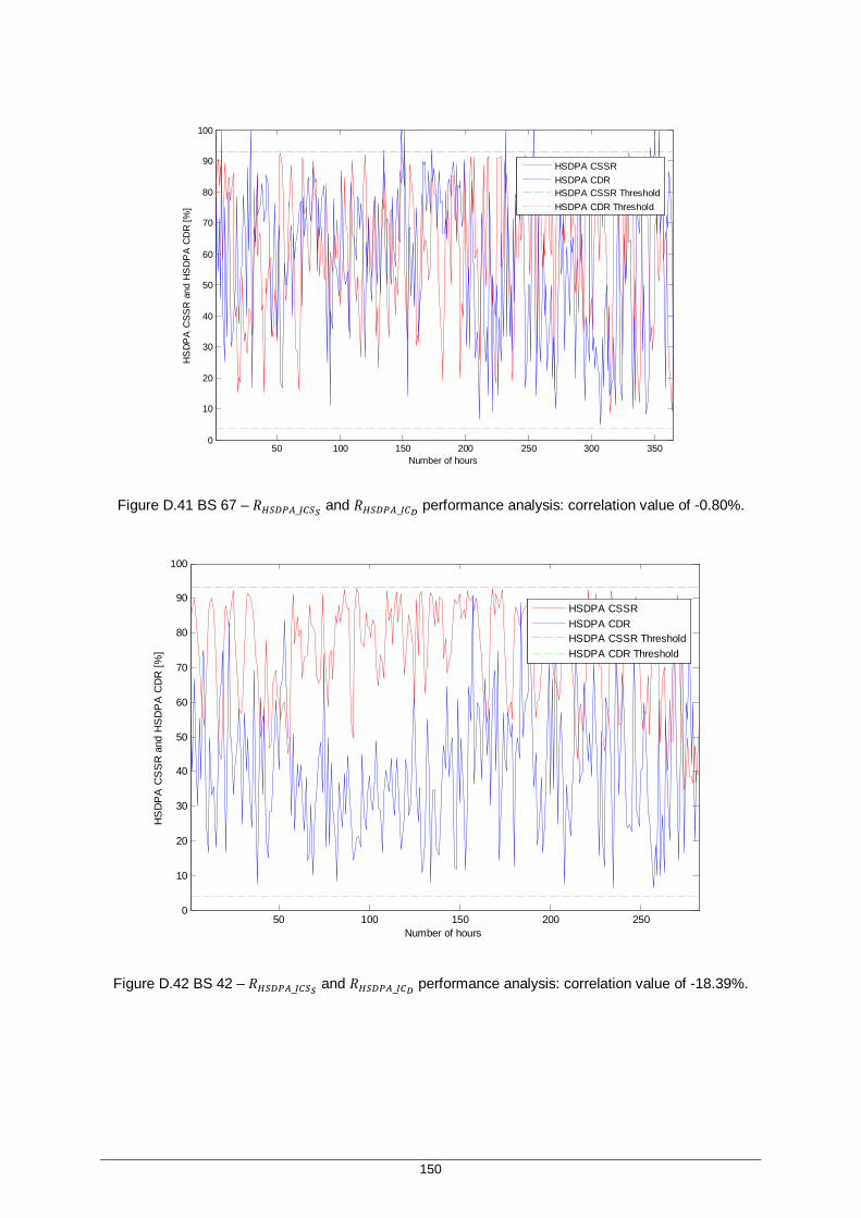
150
Figure D.41 BS 67 – 푅 _ and 푅 _ performance analysis: correlation value of -0.80%.
Figure D.42 BS 42 – 푅 _ and 푅 _ performance analysis: correlation value of -18.39%.
50 100 150 200 250 300 3500
10
20
30
40
50
60
70
80
90
100
Number of hours
HS
DPA
CSS
R a
nd H
SD
PA
CD
R [%
]
HSDPA CSSRHSDPA CDRHSDPA CSSR ThresholdHSDPA CDR Threshold
50 100 150 200 2500
10
20
30
40
50
60
70
80
90
100
Number of hours
HS
DP
A C
SS
R a
nd H
SD
PA
CD
R [%
]
HSDPA CSSRHSDPA CDRHSDPA CSSR ThresholdHSDPA CDR Threshold

151
Figure D.43 BS 55 – 푅 _ and 푅 _ performance analysis: correlation value of -18.63%.
Figure D.44 BS 39 – 푅 _ and 푅 _ performance analysis: correlation value of -7.23%.
20 40 60 80 100 120 140 160 180 2000
10
20
30
40
50
60
70
80
90
100
Number of hours
HS
DP
A C
SS
R a
nd H
SD
PA
CD
R [%
]
HSDPA CSSRHSDPA CDRHSDPA CSSR ThresholdHSDPA CDR Threshold
50 100 150 200 2500
10
20
30
40
50
60
70
80
90
100
Number of hours
HS
DP
A C
SS
R a
nd H
SD
PA
CD
R [%
]
HSDPA CSSRHSDPA CDRHSDPA CSSR ThresholdHSDPA CDR Threshold

152
Figure D.45 BS 8 – 푅 _ and 푅 _ performance analysis: correlation value of -0.85%.
Figure D.46 BS 67 – Channel Upswitch Failure Rate DL.
Figure D.47 BS 67 – Channel Upswitch Failure Rate UL.
20 40 60 80 100 120 1400
10
20
30
40
50
60
70
80
90
100
Number of hours
HS
DP
A C
SS
R a
nd H
SD
PA
CD
R [%
]
HSDPA CSSRHSDPA CDRHSDPA CSSR ThresholdHSDPA CDR Threshold
0%
5%
10%
15%
20%
25%
30%
35%
Cha
nnel
Ups
witc
h Fa
ilure
R
ate
DL
[%] Low Rate
Medium Rate
High Rate
HS
0%
20%
40%
60%
80%
100%
Cha
nnel
Ups
witc
h Fa
ilure
Rat
e U
L [%
]
Low Rate
Medium Rate
High Rate
FACH-HS

153
In BS 67 HSDPA interactive call drop rate has an average value of 57.76%. With a number of 9457
abnormal RAB PS HSDPA releases and according to the “Minutes per Drop” KPI, a user experiences
a drop call, in average, in every 1h33min9s, which does not exceed the predefined threshold. The
channel downswitch failure rate has an average value of 0.25%. Figures D.47 and D.48 represent the
percentage distribution of the channel upswitch failure rate for BS 58. It is possible to conclude that
the DL/UL HS transitions fail very often, with average values of around 30%. Analysing the call setup
success rate performance, with an average value of 61.73%, the RRC connection success rate has an
average value of 99.71% and the RAB establishment success rate has an average value of 61.90%.
Figure D.49 illustrates the comparison between the total number of failures after the admission control
and the RAB success rate.
Figure D.48 BS 67 – Total number of failures after admission control versus “RAB success rate”.
Apparently there is not any kind of correlation between the two parameters. The correlation value
between proves it: -9.59%. With a total number of 260 RRC or RAB requests denied due to admission
control, all of them are related to RAB issues: 67.83% of the fails are due to lack of DL channelisation
codes and 32.17% are due to insufficient licenses for the number of users that are attempting to
access to the network. Figure D.50 illustrates the correlation between the number of abnormal RAB
PS HSDPA releases and the number of normal RAB speech releases. With a correlation value of -
4.93%, it appears to be no correlation between the parameters.
In BS 42 HSDPA interactive call drop rate has an average value of 40.65%. With a number of 3017
abnormal RAB PS HSDPA and according to the obtained results, a user does not experiences a drop
call. The channel downswitch failure rate has an average value of 4.24%. Figures D.51 and D.52
represent the percentage distribution of the channel upswitch failure rate for BS 42.
50 100 150 200 250 300 3500
50
100
150
200
Num
ber o
f fai
lure
s af
ter t
he a
dmis
sion
con
trol
Number of hours50 100 150 200 250 300 350
0
20
40
60
80
100
RA
B s
ucce
ss ra
te [%
]

154
Figure D.49 BS 67 – Abnormal RAB PS HSDPA releases and normal RAB speech releases.
Figure D.50 BS 42 – Channel Upswitch Failure Rate DL.
Figure D.51 BS 42 – Channel Upswitch Failure Rate UL.
50 100 150 200 250 300 3500
50
100
150
200
250
300
Num
ber o
f abn
orm
al R
AB
PS
HS
DP
A re
leas
es
Number of hours50 100 150 200 250 300 350
0
50
100
150
200
250
300
350
400
450
Num
ber o
f nor
mal
RA
B s
peec
h re
leas
es
0%
5%
10%
15%
20%
25%
30%
35%
Chan
nel U
psw
itch
Failu
re R
ate
DL
[%]
Low Rate
Medium Rate
High Rate
HS
0%
20%
40%
60%
80%
100%
Chan
nel U
psw
itch
Failu
re
Rate
UL [
%] Low Rate
Medium Rate
High Rate
FACH-HS

155
It is possible to conclude that the DL/UL HS transitions fail very often, with average values of around
32% and 22%, respectively. Analysing the call setup success rate performance, with an average value
of 73.86%, the RRC connection success rate has an average value of 99.86% and the RAB
establishment success rate has an average value of 73.98%. Figure D.53 illustrates the comparison
between the total number of failures after the admission control and the RAB success rate.
Figure D.52 BS 42 – Total number of failures after admission control versus “RAB success rate”.
It is possible to see that when the number of failures increases, the RAB success rate decreases, with
a correlation value between them of -60.75%. With a total number of 17115 RRC or RAB failures after
the admission control, 14306 are RAB fails due to transport network issues and 36 are due to node
blocking problems. Analysing the number of requests denied due to admission control (total of 706),
72.35% are due to insufficient licenses for the number of users that are attempting to access to the
network and 27.65% are due to lack of DL channelisation codes. Figure D.54 illustrates the
correlation between the number of abnormal RAB PS HSDPA releases and the number of normal
RAB speech releases. With a correlation value of -24.51%, it is possible to see that in some hours
when the number of normal RAB speech releases increases, the number of abnormal RAB PS
DCH/FACH releases decreases, which does not support the establishment of any relationship in
accordance with the previsions.
In BS 55 HSDPA interactive call drop rate has an average value of 53.37%. With a number of 2092
abnormal RAB PS HSDPA releases and according to the “Minutes per Drop” KPI, a user experiences
a drop call, in average, in every 31min35s, which does not exceed the predefined threshold. The
channel donswitch failure rate has an average value of 5.30%. Figures D.55 and D.56 represent the
percentage distribution of the channel upswitch failure rate for BS 55.
50 100 150 200 2500
100
200
300
400
Num
ber o
f fai
lure
s af
ter t
he a
dmis
sion
con
trol
Number of hours50 100 150 200 250
20
40
60
80
100
RA
B s
ucce
ss ra
te [%
]
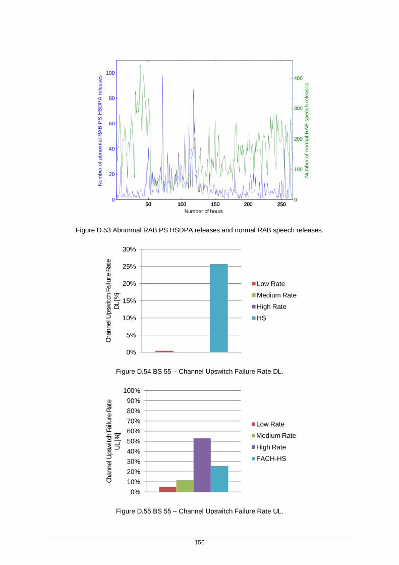
156
Figure D.53 Abnormal RAB PS HSDPA releases and normal RAB speech releases.
Figure D.54 BS 55 – Channel Upswitch Failure Rate DL.
Figure D.55 BS 55 – Channel Upswitch Failure Rate UL.
50 100 150 200 2500
20
40
60
80
100
Num
ber o
f abn
orm
al R
AB
PS
HS
DP
A re
leas
es
Number of hours50 100 150 200 250
0
100
200
300
400
Num
ber o
f nor
mal
RA
B s
peec
h re
leas
es
0%
5%
10%
15%
20%
25%
30%
Chan
nel U
psw
itch
Failu
re R
ate
DL [%
]
Low Rate
Medium Rate
High Rate
HS
0%10%20%30%40%50%60%70%80%90%
100%
Chan
nel U
psw
itch
Failu
re R
ate
UL [
%]
Low Rate
Medium Rate
High Rate
FACH-HS

157
It is possible to conclude that the DL/UL HS transitions fail very often, with average values of around
25%. Analysing the call setup success rate performance, with an average value of 71.87%, the RRC
connection success rate has an average value of 99.23% and the RAB establishment success rate
has an average value of 72.39%. Figure D.55 illustrates the comparison between the total number of
failures after the admission control and the RAB success rate.
Figure D.56 BS 55 – Total number of failures after admission control versus “RAB success rate”.
It is possible to see that when the number of failures increases, the RAB success rate decreases, with
a correlation value between them of -53.15%. With a total number of 11436 RRC or RAB failures after
the admission control, 9477 are RAB fails due to transport network issues and 453 are due to node
blocking problems. There are only 9 requests denied due to admission control so the analysis will not
be done. Figure D.57 illustrates the correlation between the number of abnormal RAB PS HSDPA
releases and the number of normal RAB speech releases. With a correlation value of 2.69%, it
appears to be no correlation between the parameters.
In BS 39 HSDPA interactive call drop rate has an average value of 62.49%. With a number of 3488
abnormal RAB PS HSDPA and according to the “Minutes per Drop” KPI, a user experiences a drop
call, in average, in every 27min40s, which does not exceed the predefined threshold. The channel
donswitch failure rate has an average value of 3.59%. Figures D.58 and D.59 represent the
percentage distribution of the channel upswitch failure rate for BS 39.
20 40 60 80 100 120 140 160 180 2000
50
100
150
200
250
300
350
400
450
500
Num
ber o
f fai
lure
s af
ter t
he a
dmis
sion
con
trol
Number of hours20 40 60 80 100 120 140 160 180 200
0
10
20
30
40
50
60
70
80
90
100
RA
B s
ucce
ss ra
te [%
]

158
Figure D.57 BS 55 – Abnormal RAB PS HSDPA releases and normal RAB speech releases.
Figure D.58 BS 39 – Channel Upswitch Failure Rate DL.
Figure D.59 BS 39 – Channel Upswitch Failure Rate UL.
20 40 60 80 100 120 140 160 180 2000
10
20
30
40
50
60
70
80
90
Num
ber o
f abn
orm
al R
AB
PS
HS
DPA
rele
ases
Number of hours20 40 60 80 100 120 140 160 180 200
0
50
100
150
200
250
300
Num
ber o
f nor
mal
RA
B s
peec
h re
leas
es
0%2%4%6%8%
10%12%14%16%18%
Chan
nel U
psw
itch
Failu
re R
ate
DL [%
]
Low Rate
Medium Rate
High Rate
HS
0%
5%
10%
15%
20%
25%
30%
35%
Chan
nel U
psw
itch
Failu
re
Rate
UL [
%] Low Rate
Medium Rate
High Rate
FACH-HS

159
It is possible to conclude that the DL/UL HS transitions fail very often, with average values of around
16%. Analysing the call setup success rate performance, with an average value of 72.34%, the RRC
connection success rate has an average value of 97.95% and the RAB establishment success rate
has an average value of 74.07%. Figure D.60 illustrates the comparison between the total number of
failures after the admission control and the RAB success rate.
Figure D.60 BS 39 – Total number of failures after admission control versus “RAB success rate”.
It is possible to see that when the number of failures increases, the RAB success rate decreases, with
a correlation value between them of -55.66%. With a total number of 14508 RRC or RAB failures after
the admission control, 9943 are RAB fails due to transport network issues and 2330 are due to node
blocking problems. There are only 19 requests denied due to admission control so the analysis will not
be done. Figure D.62 illustrates the correlation between the number of abnormal RAB PS HSDPA
releases and the number of normal RAB speech releases. With a correlation value of -28.71%, it is
possible to see that in some hours when the number of normal RAB speech releases increases, the
number of abnormal RAB PS DCH/FACH releases decreases, which does not support the
establishment of any relationship in accordance with the previsions.
In BS 8 HSDPA interactive call drop rate has an average value of 27.00%. With a number of 1124
abnormal RAB PS HSDPA and according to the “Minutes per Drop” KPI, a user experiences a drop
call, in average, in every 43min16s, which does not exceed the predefined threshold. The channel
donswitch failure rate has an average value of 6.26%. Figures D.63 and D.64 represent the
percentage distribution of the channel upswitch failure rate for BS 8.
50 100 150 200 2500
50
100
150
200
250
300
Num
ber o
f fai
lure
s af
ter t
he a
dmis
sion
con
trol
Number of hours50 100 150 200 250
0
10
20
30
40
50
60
70
80
90
100
RA
B s
ucce
ss ra
te [%
]
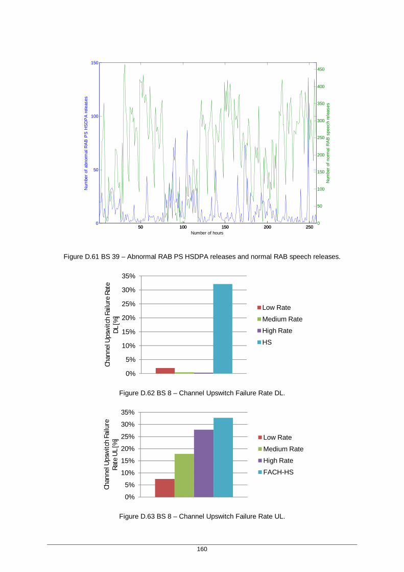
160
Figure D.61 BS 39 – Abnormal RAB PS HSDPA releases and normal RAB speech releases.
Figure D.62 BS 8 – Channel Upswitch Failure Rate DL.
Figure D.63 BS 8 – Channel Upswitch Failure Rate UL.
50 100 150 200 2500
50
100
150
Num
ber o
f abn
orm
al R
AB
PS
HS
DP
A re
leas
es
Number of hours50 100 150 200 250
0
50
100
150
200
250
300
350
400
450
Num
ber o
f nor
mal
RA
B s
peec
h re
leas
es
0%
5%
10%
15%
20%
25%
30%
35%
Chan
nel U
psw
itch
Failu
re R
ate
DL [%
]
Low Rate
Medium Rate
High Rate
HS
0%
5%
10%
15%
20%
25%
30%
35%
Chan
nel U
psw
itch
Failu
re
Rate
UL [
%] Low Rate
Medium Rate
High Rate
FACH-HS

161
It is possible to conclude that the DL/UL HS transitions fail very often, with average values of around
32%. Analysing the call setup success rate performance, with an average value of 73.40%, the RRC
connection success rate has an average value of 99.81% and the RAB establishment success rate
has an average value of 73.54%. Figure D.65 illustrates the comparison between the total number of
failures after the admission control and the RAB success rate.
Figure D.64 BS 8 – Total number of failures after admission control versus “RAB success rate”.
It is possible to see that when the number of failures increases, the RAB success rate decreases, with
a correlation value between them of -64.45%. With a total number of 12998 RRC or RAB failures after
the admission control, two failing reasons can be identified: 1 fail is due to RAB node blocking issues
and 10554 fails are due to transport network problems. The number of failures during the admission
control process is irrelevant compared to the number of failures after the process so the analysis will
not be done. Figure D.66 illustrates the correlation between the number of abnormal RAB PS HSDPA
releases and the number of normal RAB speech releases. With a correlation value of 24.04%, the
graphic representation is not very clear in order to identify any kind of relation between the two
parameters.
Similar to what was done in the 2G analysis the existence of any kind of correlation between a drop
call and HO issues will be checked. Analysing the results concerning 푅 and 푅 parameter, it is
possible to identify the percentage associated to the number of hours where the KPI value is above
the threshold level at the same time as others KPIs, Table D.9. Looking at the results it is possible to
conclude that in BSs 6, 38, 30, 11 and 21 when the speech call drop rate KPI is above the threshold
level the Soft HO KPI is below the threshold level in 83.19%, 48.26%, 42.16%, 29.55% and 25.40% of
the cases.
Analysing the results concerning 푅 _ parameter, it is possible to identify the percentage
associated to the number of hours where the KPI value is above the threshold level at the same time
as others KPIs, Table D.10. Looking at the results, although there is a considerable number of BSs
20 40 60 80 100 120 1400
50
100
150
200
250
300
350
400
450
500
Num
ber o
f fai
lure
s af
ter t
he a
dmis
sion
con
trol
Number of hours20 40 60 80 100 120 140
0
10
20
30
40
50
60
70
80
90
100
RR
C s
ucce
ss ra
te [%
]

162
with problems associated to PS R99 call drop rate KPI, that problems are not related to SHO
problems.
Analysing the results concerning 푅 _ parameter, it is possible to identify the percentage
associated to the number of hours where the KPI value is above the threshold level at the same time
as others KPIs, Table D.11. Looking at the results, although there is a considerable number of BSs
with problems associated to PS R99 call drop rate KPI, that problems are not related to SHO
problems.
Figure D.65 BS 8 – Abnormal RAB PS HSDPA releases and normal RAB speech releases.
Table D.9 푅 and 푅 analysis.
BS 푅 and 푅
(%) BS 푅 and 푅
(%) BS 푅 and 푅
(%) BS 푅 and 푅
(%)
6 83.19 13 0.83 17 0.00 42 0.00 38 48.26 25 0.71 19 0.00 45 0.00 30 42.16 4 0.37 20 0.00 46 0.00 11 29.55 48 0.30 23 0.00 47 0.00 21 25.40 1 0.00 24 0.00 49 0.00 37 19.63 2 0.00 27 0.00 51 0.00 43 18.18 3 0.00 29 0.00 52 0.00 44 9.20 5 0.00 31 0.00 53 0.00 32 6.98 7 0.00 33 0.00 54 0.00 50 6.67 8 0.00 34 0.00 55 0.00 22 5.13 9 0.00 35 0.00 57 0.00 26 4.55 10 0.00 36 0.00 58 0.00 18 2.82 12 0.00 39 0.00 59 0.00 56 1.33 14 0.00 40 0.00 60 0.00 28 1.27 15 0.00 41 0.00 61 0.00
5 10 15 20 25 300
5
10
15
20
25
30
Num
ber o
f abn
orm
al R
AB
PS
HS
DP
A re
leas
es
Number of hours5 10 15 20 25 30
0
200
400
600
800
1000
Num
ber o
f nor
mal
RA
B s
peec
h re
leas
es

163
Table D.10 푅 _ and 푅 analysis.
BS 푅 _ and 푅 (%) BS
푅 _ and 푅 (%) BS
푅 _ and 푅 (%) BS
푅 _ and 푅 (%)
15 2.14 6 0.00 21 0.00 32 0.00 19 1.96 7 0.00 22 0.00 33 0.00 41 1.61 9 0.00 23 0.00 35 0.00 14 1.53 10 0.00 24 0.00 36 0.00 8 1.52 11 0.00 25 0.00 37 0.00 34 0.55 12 0.00 26 0.00 38 0.00 1 0.00 13 0.00 27 0.00 39 0.00 2 0.00 16 0.00 28 0.00 40 0.00 3 0.00 17 0.00 29 0.00 42 0.00 4 0.00 18 0.00 30 0.00 43 0.00 5 0.00 20 0.00 31 0.00 44 0.00
Table D.11 푅 _ and 푅 analysis.
BS 푅 _ and 푅
(%) BS 푅 _ and 푅 (%) BS
푅 _ and 푅 (%) BS
푅 _ and 푅 (%)
9 13.39 21 0.33 49 0.35 18 0.00
68 9.96 11 0.32 19 0.33 22 0.00
69 9.81 43 0.29 24 0.00 72 0.00
53 5.57 77 0.29 25 0.00 73 0.00
16 3.68 81 0.28 27 0.00 75 0.00
93 2.70 59 0.23 28 0.00 78 0.00
45 2.20 30 0.22 29 0.00 80 0.00
38 1.55 79 0.22 31 0.00 82 0.00
85 1.35 32 0.2 34 0.00 84 0.00
76 1.03 23 0.19 35 0.00 86 0.00
51 0.89 39 0.18 36 0.00 87 0.00
20 0.87 98 0.18 40 0.00 88 0.00
83 0.87 26 0.16 44 0.00 89 0.00
41 0.71 33 0.12 46 0.00 90 0.00
1 0.60 4 0.00 47 0.00 91 0.00
57 0.60 5 0.00 48 0.00 92 0.00
74 0.58 6 0.00 50 0.00 94 0.00
3 0.53 7 0.00 54 0.00 95 0.00
2 0.51 8 0.00 55 0.00 96 0.00
37 0.46 10 0.00 56 0.00 97 0.00
42 0.43 12 0.00 60 0.00 100 0.00
58 0.42 13 0.00 61 0.00 101 0.00
63 0.38 14 0.00 62 0.00 102 0.00
99 0.38 15 0.00 64 0.00 103 0.00
52 0.36 17 0.00 65 0.00 104 0.00

164
165
Annex E
Site Names E. Annex E
In Annex E, the table with the correct names from the analysed BSs from the covered region is
presented. This annex is confidential.
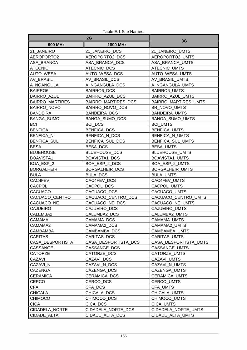
166
Table E.1 Site Names. 2G 3G
900 MHz 1800 MHz 21_JANEIRO 21_JANEIRO_DCS 21_JANEIRO_UMTS AEROPORTO2 AEROPORTO2_DCS AEROPORTO2_UMTS ASA_BRANCA ASA_BRANCA_DCS ASA_BRANCA_UMTS ATECNIC ATECNIC_DCS ATECNIC_UMTS AUTO_WESA AUTO_WESA_DCS AUTO_WESA_UMTS AV_BRASIL AV_BRASIL_DCS AV_BRASIL_UMTS A_NGANGULA A_NGANGULA_DCS A_NGANGULA_UMTS BAIRRO6 BAIRRO6_DCS BAIRRO6_UMTS BAIRRO_AZUL BAIRRO_AZUL_DCS BAIRRO_AZUL_UMTS BAIRRO_MARTIRES BAIRRO_MARTIRES_DCS BAIRRO_MARTIRES_UMTS BAIRRO_NOVO BAIRRO_NOVO_DCS BR_NOVO_UMTS BANDEIRA BANDEIRA_DCS BANDEIRA_UMTS BANGA_SUMO BANGA_SUMO_DCS BANGA_SUMO_UMTS BCI BCI_DCS BCI_UMTS BENFICA BENFICA_DCS BENFICA_UMTS BENFICA_N BENFICA_N_DCS BENFICA_N_UMTS BENFICA_SUL BENFICA_SUL_DCS BENFICA_SUL_UMTS BESA BESA_DCS BESA_UMTS BLUEHOUSE BLUEHOUSE_DCS BLUEHOUSE_UMTS BOAVISTA1 BOAVISTA1_DCS BOAVISTA1_UMTS BOA_ESP_2 BOA_ESP_2_DCS BOA_ESP_2_UMTS BORGALHEIR BORGALHEIR_DCS BORGALHEIR_UMTS BULA BULA_DCS BULA_UMTS CAC4FEV CAC4FEV_DCS CAC4FEV_UMTS CACPOL CACPOL_DCS CACPOL_UMTS CACUACO CACUACO_DCS CACUACO_UMTS CACUACO_CENTRO CACUACO_CENTRO_DCS CACUACO_CENTRO_UMTS CACUACO_NE CACUACO_NE_DCS CACUACO_NE_UMTS CAJUEIRO CAJUEIRO_DCS CAJUEIRO_UMTS CALEMBA2 CALEMBA2_DCS CALEMBA2_UMTS CAMAMA CAMAMA_DCS CAMAMA_UMTS CAMAMA2 CAMAMA2_DCS CAMAMA2_UMTS CAMBAMBA CAMBAMBA_DCS CAMBAMBA_UMTS CARITAS CARITAS_DCS CARITAS_UMTS CASA_DESPORTISTA CASA_DESPORTISTA_DCS CASA_DESPORTISTA_UMTS CASSANGE CASSANGE_DCS CASSANGE_UMTS CATORZE CATORZE_DCS CATORZE_UMTS CAZAVI CAZAVI_DCS CAZAVI_UMTS CAZAVI_N CAZAVI_N_DCS CAZAVI_N_UMTS CAZENGA CAZENGA_DCS CAZENGA_UMTS CERAMICA CERAMICA_DCS CERAMICA_UMTS CERCO CERCO_DCS CERCO_UMTS CFA CFA_DCS CFA_UMTS CHICALA CHICALA_DCS CHICALA_UMTS CHIMOCO CHIMOCO_DCS CHIMOCO_UMTS CICA CICA_DCS CICA_UMTS CIDADELA_NORTE CIDADELA_NORTE_DCS CIDADELA_NORTE_UMTS CIDADE_ALTA CIDADE_ALTA_DCS CIDADE_ALTA_UMTS
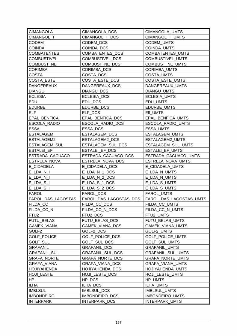
167
CIMANGOLA CIMANGOLA_DCS CIMANGOLA_UMTS CIMANGOL_T CIMANGOL_T_DCS CIMANGOL_T_UMTS CODEM CODEM_DCS CODEM_UMTS COINDA COINDA_DCS COINDA_UMTS COMBATENTES COMBATENTES_DCS COMBATENTES_UMTS COMBUSTIVEL COMBUSTIVEL_DCS COMBUSTIVEL_UMTS COMBUST_NE COMBUST_NE_DCS COMBUST_NE_UMTS CORIMBA CORIMBA_DCS CORIMBA_UMTS COSTA COSTA_DCS COSTA_UMTS COSTA_ESTE COSTA_ESTE_DCS COSTA_ESTE_UMTS DANGEREAUX DANGEREAUX_DCS DANGEREAUX_UMTS DIANGU DIANGU_DCS DIANGU_UMTS ECLESIA ECLESIA_DCS ECLESIA_UMTS EDU EDU_DCS EDU_UMTS EDURBE EDURBE_DCS EDURBE_UMTS ELF ELF_DCS Elf_UMTS EPAL_BENFICA EPAL_BENFICA_DCS EPAL_BENFICA_UMTS ESCOLA_RADIO ESCOLA_RADIO_DCS ESCOLA_RADIO_UMTS ESSA ESSA_DCS ESSA_UMTS ESTALAGEM ESTALAGEM_DCS ESTALAGEM_UMTS ESTALAGEM2 ESTALAGEM2_DCS ESTALAGEM2_UMTS ESTALAGEM_SUL ESTALAGEM_SUL_DCS ESTALAGEM_SUL_UMTS ESTALEI_EF ESTALEI_EF_DCS ESTALEI_EF_UMTS ESTRADA_CACUACO ESTRADA_CACUACO_DCS ESTRADA_CACUACO_UMTS ESTRELA_NOVA ESTRELA_NOVA_DCS ESTRELA_NOVA_UMTS E_CIDADELA E_CIDADELA_DCS E_CIDADELA_UMTS E_LDA_N_I E_LDA_N_1_DCS E_LDA_N_UMTS E_LDA_N_I E_LDA_N_2_DCS E_LDA_N_UMTS E_LDA_S_I E_LDA_S_1_DCS E_LDA_S_UMTS E_LDA_S_I E_LDA_S_2_DCS E_LDA_S_UMTS FAROL FAROL_DCS FAROL_UMTS FAROL_DAS_LAGOSTAS FAROL_DAS_LAGOSTAS_DCS FAROL_DAS_LAGOSTAS_UMTS FILDA_CC FILDA_CC_DCS FILDA_CC_UMTS FILDA_CC_N FILDA_CC_N_DCS FILDA_CC_N_UMTS FTU2 FTU2_DCS FTU2_UMTS FUTU_BELAS FUTU_BELAS_DCS FUTU_BELAS_UMTS GAMEK_VIANA GAMEK_VIANA_DCS GAMEK_VIANA_UMTS GOLF2 GOLF2_DCS GOLF2_UMTS GOLF_POLICE GOLF_POLICE_DCS GOLF_POLICE_UMTS GOLF_SUL GOLF_SUL_DCS GOLF_SUL_UMTS GRAFANIL GRAFANIL_DCS GRAFANIL_UMTS GRAFANIL_SUL GRAFANIL_SUL_DCS GRAFANIL_SUL_UMTS GRAFA_NORTE GRAFA_NORTE_DCS GRAFA_NORTE_UMTS GRAFA_VIANA GRAFA_VIANA_DCS GRAFA_VIANA_UMTS HOJIYAHENDA HOJIYAHENDA_DCS HOJIYAHENDA_UMTS HOJI_LESTE HOJI_LESTE_DCS HOJI_LESTE_UMTS HP HP_DCS HP_UMTS ILHA ILHA_DCS ILHA_UMTS IMBLSUL IMBLSUL_DCS IMBLSUL_UMTS IMBONDEIRO IMBONDEIRO_DCS IMBONDEIRO_UMTS INTERPARK INTERPARK_DCS INTERPARK_UMTS

168
ISE ISE_DCS ISE_UMTS JARDI_EDEN JARDI_EDEN_DCS JARDI_EDEN_UMTS JEMBAS JEMBAS_DCS JEMBAS_UMTS JEMBAS JEMBAS2_DCS JEMBAS_UMTS JIKA JIKA_DCS JIKA_UMTS JPIMENTA JPIMENTA_DCS JPIMENTA_UMTS JUMBO JUMBO_DCS JUMBO_UMTS KABOCOMEU KABOCOMEU_DCS KABOCOMEU_UMTS KAPALANCA KAPALANCA_DCS KAPALANCA_UMTS KAPOLO KAPOLO_DCS KAPOLO_UMTS KAPOLO2 KAPOLO2_DCS KAPOLO2_UMTS KIKOLO KIKOLO_DCS KIKOLO_UMTS KIKOLO_SUL KIKOLO_SUL_DCS KIKOLO_SUL_UMTS KIKUXI KIKUXI_DCS KIKUXI_UMTS KWANZAS KWANZAS_DCS KWANZAS_UMTS LEA LEA_DCS LEA_UMTS LIGA_AFRICANA LIGA_AFRICANA_DCS LIGA_AFRICANA_UMTS LOGITECNICA LOGITECNICA_DCS LOGITECNICA_UMTS LUANDA_SUL LUANDA_SUL_DCS LUANDA_SUL_UMTS LUSIADA LUSIADA_DCS LUSIADA_UMTS MABOR MABOR_DCS MABOR_UMTS MAIANGA MAIANGA_DCS MAIANGA_UMTS MARCAL MARCAL_DCS MARCAL_UMTS MARIN_ILHA MARIN_ILHA_DCS MARIN_ILHA_UMTS MECANAGRO MECANAGRO_DCS MECANAGRO_UMTS MECANAGR_N MECANAGR_N_DCS MECANAGR_N_UMTS METRO METRO_DCS METRO_UMTS MINISTERIO_AGRICULTURA
MINISTERIO_AGRICULTURA_DCS
MINISTERIO_AGRICULTURA_UMTS
MINISTERIO_COMERCIO MINISTERIO_COMERCIO_DCS MINISTERIO_COMERCIO_UMTS MIRAMAR MIRAMAR_DCS Miramar_UMTS MORRO_AREIA MORRO_AREIA_DCS MORRO_AREIA_UMTS MORRO_BENTO MORRO_BENTO_DCS MORRO_BENTO_UMTS MORRO_BENTO_NORTE MORRO_BENTO_NORTE_DCS MORRO_BENTO_NORTE_UMTS MORRO_LUZ MORRO_LUZ_DCS MORRO_LUZ_UMTS MR_BENTO_2 MR_BENTO_2_DCS MR_BENTO_2_UMTS MULENVOS MULENVOS_DCS MULENVOS_UMTS MULENVOS_BAIXO MULENVOS_BAIXO_DCS MULENVOS_BAIXO_UMTS NOCAL_FACTORY NOCAL_FACTORY_DCS NOCAL_FACTORY_UMTS NOVA_UNIVERSIDADE NOVA_UNIVERSIDADE_DCS NOVA_UNIVERSIDADE_UMTS NOVA_VIDA NOVA_VIDA_DCS NOVA_VIDA_UMTS NOVA_VIDA_ESTE NOVA_VIDA_ESTE_DCS NOVA_VIDA_ESTE_UMTS NOVA_VIDA_N NOVA_VIDA_N_DCS NOVA_VIDA_N_UMTS NOVA_VIDA_SUDESTE NOVA_VIDA_SUDESTE_DCS NOVA_VIDA_SUDESTE_UMTS NV_E59 NV_E59_DCS NV_E59_UMTS NV_VIDA_O NV_VIDA_O_DCS NOVA_VIDA_OESTE_UMTS OLIMPIA OLIMPIA_DCS OLIMPIA_UMTS OPERARIO OPERARIO_DCS OPERARIO_UMTS PAGA_POUCO PAGA_POUCO_DCS PAGA_POUCO_UMTS PALANCA_R4 PALANCA_R4_DCS PALANCA_R4_UMTS PANGA PANGA_DCS PANGA_UMTS
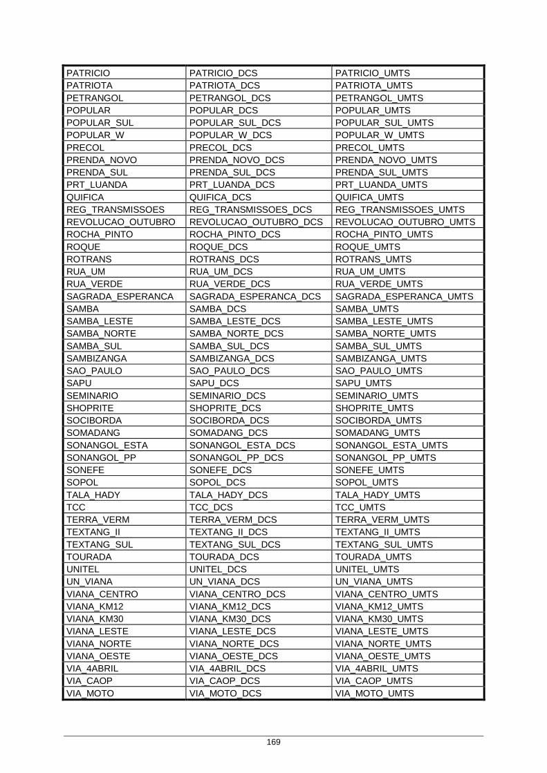
169
PATRICIO PATRICIO_DCS PATRICIO_UMTS PATRIOTA PATRIOTA_DCS PATRIOTA_UMTS PETRANGOL PETRANGOL_DCS PETRANGOL_UMTS POPULAR POPULAR_DCS POPULAR_UMTS POPULAR_SUL POPULAR_SUL_DCS POPULAR_SUL_UMTS POPULAR_W POPULAR_W_DCS POPULAR_W_UMTS PRECOL PRECOL_DCS PRECOL_UMTS PRENDA_NOVO PRENDA_NOVO_DCS PRENDA_NOVO_UMTS PRENDA_SUL PRENDA_SUL_DCS PRENDA_SUL_UMTS PRT_LUANDA PRT_LUANDA_DCS PRT_LUANDA_UMTS QUIFICA QUIFICA_DCS QUIFICA_UMTS REG_TRANSMISSOES REG_TRANSMISSOES_DCS REG_TRANSMISSOES_UMTS REVOLUCAO_OUTUBRO REVOLUCAO_OUTUBRO_DCS REVOLUCAO_OUTUBRO_UMTS ROCHA_PINTO ROCHA_PINTO_DCS ROCHA_PINTO_UMTS ROQUE ROQUE_DCS ROQUE_UMTS ROTRANS ROTRANS_DCS ROTRANS_UMTS RUA_UM RUA_UM_DCS RUA_UM_UMTS RUA_VERDE RUA_VERDE_DCS RUA_VERDE_UMTS SAGRADA_ESPERANCA SAGRADA_ESPERANCA_DCS SAGRADA_ESPERANCA_UMTS SAMBA SAMBA_DCS SAMBA_UMTS SAMBA_LESTE SAMBA_LESTE_DCS SAMBA_LESTE_UMTS SAMBA_NORTE SAMBA_NORTE_DCS SAMBA_NORTE_UMTS SAMBA_SUL SAMBA_SUL_DCS SAMBA_SUL_UMTS SAMBIZANGA SAMBIZANGA_DCS SAMBIZANGA_UMTS SAO_PAULO SAO_PAULO_DCS SAO_PAULO_UMTS SAPU SAPU_DCS SAPU_UMTS SEMINARIO SEMINARIO_DCS SEMINARIO_UMTS SHOPRITE SHOPRITE_DCS SHOPRITE_UMTS SOCIBORDA SOCIBORDA_DCS SOCIBORDA_UMTS SOMADANG SOMADANG_DCS SOMADANG_UMTS SONANGOL_ESTA SONANGOL_ESTA_DCS SONANGOL_ESTA_UMTS SONANGOL_PP SONANGOL_PP_DCS SONANGOL_PP_UMTS SONEFE SONEFE_DCS SONEFE_UMTS SOPOL SOPOL_DCS SOPOL_UMTS TALA_HADY TALA_HADY_DCS TALA_HADY_UMTS TCC TCC_DCS TCC_UMTS TERRA_VERM TERRA_VERM_DCS TERRA_VERM_UMTS TEXTANG_II TEXTANG_II_DCS TEXTANG_II_UMTS TEXTANG_SUL TEXTANG_SUL_DCS TEXTANG_SUL_UMTS TOURADA TOURADA_DCS TOURADA_UMTS UNITEL UNITEL_DCS UNITEL_UMTS UN_VIANA UN_VIANA_DCS UN_VIANA_UMTS VIANA_CENTRO VIANA_CENTRO_DCS VIANA_CENTRO_UMTS VIANA_KM12 VIANA_KM12_DCS VIANA_KM12_UMTS VIANA_KM30 VIANA_KM30_DCS VIANA_KM30_UMTS VIANA_LESTE VIANA_LESTE_DCS VIANA_LESTE_UMTS VIANA_NORTE VIANA_NORTE_DCS VIANA_NORTE_UMTS VIANA_OESTE VIANA_OESTE_DCS VIANA_OESTE_UMTS VIA_4ABRIL VIA_4ABRIL_DCS VIA_4ABRIL_UMTS VIA_CAOP VIA_CAOP_DCS VIA_CAOP_UMTS VIA_MOTO VIA_MOTO_DCS VIA_MOTO_UMTS

170
VILAKIAXI VILAKIAXI_DCS VILAKIAXI_UMTS V_CHINESA V_CHINESA_DCS V_CHINESA_UMTS V_GAMEK V_GAMEK_DCS V_GAMEK_UMTS ZANGA ZANGA_DCS ZANGA_UMTS ZANGO ZANGO_DCS ZANGO_UMTS ZANGO2 ZANGO2_DCS ZANGO2_UMTS ZONA10 ZONA10_DCS ZONA10_UMTS ZONA12 ZONA12_DCS ZONA12_UMTS ZONA16 ZONA16_DCS ZONA16_UMTS ZONA6 ZONA6_DCS ZONA6_UMTS ZONA_VERDE ZONA_VERDE_DCS ZONA_VERDE_UMTS AUTOESTRA A_NGANGU_E BR_MUNDIAL CAC_PUNIV CHINAFUND2_I CITIC CNT_FRM_UN EST_RAMIRO FUNDA GISABEL ILHA_N JRD_EDEN2 MONGO_NW NOVO_AEROPORTO PALACIO_CONGRESSOS QUENGUELA QUENGUEL_E SUPRA_MARINA VIANA_KM33 14_DE_ABRIL 14_DE_ABRIL_DCS ALVALD_CTR ALVALD_CTR_DCS BR_BOAVIST BR_BOAVIST_DCS BR_BOA_ESP BR_BOA_ESP_DCS BR_CERAM BR_CERAM_DCS BR_MUNDIMB BR_MUNDIMB_DCS BR_NOVO_W BR_NOVO_W_DCS BR_OSSOS BR_OSSOS_DCS CALEMBA2_ESTE CALEMBA2_ESTE_DCS CAOP CAOP_DCS CASSENDA CASSENDA_DCS CASSEQUEL CASSEQUEL_DCS CATORZE_W CATORZE_W_DCS CAUELELE CAUELELE_DCS CAXALA CAXALA_DCS CAZENGA_SUL CAZENGA_SUL_DCS CAZENGA_W CAZENGA_W_DCS CAZENG_E CAZENG_E_DCS CCTA CCTA_DCS CHINA CHINA_DCS CIDADELA CIDADELA_DCS

171
CIPAL CIPAL_DCS COMBUST_N COMBUST_N_DCS ENTREPOSTO ENTREPOSTO_DCS ESCOLA612 ESCOLA612_DCS EST_NOV_N EST_NOV_N_DCS FILDA_NORTE FILDA_NORTE_DCS FRANCO_NOG FRANCO_NOG_DCS HOJI_OESTE HOJI_OESTE_DCS IMBONDER_N IMBONDER_N_DCS INFINITY INFINITY_DCS KIKOLO_SE KIKOLO_SE_DCS KILAMBA_KIAXI KILAMBA_KIAXI_DCS KWAME_NKRU KWAME_NKRU_DCS LDA_SUL_KM30 LDA_SUL_KM30_DCS LIXEIRA LIXEIRA_DCS MALANGINO MALANGINO_DCS METRO_E METRO_E_DCS MOAGEM MOAGEM_DCS MO_AREIA_E MO_AREIA_E_DCS NGANGULA_N NGANGULA_N_DCS NOVA_SEDE_UNITEL_2 NOVA_SEDE_UNITEL_2_DCS NV_DESP NV_DESP_DCS PALANCA2 PALANCA2_DCS PANGUILA PANGUILA_DCS PANGUILA_S PANGUILA_S_DCS PETRANGOL_OESTE PETRANGOL_OESTE_DCS PONT_GOLF2 PONT_GOLF2_DCS REFINARIA REFINARIA_DCS RT_ROQUE RT_ROQUE_DCS SAMBZANG_E SAMBZANG_E_DCS SAPU_KAPOL2 SAPU_KAPOL2_DCS SOFFICE_T SOFFICE_T_DCS S_FAMILIA2 S_FAMILIA2_DCS TALAMAKU TALAMAKU_DCS TCC_SO TCC_SO_DCS TECNOTUNEL TECNOTUNEL_DCS VIANA_SUL VIANA_SUL_DCS VIDRUL VIDRUL_DCS ZEE1 ZEE1_DCS ZEE2 ZEE2_DCS BANCOBESA_I BANCOBESA_I_UMTS BITA BITA_UMTS CCTA_I CCTA_I_UMTS CHINAFUND1_I CHINAFUND1_I_UMTS HOTEL_TROPICO HOTEL_TROP_UMTS NOVA_SEDE_UNITEL 12SAPU_DCS NOVA_SEDE_UNITEL_UMTS RESMIRAMAR 1_MAIO_DCS RESMIRAMAR_UMTS VIANA_KM27 AEROINTE_I_DCS VIANA_KM27_UMTS 12SAPU AEROPORT_O_DCS NOVA_SEDE_UNITEL_UMTS 1_MAIO ATLANTIC_N_DCS ONDJWO_YET_UMTS AEROPORT_O BancoBPA_I_DCS RESMIRAMAR_UMTS
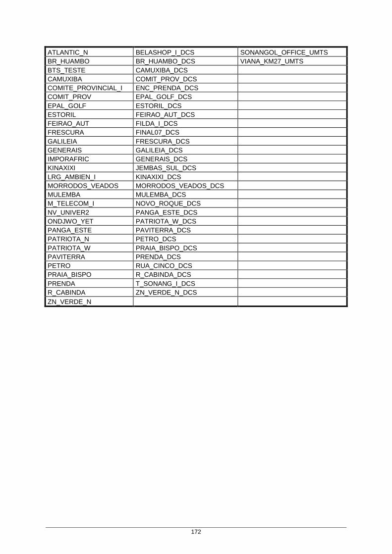
172
ATLANTIC_N BELASHOP_I_DCS SONANGOL_OFFICE_UMTS BR_HUAMBO BR_HUAMBO_DCS VIANA_KM27_UMTS BTS_TESTE CAMUXIBA_DCS CAMUXIBA COMIT_PROV_DCS COMITE_PROVINCIAL_I ENC_PRENDA_DCS COMIT_PROV EPAL_GOLF_DCS EPAL_GOLF ESTORIL_DCS ESTORIL FEIRAO_AUT_DCS FEIRAO_AUT FILDA_I_DCS FRESCURA FINAL07_DCS GALILEIA FRESCURA_DCS GENERAIS GALILEIA_DCS IMPORAFRIC GENERAIS_DCS KINAXIXI JEMBAS_SUL_DCS LRG_AMBIEN_I KINAXIXI_DCS MORRODOS_VEADOS MORRODOS_VEADOS_DCS MULEMBA MULEMBA_DCS M_TELECOM_I NOVO_ROQUE_DCS NV_UNIVER2 PANGA_ESTE_DCS ONDJWO_YET PATRIOTA_W_DCS PANGA_ESTE PAVITERRA_DCS PATRIOTA_N PETRO_DCS PATRIOTA_W PRAIA_BISPO_DCS PAVITERRA PRENDA_DCS PETRO RUA_CINCO_DCS PRAIA_BISPO R_CABINDA_DCS PRENDA T_SONANG_I_DCS R_CABINDA ZN_VERDE_N_DCS ZN_VERDE_N

173
References
References [3GPP00] 3GPP, UTRAN Overall Descripition, Report 3G TS 25.401 V3.3.0, 2000,
(http://www.3gpp.org).
[3GPP01] 3GPP, Service aspects; Services and Service Capabilities (Release 99), Technical
Specification Group Services and System Aspects, Report TS 22.105, V3.10.0, Oct. 2001
(http://www.3gpp.org).
[3GPP05] 3GPP, Service aspects; Services and Service Capabilities (Release 6), Technical
Specification Group Services and System Aspects, Report TS 22.105, V6.4.0, Sep. 2005
(http://www.3gpp.org/ftp/Specs/html-info/22105.htm).
[ABGC03] Agin,P., Bouffaut,B., Grillo,D., Colorni,G., “Soft Handover Performance for UMTS
Operations”, in Proc. of 5th European Conference on Personal Mobile Communications,
Glasgow, UK, Apr. 2003.
[BoTa07] Bourse,D., Tafazolli,R., Beyond 3G/4G Radio Access Technologies (RATs) and
Standards Roadmaps, eMobility Technology Platform, White Paper, Dec. 2007
(http://www.istemobility.org/WorkingGroups/Roadmaps/eMobility_B3G4GRMWG_WhiteP
aper_Final.pdf).
[CISL08] Chowdhury,M.Z., Islam,M.N., Seo,Y.M., Lee,Y.K., Kang,S.B., Choi,S.W., Jang,Y.M.,
“Characterizing QoS Parameters and Application of Soft-QoS Scheme for 3G Wireless
Networks”, in Proc. of 10th International Conference on Advanced Communication
Technology, Phoenix Park, Korea, Feb. 2008.
[Corr10] Correia,L.M., Mobile Communication Systems, Course Notes, IST-UTL, Lisbon, Portugal,
Mar. 2010.
[Eric06] Ericsson, Radio Network Statistics - User Description, Stockholm, Sweden, 2006.
[Eric08] Ericsson, Radio Network KPI, WCDMA RAN – User Description, Stockholm, Sweden,
2008.
[Eric09] Ericsson, Performance Statistics – Flowcharts for Counters, Stockholm, Sweden, 2008.
[Eric98] Ericsson, STS Analysis Guideline, Stockholm, Sweden, 1998.
[Gold05] Goldsmith,A., Wireless Communications, Cambridge University Press, Cambridge UK,
2005.
[HaRM03] Halonen,T., Romero,J. and Melero,J., GSM, GPRS and EDGE Performance: evolution
towards 3G/UMTS (2nd ed.), John Wiley & Sons, Chichester, UK, 2003.

174
[HoTo04] Holma,H. and Toskala,A., WCDMA for UMTS (3rd ed.), John Wiley & Sons, Chichester,
UK, 2004.
[HoTo06] Holma,H. and Toskala,A., HSDPA/HSUPA for UMTS (1st ed.), John Wiley & Sons,
Chichester, UK, 2006.
[HoTo07] Holma,H. and Toskala,A., WCDMA for UMTS – HSPA Evolution and LTE (4th ed.), John
Wiley & Sons, Chichester, UK, 2007.
[LaNW06] Laiho,J., Novosad,T., Wacker,A., Radio Network Planning and Optimisation for UMTS
(2nd ed.), John Wiley & Sons, Chichester, UK, 2006.
[LeMa01] Lempiäinien,J. and Manninen,M., Radio Interface System Planning for
GSM/GPRS/UMTS, Kluwer Academic Publishers, Dordrecht, The Netherlands, 2001.
[Lope08] Lopes,J., Performance of UMTS/HSDPA/HSUPA at the Cellular Level, M.Sc. Thesis, IST-
UTL, Lisbon, Portugal, 2008.
[Molis04] Molisch,A.F., Wireless Communications, John Wiley & Sons, Chichester, UK, 2005.
[Seyt10] Seytnazarov,S.O., “RF Optimization Issues in GSM Networks”, in Proc. of 4th International
Conference on Application of Information and Communication Technologies (AICT),
Tashkent, Uzbekistan, Oct. 2010.
[Siom05] Siomina,I., “P-CPICH Power and Antenna Tilt Optimization in UMTS Networks”, in Proc.
of Advanced Industrial Conference on Telecommunications/Service Assurance with
Partial and Intermittent Resources Conferece/E-Learning on Telecommunications
Workshop, Lisbon, Portugal, July 2005.
[SiVY06] Siomina,I., Värbrand,P., Yuan,D., “Automated Optimization of Service Coverage and
Base Station Antenna Configuration in UMTS Networks”, IEEE Wireless
Communications, Vol. 13, No. 6, Dec. 2006, pp. 16-25.
[SG11] http://www.slashgear.com, Sep. 2011.
[VaHN03] Valkealahti,K., Höglund,A., Novosad,T., “UMTS Radio Network Multiparameter Control”,
in Proc. of 14th IEEE International Symposium on Personal, Indoor and Mobile Radio
Communication, Beijing, China, Sep. 2003.