Advanced labcourse

F69 - Laue X-ray diffraction

INF 501 room 103

May 2015 - C. Neef

TABLE OF CONTENTS

1. Introduction and general safety instructions 3

2. Preparation and literature 5

3. Generation and detection of X-rays 73.1. Generation by X-ray tube . . . . . . . . . . . . . . . . . . . . . . . . . . . . . . . . 7

3.1.1. Generation by microfocus tubes . . . . . . . . . . . . . . . . . . . . . . . . 93.2. Detection of X-rays . . . . . . . . . . . . . . . . . . . . . . . . . . . . . . . . . . . 9

3.2.1. Chemical processes and image plates . . . . . . . . . . . . . . . . . . . . . 103.2.2. Counting tube . . . . . . . . . . . . . . . . . . . . . . . . . . . . . . . . . . 103.2.3. CCD cameras . . . . . . . . . . . . . . . . . . . . . . . . . . . . . . . . . . 10

4. Single crystal X-Ray diffraction 114.1. Electron density of periodic lattices . . . . . . . . . . . . . . . . . . . . . . . . . . 124.2. Structure factor . . . . . . . . . . . . . . . . . . . . . . . . . . . . . . . . . . . . . 144.3. Specifics of a Laue experiment . . . . . . . . . . . . . . . . . . . . . . . . . . . . . 15

5. Crystal structure and stereographic projections 165.1. Definition of zones and lattice planes . . . . . . . . . . . . . . . . . . . . . . . . . . 165.2. Projections . . . . . . . . . . . . . . . . . . . . . . . . . . . . . . . . . . . . . . . 175.3. Stereographic projections . . . . . . . . . . . . . . . . . . . . . . . . . . . . . . . . 18

6. Experimental setup 196.1. Sample mounting . . . . . . . . . . . . . . . . . . . . . . . . . . . . . . . . . . . . 206.2. Automatic Psi-Circle operation . . . . . . . . . . . . . . . . . . . . . . . . . . . . . 216.3. Tube and generator operation . . . . . . . . . . . . . . . . . . . . . . . . . . . . . . 216.4. Detector and Software . . . . . . . . . . . . . . . . . . . . . . . . . . . . . . . . . 236.5. Pattern simulation . . . . . . . . . . . . . . . . . . . . . . . . . . . . . . . . . . . . 25

7. Experimental scope and analysis 287.1. Identification of the orientation of a cubic crystal and sample-detector distance . . . . 287.2. Crystal shape and crystal lattice . . . . . . . . . . . . . . . . . . . . . . . . . . . . 287.3. Crystal orientation and cutting . . . . . . . . . . . . . . . . . . . . . . . . . . . . . 297.4. Evaluation . . . . . . . . . . . . . . . . . . . . . . . . . . . . . . . . . . . . . . . . 29

A. Addendum 30A.1. Systematic distinction of reflexes . . . . . . . . . . . . . . . . . . . . . . . . . . . . 30A.2. Guide for the generation of stereographic projections . . . . . . . . . . . . . . . . . 31

2

1 INTRODUCTION AND GENERAL SAFETY INSTRUC-TIONS

How do atoms arrange in a material in order to form a crystal? This and many other fundamentalquestions on condensed matter are answered by crystallography and X-ray structure determination,which are inevitable tools not only for solid state physics but many other sciences. Whenever crys-talline samples are the subject of an experiment, the structure analysis will be the first step prior tothe determination of any other physical property. It can provide information regarding structure andsymmetry, purity and defects and relation between external shape and internal crystal lattice. TheLaue X-ray diffraction method is particularly used for the analysis of single crystalline samples. Of-ten, the scope of such experiments is to find the crystallographic orientation of a sample with respectto the laboratory system, determine grain sizes or find out about defects. The method’s applicationsrange from scientific questions to industrial testing procedures like quality assurance of semicon-ductor wavers or determination of material fatigue of turbine blades.

The set up of this lab course experiment is appropriate to investigate small samples with mm-sizeddimensions. The first step of characterising unknown or new samples is to determine the symmetryin which atoms organize in a crystallographic unit cell. Then the sample’s orientation must be de-termined in order to prepare it for further physical experiments. Whenever physical properties areexpected to show anisotropy, the alignment of crystal and laboratory system is required. In practicethis means for example aligning a crystal parallel to the [001]-axis by means of the Laue setup, whichthen enables to measure a physical property along the c-axis in another experiment.

The task of this lab course experiment is to understand the relation between crystal structure (invisibleto the eye) and X-ray diffraction patterns on a screen (visible to the eye) which are a direct image ofthe elsewise abstract k-space. In fact, XRD experiments have motivated to introduce the concept ofk-space, which is a key issue for understanding modern physics. The strength of a Laue experimentthereby is the simultaneous visibility of many different diffraction spots which reproduce the sym-metry of the crystal in a single picture. Furthermore, the handling of an X-ray source and the softwaresupported diffraction-data analysis should be learned. In the process, different minerals are availablewhich will be investigated and whose structure and symmetry will be determined.

3

1. Introduction and general safety instructions

Radiation protection and tube handling

The participation of a radiation protection course is absolutely mandatory for the execution of thisexperiment.

Within the lab course at hand, an X-ray tube will be used to generate X-rays with an energy of up to50 keV. Exposition to this kind of ionising radiation can cause severe short and long term damages tobiological tissue. Although the setup is shielded within a protective cabinet, special attention shouldbe paid to the correct and safe execution of the experiment. This can only be guaranteed if theprotective cabinet is closed during use of the X-ray tube.

As a precaution, the X-ray generator is coupled to several safety switches which react on opening andclosing the cabinet doors and will be automatically shut down if the doors are opened. This procedureis however very rough and might cause damage to the tube and generator. For safe operation ofthe system, the waiting times for tube-power increase and decrease need to be followed absolutely.Unnecessary starting or stopping of the high voltage need to be desisted in any case.

Toxicity of samples

Depending on availability and choice, irritant or harmful samples might have to be processed withinthe lab course. Direct handling of sample crystals should therefore only be carried out in accordancewith the course supervisor. If necessary, protective gloves have to be used to avoid direct skin contactwith these samples. Do not swallow or inhale any components of the experiment.

Experimental setup and detector

The complete setup is already pre-adjusted, meaning that source, collimator, detector and goniometerare on a straight line. Non of these components except for the goniometer should be moved since theadjustment might easily be lost. The re-adjustment might take several days.

The X-ray detector used in this experiment is a very sensitive device. It should not be touched roughlyor moved in position. Special care has to be taken of the scintillating layer on the outside of the device.The layer must not be touched! Scratching or even touching might cause damages which make thedetector unusable.

4

2 PREPARATION AND LITERATURE

The following manual does not give a global introduction to the science of crystallography and X-raydiffraction. For a successful participation in the lab course, more sources should be consulted. Aselection of books and websites is given below. The previous participation in the condensed matterphysics lecture is strongly recommended. If this is not the case, please contact the supervising tutorin advance.

You should be able to answer the following questions before you start the lab course.

Crystal structure:

• Why do atoms arrange in a given way (crystal), what is translational symmetry?

• What kind of lattice systems do exist and how do the Bravais lattices look like?

• What are the required symmetries for the cubic system?

• What is described by the term "crystal habit"? How is it influenced by the crystal structure?

X-ray experiments:

• What are X-rays and how can they be generated?

• How can they be detected? How are they interacting with matter?

• Why are they used to study crystal structures?

• Which kinds of X-ray experiments do you know? What are they used for?

• What kind of safety precautions need to be taken while dealing with X-rays?

Data analysis and evaluation:

• What are stereographic projections? What does "angle conserving" mean?

• What is a Wulff net?

• Why does the diffraction angle (angle between incident and scattered beam) not depend on thelattice parameters in the cubic system? (Contradiction to Bragg’s law?)

5

2. Preparation and literature

The following literature can be reviewed in the university library:

• Kristallographie - Eine Einführung für Naturwissenschaftler - 8. Auflage; Walter Borchardt-Ott, Heidrun Sowa; Springer Verlag 2013.

• Moderne Röntgenbeugung - Röntgendiffraktometrie für Materialswissenschaftler, Physiker undChemiker - 2. Auflage; Lothar Spieß et al.; Vieweg + Teubner 2009.

• Festkörperphysik - 1. Auflage; Siegfried Hunklinger; Oldenbourg Wissenschaftsverlag 2007.

• Basic Concepts of Crystallography - 1st edition; Emil Zolotoyabko; Wiley-VCH 2011.

• Basic Concepts of X-Ray Diffraction - 1st edition; Emil Zolotoyabko; Wiley-VCH 2014.

• Introduction to solid state physics - 8th edition; Charles Kittel; Wiley 2011.

Helpful simulations and information can be found on the internet:

• Overview of stereographic projections along with some interactive apps:

http://www.doitpoms.ac.uk/tlplib/stereographic/index.php

• "Clip" software for the simulation of Laue patterns:

http://clip4.sourceforge.net

• Space group tables and sketches of all groups:

http://img.chem.ucl.ac.uk/sgp/large/sgp.htm

6

3 GENERATION AND DETECTION OF X-RAYS

X-rays are electromagnetic waves with photon energies of several keV. Their wavelength is in therange between 0.1 Å and 100 Å making them ideal candidates for diffraction experiments in solidstate physics. Amongst many possible experiments, structure determination of crystals is one of themain applications of X-rays, since their wavelength is in the same range as crystal lattice constants.A structure determination can be achieved by the detection of specific X-rays after interaction withthe electronic shells of molecules or atoms inside a lattice. Depending on the physical problemat hand, the requirements regarding X-ray energy, spectral distribution and intensity can be verydiverse. While high quality diffraction experiments rely on high intensity X-rays with a high degreeof monochromatization, the Laue experiment is carried out with polychromatic (i.e. "white") X-raylight. The following chapter will describe the most common ways of X-ray generation and detectionwith specific attention to the techniques used in this experiment.

3.1 GENERATION BY X-RAY TUBE

The use of so called X-ray tubes is a common and rather inexpensive way of X-ray generation. Theprinciple is based on electrons which are accelerated by a dc voltage and strike a metal target. Duringthe latter process they loose their energy by interaction with the atomic cores in the metal. A typicalsetup consists of a cathode (C) and anode (A), which are located inside an evacuated tube (see fig.3.1). The heated cathode (Uh) produces free electrons by thermoelectric emission, which are thenaccelerated towards the anode by a given dc voltage (Ua). The fast deceleration of the electronsduring collision with the anode causes the emission of electromagnetic radiation, which can than beused for the desired X-ray experiment. This kind of radiation is called "Bremsstrahlung".

The spectrum of Bremsstrahlung is given by Kramer’s rule and illustrated in fig. 3.2.

I(λ) ∝ Z · (λλmin

− 1) ·1λ2 (3.1)

With I being the spectral intensity, Z the atomic number and λmin the minimum wavelength (and thusmaximum energy) of a photon which is determined by the kinetic energy of the electrons and thus theacceleration voltage Ua:

Eelectronkin = e ∗U = Ephoton

max =2π~cλmin

(3.2)

It can be seen, that the intensity increases with increasing acceleration voltage Ua and atomic number

7

3. Generation and detection of X-rays

Figure 3.1.: Principle of X-ray generation by an X-ray tube (from: wikipedia): Thermally (Uh, C) releasedelectrons are accelerated (Ua) onto a watercooled (Win, Wout) metal target (A). The deceleration of thehighly energetic electrons leads to the generation of X-ray photons (X).

of the target material.

Figure 3.2.: X-ray spectra generated by an X-ray tube. A: Intensity trend in dependence of the targetsatomic number Z; B: intensity and shortest possible wavelength dependence of the acceleration voltageUa; C: Schematic representation of a real spectrum consisting of Bremsstrahlung and characteristic radi-ation.

In addition to the continous intensity distribution of Bremsstrahlung, narrow lines of high intensitywith a certain wavelength can appear in a spectrum, which are called charateristic lines. They appearif the acceleration energy is high enough to kick out an electron of the shell of the target materialsatoms into vacuum, leaving a hole (A) in the shell. After this kind of excitation, the atom will fallback to the ground state when the hole is filled up again by an electron of a higher shell (B). Theenergy difference between both states EB - EA can be released by emission of an X-ray photon.Characteristic lines with high intensity are generated if the hole is located in the inner K-shell of anatom. Specific lines are labelled with respect to the shell origin of the electron which is filling thehole: L-shell corresponds to Kα, M-shell: Kβ, etc. Tab. 3.1 shows the wavelength of specific lines

8

3.2. Detection of X-rays

for some common anode materials.

Element Z Kα Å(keV) Kβ Å(keV)Co 27 1.79 (6.92) 1.62 (7.65)Cu 29 1.54 (8.05) 1.39 (8.92)Mo 42 0.71 (17.46) 0.63 (19.68)W 74 0.21 (59.0) 0.18 (68.9)

Table 3.1.: Characteristic lines

As can be deduced from simple atomic models, the energy intervals between different atomic shellsscale proportional to Z2, meaning that X-Ray energies increase quadratic with the atomic number.Fig. 3.2 B shows a simple spectrum consisting of characteristic lines and Bremsstrahlung. Therelative linewidth of characteristic radiation is of the order of ∆E/E ≈ 10(−4). Note, that a realspectrum can be very complex and may show various overlapping lines due to the number of possibleelectronic states and multi-step relaxation processes. In many diffraction experiments, only the Kα1

line, corresponding to an electronic transition from 2p3/2 state to 1s1/2 exhibitting the highest intensityof all lines, is used. For that purpose, special monochromators must be applied to filter out othercharacteristic lines and the continuum of Bremsstrahlung.

Besides the right choice of materials and acceleration voltage, tube design and electron beam focushave great influence on the quality and intensity of the generated X-rays. Generally, the efficiency ofconventional tubes is of the order of 1%, meaning that almost all of the cathode’s energy transformsto heat and needs to be cooled off the tube again. Additionaly, most experiments will need a beamwith small angular divergence, which reduces the efficiency even further, since only a small part ofthe distributed X-rays can be used. The power input of a typical tube is some kW, while the X-rayoutput will be of the order of one Watt.

3.1.1 GENERATION BY MICROFOCUS TUBES

A drastic increase of efficiency and thus decrease of input power could be achieved by application ofso called "microfocus X-ray tubes". Thereby the electron beam is focused on a spotsize of 10 µm to100 µm leading to a much higher power density on the anode. This can increase the brightness of thetube by a factor of 100 compared to conventional tubes. The input power of such a system lies in therange of several W. Note however, that due to the high thermal load on the focus spot, the lifetime ofmicro focus tubes is relatively short.

3.2 DETECTION OF X-RAYS

The detection of X-rays can be achieved by fotographic ex-situ techniques as well as in-situ cameras.Depending on the experiment and physical problem, direction, energy and intensity of these photonsneed to be measured. In the following, the most common methods will be presented.

9

3. Generation and detection of X-rays

3.2.1 CHEMICAL PROCESSES AND IMAGE PLATES

X-rays can be made visible by using films which have either fluoreszent properties or change theirchemical composition during irradiation. A prominent example for the latter option is the use of ionicAgBr crystals which are pasted on a photo plate. The Ag+ Br− bond can be broken by an X-rayphoton, which leads to the reduction of Ag to atomic silver. Thereby a crystal defect is generated,that will darken the film. A broad variety of other materials and techniques with different X-ray sens-itivity and resolution exist, however all have in common, that a seperate visualization or digitalizationprocess is neccesary making it impossible to observe an experiment in situ.

3.2.2 COUNTING TUBE

The counting tube is based on the ability of X-rays to ionize atoms in a gas by building pairs ofelectrons and ions. Typical ionization energies of gas molecules are in the range of 10 eV, whichmeans that an X-ray photon with an energy of several keV will ionize a great number of atoms. Ifa high dc voltage is applied over the gas volume in the tube, ions and electrons can be seperated anlead to a current in the system, which is used as signal for measurement. In an ideal case, the strengthof this signal is proportional to the energy of the X-ray photon. This principle can be extended byarranging several circuits in an array to form an area detector.

3.2.3 CCD CAMERAS

For direct digital processing of the Laue data, the combination of a szintillating screen and a CCDcamera can be utilized. The conversion of X-ray photons into detectable photons in the visible rangeis carried out by the szintillator material Gadox (Terbium doped Gd2O2S) in the case of the CCDdetector used in this experiment. The underlying process is the generation of electron hole pairs insidethe material by the high energetic X-Ray photons that can than recombine by emission of visible lightat an Terbium activator. In the case of Gadox, the wavelength of emitted light is in the range between382 nm and 622 nm with a maximum in the green region. The advantage of this material arises fromit’s high density and the high atomic number of Gadolinium which makes it a good interactor withX-ray photons.

CCD detectors can thereby yield a high sensitivity due to a high quantum efficiency and the smallformation energy of electron hole pairs as compared to the ionisation energy of gas molecules. Ahigh spatial resolution given by the small pixel size and a comparably low cost can be achieved dueto the industrial availability of CCD chips.

10

4 SINGLE CRYSTAL X-RAY DIFFRACTION

The following chapter will give a short introduction on elastic scattering of X-rays by interaction withelectronic shells in a periodic lattice. The concept of an incident monochromatic plane wave Ei willbe used, which is scattered on a certain electron density ρ(r). This density is of course strongly relatedto the lattice and atomic positioning of the crystal. The final step of an diffraction experiment willthen be to figure out the lattice from the measured X-ray intensity I(R).

If a plane wave Ei is ellastically scattered by an electron at position r, the electron becomes the startingpoint of a spherical wave Es. Both amplitudes can be described by functions as follows:

Ei(r) = E0 · exp(−i(ω0t − k0r)

Es(r∗) =Er∗· exp(−i(ω0t − k0r∗)

(4.1)

with ω being the angular frequency, k0 the wave wector and E0, E the amplitudes. In the case ofseveral scattering centres or a electron density ρ(r), the total scattered intensity follows from theoverlap of all scattered waves. As can be seen from fig. 4.1 these waves differ by a certain phaseshift, which is given by their position of origin r. If an arbitrary point of origin "‘0"’ is chosen,the scattered wave from a volume element at position r will have a path length difference of δs =

∆S1 + ∆S2 = (k · r)/k − (k0 · r)/k0, when seen from a detector in direction of k. In the elastic limit,k = k0 and δs becomes (k − k0)/k · r.

Figure 4.1.: Principle of a diffraction experiment (from: Festkörperphysik - S. Hunklinger, 2007, Olden-bourg). An elastically scattered plane wave k0 → k has a path length different δs(r) which will lead toconstructive interference or extinction measured by a detector.

The contribution from the volume element dV at position r to the amplitude seen at the detector r∗

11

4. Single crystal X-Ray diffraction

gets thereby:

dEs = ρ(r)EsdV =Er∗ρ(r) · exp(−i(ω0t − kr ∗ +(k − k0)r)dV (4.2)

And the integrated scattering amplitude of sample volume V gets:

E =Er∗· exp(−i(ω0t − kr∗)

∫Vρ(r) · exp(−i((k − k0)r)dV (4.3)

The volume integral can be identified with the Fourier transformation of the electron density ρ(r). Ifthe scattering amplitude is measured, it should be possible to carry out a backwards Fourier trans-formation in order to calculate this density and thus the atomic structure of the sample volume. Thisis however not possible, since only the intensity I ∝ |E|2 and not the amplitude itself can be measured.The accompanying loss of phase information is known as the "’phase problem"’ in crystallography.Luckily one can still gather a lot of information from the intensity itself. Since the problem can notbe solved by direct calculation, it is usefull to compare a measured intensity with the calculated in-tensity I′ derived from known or calculated structures ρ′(r). One possibility is thereby to search for amatching intensity pattern in crystal structure databases. Similar structures can offer a good startingpoint to construct a model that describes the own data. Another possibility is to try to solve the crystalstructure just by trial and error methods. Thereby complex numerical algorithms like the "‘charge flipprocedure"’ are used to find a matching structure starting from a completely random density ρ′(r).The convergence of such a procedure is of course particullarly depending on the data quality and goodsingle crystals are needed.

4.1 ELECTRON DENSITY OF PERIODIC LATTICES

After discussing general scattering at an unspecific charge density ρ(r), the special case of scatteringat an ordered crystal lattice will be considered in the following. The periodicity and symmetry of thelattice ρ(r) = ρ(r + R), with R = ua1 + va2 + wa3 being a lattice vector will be used to expand thecharge density in a Fourier series:

ρ(r) =∑h,k,l

·exp(iGhklr) (4.4)

with G being a reciprocal lattice vector and h,k,l integers. From translation invariance exp(iGhklr) =

exp(iGhklr + R) follows directly Ghkl·R = 2πp, with p being an integer, which is exactly the definitionfor the reciproke lattice.

If a scattering vector K = k0 − k is introduced, the scattering intensity can be written as (comparewith equation: 4.3):

|A(K)|2 =

∣∣∣∣∣∣∣∑h,k,l ρhklh,k,l

∫V

exp(i(G −K)r)

∣∣∣∣∣∣∣2

(4.5)

It can be see that the integral over an infinitely large volume V equals 0 because of the oscillating

12

4.1. Electron density of periodic lattices

character of the exponential function. This means a cancellation of the scattering intensity in alldirections that do not fullfill the condition G −K = 0. In the case of crystal volumes which are largecompared to the unit cell, a finite scattering intensity will thus only be measured if X-ray beam (k0),crystal (Ghkl) and position of detector (direction of k) are matching. Of course the scattered intensitywill be influenced by additional parameters in real experiments. First of all the source will show somedegree of polychromaticity (k , const) and beam divergence, secondly small crystallite sizes or thefinite penetration depths of x-rays as well as thermal movement of atoms will lead to a broadening ofscattered reflection peaks or decrease of intensity.

The scattering condition can be visualized nicely with the so called "’Ewald-sphere"’, see fig. 4.2 A.Thereby all matching reciproke vectors can be found, that fit to an elastic scattering with |k| = |k0|

which is represented by the radius of the "‘Ewald-sphere"’. In the picture shown, the condition is onlyfullfileld for TWO reciprocal vectors (310), (5-60) and intensity could be measured in the directionof k and k′ only.

Figure 4.2.: Ewald-sphere representing the scattering condition G−K = 0. A: For monochromatic X-raysk0; B: for polychromatic X-rays k0 ∈ [kmin, kmax]

Additionaly, the scattering condition can be transformed into famous Bragg’s law with:

dhkl = 2π/ |Ghkl| (4.6)

with dhkl being the distance between two lattice planes (hkl).

|K| = |k − k0| = 2k0sin(θ) = 4πsin(θ)/λ (4.7)

with λ being the wavelength of the incident X-ray beam and θ half the angle between k and k0.Introducing into the condition G −K = 0 yields:

2dhklsin(θ) = λ (4.8)

An equivalent description can be given by the so called Laue conditions, which is another transform-

13

4. Single crystal X-Ray diffraction

ation of the scattering condition G − K = 0. The scalar product of G = hb1 + kb2 + lb3 with thelattice vectors ai yields due to the relation bi · aj = 2πδi j:

(k − k0)/k · a1 = λh

(k − k0)/k · a2 = λk

(k − k0)/k · a3 = λl

(4.9)

Since k/k and k0/k are known or measured during the experiment, h,k,l can be deduced by the know-ledge of the lattice constants. Each of the three Laue conditions can be geometrically interpreted inthe picture of Laue cones. Therefore we consider the condition for k for which constructive inter-ference will be observed. At fixed wavelength and setup geometry, k0 and the ai are constant. For aparticular lattice plane (hkl), each equation can be written as:

kai = const. (4.10)

or

cos(α) · k · ai = const. (4.11)

,with α being the angle between k and ai. Constructive interence can thus be possible if the scatteredX-ray beam k lies within a cone with specific opening angle α with respect to a lattice vector ai (seetherefore fig. 5.1 A in section 5). Note however that all three Laue conditions need to be fullfilledat the same time. This means that constructive interference will only be observed if k points to theintersection of three Laue cones generated by the three Laue conditions.

4.2 STRUCTURE FACTOR

While the general scattering condition K = G could be explained as a property following from thetranslation symmetry of the lattice, the influence of further symmetries and atomic properties willshow up in the intensity and disappearance of certain diffraction peaks. These information wereabsorbed into the Fourier coefficients ρhkl in equation 4.5, which are given by:

ρhkl = 1/VZ ·

∫VZ

ρ(r)exp(−iGhklr)dV (4.12)

with VZ being the unit cell volume. The electronic density ρ(r) needs to be considered as a functionof the atomic positions inside the base on the one hand, and the internal structure, e.g. atomic shells ofthese atoms on the other hand. The latter is called atomic structure factor fatom and can be calculatedor deduced from collision experiments. In practical diffraction analysis, these factors will only betaken from tables but not refined from the data, since the approximation of free atoms or ions willoften be sufficient for the interpretation of diffraction patterns. The positioning of atoms inside thebase however will have crucial influence on these patterns, since it gives an additional interferencebetween X-rays scattered by different atoms. If this kind of distinction between atomic positions andatomic stucture factor is done, equation 4.12 can be written as:

14

4.3. Specifics of a Laue experiment

ρhkl =1

VZ·

∑base

exp(−iGratom)∫

Vatom

ρatom(r∗)exp(−iGr∗)dV =1

VZ·

∑base

fatom(G) · exp(−iGratom)

(4.13)

with ratom being the discrete atomic positions and the sum being executed over all atoms in the base.Equation 4.13 can be simplified if ratom is written in terms of the unit cell vectors ratom = ua1 + va2 +

wa3 and the relations between R and G are used:

ρhkl = 1/VZ ·∑base

fatom(G) · exp(−2πi(hu + kv + lw)) (4.14)

Depending on the atomic position and symmetries of the crystal, ρhkl can become 0 if the terms insidethe sum cancel each other out. An overview for several crystal symmetries and cancellation of reflexesis given in the appendix.

4.3 SPECIFICS OF A LAUE EXPERIMENT

While for the derivation of this scattering theory, the assumption of an monochromatic X-ray source(|k0| = const.) was made, the situation at a Laue experiment is different. Here we are using a poly-chromatic or "‘white"’ X-ray source and thus the scattering condition is fullfilled for many differentreflexes at once. The picture of "‘Ewald-sphere"’ can however still be used to explain the outcomeof the experiment if k0 is replaced by an interval [kmin, kmax] while kmax is given by the accelerationvoltage and kmin by the decreasing trend of X-ray efficiency for lower wavelengths (see section 3.1).Instead of one Ewald sphere we now find a volume between the Ewald spheres corresponding to kmin

and kmax (see fig. 4.2 B). It can be seen that many reflexes will be found under different directions.The benefit of this method is obvious: if an area detector is used, a lot of different reflexes will be seenat once and the orientation and symmetry of the crystal under investigation can be deduced imidiately.It should on the other hand be clear, that an advanced crystal structure analysis can not be carried outby this method, since all the information, which is carried by the reflex intensity, is nearly lost becauseof the wavelength dependent beam intensity.

15

5 CRYSTAL STRUCTURE AND STEREOGRAPHIC PRO-JECTIONS

The basic concepts of crystal structure and lattice symmetries should be known and can be obtainedfrom standard literature. The following section will only discuss specific aspects which are particul-larly important for the Laue experiment.

5.1 DEFINITION OF ZONES AND LATTICE PLANES

Real space straight lines inside the lattice can be represented as linear combinations of the unit cellvectors ai: x = ua1 + va2 + wa3 as lattice vector [uvw]. Note that [uvw] does not only representthe straight line between 0 and x but also any parallel line within the translation invariance of thelattice. A lattice plane is spanned by two non parallel lattice vectors [u1v1w1] and [u2v2w2] and canbe defined by the straight line normal to this plane with Miller indices (hkl). These indices followfrom the zone euqations:

h · u1 + k · v1 + l · w1 = 0

h · u2 + k · v2 + l · w2 = 0(5.1)

Note again that (hkl) does not only represent one plane, but any possible parallel lattice plane withdistance n · dhkl. Conversely the intersection of two planes (h1k1l1) and (h2k2l2) will give a latticevector [uvw] following:

u · h1 + v · k1 + w · l1 = 0

u · h2 + v · k2 + w · l2 = 0(5.2)

Since the assignment of lattice vectors and plains is not unique, the term "‘zone axis"’ [uvw] is usedto describe the family of planes (hikili) that all contain the axis [uvw]. It is important to note that azone [uvw] is represented as a vector in real space but as a plane (containing all reciprocal vectors(hikili)) in reciprocal space. Vice versa a real space lattice plane (hkl) containing all perpendicularvectors [uiviwi] is represented as vector in reciprocal space.

16

5.2. Projections

5.2 PROJECTIONS

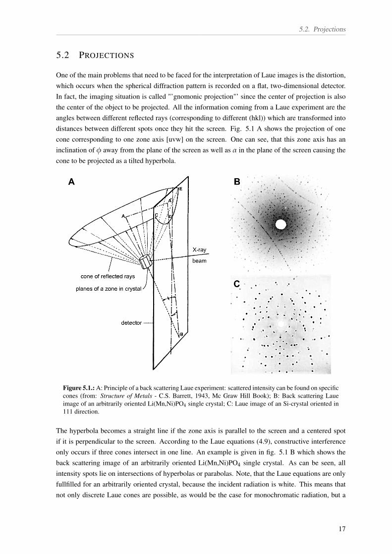
One of the main problems that need to be faced for the interpretation of Laue images is the distortion,which occurs when the spherical diffraction pattern is recorded on a flat, two-dimensional detector.In fact, the imaging situation is called "’gnomonic projection"’ since the center of projection is alsothe center of the object to be projected. All the information coming from a Laue experiment are theangles between different reflected rays (corresponding to different (hkl)) which are transformed intodistances between different spots once they hit the screen. Fig. 5.1 A shows the projection of onecone corresponding to one zone axis [uvw] on the screen. One can see, that this zone axis has aninclination of φ away from the plane of the screen as well as α in the plane of the screen causing thecone to be projected as a tilted hyperbola.

Figure 5.1.: A: Principle of a back scattering Laue experiment: scattered intensity can be found on specificcones (from: Structure of Metals - C.S. Barrett, 1943, Mc Graw Hill Book); B: Back scattering Laueimage of an arbitrarily oriented Li(Mn,Ni)PO4 single crystal; C: Laue image of an Si-crystal oriented in111 direction.

The hyperbola becomes a straight line if the zone axis is parallel to the screen and a centered spotif it is perpendicular to the screen. According to the Laue equations (4.9), constructive interferenceonly occurs if three cones intersect in one line. An example is given in fig. 5.1 B which shows theback scattering image of an arbitrarily oriented Li(Mn,Ni)PO4 single crystal. As can be seen, allintensity spots lie on intersections of hyperbolas or parabolas. Note, that the Laue equations are onlyfullfilled for an arbitrarily oriented crystal, because the incident radiation is white. This means thatnot only discrete Laue cones are possible, as would be the case for monochromatic radiation, but a

17

5. Crystal structure and stereographic projections

continuum. Hence a lot of cone intersections and thus spots on the screen are possible for any kind ofcrystal orientation. Fig. 5.1 C shows the back-scattering diffraction image of a Silicon crystal whichis oriented in 111-direction. The intensity spots are symmetric with respect to this axis and a threefoldsymmetry can be observed.

There are several options of how to find the angles between different zone axis and thus the ori-entation of the crystal under investigation. One is simply by calculation and transformation of thezone dependend reflections from the laboratory system into the crystal system. While processing this"’by hand"’ can be very time consuming, pen and paper methods have been developed to solve thisproblem in a graphical way. The "’Greninger Net"’ is an easy tool to obtain meridian and parallelcoordinates of spots, similar to coordinates on a globe. It will be used during the lab course to findthe orientation of a simple cubic crystal.

Another approach comes from the opposite direction: If the crystal structure is known, a simulatedLaue pattern can be generated and compared with the measured pattern. Especially for complexlattices, the use of suitable software can be very helpfull to obtain the orientation in a short time.

5.3 STEREOGRAPHIC PROJECTIONS

Plotting the diffraction spots as a stereographic projection is a helpfull tool to find the crystal ori-entation. Stereographic means projecting a sphere onto a plane as it is for example done with twodimensional images of the globe (see fig. 5.2 A). A stereographic projection is also angle preserving,this means, that angular differences between diffraction spots will not change if the direction of pro-jection is changed. Fig. 5.2 B shows the standard projection of a cubic crystal in (100) direction(corresponding to 0◦). The (010) and (001) faces are perpendicular to the viewing direction and thuscan be found on the outer great circle (90◦).

Figure 5.2.: A: Stereographic projection of the globe (from Encyclopædia Britannica, 2010); B: Standardprojection of a cubic crystal with 100 direction corresponding to 0◦ longitude and latitude (from LaueAtlas - E. Preuss et al, 1974, Wiley).

Similar to the globe, the position on a stereographic projections can be given by a longitude (Längen-grad, δ) and latitude (Breitengrad γ). A so called Wulff net will be used during the lab course to findthe relative angles between different lattice planes of a crystal.

18

6 EXPERIMENTAL SETUP

A schematic sketch of the setup is given in fig. 6.1. The collimated X-rays from the tube pass thedetector through a centered hole and are scattered by the sample. The diffraction image is taken bythe detector in back scattering geometry.

Figure 6.1.: Schematic sketch of the experimental setup. The tube and beamline are positioned inside asafety cabinet.

Generally a Laue experiment consists of 4 steps:

1. Adjustment of the sample on a goniometer and positioning in the beam line.

2. Starting of the X-ray source and data acquisition.

3. Stopping of X-ray source.

4. Data analysis.

Depending on the scientific question, this procedure than needs to be repeated several times, forexample to find the right sample orientation. While operation of tube and detector are straight forward,as will be described below, the deal of a Laue experiment is the data analysis (e.g. determination of

19

6. Experimental setup

orientation, symmetry, etc.) and the correct translation of these information into the laboratory systemif, for example, the goniometer should be used to orient the sample in a specific direction.

6.1 SAMPLE MOUNTING

In general, single crystalline samples may not have a regular shape since they might be broken or cutof bigger entities (e.g. rocks, polycrystalline fabric). Without any hints by visible external faces, thesample will have to be rotated around three different axes to get into the desired orientation.

Several fixed samples will be provided which can directly be mounted on the goniometer column.New samples can easily be glued on a goniometer head.

Figure 6.2.: Goniometer system. A: Coordinate transformation by z, y’, x” convention (1. Ψ, 2. θ, 3. Φrotation) (from: wikipedia); B: Coordinate system of the used goniometer.

In this experiment a goniometer will be used which allows for the orientation of the sample using threeEuler’s angles on the one hand and for a shift of the sample in three directions in order to hit a specificspot with the X-ray beam on the other hand. The angular system used for this kind of goniometerfollows the z, y’, x” convention and is called yaw (Gier), pitch (Nick), roll (Roll) system. Thesenames origin from automotive engineering. Fig. 6.2 A shows the procedure of achieving a specificorientation. The starting coordinate system (x,y,z) corresponds with the lab system (see fig. 6.2 B).First, the sample, which is positioned at the origin of the system, is rotated around the z-axis (Ψ-rotation). Thereby the x- and y- axis are transformed into x’- and y’ axis. The next rotation is madearound the new y’-axis (θ- or Ry-rotation) giving new x”- and z”-axis. The last rotation (Φ or Rx)around the x”-axis gives the final coordinate system (red X=x”,Y,Z in fig. 6.2 A).

The option of linear shifting is implemented in the upper part of the goniometer. This means that itdoes not influence the angular changes made by the Ψ,Ry,Rx rotations since it is also rotated. It canbe considered as a shift within the final "red" coordinate system X,Y,Z→X+∆X,Y+∆Y,Z+∆Z.

The last free parameter is the distance between sample and detector which can be adjusted on the

20

6.2. Automatic Psi-Circle operation

linear rail by moving the whole goniometer column. For all experiments however a fixed distance of30 mm should be kept in order to ease the graphical and software supported data analysis. For thispurpose a special distance piece is available which enables a quick adjustment. Nevertheless specialcare needs to be taken not to touch the scintillating layer on the detector’s surface. The metallicdistance piece might easily scratch and destroy this layer!

6.2 AUTOMATIC PSI-CIRCLE OPERATION

The goniometer base is rotatable by an automatic step drive. This corresponds to a Ψ-rotation of thegoniometer around the z-axis. The step drive can be operated even when the X-ray tube is running,which enables to take images of different orientations without having to actually touch the sample andgoniometer. The drive can be controlled on the panel next to the pc. After the controler was turned on(red on/off switch), the electronics should be reseted by switching the 3-position I/0/II switch to "0"for few seconds and then back to position "II". The drive can now be activated by pressing the enableswitch. Pushing the direction switch will invert the direction.

It is absolutely neccesary to ensure that no part of the goniometer can collide with the detector dueto rotation, before using the automatic drive! Any collision or scratch might destroy the sensitivedetector surface.

6.3 TUBE AND GENERATOR OPERATION

The X-ray tube can and must only be operated if the protection cabinet is properly closed. Openingof the cabinet during X-ray operation must be avoided.

The generator used in this experiment is a "Kristalloflex 710 X-ray Generator" by Siemens. It iscapable of applying a high voltage between 20 kV and 50 kV at a tube current of 5 mA to 40 mAwith a total output power of 2 kW. The cathode is heated with a power of up to 50 W. As mentionedin chapter 3, most of the input power is converted to heat since the efficiency of the X-ray tubes usedin this experiment is very low. To cool off the waste heat, both generator and tube are connected tocooling water. In order to operate the generator, the water valve needs to be completely opened. Theflow can be checked at the flow meter. A miminum flow rate of 3.5 l/min must be kept.

To protect the tube from damages, the high voltage needs to be set slowly. Depending on the tube’shistory, there are certain delay times during which the voltage needs to be kept constant. Tab. 6.1Shows the retention times in dependence of the time that the tube has not been used. As an example,if the tube has not been used for 5 days and a voltage of 35 kV shall be applied, it needs to be poweredup in 4 steps: Starting at the minimum voltage of 20 kV and minimum current of 5 mA followed by120 s of waiting; Slow increase of voltage to 25 kV followed by 120 s of waiting; Slow increase ofvoltage to 30 kV followed by 180 s of waiting; Slow increase to 35 kV followed by 180 s of waiting.After this procedure, the current can be adjusted to the desired level. This should also be done in stepsof 10 mA with a retention time of 120 s.

Before switching off the tube, the current needs to be set back to the minimum of 5 mA. After that,the voltage is to be set back to the minimum of 20 kV and the tube can be shut down. The values for

21

6. Experimental setup

Stop Retention time (min)(days) 20kV 25kV 30kV 35kV 40kV 45kV 50kV 55kV0.5 to 3 2 2 2 2 3 3 3 33 to 30 2 2 3 3 5 5 10 10>30 2 2 3 3 5 10 15 15

Table 6.1.: Tube retention time

high voltage and tube current can be read by pressing the respective black button "kV" and releasingthe button on the front of the generator. The heating current can be measured by pressing the button"A".

Figure 6.3.: Front side of the hV generator.

The starting procedure is described in the following list step by step (see also fig. 6.3:

1. Turn on external cooling water supply and check water flow.

2. Switch on main switch on the cabinet panel and make sure cabinet doors are properly closed.

3. Set control potentiometers for high voltage (kV) and current (mA) to left minimum (20 kV, 5mA).

4. Set keyswitch (generator main) to "ON"

22

6.4. Detector and Software

5. Press the red "Heating" key and wait for green "Operate" key (hV on) to light. The tube heatingis now activated. Wait for 120 s.

6. Press green "Operate" key (hV on). The tube is now running and emits X-rays.

7. Adjust the high voltage to the desired level in accordance to tab. 6.1 using the control poten-tiometer (kV). (max. 0.2 kV/s)

8. Adjust the current to the desired level using the control potentiometer (mA). Maximum stepsare 10 mA with 120 s retention time. (max. 0.1 mA/s)

The tube is now running and detector images can be taken using the software as is described below.The shut down procedure is described in the following list:

1. Decrease the current to the minimum of 5 mA using the control potentiometer (mA). (max. 0.1mA/s)

2. Slowly decrease the high voltage to the minimum of 20 kV using the control potentiometer(kV). (max. 0.2 kV/s)

3. Press the red key (Heating). The high voltage is now off and it is safe to open the X-ray cabinet.

4. In order to switch off the heating, press the yellow button (off). This should only be done at theend of the experiment.

At the end of the day or experiment, the generator and complete system (PC, detector) should be shutdown by using the key-switch and main-switch. The cooling water should be switched off by closingthe valve again.

6.4 DETECTOR AND SOFTWARE

The CCD detector used in this experiment consists of two seperate CCD chips with 1392 x 1040pixels and an active area of 85 mm · 110 mm each. The incident X-ray beam can pass the detectorthrough a middle hole between both chips. Each pixel is read out by an A/D converter giving a12 bit intensity value. To minimize noise by stray radiation, both CCDs are placed inside a blackbox. The front side is however covered with a light impermeable but X-ray transparent capton layer.The szintillating Gadox layer and following optics are placed directly in front of the CCD chips.Furthermore, thermal noise is reduced by cooling the chips with two peltier elements to -10 Â◦C. Toensure proper cooling, the detector should be switched on 20 minutes prior to image acquisition. Thepower supply is activated automatically by turning the main-switch on (see fig. 6.3).

The read out and analysis software can be started with the "PSLView" icon on the computer’s desktop.Before this is done, the detector should be running. To activate the data transfer, the detector can bestarted by choosing the NTXLaue option in the camera menu of PSLView (see fig. 6.4). Fig. 6.5shows the main screen of the software which consists of a toolbar on the left and the image displayon the right.

Several instances of the main screen can be opened, e.g. for comparison of different images. Acquis-ition of a new image however is only possible in the window which was started first.

Before acquiring an image, all options can be set in the area marked red. The measurement can thenbe started by clicking the "play" button marked green. To enhance contrast, the maximum intensity

23

6. Experimental setup

Figure 6.4.: Start-up screen of the PSLViewer software. The Laue camera can be chosen in the "Camera"menu.

corresponding to "white" can be set in the area marked magenta. The image option are explained inmore detail below.

Figure 6.5.: Main window of the PSLViewer software. The toolbar on the left will open several sub-menus. Acquired images are shown on the right

• Exposure: The image and spot intensity is mainly given by the exposure time. More integratedintensity is always beneficial since it will allow a better interpretation of the measured patterns.This is however limited by the maximum photon count of the CCD’s pixels. An overloadof intensity will firstly become noticeable in the center of an image since the back scatteredintensity is strongest for small angles. Furthermore, very long integration times (t > 600s) willalso amplify the CCDs characteristics e.g. dark current, hot pixels, etc. which then requires theuse of backround subtraction techniques.

• Acquisition mode: Besides the option of taking a single image, several consecutive images canbe taken. The respective intesities can either be summed up or averaged which reduces theoverall image noise.

• Binning: Using the hardware binning option will effectively combine the measured intensityof several pixels, resulting in a higher sensitivity however smaller resolution. Since a highersensitivity will always allow smaller integration times, binning should be used up unto a level

24

6.5. Pattern simulation

that still resolves diffraction spots well enough. This means: perceptibility of the spot positionshould not be affected and distinctness of neighboring spots should still be given. As the spot-size mainly depends on the size of the collimated beam, the binning should also be chosen withrespect to the used collimator.

Images can be saved by right clicking on the image area and choosing "SaveAs...". The standardimage format is *.tif which features lossless data treatment in a greyscale format. Note howeverthat the intensity or greyscale is not saved as an absolute value. To display an image correctly, themaximum value corresponding to white and minimum value corresponding to black must be given inaddition. If needed, all images can also be saved as *.jpeg or *.bmp. Note however, that it is stronglyrecommended to save every image in *.tif format since mathematical operations can only be executedwith this format.

Besides the task of image acquisition, the software is also capable of executing mathematical opera-tions and image enhancement techniques as well as, more importantly, finding and refining the crystalorientation of a sample with known lattice constants and symmetry.

6.5 PATTERN SIMULATION

With PSLViewer software

The peak symbol in the PSLViewer toolbar (marked magenta in fig. 6.6) offers the possibility of auto-matic peak detection. Depending on the parameters given, the image will be evaluated and possiblepeaks will be marked with red circles. The threshold parameter in particular determines how big thecontrast needs to be between backround and peak in order to be recognized as such. In case a peakdetection is not desired, the threshold can be set to a high value, e.g. 1000.

The crystal structure symbol (marked blue in fig. 6.6) will open the symulation and fitting option. Insub-menu "Crystal data", the lattice constants, angles and space group need to be entered in order tosimulate the theoretical pattern of such a crystal. The sub-menu "Instrument data" contains all theparameters associated with the detector (e.g. area of detector and tilting angles). The only adjustableparameter however is the sample detector distance. All other parameters should be kept at their values.

In order to simulate a specific direction in terms of hkl, the sub-menu "Find <hkl> spot" will rotatethe pattern into the right direction after pressing the "Find" button. The pattern can than be rotatedor shifted by pressing left or right mouse button and moving the mouse. Alternatively the orientationcan directly be set by entering orientation angles in the lower part of the menu. A detailed writteninstruction is available in the laboratory.

With CLIP software

Alternatively to the techniques offered by PSLViewer, other software is available for the simulationof patterns. The Cologne Laue Indexation Programme (CLIP) is free of charge and might be moresuitable to find a specific orientation, since the system of rotations is more user friendly. The softwarecan be started from the desktop. A detailed manual is available in the laboratory. Since CLIP has no

25

6. Experimental setup

Figure 6.6.: Main window of the PSLViewer software with shape detection and orientation menus.

26

6.5. Pattern simulation

direct link to the detector, images need to be imported either as *.png or *.jpeg. To do this, first adjustcontrast and brightness with PSLViewer and import the image in CLIP using the folder-like buttonin the main window. It is neccessary to input the experiments geometry (detector width and height,distance) in the configuration section (press screw-wrench button) for a correct simulation. Input ofall crystal data is analog to PSLViewer.

27

7 EXPERIMENTAL SCOPE AND ANALYSIS

Depending on the availability of single crystals, the scope of this lab course can be adapted. Task 7.1is however mandatory and the second task should comprehend the relation between crystal structure,symmetry and observed Laue images.

7.1 IDENTIFICATION OF THE ORIENTATION OF A CUBIC CRYSTAL AND

SAMPLE-DETECTOR DISTANCE

• Take several Laue images of one of the cubic crystals in arbitrary orientation and find suitablevalues for binning and integration time of the detector at 30 kV, 20 mA tube power.

• Take an image of high quality which shows a spot of high symmetry. Therefore you might needto re-orient the sample. Make sure the sample almost touches the spacer to have a well definedsample-detector distance.

• Use PSLViewer’s simulation option to find the orientation of the crystal.

• Refine the sample-detector distance. This value will be needed for all further experiments.

7.2 CRYSTAL SHAPE AND CRYSTAL LATTICE

• Choose one of the regularly shaped minerals and take Laue images perpendicular to the visiblecrystal faces with low binning and long integration time. Fix the sample to the goniometer headin a way that allows to use the automatic rotation option. Make sure the samples centerlinecoincides with the axis of rotation.

• Deduce the corresponding crystallographic planes using the PSL orientation software and makea sketch of your sample that shows the visible faces and their crystallographic directions.

• What kind of symmetries can be found in the patterns?

• Explain the crystal shape with respect to the unit cell, atomic positions and symmetries.

• Find the positions of pregnant diffraction spots and create an ascii file with the pixel positions(x [TAB] y). Make sure to quote enough spots so that the symmetries are still indentifiableby these spots (around 50 per image should be sufficient if distributed well over the image).You can also put the hkl index in a third column (x [TAB] y [TAB] hkl) (see example.txt ondesktop).

• Generate a stereographic projection by using the mathematica file "LaueVersuch.nb"

28

7.3. Crystal orientation and cutting

• Compare with a given standard projection. Explain the absence of specific diffraction spots bythe crystal’s symmetry.

7.3 CRYSTAL ORIENTATION AND CUTTING

• Find the crystallographic main directions (100), (010), (001) of an unknown sample and cut thesample to a cuboidal shape.

• Explain the crystal’s symmetry and the resulting symmetry of the Laue images.

Important:Whenever you take an image, write down all the parameters, such as: binning, integration

time, number of pictures and all the goniometer angles (Ψ of auto-drive, 2 angles ofgoniometer head). Save all your images as *.tif and *.png files. If neccessary, save your

analysis/fits as screenshot. If you found an orientation, write down the position and indizes ofimportant diffraction spots and most importantly write down the three angles (α, β, γ), given

by the software, that define your orientation.

7.4 EVALUATION

Your experiment’s evaluation and discussion should contain print-outs of the important Laue imagesas well as the stereographic projection you developed. To understand those images, a sketch of theexperimental setup containing the beam line, sample and detector should be added which shows thegeometrical arrangement of those objects and the meaning of longitude and latitude of a diffractionspot. Furthermore the trigonometric functions should be given which transform a position on thedetector (e.g. x,y-pixel) into those angles.

To understand your diffraction images, you should explain your experimental approach as well as thepatterns themselves. Therefore, index the diffraction spots and add lines depicting any mirror planesor other symmetry axes/planes. In case of the regularly shaped minerals, you should also make asketch of the sample and index the visible faces with their crystallographic directions. You shouldalso have a look at the crystal structure (see *.cif files) in order to explain the crystal’s morphologyin terms of atomic bonds or distances within the lattice. Therefore compare the real space crystal-structure with the shape of the mineral you investigated. Can you convey reasons from the atomicpositioning and bonds why it might be favorable to develop the visible crystal faces?

Calculate the maximum values hkl that are theoretically visible for the acceleration voltage you ap-plied. (Compare minimum wavelength and minimum lattice distance dhkl). Is this in agreement withyour experimental observations?

Discuss the possible measurement errors. Which parameters of the geometry are unknown? How willa tilted detector / poorly collimated beam or variable sample-detector distance effect the pattern? Didyou experience any effects of crystal imperfection and defects?

29

A ADDENDUM

A.1 SYSTEMATIC DISTINCTION OF REFLEXES

Systematic distinction of reflexes by the Bravais type lattice

centering reflex condition centering reflex conditionprimitive - no cancellation

A-centered - k+l = 2n body centered hkl h+k+l = 2nB-centered - h+l = 2n face centered hkl h+k=2n, h+l=2n, k+l=2nC-centered - h+k = 2n rhomboedric hkl -h+k+l = 3n

Zonal distinction of reflexes by mirror glide planes

glide plane position glide vector reflex conditiona (001) a/2 hk0 h = 2nb (001) b/2 hk0 k = 2nn (001) a/2 + b/2 hk0 h+k = 2nd (001) a/4 +/- b/4 hk0 h+k = 4n, h = 2n, k = 2na (010) a/2 h0l h = 2nc (010) c/2 h0l l = 2nn (010) a/2 + c/2 h0l h+l = 2nd (010) a/4 + c/4 h0l h+l = 4n, h=2n, l=2nb (100) b/2 0kl k = 2nc (100) c/2 0kl l = 2nn (100) b/2 + c/2 0kl k+l = 2nd (100) b/4 +/- c/4 0kl k+l = 4n, k = 2n, l = 2n

Serial distinction of reflexes by screw axes

screw axis position reflex condition screw axis position reflex condition21; 42; 63 [100] h00 h = 2n 41; 43 [010] 0k0 k = 4n

31; 32; 62; 64 [100] h00 h = 3n 61; 65 [010] 0k0 k = 6n41; 43 [100] h00 h = 4n 21; 42; 63 [001] 00l l = 2n61; 65 [100] h00 h = 6n 31; 32; 62; 64 [001] 00l l = 3n

21; 42; 63 [010] 0k0 k = 2n 41; 43 [001] 00l l = 4n31; 32; 62; 64 [010] 0k0 k = 3n 61; 65 [001] 00l l = 6n

30

A.2. Guide for the generation of stereographic projections

A.2 GUIDE FOR THE GENERATION OF STEREOGRAPHIC PROJECTIONS

The provided mathematica script (LaueVersuch.nb on the desktop) offers a basic method of calculat-ing longitude (δ) and latitude (γ) from the pixel position of a diffraction spot. The input format isan ascii textfile formated as "x-pixel-position" [TAB] "y-pixel position". Multiple diffraction spotsare written in seperate lines. (As an example: see example.txt on the desktop). If needed, additionalinformation as the associated (hkl) indizes can be written in a third column. Experimental parametersas detector-sample distance and resolution (number of pixels) are given in the first block and need tobe adjusted. The second block concerns the processing of pixel lists. Therefore you need to changeall the directories in the script to your data directory which contains your lists. Running the scriptwill output several *.txt files containing corresponding latitude and longitude of the spots. The thirdblock outputs a graphic of the stereographic projection as well as a list of positions projected on a2D-plane. Before altering the script, please save a copy in your data directory and leave the originalscript unchanged.

In case you want to merge several diffraction images in order to get one big stereographic map of yoursystem, it might be convenient to start with one centered image and arrange all other images aroundit. It is recommended to follow these steps:

1. Process all spot-lists with the mathematica script in order to get longitude/latitude files.

2. Choose one image and one crystallographic main direction, that you want to have in the cen-ter of your projection. Find out the longitude and latitude of this particular spot. Since thestereographic projection is angle preserving, you are free to shift your spots by any angle. Itwill not change the angular differences between individual spots. To center your chosen crys-tallographic direction, subtract the longitude and latitude of the corresponding spot from everycoordinate in your list. Mathematica allows to directly subtract lists from each other. One wayis to generate a list with arbitrary length, only containing the angles you want to subtract, usingthe "Table" command: NewList = OldList − Table[{latitude, longitude}, {Length[OldList]}].The "Length" command gives the number of entries in a list.

3. In order to merge two or more data sets from Laue images, it is most convenient to find onediffraction spot, which is present in two images respectively. One of the data sets can then becorrected by the angular difference of this spot in both images.{lat1, long1}: angles in image 1 of one spot, {lat2, long2}: angles in image 2 of same spot.An arbitrary spot can thereby be transformed as:{lat, long}image1 = {lat, long}image2 − {lat2, long2} + {lat1, long1}

You can use similar operations on lists to calculate the new spot positions as given above.

4. The merging step can either be done by manually copying all corrected values from severallists into one list (text editor) or by using the "Join" command, which will do the merging stepwithin Mathematica in the form: Join[list1, list2, ...].

5. Plot a stereographic projection of the merged images by using the third block in the mathemat-ica script.

This method however only allows for the merge of images that have been taken in the same coordinatesystem. In practice this refers to images of a sample that has only been re-oriented by changing

31

A. Addendum

it’s longitude and latitude with respect to the beam-line. Use of the automatic Ψ-drive for examplecorresponds to a change of longitude of the sample. Hence images can easily be merged. If the samplewas however rotated around the beam-line direction, two pictures can not be merged by modulatingtheir latitude and longitude (see fig. A.1. Moreover the additional rotation needs to be taken intoaccount. This can be done by re-rotating an image in the first part of the mathematica programaround the beam axis by an angle µ (korrMu).

Figure A.1.: Consequences of γ-, δ-rotation and µ-rotation on the orientation of Laue images.

32