Adiabatic particle pumping and anomalous...
67
Adiabatic particle pumping and anomalous velocity November 17, 2015 November 17, 2015 1 / 31
Transcript of Adiabatic particle pumping and anomalous...

Adiabatic particle pumping and anomalous velocity
November 17, 2015
November 17, 2015 1 / 31

Literature:1 J. K. Asboth, L. Oroszlany, and A. Palyi, arXiv:1509.02295
2 D. Xiao, M-Ch Chang, and Q. Niu, Rev. Mod. Phys. 82, 1959.
November 17, 2015 2 / 31

SSH model, adiabatic evolution, Chern number
A couple of the ideas discussed on previous occasions will be combined.
i) Su-Schrieffer-Heeger (Rice-Mele) model
ii) Adiabatic evolution of eigenstates
iii) Chern number
November 17, 2015 3 / 31

SSH model, adiabatic evolution, Chern number
A couple of the ideas discussed on previous occasions will be combined.
i) Su-Schrieffer-Heeger (Rice-Mele) model
ii) Adiabatic evolution of eigenstates
iii) Chern number
Figure : A segment of the periodic SSH model.
November 17, 2015 3 / 31

Overview
1) Model system
2) Particle current and group velocity
3) Quasi adiabatic time evolution
4) Pumped current and Berry curvature
5) Anomalous velocity of electrons
November 17, 2015 4 / 31

Model system
Figure : A segment of the periodic SSH model.
Rice-Mele model
H(t) = v(t)N∑
m=1
|m,B〉〈m,A|+ h.c .) + w(t)N−1∑
m=1
(|m + 1,A〉〈m,B |+ h.c .)
+u(t)
N∑
m=1
(|m,A〉〈m,A| − |m,B〉〈m,B |)
November 17, 2015 5 / 31

Model system
Because of spatial periodicity, the eigenstates are Bloch wave functions.The instantaneous eigenstates read |Ψn,k(t)〉 = |k〉 ⊗ |un(k , t)〉, wheren = 1, 2 are the two bands, k wavenumber.
November 17, 2015 6 / 31

Model system
Because of spatial periodicity, the eigenstates are Bloch wave functions.The instantaneous eigenstates read |Ψn,k(t)〉 = |k〉 ⊗ |un(k , t)〉, wheren = 1, 2 are the two bands, k wavenumber.Reminder:
|k〉 = 1√N
N∑
m=1
e imk |m〉 m : site index
and |un(k , t)〉 satisfy the instantaneous Schrodinger equation
H(k , t)|un(k , t)〉 = En(k , t)|un(k , t)〉.
Note, that this is a different convention regarding |un(k , t)〉 than whatwe used the last time to define the Bloch wave functions.
November 17, 2015 6 / 31
Model system
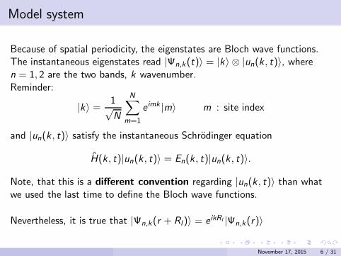
Because of spatial periodicity, the eigenstates are Bloch wave functions.The instantaneous eigenstates read |Ψn,k(t)〉 = |k〉 ⊗ |un(k , t)〉, wheren = 1, 2 are the two bands, k wavenumber.Reminder:
|k〉 = 1√N
N∑
m=1
e imk |m〉 m : site index
and |un(k , t)〉 satisfy the instantaneous Schrodinger equation
H(k , t)|un(k , t)〉 = En(k , t)|un(k , t)〉.
Note, that this is a different convention regarding |un(k , t)〉 than whatwe used the last time to define the Bloch wave functions.
Nevertheless, it is true that |Ψn,k(r + Rl)〉 = e ikRl |Ψn,k(r)〉
November 17, 2015 6 / 31

Model system
We assume that the Hamiltonian is also periodic in time, therefore
1 H(k + 2π, t) = H(k , t)
2 H(k , t + T ) = H(k , t), and Ω = 2π/T .
November 17, 2015 7 / 31

Model system
We assume that the Hamiltonian is also periodic in time, therefore
1 H(k + 2π, t) = H(k , t)
2 H(k , t + T ) = H(k , t), and Ω = 2π/T .
We can rewrite the problem using the following notation. The Hamiltonianis given by (two-band insulator model):
H(d(k , t)) = dxσx + dyσy + dzσz = d · σThe parameter vector d(k , t) reads:
d(k , t) =
ν + cosΩt + cos ksin ksinΩt
⇐⇒v(t) = ν + cosΩt
w(t) = 1u(t) = sinΩt
November 17, 2015 7 / 31

Overview
1) Model system
2) Particle current and group velocity
3) Quasi adiabatic time evolution
4) Pumped current and Berry curvature
5) Anomalous velocity of electrons
November 17, 2015 8 / 31

Influx of particles into a segment
Figure : A segment of the periodic SSH model.
The number of particles NS in segment S is given by the expectationvalue of the operator
NS =∑
m∈S
∑
α∈A,B
|m, α〉〈m, α|
November 17, 2015 9 / 31

Influx of particles into a segment
Figure : A segment of the periodic SSH model.
The number of particles NS in segment S is given by the expectationvalue of the operator
NS =∑
m∈S
∑
α∈A,B
|m, α〉〈m, α|
Due to the time-dependence, the number of particles in a given regionchanges.
November 17, 2015 9 / 31

Influx of particles into a segment
Figure : A segment of the periodic SSH model.
The change of the number of particles is given by the Heisenberg equationof motion
∂N (t)S∂t
= jS (t) = −i [N , H]
November 17, 2015 10 / 31

Influx of particles into a segment
Figure : A segment of the periodic SSH model.
The change of the number of particles is given by the Heisenberg equationof motion
∂N (t)S∂t
= jS (t) = −i [N , H]
One finds
jS (t) = −iw(t) [|p + 1,A〉〈p,B | − |p,B〉〈p + 1,A|+ |q,B〉〈q + 1,A| − |q + 1,A〉〈q,B |]
November 17, 2015 10 / 31

Particle current operator
Figure : A segment of the periodic SSH model.
jS (t) = −iw(t) [|p + 1,A〉〈p,B | − |p,B〉〈p + 1,A|+ |q,B〉〈q + 1,A| − |q + 1,A〉〈q,B |]
The particle number can change through the interface at m = p andthrough the interface at m = q.
November 17, 2015 11 / 31

Particle current operator
Figure : A segment of the periodic SSH model.
jS (t) = −iw(t) [|p + 1,A〉〈p,B | − |p,B〉〈p + 1,A|+ |q,B〉〈q + 1,A| − |q + 1,A〉〈q,B |]
The particle number can change through the interface at m = p andthrough the interface at m = q.One can define
jm+1/2(t) = −iw(t) (|m + 1,A〉〈m,B | − |m,B〉〈m + 1,A|)which is interpreted as the operator describing the net particle flow
through the cross-section at m + 1/2.November 17, 2015 11 / 31

Particle current and group velocity
Remember: the instantaneous eigenstates read |Ψn,k(t)〉 = |k〉 ⊗ |un(k , t)〉where
|k〉 = 1√N
N∑
m=1
e imk |m〉 m : site index
and|un(k , t)〉 = an(k , t)|A〉+ bn(k , t)|B〉
November 17, 2015 12 / 31

Particle current and group velocity
Remember: the instantaneous eigenstates read |Ψn,k(t)〉 = |k〉 ⊗ |un(k , t)〉where
|k〉 = 1√N
N∑
m=1
e imk |m〉 m : site index
and|un(k , t)〉 = an(k , t)|A〉+ bn(k , t)|B〉
We can calculate the diagonal matrix elements of the current operator
〈Ψn,k(t)|jm+1/2(t)|Ψn,k(t)〉 = 〈un(k , t)|jm+1/2(k , t)|un(k , t)〉
where
jm+1/2(k , t) =1
N
(
0 −iw(t)e−ik
iw(t)e ik 0
)
November 17, 2015 12 / 31

Particle current and group velocity
jm+1/2(k , t) =1
N
(
0 −iw(t)e−ik
iw(t)e ik 0
)
We can recognize that
jm+1/2(k , t) =1
N∂k H(d(k , t))
=⇒ the momentum diagonal elements of the current operator are relatedto the momentum-space Hamiltonian.
November 17, 2015 13 / 31

Particle current and group velocity
jm+1/2(k , t) =1
N
(
0 −iw(t)e−ik
iw(t)e ik 0
)
We can recognize that
jm+1/2(k , t) =1
N∂k H(d(k , t))
=⇒ the momentum diagonal elements of the current operator are relatedto the momentum-space Hamiltonian.
This is a very general result. It applies not only to the Rice-Mele problembut to time-independent problems defined on a lattice and can begeneralized to (quasi) two dimensional case (Buttiker formalism etc.)
November 17, 2015 13 / 31

Particle current and group velocity
Matrix elements of the current operator: in terms of the instantaneouseigenvalues
〈un(k , t)|jm+1/2(k , t)|un(k , t)〉 =1
N〈un(k , t)|∂k H|un(k , t)〉
=∂kE (k , t)
N=
vn(k , t)
N
Here vn(k , t) is the instantaneous group velocity of the eigenstate.
November 17, 2015 14 / 31

Overview
1) Model system
2) Particle current and group velocity
3) Quasi adiabatic time evolution
4) Pumped current and Berry curvature
5) Anomalous velocity of electrons
November 17, 2015 15 / 31

Time evolution governed by quasi-adiabatic Hamiltonian
We want to calculate the total particle current over one cycle of driving.
November 17, 2015 16 / 31

Time evolution governed by quasi-adiabatic Hamiltonian
We want to calculate the total particle current over one cycle of driving.
For this we need to consider the time evolution of the eigenstates (notonly the instantaneous eigenstates)
November 17, 2015 16 / 31

Time evolution governed by quasi-adiabatic Hamiltonian
We want to calculate the total particle current over one cycle of driving.
For this we need to consider the time evolution of the eigenstates (notonly the instantaneous eigenstates)
Remarks
i) due to the spatial periodicity, the wave number k remains a goodquantum number. Therefore we consider the time evolution of a set oftwo-level system, each labelled by a different k
ii) basically, we are going to use time dependent perturbation theory tocalculate the time evolution of the eigenstates
November 17, 2015 16 / 31
Time evolution governed by quasi-adiabatic Hamiltonian
Quasi adiabatic: for the driving Ω it is fulfilled that Ω ≪ ∆E where∆E = min∀k,t,t→T (E2(k , t)− E1(k , t)).
November 17, 2015 17 / 31

Time evolution governed by quasi-adiabatic Hamiltonian
Quasi adiabatic: for the driving Ω it is fulfilled that Ω ≪ ∆E where∆E = min∀k,t,t→T (E2(k , t)− E1(k , t)).We are looking for the solutions of the following time dependentSchrodinger equation.
i~∂
∂t|u(t)〉 = H(t)|u(t)〉
One can expand the wave function in terms of the instantaneouseigenstates of H(t)
|u(t)〉 =∑
n
exp
(
− i
~
∫ t
0dt ′En(t
′)
)
an(t)|un(t)〉
The coefficients satisfy
∂tan(t) = −∑
l
al(t)〈un(t)|∂t |ul(t)〉 exp(
− i
~
∫ t
0dt ′[El (t
′)− En(t′)]
)
November 17, 2015 17 / 31

Time evolution governed by quasi-adiabatic Hamiltonian
It is convenient to impose the parallel transport gauge. This fixes thephases of the instantaneous eigenstates |un(t)〉 such that
〈un(t)|∂t |un(t)〉 = ∂td(t)〈un(t)|∂
∂d|un(t)〉 = 0.
The wave function obtained with this gauge will be denoted by |u(t)〉.
November 17, 2015 18 / 31

Time evolution governed by quasi-adiabatic Hamiltonian
It is convenient to impose the parallel transport gauge. This fixes thephases of the instantaneous eigenstates |un(t)〉 such that
〈un(t)|∂t |un(t)〉 = ∂td(t)〈un(t)|∂
∂d|un(t)〉 = 0.
The wave function obtained with this gauge will be denoted by |u(t)〉.
This condition basically corresponds to neglecting the acquired Berryphase, which turns out to be not important in this case.
November 17, 2015 18 / 31
Time evolution governed by quasi-adiabatic Hamiltonian
It is convenient to impose the parallel transport gauge. This fixes thephases of the instantaneous eigenstates |un(t)〉 such that
〈un(t)|∂t |un(t)〉 = ∂td(t)〈un(t)|∂
∂d|un(t)〉 = 0.
The wave function obtained with this gauge will be denoted by |u(t)〉.
This condition basically corresponds to neglecting the acquired Berryphase, which turns out to be not important in this case.
The characteristic frequency for ∂td(t) is Ω.If ∂td(t) → 0 then in zeroth order
∂tan(t) = 0
November 17, 2015 18 / 31

Time evolution governed by quasi-adiabatic Hamiltonian
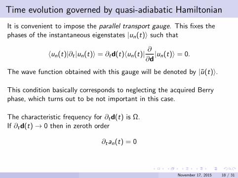
It is convenient to impose the parallel transport gauge. This fixes thephases of the instantaneous eigenstates |un(t)〉 such that
〈un(t)|∂t |un(t)〉 = ∂td(t)〈un(t)|∂
∂d|un(t)〉 = 0.
The wave function obtained with this gauge will be denoted by |u(t)〉.
This condition basically corresponds to neglecting the acquired Berryphase, which turns out to be not important in this case.
The characteristic frequency for ∂td(t) is Ω.If ∂td(t) → 0 then in zeroth order
∂tan(t) = 0
If the system is initially in the nth eigenstate then approximately it willstay in that eigenstate =⇒ adiabatic theorem.
November 17, 2015 18 / 31

Time evolution governed by quasi-adiabatic Hamiltonian
First order corrections:Initially, an(t = 0) = 1 and an′ 6=n(t = 0) = 0.The equation for an′ 6=n:
∂tan′ = −〈un′(t)|∂t |un(t)〉 exp(
− i
~
∫ t
0dt ′[En(t
′)− En′(t′)]
)
November 17, 2015 19 / 31

Time evolution governed by quasi-adiabatic Hamiltonian
First order corrections:Initially, an(t = 0) = 1 and an′ 6=n(t = 0) = 0.The equation for an′ 6=n:
∂tan′ = −〈un′(t)|∂t |un(t)〉 exp(
− i
~
∫ t
0dt ′[En(t
′)− En′(t′)]
)
The approximate solution, up to first order in ∂td(t) is then
an′ = −〈un′(t)|∂t |un(t)〉En − En′
i~ exp
(
− i
~
∫ t
0dt ′[En(t
′)− En′(t′)]
)
November 17, 2015 19 / 31
Time evolution governed by quasi-adiabatic Hamiltonian
Let us now go back to the Rice-Mele model (two-levels).The time evolution of the lower energy state (ground state) in terms ofthe instantaneous eigenstates |u1,2(t)〉
|u1(t)〉 = e−i∫ t0 dt′E1(t
′)
[
|u1(t)〉+ i〈u2(t)|∂t |u1(t)〉E2(t)− E1(t)
|u2(t)〉]
November 17, 2015 20 / 31

Time evolution governed by quasi-adiabatic Hamiltonian
Let us now go back to the Rice-Mele model (two-levels).The time evolution of the lower energy state (ground state) in terms ofthe instantaneous eigenstates |u1,2(t)〉
|u1(t)〉 = e−i∫ t0 dt′E1(t
′)
[
|u1(t)〉+ i〈u2(t)|∂t |u1(t)〉E2(t)− E1(t)
|u2(t)〉]
Reminder: |u1(t)〉 satisfies i~ ∂∂t |u1(t)〉 = H(t)|u1(t)〉
Most of the weight is in the instantaneous ground state |u1(t)〉 with asmall admixture of the instantaneous excited state |u2(t)〉.
November 17, 2015 20 / 31

Time evolution governed by quasi-adiabatic Hamiltonian
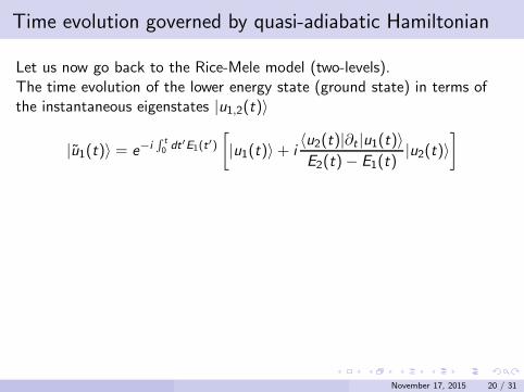
Let us now go back to the Rice-Mele model (two-levels).The time evolution of the lower energy state (ground state) in terms ofthe instantaneous eigenstates |u1,2(t)〉
|u1(t)〉 = e−i∫ t0 dt′E1(t
′)
[
|u1(t)〉+ i〈u2(t)|∂t |u1(t)〉E2(t)− E1(t)
|u2(t)〉]
Reminder: |u1(t)〉 satisfies i~ ∂∂t |u1(t)〉 = H(t)|u1(t)〉
Most of the weight is in the instantaneous ground state |u1(t)〉 with asmall admixture of the instantaneous excited state |u2(t)〉.
In the case of cyclic change of parameters, the final state |u1(t = T )〉 maydiffer from the initial state |u1(t = 0)〉 by a phase factor e iγ1 (Berryphase).
November 17, 2015 20 / 31
Overview
1) Model system
2) Particle current and group velocity
3) Quasi adiabatic time evolution
4) Pumped current and Berry curvature
5) Anomalous velocity of electrons
November 17, 2015 21 / 31

Pumped probability current and Berry curvature
Figure : A segment of the periodic SSH model.
We want to calculate the number of particles N through a cross section atm + 1/2 in a time interval [0,T ].
N =
∫ T
0dt
∑
k∈BZ
〈Ψ1(k , t)|jm+1/2(t)|Ψ1(k , t)〉
November 17, 2015 22 / 31

Pumped probability current and Berry curvature
Figure : A segment of the periodic SSH model.
We want to calculate the number of particles N through a cross section atm + 1/2 in a time interval [0,T ].
N =
∫ T
0dt
∑
k∈BZ
〈Ψ1(k , t)|jm+1/2(t)|Ψ1(k , t)〉
Here Ψ1(k , t) ≈ |k〉 ⊗ |u1(k , t)〉
November 17, 2015 22 / 31

Pumped probability current and Berry curvature
We can write
N =
∫ T
0dt
∑
k∈BZ
〈u1(k , t)|jm+1/2(k , t)|u1(k , t)〉
=1
N
∫ T
0dt
∑
k∈BZ
〈u1(k , t)|∂k H(k , t)|u1(k , t)〉
November 17, 2015 23 / 31

Pumped probability current and Berry curvature
We can write
N =
∫ T
0dt
∑
k∈BZ
〈u1(k , t)|jm+1/2(k , t)|u1(k , t)〉
=1
N
∫ T
0dt
∑
k∈BZ
〈u1(k , t)|∂k H(k , t)|u1(k , t)〉
We insert
|u1(k , t)〉 = e−i∫ t0 dt′E1(k,t′)
[
|u1(k , t)〉+ i〈u2(k , t)|∂t |u1(k , t)〉E2(k , t)− E1(k , t)
|u2(k , t)〉]
November 17, 2015 23 / 31

Pumped probability current and Berry curvature
〈u1(k , t)|jm+1/2(k , t)|u1(k , t)〉 = v1(k , t) + i〈u1|∂k H |u2〉〈u2|∂t |u1〉
E2 − E1+ c .c
November 17, 2015 24 / 31

Pumped probability current and Berry curvature
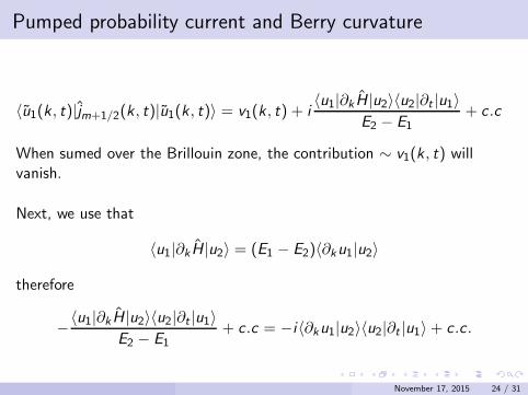
〈u1(k , t)|jm+1/2(k , t)|u1(k , t)〉 = v1(k , t) + i〈u1|∂k H |u2〉〈u2|∂t |u1〉
E2 − E1+ c .c
When sumed over the Brillouin zone, the contribution ∼ v1(k , t) willvanish.
November 17, 2015 24 / 31

Pumped probability current and Berry curvature
〈u1(k , t)|jm+1/2(k , t)|u1(k , t)〉 = v1(k , t) + i〈u1|∂k H |u2〉〈u2|∂t |u1〉
E2 − E1+ c .c
When sumed over the Brillouin zone, the contribution ∼ v1(k , t) willvanish.
Next, we use that
〈u1|∂kH |u2〉 = (E1 − E2)〈∂ku1|u2〉
November 17, 2015 24 / 31
Pumped probability current and Berry curvature
〈u1(k , t)|jm+1/2(k , t)|u1(k , t)〉 = v1(k , t) + i〈u1|∂k H |u2〉〈u2|∂t |u1〉
E2 − E1+ c .c
When sumed over the Brillouin zone, the contribution ∼ v1(k , t) willvanish.
Next, we use that
〈u1|∂kH |u2〉 = (E1 − E2)〈∂ku1|u2〉
therefore
−〈u1|∂k H |u2〉〈u2|∂t |u1〉E2 − E1
+ c .c = −i〈∂ku1|u2〉〈u2|∂t |u1〉+ c .c .
November 17, 2015 24 / 31

Pumped probability current and Berry curvature
Using the parallel transport gauge 〈u1|∂t |u1〉 = 0, one can write
−i〈∂ku1|u2〉〈u2|∂t |u1〉+ c .c . = −i〈∂ku1|∂tu1〉+ c .c
= −i(〈∂ku1|∂tu1〉 − 〈∂tu1|∂ku1〉)= −i(∂k〈u1|∂tu1〉)− ∂t〈u1|∂ku1〉)
November 17, 2015 25 / 31

Pumped probability current and Berry curvature
Using the parallel transport gauge 〈u1|∂t |u1〉 = 0, one can write
−i〈∂ku1|u2〉〈u2|∂t |u1〉+ c .c . = −i〈∂ku1|∂tu1〉+ c .c
= −i(〈∂ku1|∂tu1〉 − 〈∂tu1|∂ku1〉)= −i(∂k〈u1|∂tu1〉)− ∂t〈u1|∂ku1〉)
The last expression is exactly the Berry curvature Ω(1)(k , t) defined in theparameter space (k , t).
Finally, the number of pumped particles in a given driving cycle is
N =
∫ T
0dt
∫
BZ
dk
2πΩ(1)(k , t)
given by the integral of the Berry curvature.
November 17, 2015 25 / 31

Pumped probability current and Berry curvature
Figure : Number of pumped particles as a function of time.
November 17, 2015 26 / 31

Pumped probability current and Berry curvature
Figure : Number of pumped particles as a function of time.
Does it have to be an integer number ?
November 17, 2015 26 / 31

Overview
1) Model system
2) Particle current and group velocity
3) Quasi adiabatic time evolution
4) Pumped current and Berry curvature
5) Anomalous velocity of electrons
November 17, 2015 27 / 31

Anomalous velocity of electrons
Let us consider a crystal under the perturbation of a weak electric field E.We represent the electric field through a uniform vector potential A(t)which is time dependent.
November 17, 2015 28 / 31

Anomalous velocity of electrons
Let us consider a crystal under the perturbation of a weak electric field E.We represent the electric field through a uniform vector potential A(t)which is time dependent.
Using minimal coupling theory, the Hamiltonian can be written
H(t) =[p+ eA]2
2me+ V (r)
V (r) lattice periodic potential.
Because of the translation invariance, the solutions are Bloch wavefunctions.The Hamiltonian that acts on the lattice periodic part of the Bloch wavefunctions can be written
H(k, t) = H(
k+e
~A(t)
)
November 17, 2015 28 / 31

Anomalous velocity of electrons
Since A preserves translation invariance, k is a good quantum number andis a constant of motion. Therefore
d
dtq =
d
dt
(
k+e
~A(t)
)
=e
~
d
dtA(t) = −e
~E
November 17, 2015 29 / 31

Anomalous velocity of electrons
Since A preserves translation invariance, k is a good quantum number andis a constant of motion. Therefore
d
dtq =
d
dt
(
k+e
~A(t)
)
=e
~
d
dtA(t) = −e
~E
One can define the average velocity in band n as a function of q:
v(n)(q) = 〈un(k, t)|∂qH |un(k, t)〉
Using
i) the results for the adiabatic evolution of |un(k, t)〉ii) that ∂/∂ki = ∂/∂qi and ∂/∂t = −(e/~)Ei∂/∂qi
November 17, 2015 29 / 31

Anomalous velocity of electrons
One can write the average velocity as
v(n)(q) =∂En(q)
~∂q− e
~E×Ω(n)(q)
where Ω(n)(q) is the Berry curvature of the nth band
Ω(n)(q) = i〈∇qun(k)| × |∇qun(q)〉
November 17, 2015 30 / 31

Anomalous velocity of electrons
One can write the average velocity as
v(n)(q) =∂En(q)
~∂q− e
~E×Ω(n)(q)
where Ω(n)(q) is the Berry curvature of the nth band
Ω(n)(q) = i〈∇qun(k)| × |∇qun(q)〉
One can see that there is an anomalous velocity component
e
~E×Ω(n)(q)
which is transverse to the electric field.
November 17, 2015 30 / 31

Anomalous velocity of electrons
Symmetry considerations
The velocity v(n)(q) should obey certain symmetry constraints:
i) under time reversal, v(n) and q) change sign, while E is fixed
ii) under spatial inversion, v(n), q), E change sign
November 17, 2015 31 / 31

Anomalous velocity of electrons
Symmetry considerations
The velocity v(n)(q) should obey certain symmetry constraints:
i) under time reversal, v(n) and q) change sign, while E is fixed
ii) under spatial inversion, v(n), q), E change sign
This requires that
i) if the unperturbed system has time reversal symmetry thenΩ(n)(−q) = −Ω(n)(q)
ii) if the unperturbed system has spatial inversion symmetry thenΩ(n)(−q) = Ω(n)(q)
In crystals with simultaneous time-reversal and inversion symmetry theBerry curvature vanishes in the whole Brillouin zone.
November 17, 2015 31 / 31