adiabatic formalism

8/7/2019 adiabatic formalism

http://slidepdf.com/reader/full/adiabatic-formalism 1/156

The Adiabatic Connection:Generating DFT Functionals fromCoupled-Cluster Theory

Andrew M. Teale

CMA-CTCC workshop on computationalquantum mechanics

13th January 2009

1 / 2 8



Wavefunction and DFT Approaches to the ElectronicStructure Problem

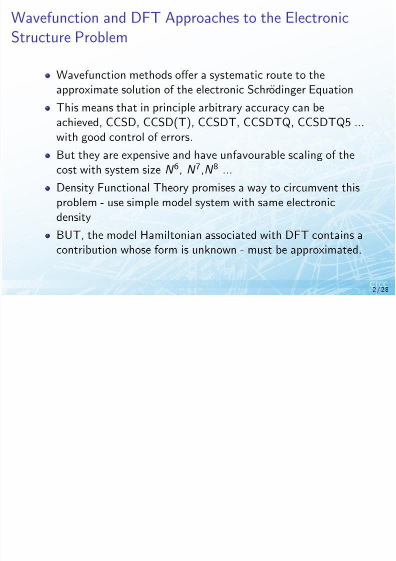
Wavefunction methods offer a systematic route to theapproximate solution of the electronic Schrodinger Equation

2 / 2 8





This means that in principle arbitrary accuracy can beachieved, CCSD, CCSD(T), CCSDT, CCSDTQ, CCSDTQ5 ...

with good control of errors.

2 / 2 8






with good control of errors.But they are expensive and have unfavourable scaling of thecost with system size N 6, N 7,N 8 ...

2 / 2 8






with good control of errors.But they are expensive and have unfavourable scaling of thecost with system size N 6, N 7,N 8 ...

Density Functional Theory promises a way to circumvent this

problem - use simple model system with same electronicdensity

BUT, the model Hamiltonian associated with DFT contains acontribution whose form is unknown - must be approximated.

2 / 2 8




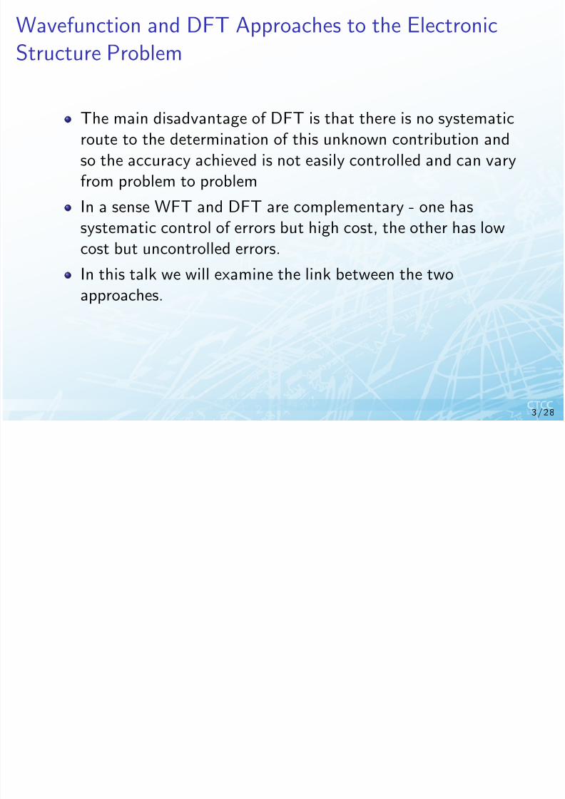
The main disadvantage of DFT is that there is no systematicroute to the determination of this unknown contribution andso the accuracy achieved is not easily controlled and can varyfrom problem to problem

3 / 2 8





In a sense WFT and DFT are complementary - one hassystematic control of errors but high cost, the other has lowcost but uncontrolled errors.

3 / 2 8





In a sense WFT and DFT are complementary - one hassystematic control of errors but high cost, the other has lowcost but uncontrolled errors.

In this talk we will examine the link between the two

approaches.

3 / 2 8



The Generalized Lieb Formulation of DFTConsider a generalized Hamiltonian of the form

H λ[v ] = T + λW + i

v (ri ) = −1

2

i

2

i

+ λi > j

1

r ij

+ i

v (ri )

the electronic interaction strength can be varied with theparameter λ

4 / 2 8




H λ[v ] = T + λW + i

v (ri ) = −1

2

i

2

i

+ λi > j

1

r ij

+ i

v (ri )

the electronic interaction strength can be varied with theparameter λThe ground state energy for an external potential v is

E λ[v ] = inf γ →N

Tr H λ[v ]γ

where the minimization is over all ensemble density matrices γ containing N electrons

4 / 2 8




H λ[v ] = T + λW + i

v (ri ) = −1

2

i

2

i

+ λi > j

1

r ij

+ i

v (ri )

the electronic interaction strength can be varied with theparameter λThe ground state energy for an external potential v is

E λ[v ] = inf γ →N

Tr H λ[v ]γ

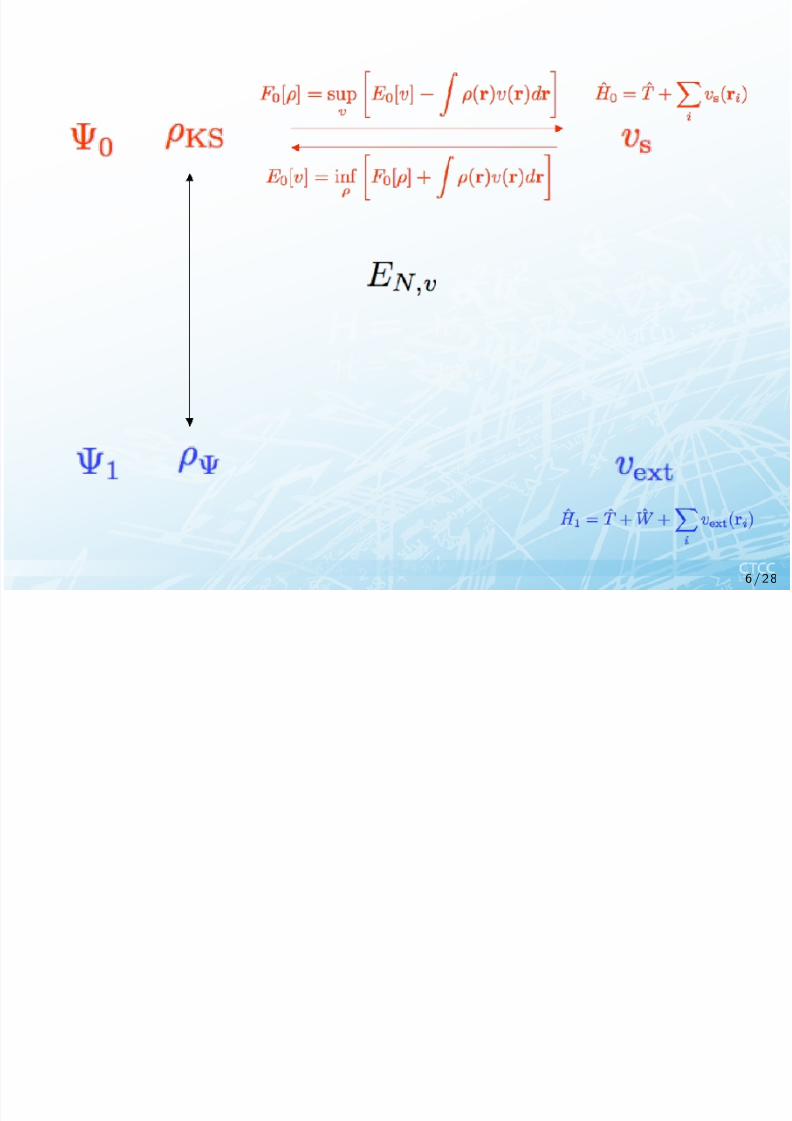
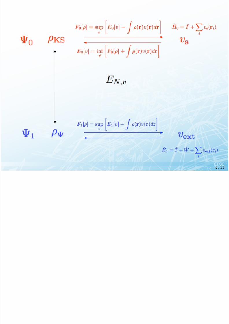
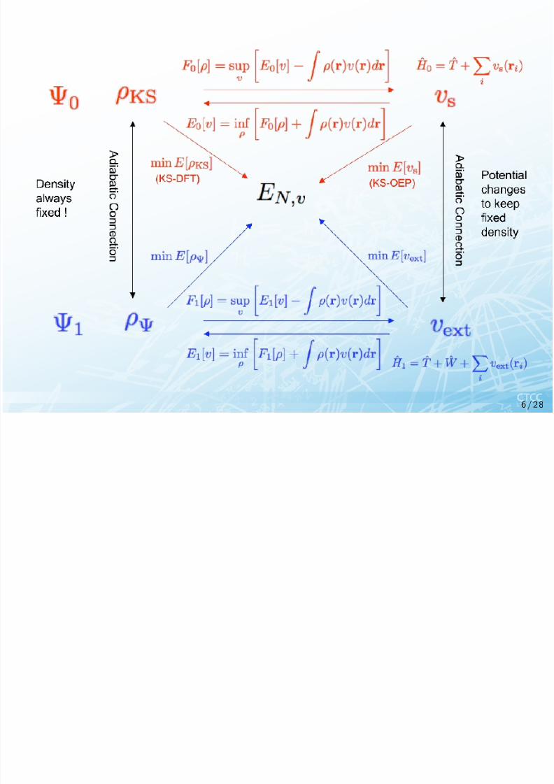
where the minimization is over all ensemble density matrices γ containing N electronsLieb established the mutual Legendre-Fenchel transforms for

the energy and universal functional

F λ[ρ] = supv ∈X ∗

E λ[v ]−

ρ(r)v (r) dr

E λ[v ] = inf ρ∈X F λ[ρ] +

ρ(r)v (

r)dr

4 / 2 8



The Lieb Formulation of DFT

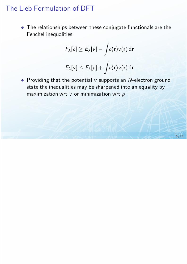
The relationships between these conjugate functionals are the

Fenchel inequalities

F λ[ρ] ≥ E λ[v ]−

ρ(r)v (r) dr

E λ[v ] ≤ F λ[ρ] + ρ(r)v (r) dr

5 / 2 8






F λ[ρ] ≥ E λ[v ]−

ρ(r)v (r) dr

E λ[v ] ≤ F λ[ρ] + ρ(r)v (r) dr

Providing that the potential v supports an N -electron groundstate the inequalities may be sharpened into an equality bymaximization wrt v or minimization wrt ρ

5 / 2 8






F λ[ρ] ≥ E λ[v ]−

ρ(r)v (r) dr

E λ[v ] ≤ F λ[ρ] + ρ(r)v (r) dr

Providing that the potential v supports an N -electron groundstate the inequalities may be sharpened into an equality bymaximization wrt v or minimization wrt ρ

So, given a potential v or density ρ for any interactionstrength λ we can determine its conjugate partnerE. H. Lieb, Int. J. Quant. Chem., 24, 243, (1983)

5 / 2 8



6 / 2 8



The Adiabatic ConnectionI t s f th li d H ilt i



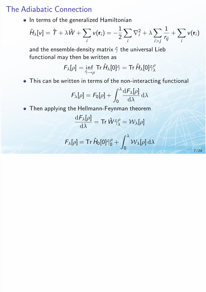
In terms of the generalized Hamiltonian

H λ[v ] = T + λW + i

v (ri ) = −1

2

i

2i + λ

i > j

1

r ij

+ i

v (ri )

and the ensemble-density matrix γ the universal Liebfunctional may then be written as

F λ[ρ] = inf γ →ρ

Tr H λ[0]γ = Tr H λ[0]γ ρλ

This can be written in terms of the non-interacting functional

F λ[ρ] = F 0[ρ] +

λ0

dF λ[ρ]

dλdλ

7 / 2 8

The Adiabatic ConnectionIn terms of the generalized Hamiltonian



In terms of the generalized Hamiltonian

H λ[v ] = T + λW + i

v (ri ) = −1

2 i

2i + λ

i > j

1

r ij

+ i

v (ri )

and the ensemble-density matrix γ the universal Liebfunctional may then be written as

F λ[ρ] = inf γ →ρ

Tr H λ[0]γ = Tr H λ[0]γ ρλ

This can be written in terms of the non-interacting functional

F λ[ρ] = F 0[ρ] +

λ0

dF λ[ρ]

dλdλ

Then applying the Hellmann-Feynman theorem

dF λ[ρ]

dλ= Tr W γ ρλ = W λ[ρ]

F λ[ρ] = Tr H 0[0]γ ρ0 + λ

0

W λ[ρ]dλ

7 / 2 8

The Adiabatic ConnectionThis may be written in the alternative form



This may be written in the alternative form

F λ[ρ] = Tr H λ[0]γ ρ0 + λ

0

W c,λ[ρ] dλ, W c,λ[ρ] = W λ[ρ]−W 0[ρ]

8 / 2 8





F λ[ρ] = Tr H λ[0]γ ρ0 + λ

0


Term 1 is the uncorrelated kinetic energy plus λ times thecoulomb and exchange contributions. Term 2 is the correlationcorrection required upto the chosen interaction strength

8 / 2 8





F λ[ρ] = Tr H λ[0]γ ρ0 + λ

0


Term 1 is the uncorrelated kinetic energy plus λ times thecoulomb and exchange contributions. Term 2 is the correlationcorrection required upto the chosen interaction strengthThe universal functional is then decomposed in the usual

manner

F λ[ρ] = T s[ρ] + λJ [ρ] + λE x[ρ] + E c,λ[ρ]

T s[ρ] = Tr H 0[0]γ ρ0 = Tr T γ ρ0 = minγ →ρ

Tr T γ

J [ρ] =

ρ(r1)ρ(r2)r −112 dr1dr2

E x[ρ] = W 0[ρ]− J [ρ]

E c,λ[ρ] =

λ

0 W c,λ[ρ]d

λ 8 / 2 8

Adiabatic Connection

W ls d fi s t ti f th



We can also define a representation for theexchange-correlation energy as

W xc,λ[ρ] = E x[ρ] + W c,λ[ρ] = W λ[ρ] − J [ρ]

E xc,λ[ρ] =

λ0W xc,λ[ρ] dλ

9 / 2 8


We can also define a representation for the





E xc,λ[ρ] =

λ0W xc,λ[ρ] dλ

The correlation contribution to the kinetic energy may also bedetermined via

T c,λ[ρ] = E c,λ[ρ]−W c,λ[ρ] = λ

0

(W c,µ[ρ] −W c,λ[ρ])dµ

9 / 2 8


We can also define a representation for the





E xc,λ[ρ] =

λ0W xc,λ[ρ] dλ

The correlation contribution to the kinetic energy may also bedetermined via

T c,λ[ρ] = E c,λ[ρ]−W c,λ[ρ] = λ

0

(W c,µ[ρ] −W c,λ[ρ])dµ

So we can obtain the unknown exchange–correlation andcorrelation contributions via a coupling constant integration of W xc,λ[ρ] and W c,λ[ρ]

9 / 2 8

Adiabatic Connection - Geometrical View



10/28




10/28

Calculation of Adiabatic Connection CurvesWe typically choose CC wavefunctions and to begin withd i h CC d i f ll i i h hi i



determine the CC density at full interaction strength this isthen reproduced for all values of λ

11/28

Calculation of Adiabatic Connection CurvesWe typically choose CC wavefunctions and to begin withd i h CC d i f ll i i h hi i




Our task is then to perform the maximization

F λ[ρ] = maxv

E λ[v ]−

ρλ=1(r)v (r)d r

= max

v [C λ[v ]]

11/28



Calculation of Adiabatic Connection CurvesWe typically choose CC wavefunctions and to begin withdetermine the CC densit at f ll interaction strength this is





F λ[ρ] = maxv

E λ[v ]−

ρλ=1(r)v (r)d r

= max

v [C λ[v ]]

To do this we choose the following form for v

v (r) = v ext(r) + (1 − λ)v ref (r) +

t b t g t (r)

and use the known derivativesδC λδb t

=

[ρ(r)− ρλ=1(r)] g t (r)d r

H ut =

g u (r

)g t (r)δρ(r)

δv (r)d rd r

11/28

Calculation of Adiabatic Connection CurvesWe typically choose CC wavefunctions and to begin withdetermine the CC density at full interaction strength this is





F λ[ρ] = maxv

E λ[v ]−

ρλ=1(r)v (r)d r

= max

v [C λ[v ]]

To do this we choose the following form for v

v (r) = v ext(r) + (1 − λ)v ref (r) +

t b t g t (r)

and use the known derivativesδC λδb t

=

[ρ(r)− ρλ=1(r)] g t (r)d r

H ut =

g u (r

)g t (r)δρ(r)

δv (r)d rd r

Once maximized the potential is the conjugate partner of thephysical density, at a chosen interaction strength

11/28

Calculating Adiabatic Connections



A. M. Teale, S. Coriani and T. U. Helgaker, (accepted JCP)

12/28

Application to Two Electron SystemsRepeating the optimization many times allows us to build upthe AC curve This allows us to determine E via



the AC curve. This allows us to determine E xc via

E xc = 1

0W xc,λd λ

13/28





E xc = 1

0W xc,λd λ

This may be compared with

E FCI xc = E FCI − T s − J − E ne − E nn

13/28





E xc = 1

0W xc,λd λ



The T s component is the only unknown part - this can beobtained from maximizing C [v ] at λ = 0 since F 0 = T s .

13/28

Application to Two Electron SystemsRepeating the optimization many times allows us to build upthe AC curve This allows us to determine E c via




E xc = 1

0W xc,λd λ




In two electron systems it is also the von Weizsackerexpression (a simple functional of the FCI density)

T s[ρ(r)] = 18

|ρ(r)|ρ(r)

d r

13/28

Application to Two Electron SystemsRepeating the optimization many times allows us to build upthe AC curve This allows us to determine Exc via




E xc = 1

0W xc,λd λ




In two electron systems it is also the von Weizsackerexpression (a simple functional of the FCI density)

T s[ρ(r)] = 18

|ρ(r)|ρ(r)

d r

To provide estimates of the basis set limit energies and ACcurves we apply basis set extrapolation techniques.

13/28

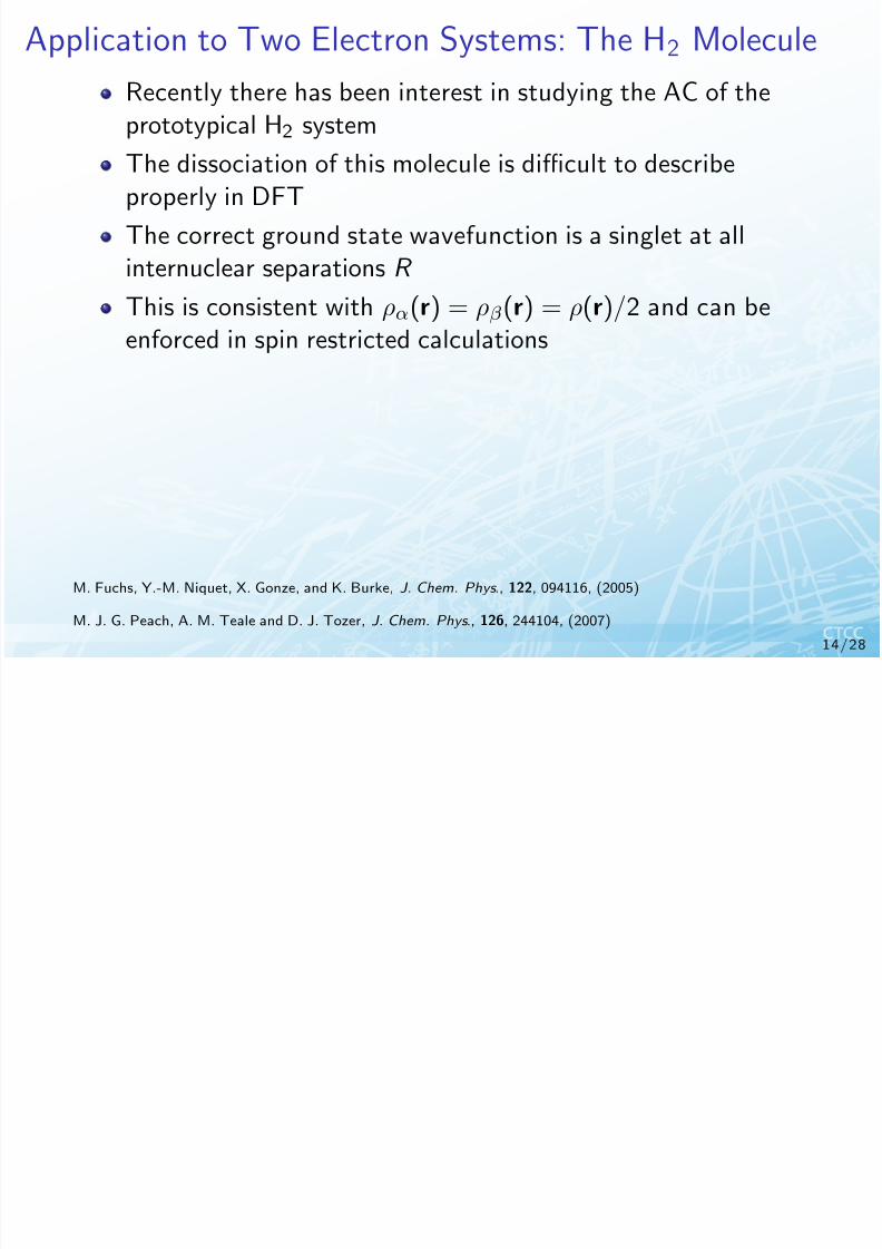
Application to Two Electron Systems: The H2 Molecule

Recently there has been interest in studying the AC of theprototypical H2 system



prototypical H2 system

M. Fuchs, Y.-M. Niquet, X. Gonze, and K. Burke, J. Chem. Phys., 122, 094116, (2005)

M. J. G. Peach, A. M. Teale and D. J. Tozer, J. Chem. Phys., 126, 244104, (2007)

14/28






The dissociation of this molecule is difficult to describeproperly in DFT



14/28







The correct ground state wavefunction is a singlet at allinternuclear separations R



14/28



Application to Two Electron Systems: The H2 MoleculeRecently there has been interest in studying the AC of theprototypical H2 system



p yp 2 y



This is consistent with ρα(r) = ρβ (r) = ρ(r)/2 and can be

enforced in spin restricted calculationsHowever this gives very poor dissociation energies - these canbe fixed by using a spin unrestricted formalism



14/28




p yp 2 y

The dissociation of this molecule is difficult to describe

properly in DFT




BUT the success comes at a price - the spin densities now

localize so that α is on one side, and β is on the other !



14/28




p yp y

The dissociation of this molecule is difficult to describe

properly in DFT




BUT the success comes at a price - the spin densities now

localize so that α is on one side, and β is on the other !This is clearly unphysical at R = ∞ we should have two spinunpolarized H atoms



14/28




15/28




16/28




As the electron-electron interactions are switched on thenature of the wavefunction changes from the KS singledeterminant to the real electronic wavefuntion

This is reflected in the one-electron density matrix. Althoughthe spatial density ρ(r) is fixed

17/28



As the electron-electron interactions are switched on thenature of the wavefunction changes from the KS singledeterminant to the real electronic wavefuntion

This is reflected in the one-electron density matrix. Althoughthe spatial density ρ(r) is fixed

The eigenvectors / eigenvalues of the reduced one-electrondensity matrix are the natural orbitals / occupation numbers

We can examine the occupation numbers as a function of interaction strength to gauge how the wavefunction evolves

17/28




18/28




18/28

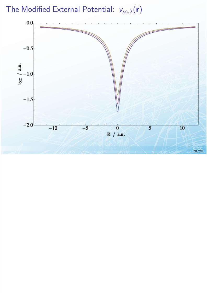
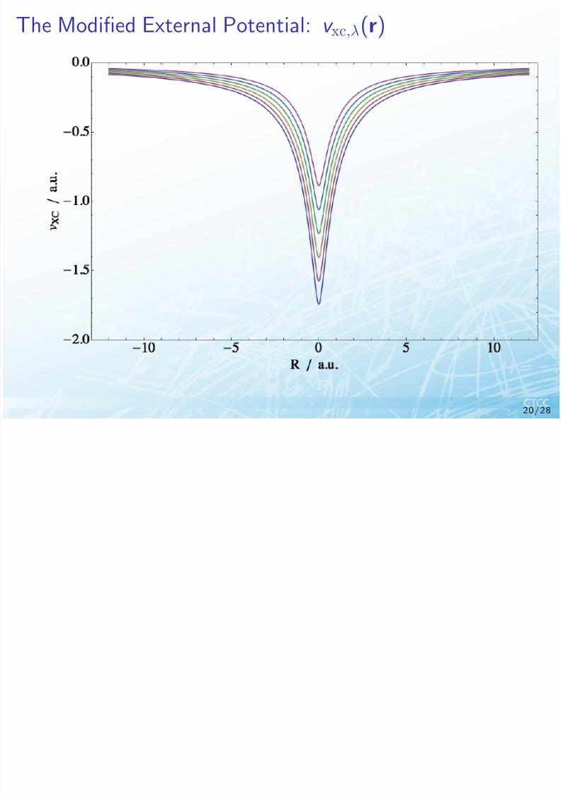
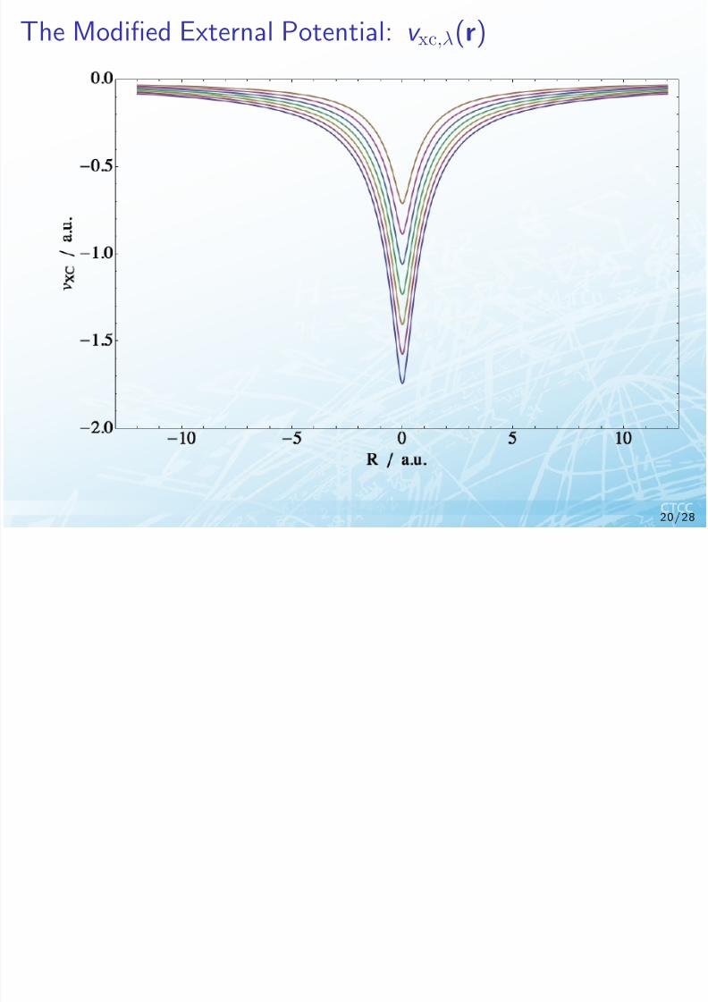
The Modified External PotentialThe potential was expanded as

v λ(r) = v ext(r) + (1− λ)v J(r) + v xc,λ(r)



= v ext(r) + (1− λ)v ref (r) +

t b t g t (r)

T. Heaton-Burgess, F. A. Bulat and W. Yang, Phy. Rev. Lett., 98, 256401, (2007)

19/28



= v ext(r) + (1− λ)v ref (

r) +

t b t g t (

r)

The exchange–correlation contribution is then

v xc,λ(r) = (1 − λ)[v ref (r)− v J(r)] +

t b t g t (r)

For 2 electron systems we can also use v x (r) = −12v J (r) toget the correlation potential

v c,λ(r) = v xc,λ(r) +(1− λ)

2v J(r)


19/28





= v ext(r) + (1− λ)v ref (

r) +

t b t g t (

r)

The exchange–correlation contribution is then

v xc,λ(r) = (1 − λ)[v ref (r)− v J(r)] +

t b t g t (r)

For 2 electron systems we can also use v x (r) = −12v J (r) toget the correlation potential

v c,λ(r) = v xc,λ(r) +(1− λ)

2v J(r)

Whilst the potentials may not be unique in a finite basis apenalty function minimization can be performed to givesmooth potentials, changing W λ by less than 10−5 a.u.


19/28

The Modified External Potential: v xc,λ(r)



20/28




20/28

The Modified External Potential: v c,λ(r)



C Umrigar and X Gonze, Phys. Rev. A, 58, 3827, (1994)

21/28





21/28




Building DFT Functionals Using the ACThe obvious motivation for studying the AC is to developimproved E xc functionals.

Simple forms for approximating W λ can be turned directly

into Exc functionals by integration



into E xc functionals by integration.

A. D. Becke, J. Chem. Phys., 98, 1372, (1993)M. Ernzerhof, Chem. Phys. Lett., 263, 499, (1996)

A. J. Cohen, P. Mori-Sanchez and W. Yang, J. Chem. Phys., 127, 034101, (2007)

22/28





into Exc functionals by integration



into E functionals by integration.This idea has been followed before,

The Becke H&H funcitonal used linear interpolation with E xfor the W 0 and E LDAxc for W 1

Ernzerhof considered a Pade type form



22/28





into E xc functionals by integration.



into functionals by integration.This idea has been followed before,

The Becke H&H funcitonal used linear interpolation with E xfor the W 0 and E LDAxc for W 1

Ernzerhof considered a Pade type formMori-Sanchez, Cohen and Yang considered a variety of simpleforms

We investigated a variety of forms for H2 and the HeliumIsoelectronic series with the input parameters determined fromFCI data.



22/28

Building DFT Functionals Using the ACTwo forms were found to give good performance for these twoelectron systems; A Pade type form and an Exponential form.




M. J. G. Peach, A. M. Miller, A. M. Teale and D. J. Tozer, J. Chem. Phys., 129, 244104, (2008)

23/28

Building DFT Functionals Using the ACTwo forms were found to give good performance for these twoelectron systems; A Pade type form and an Exponential form.

The Pade type form is

W AC1xc λ = a + b λ

1 λ



xc,λ +1 + c λ

E AC1xc = a + b

c − loge (1 + c )

c 2

a = W xc,0 = E x

b = W xc,0 = E GL2c

c =W

xc,0

W xc,1 −W xc,0− 1

W xc,1 =

Ψ1 ˆW

Ψ1

− J



23/28

Building DFT Functionals Using the AC

The Exponential form is

W AC6xc,λ = a + b exp(c λ)



, p( )

E AC6xc = a +b

c (1− exp(−c ))

b (1− exp(W xc,0/b )) = W xc,0 −W xc,1

a = W xc,0 − b

c =W

xc,0

b


24/28

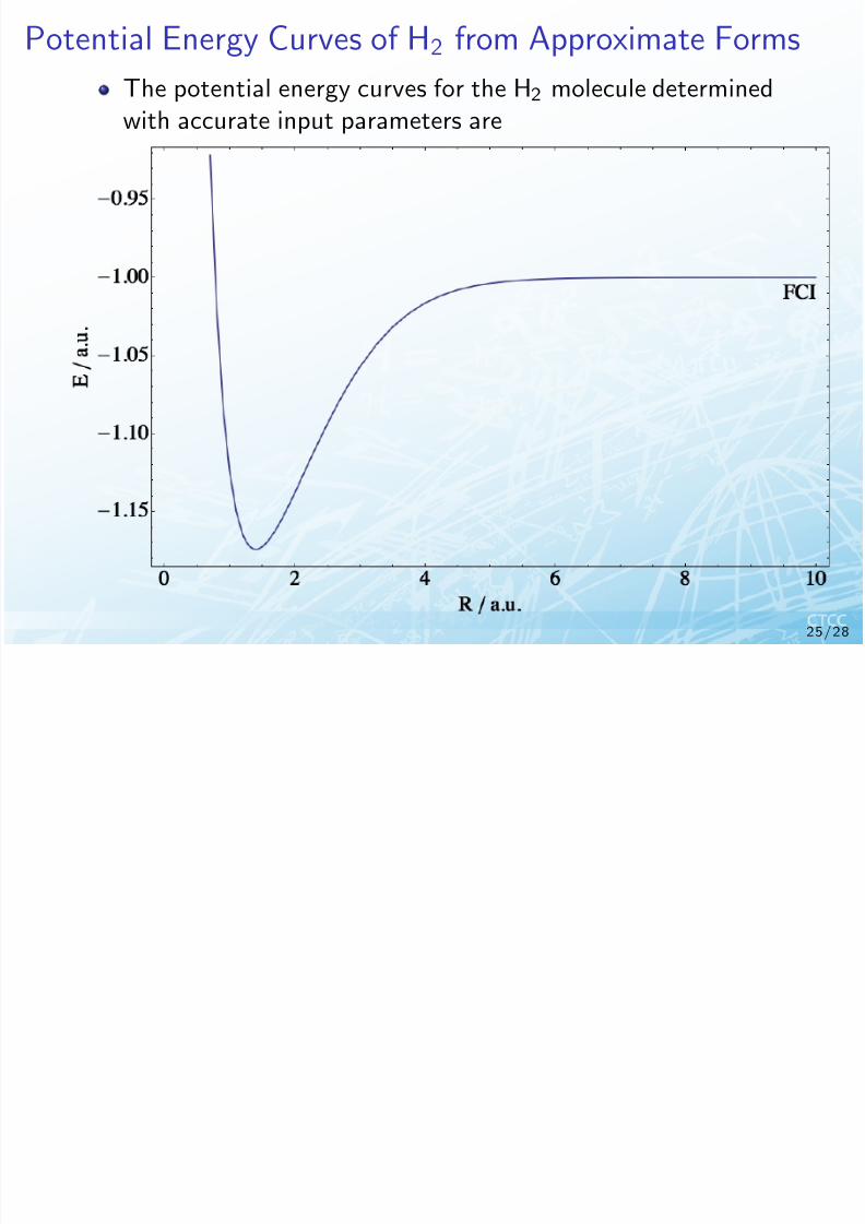
Potential Energy Curves of H2 from Approximate FormsThe potential energy curves for the H2 molecule determinedwith accurate input parameters are



25/28




Comparison with the Accurate Integrand



A. M. Teale, S. Coriani, and T. U. Helgaker (accepted, JCP)

26/28





26/28




ConclusionsWe can calculate AC curves corresponding to accuratecoupled cluster wavefunctions

The resulting curves accurately reproduce the CC density and

the correct exchange–correlation energies



27/28






The direct optimization approach provides a rapidlyconvergent scheme, this is ensured by our calculation of thesecond derivative

27/28




Th di i i i h id idl




The curves provide the missing link between constrainedsearch methods which provide the Kohn-Sham potential butno associated energy functional and approximate energyfunctionals suitable for practical use

27/28

Conclusions

We can calculate AC curves corresponding to accuratecoupled cluster wavefunctions



Th di i i i h id idl




The curves provide the missing link between constrainedsearch methods which provide the Kohn-Sham potential butno associated energy functional and approximate energyfunctionals suitable for practical use

The curves determined are useful for understandingapproximate exchange–correlation forms and the developmentof new ones

27/28

Acknowledgements

Trygve Helgaker Sonia Coriani



David Tozer Michael Peach

28/28

adiabatic formalism

Documents

Transcript of adiabatic formalism