Adaptive optics with 4 laser guide stars: cone effect correction on large telescopes

Elise Viard, Norbert Hubin and Miska Le Louarn

ESO, Karl Schwarzschild Str. 2, D-85748 Garching, Germany

ABSTRACT

In this paper, we study the performance of an adaptive optics system with 4 laser guide stars (LGS) and a natural guide star (NGS), and compare it to the system with 1 LGS, both installed on an 8-m telescope. Focus anisoplanatism is obtained with a numerical simulation. The typical errors of NGS wavefront are computed with analytical formulae. The entire system is studied to obtain its performance in terms of achievable Strehl ratio.

This 4-LGS method allows to push adaptive optics system towards the visible part of the spectrum without tomographic reconstruction of 3D atmospheric perturbation. The cone effect is two times smaller with 4-LGS than with l-LGS, allowing to reach almost a Strehl ratio of 0.5 at 500 nm. Considering the NGS errors and the focus anisoplanatism, the Strehl ratio (SR) can reach 0.45 at 1.25 ,wrn under good seeing (GS) conditions with the Nasmyth Adaptive Optics System (14 x 14 sub-pupils wavefront sensor) at the Very Large Telescope.

Keywords: Multiple Laser Guide Star, Adaptive Optics, focus anisoplanatism

I. INTRODUCTION

Adaptive Optics (AO) systems installed on 4 meters class telescopes, like ADONIS or PUEO, have demonstrated their efficiency in improving the image quality for astronomical observations. These performances are generally known and most of large telescopes are now being equipped with such A0 systems. To correct for the atmosphere, a bright guide star is needed, but as sky coverage studies demonstrate it, bright objects candidates are rare (see, for example, Le Louarn et all). A0 systems are only used for near-infrared observations, the sky coverage in the visible being almost zero. Pushing the A0 systems towards the visible part of the spectrum remains a real challenge. In this paper, we study one of the problems related to A0 in the visible.

The lack of bright Natural Guide Stars (NGS) has been compensated by developing techniques to create Laser Guide Stars (LGS). Foy & Labeyrie2 proposed to use a laser beam to create an artificial star in upper atmospheric layers. Either Rayleigh and Mie scattering at altitudes around lo-20 km or resonant scattering by sodium atoms near 90 km can be used to create an artificial guide star. The LGS brings two main problems. Due to the round trip of the laser light, the tip-tilt measurement cannot be obtained from a LGS. The second drawback is the consequence of the finite altitude of the artificial star. The LGS emits a spherical wavefront, which does not pass through the same turbulence as the science object. Nevertheless, the science object is corrected by using the phase measurements of the laser light. The error induced is called focus anisoplanatism or cone effect. It induces a systematic wrong correction and thus limits the improvement of the image quality. It becomes more critical towards shorter wavelengths, for larger telescope apertures, or for worse seeing. At an average astronomical site and for an 8-m telescope, due to the cone effect, the Strehl ratio (SR) due to the cone effect is attenuated almost to zero at visible wavelengths. The focus anisoplanatism has already been largely studied and the best solution is to use several guide stars.

The tomographic method has been proposed to sense all the atmosphere and to reconstruct the 3D volume (see3). It is currently under study and will likely solve most of the cone effect allowing the implementation of an A0 system in the visible. Simpler methods using multiple LGS have also been proposed to correct for the cone effect. In these methods, only the perturbation over the telescope pupil is measured without any knowledge of the atmospheric perturbation 3D distribution. Three different techniques have been proposed by Parenti & Sasiela,4 so-called merging, stitching and butting. The principle is to measure all the LGS with only one wavefront sensor.

Further author information: (Send correspondence to EV) EV: E-mail: eviard@eso.org NH: E-mail: nhubin@eso.org MLL: E-mail: lelouarn@eso.org

Proc. of SPIE Vol. 4007, Adaptive Optical Systems Technology, ed. P. Wizinowich, P. Wizinowich (Apr, 2000) Copyright SPIE

106

The difference between the three methods is the way in which the LGS are considered. In the case of merging, each LGS is measured by the entire sensor, whereas in the butting method the sensor is “divided” in sub-systems, each of them sees only one LGS. The stitching method follows the same idea as the butting one, but it considers the edge problems between the sub-systems and overlaps small parts of the beams in order to combine their measurements together.

The three methods have not been fully studied, so the aim of this paper is to obtain a rigorous knowledge of the butting method. We call it the 4-LGS method hereafter. In order to avoid discontinuities between the different LGS measurements, we use a NGS to glue the measurements together, by measuring the tip-tilt at each sub-pupil. It is easy to compute all the modes obtained with 4 sub-pupils and a tip-tilt measurement in each of them. All the modes up to the astigmatism included have to be measured by the NGS.

A numerical simulation is used to obtain the focus anisoplanatism related to the 4-LGS. It allows to compare the 4-LGS Strehl ratio to the I-LGS one. Then, in order to consider all the errors of an adaptive optics system, we use the analytical formulae describing the usual NGS errors. By adding all of them together, the entire system 4-LGS plus 1-NGS for the low orders is studied and its Strehl ratio dependence on the wavelength, on the NGS magnitude and on the NGS off-axis angle are obtained.

This method is simpler than the tomographic method and gives enough improvement to be used in the visible. In the first part of the paper, the geometry of the system is described. Then, the focus anisoplanatism is computed for our system composed of 4-LGS. It is followed by an analytical study of the 4 LGS method to obtain the SR dependence on the wavelength, NGS magnitude and off-axis angle in the visible.

2. THE GEOMETRY OF THE SYSTEM

The focus anisoplanatism has been characterized by Tyler5 by the ratio of the telescope diameter D to the so-called de parameter depending on the turbulence profile and on the wavelength. As focus anisoplanatism is proportional to D, for a given d 0, the 4-LGS method will have smaller focus anisoplanatism error than the other methods, each LGS being only measured by a part of the sensor. A schematic view of the system is presented in figure 1.

The first-generation A0 system for the VLT (Very Large Telescope*) called NAOS (Nasmyth Adaptive Optics System+) will be soon installed at Cerro Paranal (in Chile). It will be used for mid-IR observations only. The second generation of instruments is already in study and the goal is to have a visible A0 system by 2006. We study the 4-LGS method using NAOS characteristics in order to know the performance of such a system. Each laser is only seen by a part of the wavefront sensor. With four laser guide stars, we can define four sub-systems composed of a quarter of the sensor and a LGS. In order to have a minimum focus anisoplanatism, each LGS has to be positioned above the center of gravity of its own sub-pupil.

The gravity center of a 90’ sector with a unit radius is located at a distance of 4@(37r) = 0.600. From the center, for an 8 meter telescope, we obtain:

TOP = 2.40 m,

or

for a sodium layer altitude H = 90 km. roPIH = 5.50”

The technique to determine the residual distortion of the wavefront is described in section 3.1. We obtain the smallest mean-square residual wavefront distortion for LGS offsets between 5 and 5.7 arcsec. The NGS is assumed to be on-axis to eliminate the errors related to anisoplanatism.

The system itself is composed of a Shack-Hartman wavefront Sensor (SHS) with 14 by 14 sub-apertures. The 4-LGS are 9 magnitude artificial stars. All the other parameters are given in table 1 and in figure 1.

The NGS measurements are made with a 4 by 4 SHS in order to be able to combine the laser measurements. This is the mimimum size needed to measure up to the radial degree n=3 but by taking more sub-apertures we would have more photon noise. In order to have an idea of the performance of the future A0 system, we consider also a 40 x 40 sub-apertures SHS with a 6 magnitude LGSs and called it “NAOS-40”. Now, the system being defined, the focus anisoplanatism of the 4-LGS method has to be determined.

* http://www.eso.org/projects/vlt/ +http://www.eso.org/instruments/naos/index.html

Proc. SPIE Vol. 4007 107

* 1 NGS * 1 NGS

4 LGS

-3 8 meter telescope

Figure 1. The two systems studied are presented. The SR obtained with 4-LGS and NAOS-40 are compared to those obtained with I-LGS and NAOS-40. The 4-LGS and I-LGS methods are also compared with the NAOS-14 configuration.

Parameters NAOS-14 NAOS-40 NGS tip-tilt NGS higher order Sub-apertures number 14 x 14 40 x 40 2x2 4x4 Pixel number per sub-aperture 8 8 8 8 Pixel FOV (arcsec) 0.29 0.1 0.5 0.5 Optimized Wavelength (pm) 2.2 0.9

Table 1. The different configurations used to compute the performances.The optimized size has been computed for good seeing conditions (TO = 0.25m).

3. THE FOCUS ANISOPLANATISM

3.1. Phase variance due to the focus anisoplanatism

A0 systems are affected by different kinds of errors precluding a perfect correction. Most of them are associated with the system itself and so depend on the sensor characteristics. We will present them more extensively in the next part, but first, we study the focus anisoplanatism of a 4-LGS system.

The cone effect is a consequence of the finite LGS altitude. The spherical wavefront coming from an artificial star does not pass through the same portion of the atmosphere as the plane wavefront of the science object. The mean-square residual wavefront distortion is defined by:

a2 cone = s dr-?/R){[$(f? - hGS(f?12}

s drWrl R) 7 (1)

where W(r/R) is the pupil function equal to 1 if r < R, zero otherwise. qb(r3 and &G,#) are, respectively, the wavefronts measured by the NGS and by the LGS. Tyler5 found that ozone can be estimated for 1 LGS with the following expression:

o2 = (D/d0)5/3,

do = x6/5 cos3/5

(2)

Proc. SPIE Vol. 4007108

where F(h/H) is a combination of hyper-geometric functions5

Knowing the C:(h) and the wavelength, the cone effect can be computed from (2). It is also possible to calculate it from (1). The analytical solution found by Tyler is only valid for 1 LGS, then a numerical computation must be done to obtain the focus anisoplanatism of the 4 LGS method.

The main concept of LA30S2 (Laser Aided Astronomical Adaptive Optics System Simulator) simulation software is described in Delplancke et al? and Carbillet et al? This software, developed in the frame of a TMR network, allows to simulate A0 systems. We summarize here the atmospheric simulation. The perturbation is modeled by several layers. Only phase variations are considered and they are supposed to be weak. Scintillation is neglected. The atmospheric parameters are summarized in table 2. Due to its spherical wavefront, the LGS light passes through

Parameters Good Seeing conditions Median Seeing conditions (GS) (MS)

f-0 cm> 0.25 0.15 h (km) 1 1 Cl 0.7 0.7 ha (km) 10 10 c2 0.3 0.3 do cm> 5 3

Table 2. Atmospheric parameters considered in the simulation. Two layers are simulated at altitudes hi with relative strengths ci.

a smaller part of the upper layers than the NGS wavefront. In the simulation, we magnify each layer by the factor ( j$f&( h w ere H is the sodium layer altitude and hl, is the atmospheric layer altitude) before summing up all the phase screens to obtain the phase perturbation on the telescope pupil.

Focus Anisoplanatism

o.ok’ I I I I I I 1 I I 1 1 I I I I I I 1

500 1000 1500 2000 2500 Wavelength (nm)

Figure 2. SR obtained with the 4-LGSs (J, and full lines) method compared to the results of 1 LGS (dashed lines). Results with good and median seeing are plotted in this figure. The upper solid and dashed lines are for ro = 0.25 m, the lower solid and dashed lines are for rg = 0.15 m.

Considering one LGS, the focus anisoplanatism can be computed with (1) or with the analytical formula (2). The two methods give the same focus anisoplanatism for 1 LGS. At 1 pm, under GS conditions, we obtain SR of 0.64 It validates the method and gives us a way to determine the focus anisoplanatism for the 4 LGS method.

Proc. SPIE Vol. 4007 109

3.2. Numerical simulation for 4 LGS system

We use eq. (1) to compute the residual variance for the 4-LGSs method. As explained in the previous section, each sub-system sees only one LGS to sense the atmosphere above a part of the pupil. In order to have good statistics, we simulate 100 statistically different wavefronts. We compute a composite wavefront made of 4 different quarters of the 4 LGSs wavefronts. By computing the statistical variance of the difference between &LGS and &GS we obtain the mean-square residual distortion for 4 LGSs. The results are shown in the figure 2. They do not depend on the SHS characteristics. The SR obtained with 1 LGS is almost zero in the visible under Median Seeing (MS) conditions giving poor corrections with an adaptive optics system. With 4 LGS, at X =500 nm, the SR increases to 0.4 under Good Seeing (GS) conditions. Without considering the sensor limitations, the 4-LGS configuration is sufficient to obtain a good correction in the visible. But what are the results obtained with 4-LGS and a real A0 system? The cone effect evaluation has to be added to the other usual errors of A0 system working with a NGS. We study the performance reached by the NAOS system using 4-LGS method. In order to get an idea of a higher-order system characteristics and its performance, we will compare NAOS to a 40 by 40 subapertures SHS system, called NAOS-40.

4. ANALYTICAL STUDY OF THE CONFIGURATIONS

4. I. The analytical formulae

The different errors in an A0 system have already been expressed by analytical formulae in a number of papers (see Greenwood et al.,8 Rigaut.g , Parenti & Sasiela,4 Roussetl” and Sandler et al?). These formulae allow to study the entire error budget of a specified A0 system.

These errors reduce the performance of an A0 system. Some are related to the geometry of the system like the sensor noise, the fitting and aliasing errors, the others are the consequences of external noise like the sky background or the photon noise directly related to the number of photons emitted by the source. All these errors are highly dependent on the sensor characteristics. The fitting and aliasing errors given by Rigautg and Greenwood decrease with wavelength (& + Cr,2lia = 0.54(d,/ro)5/3 cx X6j5). The larger is the sub-aperture, the bigger is this error. With a 4 by 4 SHS, the variance obtained is 5 rad2 at 500 nm with a median seeing, giving SR = 0.

The sensor noise (a;) is described in Rousset et al. lo It depends mainly on the ratio of the sensor wavelength to the science object one, on the sky background noise, the number of pixels per sub-aperture, the number of photons, the sub-aperture diameter and the r 0. It decreases with wavelength (oc Xe4i5) and with the photon flux (oc Npi2).

The photon noise (o:,‘” and4)depends on the photon number and on the wavefront sensor wavelength. It decreases with the number of photon as A$;‘. Its wavelength dependence is XV2i5.

The phase global variance for an A0 system with 4-LGS is defined by:

o2 2 2 = %o + %,

gtO beeing the high-order errors related to the 4-LGS and NAOS-14 (or NAOS-40) systems and 012, the low-order errors on the NGS measurements. These variances are defined by:

2 Oho + 6 + ,;, + o:o~w

and 2

% = &lo + gzh-lo + dniso,

After the variance definition, we can study how the system performance depends on wavelength (section 4.2), on magnitude (section 4.3) and on the NGS off-axis angle (section 4.4).

Proc. SPIE Vol. 4007110

NAOS-14 1.0 “““*““o”“““j

0.8

0 ‘A

$ 0.6 k

2 : 0.4 s

0.2

0.0 1000 1500 2000 2500 500 1000 .I.500 2000 2500

Wavelength (nm) wavelmgth. (nm)

Figure 3. SR obtained with the 4 LGS method (jc) compared to the results of 1 LGS (dashed line) under GS conditions (upper curves) and under MS conditions (lower curves). Left: the LGS magnitude is 9, the system is NAOS with a 14 x 14 sub-apertures SHS. Right: the LGS magnitude is 6, the system is a 40 x 40 sub-apertures SHS.

4.2. SR dependence on the wavelength

All the SHS errors defined in the previous section are proportional to the wavelength. So the main issue of this study is to know which error dominates in the NAOS-14 and in the NAOS-40. The left curve of the figure (3) shows the Strehl ratio dependence on the wavelength for the NAOS-14 system. The 4-LGS and 1 LGS methods are compared under GS and MS conditions. The right curve of the figure (3) shows the Strehl ratio dependence on the wavelength for the NAOS-40 system.

The two systems have sub-aperture size optimized for different wavelengths. NAOS-40 optimized wavelength is 1.2 pm whereas NAOS-14 is optimized around 3pm. So, of course the two systems give bad SR in the visible as the fitting and aliasing errors dominate. At lpm, the NAOS-40 gives a SR of 0.7 for the 4-LGS method whereas the 1 LGS method with the NAOS-40 gives SR of 0.5 (under GS conditions). The improvement is lower under Median Seeing (MS) conditions, the 4-LGS results for NAOS-40 reaching only 0.45 SR. With the NAOS-14 system, the aliasing and fitting errors dominate up to approximately 1.5 pm. Hence SR of 4-LGS is only 26% better than that of l-LGS at lpm.

Even if the NAOS-40 system is highly dependent on seeing conditions, the 4-LGS method with NAOS-40 allows to reach good performance with an A0 system at lpm.

4.3. Effect of the NGS magnitude on the SR

The performance difference between the 1 LGS and the 4-LGSs methods is mainly seen between 700 nm and 1500 nm. We therefore study the two methods dependence on the NGS magnitude at 1250 nm. Indeed, the main limitation of the 4-LGS method is the NGS magnitude. A 4-LGS method needs a brighter NGS than the I-LGS method to be able to combine the 4-LGS measurements together. Then, for faint NGS, the performance of the 4-LGS method is lower than that of the l-LGS method. The Strehl ratio dependence on the NGS magnitude is shown in the figure (4). The left part gives the NAOS-14 performance with 4-LGS (solid lines), I-LGS (diamonds lines) under MS and GS conditions. The right plot shows the NAOS-40 performance.

The two systems have approximately the same limiting magnitude. When the NGS is fainter than llm, the 4-LGS performance decreases. If the NSG is fainter than 14”, the I-LGS method gives better SR than the 4-LGS method.

The 4-LGS method is strongly dependent on the NGS magnitude. Even with the NAOS-40 system, the NGS has to be brighter than R = 15.

Proc. SPIE Vol. 4007 111

NAOS-14 NAOS-40 1.0 1.0

0.8 0.8

0 0 ‘r( 2

*d 0.6 2 0.6

k k

2 2 f 0.4 E 0.4 t; z

0.2 0.2

5 10 15 Guide star R magnitude

5 10 15 Guide star R magnitude

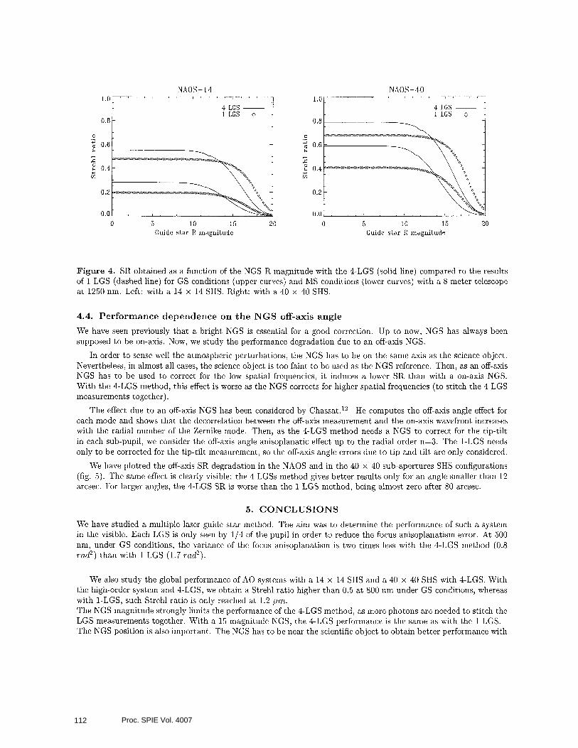
Figure 4. SR obtained as a function of the NGS R magnitude with the 4-LGS (solid line) compared to the results of 1 LGS (dashed line) for GS conditions (upper curves) and MS conditions (lower curves) with a 8 meter telescope at 1250 nm. Left: with a 14 x 14 SHS. Right: with a 40 x 40 SHS.

4.4. Performance dependence on the NGS off-axis angle

We have seen previously that a bright NGS is essential for a good correction. Up to now, NGS has always been supposed to be on-axis. Now, we study the performance degradation due to an off-axis NGS.

In order to sense well the atmospheric perturbations, the NGS has to be on the same axis as the science object. Nevertheless, in almost all cases, the science object is too faint to be used as the NGS reference. Then, as an off-axis NGS has to be used to correct for the low spatial frequencies, it induces a lower SR than with a on-axis NGS. With the 4-LGS method, this effect is worse as the NGS corrects for higher spatial frequencies (to stitch the 4 LGS measurements together).

The effect due to an off-axis NGS has been considered by Chassat. l2 He computes the off-axis angle effect for each mode and shows that the decorrelation between the off-axis measurement and the on-axis wavefront increases with the radial number of the Zernike mode. Then, as the 4-LGS method needs a NGS to correct for the tip-tilt in each sub-pupil, we consider the off-axis angle anisoplanatic effect up to the radial order n=3. The I-LGS needs only to be corrected for the tip-tilt measurement, so the off-axis angle errors due to tip and tilt are only considered.

We have plotted the off-axis SR degradation in the NAOS and in the 40 x 40 sub-apertures SHS configurations (fig. 5). The same effect is clearly visible: the 4 LGSs method gives better results only for an angle smaller than 12 arcsec. For larger angles, the 4-LGS SR is worse than the 1 LGS method, being almost zero after 80 arcsec.

5. CONCLUSIONS

We have studied a multiple laser guide star method. The aim was to determine the performance of such a system in the visible. Each LGS is only seen by l/4 of the pupil in order to reduce the focus anisoplanatism error. At 500 nm, under GS conditions, the variance of the focus anisoplanatism is two times less with the 4-LGS method (0.8 rad2) than with 1 LGS (1.7 rad2).

We also study the global performance of A0 systems with a 14 x 14 SHS and a 40 x 40 SHS with 4-LGS. With the high-order system and 4-LGS, we obtain a Strehl ratio higher than 0.5 at 800 nm under GS conditions, whereas with I-LGS, such Strehl ratio is only reached at 1.2 pm. The NGS magnitude strongly limits the performance of the 4-LGS method, as more photons are needed to stitch the LGS measurements together. With a 15 magnitude NGS, the 4-LGS performance is the same as with the 1 LGS. The NGS position is also important. The NGS has to be near the scientific object to obtain better performance with

Proc. SPIE Vol. 4007112

NAOS-14 NAOS-40 1.0

1 LGS . . . . . . . . . . . . . . . . . . - 0.8

s -rl 4 z 0.6

2 k?

d 0.4

E

20 40 60 80 100 0 20 40 60 80 100 Off-axis angle (arcsec) Off-axis angle (arcsec)

Figure 5. Performance degradation as a function of the NGS off-axis angle (in arcsec) at 1250 nm. The 4 LGS SR loss is plotted in solid line, while the 1 LGS SR loss is plotted in dashed line. The results are presented for both the GS and MS conditions. Left: NAOS case. Right: 40 x 40 SHS case.

the 4-LGS method than the I-LGS method. If the NGS is further than 12 arcsec the I-LGS gives better results at 1250 nm.

ACKNOWLEDGMENTS

Many thanks to Andrei Tokovinine for his helpful corrections and comments on the last stages of this work. Thanks to Michel Tallon and Christian Perrier-Bellet for their comments.

The LA30S2 software has been developed in the frame of the European Training Mobility of Researchers Network “Laser guide Stars for 8 meter telescopes” of the European Union, contract #ERBFMRXCT960094.

REFERENCES

1. M. Le Louarn, R. Foy, N. Hubin, and M. Tallon, “Laser guide star for 3.6m and 8m telescopes: performances and astrophysical implications,” iWVK4S 295(4), p. 756, 1998.

2. R. Foy and A. Labeyrie, “Feasability of adaptive optics telescope with laser probe,” A&on. Astrophys. 152, pp. L29-L31, 1985.

3. M. Le Louarn and M. Tallon, “A solution to the cone effect: the 3d mapping of turbulence,” J. Opt. Sot. Am. A to be submitted, 2000.

4. R. R. Parenti and R. J. Sasiela, “Laser guide star systems for astronomical applications,” J. Opt. Sot. Am. A 11, pp. 288-309, February 1994.

5. G. A. Tyler, “Rapid evaluation of do: the effective diameter of a laser guide star adaptive optics system,” J. Opt. Sot. Am. A 11, pp. 325-338, February 1994.

6. F. Delplancke, M. Carbillet, N. N. Hubin, S. Esposito, F. J. Rigaut, E. Marchetti, A. Riccardi, E. Viard, R. Ragazzoni, M. Le Louarn, and L. Fini, “Laser guide star simulations for 8-m class telescopes,” in SW,?Z, vol. 3353, pp. 371-382, 1998.

7. M. Carbillet, F. Delplancke, S. Esposito, B. Femenia, L. Fini, A. Riccardi, E. Viard, N. Hubin, and F. Rigaut, “LA30S2: A Software Package for Laser Guide Star Adaptive Optics Systems,” in SPIE, vol. 3762, pp. 379- 389, 1999.

8. D. P. Greenwood, ‘LMutual coherence of a wave front corrected by zonal adaptive optics,” J. Opt. Sot. Am. 69(4), pp. 549-554, 1979.

9. F. Rigaut, 0. Lai, and J. P. V&an, “Pueo’s performance: image quality improvement,” tech. rep., Observatoire de Paris. 1996.

Proc. SPIE Vol. 4007 113

10. G. Rousset, Adaptive Optics for astronomy, pp. 115-137. Kluwer Academic Publisher, 1994. 11. D. G. Sandler, S. Stahl, M. Angel, J. R. P.and Lloyd-Hart, and D. McCarthy, “Adaptive optics for diffraction-

limited infrared imaging with 8-m telescopes,” J. Opt. Sot. Am. A 11, p. 925, Feb. 1994. 12. F. Chassat, “Calcul du domaine d’isoplani3tisme d’un systhme d’optique adaptative fonctionnant B travers la

turbulence atmosph&ique,” J. Optics (Paris) 20(l), pp. 13-23, 1989.

Proc. SPIE Vol. 4007114