Adaptive classiﬁcation of marine ecosystems: Identifying ... and Bodtker 2007.pdf · Adaptive...

ARTICLE IN PRESS

0967-0637/$ - see

doi:10.1016/j.ds

�CorrespondiE-mail addre

Deep-Sea Research I 54 (2007) 385–402

www.elsevier.com/locate/dsri

Adaptive classification of marine ecosystems: Identifyingbiologically meaningful regions in the marine environment

Edward J. Gregr�, Karin M. Bodtker

Marine Mammal Research Unit, Fisheries Centre, University of British Columbia, 6248 Biological Sciences Road,

Vancouver, BC, Canada V6T 1Z4

Received 26 April 2005; received in revised form 21 November 2006; accepted 30 November 2006

Available online 2 February 2007

Abstract

The move to ecosystem-based management of marine fisheries and endangered species would be greatly facilitated by a

quantitative method for identifying marine ecosystems that captures temporal dynamics at meso-scale (10s or 100s of

kilometers) resolutions. Understanding the dynamics of ecosystem boundaries, which may differ according to the species of

interest or the management objectives, is a fundamental challenge of ecosystem-based management. We present an adaptive

ecosystem classification that begins to address these challenges. To demonstrate the approach, we quantitatively bounded

distinct, biologically meaningful marine regions in the North Pacific Ocean based on physical oceanography. We identified

the regions by applying image classification algorithms to a comprehensive description of the ocean’s surface, derived from an

oceanographic circulation model. Our resulting maps illustrate 15 distinct marine regions. The size and location of these

regions related well to previously described water masses in the North Pacific. We investigated seasonal and long-term

changes in the pattern of regions and their boundaries by dividing the oceanographic data into four seasons and two 10-year

time periods, one on either side of the 1976–1977 North Pacific Ocean climate regime shift. We compared our results for each

season across the regime shift and for sequential seasons within regimes using the Kappa Index of Agreement and the index

of Average Mutual Information. Seasonal patterns were more similar between regimes than from one season to the next

within a regime, while the magnitude of seasonal transitions appeared to differ before and after the regime shift. We assessed

the biological relevance of the identified regions using seasonal maps derived from remotely sensed chlorophyll-a

concentrations ([chl-a]). We used Kruskal–Wallis and Wilcoxon rank sum tests to evaluate the correspondence between the

[chl-a] maps and our post-regime shift regions. There was a significant difference in [chl-a] among the regions in all seasons.

We found that the number of regions with distinct chlorophyll signatures, and the associations between different regions,

varied by season. The overall pattern of association between the regions was suggestive of observed, broad-scale patterns in

the seasonal development and distribution of primary production in the North Pacific. This demonstrated that regions with

different biological properties can be delineated using only physical variables. The flexibility of our approach will enable

researchers to visualize the geographic extents of regions with similar physical conditions, providing insight into ocean

dynamics and changes in marine ecosystems. It will also provide resource managers with a powerful tool for broad

application in ecosystem-based management and conservation of marine resources.

r 2007 Elsevier Ltd. All rights reserved.

Keywords: Ecoregion; Biogeography; Ecosystem management; Habitat modeling; Ecosystem models; Habitat classification; North Pacific

front matter r 2007 Elsevier Ltd. All rights reserved.

r.2006.11.004

ng author.

ss: [email protected] (E.J. Gregr).

www.elsevier.com/locate/dsri

dx.doi.org/10.1016/j.dsr.2006.11.004

mailto:[email protected]

ARTICLE IN PRESSE.J. Gregr, K.M. Bodtker / Deep-Sea Research I 54 (2007) 385–402386

1. Introduction

Studies at the ecosystem level are relevant to bothfisheries management and protected areas defini-tion. Fisheries managers are increasingly required totake ecosystem considerations into account whenassessing commercially exploited stocks, while con-servation efforts are increasingly focused on deli-neating areas that will protect habitats of species atrisk at all life stages. The determination of habitatboundaries (e.g., essential or critical habitat) forboth endangered and commercial marine species hasbeen a legal requirement in the United States fordecades under both the Endangered Species Act(1973) and the Magnuson-Stevenson FisheriesConservation and Management Act (1996). InCanada, similar legislation is now in place in theform of the Species at Risk Act (2002). Thisincreasing focus on ecosystem-based management,first advocated at least 70 years ago (Allee, 1934),presents significant challenges, including the map-ping of marine ecosystems in space and time.

Ecosystem mapping—the characterization of aphysical environment and its associated biota—iscomplex. Even in terrestrial ecology, commonlydescribed as being decades ahead of marine ecologyin terms of ecosystem classification, there is nosingle, general non-taxonomic classification systemfor ecological units beyond the species level(Morrison et al., 1998). Instead, terrestrial regionsare often delineated based on biological, geo-graphic, and climatic characteristics (e.g., biogeocli-matic zones). This works well as an operationaldefinition of terrestrial ecosystems because thebiological component (i.e., flora) is relativelyimmobile. It is only an operational definitionbecause it does not include the more mobilecomponents of the terrestrial ecosystem (e.g.,insects, birds, ungulates). Biogeoclimatic zones thusprovide landscape ecologists a bio-physical pattern,a spatial context, in which the more mobilecomponents of the terrestrial ecosystem exist.

There has been limited success in applying themethods of landscape ecology to the oceans. Whileeven a cursory examination reveals physical andbiological patterns in the oceans at a range of spatialand temporal scales (e.g., Bakun, 1996; Mann andLazier, 1996), the patterns are ephemeral andmanifest themselves differently across spatial scales.In contrast to the landscape, marine primaryproduction (phytoplankton) is patchy, ephemeral,and quickly consumed by higher trophic levels. The

processes responsible for creating the patterns inphytoplankton distribution are largely a function ofphysical forcing and the associated biological re-sponse (Platt and Sathyendranath, 1999). The overallbiogeographic patterns (ecosystems) thus represent acombination of environmental structure, speciesbehavior, and population dynamics (MacArthur,1972).

Variability in physical forcing results in physicalpatterns with different spatial and temporal scalesthat provide the environmental structure for theoverlying biology. However observations of thesebiological patterns and their integration into theclassification can be complicated by species atvarious trophic levels, operating at different spa-tio-temporal scales (Steele, 1989). Given the dy-namic nature of the marine environment and themobility of the species of interest (marine mammalsand commercial fishes), methods for delineatingecological marine boundaries must be adaptable toa range of spatial and temporal scales. Thedelineation and mapping of a dynamic geo-physicalcontext has the potential to be as useful to marineecology as biogeoclimatic zones are to terrestrialecology.

In this study, our objective was to apply imageclassification techniques to the marine environmentas a method for classifying this environmentalstructure. We hypothesized that regions of similar-ity identified by a classification based solely onphysical parameters would have both physical andbiological significance, and consequently assessedthe resulting maps in terms of both physical andbiological relevance. Since we are undertaking thetask of mapping ocean regions that are bothphysically and biologically meaningful, a brief lookat previous efforts to classify the marine environ-ment into meaningful regions is warranted.

1.1. Existing classification systems

Marine ecosystems have commonly been defined inone of four ways (Laevastu et al., 1996): the nature ofthe dominant organisms (e.g., planktonic ecosys-tems); specific physical features (e.g., reef and benthicecosystems); geographic locations (e.g., Bering Seaecosystem); or some combination of these. Classifica-tion systems have been developed to describe suchboundaries. A shared characteristic of most classifica-tion schemes is that they operate on a single spatialand temporal scale. Generally, these scales tend to belarge (coarse resolution) and have no temporal

ARTICLE IN PRESSE.J. Gregr, K.M. Bodtker / Deep-Sea Research I 54 (2007) 385–402 387

variability. Higher resolution (i.e., meso-scale) classi-fications have been limited to nearshore areas(particularly reefs, coastlines, and estuaries) becauseof the tendency to associate ecological boundarieswith tangible features (e.g., bathymetry) or withpolitical boundaries. Explicitly temporal (i.e., seaso-nal) classifications are extremely rare.

Marine classifications using some combination ofbiological and physical features, and geographiclocation, are by far the most common. The threemost frequently cited systems are: Cowardin’s(1979) classification of wetlands and deepwaterhabitats; Sherman’s (1986) Large Marine Ecosys-tems (LMEs); and Longhurst’s (1998) biomes andprovinces. These can be characterized as bottom-upclassifications, where lower trophic biology, physics,and/or chemistry are used to define marine bound-aries assumed to be meaningful for an entire multi-trophic ecosystem.

Cowardin’s (1979) system is primarily designedfor wetlands, with the marine portion limited tosubstrate characterization. LMEs (Fig. 1a), de-scribed as being characterized by unique hydro-graphic regimes, submarine topography, andtrophically-linked populations, have been exten-sively applied to ecosystem studies and management(Sherman, 1986). While the LME approach hasbeen useful, we could find no quantitative descrip-tion of how LME boundaries were identified, orhow the distinctiveness of each LME might bequantified. Longhurst’s (1998) classification of theworld’s oceans into biomes and provinces (Fig. 1b)does integrate physical oceanography with biogeo-graphy. However, Longhurst (1998) cautions thatthe boundaries illustrated are somewhat arbitrary,intended to represent approximate spatial relation-ships between the provinces.

Fig. 1. Ecosystem boundaries according to two well-known marine cl

(1986) and (b) Longhurst (1998).

Classifications have also been undertaken at localscales, typically applied to shelf waters (e.g.,Zacharias et al., 1998, in British Columbia; Bredinet al., 2001, in the Bay of Fundy). These can betermed ‘cookie cutter’ approaches, because datalayers are overlaid, and regions are defined as theintersection of the categories contained in eachlayer. Boundaries are thus a function of the spatialintersection of the source data and are often drivenby spatially invariant bathymetry or benthic cate-gories. When dynamic variables such as tempera-ture or salinity are included, seasonality is typicallyignored.

We found a single ‘‘top–down’’ approach thatattempted to identify regions based on biologicallydominant species and communities occurring there.Ray and Hayden (1993) applied Principal Compo-nent Analysis to the habitat ranges of 86 species inthe Bering, Chukchi, and Beaufort Seas andmapped six ‘provinces’ based on the highest loadingprincipal components. They noted that theseprovinces did not correspond well to the outer,middle, and inner shelf domains that are typicallyused to characterize the Bering Sea, suggesting thata single ecosystem classification does not suit allapplications.

Roff and Taylor (2000) proposed a hierarchicalscheme for classifying representative or distinctivemarine habitats for marine conservation. Theirproposed approach for linking biological andphysical attributes, while similar to ours, does notaddress the dynamic nature of boundaries. From aconservation perspective, the consequences of dy-namic ecosystem boundaries are significant (Wilsonet al., 2004).

Finally, Platt and Sathyendranath (1999) pro-posed an operational definition of ocean structure

assification systems applied to the North Pacific by (a) Sherman


for identifying production domains using biologicalrate parameters derived from remotely sensedchlorophyll. Their approach maps dynamic, bio-geochemical provinces, lends itself to seasonalanalyses, and provides a framework for investigat-ing the underlying physical processes. However,extending this approach to higher trophic levelswould require identification of the appropriate rateparameters, and their integration over the appro-priate spatial and temporal scales.

While these approaches to classification havehelped us understand some aspects of oceanicstructure, they do not provide a means of quantify-ing and mapping the dynamics of ecosystemboundaries. For example, if understanding that aCalifornia Current ecosystem exists is important,delineating its seasonal and spatial extents in anygiven season or year must be equally important.

1.2. Adaptable marine classification

Certainly, there is not one correct way to classifymarine ecosystems (Grossman et al., 1999; Steele,1989). Rather, management objectives (Grossmanet al., 1999; Perry and Ommer, 2003), processes(Morrison et al., 1998), or species (deYoung et al.,2004) determine the appropriate methods and scales(in terms of extent and resolution). By definition,the multi-species objectives of ecosystem manage-ment require a classification approach that canadapt to multiple temporal and spatial scales. Thereis some evidence that species distributions at highertrophic levels (e.g., pelagic fish and squid) arespatially linked to specific water masses and thatthese links persist across time and across contrastingphysical conditions (e.g., Garrison et al., 2002;Polovina et al., 2001). This suggests that identifyingregions of similar hydrographic properties overappropriate temporal scales may provide usefuldescriptions of species’ habitats.

In this study, we address this issue by illustratinga classification approach that is adaptable in termsof scale and input data sets, and bounds hydro-graphic structures in the oceanic marine environ-ment. Our approach differs from other marineclassification efforts because it allows availablephysical and biological data to be integrated acrossany specified spatial or temporal scale supported bythe data. While the relevant scales will be somewhatspecies-specific, resource managers must deal withseasonal and inter-annual temporal dynamics andspatial scales on the order of 10s or 100s of

kilometers. Thus, any relevant definition of amarine ecosystem must provide information atthese scales.

2. Methods

We applied image classification (a method foridentifying classes in remotely sensed images) to acomprehensive physical oceanographic data setdescribing the surface of the North Pacific to findregions of similarity within the seascape (Fig. 2). Weexamined the oceanographic and ecological rele-vance of the identified regions in three ways. First,we qualitatively compared them to documentedupper zone, hydrographic features, such as majorwater masses and surface currents. Second, wecompared changes in the patterns of regions todocumented changes resulting from the 1976–1977regime shift (e.g., Anderson and Piatt, 1999; Bensonand Trites, 2002). We also calculated the relativesimilarity of the patterns of regions among andbetween seasons for two 10-year time periods beforeand after this regime shift. Finally, we assessed thebiological significance of the regions identified in thepost-regime shift period by testing for differences inseasonal chlorophyll-a concentrations ([chl-a]), de-rived by remote sensing, among the regions.

2.1. Study area and resolution

We conducted our basin-wide classifications ofthe temperate North Pacific on a 100 by 100 km gridfor all oceanic waters between 301N and 651N. Weselected this grid size partly because of the resolu-tion of the source data (11 longitude–latitude grid),but also because the coupling of space and timescales suggests that this may be an appropriateresolution for examining meso-scale patterns typi-cally observed in open ocean ecosystems (Mann andLazier, 1996, p. 258). Since seasonal changes can berelatively pronounced at these latitudes, we chose atemporal resolution of four seasons. To visualizeand evaluate changes in the oceanic regions due todecadal scale changes in ocean climate, we producedseasonal results for two 10-year periods (1966–1975and 1980–1989). We did not evaluate inter-annualchanges.

2.2. Data

The nature of our analysis placed several con-straints on the suitability of data sets. We required

ARTICLE IN PRESS

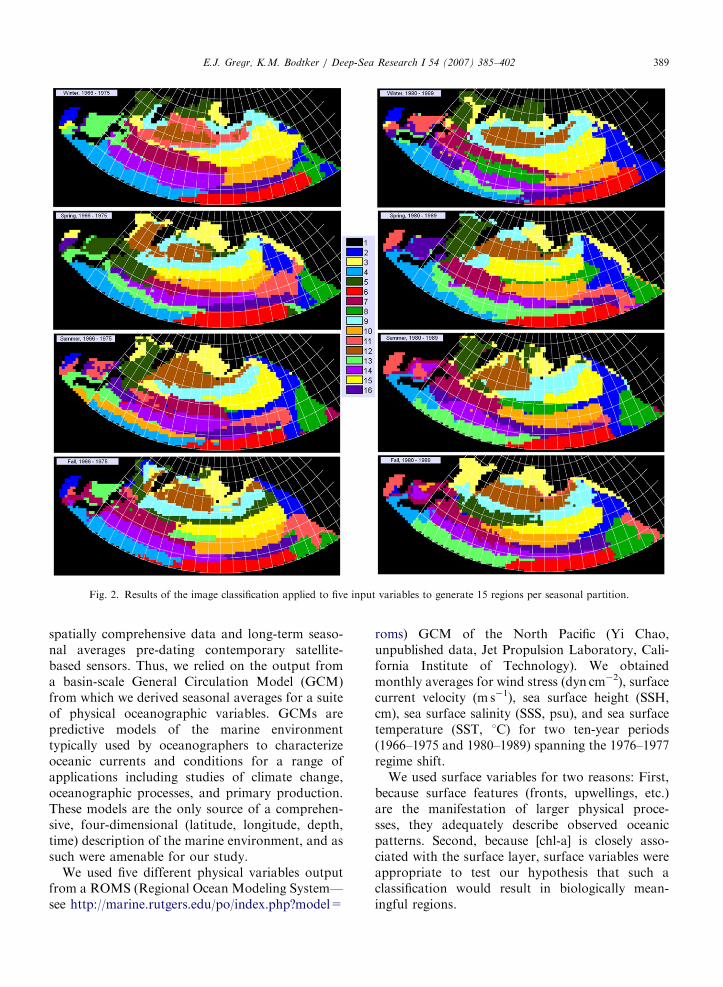
Fig. 2. Results of the image classification applied to five input variables to generate 15 regions per seasonal partition.

E.J. Gregr, K.M. Bodtker / Deep-Sea Research I 54 (2007) 385–402 389

spatially comprehensive data and long-term seaso-nal averages pre-dating contemporary satellite-based sensors. Thus, we relied on the output froma basin-scale General Circulation Model (GCM)from which we derived seasonal averages for a suiteof physical oceanographic variables. GCMs arepredictive models of the marine environmenttypically used by oceanographers to characterizeoceanic currents and conditions for a range ofapplications including studies of climate change,oceanographic processes, and primary production.These models are the only source of a comprehen-sive, four-dimensional (latitude, longitude, depth,time) description of the marine environment, and assuch were amenable for our study.

We used five different physical variables outputfrom a ROMS (Regional Ocean Modeling System—see http://marine.rutgers.edu/po/index.php?model=

roms) GCM of the North Pacific (Yi Chao,unpublished data, Jet Propulsion Laboratory, Cali-fornia Institute of Technology). We obtainedmonthly averages for wind stress (dyn cm�2), surfacecurrent velocity (m s�1), sea surface height (SSH,cm), sea surface salinity (SSS, psu), and sea surfacetemperature (SST, 1C) for two ten-year periods(1966–1975 and 1980–1989) spanning the 1976–1977regime shift.

We used surface variables for two reasons: First,because surface features (fronts, upwellings, etc.)are the manifestation of larger physical proce-sses, they adequately describe observed oceanicpatterns. Second, because [chl-a] is closely asso-ciated with the surface layer, surface variables wereappropriate to test our hypothesis that such aclassification would result in biologically mean-ingful regions.

http://marine.rutgers.edu/po/index.php?model=roms

http://marine.rutgers.edu/po/index.php?model=roms


We divided the year into four equal three-monthseasons starting with January–March. This resultedin a total of 40 coverages (i.e., digital maps), eachrepresenting one of five input variables for eighttemporal snapshots (four seasons in each of twotime periods).

2.3. Image classification

We used an unsupervised cluster analysis algo-rithm provided by the IDRISI software system(Clark Labs, 2003) to statistically organize theoceanographic input variables into distinct marineregions. The approach is analogous to terrestrialclassifications of multi-spectral satellite imagery intolandscape classes (e.g., agricultural, urban, forest,etc.). The algorithm partitions the study area into aspecified number of regions according to thevariance structure of the data.

Clustering results are most robust if the inputvariables are standardized and transformed to amultivariate-normal parameter space. We thereforeexamined the histograms for each variable andapplied a transformation to improve normalitywhen necessary. The values were then standardizedby converting each file to byte format (256 classes).

We applied IDRISI’s ISOCLUST routine (basedon H-means and K-means clustering procedures—Hartigan, 1975) to create clusters representingregions of similarity. We chose the number ofclusters to keep by examining histograms of pixelsper cluster for significant breaks in the slope. Thebreaks in slope represent different levels of general-ization of the data. Clusters with small numbers ofpixels (i.e., where the slope of the histogram flattens)are relatively insignificant. To allow comparisonsamong seasons and regimes, the resulting partitions(mapped results) required the same number ofclusters. We chose to keep 15 clusters based on avisual examination of the eight histograms.

2.4. Evaluating classification results

To evaluate the oceanographic relevance of ourregions, we compared our results with the upperzone domains identified by Dodimead et al. (1963).Specifically, we projected the results from oursummer pre-1976 analysis into geographic (lat–lon)coordinates and overlaid the schematic drawn byDodimead et al. (1963), which was based on ananalysis of summer SST, SSS, and surface currentdata from 1955–1959. These domains have proven

to be robust over time in the sense that they are stillreferred to by name in oceanographic literature.We also qualitatively compared our results tofeatures commonly mentioned in the oceanographicliterature.

We compared seasonal partitions within andbetween time periods using both the Kappa Indexof Agreement (KIA) (Pontius Jr., 2000) and theAverage of Mutual Information (AMI) (Finn,1993). KIA is a measure of the similarity of twoimages and takes into account the location andquantity of pixels in matching regions. KIA, whenused as a measure of model accuracy to comparemodeled output to reference data, assumes that theregions compared between images match or repre-sent the same class. In our case, because eachpartition was the output from an independentclassification analysis, there was no inherent rela-tionship between the regions in one partition andthe regions in another. We therefore matchedregions between images using a cluster separationmeasure and consistency of location as our guides,and used KIA scores to provide a relative measureof similarity between partitions.

On the other hand, AMI quantifies the amount ofinformation shared between two images. AMI isdescribed as a measure of consistency rather thancorrectness (Finn, 1993). To quantify shared in-formation, AMI calculates the conditional prob-abilities that an area in one map is a member of aparticular class given the class of that area in thesecond map (Finn, 1993). Thus, AMI provides ameans of quantifying similarity between maps withdifferent themes (Couto, 2003).

We calculated KIA scores, using IDRISI’sVALIDATE module (Clark Labs, 2003), for se-quential seasonal partitions within time periods andpaired seasonal partitions before and after the1976–1977 regime shift. KIA values range from�1, indicating complete disagreement, to +1,meaning perfect agreement. Positive KIA valuesindicate that two partitions are more similar thanchance alone would dictate, and greater similarityscores higher. Negative KIA values indicate thattwo images are more different than one wouldexpect due to chance. We calculated AMI scores forthe same image pairs for which we calculated theKIA. Since AMI scores depend on the application,we calculated the maximum theoretical value fortwo identical maps of 15 regions and reported bothabsolute scores and scores as a proportion of themaximum.


To assess the potential biological relevance of theregions identified in our classification analyses, wecompared seasonal [chl-a] among our post-1976regions in the North Pacific. We obtained monthly,remotely sensed [chl-a] climatologies (long-termaverages) from September 1997 to March 2006(SeaWiFS Project, 2006), projected these climatol-ogies onto our study grid, and calculated seasonalaverages. While there is evidence for additionalregime shifts in 1989 and 1998, these are notthought to have reversed the 1976–1977 shift (Bondet al., 2003). Therefore, the [chl-a] climatologiesrepresent the best available biological data withwhich to evaluate the relevance of our regions.

We tested the null hypothesis that there were nosignificant differences in distributions of [chl-a]among the regions within each season using theKruskal–Wallis H-test. We then examined thesignificant results for each season by testing allpair-wise comparisons for a significant differenceusing the Wilcoxon rank sum test (also known asthe Mann–Whitney test) with a Bonferroni cor-rected alpha level (Sokal and Rohlf, 1995). Both ofthese tests are non-parametric, rank-based tests andare consequently robust to non-normality in thedistributions. In cases where parametric methodswould also be applicable, these non-parametric testsare considered to be 95% as powerful (Zar, 1996).The normal approximation of the Wilcoxon teststatistic was used because of the large sample sizesin our study.

3. Results

3.1. Oceanic regions

Overall, the individual oceanic regions (Fig. 2)were reasonably spatially coherent despite the non-spatial nature of the image classification (i.e., thelocations of pixels were not considered during theclustering). Visual inspection of the results sug-gested that some geographic areas of the NorthPacific exhibit greater relative variability thanothers within the time period captured. This wasdemonstrated by a higher number of smaller, lesscontiguous clusters. For example, the Sea of Japanappeared quite variable especially in summer andfall when it was divided among three or fourdifferent clusters. In contrast, the large coastal shelfin the eastern Bering Sea was always represented byone or two clusters, suggesting greater homogeneity.The Sea of Okhotsk also appeared to be a fairly

homogenous region (except in fall pre-1976), whilethe area east of Japan (the location of the dynamicKuroshio Current) was dominated by high varia-bility across most seasons in both regimes.

3.2. Correspondence with known features

The patterns of oceanic regions for summer pre-1976 were very similar to the upper zone domainsdescribed by Dodimead et al. (1963) (Fig. 3). In fact,several features in the schematic were associated quiteclearly with colored regions and their boundaries. TheAlaska Gyre corresponded well to the pale blueregion (#9), although this region extended furtherwest and also encompassed most of the westernsubarctic gyre. The subarctic boundary and thenorthern boundary of the transitional domain bothcorresponded roughly to boundaries between coloredregions and this correspondence persisted acrossseasons and regimes. However, some of the featuresin the schematic were not well represented in our mapof regions including the Okhotsk Sea gyre and theBering Sea gyre. Furthermore, while the partitioncontained several divisions from east to west, theboundary between western and central subarcticdomains depicted by Dodimead et al. (1963) inter-sected the middle of two colored regions. Similarly,the Bering Sea was split into two regions in ouranalysis, but the boundary between them was offsetfrom the boundary of the Bering Sea coastal domainshown on the schematic. The locations of theseboundaries between regions shifted considerably inboth latitude and longitude among the seasons andbetween climate regimes in our results (Fig. 2).

Dodimead et al. (1963) recognized five majordomains, based on an analysis of sparse shipboardsampling. The results of our classification were bestrepresented by 15 unique, relatively homogenousregions. It was therefore not surprising that some ofthe domains identified by Dodimead et al. (1963)were best represented by a combination of regions.For example, the central subarctic domain con-tained the bright yellow region (#15), part of theAlaska Gyre pale blue region (#9), and part of theburgundy region (#7) (Fig. 3). Similarly, thetransitional domain contained portions of severalregions, most notably deep blue (#2), green (#8),and peach (#11) (Fig. 3). In contrast, the Alaskanstream domain did not correspond to a uniquecolored region in any of our results (Fig. 2).Although our results distinguished between theAlaskan stream domain and the Alaska Gyre area,

ARTICLE IN PRESS

Fig. 3. Upper zone domains of Dodimead et al. (1963) overlaid with regions identified by our classification method for summer pre-1976.

E.J. Gregr, K.M. Bodtker / Deep-Sea Research I 54 (2007) 385–402392

the former was not always distinct from the BeringSea shelf or the western Bering Sea/westernsubarctic. In addition, our analyses divided theDodimead et al. (1963) coastal domain intonumerous regions across the study area, except inspring pre-1976 and fall post-1976 (Fig. 2), when thecoast was classified as fairly homogenous. Finally,our results suggested that the single westernsubarctic domain was both heterogeneous withineach partition and differed considerably amongseasons and regimes.

The transitional domain was, not surprisingly,made up of several regions in all partitions.However its southern extent (the subarctic bound-ary), which stretches eastward across the Pacific atabout 401N from the Japan coast to about 1501Wand then veers south, was evident in all partitions,though its location fluctuated by a few degreeslatitude among partitions (Fig. 2).

The location identified as the bifurcation of thesubarctic current (including parts of the centralsubarctic and transitional domains) was an area ofhigh change between seasons and regimes in ourresults (as indicated by the pattern of multipleregions within most partitions—Fig. 2). The patternof a northward curve of the northern transitionzone boundary was evident in most partitions as aboundary between regions and was quite persistentacross partitions, though the precise locationfluctuated.

3.3. Seasonal and regime transitions

In our search for qualitative descriptions of howoceanic domains change seasonally we found a

single description of how a North Pacific upper zonedomain or water mass shifted in location by season.Ware and McFarlane (1989) described the averageposition of the subarctic current as fluctuatingseasonally between near 501N in summer and451N in winter. In our post-1976 partitions, thebright yellow cluster (#15—Fig. 2) straddled 451Nin winter, between 1751W and 1351W, and waslocated progressively further north in spring andsummer, when it lay almost completely north of451N. This cluster may therefore capture the spatialextents and seasonal movements of the subarcticcurrent.

The Aleutian Low pressure system, which dom-inates the climatological winter pattern in the NorthPacific and stretches from Kamchatka to the AlaskaPeninsula, is strongest in the winter and weakens asit shifts to the northwest in the spring (Ware andMcFarlane, 1989). Our analysis identified a region(#12, brown—Fig. 2) that corresponded to thisdescription of location and seasonal shift of theAleutian Low in both the pre- and post-1976partitions. This correspondence may illustrate anunspecified mechanistic connection between atmo-sphere and ocean.

Several notable changes related to the 1976–1977regime shift included a deepening and eastward shiftof the Aleutian Low pressure system resulting in astronger flow in the Alaskan Gyre (Benson andTrites, 2002), a warming of the Northeast Pacific,especially in a broad band along the NorthAmerican coast, the cooling of the central NorthPacific (Hare and Mantua, 2000), and reduced seaice extents in the Bering Sea (Wyllie-Echeverria andWooster, 1998). The stronger Aleutian Low may be

ARTICLE IN PRESS

Table 1

Kappa index of agreement (KIA) and Average of Mutual

Information (AMI) scores for comparisons of partitions (classi-

fication results) between consecutive seasons within regimes and

between regimes for each season

Regime/season KIA AMI Prop. of Max

Within-regime comparison

Pre-1976

Winter–spring 0.32 2.192 0.56

Spring–summer 0.42 2.222 0.57

Summer–fall 0.38 2.062 0.53

Fall–winter 0.47 2.286 0.59

Mean 0.40

Post-1976

Winter–spring 0.29 2.102 0.54

Spring–summer 0.41 2.185 0.56

Summer–fall 0.50 2.334 0.60

Fall–winter 0.32 2.277 0.58

Mean 0.38

Between-regime comparison

Winter 0.50 2.461 0.63

Spring 0.50 2.310 0.59

Summer 0.47 2.442 0.63

Fall 0.49 2.410 0.62

Mean 0.49

Prop. of max. is the proportion of the maximum theoretical value

(3.906) achieved by the AMI score.


reflected in the larger, more contiguous brownregion (#12—Fig. 2) in winter post-1976 comparedto pre-1976, especially in the area of the AlaskanGyre. Some of the highest variance in the pattern ofregions did occur in the areas of greatest SSTchange: in the area where greatest cooling occurredin winter (between 391N and 441N, from 1701E to1751W—see Fig. 8a in Hare and Mantua, 2000), a‘new’ green region (#8—Fig. 2) appeared in ourpost-1976 winter partition. Similarly, the NortheastPacific coastal areas, where the greatest warmingoccurred (see Fig. 8a in Hare and Mantua, 2000),differed greatly between pre- and post-1976, espe-cially the size and location of the dark blue and paleyellow winter regions (#2 and #3—Fig. 2). Inaddition, the extent and location of regions on theeastern Bering Sea shelf differed between pre-1976and post-1976 winter partitions, possibly indicativeof changes in sea ice cover over time.

3.4. Similarity of oceanic partitions

Visual comparison of the different partitionsshowed considerable seasonal and inter-regimedifferences. The KIA and the AMI quantified thesedifferences in terms of the size and location ofregions, and the consistency of the patterns ofregions, respectively. The KIA scores were lowerbetween seasons in the within-regime comparison(mpre-1976 ¼ 0.40, mpost-1976 ¼ 0.38) than within aseason across regimes (m ¼ 0.49) (Table 1). There-fore, patterns for consecutive seasons were consis-tently more different than the patterns for the sameseasons between regimes. KIA scores comparingpatterns between regimes showed little variationamong season (e.g., ranged from 0.47 to 0.50),suggesting that any regime shift effects weremanifested equally across the seasonal oceanicpatterns.

While our KIA scores could not be tested forstatistically significant differences (because we didnot compare model results to data), a relativecomparison of the scores for consecutive seasonsimplied that fall and winter were more similarbefore than after the regime shift. Conversely,summer and fall were more similar after 1976 thanbefore (Table 1).

Overall, the AMI scores (Table 1) were consistentwith the KIA results and likewise suggested that anyseasonal pattern was a better predictor of the sameseason post-regime shift than it was of thesubsequent season in the same regime. Summer

was a better predictor of fall post-1976, than it waspre-1976, corroborating the KIA results.

3.5. Biological relevance

The Kruskal–Wallis test score allowed us to rejectthe null hypothesis of no difference in [chl-a]between regions in all four post-regime shiftpartitions. When we applied pair-wise comparisonsof regions using the Wilcoxon rank sum test toidentify the region(s) with significantly different[chl-a] distributions, we rejected the null hypothesis(that [chl-a] distributions were identical betweenregions) when p-values were less than 0.000476. Thiscorresponded to a Bonferroni-corrected alpha levelof 0.05, for 105 pair-wise comparisons done for eachseason (Sokal and Rohlf, 1995). Overall, we failedto reject 42 pair-wise comparisons in spring, 14in summer, only 6 in fall, and 13 in winter(Fig. 4) showing that many regions were signifi-cantly different from each other in terms of thedistribution of their [chl-a].


Specifically, our spring season (Jan–Mar) showedthe least differences between clusters, implying arelatively homogenous [chl-a] distribution through-out the study area at the scale of these regions.Exceptions included regions #3 and #11 with highconcentrations, and region #6 with the lowestconcentration (Fig. 5).

Summer showed a distinction developing betweenthe regions as [chl-a] began to increase in someregions. Regions #3 and #5 were not statisticallydifferent and, when combined, potentially capturethe spring bloom in the Bering Sea and the Sea ofOkhotsk. Regions #6 and #13 were distinct from allother regions in this season, though both had verylow [chl-a]. Their location at the southern extent ofour study area (near 301N) strongly implied their

Spring 2

4

5

7

8

9

10

11

12

13

14

15

16

3

6 1

1

12

13

2

4

5

7

8

9

10

11

12

15

16

3

6

13

14

S

Fall W

Fig. 4. Plot of results from multiple comparisons tests for each season.

of [chl-a] values within the two regions is identical) could not be rejected

from all others are circled.

association with the less productive sub-tropicalgyre.

Regions were most distinct in the fall, with 4unique regions, 3 of which (#6, #13, and #14) againshowed low chlorophyll concentrations. This waspotentially related to the northward movement ofthe Transition Zone Chlorophyll Front in summer(Polovina et al., 2001). [Chl-a] distributions inclusters #11 and #12 were not dissimilar andcombined they formed a region with the secondhighest chlorophyll concentration. While #11 islocated in the vicinity of the California upwelling(and the Yellow Sea) and #12 is in the Bering Sea,the co-occurrence of clusters #11 and #12 along theAlaskan peninsula and the Aleutian Islands sug-gested that different combinations of physical

2

4

5

7

8

9

10

11

2

14

15

16

3

6

3

2

4

5

8

910

11

14

15

16

6

3

7

ummer

inter

Pairs of regions for which the null hypothesis (Ho: the distribution

are connected with lines. Regions that were significantly different

ARTICLE IN PRESS

0.0

0.5

1.0

1.5

2.0

2.5

3.0

0

2

4

5

6

0.0

0.5

1.0

1.5

2.0

2.5

3.0

0.0

0.5

1.0

1.5

2.0

2.5

3.0

Spring Summer

Fall Winter

2 3 4 5 6 7 8 9 10 11 12 13 14 15 16 2 3 4 5 6 7 8 9 10 11 12 13 14 15 16

[Chl-a]

[Chl-a]

Cluster

1

3

Fig. 5. Bar plots of [chl-a] concentrations for each of the regions identified in our basin-wide classification analyses for each season, post-

1976. Note the scale for the summer season is 2x that of the other three seasons.


variables—with possibly different mechanisms—gave rise to similar [chl-a].

In winter, region #2 expanded to include a largeportion of the eastern coastal region, and theassociated mean chlorophyll concentration doubledfrom the previous season (Fig. 5). Regions #3 and#5 in the Gulf of Alaska and Bering Sea were againnot significantly different from each other andshowed the highest chlorophyll concentrations(Fig. 5).

4. Discussion

Our results demonstrate that relatively contig-uous oceanic regions can be identified using decadalaverages of physical oceanographic variables and aseasonal temporal resolution. Also, these regionscan be related, by size and location, to previouslywell-known water masses (e.g., the Alaskan Gyre,the subarctic current) before and after the1976–1977 regime shift, and differences betweenpartitions can be related to seasonal variations inthese water masses. Given the spatial autocorrela-tion (i.e., spatial coherence) of the input variables,

some homogeneity in the result was to be expected.Nevertheless, the temporal analysis we conductedprovides insight into the dynamics of these spatialcorrelations.

Statistical comparisons using indices of similarityshowed that the seasonal patterns of regions weremore similar between regimes than from one seasonto the next within a regime, and indicated differ-ences in seasonal comparisons before and after theregime shift. We also found significant correspon-dence with the spatial distribution of chlorophyllconcentrations, suggesting that the regions identi-fied by our classification analyses have bothbiological and physical relevance.

4.1. Comparison with other classification systems

While the comparison with large-scale classicdomains demonstrates some similarities between thetwo maps, differences were also apparent betweenour regions and those of Dodimead et al. (1963)(Fig. 3). This may simply be due to the differentnumber of regions defined in our analysis (15)versus the 11 domains identified by Dodimead et al.


(1963). A higher fidelity with Dodimead et al.’s(1963) regions may therefore have been achieved byreducing the number of regions (clusters retained inthe analyses) and/or the number of variables in ourstudy, and perhaps adjusting the temporal boundsof the seasons.

However, our objective was not to duplicate anyprevious classifications, or to generate a newclassification scheme for the North Pacific. Ratherwe wanted to demonstrate the value of identifyingbiologically relevant regions for a particular marineenvironment, by classifying physical variables in aspatial context. Thus, while our adaptive classifica-tion approach likely could, through the selection ofappropriate variables and scales, produce resultssimilar to Dodimead’s domains or Sherman’sLME’s, that was not our intent. This is also therationale for not including chlorophyll concentra-tion in the classification scheme, but rather using itas a test of biological relevance.

4.2. Temporal transitions

While the seasonality of physical properties hasbeen extensively examined at many locations in theeastern North Pacific, we have found little publishedliterature on seasonal changes of water masses. Anotable exception is the work done on meso-scaleeddies in the eastern North Pacific (e.g., Thomsonand Gower, 1998). Our analysis strongly suggeststhat marine domains (e.g., Alaskan Gyre, subarcticcurrent) are less spatially static across time (seasonsand regimes) than is commonly assumed in ecolo-gical studies. We believe that seasonal transitionsare of crucial biological importance, because essen-tial life processes of many temperate species are tiedto seasonality. In our within-regime comparisons ofseasonal partitions, a notable difference was in-creased similarity between summer and fall, anddecreased similarity between fall and winter, pre-1976 compared to post-1976 (Table 1). This implieseither a change in the magnitude of seasonaltransitions or a change in the temporal boundariesof seasons. Bograd et al. (2002) investigated thevariable phase and amplitude of seasonal sea levelpressure at two locations in the North Pacific andconcluded that long term changes in the NorthPacific may be associated with changing seasonality.These seasonal transitions therefore warrant moreecological attention.

In addition, the equivalence of the similarityscores in the season to season, between-regime

comparisons (Table 1) implies that the influence ofthe studied regime shift was similar across allseasons. This balanced impact was surprisingbecause many of the indices of regime shifts in theNorth Pacific are dominated by the intensity of theAleutian Low (Benson and Trites, 2002); a phenom-enon with a very pronounced seasonal cycle,strongest in winter. Our results provide evidencethat seasonal atmospheric influences are manifestedthroughout the year. Our approach may thereforefacilitate the ‘discovery’ and description of seasonalchanges and help formulate hypotheses about theprocesses involved in seasonal transitions.

4.3. Biological relevance

Several of the boundaries and regions identified inour study correspond to well-described biogeo-graphic distributions. The southern boundary ofthe transitional domain, evident in all our partitions,corresponds to a well-documented steep latitudinalgradient of phytoplankton and zooplankton bio-mass between 381N and 431N (McGowan andWilliams, 1973). The signature of the TransitionZone Chlorophyll Front’s (Polovina et al., 2001)seasonal northward movement in the summermonths could be reflected in the increasing chlor-ophyll concentrations in region #2 (blue–Fig. 3).

The northern boundary of the transitional do-main appeared as a boundary in most partitionsalthough the actual location fluctuated (Fig. 3). Thisregion has been subject to zoogeographic classifica-tion (e.g., McGowan, 1971; McGowan, 1974) andmuch fisheries oceanography research (Fulton andLeBrasseur, 1985; Ware and McFarlane, 1989;Zebdi and Collie, 1995). Ware and McFarlane(1989) described the transition zone in terms ofthree major fisheries production domains, whileFulton and LeBrasseur (1985) documented inter-annual variation in the amount of northward versussouthward flow as well as possible effects on somefaunal distributions. Others since have noted thatherring recruitment (Zebdi and Collie, 1995) andsalmon survival (Mueter et al., 2002) patterns aresynchronous within domains but not betweendomains. Our results can be seen to bolster theconclusions of these studies, while application ofour classification approach could help to determineregional boundaries and defining characteristics forstudies such as these.

Our statistical analysis demonstrated significantassociations between chlorophyll concentrations


and the oceanic regions identified. This demon-strates the biological relevance of the patternsidentified by our physically based classification.We note that three of the surface variables we used(sea surface temperature, wind stress, and seasurface height) are related to processes linked toplankton production. However, our oceanic regionswere based on long-term, seasonal averages of thesephysical conditions, for a different decade than theseasonally averaged chlorophyll concentrations.Thus, either our results are spurious, or we mightexpect that a classification using oceanographic datacontemporaneous with the [chl-a] data may demon-strate even stronger associations.

Since our classification integrated long-term,average values, we suggest that the linkagesresponsible for the biological correspondence arerelated to the persistence and predictability ofparticular features important to phytoplanktonproduction. These features are driven by physicalprocesses and thus they were ‘captured’ in ourclassification results. For example, areas corre-sponding to higher chlorophyll concentrationsprobably represent locations where oceanographicconditions regularly provide enrichment, concentra-tion, and/or entrainment features (Bakun, 1996)that allow plankton blooms to occur on a pre-dictable basis. While the processes responsible forplankton production have been studied for decades,few studies, if any, have mapped the spatial extentsand seasonal variability in the extents of theunderlying processes. This is a critical aspect ofecosystem-based management that can be addressedusing an adaptive classification approach.

4.4. Characteristics of adaptive classification

Adaptive classification provides enormous flex-ibility in terms of variable selection, spatial extent,and resolution. One consequence of this flexibility isthat the resulting region boundaries are dependenton the nature (mean, variance, etc.) of physicalparameters used and on their spatial and temporalresolution. Thus, the partitioning of a suite of datafor any region is a somewhat exploratory exercise.However, the range of options can be narrowedwith a clear statement of objectives since theappropriate scale of analysis will be best determinedby the questions and species of interest. In fact, theflexibility of the approach is crucial for linking thebiology to the physics, because species experience

their world at space and time scales relative to theirsize and life history.

Constrained only by the need to have compre-hensive (study-area wide) coverage, the analysis isalso adaptable in terms of the nature (variables andresolution) of the oceanographic data used. In ourexamples we identified self-similar regions based onmean oceanographic conditions, derived from anoceanographic model. However, regions could alsobe defined on the basis of dynamic oceanography(i.e., high variance), extreme conditions, or anyother derived characteristic. We are currentlyexploring how the inclusion of the temporalvariance of parameters and extreme values, inaddition to means, affects the partitioning. Onetestable hypothesis is to investigate whether general-ist species are more closely associated with regionsbased on mean values, and habitat specialists aremore closely associated with regions identified usingextreme values.

Finally, while an association between classifiedregions and known species occurrence or habitatprovides an indication that the physically definedregions have biological relevance, it is worthconsidering what the regions actually represent.This issue is most clearly illustrated by a seriesof images such as those showing seasonal change(Fig. 2). The colored regions generally do not havesimilar oceanographic characteristics from oneperiod to the next—i.e., they do not represent thesame water mass in a different season, and thisraises fundamental questions regarding the natureof marine ecosystem boundaries: Are marineecosystems (relatively) fixed in space, with char-acteristics that change from season to season? Or doregions/water masses with consistent characteristicsmove around in response to the physics, movingtheir associated ecosystems with them? Thesequestions could be explored by comparing thesimilarity of neighboring regions between seasons.Common marine ecosystem features such as upwel-ling zones, gyres, fronts, etc., are inherentlyephemeral, and although they occur with repeat-ability from year to year, there may be considerablespatial and temporal variance in their location andcomposition. The issue of bounding ecosystems inspace and time is a complex one and our classifica-tion approach, while only scratching the surface,does provide a means to visualize the spatial andtemporal changes.

In our study, the regions and boundaries wereintimately tied to the issue of scale. The regions


changed in both their boundaries and composition,depending on the spatial (i.e., size of the study unit)or temporal (i.e., seasonal and inter-annual) aggre-gation. Our approach captures boundaries for asnapshot in time, which may be a year, a decade, orlonger. However, the boundaries apply only to thatparticular (in this case temporal) aggregation. Wesuggest that this dynamic approach to marineecosystem boundaries may be the most reasonablerepresentation of ecosystems in the dynamic envir-onment that is the ocean.

One aspect of the pattern comparison thatremains a challenge is the determination of sig-nificant differences. While KIA scores can beevaluated for significant differences (Couto, 2003),the comparison depends on the use of a referenceimage that represents the ‘truth’. Lacking any such apriori definition, new methods will be needed todetermine if various regions are significantly differ-ent from one another. It may well be that such testsof significance are best related back to the biota forwhich the regions were defined (i.e., a partitionwould be significantly ‘better’ if it was significantlymore correlated with the species, or community ofinterest).

4.5. Variable and scale selection

Although selecting the input variables for ex-ploratory classification analyses such as ours iscomplicated, there are several guidelines that wetried to follow. Variables should be as widelyrepresentative of variation in the domain as possible(Howard, 1991). In our analysis, we were interestedin mapping the water masses in the surface domain,so we chose a suite of physical oceanographicvariables that we assumed represented the variationin this domain. Variables should also be chosen toreflect the phenomenon of interest. We wereinterested in coherent and persistent water masses,so we chose long-term seasonal mean values for ourparameters. The correspondence of our long-termregions with primary production showed howpersistent these ecosystems are over time, despitethe relatively ephemeral nature of the bioticcomponent. If one wished to more precisely capturedomains of primary productivity, it would beappropriate to aggregate the physical and biologicalcomponents at a finer temporal resolution. On theother hand, if identifying well-mixed zones were thegoal of the analysis, the use of variables such as seasurface height and current velocities might be

appropriate. Moreover, some variables are moreappropriate than others for particular study areas.For example, bathymetry is appropriate in an on-shelf classification, perhaps to depths of around400m, and around sea mounts, but unless thespecies of interest are primarily demersal or benthic,bathymetry is likely to be less important.

As variables are added, several undesirablefeatures begin to emerge including multicolinearity(resulting in the unintentional weighting of certainfeatures and interactions over others) and thedanger of unnecessary model complexity (Howard,1991). We chose to ignore any possible effectsdue to multicolinearity or autocorrelation fortwo reasons. First, despite the common assum-ptions of stationarity and isotropy (see Haining,1990), any auto- or cross-correlations are not likelyto be consistent across space with extents suchas ours. Thus, while the signal that identifies regionsof similarity may be enhanced by correlationsbetween variables in some regions, individualvariables may drive the variability independentlyin other regions. Second, there appears to be noanalytical reason to exclude regions of highcorrelation (or autocorrelation) a priori, as theseregions may be of interest. The same applies to theputative problem of unintentional weighting. Thequestion of unnecessary complexity requires furtherresearch, but could be addressed operationally withan exploratory approach where results based ondifferent combinations of variables are examinedand compared.

Selecting the (temporal and spatial) resolution ofthe study should also be related to the phenomenaof interest. While data availability plays a role, thereare temporal and spatial aspects to this resolutionquestion. Temporally, an annual average will have apoorer correspondence with a two or three weekphenomenon than a monthly or even a seasonalaverage because the averaging removes the ephem-eral peaks of interest. The complication is that theconverse—where a monthly resolution will be lessable to detect a multi-year trend—is also true,making the selection of temporal resolution offundamental importance. Spatially, the question ismore straightforward, since the analysis is bestcarried out at the highest resolution possible. Thepossibility of over-sampling and masking signals ofinterest due to too much detail is, from ourexperience, fairly low, and if over-sampling issuspected, a posteriori aggregation of pixels is astraightforward task.


In addition to resolution, spatial extents will alsoaffect analytical results since the size of the studyarea determines the means, variances, and range ofeach variable. For example, we initially ran theclustering algorithm on extents that ran from coastto coast across the Pacific and from the equator to651N. In that analysis, most of the variability wassouth of 301N, resulting in little discrimination inthe Gulf of Alaska and Bering Sea. By reducing theextents of our study area, we achieved greaterdiscrimination in the off-shelf, North Pacific, ourarea of interest. The implication is that study areaboundaries should be informed by the objective ofthe analysis and possibly by exploratory analyses inorder to capture the appropriate data structure(data range and variance).

Generally, the identification of region boundariesof importance for specific species would be en-hanced by the careful selection of variables, scalesand extents. While this may appear to be the idealapproach, it is complicated when considering multi-ple species in ecosystem studies. Things are furthercomplicated by the trade-off between this increasedspecificity and the generality of the results. Classi-fications based on many averaged properties, likethe examples we presented here, are likely to yieldgeneral regions which, while less likely to be optimalfor any single purpose, do prove sufficient for moregeneral applications. A classification based on a fewpurposefully selected properties, while potentiallyoptimal with respect to those properties, would alsobe of less general use (Sokal, 1974).

The parameterization of an analysis must there-fore consider this trade-off between specificity andgenerality. The selected variables, extents, andresolution will predispose the relevance of thesubsequent regions to those biological processesthat are related to the selected variables, at thespecified scales. Fortunately, virtually all marinespecies operate at several spatial scales during theirlife span. Therefore, regions defined at a particularscale may be biologically meaningful to species at acorresponding life history stage(s).

Finally, there is no reason comprehensive biolo-gical variables (e.g., [chl-a]) could not be used asinputs to this kind of classification approach. Thiswould be most appropriate if they were believed tocreate a context for the species or managementobjective of interest. Unfortunately, most biologicaldata are patchy and thus not suitable for inclusionas input, but would be valuable correlates toclassification results.

4.6. Applications

Our approach provides a means of visualizing theinter-annual and seasonal changes in the patterns ofwater masses in the oceans. This has implicationsfor a wide range of research activities includingcompetition studies, species–habitat relationships,trophic balance models, ecosystem indicator selec-tion and use, and the design of sampling programs.All these activities make (often implicit) assump-tions about the study area, which is typically definedby boundaries of convenience (e.g., political, geo-graphic, or management units) rather than bound-aries derived quantitatively, based on physics orecology. While such boundaries of convenience aresufficient for some applications, we believe thatquantitatively derived boundaries will be an im-provement in many cases especially where consis-tency and repeatability are important.

Studies of spatial overlap and competitionbetween species are likely to be essential for thedelineation of multi-species marine protected areas.These are often based on analyses of species–habitatrelationships and predictions of spatial distributiontypically conducted on a spatial grid (e.g., Austin,2002; Guisan and Zimmerman, 2000; Redfern et al.,2006). However, the analysis of spatially griddeddata continues to face a number of methodologicalhurdles, including the validity of various statisticalmethods, the selection of study area boundaries,and a lack of spatial validation methods. Gregr(2004) described the problem of sample size andspatial autocorrelation associated with using gridcells as the study unit. This problem would beeliminated by using regions identified in a classifica-tion analysis as the study units. This would alsohave the advantage of making such studies tractablefor larger spatial extents at finer resolution—some-thing that is constrained when using gridded databecause of the processing requirements of 100s ofthousands of grid cells. Using regions defined fromhigh resolution grid cells as study units wouldeffectively trade-off an unmanageable number ofgrid cells for a much smaller number of relativelyhomogeneous regions.

Studies of species–habitat relationships using spa-tial data also typically assume that the processesunder study are spatially invariant, meaning that therelationships identified apply equally throughout thestudy area. Since the boundaries of such studies arecommonly based on non-ecological factors, thisassumption may be invalid. A preliminary spatial


classification of the independent variables to be usedin the species–habitat analysis could provide moreecologically defensible study area boundaries, andlend greater validity to the assumption of stationarity.

Species–area relationships developed using moretraditional approaches could also be tested usingclassified marine regions because they are, bydefinition, regions of similarity. For example, Frankand Shackell (2001) showed a positive relationshipbetween the number of finfish species and the totalarea of submarine offshore banks, implicitly assum-ing that all banks provided similar habitat. Quanti-tative classification could be used to test thisassumption and to refine the analysis by exploringthe relationships between species and the differentregions identified by the classification. The degree ofspecies overlap in the different regions could alsoprovide an indication of habitat use and partition-ing, further informing studies of spatial competition.

Finally, trophic balance models are typicallyapplied to regions with vague or arbitrarily definedboundaries and generally lack a spatially explicitcomponent. These models address the flow ofbiomass into and out of the study area usingdispersal or migration values (Christensen et al.,2004). Combined with our approach, these ‘‘leak-age’’ parameters could be used as a metric toidentify boundaries with the least leakage for thearea of interest. For example, in a recent effort todefine marine ecosystem boundaries from theperspective of apex predator, Ciannelli et al.(2002) calculated the biomass import required forstudy areas with three different radii (50, 100, and150 nm) and found that the 100 nm study area hadthe lowest biomass import. They concluded that thisdistance represented an ecosystem boundary butrecognized the need to allow for more realisticallyshaped boundaries. Our classification approachmay provide a reasonable mechanism to define suchboundaries. Further, by developing a regionaltrophic balance model for each of the regionswithin a particular partition, ecosystem modelscould be extended spatially without resorting tothe computational expense of creating a grid for thestudy area (e.g., as with EcoSpace; Christensenet al., 2004).

Fisheries managers in particular, would benefitfrom quantitative, repeatable boundary identifica-tion for at least two reasons. First, if ecosystem-based indicators are to be comparable across yearswith different oceanographic conditions, a quanti-tative method to bound regions of comparison

seems essential. Second, fisheries managers in theUS have been mandated to define essential fishhabitat for commercially harvested species since theMagnuson–Stevens Act was passed in 1996. Whilethis effort has produced tractable classificationschemes for coral reefs, shallow bays, and estuaries,it has led to only very general descriptions of habitatin the pelagic marine environment. If fish speciescould be differentially associated with ecologicallysignificant physical regions—ecoregions—then com-prehensive habitat maps could be rapidly devel-oped, tested, and updated over time.

5. Conclusions

Effective ecosystem-based management and thedesignation of marine protected areas ultimatelydepend on operational definitions of the geographicarea of interest. The approach we demonstrated inthis paper represents a method of combining inputvariables to identify regions of similarity and theirboundaries. The method is robust, quantitative, andadaptable in terms of the spatial and temporal scalesof interest and the range of input variables that maybe used. It applies a minimal set of straightforwardassumptions and integrates the inherent dynamicnature of our oceans.

We combined variables describing the physicalocean environment and found that the regionsidentified did have biological relevance. To ourknowledge, this is the first report of biologicalrelevance being quantified in relation to physicallyderived patterns (traditionally, the biology ofinterest is included in the analysis). We feel thisrepresents the first step towards a quantitativedescription of ecosystem boundaries in the marineenvironment that apply across a range of biotarather than a single species or taxonomic group.

By integrating spatial data on species assemblagesinto this approach, which would inherently inte-grate interactions between and within the biologicaland physical components, we may begin to visualizerealistic ecosystem boundaries—as originally envi-sioned by Tansley (1935). Quantitative classificationappears to be rich with possibilities and has thepotential to significantly benefit both managementand conservation efforts.

Acknowledgments

We thank Andrew W. Trites for supporting andencouraging our exploratory analyses and Ryan


Coatta for providing valuable technical support.Our development of the analytical methods bene-fited from discussions with Stephen Ban and RuthJoy, and from constructive comments by Ian Perry.Yi Chao from the Jet Propulsion Laboratoryprovided long-term averaged oceanographic modeloutput. Reviews by Volker Deecke, Gordon Hastie,Andrea Coombs and two anonymous reviewersgreatly improved the quality and clarity of thepaper. This work was funded by NOAA throughgrants from the North Pacific Marine ScienceFoundation to the North Pacific UniversitiesMarine Mammal Research Consortium.

References

Allee, W.C., 1934. Concerning the organization of marine coastal

communities. Ecological Monographs 4, 541–554.

Anderson, P.J., Piatt, J.F., 1999. Community reorganization in

the Gulf of Alaska following ocean climate regime shift.

Marine Ecology Progress Series 189, 117–123.

Austin, M.P., 2002. Spatial prediction of species distribution: an

interface between ecological theory and statistical modelling.

Ecological Modelling 157, 101–118.

Bakun, A., 1996. Patterns in The Ocean California Sea Grant

College. La Paz,, Mexico.

Benson, A.J., Trites, A.W., 2002. Ecological effects of regime

shifts in the Bering Sea and eastern North Pacific Ocean. Fish

and Fisheries 3, 95–113.

Bograd, S., Schwing, F., Mendelssohn, R., Green-Jessen, P.,

2002. On the changing seasonality over the North Pacific.

Geophysical Research Letters 29.

Bond, N.A., Overland, J.E., Spillane, M., Stabeno, P., 2003.

Recent shifts in the state of the North Pacific. Geophysical

Research Letters 30, 2183.

Bredin, K.A., Gerriets, S.H., Van Guelpen, L., 2001. Distribution

of Rare, Endangered, and Keystone Marine Vertebrate

Species in Bay of Fundy Seascapes. Atlantic Conservation

Data Centre, Sackville, NB.

Christensen, V., Walters, C., Pauly, D., 2004. EcoPath With

EcoSim: A User’s Guide. Fisheries Centre, Vancouver.

Ciannelli, L., Brodeur, R.D., Swartzman, G.L., Salod, S., 2002.

Physical and biological factors influencing the spatial

distribution of age-0 walleye pollock (Theragra chalcogram-

ma) around the Pribilof Islands, Bering Sea. Deep-Sea

Research II 49, 6109–6126.

Clark Labs, 2003. IDRISI. Clark University, Worcester, MA.

Couto, P., 2003. Assessing the accuracy of spatial simulation

models. Ecological Modelling 167, 181–198.

Cowardin, L.M., Carter, V., Golet, F.C., LaRoe, E.T., 1979.

Classification of Wetlands and Deepwater Habitats of the

United States. US Department of the Interior, Fish and

Wildlife Service, Washington, DC.

deYoung, B., Heath, M., Werner, F., Chai, F., Megrey, B.A.,

Monfray, P., 2004. Challenges of modeling ocean basin

ecosystems. Science 304, 1463–1466.

Dodimead, A.J., Favorite, F., Hirano, T., 1963. Salmon of the

North Pacific Ocean, Part II: Review of Oceanography of the

Subarctic Pacific region. Report No. 13. International North

Pacific Fisheries Commission, Vancouver, Canada.

Finn, J.T., 1993. Use of the average mutual information index in

evaluating classification error and consistency. International

Journal of Geographical Information Systems 7, 349–366.

Frank, K.T., Shackell, N.L., 2001. Area-dependent patterns of

finfish diversity in a large marine ecosystem. Canadian

Journal of Fisheries and Aquatic Sciences 58, 1703–1707.

Fulton, J.D., LeBrasseur, R.J., 1985. Interannual shifting of the

subarctic boundary and some of the biotic effects on juvenile

salmonids. In: Wooster, W.S., Fluharty, D.L. (Eds.), El Nino

North. Washington Sea Grant Program, Seattle, pp. 237–252.

Garrison, L.P., Michaels, W., Link, J.S., Fogarty, M.J., 2002.

Spatial distribution and overlap between ichthyoplankton

and pelagic fish and squids on the southern flank of Georges

Bank. Fisheries Oceanography 11, 267–285.

Gregr, E.J., 2004. Modeling species–habitat relationships in the

marine environment: a comment on Hamazaki 2002. Marine

Mammal Science 20, 353–355.

Grossman, D.H., Bourgeron, P., Busch, W.N., Cleland, D.,

Platts, W., Ray, G.C., Robins, C.R., Roloff, G., 1999.

Ecological Classification. In: Johnson, N.C., Malk, A.J.,

Sexton, W.T., Szaro, R. (Eds.), Ecological Stewardship: A

Common Reference for Ecosystem Management, Vol. 2.

Elsevier Science Ltd., Oxford, UK, p. 741.

Guisan, A., Zimmerman, N.E., 2000. Predictive habitat distribu-

tion models in ecology. Ecological Modelling 135, 147–186.

Haining, R., 1990. Spatial Data Analysis in The Social and

Environmental Sciences. Cambridge University Press, Cam-

bridge, UK.

Hare, S.R., Mantua, N.J., 2000. Empirical evidence for North

Pacific regime shifts in 1977 and 1989. Progress in Oceano-

graphy 47, 103–145.

Hartigan, J.A., 1975. Clustering Algorithms. Wiley, New York.

Howard, P.J.A., 1991. An Introduction to Environmental Pattern

Analysis. Parthenon Publishing Group, Park Ridge, NJ.

Laevastu, T., Alverson, D.L., Marasco, R.J., 1996. Exploitable

Marine Ecosystems: Their Behaviour and Management.

Fishing News Books, Cambridge, MA.

Longhurst, A.R., 1998. Ecological Geography of the Sea.

Academic Press, San Diego.

MacArthur, R.H., 1972. Geographical Ecology: Patterns in The

Distribution of Species. Harper & Row, New York.

Mann, K.H., Lazier, J.R.N., 1996. Dynamics of Marine

Ecosystems, second ed. Blackwell Scientific Publications,

Cambridge.

McGowan, J.A., 1971. Oceanic biogeography of the Pacific. In:

Funnell, B.M., Riedel, W.R. (Eds.), The Micropalaeontology

of Oceans. Cambridge University Press, Cambridge, pp. 3–74.

McGowan, J.A., 1974. The nature of oceanic ecosystems. In:

Miller, C.B. (Ed.), The Biology of the Oceanic Pacific. Oregon

State University Press, Corvallis, pp. 9–28.

McGowan, J.A., Williams, P.M., 1973. Oceanic habitat differ-

ences in the North Pacific. Journal of Experimental Marine

Biology and Ecology 12, 187–217.

Morrison, M.L., Marcot, B.G., Mannan, R.W., 1998. Wild-

life–Habitat Relationships: Concepts and Applications, sec-

ond ed. University of Wisconsin Press, Madison, Wisconsin.

Mueter, F.J., Peterman, R.M., Pyper, B.J., 2002. Opposite effects

of ocean temperature on survival rates of 120 stocks of Pacific

salmon (Oncorhynchus spp.) in northern and southern areas.


Canadian Journal of Fisheries and Aquatic Sciences 59,

456–463.

Perry, R.I., Ommer, R.E., 2003. Scale issues in marine ecosystems

and human interactions. Fisheries Oceanography 12,

513–522.

Platt, T., Sathyendranath, S., 1999. Spatial structure of pelagic

ecosystem processes in the global ocean. Ecosystems 2,

384–394.

Polovina, J.J., Howell, E., Kobayashi, D.R., Seki, M.P., 2001.

The transition zone chlorophyll front, a dynamic global

feature defining migration and forage habitat for marine

resources. Progress in Oceanography 49, 469–483.

Pontius Jr., R.G., 2000. Quantification error versus location error

in comparison of categorical maps. Photogrammetric En-

gineering and Remote Sensing 66, 1011–1016.

Ray, G.C., Hayden, B.P., 1993. Marine biogeographic provinces

of the Bering, Chukchi, and Beaufort Seas. In: Sherman, K.,

Alexander, L.M., Gold, B.D. (Eds.), Large Marine Ecosys-

tems: Stress, Mitigation, and Sustainability. American Asso-

ciation for the Advancement of Science, Washington, DC,

pp. 175–184.

Redfern, J.V., Ferguson, M.C., Becker, E.A., Hyrenbach, K.D.,

Good, C., Barlow, J., Kaschner, K., Baumgartner, M.F.,

Forney, K.A., Ballance, L.T., Fauchald, P., Halpin, P.,

Hamazaki, T., Pershing, A.J., Qian, S.S., Read, A., Reilly,

S.B., Torres, L., Werner, F., 2006. Techniques for cetacean–

habitat modeling. Marine Ecology Progress Series 310,

271–295.

Roff, J.C., Taylor, M.E., 2000. National frameworks for marine

conservation—a hierarchical geophysical approach. Aquatic

Conservation: Marine and Freshwater Ecosystems 10,

209–223.

SeaWiFS Project, 2006. Level 3 global ocean color. In: Ocean

Color Web, vol. 2006. NASA/Goddard Space Flight Center

and ORBIMAGE.

Sherman, K., 1986. Introduction to parts one and two: large

marine ecosystems as tractable entities for measurement and

management. In: Sherman, K., Alexander, L.M. (Eds.),

Variability and Management of Large Marine Ecosystems.

Westview Press, Boulder, CO, p. 319.

Sokal, R.R., 1974. Classification: purposes, principles, progress,

prospects. Science 185, 1115–1123.

Sokal, R.R., Rohlf, F.J., 1995. Biometry, third ed. W.H.

Freeman and Company, New York.

Steele, J.H., 1989. The ocean landscape. Landscape Ecology 3,

185–192.

Tansley, A.G., 1935. The use and abuse of vegetational concepts

and terms. Ecology 16, 284–307.

Thomson, R.E., Gower, J.F.R., 1998. A basin-scale oceanic

instability event in the Gulf of Alaska. Journal of Geophysical

Research—Oceans 103, 3033–3040.

Ware, D.M., McFarlane, G.A., 1989. Fisheries production

domains in the Northeast Pacific Ocean. In: Beamish, R.J.,

McFarlane, G.A. (Eds.), Effects of Ocean Variability on

Recruitment and an Evaluation of Parameters Used in Stock

Assessment Models, vol. 108, Canadian Special Publication of

Fisheries and Aquatic Sciences, pp. 359–379.

Wilson, B., Reid, R.J., Grellier, K., Thompson, P.M., Hammond,

P.S., 2004. Considering the temporal when managing the

spatial: a population range expansion impacts protected

areas-based management for bottlenose dolphins. Animal

Conservation 7, 331–338.

Wyllie-Echeverria, T., Wooster, W.S., 1998. Year-to-year varia-

tions in Bering Sea ice cover and some consequences for fish

distributions. Fisheries Oceanography 7, 159–170.

Zacharias, M.A., Howes, D.E., Harper, J.R., Wainwright, P.,

1998. The British Columbia marine ecosystem classification:

rationale, development and verification. Coastal Management

26, 105–124.

Zar, J.H., 1996. Biostatistical Analysis, third ed. Prentice-Hall,

Englewood Cliffs, NJ.

Zebdi, A., Collie, J.S., 1995. Effect of climate on herring (Clupea

pallasi) population dynamics in the Northeast Pacific Ocean.

In: Beamish, R.J. (Ed.), Climate Change and Northern Fish

Populations, Vol. 121. Canadian Special Publication of

Fisheries and Aquatic Sciences, pp. 277–290.

Adaptive classiﬁcation of marine ecosystems: Identifying ... and Bodtker 2007.pdf · Adaptive...

Documents

Transcript of Adaptive classiﬁcation of marine ecosystems: Identifying ... and Bodtker 2007.pdf · Adaptive...