Active Polyhedron: Surface Evolution Theory Applied to Deformable Meshes

Greg Slabaugh, Gozde UnalIntelligent Vision and Reasoning Department

Siemens Corporate ResearchPrinceton, NJ 08540

Abstract

This paper presents a novel 3D deformable surface thatwe call an active polyhedron. Rooted in surface evolutiontheory, an active polyhedron is a polyhedral surface whosevertices deform to minimize a regional and/or boundary-based energy functional. Unlike continuous active surfacemodels, the vertex motion of an active polyhedron is com-puted by integrating speed terms over polygonal faces ofthe surface. The resulting ordinary differential equations(ODEs) provide improved robustness to noise and allow forlarger time steps compared to continuous active surfacesimplemented with level set methods. We describe an elec-trostatic regularization technique that achieves global reg-ularization while better preserving sharper local features.Experimental results demonstrate the effectiveness of an ac-tive polyhedron in solving segmentation problems as well assurface reconstruction from unorganized points.

1 Introduction

Active surfaces, the 3D version of 2D active contours,are an essential component of many computer vision andimage processing techniques. After a surface is initializedin 3D space, it is subjected to various forces to evolve (ordeform) it to solve a variety of problems, such as segmen-tation, shape modeling, multi-view 3D reconstruction, andmore.

1.1 Related work

In general, two representations of an active surface arecommonly used: explicit and implicit. Explicit representa-tions [4, 6, 10, 11, 14] have been used in numerous medicalimaging problems, including the segmentation of anatom-ical structures from 3D ultrasound, which is our primaryapplication. An important explicit representation is a meshcomposed of triangles in 3D space, precisely the surfacerepresentation we employ in this paper.

While it is possible to model topological changes us-ing an explicit surface representation, an advantage of thesecond major category of segmentation approaches, thosebased on implicit representations [1, 3, 9, 15], is that theycan automatically change topology when necessary. In par-ticular, the method presented in [1] uses statistical modelingof data inside and outside a contour to achieve ultrasoundsegmentation; however the amount of noise in the exampleswe segment is typically much larger.

Several other techniques for ultrasound segmentationthat do not use deformable models also exist. For example,Boukerroui et al. [2] present a multi-resolution frameworkwith estimation of local textural and acoustic features of theultrasound data to increase robustness against speckle noise.

1.2 Our contribution

Although the function that controls the speed of each ver-tex in either the explicit or implicit schemes may depend ona local, regional, or global statistic or descriptor, the mo-tion of each vertex is not coupled to its neighbor verticesor adjacent faces. In this paper, we present a polyhedralsurface that we call an active polyhedron, which integratesthese forces once more over the polyhedral faces, effec-tively providing a lowpass filtering effect on the data mea-surements. Consequently, the active polyhedron approachdiffers significantly from previous 3D active surfaces andoffers increased robustness to noise, including speckle noisethat is observed in ultrasound data. This type of noise isspatially correlated and contaminates pointwise image mea-surements. As a result, an active polyhedron is much lessprone to segmentation errors resulting from local variationsin the speed function, and in such cases, will be more ef-fective at aligning its faces with the target structure. Com-pared with previous methods, our active polyhedron modelprefers well-separated vertices since the information is be-ing accumulated over adjacent faces of a vertex to deter-mine its motion. This idea builds upon Unal et al.’s activepolygon framework [12, 13], which accumulates 2D imageinformation over adjacent edges of a 2D polygon’s vertex.

In addition to contributing this active polyhedron model, wepresent the general theory describing its evolution by deriv-ing the vertex motion using surface evolution theory. Wealso formulate the extension of 2D electrostatic regulariza-tion into 3D, which requires special attention to achieve thedesired regularization.

The rest of this paper is organized as follows. In Sec-tion 2, we derive the vertex motion of an active polyhedronand discuss our 3D electrostatic regularizer. Next, in Sec-tion 3 we describe implementation details. Then, in Sec-tion 4 we present some experimental results that demon-strate the usefulness of the proposed method in solving seg-mentation problems as well as reconstruction from unorga-nized points.

2 Active Polyhedron

In this section we derive, for the first time, the equationof motion for an active polyhedron by minimizing an energyfunctional using gradient descent. This derivation is basedon that of the 2D active polygon [13], however, is quite dif-ferent due to the 3D surface we use and its parametrization.

We begin with a surface S : R2 → R3 around a re-gion R ⊂ R3, as well as a function f : R3 → R, and usethe divergence theorem to express the energy of the surfacecomputed over R as a surface integral over ∂R,

E(S) =∫∫∫

R

f(x, y, z)dxdydz =∫∫

S=∂R

〈F,N〉dS,

(1)where N denotes the outward unit normal to S, and Fis chosen so that ∇ · F = f , dS is the differential areaon the surface, the surface is parameterized by S(u, v) =(x(u, v), y(u, v), z(u, v)), and 〈·〉 is the inner product oper-ator.

Next, we take the derivative of E(S) with respect to avariable p whose variation affects the geometry of the sur-face, but is independent of the parametrization variables(u, v). This derivative can be shown [16] to have the form

Ep(S) =∫∫

S

f〈Sp,N〉dS. (2)

Equation 2 applies both to a continuous active surface aswell as a surface discretely sampled using a polygonalmesh.

Let us now add the constraint that S be a mesh of Ntriangles. Si, the ith triangle of S, can be parameterized as

Si(u, v) = v1i + ue1i + ve2i, (3)

where points v1i, v2i, and v3i are triangle vertices, triangleedge vectors e1i = v2i−v1i, e2i = v3i−v1i, and u ∈ [0, 1]and v ∈ [0, 1 − u] are the parametrization variables over

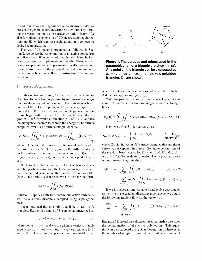
(a) (b)

Figure 1. The vertices and edges used in theparametrization of a triangle are shown in (a).Any point on the triangle can be expressed asxi = (v1i + ue1i + ve2i). In (b), vk’s neighbortriangles Dk are shown.

which the integrals in the equations below will be evaluated.A depiction appears in Figure 1(a).

With this parametrization, we can express Equation 2 asa sum of piecewise continuous integrals over the trianglefaces,

Ep(S) =N∑

i=1

∫∫Si

f(v1i+ue1i+ve2i)〈Sip,Ni〉dSi. (4)

Next, we define Sip for vertex vk as

Sip(u, v,vk) ={

(1− u− v)e, Si ∈ Dk

0, otherwise(5)

where Dk is the set of M surface triangles that neighborvertex vk, as depicted in Figure 1(b), and e denotes one ofthe standard basis vectors for R3, (i.e., [1, 0, 0]T , [0, 1, 0]T ,or [0, 0, 1]T ). We evaluate Equation 4 with p equal to oneof coordinates of vk, yielding

Ep(S) =∑

Si∈Dk

∫∫Si

f(Si(u, v))〈(1− u− v)e,Ni〉dSi

=∑

Si∈Dk

〈e,Ni〉∫∫

Si

(1− u− v)f(Si(u, v))dSi.

If we introduce a time variable t and evolve coordinates(xi, yi, zi) in the gradient directions given above, we obtainthe following gradient flow for the vertex vk,

dvk

dt=

∑Si∈Dk

∫∫Si

(1− u− v)f(Si(u, v))dSiNi(6)

= A(vk)

Equation 6 is an ordinary differential equation that describesthe vertex motion of the active polyhedron. This equa-tion can be computed using MK2 operations, where K isthe number of samples (in one dimension) on a triangle at

which the integration occurs. Note that Equation 6 is sig-nificantly different than previous models as the function fis integrated over triangular faces rather than applied point-wise. As we shall see, this integration of f provides addedrobustness to noise. Also note that the image-based dataterm f in Equation 6 is completely general, allowing one todesign different flows for solving various problems.

2.1 Electrostatic Regularization

The flow of an active polyhedron may, under the soleinfluence of a data term, become irregular when a vertexbecomes infinitesimally close to a non-neighbor face of thepolyhedron. To address this issue, we incorporate a naturalregularization term introduced in [13] that is based on elec-trostatic principles. However, the 3D version of this regu-larization requires special attention so that it achieves thedesired effect.

The electrostatic regularization technique models a uni-form charge density λ along each surface triangle. Thischarge density induces a global electric field G ∈ R3

that applies a repulsive force at each vertex. To computethe electric field at a general point p ∈ R3, we mustconsider the differential electric field dG(p) exerted by acharged particle at location xi on triangle Si. As given byCoulomb’s law [7], the electric force is inversely propor-tional to the square of the Euclidean distance ||p− xi||2between the charged particles, and directed along the vector(p− xi)/ ||p− xi||.

G(p) =N∑

i=1

∫∫Si

λp− xi

||p− xi||ndSi, (7)

where xi = (v1i +ue1i +ve2i) is a point on Si, and n = 3.While using n = 3 in Equation 7 will impart a repul-

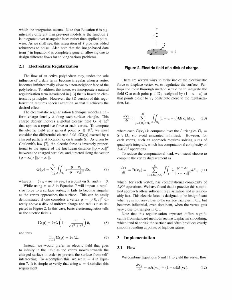
sive force to a surface vertex, it fails to become singularas the vertex approaches the surface. This can be easilydemonstrated if one considers a vertex p = [0, 0, z]T di-rectly above a disk of uniform charge and radius r as de-picted in Figure 2. In this case, basic electromagnetics tellsus the electric field is

G(p) = 2πλ

(1− z√

z2 + r2

)z, (8)

and thuslimz→0

G(p) = 2πλz. (9)

Instead, we would prefer an electric field that goesto infinity in the limit as the vertex moves towards thecharged surface in order to prevent the surface from self-intersecting. To accomplish this, we set n = 4 in Equa-tion 7. It is simple to verify that using n = 4 satisfies thisrequirement.

Figure 2. Electric field of a disk of charge.

There are several ways to make use of the electrostaticforce to displace vertex vk to regularize the surface. Per-haps the most thorough method would be to integrate thefield G at each point p ∈ Dk, weighted by (1 − u − v) sothat points closer to vk contribute more to the regulariza-tion, i.e.,

dvk

dt=

M∑j=1,Sj∈Dk

∫∫Sj

(1− u− v)G(xj)dSj , (10)

where each G(xj) is computed over the L triangles Ck =S \ Dk (to avoid unwanted infinities). However, foreach vertex, such an approach requires solving sums ofquadruple integrals, which has computational complexity ofLMK4 operations.

To reduce the computational load, we instead choose tocompute the vertex displacement as

dvk

dt= B(vk) =

L∑i=1,Si∈Ck

∫∫Si

λp− xi

||p− xi||4dSi, (11)

which, for each vertex, has computational complexity ofLK2 operations. We have found that in practice this simpli-fied approach offers sufficient regularization and is reason-ably fast. This electric force is designed to be insignificantwhen vk is not very close to the surface triangles in Ck, butbecomes influential, even dominant, when the vertex getsvery close to triangles in Ck.

Note that this regularization approach differs signifi-cantly from standard methods such as Laplacian smoothing,which tend to shrink the surface and often produces overlysmooth rounding at points of high curvature.

3 Implementation

3.1 Flow

We combine Equations 6 and 11 to yield the vertex flow

dvk

dt= αA(vk) + (1− α)B(vk), (12)

where α is a constant that weights the data term relative tothe regularization term. In practice, we have found a valueof α = 0.95 to offer good performance. With this heavierweight on the data term, the regularization only contributessignificantly to the flow when degeneracy occurs, allowingfor the data term to govern the evolution during most ofthe evolution. Since updating a single vertex requires (L +M)K2 = NK2 operations, the computational complexityof our model is N2K2 operations for each time step.

3.2 Mesh Operations

While the surface is deforming, it is necessary to performsome mesh operations to ensure that the mesh has a propervertex distribution. Towards this goal we implement somestandard mesh operations:

1. Edge split. This operation splits any edge whoselength goes above a maximum length. A new vertexis placed at the center of the edge, and each trianglethat included the edge is split into two, as shown inFigure 3.

2. Edge collapse. This operation collapses any edgewhose length goes below a minimum length. The twovertices that comprise the edge are merged to one ver-tex, as shown in Figure 3.

3. Face split. During evolution, the magnitude of the im-age force applied to each face is computed. If facesplitting is enabled, the triangle with the largest mag-nitude force is split into three triangles by placing anew vertex at the triangle center, as shown in Figure 3.The intuition here is that the edges with higher imagespeeds are close to image structures that may requirefiner details. Face splitting is enabled periodically dur-ing the surface flow.

These operations allow the surface to grow and to shrink;however, topological changes are not currently supported inour implementation. For many applications this is an advan-tage rather than a disadvantage. Techniques such as [5] re-quire special algorithms to keep the topology of the level-setsurface simple because it is very easy for implicit surfaces tobreak or leak to surrounding unrelated regions while prop-agating. This is not a problem for our model. On the otherhand, topology adaptivity can be added to an active polyhe-dron as has been done in other mesh-based approaches suchas [8, 11].

3.3 Speed term

3.3.1 Region-based functional for segmentation

As mentioned previously, the image-based speed term f de-scribed in Equation 6 has a general form that can be cus-

Figure 3. Mesh operations. The topmostmesh is refined using the edge split opera-tor (lower left), edge collapse operator (lowercenter) and face split operator (lower right).

tomized for specific tasks. For image segmentation, we em-ploy the piecewise constant region-based energy functionalthat uses mean statistics [3],

f(x) = −(I(x)−mi)2 + (I(x)−mo)2, (13)

where I is the 3D image, x is a point on the surface, mi andmo are the mean values of I inside and outside the poly-hedron, respectively. This speed function is well suited tothe segmentation of noisy images, as it does not rely on theimage gradients. The voxels inside and outside the surfaceare found via scanline rasterization of the polyhedron.

3.3.2 Boundary-based functional for reconstructionfrom unorganized points

For reconstructing surfaces from unorganized points, wefollow the example of [15] who implement a gradient flowon a distance volume to find the minimal distance surface.That is,

f(x) = −∇D(x) ·N(x), (14)

where D is a distance volume formed by placing the un-organized points into a volumetric grid and computing theunsigned distance at each voxel to the closest unorganizedpoint, and N is the surface normal.

4 Experimental Results

We now present experimental results showing an activepolyhedron’s ability to segment 3D image data and to re-construct surfaces from unorganized points.

4.1 Validation

First, we validate the active polyhedron using groundtruth data. For comparison, we also produce results usingcontinuous active surfaces implemented with level set meth-ods.

Our first example consists of a 1283 volume of syntheticultrasound data. The data suffers poor contrast and corrup-tion by speckle noise, a common form of ultrasound noiseresulting from coherent backscattering of echo signals. In-side the volume is a darker cylindrical structure of radius10 units and height 64 units that simulates a blood vessel.We segment this data by placing a cube inside and at oneend of the vessel, and evolve the active polyhedron usingthe speed term of Equation 13 and the electrostatic regu-larizer. Figure 5 shows the evolving active polyhedron fort = 0, 10, 20, 30, and 35 iterations, upon which the sur-face converged. On the right of Figure 5 we show the seg-mentation result achieved with the same data term and acurvature-based regularizer using a continuous active sur-face implemented with level set methods. Notice that resultobtained with the active polyhedron is much smoother dueto the integration of the data term along each triangle face,compared to the pointwise motion of the continuous activesurface, which suffers multiple topology changes and leak-ing due to the speckle. Although it is possible to increasethe regularization of the continuous active surface, doing soresults in unsatisfactory results as the data term becomesineffective in being attracted to target image features. Theactive polyhedron model produces better segmentation re-sults, as is visually apparent in 2D slices of the volume,shown in Figure 4. Furthermore, in Table 1 we computethe surface area and volume of the segmentation results andcompare them to the ground truth. The erratic shape of thecontinuous active surface results in over twice the actualsurface area, while the active polyhedron more faithfullyrepresents the shape.

In Figure 6 we reconstruct sphere from point cloud data.We generated a “clean” set of 625 points by sampling theequation of radius = 15 sphere to produce the point cloudon the top left of the figure, and in the bottom left of the fig-ure we perturbed each point by adding zero-mean Gaussiandistributed noise in the range [−10, 10] to each coordinateof each vertex and adding 5% outliers uniformly distributedin the volume to produce a “noisy” point cloud. We embed-ded the point cloud in a 643 grid and formed an unsigneddistance volume. The middle figures show the result of re-constructing a surface from the unorganized points using alevel set implementation and Equation 14 with a curvature-based regularizer, while the right figures show the result ofusing the active polyhedron, Equation 14, and the electro-static regularizer. As expected, the reconstruction of theclean data results in a polyhedral representation of a sphere.The reconstruction of the noisy data shows the susceptibil-ity of the continuous active surface to local noise variations.However, the active polyhedron produces a smoother, morespherical surface due to its integration of the speed terms onthe polygonal faces.

(a) (b)

(c) (d)

Figure 4. 2D slices showing the segmenta-tion results of Figure 5. In (a) and (b) weshow slices 50 and 90 used with the polyhe-dral model. In (c) and (d) we show the sameslices from the segmentation result using acontinuous active surface implemented withlevel set methods.

4.2 Applications

The active polyhedron excels at representing polyhedralshapes, but since triangle meshes are such a powerful shaperepresentation, the method also is useful for representingmore organic shapes, such as those found in medical imag-ing. The improved robustness to noise helps prevent erro-neous segmentations.

In Figures 7 and 8 we demonstrate a segmentation ofa darker structure in breast ultrasound data. Such struc-tures are often candidates for tumor analysis in computeraided diagnosis applications. In (a) and (b) of each figure,we show the segmentation using a continuous active sur-face implemented with level set methods. As with the syn-thetic example in the previous subsection, the continuoussurface breaks apart and takes on an irregular shape due tothe speckle noise; so much so in Figure 8 that the result isnearly unusable. In (c) and (d) of each figure we show theresult using the active polyhedron. As expected, the activepolyhedron produces a much less ragged result due to its in-creased robustness. We have observed similar results withother noisy ultrasound images.

We used an active polyhedron to segment an atrial cham-ber from a 2563 volume of cardiac ultrasound data. The re-sults are shown in (a) and (b) of Figure 9. In (a), we showthe 3D polyhedral surface overlaid with a slice through thevolume, and in (b), we show the corresponding 2D slice.

Figure 5. 3D segmentation using an active polyhedron. Left to right: 0, 10, 20, 30, and 35 iterations(using a time step of 1.0). For comparison, on the far right is the segmentation result using acontinuous active surface implemented with level set methods (using a time step of 0.125 to satisfyCFL conditions).

Approach Volume (units3) Surface Area (units2)Ground Truth 20106 4649

Continuous (Level sets) 21096 11510Discrete (Active polyhedron) 19230 4867

Table 1. Volume and surface area, ground truth and estimated, for the ultrasound example of Figure 5.

(a) (b)

Figure 6. Reconstructing a polyhedral sphere from clean (a) and noisy (b) point cloud data. Left toright: Point cloud data, continuous reconstruction using level sets using a time step of 0.125, discretereconstruction using the active polyhedron using a time step of 1.0.

As another example, we used an active polyhedron to seg-ment the trachea from a 256 x 256 x 319 volume of lung CTdata. The results are shown in (c) and (d) of Figure 9. In(c), we show the 3D polyhedral surface overlaid with a slicethrough the volume, and in (d), we show the corresponding2D slice.

We reconstruct a surface of part of the human ear canalfrom point cloud data obtained by laser scanning a moldformed in a person’s ear. The point cloud data was placedinto a 1283 volume and the active polyhedron was used re-construct the surface at different resolutions, as shown inFigure 10. We run a similar experiment for reconstructingthe Stanford bunny in Figure 11, that later of which shows

an example with more interesting geometry. As the resolu-tion of the surface increases, more details emerge. As onefurther increases the resolution of the active polyhedron,finer surface details are modeled. However, for regularityand robustness to noise, the active polyhedron prefers well-separated vertices.

5 Conclusion

In this paper we presented a novel deformable surface, anactive polyhedron, for 3D medical image segmentation, andadditionally show its use in reconstructing surfaces from un-organized points. Starting with the general theory of surface

(a) (b) (c) (d)

Figure 7. Using an active polyhedron to segment breast ultrasound data. We show a 3D segmentationusing a continuous surface implemented with level set methods (a) and a slice through segmentedvolume (b). We repeat the experiment using the active polyhedron and show the results in (c) and(d).

(a) (b) (c) (d)

Figure 8. Another breast ultrasound example. Continuous surface (a) and (b), and active polyhedron(c) and (d). Note that the active polyhedron solution is much more robust.

(a) (b) (c) (d)

Figure 9. Using an active polyhedron to segment 3D medical data. In (a) and (b) we show a segmen-tation of an atrial chamber from ultrasound data, and in (c) and (d) we show a segmentation of thetrachea from CT data. A time step of 1.0 was used in both evolutions.

evolution, we derived the equation of motion of a polyhe-dral surface by minimizing an energy functional using gra-dient descent. We also described an electrostatic regularizerthat preserves sharper features but prevents the surface fromself-intersecting. We then demonstrated the usefulness ofan active polyhedron in segmenting noisy 3D medical im-ages, as well as reconstruction from unorganized points, andoffered a comparison to a continuous active surface imple-mented with level set methods. While more in-depth exper-imentation is required, from our results we conclude thatthe integration of the speed term over the active polyhe-

dron’s faces results in significant robustness to noise. Theincreased time step one can use in the active polyhedronframework is an additional benefit that, depending on thenumber of triangles used in the mesh, can result in fasterevolutions than narrowband level set methods. However,due to space constraints, we do not present runtime resultsin this paper.

Like many deformable surfaces, the active polyhedrondescribed in this paper is capable of mesh refinement, butdoes not support topological changes. This is not neces-sarily a disadvantage, as in many applications the topology

Figure 10. Using an active polyhedron to reconstruct a portion of a human ear canal shape. Left:point cloud. Next: reconstruction with edge length = 40, 25, and 10 units. Right: slice going throughdistance volume upon convergence.

Figure 11. Different resolutions of reconstruc-tions of the Stanford Bunny from point clouddata. A time step of 1.0 was used.

of the object being segmented is known a priori, and topo-logical changes are undesirable [5]. However, it would bepossible to incorporate topological operations [4, 8, 11] intoour model. This is left for future work.

The quality of the results of presented in this paperare dependent on the image-based terms we implement toevolve the active polyhedron, particularly for segmentation.More advanced functions that rely on higher order statistics,probabilistic measures, and textural properties [2, 13] willlikely be required to further improve results. We believethat the active polyhedron framework is very promising andcould also be applied to problems in object recognition, 3Dtracking, and multi-view stereo reconstruction.

6 Acknowledgements

We thank Ganesh Sundaramoorthi at Georgia Tech fordiscussions regarding electric field regularization, and JasonTyan at SCR for support of this work.

References

[1] B. Baillard and C. Barillot. Robust 3D Segmentation ofAnatomical Structures with Level Sets. In The Intl. Conf.on Medical Image Computing and Computer-Assisted Inter-vention, pages 236–245, 2000.

[2] D. Boukerroui, O. Basset, A. Baskurt, and G. Gimenez. Amultiparametric and multiresolution segmentation algorithm

of 3-d ultrasonic data. IEEE Trans. on Ultrasonics, Ferro-electrics, and Frequency Control, 48(1):64–77, 2001.

[3] T. Chan and L. Vese. Active contours without edges. IEEETrans. on Image Processing, 10(2):266–277, 2001.

[4] Y. Duan, L. Yang, H. Qin, and D. Samaras. Shape Re-construction from 3D and 2D Data Using PDE-Based De-formable Surfaces. In European Conference on ComputerVision, volume III, pages 238–251, 2004.

[5] X. Han, C. Xu, and J. Prince. A topology preserving level setmethod for geometric deformable models. IEEE Trans. onPatt. Anal. and Machine Intelligence, 25(6):755–768, 2003.

[6] M. Kass, A. Witkin, and D. Terzopoulos. Snakes: Activecontour models. Intl. Journal of Computer Vision, 1(4):321–331, 1987.

[7] J. Kraus. Electromagnetics. McGraw-Hill, New York, fourthedition, 1992.

[8] J. Lachaud and J.Montanvert. Deformable meshes with au-tomated topology changes for coarse-to-fine 3d surface ex-traction. Medical Image Analysis, 3(2):187–207, 1999.

[9] R. Malladi, J. Sethian, and B. Vemuri. Shape modeling withfront propagation: A level set approach. IEEE Trans. onPatt. Anal. and Machine Intelligence, 17(2):158–175, 1995.

[10] T. McInerney and D. Terzopoulos. Deformable models inmedical image analysis: A survey. Medical Image Analysis,1(2):91–108, 1996.

[11] T. McInerney and D. Terzopoulos. Topology adaptive de-formable surfaces for medical image volume segmentation.IEEE Trans. on Medical Imaging, 18(10):840–850, 1999.

[12] G. Unal, H. Krim, and A. Yezzi. A Vertex-Based Represen-tation of Objects in Images. In IEEE Intl. Conference onImage Processing, volume I, pages 896–899, 2002.

[13] G. Unal, A. Yezzi, and H. Krim. Information-theoretic activepolygons for unsupervised texture segmentation. The Intl.Journal of Computer Vision, 62(3):199–220, 2005.

[14] R. Zaritsky, N. Peterfreund, and N. Shimkin. Velocity-guided tracking of deformable contours in three dimensionalspace. The Intl. J. of Computer Vision, 51(3):219–238, 2003.

[15] H. K. Zhao, S. Osher, and R. Fedkiw. Fast Surface Re-construction Using the Level Set Method. In Proc. IEEEWorkshop on Variational and Level Set Methods (VLSM’01),pages 194–202, 2001.

[16] S. Zhu and A. Yuille. Region competition: Unifying snakes,region growing, and bayes/mdl for multi-band image seg-mentation. IEEE Trans. on Patt. Anal. and Machine Intelli-gence, 18(9):884–900, 1996.