Abstract awakenings in algebra:

Early group theory in the works of Lagrange, Cauchy, and Cayley

Janet Heine Barnett∗

19 August 2010

Introduction

The problem of solving polynomial equations is nearly as old as mathematics itself. In addition tomethods for solving linear equations in ancient India, China, Egypt and Babylonia, solution methodsfor quadratic equations were known in Babylonia as early as 1700 BCE. Written out entirely in wordsas a set of directions for calculating a solution from the given numerical coefficients, the Babylonian

procedure can easily be translated into the well-known quadratic formula: x = −b±√b2−4ac2a , given that

ax2+bx+c = 0. But what about a ‘cubic formula’ for third degree equations, or a ‘quartic formula’ forequations of degree four? More generally, is it always possible to compute the solutions of polynomialequations of a given degree by means of a formula based on its coefficients, elementary arithmeticoperations and the extraction of roots alone?

As basic as this latter question may sound, its answer eluded mathematicians until the early nine-teenth century. In connection with its rather surprising resolution (revealed later in this introduction),there emerged a new and abstract algebraic structure known as a group. Algebra, understood priorto that time as the study of solution techniques for equations, was forever changed as a result. Thegoal of this project is to develop an understanding of the basic structure and properties of a groupby examining selected works of mathematicians involved in the early phases of its evolution. In theremainder of this introduction, we place these readings in context with a brief historical sketch of effortsto find formulas for higher degree polynomial equations.

In a sense, the search for the solution to higher degree polynomials was also pursued by ancientBabylonian mathematicians, whose repertoire included methods for approximating solutions of certaintypes of cubic equations. The problem of finding exact (versus approximate) solutions can be saidto have originated within the somewhat later geometric tradition of ancient Greece, in which therearose problems such as the ‘duplication of a cube’ (i.e., constructing a cube with twice the volume of agiven cube) which correspond to cubic equations when translated into today’s algebraic symbolism (i.e.,x3 = 2). In order to construct the line segments which served as geometrical roots of these equations,Greek mathematicians developed various new curves, including the conic sections (i.e., parabolas,hyperbolas and ellipses).1 The Islamic mathematician and poet Omar Khayyam (1048–1131), who wasthe first to systematize these geometric procedures, solved several different cubic equation forms byintersecting appropriate conic sections. For example, for a cubic equation of the form x3 + d = bx2,the points of intersection of the hyperbola xy = d and the parabola y2 + dx − db = 0 correspond to

∗Department of Mathematics and Physics; Colorado State University-Pueblo; Pueblo, CO 81001-4901;janet.barnett@colostate-pueblo.edu.

1Using abstract algebra, it can now be shown that certain of these construction problems, including the duplication ofthe cube, are impossible using only the Euclidean tools of a collapsible compass and an unmarked straightedge. Likewise,these ideal Euclidean tools are not sufficient to construct a conic section.

1

the real roots of the polynomial.2 Because negative numbers were not allowed as coefficients (or roots)of equations at this point, however, the polynomial x3 + d = bx2 was only of thirteen possible cubicforms, each of which required different conic sections for their solution.

Unlike the Greeks, Khayyam and his fellow medieval Islamic mathematicians hoped to find algebraicalgorithms for cubic equations, in addition to geometric constructions based on curves. Although theywere unsuccessful in this regard, it was through Islamic texts that algebra became known in WesternEurope. As a result, the search for an algebraic method of solution for higher degree equations was nexttaken up in Renaissance Italy beginning in the 14th century. Some equations studied in this settingwere solved through substitutions which reduced the given equation to a quadratic or to a special formlike xn = a. Most higher degree equations, however, can not be solved this way. Only in the 16thcentury, when methods applying to all cubic and quartic polynomials were finally developed, did theItalian search for general solutions achieve some success. The culmination of this search — which wedescribe in footnote 3 below — is one of the great stories in the history of mathematics.3

Although the solution methods discovered in the 16th century are interesting in and of themselves,certain consequences of their discovery were of even greater importance to later developments in math-ematics. One such consequence was the discovery of complex numbers, whose eventual acceptancewas promoted by the fact that roots of negative numbers often appear during the course of applyingthe cubic or quartic formulas to specific equations, only to cancel out and leave only real roots in theend.4 The increased use of symbolism which characterized Western European algebra in the Renais-sance period also had important consequences, including the relative ease with which this symbolismallowed theoretical questions to be asked and answered by mathematicians of subsequent generations.Questions about the number and kind of roots that a polynomial equation possesses, for example, ledto the Fundamental Theorem of Algebra, the now well-known assertion that an nth degree equationhas exactly n roots, counting complex and multiple roots. Algebraic symbolism also allowed questionsabout the relation of roots to factors to be carefully formulated and pursued, thereby leading to dis-coveries like the Factor Theorem, which states that r is a root of a polynomial if and only if (x− r) isone of its factors.

Despite this progress in understanding the theory of equations, the problem of finding a solution toequations of degree higher than four resisted solution until the Norwegian Niels Abel (1802–1829) settledit in a somewhat unexpected way. In a celebrated 1824 pamphlet, Abel proved that a ‘quintic formula’

2To verify this, substitute y = dx

from the equation of the hyperbola into the equation of the parabola, and simplify.Of course, modern symbolism was not available to Khayyam, who instead wrote out his mathematics entirely in words.

3Set in the university world of 16th century Italy, where tenure did not exist and faculty appointments were influencedby a scholar’s ability to win public challenges, the tale of the discovery of general formulas for cubic and quartic equationsbegins with Scipione del Ferro (1465–1526), a professor at the University of Bologna. Having discovered a solution methodfor equations of the form x3 + cx = d, del Ferro guarded his method as a secret until just before his death, when hedisclosed it to his student Antonio Maria Fiore (ca. 1506). Although this was only one of thirteen forms which cubicequations could assume, knowing its solution was sufficient to encourage Fiore to challenge Niccolo Tartaglia of Brescia(1499–1557) to a public contest in 1535. Tartaglia, who had been boasting he could solve cubics of the form x3 + bx2 = d,accepted the challenge and went to work on solving Fiore’s form x3 + cx = d. Finding a solution just days before thecontest, Tartaglia won the day, but declined the prize of 30 banquets to be prepared by the loser for the winner and hisfriends. (Poisoning, it seems, was not an unknown occurrence.) Hearing of the victory, the mathematician, physician andgambler Gerolamo Cardano (1501–1576) wrote to Tartaglia seeking permission to publish the method in an arithmeticbook. Cardano eventually convinced Tartaglia to share his method, which Tartaglia did in the form of a poem, but onlyunder the condition that Cardano would not publish the result. Although Cardano did not publish Tartaglia’s solution inhis arithmetic text, his celebrated 1545 algebra text Ars Magna included a cubic equation solution method which Cardanoclaimed to have found in papers of del Ferro, then 20 years dead. Not long after, a furious Tartaglia was defeated in apublic contest by one of Cardano’s student, Lodovico Ferrari (1522–1565), who had discovered a solution for equations ofdegree four. The cubic formula discovered by Tartaglia now bears the name ‘Cardano’s formula.’

4The first detailed discussion of complex numbers and rules for operating with them appeared in Rafael Bombelli’sAlgebra of 1560. Their full acceptance by mathematicians did not occur until the nineteenth century, however.

2

for the general fifth degree polynomial is impossible.5 The same is true for equations of higher degree,making the long search for algebraic solutions to general polynomial equations perhaps seem fruitless.Then, as often happens in mathematics, Abel’s ‘negative’ result produced fruit. Beginning with thecentral idea of Abel’s proof — the concept of a ‘permutation’ — the French mathematician EvaristeGalois (1811–1832) used a concept which he called a ‘group of permutations’ as a means to classifythose equations which are solvable by radicals. Soon after publication of Galois’ work, permutationgroups in the sense that we know them today6 appeared as just one example of a more general groupconcept in the 1854 paper On the theory of groups, as depending on the symbolic equation θn = 1,written by British mathematician Arthur Cayley (1821–1895). Although it drew little attention at thetime of its publication, Cayley’s paper has since been recognized as the inaugural paper in abstractgroup theory. By the end of the nineteenth century, group theory was playing a central role in a numberof mathematical sub-disciplines, as it continues to do even today.

Cayley’s ground-breaking paper forms the centerpiece of our study of groups in this project. Inkeeping with the historical record, and to provide a concrete example on which to base our abstraction,we first study the particular example of permutation groups. We begin in Section 1 with selections fromthe writings the 18th century French mathematician J. L. Lagrange (1736–1813), the first to suggesta relation between permutations and the solution of equations by radicals. In Section 2, we continuewith selections from the writings of another French mathematician, Augustin Cauchy (1789–1857), inwhich a more general theory of permutations was developed independently of the theory of equations.We then turn to a detailed reading of Cayley’s paper in Sections 3 and 4, paying careful attentionto the similarities between the theory of permutation groups as it was developed by Cauchy and themodern notion of an abstract group as it was unveiled by Cayley.

1 Roots of unity, permutations and equations: J. L. Lagrange

Born on January 25, 1736 in Turin, Italy to parents of French ancestry, Joseph Louis Lagrange wasappointed as a professor of mathematics at the Turin Royal Artillery School by the age of 19. He spentthe first eleven years of his professional life teaching there, the next twenty as a mathematical researcherat the Berlin Academy of Sciences, and the final twenty seven as both a teacher and researcher in Paris,where he died on April 10, 1813. Largely self taught, he is remembered today for contributions to everybranch of eighteenth century mathematics, and especially for his work on the foundations of calculus.His work in algebra is also recognized as sowing one of the seeds that led to the development of grouptheory in the nineteenth century.

Lagrange’s work on the algebraic solution of polynomial equations was first published as a lengthyarticle entitled ‘Reflexions sur la resolution algebrique des equations’ in the Memoire de l’Academiede Berlin of 1770 and 1771. As with all his research, generality was Lagrange’s primary goal in hisworks on equations. In seeking a general method of algebraically solving all polynomial equations, hebegan by looking for the common features of the known solutions of quadratics, cubics, and quartics.Following a detailed analysis of the known methods of solution, he concluded that one thing they hadin common was the existence of an auxiliary (or resolvent) equation whose roots (if they could befound) would allow one to easily find the roots of the originally given equation. Furthermore, Lagrangediscovered that it was always possible, for any given equation, to find a resolvent equation with rootswhich are related to the roots of the original equation in a very special way. This special relationship,and a summary of its importance to his work, are nicely described in Lagrange’s own words in the

5The Italian mathematician Paolo Ruffini published this same result in 1799, but his proposed proof contained a gap.Abel, who was not aware of Ruffini’s work until 1826, described it as “so complicated that it is very difficult to decidethe correctness of his reasoning” (as quoted in [14, p. 97]).

6Galois used the term ‘group’ in a slightly different way than we do today.

3

following excerpt from the 1808 edition of his Traite de la resolution des equations numeriques [11].7

∞∞∞∞∞∞∞∞

On the solution of algebraic equations8

The solution of second degree equations is found in Diophantus and can also be deduced from severalpropositions in Euclid’s Data; but it seems that the first Italian algebraists learned of it from the Arabs.They then solved third and fourth degree equations; but all efforts made since then to push the solutionof equations further has accomplished nothing more than finding new methods for the third and the fourthdegree, without being able to make a real start on higher degrees, other than for certain particular classesof equations, such as the reciprocal equations, which can always be reduced to a degree less than half [theoriginal degree] . . .

In Memoire de l’Academie de Berlin (1770, 1771), I examined and compared the principal methodsknown for solving algebraic equations, and I found that the methods all reduced, in the final analysis, to theuse of a secondary equation called the resolvent, for which the roots are of the form

x′ + αx′′ + α2x′′′ + α3x(iv) + . . .

where x′, x′′, x′′′, . . . designate the roots of the proposed equation, and α designates one of the roots ofunity, of the same degree as that of the equation.

I next started from this general form of roots, and sought a priori for the degree of the resolvent equationand the divisors which it could have, and I gave reasons why this [resolvent] equation, which is always ofa degree greater than that of the given equation, can be reduced in the case of equations of the third andthe fourth degree and thereby can serve to resolve them.

∞∞∞∞∞∞∞∞

Lagrange’s emphasis on the form of the roots of the resolvent equation is a mark of the moreabstract approach he adopted throughout his mathematics, and a critical piece of his analysis in thisparticular study. Although we will not go through the analysis which led him to this form, we will readseveral arguments which he based on it in Subsection 1.2 below.9 Notice for now that the expressionfor the roots t of the resolvent equation for a polynomial of degree m is actually the sum of only finitelymany terms:

t = x′ + αx′′ + α2x′′′ + α3x(iv) + . . .+ αm−1x(m).

Lagrange used prime notation (x′, x′′, x′′′, . . .) here instead of subscripts (x1, x2, x3, . . .) to denote the mroots of the original equation (and not to indicate derivatives). Similarly, x(m) denotes one of these m

7As suggested by its title, Traite de la resolution des equations numeriques primarily addressed the problem of nu-merically approximating solutions to equations, but it also included a summary of Lagrange’s 1770/1771 work on findingexact solutions to polynomial equations as an appendix entitled ‘Note XIII: Sur le resolution des equations algebriques’(see [11, pp. 295-327]). The first edition of Traite de la resolution des equations numeriques appeared in 1798; the revisedand extended 1808 edition from which the excerpts in this project were taken is considered the definitive edition.

8To set them apart from the project narrative, all original source excerpts are set in sans serif font and bracketed bythe following symbol at their beginning and end: ∞∞∞∞∞∞∞∞

9As indicated in the excerpt, Lagrange arrived at this expression for the roots of the resolvent equation by examiningseveral specific methods for solving cubics and quartics; that is, his knowledge of this general principle arose from an aposteriori analysis of particular instances. An a priori analysis, in contrast, is one that starts from a general law andmoves to particular instances. The literal meanings of these Latin terms are ‘from what comes after’ (a posteriori) and‘from what comes first’ (a priori). The arguments we will see below illustrate how Lagrange argued from general algebraicproperties in an a priori fashion to deduce the degree of the resolvent equation.

4

roots (and neither a derivative nor a power of x). The symbols α2, α3, . . . here do denote powers of α,however, where α itself denotes an mth root of unity: that is, a number for which αm = 1. Of course,α = 1 is always a solution of the equation αm = 1. By the Fundamental Theorem of Algebra, however,we know that α = 1 is only one of m distinct solutions of the equation αm = 1. Letting i =

√−1, for

example, the four fourth roots of unity are 1, i,−1,−i.10 Although Lagrange specified no restrictionson the value which α may assume in the formula for the resolvent’s roots in the preceding excerpt, his1808 summary later made it clear that for m > 2, this formula requires α to be a complex-valued rootof unity.

Because complex roots of unity play such a large role in his analysis, Lagrange included a detaileddiscussion of their properties in his works on the theory of equations. We will consider excerpts of thisdiscussion — especially those parts which relate to group theory concepts — in Subsection 1.1 below.We will also look at methods for computing the values of complex roots of unity in that subsection. InSubsection 1.2, we will then return to the formula Lagrange gave for the roots of the resolvent equation(t = x′ + αx′′ + α2x′′′ + α3x(iv) + . . .+ αm−1x(m)), and examine how rearranging (or permutating) theroots x′, x′′, x′′′, . . . within this formula provides us with information about the degree of the resolventequation.

To set the stage for both these discussions, we first look at a specific example to see how an auxiliaryequation, even one of higher degree than the original, can be used to solve a given equation. We notethat our primary purpose with this example and its continuation in several later tasks is to provide acontext for the group-theoretic connections which emerge from Lagrange’s theoretical work on resolventequations (e.g., roots of unity and permutations), rather than to provide a complete development ofthat work.

Task 1This task is based on the analysis in Lagrange’s 1770 Memoire [10] of the solution given byGerolamo Cardano (see footnote 3, page 2) to the cubic equation

x3 + nx+ p = 0, (1)

where n and p are assumed to be positive real numbers.

In particular, we will see how all three roots of this cubic can be determined from the sixroots of the following sixth degree equation:

t6 + 27pt3 − 27n3 = 0 (2)

Later in this section, after developing some necessary groundwork, we will also see howthe roots of these two equations fit into the special form discussed above by Lagrange.Accordingly, we follow Lagrange’s terminology throughout this task, and refer to the sixthdegree equation (2) as the resolvent of the given cubic equation (1).

(a) Verify that the substitution x = t3 −

nt , where t 6= 0, transforms the cubic equation (1)

into the resolvent equation (2).

This means that any solution t of the resolvent which can be expressed in terms ofits coefficients, elementary arithmetic operations and the extraction of roots, in turngives a solution x = t

3 −nt of the original cubic involving only elementary arithmetic

operations and the extraction of roots beginning from the coefficients 1, n, p.

Speculate on how the six roots of the resolvent equation will ultimately result in justthree roots for the given cubic, in keeping with the Fundamental Theorem of Algebra.

10This can be verified by raising each number to the fourth power, or by solving (α2 − 1)(α2 + 1) = 0 directly. As apreview of ideas studied later in this project, note that powers of i give all four roots: i1 = i , i2 = −1 , i3 = −i , i4 = 1.

5

Task 1 - continued

(b) Note that the resolvent equation is quadratic in t3:[t3]2

+ 27p[t3]− 27n3 = 0.

Let θ1 and θ2 denote the roots of θ2 + 27pθ − 27n3.

Use the fact that n, p are positive reals to prove θ1, θ2 are distinct real numbers, andexplain how it follows from this that t1 = 3

√θ1 and t2 = 3

√θ2 are distinct real roots of

the resolvent which can be expressed in the required form.11

How many real roots do you think the cubic (1) will have? Justify your conjecture.

(c) Recall that complex roots of real-valued polynomials come in conjugate pairs.

Thus, either all three roots of the cubic x3 + nx+ p are real (possibly repeated),or this cubic has exactly one real root and two (distinct) complex roots.

In this part of the task, we show that the latter is the case.

Our first step is to express the six roots of the resolvent in a suitable form.

For two of these roots (t1 = 3√θ1 and t2 = 3

√θ2), this has already been done.

In his 1770 article, Lagrange expressed the remaining four (complex) rootsas products involving t1, t2 and the two complex-valued cubic roots of unity.12

Do this for one of the four complex roots of the resolvent as follows:

Let α denote a complex number with α3 = 1, and set t3 = αt1.(In Subsection 1.1, we will see how to explicitly write α in the required form.)

Show that t3 is a complex root of the resolvent equation.13

Explain why x3 = t33 −

nt3

must therefore be a complex root of the given cubic.

Finally, explain why the given cubic must have two distinct complex rootsand one real root. (You do not need to find the second complex rootj!)

(d) In this part, we resolve an apparent paradox in the preceding results:

How is it that the resolvent equation has two distinct real roots (t1 6= t2),each of which can be used to define a real root for the given cubic via thesubstitution x = t

3 −nt , while the cubic equation itself has only one real root

and that single real root itself has a multiplicity of only one?

Begin by setting x1 = t13 −

nt1

and x2 = t23 −

nt2

, and recall that t1 = 3√θ1 and t2 = 3

√θ2.

Also recall that θ1 and θ2 denote the roots of f(θ) = θ2 + 27pθ − 27n3.

Thus, by the Factor Theorem, f(θ) = (θ − θ1)(θ − θ2).Expand this expression for f(θ) to show that θ1θ2 = (−3n)3.

Conclude that t1t2 = −3n, and use this fact to show that x1 = 13 (t1 + t2).

Proceed similarly to show that x2 = 13 (t1 + t2).

Comment on how this resolves the apparent paradox described above.14

11You do not need to solve for θ1, θ2 to do this or any other part of this task, but you will want to include the fact thatthe quadratic formula ensures θ1, θ2 can be expressed in the required form as part of your explanation.

12We could also express the four complex roots of the resolvent directly in terms of i and the roots θ1, θ2 of the quadratic

θ2 + pt3 − n3

27by using the substitution θ = t3 to first rewrite the resolvent as follows, and then applying the quadratic

formula: t6 + pt3 − n3/27 = (t3 − θ1)(t3 − θ2) = (t− 3√θ1)(t2 + 3

√θ1t+ 3

√θ1

2)(t− 3

√θ2)(t2 + 3

√θ2t+ 3

√θ2

2).

13The remaining complex roots of the resolvent equation can be similarly obtained; that is, letting α, β denote the twocomplex cubic roots of unity, the four complex roots of the resolvent are t3 = αt1 , t4 = βt1 t5 = αt2 and t6 = βt2.

14In Task 10, we will see that the two complex roots of the cubic can also be written as 13

(ti + tj) for appropriatelychosen values ti, tj selected from the four complex roots t3, t4, t5, t6 of the resolvent equation. We will then use theseexpressions in Task 14 to establish that Lagrange’s form t = x′ + αx′′ + α2x′′′ holds for this particular example.

6

1.1 Roots of unity in Lagrange’s analysis

As suggested above, roots of unity played an important role in Lagrange’s formula for the roots of theresolvent equation, and more generally in the theory of equations. In this subsection, we consider someproperties of these special roots as they were described by Lagrange. Our first excerpt on roots of unityalso touches on an important point about ‘solvability’ which we have already raised; namely, the notionof ‘solvability’ can be defined in a variety of ways. In our context, ‘algebraic solvability’ specificallyrequires that the roots of a given equation can be determined from its coefficients by way of a finitenumber of steps involving only elementary arithmetic operations (+,−,×,÷) and the extraction ofroots. Thus, just as Omar Khayyam continued to seek an algebraic algorithm for the roots of cubicequations even after he showed these roots existed by intersecting conic sections in a way that wouldhave satisfied Greek mathematicians, the solution involving trigonometric functions described belowby Lagrange would not count as an algebraic solution for today’s algebraist (nor would it for Lagrange)unless the specific trigonometric values involved could be expressed in the permitted form. We examinethis issue further in the following excerpt, taken from Note XIV of Lagrange’s Traite de la resolutiondes equations numeriques [11].

∞∞∞∞∞∞∞∞

Although equations with two terms such as

xm −A = 0, or more simply xm − 1 = 0

(since the former is always reducible to the latter, by putting x m√A in for x), are always solvable by

trigonometric tables in a manner that allows one to approximate the roots as closely as desired, by employingthe known formula15

x = cosk

m360 + sin

k

m360√−1

and letting k = 1, 2, 3, . . . ,m successively, their algebraic solution is no less interesting for Analysis, andmathematicians have greatly occupied themselves with it.

∞∞∞∞∞∞∞∞

Today, this trigonometric formula for the mth roots of unity is written in terms of the radianmeasure of a circle, 2π, and the now-standard symbol i =

√−1:

xm − 1 = 0 ⇔ x = cos

(2πk

m

)+ i sin

(2πk

m

), where k = 1, 2, 3, . . . ,m.

For example, the solutions of x3 − 1 = 0 are readily obtained from this formula as follows:

k = 1 ⇒ x = cos(2π·13

)+ i sin

(2π·13

)= cos

(2π3

)+ i sin

(2π3

)= −1

2 +√32 i

k = 2 ⇒ x = cos(2π·23

)+ i sin

(2π·23

)= cos

(4π3

)+ i sin

(4π3

)= −1

2 −√32 i

k = 3 ⇒ x = cos(2π·33

)+ i sin

(2π·33

)= cos (2π) + i sin (2π) = 1

Notice that these roots include one real root and two complex roots which are conjugates of each other.Also note that the particular trigonometric values involved here can be expressed in terms of only

15A proof of this formula lies outside the scope of this project.

7

finitely many basic arithmetic operations on rational numbers and their roots (including i =√−1).16

In fact, we could instead solve x3 − 1 = 0 by first factoring [x3 − 1 = (x − 1)(x2 + x + 1)] and thenusing the quadratic formula. Thus, the cubic roots of unity are bona fide algebraic solutions of thisequation.

In his celebrated doctoral dissertation Disquisitiones Arithmetica of 1801, the great German math-ematician Frederic Gauss (1777–1855) proved that xm− 1 = 0 can always be solved algebraically. Thisfact in turn implied Lagrange could legitimately use roots of unity in his formula for the roots of theresolvent and still obtain an algebraic solution. Lagrange commented on this technical point in his1808 summary, saying of Gauss’ work that it was ‘as original as it was ingenious’ [11, p. 329].

Task 2Without employing a calculator or computer, use the formula x = cos

(2πkm

)+ i sin

(2πkm

)(with m = 6) to express all sixth roots of unity in terms of the elementary arithmeticoperations on rational numbers and their roots only.

What difficulties do you encounter when you attempt to do this for the fifth roots of unity?How else might you proceed in this case?

Note: Lagrange found the fifth roots of unity to be 1,√5−14 ± 10+2

√5

4 i, and −√5+14 ± 10−2

√5

4 i.

As Lagrange commented in the preceding excerpt, this formula for the mth roots of unity in termsof the trigonometric functions was well known by his time. It is straightforward to check its correctness(see Appendix I, Task I.1) using another formula that was then well known:

de Moivre’s Formula: (cos θ + i sin θ)n = cos(nθ) + i sin(nθ)

The French mathematician for which this formula is named, Abraham de Moivre (1667–1754), appearsto have had some understanding of it as early as 1707; it seems likely that he discovered it by way ofthe standard sum identities for trigonometric functions, although he never published a proof. In thefirst precalculus text ever to be published, Introductio in analysin infinitorum (1748), the celebratedmathematician Leonhard Euler (1707–1783) did use trigonometric identities to prove de Moivre’s for-mula in the case where n is a natural number (see Appendix I, Task I.2). As was typical of Euler, hethen took matters a step further and used ideas related to power series (see Appendix I, Task I.3) toestablish another amazing formula:

Euler’s formula: eiθ = cos θ + i sin θ

As a corollary to Euler’s formula, de Moivre’s formula is easy to prove, although the almost magicalease of this proof makes it seem no less mysterious:17

16Had the coefficients of the original equation included irrational or imaginary numbers, then any number obtainedin a finite number of steps from those coefficients with basic arithmetic operations or extraction of roots would also beallowed. Since the coefficients of x3 − 1 = 0 are integers, these operations allow only rational numbers and their roots.

17Another easy but mysterious consequence of Euler’s formula, obtained by letting θ = π, is Euler’s Identity relatingthe five most important mathematical constants in a single equation: eiπ + 1 = 0. After proving Euler’s identity to anundergraduate class at Harvard, the American algebraist Benjamin Peirce (1809–1880) is reported in [1] to have said:“Gentlemen, that is surely true, it is absolutely paradoxical; we cannot understand it, and we don’t know what it means.But we have proved it, and therefore we know it must be the truth.”

8

(cos θ + i sin θ)n = (eiθ)n = ei(nθ) = cos(nθ) + i sin(nθ)

Additionally, Euler’s formula gives us another (more concise) way to represent roots of unity:

xm − 1 = 0 ⇔ x = cos

(2πk

m

)+ i sin

(2πk

m

)⇔ x = e

2πkmi, where k = 1, 2, 3, . . . ,m.

Although Lagrange himself did not make use of this exponential representation in his own writing(despite his familiarity with Euler’s identity), we use it in this project as a convenient means toabbreviate notation and simplify computations. For example, the three cubic roots of unity can bewritten as follows:

k = 1 ⇒ x = e2π·13i = e

2πi3

k = 2 ⇒ x = e2π·23i = e

4πi3

k = 3 ⇒ x = e2π·33i = e2πi

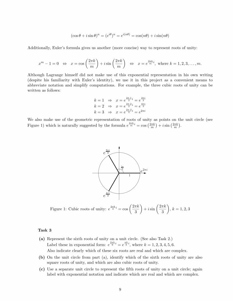
We also make use of the geometric representation of roots of unity as points on the unit circle (see

Figure 1) which is naturally suggested by the formula e2πkmi = cos

(2πkm

)+ i sin

(2πkm

).

1

e4πi3

e2πi3

e2πi2π3

Figure 1: Cubic roots of unity: e2πk3i = cos

(2πk

3

)+ i sin

(2πk

3

), k = 1, 2, 3

Task 3

(a) Represent the sixth roots of unity on a unit circle. (See also Task 2.)

Label these in exponential form: e2πk6i = e

πk3i, where k = 1, 2, 3, 4, 5, 6.

Also indicate clearly which of these six roots are real and which are complex.

(b) On the unit circle from part (a), identify which of the sixth roots of unity are alsosquare roots of unity, and which are also cubic roots of unity.

(c) Use a separate unit circle to represent the fifth roots of unity on a unit circle; againlabel with exponential notation and indicate which are real and which are complex.

9

Real

Imaginary

r

z = a+ bi

a

b

θ

Figure 2: Geometric representation of z = a+ bi = reiθ, where r =√a2 + b2

Although the geometric representation of the set of all complex numbers as points in the two-dimensional plane shown in Figure 2 was first published after Lagrange’s work on algebraic solvability,18

mathematicians of his era were well aware of the connection of roots of unity to the unit circle.19 Infact, Lagrange explicitly used the geometric representation of roots of unity as points on the unit circleto determine the total number and type (real versus complex) of mth roots of unity, as we read in thefollowing excerpt from his 1770 Memoire.20 It may be helpful to refer back to the unit circles in Figure1 and Task 3 (both on page 9) as you read this excerpt.

∞∞∞∞∞∞∞∞

We first remark concerning this solution that each of the roots of the equation xm − 1 = 0 should bedifferent from each other, since on the circumference there are not two different arcs which simultaneouslyhave the same sine and the same cosine. It is further easy to see that all the roots will be imaginary, withthe exception of the last which corresponds to k = m and which will always equal 1, and of that whichcorresponds to k = m

2 , when m is even, which will equal −1; since in order for the imaginary part of theexpression of x to vanish, it is necessary to have

sin

(k

m360

)= 0,

which never occurs unless the arc is equal to 360 or to 180; in which case we will have either km = 1 or

= 12 , and consequently either k = m or k = m

2 ; in the first case, the real part cos(km360

)will become

cos 360 = 1; and in the second it will become cos 180 = −1.

∞∞∞∞∞∞∞∞

18The name of Parisian bookkeeper Jean-Robert Argand (1768–1822) is frequently cited in connection with the devel-opment of the complex plane, in recognition of an 1806 pamphlet which he produced on the topic. Although there areindications that Gauss was in possession of the geometric representation of complex numbers as early as 1796, he did notpublish on the subject until 1831. Credit for the first publication on the subject instead belongs to the Norwegian CasparWessel (1745–1818); unfortunately, Wessel’s 1797 paper was written in Danish and went unnoticed until 1897.

19It was this relation of the mth roots of unity to points on the unit circle that led to the term ‘cyclotomic polynomial’being used for the expression ‘xm−1 +xm−2 + . . .+ 1’ which arises as a factor of xm− 1 = (x− 1)(xm−1 +xm−2 + . . .+ 1).

20Because the following excerpt comes from a different source than that which we have quoted thus far, we have alteredthe notation in it slightly (replacing, for example, n by m) to be consistent with the notation used in our other excerpts.

10

Task 4Compare Lagrange’s claim concerning the number and type of mth roots of unity in thepreceding excerpt to what you found for m = 6 in parts (a) and (b) of Task 3.

How convincing do you find Lagrange’s argument in general?

We now read the continuation of Lagrange’s comments on roots of unity, in which ideas related towhat later came to be known as a ‘cyclic group’ arise for the first (but not last!) time in this project.

∞∞∞∞∞∞∞∞

Now, if we let

α = cos

(360

m

)+ sin

(360

m

)√−1,

we will have . . .

αk = cos

(k

m360

)+ sin

(k

m360

)√−1;

so that the different roots of xm − 1 = 0 will all be expressed by the powers of this quantity α; and thusthese roots will be α, α2, α3, . . . αm, of which the last αm will always be equal to 1 . . . .

∞∞∞∞∞∞∞∞

We pause at this point in our reading of Lagrange to illustrate his central idea for the specific case

of m = 3. Using exponential notation, we set α = e2πi3 . Then, as noted by Lagrange, the remaining

cubic roots of unity can be obtained simply by taking powers of α, since α2 =[e

2πi3

]2= e

4πi3 and

α3 =[e

2πi3

]3= e2πi = 1. Because it is possible to generate all the cubic roots of unity from α in this

way, α is called a primitive cubic root of unity.

Task 5Let m = 6 and set α = cos

(2π6

)+ i sin

(2π6

)= e

πi3 .

Verify that α is a primitive sixth root of unity by computing αk for k = 2, 3, 4, 5, 6.Comment on how these results compare to your answer to Task 3(a).

Return now to Lagrange’s comments on primitive roots of unity.

∞∞∞∞∞∞∞∞

It is good to observe here that if m is a prime number, one can always represent all the roots ofxm − 1 = 0 by the successive powers of any one of these same roots, excepting only the last; let, forexample, m = 3, the roots will be α, α2, α3: if we take the next root α2 in place of α, we have the threeroots α2, α4, α6; but, since α3 = 1, it is clear that α4 = α and that α6 = α3; so that these roots will beα2, α, α3, the same as before.

∞∞∞∞∞∞∞∞

11

Let us consider what Lagrange is claiming here in more detail. In light of his comments on primitiveroots of unity in the first excerpt on page 11, we know the expression ‘the last root’ is a reference to

the real number ‘1’, obtained by taking the ‘last’ power (αm) of α = e2πim . We also know from what

Lagrange has already said that α = e2πim is a primitive mth root of unity, since taking powers of α has

the effect of cycling through all the mth roots of unity. In the excerpt we have just read, Lagrange hasgone beyond this to claim that every mth root of unity — other than the last root 1 — behaves inexactly this same way, provided m is prime. In other words:

TheoremIf m is prime and β is a complex mth root of unity, then β is a primitive mth root of unity.

Lagrange’s illustration of this theorem for the prime m = 3 in the preceding excerpt used the fact

that α = e2πi3 is already known to be a primitive cubic root of unity; thus, the only other complex

root of unity β can be written as a power of α; namely, β = α2. Using this notation, we can re-writeLagrange’s power computations as follows: β1 = α2, β2 = α4 = α3α = α and β3 = α6 = [α3]2 = 1.This shows that β = α2 is also a primitive root of unity, and the theorem holds in this case.

Task 6In the continuation of the preceding excerpt, Lagrange next considered the case m = 5,

where α = cos(2π5

)+ i sin

(2π5

)= e

2πi5 and the five fifth roots of unity are α, α2, α3, α4, α5 =

1.

Complete the following to prove that α2, α3, and α4 are also primitive fifth root of unity.

(a) Find the first five powers of α2, and show that these are the same as the five originalroots rearranged in the following order: α2, α4, α, α3, α5

(b) Find the first five powers of α3, and show that these generate the five original rootsrearranged in the following order: α3, α, α4, α2, α5.

(c) Determine the order in which the original roots are generated using powers of α4.

In the next task, the specific case of m = 6 is used to show that the restriction to prime numbers inthe preceding theorem is necessary; that is, when m is composite, it is no longer the case that everycomplex root of unity is also a primitive root of unity. A proof of the theorem for the prime case isthen outlined in Task 8, followed by further explorations of the composite case in Task 9.

Task 7In this task, the case m = 6 is used to show that the restriction to prime numbers in thepreceding theorem is necessary; that is, when m is composite, it is no longer the case thatpowers of every root of unity can be used to generate all the roots of unity via powers. (Youmay wish to briefly review Task 2 and parts (a), (b) of Task 3.)

Set α = cos(2π6

)+ i sin

(2π6

)= e

π3i.

(a) Explain why all the sixth roots of unity are obtained by taking powers of α.

(b) Now consider powers of β = α2. Which of the sixth roots of unity do you obtain?

(c) Next consider powers of γ = α3. Which of the sixth roots of unity do you obtain?

(d) Which of the powers of α, other than α1 = α, are also primitive roots of unity? Thatis, which powers of α generate all six of the sixth roots of unity? Justify your response.

12

Task 8In this task, we return to the case where m is prime, and sketch a general proof for La-grange’s claim that every complex mth root of unity β except β = 1 is primitive.

Begin by assuming that m is prime and that β 6= 1 is a complex mth root of unity.

Also let α = e2πim , and choose n ∈ Z+ such that β = αn with 1 ≤ n < m, where Z+ denotes

the set of positive integers. (How do we know that such a value of n exists?)

Our goal is to prove that the powers of β generate all possible mth root of unity.In other words, we wish to show that the list β , β2 , . . . , βm consisting of the first mpositive integer powers of β corresponds to some arrangement of the list α , α2 , . . . , αm ofall mth roots of unity.

(a) Begin by explaining why βs is an mth root of unity for every s ∈ Z+ with 1 ≤ s ≤ m.

Note: Since different powers of β could produce the same complex number, this provesonly that the list β , β2 , . . . , βm contains at most m distinct mth root of unity.

(b) Use the fact that m is prime to prove the following:

Lemma For all s ∈ Z+, βs = 1 if and only if m divides s.

Hint? Remember that β = αn, where 1 ≤ n < m and α = e2πim = cos

(2πm

)+ i sin

(2πm

).

Note: This shows that m is the first positive power of β that generates ‘the last root’1; that is, the real root 1 = βm appears only once within the list β , β2 , . . . , βm.

It remains to show that none of the other mth roots of unity are repeated in this list.

(c) Suppose that the list β , β2 , . . . , βm contains fewer than m distinct values.That is, suppose that βs = βt for some integers s, t with 1 ≤ s < t ≤ m.

Use the lemma proven in part (b) to derive a contradiction.

Hint? Notice that 1 ≤ t− s < m.

(d) Optional: Re-write the proof that there are no repeated elements in the list β , β2 , . . . , βm

from part (c) without using proof by contradiction.

Task 9We now return to the case where m is a composite number and consider the number ofprimitive mth roots of unity in this case.

To this end, let α = e2πmi.

(a) Recall that for m = 4, the primitive fourth roots of unity are α = i and α3 = −i.Also review the results which you obtained in Task 7 for the case m = 6 .

Use this data to develop a general conjecture concerning exactly which powers of αare primitive roots and which are not in the case where m is composite.

(b) Test your conjecture from part (a) in the cases of m = 8 and m = 9.Clearly record your evidence that αs is or is not a primitive root for each value of s.

Refine your conjecture as needed before testing it for the case of m = 12.Continue to refine and re-test it further as needed.

Once you are satisfied with your conjecture, write a general proof for it.Discuss proof strategies as needed with other students and/or your course instructor.

(c) Optional: Modify your conjecture concerning primitive roots of unity in the case wherem is composite so that it applies to all values of m, both prime and composite.Also modify your proof as needed to apply to this more general conjecture.

13

We close this subsection with a task related to the cubic equation example from Task 1. In Task14 of the next subsection, we will use the expressions obtained for x, x′, x′′ below to establish that thespecial relationship t = x′ + αx′′ + α2x′′′ which Lagrange claimed will hold between the roots of anequation (x, x′, x′′) and the roots of its resolvent (t) does indeed hold in this particular example.

Task 10Recall from Task 1 that the roots of the cubic equation x3 + nx + p = 0, where n, pare positive real numbers, are related to the roots of the sixth degree resolvent equationt6 + 27pt3 − 27n3 = 0 by the expression x = t

3 −nt .

Also recall that the six (distinct) roots t1, t2, t3, t4, t4, t6 of the resolvent can be expressedas products of its two real roots (t1, t2) and the three cubic roots of unity. Denoting thecubic roots of unity by 1, α, α2, where α is a primitive cubic root of unity, we thus have

t1 = 3√θ1 t3 = αt1 t5 = α2t1

t2 = 3√θ2 t4 = αt2 t6 = α2t2,

where θ1, θ2 are the two (distinct) real roots of θ2 + 27pθ − 27n3.

In Task 1(d), we used the fact that t1t2 = −3n to show that t13 −

nt1

= 13(t1 + t2) = t2

3 −nt2

,

concluding that x′ = 13(t1 + t2) is the only real root of the given cubic.

Use this same fact [t1t2 = −3n] to show that t43 −

nt4

= 13(t4 + t5) = t5

3 −nt5

.

Conclude that x′′ = 13(t4 + t5) is one of the two complex roots of the given cubic.

Denoting the second complex root of the given cubic by x′′′,write an expression for x′′′ in terms of t3, t6, and verify that your expression is correct.

1.2 Permutations of roots in Lagrange’s analysis

We now turn to Lagrange’s treatment of general polynomial equations in his 1808 note on this topic.The first excerpt we consider states a relationship between the roots and the coefficients of an equationwhich was well known to algebraists of his time; following the excerpt, we will see how this relationshipleads to the idea of permuting roots.

∞∞∞∞∞∞∞∞

We represent the proposed equation by the general formula

xm −Axm−1 +Bxm−2 − Cxm−2 + . . . = 0,

and we designate its m roots by x′, x′′, x′′′, . . . , x(m); we will then have, by the known properties of equations,

A = x′ + x′′ + x′′′ + . . .+ x(m),B = x′x′′ + x′x′′′ + . . .+ x′′x′′′ + . . . ,C = x′x′′x′′′ + . . .

∞∞∞∞∞∞∞∞

14

Task 11

(a) For m = 2, note that the general equation becomes x2−Ax+B = 0, where Lagrangeclaimed that A = x′ + x′′ and B = x′x′′. Verify that these formulas for A and B arecorrect by expanding the factored form of the polynomial: (x− x′)(x− x′′).

(b) Now write down the formulas for the coefficients A,B,C of the cubic polynomialx3 − Ax2 + Bx − C in terms of its roots x′, x′′, x′′′, and again verify that these arecorrect by expanding the factored form of the polynomial.

(c) Use the formulas found in part (b) for the coefficients A,B,C of the cubic polynomialx3−Ax2+Bx−C to determine the expanded form of the following polynomials withoutmultiplying out the given factors.

(i) (x− 2)(x− 3)(x− 5) (ii) (x− 1)(x− (1 + 2i))(x− (1− 2i))

In Lagrange’s expressions for the coefficients A,B,C . . ., note that the roots x′, x′′, x′′′, . . . , x(m) canbe permuted in any way we wish without changing the (formal) value of the expression. For example,if we exchange x′ for x′′ (and vice-versa) in the case where m = 2, we get A = x′′ + x′ and B = x′′x′,both clearly equal to the original expressions (A = x′ + x′′ and B = x′x′′). For m = 3 (or higher),more complicated permutations of the roots arise. For example, we could simultaneously replace eachoccurrence of x′ by x′′′, each occurrence of x′′ by x′ and each occurrence of x′′′ by x′′ in the originalexpressions for A,B,C, thereby obtaining the following:

A = x′ + x′′ + x′′′ ⇒ A = x′′′ + x′ + x′′

B = x′x′′ + x′x′′′ + x′′x′′′ ⇒ B = x′′′x′ + x′′′x′′ + x′x′′

C = x′x′′x′′′ ⇒ C = x′′′x′x′′

Again, however, we see that the expressions resulting from this particular permutation of the givenroots are formally equivalent to the original expressions. It is similarly straightforward to check thatthis occurs with every possible permutation of the three roots. (Try it!)

Expressions with the property that every permutation of the variables results in the same formalvalue are said to be symmetric functions.21 In contrast, the expression x1x2 +x3 is not a symmetricfunction since, for example, exchanging x1 and x3 results in a different formal value (x3x2 + x1), eventhough exchanging x1 and x2 results in an expression (x2x1 +x3) equivalent to the original (x1x2 +x3).

Task 12Determine which of the following are symmetric expressions in x1, x2, x3.

For any which is not, describe a permutation of x1, x2, x3 that changes the formal expression,and (if possible) another permutation which does not change the formal expression.

(a) (x1 + x2 + x3)2 (b) x21 + (x2 + x3)

2 (c) (x1 + x2)(x2 + x3)

Returning now to Lagrange, we read two suggestions concerning how one might proceed to find theresolvent equation whose solution would allow us to find an algebraic solution of the original equation.

21The symmetric functions given by the coefficients of the polynomial∏mk=1(x− xk) are called the elementary sym-

metric polynomials. An example of a non-elementary symmetric function on three variables is given by x21 + x22 + x23.

15

∞∞∞∞∞∞∞∞

To obtain the [resolvent] equation . . . , it will be necessary to eliminate the m unknowns x′ ,x′′ , x′′′,. . . , x(m) by means of the preceding equations, which are also m in number; but this process requires longcalculations, and it will have, moreover, the inconvenience of arriving at a final equation of degree higherthan it needs to be.

One can obtain the equation in question directly and in a simpler fashion, by employing a method whichwe have made frequent use of here, which consists in first finding the form of all the roots of the equationsought, and then composing this equation by means of its roots.

∞∞∞∞∞∞∞∞

In other words, one can either find the resolvent equation by solving m equations in m unknownsthrough a series of long calculations involving symmetric functions . . . . . . or one can simplify thisprocess by using the form of the roots to obtain the resolvent equation by way of the relation betweenthe roots and the factors given by the Factor Theorem, with each root contributing a factor towardsbuilding up the resolvent equation.

In our remaining excerpts from Lagrange’s work, we will see how he set out to implement thissecond plan. The tasks interspersed between these excerpts examine his argument in the specific casem = 3. We begin with an excerpt in which Lagrange first reminded his readers about the way in whichthe roots t of the resolvent appear as a function of the roots x′, x′′, . . . x(m) of the original equation andthe powers of a primitive mth root of unity α. His main goal in this excerpt was to deduce the degreeof the resolvent equation, based on the total number of roots which can be formed in this way.

∞∞∞∞∞∞∞∞

Let t be the unknown of the resolvent equation; in keeping with what was just said, we set

t = x′ + αx′′ + α2x′′′ + α3x(iv) + . . .+ αm−1x(m),

the quantity α being one of the mth roots of unity, that is to say, one of the roots of the binomial equationym − 1 = 0. . . . . . . . . . . . .

It is first of all clear that, in the expression t, one can interchange the roots x′, x′′, x′′′, . . . , x(m) at willsince there is nothing to distinguish them here from one and another; from this it follows that one obtainsall the different values of t by making all possible permutations of the roots x′, x′′, x′′′, . . . , x(m) and thesevalues will necessarily be the roots of the resolvent in t which we wish to construct.

Now one knows, by the theory of combinations, that the number of permutations which can be obtainedfrom m things is expressed in general by the product 1.2.3 . . .m; but we are going to see that this equationis capable of being reduced by the very form of its roots.

∞∞∞∞∞∞∞∞

In our next task, we see how permuting the roots of the original equation in the formula for theresolvent’s roots produces m! resolvent roots in the specific case of m = 3. Of course, since m! > mfor m > 2, Lagrange’s conclusion that an equation of degree m has a resolvent equation of degreem! hardly seems like much progress. In Lagrange’s ensuing analysis, however, we will see how ‘this[resolvent] equation is capable of being reduced by the very form of its roots’ to a lower degree.

16

Task 13Consider the case m = 3 and let x′, x′′, x′′′ denote the three roots of an arbitrary cubicequation and α denote a primitive cubic root of unity. According to Lagrange’s analysis inthe preceding excerpt, the resolvent for the given cubic will have a total of 3! = 6 roots,arising from the 3! = 6 possible permutations of x′, x′′, x′′′ in the given formula.

Complete the list of these six roots below.

t = x′ + αx′′ + α2x′′′

t = x′ + αx′′′ + α2x′′

t =t =t =t =

Before returning to Lagrange’s analysis, remember what we saw in Task 1: even though the originaldegree 3 equation in that task had a resolvent equation of degree 6, that resolvent was quadratic in form,allowing us to essentially reduce the degree of the resolvent to 2 by way of a substitution. Lagrangeended the preceding excerpt with the claim that a similar reduction in the degree of the resolventis always possible, regardless of the specific polynomial given or its degree. Once this reduction isachieved, the next question will be whether the reduced degree is sufficiently small that one couldproceed to find an algebraic solution with known methods; if not, then some further reduction in theresolvent’s degree would be required to complete the process.

As Lagrange emphasized throughout his work, the key to reducing the degree of the resolvent in thegeneral case will be to consider the form of these roots, t = x′+αx′′+α2x′′′+α3x(iv) + . . .+αm−1x(m),and the effect of permutations on this form. To set the stage for his analysis of the general case, wereturn to the specific cubic polynomial introduced in Task 1 and complete the proof that the six rootsof its resolvent equation assume the required form.

Task 14In this task, we return to the cubic equation introduced in Task 1, x3 + nx + p = 0, forwhich n, p are positive reals and the sixth degree resolvent equation is t6+27pt3−27n3 = 0.

Recall from our continuation of that example in Task 10 that the resolvent’s roots are:

t1 t3 = αt1 t5 = α2t1t2 t4 = αt2 t6 = α2t2,

where t1, t2 are the real roots of the resolvent and α is a given primitive cubic root of unity.

Further recall from Task 10 that the three roots of the given cubic can be written as follows:

x′ = 13(t1 + t2) x′′ = 1

3(t4 + t5) x′′′ = 13(t3 + t6)

In this task, we show that the six roots of the resolvent can be obtained via permutationsof x′, x′′, x′′′ in the expression t = x′ + αx′′ + α2x′′′.

17

Task 14 - continued

(a) Begin this task by verifying the following useful fact about sums of powers of primitivecubic roots of unity:

1 + α+ α2 = 0

• One way to do this is by direct computation, remembering that since α is notspecified to be any particular primitive cubic root of unity, there are technically

two cases to check: α = −12 +

√32 i and α = −1

2 −√32 i. A geometric diagram may

be suggestive of what is happening in this sum, but does not constitute a proof!

• Alternatively, this can be done by first recalling, from Task 11(b), that the co-efficients A,B,C of the cubic x3 − Ax2 + Bx − C are given by the elementarysymmetric functions on the roots x1, x2, x3 of that equation:

A = x1 + x2 + x3B = x1x2 + x1x3 + x2x3C = x1x2x3

Then consider the third degree polynomial x3− 1, for which the coefficient valuesare A = 0, B = 0 and C = 1 and the roots are the three cubic roots of unitygenerated by the primitive root x1 = α.

OPTIONAL: State and prove a generalization for the sum of the first m powers ofβ, where β is a primitive mth root of unity.

(This generalization is not needed in the remainder of this task, but could beused in later tasks. A geometric diagram may again be suggestive.)

(b) Substitute the values for x′, x′′, x′′′ and t3, t4, t5, t6 found in Task 10 (re-stated above)into the expression x′ + αx′′ + α2x′′′, then simplify using the fact that 1 + α+ α2 = 0which was proven in part (a) of this task. Conclude that x′ + αx′′ + α2x′′′ = t1.

(c) Proceed as in part (b) to show that x′ + αx′′′ + α2x′′ = t2.

(d) Show that α(x′ + αx′′ + α2x′′′) = x′′′ + αx′ + α2x′′.Use this fact along with the result of part (b) to conclude that x′′′ + αx′ + α2x′′ = t3.

(e) Show that α2(x′ + αx′′′ + α2x′′) = x′′′ + αx′′ + α2x′.Use this fact along with the result of part (c) to conclude that x′′′ + αx′′ + α2x′ = t6.

(f) Determine which permutations of the x′, x′′, x′′′ in the expression t = x′+αx′′+α2x′′′

give the remaining two resolvent roots, t4 and t5.

We now return to Lagrange’s argument that is always possible to reduce the degree of the resolventequation of an mth degree polynomial to a number less than m!. We consider the rest of this argumentin two separate excerpts. As you read through the first of these two excerpts, remember that he hasalready established that every permutation of x′, x′′, x′′′, . . . in the expression t will result in a root ofthe resolvent equation.

18

∞∞∞∞∞∞∞∞

One first sees that this expression is an unvariable function of the quantities α0x′, αx′′, α2x′′′, . . ., andalso that the result of permuting the roots x′, x′′, x′′′, . . . among themselves will be the same as that of[permuting] the powers of α among themselves.

It follows from this that αt will be the result of the simultaneous permutations of [substituting] x′ infor x′′, x′′ in for x′′′, . . .x(m) in for x′, since αm = 1. Similarly, α2t will be the result of the simultaneouspermutations of [substituting] x′ in for x′′′, x′′ in for xiv, . . .x(m−1) in for x′ and x(m) in for x′′, sinceαm = 1, αm+1 = α , and so on.

∞∞∞∞∞∞∞∞

Task 15Consider the case m = 3, so that t = x′ + αx′′ + α2x′′′ and α3 = 1.

(a) Write the expression which results from t under the permutation of roots that simul-taneously substitutes x′ in for x′′ , x′′ in for x′′′ and x′′′ in for x′.

(b) Write the expression which results from t under the permutation of powers of α thatsimultaneously substitutes α in for α0 , α2 in for α , and α0 in for α2.

(c) Compare the results of (a) and (b), and comment on how this illustrates that ‘theresult of permuting the roots x′, x′′, x′′′, . . . among themselves will be the same as thatof [permuting] the powers of α among themselves.’

(d) Now determine the product αt and compare it to the results of parts (a) and (b).Explain why this proves that αt is also a root of the resolvent.

(e) Determine the permutation of the powers of α which corresponds to the permutationof roots that simultaneously substitutes x′ in for x′′′, x′′ in for x′′′ and x′′′ in for x′.How could we obtain this same expression as a product of t by a power of α?

We now continue with the remainder of Lagrange’s argument that the degree of the resolvent canalways be reduced to something less than m!. Tasks 16 and 17 examine this argument more formallyfor the specific cases of m = 3 and m = 4 respectively.

∞∞∞∞∞∞∞∞

Thus, t being one of the roots of the resolvent equation in t, then αt, α2t, α3t, . . .αm−1t will also beroots of this same equation; consequently, the [resolvent] equation . . . will be such that it does not changewhen t is replaced there by αt, by α2t, by α3t, . . . , by αm−1t, from which it is easy to conclude first thatthis equation can only contain powers of t for which the exponent will be a multiple of m.

If therefore one substitutes θ = tm, one will have an equation in θ which will be of degree only1.2.3 . . . [m− 1].

∞∞∞∞∞∞∞∞

Let us pause here to consider exactly what Lagrange has just claimed, and why he believed hisclaims to be true. Based on Task 15, the first claim in the excerpt should seem quite believable;namely,

Thus, t being one of the roots of the resolvent equation in t, then αt, α2t, α3t, . . .αm−1t willalso be roots of this same equation.

19

Note that no claim has been made that thesem resolvent roots (t , αt , α2t , α3t, . . . , αm−1t) are distinct,but only that this list accounts for m of the m! roots of the resolvent. Lagrange continued by stating,without proof, the following consequence of this fact:

. . . consequently, the [resolvent] equation . . . will be such that it does not change when t isreplaced there by αt, by α2t, by α3t, . . . , by αm−1t;

Lagrange appears to again be considering the form of the resolvent equation here. For example, lettingm = 3 and t be a root of the sixth degree resolvent, we can write the resolvent equation as follows:

a6t6 + a5t

5 + a4t4 + a3t

3 + a2t2 + a1t+ a0 = 0.

Since αt is also a root of the resolvent for any primitive cubic root α, we can replace t by αt to obtaina second form of this equation:

a6(αt)6 + a5(αt)

5 + a4(αt)4 + a3(αt)

3 + a2(αt)2 + a1(αt) + a0 = 0.

But Lagrange’s assertion that the resolvent equation ‘does not change when t is replaced there by αt’seems to be saying that — despite their apparent initial differences in form — these two equationsmust ultimately possess an identical form. To see how this identical form might be derived, begin withthe fact that α is a cubic root of unity (so that α3 = 1) in order to re-write the second equation asfollows:

a6t6 + a5α

2t5 + a4αt4 + a3t

3 + a2α2t2 + a1αt+ a0 = 0.

Comparing this to the original equation (and remembering that α 6= 0), note that setting a5 = a4 =a2 = a1 = 0 does indeed produce an identical form, namely

a6t6 + a3t

3 + a0 = 0.

Setting θ = t3, we thus arrive at the following equation of degree (m− 1)! = 2! = 2 for the resolvent:

a6θ2 + a3θ + a0 = 0.

Looking at the form of the resolvent in this way should make it easier to agree with Lagrange’sfinal conclusions:

. . . it is easy to conclude first that this equation can only contain powers of t for which theexponent will be a multiple of m.

If therefore one substitutes θ = tm, one will have an equation in θ which will be of degree only1.2.3 . . . [m− 1].

Of course, thinking of the equation a6t6 + a5t

5 + a4t4 + a3t

3 + a2t2 + a1t

1 + a0 = 0 in numerical terms,it may not be at all clear that setting the coefficients a5, a4, a2 and a1 equal to zero is the only wayin which to obtain the desired outcome. After all, there are lots of ways in which a sum with non-zeroterms can end up being equal to zero, as Lagrange was well aware. Tasks 16 and 17, however, outlinehow this worry can be laid to rest by employing certain special numerical properties of roots of unity.22

22The proofs given in these tasks are also designed to foreshadow certain features of permutations which we will studyin the next section.

20

Task 16This task outlines a rigorous proof of Lagrange’s claim that the resolvent ‘can only containpowers of t for which the exponent will be a multiple of m’ in the case of m = 3.

That is, given an arbitrary cubic equation, we use the fact that the roots of its resolventhave the form x′ + αx′′ + α2x′′′, where x′ , x′′, and x′′′ are the roots of the original cubicand α is a primitive cubic root of unity,23 to show that the resolvent has powers of t3 only,thereby proving that the resolvent of a cubic equation is necessarily quadratic in form.

We begin by letting t1, t2 denote the following two roots of the resolvent equation:24

t1 = x′ + αx′′ + α2x′′′

t2 = x′ + αx′′′ + α2x′′

(a) Explain why the products αt1 and α2t1 give us two of the four remaining roots of theresolvent equation.25

Comment on anything you notice about the formal expressions for t1, αt1 and α2t1.

(b) Explain why the remaining two roots of the resolvent are αt2 and α2t2.

Comment on anything you notice about the formal expressions for t2, αt2 and α2t2.

(c) Using the results of parts (a) and (b) in the Factor Theorem, we can write the resolventequation as follows:

(t− t1)(t− αt1)(t− α2t1)(t− t2)(t− αt2)(t− α2t2) = 0

For the purpose of the next part of our argument, group these factors together to getthe following cubic functions:

g1(t) = (t− t1)(t− αt1)(t− α2t1) ; g2(t) = (t− t2)(t− αt2)(t− α2t2)

(i) Use the fact that α is a primitive cubic root of unity to show that g1(t) = t3 − t31.Hint? Review Task11(c) and also Task 14(a) to see how the elementary symmetricfunctions can be used to avoid literally multiplying out this expression.

(ii) Proceed as in part (i) to show that g2(t) = t3 − t32.

(d) Use the results of part (c) to show that the resolvent contains only powers of t forwhich the exponent is a multiple of 3, and is therefore quadratic in form.

23Although there are two primitive cubic roots of unity,− 12

+√

32i and − 1

2−√3

2i, the argument outlined below does not

depend on which of these is used.24Note that we are not assuming that t1, t2 are real-valued here! Nor are we assuming that t1 6= t2. Rather, we are

only assuming that t1, t2 are the roots of the sixth degree resolvent equation given by these particular arrangements ofx′, x′′, x′′′ in the formula for the resolvent’s roots. Our choice of which of the six possible arrangements to label as t1was completely arbitrary (other than a desire to maintain consistency with the notation used in Tasks 1, 10 and 14 forthe specific cubic equation x3 + nx + p = 0). Once t1 was selected, however, our choice for t2 had to differ from thearrangements given by t1, αt1 and α2t1 (for reasons which should become clear later in this task).

25In our analysis of the specific cubic equation from Task 1(c), we arrived at these same conclusions by substitutingvalues into the resolvent equation which we already knew to be quadratic in form. We can not do that in this generalcase, since we are now trying to prove the resolvent is quadratic in form.

21

Task 17This task outlines a rigorous proof Lagrange’s claim that the resolvent ‘can only containpowers of t for which the exponent will be a multiple of m’ in the case of m = 4.

Let x1, x2, x3, x4 be the four roots of an arbitrary quartic equation.

Let α be a primitive fourth root of unity.26

(a) Show that the 4!=24 roots of the resolvent for the given quartic can be partitionedinto six disjoint sets of 4 roots each of which has the form Si = ti , αti , α2ti , α

3ti ,where i ∈ 1, 2, 3, 4, 5, 6 and ti a particular root of the resolvent.

You might start, for example, by setting

t1 = x′ + αx′′ + α2x′′′ + α3x(iv) .

Denoting the order in which the four roots appear in this expression by ‘1, 2, 3, 4’ inorder to abbreviate writing, note that the set S1 then contains the roots correspondingto the following formal expressions:

t1 = x′ + αx′′ + α2x′′′ + α3x(iv) (1, 2, 3, 4)

αt1 = x(iv) + αx′ + α2x′′ + α3x′′′ (4, 1, 2, 3)

α2t1 = x′′′ + αx(iv) + α2x′ + α3x′′ (3, 4, 1, 2)

α3t1 = x′′ + αx′′′ + α2x(iv) + α3x′ (2, 3, 4, 1)

You can then choose t2 to be any of the remaining 20 expressions obtained by someother permutation of x′, x′′, x′′′, x(iv) in the formula for the resolvent roots.

Explain how you can now be sure that the formal expressions for the elements in the setS1 = t1 , αt1 , α2t1 , α

3t1 are distinct from those in the set S2 = t2 , αt2 , α2t2 , α3t2 .

Then indicate values that can be used for t3, t4, t5, t6 (without necessarily writing outall the terms) and explain how you are sure the sets they define are similarly disjointwith respect to formal expressions.

(b) For i ∈ 1, 2, 3, 4, 5, 6, let gi(t) = (t− ti)(t− αti)(t− α2ti)(t− α3ti).

Show that gi(t) = t4 − t4i .Hint? To avoid literally multiplying out the four factors in gi, it will be helpful towrite out the elementary symmetric functions which define the coefficients of a quartict4 −At3 +Bt2 − Ct+D in terms of its roots. (Task 11 may help with this.)Also remember that α is a primitive fourth root of unity (either i or −i), and thinkabout the values of α2 + 1 and 1 + α+ α2 + α3 in either case.

(c) Conclude that the resolvent is a function of t4, and explain why it can therefore betreated as a polynomial of degree 6 only. Why is this not a sufficient reduction tocomplete the algebraic solution of the original quartic?

26Although there are also two primitive fourth roots of unity, i and −i, the argument outlined below does not dependon which of these is used. Be careful not to implicitly assume that α = i as you complete it.

22

Although the fact that the resolvent ‘can only contain powers of t for which the exponent will bea multiple of m’ reduces the degree of the resolvent from m! to (m − 1)!, as illustrated in Tasks 16and 17, some difficulty remains even with relatively small values of m. Granted, a resolvent for aquintic equation undergoes a reduction from degree 5! = 120 down to degree 4! = 24 — but 24 is stillconsiderably larger than the original equation’s degree of 5. Although a similar problem would seemto arise for quartics, where the initial resolvent degree of 4! = 24 is reduced only to 3! = 6, Lagrangeused other arguments to show that the resolvent in this case could be further reduced to just a cubicequation.27 He also explained how this reduction relates to the effect of permuting x′, x′′, x′′′, x(iv) inthe expression for the resolvent’s roots t, again focusing on the form of the expression in question. Inessence, he showed that the resolvent root t can be written in a sufficiently symmetric way that only3 ‘values’ arise when x′, x′′, x′′′, x(iv) are permuted in all possible ways. More specifically, Lagrange

showed that t = x′x′′+x′′′x(iv)

2 , and that this (nearly symmetric) expression assumes only three distinct

forms when x′, x′′, x′′′, x(iv) are permuted in all 24 possible ways — check this if you like!Despite his success with polynomials of degree 3 and 4, Lagrange suspected (and Abel and Galois

later confirmed) that it is not always possible to express the resolvent roots of equations in a formthat is sufficiently symmetric to achieve a similar result for polynomials of degree five and higher.Nevertheless, Lagrange’s introduction of permutations into the picture was the first significant stepforward in the study of algebraic solvability in centuries. It also paved the way for Cauchy’s work inthe theory of permutations, as we will see in Section 2. Interestingly, Cauchy’s further developmentof the theory of permutations essentially ignored the connection of permutations to the solution ofequations, a move towards further abstraction which promoted Cayley’s ability to eventually define thenotion of a completely abstract group.

2 An independent theory of permutations: A. Cauchy

Augustin Cauchy was born in Paris on August 21, 1789, the year the French Revolution began. Hisfamily moved to Arcueil, a town just outside of Paris, to avoid the turmoil of the revolution, and Cauchyspent his earliest days there. He was educated by his father, who counted a number of importantscientists and mathematicians, including Lagrange, among his friends. It was Lagrange, in fact, whoadvised Cauchy’s father that his son should obtain a good grounding in languages before starting aserious study of mathematics. Cauchy studied classical languages for two years before being trainedas an engineer. He worked as an engineer in Cherbourg, France from 1810–1812, during which timehe undertook his first mathematical researches. He then lived and worked as a mathematician inParis for most of his remaining life, with the exception of eight years (1830–1838) of self-imposedexile from France for political reasons.28 Even after returning to Paris in 1838, he refused to take anoath of allegiance to the political regime then in power and was unable to regain his various teachingpositions. Cauchy’s staunch royalism and his equally staunch religious zeal made him contentious,and his relations with other mathematicians and scientists were often strained.29 Nevertheless, hismathematical contributions were (and still are) widely admired for their depth, their breadth, andtheir rigor. He is especially remembered for his efforts to reformulate calculus in terms of limits.Cauchy died near Paris in the village of Sceaux on May 23, 1857 after contracting a fever on a trip tothe country to help restore his health, which had always been weak.

27The strategy of reducing a quartic to a cubic was known to Renaissance algebraists; see footnote 3, page 2.28Interestingly, Cauchy taught for a time in Turin, Italy, where Lagrange had his start, during this period of self-exile.29Cauchy is particularly noted for being unsupportive of young mathematicians. Both Abel and Galois, for example,

submitted papers to the French Academy of Sciences which were assigned to Cauchy for review; in each case, Cauchyeither failed to return the papers promptly or lost them completely.

23

Cauchy’s research on permutations was completed in two different periods, the first of which oc-curred around 1812. In that year, he presented a paper entitled Essai sur les fonctions symetriques tothe French Academy of Sciences, the contents of which were later published in two articles in 1815.30

He did not publish anything further on permutations until 1844–1846, when his extensive Memoiresur les arrangements que l’on peut former avec des lettres donnees appeared, in addition to 27 shorterarticles. In these later works, Cauchy made no mention of polynomial equations, focusing instead onthe systematic development of the algebraic properties of permutations as interesting objects of studyin their own right. In doing so, Cauchy established the theory of permutations as an independentbranch of mathematics which could, by virtue of its generality, then be applied to a variety of math-ematical problems; both Cauchy and Cayley made use of permutations in their work on the theory ofdeterminants, for example.

In the introduction of his earliest manuscript [2], however, Cauchy made it clear that his ideas aboutpermutations were initially stimulated by the specific problem of algebraic solvability, and Lagrange’swork in that area in particular. As you read the following excerpt from that introduction, rememberthat Lagrange had identified the number of distinguishable forms that result from permuting thevariables in an expression as a potential tool in studying algebraic solvability.31 It is this idea thatCauchy extended beyond the realm of formulas for the roots of a resolvent equation, applying it moregenerally to any function of n variables.

∞∞∞∞∞∞∞∞

Memoire on the number of forms that a function can assumeby permuting the quantities involved in all possible ways

Messieurs Lagrange and Vandermonde32 were, I believe, the first to have considered functions of severalvariables relative to the number of forms they can assume when one substitutes these variables in placeof each other. . . . Since then, several Italian mathematicians have productively occupied themselves withthis matter, and particularly Monsieur Ruffini33 . . . One of the most remarkable consequences of the workof these various mathematicians is that, for a given number of letters, it is not always possible to form afunction which has a specified number of forms.

∞∞∞∞∞∞∞∞

Let us relate the final statement of this excerpt back to our reading of Lagrange. We start with apositive result; namely, that it is possible to find a function t(x1, x2, x3, x4) of 4 variables which hasexactly 3 forms when its variables are permuted in all possible 4!=24 ways. In the context of Lagrange’sanalysis, the function t gave the roots of a resolvent equation in terms of the roots x1, x2, x3, x4 of theoriginal quartic polynomial, and the fact that t has just three distinct forms under permutations ofthese roots meant that the resolvent equation has just three roots.34 On the other hand, the degree ofthe resolvent equation for a quintic can not in general be reduced to degree four, due to the fact thatit is impossible to form a function of 5 variables t(x1, x2, x3, x4, x5) which has exactly 4 forms whenthe variables are permuted in all the 5!=120 possible ways. As noted earlier, the impossibility of such

30See [2, 3] in the bibliography for their titles.31This number can be considered in a sense to be a measure of the amount of symmetry present in the given expression.32Alexandre-Theophile Vandermonde (1735–1796) was a French musician and musical theorist who wrote four mathe-

matical papers between 1771 and 1773. The first of these considered the solvability of algebraic equations, and appearednearly simultaneously with Lagrange’s work on this same problem. Lagrange concluded his own 1808 note on algebraicsolvability with a summary of ‘the beautiful work done by Vandermonde.’

33See footnote 5, page 3, for more information on Ruffini.34See the discussion at the top of page 23 for further detail.

24

a function was suspected by Lagrange, and proven by his successors. As a natural follow-up to thisand similar impossibility statements, Cauchy pursued the following question in his earliest manuscripton permutations: for a given number n of variables, what can be said about the possible number ofdistinct forms which a function of n variables can produce under permutations of those variables?

In developing an answer to this question, Cauchy introduced new notation for permutations whichwas far superior to that used by Lagrange. (In fact, we have not used Lagrange’s notation in thisproject because it was so unwieldy.) Our next excerpt, taken from Cauchy’s 1844 manuscript on thetheory of permutations [4], explains this notation.

∞∞∞∞∞∞∞∞

Memoire on the arrangements that can be formed with given letters,and on the permutations or substitutions which provide the passage from one arrangement to another

§1st - General Considerations

Let x, y, z, . . . be distinct letters, which we assume to represent independent variables. If we numberthe places occupied by these variables in a certain function Ω, and then write these variables x, y, z . . . inthe order assigned to the places that they occupy, we obtain a certain arrangement

xyz . . . ,

and when the variables are displaced, this arrangement will be replaced by another, which can be comparedto the first by knowing the nature of the displacements.

. . .We call permutation or substitution the operation which consists of displacing these variable, by substi-

tuting them for each other, in the form given by the function Ω, or in the corresponding arrangement. Todenote this permutation, we write the new arrangement that is produced below the original, and we closethe system of these two arrangements between parentheses. Thus, for example, being given the function

Ω = x+ 2y + 3z,

where the variables x, y, z occupy respectively the first, the second and the third place, and consequentlysucceed each other in the order indicated by the arrangement

xyz,

if we exchange the variables y, z which occupy the two final places, we obtain a new form Ω′ from Ω, whichwill be distinct from the first, and is determined by the formula

Ω′ = x+ 2z + 3y.

Moreover, the new arrangement, corresponding to the new form, will be

xzy,

and the permutation by which we pass from the first form to the second will be represented by the notation35(xyzxzy

)which indicates sufficiently the manner in which the variables have been displaced.

35Cauchy himself wrote the new arrangement above the original arrangement; throughout this project, we modifyCauchy’s notation slightly so that it will be identical to that used in current texts.

25

This done, the different forms of a function of n letters correspond evidently to the distinct arrangementsthat one can form with these n letters. Moreover, the number of these arrangements is, as we know, givenby the product

1.2.3 . . . n.

[W]e . . . put, as an abbreviation,

N = 1.2.3 . . . n

. . .Observe that we can, with no inconvenience, erase any letter that appears in the same place in the two

terms of a given permutation, thereby indicating that the letter will not be displaced. Thus, in particular,we will have (

xyzxzy

)=

(yzzy

),

which sufficiently indicates the manner in which the variables are displaced. The two arrangements xyz,xzy, included in this permutations, form that which we will call its two terms, or its numerator and itsdenominator.

∞∞∞∞∞∞∞∞

Task 18Let Ω = x+ 2y + 3z.

(a) Use Cauchy’s notation to write the permutation associated with Ω′′ = y + 2z + 3x.

(b) Write the form Ω′′′ obtained from applying the permutation

(xyzzyx

)to Ω .

Note that Cauchy used the term ‘arrangement’ when referring to an ordered list of variables (e.g.,‘xyz’, ‘xzy’). Today, the term ‘permutation’ is often used for this purpose; this is especially commonusage in probability and combinatorics, where the ordered list ‘xzy’ is called a permutation of theletters x, y, z. In group theory, the word ‘permutation’ continues to be used in Cauchy’s sense of theword, and refers to the process which changes one arrangement (such as ‘xyz’) to another arrangement(such as ‘xzy’). In other words, a permutation is a function which maps one set of objects (in thiscase, the letters x, y, z) onto the same set in a one-to-one fashion. The notation Cauchy used forpermutations is especially well-suited to remind us of this, given its resemblance to a table of function

values. Thus, if we let f =

(xyzxzy

), then we would have f(x) = x, f(y) = z and f(z) = y.

Cauchy himself used the terms ‘permutation’ and ‘substitution’ interchangeably in his later work.In the remainder of this project, we will use the term ‘permutation’ in our translation of his work intoEnglish, in keeping with current usage. In Subsection 2.1, we examine excerpts from his 1845 workwhich explain the notion of permutation multiplication and its basic properties. With these propertiesin hand, we then turn in Subsection 2.2 to Cauchy’s study of the algebraic structure obtained byconsidering a set of permutations together with the operation of permutation multiplication, a structureknown today as a permutation group.

26

2.1 Multiplication of permutations in Cauchy’s theory

Although he did not explicitly discuss the fact that permutations are one-to-one functions from aset onto itself,36 Cauchy was certainly aware of their function nature. This is clear from the followingexcerpt, in which two types of products involving permutations are discussed. As you read this excerpt,notice that the first type of product — that of an arrangement by a permutation — simply treats the

arrangement xyz as an input value for the function f defined by the permutation

(xyzxzy

), with the

function values f(x), f(y), f(z) evaluated all at once. The second type of product — that of twopermutations — is the operation of function composition. It is this second operation — functioncomposition — that mathematicians have in mind when speaking of permutation products today.

∞∞∞∞∞∞∞∞

The product of a given arrangement xyz by a permutation

(xyzxzy

)is the new arrangement xzy which

is obtained by applying this same substitution to the given arrangement. The product of two permutationswill be the new permutation that always furnishes, for any arbitrary arrangement, the result obtained by theapplication of the two [permutations], applied one after the other. The two given permutations are calledthe two factors of the product. The product of an arrangement by a permutation or of a permutation byanother [permutation] will be indicated by the [same] notation which serves to indicate the product of twoquantities . . . We find, for example, (

xyzxzy

)xyz = xzy

and (xyzuyxuz

)=

(xyyx

)(zuuz

)There is more; we can, in the second part of the last equation, interchange the two factors with noinconvenience, so that one will have again(

xyzuyxuz

)=

(zuuz

)(xyyx

).

But this interchange will not always be possible, and the product of two permutations will often vary whenthe two factors are interchanged. Thus, in particular, we will find(

xyyx

)(yzzy

)=

(xyzyzx

) (yzzy

)(xyyx

)=

(xyzzxy

)We will say that two permutations commute, when their product is independent of the order in which thetwo factors occur.

∞∞∞∞∞∞∞∞

To verify the products in Cauchy’s illustration of the non-commutative nature of permutationmultiplication, remember that each ‘product’ is really a composition function with (g f) (z) = g(f(z)).To compute the product of permutations, therefore, we must begin with the right most factor (orfunction), and then move to the left. For example, to determine where z is mapped by the product

36A one-to-one onto function is also called a bijection.

27

(xyyx

)(yzzy

), we first look at the effect of the (right-most) permutation

(yzzy

)on the input z, finding

that z is mapped to y. We then use y as our input and look at how it is transformed by the (left-most)

permutation

(xyyx

), finding that y is mapped to x. We conclude that z is mapped to x by the product

permutation, as is indeed the case in Cauchy’s example:

(xyyx

)(yzzy

)=

(xyzyzx

).

Task 19

(a) By tracing the effect which each factor has on individual variables, moving from rightto left, explain why x is mapped to y and why y is mapped to z by the product(xyyx

)(yzzy

). This completes the verification of the first half of Cauchy’s illustration.

(b) Verify the second half of Cauchy’s illustration:

(yzzy

)(xyyx

)=

(xyzzxy

)

(c) Compute and compare the two products

(xyuuxy

)(xzuzux

)and

(xzuzux

)(xyuuxy

).

Write each in the form

(x y z u∗ ∗ ∗ ∗

).

(d) Compute and compare the two products

(xyuuxy

)(zvwwvz

)and

(zvwwvz

)(xyuuxy

).

Write each in the form

(x y z u v w∗ ∗ ∗ ∗ ∗ ∗

).

(e) Based on Cauchy’s examples and parts (c) and (d) of this task, what conjectures, ifany, do you have about permutations that commute? Explain your reasoning.

Task 20Recall that function composition is associative, so that (f g) h = f (g h).Accordingly, permutation multiplication is also associative. Verify this in the followingparticular case by computing the product below in the two ways indicated:

(a)

[(xyzuyxzu

)(xyzuzxuy

)](xyzuuxyz

)(b)

(xyzuyxzu

)[(xyzuzxuy

)(xyzuuxyz

)]

Task 21Cauchy sometimes used indexed letters x1, x2, . . . to denote the objects being permuted.Clearly, this does not affect how permutation products are computed, but only how muchwriting we do and how easy it is to read the results. To see this, compute the following:(

x1 x2 x3 x4 x5x3 x1 x2 x5 x4

)(x1 x2 x3 x4 x5x5 x4 x2 x3 x1

)How might we denote permutations involving indexed letters more concisely?

28

In our next two excerpts, the results of multiplying a permutation by itself are explored, and an idearelated to the algebraic structure of the set of mth roots of unity is introduced. The commentary andproject tasks interspersed between and following these two excerpts will elaborate on the details ofCauchy’s arguments. Note that Cauchy has used i to denote a natural number, not the imaginarysquare root of −1. Also remember that ‘1’ now represents the multiplicative identity for permutations.

∞∞∞∞∞∞∞∞

Nothing is lost if we represent the arrangements formed by several variables by simple letters

A,B,C, . . .

or by letters affixed with indices

A1, A2, A3, . . . .

Then the permutation which has for its terms A and B will be simply represented in the form(AB

). . .

The total number of permutations relative to a system of n variables . . . will evidently be equal to thenumber N of arrangements that can be formed with these variables. . . . The permutation for which thenumerator and the denominator are the same, can be supposed to reduce to unity, since one can evidentlyreplace it by the factor 1 in products:(

AA

)C = C,

(AA

)(CD

)=

(CD

).

A permutation

(AB

), multiplied by itself several times in a row, gives for successive products its square,

its cube, and generally its different powers, which are naturally represented by the notation(AB

)2,

(AB

)3,

(AB

)4. . . ,

can never include more than N actually distinct permutations. Therefore, in extending this series, we willeventually see the same permutations.

What’s more, if we suppose that (AB

)h=

(AB

)l,

h being < l, then, in setting, as an abbreviation,

l = i+ h

we will have37 (AB

)h=

(AB

)l=

(AB

)i+h=

(AB

)i(AB

)h,

consequently (AB

)i= 1,

i being evidently less than l.

∞∞∞∞∞∞∞∞

37In the interest of clarity, a minor modification has been made in the next line of Cauchy’s original text.

29

The central objective of the excerpt we have just read was to prove that for every permutation(AB

), there exists a natural number i ≤ N for which

(AB

)i= 1, where N = n! is the number

of all distinct permutations. Task 22 explores the property which defines the number i for a givenpermutation, while Task 23 further examines Cauchy’s proof of the existence of such a number for anypermutation.

Task 22

Letting

(AB

)=

(xyzuuxyz

), compute powers of

(AB

)to determine the smallest natural

number i for which

(AB

)i= 1. (Since there are 4! = 24 different permutations of 4

variables, we know i ≤ 24 . . . hopefully, you won’t have to go as far as the 24th power!)

Task 23

In the preceding excerpt, Cauchy derived his conclusion that

(AB

)i= 1 directly from the

fact38 that

(AB

)h=

(AB

)i(AB

)h. Setting X =

(AB

)hand Y =

(AB

)i, we can rewrite

this part of his argument as follows:

X = XY ⇒ Y = 1, where 1 represents the identity.

Although this algebraic property always holds in the case where X,Y are non-zero real orcomplex numbers, it does not hold in all algebraic structures.

(a) Illustrate the failure of this fact in matrix algebra by showing that we have XY = Xwith X 6= 0 and Y 6= I (where I is the 2× 2 identity matrix) for the following specificmatrices:

X =

[0 00 7

]and Y =

[2 30 1

].

(b) Now let X,Y be permutations and suppose X = XY . According to Cauchy’s argu-ment, this is sufficient to conclude, without further ado, that Y must be the identitypermutation in this case. Write as convincing an argument as you can to justify thisconclusion, based only on what you already know about how permutations behave.

We now look at the continuation of the preceding excerpt, where we will see Cauchy’s argument

that the powers of

(AB

)behave periodically, in a fashion reminiscent of the roots of unity. Notice that

this proof starts from the (already established) fact that there exists a power i with

(AB

)i= 1. Be

sure that you can justify each step of the argument that follows from there as you read through it.

38Cauchy’s argument for this fact is based on the so-called ‘Pigeonhole Principle.’ With only a finite number (N = n!)

of different values possible for all the infinitely many powers of

(AB

), some two of these powers (pigeons) must share the

same value (hole). That is, there must be some h 6= l such that

(AB

)h=

(AB

)l.

30

∞∞∞∞∞∞∞∞

There is more; if, taking i to be the value determined by the preceding formula, we let l be an arbitrarywhole number, k the quotient when l is divided by i, and j the remainder of this division, so that we have

l = ki+ j,

j being less than i, we will find not only that

(AB

)ki=

[(AB

)i]k= 1k = 1,

but, furthermore, that (AB

)l=

(AB

)ki(AB

)j=

(AB

)j,

and, examining the former formula in the case where the number k is reduced to zero, we will also have(AB

)0

= 1

In virtue of these remarks that we have just made, if we prolong indefinitely the series whose terms are(AB

)0

= 1 ,

(AB

),

(AB

)2

,

(AB

)3

, etc . . . ,

the unity [1] will be the first of these terms that will be repeated, and from there the rest of the termsalready found will reappear periodically in the same order, so that one will have, for example

1 =

(AB

)i=

(AB

)2i

= . . . ,

(AB

)=

(AB

)i+1

=

(AB

)2i+1

= . . . ,

(AB

)2

=

(AB

)i+2

=

(AB

)2i+2

= . . . ,

etc. . . .

Therefore the number i of distinct terms of the series will always be the smallest natural number value of iwhich satisfies the formula (

AB

)i= 1

The number i thereby determined, or the degree of the smallest power of

(AB

)equivalent to the identity,

is what we will call the degree or the order of the permutation

(AB

).

∞∞∞∞∞∞∞∞

31

Cauchy’s definition of the order of a permutation is still used today. For an example illustratingthis concept, look back at Task 22, where you should have found that i = 4 is the smallest natural

number for which

(xyzuuxyz

)i= 1. This means that 4 is the order of the permutation

(xyzuuxyz

).

Task 24Compute powers of the following permutations to determine the order of each.

(a)

(xyzuzxyu

)(b)

(xyzuxzyu

)(c)

(xyzuvzxyvu

)

As you have been computing products and powers of permutations, you may have noticed that somepermutations behave simply by cycling through all the variables in a particular order, as in the case of(xyzuuxyz

), where we have x→ u→ z → y → x. Other permutations have more complicated behavior,

but still exhibit this sort of cyclic behavior on various subsets of their variables; for example, the

permutation

(xyzuvzxyvu

)could be thought of as two separate cycles: x→ z → y → x and u→ v → u. In

our next excerpt, Cauchy’s terminology and notation for permutations with this behavior is introduced.

∞∞∞∞∞∞∞∞

We now suppose that a permutation reduced to its simplest expression has the form(xy . . . uvwyz . . . vwx

)that is to say that it operates by replacing x by y, then y by z, . . . , and so in succession until the final variablew is reached, which is replaced by the variable x with which we began. To carry out this permutation, wecan arrange the different variables,

x, y, z, . . . , u, v, w,

on the circumference of an indicator circle, divided in equal parts, placing the first, the second, the third,. . . [variable] on the first, the second, the third, . . . point of the division, then to replace every variable withthat which comes to take its place when we turn the indicator circle in a certain direction. For this reasonwe give the permutation in question the name circular permutation. We will represent it, as an abbreviation,by the notation

(x, y, z, . . . , u, v, w);

and it is clear, in this notation, that any one of the variables

x, y, z, . . . , u, v, w

can occupy the first place. Thus, for example, we have the identity

(x, y, z) = (y, z, x) = (z, x, y).

∞∞∞∞∞∞∞∞

32

Today, we use the (shorter) term cycle for what Cauchy called a circular permutation. Althoughmany current texts also omit the commas between elements in a cycle as a notational abbreviation, wefollow Cauchy’s convention in this regard in the remainder of this project.

Task 25Which of the following cycles are equal?

(x, y, z, u, v) ; (y, z, v, x, u) ; (z, u, v, x, y) ; (u, z, x, y, v) ; (v, x, u, y, z)

Our next excerpt from Cauchy gives a simple rule for finding the order of a cycle. We omit Cauchy’sargument for this rule, which involved examining how far the ‘indicator circle’ must be turned in orderto return all the variables to themselves. You should, however, be able to convince yourself of the truthof the rule he gives simply by thinking about the nature of cycles. Cauchy also gave two examples toillustrate the fact that his rule for the order of a cycle gives the same result as would be obtained bytaking powers of the cycle until we arrive at the identity; the first of his examples is included in thisexcerpt and further examined in Task 26; the second of his examples is considered in Task 27.

∞∞∞∞∞∞∞∞

If we call i the number of variables included in a circular permutation

(x, y, z, . . . , u, v, w),

then . . . . . . the order of a circular permutation will be exactly the number i of letters that it contains.. . .

If, to fix these ideas, we let i = 4, then, in raising the circular permutation

(x, y, z, u),

to the second and to the third power, we would find

(x, y, z, u)2 = (x, z)(y, u) , (x, y, z, u)3 = (x, u, z, y)

.∞∞∞∞∞∞∞∞

Referring to a cycle that involves exactly i letters as an i-cycle, Cauchy has just claimed that everyi-cycle has order i. In addition to further exploring this claim, the next two tasks direct our attentionto similarities in the behavior of an i-cycle and that of a primitive ith root of unity.

Task 26Consider the 4-cycle α = (x, y, z, u).

(a) Verify Cauchy’s claims in the preceding excerpt that α2 = (x, z)(y, u) and that α3 =

(x, u, z, y). Then verify that α4 = 1, either by computing[α2]2

or α3α.

Explain why this confirms that any arbitrary 4-cycle will have order 4.

(b) Note that the permutation α3 = (x, u, z, y) is also a 4-cycle and thus has order 4.Determine the order of the permutation α2 = (x, z)(y, u), and justify your answer.

(c) Compare the set α, α2, α3, 1 with the set of 4th roots of unity i,−1,−i, 1.

33

Task 27Consider an arbitrary 6-cycle β = (x, y, z, u, v, w).

(a) Compute the permutations βk for k = 2, 3, 4, 5, 6 to confirm that β has order 6.

(b) Which of the permutations βk, other than β itself, also have order 6? Justify.

(c) What is the order of the permutations βk which are not of order 6? Justify.

(d) Compare the set β, β2, β3, β4, β5, 1 with the set of 6th roots of unity. (See Task 3.)

From your work in Tasks 26 and 27, it should be clear that the power of a cycle can be a productof two or more cycles, rather than just a single cycle. For instance, for α = (x, y, z, u), we haveα2 = (x, z)(y, u). Notice also that none of the elements in these factors overlap; in other words, thecycles that appear as factors in this product are disjoint. In the following excerpt, Cauchy explainedthat every permutation can be written as the product of disjoint cycles in this way. We call thisproduct the cycle decomposition of the permutation α. As you continue reading, keep the questionof whether a cycle decomposition is necessarily unique (up to the order of the factors) in mind.

∞∞∞∞∞∞∞∞Now let A and B be two arbitrary arrangements formed with n variables x, y, z, . . .. To substitute the

second arrangement for the first, it will evidently suffice to operate with one or several circular permutations[cycles], that can be readily formed by placing two variables in the order in which the one will be replaced bythe other when we pass from the first arrangement to the second. Consequently, the permutation, reducedto its simplest expression, will necessarily be either a circular permutation [cycle], or the product of severalcircular permutations [cycles]. We find, for example, . . .(

xyzuuzyx

)= (x, u)(y, z) ,

(xyzuvzuvyx

)= (x, z, v)(y, u)

The circular permutations [cycles] of which the arbitrary permutation

(AB

)will be the product are

called the cyclic factors of

(AB

). Any arbitrary two of these [cyclic factors], being composed of distinct

letters, will clearly commute. Thus, all the cyclic factors of a permutation commute with each other, andwill represent the permutation in question in any order.

∞∞∞∞∞∞∞∞

You may already have noticed that disjoint cycles necessarily commute, as noted above by Cauchy.Look back, for example, at your explorations in Task 19, especially part (e). You may also haveremarked how useful the commutativity of disjoint cycles can be when computing products or powers.Representing a permutation by its cycle decomposition allows us to take full advantage of this. Forexample, using commutativity of disjoint cycles, together with associativity of permutation products,we know that

[(x, u)(y, z)] [(x, u)(y, z)] = [(x, u)(x, u)] [(y, z)(y, z)] ,

so that (xyzuuzyx

)2

= [(x, u)(y, z)]2 = (x, u)2(y, z)2 = 1

Note that this also shows that the permutation

(xyzuuzyx

)has order 2.

34

Task 28Use the fact that disjoint cycles commute to simplify computations in this task.

[Remember that multiplication of permutations in general is not commutative!]

(a) Explain why the following permutation has order 2: α =

(xyzuzuxy

)= (x, z)(y, u)

(b) Explain why the following permutation has order 2: β =

(xyzuvwzuxyvw

)= (x, z)(y, u)(v, w)

(c) What is the order of the following permutation? Justify. γ =

(xyzuvwzxyvwu

)= (x, z, y)(u, v, w)

Task 29

Consider the permutation α =

(xyzuvzuvyx

)= (x, z, v)(y, u)

(a) Make a conjecture concerning the order of the permutation α; explain why you thinkthis will be correct based on what we know about the order of cycles.

(b) Find the order of α by computing its powers until the identity 1 is reached.

Use the fact that disjoint cycles commute to simplify the computation.

[Remember that multiplication of permutations in general is not commutative!]

(c) Was your conjecture in part (a) correct? If not, how would you modify it?

Task 30Products of disjoint cycles are just one representation form for permutations Cauchy stud-ied; this task explores another such product decomposition which remains important today.

We will say that a permutation P is a transposition if and only if P is a 2-cycle.39

Note that a 3-cycle can be written as the product of transpositions in (at least) two ways:

(x1 , x2 , x3) = (x1 , x2)(x2 , x3) and (x1 , x2 , x3) = (x1 , x3)(x1 , x2)

Also note that both decompositions involve exactly two transpositions.Although it is not possible to decompose a 3-cycle into fewer than two transpositions,it can be done with more; for example, (x1 , x2 , x3) = (x1 , x2)(x3 , x1)(x1 , x3)(x2 , x3).

(a) Using as few transpositions as possible, write the general 4-cycle (x1 , x2 , x3 , x4)as the product of transpositions in at least two different ways.

(b) Using as few transpositions as possible, write the general n-cycle (x1 , x2 , . . . , xn)as the product of transpositions in two different ways.

(c) Explain how to write an arbitrary permutation P as the product of transpositions.Don’t forget that the identity 1 is also a permutation!

39Cauchy introduced this definition in his earliest works on permutation theory.

35

Before we turn to Cauchy’s writing on systems of permutations in Subsection 2.2, we need one morealgebraic idea related to individual permutations, that of an inverse permutation. Cauchy wroteabout inverses in several sections of his 1845 manuscript; in the next excerpt, we have selected onlythose of his comments which are relevant to our immediate purposes of this project.

∞∞∞∞∞∞∞∞

It is good to observe that if, after substituting for the arrangement A another arrangement B, we wishto return from the arrangement B to the arrangement A, this second operation, the inverse of the first,

will be represented not by the notation

(AB

), but by the notation

(BA

). Consequently, it is natural to say

that the two permutations (AB

),

(BA

)are inverses of each other. That said, it is clear that, if the permutation which puts in the place of x anothervariable y, the inverse permutation will put, oppositely, y in the place of x. . . .

. . . . . . . . .

. . . [I]f we let P =

(AB

), then P−1 will be the permutation which, when multiplied by

(AB

), will have

as its product 1; that is to say, the permutation

(BA

), inverse of

(AB

). Thus, the notations

P, P−1

designate in general two permutations which are inverses of each other.

∞∞∞∞∞∞∞∞

It is perhaps important to remark here that the excerpt you have just read omits the algebraicargument which Cauchy gave concerning why it makes sense to denote the inverse of a permutationP by the (negative) power P−1. You are, of course, already familiar with this notation for inversefunctions from calculus.40 The general algebraic identity P−1P 1 = P−1+1 = P 0 = 1, which is more inkeeping with Cauchy’s actual argument in favor of this notation, will also be familiar to you.

What may be less familiar is the process of actually finding the inverse of a given permutation. Inthe first part of this excerpt, Cauchy suggested that one way to find the inverse of the permutation

P =

(AB

)is to simply reverse the two rows, to get P−1 =

(BA

). For example, if we let

P =

(xyzuyzux

)then

P−1 =

(yzuxxyzu

).

If this last permutation looks somehow disarranged to you, it is only because we have been writing thetop row as ‘xyzu’ in this project; putting the variables of the top row back in the order we have cometo expect them and moving the corresponding variables in the bottom row along with them, we get

P−1 =

y z u x| | | |x y z u

=

x y z u| | | |u x y z

=

(xyzuuxyz

)

40Since a permutation is really a one-to-one onto function, it necessarily has an inverse function.

36

Finding inverses of cycles is particularly easy, since we can simply reverse the order, as shown here:

P =

(xyzuyzux

)= (x, y, z, u) ⇒ P−1 = (x, y, z, u)−1 = (u, z, y, x) = (x, u, z, y)

There are other procedures for finding the inverse of a given permutation as well. However, theactual procedure for doing this is less important than the general algebraic concept involved; namely,for every permutation P , there is a unique permutation P−1 for which PP−1 = P−1P = 1. Usingthis concept, for instance, allows us to easily prove that the equation XY = X implies Y = 1 inpermutation theory by simply multiplying both sides of the equation XY = X on the left by X−1.To more fully appreciate the (algebraic) power offered by the existence of inverses, you may wish tocompare this proof to the one which you gave for this same fact in Task 23(b).

Task 31

(a) Find the inverse of the following permutations without resorting to cycle notation.

(i) R =

(xyzuvzxvuy

)(ii) S =

(xyzuvzuvyx

)(b) Find the inverse of the following cycles.

(i) T = (z, y, x) (ii) U = (u, v, y, x, z)

Task 32In matrix theory, we know that (MN)−1 = N−1M−1, where M,N are invertible matrices.

(a) Explain why this product inverse rule also holds when M,N are permutations.Hint? Look at [MN ][N−1M−1] and [N−1M−1][MN ].

(b) Give an example to show that (MN)−1 = M−1N−1 may fail to hold for permutations.

(c) Use the rule (MN)−1 = N−1M−1 to compute the inverses of each of the following.Then write each result as a product of disjoint cycles.

(i) P = (x, u, z, y)(x, s, y) (ii) Q = (s, z, y, u)(x, t, u)(s, x)

(d) Compute the inverse of each of the following by first writing the given permutation asthe product of disjoint cycles, and then inverting.

(i) P = (x, u, z, y)(x, s, y) (ii) Q = (s, z, y, u)(x, t, u)(s, x)

Why is it no longer strictly necessary (but perhaps advisable) to use the permutationproduct inverse rule (MN)−1 = N−1M−1 as part of this method?

(e) Which of the inverse methods used in parts (c) and (d) do you prefer, and why?

(f) Find the inverses of each of the following by first writing the given permutations asproducts of disjoint cycles.

(i) R =

(xyzuvzxvuy

)(ii) S =

(xyzuvzuvyx

)Compare your results to those you obtained in Task 31(a).Comment on which method of finding inverses you prefer, and why.

Task 33Let P be a permutation of order i, where i ∈ Z+. Show that P−1 = P i−1.

37

Task 34This task continues the exploration of transposition decompositions begun in Task 30.

Recall from that task that ‘transposition’ is another term for a 2-cycle.Also recall that every permutation can be decomposed into transpositions in multiple ways.

We will say that a permutation is even (odd) if it can be written as the product of an even(odd) number of transpositions.

For example, since every 3-cycle can be written as the product of two permutations (asshown in Task 30), all 3-cycles are even permutations.

(a) Show that the identity permutation 1 is an even permutation.

Note: Although we will not do so here, it is straightforward to prove that the identitypermutation can only be written as the product of an even number of permutations.(This proof can be found in most undergraduate textbooks on abstract algebra.)

(b) Use your findings from Task 30 to explain why an n-cycle is even when n is odd.

(c) Let P be an arbitrary permutation. Show that P−1 is even if and only if P is even.

(d) For the definition of even/odd permutation to be meaningful, we must prove that nopermutation is both even and odd.

Use the fact that the identity permutation 1 can only be written as the product of aneven number of permutations (see part (a)) to write a careful proof (by contradiction)that no permutation is both even and odd. Begin by assuming P is a permutationwhich can be written as the product of an even number of permutations and also asthe product of an odd number of permutations. Then consider the product PP−1.

2.2 ‘Systems of conjugate permutations’ in Cauchy’s theory

Up to this point in his manuscript, Cauchy was considering just one or two permutations at a time. Inthis subsection, we turn to excerpts in which he considered sets of permutations formed in a particularway. The resulting structure, which Cauchy called a ‘system of conjugate permutations,’ is equivalentto what is today called a permutation group or a group of permutations.41 We say more about today’snotation for permutation groups at the end of Subsection 2.2. In our excerpts from Cauchy, however,we use his term ‘system of conjugate permutations’ and his notation in recognition of the fact that thegeneral group concept had not yet emerged at the time he did his work.

∞∞∞∞∞∞∞∞

Being given one or several permutations which contain n letters x, y, z, . . . or at least several of these,I will call derived permutations all those [permutations] which can be generated from multiplying the oneor more of the given permutations, by each other or by themselves, in any arbitrary order; and the givenpermutations, joined [together] with the derived permutations, will form what I call a system of conjugatepermutations. The order of the system will be the total number of permutations present, including the[identity] permutation which . . . reduces to unity.

When only a single permutation P is given, the derived permutations are the powers of P and form asystem of conjugate permutations which has the same order as that of the permutation P .

∞∞∞∞∞∞∞∞

41In group theory today, there is a concept called a ‘conjugate’ which is related to some of Cauchy’s work on permuta-tions, but not directly related to his use of the term here; we will not consider the modern concept in this project.

38

Let us pause in our reading to consider some examples. Suppose we are given the two permutations

P = (x, y) and Q = (z, u).

The derived permutations here will include all permutations obtained by multiplying P and Q bythemselves and with each other, perhaps repeatedly; in general, this will include products like PQ,QP , P 2, Q2, P 2Q, PQP , QPQ, QP 2QP , P 3, and so on. In this particular example, however, we knowthat P 2 = 1, Q2 = 1 and PQ = QP ; thus, all these variations reduce to just four derived permutations:

1 , P = (x, y) , Q = (z, u) and PQ = (x, y)(z, u).

The system of conjugate permutations, which consists of all the given permutations together with allderived permutations, is therefore this same set:42

1 , P , Q , PQ.

Since this set has four elements, we will say (as did Cauchy) that this system has order 4. Notice toothat this set is closed under products; that is, the product of any two of the permutations in thisset is also in the set. You should convince yourself that this is the case for any system of conjugatepermutations (i.e., permutation group), in light of how such a system is formed by collecting togetherall possible products formed from the given permutations.

Task 35Suppose we are given the two permutations P = (x, y, z) and Q = (u, v).

(a) Explain why the derived permutations have the form P kQm, where k = 1, 2, 3 andm = 1, 2, so that the system of conjugate permutations generated by P,Q is the set

1 , P , P 2 , Q , PQ , P 2Q

Conclude that the system of conjugate permutations in this example has order 6.

(b) Show that this system is closed under inverses; that is, for every permutation in thesystem, show that its inverse is also in the system.

(c) Show this system includes two permutations of order 6, two permutations of order 3,and one permutation of order 2. Compare this to the 6th roots of unity. (See Task 3.)

Task 36Suppose we are given just the one permutation P = (x, y, z, u, v, w).

(a) Explain why the system of conjugate permutations in this example also has order 6.

(b) Show that this system is closed under inverses, as this is defined in Task 35(b).

(c) Show this system includes two permutations of order 6, two permutations of order 3,and one permutation of order 2. Compare this to the 6th roots of unity. (See Task 3.)

42Since permutations on finite sets of variables will always have finite order, the given permutations will also beconsidered derived permutations. This is not true for permutations on infinite sets, but this case was not considered byCauchy. Thus, it is unclear why he distinguished between the set of derived permutations and the system of conjugatepermutations since these sets are the same in all his examples.

39

Task 37Suppose we are given the two permutations P = (x, y) and Q = (x, z).

Note that P and Q are not disjoint cycles, and therefore do not commute! However, sinceP 2 = 1 and Q2 = 1, the derived permutations all come from the following forms:43

P, PQ,PQP,PQPQ,PQPQP, . . . and Q,QP,QPQ,QPQP,QPQPQ, . . .

(a) Show that PQP = QPQ by computing these two permutations.

This means that the list of forms we need to compute is reduced to the following:

P, PQ,PQP,PQPQ,PQPQP, . . . and Q,QP

(b) Show that PQPQ = QP by computing these two permutations.

Thus, the list of forms we need to compute is further reduced to the following:

P, PQ,PQP and Q,QP

(c) Conclude that the system of conjugate permutations in this example has order 6.List each of the six permutations as a product of disjoint cycles.Also show that this system is closed under inverses, as this is defined in Task 35(b).

(d) Show that — unlike the systems in Tasks 35 and 36 — none of the individual permu-tations in this system of conjugate permutations is of order 6, even though the systemitself has order 6.

Note: This shows that, although individual permutations behave in a fashion analo-gous to a root of unity of the same order as that permutation, a system of conjugatepermutations may not have the same algebraic structure as the set of roots of unityof the same order as the system of conjugate permutations.

We return now to Cauchy’s comments on systems of conjugate permutations.

∞∞∞∞∞∞∞∞

The system of all permutations that one can form with n letters x, y, z . . . is evidently a system ofconjugate permutations. If one names the different arrangements that can be formed with n variablesx, y, z, . . . by

A, B, C, . . .

then the system in question will be

(1)

(AA

),

(AB

),

(AC

), . . .

and the number N of these permutations, or the order of the system, will be determined by the formula

N = 1.2.3 . . . n.

43If P instead had order 3, while Q had order 2, we would also need to consider permutations of the formsP 2 , P 2Q ; P 2QP , P 2QP 2 ; P 2QPQ , P 2QP 2Q ; P 2QPQP , P 2QPQP 2 , P 2QP 2QP , P 2QP 2QP 2 ; . . . and of the formsQ , QP 2 ; QP 2Q ; QP 2QP , QP 2QP 2 ; QP 2QPQ , QP 2QP 2Q . . ..

40

Now let

(2) 1, P,Q,R . . .

be an arbitrary system of conjugate permutations. According to the very definition of such a system, we willalways reproduce the same permutations, only arranged in a different manner, if each of them is multipliedseparately by some particular one of them, or if some one of them is multiplied by itself and by the others.Thus, if we let S be some arbitrary one of the permutations in (2), then the distinct terms of the series

(3) S, SP, SQ, SR, . . . ,

as well as [the terms] of the series

(4) S, PS, QS, RS, . . . ,

are the same as the terms of the series (2) arranged in a new order.

∞∞∞∞∞∞∞∞

Again we pause in our reading for an example. Consider the system of conjugate permutations oforder four consisting of the following permutations:44

1 , P = (x, y) , Q = (z, u) , R = (x, y)(z, u).

We wish to (left) multiply each term of this system by some one particular permutation (which Cauchylabeled S) in the system. For the sake of specificity, let us take S = Q = (z, u). In this case, theresulting series is given by:

(z, u)︸ ︷︷ ︸S

, (z, u)(x, y)︸ ︷︷ ︸SP

, (z, u)(z, u)︸ ︷︷ ︸SQ

, (z, u)(x, y)(z, u)︸ ︷︷ ︸SR

But notice that we also have the following:

S = (z, u) = Q SP = (z, u)(x, y) = (x, y)(z, u) = RSQ = (z, u)(z, u) = 1 SR = (z, u)(x, y)(z, u) = (x, y)(z, u)2 = (x, y) = P

Thus, the series S , SP , SQ , SR is simply the original system arranged in a new order: Q , R , 1 , P .

Tasks 38 and 39 provide some additional concrete examples to solidify this idea. But, as Cauchyremarked, it is expected from the very definition of a system of conjugate permutations that we willget the entire original series back. Since a system of conjugate permutations is closed under products,and S is itself a permutation in the system, multiplying any element of the system by S must give usan element of the system. You may be wondering though how we know these products are necessarilydistinct — could we somehow end up with SP = SQ for some P 6= Q? If so, then only some (not all)of the permutations in the system would be listed in the series S, PS, QS, RS, . . ., and Cauchy’s claimwould be false. Using what you know about inverses, however, you should be able to convince yourselfthat SP = SQ can only occur in a system of conjugate permutations when P = Q.

44We looked at this example in the final paragraph on page 39; here, we have set R = PQ = QP .

41

Task 38Consider the example discussed above, on page 41:

1 , P = (x, y) , Q = (z, u) , R = (x, y)(z, u).

(a) Again letting S = Q = (z, u), determine the series S, PS,QS,RS.

Recall from the discussion on page 41 that multiplication of the elements 1, P,Q,R onthe left by S re-ordered these elements in the following way: Q,R, 1, P .

Compare this to the order in which the elements 1, P,Q,R occur in the series obtainedfrom right multiplication by S.

(b) In general, do you think the original permutations will appear in the same order whenleft-multiplication is used (e.g., S, SP, SQ, SR, ST, . . .) as when right-multiplication isused (e.g., S, PS,QS,RS, TS, . . .)? Why or why not?

Task 39Consider the system of conjugate permutations of order 6 from Task 37:

1 , P = (x, y) , Q = (x, z) , R = (x, z, y) , S = (y, z) , T = (x, y, z)

(a) Verify that the series S, SP, SQ, SR, S2, ST gives us all six of the original permutationsarranged in a new order.

(b) Verify that the series S, PS,QS,RS, S2, TS gives us all six of the original permutationsarranged in a new order.

(c) Compare the order in which the original permutations appear in the two series foundin parts (a) and (b). Would you now change your answer to part (b) of Task 38? Whyor why not?

Our final excerpt from Cauchy’s comments on systems of conjugate permutations (i.e., permutationgroups) gives the proof of an extremely important theorem in group theory. In fact, we will see Cayleyuse it very early in his paper on abstract groups in the next section. Cauchy, of course, was thinkingonly of permutation groups in his proof. However, his proof strategy works perfectly well for abstractgroups, even though it differs somewhat from the proof strategy found in most of today’s textbooks.You will encounter the theorem (stated for groups in general) in any current algebra textbook — lookfor it under the name ‘Lagrange’s Theorem’ — along with a proof reminiscent of Cauchy’s approach(but phrased in terms of ‘cosets,’ a concept we consider in passing later in this project). AlthoughLagrange did state a result related to the theorem we are about to see, his work was always done in the(more limited) context of the number of forms resulting from permutations of variables of a function.See [12] for more on the history of this theorem, its proof and how it came to have its current name.We say more about the modern statement of the theorem and its proof below.

You should read (and re-read!) Cauchy’s proof of Lagrange’s Theorem (for permutation groups) inthe following excerpt until you feel that you understand its details. We provide some comments on hisproof strategy following the excerpt, and introduce the current terminology which corresponds to theideas he used in it. In Task 41, you will be asked to re-write this proof using this terminology.

42

Before reading Cauchy’s proof for the first time, recall that he has already introduced thefollowing conventions in the preceding excerpt:

• Series (1) designates the system of all possible N = n! permutations on n letters;

• Series (2) designates an arbitrary system of conjugate permutations on n variables,with the individual permutations in the series denoted as 1, P,Q,R . . .

• The order of a system of conjugate permutations is its cardinality as a set.45

∞∞∞∞∞∞∞∞

Theorem 1 The order of a system of conjugate permutations in n variables will always be a divisor ofthe number of arrangements N that one can form with these variables.

Proof We suppose that the given system is given by the series (2), and we let M be the order of thissystem. If the series (2) is the same as the series (1), then we have exactly M = N ; otherwise, we designateby U, V,W, . . . those permutations which are part of the series (1) but do not appear in the series (2). Ifwe call m the number of terms of the series

(5) 1, U, V,W, . . . . . .

then the table

(6)

1, P, Q, R, . . .U, UP, UQ, UR, . . .V, V P, V Q, V R, . . .W, WP, WQ, WR, . . .etc,

will give us m horizontal rows each composed of M terms, with all the terms of each row distinct fromeach other. If, moreover, two different horizontal rows, for example the second and the third, include equalterms, in which case we would have

V Q = UP,

we would conclude from this that

V = UPQ−1

or simply

V = US,

S = PQ−1 being one of the terms of series (2). In this case, the first term V of the third horizontalrow in the table (6) would be one of the terms of the second [horizontal rows]. Thus, if the first term ofeach horizontal row is taken from outside [of all of] the preceding series, all the terms of table (6) will bedistinct from each other. Granting that this condition is fulfilled, we continuously add new series to table(6), thereby increasing the number m [of rows]. This operation will stop only when the table (6) includesall N terms contained in the series (1); but then we will evidently have

N = mM.

Thus, M will be a divisor of N .

∞∞∞∞∞∞∞∞

45The cardinality of a set is simply the number of elements that it contains.

43

Cauchy’s basic strategy in his proof of this theorem was to form an m by M array in which everyone of the possible N = n! permutations on n letters appears exactly once, and M is the order of thegiven system of conjugate permutations. The key to doing this is to make sure that:

(i) no row contains repeated elements ; and

(ii) no element of a given row appears in some earlier row.

Cauchy really did not say how he knew condition (i) held for all rows in the array, although (i) clearlyholds for the first row in which each of the M distinct permutations of the given system are listedexactly once. To convince yourself that condition (i) holds for the other rows, consider what wouldhappen, for example, if UP = UT , remembering that P 6= T . Concerning condition (ii), Cauchygave considerably more detail, arguing essentially that careful selection of the first element of eachrow permits us to successively add new rows containing exactly M elements, all of which are distinctfrom the elements in every preceding row, until all N = n! possible permutations on n variables areexhausted. In Task 40 below, you will complete the construction of a table satisfying both conditionsin a specific case.

Again, you should reread this part of Cauchy’s proof in detail and discuss it with others as neededuntil you are ready to complete Task 41 in which you will re-write Cauchy’s proof using the currentterminology of permutation groups. The following list explains this terminology and comments on howit is related to that of Cauchy.

• The symmetric group Sn is the set of all permutations on n objects.46

– This is what Cauchy called (somewhat long-windedly):‘the system of all permutations that one can form with n letters x, y, z . . .’.

– In Cauchy’s proof of Theorem 1, series (1) lists the elements of Sn.

– The order of Sn is n!.

Textbooks use different notation to denote the order of a group (or subgroup).A common way to do this would be to write: |Sn| = n!.

• A subgroup of Sn is a subset H ⊆ Sn which consists of a collection of given permutationstogether with all permutations derived from that collection. In other words, a subgroup of Sn isa non-empty subset H ⊆ Sn which is closed under products.

– This is what Cauchy called a ‘system of conjugate permutations.’

– In Cauchy’s proof of Theorem 1, series (2) lists the elements of a subgroup H.

– To denote that H is a subgroup of Sn, we write H ≤ Sn.

– Sn is always considered a subgroup of itself, since Sn ⊆ Sn.

Using this terminology, we now re-state Cauchy’s Theorem 1 as follows:

Lagrange’s Theorem for the Symmetric Group SnIf H is a subgroup of Sn, then the order of H divides the order of Sn.

46The term ‘symmetric’ in this definition appears to relate back to Lagrange’s original analysis of algebraic solvability,where permutations helped to measure the degree to which a given function (for the resolvent’s roots) was symmetric.

44

Task 40This task examines Cauchy’s proof of Lagrange’s Theorem for Sn in a specific example.

Consider S4 to be the set of all permutations on the four letters x, y, z, u.

Let H = h1 , h2 , h3 , h4 where the elements h1, h2, h3, h4 are as follows:

h1 = 1 ; h2 = (x, y, z, u) ; h3 = h22 = (x, z)(y, u) ; h4 = h32 = (x, u, z, y)

(a) Explain how we know that H is a subgroup of S4.

(b) What are the values of N and M in Cauchy’s proof for this specific example?Use these values to explain why the completed table should have six rows.

(c) In the partially completed table below, a first element (denoted r2, r3, r4 respectively)has been selected for rows 2 - 4.

(i) Assume for now that the selections made for r2, r3, r4 are valid.WITHOUT COMPUTING ANY ADDITIONAL PRODUCTS, explain why:

(α) r4h3 6= r4h4 (β) r3h3 6= r4h3 (γ) r4h3 6= r2h4

Note: Part (γ) corresponds to the section of Cauchy’s proof (beginning with theassumption V Q = UP ) which shows different rows do not include equal terms.

(ii) Explain why the particular values chosen for r2 and r3 are valid choices.

(iii) Complete row 3, and explain why the particular value chosen for r4 is valid.

(iv) Complete row 4, and explain why there are now eight possible choices for the firstentry (r5) of row 5. Select one of these and explain why your choice is valid.How many possible choices remain for the first entry (r6) of row 6?(You do not need to complete these last two rows, buy may do so if you wish.)

h1 = 1 h2 = (x, y, z, u) h3 = (x, z)(y, u) h4 = (x, u, z, y)

r2 = (x, y) r2h2 = (x, y)(x, y, z, u) r2h3 = (x, y)(x, z)(y, u) r2h4 = (x, y)(x, u, z, y)

= (y, z, u) = (x, z, y, u) = (x, u, z)

r3 = (x, z) r3h2 = (x, z)(x, y, z, u) r3h3 = (x, z)(x, z)(y, u) r3h4 = (x, z)(x, u, z, y)

= = =

r4 = (x, u)

(d) Suppose the first element of row 2 in the above table were chosen to be r′2 = (y, z, u),instead of r2 = (x, y). How would this change the resulting table. Would we havebeen able to use the same values of r3, r4, r5, r6 in this case? Why or why not?

45

Task 41Write a fully general rigorous proof of ‘Lagrange’s Theorem for Sn’ using Cauchy’s strategyof building an m ×M array in which all N = n! elements of Sn appear exactly once andM = |H| for a given subgroup H. Use the current terminology introduced on page 44.In order to do this in full generality, you should introduce indexed variables to denote theelements of H as well as the first element of each row of the array. (See Task 40.) Thenformally (and carefully) define the array recursively and explicitly prove that the completedarray satisfies both conditions (i) and (ii) discussed on page 44. Also add detail and/orrephrase Cauchy’s reasoning where you feel this is needed and/or helpful.

Task 42As a corollary to his Theorem 1 (aka, Lagrange’s Theorem for the Symmetric Group Sn),Cauchy gave the following result, stated here in the terminology currently in use:

Corollary IIf H is a subgroup of Sn and P is an arbitrary permutation in H,then the order of P divides the order of H.

Cauchy proved Corollary I using an array strategy similar to the one he used to proveLagrange’s Theorem for Sn. Rather than go through the details of this strategy again, thistask examines the following somewhat less general corollary:

Corollary IIFor every permutation P ∈ Sn, the order of P divides the order of Sn.

To prove Corollary II directly from Lagrange’s Theorem, we only need to find a subgroupH which we know has the same order as the permutation P . The natural candidate for thissubgroup H is the set which contains all powers of P ; that is, let

H = P k | k ∈ Z+ .

Today, this set H is called the cyclic subgroup generated by P , denoted H = 〈P 〉.

(a) Explain why H is a subgroup of Sn.

(b) Explain why the order of subgroup H is equal to the order of the permutation P .

(c) Explain why Corollary II now follows from Lagrange’s Theorem.

Cauchy proved much (much!) more about the theory of permutations in his manuscripts of 1844–1845, which regrettably lies beyond the scope of this project. Before we turn to the next part of thisproject — Cayley’s paper on abstract groups — we mention one final thing about how the symmetricgroup of permutations Sn is typically thought of today. Namely, rather than use a set of n letters as theunderlying objects being permuted, it is standard to use permutations of the first n natural numbers:1, 2, 3, . . . , n. This idea was actually first used by Cauchy himself, who employed it in his earliest (1815)paper [2] by first introducing indexed letters (e.g., x1, x2, . . . , xn) to represent n variables, and thenrepresenting these variables by their subscripts alone.

46

Look back, for example, at the product in Task 21:(x1 x2 x3 x4 x5x3 x1 x2 x5 x4

)(x1 x2 x3 x4 x5x5 x4 x2 x3 x1

).

Using subscripts to represent each variable, Cauchy represented this product more simply as(1 2 3 4 53 1 2 5 4

)(1 2 3 4 55 4 2 3 1

),

which can be even more simply written using cycle decomposition:

[(1, 3, 2)(4, 5)] [(1, 5)(2, 4, 3)] .

You can check that the final product in this example is the 5-cycle (1, 4, 2, 5, 3). The main pointwe wish to make here, however, is that mathematicians today think of Sn as a set of permutationson numbers (e.g., 1, 2, 3, 4, 5), rather then a more cumbersome version of these same permutationsinvolving letters, either indexed or not. In fact, it is something of a mystery why Cauchy did not dothis in his later works on permutation theory. This may have been because he was no longer thinkingof the letters as variables in functions, but rather treating permutations as interesting mathematicalobjects in their own right (which they are!).

As illustrations of the notation currently in use, we list the elements of the symmetric groups S2and S3 in this form:

S2 = (1)(2) , (1, 2)

S3 = (1)(2)(3) , (1, 2, 3) , (1, 3, 2) , (1, 2) , (1, 3) , (2, 3) .

Note that the identity permutation is written here as the product of 1-cycles, in order to avoid anypossible confusion about whether ‘1’ is the identity permutation or one of the numbers being permuted.In part because of this potential confusion, it has also become standard practice to label the identitypermutation as ‘ε’ (rather than ‘1’); thus, we might write ‘(1, 3, 2)3 = ε’, or ‘XY = X ⇒ Y = ε’.As you gain practice with permutation computations using the currently standard notation in Task 43below, watch for ways in which the identity permutation ε can be used to simplify computations —but also be careful to avoid the trap of using commutativity where it doesn’t apply!

Task 43

(a) Find the cycle decomposition of the following.

(i)

(1 2 3 4 5 61 3 2 5 6 4

)(ii)

(1 2 3 4 5 6 77 3 5 2 4 6 1

)(iii)

(1 2 3 4 5 66 2 5 1 4 3

)−1(b) Find each of the following products; write each as the product of disjoint cycles.

(i) (1, 3, 2, 5)(1, 5, 4)(2, 3, 6, 4) (iii) [(1, 2, 5, 4)(3, 1, 4)]3

(ii) (1, 5, 4, 2)−1(4, 2, 3)(1, 5, 4, 2) (iv) (1, 2, 5, 4)3(3, 1, 4)3

(c) Determine the order of each of the following permutations. Justify your answer.

(i) (7, 1, 4, 5, 3) (iii) (7, 1, 4)(5, 3) (v) (3, 1, 4)(1, 5, 6)

(ii) (7, 1, 4, 5, 3)−1 (iv) (7, 1, 4)(7, 3) (vi) (3, 1, 4)(7, 5, 6)

47

3 The first paper on abstract group theory: A. Cayley

In Section 1, we saw how the concept of a permutation first arose in connection with the algebraicsolution of polynomial equations in Lagrange’s work. Within that context, we also examined certainalgebraic properties of roots of unity. We then saw, in Section 2, how Cauchy’s work on permutationsmoved in a new direction by treating permutations as algebraic objects in their own right. One of theinteresting properties that surfaced there is the fact that every individual permutation α of order nbehaves in a fashion analogous to a primitive nth roots of unity, even though a system of permutations(or permutation group) might have an algebraic structure quite different from that of the roots of unityof the same order as that system.47 Having carefully studied Cauchy’s work, the British mathematicianArthur Cayley was familiar with these ideas.48 Cayley was also well versed in the symbolic algebratradition which dominated British mathematics at the time. By drawing on his understanding of bothareas, Cayley became the first to formulate a description of the algebraic structure now known as anabstract group. In this section, we study the celebrated 1854 paper in which he announced this concept:On the theory of groups, as depending on the symbolic equation θn = 1.

Born in Surrey County, England, on August 16, 1821, Arthur Cayley and his parents lived in St.Petersburg, Russia during the first eight years of his childhood before returning to England to livenear London. Cayley began publishing research papers in mathematics while still an undergraduateat Trinity College, Cambridge. Following his graduation in 1842, he taught as a Fellow at Cambridgefor four years before training as a lawyer to secure a means of support. Admitted to the bar in 1849,Cayley worked as a lawyer for 14 years while continuing his mathematical research. The approximately250 mathematical papers he published during this time include both the first paper ever written onmatrix theory and the first paper ever written on group theory. Despite a significant decrease inincome, Cayley left the legal profession in 1863 to accept an appointment as Sadleirian professor ofPure Mathematics at Cambridge, thereafter devoting his professional life to mathematical researchuntil his death on January 26, 1895.

Cayley’s mathematical interests were strongly influenced by the general state of British mathematicsat the time. Over the course of the eighteenth century, British mathematics had become cut off fromthat of the European continent, in part due to a priority controversy concerning the invention ofcalculus by Gottfried Leibniz (1646–1716) and Isaac Newton (1643–1727). On the continent, thedifferential techniques and notation of Leibniz allowed mathematicians to make significant advancesin the development of calculus. In comparison, British mathematics appeared almost stagnant. Bythe early nineteenth century, however, changes began to emerge in English society as a result of theIndustrial Revolution, and the role of universities in promoting research and science became a subjectof concern. One outcome of these changes for mathematics was the formation of ‘The Analytic Society’by a group of mathematicians at Cambridge in 1812. As Society members began to import continentalmethods of symbolic manipulation into the university curriculum, concerns about the foundations ofalgebra arose, including questions about the meaning of negative and imaginary numbers. The concept

47For example, multiplication in a permutation group need not be commutative, whereas roots of unity are complexnumbers and, therefore, do have commutative products. Another difference between these two structures is the fact thatthe set of nth roots of unity always includes one or more primitive roots of order n (as we saw in Tasks 6–9), while apermutation group of order n might not contain any permutations of order n (as we saw in Task 37).

48Cayley was familiar with the work of continental mathematicians in general, including Galois’ articles on algebraicsolvability which were fully published in 1846 (thirteen years after Galois’ own death). Cayley’s familiarity with the studyof algebraic solvability probably dates back to his undergraduate days. In the year he graduated from Cambridge (1842),the Tripos Exam (a notoriously challenging written examination completed by all undergraduate students at Cambridge)included the following question: “All equations whose coefficients are rational are resolvable into simple or quadraticfactors. In what sense is it said that no equation above the fourth degree admits of resolution?” Although Galois’ workhad not yet been published in 1842, the work of Abel (and Ruffini) was known by that time.

48

of a ‘symbolical algebra’ was developed in response to these questions.In contrast to ‘arithmetical algebra,’ which derives its laws from the actual meaning of operations

on numbers, a ‘symbolical algebra’ begins with formal laws for a given set of symbols and operationson those symbols, and only later interprets these as having particular meaning. A good illustration ofsymbolic algebra is the work done by George Boole (1815–1864) on the logic of classes (or sets) whicheventually developed into the algebraic structure known as a boolean algebra. Among the propertiesof symbolic logic first stated by Boole, one finds such non-standard ‘algebra’ laws as ‘idempotency’[x2 = x] and ‘distributivity of addition over multiplication’ [x + yz = (x + y)(x + z)]. Cayley wascertainly familiar with Boole’s work on the algebra of logic; in fact, the two were regular correspondentsand shared a number of mathematical interests.

Another symbolic algebra system with which Cayley was familiar was that of the quaternions —a set of ‘numbers’ of the form a + bi + cj + dk subject to certain special ‘arithmetic’ rules discoveredin 1843 by William Rowan Hamilton (1805–1865). Hamilton was led to his discovery while seeking analgebraic system that would faithfully represent the three-dimensional geometrical space of physics, in amanner analogous to the interpretation of the algebra of complex numbers a+bi as geometrical objectsin a two-dimensional plane.49 After years of unsuccessful attempts to define appropriate operationson triplets consisting of one real and two imaginary components (a + bi + cj), Hamilton came to thefollowing revelation (as quoted in [13, p. 230]):

And here there dawned on me the notion that we must admit, in some sense, a fourth dimensionof space for the purpose of calculating with triplets; ... or transferring the paradox to algebra,[we] must admit a third distinct imaginary symbol k, not to be confounded with either i or j,but equal to the product of the first as multiplier, and the second as multiplicand; and therefore[I] was led to introduce quaternions such as a+ ib+ jc+ kd, or (a, b, c, d).

Even after adjoining these three purely imaginary components to one real component, however, Hamil-ton was only able to faithfully represent the mechanics of three-dimensional physics by defining multi-plication on the resulting quaternions in a way that abandoned the property of commutativity.50

It was within this setting of new and strange algebraic structures that Cayley’s inaugural paper onabstract groups appeared.

3.1 Cayley’s Definition of an Abstract Group

We begin our study of Cayley’s work by quoting the opening paragraph of his ground-breaking paper[5] in its entirety. In this paragraph, Cayley discussed some basic ideas about operations and theiralgebraic properties. Many of these properties will sound familiar from Cauchy’s theory of permuta-tions, although we will see that Cayley is thinking of them far more generally. As you read throughthe excerpt, keep an eye out for ideas which we have already encountered in this project, as well asthose which seem to be completely news. Following this rather lengthy excerpt (which you should readat least once in its entirety), we will examine specific portions of it to see how Cayley’s more generalnotion of group fits with the theory of permutations.

49Although the geometrical interpretation of complex numbers as points (or vectors) in a two-dimensional plane is nowconsidered standard, remember that it was developed only in the early 1800’s. Thus, it was a relatively new idea whenHamilton began his search for an algebraic representation of the three-dimensional space of physics.

50Soon after Hamilton’s discovery, physicists realized that only the ‘vector part’ bi+ cj+dk of a quaternion was neededto represent three-dimensional space, so that the real component a could be dropped from consideration. Although vectorsreplaced quaternions in physics by the end of the nineteenth century, the vector operation of cross product retains thenon-commutativity of quaternions. Compare, for example, the quaternion multiplication rules ij = k and ji = −k, withthe vector cross products ~i×~j = ~k and ~j ×~i = −~k which hold in a right-handed coordinate system.

49

∞∞∞∞∞∞∞∞

On the theory of groups, as depending on the symbolic equation θn = 1

Let θ be a symbol of operation, which may, if we please, have for its operand, not a single quantity x,but a system (x, y, . . . ), so that

θ(x, y, . . . ) = (x′, y′, . . . ),

where x′, y′, . . . are any functions whatever of x, y, . . . , it is not even necessary that x′, y′, . . . should bethe same in number with x, y, . . . . In particular, x′, y′, &c. may represent a permutation of x, y, &c.,θ is in this case what is termed a substitution; and if, instead of a set x, y, . . . , the operand is a singlequantity x, so that θx = x′ = fx, θ is an ordinary functional symbol. It is not necessary (even if thiscould be done) to attach any meaning to a symbol such as θ ± φ, or to the symbol 0, nor consequentlyto an equation such as θ = 0 or θ ± φ = 0; but the symbol 1 will naturally denote an operation which ...leaves the operand unaltered, and the equation θ = φ will denote that the operation θ is . . . equivalent toφ, and of course θ = 1 will in like manner denote the equivalence of the operation θ to the operation 1. Asymbol θφ denotes the compound operation, the performance of which is equivalent to the performance,first of the operation φ, and then of the operation θ; θφ is of course in general different from φθ. Butthe symbols θ, φ, ... are in general such that θ.φχ = θφ.χ, &c., so that θφχ, θφχω, &c. have a definitesignification independent of the particular mode of compounding the symbols; this will be the case evenif the functional operations involved in the symbols θ, φ, &c. contain parameters such as the quaternionimaginaries i, j, k; but not if these functional operations contain parameters such as the imaginaries whichenter into the theory of octaves, and for which, e.g. α.βγ is something different from αβ.γ, a suppositionwhich is altogether excluded from the present paper. The order of the factors of a product θφχ . . . mustof course be attended to, since even in the case of a product of two factors the order is material; it is veryconvenient to speak of the symbols θ, φ . . . as the first or furthest, second, third, &c., and last or nearestfactor. What precedes may be almost entirely summed up in the remark, that the distributive law has noapplication to the symbols θφ . . . ; and that these symbols are not in general convertible, but are associative.It is easy to see that θ0 = 1, and that the index law θm.θn = θm+n, holds for all positive or negative integervalues, not excluding zero. It should be noticed also that, if θ = φ, then, whatever the symbols α, β maybe, αθβ = αφβ, and conversely.

∞∞∞∞∞∞∞∞

Let us begin again at the beginning, and look back at what Cayley had to say about the behaviorof the sort of operations to be considered in his paper. Although it may not be completely clear whathe meant by the term ‘operation,’ it is clear that permutations fall under this category. Cayley willlater make it very clear that permutations are not the only operations he had in mind — in fact,he mentioned that ‘quaternion imaginaries’ can be involved midway through his opening paragraph.Generally speaking, however, this paragraph tells us that the operations of interest with regard togroups will always have certain characteristics that are exemplified by permutations. For example,in thinking of a permutation as the process of substituting one arrangement of objects for another,the idea of adding or subtracting two permutations really does not arise, nor does the concept of anadditive identity (‘0’). On the other hand, the idea of an identity operation (‘1’) which leaves everyarrangement unaltered arises quite naturally in permutation theory, as does the notion of following onesubstitution φ with another θ to obtain the composition function (or ‘compound operation’) denotedby the symbol θφ. Again quite naturally, commutativity fails to hold when multiplication is interpretedas function composition in this way.

50

In the sentence following Cayley’s declaration that ‘θφ is of course in general different from φθ,’ wefind his discussion of another algebraic property: associativity. Look back at what Cayley had to sayin this regard, and especially how the ‘quaternion imaginaries’ differ from the ‘imaginaries which enterinto the theory of octaves’ with regard to this property. By stipulating that the former (quaternionimaginaries) were allowed while the latter (octave imaginaries) were ‘altogether excluded from thepresent paper,’ Cayley explicitly excluded any non-associative system of operations for which ‘α.βγ issomething different from αβ.γ.’ Cauchy, on the other hand, did not even mention associativity in hiswork on permutations, perhaps because it had not yet occurred to anyone that multiplication could failto be associative. Stop now to convince yourself that (f g) h = f (g h) for any functions f, g, h.In Task 44, we consider the system of quaternion imaginaries, both to provide a concrete example of agroup which does not involve permutations and to further examine the value of associativity. Althoughoctave imaginaries will not form a group due to their non-associative nature, we also consider thembriefly in Task 45 as another illustration of why associativity is important.

Task 44Recall from the introduction to Section 3 (page 49) that a quaternion is a linear expressionof the form a+bi+cj+dk, where i, j, k are considered to be three (independent) imaginaryunits and a, b, c, d are real numbers.

By defining addition and scalar multiplication componentwise, the set of quaternions canbe viewed as a four-dimensional vector space over the real numbers with basis 1, i, j, k.

Although the formal concepts of ‘vector space’ and ‘basis’ were defined only much later,Hamilton clearly recognized the essential role played in his system by these four basiselements. In particular, he noted that multiplication of quaternions required only ninebasic products (i2 , ij , ik , ji , j2 , jk , ki , kj , k2) to be determined.51

This task examines properties of the group formed by considering these four basis elementstogether with their opposites under the operation of multiplication defined by Hamilton.

To this end, we define the quaternion group to be the set

G = 1 , −1 , i , −i , j , −j , k , −k

under a product with multiplicative identity 1 for which the following rules are given:

i2 = j2 = k2 = −1 (−1)i = i(−1) = −i(−1)2 = 12 = 1 (−1)j = j(−1) = −ji(jk) = (ij)k = −1 (−1)k = k(−1) = −k

We also assume for the purpose of this task that multiplication is associative.52 In thefollowing exercises, we use these facts to determine the values of the products ij, ji, ik, ki,jk and kj, and to further explore the properties of associativity and commutativity.

51To see why this is true, assume that multiplication is distributive over addition and write out the terms of the product(a+ bi+ cj + dk)(a′ + b′i+ c′j + d′k.)

52For Hamilton, the associativity of quaternion multiplication followed from the geometry of 3-space which he wasattempting to model.

51

Task 44 - continued

(a) By multiplying both sides of the equation ‘ijk = −1’ on the right by −k,and then simplifying according to the given rules, we get the following:

(ijk)(−k) = (−1)(−k) ⇒ (ij)k[(k)(−1)] = (−1)[(−1)k]

⇒ (ij)k2(−1) = (−1)2k

⇒ (ij)[(−1)(−1)] = (1)k

⇒ ij(1) = k

⇒ ij = k

(i) Notice that by writing ‘ijk’ without parentheses, we have already made use ofassociativity in writing the initial equation ijk = −1.Identify all other instances where associativity was used in the derivation above.

(ii) Use a similar strategy to show that jk = i and ki = j.Be careful not to commute elements unless the given rules explicitly allow this!(For example, (−1)k = k(−1) = −k allows us to commute k and −1.)

Hint? For ki = j, multiply ‘ijk = −1’ by i on the right and the left of both sides.

(b) From part (a), we know that j = ki , i = jk and k = ij.

Use these facts to show that ji = −k, kj = −i and ki = −j.Conclude that quaternion multiplication is not commutative.

(c) What are the values of (−i)(−j) and (−i)j? Use associativity to justify your answers.

(d) Construct an 8 by 8 multiplication table for G using the multiplication facts given orderived thus far, along with any additional derivations needed to fill in all 64 products.Follow the convention that the row denotes the element on the left in a product andthe column denotes the element on the right in a product. Comment on patterns.

Task 45The discovery of an algebraic system involving 8 elements (1, i, j, k, p, q, r, s) and their oppo-sites was discovered independently by two men soon after Hamilton’s announcement of thequaternions. One of these men was Cayley; the other was the Irish jurist and mathemati-cian John T. Graves (1806–1870), a close friend of Hamilton.53 Concerning the propertiesof octaves, Hamilton declared (as quoted by Crilly, [9, p. 102]):

To this associative principle, or property of multiplication, I attach great importance.. . . . . . The absence of associativity appears to me to be a great inconvenience in theoctaves or octonomials of Messrs. J. T. Graves and Arthur Cayley.

To see how this inconvenience arises, consider the (partial) multiplication table54 for thesystem of octaves given below.

53Graves appears to have had precedence in terms of discovery, but Cayley was the first to publish. For this reason,the elements of this system of octaves are sometimes referred to as ‘Cayley numbers.’

54The complete 16×16 table can be obtained by assuming the system of octaves satisfies two familiar rules of opposites:(−x)y = x(−y) = −(xy) and (−x)(−y) = xy for all x, y.

52

Task 45 - continued

1 i j k p q r s

1 1 i j k p q r s

i i −1 p s −j r −q −kj j −p −1 q i −k s −rk k −s −q −1 r j −p i

p p j −i −r −1 s k −qq q −r k −j −s −1 i p

r r q −s p −k −i −1 j

s s k r −i q −p −j −1

(a) Following the convention that the row denotes the element on the left in a product andthe column denotes the element on the right in a product, the multiplication table foroctaves given above indicates that jk = q. Use this table to explain why it is impossiblein this system to assign a value to the product jkp. Indicate how this relates to thelack of associativity for octaves, and comment on why this is inconvenient.

(b) Now find a specific example to show that octave multiplication is also non-commutative.

We return now to Cayley’s opening paragraph, beginning with:

What precedes may be almost entirely summed up in the remark, that the distributive law hasno application to the symbols θφ . . . ; and that these symbols are not in general convertible, butare associative.

Since distributivity involves two methods of combination (e.g., addition and multiplication), Cayley’sdismissal of the distributivity law [θ(φ+ ω) = θφ+ θω] here is in keeping with his interest in studyingan algebraic structure with just a single way to combine elements (e.g., multiplication). As you nodoubt surmised from the context, ‘convertible’ was Cayley’s term for ‘commutative’, while ‘associative’had the same sense then as now. The properties of exponents (θ0 = 1 and θmθn = θm+n) which Cayleynext asserted to be ‘easy to prove’ are also already familiar to you, both from what you knew aboutreal numbers before this project, and from you have learned about permutations in this project. SinceCayley was considering operations in general, and not just permutations, today’s mathematician maywonder what sort of proof he had in mind with respect to these properties. Within the context ofBritish symbolic algebra, however, properties such as these had been extensively studied as part ofthe ‘calculus of operations’ prior to Cayley’s work on groups. For this and other reasons, we will notconsider their proofs of in this project.

There is, however, one important consequence of these exponential properties which must be noted.Namely, by declaring that the index law (θmθn = θm+n) holds ‘for all positive or negative integervalues, not excluding zero,’ Cayley essentially decreed his interest in only those systems with thefollowing property, referred to today as the Inverse Property :

For every operation θ, there exists an operation θ−1 such that θθ−1 = θ−1θ = 1.

Again, it is clear from our reading of Cauchy that all permutations necessarily have inverses (as doall non-zero real numbers). For quaternions, it is also easy to check that −i is the inverse of i, and

53

similarly for −j, j and −k, k. (Do this!) The next task explores the general role played by the InverseProperty in solving group equations.

Task 46Suppose we are given an arbitrary set of operation symbols and an associative product onthis set which possesses an identity element 1 and satisfies the Inverse Property.

Assume α, β, γ, θ are operation symbols in this set.

Solve the equations and systems of equations given in parts (a) - (d) below for θ.Be careful not to assume commutativity, and pay attention to where associativity is used.

For example, we can solve the system

αθ2 = βθ3 = 1

for θ by first right-multiplying

both sides of the top equation by θ, and then simplifying as follows:

αθ2θ = βθ ⇒ αθ3 = βθ ⇒ α·1 = βθ ⇒ α = βθ ⇒ β−1α = β−1β︸ ︷︷ ︸β−1β =1

θ ⇒ β−1α = θ

(a) αθβ = 1 (b) αθβ = γ (c)

θ2 = β2

θ5 = 1(d)

θ2α = β−1θγ−1

αγθ = θαγ

We come now to the last sentence of Cayley’s opening paragraph, in which he asserted that a certainstatement and its converse were both true:

It should be noticed also that, if θ = φ, then, whatever the symbols α, β may be, αθβ = αφβ,and conversely.

Beginning with the converse, we obtain a property known today as the Cancellation Property :55

For all operations α, β, θ and φ, if αθβ = αφβ, then θ = φ.

Do you see how easily we can prove that the Cancellation Property holds in any system which satisfiesthe Inverse Property? This would have been equally clear to Cayley and his colleagues, given theirexperience with operations satisfying the Inverse Property. As for how Cayley and his contemporarieswould have thought of the original statement — that θ = φ implies αθβ = αφβ, regardless of whetherα, β, θ, φ represent permutations, or quaternion imaginaries, or some other type of operation altogether— it is again likely that the conception of ‘operation’ which was standard at the time also made this astraightforward claim to accept. Indeed, you should have little trouble convincing yourself of its truthin the case where α, β, θ, φ are permutations. In the case where these symbols represent quaternionimaginaries, you probably also have no difficulty believing that θ = φ implies αθβ = αφβ. In fact,you may be wondering how a product could fail to behave in this way; we illustrate this possibilityin Task 47. Today, we say that multiplication which behaves in this way (θ = φ ⇒ αθβ = αφβ forall α, β, θ, φ) is well-defined. Like Cayley, we also work only with systems in which multiplication iswell-defined whenever we are talking of groups.

55In fact, it has become standard to distinguish between left cancellation (αθ = αφ ⇒ θ = φ) and right cancellation(θβ = φβ ⇒ θ = φ) when stating this property, especially in the context of non-commutative products.

54

Task 47In this task, we examine how a ‘product’ can fail to be well-defined.

(a) We first define a product ∗ on the rational numbers in such a way that it will bepossible to have b = c with a ∗ b 6= a ∗ c.Assume a, b are rational numbers and define the product a ∗ b as follows:

a ∗ b =ma

nb, where a = ma

na, b = mb

nb, and ma, na,mb, nb are integers.

For example, if a = 35 and b = 9

10 , then a ∗ b = 310 .

Let a = 23 , b = 3

4 , and c = 68 . Note that b = c.

Show that ∗ is not well-defined by computing a ∗ b and a ∗ c.

(b) We now modify the definition of ∗ from part (a) to obtain a well-defined operation.

Again assume a, b are rational numbers and define the product a ∗ b as follows:

a ∗ b = manb

, where a = mana

, b = mbnb

, and ma, na,mb, nb are positive integers

with gcd(ma, na) = gcd(mb, nb) = 1.

Explain how modifying the definition in this way implies that ∗ is well-defined.

That is, why does b = c now imply that a ∗ b = a ∗ c for any rational numbers a, b, c?

This (finally!) completes our commentary on Cayley’s first paragraph, and we return to our readingof his paper. Up to now, we have not heard his full definition of a group. But having set the stage inhis first paragraph with a description of the general properties of operation symbols, Cayley was readyfor his lead player to make an entrance. As you read his definition of a group below, keep in mindthat Cayley has already told us (without explicitly saying so) that multiplication in a group will bewell-defined, associative, possess an identity element 1, and satisfy the Inverse Property. This is verynearly the modern definition of a group. The only property missing from this list is one that we havealready encountered in our reading of Cauchy: closure under products. After adding closure to theproperties already described, Cayley discussed one of its consequences by introducing, for the first timein mathematics, a table similar to the one used in Task 45 to define octave multiplication. We willexplore these tables, known today as Cayley tables or group tables, further in the next subsection.In the rest of this subsection, we focus on the definition of a group as Cayley presented it in this paper.

∞∞∞∞∞∞∞∞

A set of symbols,

1, α, β, . . .

all of them different, and such that the product of any two of them (no matter what order), or the productof any one of them into itself, belongs to the set, is said to be a group.56 It follows that if the entire groupis multiplied by any one of the symbols, either as further or nearer factor, the effect is simply to reproducethe group; or what is the same thing, that if the symbols of the group are multiplied together so as to forma table57 thus:

56[Cayley’s footnote]: The idea of a group as applied to permutations or substitutions is due to Galois, and the introductionof it may be considered as marking an epoch in the progress of the theory of algebraical equations.

57Cayley himself placed the further (right) factors along the top of his table and the nearer (left) factors along its side.We have transposed rows and columns throughout his paper so that tables in this project conform with the now standardpractice of placing the product of the ith row factor by the jth column factor in the (i, j)th table position.

55

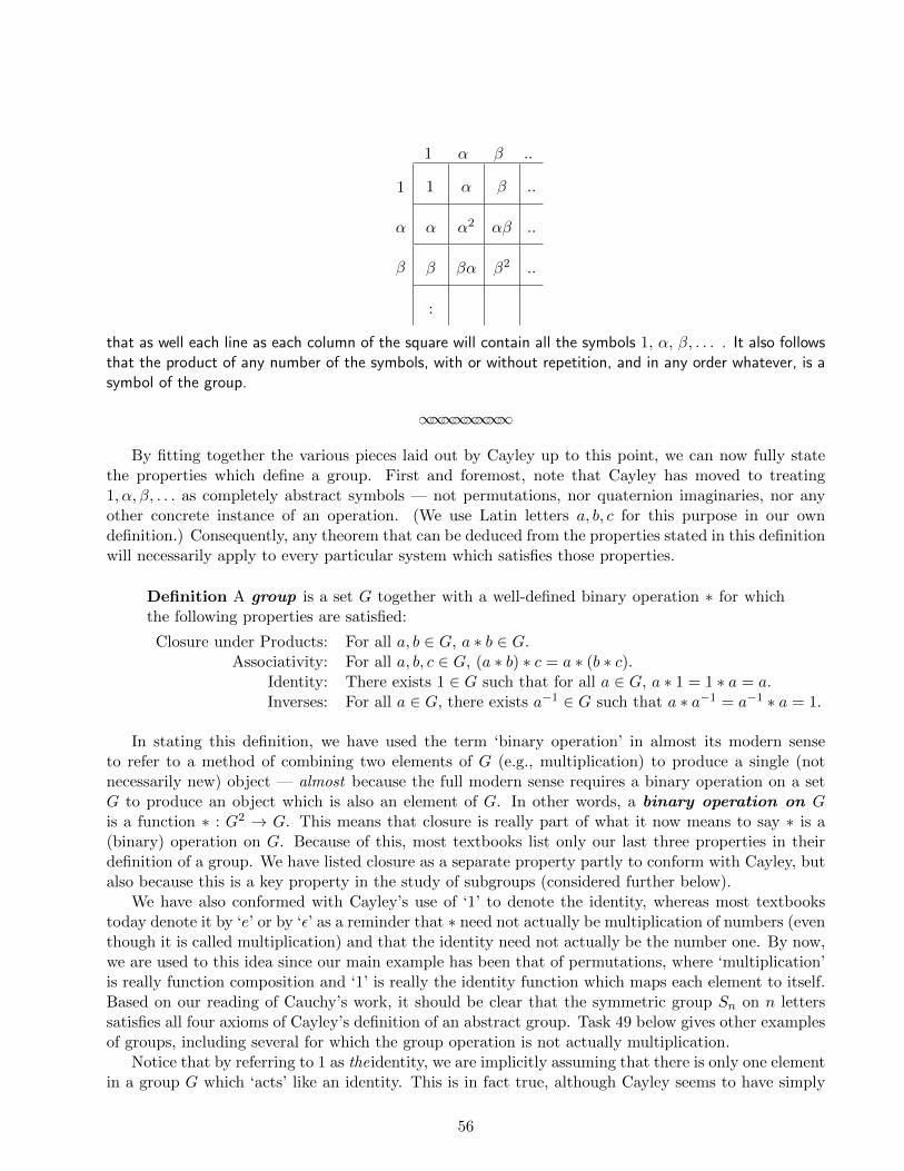
1 α β ..

1

α

β

1 α β ..

α α2 αβ ..

β βα β2 ..

:

that as well each line as each column of the square will contain all the symbols 1, α, β, . . . . It also followsthat the product of any number of the symbols, with or without repetition, and in any order whatever, is asymbol of the group.

∞∞∞∞∞∞∞∞

By fitting together the various pieces laid out by Cayley up to this point, we can now fully statethe properties which define a group. First and foremost, note that Cayley has moved to treating1, α, β, . . . as completely abstract symbols — not permutations, nor quaternion imaginaries, nor anyother concrete instance of an operation. (We use Latin letters a, b, c for this purpose in our owndefinition.) Consequently, any theorem that can be deduced from the properties stated in this definitionwill necessarily apply to every particular system which satisfies those properties.

Definition A group is a set G together with a well-defined binary operation ∗ for whichthe following properties are satisfied:

Closure under Products: For all a, b ∈ G, a ∗ b ∈ G.Associativity: For all a, b, c ∈ G, (a ∗ b) ∗ c = a ∗ (b ∗ c).

Identity: There exists 1 ∈ G such that for all a ∈ G, a ∗ 1 = 1 ∗ a = a.Inverses: For all a ∈ G, there exists a−1 ∈ G such that a ∗ a−1 = a−1 ∗ a = 1.

In stating this definition, we have used the term ‘binary operation’ in almost its modern senseto refer to a method of combining two elements of G (e.g., multiplication) to produce a single (notnecessarily new) object — almost because the full modern sense requires a binary operation on a setG to produce an object which is also an element of G. In other words, a binary operation on Gis a function ∗ : G2 → G. This means that closure is really part of what it now means to say ∗ is a(binary) operation on G. Because of this, most textbooks list only our last three properties in theirdefinition of a group. We have listed closure as a separate property partly to conform with Cayley, butalso because this is a key property in the study of subgroups (considered further below).

We have also conformed with Cayley’s use of ‘1’ to denote the identity, whereas most textbookstoday denote it by ‘e’ or by ‘ε’ as a reminder that ∗ need not actually be multiplication of numbers (eventhough it is called multiplication) and that the identity need not actually be the number one. By now,we are used to this idea since our main example has been that of permutations, where ‘multiplication’is really function composition and ‘1’ is really the identity function which maps each element to itself.Based on our reading of Cauchy’s work, it should be clear that the symmetric group Sn on n letterssatisfies all four axioms of Cayley’s definition of an abstract group. Task 49 below gives other examplesof groups, including several for which the group operation is not actually multiplication.

Notice that by referring to 1 as theidentity, we are implicitly assuming that there is only one elementin a group G which ‘acts’ like an identity. This is in fact true, although Cayley seems to have simply

56

taken it for granted. To prove the uniqueness of the identity, suppose 11 and 12 both act like groupidentities, so that for any x ∈ G, we have 11 ∗x = x ∗ 11 = x and 12 ∗x = x ∗ 12 = x. Then 11 = 11 ∗ 12(since 12 is an identity) and 11 ∗ 12 = 12 (since 11 is an identity), which implies 11 = 12. Inverses arealso unique, since given x ∈ G and elements y, z ∈ G with x ∗ y = y ∗ x = 1 and x ∗ z = z ∗ x = 1,associativity allows us to conclude that y = y ∗ 1 = y ∗ (x ∗ z) = (y ∗ x) ∗ z = 1 ∗ z = z. In other words,any element that acts like an inverse of x really is the inverse of x.

Task 48In this task, we use the uniqueness of inverses to prove three elementary results about groupinverses. Assume G is a group with identity element 1 and let x, y ∈ G.

(a) Use uniqueness of inverses to prove that (x−1)−1 = x.That is, show that x acts like the inverse of x−1.

(b) Use uniqueness of inverses to prove that (xy)−1 = y−1x−1.

(c) Prove that xy = 1 ⇒ y = x−1.This means that we can establish y is the inverse of x simply by checking that xy = 1,even in the case where G is non-abelian.

Task 49In this task, we examine the defining properties of a group by analyzing some additionalexamples and non-examples. Note that several of the groups in this task are infinite.

(a) Consider the set of non-zero rational numbers Q∗ =mn |m,n ∈ Z

∗ under multipli-cation ×, where Z∗ denotes the set of non-zero integers. Given that × is associative,show (Q∗,×) is a group by checking that it satisfies the other three group properties.For an arbitrary q = m

n ∈ Q∗, identify q−1 clearly and verify that q−1 ∈ Q∗.

Note: Since rational multiplication is commutative, (Q∗,×) is our first example of acommutative group, also referred to as an abelian group.

(b) Explain why the set of non-zero integers Z∗ is not a group under multiplication.Identify all properties of the group definition that fail.

(c) Now consider Z under addition. Given that integer addition is closed and associative,explain why (Z,+) is a group with identity element 0 and n−1 = −n for each n ∈ Z.

Note: (Z,+) is an example of an additive group for which it is standard to use thesymbols ‘+,’ ‘0,’ and ‘−n’ to denote the group operation, identity and inverse of nrespectively. (Z,+) is also an abelian group.

(d) Let Z6 = 0 , 1 , 2 , 3 , 4 , 5 and let + denote addition modulo 6.

That is, to find i+ j, we take the remainder of the sum when divided by 6.(Or think of arithmetic on a clock with 0, 1, 2, 3, 4, 5 equally spaced on its face.)58

For example: 3 + 4 = 1 ; 5 + 5 = 4 ; 1 + 2 = 3 ; 1 + 5 = 0 ; 4 + 0 = 4

Given that + is associative with identity 0, show that (Z6,+) is a group by explainingwhy Z6 is closed under +, and then finding the inverse element −n for each n ∈ Z6.Is (Z6,+) abelian? Why or why not?

(e) Consider the set M = X |X is a 2× 2 matrix under matrix multiplication ×.Given that × is associative, show that there is an identity element I, but that (M,×)is not a group. How could we modify the definition of M to obtain a group under ×?

58Compare this to your diagram of the 6th roots of unity in Task 3.

57

Task 50This task explores the definition and properties of integer exponents for group elements.

Let (G, ∗) be a group. For x ∈ G and n ∈ Z+, define xn = x ∗ x ∗ . . . ∗ x︸ ︷︷ ︸n factors

.

(a) Given x, y ∈ G and n ∈ Z+, explain why it is not generally the case that (xy)n = xnyn.Is it generally the case that (xy)n = ynxn? Why or why not?

(b) Assume G is an abelian group. Prove by induction that (xy)n = xnyn for all x, y ∈ Z+.

(c) In this part, assume only that G is a group (not necessarily abelian), but let x, y ∈ Gbe such that xy = yx; that is, assume that the specific group elements x, y commutewith each other, but do not assume that all group elements commute. Indicate howto modify your proof in part (b) to show that (xy)n = xnyn for all n ∈ Z+.

(d) Use part (c) and uniqueness of inverses to prove that (xn)−1 = (x−1)n.That is, show that (x−1)n acts like the inverse of xn.

(e) Using part (d), we extend the definition of integer powers for a group element x ∈ Gto include negative integer powers by setting x−n = (xn)−1 for all n ∈ Z+.To complete the definition, we also let x0 = 1 for all x ∈ G.

Assume that G is a group, x, y ∈ G and m, k ∈ Z.

Use cases (based on the signs of k,m) and the (extended) definition of integer powersto prove the following exponential properties hold in a group:

(i) (xk)m = xkm

(ii) xkxm = xk+m

(iii) If xy = yx, then (xy)m = xmym. (The case m > 0 was done in part (c).)

While we are looking at examples of groups, we should also look at some subgroup examples. Cayleyhimself did not use this term, but his emphasis on the closure property and other aspects of his worktell us that he was aware of the subgroup concept. He was also familiar with Cauchy’s work, where theidea of a subgroup arises in Cauchy’s notion of a ‘system of conjugate permutations.’ Recall from ourdiscussion of Cauchy’s work that we defined a subgroup of Sn to be any subset H ⊆ Sn which is closedunder products. Of course, Sn is a very special example of a group. In particular, all of its elements(i.e., permutations on n objects) are of finite order; under this condition, closure under products issufficient to obtain a subgroup, as we will prove in Task 54.

In general, however, closure of products is not enough to capture Cauchy’s full notion of a ‘systemof conjugate permutations.’ Taking our cue from what Cauchy said about these systems, the essentialidea will be to ensure that H is a subset of G which is itself a group in its own right — a group livinginside another group, so to speak. To ensure this, it may seem that we will need to check that an allegedsubgroup H has all four properties from the definition of group. However, since G is already known tobe a group and H ⊆ G, then we already know that associativity applies to all of G’s elements, includingthose belonging to H. Also, if H is closed under both products and inverses, then given h ∈ H, we’llhave h−1 ∈ H (by closure under inverses), so that 1 = hh−1 ∈ H (by closure under products). Inshort, to define the general notion of a subgroup, only two properties from the definition of a groupare needed:

Definition Let G be a group and H a non-empty subset of G. Then H is a subgroup ofG iff the following properties are satisfied:

Closure under Products: For all a, b ∈ H, a ∗ b ∈ H.Closure under Inverses: For all a ∈ H, a−1 ∈ H.

58

You may feel we stretched the truth a bit in saying that there are only two properties to check; infact, H must satisfy four properties in all: (1) H must be a subset of G; (2) H must be non-empty; (3)H must be closed under products; and (4) H must be closed under inverses. It is usually easy to checkthe first of these (that H ⊆ G), while checking the second (that H 6= ∅) is typically done by showing1 ∈ H. (In fact, H = 1 is always a subgroup of a group G, known as the trivial subgroup, so that1 may be the only element in a subgroup H.)

As for the two closure properties required for a non-empty subset to be a subgroup, note that theseare not a matter of checking that multiplication is well-defined, or that inverses exist for all elements.We already know both these things to be true, since G is given as a group. Rather, we must show thatproducts and inverses formed from elements of H live in the right place — namely, in H. For example,even though every non-zero integer n has a multiplicative inverse 1

n , it is not generally the case that1n is itself an integer; thus, Z∗ is not closed under multiplicative inverses,59 which in turn implies that(Z∗,×) is NOT a subgroup of the group (Q∗,×). On the other hand, (Q∗,×) IS a subgroup of thegroup (R∗,×) since both the products and the inverses of non-zero rational numbers are necessarilynon-zero rational numbers. The remaining five tasks in this subsection will give you some practice withthis important idea.

Task 51In this task, we examine examples and non-examples of subgroups of specific groups.

(a) Consider the group (Q∗,×) and let H = 12m |m ∈ Z

+, where Z+ denotes the set ofnatural numbers. Note that H is a non-empty subset of Q∗. Show that H is closedunder products, but is not a subgroup of Q∗.

(b) Again consider the group (Q∗,×), but now let K = 12m |m ∈ Z .

Show that K is a subgroup of Q∗.(c) Note that (R,+) is a group with identity 0, where R denotes the set of real numbers.

Let J1 = log(a) | a ∈ Q+ . Determine whether J1 is a subgroup of R under +, andjustify your reply. What about J2 = log(a) | a ∈ Z+ ?

Task 52In this task, we examine results related to the special case of a subgroup which is cyclic.

(a) Assume that G is a group with identity 1, where G is not necessarily abelian.

Let α ∈ G and H = 〈α〉 = αk | k ∈ Z .Prove that H is an abelian subgroup of G.

Note: H is called the cyclic subgroup generated by α.

(b) Identify all cyclic subgroups of (Z6,+), where + denotes addition modulo 6.

Note: In this case, we are looking at additive subgroups: 〈α〉 = kα |k ∈ Z.(Why we really only need to consider the values of integer k for which 1 ≤ k ≤ 6 here?)

(c) If there is an element of G which generates the entire group G, we say that G is cyclic.Prove (Z,+) is cyclic and find all its generators. Is (Q,+) cyclic? Explain.

59Note that Z∗,×) is closed under products.

59

Task 53In this task, we examine some more general ways to obtain subgroups of a given group G.

(a) Assume G is an abelian group with identity 1. Let H = x ∈ G |x = x−1 .Prove H is a subgroup of G, indicating clearly where the abelian assumption is used.

(b) Assume G is an abelian group with identity 1. Let n ∈ Z and K = x ∈ G |xn = 1 .Prove K is a subgroup of G, indicating clearly where the abelian assumption is used.

(c) Assume G is a group with identity 1, but not necessarily abelian.Define the center of G to be the set C = x ∈ G |xa = ax for all a ∈ G .(Thus, C consists of all the elements of G that commute with every element of G.)

Prove that C is a subgroup of G

Task 54In this task, we prove that closure under products is a sufficient condition for H to be asubgroup of G in the case where G is a group in which every element is of finite order,where the definition of order for permutations generalizes to abstract groups as follows:

Definition Let G be a group with identity element 1 and let α ∈ G. Then theorder of α in G is the least positive integer r for which αr = 1, provided sucha number exists. If such a number exists, we say α has finite order .

Assume G is a group with identity element 1 and that every element of G has finite order.

(a) Let α ∈ G, α 6= 1, and suppose α has order r ∈ Z+. Explain why α−1 = αr−1.

(b) Now assume that H is a non-empty subset of G which is closed under products.Prove that H is a subgroup of G.

Task 55In this task, we examine a special subgroup of Sn, where n ∈ Z+ and n ≥ 2.

Recall from Tasks 30 and 34 that every permutation can be written as the product oftranspositions, where a transposition is a 2-cycle.

Also recall that, although this decomposition is not unique, the parity (even versus odd) ofthe number of transpositions used is unique, since a permutation can be written either asthe product of an even number of transpositions, or as the product of an odd number oftranspositions, but never both. The parity (even or odd) of a permutation is defined to bethe parity (even or odd) of this number.

(a) Show that the product of two permutations is even if and only if both permutationshave the same parity (i.e., both are even or both are odd).

Note: Your proof must consider all three parity cases (even/even, odd/odd, even/odd).Do you see why?

(b) Let An be the subset of Sn consisting of all even permutations.Prove that An is a subgroup of Sn. Note: An is called the alternating subgroup.

(c) Explain why the set Sn −An of all odd permutations is never a subgroup of Sn.Give at least two reasons.

(d) Show that Sn contains an equal number of even and odd permutations byletting An = α1 , α2 , . . . , αk and Sn −An = β1 , β2 , . . . , βm, where k,m ∈ Z+,and then proving k = m. Explain why we can then conclude that |An| = n!

2 .

Hint? Consider the sets β1α1 , β1α2 , . . . , β1αk and β1β1 , β1β2 , . . . , β1βm.

60

Task 56In this task, we connect the notion of a subgroup to that of a Cayley table.

Consider the set M2,2 = X |X is a 2× 2 matrix, det(X) 6= 0. Since matrices with non-zero determinants are invertible, M2,2 is a (non-abelian) group under matrix multiplication.

Let G = I, A,B,C,D,E, with I the identity matrix and A,B,C,D,E as follows:

A =

[−1 −11 0

]B =

[0 1−1 −1

]C =

[0 11 0

]

D =

[−1 −10 1

]E =

[1 0−1 −1

]

(a) Complete the following Cayley table for G, and explain how it shows that G is asubgroup of M2,2. In particular, indicate how the table shows that G satisfies theInverse Property.

I A B C D E

I I A B C D E

A A I

B B I

C C I

D D I

E E I

(b) Determine the order of each element of G. (See Task 54 for definition of ‘order’.)Which familiar group of order 6 does G remind you of, and why?

3.2 Some Theorems on Groups

Look again at the Cayley table you completed in Task 56, and notice how each element of G appearsexactly once in every row and every column. This is exactly the theorem stated by Cayley (withoutproof) immediately following his definition of group. We re-state this theorem here, somewhat moreformally, and label it as ‘Cayley’s Theorem 1’ for future reference.

Cayley’s Theorem 1If G = 1 , α , β , . . . is a group with identity element 1, then the Cayley table for G is suchthat every row (e.g., α , α2 , αβ , . . .) and every column (e.g., α , α2 , βα , . . .) containsevery element of G exactly once.

61

Here, Cayley’s rows and columns correspond to the two series of permutations S, SP, SQ, SR, . . . andS, PS, QS, RS, . . . which Cauchy discussed in the excerpt on page 41 of this project. Cauchy alsonoted in that excerpt (again without proof) that the terms of these series are the same as those of theoriginal given system of permutations (1, P, Q, R, . . .) only ‘arranged in a new order’.60 The majordifference between the assertions of the two mathematicians is that Cauchy was speaking only aboutpermutations, while Cayley’s claim applied to any set of operation symbols that satisfied his definitionof a group. As a result, Cayley’s result is far more general than that of Cauchy. In Task 57, we outlinea proof of Cayley’s Theorem 1 using only the properties appearing in Cayley’s definition of group. Task58 then looks at a more formal version of this same theorem, and introduces some current notationand terminology related to it.

Task 57Let G = 1 , α , β , . . . be a group with identity element 1. Let φ ∈ G be arbitrary.

(a) Using only the properties of a group given in the definition of a group on page 56,explain why the row corresponding to φ in the Cayley table for G (see below) includesevery element of G exactly once. Write your explanation as a formal proof, and clearlyindicate which properties of the definition you are using and where they are needed.

Note that there are two things to show here:

(i) Every element of G appears somewhere in the row corresponding to φ.That is, given any θ ∈ G, there is some γ ∈ G for which θ = φγ.(After introducing θ as an arbitrary element of G, explicitly define γ, indicate howyou know γ is an element of G, and verify that θ = φγ for this choice of γ.)

Note: Since φ is also arbitrary, this corresponds to the formal statement:

(∀φ ∈ G) (∀θ ∈ G) (∃γ ∈ G) (θ = φγ)

(ii) No element of G appears more than once in the row corresponding to φ.That is, given γ1, γ2 ∈ G with φγ1 = φγ2, it follows that γ1 = γ2.(Start by introducing γ1, γ2 as arbitrary elements of G and assuming φγ1 = φγ2.)

Note: Since φ is also arbitrary, this corresponds to the formal statement:

(∀φ ∈ G) (∀γ1, γ2 ∈ G) (φγ1 = φγ2 ⇒ γ1 = γ2)

1 α β . . . φ . . . γ . . .

1

α

β

:

φ

:

φ φα φβ . . . φ2 . . . φγ . . .

(b) How would you modify this explanation to apply to the columns of the Cayley table?

60You may wish to review Tasks 38 and 39 concerning this part of Cauchy’s paper.

62

Task 58In this task, we explore a theorem related to Cayley’s Theorem 1. We first state thistheorem in the more formalized terms that one finds in current textbooks and comment ontheir meaning and importance. We then outline its proof for you to complete.

Cayley’s Theorem 1 - A Formalized Variation

If G = 1 , α , β , . . . is a group with identity element 1 and φ ∈ G is arbitrary,then Gφ = G = φG, where Gφ = φ , αφ , βφ , . . . and φG = φ , φα , φβ , . . ..

Comments

• The equation φG = Gφ does not imply that the elements of G commute, but onlythat these sets contain the same elements, possibly arranged in a different order.61

• By using set notation in the conclusion φG = G of this theorem, we are no longerexplicitly stating that every element of G appears in the form φγ for only one elementγ ∈ G. This fact still holds, however, as proved Task 57(a-ii).

• It is important that φ is assumed to be an element of the group G in this theorem!

To see this, remember that Cauchy’s proof of Lagrange’s Theorem for Sn (discussedin Subsection 2.2) relied on sets of the form U , UP , UQ , . . ., which were obtainedby (left) multiplying the elements of the set 1 , P , Q , . . . by the permutation U .In that proof, the set 1 , P , Q , . . . was specified to be a subgroup of Sn and thepermutation U came from outside of that subgroup (but inside Sn). Consequently, asCauchy argued, the two sets U , UP , UQ , . . . and 1 , P , Q , . . . are disjoint.

In current adaptations of Cauchy’s proof of Lagrange’s Theorem for Sn to the case ofa general group G, it is standard to refer to the type of set employed in the proof asa (left) coset, denoted and defined by aH = ah|h ∈ H, where H is a subgroup of Gand a ∈ G. In this context, it may or may not be the case that a ∈ H and the formalvariation of Cayley’s Theorem 1 that we are looking at in this task may not apply.In the event that a ∈ H, then this theorem does apply, and we can conclude thataH = H. In the contrary case, where a 6∈ H, we would be able to show Ha ∩H = ∅in exactly the same way that Cauchy established this result for permutation groups.

Proof Sketch: Formalized Variation of Cayley’s Theorem 1

Let G = 1 , α , β , . . . be a group with identity element 1. Let φ ∈ G be arbitrary.

Define the sets Gφ = φ , αφ , βφ , . . . and φG = φ , φα , φβ , . . ..

(a) Complete the following details to show that Gφ = G.

(i) Explain why Gφ ⊆ G.That is, given x ∈ Gφ, what property of groups allows us to conclude that x ∈ G?

(ii) To show that G ⊆ Gφ, we let y ∈ G and show that y ∈ Gφ.Explain why this requires us to find some z ∈ G for which y = zφ.Then use group properties to determine z. How do we know that z ∈ G?

(b) Now prove that φG = G.

61It may be helpful to review Tasks 38 and 39 in this regard.

63

We now return to our reading of Cayley’s second paragraph, in which he makes a connection betweenfinite groups of order n and the set of nth roots of unity. This excerpt is packed with theorems! As youread through it, try to identify as many of these as possible. Also notice that Cayley is consideringonly finite groups in what follows.

∞∞∞∞∞∞∞∞

Suppose that the group1, α, β, . . .

contains n symbols, it may be shown that each of these symbols satisfies the equation

θn = 1;

so that a group may be considered as representing a system of roots of this symbolic equation. It is,moreover, easy to show that if any symbol α of the group satisfies the equation θr = 1, where r is lessthan n, then that r must be a submultiple of n; it follows that when n is a prime number, the group is ofnecessity of the form

1, α, α2, . . . αn−1, (αn = 1);

and the same may be (but is not necessarily) the case, when n is a composite number. But whether nbe prime or composite, the group, assumed to be of the form in question, is in every respect analogous tothe system of the roots of the ordinary binomial equation xn − 1 = 0; thus, when n is prime, all the roots(except the root 1) are prime roots; but when n is composite, there are only as many prime roots as thereare numbers less than n and prime to it, &c.

∞∞∞∞∞∞∞∞

In the remainder of this subsection, we separate the various theorems including in this excerpt,stating each in current terminology and numbering them in the order in which Cayley cited them. SinceCayley himself did not provide proofs, we will also examine why he felt they were so straightforwardin light of what we know about permutation groups, and write our own proofs for them using currentterminology and notation. We begin with three theorems drawn from the first two sentences of theexcerpt.

Cayley’s Theorem 2Let G be a finite group of order n with identity element 1 and let α ∈ G be arbitrary. Thenαn = 1.

Cayley’s Theorem 362

Let G be a finite group of order n with identity element 1 and suppose α ∈ G has order r.Then r is a divisor (submultiple) of n.

Cayley’s Theorem 4Every group G of prime order is cyclic.That is, if n is prime and |G| = n, then G = 〈α〉 = 1 , α , α2 , . . . , αn−1 for some α ∈ G.

62Notice that we have interpreted Cayley slightly here, since he did not explicitly state that r had to be the least numberfor which αr = 1, but only required that r be less than n. However, r < n is not enough for Cayley’s conclusion to hold.For example, if G is a group of order 6 and α ∈ G has order 2, then we will have α4 = (α2)2 = 12 = 1 with 4 < 6, eventhough 4 is not a divisor of 6. A specific example of this occurs when G = S3 and α = (1, 2).

64

All three of these theorems bear a resemblance to facts we already know about permutation groups.In Task 42, for example, we saw how the following version of Cayley’s Theorem 3 follows from Lagrange’sTheorem for Sn:

Cayley’s Theorem 3 - Restricted to SnFor every permutation P ∈ Sn, the order of P divides the order of Sn.

The standard proof given today for the fully general version of Cayley’s Theorem 3 (i.e., withoutthe restriction to permutation groups) uses the fully generalized version of Lagrange’s Theorem, ina fashion similar to that you employed in Task 42. We will say more about this below (and remindyou of Lagrange’s Theorem along the way). But first, it will be helpful to look at some facts relatedto the order of elements in an abstract group, drawing on what we already know about the order ofpermutations. We begin by restating the definition of order for group elements, and extending it justa bit to include elements which are not of finite order:

Definition Let G be a group with identity element 1 and let α ∈ G. Then the order of αin G is the smallest natural number r for which αr = 1, provided such a number exists.If such a natural number exists, α has finite order ; otherwise, α has order infinity .

Some groups (e.g., (Z,+)) contain only one element of finite order (i.e., the identity). In contrast, everyelement of the permutation group Sn has finite order. It turns out — as Cayley’s Theorem 2 implies— that every group of finite order contains only elements of finite order. This claim is straightforwardto prove directly from the Pigeonhole Principle, just as Cauchy did in his proof that every permutationhas finite order. We start our proofs of Cayley’s theorems by doing this and examining some otherfacts related to the order of group elements in Tasks 60 – 62. We then use these facts to prove atheorem about cyclic groups in Task 63. Task 59 first provides examples of order computations forgroup elements in non-permutation groups to provide some concrete context for these various proofs.

Task 59In this task, you will compute the order of specific elements in non-permutation groups.

(a) Consider Z8 = 0 , 1 , 2 , 3 , 4 , 5 , 6 , 7 under addition modulo 8.

Determine the order of each element; indicate which of these generate the entire group.

Remember that 0 is now the identity in this additive group!

(c) Find all elements of finite order in the group of non-zero rational numbers (Q∗,×).

Task 60In this task, you will formally prove the following:

Order Fact 1If G is a finite group and α ∈ G, then α has finite order.

Begin by assuming G is a finite group of order n with identity element 1 and α ∈ G.

(a) Apply the Pigeonhole Principle (see footnote 33, page 30) to the setH = αm |m ∈ Z+ in order to obtain h, l ∈ Z+ such that αh = αl and h < l.

(b) Use group properties to show that αl−h = 1.Explain how this shows that the set K = k ∈ Z+ |αk = 1 is non-empty.

(c) Complete the proof by applying the Well Ordering Principle63 to the set K.

63The Well Ordering Principle states that every non-empty subset of Z+ has a least element.

65

Task 61In this task, you will formally prove the following:

Order Fact 2If α ∈ G has finite order r and m ∈ Z with αm = 1, then r is a divisor of m.

Begin by first stating all necessary assumptions, and using the division algorithm to obtaink, j ∈ Z such that m = kr + j and 0 ≤ j < r. Then employ the assumption that α hasorder r to show that j = 0.

Note: This proof does not require the group G itself to have finite order.

Task 62In this task, you will formally prove the following:

Order Fact 364

The order of an element α ∈ G is equal to the order of the cyclic subgroup〈α〉 = αm |m ∈ Z generated by α.

Begin by assuming G is a group and noting that there are two cases to consider:(i) α ∈ G has finite order r, r ∈ Z+; and (ii) α ∈ G has in finite order.

Beginning with the finite case, assume α ∈ G has finite order r, where r ∈ Z+.

(a) Let m ∈ Z. Use the division algorithm to obtain k, j ∈ Z such that m = kr + j and0 ≤ j < r. Show that αm ∈ 1 , α , α2 , . . . , αr−1 . Note that this means that 〈α〉contains at most r elements.

(b) Let h, l ∈ 0 , 1 , . . . , r− 1 and suppose that αh = αl. Use the fact that r is the leastnatural number for which αr = 1 to show that h = l.

(c) Explain how (a) and (b) allow us to conclude that 〈α〉 = 1 , α , α2 , . . . , , αr−1 contains exactly r elements.

(d) At this point in the proof, the following implication has been established:If ord(α) = r, where r ∈ Z+, then |〈α〉| = r.

Now prove its converse:

If 〈α〉 = αk |k ∈ Z has finite order r, then α has order r.

Note: You need to show that (i) αr = 1 and (ii) αi 6= 1 for i ∈ Z+ with i < r.

(e) Part (d) completes the proof of the finite case. Explain why the case in which α hasinfinite order now follows directly from the contrapositive of the following statement:

〈α〉 = αm |m ∈ Z can be infinite iff there is no r ∈ Z+ for which αr = 1.

64Both Cauchy and Cayley hinted at this relationship in their work; in fact, Cauchy explicitly proved it for permutationgroups, while Cayley took it for granted as another easy-to-establish result.

66

Task 63This task uses ideas similar to those used in the proofs of Order Facts 1 – 3 in order toprove the following theorem about subgroups of cyclic groups:65

Every subgroup of a cyclic group is cyclic.

Begin by assuming G = 〈α〉 is a cyclic group with generator α and H is a subgroup of G.(We do not need to assume that either G or H is finite.)

To show that H is cyclic, we must find a generator. Note that if H = 1, then we aredone. (Why? ) Thus, we can assume that H is a non-trivial subgroup.

(a) Explain why the set K = m ∈ Z+ |αm ∈ H is non-empty.

Then apply the well-ordering principle to K to obtain the least natural number m0

such that αm0 ∈ H. Our plan is to show that H is generated by αm0 , or H = 〈αm0〉.(b) Begin with the easy direction, and explain why 〈αm0〉 ⊆ H.

(c) For the other direction, let β ∈ H and show β ∈ 〈αm0〉 as follows:

(i) Explain how we know that there exists some m ∈ Z such that β = αm.

(ii) Use the division algorithm to obtain k, j ∈ Z+ with m = km0+j and 0 ≤ j < m0.

(iii) Use part (ii) and the definition of subgroup to explain why the element αj mustbe in H. Then conclude from the definition of m0 that j = 0.

(iv) Complete the proof by explaining why j = 0 implies that β ∈ 〈αm0 〉.

We are now ready to consider the proof of Cayley’s Theorem 3, which states that the order of anyelement divides the order of the entire group. First, some notation and reminders. Assume G is a groupof order n and α ∈ G. By Order Fact 1, we know that α has some finite order r. To distinguish thenotion of group order (cardinality) from that of element order, we will write |G| = n and ord(α) = r. Ifwe knew that αn = 1 (Cayley’s Theorem 2), then we could conclude that r divides n by Order Fact 2.But we have not yet established Cayley’s Theorem 2 in this project; in fact, we plan to prove Cayley’sTheorem 2 as a corollary to Cayley’s Theorem 3. Thus, to avoid circular reasoning, we will need toprove that r divides n in some other way. We do this by bringing in the cyclic subgroup H = 〈α〉generated by α. As we know from our proof of Order Fact 3, the definition of ord(α) as the leastnatural number for which αr = 1 implies that |H| = r. The only remaining piece needed to prove thatr = ord(α) = |H| divides n = |G| is to recall what Lagrange’s Theorem says about the orders of agroup and its subgroups:

Lagrange’s Theorem for Finite GroupsIf H is a subgroup of the finite group G, then the order of H divides the order of G.

Remember that our first statement of Lagrange’s Theorem in Subsection 2.2 applied only to the par-ticular group Sn of permutations on n elements. But as we commented at that time, Cauchy’s proofstrategy for permutation groups is readily adapted to the general case of any finite group, either directlyor by re-casting it in the language of cosets. You can look back at the proof you wrote in Task 41 to seehow easy this is to do directly from Cauchy’s proof; in Appendix II, we also outline the now-standardcoset proof of the general theorem. For the rest of this project, however, we simply assume (as Cayleyseemed to have done) that Lagrange’s Theorem holds for groups in general.

65Although this theorem does not involve facts about the order of elements, the similarity of its proof to those of OrderFacts 1, 2 and 3 makes it a good exercise with these proof techniques.

67

Task 64Use Lagrange’s Theorem for Finite Groups and the ideas we sketched out just above itsstatement to write a complete formal proof of Cayley’s Theorem 3:

If G is a finite group and α ∈ G, then ord(α)∣∣ |G|.

Task 65Assume G is a group of order n with identity element 1 and let α ∈ G be arbitrary.

Now that we know (by Cayley’s Theorem 3) that ord(α) divides |G|,it is easy to establish Cayley’s Theorem 2 by proving that α|G| = 1.

Do this by letting n = kr, where |G| = n, ord(α) = r and k ∈ Z+.Write your proof out completely and carefully, explaining clearly how k is obtained.

Of course, it may be that Cayley had some proof of his Theorem 2 in mind which somehow didnot require first proving his Theorem 3. Given Cauchy’s work on permutations, however, the proofyou just completed in Task 65 is a good possibility for how Cayley himself arrived at his Theorem 2;it is also how Cayley’s Theorem 2 is typically proven today. Cayley’s Theorem 3 also makes it easyto prove Cayley’s Theorem 4 — that every group of prime order is cyclic — although this too can beproven directly from Lagrange’s Theorem.

Task 66

Assume n is prime and G is a group of order n with identity element 1.

Let α ∈ G be such that α 6= 1. (How do we know such an element exists?)Use the fact that ord(α) divides |G| (from Cayley’s Theorem 3) to show that G = 〈α〉.

Note: If you prefer, you can instead show that G is cyclic by using Lagrange’s Theorem.

Before we return to the remaining theorems stated by Cayley in the previous excerpt from hispaper, we comment on one more aspect of Lagrange’s Theorem. Clearly, this theorem tells us thatthe order of a subgroup can assume only certain very specific values; namely, only those which are thedivisors of the order of a group. Thus, for instance, a group of order 6 can not have a subgroup oforder 4 or 5. However, Lagrange’s Theorem does not say that a group of order 6 must have a subgroupof order 1, 2, 3 or 6, even though these are all divisors of its order. As it turns out, every group oforder 6 does have subgroups of every possible order, as do all cyclic groups.66 The Alternating GroupA4 consisting of all even permutations in S4, on the other hand, is a group of order 12 which containsno subgroup of order 6, even though 6 is a divisor of the order of the group.67

66For groups of order 6, this follows from a proof we will see in Subsection 4.2 in which Cayley showed that all groupsof order 6 necessarily have elements of order 2 and 3, which in turn generate subgroups of order 2 and 3. AlthoughCayley employed Lagrange’s Theorem as a tool in this proof, the existence of these subgroups does not follow directlyfrom Lagrange’s Theorem and can be proven without making use of it.

The proof that a cyclic group of order n has a (cyclic) subgroup of order d for every divisor d of n likewise does notrequire Lagrange’s Theorem, but relies instead on basic facts about the order of elements established in Tasks 60–63.(Writing out this proof would serve as a good review and application of those facts!)

67An was defined in Task 55 and shown there to have order n!2

. The claim that A4 has no subgroup of order 6 canbe verified by writing down the 12 even permutations in S4, and using the closure properties to eliminate the possibilityof building a subgroup containing exactly 6 elements from that list. (It may be easier to first write down the 12 oddpermutations in S4 since this can be done using what we know about the parity of n-cycles.) In Task 75, we will provethat A4 does contain subgroups of order 2, 3 and 4.

68

Similarly, although Cayley’s Theorem 3 tells us that the order of any element in a finite group mustdivide the order of the group, that theorem does not imply the existence of elements of any particularorder. In fact, the only way a group of order n could have an element of order n would be if the groupwere cyclic. But as Cayley remarked in the preceding excerpt, for a composite number n (such asn = 6):

“ it may be (but is not necessarily) the case that the group is of the form

1, α, α2, . . . αn−1, (αn = 1).′′

Cayley again gave no proof for this, but we have already seen several examples that illustrate its truth.The following task reminds us of these examples for the case n = 6.

Task 67

(a) Show that (Z6,+) is cyclic and find all its generators. (See Task 52(b).)

(b) Let U6 =e

2πk6i∣∣ k = 1, 2, 3, 4, 5, 6

denote the set of the 6th roots of unity.

Recall from Task 5 that α = e2π6i = e

π3i is a primitive root of unity, meaning that

U6 = 1 , α , α2 , α3 , α4 , α5 . Thus, (U6,×) is a cyclic group generated by α.

Determine all other generators of U6. (Task 3 may also be helpful.)

What similarities/differences do you notice between the groups U6 and Z6?

(c) Consider the group of matrices H = I, A,B,C,D,E defined in Task 56.

Explain how we know that H is non-cyclic. (Give at least two pieces of evidence.)

What similarities/differences do you notice between H and the groups U6 and Z6?

(d) Explain how we know that the symmetric group S3 is non-cyclic, where

S3 = (1)(2)(3) , (1, 2, 3) , (1, 3, 2) , (1, 2) , (1, 3) , (2, 3) .

What similarities/differences do you notice between S3 and the groups in (a) – (c)?

Although a group of composite order may or may not be cyclic, Cayley concluded the excerpt fromwhich we are extracting our list of his theorems with the following observations about cyclic groups ingeneral:

But whether n be prime or composite, the group, assumed to be of the form in question [thatis, 1, α, α2, . . . αn−1, (αn = 1)] is in every respect analogous to the system of the roots ofthe ordinary binomial equation xn−1 = 0; thus, when n is prime, all the roots (except the root1) are prime roots; but when n is composite, there are only as many prime roots as there arenumbers less than n and prime to it.

Cayley’s ‘system of the roots of the ordinary binomial equation xn − 1 = 0’ is exactly the systemof nth roots of unity that we first encountered in our reading of Lagrange. In fact, Lagrange himselfexplained that this system forms a cyclic group of order n, although not in this exact language. Denoting

this set by Un = e2πkni | k = 1, 2, 3, . . . , n, Lagrange also discussed its generators (or primitive roots)

and came to the same conclusions stated by Cayley above. (Cayley referred to the generators as ‘primeroots’.) What Cayley has added to Lagrange’s insights is the idea that any cyclic group of order nwill behave in exactly the same manner as Un. For example, as we have suggested at various points

69

in this project, the additive group Z6 is essentially the same of the multiplicative group U6, althoughwith different names and interpretations attached to its elements and operation.

The technical term used today to express the idea that two groups are ‘in every respect analogous’is to say that these groups are isomorphic. This term comes from the Greek iso, meaning ‘same,’and morph, meaning ‘form.’ Notice how the following formal definition uses a special sort of bijectivefunction to convey the idea that the underlying group structure (or form) is being maintained, withonly the names of the elements changed by the function (e.g., from ‘a’ to ‘f(a)’).

Definition Let (G, ∗) and (G′, ?) be two groups. Then G is a isomorphic to G′ iff thereexists a one-to-one onto function f : G→ G′ with the following property:

For all a, b ∈ G, f(a ∗ b) = f(a) ? f(b).

The function f is called a (group) isomorphism .

The two symbols ∗ and ? are used here to emphasize that the group operation in the domain G neednot be the same as the group operation in the range G′. For example, to show that the additive group

Zn is isomorphic to the multiplicative group Un, we could define f : Zn → Un by f(k) = e2πkni, and

then check that f is one-to-one, onto and satisfies f(k +m) = f(k)f(m) for all k,m ∈ Zn.

Task 68

(a) Use the function f defined above to formally prove (Zn,+) is isomorphic to (Un,×).

(b) Define a function g : H → S3 which could be used to show that the group of matricesH = I, A,B,C,D,E defined in Task 56 is isomorphic to the symmetric group S3.Explain carefully how you decided what each particular function value should be andwhy these choices will preserve the algebraic structure of H. Is your function the onlypossible isomorphism between these two groups? Why or why not?

Note: It may be useful to review parts (c) and (d) of Task 67.

To further illustrate the idea that isomorphic groups are really the same groups, but with the nameschanged to partially disguise this fact, the next task examines some group properties that are preservedby isomorphisms.

Task 69In this task, we look at some group properties preserved by isomorphisms.

Assume that (G, ∗) and (G′, ?) are isomorphic groups with identities 1, 1′ respectively.Let f : G→ G′ be a group isomorphism.

(a) Prove that f(1) = 1′ by showing that f(1) ? y = y ? f(1) = y for all y ∈ G′.This shows that identities are preserved by group isomorphisms.

Note: Starting with y ∈ G′ arbitrary, you will need to find some x ∈ G with f(x) = y.Explain carefully how we know that such an element x exists.

(b) Given x ∈ G, prove that [f(x)]−1 = f(x−1) by showing that f(x−1) ? f(x) = 1′.This shows that inverses are preserved by group isomorphisms.

(c) Given x ∈ G with finite order r in G, prove that ord[f(x)] = r in G′

by showing that r is the least natural number with [f(x)]r = 1′.This shows that order is preserved by group isomorphisms.

Hint? Start by using induction to prove that f(xk) = [f(x)]k for all k ∈ Z+.

(d) Prove that G is abelian if and only if G′ is abelian.This shows that the property of being abelian is preserved by group isomorphisms.

70

Using the language of isomorphisms, we can restate Cayley’s assertion that cyclic groups are ‘inevery respect analogous to the system of the roots of the ordinary binomial equation xn−1 = 0’ as follows;we also give the modified version of this same which is more likely to be found in current textbooks.The proof of either version proceeds by defining f(αk) = βk for 0 ≤ k ≤ n−1, where α, β are generatorsof the two groups in question — be sure that you can verify these details if asked!

Cayley’s Theorem 5Let G be a cyclic group of order n, with G = 〈α〉 = 1 , α , α1 , . . . , αn−1 for some α ∈ G.

Then G is isomorphic to the group Un = e2πkni | k = 1, 2, 3, . . . , n under multiplication.

Cayley’s Theorem 5 - A Modern VariationEvery cyclic group of order n is isomorphic to the group Zn under addition modulo n.

This leaves us with just two more theorems from Cayley’s second paragraph, both of which were alsodiscussed by Lagrange for the specific case of the nth roots of unity.

Cayley’s Theorem 6If G is a cyclic group of prime order, then every element of G other than the identity elementis a generator.

Cayley’s Theorem 7Let φ(n) denote the number of natural numbers k < n for which gcd(k, n) = 1.If G is a cyclic group of order n, then G has φ(n) generators.

The function φ in Cayley’s Theorem 7 is known as the Euler phi function, and plays an importantrole in number theory, as well as in algebra. The proof of Cayley’s Theorem 7 lies beyond our immediatepurposes, but appears in many current algebra textbooks. To illustrate it in the specific case of n = 6,first that there are only two natural numbers less than 6 which are relatively prime to 6 (namely, 1and 5), so that φ(6) = 2. Thus, Cayley’s Theorem 7 predicts that Z6 will have only two generators, afact that you proved in Task 67(a). Notice also that if n is prime, then every natural number less thann is relatively prime to n, so that φ(n) = n− 1. Thus, one way to prove Cayley’s Theorem 6 would beto apply Cayley’s Theorem 7 to the particular case where n is prime. Since you have already proved(in Task 66) that G = 〈α〉 for any arbitrary non-identity element α ∈ G in a group of prime order,however, no further proof of Cayley’s Theorem 6 is needed!

Task 70In this task, we look at Cayley’s Theorem 7 in some additional particular cases.

(a) Explain why φ(8) = 4 and identify the four generators of Z8.

(b) Explain why φ(9) = 6 and identify the five generators of Z9.

(c) Make a conjecture concerning what the generators will be for Zn. Test your conjecturefor n = 10 and n = 18 and refine it as needed before writing a formal proof for it.

4 Cayley’s Classification of Groups of Small Order

We have now arrived at the heart of Cayley’s paper: the classification of groups of finite order accordingto their form. In fact, by asserting that all groups of prime order have the same form as the cyclicgroup Up, Cayley had already accomplished this classification for groups of prime order p. Althoughwe are more likely today to consider the integers mod p under addition (rather than the pth roots ofunity under multiplication) as the prototype for cyclic groups of order p, the key idea here is the same:

71

for any given prime p, there is essentially only one group of order p. As Cayley well knew, however, agroup G of order n might not be isomorphic to Zn when n is composite; in fact, a group of compositeorder need not even be abelian.

The problem which Cayley therefore began to study at this point of his paper was that of identifyingall possible non-isomorphic groups of order n for various composite values of n. If these distinct non-isomorphic group structures could be fully identified, they would in turn serve as prototypes for allgroups of that same order, much as Zp serves as the prototypical group of order p when p is prime. Thatis, any group of order n would necessarily be isomorphic to one of the distinct prototypical structuresavailable for that order.

We will see Cayley’s classification of all groups of order n = 4 and n = 6 below; in a later paper,published in 1859, he also gave the classification of groups of order n = 8 (see [7]). In time, however, itbecame clear that the problem of classifying all groups of finite order is a very difficult one — so difficultthat mathematicians eventually turned to the (presumably more straightforward) task of classifyingcertain types of finite groups. One particular type of group was considered especially important in thisregard, due to the special role it plays within group theory. Namely, much as prime numbers serve asthe basic building blocks of all natural numbers, simple groups serve as the basic building blocks of allgroups. The definition of a ‘simple group’ is given in Appendix II of this project; its basic concept canbe traced back to the work of Galois on algebraic solvability.

The first major results related to the classification of finite simple groups were published in 1870 bythe French mathematician Camille Jordan (1838–1922). Yet it was not until 1981, after a coordinatedeffort by over 100 different mathematicians beginning in 1965, that the search for all finite simple groupswas declared complete. Even then, gaps initially remained in the proof — as might well be expectedwith a proof that stretched out over approximately 500 journal articles totaling 10,000–15,000 pages.Known as the ‘Enormous Theorem’ in recognition of the complexity of its proof, the Classification ofFinite Simple Groups Theorem is now considered by experts in the field to be fully established. Thepublication of a revised ‘second generation proof’ expected to fill approximately twelve volumes and3000–4000 pages is also currently under way by the American Mathematical Society.

4.1 Groups of Order 4

Cayley started his classification efforts, naturally enough, with the first composite number, n = 4.

∞∞∞∞∞∞∞∞

The distinction between the theory of the symbolic equation θn = 1, and that of the ordinary equationxn − 1 = 0, presents itself in the very simplest case, n = 4. For consider the group

1, α, β, γ,

which are a system of roots of the symbolic equation

θ4 = 1.

There is, it is clear, at least one root β, such that β2 = 1; we may therefore represent the group thus,

1, α, β, αβ, (β2 = 1);

then multiplying each term by α as the further factor, we have for the group α, α2, αβ, α2β, so that α2

must be equal either to β or else to 1. In the former case the group is

1, α, α2, α3 (α4 = 1),

which is analogous to the system of roots of the ordinary equation x4 − 1 = 0.

72

For the sake of comparison with what follows, I remark, that, representing the last mentioned group by

1, α, β, γ,

we have the table

1 α β γ

1

α

β

γ

1 α β γ

α β γ 1

β γ 1 α

γ 1 α β

If, on the other hand, α2 = 1, then it is easy by similar reasoning to show that we must have αβ = βα,so that the group in this case is

1, α, β, αβ, (α2 = 1, β2 = 1, αβ = βα);

or if we represent the group by

1, α, β, γ,

we have the table68

1 α β γ

1

α

β

γ

1 α β γ

α 1 γ β

β γ 1 α

γ β α 1

or, if we please, the symbols are such that

α2 = β2 = γ2 = 1,α = βγ = γβ,β = γα = αγ,γ = αβ = βα

[and we have thus a group essentially distinct from that of the system of roots of the ordinary equationx4 − 1 = 0].

∞∞∞∞∞∞∞∞

68Notice the double lines that Cayley used to break this table into four smaller squares, with the smaller squares formingtwo disjoint pairs. One of these pairs corresponds to the subgroup H = 〈α〉 = 1 , α . The other corresponds to the setobtained by multiplying the elements of H by β: βH = β , βα = β , γ . The set βH is called the left coset of Hcorresponding to β. See also the comments about cosets in Task 58.

73

It is easy to see just by looking at their Cayley tables that these two groups are non-isomorphic.Among their distinguishing features, the first is cyclic and has only one element of order 2, while thesecond is non-cyclic and has three elements of order 2. Each of these characteristics would have beenpreserved by an isomorphism, if one existed. Of course, Cayley’s claim is not just that these are distinctgroups of order 4, but that these are the only two groups of order 4 possible (up to isomorphism). Theanalysis given by Cayley in support of this claim began with the assertion “there is, it is clear, at leastone root β, such that β2 = 1.” Given the essential role this fact played in his analysis, let us take sometime to carefully prove it, and also to fill in the details of how it implies there are only two distinctgroups of order 4. Interestingly, since both these groups are abelian, we can then conclude that everygroup of order 4 is abelian.

Task 71This task fills in the details of Cayley’s proof that there are exactly two groups of order 4.

Let G = 1, α, β, γ be a group of order 4.Thus, the four symbols represent four distinct elements, so that α 6= 1, β 6= γ, etc.

(a) Explain why every element of G other than the identity must have order 2 or 4.

If ord(α) = 2, note that Cayley’s claim that G contains at least one element of order2 is clearly true. Suppose therefore that ord(α) = 4, and explain how we know that Gmust also contain at least one element of order 2 in this case.

In the remainder of this task, we will let β denote an element of order 2(as Cayley did), since this involves no loss of generality.

(b) Explain why γ must be equal to αβ.That is, explain how we know that αβ 6= 1, αβ 6= α and αβ 6= β.

Hint? It may be helpful to remember that β2 = 1, per part (a).

(c) Since multiplying each element by α will reproduce all the elements of the group simplyre-arranged in some different order, we now know that 1, α, β, αβ = α, α2, αβ, α2β .

Note: This is simply Cayley’s Theorem 1, since the ordered list (α, α2, αβ, α2β)is just the row of the Cayley table corresponding to (left) multiplication by α.

In particular, α2 must be equal to one of the original four elements of the group.

Explain how we know that α2 6= α and α2 6= αβ.

This leaves only two remaining cases to consider: α2 = 1 and α2 = β.

(d) Explain why the assumption α2 = β implies that α has order 4.This case corresponds to the cyclic group of order 4 in Cayley’s first table.

(e) Finally, suppose α2 = 1 and employ ‘similar reasoning’ to obtain the second group.That is, multiply through (on the left) by β to reproduce G (Cayley’s Theorem 1!),so that 1, α, β, αβ = β, βα, β2, βαβ .• Explain why βα can not equal 1, α or β, and conclude that βα = αβ.

• Use the defining equations obtained for this case (β2 = 1, α2 = 1, αβ = βα )to explain why γ = αβ also has order 2.

This case corresponds to the non-cyclic group of order 4 in Cayley’s second table.

We should remark here again that, although every group of order 4 must have an element of order2, as you proved in part (a) of the previous task, it is not generally true that a group G will have anelement of order d for every divisor d of |G|. In fact, Cayley’s example of a non-cyclic group of order

74

4, shows it is possible for a group of order 4 to contain no elements of order 4, despite the fact that 4is a divisor of the group’s order. Similarly, even though 6 is a divisor of |S3| = 6, we know S3 has noelement of order 6. Later in this section, we will also see a group of order 8 which has no elements oforder 4 or of order 8. As another counterexample involving a proper divisor of the group’s order, recallthat the 12-element group A4 has no subgroup (and hence no element) of order 6, as was noted in anearlier section.69 Thus, although the order of every element in a finite group must divide the order ofthe group (Cayley’s Theorem 3), the reverse does not generally hold.

There is, however, a partial converse to Cayley’s Theorem 3, which we state here without proof:

Cauchy’s TheoremA finite group G contains an element of order p for every prime divisor p of |G|.

Despite its name, Cauchy’s Theorem was not known in its current form to either Cauchy or Cayley70

— much as Lagrange’s Theorem was not known in its current form to Lagrange — and Cayley couldnot simply invoke it to conclude that a group of order 4 must have an element of order 2. Rather,Cayley deduced this fact directly from what he knew about the structure of 4 element groups. There is,however, an even more direct way to prove that there is only one non-cyclic group of order 4, withoutusing the fact that all groups of order 4 have an element of 2. The following task outlines this proof.

Task 72In this task, you will give another proof that there is only one non-cyclic group of order 4.

Begin by assuming that G = 1, α, β, γ is non-cyclic.

First explain why this means that every non-identity element must be of order 2.This fact gives us the partially completed Cayley table for G shown below.

Apply Cayley’s Theorem 1 (i.e., that each row and column contains each group elementonce and only once) directly to this Cayley table in order to fill in the remaining entries.Keep track of the order in which you fill in each entry, and explain how you know whatelement of the group belongs there.

Finally, explain how this proves that there is only one non-cyclic group of order 4.

1 α β γ

1

α

β

γ

1 α β γ

α 1

β 1

γ 1

The non-cyclic group of order 4 which Cayley identified as the second of only two possible 4-elementgroups later became known as the Klein four-group, after the German mathematician Felix Klein

69See footnote 65, page 68.70Cauchy published a proof for permutation groups in 1844 about which Cayley later commented “the whole course of

the investigation is peculiar to [permutations], and I see no way of extending it to [groups] in general — otherwise it would bethe very theorem which I mentioned . . . I was in want of . . . ” (as quoted in [9, p. 248].)

75

(1849–1925), or as the Viergruppe, where ‘Vier’ is German for ‘four’. This group can be visualized asthe symmetry group of a rectangle, where the four elements represent the identity, the rotation through180, the vertical reflection, and the horizontal reflection.71 Cayley’s own insights into its structureare especially impressive in light of the fact that he arrived at it by purely formal means at a timewhen permutations were the only objects that had been explicitly studied as groups by anyone. Notonly did Cayley completely describe the algebraic structure of the Viergruppe for the first time ever,he also identified several specific mathematical phenomena other than permutations which exhibit thisstructure. We examine two of his examples in the following excerpt.

∞∞∞∞∞∞∞∞Systems of this form are of frequent occurrence in analysis, and it is only on account of their extreme

simplicity that they have not been expressly remarked. For instance, in the theory of elliptic functions, if nbe the parameter, and

α(n) =c2

n; β(n) = −c

2 + n

1 + n; γ(n) = −c

2(1 + n)

c2 + n,

then α, β, γ form a group of the species in question. ...Again, in the theory of matrices, if I denote the operation of inversion, and tr that of transposition, ...

we may write

α = I, β = tr, γ = I.tr = tr.I.

∞∞∞∞∞∞∞∞

Task 73Let G = 1, α, β, γ , where 1 is the identity function defined on R by 1(n) = n,and α, β, γ are the real-valued functions defined for n ∈ R as follows:

α(n) =c2

n; β(n) = −c

2 + n

1 + n; γ(n) = −c

2(1 + n)

c2 + n

Using multiplicative notation to denote function composition, verify that G is the Vier-gruppe by showing that α2 = β2 = γ2 = 1 and αβ = βα.

Task 74Let Mn,n denote the set of all n× n invertible matrices, where n ∈ Z+.

Given X ∈Mn,n, let XT denote the transpose of X.

Let G = 1, α, β, γ , where 1 is the identity function defined on Mn,n by 1(X) = Xand the functions α, β, γ are defined for X ∈Mn,n as follows:

α(X) = X−1 ; β(X) = XT ; γ(X) = (αβ)(X) = α(β(X)) = [XT ]−1

Again use multiplicative notation to denote function composition, and let X ∈Mn,n.

Then the properties of matrix algebra imply that:

(βα)(X) = β(α(X)) = β(X−1) = [X−1]T = [XT ]−1 = γ(X)

Complete the verification that G is the Viergruppe by showing that α2 = β2 = γ2 = 1.

71You may find it interesting to explore what this means further, and to consider groups defined by the symmetries ofother geometrical figures, such as a square or an equilateral triangle. (We will see the former of these in Task 83, andhave already encountered the latter in a different guise — can you identify it?)

76

Task 75This task examines the subgroup structure of the alternating group An for n ≥ 4,thereby providing another specific instance of the Viergruppe.

Recall from Task 55 that An is the subgroup of Sn consisting of all n!2 even permutations.

Also review the statement of Cauchy’s Theorem on page 75.

(a) Explain how Cauchy’s Theorem implies An contains a cyclic subgroup of order 2.Then explain why the generator of this subgroup can not be a 2-cycle.Finally, give a specific example of such a subgroup in A4 by exhibiting its generator.

(b) Explain how Cauchy’s Theorem implies An contains a cyclic subgroup of order 3.Then explain why every 3-cycle in Sn generates such a subgroup. (Begin by showingthat every 3-cycle is an element of An.) Then give an example of a cyclic subgroup oforder 3 in A6 for which the generator is not a 3-cycle.

(c) As noted previously, A4 contains a subgroup of order 4, but no element of order 4.

(i) Provide convincing evidence that A4 does not contain an element of order 4.Note: One way to do this is to find all elements of A4 and their orders;another is to find all elements of order 4 in S4 and show they are odd.You may find some other approach that you prefer to these two.

(ii) Assuming that a 4-element subgroup of A4 exists, explain why it must be isomor-phic to the Viergruppe. Then find a specific subgroup H = 1 , α , β , γ of A4

and verify that it is the Viergruppe by showing that α2 = β2 = γ2 = 1.

(d) Now assume n > 4. Show that An contains a subgroup of order 4 which is isomorphicto the Viergruppe by explicitly finding such a subgroup. For which values of n will Analso contain a cyclic subgroup of order 4? Justify.

4.2 Groups of Order 6

We now look at Cayley’s analysis of groups of order 6, the next greatest composite number. We considerthis analysis in three separate excerpts in order to assimilate it more completely. The first of these givesCayley’s argument that every group of order 6 must have an element of order 3, or as Cayley phrasedit, an element of index 3. Cayley again based this argument directly on the structure of the group,examining how elements of a group of order 6 can (and can not) interact with each other. Althoughhe could not simply invoke Cauchy’s Theorem, he did know (by Cayley’s Theorem 3) that the onlypossible orders for elements in a group of order 6 are 1, 2, 3 and 6. As we will see, Lagrange’s Theoremconcerning the order of subgroups also played a central role in his argument. Although Cayley did notknow this theorem by that name — nor did he have a separate term for the concept of a subgroup —it was necessary for him to somehow refer to subgroups in order to incorporate this theorem into hisargument. Notice how the language he used to do this reinforces the idea that a subgroup is a groupwhich happens to be part of another group.

∞∞∞∞∞∞∞∞

I proceed to the case of a group of six symbols,

1, α, β, γ, δ, ε,

which may be considered as representing a system of roots of the symbolic equation

θ6 = 1.

77

It is in the first place to be shown that there is at least one root which is a prime root of θ3 = 1, or (touse a simpler expression) a root having the index 3. It is clear that if there were a prime root, or root havingthe index 6, the square of this root would have the index 3. It is therefore only necessary to show that itis impossible that all roots should have index 2. This may be done by means of a theorem which I shallfor the present assume, viz. that if among the roots of the symbolic equation θn = 1, there are containeda system of roots of the symbolic equation (or, in other words, if among the symbols forming a group ofthe order there are contained symbols forming a group of the order p), the p is a submultiple of n. In theparticular case in question, a group of the order 4 cannot form part of the group of the order 6. Suppose,then, that γ, δ are two roots of θ6 = 1, having each of them the index 2; then if γδ had also the index 2,we should have γδ = δγ; and 1, γ, δ, δγ, which is part of the group of the order 6, would be a group of theorder 4. It is easy to see that γδ must have the index 3, and that the group is, in fact, 1, γδ, δγ, γ, δ, γδγ,which is, in fact, one of the groups to be presently obtained;

∞∞∞∞∞∞∞∞

Let us stop here to fill in the details of Cayley’s argument (by contradiction) that a group G oforder 6 must contain an element of order 3. Note that he first took care of the case where G is cyclicby noting that ord(α2) = 3 for any generator α of G. Thus, he could assume that G is not cyclic, sothat all elements are of order 1, 2, or 3 by virtue of Cayley’s Theorem 3. To set up the contradiction,Cayley assumed that every element (other than the identity) has order 2. The crux of his argumentwas then to show that this leads to a subgroup of order 4, which is impossible by Lagrange’s Theorem.

Task 76This task examines the details of Cayley’s argument that a group order 6 contains anelement of order 3.

(a) Assume in this part that G is a group of order 6 and that γ, δ ∈ G are such that thethree elements γ, δ and γδ are of order 2.

(i) Explain why this means that γ−1 = γ, that δ−1 = δ and that (γδ)−1 = γδ.

(ii) Use the facts established in part (a) to prove Cayley’s claim that γδ = δγ

(ii) Explain why H = 1 , γ , δ , γδ must therefore be a subgroup of G.That is, how do we know that H is closed under products and inverses?

(b) Use the result of part (a) to write a proof (by contradiction) that it is impossible forevery non-identity element to have order 2 in a group G of order 6.

After proving that it is not possible for the three elements γ, δ and γδ to all have order 2, Cayleyremarked in the preceding excerpt that it is ‘easy to see’ that the assumption that ord(γ) = ord(δ) = 2leads to two conclusions. The first conclusion, that ord(γδ) = 3, is indeed easy to see; the second, thatG = 1, γδ, δγ, γ, δ, γδγ, is somewhat less obvious. We will not look at the details of how to provethis claim, although you should feel free to do so on your own! Instead, we continue to follow Cayley’sanalysis of groups of order 6 starting from the now-established fact that all such groups have an elementof order 3. Our next excerpt begins with a statement of Cayley’s own preference for continuing theanalysis in this way. He then invoked the now familiar strategy of multiplying the group by a particularelement in order to reproduce the entire group.

78

∞∞∞∞∞∞∞∞

I prefer commencing with the assumption of a root having the index 3. Suppose that α is such a root,the group must clearly be of the form

1, α, α2, γ, αγ, α2γ, (α3 = 1);

and multiplying the entire group by γ as nearer factor, it becomes γ, αγ, α2γ, γ2, αγ2, α2γ2; we musttherefore have γ2 = 1, α or α2. But the supposition γ2 = α2 gives γ4 = α4 = α, and the group is in thiscase 1, γ, γ2, γ3, γ4, γ5, (γ6 = 1); and the supposition γ2 = α gives also the same group.

∞∞∞∞∞∞∞∞

Cayley’s argument in this excerpt should seem reasonably straightforward. Starting from the pre-viously justified assumption ord(α) = 3, the three elements in the subgroup H = 〈α〉 = 1, α, α2 are certainly distinct. Taking γ to be some element of G which in not in H, you should also able toexplain why the elements in the set Hγ = γ , αγ , α2γ are both mutually distinct, and distinct fromthe elements in H.72 (Pause for a moment to be sure you can do this!) Then since H ∪Hγ gives ussix distinct elements — so that G = 1 , α , α2 , γ , αγ , α2γ — it is not hard to say why γ2 mustbe either 1, α or α2, or equivalently, why γ2 6= γ, γ2 6= γα, and γ2 6= γ2α2. This leaves us with onlyCayley’s final claim in the excerpt to explain: why do two of these cases (γ2 = α2 and γ2 = α) implythat G is the cyclic group generated by γ? In both these cases, however, simply taking powers of γreadily shows that all six elements of G belong to 〈γ〉. In the case of γ2 = α2, for example, we get:

γ1 = γ ; γ2 = α2 ; γ3 = γ2γ = α2γ ; γ4 = (γ2)2 = α4 = α ; γ5 = γ4γ = αγ ; γ6 = (γ2)3 = α6 = 1

Task 77This task completes the details above, by showing that G is cyclic when γ2 = α.

Assume G = 1 , α , α2 , γ , αγ , α2γ is a group of order 6 with α3 = 1 and γ2 = α.By taking powers of γ, show that G = 〈γ〉.

Cayley now had only one case to consider: γ2 = 1. We see in the next excerpt how this case leadsto two subcases. Remember that to arrive at this point in his analysis, Cayley used the following fact:

G = 1 , α , α2 , γ , αγ , α2γ = γ , αγ , α2γ , γ2 , αγ2 , α2γ2

By multiplying the entire group G by γ as a further factors (i.e., on the left), Cayley also had thefollowing fact available to him:

G = γ , γα , γα2 , γ2 , γ2α , γ2α2

Again, these six elements are just another arrangement of G’s elements; as such, they are mutuallydistinct. Thus, in assuming that γ2 = 1 (the final remaining case), Cayley also assumed that no otherelement in the list (γ , γα , γα2 , γ2 , γ2α , γ2α2) is equal to 1. In particular, it follows that γα 6= 1.73

Concerning the possible values for γα among G’s five non-identity elements (α , α2 , γ , αγ , α2γ),our next excerpt begins with Cayley’s assertion that there are actually only two possibilities. As was

72Recall from Task 58 that sets of the form Hγ = xγ |x ∈ H are called the (right) cosets of H. Note that in thiscase, the coset Hγ = γ , αγ , α2γ is not a subgroup of G — can you see why? We will say more about this and cosetsmore generally later in this section.

73Another way to show that γα 6= 1 would be to note that γ2 = 1 implies γ−1 = γ. Thus, γα = 1 would implyα = γ−1 = γ, contrary to the fact that α, γ are distinct elements.

79

often the case, he did so without providing explicit reasons for ruling out the other three possibilities.However, you will have little difficulty by now convincing yourself (and others) that γα 6= α, γα 6= α2,and γα 6= γ, given that α and γ are distinct non-identity elements of G. Following the excerpt, wewill look at the details concerning why a cyclic group results from the first subcase discussed, and usethese to introduce some ideas related to groups in general.

∞∞∞∞∞∞∞∞

It only remains, therefore, to assume γ2 = 1; then we must have either γα = αγ or else γα = α2γ.The former assumption leads to the group

1, α, α2, γ, αγ, α2γ, (α3 = 1, γ2 = 1, γα = αγ),

which is, in fact, analogous to the system of roots of the ordinary equation x6 − 1 = 0; and by puttingαγ = λ, might be exhibited in the form 1, λ, λ2, λ3, λ4, λ5, (λ6 = 1), under which this system has previouslybeen considered. The latter assumption leads to the group

1, α, α2, γ, αγ, α2γ, (α3 = 1, γ2 = 1, γα = α2γ),

and we have thus two, and only two essentially distinct forms of a group of six.

∞∞∞∞∞∞∞∞

The next task fills in some proof details for Cayley’s claims in the preceding excerpt. Tasks 79 and80 then extend some of the ideas raised in this proof to more general group settings.

Task 78This task considers Cayley’s claim that G is cyclic in the case where γα = αγ.

Assume (with Cayley) that G = 1 , α , α2 , γ , αγ , α2γ is a group of order 6 withord(α) = 3 and ord(γ) = 2. Further assume that γα = αγ and let λ = αγ.

Recall from Task 50(e) that, since γα = αγ, we know (αγ)k = αkγk for all k ∈ Z.

Note: Although we are only assuming that γ and α commute here, you should be able toconvince yourself from the way in which G is defined in terms of these two generators thatG is, in fact, abelian. This fact will also immediately follow once we prove G is cyclic.

(a) Calculate powers of λ to show that ord(λ) = 6.For example: λ2 = (αγ)2 = α2γ2 = (α2)(1) = α2.

(b) Explain why the results of part (a) imply that G is cyclic with generator λ.

80

Task 79This task generalizes ideas from the example in Task 78 to obtain general results about theorder of group elements.

(a) Give an example of a finite non-abelian group G containing elements γ and αwhich commute and are of order 2 and 3 respectively. (Hint? Think permutations!)

Verify that ord(αγ) = 6 in this case.

Note that G is not cyclic, since it is non-abelian.Why does this not contradict the result of Task 78?

In the remainder of this task, let G be an arbitrary group with identity 1.Also let α, γ ∈ G and assume that α, γ commute.

Note: The group G itself may or may not be abelian, as shown in part (a).We also can not assume that α, γ generate G, as was the case in Task 78.By Task 50(e), however, it is still the case that (αγ)k = αkγk for all k ∈ Z.

(b) Suppose that ord(α) = 2 and ord(γ) = 3.Show that αγ 6= 1 by deriving a contradiction from the assumption αγ = 1.Then explain carefully how we know that (αγ)k 6= 1 for k = 2, 3, 4, 5.Complete the verification that ord(αγ) = 6 by showing that (αγ)6 = 1.

(c) Suppose that ord(α) = 3 and ord(γ) = 4. Show carefully that ord(αγ) = 12.In particular, indicate clearly how we know that (αγ)k 6= 1 for 1 ≤ k ≤ 11.

(d) Suppose that ord(α) = m and ord(γ) = n, where m,n > 1.State a conjecture concerning ord(αγ).Test your conjecture in the case where m = 2 and n = 6, and modify it as needed.

(e) Consider the elements α = (2, 3, 4) and γ = (2, 4, 3) from the symmetric group S4.

Show α, γ commute (even though S4 is non-abelian) and determine ord(αγ).Use the result to modify your conjecture from part (d) as needed.State your final conjecture carefully, and provide a complete proof.

Task 80This task introduces a general group concept suggested by the preceding task.

Let G,H be groups with identities 1G, 1H respectively.

Consider the set G×H = (α, γ) |α ∈ G, γ ∈ Hunder componentwise multiplication, so that (α, γ)(β, δ) = (αβ, γδ).

Then G×H is a group known as the direct product of G,H.

(a) Verify that the identity of G×H is the ordered pair (1G , 1H).

(b) Given (α, γ) ∈ G×H, what is (α, γ)−1? Explain.

(c) Prove that the direct product of two abelian groups is necessarily abelian.

(d) Write out all six elements of Z2×Z3 and show Z2×Z3 is cyclic by finding a generator.

(e) For arbitrary groupsG,H and (α , γ) ∈ G×H, prove that ord( (α , γ) ) = lcm( ord(α), ord(γ) ).Compare this to your final conjecture in Task 79(d), and comment on why the rela-tionship between ord( (α , γ) ) and lcm( ord(α), ord(γ) ) is different in these two cases.

(f) Give an example to show the direct product of two cyclic groups need not be cyclic.

Hint? Look at examples of the form Zm ×Zn, with part (e) of this task in mind.

81

Although Cayley’s analysis of groups of order 6 was complete once he concluded that there areonly two distinct groups of order 6, he went on in his paper to display the Cayley tables for these twogroups. The first you will recognize as Z6 — in disguise, of course. Or, if you prefer, this group couldbe described as Z2 × Z3 (again in disguise), in keeping with Cayley’s emphasis on the generatingelements α, γ, of order 2 and 3 respectively. The equations which Cayley used to describe this group(α3 = 1, γ2 = 1, γα = αγ) are referred to as the generating equations of the group. The generatingequations for the second possible group of order 6 (α3 = 1, γ2 = 1, γα = α2γ) lead to the second tablein the next excerpt.74 In the closing task of this section, we provide some practice in working withgroups defined by generating equations.

∞∞∞∞∞∞∞∞

If we represent the first of these two forms, viz. the group

1, α, α2, γ, αγ, α2γ, (α3 = 1, γ2 = 1, γα = αγ),

by the general symbols

1, α, β, γ, δ, ε,

we have the table

1 α β γ δ ε

1

α

β

γ

δ

ε

1 α β γ δ ε

α β γ δ ε 1

β γ δ ε 1 α

γ δ ε 1 α β

δ ε 1 α β γ

ε 1 α β γ δ

while if we represent the second of these two forms, viz. the group

1, α, α2, γ, αγ, α2γ, (α3 = 1, γ2 = 1, γα = α2γ),

by the general symbols

1, α, β, γ, δ, ε,

we have the table

74As you examine its table, see if you can recognize this second group as isomorphic to S3, a fact made explicit byCayley towards the end of the excerpt.

82

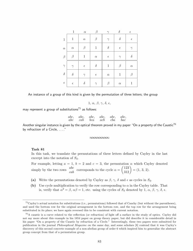
1 α β γ δ ε

1

α

β

γ

δ

ε

1 α β γ δ ε

α β 1 δ ε γ

β 1 α ε γ δ

γ ε δ 1 β α

δ γ ε α 1 β

ε δ γ β α 1

An instance of a group of this kind is given by the permutation of three letters; the group

1, α, β, γ, δ, ε,

may represent a group of substitutions75 as follows:

abc, abc, abc, abc, abc, abc,abc cab bca acb cba bac

Another singular instance is given by the optical theorem proved in my paper “On a property of the Caustic76

by refraction of a Circle, . . . .”

∞∞∞∞∞∞∞∞

Task 81In this task, we translate the permutations of three letters defined by Cayley in the lastexcerpt into the notation of S3.

For example, letting a = 1, b = 2 and c = 3, the permutation α which Cayley denoted

simply by the two rowsabccab

corresponds to the cycle α =

(123312

)= (1, 3, 2).

(a) Write the permutations denoted by Cayley as β, γ, δ and ε as cycles in S3.

(b) Use cycle multiplication to verify the row corresponding to α in the Cayley table. Thatis, verify that α2 = β, αβ = 1, etc. using the cycles of S3 denoted by 1, α, β, γ, δ, ε.

75Cayley’s actual notation for substitutions (i.e., permutations) followed that of Cauchy (but without the parentheses),and used the bottom row for the original arrangement in the bottom row, and the top row for the arrangement beingsubstituted in its place; we have again reversed this to be consistent with current notation.

76A caustic is a curve related to the reflection (or refraction) of light off a surface in the study of optics. Cayley didnot say more about this example in his 1854 paper on group theory paper, but did describe it in considerable detail inhis paper “On a property of the Caustic by refraction of a Circle.” Interestingly, these two papers were submitted forpublication in the journal Philosophical Magazine on the same day, and some scholars [8] contend that it was Cayley’sdiscovery of this second concrete example of a non-abelian group of order 6 which inspired him to generalize the abstractgroup concept from that of a permutation group.

83

Task 82This task explores some properties of cosets within the specific example of the group S3.

We assume the elements of S3 are denoted as in Task 81; for example, α = (1, 3, 2). Thus,the Cayley table given in the last excerpt can be used to determine all necessary products.

Recall from Task 58 that the left coset of H corresponding to γ is the set defined byγH = γx |x ∈ H, where H is a subgroup of G and γ an element of G.

(a) Let H = 〈α〉.(i) Use the Cayley table for S3 to verify that H = 1 , α , β and γH = γ , ε , δ .

Describe where H, γH show up in the Cayley table of S3.Also explain why γH is not a subgroup of G.

(ii) Find and compare the left cosets 1H = H, αH, and βH.Also find and compare the left cosets γH, δH, and εH.Comment on what you observe.

(iii) Now consider the right coset Hγ = xγ |x ∈ H.Show that γH = Hγ in this particular example.Do you think it will always be the case that γH = Hγ. Why or why not?

(b) Now consider the subgroup K = 〈γ〉 = 1 , γ in S3.

Use the Cayley table of S3 to find all left and right cosets of K and compare these.

Would you now change your answer to the question of whether the left and right cosetscorresponding to an element are always equal? Why or why not?

Task 83In this task, we look at some groups of order 8, starting from their generating equations.

(a) Write the Cayley table for the group G = 1 , a , b , b2 , b3 , ab , ab2 , ab3 with generating equations a2 = 1 , b4 = 1 , ba = ab3.

This group is known as the dihedral group D4.77

In general, the dihedral group Dn for n ∈ Z+ is a group of order 2ndefined by two generators a, b satisfying an = 1 , b2 = 1 and ba = abn−1.

(b) Write the Cayley table for the group G = 1 , a , b , b2 , b3 , ab , ab2 , ab3 with generating equations a2 = b2 , b4 = 1 , ba = ab3.

Explain why this group is isomorphic to the quaternion group (see Task 44).

(c) Write the Cayley table for the group G = 1 , a , b , c , ab , ac , bc , abc with generating equations a2 = b2 = c2 = 1, ba = ab , ca = ac.

Explain why this group78 is isomorphic to Z2 ×Z2 ×Z2.

(d) Find two other groups of order 8, and explain how we know these groups are distinctfrom those in parts (a), (b) and (c). Hint? Try using direct products.

EXTRA CREDIT:Are these five groups the only groups of order 8 possible, up to isomorphism?If so, prove this. If not, find all possible groups of order 8, up to isomorphism.

77D4 can be interpreted as the group of symmetries of a square, in a fashion similar to that in which the Viergrupperepresents the group of symmetries of a rectangle, by letting a represent a reflection across one of the two diagonals and brepresent a rotation through 90. Similarly, D2n can be interpreted as the symmetries of a regular polygon with 2n sides.

78Note that this group contains no elements of order 4 or 8, even though both 4 and 8 divide the order of the group.

84

5 Concluding Remarks, and Cayley’s Theorem Today

With the classification of all groups of order 6, our study of Cayley’s ground-breaking paper on groupscomes to an end. Cayley himself went on in this paper to describe two non-cyclic groups of higherorder — one of order 18 and the other of order 27. Although he apparently never fully classified groupsof these orders, his complete classification of all groups of order 8 was published five years later, in1859.79 Cayley did not return to the study of groups until 1878, when he published another four papersin group theory. In one of these, he explicitly stated the one theorem named after him in group theorytoday:

Cayley’s Theorem: Every group is isomorphic to a group of permutations.

This theorem tells us that, in a sense, everything there is to know about groups in general is alreadytrue of permutation groups in particular. Although it may not surprise you to learn that Cayley statedthis theorem without proof, you probably also won’t find it very difficult to believe the theorem is true.In essence, each row (or column) of a Cayley table can be used as a (somewhat long) label for theelement it represents; that is, the Cayley table gives us a 1-to-1 correspondence between the elementsα of a group and the ordered list obtained by multiplying each element of the group by α. But thislist of elements (i.e., the row) is really nothing more than a permutation of the elements of the group!Our concluding task outlines a formal proof of this theorem, as it would appear in a current textbook.

Task 84In this task, we outline a formal proof of Cayley’s Theorem.

Let G be a group. We must find a permutation group with the same group structure as G.

To do this, define a function πα : G→ G for each α ∈ G by setting πα(x) = αx .(This should remind you of how we get rows in the Cayley table!)

Let G∗ = πα |α ∈ G . Our plan is to show that G∗ is the desired permutation group.

(a) We first must show that the elements of G∗ are permutations.

To do this, let α ∈ G and prove that πα is one-to-one and onto.

(b) We next prove that G∗ is a group under composition, by completing the following:

(i) For arbitrary α, β ∈ G, show that παπβ = παβ.(Do this by showing πα πβ(x) = παβ(x) for an arbitrary x ∈ G.)Explain why this proves that G∗ is closed under products.

(ii) For arbitrary α ∈ G, show that παπ1 = π1πα = πα.Explain why this proves that π1 is an identity for G∗.

(iii) For arbitrary α ∈ G, show that παπα−1 = π1.Explain why this proves that πα−1 is the (group) inverse of πα.

(c) Finally, prove that G is isomorphic to G∗ by showing that the function Φ : G → G∗

defined by Φ(α) = πα is an isomorphism. That is, prove that Φ is one-to-one, ontoand satisfies Φ(α)Φ(β) = Φ(αβ) for all α, β ∈ G.

By the late nineteenth century, when the paper in which Cayley stated the theorem which nowbears his name appeared in print, the time was mathematically ripe for mathematicians in general tofully recognize how the concept of group served as a powerful tool in geometry, number theory and thetheory of equations. The rest, one might say, is history!

79His classification appears in [7], if you’d like to check your answer to the extra credit question in Task 83!

85

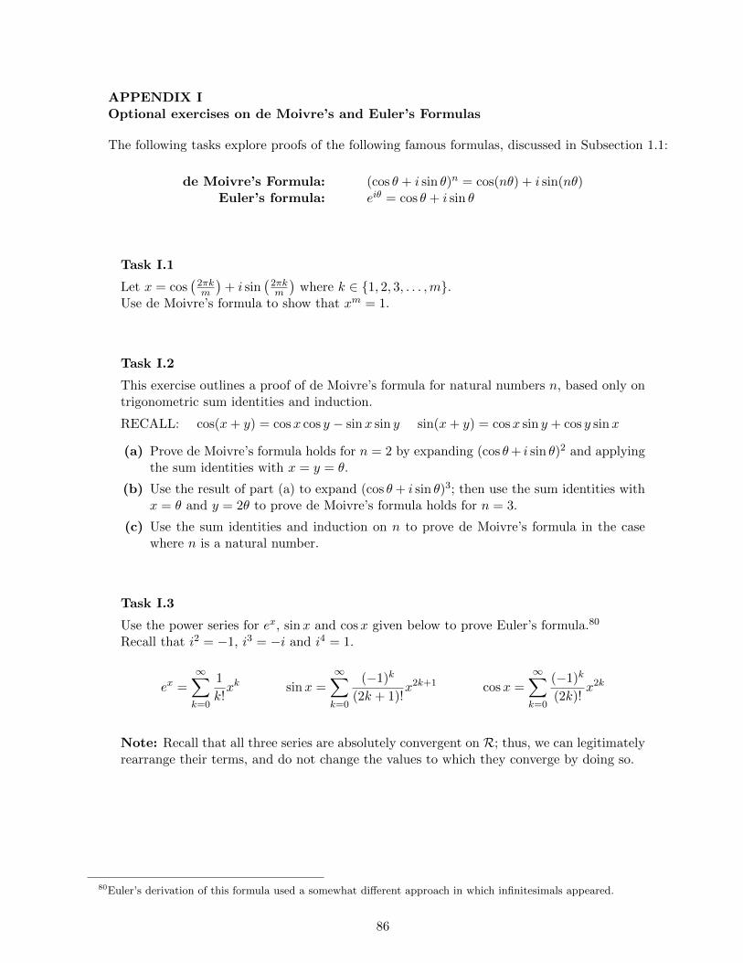
APPENDIX IOptional exercises on de Moivre’s and Euler’s Formulas

The following tasks explore proofs of the following famous formulas, discussed in Subsection 1.1:

de Moivre’s Formula: (cos θ + i sin θ)n = cos(nθ) + i sin(nθ)Euler’s formula: eiθ = cos θ + i sin θ

Task I.1

Let x = cos(2πkm

)+ i sin

(2πkm

)where k ∈ 1, 2, 3, . . . ,m.

Use de Moivre’s formula to show that xm = 1.

Task I.2

This exercise outlines a proof of de Moivre’s formula for natural numbers n, based only ontrigonometric sum identities and induction.

RECALL: cos(x+ y) = cosx cos y − sinx sin y sin(x+ y) = cosx sin y + cos y sinx

(a) Prove de Moivre’s formula holds for n = 2 by expanding (cos θ+ i sin θ)2 and applyingthe sum identities with x = y = θ.

(b) Use the result of part (a) to expand (cos θ+ i sin θ)3; then use the sum identities withx = θ and y = 2θ to prove de Moivre’s formula holds for n = 3.

(c) Use the sum identities and induction on n to prove de Moivre’s formula in the casewhere n is a natural number.

Task I.3

Use the power series for ex, sinx and cosx given below to prove Euler’s formula.80

Recall that i2 = −1, i3 = −i and i4 = 1.

ex =

∞∑k=0

1

k!xk sinx =

∞∑k=0

(−1)k

(2k + 1)!x2k+1 cosx =

∞∑k=0

(−1)k

(2k)!x2k

Note: Recall that all three series are absolutely convergent on R; thus, we can legitimatelyrearrange their terms, and do not change the values to which they converge by doing so.

80Euler’s derivation of this formula used a somewhat different approach in which infinitesimals appeared.

86

APPENDIX IICosets, Lagrange’s Theorem and Factor Groups

In the latter part of this project, the concept of a coset came up in passing at several points.In this appendix, we outline a proof of Lagrange’s Theorem for Finite Groups cast in the languageof cosets, and introduce the notion of a factor group (or quotient group) which arises by imposing abinary operation on the collection of all cosets. We begin by formally stating the definition of a coset.

DefinitionLet G be a group, H a subgroup of G, and a ∈ G.The left coset of H corresponding to a is the set aH = ah |h ∈ H .The right coset of H corresponding to a is the set Ha = ha |h ∈ H .

In other words, (left) cosets are formed by collecting together all the products ah, where h rangesover the entire subgroup H and a is fixed. If you think back to the table that Cauchy used to proveLagrange’s Theorem for Sn, you will see that the first row of that table was the given subgroup H(itself the coset corresponding to a = 1), and that the rows below it were cosets of H that correspondedto permutations selected from outside of H. In his proof of Lagrange’s theorem, Cauchy described andmade use of several properties concerning the way in which these cosets (i.e., rows of his array) wereinterrelated. We state these various properties in the language of cosets here, along with some otherproperties of cosets which were suggested by our reading of Cayley’s paper. As you read through them,consider which of these properties you already believe based on your previous work in this project.The subsequent task outlines a proof for each; the properties are arranged in an order which will makeseveral of these proofs appears as corollaries of earlier ones.

Coset PropertiesLet G be a group and H a subgroup of G.

1. For all a ∈ G, a ∈ aH and a ∈ Ha.

2. G =⋃a∈G

aH =⋃a∈G

Ha.

Note: Property 2 formalizes Cauchy’s somewhat vague procedure of adding rows tothe table used in his proof of Lagrange’s Theorem for Sn until all the elements of thegroup appear somewhere in that table.

3. For all a ∈ G, if a 6∈ H, then H ∩Ha = ∅ = H ∩ aH.

4. For all a, b ∈ G, if aH ∩ bH 6= ∅, then aH = bH.Similarly, if Ha ∩Hb 6= ∅, then Ha = Hb.

5. For all a, b ∈ G, a ∈ bH if and only if aH = bH.Similarly, a ∈ Hb if and only if Ha = Hb.

6. For all a ∈ G, a ∈ H if and only if Ha = H = aH.

7. For all a ∈ G, |aH| = |Ha| = |H|.

8. If G is abelian, then Ha = aH for all a ∈ G.

87

Task II.1In this task, you will prove the eight elementary properties given above for left cosets.81

Begin by assuming G is a group, H a subgroup of G, and a, b ∈ G.

(a) Use the definition of (left) coset to prove Coset Property 1.That is, let a ∈ G and explain how we know that a = ah for some h ∈ H.

(b) Use Coset Property 1 to prove Coset Property 2.

That is, show that x ∈ G if and only if x ∈⋃a∈G

aH.

(c) Use contradiction to prove Coset Property 3.That is, suppose a 6∈ H and H ∩ aH 6= ∅, so that h1 = ah2 for some h1, h2 ∈ H.Then show that this contradicts the assumption that a 6∈ H.

(d) Use properties of subgroups to prove Coset Property 4.Begin by assuming a, b ∈ G with aH ∩ bH 6= ∅, and let x ∈ aH ∩ bH.Taking h1, h2 ∈ H with x = ah1 and x = bh2, explain why ah1 = bh2 implies a ∈ bH.Then use the fact that a = bh for some h ∈ H to show that y ∈ aH implies y ∈ bH.This tells us that aH ⊆ bH.

Follow a similar plan to show that bH ⊆ aH, and conclude that aH = bH.

(e) Use Coset Properties 1 and 4 to prove the ‘only if’ direction of Coset Property 5.That is, given a, b ∈ G with a ∈ bH, explain why aH = bH.

To prove the ‘if’ direction, assume aH = bH and explain how a ∈ bH follows.

(f) Use Coset Property 5 with b = 1 to prove Coset Property 6.

(g) Use the function f : H → aH defined by f(h) = ah to prove Coset Property 7.That is, show that f is one-to-one and onto.

(h) Use the definition of an abelian group to prove Coset Property 8.That is, show that x ∈ Ha if and only if x ∈ aH.

Coset Properties 2 and 4 correspond to two central ideas in Cauchy’s proof of Lagrange’s Theoremfor Sn.82 Today, we would say that these two properties imply that the collection of all left (or right)cosets of a group forms a partition of G. The concept of a partition does not apply only to groups,however, as indicated by the following formal definition of a partition for any general set S.

81The left coset proofs that you will write in this task and elsewhere in this appendix are easily adapted to right cosets.82Cauchy himself used Coset Property 3 to explain why the top row of his table did not overlap with any of its other

rows; today we would simply consider the top row to be another coset (H = 1H), so that only Coset Property 2 is neededto know that there is no overlap between any of the rows.

88

Definition83

Let S be a set and Pα a non-empty subset of S for each α ∈ I, where I is an indexing set.The collection P = Pα α∈I is a partition of S if and only if every element of S appearsin one and only one Pα ∈ P. That is, if and only if

1. The subsets Pα are mutually disjoint: given α, β ∈ I with Pα 6= Pβ, then Pα ∩Pβ = ∅.

2. S =⋃α∈I

Pα.

Applying this definition to the collection of all (left) cosets of a group, you should be able to convinceyourself (and others!) that Coset Properties 2 and 4 do indeed prove that P = aH a∈G is a partitionof G. Once you’re convinced, use this fact to see how easily we can now prove Lagrange’s Theorem inthe general case where G is any finite group.

Task II.2Let G be a finite group and H a subgroup of G.

Set r = |H|, n = |G| and let k be the number of distinct left cosets of H.(The number k is called the index of H in G, denoted (G : H).)

Use the fact that P = aH a∈G is a partition of G along with Coset Property 7 to explain

why n = kr. Conclude that |H| divides |G|, and that (G : H) = |G||H| .

Although Task II.2 concludes our discussion of how to prove Lagrange’s Theorem using the languageof cosets, there are some other issues related to cosets which will be useful in your study of moreadvanced group theory. We comment on these in the remainder of this appendix.

One thing that may have puzzled you about the requirement that the aH be mutually disjoint isthe fact that it is often the case that aH = bH for some a 6= b. For example, the group table given byCayley for S3 makes it clear that 1H = αH = βH and γH = δH = εH. (See Task 82(a-ii)). In fact,Coset Property 6 implies that Ha = H = Hb for any a, b ∈ H. But this doesn’t mean that the Ha andHb are two distinct non-disjoint cosets; rather, it means that ‘Ha’ and ‘Hb’ are two different namesfor the same coset. This is exactly what happens with rational numbers where, for instance, 3

4 and 68

are two different names for just one rational number. Similarly, each individual coset aH is an objectin its own right, but with several different representations.84

Another question you may have had about cosets is how the left and right cosets corresponding toa particular element are related. This is another of the ideas that you explored in Task 82, which weremind you of here while adding some insights into this example which come from Lagrange’s Theorem.Recall first that, in that task, we had G = S3 = 1 , α , β , γ , δ , ε, with

α = (1, 3, 2) , β = (1, 2, 3) , γ = (2, 3) , δ = (1, 3) , ε = (1, 2).

For the first subgroup considered in the task, H = 〈α〉 = 1 , α , β , it turned out to be the case thatγH = δH = εH and that γH = Hγ. In fact, since |G| = 6, |H| = 3 and (G : H) = 6

3 = 2, we would

83You may wish to read more about partitions in an algebra or other mathematics textbook, especially to see how theyare related to equivalence relations, another important tool in much of mathematics (including group theory) today.

84This idea was also implicit in Task 40(d) where Cauchy’s proof of Lagrange’s Theorem for Sn was explored in aspecific case.

89

now be able to predict in advance that H has exactly two distinct left cosets. By Coset Property 6, thefirst of these left cosets will be H = αH = βH. Since all cosets are the same size (by Coset Property7), we could then conclude that the second left coset consists of the three remaining elements of G, orγH = δH = εH = γ , δ , ε. Similarly, since there are only two distinct right cosets, one of which isH = Hα = Hβ, it must be the case that Hγ = Hδ = Hε. This means that not only does γH = Hγhold in this example, as you proved in Task 82, but also that δH = Hδ and εH = Hε. Combining thiswith Coset Property 6, it follows that θH = Hθ for every θ ∈ G, again in this particular case.85

Again in Task 82, however, we saw how another choice of subgroup led to quite different results.Namely, letting K = 〈γ〉 = 1 , γ , the left and right cosets of an element were generally different. Forinstance, αK = α , δ , while Kα = α , ε . Or, taking another example for this same subgroup K,δK = δ , α , while Kδ = δ , γ . Thus, we see that, in general, the left and right cosets correspondingto a particular element may not equal and, furthermore, that this depends on the particular subgroupinvolved, more so than the particular group.

These comments lead us to the following definition of a special type of subgroup, which we feelcompelled to state for both its beauty and its importance.

DefinitionLet G be a group and H a subgroup of G.Then H is a normal subgroup if and only if aH = Ha for every a ∈ G.

The notion of a normal subgroup is precisely what is needed to define the concept of a simple groupwhich was discussed at the beginning of Section 4; namely, a a nontrivial group is simple if and onlyif its only normal subgroups are the trivial group and the group itself. Another reason why normalsubgroups are important is that they allow us to impose group structure on the collection of all left(or right) cosets. This is done by first defining coset multiplication in the following natural way:

DefinitionGiven a group G with a, b ∈ G and H a subgroup of G, the product of the left cosetsaH and bH is defined as

(aH)(bH) = (ab)H.

That is, the product of the left cosets corresponding to a, b ∈ G is the left coset correspond-ing to the product ab.

Naturally, the first thing to worry about here is whether coset multiplication is well-defined. After all,each individual left coset, just like any given rational numbers, can be represented by several differentnames. Thus, we would want to be sure that given aH = cH and bH = dH, we will also have(aH)(bH) = (cH)(dH). It turns out that this is the case, provided the subgroup H is normal. Weomit the proof of this, as well as the proof of the theorem in the following statement, both of whichyou can find it in any current algebra textbook.

Definition and TheoremLet G be a group, H a normal subgroup of G, and G/H = aH | a ∈ G.Then G/H is a group under coset multiplication, called the factor group of G by H.

G/H is also called a quotient group, and turns out (not surprisingly) to have an algebraic structureintimately related to that of G. We encourage you to study this relationship further — look for it underthe name Fundamental Homomorphism Theorem in any group theory textbook, and enjoy!

85Remember that γH = Hγ does not imply that the element γ commutes with the elements of H. This is clearly nottrue in this example, since γα = ε, while αγ = δ. Rather, γH = Hγ means that the list of elements in γH is the same asthe list of elements in Hγ, only arranged in a different order.

90

References

[1] Archibald, R.C., benjamin Peirce, 1809–1880: Biographical Sketch and Bibliography, 1925.

[2] Cauchy, Augustin, Memoire sur le nombre des valeurs qu’une fonction peut acquerir, lorsqu’on ypermute de toutes les manieres possibles les quantites qu’elle renferme, Journal de l’Ecole Poly-technique, Cahier XVII, Tome X (1815), 1–28, and in Œuvres completes de Augustin Cauchy, Serie2, Tome 1 (1905), 64–90.

[3] Cauchy, Augustin, Memoire sur les fonctions que ne peuvent obtenir que deux valeuers egaleset de signes contraires par suite des transpositiosn operees entre les variable qu’elles renferment,Journal de l’Ecole Polytechnique, Cahier XVII, Tome X (1815), 29–117, and in Œuvres completesde Augustin Cauchy, Serie 2, Tome 1 (1905), 91–169.

[4] Cauchy, Augustin, Memoire sur les arrangements que l’on peut former avec des lettres donnees,et sur les permutations ou substitutions a l’aide desquelles on passe d’un arrangement a un autre,in Exercises d’Analyse et de Mathematiques Physiques, Tome III (1844), 151–242, and in Œuvrescompletes de Augustin Cauchy, Serie 2, Tome 13 (1933), 171–282.

[5] Cayley, Arthur, On the theory of groups, as depending on the symbolic equation θn = 1 - PartI, Philosophical Magazine, 7 (1854), 40–47, and in The Collected Mathematical Papers of ArthurCayley, Cambridge: Cambridge University Press, vol. 2 (1889), 123–130.

[6] Cayley, Arthur, On the theory of groups, as depending on the symbolic equation θn = 1 - Part II,Philosophical Magazine, 7 (1854), 408–409, and in The Collected Mathematical Papers of ArthurCayley, Cambridge: Cambridge University Press, vol. 2 (1889), 131–132.

[7] Cayley, Arthur, On the theory of groups, as depending on the symbolic equation θn = 1 - Part IIIPhilosophical Magazine, 18 (1859), 34–37, and in The Collected Mathematical Papers of ArthurCayley, Cambridge: Cambridge University Press, vol. 3 (1889), 594–602.

[8] Chakraborty, Sujoy and Chowdhury, Munibur Rahman, Arthur Cayley and the Abstract GroupConcept, Mathematics Magazine, vol. 78, vol. 4 (Oct. 2005), 269–282.

[9] Crilly, Tony, Arthur Cayley: Mathematician Laureate of the Victorian Age, Baltimore: JohnsHopkins University Press, 2006.

[10] Lagrange, J. L., Reflexions sur la resolution algebrique des equations, Memoire de l’Academie deBerlin, 1770-1771, pp..

[11] Lagrange, J. L., Traite de la resolution des equations numeriques de tous les degres, avec des notessur plusieurs points de la theorie des equations algebriques, Paris: Courcier, 1808.

[12] Roth, Richard L., A History of Lagrange’s Theorem on Groups, Mathematics Magazine, vol. 74,no. 2 (April 2001), 99–108.

[13] van der Waerden, B. L., Hamilton’s Discovery of Quaternions, Mathematics Magazine, Vol. 49,No. 5 (Nov., 1976), 227–234.

[14] Wussing, Hans, The Genesis of the Abstract Group Concept: A Contribution to the History of theOrigins of Abstract Group Theory, Cambridge and London: MIT Press, 1984.

91