Algebra Math Notes • Study Guide

Abstract Algebra

Table of Contents Rings ................................................................................................................................................... 3

Rings ............................................................................................................................................... 3

Subrings and Ideals ......................................................................................................................... 4

Homomorphisms .............................................................................................................................. 4

Fraction Fields ................................................................................................................................. 5

Integers ............................................................................................................................................ 5

Factoring ............................................................................................................................................. 7

Factoring .......................................................................................................................................... 7

UFDs, PIDs, and Euclidean Domains .............................................................................................. 7

Algebraic Integers ............................................................................................................................ 8

Quadratic Rings ............................................................................................................................... 8

Gaussian Integers ............................................................................................................................ 9

Factoring Ideals ............................................................................................................................... 9

Ideal Classes ................................................................................................................................. 10

Real Quadratic Rings ..................................................................................................................... 11

Polynomials ....................................................................................................................................... 12

Polynomials ................................................................................................................................... 12

℞[𝑋] ............................................................................................................................................... 12

Irreducible Polynomials .................................................................................................................. 13

Cyclotomic Polynomials ................................................................................................................. 14

Varieties ......................................................................................................................................... 14

Nullstellensatz ................................................................................................................................ 15

Fields................................................................................................................................................. 17

Fundamental Theorem of Algebra .................................................................................................. 17

Algebraic Elements ........................................................................................................................ 17

Degree of a Field Extension ........................................................................................................... 17

Finite Fields ................................................................................................................................... 19

Modules ............................................................................................................................................. 21

Modules ......................................................................................................................................... 21

Structure Theorem ......................................................................................................................... 22

Noetherian and Artinian Rings ....................................................................................................... 23

Application 1: Abelian Groups ........................................................................................................ 23

Application 2: Linear Operators ...................................................................................................... 24

Polynomial Rings in Several Variables ........................................................................................... 25

Tensor Products ............................................................................................................................ 25

Galois Theory .................................................................................................................................... 27

Symmetric Polynomials .................................................................................................................. 27

Discriminant ................................................................................................................................... 27

Galois Group .................................................................................................................................. 27

Fixed Fields ................................................................................................................................... 28

Galois Extensions and Splitting Fields ........................................................................................... 28

Fundamental Theorem ................................................................................................................... 29

Roots of Unity ................................................................................................................................ 29

Cubic Equations ............................................................................................................................. 30

Quartic Equations .......................................................................................................................... 30

Quintic Equations and the Impossibility Theorem ........................................................................... 31

Transcendence Theory .................................................................................................................. 32

Algebras ............................................................................................................................................ 33

Division Algebras ........................................................................................................................... 33

References ........................................................................................................................................ 34

1 Rings 1-1 Rings

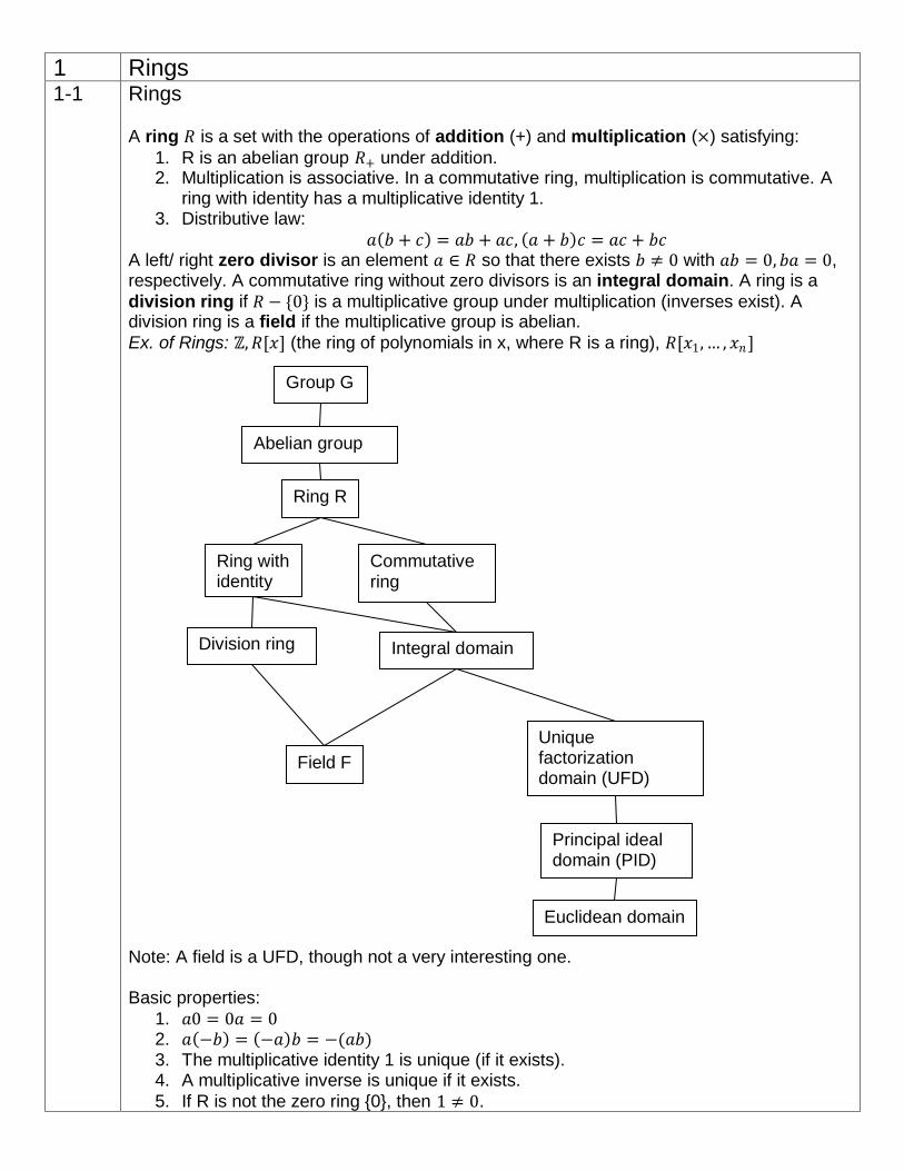
A ring 𝑅 is a set with the operations of addition (+) and multiplication (×) satisfying:

1. R is an abelian group 𝑅+ under addition. 2. Multiplication is associative. In a commutative ring, multiplication is commutative. A

ring with identity has a multiplicative identity 1. 3. Distributive law:

𝑎 𝑏 + 𝑐 = 𝑎𝑏 + 𝑎𝑐, 𝑎 + 𝑏 𝑐 = 𝑎𝑐 + 𝑏𝑐 A left/ right zero divisor is an element 𝑎 ∈ 𝑅 so that there exists 𝑏 ≠ 0 with 𝑎𝑏 = 0, 𝑏𝑎 = 0, respectively. A commutative ring without zero divisors is an integral domain. A ring is a

division ring if 𝑅 − {0} is a multiplicative group under multiplication (inverses exist). A division ring is a field if the multiplicative group is abelian.

Ex. of Rings: ℞, 𝑅[𝑥] (the ring of polynomials in x, where R is a ring), 𝑅[𝑥1, … , 𝑥𝑛 ]

Note: A field is a UFD, though not a very interesting one. Basic properties:

1. 𝑎0 = 0𝑎 = 0 2. 𝑎 −𝑏 = −𝑎 𝑏 = −(𝑎𝑏) 3. The multiplicative identity 1 is unique (if it exists). 4. A multiplicative inverse is unique if it exists.

5. If R is not the zero ring {0}, then 1 ≠ 0.

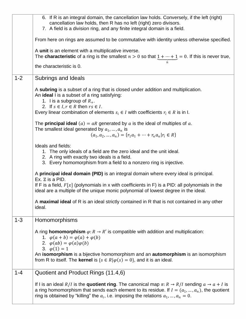
Group G

Abelian group

Ring R

Commutative ring

Ring with identity

Integral domain Division ring

Field F

Principal ideal domain (PID)

Euclidean domain

Unique factorization domain (UFD)

6. If R is an integral domain, the cancellation law holds. Conversely, if the left (right) cancellation law holds, then R has no left (right) zero divisors.

7. A field is a division ring, and any finite integral domain is a field. From here on rings are assumed to be commutative with identity unless otherwise specified. A unit is an element with a multiplicative inverse.

The characteristic of a ring is the smallest 𝑛 > 0 so that 1 + ⋯ + 1 𝑛

= 0. If this is never true,

the characteristic is 0.

1-2 Subrings and Ideals A subring is a subset of a ring that is closed under addition and multiplication. An ideal I is a subset of a ring satisfying:

1. I is a subgroup of 𝑅+. 2. If 𝑠 ∈ 𝐼, 𝑟 ∈ 𝑅 then 𝑟𝑠 ∈ 𝐼.

Every linear combination of elements 𝑠𝑖 ∈ 𝐼 with coefficients 𝑟𝑖 ∈ 𝑅 is in I. The principal ideal 𝑎 = 𝑎𝑅 generated by 𝑎 is the ideal of multiples of 𝑎.

The smallest ideal generated by 𝑎1, … , 𝑎𝑛 is 𝑎1, 𝑎2 , … , 𝑎𝑛 = 𝑟1𝑎1 + ⋯ + 𝑟𝑛𝑎𝑛 𝑟𝑖 ∈ 𝑅

Ideals and fields:

1. The only ideals of a field are the zero ideal and the unit ideal. 2. A ring with exactly two ideals is a field. 3. Every homomorphism from a field to a nonzero ring is injective.

A principal ideal domain (PID) is an integral domain where every ideal is principal.

Ex. ℞ is a PID. If F is a field, 𝐹[𝑥] (polynomials in x with coefficients in F) is a PID: all polynomials in the ideal are a multiple of the unique monic polynomial of lowest degree in the ideal. A maximal ideal of R is an ideal strictly contained in R that is not contained in any other ideal.

1-3 Homomorphisms A ring homomorphism 𝜑: 𝑅 → 𝑅′ is compatible with addition and multiplication:

1. 𝜑 𝑎 + 𝑏 = 𝜑 𝑎 + 𝜑(𝑏) 2. 𝜑 𝑎𝑏 = 𝜑 𝑎 𝜑(𝑏)

3. 𝜑 1 = 1 An isomorphism is a bijective homomorphism and an automorphism is an isomorphism

from R to itself. The kernel is {𝑠 ∈ 𝑅|𝜑 𝑠 = 0}, and it is an ideal.

1-4 Quotient and Product Rings (11.4,6) If I is an ideal 𝑅/𝐼 is the quotient ring. The canonical map 𝜋: 𝑅 → 𝑅/𝐼 sending 𝑎 → 𝑎 + 𝐼 is

a ring homomorphism that sends each element to its residue. If 𝐼 = (𝑎1, … , 𝑎𝑛 ), the quotient

ring is obtained by “killing” the 𝑎𝑖 , i.e. imposing the relations 𝑎1, … , 𝑎𝑛 = 0.

Mapping Property: Let 𝑓: 𝑅 → 𝑅′ be a ring homomorphism with kernel K and let 𝐼 ⊆ 𝐾 be an

ideal. Let 𝜋: 𝑅 → 𝑅/𝐼 = 𝑅 be the canonical map. There is a unique homomorphism 𝑓 : 𝑅 → 𝑅′ so that 𝑓 𝜋 = 𝑓.

First Isomorphism Theorem: If f is surjective and 𝐼 = 𝐾 then 𝑓 is an automorphism. Correspondence Theorem: If f is surjective with kernel K,

There is a bijective correspondence between ideals of 𝑅 and ideals of 𝑅′ that contain

𝐾. A subgroup of G containing K is associated with its image.

If 𝐼 corresponds to 𝐼′, 𝑅/𝐼 ≅ 𝑅′/𝐼′. Corollary: Introducing relations one at a time (killing 𝑎, then 𝑏 ) or together (killing 𝑎, 𝑏)

gives the same ring. Useful in polynomial rings.

The product ring 𝑅 × 𝑅′ is the product set with componentwise addition and multiplication. 1. The additive identity is (0,0) and the multiplicative identity is (1,1).

2. The projections 𝜋 𝑥, 𝑥′ = 𝑥, 𝜋 ′ 𝑥, 𝑥′ = 𝑥′ are ring homomorphisms to 𝑅, 𝑅′. 3. 1,0 , (0,1) are idempotent elements- elements such that 𝑒2 = 1.

Let e be an idempotent element of a ring S.

1. 𝑒′ = 1 − 𝑒 is idempotent, and 𝑒𝑒′ = 0. 2. 𝑒𝑆 is a ring (but not a subring of S unless e=1) with identity e, and multiplication by e

is a ring homomorphism 𝑆 → 𝑒𝑆. 3. 𝑆 ≅ 𝑒𝑆 × 𝑒′𝑆.

1-5 Fraction Fields Every integral domain can be embedded as a subring of its fraction field F. Its elements

are 𝑎

𝑏 𝑎, 𝑏 ∈ 𝑅, 𝑏 ≠ 0 , where

𝑎1

𝑏1=

𝑎2

𝑏2⇔ 𝑎1𝑏2 = 𝑎2𝑏1. Addition and multiplication are defined

as in arithmetic: 𝑎

𝑏+

𝑐

𝑑=

𝑎𝑑 +𝑏𝑐

𝑏𝑑,𝑎

𝑏

𝑐

𝑑=

𝑎𝑐

𝑏𝑑, and

𝑎

1= 𝑎. The field of fractions of the polynomial

ring 𝐾[𝑥], K a field, is the field of rational functions 𝐾(𝑥). Mapping Property:

Let R be an integral domain with field of fractions F, and let 𝜑: 𝑅 → 𝐹′ be an injective homomorphism from 𝑅 to a field 𝐹’. 𝜑 can be extended uniquely to an injective

homomorphism Φ: 𝐹 → 𝐹′ by letting Φ 𝑎

𝑏 = 𝜑 𝑎 𝜑 𝑏 −1.

1-6 Integers

Peano’s Axioms for ℕ: 1. 1 ∈ ℕ 2. Successor function: The map 𝜎: ℕ → ℕ sends an integer to the next integer 𝑥′ =

𝜎(𝑥); 𝜎 1 = 2, 𝜎 2 = 3 … 𝜎 is injective, and 𝜎 𝑛 ≠ 1 for any 𝑛 (i.e. 1 is the first element).

3. Induction axiom: Let S be a subset of ℕ having the following properties: a. 1 ∈ 𝑆

b. If 𝑛 ∈ 𝑆 then 𝑛′ ∈ 𝑆. Then 𝑆 = ℕ. (Counting runs through all the natural numbers.)

𝑅 𝑅′

𝑅 = 𝑅/𝐼

𝑓

𝜋 𝑓

Inductive/ Recursive Definition: By induction, if an object 𝐶1 is defined, and a rule for determining 𝐶𝑛 ′ = 𝐶𝑛+1 from 𝐶𝑛 is given, then the sequence 𝐶𝑘 is determined uniquely.

Recursive definition of…

1. Addition: 𝑚 + 1 = 𝑚′, 𝑚 + 𝑛′ = (𝑚 + 𝑛)′ (i.e. 𝑚 + 𝑛 + 1 = 𝑚 + 𝑛 + 1)

2. Multiplication: 𝑚 × 1 = 𝑚, 𝑚 × 𝑛′ = 𝑚 × 𝑛 + 𝑚 (i.e. 𝑚 × 𝑛 + 1 = 𝑚 × 𝑛 + 𝑚) From these, the associative, distributive, and distributive laws can be verified. (“Peano

playing”) The integers can be developed from ℕ by introducing an additive inverse for every element.

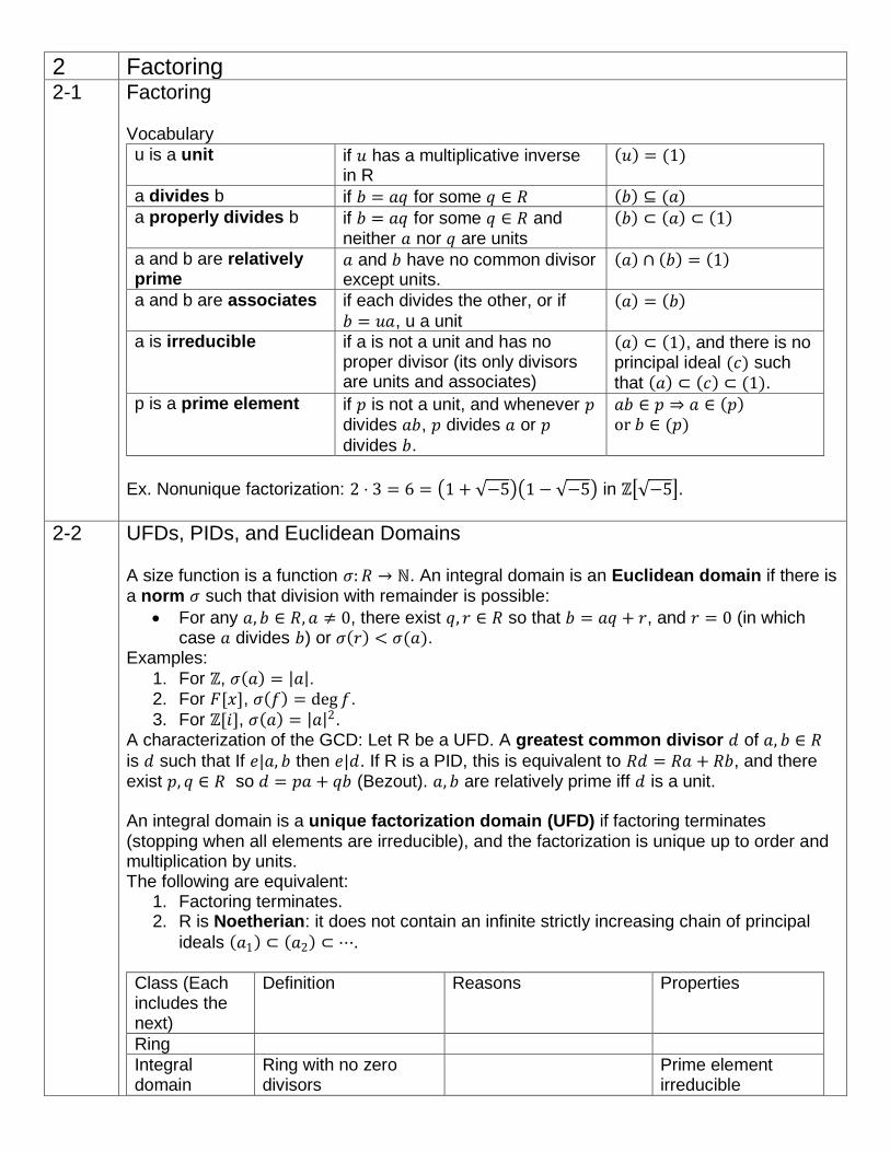
2 Factoring 2-1 Factoring

Vocabulary

u is a unit if 𝑢 has a multiplicative inverse in R

𝑢 = (1)

a divides b if 𝑏 = 𝑎𝑞 for some 𝑞 ∈ 𝑅 𝑏 ⊆ (𝑎)

a properly divides b if 𝑏 = 𝑎𝑞 for some 𝑞 ∈ 𝑅 and neither 𝑎 nor 𝑞 are units

𝑏 ⊂ 𝑎 ⊂ 1

a and b are relatively prime

𝑎 and 𝑏 have no common divisor except units.

𝑎 ∩ 𝑏 = 1

a and b are associates if each divides the other, or if

𝑏 = 𝑢𝑎, u a unit

𝑎 = 𝑏

a is irreducible if a is not a unit and has no proper divisor (its only divisors are units and associates)

𝑎 ⊂ 1 , and there is no principal ideal (𝑐) such that 𝑎 ⊂ 𝑐 ⊂ (1).

p is a prime element if 𝑝 is not a unit, and whenever 𝑝 divides 𝑎𝑏, 𝑝 divides 𝑎 or 𝑝

divides 𝑏.

𝑎𝑏 ∈ 𝑝 ⇒ 𝑎 ∈ 𝑝 or 𝑏 ∈ (𝑝)

Ex. Nonunique factorization: 2 ⋅ 3 = 6 = 1 + −5 1 − −5 in ℞ −5 .

2-2 UFDs, PIDs, and Euclidean Domains A size function is a function 𝜎: 𝑅 → ℕ. An integral domain is an Euclidean domain if there is a norm 𝜎 such that division with remainder is possible:

For any 𝑎, 𝑏 ∈ 𝑅, 𝑎 ≠ 0, there exist 𝑞, 𝑟 ∈ 𝑅 so that 𝑏 = 𝑎𝑞 + 𝑟, and 𝑟 = 0 (in which case 𝑎 divides 𝑏) or 𝜎 𝑟 < 𝜎(𝑎).

Examples:

1. For ℞, 𝜎 𝑎 = 𝑎 . 2. For 𝐹[𝑥], 𝜎 𝑓 = deg 𝑓.

3. For ℞[𝑖], 𝜎 𝑎 = 𝑎 2. A characterization of the GCD: Let R be a UFD. A greatest common divisor 𝑑 of 𝑎, 𝑏 ∈ 𝑅

is 𝑑 such that If 𝑒|𝑎, 𝑏 then 𝑒|𝑑. If R is a PID, this is equivalent to 𝑅𝑑 = 𝑅𝑎 + 𝑅𝑏, and there exist 𝑝, 𝑞 ∈ 𝑅 so 𝑑 = 𝑝𝑎 + 𝑞𝑏 (Bezout). 𝑎, 𝑏 are relatively prime iff 𝑑 is a unit. An integral domain is a unique factorization domain (UFD) if factoring terminates (stopping when all elements are irreducible), and the factorization is unique up to order and multiplication by units. The following are equivalent:

1. Factoring terminates. 2. R is Noetherian: it does not contain an infinite strictly increasing chain of principal

ideals 𝑎1 ⊂ 𝑎2 ⊂ ⋯.

Class (Each includes the next)

Definition Reasons Properties

Ring

Integral domain

Ring with no zero divisors

Prime element irreducible

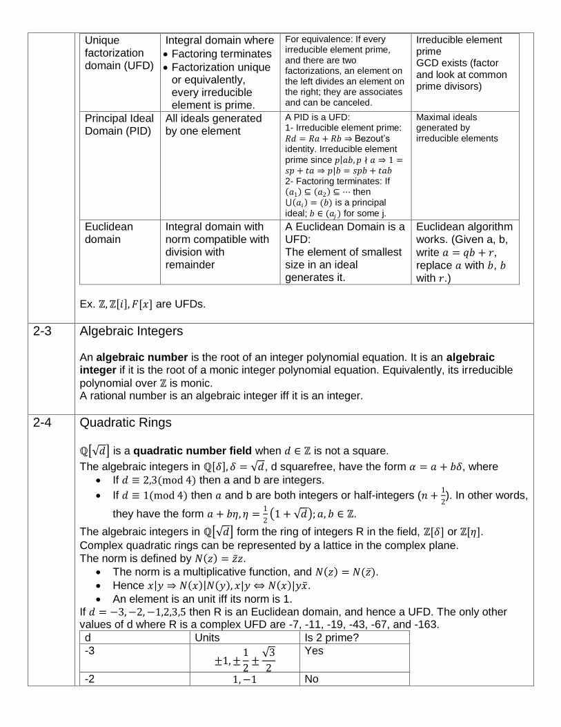
Unique factorization domain (UFD)

Integral domain where

Factoring terminates

Factorization unique or equivalently, every irreducible element is prime.

For equivalence: If every irreducible element prime, and there are two factorizations, an element on the left divides an element on the right; they are associates and can be canceled.

Irreducible element prime GCD exists (factor and look at common prime divisors)

Principal Ideal Domain (PID)

All ideals generated by one element

A PID is a UFD: 1- Irreducible element prime:

𝑅𝑑 = 𝑅𝑎 + 𝑅𝑏 ⇒ Bezout’s identity. Irreducible element

prime since 𝑝 𝑎𝑏, 𝑝 ∤ 𝑎 ⇒ 1 =𝑠𝑝 + 𝑡𝑎 ⇒ 𝑝 𝑏 = 𝑠𝑝𝑏 + 𝑡𝑎𝑏 2- Factoring terminates: If 𝑎1 ⊆ 𝑎2 ⊆ ⋯ then ⋃ 𝑎𝑖 = (𝑏) is a principal

ideal; 𝑏 ∈ (𝑎𝑗 ) for some j.

Maximal ideals generated by irreducible elements

Euclidean domain

Integral domain with norm compatible with division with remainder

A Euclidean Domain is a UFD: The element of smallest size in an ideal generates it.

Euclidean algorithm works. (Given a, b,

write 𝑎 = 𝑞𝑏 + 𝑟, replace 𝑎 with 𝑏, 𝑏 with 𝑟.)

Ex. ℞, ℞ 𝑖 , 𝐹[𝑥] are UFDs.

2-3 Algebraic Integers An algebraic number is the root of an integer polynomial equation. It is an algebraic integer if it is the root of a monic integer polynomial equation. Equivalently, its irreducible

polynomial over ℞ is monic. A rational number is an algebraic integer iff it is an integer.

2-4 Quadratic Rings

ℚ 𝑑 is a quadratic number field when 𝑑 ∈ ℞ is not a square.

The algebraic integers in ℚ 𝛿 , 𝛿 = 𝑑, d squarefree, have the form 𝛼 = 𝑎 + 𝑏𝛿, where

If 𝑑 ≡ 2,3(mod 4) then a and b are integers.

If 𝑑 ≡ 1(mod 4) then 𝑎 and b are both integers or half-integers (𝑛 +1

2). In other words,

they have the form 𝑎 + 𝑏𝜂, 𝜂 =1

2 1 + 𝑑 ; 𝑎, 𝑏 ∈ ℞.

The algebraic integers in ℚ 𝑑 form the ring of integers R in the field, ℞[𝛿] or ℞[𝜂]. Complex quadratic rings can be represented by a lattice in the complex plane.

The norm is defined by 𝑁 𝑧 = 𝑧 𝑧.

The norm is a multiplicative function, and 𝑁 𝑧 = 𝑁(𝑧 ).

Hence 𝑥 𝑦 ⇒ 𝑁 𝑥 𝑁 𝑦 , 𝑥|𝑦 ⇔ 𝑁 𝑥 |𝑦𝑥 . An element is an unit iff its norm is 1.

If 𝑑 = −3, −2, −1,2,3,5 then R is an Euclidean domain, and hence a UFD. The only other values of d where R is a complex UFD are -7, -11, -19, -43, -67, and -163.

d Units Is 2 prime?

-3 ±1, ±

1

2±

3

2

Yes

-2 1, −1 No

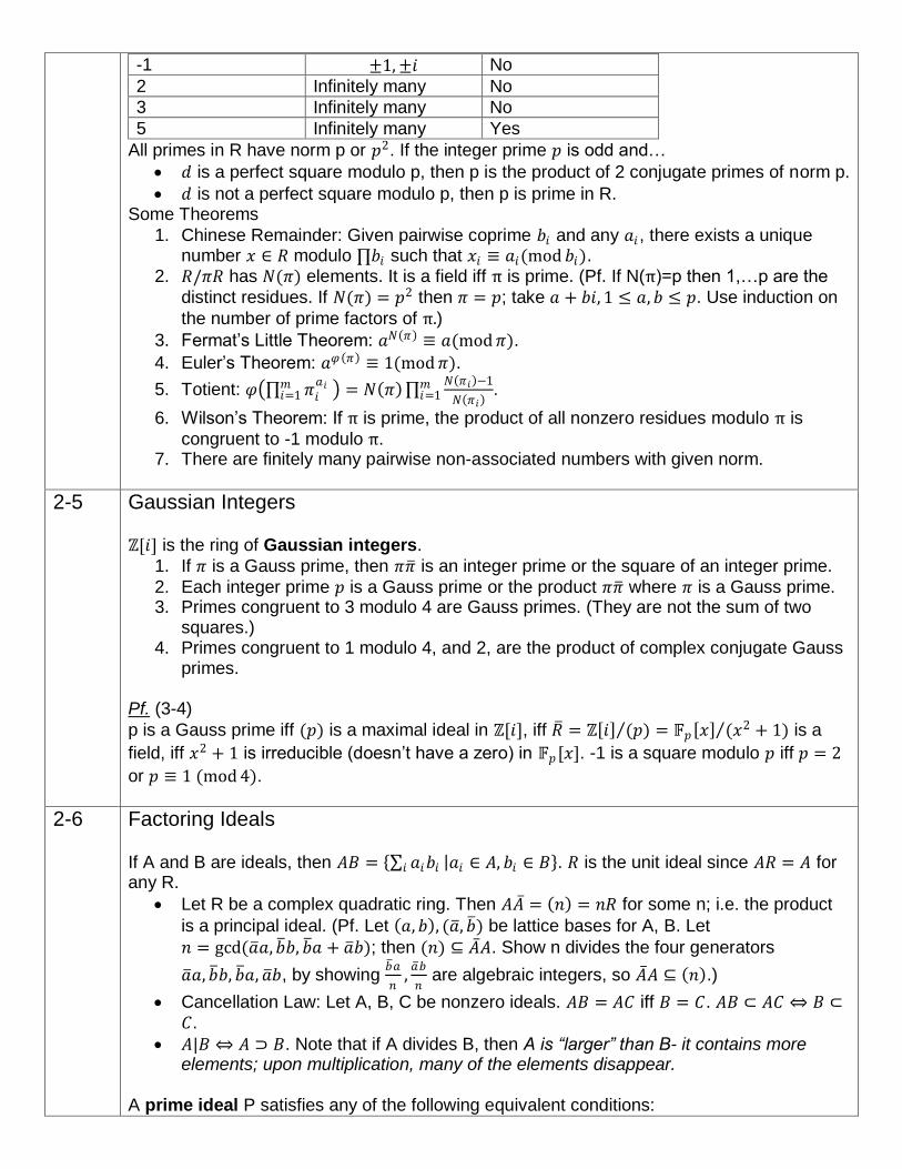
-1 ±1, ±𝑖 No

2 Infinitely many No

3 Infinitely many No

5 Infinitely many Yes

All primes in R have norm p or 𝑝2. If the integer prime 𝑝 is odd and…

𝑑 is a perfect square modulo p, then p is the product of 2 conjugate primes of norm p.

𝑑 is not a perfect square modulo p, then p is prime in R. Some Theorems

1. Chinese Remainder: Given pairwise coprime 𝑏𝑖 and any 𝑎𝑖 , there exists a unique number 𝑥 ∈ 𝑅 modulo ∏𝑏𝑖 such that 𝑥𝑖 ≡ 𝑎𝑖(mod 𝑏𝑖).

2. 𝑅/𝜋𝑅 has 𝑁(𝜋) elements. It is a field iff π is prime. (Pf. If N(π)=p then 1,…p are the

distinct residues. If 𝑁(𝜋) = 𝑝2 then 𝜋 = 𝑝; take 𝑎 + 𝑏𝑖, 1 ≤ 𝑎, 𝑏 ≤ 𝑝. Use induction on

the number of prime factors of π.) 3. Fermat’s Little Theorem: 𝑎𝑁 𝜋 ≡ 𝑎(mod 𝜋).

4. Euler’s Theorem: 𝑎𝜑 𝜋 ≡ 1(mod 𝜋).

5. Totient: 𝜑 ∏ 𝜋𝑖𝑎𝑖 𝑚

𝑖=1 = 𝑁 𝜋 ∏𝑁 𝜋𝑖 −1

𝑁 𝜋𝑖 𝑚𝑖=1 .

6. Wilson’s Theorem: If π is prime, the product of all nonzero residues modulo π is

congruent to -1 modulo π. 7. There are finitely many pairwise non-associated numbers with given norm.

2-5 Gaussian Integers ℞[𝑖] is the ring of Gaussian integers.

1. If 𝜋 is a Gauss prime, then 𝜋𝜋 is an integer prime or the square of an integer prime.

2. Each integer prime 𝑝 is a Gauss prime or the product 𝜋𝜋 where 𝜋 is a Gauss prime. 3. Primes congruent to 3 modulo 4 are Gauss primes. (They are not the sum of two

squares.) 4. Primes congruent to 1 modulo 4, and 2, are the product of complex conjugate Gauss

primes. Pf. (3-4)

p is a Gauss prime iff (𝑝) is a maximal ideal in ℞[𝑖], iff 𝑅 = ℞ 𝑖 (𝑝) = 𝔽𝑝 𝑥 (𝑥2 + 1) is a

field, iff 𝑥2 + 1 is irreducible (doesn’t have a zero) in 𝔽𝑝[𝑥]. -1 is a square modulo 𝑝 iff 𝑝 = 2

or 𝑝 ≡ 1 (mod 4).

2-6 Factoring Ideals

If A and B are ideals, then 𝐴𝐵 = 𝑎𝑖𝑏𝑖𝑖 𝑎𝑖 ∈ 𝐴, 𝑏𝑖 ∈ 𝐵 . 𝑅 is the unit ideal since 𝐴𝑅 = 𝐴 for any R.

Let R be a complex quadratic ring. Then 𝐴𝐴 = 𝑛 = 𝑛𝑅 for some n; i.e. the product

is a principal ideal. (Pf. Let 𝑎, 𝑏 , (𝑎 , 𝑏 ) be lattice bases for A, B. Let

𝑛 = gcd(𝑎 𝑎, 𝑏 𝑏, 𝑏 𝑎 + 𝑎 𝑏); then (𝑛) ⊆ 𝐴 𝐴. Show n divides the four generators

𝑎 𝑎, 𝑏 𝑏, 𝑏 𝑎, 𝑎 𝑏, by showing 𝑏 𝑎

𝑛,𝑎 𝑏

𝑛 are algebraic integers, so 𝐴 𝐴 ⊆ 𝑛 .)

Cancellation Law: Let A, B, C be nonzero ideals. 𝐴𝐵 = 𝐴𝐶 iff 𝐵 = 𝐶. 𝐴𝐵 ⊂ 𝐴𝐶 ⇔ 𝐵 ⊂𝐶.

𝐴|𝐵 ⇔ 𝐴 ⊃ 𝐵. Note that if A divides B, then A is “larger” than B- it contains more elements; upon multiplication, many of the elements disappear.

A prime ideal P satisfies any of the following equivalent conditions:

1. 𝑅/𝑃 is an integral domain. 2. 𝑃 ≠ 𝑅, and 𝑎𝑏 ∈ 𝑃 ⇒ 𝑎 ∈ 𝑃 or 𝑏 ∈ 𝑃. 3. 𝑃 ≠ 𝑅, and if A, B are ideals of R, 𝐴𝐵 ⊆ 𝑃 ⇒ 𝐴 ⊆ 𝑃 or 𝐵 ⊆ 𝑃.

Any maximal ideal is prime. If P is prime and not zero, and 𝑃|𝐴𝐵, then 𝑃|𝐴 or 𝑃|𝐵. Letting R be a complex quadratic ring, and B be a nonzero ideal,

1. B has finite index in R. 2. Finitely many ideals in R contain B. (Pf. Look at lattice) 3. B is in a maximal ideal.

4. B is prime iff it is maximal. (Pf. 𝑅/𝑃 is a field.) Every proper ideal of a complex quadratic ring R factors uniquely into a product of prime ideals (up to ordering).1 (Pf. Use 2 and cancellation law.)

Warning: Most rings do not have unique ideal factorization since 𝑃 ⊇ 𝐵 ⇏ 𝑃|𝐵. The complex quadratic ring R is a UFD iff it is a PID. (Pf. If P is prime, P contains a prime divisor π of some element in P. Then 𝑃 = (𝜋).) Below, P is nonzero and prime, p is an integer prime, and π is a Gauss prime.

1. If 𝑃 𝑃 = (𝑛) then 𝑛 = 𝑝 or 𝑝2 for some p.

2. (𝑝) is a prime ideal (p “remains prime”), or 𝑝 = 𝑃 𝑃 (p splits; if 𝑃 = 𝑃 then p ramifies).

3. If 𝑑 ≡ 2,3(mod 4), then p generates a prime ideal iff d is not a square modulo p, iff 𝑥2 − 𝑑 is irreducible in 𝔽𝑝[𝑥]. [Pf. by diagram]

4. If 𝑑 ≡ 1 mod 4 , then p generates a prime ideal iff 𝑥2 − 𝑥 +1−𝑑

4 is irreducible in 𝔽𝑝[𝑥].

Random: For nonzero ideals A, B, C, 𝐵 ⊃ 𝐶 ⇒ 𝐵: 𝐶 = 𝐴𝐵: 𝐴𝐶 . (Show for prime ideal A, split into 2 cases based on (2).)

2-7 Ideal Classes Ideals A and B are similar if 𝐵 = 𝜆𝐴 for some 𝜆 ∈ ℂ. (The lattices are similar and oriented the same.) Similarity classes of ideals are ideal classes; the ideal class of A is denoted by

⌌𝐴⌍. The class of the unit ideal ⌌𝑅⌍ consists of the principal ideals. The ideal classes form the (abelian) class group C of R, with ⌌𝐴⌍⌌𝐵⌍ = ⌌𝐴𝐵⌍. (Note ⌌𝐴⌍−1 =⌌𝐴 ⌍.) The class number |𝐶| tells how “badly” unique factorization of elements fails. Measuring the size of an ideal:

Norm: 𝑁 𝐴 = 𝑛, where (𝑛) = 𝐴 𝐴. Multiplicative function.

Index [𝑅: 𝐴] of A in R.

Δ(𝐴), the area of the parallelogram spanned by a lattice basis.

Minimal norm of nonzero elements of A. Relationships:

𝑁 𝐴 = 𝑅: 𝐴 =Δ 𝐴

Δ 𝑅

If 𝑎 ∈ 𝐴 has minimal nonzero norm, 𝑁 𝑎 ≤ 𝑁 𝐴 𝜇, 𝜇 =

2 𝑑

3, if 𝑑 ≡ 2,3 (mod 4)

𝑑

3, if 𝑑 ≡ 1 (mod 4)

. (Pf.

𝑁 𝑎 ≤2

3Δ(𝐴))

1. Every ideal class contains an ideal A with norm 𝑁 𝐴 ≤ 𝜇. (Pf. Choose nonzero

1 A Dedekind domain is a Noetherian, integrally closed integral domain with every nonzero prime ideal maximal (such as

the complex quadratic rings). “Integrally closed” means that the ring contains all algebraic integers that are in its ring of fractions. Prime factorization of ideals holds in any Dedekind domain. See Algebraic Number Theory.

element with minimal norm, 𝑎 = 𝐴𝐶 for some C, 𝑁 𝐶 ≤ 𝜇, ⌌𝐶⌍ = ⌌𝐴 ⌍,⌌𝐴⌍ = ⌌𝐶 ⌍.) 2. The class group C is generated by ⌌𝑃⌍, for prime ideals P with prime norm 𝑝 ≤ 𝜇. (Pf.

Factor. Either 𝑁(𝑃) = 𝑝 or 𝑃 = (𝑝).) 3. The class group is finite. (Pf. There are at most 2 prime ideals with norms a given

integer since 𝐴𝐴 = (𝑝) has unique factorization; use multiplicativity of norm.)

Computing the Class Group of 𝑅 = ℞[ 𝑑] . 1. List the primes 𝑝 ≤ ⌊𝜇⌋. 2. For each p, determine whether p splits in R by checking whether 𝑥2 − 𝑑 𝑑 ≡

2,3mod4, 𝑥2−𝑥+1−𝑑4 𝑑≡1mod4 are reducible.

3. If 𝑝 = 𝐴 𝐴 splits in R, include ⌌𝐴⌍ in the list of generators. 4. Compute the norm of some small elements (with prime divisors in the list found

above), like 𝑘 + 𝛿. 𝑘 ∈ ℞. Factor 𝑁(𝑎) to factor 𝑎 𝑎 = 𝑁 𝑎 ; match factors using

unique factorization. Note ⌌ 𝑎 ⌍ = ⌌ 𝑎 ⌍ = ⌌𝑅⌍ = 1. As long as 𝑎 is not divisible by one of the prime factors of 𝑁(𝑎), this amounts to replacing each prime in the factorization

of 𝑁 𝑎 by one of its corresponding ideals in (3) and setting equal to 1. Repeat until

there are enough relations to determine the group. [This works since if ∏ ⌌𝑃𝑖⌍𝑎𝑖

𝑖 =1, 𝑁 𝑃𝑖 = 𝑝𝑖 then there is an element 𝑎, 𝑁 𝑎 = ∏ 𝑝𝑖

𝑎𝑖𝑖 .]

5. For the prime 2,

a. If 𝑑 ≡ 2,3(mod 4), 2 ramifies: 2 = 𝑃𝑃 . 𝑃 has order 2 for 𝑑 ≠ −1, −2.

b. If 𝑑 ≡ 2(mod 4), 𝑃 = 2, 𝛿 . c. If 𝑑 ≡ 3 mod 4 , 𝑃 = 2,1 + 𝛿 .

2-8 Real Quadratic Rings

Represent ℞[ 𝑑] as a lattice in the plane by associating 𝛼 = 𝑎 + 𝑏 𝑑 with

𝑢, 𝑣 = (𝑎 + 𝑏 𝑑, 𝑎 − 𝑏 𝑑). (The coordinates represent the two ways that 𝐹[𝛿] can be

embedded in the real numbers, where δ is the abstract square root of d: 𝛿2 = 𝑑.)

The norm is 𝑁 𝑎 = 𝑎2 − 𝑏2𝑑 (sometimes the absolute value is used).

The units satisfy 𝑁 𝑎 = 1; they lie on the hyperbola 𝑢𝑣 = ±1. The units form an infinite group in R. 2 proofs: 1. The Pell’s equation has infinitely many solutions.

2. Let Δ be the determinant for the lattice of ℞[ 𝑑] and 𝐷𝑠 = {(𝑢, 𝑣)|𝑢2

𝑠2 + 𝑠2𝑣2 ≤2

3Δ}. For

any lattice with determinant Δ, 𝐷1 contains a nonzero lattice point (take the point nearest

the origin and use geometry). 𝜑 𝑥, 𝑦 = (𝑠𝑥,𝑦

𝑠) is an area-preserving map; by applying 𝜑

to the lattice, we get that every 𝐷𝑠 has a nonzero lattice point. These points have bounded norm; one norm is hit an infinite number of times. The ratios of these quadratic integers are units.

3 Polynomials 3-1 Polynomials

A polynomial with coefficients in R is a finite combination of nonnegative powers of the variable x. The polynomial ring over R is

𝑅 𝑋 = 𝑎𝑖𝑥𝑛

𝑛

𝑖=0

|𝑎𝑖 ∈ 𝑅

with X a formal variable and addition and multiplication defined by: (𝑓 𝑥 = 𝑎𝑖𝑥𝑖

𝑖 , 𝑔 𝑥 = 𝑏𝑖𝑥

𝑖𝑖 )

1. 𝑓 𝑥 + 𝑔 𝑥 = 𝑎𝑖 + 𝑏𝑖 𝑥𝑖

𝑖

2. 𝑓 𝑥 𝑔 𝑥 = 𝑎𝑖𝑏𝑗 𝑥𝑖+𝑗

𝑖

R is a subring of R[X] when identified with the constant polynomials in R. The ring of formal

series 𝑅[ 𝑋 ] is defined similarly but combinations need not be finite. Iterating, the ring of polynomials with variables 𝑥1, 𝑥2, … , 𝑥𝑛 is 𝑅[𝑥1, 𝑥2 , … , 𝑥𝑛 ]. (Formally, use the substitution

principle below to show we can identify 𝑅 𝑥 𝑦 with 𝑅[𝑥, 𝑦].) Basic vocab: monomial, degree, constant, leading coefficient, monic Division with Remainder: Let 𝑓, 𝑔 ∈ 𝑅[𝑋] with the leading coefficient of 𝑓 a unit. There are unique polynomials 𝑞, 𝑟 ∈ 𝑅[𝑋] (the quotient and remainder) so that

𝑔 𝑥 = 𝑓 𝑥 𝑞 𝑥 + 𝑟 𝑥 , deg 𝑟 < deg 𝑓

Substitution Principle: Let 𝜑: 𝑅 → 𝑅′ be a ring homomorphism. Given 𝑎1, … , 𝑎𝑛 ∈ 𝑅′, there is

a unique homomorphism Φ: 𝑅 𝑥1, … , 𝑥𝑛 → 𝑅′ which agrees with the map 𝜑 on constant polynomials, and sends 𝑥𝑖 → 𝑎𝑖 . For 𝑅 = 𝑅′, this map is just substituting 𝑎𝑖 for the variable 𝑥𝑖 and evaluating the polynomial. A characterization of the GCD: The greatest common divisor 𝑑 of 𝑓, 𝑔 ∈ 𝑅 = 𝐹[𝑥] is the monic polynomial defined by any of the following equivalent conditions:

1. 𝑅𝑑 = 𝑅𝑓 + 𝑅𝑔

2. Of all polynomials dividing f and g, 𝑑 has the greatest degree. 3. If 𝑒|𝑓, 𝑔 then 𝑒|𝑑.

From (1), there exist 𝑝, 𝑞 ∈ 𝑅 so 𝑑 = 𝑝𝑓 + 𝑞𝑔. Adjoining Elements Suppose 𝛼 is an element satisfying no relation other than that implied by 𝑓 𝛼 = 0 where 𝑓 ∈ 𝑅[𝑥] and has degree n. Then 𝑅 𝛼 ≅ 𝑅 𝑥 /(𝑓) is the ring extension. If f is monic, its

distinct elements are the polynomials in 𝛼 (with coefficients in R) of degree less than n, with (1, 𝛼, … , 𝛼𝑛−1) a basis. A polynomial in 𝛼 is equivalent to its remainder upon division by f. 𝑅

can be identified with a subring of 𝑅[𝛼] as long as no constant polynomial is identified with 0.

3-2 ℞[𝑋] Tools for factoring in ℞[𝑋]:

1. Inclusion in ℚ[𝑋]. 2. Reduction modulo prime p:𝜓𝑝 : ℞ 𝑋 → 𝔽𝑝[𝑋].

A polynomial in ℞[𝑋] is primitive if the greatest common divisor of its coefficients is 1, it is not constant, and the leading coefficient is positive. Gauss’s lemma: The product of primitive polynomials is primitive. Pf. Any prime 𝑝 in ℞ is prime in ℞[𝑥], and a prime divides a polynomial iff it divides every coefficient.

Every nonconstant polynomial 𝑓 𝑥 ∈ ℚ[𝑥] can be written uniquely as 𝑓 𝑥 = 𝑐𝑓0 𝑥 , 𝑐 ∈ ℚ and 𝑓0(𝑥) primitive.

If 𝑓0 is primitive and 𝑓0|𝑔 ∈ ℞[𝑥] in ℚ[𝑥], then 𝑓0|𝑔 in ℞[𝑥]. If two polynomials have a

common nonconstant factor in ℚ[𝑥] , they have a common nonconstant factor in ℞[𝑥]. An element of ℞[𝑥] is irreducible iff it is a prime integer or a primitive irreducible

polynomial in ℚ[𝑥], so every irreducible element of ℞[𝑥] is prime.

Hence ℞[𝑥] is a UFD, and each nonzero polynomial can be written uniquely (up to

ordering) as (𝑝𝑖 primes, 𝑞𝑖 primitive irreducible polynomials) 𝑓 𝑥 = ±𝑝1 ⋯ 𝑝𝑚𝑞1 𝑥 ⋯𝑞𝑛(𝑥)

This technique can be generalized: replace ℞ with a UFD R, and ℚ with the field of fractions of R.

By induction, if R is a UFD, then 𝑅[𝑥1, … , 𝑥𝑛 ] is a UFD.

Rational Roots Theorem: Let 𝑓 𝑥 = 𝑎𝑛𝑥𝑛 + ⋯ + 𝑎0 , 𝑎𝑛 ≠ 0. –𝑏0

𝑏1 (in reduced form) is a root

iff 𝑏1𝑥 + 𝑏0 divides f; if 𝑏1𝑥 + 𝑏0 divides f then 𝑏1|𝑎𝑛 and 𝑏0|𝑎0.

3-3 Irreducible Polynomials The derivative of a polynomial is formally defined (without calculus) as

𝑎𝑖𝑥𝑖

𝑛

𝑖=0

′

= 𝑖𝑎𝑖𝑥𝑖−1

𝑛

𝑖=1

.

𝛼 is a multiple root of 𝑓 𝑥 ∈ 𝐹 𝑥 iff 𝛼 is a root of both 𝑓(𝑥) and 𝑓 ′ 𝑥 . 𝛼 appears as

a root exactly 𝑛 times if 𝑓 𝑖 𝛼 = 0 for 0 ≤ 𝑖 < 𝑛 but 𝑓 𝑛 𝛼 ≠ 0.

𝑓, 𝑓′ have a common factor other than 1 iff there is a field extension where f has a multiple root.

If f is irreducible, and 𝑓 ′ ≠ 0, then f has no multiple root (in any field extension). If F has characteristic 0, then f has no multiple root (in any field extension).

If 𝑓 𝑥 = 𝑎𝑛𝑥𝑛 + ⋯ + 𝑎0 ∈ ℞[𝑥], 𝑝 ∤ 𝑎𝑛 , and the residue of f modulo p is irreducible in 𝔽𝑝[𝑥],

then f is irreducible in ℚ[𝑥]. Irreducible polynomials in 𝔽𝑝[𝑥] can be found using the sieve

method.

Eisenstein Criterion: If 𝑓 𝑥 = 𝑎𝑛𝑥𝑛 + ⋯ + 𝑎0 ∈ ℞ 𝑥 , 𝑝 ∤ 𝑎𝑛 , 𝑝|𝑎𝑛−1, … , 𝑎0, 𝑝2 ∤ 𝑎0, then f is

irreducible in ℚ[𝑥].

Pf. Factor and take it modulo p; get 𝑓 = 𝑏𝑟𝑥𝑟 (𝑐𝑠𝑥

𝑠). But if 𝑟, 𝑠 ≠ 0, 𝑝2|𝑎0.

Extended Eisenstein’s Criterion

Schönemann’s Criterion: Suppose

𝑘 = 𝑓𝑛 + 𝑝𝑔, 𝑛 ≥ 1, 𝑝 prime, 𝑓, 𝑔 ∈ ℞[𝑥]

deg 𝑓𝑛 > deg(𝑔)

𝑘 primitive

𝑓 is irreducible in 𝔽𝑝[𝑥]

𝑓 ∤ 𝑔 .

Then k is irreducible in ℚ[𝑥].

Cohn’s Criterion: Let 𝑏 ≥ 2 and let p be a prime number. Write 𝑝 = 𝑎𝑛𝑏𝑛 + ⋯ + 𝑎1𝑏 + 𝑎0 in

base b. Then 𝑓 𝑋 = 𝑎𝑛𝑋𝑛 + ⋯ + 𝑎1𝑋 + 𝑎0 is irreducible in ℚ[𝑋].

Capelli’s Theorem: Let K be a subfield of ℂ and 𝑓, 𝑔 ∈ 𝐾[𝑋]. Let 𝑎 be a complex root of f and

assume that f is irreducible in 𝐾[𝑋] and 𝑔 𝑋 − 𝑎 is irreducible in 𝐾 𝑎 [𝑋]. Then 𝑓 𝑔 𝑋 is

irreducible in 𝐾[𝑋].

[Add proof sketches.]

3-4 Cyclotomic Polynomials A primitive nth root of unity satisfies 𝜔𝑛 = 1, but 𝜔𝑚 ≠ 1 for 𝑛 ∈ ℕ, 0 < 𝑚 < 𝑛. The nth cyclotomic polynomial is

Φ𝑛 𝑋 = (𝑋 − 𝜔)𝜔 primitive nth root

.

The cyclotomic polynomial is an irreducible polynomial in ℞[𝑋] of degree 𝜑(𝑛). Each

polynomial 𝑋𝑛 − 1 is a product of cyclotomic polynomials:

𝑋𝑛 = Φ𝑑(𝑋)𝑑|𝑛

⇒ Φ𝑛 𝑋 =𝑋𝑛 − 1

∏ Φ𝑑 𝑋 𝑑|𝑛 ,𝑑<𝑛

so Φ𝑛(𝑋) has integer coefficients. Pf. of irreducibility: Lemma- if 𝜔 is a primitive nth root of unity and a zero of 𝑓 ∈ ℞[𝑋] then

𝜔𝑝 is a root for 𝑝 ∤ 𝑛. Proof- Suppose Φ𝑛 = 𝑔𝑕, 𝑕 𝜔 = 0, h irreducible (the minimal polynomial of 𝜔). 𝜔𝑝 is also a zero of Φ𝑛 . Suppose it is a zero of 𝑔. Then 𝜔 is a zero of 𝑔(𝑥𝑝), so 𝑔 𝑥𝑝 = 𝑕𝑘. Mod p, 𝑔 𝑥 𝑝 = 𝑕𝑘, so g and h have a root in cogmmon, contradicting

that 𝑋𝑛 − 1 ∈ ℞𝑝[𝑋] has no multiple root (derivative has no common factors with 𝑋𝑛 − 1).

Hence 𝜔𝑝 is a zero of h. ∎ Take powers to different primes to show that all primitive nth roots of unity divide h. Then 𝑕 = Φ𝑛 is irreducible.

3-5 Varieties

1. The set 𝐴𝑛 of n-tuples in a field K is the affine n-space.

2. If S is a set of polynomials in 𝐾 𝑋1, … , 𝑋𝑛 then 𝑉 𝑆 = 𝑥 ∈ 𝐴𝑛 𝑓 𝑥 = 0 for all 𝑓 ∈ 𝑆

is a (affine) variety.

3. For 𝑋 ⊆ 𝐴𝑛 , define the ideal of X to be 𝐼 𝑋 = 𝑓 ∈ 𝐾 𝑋1, … , 𝑋𝑛 𝑓 vanishes on 𝑋

Note 𝑆 ⊆ 𝐾 𝑋1, … , 𝑋𝑛 , 𝑋 ⊆ 𝐴𝑛 , 𝑉 𝑆 ⊆ 𝐴𝑛 , 𝐼 𝑋 ⊆ 𝐾 𝑋1, … , 𝑋𝑛 . 4. The radical of the ideal I in a ring T is the ideal

𝐼 = {𝑓 ∈ 𝑅|𝑓𝑟 ∈ 𝐼 for some 𝑟 ∈ ℕ} 𝐴𝑛 can be made into a topology (the Zariski topology) by taking varieties as closed sets (1-4 below).

Properties: 1. 𝑉 𝑆 = 𝑉 𝐼 where I is the ideal generated by S.

2. ∩ 𝑉 𝐼𝑗 = 𝑉(∪ 𝐼𝑗 )

3. If 𝑉𝑗 = 𝑉(𝐼𝑗 ) then ⋃ 𝑉𝑗𝑟𝑗=1 = 𝑉( 𝑓1 ⋯ 𝑓𝑟 𝑓𝑗 ∈ 𝐼𝑗 , 1 ≤ 𝑗 ≤ 𝑟 ).

4. 𝐴𝑛 = 𝑉 0 , 𝜙 = 𝑉(1)

5. 𝑋 ⊆ 𝑌 ⇒ 𝐼 𝑌 ⊆ 𝐼(𝑋), 𝑆 ⊆ 𝑇 ⇒ 𝑉 𝑇 ⊆ 𝑉(𝑆) 6. 𝑆 ⊆ 𝐼𝑉 𝑆 , 𝑋 ⊆ 𝑉𝐼(𝑋) 7. 𝑉𝐼𝑉 𝑆 = 𝑉 𝑆 , 𝐼𝑉𝐼 𝑋 = 𝐼(𝑋)

8. 𝐼 0 = 𝐾[𝑋1, … , 𝑋𝑛 ] 9. If K is an infinite field, 𝐼 𝐴𝑛 = {0}.

a. For n=1, a nonzero polynomial only has finitely many zeros. Extend by induction.

10. 𝐼 𝑎1, … , 𝑎𝑛 = (𝑋1 − 𝑎1, … , 𝑋𝑛 − 𝑎𝑛 ) (the ideal generated by 𝑋𝑖 − 𝑎𝑖 ) a. Use division with remainder.

11. If 𝑎1, … 𝑎𝑛 ∈ 𝐴𝑛 then 𝐼 = (𝑋1 − 𝑎1, … , 𝑋𝑛 − 𝑎𝑛) is a maximal ideal. a. Apply the division algorithm to 𝑓 ∈ 𝐽\𝐼.

12. 𝐼 ⊆ 𝐼𝑉(𝐼)

3-6 Nullstellensatz Hilbert Basis Theorem: If R is Noetherian, then 𝑅[𝑥] is Noetherian. Thus so is 𝑅[𝑥1, … , 𝑥𝑛 ]. In particular, this holds for 𝑅 = ℞ or a field F. Pf. For 𝐼 ⊆ 𝑅[𝑥] an ideal, the set whose elements are the leading coefficients of the polynomials in I (including 0) forms the ideal of leading coefficients in R. Take generators for this ideal and polynomials with those leading coefficients, multiplying by x as necessary so they have the same degree n. The polynomials with degree less than n form a free, Noetherian R-module P with basis (1, 𝑥, … 𝑥𝑛−1). 𝑃 ∩ 𝐼 has a finite generating set. Put the two generating sets together. The ring of formal power series 𝑅[ 𝑋 ] is also Noetherian. Noether Normalization Lemma: Let A be a finitely generated K-algebra. There exists a

subset 𝑦1, … , 𝑦𝑟 of A such that the 𝑦𝑖 are algebraically independent over K and A is integral over 𝐾[𝑦1, … , 𝑦𝑟] (all elements of A are algebraic integers over 𝐾[𝑦1, … , 𝑦𝑟]). Pf. Induct on n; n=1 trivial. Take a maximally algebraically independent subset 𝑥1, … , 𝑥𝑟 ⊆{𝑥1, … , 𝑥𝑛}; assume 𝑛 > 𝑟. By algebraic dependency, there exists 𝑓 ∈ 𝐾 𝑋1, … , 𝑋𝑛 so that 𝑓 𝑥1, … , 𝑥𝑛 = 0. Lexicographically order the monomials, and choose weights 𝑤𝑖 to match

the lexicographic order. Set 𝑥𝑖 = 𝑧𝑖 + 𝑥𝑛𝑤𝑖 . Then we get a polynomial in 𝑥𝑛 , where term with

the highest power of 𝑥𝑛 is uncancelled. 𝑥𝑛 is integral over 𝐾[𝑧1, … , 𝑧𝑛−1]; finish by induction.

Cor. If B is a finitely generated K-algebra, and I is a maximal ideal, then 𝐵 𝐼 is a finite

extension of K (K is embedded via 𝑐 ⇝ 𝑐 + 𝐼.): In the above, we must have 𝑟 = 0; B/I is algebraic over K.

Hilbert’s Nullstellensatz: For any field K and 𝑛 ∈ ℕ, the following are equivalent: 1. K is algebraically closed. 2. (Maximal Ideal Theorem) The maximal ideals of 𝐾[𝑋1, … , 𝑋𝑛 ] are the ideals of the

form (𝑋1 − 𝑎1, … , 𝑋𝑛 − 𝑎𝑛). 3. (Weak Nullstellensatz) If I is a proper ideal of 𝐾[𝑋1, … , 𝑋𝑛], then 𝑉(𝐼) is not empty.

4. (Strong Nullstellensatz) If I is an ideal of 𝐾[𝑋1, … , 𝑋𝑛 ] then 𝐼𝑉 𝐼 = 𝐼. (2)⇒(3): For I a proper ideal, let J be a maximal ideal containing it. Then 𝑉 𝐽 ⊆ 𝑉(𝐼) so 𝐽 = (𝑋1 − 𝑎1 , … , 𝑋𝑛 − 𝑎𝑛), 𝑎 ∈ 𝑉(𝐽).

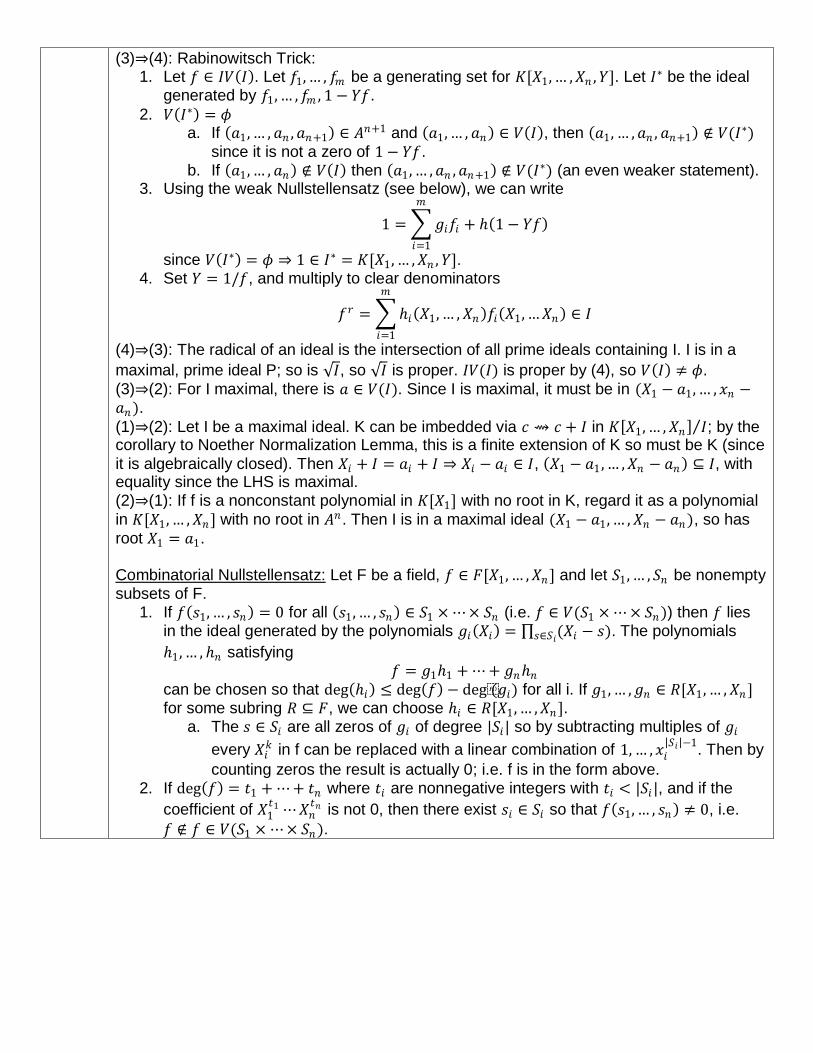
(3)⇒(4): Rabinowitsch Trick: 1. Let 𝑓 ∈ 𝐼𝑉 𝐼 . Let 𝑓1, … , 𝑓𝑚 be a generating set for 𝐾[𝑋1, … , 𝑋𝑛 , 𝑌]. Let 𝐼∗ be the ideal

generated by 𝑓1, … , 𝑓𝑚 , 1 − 𝑌𝑓.

2. 𝑉 𝐼∗ = 𝜙 a. If 𝑎1, … , 𝑎𝑛 , 𝑎𝑛+1 ∈ 𝐴𝑛+1 and 𝑎1, … , 𝑎𝑛 ∈ 𝑉 𝐼 , then 𝑎1, … , 𝑎𝑛 , 𝑎𝑛+1 ∉ 𝑉(𝐼∗)

since it is not a zero of 1 − 𝑌𝑓. b. If 𝑎1, … , 𝑎𝑛 ∉ 𝑉 𝐼 then 𝑎1, … , 𝑎𝑛 , 𝑎𝑛+1 ∉ 𝑉(𝐼∗) (an even weaker statement).

3. Using the weak Nullstellensatz (see below), we can write

1 = 𝑔𝑖𝑓𝑖 + 𝑕 1 − 𝑌𝑓

𝑚

𝑖=1

since 𝑉 𝐼∗ = 𝜙 ⇒ 1 ∈ 𝐼∗ = 𝐾[𝑋1, … , 𝑋𝑛 , 𝑌]. 4. Set 𝑌 = 1/𝑓, and multiply to clear denominators

𝑓𝑟 = 𝑕𝑖 𝑋1, … , 𝑋𝑛 𝑓𝑖 𝑋1, … 𝑋𝑛

𝑚

𝑖=1

∈ 𝐼

(4)⇒(3): The radical of an ideal is the intersection of all prime ideals containing I. I is in a

maximal, prime ideal P; so is 𝐼, so 𝐼 is proper. 𝐼𝑉(𝐼) is proper by (4), so 𝑉 𝐼 ≠ 𝜙.

(3)⇒(2): For I maximal, there is 𝑎 ∈ 𝑉(𝐼). Since I is maximal, it must be in (𝑋1 − 𝑎1, … , 𝑥𝑛 −𝑎𝑛).

(1)⇒(2): Let I be a maximal ideal. K can be imbedded via 𝑐 ⇝ 𝑐 + 𝐼 in 𝐾 𝑋1, … , 𝑋𝑛 𝐼 ; by the corollary to Noether Normalization Lemma, this is a finite extension of K so must be K (since

it is algebraically closed). Then 𝑋𝑖 + 𝐼 = 𝑎𝑖 + 𝐼 ⇒ 𝑋𝑖 − 𝑎𝑖 ∈ 𝐼, 𝑋1 − 𝑎1 , … , 𝑋𝑛 − 𝑎𝑛 ⊆ 𝐼, with equality since the LHS is maximal. (2)⇒(1): If f is a nonconstant polynomial in 𝐾[𝑋1] with no root in K, regard it as a polynomial

in 𝐾[𝑋1, … , 𝑋𝑛 ] with no root in 𝐴𝑛 . Then I is in a maximal ideal (𝑋1 − 𝑎1, … , 𝑋𝑛 − 𝑎𝑛), so has

root 𝑋1 = 𝑎1. Combinatorial Nullstellensatz: Let F be a field, 𝑓 ∈ 𝐹[𝑋1, … , 𝑋𝑛 ] and let 𝑆1, … , 𝑆𝑛 be nonempty subsets of F.

1. If 𝑓 𝑠1, … , 𝑠𝑛 = 0 for all 𝑠1, … , 𝑠𝑛 ∈ 𝑆1 × ⋯ × 𝑆𝑛 (i.e. 𝑓 ∈ 𝑉(𝑆1 × ⋯ × 𝑆𝑛)) then 𝑓 lies in the ideal generated by the polynomials 𝑔𝑖 𝑋𝑖 = ∏ (𝑋𝑖 − 𝑠)𝑠∈𝑆𝑖

. The polynomials

𝑕1, … , 𝑕𝑛 satisfying 𝑓 = 𝑔1𝑕1 + ⋯ + 𝑔𝑛𝑕𝑛

can be chosen so that deg 𝑕𝑖 ≤ deg 𝑓 − deg(𝑔𝑖) for all i. If 𝑔1, … , 𝑔𝑛 ∈ 𝑅[𝑋1, … , 𝑋𝑛] for some subring 𝑅 ⊆ 𝐹, we can choose 𝑕𝑖 ∈ 𝑅[𝑋1, … , 𝑋𝑛].

a. The 𝑠 ∈ 𝑆𝑖 are all zeros of 𝑔𝑖 of degree |𝑆𝑖| so by subtracting multiples of 𝑔𝑖

every 𝑋𝑖𝑘 in f can be replaced with a linear combination of 1, … , 𝑥𝑖

𝑆𝑖 −1. Then by

counting zeros the result is actually 0; i.e. f is in the form above. 2. If deg 𝑓 = 𝑡1 + ⋯ + 𝑡𝑛 where 𝑡𝑖 are nonnegative integers with 𝑡𝑖 < |𝑆𝑖|, and if the

coefficient of 𝑋1𝑡1 ⋯ 𝑋𝑛

𝑡𝑛 is not 0, then there exist 𝑠𝑖 ∈ 𝑆𝑖 so that 𝑓 𝑠1, … , 𝑠𝑛 ≠ 0, i.e.

𝑓 ∉ 𝑓 ∈ 𝑉(𝑆1 × ⋯ × 𝑆𝑛).

4 Fields Examples of Fields An extension K of a field F (also denoted 𝐾/𝐹) is a field containing F.

Number field: subfield of ℂ

Finite field: finitely many elements

Function field: Extensions of ℂ(𝑡) of rational functions

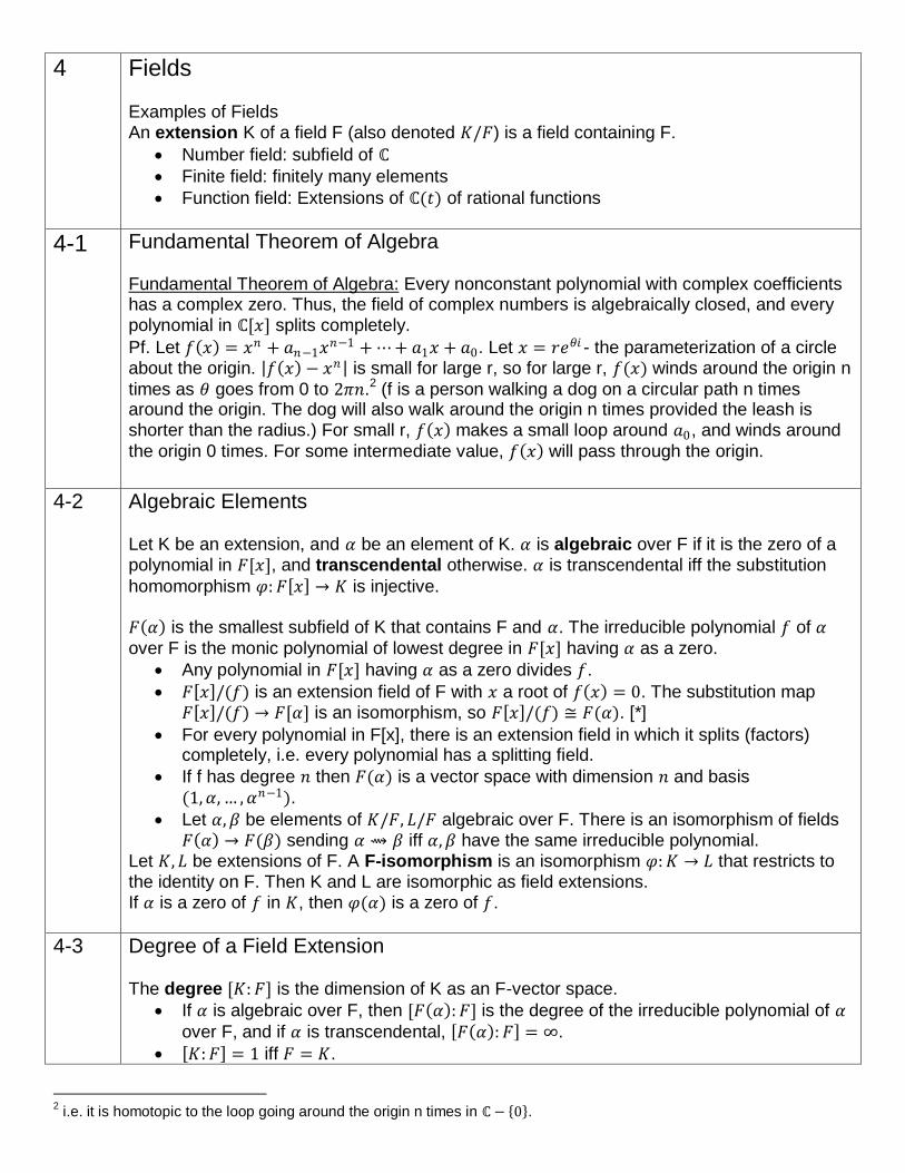
4-1 Fundamental Theorem of Algebra Fundamental Theorem of Algebra: Every nonconstant polynomial with complex coefficients has a complex zero. Thus, the field of complex numbers is algebraically closed, and every polynomial in ℂ[𝑥] splits completely.

Pf. Let 𝑓 𝑥 = 𝑥𝑛 + 𝑎𝑛−1𝑥𝑛−1 + ⋯ + 𝑎1𝑥 + 𝑎0. Let 𝑥 = 𝑟𝑒𝜃𝑖 - the parameterization of a circle about the origin. 𝑓 𝑥 − 𝑥𝑛 is small for large r, so for large r, 𝑓(𝑥) winds around the origin n

times as 𝜃 goes from 0 to 2𝜋𝑛.2 (f is a person walking a dog on a circular path n times around the origin. The dog will also walk around the origin n times provided the leash is shorter than the radius.) For small r, 𝑓 𝑥 makes a small loop around 𝑎0, and winds around

the origin 0 times. For some intermediate value, 𝑓 𝑥 will pass through the origin.

4-2 Algebraic Elements

Let K be an extension, and 𝛼 be an element of K. 𝛼 is algebraic over F if it is the zero of a polynomial in 𝐹[𝑥], and transcendental otherwise. 𝛼 is transcendental iff the substitution

homomorphism 𝜑: 𝐹 𝑥 → 𝐾 is injective. 𝐹 𝛼 is the smallest subfield of K that contains F and 𝛼. The irreducible polynomial 𝑓 of 𝛼

over F is the monic polynomial of lowest degree in 𝐹[𝑥] having 𝛼 as a zero.

Any polynomial in 𝐹[𝑥] having 𝛼 as a zero divides 𝑓.

𝐹 𝑥 /(𝑓) is an extension field of F with 𝑥 a root of 𝑓 𝑥 = 0. The substitution map 𝐹 𝑥 /(𝑓) → 𝐹[𝛼] is an isomorphism, so 𝐹 𝑥 /(𝑓) ≅ 𝐹(𝛼). [*]

For every polynomial in F[x], there is an extension field in which it splits (factors) completely, i.e. every polynomial has a splitting field.

If f has degree 𝑛 then 𝐹(𝛼) is a vector space with dimension 𝑛 and basis

(1, 𝛼, … , 𝛼𝑛−1).

Let 𝛼, 𝛽 be elements of 𝐾/𝐹, 𝐿/𝐹 algebraic over F. There is an isomorphism of fields 𝐹 𝛼 → 𝐹(𝛽) sending 𝛼 ⇝ 𝛽 iff 𝛼, 𝛽 have the same irreducible polynomial.

Let 𝐾, 𝐿 be extensions of F. A F-isomorphism is an isomorphism 𝜑: 𝐾 → 𝐿 that restricts to the identity on F. Then K and L are isomorphic as field extensions. If 𝛼 is a zero of 𝑓 in 𝐾, then 𝜑(𝛼) is a zero of 𝑓.

4-3 Degree of a Field Extension The degree [𝐾: 𝐹] is the dimension of K as an F-vector space.

If 𝛼 is algebraic over F, then [𝐹 𝛼 : 𝐹] is the degree of the irreducible polynomial of 𝛼

over F, and if 𝛼 is transcendental, 𝐹 𝛼 : 𝐹 = ∞.

𝐾: 𝐹 = 1 iff 𝐹 = 𝐾.

2 i.e. it is homotopic to the loop going around the origin n times in ℂ − 0 .

If 𝐾: 𝐹 = 2 then K can be obtained by adjoining a square root 𝛿 of an element in F: 𝛿2 ∈ 𝐹

Multiplicative property: If 𝐹 ⊆ 𝐾 ⊆ 𝐿, then 𝐿: 𝐹 = 𝐿: 𝐾 [𝐾: 𝐹]. o If K is a finite extension of F, and 𝛼 ∈ 𝐾, then the degree of 𝛼 divides [𝐾: 𝐹]. o If 𝛼 ∈ 𝐿 is algebraic over F, it is algebraic over 𝐾 with degree less than or

equal to its degree over 𝐹. o A field extension generated by finitely many algebraic elements is a finite

extension. o The set of elements of K that are algebraic over F is a subfield of K.

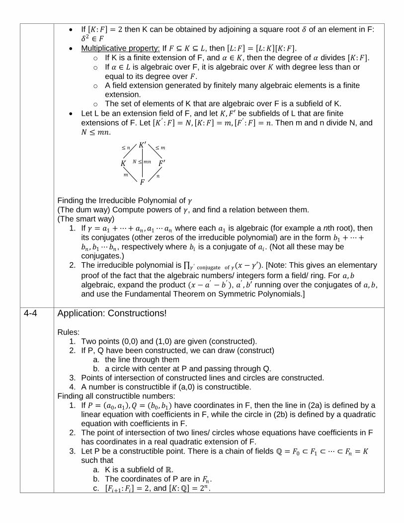
Let L be an extension field of F, and let 𝐾, 𝐹′ be subfields of L that are finite

extensions of F. Let 𝐾′ : 𝐹 = 𝑁, 𝐾: 𝐹 = 𝑚, 𝐹′ : 𝐹 = 𝑛. Then m and n divide N, and 𝑁 ≤ 𝑚𝑛.

Finding the Irreducible Polynomial of 𝛾 (The dum way) Compute powers of 𝛾, and find a relation between them. (The smart way)

1. If 𝛾 = 𝑎1 + ⋯ + 𝑎𝑛 , 𝑎1 ⋯ 𝑎𝑛 where each 𝑎1 is algebraic (for example a nth root), then

its conjugates (other zeros of the irreducible polynomial) are in the form 𝑏1 + ⋯ +𝑏𝑛 , 𝑏1 ⋯ 𝑏𝑛 , respectively where 𝑏𝑖 is a conjugate of 𝑎𝑖 . (Not all these may be conjugates.)

2. The irreducible polynomial is ∏ (𝑥 − 𝛾′)𝛾 ′ conjugate of 𝛾 . [Note: This gives an elementary

proof of the fact that the algebraic numbers/ integers form a field/ ring. For 𝑎, 𝑏 algebraic, expand the product (𝑥 − 𝑎′ − 𝑏′ ), 𝑎′ , 𝑏′ running over the conjugates of 𝑎, 𝑏, and use the Fundamental Theorem on Symmetric Polynomials.]

4-4 Application: Constructions! Rules:

1. Two points (0,0) and (1,0) are given (constructed). 2. If P, Q have been constructed, we can draw (construct)

a. the line through them b. a circle with center at P and passing through Q.

3. Points of intersection of constructed lines and circles are constructed. 4. A number is constructible if (a,0) is constructible.

Finding all constructible numbers: 1. If 𝑃 = 𝑎0, 𝑎1 , 𝑄 = (𝑏0 , 𝑏1) have coordinates in F, then the line in (2a) is defined by a

linear equation with coefficients in F, while the circle in (2b) is defined by a quadratic equation with coefficients in F.

2. The point of intersection of two lines/ circles whose equations have coefficients in F has coordinates in a real quadratic extension of F.

3. Let P be a constructible point. There is a chain of fields ℚ = 𝐹0 ⊂ 𝐹1 ⊂ ⋯ ⊂ 𝐹𝑛 = 𝐾 such that

a. K is a subfield of ℝ. b. The coordinates of P are in 𝐹𝑛 . c. 𝐹𝑖+1: 𝐹𝑖 = 2, and 𝐾: ℚ = 2𝑛 .

𝐾′

𝐹

𝐹′ 𝐾 𝑁 ≤ 𝑚𝑛

𝑛 𝑚

≤ 𝑛 ≤ 𝑚

Thus a constructible number has degree over ℚ a power of 2. 4. Conversely, if a chain of fields satisfies the conditions above, then every element of K

is constructible. Examples:

1. Trisecting the angle with compass and straightedge is impossible. cos 20° is not constructible.

2. For p prime, a regular p-gon can be constructed iff 𝑝 = 2𝑟 + 1.

4-5 Finite Fields A finite field is a vector space over 𝔽𝑝 for some prime p, so has order 𝑞 = 𝑝𝑟 . The (unique)

field of order q is denoted by 𝔽𝑞 .

1. The elements in a field of order q are roots of 𝑥𝑞 − 𝑥 = 0 (everything is modulo p). a. The multiplicative group 𝔽𝑞

× of nonzero elements has order 𝑞 − 1. The order of

any element divides 𝑞 − 1 so 𝛼𝑞−1 = 0 for any 𝛼 ∈ 𝔽𝑞.

2. 𝔽𝑞× is a cyclic group of order 𝑞 − 1.

a. By the Structure Theorem for Abelian Groups, 𝔽𝑞× is a direct product of cyclic

subgroups of orders 𝑑1| ⋯ |𝑑𝑘 , and the group has exponent 𝑑𝑘 . 𝑥𝑑𝑘 − 1 = 0

has at most 𝑑𝑘 roots, so 𝑘 = 1, 𝑑𝑘 = 𝑞 − 1. 3. There exists a unique field of order q (up to isomorphism).

a. Existence: Take a field extension where 𝑥𝑞 − 𝑥 splits completely. If 𝛼, 𝛽 are roots of 𝑥𝑞 − 𝑥 = 0 then 𝛼 + 𝛽 𝑞 = 𝛼 + 𝛽. Since −1 is a root, −𝛼 is a root. The roots form a field.

b. Uniqueness: Suppose 𝐾, 𝐾′ have order 𝑞. Let 𝛼 be a generator of 𝐾×; 𝐾 = 𝐹(𝛼). The irreducible polynomial 𝑓 ∈ 𝐾[𝑥] with root 𝛼 divides 𝑥𝑞 − 𝑥.

𝑥𝑞 − 𝑥 splits completely in both 𝐾, 𝐾′, so f has a root 𝛼′ ∈ 𝐾′. Then 𝐹 𝛼 ≅𝐹 𝑥 /(𝑓) ≅ 𝐹(𝛼′) = 𝐾′.

4. A field of order 𝑝𝑟 contains a subfield of order 𝑝𝑘 iff 𝑘|𝑟. (Note this is a relation between the exponents, not the orders.)

a. 𝔽𝑝𝑘 ⊆ 𝔽𝑝𝑟 ⇒ 𝑘|𝑟: Multiplicative property of the degree.

b. 𝔽𝑝𝑘 ⊆ 𝔽𝑝𝑟 ⇐ 𝑘|𝑟: 𝑝𝑟 − 1|𝑝𝑘 − 1. Cyclic 𝔽𝑝𝑟× contains a cyclic group of order 𝑝𝑘 .

Including 0, they are the roots of 𝑥𝑝𝑘− 𝑥 = 0 and thus form a field by 3a.

5. The irreducible factors of 𝑥𝑞 − 𝑥 over 𝔽𝑝 are the irreducible polynomials 𝑔 in 𝐹[𝑥]

whose degrees divide r.

a. ⇒: Multiplicative property b. ⇐: Let 𝛽 be a root of g. If 𝑘|𝑟, by (4), 𝔽𝑞 contains a subfield isomorphic to

𝐹(𝛽). 𝑔 has a root in 𝔽𝑞 so divides 𝑥𝑞 − 𝑥.

6. For every r there is an irreducible polynomial of degree r over 𝔽𝑝 .

a. 𝔽𝑞(𝑞 = 𝑝𝑟) has degree r over 𝔽𝑝 , and has a cyclic multiplicative group

generated by an element 𝛼. 𝔽𝑝(𝛼) has degree r over 𝔽𝑝 .

To compute in 𝔽𝑞 , take a root 𝛽 of the irreducible factor of 𝑥𝑞 − 𝑥 of degree r; (1, 𝛽, … , 𝛽𝑟−1)

is a basis. Let 𝑊𝑝(𝑑) be the number of irreducible monic polynomials of degree d in 𝔽𝑝 . Then by (2),

𝑝𝑛 = 𝑑𝑊𝑝(𝑑)𝑑|𝑛

.

By Möbius inversion,

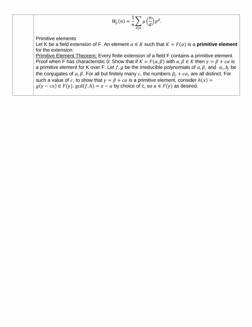
𝑊𝑝 𝑛 =1

𝑛 𝜇

𝑛

𝑑 𝑝𝑑

𝑑|𝑛

.

Primitive elements Let K be a field extension of F. An element 𝛼 ∈ 𝐾 such that 𝐾 = 𝐹(𝛼) is a primitive element for the extension. Primitive Element Theorem: Every finite extension of a field F contains a primitive element. Proof when F has characteristic 0: Show that if 𝐾 = 𝐹(𝛼, 𝛽) with 𝛼, 𝛽 ∈ 𝐾 then 𝛾 = 𝛽 + 𝑐𝛼 is a primitive element for K over F. Let 𝑓, 𝑔 be the irreducible polynomials of 𝛼, 𝛽, and 𝛼𝑖 , 𝑏𝑗 be

the conjugates of 𝛼, 𝛽. For all but finitely many 𝑐, the numbers 𝛽𝑗 + 𝑐𝛼𝑖 are all distinct. For

such a value of 𝑐, to show that 𝛾 = 𝛽 + 𝑐𝛼 is a primitive element, consider 𝑕 𝑥 =𝑔 𝛾 − 𝑐𝑥 ∈ 𝐹(𝛾). gcd 𝑓, 𝑕 = 𝑥 − 𝛼 by choice of c, so 𝛼 ∈ 𝐹(𝛾) as desired.

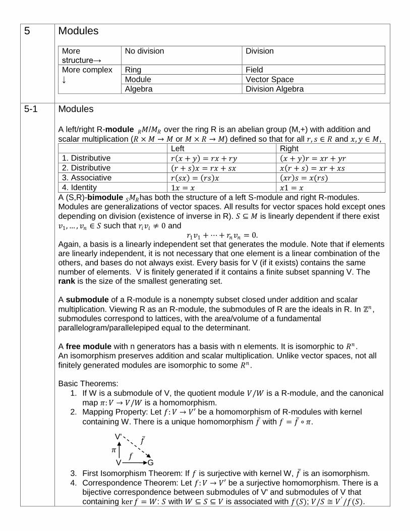
5 Modules

More structure→

No division Division

More complex ↓

Ring Field

Module Vector Space

Algebra Division Algebra

5-1 Modules

A left/right R-module 𝑀𝑅 /𝑀𝑅 over the ring R is an abelian group (M,+) with addition and

scalar multiplication (𝑅 × 𝑀 → 𝑀 or 𝑀 × 𝑅 → 𝑀) defined so that for all 𝑟, 𝑠 ∈ 𝑅 and 𝑥, 𝑦 ∈ 𝑀,

Left Right

1. Distributive 𝑟 𝑥 + 𝑦 = 𝑟𝑥 + 𝑟𝑦 𝑥 + 𝑦 𝑟 = 𝑥𝑟 + 𝑦𝑟

2. Distributive 𝑟 + 𝑠 𝑥 = 𝑟𝑥 + 𝑠𝑥 𝑥 𝑟 + 𝑠 = 𝑥𝑟 + 𝑥𝑠

3. Associative 𝑟 𝑠𝑥 = 𝑟𝑠 𝑥 𝑥𝑟 𝑠 = 𝑥(𝑟𝑠)

4. Identity 1𝑥 = 𝑥 𝑥1 = 𝑥

A (S,R)-bimodule 𝑀𝑅𝑆 has both the structure of a left S-module and right R-modules.

Modules are generalizations of vector spaces. All results for vector spaces hold except ones

depending on division (existence of inverse in R). 𝑆 ⊆ 𝑀 is linearly dependent if there exist

𝑣1, … , 𝑣𝑛 ∈ 𝑆 such that 𝑟𝑖𝑣𝑖 ≠ 0 and 𝑟1𝑣1 + ⋯ + 𝑟𝑛𝑣𝑛 = 0.

Again, a basis is a linearly independent set that generates the module. Note that if elements are linearly independent, it is not necessary that one element is a linear combination of the others, and bases do not always exist. Every basis for V (if it exists) contains the same number of elements. V is finitely generated if it contains a finite subset spanning V. The rank is the size of the smallest generating set. A submodule of a R-module is a nonempty subset closed under addition and scalar

multiplication. Viewing R as an R-module, the submodules of R are the ideals in R. In ℞𝑛 , submodules correspond to lattices, with the area/volume of a fundamental parallelogram/parallelepiped equal to the determinant. A free module with n generators has a basis with n elements. It is isomorphic to 𝑅𝑛 . An isomorphism preserves addition and scalar multiplication. Unlike vector spaces, not all

finitely generated modules are isomorphic to some 𝑅𝑛 . Basic Theorems:

1. If W is a submodule of V, the quotient module 𝑉/𝑊 is a R-module, and the canonical

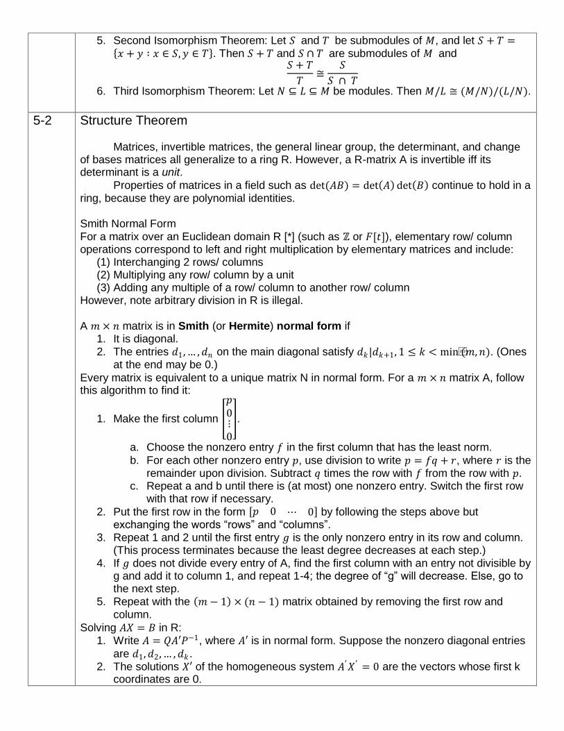
map 𝜋: 𝑉 → 𝑉/𝑊 is a homomorphism. 2. Mapping Property: Let 𝑓: 𝑉 → 𝑉′ be a homomorphism of R-modules with kernel

containing W. There is a unique homomorphism 𝑓 with 𝑓 = 𝑓 ∘ 𝜋.

3. First Isomorphism Theorem: If 𝑓 is surjective with kernel W, 𝑓 is an isomorphism.

4. Correspondence Theorem: Let 𝑓: 𝑉 → 𝑉′ be a surjective homomorphism. There is a bijective correspondence between submodules of V' and submodules of V that containing ker 𝑓 = 𝑊: 𝑆 with 𝑊 ⊆ 𝑆 ⊆ 𝑉 is associated with 𝑓(𝑆); 𝑉/𝑆 ≅ 𝑉 ′/𝑓(𝑆).

V'

V G

𝑓

𝑓 𝜋

5. Second Isomorphism Theorem: Let 𝑆 and 𝑇 be submodules of 𝑀, and let 𝑆 + 𝑇 = 𝑥 + 𝑦 ∶ 𝑥 ∈ 𝑆, 𝑦 ∈ 𝑇 . Then 𝑆 + 𝑇 and 𝑆 ∩ 𝑇 are submodules of 𝑀 and

𝑆 + 𝑇

𝑇≅

𝑆

𝑆 ∩ 𝑇

6. Third Isomorphism Theorem: Let 𝑁 ⊆ 𝐿 ⊆ 𝑀 be modules. Then 𝑀/𝐿 ≅ (𝑀/𝑁)/(𝐿/𝑁).

5-2 Structure Theorem

Matrices, invertible matrices, the general linear group, the determinant, and change of bases matrices all generalize to a ring R. However, a R-matrix A is invertible iff its determinant is a unit.

Properties of matrices in a field such as det(𝐴𝐵) = det 𝐴 det 𝐵 continue to hold in a ring, because they are polynomial identities. Smith Normal Form For a matrix over an Euclidean domain R [*] (such as ℞ or 𝐹[𝑡]), elementary row/ column operations correspond to left and right multiplication by elementary matrices and include:

(1) Interchanging 2 rows/ columns (2) Multiplying any row/ column by a unit (3) Adding any multiple of a row/ column to another row/ column

However, note arbitrary division in R is illegal. A 𝑚 × 𝑛 matrix is in Smith (or Hermite) normal form if

1. It is diagonal. 2. The entries 𝑑1, … , 𝑑𝑛 on the main diagonal satisfy 𝑑𝑘|𝑑𝑘+1, 1 ≤ 𝑘 < min(𝑚, 𝑛). (Ones

at the end may be 0.)

Every matrix is equivalent to a unique matrix N in normal form. For a 𝑚 × 𝑛 matrix A, follow this algorithm to find it:

1. Make the first column

𝑝0⋮0

.

a. Choose the nonzero entry 𝑓 in the first column that has the least norm.

b. For each other nonzero entry 𝑝, use division to write 𝑝 = 𝑓𝑞 + 𝑟, where 𝑟 is the remainder upon division. Subtract 𝑞 times the row with 𝑓 from the row with 𝑝.

c. Repeat a and b until there is (at most) one nonzero entry. Switch the first row with that row if necessary.

2. Put the first row in the form 𝑝 0 ⋯ 0 by following the steps above but exchanging the words “rows” and “columns”.

3. Repeat 1 and 2 until the first entry 𝑔 is the only nonzero entry in its row and column. (This process terminates because the least degree decreases at each step.)

4. If 𝑔 does not divide every entry of A, find the first column with an entry not divisible by g and add it to column 1, and repeat 1-4; the degree of “g” will decrease. Else, go to the next step.

5. Repeat with the 𝑚 − 1 × (𝑛 − 1) matrix obtained by removing the first row and column.

Solving 𝐴𝑋 = 𝐵 in R: 1. Write 𝐴 = 𝑄𝐴′𝑃−1, where 𝐴′ is in normal form. Suppose the nonzero diagonal entries

are 𝑑1, 𝑑2, … , 𝑑𝑘 . 2. The solutions 𝑋′ of the homogeneous system 𝐴′𝑋′ = 0 are the vectors whose first k

coordinates are 0.

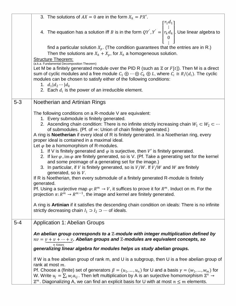
3. The solutions of 𝐴𝑋 = 0 are in the form 𝑋𝑕 = 𝑃𝑋′.

4. The equation has a solution iff 𝐵 is in the form 𝑄𝑌′ , 𝑌′ =

𝑟1𝑑1

⋮𝑟𝑘𝑑𝑘

0⋮

. Use linear algebra to

find a particular solution 𝑋𝑝 . (The condition guarantees that the entries are in R.)

Then the solutions are 𝑋𝑕 + 𝑋𝑝 , for 𝑋𝑕 a homogeneous solution.

Structure Theorem: (a.k.a. Fundamental Decomposition Theorem)

Let M be a finitely generated module over the PID R (such as ℞ or 𝐹[𝑡]). Then M is a direct sum of cyclic modules and a free module 𝐶1 ⊕ ⋯ ⊕ 𝐶𝑘 ⊕ 𝐿, where 𝐶𝑖 ≅ 𝑅/(𝑑𝑖). The cyclic modules can be chosen to satisfy either of the following conditions:

1. 𝑑1|𝑑2 ⋯ |𝑑𝑘 2. Each 𝑑𝑖 is the power of an irreducible element.

5-3 Noetherian and Artinian Rings The following conditions on a R-module V are equivalent:

1. Every submodule is finitely generated.

2. Ascending chain condition: There is no infinite strictly increasing chain 𝑊1 ⊂ 𝑊2 ⊂ ⋯ of submodules. (Pf. of ⇒: Union of chain finitely generated.)

A ring is Noetherian if every ideal of R is finitely generated. In a Noetherian ring, every proper ideal is contained in a maximal ideal.

Let 𝜑 be a homomorphism of R-modules. 1. If V is finitely generated and 𝜑 is surjective, then 𝑉′ is finitely generated. 2. If ker 𝜑 , im 𝜑 are finitely generated, so is V. (Pf. Take a generating set for the kernel

and some preimage of a generating set for the image.)

3. In particular, if 𝑉 is finitely generated, so is 𝑉/𝑊. If 𝑉/𝑊 and 𝑊 are finitely generated, so is 𝑉.

If R is Noetherian, then every submodule of a finitely generated R-module is finitely generated.

Pf. Using a surjective map 𝜑: 𝑅𝑚 → 𝑉, it suffices to prove it for 𝑅𝑚 . Induct on m. For the

projection 𝜋: 𝑅𝑚 → 𝑅𝑚−1, the image and kernel are finitely generated. A ring is Artinian if it satisfies the descending chain condition on ideals: There is no infinite

strictly decreasing chain 𝐼1 ⊃ 𝐼2 ⊃ ⋯ of ideals.

5-4 Application 1: Abelian Groups

An abelian group corresponds to a ℞-module with integer multiplication defined by 𝑛𝑣 = 𝑣 + 𝑣 + ⋯ + 𝑣

𝑛 times

. Abelian groups and ℞-modules are equivalent concepts, so

generalizing linear algebra for modules helps us study abelian groups. If W is a free abelian group of rank m, and U is a subgroup, then U is a free abelian group of

rank at most 𝑚. Pf. Choose a (finite) set of generators 𝛽 = (𝑢1, … , 𝑢𝑛) for U and a basis 𝛾 = (𝑤1, … , 𝑤𝑚 ) for

W. Write 𝑢𝑗 = 𝑤𝑖𝑎𝑖𝑗𝑖 . Then left multiplication by A is an surjective homomorphism ℞𝑛 →

℞𝑚 . Diagonalizing A, we can find an explicit basis for U with at most 𝑛 ≤ 𝑚 elements.

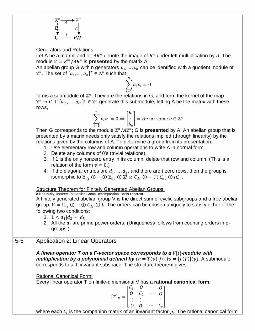
Generators and Relations

Let A be a matrix, and let 𝐴𝑅𝑛 denote the image of 𝑅𝑛 under left multiplication by 𝐴. The module 𝑉 = 𝑅𝑚 /𝐴𝑅𝑛 is presented by the matrix A.

An abelian group G with n generators 𝑣1, … , 𝑣𝑛 can be identified with a quotient module of

℞𝑛 . The set of 𝑎1, … , 𝑎𝑛 𝑇 ∈ ℞𝑛 such that

𝑎𝑖𝑣𝑖

𝑛

𝑖=1

= 0

forms a submodule of ℞𝑛 . They are the relations in G, and form the kernel of the map

℞𝑛 → 𝐺. If 𝑎𝑖1 , … , 𝑎𝑖𝑛 𝑇 ∈ ℞𝑛 generate this submodule, letting A be the matrix with these rows,

𝑏𝑖𝑣𝑖

𝑛

𝑖=1

= 0 ⇔ 𝑏1

⋮𝑏𝑛

= 𝐴𝑣 for some 𝑣 ∈ ℞𝑛

Then G corresponds to the module ℞𝑛/𝐴℞𝑛 ; G is presented by A. An abelian group that is presented by a matrix needs only satisfy the relations implied (through linearity) by the relations given by the columns of A. To determine a group from its presentation:

1. Use elementary row and column operations to write A in normal form. 2. Delete any columns of 0’s (trivial relations). 3. If 1 is the only nonzero entry in its column, delete that row and column. (This is a

relation of the form 𝑣 = 0.)

4. If the diagonal entries are 𝑑1, … , 𝑑𝑘 , and there are 𝑙 zero rows, then the group is

isomorphic to ℞𝑑1⊕ ⋯ ⊕ ℞𝑑𝑘

⊕ ℞𝑙 ≅ 𝐶𝑑1⊕ ⋯ ⊕ 𝐶𝑑𝑘

⊕ 𝑙𝐶∞ .

Structure Theorem for Finitely Generated Abelian Groups: a.k.a Unicity Theorem for Abelian Group Decomposition, Basis Theorem

A finitely generated abelian group V is the direct sum of cyclic subgroups and a free abelian group: 𝑉 = 𝐶𝑑1

⊕ ⋯ ⊕ 𝐶𝑑𝑘⊕ 𝐿. The orders can be chosen uniquely to satisfy either of the

following two conditions:

1. 1 < 𝑑1|𝑑2 ⋯ |𝑑𝑘 2. All the 𝑑𝑖 are prime power orders. (Uniqueness follows from counting orders in p-

groups.)

5-5 Application 2: Linear Operators A linear operator T on a F-vector space corresponds to a 𝐹[𝑡]-module with multiplication by a polynomial defined by 𝑡𝑣 = 𝑇 𝑣 , 𝑓 𝑡 𝑣 = 𝑓 𝑇 (𝑣). A submodule corresponds to a T-invariant subspace. The structure theorem gives: Rational Canonical Form: Every linear operator T on finite-dimensional V has a rational canonical form.

𝑇 𝛽 =

𝐶1 𝑂𝑂 𝐶2

⋯ 𝑂⋯ 𝑂

⋮ ⋮𝑂 𝑂

⋮⋯ 𝐶𝑟

where each 𝐶𝑖 is the companion matrix of an invariant factor 𝑝𝑖 . The rational canonical form

℞𝑛

UL

W

𝐶

𝑖

𝐵

℞𝑚 𝐴

is unique under the condition 𝑝𝑖+1|𝑝𝑖 for each 1 ≤ 𝑖 < 𝑟.

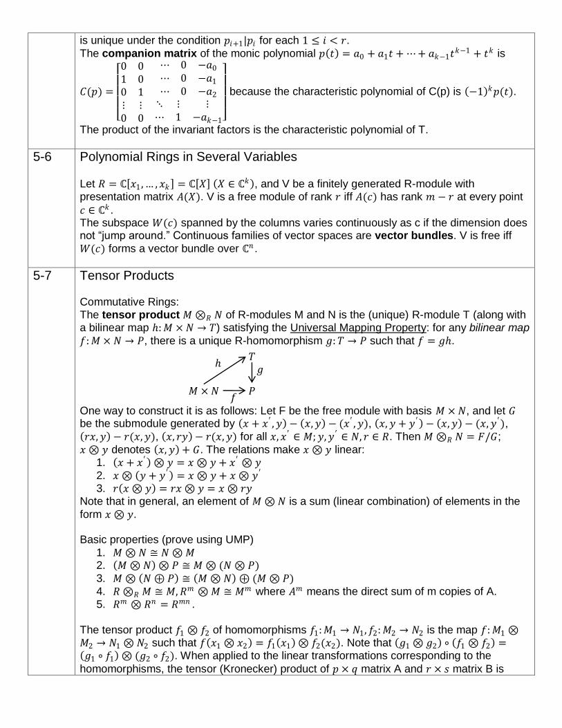
The companion matrix of the monic polynomial 𝑝 𝑡 = 𝑎0 + 𝑎1𝑡 + ⋯ + 𝑎𝑘−1𝑡𝑘−1 + 𝑡𝑘 is

𝐶(𝑝) =

0 01 00 1

⋯ 0 −𝑎0

⋯ 0 −𝑎1

⋯ 0 −𝑎2

⋮ ⋮0 0

⋱ ⋮ ⋮⋯ 1 −𝑎𝑘−1

because the characteristic polynomial of C(p) is −1 𝑘𝑝(𝑡).

The product of the invariant factors is the characteristic polynomial of T.

5-6 Polynomial Rings in Several Variables

Let 𝑅 = ℂ 𝑥1 , … , 𝑥𝑘 = ℂ 𝑋 𝑋 ∈ ℂ𝑘 , and V be a finitely generated R-module with presentation matrix 𝐴(𝑋). V is a free module of rank 𝑟 iff 𝐴(𝑐) has rank 𝑚 − 𝑟 at every point

𝑐 ∈ ℂ𝑘 . The subspace 𝑊(𝑐) spanned by the columns varies continuously as c if the dimension does not “jump around.” Continuous families of vector spaces are vector bundles. V is free iff

𝑊(𝑐) forms a vector bundle over ℂ𝑛 .

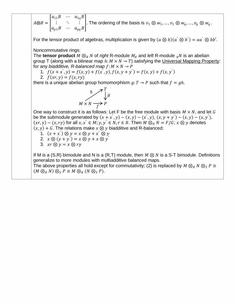
5-7 Tensor Products Commutative Rings: The tensor product 𝑀 ⊗𝑅 𝑁 of R-modules M and N is the (unique) R-module T (along with a bilinear map 𝑕: 𝑀 × 𝑁 → 𝑇) satisfying the Universal Mapping Property: for any bilinear map

𝑓: 𝑀 × 𝑁 → 𝑃, there is a unique R-homomorphism 𝑔: 𝑇 → 𝑃 such that 𝑓 = 𝑔𝑕.

One way to construct it is as follows: Let F be the free module with basis 𝑀 × 𝑁, and let 𝐺 be the submodule generated by 𝑥 + 𝑥′ , 𝑦 − 𝑥, 𝑦 − (𝑥′ , 𝑦), 𝑥, 𝑦 + 𝑦 ′ − 𝑥, 𝑦 − (𝑥, 𝑦 ′), 𝑟𝑥, 𝑦 − 𝑟(𝑥, 𝑦), 𝑥, 𝑟𝑦 − 𝑟(𝑥, 𝑦) for all 𝑥, 𝑥′ ∈ 𝑀; 𝑦, 𝑦 ′ ∈ 𝑁, 𝑟 ∈ 𝑅. Then 𝑀 ⊗𝑅 𝑁 = 𝐹/𝐺;

𝑥 ⊗ 𝑦 denotes 𝑥, 𝑦 + 𝐺. The relations make 𝑥 ⊗ 𝑦 linear: 1. 𝑥 + 𝑥′ ⊗ 𝑦 = 𝑥 ⊗ 𝑦 + 𝑥′ ⊗ 𝑦

2. 𝑥 ⊗ 𝑦 + 𝑦 ′ = 𝑥 ⊗ 𝑦 + 𝑥 ⊗ 𝑦 ′ 3. 𝑟 𝑥 ⊗ 𝑦 = 𝑟𝑥 ⊗ 𝑦 = 𝑥 ⊗ 𝑟𝑦

Note that in general, an element of 𝑀 ⊗ 𝑁 is a sum (linear combination) of elements in the

form 𝑥 ⊗ 𝑦. Basic properties (prove using UMP)

1. 𝑀 ⊗ 𝑁 ≅ 𝑁 ⊗ 𝑀 2. 𝑀 ⊗ 𝑁 ⊗ 𝑃 ≅ 𝑀 ⊗ (𝑁 ⊗ 𝑃)

3. 𝑀 ⊗ 𝑁 ⊕ 𝑃 ≅ 𝑀 ⊗ 𝑁 ⊕ (𝑀 ⊗ 𝑃)

4. 𝑅 ⊗𝑅 𝑀 ≅ 𝑀, 𝑅𝑚 ⊗ 𝑀 ≅ 𝑀𝑚 where 𝐴𝑚 means the direct sum of m copies of A. 5. 𝑅𝑚 ⊗ 𝑅𝑛 = 𝑅𝑚𝑛 .

The tensor product 𝑓1 ⊗ 𝑓2 of homomorphisms 𝑓1: 𝑀1 → 𝑁1, 𝑓2: 𝑀2 → 𝑁2 is the map 𝑓: 𝑀1 ⊗𝑀2 → 𝑁1 ⊗ 𝑁2 such that 𝑓 𝑥1 ⊗ 𝑥2 = 𝑓1 𝑥1 ⊗ 𝑓2(𝑥2). Note that 𝑔1 ⊗ 𝑔2 ∘ 𝑓1 ⊗ 𝑓2 = 𝑔1 ∘ 𝑓1 ⊗ (𝑔2 ∘ 𝑓2). When applied to the linear transformations corresponding to the

homomorphisms, the tensor (Kronecker) product of 𝑝 × 𝑞 matrix A and 𝑟 × 𝑠 matrix B is

𝑀 × 𝑁 𝑃

𝑇 𝑕

𝑓

𝑔

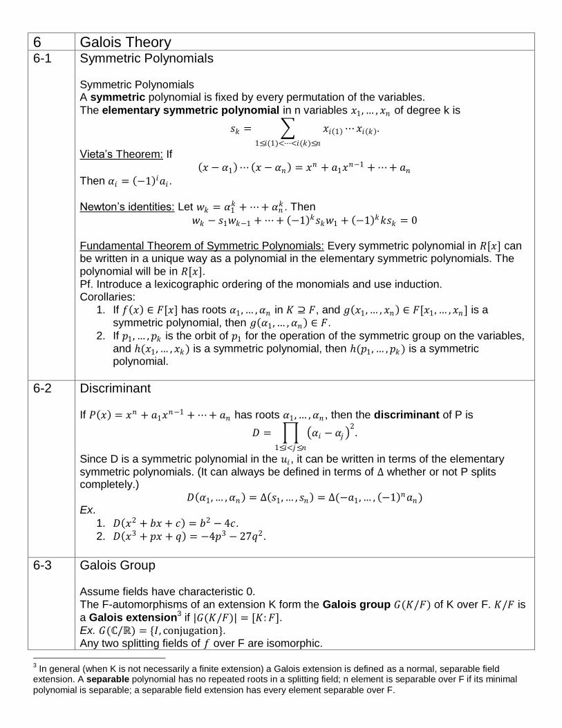
𝐴⨂𝐵 =

𝑎11𝐵 ⋯ 𝑎1𝑞𝐵

⋮ ⋱ ⋮𝑎𝑝1𝐵 ⋯ 𝑎𝑝𝑞 𝐵

. The ordering of the basis is 𝑣1 ⊗ 𝑤1, … , 𝑣1 ⊗ 𝑤𝑞 , … , 𝑣𝑝 ⊗ 𝑤𝑞 .

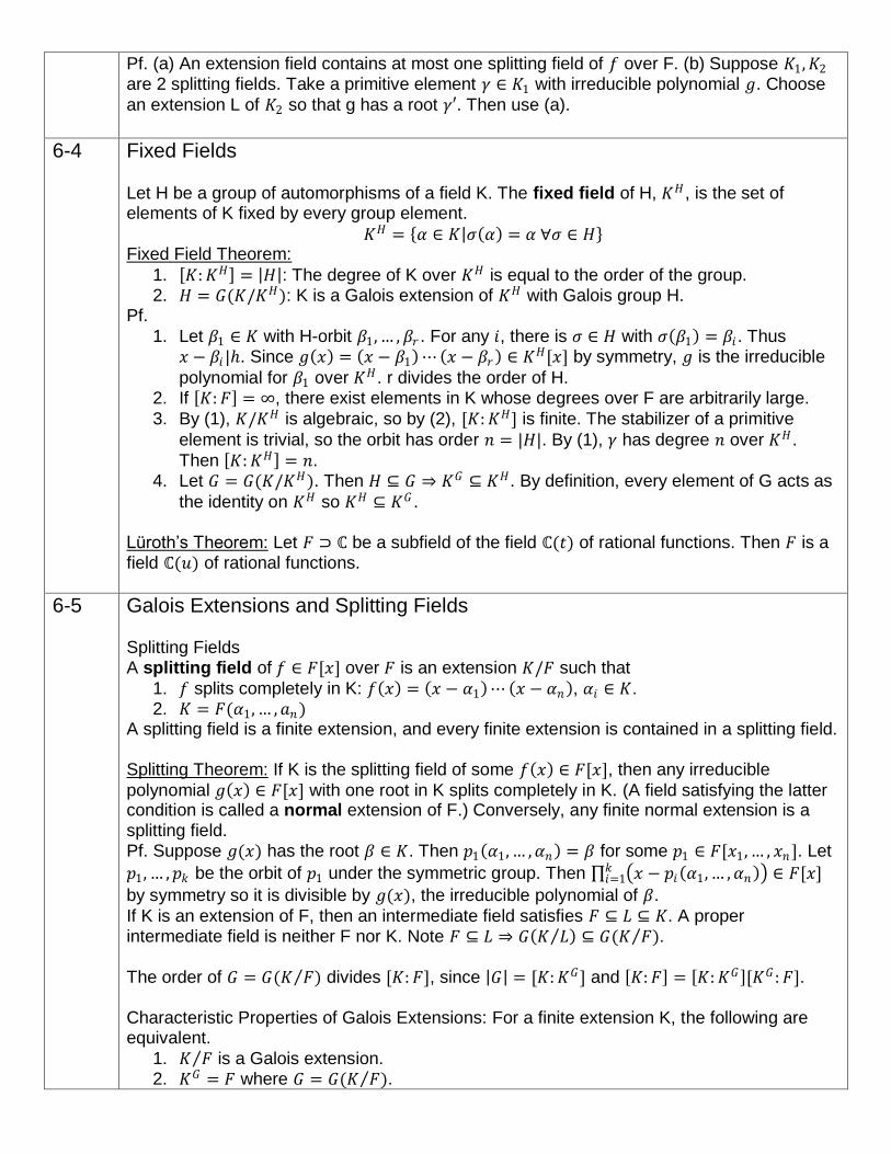
For the tensor product of algebras, multiplication is given by 𝑎 ⊗ 𝑏 𝑎′ ⊗ 𝑏′ = 𝑎𝑎′ ⊗ 𝑏𝑏′. Noncommutative rings: The tensor product 𝑀 ⊗𝑅 𝑁 of right R-module 𝑀𝑅 and left R-module 𝑁𝑅

is an abelian

group T (along with a bilinear map 𝑕: 𝑀 × 𝑁 → 𝑇) satisfying the Universal Mapping Property: for any biadditive, R-balanced map 𝑓: 𝑀 × 𝑁 → 𝑃

1. 𝑓 𝑥 + 𝑥′ , 𝑦 = 𝑓 𝑥, 𝑦 + 𝑓 𝑥′ , 𝑦 , 𝑓 𝑥, 𝑦 + 𝑦 ′ = 𝑓 𝑥, 𝑦 + 𝑓 𝑥, 𝑦 ′ 2. 𝑓 𝑥𝑟, 𝑦 = 𝑓(𝑥, 𝑟𝑦)

there is a unique abelian group homomorphism 𝑔: 𝑇 → 𝑃 such that 𝑓 = 𝑔𝑕.

One way to construct it is as follows: Let F be the free module with basis 𝑀 × 𝑁, and let 𝐺 be the submodule generated by 𝑥 + 𝑥′ , 𝑦 − 𝑥, 𝑦 − (𝑥′ , 𝑦), 𝑥, 𝑦 + 𝑦 ′ − 𝑥, 𝑦 − (𝑥, 𝑦 ′), 𝑥𝑟, 𝑦 − (𝑥, 𝑟𝑦) for all 𝑥, 𝑥′ ∈ 𝑀; 𝑦, 𝑦 ′ ∈ 𝑁, 𝑟 ∈ 𝑅. Then 𝑀 ⊗𝑅 𝑁 = 𝐹/𝐺; 𝑥 ⊗ 𝑦 denotes 𝑥, 𝑦 + 𝐺. The relations make 𝑥 ⊗ 𝑦 biadditive and R-balanced:

1. 𝑥 + 𝑥′ ⊗ 𝑦 = 𝑥 ⊗ 𝑦 + 𝑥′ ⊗ 𝑦 2. 𝑥 ⊗ 𝑦 + 𝑦 ′ = 𝑥 ⊗ 𝑦 + 𝑥 ⊗ 𝑦 ′

3. 𝑥𝑟 ⊗ 𝑦 = 𝑥 ⊗ 𝑟𝑦

If M is a (S,R) bimodule and N is a (R,T) module, then 𝑀 ⊗ 𝑁 is a S-T bimodule. Definitions generalize to more modules with multiadditive balanced maps.

The above properties all hold except for commutativity; (2) is replaced by 𝑀 ⊗𝑅 𝑁 ⊗𝑆 𝑃 ≅ 𝑀 ⊗𝑅 𝑁 ⊗𝑆 𝑃 ≅ 𝑀 ⊗𝑅 (𝑁 ⊗𝑆 𝑃).

𝑀 × 𝑁 𝑃

𝑇 𝑕

𝑓

𝑔

6 Galois Theory 6-1 Symmetric Polynomials

Symmetric Polynomials A symmetric polynomial is fixed by every permutation of the variables.

The elementary symmetric polynomial in n variables 𝑥1, … , 𝑥𝑛 of degree k is

𝑠𝑘 = 𝑥𝑖 1 ⋯𝑥𝑖 𝑘

1≤𝑖(1)<⋯<𝑖(𝑘)≤𝑛

.

Vieta’s Theorem: If 𝑥 − 𝛼1 ⋯ 𝑥 − 𝛼𝑛 = 𝑥𝑛 + 𝑎1𝑥𝑛−1 + ⋯ + 𝑎𝑛

Then 𝛼𝑖 = −1 𝑖𝑎𝑖 .

Newton’s identities: Let 𝑤𝑘 = 𝛼1𝑘 + ⋯ + 𝛼𝑛

𝑘 . Then

𝑤𝑘 − 𝑠1𝑤𝑘−1 + ⋯ + −1 𝑘𝑠𝑘𝑤1 + −1 𝑘𝑘𝑠𝑘 = 0 Fundamental Theorem of Symmetric Polynomials: Every symmetric polynomial in 𝑅[𝑥] can be written in a unique way as a polynomial in the elementary symmetric polynomials. The polynomial will be in 𝑅[𝑥]. Pf. Introduce a lexicographic ordering of the monomials and use induction. Corollaries:

1. If 𝑓 𝑥 ∈ 𝐹[𝑥] has roots 𝛼1, … , 𝛼𝑛 in 𝐾 ⊇ 𝐹, and 𝑔 𝑥1, … , 𝑥𝑛 ∈ 𝐹[𝑥1, … , 𝑥𝑛 ] is a symmetric polynomial, then 𝑔 𝛼1, … , 𝛼𝑛 ∈ 𝐹.

2. If 𝑝1, … , 𝑝𝑘 is the orbit of 𝑝1 for the operation of the symmetric group on the variables, and 𝑕(𝑥1, … , 𝑥𝑘) is a symmetric polynomial, then 𝑕(𝑝1, … , 𝑝𝑘) is a symmetric polynomial.

6-2 Discriminant If 𝑃 𝑥 = 𝑥𝑛 + 𝑎1𝑥𝑛−1 + ⋯ + 𝑎𝑛 has roots 𝛼1, … , 𝛼𝑛 , then the discriminant of P is

𝐷 = 𝛼𝑖 − 𝛼𝑗 2

1≤𝑖<𝑗≤𝑛

.

Since D is a symmetric polynomial in the 𝑢𝑖 , it can be written in terms of the elementary symmetric polynomials. (It can always be defined in terms of Δ whether or not P splits completely.)

𝐷 𝛼1, … , 𝛼𝑛 = Δ 𝑠1, … , 𝑠𝑛 = Δ(−𝑎1, … , −1 𝑛𝑎𝑛) Ex.

1. 𝐷 𝑥2 + 𝑏𝑥 + 𝑐 = 𝑏2 − 4𝑐.

2. 𝐷 𝑥3 + 𝑝𝑥 + 𝑞 = −4𝑝3 − 27𝑞2.

6-3 Galois Group Assume fields have characteristic 0. The F-automorphisms of an extension K form the Galois group 𝐺(𝐾/𝐹) of K over F. 𝐾/𝐹 is

a Galois extension3 if |𝐺(𝐾/𝐹)| = [𝐾: 𝐹]. Ex. 𝐺(ℂ/ℝ) = {𝐼, conjugation}. Any two splitting fields of 𝑓 over F are isomorphic.

3 In general (when K is not necessarily a finite extension) a Galois extension is defined as a normal, separable field

extension. A separable polynomial has no repeated roots in a splitting field; n element is separable over F if its minimal

polynomial is separable; a separable field extension has every element separable over F.

Pf. (a) An extension field contains at most one splitting field of 𝑓 over F. (b) Suppose 𝐾1, 𝐾2 are 2 splitting fields. Take a primitive element 𝛾 ∈ 𝐾1 with irreducible polynomial 𝑔. Choose

an extension L of 𝐾2 so that g has a root 𝛾′. Then use (a).

6-4 Fixed Fields

Let H be a group of automorphisms of a field K. The fixed field of H, 𝐾𝐻, is the set of elements of K fixed by every group element.

𝐾𝐻 = 𝛼 ∈ 𝐾 𝜎 𝛼 = 𝛼 ∀𝜎 ∈ 𝐻 Fixed Field Theorem:

1. 𝐾: 𝐾𝐻 = 𝐻 : The degree of K over 𝐾𝐻 is equal to the order of the group. 2. 𝐻 = 𝐺(𝐾/𝐾𝐻): K is a Galois extension of 𝐾𝐻 with Galois group H.

Pf.

1. Let 𝛽1 ∈ 𝐾 with H-orbit 𝛽1, … , 𝛽𝑟 . For any 𝑖, there is 𝜎 ∈ 𝐻 with 𝜎 𝛽1 = 𝛽𝑖 . Thus 𝑥 − 𝛽𝑖 |𝑕. Since 𝑔 𝑥 = 𝑥 − 𝛽1 ⋯ 𝑥 − 𝛽𝑟 ∈ 𝐾𝐻[𝑥] by symmetry, 𝑔 is the irreducible

polynomial for 𝛽1 over 𝐾𝐻. r divides the order of H. 2. If 𝐾: 𝐹 = ∞, there exist elements in K whose degrees over F are arbitrarily large.

3. By (1), 𝐾/𝐾𝐻 is algebraic, so by (2), [𝐾: 𝐾𝐻] is finite. The stabilizer of a primitive

element is trivial, so the orbit has order 𝑛 = |𝐻|. By (1), 𝛾 has degree 𝑛 over 𝐾𝐻.

Then 𝐾: 𝐾𝐻 = 𝑛. 4. Let 𝐺 = 𝐺(𝐾/𝐾𝐻). Then 𝐻 ⊆ 𝐺 ⇒ 𝐾𝐺 ⊆ 𝐾𝐻. By definition, every element of G acts as

the identity on 𝐾𝐻 so 𝐾𝐻 ⊆ 𝐾𝐺 . Lüroth’s Theorem: Let 𝐹 ⊃ ℂ be a subfield of the field ℂ(𝑡) of rational functions. Then 𝐹 is a field ℂ(𝑢) of rational functions.

6-5 Galois Extensions and Splitting Fields Splitting Fields A splitting field of 𝑓 ∈ 𝐹[𝑥] over 𝐹 is an extension 𝐾/𝐹 such that

1. 𝑓 splits completely in K: 𝑓 𝑥 = 𝑥 − 𝛼1 ⋯ 𝑥 − 𝛼𝑛 , 𝛼𝑖 ∈ 𝐾. 2. 𝐾 = 𝐹(𝛼1, … , 𝑎𝑛)

A splitting field is a finite extension, and every finite extension is contained in a splitting field. Splitting Theorem: If K is the splitting field of some 𝑓 𝑥 ∈ 𝐹[𝑥], then any irreducible

polynomial 𝑔 𝑥 ∈ 𝐹[𝑥] with one root in K splits completely in K. (A field satisfying the latter condition is called a normal extension of F.) Conversely, any finite normal extension is a splitting field. Pf. Suppose 𝑔(𝑥) has the root 𝛽 ∈ 𝐾. Then 𝑝1 𝛼1, … , 𝛼𝑛 = 𝛽 for some 𝑝1 ∈ 𝐹[𝑥1, … , 𝑥𝑛]. Let

𝑝1, … , 𝑝𝑘 be the orbit of 𝑝1 under the symmetric group. Then ∏ 𝑥 − 𝑝𝑖 𝛼1, … , 𝛼𝑛 𝑘𝑖=1 ∈ 𝐹[𝑥]

by symmetry so it is divisible by 𝑔(𝑥), the irreducible polynomial of 𝛽.

If K is an extension of F, then an intermediate field satisfies 𝐹 ⊆ 𝐿 ⊆ 𝐾. A proper intermediate field is neither F nor K. Note 𝐹 ⊆ 𝐿 ⇒ 𝐺 𝐾 𝐿 ⊆ 𝐺(𝐾 𝐹 ).

The order of 𝐺 = 𝐺(𝐾 𝐹 ) divides [𝐾: 𝐹], since 𝐺 = [𝐾: 𝐾𝐺] and 𝐾: 𝐹 = 𝐾: 𝐾𝐺 [𝐾𝐺 : 𝐹]. Characteristic Properties of Galois Extensions: For a finite extension K, the following are equivalent.

1. 𝐾 𝐹 is a Galois extension. 2. 𝐾𝐺 = 𝐹 where 𝐺 = 𝐺(𝐾 𝐹 ).

3. 𝐾 is a splitting field over F. Pf. (1)⇔(2): By the Fixed Field Theorem, 𝐺 = [𝐾: 𝐾𝐺]. (1)⇔(3): Let 𝛾1 be a primitive element for K, with irreducible polynomial 𝑓. Let 𝛾1, … , 𝛾𝑟 be

the roots of 𝑓 in K. There is a unique F-automorphism 𝜎𝑖 sending 𝛾1 ⇝ 𝛾𝑖 for each i, and these make up the group 𝐺(𝐾 𝐹 ). Thus the order of 𝐺(𝐾 𝐹 ) is equal to the number of

conjugates of 𝛾1 in K. So 𝐾 𝐹 Galois⇔ 𝑟 = 𝐺 = 𝐾: 𝐾𝐺 ⇔ 𝑓 (degree r) splits completely in

K⇔ K is a splitting field. If 𝐾 𝐹 is a Galois extension, and 𝑔 ∈ 𝐹[𝑥] splits completely in K with roots 𝛽1, … , 𝛽𝑟 , then

G operates on the set of roots {𝛽𝑖}. G operates faithfully if K is a splitting field of 𝑔 over 𝐹.

G operates transitively if 𝑔 is irreducible over F.

If K is the splitting field of irreducible 𝑔, then G embeds as a transitive subgroup of 𝑆𝑟 .

6-6 Fundamental Theorem Fundamental Theorem of Galois Theory: Let K be a Galois extension of a field F, and let 𝐺 = 𝐺(𝐾/𝐹). Then there is a bijection between subgroups of G and intermediate fields, defined by

𝐻 ⇝ 𝐾𝐻 𝐺(𝐾 𝐿 ) ⇜ 𝐿

Let 𝐿 = 𝐾𝐻 (the fixed field of a subgroup H of G). 𝐿 𝐹 is a Galois extension iff H is a normal subgroup of G. If so, 𝐺 𝐿 𝐹 ≅ 𝐺 𝐻 .

Pf. Let 𝛾1 be a primitive element for 𝐿 𝐹 and let 𝑔 be the irreducible polynomial for 𝛾1 over

F. Let the roots of 𝑔 in 𝐾 be 𝛾1, … , 𝛾𝑟 . For 𝜎 ∈ 𝐺, 𝜎 𝛾1 = 𝛾𝑖 , the stabilizer of 𝛾𝑖 is 𝜎𝐻𝜎−1.

Thus 𝜎𝐻𝜎−1 = 𝐻 ⇔ 𝛾𝑖 ∈ 𝐿 = 𝐾𝐻. H is normal⇔All 𝛾𝑖 ∈ 𝐿 ⇔ 𝐿 𝐹 Galois. Restricting 𝜎 to L gives a homomorphism 𝜑: 𝐺 → 𝐺(𝐿 𝐹 ) with kernel H.

6-7 Roots of Unity

Let 𝜁𝑛 = 𝑒2𝜋𝑖

𝑛 . 𝐹(𝜁𝑛) is a cyclotomic field. For p prime, the Galois group of 𝐹(𝜁𝑝) is

isomorphic to 𝔽𝑝×, of order 𝑝 − 1.

Ex. For 𝑝 = 2𝑟 + 1, G is cyclic of order 2𝑟 . Let 𝜉 be a primitive root modulo 𝑝, and 𝜎 𝜁 = 𝜁𝜉 .

The degree of each extension in the following chain is 2: 𝐹 = 𝐾⌌𝜎⌍ ⊂ 𝐾⌌𝜎2⌍ ⊂ ⋯ ⊂ 𝐾⌌𝜎2𝑟−1⌍ ⊂

𝐾⌌𝜎2𝑟⌍ = 𝐾. cos

2𝜋

𝑝 generates 𝐾⌌𝜎2𝑟−1

⌍ so the regular p-gon can be constructed.

Kronecker-Weber Theorem: Every Galois extension of ℚ whose Galois group is abelian is contained in a cyclotomic field ℚ(𝜁𝑛). Ex. If p is prime and L is the unique quadratic extension of ℚ in ℚ(𝜁𝑝),

1. If 𝑝 ≡ 1 (mod 4) then 𝐿 = ℚ( 𝑝).

2. If 𝑝 ≡ 3 (mod 4) then 𝐿 = ℚ(𝑖 𝑝).

Show this by letting 𝜎 be a generator as before, take the orbit sums of the roots for ⌌𝜎2⌍. Kummer Extensions

K

L

F

{ }

} 𝐺 = 𝐺(𝐾 𝐹 ) operates on K fixing F.

𝐻 = 𝐺(𝐾 𝐿 ) operates on K fixing L.

𝐻 normal: 𝐺 𝐻 ≅ 𝐺 𝐿 𝐹 operates here.

Let 𝐹 be a subfield of ℂ containing 𝜁 = 𝑒2𝜋𝑖 𝑝 , and let 𝐾 𝐹 be a Galois extension of degree p. Then K is obtained by adjoining a pth root (some 𝛽 with 𝛽𝑝 ∈ 𝐹). Pf.

1. For 𝑏 ∈ 𝐹, 𝑔 𝑥 = 𝑥𝑝 − 𝑏 is either irreducible in F, or splits completely in F. (Take

𝐼 ≠ 𝜎 ∈ 𝐺(𝐾 𝐹 ); then 𝜎𝑘 𝛽 = 𝜁𝑘𝑣𝛽 for some 𝑣 ≠ 0, so G operates transitively on the roots of 𝑔.)

2. K is a vector space over F; each 𝜎 ∈ 𝐺 is a linear operator. Choose a generator 𝜎.

𝜎𝑝 = 𝐼 implies that the matrix is diagonalizable and all eigenvalues are powers of 𝜁.

Let 𝛽 be an eigenvector with eigenvalue 𝜆 ≠ 1; then 𝜎 𝛽𝑝 = 𝛽𝑝 ⇒ 𝛽𝑝 ∈ 𝐾𝐺 = 𝐹, but

𝛽 ∉ 𝐹, so 𝐹 𝛽 = 𝐾.

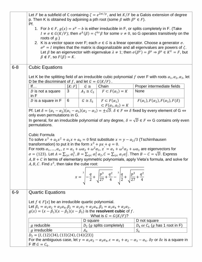
6-8 Cubic Equations Let K be the splitting field of an irreducible cubic polynomial 𝑓 over F with roots 𝛼1, 𝛼2 , 𝛼3, let

D be the discriminant of 𝑓, and let 𝐺 = 𝐺 𝐾 𝐹 . If… 𝐾: 𝐹 𝐺 ≅ Chain Proper intermediate fields

𝐷 is not a square in F

3 𝐴3 ≅ 𝐶3 𝐹 ⊂ 𝐹 𝛼1 = 𝐾 None

𝐷 is a square in F 6 𝐺 ≅ 𝑆3 𝐹 ⊂ 𝐹 𝛼1 ⊂ 𝐹 𝛼1, 𝑎2 = 𝐾

𝐹 𝛼1 , 𝐹 𝛼2 , 𝐹 𝛼3 , 𝐹(𝛿)

Pf. Let 𝛿 = 𝛼1 − 𝛼2 𝛼1 − 𝛼3 𝛼2 − 𝛼3 = ± 𝐷. 𝛿 ∈ 𝐹 ⇔ 𝛿 fixed by every element of G ⇔ only even permutations in G.

In general, for an irreducible polynomial of any degree, 𝛿 = 𝐷 ∈ 𝐹 ⇔ G contains only even permutations.

Cubic Formula

To solve 𝑥3 + 𝑎2𝑥2 + 𝑎1𝑥 + 𝑎0 = 0 first substitute 𝑥 = 𝑦 − 𝑎2/3 (Tschirnhausen

transformation) to put it in the form 𝑥3 + 𝑝𝑥 + 𝑞 = 0.

For roots 𝛼1, … , 𝛼𝑛 , 𝑧 = 𝛼1 + 𝜔𝛼2 + 𝜔2𝛼3, 𝑧′ = 𝛼1 + 𝜔2𝛼2 + 𝜔𝑎3 are eigenvectors for

𝜎 = (123). Let 𝐴 = 𝛼13

cyc , 𝐵 = 𝛼12

cyc 𝛼2, 𝐶 = 𝛼1𝛼22

cyc . Then 𝐵 − 𝐶 = 𝐷. Express

𝐴, 𝐵 + 𝐶 in terms of elementary symmetric polynomials, apply Vieta’s formula, and solve for 𝐴, 𝐵, 𝐶. Find 𝑧3, then take the cube root:

𝑥 = −𝑞

2+

𝑝3

27+

𝑞2

4

3

− 𝑞

2+

𝑝3

27+

𝑞2

4

3

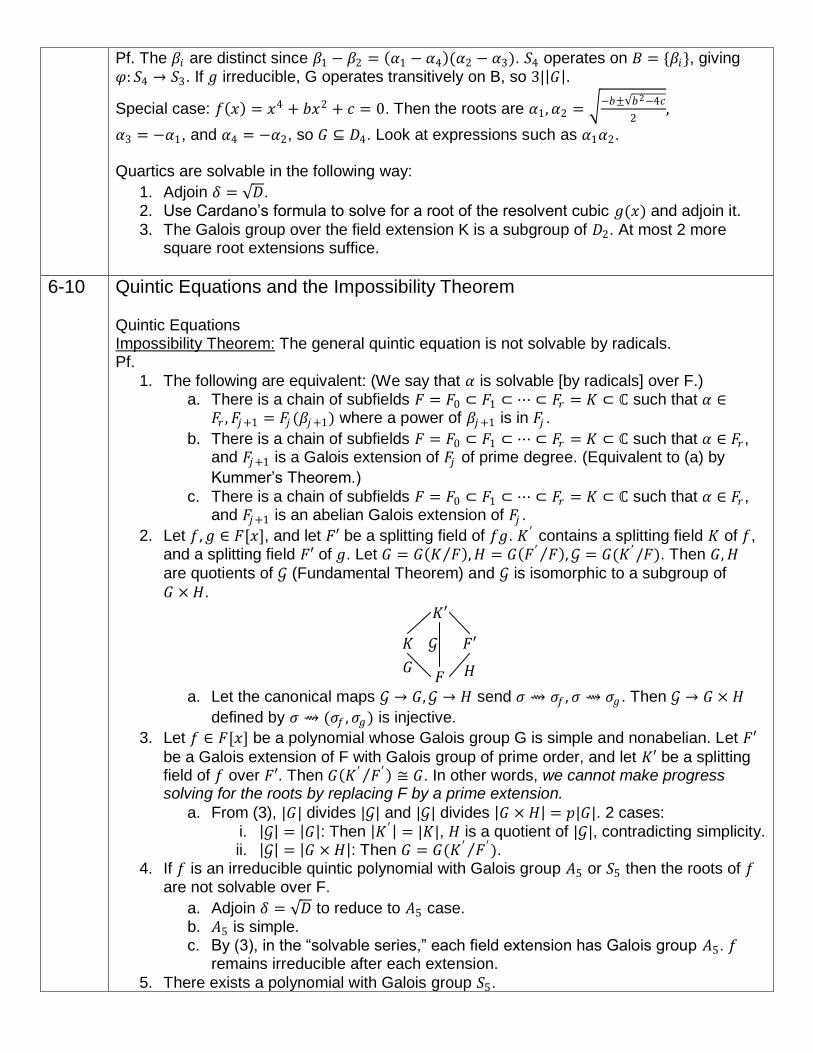
6-9 Quartic Equations Let 𝑓 ∈ 𝐹[𝑥] be an irreducible quartic polynomial.

Let 𝛽1 = 𝛼1𝛼2 + 𝛼3𝛼4, 𝛽2 = 𝛼1𝛼3 + 𝛼2𝛼4, 𝛽3 = 𝛼1𝛼4 + 𝛼2𝛼3. 𝑔 𝑥 = 𝑥 − 𝛽1 𝑥 − 𝛽2 (𝑥 − 𝛽3) is the resolvent cubic of 𝑓.

What is 𝐺 = 𝐺(𝐾/𝐹)?

D square D not square

𝑔 reducible 𝐷2 (𝑔 splits completely) 𝐷4 or 𝐶4 (𝑔 has 1 root in F)

𝑔 irreducible 𝐴4 𝑆4

𝐷2 = {𝐼, 12 34 , 13 24 , 14 23 } For the ambiguous case, let 𝛾 = 𝛼1𝛼2 − 𝛼3𝛼4, 𝜖 = 𝛼1 + 𝛼2 − 𝛼3 − 𝛼4. 𝛿𝛾 or 𝛿𝜖 is a square in F iff 𝐺 = 𝐶4.

Pf. The 𝛽𝑖 are distinct since 𝛽1 − 𝛽2 = 𝛼1 − 𝛼4 (𝛼2 − 𝛼3). 𝑆4 operates on 𝐵 = {𝛽𝑖}, giving 𝜑: 𝑆4 → 𝑆3. If 𝑔 irreducible, G operates transitively on B, so 3| 𝐺 .

Special case: 𝑓 𝑥 = 𝑥4 + 𝑏𝑥2 + 𝑐 = 0. Then the roots are 𝛼1, 𝛼2 = −𝑏± 𝑏2−4𝑐

2,

𝛼3 = −𝛼1, and 𝛼4 = −𝛼2, so 𝐺 ⊆ 𝐷4. Look at expressions such as 𝛼1𝛼2. Quartics are solvable in the following way:

1. Adjoin 𝛿 = 𝐷. 2. Use Cardano’s formula to solve for a root of the resolvent cubic 𝑔(𝑥) and adjoin it.

3. The Galois group over the field extension K is a subgroup of 𝐷2. At most 2 more square root extensions suffice.

6-10 Quintic Equations and the Impossibility Theorem Quintic Equations Impossibility Theorem: The general quintic equation is not solvable by radicals. Pf.

1. The following are equivalent: (We say that 𝛼 is solvable [by radicals] over F.) a. There is a chain of subfields 𝐹 = 𝐹0 ⊂ 𝐹1 ⊂ ⋯ ⊂ 𝐹𝑟 = 𝐾 ⊂ ℂ such that 𝛼 ∈

𝐹𝑟 , 𝐹𝑗+1 = 𝐹𝑗 (𝛽𝑗 +1) where a power of 𝛽𝑗 +1 is in 𝐹𝑗 .

b. There is a chain of subfields 𝐹 = 𝐹0 ⊂ 𝐹1 ⊂ ⋯ ⊂ 𝐹𝑟 = 𝐾 ⊂ ℂ such that 𝛼 ∈ 𝐹𝑟 , and 𝐹𝑗+1 is a Galois extension of 𝐹𝑗 of prime degree. (Equivalent to (a) by

Kummer’s Theorem.)

c. There is a chain of subfields 𝐹 = 𝐹0 ⊂ 𝐹1 ⊂ ⋯ ⊂ 𝐹𝑟 = 𝐾 ⊂ ℂ such that 𝛼 ∈ 𝐹𝑟 , and 𝐹𝑗+1 is an abelian Galois extension of 𝐹𝑗 .

2. Let 𝑓, 𝑔 ∈ 𝐹[𝑥], and let 𝐹′ be a splitting field of 𝑓𝑔. 𝐾′ contains a splitting field 𝐾 of 𝑓, and a splitting field 𝐹′ of 𝑔. Let 𝐺 = 𝐺 𝐾 𝐹 , 𝐻 = 𝐺 𝐹′ 𝐹 , 𝒢 = 𝐺(𝐾′ /𝐹). Then 𝐺, 𝐻

are quotients of 𝒢 (Fundamental Theorem) and 𝒢 is isomorphic to a subgroup of

𝐺 × 𝐻.

a. Let the canonical maps 𝒢 → 𝐺, 𝒢 → 𝐻 send 𝜎 ⇝ 𝜎𝑓 , 𝜎 ⇝ 𝜎𝑔 . Then 𝒢 → 𝐺 × 𝐻

defined by 𝜎 ⇝ (𝜎𝑓 , 𝜎𝑔) is injective.

3. Let 𝑓 ∈ 𝐹[𝑥] be a polynomial whose Galois group G is simple and nonabelian. Let 𝐹′ be a Galois extension of F with Galois group of prime order, and let 𝐾′ be a splitting field of 𝑓 over 𝐹′. Then 𝐺 𝐾′ 𝐹′ ≅ 𝐺. In other words, we cannot make progress solving for the roots by replacing F by a prime extension.

a. From (3), |𝐺| divides |𝒢| and |𝒢| divides 𝐺 × 𝐻 = 𝑝|𝐺|. 2 cases:

i. 𝒢 = 𝐺 : Then 𝐾′ = |𝐾|, 𝐻 is a quotient of |𝒢|, contradicting simplicity. ii. 𝒢 = 𝐺 × 𝐻 : Then 𝐺 = 𝐺(𝐾′ 𝐹′ ).

4. If 𝑓 is an irreducible quintic polynomial with Galois group 𝐴5 or 𝑆5 then the roots of 𝑓 are not solvable over F.

a. Adjoin 𝛿 = 𝐷 to reduce to 𝐴5 case. b. 𝐴5 is simple. c. By (3), in the “solvable series,” each field extension has Galois group 𝐴5. 𝑓

remains irreducible after each extension.

5. There exists a polynomial with Galois group 𝑆5.

𝐾′

𝐹′ 𝐾

𝐹 𝐺 𝐻

𝒢

a. A subgroup of 𝑆5 containing a 5-cycle and transposition is the whole group. b. If 𝑓 is a quintic irreducible polynomial with exactly 3 real roots, then the Galois

group is 𝑆5 by (a).

c. Example: 𝑥5 + 16𝑥 + 2. In general, a polynomial equation over a field of characteristic 0 is solvable by radicals iff its Galois group is a solvable group. In (4) above, the Galois group after adjoining an element is a subgroup of the previous one, with factor group prime cyclic.

6-11 Transcendence Theory

Lindemann–Weierstrass Theorem: If 𝛼1, . . . , 𝛼𝑛 are algebraic numbers linearly independent

over the rational numbers ℚ, then 𝑒𝛼1 , . . . , 𝑒𝛼𝑛 are algebraically independent over ℚ; in other words the extension field ℚ 𝑒𝛼1 , . . . , 𝑒𝛼𝑛 has transcendence degree n over ℚ. [Incomplete]

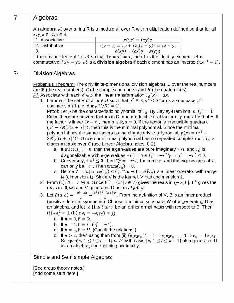
7 Algebras An algebra 𝒜 over a ring R is a module 𝒜 over R with multiplication defined so that for all

𝑥, 𝑦, 𝑧 ∈ 𝒜, 𝑐 ∈ 𝑅,

1. Associative 𝑥 𝑦𝑧 = 𝑥𝑦 𝑧

2. Distributive 𝑥 𝑦 + 𝑧 = 𝑥𝑦 + 𝑥𝑧, 𝑥 + 𝑦 𝑧 = 𝑥𝑧 + 𝑦𝑧 3. 𝑐 𝑥𝑦 = 𝑐𝑥 𝑦 = 𝑥(𝑐𝑦)

If there is an element 1 ∈ 𝒜 so that 1𝑥 = 𝑥1 = 𝑥, then 1 is the identity element. 𝒜 is commutative if 𝑥𝑦 = 𝑦𝑥. 𝒜 is a division algebra if each element has an inverse (𝑥𝑥−1 = 1).

7-1 Division Algebras Frobenius Theorem: The only finite-dimensional division algebras D over the real numbers

are ℝ (the real numbers), ℂ (the complex numbers) and 𝐻 (the quaternions). Pf. Associate with each 𝑑 ∈ 𝐷 the linear transformation 𝑇𝑑 𝑥 = 𝑑𝑥.

1. Lemma: The set V of all 𝑎 ∈ 𝐷 such that 𝑎2 ∈ ℝ, 𝑎2 ≤ 0 forms a subspace of codimension 1 (i.e. dimℝ(𝑉/𝐷) = 1).

Proof: Let 𝑝 be the characteristic polynomial of 𝑇𝑎 . By Cayley-Hamilton, 𝑝 𝑇𝑎 = 0.

Since there are no zero factors in D, one irreducible real factor of 𝑝 must be 0 at 𝑎. If the factor is linear (𝑥 − 𝑟), then 𝑎 ∈ ℝ, 𝑎 = 0. If the factor is irreducible quadratic (𝑥2 − 2ℜ 𝑟 𝑥 + 𝑟 2), then this is the minimal polynomial. Since the minimal

polynomial has the same factors as the characteristic polynomial, 𝑝 𝑥 = 𝑥2 −2ℜ 𝑟 𝑥 + 𝑟 2 𝑘 . Since our minimal polynomial has no repeated complex root, 𝑇𝑎 is

diagonalizable over ℂ (see Linear Algebra notes, 8-2). a. If trace 𝑇𝑎 = 0, then the eigenvalues are pure imaginary ±𝑟𝑖, and 𝑇𝑎

2 is

diagonalizable with eigenvalues – 𝑟2. Thus 𝑇𝑎2 = −𝑟2𝐼𝑉 ⇒ 𝑎2 = −𝑟2 ≤ 0.

b. Conversely, if 𝑎2 ≤ 0, then 𝑇𝑎2 = −𝑟2𝐼𝑉 for some 𝑟, and the eigenvalues of 𝑇𝑎

can only be ±𝑟𝑖. Then trace 𝑇𝑎 = 0. c. Hence 𝑉 = {𝑎| trace 𝑇𝑎 ≤ 0}. 𝑇: 𝑎 → trace(𝑇𝑎) is a linear operator with range

ℝ (dimension 1). Since V is the kernel, V has codimension 1. 2. From (1), 𝐷 = 𝑉 ⊕ ℝ. Since 𝑉2 = {𝑣2|𝑣 ∈ 𝑉} gives the reals in (−∞, 0], 𝑉4 gives the

reals in [0, ∞) and V generates D as an algebra.

3. Let 𝐵 𝑎, 𝑏 =−𝑎𝑏−𝑏𝑎

2=

𝑎2+𝑏2− 𝑎+𝑏 2

2. From the definition of V, B is an inner product

(positive definite, symmetric). Choose a minimal subspace W of V generating D as

an algebra, and let 𝑒𝑖 1 ≤ 𝑖 ≤ 𝑛 be an orthonormal basis with respect to B. Then

i – 𝑒𝑖2 = 1, ii 𝑒𝑖𝑒𝑗 = −𝑒𝑗𝑒𝑖(𝑖 ≠ 𝑗).

a. If 𝑛 = 0, 𝑉 ≅ ℝ.

b. If 𝑛 = 1, 𝑉 ≅ ℂ. (𝑒12 = −1)

c. If 𝑛 = 2, 𝑉 ≅ 𝐻. (Check the relations.)

d. If 𝑛 > 2, then using then from (ii) 𝑒1𝑒2𝑒𝑛 2 = 1 ⇒ 𝑒1𝑒2𝑒𝑛 = ±1 ⇒ 𝑒𝑛 = ±𝑒1𝑒2. So span 𝑒𝑖 1 ≤ 𝑖 ≤ 𝑛 − 1 ⊂ 𝑊 with basis 𝑒𝑖 1 ≤ 𝑖 ≤ 𝑛 − 1 also generates D as an algebra, contradicting minimality.

Simple and Semisimple Algebras

[See group theory notes.] [Add some stuff here.]

References [A] Algebra by Michael Artin [EoAA] Elements of Abstract Algebra by Richard Dean [PftB] Proofs from the Book by Titu Andreescu and Gabriel Dospinescu [TBGY] Abstract Algebra: The Basic Graduate Year, by Robert Ash Wikipedia