About stability and regularization of ill-posed elliptic Cauchy problems: the case of Lipschitz...

This article was downloaded by: [Moskow State Univ Bibliote]On: 15 December 2013, At: 07:36Publisher: Taylor & FrancisInforma Ltd Registered in England and Wales Registered Number: 1072954 Registeredoffice: Mortimer House, 37-41 Mortimer Street, London W1T 3JH, UK

Applicable Analysis: An InternationalJournalPublication details, including instructions for authors andsubscription information:http://www.tandfonline.com/loi/gapa20

About stability and regularization ofill-posed elliptic Cauchy problems: thecase of Lipschitz domainsLaurent Bourgeois a & Jérémi Dardé a ba Laboratoire POEMS , 32, Boulevard Victor, 75739 Paris Cedex 15,Franceb Laboratoire J.-L. Lions , Université Pierre et Marie Curie , 175,Rue du Chevaleret, 75252 Paris Cedex 05, FrancePublished online: 24 May 2010.

To cite this article: Laurent Bourgeois & Jérémi Dardé (2010) About stability and regularizationof ill-posed elliptic Cauchy problems: the case of Lipschitz domains, Applicable Analysis: AnInternational Journal, 89:11, 1745-1768, DOI: 10.1080/00036810903393809

To link to this article: http://dx.doi.org/10.1080/00036810903393809

PLEASE SCROLL DOWN FOR ARTICLE

Taylor & Francis makes every effort to ensure the accuracy of all the information (the“Content”) contained in the publications on our platform. However, Taylor & Francis,our agents, and our licensors make no representations or warranties whatsoever as tothe accuracy, completeness, or suitability for any purpose of the Content. Any opinionsand views expressed in this publication are the opinions and views of the authors,and are not the views of or endorsed by Taylor & Francis. The accuracy of the Contentshould not be relied upon and should be independently verified with primary sourcesof information. Taylor and Francis shall not be liable for any losses, actions, claims,proceedings, demands, costs, expenses, damages, and other liabilities whatsoever orhowsoever caused arising directly or indirectly in connection with, in relation to or arisingout of the use of the Content.

This article may be used for research, teaching, and private study purposes. Anysubstantial or systematic reproduction, redistribution, reselling, loan, sub-licensing,systematic supply, or distribution in any form to anyone is expressly forbidden. Terms &

http://www.tandfonline.com/loi/gapa20

http://www.tandfonline.com/action/showCitFormats?doi=10.1080/00036810903393809

http://dx.doi.org/10.1080/00036810903393809

Conditions of access and use can be found at http://www.tandfonline.com/page/terms-and-conditions

Dow

nloa

ded

by [

Mos

kow

Sta

te U

niv

Bib

liote

] at

07:

36 1

5 D

ecem

ber

2013

http://www.tandfonline.com/page/terms-and-conditions

http://www.tandfonline.com/page/terms-and-conditions

Applicable AnalysisVol. 89, No. 11, November 2010, 1745–1768

About stability and regularization of ill-posed elliptic Cauchy

problems: the case of Lipschitz domains

Laurent Bourgeoisa* and Jeremi Dardeab

aLaboratoire POEMS, 32, Boulevard Victor, 75739 Paris Cedex 15, France;bLaboratoire J.-L. Lions, Universite Pierre et Marie Curie, 175, Rue du Chevaleret,

75252 Paris Cedex 05, France

Communicated by B. Hofmann

(Received 22 September 2009; final version received 2 October 2009)

This article is devoted to a conditional stability estimate related to theill-posed Cauchy problems for Laplace’s equation in domains withLipschitz boundary. It completes the results obtained by Bourgeois[Conditional stability for ill-posed elliptic Cauchy problems: The case ofC1,1 domains ( part I ), Rapport INRIA 6585, 2008] for domains of classC1,1. This estimate is established by using an interior Carleman estimateand a technique based on a sequence of balls which approach theboundary. This technique is inspired by Alessandrini et al. [Optimalstability for inverse elliptic boundary value problems with unknownboundaries, Annali della Scuola Normale Superiore di Pisa 29 (2000),pp. 755–806]. We obtain a logarithmic stability estimate, the exponent ofwhich is specified as a function of the boundary’s singularity. Such stabilityestimate induces a convergence rate for the method of quasi-reversibilityintroduced by Lattes and Lions [Methode de Quasi-Reversibilite etApplications, Dunod, Paris, 1967] to solve the Cauchy problems.The optimality of this convergence rate is tested numerically, precisely adiscretized method of quasi-reversibility is performed by using anonconforming finite element. The obtained results show very goodagreement between theoretical and numerical convergence rates.

Keywords: Carleman estimate; Cauchy problem; Lipschitz domain; quasi-reversibility; stability estimate

AMS Subject Classifications: 35A15; 35A27; 35N25; 35R25; 65N30

1. Introduction

The problem of stability for ill-posed elliptic Cauchy problems plays an importantrole in the fields of inverse problems governed by elliptic partial differentialequations (PDEs). It can be considered as a first step to study the stability of manyinverse problems of interest, such as the data completion problem (see Remark 6hereafter), the inverse obstacle problem [1] or the corrosion detection problem [2].

*Corresponding author. Email: [email protected]

ISSN 0003–6811 print/ISSN 1563–504X online

� 2010 Taylor & Francis

DOI: 10.1080/00036810903393809

http://www.informaworld.com

Dow

nloa

ded

by [

Mos

kow

Sta

te U

niv

Bib

liote

] at

07:

36 1

5 D

ecem

ber

2013

This article can be considered as the continuation of [3], and consequently we refer to

the introduction of such article for a more precise description of this subject and

some bibliography. In [3], the following conditional stability result was obtained in

the case of operator P¼�D. �k., with k2R.For a bounded and connected open domain ��R

N with C1,1 boundary, if �0 is

an open part of @�, then for all �2 ]0, 1[ there exists C such that for all functions

u2H2(�) which satisfy

kukH2ð�Þ �M, kPukL2ð�Þ þ kukH1ð�0Þþ k@nukL2ð�0Þ

� �,

for some constant M and sufficiently small �,

kukH1ð�Þ � CM

ðlogðM=�ÞÞ�:

Furthermore, the upper bound �¼ 1 of the exponent cannot be improved.The result obtained in [1] is a generalization of the one obtained in [4] for

domains with C1 boundary. The proof mainly relies on a Carleman estimate near

the boundary, in which the weight function is expressed in terms of the distance to

the boundary. Since we have to differentiate twice this weight function, we need the

boundary @� to be at least C1,1. In this article, we now study how such a conditional

stability result can be extended to Lipschitz domains, the boundary of which is not

smooth enough to apply the same method.We hence consider an open, bounded and connected domain ��R

N the

boundary @� of which is Lipschitz. In particular, this is equivalent to the fact that �

satisfies the cone property (see Definition 2.4.1 and Theorem 2.4.7 of [5]). The cone

property implies in particular that there exist � 2 ]0,�/2[ and R04 0 such that for all

x02 @�, there exists �2RN, j�j ¼ 1, such that the finite cone

C ¼ fx2RN, ðx� x0Þ:�4 jx� x0j cos �, jx� x0j5R0g

is included in �.As above, �0 denotes an open part of @� which is C1,1. Lastly, we assume that k is

not a Dirichlet eigenvalue of the operator �D in �. The main result we obtain is that

for all �2 [0, 1], for all �2 ]0, (1þ �)�0(�)/2[ there exists C such that for all functions

u2C1,�ð�Þ such that Du2L2(�) and

kukC1,�ð�Þ �M, kPukL2ð�Þ þ kukH1ð�0Þþ k@nukL2ð�0Þ

� �,

for some constant M and sufficiently small �, then

kukH1ð�Þ � CM

ðlogðM=�ÞÞ�: ð1Þ

Here, �0(�) is the solution of the following simple maximization problem

�0ð�Þ ¼1

2supx40

sin �ð1� e�xÞffiffiffiffiffiffiffiffiffiffiffi1þ xp

� sin �:

The continuous function �0 is increasing on the segment [0,�/2] and ranges from

�0(0)¼ 0 to �0(�/2)¼ 1. Since a domain of class C1 has a Lipschitz boundary which

satisfies the cone property with any � 2 ]0,�/2[, we obtain that (1) is satisfied for all

1746 L. Bourgeois and J. Darde

Dow

nloa

ded

by [

Mos

kow

Sta

te U

niv

Bib

liote

] at

07:

36 1

5 D

ecem

ber

2013

�2 ]0, (1þ �)/2[ in that case. The analysis of the conditional stability in Lipschitzdomains was already addressed in [1,6], but in these works, the exponent of thelogarithm was not specified. This is the main novelty of this article to specify theexponent as a function of the geometric singularity. It is obtained by using asequence of three spheres inequalities, the sequence of centres of these spheresapproaching the boundary, and the sequence of radii tending to 0. This technique isborrowed from [1], with two differences. First, the three spheres inequalities resultfrom Carleman estimates instead of doubling properties. Second, we perform anoptimization of this sequence of inequalities in order to obtain the best possiblelogarithmic exponent.

Another concern is to obtain a convergence rate for the method of quasi-reversibility to solve the ill-posed Cauchy problems for the operator P. This requiresa stability estimate for functions that are only inH2(�). For N¼ 2, we obtain that forall �2 ]0, �0(�)/2[ there exists C such that for all functions u2H2(�) which satisfy


� �,

for some constant M and sufficiently small �, then

kukH1ð�Þ � CM


For N¼ 3, we have the same result for all �2 ]0, �0(�)/4[. As a consequence, we provea logarithmic convergence rate for the method of quasi-reversibility, with the limitexponent �0(�)/2 in 2D and �0(�)/4 in 3D, possibly �0(�) provided we assumeadditional regularity for the solution of quasi-reversibility and the ‘true’ solution.

From a numerical point of view, a connected question is to determine if theinfluence of the geometric singularity on the logarithmic exponent can be actuallyobserved in numerical experiments. An easy way to test this is to capture theconvergence rate of a discretizedmethod of quasi-reversibility for a fixed refinedmesh,when the regularization parameter tends to 0. In 2D, we analyse this convergence rateas a function of the smallest angle of a polygonal domain, and observe a pretty goodagreement between numerical and theoretical convergence rates.

The article is organized as follows. In Section 2, we establish some preliminaryuseful results related to the three spheres inequality. Section 3 is devoted to theestimate up to the Lipschitz boundary, which leads to the main results of conditionalstability in �. Lastly, in Section 4, we derive from this conditional stability someconvergence rate for the method of quasi-reversibility in Lipschitz domains.It enables us to compare such convergence rate with the convergence rate obtainednumerically by using a discretized method of quasi-reversibility, and hence to testthe optimality of our stability estimate.

2. Some preliminary results

This section consists of several lemmas that will be used in next section. Theyconcern the three spheres inequality. We first recall the following interior Carlemanestimate.

LEMMA 2.1 We consider the operator P¼�D. �ak. with a, k2R, a2 ]0, 1[. Let !, Udenote two bounded and open domains with ! � U � R

N. Let � be a smooth function

Applicable Analysis 1747

Dow

nloa

ded

by [

Mos

kow

Sta

te U

niv

Bib

liote

] at

07:

36 1

5 D

ecem

ber

2013

defined in U such that r� does not vanish in U. Let us denote P� ¼ h2e�h � P � e�

�h, and

p�(x, �) the principal part of operator P�. We assume that

9c1 4 0, p�ðx, �Þ ¼ 0 and ðx, �Þ 2U�RN) fRe p�, Im p�gðx, �Þ � c1: ð2Þ

Then there exist K, h04 0, with K independent of ak, with h0 depending on ak only

through jkj, such that 8h2 ]0, h0[, we haveZ!

u2e2�h dxþ h2

Z!

jruj2e2�h dx � Kh3

Z!

jPuj2e2�h dx, ð3Þ

for all function u2H10ð!,DÞ, where H1

0ð!,DÞ is the closure of C10 ð!Þ in

H1(!,D)¼ {u2H1(!), Du2L2(!)}.

Proof The inequality (3) is obtained in [7] for k¼ 0, that is in the case of the Laplace

operator �D. There exist K, h04 0, such that 8h2 ]0, h0[, we have for all functions

u2H10ð!,DÞ Z

!

u2e2�h dxþ h2

Z!

jruj2e2�h dx � Kh3

Z!

jPuþ akuj2e2�h dx:

Since jPuþ akuj2� 2(jPuj2þ k2u2), if we assume that in addition h satisfies

2Kk2h35 1/2, we obtain (3) provided we replace K by 4K on the right-hand side

of the inequality. g

A short calculation shows that

Re p� ¼ j�j2 � jr�j2, Im p� ¼ 2�:r�

and

fRe p�, Im p�g ¼ 4Xnj¼1

r@�

@xj

� �: �j� þ

@�

@xjr�

� �:

One considers now a smooth function defined on U such that r 6¼ 0 on U, and

for �4 0, �(x)¼ e� (x). We obtain

fRe p�, Im p�g ¼ 4�� t:r2 :� þ �2�2ðrt :r2 :r Þ þ �ð�:r Þ2 þ �3�2jr j4� �

,

whence by denoting 0(x) the smallest eigenvalue of r2 (x),

fRe p�, Im p�g � 4�� 0ðj�j2 þ �2�2jr j2Þ þ �ð�:r Þ2 þ �3�2jr j4

� �:

For p�(x, �)¼ 0, we have

j�j2 ¼ �2�2jr j2, �:r ¼ 0,

whence

fRe p�, Im p�g � 4�3�3jr j2 20 þ �jr j2

� �:

If we define

m0 :¼ infx2U

0ðxÞ, c0 :¼ infx2Ujr j2,


Dow

nloa

ded

by [

Mos

kow

Sta

te U

niv

Bib

liote

] at

07:

36 1

5 D

ecem

ber

2013

and if m05 0, we have {Re p�, Im p�}� c14 0 on U�RN when p�(x, �)¼ 0 for

�4 � 2m0

c0:

We now consider the particular domain !¼B(R1,R2) :¼ {x2RN, R15 jx� qj5R2}

with q2RN, and the function (x)¼�jx� qj2. We can take U¼B(q,R1 �",R2þ")

for small "4 0. We obtain m0¼�2 and c0¼ 4(R1 �")2, and finally assumption (2)

holds as soon as �4 1=R21.

We now apply Lemma 2.1 and Lemma 3 in [3] to obtain a so-called three spheres

inequality. The proof of such inequality is classical [4,8], but it is reproduced here in

order to find how the constants involved in the inequality depend on some useful

parameters.

LEMMA 2.2 We consider the operator P¼�D� ak. with a, k2R and a2 ]0, 1[.

Let q2�, and let 05 r05 r15 r25 r35 r45 r55 r6 such that B(q, r6)��. If �satisfies �r20 4 1, then there exists a constant C, which depends on ak only through jkj,

such that we have for all u2H1(�,D),

kukH1ðBðq,r3ÞÞ � C kPukL2ðBðq,r6ÞÞ þ kukH1ðBðq,r2ÞÞ

� � ssþ1kuk

1sþ1

H1ðBðq,r6ÞÞ, ð4Þ

with

s ¼gðr3Þ � gðr4Þ

gðr1Þ � gðr3Þ, gðrÞ ¼ e��r

2

:

Proof One applies Lemma 2.1 in the domain !¼B(r0, r6) for �¼ e� with

(x)¼�jx� qj2. We have seen that assumption (2) is satisfied as soon as �r20 4 1.

Assuming that this inequality holds, we obtain there exists K, h04 0 such that for

05 h5 h0 (K does not depend on ak, h0 depends on ak only through jkj),

Z!

ðjvj2 þ jrvj2Þe2�h dx � K

Z!

jPvj2e2�h dx, ð5Þ

for all functions v2H10ð!,DÞ.

Now we take u2H1(�,D) and v ¼ u2H10ð!,DÞ, where is a C1 cut-off

function such that 2 [0, 1] and

¼ 0 in Bðr0, r1Þ [ Bðr5, r6Þ ¼ 1 in Bðr2, r4Þ:

�

In the following we denote g(r)¼ e��r2

. Hence g is a non-increasing function.

Z!

ðjvj2 þ jrvj2Þe2�h dx � e2

gðr3Þ

h

ZBðr2,r3Þ

ðjuj2 þ jruj2Þ dx,

andZ!

jPvj2e2�h dx ¼

ZBðr2,r4Þ

jPuj2e2�h dxþ

ZBðr1,r2Þ

jPðuÞj2e2�h dxþ

ZBðr4,r5Þ

jPðuÞj2e2�h dx:


Dow

nloa

ded

by [

Mos

kow

Sta

te U

niv

Bib

liote

] at

07:

36 1

5 D

ecem

ber

2013

Since we have P(u)¼(Pu)� 2r. ru� (D)u, we obtain the following estimates

(K is a constant which depends only on ):ZBðr2,r4Þ

jPuj2e2�h dx � e2

gðr2Þ

h

ZBðr2,r4Þ

jPuj2 dx,ZBðr1,r2Þ

jPðuÞj2e2�h dx � e2

gðr1Þ

h

ZBðr1,r2Þ

jPuj2 dxþ Ke2gðr1 Þ

h

ZBðr1,r2Þ

ðjuj2 þ jruj2Þ dx,ZBðr4,r5Þ

jPðuÞj2e2�h dx � e2

gðr4Þ

h

ZBðr4,r5Þ

jPuj2 dxþ Ke2gðr4 Þ

h

ZBðr4,r5Þ

ðjuj2 þ jruj2Þ dx:

Gathering the above inequalities, it follows thatZ!

jPvj2e2�h dx � K1e

2gðr1 Þ

h

ZBðq,r6Þ

jPuj2 dxþ

ZBðq,r2Þ

ðjuj2 þ jruj2Þ dx

� �

þ K2e2gðr4Þ

h

ZBðq,r6Þ

ðjuj2 þ jruj2Þ dx,

where K1 and K2 are two constants which are independent of ak.Finally, the inequality (5) implies

e2gðr3 Þ

h kuk2H1ðBðr2,r3ÞÞ� K1 e

2gðr1 Þ

h kPuk2L2ðBðq,r6ÞÞþ kuk2H1ðBðq,r2ÞÞ

� þ K2 e

2gðr4 Þ

h kuk2H1ðBðq,r6ÞÞ:

Using

kuk2H1ðBðq,r3ÞÞ¼ kuk2H1ðBðq,r2ÞÞ

þ kuk2H1ðBðr2,r3ÞÞ,

we obtain

e2gðr3 Þ

h kuk2H1ðBðq,r3ÞÞ� K1 e

2gðr1 Þ

h kPuk2L2ðBðq,r6ÞÞþ kuk2H1ðBðq,r2ÞÞ

� þ K2 e

2gðr4Þ

h kuk2H1ðBðq,r6ÞÞ:

Denoting k1¼ g(r1)� g(r3)4 0 and k2¼ g(r3)� g(r4)4 0, we obtain

kukH1ðBðq,r3ÞÞ � K1 ek1h kPukL2ðBðq,r6ÞÞ þ kukH1ðBðq,r2ÞÞ

� �þ K2 e

�k2h kukH1ðBðq,r6ÞÞÞ:

Let s4 0 and c4 0 such that

c

"¼ K1e

k1h , "s ¼ K2e

�k2h :

A simple calculation proves that

s ¼k2k1¼

gðr3Þ � gðr4Þ

gðr1Þ � gðr3Þ, c ¼ K1ðK2Þ

ðk1=k2Þ,

and we obtain for all u2H1(�,D), for all "2 ]0, "0[ with

"0 ¼ Kðk1=k2Þ2 e

�k1h0 ,

the inequality

kukH1ðBðq,r3ÞÞ �c

"kPukL2ðBðq,r6ÞÞ þ kukH1ðBðq,r2ÞÞ

� �þ "skukH1ðBðq,r6ÞÞ:


Dow

nloa

ded

by [

Mos

kow

Sta

te U

niv

Bib

liote

] at

07:

36 1

5 D

ecem

ber

2013

The constant c does not depend on ak, "0 depends on ak only through jkj. It remains

to apply Lemma 3 in [3], since kukH1(B(q,r3))�kukH1(B(q,r6))

. g

LEMMA 2.3 Let us denote Pk the operator �D. �k., with k2R. Let ~q2�, and let

05 ~r0 5 ~r1 5 ~r2 5 ~r3 5 ~r4 5 ~r5 5 ~r6 such that Bð ~q, ~r6Þ � �. Consider now q2� and

for 2 ]0, 1[, ri ¼ ~ri (i¼ 1, 2, . . . , 6), with B(q, r6)��.We assume that the three spheres inequality (4) associated with the operator P2k

and the sequence of balls Bð ~q, ~riÞ is satisfied with the constants ~C and s. Then the three

spheres inequality (4) associated with the operator Pk and the sequence of balls B(q, ri)

is satisfied with the constants C ¼ ~C= and s.

Proof The proof relies on the change of variables x� q ¼ ð ~x� ~qÞ. We define the

function u as ~uð ~xÞ ¼ uðxÞ ¼ ~uð ~qþ ðx� qÞ=Þ.We obtainZ

Bðq,riÞ

juðxÞj2 þ jruðxÞj2 dx ¼ N

ZBð ~q, ~riÞ

j ~uð ~xÞj2 þ1

2jr ~uð ~xÞj2 d ~x

� �,

whence

N2k ~ukH1ðBð ~q, ~riÞÞ � kukH1ðBðq,riÞÞ �

N2�1k ~ukH1ðBð ~q, ~riÞÞ:

Similarly, we obtain

kPkukL2ðBðq,riÞÞ ¼ N2�2kP2k ~ukL2ðBð ~q, ~riÞÞ:

By using the three spheres inequality (4) associated with the balls Bð ~q, ~riÞ for operator

P2k, we obtain

kukH1ðBðq,r3ÞÞ � N2�1k ~ukH1ðBð ~q, ~r3ÞÞ

� ~CN2�1 kP2k ~ukL2ðBð ~q, ~r6ÞÞ þ k ~ukH1ðBð ~q, ~r2ÞÞ

� � ssþ1k ~uk

1sþ1

H1ðBð ~q, ~r6ÞÞ

� ~CN2�1

1

N2�2kPkukL2ðBðq,r6ÞÞ þ

1

N2

kukH1ðBðq,r2ÞÞ

� � ssþ1 1

N2

kukH1ðBðq,r6ÞÞ

� � 1sþ1

�~C

kPkukL2ðBðq,r6ÞÞ þ kukH1ðBðq,r2ÞÞ

� � ssþ1kuk

1sþ1

H1ðBðq,r6ÞÞ,

which completes the proof. g

3. The two main theorems

Our main theorems are based on the following proposition, which is similar to

Proposition 4 in [3]. It concerns the propagation of data from the interior of the

domain up to the boundary of such domain. However, it should be noted that in

Proposition 4 of [3], we estimated the H1 norm of the function in a neighbourhood of

a point x02 @� with the help of the H1 norm of the function in an open domain

!1 ! �. Here, we estimate the value of the function and its first derivatives at x0 with

the help of the H1 norm of the function in !1. As a result, the regularity assumptions

concerning the function u are not the same as in [3].


Dow

nloa

ded

by [

Mos

kow

Sta

te U

niv

Bib

liote

] at

07:

36 1

5 D

ecem

ber

2013

PROPOSITION 3.1 There exists an open domain !1 ! � such that for all �2 ]0, 1], forall �5��0(�) and �

05 �0(�), with

�0ð�Þ ¼1

2supx40


� sin �, ð6Þ

there exists c4 0 such that for sufficiently small ", for all u2C1,�ð�Þ with Du2L2(�),

kukC1ð@�Þ � ec="ðkPukL2ð�Þ þ kukH1ð!1ÞÞ þ "�kukC1,�ð ��Þ,

kukC0ð@�Þ � ec="ðkPukL2ð�Þ þ kukH1ð!1ÞÞ þ "�

0

kukC1,�ð ��Þ:

The second inequality holds also in the case �¼ 0.

In order to obtain Proposition 3.1, we need the two following lemmas. The first

one is a minor generalization of the lemma proved in [8] in the particular case ¼ 1,

while the second one is the counterpart of Lemma 3 in [3].

LEMMA 3.2 Let �n4 0 satisfy for n2N,

�nþ1 �1

nð�n þ AÞ�B1��,

with A4 0, B4 0, �2 ]0, 1[, 2 ]0, 1[ and �n�B. Then one has for n2N*

�n �2

11��

n�11��

ð�0 þ AÞ�n

B1��n :

Proof If B5�0þA, the proof is complete. If �0þA�B, in particular A�B, we

have

�nþ1B�

1

n

�n þ A

B

� ��

and

A

B�

1

n

A

B

� ��

1

n

�n þ A

B

� ��:

From the two above inequalities, it follows that

�nþ1 þ A

21

1��B�

1

n

�n þ A

21

1��B

� ��,

that is

xnþ1 �x�nn

, xn :¼�n þ A

21

1��B:

By iterating the above inequality, we obtain

xn �1

� �n�1þðn�2Þ�þðn�3Þ�2þ��þ�n�2

x�n

0

�1

� �ðn�1Þð1þ�þ�2þ��þ�n�2Þx�

n

0 �1

� �n�11��

x�n

0 ,


Dow

nloa

ded

by [

Mos

kow

Sta

te U

niv

Bib

liote

] at

07:

36 1

5 D

ecem

ber

2013

whence

�n �2

11��

n�11��

ð�0 þ AÞ�n

B1��n ,


LEMMA 3.3 Let C, �, A and B denote four non-negative reals and �2 ]0, 1[ such that

� � CA�B1��:

Then 8"4 0,

� �c

"Aþ "s B,

with

s ¼�

1� �, c ¼

C

s1=ðsþ1Þ þ s�s=ðsþ1Þ

� �sþ1s

:

Proof For c, s4 0 as defined in the statement of the lemma, the minimum of the

function f defined for "4 0 by

f ð"Þ ¼c

"Aþ "s B

is CA�B1��, which completes the proof. g

Proof of proposition 3.1 The proof is divided into three parts. In the first step of the

proof we follow the technique of [1], which consists in defining a sequence of balls the

radii of which is decreasing and the centre of which is approaching the boundary

of the domain. Since � satisfies the cone property (see our definition in the

introduction), there exist R04 0, � 2 ]0,�/2[ with R0 and � independent of x02 @�,

and � 2RN with j�j ¼ 1 such that the finite cone

C ¼ fx, jx� x0j5R0, ðx� x0Þ:�4 jx� x0j cos �g

satisfies C��. We also denote

C0 ¼ fx, jx� x0j5R0, ðx� x0Þ:�4 jx� x0j cos �0g,

with

�0 ¼ arcsinðt sin �Þ, ð7Þ

where the coefficient t2 ]0, 1[ will be specified further. It should be noted that

definition (7) leads to �0 2 ]0,�/2[. We now denote q0¼ x0þ (R0/2) �, d0¼ jq0� x0j

and 0¼ d0 sin �0. We hence have B(q0, 0)2C0. Let us define the sequence of balls

B(qn, n)�C0 with dn¼ jqn� x0j and n¼ dn sin �0 by following induction:

qnþ1 ¼ qn � �n�

nþ1 ¼ n

dnþ1 ¼ dn,

8><>: ð8Þ


Dow

nloa

ded

by [

Mos

kow

Sta

te U

niv

Bib

liote

] at

07:

36 1

5 D

ecem

ber

2013

where �n and will be defined further. From the above equations, we deduce that

�n ¼ ð1� Þdn: ð9Þ

The objective is to use a three spheres inequality such as (4) for each n, the centre

of these three spheres being q¼ qn. We hence define, for n2N, 05 r0n5 r1n5r2n¼ n5 r3n5 r4n5 r5n5 r6n and yin¼ rin/r0n4 1 for i¼ 1, . . . , 6. We assume that

the yin do not depend on n, that is yin :¼ yi. We specify t¼ r2n/r6n¼ y2/y6 in (7), so that

we have B(qn, r6n)2C�� for all n (Figure 1).On the other hand, if �n is chosen such that

nþ1 þ �n ¼ r3n, ð10Þ

we have B(qnþ1, nþ1)�B(qn, r3n) since for jx� qnþ1j5 nþ1,

jx� qnj � jx� qnþ1j þ jqnþ1 � qnj5 nþ1 þ �n ¼ r3n:

Equations (9) and (10) uniquely define as

¼r6n � r3n sin �

r6n � r2n sin �¼

y6 � y3 sin �

y6 � y2 sin �2 0, 1½:

By using the notation Pk¼�D. �k., we now apply Lemma 2.2 for operator P2nk and

for the spheres of centre q0 and of radii ri0, with � such that � :¼ �r200 4 1. We thus

obtain for u2H1(�,D),

kukH1ðBðq0,r30ÞÞ � C kP2nkukL2ðBðq0,r60ÞÞ þ kukH1ðBðq0,r20ÞÞ

� � ssþ1kuk

1sþ1

H1ðBðq0,r60ÞÞ,

∂Ω

θ

θ

ξx0

r06

r03

r02

q0

qn

Figure 1. The sequence of three spheres inequalities.


Dow

nloa

ded

by [

Mos

kow

Sta

te U

niv

Bib

liote

] at

07:

36 1

5 D

ecem

ber

2013

with C independent of and n. With the help of Lemma 2.3, and since rin¼nri0 for

i¼ 1, . . . , 6, the three spheres inequality for the spheres of centre qn and of radii rin is

kukH1ðBðqn,r3nÞÞ �C

nkPkukL2ðBðqn,r6nÞÞ þ kukH1ðBðqn,r2nÞÞ

� � ssþ1kuk

1sþ1

H1ðBðqn,r6nÞÞ,

which implies that for all u2H1(�,D),

kukH1ðBðqnþ1, nþ1ÞÞ �C

nkPukL2ð�Þ þ kukH1ðBðqn, nÞÞ

� � ssþ1kuk

1sþ1

H1ð�Þ:

It should be noted that in the above inequality, C and s are independent of n, in

particular

s ¼e��y

23 � e��y

24

e��y21 � e��y

23

:

Without loss of generality we assume that C� 1, so that by denoting C0 ¼Csþ1,

kukH1(B(qnþ1, nþ1))�C0kukH1(�), and we can apply Lemma 3.2 with �n¼kukH1(B(qn, n))

,

A¼kPukL2(�), B¼C0kukH1(�), �¼ s/(sþ 1). We obtain

kukH1ðBðqn, nÞÞ �2

11��

n�11��

kPukL2ð�Þ þ kukH1ðBðq0, 0ÞÞ

� ��nC0kukH1ð�Þ

� �1��n:

We apply now Lemma 3.3 and obtain 8"4 0,

kukH1ðBðqn, nÞÞ �cn"kPukL2ð�Þ þ kukH1ðBðq0, 0ÞÞ

� �þ "sn C0kukH1ð�Þ

with

sn ¼�n

1� �n, cn ¼

21

1��

n�11��

1

EðsnÞ

!snþ1sn

,

and

EðsÞ :¼ s1=ðsþ1Þ þ s�s=ðsþ1Þ:

We notice that for s4 0, E(s)4 1, whence

log2

11��

n�11��

1

EðsnÞ

!5

1

1� �log

2

n�1

� �:

As a result,

05 cn 5 e1sn

1

ð1��Þ2log 2

n�1

� ¼ e

csnlog 2

n�1

� ,

for some constant c4 0. Here we have used the fact that snþ 15 1/(1� �). Sincesn4 �n, we finally obtain 8n2N

*, 8"4 0 and 8u2H1(�,D),

kukH1ðBðqn, nÞÞ �e

c�nlog�

2

n�1

�"


� �þ C0"�

n

kukH1ð�Þ:ð11Þ


Dow

nloa

ded

by [

Mos

kow

Sta

te U

niv

Bib

liote

] at

07:

36 1

5 D

ecem

ber

2013

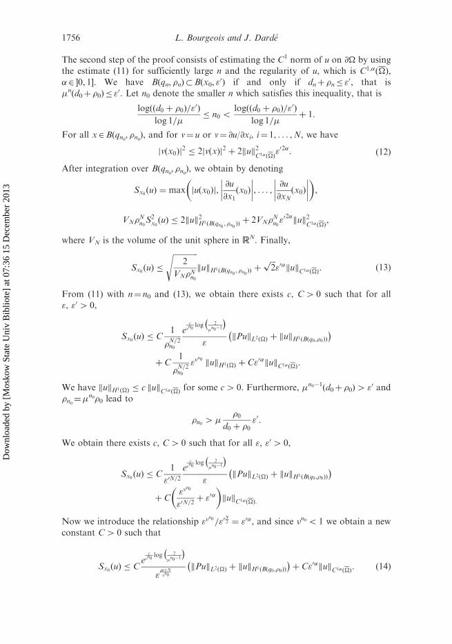
The second step of the proof consists of estimating the C1 norm of u on @� by using

the estimate (11) for sufficiently large n and the regularity of u, which is C1,�ð�Þ,

�2 ]0, 1]. We have B(qn, n)�B(x0, "0) if and only if dnþ n� "

0, that is

n(d0þ 0)� "0. Let n0 denote the smaller n which satisfies this inequality, that is

logððd0 þ 0Þ="0Þ

log 1=� n0 5

logððd0 þ 0Þ="0Þ

log 1=þ 1:

For all x2B(qn0, n0), and for v¼ u or v¼ @u/@xi, i¼ 1, . . . ,N, we have

jvðx0Þj2 � 2jvðxÞj2 þ 2kuk2

C1,�ð�Þ"02�: ð12Þ

After integration over B(qn0, n0), we obtain by denoting

Sx0ðuÞ ¼ max juðx0Þj,@u

@x1ðx0Þ

, . . . ,

@u

@xNðx0Þ

� �,

VN Nn0S2x0ðuÞ � 2kuk2H1ðBðqn0 , n0 ÞÞ

þ 2VN Nn0"02�kuk2

C1,�ð�Þ,

where VN is the volume of the unit sphere in RN. Finally,

Sx0ðuÞ �

ffiffiffiffiffiffiffiffiffiffiffiffiffi2

VN Nn0

skukH1ðBðqn0 , n0 ÞÞ

þffiffiffi2p"0�kukC1,�ð�Þ: ð13Þ

From (11) with n¼ n0 and (13), we obtain there exists c, C4 0 such that for all

", "04 0,

Sx0 ðuÞ � C1

N=2n0

ec�n0

log�

2

n0�1

�"


� �þ C

1

N=2n0

"�n0kukH1ð�Þ þ C"0�kukC1,�ð�Þ:

We have kukH1ð�Þ � c kukC1,�ð�Þ for some c4 0. Furthermore, n0�1(d0þ 0)4 "0 and n0¼

n0 0 lead to

n0 4 0

d0 þ 0"0:

We obtain there exists c, C4 0 such that for all ", "04 0,

Sx0ðuÞ � C1

"0N=2e

c�n0

log�

2

n0�1

�"


� �þ C

"�n0

"0N=2þ "0�

� �kukC1,�ð�Þ:

Now we introduce the relationship "�n0 ="0

N2 ¼ "0�, and since �n05 1 we obtain a new

constant C4 0 such that

Sx0ðuÞ � Ce

c�n0

log�

2

n0�1

�"0�þN�n0


� �þ C"0�kukC1,�ð�Þ: ð14Þ


Dow

nloa

ded

by [

Mos

kow

Sta

te U

niv

Bib

liote

] at

07:

36 1

5 D

ecem

ber

2013

Since 1/�n0¼ en0log(1/�), we have

1

�n05 elogð1=�Þ

logððd0þ 0 Þ="0 Þ

logð1=Þ þ1� �

¼1

�

d0 þ 0"0

� ��0,

with �0¼ log(1/�)/log(1/).Furthermore, since 1/n0�15 (d0þ 0)/"

0, we have

log2

n0�1

� �5 log

2ðd0 þ 0Þ

"0

� �:

Then,

ec�n0

log 2

n0�1

� "0ð�þNÞ=�

n0¼ e

1�n0

c log 2

n0�1

� þð�þNÞ log 1

"0ð Þ

� � e

1�

d0þ 0"0

� ��0c log

2ðd0þ 0Þ

"0

� �þð�þNÞ log 1

"0ð Þ� �

:

As a result, for some new c04 0, for sufficiently small "0 we have

ec�n0

log 2

n0�1

� "0ð�þNÞ=�

n0� e

c0

"0�0logð1

"0Þ:

For all �4 �0, for some new c04 0, for sufficiently small "0 we have

ec�n0

log�

2

n0�1

�"0ð�þNÞ=�

n0� e

c0

"0� :

Coming back to (14), we obtain

Sx0ðuÞ � ec0="0� kPukL2ð�Þ þ kukH1ðBðq0, 0ÞÞ

� �þ C"0�kukC1,�ð�Þ:

By denoting "¼ "0� for any �4 �0, for small "4 0,

Sx0 ðuÞ � ec0=" kPukL2ð�Þ þ kukH1ðBðq0, 0ÞÞ

� �þ C0"�=�kukC1, �ð�Þ:

Finally, by denoting �0¼ 1/�0, for all �5��0 there exists c, "04 0 such that for all

"5 "0,

Sx0 ðuÞ � ec=" kPukL2ð�Þ þ kukH1ðBðq0, 0ÞÞ

� �þ "�kukC1,�ð�Þ:

By following the history of the constants c and "0 throughout the proof, it is readilyseen that c and "0 do not depend on x02 @�. Furthermore, if we define !1 ! � as the

union of the balls B(q0, 0) when x0 describes @�, we obtain that for all �5��0, thereexists c, "04 0 such that for all "5 "0, for all u2C

1,�ð�Þ with Du2L2(�),

kukC1ð@�Þ � ec=" kPukL2ð�Þ þ kukH1ð!1Þ

� �þ "�kukC1, �ð�Þ, ð15Þ

which is the first inequality of the proposition.The second inequality is obtained by using the embedding C1,�ð�Þ ! C1ð�Þ,

for all �2 [0, 1]. For x2B(qn0, n0), we replace (12) by

juðx0Þj2 � 2juðxÞj2 þ 2kuk2

C1ð�Þ"02,

and we use the same technique as above.


Dow

nloa

ded

by [

Mos

kow

Sta

te U

niv

Bib

liote

] at

07:

36 1

5 D

ecem

ber

2013

The third step of the proof consists in maximizing

�0 ¼logð1=Þ

logð1=�Þ,

with

1

¼

y6 � y2 sin �

y6 � y3 sin �,

1

�¼

e�ð y24�y2

1Þ � 1

e�ð y24�y2

3Þ � 1

:

The inequality (15) holds for all �5 ~�0, with

~�0 ¼ sup15�, 15y15y25y35y45y6

logy6 � y2 sin �

y6 � y3 sin �

� ��log

e�ð y24�y2

1Þ � 1

e�ð y24�y2

3Þ � 1

!: ð16Þ

Now, let us specify � and the yi as follows, for k2 ]0, 1[ and �4 0,

� ¼ffiffiffiffiffiffiffiffiffiffiffiffiffi1þ k2p

,

y :¼ ð1þ k2Þ1=4,

y1 ¼ y,

y2 ¼ yð1þ k2�Þ,

y3 ¼ yð1þ k�þ k2�Þ,

y4 ¼ yð1þ �þ k2�Þ,

y6 ¼ yð1þ �þ 2k2�Þ:

8>>>>>>>>>>><>>>>>>>>>>>:

ð17Þ

A first order expansion in k around 0 for fixed � leads to

logy6 � y2 sin �

y6 � y3 sin �

� �¼

� sin �

1þ �� sin �kþ o�ðkÞ,

loge�ð y

24�y2

1Þ � 1

e�ð y24�y2

3Þ � 1

!¼ 2�

e2�þ�2

e2�þ�2� 1

kþ o�ðkÞ

By passing to the limit k! 0 and by taking the sup in �, we obtain the following

particular value �0 � ~�0:

�0 ¼ sup�40

1

2

sin �

1þ �� sin �1� e�ð2�þ�

2Þ�

,

and the optimization problem (6) follows by setting x¼ 2�þ �24 0. g

Remark 1 We can verify that in fact the values ~�0 and �0, defined by (16) and (6)

respectively, actually satisfy ~�0 ¼ �0. First, we eliminate � in (16) simply by using

the change of variables zi ¼ffiffiffi�p

yi with i¼ 1, . . . , 6. We obtain

~�0 ¼ sup15z15z25z35z45z6

logz6 � z2 sin �

z6 � z3 sin �

� ��log

ez24�z2

1 � 1

ez24�z2

3 � 1

!: ð18Þ

We remark that the function to maximize in (18) is an increasing function of z1 and

a decreasing function of z6, that is why we can consider only the asymptotic situation


Dow

nloa

ded

by [

Mos

kow

Sta

te U

niv

Bib

liote

] at

07:

36 1

5 D

ecem

ber

2013

z1! z2 and z6! z4. In order to simplify the analysis with the remaining variablesz2, z3, z4, we denote

z3 � z2 ¼ ~k ~�z2, z4 � z2 ¼ ~�z2, z2 ¼ ~z,

with ~�4 0 and ~k2 0, 1½. We obtain

~�0 ¼ sup15 ~z, 05 ~�, 05 ~k5 1

log1þ ~�� sin �

1þ ~�� sin � � ~k ~� sin �

!�log

eð2~�þ ~�2Þ ~z2 � 1

eð2ð1� ~kÞ ~�þð1� ~k2Þ ~�2Þ ~z2 � 1

!:

Furthermore, it is easy to prove that since 2 ~�þ ~�2 4 2ð1� ~kÞ ~�þ ð1� ~k2Þ ~�2, for fixedð ~k, ~�Þ, the function to maximize is a non-increasing function of ~z4 1, so that themaximum of the function is obtained for ~z! 1, and

~�0 ¼ sup05 ~�, 05 ~k5 1

log1þ ~�� sin �

1þ ~�� sin � � ~k ~� sin �

!�log

e2~�þ ~�2 � 1

e2ð1� ~kÞ ~�þð1� ~k2Þ ~�2 � 1

!:

We notice that for fixed ~�, the maximum of the function of two variables is obtainedfor ~k! 0, and a first order expansion in ~k leads us to the same expression as (6),that is ~�0 ¼ �0.

In order to obtain our main theorem, we recall the two following results, the firstone is obtained in [4] while the second one is obtained in [3].

PROPOSITION 3.4 Let !0, !1 be two open domains such that !0, !1 ! �. There exists, c, "04 0 such that 8"2 ]0, "0[, 8u2H

1(�,D),

kukH1ð!1Þ�

c

"kPukL2ð�Þ þ kukH1ð!0Þ

� �þ "s kukH1ð�Þ:

PROPOSITION 3.5 Assume �0� @� is of class C1,1 and let x02�0 and �4 0 such that@�\B(x0, �)��0. There exists a neighbourhood !0 of x0, there exist s, c, "04 0such that 8"2 ]0, "0[, for all u2H

2(�),

kukH1ð�\!0Þ�

c

"kPukL2ð�Þ þ kukH1ð�0Þ

þ k@nukL2ð�0Þ

� �þ "s kukH1ð�Þ:

The inequality holds also for all u2C1ð�Þ with Du2L2(�).

We are now in a position to state the main theorem, which is a consequence ofPropositions 3.1, 3.4 and 3.5.

THEOREM 3.6 Let ��RN be a bounded and connected open domain with Lipschitz

boundary. If the cone property is satisfied with angle � 2 ]0,�/2[, let �0(�) denote thesolution of the following maximization problem:

�0ð�Þ ¼1

2supx40


� sin �:

Let �0 be a non-empty C1,1 open part of @� and let us introduce the operatorP¼�D.� k., where k is not a Dirichlet eigenvalue of the operator �D in �.

For �2 [0, 1], for all �2 ]0, (1þ �)�0(�)/2[, there exist C, �0 such that for all�2 ]0, �0[, for all functions u2C

1,�ð�Þ such that Du2L2(�) and which satisfy

kukC1,�ð�Þ �M, kPukL2ð�Þ þ kukH1ð�0Þþ k@nukL2ð�0Þ

� �, ð19Þ


Dow

nloa

ded

by [

Mos

kow

Sta

te U

niv

Bib

liote

] at

07:

36 1

5 D

ecem

ber

2013

where M4 0 is a constant, then

kukH1ð�Þ � CM


If we do not assume that �0 is of class C1,1, the estimate (20) holds under assumption

(19) provided we restrict to the functions u which satisfy uj�0¼ 0 and @nuj�0

¼ 0.

Proof Assume first that �2 ]0, 1]. By using Proposition 3.1, there exists a domain

!1 ! � such that for any �5��0(�) and any �05 �0(�), there exist c, "04 0 such that

for all "5 "0, for all u2C1,�ð�Þ with Du2L2(�),

kukC1ð@�Þ � ec="ðkPukL2ð�Þ þ kukH1ð!1ÞÞ þ "�kukC1, �ð�Þ,

and

kukC0ð@�Þ � ec="ðkPukL2ð�Þ þ kukH1ð!1ÞÞ þ "�

0

kukC1,�ð�Þ:

If u¼ 0 and @nu¼ 0 on �0 (case 2), since @�\B(x0, �)��0, the extension u of u by 0

in B(x0, �) belongs to H1(�[B(x0, �), D). By applying Proposition 3.4 to function u

in domain �[B(x0, �) and by choosing !0!Bðx0, �Þ \�c, we obtain that for

sufficiently small ", for all u2C1,�ð�Þ such that Du2L2(�),

kukC1ð@�Þ � ec="kPukL2ð�Þ þ "�kukC1,�ð�Þ,

kukC0ð@�Þ � ec="kPukL2ð�Þ þ "�0 kukC1, �ð�Þ:

We conclude that if moreover u satisfies assumption (19) then

kukC1ð@�Þ � ec="�þ "�M, kukC0ð@�Þ � ec="�þ "�0

M:

By using the same " optimization procedure as in Corollary 1 of [3], we obtain that

for all �5��0(�) and �05 �0(�), there exists C4 0 such that for sufficiently small �,

kukC1ð@�Þ � CM

ðlogðM=�ÞÞ�, kukC0ð@�Þ � C

M

ðlogðM=�ÞÞ�0 : ð21Þ

Since k is not a Dirichlet eigenvalue of the operator �D in �, there exists a constant

C04 0 such that for all u2H1(�,D),

kukH1ð�Þ � C0ðkPukL2ð�Þ þ kukH1=2ð@�ÞÞ: ð22Þ

With the help of an interpolation inequality, we obtain for some constant c4 0,

kukH1=2ð@�Þ � ckuk1=2L2ð@�Þkuk1=2

H1ð@�Þ, ð23Þ

hence for some new constant c,

kukH1=2ð@�Þ � ckuk1=2C0ð@�Þkuk1=2

C1ð@�Þ, ð24Þ

and it follows from (21) that

kukH1=2ð@�Þ � cCM

ðlogðM=�ÞÞð�þ�0Þ=2:

The result follows from (22).


Dow

nloa

ded

by [

Mos

kow

Sta

te U

niv

Bib

liote

] at

07:

36 1

5 D

ecem

ber

2013

If we do not assume that u¼ 0 and @nu¼ 0 on �0, but if moreover �0 is of classC1,1 (case 1), then we can apply Proposition 3.5 in addition to Propositions 3.1 and3.4, hence for all �5��0(�) and �05 �0(�), there exist c, "04 0 such that for all"5 "0, for all u2C

1,�ð�Þ such that Du2L2(�),

kukC1ð@�Þ � ec="ðkPukL2ð�Þ þ kukH1ð�0Þþ k@nukL2ð�0Þ

Þ þ "�kukC1, �ð�Þ,


Þ þ "�0

kukC1,�ð�Þ:

We complete the proof as in case 2.As concerns the case �¼ 0, the result follows from (24), from the second

inequality of (21), which remains true, and from the fact that kukC1(@�)�M. g

Remark 2 It is readily shown by analysing the variations of the function k� definedon [0,þ1[ by

k�ðxÞ ¼1

2


� sin �, ð25Þ

that the maximization problem (6) is well-posed. In particular, the argument x thatmaximizes the function is unique. In Figure 2, the graph of function k� is plotted forincreasing values of �, and the values of function �0 are plotted for all values of� 2 [0,�/2]. The function �0 is increasing on the segment [0,�/2], with �0(0)¼ 0 and�0(�/2)¼ 1.

Remark 3 The fact that �0(0)¼ 0 indicates that when �! 0, which means that thedomain � has a cusp, the logarithmic stability does not hold any more. This isconsistent with the result obtained in [1] when the domain is not Lipschitz, thena logarithmic–logarithmic estimate was established.

Remark 4 The fact that �0(�/2)¼ 1 implies that for domains of classC1, Theorem 3.6holds for all �5 (1þ �)/2. Hence, in the case of functions u inC1,1ð�Þ � H2ð�Þ (�¼ 1),Theorem 3.6 extends the result of Corollary 1 in [3], which was satisfied for domains ofclassC1,1, to domains of classC1, provided either �0 is of classC

1,1 or we restrict to thefunctions u which satisfy u¼ 0 and @nu¼ 0 on �0. It is also interesting to note that

0 2 4 6 8 100

0.1

0.2

0.3

0.4

0.5

0.6

0.7

0.8

0.9

1

0 π/16 π/8 3π/16 π/4 5π/16 3π/8 7π/16 π/20

0.1

0.2

0.3

0.4

0.5

0.6

0.7

0.8

0.9

1

Figure 2. Left: graph of function k� for increasing values of �: �/16, �/10, �/6, �/4, �/3, 3�/8,7�/16, �/2. Right: function �0(�).


Dow

nloa

ded

by [

Mos

kow

Sta

te U

niv

Bib

liote

] at

07:

36 1

5 D

ecem

ber

2013

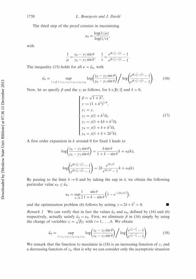
in 2D, if � has only reentrant corners, then the cone property is satisfied for any

� 2 ]0,�/2[, and Theorem 3.6 holds for all �5 1. Hence, the corners of angle smaller

than � deteriorate the exponent of the logarithmic stability, while those of angle larger

than � do not. A similar remark can be done in 3D.

Remark 5 The obtained function (25) is greatly dependent on the choice of the

function (x)¼�jx� qj2 which was used in the exponential weight �¼ e� of our

Carleman estimate (3). Besides, the values of �0(�) induced by this choice and given

by (6) are not necessarily optimal, except for �¼�/2, for which we have proved in [3]

that �0(�/2)¼ 1 is optimal. By testing other types of function , in particular

(x)¼�jx� qj� with other values of �4 0 and (x)¼�log jx� qj, we have found

other functions �0, but taking lower values.

Remark 6 From the proof of Theorem 3.6, we obtain the following corollary

concerning the data completion problem. This problem consists, for a function u that

solves Pu¼ 0 in � in the sense of distributions, to compute with the help of the values

of u and @nu on �0, the values of u and @nu on the complementary part �1.

If u2C1,�ð�Þ, �2 ]0, 1], solves Pu¼ 0 in � and satisfies kukC1,�ð�Þ �M and

kukC1ð�0Þ� �, then for all �5��0(�), there exists C, �04 0 such that for �5 �0,

kukC1ð�1Þ� CM=ðlogðM=�ÞÞ�.

In a view to derive a convergence rate of the method of quasi-reversibility,

we now study the case of functions that are H2(�) for N¼ 2 and N¼ 3. We obtain

the following theorem.

THEOREM 3.7 We define the sets �, �0 and the operator P exactly as in the statement

of Theorem 3.6.In the case N¼ 2 (respectively N¼ 3), for all �2 ]0, �0(�)/2[ (respectively

�2 ]0, �0(�)/4[ ), there exist C, �0 such that for all �2 ]0, �0[, for all functions

u2H2(�) which satisfy


� �, ð26Þ

where M4 0 is a constant, then

kukH1ð�Þ � CM


If we do not assume that �0 is of class C1,1, the estimate (27) holds under assumption

(26) provided we restrict to the functions u which satisfy uj�0¼ 0 and @nuj�0

¼ 0.

Proof By classical embeddings for Sobolev spaces (see e.g. [9], p. 108]), we have that

for N¼ 2, H2ð�Þ ! C0,�ð�Þ, for all �2 [0, 1[, and for N¼ 3, H2ð�Þ ! C0,1=2ð�Þ.Then the proof is very similar to the proof of Theorem 3.6. For all �5 �0(�) in the

case N¼ 2 (respectively for all �5 �0(�)/2 in the case N¼ 3), there exists c4 0 such

that for sufficiently small ", for all u2H2(�),

kukC0ð@�Þ � ec="ðkPukL2ð�Þ þ kukH1ð!1ÞÞ þ "�kukH2ð�Þ,

and then by using propositions 3.4 and 3.5,


Þ þ "�kukH2ð�Þ:


Dow

nloa

ded

by [

Mos

kow

Sta

te U

niv

Bib

liote

] at

07:

36 1

5 D

ecem

ber

2013

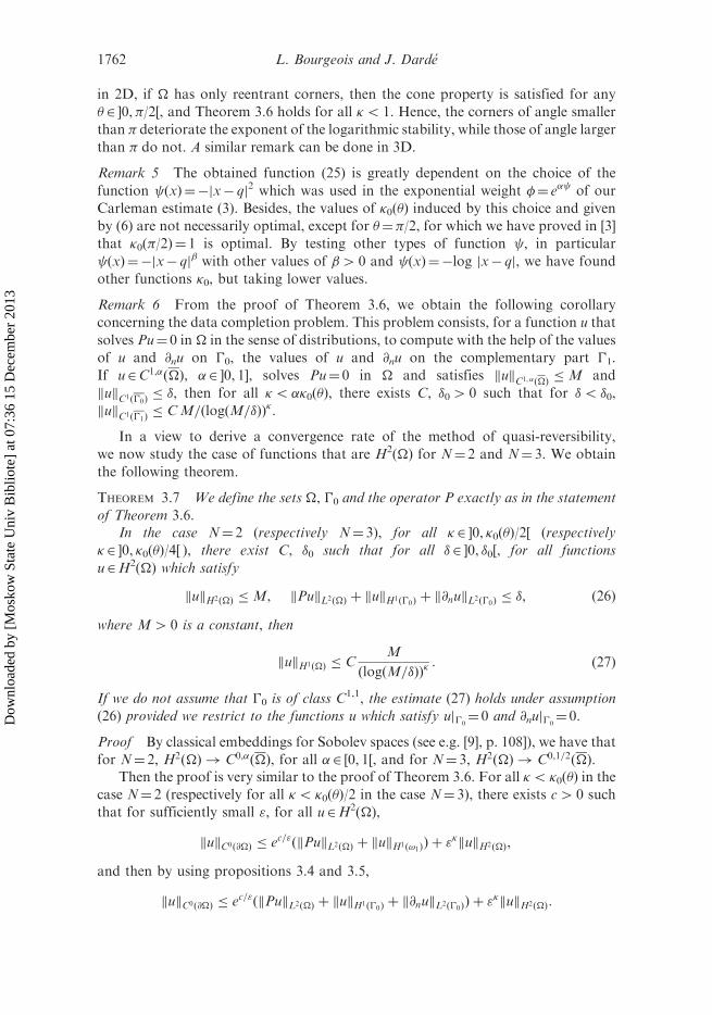
Then assumption (26) implies

kukC0ð@�Þ � ec="�þ "�M:

By using the same " optimization procedure as in Corollary 1 of [3], we obtain thatthere exists C4 0 such that for sufficiently small �,

kukC0ð@�Þ � CM


Combining (22) and (23), we obtain

kukH1ð�Þ � C kPukL2ð�Þ þ kuk1=2C0ð@�Þkuk1=2

H1ð@�Þ

� :

By using a classical trace inequality, we obtain

kukH1ð�Þ � C kPukL2ð�Þ þ kuk1=2C0ð@�Þkuk1=2

H2ð�Þ

� ,


4. Application to the method of quasi-reversibility

In this section, we use the stability estimates obtained in previous section to derive aconvergence rate for the quasi-reversibility method, and therefore to complete theresults already obtained in [3,10]. The method of quasi-reversibility, first introducedin [11], enables one to regularize the ill-posed elliptic Cauchy problems.

Specifically, we consider a bounded and connected open domain ��RN with

Lipschitz boundary and an open part �0. Now we assume that u2H2(�) solves theill-posed Cauchy problem with data ð g0, g1Þ 2H

1ð�0Þ � L2ð�0Þ:

Pu ¼ 0 in �uj�0¼ g0

@nuj�0¼ g1:

8<: ð28Þ

In order to solve the Cauchy problem with these uncorrupted data (g0, g1), for �4 0we consider the formulation of quasi-reversibility, written in the following weakform: find u�2H

2(�) such that 8v2H2(�), vj�0¼ @nvj�0

¼ 0,

ðPu�,PvÞL2ð�Þ þ �ðu�, vÞH2ð�Þ ¼ 0

u�j�0¼ g0

@nu�j�0¼ g1:

8><>: ð29Þ

Using Lax–Milgram theorem and introducing the solution u to the system (28), weeasily prove that formulation (29) is well-posed. On the other hand, it follows from(28) and (29) that there exist constants C1, C24 0 such that

ku� � ukH2ð�Þ � C1, kPðu� � uÞkL2ð�Þ � C2

ffiffiffi�p

: ð30Þ

Using (30) and Theorem 3.7 in case 2 for the function u�� u2H2(�), we obtain thefollowing convergence rate: there exists C4 0 for all �2 ]0, �0(�)/2[ (respectively�2 ]0, �0(�)/4[ ) for N¼ 2 (respectively for N¼ 3), such that for sufficiently small�4 0,

ku� � ukH1ð�Þ � C1

ðlogð1=�ÞÞ�: ð31Þ


Dow

nloa

ded

by [

Mos

kow

Sta

te U

niv

Bib

liote

] at

07:

36 1

5 D

ecem

ber

2013

Note that if additionally we assume that u�� u2H3(�) and

ku� � ukH3ð�Þ � C1, ð32Þ

with the help of the embeddings H3ð�Þ ! C1,�ð ��Þ for all �2 [0, 1[ and H3ð�Þ !

C1,1=2ð�Þ, the estimate (31) holds for all �2 ]0, �0(�)[ (respectively �2 ]0, 3�0(�)/4[) forN¼ 2 (respectively for N¼ 3).

In order to test the optimality of (31), we introduce a discretized weak

formulation of quasi-reversibility, which is associated to the continuous weak

formulation (29). In this view, we consider the particular case N¼ 2, P¼�D, and �

is a polygonal domain. We use the so-called Fraeijs de Veubeke’s finite element

(F.V.1), introduced in [12] and analysed in [13]. This non-conforming finite element,

initially designed to solve plate bending problems, can be also used to solve the

quasi-reversibility formulation (29). In this article, we briefly describe such element,

but a comprehensive analysis of the discretized formulation is postponed in [14].We consider a regular triangulation T h of � (see [15] for definition) such that the

diameter of each triangle K2T h is bounded by h. The set �0 consists of the union of

the edges of some triangles K2T h, and the complementary part of the boundary @�is denoted �1. We denote Wh, the set of functions wh2L

2(�) such that for all K2T h,

whjK belongs to the space of shape functions PK in K (see [13] for definition of PK),

and such that the degrees of freedom coincide, that is: the values of the function at

the vertices, the values at the mid-points of the edges of the element, and the mean

values of the normal derivative along each edge.Then, we define Vh,0 as the subset of functions of Wh for which the degrees of

freedom on the edges contained in �0 vanish, and Vh as the subset of functions ofWh

for which the degrees of freedom on the edges contained in �0 coincide with the

corresponding values obtained with data g0 and g1.For �4 0, we consider the discretized formulation of quasi-reversibility, written

in the following weak form: find uh,�2Vh, such that for all wh2Vh,0,XK2T h

ðDuh,�,DwhÞL2ðKÞ þ �ðuh,�,whÞH2ðKÞ

n o¼ 0: ð33Þ

To analyse convergence when h tends to 0, we introduce the norms k�k2,h and k�k1,h,

which are defined, for wh2Wh, by

kwhk22,h ¼

XK2T h

kwhk2H2ðKÞ, kwhk

21,h ¼

XK2T h

kwhk2H1ðKÞ:

By adapting to our case the arguments used in [16] with Morley’s finite element for

the plate bending problem, we prove that provided u� is smooth enough, then for

fixed �, kuh,��h u�k2,h! 0 like h when h! 0, where �h u� is the interpolate of u�in Wh. By using the estimate (31), we conclude that for small fixed h, we have the

approximate convergence rate in �:

kuh,� � �huk19hC1

ðlogð1=�ÞÞ�: ð34Þ

This is the reason why we hope to capture the logarithmic exponent � by using a

refined mesh.


Dow

nloa

ded

by [

Mos

kow

Sta

te U

niv

Bib

liote

] at

07:

36 1

5 D

ecem

ber

2013

In our numerical experiments, we solve the problem (33) with data g0¼ uj�0and

g1¼ @n uj�0for different harmonic functions u defined by um¼Re(z

m), with z¼ xþ iy

and m¼ 1, 2, . . . . For increasing values of m, the corresponding function um is more

and more oscillating, which is likely to deteriorate the convergence rate in � for fixed

h. We stop increasing m as soon as kuh,��huk1,h becomes bigger than 0.1 k�huk1,h,that is when h is not sufficiently small to enable the regularization process in �.In order to test different angles �, � is either a triangle of smaller angle 2�¼�/8,2�¼�/5, 2�¼�/3, or a pentagon of smaller angle 2�¼�/2 (Figure 3). The set �0

covers 60% of the total boundary @� in all cases. The size of the mesh h is fixed to

1/150, which has to be compared to the edge of length 1 as shown in Figure 3.

Figure 4 represents the function �h u for u¼Re(z3) in the case 2�¼�/3, as well asthe function uh,��hu, where uh,� is the solution of (33) for �¼ 10�2, �¼ 10�4 and

�¼ 10�6. In order to capture the dependence of kuh,��huk1,h on � given by (34),

we plot

logðkuh,� � �huk1,hÞ ¼ Fðlogðlogð1=�ÞÞÞ

for functions u¼ um which correspond to increasing values of m. The first important

result is that the graph of the function F we obtain is actually a line of negative slope,

which is an experimental confirmation of the logarithmic stability we have

established. Furthermore, we remark that this slope is decreasing with m, as

predicted above. Figure 5 clearly illustrates this fact, in the case 2�¼�/3, for

m¼ 2, 3, 5. The second and main important result is the way the slope depends on the

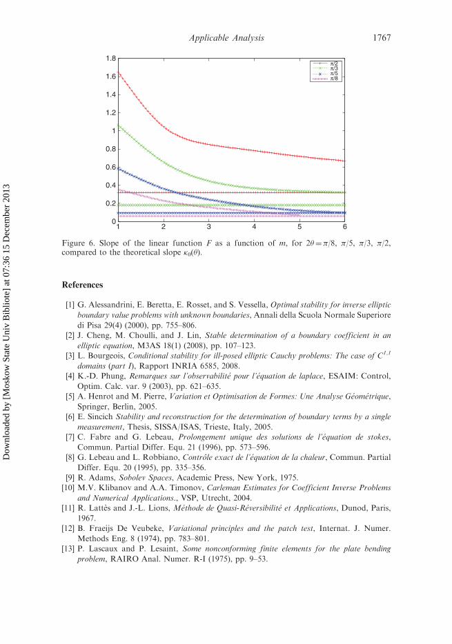
smaller angle 2� of the polygon. As can be seen in Figure 6, the slope of F is

increasing as a function of � for fixed m, as predicted by (6). More precisely, we

observe that for increasing values of m, the slope tends asymptotically to some value

which is approximately the value �0(�) given by (6), in particular for small values of �.Hence, it turns out that our estimate (31) for any �5 �0(�) (with the additional

regularity assumption (32)), which is not proved to be optimal, seems not far away

from optimality.

1

x

y

(0,0)

Γ0

Γ1

2Θ Ω

1

(0,0)x

y

Γ0

Ω

2Θ

Γ1

Figure 3. Domains � under consideration.


Dow

nloa

ded

by [

Mos

kow

Sta

te U

niv

Bib

liote

] at

07:

36 1

5 D

ecem

ber

2013

Figure 4. Exact solution Re(z3) for angle 2�¼�/3, discrepancy between the retrieved and theexact solution for �¼ 10�2, �¼ 10�4 and �¼ 10�6.

–3

–2.5

–2

–1.5

–1

–0.5

0

0.8 1 1.2 1.4 1.6 1.8 2 2.2 2.4 2.6

m=2m=3m=5

Figure 5. Function F for 2�¼�/3 and m¼ 2, 3, 5.


Dow

nloa

ded

by [

Mos

kow

Sta

te U

niv

Bib

liote

] at

07:

36 1

5 D

ecem

ber

2013

References

[1] G. Alessandrini, E. Beretta, E. Rosset, and S. Vessella, Optimal stability for inverse elliptic

boundary value problems with unknown boundaries, Annali della Scuola Normale Superiore

di Pisa 29(4) (2000), pp. 755–806.[2] J. Cheng, M. Choulli, and J. Lin, Stable determination of a boundary coefficient in an

elliptic equation, M3AS 18(1) (2008), pp. 107–123.[3] L. Bourgeois, Conditional stability for ill-posed elliptic Cauchy problems: The case of C1,1

domains (part I), Rapport INRIA 6585, 2008.[4] K.-D. Phung, Remarques sur l’observabilite pour l’equation de laplace, ESAIM: Control,

Optim. Calc. var. 9 (2003), pp. 621–635.[5] A. Henrot and M. Pierre, Variation et Optimisation de Formes: Une Analyse Geometrique,

Springer, Berlin, 2005.[6] E. Sincich Stability and reconstruction for the determination of boundary terms by a single

measurement, Thesis, SISSA/ISAS, Trieste, Italy, 2005.[7] C. Fabre and G. Lebeau, Prolongement unique des solutions de l’equation de stokes,

Commun. Partial Differ. Equ. 21 (1996), pp. 573–596.[8] G. Lebeau and L. Robbiano, Controle exact de l’equation de la chaleur, Commun. Partial

Differ. Equ. 20 (1995), pp. 335–356.[9] R. Adams, Sobolev Spaces, Academic Press, New York, 1975.[10] M.V. Klibanov and A.A. Timonov, Carleman Estimates for Coefficient Inverse Problems

and Numerical Applications., VSP, Utrecht, 2004.[11] R. Lattes and J.-L. Lions, Methode de Quasi-Reversibilite et Applications, Dunod, Paris,

1967.[12] B. Fraeijs De Veubeke, Variational principles and the patch test, Internat. J. Numer.

Methods Eng. 8 (1974), pp. 783–801.[13] P. Lascaux and P. Lesaint, Some nonconforming finite elements for the plate bending

problem, RAIRO Anal. Numer. R-I (1975), pp. 9–53.

0

0.2

0.4

0.6

0.8

1

1.2

1.4

1.6

1.8

1 2 3 4 5 6

π/2π/3π/5π/8

Figure 6. Slope of the linear function F as a function of m, for 2�¼�/8, �/5, �/3, �/2,compared to the theoretical slope �0(�).


Dow

nloa

ded

by [

Mos

kow

Sta

te U

niv

Bib

liote

] at

07:

36 1

5 D

ecem

ber

2013

[14] L. Bourgeois and J. Darde, A quasi-reversibility approach to solve the inverse obstacle

problem (Submitted).

[15] P.-G. Ciarlet, The Finite Element Method for Elliptic Problems., North Holland,

Amsterdam, 1978.

[16] C. Bernardi, Y. Maday, and F. Rapetti, Discretisations Variationnelles de Problemes aux

Limites Elliptiques, Springer-Verlag, Berlin, 2004.


Dow

nloa

ded

by [

Mos

kow

Sta

te U

niv

Bib

liote

] at

07:

36 1

5 D

ecem

ber

2013

About stability and regularization of ill-posed elliptic Cauchy problems: the case of Lipschitz...

Documents

Transcript of About stability and regularization of ill-posed elliptic Cauchy problems: the case of Lipschitz...