Aberystwyth University

Enriched ant colony optimization and its application in feature selectionForsati, Rana; Moayedikia, Alireza; Jensen, Richard; Shamsfard, Mehrnoush; Meybodi, Mohammad Reza

Published in:Neurocomputing

DOI:10.1016/j.neucom.2014.03.053

Publication date:2014

Citation for published version (APA):Forsati, R., Moayedikia, A., Jensen, R., Shamsfard, M., & Meybodi, M. R. (2014). Enriched ant colonyoptimization and its application in feature selection. Neurocomputing, 142, 354-371.https://doi.org/10.1016/j.neucom.2014.03.053

General rightsCopyright and moral rights for the publications made accessible in the Aberystwyth Research Portal (the Institutional Repository) areretained by the authors and/or other copyright owners and it is a condition of accessing publications that users recognise and abide by thelegal requirements associated with these rights.

• Users may download and print one copy of any publication from the Aberystwyth Research Portal for the purpose of private study orresearch. • You may not further distribute the material or use it for any profit-making activity or commercial gain • You may freely distribute the URL identifying the publication in the Aberystwyth Research Portal

Take down policyIf you believe that this document breaches copyright please contact us providing details, and we will remove access to the work immediatelyand investigate your claim.

tel: +44 1970 62 2400email: is@aber.ac.uk

Download date: 14. Dec. 2021

Enriched ant colony optimization and its application in feature

selection

Rana Forsati, a, 1,2

Alireza Moayedikia,a,b

Richard Jensen, c Mehrnoush Shamsfard,

a Mohammad Reza

Meybodid

a Natural Language Processing Research Laboratory, Faculty of Electrical and Computer Engineering, Shahid

Beheshti University, Tehran, Iran.

b Department of computing, Asia Pacific University, Kuala Lumpur, Malaysia.

c Department of Computer Science, Aberystwyth University, Ceredigion, Wales, UK.

d Department of Computer Engineering and Information Technology, Soft Computing Laboratory, Amirkabir

University of Technology, Tehran, Iran.

Abstract

This paper presents a new variant of ant colony optimization (ACO), called enRiched Ant Colony Optimization

(RACO). This variation tries to consider the previously traversed edges in the earlier executions to adjust the

pheromone values appropriately and prevent premature convergence. Feature selection (FS) is the task of selecting

relevant features or disregarding irrelevant features from data. In order to show the efficacy of the proposed

algorithm, RACO is then applied to the feature selection problem. In the RACO-based feature selection (RACOFS)

algorithm, it might be assumed that the proposed algorithm considers later features with a higher priority. Hence in

another variation, the algorithm is integrated with a capability local search procedure to demonstrate that this is not

the case. The modified RACO algorithm is able to find globally optimal solutions but suffers from entrapment in

local optima. Hence, in the third variation, the algorithm is integrated with a local search procedure to tackle this

problem by searching the vicinity of the globally optimal solution. To demonstrate the effectiveness of the proposed

algorithms, experiments were conducted using two measures, kappa statistics and classification accuracy, on several

standard datasets. The comparisons were made with a wide variety of other swarm-based algorithms and other

feature selection methods. The results indicate that the proposed algorithms have superiorities over competitors.

Key Words: Ant colony optimization; Feature selection; Hybrid algorithms; Swarm intelligence.

1. Introduction

Data preprocessing is a vital step to reduce the effect of noise and improve the quality of data

processing tasks, with the aim of increasing the final efficiency of the tasks. Nowadays, real

world datasets may have many irrelevant and noisy features that mislead or impede pattern

recognition resulting in the discovery of finding less meaningful or even useless patterns.

Through the use of feature selection, such problematic descriptors can be automatically detected

and removed, resulting in more reliable pattern discovery. In addition, the availability of

irrelevant dimensions in the original dataset may slow the learning process. So the reduced

processing time is another benefit of FS. For example in text categorization [1], feature selection

is used to reduce the size of word-document matrices and accelerates the categorization process

1 Corresponding author: Dr. Rana Forsati, is with the department of computer and electrical engineering, Shahid Beheshti

University, Evin, Velenjak, Tehran, Iran, r_forsati@sbu.ac.ir 2 Part of this research was done while the corresponding author was a research fellow at Minnesota University,

forsa003@umn.edu.

as just the most important dimensions are considered. Feature selection also has applications in

systems monitoring [2], where the most significant indices of the system are identified and only

those selected indices are used to check the system performance, requiring less measurement and

less computation.

In recent years many evolutionary and swarm based algorithms such as ant colony

optimization [3], harmony search [4], and particle swarm optimization [5] have been utilized

to tackle the feature selection problem. Ant colony optimization is a nature-inspired swarm-

based approach that relies on the method that ants use to identify valuable food resources. In

nature, real ants aim to find the shortest route between a food source and their nest without the

use of visual information and possess no global world model, adapting to changes in the

environment. One factor that the ants benefit from is pheromone deposition which enables them

to reach their goal gradually. Each ant probabilistically prefers to follow a direction. The

pheromone decays over time, resulting in much less pheromone on less popular paths. Given that

over time the shortest route will have the higher rate of ant traversal, this path will be reinforced

and the others diminished until all the ants follow the same, shortest path.

Ant colony optimization has been considered an effective approach for finding optimal

subsets in feature selection problems. The first ant colony optimization approach was presented

by Dorigo, and colleagues, [6], known as Ant System (AS), in which all the pheromones are

updated by all the ants which build a solution within an iteration. Another ant algorithm is Max-

Min Ant System (MMAS) by Stutzle and Hoos [7] in which the pheromone values are restricted

within a desired interval (e.g. [0, 1]) and only the global-best or iteration-best solutions are used

to update the pheromone. The problems associated with these ant colony algorithms is their

premature convergence after a certain number of iterations. To solve this problem, Ant Colony

System (ACS), another variation, was proposed by Gambardella and Dorigo [8]. Its

characteristic is that a local pheromone update is utilized to update the pheromone of the edge

after an ant traversed it. The aim of local pheromone update is to diversify the exploration of the

ants and make it possible for other parts of the solution space to be explored.

In this paper, a new variant of ACO is introduced, called enRiched Ant Colony Optimization

(RACO). In RACO, the ants are called enriched since they consider the traversals done in the

previous and current iterations. In fact the information contained in the traversals of the previous

iterations is modeled as a rich source that will guide the ants’ future path selections and

pheromone updating stages. The purpose of considering previous traversals is to deal with the

problem of premature convergence. To show the efficiency of the proposed algorithm, RACO is

applied to the task of feature selection, resulting in RACO-based feature selection (RACOFS). It

might be assumed that RACOFS suffers from the problem of inequality of selection in which

later features have higher priorities of selection compared to earlier ones. Hence in order to show

that this is not the case, RACOFS is integrated with a capability local procedure, capability

RACOFS (C-RACOFS). This feature selection algorithm is a global search that is likely to

become trapped in local optima. Although C-RACOFS performs a simple and superficial search

in the vicinity of the globally optimal subset, it does not guarantee an appropriate improvement.

Therefore it is required that the vicinity of the globally optimal solution to be searched deeply.

To this end the RACOFS algorithm is integrated with an improved local procedure; this third

variation is called Improver RACOFS (I-RACOFS). The main contributions of this paper is

summarized below:

A new variation of ant colony optimization (ACO) that utilizes an intelligent method for

selection of edges and updating the pheromone of solutions to better guide the search

process. The proposed algorithm is referred to as RACO.

An application of the proposed RACO algorithm to the feature selection problem, as one

of the most practical areas of data processing.

An integration of the RACOFS method with a local procedure to demonstrate the

capabilities of RACO in exploiting the knowledge preserved in the previous iteration

traversals.

A hybridization of RACO with an improver hybrid procedure to escape from local

optima, as one of the most prevalent deficiencies of the algorithm.

A comprehensive set of experiments on real datasets to demonstrate the merits and

advantages of the proposed method and its variations in application to the feature

selection problem.

Outline. The rest of the paper is organized as follows. Section 2 reviews some of the recent

works on feature selection that utilizes swarm-based approaches. Also some of the applications

of feature selection are reviewed. Section 3 describes the improved ant colony algorithm. In

Section 4, the improved ant colony based feature selection algorithm is discussed. Section 5

presents the data sets used in our experiments, an empirical study of parameters on

convergence on the behavior of proposed algorithms, and comparison of different algorithms.

Finally section 6 concludes the paper.

2. Literature review

Feature selection algorithms are mainly divided into three types: wrapper, filter and hybrid

approaches. The wrapper approach involves wrapping the feature selection method with a

learning model. Wrapper methods often find good subsets for a particular learning model, but

incur a high computational overhead as a result of the model construction and evaluation for

every considered subset. The filter approach is simpler in the sense that no model is constructed;

instead, an evaluation function is used to assess the subset quality. Hence, subsets found via this

approach tend to be inferior in terms of quality to wrapper algorithms while the execution of

filter algorithms is faster. The hybrid approach [9] [10] tries to benefit from the advantages of

both methods. Hybrid methods are more time consuming than both wrapper and filter

approaches, since they combine the benefits of the both algorithms. Provision of local search (i.e.

helping the algorithm to escape from local optima, and tackling the entrapment problem) as a

result of hybridization is one of the advantages of the hybridization. Feature selection algorithms

are modeled using different sorts of optimization algorithms such as swarm intelligence (SI) [11]

[12] [13] or evolutionary algorithms (EAs) [14] such as harmony search [15] [4] [16] or genetic

algorithms [17] [10]. In this section, feature selection algorithms relying on SI such as ant colony

optimization, bee colony optimization (BCO) and particle swarm optimization (PSO) are

reviewed and outlined in Table 1.

Table 1 – Outlining the reviewed papers

Paper Swarm Intelligence approach Classifier

PSO BCO ACO

Kabir and colleagues [3] √ Artificial neural network

Viera and colleagues [18] √ Fuzzy

Jensen and colleagues [12] √ C4.5

Ke and colleagues [19] √ Rule-based

Chen and colleagues [20] √ Rule-based

Forsati and colleagues [13] √ k-nearest neighbor

Wang and colleagues [21] √ Rule-based

Chuang and colleagues [22] √ k-nearest neighbor

Huang and Dun [23] √ Support vector machine

Unler and colleagues [5] √ Support vector machine

Swarm intelligence algorithms

Monirol Kabir and colleagues [3] proposed a new ACO based feature selection method. The

algorithm considers the heuristic information of each feature as filter information while neural

networks are used in the wrapper step of the algorithm. Two types of heuristic information were

used for each feature, namely random and probabilistic, which have different impacts on the

execution of the algorithm. The experiments showed promising results. Vieira and colleagues

[18] proposed a feature selection algorithm that divides the feature selection problem into two

objectives: choosing an optimal number of features and finding the most relevant features. The

experiments showed good results produced from the integration of a fuzzy model classifier and

the ACO algorithm. Jensen and Shen [12] proposed another algorithm that addresses the results

of conventional problems associated with hill-climbing for feature selection using ant colony

optimization for fuzzy-rough dimensionality reduction. Ke and colleagues [19] proposed an

algorithm that integrates ACO with rough sets. The main facets of the work were the updating

procedure of the pheromone trails of the edges connecting each pair of different attributes of the

best-so-far solution, and also limiting the pheromone values between the upper and lower trails.

As a result of solution construction and pheromone update rules, the algorithm is able to find

solutions with low cardinality quickly.

Chen and colleagues [20] proposed another feature selection method that uses rough sets

and ACO, which adopts mutual information as a heuristic for assessing the features’

significance. The method embarks from the core (i.e. essential features) and then uses mutual

information as a heuristic for feature selection. The concept of the core was first utilized in ACO

in [20] such that all the ants should start with the core at the beginning of their search, and in the

selection process those solutions near the core will be selected. Also other swarm-based methods

exist, such as bee colony optimization. Forsati and colleagues [13] utilize the bee colony

approach as one of the most recent approaches for feature selection, such that each bee produces

a partial solution randomly and then returns to the hive for subsets assessment. Ultimately, the

purpose is to find the most promising bees in finding solutions at the end of each iteration. The

algorithm uses k-nearest neighbor classification (k-NN) along with leave one out cross

validation, and outperforms some algorithms in this area.

Particle swarm optimization (PSO) [24] is an effective population-based method that has

been used for many feature selection approaches in the last few years. A rough set-based binary

PSO algorithm is proposed by Wang and colleagues [21] to perform attribute reduction. In the

algorithm, each particle represents a potential solution, and these are evaluated using the rough

set dependency degree. Chuang and colleagues [22], proposed a catfish approach that improves

the binary PSO for feature selection. In this method, catfish particles start a new search when the

global best value in PSO remains unchanged for three iterations. By directing PSO toward more

promising regions better solutions were found. Huang and Dun [23] proposed a PSO-based

feature selection method in combination with support vector machines (SVM) as the learning

algorithm. Two types of PSO were combined, i.e. discrete and continuous PSO methods, for both

performing the optimization of input feature subset selection and SVM kernel parameter setting

concurrently. For the implementation, a distributed architecture was used using web service

technology for the purpose of computational time complexity reduction. Unler and colleagues [5]

proposed a new wrapper-filter method with PSO for feature selection in which PSO is used as a

wrapper approach while mutual information is used as a filter approach. In fact, mutual

information is used for measuring both feature redundancy and feature relevancy. Their

experiments show that the algorithm is competitive in terms of computational time and

classification accuracy.

Feature selection applications

Feature selection is a field of research with many applications ranging from fraud

detection [25] and stock prediction [26] to advanced areas like knowledge-based authentication

[27] and sentiment analysis [28]. A brief overview of some of the recent applications is given

here.

Tsai and Hsiao [26] proposed a system to predict the stock price through the combination

of many feature selection methods to identify more representative variables for better prediction.

Duric and Song [28] proposed a new set of feature selection schemes, that rely on a

content and syntax model to automatically learn a set of features. The learning process is

achieved by separating the entities that are being reviewed from the subjective expressions, and

describing those entities in terms of polarities. By focusing only on the subjective expressions

and ignoring the entities, more salient features can be selected for document-level sentiment

analysis.

Chyzhyk and colleagues [29] proposed a FS algorithm that benefits from genetic

algorithms and extreme learning machines for applications in bioinformatics. The primary

feature set is extracted as a voxel selection from anatomical brain magnetic resonance imaging

(MRI). Voxel selection is provided by voxel based morphometry which finds statistically

significant clusters of voxels that have differences across MRI volumes on a paired dataset of

Alzheimer disease and healthy controls.

In another example of FS application, Chen and Liginlal [27] used a wrapper method for

knowledge-based authentication. Here, the learning machine is a generative probabilistic model,

with the objective of maximizing the Kullback–Leibler divergence between the true empirical

distribution defined by the legitimate knowledge and the approximating distribution representing

an attacking strategy that both reside in the same feature space. The experiments showed that the

proposed adaptive methods performed better than the commonly used random selection method.

Ravisankar and colleagues [25] used feature selection algorithms as a tool to identify

firms prone to financial statement fraud. Many techniques such as Multilayer Feed Forward

Neural Network (MLFF), Support Vector Machines, Genetic Programming (GP), Group Method

of Data Handling (GMDH), Logistic Regression (LR), and Probabilistic Neural Networks (PNN)

are used to perform this task. The experiments were conducted using Chinese companies and

revealed that PNN can outperform all the techniques without feature selection, while GP and

PNN did outperform other techniques with feature selection and with marginally equal

accuracies.

3. RACO: enRiched Ant Colony Optimization

The ACO algorithm [30] is a nature-inspired algorithm that simulates the natural behavior of

ants, including mechanisms of cooperation and adaptation. This algorithm has been shown to be

both robust and versatile, in the sense that it has been applied successfully to a range of different

combinatorial optimization problems. In this section we propose a new ant colony algorithm,

known as enRiched Ant Colony Optimization (RACO).

In the baseline ant colony optimization approaches, such as ant system, min-max ant system

and ant colony system, the algorithms do not consider previously traversed edges and their

pheromone values as a resource to guide future movements. In this paper, a new variation is

proposed that considers the previous traversals as a rich source of information, to guide the

explorations of the solution space to generate diverse solutions. Diversification of solutions can

be achieved by increasing the exploration and exploitation abilities of the ants. To this end,

during the local and final pheromone updates, the traversals of the current iterations are not only

considered, but also previously traversed edges to adjust pheromones of the edges. This

hypothesis is implemented through introducing the concentration rate that indicates the extent to

which the algorithm should concentrate on the previously traversed edges or the traversals of the

current iteration.

Figure 1 shows the stages of the algorithm that benefit from the information from traversals.

Here, the algorithm uses two datasets of current and previous traversals. Different stages of the

algorithm benefit from these stored data. In the selection stage, the ants consider the previous

tours taken by ants to select an appropriate edge. In the local pheromone update phase, the

databases are used to lay an appropriate pheromone value on the edge and finally in the final

pheromone stage the traversals information is used for the global update of the edges. The

interactions with the previous traversal database is unidirectional in the sense that the ants are

only allowed to use the previous traversals’ information without manipulating them, while the

current database traversals can be either read from or manipulated by the ants, in the sense that

the pheromone in the current database can be updated. After finishing the current iteration, the

data that resides in the current traversal database will be added to the previous traversals’

database.

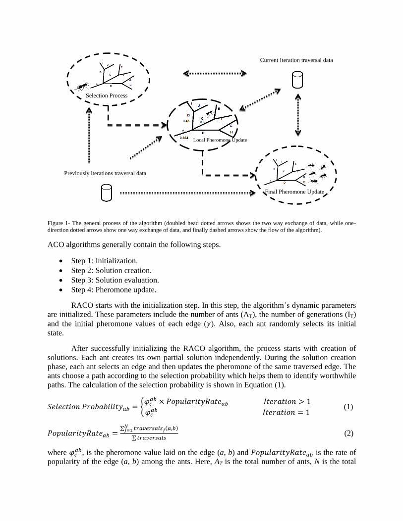
Figure 1- The general process of the algorithm (doubled head dotted arrows shows the two way exchange of data, while one-

direction dotted arrows show one way exchange of data, and finally dashed arrows show the flow of the algorithm).

ACO algorithms generally contain the following steps.

Step 1: Initialization.

Step 2: Solution creation.

Step 3: Solution evaluation.

Step 4: Pheromone update.

RACO starts with the initialization step. In this step, the algorithm’s dynamic parameters

are initialized. These parameters include the number of ants (AT), the number of generations (IT)

and the initial pheromone values of each edge ( ). Also, each ant randomly selects its initial

state.

After successfully initializing the RACO algorithm, the process starts with creation of

solutions. Each ant creates its own partial solution independently. During the solution creation

phase, each ant selects an edge and then updates the pheromone of the same traversed edge. The

ants choose a path according to the selection probability which helps them to identify worthwhile

paths. The calculation of the selection probability is shown in Equation (1).

(1)

(2)

where , is the pheromone value laid on the edge (a, b) and is the rate of

popularity of the edge (a, b) among the ants. Here, AT is the total number of ants, N is the total

Previously iterations traversal data

Current Iteration traversal data

Selection Process

Final Pheromone Update

Local Pheromone Update

number of ants that have traversed edge (a, b), is the total number of

traversals that include edge (a, b), and finally is the total number of traversals by

the ants. We try to measure how many ants have traversed the edge (a, b) in proportion to the

total traversals, within the current and previous traversals. The more the edge (a, b) is selected its

selection probability increases. Merely considering popularity rate will not help to prevent

premature convergence, and on the other hand will encourage ants to select edges that are

selected frequently. Therefore the current pheromone of the edge (a, b) should be

considered to reflect the importance of the edge in comparison to its neighbors and generally in

the solution space, to measure how useful an edge is. For example, in the calculation of the

probability of selection of the edge (b, c), if in total the ants have traversed 183 edges so far and

the edge (b, c) has appeared 27 times in their traversals, then the popularity rate will be 0.147.

This value multiplied by the previously laid pheromone value of the edge will give the selection

probability. Equation (2) requires the availability of previous traversals information, while in the

first iteration (Iteration =1 as shown in Equation 1) this information is not available. Therefore

in the first iteration, the ants choose the edges according to pheromone values only.

Equation (1) would make the selection of the edges strongly dependent on the initial

pheromone values, in the sense that an edge with initially high pheromone will have high

probability of selection in future traversals, and consequently will lead to premature

convergence. Hence a local pheromone update is required to increase the exploration ability of

the ants and prevent premature convergence. Equation (3) is the local pheromone update policy:

(3)

where and

is the current pheromone value and the new pheromone value of the edge (a,

b) and is defined according to Equation (4). The purpose is to decrease the probability of

selection of the frequently traversed edges, and consequently increase the exploration ability.

Hence the pheromone value of an edge with high rate of traversals should be reduced.

(4)

Here, and (or and ) are the number of traversals involving

(a, b) and total traversals within the current iteration (or the number of traversals involving (a, b)

and total traversals within the previous iterations), respectively. To analyze Equation (4), by

increasing the difference between and (or and ) the logarithm

parameter becomes larger, which indicates that the edge (a, b) has been visited less than other

edges. Therefore the edge is prone to be visited more, and more pheromone should be laid on it.

In contrast, if the difference becomes lower, the pheromone value should be decreased. This fact

will increase the ability of the ants to explore the solution space. However an exceptional case

occurs when N(s) = Nab(s); for instance, when the first ant in the first iteration traverses the first

edge, while by increasing the number of traversals, N(s) and Nab(s) will no longer be equal. In

this case since the logarithm’s input is one. Also in the first iteration the traversals of the

current iteration and the previous traversals are the same (i.e. N ).

The parameter is the concentration rate which plays the role of the

pheromone decay coefficient, and is a variable which identifies the extent to which the algorithm

should focus on within-iteration traversals or total traversals of the previous iterations. The

higher this value is, the more emphasis there will be on the current iteration’s traversals. As all

the ants created their solutions, the quality of each solution should be checked. This assessment

can be done using a given fitness function that satisfies the algorithm’s objective.

The last step of the ant colony algorithm is the final pheromone update in which all the

ants are allowed to update only the edges that they have traversed, but the effects of their updates

on the same edge are not identical. In simpler terms, those ants with a higher value of fitness fx,

can increase the pheromone of the edge (a, b) (if this edge is included in their traversal) more

than those ants that have traversed this edge but their fitness is lower than fx. To implement this

idea we propose a final pheromone equation which involves three main parts:

(5)

As shown in Equation (5) the final pheromone of an edge indicates its relative importance

in the solution space. Hence, three factors can influence the pheromone value of an edge. The

more an edge is popular, the more useful it is. Therefore the popularity rate of an edge should be

measured as explained in Equation (2). In addition, the frequency of selection does not

necessarily mean high importance, since frequent traversals of an edge might lead to poor results.

Therefore the level of contribution of a given edge (a, b) towards the fitness function should be

taken into account to accurately adjust the pheromone values. The is the

average of the fitness values of those ants that have the edge (a, b) in their traversal, normalized

by dividing by the total fitness. The aim is to measure the contribution of the edge (a, b) by

looking at the fitness values of the ants.

(6)

Here, AT is the total number of ants and N is the total number of ants that have traversed edge

(a, b). is the fitness value of the ant that has edge (a, b) in its traversal, and is the fitness

value of the i-th ant. If the frequency of selection of an edge leads to poor results, then the ants

having this edge in their traversals will mostly have low fitness values on average, and finally

will lead to a lower contribution rate.

To reflect the importance of an edge in comparison to other edges in the solution space, the

average of the pheromone values assigned to an edge is considered. In fact, if an edge is

significant in comparison to its neighborhood edges, its average is higher than the others, and

consequently the pheromone value increases. In the local pheromone value update, the aim is to

reduce the pheromone of the frequently visited edges, while increasing the pheromone value of

the rarely visited edges, to increase the exploration ability. In the final pheromone update the aim

is to increase the pheromone of the worthwhile edges to increase the exploitation ability of the

ants.

(7)

Equation (7) calculates the average of the changes made in the pheromone values of the edge

(a, b) during the g-th iteration. The higher the value of AverageWeights, the more pheromone

will be laid on the edge (a, b). In Equation (7), is the local pheromone value

that was laid on edge (a, b) in the g-th generation when the u-th ant traversed it, and N is the

number of ants that have edge (a, b) in their traversals.

4. Feature selection with RACO

In this section we propose a new RACO-based feature selection method, RACOFS. In this

algorithm, solutions are encoded as a string of serial bits of 0s and 1s, in which 1 indicates a

selected feature and 0 an ignored feature. For instance, Figure 2 shows that the first, sixth and the

seventh features are selected, and the other features are unselected.

1 0 0 0 0 1 1 Figure 2- Solution representation

The first step is the initialization of the algorithm. In the initialization stage the number of

ants and iterations are chosen by the user. Then each ant is randomly assigned to a number

between 1 and F as its initially selected features, in which F is the total number of features.

Additionally, the pheromone on each edge is initialized randomly.

Algorithm 1: Selection probability rule

Input:

Initially selected feature of an ant

Output:

Created solution of an ant

Algorithm:

while true Generate a probability number Pn using selection probability equation

Select the edge with smallest pheromone that is bigger than, Pn

if the selected edge leads to the last feature Select the last feature;

break;

else

Select the feature;

end if

if the selected edge leads to feature F-1

Generate a probability number Pl using selection probability equation

if Pl is bigger than the pheromone of the edge leading to feature F

Select the last feature. break;

end if

end if

end while

Using the selection probability relation (Equation 1), the ants will select their next feature

to select. In order to prevent from some common mistakes such as a non-stop loops of traversal

and edge selection, in this algorithm if an ant chooses the i-th feature, it then cannot choose the j-

th feature if j<i. If the selected feature’s number does not make it possible for the ants to proceed

further (i.e. one before the last feature is selected), then no further movement is allowed; that is

the point the solution construction for the i-th ant is completed and the solution should be

evaluated.

The problem occurring in this type of selection is that in most cases, the last feature can

be selected if the feature F-1 is also selected. Therefore if the number of the currently selected

features is equal to F-1 then the last feature is selected only if the selection probability value is

bigger than the pheromone connecting the two last features to each other. Algorithm 1 shows the

selection probability rule of the algorithm. After traversing an edge, the local pheromone value is

updated according to the local pheromone update policy (Equation (3)). Finally after the

generation of each solution by each ant, the solutions must be assessed to identify their goodness.

The last stage is the local pheromone update in which the edges connecting features are updated

based on the final pheromone rule discussed in Equation (5). Since the outcome of selection

probability of each edge is a number within the interval [0,1] it is likely that the deposited

pheromone will become greater than 1 during the pheromone update stages. To overcome this

problem the pheromone value of each edge is normalized; the pheromone values on each edge

that connects a parent to its children should sum to one. The algorithm iterates for IT number of

iterations. The complete process of RACOFS is shown in Algorithm 2.

Algorithm 2: RACOFS

Input:

Number of iterations and ants

α value

Output:

The best ant in terms of fitness

Algorithm:

while G number of iterations are not finished

Initialize the ants’ first movement.

foreach ant in the i-th iteration

Select the next feature according to selection probability rule

Update the pheromone laid on the last traversed edge using local pheromone update rule Apply the pheromone normalization step

if further movement for the i-th ant is impossible

Assess the fitness for the generated solution.

end for

Apply final pheromone update

Apply the pheromone normalization

end while

4.1. Hybrid algorithms

It might be assumed that RACOFS suffers from an inequality of selection in the sense that

the first features have a lower probability of selection while the later features will have higher

priorities. Hence, a local procedure is integrated with RACOFS to:

Evaluate this assumption of inequality of selection.

Show that the reliance on previous traversals is effective to distinguish relevant and

irrelevant features to improve the quality of the solutions.

Since the primary aim of using this hybrid procedure is to show the capability of

RACOFS this variation is called capability RACOFS (C-RACOFS). According to Algorithm 3,

in C-RACOFS after the generation of a solution all the features are tested to see if there is an

improvement in subset quality by their removal or addition. A selected feature will be changed

temporarily to an unselected one, while an unselected feature is changed temporarily to a

selected one. If the fitness of this solution is better than the fitness of the older solution, then the

new solution will replace the older one. The aim is to determine if RACOFS has included or

excluded a feature mistakenly in the final subset.

Algorithm 3: C-RACOFS

Input:

A set of solutions created by the ants

Output:

Improved set of solutions

Algorithm:

foreach solution created by each ant

foreach feature

if the feature is not selected Change it to a selected one;

Assess the fitness of this new solution Sn;

if the Sn is better than the older solution Sd Replace Sn with Sd;

else

Change it to a selected one; Assess the fitness of this new solution Sn;

if the Sn is better than the older solution Sd

Replace Sn with Sd;

end if

end for

end for

Figure 3 - C-RACOFS graphical illustration

The capability hybrid algorithm should not be considered as a greedy search algorithm. For

greedy search algorithms, in a solution space with the size of n, there will be 2n number of

different combination of the features, and correspondingly 2n number of different solutions,

while in this hybrid algorithm for a solution with n number of features, n+1 number of different

solutions is available (including original solution). As shown in Figure 3, each

selected/unselected bit is changed to an unselected/selected one.

Ant colony optimization is effective in performing global search and finding the approximate

region of the globally optimal solution, but suffers from entrapment in local optima. Therefore its

hybridization with a local search procedure is inevitable, to improve the final results. According

to Figure 3, if the original solution is considered as globally optimal, then changing the bits

iteratively to check further improvements would be a kind of superficial local search in the sense

that a small vicinity of the globally optimal solution is searched for possible improvements.

However this type of local search is superficial and does not guarantee to be applicable enough.

Therefore RACOFS should be integrated with another local search procedure which not only

searches deeper vicinities of the globally optimal solution, but also ensures superiority over

RACOFS and C-RACOFS.

The algorithm ImprovementProcedure, as shown in Algorithm 4, is another local search

algorithm that is applied to RACOFS that ensures better search around a good solution. This

local search procedure is also applied to GA-based feature selection [10] and showed good

performance in improving solutions produced by simple genetic algorithms. Hence this local

search is applied to RACOFS and named as Improver RACOFS (I-RACOFS) since it aims at

improving RACOFS.

I-RACOFS heavily depends on the atomic operations of ripple_rem(r) and ripple_add(r) and

a prespecified subset size (d), for its execution. The ripple_rem(r) operation removes r number of

least significant features and adds r-1 of the most significant features. On the other hand

ripple_add(r) adds r of the most significant features while removing the r-1 least significant

features. The procedure of adding and removing iterates until the condition |X| = d is met. In

Algorithm 4, three scenarios might occur:

Scenario 1(|X|=d): Then ripple_add(r) and ripple_rem(r), will add r of the most

significant features and remove r of the least significant features, respectively.

Scenario 2(|X|>d): ripple_rem removes r of the least significant features, while

ripple_add removes r-1 of the most significant features.

Scenario 3(|X|<d): ripple_add adds r of the most significant features, while ripple_rem

removes r-1 of the least significant features.

A feature is least significant if the level of its contribution toward the quality of solution in

comparison to other features is low (i.e. by removing the feature from the original subset the

quality of the solution does not decrease much). A feature is most significant if the level of its

contribution toward the quality of solution in comparison to other features is high (i.e. by

removing the feature from the original subset the quality of the solution decreases).

Algorithm4: ImprovementProcedure

Input:

A solution, Gsol Ripple factor: r.

Desired subset size, d.

Output:

A locally improved solution.

Algorithm:

Put selected features of solution S in the set X

Put unselected features of solution S in the set Y

if |X| = d

Select r of the most significant feature from the set Y

Remove r of the least significant features from the set X if |X| > d

while |X| and d are not equal Select r-1 of the most significant feature from the set Y

Remove r of the least significant features from the set X

end while

end if

if |X| < d

while |X| and d are not equal Select r of the most significant feature from the set Y

Remove r-1 of the least significant features from the set X

end while

end if

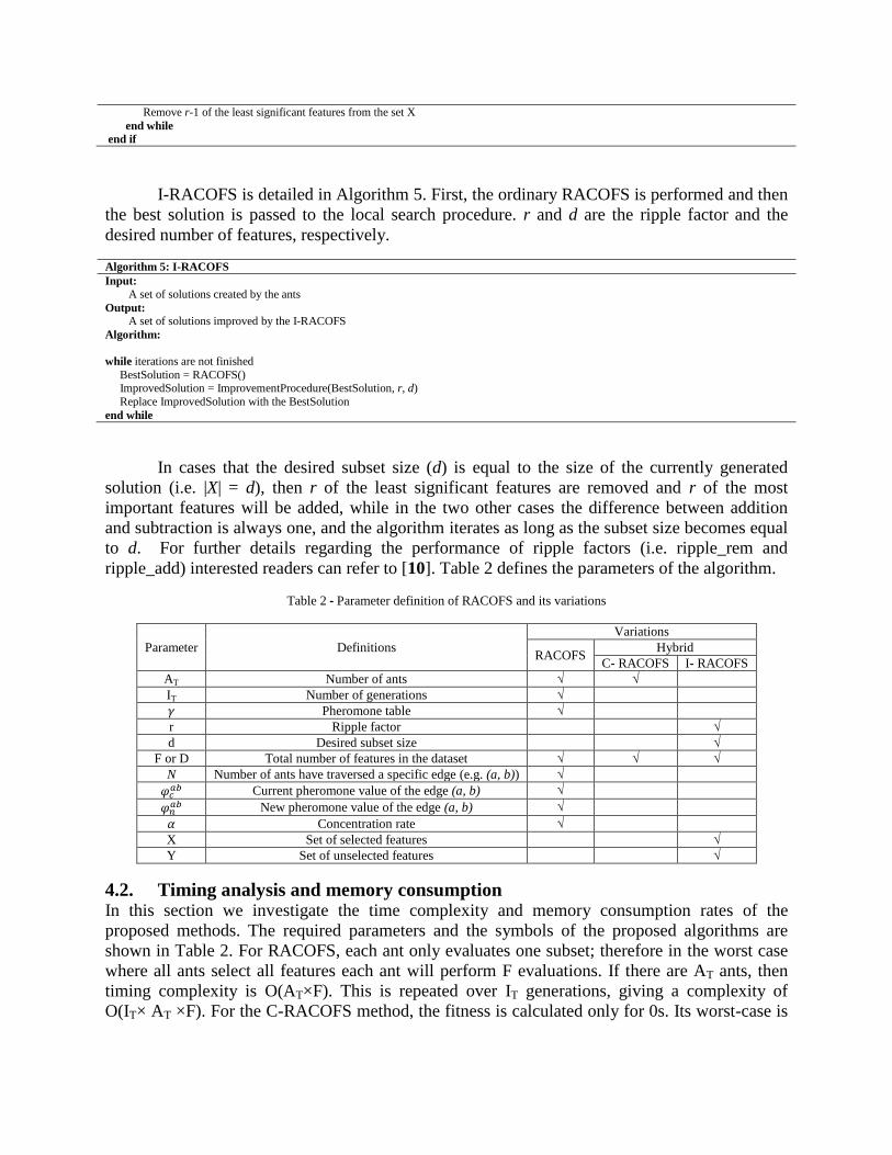
I-RACOFS is detailed in Algorithm 5. First, the ordinary RACOFS is performed and then

the best solution is passed to the local search procedure. r and d are the ripple factor and the

desired number of features, respectively.

Algorithm 5: I-RACOFS

Input:

A set of solutions created by the ants

Output:

A set of solutions improved by the I-RACOFS

Algorithm:

while iterations are not finished

BestSolution = RACOFS() ImprovedSolution = ImprovementProcedure(BestSolution, r, d)

Replace ImprovedSolution with the BestSolution

end while

In cases that the desired subset size (d) is equal to the size of the currently generated

solution (i.e. |X| = d), then r of the least significant features are removed and r of the most

important features will be added, while in the two other cases the difference between addition

and subtraction is always one, and the algorithm iterates as long as the subset size becomes equal

to d. For further details regarding the performance of ripple factors (i.e. ripple_rem and

ripple_add) interested readers can refer to [10]. Table 2 defines the parameters of the algorithm.

Table 2 - Parameter definition of RACOFS and its variations

Parameter Definitions

Variations

RACOFS Hybrid

C- RACOFS I- RACOFS

AT Number of ants √ √

IT Number of generations √

Pheromone table √

r Ripple factor √

d Desired subset size √

F or D Total number of features in the dataset √ √ √

N Number of ants have traversed a specific edge (e.g. (a, b)) √

Current pheromone value of the edge (a, b) √

New pheromone value of the edge (a, b) √

Concentration rate √

X Set of selected features √

Y Set of unselected features √

4.2. Timing analysis and memory consumption In this section we investigate the time complexity and memory consumption rates of the

proposed methods. The required parameters and the symbols of the proposed algorithms are

shown in Table 2. For RACOFS, each ant only evaluates one subset; therefore in the worst case

where all ants select all features each ant will perform F evaluations. If there are AT ants, then

timing complexity is O(AT×F). This is repeated over IT generations, giving a complexity of

O(IT× AT ×F). For the C-RACOFS method, the fitness is calculated only for 0s. Its worst-case is

O(IT× AT ×F+IT×F×F), for each feature 0 appearing in the solution (worst case F), then the

subset is re-evaluated (taking F time).

The general timing analysis for I-RACOFS operator is difficult, as it is unknown how

many 0s will appear in any given subset. The worst case is where all bits are 0. We know that for

a subset of size s, (F-s) bits will be zero, so the fitness is evaluated (F-s) times. Also, for I-

RACOFS, the local search only considers the addition of single features, by considering feature

elimination the worst-case complexity would be the same, though it would take a bit more time

on average. But I-RACOFS differs from the others. In Algorithm 3 the subset size should be

known prior to timing analysis. Some papers [10] have used big-O or number of subset

evaluations, but they are not helpful because subsets with different sizes may produce different

amounts of time computation.

Since the proposed algorithms rely on the previous traversals in the previous iterations,

some discussions regarding the memory consumption rates might be necessary. Considering a

solution space with the size of F, there will be

number of edges connecting each node to

all other nodes in the space. If preservation of each pheromone value consumes M bytes of

memory, then the total memory consumption that preserves the information of a given iteration

will be

bytes. Consequently for IT number of generations the memory consumption

rate will be

. IT and M are constant values hence the memory consumption will

be highly dependent on F, the number of features in a dataset.

5. Experimental results and discussions

In this section the proposed algorithms are evaluated and compared with a wide range of

the other state-of-the-art algorithms. We compare our work with a wide range of other related

works, such as swarm intelligence algorithms including ant colony optimization algorithms

implemented as feature selection such as [6] [7] [8] [31], and other swarm-based feature

selection algorithms including bee colony [13], PSO [5] and ant colony [3]. In [3] the authors

have proposed two variations, random and probabilistic, and these two variations in this paper

are named as ACOFS-R, and ACOFS-P, respectively. Also comparisons with other non-swarm

algorithms are made, such as genetic [10] and the baseline FS algorithms.

Two well-known measures of classification accuracy (CA) and kappa statistics (KS) are

used to show the inferiorities and superiorities of the proposed works. CA is introduced in

Equation 8, where TotalSamples is the number of instances in the dataset and, correctly

classified samples are the number of samples whose class was predicted correctly.

(8)

The other measure used is the kappa statistic [32], which is a prevalent statistical measure

that models the performance and allows for input sampling bias. This measure has been used in

many feature selection methods e.g. [33], [5], [34], etc. The aim of using this measure is to

assess the level of agreement between the classifier’s output and the actual classes of the dataset.

The kappa statistic can be calculated as follows:

(9)

(10)

(11)

where N is the total number of samples and Ni is the number of samples in a data set which are

correctly classified by the classifier. In Equation (10), Ni* is the number of instances recognized

as class i, by the classifier and N*i is the number of instances belonging to class i in the dataset.

The purpose is to maximize this measure. Finally kappa can be measure as Equation (11) in

which , kappa = 0 and kappa = 1, means there is not agreement between classifier

and the actual classes, and perfect agreement on every example, respectively. In the rest of this

section the datasets are introduced then some experiments are done which justifies the selection

of the classifier. The hybridization parameters of ripple factor (r) and the desired subset size (d)

are tested to investigate the effects of these parameters on searching the solution space and

generally on the behavior of the proposed variations. Comparisons and the timing analysis of the

proposed algorithms constitute the last two subsections.

5.1. Datasets

The used datasets are shown in Table 3. All of the datasets were downloaded from the

UCI Machine Learning Repository3. Based on the categorization by UCI, datasets are divided

into three categories of small (dimension equal to or smaller than 10), medium (dimension

between 10 and 100) and large (dimension equal to or greater than 100). The first three columns

are related to the datasets description, while the last three columns outline the size and

dimensions of the datasets. The middle column, concentration rate, indicates the extent to which

the proposed algorithms relied on the traversals of the current iteration. This parameter is fine-

tuned for each dataset separately.

Table 3- UCI datasets

Category type Dataset Symbols Concentration

rate (α) # samples # features # classes

# features ≤10

(Small)

Monk1 MK1 0.15 124 6 2

Monk2 MK2 0.05 169 6 2

Post-Operative PO 0.05 90 8 2

BreastCancer BC 0.2 699 9 2

Glass GL 0.5 214 10 7

Vowel VW 0.1 990 10 11

10 < # features< 100

(Medium)

Wine WI 0.95 178 13 2

Zoo ZO 0.25 101 17 10

Horse HR 0.85 368 27 2

Ionosphere IO 0.25 351 34 2

Soybean-Small SS 0.05 35 47 4

Sonar SO 0.55 208 60 2

# features ≥100 (Large)

Arrhythmia ARR 0.02 452 279 16

Hill-Valley HV 0.02 606 101 2

3 http://archive.ics.uci.edu/ml/datasets.html.

5.2. Classifier performances

In this section some experiments are carried out using RACOFS variations to show the

effectiveness of k-NN for our algorithms. One of the reasons behind the utilization of k-NN is the

type of datasets that have been used. As we have conducted our experiments on datasets having

more than two class labels, k-NN in such cases would be reasonable, easier and of higher utility

compared to other classifiers such as support vector machine, as SVM classifiers utilization for

samples having more than two class labels is intractably difficult. The use of other types of

classifier (e.g. CART) does not seem reasonable, as these rely on a training process to construct

the classifier, to then be able to classify test samples. In this example, some datasets that are

intrinsically divided into two disjoint groups of train-test (e.g. MK1, MK2 and HV) might

benefit from CART. The naïve Bayesian classifier (or simply Bayesian) can be seen as another

suitable classifier. Hence its performance is tested against k-NN in three datasets of BC, HR and

HV; each representing a category of small, medium and large datasets, respectively. The

performance comparisons are made in terms of accuracy and timing execution, under similar

conditions as outlined in Table 4.

Figure 4 compares the k-NN and Bayesian classifiers in terms of classification accuracy.

The testing conditions, in terms of the number of ants and iterations are the same for both

classifiers, while in the Bayesian classifier we used the equiprobable partitioning technique [3]

[35] for data partitioning. According to the experiments illustrated in Figure 4, k-NN classifies

the samples better than the Bayesian classifier in all three categories. The inferiority of the

Bayesian approach could be as a result of the data partitioning stage, as partitioning makes the

data more general, resulting in a loss of useful information, while k-NN considers the actual,

unchanged, data during classification.

Figure 4 – k-NN and naïve Bayesian comparisons on three representative datasets in terms of accuracy

The other comparison criterion is the execution time. In Figure 5, the aim is to show the

execution time of k-NN and naïve Bayesian classifiers for different subset sizes, using a 2-class

dataset. Theoretically, by increasing the number of instances of a dataset, the k-NN execution

time increases. Also, k-NN relies on the distances between samples (e.g. Euclidean distance) for

classification. Hence increasing the number of available dimensions (features) of the dataset

prolongs the distance measurement calculation time. Therefore, the k-NN execution time

30

40

50

60

70

80

90

100

BC HR HV

Acc

ura

cy (

%)

Datasets

k-NN NaiveBayesian

depends on the subset size and the number of instances. Bayesian classifiers also can be affected

by the number of instances of the dataset, but do not use any distance measure in the

classification process. Hence the use of a distance function prolongs the execution of k-NN

compared to naïve Bayesian, but assures better results.

Figure 5 – Timing analysis of k-NN and Bayesian classifiers in a 2-class dataset for different subset sizes

Hence k-NN is used as the main classifier. However fine-tuning of the parameter k, is

necessary. In Figure 6, some experiments are carried out to study the effects of this parameter.

As expected, by increasing the number of neighbors the accuracy of classification increases. This

behavior stems from the fact that increasing the value of k would prevent over-fitting to a certain

extent.

In this paper the value of k has been set to 1 in order to have a fair and consistent

comparison with the literature [13] [10]. In datasets that are intrinsically divided into two sets of

training and testing such as MK1, MK2 and HV the experiments were carried out in this form

with 1-NN as classifier, instead of LOOCV and k-NN, in which k=1.

Figure 6 - Studying the effects of parameter k in k-NN classifier on three representative datasets

0 200 400 600 800

1000 1200 1400 1600 1800

5 10 15 20

Exec

uti

on T

ime

(mil

lise

cond

s)

Subset size

k-NN Bayesian

30

40

50

60

70

80

90

100

1 5 10 15 20 25 30

Acc

ura

cy (

%)

k (number of neighbours)

BC HR HV

5.3. Effects of hybridization parameters

In Figures 7 to 9, the effects of the ripple factor (r) and the desired subset size (d) are

tested. The proposed hybrid algorithm of I-RACOFS relies heavily on these two parameters.

Therefore in this section, some experimentation is given to show the effects of increasing or

decreasing the ripple factor and the desired subset size on the algorithms behavior, using three

deliberate datasets of SO, HR and HV. The appropriate values of r in all the datasets are 1, 2, 3

and 4, and for d = D/5, 2D/5, 3D/5 and 4D/5, as used in [10]. Ripple factors cannot be applied

when r>d [10].

Figure 7 - The effect of ripple factor for the HR dataset

Figure 8 - The effect of ripple factor for the SO dataset

74

75

76

77

78

79

80

81

82

1 2 3 4

Acc

ura

cy (

%)

Ripple Values (r)

d=6

d=12

d=18

d=24

92

92.5

93

93.5

94

94.5

95

95.5

1 2 3 4

Acc

ura

cy (

%)

Ripple Factor (r)

d=12

d=24

d=36

d=48

Figure 9 - The effects of ripple factor for the HV dataset

Ripple factor affects the fitness value of a solution.

This point indicates that the ripple factor makes the search in the local optima stronger

that would lead to improved fitness value. However this may not be the case for all datasets and

depends on the dataset characteristics like number of dimensions or instances. For instance in

Figure 8, when d=24 the fitness for r=3 is around 94% while the same rate of accuracy was

preserved for higher amounts of ripple factor (e.g. r=2, 3 and 4).

Always increasing/decreasing the subset size and ripple factor is not effective.

For example, in Figure 7, the best result is obtained when d=12 and r=4. But when the

value of d is too small (e.g. d=6) or too large (e.g. d=24), the ignored or added features have

negative effects on the classification accuracy, in the sense that the newly added or ignored

features will decrease the accuracy. The solution space size can affect the selection of ripple

factor as well. The selection of the value of the ripple factor is critical in the sense that choosing

low rates for this would decrease the searching ability of the hybrid procedure while very high

values of the ripple factor results in a time-consuming algorithm. Therefore it is likely that in

solution spaces with low dimensions, small values of r lead to an algorithm with satisfactory

results, while by increasing the size of the solution space, it is less likely to reach an optimal

solution when r is small. Similarly for datasets with high numbers of features like datasets with

size greater than 100 (Figure 9), it is needed to define larger subset sizes (e.g. 3D/5 or 4D/5),

while in small or medium-sized datasets, the selection of a low subset size (e.g. D/5 or 2D/5)

would help to attain to an optimal solution.

Effects on convergence criterion.

The higher the ripple value is, the sooner the algorithm converges. The convergence of an

ordinary global search algorithm would take place after many iterations, while in this hybrid

algorithm the convergence to the optimal result would be faster with a suitable ripple factor.

5.4. Comparisons

52 53 54 55 56 57 58 59 60 61

1 2 3 4

Acc

ura

cy (

%)

Ripple Factor (r)

d=20

d=40

d=60

d=80

In this section of the experimental results, the performance of the proposed algorithms is

compared to some of the most recent swarm intelligence algorithms, proposed either for FS or

non-FS tasks. The comparisons are divided into two sections. In the first subsection, swarm-

based algorithms are compared, and the second section contains some comparisons with genetic

and baseline feature selection algorithms. Parameters of the implemented algorithms are set

according to Table 4.

In all algorithms the number of ants and iterations are set to the ones used in this

algorithm (RACOFS). The algorithms were tested in ten independent executions for justifiable

comparisons. In BCOFS [13], the number of constructive steps (NC) has different values based

on the dimensions of the dataset. NC for small datasets is D/3, and for medium and large datasets

NC is equal to D/5 and D/10, respectively.

Table 4- Parameter setting of the implemented algorithms4

Algorithms Parameter settings

Proposed

Algorithms

RACOFS IT = 10, AT = 100, = randomly between 0 and 1.

C-RACOFS

I-RACOFS IT = 10, AT = 100, d=based on the dataset size, r [1-4]

Baseline ACO

Algorithms

AS

Iterations = 10, ants = 100, pheromone decay coefficient = 0.1, evaporation_Rate = 0.3, q =3, ῤ = 0.7,

α=1 , β=3.

MMAS Iterations = 10, ants = 100, pheromone decay coefficient = 0.1, evaporation_Rate = 0.3, min_pheromone

= 0.5, max_pheromone = 1, q =1, ῤ = 0.9, α=1 , β=3.

ACS

Iterations = 10, ants = 100, pheromone decay coefficient = 0.1, evaporation_Rate = 0.3, q =1, ῤ = 0.9,

α=1 , β=3.

Recent ACO

Algorithms

TSIACO1 α=1 , β=6 , r=5, = 0.999, =0.001 , m1 = 0.15, m2=1, ῤ1 = 0.01, ῤ2=0.03.

TSIACO2 α=1 , β=6 , r=5, = 0.999, =0.001 , m1 = 0.15, m2=0.5, c1=0.9, ῤ1 = 0.002, ῤ2=0.03.

ACOFS-R α=1,

ACOFS-P

BCO BCOFS Bees = 100, iterations= 10, NC = depends on the dataset size

5.4.1. Swarm-based comparisons

In this section we compare the proposed RACOFS algorithms with the ant and bee

colony algorithms proposed in [31] and [13] respectively. The comparisons reveal significant

superiorities over competitors. In Tables 5, 6 and 7, the results are shown in the form of x-y(z),

where x, y and z are the average of CA, KS values and the subset size of the best solution,

respectively.

In Table 5, the comparisons are made for small datasets. Ant colony comparisons are

divided into two types of baseline [6], [7], [8] and recently proposed variations [31] [3] in which

the algorithms are implemented as feature selection algorithms while the other ant-based feature

selection method [3] was implemented and tested in more datasets, using LOOCV and 1-NN.

BCOFS [13] is our previously proposed algorithm.

For the MK1 and MK2 datasets I-RACOFS compared to two other variations of

RACOFS and C-RACOFS could not show satisfactory results, as it ignored an optimal subset

4 For the implemented algorithms the parameter settings were done based on the settings proposed in the reference papers (except number of ants

and iterations), while baseline algorithms were fine-tuned to the most optimal results.

size gained by RACOFS and C-RACOFS. In the MK 1 and MK2 datasets, the optimal subset

sizes are three and six, respectively. For these datasets RACOFS is also superior to other

algorithms of ant colony and bee colony as compared in Table 5.

For the PO dataset, the performances of I-RACOFS and RACOFS are the same for d=2,

while by increasing the desired subset size in I-RACOFS the performance deteriorates. Also

RACOFS could outperform other variations of ant colony but was inferior to BCOFS. For the

BC dataset, the best result in terms of CA was gained by RACOFS with the size of four, while I-

RACOFS could outperform other variations when d=4, in terms of the KS measure. For the GL

dataset the proposed variations did outperform the competitors. For the VW dataset, in the

proposed variation the best result was gained by RACOFS with the size of eight. However this

algorithm did not outperform baseline ant algorithms. In I-RACOFS other variations, except

baseline ACOs, are outperformed in terms of the KS measure only.

Determination of the desired subset size would be one of the most important factors of

inferiorities of I-RACOFS over the other variation, while in some datasets for specified values of

d and r, I-RACOFS outperformed the competitors. Also, the partial reliance of RACOFS on

previous traversals would be the most prominent factor leading to the algorithm’s superiority

over its competitors.

In Table 6, the proposed variations are compared with other swarm-based algorithms for

medium-sized datasets. In RACOFS experiments in the WI dataset, RACOFS and its variations

could not show any superiority over other algorithms and it is likely that the variations in this

dataset suffer from the classifier settings of the proposed algorithm, as RACOFS uses k-NN with

k=1, while this dataset may require k>1. In the ZO dataset, RACOFS is superior over the

competitors in terms of both CA and KS measures.

In the HR dataset, I-RACOFS outperformed all other algorithms, including RACOFS and

C-RACOFS, when d=12 and r>2. In the SS dataset, the results of the algorithms are the same

while the differences are in the subset sizes, in which RACOFS is better. In two other datasets,

IO and SO, the hybridization is more significant. I-RACOFS could improve both variations of

RACOFS and C-RACOFS in the SO and IO datasets. The competitors were outperformed by

either RACOFS or I-RACOFS in terms of CA and KS measures.

The proposed variations in general have a significant superiority over the competitors,

including ant colony and bee colony based algorithms. This superiority was gained as a result of

the proportional reliance of the algorithms on the previous traversals of the ants that increases

their abilities in exploring and exploiting the solution space. Also, the hybridization of RACOFS

with the local improver procedure becomes more significant as the dataset size (i.e. number of

features) grows and additionally, poor results for the WI dataset requires that the experiments to

be carried out on this dataset with k>1.

Table 5- Ant and bee colony comparisons on small datasets using CA and KS measures (all the units are in %).

BC

OF

S

50

-

49.9

(2)

67.1

- 67

(4)

68

- 68

(4)

85.3

-

85.4

(5)

100

-

100

(4)

99

- 91

( 5)

Bas

elin

e A

CO

AC

S

100

-

100

(3)

64.2

6

-

64.2

6

(3)

39.3

2

-

39.3

2

(3)

92.4

-

92.4

(1)

99

- 99

(2)

100

-

100

(3)

MM

AS

100

-

100

(3)

64.2

6

-

64.2

6

(3)

38.2

-

38.2

(3)

94

- 94

(2)

54.2

-

54.2

(2)

100

-

100

(3)

AS

68.4

5

-

68.4

4

(3)

64.2

6

-

64.2

6

(3)

39.3

2

-

39.3

2

(3)

94

- 94

(2)

98.6

-

98.6

(6)

100

-

100

(3)

Rec

ent

AC

O

TS

I

AC

O2

100

-

100

(3)

67.1

2

- 67

(2)

42.2

-

61.2

5

(2)

95.7

- 95

(3)

100

-

100

(5)

91.6

-

91

.2

(4)

TS

I

AC

O1

10

0

-

10

0

(3)

67

.12

- 67

(2)

61

.25

-

61

.25

(2)

96

.85

-

95

.8

(4)

10

0

-

10

0

(5)

99

.6

- 99

(7)

AC

OF

S-

R

10

0

-

10

0

(3)

65

-

68

.3

(3)

37

.8

-

37

.65

(3)

94

.7

-

94

.7

(3)

99

.53

-

99

.53

(4)

92

.8

-

98

.8

(6)

AC

OF

S-P

10

0

-

10

0

(3)

65

-

68

.3

(3)

39

.32

-

39

.32

(2)

94

.7

-

94

.7

(3)

99

.53

-

99

.86

(4)

93

-

98

.9

(4)

Pro

po

sed

Alg

ori

thm

s

C-

RA

CO

F

S

10

0

–

93

(3)

79

.4

-

79

.4

(6)

64

.4

–

61

.25

(2)

96

.1

- 96

(4)

10

0

-

99

.9

(4)

99

.7

-

99

.8

(8)

RA

CO

FS

10

0

–

93

(3

)

79

.4

-

79

.4

(6)

64

.4

–

61

.25

(2)

96

.9

- 96

(4)

10

0

-

99

.9

(4)

99

.7

-

99

.8

(8)

I-

RA

CO

FS

(4)

N/A

N/A

97

.2-9

3

88

.2-9

3

N/A

N/A

63

.4

68

.7-6

0.5

N/A

64

.4-6

4.8

31

.1-3

1.5

30-3

1.5

N/A

N/A

96

.3-1

00

96

.3-9

9.8

N/A

N/A

10

0-1

00

10

0-9

9.8

N/A

88

.9-9

8.5

94

.7-

99

.75

95

.7-

99

.94

I-

RA

CO

FS

(3

)

N/A

N/A

97

.2-9

3

88

.2-9

3

N/A

N/A

63

.4-6

0

68

.7-6

0.5

N/A

64

.4-6

4.8

31

.1-3

1.5

30-3

1.5

N/A

96

.3-1

00

96

.3-1

00

96

.3-9

9.8

N/A

10

0-1

00

10

0-1

00

10

0-9

9.8

N/A

88

.9-9

8.5

94

.7-9

9.7

5

95

.7-9

9.9

4

I-

RA

CO

FS

(2

)

N/A

66.6

-54.5

97.2

-93

88.2

-93

N/A

67.3

-67

63.4

-60

68.7

-60.5

64.4

-64

.2

64.4

-64.8

31.1

-31.5

30

-31.5

96.3

-99

.8

96.3

-99

.7

96.3

-99.8

96.3

-99.8

99.5

-99.6

100

-99.8

6

100

-99.9

3

100-9

9.8

48.3

-90.8

88.9

-98.5

94.7

-99.7

95.7

-99.8

8

I-R

AC

OF

S(1

)

50-5

0

66.6

-54.5

97.2

-93

88.2

-93

67.3

-67

67.3

-67

63.4

-60

68.7

-60.5

64.4

-64

.2

64.4

-64.8

31.1

-31.5

30-3

1.5

96.3

-99.5

96.3

-99.7

96.3

-93

8.7

96.3

-99.8

99.5

-99.5

100

-99.7

100

-99.7

100

-99.7

48.3

-90.8

88.9

-98.5

94.2

-99.7

95.7

-99.8

8

d

1

2

4

5

1

2

4

5

2

4

6

7

2

4

6

8

2

4

6

8

2

4

6

8

Dat

aset

MK

1

MK

2

PO

BC

GL

VW

Table 6 - Ant and bee colony comparisons on medium datasets using CA and KS measures (all the units are in %).

BC

O

FS

95

-

73.2

(8)

51.5

- 86

(5)

65.2

3

-

65.1

(13)

93.1

6

-

93.1

(15)

100

-

100

(5)

91

- 90

(42

)

Bas

elin

e A

CO

AC

S

86.3

- 86

(5)

99.4

-

99.4

2

(9)

80

-

81.3

(6)

91

- 91

(13

)

100

-

100

(7)

88.5

- 88

(29

)

MM

AS

92.1

5

- 92

(7)

98.5

7

-

98.5

(7)

77.1

5

-

77.1

5

(6)

85

- 85

(12

)

100

-

100

(7)

70.7

- 70

(22

)

AS

91.6

- 91

(11

)

98.8

5

-

98.8

5

(6)

74.8

-

74.8

(6)

88.9

- 88

(10

)

100

-

100

(7)

89.4

2

- 89

(19)

Rec

ent

AC

O

TS

IAC

O2

95.5

- 95

(8)

97

- 97

(5)

70.6

- 70

(12

)

91.1

6

-

91.1

6

(16

)

100

-

100

(10

)

89.9

- 89

(31

)

TS

IA

CO

1

94.9

4

- 94

(6)

97

- 97

(6)

72.4

- 72

(10

)

91.1

6

-

91.1

6

(14

)

100

-

100

(9)

86.0

5

- 86

(10)

AC

OF

S

-R

83.1

5

-

88.7

(3)

81.2

-

94.6

(6)

59.5

- 60

(3)

90.8

8

-

90.8

5

(6)

95

.75

-

100

(14)

84

-

84.5

4

(25

)

AC

OF

S-P

66.4

-

64.9

7

(5)

88

- 88

(7)

59.7

-

59.7

(4)

57.4

-

52.6

(12)

100

-

100

(3)

58.2

- 57

(15

)

Pro

pose

d A

lgori

thm

s

C-

RA

C

OF

S

79

.21

-

76

.8

(6)

99

.3

-

99.3

(15

)

79

-

80

.8

(3)

94

.01

-

93

.14

(15

)

10

0

-

10

0

(2)

89

.42

-

91

.45

(11

)

RA

C

OF

S

79

.21

-

76

.8

(6)

99

.3

-

99

.3

(15)

80

–

80

.8

(3

)

94

.01

-

93

.14

(1

5)

10

0

-

10

0

(2)

87

.5

-

91

.45

(11

)

I-R

AC

OF

S(4

)

N/A

79

.21

-76

.6

79

.21

-76

.6

79

.21

-76

.6

N/A

97

.02

-99

.3

98

.01

-10

0

98

.01

-99

.6

79

.6-8

8.3

80

.4-8

5.5

79

.6-7

9.6

77

-69

.5

95

.15

-95

.7

94

.87

-94

.8

93

.73

-91

.8

91

.45

-87

.8

10

0-1

00

10

0-1

00

10

0-1

00

10

0-1

00

93

.75

-96

.8

93

.26

-97

.6

94

.7-9

5.6

93

.26

-96

.1

I-R

AC

OF

S(3

)

78

.08

-76

.8

79

.21

-76

.6

79

.21

-76

.6

79

.21

-76

.6

78

.21

-98

.3

97

.02

-99

.3

98

.01

-99

.6

98

.01

-99

.6

79

.8-8

8.3

80

.4-8

5.5

79

.5-7

9.6

77-6

9.5

95

.15

-95

.7

94

.87

-94

.8

91

.45

-91

.8

91

.45

-87

.8

10

0-1

00

10

0-1

00

10

0-1

00

10

0-1

00

93

.75

-96

.8

95

.2-9

7.6

94

.7-9

5.6

93

.26

-96

.1

I-R

AC

OF

S(2

)

78.0

8-7

6.8

79.2

1-7

6.6

79.2

1-7

6.6

79.2

1-7

6.6

78.2

1-9

8.3

97.0

2-9

9

98.0

1-9

9.3

98.0

1-9

9.3

79.7

-88.1

79.4

-85.5

79.4

-79.6

77-6

9.5

95.1

5-9

4.6

94.8

7-9

3.4

91.1

6-9

1.4

83.1

9-8

7.5

100-1

00

100-1

00

100-1

00

100-1

00

93.2

6-9

6.8

94.7

1-9

7.6

94.2

3-9

5.6

93.2

6-9

6.1

I-R

AC

OF

S(1

)

78.0

8-7

6.8

79.2

1-7

6.6

79.2

1-7

6.6

79.2

1-7

6.6

78.2

1-9

7.6

97.0

2 –

98.6

98.0

1-9

9

98.0

1-9

9.3

78.6

-84.5

74.7

5-8

3.8

78.1

-79.6

76.8

5-6

9.5

95.1

5-9

3.7

94.0

1-9

3.4

94.0

1-9

1.7

83.4

7-8

7.5

100

-100

100

-100

100

-100

100

-100

93.2

6-9

6.8

93.2

6-9

6.8

92.3

1-9

5.6

92.3

1-9

5.4

d

3

5

8

10

3

6

10

13

6

12

18

24

7

14

20

27

7

14

21

28

12

24

36

48

Dat

aset

WI

ZO

HR

IO

SS

SO

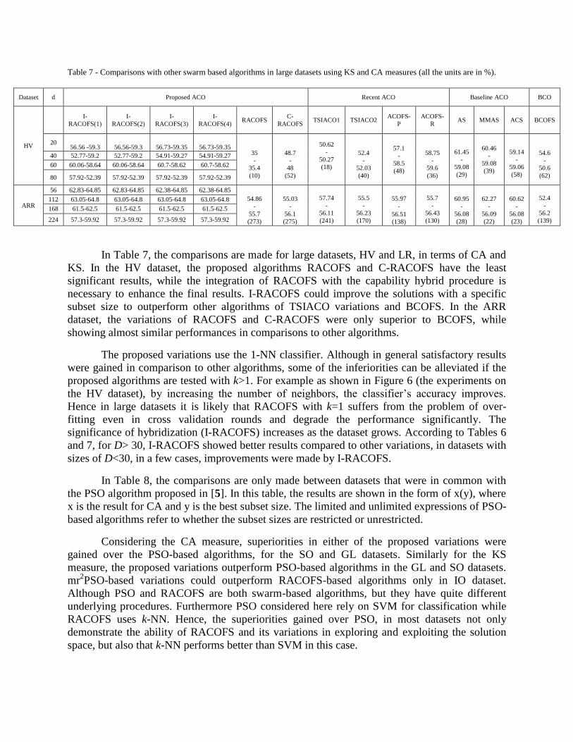
Table 7 - Comparisons with other swarm based algorithms in large datasets using KS and CA measures (all the units are in %).

Dataset d Proposed ACO Recent ACO Baseline ACO BCO

HV

I-

RACOFS(1)

I-

RACOFS(2)

I-

RACOFS(3)

I-

RACOFS(4) RACOFS

C-

RACOFS TSIACO1 TSIACO2

ACOFS-

P

ACOFS-

R AS MMAS ACS BCOFS

20 56.56 -59.3 56.56-59.3 56.73-59.35 56.73-59.35

35

-

35.4

(10)

48.7

-

48

(52)

50.62

-

50.27

(18)

52.4

-

52.03

(40)

57.1

-

58.5

(48)

58.75

-

59.6

(36)

61.45

-

59.08

(29)

60.46

-

59.08

(39)

59.14

-

59.06

(58)

54.6

-

50.6

(62)

40 52.77-59.2 52.77-59.2 54.91-59.27 54.91-59.27

60 60.06-58.64 60.06-58.64 60.7-58.62 60.7-58.62

80 57.92-52.39 57.92-52.39 57.92-52.39 57.92-52.39

ARR

56 62.83-64.85 62.83-64.85 62.38-64.85 62.38-64.85

54.86

-

55.7

(273)

55.03

-

56.1

(275)

57.74

-

56.11

(241)

55.5

-

56.23

(170)

55.97

- 56.51

(138)

55.7

-

56.43

(130)

60.95

-

56.08

(28)

62.27

-

56.09

(22)

60.62

-

56.08

(23)

52.4

-

56.2

(139)

112 63.05-64.8 63.05-64.8 63.05-64.8 63.05-64.8

168 61.5-62.5 61.5-62.5 61.5-62.5 61.5-62.5

224 57.3-59.92 57.3-59.92 57.3-59.92 57.3-59.92

In Table 7, the comparisons are made for large datasets, HV and LR, in terms of CA and

KS. In the HV dataset, the proposed algorithms RACOFS and C-RACOFS have the least

significant results, while the integration of RACOFS with the capability hybrid procedure is

necessary to enhance the final results. I-RACOFS could improve the solutions with a specific

subset size to outperform other algorithms of TSIACO variations and BCOFS. In the ARR

dataset, the variations of RACOFS and C-RACOFS were only superior to BCOFS, while

showing almost similar performances in comparisons to other algorithms.

The proposed variations use the 1-NN classifier. Although in general satisfactory results

were gained in comparison to other algorithms, some of the inferiorities can be alleviated if the

proposed algorithms are tested with k>1. For example as shown in Figure 6 (the experiments on

the HV dataset), by increasing the number of neighbors, the classifier’s accuracy improves.

Hence in large datasets it is likely that RACOFS with k=1 suffers from the problem of over-

fitting even in cross validation rounds and degrade the performance significantly. The

significance of hybridization (I-RACOFS) increases as the dataset grows. According to Tables 6

and 7, for D> 30, I-RACOFS showed better results compared to other variations, in datasets with

sizes of D<30, in a few cases, improvements were made by I-RACOFS.

In Table 8, the comparisons are only made between datasets that were in common with

the PSO algorithm proposed in [5]. In this table, the results are shown in the form of x(y), where

x is the result for CA and y is the best subset size. The limited and unlimited expressions of PSO-

based algorithms refer to whether the subset sizes are restricted or unrestricted.

Considering the CA measure, superiorities in either of the proposed variations were

gained over the PSO-based algorithms, for the SO and GL datasets. Similarly for the KS

measure, the proposed variations outperform PSO-based algorithms in the GL and SO datasets.

mr2PSO-based variations could outperform RACOFS-based algorithms only in IO dataset.

Although PSO and RACOFS are both swarm-based algorithms, but they have quite different

underlying procedures. Furthermore PSO considered here rely on SVM for classification while

RACOFS uses k-NN. Hence, the superiorities gained over PSO, in most datasets not only

demonstrate the ability of RACOFS and its variations in exploring and exploiting the solution

space, but also that k-NN performs better than SVM in this case.

Table 8 - Comparisons with PSO algorithms proposed in [5] (all units are in %).

Proposed ant colony feature selection algorithms PSO-based algorithms

Measure Dataset d I-RACOFS(1) I-RACOFS(2) I-RACOFS(3) I-RACOFS(4) RACOFS C-RACOFS Mr2PSOAcc

(Limited)

Mr2PSOAcc

(Unlimited)

Mr2PSOMI

(Unlimited)

Cla

ssif

icat

ion A

ccu

racy

(C

A)

SO

12 93.26 93.26 93.75 93.75

87.5

(11)

89.42

(11)

88.15±1.3

(15)

85.67±1.7

(15) 84.28±1.3

24 93.26 94.71 95.2 93.26

36 92.31 94.23 94.7 94.7

48 92.31 93.26 93.26 93.26

IO

7 95.15 95.15 95.15 95.15

94.01

(15)

94.01

(15)

94.92± 0.4 (6)

95.44±0.4 (6)

95.44±0.4 14 94.01 94.87 94.87 94.87

20 94.01 91.16 91.45 93.73

27 83.47 83.19 91.45 91.45

WI

3 78.08 78.08 78.08 N/A

79.21 (6)

79.21 (6)

99.72±0.3 (6)

99.72±0.3 (6)

99.19±0.4 5 79.21 79.21 79.21 79.21

8 79.21 79.21 79.21 79.21

10 79.21 79.21 79.21 79.21

GL

2 99.5 99.5 N/A N/A

100

(4)

100

(4)

79.77±2.0 (5)

80.28±1.9 (5)

78.5±3.9 4 100 100 100 100

6 100 100 100 100

8 100 100 100 100

Kap

pa

Sta

tist

ics

(KS

)

SO

12 96.8 96.8 96.8 96.8

91.45

91.45 84.35±1.7 81.17±2.3

79.36±1.9

24 96.8 97.6 97.6 97.6

36 95.6 95.6 95.6 95.6

48 95.4 96.1 96.1 96.1

IO

7 93.7 94.6 95.7 95.7

93.14

93.14 93.47±0.6 94.27±0.5 94.13±0. 6 14 93.4 93.4 94.8 94.8

20 91.7 91.4 91.8 91.8

27 87.5 87.5 87.8 87.8

WI

3 76.8 76.8 76.8 N/A

76.8 76.8 99.64±2.4 99.64±0.5 98.96±0. 5

5 76.6 76.6 76.6 76.6

8 76.45 76.45 76.45 76.45

10 76 76 76 76

GL

2 99.5 99.6 N/A N/A

99.9 99.9 74.33±2.4 74.83±2.3 72.87±4.8 4 99.7 99.86 100 N/A

6 99.7 99.93 100 100

8 99.7 99.8 99.8 99.8

5.4.2. Other comparisons

In this section the proposed algorithms are compared with other feature selection algorithms such

as classical and genetic algorithms. Since RACOFS is mainly superior over or similar to C-

RACOFS, in this set of experiments C-RACOFS is not included. To make justified comparisons

only datasets that are in common were selected. Also the proposed algorithms’ settings such as

number of iterations and independent executions were set based on what was reported in [10].

In Table 9, the comparisons are made with classical approaches like sequential forward

selection (SFS), plus-l take away-r (PTA) and sequential floating forward selection (SFFS). In

PTA r is not the ripple factor but is the number of features that should be removed. The results

are extracted from [10]. In the GL dataset, there is not much difference in the performance. In the

VW dataset, I-RACOFS could not outperform the classical algorithms, while RACOFS had

similar performances to the classical algorithms with subset size of eight. For the SO dataset

RACOFS could only outperform SFS with d=12, while the hybrid procedure has superiorities

overall.

Table 9- Comparisons with some other baseline feature selection algorithms (classical) using CA (all units are in %).

Datasets d SFS PTA SFFS I-RACOFS(1) I-RACOFS(2) I-RACOFS(3) I-RACOFS(4) RACOFS

GL

2 99.07 99.07 99.07 99.5 99.5 N/A N/A

100

(4)

4 100 100 100 100 100 100 100

6 100 100 100 100 100 100 100

8 100 100 100 100 100 100 100

VW

2 62.02 62.02 62.02 48.3 48.3 N/A N/A

99.7

(8)

4 92.63 92.83 92.83 88.9 88.9 88.9 88.9

6 98.28 98.79 98.79 94.2 94.7 94.7 94.7

8 99.70 99.70 99.70 95.7 95.7 95.7 95.7

SO

12 87.02 89.42 92.31 93.26 93.26 93.75 93.75

87.5 (11)

24 89.90 90.87 93.75 93.26 94.71 95.2 93.26

36 88.46 91.83 93.27 92.31 94.23 94.7 94.7

48 91.82 92.31 91.35 92.31 93.26 93.26 93.26

IO

7 93.45 93.45 93.45 95.15 95.15 95.15 95.15

94.01

(15)

14 90.8 92.59 93.73 94.01 94.87 94.87 94.87

20 90.03 92.02 92.88 94.01 91.16 91.45 93.73

27 89.17 91.17 90.88 83.47 83.19 91.45 91.45

WI

3 93.82 93.82 93.82 78.08 78.08 78.08 N/A

79.21

(6)

5 94.38 94.38 94.94 79.21 79.21 79.21 79.21

8 95.51 95.51 95.51 79.21 79.21 79.21 79.21

10 92.13 92.13 92.7 79.21 79.21 79.21 79.21

In the IO dataset RACOFS outperformed all other competitors, and also in the hybrid

procedures superiorities are gained over the competitors. Comparing RACO-based feature

selection algorithm to the classical algorithms, the proposed algorithm has been mostly superior

over the competitors due to the retention of the knowledge of the previously traversed edges, as a

rich source of information that is available for the ants to adjust the pheromone appropriately. In

Table 10, comparisons are made between hybrid genetic algorithms and the proposed ant-based

algorithms, with the same hybridization procedures. The testing conditions are the same and the

selected datasets are divided into two disjoint sets of testing and training according to [10] to

have justifiable comparisons.

According to the results in Table 10, the overall performance of I-RACOFS algorithms is

not better than HGAs. In the SO dataset, for d=48, I-RACOFS is superior to HGA only for r with

values of 2, 3 and 4. In the IO dataset, for d=27 and r=3 and r=4, the outcomes of the I-RACOFS

is similar to those of HGAs, while in the other settings of r and d variables the proposed

algorithms are inferior. In the VW dataset, RACOFS has superiority over HGA for d with values

of 2, 4 and 6. Hybridization is not effective in this dataset to improve the results. Lastly the

proposed algorithms in WI dataset are not better than HGAs. Genetic algorithm is an

evolutionary based algorithm, while ant colony relies on a different framework (swarm

intelligence). Hence, based on the comparisons the genetic algorithm compared here is in general

superior over the proposed swarm-based techniques.

Table 10- Comparisons with hybrid genetic algorithms using CA (all units are in %).

Dataset d HGA(1) HGA (2) HGA(3) HGA(4) I-RACOFS(1) I-RACOFS(2) I-RACOFS(3) I-RACOFS(4) RACOFS

GL

2 99.07 99.07 N/A N/A 99.5 99.5 N/A N/A

100

(4)

4 100 100 100 100 100 100 100 100

6 100 100 100 100 100 100 100 100

8 100 100 100 100 100 100 100 100

SO

12 93.65 94.71 94.61 94.81 93.26 93.26 93.75 93.75

87.5 (11)

24 95.86 95.96 96.34 96.15 93.26 94.71 95.2 93.26

36 95.67 95.82 95.67 95.67 92.31 94.23 94.7 94.7

48 92.6 93.17 93.17 93.08 92.31 93.26 93.26 93.26

IO

7 95.38 95.5 95.56 95.56 95.15 95.15 95.15 95.15

94.01

(15)

14 94.93 95.56 95.21 95.21 94.01 94.87 94.87 94.87

20 93.9 94.19 93.73 94.13 94.01 91.16 91.45 93.73

27 91.45 91.45 91.45 91.45 83.47 83.19 91.45 91.45

VW

2 62.02 62.02 N/A N/A 48.3 48.3 N/A N/A

99.7

(10)

4 92.83 92.83 92.83 92.83 88.9 88.9 88.9 88.9

6 98.79 98.79 98.79 98.79 94.2 94.7 94.7 94.7

8 99.7 99.7 99.7 99.7 95.7 95.7 95.7 95.7

WI

3 93.82 93.82 93.82 N/A 78.08 78.08 78.08 N/A

79.21 (6)

5 95.51 95.51 95.51 95.51 79.21 79.21 79.21 79.21

8 95.51 95.51 95.51 95.51 79.21 79.21 79.21 79.21

10 92.7 92.7 92.7 92.7 79.21 79.21 79.21 79.21

5.5. Timing discussions

In this section we investigate the amount of required running time for the proposed

feature selection algorithms. In order to show the execution time differences between the

proposed variations, a medium-sized dataset such as WI is suitable. According to Figure 10

RACOFS is a faster algorithm in comparison to C-RACOFS. As the number of ants increase the

algorithms need more execution time. Figure 10 indicates that for a low number of ants (e.g. 50),

the execution time differs between RACOFS and C-RACOFS while by increasing the number of

ants this difference increases greatly. Hence within a given iteration the execution time of C-

RACOFS is more dependent on the number of ants compared to RACOFS.

In Figures 11 to 14, timing analysis of the hybrid algorithm of I-RACOFS is shown.

Comparisons are made based on the dependencies that the hybrid algorithm has on the desired

subset size and ripple factors. By increasing the desired subset size, d, and ripple factor, r, the

running time grows, as the ripple factor values intensify the search around local optima stronger.

Hence the algorithm requires longer execution time. However the desired subset size, d, has

more impact on the execution time. For instance, in Figure 11 where d= 3, the required time for

the algorithms to converge are similar. On the other hand as the required subset size increased to

5, according to Figure 12, the timing complexity between r = 3 and 4 increase significantly. Also

in Figures 13 and 14 it can be seen that the required execution time for the algorithm is affected

greatly as the desired subset size increases. Therefore the timing complexity is more dependent

on subset size rather than ripple factor and for datasets with large numbers of features the

algorithm requires a large running time. For further analysis of the timing analysis of improver

hybrid procedure interested readers can refer to [10].

Figure 10 - Comparisons of RACOFS and C-RACOFS

Figure 11 - I-RACOFS timing results for d=3

Figure 12 - I-RACOFS timing results for d=5

270

2270

4270

6270

8270

50 100 150 200 250 300 350

Exe

cuti

on

Tim

e (

s)

Number of Ants

RACOFS C-RACOFS

0

200

400

600

800

1000

1 3 5 7 9 11 13 15 17 19 21 23 25 27 29

Exe

cuti

on

Tim

e (

s)

Iterations

(r=1) (r=2) (r=3) (r=4)

20

520

1020

1520

2020

2520

0 2 4 6 8 10 12 14 16 18 20 22 24 26 28

Exe

cuti

on

Tim

e (

s)

Iterations

(r=1) (r=2) (r=3) (r=4)

Figure 13 - I-RACOFS timing results for d=8

Figure 14 - I-RACOFS timing results for d=10

6. Conclusion and future works

In this paper we introduced a new ant colony algorithm, RACO, that benefits from the

traversals of the previously traversed edges. The previous traversals are seen as a rich source of

information helping to adjust the pheromone values laid on the edges as accurately as possible.

The aim of using previously traversed edges is to provide a new methodology to increase the

exploration and exploitation abilities of the ants and correspondingly prevent the algorithm

converging prematurely.

Then, RACO is applied to the task of feature selection (RACOFS) to show the

effectiveness of the algorithm in its application. It was assumed that RACOFS suffers from the

problem of inequality of selection. Hence C-RACOFS, a second variation, was introduced to test

this assumption. RACOFS is capable of finding globally optimal solutions, but is prone to be

entrapped in local optimal. Therefore the third variation, I-RACOFS, was introduced that

integrates a local search procedure with RACOFS and investigates further possible

improvements by searching the vicinity of the globally optimal solution.

20

1020

2020

3020

4020

5020

0 2 4 6 8 10 12 14 16 18 20 22 24 26 28

Exe

cuti

on

Tim

e (

s)

Iterations

(r=1) (r=2) (r=3) (r=4)

20

2020

4020

6020

0 2 4 6 8 10 12 14 16 18 20 22 24 26 28

Exe

cuti

on

Tim

e (

s)

Iterations

(r=1) (r=2) (r=3) (r=4)

RACOFS, compared to other ant-based feature selection algorithms, showed significant

superiority in both the KS and CA measures. This superiority is gained as a result of reliance on

the previous iterations’ traversals. RACOFS is capable of using the rich sources of previously

traversed edges and finding globally optimal solutions, in small and medium datasets, while in

large datasets hybrid algorithms are better to reach an optimal solution. In order to reach an

optimal solution in large datasets, RACOFS is required to be executed with k-NN where k>1.

The timing analysis results indicate RACOFS as the fastest variation in comparison to two other

variations, and I-RACOFS is the slowest variation. The execution time of I-RACOFS heavily

depends on the hybridization parameters of ripple factor and the desired subset size, while as the

experiments indicated the execution time is more dependent on the desired subset size, rather

than ripple factor.

As some suggestions for future work, although the proposed algorithm showed

significant performances using k-NN with k=1, the proposed algorithms can be extended by

testing for different values of k (e.g. k>1), especially for the WI dataset, to investigate further

improvements for this dataset. The hybridization is applied to the outcome of RACOFS while it

also can be applied to C-RACOFS or to each solution created by the ants.

Acknowledgement

We would like to thank Dr. Myra Wilson, Aberystwyth University, for reviewing early drafts of

this paper.

References

[1] R. Jensen and Q. Shen, "Fuzzy–rough attribute reduction with application to web

categorization”, Fuzzy Sets and Systems, vol. 141, no. 3, pp. 469–485, 2004.

[2] Q. Shen and R. Jensen, "Selecting informative features with fuzzy-rough sets and its

application for complex systems monitoring”, Pattern Recognition, vol. 37, no. 7, pp. 1351–

1363, 2004.

[3] M.D. Monirul Kabir, M.D. Monirul Islam, and K. Murase, "A new hybrid ant colony

optimization algorithm for feature selection”, Expert Systems with Applications, vol. 39, pp.

3747–3763, 2012.

[4] R. Forsati, A. Moayedikia, and B. Safarkhani, "Heuristic Approach to Solve Feature

Selection Problem”, in Lecture Notes in Computer Science. Springer, Verlag Berlin

Heidelberg, 2011, pp. 707-717.

[5] A. Unler, A. Murat, and R.B. Chinnam, "mr2PSO: A maximum relevance minimum

redundancy feature selection method based on swarm intelligence for support vector

machine classification”, Information Sciences, vol. 181, pp. 4625–4641, 2011.

[6] M. Dorigo, V. Maniezzi, and A. Colony, "Ant System: Optimization by a Colony of

Cooperating Agents”, IEEE Trans. on Systems, Man. and Cybernetics—Part B, vol. 26, no.

1, pp. 29–41, 1996.

[7] T. Stutzle and H.H. Hoos, "Max-min Ant System”, Future Generation Computer Systems,

vol. 16, no. 8, pp. 889–914, 2000.

[8] L.M. Gambardella and M. Dorigo, "Solving Symmetric and Asymmetric TSPs by Ant

Colonies”, in In Evolutionary Computation, 1996, Proceedings of IEEE International

Conference on, 1996, pp. 622–627.

[9] H.H. Hsu, C.W. Hsieh, and M.D. Lu, "Hybrid Feature Selection by Combining Filters and

Wrappers”, Expert Systems with Applications, vol. 38, no. 7, pp. 8144–8150, 2011.

[10] Il-S. Oh, J-S. Lee, and B-R. Moon, "Hybrid genetic algorithms for feature selection”, IEEE

Trans. On pattern analysis and machine intelligence, vol. 26, no. 11, pp. 1424-1437, 2004.

[11] C.L. Huang, "ACO-based hybrid classification system with feature subset selection and

model parameters optimization”, Neurocomputing, vol. 73, pp. 438–448, 2009.

[12] R. Jensen and Q. Shen, "Fuzzy-rough data reduction with ant colony optimization”, Fuzzy

Sets and Systems, vol. 149, pp. 5-20, 2005.

[13] R. Forsati, A. Moayedikia, and A. Keikhah, "A Novel Approach for Feature Selection based

on the Bee Colony Optimization”, International Journal of Computer Applications, vol. 43,

no. 8, pp. 30-34, 2012.

[14] C. Jun Tan, C. Peng Lim, and Y.N. Cheah, "A multi-objective evolutionary algorithm-based

ensemble optimizer for feature selection and classification with neural network models”,

Neurocomputing, vol. 125, no. 11, pp. 217-228, 2014.

[15] R. Diao and Q. Shen, "Two New Approaches to Feature Selection with Harmony Search”,

in Fuzzy Systems, 2010 IEEE International Conference on, Barcelona, Spain, 2010.

[16] M. Mirkhani, R. Forsati, Alireza Mohammad Shahri, and Alireza Moayedikia, "A novel

efficient algorithm for mobile robot localization”, Robotics and Autonomous Systems , 2013.

[17] M.D. Monirul Kabir, M. Shahjahan, and K. Murase, "A New Local Search based Hybrid

Genetic Algorithm for Feature Selection”, Neurocomputing, vol. 74, pp. 2914–2928, 2011.

[18] S.M. Vieira, J. M. C. Sousa, and T.A. Runkler, "Two cooperative ant colonies for feature

selection using fuzzy models”, Expert Systems with Applications, vol. 37, pp. 2714–2723,

2010.

[19] L. Ke, Z. Feng, and Z. Ren, "An Efficient Ant Colony Optimization Approach to Attribute

Reduction in Rough Set Theory”, Pattern Recognition Letters, vol. 29, no. 9, pp. 1351-

1357, 2008.

[20] Y. Chen, D. Miao, and R. Wang, "A Rough Set Approach to Feature Selection Based on

Ant Colony Optimization”, Pattern Recognition Letters, vol. 31, no. 3, pp. 226-233, 2010.

[21] X. Wang, J. Yang, X. Teng, W. Xaia, and R. Jensen, "Feature selection based on rough sets

and particle swarm optimization”, Pattern Recognition Letters, vol. 28, pp. 459–471, 2007.

[22] L.Y. Chuang, S.W. Tsai, and C.H. Yang, "Improved Binary Particle Swarm Optimization

using Catfish Effect for Feature Selection”, Expert Systems with Applications, vol. 38, no.

10, pp. 12699-12707, 2011.

[23] C.L. Huang and J. F. Dun, "A distributed PSO–SVM hybrid system with feature selection

and parameter optimization”, Applied Soft Computing, vol. 8, pp. 1381–1391, 2008.

[24] J. Kennedy and R. Eberhart, "Particle Swarm Optimization”, in Neural Networks, 1995.

Proceedings, IEEE International Conference on , 1995, pp. 1942-1948.

[25] P. Ravisankar, V. Ravi, G. Raghava Rao, and I. Bose, "Detection of financial statement

fraud and feature selection using data mining techniques”, Decision Support Systems, vol.

50, no. 2, pp. 491-500, 2011.

[26] C.F. Tsai and Y.C. Hsiao, "Combining multiple feature selection methods for stock

prediction: Union, intersection, and multi-intersection approaches”, Decision Support

Systems, vol. 50, no. 1, pp. 258-269, 2010.

[27] Y. Chen and D. Liginlal, "A maximum entropy approach to feature selection in knowledge-

based authentication”, Decission Support Systems, vol. 46, no. 1, pp. 388-398, 2008.

[28] A. Duric and F. Song, "Feature selection for sentiment analysis based on content and syntax

models”, Decision Support Systems, vol. 53, no. 4, pp. 704-711, 2012.

[29] D. Chyzhyk, A. Savio, and M. Grana, "Evolutionary ELM wrapper feature selection for

Alzheimer's disease CAD on anatomical brain MRI”, Neurocomputing, November 2013.

[30] M. Dorigo, G.D. Caro, and L. M. Gambradella, "Ant Algorithms for Discrete

Optimization”, Artificial Life, vol. 5, no. 2, pp. 137-172, 1999.

[31] Z. Zhang and Z. Feng, "Two-stage updating pheromone for invariant ant colony

optimization algorithm”, Expert Systems with Applications, vol. 39, pp. 706-712, 2012.

[32] J. Cohen, "A coefficient of agreement for nominal scales”, Educational and psychological

measurement, vol. 20, no. 1, pp. 37–46, 1960.

[33] A. Tsymbal, M. Pechenizkiy, and P. Cunningham, "Diversity in search strategies for

ensemble feature selection”, Information Fusion, vol. 6, no. 1, pp. 83-98, 2005.

[34] J. Huang, Y. Cai, and X. Xu, "A hybrid genetic algorithm for feature selection wrapper

based on mutual information”, Pattern Recognition Letters, vol. 28, pp. 1825–1844, 2007.

[35] A.M. Fraster and H.L. Swinney, "Independent coordinates for strange attractors from

mutual information”, Physical Review A, vol. 33, no. 2, pp. 1134 - 1140, 1986.