Ab Initio and Effective Fragment Potential Dynamics

Heather M. Netzloff and Mark S. Gordon

Iowa State University

Outline

Computer simulations– Treatment of liquids

Effective Fragment Potential Method Molecular Dynamics in GAMESS Applications Future Plans

Microscopic details

Macroscopic properties

Test theories and compare with experiments Simulate under extreme conditions

unattainable to experimentalists

Laws of Statistical Mechanics

Computer simulation:Motivation

Computer simulations:Condensed phase

Treatment of fluid-like states and solvation is essentially a many-particle problem…– Importance of accuracy and reliability of

the method used• Limited by the size of the system and

computational costs

GOAL: model CLUSTER to BULK behavior

Condensed phase For accuracy,

preference = ab initio methods, BUT…– Computationally expensive– Only realistic for small systems

Solvation Models:– Clusters:

• Ab initio, DFT, Effective Fragment Potential,…– Bulk:

• Continuum methods, TIPnP, SPC/E,…

Limited number of methods which span the clusterbulk gap well

The Effective Fragment Potential Method1,2

Treatment of discrete solvent effects

EFP1/HF: – Developed at Hartree Fock level of theory (DH(d,p))– Reproduces RHF/ab initio results…

Esystem = Eab initio + Einteraction

Standard Ab Initio Calculation

Effective Fragment Potential Calculation

1Day et. al. J. Chem. Phys. 105,1968(1996). 2Gordon et. al. J. Phys. Chem A. 105,2(2001).

EFP:Menshutkin Reaction

R3N + RX R4N+X-

– Reaction rate increases with polarity of solvent– Study process of solvation on ion formation

EFP test (Simon Webb): NH3 + CH3Br – Add EFP waters; AI solute/solvent (RHF/DZVP)

-20

-10

0

10

20

30

-20.0 -10.0 0.0 10.0 20.0 30.0 40.0

Reaction Coordinate (amu 1/2bohr)

all ab initio MEP

2 EFP water molecules MEP

EFP:Water Clusters

Monte Carlo Simulated Annealing with EFP (Paul Day, Grant Merrill, Ruth Pachter) – N = 6 - 20

• Water hexamer– Re-optimization with HF, MP2– CCSD(T) single points

(H2O)6 RELATIVE ENERGIES (KCAL/MOL)

Relative Energies(kcal/mol)

Prism Cage Book Bag Cyclic Boat

EFP 0.0 0.5 1.0 1.8 1.3 2.3RHF 0.0 0.4 0.4 1.3 -0.2 0.7MP2//MP2 0.0 0.7 1.7 2.6 2.5 3.9CCSD(T)//MP2 0.0 0.8 2.0 2.9 2.9 4.3

Effect of “solvent” molecules (fragments) added as one-electron terms to ab initio Hamiltonian, HAR

V = Fragment interaction potential

Effective Fragment Potential Method

Ab initio region

EFP region

Hsystem=HAR +V

€

V = V elec +V pol +V rep

Effective Fragment Potential Method

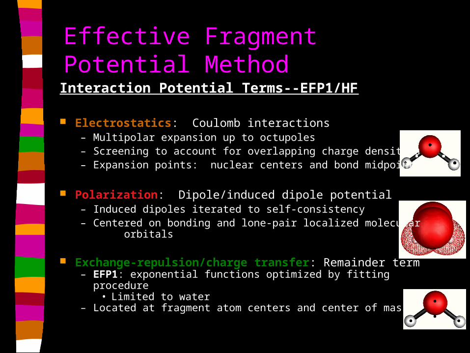
Interaction Potential Terms--EFP1/HF

Electrostatics: Coulomb interactions– Multipolar expansion up to octupoles– Screening to account for overlapping charge densities– Expansion points: nuclear centers and bond midpoints

Polarization: Dipole/induced dipole potential– Induced dipoles iterated to self-consistency– Centered on bonding and lone-pair localized molecular orbitals

Exchange-repulsion/charge transfer: Remainder term– EFP1: exponential functions optimized by fitting procedure

• Limited to water – Located at fragment atom centers and center of mass

Effective Fragment Potential Method

Solute explicitly treated with ab initio wavefunction of choice; remainder treated as effective fragments QM/MM method

Multipoles and polarizabilities – Determined from ab initio calculations on a single solvent molecule– Potential can be systematically improved!

Exchange repulsion/charge transfer term– EFP1/HF: Currently fit to functional form solvent specific– EFP2: generalize for any solvent

• NO FITS: Exchange repulsion from LMO intermolecular overlap and kinetic energy integrals

NEW!! EFP1/DFT (B3LYP)

All 3 terms are calculated independently from each other Only ONE-ELECTRON integrals are needed

– MUCH less CPU intensive than quantum mechanics

EFP/Molecular Dynamics

•Do i = 1, number of simulation steps

Calculate PE and gradients forces for particle at time t

Solve equations of motion for each particle to obtain KE at time t and new positions at time t + dt

•End do

First test of EFP to reproduce bulk behavior with its implementation with Molecular Dynamics

Basic MD Simulation loop:(user specifies time step size, dt, and length of simulation)

MD is dependent upon the accuracy and reliability of the potential used to generate gradients/forces…

Molecular Dynamics

Solve Newton’s equations of motion

– Require both ENERGY and GRADIENT from PE routine

– Integrate simultaneously for all atoms in the system to generate a trajectory for each atom

– Perform integration in SMALL time steps (usually 1-10 fs)

• Time step size Energy conservation

€

rF i = mi

d2r r i( t)dt2

r F i = −

∂V (r r i, ...

r r N )

∂r r i

Current MD Implementation in GAMESS

EFP fragment-fragment interaction (EFP-EFP MD)– Classical interaction terms– EFP: EFP1/HF, EFP1/HF, EFP2

Ab initio interaction (AI MD)– Ab initio interaction– Basis set and level of theory of choice and

availability in GAMESS

Current MD Implementation:EFP-EFP MD

Integration EFP treats water as a rigid molecule

– Center of mass motion:• Translational motion leapfrog integration algorithm• Rotational motion quaternions and modified leapfrog

integration algorithm

Water model parameters (calculated based on ab initio methods) are stored in GAMESS or given with input file– After each move all information must be

rotated/translated along with the fragment

Current MD Implementation:EFP-EFP MD

T0

T(t) T0 = desired/bath temperature

T(t) = temperature obtained from translational or rotational

kinetic energy at time t

Ensembles: NVE (constant energy)

NVT (constant temperature) : based on velocity scaling– Separate treatment for translational and rotational

velocity components– Rescale by:

Periodic Boundary Conditions

Minimum Image Convention

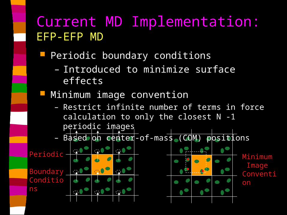
Current MD Implementation:EFP-EFP MD

Periodic boundary conditions – Introduced to minimize surface effects

Minimum image convention– Restrict infinite number of terms in force calculation to only

the closest N -1 periodic images– Based on center-of-mass (COM) positions

Current MD Implementation:AI MD

Each atom is treated independently– Leapfrog integration algorithm

NVE and NVT (velocity scaling) ensembles

No periodic boundary conditions or minimum image convention currently implemented

EFP-EFP MD ApplicationsPreparation of the system Heating:

– NVE ensemble: Initial target temp = 50 K• Initial quaternions chosen randomly• Initial translational velocities sampled from Maxwell-Boltzmann

distribution at 100 K; angular velocities start from zero– Use these coordinates to start simulation at 100 K– Same procedure to start 200 K and 300 K runs

Equilibration--TARGET TEMP = 300 K:– Coordinates taken from 300 K heating run; initial translational

velocities sampled from Maxwell-Boltzmann distribution at 600 K– NVT ensemble at 300K

• velocities rescaled only if they are outside 300 + 5 K (scaling factors not allowed to exceed 1.3)

Production:– Initial coordinates, velocities, and quaternions from equilibration– NVE and/or NVT ensemble: measure observables of interest

Compare with other water potentials…Example:

– SPC/E (Simple Extended Point Charge)4

• Point charges on O and H sites• Reparameterized SPC model to include polarization

• Values for O, O, and q (point charge) are determined by parameterization with experimental density and Evap as targets

EFP-EFP MD Applications

Vab =qiqje

2

rijij∑ +4εO

σO

rOO

⎛

⎝ ⎜

⎞

⎠ ⎟

12

−σO

rOO

⎛

⎝ ⎜

⎞

⎠ ⎟

6⎡

⎣ ⎢ ⎢

⎤

⎦ ⎥ ⎥

+0.4238e+0.4238e

-2.0qH

4Berendsen et. al. J. Phys. Chem. 92,6269(1987).

EFP-EFP MD Applications

Radial Distribution Function (RDF):– Measures the number of atoms a distance r from a given atom

compared with the number at the same distance in an ideal gas at the same density

– Gives information on how molecules pack in ‘shells’ of neighbors, as well as average structure

– Can be measured spectroscopically (X-ray or neutron diffraction)

– Test theoretical models versus experimental results

3 SITE-SITE radial distribution functions for water:– gOO(r), gOH(r), gHH(r)

gOO(r)--EFP1/HF

0

0.5

1

1.5

2

2.5

3

3.5

0 1 2 3 4 5 6 7

gOO

(r)

r (Angstroms)

Initial structure: 62 EFP waters, 26 ps equilibration

Timestep size = 1 fs, Simulation = 5000 fs

EFP1/HF--NVEEFP1/HF--NVTSPC/E--NVTExp (THG)

Exp (THG): X-ray; Sorenson et. al. J. Chem. Phys. 113,9149(2000).

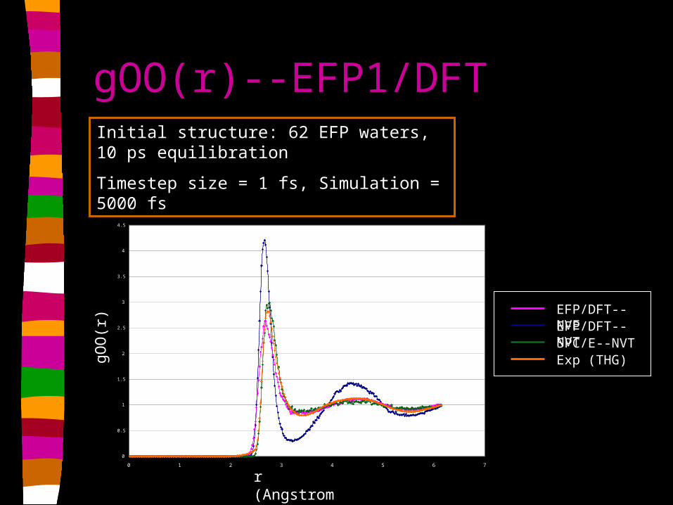
gOO(r)--EFP1/DFT

0

0.5

1

1.5

2

2.5

3

3.5

4

4.5

0 1 2 3 4 5 6 7

gOO

(r)

r (Angstroms)

EFP/DFT--NVEEFP/DFT--NVTSPC/E--NVTExp (THG)

Initial structure: 62 EFP waters, 10 ps equilibration

Timestep size = 1 fs, Simulation = 5000 fs

gOO(r) Error:62 water analysis

Err

or =

gO

O(e

xp)-

gOO

(X)

r (Angstroms)

-1.5

-1

-0.5

0

0.5

1

1.5

2

0 1 2 3 4 5 6 7

X

X

X

X

EFP/DFT--NVEEFP1/HF--NVTSPC/E--NVT

X Exp peak/valley locations

gOO(r)--EFP1/HF:62 water analysis with Monte Carlo

0

0.5

1

1.5

2

2.5

3

3.5

4

0 1 2 3 4 5 6 7

0

0.5

1

1.5

2

2.5

3

0 1 2 3 4 5 6 7

Initial structure: 62 EFP waters, 1.0 ps MD equilibration

RDF measured with MC accepted structures (2 criteria for EFP MC) 6790 accepted (100,000)

gOO

(r)

r (Angstroms)

gOO

(r)

EFP1/HF--MC

Exp (THG)

Polynomial Fit (4th order) to EFP

gOO(r)--EFP1/HF:512 water analysis

0

0.5

1

1.5

2

2.5

3

0 2 4 6 8 10 12 14

gOO

(r)

r (Angstroms)-1

-0.5

0

0.5

1

1.5

2

0 2 4 6 8 10 12 14

X

X

X

X

X

Initial structure: 512 EFP waters, 7.5 ps equilibration

Timestep size = 1 fs, Simulation = 5000 fs

r (Angstroms)

Err

or =

gO

O(e

xp)-

gOO

(X)

EFP1/HF--NVTSPC/E--NVTExp (THG)

gOH(r):EFP1/HF, EFP1/DFT, SPC/E62 waters

0

0.2

0.4

0.6

0.8

1

1.2

1.4

1.6

1.8

0 1 2 3 4 5 6 7

EFP/DFT--NVEEFP/HF--NVTSPC/E--NVTExp (ND)

gOH

(r)

r (Angstroms)

Exp (ND): Neutron Diffraction; Soper et. al.

gHH(r):EFP1/HF, EFP1/DFT, SPC/E62 waters

0

0.2

0.4

0.6

0.8

1

1.2

1.4

1.6

0 1 2 3 4 5 6 7

EFP/DFT--NVEEFP/HF--NVTSPC/E--NVTExp (ND)

gHH

(r)

r (Angstroms)

Timings: Energy + Gradient calculation

Method*20 water molecules

62 water molecules

122 water molecules

512 water molecules

Ab initio** 3.19 hrs --- --- ~157 yrs***

EFP2 3.3 sec 26.1 sec 95.3 sec 26.8 min

EFP1/HF 0.2 sec 2.6 sec 5.1 sec 97.8 sec

SPC/E 0.02 sec 0.02 sec 0.1 sec 0.7 sec

* Run on 1200 MHz Athlon/Linux machine

**Ab initio: DZP basis set, *** Assuming N4 scaling

Future Plans Addition of minimum image convention to EFP2

implementation and AI MD– Coordinates, not only distances, must be manipulated

Treatment of long range forces– First layer: Ewald sum method for charge-charge interaction– Second layer: Fast Multipole Method– Use continuum versus minimum image convention/periodic

boundary conditions

Utilization/development of parallel algorithms– Utilize parallel AI GAMESS code for calculation of AI energy

and gradient– Parallelization of the EFP method

Acknowledgements

Jon Sorenson, Grant Merrill, Mark Freitag

$$$$$

DOE Computational Science Graduate Fellowship

Thank You!