Aalborg Universitet

Robust Stabilization and Disturbance Rejection for Autonomous Helicopter

Danapalasingham, Kumeresan

Publication date:2010

Document VersionAccepted author manuscript, peer reviewed version

Link to publication from Aalborg University

Citation for published version (APA):A. Danapalasingam, K. (2010). Robust Stabilization and Disturbance Rejection for Autonomous Helicopter.Aalborg Universitet.

General rightsCopyright and moral rights for the publications made accessible in the public portal are retained by the authors and/or other copyright ownersand it is a condition of accessing publications that users recognise and abide by the legal requirements associated with these rights.

? Users may download and print one copy of any publication from the public portal for the purpose of private study or research. ? You may not further distribute the material or use it for any profit-making activity or commercial gain ? You may freely distribute the URL identifying the publication in the public portal ?

Take down policyIf you believe that this document breaches copyright please contact us at vbn@aub.aau.dk providing details, and we will remove access tothe work immediately and investigate your claim.

Downloaded from vbn.aau.dk on: juli 26, 2018

Kumeresan A. Danapalasingam

Robust Stabilization and DisturbanceRejection for

Autonomous Helicopter

Robust Stabilization and Disturbance Rejection for Autonomous HelicopterPh.D. thesis

ISBN: 987-87-92328-40-3October 2010

Copyright 2007-2010 c© Kumeresan A. Danapalasingam

Contents

Contents III

Preface VII

Abstract IX

Synopsis XI

1 Introduction 11.1 Autonomous Helicopter in Practical Applications . . . . . . . . . . . . . 11.2 Motivation . . . . . . . . . . . . . . . . . . . . . . . . . . . . . . . . . . 21.3 State of the Art and Background . . . . . . . . . . . . . . . . . . . . . . 41.4 Outline of the Thesis . . . . . . . . . . . . . . . . . . . . . . . . . . . . 11

2 Methodology 132.1 Trim . . . . . . . . . . . . . . . . . . . . . . . . . . . . . . . . . . . . . 132.2 Lyapunov Stability . . . . . . . . . . . . . . . . . . . . . . . . . . . . . 142.3 π-trajectory . . . . . . . . . . . . . . . . . . . . . . . . . . . . . . . . . 142.4 Differential Inclusions . . . . . . . . . . . . . . . . . . . . . . . . . . . 142.5 Input-to-State Stability . . . . . . . . . . . . . . . . . . . . . . . . . . . 152.6 Simulation . . . . . . . . . . . . . . . . . . . . . . . . . . . . . . . . . . 152.7 Flight Tests . . . . . . . . . . . . . . . . . . . . . . . . . . . . . . . . . 16

3 Summary of Contributions 173.1 Disturbance Effects . . . . . . . . . . . . . . . . . . . . . . . . . . . . . 173.2 Feedforward Control Strategy for Disturbance Rejection . . . . . . . . . 173.3 Robustly Stabilizing State Feedback with Feedforward . . . . . . . . . . 183.4 Wind Disturbance Estimation and Helicopter Stabilization . . . . . . . . 19

4 Conclusion 214.1 Objectives of the Project . . . . . . . . . . . . . . . . . . . . . . . . . . 214.2 Contributions of the Project . . . . . . . . . . . . . . . . . . . . . . . . . 224.3 Future Work . . . . . . . . . . . . . . . . . . . . . . . . . . . . . . . . . 23

References 25

Paper A: Feedforward Control of an Autonomous Helicopter using Trim Inputs 29

III

CONTENTS

5.1 Introduction . . . . . . . . . . . . . . . . . . . . . . . . . . . . . . . . . 325.2 Concept . . . . . . . . . . . . . . . . . . . . . . . . . . . . . . . . . . . 345.3 Results . . . . . . . . . . . . . . . . . . . . . . . . . . . . . . . . . . . . 385.4 Discussion . . . . . . . . . . . . . . . . . . . . . . . . . . . . . . . . . . 395.5 Conclusion . . . . . . . . . . . . . . . . . . . . . . . . . . . . . . . . . 47

References 49

Paper B: Disturbance Effects in Nonlinear Control Systems and FeedforwardControl Strategy 516.1 Introduction . . . . . . . . . . . . . . . . . . . . . . . . . . . . . . . . . 536.2 Preliminaries and Problem Statement . . . . . . . . . . . . . . . . . . . . 546.3 Lyapunov Stability Analysis . . . . . . . . . . . . . . . . . . . . . . . . 566.4 Disturbance Feedforward Control . . . . . . . . . . . . . . . . . . . . . 576.5 Simulation Results . . . . . . . . . . . . . . . . . . . . . . . . . . . . . 586.6 Discussions . . . . . . . . . . . . . . . . . . . . . . . . . . . . . . . . . 596.7 Conclusion . . . . . . . . . . . . . . . . . . . . . . . . . . . . . . . . . 62

References 65

Paper C: A Robust Stabilization using State Feedback with Feedforward 677.1 Introduction . . . . . . . . . . . . . . . . . . . . . . . . . . . . . . . . . 697.2 Preliminaries . . . . . . . . . . . . . . . . . . . . . . . . . . . . . . . . 707.3 Supplementary Results . . . . . . . . . . . . . . . . . . . . . . . . . . . 737.4 Completion of the proof . . . . . . . . . . . . . . . . . . . . . . . . . . . 777.5 Simulation Results . . . . . . . . . . . . . . . . . . . . . . . . . . . . . 797.6 Conclusion . . . . . . . . . . . . . . . . . . . . . . . . . . . . . . . . . 81

References 83

Paper D: Robust Helicopter Stabilization in the Face of Wind Disturbance 878.1 Introduction . . . . . . . . . . . . . . . . . . . . . . . . . . . . . . . . . 898.2 Preliminaries . . . . . . . . . . . . . . . . . . . . . . . . . . . . . . . . 908.3 Controller Design . . . . . . . . . . . . . . . . . . . . . . . . . . . . . . 918.4 Simulation Results . . . . . . . . . . . . . . . . . . . . . . . . . . . . . 998.5 Conclusion and Future Works . . . . . . . . . . . . . . . . . . . . . . . . 101

References 103

Paper E: Nonlinear Feedforward Control for Wind Disturbance Rejection onAutonomous Helicopter 1059.1 Introduction . . . . . . . . . . . . . . . . . . . . . . . . . . . . . . . . . 1079.2 Previous Work . . . . . . . . . . . . . . . . . . . . . . . . . . . . . . . . 1079.3 Helicopter Model . . . . . . . . . . . . . . . . . . . . . . . . . . . . . . 1089.4 Feedforward Control . . . . . . . . . . . . . . . . . . . . . . . . . . . . 1139.5 Disturbance Measurement . . . . . . . . . . . . . . . . . . . . . . . . . 1159.6 Results . . . . . . . . . . . . . . . . . . . . . . . . . . . . . . . . . . . . 1159.7 Discussions and Future Works . . . . . . . . . . . . . . . . . . . . . . . 117

IV

CONTENTS

References 119

Paper F: Robust Helicopter Stabilization with Wind Disturbance Elimination 12110.1 Introduction . . . . . . . . . . . . . . . . . . . . . . . . . . . . . . . . . 12310.2 Preliminaries . . . . . . . . . . . . . . . . . . . . . . . . . . . . . . . . 12410.3 Controller Design . . . . . . . . . . . . . . . . . . . . . . . . . . . . . . 12710.4 Simulation Results . . . . . . . . . . . . . . . . . . . . . . . . . . . . . 13910.5 Conclusion and Future Works . . . . . . . . . . . . . . . . . . . . . . . . 141

References 165

V

Preface and Acknowledgements

This thesis is submitted as a collection of papers in the partial fulfilment of the require-ments for a Doctor of Philosophy at the Section of Automation and Control, Departmentof Electronic Systems, Aalborg University, Denmark. The work has been carried out inthe period from February 2007 to September 2010 under the supervision of AssociateProfessor Anders la Cour-Harbo and Assistant Professor Morten Bisgaard.

This Ph.D. study is supported by Ministry of Higher Education Malaysia (MOHE)and Universiti Teknologi Malaysia (UTM).

First and foremost I would like to express my deepest gratitude to John-Josef Lethfor his support, guidance and encouragement that have made this thesis a fruitful one.His sincere assistance and dedication have certainly helped me in completing the criticalstage of this Ph.D. study. I am thankful to my supervisors, Anders la Cour-Harbo andMorten Bisgaard whose effort in all these years led to the completion of this project. Iam also very much indebted to Professor Rafal Wisniewski whose kind heart and seem-ingly abundant knowledge in mathematics saved me whenever I felt like drowning in theturbulence of this research.

I would like to take this opportunity to acknowledge all the employees at the Sectionof Automation and Control who have contributed either directly or indirectly in makingthis journey as gratifying as possible. Special thanks go to the lovely secretaries of thesection, Karen Drescher and Jette Damkjær for their warmth, hospitality and kindnessthat I will treasure forever in my memory.

To my family and friends who have been my pillars of support during my ups anddowns in the course of my stay in Denmark, I say thank you very much. Finally, I wouldlike to thank MOHE and UTM for the given opportunity and financial support that madethis Ph.D. study possible.

VII

Abstract

The applicability of autonomous helicopters in execution of various tasks including someof the critical ones such as wind turbine inspection, deep-sea search and rescue and naturaldisaster monitoring demands a high performance controller. In wind turbine inspectionfor instance, a helicopter would be required to fly autonomously from a suitable locationto the rotating structure. In cases where an inspection routine involves prolonged anddetailed measurements, it is expected that the helicopter is able to fly as close as possibleto the wind turbine with minimum deviations. And since the undesirable influence fromwind disturbances and rotor wake interactions between the helicopter and the structureare unavoidable, wind turbine inspection using an autonomous helicopter presents itselfas a challenging control problem.

To meet general requirements of practical applications utilizing autonomous heli-copters, it is highly desirable to be equipped with a controller that is capable of carryingout designated objectives from an arbitrary initial helicopter state in the presence of winddisturbances. Often, exact values of helicopter physical parameters and aerodynamic co-efficients are not known. Thus, a control design should be able to cope with model andparameter uncertainties. However, the design of such a controller is challenging due to thehighly nonlinear and coupled helicopter model. The difficulty to obtain measurements ofthe wind disturbance for stabilizing control input generation further aggravates the controldesign problem.

In this research, for a general nonlinear control system with a persistent disturbance asone of its external inputs whose measurements are available, it is shown that the existenceof a smooth uniform control Lyapunov function implies the existence of a stabilizing statefeedback with feedforward control which is insensitive to small measurement errors andsmall external disturbance for fast sampling. Conversely, it is shown that there exists asmooth uniform control Lyapunov function if there is such a stabilizer. By introducingthe notion of disturbance effect, a feedforward control scheme that can be augmented toan existing state feedback control is proposed to guarantee asymptotic stability. However,in the helicopter case due to the difficulty in obtaining accurate wind disturbance mea-surements, an estimate of the wind disturbance is introduced to be adapted using statemeasurements for stabilization of position and translational velocity. By assuming thatthe wind disturbance is a sum of a fixed number of sinusoids with unknown amplitudes,frequencies and phases, a nonlinear controller is designed based on nonlinear adaptiveoutput regulation and robust stabilization of a chain of integrators by a saturated feed-back. Even though the control design is based on a simplified model, simulations of thecontroller implementation in a model of higher complexity show a satisfactory perfor-mance in the stabilization of helicopter motion in the presence of model and parameteruncertainties.

IX

Synopsis

At anvende autonome helikoptere i forbindelse med opgaver som inspektion af vindmller,sredning, overvgning og lignende stiller store krav til stabiliten og prcisionen af flyvnin-gen. For eksempel, ved vindmlleinspektion er det ndvendigt for helikopteren at starte fraet egnet startpunkt og flyve autonomt til de roterende blade. I tilflde, hvor en inspektionindebrer langvarige og detaljerede mlinger, forventes det, at helikopteren er i stand tilat flyve s tt som muligt p vindmllen. Eftersom helikopteren uundgligt vil blive pvirketaf turbulens fra vindmllen, er inspektion af denne ved hjlp af en autonom helikopter etudfordrende reguleringsproblem.

For at opfylde sdanne krav i applikationer for autonome helikoptere, er det ndvendigtmed en regulering, der er i stand til at udfre missioner og stabilisere helikopteren fra envilkrlig starttilstand under vindforstyrrelser. Helikopterens fysiske parametre og aerody-namiske koefficienter er ofte ikke prcist kendte og et reguleringsdesign m derfor vre istand til at hndtere model- og parameterusikkerheder. Et design af en sdan regulator erdog udfordrende p grund af den meget ikke-linere og koblede helikoptermodel. Vanske-lighederne ved at mle vindforstyrrelserne til brug i stabilisering gr reguleringsproblemetsvrere.

Det er i denne afhandling vist at eksistensen af en glat uniform control Lyapunovfunktion for et generelt ikke-linert system med en uafbrudt forstyrrelse som et output,forudstter eksistensen af en stabiliserende feedback tilstandsregulering med feedforwardregulering, der er uflsom over for sm mlefejl og eksterne forstyrrelser ved hurtig sam-pling. Det er ogs vist, at der eksisterer en glat uniform control Lyapunov funktion, hvisen sdan stabiliserende regulering eksisterer. En feedforward regulering, der kan sup-plere en eksisterende feedback tilstandsregulator, kan garantere asymptotisk stabilitet vedat introducere begrebet forstyrrelseseffekt. Da det i forbindelse med en helikopter ervanskeligt direkte at mle vindforstyrrelserne er en adaptiv estimator til bestemmelse afvindforstyrrelserne ud fra tilstandsmlinger blevet introduceret. En ikke-liner regulator,baseret p ikke-liner adaptiv output regulering og robust stabilisering af en kde af integra-torer ved satureret feedback, kan designes ved at antage at vindforstyrrelserne er en sumaf et fast antal sinus-funktioner med ukendt amplitude, frekvens og fase. Selv om reg-uleringsdesigned er baseret p en simplificeret model, vister simuleringer af regulatorenmed en model af hjere kompleksitet tilfredsstillende performance under stabilisering afhelikopteren med model- og parameterusikkerheder.

XI

1 Introduction

An autonomous helicopter is an airborn vehicle capable of flying without a human pilot.Equipped with onboard sensors and a computing capability, an autonomous helicoptercan be a reliable mechanical assistant to humans in a variety of applications includingreconnaissance, agriculture, firefighting and land mine detection. While a human pilotcan successfully fly a helicopter in a wide range of maneuvers, the execution of even thesimplest unmanned helicopter flight is widely regarded as a challenging control problem.The challenge stems from the fact that a helicopter is a nonlinear, high dimensional, cou-pled and underactuated control system. The presence of wind disturbances, measurementerrors, and model and parameter uncertainties poses further complications in the controldesign. The main theme of this thesis is helicopter stabilization in the presence of a winddisturbance. In this chapter, motivation behind the need for a concept of disturbanceeffect and feedforward control for a general nonlinear control system, and disturbanceestimation in helicopter stabilization is presented. An overview of recent developmentsin related research fields is also given. To begin with, some practical applications ofautonomous helicopters are proposed.

1.1 Autonomous Helicopter in Practical Applications

In many specialized tasks, while humans are highly reliable in performing desired activ-ities, a better alternative that would result in a higher precision, cost saving, increasedefficiency and better safety is often considered. Due to its small size, agility, manuev-erability and unique hovering capability, potrayal of autonomous helicopters as a goodcandidate in real life implementations is inevitable.

An example of application of autonomous helicopters to assist human beings is windturbine inspection. Periodic inspections of wind turbines are crucial to ensure consistentintegrity and to avoid inconvenient shutdowns due to system failures. To curb complica-tions in a wind turbine before serious problems involving increased down time and profitloss could ensue, preventive maintenance inspections are essential. Visual inspectionsand other non-destructive tests including ultrasonic inspection, eddy current inspectionand alternating current field measurement to detect cracks, corrosion, weld flaws andother defects are conventionally conducted by using rope access techniques. Rope accessis a method that allows workers to inspect and perform maintanence services on wind tur-bines using ropes. As the involvement of humans in such a risky environment naturallyraises safety and cost issues, wind turbine inspection using autonomous helicopters canbe an advantageous procedure. A group of autonomous helicopters can be dispatched in

1

Introduction

a wind farm for simultaneous inspection of the wind turbines. The coordinated approachwill not only be time efficient, but could also enable a reduced cost and increased persis-tent quality inspection method. However, one should realize that the windy and turbulentconditions in wind farms are the greatest hurdle in accomplishing effective wind turbineinspections using autonomous helicopters.

Another potential real life application in which autonomous helicopters can be utilizedis air-sea rescue. In search and rescue operations of survivors of an aircraft crash anddistressed ship crew members and passengers for instance, autonomous helicopters canbe an excellent aid to search and locate victims in a prescribed area. Generally, full scalemanned helicopters play a major function in search and rescue operations. While they canhandle harsh weather conditions and are able to transport survivors in need of medicalcare to emergency facilities, the loud noise disrupts communication between rescuers andsurvivors. Another drawback is the deteriorating effect of strong helicopter downdraft oncold and possibly hypothermic survivors during rescue operations. The high expendituresinvolved in the purchase of helicopters, and in search and rescue operations includingsalaries of onboard and standy crew members could further demotivate the application offull scale helicopters. On the other hand, using a number of autonomous helicopters incoordination, a wider search area can be covered for a faster search process. Once a crashsite or survivors have been identified, crucial information can be sent to a ground stationor rescue boats for further actions. While waiting for the rescue boats to arrive, oneor more autonomous helicopters can remain hovering close to the survivors to provideemergency supplies and to boost the spirits of the victims. Note that the search andrescue operations using autonomous helicopters could be considerably affected withoutcontrollers that could cope with harsh weather conditions at sea.

Even though the involvement of autonomous helicopters in the above mentioned ap-plications is an appealing approach, great challenges and implementation issues that im-mediately arise have to be addressed before it could be put into practice. For an example,in both wind turbine inspection and air-sea rescue, the ability of an autonomous heli-copter to perform instructions accurately despite the windy condition is obligatory. It isexpected that an autonomous helicopter is capable of starting an operation by flying au-tonomously from a given ground base to a required destination on a computed path whileavoiding obstacles. Since the design of a controller to enable an autonomous flight of-ten requires the knowledge of helicopter physical parameters, aerodynamic coefficients,wind disturbance, etc., robustness against uncertainties in the values of these quantities isimportant.

1.2 Motivation

In general, helicopter control is made possible by using a state feedback that generatescontrol inputs using state measurements (see e.g., [ACN10], [Xu10] and [BlCHB10]).If wind disturbance measurements are available in addition to the state measurements,the design of a state feedback with feedforward can be proven advantageous since moreinformation about the system to be controlled is now available. However in helicoptercontrol, a useful disturbance measurement is often hard to obtain. In such a case, distur-bance estimation can be a method to quantify the effects of the external influence for acontroller synthesis.

2

2 Motivation

+ ++

++-

r e y

d

G(s)

D(s)

Cfb(s)

Cff(s)

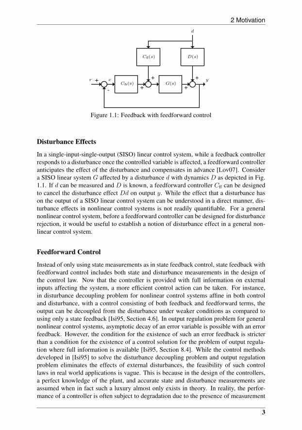
Figure 1.1: Feedback with feedforward control

Disturbance Effects

In a single-input-single-output (SISO) linear control system, while a feedback controllerresponds to a disturbance once the controlled variable is affected, a feedforward controlleranticipates the effect of the disturbance and compensates in advance [Lov07]. Considera SISO linear system G affected by a disturbance d with dynamics D as depicted in Fig.1.1. If d can be measured and D is known, a feedforward controller Cff can be designedto cancel the disturbance effect Dd on output y. While the effect that a disturbance hason the output of a SISO linear control system can be understood in a direct manner, dis-turbance effects in nonlinear control systems is not readily quantifiable. For a generalnonlinear control system, before a feedforward controller can be designed for disturbancerejection, it would be useful to establish a notion of disturbance effect in a general non-linear control system.

Feedforward Control

Instead of only using state measurements as in state feedback control, state feedback withfeedforward control includes both state and disturbance measurements in the design ofthe control law. Now that the controller is provided with full information on externalinputs affecting the system, a more efficient control action can be taken. For instance,in disturbance decoupling problem for nonlinear control systems affine in both controland disturbance, with a control consisting of both feedback and feedforward terms, theoutput can be decoupled from the disturbance under weaker conditions as compared tousing only a state feedback [Isi95, Section 4.6]. In output regulation problem for generalnonlinear control systems, asymptotic decay of an error variable is possible with an errorfeedback. However, the condition for the existence of such an error feedback is stricterthan a condition for the existence of a control solution for the problem of output regula-tion where full information is available [Isi95, Section 8.4]. While the control methodsdeveloped in [Isi95] to solve the disturbance decoupling problem and output regulationproblem eliminates the effects of external disturbances, the feasibility of such controllaws in real world applications is vague. This is because in the design of the controllers,a perfect knowledge of the plant, and accurate state and disturbance measurements areassumed when in fact such a luxury almost only exists in theory. In reality, the perfor-mance of a controller is often subject to degradation due to the presence of measurement

3

Introduction

errors and other uncertainties. To address the aforementioned implementation issues andto benefit from state feedback with feedforward control, a controller that is robust with re-spect to state measurement errors, disturbance measurement errors and model mismatchis needed. Therefore, it is important to set up a condition for the existence of a state feed-back with feedforward for general nonlinear control systems, that is less sensitive to stateand disturbance measurement errors, and model uncertainties. The establishment of suchan existence condition will aid the design of a robust state feedback with feedforwardcontroller for the stabilization of a plant to be controlled.

Disturbance Estimation

While the availability of the information on wind disturbances is highly preferred in heli-copter control, the reality is that such measurements are difficult to obtain. The challengeprimarily emerges due to main rotor downwash that would corrupt wind sensor readings.In addition to the installation problem, the need for a sensor of a suitable size and accu-racy which is directly proportional to the cost, further dampens the effort to obtain reliabledata for control purposes. Other factors related to wind disturbance measurements thatinfluence a control performance include range, response time, precision, sensitivity anddead band of a wind sensor. In order to still deliver information on the exogenous inputto the controller for helicopter stabilization, a disturbance estimate can be a promisingoption. The disturbance estimate can be generated by an internal model tuned by meansof an appropriate adaptation law driven by state measurements. This then can be usedfor the synthesis of a robust controller which is less sensitive to parameter uncertaintiesfor helicopter stabilization in the presence of a wind disturbance. However, given the in-volvement of state measurements in the disturbance estimation, once again the accuracyof measurements has to be taken into account. Morever, the reliability of a wind distur-bance model assumed in the estimation in representing actual external wind disturbancesplays an important role to ensure a high quality helicopter control.

1.3 State of the Art and Background

In line with the main theme of this thesis that is helicopter stabilization with wind dis-turbance rejection, the motivation for a concept of disturbance effect and feedforwardcontrol for general nonlinear control systems, and disturbance estimation in helicopterstabilization is laid out in Section 1.2. With regards to the aforementioned components ofcontrol theory, some preliminaries and related developments in state feedback with feed-forward control of nonlinear systems, nonlinear adaptive output regulation and helicoptercontrol are presented in this section. Concerning the control that depends on both state ofthe system and external disturbance input, well established nonlinear control theories ondisturbance decoupling and full information output regulation are reviewed here. Lastly, aconcise study of various helicopter control techniques are given. The literature review onhelicopter control covers previous works done in trajectory tracking, robust stabilizationand disturbance attenuation.

4

3 State of the Art and Background

State Feedback with Feedforward Control of Nonlinear Systems

Provided that the state and external disturbance input of a nonlinear system are availablefor measurements, a state feedback with feedforward control consists of a feedback on thestate of the system and a feedforward on the disturbance. While occasionally it is possibleto measure disturbances in nonlinear control applications, one should not expect such anadvantage in general control settings. Even though desired control actions are feasibleby only using state or error measurements in control input generation, the inclusion ofdisturbance measurements certainly simplies the design of control laws. Next, two statefeedback with feedforward control methods are reviewed.

Disturbance Decoupling

In this part, a control method to produce an output free from the influence of disturbancesaffecting the state of a nonlinear system is reviewed. Firstly, the category of nonlinearcontrol systems considered in the disturbance decoupling problem is stated. Secondly, theform of the control law that depends on state and disturbance measurements is introducedto solve the disturbance decoupling problem.

Consider a single-input-single-output nonlinear system affine in control and distur-bance of the form

x = f(x) + g(x)u+ p(x)w,

y = h(x),(1.1)

where f(x), g(x), p(x) and h(x) are smooth functions with state x belonging to an openset U ⊂ R, control input u ∈ R and disturbance w ∈ R.

If measurements of the disturbance w is available, then the disturbance decouplingproblem is that of finding a static state feedback with feedforward control

u = α(x) + β(x)v + γ(x)w (1.2)

such that the output y of system (1.1) is decoupled from the disturbance w. As shown in[Isi95, Section 4.6], there exists a necessary and sufficient condition to solve the distur-bance decoupling problem with such a control (1.2) defined locally. It turns out that ifone opts to use a feedback control of the form

u = α(x) + β(x)v,

a stricter condition has to be satisfied to have the output y of system (1.1) completelyindependent of the disturbance w [Isi95, Proposition 4.6.1].

Full Information Output Regulation

In the disturbance decoupling problem as decribed above, using the state feedback withfeedforward control (1.2) the output of the nonlinear system (1.1) is completely decoupledfrom the disturbance w. Subsequently, one can further design the control v in (1.2) toachieve an additional control performance such as asymptotic stability [Isi95]. Anotherproblem in nonlinear control theory is the design of a control law such that the output ofa nonlinear system tracks a reference output in a given family. A similar control problem

5

Introduction

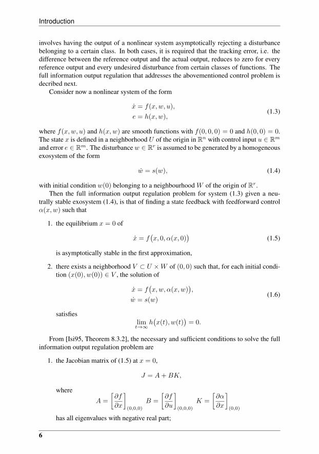
involves having the output of a nonlinear system asymptotically rejecting a disturbancebelonging to a certain class. In both cases, it is required that the tracking error, i.e. thedifference between the reference output and the actual output, reduces to zero for everyreference output and every undesired disturbance from certain classes of functions. Thefull information output regulation that addresses the abovementioned control problem isdecribed next.

Consider now a nonlinear system of the form

x = f(x,w, u),

e = h(x,w),(1.3)

where f(x,w, u) and h(x,w) are smooth functions with f(0, 0, 0) = 0 and h(0, 0) = 0.The state x is defined in a neighborhood U of the origin in Rn with control input u ∈ Rmand error e ∈ Rm. The disturbancew ∈ Rr is assumed to be generated by a homogeneousexosystem of the form

w = s(w), (1.4)

with initial condition w(0) belonging to a neighbourhood W of the origin of Rr.Then the full information output regulation problem for system (1.3) given a neu-

trally stable exosystem (1.4), is that of finding a state feedback with feedforward controlα(x,w) such that

1. the equilibrium x = 0 of

x = f(x, 0, α(x, 0)

)(1.5)

is asymptotically stable in the first approximation,

2. there exists a neighborhood V ⊂ U ×W of (0, 0) such that, for each initial condi-tion (x(0), w(0)) ∈ V , the solution of

x = f(x,w, α(x,w)

),

w = s(w)(1.6)

satisfieslimt→∞

h(x(t), w(t)

)= 0.

From [Isi95, Theorem 8.3.2], the necessary and sufficient conditions to solve the fullinformation output regulation problem are

1. the Jacobian matrix of (1.5) at x = 0,

J = A+BK,

where

A =

[∂f

∂x

](0,0,0)

B =

[∂f

∂u

](0,0,0)

K =

[∂α

∂x

](0,0)

has all eigenvalues with negative real part;

6

3 State of the Art and Background

++w = s(w)

eu

w

K

x = f(x,w, u)

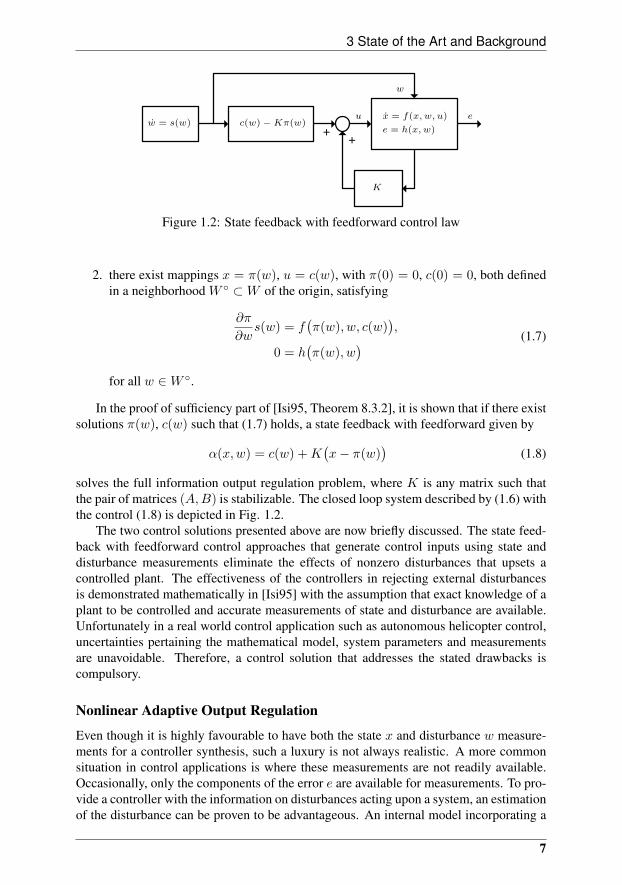
e = h(x,w)c(w)−Kπ(w)

Figure 1.2: State feedback with feedforward control law

2. there exist mappings x = π(w), u = c(w), with π(0) = 0, c(0) = 0, both definedin a neighborhood W ⊂W of the origin, satisfying

∂π

∂ws(w) = f

(π(w), w, c(w)

),

0 = h(π(w), w

) (1.7)

for all w ∈W .

In the proof of sufficiency part of [Isi95, Theorem 8.3.2], it is shown that if there existsolutions π(w), c(w) such that (1.7) holds, a state feedback with feedforward given by

α(x,w) = c(w) +K(x− π(w)

)(1.8)

solves the full information output regulation problem, where K is any matrix such thatthe pair of matrices (A,B) is stabilizable. The closed loop system described by (1.6) withthe control (1.8) is depicted in Fig. 1.2.

The two control solutions presented above are now briefly discussed. The state feed-back with feedforward control approaches that generate control inputs using state anddisturbance measurements eliminate the effects of nonzero disturbances that upsets acontrolled plant. The effectiveness of the controllers in rejecting external disturbancesis demonstrated mathematically in [Isi95] with the assumption that exact knowledge of aplant to be controlled and accurate measurements of state and disturbance are available.Unfortunately in a real world control application such as autonomous helicopter control,uncertainties pertaining the mathematical model, system parameters and measurementsare unavoidable. Therefore, a control solution that addresses the stated drawbacks iscompulsory.

Nonlinear Adaptive Output Regulation

Even though it is highly favourable to have both the state x and disturbance w measure-ments for a controller synthesis, such a luxury is not always realistic. A more commonsituation in control applications is where these measurements are not readily available.Occasionally, only the components of the error e are available for measurements. To pro-vide a controller with the information on disturbances acting upon a system, an estimationof the disturbance can be proven to be advantageous. An internal model incorporating a

7

Introduction

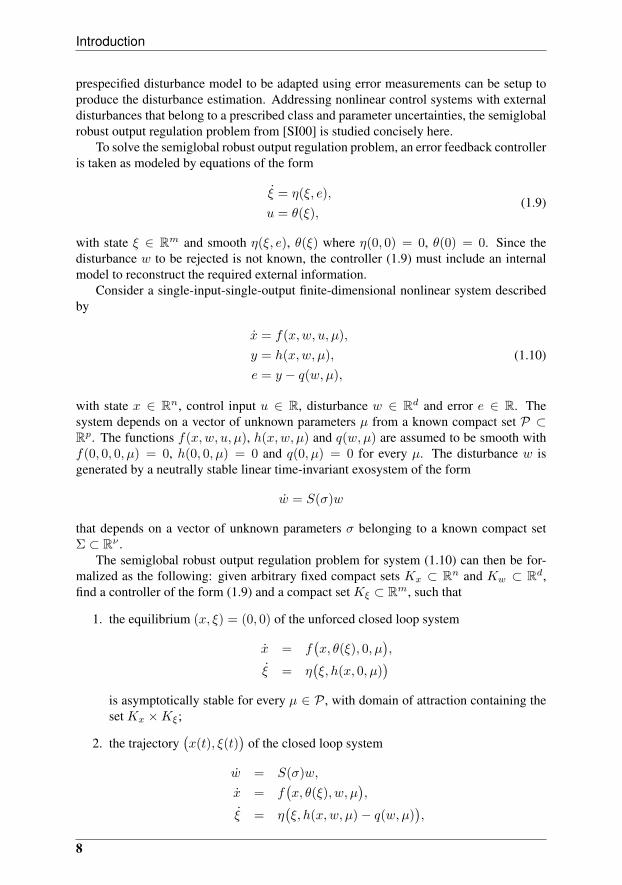
prespecified disturbance model to be adapted using error measurements can be setup toproduce the disturbance estimation. Addressing nonlinear control systems with externaldisturbances that belong to a prescribed class and parameter uncertainties, the semiglobalrobust output regulation problem from [SI00] is studied concisely here.

To solve the semiglobal robust output regulation problem, an error feedback controlleris taken as modeled by equations of the form

ξ = η(ξ, e),

u = θ(ξ),(1.9)

with state ξ ∈ Rm and smooth η(ξ, e), θ(ξ) where η(0, 0) = 0, θ(0) = 0. Since thedisturbance w to be rejected is not known, the controller (1.9) must include an internalmodel to reconstruct the required external information.

Consider a single-input-single-output finite-dimensional nonlinear system describedby

x = f(x,w, u, µ),

y = h(x,w, µ),

e = y − q(w, µ),

(1.10)

with state x ∈ Rn, control input u ∈ R, disturbance w ∈ Rd and error e ∈ R. Thesystem depends on a vector of unknown parameters µ from a known compact set P ⊂Rp. The functions f(x,w, u, µ), h(x,w, µ) and q(w, µ) are assumed to be smooth withf(0, 0, 0, µ) = 0, h(0, 0, µ) = 0 and q(0, µ) = 0 for every µ. The disturbance w isgenerated by a neutrally stable linear time-invariant exosystem of the form

w = S(σ)w

that depends on a vector of unknown parameters σ belonging to a known compact setΣ ⊂ Rν .

The semiglobal robust output regulation problem for system (1.10) can then be for-malized as the following: given arbitrary fixed compact sets Kx ⊂ Rn and Kw ⊂ Rd,find a controller of the form (1.9) and a compact set Kξ ⊂ Rm, such that

1. the equilibrium (x, ξ) = (0, 0) of the unforced closed loop system

x = f(x, θ(ξ), 0, µ

),

ξ = η(ξ, h(x, 0, µ)

)is asymptotically stable for every µ ∈ P , with domain of attraction containing theset Kx ×Kξ;

2. the trajectory(x(t), ξ(t)

)of the closed loop system

w = S(σ)w,

x = f(x, θ(ξ), w, µ

),

ξ = η(ξ, h(x,w, µ)− q(w, µ)

),

8

3 State of the Art and Background

with initial conditions(x(0), ξ(0), w(0)

)∈ Kx ×Kξ ×Kw exists for all t ≥ 0, is

bounded and satisfieslimt→∞

e(t) = 0

for every µ ∈ P and every σ ∈ Σ.

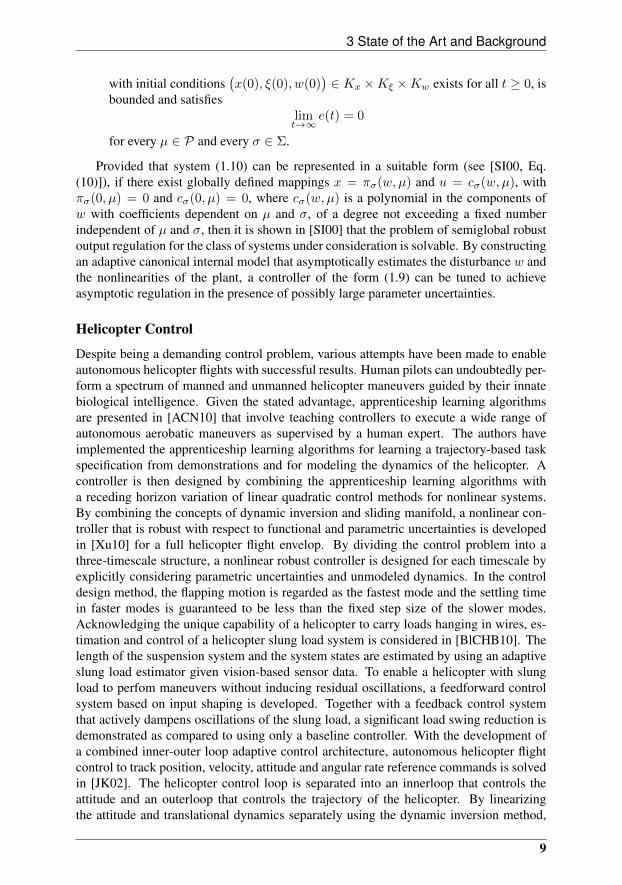
Provided that system (1.10) can be represented in a suitable form (see [SI00, Eq.(10)]), if there exist globally defined mappings x = πσ(w, µ) and u = cσ(w, µ), withπσ(0, µ) = 0 and cσ(0, µ) = 0, where cσ(w, µ) is a polynomial in the components ofw with coefficients dependent on µ and σ, of a degree not exceeding a fixed numberindependent of µ and σ, then it is shown in [SI00] that the problem of semiglobal robustoutput regulation for the class of systems under consideration is solvable. By constructingan adaptive canonical internal model that asymptotically estimates the disturbance w andthe nonlinearities of the plant, a controller of the form (1.9) can be tuned to achieveasymptotic regulation in the presence of possibly large parameter uncertainties.

Helicopter Control

Despite being a demanding control problem, various attempts have been made to enableautonomous helicopter flights with successful results. Human pilots can undoubtedly per-form a spectrum of manned and unmanned helicopter maneuvers guided by their innatebiological intelligence. Given the stated advantage, apprenticeship learning algorithmsare presented in [ACN10] that involve teaching controllers to execute a wide range ofautonomous aerobatic maneuvers as supervised by a human expert. The authors haveimplemented the apprenticeship learning algorithms for learning a trajectory-based taskspecification from demonstrations and for modeling the dynamics of the helicopter. Acontroller is then designed by combining the apprenticeship learning algorithms witha receding horizon variation of linear quadratic control methods for nonlinear systems.By combining the concepts of dynamic inversion and sliding manifold, a nonlinear con-troller that is robust with respect to functional and parametric uncertainties is developedin [Xu10] for a full helicopter flight envelop. By dividing the control problem into athree-timescale structure, a nonlinear robust controller is designed for each timescale byexplicitly considering parametric uncertainties and unmodeled dynamics. In the controldesign method, the flapping motion is regarded as the fastest mode and the settling timein faster modes is guaranteed to be less than the fixed step size of the slower modes.Acknowledging the unique capability of a helicopter to carry loads hanging in wires, es-timation and control of a helicopter slung load system is considered in [BlCHB10]. Thelength of the suspension system and the system states are estimated by using an adaptiveslung load estimator given vision-based sensor data. To enable a helicopter with slungload to perfom maneuvers without inducing residual oscillations, a feedforward controlsystem based on input shaping is developed. Together with a feedback control systemthat actively dampens oscillations of the slung load, a significant load swing reduction isdemonstrated as compared to using only a baseline controller. With the development ofa combined inner-outer loop adaptive control architecture, autonomous helicopter flightcontrol to track position, velocity, attitude and angular rate reference commands is solvedin [JK02]. The helicopter control loop is separated into an innerloop that controls theattitude and an outerloop that controls the trajectory of the helicopter. By linearizingthe attitude and translational dynamics separately using the dynamic inversion method,

9

Introduction

linear compensators are designed to control the forces and moments acting on the heli-copter. To handle parametric uncertainties in the linearized helicopter model, an artificialneural network is used as an adaptive element. With the use of Pseudo-Control-Hedging,unwanted adaptations to plant input characteristics such as actuator dynamics and to in-nerloop dynamics are successfully prevented. Isidori et al. addressed a challenging prob-lem in [IMS01] regarding the control of vertical motion of a helicopter while stabilizingthe lateral and longitudinal positions and maintaining a constant attitude. Consideringan application involving landing operations of an autonomous helicopter on a ship deck,the unknown motion of the ship deck is taken as the sum of a fixed number of sinu-soidal signals. By assuming that state measurements are available, a semiglobal robuststabilization scheme is developed based on nonlinear adaptive regulation and robust sta-bilization of systems in feedforward form by means of saturated controls. It is shownby simulations that the proposed controller performs well in the presence of parametricuncertainties and unmodeled dynamics. While a helicopter vertical trajectory trackingproblem is considered in [IMS01], Bejar et al. expand the control solution to includehorizontal motion control. In spite of the nonlinearity of helicopter dynamics and strongcoupling between forces and torques in a helicopter, vertical and horizontal trajectorycontrol problem is dealt with successfully in [BIMN05]. Given references with specificbounds on the higher order time derivatives, a nonlinear controller is constructed thatasymptotically tracks the desired trajectories in the presence of physical and aerodynam-ical parameter uncertainties. In the derivation of the control law, engine dynamics of themain rotor is included. Simulation results justify the reliability of the proposed controlscheme in the face of uncertainties concerning helicopter parameters and actuator model.

In all of the above reviewed research works, the controller designs for an autonomoushelicopter do not include wind disturbances either in the control synthesis or controllerperformance testing. In outdoor flights, the influence of wind disturbances on a helicopteris inevitable and measures to counter its effects have to be taken. In another multi-loophelicopter control design, a control structure combining robust H-infinity and PI control inthe presence of model uncertainty, gust disturbance and multi-mode flight requirementsis developed in [WMWD09]. By taking a state space representation of the helicoptermathematical model including parameter uncertainties and gust disturbance, a H-infinitycontroller is designed in the innerloop for robust stability and gust attenuation. To ad-dress tracking performance according to flight requirements, PI control is implementedin the outerloop. Stabilization of a simple nonlinear helicopter model in the face of ver-tical wind gusts is studied in [MLA09]. To achieve disturbance compensation in the 3degrees of freedom model helicopter mounted on an experimental platform, robust con-trol approaches including robust nonlinear feedback control, active disturbance rejectioncontrol based on a nonlinear extended state observer and backstepping control are sim-ulated for comparison purposes. While each of the control techniques possesses its ownadvantage over the others, simulation results verify the effectiveness of the controllers inhandling disturbances and modeling uncertainties. In [GSC+09], a high bandwidth innerloop controller is developed for an autonomous helicopter to provide attitude and velocitystabilization in the presence of wind disturbances based on the L1 adaptive control theory.The L1 adaptive controller is designed using a linear time-varying helicopter model withthe control objective to track desired bounded reference trajectory and orientation. Bysimulating the designed controller in a full nonlinear helicopter model with wind distur-bances generated using the Von Karman wind model and wind gusts, the superiority of

10

4 Outline of the Thesis

the L1 controller over a linear state feedback controller is verified.To land autonomous helicopters on ships at sea poses an immediate challenge due

to ship motion caused by waves and the presence of hostile turbulence. Even thoughhelicopter landing control problem is successfully resolved in [IMS01], the effect of winddisturbances is not taken into account. As analyzed above, although the performanceof the controllers developed in [WMWD09, MLA09, GSC+09] is tested for robustnessagainst wind disturbances, the disturbance information is not included explicitly in thecontrol design. To address the problem of controlling heave motion of an autonomoushelicopter in the presence of horizontal wind gusts, Yang et al. derived a heave motionmodel of an autonomous helicopter to capture the main influence of thrust variations inhover [YPG09]. A gust estimator is developed to obtain information on wind gust levelsin the presence of sensor errors including accelerometer vibration, accelerometer drift andmeasurement error of vertical velocity. The estimation of the wind gusts is then fed toa feedback-feedforward proportional derivative controller to compensate for the effectsfrom the horizontal gusts in the stabilization of helicopter heave motion.

1.4 Outline of the Thesis

In the next chapter, research methodology is presented describing undertaken approachesto find solutions for the problems in hand. After a summary of contributions of the Ph.D.project is given in Chapter 3, this thesis in concluded in Chapter 4.

The following papers are part of the thesis.

1. Paper A [DCHB09b]In this paper, a simple feedforward control scheme for wind disturbance rejectionin an autonomous helicopter is introduced. The feedforward control inputs thatare generated by trimming the helicopter model subjected to wind disturbance isadded to a feedback controller for helicopter stabilization in the presence of winddisturbance.

2. Paper B [DCHB09a]Assuming that a disturbance affecting a nonlinear plant could be measured, theconcept of disturbance effect is defined here. This is then used in the developmentof a feedforward control scheme independent of an existing feedback controller fordisturbance rejection in nonlinear control systems.

3. Paper C [DCHCB10]In this work, a necessary and sufficient condition for the existence of a stabilizingstate feedback with feedforward control that is robust with respect to state anddisturbance measurement errors, and external disturbances for a nonlinear controlsystem is developed.

4. Paper D [DLCHB10]Taking a sum of a fixed number of sinusoidal signals of unknown amplitudes, fre-quencies and phases as the wind disturbance, a feedback controller incorporating anadaptive internal model is constructed for helicopter stabilization that is insensitiveto parameter uncertainties.

11

Introduction

5. Paper E [BCHD10]By inverting a simplified helicopter model provided wind disturbance measure-ments, feedforward main rotor collective and cyclic pitch angles are generated here.The model based nonlinear feedforward control design for vertical and horizontalwind disturbance rejection is tested in actual flights in a laboratory with controllablewind sources.

6. Paper F [DLCHB]This journal paper is a extended version of Paper D that includes derivations ofequations and proofs of theorems presented in the conference paper.

Based on the definition of disturbance effect and feedforward control strategy for dis-turbance rejection in nonlinear control systems developed in Paper B, the feedforwardcontrol scheme using trim inputs for helicopter stabilization with wind disturbance elim-ination is proposed in Paper A. Using a higher complexity approach to produce feed-forward control inputs given wind disturbance measurements, wind disturbance rejectionis demonstrated in Paper E with reference to the same background obtained from PaperB. The control scheme introduced in Paper B and adapted in Paper A and E is a modelbased approach with the assumption that accurate state and disturbance measurements areavailable. To address a more realistic scenario, a state feedback with feedforward controlthat is less sensitive to measurement errors and additive model uncertainties is studiedin Paper C. Realizing the challenge in autonomous helicopter control to obtain precisewind disturbance measurements for control input generation, three dimensional wind dis-turbance estimation is developed in Paper D for robust helicopter stabilization. Althoughthe developed control law is highly mathematical, only a fraction of the steps taken in thecontrol development is presented in Paper D due to the limited number of pages of theconference paper. In Paper F, details of controller constructed in Paper D is elaboratedand more simulation results are included.

12

2 Methodology

In Section 1.2 of the previous chapter, challenging aspects of the helicopter control designfor stabilization with wind disturbance elimination are identified. Given the motivationalong with the nature of practical helicopter control, some of the relevant tools that areutilized to solve the problem in hand are listed here. Among others, in [DCHB09a] Lya-punov stability analysis is used to quantify the effects that external disturbances havein nonlinear control systems for the development of a feedforward control strategy fordisturbance rejection. With reference to the contribution in [DCHB09a], feedforwardcontrol inputs generated by trimming a helicopter model subject to wind disturbancesare used for helicopter stabilization. In the derivation of the necessary and sufficientcondition for the existence of a robustly stabilizing state feedback with feedforward, theconcepts of π-trajectory and differential inclusions play an important role in [DCHCB10].In [DLCHB10, DLCHB], input-to-state stability of an autonomous helicopter system per-turbed by wind disturbances with parameter uncertainties is analyzed. In general, eventhough a controller developed is mathematically sound, simulations and actual implemen-tations need to be carried out for the verification of proposed control methods. While onlya brief introduction on the research methods is given in this chapter, detailed steps andapproaches can be referred to in the papers attached as cited below.

2.1 Trim

Trimming a helicopter model involves computing a control input such that the rate ofchange of a helicopter state is zero and the resultant applied forces and moments is zero[Pad07]. Consider for instance, that a helicopter is in hover in the presence of a winddisturbance with a certain velocity in the negative x direction (see Fig. 5.3). Note thatthe control needed to sustain such a flight condition is equivalent to a control required toenable the helicopter to fly in the positive x direction with the same velocity (as the winddisturbance in the case). Therefore, if measurements of a wind disturbance are avail-able, control inputs to counter the effects of the wind disturbance can be computed byincluding the wind velocity measurements in the trim equations [DCHB09b]. Dependingon the complexity of a helicopter mathematical model used in the control approach pro-posed in [DCHB09b], real time implementations can be an issue. Note that the controlscheme using trim values assumes a perfect knowledge of the plant to be controlled withprecise state and disturbance measurements. Thus, any model mismatch or measurementinaccuracies will possibly affect the performance of the controller.

13

Methodology

2.2 Lyapunov Stability

As explained in the previous chapter, in a SISO linear control system, the effect that adisturbance has on output y is known provided that the measurements of disturbance dare available and dynamics D of the disturbance are known (see Fig. 1.1). The impor-tance of the knowledge of disturbance effect in linear control systems is easily noticedas the design of a feedforward controller Cff explicity involves the cancellation of thedisturbance effect on the output. In a nonlinear control system (see for e.g. (6.1)) how-ever, since disturbance w is just one of the arguments of nonlinear function f , an effort todesign a feedforward controller for a complete disturbance rejection could be dampeneddue to the lack of information on how an output is actually affected by the disturbance.In view of the Lyapunov stability criterion, if there exists a control-Lyapunov pair as de-scribed by [DCHB09a, Definition 2] for nonlinear systems considered therein with zerodisturbance input, asymptotic controllability is not guaranteed in the presence of nonzerodisturbance w. Keeping that in mind, a concept of disturbance effect for nonlinear sys-tems is defined. As stated in [DCHB09a, Definition 3], the disturbance effect is taken asthe difference between state derivative of a control system with a nonzero disturbance andstate derivative of an asymptotically controllable disturbance free nonlinear system withfeedback control. With the establishment of the disturbance effect notion for nonlinearsystems, a feedforward control scheme is proposed to nullify the disturbance effect toretain asymptotic controllability.

2.3 π-trajectory

In real world control applications, due to finite sampling frequencies of sensors used instate and disturbance measurements, constant control inputs over each sampling period isapplied to continuous plants. Furthermore, stabilizing control laws are in general discon-tinuous for general nonlinear control systems [LS99]. Thus it is natural to ponder howto define the solutions of differential equations governing the nonlinear control systemswith discontinuous right-hand sides. In other words, a clear definition of the state trajec-tories under piecewise constant control inputs is needed before stability conditions can beestablished. By adopting the notion of π-trajectory introduced in [CLSS99], the existenceof a robustly stabilizing state feedback with feedforward is studied in [DCHCB10].

2.4 Differential Inclusions

The main theorem in [DCHCB10] establishes a necessary and sufficient condition for theexistence of a robustly stabilizing state feedback with feedforward for a general nonlinearcontrol system. In the proof of [DCHCB10, Theorem 1], even though the necessary partis done in a direct way with minimum difficulty, the sufficiency part of the proof requires amore elaborate approach involving the converse Lyapunov function theorem for a stronglyasymptotically stable differential inclusion as stated in [DCHCB10, Theorem 2]. If thereexists a stabilizing state feedback with feedforward m that is robust with respect to stateand disturbance measurement errors and external disturbances for control system (7.1),then it is shown that differential inclusion

x ∈ G(x)

14

5 Input-to-State Stability

with multivalued function

G(x) :=⋂ε>0

co⋃d∈D

f(x,m(x+ εB, d+ εB), d

)is strongly asymptotically stable, where f is a continuous function and d is a persistentdisturbance ranging in a compact set D. In the equation above, B is a closed unit balland coS is the closure of the convex hull of a set S. From [DCHCB10, Theorem 2],this implies the existence of a smooth strong Lyapunov function for differential inclusion(7.12) and (7.13). It can be easily observed that the function is a smooth uniform controlLyapunov function for control system (7.1).

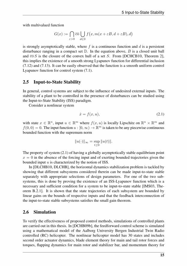
2.5 Input-to-State Stability

In general, control systems are subject to the influence of undesired external inputs. Thestability of a plant to be controlled in the presence of disturbances can be studied usingthe Input-to-State Stability (ISS) paradigm.

Consider a nonlinear system

x = f(x, u), (2.1)

with state x ∈ Rn, input u ∈ Rm where f(x, u) is locally Lipschitz on Rn × Rm andf(0, 0) = 0. The input function u : [0,∞)→ Rm is taken to be any piecewise continuousbounded function with the supremum norm

‖u(·)‖∞ = supt≥0‖u(t)‖.

The property of system (2.1) of having a globally asymptotically stable equilibrium pointx = 0 in the absence of the forcing input and of exerting bounded trajectories given thebounded input u is characterized by the notion of ISS.

In [DLCHB10, DLCHB], the horizontal dynamics stabilization problem is tackled byshowing that different subsystems considered therein can be made input-to-state stableseparately with appropriate selections of design parameters. For one of the two sub-systems, this is done by proving the existence of an ISS-Lyapunov function which is anecessary and sufficient condition for a system to be input-to-state stable [IMS03, The-orem B.2.1]. It is shown that the state trajectories of each subsystem are bounded bylinear gains on the bounds of respective inputs and that the feedback interconnection ofthe input-to-state stable subsystems satisfies the small gain theorem.

2.6 Simulation

To verify the effectiveness of proposed control methods, simulations of controlled plantsare carried out in this thesis. In [DCHB09b], the feedforward control scheme is simulatedusing a mathematical model of the Aalborg University Bergen Industrial Twin Radiocontrolled (RC) helicopter. The nonlinear helicopter model has 30 states and includessecond order actuator dynamics, blade element theory for main and tail rotor forces andtorques, flapping dynamics for main rotor and stabilizer bar, and momentum theory for

15

Methodology

the inflow model. Using wind velocity measurements obtained from a WindSonic IIwind sensor, trim feedforward control inputs are computed and used in the simulations todemonstrate the feasibility of the proposed approach. Due to the advanced control designin [DLCHB10, DLCHB], a simpler mathematical model of a helicopter is considered. Inthis model, the overall control input is provided by the main rotor thrust, tail rotor thrust,longitudinal flapping angle and lateral flapping angle. While the control design is carriedout based on a simplified resultant external force model, the performance of the controllerin a model of higher complexity is investigated by means of simulations.

2.7 Flight Tests

The model based nonlinear feedforward controller developed in [BCHD10] is tested inactual flights of the Aalborg University Corona Rapid Prototyping Platform. The au-tonomous helicopter is capable of performing full autonomous flights and due to its smallsize, all control computations are done on ground and transmitted through a standard RCsystem. The helicopter state and wind disturbance measurements are provided by a Viconmotion tracking system and a R.M. Young 81000 3D ultrasonic anemometer respectively.To enable a controlled experimental setup, the flight tests are carried out in a laboratoryequipped with three Big Bear II fans with a diameter of 0.6m. In order to demonstrate thefeasibility of the proposed feedforward control technique for measured wind disturbancecompensation, two different flight tests are carried out consisting hovering in front of thefans which are then turned on and flying the helicopter through wind stream of runningfans.

16

3 Summary of Contributions

Attached to this thesis, are published and submitted papers in chronological order to indi-cate the progressive steps taken towards achieving helicopter stabilization in the presenceof wind disturbances. Each paper reports separate contributions of this Ph.D. project de-tailing specific targeted problems, solutions and verifications of proposed designs. In thischapter, main contributions of this thesis are highlighted with regards to the identifiedresearch problems.

3.1 Disturbance Effects

The first contribution of this Ph.D. work is published in [DCHB09a] where the definitionof disturbance effects in a nonlinear control system influenced by an external disturbanceis given. As pointed out in Section 1.2 with reference to Fig. 1.1, the effect that a distur-bance d has on the output y of a single-input-single-output (SISO) linear control system isquantifiable if measurements of the disturbance are available and the disturbance dynam-ics D are known. With appropriate conditions concerning a SISO linear control system,this information is useful to derive a feedforward controller to produce a disturbance freeoutput (see Section 6.2). In a general nonlinear control system however (see e.g. (6.1)),since disturbancew is one the external inputs of system f , the influence of the disturbanceon system state is not readily understood. If one desires to employ feedforward controlfor disturbance rejection, a clear definition of disturbance effect is crucial so that its elim-ination can be verified to ensure a disturbance free system response. In [DCHB09a],guided by the outcome obtained from disturbance feedforward control of a SISO linearcontrol system with a known disturbance effect, the notion of disturbance effect D in anonlinear control system affected by an external disturbance w is introduced using Lya-punov stability analysis. The disturbance effect D is defined as the difference betweenstate derivative of a control system f with nonzero disturbance w and state derivative ofan asymptotically controllable disturbance free nonlinear system with feedback controlufb (see (6.5)).

3.2 Feedforward Control Strategy for Disturbance Rejection

With the establishment of the disturbance effects notion, the next contribution concerninga feedforward control scheme for disturbance rejection is reported in [DCHB09a]. Givena SISO linear control system as depicted in Fig. 1.1, provided that the disturbance d andits dynamicsD are known, feedforward control is an efficient technique of controlling the

17

Summary of Contributions

undesirable disturbance effect Dd on system output y by compensating before the effectstake place. As elaborated in Section 6.2, with the inclusion of the feedforward controllerCff, system output y appears to be only controlled by a feedback Cfb with complete elim-ination of the external disturbance d. Keeping that in mind, and given the definition ofdisturbance effect D when disturbance w is included in an asymptotically controllabledisturbance free nonlinear system with feedback ufb (see (6.5)), a feedforward control uffis taken as the control signal that can be added to the feedback ufb such that D = 0 asin (6.6). It is shown that the addition of feedforward control uff in a nonlinear controlsystem (6.1) affected by external disturbance w would result in a system appearing tobehave as if only feedback control ufb is present with zero disturbance input. Thus, thefeedforward control retains the asymptotic controllability of the feedback control systemwithout disturbance as shown in (6.7).

3.3 Robustly Stabilizing State Feedback with Feedforward

Even though the feedforward controller proposed in [DCHB09a] is effective in distur-bance rejection, the existence of such a control solution is not guaranteed. By developinga condition for the existence of a stabilizing state feedback with feedforward for non-linear control systems, a significant contribution is made in this thesis as published in[DCHCB10]. Consider general nonlinear control systems of the type

x = f(x, u, d), x ∈ Rn, u ∈ U, d ∈ D, (3.1)

where U ⊂ Rc is a compact set, persistent disturbance d = d(·) is a measurable functiontaking values in some compact set D ⊂ Rw and f : Rn × U × D → Rn is a continuousfunction.

In [LS99], it is shown that the existence of a smooth uniform control Lyapunov func-tion V for system (3.1) satisfying the following infinitesimal decrease condition

minu∈U

maxd∈D〈∇V (x), f(x, u, d)〉 ≤ −W (x) ∀x ∈ X, x 6= 0, (3.2)

where W : Rn → R≥0 is a continuous function and X ⊂ Rn is a bounded set, impliesthe existence of a robustly stabilizing state feedback. Futhermore, it is also proven that ifthere exists a robustly stabilizing state feedback then there exists a smooth uniform controlLyapunov function. Robustness in this context means that given any pair 0 < r < R,the state feedback drives all states in the ball of radius R into the ball of radius r aftersome time T for fast enough sampling and small enough measurement errors and externaldisturbances.

In this Ph.D. work, guided by the approach taken in [LS99], for control applicationswhere measurements of a persistent disturbance d are available, a necessary and suffi-cient condition for the existence of a stabilizing state feedback with feedforward which isinsensitive to measurement errors and external disturbances is developed.

Concerning the sufficiency part, if there exists a smooth uniform control Lyapunovfunction V for system (7.1) satisfying the infinitesimal decrease condition (see (7.3))

minu∈U〈∇V (x), f(x, u, d)〉 ≤ −W (x) ∀x ∈ X, x 6= 0,∀d ∈ D, (3.3)

18

4 Wind Disturbance Estimation and Helicopter Stabilization

then there always exists a (discontinuous in general) state feedback with feedforwardm : Rn × Rw → U which satisfies⟨

∇V (x), f(x,m(x, d), d

)⟩≤ −W (x), ∀x ∈ X, x 6= 0,∀d ∈ D. (3.4)

Note that the infinitesimal decrease condition (3.3) adopted in this thesis is different than(3.2) considered in [LS99]. To prove that the state feedback with feedforward m satisfy-ing (3.4) is robustly stabilizing, [DCHCB10, Lemma 2] is developed. The lemma showsthat given fast enough sampling and small enough measurement errors and external dis-turbances, every π-trajectory of (7.6) does not blow-up and that the time derivative of Vremains negative in each sampling interval.

The establishment of the necessary condition involves a more elaborate formulation.A necessary and sufficient condition is developed for the existence of a robustly stabi-lizing state feedback with feedforward m concerning the stability property of differentialinclusion (7.12) with multivalued right-hand side (7.13). This result is formulated in[DCHCB10, Proposition 2] whose proof requires a relationship between solutions of per-turbed system (7.6) and solutions of differential inclusion (7.12) and (7.13) as devised in[DCHCB10, Lemma 1]. Subsequently, using the converse Lyapunov function theoremfrom [CLS98] for differential inclusions with upper semicontinuous right-hand side, theexistence of a smooth uniform control Lyapunov function V for system (7.1) is verified.

3.4 Wind Disturbance Estimation and Helicopter Stabilization

Acknowledging the challenge involved in obtaining reliable wind disturbance measure-ments for helicopter control, a state feedback controller equipped with an adaptive inter-nal model for three dimensional wind disturbance estimation is developed in [DLCHB10,DLCHB] and is considered as the main contribution of this thesis. In [IMS03], a specifichelicopter control application is addressed where an autonomous helicopter is required toland on the deck of a ship which is subject to oscillations due to sea waves. To solve thecontrol problem, an adaptive internal-model-based controller is designed for enable thehelicopter to track a vertical reference trajectory given as the sum of a fixed number ofsinusoidal functions of time, of unknown frequency, amplitude and phase, that has to beestimated using tracking errors. Despite large uncertainties in parameters characterizingthe motion of the landing deck and large model uncertainties, the control solution whichis based on nonlinear adaptive output regulation and robust stabilization of systems infeedforward form by means of saturated controls, solves the trajectory tracking problemfor any arbitrary large set of initial conditions.

Motivated by the satisfactory performance reported in [IMS03], a more challengingproblem is tackled in this thesis involving helicopter stabilization in the presence of winddisturbances in all three axes. While one of the objectives of the adaptive internal modelincluded in the vertical dynamics in [IMS03] is to estimate the vertical motion of a shipdeck, adaptive internal models are used in [DLCHB10, DLCHB] to estimate wind distur-bances affecting translational motions of the helicopter in all axes. Realizing the impor-tance of information on the wind disturbance in stabilizing control input generation andaddressing a realistic scenario where accurate onboard disturbance measurements are notavailable, the estimation is considered as an integral part of the control design. To developan adaptive internal-model-based controller, the wind disturbances are taken to be the sum

19

Summary of Contributions

of a fixed number of sinusoids whose frequencies, amplitudes and phases are unknownconstants. This assumption is crucial so that the wind disturbance can be viewed as anoutput of an linear autonomous exosystem to facilitate the synthesis of a robust nonlinearcontroller of the following form

ξ = φ(ξ, pi, pi),

u = θ(ξ, pi, pi, q, ωb),(3.5)

incorporating the linear internal model φ, where pi and ωb denote the position (expessedin an inertial coordinate frame) of the center of mass and angular velocity (expessed ina body-fixed coordinate frame) of the helicopter respectively, q is the vector part of unitquarternions and ξ is the state of the feedback controller. The vector u = [TM a b TT ]>

is taken as the control input, where TM , TT , a and b are main rotor thrust, tail rotor thrust,longitudinal main rotor tip path plane tilt angle and lateral main rotor tip path plane tiltangle respectively.

The problem of helicopter stabilization with wind disturbance elimination is solvedby first designing a control law to generate the main rotor thrust TM for vertical dynamicsstabilization. Since the objective of the control law is to compensate for the gravity forcegM and the vertical wind disturbance dz (see (10.7)), an internal model is required toestimate the unknowns. It is shown in [DLCHB10, DLCHB] that the control law (10.15),(10.18) and (10.19) renders the vertical dynamics stable provided that q is sufficientlysmall, which can be ensured by tuning the control law (10.23) and (10.25) for controlinput v = [a b TT ]> (see [DLCHB, Proposition 5]). Next, the stability of longitudinaland lateral dynamics is proven by showing that the feedback interconnection of input-to-state stable subsystems (10.30) and (10.36) satisfies the small gain theorem as formalizedin [DLCHB, Proposition 6]. As part of the proof of [DLCHB, Proposition 6], [DLCHB,Lemma 3] establishes the existence of a selection of tuning parameters of control law v(that matches the requirements of [DLCHB, Proposition 5]) which assures that subsystem(10.36) is input-to-state stable.

20

4 Conclusion

With numerous application possibilities of autonomous helicopters, an immediate chal-lenge arises involving the ability to cope with wind disturbances. While state feedbackcontrollers without any information on the external effects would suffice in some in-stances, control input generation which relies on knowledge on the wind disturbancesis certainly desired for higher quality flights. This is because, given the wind disturbancemeasurements a complete information on external inputs affecting the controlled plant isnow available which is crucial for an effective helicopter control.

4.1 Objectives of the Project

Given the primary objective of this thesis that is to achieve helicopter stabilization inthe face of wind disturbances, helicopter control that requires the influence of wind dis-turbances in control input generation is studied. In other words, stabilization of an au-tonomous helicopter using control inputs as a function of the measurements or estimationof wind disturbances is the main goal here. In nonlinear control systems where mea-surements of external disturbances are available, state feedback with feedforward controlmethods such as full information output regulation and disturbance decoupling can en-sure stabilization despite the influence of the disturbance. Under suitable conditions,these control schemes that require system state and disturbance measurements guaranteedisturbance free outputs. In helicopter stabilization where wind disturbances could bemeasured, in addition to disturbance attenuation, it is also of interest to understand theeffects that the wind disturbances have on the helicopter system. With the quantificationof the disturbance effects, a feedforward control added to an existing feedback can bethe one that nullifies the disturbance effects. Acknowledging the challenges in reality toobtain accurate mathematical description of a helicopter and state and disturbance mea-surements, the development of a state feedback with feedforward that is insensitive tomeasurement errors and model uncertainties is set as one the goals of this research. Animmediate concern in the design of a state feedback with feedforward for helicopter con-trol is regarding the availability of wind disturbance measurements. Crucial issues per-taining sensor mounting location, accuracy, cost, time delay, etc. hamper the developmentof such a control scheme. Given the problem of having reliable wind disturbance mea-surements and realizing the importance of the information on wind disturbances in sta-bilizing control input generation, three dimensional wind disturbance estimation presentsitself as an important objective of this thesis.

21

Conclusion

4.2 Contributions of the Project

In this thesis, a preliminary idea based on disturbance feedforward control in SISO linearcontrol systems led to the establishment of the definition of disturbance effects in non-linear control systems influenced by external disturbances. The effects of a disturbancein a nonlinear control system are described through comparison with the same controlsystem that is asymptotically controllable with a feedback control in the absence of thedisturbance. As a consequence of the first contribution on this thesis, a feedforward con-trol strategy for disturbance rejection in nonlinear control systems that can be added toan existing feedback to cancel the disturbance effects is proposed. The formulation of thedisturbance effects and the related feedforward control scheme for nonlinear control sys-tems form the foundation of the development of feedforward control approaches for au-tonomous helicopters using trim inputs and inverted helicopter model. The feasibility ofthe proposed control methods for wind disturbance cancellation is demonstrated throughsimulations and flight tests. Since the performance of the control approach depends en-tirely on the availability of an exact mathematical model of a system to be controlled andprecise disturbance measurements, application issues involving model and measurementuncertainties need to be addressed. This led to the establishment of a necessary and suf-ficient condition for the existence of a robust state feedback with feedforward control forthe stabilization of nonlinear control systems. Given the fact that in general such a controlis discontinuous, the notion of π-trajectory is used to define the solution of a nonlinearcontrol system under a possibly discontinuous state feedback with feedforward control,in the presence of disturbances, state and disturbance measurement errors, and additivemodel uncertainties. The result presented in this thesis concerning the state feedback withfeedforward control that is insensitive to measurement errors and external disturbances isderived employing among others, the converse Lyapunov function theorem for stronglyasymptotically stable differential inclusions with upper semicontinuous right-hand side.Even though the specified contribution in nonlinear control deals with uncertainties that isinevitable in practical implementations, in helicopter control even wind disturbance mea-surements of modest quality can be a luxury given the influence of main rotor downwash.Therefore, three dimensional wind disturbance estimation for autonomous helicopter sta-bilization is developed and considered as the main contribution of this thesis. Equippedwith an adaptive internal model for wind disturbance estimation and to handle parameteruncertainties, a controller is designed based on nonlinear adaptive output regulation androbust stabilization of systems in feedforward form by saturated feedback controls. Thedeveloped control law solves the problem of helicopter stabilization with wind distur-bance elimination whose performance is verified through simulations.

In practical autonomous helicopter control, some complications due to the presenceof model and parameter uncertainties, measurement errors and unmodelled dynamics willnaturally arise. If a persistently acting wind disturbance can be measured, a robustly stabi-lizing state feedback with feedforward is expected to render the helicopter asymptoticallystable provided that the measurement errors and model uncertainties are small enoughand that the sampling is fast enough. However, since it is cumbersome to measure thewind disturbance on an autonomous helicopter, an estimate of the wind disturbance usingan adaptive internal model can be a good substitute. While the nonlinear controller withan internal model can handle parameter uncertainties, there is no surety that it is insensi-tive to measurement errors. Returning to the wind turbine inspection application, owing

22

3 Future Work

to the contribution of this thesis, a helicopter can now be dispatched from any permit-ted location around a wind turbine to execute designated routines. This is because theinternal model based nonlinear controller guarantees helicopter stabilization in the faceof wind disturbances from any initial conditions ranging in an arbitrarily large compactset. Equipped with the explicit capability to handle parameter uncertainties, the proposedhelicopter control technique is an enabling technology in wind turbine inspection and aspectrum of other unmanned real world applications.

4.3 Future Work

In the course of this Ph.D. project, several contributions related to nonlinear control andhelicopter stabilization are achieved. Even though significant results are obtained satis-fying the objectives of this thesis, there is still room for more works. In particular, totest the feasibilty of the proposed adaptive internal model based controller developed in[DLCHB10, DLCHB], an actual helicopter flight implementation will certainly be the ac-tion to be taken next. Recall that in this thesis, the control input is provided by main rotorthrust, tail rotor thrust, longitudinal main rotor tip path plane tilt angle and lateral mainrotor tip path plane tilt angle. While significant simplification is obtained in the controldesign due to the absence of nonlinearities of servo and rotor flapping dynamics, the useof such an actuator model does not represent the real world helicopter control problem.Hence, before the proposed control could be applied on an actual helicopter, servo androtor flapping dynamics have to be included in the control synthesis.

When the helicopter equipped with the improved controller is ready for actual flights,a subsequent future work could involve a suitable practical application. In wind turbineinspection using autonomous helicopters for instance, while the stabilization of a heli-copter with wind disturbance elimination plays a major role in effective test and checkroutines, it is still inadequate to perform a fully autonomous inspection. To carry outdesired tasks with minimum intervention from human operators, a helicopter has to beequipped with more autonomous capabilities such as autonomous lift-off and landing,path planning, trajectory tracking, obstacle avoidance, etc.

In general, autonomous helicopters are small in size. Consequently, with limitedability to generate force to drive its dynamic motion, the level of wind disturbances thatcould be withstood is limited. In critical applications where only a small error margin isallowed, it would be beneficial to identify the constraint in wind disturbances that could behandled for helicopter stabilization. This would be another important course of researchsince by knowing the intrinsic limitation of an autonomous helicopter in wind disturbancerejection, efficiency and safety in practical implementations will be certainly improved.

23

References

[ACN10] Pieter Abbeel, Adam Coates, and Andrew Y. Ng. Autonomous HelicopterAerobatics through Apprenticeship Learning. The International Journal ofRobotics Research, 29(8), 2010.

[BCHD10] M. Bisgaard, A. Cour-Harbo, and K. A. Danapalasingam. Nonlinear feed-forward control for wind disturbance rejection on autonomous helicopter.In 2010 IEEE/RSJ International Conference on Intelligent Robots and Sys-tems, October 2010.

[BIMN05] M. Bejar, A. Isidori, L. Marconi, and R. Naldi. Robust vertical/lateral/lon-gitudinal control of an helicopter with constant yaw-attitude. In Decisionand Control, 2005 and 2005 European Control Conference. CDC-ECC ’05.44th IEEE Conference on, pages 6192 – 6197, 12-15 2005.

[BlCHB10] Morten Bisgaard, Anders la Cour-Harbo, and Jan Dimon Bendtsen. Adap-tive control system for autonomous helicopter slung load operations. Con-trol Engineering Practice, 18(7):800 – 811, 2010. Special Issue on AerialRobotics.

[CLS98] F. H. Clarke, Yu. S. Ledyaev, and R. J. Stern. Asymptotic stability andsmooth Lyapunov functions. J. Differential Equations, 149(1):69–114,1998.

[CLSS99] F. H. Clarke, Yu. S. Ledyaev, E.D. Sontag, and A. I. Subbotin. Asymptoticcontrollability implies feedback stabilization. IEEE Trans. Autom. Control,42:1394–1407, 1999.

[DCHB09a] K. A. Danapalasingam, A. Cour-Harbo, and M. Bisgaard. Disturbance ef-fects in nonlinear control systems and feedforward control strategy. In The7th IEEE International Conference on Control and Automation, December2009.

[DCHB09b] K. A. Danapalasingam, A. Cour-Harbo, and M. Bisgaard. Feedforwardcontrol of an autonomous helicopter using trim inputs. In AIAA In-fotech@Aerospace Conference and AIAA Unmanned...Unlimited Confer-ence, April 2009.

[DCHCB10] K. A. Danapalasingam, A. Cour-Harbo, G. Chowdhary, and M. Bisgaard. Arobust stabilization using state feedback with feedforward. In 2010 Ameri-can Control Conference, June 2010.

25

REFERENCES

[DLCHB] K. A. Danapalasingam, J. Leth, A. Cour-Harbo, and M. Bisgaard. Robusthelicopter stabilization with wind disturbance elimination. Submitted toInternational Journal of Robust and Nonlinear Control.

[DLCHB10] K. A. Danapalasingam, J. Leth, A. Cour-Harbo, and M. Bisgaard. Robusthelicopter stabilization in the face of wind disturbance. In 49th IEEE Con-ference on Decision and Control, December 2010.

[GSC+09] B.J. Guerreiro, C. Silvestre, R. Cunha, C. Cao, and N. Hovakimyan. L1adaptive control for autonomous rotorcraft. pages 3250 –3255, jun. 2009.

[IMS01] A. Isidori, L. Marconi, and A. Serrani. Robust nonlinear motion control ofa helicopter. volume 5, pages 4586–4591 vol.5, 2001.

[IMS03] Alberto Isidori, Lorenzo Marconi, and Andrea Serrani. Robust autonomousguidance: An internal model approach. Advances in Industrial Control.Springer-Verlag New York, Inc., Secaucus, NJ, USA, 2003.

[Isi95] Alberto Isidori. Nonlinear control systems. Communications and ControlEngineering Series. Springer-Verlag, Berlin, third edition, 1995.

[JK02] E.N. Johnson and S.K. Kannan. Adaptive flight control for an autonomousunmanned helicopter. In Proceedings of the AIAA Guidance, Navigation,and Control Conference, pages 2002–4439, 2002.

[Lov07] Jonathan Love. Process Automation Handbook: A Guide to Theory andPractice. Springer, London, 2007.

[LS99] Yuri S. Ledyaev and Eduardo D. Sontag. A Lyapunov characterization ofrobust stabilization. Nonlinear Anal., 37(7, Ser. A: Theory Methods):813–840, 1999.

[MLA09] Adnan Martini, Franois Lonard, and Gabriel Abba. Dynamic modellingand stability analysis of model-scale helicopters under wind gust. Journalof Intelligent and Robotic Systems, 54:647–686, 2009.

[Pad07] G. Padfield. Helicopter Flight Dynamics, Second Edition: The Theoryand Application of Flying Qualities and Simulation Modeling. BlackwellScience Ltd, 2nd edition, 2007.

[SI00] A. Serrani and A. Isidori. Semiglobal nonlinear output regulation withadaptive internal model. In Decision and Control, 2000. Proceedings ofthe 39th IEEE Conference on, volume 2, pages 1649 –1654 vol.2, 2000.

[WMWD09] Hong-qiang Wang, Ashfaq Mian, Dao-bo Wang, and Hai-bin Duan. Ro-bust multi-mode flight control design for an unmanned helicopter basedon multi-loop structure. International Journal of Control, Automation andSystems, 7:723–730, 2009.

[Xu10] Yunjun Xu. Multi-timescale nonlinear robust control for a miniaturehelicopter. Aerospace and Electronic Systems, IEEE Transactions on,46(2):656 –671, april 2010.

26

[YPG09] X. Yang, H. Pota, and M. Garratt. Design of a gust-attenuation controllerfor landing operations of unmanned autonomous helicopters. In 18th IEEEInternational Conference on Control Applications, pages 1300 – 1305, July2009.

27

Paper A

Feedforward Control of an Autonomous Helicopter using TrimInputs

Kumeresan A. Danapalasingam, Anders la Cour-Harbo and Morten Bisgaard

This paper was published in:Proceedings of the AIAA Unmanned...Unlimited 2009 Conference and Exhibit

06–09 April 2009, Seattle, Washington, United States of America

Copyright c©2009 AIAAThe layout has been revised

Abstract

In this paper, a feedforward control strategy augmented to an existing feedbackcontroller is demonstrated for an autonomous helicopter. The sole purpose of thefeedforward controller is to assist the feedback loop in rejecting wind disturbancesbased on wind velocity measurements made onboard the helicopter. The feedforwardcontrol actions are obtained through trimming of the helicopter model subjected to asimulated wind, while a linear quadratic regulator (LQR) is implemented as the feed-back controller. Based on simulations performed using mathematical model of theBergen Industrial Twin autonomous helicopter with various wind velocity measure-ments, the feasibility of this approach for wind disturbance rejection is verified.

Nomenclature

d external disturbancer reference inputy plant outputCff feedforward controllerCfb feedback controllerP linear plantD external disturbance dynamicsf helicopter nonlinear equation of motionu control input vectorx state vectorx state derivative vectorn state space dimensionm control input space dimensionxe equilibrium state vectorue trim control input vectorx position in x-axisy position in y-axisz position in z-axisvx body translational velocity in x-axisvy body translational velocity in y-axisvz body translational velocity in z-axisdx wind velocity in x-axisdy wind velocity in y-axisdz wind velocity in z-axisξb trim condition based on body velocityξd trim condition based on wind disturbance velocityξ0 trim condition for hoverVb helicopter body velocity vector [vx vy vz]Vd wind disturbance velocity vector [dx dy dz]Vb length of Vb

γw sideslip angleγfp flight plane angleψtrim yaw rotation rateT trim function

31

Paper A

ufb feedback control inputuff feedforward control input∆ufb change in feedback control inputImp performance measurexfb output state vector with feedback control onlyxfb+ff output state vector with feedback and feedforward control

5.1 Introduction

Autonomous helicopters are small-scale helicopters, mostly equipped with on-board in-telligence capable of performing various tasks to assist human beings in their daily lives.Due to the physical scaling effects and specific design features found in helicopters of thatsize, unmanned autonomous helicopters are agile and highly maneuverable making themthe best candidates for many applications [1]. Such applications include surveillance,search and rescue, law enforcement, aerial mapping, cinematography, inspection, etc. Inagricultural applications for instance, autonomous helicopters can be used to detect pestinfestations, pesticide and fertilizer distribution, seed application, etc. In carrying outdesignated tasks as accurately as possible, the design of high performance controllers thatcould reject known and unknown disturbances and at the same time guarantee stabilityto produce desired flight quality is crucial. To date, numerous controller designs for au-tonomous helicopters have been accomplished with excellent results and a brief reviewwill be given here.

In Ref. [2] and [3], a hierarchical flight control system for unmanned aerial vehi-cles is designed where the lower level of stabilization and tracking problem is solved byusing both multi-loop PID controller and nonlinear MPC separately for comparison pur-poses. At each sample time, a nonlinear MPC computes a finite control sequence, whichminimizes a cost function, typically a weighted quadratic sum of states and input over afinite horizon. Kim et al. used a discretized internal model obtained from a partially non-linear continuous-time model (with nonlinear force terms and full nonlinear kinematicequations). In another work, Kim et al. investigated the feasibility of a nonlinear modelpredictive tracking control by formulating a nonlinear MPC algorithm for planning pathsunder input and state constraints and tracking the generated position and heading trajec-tories, and implement an on-line optimization controller using gradient-descent method.It was shown in Ref. [4] that the nonlinear MPC outperforms the conventional multi-loopPD controller in the tracking performance when the nonlinear kinematics and couplingdominate the vehicle dynamics even in the presence of model uncertainty.

In Ref. [5], an interesting problem is solved by Shim et al. with the implementation ofMPC in unmanned aerial vehicle autonomous exploration in unknown urban environment.Here, information about the surroundings is gathered, and obstacles in the flight path areavoided by building local obstacle maps and solving for conflict-free trajectory usingMPC framework. An MPC algorithm with a cost function that penalizes the proximity tothe nearest obstacle plans recurrently the flight path in real-time. It is reported that theproposed approach successfully guided the vehicle safely through the urban canyon.

Wan et al. [6] described a method for helicopter control through the use of the Flight-Lab simulator coupled with nonlinear control techniques. FlightLab is a commercialsoftware product developed by Advanced Rotorcraft Technologies. One of the outstand-ing features of the FlightLab is its ability to accurately model the main rotor and the

32

1 Introduction

interaction between it and other components, such as the tail rotor (through the use ofempirical formulas), external wind (e.g., through an external wind server), ground effects(including both in- and out-of-ground effects with an image method, a free wake model,and horse-shoe ground vortex model), etc. It also includes the modeling of dynamicstall, transonic flow, aero elastic response, vortex wake, blade element aerodynamics, andcan also provide finite element structure analysis. In the approach which referred to asmodel predictive neural control (MPNC), a feedback controller as a combination of astate-dependent Riccati equation (SDRE) controller and an optimal neural controller isutilized. The SDRE controller provides a robust stabilizing control, while the weights ofthe neural networks are optimized to minimize the overall receding horizon MPC cost.FlightLab has the built-in capability of incorporating some forms of winds (e.g., sinu-soidal gusts, stochastic atmospheric turbulent wind, etc.) into the calculation of total airloads on the rotors as well as fuselage. In Ref. [6], the existing atmospheric turbulentwind component (ATMTUR) is replaced with the one developed to allow inputs from anexternal wind server.

It is common to separate the autonomous helicopter flight control problem into an in-nerloop that controls attitude and an outerloop that controls the trajectory of the helicopter[7]. A neural network based direct adaptive control was applied in Ref. [7] to control ahelicopter where the reference commands include position, velocity, attitude and angularrate. E. N. Johnson and S. K. Kannan used the neural network to minimize the effectsof parametric uncertainty due to approximate inversion and pseudo control hedging tomodify the innerloop reference model dynamics. With the control approach along withcorrect placement of the combined poles of the linearized system, it was reported that theinner/outer loop interaction problems was mitigated and outer loop bandwidth increased,improving tracking performance further.

In this paper, the capability of a combination of feedback and feedforward controllersto remove the effects of wind disturbance on an autonomous helicopter will be demon-strated. As opposed to feedback controllers where unknown disturbances with unknowneffects are handled to obtain desired output response, feedforward controllers eliminatedisturbances more effectively by responding to measured disturbances with known dy-namics before the system is affected [8]. Here, the authors generate the feedforwardcontrol inputs from a trimmed helicopter model given wind disturbance measurements.A trimmed helicopter model is defined as a mathematical model where the rate of changeof the helicopter’s state vector is zero and the resultant of the applied forces and momentsis zero [9]. By providing wind velocity measurements to the trim equations, feedforwardcontrol inputs needed to reject the disturbances are calculated.

In the remainder of this paper, main concepts of feedforward control of an autonomoushelicopter using trim control inputs is explained after which a brief introduction on thehelicopter model used and simulation results are given. In Section 5.2, the idea of feed-forward control using trim inputs is detailed. The hardware which the simulation is basedon and simulation results are given in Section 5.3. In Section 5.4 and 5.5, discussion andconclusion are provided respectively.

33

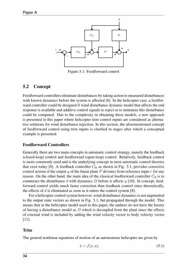
Paper A

+ -+

++-

r y

d

P

D

Cfb

Cff

Figure 5.1: Feedforward control

5.2 Concept

Feedforward controllers eliminate disturbances by taking action to measured disturbanceswith known dynamics before the system is affected [8]. In the helicopter case, a feedfor-ward controller could be designed if wind disturbance dynamic model that affects the endresponse is available and additive control signals to reject or to minimize this disturbancecould be computed. Due to the complexity in obtaining these models, a new approachis presented in this paper where helicopter trim control inputs are considered as alterna-tive solutions for wind disturbance rejection. In this section, the aforementioned conceptof feedforward control using trim inputs is clarified in stages after which a conceptualexample is presented.

Feedforward Controllers

Generally there are two main concepts in automatic control strategy, namely the feedback(closed-loop) control and feedforward (open-loop) control. Relatively, feedback controlis more commonly used and is the underlying concept in most automatic control theoriesthat exist today [8]. A feedback controller Cfb as shown in Fig. 5.1, provides correctivecontrol actions if the output y of the linear plant P deviates from reference input r for anyreason. On the other hand, the main idea of the classical feedforward controller Cff is tocounteract the disturbance d with dynamics D before it affects y [10]. In concept, feed-forward control yields much faster correction than feedback control since theoretically,the effects of d is eliminated as soon as it enters the control system [8].

For a helicopter control system however, wind disturbance dynamics is not augmentedto the output state vectors as shown in Fig. 5.1, but propagated through the model. Thismeans that in the helicopter model used in this paper, the authors do not have the luxuryof having a disturbance model as D which is decoupled from the plant since the effectsof external wind is included by adding the wind velocity vector to body velocity vector[11].

Trim

The general nonlinear equations of motion of an autonomous helicopter are given by

x = f(x, u), (5.1)

34

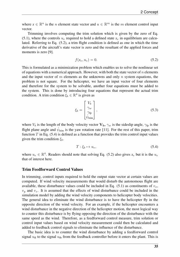
2 Concept

where x ∈ Rn is the n element state vector and u ∈ Rm is the m element control inputvector.

Trimming involves computing the trim solution which is given by the zero of Eq.(5.1), where the controls ue required to hold a defined state xe in equilibrium are calcu-lated. Referring to Eq. (5.2), a trim flight condition is defined as one in which the timederivative of the aircraft’s state vector is zero and the resultant of the applied forces andmoments is zero [9].

f(xe, ue) = 0. (5.2)

This is formulated as a minimization problem which enables us to solve the nonlinear setof equations with a numerical approach. However, with both the state vector of n elementsand the input vector of m elements as the unknowns and only n system equations, theproblem is not square. For the helicopter, we have an input vector of four elementsand therefore for the system to be solvable, another four equations must be added tothe system. This is done by introducing four equations that represent the actual trimcondition. A trim condition ξb ∈ R4 is given as

ξb =

Vbγwγfp

ψtrim

, (5.3)

where Vb is the length of the body velocity vector Vb, γw is the sideslip angle, γfp is theflight plane angle and ψtrim is the yaw rotation rate [11]. For the rest of this paper, trimfunction T in Eq. (5.4) is defined as a function that provides the trim control input valuesgiven the trim condition ξb.

T : ξb 7→ ue, (5.4)

where ue ∈ R4. Readers should note that solving Eq. (5.2) also gives xe but it is the uethat of interest here.

Trim Feedforward Control Values

In trimming, control inputs required to hold the output state vector at certain values arecomputed. If wind velocity measurements that would disturb the autonomous flight areavailable, these disturbance values could be included in Eq. (5.1) as constituents of vx,vy and vz . It is assumed that the effects of wind disturbance could be included in thesimulation model by adding the wind velocity components to helicopter body velocities.The general idea to eliminate the wind disturbance is to have the helicopter fly in theopposite direction of the wind velocity. For an example, if the helicopter encounters awind disturbance in the negative direction of the helicopter motion, the most logical wayto counter this disturbance is by flying opposing the direction of the disturbance with thesame speed as the wind. Therefore, as a feedforward control measure, trim solution orcontrol input values based on wind velocity measurement could then be calculated andadded to feedback control signals to eliminate the influence of the disturbance.

The basic idea is to counter the wind disturbance by adding a feedforward controlsignal uff to the signal ufb from the feedback controller before it enters the plant. This is

35

Paper A

+ ++-

r xufb

uff Vd

Cfb f(

x(Vd), u)

Figure 5.2: A simple representation of feedforward control for helicopter

shown in Fig 5.2. Since T (ξd) is the control input needed to keep the helicopter in theequilibrium state related to the wind disturbance trim condition, T (ξb) provided by thefeedback controller from the given body velocity must be subtracted. This is illustratedin Fig. 5.2, where the plant is disturbed by a wind velocity Vd as depicted in Fig. 5.3.Thus, effective values of feedforward control inputs would be given by

uff = T (ξd)− T (ξb), (5.5)

where ξd is the trim condition based on disturbance velocity vector Vd = [dx dy dz]and ξb is the trim condition based on current body velocity Vb. For better understandingof the trim condition based on Vd, Fig. 5.4 illustrates the flight condition that resultsfrom the application of T (ξd). Now, assume a hover flight condition and that the winddisturbance is coming from the front of the helicopter. These assumptions do not causeloss of generality since the feedforward control concept is independent of wind direction,and trim values can be computed for any equilibrium flight condition. Consequently, wenow assume Vd = [dx 0 0]. With the assumption that the feedback controller alwaysbrings the helicopter back to hover in the face of disturbances, corrective feedforwardcontrol inputs

uff = T (ξd)− T (ξ0) (5.6)

is added to feedback control signals where ξd is trim condition based on Vd = [dx 0 0]and ξ0 is trim condition based on Vb = [0 0 0]. Referring to Fig. 5.5, conceptually, theeffects of wind disturbance could be eliminated by providing only T (ξd) control signals tothe helicopter but this would eliminate the feedback loop and make the system vulnerableto even the slightest perturbations. In a hover flight, it is valid to assume that the feedbackcontroller generates the trim control inputs for hover T (ξ0) plus some perturbations ∆ufb(Fig. 5.6). By only considering the steady-state output value of the feedback controller(T (ξ0)) in the absence of disturbance and to still include the feedback loop, uff as givenby Eq. (5.6) is acceptable as the feedforward control signal. This setup is used in thefollowing section for simulation.

Artificial Neural Network (ANN)

In the field of artificial intelligence, artificial neural networks have been applied success-fully to pattern recognition, speech recognition, machine learning, control problems andvarious other engineering and nonengineering issues [12],[13],[14],[15].

As stated earlier, to enable a feedforward control action in the simulation, trim controlinputs have to be calculated using wind velocity as desired equilibrium states and added

36

2 Concept

Helicopter

x

y

Vd

Figure 5.3: Wind disturbance direction

T (ξd)

xeVb = [dx dy dz ]

f(x, u)

Figure 5.4: Trimmed flight. When the plant is given trim control input ue and the relatedtrim state xe, the resultant body velocity Vb is as provided in ξd.

T (ξd)

xVb = [0 0 0]

f(

x(Vd), u)

Vd = [dx 0 0]

Figure 5.5: Trim flight in the face of disturbance

+ ++-

r x

T (ξ0) + ∆ufb

T (ξd)− T (ξ0) Vd

Cfb f(

x(Vd), u)

Figure 5.6: Feedforward control in the face of wind disturbance

37

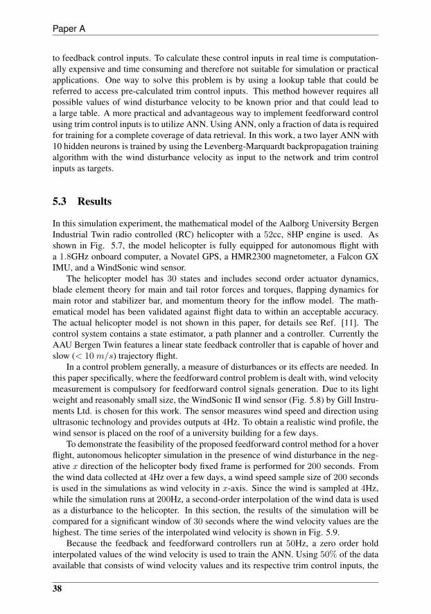
Paper A

to feedback control inputs. To calculate these control inputs in real time is computation-ally expensive and time consuming and therefore not suitable for simulation or practicalapplications. One way to solve this problem is by using a lookup table that could bereferred to access pre-calculated trim control inputs. This method however requires allpossible values of wind disturbance velocity to be known prior and that could lead toa large table. A more practical and advantageous way to implement feedforward controlusing trim control inputs is to utilize ANN. Using ANN, only a fraction of data is requiredfor training for a complete coverage of data retrieval. In this work, a two layer ANN with10 hidden neurons is trained by using the Levenberg-Marquardt backpropagation trainingalgorithm with the wind disturbance velocity as input to the network and trim controlinputs as targets.

5.3 Results

In this simulation experiment, the mathematical model of the Aalborg University BergenIndustrial Twin radio controlled (RC) helicopter with a 52cc, 8HP engine is used. Asshown in Fig. 5.7, the model helicopter is fully equipped for autonomous flight witha 1.8GHz onboard computer, a Novatel GPS, a HMR2300 magnetometer, a Falcon GXIMU, and a WindSonic wind sensor.

The helicopter model has 30 states and includes second order actuator dynamics,blade element theory for main and tail rotor forces and torques, flapping dynamics formain rotor and stabilizer bar, and momentum theory for the inflow model. The math-ematical model has been validated against flight data to within an acceptable accuracy.The actual helicopter model is not shown in this paper, for details see Ref. [11]. Thecontrol system contains a state estimator, a path planner and a controller. Currently theAAU Bergen Twin features a linear state feedback controller that is capable of hover andslow (< 10 m/s) trajectory flight.

In a control problem generally, a measure of disturbances or its effects are needed. Inthis paper specifically, where the feedforward control problem is dealt with, wind velocitymeasurement is compulsory for feedforward control signals generation. Due to its lightweight and reasonably small size, the WindSonic II wind sensor (Fig. 5.8) by Gill Instru-ments Ltd. is chosen for this work. The sensor measures wind speed and direction usingultrasonic technology and provides outputs at 4Hz. To obtain a realistic wind profile, thewind sensor is placed on the roof of a university building for a few days.

To demonstrate the feasibility of the proposed feedforward control method for a hoverflight, autonomous helicopter simulation in the presence of wind disturbance in the neg-ative x direction of the helicopter body fixed frame is performed for 200 seconds. Fromthe wind data collected at 4Hz over a few days, a wind speed sample size of 200 secondsis used in the simulations as wind velocity in x-axis. Since the wind is sampled at 4Hz,while the simulation runs at 200Hz, a second-order interpolation of the wind data is usedas a disturbance to the helicopter. In this section, the results of the simulation will becompared for a significant window of 30 seconds where the wind velocity values are thehighest. The time series of the interpolated wind velocity is shown in Fig. 5.9.

Because the feedback and feedforward controllers run at 50Hz, a zero order holdinterpolated values of the wind velocity is used to train the ANN. Using 50% of the dataavailable that consists of wind velocity values and its respective trim control inputs, the

38

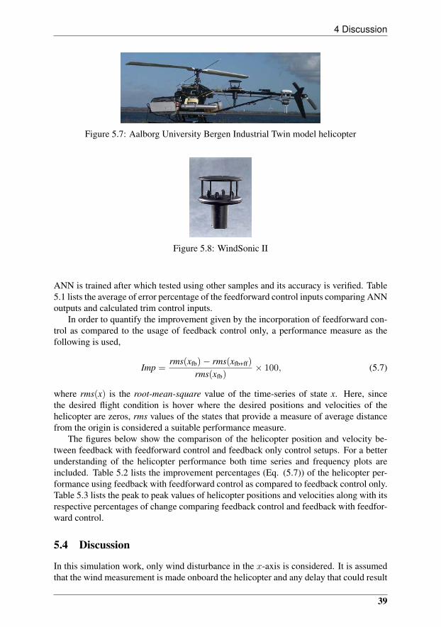
4 Discussion

Figure 5.7: Aalborg University Bergen Industrial Twin model helicopter

Figure 5.8: WindSonic II

ANN is trained after which tested using other samples and its accuracy is verified. Table5.1 lists the average of error percentage of the feedforward control inputs comparing ANNoutputs and calculated trim control inputs.

In order to quantify the improvement given by the incorporation of feedforward con-trol as compared to the usage of feedback control only, a performance measure as thefollowing is used,

Imp =rms(xfb)− rms(xfb+ff)

rms(xfb)× 100, (5.7)

where rms(x) is the root-mean-square value of the time-series of state x. Here, sincethe desired flight condition is hover where the desired positions and velocities of thehelicopter are zeros, rms values of the states that provide a measure of average distancefrom the origin is considered a suitable performance measure.

The figures below show the comparison of the helicopter position and velocity be-tween feedback with feedforward control and feedback only control setups. For a betterunderstanding of the helicopter performance both time series and frequency plots areincluded. Table 5.2 lists the improvement percentages (Eq. (5.7)) of the helicopter per-formance using feedback with feedforward control as compared to feedback control only.Table 5.3 lists the peak to peak values of helicopter positions and velocities along with itsrespective percentages of change comparing feedback control and feedback with feedfor-ward control.

5.4 Discussion

In this simulation work, only wind disturbance in the x-axis is considered. It is assumedthat the wind measurement is made onboard the helicopter and any delay that could result

39

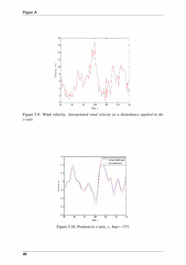
Paper A

Figure 5.9: Wind velocity. Interpolated wind velocity as a disturbance applied in thex-axis

Figure 5.10: Position in x-axis, x. Imp= 17%

40

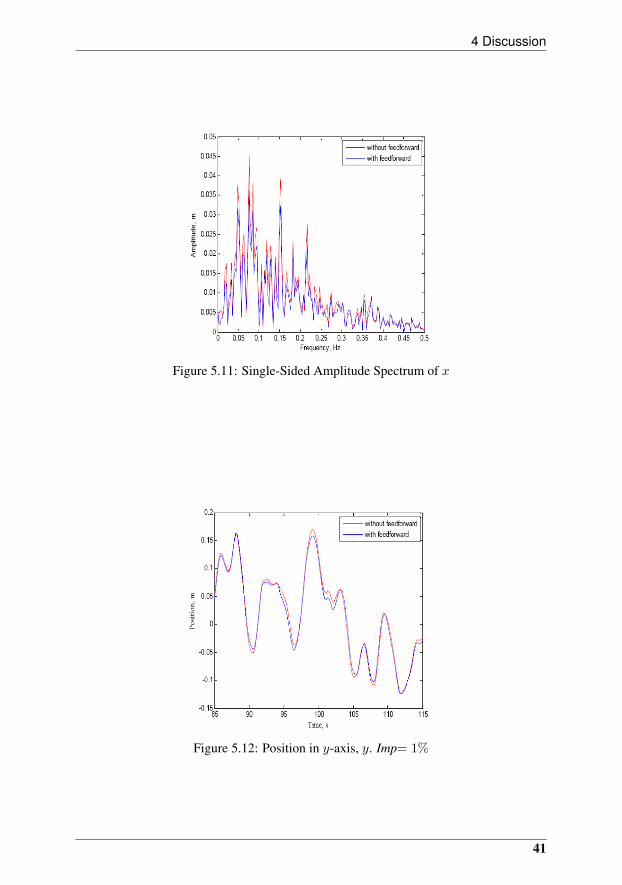
4 Discussion

Figure 5.11: Single-Sided Amplitude Spectrum of x

Figure 5.12: Position in y-axis, y. Imp= 1%

41

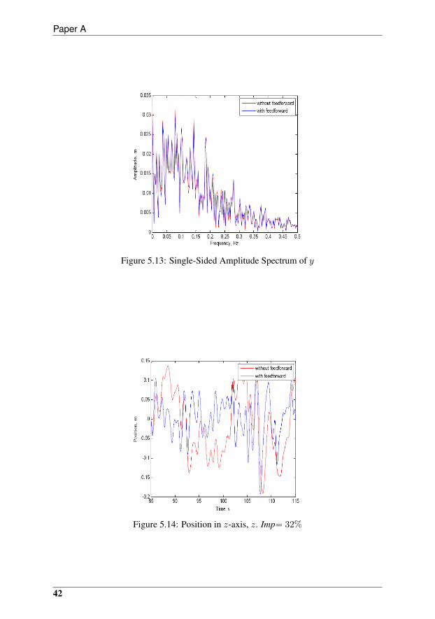
Paper A

Figure 5.13: Single-Sided Amplitude Spectrum of y

Figure 5.14: Position in z-axis, z. Imp= 32%

42

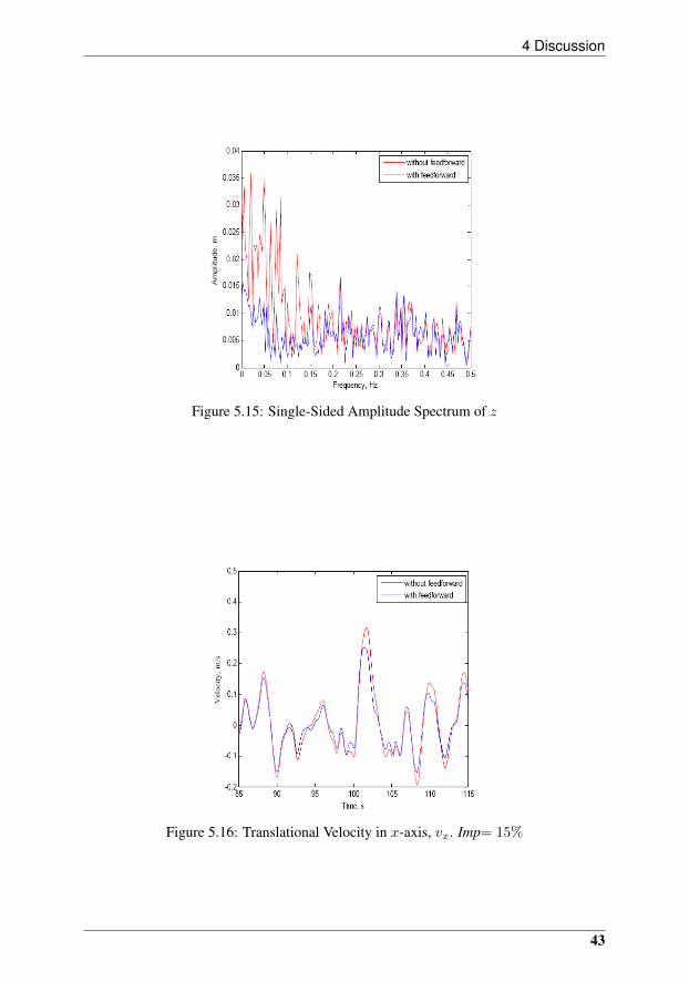
4 Discussion

Figure 5.15: Single-Sided Amplitude Spectrum of z

Figure 5.16: Translational Velocity in x-axis, vx. Imp= 15%

43

Paper A

Figure 5.17: Single-Sided Amplitude Spectrum of vx

Figure 5.18: Translational Velocity in y-axis, vy . Imp= −3%

44

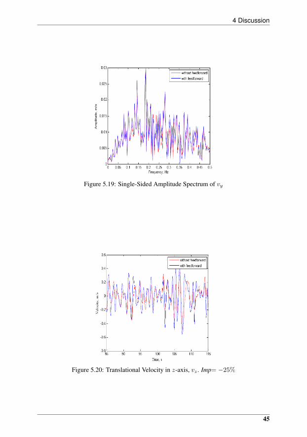
4 Discussion

Figure 5.19: Single-Sided Amplitude Spectrum of vy

Figure 5.20: Translational Velocity in z-axis, vz . Imp= −25%

45

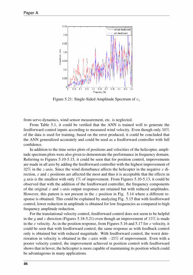
Paper A

Figure 5.21: Single-Sided Amplitude Spectrum of vz

from servo dynamics, wind sensor measurement, etc. is neglected.From Table 5.1, it could be verified that the ANN is trained well to generate the

feedforward control inputs according to measured wind velocity. Even though only 50%of the data is used for training, based on the error produced, it could be concluded thatthe ANN generalized accurately and could be used as a feedforward controller with fullconfidence.

In addition to the time series plots of positions and velocities of the helicopter, ampli-tude spectrum plots were also given to demonstrate the performance in frequency domain.Referring to Figures 5.10-5.15, it could be seen that for position control, improvementsare made in all axis by adding the feedforward controller with the highest improvement of32% in the z-axis. Since the wind disturbance affects the helicopter in the negative x di-rection, x and z positions are affected the most and thus it is acceptable that the effects iny axis is the smallest with only 1% of improvement. From Figures 5.10-5.13, it could beobserved that with the addition of the feedforward controller, the frequency componentsof the original x and z-axis output responses are retained but with reduced amplitudes.However, this pattern is not present in the z position in Fig. 5.14 where a different re-sponse is obtained. This could be explained by analyzing Fig. 5.15 that with feedforwardcontrol, lower reduction in amplitude is obtained for low frequencies as compared to highfrequency amplitude reduction.

For the translational velocity control, feedforward control does not seem to be helpfulin the y and z direction (Figures 5.18-5.21) even though an improvement of 15% is madein the x velocity. As in the position response, from Figures 5.16 and 5.17 for x velocity, itcould be seen that with feedforward control, the same response as with feedback controlonly is obtained but with reduced magnitude. With feedforward control, the worst dete-rioration in velocity is obtained in the z-axis with −25% of improvement. Even with apoorer velocity control, the improvement achieved in position control with feedforwardshows that in hover, the helicopter is more capable of maintaining its position which couldbe advantageous in many applications.

46

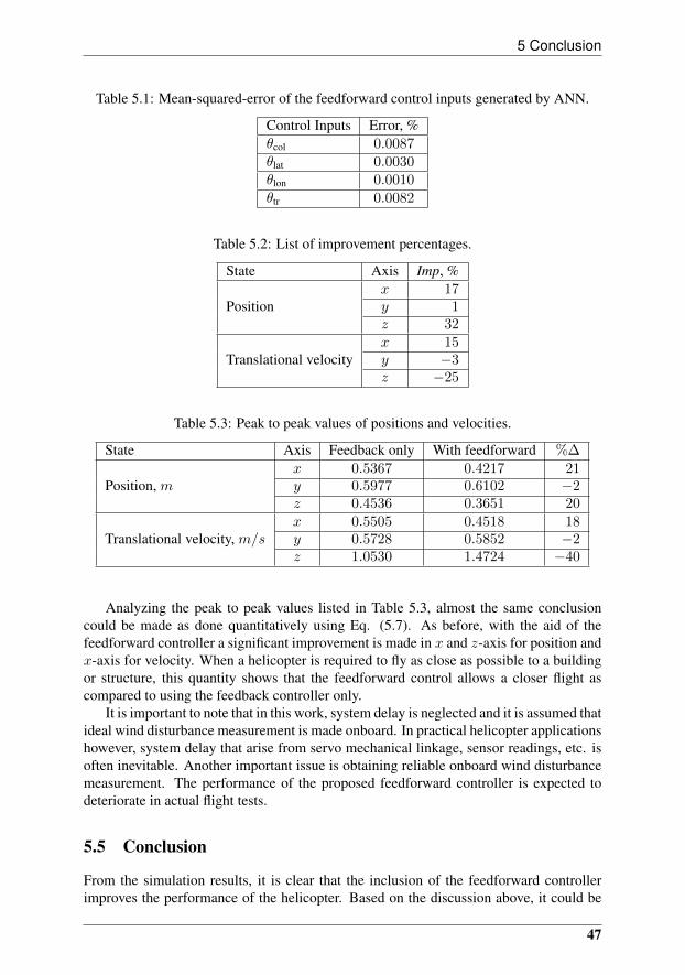
5 Conclusion

Table 5.1: Mean-squared-error of the feedforward control inputs generated by ANN.

Control Inputs Error, %θcol 0.0087θlat 0.0030θlon 0.0010θtr 0.0082

Table 5.2: List of improvement percentages.

State Axis Imp, %x 17

Position y 1z 32x 15

Translational velocity y −3z −25

Table 5.3: Peak to peak values of positions and velocities.

State Axis Feedback only With feedforward %∆x 0.5367 0.4217 21

Position, m y 0.5977 0.6102 −2z 0.4536 0.3651 20x 0.5505 0.4518 18

Translational velocity, m/s y 0.5728 0.5852 −2z 1.0530 1.4724 −40

Analyzing the peak to peak values listed in Table 5.3, almost the same conclusioncould be made as done quantitatively using Eq. (5.7). As before, with the aid of thefeedforward controller a significant improvement is made in x and z-axis for position andx-axis for velocity. When a helicopter is required to fly as close as possible to a buildingor structure, this quantity shows that the feedforward control allows a closer flight ascompared to using the feedback controller only.

It is important to note that in this work, system delay is neglected and it is assumed thatideal wind disturbance measurement is made onboard. In practical helicopter applicationshowever, system delay that arise from servo mechanical linkage, sensor readings, etc. isoften inevitable. Another important issue is obtaining reliable onboard wind disturbancemeasurement. The performance of the proposed feedforward controller is expected todeteriorate in actual flight tests.

5.5 Conclusion

From the simulation results, it is clear that the inclusion of the feedforward controllerimproves the performance of the helicopter. Based on the discussion above, it could be

47

Paper A

deduced that in order to control the position of the helicopter, it is unavoidable that thevelocity control to be expensed to a certain degree. This is not regarded as a weaknesssince in an application such as flying a helicopter in hover close to a building, the velocityvariation is less crucial than the position variation. In this work, only wind disturbance inx-axis is handled and the authors acknowledge the simplicity involved in formulating thefeedforward control law. The authors are also aware of the difficulty in obtaining accu-rate onboard wind disturbance measurements in real life. However, due to the promisingresults obtained, it is considered as an acceptable control approach for simulation pur-poses and would be a good start off point for a more practical work. As a future work,the mathematical approach of the proposed method will be explored for multi directionalwind disturbances. It is also expected that this method to be applied on a model helicopterfor actual autonomous flights in the near future.

48

References

[1] V. Gavrilets, B. Mettler, and E. Feron, “Dynamic model for a miniature aerobatic he-licopter,” Massachusetts Institute of Technology, MIT-LIDS report #LIDS-P-2579,2003.

[2] H. Kim and D. Shim, “A flight control system for aerial robots: algorithmsand experiments,” Control Engineering Practice, vol. 11, no. 12, pp. 1389 –1400, 2003, award winning applications-2002 IFAC World Congress. [Online].Available: http://www.sciencedirect.com/science/article/B6V2H-48PV8YC-4/2/928287d2c91e0da0c2d54415dec97ebf

[3] H. Kim, D. Shim, and S. Sastry, “Flying robots: Sensing, control and decision mak-ing,” University of California at Berkeley,” Submitted to 2002 IEEE InternationalConference on Robotics and Automation, 2002.

[4] ——, “Nonlinear model predictive tracking control for rotorcraft-based unmannedaerial vehicles,” in American Control Conference, 2002. Proceedings of the 2002,vol. 5, 2002, pp. 3576 – 3581 vol.5.

[5] D. Shim, H. Chung, H. Kim, and S. Sastry, “Autonomous exploration in unknownurban environments for unmanned aerial vehicles,” in in Proc. AIAA GN&C Con-ference, 2005.

[6] E. Wan, A. Bogdanov, R. Kieburtz, A. Baptista, M. Carlsson, Y. Zhang, and M. Zu-lauf, “Model predictive neural control for aggressive helicopter maneuvers,” in Soft-ware Enabled Control: Information Technologies for Dynamical Systems, chapter10. IEEE Press, John Wiley & Sons, 2003, pp. 175–200.

[7] E. Johnson and S. Kannan, “Adaptive flight control for an autonomous unmannedhelicopter,” in Proceedings of the AIAA Guidance, Navigation, and Control Confer-ence, 2002, pp. 2002–4439.

[8] B. Liptak, Instrument Engineers’ Handbook, 4th Edition, Vol. 2: Process Controland Optimization, 4th ed. ISA/CRC Press, 2005.

[9] G. Padfield, Helicopter Flight Dynamics, Second Edition: The Theory and Applica-tion of Flying Qualities and Simulation Modeling, 2nd ed. Blackwell Science Ltd,2007.

[10] J. van de Vegte, Feedback control systems (3rd ed.). Upper Saddle River, NJ, USA:Prentice-Hall, Inc., 1994.

49

REFERENCES

[11] M. Bisgaard, “Modeling, estimation, and control of helicopter slung load system,”Aalborg University,” Ph.D. Thesis, 2007.

[12] M. Negnevitsky, Artificial Intelligence: A Guide to Intelligent Systems. Boston,MA, USA: Addison-Wesley Longman Publishing Co., Inc., 2001.

[13] B. Chowdary, “Back-propagation artificial neural network approach for machiningcentre selection,” Journal of Manufacturing Technology Management, vol. 18, no. 3,pp. 315 – 332, 2007.

[14] D. E. Rumelhart, G. E. Hinton, and R. J. Williams, “Learning internal representa-tions by error propagation,” pp. 318–362, 1986.

[15] S. Ng, S. Leung, and A. Luk, “A generalized back-propagation algorithm for fasterconvergence,” in Neural Networks, 1996., IEEE International Conference on, vol. 1,June 1996.

50

Paper B

Disturbance Effects in Nonlinear Control Systems and FeedforwardControl Strategy

Kumeresan A. Danapalasingam, Anders la Cour-Harbo and Morten Bisgaard

This paper was published in:In Proceedings of the 7th IEEE International Conference on Control &

Automation09-11 December 2009, Christchurch, New Zealand

Copyright c©2009 IEEEThe layout has been revised

1 Introduction

Abstract

This work concerns the development of a feedforward control strategy for mea-surable disturbance rejection in general nonlinear systems with feedback control. Inother words, a separate design of disturbance feedforward controller is carried out tobe augmented to an existing nonlinear feedback control system. With reference to awell known disturbance feedforward control of linear systems, feedforward controlproblem for general nonlinear control systems is formulated. The notion of distur-bance effect is introduced with the aid of Lyapunov stability analysis of an asymp-totically stable disturbance free nonlinear system with feedback control. With the es-tablishment of the disturbance effect description, a feedforward control scheme thatguarantees asymptotic stability in the presence of external disturbance is proposedand verified using the inverted pendulum system as an illustrative example.

6.1 Introduction

In a feedback control system with external disturbance, corrective action to eliminate thedisturbance effects is only taken after the process has been affected. If the disturbanceis measurable, feedforward control can be an effective open-loop control technique toprevent undesirable response due to the ability to take corrective actions before the dis-turbance affects the system. Feedforward control has been widely used in industry [1]and this efficient approach for disturbance rejection has motivated extensive research inthe combination of feedback and feedforward control methods [2, 3, 4, 5, 6, 7].

Some significant results in feedforward control involving nonlinear systems will bereviewed here. In [8], discrete-time feedforward/feedback controllers are developed forgeneral nonlinear processes with stable zero dynamics and its connections with modelpredictive approaches are established. It is claimed that the derived controllers couldreduce if not eliminate completely the effect of measurable disturbances and produce aprespecified linear response with respect to a reference input. The design of the con-trollers is synthesized in a coupled manner where separate objectives of the feedforwardand feedback controllers are realized by means of one unified control law. In a recentwork, an adaptive neural network feedforward compensator for external disturbances af-fecting a specific class of closed-loop system is introduced [9]. A nonlinear disturbancemodel is estimated to counteract the disturbance affecting a linear discrete closed-loopsystem. In this scheme, the disturbance model output is required to match the compen-sation signal for an effective rejection of the disturbance. Another feedforward controlscheme using artificial neural networks is reported in [10] describing a nonlinear adap-tive feedforward controller for compensation of external load disturbances in the idlespeed control of an automotive engine. The feedforward only approach is based on Ra-dial Basis Function network approximation of certain input-output mappings describingthe system. The mapping involves optimal control input and a system variable that mini-mizes a quadratic performance index as the control objective. In another related work, theproblem of adaptive feedforward compensation for input-to-state (and locally exponen-tially) convergent nonlinear systems is investigated [11]. The proposed scheme achieveddisturbance rejection of a harmonic disturbance at the input of the nonlinear system class.

In this paper, preliminary results concerning feedforward control for external distur-bance rejection in general nonlinear feedback control systems is presented. Given an

53

Paper B

asymptotically controllable disturbance free nonlinear system with feedback control, adecoupled design of feedforward control is accomplished for disturbance elimination andhence to guarantee asymptotic controllability in the face of disturbance. Before a strat-egy could be developed involving measuring the disturbance and generating appropriatefeedforward control signals, the effects of the disturbance on the system has to be wellunderstood. For better understanding of the concept and to be aware of the objective ofa feedforward control, the notion of disturbance effect in a nonlinear system affected byan external disturbance is introduced using Lyapunov stability analysis. A feedforwardcontrol strategy therefore can be one that nullifies the disturbance effect completely. Itis shown that the proposed feedforward controller (to assist the feedback controller) thatmeasures current disturbance and generates a corrective control signal warrants a decreas-ing control-Lyapunov function to achieve asymptotic controllability.

The paper is organized as follows: Section 6.2 introduces preliminary background onnonlinear dynamical systems and classical approach of disturbance feedforward controlfor linear systems with additive disturbance, after which the problem statement of distur-bance feedforward control of nonlinear systems is described. In Section 6.3, properties ofLyapunov stability is given and some definitions are introduced. A disturbance feedfor-ward control scheme to assist a feedback controller for nonlinear systems is proposed inSection 6.4. Finally, a simulation example is given in Section 6.5 followed by conclusionin Section 6.7.

6.2 Preliminaries and Problem Statement

Before the concept of disturbance effect and disturbance feedforward control for nonlin-ear systems could be formulated, the classical approach of feedforward control of linearsystems with additive disturbance has to be reviewed. This is essential to gain insights forderiving an equivalent technique for effective external disturbance rejection in nonlinearcontrol systems.

Nonlinear Dynamical Systems

We deal with a nonlinear finite-dimensional control system of the following form:

x(t) = f(x(t), u(t), w(t)

), (6.1)

where states x(t) ∈ Rn (the integer n is the dimension of the system), controls inputs aremeasurable locally essentially bounded maps

u : [0,+∞)→ U ⊆ Rm

into the control-value set and external disturbance w(t) ∈ Rd. It is assumed that f islocally Lipschitz on (x, u, w) and f(0, 0, 0) = 0. The maximal solution x(·) of (6.1)corresponding to a given initial state x(t0) = x0, control u and disturbance w, is definedon some maximal interval [t0, tmax(x0, u, w)) and is denoted by x(t;x0, u, w).

The notion of state plays a central role in the definition of a dynamical system. Statevariables describe processes in the interior of the system and for system (6.1), two basicconditions are required [12]:

54

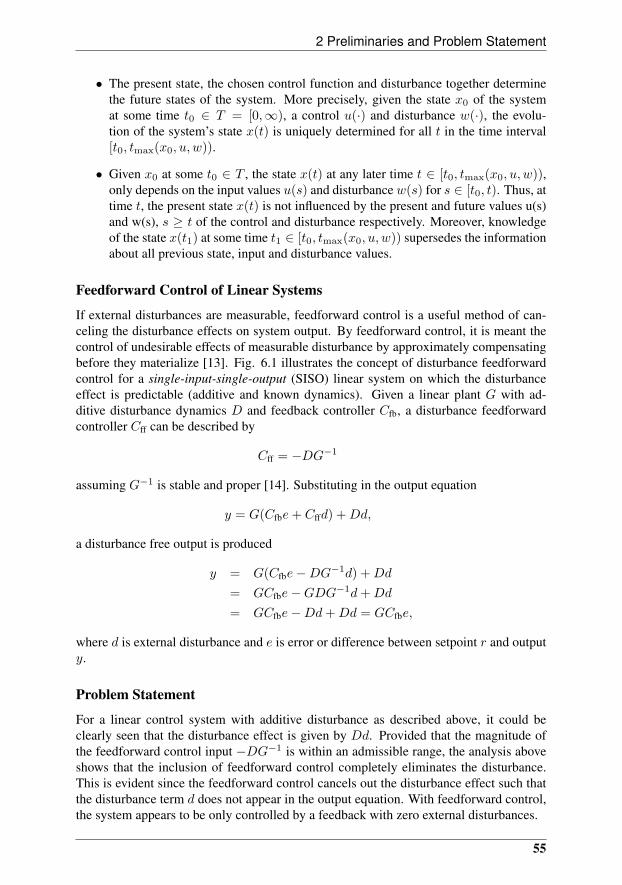
2 Preliminaries and Problem Statement

• The present state, the chosen control function and disturbance together determinethe future states of the system. More precisely, given the state x0 of the systemat some time t0 ∈ T = [0,∞), a control u(·) and disturbance w(·), the evolu-tion of the system’s state x(t) is uniquely determined for all t in the time interval[t0, tmax(x0, u, w)).

• Given x0 at some t0 ∈ T , the state x(t) at any later time t ∈ [t0, tmax(x0, u, w)),only depends on the input values u(s) and disturbance w(s) for s ∈ [t0, t). Thus, attime t, the present state x(t) is not influenced by the present and future values u(s)and w(s), s ≥ t of the control and disturbance respectively. Moreover, knowledgeof the state x(t1) at some time t1 ∈ [t0, tmax(x0, u, w)) supersedes the informationabout all previous state, input and disturbance values.

Feedforward Control of Linear Systems

If external disturbances are measurable, feedforward control is a useful method of can-celing the disturbance effects on system output. By feedforward control, it is meant thecontrol of undesirable effects of measurable disturbance by approximately compensatingbefore they materialize [13]. Fig. 6.1 illustrates the concept of disturbance feedforwardcontrol for a single-input-single-output (SISO) linear system on which the disturbanceeffect is predictable (additive and known dynamics). Given a linear plant G with ad-ditive disturbance dynamics D and feedback controller Cfb, a disturbance feedforwardcontroller Cff can be described by

Cff = −DG−1

assuming G−1 is stable and proper [14]. Substituting in the output equation

y = G(Cfbe+ Cffd) +Dd,

a disturbance free output is produced

y = G(Cfbe−DG−1d) +Dd

= GCfbe−GDG−1d+Dd

= GCfbe−Dd+Dd = GCfbe,

where d is external disturbance and e is error or difference between setpoint r and outputy.

Problem Statement

For a linear control system with additive disturbance as described above, it could beclearly seen that the disturbance effect is given by Dd. Provided that the magnitude ofthe feedforward control input −DG−1 is within an admissible range, the analysis aboveshows that the inclusion of feedforward control completely eliminates the disturbance.This is evident since the feedforward control cancels out the disturbance effect such thatthe disturbance term d does not appear in the output equation. With feedforward control,the system appears to be only controlled by a feedback with zero external disturbances.

55

Paper B

+ ++

++-

r e y

d

G(s)

D(s)

Cfb(s)

Cff(s)

Figure 6.1: Concept of feedforward control for a linear system with known additive dis-turbances.

One promising approach to derive a feedforward controller for a nonlinear systemwith external disturbance (6.1) is to expect the same outcome as obtained in the linear caseabove. It is desirable to have the nonlinear system behave as if there is no disturbanceacting upon it with feedforward control. In addition, the nonlinear system should nowappear to be controlled by only a feedback, i.e.

f(x, ufb + uff, w) = f(x, ufb, 0), (6.2)

where locally bounded functions ufb : Rn → U and uff : Rn × Rd → U are calledfeedback and feedforward respectively.

6.3 Lyapunov Stability Analysis

Even though it is made clear in (6.2) the desired system behavior with feedforward con-trol, it is not obvious what is being compensated for. In feedforward control for distur-bance rejection, a clear definition of disturbance effect is compulsory so that its elimina-tion can be verified to produce a disturbance free system response. In this section, thenotion of disturbance effect will be defined with the aid of Lyapunov stability analysis ofsystem (6.1). Some related definitions and theorem are given as follows [15], [16].

Definition 1. System (6.1) is asymptotically controllable if:

1. (attractiveness) for each x0 ∈ Rn there exists some control u such that the trajec-tory x(t) = x(t;x0, u, w) is defined for all t ≥ 0 and x(t)→ 0 as t→ +∞;

2. (Lyapunov stability) for each ε > 0 there exists δ > 0 such that for each x0 ∈ Rnwith |x0| < δ there is a control u as in 1 such that |x(t)| < ε for all t ≥ 0;

3. (bounded controls) there are a neighbourhood X0 of 0 in Rn and a compact subsetU0 of U such that, if the initial state x0 in 2 satisfies also x0 ∈ X0, then the controlin 2 can be chosen with u(t) ∈ U0 for almost all t.

Definition 2. A control-Lyapunov pair for (6.1) consists of two continuous functionsV,W : Rn → R≥0 such that the following properties hold.

56

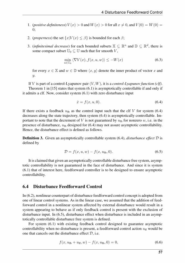
4 Disturbance Feedforward Control

1. (positive definiteness) V (x) > 0 andW (x) > 0 for all x 6= 0, and V (0) = W (0) =0;

2. (properness) the set x|V (x) ≤ β is bounded for each β;

3. (infinitesimal decrease) for each bounded subsets X ⊆ Rn and D ⊆ Rd, there issome compact subset U0 ⊆ U such that for smooth V ,

minu∈U0

〈∇V (x), f(x, u, w)〉 ≤ −W (x) (6.3)

for every x ∈ X and w ∈ D where 〈x, y〉 denote the inner product of vector x andy.

If V is part of a control-Lyapunov pair (V,W ), it is a control-Lyapunov function (clf).Theorem 1 in [15] states that system (6.1) is asymptotically controllable if and only if

it admits a clf. Now, consider system (6.1) with zero disturbance input

x = f(x, u, 0). (6.4)

If there exists a feedback ufb as the control input such that the clf V for system (6.4)decreases along the state trajectory, then system (6.4) is asymptotically controllable. Im-portant to note that the decrement of V is not guaranteed by ufb for nonzero w, i.e. in thepresence of disturbance, ufb designed for (6.4) may not assure asymptotic controllability.Hence, the disturbance effect is defined as follows.

Definition 3. Given an asymptotically controllable system (6.4), disturbance effect D isdefined by

D = f(x, u, w)− f(x, ufb, 0). (6.5)

It is claimed that given an asymptotically controllable disturbance free system, asymp-totic controllability is not guaranteed in the face of disturbance. And since it is system(6.1) that of interest here, feedforward controller is to be designed to ensure asymptoticcontrollability.

6.4 Disturbance Feedforward Control

In (6.2), nonlinear counterpart of disturbance feedforward control concept is adopted fromone of linear control systems. As in the linear case, we assumed that the addition of feed-forward control in a nonlinear system affected by external disturbance would result in asystem appearing to behave as if only feedback control is present with the exclusion ofdisturbance input. In (6.5), disturbance effect when disturbance is included in an asymp-totically controllable disturbance free system is defined.

For system (6.1) with existing feedback control designed to guarantee asymptoticcontrollability when no disturbance is present, a feedforward control action uff would beone that cancels out the disturbance effect D, i.e.

f(x, ufb + uff, w)− f(x, ufb, 0) = 0, (6.6)

57

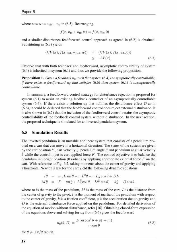
Paper B

where now u := ufb + uff in (6.5). Rearranging,

f(x, ufb + uff, w) = f(x, ufb, 0)

and a similar disturbance feedforward control approach as agreed in (6.2) is obtained.Substituting in (6.3) yields

〈∇V (x), f(x, ufb + uff, w)〉 = 〈∇V (x), f(x, ufb, 0)〉≤ −W (x) (6.7)

Observe that with both feedback and feedforward, asymptotic controllability of system(6.4) is inherited in system (6.1) and thus we provide the following proposition.

Proposition 1. Given a feedback ufb such that system (6.4) is asymptotically controllable,if there exists a feedforward uff that satisfies (6.6) then system (6.1) is asymptoticallycontrollable.

In summary, a feedforward control strategy for disturbance rejection is proposed forsystem (6.1) to assist an existing feedback controller of an asymptotically controllablesystem (6.4). If there exists a solution uff that nullifies the disturbance effect D as in(6.6), it could be deduced that the feedforward control does reject external disturbance. Itis also shown in (6.7) that the inclusion of the feedforward control retains the asymptoticcontrollability of the feedback control system without disturbance. In the next section,the proposed technique is simulated for an inverted pendulum system.

6.5 Simulation Results

The inverted pendulum is an unstable nonlinear system that consists of a pendulum piv-oted on a cart that can move in a horizontal direction. The states of the system are givenby the cart position Y , cart velocity y, pendulum angle θ and pendulum angular velocityθ while the control input is cart applied force F . The control objective is to balance thependulum in upright position (0 radian) by applying appropriate external force F on thecart. With reference to Fig. 6.2, taking moments about the center of gravity and applyinga horizontal Newton’s law for the cart yield the following dynamic equations

Iθ = mgL sin θ −mL2θ −mLy cos θ +DL

My = F −m(y + Lθ cos θ − Lθ2 sin θ)− ky −D cos θ,

where m is the mass of the pendulum, M is the mass of the cart, L is the distance fromthe center of gravity to the pivot, I is the moment of inertia of the pendulum with respectto the center of gravity, k is a friction coefficient, g is the acceleration due to gravity andD is the external disturbance force applied on the pendulum. For detailed derivation ofthe equation of motion without disturbance, refer [16]. Obtaining closed-form expressionof the equations above and solving for uff from (6.6) gives the feedforward

uff(θ,D) =D(m cos2 θ +M +m)

m cos θ(6.8)

for θ 6= ±π/2 radian.

58

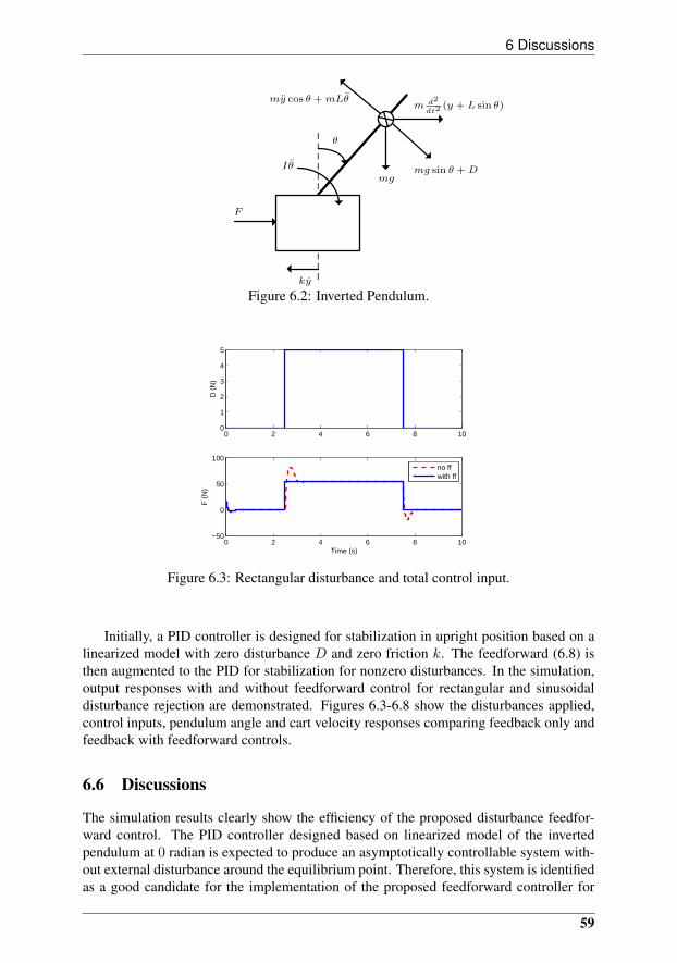
6 Discussions

F

ky

Iθ

θ

mgmg sin θ +D

my cos θ +mLθm d2

dt2(y + L sin θ)

Figure 6.2: Inverted Pendulum.

0 2 4 6 8 100

1

2

3

4

5

D (

N)

0 2 4 6 8 10−50

0

50

100

Time (s)

F (

N)

no ffwith ff

Figure 6.3: Rectangular disturbance and total control input.

Initially, a PID controller is designed for stabilization in upright position based on alinearized model with zero disturbance D and zero friction k. The feedforward (6.8) isthen augmented to the PID for stabilization for nonzero disturbances. In the simulation,output responses with and without feedforward control for rectangular and sinusoidaldisturbance rejection are demonstrated. Figures 6.3-6.8 show the disturbances applied,control inputs, pendulum angle and cart velocity responses comparing feedback only andfeedback with feedforward controls.

6.6 Discussions

The simulation results clearly show the efficiency of the proposed disturbance feedfor-ward control. The PID controller designed based on linearized model of the invertedpendulum at 0 radian is expected to produce an asymptotically controllable system with-out external disturbance around the equilibrium point. Therefore, this system is identifiedas a good candidate for the implementation of the proposed feedforward controller for

59

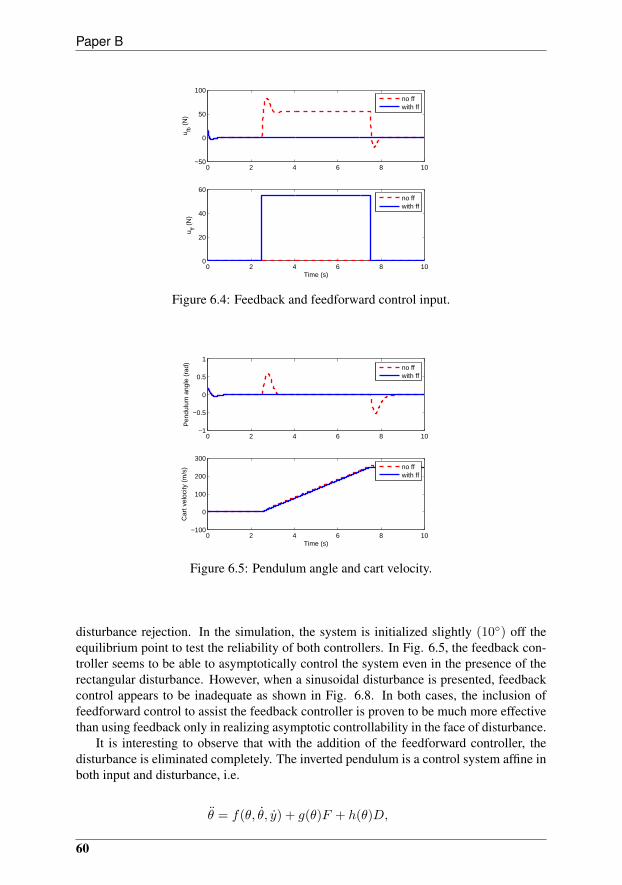
Paper B

0 2 4 6 8 10−50

0

50

100

u fb (

N)

no ffwith ff

0 2 4 6 8 100

20

40

60

Time (s)

u ff (N

)

no ffwith ff

Figure 6.4: Feedback and feedforward control input.

0 2 4 6 8 10−1

−0.5

0

0.5

1

Pen

dulu

m a

ngle

(ra

d)

no ffwith ff

0 2 4 6 8 10−100

0

100

200

300

Time (s)

Car

t vel

ocity

(m

/s)

no ffwith ff

Figure 6.5: Pendulum angle and cart velocity.

disturbance rejection. In the simulation, the system is initialized slightly (10) off theequilibrium point to test the reliability of both controllers. In Fig. 6.5, the feedback con-troller seems to be able to asymptotically control the system even in the presence of therectangular disturbance. However, when a sinusoidal disturbance is presented, feedbackcontrol appears to be inadequate as shown in Fig. 6.8. In both cases, the inclusion offeedforward control to assist the feedback controller is proven to be much more effectivethan using feedback only in realizing asymptotic controllability in the face of disturbance.

It is interesting to observe that with the addition of the feedforward controller, thedisturbance is eliminated completely. The inverted pendulum is a control system affine inboth input and disturbance, i.e.

θ = f(θ, θ, y) + g(θ)F + h(θ)D,

60

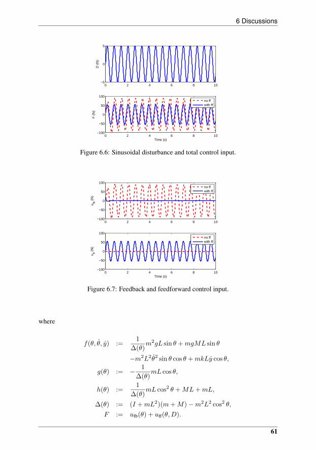
6 Discussions

0 2 4 6 8 10−5

0

5

D (

N)

0 2 4 6 8 10−100

−50

0

50

100

Time (s)

F (

N)

no ffwith ff

Figure 6.6: Sinusoidal disturbance and total control input.

0 2 4 6 8 10−100

−50

0

50

100

u fb (

N)

no ffwith ff

0 2 4 6 8 10−100

−50

0

50

100

Time (s)

u ff (N

)

no ffwith ff

Figure 6.7: Feedback and feedforward control input.

where

f(θ, θ, y) :=1

∆(θ)m2gL sin θ +mgML sin θ

−m2L2θ2 sin θ cos θ +mkLy cos θ,

g(θ) := − 1

∆(θ)mL cos θ,

h(θ) :=1

∆(θ)mL cos2 θ +ML+mL,

∆(θ) := (I +mL2)(m+M)−m2L2 cos2 θ,

F := ufb(θ) + uff(θ,D).

61

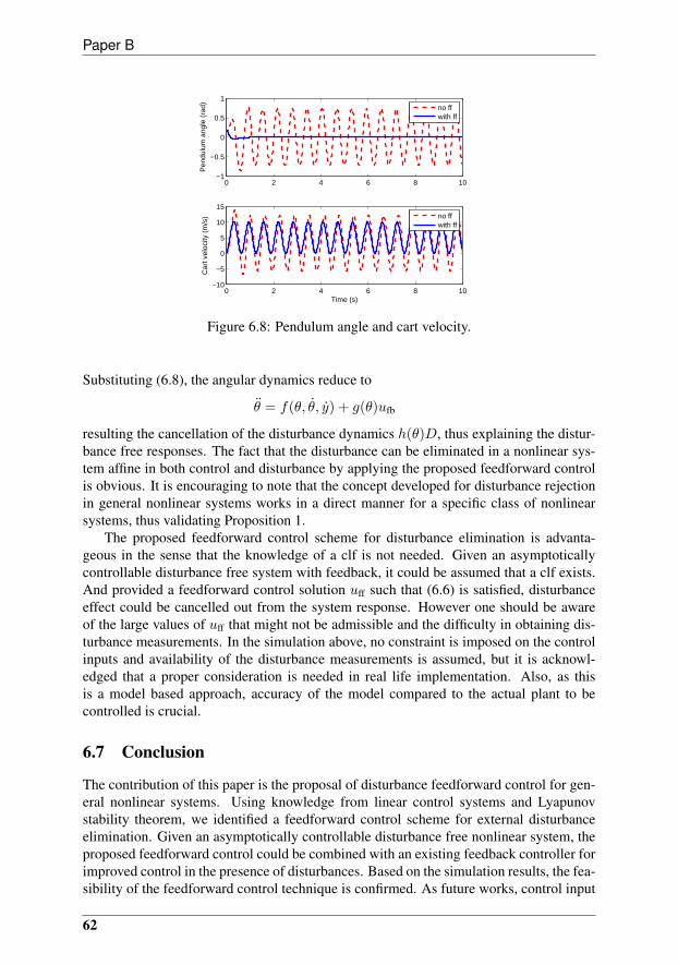
Paper B

0 2 4 6 8 10−1

−0.5

0

0.5

1

Pen

dulu

m a

ngle

(ra

d)

no ffwith ff

0 2 4 6 8 10−10

−5

0

5

10

15

Time (s)

Car

t vel

ocity

(m

/s)

no ffwith ff

Figure 6.8: Pendulum angle and cart velocity.

Substituting (6.8), the angular dynamics reduce to

θ = f(θ, θ, y) + g(θ)ufb

resulting the cancellation of the disturbance dynamics h(θ)D, thus explaining the distur-bance free responses. The fact that the disturbance can be eliminated in a nonlinear sys-tem affine in both control and disturbance by applying the proposed feedforward controlis obvious. It is encouraging to note that the concept developed for disturbance rejectionin general nonlinear systems works in a direct manner for a specific class of nonlinearsystems, thus validating Proposition 1.

The proposed feedforward control scheme for disturbance elimination is advanta-geous in the sense that the knowledge of a clf is not needed. Given an asymptoticallycontrollable disturbance free system with feedback, it could be assumed that a clf exists.And provided a feedforward control solution uff such that (6.6) is satisfied, disturbanceeffect could be cancelled out from the system response. However one should be awareof the large values of uff that might not be admissible and the difficulty in obtaining dis-turbance measurements. In the simulation above, no constraint is imposed on the controlinputs and availability of the disturbance measurements is assumed, but it is acknowl-edged that a proper consideration is needed in real life implementation. Also, as thisis a model based approach, accuracy of the model compared to the actual plant to becontrolled is crucial.

6.7 Conclusion

The contribution of this paper is the proposal of disturbance feedforward control for gen-eral nonlinear systems. Using knowledge from linear control systems and Lyapunovstability theorem, we identified a feedforward control scheme for external disturbanceelimination. Given an asymptotically controllable disturbance free nonlinear system, theproposed feedforward control could be combined with an existing feedback controller forimproved control in the presence of disturbances. Based on the simulation results, the fea-sibility of the feedforward control technique is confirmed. As future works, control input

62

7 Conclusion

constraint is to be included in the formulation and a robust feedforward control methodwill be investigated to include model uncertainties, inaccurate sensor measurements, etc.In addition, the existence of such a feedforward control solution and methods to obtainthem will be studied.

63

References

[1] F. Shinskey, Process control systems: Application, design and tuning. New York:McGraw-Hill, 1988.

[2] J.-P. Calvet and Y. Arkun, “Feedforward and feedback linearization of nonlinearsystems with disturbances,” Internat. J. Control, vol. 48, no. 4, pp. 1551–1559,1988. [Online]. Available: http://dx.doi.org/10.1080/00207178808906268

[3] ——, “Feedforward and feedback linearization of nonlinear systems with distur-bances and its implementation using internal model control,” Ind. Eng. Chem. Res.,vol. 27, p. 1882, 1988.

[4] P. Daoutidis and C. Kravaris, “Synthesis of feedforward/state feedback controllersfor nonlinear processes,” AIChE J., vol. 35, no. 10, pp. 1602–1616, 1989.

[5] P. Daoutidis, M. Soroush, and C. Kravaris, “Feedforward/feedback control of mul-tivariable nonlinear processes,” AIChE J., vol. 36, no. 10, pp. 1471–1484, 1990.

[6] C. E. Garcia and M. Morari, “Internal model control. 2. design procedure for multi-variable systems,” Ind. Eng. Chem. Process Des. Dev., vol. 24, no. 2, pp. 472–484,1985.

[7] Z. Palmor and D. Powers, “Feedforward properties of dead-time compensation con-trollers,” in American Control Conference, 1981.

[8] M. Soroush and C. Kravaris, “Synthesis of discrete-time nonlinear feedfor-ward/feedback controllers,” AIChE J., vol. 40, no. 3, pp. 473–495, 1994.

[9] G. Herrmann, F. L. Lewis, S. S. Ge, and J. Zhang, “Discrete adaptive neuralnetwork disturbance feedforward compensation for non-linear disturbances inservo-control applications,” Internat. J. Control, vol. 82, no. 4, pp. 721–740, 2009.[Online]. Available: http://dx.doi.org/10.1080/00207170802227191

[10] D. Gorinevsky and L. Feldkamp, “Rbf network feedforward compensation of loaddisturbance in idle speed control,” Control Systems Magazine, IEEE, vol. 16, no. 6,pp. 18 –27, dec 1996.

[11] S. Messineo and A. Serrani, “Adaptive feedforward disturbance rejection in nonlin-ear systems,” in Decision and Control, 2008. CDC 2008. 47th IEEE Conference on,9-11 2008, pp. 2575 –2580.

65

REFERENCES

[12] D. Hinrichsen and A. J. Pritchard, Mathematical Systems Theory I: Modelling,State Space Analysis, Stability and Robustness, ser. Texts in Applied Mathematics.Springer, 2005, vol. 48.

[13] K. Ogata, Modern Control Engineering, fourth edition ed. Prentice-Hall, 2001.

[14] G. C. Goodwin, S. F. Graebe, and M. E. Salgado, Control System Design. UpperSaddle River, NJ: Prentice Hall, 2001.

[15] F. H. Clarke, Y. S. Ledyaev, E. D. Sontag, and A. I. Subbotin, “Asymptoticcontrollability implies feedback stabilization,” IEEE Trans. Automat. Control,vol. 42, no. 10, pp. 1394–1407, 1997. [Online]. Available: http://dx.doi.org/10.1109/9.633828

[16] H. K. Khalil, Nonlinear Systems, 3rd ed. New York: Macmillan, 2001.

66

Paper C

A Robust Stabilization using State Feedback with Feedforward

Kumeresan A. Danapalasingam, Anders la Cour-Harbo, Girish Chowdhary andMorten Bisgaard

This paper was published in:In Proceedings of the 2010 American Control Conference

30 June-2 July 2010, Baltimore, Maryland, USA

Copyright c©2010 AACCThe layout has been revised

1 Introduction

Abstract

In a general nonlinear control system a stabilizing control strategy is often pos-sible if complete information on external inputs affecting the system is available.Assuming that measurements of persistent disturbances are available it is shown thatthe existence of a smooth uniform control Lyapunov function implies the existenceof a stabilizing state feedback with feedforward control which is robust with respectto measurement errors and external disturbances. Conversely, using differential in-clusions parameterized as nonlinear systems with state and disturbance measurementerrors, it is shown that there exists a smooth uniform control Lyapunov function ifthere is a robustly stabilizing state feedback with feedforward. This paper demon-strates that if there exists a smooth control Lyapunov function for a general nonlinearsystem with persistent disturbances for which one has previously designed a feedbackcontroller, a feedforward always exists to be augmented for stability.

7.1 Introduction

In nonlinear systems, the design of stabilizing feedback controllers guarantees stabilitywhen no persistent disturbance is present. Even though in some cases a feedback wouldsuffice [1], in general a state feedback with feedforward is inevitable for stability whennonzero disturbances affect the system. It could be advantageous however, if one only hasto design a feedforward that can be simply augmented to an existing feedback for requiredstability in the presence of persistent disturbances. Some previous works on feedforwardcontrol will be reviewed here.

In [2] discrete-time feedback/feedforward controllers are developed for general non-linear processes with stable zero dynamics. The design of the controllers is synthesized ina coupled manner where separate objectives of the feedforward and feedback controllersare realized by means of one unified control law. A feedforward only approach usingartificial neural networks is reported in [3] describing a nonlinear adaptive feedforwardcontroller for compensation of external load disturbances in the idle speed control of anautomotive engine. In another work, [4] employed a feedforward control to handle mea-surable additive disturbances with linear dynamics affecting a nonlinear plant. In thispaper, we study the existence of a separate robust feedforward whose control inputs canbe added to those of an existing feedback to ensure stability of general nonlinear systemswith persistent disturbances as one of its external inputs.

In this work, by adding a feedforward term and restricting the persistent disturbanceto be a Lipschitz function, [1] is extended using similar approach therein to accommodateour purposes. While only a feedback is considered in the main reference [1], here we em-ploy a feedback with feedforward control and a stricter smooth uniform control Lyapunovfunction for robust stability. This paper is organized as follows: Section 7.2 contains theproblem statement and some definitions. The main theorem of this paper, Theorem 1as well as the converse Lyapunov theorem from [5], Theorem 2 are also stated here. Inaddition, nonlinear systems with state and disturbance measurement errors parameter-ized by differential inclusions are shown to be upper semicontinuous here. This is thenused in Section 7.3 to establish a relation between a robustly stabilizing state feedbackwith feedforwardm and asymptotic stability of the aforementioned differential inclusion.Subsequently, the proof of the main theorem is completed in Section 7.4 after which asimulation example is given in Section 7.5. The paper is concluded in Section 7.6.

69

Paper C

7.2 Preliminaries

This work concerns the development of a feedforward control strategy for general non-linear control systems of the type

x = f(x, u, d), x ∈ Rn, u ∈ U, d ∈ D, (7.1)

where U is a compact subset of Rc, persistent disturbance d = d(·) is a measurableLipschitz function taking values in some compact set D ⊂ Rw containing 0 and f :Rn × U × D → Rn is a continuous function. Given an existing stabilizing feedbackk : Rn → U designed for (7.1) with d = 0, the feedforward stabilization problem is thatof finding a feedforward control l : Rn × D→ U with l(x, 0) = 0 such that the origin inRn is asymptotically stable with respect to the trajectories of the closed-loop system

x = f(x, k(x) + l(x, d), d

). (7.2)

The remainder of this section provides a series of essential definitions and theorems.A function V : Rn → R≥0 is said to be positive (definite) if V (0) = 0 and V (x) > 0

for all x 6= 0, and proper if the sublevel set x : V (x) ≤ a is compact for all a > 0.

Definition 4. A smooth function V : Rn → R≥0 is defined as a smooth uniform controlLyapunov function for system (7.1) if V is positive, proper and satisfies the followinginfinitesimal decrease condition: There exists a continuous positive function W : Rn →R≥0 such that, for any bounded set X ⊂ Rn,

minu∈U〈∇V (x), f(x, u, d)〉 ≤ −W (x), ∀x ∈ X, x 6= 0, (7.3)

where 〈·, ·〉 denotes the inner product in Rn (cf. (14) in [1]).

It follows from the infinitesimal decrease condition (7.3) that there always exists astate feedback with feedforward m : Rn × D→ U which satisfies

〈∇V (x), f(x,m(x, d), d

)〉 ≤ −W (x), ∀x ∈ X, x 6= 0. (7.4)

Here, we define the state feedback with feedforward as

m(x, d) := k(x) + l(x, d). (7.5)

Such a controlmwill be in general discontinuous [6, 7]. It will be shown that a feedback kand a feedforward l satisfying (7.5) and (7.4) will drive the state of the system (7.2) to theorigin in Rn and this stabilizing state feedback with feedforward m is robust with respectto state measurement errors ex(·), disturbance measurement errors ed(·) and externaldisturbances w(·) in the perturbed system

x = f(x,m

(x+ ex(t), d(t) + ed(t)

), d(t)

)+ w(t). (7.6)

As described in Definition 5, robustness in this context refers to the insensitivity of m inhandling measurement errors and additive external disturbances to drive all states to anarbitrary neighborhood of the origin for fast enough sampling and small enough measure-ment errors and external disturbances.

70

2 Preliminaries

Next, the state trajectory of a system with a discontinuous control is defined similarlyto [6]. Let π = tii≥0 be any partition of [0,+∞] with

0 = t0 < t1 < . . .

and limi→∞ ti = +∞. The π-trajectory of the perturbed system (7.6) starting from x0,under the action of a possibly discontinuous state feedback with feedforward m and inthe presence of disturbance d(·), state measurement errors ex(·), disturbance measure-ment errors ed(·) and external disturbances w(·), is defined recursively on the intervals[ti, ti+1], i = 0, 1, . . . , as the solution of the differential equation

x(t) = f(x(t), ui, d(t)

)+ w(t), a.a. t ∈ [ti, ti+1], (7.7)

where ui = m(x(ti) + ex(ti), d(ti) + ed(ti)

), x(0) = x0. To be noted, x(·) may fail to

exist on one of the intervals [ti, ti+1] when there exists a T < +∞ such that the x(·) onlyexists on [0, T ) and limt↑T |x(t)| = +∞, where | · | denotes the Euclidean norm. Such anx(·) is called a blown-up trajectory.

Definition 5. The state feedback with feedforward m is robustly s-stabilizing (samplingstabilizing) if for any 0 < r < R there exists positive T = T (r,R), δ = δ(r,R),η = η(r,R) and M(R) such that for any state measurement error ex(·), disturbancemeasurement error ed(·) (arbitrary bounded functions ex : [0,+∞) → Rn and ed :[0,+∞) → D) and external disturbance w(·) (measurable essentially bounded functionw : [0,+∞)→ Rn) for which

|ex(t)| ≤ η, |ed(t)| ≤ η, ∀t ≥ 0, ‖w(·)‖∞ ≤ η, (7.8)

and any partition π with diam := supi≥0(ti+1−ti) ≤ δ, every π-trajectory with |x(0)| ≤R does not blow-up and satisfies the following relations:

1. Uniform attractivity

|x(t)| ≤ r, ∀t ≥ T (7.9)

2. Bounded overshoot

|x(t)| ≤M(R), ∀t ≥ 0 (7.10)

3. Lyapunov stability

limR↓0

M(R) = 0. (7.11)

The following is the main theorem of this paper.

Theorem 1. The control system (7.1) admits a smooth uniform control Lyapunov functionif and only if there exists a robustly s-stabilizing state feedback with feedforward m.

71

Paper C

In the proof of the sufficiency part of Theorem 1, it is shown that if there exists astabilizing state feedback with feedforward m that is robust with respect to state anddisturbance measurement errors and external disturbances for the control system (7.1),then the differential inclusion

x ∈ G(x) (7.12)

with multivalued function

G(x) :=⋂ε>0

co⋃d∈D

f(x,m(x+ εB, d+ εB), d

)(7.13)

is strongly asymptotically stable, where B is a closed unit ball and coS the closure of theconvex hull of a set S. As we shall see at the end of this section, the multifunction (7.13)satisfies Hypothesis (H) which is given as follows:

(H1) The multifunction G is upper semicontinuous, i.e. for any x ∈ Rn and any ε > 0there is a δ > 0 such that,

G(x′) ⊂ G(x) + εB, ∀x′ ∈ x+ δB.

(H2) G(x) is a compact convex subset of Rn for each x ∈ Rn.

Definition 6. The differential inclusion (7.12) is strongly asymptotically stable if it hasno blown-up solutions and

1. (Attractivity) for any solution x(·)

limt→∞

x(t) = 0. (7.14)

2. (Strong Lyapunov stability) for any ε > 0, there exists δ > 0 such that everysolution of (7.12) with x(0) ≤ δ satisfies

|x(t)| < ε, ∀t ≥ 0. (7.15)

Strong asymptotic stability of differential inclusion (7.12) implies that there are no solu-tions x(·) of (7.12) exhibiting finite time blow-up and for any positive r < R there existT = T (r,R) and M(R) such that any solution with |x(0)| ≤ R satisfies (7.9) and (7.10)and (7.11) holds [5, Prop. 2.2].

Definition 7. The smooth function V : Rn → R≥0 is said to be a smooth strong Lya-punov function for the differential inclusion (7.12) if it is positive, proper and satisfies thefollowing infinitesimal decrease condition:

maxz∈G(x)

〈∇V (x), z〉 ≤ −W (x), (7.16)

where W is a positive continuous function.

The following theorem is proved in [5].

72

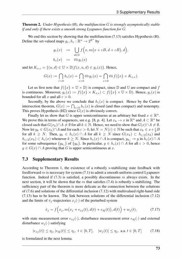
3 Supplementary Results

Theorem 2. Under Hypothesis (H), the multifunction G is strongly asymptotically stableif and only if there exists a smooth strong Lyapunov function for G.

We end this section by showing that the multifunction (7.13) satisfies Hypothesis (H).Define the set-valued maps gε, hε : Rn → 2R

n

by

gε(x) :=⋃d∈D

f(x,m

(x+ εB, d+ εB

), d),

hε(x) := co gε(x)

and let Kx,ε = (u, d) ∈ U× D|f(x, u, d) ∈ gε(x). Hence,

G(x) :=⋂ε>0

hε(x) =⋂ε>0

co gε(x) =⋂ε>0

co f(x ×Kx,ε).

Let us first note that f(x × U × D) is compact, since D and U are compact and fis continuous. Moreover, gε(x) := f(x ×Kx,ε) ⊂ f(x × U × D). Hence, gε(x) isbounded for all x and all ε > 0.

Secondly, by the above we conclude that hε(x) is compact. Hence by the Cantorintersection theorem, G(x) :=

⋂ε>0 hε(x) is closed (and thus compact) and nonempty.

This proves Hypothesis (H2) since G(x) is obviously convex.Finally let us show that G is upper semicontinuous at an arbitrary but fixed x ∈ Rn.

We prove this in terms of sequences, see e.g. [8, p. 4]. Let xk → x in Rn and A ⊂ Rn beclosed such thatG(xk)∩A 6= ∅ for all k ∈ N. Hence, we need to show thatG(x)∩A 6= ∅.Now let yk ∈ G(xk)∩A and for each ε > 0, letN = N(ε) ∈ N be such that xk ∈ x+ ε

2Bfor all k ≥ N . Then, yk ∈ hε(x) ∩ A for all k ≥ N since G(xk) ⊂ hε/2(xk) andhε/2(xk) ⊂ hε(x) whenever k ≥ N . Since hε(x)∩A is compact, ykj → y in hε(x)∩Afor some subsequence ykj of yk. In particular, y ∈ hε(x) ∩ A for all ε > 0, hencey ∈ G(x) ∩A proving that G is upper semicontinuous at x.

7.3 Supplementary Results

According to Theorem 1, the existence of a robustly s-stabilizing state feedback withfeedforwardm is necessary for system (7.1) to admit a smooth uniform control Lyapunovfunction. Indeed if (7.3) is satisfied, a possibly discontinuous m always exists. In thenext section, it will be shown that the m that satisfies (7.4) is robustly s-stabilizing. Thesufficiency part of the theorem is more delicate as the connection between the solutionsof (7.6) and solutions of the differential inclusion (7.12) with multivalued right-hand side(7.13) has to be known. The link between solutions of the differential inclusion (7.12)and the limits of πj-trajectories xj(·) of the perturbed system

xj = f(xj ,m

(xj + exj(t), d(t) + edj(t)

), d(t)

)+ wj(t), (7.17)

with state measurement error exj(·), disturbance measurement error edj(·) and externaldisturbance wj(·) satisfying

|exj(t)| ≤ ηj , |edj(t)| ≤ ηj , t ∈ [0, T ], |wj(t)| ≤ ηj , a.a. t ∈ [0, T ] (7.18)

is formulated in the next lemma.

73

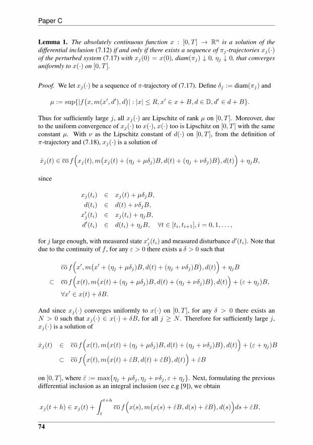
Paper C

Lemma 1. The absolutely continuous function x : [0, T ] → Rn is a solution of thedifferential inclusion (7.12) if and only if there exists a sequence of πj-trajectories xj(·)of the perturbed system (7.17) with xj(0) = x(0), diam(πj) ↓ 0, ηj ↓ 0, that convergesuniformly to x(·) on [0, T ].

Proof. We let xj(·) be a sequence of π-trajectory of (7.17). Define δj := diam(πj) and

µ := sup|f(x,m(x′, d′), d

)| : |x| ≤ R, x′ ∈ x+B, d ∈ D, d′ ∈ d+B.

Thus for sufficiently large j, all xj(·) are Lipschitz of rank µ on [0, T ]. Moreover, dueto the uniform convergence of xj(·) to x(·), x(·) too is Lipschitz on [0, T ] with the sameconstant µ. With ν as the Lipschitz constant of d(·) on [0, T ], from the definition ofπ-trajectory and (7.18), xj(·) is a solution of

xj(t) ∈ co f(xj(t),m

(xj(t) + (ηj + µδj)B, d(t) + (ηj + νδj)B

), d(t)

)+ ηjB,

since

xj(ti) ∈ xj(t) + µδjB,

d(ti) ∈ d(t) + νδjB,

x′j(ti) ∈ xj(ti) + ηjB,

d′(ti) ∈ d(ti) + ηjB, ∀t ∈ [ti, ti+1], i = 0, 1, . . . ,

for j large enough, with measured state x′j(ti) and measured disturbance d′(ti). Note thatdue to the continuity of f , for any ε > 0 there exists a δ > 0 such that

co f(x′,m

(x′ + (ηj + µδj)B, d(t) + (ηj + νδj)B

), d(t)

)+ ηjB

⊂ co f(x(t),m

(x(t) + (ηj + µδj)B, d(t) + (ηj + νδj)B

), d(t)

)+ (ε+ ηj)B,

∀x′ ∈ x(t) + δB.

And since xj(·) converges uniformly to x(·) on [0, T ], for any δ > 0 there exists anN > 0 such that xj(·) ∈ x(·) + δB, for all j ≥ N . Therefore for sufficiently large j,xj(·) is a solution of

xj(t) ∈ co f(x(t),m

(x(t) + (ηj + µδj)B, d(t) + (ηj + νδj)B

), d(t)

)+ (ε+ ηj)B

⊂ co f(x(t),m

(x(t) + εB, d(t) + εB

), d(t)

)+ εB

on [0, T ], where ε := maxηj + µδj , ηj + νδj , ε + ηj. Next, formulating the previousdifferential inclusion as an integral inclusion (see e.g [9]), we obtain

xj(t+ h) ∈ xj(t) +

∫ t+h

t

co f(x(s),m

(x(s) + εB, d(s) + εB

), d(s)

)ds+ εB,

74

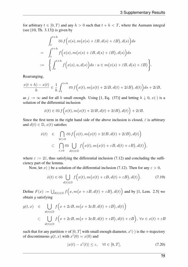
3 Supplementary Results

for arbitrary t ∈ [0, T ) and any h > 0 such that t + h < T , where the Aumann integral(see [10, Th. 3.13]) is given by∫ t+h

t

co f(x(s),m

(x(s) + εB, d(s) + εB

), d(s)

)ds

=

∫ t+h

t

f(x(s),m

(x(s) + εB, d(s) + εB

), d(s)

)ds

:=

∫ t+h

t

f(x(s), u, d(s)

)ds : u ∈ m

(x(s) + εB, d(s) + εB

).

Rearranging,

x(t+ h)− x(t)

h∈ 1

h

∫ t+h

t

co f(x(t),m

(x(t) + 2εB, d(t) + 2εB

), d(t)

)ds+ 2εB,

as j → ∞ and for all h small enough. Using [1, Eq. (37)] and letting h ↓ 0, x(·) is asolution of the differential inclusion

x(t) ∈ co f(x(t),m

(x(t) + 2εB, d(t) + 2εB

), d(t)

)+ 2εB.

Since the first term in the right hand side of the above inclusion is closed, ε is arbitraryand d(t) ∈ D, x(t) satisfies

x(t) ∈⋂

2ε>0

co f(x(t),m

(x(t) + 2εB, d(t) + 2εB

), d(t)

)⊂

⋂ε>0

co⋃

d(t)∈D

f(x(t),m

(x(t) + εB, d(t) + εB

), d(t)

),

where ε := 2ε, thus satisfying the differential inclusion (7.12) and concluding the suffi-ciency part of the lemma.

Now, let x(·) be a solution of the differential inclusion (7.12). Then for any ε > 0,

x(t) ∈ co⋃

d(t)∈D

f(x(t),m

(x(t) + εB, d(t) + εB

), d(t)

). (7.19)

Define F (x) :=⋃d(t)∈D f

(x,m

(x + εB, d(t) + εB

), d(t)

)and by [1, Lem. 2.5] we

obtain g satisfying

g(t, x) ∈⋃

d(t)∈D

f(x+ 2εB,m

(x+ 3εB, d(t) + εB

), d(t)

)⊂

⋃d(t)∈D

f(x+ 2εB,m

(x+ 3εB, d(t) + εB

), d(t) + εB

), ∀x ∈ x(t) + εB

such that for any partition π of [0, T ] with small enough diameter, x′(·) is the π-trajectoryof discontinuous g(t, x) with x′(0) = x(0) and

|x(t)− x′(t)| ≤ ε, ∀t ∈ [0, T ], (7.20)

75

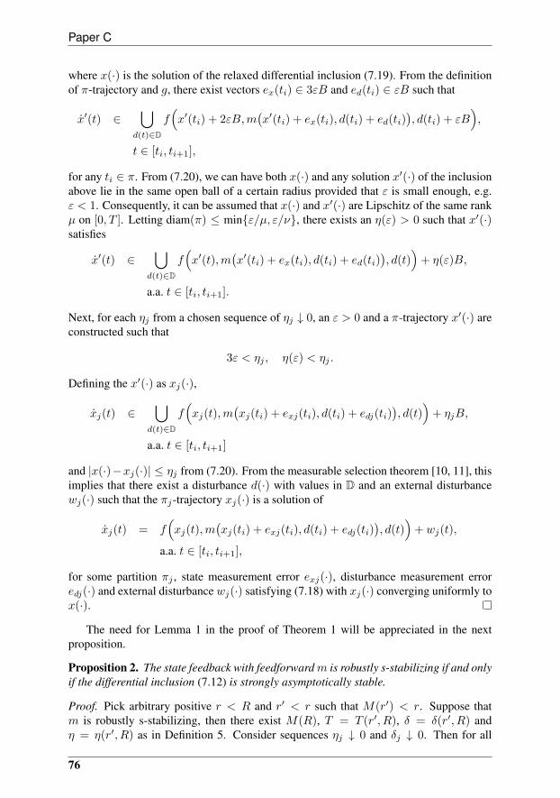
Paper C

where x(·) is the solution of the relaxed differential inclusion (7.19). From the definitionof π-trajectory and g, there exist vectors ex(ti) ∈ 3εB and ed(ti) ∈ εB such that

x′(t) ∈⋃

d(t)∈D

f(x′(ti) + 2εB,m

(x′(ti) + ex(ti), d(ti) + ed(ti)

), d(ti) + εB

),

t ∈ [ti, ti+1],

for any ti ∈ π. From (7.20), we can have both x(·) and any solution x′(·) of the inclusionabove lie in the same open ball of a certain radius provided that ε is small enough, e.g.ε < 1. Consequently, it can be assumed that x(·) and x′(·) are Lipschitz of the same rankµ on [0, T ]. Letting diam(π) ≤ minε/µ, ε/ν, there exists an η(ε) > 0 such that x′(·)satisfies

x′(t) ∈⋃

d(t)∈D

f(x′(t),m

(x′(ti) + ex(ti), d(ti) + ed(ti)

), d(t)

)+ η(ε)B,

a.a. t ∈ [ti, ti+1].

Next, for each ηj from a chosen sequence of ηj ↓ 0, an ε > 0 and a π-trajectory x′(·) areconstructed such that

3ε < ηj , η(ε) < ηj .

Defining the x′(·) as xj(·),

xj(t) ∈⋃

d(t)∈D

f(xj(t),m

(xj(ti) + exj(ti), d(ti) + edj(ti)

), d(t)

)+ ηjB,

a.a. t ∈ [ti, ti+1]

and |x(·)−xj(·)| ≤ ηj from (7.20). From the measurable selection theorem [10, 11], thisimplies that there exist a disturbance d(·) with values in D and an external disturbancewj(·) such that the πj-trajectory xj(·) is a solution of

xj(t) = f(xj(t),m

(xj(ti) + exj(ti), d(ti) + edj(ti)

), d(t)

)+ wj(t),

a.a. t ∈ [ti, ti+1],

for some partition πj , state measurement error exj(·), disturbance measurement erroredj(·) and external disturbance wj(·) satisfying (7.18) with xj(·) converging uniformly tox(·).

The need for Lemma 1 in the proof of Theorem 1 will be appreciated in the nextproposition.

Proposition 2. The state feedback with feedforwardm is robustly s-stabilizing if and onlyif the differential inclusion (7.12) is strongly asymptotically stable.

Proof. Pick arbitrary positive r < R and r′ < r such that M(r′) < r. Suppose thatm is robustly s-stabilizing, then there exist M(R), T = T (r′, R), δ = δ(r′, R) andη = η(r′, R) as in Definition 5. Consider sequences ηj ↓ 0 and δj ↓ 0. Then for all

76

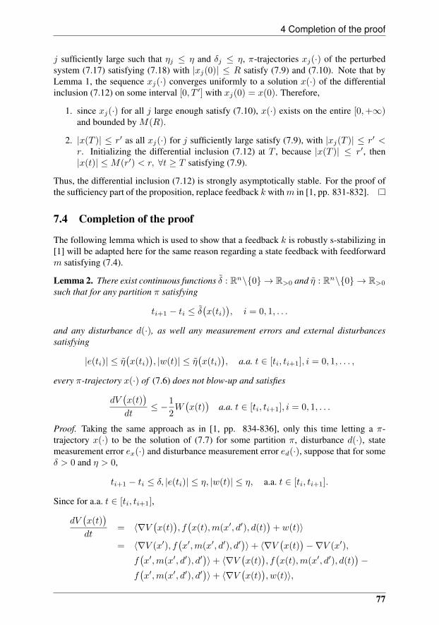
4 Completion of the proof

j sufficiently large such that ηj ≤ η and δj ≤ η, π-trajectories xj(·) of the perturbedsystem (7.17) satisfying (7.18) with |xj(0)| ≤ R satisfy (7.9) and (7.10). Note that byLemma 1, the sequence xj(·) converges uniformly to a solution x(·) of the differentialinclusion (7.12) on some interval [0, T ′] with xj(0) = x(0). Therefore,

1. since xj(·) for all j large enough satisfy (7.10), x(·) exists on the entire [0,+∞)and bounded by M(R).

2. |x(T )| ≤ r′ as all xj(·) for j sufficiently large satisfy (7.9), with |xj(T )| ≤ r′ <r. Initializing the differential inclusion (7.12) at T , because |x(T )| ≤ r′, then|x(t)| ≤M(r′) < r, ∀t ≥ T satisfying (7.9).

Thus, the differential inclusion (7.12) is strongly asymptotically stable. For the proof ofthe sufficiency part of the proposition, replace feedback k withm in [1, pp. 831-832].

7.4 Completion of the proof

The following lemma which is used to show that a feedback k is robustly s-stabilizing in[1] will be adapted here for the same reason regarding a state feedback with feedforwardm satisfying (7.4).

Lemma 2. There exist continuous functions δ : Rn\0 → R>0 and η : Rn\0 → R>0

such that for any partition π satisfying

ti+1 − ti ≤ δ(x(ti)

), i = 0, 1, . . .

and any disturbance d(·), as well any measurement errors and external disturbancessatisfying

|e(ti)| ≤ η(x(ti)

), |w(t)| ≤ η

(x(ti)

), a.a. t ∈ [ti, ti+1], i = 0, 1, . . . ,

every π-trajectory x(·) of (7.6) does not blow-up and satisfies

dV(x(t)

)dt

≤ −1

2W(x(t)

)a.a. t ∈ [ti, ti+1], i = 0, 1, . . .

Proof. Taking the same approach as in [1, pp. 834-836], only this time letting a π-trajectory x(·) to be the solution of (7.7) for some partition π, disturbance d(·), statemeasurement error ex(·) and disturbance measurement error ed(·), suppose that for someδ > 0 and η > 0,

ti+1 − ti ≤ δ, |e(ti)| ≤ η, |w(t)| ≤ η, a.a. t ∈ [ti, ti+1].

Since for a.a. t ∈ [ti, ti+1],

dV(x(t)

)dt

= 〈∇V(x(t)

), f(x(t),m(x′, d′), d(t)

)+ w(t)〉

= 〈∇V (x′), f(x′,m(x′, d′), d′

)〉+ 〈∇V

(x(t)

)−∇V (x′),

f(x′,m(x′, d′), d′

)〉+ 〈∇V

(x(t)

), f(x(t),m(x′, d′), d(t)

)−

f(x′,m(x′, d′), d′

)〉+ 〈∇V

(x(t)

), w(t)〉,

77

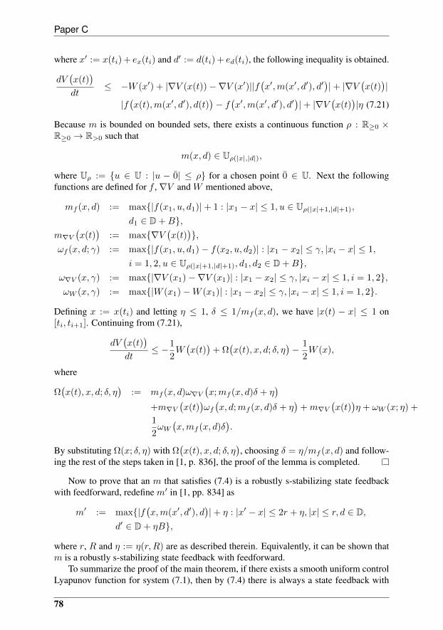
Paper C

where x′ := x(ti) + ex(ti) and d′ := d(ti) + ed(ti), the following inequality is obtained.

dV(x(t)

)dt

≤ −W (x′) + |∇V (x(t))−∇V (x′)||f(x′,m(x′, d′), d′

)|+ |∇V

(x(t)

)|

|f(x(t),m(x′, d′), d(t)

)− f

(x′,m(x′, d′), d′

)|+ |∇V

(x(t)

)|η (7.21)

Because m is bounded on bounded sets, there exists a continuous function ρ : R≥0 ×R≥0 → R>0 such that

m(x, d) ∈ Uρ(|x|,|d|),

where Uρ := u ∈ U : |u − 0| ≤ ρ for a chosen point 0 ∈ U. Next the followingfunctions are defined for f ,∇V and W mentioned above,

mf (x, d) := max|f(x1, u, d1)|+ 1 : |x1 − x| ≤ 1, u ∈ Uρ(|x|+1,|d|+1),

d1 ∈ D +B,m∇V

(x(t)

):= max∇V

(x(t)

),

ωf (x, d; γ) := max|f(x1, u, d1)− f(x2, u, d2)| : |x1 − x2| ≤ γ, |xi − x| ≤ 1,

i = 1, 2, u ∈ Uρ(|x|+1,|d|+1), d1, d2 ∈ D +B,ω∇V (x, γ) := max|∇V (x1)−∇V (x1)| : |x1 − x2| ≤ γ, |xi − x| ≤ 1, i = 1, 2,ωW (x, γ) := max|W (x1)−W (x1)| : |x1 − x2| ≤ γ, |xi − x| ≤ 1, i = 1, 2.

Defining x := x(ti) and letting η ≤ 1, δ ≤ 1/mf (x, d), we have |x(t) − x| ≤ 1 on[ti, ti+1]. Continuing from (7.21),

dV(x(t)

)dt

≤ −1

2W(x(t)

)+ Ω

(x(t), x, d; δ, η

)− 1

2W (x),

where

Ω(x(t), x, d; δ, η

):= mf (x, d)ω∇V

(x;mf (x, d)δ + η

)+m∇V

(x(t)

)ωf(x, d;mf (x, d)δ + η

)+m∇V

(x(t)

)η + ωW (x; η) +

1

2ωW(x,mf (x, d)δ

).

By substituting Ω(x; δ, η) with Ω(x(t), x, d; δ, η

), choosing δ = η/mf (x, d) and follow-

ing the rest of the steps taken in [1, p. 836], the proof of the lemma is completed.

Now to prove that an m that satisfies (7.4) is a robustly s-stabilizing state feedbackwith feedforward, redefine m′ in [1, pp. 834] as

m′ := max|f(x,m(x′, d′), d

)|+ η : |x′ − x| ≤ 2r + η, |x| ≤ r, d ∈ D,

d′ ∈ D + ηB,

where r, R and η := η(r,R) are as described therein. Equivalently, it can be shown thatm is a robustly s-stabilizing state feedback with feedforward.

To summarize the proof of the main theorem, if there exists a smooth uniform controlLyapunov function for system (7.1), then by (7.4) there is always a state feedback with

78

5 Simulation Results

feedforward m. Using Lemma 2 and the subsequent proof above, we know that suchan m is robustly s-stabilizing. Conversely, if there exists a robustly s-stabilizing statefeedback with feedforward m, then by Proposition 1 the differential inclusion (7.12) isstrongly asymptotically stable. Since it satisfies Hypothesis (H), Theorem 2 warrants theexistence of a smooth strong Lyapunov function V that satisfies the infinitesimal decreasecondition (7.16). Since

f(x,m(x, d), d

)∈⋂ε>0

co⋃d∈D

f(x,m(x+ εB, d+ εB), d

)for any d ∈ D, from (7.16),

〈∇V (x), f(x,m(x, d), d

)〉 ≤ −W (x), ∀d ∈ D.

Hence, V is a smooth uniform control Lyapunov function for the control system (7.1).Now we shall return to the earlier problem of finding a robustly s-stabilizing feedfor-

ward l for system (7.1) that is equipped with a robustly s-stabilizing feedback k designedto make the system

x = f(x, u, 0)

asymptotically stable. Obviously, the implementation of the feedback k in system (7.1)only guarantees asymptotic stability if there exists a smooth uniform control Lyapunovfunction satisfying the infinitesimal decrease condition [1]

maxd∈D〈∇V (x), f

(x, k(x), d

)〉 ≤ −W (x), ∀x 6= 0, 0 ∈ D

making the need for a feedforward l redundant. However, if there only exists a smoothuniform control Lyapunov function with a stricter infinitesimal decrease condition (7.3)as considered in this paper, one would then need a controller with a complete knowledgeof the system to provide asymptotic stability, i.e. one that has both the state x and distur-bance d as its arguments. The existence of a smooth uniform control Lyapunov functionimplies that there always exists a state feedback with feedforward m as defined by (7.5).Since the state feedback k is given, one only needs to find a feedforward l that satisfies(7.5) and (7.4), and Theorem 1 guarantees that such a combination of a feedback k and afeedforward l is robustly s-stabilizing.

7.5 Simulation Results

We will now show the existence of a robustly s-stabilizing state feedback with feedfor-ward for the control of wing rock motion of an aircraft [12]. From Theorem 1, we knowthat this is an implication of the existence of a smooth uniform control Lyapunov functionfor the system in question. The following are the equations governing a wing rock motionwith disturbance and neglecting actuator dynamics, see e.g. [13].

x1 = x2

x2 = u+ ∆(x1, x2) + d, (7.22)

79

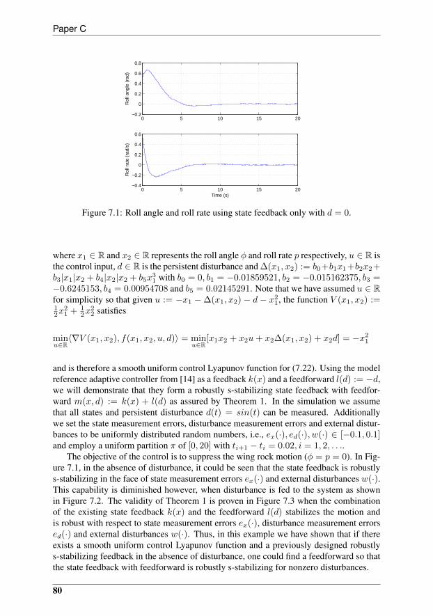
Paper C

0 5 10 15 20−0.2

0

0.2

0.4

0.6

0.8

Rol

l ang

le (

rad)

0 5 10 15 20−0.4

−0.2

0

0.2

0.4

0.6

Rol

l rat

e (r

ad/s

)

Time (s)

Figure 7.1: Roll angle and roll rate using state feedback only with d = 0.

where x1 ∈ R and x2 ∈ R represents the roll angle φ and roll rate p respectively, u ∈ R isthe control input, d ∈ R is the persistent disturbance and ∆(x1, x2) := b0+b1x1+b2x2+b3|x1|x2 + b4|x2|x2 + b5x

31 with b0 = 0, b1 = −0.01859521, b2 = −0.015162375, b3 =

−0.6245153, b4 = 0.00954708 and b5 = 0.02145291. Note that we have assumed u ∈ Rfor simplicity so that given u := −x1 −∆(x1, x2)− d− x2

1, the function V (x1, x2) :=12x

21 + 1

2x22 satisfies

minu∈R〈∇V (x1, x2), f(x1, x2, u, d)〉 = min

u∈R[x1x2 + x2u+ x2∆(x1, x2) + x2d] = −x2

1

and is therefore a smooth uniform control Lyapunov function for (7.22). Using the modelreference adaptive controller from [14] as a feedback k(x) and a feedforward l(d) := −d,we will demonstrate that they form a robustly s-stabilizing state feedback with feedfor-ward m(x, d) := k(x) + l(d) as assured by Theorem 1. In the simulation we assumethat all states and persistent disturbance d(t) = sin(t) can be measured. Additionallywe set the state measurement errors, disturbance measurement errors and external distur-bances to be uniformly distributed random numbers, i.e., ex(·), ed(·), w(·) ∈ [−0.1, 0.1]and employ a uniform partition π of [0, 20] with ti+1 − ti = 0.02, i = 1, 2, . . ..

The objective of the control is to suppress the wing rock motion (φ = p = 0). In Fig-ure 7.1, in the absence of disturbance, it could be seen that the state feedback is robustlys-stabilizing in the face of state measurement errors ex(·) and external disturbances w(·).This capability is diminished however, when disturbance is fed to the system as shownin Figure 7.2. The validity of Theorem 1 is proven in Figure 7.3 when the combinationof the existing state feedback k(x) and the feedforward l(d) stabilizes the motion andis robust with respect to state measurement errors ex(·), disturbance measurement errorsed(·) and external disturbances w(·). Thus, in this example we have shown that if thereexists a smooth uniform control Lyapunov function and a previously designed robustlys-stabilizing feedback in the absence of disturbance, one could find a feedforward so thatthe state feedback with feedforward is robustly s-stabilizing for nonzero disturbances.

80

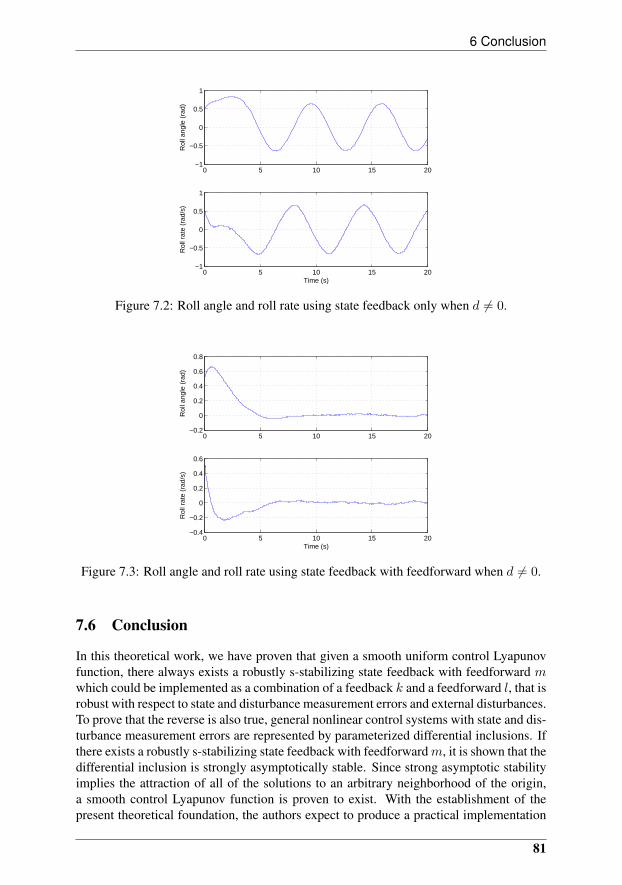
6 Conclusion

0 5 10 15 20−1

−0.5

0

0.5

1

Rol

l ang

le (

rad)

0 5 10 15 20−1

−0.5

0

0.5

1

Rol

l rat

e (r

ad/s

)

Time (s)

Figure 7.2: Roll angle and roll rate using state feedback only when d 6= 0.

0 5 10 15 20−0.2

0

0.2

0.4

0.6

0.8

Rol

l ang

le (

rad)

0 5 10 15 20−0.4

−0.2

0

0.2

0.4

0.6

Rol

l rat

e (r

ad/s

)

Time (s)

Figure 7.3: Roll angle and roll rate using state feedback with feedforward when d 6= 0.

7.6 Conclusion

In this theoretical work, we have proven that given a smooth uniform control Lyapunovfunction, there always exists a robustly s-stabilizing state feedback with feedforward mwhich could be implemented as a combination of a feedback k and a feedforward l, that isrobust with respect to state and disturbance measurement errors and external disturbances.To prove that the reverse is also true, general nonlinear control systems with state and dis-turbance measurement errors are represented by parameterized differential inclusions. Ifthere exists a robustly s-stabilizing state feedback with feedforwardm, it is shown that thedifferential inclusion is strongly asymptotically stable. Since strong asymptotic stabilityimplies the attraction of all of the solutions to an arbitrary neighborhood of the origin,a smooth control Lyapunov function is proven to exist. With the establishment of thepresent theoretical foundation, the authors expect to produce a practical implementation

81

Paper C

of the feedforward control for disturbance rejection as a future work.

Acknowledgment

The authors would like to express their uttermost gratitude to John-Josef Leth and RafalWisniewski for their guidance and valuable contributions.

82

References

[1] Y. S. Ledyaev and E. D. Sontag, “A Lyapunov characterization of robust stabiliza-tion,” Nonlinear Anal., vol. 37, no. 7, Ser. A: Theory Methods, pp. 813–840, 1999.

[2] M. Soroush and C. Kravaris, “Synthesis of discrete-time nonlinear feedfor-ward/feedback controllers,” AIChE Journal, vol. 40, no. 3, pp. 473–495, 1994.

[3] D. Gorinevsky and L. A. Feldkamp, “RBF network feedforward compensation ofload disturbance in idlespeed control,” in Control Systems Magazine, IEEE, Decem-ber 1996.

[4] M. J. Grimble, “Non-linear generalized minimum variance feedback, feedforwardand tracking control,” Automatica, vol. 41, no. 6, pp. 957–969, 2005.

[5] F. H. Clarke, Y. S. Ledyaev, and R. J. Stern, “Asymptotic stability and smooth Lya-punov functions,” J. Differential Equations, vol. 149, no. 1, pp. 69–114, 1998.

[6] F. H. Clarke, Y. S. Ledyaev, E. D. Sontag, and A. I. Subbotin, “Asymptotic con-trollability implies feedback stabilization,” IEEE Trans. Automat. Control, vol. 42,no. 10, pp. 1394–1407, 1997.

[7] Y. S. Ledyaev, “Robustness of discontinuous feedback in control under disturbance,”in IEEE Conference on Decision and Control, Nevada, USA, December 2002.

[8] K. Deimling, Multivalued differential equations, ser. de Gruyter Series in NonlinearAnalysis and Applications. Berlin: Walter de Gruyter & Co., 1992, vol. 1.

[9] P. S. Macansantos, “An existence theorem for differential inclusions using theKurzweil integral,” Science Diliman, vol. 10, no. 10, pp. 31–38, 1998.

[10] F. H. Clarke, Optimization and nonsmooth analysis, 2nd ed., ser. Classics in AppliedMathematics. Philadelphia, PA: Society for Industrial and Applied Mathematics(SIAM), 1990, vol. 5.

[11] G. V. Smirnov, Introduction to the theory of differential inclusions, ser. GraduateStudies in Mathematics. Providence, RI: American Mathematical Society, 2002,vol. 41.

[12] M. S. Monahemi and M. Krstic, “Control of wing rock motion using adaptive feed-back linearization,” Guidance, Control and Dynamics, vol. 19, no. 4, pp. 905–912,1996.

83

REFERENCES

[13] K. Y. Volyanskyy, A. J. Calise, and B.-J. Yang, “A novel Q-modification term foradaptive control,” in American Control Conference, June 2006.

[14] G. Chowdhary and E. Johnson, “A least squared based modification term for adap-tive control,” Georgia Institute of Technology, Tech. Rep., 2009.

84

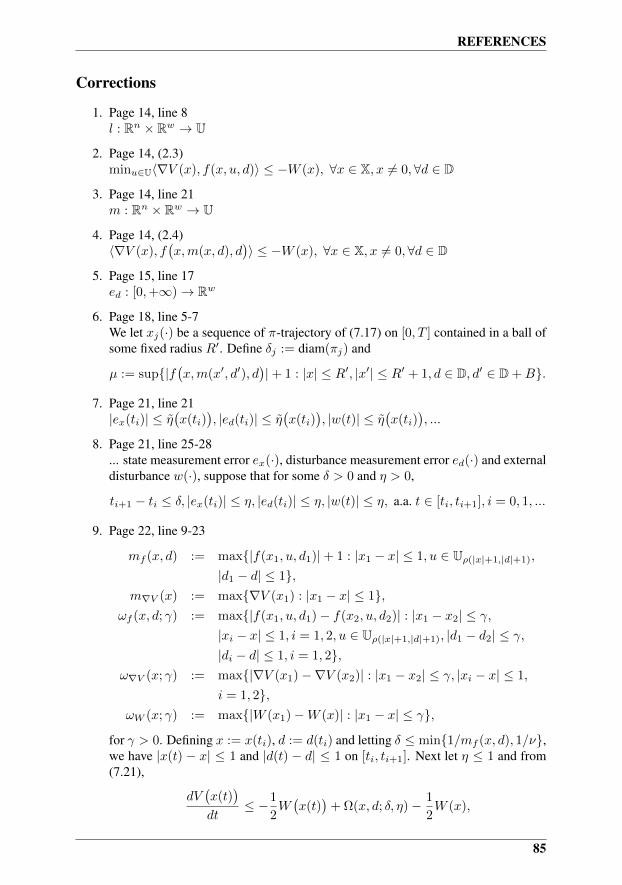
REFERENCES

Corrections

1. Page 14, line 8l : Rn × Rw → U

2. Page 14, (2.3)minu∈U〈∇V (x), f(x, u, d)〉 ≤ −W (x), ∀x ∈ X, x 6= 0,∀d ∈ D

3. Page 14, line 21m : Rn × Rw → U

4. Page 14, (2.4)〈∇V (x), f

(x,m(x, d), d

)〉 ≤ −W (x), ∀x ∈ X, x 6= 0,∀d ∈ D

5. Page 15, line 17ed : [0,+∞)→ Rw

6. Page 18, line 5-7We let xj(·) be a sequence of π-trajectory of (7.17) on [0, T ] contained in a ball ofsome fixed radius R′. Define δj := diam(πj) and

µ := sup|f(x,m(x′, d′), d

)|+ 1 : |x| ≤ R′, |x′| ≤ R′ + 1, d ∈ D, d′ ∈ D +B.

7. Page 21, line 21|ex(ti)| ≤ η

(x(ti)

), |ed(ti)| ≤ η

(x(ti)

), |w(t)| ≤ η

(x(ti)

), ...

8. Page 21, line 25-28... state measurement error ex(·), disturbance measurement error ed(·) and externaldisturbance w(·), suppose that for some δ > 0 and η > 0,

ti+1 − ti ≤ δ, |ex(ti)| ≤ η, |ed(ti)| ≤ η, |w(t)| ≤ η, a.a. t ∈ [ti, ti+1], i = 0, 1, ...

9. Page 22, line 9-23

mf (x, d) := max|f(x1, u, d1)|+ 1 : |x1 − x| ≤ 1, u ∈ Uρ(|x|+1,|d|+1),

|d1 − d| ≤ 1,m∇V (x) := max∇V (x1) : |x1 − x| ≤ 1,

ωf (x, d; γ) := max|f(x1, u, d1)− f(x2, u, d2)| : |x1 − x2| ≤ γ,|xi − x| ≤ 1, i = 1, 2, u ∈ Uρ(|x|+1,|d|+1), |d1 − d2| ≤ γ,|di − d| ≤ 1, i = 1, 2,

ω∇V (x; γ) := max|∇V (x1)−∇V (x2)| : |x1 − x2| ≤ γ, |xi − x| ≤ 1,

i = 1, 2,ωW (x; γ) := max|W (x1)−W (x)| : |x1 − x| ≤ γ,

for γ > 0. Defining x := x(ti), d := d(ti) and letting δ ≤ min1/mf (x, d), 1/ν,we have |x(t) − x| ≤ 1 and |d(t) − d| ≤ 1 on [ti, ti+1]. Next let η ≤ 1 and from(7.21),

dV(x(t)

)dt

≤ −1

2W(x(t)

)+ Ω(x, d; δ, η)− 1

2W (x),

85

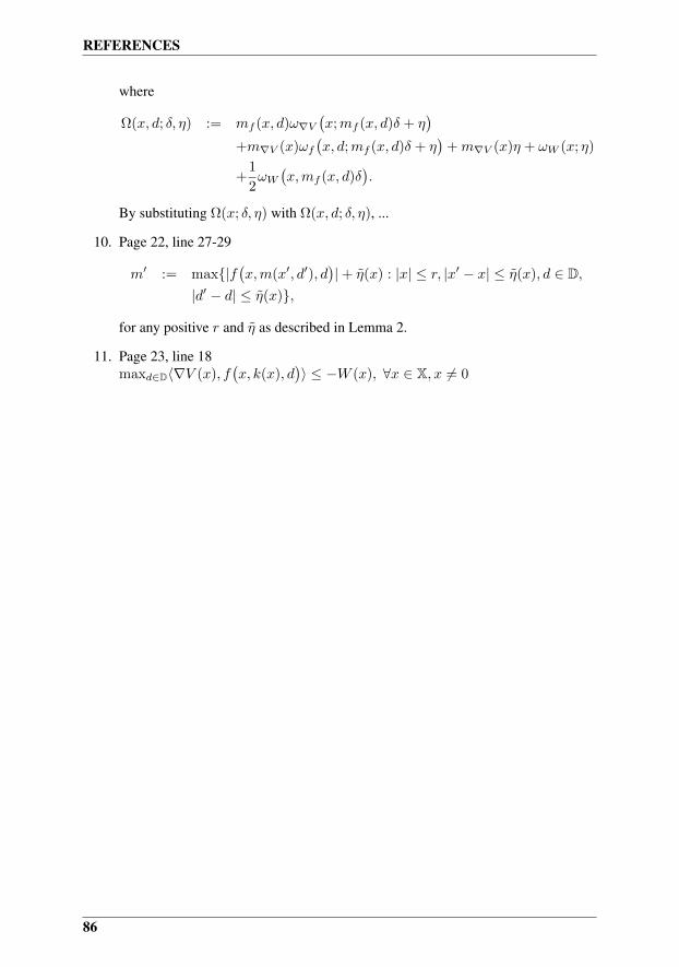
REFERENCES

where

Ω(x, d; δ, η) := mf (x, d)ω∇V(x;mf (x, d)δ + η

)+m∇V (x)ωf

(x, d;mf (x, d)δ + η

)+m∇V (x)η + ωW (x; η)

+1

2ωW(x,mf (x, d)δ

).

By substituting Ω(x; δ, η) with Ω(x, d; δ, η), ...

10. Page 22, line 27-29

m′ := max|f(x,m(x′, d′), d

)|+ η(x) : |x| ≤ r, |x′ − x| ≤ η(x), d ∈ D,

|d′ − d| ≤ η(x),

for any positive r and η as described in Lemma 2.

11. Page 23, line 18maxd∈D〈∇V (x), f

(x, k(x), d

)〉 ≤ −W (x), ∀x ∈ X, x 6= 0

86

Paper D

Robust Helicopter Stabilization in the Face of Wind Disturbance

Kumeresan A. Danapalasingam, John-Josef Leth, Anders la Cour-Harbo andMorten Bisgaard

This paper was published in:In Proceedings of the 49th IEEE Conference on Decision and Control

15-17 December 2010, Atlanta, Georgia, USA

Copyright c©2010 IEEEThe layout has been revised

1 Introduction

Abstract

When a helicopter is required to hover with minimum deviations from a desiredposition without measurements of a persistent wind disturbance, a robustly stabilizingcontrol action is vital. In this paper, the stabilization of the position and translationalvelocity of a nonlinear helicopter model affected by a wind disturbance is addressed.The wind disturbance is assumed to be a sum of a fixed number of sinusoids withunknown amplitudes, frequencies and phases. An estimate of the disturbance is in-troduced to be adapted using state measurements for control purposes. A nonlinearcontroller is then designed based on nonlinear adaptive output regulation and robuststabilization of a chain of integrators by a saturated feedback. Simulation results showthe effectiveness of the control design in the stabilization of helicopter motion and thebuilt-in robustness of the controller in handling parameter and model uncertainties.

8.1 Introduction

Autonomous helicopters are highly agile and have six degrees of freedom maneuverabil-ity making them a favourite candidate for a wide range of practical applications includingagriculture, cinematography, inspection, surveillance, search and rescue, reconnaissance,etc. For certain tasks the ability of a helicopter to follow a given state reference is crucialfor a successful outcome; for instance when hovering over a ship for rescue operations orwhen flying close to power lines or wind turbines for inspections. In windy conditionsthis becomes a significant challenge for any pilot and hence an autopilot capable of ac-counting effectively for the wind disturbance is a realistic alternative. In this work, theauthors present a control design for longitudinal, lateral, and vertical helicopter stabiliza-tion in the presence of a wind disturbance, with intrinsic robustness property in handlingparameter and model uncertainties.

Firstly, some previous works are reviewed. In [1], a feedback-feedforward propor-tional differential (PD) controller is developed for heave motion control. With the as-sistance of a gust estimator, the controller is reported to be able to handle the influencefrom horizontal gusts. The effects of rotary gusts in forward and downward velocity ofa helicopter is addressed in [2]. It is shown that via a state feedback law, the rotary gustrejection problem is always solvable. In a work by Wang et al., a multi-mode linear con-trol stategy is designed for unmanned helicopters in the presence of model uncertainties,atmospheric disturbances and handling qualities requirements [3].

In the present work, assuming that all the state variables (position, attitude and deriva-tives hereof) are available for measurements, a control strategy combining nonlinear adap-tive output regulation and robust stabilization of a chain of integrators by a saturated feed-back is carried out (see for instance, [4], [5] and [6]). Guided by a control solution forvertical trajectory tracking presented in [6] and [7], the design technique presented thereinis extended here for helicopter stabilization in the presence of horizontal and vertical winddisturbance. This is done by means of a robust longitudinal, lateral and vertical stabilizercapable of compensating for parameter and model uncertainties.

In Section 8.2, a mathematical model governing a model helicopter and a problemstatement are given. This is followed by Section 8.3 which covers the vertical, longitu-dinal and lateral stabilization. After the presentation of simulation results in Section 8.4,conclusion and future works are discussed in Section 8.5.

89

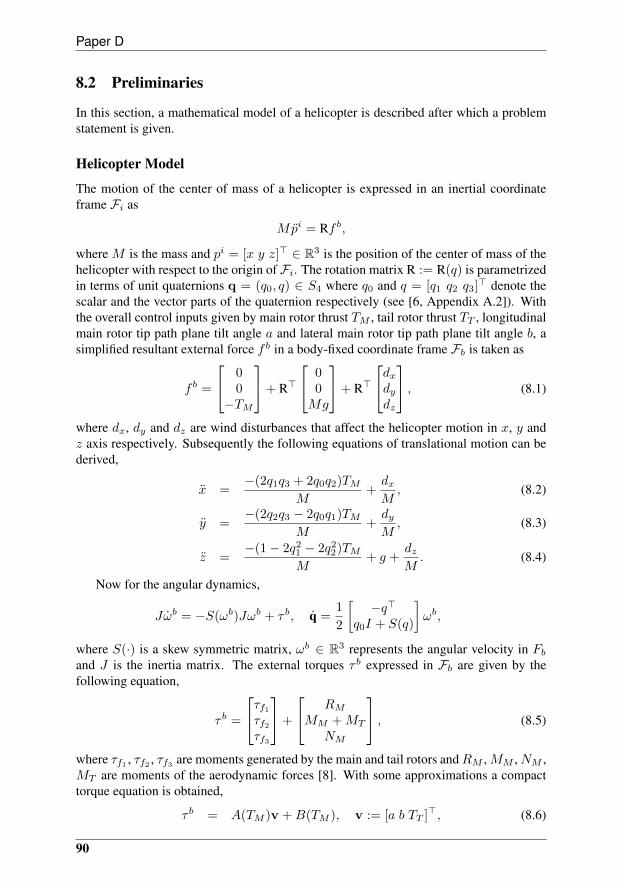
Paper D

8.2 Preliminaries

In this section, a mathematical model of a helicopter is described after which a problemstatement is given.

Helicopter Model

The motion of the center of mass of a helicopter is expressed in an inertial coordinateframe Fi as

Mpi = Rf b,

where M is the mass and pi = [x y z]> ∈ R3 is the position of the center of mass of thehelicopter with respect to the origin of Fi. The rotation matrix R := R(q) is parametrizedin terms of unit quaternions q = (q0, q) ∈ S4 where q0 and q = [q1 q2 q3]> denote thescalar and the vector parts of the quaternion respectively (see [6, Appendix A.2]). Withthe overall control inputs given by main rotor thrust TM , tail rotor thrust TT , longitudinalmain rotor tip path plane tilt angle a and lateral main rotor tip path plane tilt angle b, asimplified resultant external force f b in a body-fixed coordinate frame Fb is taken as

f b =

00−TM

+ R>

00Mg

+ R>

dxdydz

, (8.1)

where dx, dy and dz are wind disturbances that affect the helicopter motion in x, y andz axis respectively. Subsequently the following equations of translational motion can bederived,

x =−(2q1q3 + 2q0q2)TM

M+dxM, (8.2)

y =−(2q2q3 − 2q0q1)TM

M+dyM, (8.3)

z =−(1− 2q2

1 − 2q22)TM

M+ g +

dzM. (8.4)

Now for the angular dynamics,

Jωb = −S(ωb)Jωb + τ b, q =1

2

[−q>

q0I + S(q)

]ωb,

where S(·) is a skew symmetric matrix, ωb ∈ R3 represents the angular velocity in Fband J is the inertia matrix. The external torques τ b expressed in Fb are given by thefollowing equation,

τ b =

τf1τf2τf3

+

RMMM +MT

NM

, (8.5)

where τf1 , τf2 , τf3 are moments generated by the main and tail rotors andRM ,MM ,NM ,MT are moments of the aerodynamic forces [8]. With some approximations a compacttorque equation is obtained,

τ b = A(TM )v +B(TM ), v := [a b TT ]>, (8.6)

90

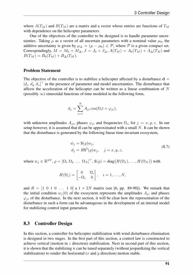
3 Controller Design

where A(TM ) and B(TM ) are a matrix and a vector whose entries are functions of TMwith dependence on the helicopter parameters.

One of the objectives of the controller to be designed is to handle parameter uncer-tainties. Taking µ as a vector of all uncertain parameters with a nominal value µ0, theadditive uncertainty is given by µ∆ = (µ − µ0) ∈ P , where P is a given compact set.Correspondingly, M = M0 + M∆, J = J0 + J∆, A(TM ) = A0(TM ) + A∆(TM ) andB(TM ) = B0(TM ) +B∆(TM ).

Problem Statement

The objective of the controller is to stabilize a helicopter affected by a disturbance d =[dx dy dz]

> in the presence of parameter and model uncertainties. The disturbance thataffects the acceleration of the helicopter can be written as a linear combination of N(possibly∞) sinusoidal functions of time modeled in the following form,

dj =

N∑i=1

Aji cos(Ωit+ ϕji),

with unknown amplitudes Aji, phases ϕji and frequencies Ωi, for j = x, y, z. In oursetup however, it is assumed that d can be approximated with a small N . It can be shownthat the disturbance is generated by the following linear time-invariant exosystem,

wj = S(%)wj ,

dj = RS2(%)wj , j = x, y, z,(8.7)

where wj ∈ R2N , % = [Ω1 Ω2 . . . ΩN ]>, S(%) = diag(H(Ω1), . . . ,H(ΩN )

)with

H(Ωi) =

[0 Ωi−Ωi 0

], i = 1, . . . , N,

and R = [1 0 1 0 . . . 1 0] a 1 × 2N matrix (see [6, pp. 89-90]). We remark thatthe initial condition wj(0) of the exosystem represents the amplitudes Aji and phasesϕji of the disturbance. In the next section, it will be clear how the representation of thedisturbance in such a form can be advantageous in the development of an internal modelfor stabilizing control input generation.

8.3 Controller Design

In this section, a controller for helicopter stabilization with wind disturbance eliminationis designed in two stages. In the first part of this section, a control law is constructed toachieve vertical (motion in z direction) stabilization. Next in second part of this section,it is shown that the stabilizing v can be tuned separately (without jeopardizing the verticalstabilization) to render the horizontal (x and y direction) motion stable.

91

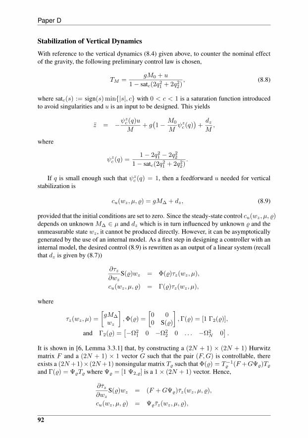
Paper D

Stabilization of Vertical Dynamics

With reference to the vertical dynamics (8.4) given above, to counter the nominal effectof the gravity, the following preliminary control law is chosen,

TM =gM0 + u

1− satc(2q21 + 2q2

2), (8.8)

where satc(s) := sign(s) min|s|, c with 0 < c < 1 is a saturation function introducedto avoid singularities and u is an input to be designed. This yields

z = −ψzc (q)u

M+ g(1− M0

Mψzc (q)

)+dzM,

where

ψzc (q) =1− 2q2

1 − 2q22

1− satc(2q21 + 2q2

2).

If q is small enough such that ψzc (q) = 1, then a feedforward u needed for verticalstabilization is

cu(wz, µ, %) = gM∆ + dz, (8.9)

provided that the initial conditions are set to zero. Since the steady-state control cu(wz, µ, %)depends on unknown M∆ ∈ µ and dz which is in turn influenced by unknown % and theunmeasurable state wz , it cannot be produced directly. However, it can be asymptoticallygenerated by the use of an internal model. As a first step in designing a controller with aninternal model, the desired control (8.9) is rewritten as an output of a linear system (recallthat dz is given by (8.7))

∂τz∂wz

S(%)wz = Φ(%)τz(wz, µ),

cu(wz, µ, %) = Γ(%)τz(wz, µ),

where

τz(wz, µ) =

[gM∆

wz

],Φ(%) =

[0 00 S(%)

],Γ(%) = [1 Γ2(%)],

and Γ2(%) =[−Ω2

1 0 −Ω22 0 . . . −Ω2

N 0].

It is shown in [6, Lemma 3.3.1] that, by constructing a (2N + 1) × (2N + 1) Hurwitzmatrix F and a (2N + 1) × 1 vector G such that the pair (F,G) is controllable, thereexists a (2N +1)× (2N +1) nonsingular matrix T% such that Φ(%) = T−1

% (F +GΨ%)T%and Γ(%) = Ψ%T% where Ψ% = [1 Ψ2,%] is a 1× (2N + 1) vector. Hence,

∂τz∂wz

S(%)wz = (F +GΨ%)τz(wz, µ, %),

cu(wz, µ, %) = Ψ%τz(wz, µ, %),

92

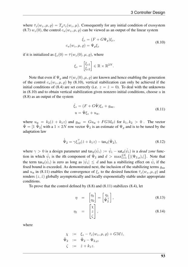
3 Controller Design

where τz(wz, µ, %) = T%τz(wz, µ). Consequently for any initial condition of exosystem(8.7) wz(0), the control cu(wz, µ, %) can be viewed as an output of the linear system

ξz = (F +GΨ%)ξz,

cu(wz, µ, %) = Ψ%ξz(8.10)

if it is initialized as ξz(0) = τ(wz(0), µ, %), where

ξz =

[ξz1ξz2

]∈ R× R2N .

Note that even if Ψ% and τ(wz(0), µ, %) are known and hence enabling the generationof the control cu(wz, µ, %) by (8.10), vertical stabilization can only be achieved if theinitial conditions of (8.4) are set correctly (i.e. z = z = 0). To deal with the unknownsin (8.10) and to obtain vertical stabilization given nonzero initial conditions, choose u in(8.8) as an output of the system

ξz = (F +GΨ)ξz + gstz,

u = Ψξz + ust,(8.11)

where ust = k2(z + k1z) and gstz = Gust + FGM0z for k1, k2 > 0 . The vectorΨ = [1 Ψ2] with a 1 × 2N row vector Ψ2 is an estimate of Ψ% and is to be tuned by theadaptation law

˙Ψ2 = γξ>z2(z + k1z)− tasd(Ψ2), (8.12)

where γ > 0 is a design parameter and tasd(ψi) := ψi − satd(ψi) is a dead zone func-tion in which ψi is the ith component of Ψ2 and d > max2N

i=1

|(Ψ2,%)i|

. Note that

the term tasd(ψi) is zero as long as |ψi| ≤ d and has a stabilizing effect on ψi if thefixed bound is exceeded. As demonstrated next, the inclusion of the stabilizing terms gstzand ust in (8.11) enables the convergence of ξz to the desired function τz(wz, µ, %) andrenders (z, z) globally asymptotically and locally exponentially stable under appropriateconditions.

To prove that the control defined by (8.8) and (8.11) stabilizes (8.4), let

η =

[η1

η2

]=

[η1

Ψ>2

], (8.13)

η1 =

χzζ

, (8.14)

where

χ := ξz − τz(wz, µ, %) +GMz,

Ψ2 := Ψ2 −Ψ2,%,

ζ := z + k1z.

93

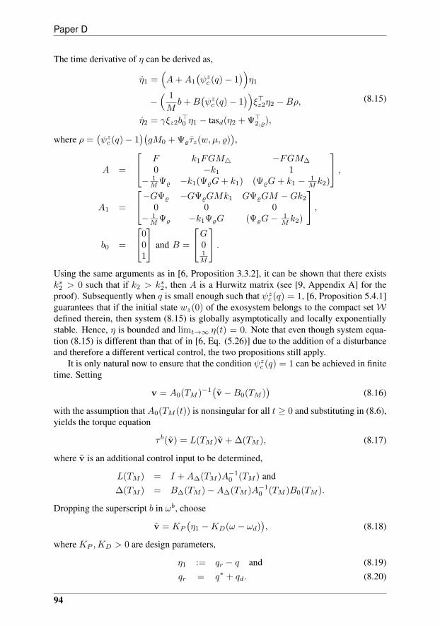
Paper D

The time derivative of η can be derived as,

η1 =(A+A1

(ψzc (q)− 1

))η1

−( 1

Mb+B

(ψzc (q)− 1

))ξ>z2η2 −Bρ,

η2 = γξz2b>0 η1 − tasd(η2 + Ψ>2,%),

(8.15)

where ρ =(ψzc (q)− 1

)(gM0 + Ψ%τz(w, µ, %)

),

A =

F k1FGM4 −FGM∆

0 −k1 1− 1MΨ% −k1(Ψ%G+ k1) (Ψ%G+ k1 − 1

M k2)

,A1 =

−GΨ% −GΨ%GMk1 GΨ%GM −Gk2

0 0 0− 1MΨ% −k1Ψ%G (Ψ%G− 1

M k2)

,b0 =

001

and B =

G01M

.Using the same arguments as in [6, Proposition 3.3.2], it can be shown that there existsk∗2 > 0 such that if k2 > k∗2 , then A is a Hurwitz matrix (see [9, Appendix A] for theproof). Subsequently when q is small enough such that ψzc (q) = 1, [6, Proposition 5.4.1]guarantees that if the initial state wz(0) of the exosystem belongs to the compact setWdefined therein, then system (8.15) is globally asymptotically and locally exponentiallystable. Hence, η is bounded and limt→∞ η(t) = 0. Note that even though system equa-tion (8.15) is different than that of in [6, Eq. (5.26)] due to the addition of a disturbanceand therefore a different vertical control, the two propositions still apply.

It is only natural now to ensure that the condition ψzc (q) = 1 can be achieved in finitetime. Setting

v = A0(TM )−1(v −B0(TM )

)(8.16)

with the assumption that A0(TM (t)) is nonsingular for all t ≥ 0 and substituting in (8.6),yields the torque equation

τ b(v) = L(TM )v + ∆(TM ), (8.17)

where v is an additional control input to be determined,

L(TM ) = I +A∆(TM )A−10 (TM ) and

∆(TM ) = B∆(TM )−A∆(TM )A−10 (TM )B0(TM ).

Dropping the superscript b in ωb, choose

v = KP

(η1 −KD(ω − ωd)

), (8.18)

where KP ,KD > 0 are design parameters,

η1 := qr − q and (8.19)qr = q∗ + qd. (8.20)

94

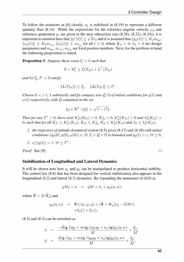
3 Controller Design

To follow the notations in [6] closely, η1 is redefined in (8.19) to represent a differentquantity than (8.14). While the expressions for the reference angular velocity ωd andreference quaternion qr are given in the next subsection (see (8.28), (8.22), (8.24)), it isimportant to mention here that ‖q∗(t)‖ ≤

√3λ3 and it is assumed that ‖qd(t)‖ ≤ Kdmqd ,

‖ωd(t)‖ ≤ Kdmωd, ‖ωd(t)‖ ≤ mωd

for all t ≥ 0, where Kd > 0, λ3 > 0 are designparameters andmqd ,mωd

,mωdare fixed positive numbers. Next, for the problem in hand

the following proposition is stated.

Proposition 3. Suppose there exists l∗1 > 0 such that

0 < 2l∗1 ≤ L(TM ) + L>(TM )

and let l∗2 , δ∗ > 0 satisfy

‖L(TM )‖ ≤ l∗2, ‖∆(TM )‖ ≤ δ∗.

Choose 0 < ε < 1 arbitrarily and fix compact setsQ, Ω of initial conditions for q(t) andω(t) respectively, with Q contained in the set

q ∈ R3 : ‖q‖ <√

1− ε2.

Then for any T ∗ > 0, there exist K∗P (KD) > 0, K∗D > 0, K∗d(KD) > 0 and λ∗3(KD) >0, such that for all KP ≥ K∗P (KD), KD ≤ K∗D, Kd ≤ K∗d(KD) and λ3 ≤ λ∗3(KD),

1. the trajectory of attitude dynamical system (8.5) given (8.17) and (8.18) with initialconditions (q0(0), q(0), ω(0)) ∈ (0, 1]×Q×Ω is bounded and q0(t) > ε, ∀t ≥ 0,

2. ψzc (q(t)) = 1, ∀t ≥ T ∗.

Proof. See [9].

Stabilization of Longitudinal and Lateral Dynamics

It will be shown now how q1 and q2 can be manipulated to produce horizontal stability.The control law (8.8) that has been designed for vertical stabilization also appears in thelongitudinal (8.2) and lateral (8.3) dynamics. By expanding the numerator of (8.8) as

gM0 + u = gM + dz + yη(η, w),

where Ψ = [0 Ψ2] and

yη(η, w) = Ψτz(w, µ, %) + (Ψ + Ψ%)(χ−GMz)

+k2(z + k1z),

(8.2) and (8.3) can be rewritten as

x =−d(q, t)q2 +m(q, t)q1q3 + nx(q)yη(η, w)

M+dxM,

y =d(q, t)q1 +m(q, t)q2q3 + ny(q)yη(η, w)

M+dyM,

95

Paper D

where

d(q, t) =2(gM + dz)q0

1− satc(2q21 + 2q2

2),

m(q, t) = − 2(gM + dz)

1− satc(2q21 + 2q2

2),

nx(q) =−(2q1q3 + 2q0q2)

1− satc(2q21 + 2q2

2),

ny(q) =−(2q2q3 − 2q0q1)

1− satc(2q21 + 2q2

2).

Recall that from the previous analysis on vertical stabilization, with an appropriate selec-tion of the design parameters, yη(η, w) is an asymptotically diminishing signal.

Next by introducing a group of integrators ηx = x, ηy = y and ηq = q3, the followingnew state variables are defined,

ζ1 := [ηy ηx]>,

ζ2 := [y x]> + λ1σ(K1

λ1ζ1),

ζ3 := [y x ηq 0 · · · 0]> + P1λ2σ(K2

λ2ζ2),

(8.21)

where

P1 =

[0 1 0 · · · 01 0 0 · · · 0

]>.(4N+2)×2

By adopting the following nested saturated control law

q∗ = −P2λ3σ(K3

λ3ζ3), (8.22)

where P2 is a matrix, σ(·) is a vector-valued saturation function of suitable dimension(see [9]), Ki, λi, i = 1, 2, 3 are design parameters, the time derivatives can be written as

ζ1 = −λ1σ(K1

λ1ζ1) + ζ2,

ζ2 = −λ2σ(K2

λ2ζ2) + P0ζ3 +K1σ

′(K1

λ1ζ1)ζ1,

Mζ3 = −D(t)P2λ3σ(K3

λ3ζ3) + D(t)qd,

+MK2P1σ′(K2

λ2ζ2)ζ2 − D(t)η1 + p+ dh,

(8.23)

96

3 Controller Design

in which

D1(t) =

d(q, t) m(q, t)q3 0

m(q, t)q3 −d(q, t) 00 0 M

,D(t) =

[D1(t) 0

0 0

],(4N+2)×(4N+2)

p =

ny(q)yη(η, w)nx(q)yη(η, w)

0...0

, dh =

dydx0...0

, η1 =

η1

0...0

,

P0 =

[1 0 0 · · · 00 1 0 · · · 0

].2×(4N+2)

In a generic notation, for σ : Rn → Rn, σ′(υ) = dσ(υ)/d(υ), where υ ∈ Rn. Note thatif one can set qd = −D0(t)dh, where

D0(t) =

[D−1

1 (t) 00 0

],

the disturbance dh can be completely eliminated from subsystem (8.23). In this case,(8.23) can be shown to be input-to-state stable (ISS) with restrictions on the inputs (η1, p)and linear asymptotic gains [6, Lemma 5.7.4].

Since qd is a function of uncertainM and unknown dh, it cannot be generated directly.Thus the following is proposed,

qd := −KdD0(t)d, (8.24)

where d = [dy dx 0 · · · 0]> is a disturbance estimate to be adapted and

D1(t) =

d0(q, t) m0(q, t)q3 0

m0(q, t)q3 −d0(q, t) 00 0 1

,D0(t) =

[D1(t) 0

0 0

],(4N+2)×(4N+2)

(8.25)

where

d0(q, t) =

(1− satc(2q2

1 + 2q22))q0

2(q20 + q2

3)(gM0 + u),

m0(q, t) =−(1− satc(2q2

1 + 2q22))

2(q20 + q2

3)(gM0 + u),

with u given by (8.11) (see [9, Appendix C] for the expression of d). It is important tonotice at this point that a constraint on dz should be imposed. Because limt→∞

(gM0 +

97

Paper D

u(t))

= gM + dz , it is required that dz(t) 6= −gM for all t ≥ 0 to avoid singularities in(8.25). In this paper we assume that |dz(t)| < gM for all t ≥ 0. As a result, TM > 0 forall t ≥ 0. Next, the following state variable are defined,

η2 := ω − ωd −1

KDη1, (8.26)

η3 := Jη2 −Kdeξ, (8.27)

where eξ is the internal model error, and ω and J is a vector and a matrix respectively(see [9]). Note that in (8.26), η2 is redefined to represent a different variable than that ofin (8.13). From (8.24), we may write qd = [qd1 qd2 0 · · · 0]> and the desired angularvelocity is defined as

ωd = Qdqd, (8.28)

Taking the time derivatives,

˙η1 = −1

2

(q0I + S(q)

)(η2 +

1

KDη1 + ωd) + qr,

J η2 = −S(ω)J(η2 +1

KDη1 + ωd)−KPKDL(TM )η2

+ ∆(TM )− J ωd −1

KDJ ˙η1,

η3 = J η2 −Kdeξ.

(8.29)

See [9, Appendix C] for a complete expression of (8.28) and (8.29).We will now study the stability of feedback interconnection of subsystems (8.23) and

(8.29). Subsystem (8.23) is a system with state (ζ1, ζ2, ζ3) and input (η1, η2, η3, p0),while subsystem (8.29) has (η1, η2, η3) and (yζ0, yζ1, Iη1 , Iη2 , Iη3) as its state and inputrespectively (see [9, Appendix C]). Since the vertical stability analysis in first part ofSection 8.3 guarantees that q0(t) > ε > 0 for all t ≥ 0 for an allowed range of the designparameters and initial conditions, it is assumed so in the next proposition. Morever, letML, MU , dL and dU be such that ML ≤ M ≤ MU and 0 < dL ≤ d(q, t) ≤ dU for allt ≥ 0. With that, the following proposition is presented.

Proposition 4. LetKD be fixed and letK∗i and λ∗i , i = 1, 2, 3, be such that the followinginequalities are satisfied

λ∗2K∗2

<λ∗14,

λ∗3K∗3

<λ∗24, 4K∗1λ

∗1 <

λ∗24,

4K∗2λ∗2 <

dL

MU

λ∗38, 24

K∗1K∗2

<1

6

and 24K∗2K∗3

<1

6

dL

dUML

MU.

Then, there exist positive numbers K∗P , K∗d , ε∗L, ε∗U , Rζ1, γζ1, γη1, γη2 and γη3 such that,taking λi = εi−1λ∗i and Ki = εK∗i , i = 1, 2, 3, for all KP ≥ K∗P , Kd ≤ K∗d andε∗L ≤ ε ≤ ε∗U , the feedback interconnection of subsystems (8.23) and (8.29) is ISS

98

4 Simulation Results

1. without restrictions on the initial state;

2. with restrictions (ε2Rζ1, Rη1, Rη2, Rη3) on input (p0, Iη1 , Iη2 , Iη3), where Rη1,Rη2 and Rη3 are arbitrary positive numbers;

3. with linear asymptotic gains.

Therefore, if ‖p0‖∞ < ε2Rζ1, ‖Iη1‖∞ < Rη1, ‖Iη2‖∞ < Rη2 and ‖Iη3‖∞ < Rη3, then(ζ1(t), ζ2(t), ζ3(t), η1(t), η2(t), η3(t)) satisfies the asymptotic bound

‖(ζ1, ζ2, ζ3, η1, η2, η3)‖a ≤

maxγζ1‖p0‖a,KDγη1‖Iη1‖a,

γη2

KP‖Iη2‖a,

γη3

KP‖Iη3‖a

,

where ‖ · ‖∞ and ‖ · ‖a denote the L∞ norm and asymptotic L∞ norm respectively [10].

Proof. The proof of Proposition 4 involves showing that subsystems (8.23) and (8.29)are ISS separately and that the composed system satisfies the small gain theorem (see[9]).

Note that by choosing large enough KP and sufficiently small λ3 and Kd, require-ments for vertical, longitudinal and lateral dynamics stabilization as dictated by Proposi-tion 3 and 4 can be simultaneously satisfied. To conclude the control design, considerthe controller given by (8.8), (8.11), (8.16), (8.18), (8.19), (8.20), (8.28), (8.22) and(8.24). Choose the design parameters according to Proposition 3 and 4. Then for anyinitial conditions w(0) ∈ W , η(0) ∈ Z , (x(0), x(0), y(0), y(0)) ∈ R4, q0(0) > 0,(q(0), ω(0)) ∈ Q × Ω where Z is an arbitrary compact set, (x(t), x(t), y(t), y(t)) con-verges to a neighborhood of the origin which can be rendered arbitrarily small by choos-ing KP and KD sufficiently large and small respectively. In addition,

limt→∞

‖(z(t), z(t))‖ = 0.

8.4 Simulation Results

Hover flight of an autonomous helicopter equipped with the proposed autopilot and influ-enced by a wind disturbance is simulated. The simulation results presented here are basedon a model of a small autonomous helicopter from [11]. To test the robustness propertyof the controller, parameter uncertainties are taken up to 30% of the nominal values. Eventhough the controller is designed based on simplified force and torque equations as de-scribed by (8.1) and (8.6) respectively, the helicopter model assumes full torque, (8.5)and full force equations. The wind disturbance shown in Fig. 8.1 is presented to the heli-copter as a persistently acting external force generated by a 8-dimensional neutrally sta-ble exosystem with % = (1, 1.5, 0.1, 10), wx(0) = (20, 1, 4, 0,−1800, 0,−0.1,−0.02),wy(0) = (10, 2, 10, 2, 1500, 0, 0.1, 0) and wz(0) = (5, 0, 1, 0, 2000, 0, 0.01, 0.01). Tofurther challenge the controller, only 5-dimensional internal models are used. Positionsof the helicopter in the face of the wind disturbance without (γ = 0) and with disturbanceadaptation are given in Fig. 8.2 and 8.3 respectively.

Without disturbance adaptation, while the controller fails to stabilize the x and y posi-tions, z does converge fairly close to zero as could be seen in Fig. 8.2. Apparently, TM is

99

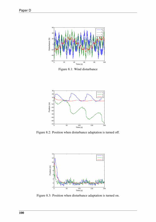
Paper D

0 20 40 60 80 100−60

−40

−20

0

20

40

60

Time (s)

Dis

turb

ance

(N

)

d

x

dy

dz

Figure 8.1: Wind disturbance

0 50 100 150 200−70

−60

−50

−40

−30

−20

−10

0

10

20

30

Time (s)

Pos

ition

(m

)

xyz

Figure 8.2: Position when disturbance adaptation is turned off.

0 50 100 150 200−2

0

2

4

6

8

10

12

14

Time (s)

Pos

ition

(m

)

xyz

Figure 8.3: Position when disturbance adaptation is turned on.

100

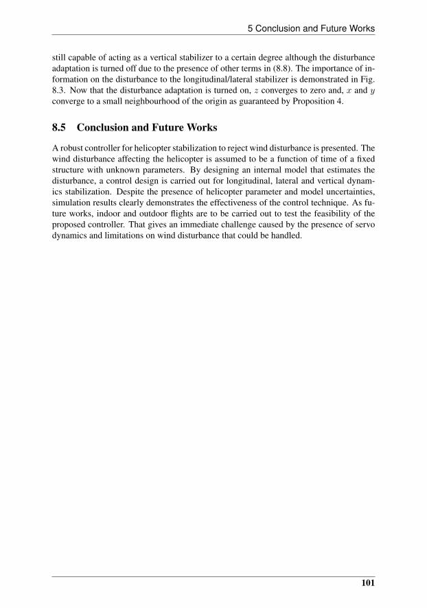
5 Conclusion and Future Works

still capable of acting as a vertical stabilizer to a certain degree although the disturbanceadaptation is turned off due to the presence of other terms in (8.8). The importance of in-formation on the disturbance to the longitudinal/lateral stabilizer is demonstrated in Fig.8.3. Now that the disturbance adaptation is turned on, z converges to zero and, x and yconverge to a small neighbourhood of the origin as guaranteed by Proposition 4.

8.5 Conclusion and Future Works

A robust controller for helicopter stabilization to reject wind disturbance is presented. Thewind disturbance affecting the helicopter is assumed to be a function of time of a fixedstructure with unknown parameters. By designing an internal model that estimates thedisturbance, a control design is carried out for longitudinal, lateral and vertical dynam-ics stabilization. Despite the presence of helicopter parameter and model uncertainties,simulation results clearly demonstrates the effectiveness of the control technique. As fu-ture works, indoor and outdoor flights are to be carried out to test the feasibility of theproposed controller. That gives an immediate challenge caused by the presence of servodynamics and limitations on wind disturbance that could be handled.

101

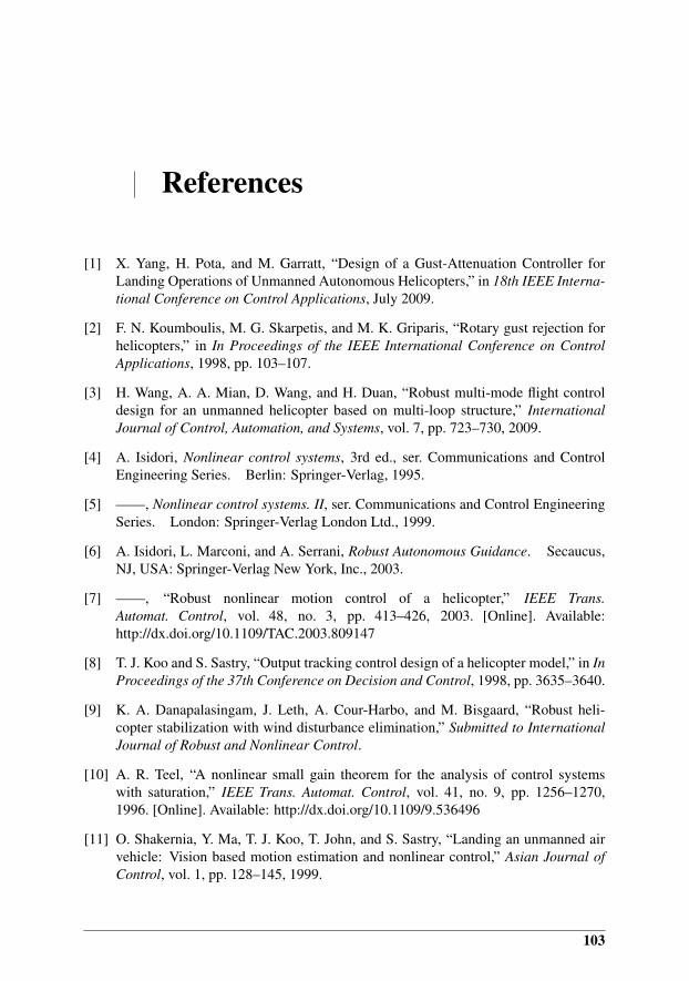
References

[1] X. Yang, H. Pota, and M. Garratt, “Design of a Gust-Attenuation Controller forLanding Operations of Unmanned Autonomous Helicopters,” in 18th IEEE Interna-tional Conference on Control Applications, July 2009.

[2] F. N. Koumboulis, M. G. Skarpetis, and M. K. Griparis, “Rotary gust rejection forhelicopters,” in In Proceedings of the IEEE International Conference on ControlApplications, 1998, pp. 103–107.

[3] H. Wang, A. A. Mian, D. Wang, and H. Duan, “Robust multi-mode flight controldesign for an unmanned helicopter based on multi-loop structure,” InternationalJournal of Control, Automation, and Systems, vol. 7, pp. 723–730, 2009.

[4] A. Isidori, Nonlinear control systems, 3rd ed., ser. Communications and ControlEngineering Series. Berlin: Springer-Verlag, 1995.

[5] ——, Nonlinear control systems. II, ser. Communications and Control EngineeringSeries. London: Springer-Verlag London Ltd., 1999.

[6] A. Isidori, L. Marconi, and A. Serrani, Robust Autonomous Guidance. Secaucus,NJ, USA: Springer-Verlag New York, Inc., 2003.

[7] ——, “Robust nonlinear motion control of a helicopter,” IEEE Trans.Automat. Control, vol. 48, no. 3, pp. 413–426, 2003. [Online]. Available:http://dx.doi.org/10.1109/TAC.2003.809147

[8] T. J. Koo and S. Sastry, “Output tracking control design of a helicopter model,” in InProceedings of the 37th Conference on Decision and Control, 1998, pp. 3635–3640.

[9] K. A. Danapalasingam, J. Leth, A. Cour-Harbo, and M. Bisgaard, “Robust heli-copter stabilization with wind disturbance elimination,” Submitted to InternationalJournal of Robust and Nonlinear Control.

[10] A. R. Teel, “A nonlinear small gain theorem for the analysis of control systemswith saturation,” IEEE Trans. Automat. Control, vol. 41, no. 9, pp. 1256–1270,1996. [Online]. Available: http://dx.doi.org/10.1109/9.536496

[11] O. Shakernia, Y. Ma, T. J. Koo, T. John, and S. Sastry, “Landing an unmanned airvehicle: Vision based motion estimation and nonlinear control,” Asian Journal ofControl, vol. 1, pp. 128–145, 1999.

103

Paper E

Nonlinear Feedforward Control for Wind Disturbance Rejection onAutonomous Helicopter

Morten Bisgaard, Anders la Cour-Harbo and Kumeresan A. Danapalasingam

This paper was published in:In Proceedings of the 2010 IEEE/RSJ International Conference on Intelligent

Robots and Systems18-22 October 2010, Taipei, Taiwan

Copyright c©2010 IEEEThe layout has been revised

1 Introduction

Abstract

This paper presents the design and verification of a model based nonlinear feed-forward controller for vertical and horizontal wind disturbance rejection on autonomoushelicopters. The feedforward control is based on a helicopter model that is derivedusing a number of carefully chosen simplifications to make it suitable for the pur-pose. The model is inverted for the calculation of rotor collective and cyclic pitchangles given the wind disturbance. The control strategy is then applied on a smallhelicopter in a controlled wind environment and the effectiveness and advantage ofthe feedforward controller is demonstrated through flight tests.

9.1 Introduction

Autonomous helicopters are small-scale helicopters, mostly equipped with on-board in-telligence capable of performing various tasks like surveillance, search and rescue, lawenforcement, aerial mapping, cinematography, inspection, etc. In this paper a feedfor-ward control scheme capable of rejecting wind disturbances on the helicopter will be de-veloped. The concept is to measure the wind disturbance at the helicopter and counteringit before it can affect the position of the helicopter.

Sudden changes in wind can occur for instance when flying in an urban environment.An example of a system where wind disturbance rejection can be crucial is an emergencyvehicle assistance system, where a small helicopter fly autonomously some distance infront of, say, an ambulance. The helicopter leapfrogs between intersections along theroute of the ambulance, alerting nearby traffic to stay clear and report any possible prob-lems ahead to the ambulance driver. An application like this requires, among other things,high performance control since the helicopter will operate in close proximity to obstacleslike buildings, power lines, street lights, etc. Only very little error margin can be allowedin the trajectory tracking control and therefore the design of high performance controllersthat could reject known and unknown disturbances to produce desired flight quality iscrucial. When flying through a road intersection, sudden cross winds can be difficult tohandle, even for a high performance feedback controller.

Another example where wind disturbance rejection is important is the use of an au-tonomous helicopter for inspection of offshore wind turbines and oil rig flare towers. Thehelicopter must operate very close to the turbine or tower and can easily experience verystrong wind gusts which can lead to potentially dangerous situations.

This paper presents the design of a model based feedforward controller to counterwind disturbance effects on autonomous helicopters. This is achieved by deriving a sim-plified helicopter model in section 9.3. This model is then used for the design of thefeedforward controller in section 9.4. In section 9.6 results are presented from flight testsof the feedforward controller in a controlled environment and finally a discussion andconclusion is given in section 9.7.

9.2 Previous Work

To date numerous feedback controller designs for autonomous helicopters have been ac-complished with good results, but only little attention has been given to feedforward typecontrol.

107

Paper E

Nonlinear model predictive control (MPC) based on a neural network is used in con-junction with state dependent Riccati equation (SDRE) control in [1] for helicopter con-trol. The SDRE controller provides robust stabilization of the helicopter using a sim-plified model while the neural MPC uses high fidelity nonlinear models for improvedperformance. The neural MPC was trained to include wind fields and simulations usinga high fidelity wind model, including eddies and turbulence, and by accounting for thewind in a feedforward manner in the MPC, performance could be significantly improved.However, the use of nonlinear MPC – and also SDRE – as means of stabilizing the he-licopter has the disadvantage that a highly intensive computational effort is needed forreal time implementation of the control scheme. It can be difficult to achieve real timecontrol of a small high-bandwidth helicopter with such methods. Therefore, a controlsystem based only on SDRE, but with a nonlinear feedforward compensation to accountfor model simplifications has been proposed [2]. Good tracking performance is shown ontwo different helicopters. The nonlinear feedforward compensator is shown to be able toimprove performance if provided with a static estimate of the wind conditions.

An adaptive trajectory tracking controller is presented in [3] where inverse dynamicstogether with a neural network is used for feedback linearization. The actual design isdone using a cascading principle with a attitude controlling inner loop and a translationalcontrolling outer loop. PD feedback from a reference model error is used to suppressdisturbances and shape the two loops. The controller has been tested on a wide rangeof flying vehicles and has shown excellent tracking performance in a wide flight enve-lope, while being robust to changes in vehicle parameters. The approach with dynamicinversion resembles feedforward control and could most likely be extended to account forwind disturbances.

A feedforward control strategy augmented to an existing feedback controller is demon-strated for an autonomous helicopter in [4]. The purpose of the feedforward controller isto assist the feedback loop in rejecting wind disturbances based on wind velocity mea-surements made onboard the helicopter. The feedforward control actions are obtainedthrough trimming of the helicopter model subjected to a simulated wind. These differenttrim points in state space are then used as training input for a neural network that is thenused as the online feedforward controller. Simulations, using measured wind profiles,showed the feasibility of this approach for wind disturbance rejection. Stability for anonlinear feedforward controller for wind disturbance rejection has been proven [5]. In asimilar field, results on the use of feedforward on wind turbines to react to wind changeshave been reported [6].

9.3 Helicopter Model

The helicopter model derived here is intended for use directly in the feedforward con-trol and is a simplified version of the AAU Helisim model [7]1. This simplified versionneglects hinge offset and servo actuator dynamics. Inflow is assumed uniform and mainrotor and stabilizer bar are considered steady state. The model is derived using bladeelement analysis and momentum theory.

While the model derived here is similar to models found in other literature, it is chosento describe it thoroughly here as a number of specific assumptions are take to make it

1The AAU Helisim model can be downloaded for Matlab/Simulink at http://www.uavlab.org

108

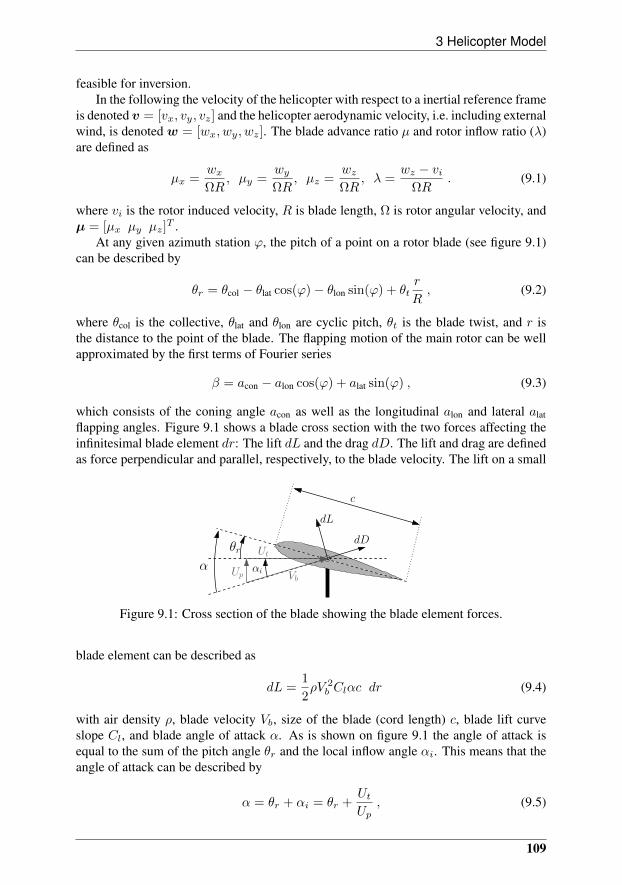
3 Helicopter Model

feasible for inversion.In the following the velocity of the helicopter with respect to a inertial reference frame

is denoted v = [vx, vy, vz] and the helicopter aerodynamic velocity, i.e. including externalwind, is denoted w = [wx, wy, wz]. The blade advance ratio µ and rotor inflow ratio (λ)are defined as

µx =wxΩR

, µy =wyΩR

, µz =wzΩR

, λ =wz − vi

ΩR. (9.1)

where vi is the rotor induced velocity, R is blade length, Ω is rotor angular velocity, andµ = [µx µy µz]

T .At any given azimuth station ϕ, the pitch of a point on a rotor blade (see figure 9.1)

can be described by

θr = θcol − θlat cos(ϕ)− θlon sin(ϕ) + θtr

R, (9.2)

where θcol is the collective, θlat and θlon are cyclic pitch, θt is the blade twist, and r isthe distance to the point of the blade. The flapping motion of the main rotor can be wellapproximated by the first terms of Fourier series

β = acon − alon cos(ϕ) + alat sin(ϕ) , (9.3)

which consists of the coning angle acon as well as the longitudinal alon and lateral alatflapping angles. Figure 9.1 shows a blade cross section with the two forces affecting theinfinitesimal blade element dr: The lift dL and the drag dD. The lift and drag are definedas force perpendicular and parallel, respectively, to the blade velocity. The lift on a small

dL

dD

VbUp

Ut

c

α

θr

αi

Figure 9.1: Cross section of the blade showing the blade element forces.

blade element can be described as

dL =1

2ρV 2

b Clαc dr (9.4)

with air density ρ, blade velocity Vb, size of the blade (cord length) c, blade lift curveslope Cl, and blade angle of attack α. As is shown on figure 9.1 the angle of attack isequal to the sum of the pitch angle θr and the local inflow angle αi. This means that theangle of attack can be described by

α = θr + αi = θr +UtUp

, (9.5)

109

Paper E

where αi is approximately equal to the ratio of the horizontal (Ut) to the vertical (Up)elements of Vb when assuming that the induced velocity is much smaller that the rotationalvelocity of the blade. This assumption also gives

Vb =√U2t + U2

p ' Ut , (9.6)

which leads to the final description of the lift as

dL =1

2ρU2

t Clc(θr +

UtUp

)dr . (9.7)

The drag dD on the blade element can be described similar to the lift

dD =1

2ρV 2

b Cdc dr , (9.8)

where Cd is the blade drag coefficient.Two different contributions can be identified for the horizontal blade velocity. The

rotation of the blade around the shaft and the helicopter motion. The contribution fromthe helicopter motion can be expressed as the translational velocities mapped to the bladeby the blade azimuth station and together with element from the blade rotation it formsUt as

Ut ' ΩR( rR

+ µxsin(ϕ)− µycos(ϕ)). (9.9)

It is here assumed that the vertical blade velocity consists simply of the induced velocityfrom the rotor which result in

Up ' ΩR(λ− µxβ cos(ϕ)− µyβ sin(ϕ)

)− βr . (9.10)

Flapping

The flapping of the main rotor and stabilizer bar is an integral part of the helicopter dy-namics. However, both rotors have dynamics that are significantly faster than the rigidbody dynamics and it is therefore in this case reasonable to consider them steady state.

In order to determine the dynamic flapping motion we use an equilibrium equation ofthe blade torques

τa + τcf + τβ = 0 (9.11)

where the torques in order of appearance are aerodynamic, centrifugal, and inertial torque.Effects from helicopter motion are neglected and therefore Coriolis torque and torquefrom body angular and normal acceleration are zero. Furthermore, the torque due to theflexing of the blade is neglected as it is typically orders of magnitude smaller than thecentrifugal torque.

The aerodynamic torque is the primary torque and it originates from the lift forceacting on a blade. The torque around the flapping hinge is found by integrating the lift dLover the blade length to R and multiplying with the lever r. This yields

τa =

∫ R

0

1

2ρU2

t Clc(θr +

UtUp

)r dr . (9.12)

110

3 Helicopter Model

The centrifugal force acts perpendicular to the rotation axis and as the blade flaps thisresults in a torque around the flapping hinge. Assuming a small flapping angle, the cen-trifugal force can be found as

τcf = −Ω2Ibβ , (9.13)

where Ib is the blade moment of inertia. The torque due to flapping originates from theblade angular acceleration around the flapping hinge and can be expressed as

τβ = −Ibβ . (9.14)

The different torques are substituted into (9.11) and all higher harmonics are discarded.To find the tip-path plane dynamics, the elements containing sin(ϕ) form the equation foralat and the elements containing cos(ϕ) form the equation for ¨alon. Coning is neglected,effects from helicopter motion are discarded and all flapping derivatives are zeroed due tothe steady state assumption. The resulting simplified equations are solved for the flappingangles and yields

alat = −2

(4

3θcol + θt + λ

)µy − θlat (9.15)

alon = 2

(4

3θcol + θt + λ

)µx − θlon (9.16)

The flapping of the stabilizer bar is mixed with the pitch input from the swashplatethrough the Bell-Hiller gain and works as a rate-stabilizing feedback. It can be calcu-lated in a similar fashion to the main rotor, but for most helicopters the deciding factorfor the stabilizer bar flapping is the helicopter rotation and wind has little influence on it.Therefore, while the stabilizer bar is a very important part of the helicopter dynamics, itis resonable in this case to assume

alat,st = −θlat, alon,st = θlon , (9.17)

which effectively means that the control rotor has no influence on the feedforward.

Rotor Forces

Using these assumptions the infinitesimal force equations can be simplified to

dFxmr = −dD sin(ϕ) + dL(β cos(ϕ)±αi sin(ϕ)) ,

dFymr = dD cos(ϕ) + dL(β sin(ϕ)− αi cos(ϕ)) ,

dFzmr = −dL .

The infinitesimal forces are then integrated over r along the blade from 0 to R − e.Averaging over one revolution is done by one more integration. Finally, the resulting

111

Paper E

forces are found by multiplying with the number of blades b

Fx =bc

2π

ρ

2

∫ 2π

0

∫ R

0

U2t

(Cl(θr +

UpUt

)UpUt

sin(ϕ) − Cd sin(ϕ)

)drdϕ , (9.18)

Fy =bc

2π

ρ

2

∫ 2π

0

∫ R

0

U2t

(− Cl

(θr +

UpUt

)UpUt

cos(ϕ) + Cd cos(ϕ)

)drdϕ , (9.19)

Fz = − bc

2π

ρ

2Cl

∫ 2π

0

∫ R

0

U2t

(θr +

UtUp

)drdϕ . (9.20)

Solving the integrals yields

Fx =1

2ρClbcΩ

2R3

((1

2µx λ− 1

3alon

)θcol −

3

4λalon+

1

4(µx λ− alon) θt +

1

4(µx alon − λ) θlon −

Cdµx2a

), (9.21)

Fy =1

2ρClbcΩ

2R3

((1

2µy λ+

1

3alat

)θcol +

3

4λalat+

1

4(µy λ+ alon) θt +

1

4(µy alat + λ) θlat −

Cdµy2a

), (9.22)

Fz = −1

2ρClbcΩ

2R3

(1

2λ+

(1

2µx

2 +1

3+

1

2µy

2

)θcol

+1

4

(1 + µx

2 + µy2) θt +

1

2(θlat µy − θlon µx)

). (9.23)

Induced Inflow

Momentum theory assumes that the rotor behaves like a circular wing and thrust (T =−Fz) is generated when the rotor moves air downwards through what is assumed to be avirtual tube. The amount of thrust generated is determined by the change of momentumfor the air when it is moved by the rotor from far above the helicopter (upstream) to farbelow the helicopter (downstream). As the steam tube is assumed a closed system, themass flux is constant through it and therefore the change of momentum is generated bythe air velocity change. This velocity change comes from the induced velocity vi andrelates to the thrust as

T = 2ρA|v|vi ⇔ vi =T

2ρA√wx2 + wy2 + (wz − vi)2

.

A dimensionless thrust coefficient CT is in introduced

CT =T

ρA(ΩR)2, (9.24)

and substituted together with the expression for vi into the inflow ratio λ

λ =wz − vi

ΩR= µz −

CT

2√

(µ2x + µ2

y) + λ2, (9.25)

and λ is then found by analytically solving this fourth order equation.

112

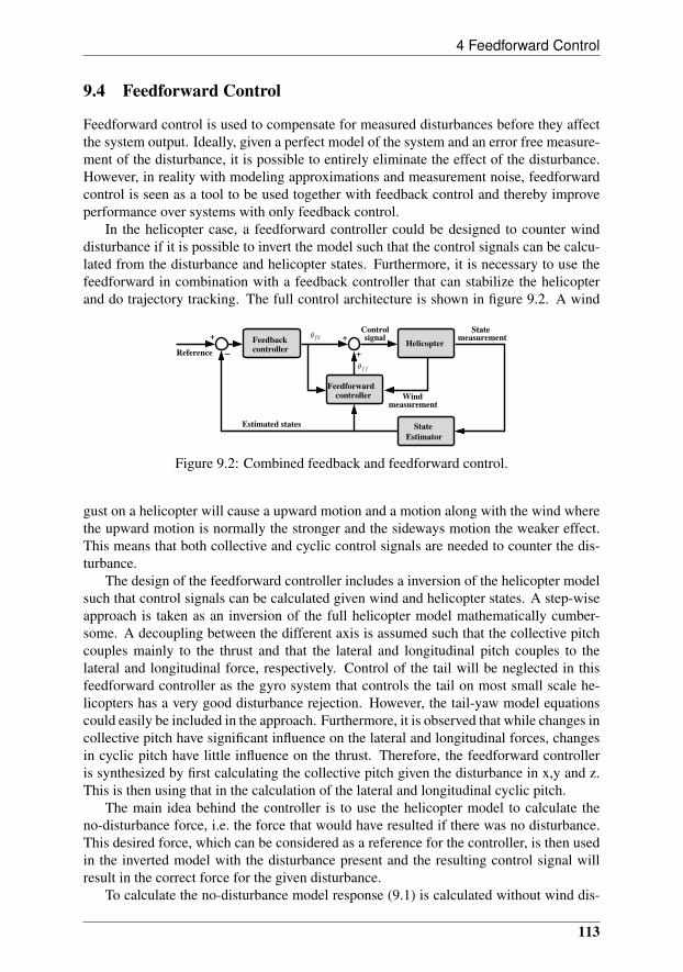
4 Feedforward Control

9.4 Feedforward Control

Feedforward control is used to compensate for measured disturbances before they affectthe system output. Ideally, given a perfect model of the system and an error free measure-ment of the disturbance, it is possible to entirely eliminate the effect of the disturbance.However, in reality with modeling approximations and measurement noise, feedforwardcontrol is seen as a tool to be used together with feedback control and thereby improveperformance over systems with only feedback control.

In the helicopter case, a feedforward controller could be designed to counter winddisturbance if it is possible to invert the model such that the control signals can be calcu-lated from the disturbance and helicopter states. Furthermore, it is necessary to use thefeedforward in combination with a feedback controller that can stabilize the helicopterand do trajectory tracking. The full control architecture is shown in figure 9.2. A wind

Helicopter

−

+ +

+Reference

Controlsignal measurement

State

Feedbackcontroller

Estimated states

Feedforwardcontroller Wind

measurement

State

Estimator

θff

θfb

Figure 9.2: Combined feedback and feedforward control.

gust on a helicopter will cause a upward motion and a motion along with the wind wherethe upward motion is normally the stronger and the sideways motion the weaker effect.This means that both collective and cyclic control signals are needed to counter the dis-turbance.

The design of the feedforward controller includes a inversion of the helicopter modelsuch that control signals can be calculated given wind and helicopter states. A step-wiseapproach is taken as an inversion of the full helicopter model mathematically cumber-some. A decoupling between the different axis is assumed such that the collective pitchcouples mainly to the thrust and that the lateral and longitudinal pitch couples to thelateral and longitudinal force, respectively. Control of the tail will be neglected in thisfeedforward controller as the gyro system that controls the tail on most small scale he-licopters has a very good disturbance rejection. However, the tail-yaw model equationscould easily be included in the approach. Furthermore, it is observed that while changes incollective pitch have significant influence on the lateral and longitudinal forces, changesin cyclic pitch have little influence on the thrust. Therefore, the feedforward controlleris synthesized by first calculating the collective pitch given the disturbance in x,y and z.This is then using that in the calculation of the lateral and longitudinal cyclic pitch.

The main idea behind the controller is to use the helicopter model to calculate theno-disturbance force, i.e. the force that would have resulted if there was no disturbance.This desired force, which can be considered as a reference for the controller, is then usedin the inverted model with the disturbance present and the resulting control signal willresult in the correct force for the given disturbance.

To calculate the no-disturbance model response (9.1) is calculated without wind dis-

113

Paper E

turbance as

µ∗x =vxΩR

, µ∗y =vyΩR

, µ∗z =vzΩR

, λ∗ =vz − vi

ΩR, (9.26)

where ∗ indicates no-disturbance variable. The first step is to calculate the no-disturbanceinflow ratio using the analytical solution to (9.25) as

λ∗ = f(9.25)(µ∗, θcol,fb, θlat,fb, θlon,fb) , (9.27)

which is then used in the calculation of the no-disturbance thrust

F ∗z = f(9.23)(λ∗,µ∗, θcol,fb, θlat,fb, θlon,fb) . (9.28)

where f(9.23) is equation 9.23 as a function. We can then find the collective pitch thatwill result in a thrust force F ∗z given the disturbance. The corresponding λ given thedisturbance is calculated

λff = f(9.25)(µ, F∗z ) , (9.29)

and used in the final calculation of the feedforward collective pitch which is found triviallyas (9.23) solved for θcol

θcol,ff = f−1(9.23)(µ, F

∗z , θlat,fb, θlon,fb) , (9.30)

where f−1(9.23) represent the model inversion of (9.23).

The procedure for the lateral and longitudinal axis is similar to the vertical axis. Firstthe no-disturbance forces are calculated

a∗lat = f(9.15)(µ∗, λff, θcol,ff, θlat,fb) , (9.31)

a∗lon = f(9.16)(µ∗, λff, θcol,ff, θlon,fb) , (9.32)

Fy∗ = f(9.22)(µ

∗, λff, a∗lat, θlat,ff) , (9.33)

Fx∗ = f(9.21)(µ

∗, λff, a∗lon, θlon,ff) . (9.34)

For the next step, the flapping equations (9.15) and (9.16) are substituted into (9.21)and (9.22). The resulting (second order) equations are then solved for θlat and θlon, re-spectively

θlat,ff = f−1(9.15),(9.22)(µ, λff, θcol,ff) , (9.35)

θlon,ff = f−1(9.16),(9.21)(µ, λff, θcol,ff) . (9.36)

The final feedforward controller output is calculated as

θff =

θcol,ffθlat,ffθlon,ff

−θcol,fbθlat,fbθlon,fb

, (9.37)

were the subtraction of θfb is done to ensure that the feedforward controller generatesperturbations from the feedback control trajectory. If no disturbance is present, the feed-forward equations simply calculates back and forth and result in θcol,fb = θcol,ff etc. whichthen in turn result in a zero θff.

114

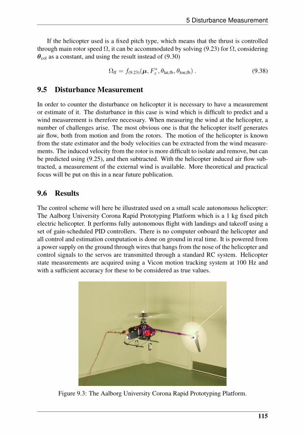
5 Disturbance Measurement

If the helicopter used is a fixed pitch type, which means that the thrust is controlledthrough main rotor speed Ω, it can be accommodated by solving (9.23) for Ω, consideringθcol as a constant, and using the result instead of (9.30)

Ωff = f(9.23)(µ, F∗z , θlat,fb, θlon,fb) . (9.38)

9.5 Disturbance Measurement

In order to counter the disturbance on helicopter it is necessary to have a measurementor estimate of it. The disturbance in this case is wind which is difficult to predict and awind measurement is therefore necessary. When measuring the wind at the helicopter, anumber of challenges arise. The most obvious one is that the helicopter itself generatesair flow, both from motion and from the rotors. The motion of the helicopter is knownfrom the state estimator and the body velocities can be extracted from the wind measure-ments. The induced velocity from the rotor is more difficult to isolate and remove, but canbe predicted using (9.25), and then subtracted. With the helicopter induced air flow sub-tracted, a measurement of the external wind is available. More theoretical and practicalfocus will be put on this in a near future publication.

9.6 Results

The control scheme will here be illustrated used on a small scale autonomous helicopter:The Aalborg University Corona Rapid Prototyping Platform which is a 1 kg fixed pitchelectric helicopter. It performs fully autonomous flight with landings and takeoff using aset of gain-scheduled PID controllers. There is no computer onboard the helicopter andall control and estimation computation is done on ground in real time. It is powered froma power supply on the ground through wires that hangs from the nose of the helicopter andcontrol signals to the servos are transmitted through a standard RC system. Helicopterstate measurements are acquired using a Vicon motion tracking system at 100 Hz andwith a sufficient accuracy for these to be considered as true values.

Figure 9.3: The Aalborg University Corona Rapid Prototyping Platform.

115

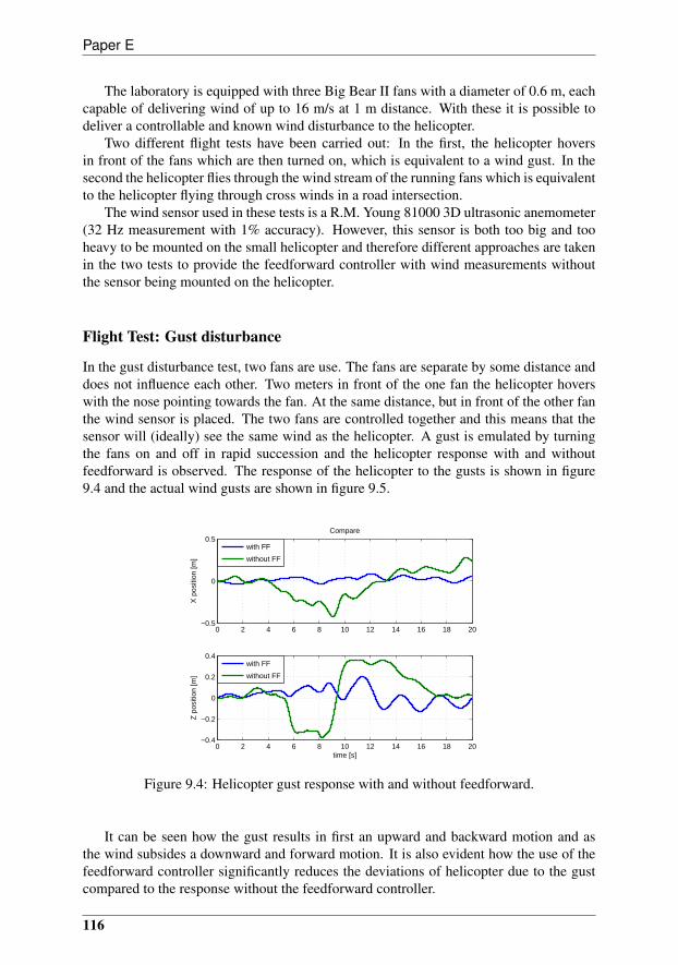
Paper E

The laboratory is equipped with three Big Bear II fans with a diameter of 0.6 m, eachcapable of delivering wind of up to 16 m/s at 1 m distance. With these it is possible todeliver a controllable and known wind disturbance to the helicopter.

Two different flight tests have been carried out: In the first, the helicopter hoversin front of the fans which are then turned on, which is equivalent to a wind gust. In thesecond the helicopter flies through the wind stream of the running fans which is equivalentto the helicopter flying through cross winds in a road intersection.

The wind sensor used in these tests is a R.M. Young 81000 3D ultrasonic anemometer(32 Hz measurement with 1% accuracy). However, this sensor is both too big and tooheavy to be mounted on the small helicopter and therefore different approaches are takenin the two tests to provide the feedforward controller with wind measurements withoutthe sensor being mounted on the helicopter.

Flight Test: Gust disturbance

In the gust disturbance test, two fans are use. The fans are separate by some distance anddoes not influence each other. Two meters in front of the one fan the helicopter hoverswith the nose pointing towards the fan. At the same distance, but in front of the other fanthe wind sensor is placed. The two fans are controlled together and this means that thesensor will (ideally) see the same wind as the helicopter. A gust is emulated by turningthe fans on and off in rapid succession and the helicopter response with and withoutfeedforward is observed. The response of the helicopter to the gusts is shown in figure9.4 and the actual wind gusts are shown in figure 9.5.

0 2 4 6 8 10 12 14 16 18 20−0.5

0

0.5

X p

ositi

on [m

]

Compare

0 2 4 6 8 10 12 14 16 18 20−0.4

−0.2

0

0.2

0.4

time [s]

Z p

ositi

on [m

]

with FF

without FF

with FF

without FF

Figure 9.4: Helicopter gust response with and without feedforward.

It can be seen how the gust results in first an upward and backward motion and asthe wind subsides a downward and forward motion. It is also evident how the use of thefeedforward controller significantly reduces the deviations of helicopter due to the gustcompared to the response without the feedforward controller.

116

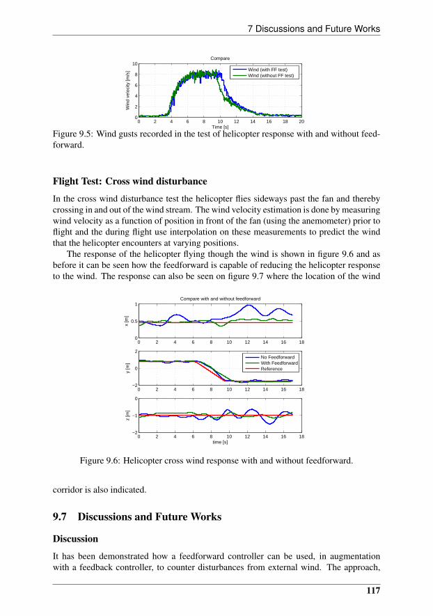
7 Discussions and Future Works

0 2 4 6 8 10 12 14 16 18 200

2

4

6

8

10

Time [s]W

ind

velo

city

[m/s

]

Compare

Wind (with FF test)Wind (without FF test)

Figure 9.5: Wind gusts recorded in the test of helicopter response with and without feed-forward.

Flight Test: Cross wind disturbance

In the cross wind disturbance test the helicopter flies sideways past the fan and therebycrossing in and out of the wind stream. The wind velocity estimation is done by measuringwind velocity as a function of position in front of the fan (using the anemometer) prior toflight and the during flight use interpolation on these measurements to predict the windthat the helicopter encounters at varying positions.

The response of the helicopter flying though the wind is shown in figure 9.6 and asbefore it can be seen how the feedforward is capable of reducing the helicopter responseto the wind. The response can also be seen on figure 9.7 where the location of the wind

0 2 4 6 8 10 12 14 16 180

0.5

1

x [m

]

Compare with and without feedforward

0 2 4 6 8 10 12 14 16 18−2

0

2

y [m

]

0 2 4 6 8 10 12 14 16 18−2

−1

0

time [s]

z [m

]

No FeedforwardWith FeedforwardReference

Figure 9.6: Helicopter cross wind response with and without feedforward.

corridor is also indicated.

9.7 Discussions and Future Works

Discussion

It has been demonstrated how a feedforward controller can be used, in augmentationwith a feedback controller, to counter disturbances from external wind. The approach,

117

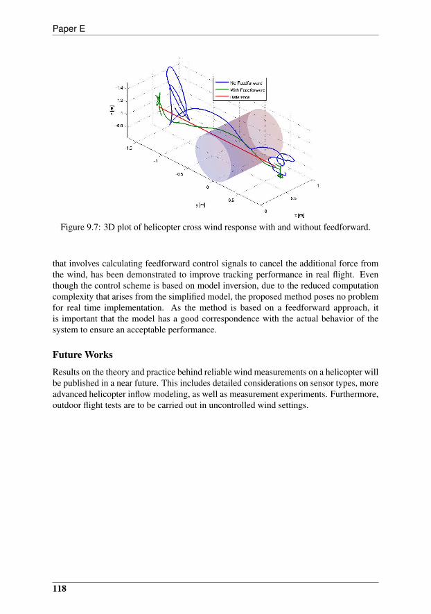
Paper E

Figure 9.7: 3D plot of helicopter cross wind response with and without feedforward.

that involves calculating feedforward control signals to cancel the additional force fromthe wind, has been demonstrated to improve tracking performance in real flight. Eventhough the control scheme is based on model inversion, due to the reduced computationcomplexity that arises from the simplified model, the proposed method poses no problemfor real time implementation. As the method is based on a feedforward approach, itis important that the model has a good correspondence with the actual behavior of thesystem to ensure an acceptable performance.

Future Works

Results on the theory and practice behind reliable wind measurements on a helicopter willbe published in a near future. This includes detailed considerations on sensor types, moreadvanced helicopter inflow modeling, as well as measurement experiments. Furthermore,outdoor flight tests are to be carried out in uncontrolled wind settings.

118

References

[1] E. Wan, A. Bogdanov, R. Kieburtz, A. Baptista, M. Carlsson, Y. Zhang, and M. Zu-lauf, Software Enabled Control: Information Technologies for Dynamical Systems.John Wiley & Sons, 2003, ch. 10, Model predictive neural control for aggressivehelicopter maneuvers.

[2] A. Bogdanov, E. Wan, and G. Harvey, “Sdre flight control for x-cell and r-max au-tonomous helicopters,” in The 43rd IEEE Conference on Decision and Control, 2004.

[3] E. N. Johnson and S. K. Kannan, “Adaptive trajectory control for autonomous heli-copters,” AIAA Journal of Guidance, Control, and Dynamics, Vol 28, No 3, 2005.

[4] K. A. Danapalasingam, A. la Cour-Harbo, and M. Bisgaard, “Feedforward control ofan autonomous helicopter using trim inputs,” in AIAA Infotech@Aerospace & AIAAUnmanned...Unlimited Conference and Exhibit, 2009.

[5] ——, “Disturbance effects in nonlinear control systems and feedforward controlstrategy,” in 7th International Conference on Control and Automation, 2009.

[6] E. van der Hooft and T. van Engelen, “Estimated wind speed feed forward control forwind turbine operation optimisation,” in European wind energy conference, 2004.

[7] M. Bisgaard, “Modeling, estimation, and control of helicopter slung load system,”Ph.D. dissertation, Aalborg University, 2008.

119

Paper F

Robust Helicopter Stabilization with Wind Disturbance Elimination

Kumeresan A. Danapalasingam, John-Josef Leth, Anders la Cour-Harbo andMorten Bisgaard

This paper has been submitted to:International Journal of Robust and Nonlinear Control

Copyright c©2010 John Wiley & Sons, Inc.The layout has been revised

1 Introduction

Abstract

When a helicopter is required to hover with minimum deviations from a desiredposition without measurements of a persistent wind disturbance, a robustly stabilizingcontrol action is vital. In this paper, the stabilization of the position and translationalvelocity of a nonlinear helicopter model affected by a wind disturbance is addressed.The wind disturbance is assumed to be a sum of a fixed number of sinusoids withunknown amplitudes, frequencies and phases. An estimate of the disturbance is in-troduced to be adapted using state measurements for control purposes. A nonlinearcontroller is then designed based on nonlinear adaptive output regulation and robuststabilization of a chain of integrators by a saturated feedback. Simulation results showthe effectiveness of the control design in the stabilization of helicopter motion and thebuilt-in robustness of the controller in handling parameter and model uncertainties.

10.1 Introduction

Autonomous helicopters are highly agile and have six degree of freedom maneuverabilitymaking them a favourite candidate for a wide range of practical applications includingagriculture, cinematography, inspection, surveillance, search and rescue, reconnaissance,etc. For certain tasks the ability of a helicopter to follow a given state reference is crucialfor a successful outcome; for instance when hovering over a ship for rescue operations orwhen flying close to power lines or wind turbines for inspections. In windy conditions thisbecomes a significant challenge for any pilot and hence an autopilot capable of accountingeffectively for the wind disturbance is a realistic alternative. In this work, the authorspresent a control design for longitudinal, lateral, and vertical helicopter stabilization in thepresence of a wind disturbance, with intrinsic robustness property in handling parameterand model uncertainties.

Firstly, some previous works are reviewed. In [1], a feedback-feedforward propor-tional differential (PD) controller is developed for heave motion control. With the as-sistance of a gust estimator, the controller is reported to be able to handle the influencefrom horizontal gusts. The effects of rotary gusts in forward and downward velocity ofa helicopter is addressed in [2]. It is shown that via a state feedback law, the rotary gustrejection problem is always solvable. In a work by Wang et al., a multi-mode linear con-trol stategy is designed for unmanned helicopters in the presence of model uncertainties,atmospheric disturbances and handling qualities requirements [3].

In the present work, assuming that all the state variables (position, attitude and deriva-tives hereof) are available for measurements, a control strategy combining nonlinear adap-tive output regulation and robust stabilization of a chain of integrators by a saturated feed-back is carried out (see for instance, [4], [5] and [6]). Guided by a control solution forvertical trajectory tracking presented in [6] and [7], the design technique presented thereinis extended here for helicopter stabilization in the presence of horizontal and vertical winddisturbance. This is done by means of a robust longitudinal, lateral and vertical stabilizercapable of compensating for parameter and model uncertainties.

In Section 10.2, a mathematical model governing a model helicopter and a problemstatement are given. This is followed by Section 10.3 which covers the vertical, longi-tudinal and lateral stabilization. After the presentation of simulation results in Section10.4, conclusion and future works are discussed in Section 10.5. Additionally, a numberof appendices is included for relevant derivations and proofs.

123

Paper F

10.2 Preliminaries

In this section, a mathematical model of a helicopter is described after which a problemstatement is given.

Helicopter Model

The position and attitude of a helicopter in the three-dimensional Euclidean space E3

is described by the relative position and orientation respectively between a body-fixedcoordinate frameFb and an inertial coordinate frameFi. A coordinate frameF is denotedby the set

F = O, i, j, k,

where i, j and k are right-handed, mutually orthogonal unit vectors with a common originO in E3.

The motion of the center of mass of a helicopter is expressed in an inertial coordinateframe Fi = Oi, ii, ji, ki (whose axes are henceforth denoted as x, y and z axis) as

Mpi = Rf b, (10.1)

where M is the mass and pi = [x y z]> ∈ R3 is the position of the center of mass of thehelicopter with respect to Oi. The rotation matrix R := R(q) is parametrized in terms ofunit quaternions q = (q0, q) ∈ S4 where q0 and q = [q1 q2 q3]> denote the scalar andthe vector parts of the quaternion respectively, as given by

R =

1− 2q22 − 2q2

3 2q1q2 − 2q0q3 2q1q3 + 2q0q2

2q1q2 + 2q0q3 1− 2q21 − 2q2

3 2q2q3 − 2q0q1

2q1q3 − 2q0q2 2q2q3 + 2q0q1 1− 2q21 − 2q2

2

.The overall force f b that acts on the helicopter in a body-fixed coordinate frame Fb =Ob, ib, jb, kb is given by

f b =

XM

YM + YTZM

+ R>

00Mg

+ R>

dxdydz

, (10.2)

where g is the gravitational acceleration and, dx, dy and dz are wind disturbances thataffect the helicopter motion in x, y and z axis respectively. Moreover,

XM = −TM sin a, YM = TM sin b,

ZM = −TM cos a cos b, YT = −TT ,

where TM , TT , a and b are main rotor thrust, tail rotor thrust, longitudinal main rotor tippath plane tilt angle and lateral main rotor tip path plane tilt angle respectively (see Fig.10.1). For convenience of subsequent analysis, it is assumed that a and b are small suchthat

sin a ≈ a, sin b ≈ b, cos a ≈ 1 and cos b ≈ 1. (10.3)

124

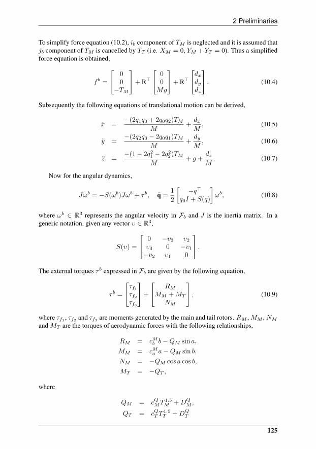
2 Preliminaries

To simplify force equation (10.2), ib component of TM is neglected and it is assumed thatjb component of TM is cancelled by TT (i.e. XM = 0, YM + YT = 0). Thus a simplifiedforce equation is obtained,

f b =

00−TM

+ R>

00Mg

+ R>

dxdydz

. (10.4)

Subsequently the following equations of translational motion can be derived,

x =−(2q1q3 + 2q0q2)TM

M+dxM, (10.5)

y =−(2q2q3 − 2q0q1)TM

M+dyM, (10.6)

z =−(1− 2q2

1 − 2q22)TM

M+ g +

dzM. (10.7)

Now for the angular dynamics,

Jωb = −S(ωb)Jωb + τ b, q =1

2

[−q>

q0I + S(q)

]ωb, (10.8)

where ωb ∈ R3 represents the angular velocity in Fb and J is the inertia matrix. In ageneric notation, given any vector υ ∈ R3,

S(υ) =

0 −υ3 υ2

υ3 0 −υ1

−υ2 υ1 0

.The external torques τ b expressed in Fb are given by the following equation,

τ b =

τf1τf2τf3

+

RMMM +MT

NM

, (10.9)

where τf1 , τf2 and τf3 are moments generated by the main and tail rotors. RM ,MM ,NMand MT are the torques of aerodynamic forces with the following relationships,

RM = cMb b−QM sin a,

MM = cMa a−QM sin b,

NM = −QM cos a cos b,

MT = −QT ,

where

QM = cQMT1.5M +DQ

M ,

QT = cQT T1.5T +DQ

T

125

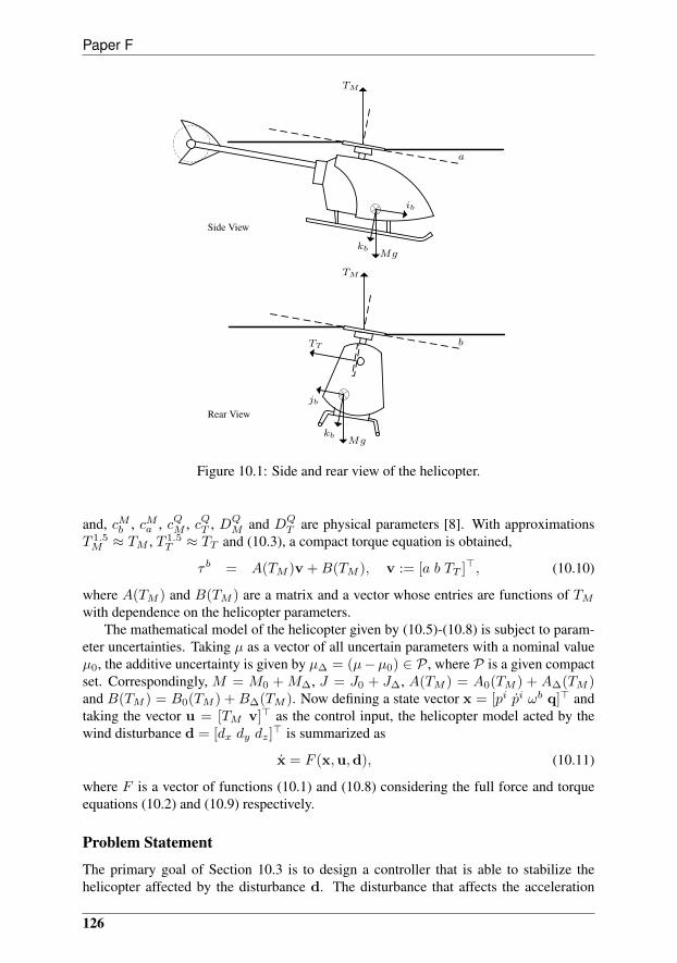
Paper F

TM

TM

TT

ib

jb

kb

kb

Mg

Mg

Side View

Rear View

a

b

Figure 10.1: Side and rear view of the helicopter.

and, cMb , cMa , cQM , cQT , DQM and DQ

T are physical parameters [8]. With approximationsT 1.5M ≈ TM , T 1.5

T ≈ TT and (10.3), a compact torque equation is obtained,

τ b = A(TM )v +B(TM ), v := [a b TT ]>, (10.10)

where A(TM ) and B(TM ) are a matrix and a vector whose entries are functions of TMwith dependence on the helicopter parameters.

The mathematical model of the helicopter given by (10.5)-(10.8) is subject to param-eter uncertainties. Taking µ as a vector of all uncertain parameters with a nominal valueµ0, the additive uncertainty is given by µ∆ = (µ−µ0) ∈ P , where P is a given compactset. Correspondingly, M = M0 + M∆, J = J0 + J∆, A(TM ) = A0(TM ) + A∆(TM )and B(TM ) = B0(TM ) + B∆(TM ). Now defining a state vector x = [pi pi ωb q]> andtaking the vector u = [TM v]> as the control input, the helicopter model acted by thewind disturbance d = [dx dy dz]

> is summarized as

x = F (x,u,d), (10.11)

where F is a vector of functions (10.1) and (10.8) considering the full force and torqueequations (10.2) and (10.9) respectively.

Problem Statement

The primary goal of Section 10.3 is to design a controller that is able to stabilize thehelicopter affected by the disturbance d. The disturbance that affects the acceleration

126

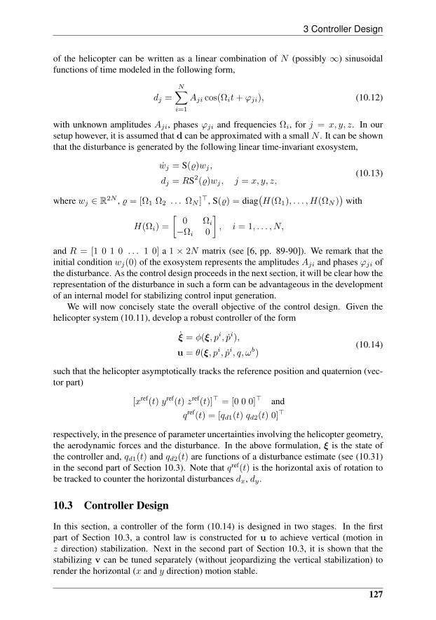
3 Controller Design

of the helicopter can be written as a linear combination of N (possibly ∞) sinusoidalfunctions of time modeled in the following form,

dj =

N∑i=1

Aji cos(Ωit+ ϕji), (10.12)

with unknown amplitudes Aji, phases ϕji and frequencies Ωi, for j = x, y, z. In oursetup however, it is assumed that d can be approximated with a small N . It can be shownthat the disturbance is generated by the following linear time-invariant exosystem,

wj = S(%)wj ,

dj = RS2(%)wj , j = x, y, z,(10.13)

where wj ∈ R2N , % = [Ω1 Ω2 . . . ΩN ]>, S(%) = diag(H(Ω1), . . . ,H(ΩN )

)with

H(Ωi) =

[0 Ωi−Ωi 0

], i = 1, . . . , N,

and R = [1 0 1 0 . . . 1 0] a 1 × 2N matrix (see [6, pp. 89-90]). We remark that theinitial condition wj(0) of the exosystem represents the amplitudes Aji and phases ϕji ofthe disturbance. As the control design proceeds in the next section, it will be clear how therepresentation of the disturbance in such a form can be advantageous in the developmentof an internal model for stabilizing control input generation.

We will now concisely state the overall objective of the control design. Given thehelicopter system (10.11), develop a robust controller of the form

ξ = φ(ξ, pi, pi),

u = θ(ξ, pi, pi, q, ωb)(10.14)

such that the helicopter asymptotically tracks the reference position and quaternion (vec-tor part)

[xref(t) yref(t) zref(t)]> = [0 0 0]> andqref(t) = [qd1(t) qd2(t) 0]>

respectively, in the presence of parameter uncertainties involving the helicopter geometry,the aerodynamic forces and the disturbance. In the above formulation, ξ is the state ofthe controller and, qd1(t) and qd2(t) are functions of a disturbance estimate (see (10.31)in the second part of Section 10.3). Note that qref(t) is the horizontal axis of rotation tobe tracked to counter the horizontal disturbances dx, dy .

10.3 Controller Design

In this section, a controller of the form (10.14) is designed in two stages. In the firstpart of Section 10.3, a control law is constructed for u to achieve vertical (motion inz direction) stabilization. Next in the second part of Section 10.3, it is shown that thestabilizing v can be tuned separately (without jeopardizing the vertical stabilization) torender the horizontal (x and y direction) motion stable.

127

Paper F

Stabilization of Vertical Dynamics

With reference to the vertical dynamics (10.7) given above, to counter the nominal effectof the gravity, the following preliminary control law is chosen,

TM =gM0 + u

1− satc(2q21 + 2q2

2), (10.15)

where satc(s) := sign(s) min|s|, c with 0 < c < 1 is a saturation function introducedto avoid singularities and u is an input to be designed. This yields

z = −ψzc (q)u

M+ g(1− M0

Mψzc (q)

)+dzM,

where

ψzc (q) =1− 2q2

1 − 2q22

1− satc(2q21 + 2q2

2).

If q is small enough such that ψzc (q) = 1, then a feedforward u needed for verticalstabilization is

cu(wz, µ, %) = gM∆ + dz, (10.16)

provided that the initial conditions are set to zero. The term feedforward is used to in-dicate that cu(wz, µ, %) is a control applied to achieve a desired performance [9]. Sincethe steady-state control cu(wz, µ, %) depends on unknown M∆ ∈ µ and dz which is inturn influenced by unknown % and the unmeasurable state wz , it cannot be produced di-rectly. However, it can be asymptotically generated by the use of an internal model. Asa first step in designing a controller with an internal model, the desired control (10.16) isrewritten as an output of a linear system (recall that dz is given by (10.13))

∂τz∂wz

S(%)wz = Φ(%)τz(wz, µ),

cu(wz, µ, %) = Γ(%)τz(wz, µ),

where

τz(wz, µ) =

[gM∆

wz

], Φ(%) =

[0 00 S(%)

],

Γ(%) =[1 Γ2(%)

],

and

Γ2(%) =[−Ω2

1 0 −Ω22 0 . . . −Ω2

N 0].

It is shown in [6, Lemma 3.3.1] that, by constructing a (2N + 1) × (2N + 1) Hurwitzmatrix F and a (2N + 1) × 1 vector G such that the pair (F,G) is controllable, there

128

3 Controller Design

exists a (2N +1)× (2N +1) nonsingular matrix T% such that Φ(%) = T−1% (F +GΨ%)T%

and Γ(%) = Ψ%T% where Ψ% = [1 Ψ2,%] is a 1× (2N + 1) vector. Hence,

∂τz∂wz

S(%)wz = (F +GΨ%)τz(wz, µ, %),

cu(wz, µ, %) = Ψ%τz(wz, µ, %),

where τz(wz, µ, %) = T%τz(wz, µ). Consequently for any initial condition of exosystem(10.13) wz(0), the control cu(wz, µ, %) can be viewed as an output of the linear system

ξz = (F +GΨ%)ξz,

cu(wz, µ, %) = Ψ%ξz(10.17)

if it is initialized as ξz(0) = τ(wz(0), µ, %), where

ξz =

[ξz1ξz2

]∈ R× R2N .

Note that even if Ψ% and τ(wz(0), µ, %) are known and hence enabling the generationof the control cu(wz, µ, %) by (10.17), vertical stabilization can only be achieved if theinitial conditions of (10.7) are set correctly (i.e. z = z = 0). To deal with the unknownsin (10.17) and to obtain vertical stabilization given nonzero initial conditions, choose uin (10.15) as an output of the system

ξz = (F +GΨ)ξz + gstz

u = Ψξz + ust,(10.18)

where ust = k2(z + k1z) and gstz = Gust + FGM0z for k1, k2 > 0 . The vectorΨ = [1 Ψ2] with a 1 × 2N row vector Ψ2 is an estimate of Ψ% and is to be tuned by theadaptation law

˙Ψ2 = γξ>z2(z + k1z)− tasd(Ψ2), (10.19)

where γ > 0 is a design parameter and tasd(ψi) := ψi− satd(ψi) is a dead zone functionin which ψi is the ith component of Ψ2 and d > max2N

i=1

|(Ψ2,%)i|

. Note that the

term tasd(ψi) is zero as long as |ψi| ≤ d and has a stabilizing effect on ψi if the fixedbound is exceeded, thus making the adaptation law robust to the drift phenomena [10].As demonstrated next, the inclusion of the stabilizing terms gstz and ust in (10.18) enablesthe convergence of ξz to the desired function τz(wz, µ, %) and renders (z, z) globallyasymptotically and locally exponentially stable under appropriate conditions.

To prove that the control defined by (10.15) and (10.18) stabilizes (10.7), let

η =

[η1

η2

]=

[η1

Ψ>2

], with (10.20)

η1 =

χzζ

, (10.21)

129

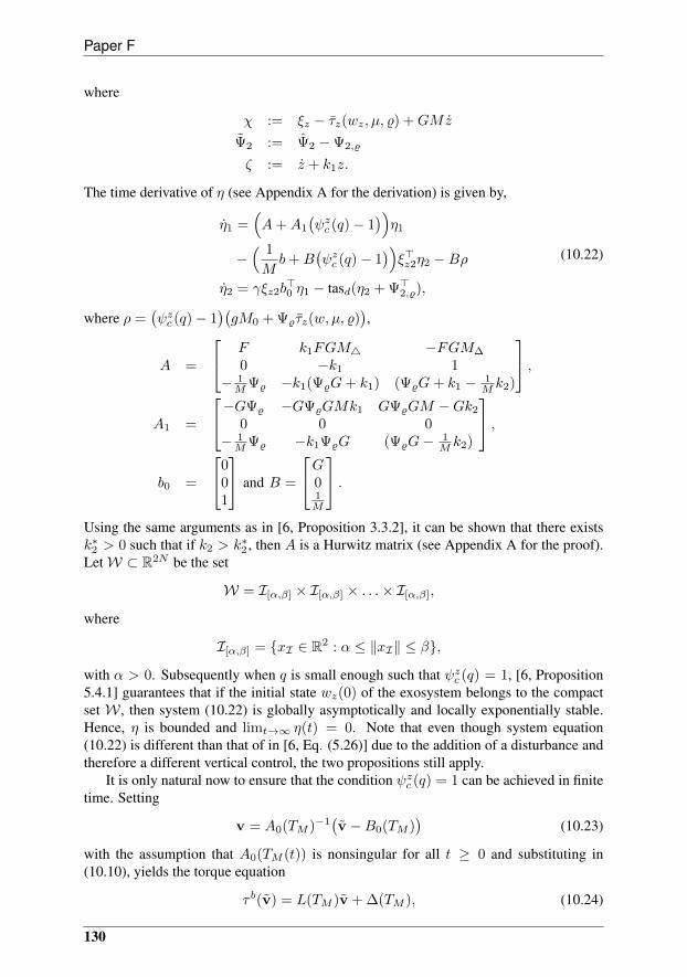
Paper F

where

χ := ξz − τz(wz, µ, %) +GMz

Ψ2 := Ψ2 −Ψ2,%

ζ := z + k1z.

The time derivative of η (see Appendix A for the derivation) is given by,

η1 =(A+A1

(ψzc (q)− 1

))η1

−( 1

Mb+B

(ψzc (q)− 1

))ξ>z2η2 −Bρ

η2 = γξz2b>0 η1 − tasd(η2 + Ψ>2,%),

(10.22)

where ρ =(ψzc (q)− 1

)(gM0 + Ψ%τz(w, µ, %)

),

A =

F k1FGM4 −FGM∆

0 −k1 1− 1MΨ% −k1(Ψ%G+ k1) (Ψ%G+ k1 − 1

M k2)

,A1 =

−GΨ% −GΨ%GMk1 GΨ%GM −Gk2

0 0 0− 1MΨ% −k1Ψ%G (Ψ%G− 1

M k2)

,b0 =

001

and B =

G01M

.Using the same arguments as in [6, Proposition 3.3.2], it can be shown that there existsk∗2 > 0 such that if k2 > k∗2 , then A is a Hurwitz matrix (see Appendix A for the proof).LetW ⊂ R2N be the set

W = I[α,β] × I[α,β] × . . .× I[α,β],

where

I[α,β] = xI ∈ R2 : α ≤ ‖xI‖ ≤ β,

with α > 0. Subsequently when q is small enough such that ψzc (q) = 1, [6, Proposition5.4.1] guarantees that if the initial state wz(0) of the exosystem belongs to the compactset W , then system (10.22) is globally asymptotically and locally exponentially stable.Hence, η is bounded and limt→∞ η(t) = 0. Note that even though system equation(10.22) is different than that of in [6, Eq. (5.26)] due to the addition of a disturbance andtherefore a different vertical control, the two propositions still apply.

It is only natural now to ensure that the condition ψzc (q) = 1 can be achieved in finitetime. Setting

v = A0(TM )−1(v −B0(TM )

)(10.23)

with the assumption that A0(TM (t)) is nonsingular for all t ≥ 0 and substituting in(10.10), yields the torque equation

τ b(v) = L(TM )v + ∆(TM ), (10.24)

130

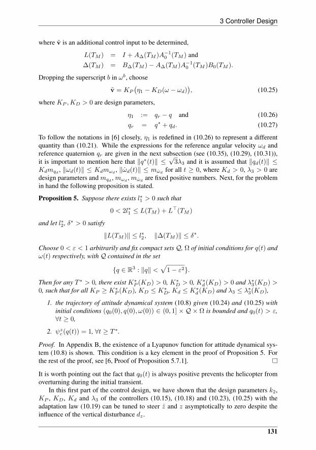
3 Controller Design

where v is an additional control input to be determined,

L(TM ) = I +A∆(TM )A−10 (TM ) and

∆(TM ) = B∆(TM )−A∆(TM )A−10 (TM )B0(TM ).

Dropping the superscript b in ωb, choose

v = KP

(η1 −KD(ω − ωd)

), (10.25)

where KP ,KD > 0 are design parameters,

η1 := qr − q and (10.26)qr = q∗ + qd. (10.27)

To follow the notations in [6] closely, η1 is redefined in (10.26) to represent a differentquantity than (10.21). While the expressions for the reference angular velocity ωd andreference quaternion qr are given in the next subsection (see (10.35), (10.29), (10.31)),it is important to mention here that ‖q∗(t)‖ ≤

√3λ3 and it is assumed that ‖qd(t)‖ ≤

Kdmqd , ‖ωd(t)‖ ≤ Kdmωd, ‖ωd(t)‖ ≤ mωd

for all t ≥ 0, where Kd > 0, λ3 > 0 aredesign parameters and mqd , mωd

, mωdare fixed positive numbers. Next, for the problem

in hand the following proposition is stated.

Proposition 5. Suppose there exists l∗1 > 0 such that

0 < 2l∗1 ≤ L(TM ) + L>(TM )

and let l∗2 , δ∗ > 0 satisfy

‖L(TM )‖ ≤ l∗2, ‖∆(TM )‖ ≤ δ∗.

Choose 0 < ε < 1 arbitrarily and fix compact setsQ, Ω of initial conditions for q(t) andω(t) respectively, with Q contained in the set

q ∈ R3 : ‖q‖ <√

1− ε2.

Then for any T ∗ > 0, there exist K∗P (KD) > 0, K∗D > 0, K∗d(KD) > 0 and λ∗3(KD) >0, such that for all KP ≥ K∗P (KD), KD ≤ K∗D, Kd ≤ K∗d(KD) and λ3 ≤ λ∗3(KD),

1. the trajectory of attitude dynamical system (10.8) given (10.24) and (10.25) withinitial conditions (q0(0), q(0), ω(0)) ∈ (0, 1] × Q × Ω is bounded and q0(t) > ε,∀t ≥ 0,

2. ψzc (q(t)) = 1, ∀t ≥ T ∗.

Proof. In Appendix B, the existence of a Lyapunov function for attitude dynamical sys-tem (10.8) is shown. This condition is a key element in the proof of Proposition 5. Forthe rest of the proof, see [6, Proof of Proposition 5.7.1].

It is worth pointing out the fact that q0(t) is always positive prevents the helicopter fromoverturning during the initial transient.

In this first part of the control design, we have shown that the design parameters k2,KP , KD, Kd and λ3 of the controllers (10.15), (10.18) and (10.23), (10.25) with theadaptation law (10.19) can be tuned to steer z and z asymptotically to zero despite theinfluence of the vertical disturbance dz .

131

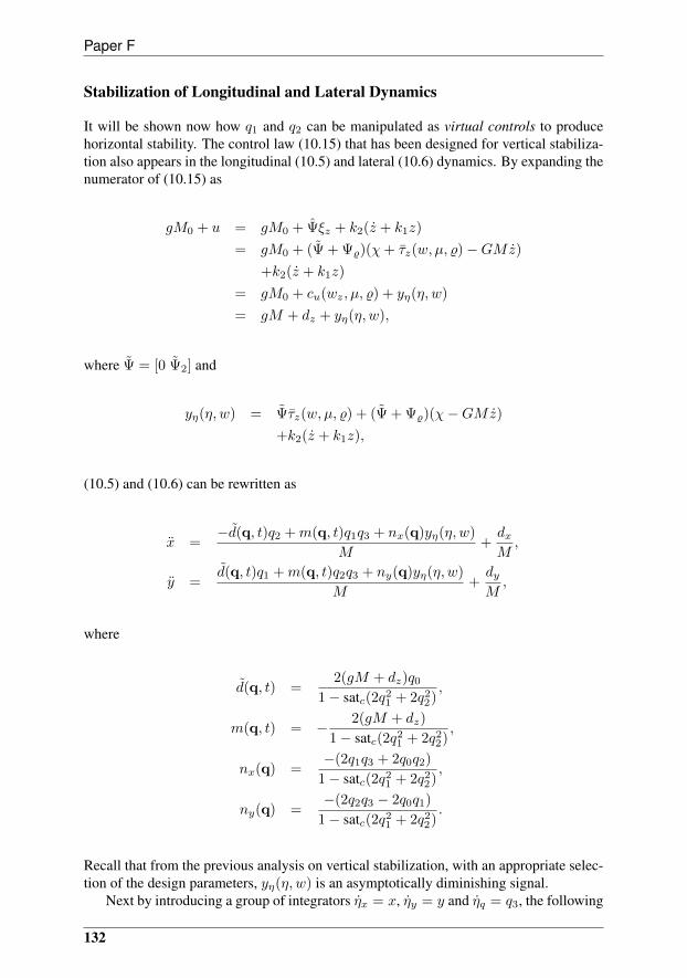
Paper F

Stabilization of Longitudinal and Lateral Dynamics

It will be shown now how q1 and q2 can be manipulated as virtual controls to producehorizontal stability. The control law (10.15) that has been designed for vertical stabiliza-tion also appears in the longitudinal (10.5) and lateral (10.6) dynamics. By expanding thenumerator of (10.15) as

gM0 + u = gM0 + Ψξz + k2(z + k1z)

= gM0 + (Ψ + Ψ%)(χ+ τz(w, µ, %)−GMz)

+k2(z + k1z)

= gM0 + cu(wz, µ, %) + yη(η, w)

= gM + dz + yη(η, w),

where Ψ = [0 Ψ2] and

yη(η, w) = Ψτz(w, µ, %) + (Ψ + Ψ%)(χ−GMz)

+k2(z + k1z),

(10.5) and (10.6) can be rewritten as

x =−d(q, t)q2 +m(q, t)q1q3 + nx(q)yη(η, w)

M+dxM,

y =d(q, t)q1 +m(q, t)q2q3 + ny(q)yη(η, w)

M+dyM,

where

d(q, t) =2(gM + dz)q0

1− satc(2q21 + 2q2

2),

m(q, t) = − 2(gM + dz)

1− satc(2q21 + 2q2

2),

nx(q) =−(2q1q3 + 2q0q2)

1− satc(2q21 + 2q2

2),

ny(q) =−(2q2q3 − 2q0q1)

1− satc(2q21 + 2q2

2).

Recall that from the previous analysis on vertical stabilization, with an appropriate selec-tion of the design parameters, yη(η, w) is an asymptotically diminishing signal.

Next by introducing a group of integrators ηx = x, ηy = y and ηq = q3, the following

132

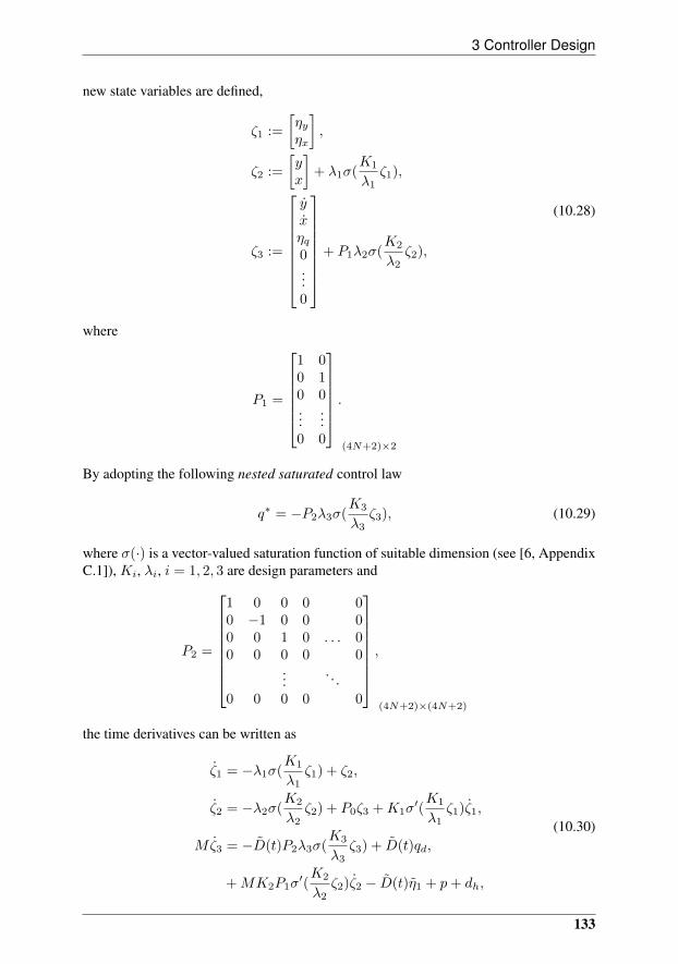
3 Controller Design

new state variables are defined,

ζ1 :=

[ηyηx

],

ζ2 :=

[yx

]+ λ1σ(

K1

λ1ζ1),

ζ3 :=

yxηq0...0

+ P1λ2σ(

K2

λ2ζ2),

(10.28)

where

P1 =

1 00 10 0...

...0 0

.(4N+2)×2

By adopting the following nested saturated control law

q∗ = −P2λ3σ(K3

λ3ζ3), (10.29)

where σ(·) is a vector-valued saturation function of suitable dimension (see [6, AppendixC.1]), Ki, λi, i = 1, 2, 3 are design parameters and

P2 =

1 0 0 0 00 −1 0 0 00 0 1 0 . . . 00 0 0 0 0

.... . .

0 0 0 0 0

,

(4N+2)×(4N+2)

the time derivatives can be written as

ζ1 = −λ1σ(K1

λ1ζ1) + ζ2,

ζ2 = −λ2σ(K2

λ2ζ2) + P0ζ3 +K1σ

′(K1

λ1ζ1)ζ1,

Mζ3 = −D(t)P2λ3σ(K3

λ3ζ3) + D(t)qd,

+MK2P1σ′(K2

λ2ζ2)ζ2 − D(t)η1 + p+ dh,

(10.30)

133

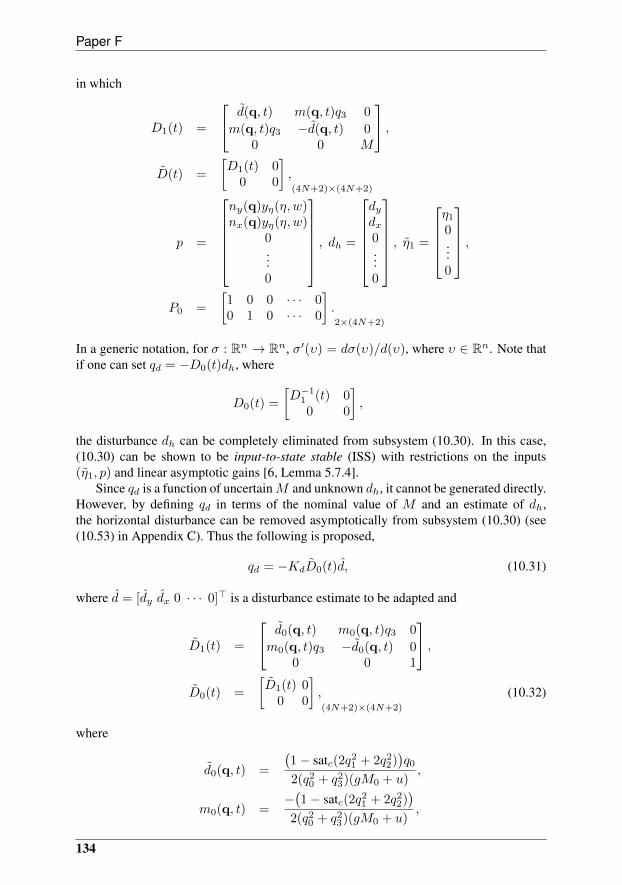
Paper F

in which

D1(t) =

d(q, t) m(q, t)q3 0

m(q, t)q3 −d(q, t) 00 0 M

,D(t) =

[D1(t) 0

0 0

],(4N+2)×(4N+2)

p =

ny(q)yη(η, w)nx(q)yη(η, w)

0...0

, dh =

dydx0...0

, η1 =

η1

0...0

,

P0 =

[1 0 0 · · · 00 1 0 · · · 0

].2×(4N+2)

In a generic notation, for σ : Rn → Rn, σ′(υ) = dσ(υ)/d(υ), where υ ∈ Rn. Note thatif one can set qd = −D0(t)dh, where

D0(t) =

[D−1

1 (t) 00 0

],

the disturbance dh can be completely eliminated from subsystem (10.30). In this case,(10.30) can be shown to be input-to-state stable (ISS) with restrictions on the inputs(η1, p) and linear asymptotic gains [6, Lemma 5.7.4].

Since qd is a function of uncertainM and unknown dh, it cannot be generated directly.However, by defining qd in terms of the nominal value of M and an estimate of dh,the horizontal disturbance can be removed asymptotically from subsystem (10.30) (see(10.53) in Appendix C). Thus the following is proposed,

qd = −KdD0(t)d, (10.31)

where d = [dy dx 0 · · · 0]> is a disturbance estimate to be adapted and

D1(t) =

d0(q, t) m0(q, t)q3 0

m0(q, t)q3 −d0(q, t) 00 0 1

,D0(t) =

[D1(t) 0

0 0

],(4N+2)×(4N+2)

(10.32)

where

d0(q, t) =

(1− satc(2q2

1 + 2q22))q0

2(q20 + q2

3)(gM0 + u),

m0(q, t) =−(1− satc(2q2

1 + 2q22))

2(q20 + q2

3)(gM0 + u),

134

3 Controller Design

with u given by (10.18). It is important to notice at this point that a constraint on dzshould be imposed. Because limt→∞

(gM0 + u(t)

)= gM + dz , it is required that

dz(t) 6= −gM for all t ≥ 0 to avoid singularities in (10.32). Since dz is given by (10.12),in this paper we assume that |dz(t)| < gM for all t ≥ 0. As a result, TM > 0 for allt ≥ 0. Next, the following state variable are defined,

η2 := ω − ωd −1

KDη1, (10.33)

η3 := Jη2 −Kdeξ, (10.34)

where eξ is the internal model error (10.48),

ω =

ω0...0

and J =

[J 00 I

].

Note that in (10.33), η2 is redefined to represent a different variable than that of in (10.20).From (10.31), we may write qd = [qd1 qd2 0 · · · 0]> and the desired angular velocity isdefined as

ωd = Qdqd, (10.35)

where

Qd0 =2

ε

ε2 + q2d1 qd1qd2 −εqd2

qd1qd2 ε2 + q2d2 εqd1

εqd2 −εqd1 ε2

,Qd =

[Qd0 0

0 0

],

for arbitrary ε < ε < 1. Taking the time derivatives,

˙η1 = −1

2

(q0I + S(q)

)(η2 +

1

KDη1 + ωd) + qr,

J η2 = −S(ω)J(η2 +1

KDη1 + ωd)−KPKDL(TM )η2

+ ∆(TM )− J ωd −1

KDJ ˙η1,

η3 = J η2 −Kdeξ,

(10.36)

135

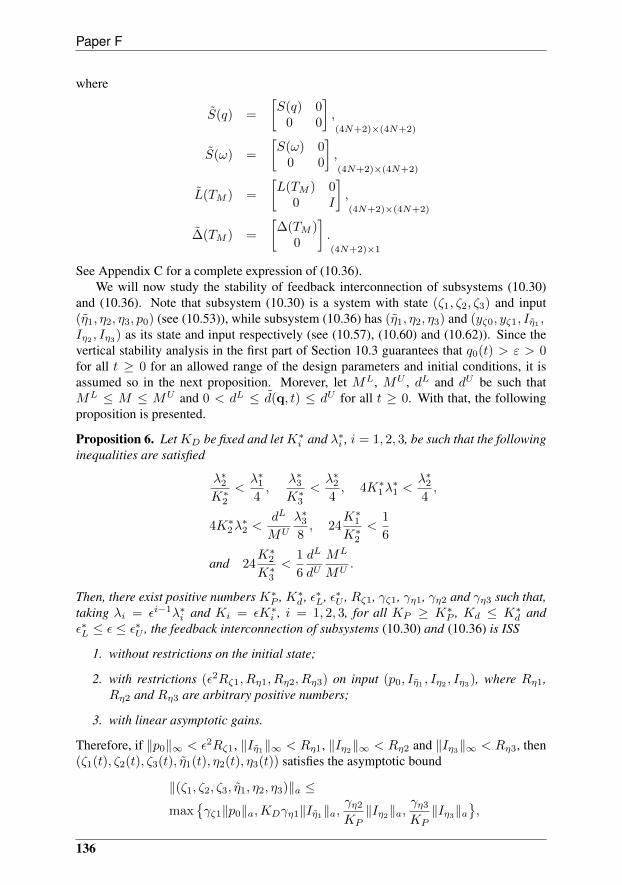
Paper F

where

S(q) =

[S(q) 0

0 0

],(4N+2)×(4N+2)

S(ω) =

[S(ω) 0

0 0

],(4N+2)×(4N+2)

L(TM ) =

[L(TM ) 0

0 I

],(4N+2)×(4N+2)

∆(TM ) =

[∆(TM )

0

].(4N+2)×1

See Appendix C for a complete expression of (10.36).We will now study the stability of feedback interconnection of subsystems (10.30)

and (10.36). Note that subsystem (10.30) is a system with state (ζ1, ζ2, ζ3) and input(η1, η2, η3, p0) (see (10.53)), while subsystem (10.36) has (η1, η2, η3) and (yζ0, yζ1, Iη1 ,Iη2 , Iη3) as its state and input respectively (see (10.57), (10.60) and (10.62)). Since thevertical stability analysis in the first part of Section 10.3 guarantees that q0(t) > ε > 0for all t ≥ 0 for an allowed range of the design parameters and initial conditions, it isassumed so in the next proposition. Morever, let ML, MU , dL and dU be such thatML ≤ M ≤ MU and 0 < dL ≤ d(q, t) ≤ dU for all t ≥ 0. With that, the followingproposition is presented.

Proposition 6. LetKD be fixed and letK∗i and λ∗i , i = 1, 2, 3, be such that the followinginequalities are satisfied

λ∗2K∗2

<λ∗14,

λ∗3K∗3

<λ∗24, 4K∗1λ

∗1 <

λ∗24,

4K∗2λ∗2 <

dL

MU

λ∗38, 24

K∗1K∗2

<1

6

and 24K∗2K∗3

<1

6

dL

dUML

MU.

Then, there exist positive numbers K∗P , K∗d , ε∗L, ε∗U , Rζ1, γζ1, γη1, γη2 and γη3 such that,taking λi = εi−1λ∗i and Ki = εK∗i , i = 1, 2, 3, for all KP ≥ K∗P , Kd ≤ K∗d andε∗L ≤ ε ≤ ε∗U , the feedback interconnection of subsystems (10.30) and (10.36) is ISS

1. without restrictions on the initial state;

2. with restrictions (ε2Rζ1, Rη1, Rη2, Rη3) on input (p0, Iη1 , Iη2 , Iη3), where Rη1,Rη2 and Rη3 are arbitrary positive numbers;

3. with linear asymptotic gains.

Therefore, if ‖p0‖∞ < ε2Rζ1, ‖Iη1‖∞ < Rη1, ‖Iη2‖∞ < Rη2 and ‖Iη3‖∞ < Rη3, then(ζ1(t), ζ2(t), ζ3(t), η1(t), η2(t), η3(t)) satisfies the asymptotic bound

‖(ζ1, ζ2, ζ3, η1, η2, η3)‖a ≤

maxγζ1‖p0‖a,KDγη1‖Iη1‖a,

γη2

KP‖Iη2‖a,

γη3

KP‖Iη3‖a

,

136

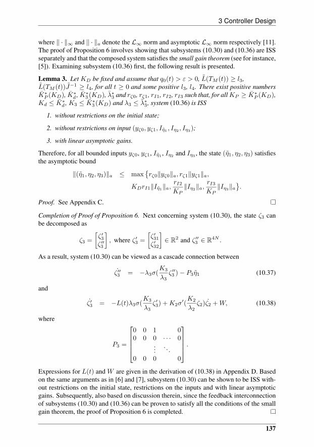
3 Controller Design

where ‖ · ‖∞ and ‖ · ‖a denote the L∞ norm and asymptotic L∞ norm respectively [11].The proof of Proposition 6 involves showing that subsystems (10.30) and (10.36) are ISSseparately and that the composed system satisfies the small gain theorem (see for instance,[5]). Examining subsystem (10.36) first, the following result is presented.

Lemma 3. Let KD be fixed and assume that q0(t) > ε > 0, L(TM (t)) ≥ l3,L(TM (t))J−1 ≥ l4, for all t ≥ 0 and some positive l3, l4. There exist positive numbersK∗P (KD), K∗d , K∗3 (KD), λ∗3 and rζ0, rζ1, rI1, rI2, rI3 such that, for allKP ≥ K∗P (KD),Kd ≤ K∗d , K3 ≤ K∗3 (KD) and λ3 ≤ λ∗3, system (10.36) is ISS

1. without restrictions on the initial state;

2. without restrictions on input (yζ0, yζ1, Iη1 , Iη2 , Iη3);

3. with linear asymptotic gains.

Therefore, for all bounded inputs yζ0, yζ1, Iη1 , Iη2 and Iη3 , the state (η1, η2, η3) satisfiesthe asymptotic bound

‖(η1, η2, η3)‖a ≤ maxrζ0‖yζ0‖a, rζ1‖yζ1‖a,

KDrI1‖Iη1‖a,rI2KP‖Iη2‖a,

rI3KP‖Iη3‖a

.

Proof. See Appendix C.

Completion of Proof of Proposition 6. Next concerning system (10.30), the state ζ3 canbe decomposed as

ζ3 =

[ζ ′3ζ ′′3

], where ζ ′3 =

[ζ ′31

ζ ′32

]∈ R2 and ζ ′′3 ∈ R4N .

As a result, system (10.30) can be viewed as a cascade connection between

˙ζ ′′3 = −λ3σ(K3

λ3ζ ′′3 )− P3η1 (10.37)

and

ζ ′3 = −L(t)λ3σ(K3

λ3ζ ′3) +K2σ

′(K2

λ2ζ2)ζ2 +W, (10.38)

where

P3 =

0 0 1 00 0 0 · · · 0

.... . .

0 0 0 0

.Expressions for L(t) and W are given in the derivation of (10.38) in Appendix D. Basedon the same arguments as in [6] and [7], subsystem (10.30) can be shown to be ISS with-out restrictions on the initial state, restrictions on the inputs and with linear asymptoticgains. Subsequently, also based on discussion therein, since the feedback interconnectionof subsystems (10.30) and (10.36) can be proven to satisfy all the conditions of the smallgain theorem, the proof of Proposition 6 is completed.

137

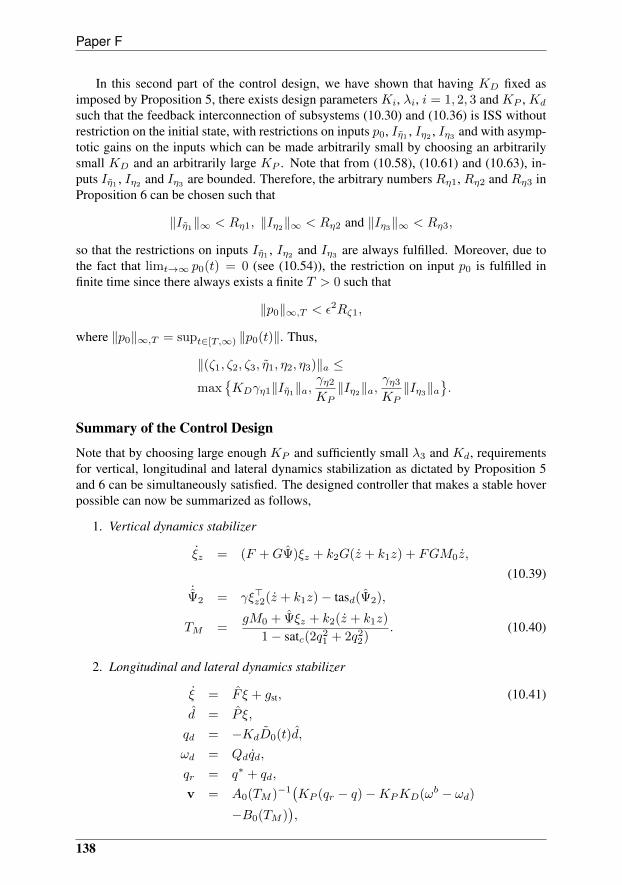
Paper F

In this second part of the control design, we have shown that having KD fixed asimposed by Proposition 5, there exists design parameters Ki, λi, i = 1, 2, 3 and KP , Kd

such that the feedback interconnection of subsystems (10.30) and (10.36) is ISS withoutrestriction on the initial state, with restrictions on inputs p0, Iη1 , Iη2 , Iη3 and with asymp-totic gains on the inputs which can be made arbitrarily small by choosing an arbitrarilysmall KD and an arbitrarily large KP . Note that from (10.58), (10.61) and (10.63), in-puts Iη1 , Iη2 and Iη3 are bounded. Therefore, the arbitrary numbers Rη1, Rη2 and Rη3 inProposition 6 can be chosen such that

‖Iη1‖∞ < Rη1, ‖Iη2‖∞ < Rη2 and ‖Iη3‖∞ < Rη3,

so that the restrictions on inputs Iη1 , Iη2 and Iη3 are always fulfilled. Moreover, due tothe fact that limt→∞ p0(t) = 0 (see (10.54)), the restriction on input p0 is fulfilled infinite time since there always exists a finite T > 0 such that

‖p0‖∞,T < ε2Rζ1,

where ‖p0‖∞,T = supt∈[T,∞) ‖p0(t)‖. Thus,

‖(ζ1, ζ2, ζ3, η1, η2, η3)‖a ≤

maxKDγη1‖Iη1‖a,

γη2

KP‖Iη2‖a,

γη3

KP‖Iη3‖a

.

Summary of the Control Design

Note that by choosing large enough KP and sufficiently small λ3 and Kd, requirementsfor vertical, longitudinal and lateral dynamics stabilization as dictated by Proposition 5and 6 can be simultaneously satisfied. The designed controller that makes a stable hoverpossible can now be summarized as follows,

1. Vertical dynamics stabilizer

ξz = (F +GΨ)ξz + k2G(z + k1z) + FGM0z,

(10.39)˙Ψ2 = γξ>z2(z + k1z)− tasd(Ψ2),

TM =gM0 + Ψξz + k2(z + k1z)

1− satc(2q21 + 2q2

2). (10.40)

2. Longitudinal and lateral dynamics stabilizer

ξ = F ξ + gst, (10.41)d = P ξ,

qd = −KdD0(t)d,

ωd = Qdqd,

qr = q∗ + qd,

v = A0(TM )−1(KP (qr − q)−KPKD(ωb − ωd)

−B0(TM )),

138

4 Simulation Results

where

ξ =

[ξyξx

], with ξi =

[ξi1ξi2

]∈ R× R2N , i = x, y,

F =

[F +GΨ 0

0 F +GΨ

], P =

Ψ 0

0 Ψ0 0

and

gst =

[k4(y + k3y)Gk4(x+ k3x)G

], k3, k4 > 0.

Thus, a controller of the from (10.14) is developed where

ξ =

ξξzΨ>2

.To conclude the control design, consider the controller above and choose the design

parameters according to Proposition 5 and 6. Then for any initial conditions w(0) ∈ W ,η(0) ∈ Z , (x(0), x(0), y(0), y(0)) ∈ R4, q0(0) > 0, (q(0), ω(0)) ∈ Q×Ω where Z is anarbitrary compact set, (x(t), x(t), y(t), y(t)) converges to a neighborhood of the originwhich can be rendered arbitrarily small by choosing KP and KD sufficiently large andsmall respectively. In addition,

limt→∞

‖(z(t), z(t))‖ = 0.

10.4 Simulation Results

Hover flight of an autonomous helicopter equipped with the proposed autopilot and influ-enced by a wind disturbance is simulated.

The simulation results presented here are based on a model of a small autonomoushelicopter from [12]. To test the robustness property of the controller, parameter uncer-tainties are taken up to 30% of the nominal values. Even though the controller is de-signed based on simplified force and torque equations as described by (10.4) and (10.10)respectively, the helicopter model assumes full torque, (10.9) and full force equations.The wind disturbance shown in Fig. 10.2 is presented to the helicopter as a persistentlyacting external force generated by a 8-dimensional neutrally stable exosystem with % =(1, 1.5, 0.1, 10), wx(0) = (20, 1, 4, 0,−1800, 0,−0.1,−0.02), wy(0) = (10, 2, 10, 2,1500, 0, 0.1, 0) and wz(0) = (5, 0, 1, 0, 2000, 0, 0.01, 0.01). To further challenge thecontroller, only 5-dimensional internal models (10.39) and (10.41) are used for each axis.Position of the helicopter in the face of the wind disturbance when disturbance measure-ments are available without parameter uncertainties are shown in Fig. 10.3. When winddisturbance measurements are not available, helicopter position without (γ = 0) and withdisturbance adaptation are given in Fig. 10.4 and 10.5 respectively.

Without disturbance adaptation, while the controller fails to stabilize the x and y po-sitions, z does converge fairly close to zero as could be seen in Fig. 10.4. Apparently, TMis still capable of acting as a vertical stabilizer to a certain degree although the disturbanceadaptation is turned off due to the presence of other terms in (10.40). The importance of

139

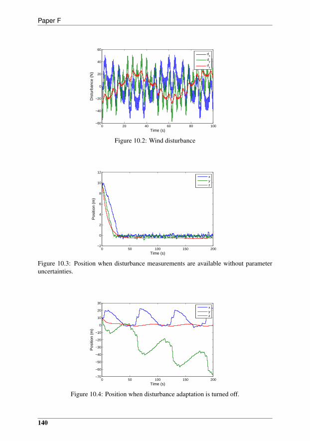
Paper F

0 20 40 60 80 100−60

−40

−20

0

20

40

60

Time (s)

Dis

turb

ance

(N

)

d

x

dy

dz

Figure 10.2: Wind disturbance

0 50 100 150 200−2

0

2

4

6

8

10

12

Time (s)

Pos

ition

(m

)

xyz

Figure 10.3: Position when disturbance measurements are available without parameteruncertainties.

0 50 100 150 200−70

−60

−50

−40

−30

−20

−10

0

10

20

30

Time (s)

Pos

ition

(m

)

xyz

Figure 10.4: Position when disturbance adaptation is turned off.

140

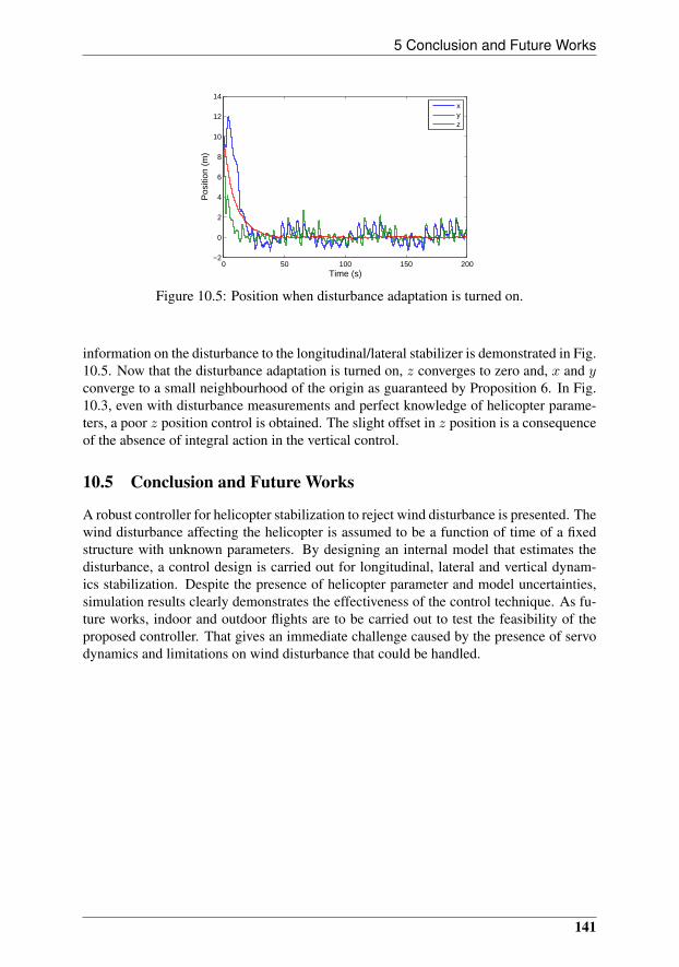
5 Conclusion and Future Works

0 50 100 150 200−2

0

2

4

6

8

10

12

14

Time (s)

Pos

ition

(m

)

xyz

Figure 10.5: Position when disturbance adaptation is turned on.

information on the disturbance to the longitudinal/lateral stabilizer is demonstrated in Fig.10.5. Now that the disturbance adaptation is turned on, z converges to zero and, x and yconverge to a small neighbourhood of the origin as guaranteed by Proposition 6. In Fig.10.3, even with disturbance measurements and perfect knowledge of helicopter parame-ters, a poor z position control is obtained. The slight offset in z position is a consequenceof the absence of integral action in the vertical control.

10.5 Conclusion and Future Works

A robust controller for helicopter stabilization to reject wind disturbance is presented. Thewind disturbance affecting the helicopter is assumed to be a function of time of a fixedstructure with unknown parameters. By designing an internal model that estimates thedisturbance, a control design is carried out for longitudinal, lateral and vertical dynam-ics stabilization. Despite the presence of helicopter parameter and model uncertainties,simulation results clearly demonstrates the effectiveness of the control technique. As fu-ture works, indoor and outdoor flights are to be carried out to test the feasibility of theproposed controller. That gives an immediate challenge caused by the presence of servodynamics and limitations on wind disturbance that could be handled.

141

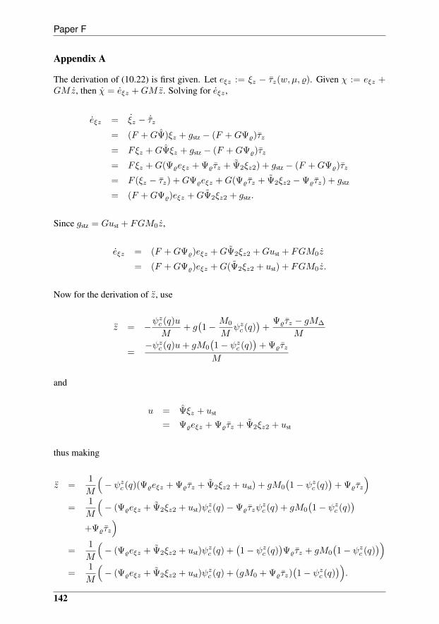
Paper F

Appendix A

The derivation of (10.22) is first given. Let eξz := ξz − τz(w, µ, %). Given χ := eξz +GMz, then χ = eξz +GMz. Solving for eξz ,

eξz = ξz − ˙τz

= (F +GΨ)ξz + gstz − (F +GΨ%)τz

= Fξz +GΨξz + gstz − (F +GΨ%)τz

= Fξz +G(Ψ%eξz + Ψ%τz + Ψ2ξz2) + gstz − (F +GΨ%)τz

= F (ξz − τz) +GΨ%eξz +G(Ψ%τz + Ψ2ξz2 −Ψ%τz) + gstz

= (F +GΨ%)eξz +GΨ2ξz2 + gstz.

Since gstz = Gust + FGM0z,

eξz = (F +GΨ%)eξz +GΨ2ξz2 +Gust + FGM0z

= (F +GΨ%)eξz +G(Ψ2ξz2 + ust) + FGM0z.

Now for the derivation of z, use

z = −ψzc (q)u

M+ g(1− M0

Mψzc (q)

)+

Ψ%τz − gM∆

M

=−ψzc (q)u+ gM0

(1− ψzc (q)

)+ Ψ%τz

M

and

u = Ψξz + ust

= Ψ%eξz + Ψ%τz + Ψ2ξz2 + ust

thus making

z =1

M

(− ψzc (q)(Ψ%eξz + Ψ%τz + Ψ2ξz2 + ust) + gM0

(1− ψzc (q)

)+ Ψ%τz

)=

1

M

(− (Ψ%eξz + Ψ2ξz2 + ust)ψ

zc (q)−Ψ%τzψ

zc (q) + gM0

(1− ψzc (q)

)+Ψ%τz

)=

1

M

(− (Ψ%eξz + Ψ2ξz2 + ust)ψ

zc (q) +

(1− ψzc (q)

)Ψ%τz + gM0

(1− ψzc (q)

))=

1

M

(− (Ψ%eξz + Ψ2ξz2 + ust)ψ

zc (q) + (gM0 + Ψ%τz)

(1− ψzc (q)

)).

142

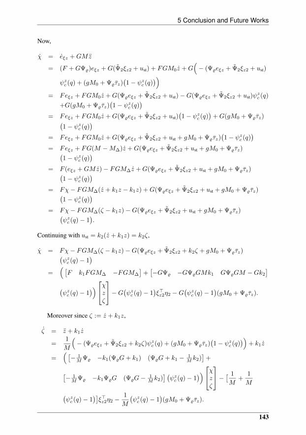
5 Conclusion and Future Works

Now,

χ = eξz +GMz

= (F +GΨ%)eξz +G(Ψ2ξz2 + ust) + FGM0z +G(− (Ψ%eξz + Ψ2ξz2 + ust)

ψzc (q) + (gM0 + Ψ%τz)(1− ψzc (q)

))= Feξz + FGM0z +G(Ψ%eξz + Ψ2ξz2 + ust)−G(Ψ%eξz + Ψ2ξz2 + ust)ψ

zc (q)

+G(gM0 + Ψ%τz)(1− ψzc (q)

)= Feξz + FGM0z +G(Ψ%eξz + Ψ2ξz2 + ust)

(1− ψzc (q)

)+G(gM0 + Ψ%τz)(

1− ψzc (q))

= Feξz + FGM0z +G(Ψ%eξz + Ψ2ξz2 + ust + gM0 + Ψ%τz)(1− ψzc (q)

)= Feξz + FG(M −M∆)z +G(Ψ%eξz + Ψ2ξz2 + ust + gM0 + Ψ%τz)(

1− ψzc (q))

= F (eξz +GMz)− FGM∆z +G(Ψ%eξz + Ψ2ξz2 + ust + gM0 + Ψ%τz)(1− ψzc (q)

)= Fχ− FGM∆(z + k1z − k1z) +G(Ψ%eξz + Ψ2ξz2 + ust + gM0 + Ψ%τz)(

1− ψzc (q))

= Fχ− FGM∆(ζ − k1z)−G(Ψ%eξz + Ψ2ξz2 + ust + gM0 + Ψ%τz)(ψzc (q)− 1

).

Continuing with ust = k2(z + k1z) = k2ζ,

χ = Fχ− FGM∆(ζ − k1z)−G(Ψ%eξz + Ψ2ξz2 + k2ζ + gM0 + Ψ%τz)(ψzc (q)− 1

)=

( [F k1FGM∆ −FGM∆

]+[−GΨ% −GΨ%GMk1 GΨ%GM −Gk2

](ψzc (q)− 1

))χzζ

−G(ψzc (q)− 1)ξ>z2η2 −G

(ψzc (q)− 1

)(gM0 + Ψ%τz).

Moreover since ζ := z + k1z,

ζ = z + k1z

=1

M

(− (Ψ%eξz + Ψ2ξz2 + k2ζ)ψzc (q) + (gM0 + Ψ%τz)

(1− ψzc (q)

))+ k1z

=( [− 1MΨ% −k1(Ψ%G+ k1) (Ψ%G+ k1 − 1

M k2)]

+

[− 1MΨ% −k1Ψ%G (Ψ%G− 1

M k2)] (ψzc (q)− 1

))χzζ

− [ 1

M+

1

M(ψzc (q)− 1

)]ξ>z2η2 −

1

M

(ψzc (q)− 1

)(gM0 + Ψ%τz).

143

Paper F

Collecting the derived equations above,χzζ

=

( F k1FGM4 −FGM∆

0 −k1 1− 1MΨ% −k1(Ψ%G+ k1) (Ψ%G+ k1 − 1

M k2)

+

−GΨ% −GΨ%GMk1 GΨ%GM −Gk2

0 0 0− 1MΨ% −k1Ψ%G (Ψ%G− 1

M k2)

(ψzc (q)− 1))χz

ζ

−(

1

M

001

+

G01M

(ψzc (q)− 1))ξ>z2η2 −

G01M

(ψzc (q)− 1)(gM0 + Ψ%τz).

Now guided by the steps taken in [6, Proof of Proposition 3.3.2], it is shown that withan appropriate selection of k2, A can be made Hurwitz. Recall that F is Hurwitz and thusthere exists a symmetric positive definite matrix Q such that

QF + F>Q = −I.

As a result, a positive definite matrix

P =

Q 0 00 a 00 0 1

can be constructed where a > 0. Next the following matrix equation is solved,

PA+A>P =

−I m1 m2

m>1 −2ak1 m3

m>2 m3 m4

,where

m1 = k1QFGM∆

m2 = −QFGM∆ −1

MΨ>%

m3 = a− k1(Ψ%G+ k1)

m4 = 2(Ψ%G+ k1 −1

Mk2).

Consider the block [−I m1

m>1 −2ak1

].

It is shown now that given any number 0 < a0 < 1, there exists a∗ such that if a ≥ a∗,[−I m1

m>1 −2ak1

]≤ −a0I.

144

5 Conclusion and Future Works

Recall that the above inequality is by definition

x>0

([−I m1

m>1 −2ak1

]+ a0I

)x0 ≤ 0,

for all non-zero vectors x0 = [x1 x2]> ∈ R2N+1 × R. Expanding,

(a0 − 1)x>1 x1 + (a0 − 2ak1)x22 + 2x2x

>1 m1 ≤ 0.

It is easy to see that there exists a number a∗, such that if a ≥ a∗ then the above inequalityholds. Fixing such an a, let us compute x>4 (PA+A>P )x4,

x>4

−I m1 m2

m>1 −2ak1 m3

m>2 m3 m4

x4 = x>0

[−I m1

m>1 −2ak1

]x0 +m4x

23 + 2x3x

>0 [m>2 m3]>,

where x4 = [x0 x3]> ∈ R2N+2 × R is a non-zero vector. Thus there exists a number k∗2such that for all k2 ≥ k∗2 ,

PA+A>P ≤ −a0I.

145

Paper F

Appendix B

In this appendix, a candidate Lyapunov function for attitude dynamical system (10.8) ischosen and shown that it can be made strictly negative with an appropriate selection ofthe design parameters. Defining ω := ω + KDq where KD := 1

KD, the chosen control

law becomes

v = KP qr −KP

KDω +

KP

KDωd.

Consider a Lyapunov function candidate

V (q0, ω) =1− q0

q0 − ε+

1

2ω>Jω

defined on (ε, 1]× R3. Thus,

V = − (1− ε)2(q0 − ε)2

KD‖q‖2 + ω>( (1− ε)

2(q0 − ε)2I − K2

DS(q)J − K2D

2q0J)q

+ω>(KDS(q)J − KP

KDL(TM ) +

KD

2q0J +

KD

2JS(q)

)ω +KP ω

>L(TM )qr

+KP

KDω>L(TM )ωd + ω>∆(TM ).

Using [6, Lemma 5.9.1], a T ∗ > 0 can be chosen such that if ψzc (q(t)) = 1 for all t ≥ T ∗,then 2l1I ≤ L(TM (t)) + LT (TM (t)), ‖L(TM (t))‖ ≤ l2 and ‖∆(TM (t))‖ ≤ δ for allt > 0. Since ‖q∗‖ ≤

√3λ3, ‖qd‖ ≤ Kdmqd and ‖ωd‖ ≤ Kdmωd

,

V ≤ −KD(1− ε)

2(q0 − ε)2‖q‖2 + (2KDc2 −

KP

KDl1)‖ω‖2 +

(a3 +

3

2K2Dc2 +KP l2(

√3λ3

+Kdmqd) + δ +KP

KDKdl2mωd

)‖ω‖,

where 0 < c1 ≤ ‖J‖ ≤ c2 and

a3 = maxq0∈S

1− ε2(q0 − ε)2

,

with the compact set S and the open setM as defined in [6, Proof of Proposition 5.7.1].To show that V can be made negative definite, it is desired to have

(2KDc2 −KP

KDl1)‖ω‖2 +

(a3 +

3

2K2Dc2 +KP l2(

√3λ3 +Kdmqd) + δ +

KP

KDKdl2mωd

)‖ω‖ ≤ −KD

1− ε4

c2‖w‖2.

Rearranging and letting

a1 = minω∈S/M

‖ω‖, a2 = maxω∈S/M

‖ω‖,

146

5 Conclusion and Future Works

we obtain

KP

KD

(l1a1 −

√3λ3KDl2 −Kd(KDmqd +mωd

)l2)

≥(a3 +

3

2K2Dc2 + δ

)+ KDc2

(9− ε4

)a2.

If λ3 ≤ λ∗3(KD), Kd ≤ K∗d(KD) and KP ≥ K∗P (KD), where

λ∗3(KD) =l1a1

4√

3KDl2, K∗d(KD) =

l1a1

4(KDmqd +mωd)l2,

K∗P (KD) =3c2a1l1

K3D +

(9− ε)a2c22a1l1

K2D +

2(a3 + δ)

a1l1KD,

then

V (q0, ω) ≤ −KD1− ε

2

( ‖q‖2

(q0 − ε)2+c22‖ω‖2

)for a fixed KD ≥ K∗D and all (q0, ω) ∈ S , where K∗D is a positive number as defined in[6, Proof of Proposition 5.7.1].

147

Paper F

Appendix C

In this part, we expand the equations of subsystem (10.36) and show that it is ISS. Butfirst, expressions for some relevant variables are derived.

The disturbance dy(wy) that affects the helicopter translational motion in y-axis isgenerated by an autonomous exosystem given by

wy = S(%)wy

dy(wy) = RS2(%)wy,(10.42)

where wy ∈ R2N . Note that N is the number of sinusoids with unknown constant fre-quencies Ωi, amplitudes Ai and phases ϕi for i = 1, . . . , N , that compose dy(wy). Sim-ilar to the approach taken in the stabilization of vertical dynamics, dy can be regarded asan output of a linear system. Defining

τy(wy) =

[0wy

],

exosystem (10.42) can be rewritten as,

∂τy∂wy

S(%)wy = Φ(%)τy(wy)

dy(wy) = Γ(%)τy(wy).

Please refer to Section 10.3 for quantities that are not defined here. Consequently, refer-ring to [6, Lemma 3.3.1], dy(wy) can be thought of as generated by

∂τy∂wy

S(%)wy = (F +GΨ%)τy(wy)

dy(wy) = Ψ%τy(wy),

where τy(wy) = T%τy(wy). Accordingly, the disturbance that affects the helicopter trans-lational motion in x-axis can be taken as

∂τx∂wx

S(%)wx = (F +GΨ%)τx(wx)

dx(wx) = Ψ%τx(wx).

Therefore, the horizontal disturbance vector dh(wx, wy) = [dy(wy) dx(wx) 0 · · · 0]>

can be given by

˙τ(wx, wy) = F τ(wx, wy) (10.43)dh(wx, wy) = P τ(wx, wy), (10.44)

where

τ(wx, wy) =

[τy(wy)τx(wx)

], F =

[F +GΨ% 0

0 F +GΨ%

]and

P =

Ψ% 00 Ψ%

0 0

.(4N+2)×(4N+2)

148

5 Conclusion and Future Works

Since dh(wx, wy) is a function of unmeasurable states wx and wy , and depends onunknown %, it has to be estimated by means of an internal model of the form

ξ = F ξ + gst (10.45)d = P ξ, (10.46)

where d is an estimate of dh(wx, wy) and

gst =

[gstygstx

]=

[k4(y + k3y)Gk4(x+ k3x)G

]= k4G(ζ2 −K1σ

′(K1

λ1ζ1)ζ1 + k3ζ1)

for arbitrary k3, k4 > 0. Also,

ξ =

[ξyξx

], where ξi =

[ξi1ξi2

]∈ R× R2N for i = x, y,

F =

[F +GΨ 0

0 F +GΨ

], P =

Ψ 0

0 Ψ0 0

,(4N+2)×(4N+2)

G =

[G 00 G

].

Note that the earlier assumption in the first part of Section 10.3 that qd is bounded impliesthat ξ is bounded too. Recall that since Ψ2 = Ψ2 −Ψ2,%,

Ψξi =[1 Ψ2 + Ψ2,%

]ξi

=( [

1 Ψ2,%

]+[0 Ψ2

] )ξi

= Ψ%ξi + Ψ2ξi2, i = x, y.

Hence,

d = Pξ + P2ξ2, (10.47)

where

ξ2 =

[ξy2

ξx2

]and P2 =

Ψ2 0

0 Ψ2

0 0

.(4N+2)×4N

Recall from the first part of Section 10.3 that the internal model in (10.18) can be de-signed to generate Ψ2 that converges to Ψ2,% in steady state. Therefore, the objective ofinternal model (10.45) is set to produce ξ that converges to τ(wx, wy)/Kd which in turnmultiplied by P , yields dh(wx, wy)/Kd in steady state. The following internal modelerror is then defined,

eξ =ξ − τ(wx, wy)/Kd

Kd, (10.48)

where

eξ =

[eξyeξx

].

149

Paper F

Further steps are taken now to obtain a practical expression of d. Continuing from (10.47)by substituting ξ with an expression derived from (10.48) where τ := τ(wx, wy),

d = P (Kdeξ +1

Kdτ) + P2ξ2. (10.49)

Next solving for eξ from (10.34),

d = KdP (Jη2 − η3

Kd) +

1

KdP τ + P2ξ2

= P Jη2 − Pη3 +1

KdP τ + P2ξ2.

Before proceeding further, an equation for ξ2 is developed. Note that

ξy2 = P4ξy,

where

P4 =

0 1 0 · · · 00 0 1 0...

. . ....0

0 0 0 · · · 0 1

.2N×(2N+1)

So,

ξ2 = P5ξ

= P5(Kdeξ + τ /Kd)

= KdP5(Jη2 − η3

Kd) +

1

KdP5τ

= P5Jη2 − P5η3 +1

KdP5τ ,

where

P5 =

[P4 00 P4

].

Back to d,

d = P Jη2 − Pη3 +1

KdP τ + P2(P5Jη2 − P5η3 +

1

KdP5τ) = G0Jη2 −G0η3 +

1

KdG0τ ,

where G0 = P + P2P5.

150

5 Conclusion and Future Works

Before the time derivatives of (10.26), (10.33) and (10.34) are computed, ˙d, qd, qd, q∗

and eξ have to be expressed in a suitable form. Starting with ˙d, from (10.49),

˙d = KdP eξ +

1

KdP ˙τ + ˙P2ξ2 + P2ξ2.

An expression for eξ is first developed. From (10.45),

ξy = (F +GΨ)ξy + gsty

= F (Kdeξy +1

Kdτy) +G(Ψ%ξy + Ψ2ξy2) + gsty

= KdFeξy +1

KdF τy +GΨ%(Kdeξy +

1

Kdτy) +GΨ2ξy2 + gsty

= Kd(F +GΨ%)eξy +1

Kd(F +GΨ%)τy +GΨ2ξy2 + gsty

and similarly,

ξx = Kd(F +GΨ%)eξx +1

Kd(F +GΨ%)τx +GΨ2ξx2 + gstx.

Thus,

ξ = KdF eξ +1

KdF τ + GP2ξ2 + gst

= KdF (Jη2 − η3

Kd) +

1

KdF τ +

GP2(P5Jη2 − P5η3 +1

KdP5τ) + gst

= G1Jη2 −G1η3 +1

KdG1τ + gst,

where G1 = F + GP2P5 and

G =

[G 0 00 G 0

].(4N+2)×(4N+2)

Rearranging and dividing by Kd,

ξ − 1KdF τ

Kd=

1

Kd

(G1Jη2 −G1η3 +

1

KdGP2P5τ + gst

).

Referring to (10.43) and (10.48),

eξ =1

Kd

(G1Jη2 −G1η3 +

1

KdGP2P5τ + gst

). (10.50)

151

Paper F

Now back to ˙d,

˙d = P (G1Jη2 −G1η3 +

1

KdGP2P5τ + gst) +

1

KdPF τ + ˙P2(P5Jη2 − P5η3 +

1

KdP5τ) + P2P5(G1Jη2 −G1η3 +

1

KdG1τ + gst)

= G2Jη2 −G2η3 +1

KdG2τ +G0gst,

where G2 = PG1 + ˙P2P5 + P2P5G1.Recall that qd = −KdD0(t)d. Hence,

qd = −KdD0(t)(G0Jη2 −G0η3 +1

KdP τ +

1

KdP2P5τ).

From (10.44),

qd = −KdD0(t)(G0Jη2 −G0η3)− D0(t)dh − D0(t)P2P5τ , (10.51)

where dh := dh(wx, wy).With D0 := D0(t), an expression for qd is developed.

qd = −Kd(˙D0d+ D0

˙d)

= −Kd˙D0(G0Jη2 −G0η3 +

1

KdG0τ)−KdD0(G2Jη2 −G2η3 +

1

KdG2τ +

G0gst)

= −KdG3Jη2 +KdG3η3 −G3τ −KdD0G0gst, (10.52)

where G3 = ˙D0G0 + D0G2.Before an equation for q∗ could be developed, an expression for ζ3 is needed. From

(10.30),

ζ3 = − 1

MDP2λ3σ(

K3

λ3ζ3) +

1

MDqd +K2P1σ

′(K2

λ2ζ2)ζ2 −

1

MDη1 +

p

M+dhM,

where D := D(t). Substituting (10.51),

ζ3 = − 1

MDP2λ3σ(

K3

λ3ζ3) +K2P1σ

′(K2

λ2ζ2)ζ2 +

p

M+dhM− 1

MLddh −

1

MDη1 −

Kd

MLdG0Jη2 +

Kd

MLdG0η3 −

1

MLdP2P5τ ,

where Ld = DD0. Note that

Ld0 =

ld 0 00 ld 00 0 M

, Ld =

[Ld0 00 0

],

152

5 Conclusion and Future Works

where

ld =gM + dz

gM + dz + yη(η, w)

and thus dh/M − Lddh/M = (I − Ld)dh/M is asymptotically vanishing since

limt→∞

Ld(t) =

[Ld1 00 0

], Ld1 =

1 0 00 1 00 0 M

.Collecting all asymptotically vanishing terms in p0 (recall that by [6, Proposition 5.4.1],limt→∞ p(t) = 0 and limt→∞ P2(t) = 0),

ζ3 = − 1

MDP2λ3σ(

K3

λ3ζ3) +K2P1σ

′(K2

λ2ζ2)ζ2 +

p0

M− 1

MDη1 −

Kd

MLdG0Jη2 +

Kd

MLdG0η3, (10.53)

where

p0 = p+ (dh − Lddh)− LdP2P5τ . (10.54)

It is known that

q∗ = −K3P2σ′(K3

λ3ζ3)ζ3.

Hence,

q∗ = −K3P2σ′(K3

λ3ζ3)(− 1

MDP2λ3σ(

K3

λ3ζ3) +K2P1σ

′(K2

λ2ζ2)ζ2 +

p0

M

)+K3

MP2σ

′(K3

λ3ζ3)Dη1 +

KdK3

MP2σ

′(K3

λ3ζ3)LdG0Jη2

−KdK3

MP2σ

′(K3

λ3ζ3)LdG0η3

= yζ0 +K3G4η1 +KdK3G5Jη2 −KdK3G5η3, (10.55)

where

yζ0 = −K3P2σ′(K3

λ3ζ3)(− 1

MDP2λ3σ(

K3

λ3ζ3) +K2P1σ

′(K2

λ2ζ2)ζ2 +

p0

M

),(10.56)

G4 =1

MP2σ

′(K3

λ3ζ3)D,

G5 =1

MP2σ

′(K3

λ3ζ3)LdG0.

Now with all the required equations in hand, η1 is computed. From (10.26) and(10.27), it is known that

η1 = q∗ + qd − q.

153

Paper F

Based on (10.8), (10.33), (10.35), (10.52) and (10.55),

˙η1 = −1

2

(q0I + S(q)

)(η2 +

1

Kdη1) +

(I − 1

2

(q0I + S(q)

)Qd

)(−KdG3Jη2 +

KdG3η3 −G3τ −KdD0G0gst) + yζ0 +K3G4η1 +KdK3G5Jη2 −KdK3G5η3

=

(− 1

2KDq0I −

1

2KDS(q) +K3G4

)η1 −

(1

2

(q0I + S(q)

)+Kd

((I − 1

2

(q0I

+S(q))Qd

)G3 −K3G5

)J

)η2 +Kd

((I − 1

2

(q0I + S(q)

)Qd

)G3

−K3G5

)η3 −Kdk4

(I − 1

2

(q0I + S(q)

)Qd

)D0G0yζ1 + yζ0 + Iη1 , (10.57)

where

Iη1 = −(I − 1

2

(q0I + S(q)

)Qd

)G3τ , (10.58)

yζ1 = G(ζ2 −K1σ′(K1

λ1ζ1)ζ1 + k3ζ1). (10.59)

Next from (10.33),

J η2 = J ˙ω − J ωd −1

KDJ ˙η1.

Solving J ˙ω first, from (10.8), (10.24), (10.25) and (10.33),

J ˙ω = −S(ω)J ω + L(−KPKDη2) + ∆

= − 1

KDS(ω)J η1 −

(S(ω)J(I −KdQdG3J) +KPKDL

)η2 −KdS(ω)JQdG3η3

+S(ω)JQdG3τ +KdS(ω)JQdD0G0gst + ∆,

where L := L(TM ) and ∆ := ∆(TM ). Thus,

J η2 =

(− 1

KDS(ω)J +

1

2K2D

J(q0I + S(q)

)− K3

KDJG4

)η1 +

(−KPKDL

−S(ω)J(I −KdQdG3J) +1

2KDJ(q0I + S(q)

)+Kd

KDJ

((I − 1

2

(q0I +

S(q))Qd

)G3 −K3G5

)J

)η2 −Kd

((S(ω)JQd +

1

KDJ(I − 1

2

(q0I

+S(q))Qd

))G3 −

K3

KDJG5

)η3 +Kdk4

(S(ω)JQd +

1

KDJ(I − 1

2

(q0I +

S(q))Qd

))D0G0yζ1 −

1

KDJyζ0 + Iη2 , (10.60)

154

5 Conclusion and Future Works

where

Iη2 =

(S(ω)JQd +

1

KDJ(I − 1

2

(q0I + S(q)

)Qd

))G3τ

+∆− J ωd. (10.61)

Finally for η3, from (10.34) and (10.50),

η3 = J η2 −Kdeξ

=

(− 1

KDS(ω)J +

1

2K2D

J(q0I + S(q)

)− K3

KDJG4

)η1 +

(−KPKDL

−S(ω)J(I −KdQdG3J) +1

2KDJ(q0I + S(q)

)+Kd

KDJ

((I − 1

2

(q0I +

S(q))Qd

)G3 −K3G5

)J

)J−1(η3 +Kdeξ)−Kd

((S(ω)JQd +

1

KDJ(I −

1

2

(q0I + S(q)

)Qd

))G3 −

K3

KDJG5

)η3 +Kdk4

(S(ω)JQd +

1

KDJ(I −

1

2

(q0I + S(q)

)Qd

))D0G0yζ1 −

1

KDJyζ0 +

(S(ω)JQd +

1

KDJ(I − 1

2

(q0I

+S(q))Qd

))G3τ + ∆− J ωd −

(G1J J

−1(η3 +Kdeξ)−G1η3 +1

KdGP2P5τ

+gst)

=

(− 1

KDS(ω)J +

1

2K2D

J(q0I + S(q))− K3

KDJG4

)η1 +

(−KPKDLJ

−1 −

S(ω)J(I −KdQdG3J)J−1 +1

2KDJ(q0I + S(q))J−1 +

Kd

KDJ(I − 1

2(q0I +

S(q))Qd)G3 −Kd

(S(ω)JQd +

1

KDJ(I − 1

2(q0I + S(q))Qd

))G3

)η3 +

k4

(Kd

(S(ω)JQd +

1

KDJ(I − 1

2

(q0I + S(q)

)Qd

))D0G0 − I

)yζ1 −

1

KDJyζ0 + Iη3 , (10.62)

where

Iη3 =

((S(ω)JQd +

1

KDJ(I − 1

2

(q0I + S(q)

)Qd

))G3 −

1

KdGP2P5

)τ + ∆−

J ωd +Kd

((−KPKDL− S(ω)J(I −KdQdG3J) +

1

2KDJ(q0I + S(q)

)+Kd

KDJ(I − 1

2

(q0I + S(q)

)Qd

)G3J

)−G1J −

KdK3

KDJG5J

)J−1eξ.(10.63)

155

Paper F

Now we are ready for the proof of Lemma 3. Define a candidate ISS-Lyapunov func-tion for (10.36)

V (η1, η2, η3) = V1(η1) + V2(η2) + V3(η3)

= η>1 η1 +1

2η>2 Jη2 +

1

2η>3 η3. (10.64)

Taking the derivatives along the solutions of subsystem (10.36),

V1 = 2η>1 ˙η1

<(− 1

KDε+

1

KD(√

3λ3 +Kdmqd) + 2K3m4

)‖η1‖2 + 2

(1 +Kdc3

(m3(1 +

mQd) +K3m5

))‖η1‖ ‖η2‖+ 2Kd

(m3(1 +mQd

) +K3m5

)‖η1‖ ‖η3‖

+2Kdk4mD0m0(1 +mQd

)‖η1‖ ‖yζ1‖+ 2‖η1‖ ‖yζ0‖+ 2‖η1‖ ‖Iη1‖,

V2 = η>2 J η2

≤ 1

KDc3(mω +

1

KD+K3m4

)‖η1‖ ‖η2‖+

(−KPKDl3 +mωc3(1 +

KdmQdm3c3) +

1

KDc3 +

Kd

KDc23(m3(1 +mQd

) +K3m5

))‖η2‖2 +Kd(

m3

(mωc3mQd

+1

KDc3(1 +mQd

))

+K3

KDc3m5

)‖η2‖ ‖η3‖+

Kdk4mD0m0

(mωc3mQd

+1

KDc3(1 +mQd

))‖η2‖ ‖yζ1‖+

1

KDc3‖η2‖ ‖yζ0‖

+‖η2‖ ‖Iη2‖V3 = η>3 η3

≤ 1

KDc3(mω +

1

KD+K3m4

)‖η1‖ ‖η3‖+

(−KPKDl4 + c3m6

(mω +

1

KD

)+

2Kd

KDc3m3(1 +mQd

) +Kdc3m3mωmQd(1 + c3m6)

)‖η3‖2 +

k4

(KdmD0

m0

(mωc3mQd

+1

KDc3(1 +mQd

))

+ 1

)‖η3‖ ‖yζ1‖+

1

KDc3‖η3‖ ‖yζ0‖+ ‖η3‖ ‖Iη3‖,

where ‖J‖ ≤ c3, ‖q0I + S(q)‖ ≤ 2, ‖S(q)‖ = ‖S(q∗ + qd − η1)‖ ≤ ‖S(q∗)‖ +‖S(qd)‖+ ‖S(η1)‖ and η>1 S(η1) = 0. Besides, ‖G0‖ ≤ m0, ‖G1‖ ≤ m1, ‖G3‖ ≤ m3,‖G4‖ ≤ m4, ‖G5‖ ≤ m5, ‖Qd‖ ≤ mQd

, ‖D0‖ ≤ mD0, ‖ω‖ ≤ mω , ‖J−1‖ ≤ m6,

L ≥ l3 and LJ−1 ≥ l4 and for fixed positive numbers c3, m0, m1, m3, m4, m5, m6,mQd

, mD0and mω . Therefore,

V < `1‖η1‖2 + `2‖η2‖2 + `3‖η3‖2 + `4‖η1‖ ‖η2‖+ `5‖η1‖ ‖η3‖+ `6‖η2‖ ‖η3‖+

`7‖η1‖ ‖yζ1‖+ `8‖η2‖ ‖yζ1‖+ `9‖η3‖ ‖yζ1‖+ 2‖η1‖ ‖yζ0‖+1

KDc3‖η2‖ ‖yζ0‖

+1

KDc3‖η3‖ ‖yζ0‖+ 2‖η1‖ ‖Iη1‖+ ‖η2‖ ‖Iη2‖+ ‖η3‖ ‖Iη3‖,

156

5 Conclusion and Future Works

where

`1 = − 1

KDε+

1

KD(√

3λ3 +Kdmqd) + 2K3m4

`2 = −KPKDl3 +mωc3(1 +KdmQdm3c3) +

1

KDc3 +

Kd

KDc23(m3(1 +mQd

) +

K3m5

)`3 = −KPKDl4 + c3m6

(mω +

1

KD

)+ 2

Kd

KDc3m3(1 +mQd

) +

Kdc3m3mωmQd(1 + c3m6)

`4 = 2(

1 +Kdc3(m3(1 +mQd

) +K3m5

))+

1

KDc3(mω +

1

KD+K3m4

)`5 = 2Kd

(m3(1 +mQd

) +K3m5

)+

1

KDc3(mω +

1

KD+K3m4

)`6 = Kd

(m3

(mωc3mQd

+1

KDc3(1 +mQd

))

+K3

KDc3m5

)`7 = 2Kdk4mD0

m0(1 +mQd)

`8 = Kdk4mD0m0

(mωc3mQd

+1

KDc3(1 +mQd

))

`9 = k4

(KdmD0

m0

(mωc3mQd

+1

KDc3(1 +mQd

))

+ 1

).

157

Paper F

From Young’s inequalities,

‖η1‖ ‖η2‖ ≤δ02‖η1‖2 +

1

2δ0‖η2‖2

‖η1‖ ‖η3‖ ≤δ02‖η1‖2 +

1

2δ0‖η3‖2

‖η1‖ ‖yζ0‖ ≤δ02‖η1‖2 +

1

2δ0‖yζ0‖2

‖η1‖ ‖yζ1‖ ≤δ02‖η1‖2 +

1

2δ0‖yζ1‖2

‖η1‖ ‖Iη1‖ ≤δ02‖η1‖2 +

1

2δ0‖Iη1‖2

‖η2‖ ‖η3‖ ≤δ12‖η2‖2 +

1

2δ1‖η3‖2

‖η2‖ ‖yζ0‖ ≤δ12‖η2‖2 +

1

2δ1‖yζ0‖2

‖η2‖ ‖yζ1‖ ≤δ12‖η2‖2 +

1

2δ1‖yζ1‖2

‖η2‖ ‖Iη2‖ ≤δ12‖η2‖2 +

1

2δ1‖Iη2‖2

‖η3‖ ‖yζ0‖ ≤δ22‖η3‖2 +

1

2δ2‖yζ0‖2

‖η3‖ ‖yζ1‖ ≤δ22‖η3‖2 +

1

2δ2‖yζ1‖2

‖η3‖ ‖Iη3‖ ≤δ22‖η3‖2 +

1

2δ2‖Iη3‖2,

for arbitrary δ0 > 0, δ1 > 0 and δ2 > 0. Consequently,

V <(`1 +

δ02

(`4 + `5 + `7 + 4

))‖η1‖2 +

(`2 +

`42δ0

+δ12

(`6 + `8 +

1

KDc3 +

1))‖η2‖2 +

(`3 +

1

2

( `5δ0

+`6δ1

)+δ22

(`9 +

1

KDc3 + 1

))‖η3‖2

+( 1

δ0+

1

2KDc3( 1

δ1+

1

δ2

))‖yζ0‖2 +

1

2

( `7δ0

+`8δ1

+`9δ2

)‖yζ1‖2 +

1

δ0‖Iη1‖2

+1

2δ1‖Iη2‖2 +

1

2δ2‖Iη3‖2.

Firstly set

λ∗3 =ε

5√

3,

K∗d =ε

5mqd

,

K∗3 (KD) =ε

10KDm4,

δ0 =2ε

5KD(`4 + `5 + `7 + 4),

158

5 Conclusion and Future Works

and thus for all Kd ≤ K∗d , K3 ≤ K∗3 (KD) and all λ3 ≤ λ∗3,

`1 +δ02

(`4 + `5 + `7 + 4

)≤ − ε

5KD.

Next define

`∗2(KP ,KD) = −KPKDl3 +mωc3(1 + K∗dmQdm3c3) +

1

KDc3 +

K∗dKD

c23(m3(1 +

mQd) + K∗3 (KD)m5

),

`∗4(KD) = 2(

1 + K∗dc3(m3(1 +mQd

) + K∗3m5

))+

1

KDc3(mω +

1

KD+

K∗3m4

),

`∗5(KD) = 2K∗d(m3(1 +mQd

) + K∗3m5

)+

1

KDc3(mω +

1

KD+ K∗3m4

),

`∗7 = 2K∗dk4mD0m0(1 +mQd

),

δ∗0(KD) =2ε

5KD

(`∗4(KD) + `∗5(KD) + `∗7 + 4

) ,and hence for all Kd ≤ K∗d1 and all K3 ≤ K∗3 (KD),

`2 +`42δ0≤ `∗2(KP ,KD) +

`∗4(KD)

2δ∗0(KD).

By fixing

δ1 =KPKDl3

`6 + `8 + 1KD

c3 + 1,

it is easy to see that there exists a number K∗P1 > 0 such that for all KP ≥ K∗P1

KD,

`∗2(KP ,KD) +`∗4(KD)

2δ∗0(KD)+

1

2KPKDl3 ≤ −

ε

5KD.

Hence for all Kd ≤ K∗d and all K3 ≤ K∗3 (KD) and KP ≥ K∗P1

KD,

`2 +`42δ0

+δ12

(`6 + `8 +

c2KD

+ 1)≤ − ε

5KD.

Now let

`∗3(KP ,KD) = −KPKDl4 + c3m6

(mω +

1

KD

)+ 2

K∗dKD

c3m3(1 +mQd) +

K∗dc3m3mωmQd(1 + c3m6),

`∗6(KD) = K∗d

(m3

(mωc3mQd

+1

KDc3(1 +mQd

))

+K∗3KD

c3m5

),

`∗8(KD) = K∗dk4mD0m0

(mωc3mQd

+1

KDc3(1 +mQd

)),

δ∗1(KP ,KD) =KPKDl3

`∗6(KD) + `∗8(KD) + 1KD

c3 + 1.

159

Paper F

Note that for all Kd ≤ K∗d and all K3 ≤ K∗3 (KD),

`3 +1

2

( `5δ0

+`6δ1

)≤ `∗3(KP ,KD) +

1

2

( `∗5(KD)

δ∗0(KD)+

`∗6(KD)

δ∗1(KP ,KD)

),

and by choosing

δ2 =KPKDl4

`9 + 1KD

c3 + 1,

there exists a number K∗P2 > 0 such that for all KP ≥ K∗P2

KD, Kd ≤ K∗d and all K3 ≤

K∗3 (KD),

`3 +1

2

( `5δ0

+`6δ1

)+δ22

(`9 +

1

KDc3 + 1

)≤ − ε

5KD.

As a result, for any given KD, for all Kd ≤ K∗d , K3 ≤ K∗3 (KD), λ3 ≤ λ∗3 and allKP ≥ K∗P 1

KD,

V < − ε

5KD(‖η1‖2 + ‖η2‖2 + ‖η3‖2) +

( 1

δ∗0(KD)+

1

2KDc3( 1

δ∗1(KD)+

1

δ∗2(KP ,KD)

))‖yζ0‖2 +

1

2

( `∗7δ∗0(KD)

+`∗8(KD)

δ∗1(KD)+

`∗9(KD)

δ∗2(KP ,KD)

)‖yζ1‖2 +

1

δ∗0(KD)‖Iη1‖2 +

1

2δ∗1(KP ,KD)‖Iη2‖2 +

1

2δ∗2(KP ,KD)‖Iη3‖2,

where K∗P (KD) = 1KD

maxK∗P1, K∗P2,

`∗9(KD) = k4

(K∗dmD0

m0

(mωc3mQd

+1

KDc3(1 +mQd

))

+ 1

),

δ∗2(KP ,KD) =KPKDl4

`∗9(KD) + 1KD

c3 + 1.

The above inequality confirms that (10.64) is an ISS-Lyapunov function (see [5, Lemma10.4.2]) for subsystem (10.36). Accordingly, subsystem (10.36) is ISS and conforms withLemma 3 [5, Theorem 10.4.1].

160

5 Conclusion and Future Works

Appendix D

Here, given

ζ ′3 =

[yx

]+

[1 00 1

]λ2σ(

K2

λ2ζ2)

and

M

[yx

]=

[d mq3

mq3 −d

] [q1

q2

]+ p′ + d′h,

where d := d(q, t), m := m(q, t), p′ = [py px]> and d′h = [dy dx]>, ζ ′3 is derived.Taking the time derivative,

ζ ′3 =

[yx

]+

[1 00 1

]K2σ

′(K2

λ2ζ2)ζ2

= T1 +1

Mp′ +

1

Md′h +K2σ

′(K2

λ2ζ2)ζ2,

where

T1 =1

M

[d mq3

mq3 −d

] [q1

q2

].

Next,

T1 = − 1

M

[d mq3

mq3 −d

](q′r − q′ − q′r)

= T2 + T3,

where q′ = [q1 q2]>, q′r = [qr1 qr2]>,

T2 = − 1

M

[d mq3

mq3 −d

](q′r − q′) and

T3 =1

M

[d mq3

mq3 −d

]q′r.

Recall that from (10.27) and (10.29),

qr =

qr1qr2qr3

=

−λ3σ(K3

λ3ζ ′31) + qd1

λ3σ(K3

λ3ζ ′32) + qd2

−λ3σ(K3

λ3ζ ′′3 ),

161

Paper F

since qd = [qd1 qd2 0]>. Expanding T3,

T3 =1

M

[d mq3

mq3 −d

][−λ3σ(K3

λ3ζ ′31) + qd1

λ3σ(K3

λ3ζ ′32) + qd2

]

= −L(t)

[λ3σ(K3

λ3ζ ′31)

λ3σ(K3

λ3ζ ′32)

]+

1

M

[mq3λ3σ(K3

λ3ζ ′32)

−mq3λ3σ(K3

λ3ζ ′31)

]

− 1

MKd

[d mq3

mq3 −d

] [d0 m0q3

m0q3 −d0

]d′

= −L(t)

[λ3σ(K3

λ3ζ ′31)

λ3σ(K3

λ3ζ ′32)

]+

1

M

[mq3λ3σ(K3

λ3ζ ′32)

−mq3λ3σ(K3

λ3ζ ′31)

]− 1

MKdL

′dd′,

where d′ = [dy dx]>,

L(t) =1

M

[d 0

0 d

]and L′d =

[ld 00 ld

].

Continuing with T2,

T2 = − 1

M

[d mq3

mq3 −d

] [−λ3σ(K3

λ3ζ ′31) + qd1 − q1

λ3σ(K3

λ3ζ ′32) + qd2 − q2

]

= − 1

M

[d mq3

mq3 −d

] [−λ3σ(K3

λ3ζ ′31) + qd1 − q1

λ3σ(K3

λ3ζ ′32) + qd2 − q2

]

− 1

M

[ (mλ3σ(K3

λ3ζ ′32)

)(− λ3σ(K3

λ3ζ ′′3 )− q3

)(−mλ3σ(K3

λ3ζ ′31)

)(− λ3σ(K3

λ3ζ ′′3 )− q3

)]

+1

M

[ (mλ3σ(K3

λ3ζ ′32)

)(− λ3σ(K3

λ3ζ ′′3 )− q3

)(−mλ3σ(K3

λ3ζ ′31)

)(− λ3σ(K3

λ3ζ ′′3 )− q3

)]

= − 1

MR(t)

−λ3σ(K3

λ3ζ ′31) + qd1 − q1

λ3σ(K3

λ3ζ ′32) + qd2 − q2

−λ3σ(K3

λ3ζ ′′3 )− q3

+

1

M

[ (mλ3σ(K3

λ3ζ ′32)

)(− λ3σ(K3

λ3ζ ′′3 )− q3

)(−mλ3σ(K3

λ3ζ ′31)

)(− λ3σ(K3

λ3ζ ′′3 )− q3

)]

= − 1

MR(t)(qr − q) +

1

M

[ (mλ3σ(K3

λ3ζ ′32)

)(− λ3σ(K3

λ3ζ ′′3 ))(

−mλ3σ(K3

λ3ζ ′31)

)(− λ3σ(K3

λ3ζ ′′3 ))]

+1

M

[−mq3λ3σ(K3

λ3ζ ′32)

mq3λ3σ(K3

λ3ζ ′31)

]

= − 1

MR(t)(qr − q) +

1

ME(t)λ3σ(

K3

λ3ζ ′′3 ) +

1

M

[−mq3λ3σ(K3

λ3ζ ′32)

mq3λ3σ(K3

λ3ζ ′31)

],

162

5 Conclusion and Future Works

where

R(t) =

[d mq3 mλ3σ(K3

λ3ζ ′32)

mq3 −d −mλ3σ(K3

λ3ζ ′31)

]and

E(t) = λ3

[−σ(K3

λ3ζ ′32)

σ(K3

λ3ζ ′31)

]m.

Now back to T1,

T1 = T2 + T3

= − 1

MR(t)(qr − q) +

1

ME(t)λ3σ(

K3

λ3ζ ′′3 )− L(t)λ3σ(

K3

λ3ζ ′3)− 1

MKdL

′dd′,

and hence

ζ ′3 = −L(t)λ3σ(K3

λ3ζ ′3) +K2σ

′(K2

λ2ζ2)ζ2 +

1

Mp′ − 1

MR(t)η1 +

1

ME(t)λ3σ(

K3

λ3ζ ′′3 )

− 1

MKdL

′dd′ +

1

Md′h.

From (10.44) and (10.50),

d′ = G′0P3Jη2 −G′0η3 +1

KdG′0τ

= G′0P3Jη2 −G′0η3 +1

Kdd′h +

1

KdP ′2P5τ ,

where G′0 = P ′ + P ′2P5,

P ′ =

[Ψ% 00 Ψ%

]and P ′2 =

[Ψ2 0

0 Ψ2

].

Thus,

ζ ′3 = −L(t)λ3σ(K3

λ3ζ ′3) +K2σ

′(K2

λ2ζ2)ζ2 +

1

Mp′ − 1

MR(t)η1 +

1

ME(t)λ3σ(

K3

λ3ζ ′′3 )

− 1

MKdL

′d

(G′0P3Jη2 −G′0η3 +

1

Kdd′h +

1

KdP ′2P5τ

)+

1

Md′h

= −L(t)λ3σ(K3

λ3ζ ′3) +K2σ

′(K2

λ2ζ2)ζ2 +W,

where

W =1

Mp′ − 1

MR(t)η1 −

1

MKdL

′d

(G′0P3Jη2 −G′0η3

)+

1

ME(t)λ3σ(

K3

λ3ζ ′′3 ) +

1

M(I − L′d)d′h −

1

ML′dP

′2P5τ . (10.65)

163

References

[1] X. Yang, H. Pota, and M. Garratt, “Design of a Gust-Attenuation Controller forLanding Operations of Unmanned Autonomous Helicopters,” in 18th IEEE Interna-tional Conference on Control Applications, July 2009.

[2] F. N. Koumboulis, M. G. Skarpetis, and M. K. Griparis, “Rotary gust rejection forhelicopters,” in In Proceedings of the IEEE International Conference on ControlApplications, 1998, pp. 103–107.

[3] H. Wang, A. A. Mian, D. Wang, and H. Duan, “Robust multi-mode flight controldesign for an unmanned helicopter based on multi-loop structure,” InternationalJournal of Control, Automation, and Systems, vol. 7, pp. 723–730, 2009.

[4] A. Isidori, Nonlinear control systems, 3rd ed., ser. Communications and ControlEngineering Series. Berlin: Springer-Verlag, 1995.

[5] ——, Nonlinear control systems. II, ser. Communications and Control EngineeringSeries. London: Springer-Verlag London Ltd., 1999.

[6] A. Isidori, L. Marconi, and A. Serrani, Robust autonomous guidance: An inter-nal model approach, ser. Advances in Industrial Control. Secaucus, NJ, USA:Springer-Verlag New York, Inc., 2003.

[7] ——, “Robust nonlinear motion control of a helicopter,” IEEE Trans.Automat. Control, vol. 48, no. 3, pp. 413–426, 2003. [Online]. Available:http://dx.doi.org/10.1109/TAC.2003.809147

[8] T. J. Koo and S. Sastry, “Output tracking control design of a helicopter model,” in InProceedings of the 37th Conference on Decision and Control, 1998, pp. 3635–3640.

[9] T. Meurer, K. Graichen, and E.-D. Gilles, Control and observer design for nonlinearfinite and infinite dimensional systems. Birkhauser, 2005.

[10] P. Ioannou, “Robust direct adaptive control,” in Decision and Control, 1984. The23rd IEEE Conference on, vol. 23, dec. 1984, pp. 1015 –1020.

[11] A. R. Teel, “A nonlinear small gain theorem for the analysis of control systemswith saturation,” IEEE Trans. Automat. Control, vol. 41, no. 9, pp. 1256–1270,1996. [Online]. Available: http://dx.doi.org/10.1109/9.536496

[12] O. Shakernia, Y. Ma, T. J. Koo, T. John, and S. Sastry, “Landing an unmanned airvehicle: Vision based motion estimation and nonlinear control,” Asian Journal ofControl, vol. 1, pp. 128–145, 1999.

165