Aalborg Universitet Efficient Water Supply in HVAC Systems...
156
Aalborg Universitet Efficient Water Supply in HVAC Systems Komareji, Mohammad Publication date: 2009 Document Version Publisher's PDF, also known as Version of record Link to publication from Aalborg University Citation for published version (APA): Komareji, M. (2009). Efficient Water Supply in HVAC Systems. Aalborg: Section of Automation & Control, Department of Electronic Systems, Aalborg University. General rights Copyright and moral rights for the publications made accessible in the public portal are retained by the authors and/or other copyright owners and it is a condition of accessing publications that users recognise and abide by the legal requirements associated with these rights. ? Users may download and print one copy of any publication from the public portal for the purpose of private study or research. ? You may not further distribute the material or use it for any profit-making activity or commercial gain ? You may freely distribute the URL identifying the publication in the public portal ? Take down policy If you believe that this document breaches copyright please contact us at [email protected] providing details, and we will remove access to the work immediately and investigate your claim. Downloaded from vbn.aau.dk on: august 09, 2018
Transcript of Aalborg Universitet Efficient Water Supply in HVAC Systems...

Aalborg Universitet
Efficient Water Supply in HVAC Systems
Komareji, Mohammad
Publication date:2009
Document VersionPublisher's PDF, also known as Version of record
Link to publication from Aalborg University
Citation for published version (APA):Komareji, M. (2009). Efficient Water Supply in HVAC Systems. Aalborg: Section of Automation & Control,Department of Electronic Systems, Aalborg University.
General rightsCopyright and moral rights for the publications made accessible in the public portal are retained by the authors and/or other copyright ownersand it is a condition of accessing publications that users recognise and abide by the legal requirements associated with these rights.
? Users may download and print one copy of any publication from the public portal for the purpose of private study or research. ? You may not further distribute the material or use it for any profit-making activity or commercial gain ? You may freely distribute the URL identifying the publication in the public portal ?
Take down policyIf you believe that this document breaches copyright please contact us at [email protected] providing details, and we will remove access tothe work immediately and investigate your claim.
Downloaded from vbn.aau.dk on: august 09, 2018

Efficient Water Supply in HVAC Systems
Mohammad Komareji
Ph.D. Thesis
Section of Automation & Control
Department of Electronic Systems
Aalborg University
9220 Aalborg
DENMARK

ii

Efficient Water Supply in HVAC Systems
Ph.D. thesis
ISBN 978-87-92328-07-6
September 2008
i

ii
Preface
This thesis is submitted in partial fulfilment of the requirements for the PhD degreeat Section of Au-
tomation & Control, Department of Electronic Systems, Aalborg University, Denmark. The work has
been carried out in the period of three years, from September 2005 to September 2008, under supervision
of Professor Jakob Stoustrup and Associate Professor Henrik Rasmussen.
The project was jointly sponsored by Danish Energy Net, Center for Embedded Software Systems,
and The Faculty of Engineering and Science at Aalborg University. It was carried out as a cooperation
between Aalborg University, Grundfos A/S, Exhausto A/S, and Danish Technological Institute.
iii


Acknowledgements
I would like to express my gratitude to all people who gave me a very enjoyable timeat Aalborg Univer-
sity and created a comfortable working environment in Section of Automation and Control, Department
of Electronic Systems.
A very special thanks goes to my great academic advisors: Professor Jakob Stoustrup, an outstand-
ing professor in mathematics and control theory, and Associate Professor Henrik Rasmussen, who has
lifetime experience in control theory and its applications, from whose profound knowledge and inspira-
tion I benefited a lot during this project.
Particular thanks to Dr. Niels Bidstrup, chief engineer in Grundfos A/S, and Finn Nielsen, project
manager in Exhausto A/S, for their invaluable guidance that this project required.
Thanks also to Peter Svendsen, project manager in Danish Technological Institute, for his coopera-
tion and patience in setting-up the HVAC system in the lab and runnig several experiments afterwards.
I am grateful to the Center for Embedded Software Systems (CISS) headed by Professor Kim Guld-
strand Larsen for partial financial support of this project.
I would like to thank Professor William Bahnfleth for giving me the opportunity tostay at the
Pennsyvania State University and valuable helps while I was there.
I am deeply indebted to my parents, Akbar and Maryam, for their prayers and encouragements made
this accomplishment possible.
September 2008, Aalborg, Denmark
Mohammad Komareji
v

Abstract
Increased energy costs have brought about increased concern by building owners about the operating
cost and energy budgets for buildings. This growing energy conservation consciousness has brought
about many changes in the attention focused on the energy performance of buildings, particularly that of
heating, ventilating, and airconditioning systems - hereafter abbreviated HVAC systems. Various types
of heating, ventilating, and air-conditioning (HVAC) applications are: apartment buildings, banks, office
buildings, hospitals, industrial plants, schools, restaurants, departmentstores, hotels, etc.
This project aims at optimal model-based control of a typical industrial HVACsystem consisting of
a heat rocovery wheel and a water-to-air heat exchanger. In the current HVAC system a certain amount
of water circulates through the coil and the temperature of the inlet air is controlled by the amount of
hot water injected to the hydronic circuit where the coil is installed. However, in the new HVAC system
the water flow through the coil is manipulated as a control variable too. Thus,it will result in less
energy consumption by the pump which supplies the coil as the pump speed will decrease at part load
conditions.
HVAC systems are in steady state conditions more than 95% of their operating time.To that end,
to derive optimality criteria a static model for the HVAC system is supposed. Theobjective function
is composed of the electrical power for different components, encompassing fans, primary/secondary
pump, tertiary pump, and air-to-air heat exchanger wheel; and a fractionof thermal power used by
the HVAC system. The goals that have to be achieved by the HVAC system appear as constraints in
the optimization problem. Solving the defined problem results in two optimality criteria:1- maximum
exploitation of the heat recovery wheel. 2- equality of the supply hot waterflow and the water flow
going through the coil.
Then the optimal model-based controller (Here Model Predictive Control ’MPC’ is applied) is de-
signed to follow the goals of the HVAC system (comfort conditions) while the optimality criteria are met.
The HVAC system is splitted into two independent subsystems (the heat recovery wheel and the water-
to-air heat exchanger) through an internal feedback. By selecting theright set-points and appropriate
cost functions for each subsystem’s controller the optimal control strategy is respected to gaurantee the
minimum thermal and electrical energy consumption. Then, the optimal control strategy which was de-
vii

viii Abstract
veloped is adopted for implemenation in a real life HVAC system. The bypass flow problem is addressed
and a controller is introdeuced to deal with this problem.
Finally, a simplified control structure is proposed for optimal control of the HVAC system. The pro-
posed simple control algorithm can be implemented through two propotional-integral (PI) controllers.
All models and control algorithms which are developed throughout this thesishave been verified exper-
imentally.
Resume
Øgede udgifter til energi har medført øget bekymring ved at bygge ejere om driftsomkostninger og
energi budgetter for bygninger. Denne voksende energibesparelser bevidsthed har medført mange æn-
dringer i den opmærksomhed koncentreret om bygningers energimæssige ydeevne, især, at af varme,
ventilation og aircondition systemer - herefter forkortet HVAC-systemer. Forskellige former for op-
varmning, ventilation og aircondition (HVAC) ansøgninger er: boligkomplekser, banker, kontorbygninger,
sygehuse, fabrikker, skoler, restauranter, varehuse, hoteller osv.
Dette projekt sigter pa optimal model-baseret kontrol af en typisk industrielle HVAC system bestar
af en varme rocovery hjul og en vand-til-luft-varmeveksler. I den nuværende HVAC system en vis
mængde vand cirkulerer gennem spolen og temperaturen af den luft er kontrolleret af den mængde
varmt vand injiceret til hydronic kredsløb, hvor bredband er installeret. Men i den nye HVAC system
vandet løber gennem spolen er manipuleret som en kontrol variable ogsa. Saledes vil det resultere i
lavere energiforbrug ved pumpen, der forsyner tændspole som pumpens hastighed vil falde pa en del
belastningsforhold.
HVAC-systemer er i steady state betingelser mere end 95% af deres driftstid. Til dette formal, at
fa optimal udnyttelse kriterier en statisk model for HVAC system er meningen. Formalet funktion er
sammensat af den elektriske strøm til forskellige komponenter, der omfatter fans, primære/sekundære
pumpe, tertiær pumpe, og luft-til-luft varmeveksler hjulet, og en brøkdel af termiske kraftværker anven-
des af HVAC system. De mal, der skal opfyldes af HVAC system vises som begrænsninger i optimering
problem. Løse defineret problem resulterer i to optimal udnyttelse kriterier: 1 - maksimal udnyttelse af
varmegenvinding hjulet. 2 - lige levering varmt vand, strøm og vand flow igennem spolen.
Sa den optimale model-baseret controller (Her Model Predictive Control ’MPC’ er anvendt) er
designet til at følge malene i HVAC system (komfort betingelser), mens optimal udnyttelse kriterierer
opfyldt. Den HVAC system er delt i to uafhængige delsystemer (de varmegenvinding hjulet og vand-
til-luft-varmeveksler) gennem en indre feedback. Ved at vælge den rigtige set-punkter og relevante
omkostninger funktioner for hvert delsystem’s controller den optimale strategi for kontrol er overholdt
for at sikre et mindstemal af termisk og elektrisk energi forbrug. Derefter skal den optimale kontrol
strategi, der blev udviklet er vedtaget for implemenation i det virkelige liv HVAC system. Shunt flow
ix

x Resume
problem er rettet og en controller er introdeuced at handtere dette problem.
Endelig er en forenklet kontrol struktur er foreslaet for optimal kontrol med HVAC system. Den
foreslaede enkle kontrol algoritme kan gennemføres ved hjælp af to propotional-integrerende (PI) con-
trollere. Alle modeller og kontrol algoritmer, som er udviklet i hele denne afhandling er blevet bekræftet
eksperimentelt.
List of Figures
1.1 The HVAC system . . . . . . . . . . . . . . . . . . . . . . . . . . . . . . . . . . . . .7
1.2 Primary-only hydronic circuit . . . . . . . . . . . . . . . . . . . . . . . . . . . .. . . . 8
1.3 Primary-secondary hydronic circuit . . . . . . . . . . . . . . . . . . . . . .. . . . . . 10
1.4 Primary-secondary-tertiary hydronic circuit . . . . . . . . . . . . . . . .. . . . . . . . 11
2.1 The air-to-air heat exchanger scheme . . . . . . . . . . . . . . . . . . . . .. . . . . . . 24
2.2 Dependency ofηt2 onqa while n=10 rpm;qsa andqr
a represent supply air flow and return
air flow, respectively. . . . . . . . . . . . . . . . . . . . . . . . . . . . . . . . . . .. . 24
2.3 Normalized dependency ofηt2 on n . . . . . . . . . . . . . . . . . . . . . . . . . . . . 25
2.4 The water-to-air heat exchanger scheme . . . . . . . . . . . . . . . . . . .. . . . . . . 25
2.5 Result of experiments on water-to-air heat exchanger . . . . . . . . . .. . . . . . . . . 26
2.6 Counter flow energy wheel . . . . . . . . . . . . . . . . . . . . . . . . . . . . .. . . . 28
2.7 Coil model verification, blue curve: real output, green curve: simulatedoutput . . . . . . 29
2.8 Tertiary pump power vsqwt . . . . . . . . . . . . . . . . . . . . . . . . . . . . . . . . . 31
2.9 Primary pressure drop vsqws . . . . . . . . . . . . . . . . . . . . . . . . . . . . . . . . 32
2.10 Fan power vs air flow (qa) . . . . . . . . . . . . . . . . . . . . . . . . . . . . . . . . . 32
2.11 Wheel power consumption vsn . . . . . . . . . . . . . . . . . . . . . . . . . . . . . . . 33
2.12 Feasible region whileqws≤ qwt ( TE21= −12,T pin= 80 andqa = 2104.9 ) . . . . . . 36
2.13 Feasible region whileqws≥ qwt ( TE21= −30,T pin= 60 andqa = 1674.1 ) . . . . . . 37
2.14 New control system . . . . . . . . . . . . . . . . . . . . . . . . . . . . . . . . . .. . . 39
2.15 Typical industrial HVAC control system . . . . . . . . . . . . . . . . . . . .. . . . . . 39
2.16 Wheel speed vs. voltage . . . . . . . . . . . . . . . . . . . . . . . . . . . . . .. . . . 40
2.17 Four temperatures around the bypass pipe . . . . . . . . . . . . . . . . . .. . . . . . . 44
2.18 MPC controller along with bypass compensator . . . . . . . . . . . . . . . . .. . . . . 47
2.19 Simplified optimal control scheme . . . . . . . . . . . . . . . . . . . . . . . . . . . .. 48
2.20 Return primary water temperature . . . . . . . . . . . . . . . . . . . . . . . . . .. . . 48
xi
xii LIST OF FIGURES
2.21 Optimal trajectory . . . . . . . . . . . . . . . . . . . . . . . . . . . . . . . . . . . . .. 50
4.1 The Air-to-air heat exchanger scheme . . . . . . . . . . . . . . . . . . . . .. . . . . . 55
4.2 Dependency ofηt2 onqa while n=10 rpm;qsa andqr
a represent supply air flow and return
air flow, respectively. . . . . . . . . . . . . . . . . . . . . . . . . . . . . . . . . . .. . 55
4.3 Normalized dependency ofηt2 on n . . . . . . . . . . . . . . . . . . . . . . . . . . . . 56
4.4 The water-to-air heat exchanger scheme . . . . . . . . . . . . . . . . . . .. . . . . . . 56
4.5 Result of experiments on water-to-air heat exchanger . . . . . . . . . .. . . . . . . . . 57
4.6 Tertiary pump power vsqwt . . . . . . . . . . . . . . . . . . . . . . . . . . . . . . . . . 59
4.7 Primary pressure drop vsqws . . . . . . . . . . . . . . . . . . . . . . . . . . . . . . . . 60
4.8 Fan power vs air flow (qa) . . . . . . . . . . . . . . . . . . . . . . . . . . . . . . . . . 61
4.9 Wheel power consumption vsn . . . . . . . . . . . . . . . . . . . . . . . . . . . . . . . 61
4.10 Feasible region whileqws≤ qwt ( TE21= −12,T pin= 80 andqa = 2104.9 ) . . . . . . 64
4.11 Feasible region whileqws≥ qwt ( TE21= −30,T pin= 60 andqa = 1674.1 ) . . . . . . 65
5.1 The Air-to-air heat exchanger scheme . . . . . . . . . . . . . . . . . . . . .. . . . . . 72
5.2 Dependency ofηt2 onqa while n=10 rpm;qsa andqr
a represent supply air flow and return
air flow, respectively. . . . . . . . . . . . . . . . . . . . . . . . . . . . . . . . . . .. . 73
5.3 Normalized dependency ofηt2 on n . . . . . . . . . . . . . . . . . . . . . . . . . . . . 74
5.4 Counter flow energy wheel . . . . . . . . . . . . . . . . . . . . . . . . . . . . .. . . . 75
5.5 The water-to-air heat exchanger scheme . . . . . . . . . . . . . . . . . . .. . . . . . . 76
5.6 Coil model verification, blue curve: real output, green curve: simulated output . . . . . . 77
5.7 Wheel speed vs. voltage . . . . . . . . . . . . . . . . . . . . . . . . . . . . . . .. . . 81
5.8 The controller performance (a) . . . . . . . . . . . . . . . . . . . . . . . . . .. . . . . 83
5.9 The controller performance (b) . . . . . . . . . . . . . . . . . . . . . . . . . .. . . . . 84
6.1 The air-to-air heat exchanger scheme . . . . . . . . . . . . . . . . . . . . .. . . . . . . 89
6.2 The water-to-air heat exchanger scheme . . . . . . . . . . . . . . . . . . .. . . . . . . 89
6.3 The current control scheme . . . . . . . . . . . . . . . . . . . . . . . . . . . .. . . . . 90
6.4 The optimal control scheme . . . . . . . . . . . . . . . . . . . . . . . . . . . . . . .. . 91
6.5 The implementation result of the practical optimal controller (a) . . . . . . . . .. . . . 92
6.6 The implementation result of the practical optimal controller (b) . . . . . . . . .. . . . 93
6.7 The control system along with the bypass compensator . . . . . . . . . . . .. . . . . . 97
6.8 Simplified optimal control scheme . . . . . . . . . . . . . . . . . . . . . . . . . . . . .98
6.9 Results of applying simplified optimal control system(a) . . . . . . . . . . . . . .. . . 99
6.10 Results of applying simplified optimal control system(b) . . . . . . . . . . . . .. . . . 100
LIST OF FIGURES xiii
A.1 Decoupling control for water-to-air heat exchanger along with bypass compensation . . . 111
B.1 The family of observer-based controllers introduced by theorem 1 . .. . . . . . . . . . 120
B.2 Eigen Value Plot of The Closed Loop System in Example 1 where Gain Interpolation
(red curve) and Theorem Interpolation (green curve) of Observer-Based Controllers are
applied. . . . . . . . . . . . . . . . . . . . . . . . . . . . . . . . . . . . . . . . . . . . 121
B.3 inlet temperature while applying state feedbacks F1 and F2 . . . . . . . . . .. . . . . . 122
B.4 inelt temperature, scheduling parameter (γ), and the control input when a family of state
feedbacks presented by theorem 1 acting upon the HVAC system . . . . . .. . . . . . . 123
C.1 HVAC test system . . . . . . . . . . . . . . . . . . . . . . . . . . . . . . . . . . . . .. 127
C.2 Heat recovery wheel . . . . . . . . . . . . . . . . . . . . . . . . . . . . . . . .. . . . 128
C.3 inlet air flow vs. pressure difference(fan voltage: 10 V, 8 V, 6 V and 4 V) . . . . . . . . . 129
C.4 outlet air flow vs. pressure difference (fan voltage: 10 V, 8 V, 6 V and 4 V) . . . . . . . . 130
C.5 inlet air flow curves . . . . . . . . . . . . . . . . . . . . . . . . . . . . . . . . . . .. . 130
C.6 outlet air flow curves . . . . . . . . . . . . . . . . . . . . . . . . . . . . . . . . . .. . 131
C.7 water-to-air heat exchanger . . . . . . . . . . . . . . . . . . . . . . . . . . .. . . . . . 131

xiv LIST OF FIGURES

List of Tables
4.1 Optimal Set-points in Different Conditions Whileqws≤ qwt . . . . . . . . . . . . . . . . 67
xv

xvi LIST OF TABLES
Contents
i
Preface iii
Acknowledgements v
Abstract vii
Resume ix
1 Introduction 1
1.1 Project Background . . . . . . . . . . . . . . . . . . . . . . . . . . . . . . . . .. . . . 1
1.2 Motivations . . . . . . . . . . . . . . . . . . . . . . . . . . . . . . . . . . . . . . . . .2
1.3 HVAC Systems . . . . . . . . . . . . . . . . . . . . . . . . . . . . . . . . . . . . . . . 2
1.3.1 Components of HVAC Systems . . . . . . . . . . . . . . . . . . . . . . . . . . 3
1.4 The HVAC System . . . . . . . . . . . . . . . . . . . . . . . . . . . . . . . . . . . . .6
1.5 Different Hydronic Circuit Configuration . . . . . . . . . . . . . . . . . . .. . . . . . 8
1.5.1 Primary-Only Hydronic Circuit . . . . . . . . . . . . . . . . . . . . . . . . . . 8
1.5.2 Primary-Secondary Hydronic Circuit . . . . . . . . . . . . . . . . . . . . .. . 9
1.5.3 Primary-Secondary-Tertiary Hydronic Circuit . . . . . . . . . . . . . .. . . . . 10
1.5.4 The Suitable Hydronic Circuit Configuration for This Project . . . . . .. . . . . 11
1.6 Review of Previous Work . . . . . . . . . . . . . . . . . . . . . . . . . . . . . . .. . . 12
1.6.1 Modeling of HVAC Systems . . . . . . . . . . . . . . . . . . . . . . . . . . . . 12
1.6.2 Optimal Control of HVAC Systems . . . . . . . . . . . . . . . . . . . . . . . . 13
1.7 Contributions . . . . . . . . . . . . . . . . . . . . . . . . . . . . . . . . . . . . . . . .15
1.7.1 Contribution 1 . . . . . . . . . . . . . . . . . . . . . . . . . . . . . . . . . . . 15
1.7.2 Contribution 2 . . . . . . . . . . . . . . . . . . . . . . . . . . . . . . . . . . . 15
1.7.3 Contribution 3 . . . . . . . . . . . . . . . . . . . . . . . . . . . . . . . . . . . 16
xvii

xviii CONTENTS
1.7.4 Contribution 4 . . . . . . . . . . . . . . . . . . . . . . . . . . . . . . . . . . . 16
1.7.5 Contribution 5 . . . . . . . . . . . . . . . . . . . . . . . . . . . . . . . . . . . 16
1.7.6 Contribution 6 . . . . . . . . . . . . . . . . . . . . . . . . . . . . . . . . . . . 16
1.7.7 Contribution 7 . . . . . . . . . . . . . . . . . . . . . . . . . . . . . . . . . . . 17
1.8 Outline of Thesis . . . . . . . . . . . . . . . . . . . . . . . . . . . . . . . . . . . . . .17
2 Summary of Work 23
2.1 Modeling . . . . . . . . . . . . . . . . . . . . . . . . . . . . . . . . . . . . . . . . . . 23
2.1.1 Static Modeling . . . . . . . . . . . . . . . . . . . . . . . . . . . . . . . . . . . 23
2.1.2 Dynamic Modeling . . . . . . . . . . . . . . . . . . . . . . . . . . . . . . . . . 26
2.2 Optimality Criteria . . . . . . . . . . . . . . . . . . . . . . . . . . . . . . . . . . . . . 30
2.2.1 Objective Function . . . . . . . . . . . . . . . . . . . . . . . . . . . . . . . . . 30
2.2.2 Computing Optimal Set-points whileqws≤ qwt . . . . . . . . . . . . . . . . . . 34
2.2.3 Computing Optimal Set-points whileqws≥ qwt . . . . . . . . . . . . . . . . . . 35
2.2.4 Optimality Criteria . . . . . . . . . . . . . . . . . . . . . . . . . . . . . . . . . 37
2.3 Optimal Model-based Control . . . . . . . . . . . . . . . . . . . . . . . . . . . . .. . 37
2.3.1 Controller Design . . . . . . . . . . . . . . . . . . . . . . . . . . . . . . . . . . 37
2.3.2 Comparison of New Control System with Current Control System . . . .. . . . 38
2.3.3 Air-to-air Heat Exchanger Controller . . . . . . . . . . . . . . . . . . . . .. . 40
2.3.4 Water-to-air Heat Exchanger Controller . . . . . . . . . . . . . . . . . . .. . . 41
2.4 Bypass Flow Problem . . . . . . . . . . . . . . . . . . . . . . . . . . . . . . . . . .. . 43
2.4.1 Measuring The Bypass Flow . . . . . . . . . . . . . . . . . . . . . . . . . . . .45
2.4.2 Slow Bypass Compensation . . . . . . . . . . . . . . . . . . . . . . . . . . . . 46
2.4.3 Simplified Optimal Control System Scheme . . . . . . . . . . . . . . . . . . . . 47
2.4.4 Optimal Solution when Applying Improperly Dimensioned Coil Applied . . . . 47
3 Conclusions and Future Work 51
3.1 Conclusions . . . . . . . . . . . . . . . . . . . . . . . . . . . . . . . . . . . . . . . .. 51
3.2 Future Work . . . . . . . . . . . . . . . . . . . . . . . . . . . . . . . . . . . . . . . .. 52
4 Optimal Set-point Synthesis in HVAC Systems 53
4.1 Introduction . . . . . . . . . . . . . . . . . . . . . . . . . . . . . . . . . . . . . . . .. 54
4.2 The HVAC System Description . . . . . . . . . . . . . . . . . . . . . . . . . . . . .. . 54
4.2.1 The Air-to-air Heat Exchanger . . . . . . . . . . . . . . . . . . . . . . . . .. . 54
4.2.2 The Water-to-air Heat Exchanger . . . . . . . . . . . . . . . . . . . . . . .. . 55
4.3 Problem Formulation . . . . . . . . . . . . . . . . . . . . . . . . . . . . . . . . . . . .57
CONTENTS xix
4.3.1 Objective Function . . . . . . . . . . . . . . . . . . . . . . . . . . . . . . . . . 58
4.3.2 Tertiary Pump Power (Ppt) . . . . . . . . . . . . . . . . . . . . . . . . . . . . . 58
4.3.3 Primary Pumping Power(Ppp) . . . . . . . . . . . . . . . . . . . . . . . . . . . 59
4.3.4 Fan Power(Pf ) . . . . . . . . . . . . . . . . . . . . . . . . . . . . . . . . . . . 60
4.3.5 Wheel Rotation Power(Pw) . . . . . . . . . . . . . . . . . . . . . . . . . . . . . 60
4.3.6 Thermal Power (Φ) . . . . . . . . . . . . . . . . . . . . . . . . . . . . . . . . . 62
4.4 Determining Optimal Set-points . . . . . . . . . . . . . . . . . . . . . . . . . . . . . . 62
4.4.1 Computing Optimal Set-points Whileqws≤ qwt . . . . . . . . . . . . . . . . . . 62
4.4.2 Computing Optimal Set-points Whileqws≥ qwt . . . . . . . . . . . . . . . . . . 64
4.4.3 Consideration of Results . . . . . . . . . . . . . . . . . . . . . . . . . . . . . . 66
4.5 Conclusions . . . . . . . . . . . . . . . . . . . . . . . . . . . . . . . . . . . . . . . .. 66
5 Optimal Model-Based Control in HVAC Systems 71
5.1 Introduction . . . . . . . . . . . . . . . . . . . . . . . . . . . . . . . . . . . . . . . .. 72
5.2 Dynamic Modeling . . . . . . . . . . . . . . . . . . . . . . . . . . . . . . . . . . . . . 72
5.2.1 Air-to-air Heat Exchanger . . . . . . . . . . . . . . . . . . . . . . . . . . . .. 73
5.2.2 Water-to-air Heat Exchanger . . . . . . . . . . . . . . . . . . . . . . . . . .. . 75
5.2.3 Linearization of The Nonlinear HVAC System Model . . . . . . . . . . . . .. . 78
5.3 Optimal Model-based Control . . . . . . . . . . . . . . . . . . . . . . . . . . . . .. . 79
5.3.1 Control Strategy . . . . . . . . . . . . . . . . . . . . . . . . . . . . . . . . . . 79
5.3.2 Controller Design . . . . . . . . . . . . . . . . . . . . . . . . . . . . . . . . . . 79
5.4 Results . . . . . . . . . . . . . . . . . . . . . . . . . . . . . . . . . . . . . . . . . . . .82
5.5 Coclusions . . . . . . . . . . . . . . . . . . . . . . . . . . . . . . . . . . . . . . . . .. 84
5.6 Acknowledgements . . . . . . . . . . . . . . . . . . . . . . . . . . . . . . . . . . . .. 84
6 Simplified Optimal Control in HVAC Systems 87
6.1 Introduction . . . . . . . . . . . . . . . . . . . . . . . . . . . . . . . . . . . . . . . .. 88
6.2 The HVAC System Explanation . . . . . . . . . . . . . . . . . . . . . . . . . . . . .. 88
6.3 Optimal Model-based Control . . . . . . . . . . . . . . . . . . . . . . . . . . . . .. . 89
6.3.1 Optimal Control Strategy . . . . . . . . . . . . . . . . . . . . . . . . . . . . . . 90
6.3.2 Optimal Dynamic Control . . . . . . . . . . . . . . . . . . . . . . . . . . . . . 90
6.3.3 Controller Implementation and Results . . . . . . . . . . . . . . . . . . . . . . 91
6.4 Bypass Flow Problem . . . . . . . . . . . . . . . . . . . . . . . . . . . . . . . . . .. . 94
6.4.1 Measuring The Bypass Flow . . . . . . . . . . . . . . . . . . . . . . . . . . . .94
6.4.2 Problem Definition . . . . . . . . . . . . . . . . . . . . . . . . . . . . . . . . . 96
6.4.3 Bypass Flow Compensation . . . . . . . . . . . . . . . . . . . . . . . . . . . . 96
CONTENTS 1
6.5 Simplified Optimal Control Structure . . . . . . . . . . . . . . . . . . . . . . . . . . .. 96
6.6 Energy Saving Aspects . . . . . . . . . . . . . . . . . . . . . . . . . . . . . . . .. . . 98
6.7 Conclusions . . . . . . . . . . . . . . . . . . . . . . . . . . . . . . . . . . . . . . . .. 101
6.8 Acknowledgements . . . . . . . . . . . . . . . . . . . . . . . . . . . . . . . . . . . .. 101
Nomenclature 105
Appendix A Decoupling of the HVAC System 109
Appendix B A Parameterization of The Observer-Based Controllers 113
B.1 Introduction . . . . . . . . . . . . . . . . . . . . . . . . . . . . . . . . . . . . . . . .. 113
B.2 Preliminaries . . . . . . . . . . . . . . . . . . . . . . . . . . . . . . . . . . . . . . . . 114
B.3 Main Results . . . . . . . . . . . . . . . . . . . . . . . . . . . . . . . . . . . . . . . . 115
B.4 Numerical Examples . . . . . . . . . . . . . . . . . . . . . . . . . . . . . . . . . . . .120
B.5 Conclusions . . . . . . . . . . . . . . . . . . . . . . . . . . . . . . . . . . . . . . . .. 123
Appendix C HVAC test system set-up 127
C.1 Heat Recovery Wheel . . . . . . . . . . . . . . . . . . . . . . . . . . . . . . . .. . . . 127
C.2 Air Flow Measurement . . . . . . . . . . . . . . . . . . . . . . . . . . . . . . . . . .. 128
C.3 Water-to-air Heat Exchanger . . . . . . . . . . . . . . . . . . . . . . . . . . .. . . . . 132
C.4 Control Interface Module . . . . . . . . . . . . . . . . . . . . . . . . . . . . . .. . . . 132

2 CONTENTS

Chapter 1
Introduction
1.1 Project Background
This PhD project was offered at Section of Automation and Control, Department of Electronic Systems,
Aalborg University. It was jointly sponsored by Danish Energy Net1, Center for Embedded Software
Systems2, and The Faculty of Engineering and Science at Aalborg University. The project was carried
out as a cooperation between Aalborg University, Grundfos A/S3, Exhausto A/S4, and Danish Techno-
logical Institute5.
A pre-project [1] which was done by The Danish Technological Institute,energy and industry sec-
tion, in partnership with Exhausto A/S, Grundfos A/S, and Aalborg University has documented that
there is nothing in the design that prevents us from using variable flow in the heating surfaces. Thus, the
project named Efficient Water Supply in Heating, Ventilating, and Air-Conditioning (HVAC) Systems
was defined and developed based on the knowledge achieved in the pre-project.
1www.danskenergi.dk2www.ciss.dk3An annual production of approximately 16 million pump units makes Grundfos one of the worlds leading pump manufac-
turers. The pumps are manufactured by Group production companiesin Brasil, China, Denmark, Finland, France, Germany,Hungary, Italy, Switzerland, Taiwan, United Kingdom and the United States.In addition to pumps and pump systems, Grund-fos develops, produces and sells electric motors and high-technology electronic equipment to make the pumps intelligent,increase their capacity and minimize their power consumption. website: www.grundfos.com
4EXHAUSTO A/S develops, manufactures, markets, and delivers ventilation units with heat recovery, roof fans, wall fansand box fans, control devices, cooker hoods, and a variety of otherventilation components for complete ventilation systemsfor the professional ventilation market. Website: www.exhausto.com
5www.dti.dk
1
2 Introduction
1.2 Motivations
The mission of a heating, ventilating, air-conditioning (HVAC) system is to deliver conditioned air to
maintain thermal comfort and indoor air quality.
Literature documents direct linkages of worker performance with air temperatures without appar-
ent effects on worker health. Many but not all studies indicate that small (few degrees of centigrade)
differences in temperatures can influence workers speed or accuracy by 2% to 20% in tasks such as
typewriting, learning performance, reading speed, multiplication speed, and word memory. Thus, main-
taining thermal comfort is a crucial issue.
As the price of crude oil is getting higher and higher (more than 100% price increase in less than
a year), the energy consumption issue is attracting more and more attentions. Thus, the energy con-
sumption by HVAC system is also another important issue. The consumption of energy by heating,
ventilating, and air conditioning (HVAC) equipment in industrial and commercialbuildings constitutes
more than 50% of the world energy consumption. In spite of the advancementsmade in microproces-
sor technology and its impact on the development of new control methodologies for HVAC systems
aiming at improving their energy efficiency, the process of operating HVACequipment in commercial
and industrial buildings is still an inefficient and high-energy consumption process. According to the
estimations by optimal control of HVAC systems almost 100 GWh electrical energy can be saved yearly
in Denmark with five millions inhabitants.
To summarize, the most desirable HVAC system is one which maintain thermal comfort and indoor
air quality while consuming the minimum energy. In this project we will approach these goals by
introducing new control strategies for the HVAC system.
1.3 HVAC Systems
The mission of a heating, ventilating, and air-conditioning (HVAC) system is to deliver conditioned air
to maintain thermal comfort and indoor air quality. On average we spend around 90% of our whole
life inside buildings. Literature documents direct linkage of worker performance with air temperatures
without apparent effects on worker health. Many but not all studies indicate that small (few degrees of
centigrade) differences in temperatures can influence workers speedor accuracy by 2% to 20% in tasks
such as typewriting,, learning performance, reading speed, multiplication speed, and word memory.
Thus, maintaining thermal comfort and as a result HVAC systems are importantissues in our life.
In this chapter first the basic components of HVAC systems along with some describing equations
are introduced. Then the HVAC system which will be considered in this thesisfor optimal control design
is presented. Finally, different hydronic circuits are expressed and the suitable hydronic circuit for the
mentioned HVAC system is discussed.
1.3 HVAC Systems 3
1.3.1 Components of HVAC Systems
In this section basic elements of a HVAC are described. Some simple equations along with the com-
ponents’ descriptions are also presented which can help to build up a basefor better understanding the
coming chapters.
Duct
Ducts are used in HVAC systems to deliver and remove the air. These needed air flows include, for
example, supply air, return air, and exhaust air.
Like modern steel food cans, at one time air ducts were often made of tin. Tin ismore corrosion
resistent than plain steel, but is also more expensive. With improvements in mild steel production and
its galvanization to resist rust steel sheet metals has replaced tin in ducts. Ducts are commonly wrapped
or lined with fiberglass thermal insulation, both to reduce heat loss or gain through the duct walls and
water vapor from condensing on the exterior of the duct when the duct iscarrying cooled air. Insulation,
particularly duct liner, also reduces duct-borne noise. Both types of insulation reduce breakout noise
through the ducts’ sidewalls. In all new construction (except low-rise residential buildings), air-handling
ducts and plenums installed as part of an HVAC air distribution system should be thermally insulated in
accordance with section 6.2.4.2 of ASHRAE Standard 90.1. Duct insulation for new low-rise residential
buildings should be in compliance with ASHRAE Standard 90.2. Existing buildingsshould meet the
requirements of ASHRAE Standard 100.
Duct system losses are the irreversible transformation of mechanical energy into heat. The two
types are losses are: friction losses and dynamic losses. Friction losses are due to fluid viscosity and
are a result of momentum exchange between molecules in laminar flow (Reynolds number less than
2000) and between individual particles of adjacent fluid layers moving atdifferect velocities in turbulant
flow. Friction losses occur along the entire duct length. For fluid flow in conduits, friction loss can be
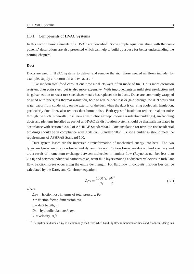
calculated by the Darcy and Colebrook equation:
∆pf =1000f L
Dh
ρV2
2(1.1)
where
∆pf = friction loss in terms of total pressure,Pa
f = friction factor, dimenssionless
L = duct length,m
Dh = hydraulic diameter6, mm
V = velocity,m/s
6The hydraulic diameter,Dh is a commonly used term when handling flow in noncircular tubes and channels. Using this
4 Introduction
ρ = density,Kg/m3
Dynamic losses result from flow disturbances caused by duct-mounted equipment and fittings that
change air flow’s path direction and/or area. These fittings include entries, exits, elbows, transitions,
and junctions. If the air density is constant and there is no elevation, according to the bernoulli equation
dynamic losses are proportional to the square velocity.
Considering the recent discussion and equation (1.1) reveals that the total losses in the duct network
(friction losses plus dynamic losses) are proportional to the square air flow rate:
∆pt ∝ q2 (1.2)
whereq is the air flow7.
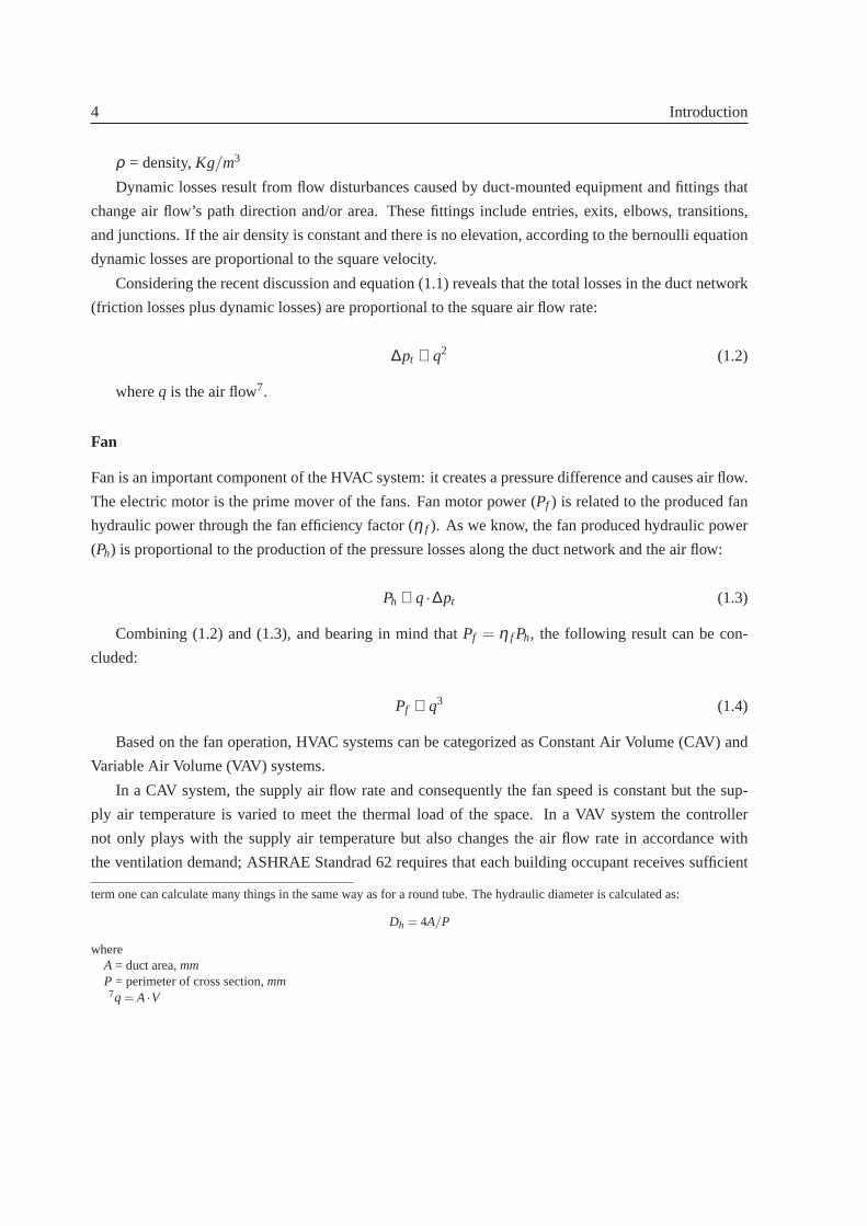
Fan
Fan is an important component of the HVAC system: it creates a pressure difference and causes air flow.
The electric motor is the prime mover of the fans. Fan motor power (Pf ) is related to the produced fan
hydraulic power through the fan efficiency factor (η f ). As we know, the fan produced hydraulic power
(Ph) is proportional to the production of the pressure losses along the duct network and the air flow:
Ph ∝ q·∆pt (1.3)
Combining (1.2) and (1.3), and bearing in mind thatPf = η f Ph, the following result can be con-
cluded:
Pf ∝ q3 (1.4)
Based on the fan operation, HVAC systems can be categorized as Constant Air Volume (CAV) and
Variable Air Volume (VAV) systems.
In a CAV system, the supply air flow rate and consequently the fan speed is constant but the sup-
ply air temperature is varied to meet the thermal load of the space. In a VAV system the controller
not only plays with the supply air temperature but also changes the air flow rate in accordance with
the ventilation demand; ASHRAE Standrad 62 requires that each building occupant receives sufficient
term one can calculate many things in the same way as for a round tube. Thehydraulic diameter is calculated as:
Dh = 4A/P
whereA = duct area,mmP = perimeter of cross section,mm7q = A·V
1.3 HVAC Systems 5
outdoor ventilation air to maintain his or her zone’s maximumCO2 concentration at or below 0.1%.
The requirement could be met through direct measurement or by supplyinga fixed quantity of outdoor
outdoor ventilation air per person (10-15 l/s per person). The big advantage of VAV systems is that they
conserve considerable amount of energy in comparison with CAV systems.The reason for this energy
saving is quite obvious from (1.4) which indicates the dependency of the fan power consumption on the
cube air flow rate. Due to this fan energy saving VAV systems are more common. However, in small
buildings and residences CAV systems are often the system of choice because of simplicity, low cost
and reliability.
Pipe and Valve
Pipes interconnect individual components in a hydronic circuit. Pressure drop caused by fluid friction
in fully developed flows of all well-behaved (Newtonian) fluids is described by the Darcy-Weisbach
equation:
∆pf =LD
ρV2
2(1.5)
where
∆p = pressre drop,Pa
f = friction factor, dimenssionless
L = length of pipe,m
D = internal diameter of pipe,m
ρ = fluid density at mean temperature,Kg/m3
V = average velocity,m/s
Noise, erosion, installation, and operating costs limit the maximum and minimum velocities in pip-
ing systems.
A valve regualtes the flow of materials such as gases, fluidized solids and liquids by opening, closing
or partially obstructing various passageways. Valves and fittings cause pressure losses greater than those
caused by the pipe alone. These losses can be expressed as
∆pv = KρV2
2(1.6)
whereK is the geometry and size-dependent loss coefficient.
Combining equations (1.5) and (1.6) results in that the total pressure drop (∆pt = ∆pf +∆pv) through
the hydronic circuit is proportional to the square fluid flow rate (Q):
∆pt ∝ Q2 (1.7)
6 Introduction
Pump
A pump moves liquids or gases from lower pressure to higher and overcomes this difference by adding
energy to the system. Pumps fall into two major groups: rotodynamic pumps and positive displacement
pumps. Their names describe the method for moving a fluid.
Rotodynamic pump uses for example a rotating impeller to increse the velocity of a fluid. However,
a positive displacement pump causes a fluid to move by trapping a fixed amount of it then forcing that
trapped volume into the discharge pipe. The periodic fluid displacement results in a direct increase in
pressure.
Following the similar discussion as it was mentioned about fan power consumption, it can be con-
cluded that the pump power consumption is also proportional to the cube fluid flow rate:
Pp ∝ Q3 (1.8)
Again similarly, playing with the speed of the pump will result in huge amount of pump energy
saving.
Heat Exchanger
The task of a heat exchanger is to efficiently transfer heat from one medium to another, whether the
media are separated by a solid wall so that they never mix, or the media are in direct contact. There
are plenty of different types of heat exchangers for enormous various purposes. In the next section two
kinds of heat exchangers will be described.
1.4 The HVAC System
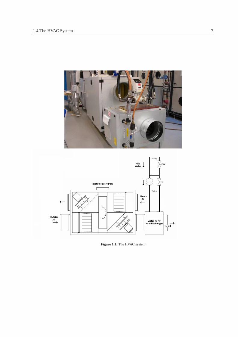
The HVAC system which will be considered here is a typical HVAC system made by Exhausto A/S and
shown in Fig 1.1. It is composed of two heat exchangers: heat recovery part and a water-to-air heat
exchanger (an air coil).
In general the heat recovery part has the mission of transferring heat from the exhausted room air to
the fresh sucked air. Throughout this process there can be either mixingbetween the exhausted and fresh
air or no mixing between them at all. Here a heat recovery wheel is applied as a heat recovery part. As
can be seen in Fig 1.1, there are two separate ducts for conducting the exhausted room air and the fresh
outdoor air. An aluminum made wheel rotates between two ducts and recovers the thermal energy from
exhausted air. It should be noted that there is no mixing between two air streams ( Practically there is a
little bit leakage between the two air streams ). Temperature of the fresh air thatleaves the heat recovery
part is controllable through the wheel rotation speed manipulation.
1.4 The HVAC System 7
Figure 1.1: The HVAC system

8 Introduction
Figure 1.2: Primary-only hydronic circuit
After preliminary warming up of the fresh air, it goes through the water-to-air heat exchanger for
the final heating. The main task of the water-to-air heat exchanger is to transfer thermal energy from hot
water to the fresh air through the coil. The coil is connected to a hydronic circuit which supplies the hot
water. The configuration of the hydronic circuit has a significant role in the control of the water-to-air
heat exchanger. Thus, we will elaborate this issue in the following section.
1.5 Different Hydronic Circuit Configuration
In this section different hydronic circuit configurations will be described. Then we will argue about the
most suitable hydronic circuit cinfiguration for this project.
1.5.1 Primary-Only Hydronic Circuit
A primary-only hydronic circuit is shown in Fig 1.2. Pumps are equipped with variable speed drives
(VSD) to adapt the pump speed to the required water flow. Water flow can bechanged by using the
control valve but using VSD is more energy-efficient. A bypass valve can be seen in the picture. In
heating purposes this valve can be eliminated but when we are going to use primary-only circuit in
cooling purposes we need to guarantee the minimum flow through the chillers. Therefore, in this case
the bypass valve has the responsibility to maintain the minimum flow through the chillers. Advantages
and disadvantages of primary-only hydronic circuits can be summarized asfollows:
Advantages:
• Lower first costs: This is due to the elimination of the secondary pumps and associated fittings,
vibration isolation, starters, power wiring, controls, etc. These savings are partly offset by higher

1.5 Different Hydronic Circuit Configuration 9
costs of variable speed drives for the p-only system and the cost of thebypass valve and associated
controls.
• Less space required: again due to the eliminated secondary pumps. This can result in substantial
cost reductions, depending on the plant layout and space constraints.
• Reduced pump design motor power requirement and size: There are two reasons for this reduction.
First, the additional fittings and devices (shut-off valves, strainers, suction diffusers, check valves,
headers, etc.) required for the secondary pumps are eliminated. Second, in most cases, average
pump efficiency is also higher with the p-only system.
• Lower pump energy costs: Contrary to conventional wisdom, p-only systems always use less
pump energy. This is in part due to the reduced pump full-load power requirement, but mostly
because the variable speed drives provide near cube-law savings for both flow through the primary
circuit as well as flow through the secondary circuit.
Disadvantages:
• Bypass Control Problem: In cooling systems a minimum flow is required not to harm the chillers.
• Complexity of Control: Complex control systems are prone to failure and they need on-site trained
professionals for checking and maintenance.
• Less Flexibility: If some changes happen in the demand, a new pump might be replaced. This
replacement can result in expensive cost because the main pump has to bechanged. To avoid this
problem the pump can be selected oversized but still it may cause huge different cost.
1.5.2 Primary-Secondary Hydronic Circuit
A primary-secondary hydronic circuit is shown in Fig 1.3. As can be seenin the Fig 1.3, the configu-
ration of the primary pumps are dedicated. However, it is not a necessaryconfiguration. They can be
used as manifolded in Fig 1.2. Also, in the primary-only configuration the pumpscan be arranged as
dedicated.
Primary pumps in primary-secondary configuration are often constant speed pumps and the variable
speed pumps are installed in the secondary circuit to provide the required water flow in accordance with
the load. The main advantage of primary-secondary hydronic circuit is its simplicity. Thus, it is easy to
control and complicated control procedures is not required. Becauseof its simplicity, also highly skilled
on-site staff is not needed.

10 Introduction
Figure 1.3: Primary-secondary hydronic circuit
1.5.3 Primary-Secondary-Tertiary Hydronic Circuit
A primary-secondary-tertiary hydronic circuit is shown in Fig 1.4. The primary-secondary-tertiary
pumping makes the building, or load, loop hydraulically independent of the distribution loop and sep-
arates both from generation loop. This type of pumping system allows for blending of the water at
supply temperature from the central plant with return water at each building, so each building gets a
different supply temperature, which sometimes is called thermal independence from building to build-
ing. The coils in a given building can be provided with any temperature, ranging from the hot water
supply temperature coming from the boiler to the chilled water supply temperaturecoming from the
chiller evaporator. Proper design of the low-pressure-drop common pipe is essential to achieve the loops
hydraulic and thermal independence. We can control the blending process at the common pipe con-
nection between the distribution (secondary) loop and the building (tertiary)loop by using a controller.
This controller must be carefully programmed to establish some priorities in determining the valve’s
position and the amount of recirculation that occurs. The first of these priorities is the blended supply
temperature going to the building coils. Closing the valve in the secondary crossover bridge reduces the
secondary flow with respect to the tertiary, or building, flow existing at thatmoment. This reduction
forces blending of return water with supply water and decreases the secondary pump’s energy cost. In
hot water system, a substantial amount of blending could occur, resulting inconsiderable secondary
flow and pumping cost decreases. This is possible because hot water coils can be selected to provide
significant heat output even at low supply temperature. Chilled water systems require more careful con-
trol. With chilled water coils, excessive blending causes the supply temperature to the coils to rise above
the dew point of the air passing over the coil; thus, the coil no longer can dehumidify the air. Totally,
primary-secondary-tertiary pumping system has significant advantagesin large central plant systems.

1.5 Different Hydronic Circuit Configuration 11
Figure 1.4: Primary-secondary-tertiary hydronic circuit
1.5.4 The Suitable Hydronic Circuit Configuration for This Project
All distributing pumps are centrally located with balancing valves and control valves installed at cooling
coils, heating coils, and heat exchangers to restrict and regulate water flow by creating water pressure
drops and power losses across the valves. In a system with a large number of balancing valves and
control valves, total water power and energy losses across the valvescan be significant. This wasted
pump power and energy would be eliminated if the balancing valves and control valves were removed
from the piping system. Thus, it will be objective to use a pumping system where pumps are locally
located at the coils. The local pumps circulate and regulate water through thecooling coils, heating coils,
and heat exchangers without balancing valves and control valves. Ina local pumping system, a variable
speed pump is installed at each cooling or heating coil without a centrally located pump. Pump speed
and flow rate are controlled by the same controller that would otherwise regulate the control valve.
The local pump will circulate and regulate water as required through the coiland the piping system,
eliminating the need for control valves which eliminates the pressure drops and power losses across the
valves. Pump head and power overcome only the essential piping and equipment pressure losses. The
head of each pump is varied and depends on the pump location. The head is determined by summing all
of the pressure losses in its flow path. Also, the local pumping system requires less horsepower than the
central system at design load. Therefore, equipment costs (including pumps, motors and VSD) of the
local pumping system should be lower in proportion to the reduced horsepower. Totally, the lower first
cost in conjunction with lower operating cost make it desirable to select the local pumping system.
In this project to benefit the advantages of local pumping system, we suppose a variable speed pump
for each water-to-air heat exchanger which regulates water flow through the coil. According to the
definitions, this part will be called tertiary hydronic circuit. Depending on thesize of the system and the
12 Introduction
way that hot or cold water is provided we can have primary/secondary pumps or only primary pumps.
The focus of this project will be on the tertiary hydronic part. We will try to find the optimal control
algorithm for this part respecting the thermal comfort standards.
1.6 Review of Previous Work
In this project, optimal model-based control of a heating, ventilating, air-conditioning (HVAC) system
will be considered. First, we will derive the steady state optimality criterion forthe HVAC system.
Then, we will design the dynamic controllers in such a way that this optimality criterion is satisfied.
This is a reasonable approach because HVAC systems are in steady state conditions around 95% of their
operating time.
We review the previous works under two distinctive categories: modeling ofHVAC systems and
optimal control of HVAC systems.
1.6.1 Modeling of HVAC Systems
Due to our approach to solve the optimal control problem of the HVAC system,which was mentioned
above, we will need both static (steady-state) model and dynamic model of theHVAC system.
The steady state models of HVAC systems are important because they can be applied to estimate en-
ergy comsuptions and to optimize the performance of the system. In [11] they developed a mathematical
model of a section of a building. The building model includes the effects of airexchange, conduction
through walls and fenestration, solar radiation, energy storage in furniture, and internal loads from oc-
cupants and equipment. It can predict both transient and static behavior of the system. The model is
modular (including six modules: external wall, internal wall, window, ceiling, floor, and air) so that they
can be easily replaced with others and make the number of rooms adjustable.
[15] develops HVAC system steady-state models and validates them againstthe monitored data of a
existing VAV system to use for energy consumption and thermal comfort calculations. The final goal of
this work is to develop a supervisory layer which perfroms based on the two-objective genetic algorithm
to optimize the operation of a HVAC system.
Steady-state models of HVAC system components are developed in [16]. Those models are inter-
connected to simulate the responses of the VAV system. The developed steady state model later is used
to formulate the optimal control probelm.
The rotary regenerator (also called the heat wheel) is an important component of energy intensive
sectors, which is used in many heat recovery systems due to its high efficiency. In [17] a model of a
rotary enthalpy wheel heat exchanger based on a new semi-empirical NTU correction factor method

1.6 Review of Previous Work 13
is developed. Given only two reference data points, the model is able to predict effectiveness for any
balanced and unbalanced flow condition.
A model for heat wheel based on physical principles is developed in [18]. Then they analyse the
temperature distribution and its variations in time and investigate how the airflow, temperature and
rotational speed of the wheel influence upon the dynamic response.
[19] develops a 2D, steady state model of a rotary desiccant wheel. Themodel is capable of
predicting steady state behavior of desiccant wheels having at the most three sections (process, purge,
and regeneration).
The fundamental dimensionless groups for air-to-air energy wheels thattransfer both sensible heat
and water vapor can be derived from the governing nonlinear and coupled heat and moisture transfer
equations. These dimensionless groups for heat and moisture transfer are found to be functions of the
operating temperature and humidity of the energy wheel. Unlike heat exchangers that transfer only
sensible heat, the effectiveness of energy wheels is a function of the operating temperature and humidity
as has been observed by several energy wheel manufacturers andresearchers. The physical meaning
of the dimensionless groups and the importance of the operating condition factor are explained in [20],
[21], [22], and [23].
Underwood and Crawford develop a model to predict the effects of inletair temperature, air flow
rate, and inlet water temperature during closed loop control of the outlet airtemperature using water flow
rate as control variable [24]. This model is characterized by two first order differential equations (one
for air side and one for water side). Least squares fits are performedto identify the model parameters on
the basis of a series of open loop tests.
[25] presents A new dynamic coil model. This model is developed via the exact solution of a previ-
ously unsolved partial differential equation, which governs the coil dynamics for a step change in water
flow rate. This new model is the first step toward developing a future model that can accurately predict
the coil dynamics for several varying coil inlet conditions expected to occur under MIMO control. The
model is compared with previously published simplified PDE coil models, which used an approxima-
tion to this exact solution, and against actual measured coil dynamics. The coil model is shown to have
superior performance in predicting the actual coil behavior.
1.6.2 Optimal Control of HVAC Systems
Most existing HVAC system processes are optimized at the local loop level. However, a strategy using
the optimization of the individual zone air temperature setpoints combined with other controller set-
points during occupied periods could reduce further system energy use. Using a multi-objective genetic
algorithm, which will permit the optimal operation of the buildings mechanical systems when installed
in parallel with a buildings central control system, optimization process, the supervisory control strategy
14 Introduction
setpoints, such as supply air temperature, supply duct static pressure, chilled water supply temperature,
minimum outdoor ventilation, reheat (or zone supply air temperature), and zone air temperatures are
optimized with respect to energy use and thermal comfort [15].
In [12] an objective function which consists of costs and energy demandis defined. The limitations
in the system appear as constraints to this objective function. Solving the recent optimization problem
results in an optimal combination of the characteristics of the HVAC system and the control strategy.
Then a sequential control is developed, tested by simulation and implemented in an existing plant.
The HVAC system here consists of the following components: sorption regenerator, heat regenerator,
humidifier and air heater for supply air and humidifier and air heater for return air. The supply air fan
as well as the return air fan transport the air masses. The heaters are loaded by hot water. In winter the
HVAC system works as a conventional air conditioning system. With the aid of the two regenerators a
high level of recovery of heat and humidity is possible. In the summer the heater for supply air is out
of action. The dehumidification is done by the sorption regenerator. The cooling can be achieved by an
adiabatic humidification.
They show in [13] how gradient-based optimization can be used to minimize energy consumption of
distributed environmental control systems without increasing occupant thermal dissatisfaction. Fuzzy
rules have been generated by data from gradient optimization, showing that a fuzzy logic control scheme
based on nearest neighbors approximates closely the gradient-based optimized results.
It is well known that a building’s thermal mass influences thermal conditions within the space.
Thermal mass is generally considered to be negative in the case of intermittentair conditioning, since
the heat load tends to increase due to heat storage load. However, takingan HVAC system with heat
storage tanks as an analogy, there would appear to be a possibility of storing heat in the building structure
during times of non-occupancy, thus reducing equipment capacity requirements or saving running costs
by utilizing cheap night-rate electricity. [14] proposes a dynamic optimization technique that minimizes
objective functions such as running cost or peak energy consumption taking advantage of the recent
mentioned phenomenon.
Classical HVAC control techniques such as ON/OFF controllers (thermostats) and proportional-
integral-derivative (PID) controllers are still very popular because of their low commissioning cost.
However, in the long run, these controllers are expensive because they operate at a very low-energy
efficiency. One important factor affecting the efficiency of air conditioning systems is the fact that
most HVAC systems are set to operate at design thermal loads while actual thermal loads affecting the
system are time-varying. Therefore, control schemes that take into consideration time varying loads
should be able to operate more efficiently and better keep comfort conditionsthan conventional control
schemes. [26] presents a nonlinear controller for a heating, ventilating, and air conditioning (HVAC)
system capable of maintaining comfort conditions under time varying thermal loads. The controller
1.7 Contributions 15
consists of a regulator and a disturbance rejection component designed using Lyapunov stability theory.
The mitigation of the effect of thermal loads other than design loads on the system is due to an on-line
thermal load and state estimator. The availability of the thermal load estimates allows the controller
to keep comfort regardless of the thermal loads affecting the thermal space being heated or cooled.
Simulation results are used to demonstrate the potential for keeping comfort and saving energy of this
methodology on a variable-air-volume HVAC system operating on cooling mode. The same idea follows
in [27]. The control system attempts to find an economic optimum to supply heat tothe building with
the use of a predictor for the indoor temperature, while maintaining a comfortable temperature in the
building.
1.7 Contributions
This section presents the contributions of this thesis. This project requireslots of modeling which is
the first step in model-based approaches. There are plenty different models of HVAC systems in the
literature but rarely models which are useful from control point of view can be found. The major
controllers have been used for HVAC systems are PID controllers because of their cheap first-cost and
simplicity while in this project advanced control techniques are used. Finally,the advanced controller is
simplified for commercialization purposes.
1.7.1 Contribution 1
Optimal set-point synthesis for a HVAC system applied to meet ventilation demands of a single-
zone area: HVAC systems often work in their steady state regime (more than 95% of their operating
time). Thus, to control the system optimally set-point optimization approach seemsobjective. To derive
the optimality criteria static model for the HVAC system is applied. So, we define anobjective (cost)
function composed of all electrical and thermal power consumptions in the system. Ventilation goals
and actuator limits appear as constraints in the optimization problem. Finally, the optimization problem
is solved and the optimality criteria are derived [28].
This approach results in a performance that is very close to the ideal optimaloperation while it has
the advantage of less complication in computation and implementation.
1.7.2 Contribution 2
Developing a nonlinear dynamic model for a water-to-air heat-exchanger: In this project control
inputs to the water-to-air heat exchanger are primary water flow and tertiary water flow. The output of the
heat exchanger is inlet temperature. Therefore, to develop a model which is a true representative of the

16 Introduction
inputs and the output of the system the nonlinear water-to-air heat exchanger model which was proposed
in [24] is extended. The proposed water-to-air heat exchanger modelassumed constant temperature for
the hot water supply to the coil. We include the energy balance equation of thesupply hydronic circuit in
the nonlinear model of the water-to-air heat exchanger to have the variable supply hot water temperature
for the coil. In other hand, by doing that we will have primary water flow andtertiary water flow as
control inputs to the system [29].
1.7.3 Contribution 3
Developing a gain varying model for a rotary heat recovery wheel:The temperature of the fresh air
that leaves the rotary heat recovery wheel is controllable by changing the rotation speed of the wheel.
Thus, for model-based control of the rotary heat recovery wheel a model which describes that relation is
neccessary. In the literature there are plenty of models for rotary heat recovery wheels but unfortunately
none of them are useful from a control point of view. We estimate the steady state gain by benefiting
from the results of the static analysis part. Then we discuss that a first order model can capture the
dynamic behavior of the rotary heat recovery wheel. So, totally the model will be a first order system
along with a variable gain [29].
1.7.4 Contribution 4
Design and implementation of the optimal model-based controller forthe HVAC system: Dynamic
model of the system is analyzed and then the system is broken into two independent subsystems (rotary
heat recovery wheel and water-to-air heat exchanger). Utilizing the excellent features of the model
predictive control (MPC) and introducing an internal feedback in the system the optimality criteria are
met [29].
1.7.5 Contribution 5
Design and implementation of the simplified optimal controller for the HVAC system: Implicit
measuring of the water flow by means of thermocouples leads us to a simplified optimal controller for
the system. This control scheme consists of two PI controller. One of them controls the inlet temperature
by manipulating the primary water flow while the other one tries to keep the primary and the tertiary
flows close as far as possible [30].
1.7.6 Contribution 6
Experimental verifications of the new developed models and control algorithms for the HVAC
system: All the new models and control algorithms which were developed throughoutthis thesis are
1.8 Outline of Thesis 17
verified experimentally in the Danish Technological Institute’s lab on a typicalHVAC system manu-
factured by Exhausto while hot water is pumped to the system via Grundfos new permanent magnet
variable speed pump [28], [29], [30].
1.7.7 Contribution 7
A parameterization of the observer-based controllers; bumplesstransfer by covariance interpo-
lation: HVAC systems are nonlinear systems. One of the most common ways to control anonlinear
system is to linearize the nonlinear system around some specific operating points and then applying the
linear control techniques. Afterwards the problem of how to switch between different linear controllers
comes up.
Interpolation between two observer-based controllers is not a trivial task because the simple gain
interpolation can leave the system unstable for some intermediate points. So, wehave proposed an
algorithm to interpolate between two observer-based controllers for a linear multivarible system such
that the closed loop system remains stable throughout the interpolation. The proposed algorithm can be
applied for bumpless transfer between two observer-based controllers. This algorithm has been used in
bumpless transfer between two observer-based controllers which weredesigned based on the linearized
model of the HVAC system. However, the proposed algorithm is still too naiveto be applied for the real
HVAC system which has nonlinear behaviors [31].
1.8 Outline of Thesis
This thesis is presented as a collection of papers. Thus, the rest of this thesis is organized as follows:
Summary of work: This chapter presents a brief description of the work that was carried out in
this project. The main goal is to give a comprehensive formulation of the problem and its solution while
there will be no need for the reader to go through the paper collections.
Conclutions: Conclusions, perspectives, and possible future works are discussed here.
Optimal Set-point Synthesis in HVAC Systems:This paper presents optimal set-point synthesis
for the heating, ventilating, and air-conditioning (HVAC) system. The objective function is composed
of the electrical power for different components, encompassing fans,primary/secondary pump, tertiary
pump, and air-to-air heat exchanger wheel; and a fraction of thermal power used by the HVAC sys-
tem. The goals that have to be achieved by the HVAC system appear as constraints in the optimization
problem. To solve the optimization problem, a steady state model of the HVAC system is derived while
different supplying hydronic circuits are studied for the water-to-air heat exchanger. Finally, the optimal
set-points and the optimal supplying hydronic circuit are resulted.

18 Introduction
Optimal Model-Based Control in HVAC Systems:This paper presents optimal model-based con-
trol of the heating, ventilating, and air-conditioning (HVAC) system. First dynamic model of the HVAC
system is developed. Then the optimal control structure is designed and implemented. The HVAC sys-
tem is splitted into two subsystems. By selecting the right set-points and appropriate cost functions for
each subsystem controller the optimal control strategy is respected to gaurantee the minimum thermal
and electrical energy consumption. Finally, the controller is applied to control the mentioned HVAC
system.
Simplified Optimal Control in HVAC Systems: This paper presents simplified optimal control of
the heating, ventilating, and air-conditioning (HVAC) system. First the optimal control strategy which
was developed is adopted for implemenation in a real life HVAC system. Then thebypass flow problem
is addressed and a controller is introdeuced to deal with this problem. Finally asimplified control
structure is proposed for optimal control of the HVAC system.
Appendices:
• Appendix A: This section deals with the decoupling of the HVAC system.
• Appendix B (A Parameterization of The Observer-Based Controllers: Bumpless Transfer by Co-
variance Interpolation): This paper presents an algorithm to interpolate between two observer-
based controllers for a linear multivarible system such that the closed loop system remains stable
throughout the interpolation. The method interpolates between the inverse Lyapunov functions
for the two original state feedbacks and between the Lyapunov functionsfor the two original ob-
server gains to determine an intermediate observer-based controller. Thisalgorithm has been used
in bumpless transfer between two observer-based controllers which were designed based on the
linearized model of the HVAC system. However, the proposed algorithm is stilltoo naive to be
applied for the real HVAC system which has nonlinear behaviors.
• Appendix C: This part describes the HVAC test system set-up.

Bibliography
[1] P. Svendsen and H. Andersen, ”Energy Efficient Pump Coupling inHVAC Systems”,Technical
Report, Danish Technological Institute (Industry and Energy Section), 2005.
[2] S. Somasundaram, D.W. Winiarski, D.B. Belzer, ”Screening Analysis for EPACT-Covered Com-
mercial HVAC and Water-Heating Equipment”,Transaction of the ASME, Vol. 124, June 2002, pp
116-124.
[3] J. Lin, S. Chen, and P.D. Roberts, ”Modified Algorithm for Steady-state Integrated System Opti-
mization and Parameter Estimation”,IEE Proceedings, Vol. 135, March 1988.
[4] S. Gros, B. Srinivasan, and D. Bonvin, ”Static Optimization via Tracking of The Necessary Con-
ditions of Optimality Using Neighboring Extremals”,American Control Conference Proceeding,
June 2005, pp 251-255.
[5] N. Nassif, S. Kajl, and R. Sabourin, ”Two-Objective On-Line Optimization of Supervisory Control
Strategy”,Building Services Engineering Research and Technology, 2004, pp 241-251.
[6] L.F.S. Larsen, ”Model Based Control of Refrigeration Ssytems”,Ph.D. Thesis, Aalborg University,
Denmark, 2005.
[7] M. Wetter, ”Simulation Model: Air-to-air Heat Exchnager”,Technical Report, Lawrence Berkeley
National Laboratory, 1999.
[8] N. Nassif, S. Kajl, and R. Sabourin, ”Ventilation Control Strategy Using SupplyCO2 Concentra-
tion Set Point”,International Journal of HVAC & R Research, 2005, pp 239-262.
[9] R.H. Green, ”An Air-Conditioning Control System Using Variable-speed Water Pumps”,ASHRAE
Transaction:Research, part 1, 1994, pp 463-470.
[10] W.P. Bahnfleth, ”Varying Views on Variable-primary Flow”,Chilled Water Engineering J., March
2004.
19
20 BIBLIOGRAPHY
[11] Craig Lin, Clifford C. Federspiel, David M. Auslander, Multi-Sensor Single-Actuator Control of
HVAC Systems,Energy Systems Laboratory, 2002.
[12] Clemens Felsmann and Gottfried Knabe, Simulation and Optimal Control Strategies of HVAC
Systems,Seventh International IBPSA Conference, August 2001.
[13] S. Ari, I.A. Cosden, H.E. Khalifa, J.F. Dannenhoffer, P. Wilcoxen, and C. Isik, Constrained Fuzzy
Logic Approximation for Indoor Comfort and Energy Optimization,Fuzzy Information Processing
Society, Annual Meeting of the North American, June 2005.
[14] Tatsuo Nagai, Dynamic optimization technique for control of HVAC system utilizing building
thermal storage,IBPSA proceedings, 1999.
[15] Nabil Nassif, Stanislaw Kajl, Robert Sabourin, Optimization of HVAC Control System Strategy
Using Two-Objective Genetic Algorithm,HVAC&R Research, Vol. 11, No. 3, July 2005.
[16] G. R. Zheng and M. Zaheer-Uddin, Optimization of thermal processes in a variable air volume
HVAC system,IEEE Control Systems, 1995.
[17] S.W. Freund, Simulation of air-to-air energy recovery systems for HVAC energy conservation in
an animal housing facility,Master thesis, University of Wisconsin-Madison, 2003.
[18] Zhuang Wu, Roderick V.N. Melnik, Finn Borup, Model-based analysis and simulation of regener-
ative heat wheel,Energy and Buildings, 2005.
[19] Y.M. Harshe, R.P. Utikar, V.V. Ranade, D. Pahwa, Modeling of rotary desiccant wheels,Chemical
Engineering Technology, Vol. 28, No. 12, 2005.
[20] C.J. Simonson and R.W. Besant, Energy wheel effectiveness: part I-development of dimensionless
groups,International journal of heat and mass transfer, 1998.
[21] L.A. Sphaier, W.M. Worek, Analysis of heat and mass transfer in porous sorbents used in rotary
regenerators,International journal of heat and mass transfer, 2004.
[22] L.Z. Zhang, J.L. Niu, Performance comparisons of desiccant wheels for air dehumidification and
enthalpy recovery,Applied thermal engineering, March 2002.
[23] N. Ghodsipour, M. Sadrameli, Experimental and sensitivity analysis of a rotary air preheater for
the flue gas heat recovery,Applied thermal engineering, November 2002.
[24] D.M. Underwood and R.R. Crawford, Dynamic nonlinear modeling of ahot-water-to-air heat ex-
changer for control applications,ASHRAE transactions: research, 1991.

BIBLIOGRAPHY 21
[25] Chris C. Delnero, Dave Dreisigmeyer, Douglas C. Hittle, Peter M. Young, Charles W. Anderson,
Michael L. Anderson, Exact Solution to the Governing PDE of a Hot Waterto Air Finned Tube
Cross Flow Heat Exchanger,International journal of HVAC&R research, 2004.
[26] Betzaida Arguello-Serrano and Miguel Velez-Reyes, Nonlinear Control of a Heating, Ventilating,
and Air Conditioning System with Thermal Load Estimation,IEEE transactions on control systems
technology, Vol. 7, No. 1, January 1999.
[27] Peter Lute and Dolf van Paassen, Optimal Indoor Temperature Control Using a Predictor,IEEE
Control Systems, 1995.
[28] M. Komareji, J. Stoustrup, H. Rasmussen, N. Bidstrup, F. Nielsen, P. Svendsen, Optimal set-point
synthesis in HVAC systems, American Control Conference, New York, NY, 2007.
[29] M. Komareji, J. Stoustrup, H. Rasmussen, N. Bidstrup, F. Nielsen, P. Svendsen, Optimal model-
based control of HVAC systems, American Control Conference, Seattle,WA, 2008.
[30] M. Komareji, J. Stoustrup, H. Rasmussen, N. Bidstrup, F. Nielsen, P. Svendsen, Simplified optimal
control in HVAC systems, Submitted for publication, 2008.
[31] J. Stoustrup, M. Komareji; A parameterization of the observer-based controllers: bumpless transfer
by covariance interpolation, Submitted for publication, 2008.


Chapter 2
Summary of Work
This chapter presents a brief description of the work that was carried out in this project. The main goal
is to give a comprehensive formulation of the problem and its solution while the collection of papers
serves as a complimentary for further insight.
First optimality criteria based on the static model of the HVAC system are derived. It is objective
to apply the static model of the system because HVAC systems are in steady stateconditions more than
95% of their operating time. Then the model-based controller is designed to follow the objectives of the
HVAC system while the optimality criteria are met. Finally, the control system is simplified and some
practical issues are addressed.
2.1 Modeling
2.1.1 Static Modeling
The HVAC system that will be considered consists of two heat exchangers: an air-to-air heat exchanger
and a water-to-air heat exchanger. In this section the temperature efficiency of these two heat exchangers,
which can be used as a steady state model of heat exchangers, will be described.
Air-to-air Heat Exchanger
The air-to-air heat exchanger is a rotary heat exchanger in aluminum, withlow pressure loss (shown in
Fig. 2.1). The rotor control comprises a gear motor with frequency converter. Two fans are installed
to produce the desired inlet and outlet air flow. Here, it is supposed that the ratio of the supply air flow
to the return air flow is one. Therefore,ηt2 will be a function of air flow (qa), that is the same for both
supply and return air, and the rotation speed of the wheel (n).
23
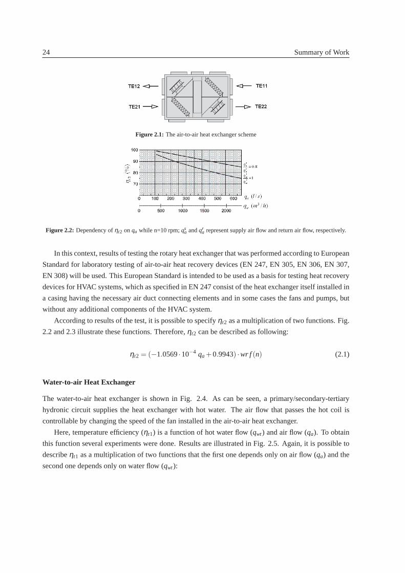
24 Summary of Work
Figure 2.1: The air-to-air heat exchanger scheme
Figure 2.2: Dependency ofηt2 onqa while n=10 rpm;qsa andqr
a represent supply air flow and return air flow, respectively.
In this context, results of testing the rotary heat exchanger that was performed according to European
Standard for laboratory testing of air-to-air heat recovery devices (EN 247, EN 305, EN 306, EN 307,
EN 308) will be used. This European Standard is intended to be used as a basis for testing heat recovery
devices for HVAC systems, which as specified in EN 247 consist of the heat exchanger itself installed in
a casing having the necessary air duct connecting elements and in some cases the fans and pumps, but
without any additional components of the HVAC system.
According to results of the test, it is possible to specifyηt2 as a multiplication of two functions. Fig.
2.2 and 2.3 illustrate these functions. Therefore,ηt2 can be described as following:
ηt2 = (−1.0569·10−4 qa +0.9943) ·wr f (n) (2.1)
Water-to-air Heat Exchanger
The water-to-air heat exchanger is shown in Fig. 2.4. As can be seen, aprimary/secondary-tertiary
hydronic circuit supplies the heat exchanger with hot water. The air flowthat passes the hot coil is
controllable by changing the speed of the fan installed in the air-to-air heat exchanger.
Here, temperature efficiency (ηt1) is a function of hot water flow (qwt) and air flow (qa). To obtain
this function several experiments were done. Results are illustrated in Fig. 2.5. Again, it is possible to
describeηt1 as a multiplication of two functions that the first one depends only on air flow (qa) and the
second one depends only on water flow (qwt):
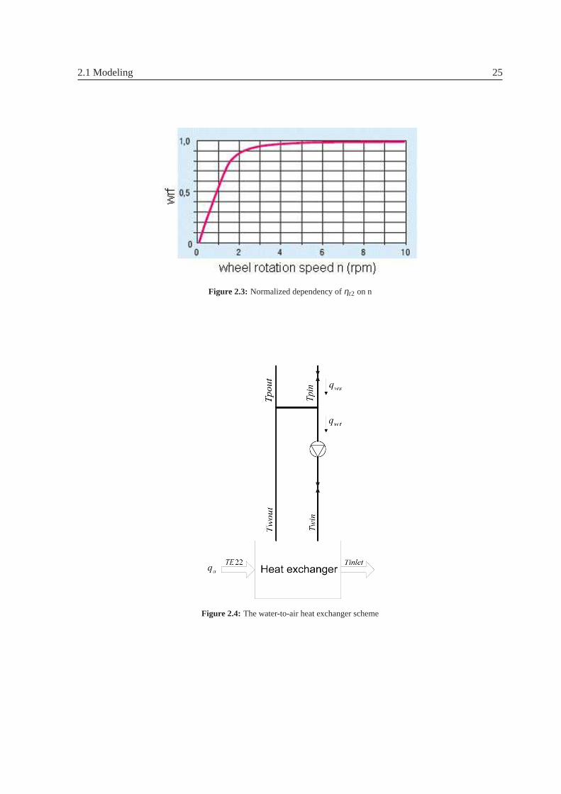
2.1 Modeling 25
Figure 2.3: Normalized dependency ofηt2 on n
Figure 2.4: The water-to-air heat exchanger scheme
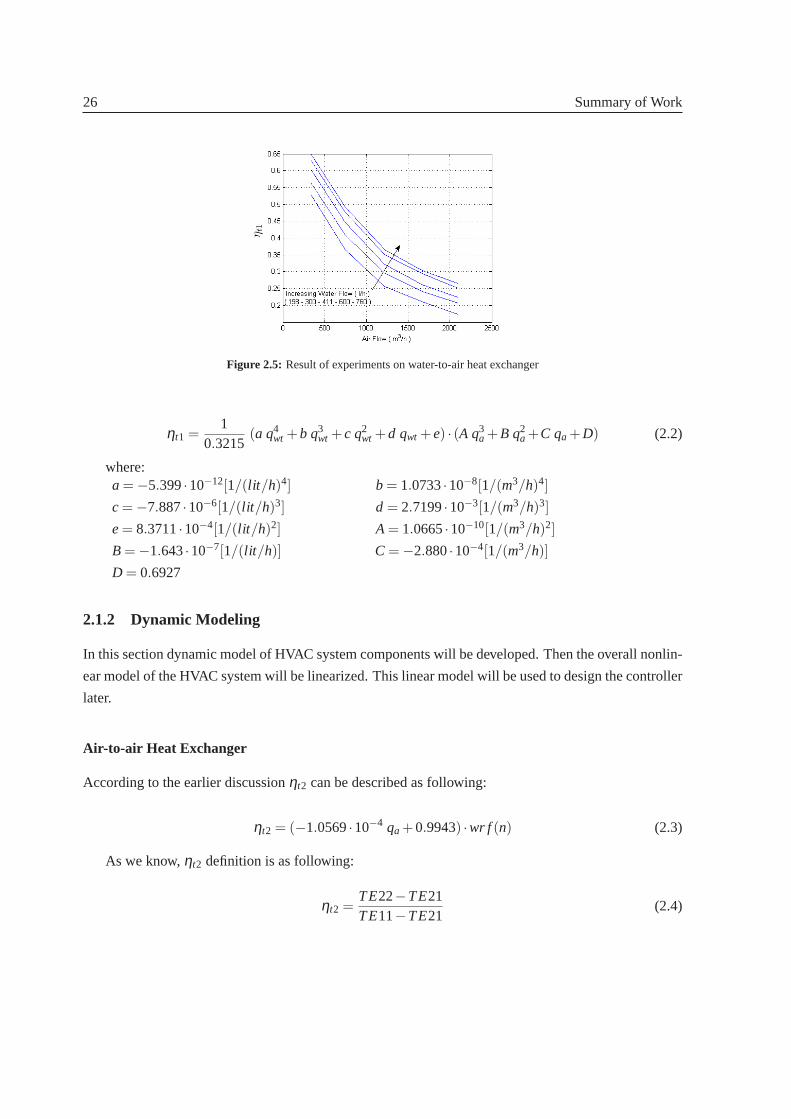
26 Summary of Work
Figure 2.5: Result of experiments on water-to-air heat exchanger
ηt1 =1
0.3215(a q4
wt +b q3wt +c q2
wt +d qwt +e) · (A q3a +B q2
a +C qa +D) (2.2)
where:a = −5.399·10−12[1/(lit /h)4] b = 1.0733·10−8[1/(m3/h)4]
c = −7.887·10−6[1/(lit /h)3] d = 2.7199·10−3[1/(m3/h)3]
e= 8.3711·10−4[1/(lit /h)2] A = 1.0665·10−10[1/(m3/h)2]
B = −1.643·10−7[1/(lit /h)] C = −2.880·10−4[1/(m3/h)]
D = 0.6927
2.1.2 Dynamic Modeling
In this section dynamic model of HVAC system components will be developed. Then the overall nonlin-
ear model of the HVAC system will be linearized. This linear model will be usedto design the controller
later.
Air-to-air Heat Exchanger
According to the earlier discussionηt2 can be described as following:
ηt2 = (−1.0569·10−4 qa +0.9943) ·wr f (n) (2.3)
As we know,ηt2 definition is as following:
ηt2 =TE22−TE21TE11−TE21
(2.4)

2.1 Modeling 27
Combining recent equations ( equations 2.3 and 2.4 ) will result in the steady state gain for the wheel
model:
TE22= TE21+wr f (n) · (TE11−TE21) · (−1.0569·10−4qa +0.9943) (2.5)
Fig 2.6 shows an energy wheel operating in a counter flow arrangement. Under typical operating
conditions, warm air enters the tube during the supply part of the cycle andtransfers energy to the
matrix. This energy is then transferred from the matrix to the air during the exhaust part of the cycle.
The half plane of the matrix tube is assumed impermeable and adiabatic and the bulkmean temperatures
of air are used in the model. The formulation is therefore one dimensional andtransient with space (x)
and time (t or θ = w· t) as the independent variables. The governing equations for heat transfer (energy
equations) in energy wheel for air and matrix include energy storage, convection, conduction based on
the usual assumptions are as follows respectively:
ρaCpaAa∂Ta
∂ t+UρaCpaAa
∂Ta
∂x+h
As
L(Ta−Tm) = 0 (2.6)
ρmCpmAm∂Tm
∂ t−h
As
L(Tm−Ta) =
∂∂x
(KmAm∂Tm
∂x) (2.7)
It is reasonable to suppose that the conductivity has a small share in heattransfer through the matrix.
Thus, equation (2.7) can be rewritten as following:
∂Tm
∂ t+
NTUC∗
r PTm =
NTUC∗
r PTa (2.8)
Equation (2.8) shows that air temperature (Ta) can be assumed as the input for the matrix temperature
(Tm) differential equation. It means the matrix temperature as a function of time (t) will perform as an
output of the ordinary first order differential equation. Another pointthat should be emphasized is that
the time constant (C∗r P
NTU)in the differential equation is fixed. That is, the time constant depends on matrix
(wheel) properties. Thus, it is a design parameter not a control parameter. It is claimed that air stream
temperature has the same behavior as matrix temperature. So, The air stream temperature shows first
order dynamic behavior.
As a result, the wheel behavior can be modeled by a first order transferfunction. So, we will have:
TE22(s) =TE21τ s+1
+wr f (s) · (TE11−TE21)(−1.0569×10⁻⁴qa +0.9943)
τ s+1(2.9)
The first part on the right side of the equation (2.9) will be treated as disturbance. That is, the transfer
function fromTE22 towr f is as following:

28 Summary of Work
Figure 2.6: Counter flow energy wheel
TE22(s)wr f (s)
=(TE11−TE21)(−1.0569×10⁻⁴qa +0.9943)
τ s+1(2.10)
As it was discussed, the time constant (τ) is fixed and according to the experiments, it is 28.0374
seconds.
Water-to-air Heat Exchanger
Here, the nonlinear coil model that was developed by Underwood and Crawford will be applied. Accord-
ing to their model, the differential equations, resulted from energy balanceequations, which describe
the coil behavior are as follows:
[(−Cpw−b/2)mwt(t)−d/2ma(t)−a/2] Twout(t)+ [(Cpw−b/2)mwt(t)−d/2ma(t)−a/2] Twin(t)
+(b mwt(t)+d ma +a) TE22(t) = Cwddt
Twout(t) (2.11)
−ma(t)CpaTinlet(t)+ [(Cpa−d)ma(t)−bmwt(t)−a] ·TE22(t)+(a/2+b/2mwt(t)+d/2ma(t))Twin(t)
+(a/2+b/2mwt(t)+d/2ma(t))Twout(t) = Caddt
Tinlet(t) (2.12)
wherea, b, d, Cpa, Cpw, Ca, andCw are unknown parameters that have to be identified through the
experiments.
The unknown parameters have identified through some experiments on the coil. Fig 2.7 show veri-
fication of the model along with identified parameters.
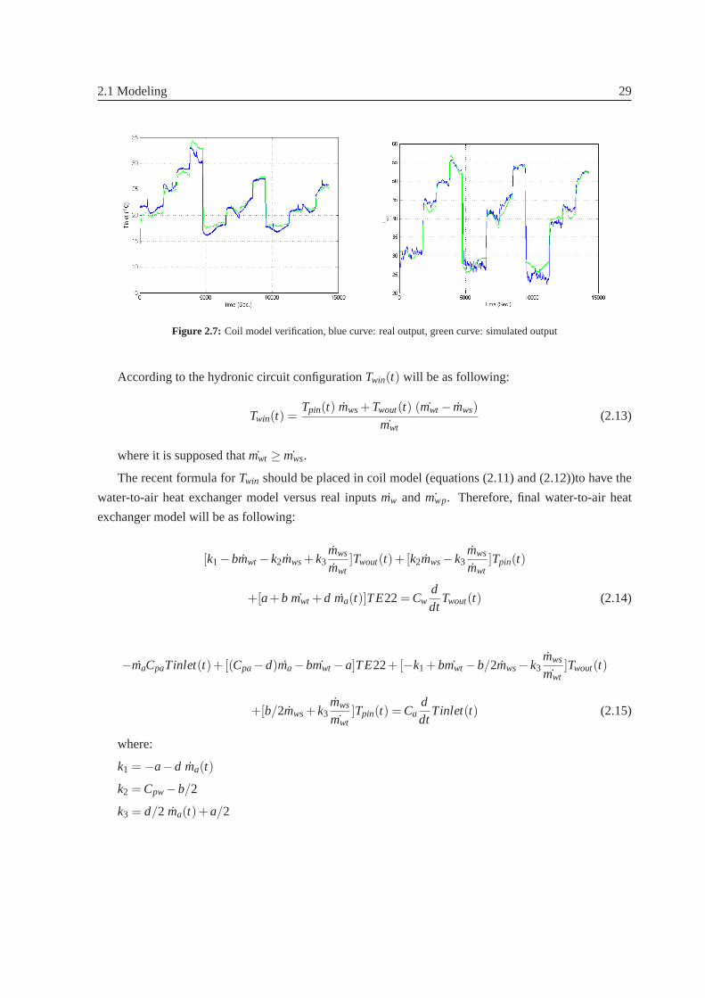
2.1 Modeling 29
Figure 2.7: Coil model verification, blue curve: real output, green curve: simulated output
According to the hydronic circuit configurationTwin(t) will be as following:
Twin(t) =Tpin(t) mws+Twout(t) (mwt − mws)
mwt(2.13)
where it is supposed that ˙mwt ≥ mws.
The recent formula forTwin should be placed in coil model (equations (2.11) and (2.12))to have the
water-to-air heat exchanger model versus real inputs ˙mw and ˙mwp. Therefore, final water-to-air heat
exchanger model will be as following:
[k1−bmwt −k2mws+k3mws
mwt]Twout(t)+ [k2mws−k3
mws
mwt]Tpin(t)
+[a+b mwt +d ma(t)]TE22= Cwddt
Twout(t) (2.14)
−maCpaTinlet(t)+ [(Cpa−d)ma−bmwt −a]TE22+[−k1 +bmwt −b/2mws−k3mws
mwt]Twout(t)
+[b/2mws+k3mws
mwt]Tpin(t) = Ca
ddt
Tinlet(t) (2.15)
where:
k1 = −a−d ma(t)
k2 = Cpw−b/2
k3 = d/2 ma(t)+a/2
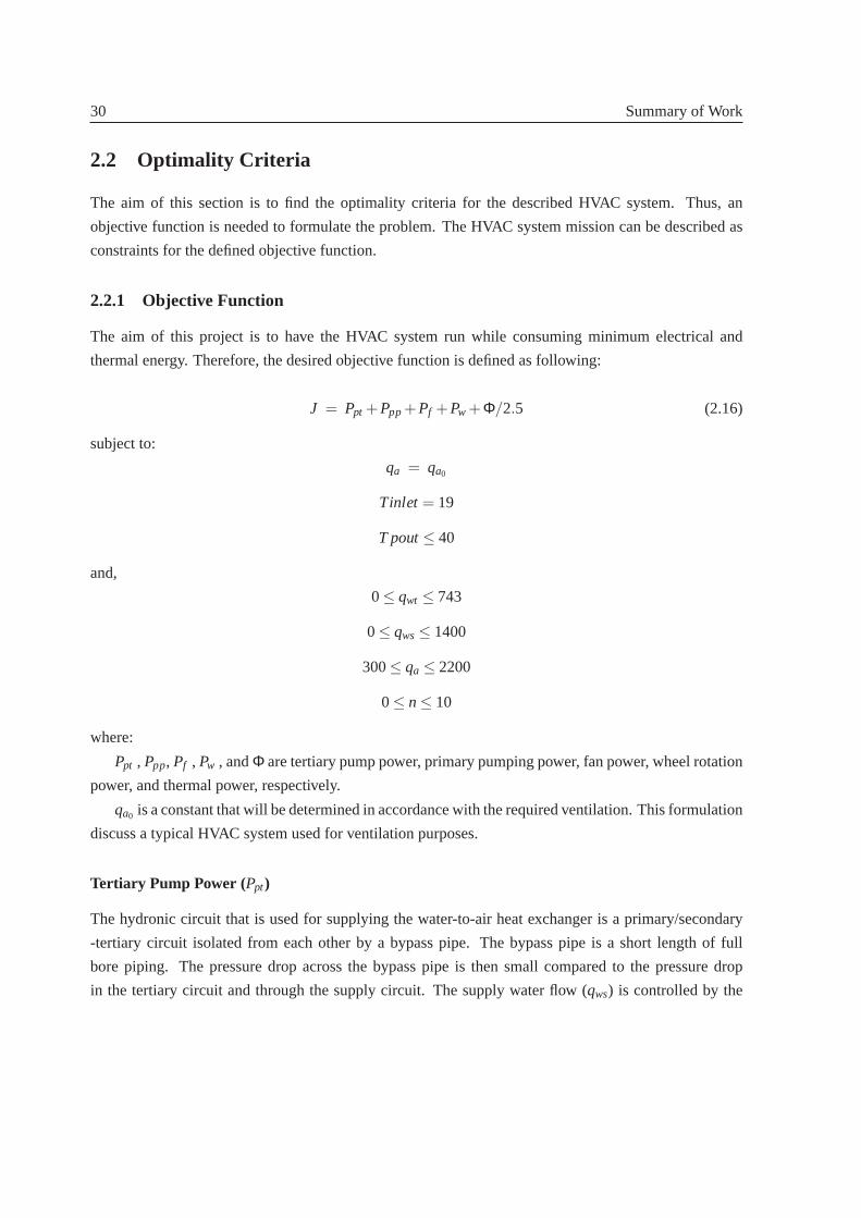
30 Summary of Work
2.2 Optimality Criteria
The aim of this section is to find the optimality criteria for the described HVAC system. Thus, an
objective function is needed to formulate the problem. The HVAC system missioncan be described as
constraints for the defined objective function.
2.2.1 Objective Function
The aim of this project is to have the HVAC system run while consuming minimum electrical and
thermal energy. Therefore, the desired objective function is defined as following:
J = Ppt +Ppp+Pf +Pw +Φ/2.5 (2.16)
subject to:
qa = qa0
Tinlet = 19
T pout≤ 40
and,
0≤ qwt ≤ 743
0≤ qws≤ 1400
300≤ qa ≤ 2200
0≤ n≤ 10
where:
Ppt , Ppp, Pf , Pw , andΦ are tertiary pump power, primary pumping power, fan power, wheel rotation
power, and thermal power, respectively.
qa0 is a constant that will be determined in accordance with the required ventilation. This formulation
discuss a typical HVAC system used for ventilation purposes.
Tertiary Pump Power (Ppt)
The hydronic circuit that is used for supplying the water-to-air heat exchanger is a primary/secondary
-tertiary circuit isolated from each other by a bypass pipe. The bypass pipe is a short length of full
bore piping. The pressure drop across the bypass pipe is then small compared to the pressure drop
in the tertiary circuit and through the supply circuit. The supply water flow (qws) is controlled by the

2.2 Optimality Criteria 31
Figure 2.8: Tertiary pump power vsqwt
motorized primary/secondary valve. A variable speed pump and a valve is installed in the tertiary circuit.
The tertiary valve is used to set the desired maximum flow rate through the variable speed pump. By
changing the speed of the tertiary pump, it is possible to sweep the interval between 330 (l/h) and 743
(l/h) for the tertiary water flow (qwt). If the tertiary water flow has to be less than 330 (l/h), the pump will
be pulsed. Fig. 2.8 illustrates power of the tertiary pump as a function ofqwt. This curve is approximated
by the following polynomial:
Ppt = Ap q3wt +Bp q2
wt +Cp qwt +Dp (2.17)
where:Ap = 5.1873·10−7[1/(lit /h)3] Bp = −6.4260·10−4[1/(lit /h)2]
Cp = 3.2906·10−1[1/(lit /h)] Dp = −48.8641
When the pump is pulse width modulated, it is assumed that the power of the pump is the duty cycle
fraction of the pump power while it is running at its minimum speed, i.e. it is proportional to the pump
working period.
Primary Pumping Power(Ppp)
The primary/secondary pumping power has to be measured implicitly because there is no direct access
to the primary/secondary pump. Therefore, it is supposed that the efficiency of the pump in convert-
ing electrical power to hydraulic power is 50%. The curve indicating required pressure drop versus
primary/secondary water flow (qws) is shown in Fig. 2.9. A second order polynomial is used to repre-
sent this curve. As we know, multiplying water flow by head results in hydraulic power. So, primary
pumping power can be expressed as follows:
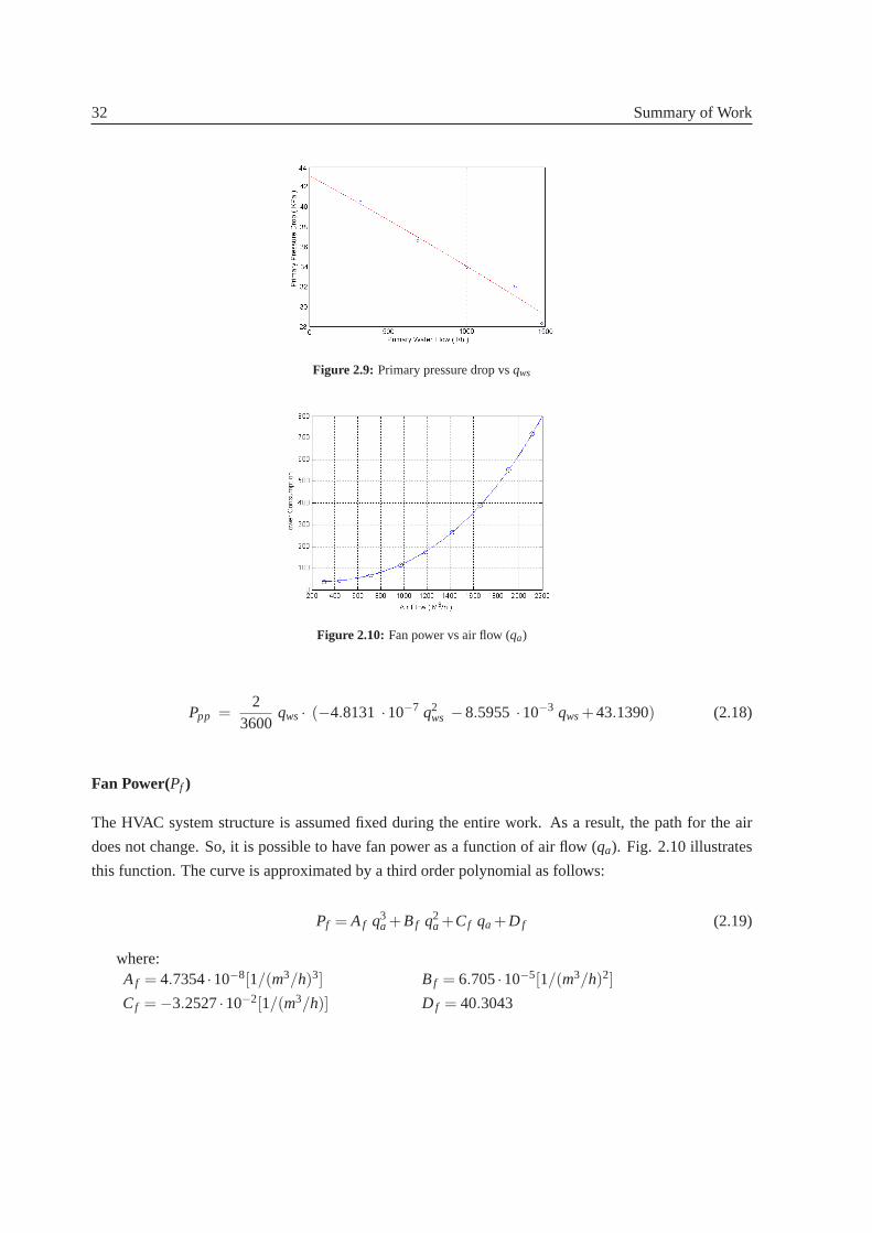
32 Summary of Work
Figure 2.9: Primary pressure drop vsqws
Figure 2.10: Fan power vs air flow (qa)
Ppp =2
3600qws· (−4.8131 ·10−7 q2
ws −8.5955 ·10−3 qws+43.1390) (2.18)
Fan Power(Pf )
The HVAC system structure is assumed fixed during the entire work. As a result, the path for the air
does not change. So, it is possible to have fan power as a function of airflow (qa). Fig. 2.10 illustrates
this function. The curve is approximated by a third order polynomial as follows:
Pf = Af q3a +Bf q2
a +Cf qa +D f (2.19)
where:Af = 4.7354·10−8[1/(m3/h)3] Bf = 6.705·10−5[1/(m3/h)2]
Cf = −3.2527·10−2[1/(m3/h)] D f = 40.3043

2.2 Optimality Criteria 33
Figure 2.11: Wheel power consumption vsn
Wheel Rotation Power(Pw)
The electrical power input to the wheel as a function of rotation speed of the wheel is sketched in Fig.
2.11. The step change in the figure is due to the frequency converter used to control rotation speed of
the wheel.
As Fig. 2.11 reveals, it is feasible to assume that the electrical power of the wheel is composed of
three parts:
Pw = 23.5 W 10 rpm≥ n > 2.5 rpm (1≥ wr f > 0.9)
Pw = 13 W 2.5 rpm≥ n > 0 rpm (0.9≥ wr f > 0)
Pw = 0 W n= 0 rpm (wr f = 0) (2.20)
Thermal Power (Φ)
Φ is the thermal power that is being used by the water-to-air heat exchanger:
Φ = ρw qwt Cpw (Twin−Twout) (2.21)
In steady state conditions:
ρw qwt Cpw (Twin−Twout) = ρa qa Cpa (Tinlet−TE22) (2.22)
According to the definitions, we have:
Tinlet = TE22+ηt1 (Twin−TE22) (2.23)
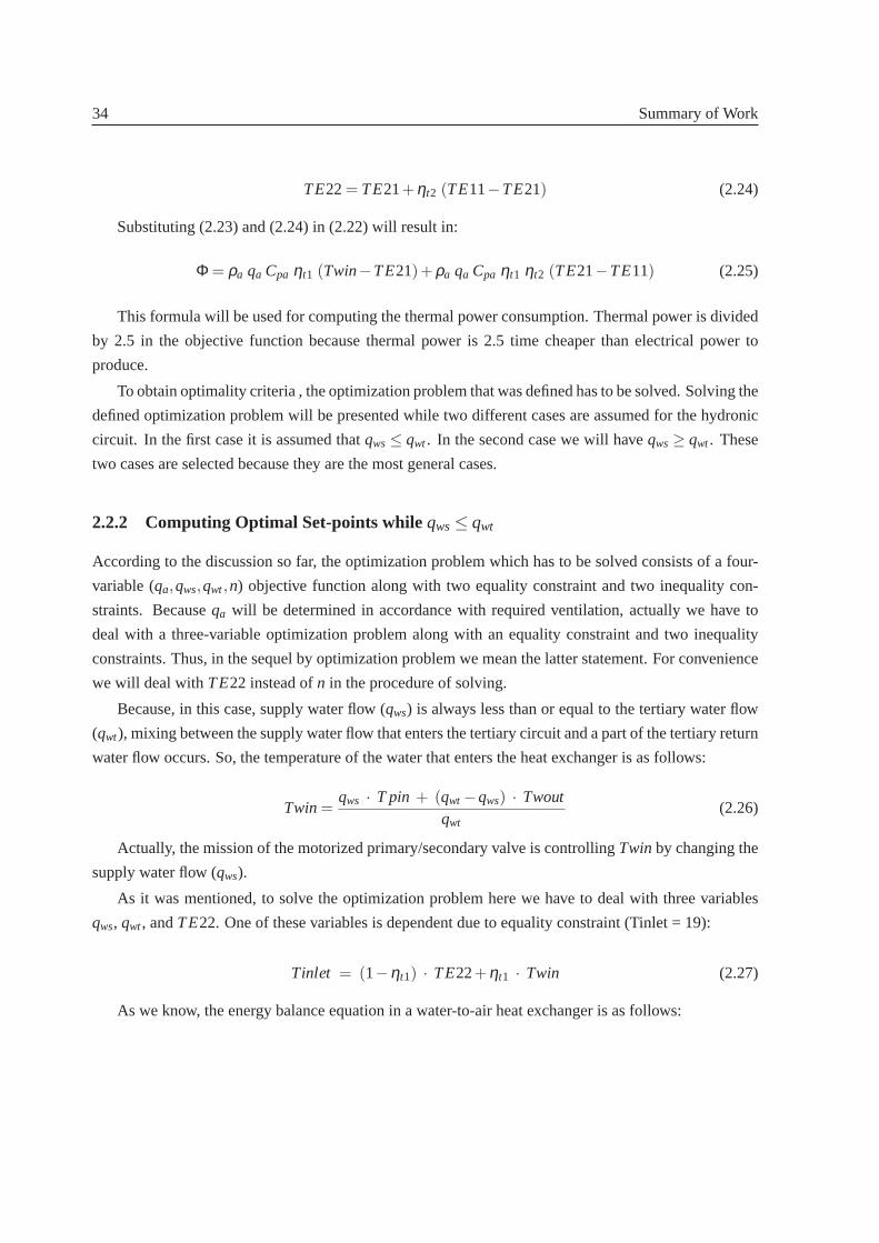
34 Summary of Work
TE22= TE21+ηt2 (TE11−TE21) (2.24)
Substituting (2.23) and (2.24) in (2.22) will result in:
Φ = ρa qa Cpa ηt1 (Twin−TE21)+ρa qa Cpa ηt1 ηt2 (TE21−TE11) (2.25)
This formula will be used for computing the thermal power consumption. Thermal power is divided
by 2.5 in the objective function because thermal power is 2.5 time cheaper thanelectrical power to
produce.
To obtain optimality criteria , the optimization problem that was defined has to be solved. Solving the
defined optimization problem will be presented while two different cases areassumed for the hydronic
circuit. In the first case it is assumed thatqws≤ qwt. In the second case we will haveqws≥ qwt. These
two cases are selected because they are the most general cases.
2.2.2 Computing Optimal Set-points whileqws≤ qwt
According to the discussion so far, the optimization problem which has to be solved consists of a four-
variable (qa,qws,qwt,n) objective function along with two equality constraint and two inequality con-
straints. Becauseqa will be determined in accordance with required ventilation, actually we have to
deal with a three-variable optimization problem along with an equality constraintand two inequality
constraints. Thus, in the sequel by optimization problem we mean the latter statement. For convenience
we will deal withTE22 instead ofn in the procedure of solving.
Because, in this case, supply water flow (qws) is always less than or equal to the tertiary water flow
(qwt), mixing between the supply water flow that enters the tertiary circuit and a part of the tertiary return
water flow occurs. So, the temperature of the water that enters the heat exchanger is as follows:
Twin=qws · T pin + (qwt −qws) · Twout
qwt(2.26)
Actually, the mission of the motorized primary/secondary valve is controllingTwinby changing the
supply water flow (qws).
As it was mentioned, to solve the optimization problem here we have to deal with three variables
qws, qwt, andTE22. One of these variables is dependent due to equality constraint (Tinlet= 19):
Tinlet = (1−ηt1) · TE22+ηt1 · Twin (2.27)
As we know, the energy balance equation in a water-to-air heat exchanger is as follows:

2.2 Optimality Criteria 35
ρw qwt Cpw (Twin−Twout) = ρa qa Cpa (Tinlet−TE22) (2.28)
Substituting the two recent equations in equation (2.26) will result in a formula for qws versusqwt
andTE22 :
qws =k ηt1 qwt (19−TE22)
ηt1qwt(T pin−TE22)+(qwt −kηt1)(TE22−19)(2.29)
Also, in this caseqws≤ qwt; Therefore, substituting equation (2.29) in the recent inequality results
in an inequality as following:
TE22≥ 19−T pin ηt1
1−ηt1(2.30)
Combining equations (2.27) and (2.28) results in a formula forTwout :
Twout=19qwt +TE22(−qwt +ηt1qwt +kηt1)−19kηt1
ηt1qwt(2.31)
In this case,Twout is equal toT pout because the supply water flow is less than or equal to the
tertiary water flow. Thus, the inequality constraint (T pout≤ 40) can be translated into the following
inequality:
(−qwt +ηt1qwt +kηt1) TE22≤ 40ηt1qwt +19kηt1−19qwt (2.32)
Finally, the optimization problem transferred to an objective function of two variables (qwt and
TE22) with two inequality constraints (inequalities (2.30) and (2.32)). The typical feasible region of
this optimization problem is shown in Fig. 2.12 (assumingTE21= −12, T pin= 80 andqa = 2104.9
). Then optimal set-points in different conditions as a result of solving the optimization problem have
been derived.
2.2.3 Computing Optimal Set-points whileqws≥ qwt
We have to deal with a three-variable optimization problem along with an equality constraint and two
inequality constraints again. The only difference is the fact that supply water flow is greater than or
equal to tertiary water flow. The impact of keeping supply water flow higherthan or equal to the tertiary
water flow on the system is that the supply tertiary water flow to the water-to-airheat exchanger will not
be mixed water. So,Twin will be equal to theT pin. Actually, water mixing occur between the return
36 Summary of Work
Figure 2.12: Feasible region whileqws≤ qwt ( TE21= −12,T pin= 80 andqa = 2104.9 )
tertiary water flow (qws) and the hot water passes the balance pipe (qws−qwt). Therefore, we have:
T pout=qwt · Twout+(qws−qwt) · T pin
qws(2.33)
According to the equality constraint (Tinlet = 19) and the fact thatTwin is always equal toT pin, it
is possible to haveTE22 as a function ofqwt:
TE22=19−T pin ηt1
1−ηt1(2.34)
Substituting equations (2.28) and (2.34) in equation (2.33) will result in the desired formula for
T pout:
T pout=−(T pin−19) k ηt1 +T pin qws−T pin ηt1 qws
(1−ηt1) qws(2.35)
Using the recent formula forT pout, the inequality constraint (T pout≤ 40) can be translated into
the following inequality:
qws≤(T pin−19) k ηt1
(T pin − 40) (1−ηt1)(2.36)
To summarize, the optimization problem transferred to an objective function oftwo variables (qwt
andqws) with two inequality constraint (inequality (2.36) andqws≥ qwt). The typical feasible region in
this case is sketched in Fig. 2.13 (supposedTE21= −30,T pin= 60 andqa = 1674.1 ).
Solving the optimization problem in this case results in the same optimal values obtained in the
previous case.
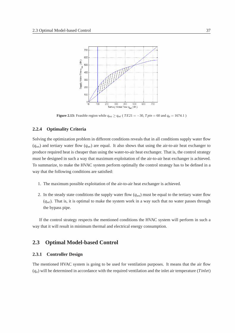
2.3 Optimal Model-based Control 37
Figure 2.13: Feasible region whileqws≥ qwt ( TE21= −30,T pin= 60 andqa = 1674.1 )
2.2.4 Optimality Criteria
Solving the optimization problem in different conditions reveals that in all conditions supply water flow
(qws) and tertiary water flow (qwt) are equal. It also shows that using the air-to-air heat exchanger to
produce required heat is cheaper than using the water-to-air heat exchanger. That is, the control strategy
must be designed in such a way that maximum exploitation of the air-to-air heat exchanger is achieved.
To summarize, to make the HVAC system perform optimally the control strategy has to be defined in a
way that the following conditions are satisfied:
1. The maximum possible exploitation of the air-to-air heat exchanger is achieved.
2. In the steady state conditions the supply water flow (qws) must be equal to the tertiary water flow
(qwt). That is, it is optimal to make the system work in a way such that no water passes through
the bypass pipe.
If the control strategy respects the mentioned conditions the HVAC system willperform in such a
way that it will result in minimum thermal and electrical energy consumption.
2.3 Optimal Model-based Control
2.3.1 Controller Design
The mentioned HVAC system is going to be used for ventilation purposes. It means that the air flow
(qa) will be determined in accordance with the required ventilation and the inlet air temperature (Tinlet)

38 Summary of Work
has to be kept at 19oC. So, the optimal controller task is to track the set-point for the inlet air tempera-
ture while satisfying the conditions that were described in the control strategy section to guarantee the
optimal performance of the system. The traditional way to design the control system that works in this
way is applying the two-layer hierarchical control system. The lower layerperforms direct regulatory
control, where the aim is to maintain selected process variables at their desired set-point values, and the
upper layer, known as the supervisory layer, has the task of determiningthe set-points of the regulatory
controllers to obtain optimal steady state performance.
Looking at the linear model that was developed before reveals that the HVAC system can be splitted
into two decoupled subsystems as follows:
[
T inlet
Twout
]
=
[
a4 a3
0 a1
]
·[
Tinlet
Twout
]
+
[
b3 b4
b1 b2
]
·[
mws
mwt
]
+
[
a5
a2
]
·TE22
y = [1 0] ·[
Tinlet
Twout
]
(2.37)
˙TE22= a6 ·TE22+b5 ·wr f (2.38)
It means that control of the HVAC system can be considered as control of the air-to-air heat ex-
changer and control of the water-to-air heat exchanger separately.It should be noted thatTE22 acts as
disturbance for the water-to-air heat exchanger in this new formulation.
If the set-point for temperature of the fresh air that leaves the wheel (TE22) is defined as the set-
point for temperature of the inlet air (19oC) we will be sure that the air-to-air heat exchanger has its
maximum contribution to warm up the fresh air. Thus, the first condition for optimality will be met. The
second condition for optimality can be included in the cost function that will be defined for the water-
to-air heat exchanger controller. Therefore, there is no need to design an explicit supervisory layer. The
block diagram of the HVAC system along with the new optimal control system is illustrated in Fig 2.14.
2.3.2 Comparison of New Control System with Current ControlSystem
Typical industrial HVAC control system is illustrated in Fig 2.15. As can be seen, two controllers, one
to control the wheel and another one to control the water-to-air heat exchanger, which communicate to
each other through some if-then rules are used. The main goal of this communication is to have the
maximum exploitation of the wheel. So, current controllers respect the firstoptimality criterion but it
has nothing to do to satisfy the second optimality condition. To summarize, we can say that the new
control system is simpler because those two controllers are independent and the new control system is
working in an optimal way. So, it meets all our expectations.

2.3 Optimal Model-based Control 39
Figure 2.14: New control system
Figure 2.15: Typical industrial HVAC control system
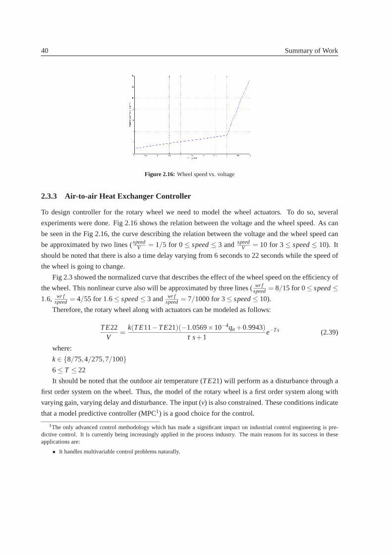
40 Summary of Work
Figure 2.16: Wheel speed vs. voltage
2.3.3 Air-to-air Heat Exchanger Controller
To design controller for the rotary wheel we need to model the wheel actuators. To do so, several
experiments were done. Fig 2.16 shows the relation between the voltage and the wheel speed. As can
be seen in the Fig 2.16, the curve describing the relation between the voltage and the wheel speed can
be approximated by two lines (speedV = 1/5 for 0≤ speed≤ 3 and speed
V = 10 for 3≤ speed≤ 10). It
should be noted that there is also a time delay varying from 6 seconds to 22 seconds while the speed of
the wheel is going to change.
Fig 2.3 showed the normalized curve that describes the effect of the wheel speed on the efficiency of
the wheel. This nonlinear curve also will be approximated by three lines (wr fspeed= 8/15 for 0≤ speed≤
1.6, wr fspeed= 4/55 for 1.6≤ speed≤ 3 and wr f
speed= 7/1000 for 3≤ speed≤ 10).
Therefore, the rotary wheel along with actuators can be modeled as follows:
TE22V
=k(TE11−TE21)(−1.0569×10⁻⁴qa +0.9943)
τ s+1e−Ts (2.39)
where:
k∈ {8/75,4/275,7/100}6≤ T ≤ 22
It should be noted that the outdoor air temperature (TE21) will perform as a disturbance through a
first order system on the wheel. Thus, the model of the rotary wheel is a first order system along with
varying gain, varying delay and disturbance. The input (v) is also constrained. These conditions indicate
that a model predictive controller (MPC1) is a good choice for the control.
1The only advanced control methodology which has made a significant impact on industrial control engineering is pre-dictive control. It is currently being increasingly applied in the process industry. The main reasons for its success in theseapplications are:
• It handles multivariable control problems naturally.

2.3 Optimal Model-based Control 41
The control problem can be formulated as follows:
minv[k/k]
6
∑i=1
‖TE22[k+ i/k]−19‖2I(i)
subject to:
0≤ v[k/k] ≤ 10 (2.40)
The sampling time for the controller is supposed to be 15 seconds. The gain and delay for the
internal model of the MPC controller are 1.7 (maximum gain) and 22 (maximum delay), respectively.
2.3.4 Water-to-air Heat Exchanger Controller
To control the water-to-air heat exchanger we have to deal with constrained inputs. We also have to
penalize inputs in a way that in the steady state conditions no water passes through the the bypass pipe.
So, again MPC is a good candidate for this control problem. To design the MPC controller we need to
modify equation (2.37) as follows:
[
T inlet
Twout
]
=
[
a4 a3
0 a1
]
·[
Tinlet
Twout
]
+
[
b3 +b4 b4
b1 +b2 b2
]
·[
mws
mwt − mws
]
+
[
a5
a2
]
·TE22
y = [1 0] ·[
Tinlet
Twout
]
(2.41)
where:a1 = −0.0352 a2 = 0.0310 a3 = 0.0564
a4 = −0.5961 a5 = 0.4833 b1 = 17232
b2 = 46628 b3 = 227635 b4 = −199119Thus, the control problem can be described as follows:
minmws[k+i/k],mwt[k+i/k]−mws[k+i/k]
6
∑i=1
‖Tinlet[k+ i/k]−19‖2I(i)
• It can take account of acctuator limitations.
• It allows operation closer to constraints (compared with conventional control), which frequently leads to more profitableoperation. Remarkably short pay-back periods have been reported.
• Control update rates are relatively low in these applications, so that there isplenty of time for the necessary on-linecomputations.

42 Summary of Work
+1
∑i=0
‖mwt[k+ i/k]− mws[k+ i/k]‖2(0.2×I(i))
subject to:
0≤ mws[k+ i/k],mwt[k+ i/k]− mws[k+ i/k] ≤ 350 (2.42)
The first term in the cost function represents the set-point tracking and the second term is the repre-
sentative of the optimality condition (no flow in the bypass pipe). Unfortunately, the controller does not
have a good performance because of the oscillations around the set-point. To deal with this problem the
two following candidates are proposed:
• First Candidate:
minmws[k+i/k],mwt[k+i/k]−mws[k+i/k]
6
∑i=1
‖Tinlet[k+ i/k]−19‖2I(i)
+1
∑i=0
‖mwt[k+ i/k]− mws[k+ i/k]‖2(0.2×I(i)) +
1
∑i=0
‖mws[k+ i/k]‖2(0.1×I(i))
subject to:
0≤ mws[k+ i/k],mwt[k+ i/k]− mws[k+ i/k] ≤ 350 (2.43)
• Second Candidate:
minmws[k+i/k],mwt[k+i/k]−mws[k+i/k]
6
∑i=1
‖Tinlet[k+ i/k]−19‖2I(i)
+1
∑i=0
‖mwt[k+ i/k]− mws[k+ i/k]‖2(0.2×I(i)) +
1
∑i=0
‖∆mws[k+ i/k]‖2(0.1×I(i))
subject to:
0≤ mws[k+ i/k],mwt[k+ i/k]− mws[k+ i/k] ≤ 350 (2.44)
Both candidates show satisfactory results.
Analyzing of the results should be divided into two separate issues as follows:
• The first issue deals with actuator modeling of the water-to-air heat exchanger ( primary valve
which controls the supply water flowqws and the variable speed pump which has control over the
tertiary water flowqwt ).
The primary valve modeled as a simple gain. Due to the sample time of 15 seconds thedynamic
behavior and the delay of the valve is not important.
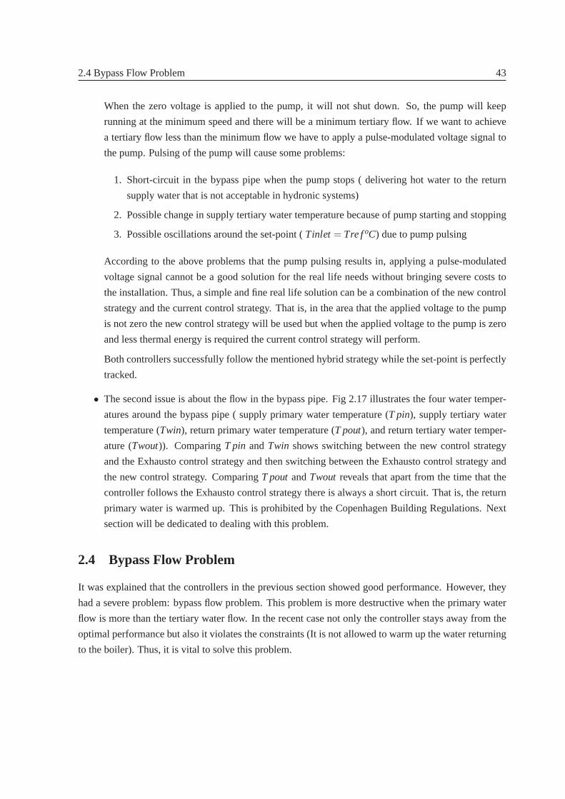
2.4 Bypass Flow Problem 43
When the zero voltage is applied to the pump, it will not shut down. So, the pumpwill keep
running at the minimum speed and there will be a minimum tertiary flow. If we want toachieve
a tertiary flow less than the minimum flow we have to apply a pulse-modulated voltagesignal to
the pump. Pulsing of the pump will cause some problems:
1. Short-circuit in the bypass pipe when the pump stops ( delivering hot water to the return
supply water that is not acceptable in hydronic systems)
2. Possible change in supply tertiary water temperature because of pump starting and stopping
3. Possible oscillations around the set-point (Tinlet = Tre foC) due to pump pulsing
According to the above problems that the pump pulsing results in, applying a pulse-modulated
voltage signal cannot be a good solution for the real life needs without bringing severe costs to
the installation. Thus, a simple and fine real life solution can be a combination of the new control
strategy and the current control strategy. That is, in the area that the applied voltage to the pump
is not zero the new control strategy will be used but when the applied voltage to the pump is zero
and less thermal energy is required the current control strategy will perform.
Both controllers successfully follow the mentioned hybrid strategy while the set-point is perfectly
tracked.
• The second issue is about the flow in the bypass pipe. Fig 2.17 illustrates the four water temper-
atures around the bypass pipe ( supply primary water temperature (T pin), supply tertiary water
temperature (Twin), return primary water temperature (T pout), and return tertiary water temper-
ature (Twout)). ComparingT pin andTwin shows switching between the new control strategy
and the Exhausto control strategy and then switching between the Exhaustocontrol strategy and
the new control strategy. ComparingT pout andTwout reveals that apart from the time that the
controller follows the Exhausto control strategy there is always a short circuit. That is, the return
primary water is warmed up. This is prohibited by the Copenhagen Building Regulations. Next
section will be dedicated to dealing with this problem.
2.4 Bypass Flow Problem
It was explained that the controllers in the previous section showed good performance. However, they
had a severe problem: bypass flow problem. This problem is more destructive when the primary water
flow is more than the tertiary water flow. In the recent case not only the controller stays away from the
optimal performance but also it violates the constraints (It is not allowed to warm up the water returning
to the boiler). Thus, it is vital to solve this problem.
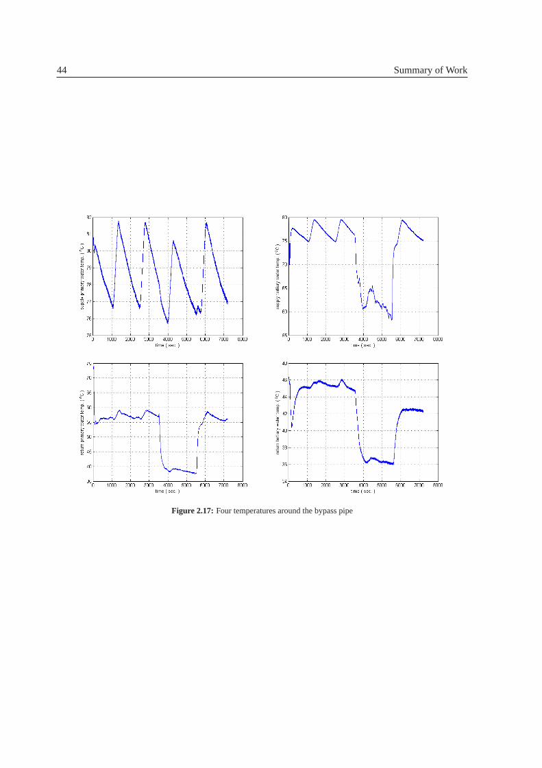
44 Summary of Work
Figure 2.17: Four temperatures around the bypass pipe
2.4 Bypass Flow Problem 45
2.4.1 Measuring The Bypass Flow
It is not reasonable to measure the bypass flow through a flow-meter in real life. However, we can
measure the bypass flow implicitly through thermocouples. This way of measurement is acceptable due
to the cheap price of thermocouples.
First we have to define the bypass flow as a quantity with direction. Consequently, we will always
treat bypass flow as a difference between the primary water flow and the tertiary water flow (qws−qwt).
That is, when the primary flow is greater than the tertiary flow the bypass flowwill have a positive sign
and when the primary flow is less than the tertiary flow a negative sign will accompany the bypass flow.
We consider two cases now:
• Negative Bypass Flow
When there is a negative bypass flow the return primary water temperature (T pout) and the re-
turn tertiary water temperature (Twout) are equal. Although, the supply primary water tempera-
ture (T pin) is always greater than the supply tertiary water temperature (Twin). The difference
between two recent temperatures is proportional to the ratio of the primary water flow and the
tertiary water flow.
The energy balance equation for the supply water side will result in the following equation:
(qwt −qws) Twout + qws T pin = qwt Twin (2.45)
By rearranging the above equation we will have:
qwt
qws=
T pin − TwoutTwin − Twout
(2.46)
We subtract 1 from both side of the equation. So,
qwt
qws−1 =
T pin − TwinTwin − Twout
(2.47)
• Positive Bypass Flow
The story of the negative bypass flow is similar to the story of the positive bypass flow. Thus,
When there is a positive bypass flow the supply primary water temperature (T pin) and the sup-
ply tertiary water temperature(Twin) are equal. Although, the return primary water temperature
(T pout) is always greater than the supply tertiary water temperature (Twout). Again, the differ-
ence between two recent temperatures is proportional to the ratio of the primary water flow and
the tertiary water flow.

46 Summary of Work
The energy balance equation for the return water side will result in the following equation:
(qws−qwt) T pin + qwt Twout = qws T pout (2.48)
By rearranging the above equation we will have:
qwt
qws=
T pin − T poutT pin − Twout
(2.49)
We subtract 1 from both sides of the equation. So,
qwt
qws−1 =
Twout − T poutT pin − Twout
(2.50)
The recent equation can be rewritten as
qwt
qws−1 =
Twout − T poutTwin − Twout
(2.51)
According to the above discussion and combining equations 2.47 and 2.51 wewill have:
qwt
qws−1 =
(T pin − Twin) + (Twout − T pout)Twin − Twout
(2.52)
or equivalently:
qwt
qws−1 =
(T pin + Twout) − (Twin + T pout)Twin − Twout
(2.53)
So, by measuring the four temperatures (T pin, T pout, Twin, andTwout) and using the recent for-
mula there will be enough information for a controller to make the bypass flow approach zero.
2.4.2 Slow Bypass Compensation
As it was mentioned before, it is vital to control the bypass flow. In the previous section designing
controllers without considering this problem was discussed. Fig 2.18 introduces a new structure for
the control system. In the new structure to design the MPC controller the same procedures as it was
explained have to be followed. That is, the MPC controller is the controller from the previous section.
To deal with the bypass problem, a bypass compensator has been added tothe control system. The
bypass compensator is much slower than the main controller. So, the main controller and the bypass
compensator are decoupled in time domain.

2.4 Bypass Flow Problem 47
Figure 2.18: MPC controller along with bypass compensator
2.4.3 Simplified Optimal Control System Scheme
Fig 2.19 shows the simplified optimal control structure. One PI controller determines the primary water
flow (qws) through the information from the inlet temperature feedback. To design thiscontroller the
linearized model from the primary water flow to the inlet temperature has been used. Tertiary water flow
(qwt) is controlled by a PI controller which tries to keep the tertiary water flow closeto the primary water
flow. The variable speed pump acts as an actuator to control the tertiary water flow. Because the variable
speed pump is much faster than the primary valve which acts as an actuator to control the primary water
flow, two controllers are decoupled in time domain again.
2.4.4 Optimal Solution when Applying Improperly Dimensioned Coil Applied
Fig. 2.20 shows the return primary water temperature while the simplified optimal controller was ap-
plied to the water-to-air heat exchanger. Considering the plot reveals that in some points the return
primary water temperature is higher than 40oC. It is so because of the inappropriate dimensioning of the
coil. The coil is designed for 60oC forward water temperature and 40oC return water temperature. Thus,
in some extreme situations the controller cannot keep the return water temperature less than 40oC while
controlling the inlet temperature. If it is not possible to apply a pump which is appropriately dimens-
sioned the remedy can be forcing the controllerC2 to mix more. It can be embedded in the simplified

48 Summary of Work
Figure 2.19: Simplified optimal control scheme
Figure 2.20: Return primary water temperature

2.4 Bypass Flow Problem 49
optimal controller as follows:
When the mixing happens the energy balance equation for the supply water side will result in the
following equation:
(qwt −qws) Twout + qws T pin = qwt Twin (2.54)
By rearranging the above equation we will have:
qwt
qws=
T pin − TwoutTwin − Twout
(2.55)
Now we need not to keep the primary water flow and tertiray water flow to meet the optimality
criteria. We have to mix more to lower the return primary water temperature. As a result, we subtract
1+x from both side of the equation:
qwt
qws− (1+x) =
T pin − TwinTwin − Twout
+α f1
Twin − Twout(2.56)
where
x = α f1Twin − Twout and f1 =
{
T pout−40 i f T pout> 40
0 i f T pout≤ 40For the return water side there is no need of manipulation in the equations. Therefore, the feedback
can be introduced as following:
qwt
qws− (1+x) =
(T pin + Twout) − (Twin + T pout)+α f1Twin − Twout
(2.57)
We expect that in some extreme situations even when the pump runs in full speed still having the
return primary water temperature less than 40oC is impossible.
Fig. 2.21 shows the optimal trajectory of the controller when the coil is not selected properly:
• Region 1 represents the situation that the variable speed pump runs at its minimumspeed and to
control the inlet temperature the controller has to follow the mixing strategy.
• Region 2 is the representative of the situation that the controller follow the optimality critoria.
• Region 3 follows when the return primary water temperature exceeds 40oC. Thus, the controller
starts to mix more to keep the return primary water temperature less than 40oC.
• Region 4 happens when the tertiary variable speed pump needs to run at its full speed to lower
the return primary water temperature. We can expect that the return primarywater temperature
sometimes goes above 40oC in this region.
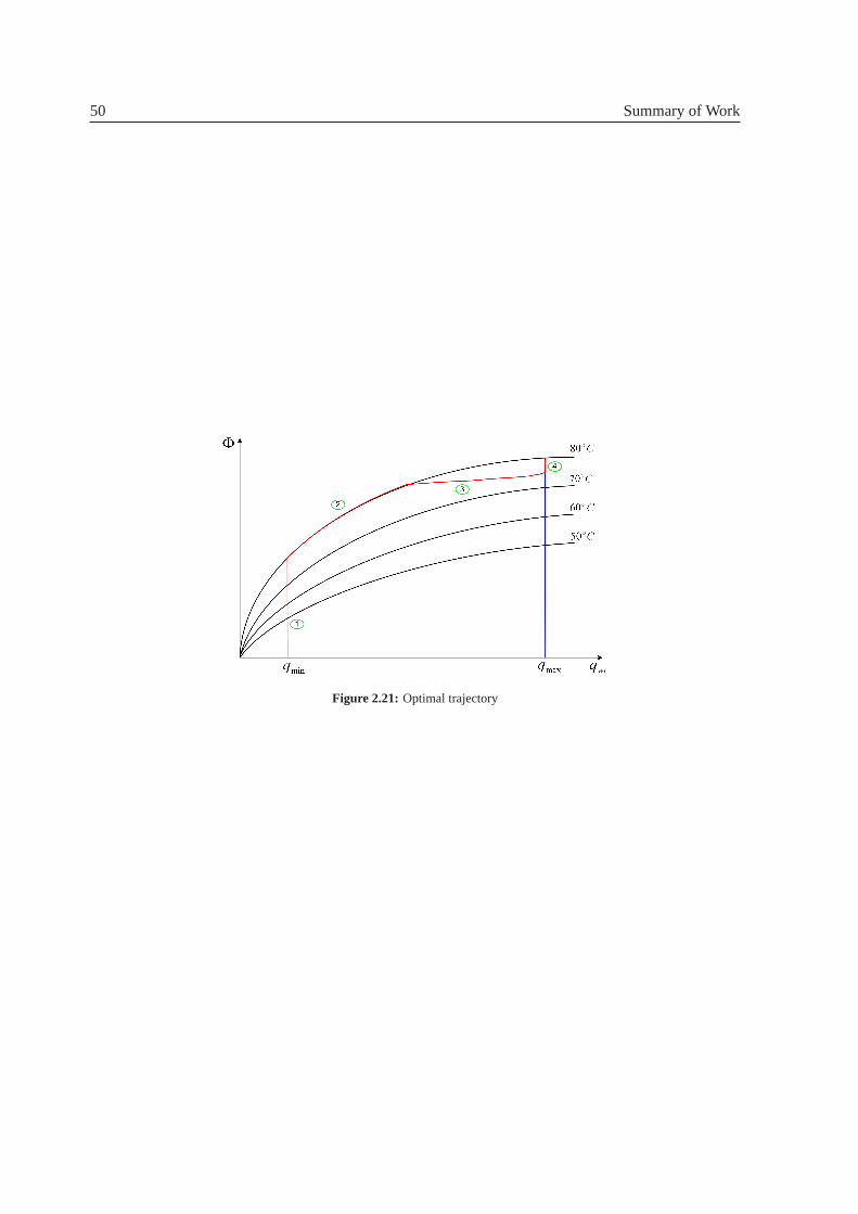
50 Summary of Work
Figure 2.21: Optimal trajectory

Chapter 3
Conclusions and Future Work
3.1 Conclusions
The goal of this project was to deal with optimal model-based control of a HVAC system. The difference
between the HVAC system which was applied in this project with other HVAC system was using variable
water flow through the coil. As a result in the new HVAC system the water flow through the coil could
be manipulated as a control variable. It resulted in less energy consumptionby the pump which supplied
the coil.
HVAC systems are in steady state conditions more than 95% of their operating time.Thus, the
optimal control strategy that we chose in this project was based on the static model of the HVAC system.
The objective function was composed of the electrical power for different components, encompassing
fans, primary/secondary pump, tertiary pump, and air-to-air heat exchanger wheel; and a fraction of
thermal power used by the HVAC system. The objectives that had to be achieved by the HVAC system
appeared as constraints in the optimization problem. Solving the optimization problem resulted in two
optimality criteria:
• The maximum advantage of the rotary wheel had to be taken. That is, the water-to-air heat ex-
changer has to be applied for warming up the fresh air when the rotary wheel is not capable of
doing that on its own.
• No water should pass through the bypass pipe (the pipe which is used to decouple the tertiary
hydronic circuit from the supply (primary/secondary) hydronic circuit).
Then the optimal model-based controller was designed to follow the objectivesof the HVAC system
while the optimality criteria were satisfied. Lack of good models from control point of view in the
literatures made us to develop our own models for the HVAC system:
51
52 Conclusions and Future Work
• We extended the nonlinear model which had proposed by Underwood andCrawford for the coil
to model the water-to-air heat exchanger.
• For model-based control of the rotary heat recovery wheel we needed a model that described the
relation between the rotation speed of the wheel and the temperature of the fresh air which was
leaving the heat exchanger. We estimated the steady state gain by benefiting from the results of
the static analysis part. Then we discussed that a first order model could capture the dynamic
behavior of the rotary heat recovery wheel. So, totally the model would bea first order system
along with a variable gain.
The next step we took was analyzing the HVAC system model and designing thecontroller. Thus,
the HVAC system was broken into two independent subsystems. Utilizing the excellent features of
the model predictive control (MPC) and introducing an internal feedback in the system the optimality
criteria were met.
To deal with the problem of the bypass flow which came up during the design of the controller for the
HVAC system led us to a simple optimal control structure for the HVAC system. Finally, we addressed
some pratical issues.
3.2 Future Work
In Denmark radiators are used as a source for warming up the room and HVAC systems are applied as a
tool for desired ventilation. In future work including the interaction betweenthe radiators and the HVAC
system in developing the optimal control strategy can lead to more comprehensive optimality criteria. It
means that HVAC system can also get involved in supplying heat to the room and the optimality criteria
must determine the HVAC system’s share in that task.
Another interesting point can be inclusion of different HVAC modules whichare supplied by the
same boiler in the control problem. There are several interesting control problems which have to be
solved in this configuration. One of the most important problems in this case is theoscillation problem.
The problem stems from the nonlinear behavior of HVAC systems. Therefore, dealing with this problem
requires sophisticated modeling and applying advanced control techniques.
Sometimes during the start-up or low heat demand time the heat coil can get frosted and it will cause
damages to the system. As a result, developing an anti-frost control for thesystem is neccessary. Then,
integration of the anti-frost control algorithm and the optimal control algorithm will be a very interesting
problem.
In this project we focused on the heating problem. In future work includingthe cooling problem as
a task for the HVAC system and extending the optimality criteria for that system also looks a charming
problem as the chillers need some specific cares.

Chapter 4
Optimal Set-point Synthesis in HVAC
Systems
M. Komareji1 , J. Stoustrup2 , H. Rasmussen3 , N. Bidstrup4 , P. Svendsen5 , F. Nielsen6
Abstract
This paper presents optimal set-point synthesis for a heating, ventilating, and air-conditioning (HVAC)
system. This HVAC system is made of two heat exchangers: an air-to-air heat exchanger and a water-to-
air heat exchanger. The objective function is composed of the electricalpower for different components,
encompassing fans, primary/secondary pump, tertiary pump, and air-to-air heat exchanger wheel; and a
fraction of thermal power used by the HVAC system. The goals that have to be achieved by the HVAC
system appear as constraints in the optimization problem. To solve the optimization problem, a steady
state model of the HVAC system is derived while different supplying hydronic circuits are studied for the
water-to-air heat exchanger. Finally, the optimal set-points and the optimal supplying hydronic circuit
are resulted.
1Mohammad Komareji is a PhD student in The Department of Control and Automation, Institute of Electronic Systems,Aalborg University, Aalborg, Denmark;[email protected]
2Jakob Stoustrup is with Aalborg University as a Professsor in The Department of Control and Automation;[email protected]
3Henrik Rasmussen is with Aalborg University as an Associate Professorin The Department of Control and Automation;[email protected]
4Niels Bidstrup is with Grundfos Management A/S as a Chief Engineer, Ph.D.; [email protected] Svendsen is with Danish Technological Institute (DTI) as a Project Manager;
[email protected] Nielsen is with Exhausto A/S as a Project Manager;[email protected]
53

54 Optimal Set-point Synthesis in HVAC Systems
4.1 Introduction
Classical HVAC control techniques such as the ON/OFF controllers (thermostats) and the proportional-
integral-derivative (PID) controllers are still very popular because of their low cost. However, in the
long run, these controllers are expensive because they operate at a non-optimal efficiency. So, there is
a high potential to apply advanced control methods to save large amount of energy. For example, by
optimal control of HVAC systems almost 100 GWh energy can be saved yearly in Denmark (five million
inhabitants) [2].
A common method used to maintain an industrial plant at its optimal operating conditionis to
calculate optimal values of feedback controller set-points, employing a steady-state mathematical model
of the process [3], [4]. Steady-state optimization of an industrial process often considers that the overall
control is performed within a two-layer hierarchical structure. The lowerlayer performs direct regulatory
control, where the aim is to maintain selected process variables at their desired set-point values, and the
upper layer, known as the supervisory layer, has the task of detreminingthe set-points of the regulatory
controllers to obtain optimal steady-state performance.
This kind of two layer control strategy has been applied before to a coolingsystem and a refriger-
ation system and has shown great results [5], [6]. Implementing the supervisory layer through genetic
algorithms in the cooling system case showed saving energy by 19.5%. In therefrigeration system case
it was proved that by using this control configuration it was possible to derive the set-points close to the
optimum and thus reduce the energy consumption with up to 20%.
In this paper, the supervisory layer of the overall control of a HVAC system is considered. In Section
4.2, the HVAC system used in analysis is described. Section 4.3 presents formulation of the problem.
Determination of optimal set-points through solving the defined problem is presented in Section 4.4.
Section 4.5 presents conclusions and final comments.
4.2 The HVAC System Description
The HVAC system that will be considered consists of two heat exchangers: an air-to-air heat exchanger
and a water-to-air heat exchanger. In this section the temperature efficiency of these two heat exchangers,
which can be used as a steady state model of heat exchangers, will be described.
4.2.1 The Air-to-air Heat Exchanger
The air-to-air heat exchanger is a rotary heat exchanger in aluminium, withlow pressure loss (shown in
Fig. 4.1). The rotor control comprises a gear motor with frequency converter. Two fans are installed to
produce the desired inlet and outlet air flow. Here, it is supposed that theratio of the supply air flow to

4.2 The HVAC System Description 55
Figure 4.1: The Air-to-air heat exchanger scheme
Figure 4.2: Dependency ofηt2 onqa while n=10 rpm;qsa andqr
a represent supply air flow and return air flow, respectively.
the return air flow is one. Therefore,ηt2 will be a function of air flow (qa) [7] , that is the same for both
supply and return air, and the rotation speed of the wheel (n).
In this context, results of testing the rotary heat exchanger that was performed according to European
Standard for laboratory testing of air-to-air heat recovery devices (EN 247, EN 305, EN 306, EN 307,
EN 308) will be used.This European Standard is intended to be used as a basis for testing heat recovery
devices for HVAC systems, which as specified in EN 247 consist of the heat exchanger itself installed in
a casing having the necessary air duct connecting elements and in some cases the fans and pumps, but
without any additional components of the HVAC system.
According to results of the test, it is possible to specifyηt2 as a multiplication of two functions. Fig.
4.2 and 4.3 illustrate these functions. Therefore,ηt2 can be described as following:
ηt2 = (−1.0569·10−4 qa +0.9943) ·wr f (n) (4.1)
4.2.2 The Water-to-air Heat Exchanger
The water-to-air heat exchanger is shown in Fig. 4.4. As can be seen, aprimary/secondary-tertiary
hydronic circuit supplies the heat exchanger with hot water. The air flowthat passes the hot coil is
controllable by changing the speed of the fan installed in the air-to-air heat exchanger.

56 Optimal Set-point Synthesis in HVAC Systems
Figure 4.3: Normalized dependency ofηt2 on n
Figure 4.4: The water-to-air heat exchanger scheme

4.3 Problem Formulation 57
Figure 4.5: Result of experiments on water-to-air heat exchanger
Here, temperature efficiency (ηt1) is a function of hot water flow (qwt) and air flow (qa). To obtain
this function several experiments were done. Results are illustrated in Fig. 4.5. Again, it is possible to
describeηt1 as a multiplication of two functions that the first one depends only on air flow (qa) and the
second one depends only on water flow (qwt):
ηt1 =1
0.3215(a q4
wt +b q3wt +c q2
wt +d qwt +e) · (A q3a +B q2
a +C qa +D) (4.2)
where:a = −5.399·10−12 A = 1.0665·10−10
b = 1.0733·10−8 B = −1.643·10−7
c = −7.887·10−6 C = −2.880·10−4
d = 2.7199·10−3 D = 0.6927
e= 8.3711·10−4
4.3 Problem Formulation
As it was mentioned, the aim of this paper is to find the optimal set-points for the described HVAC
system. Thus, an objective function is needed to formulate the problem. The HVAC system mission can
be described as constraints for the defined objective function.
58 Optimal Set-point Synthesis in HVAC Systems
4.3.1 Objective Function
The desired objective function is defined as following:
J = Ppt +Ppp+Pf +Pw +Φ/2.5 (4.3)
subject to:
qa = qa0
Tinlet = 19
T pout≤ 40
and,
0≤ qwt ≤ 743
0≤ qws≤ 1400
300≤ qa ≤ 2200
0≤ n≤ 10
where:
Ppt , Ppp, Pf , Pw , andΦ are tertiary pump power, primary pumping power, fan power, wheel rotation
power, and thermal power, respectively.
qa0 is a constant that will be determined in accordance with the required ventilation[8]. This formu-
lation discuss a typical HVAC system used for ventilation purposes.
4.3.2 Tertiary Pump Power (Ppt)
The hydronic circuit that is used for supplying the water-to-air heat exchanger is a primary or secondary
-tertiary circuit isolated from each other by a bypass pipe. The bypass pipe is a short lenghth of full
bore piping. The pressure drop across the bypass pipe is then small compared to the pressure drop
in the tertiary circuit and through the supply circuit [9]. The supply water flow (qws) is controlled by
the motorized primary/secondary valve. A variable speed pump and a valve isinstalled in the tertiary
circuit. The tertiary valve is used to set the desired maximum flow rate through the variable speed pump.
By changing the speed of the tertiary pump, it is possible to sweep the intervalbetween 330 (l/h) and
743 (l/h) for the tertiary water flow (qwt). If the tertiary water flow has to be less than 330 (l/h), the
pump will be pulsed. Fig. 4.6 illustrates power of the tertiary pump as a function of qwt. This curve is
approximated by the following polynomial:

4.3 Problem Formulation 59
Figure 4.6: Tertiary pump power vsqwt
Ppt = Ap q3wt +Bp q2
wt +Cp qwt +Dp (4.4)
where:
Ap = 5.1873·10−7 Bp = −6.4260·10−4
Cp = 3.2906·10−1 Dp = −48.8641
When the pump is pulse width modulated, it is assumed that the power of the pump is the duty cycle
fraction of the pump power while it is running at its minimum speed, i.e. it is proportional to the pump
working period.
4.3.3 Primary Pumping Power(Ppp)
The primary/secondary pumping power has to be measured implicitly because there is no direct access
to the primary/secondary pump. Therefore, it is supposed that the efficiency of the pump in convert-
ing electrical power to hydraulic power is 50%. The curve indicating required pressure drop versus
primary/secondary water flow (qws) is shown in Fig. 4.7. A second order polynomial is used to repre-
sent this curve. As we know, multiplying water flow by head results in hydraulic power. So, primary
pumping power can be expressed as follows:
Ppp =2
3600qws· (−4.8131 ·10−7 q2
ws −8.5955 ·10−3 qws+43.1390) (4.5)
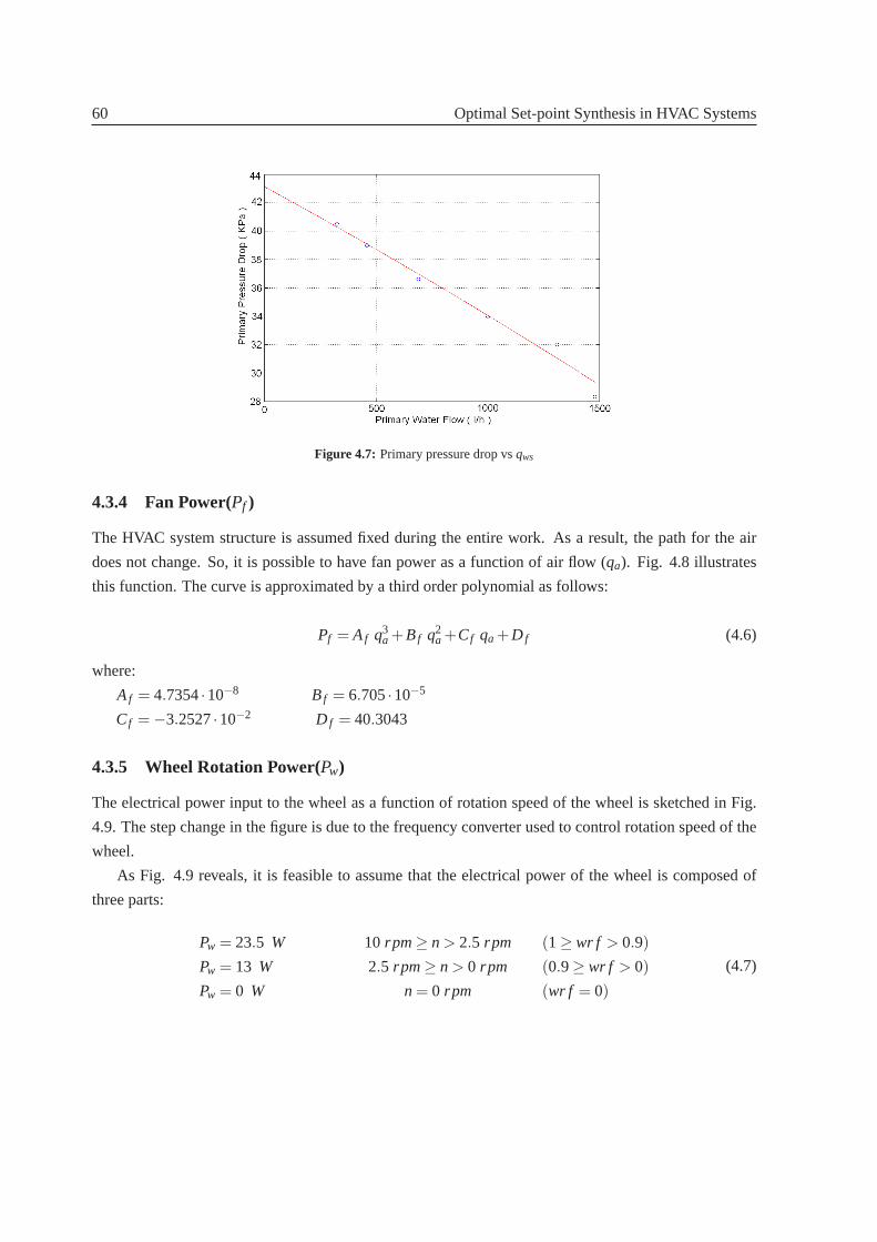
60 Optimal Set-point Synthesis in HVAC Systems
Figure 4.7: Primary pressure drop vsqws
4.3.4 Fan Power(Pf )
The HVAC system structure is assumed fixed during the entire work. As a result, the path for the air
does not change. So, it is possible to have fan power as a function of airflow (qa). Fig. 4.8 illustrates
this function. The curve is approximated by a third order polynomial as follows:
Pf = Af q3a +Bf q2
a +Cf qa +D f (4.6)
where:
Af = 4.7354·10−8 Bf = 6.705·10−5
Cf = −3.2527·10−2 D f = 40.3043
4.3.5 Wheel Rotation Power(Pw)
The electrical power input to the wheel as a function of rotation speed of the wheel is sketched in Fig.
4.9. The step change in the figure is due to the frequency converter usedto control rotation speed of the
wheel.
As Fig. 4.9 reveals, it is feasible to assume that the electrical power of the wheel is composed of
three parts:
Pw = 23.5 W 10 rpm≥ n > 2.5 rpm (1≥ wr f > 0.9)
Pw = 13 W 2.5 rpm≥ n > 0 rpm (0.9≥ wr f > 0)
Pw = 0 W n= 0 rpm (wr f = 0)
(4.7)
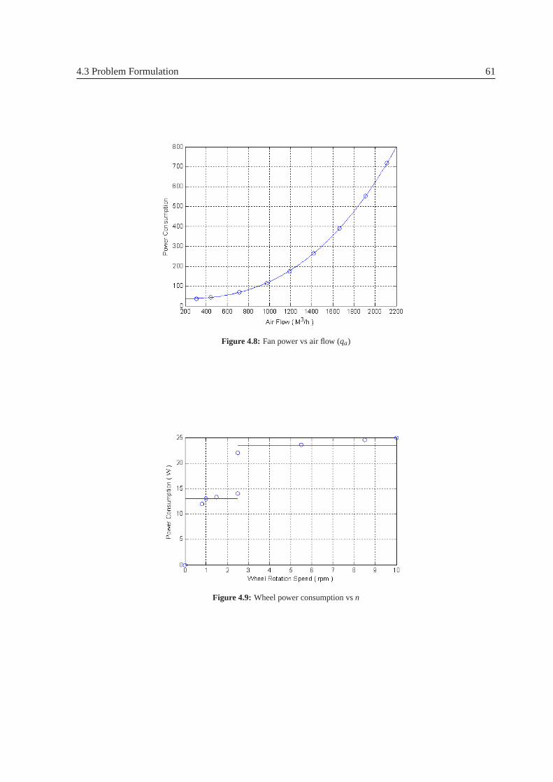
4.3 Problem Formulation 61
Figure 4.8: Fan power vs air flow (qa)
Figure 4.9: Wheel power consumption vsn
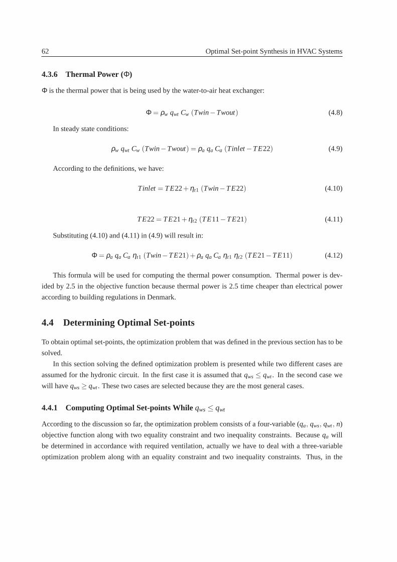
62 Optimal Set-point Synthesis in HVAC Systems
4.3.6 Thermal Power (Φ)
Φ is the thermal power that is being used by the water-to-air heat exchanger:
Φ = ρw qwt Cw (Twin−Twout) (4.8)
In steady state conditions:
ρw qwt Cw (Twin−Twout) = ρa qa Ca (Tinlet−TE22) (4.9)
According to the definitions, we have:
Tinlet = TE22+ηt1 (Twin−TE22) (4.10)
TE22= TE21+ηt2 (TE11−TE21) (4.11)
Substituting (4.10) and (4.11) in (4.9) will result in:
Φ = ρa qa Ca ηt1 (Twin−TE21)+ρa qa Ca ηt1 ηt2 (TE21−TE11) (4.12)
This formula will be used for computing the thermal power consumption. Thermal power is dev-
ided by 2.5 in the objective function because thermal power is 2.5 time cheaperthan electrical power
according to building regulations in Denmark.
4.4 Determining Optimal Set-points
To obtain optimal set-points, the optimization problem that was defined in the previous section has to be
solved.
In this section solving the defined optimization problem is presented while two different cases are
assumed for the hydronic circuit. In the first case it is assumed thatqws ≤ qwt. In the second case we
will haveqws≥ qwt. These two cases are selected because they are the most general cases.
4.4.1 Computing Optimal Set-points Whileqws≤ qwt
According to the discussion so far, the optimization problem consists of a four-variable (qa, qws, qwt, n)
objective function along with two equality constraint and two inequality constraints. Becauseqa will
be determined in accordance with required ventilation, actually we have to deal with a three-variable
optimization problem along with an equality constraint and two inequality constraints. Thus, in the

4.4 Determining Optimal Set-points 63
sequel by optimization problem we mean the latter statement. For convenience wewill deal with TE22
instead ofn in the procedure of solving.
Because, in this case, supply water flow (qws) is always less than or equal to the tertiary water flow
(qwt), mixing between the supply water flow that enters the tertiary circuit and a part of the tertiary return
water flow occurs. So, the temperature of the water that enters the heat exchanger is as follows:
Twin=qws · T pin + (qwt −qws) · Twout
qwt(4.13)
Actually, the mission of the motorized primary/secondary valve is controllingTwinby changing the
supply water flow (qws).
As it was mentioned, to solve the optimization problem here we have to deal with three variables
qws, qwt, andTE22. One of these variables is dependent due to equality constraint (Tinlet= 19):
Tinlet = (1−ηt1) · TE22+ηt1 · Twin (4.14)
As we know, the energy balance equation in a water-to-air heat exchanger is as follows:
ρw qwt Cw (Twin−Twout) = ρa qa Ca (Tinlet−TE22) (4.15)
Substituting the two recent equations in equation (2.26) will result in a formula for qws versusqwt
andTE22 :
qws =k ηt1 qwt (19−TE22)
ηt1qwt(T pin−TE22)+(qwt −kηt1)(TE22−19)(4.16)
Also, in this caseqws≤ qwt; Therefore, substituting equation (4.16) in the recent inequality results
in an inequality as following:
TE22≥ 19−T pin ηt1
1−ηt1(4.17)
Combining equations (4.14) and (4.15) results in a formula forTwout :
Twout=19qwt +TE22(−qwt +ηt1qwt +kηt1)−19kηt1
ηt1qwt(4.18)
In this case,Twout is equal toT pout because the supply water flow is less than or equal to the
tertiary water flow. Thus, the inequality constraint (T pout≤ 40) can be translated into the following
inequality:
(−qwt +ηt1qwt +kηt1) TE22≤ 40ηt1qwt +19kηt1−19qwt (4.19)
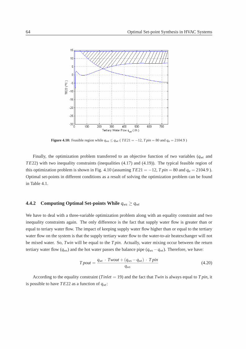
64 Optimal Set-point Synthesis in HVAC Systems
Figure 4.10: Feasible region whileqws≤ qwt ( TE21= −12,T pin= 80 andqa = 2104.9 )
Finally, the optimization problem transferred to an objective function of two variables (qwt and
TE22) with two inequality constraints (inequalities (4.17) and (4.19)). The typical feasible region of
this optimization problem is shown in Fig. 4.10 (assumingTE21= −12,T pin= 80 andqa = 2104.9 ).
Optimal set-points in different conditions as a result of solving the optimization problem can be found
in Table 4.1.
4.4.2 Computing Optimal Set-points Whileqws≥ qwt
We have to deal with a three-variable optimization problem along with an equality constraint and two
inequality constraints again. The only difference is the fact that supply water flow is greater than or
equal to teriary water flow. The impact of keeping supply water flow higherthan or equal to the tertiary
water flow on the system is that the supply tertiary water flow to the water-to-airheatexchanger will not
be mixed water. So,Twin will be equal to theT pin. Actually, water mixing occur between the return
tertiary water flow (qws) and the hot water passes the balance pipe (qws−qwt). Therefore, we have:
T pout=qwt · Twout+(qws−qwt) · T pin
qws(4.20)
According to the equality constraint (Tinlet = 19) and the fact thatTwin is always equal toT pin, it
is possible to haveTE22 as a function ofqwt:

4.4 Determining Optimal Set-points 65
Figure 4.11: Feasible region whileqws≥ qwt ( TE21= −30,T pin= 60 andqa = 1674.1 )
TE22=19−T pin ηt1
1−ηt1(4.21)
Substituting equations (4.15) and (4.21) in equation (4.20) will result in the desired formula for
T pout:
T pout=−(T pin−19) k ηt1 +T pin qws−T pin ηt1 qws
(1−ηt1) qws(4.22)
Using the recent formula forT pout, the inequality constraint (T pout≤ 40) can be translated into
the following inequality:
qws≤(T pin−19) k ηt1
(T pin − 40) (1−ηt1)(4.23)
To summarize, the optimization problem transferred to an objective function oftwo variables (qwt
andqws) with two inequality constraint (inequality (4.23) andqws≥ qwt). The typical feasible region in
this case is sketched in Fig. 4.11 (supposedTE21= −30,T pin= 60 andqa = 1674.1 ).
Solving the optimization problem in this case results in the same optimal values obtained in the
previous case. That is, Table 4.1 represents optimal set-points also in this case.
66 Optimal Set-point Synthesis in HVAC Systems
4.4.3 Consideration of Results
Regarding results of solving the optimization problem in different conditions (Table 4.1) revealvs that
in all conditions supply water flow (qws) and tertiary water flow (qwt) are equal. Therefore, from energy
point of view the optimal hydronic circuit for supplying water-to-air heat exchanger is variable-primary
flow circuit [10]. It also shows that using air-to-air heat exchanger toproduce required heat is cheaper
than using water-to-air heat exchanger. That is, the control strategy must be designed in such a way that
maximum exploitation of the air-to-air heat exchanger is achieved.
4.5 Conclusions
Optimal set-point synthesis for a HVAC system was presented in this paper.The HVAC system was a
typical HVAC system consisted of an air-to-air heat exchnager and a water-to-air heat exchanger. To
derive the optimal set-points, an objective function composed of electricalpower of different compo-
nents in the HVAC system and a fraction of thermal power used by the systemwas defined. The goals
defined for the HVAC system were treated as constraints to the objective function. Finally, the defined
optimization problem was solved using the steady state model of the system. Analysis of the obtained
results revealed that in all conditions supply water flow was equal to tertiarywater flow. Thus, the
varying-primary flow system was the optimal hydronic circuit to supply the water-to-air heat exchanger.
The synthesis done here can be applied as a supervisory layer for the two layer control of the HVAC
system to make the system work at its optimal set-points.

4.5C
onclusions67
Table4.1:O
ptimalS
et-pointsin
DifferentC
onditionsW
hileqws ≤
qw
t
Air Flow (qa) Set-pointsT pin= 80
TE21 = -1280−20
80−30
70−12
70−20
70−30
60−12
60−20
60−30
2104.9
qwt
qws
wr fTE22Twout
51.651.6
114.224.2
73.973.9
112.426.1
104.7104.7
110.128.8
62.762.7
114.224.2
90.890.8
112.426.2
131.4131.4
110.129.2
80.280.2
114.224.2
118.6118.6
112.426.5
179.0179.0
110.130.1
1674.1
qwt
qws
wr fTE22Twout
29.629.6
115.827.9
44441
14.328.9
62.862.8
112.530.2
35.835.8
115.826.9
53.353.3
114.327.9
76.576.5
112.529.2
45451
15.825.8
67.667.6
114.326.8
98.398.3
112.528.2
979.9
qwt
qws
wr fTE22Twout
441
18.329.7
9.39.31
17.431.8
15.915.9
116.332.5
4.84.81
18.328.5
11.211.2
117.429.9
19.119.1
116.330.5
6.16.11
18.327.0
14141
17.428
23.923.9
116.328.4
308.3qwt
qws
wr f
00
0.94
00
0.96
00
0.98
00
0.94
00
0.96
00
0.98
00
0.94
00
0.96
00
0.98

68 Optimal Set-point Synthesis in HVAC Systems

Bibliography
[1] S. Somasundaram, D.W. Winiarski, D.B. Belzer, ”Screening Analysis for EPACT-Covered Com-
mercial HVAC and Water-Heating Equipment”,Transaction of the ASME, Vol. 124, June 2002, pp
116-124.
[2] P. Svendsen and H. Andersen, ”Energy Efficient Pump Coupling inHVAC Systems”,Technical
Report, Danish Technological Institute (Industry and Energy Section), 2005.
[3] J. Lin, S. Chen, and P.D. Roberts, ”Modified Algorithm for Steady-state Integrated System Opti-
mization and Parameter Estimation”,IEE Proceedings, Vol. 135, March 1988.
[4] S. Gros, B. Srinivasan, and D. Bonvin, ”Static Optimization via Tracking of The Necessary Con-
ditions of Optimality Using Neighboring Extremals”,American Control Conference Proceeding,
June 2005, pp 251-255.
[5] N. Nassif, S. Kajl, and R. Sabourin, ”Two-Objective On-Line Optimization of Supervisory Control
Strategy”,Building Services Engineering Research and Technology, 2004, pp 241-251.
[6] L.F.S. Larsen, ”Model Based Control of Refrigeration Ssytems”,Ph.D. Thesis, Aalborg University,
Denmark, 2005.
[7] M. Wetter, ”Simulation Model: Air-to-air Heat Exchnager”,Technical Report, Lawrence Berkeley
National Laboratory, 1999.
[8] N. Nassif, S. Kajl, and R. Sabourin, ”Ventilation Control Strategy Using SupplyCO2 Concentra-
tion Set Point”,International Journal of HVAC & R Research, 2005, pp 239-262.
[9] R.H. Green, ”An Air-Conditioning Control System Using Variable-speed Water Pumps”,ASHRAE
Transaction:Research, part 1, 1994, pp 463-470.
[10] W.P. Bahnfleth, ”Varying Views on Variable-primary Flow”,Chilled Water Engineering J., March
2004.
69


Chapter 5
Optimal Model-Based Control in HVAC
Systems
M. Komareji1 , J. Stoustrup2 , H. Rasmussen3 , N. Bidstrup4 , P. Svendsen5 , F. Nielsen6
Abstract
This paper presents optimal model-based control of a heating, ventilating, and air-conditioning (HVAC)
system. This HVAC system is made of two heat exchangers: an air-to-air heat exchanger (a rotary
wheel heat recovery) and a water-to-air heat exchanger. First dynamic model of the HVAC system is
developed. Then the optimal control structure is designed and implemented. The HVAC system is
splitted into two subsystems. By selecting the right set-points and appropriate cost functions for each
subsystem controller the optimal control strategy is respected to gauranteethe minimum thermal and
electrical energy consumption. Finally, the controller is applied to control thementioned HVAC system
and the results show that the expected goals are fulfilled.
1Mohammad Komareji is a PhD student in The Department of Control and Automation, Institute of Electronic Systems,Aalborg University, Aalborg, Denmark;[email protected]
2Jakob Stoustrup is with Aalborg University as a Professsor in The Department of Control and Automation;[email protected]
3Henrik Rasmussen is with Aalborg University as an Associate Professorin The Department of Control and Automation;[email protected]
4Niels Bidstrup is with Grundfos Management A/S as a Chief Engineer, Ph.D.; [email protected] Svendsen is with Danish Technological Institute (DTI) as a Project Manager;
[email protected] Nielsen is with Exhausto A/S as a Project Manager;[email protected]
71

72 Optimal Model-Based Control in HVAC Systems
Figure 5.1: The Air-to-air heat exchanger scheme
5.1 Introduction
The consumption of energy by heating, ventilating, and air conditioning (HVAC) equipment in indus-
trial and commercial buildings constitutes a great part of the world energy consumption [1]. In spite of
the advancements made in microprocessor technology and its impact on the development of new control
methodologies for HVAC systems aiming at improving their energy efficiency, the process of operating
HVAC equipment in commercial and industrial buildings is still an inefficient andhigh-energy consump-
tion process.
It has been estimated that by optimal control of HVAC systems almost 100 GWh energy can be
saved yearly in Denmark (five million inhabitants) [2]. It shows that a huge amount of energy can be
saved and according to the current energy prices it will be reasonableto invest a little bit more in the
first cost of HVAC systems.
In this paper, an integrated control system is developed. That is, in the proposed control system
there is no need for an expilicit supervisory layer to make the system work inits optimal conditions.
The optimal control strategy that has been developed in [2] is implemented here. So, the controller
follows the optimal control strategy while it tracks the set-point. In Section 5.2,the dynamic model of
the HVAC system is described. The controller design is presented in Section5.3. Finally, the results of
applying the proposed control system is shown in Section 5.4.
5.2 Dynamic Modeling
The HVAC system that will be considered consists of two heat exchangers: an air-to-air heat exchanger
and a water-toair heat exchanger. In this section these components will bedescribed and their dynamic
models will be developed. Finally the overall nonlinear model of the HVAC system will be linearized.
This linear model will be used to design the controller later.

5.2 Dynamic Modeling 73
Figure 5.2: Dependency ofηt2 onqa while n=10 rpm;qsa andqr
a represent supply air flow and return air flow, respectively.
5.2.1 Air-to-air Heat Exchanger
The air-to-air heat exchanger is a rotary heat exchanger in aluminium, withlow pressure loss (shown in
Fig. 5.1). The rotor control comprises a gear motor with frequency converter. Two fans are installed to
produce the desired inlet and outlet air flow.
Steady State Gain Determination
Here, it is supposed that the ratio of the supply air flow to the return air flow isone. Therefore,ηt2 will
be a function of air flow (qa), that is the same for both supply and return air, and the rotation speed of
the wheel (n). In this context, results of testing the rotary heat exchanger that was performed according
to European Standard for laboratory testing of air-to-air heat recovery devices (EN 247, EN 305, EN
306, EN 307, EN 308) will be used. According to results of the test, it is possible to specifyηt2 as a
multiplication of two functions. Fig. 5.2 and 5.3 illustrate these functions [2]. Therefore,ηt2 can be
described as following:
ηt2 = (−1.0569·10−4 qa +0.9943) ·wr f (n) (5.1)
As we know,ηt2 definition is as following:
ηt2 =TE22−TE21TE11−TE21
(5.2)
Combining recent equations ( equations 5.1 and 5.2 ) will result in the steady state gain for the wheel
model:
TE22= TE21+wr f (n) · (TE11−TE21) · (−1.0569·10−4qa +0.9943) (5.3)
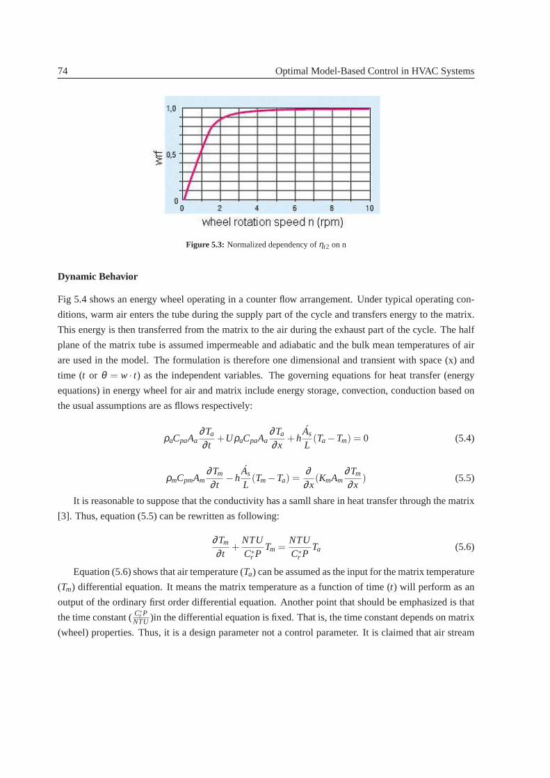
74 Optimal Model-Based Control in HVAC Systems
Figure 5.3: Normalized dependency ofηt2 on n
Dynamic Behavior
Fig 5.4 shows an energy wheel operating in a counter flow arrangement. Under typical operating con-
ditions, warm air enters the tube during the supply part of the cycle and transfers energy to the matrix.
This energy is then transferred from the matrix to the air during the exhaustpart of the cycle. The half
plane of the matrix tube is assumed impermeable and adiabatic and the bulk mean temperatures of air
are used in the model. The formulation is therefore one dimensional and transient with space (x) and
time (t or θ = w · t) as the independent variables. The governing equations for heat transfer (energy
equations) in energy wheel for air and matrix include energy storage, convection, conduction based on
the usual assumptions are as fllows respectively:
ρaCpaAa∂Ta
∂ t+UρaCpaAa
∂Ta
∂x+h
As
L(Ta−Tm) = 0 (5.4)
ρmCpmAm∂Tm
∂ t−h
As
L(Tm−Ta) =
∂∂x
(KmAm∂Tm
∂x) (5.5)
It is reasonable to suppose that the conductivity has a samll share in heattransfer through the matrix
[3]. Thus, equation (5.5) can be rewritten as following:
∂Tm
∂ t+
NTUC∗
r PTm =
NTUC∗
r PTa (5.6)
Equation (5.6) shows that air temperature (Ta) can be assumed as the input for the matrix temperature
(Tm) differential equation. It means the matrix temperature as a function of time (t) will perform as an
output of the ordinary first order differential equation. Another pointthat should be emphasized is that
the time constant (C∗r P
NTU)in the differential equation is fixed. That is, the time constant depends on matrix
(wheel) properties. Thus, it is a design parameter not a control parameter. It is claimed that air stream
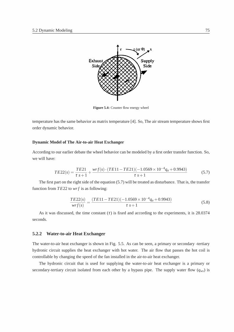
5.2 Dynamic Modeling 75
Figure 5.4: Counter flow energy wheel
temperature has the same behavior as matrix temperature [4]. So, The air stream temperature shows first
order dynamic behavior.
Dynamic Model of The Air-to-air Heat Exchanger
According to our earlier debate the wheel behavior can be modeled by a first order transfer function. So,
we will have:
TE22(s) =TE21τ s+1
+wr f (s) · (TE11−TE21)(−1.0569×10⁻⁴qa +0.9943)
τ s+1(5.7)
The first part on the right side of the equation (5.7) will be treated as disturbance. That is, the transfer
function fromTE22 towr f is as following:
TE22(s)wr f (s)
=(TE11−TE21)(−1.0569×10⁻⁴qa +0.9943)
τ s+1(5.8)
As it was discussed, the time constant (τ) is fixed and according to the experiments, it is 28.0374
seconds.
5.2.2 Water-to-air Heat Exchanger
The water-to-air heat exchanger is shown in Fig. 5.5. As can be seen, aprimary or secondary -tertiary
hydronic circuit supplies the heat exchanger with hot water. The air flowthat passes the hot coil is
controllable by changing the speed of the fan installed in the air-to-air heat exchanger.
The hydronic circuit that is used for supplying the water-to-air heat exchanger is a primary or
secondary-tertiary circuit isolated from each other by a bypass pipe. The supply water flow (qws) is
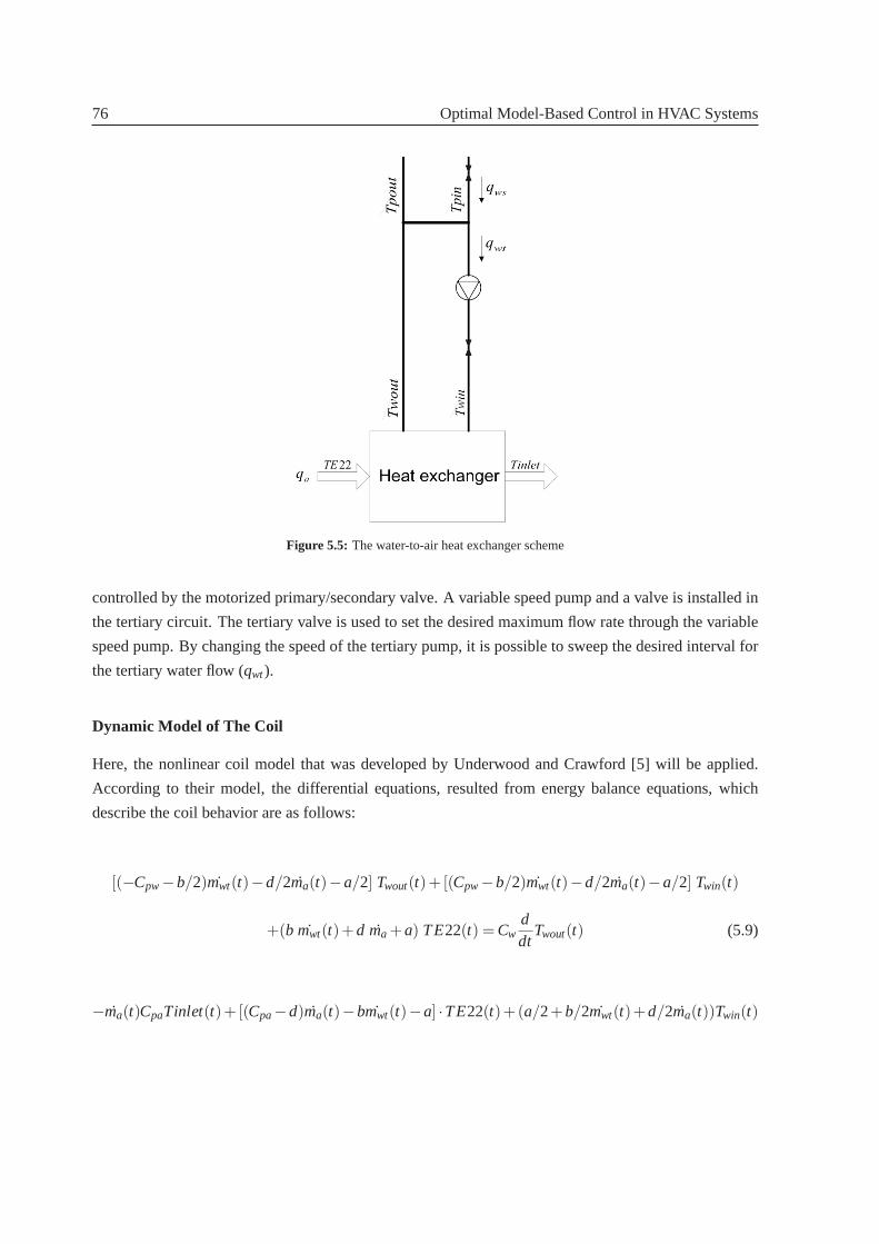
76 Optimal Model-Based Control in HVAC Systems
Figure 5.5: The water-to-air heat exchanger scheme
controlled by the motorized primary/secondary valve. A variable speed pumpand a valve is installed in
the tertiary circuit. The tertiary valve is used to set the desired maximum flow ratethrough the variable
speed pump. By changing the speed of the tertiary pump, it is possible to sweep the desired interval for
the tertiary water flow (qwt).
Dynamic Model of The Coil
Here, the nonlinear coil model that was developed by Underwood and Crawford [5] will be applied.
According to their model, the differential equations, resulted from energybalance equations, which
describe the coil behavior are as follows:
[(−Cpw−b/2)mwt(t)−d/2ma(t)−a/2] Twout(t)+ [(Cpw−b/2)mwt(t)−d/2ma(t)−a/2] Twin(t)
+(b mwt(t)+d ma +a) TE22(t) = Cwddt
Twout(t) (5.9)
−ma(t)CpaTinlet(t)+ [(Cpa−d)ma(t)−bmwt(t)−a] ·TE22(t)+(a/2+b/2mwt(t)+d/2ma(t))Twin(t)

5.2 Dynamic Modeling 77
Figure 5.6: Coil model verification, blue curve: real output, green curve: simulated output
+(a/2+b/2mwt(t)+d/2ma(t))Twout(t) = Caddt
Tinlet(t) (5.10)
wherea, b, d, Cpa, Cpw, Ca, andCw are unknown parameters that have to be identified through the
experiments.
The unknown parameters have identified through some experiments on the coil. Fig 5.6 show veri-
fication of the model along with identified parameters.
Dynamic Model of The Water-to-air Heat Exchanger
According to the hydronic circuit configurationTwin(t) will be as following:
Twin(t) =Tpin(t) mws+Twout(t) (mwt − mws)
mwt(5.11)
where it is supposed that ˙mwt ≥ mws.
The recent formula forTwin should be placed in coil model (equations (5.9) and (5.10))to have the
water-to-air heat exchanger model versus real inputs ˙mw and ˙mwp. Therefore, final water-to-air heat
exchanger model will be as following:
[k1−bmwt −k2mws+k3mws
mwt]Twout(t)+ [k2mws−k3
mws
mwt]Tpin(t)
+[a+b mwt +d ma(t)]TE22= Cwddt
Twout(t) (5.12)

78 Optimal Model-Based Control in HVAC Systems
−maCpaTinlet(t)+ [(Cpa−d)ma−bmwt −a]TE22+[−k1 +bmwt −b/2mws−k3mws
mwt]Twout(t)
+[b/2mws+k3mws
mwt]Tpin(t) = Ca
ddt
Tinlet(t) (5.13)
where:
k1 = −a−d ma(t)
k2 = Cpw−b/2
k3 = d/2 ma(t)+a/2
5.2.3 Linearization of The Nonlinear HVAC System Model
The model of the whole HVAC system consists of the air-to-air and water-to-air heat exchanger models
which were described by equations (5.8), (5.12) and (5.13). The nonlinear model of the HVAC system
can be described as following:
T inlet
Twout˙TE22
= f (Tinlet,Twout,TE22,mws,mwt,wr f ) (5.14)
where:Twout, Tinlet, andTE22 are states of the HVAC system. ˙mws, mwt, andwr f are inputs of
the HVAC system.
The linearized model of the HVAC system will have the following shape:
T inlet
Twout˙TE22
=
a4 a3 a5
0 a1 a2
0 0 a6
·
Tinlet
Twout
TE22
+
b3 b4 0
b1 b2 0
0 0 b5
·
mws
mwt
wr f
y = [1 0 0] ·
Tinlet
Twout
TE22
(5.15)
where:
a1 = (−a−b mwt −d ma−Cpw mws+b/2 mws+a/2 mwsmwt
+d/2 mws mamwt
)/Cw
a2 = (a+b mwt +d ma)/Cw
a3 = (a+b mwt +d ma−b/2 mws−a/2 mwsmwt
−d/2 mws mamwt
)/Ca
a4 = −Cpa ma/Ca
a5 = (Cpa ma−a−b mwt −d ma)/Ca

5.3 Optimal Model-based Control 79
a6 = −1/τb1 = (Cpw−a/2 1
mwt−b/2−d/2 ma
mwt)/Cw T pin+(−Cpw+a/2 1
mwt+b/2+d/2 ma
mwt)/Cw Twout
b2 = (a/2 mws(mwt)2 +d/2 mamws
(mwt)2 )/Cw T pin+(−b−a/2 mws(mwt)2 −d/2 mamws
(mwt)2 )/Cw Twout+b TE22
b3 = (a/2 1mwt
+b/2+d/2 mamwt
)/Ca T pin+(−a/2 1mwt
−b/2−d/2 mamwt
)/Ca Twout
b4 = (−a/2 mws(mwt)2 −d/2 mamws
(mwt)2 )/Ca T pin+(b+a/2 mws(mwt)2 +d/2 mamws
(mwt)2 )/Ca Twout−b TE22
b5 = 1τ (−1.0569×10⁻⁴ ma
ρa+0.9943) (TE11−TE21)
This linear model will be used in the control section to design the controller.
5.3 Optimal Model-based Control
5.3.1 Control Strategy
It is shown that to make the system perform optimally the control strategy has tobe defined in a way
that the following conditions are satisfied:
1. The maximum possible exploitation of the air-to-air heat exchanger is achieved.
2. In the steady state conditions supply water flow (qws) must be equal to the tertiary water flow (qwt).
That is, it is optimal to make the system work in a way that no water passes through the bypass
pipe. It should be noted that it is not possible to eliminate the bypass pipe because it makes the
tertiary hydronic circuit hydraulically decoupled and it is necessary to keep the bypass to remove
fast disturbances.
If the control strategy respects the mentioned conditions the HVAC system willperform in such a
way that it will result in minimum thermal and electrical energy consumption [2].
5.3.2 Controller Design
The mentioned HVAC system is going to be used for ventilation purposes. It means that the air flow
(qa) will be determined in accordance with the required ventilation and the inlet air temperature (Tinlet)
has to be kept at 19oC. So, the optimal controller task is to track the set-point for the inlet air tempera-
ture while satisfying the conditions that were described in the control startegy section to gaurantee the
optimal performance of the system. The traditional way to design the control system that works in this
way is applying the two-layer hierarchical control system. The lower layerperforms direct regulatory
control, where the aim is to maintain selected process variables at their desired set-point values, and the
upper layer, known as the supervisory layer, has the task of detreminingthe setpoints of the regulatory
controllers to obtain optimal steady state performance.
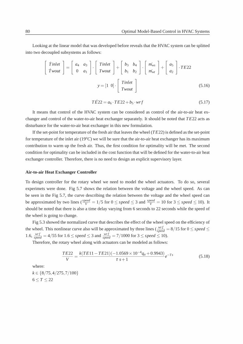
80 Optimal Model-Based Control in HVAC Systems
Looking at the linear model that was developed before reveals that the HVAC system can be splitted
into two decoupled subsystems as follows:
[
T inlet
Twout
]
=
[
a4 a3
0 a1
]
·[
Tinlet
Twout
]
+
[
b3 b4
b1 b2
]
·[
mws
mwt
]
+
[
a5
a2
]
·TE22
y = [1 0] ·[
Tinlet
Twout
]
(5.16)
˙TE22= a6 ·TE22+b5 ·wr f (5.17)
It means that control of the HVAC system can be considered as control of the air-to-air heat ex-
changer and control of the water-to-air heat exchanger separately.It should be noted thatTE22 acts as
disturbance for the water-to-air heat exchanger in this new formulation.
If the set-point for temperature of the fresh air that leaves the wheel (TE22) is defined as the set-point
for temperature of the inlet air (19oC) we will be sure that the air-to-air heat exchanger has its maximum
contribution to warm up the fresh air. Thus, the first condition for optimality willbe met. The second
condition for optimality can be included in the cost function that will be defined for the water-to-air heat
exchanger controller. Therefore, there is no need to design an explicitsupervisory layer.
Air-to-air Heat Exchanger Controller
To design controller for the rotary wheel we need to model the wheel actuators. To do so, several
experimets were done. Fig 5.7 shows the relation between the voltage and the wheel speed. As can
be seen in the Fig 5.7, the curve describing the relation between the voltage and the wheel speed can
be approximated by two lines (speedV = 1/5 for 0≤ speed≤ 3 and speed
V = 10 for 3≤ speed≤ 10). It
should be noted that there is also a time delay varying from 6 seconds to 22 seconds while the speed of
the wheel is going to change.
Fig 5.3 showed the normalized curve that describes the effect of the wheel speed on the efficiency of
the wheel. This nonlinear curve also will be approximated by three lines (wr fspeed= 8/15 for 0≤ speed≤
1.6, wr fspeed= 4/55 for 1.6≤ speed≤ 3 and wr f
speed= 7/1000 for 3≤ speed≤ 10).
Therefore, the rotary wheel along with actuators can be modeled as follows:
TE22V
=k(TE11−TE21)(−1.0569×10⁻⁴qa +0.9943)
τ s+1e−Ts (5.18)
where:
k∈ {8/75,4/275,7/100}6≤ T ≤ 22

5.3 Optimal Model-based Control 81
Figure 5.7: Wheel speed vs. voltage
It should be noted that the outdoor air temperature (TE21) will perform as disturbance through a
first order system on the wheel. Thus, the model of the rotary wheel is a first order system along with
varying gain, varying delay and disturbance. The input (v) is also constrained. These conditions remark
that model predictive controller (MPC) is a good choice for the control.
The control problem can be formulated as follows:
minv[k/k]
6
∑i=1
‖TE22[k+ i/k]−19‖2I(i)
subject to:
0≤ v[k/k] ≤ 10 (5.19)
Sampling time for the controller is supposed to be 15 seconds. The gain and delay for internal model
of the MPC controller are 1.7 and 22, respectively.
Water-to-air Heat Exchanger Controller
To control the water-to-air heat exchanger we have to deal with constrainted inputs. We also have to
penalize inputs in a way that in the steady state conditions no water passes through the the bypass pipe.
So, again MPC is a good candidate for this control problem. To design the MPC controller we need to
modify equation (5.16) as follows:
[
T inlet
Twout
]
=
[
a4 a3
0 a1
]
·[
Tinlet
Twout
]
+
[
b3 +b4 b4
b1 +b2 b2
]
·[
mws
mwt − mws
]
+
[
a5
a2
]
·TE22
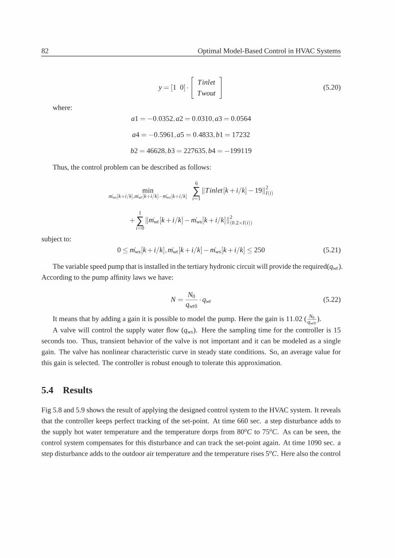
82 Optimal Model-Based Control in HVAC Systems
y = [1 0] ·[
Tinlet
Twout
]
(5.20)
where:
a1 = −0.0352,a2 = 0.0310,a3 = 0.0564
a4 = −0.5961,a5 = 0.4833,b1 = 17232
b2 = 46628,b3 = 227635,b4 = −199119
Thus, the control problem can be described as follows:
minmws[k+i/k],mwt[k+i/k]−mws[k+i/k]
6
∑i=1
‖Tinlet[k+ i/k]−19‖2I(i)
+1
∑i=0
‖mwt[k+ i/k]− mws[k+ i/k]‖2(0.2×I(i))
subject to:
0≤ mws[k+ i/k],mwt[k+ i/k]− mws[k+ i/k] ≤ 250 (5.21)
The variable speed pump that is installed in the tertiary hydronic circuit will provide the required(qwt).
According to the pump affinity laws we have:
N =N0
qwt0·qwt (5.22)
It means that by adding a gain it is possible to model the pump. Here the gain is 11.02 ( N0qwt0
).
A valve will control the supply water flow (qws). Here the sampling time for the controller is 15
seconds too. Thus, transient behavior of the valve is not important and itcan be modeled as a single
gain. The valve has nonlinear characteristic curve in steady state conditions. So, an average value for
this gain is selected. The controller is robust enough to tolerate this approximation.
5.4 Results
Fig 5.8 and 5.9 shows the result of applying the designed control system to the HVAC system. It reveals
that the controller keeps perfect tracking of the set-point. At time 660 sec.a step disturbance adds to
the supply hot water temperature and the temperature dorps from 80oC to 75oC. As can be seen, the
control system compensates for this disturbance and can track the set-point again. At time 1090 sec. a
step disturbance adds to the outdoor air temperature and the temperature rises 5oC. Here also the control
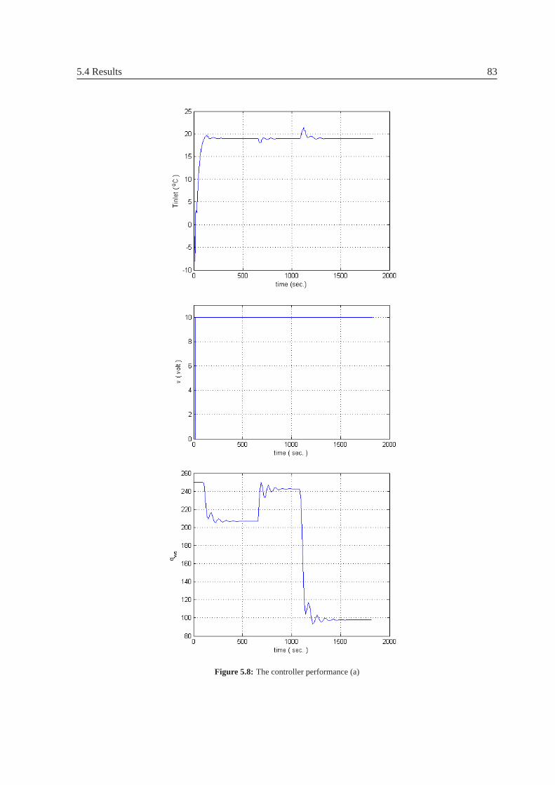
5.4 Results 83
Figure 5.8: The controller performance (a)
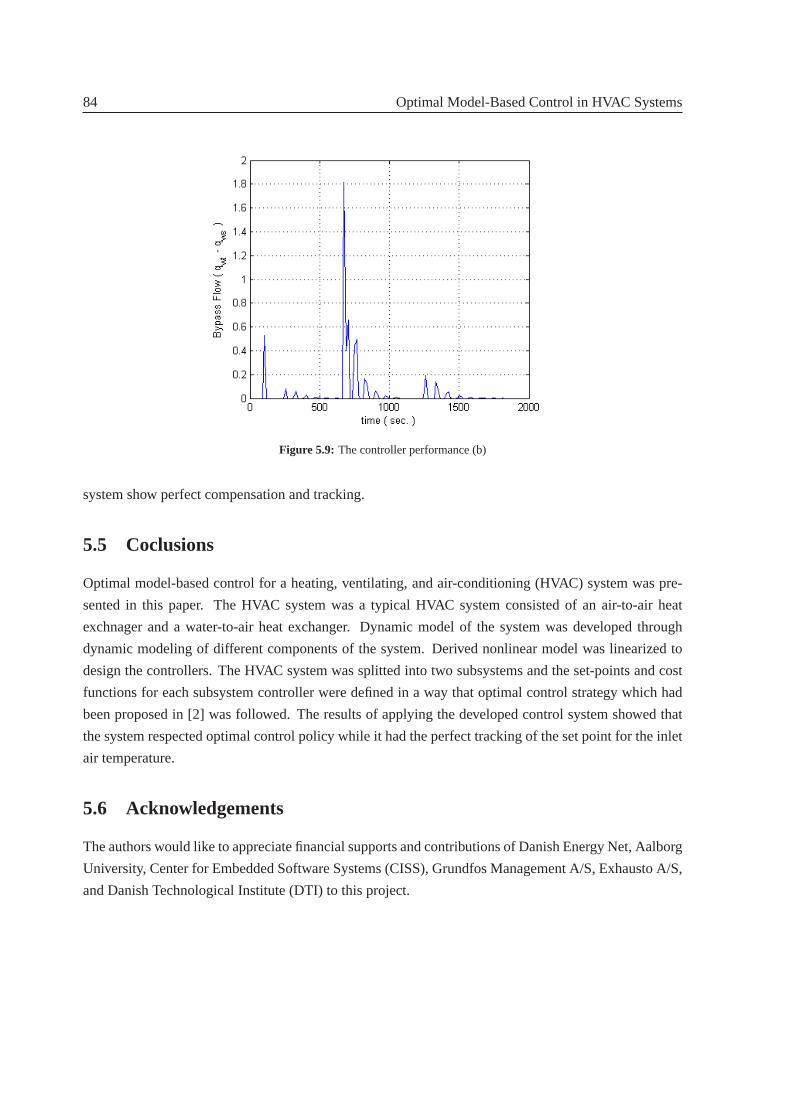
84 Optimal Model-Based Control in HVAC Systems
Figure 5.9: The controller performance (b)
system show perfect compensation and tracking.
5.5 Coclusions
Optimal model-based control for a heating, ventilating, and air-conditioning (HVAC) system was pre-
sented in this paper. The HVAC system was a typical HVAC system consistedof an air-to-air heat
exchnager and a water-to-air heat exchanger. Dynamic model of the system was developed through
dynamic modeling of different components of the system. Derived nonlinearmodel was linearized to
design the controllers. The HVAC system was splitted into two subsystems and the set-points and cost
functions for each subsystem controller were defined in a way that optimalcontrol strategy which had
been proposed in [2] was followed. The results of applying the developed control system showed that
the system respected optimal control policy while it had the perfect trackingof the set point for the inlet
air temperature.
5.6 Acknowledgements
The authors would like to appreciate financial supports and contributions of Danish Energy Net, Aalborg
University, Center for Embedded Software Systems (CISS), GrundfosManagement A/S, Exhausto A/S,
and Danish Technological Institute (DTI) to this project.

Bibliography
[1] S. Somasundaram, D.W. Winiarski, and D.B. Belzer, Screening Analysis for EPACT-Covered
Commercial HVAC and Water-Heating Equipment,Transaction of the ASME, Vol 124, June 2002,
pp 116-124.
[2] M. Komareji, J. Stoustrup, H. Rasmussen, N. Bidstrup, P. Svendsen, and F. Nielsen, Optimal
Set-point Synthesis in HVAC Systems,American Control Conference, New York, NY, 2007, pp
5076-5081.
[3] C. J. Simonson,Heat and Moisture Transfer in Energy Wheels, Ph.D. Thesis, University of
Saskatchewan, Saskatoon, Canada, 1998.
[4] O. O. Abe,Effectiveness of Energy Wheels from Transient Measurements, M.S. Thesis, University
of Saskatchewan, Saskatoon, Canada, 2005.
[5] D.M. Underwood and P.R. Crawford, Dynamic nonlinear modeling of a hot-water-to-air heat ex-
changer for control applications,ASHRAE Transactions: Research, 1991, pp. 149-155.
85


Chapter 6
Simplified Optimal Control in HVAC
Systems
M. Komareji1 , J. Stoustrup2 , H. Rasmussen3 , N. Bidstrup4 , P. Svendsen5 , F. Nielsen6
Abstract
This paper presents simplified optimal control of a heating, ventilating, and air-conditioning (HVAC)
system. This HVAC system is a typical one composed of two heat exchangers: an air-to-air heat ex-
changer (a rotary wheel heat recovery) and a water-to-air heat exchanger. First the optimal control
strategy which was developed in [1] is adopted for implemenation in a real life HVAC system. Then
the bypass flow problem is addressed and a controller is introdeuced to deal with this problem. Fi-
nally a simplified control structure is proposed for optimal control of the HVAC system. The results of
implementing the simplified optimal controller show all control objectives are met.
1Mohammad Komareji is a PhD student in The Department of Control and Automation, Institute of Electronic Systems,Aalborg University, Aalborg, Denmark;[email protected]
2Jakob Stoustrup is with Aalborg University as a Professsor in The Department of Control and Automation;[email protected]
3Henrik Rasmussen is with Aalborg University as an Associate Professorin The Department of Control and Automation;[email protected]
4Niels Bidstrup is with Grundfos Management A/S as a Chief Engineer, Ph.D.; [email protected] Svendsen is with Danish Technological Institute (DTI) as a Project Manager;
[email protected] Nielsen is with Exhausto A/S as a Project Manager;[email protected]
87

88 Simplified Optimal Control in HVAC Systems
6.1 Introduction
A great part of the produced energy in the world is consumed by heating,ventilating, and air condi-
tioning (HVAC) systems. Due to the extremely high fuel oil price and the shortage of energy supply
efficient control of HVAC systems is getting more and more attention. Optimal control of HVAC sys-
tems in Denmark (five million inhabitants) can result in saving of up to 100 GWh energy per year [1].
Regarding the recent figure makes it easy to imagine how much energy can be saved yearly by optimal
control of the HVAC systems all over the world.
Maintaining thermal comfort and energy efficiency are two primary goals in the development of
control modules for HVAC systems. Furthurmore, control modules have to perform in such a way to
guarantee that the operation of the HVAC systems do not violate any building regulations. For example,
according to the Copenhagen Building Regualtions there must be at least 40degrees of cooling of
the delivered hot water through the heating systems. Thus, developing anoptimal control strategy for
HVAC systems is a constrained optimization problem. Having derived an optimal control strategy, the
dynamic controller has to be designed to meet the optimality criteria while satisfying the thermal comfort
conditions. The final step is to adopt and simplify the controller for the real life systems.
In Section 6.2, the HVAC system is briefly described. The practical optimal control strategy and the
implementation of the optimal controller are presented in Section 6.3. Section 6.4 discusses the bypass
problem and the way to deal with that. Section 6.5 presents the simplified optimal control structure and
the implementation results. Finally Section 6.6 explains the energy saving aspects.
6.2 The HVAC System Explanation
The considered HVAC system is a typical HVAC system composed of two heat exchangers: an air-to-air
heat exchanger and a water-to-air heat exchanger.
The air-to-air heat exchanger is a rotary enthalpy wheel which plays theheat recovery role (illus-
trated in Fig. 6.1). The rotor control comprises a gear motor with frequencyconverter. Two fans are
installed to produce the desired inlet and outlet air flow.
Fig. 6.2 shows the water-to-air heat exchanger. A variable speed pump supplies hot water to the
coil. The speed change of the varible speed pump provides the mean to control the tertiary flow. The
primary/secondary flow is controlled by a motorized valve. Tertiary circuit ishydraulically decoupled
from the primary/secondary circuit through the bypass pipe.

6.3 Optimal Model-based Control 89
Figure 6.1: The air-to-air heat exchanger scheme
Figure 6.2: The water-to-air heat exchanger scheme
6.3 Optimal Model-based Control
This section first briefly reviews the optimal control strategy and the optimal dynamic control of the
HVAC system which were developed in [1] and [2]. Then the result of theimplementation of the
optimal contoller is presented.
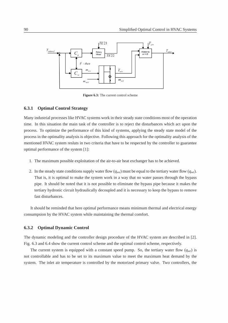
90 Simplified Optimal Control in HVAC Systems
Figure 6.3: The current control scheme
6.3.1 Optimal Control Strategy
Many industrial processes like HVAC systems work in their steady state conditions most of the operation
time. In this situation the main task of the controller is to reject the disturbances which act upon the
process. To optimize the performance of this kind of systems, applying the steady state model of the
process in the optimality analysis is objective. Following this approach for the optimality analysis of the
mentioned HVAC system resluts in two criteria that have to be respected by the controller to guarantee
optimal performance of the system [1]:
1. The maximum possible exploitation of the air-to-air heat exchanger has to be achieved.
2. In the steady state conditions supply water flow (qws) must be equal to the tertiary water flow (qwt).
That is, it is optimal to make the system work in a way that no water passes through the bypass
pipe. It should be noted that it is not possible to eliminate the bypass pipe because it makes the
tertiary hydronic circuit hydraulically decoupled and it is necessary to keep the bypass to remove
fast disturbances.
It should be reminded that here optimal performance means minimum thermal andelectrical energy
consumpsion by the HVAC system while maintaining the thermal comfort.
6.3.2 Optimal Dynamic Control
The dynamic modeling and the controller design procedure of the HVAC system are described in [2].
Fig. 6.3 and 6.4 show the current control scheme and the optimal control scheme, respectively.
The current system is equipped with a constant speed pump. So, the tertiary water flow (qwt) is
not controllable and has to be set to its maximum value to meet the maximum heat demand by the
system. The inlet air temperature is controlled by the motorized primary valve. Two controllers, the
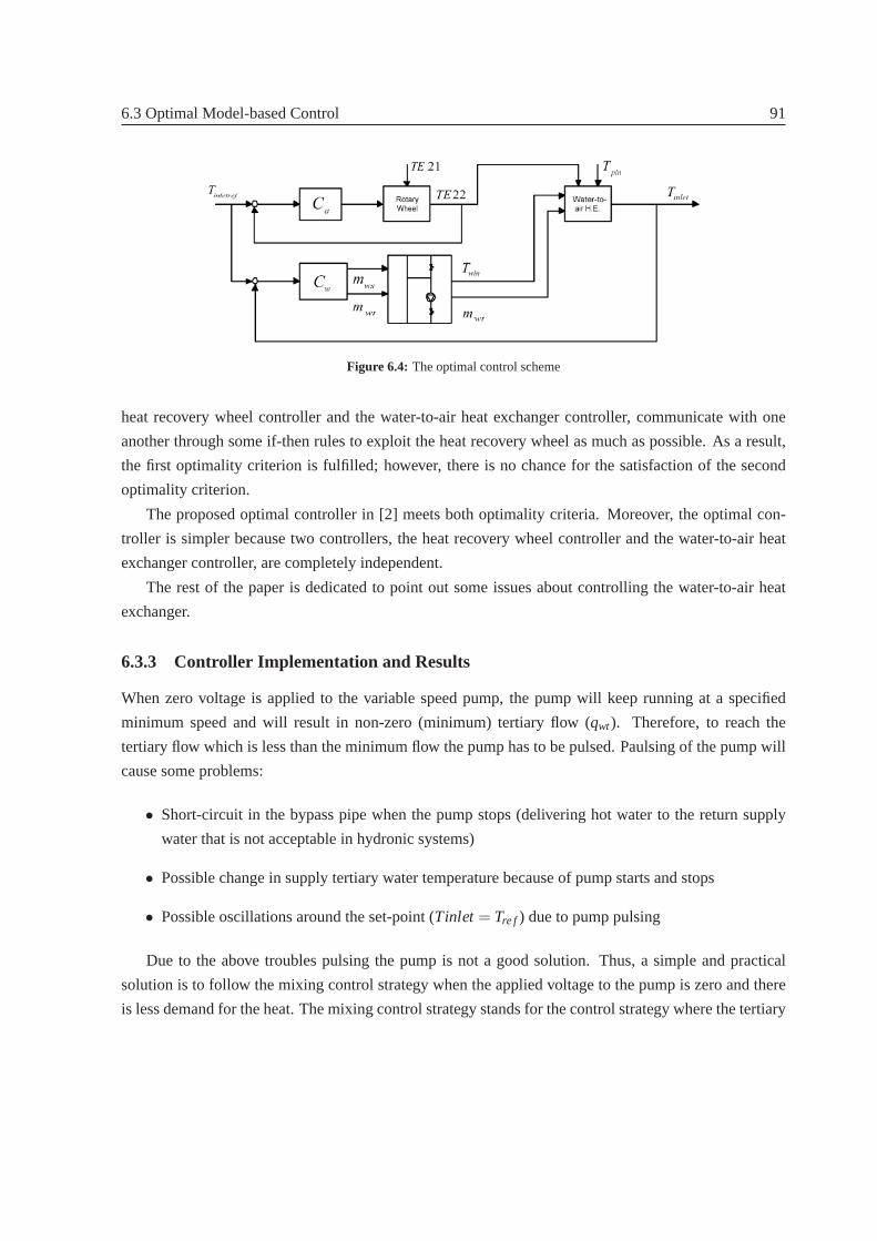
6.3 Optimal Model-based Control 91
Figure 6.4: The optimal control scheme
heat recovery wheel controller and the water-to-air heat exchangercontroller, communicate with one
another through some if-then rules to exploit the heat recovery wheel asmuch as possible. As a result,
the first optimality criterion is fulfilled; however, there is no chance for the satisfaction of the second
optimality criterion.
The proposed optimal controller in [2] meets both optimality criteria. Moreover,the optimal con-
troller is simpler because two controllers, the heat recovery wheel controller and the water-to-air heat
exchanger controller, are completely independent.
The rest of the paper is dedicated to point out some issues about controlling the water-to-air heat
exchanger.
6.3.3 Controller Implementation and Results
When zero voltage is applied to the variable speed pump, the pump will keep running at a specified
minimum speed and will result in non-zero (minimum) tertiary flow (qwt). Therefore, to reach the
tertiary flow which is less than the minimum flow the pump has to be pulsed. Paulsing of the pump will
cause some problems:
• Short-circuit in the bypass pipe when the pump stops (delivering hot waterto the return supply
water that is not acceptable in hydronic systems)
• Possible change in supply tertiary water temperature because of pump startsand stops
• Possible oscillations around the set-point (Tinlet = Tre f ) due to pump pulsing
Due to the above troubles pulsing the pump is not a good solution. Thus, a simpleand practical
solution is to follow the mixing control strategy when the applied voltage to the pump iszero and there
is less demand for the heat. The mixing control strategy stands for the control strategy where the tertiary

92 Simplified Optimal Control in HVAC Systems
Figure 6.5: The implementation result of the practical optimal controller (a)
flow (qwt) is constant and the inlet air temperature is controlled by changing the supplywater flow (qws)
by means of motorized primary valve.
The proposed controller in [2] also shows satisfactory results while following the practical optimal
control strategy. Fig. 6.5 and 6.6 illustrate the result of implementing the controller on the HVAC system.
Fig. 6.5 shows the controller perfectly tracks the set-points. Looking at thethe tertiary flow curve
reveals that when the set-point changes from 23oC to 19oC, the controller switches from the optimal
control strategy to the mixing control strategy and when the set-point changes from 19oC to 22oC the
switching from mixing control strategy to optimal control strategy happens. The switches between the
two different control strategy can be inferred by analyzing the temperature measurements shown in
Fig. 6.6 too. The controller also shows good performance in the sense of disturbance rejection. The
disturbances from outdoor air temperature (shown in Fig. 6.5) and the primary supply water temperature
(shown in Fig. 6.6) are perfectly compensated.

6.3 Optimal Model-based Control 93
Figure 6.6: The implementation result of the practical optimal controller (b)
94 Simplified Optimal Control in HVAC Systems
6.4 Bypass Flow Problem
In this section the bypass flow is defined as a quantity with directon and the implicitmeasuring of the
bypass flow is presented. Then the way to deal with this problem is discussed.
6.4.1 Measuring The Bypass Flow
It is not reasonable to measure the bypass flow through a flow-meter in real life HVAC systems. How-
ever, we can measure the bypass flow implicitly through thermocouples. This way of measurement is
acceptable due to the cheap price of thermocouples.
First the bypass flow has to be defined as a quantity with direction. Consequently, we will always
treat bypass flow as a difference between the supply water flow and the tertiary water flow (qws−qwt).
That is, when the primary flow is greater than the tertiary flow the bypass flowwill have a positive sign
and when the primary flow is less than the tertiary flow a negetive sign will accompany the bypass flow.
These two cases are considered as follows:
• Negetive Bypass Flow
When there is a ngetive bypass flow the return primary water temperature (T pout) and the re-
turn tertiary water temperature(Twout) are equal. However, the supply primary water tempera-
ture (T pin) is always greater than the supply tertiary water temperature (Twin). The difference
between two recent temperatures is propertional to the ratio of the primary water flow and the
tertiary water flow.
The energy balance equation for the supply water side will result in the following equation:
(qwt −qws) Twout + qws T pin = qwt Twin (6.1)
By rearranging the above equatoin we will have:
qwt
qws=
T pin − TwoutTwin − Twout
(6.2)
We subtract 1 from both side of the equation. So,
qwt
qws−1 =
T pin − TwinTwin − Twout
(6.3)
• Positive Bypass Flow
6.4 Bypass Flow Problem 95
The story of the negetive bypass flow is similar to the one of the positive bypass flow. Thus, When
there is a positive bypass flow the supply primary water temperature (T pin) and the supply tertiary
water temperature(Twin) are equal. Nevertheless, the return primary water temperature (T pout) is
always greater than the supply tertiary water temperature (Twout). Agian, the difference between
two recent temperatures is propertional to the ratio of the primary water flow and the tertiary water
flow.
The energy balance equation for the return water side will result in the following equation:
(qws−qwt) T pin + qwt Twout = qws T pout (6.4)
By rearranging the above equatoin we will have:
qwt
qws=
T pin − T poutT pin − Twout
(6.5)
We subtract 1 from both side of the equation. So,
qwt
qws−1 =
Twout − T poutT pin − Twout
(6.6)
The recent equation can be rewritten as
qwt
qws−1 =
Twout − T poutTwin − Twout
(6.7)
According to the above discussion and combining equations 6.3 and 6.7 we willhave:
qwt
qws−1 =
(T pin − Twin) + (Twout − T pout)Twin − Twout
(6.8)
or equivalently:
qwt
qws−1 =
(T pin − Twout) − (Twin + T pout)Twin − Twout
(6.9)
To avoid singularity in the recent equation it should be used as the following equation:
qwt
qws−1 =
(T pin − Twout) − (Twin + T pout)|Twin − Twout−1| + 1
(6.10)
So, by measuring the four temperatures (T pin, T pout, Twin, andTwout) and using the recent for-
mula there will be enough information for a controller to manipulate the bypass flow.

96 Simplified Optimal Control in HVAC Systems
Remark: Those four thermocouples which measureT pin, T pout, Twin, and Twout should be
installed sufficiently far from the bypass pipe.
6.4.2 Problem Definition
As it was mentioned, Fig. 6.6 illustrates the four water temperatures around thebypass pipe ( supply
primary water temperature (T pin), supply tertiary water temperature (Twin), return primary water tem-
perature (T pout), and return tertiary water temperature (Twout)). ComparingT poutandTwoutreveals
that apart from the time that the controller follows the mixing control strategy there is always a small
short circuit (positive bypass flow). That is, the return supply water iswarmed up. In this case, not only
the controller stays away from the optimal performance but also it violates theconstraints (Copenhagen
Building Regulations). Thus, it is vital to solve the bypass flow problem.
6.4.3 Bypass Flow Compensation
The control system structure along with the bypass flow compensator is shown in Fig. 6.7. In this control
structure the main controller (the MPC controller) is as same as before and thebypass compensator
which is slower than the MPC controller deals with the bypass flow problem. According to the equation
6.10 a simple PI controller can be applied as the bypass flow compensator.
Remark: The PI controller which controls the bypass flow has to be along with an anti-windup
module because for some time that the main controller follows the mixing control strategy there will be
accumulation of the bypass flow error.
6.5 Simplified Optimal Control Structure
Fig 6.8 shows the simplified optimal control structure. One PI controller (C1) determines the primary
water flow (qws) through the information from the inlet temperature feedback. To design thiscontroller
the linearized model from the primary water flow to the inlet temperature [2] hasbeen used. Tertiary
water flow (qwt) is controlled by a PI controller (C2) which tries to keep the tetiary water flow close
to the primary water flow. ActuallyC2 is as same as the bypass compensator butC2 is a fast controller
here. The variable speed pump acts as an actuator to control the tertiary water flow. Because the variable
speed pump is much faster than the primary valve which acts as an actuator to control the primary water
flow, the two controllers are decoupled in time domain again. Here also for the same reason that was
mentioned before the pump compensator has to be equipped with the anti-windup module.
The results of applying the recent control system to the HVAC system is shown in Fig 6.9 and 6.10.
As can be seen, the control system has perfect tracking of the set-point. The control system also shows
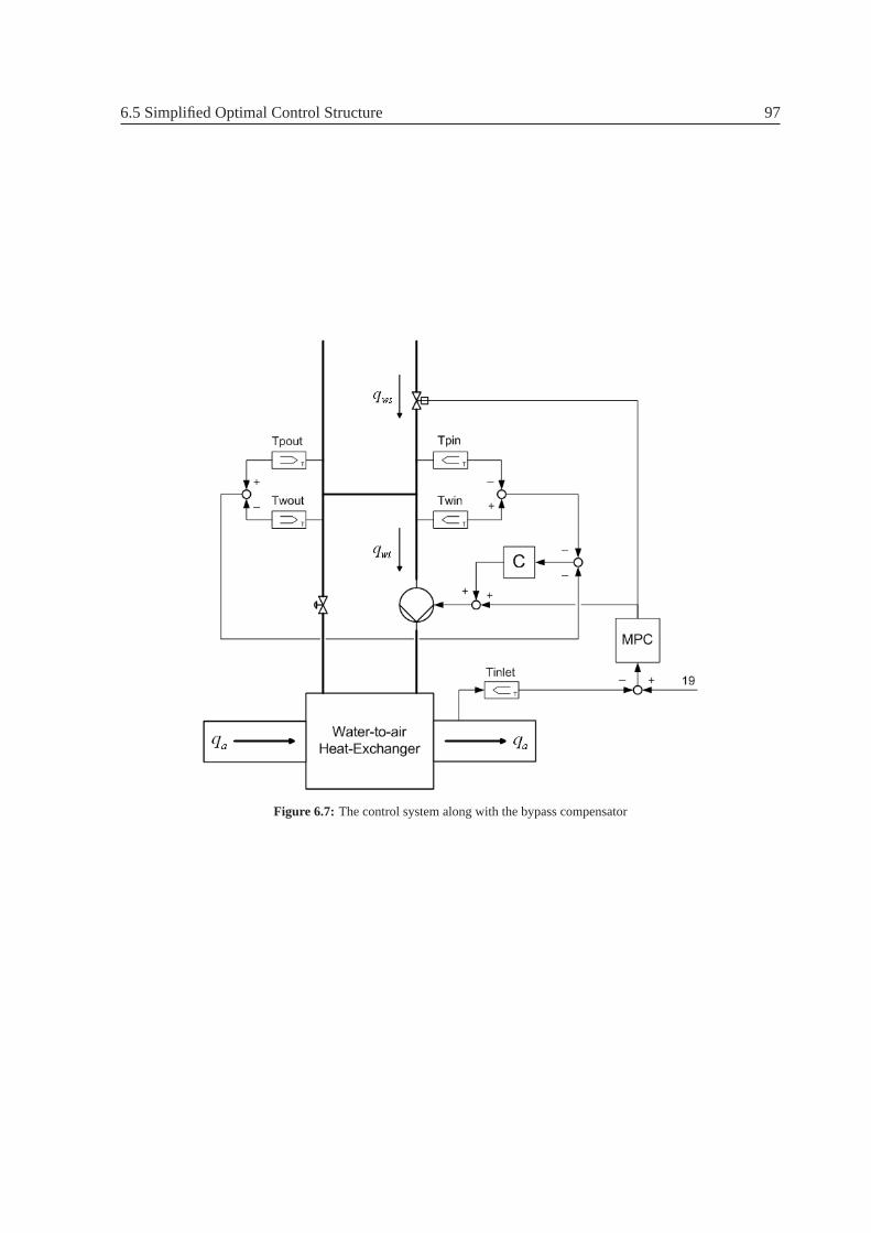
6.5 Simplified Optimal Control Structure 97
Figure 6.7: The control system along with the bypass compensator

98 Simplified Optimal Control in HVAC Systems
Figure 6.8: Simplified optimal control scheme
good disturbance rejection (disturbances from outdoor air temperature and the hot water temerature have
been successfully rejected). Either the tertiary water flow curve or the water temperature curves around
the bypass pipe obviously reveal the switch between two control strategies.
6.6 Energy Saving Aspects
The enrgy consumption of the pump is preportional to the third power of the flow. Mixing control
strategy which requires constant tertiary water flow will impose continuous circulation of 300l/h of
water through the coil. However, the optimal control strategy plays with the tertiary water flow as the
heating demand (thermal load) changes. The tertiary water flow curve in Fig. 6.9 illustrates this fact.
Therefore, applying the optimal control strategy instead of the mixing control sstrategy will save up to
82% energy consumption of the tertiary pump. The recent energy saving figure calculation is based on
the Blue Angel profile (used in the German energy labing scheme). The Europump Study Classification
of Circulators examined circulator load profiles and concluded the profile tobe appropriate for the
Europump circulator classification scheme; in addition this profile was deemed valid for all EU member
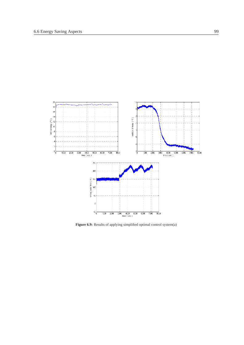
6.6 Energy Saving Aspects 99
Figure 6.9: Results of applying simplified optimal control system(a)
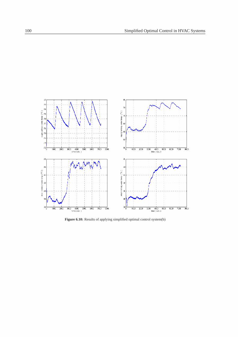
100 Simplified Optimal Control in HVAC Systems
Figure 6.10: Results of applying simplified optimal control system(b)

6.7 Conclusions 101
states.
6.7 Conclusions
Simplified optimal control for a heating, ventilating, and air-conditioning (HVAC) system was presented
in this paper. The optimal model-based controller which had been developedin [2] was implemented
while following the practical optimal control strategy. Going through the bypass flow problem and its
solution led to a simplified optimal controller. Implementation results for the recent controller showed
fulfillment of the contorl goals.
6.8 Acknowledgements
The authors would like to thank financial supports and contributions of Danish Energy Net, Aalborg
University, Center for Embedded Software Systems (CISS), GrundfosManagement A/S, Exhausto A/S,
and Danish Technological Institute (DTI) to this project.

102 Simplified Optimal Control in HVAC Systems
Bibliography
[1] M. Komareji, J. Stoustrup, H. Rasmussen, N. Bidstrup, P. Svendsen, and F. Nielsen, Optimal
Set-point Synthesis in HVAC Systems,American Control Conference, New York, NY, 2007, pp
5076-5081.
[2] M. Komareji, J. Stoustrup, H. Rasmussen, N. Bidstrup, P. Svendsen, and F. Nielsen, Optimal
Model-Based Control in HVAC Systems,American Control Conference, Seattle, WA, 2008.
103

104 BIBLIOGRAPHY

Nomenclature
qa inlet or outlet air flow (m3/h)
TE21 outdoor air temperature (oC)
TE22 temperature of outdoor air after heat recovery (oC)
TE11 room air temperature (oC)
TE12 temperature of room air after heat recovery (oC)
qwt water flow of the tertiary circuit (l/h)
qws water flow of the supply (primary/secondary) circuit (l/h)
Twin tertiary supply water temperature (oC)
Twout tertiary return water temperature (oC)
Tinlet temperature of the supply air (oC)
T pin primary/secondary supply water temperature (oC)
T pout primary/secondary return water temperature (oC)
ηt1 water-to-air heat exchanger temperature efficiency
(ηt1 = Tinlet−TE22Twin−TE22 )
ηt2 air-to-air heat exchanger temperature efficiency
(ηt2 = TE22−TE21TE11−TE21)
ρw water mass density (Kg/m3)
Cpw water specific heat (J/Kg oC)
ρa air mass density (Kg/m3)
Cpa air specific heat (J/Kg oC)
wr f wheel rotation factor (1≥ wr f ≥ 0)
n rotation speed of the wheel (10rpm≥ n≥ 0 rpm)
As heat transfer surface area of one tube (m2)
U mean air velocity in the tube (m/s)
Tm(x, t) matrix temperature (oC)
Ta(x, t) air temperature (oC)
105

106 Nomenclature
h convective heat transfer coefficient (W/m2 oK)
L wheel length (m)
Am cross sectional area of one tube of matrix (m2)
Aa cross sectional area of one tube for air (m2)
Km matrix thermal conductivity (W/m oK)
P exposion time (half of the period) (sec.)
Mm total matrix mass (Kg)
ma air mass flow rate (Kg/h)
As heat transfer surface area on the supply or exhaust side (m2)
Cpm matrix specific heat (J/Kg oC)
C∗r
Mm Cpm nma Cpa
NTU h Asma Cpa
Cpc specific heat of the coil (J/Kg oC)
mws supply water mass flow rate (Kg/h)
mwt tertiary water mass flow rate (Kg/h)
mcw effective mass of the region of the coil at an average temperature
equal to outlet water temperature (Kg)
mca effective mass of the region of the coil at an average temperature
equal to outlet air temperature (Kg)
Cw Cpc mcw (J/oC)
Ca Cpc mca (J/oC)
N pump speed (rpm)
k k = 1000· ρa Ca qaρw Cw

Appendices
107


Appendix A
Decoupling of the HVAC System
As it was mentioned, the control of the HVAC system can be broken into the control of two subsystems:
heat recovery wheel (air-to-air heat exchanger) and water-to-airheat exchanger. The following equations
describe those two subsystems:
[
T inlet
Twout
]
=
[
a4 a3
0 a1
]
·[
Tinlet
Twout
]
+
[
b3 b4
b1 b2
]
·[
mws
mwt
]
+
[
a5
a2
]
·TE22
y = [1 0] ·[
Tinlet
Twout
]
(A.1)
˙TE22= a6 ·TE22+b5 ·wr f (A.2)
where equation (A.1) represents the water-to-air heat exchanger model and equation (A.2) represents
the heat recovery wheel model.
Moreover,
a1 = −0.0352, a2 = 0.0310, a3 = 0.0564
a4 = −0.5961, a5 = 0.4833, b1 = 17232
b2 = 46628, b3 = 227635, b4 = −199119
The linearized water-to-air heat exchanger model is a two-input single-output system. However, a
system can be decoupled if it has a square transfer matrix. So, we have toadd another output to the
system. We choose the stateTwout ( return tertiary water temperature ) to be the second output for the
system. The new system model is as following:
109
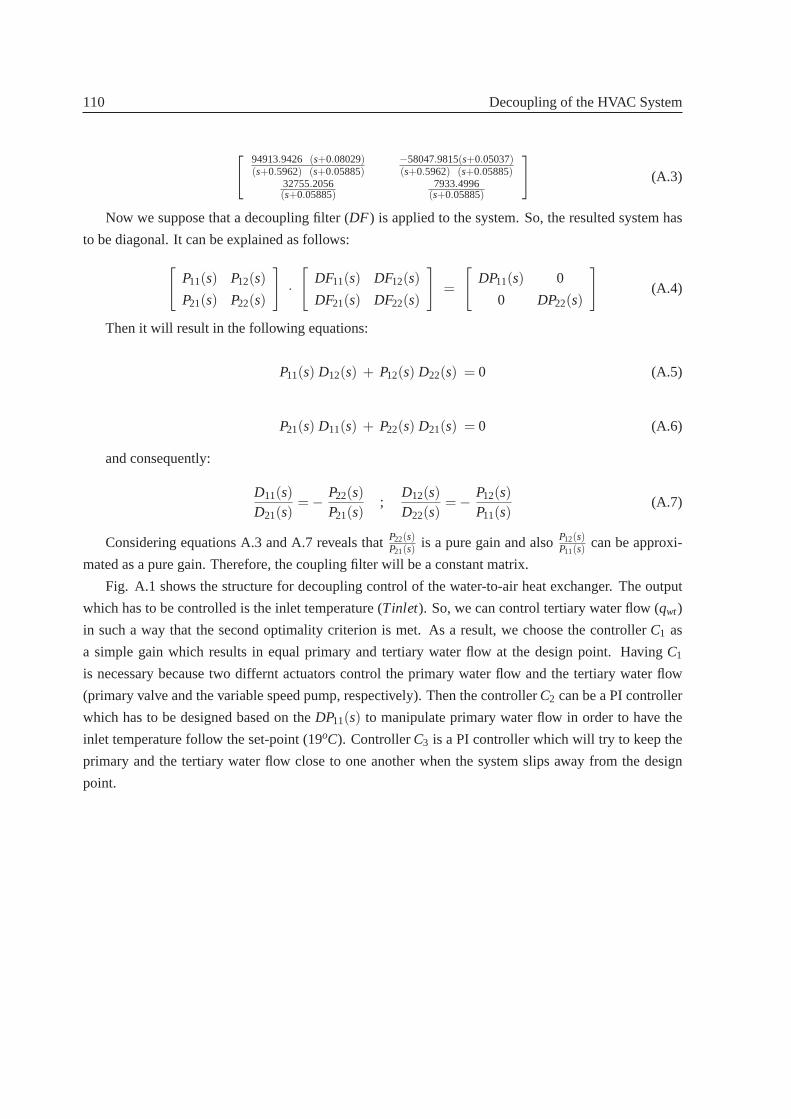
110 Decoupling of the HVAC System
[
94913.9426 (s+0.08029)(s+0.5962) (s+0.05885)
−58047.9815(s+0.05037)(s+0.5962) (s+0.05885)
32755.2056(s+0.05885)
7933.4996(s+0.05885)
]
(A.3)
Now we suppose that a decoupling filter (DF) is applied to the system. So, the resulted system has
to be diagonal. It can be explained as follows:
[
P11(s) P12(s)
P21(s) P22(s)
]
·[
DF11(s) DF12(s)
DF21(s) DF22(s)
]
=
[
DP11(s) 0
0 DP22(s)
]
(A.4)
Then it will result in the following equations:
P11(s) D12(s) + P12(s) D22(s) = 0 (A.5)
P21(s) D11(s) + P22(s) D21(s) = 0 (A.6)
and consequently:
D11(s)D21(s)
= − P22(s)P21(s)
;D12(s)D22(s)
= − P12(s)P11(s)
(A.7)
Considering equations A.3 and A.7 reveals thatP22(s)P21(s)
is a pure gain and alsoP12(s)P11(s)
can be approxi-
mated as a pure gain. Therefore, the coupling filter will be a constant matrix.
Fig. A.1 shows the structure for decoupling control of the water-to-air heat exchanger. The output
which has to be controlled is the inlet temperature (Tinlet). So, we can control tertiary water flow (qwt)
in such a way that the second optimality criterion is met. As a result, we choose thecontrollerC1 as
a simple gain which results in equal primary and tertiary water flow at the designpoint. HavingC1
is necessary because two differnt actuators control the primary water flow and the tertiary water flow
(primary valve and the variable speed pump, respectively). Then the controllerC2 can be a PI controller
which has to be designed based on theDP11(s) to manipulate primary water flow in order to have the
inlet temperature follow the set-point (19oC). ControllerC3 is a PI controller which will try to keep the
primary and the tertiary water flow close to one another when the system slips away from the design
point.

111
Figure A.1: Decoupling control for water-to-air heat exchanger along with bypasscompensation

112 Decoupling of the HVAC System

Appendix B
A Parameterization of The
Observer-Based Controllers
A Parameterization of Observer-Based Controllers: Bumpless Transfer by Covariance Interpola-
tion
Jakob Stoustrup1 and Mohammad Komareji2
Abstract
This paper presents an algorithm to interpolate between two observer-based controllers for a linear multi-
varible system such that the closed loop system remains stable throughout the interpolation. The method
interpolates between the inverse Lyapunov functions for the two original state feedbacks and between
the Lyapunov functions for the two original observer gains to determine anintermediate observer-based
controller.
B.1 Introduction
Observer-based controllers play a significant role in the industry because processing lines do not gen-
erally contain adequate number of sensors to measure all the state variablesand even in some cases it
1Jakob Stoustrup is with Aalborg University as a Professsor in The Department of Control and Automation;[email protected]
2Mohammad Komareji is a PhD student in The Department of Control and Automation, Institute of Electronic Systems,Aalborg University, Aalborg, Denmark;[email protected]
113
114 A Parameterization of The Observer-Based Controllers
may not be possible to get sensor information. Since introducing the modern control theory lots of dif-
ferent methods for designing observer-based controllers such as pole-placement methods, optimization
methods, LMI approaches and· · · have been developed.
Ideally, one would like to design a controller that is both fast and has good measurement noise re-
jection properties. Clearly this is not possible, as increasing the bandwith ofthe closed loop system will
also make the system more sensetive to measurement noise [1]. Then the option is to design two distinct
controllers: ControllerK1 which has low closed loop bandwith and is therefore not very sensetive to
noise but exhibits a slow response. ControllerK2 which has high bandwith and is therefore fast but very
sensetive to noise. Another reason to design two controllers for a certainplant can be associated with
actuator saturation [8]. Also achieving some predefined output properties in the system performance can
lead to follow the scheduled controllers approach. Having designed the twocontrollers, the next issue
which has to be addressed is how to switch between these two controllers. Inmany systems jumps in the
input to the system are not desirable. Thus, finding a smooth way to switch between the two controllers
comes up as a crucial problem.
One important step in actual gain scheduling involves implementing the family of linear controllers
such that the controller coefficient (gains) are varied (scheduled) according to the current value of the
scheduling variable, also called scheduling signal that may be either exogenous signal or endogenous
signal with respect to the plant [9]. Various issues arise here. The issue about the obsever-based con-
trollers here is that the simple gain interpolation technique which usually works well leaves the closed
loop system unstable for some intermediate points if applied to interpolate betweentwo observer based
controllers.
This paper presents an algorithm for interpolation between two observer-based controllers, designed
to control a linear multivarible system, which renders the closed loop system stable for all values of the
interpolation parameter. The family of the observer-based controllers which will be introduced here can
help the designer to achieve a safe bumpless transfer between two obsever-based controllers to reach the
control objectives. Finally, two numerical examples illustrate our claims.
B.2 Preliminaries
The following notations are used in this paper.X∗ indicates the transpose forX which is either a matrix
or a vector.X < 0 (X > 0) means thatX is symmeric and negetive definite (positive definite).Re(X)
denotes the real part of a complex number. Finally,I stands for an identity matrix with appropriate
dimension.
Consider the open loop system
x = Ax+Bu, y = Cx+Du

B.3 Main Results 115
then:
• The system is aysmptotically stable if all eigen values ofA satisfyRe(λ ) < 0 [4].
• A matrix A is Hurwits if and only if for any given positive definite symmetric matrixQ there exists
a positive definite matrixP that satisfies the Lyapunov function [3]:
PA+A∗P = −Q, Q = Q∗
or equivalently
PA+A∗P < 0
• The recent criterion can be written as
AP−1 +P−1A∗ < 0
Proof. We have to multiplyPA+A∗P by P−1 from right and left to get the new criterion3.
B.3 Main Results
Throughout this paper we will assume that(A,B) is controllable and(C,A) is observable. It should be
noted that a slightly weaker results can also result even if(A,B) and(C,A) are only stabilizable and
detectable.
J. Bertram in 1959 was perhaps the first to realize that if a given system realization was state con-
trollable, then any desired characteristic polynomial could be obtained by state-variable feedback [5].
Since then state feedback and static output feedback have been two of themost researched and written
about issues in modern control theory. There is, of course, a long history of gain scheduling in applica-
tions too. However, bumpless transfer (soft switching) between two state feedbacks need some precise
considerations because the gain interpolation of gain scheduled state feedbacks can leave the closed
loop system unstable for the intermediate points. The following lemma presents analgorithm for inter-
polating between two state feedbacks while the closed loop system remains stable for all intermediate
points.
3M andN are two arbitrary positive definite matrices. Then we have the following properties [2]:
1. M is invertible and its inverse (M−1) is also positive definite.
2. If r > 0 is a real number thenrM is positive definite.
3. The sumM +N and the productsMNM andNMN are also positive definite.

116 A Parameterization of The Observer-Based Controllers
Lemma 1. Consider the following control system:
x = Ax+Bu
and assume that u= F0 x and u= F1 x are both stabilizing state feedback laws, with Lyapunov functions:
V0(x) = x∗ X0 x and V1(x) = x∗ X1 x
respectively, with Xi > 0, i = 0,1. Then, a family of state feedback gains F(α) which stabilizes the
system for everyα , 0≤ α ≤ 1 is given by:
F(α) = Fℓ(JF ,α I) (B.1)
where
JF =
(
F0 (F1−F0)X
I I −X
)
, X = X−11 X0
Furthermore, F(α) satisfies F(0) = F0 and F(1) = F1.
Proof. DefiningY0 = X−10 andY1 = X−1
1 , we can rewrite the Lyapunov inequalities corresponding to
V0(x) andV1(x) as:
Q0 := (A+BF0)Y0 +Y0(A+BF0)∗ < 0
and
Q1 := (A+BF1)Y1 +Y1(A+BF1)∗ < 0
respectively. We will demonstrate, that the matrix valued function
Y(α) = (1−α)Y0 +αY1
which is positive definite forα ∈ (0;1), satisfies
(A+BF(α))Y(α)+Y(α)(A+BF(α))∗ < 0

B.3 Main Results 117
for all α ∈ (0;1). To that end, we observe that:
(A+BF(α))Y(α)
=(
A+B(
F0 +α(F1−F0)X(I −α(I −X))−1))((1−α)Y0 +αY1)
=(
A+BF0 +αB(F1−F0)Y1Y−10
(
I −α(
I −Y1Y−10
))−1)
((1−α)Y0 +αY1)
=(
A+BF0 +αB(F1−F0)Y1((1−α)Y0 +αY1)−1)
((1−α)Y0 +αY1)
= (A+BF0)((1−α)Y0 +αY1)+αB(F1−F0)Y1
= (1−α)(A+BF0)Y0 +α (A+BF1)Y1
from which we conclude that:
(A+BF(α))Y(α)+Y(α)(A+BF(α))∗ = (1−α)Q0 +αQ1 < 0, ∀α ∈ (0;1)
which establishes the proof.
From the last argument, note that in the special caseQ0 = Q1, which is often obtainable, the proposed
feedback will actually remain stable forall α , not just forα ∈ (0;1).
Note also that if there is a common Lyapunov function for the both state feedback controllers the
Lemma 1 interpolation reduces to the simple gain interpolation.
In most practical applications, the system states are not completely accessible and all the designer
knows are the outpupts and the inputs. Hence, the estimation of the system states is often necessary to
realize some specific design objectives. The important issue in designing theobserver gain (L) is to have
A+ LC as a stable system. Thus, the critical point in bumpless transfer between two observers is the
stability ofA+LC. The coming lemma expresses an algorithm for interpolating between two observers
while the stability ofA+LC is guaranteed.
Lemma 2. Let L0 and L1 be two different Luenberger observer gains for the following system:
x = Ax+Bu, y = Cx+Du
and suppose that
V0(x) = x∗ Z0 x and V1(x) = x∗ Z1 x
are the corresponding Lyapunov functions to A+ L0C and A+ L1C, respectively, with Zi > 0, i = 0,1.
Then a family of observer gains L(β ), 0≤ β ≤ 1 is given by:
L(β ) = Fℓ(JL,β I) (B.2)

118 A Parameterization of The Observer-Based Controllers
where
JL =
(
L0 I
Z(L1−L0) I −Z
)
, Z = Z−10 Z1
Moreover, L(β ) satisfies L(0) = L0 and L(1) = L1.
Proof. The intermediate points admit the Lyapunov function given by
Z(β ) = (1−β ) Z0 +β Z1
To verify the above the claim, we have to show that
Z(β )(A+L(β )C)+(A+L(β )C)∗Z(β ) < 0
The first term in left side of the Lyapunov inequality can be rewritten as:
Z(β )(A+L(β )C)
= ((1−β )Z0 +βZ1)(
A+(
L0 +β (I −β (I −Z))−1Z(L1−L0))
C)
= ((1−β )Z0 +βZ1)(
A+L0C+β (I −β (I −Z−10 Z1))
−1Z−10 Z1(L1−L0)C
)
= ((1−β )Z0 +βZ1)(
A+L0C+β ((1−β )Z0 +βZ1))−1Z1(L1−L0)C
)
= (1−β )Z0(A+L0C)+βZ1(A+L1C)
So, we can conclude:
Z(β )(A+L(β )C)+(A+L(β )C)∗Z(β )
= (1−β )(Z0(A+L0C)+(A+L0C)∗Z0)+β (Z1(A+L1C)+(A+L1C)∗Z1)
According to the assumptionsZ0 andZ1 are Lyapunov functions forA+L0C andA+L1C, respec-
tively. Thus, we have:
Z0(A+L0C)+(A+L0C)∗Z0 < 0
and
Z1(A+L1C)+(A+L1C)∗Z1 < 0
Then the proof is immediate.
According to the separation principle the problem of desigining an observer-based controller can be
broken into two separate parts: observer design and state feedback design. This approach facillitates the

B.3 Main Results 119
design procedure. Lemma 1 presented an algorithm for interpolation between two state feedbacks while
satisfying the stability critorion. Similar algorithm was described in lemma 2 for observers. Combining
the results from two recent lemmas leads to an algorithm for bumpless transferbetween two observer-
based controllers.
Theorem 1. Consider two observer-based controllers
K0 =
(
A+BF0 +L0C+L0DF −L0
F0 0
)
and
K1 =
(
A+BF1 +L1C+L1DF −L1
F1 0
)
for the minimal system
x = Ax+Bu, y = Cx+Du
.
which have been already designed [6].
Then a family of observer-based controllers for the mentioned system is denoted as
K(γ) = Fℓ(JK ,γI) , 0≤ γ ≤ 1 (B.3)
where
JK =
(
M11 M12
M21 M22
)
M11 =
(
A+BF0 +L0DF0 +L0C −L0
F0 0
)
M12 =
(
(L0D+B) (F1 +F0) X I
(F1−F0) X 0
)
M21 =
(
I 0
Z (L1−L0) (C+DF0) −Z (L1−L0)
)
M22 =
(
I −X 0
Z (L1−L0) D (F1−F0) X I−Z
)
X and Z are as those defined in (B.1) and (B.2).

120 A Parameterization of The Observer-Based Controllers
Figure B.1: The family of observer-based controllers introduced by theorem 1
Also, K(γ) satisfies K(0) = K0 and K(1) = K1.
Proof. Fig. B.1 shows the family of observer-based controllers presented by theorem 1 (equation (B.3)
is the LFT representation of the illustrated block diagram). Applying the principle of separation and
then results in Lemma 1 and 2, the proof is immediate.
It is interesting to see that if there is a common Lyapunov function for the closed loop system
composed of the plant and the family of observer-based controllers the interpolation reduces to the
simple gain interpolation. Furthermore, the closed loop system is stable for anyγ (not only 0≤ γ ≤ 1)
and any rate of switching [1]. Otherwise, in general case which was addressed in theorem 1 we assume
that the scheduling variable is slow enough not to cause stability problems.
B.4 Numerical Examples
Example 1: This example illustrates the fact that the gain interpolation between two stabilizing obsever-
based controller can cause instability for some intermediate points. However,it is shown that the algo-
rithm proposed by theorem 1 does not have this deficiency.
Consider the following third order system,
A =
−0.597 −0.038 0.832
1.636 −0.121 0.068
−0.334 −0.968 −0.311
, B =
−0.638
0.091
0.363
C =(
1 1 1)
, D = 0

B.4 Numerical Examples 121
−3.5 −3 −2.5 −2 −1.5 −1 −0.5 0 0.5−1.5
−1
−0.5
0
0.5
1
1.5
Gain interpolationtheorem interpolation
Figure B.2: Eigen Value Plot of The Closed Loop System in Example 1 where Gain Interpolation (red curve) and TheoremInterpolation (green curve) of Observer-Based Controllers are applied.
This system is unstable with eigen values of−1.3195 and 0.1453± 1.0314i. Then two different
observer-based controllers have been designed for stabilizing the system:
K0 =
−1.863 −1.995 −0.393
0.762 −0.896 −0.811
−1.75 −1.992 −1.751
1.353
0.861
1.367
−0.135 0.947 −0.200 0
and
K1 =
−1.152 −1.103 −0.834
1.033 −0.651 −0.376
−1.441 −1.784 −0.785
0.916
0.551
0.901
−0.567 0.233 1.175 0
Fig. B.2 illustartes the eigen value plot of the closed loop system where the gaininterpolation and
the interpolation proposed by the recent theorem for observer-basedcontrollers are applied for bumpless
transfer between the two designed controllers. The plot reveals that the naive gain interpolation of the
controllers fails to maitain the stability of the closed loop system while the interpolationappeared in the
recent theorem renders the closed loop system stable for all 0≤ γ ≤ 1.
Example 2:In this example we will show the bumpless transfer between two state feedbacks de-
signed to meet different objectives in a HVAC system applying the algorithm described by theorem
1.
We consider here the control of the inlet air temperature of a ventilation system (a water-to-air heat
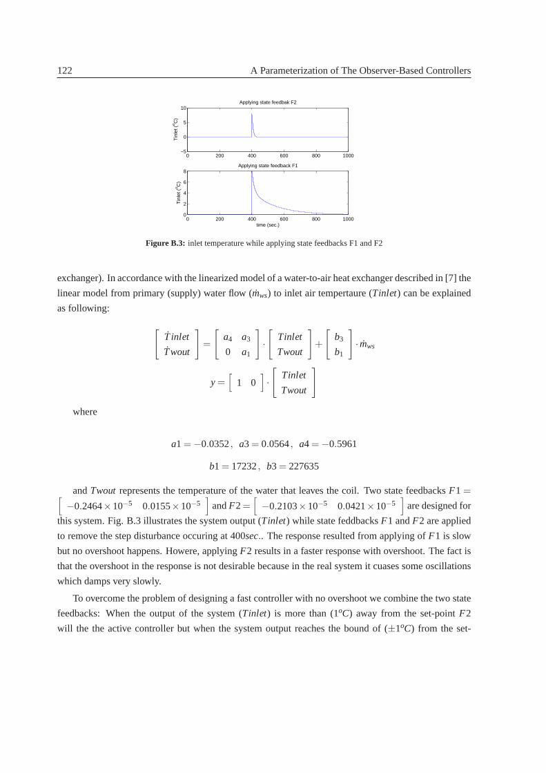
122 A Parameterization of The Observer-Based Controllers
0 200 400 600 800 1000−5
0
5
10
Tin
let (
o C)
Applying state feedbak F2
0 200 400 600 800 10000
2
4
6
8
time (sec.)
Tin
let (
o C)
Applying state feedback F1
Figure B.3: inlet temperature while applying state feedbacks F1 and F2
exchanger). In accordance with the linearized model of a water-to-air heat exchanger described in [7] the
linear model from primary (supply) water flow ( ˙mws) to inlet air tempertaure (Tinlet) can be explained
as following:
[
T inlet
Twout
]
=
[
a4 a3
0 a1
]
·[
Tinlet
Twout
]
+
[
b3
b1
]
· mws
y =[
1 0]
·[
Tinlet
Twout
]
where
a1 = −0.0352, a3 = 0.0564, a4 = −0.5961
b1 = 17232, b3 = 227635
andTwout represents the temperature of the water that leaves the coil. Two state feedbacksF1 =[
−0.2464×10⁻⁵ 0.0155×10⁻⁵]
andF2=[
−0.2103×10⁻⁵ 0.0421×10⁻⁵]
are designed for
this system. Fig. B.3 illustrates the system output (Tinlet) while state feddbacksF1 andF2 are applied
to remove the step disturbance occuring at 400sec.. The response resulted from applying ofF1 is slow
but no overshoot happens. Howere, applyingF2 results in a faster response with overshoot. The fact is
that the overshoot in the response is not desirable because in the real system it cuases some oscillations
which damps very slowly.
To overcome the problem of designing a fast controller with no overshootwe combine the two state
feedbacks: When the output of the system (Tinlet) is more than (1oC) away from the set-pointF2
will the the active controller but when the system output reaches the boundof (±1oC) from the set-

B.5 Conclusions 123
0 100 200 300 400 500 600 700 800 900 10000
5
10
Tin
let(
o C)
0 100 200 300 400 500 600 700 800 900 10000
0.5
1
γ
0 100 200 300 400 500 600 700 800 900 1000−2
0
2x 10
−5
time (sec.)
q ws (
m3 /s
)
Figure B.4: inelt temperature, scheduling parameter (γ), and the control input when a family of state feedbacks presented bytheorem 1 acting upon the HVAC system
point a bumpless transfer, applying the algorithm described in theorem 1, from F2 to F1 happens (γ is
scheduled in accordance with the distance from the set-point). Fig. B.4 shows the result of applying the
recent control strategy to remove a step disturbance occuring at 400sec.. As can be seen, we have a fast
response with no overshoot. Therefore, the recent control strategymeets the control objectives.
B.5 Conclusions
In this paper an algorithm to interpolate between two observer-based controllers was presented. The
proposed algorithm guaranteed the stability of the closed loop system for theintermediate points. At the
end, two numerical examples were presented. The first example showed that the naive gain interpolation
failed to maitain the stability of the closed loop system while the thoerem 1 algorithm worked perfectly
to keep the closed loop system stable. The second example illustrated the application of the proposed
interpolation algorithm to bumpless transfer between two observer-based controllers.

124 A Parameterization of The Observer-Based Controllers

References to Appendix B
[1] Joao P. Hespanha, A. Stephen Morse, Switching between stabilizing controllers,Automatica, 38,
pp 1905-1917, 2002.
[2] Rajendra Bhatia, Positive Definite Matrices,Princeton Series in Applied Mathematics, 2007.
[3] Hassan K. Khalil, Nonlinear Systems (third edition),Prentice Hall, 2002.
[4] Katshuhiko Ogata, Modern Control Engineering (third edition),Prentice-Hall, 1997.
[5] R.E. Kalman, P. Flab, M.A. Arbib, Topics in Mathematical System Theory,McGraw-Hill, 1969.
[6] Kemin Zhou, John C. Doyle, Keith Glover, Robust and Optimal Control,Prentice Hall, 1996.
[7] M. Komareji, J. Stoustrup, H. Rasmussen, N. Bidstrup, P. Svendsen, and F. Nielsen, Optimal
Model-Based Control in HVAC Systems,American Control Conference, Seattle, WA, June 2008,
pp 1443-1448.
[8] Solmaz Sajjadi-Kia, Faryar Jabbari, Use of Scheduling for Anti-windup Controller Design,Amer-
ican Control Conference, New York City, NY, July 2007.
[9] Wilson J. Rugh, Jeff S. Shamma, Research on Gain Scheduling,Automatica, 2000, vol 36, pp
1401-1425.
125


Appendix C
HVAC test system set-up
The HVAC test system shown in Fig. C.1 and manufactured by Exhausto A/S iscomposed of two heat
exchangers: Heat recovery wheel and water-to-air heat exchanger.
C.1 Heat Recovery Wheel
The air-to-air heat exchanger is a rotary heat exchanger in aluminium, withlow pressure loss (shown in
Fig. C.2). The rotor control comprises a gear motor with frequency converter. Two fans are installed to
produce the desired inlet and outlet air flow. Here, it is supposed that theratio of the supply air flow to
the return air flow is one. It means that the HVAC system will not change the pressure of the zone which
is connected to. On the other hand,it removes air from the zone as much as airit adds to the zone.
Figure C.1: HVAC test system
127

128 HVAC test system set-up
Figure C.2: Heat recovery wheel
In this project, results of testing the rotary heat exchanger that was performed according to European
Standard for laboratory testing of air-to-air heat recovery devices (EN 247, EN 305, EN 306, EN 307,
EN 308) have been used. This European Standard is intended to be usedas a basis for testing heat
recovery devices for HVAC systems, which as specified in EN 247 consist of the heat exchanger itself
installed in a casing having the necessary air duct connecting elements and insome cases the fans and
pumps, but without any additional components of the HVAC system.
The temperature of the fresh air which is supplied to the room is controllable bymanipulating the
rotation speed of the wheel. The faster the rotation speed, the higher the supply air temperature.
C.2 Air Flow Measurement
Airflow measurement techniques are necessary to determine the most basic of indoor air quality ques-
tions: ’Is there enough fresh air to provide a healthy environment for theoccupants of the building?’
In HVAC systems the most common ways of measuring the air flow are based on either the pressure
difference measuring or the first law of thermodynamics. For the HVAC testsystem we have applied the
former method.
The pressure difference measuring method is based on the following equation:
q = A·√
2(P2−P1)
ρa
where
q: air flow
A: cross area
Px: absolute pressure

C.2 Air Flow Measurement 129
0 100 200 300 400 500 6000
500
1000
1500
2000
2500
pressure difference (Pa)
air
flow
(m
3 /h)
0 100 200 300 400 500 6000
500
1000
1500
2000
2500
pressure difference (Pa)
air
flow
(m
3 /h)
0 50 100 150 200 250 3000
200
400
600
800
1000
1200
1400
1600
pressure difference (Pa)
air
flow
(m
3 /h)
0 50 100 1500
200
400
600
800
1000
1200
pressure difference (Pa)
air
flow
(m
3 /h)
Figure C.3: inlet air flow vs. pressure difference(fan voltage: 10 V, 8 V, 6 V and 4V)
ρa: density of the air
In the HVAC test system changing the fan speed will change the characteristic curve dispalying the
hydraulic circuit. Hence, the air flow not only depends on the pressure difference measurements but also
depends on the fan voltage. Fig. C.3 and Fig. C.4 illustrate the relation betweenthe pressure difference
and the air flow for the inlet circuit and the outlet circuit, respectively while the fan voltage has been
kept constatnt at 10 V, 8 V, 6 V, and 4 V. It is necessary to have separate measurements for the inlet air
flow and the outlet air flow because they have different characteristic curves (inlet air flow goes through
the water-to-air heat exchanger but the outlet air flow does not). To measure the air flow when the fan
voltage is an intermediate point the linear interpolation between two nearest curves has been used.
Fig. C.5 and Fig. C.6 show the final curves for measuring the inlet air flow and the outlet air flow
which are functions of pressure difference (q = Kx√
P2−P1, assuming the constant air density) and the
fan voltage, respectively.

130 HVAC test system set-up
0 100 200 300 400 500 600 7000
500
1000
1500
2000
2500
pressure difference (Pa)
air
flow
(m
3 /h)
0 100 200 300 400 500 600 7000
500
1000
1500
2000
2500
pressure difference (Pa)
air
flow
(m
3 /h)
0 50 100 150 200 250 3000
500
1000
1500
pressure difference (Pa)
air
flow
(m
3 /h)
0 20 40 60 80 1000
100
200
300
400
500
600
700
800
900
pressure difference (Pa)
air
flow
(m
3 /h)
Figure C.4: outlet air flow vs. pressure difference (fan voltage: 10 V, 8 V, 6 V and4 V)
0 100 200 300 400 500 6000
500
1000
1500
2000
2500
pressure difference (Pa)
air
flow
(m
3 /h)
fan voltage decreasing
Figure C.5: inlet air flow curves
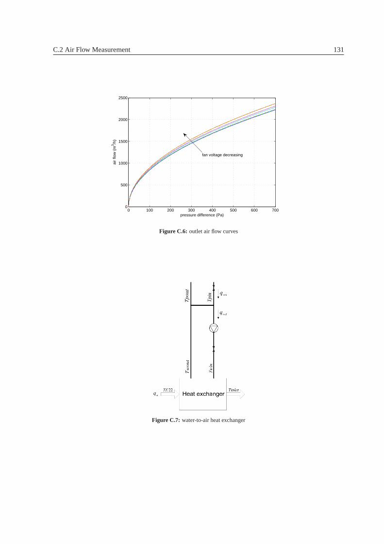
C.2 Air Flow Measurement 131
0 100 200 300 400 500 600 7000
500
1000
1500
2000
2500
pressure difference (Pa)
air
flow
(m
3 /h)
fan voltage decreasing
Figure C.6: outlet air flow curves
Figure C.7: water-to-air heat exchanger

132 HVAC test system set-up
C.3 Water-to-air Heat Exchanger
The water-to-air heat exchanger is shown in Fig. C.7. We can see in the figure that a bypass pipe is
decoupling the tertiary circuit from the supply circuit. The hot water is supplied to the coil by Grundfos
MAGNA 25-60 pump. A Siemens motorized valve control the flow of the supply hot water. On the other
hand, it controls the amount of hot water which is injected to the tertiary circuit.The differnce between
the HVAC test system and the current Exhasuto HVAC systems is the installationof the variable speed
pump in the tertiary circuit. In the current Exhausto HVAC systems the tertiary water flow is constant
(a constant speed pump is installed in the tertiary circuit) and the inlet temperature is controlled by the
primary motorized valve. However, the new set-up in the test system enablesus to examine control
algorithm which plays with the tertiary water flow as well as a control input too.
C.4 Control Interface Module
The control interface module establishes an interface between the HVAC test system and the user. It
is comprised by both hardware and software. The software is installed on the host PC, where the
SIMULINK control diagram is compiled into an executable file, which is downloaded to the target
PC through a LAN (or Internet and LAN). The target PC is equipped with two PCI National Instruments
DAQ (PCI-6703 and PCI-6031E) which are the input card and the output card to connect target PC to
the HVAC test system.