A24: DAY 1 PART1: MACHINES Ana Lucia Varbanescu, UvA A.L.Varbanescu@uva.nl

Plan (ambitious) •  Introduction: About HPC • Part I : Machines & parallelism • Part II : Applications & parallelism • Part III : Performance

ABOUT HPC

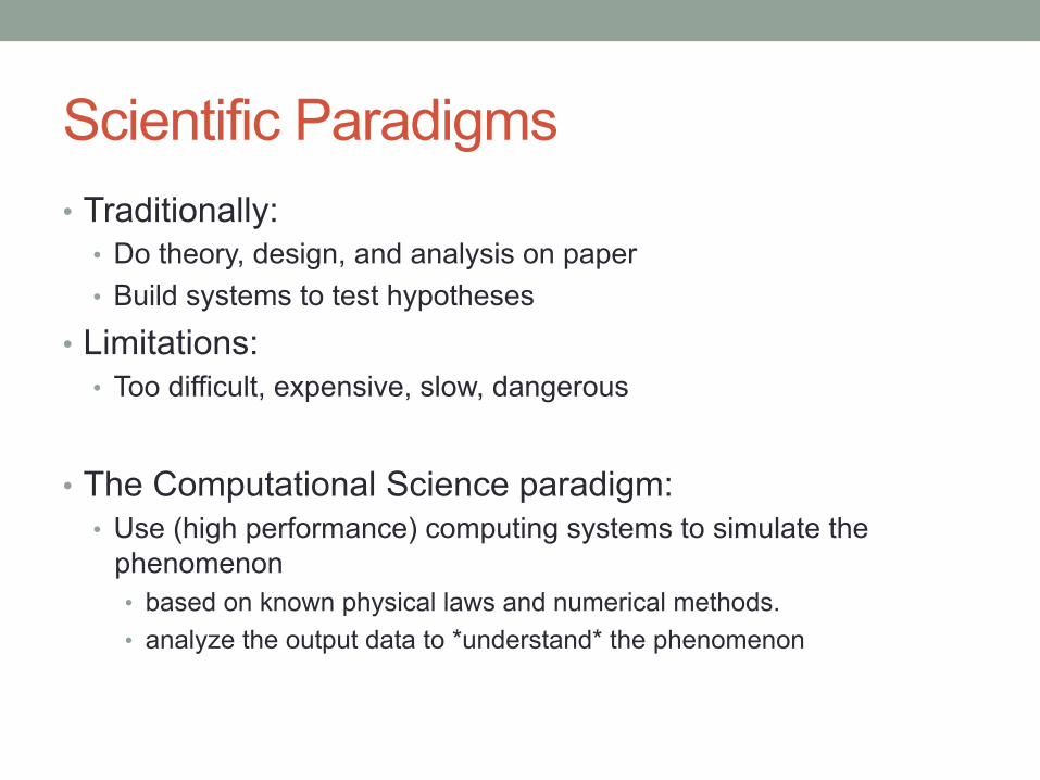
Scientific Paradigms •  Traditionally:

•  Do theory, design, and analysis on paper •  Build systems to test hypotheses

•  Limitations: •  Too difficult, expensive, slow, dangerous

•  The Computational Science paradigm: •  Use (high performance) computing systems to simulate the

phenomenon •  based on known physical laws and numerical methods. •  analyze the output data to *understand* the phenomenon

Some challenging computations • Science

•  Global climate •  Astrophysics •  Biology: genome analysis, protein folding •  Earthquake and Tsunami prediction

• Engineering •  Car-crash simulation •  Semiconductor design •  Structural analysis •  Oil and gas exploration •  Aerodynamics •  …

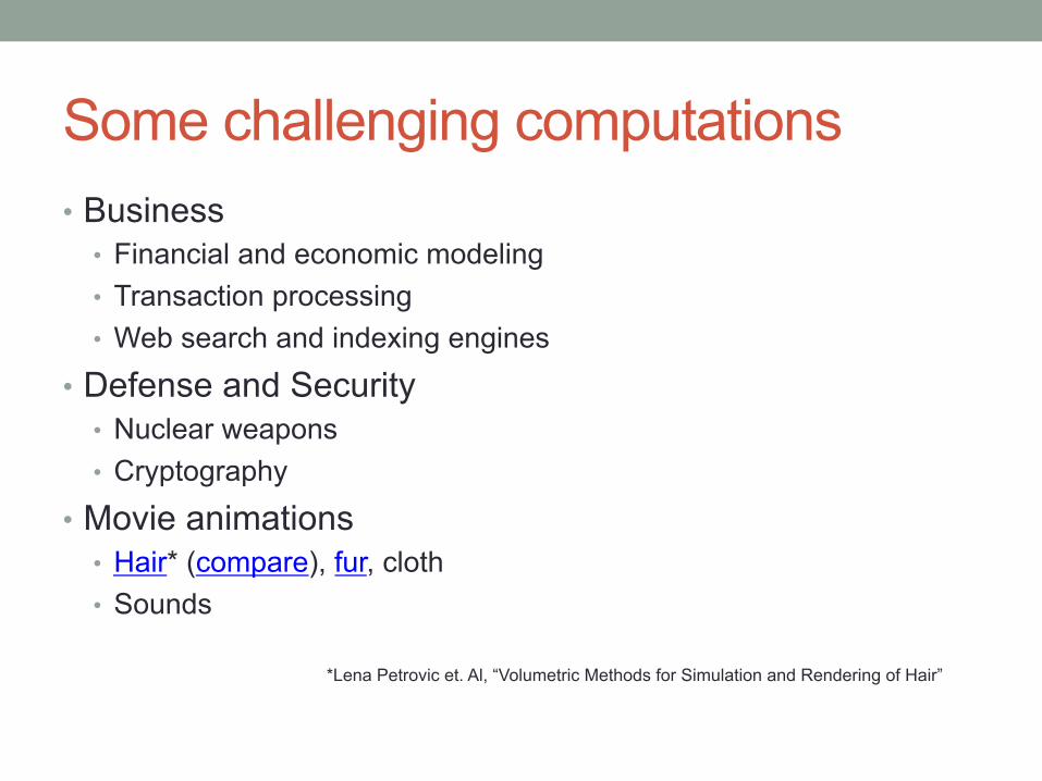
Some challenging computations • Business

•  Financial and economic modeling •  Transaction processing •  Web search and indexing engines

• Defense and Security •  Nuclear weapons •  Cryptography

• Movie animations •  Hair* (compare), fur, cloth •  Sounds

*Lena Petrovic et. Al, “Volumetric Methods for Simulation and Rendering of Hair”

Global Climate Modeling Problem • Problem: compute

•  F (latitude, longitude, elevation, time) = weather = (temperature, pressure, humidity, wind velocity)

• Approach*: •  Discretize the domain, e.g., a grid with measurement points every

N km •  Devise an model to predict climate at time t+∆t

given climate at time t

Randall, D. A. et. al., Climate modeling with spherical geodesic grids

Global Climate Modeling Problem • Model the fluid flow in the atmosphere

•  Solve the resulting Navier-Stokes equations •  ~100 Flops per grid point at 1 min. timestep •  Earth surface is approximately 5.1x108 km2

•  Grid patches =1 km2 => 5.1x1010 per time step for the whole Earth

• Computational requirements: •  Real-time: 5x 1010 flops in 60 seconds ≈ 0.8 GFlop/s •  Weather prediction (7 days in 24 hours): 5.6 Gflop/s •  Climate prediction (100 years in 30 days): 1 Tflop/s •  Scenario analysis (100 scenarios): 100 Tflop/s

The Effect of Grid Resolution • Daily precipitation during winter time: models with different

resolutions

75 km resolution

50 km resolution

300 km resolution 100 km resolution

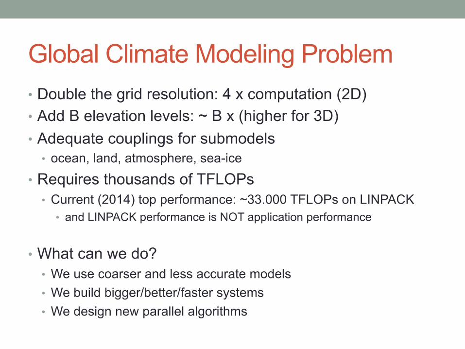
Global Climate Modeling Problem • Double the grid resolution: 4 x computation (2D) • Add B elevation levels: ~ B x (higher for 3D) • Adequate couplings for submodels

•  ocean, land, atmosphere, sea-ice

• Requires thousands of TFLOPs •  Current (2014) top performance: ~33.000 TFLOPs on LINPACK

•  and LINPACK performance is NOT application performance

• What can we do? •  We use coarser and less accurate models •  We build bigger/better/faster systems •  We design new parallel algorithms

Take home message [1] • High Performance Computing is required to make

computationally and/or data intensive problems feasible in time.

• HPC main metric = performance

• Compared “against”: •  Real-time apps => worst-case execution guarantees •  Embedded/mobile apps => power consumption •  Marketing => best-case execution time

Take home message [2] • HPC goal = maximize the performance of a given

application on a given platform

• HPC = f(Machine, Application, Parallelism) •  HPC machines

•  Super-chips, super-computers, grids, clouds •  HPC applications

•  Lots of old and new application fields, simulations, predictions, models, ...

•  HPC parallelism •  Multiple layers

HPC pulse •  TOP500 Project*

•  The 500 most powerful computers in the world

• Benchmark: Rmax of LINPACK •  Solve the Ax=b linear system

•  dense problem •  matrix A is random

•  Dominated by dense matrix-matrix multiply

• Metric: FLOPS/s •  Computational throughput: number of floating point operations per

second

• Updated twice a year: latest is Nov 2014

*Read more: www.top500.org

PARALLEL ARCHITECTURES

Classify Parallel Architectures • Shared Memory

•  Homogeneous compute nodes •  Shared address space

• Distributed Memory •  Homogeneous compute nodes •  Local (disjoint) address spaces

• Hybrids •  Heterogeneous compute nodes •  Mixed address space(s)

Shared memory machines • All processors have access to all memory locations

•  Uniform access time: UMA •  Non-uniform access times: NUMA

•  Interconnections (networks) •  Bus/buses/ring(s) •  Meshes (all-to-all) •  Cross-bars

Distributed memory machines • Every processor has its own local address space • Non-local data can only be accessed through a request to

the owning processor • Access times (may) depend on distance => non-uniform

Virtual Shared Memory • Virtual global address space

•  Memories are physically distributed •  Local access remains faster than remote access

•  NUMA •  All processors can access all memory spaces •  Hardware (or software) hide memory distribution

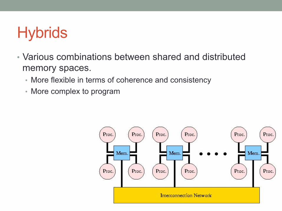
Hybrids • Various combinations between shared and distributed

memory spaces. •  More flexible in terms of coherence and consistency •  More complex to program

Major issues • Shared Memory model

•  Scalability problems (interconnect) •  Programming challenge: RD/WR Conflicts

• Distributed Memory model •  Data distribution is mandatory •  Programming challenge: remote accesses, consistency

• Virtual Shared Memory model •  Significant virtualization overhead •  Easier programming

• Hybrid models •  Local/remote data more difficult to trace

Examples • Multi-core CPUs ?

•  Shared memory with respect to system memory •  Hybrid when taking caches into account

• Clusters ? •  Distributed memory •  Could be shared if middleware for virtual shared space is provided

• Supercomputers ? •  Usually hybrid

• GPUs ? • Architectures with GPUs?

•  Distributed for traditional, off-chip GPUs •  Shared for new APUs

CORE-LEVEL PARALLELISM

Intra-Processor parallelism •  Low-level parallelism

•  Hidden from programmers •  Should be automatically addressed by compilers •  Low-level languages do expose it, if needed

•  An example: Vector / SIMD operation

• Memory hierarchies •  Caches and non-caches alike

=

+

SIMD (vector operations) • Scalar processing

•  Traditional •  One operation produces one result

• Vector processing •  With SSE, SSE2 … , AVX •  One operation produces 4

results

A1

B1

C1 =

+

A

B

C

A2

B2

C2

A3

B3

C3

A4

B4

C4

SSE/SSE2/…/SSE4 •  Assembly instructions

•  16 (or more) registers •  C/C++ intrinsics = “macro’s” to work on variables

float data[N]; for (i=0;i<N;i++) data[i]=(float)i; //vector: load first 4 elements, then next 4 __m128 myVector0=_mm_load_ps(data); __m128 myVector1=_mm_load_ps(data+4); //vector: add => 4 FLOPs __m128 myVector2=_mm_add_ps(myVector0,myVector1); // vector: _MM_SHUFFLE(x,y,z,t)=x,y from 1,z&t from 2 __m128 myVector3=_mm_shuffle_ps(myVector0, myVector1,

_MM_SHUFFLE(2,3,0,1));

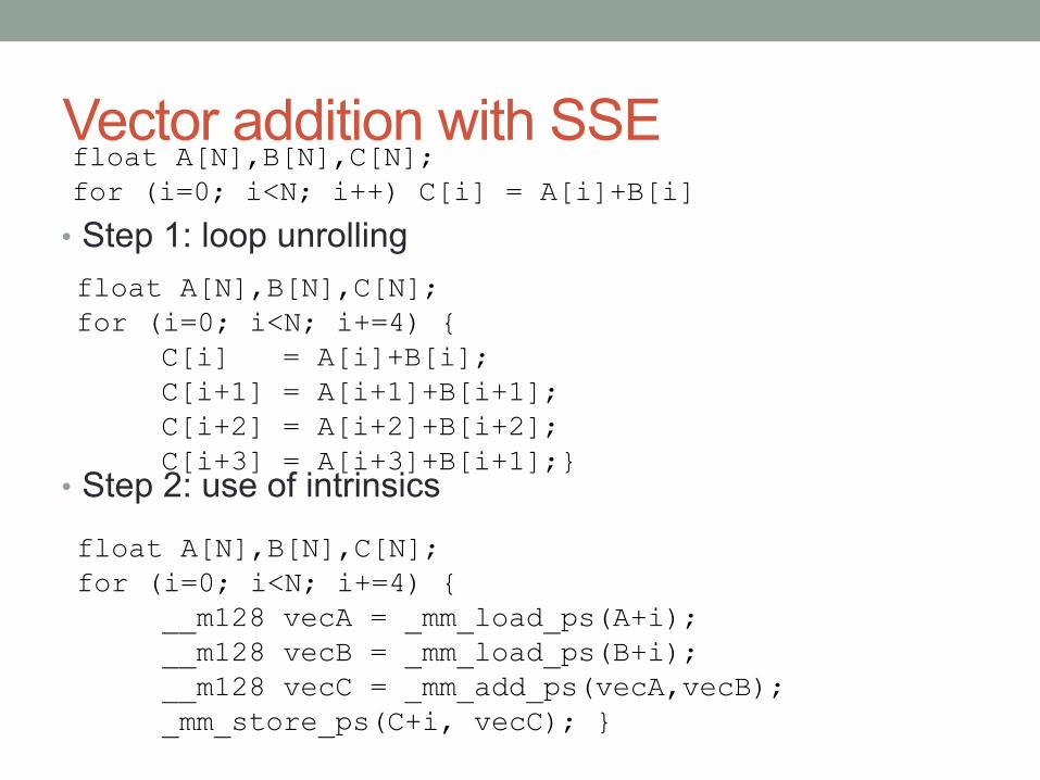
float A[N],B[N],C[N]; for (i=0; i<N; i+=4) {

__m128 vecA = _mm_load_ps(A+i); __m128 vecB = _mm_load_ps(B+i); __m128 vecC = _mm_add_ps(vecA,vecB); _mm_store_ps(C+i, vecC); }

float A[N],B[N],C[N]; for (i=0; i<N; i+=4) {

C[i] = A[i]+B[i]; C[i+1] = A[i+1]+B[i+1]; C[i+2] = A[i+2]+B[i+2]; C[i+3] = A[i+3]+B[i+1];}

float A[N],B[N],C[N]; for (i=0; i<N; i++) C[i] = A[i]+B[i]

Vector addition with SSE

• Step 1: loop unrolling

• Step 2: use of intrinsics

SSE vs. AVX •  SSE/SSEn is Intel-specific •  AVX in an extension of SSE

•  To be supported by more vendors •  Currently: AMD and Intel

•  AVX fact sheet: •  Larger registers : 256b instead of 128b •  Supports legacy instruction (lower 128b) •  Adds support for 3-operand instructions

Memory performance •  Flat memory model

•  All accesses = same latency •  Memory latency slower to improve than processor speed

The gap grows ~50% per year

… which means we wait longer for any access to the (DRAM) memory!

Solutions •  Improve latency

•  Technology •  Memory hierarchies

• Make better use of bandwidth •  Bandwidth increases 3x faster than latency! •  Collect/gather/coalesce multiple memory accesses

• Overlap computation and communication •  Prefetching •  Default/automated (low-level) •  Software-managed (aka, programmer implemented …)

Memory hierarchies • Hierarchical memory model

•  Several memory spaces •  Large size, low cost, high latency – main memory •  Small size, high cost, low latency – caches / registers

• Main idea: Bring some of the data closer to the processor •  Smaller latency => faster access •  Smaller capacity => not all data fits!

• Who can benefit? •  Applications with locality in their data accesses

•  Spatial locality •  Temporal locality

Memory hierarchies (cont’d) •  Limitations

•  Size: no space for every memory address •  Organization: what gets loaded & where ? •  Policies: who’s in, who’s out, when, why?

• Performance •  Hit = access found data in fast memory => low latency •  Miss = data not in fast memory => high latency + penalty •  Metric: hit ratio (H) = the fraction of accesses that hit •  Performance gain: ?

•  T_nocache = N * T_main_memory •  T_cache = (N-H)*(T_main_meoryoy+penalty) + H*T_cache

Why do memory hierarchies work? •  Temporal locality

•  RD(x), RD(x), RD(x): •  Main_RD, Cache_hit, Cache_hit •  Gain: Cache latency is better !

• Spatial locality •  RD(x),RD(x+1),RD(x+2):

•  Main_RD, Cache_hit, Cache_hit •  Gain: Cache latency is better + better bandwidth for coalesced

operations RD(x,x+1,x+2, … )

Memory performance in practice •  Theoretical:

•  Peak latency & bandwidth are given •  … but in theoretical optimal conditions

•  Practice: •  Microbenchmarking of the memory system

•  E.g.: Membench •  … or build your own benchmark

INTER-CORE PARALLELISM

Multi-core CPUs

35

• Architecture •  Few large cores •  (Integrated GPUs) •  Vector units

•  Streaming SIMD Extensions (SSE) •  Advanced Vector Extensions (AVX)

•  Stand-alone • Memory

•  Shared, multi-layered •  Per-core caches + shared caches

• Programming •  Multi-threading •  OS Scheduler

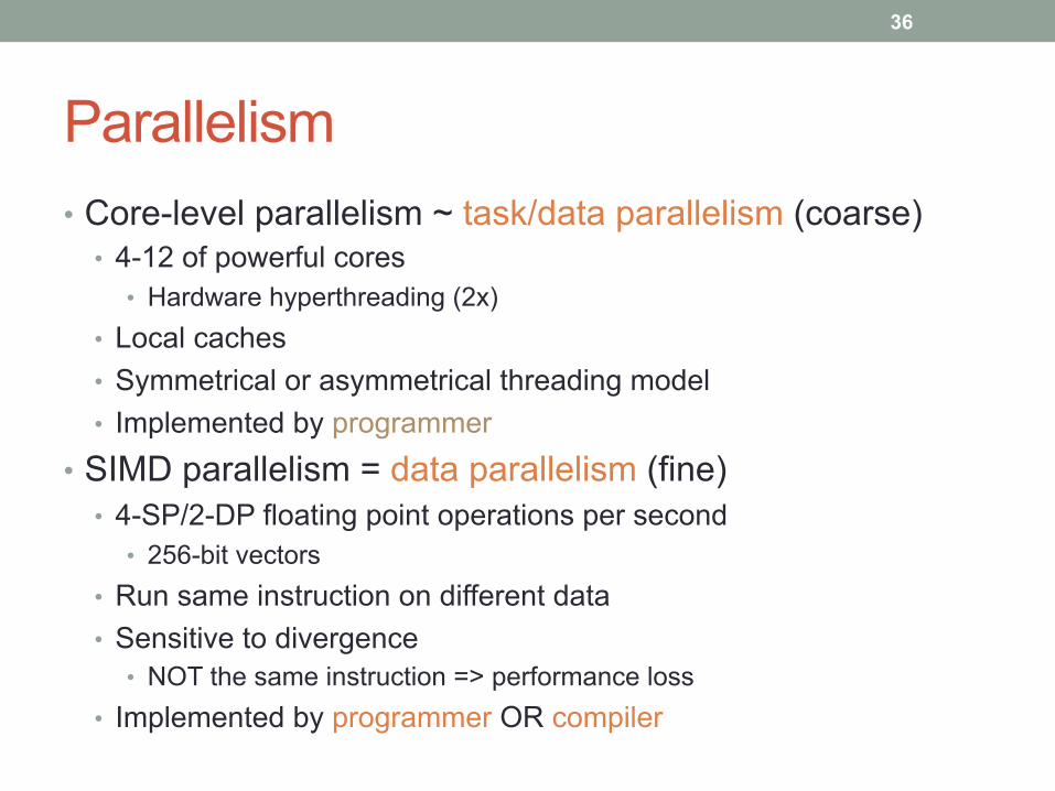
Parallelism

36

• Core-level parallelism ~ task/data parallelism (coarse) •  4-12 of powerful cores

•  Hardware hyperthreading (2x) •  Local caches •  Symmetrical or asymmetrical threading model •  Implemented by programmer

• SIMD parallelism = data parallelism (fine) •  4-SP/2-DP floating point operations per second

•  256-bit vectors •  Run same instruction on different data •  Sensitive to divergence

•  NOT the same instruction => performance loss •  Implemented by programmer OR compiler

Programming models

37

• Pthreads + intrinsics •  TBB – Thread building blocks

•  Threading library

• OpenCL •  To be discussed …

• OpenMP •  Traditional parallel library •  High-level, pragma-based

• Cilk •  Simple divide-and-conquer model Le

vel o

f abs

trac

tion

incr

ease

s

GPGPU History

38

• Current generation: NVIDIA Kepler •  7.1B transistors •  More cores, more parallelism, more performance

1995 2000 2005 2010

RIVA 128 3M xtors

GeForce® 256 23M xtors

GeForce FX 125M xtors

GeForce 8800 681M xtors

GeForce 3 60M xtors

“Fermi” 3B xtors

GPGPU History

39

• Use Graphics primitives for HPC •  Ikonas [England 1978] •  Pixel Machine [Potmesil & Hoffert 1989] •  Pixel-Planes 5 [Rhoades, et al. 1992]

• Programmable shaders, around 1998 •  DirectX / OpenGL •  Map application onto graphics domain!

• GPGPU •  Brook (2004), Cuda (2007), OpenCL (Dec 2008), ...

GPGPU History

40

Another GPGPU history

41

GPGPU @ NVIDIA

42

GPUs @ AMD

43

GPUs @ ARM

44

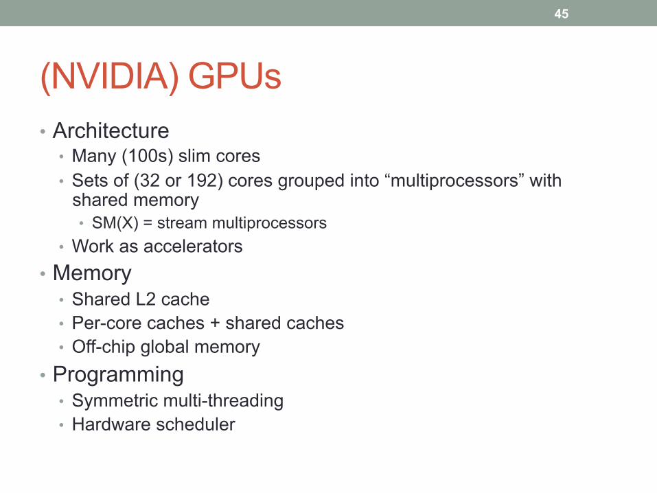
(NVIDIA) GPUs

45

• Architecture •  Many (100s) slim cores •  Sets of (32 or 192) cores grouped into “multiprocessors” with

shared memory •  SM(X) = stream multiprocessors

•  Work as accelerators • Memory

•  Shared L2 cache •  Per-core caches + shared caches •  Off-chip global memory

• Programming •  Symmetric multi-threading •  Hardware scheduler

NVIDIA’s Fermi GPU Architecture

46

Parallelism

47

• Data parallelism (fine-grain) •  Restricted forms of task parallelism possible with newest

generation of NVIDIA GPUs

• SIMT (Single Instruction Multiple Thread) execution •  Many threads execute concurrently

•  Same instruction •  Different data elements •  HW automatically handles divergence

•  Not same as SIMD because of multiple register sets, addresses, and flow paths*

• Hardware multithreading •  HW resource allocation & thread scheduling

•  Excess of threads to hide latency •  Context switching is (basically) free

*http://yosefk.com/blog/simd-simt-smt-parallelism-in-nvidia-gpus.html

Larrabee

48

• GPU based on x86 architecture •  Hardware multithreading •  Wide SIMD

• Achieved 1 tflop sustained application performance (SC09)

• Cancelled •  Dec’09

Intel Xeon Phi (=MIC) •  First product: “Knights corner”

•  Accelerator or stand-alone •  ±60 Pentium1-like cores •  512-bit SIMD

• Memory •  L1-cache per core (32KB I$ + 32KB D$) •  Very large unified L2-cache (512KB/core, ~30MB/chip) •  At least 8GB of GDDR5

• Programming •  Multi-threading

•  Traditional models: OpenMP, MPI, Cilk, TBB, parallel libraries + OpenCL •  OS thread scheduler

•  User-control via affinity

49

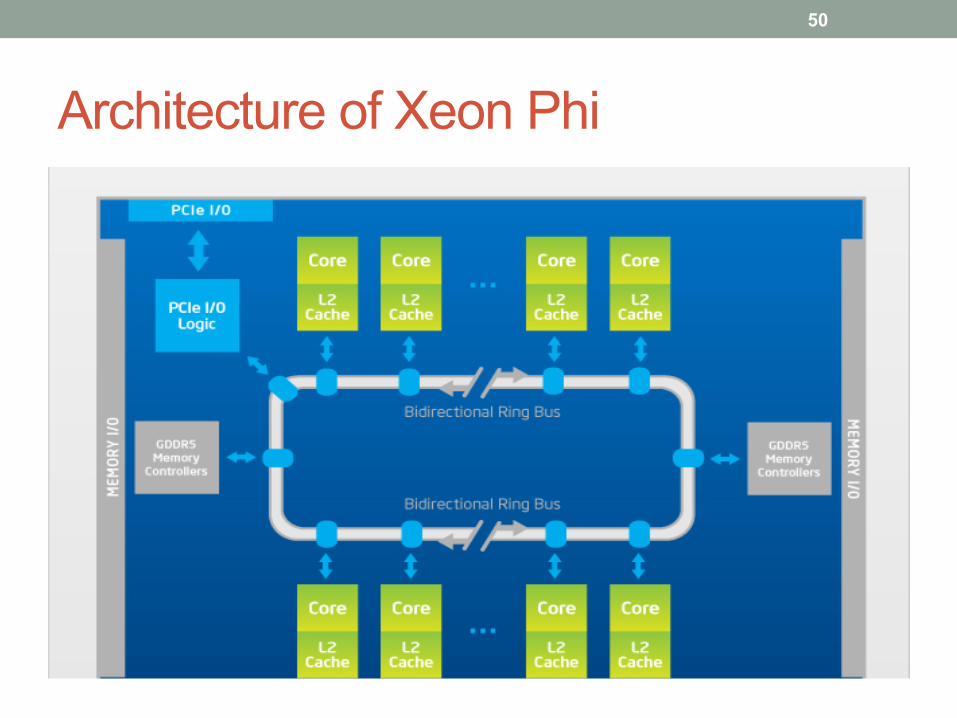
Architecture of Xeon Phi

50

Parallelism

51

•  3 operation modes •  Stand-alone •  Offload •  Hybrid

• Core-level parallelism ~ task parallelism (coarse) •  ~60 cores, 4x hyperthreading

• SIMD parallelism = data parallelism (fine) •  Fine-grained parallelism •  16 SP-Flop, 16 int-ops, 8 DP-Flop / cycle •  AVX-512 extensions

•  No support for MMX, SSE => not backward compatible

INTER-NODE PARALLELISM

Typical examples • Clusters

•  See DAS4

• Super-computers •  Half of top500

• Grids & clouds •  See Grid5000 •  See Amazon EC2

IBM’s BlueGene/Q

Take home message • Machine = Multiple layers of parallelism

•  Intra-core •  Hidden

•  ILP, pipelining, multiple functional units •  Exposed / explicit

•  Vectorization/SIMD-ization •  Memory

•  Caching

•  Inter-core •  Multiple threads per core

•  Inter-node •  Multiple processes/threads/jobs/applications