A VALUATION STUDY OF STOCK-MARKET SEASONALITY AND FIRM SIZE

Zhiwu Chen Yale School of Management

Jan Jindra

Cornerstone Research

May 2001

This Paper Can be Downloaded from Social Science Recearch Network at:http://papers.ssrn.com/paper.taf?abstract_id=273191

Yale ICF Working Paper No. 00-37

A Valuation Study of Stock-Market Seasonality and Firm Size

Zhiwu Chen, and Jan Jindra∗

May 29, 2001

∗Chen is a Professor of Finance at Yale School of Management, 135 Prospect Street, New Haven, CT 06520,Zhiwu.Chen@yale.edu, Tel. (203) 432-5948; Jindra is an Associate at Cornerstone Research, 1000 El Camino Real,Menlo Park, CA 94025, JJindra@cornerstone.com and telephone: (650) 470-7191. The earnings data used in thepaper are graciously provided to us by I/B/E/S International Inc. Any remaining errors are our responsibility alone.

0

A Valuation Study of Stock-Market Seasonality and Firm Size

Abstract

Existing studies on market seasonality and the size effect are largely based on realized returns.

This paper investigates seasonal variations and size-related differences in cross-stock valuation

distribution. We use three stock valuation measures, two derived from structural models and

one from book/market ratio. With each measure, we find that the average valuation level is the

highest in mid summer and the lowest in mid December. Furthermore, the valuation dispersion

(or, kurtosis) across stocks increases towards the yearend and reverses direction after the turn of

the year, suggesting increased movements in both the under- and overvaluation directions. Among

size groups, small-cap stocks exhibit the sharpest decline in valuation from June to December and

the highest rise from December to January. For most months, small-cap stocks have the lowest

valuation among all size groups. In a typical month, small-cap stocks show the widest cross-stock

valuation dispersion, meaning they are also the hardest to value. Overall, large stocks enjoy the

highest level of valuation uniformity and are the least subject to seasonal valuation variations.

1

1 Introduction

One of the salient facts in finance is the documented seasonality in stock returns. Specifically,

recent losers tend to experience fortune reversals in January (hence, the January effect), whereas

recent winners tend to continue and expand their fortunes in December (hence, the December

effect).1 Most studies on stock market seasonality have relied on return differences across calendar

times. In this paper, we analyze seasonality from a different perspective, that is, we implement

three alternative valuation measures and investigate how the cross-stock valuation distribution

shifts from month to month. If seasonal patterns exist, we then want to see whether they can shed

new light on the documented January and December effects. This approach should offer unique

insights into the seasonality effects by allowing us to gauge the relative and absolute valuation

characteristics of stocks in various months of the year. At the same time, given the documented

seasonal return patterns, such a study also allows us to evaluate alternative valuation measures,

with the understanding that a good stock valuation metric must be able to demonstrate in ad-

vance certain seasonal dynamics and predict such return patterns. That is, understanding which

valuation measure best anticipates the return seasonality will help guide further developments of

equity valuation models.

The fact that beaten-down stocks (especially if they are also small firms) experience return

reversals in January has long been a puzzling phenomenon and generated a large literature. There

are several proposed explanations, including ”window-dressing” by institutional investors (Lakon-

ishok, Shleifer, Thaler, and Vishny (1991)) and the tax-loss selling hypothesis (Grinblatt and

Moskowitz (1999)). The window-dressing hypothesis contends that institutional investors want to

sell losers and buy glamorous winners to prepare for their year-end reporting. Such buying and

selling create positive price pressure on winners and downward pressure on losers in the period

before the turn of the year. As the selling by institutions stops at year end, prices for the beaten-

down stocks rebound in January, producing large positive returns for last year’s losers. This effect

can be more pronounced for small stocks because of their low liquidity and high market-impact

costs. The tax-loss selling hypothesis asserts that it is the individual investors faced with cap-

ital gains taxation who sell poor-performing stocks to reduce their taxes. To achieve such tax

reduction, an investor must sell the losing stocks before year end as capital losses can be used to

offset gains only upon realization. Both hypotheses thus predict that stocks that are losers by

late fall will likely continue going lower in December, but will have high returns in January. The

window-dressing hypothesis also suggests that strong performers by late fall shall continue going

1The January effect has been documented by Dyl (1977), Roll (1983), Keim (1983,1989), Reinganum (1983),Ritter (1988), and others. Grinblatt and Moskowitz (1999) find such a December effect.

2

strong in December, which may be a key reason behind the December effect described in Grinblatt

and Moskowitz (1999).

The purpose of this paper is to identify and understand what valuation picture may be behind

the return patterns. Such an exercise can not only help deepen our understanding of the seasonality

phenomenon, but also shed new light on the development of stock valuation models. Specifically,

we implement three valuation measures in this paper. The first measure is based on the dynamic

stock valuation model developed by Bakshi and Chen (1999) and extended by Dong (2000), which

we refer to as the BCD model. The BCD model assumes a parameterized stochastic process for

each of the firm’s earnings-per-share (EPS), expected future EPS and economy-wide interest rates.

Its closed-form valuation formula is shown to contain substantial information about the extent to

which a stock may be mispriced, and investment strategies based on the BCD model valuation

offer significant abnormal returns (Chen and Dong (2000)). We refer to the percentage deviation

by the market price from a stock’s model price as the BCD mispricing. The second measure is the

value/price (V/P) ratio, where “value” is determined using the accounting residual-income model

as implemented in Lee, Myers and Swaminathan (1999). The residual-income model valuation is

based on a multi-stage discounting procedure that involves estimating both the firm’s future EPS

in excess of the required return on equity and a terminal value of the stock at the end of valuation

horizon. The last measure is the book/market (B/M) ratio, which has traditionally been viewed

and applied as an indirect valuation metric. Our results are briefly summarized below:

• According to each of the valuation measures, stocks on average become less favorably valued

as the year end approaches. In December, stocks are the least favorably valued (except that

based on the V/P ratio, November instead of December marks the lowest valuation month of

the year), while stocks reach their highest valuation levels in the May-June period. Towards

the calendar year end, the cross-stock valuation distribution also becomes increasingly dis-

persed and flattened out, with either the standard deviation or the kurtosis of the valuation

distribution growing larger. This means that undervalued stocks become more undervalued

whereas overvalued ones become more so, implying more differential and uneven treatments

of stocks as the year end approaches. After the turn of the year, all of these valuation trends

are reversed.

• From January to December, the undervalued fraction of stocks follows a U-shaped pattern,

with December and January at the high ends and May-June at the bottom. The seasonal

pattern for the overvalued fraction is the opposite and has a hump-shape.

• Across size groups, the small-cap stocks are on average the least favorably valued, followed

by mid-cap and then by large-cap stocks. This is true for most calendar months. According

3

to each measure, the valuation spread between December and June is the largest for small-

cap and the second largest for mid-cap; Similarly, the December-January valuation spread

is also the largest for small-cap. Thus, the seasonal valuation patterns are the most severe

for small-cap, in terms of changes both around the turn of the year and from year end to

mid-year.

• For each given month, the cross-stock valuation distribution is the most widely dispersed

(i.e., with the highest standard deviation) for small-cap stocks and the least dispersed for

large-cap stocks. It is again true regardless of the valuation measure.

• When we run Fama-McBeth cross-sectional regressions, separately for each calendar month,

to forecast future one-month stock returns, we find that the BCD mispricing and size have

the highest predictive power, whereas the V/P and B/M ratios are at best marginal. In

particular, the BCD mispricing and size are substantially more significant in predicting

the mid-December to mid-January returns than in predicting any other monthly returns.

The valuation seasonality captured by the BCD model anticipates the return seasonality

significantly more closely than the V/P and B/M ratios.

The findings summarized above are consistent with most of the returns-based studies on stock

market seasonality. The fact that the average valuation level is the lowest in December anticipates

the well known January return effect. The phenomenon that the valuation distribution becomes

more dispersed (with higher standard deviation or kurtosis) towards year end possibly captures

two simultaneous, but different trends: tax-loss and window-dressing selling of the losers (making

the losers more undervalued) and window-dressing buying of winners (making the winners more

overvalued, hence the December return effect).

We have also added a few items to the growing list of conclusions regarding small-cap versus

large-cap stocks: that most of the year small-cap stocks are the least favorably valued, that their

valuation dispersion is the highest, that their June-December valuation patterns are the strongest,

and that their December-to-January valuation increase is the highest. These valuation-based

findings together suggest that (i) small-cap stocks may simply be much harder to value, and (ii)

their mispricings are more difficult to be arbitraged away. Forces that have been proposed as

factors behind these difficulties with small stocks include informational asymmetry, price-impact

and trading costs (e.g., Hasbrouk (1991), and Stoll (2000)), liquidity constraints, high information-

acquisition costs but low economic benefits for institutional portfolio managers, and high arbitrage

risk (e.g., Wurgler and Zhuravskaya (2000)). All of these factors favor large-cap and work against

small-cap stocks.

4

The rest of the paper proceeds as follows. Section 2 discusses the three valuation measures

and their implementation, and describes the data sample used. Section 3 documents the valuation

seasonality for the overall stock sample. In Section 4, we divide the sample into three size groups

and address the differences across size groups. Section 5 focuses on Fama-McBeth cross-sectional

return-forecasting regressions, and the goal is to establish at a cross-sectional level a formal linkage

between valuation seasonality and return seasonality. Concluding remarks are given in Section 6.

2 Valuation Measures

To make our results independent of a particular valuation model, we use three value measures for

each traded stock: a mispricing measure based on the valuation model in Bakshi and Chen (1999)

and Dong (2000) (BCD mispricing), a value/price (V/P) ratio based on the residual-income model

in Lee, Myers and Swaminathan (1999), and book-to-market (B/M) ratio. We don’t include the

earnings/price (E/P) ratio in our study partly because it is highly correlated with the B/M, and

partly because the existence of negative earnings would make the discussion and inference difficult.

These value metrics have been applied in the literature and shown to be significant in explaining

and predicting cross-sectional stock returns.2. These measures and their implementation methods

are discussed in more detail in the subsections below.

2.1 The BCD Mispricing

For detailed derivations and discussions on this stock valuation model, see Bakshi and Chen (1999)

and Dong (2000). In this paper, we use the same data and the same implementation method as

in Chen and Dong (2000). In this subsection, we outline the main points. To describe the BCD

model, assume that a share of a firm’s stock entitles its holder to an infinite dividend stream

{D(t) : t ≥ 0}. Our goal is to determine the time-t per-share value, S(t), for each t ≥ 0. Bakshi

and Chen (1999) make the following assumptions:

• The firm’s dividend policy is such that at each time t

D(t) = δ Y (t) + ε(t) (1)

where δ is the target dividend payout ratio, Y (t) the current EPS (net of all expenses,

interest and taxes), and ε(t) a mean-zero random deviation (uncorrelated with any other

stochastic variable in the economy) from the target dividend policy.

2Among other studies, see Chen and Dong (2000), Fama and French (1992, 1993), Grinblatt and Moskowitz(1999), Lee, Myers and Swaminathan (1999).

5

• The instantaneous interest rate, R(t), follows an Ornstein-Uhlenbeck mean-reverting process:

dR(t) = κr

[µ0

r −R(t)]

dt + σr dωr(t), (2)

for constants κr, measuring the speed of adjustment to the long-run mean µ0r, and σr,

reflecting interest-rate volatility. This is adopted from the well-known single-factor Vasicek

(1977) model on the term structure of interest rates.

In Bakshi and Chen (1999), the assumed process for Y (t) do not allow for negative earnings

to occur. To resolve this modeling issue, Dong (2000) extends the original Bakshi-Chen earnings

process by adding a constant y0 to Y (t):

X(t) ≡ Y (t) + y0. (3)

X(t) can be referred to as the displaced EPS or adjusted EPS. Next, Dong (2000) assumes that

X(t) and the expected adjusted-EPS growth, G(t) follow

dX(t)X(t)

= G(t) dt + σx dωx(t) (4)

d G(t) = κg

[µ0

g −G(t)]

dt + σg dωg(t), (5)

for constants σx, κg, µ0g and σg, where G(t) is the conditionally expected rate of growth in adjusted

EPS X(t). The long-run mean for G(t) is µ0g, and the speed at which G(t) adjusts to µ0

g is reflected

by κg. Further, 1κg

measures the duration of the firm’s business growth cycle. Volatility for both

the adjusted-EPS growth and changes in expected adjusted-EPS growth is time-invariant. The

correlations of ωx(t) with ωg(t) and ωr(t) are respectively denoted by ρg,x and ρr,x.

Under the given model assumptions, the equilibrium stock price is

S(t) = δ

∫ ∞

0{X(t) exp [ϕ(τ)− %(τ) R(t) + ϑ(τ) G(t)]− y0 exp[φ0(τ)− %(τ)R(t)]} dτ, (6)

where

ϕ(τ) = −λxτ +12

σ2r

κ2r

[τ +

1− e−2κrτ

2κr− 2(1− e−κrτ )

κr

]− κrµr + σxσrρr,x

κr

[τ − 1− e−κrτ

κr

]

+12

σ2g

κ2g

[τ +

1− e−2κgτ

2κg− 2

κg(1− e−κgτ )

]+

κgµg + σxσgρg,x

κg

[τ − 1− e−κgτ

κg

]

−σrσgρg,r

κrκg

{τ − 1

κr(1− e−κrτ )− 1

κg(1− e−κgτ ) +

1− e−(κr+κg)τ

κr + κg

}(7)

6

%(τ) =1− e−κrτ

κr(8)

ϑ(τ) =1− e−κgτ

κg(9)

φ0(τ) =12

σ2r

κ2r

[τ +

1− e−2κrτ

2κr− 2(1− e−κrτ )

κr

], (10)

subject to the transversality conditions that

µr >12

σ2r

κ2r

(11)

µr − µg >σ2

r

2κ2r

− σrσxρr,x

κr+

σ2g

2κ2g

+σgσyρg,x

κg− σgσrρg,r

κgκr− λx, (12)

where λx is the risk premium for the systematic risk of earnings shocks, µg and µr are the respective

risk-neutralized long-run means of G(t) and R(t). Formula (6) represents a closed-form solution

to the equity valuation problem, except that its implementation requires numerically integrating

the inside exponential function. Therefore, the equilibrium stock price is a function of interest

rate, current EPS, expected future EPS, the firm’s required risk premium, and the structural

parameters governing the EPS and interest rate processes. We will refer to this stock-pricing

formula as the Bakshi-Chen-Dong (BCD) model.

To implement the BCD model, we need to estimate the structural parameters. To reduce the

number of parameters to be estimated, we preset ρg,x = 1 and ρg,r = ρr,x ≡ ρ, that is, actual

and expected adjusted-EPS growth rates are subject to the same shocks. In addition, for each

individual stock estimation, the three interest-rate parameters are preset at µr = 0.07, κr = 0.079,

σr = 0.007. These parameter values are backed out from the S&P 500 index data for the 1982-1996

monthly sample, and taken from Bakshi and Chen (1999). A justification for this treatment is

that the interest-rate parameters are common to all stocks and equity indices. Then, there are 8

firm-specific parameters remaining to be estimated: Φ = {y0, µg, κg, σg, σx, λx, ρ, δ}. At each time

point of valuation, the most recent 24 monthly observations on a stock (and interest rates) are

used as the basis to estimate Φ (see Chen and Dong (2000) for details on this choice). Specifically,

for each stock and for every month in the sample, Φ is chosen so as to solve

MinΦ

24∑

t=1

[ S(t)− S(t) ]2, (13)

where S(t) is as given in formula (6) and S(t) the observed market price in month t.

7

Once the parameters are estimated for a given stock and in a given month (using data from the

prior years), the parameter estimates, plus the current R(t), Y (t) and G(t) values, are substituted

into formula (6) to determine the current model price for the stock in that month. After the

model price is calculated for the stock in that month, the parameter estimation steps and the

calculation are repeated for the same stock, but for the following month and so on. This process

is independently and separately applied to every stock in the sample and for each month. For

this reason, all the model prices used in our study are determined out of sample. For each month

and each stock, the BCD mispricing is defined to be the percentage deviation by the market price

from the stock’s model price, that is, the difference between the market and model price, divided

by the model price.

2.2 The V/P Ratio

The second valuation measure is based on the residual income model.3 Specifically, we calculate

the value to price (V/P) ratio, where value is determined by the residual income model and price

is taken from the market as of each mid-month.

A stock’s intrinsic value is defined as the present value of the expected future cash flows to

shareholders:

V (t) =∞∑

i=1

Et(D(t + i))(1 + re)i

. (14)

where Et(D(t + i)) is the expected future dividend for period t + i conditional on all available

information at time t, and re is the cost of equity. Ohlson (1990, 1995) demonstrates that if the

firm’s earnings and book value are forecasted in a manner consistent with clean-surplus accounting

(i.e. a dollar of earnings increases either dividends paid out or book value by a dollar), the intrinsic

value may be rewritten as:

V (t) = B(t) +∞∑

i=1

Et [NI (t + i)− reB(t + i − 1 )](1 + re)i

(15)

= B(t) +∞∑

i=1

Et [(ROE (t + i)− re)B(t + i − 1 )(1 + re)i

, (16)

where B(t) is the book value at time t, Et[NI(t + i)] and Et[ROE(t + i)] are the conditional

expectations of both net income and after-tax return on book value of equity for period t + i.

As discussed in Lee, Myers, and Swaminathan (1999), this equation is mathematically identical

3See, among others, Preinreich (1938), Edwards and Bell (1961), Peasnell (1982), Ohlson (1990), and Lee, Myers,and Swaminathan (1999), for the literature on the residual-income model.

8

to the dividend discount model. That is, it relies on the same theory and is subject to the same

theoretical limitations as the dividend discount model.

The above equation expresses a stock’s intrinsic value in terms of an infinite sum. However, for

practical purposes, only limited future earnings forecasts are available. This limitation introduces

a need for an estimate of a terminal value. That is, we measure the intrinsic value in the following

way:

V (t) = B(t) +2∑

i=1

EPS (t + i)− reB(t + i − 1 )(1 + re)i

+ TV (17)

where EPS(t) is the consensus earnings forecast for period t, and TV is the terminal value estimate

based on the average of the last two years of data (in order to smooth cases of unusual performance

in the last year, D’Mello and Shroff (1999)):

TV = B(t) +1

2re(1 + re)2

3∑

i=2

EPS (t + i)− reB(t + i − 1 )(1 + re)

2 (18)

When implementing the model, we estimate the current book value per share, B(t), from the

most recent financial statement. Book value for any future period t + i, B(t + i), is given by the

beginning-of-period book value, B(t + i − 1), plus the forecasted EPS, EPS(t + i), minus the

forecasted dividend per share for year t + i. The forecasted dividend per share is estimated using

the current dividend payout ratio. The forecasted earnings per share, EPS(t+1), are given by the

analyst consensus forecast for the relevant year and as reported in I/B/E/S. The cost of equity

capital, re, is estimated using the CAPM and following Fama and French (1997): 60 monthly

observations prior to the month of estimation are used to estimate the stock’s beta, and then the

cost of equity capital is determined by the market T-bill rate of the month plus the beta times

the market risk premium, where the market risk premium is the average excess return on the

NYSE/AMEX/Nasdaq portfolio from January 1945 to month t-1.

2.3 B/M Ratio

Market ratios have long been used as indirect measures of value. Among them are book/market

(B/M), earnings/price (E/P), cashflow/price, and sales/price. These ratios have been shown to

be significant predictors of future returns in the empirical literature.4 Since E/P, cashflow/price

4There is a large literature on this topic. Some of the recent studies include Daniel and Titman (1997), Davis,Fama, and French (2000), Fama and French (1992,1993,1995,1996,1997), Frankel and Lee (1998), Jegadeesh andTitman (1993), Lakonishok, Shleifer, and Vishny (1994), Moskowitz (1998).

9

and sales/price are generally highly correlated with the B/M ratio, we focus our attention on just

the B/M ratio.

For the B/M ratio, the book value of equity is measured once a year at the firm’s fiscal year

end, whereas the market value of equity is calculated at the end of each month. Therefore, there

is a monthly B/M value for each stock.

2.4 Data Sample

For this study, we rely on three databases to estimate the three valuation measures for each stock

and in every month. First, dividend-inclusive monthly stock returns are obtained from the CRSP

database. Second, the actual book value data for calculating each stock’s B/M ratio are from

COMPUSTAT. Finally, for determining the BCD mispricing and the V/P ratio of each stock,

we use the analyst consensus earnings forecasts from I/B/E/S. Since I/B/E/S starts collecting

earnings forecasts in 1976, our original sample does not start until 1976. Then, for the BCD

mispricing measure, we need two years of EPS forecast and market price data in order to estimate

the BCD model parameters for each given firm. Therefore, the out-of-sample model price does

not exist for any stock until late 1978. When it started in the late 1970’s, I/B/E/S did not cover

more than a few hundred large firms. To maintain a decent sample size, we restrict our attention

to the 19-year period from January 1980 to December 1998.

For a stock to have an estimate for any of the valuation measures, there must be sufficient data

(including enough past data for estimating parameters, where applicable) to calculate the value

of that measure. Given that the BCD mispricing requires the most historical data, the remaining

sample of observations each with a BCD mispricing is the smallest and the sample of observations

with a V/P ratio value is the second smallest, whereas the B/M sample is the largest.

For each given valuation measure, we maintain and use the same sample for each investigation

to follow so that direct comparisons are possible. In one experiment, we will sort the stock universe

into size groups based on the stocks’ June market capitalizations, and then fix the groups for the

next twelve months until the following June. In another experiment, we will conduct valuation-

difference tests between calendar months, for which the valuation levels in different months of the

same stock will be matched. For these two reasons, a stock is not included in a given valuation

measure’s sample until July of year t+1, if the stock has a value of the valuation measure only for

some months (not for all of the twelve months) from June of year t to June of year t+1.

The temporal distribution of the three samples is shown in Table 1. The BCD mispricing

sample has 30,925 stock-month observations over the 19-year period; The B/M sample has 71,781

observations, where any observation with either (i) a B/M less than 0.05 or greater than 30 or (ii)

10

a book value less than $0.1 million is excluded; And there are 47,671 observations for the V/P

ratio sample.

In Table 1, the sample size for each category (say, the BCD mispricing sample) has steadily

increased from 1980 forward, due to the improving and increasingly more extensive coverage of

firms by I/B/E/S over the years. Another contributing factor is the ever increasing number of

publicly traded firms.

Table 2 provides summary statistics for each valuation measure, both over the entire sample

period and year-by-year. For ease of discussion, we use percentage values for both the V/P and

B/M ratios, indicating the intrinsic value and book value as a percentage of the stock’s market

price. Over the entire period, the average estimate is 3.27% for the BCD mispricing, 80.78% for the

V/P ratio, and 83.16% for the B/M ratio. ¿From 1980 to 1998, both the average valuation and the

cross-sectional standard deviation have varied significantly, regardless of the valuation metric. For

example, the average BCD mispricing was 9.68% (overvalued) in 1987, the last highest valuation

until the end of the sample; The average V/P ratio continued its downward trend from 1994

onward, whereas the B/M ratio started its down trend in 1990. Both ratios indicate that the U.S.

stocks had become increasingly more overvalued in recent years.

Panel B of Table 2 gives the correlations among the three measures, a stock’s past-12-month

return and its market cap. The BCD mispricing and a stock’s recent 12-month return have a

correlation of 0.408, indicating that 40.8% of the time a stock’s overvaluation (or, undervaluation)

coincides with a recent price run-up (or, run-down). The V/P ratio has the second highest

correlation with the stock’s recent return; And the B/M the lowest. The BCD mispricing has a

-0.158 correlation with the V/P and -0.054 with the B/M, suggesting that the BCD mispricing

and the B/M agree the least often. The correlations between market cap and the BCD mispricing,

V/P and B/M all imply that the larger the firm, the more likely it is favorably valued.

3 Seasonality in Valuation Measures

In this section, we first document how the cross-stock distribution of each valuation metric changes

seasonally when all stocks in each sample are included. Then, we study how the valuation distri-

bution’s seasonal patterns may differ across firm-size groups.

3.1 Month-to-month variations in valuation

To examine how the valuation distribution changes from month to month, for each given month of

the year and a given valuation metric, we compute the mean, median, standard deviation, skewness

and kurtosis of the valuation metric across all the stocks in that calendar month and for all years

11

from 1980 to 1998. That is, we pool together the same-calendar-month observations from each

year of the sample, resulting in 12 calendar-month pools. In total, we obtain 12 calendar-month

valuation distributions across individual firms.

In Table 3 we report the valuation statistics for each calendar month. First, let’s start with

the BCD mispricing. Both the mean and median BCD mispricing estimates reach their highest

values in May and June, implying stocks are on average the highest valued during mid-year, with

a median mispricing of 4.36%. From June to December, the mean and median BCD mispricing

levels decrease steadily; Then, from December to May, the BCD mispricing reverses direction and

steadily increases. For any given stock, the average mispricing difference between December and

June is 6.76%, with a standard error of 0.16% and hence a t-statistic of 42.25, whereas the average

increase in mispricing is 2.73% from December to January (with a t-statistic of 30.33). Therefore,

stocks are on average the most underpriced before year end, with a median mispricing of -1.25% in

December. January marks the beginning of the “correction” process, and by mid-February stocks

become on average fair-valued (with a median mispricing of 2.34%).

The skewness and kurtosis in Table 3 also demonstrate a significant seasonality in the BCD

mispricing. The skewness is the lowest in December, implying the least favorable valuation across

stocks in December. The kurtosis for the BCD mispricing increases each month from August

to December, reaching its high in December (and then in May again). Thus, the cross-stock

mispricing distribution becomes more fat-tailed towards December. This suggests that as the year

end approaches, stocks that are beaten down and undervalued will become even more undervalued

while stocks that are already overvalued will grow even more overvalued. This phenomenon of

extremely mispriced stocks becoming even more so (on both the under and the over-valued side)

is likely due to the working of two different factors: one due to performance-chasing at year end

by portfolio managers and the other due to tax-loss selling. It anticipates both the December and

the January effect. We will return to this disscusion later.

Figure 1 displays how the following three fractions change from month to month: (i) fraction

of stocks that are undervalued between 30% and 50% (with a BCD mispricing between -50%

and -30%), (ii) fraction of stocks that are fair-valued (with a BCD mispricing between -10% and

10%), and (iii) fraction of stocks that are overvalued (with a BCD mispricing between 30% and

50%). The chart shows that the undervalued fraction has a “hump-shape” pattern from June to

December to May, reaching its peak in December, whereas the seasonal pattern for the overvalued

fraction has a U-shape. Thus, December has the highest fraction of stocks undervalued and the

lowest fraction of stocks overvalued. On the other hand, the fair-valued fraction is relatively stable

over the year: with slightly less than half (about 45%) of the stocks fair-valued throughout the

year according to the BCD model.

12

The B/M ratio exhibits similar seasonal patterns as the BCD mispricing. In Table 3, the

mean and standard deviation for the B/M start increasing in August and reach their peak in

December, confirming the above conclusion that stocks on average become more undervalued and

the cross-stock valuation distribution grows more dispersed as December approaches. For any

stock, its average change in B/M ratio is -6.4% from December to June (with a standard error

of 0.2%), whereas the average net change is -3.3% from December to January (with a standard

error of 0.2%). Therefore, the seasonal changes in B/M are highly significant and systematic. The

skewness for the B/M is also the lowest in December.

For the V/P ratio, its mean, median, standard deviation and kurtosis each gradually increase

from June and reach their highest values in November (instead of December), and they start

gradually decreasing from November to February. Panels B and C of Figure 1 further confirm the

above observations regarding the B/M and V/P ratios: the undervalued fraction of stocks is the

highest in December according to the B/M ratio, and in November according to the V/P.

Based on Table 3 and Figure 1, our conclusions can be summarized as follows. First, regardless

of the valuation metric, stocks on average start from year-end’s undervaluation to mid-year’s

overvaluation and then back to year-end’s undervaluation again, a seasonal valuation pattern that

anticipates, and is consistent with, the well documented January stock-return effect. Second,

as the year end approaches, the dispersion of the cross-stock valuation distribution increases, or

both tails of the distribution become fatter: the overvalued stocks grow more overvalued and the

undervalued become more undervalued. This finding is consistent with both the January effect

(which is mostly about movements in the undervalued tail of the distribution around the turn

of the year) and the December effect as documented in Grinblatt and Moskowitz (1999). The

December effect is about the fact that stocks that are winners by the end of November tend to

continue doing well before the end of December. Given the relative high correlation between

recent return performance and overvaluation, these winners are also likely to be overvalued by

November’s end. Therefore, the December effect is about how the stocks in the right (overvalued)

tail of the mispricing distribution move from November to the end of December. The finding that

both tails of the BCD mispricing distribution become fatter before year end means that as the

year end approaches, winners will be even bigger winners while losers will be bigger losers.

3.2 Daily variations around the turn of the year

To see when the ”valuation correction” starts and how it evolves around the turn of the year, we

report in Table 4 the daily valuation distributions for the 10 trading days both prior to and after

the year end. For this table, the BCD model price, the intrinsic value and the book value are

13

determined as of mid December and fixed for the 20 trading days for each stock, and the daily

BCD mispricing, V/P and B/M ratios are calculated based on the daily closing prices of each

stock.

Table 4 shows that the valuation correction process starts at least 10 trading days prior to

the turn of the year, with both the valuation level going up and the cross-stock valuation kurtosis

going down gradually (based on the BCD mispricing). This process continues until about 5 to

7 trading days after the New Year, beyond which point the process begins to go back and forth

(though with a continuing up-trend). For example, 10 trading days prior to the year end, the

median BCD mispricing and the median B/M are -1.38% and 63.14%, respectively. By the last

trading day of the year, they are respectively 0.23% and 61.85%. Therefore, according to the

BCD mispricing, the median stocks are about fair-valued by the last trading day of the year.

The mispricing kurtosis is 6.05 as of 10 trading days prior to the New Year, and it goes down

to 4.92 by the last trading day, implying that as the New Year approaches, the extreme tails

of the cross-stock mispricing distribution become thinner. Thus, before the year end, valuation

correction takes place at both extremes and more stocks move toward the fair-valuation center.

The above finding seems to half contradict and half agree with the findings in Ritter (1988)

that among individual investors who had stock accounts with Merrill Lynch during 1971 to 1985,

the daily buy/sell ratio steadily declined during the 9 days prior to the year end, but reversed

direction and started to rise immediately after the turn of the year. The rising buy/sell ratio is

clearly consistent with the increasing valuation level after the year end in Table 4. For the 10

days prior to the year end, Table 4 shows a rising average valuation level whereas Ritter (1988)

finds a declining buy/sell ratio by individual investors. This seeming contradiction suggests that

institutional investors must be filling the gap: the aggregate buy/sell imbalance by institutions

must favor the buy side for the 10 days before the year end (otherwise, the January effect would

not start 10 days prior to the turn of the year).

4 Valuation Seasonality by Size Groups

The size effect is another well-documented phenomenon in which small-cap stocks on average

outperform large-cap stocks (e.g., Banz (1981), Blume and Stambaugh (1983), Fama and French

(1992, 1993), Keim (1983), and Roll (1983)). Furthermore, there is substantial evidence suggesting

that the January effect is largely due to small-cap firms. To help us understand the seasonal

patterns in the valuation distribution, we divide each June’s sample into three size groups: small-

cap, mid-cap and large-cap, each group consisting of one third of that June’s stock universe. Once

the size groups are formed, they are fixed for the next 12 months until the following June, at which

14

time the size groups are re-formed. Within each size group, we determine its cross-stock valuation

distribution for each month of the year and according to a given valuation measure. Table 5 shows

the resulting seasonal distribution panels, one for each size group.

Before discussing the valuation patterns in Table 5, note that the annual re-sorting in each

June of the stock universe into three size groups creates certain noticeable discontinuity from June

to July, especially for the small-cap group. When stocks are re-grouped according to their market

cap at the end of June, the small-cap group collects a biasedly large fraction of past losers. Since

those losers tend to be beaten down and hence likely to be undervalued, the average mispricing

for the small-cap group suddenly drops from its pre-sorting level of 7.10% to its post-sorting level

of 1.82% in July (see Panel A). In contrast, for the mid-cap and large-cap groups, their changes

in mispricing are not as dramatic from June to July (Panels B and C).

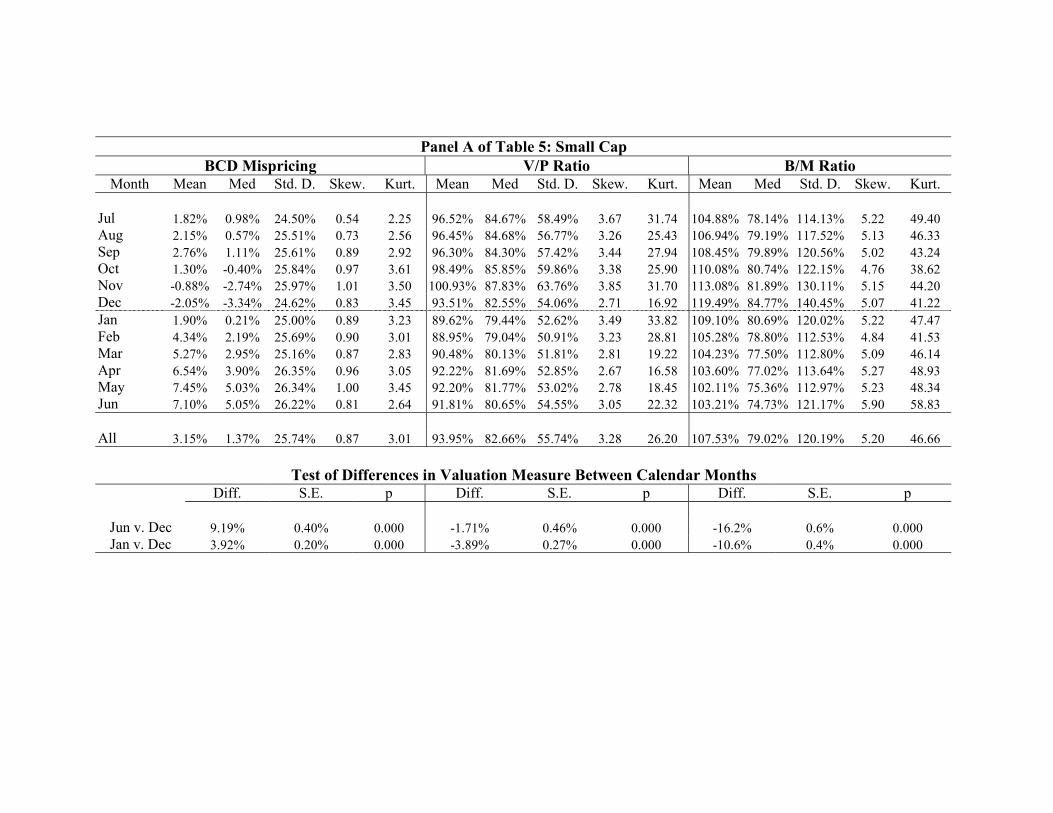
Panel A of Table 5 shows the seasonal variations in valuation distribution for small-cap stocks.

Take the BCD mispricing as a point of discussion. The seasonal changes in the average BCD

mispricing are much stronger and more pronounced for small-cap than for the overall sample in

Table 3. In June the average BCD mispricing for small-cap is 7.10%, but in December it is -2.05%,

resulting in a December-June difference of 9.19% (with a standard error of 0.4%). In contrast,

the December-June spread in average BCD mispricing is 6.76% for the overall sample in Table 3.

By mid-January, the average BCD mispricing jumps to 1.90% (from its December level of -2.05%)

for small-cap, implying a sharp reversal in valuation from December to January. For any given

small stock, the average increase in BCD mispricing from December to January is 3.92%, with a

standard error of 0.2%.

Small-cap stocks are also on average the most favorably valued in December according to

the B/M ratio, and in November based on the V/P. For these ratios, the increase from June

to December (or, November for the V/P) is gradual but monotonic and highly significant. The

average increase in B/M from June to December is 16.2%, while the decline in B/M from December

to January is -10.6% for small-cap, suggesting that most of the year’s correction in small-cap’s

misvaluation (based on B/M) occurs in January (Panel A of Table 5).

For small-cap stocks, Panel A of Figure 2 shows how the percentage of stocks in each of the

following three partitions changes with the calendar month: (i) undervalued (BCD mispricing

between -50% and -30%), (ii) fair-valued (BCD mispricing between -10% and 10%), and (iii)

overvalued stocks (BCD mispricing between 30% and 50%). While the fair-valued fraction stays

quite stable over the year, the seasonal patterns are of the opposite shapes between the undervalued

fraction and the overvalued fraction. The undervalued fraction of small-cap stocks is the highest

in December and the lowest in May, while the overvalued fraction is the lowest in December.

For the mid-cap stock group in Panel B of Table 5, these stocks also become graudally less

15

favorably valued going from June towards the end of the year. But, regardless of the valuation

measure, the slope (or, change in valuation) is not as dramatic from December to June. Take again

the BCD mispricing. As noted above, the average December-June difference in BCD mispricing

is 9.19% for small-cap firms, but it is only 6.62% for mid-cap firms, with both differences highly

statistically significant. Based on the B/M ratio, the average December-June difference is -16.2%

for small-cap stocks, but only -3.6% for mid-cap firms.

According to both the BCD mispricing and the V/P, large-cap stocks still exhibit a clear

seasonal pattern in valuation. In Panel C of Table 5, the average mispricing is 5.59% in June and

then gradually goes down to 0.16% by December, while the average V/P is 74.23% in June and

79.81% in November. The average December-June difference for large-cap is only 5.43% in BCD

mispricing, and -0.2% in B/M ratio.

In summary, small-cap firms show the strongest valuation change patterns both from mid-

year to year-end and around the turn of the year, while large-cap stocks show the least. In fact,

according to both the B/M and V/P, large-cap stocks have only slight seasonal variations and

these variations even have the wrong sign (although these stocks do show significant seasonal

variations based on the BCD mispricing). The same conclusions can be reached using Figures

2, 3 and 4. For instance, regardless of the valuation metric, the overvalued and the undervalued

fractions exhibit the strongest seasonal variations for small-cap stocks and the weakest variations

for large-cap stocks.

The fact that among all size groups, small-cap stocks have the lowest valuation in December

is consistent with the extensive documented evidence that these stocks show the strongest return-

reversal in January. Similarly, when large-cap stocks don’t have as much seasonal variations in

valuation, they should not exhibit as much return seasonality either. This fact is also illustrated

by the valuation changes from December to January for each size group. For example, in Table 5,

the average change from December to January in BCD mispricing is 3.92% for small-cap, 2.44%

for mid-cap and 1.53% for large-cap. The December-January changes in B/M ratio are -10.6%

for small-cap, -1.9% for mid-cap and 1.5% for large-cap. Therefore, not only are small stocks the

most undervalued in December, but also they experience the biggest valuation changes around the

turn of the year.

Besides the differences in seasonal valuation patterns, there are fundemental differences in the

valuation distribution itself among the size groups. This is true especially based on the V/P and

B/M ratios. We can examine this for each given calendar month, in terms of both the median

valuation level and standard deviation. First, in each month the valuation is the lowest for small-

cap and the highest for large-cap. For example, in June, the median B/M ratio is 74.73% for

small-cap, 62.02% for mid-cap and 52.94% for large-cap. In December, the median B/M ratio is

16

84.77% for small-cap, 62.47% for mid-cap and 52.41% for large-cap. The same observations can

be made based on the V/P and, for the second half of year, on the BCD mispricing. The fact

that small-cap stocks are consistently less favorably valued than large-caps may also explain the

persistence of the famous size premium, that is, small stocks on average outperform large stocks

(e.g., Banz (1981), Grinblatt and Moskowitz (1999), Keim (1983), Loughran and Ritter (2000),

and Roll (1983)).

Finally, among all size groups, the cross-stock valuation dispersion (or standard deviation) is

the highest for small-cap and the lowest for large-cap. This is true for each given calendar month

and irrespective of the valuation measure. For instance, in August, the standard deviation for

the BCD mispricing is 25.51% for small-cap, 21.63% for mid-cap and 17.93% for large-cap stocks;

In November, the standard deviation for the B/M is 130.11% for small-cap, 105.35% for mid-cap

and 95.05% for large-cap stocks. This result suggests that small firms are perhaps harder to value

and that mispricing for small-cap is more difficult to be arbitraged away. One explanation may

be that there is generally less information available about small firms. For example, typically, the

larger a firm, the more security analysts and portfolio managers following the firm, and hence the

more monitoring and scrutiny of the firm’s activities and news releases. For large institutional

portfolio managers, it is economically not meaningful to invest in small firms and hence they may

not attempt to gather and process information on these firms. The relative lack of information

and the higher information-production costs can be enough to make small stocks bounce more

easily between different valuation levels. Wider bid-ask spreads and higher price-impact costs for

small-cap firms are also enough reasons to make arbitraging the mispricing a difficult task at best

(e.g., Hasbrouk (1991) and Stoll (2000)).

Another related explanation is that as Wurgler and Zhuravskaya (2000) show, it is more difficult

to find close substitutes for small stocks. Presumably when valuation is quite dispersed across

small stocks, one would want to construct a long-short arbitrage portfolio between the two tails

of the mispricing distribution. Such arbitrage activities may be the most effective way to correct

and reduce the mispricing dispersion. But, since it is difficult to make the long and short sides

offset one another sufficiently in risk, such arbitraging is intrinsicly more risky among small-cap

than among large-cap stocks.

5 Valuation and Return Seasonalities

Using the three valuation measures, the preceding sections have shown that stocks are on average

the most favorably priced before year end and the least favorably priced in mid summer. Broadly

speaking, this valuation seasonality is consistent with the known January effect, that is, favorable

17

valuations of stocks in December are followed by abnormally high returns in January. However, we

have established this timing consistency between the two types of seasonality only at the average

stock level and across calendar months. What remains to be shown is whether cross-sectionally

those stocks that contribute the most to the January effect are also the most favorably priced in the

preceding December. Such an exercise is important because the association between the valuation

seasonality and the return seasonality could be spurious: even though the average valuation level

is the lowest in December, it could happen that stocks that are the most overvalued in December

go up in the following January whereas the undervalued ones stay unchanged or even go down

further in January. If that would occur, the average valuation in December would be the lowest

and the average January return could still be abnormally high, but the low December valuation

would not be the cause behind the high average January return. To demonstrate this is not the

case, we rely on Fama-McBeth regressions in this section.

To investigate whether the valuation seasonality documented in this paper anticipates the re-

turn seasonality, we run a cross-sectional forecasting regression for each sample month. Then, from

the monthly cross-sectional regressions, we obtain a time series of forecasting coefficient estimates.

As in the standard Fama-French regressions, we report the time-series average coefficient estimate

and its associated t-statistic. Table 6 shows the forecasting regression results based on the overall

sample, in which each stock’s one-month-forward return is the dependent variable and the three

valuation measures and size (market cap) are the independent variables.

Panel A of Table 6 serves to provide a general picture of the predictive power by the different

valuation measures and size. For this part, we include all monthly cross-sectional regressions

without focusing on any particular calendar month. In the univariate regressions, each of the

BCD mispricing, V/P and B/M ratios is a statistically signficiant predictor of future stock returns:

according to each univariate coefficient, the more favorably priced a stock, the higher its future

one-month return. When these valuation measures and size are included together in a joint

forecasting regression, only the BCD mispricing, V/P ratio and size are significant and their

respective coefficient estimates are of the correct sign, whereas the B/M ratio is not significant

and has the wrong sign.

Panel B of Table 6 shows the predictive power of future returns by the ex ante variables across

calendar months. To establish that the valuation seasonality anticipates the return seasonality,

we are particularly interested in the results for December and, to a lesser extent, for November

and January, as the January effect is the major contributor to return seasonality. Recall that

because of the mid-month sampling practice by I/B/E/S, most empirical results of this paper are

based on the mid-month value for each measure and mid-month to mid-month returns. Therefore,

the December regression results are from using the mid-December to mid-January returns as the

18

dependent variable, hence covering a crucial time period for the January effect. Furthermore, as

Table 4 has shown, the actual correction process leading to the January effect on average starts

in mid December. Thus, the December regression results should be the most informative of which

ex ante variables are the most predictive of the high January returns.

Based on the December results in Panel B of Table 6, the BCD mispricing and firm size are

the most significant in determining whether a stock will contribute to the up-coming January

effect: the more underpriced a stock in mid December and/or the smaller the firm, the higher its

return over the next month. In fact, both the magnitude and the t-statistic for the two variables’

coefficient estimates are the highest for December than for any other calendar month. For most

other calendar months, the BCD mispricing still is a significant predictor of future stock returns

(with a t-statistic around 2 for most months), but firm size is not (with a t-statistic higher than

2 only for August). Thus, the return-based size effect is mostly due to the month of January

(a result consistent with the findings in Blume and Stambaugh (1983) and Keim (1983)), but

the valuation effect according to the BCD model is not confined just to January. On the other

hand, both the V/P and B/M ratios are not significant predictors of future returns (except for

September in the case of the B/M ratio).

The above finding adds more important economic meaning to, and strengthens, the previous

results. In Tables 3 and 5, we saw that the valuation seasonality captured by the BCD mispricing

is the strongest and that small-cap stocks exhibit the strongest seasonal valuation patterns. The

finding from Table 6 indicates that the strong valuation seasonality based on the BCD mispricing

and the size-dependent valuation patterns are not noises; Instead, these patterns predict the up-

coming return reversals that define the January effect.

The results in Table 6 suggest that tax-loss-selling may not explain all of the January effect or

the size effect. Note that if the year-end tax-loss-selling were the main exclusive reason behind the

January effect, then the high January returns must be exclusively due to “valuation corrections”

and one would expect the valuation factors to be the only significiant predictive variables of the

January effect. In this sense, we can think of the valuation factors in Table 6 as representing

the tax-loss-selling factor.5 For the regressions, we have included all of the BCD mispricing, the

V/P and B/M ratios, as these are the known valuation measures in the literature. The fact that

both the BCD mispricing and size are significant in jointly explaining the January effect implies

that while tax-loss-selling (i.e., the valuation factor) is a major reason, it is not the only reason

5The reasoning that the valuation factors should capture the tax-loss-selling effect can be best seen in Roll (1983,p. 20): “There is downside price pressure on stocks that have already declines during the year, because investorssell them to realize capital losses. After the year’s end this price pressure is relieved and the returns during the nextfew days are large as those same stocks jump back up to their equilibrium values.”

19

behind the high January returns. Size appears to capture something beyond the correction of the

mis-valuation caused by tax-loss-selling.6

It is worth noting that the BCD mispricing reflects more of a stock’s current valuation relative

to its own past valuation levels, and this “mispricing” assessment is completely independent of

how other stocks are and have been valued. Recall that the stock-specific parameters in the BCD

model are all estimated via the non-linear least-squares procedure in (13) and using the stock’s

own past data (including its past market prices). These parameter estimates help “preserve” and

carry the stock’s past valuation standard applied by the market. When they are substituted back

into the BCD model to determine the stock’s current model price, its resulting BCD mispricing

captures the stock’s current deviation from its own past valuations. On the other hand, the size

factor, when defined by market capitalization, is a cross-sectional variable and serves as a good

proxy for factors that set firms of different sizes apart and that are not yet known. In other words,

the BCD mispricing captures the stock’s own “temporal” variation in valuation, whereas the size

factor is a cross-sectional relative measure. This may explain why both valuation and size are

significant predictors of the January return effect.

The fact that the BCD mispricing can predict future returns, and explain the January effect,

better than the V/P and B/M ratios also supports the BCD model valuation as a better measure

of a stock’s value. The persistence of return seasonality is a phenomenon indicative of regularly re-

curring mis-valuation by the market, and any empirically acceptable stock valuation model/metric

must produce a mispricing pattern that is consistent with, and predicts, the return seasonality.

Among the three valuation measures implemented in this paper, the BCD model has performed

the best in explaining and predicting the return seasonality. See Bakshi and Chen (1999) and

Dong (2000) for discussions on the differences between the BCD model and the residual-income

valuation model as implemented in Lee, Myers and Swaminathan (2000).

In Table 7, we divide the sample into three firm-size groups and run the same Fama-McBeth

regressions separately for each group. The size-based results re-confirm the above finding about

the BCD mispricing and firm size. Within each size group and without differentiating among the

calendar months, the BCD mispricing, the V/P and B/M are all statistically significant predictors

of future one-month returns. In predicting the January effect within the small-cap group, the

BCD mispricing, the B/M ratio and size are significant (see the December regression results in

Panel A of Table 7). For other calendar months, these measures rarely have statistically significant

6Reinganum (1983) constructs a measure of a stock’s tax-loss-selling potential, to study the extent to which theJanuary effect is due to tax-loss-selling. He concludes that after controlling for tax-loss-selling, firms still exhibita January seasonal effect that seems to be related to market capitalization. In our case, we use mid-December’svaluation as a proxy for the extent of tax-loss-selling potential.

20

predictive power. Similar conclusions hold for mid-cap and large-cap stocks, as seen from Panels

B and C of Table 7.

6 Concluding Remarks

The focus of this paper has been on documenting and understanding seasonal valuation patterns

for stocks. This is in contrast with most existing studies on stock-market seasonality where the

focus has been on observed return patterns. When researchers first started investigating stock-

market seasonality, the most natural and direct approach was clearly to use realized returns across

calendar times as the basis. A return-focused approach is in some sense free of valuation models

and hence not subject to model misspecifications.

Given the abundant evidence for stock return seasonality, it has been a challenge to find a

fundamental economic explanation. Window-dressing and tax-loss selling are among the front

runners in this direction. While the true cause for return seasonality may be window-dressing

and/or tax-loss selling and possibly others, for asset valuation theory itself the challenge still

remains: how can valuation theory capture and reconcile such return seasonality from a modelling

perspective?

In this paper, we have relied on two recent stock valuation models and one indirect valua-

tion metric to study stock-market seasonality. The dynamic valuation model of Bakshi and Chen

(1999) and Dong (2000) is a completely parameterized model that serves as the equity counter-

part of such familiar bond valuation models as the Vasicek and the Cox-Ingersoll-Ross models,

whereas the residual-income model as implemented in Lee, Myers and Swaminathan (1999) is not

a closed-form model but serves as a good approximation of valuation practice in the industry.

These rational valuation models constitute a good start for depicting and understanding seasonal

valuation patterns.

According to the BCD mispricing, the V/P and B/M ratios, stocks are on average the least

favorably priced towards year end and the most overvalued in mid-summer. The correction process

of December’s low valuation starts in mid-December, accelerates in early January, and ends by

March, after which point stocks tend to begin an overvaluation season of the year. Overall, our

study also suggests that the BCD model captures a stock’s true value better than the V/P and

B/M ratios.

Another important finding concerns the differences across size groups. For small-cap, the

seasonal valuation variations are by far the strongest and the January valuation correction is also

the sharpest. For most of the year, small-cap stocks are the least favorably valued while large-

caps are the most favorably priced. Furthermore, in any calendar month, the cross-stock valuation

21

dispersion is also the widest among small-cap, whereas valuation is the least dispersed among large-

cap firms. These findings add to the existing list of conclusions regarding the small-cap versus the

large-cap world and present more challenging questions that deserve further research.

22

References:

Bakshi, Gurdip and Zhiwu Chen, 1999, Stock valuation in dynamic economies, Working paper,Yale University.

Banz, Rolf W., 1981, The relationship between return and market value of common stocks, Journalof Financial Economics 9, 3-18.

Blume, Marshall and Robert Stambaugh, 1983, Biases in computed returns: an application to thesize effect, Journal of Financial Economics 12, 387-404.

Chen, Zhiwu and Ming Dong, 2000, Stock Valuation and Investment Strategies, Working paper,Yale University.

Daniel, Kent and Sheridan Titman, 1997, Evidence on the characteristics of cross sectional varia-tion in stock returns, Journal of Finance, 52, 1-34.

Davis, James L., Eugene Fama, and Kenneth French, 2000, Characteristics, covariances, andaverage returns: 1929-1997, Journal of Finance 55, 389-406.

D’Mello, Ranjan and Pervin Shroff, 1999, Equity undervaluation and decisions related to repur-chase tender offers: An empirical investigation, Journal of Finance forthcoming.

Dong, Ming, 2000, Stock valuation with negative earnings, Working paper, Ohio State University.

Dyl, Edward, 1977, Capital gains taxation and year-end stock market behavior, Journal of Finance32, 165-175.

Edwards, Edgar O. and Philip W. Bell, 1961, The Theory and Measurement of Business Income.University of California Press, Berkeley, CA.

Fama, Eugene and Kenneth French, 1992, The cross-section of expected stock returns, Journal ofFinance 47, 427-465.

Fama, Eugene and Kenneth French, 1993, Common risk factors in the returns on stocks and bonds,Journal of Financial Economics 33, 3-56.

Fama, Eugene and Kenneth French, 1995, Size and book-to-market factors in earnings and returns,Journal of Finance 50, 131-156.

Fama, Eugene and Kenneth French, 1996, Multifactor explanations of asset pricing anomalies,Journal of Finance 51, 55-84

23

Fama Eugene F. and French Kenneth R., 1997, Industry costs of equity, Journal of FinancialEconomics 43, 153-194

Frankel, R. and C. Lee, 1998, “Accounting valuation, market expectation, and cross sectionalstock returns,” working paper, Cornell University.

Grinblatt, Mark and Tobias J. Moskowitz, 1999, The cross section of expected returns and itsrelation to past returns: New evidence, Working paper, University of Chicago.

Hasbrouk, Joel, 1991, ”Measuring the Inofmration Content of Stock Trades,” Journal of Finance46 (March), 179-207.

Jegadeesh, N. and Sheridan Titman, 1993, “Returns to buying winners and selling losers: Impli-cations for stock market efficiency,” Journal of Finance 48, 65-91.

Jindra, Jan, 2000, “Seasoned equity offerings,overvaluation, and timing,” Cornerstone Researchworking paper.Keim, Donald,1983, Size related anomalies and the stock return seasonality: Further empiricalevidence, Journal of Financial Economics 28, 67-83.

Keim, Donald,1989, Trading patterns, bid-ask spreads, and estimated security returns: The caseof common stock at calendar turning points, Journal of Financial Economics 25, 75-97.

Lakonishok, Josef, Andrei Shleifer and Robert Vishny, 1994, “Contrarian investment, extrapola-tion, and risk,” Journal of Finance 49, 1541-1578.

Lakonishok, Josef, Andrei Shleifer, Richard Thaler, and Robert Vishny, 1991, Window dressingby pension fund managers, American Economic Review 81, 227-231.

Lee, Charles, James Myers, and Bhaskaran Swaminathan, 1999, “What is the Intrinsic Value ofthe Dow?,” Journal of Finance 54, 1693-1741.

Loughran, Timothy, 1997, “Book-to-market across firm size, exchange and seasonality: is therean effect?” Journal of Financial and Quantitative Analysis 32, 249-268.

Loughran, Timothy and Jay R. Ritter, 2000, Uniformly least powerful tests of market efficiency,Journal of Financial Economics 55 (March), 361-390.

Moskowitz, T., 1998, “Industry factors as an explanation for momentum in stock returns,” workingpaper, University of Chicago.

Ohlson, James A., 1990, “A Synthesis of Security Valuation and the Role of Dividends, CashFlows, and Earnings,” Contemporary Accounting Research 6, 648-676.

Ohlson, James A., 1995, “Earnings, Book Values, and Dividends in Equity Valuation,” Contem-

24

porary Accounting Research 11, 661-687.

Peasnell, Kenneth V., 1982, Some formal connections between economic values and yields andaccounting numbers, Journal of Business Finance and Accounting 9, 361-381

Preinreich, Gabriel A.D., 1938, Annual survey of economic theory: The theory of depreciation,Econometrica 6, 219-241.

Reinganum, Mark, 1983, The anomalous stock market behavior of small firms in January: Em-pirical tests for tax-loss selling effects, Journal of Financial Economics 12, 89-104.

Ritter, Jay R., 1988, The buying and selling behavior of individual investors at the turn of theyear, Journal of Finance 43 (July), No. 3, 701-717.

Ritter, Jay R. and Navin Chopra, 1989, Portfolio rebalancing and the turn of the year effect,Journal of Finance 44 (July), No. 1, 149-166.

Reinganum, Marc R., 1983, The anomalous stock market behavior of small firms in January:empirical tests for tax-loss-selling effects, Journal of Financial Economics 12, 89-104.

Roll, Richard,1983, Vas ist das? The turn-of-the-year effect and the return premia of small firms,Journal of Portfolio Management 9, 18-28.

Stoll, Hans R., 2000, Friction, Journal of Finance 55 (August), 1479-1514.

Wurgler, Jeffrey and Ekaterina Zhuravskaya, 2000, Does arbitrage flatten demand curves forstocks? forthcoming in Journal of Business.

25

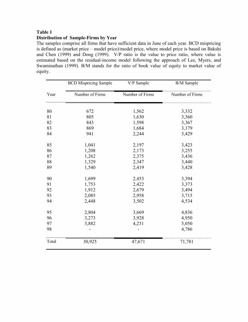
Table 1 Distribution of Sample-Firms by Year The samples comprise all firms that have sufficient data in June of each year. BCD mispricing is defined as (market price – model price)/model price, where model price is based on Bakshi and Chen (1999) and Dong (1999). V/P ratio is the value to price ratio, where value is estimated based on the residual-income model following the approach of Lee, Myers, and Swaminathan (1999). B/M stands for the ratio of book value of equity to market value of equity.

BCD Mispricing Sample V/P Sample B/M Sample

Year

Number of Firms Number of Firms Number of Firms

80 672 1,562 3,332 81 805 1,630 3,360 82 843 1,598 3,367 83 869 1,684 3,179 84 941 2,244 3,429

85 1,041 2,197 3,423 86 1,208 2,173 3,255 87 1,262 2,375 3,436 88 1,329 2,347 3,440 89 1,540 2,419 3,428

90 1,699 2,453 3,394 91 1,753 2,422 3,373 92 1,912 2,679 3,494 93 2,085 2,958 3,715 94 2,448 3,502 4,534

95 2,804 3,669 4,836 96 3,273 3,928 4,950 97 3,882 4,231 5,050 98 - - 4,786 Total

30,925 47,671 71,781

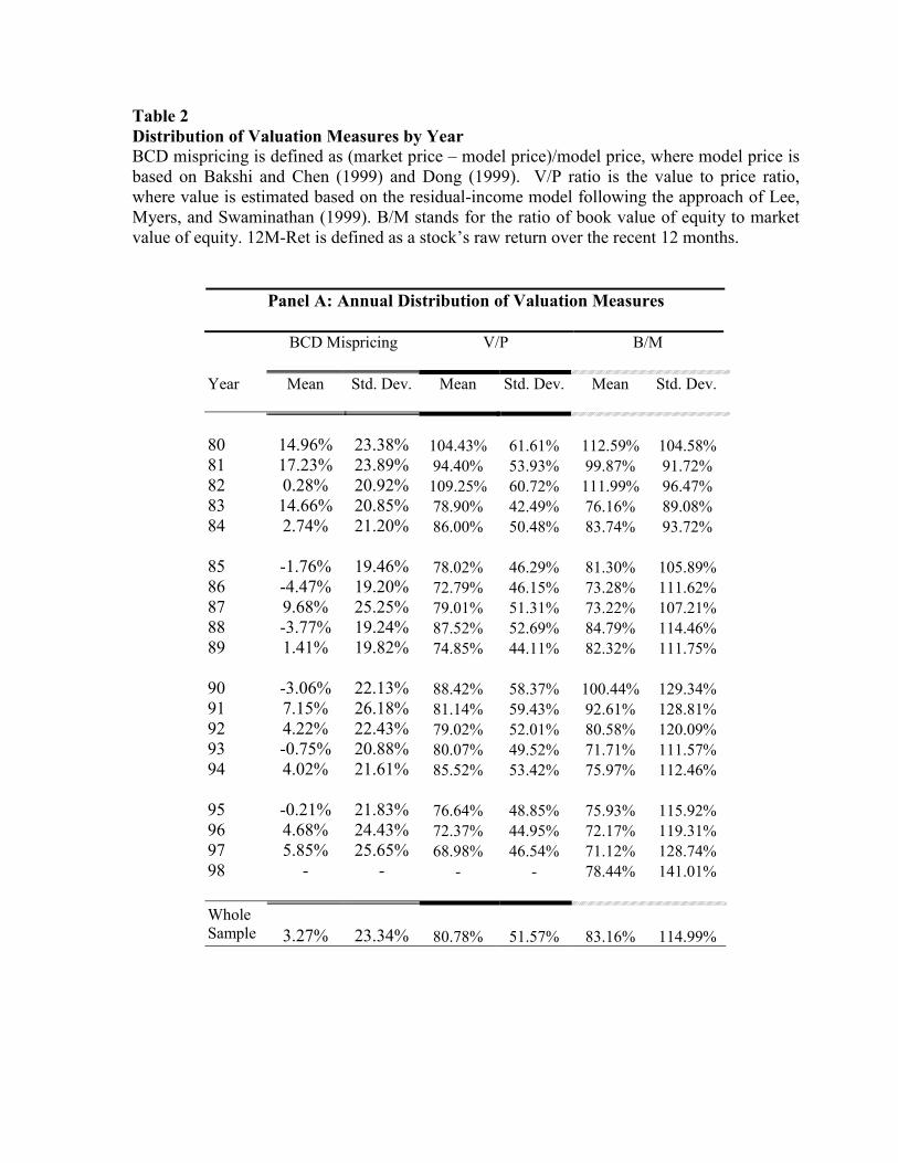
Table 2 Distribution of Valuation Measures by Year BCD mispricing is defined as (market price – model price)/model price, where model price is based on Bakshi and Chen (1999) and Dong (1999). V/P ratio is the value to price ratio, where value is estimated based on the residual-income model following the approach of Lee, Myers, and Swaminathan (1999). B/M stands for the ratio of book value of equity to market value of equity. 12M-Ret is defined as a stock’s raw return over the recent 12 months.

Panel A: Annual Distribution of Valuation Measures

B/M

BCD Mispricing V/P

Year Std. Dev.

Mean Std. Dev. Mean Std. Dev. Mean

80 14.96% 23.38% 104.43% 61.61% 112.59% 104.58% 81 17.23% 23.89% 94.40% 53.93% 99.87% 91.72% 82 0.28% 20.92% 109.25% 60.72% 111.99% 96.47% 83 14.66% 20.85% 78.90% 42.49% 76.16% 89.08% 84 2.74% 21.20% 86.00% 50.48% 83.74% 93.72% 85 -1.76% 19.46% 78.02% 46.29% 81.30% 105.89% 86 -4.47% 19.20% 72.79% 46.15% 73.28% 111.62% 87 9.68% 25.25% 79.01% 51.31% 73.22% 107.21% 88 -3.77% 19.24% 87.52% 52.69% 84.79% 114.46% 89 1.41% 19.82% 74.85% 44.11% 82.32% 111.75% 90 -3.06% 22.13% 88.42% 58.37% 100.44% 129.34% 91 7.15% 26.18% 81.14% 59.43% 92.61% 128.81% 92 4.22% 22.43% 79.02% 52.01% 80.58% 120.09% 93 -0.75% 20.88% 80.07% 49.52% 71.71% 111.57% 94 4.02% 21.61% 85.52% 53.42% 75.97% 112.46% 95 -0.21% 21.83% 76.64% 48.85% 75.93% 115.92% 96 4.68% 24.43% 72.37% 44.95% 72.17% 119.31% 97 5.85% 25.65% 68.98% 46.54% 71.12% 128.74% 98 - - - - 78.44% 141.01% Whole Sample

3.27%

23.34% 80.78% 51.57% 83.16% 114.99%

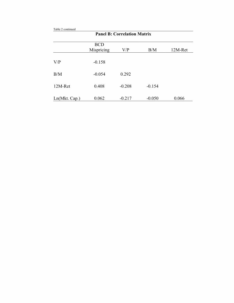
Table 2 continued

Panel B: Correlation Matrix

BCD

Mispricing V/P B/M 12M-Ret V/P -0.158 B/M -0.054 0.292 12M-Ret 0.408 -0.208 -0.154 Ln(Mkt. Cap.) 0.062 -0.217 -0.050 0.066

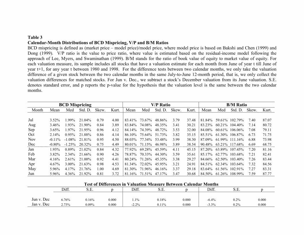
Table 3 Calendar-Month Distributions of BCD Mispricing, V/P and B/M Ratios BCD mispricing is defined as (market price – model price)/model price, where model price is based on Bakshi and Chen (1999) and Dong (1999). V/P ratio is the value to price ratio, where value is estimated based on the residual-income model following the approach of Lee, Myers, and Swaminathan (1999). B/M stands for the ratio of book value of equity to market value of equity. For each valuation measure, its sample includes all stocks that have a valuation estimate for each month from June of year t till June of year t+1, for any year t between 1980 and 1998. For the difference tests between two calendar months, we only take the valuation difference of a given stock between the two calendar months in the same July-to-June 12-month period, that is, we only collect the valuation differences for matched stocks. For Jun v. Dec., we subtract a stock’s December valuation from its June valuation. S.E. denotes standard error, and p reports the p-value for the hypothesis that the valuation level is the same between the two calendar months.

BCD Mispricing V/P Ratio B/M Ratio Month Mean Med Std. D. Skew. Kurt. Mean Med Std. D. Skew. Kurt. Mean Med Std. D. Skew. Kurt.

Jul 3.52% 1.99% 21.04% 0.79 4.00 83.41% 73.67% 48.86% 3.79 37.48 81.84% 59.61% 102.79% 7.40 87.07Aug 3.46% 1.93% 21.90% 0.84 3.89 83.84% 74.08% 48.35% 3.41 30.21 83.23% 60.21% 104.40% 7.14 80.72Sep 3.65% 1.97% 21.95% 0.96 4.12 84.14% 74.39% 48.72% 3.53 32.00 84.08% 60.61% 106.06% 7.08 79.11Oct 2.14% 0.95% 21.88% 0.86 4.14 86.10% 75.64% 51.73% 3.82 35.15 85.51% 61.30% 106.87% 6.73 71.75Nov -0.11% -1.08% 21.81% 0.95 4.50 88.03% 77.34% 53.48% 3.99 38.30 87.09% 61.99% 111.16% 6.88 73.98Dec -0.80% -1.25% 20.32% 0.75 4.49 80.01% 71.15% 46.98% 3.89 38.54 90.48% 63.21% 117.68% 6.69 68.75Jan 1.93% 0.89% 21.02% 0.84 4.32 77.92% 69.28% 45.59% 4.11 45.15 87.20% 63.89% 107.45% 7.20 81.16Feb 3.82% 2.34% 21.66% 0.90 4.26 78.87% 70.33% 44.30% 3.59 35.61 85.17% 62.77% 103.68% 7.21 82.41Mar 4.16% 2.61% 21.00% 0.92 4.41 80.24% 71.26% 45.35% 3.38 29.27 84.66% 62.50% 103.40% 7.26 83.44Apr 4.67% 3.00% 21.63% 0.98 4.53 81.34% 72.02% 45.95% 3.21 24.91 84.51% 62.34% 103.64% 7.32 84.56May 5.96% 4.17% 21.76% 1.00 4.69 81.30% 71.96% 46.16% 3.37 29.18 83.64% 61.56% 102.91% 7.27 83.31Jun 5.96% 4.36% 21.92% 0.81 3.72 81.16% 71.51% 47.17% 3.47 30.68 84.50% 61.26% 108.99% 7.59 87.77

Test of Differences in Valuation Measure Between Calendar Months

Diff. S.E. p Diff. S.E. p Diff. S.E. p

Jun v. Dec 6.76% 0.16% 0.000 1.1% 0.18% 0.000 -6.4% 0.2% 0.000Jan v. Dec 2.73% 0.09% 0.000 -2.2% 0.11% 0.000 -3.3% 0.2% 0.000

Table 4 Distributions of BCD Mispricing, V/P and B/M Ratios Around the Turn of the Year BCD mispricing is defined as (market price – model price)/model price, where model price is based on Bakshi and Chen (1999) and Dong (1999). V/P ratio is the value to price ratio, where value is estimated based on the residual-income model following the approach of Lee, Myers, and Swaminathan (1999). B/M stands for the ratio of book value of equity to market value of equity. All statistics are based on available observations in a particular calendar month of the year. For each valuation measure, its sample includes all stocks that have a valuation estimate for each month from June of year t till June of year t+1, for any year t between 1980 and 1998. Trading days are measured relative to the turn of the year, i.e. last trading day of a calendar year is set to –1, while the first trading day in a calendar year is set equal to 1.

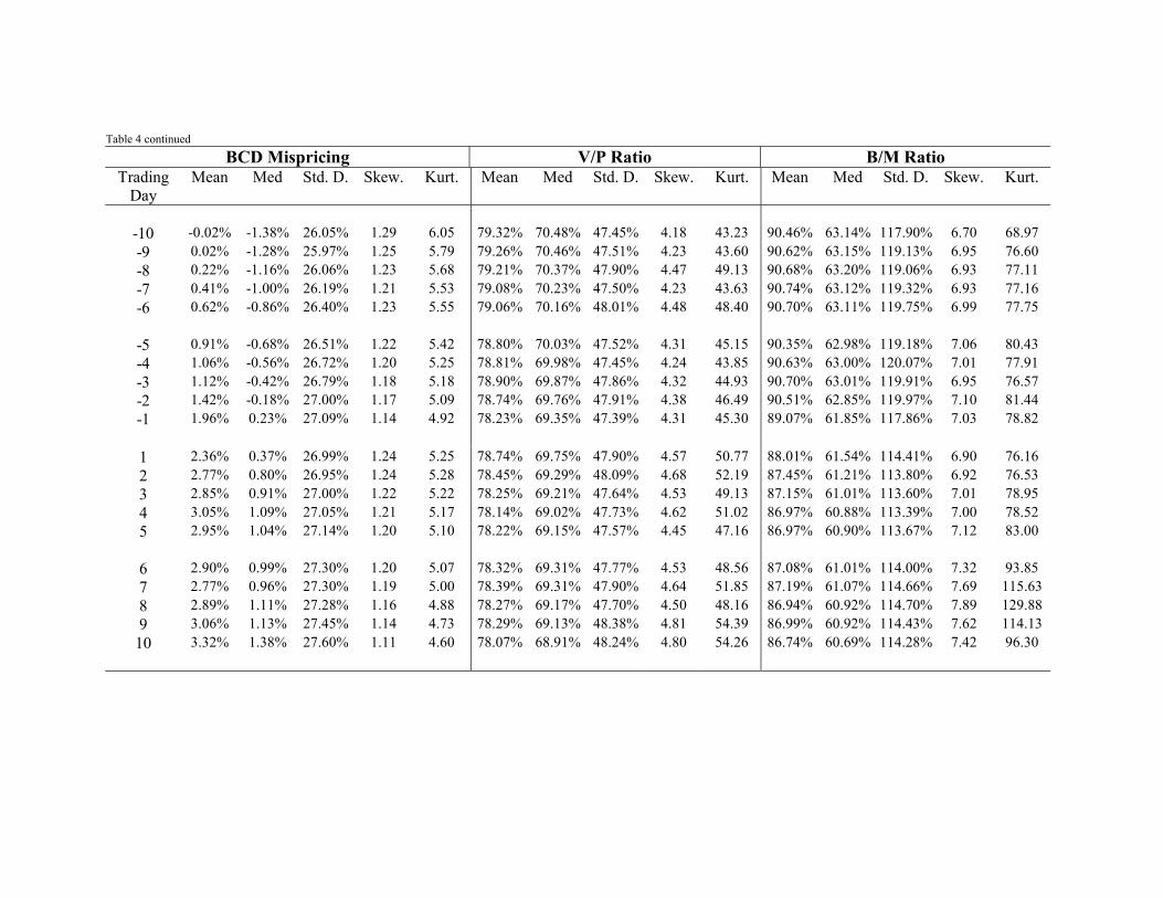
Table 4 continued

BCD Mispricing V/P Ratio B/M Ratio Trading

Day Mean Med Std. D. Skew. Kurt. Mean Med Std. D. Skew. Kurt. Mean Med Std. D. Skew. Kurt.

-10 -0.02% -1.38% 26.05% 1.29 6.05 79.32% 70.48% 47.45% 4.18 43.23 90.46% 63.14% 117.90% 6.70 68.97-9 0.02% -1.28% 25.97% 1.25 5.79 79.26% 70.46% 47.51% 4.23 43.60 90.62% 63.15% 119.13% 6.95 76.60-8 0.22% -1.16% 26.06% 1.23 5.68 79.21% 70.37% 47.90% 4.47 49.13 90.68% 63.20% 119.06% 6.93 77.11-7 0.41% -1.00% 26.19% 1.21 5.53 79.08% 70.23% 47.50% 4.23 43.63 90.74% 63.12% 119.32% 6.93 77.16-6

0.62% -0.86% 26.40% 1.23 5.55 79.06% 70.16% 48.01% 4.48 48.40 90.70% 63.11% 119.75% 6.99 77.75

-5 0.91% -0.68% 26.51% 1.22 5.42 78.80% 70.03% 47.52% 4.31 45.15 90.35% 62.98% 119.18% 7.06 80.43-4 1.06% -0.56% 26.72% 1.20 5.25 78.81% 69.98% 47.45% 4.24 43.85 90.63% 63.00% 120.07% 7.01 77.91-3 1.12% -0.42% 26.79% 1.18 5.18 78.90% 69.87% 47.86% 4.32 44.93 90.70% 63.01% 119.91% 6.95 76.57-2 1.42% -0.18% 27.00% 1.17 5.09 78.74% 69.76% 47.91% 4.38 46.49 90.51% 62.85% 119.97% 7.10 81.44-1

1.96% 0.23% 27.09% 1.14 4.92 78.23% 69.35% 47.39% 4.31 45.30 89.07% 61.85% 117.86% 7.03 78.82

1 2.36% 0.37% 26.99% 1.24 5.25 78.74% 69.75% 47.90% 4.57 50.77 88.01% 61.54% 114.41% 6.90 76.162 2.77% 0.80% 26.95% 1.24 5.28 78.45% 69.29% 48.09% 4.68 52.19 87.45% 61.21% 113.80% 6.92 76.533 2.85% 0.91% 27.00% 1.22 5.22 78.25% 69.21% 47.64% 4.53 49.13 87.15% 61.01% 113.60% 7.01 78.954 3.05% 1.09% 27.05% 1.21 5.17 78.14% 69.02% 47.73% 4.62 51.02 86.97% 60.88% 113.39% 7.00 78.525

2.95% 1.04% 27.14% 1.20 5.10 78.22% 69.15% 47.57% 4.45 47.16 86.97% 60.90% 113.67% 7.12 83.00

6 2.90% 0.99% 27.30% 1.20 5.07 78.32% 69.31% 47.77% 4.53 48.56 87.08% 61.01% 114.00% 7.32 93.857 2.77% 0.96% 27.30% 1.19 5.00 78.39% 69.31% 47.90% 4.64 51.85 87.19% 61.07% 114.66% 7.69 115.638 2.89% 1.11% 27.28% 1.16 4.88 78.27% 69.17% 47.70% 4.50 48.16 86.94% 60.92% 114.70% 7.89 129.889 3.06% 1.13% 27.45% 1.14 4.73 78.29% 69.13% 48.38% 4.81 54.39 86.99% 60.92% 114.43% 7.62 114.13

10

3.32% 1.38% 27.60% 1.11 4.60 78.07% 68.91% 48.24% 4.80 54.26 86.74% 60.69% 114.28% 7.42 96.30

Table 5 Seasonal Distributions of BCD Mispricing, V/P and B/M Ratios by Size BCD mispricing is defined as (market price – model price)/model price, where model price is based on Bakshi and Chen (1999) and Dong (1999). V/P ratio is the value to price ratio, where value is estimated based on the residual-income model following the approach of Lee, Myers, and Swaminathan (1999). B/M stands for the ratio of book value of equity to market value of equity. For each valuation measure, its sample includes all stocks that have a valuation estimate for each month from June of year t till June of year t+1, for any year t between 1980 and 1998. Panels A, B, and C report the distributions of the valuation measures for Small-, Mid-, and Large-cap firms, respectively. Small-, Mid-, and Large-cap groups are determined based on the market cap of each firm in June of year t and remain fixed for July-December of year t and for January to June of year t+1. Difference in means is calculated only for stocks present during both relevant months. S.E. denotes standard error, and p reports the p-value for the hypothesis that the valuation level is the same between the two calendar months.

Panel A of Table 5: Small Cap

BCD Mispricing V/P Ratio B/M Ratio Month Mean Med Std. D. Skew. Kurt. Mean Med Std. D. Skew. Kurt. Mean Med Std. D. Skew. Kurt.

Jul 1.82% 0.98% 24.50% 0.54 2.25 96.52% 84.67% 58.49% 3.67 31.74 104.88% 78.14% 114.13% 5.22 49.40Aug 2.15% 0.57% 25.51% 0.73 2.56 96.45% 84.68% 56.77% 3.26 25.43 106.94% 79.19% 117.52% 5.13 46.33Sep 2.76% 1.11% 25.61% 0.89 2.92 96.30% 84.30% 57.42% 3.44 27.94 108.45% 79.89% 120.56% 5.02 43.24Oct 1.30% -0.40% 25.84% 0.97 3.61 98.49% 85.85% 59.86% 3.38 25.90 110.08% 80.74% 122.15% 4.76 38.62Nov -0.88% -2.74% 25.97% 1.01 3.50 100.93% 87.83% 63.76% 3.85 31.70 113.08% 81.89% 130.11% 5.15 44.20Dec -2.05% -3.34% 24.62% 0.83 3.45 93.51% 82.55% 54.06% 2.71 16.92 119.49% 84.77% 140.45% 5.07 41.22Jan 1.90% 0.21% 25.00% 0.89 3.23 89.62% 79.44% 52.62% 3.49 33.82 109.10% 80.69% 120.02% 5.22 47.47Feb 4.34% 2.19% 25.69% 0.90 3.01 88.95% 79.04% 50.91% 3.23 28.81 105.28% 78.80% 112.53% 4.84 41.53Mar 5.27% 2.95% 25.16% 0.87 2.83 90.48% 80.13% 51.81% 2.81 19.22 104.23% 77.50% 112.80% 5.09 46.14Apr 6.54% 3.90% 26.35% 0.96 3.05 92.22% 81.69% 52.85% 2.67 16.58 103.60% 77.02% 113.64% 5.27 48.93May 7.45% 5.03% 26.34% 1.00 3.45 92.20% 81.77% 53.02% 2.78 18.45 102.11% 75.36% 112.97% 5.23 48.34Jun 7.10% 5.05% 26.22% 0.81 2.64 91.81% 80.65% 54.55% 3.05 22.32 103.21% 74.73% 121.17% 5.90 58.83 All 3.15% 1.37% 25.74% 0.87 3.01 93.95% 82.66% 55.74% 3.28 26.20 107.53% 79.02% 120.19% 5.20 46.66

Test of Differences in Valuation Measure Between Calendar Months

Diff. S.E. p Diff. S.E. p Diff. S.E. p

Jun v. Dec 9.19% 0.40% 0.000 -1.71% 0.46% 0.000 -16.2% 0.6% 0.000Jan v. Dec 3.92% 0.20% 0.000 -3.89% 0.27% 0.000 -10.6% 0.4% 0.000

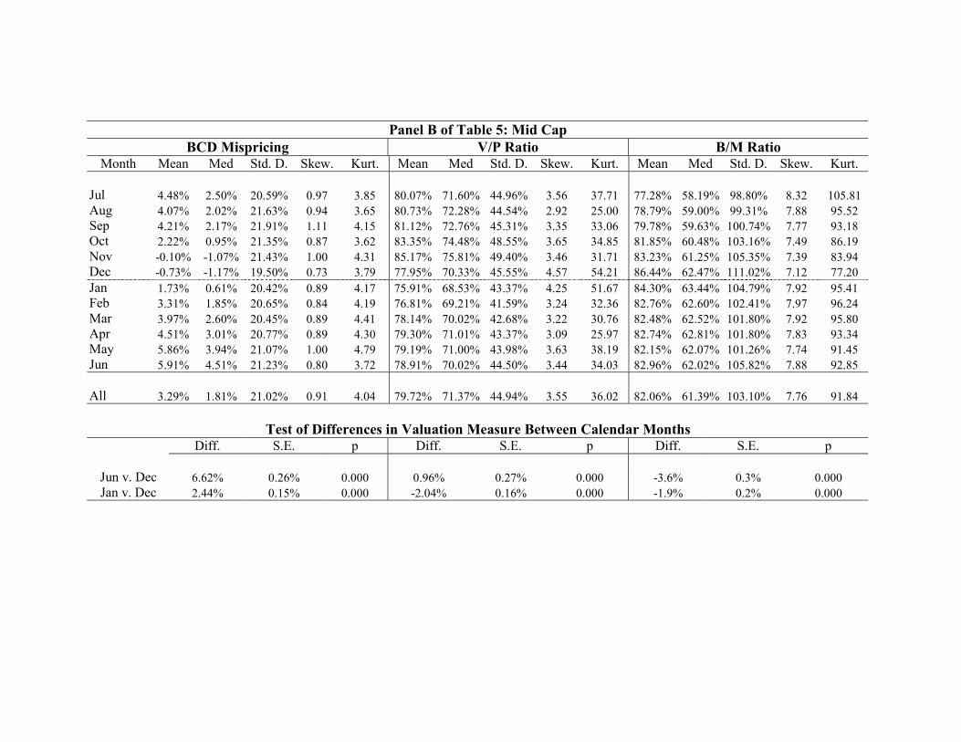
Panel B of Table 5: Mid Cap BCD Mispricing V/P Ratio B/M Ratio

Month Mean Med Std. D. Skew. Kurt. Mean Med Std. D. Skew. Kurt. Mean Med Std. D. Skew. Kurt.

Jul 4.48% 2.50% 20.59% 0.97 3.85 80.07% 71.60% 44.96% 3.56 37.71 77.28% 58.19% 98.80% 8.32 105.81Aug 4.07% 2.02% 21.63% 0.94 3.65 80.73% 72.28% 44.54% 2.92 25.00 78.79% 59.00% 99.31% 7.88 95.52Sep 4.21% 2.17% 21.91% 1.11 4.15 81.12% 72.76% 45.31% 3.35 33.06 79.78% 59.63% 100.74% 7.77 93.18Oct 2.22% 0.95% 21.35% 0.87 3.62 83.35% 74.48% 48.55% 3.65 34.85 81.85% 60.48% 103.16% 7.49 86.19Nov -0.10% -1.07% 21.43% 1.00 4.31 85.17% 75.81% 49.40% 3.46 31.71 83.23% 61.25% 105.35% 7.39 83.94Dec -0.73% -1.17% 19.50% 0.73 3.79 77.95% 70.33% 45.55% 4.57 54.21 86.44% 62.47% 111.02% 7.12 77.20Jan 1.73% 0.61% 20.42% 0.89 4.17 75.91% 68.53% 43.37% 4.25 51.67 84.30% 63.44% 104.79% 7.92 95.41Feb 3.31% 1.85% 20.65% 0.84 4.19 76.81% 69.21% 41.59% 3.24 32.36 82.76% 62.60% 102.41% 7.97 96.24Mar 3.97% 2.60% 20.45% 0.89 4.41 78.14% 70.02% 42.68% 3.22 30.76 82.48% 62.52% 101.80% 7.92 95.80Apr 4.51% 3.01% 20.77% 0.89 4.30 79.30% 71.01% 43.37% 3.09 25.97 82.74% 62.81% 101.80% 7.83 93.34May 5.86% 3.94% 21.07% 1.00 4.79 79.19% 71.00% 43.98% 3.63 38.19 82.15% 62.07% 101.26% 7.74 91.45Jun 5.91% 4.51% 21.23% 0.80 3.72 78.91% 70.02% 44.50% 3.44 34.03 82.96% 62.02% 105.82% 7.88 92.85 All 3.29% 1.81% 21.02% 0.91 4.04 79.72% 71.37% 44.94% 3.55 36.02 82.06% 61.39% 103.10% 7.76 91.84

Test of Differences in Valuation Measure Between Calendar Months

Diff. S.E. p Diff. S.E. p Diff. S.E. p

Jun v. Dec 6.62% 0.26% 0.000 0.96% 0.27% 0.000 -3.6% 0.3% 0.000Jan v. Dec 2.44% 0.15% 0.000 -2.04% 0.16% 0.000 -1.9% 0.2% 0.000

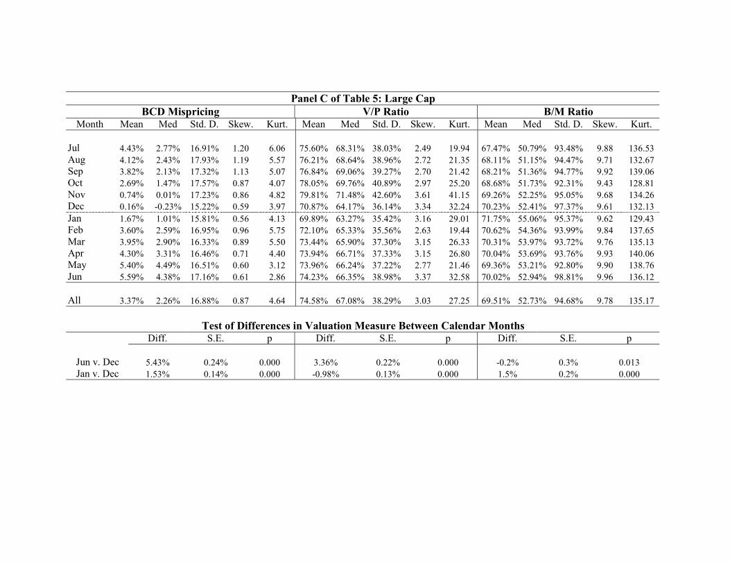
Panel C of Table 5: Large Cap BCD Mispricing V/P Ratio B/M Ratio

Month Mean Med Std. D. Skew. Kurt. Mean Med Std. D. Skew. Kurt. Mean Med Std. D. Skew. Kurt.

Jul 4.43% 2.77% 16.91% 1.20 6.06 75.60% 68.31% 38.03% 2.49 19.94 67.47% 50.79% 93.48% 9.88 136.53Aug 4.12% 2.43% 17.93% 1.19 5.57 76.21% 68.64% 38.96% 2.72 21.35 68.11% 51.15% 94.47% 9.71 132.67Sep 3.82% 2.13% 17.32% 1.13 5.07 76.84% 69.06% 39.27% 2.70 21.42 68.21% 51.36% 94.77% 9.92 139.06Oct 2.69% 1.47% 17.57% 0.87 4.07 78.05% 69.76% 40.89% 2.97 25.20 68.68% 51.73% 92.31% 9.43 128.81Nov 0.74% 0.01% 17.23% 0.86 4.82 79.81% 71.48% 42.60% 3.61 41.15 69.26% 52.25% 95.05% 9.68 134.26Dec 0.16% -0.23% 15.22% 0.59 3.97 70.87% 64.17% 36.14% 3.34 32.24 70.23% 52.41% 97.37% 9.61 132.13Jan 1.67% 1.01% 15.81% 0.56 4.13 69.89% 63.27% 35.42% 3.16 29.01 71.75% 55.06% 95.37% 9.62 129.43Feb 3.60% 2.59% 16.95% 0.96 5.75 72.10% 65.33% 35.56% 2.63 19.44 70.62% 54.36% 93.99% 9.84 137.65Mar 3.95% 2.90% 16.33% 0.89 5.50 73.44% 65.90% 37.30% 3.15 26.33 70.31% 53.97% 93.72% 9.76 135.13Apr 4.30% 3.31% 16.46% 0.71 4.40 73.94% 66.71% 37.33% 3.15 26.80 70.04% 53.69% 93.76% 9.93 140.06May 5.40% 4.49% 16.51% 0.60 3.12 73.96% 66.24% 37.22% 2.77 21.46 69.36% 53.21% 92.80% 9.90 138.76Jun 5.59% 4.38% 17.16% 0.61 2.86 74.23% 66.35% 38.98% 3.37 32.58 70.02% 52.94% 98.81% 9.96 136.12 All 3.37% 2.26% 16.88% 0.87 4.64 74.58% 67.08% 38.29% 3.03 27.25 69.51% 52.73% 94.68% 9.78 135.17

Test of Differences in Valuation Measure Between Calendar Months

Diff. S.E. p Diff. S.E. p Diff. S.E. p

Jun v. Dec 5.43% 0.24% 0.000 3.36% 0.22% 0.000 -0.2% 0.3% 0.013Jan v. Dec 1.53% 0.14% 0.000 -0.98% 0.13% 0.000 1.5% 0.2% 0.000

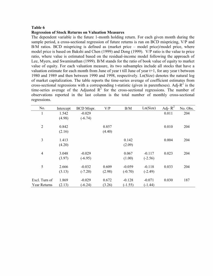
Table 6 Regression of Stock Returns on Valuation Measures The dependent variable is the future 1-month holding return. For each given month during the sample period, a cross-sectional regression of future returns is run on BCD mispricing, V/P and B/M ratios. BCD mispricing is defined as (market price – model price)/model price, where model price is based on Bakshi and Chen (1999) and Dong (1999). V/P ratio is the value to price ratio, where value is estimated based on the residual-income model following the approach of Lee, Myers, and Swaminathan (1999). B/M stands for the ratio of book value of equity to market value of equity. For each valuation measure, its two subsamples include all stocks that have a valuation estimate for each month from June of year t till June of year t+1, for any year t between 1980 and 1989 and then between 1990 and 1998, respectively. Ln(Size) denotes the natural log of market capitalization. The table reports the time-series average of coefficient estimates from cross-sectional regressions with a corresponding t-statistic (given in parentheses). Adj-R2 is the time-series average of the Adjusted R2 for the cross-sectional regressions. The number of observations reported in the last column is the total number of monthly cross-sectional regressions.

No. Intercept BCD Mispr. V/P B/M Ln(Size) Adj- R2 No. Obs.1 1.542 -0.029 0.011 204 (4.98) (-6.74)

2 0.842 0.857 0.010 204 (2.16) (4.40)

3 1.413 0.142 0.004 204 (4.20) (2.09)

4 3.048 -0.029 0.067 -0.117 0.023 204 (3.97) (-6.95) (1.00) (-2.56)

5 2.666 -0.032 0.609 -0.059 -0.118 0.033 204 (3.13) (-7.20) (2.98) (-0.70) (-2.49)

Excl. Turn of 1.869 -0.029 0.672 -0.128 -0.071 0.030 187 Year Returns (2.13) (-6.24) (3.26) (-1.55) (-1.44)

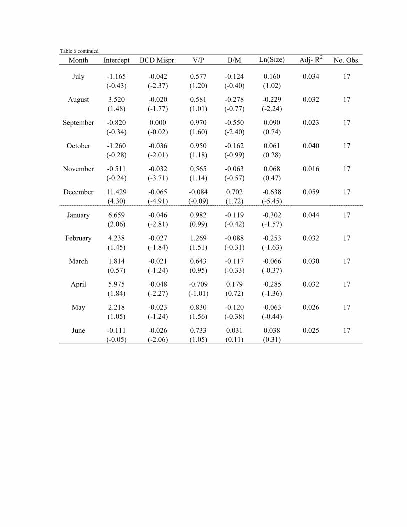
Table 6 continued

Month Intercept BCD Mispr. V/P B/M Ln(Size) Adj- R2 No. Obs.

July -1.165 -0.042 0.577 -0.124 0.160 0.034 17 (-0.43) (-2.37) (1.20) (-0.40) (1.02)

August 3.520 -0.020 0.581 -0.278 -0.229 0.032 17 (1.48) (-1.77) (1.01) (-0.77) (-2.24)

September -0.820 0.000 0.970 -0.550 0.090 0.023 17 (-0.34) (-0.02) (1.60) (-2.40) (0.74)

October -1.260 -0.036 0.950 -0.162 0.061 0.040 17 (-0.28) (-2.01) (1.18) (-0.99) (0.28)

November -0.511 -0.032 0.565 -0.063 0.068 0.016 17 (-0.24) (-3.71) (1.14) (-0.57) (0.47)

December 11.429 -0.065 -0.084 0.702 -0.638 0.059 17 (4.30) (-4.91) (-0.09) (1.72) (-5.45)

January 6.659 -0.046 0.982 -0.119 -0.302 0.044 17 (2.06) (-2.81) (0.99) (-0.42) (-1.57)

February 4.238 -0.027 1.269 -0.088 -0.253 0.032 17 (1.45) (-1.84) (1.51) (-0.31) (-1.63)

March 1.814 -0.021 0.643 -0.117 -0.066 0.030 17 (0.57) (-1.24) (0.95) (-0.33) (-0.37)

April 5.975 -0.048 -0.709 0.179 -0.285 0.032 17 (1.84) (-2.27) (-1.01) (0.72) (-1.36)

May 2.218 -0.023 0.830 -0.120 -0.063 0.026 17 (1.05) (-1.24) (1.56) (-0.38) (-0.44)

June -0.111 -0.026 0.733 0.031 0.038 0.025 17 (-0.05) (-2.06) (1.05) (0.11) (0.31)

Table 7 Regression of Stock Returns on Valuation Measures by Size The dependent variable is the future 1-month holding return. For each given month during the sample period, a cross-sectional regression of future returns is run on BCD mispricing, V/P and B/M ratios. BCD mispricing is defined as (market price – model price)/model price, where model price is based on Bakshi and Chen (1999) and Dong (1999). V/P ratio is the value to price ratio, where value is estimated based on the residual-income model following the approach of Lee, Myers, and Swaminathan (1999). B/M stands for the ratio of book value of equity to market value of equity. For each valuation measure, its two subsamples include all stocks that have a valuation estimate for each month from June of year t till June of year t+1, for any year t between 1980 and 1989 and then between 1990 and 1998, respectively. Ln(Size) denotes the natural log of market capitalization. The table reports the time-series average of coefficient estimates from cross-sectional regressions with a corresponding t-statistic (given in parentheses). Adj-R2 is the time-series average of the Adjusted R2 for the cross-sectional regressions. The number of observations reported in the last column is the total number of monthly cross-sectional regressions. Small-, Mid-, and Large-cap groups are determined based on the market cap of each firm in June of year t and remain fixed for July-December of year t and for January to June of year t+1.

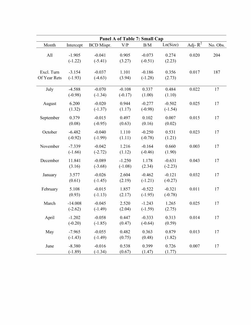
Panel A of Table 7: Small Cap

Month Intercept BCD Mispr. V/P B/M Ln(Size) Adj- R2 No. Obs.

All -1.905 -0.041 0.905 -0.073 0.274 0.020 204 (-1.22) (-5.41) (3.27) (-0.51) (2.23)

Excl. Turn -3.154 -0.037 1.101 -0.186 0.356 0.017 187 Of Year Rets (-1.93) (-4.63) (3.94) (-1.28) (2.73)

July -4.588 -0.070 -0.108 0.337 0.484 0.022 17

(-0.98) (-1.34) (-0.17) (1.00) (1.10)

August 6.200 -0.020 0.944 -0.277 -0.502 0.025 17 (1.32) (-1.37) (1.17) (-0.98) (-1.54)

September 0.379 -0.015 0.497 0.102 0.007 0.015 17 (0.08) (-0.95) (0.63) (0.16) (0.02)

October -6.482 -0.040 1.110 -0.250 0.531 0.023 17 (-0.92) (-1.99) (1.11) (-0.78) (1.21)

November -7.339 -0.042 1.216 -0.164 0.660 0.003 17 (-1.66) (-2.72) (1.12) (-0.46) (1.90)

December 11.841 -0.089 -1.250 1.178 -0.631 0.043 17 (3.16) (-3.68) (-1.08) (2.34) (-2.23)

January 3.577 -0.026 2.604 -0.462 -0.121 0.032 17 (0.61) (-1.45) (2.19) (-1.21) (-0.27)

February 5.108 -0.015 1.857 -0.522 -0.321 0.011 17 (0.93) (-1.13) (2.17) (-1.95) (-0.78)

March -14.008 -0.045 2.520 -1.243 1.265 0.025 17 (-2.62) (-1.49) (2.04) (-1.59) (2.75)

April -1.202 -0.058 0.447 -0.333 0.313 0.014 17 (-0.20) (-1.85) (0.47) (-0.64) (0.59)

May -7.965 -0.055 0.482 0.363 0.879 0.013 17 (-1.43) (-1.49) (0.75) (0.48) (1.82)

June -8.380 -0.016 0.538 0.399 0.726 0.007 17 (-1.89) (-1.34) (0.67) (1.47) (1.77)

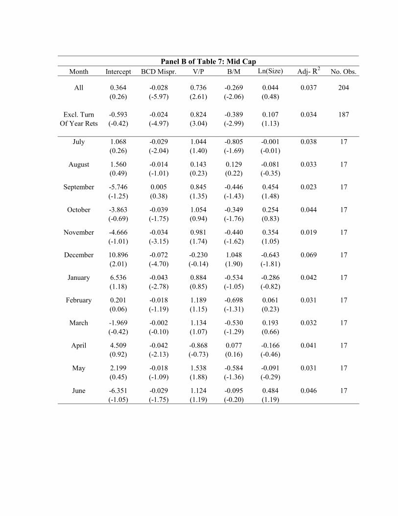
Panel B of Table 7: Mid Cap

Month Intercept BCD Mispr. V/P B/M Ln(Size) Adj- R2 No. Obs.

All 0.364 -0.028 0.736 -0.269 0.044 0.037 204 (0.26) (-5.97) (2.61) (-2.06) (0.48)

Excl. Turn -0.593 -0.024 0.824 -0.389 0.107 0.034 187 Of Year Rets (-0.42) (-4.97) (3.04) (-2.99) (1.13)

July 1.068 -0.029 1.044 -0.805 -0.001 0.038 17

(0.26) (-2.04) (1.40) (-1.69) (-0.01)

August 1.560 -0.014 0.143 0.129 -0.081 0.033 17 (0.49) (-1.01) (0.23) (0.22) (-0.35)

September -5.746 0.005 0.845 -0.446 0.454 0.023 17 (-1.25) (0.38) (1.35) (-1.43) (1.48)

October -3.863 -0.039 1.054 -0.349 0.254 0.044 17 (-0.69) (-1.75) (0.94) (-1.76) (0.83)

November -4.666 -0.034 0.981 -0.440 0.354 0.019 17 (-1.01) (-3.15) (1.74) (-1.62) (1.05)

December 10.896 -0.072 -0.230 1.048 -0.643 0.069 17 (2.01) (-4.70) (-0.14) (1.90) (-1.81)

January 6.536 -0.043 0.884 -0.534 -0.286 0.042 17 (1.18) (-2.78) (0.85) (-1.05) (-0.82)

February 0.201 -0.018 1.189 -0.698 0.061 0.031 17 (0.06) (-1.19) (1.15) (-1.31) (0.23)

March -1.969 -0.002 1.134 -0.530 0.193 0.032 17 (-0.42) (-0.10) (1.07) (-1.29) (0.66)

April 4.509 -0.042 -0.868 0.077 -0.166 0.041 17 (0.92) (-2.13) (-0.73) (0.16) (-0.46)

May 2.199 -0.018 1.538 -0.584 -0.091 0.031 17 (0.45) (-1.09) (1.88) (-1.36) (-0.29)

June -6.351 -0.029 1.124 -0.095 0.484 0.046 17 (-1.05) (-1.75) (1.19) (-0.20) (1.19)

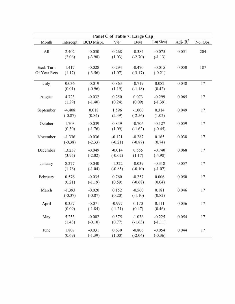
Panel C of Table 7: Large Cap

Month Intercept BCD Mispr. V/P B/M Ln(Size) Adj- R2 No. Obs.

All 2.402 -0.030 0.268 -0.384 -0.075 0.051 204 (2.06) (-3.98) (1.03) (-2.70) (-1.13)

Excl. Turn 1.417 -0.028 0.294 -0.470 -0.015 0.050 187 Of Year Rets (1.17) (-3.56) (1.07) (-3.17) (-0.21)

July 0.036 -0.019 0.863 -0.719 0.082 0.048 17

(0.01) (-0.96) (1.19) (-1.18) (0.42)

August 4.723 -0.032 0.250 0.073 -0.299 0.065 17 (1.29) (-1.40) (0.24) (0.09) (-1.39)

September -4.408 0.018 1.596 -1.000 0.314 0.049 17 (-0.87) (0.84) (2.39) (-2.56) (1.02)

October 1.703 -0.039 0.849 -0.706 -0.127 0.059 17 (0.30) (-1.76) (1.09) (-1.62) (-0.45)

November -1.336 -0.036 -0.121 -0.287 0.165 0.038 17 (-0.38) (-2.33) (-0.21) (-0.87) (0.74)

December 13.237 -0.049 -0.014 0.555 -0.740 0.068 17 (3.95) (-2.02) (-0.02) (1.17) (-4.98)

January 8.277 -0.040 -1.322 -0.039 -0.318 0.057 17 (1.76) (-1.04) (-0.85) (-0.10) (-1.07)

February 0.576 -0.035 0.760 -0.257 0.006 0.050 17 (0.21) (-1.19) (0.59) (-0.68) (0.04)

March -1.393 -0.020 0.152 -0.560 0.181 0.046 17 (-0.37) (-0.87) (0.20) (-1.10) (0.82)

April 0.357 -0.071 -0.997 0.170 0.111 0.036 17 (0.09) (-1.84) (-1.21) (0.47) (0.46)

May 5.253 -0.002 0.575 -1.036 -0.225 0.054 17 (1.43) (-0.10) (0.77) (-1.63) (-1.11)

June 1.807 -0.031 0.630 -0.806 -0.054 0.044 17 (0.69) (-1.39) (1.00) (-2.04) (-0.36)

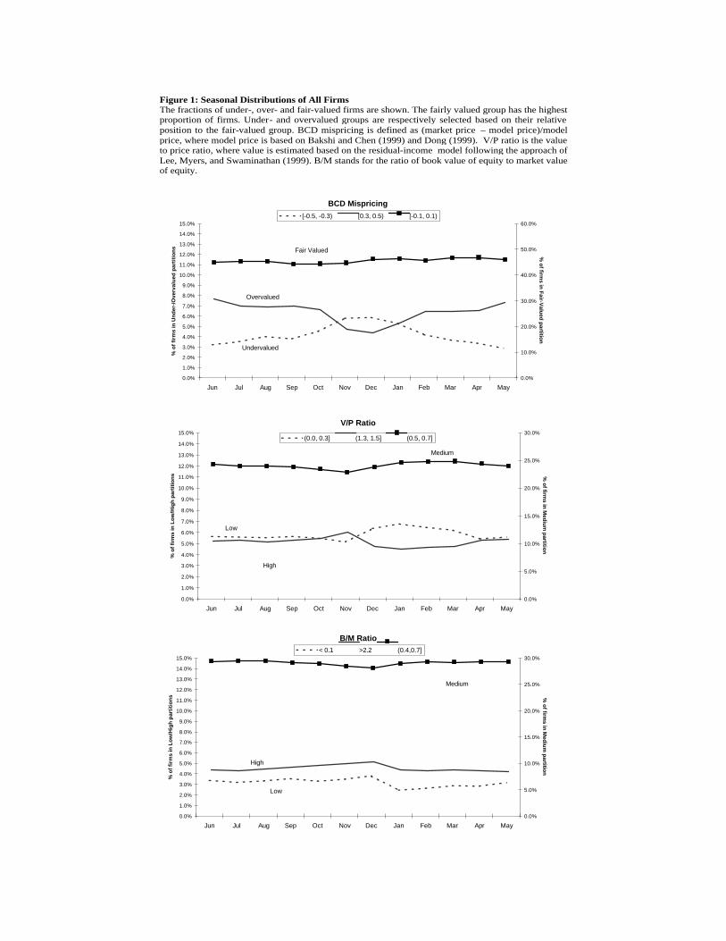
BCD Mispricing

0.0%

1.0%

2.0%

3.0%

4.0%

5.0%

6.0%

7.0%

8.0%

9.0%

10.0%

11.0%

12.0%

13.0%

14.0%

15.0%

Jun Jul Aug Sep Oct Nov Dec Jan Feb Mar Apr May

% o

f fir

ms

in U

nd

er-/

Ove

rval

ued

par

titi

on

s

0.0%

10.0%

20.0%

30.0%

40.0%

50.0%

60.0%

% o

f firms in

Fair-V

alued

partitio

n

[-0.5, -0.3) [0.3, 0.5) [-0.1, 0.1)

Undervalued

Overvalued

Fair Valued

B/M Ratio

0.0%

1.0%

2.0%

3.0%

4.0%

5.0%

6.0%

7.0%

8.0%

9.0%

10.0%

11.0%

12.0%

13.0%

14.0%

15.0%

Jun Jul Aug Sep Oct Nov Dec Jan Feb Mar Apr May

% o

f fir

ms

in L

ow

/Hig

h p

arti

tio

ns

0.0%

5.0%

10.0%

15.0%

20.0%

25.0%

30.0%

% o

f firms in

Med

ium

partitio

n

< 0.1 >2.2 (0.4,0.7]

High

Low

Medium

V/P Ratio

0.0%

1.0%

2.0%

3.0%

4.0%

5.0%

6.0%

7.0%

8.0%

9.0%

10.0%

11.0%

12.0%

13.0%

14.0%

15.0%

Jun Jul Aug Sep Oct Nov Dec Jan Feb Mar Apr May

% o

f fir

ms

in L

ow

/Hig

h p

arti

tio

ns

0.0%

5.0%

10.0%

15.0%

20.0%

25.0%

30.0%

% o

f firms in

Med

ium

partitio

n

(0.0, 0.3] (1.3, 1.5] (0.5, 0.7]

Medium

Low

High

Figure 1: Seasonal Distributions of All Firms The fractions of under-, over- and fair-valued firms are shown. The fairly valued group has the highest proportion of firms. Under- and overvalued groups are respectively selected based on their relative position to the fair-valued group. BCD mispricing is defined as (market price – model price)/model price, where model price is based on Bakshi and Chen (1999) and Dong (1999). V/P ratio is the value to price ratio, where value is estimated based on the residual-income model following the approach of Lee, Myers, and Swaminathan (1999). B/M stands for the ratio of book value of equity to market value of equity.

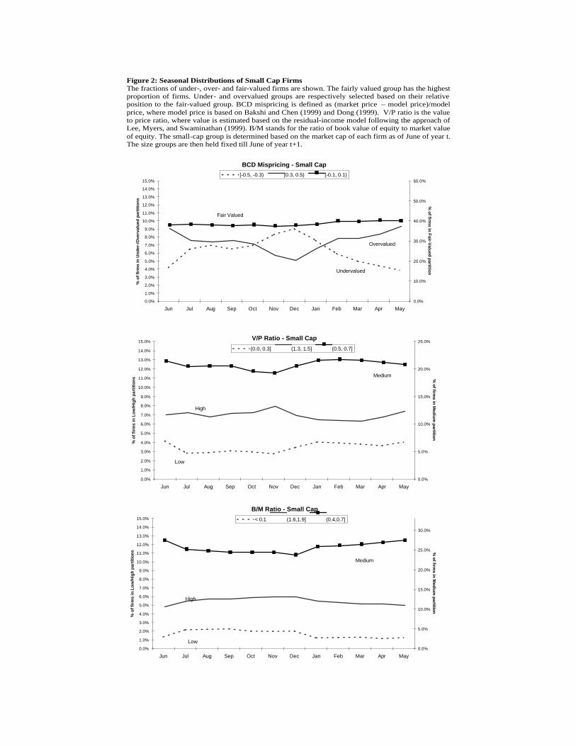
BCD Mispricing - Small Cap

0.0%

1.0%

2.0%

3.0%

4.0%

5.0%

6.0%

7.0%

8.0%

9.0%

10.0%

11.0%

12.0%

13.0%

14.0%

15.0%

Jun Jul Aug Sep Oct Nov Dec Jan Feb Mar Apr May

% o

f fir

ms

in U

nd

er-/

Ove

rval

ued

par

titi

on

s

0.0%

10.0%

20.0%

30.0%

40.0%

50.0%

60.0%

% o

f firms in

Fair-V

alued

partitio

n

[-0.5, -0.3) [0.3, 0.5) [-0.1, 0.1)

Fair Valued

Overvalued

Undervalued

B/M Ratio - Small Cap

0.0%

1.0%

2.0%

3.0%

4.0%

5.0%

6.0%

7.0%

8.0%

9.0%

10.0%

11.0%

12.0%

13.0%

14.0%

15.0%

Jun Jul Aug Sep Oct Nov Dec Jan Feb Mar Apr May

% o

f fir

ms

in L

ow

/Hig

h p

arti

tio

ns

0.0%

5.0%

10.0%

15.0%

20.0%

25.0%

30.0%

% o

f firms in

Med

ium

partitio

n

< 0.1 (1.6,1.9] (0.4,0.7]

Low

High

Medium

V/P Ratio - Small Cap

0.0%

1.0%

2.0%

3.0%

4.0%

5.0%

6.0%

7.0%

8.0%

9.0%

10.0%

11.0%

12.0%

13.0%

14.0%

15.0%

Jun Jul Aug Sep Oct Nov Dec Jan Feb Mar Apr May

% o

f fir

ms

in L

ow

/Hig

h p

arti

tio

ns

0.0%

5.0%

10.0%

15.0%

20.0%

25.0%

% o

f firms in

Med

ium

partitio

n

(0.0, 0.3] (1.3, 1.5] (0.5, 0.7]

Low

High

Medium

Figure 2: Seasonal Distributions of Small Cap Firms The fractions of under-, over- and fair-valued firms are shown. The fairly valued group has the highest proportion of firms. Under- and overvalued groups are respectively selected based on their relative position to the fair-valued group. BCD mispricing is defined as (market price – model price)/model price, where model price is based on Bakshi and Chen (1999) and Dong (1999). V/P ratio is the value to price ratio, where value is estimated based on the residual-income model following the approach of Lee, Myers, and Swaminathan (1999). B/M stands for the ratio of book value of equity to market value of equity. The small-cap group is determined based on the market cap of each firm as of June of year t. The size groups are then held fixed till June of year t+1.

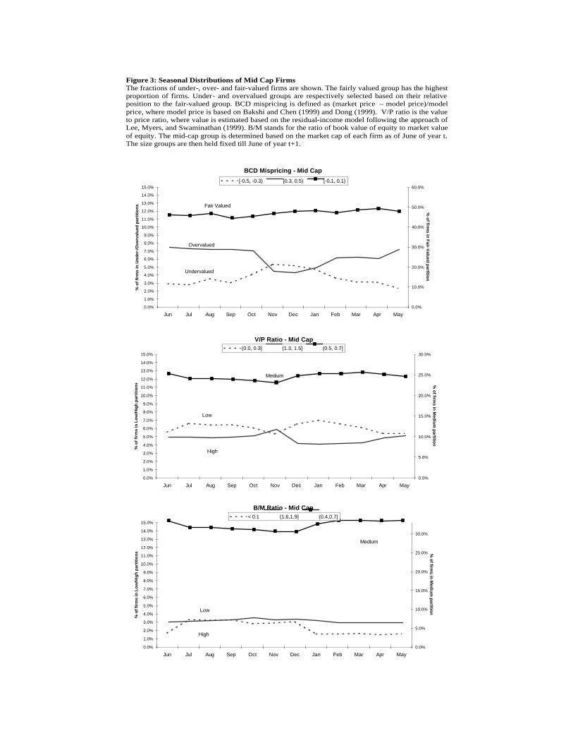
BCD Mispricing - Mid Cap

0.0%

1.0%

2.0%

3.0%

4.0%

5.0%

6.0%

7.0%

8.0%

9.0%

10.0%

11.0%

12.0%

13.0%

14.0%

15.0%

Jun Jul Aug Sep Oct Nov Dec Jan Feb Mar Apr May

% o

f fir

ms

in U

nd

er-/

Ove

rval

ued

par

titi

on

s

0.0%

10.0%

20.0%

30.0%

40.0%

50.0%

60.0%

% o

f firms in

Fair-V

alued

partitio

n

[-0.5, -0.3) [0.3, 0.5) [-0.1, 0.1)

Fair Valued

Overvalued

Undervalued

B/M Ratio - Mid Cap

0.0%

1.0%

2.0%

3.0%

4.0%

5.0%

6.0%

7.0%

8.0%

9.0%

10.0%

11.0%

12.0%

13.0%

14.0%

15.0%

Jun Jul Aug Sep Oct Nov Dec Jan Feb Mar Apr May

% o

f fir

ms

in L

ow

/Hig

h p

arti

tio

ns

0.0%

5.0%

10.0%

15.0%

20.0%

25.0%

30.0%

% o

f firms in

Med

ium

partitio

n

< 0.1 (1.6,1.9] (0.4,0.7]

Low

High

Medium

V/P Ratio - Mid Cap

0.0%

1.0%

2.0%

3.0%

4.0%

5.0%

6.0%

7.0%

8.0%

9.0%

10.0%

11.0%

12.0%

13.0%

14.0%

15.0%

Jun Jul Aug Sep Oct Nov Dec Jan Feb Mar Apr May

% o

f fir

ms

in L

ow

/Hig

h p

arti

tio

ns

0.0%

5.0%

10.0%

15.0%

20.0%

25.0%

30.0%

% o

f firms in

Med

ium

partitio

n

(0.0, 0.3] (1.3, 1.5] (0.5, 0.7]

Medium

Low

High

Figure 3: Seasonal Distributions of Mid Cap Firms The fractions of under-, over- and fair-valued firms are shown. The fairly valued group has the highest proportion of firms. Under- and overvalued groups are respectively selected based on their relative position to the fair-valued group. BCD mispricing is defined as (market price – model price)/model price, where model price is based on Bakshi and Chen (1999) and Dong (1999). V/P ratio is the value to price ratio, where value is estimated based on the residual-income model following the approach of Lee, Myers, and Swaminathan (1999). B/M stands for the ratio of book value of equity to market value of equity. The mid-cap group is determined based on the market cap of each firm as of June of year t. The size groups are then held fixed till June of year t+1.

BCD Mispricing - Large Cap

0.0%

1.0%

2.0%

3.0%

4.0%

5.0%

6.0%

7.0%

8.0%

9.0%

10.0%

11.0%

12.0%

13.0%

14.0%

15.0%

Jun Jul Aug Sep Oct Nov Dec Jan Feb Mar Apr May

% o

f fir

ms

in U

nd

er-/

Ove

rval

ued

par

titi

on

s

0.0%

10.0%

20.0%

30.0%

40.0%

50.0%

60.0%

% o

f firms in

Fair-V

alued

partitio

n

[-0.5, -0.3) [0.3, 0.5) [-0.1, 0.1)

Fair Valued

Overvalued

Undervalued

B/M Ratio - Large Cap

0.0%

1.0%

2.0%

3.0%

4.0%

5.0%

6.0%

7.0%

8.0%

9.0%

10.0%

11.0%

12.0%

13.0%

14.0%

15.0%

Jun Jul Aug Sep Oct Nov Dec Jan Feb Mar Apr May

% o

f fir

ms

in L

ow

/Hig

h p

arti

tio

ns

0.0%

5.0%

10.0%

15.0%

20.0%

25.0%

30.0%

% o

f firms in

Med

ium

partitio

n

< 0.1 (1.6,1.9] (0.4,0.7]

Low

High

Medium

V/P Ratio - Large Cap

0.0%

1.0%

2.0%

3.0%

4.0%

5.0%

6.0%

7.0%

8.0%

9.0%

10.0%

11.0%

12.0%

13.0%

14.0%

15.0%

Jun Jul Aug Sep Oct Nov Dec Jan Feb Mar Apr May

% o

f fir

ms

in L

ow

/Hig

h p

arti

tio

ns

0.0%

5.0%

10.0%

15.0%

20.0%

25.0%

30.0%

% o

f firms in

Med

ium

partitio

n

(0.0, 0.3] (1.3, 1.5] (0.5, 0.7]

Medium

Low

High

Figure 4: Seasonal Distributions of Large Cap Firms The fractions of under-, over- and fair-valued firms are shown. The fairly valued group has the highest proportion of firms. Under- and overvalued groups are respectively selected based on their relative position to the fair-valued group. BCD mispricing is defined as (market price – model price)/model price, where model price is based on Bakshi and Chen (1999) and Dong (1999). V/P ratio is the value to price ratio, where value is estimated based on the residual-income model following the approach of Lee, Myers, and Swaminathan (1999). B/M stands for the ratio of book value of equity to market value of equity. The large-cap group is determined based on the market cap of each firm as of June of year t. The size groups are then held fixed till June of year t+1.