A UTILITY-BASED AGENT FOR VEHICLE DRIVER BEHAVIOUR ...

A UTILITY-BASED AGENT FOR VEHICLE DRIVER BEHAVIOUR

MODELLING

BY

JAMES OBUHUMA IMENDE

A RESEARCH THESIS SUBMITTED IN FULFILLMENT OF THE

REQUIREMENTS FOR THE DEGREE OF DOCTOR OF PHILOSOPHY

IN COMPUTER SCIENCE

SCHOOL OF COMPUTING AND INFORMATICS

MASENO UNIVERSITY

© 2020

ii

DECLARATION

Student’s Declaration:

This thesis entitled “A Utility-Based Agent for Vehicle Driver Behaviour Modelling” is my

original work and has not been presented in any other University or Institution for consideration

of any certification.

James Obuhuma Imende ____________________ ___________________

PHD/CI/00054/2014 Signature Date

Supervisors’ Declaration:

We confirm and certify that the work reported in this thesis was carried out by the candidate

under our supervision as University supervisors.

Dr. Henry Okora Okoyo ____________________ ___________________

Maseno University Signature Date

Dr. Okoth Sylvester McOyowo ____________________ ___________________

Maseno University Signature Date

iii

ACKNOWLEDGEMENT

I would like to acknowledge the support I got from various individuals towards completion and

success of the entire research. First and foremost, I thank the Almighty God for the far He has

brought me and for seeing me through the entire period.

Special thanks to my supervisors for their invaluable input. Thanks to Dr. Okoyo H. O, my

mentor, for his commitment and thoroughness towards the entire research concepts, particularly

in the area of intelligent agents, a branch of Artificial Intelligence. Furthermore, for accepting to

go out of his way to meet me under his tight schedules especially during his occasional visits in

Nairobi. To Dr. McOyowo S. O for his unmeasurable ideas and suggestions on the research

concept and on several occasions that he could promptly read and suggest corrections on

research papers and the thesis.

Many thanks to friends and colleagues who accepted to participate as sample cases and allowed

their cars to be instrumented for data collection.

Finally, I thank my dad for his encouragement and support throughout my study and research

period. Not forgetting my late mum, who went to be with the Lord at a point when I was fine-

tuning my proposal document for final defense. She was very supportive for all my supervisor

appointments. For instance, she prepared breakfast and dinner for me during my early morning

arrivals from Nairobi and late evening departures back to Nairobi. Just to point out that she fell

ill on the night of October 2 2015 after warmly receiving me in the morning and seeing me off in

the evening as I departed back to Nairobi upon my supervisor appointment. The ailment that

never gave her a second chance to see me through the entire PhD study period, as she later went

to be with the Lord on November 21 2015. May her soul continue resting in eternal peace.

iv

DEDICATION

I dedicate this work to the Almighty God and to my lovely daughter Mildred, my dad and to my

late mum.

v

ABSTRACT

Knowledge on driver behaviour is a major factor that can possibly aid in future strategies for

minimising if not fully controlling road fatalities. The behaviour of human vehicle drivers is the

main cause of road accidents and is also the factor which has so far proved to be the most

difficult to establish and model. Studies conducted on driver behaviour modelling have been

limited by five factors: study methodology; vehicle model compatibility; cost; overestimation of

critical driving events; and scope for driver behaviour monitoring. Probabilistic reasoning and

intelligence, which are critical in modelling under stochastic environments are lacking in the

applied methodologies. Fortunately, a combination of computing and communication

technologies now makes it possible to model the behaviour of drivers operating in complex

environments. The main objective of the research was to model human vehicle driver behaviour

using a utility-based agent. To realise this objective, the research identified parameters that

describe the behaviour of a human vehicle driver operating under diverse environments,

formulated a vehicle driver behaviour dataset and developed and evaluated a vehicle driver agent

that can operate in a complex environment. A sample of 30 drivers was used, with tonnes of data

collected and analysed. Vehicle position coordinates, speed, direction, altitude, time and a

reflected signal signifying the presence of an obstacle were collected using the Global

Positioning System (GPS) comprising of satellites, GPS receivers and a server. Data analysis

generated a driver behaviour dataset that was used in the preparation of the driver agent through

three main phases: training, validation and testing. The driver agent was founded on Mixture

Models with Bayesian inferencing techniques that performed driver behavioural pattern

recognition and predictive analyses. The agent’s actions under dynamic conditions were

evaluated against sets of performance standards, yielding mean success rates of over 68%

accuracies and over 70% F-scores, +/- 5. This was an indicator of the appropriateness of the data

collection tools and techniques, data analysis algorithms and the driver behaviour dataset. The

significance of the study is three-fold. First, the function of the system could be extended to

providing advisory services to drivers in real-time. Second, data gathered from the system could

be used by road safety stakeholders to vet drivers and to diagnose causes of road accidents.

Finally, the resulting knowledge-base could establish standards of rationality in driving and/or

formulate rules for use in driverless vehicle control systems.

vi

TABLE OF CONTENTS

DECLARATION ............................................................................................................................ ii

ACKNOWLEDGEMENT ............................................................................................................. iii

DEDICATION ............................................................................................................................... iv

ABSTRACT .....................................................................................................................................v

TABLE OF CONTENTS ............................................................................................................... vi

LIST OF ABBREVIATIONS ........................................................................................................ ix

DEFINITION OF TERMS ........................................................................................................... xii

LIST OF TABLES ....................................................................................................................... xiii

LIST OF FIGURES ..................................................................................................................... xvi

LIST OF APPENDICES ............................................................................................................ xviii

CHAPTER 1: INTRODUCTION ................................................................................................1

1.1 BACKGROUND OF THE STUDY .................................................................................1

1.2 PROBLEM STATEMENT ...............................................................................................4

1.3 RESEARCH HYPOTHESIS ............................................................................................4

1.4 RESEARCH OBJECTIVES .............................................................................................4

1.4.1 MAIN OBJECTIVE...................................................................................................4

1.4.2 SPECIFIC OBJECTIVES ..........................................................................................5

1.5 RESEARCH QUESTIONS ...............................................................................................5

1.6 ASSUMPTIONS ...............................................................................................................5

1.7 LIMITATIONS .................................................................................................................6

1.8 SCOPE OF THE STUDY .................................................................................................7

1.9 SIGNIFICANCE OF THE STUDY ..................................................................................7

1.10 SUMMARY ......................................................................................................................9

CHAPTER 2: LITERATURE REVIEW ..................................................................................10

2.1 ROAD SAFETY AND FACTORS LEADING TO TRAFFIC COLLISIONS ..............10

2.1.1 THE STATE OF GLOBAL ROAD SAFETY ........................................................10

2.1.2 FACTORS CONTRIBUTING TO TRAFFIC COLLISIONS ................................11

2.2 PREVIOUS WORK ON VEHICLE DRIVER BEHAVIOUR MODELLING ..............12

2.2.1 DRIVER BEHAVIOUR MODELLING AND PROFILING ..................................12

vii

2.2.2 DRIVER ASSISTANCE .........................................................................................24

2.2.3 DRIVER MODELLING ..........................................................................................28

2.3 THE IDENTIFIED GAP .................................................................................................30

2.4 SUMMARY ....................................................................................................................32

CHAPTER 3: METHODOLOGY .............................................................................................33

3.1 RESEARCH DESIGN ....................................................................................................33

3.2 LOCATION OF THE STUDY .......................................................................................33

3.3 LOGICAL AND ETHICAL CONSIDERATIONS ........................................................34

3.4 THEORETICAL FRAMEWORK ..................................................................................34

3.5 CONCEPTUAL FRAMEWORK ...................................................................................37

3.6 SYSTEM MODEL ..........................................................................................................40

3.6.1 THE BLOCK DIAGRAM .......................................................................................40

3.6.2 GPS TECHNOLOGY ..............................................................................................41

3.6.3 THE LEARNING AGENT ......................................................................................41

3.7 DATA COLLECTION PROCESS .................................................................................44

3.7.1 SOURCES OF DATA .............................................................................................44

3.7.2 TARGET POPULATION ........................................................................................44

3.7.3 SAMPLING AND SAMPLE SIZE .........................................................................45

3.7.4 DATA COLLECTION TOOLS AND TECHNIQUES ...........................................48

3.8 DATA ANALYSIS AND PRESENTATION ................................................................58

3.8.1 DATA MANAGEMENT.........................................................................................58

3.8.2 DATA SCREENING ...............................................................................................58

3.8.3 DATA ANALYSIS TOOLS AND TECHNIQUES ................................................60

3.8.4 DATA ANALYSIS ALGORITHMS ......................................................................61

3.9 SUMMARY ....................................................................................................................74

CHAPTER 4: RESULTS AND DISCUSSIONS ......................................................................75

4.1 PRESTUDY RESULTS ..................................................................................................75

4.1.1 VALIDITY OF DATA COLLECTION TOOLS AND METHODS ......................75

4.1.2 DATA CONSISTENCY (RESULTS WITHOUT OBSTACLE SENSORS) .........84

4.1.3 DATA CONSISTENCY (RESULTS WITH OBSTACLE SENSORS) .................94

4.1.4 PRESTUDY CHALLENGES AND THEIR EFFECTS TO THE MAIN STUDY 96

viii

4.1.5 CONCLUSION OF PRESTUDY RESULTS ..........................................................97

4.2 MAIN STUDY’S GENERAL AND DEMOGRAPHIC INFORMATION ....................97

4.2.1 CATEGORIES OF ROADS IN KENYA ................................................................97

4.2.2 VEHICLE SERVICE CATEGORIES IN KENYA .................................................97

4.2.3 SAMPLED DRIVERS .............................................................................................98

4.2.4 SAMPLED DRIVERS’ EXPERIENCE ..................................................................99

4.3 MAIN STUDY RESULTS AND DISCUSSION BASED ON OBJECTIVES ............100

4.3.1 ESTABLISHMENT OF VEHICLE DRIVER BEHAVIOUR ..............................100

4.3.2 FORMULATION OF DRIVER BEHAVIOUR DATASET .................................128

4.3.3 DEVELOPMENT AND EVALUATION OF A VEHICLE DRIVER AGENT ...129

4.4 SUMMARY OF STUDY FINDINGS ..........................................................................136

4.5 SUMMARY ..................................................................................................................138

CHAPTER 5: CONCLUSION AND RECOMMENDATIONS ...........................................139

5.1 CONCLUSION .............................................................................................................139

5.2 RECOMMENDATIONS FOR FURTHER RESEARCH ............................................139

5.2.1 RECOMMENDATIONS MADE DIRECTLY FROM DATA .............................139

5.2.2 RECOMMENDATIONS BASED ON CHALLENGES .......................................140

5.3 RECOMMENDATIONS FOR POLICY AND PRACTICE ........................................142

REFERENCES ............................................................................................................................145

APPENDICES .............................................................................................................................152

ix

LIST OF ABBREVIATIONS

2TBN Two-Timeslice Bayesian Network

AC Alternating Current

ANOVA Analysis of Variance

ARM Advanced RISC Machines

ASR Automatic Speech Recognition

AVL Automatic Vehicle Location

AVR Alf and Vegard's RISC

BDD Berkeley DeepDrive

BN Bayesian Network

CAN-Bus Controller Area Network - Bus

COM Communication

CRSS Centre for Robust Speech System

DBN Dynamic Bayesian Network

DC Direct Current

DCU Data Collection Unit

DOF Degree of Freedom

DOP Dilution of Precision

DSL Dynamic Speed Limit

DSRC Dedicated Short Range Communication

DTW Dynamic Time Warping

EM Expectation Maximisation

FFT First Fourier Transforms

FMCW Frequency-Modulated Continuous-Wave

Fn False Negative

Fp False Positive

GMM Gaussian Mixture Model

GPRMC Recommended Minimum Specific GPS/Transmit Data

GPRS General Packet Radio Service

GPS Global Positioning System

x

GSM Global System for Mobile

HCA Hierarchical Cluster Analysis

HDOP Horizontal Dilution of Precision

HMM Hidden Markov Model

ICSP In-Circuit Serial Programming

IDE Integrated Development Environment

IP Internet Protocol

IRTAD International Traffic Safety Data and Analysis Group

ITS Intelligent Transportation Systems

KNN K-Nearest Neighbour

LIDAR Light Imaging Detection and Ranging

MANET Mobile Ad-hoc Network

MANOVA Multiple Analysis of Variance

MSP Mixed Signal Processor

MT Maneuver Time

MVDR Minimal Variance Distortionless Response

NC Normally Connected

NGSIM Next Generation Simulation

NMEA National Marine Electronics Association

NO Normally Open

OBD On-Board Diagnostics

PCA Principal Component Analysis

PCB Printed Circuit Board

PIC Peripheral Interface Controller

PRT Perception Reaction Time

PSV Public Service Vehicle

PWM Pulse Width Modulation

RADAR Radio Detection and Ranging

RISC Reduced Instruction Set Computer

RPM Revolutions per minute

RSA Road Safety Authority

xi

RSU Roadside Unit

SFFS Sequential Floating Forward Selection

SIM Subscriber Identity Module

SMS Short Message Services

SPDT Single Pole Double Throw

SQL Structure Query Language

SSD Stopping Sight Distance

TCP Transmission Control Protocol

THW Time Headway

Tn True Negative

Tp True Positive

TTC Time-to-Collision

TTL Time to Live

UDP User Datagram Protocol

USA United States of America

USB Universal Serial Bus

USL Uniform Speed Limit

UTC Coordinated Universal Time

UTDrive The Smart Vehicle Project, University of Texas at Dallas

V2I Vehicle-to-Infrastructure

V2V Vehicle-to-Vehicle

VANET Vehicular Ad-hoc Network

VMS Variable Message Sign

VRC Vehicle-to-Roadside Communication

VSL Variable Speed Limit

WHO World Health Organisation

xii

DEFINITION OF TERMS

Agent: An entity that can be viewed as perceiving its environment through

sensors and acting upon that environment through effectors.

Driver Behaviour Model: A representation of a human vehicle driver.

Machine Learning: An application of artificial intelligence (AI) that provides systems the

ability to automatically learn and improve from experience without being

explicitly programmed.

Model: A model is an abstraction of reality or a representation of a real object or

situation. In other words, a model presents a simplified version of

something.

Modelling: The act of coming up with a model of something. In the context of this

study, the main objective was to come up with a model of a human vehicle

driver.

Public Service Vehicles: A category of vehicles that serves the public, mostly at a fee i.e.

some ferry passengers at a fee.

Private Service Vehicles: A category of vehicles that are mostly individually owned and that

are dedicated for personal or private kind of usage.

Software Agent: A computer based implementation of an agent.

Utility-Based Agent: A type of agent that uses a model of the world, along with a utility

function that measures its preferences among states of the world by

choosing actions that leads to the best-expected utility, where expected

utility is computed as an average of all possible outcome states, weighted

by the probability of the outcome.

xiii

LIST OF TABLES

Table 2.1. Summary of Major Reviewed Models Leading to the Gap ......................................... 31

Table 3.1. Comparison between the Human Driver and the Driver Agent ................................... 36

Table 3.2. Effects of Independent Variables over Dependent Variables ...................................... 39

Table 3.3. Effects of Intervening Variables over Dependent Variables ....................................... 39

Table 3.4. Sampling Grid .............................................................................................................. 47

Table 3.5. HC-SR04 Technical Specifications ............................................................................. 52

Table 3.6. Categories of Driver Behaviour Attributes .................................................................. 61

Table 4.1. Sample Data for the Journey ........................................................................................ 80

Table 4.2. Driver Behaviour and Operational Environment Probabilities per Time-slice ........... 81

Table 4.3. Descriptive Statistics.................................................................................................... 82

Table 4.4. ANOVA Single Factor Analysis.................................................................................. 83

Table 4.5. Correlation Analysis .................................................................................................... 83

Table 4.6. Covariance Analysis .................................................................................................... 83

Table 4.7. Driver Behaviour Analysis .......................................................................................... 90

Table 4.8. Normal Acceleration Analysis (ANOVA Single Factor) ............................................ 91

Table 4.9. Harsh Acceleration Analysis (ANOVA Single Factor) ............................................... 91

Table 4.10. Normal Braking Analysis (ANOVA Single Factor) .................................................. 91

Table 4.11. Harsh Braking Analysis (ANOVA Single Factor) .................................................... 92

Table 4.12. Highest Speed Analysis (ANOVA Single Factor) ..................................................... 92

Table 4.13. Normal Cornering Analysis (ANOVA Single Factor) .............................................. 93

Table 4.14. Harsh Cornering Analysis (ANOVA Single Factor) ................................................. 93

Table 4.15. Driver Behaviour Categorisation with their Respective Data Parameters ............... 102

Table 4.16. Speeding Behaviour for Private Service Drivers (Descriptive Statistics) ............... 106

Table 4.17. Speeding Behaviour for Private Service Drivers (ANOVA Single Factor) ............ 107

Table 4.18. Acceleration and Deceleration Behaviour for Private Service Drivers (Descriptive

Statistics) ..................................................................................................................................... 107

Table 4.19. Acceleration and Deceleration Behaviour for Private Service Drivers (ANOVA

Single Factor) .............................................................................................................................. 108

Table 4.20. Speeding Behaviour for Public Service Drivers (Descriptive Statistics) ................ 109

xiv

Table 4.21. Speeding Behaviour for Public Service Drivers (ANOVA Single Factor) ............. 109

Table 4.22. Acceleration and Deceleration for Public Service Drivers (Descriptive Statistics) 110

Table 4.23. Acceleration and Deceleration Behaviour for Public Service Drivers (ANOVA

Single Factor) .............................................................................................................................. 110




Statistics) ..................................................................................................................................... 113


Single Factor) .............................................................................................................................. 113


Table 4.29. Speeding Behaviour for Public Service Vehicle Drivers (ANOVA Single Factor) 115

Table 4.30. Acceleration and Deceleration Behaviour for Public Service Drivers (Descriptive

Statistics) ..................................................................................................................................... 116


Single Factor) .............................................................................................................................. 116



Table 4.34. Acceleration and Deceleration Behaviour for Private Service Vehicle Drivers

(Descriptive Statistics) ................................................................................................................ 119


Single Factor) .............................................................................................................................. 119


Table 4.37. Speeding Behaviour for Public Service Drivers (ANOVA Single Factor) ............. 121

Table 4.38. Acceleration and Deceleration for Public Service Drivers (Descriptive Statistics) 122

Table 4.39. Acceleration and Deceleration Behaviour for Public Service Driver (ANOVA Single

Factor) ......................................................................................................................................... 122

Table 4.40. Speeding, Acceleration and Deceleration Behaviour Summary .............................. 123

Table 4.41. Stopping Behaviour Analysis .................................................................................. 126

Table 4.42. Agent Actions Testing ............................................................................................. 133

Table 4.43. Model Benchmarking .............................................................................................. 138

xv

Table 5.1. Factors that Could Aid or Hinder Adoption of the Model ......................................... 144

Table 0.1. Behaviour and Environment Probabilities per Driving State .................................... 153

Table 0.2. Sample Data for a Test Segment in Figure 4.1 (Prestudy) ........................................ 160

Table 0.3. Sample Data for a Test Segment in Figure 4.7 (Prestudy) ........................................ 164

Table 0.4. Normal Acceleration Analysis (Descriptive Statistics) ............................................. 166

Table 0.5. Harsh Acceleration Analysis (Descriptive Statistics) ................................................ 166

Table 0.6. Speed Analysis (Descriptive Statistics) ..................................................................... 167

Table 0.7. Normal Braking Analysis (Descriptive Statistics) ..................................................... 167

Table 0.8. Harsh Braking Analysis (Descriptive Statistics) ....................................................... 168

Table 0.9. Normal Cornering Analysis (Descriptive Statistics) ................................................. 168

Table 0.10. Harsh Cornering Analysis (Descriptive Statistics) .................................................. 169

Table 0.11. Sample Data for a Test Segment in Figure 0.1 (Prestudy) ...................................... 170

Table 0.12. Driver D1 of the Public Service Vehicle Category .................................................. 182

Table 0.13. Driver D4 of the Public Service Vehicle Category .................................................. 186

Table 0.14. Driver D2 of the Private Service Vehicle Category ................................................ 188

Table 0.15. Driver D4 of the Private Service Vehicle Category ................................................ 190

Table 0.16. Sample Agent Training Data ................................................................................... 192

Table 0.17. Agent Training Data Points for Sample Route ........................................................ 195

Table 0.18. Complete Agent Actions on Test Environment in Figure 4.23 ............................... 198

Table 0.19. Monthly Task Research Schedule............................................................................ 205

Table 0.20. Yearly Itemised Research Budget............................................................................ 206

xvi

LIST OF FIGURES

Figure 3.1. The Driver Agent’s Theoretical Framework .............................................................. 35

Figure 3.2 Conceptual Framework ............................................................................................... 38

Figure 3.3. The System Model ...................................................................................................... 40

Figure 3.4. The Structure of the Learning Utility-based Driver Agent ........................................ 43

Figure 3.5. Circuit Diagram for the Data Collection Unit ............................................................ 50

Figure 3.6. Internal Layout for a Power Relay ............................................................................. 52

Figure 3.7. Microcontroller Communication with the Proximity Sensor ..................................... 53

Figure 3.8. Flowchart of Events at the Data Receiver .................................................................. 56

Figure 3.9. Bayesian Network of Five Variables .......................................................................... 63

Figure 3.10. A 2TBN for Establishing Driver Behaviour and Operational Environment ............ 64

Figure 3.11. Road Segment with Gaussians ................................................................................. 68

Figure 3.12. Example of a Gaussian Distribution ......................................................................... 71

Figure 4.1. Sample Half-Dual and Half-Single Carriageway ....................................................... 76

Figure 4.2. Patterns for Acceleration and Deceleration ................................................................ 76

Figure 4.3. Patterns for Speed Changes ........................................................................................ 77

Figure 4.4. Patterns for Direction Changes ................................................................................... 78

Figure 4.5. Patterns for Altitude Changes ..................................................................................... 79

Figure 4.6. Patterns for GPS Signal Strength ............................................................................... 79

Figure 4.7. Sample Single Carriageway (Prestudy) ...................................................................... 85

Figure 4.8. Patterns for Acceleration and Deceleration ................................................................ 86

Figure 4.9. Patterns for Speed Changes ........................................................................................ 87

Figure 4.10. Patterns for Direction Changes ................................................................................. 87

Figure 4.11. Patterns for Altitude Changes ................................................................................... 88

Figure 4.12. Patterns for GPS Signal Strength ............................................................................. 89

Figure 4.13. Sampled Drivers per Service Vehicle Category ....................................................... 98

Figure 4.14. Sampled Drivers per Road Category ........................................................................ 99

Figure 4.15. A Sunburst Enumeration of Factors Characterizing a Vehicle Driver’s Environment

..................................................................................................................................................... 101

Figure 4.16. Southern Bypass (Dual Carriageway) .................................................................... 106

xvii

Figure 4.17. Waiyaki Way (Dual Carriageway) ......................................................................... 108

Figure 4.18. Magadi Road and Masai Lodge Road (Single Carriageway) ................................. 111

Figure 4.19. Kijabe to Gilgil (Single Carriageway) .................................................................... 114

Figure 4.20. Nairobi – Nakuru Highway (Long Distance Highway) ......................................... 117

Figure 4.21. Nairobi – Nakuru Highway (Long Distance Highway) ......................................... 120

Figure 4.22. Human Agent Verses Vehicle Driver Agent Dashboard ........................................ 131

Figure 4.23. Driver Agent Test Environment ............................................................................. 132

Figure 4.24 Confusion Matrices for Agent Testing .................................................................... 135

Figure 4.25. Driver Agent Model ............................................................................................... 136

Figure 0.1. Sample Half-Dual and Half-Single Carriageway (Prestudy) ................................... 169

Figure 0.2. Study Approval Letter by School of Graduate Studies, Maseno University ............ 207

Figure 0.3. Research Permit (NACOSTI) ................................................................................... 208

xviii

LIST OF APPENDICES

Appendix A: Microcontroller Program for Proximity Sensors………….………………….152

Appendix B: Behavioural Probabilities……………………………………………………. 153

Appendix C: Database Schema……………………………………….……………………. 155

Appendix D: Sample Prestudy Data……………………………………………….…….… 160

Appendix E: Sample Main Study Data (Driver Behaviour Dataset) …………………….... 182

Appendix F: Sample Agent Training, Testing and Evaluation Data………………………. 192

Appendix G: Author Academic Writing and Publications………………………………… 200

Appendix H: Research Schedule…………………………………………………………... 205

Appendix I: Research Budget……………………………………………………………… 206

Appendix J: Research Approval and Permit………….………………………....…………. 207

1

CHAPTER 1

INTRODUCTION

This chapter lays a foundation to the study by outlining the background of the study, problem

statement and its justification, the study hypothesis, objectives and research questions. The

chapter further describes assumptions and limitations leading to the scope of the study. The

significance of the study is also outlined.

1.1 BACKGROUND OF THE STUDY

Road traffic injuries are estimated to be the eighth leading cause of death globally [1], [2].

According to the World Health Organisation’s global status reports on road safety for the years

2013, 2015 and 2018, the total number of road traffic deaths remains unacceptably high at over a

million people annually [1]–[3]. Majority of the victims are vulnerable road users, including:

pedestrians, motorcyclists and cyclists. In addition, nearly one-third of deaths are passengers,

many of whom are killed in unsafe forms of public transportation. Worryingly, the World Health

Organisation predicts that road traffic injuries will become the fifth leading cause of death by the

year 2030 unless urgent action is taken [4].

Studies have established that road traffic accidents may be attributed to a combination of four

main factors, namely: structures of roads; states of roads; states of vehicles; and behaviours of

human vehicle drivers [5], [6]. The structure and state of the road includes terrain, type and

condition of the road, incline of the road, intersections among other factors. On the other hand,

the state of the vehicle relates to the maintenance level of the vehicle. Each of these factors has

some impact on road safety. According to the Road Safety Authority [5], the contributory factors

listed by An Garda Siochana on collision report between 2007 and 2011 showed that: driver

error accounted for 84.8% of all contributory factors identified in fatal collisions; pedestrian

error accounted for 7.8%; road factors accounted for 4.6%; environmental factors accounted for

2.5% while vehicle mechanical factors accounted for 0.3%. A different study carried out in the

year 2010 showed that human factors accounted for 74% of road crashes in Tanzania, vehicle

mechanical factors accounted for 12% while road conditions accounted for 14% [6]. Considering

the aforementioned facts, the behaviour of human vehicle drivers stands out as a leading factor to

2

road crashes. It is worth noting that potentially aggressive driving behaviour has been established

to be currently a leading cause of traffic fatalities in the United States of America with drivers

being unaware that they commit the actions daily [7]. Over 60% of fatalities on highways, urban

and rural roads could be avoided if there were measures for alerting vehicle drivers or road users

of looming danger before it occurs [8]. It is vital to build up mobility models and algorithms for

safe and efficient environment.

Mechanisms to notify and alert drivers in realtime on the status of roads ahead of them are hence

paramount. Luckily, technological advances make innovations easier with feasible solutions to

complex problems. For instance, Intelligent Transportation Systems (ITS) are a set of

technological solutions used to improve performance and road safety [9]. Such systems could be

applied in predicting and alerting drivers on undesirable situations in their operational

environment [9]. One such great application, is the use of vehicular network systems in ITS

where future vehicles would be embedded with an On-Board Unit (OBU), Wireless Sensors,

GPS, and GPS receivers and supplemented with road side units (RSUs) to provide intelligence

among vehicles [10].

The exchange of safety messages among moving vehicles within a specific timeframe and

distance ranges using Vehicular Ad-hoc Networks (VANETs) is attracting lots of attention in

various sectors, including, automobile industries, governmental organisations,

telecommunication sectors and academia [10]. Thus, contemporary research in the transport and

road safety industry is experiencing a paradigm shift towards intelligent vehicles as a way to

transform the transportation industry. This is resulting in the evolution of self-driving and highly

automated vehicles that are required to navigate smoothly while avoiding obstacles and

understanding high levels of scene semantics [11].

Despite all these advances in car technology leading to self-driving cars, human vehicle drivers

still remain to be critical agents on world roads. Their behaviour in terms of driving styles

impacts heavily on the behaviour of other road users. Furthermore, the behaviour also has a

direct correlation to road safety. Ohn-Bar and Trivedi [11] explored a human element in three

domains, namely, human in the cabin, human around the vehicle and human in surrounding

vehicles. Each of the three perspectives have an influence on a vehicle driver on the wheel. It is

3

hence vital for any intelligent solution for vehicle driver modelling to put this into consideration.

Ohn-Bar and M. M. Trivedi’s [11] study was just a review of other studies with a discussion of

techniques that could be applied per domain.

To model the behaviour of a human vehicle driver requires clear mechanisms to monitor and

collect behavioural parameters in realtime, mechanisms to analyse the data and finally

mechanisms to utilise the outcome in the development of the model. It is worth noting that

vehicle drivers operate under diverse and dynamic environments full of other agents. A vivid

picture of a vehicle driver behaviour can only be established if such behaviour is monitored in

realtime and over varied operational environments. Hence, studies on vehicle driver behaviour

merit attention. It is worth noting that vehicle drivers operate under dynamic, nondeterministic,

strategic and stochastic environments. Such environments are difficult to monitor, analyse and

model. Fortunately, the rapid technological changes are creating avenues for automation of

complex processes.

Notable attempts have been made in the recent past towards modelling vehicle driver behaviour.

These studies include: a simulator model by Wakitani et al. [12], a neural car-following model

by Morton, Wheeler and Kochenderfer [13], a steering model for predicting driver behaviour by

Schnelle, Wang, Su and Jagacinski [14], a highly automated driver agent by Noh et al. [15]

among other studies. Whereas most of the recent studies are simulator-based, some of them have

considered using vehicles equipped with multiple sensors as others focus on the use of

preexisting datasets. Extensive scientific investigations, for instance, have seen deployments of

instrumented vehicles with improved safety capabilities in Asia, America and Europe [16]. The

UTDrive project is such an example whose principal objectives were to collect and research rich

multi-modal data recorded in actual car environments for analysing and modelling driver

behaviour [17], [18]. The platform has been applied in several studies on driver behaviour. For

example studies by Li, Jain and Busso [19], Sathyanarayana, Boyraz and Hansen [20],

Sathyanarayana et al. [21]. In spite of these, a major issue worth addressing is the integration of

major data streams associated with driving styles in advanced data analytics techniques geared

towards modelling driver behaviour.

4

1.2 PROBLEM STATEMENT

A number of notable factors impact on road safety. A significant number of studies have

identified driver behaviour as the major cause of traffic injuries worldwide. Unfortunately, the

behaviour of vehicle drivers has so far proved to be the most difficult factor to monitor, analyse

and model. The complexity in modelling human vehicle driver behaviour stems from the fact

that drivers operate under dynamic, nondeterministic, strategic and stochastic environments.

Attempts to monitor and analyse driver behaviour are revealed in notable studies including: a

study on detection of driver distraction levels due to engagement in secondary tasks while driving by Li,

Jain and Busso [19]; a study on driving style analysis using data mining techniques by

Constantinescu, Marinoiu and Vladoiu [22] and studies on recognition of driving sub-tasks,

maneuvers and routes by Sathyanarayana et al. [20], [21]. Scopes of these studies have been

limited by a number of factors, namely: study methodology; vehicle model compatibility; study

cost; overestimation of critical driving events; and scope for driver behaviour monitoring. These

has seen modern-day studies inclined towards simulator models and the use of pre-existing

datasets on driver behaviour. Examples of these models include: a neural car-following model based

on naturalistic driving data by Morton, Wheeler and Kochenderfer [13] and a controller design

scheme for driver modelling by Wakitani et al. [12]. Probabilistic reasoning and intelligence, which

are critical tools in modelling dynamic, nondeterministic, strategic and stochastic environments

have been found lacking in the applied methodologies.

1.3 RESEARCH HYPOTHESIS

A utility-based agent can be used as a basis for modelling human vehicle driver behaviour.

1.4 RESEARCH OBJECTIVES

1.4.1 MAIN OBJECTIVE

To model human vehicle driver behaviour using a utility-based agent.

5

1.4.2 SPECIFIC OBJECTIVES

To achieve the main research objective, the following specific objectives were considered:

1. To identify parameters that describe the behaviour of a human vehicle driver operating

under diverse environments.

2. To formulate a vehicle driver behaviour dataset.

3. To develop a vehicle driver agent which can operate in a complex environment.

4. To evaluate the performance of vehicle driver agent.

1.5 RESEARCH QUESTIONS

The following research questions were considered in relation to the objectives:

1. What parameters may be used to objectively describe the behaviour of a human vehicle

driver?

2. How can driver behaviour be analysed to formulate a dataset of behavioural patterns?

3. What constitutes an intelligent agent that models a human vehicle driver operating under

challenging diverse environment?

4. How can a driver behaviour agent be evaluated for performance measurement?

1.6 ASSUMPTIONS

1. The performance and behaviour of a vehicle driver is influenced by numerous factors

including type and state of the vehicle; state and type of the road; environmental conditions;

time of day and the state of the driver among other factors. Due to the complex nature of

these factors:

i) The study sample comprised different types of vehicles with different states assumed

to be a representative of other vehicle types and states.

ii) To accommodate the varied states and types of roads, drivers were subject to different

road segments with average behaviour established.

iii) Analysis was not specific on time of day and other environmental conditions during

the test i.e. either wet or dry roads, day or night time.

6

iv) A vehicle validly licensed to operate on Kenyan roads with valid inspection permits is

considered to be road worthy, hence mechanically okay.

v) A vehicle driver in possession of a valid driving permit was assumed to be

experienced in driving.

vi) The sampled drivers were assumed to be sober i.e. not under that influence of alcohol.

vii) The sampled drivers were assumed to be relaxed with energy and vigour i.e. not

exhausted, stressed and/or fatigued.

2. Power supply and internet connection to the GPS server during the testing period would be

stable with minimal and/or no downtimes, to ensure that no update from GPS receivers is

lost. The server was put on Uninterruptable Power Supply (UPS) to mitigate on any power

blackouts not exceeding 15 minutes.

3. The GSM network would be stable and available. A GPS receiver operating in a low GSM

network region may fail or delay to relay updates to the server hence compromising on

accuracy during analysis. The study attempted to mitigate this challenge by using SIMs from

reputable GSM network service providers with a wide stable network coverage.

1.7 LIMITATIONS

1. GPS is provided by the Government of the United States of America (USA) to civilians at

performance levels specified in the GPS Standard Positioning Service Performance Standard.

GPS signal in space suffer a worst-case pseudorange accuracy of 7.8 meters at a 95%

confidence level [23]. The actual accuracy users attain depends on varied factors, including

atmospheric effects, sky blockage, and receiver quality. According to the Official USA

Government information about GPS [23], real-world data from the Federal Aviation

Administration show that high-quality GPS Service Performance Standard receivers provide

horizontal accuracy better than 3.5 meters. Furthermore, GPS signal strength is a horizontal

dilution of precision (HDOP) value as a measure of the geometric quality of a GPS satellite

configuration in the sky. It is a major factor in determination of the relative accuracy of a

horizontal position for a GPS receiver. The smaller the dilution of precision (DOP) number,

the better the geometry. This study was hence based on the assumptions that:

7

i) A maximum GPS position radius accuracy of 3.5 meters would be good enough to

establish and model driver behaviour. This is based on the maximum expected

horizontal accuracy rating of 3.5 meters for high-quality GPS Service Performance

Standard receivers [23].

ii) A HDOP value less than 5 would be an indicator of good GPS signal strength per data

point received at the server.

2. Real-time tracking in this case is meant to be some few seconds (approximately 3 seconds)

behind the normal global time. This is based on the fact that the GPS receiver has to gather

then process the data before sending hence some delay in the entire process in addition to

network latency aspects.

1.8 SCOPE OF THE STUDY

The study aimed at modelling human vehicle driver behaviour using a utility-based agent. It

should be noted that vehicle drivers operate under dynamic, multiagent, stochastic, partially

observable, unknown and nondeterministic environments. This poses a complexity challenge in

modelling of driver behaviour since not all behavioural parameters are accessible. The study was

hence limited to speeding, acceleration, deceleration, stopping and cornering trends. In addition,

detection of driver operational environment was limited to detection of road pattern and road

terrain.

1.9 SIGNIFICANCE OF THE STUDY

The study contributes towards the efforts of understanding human vehicle driver behaviour and

possibly aid in future strategies for minimising if not fully controlling the rate of fatalities. The

findings of the study contribute greatly to the society. For instance, information acquired by

means of the study is a basis for a knowledge-base on driver behaviour. These could find

numerous applications that include: formulation of rules for use in driverless vehicle control

systems; establishment of standards of rationality in driving; formulation of policies by road

safety stakeholders; vetting of drivers by driver recruiting firms; formulation of road safety and

advisory messages among others. The functions of the driver behaviour monitoring model could

also be extended to providing advisory services to drivers in real-time. Moreover, the resulting

8

driver behaviour dataset could be used by other researcher in the same area. Finally, the resulting

full model provides a data collection and analysis platform that could be used by any interested

parties for any kind of study on driver behaviour. These may in turn result to an African context

driver behaviour dataset and a data collection and analysis platform.

The outcome of the study is vital to two main categories of beneficiaries: researchers in the same

field and other varied categories of stakeholders:

A. Researchers Working in the Same Field of Study

Researchers and scholars in the field of transport and safety could find the dataset as a

foundation for their studies. Furthermore, they could find the model for monitoring and

determining driver behaviour useful to them in the sense that they could use it to build

customized datasets.

B. Different Categories of Stakeholders:

1. Policy makers in the transport sector

The dataset could be a major basis in the formulations of policies on transport and safety

guided by different driver behaviour on the roads. Policy makers could also use the model to

gather and determine behaviour on different road segments, regions and vehicle service

sector of interest.

2. Insurance companies

Adoption of the model for monitoring and determining driver behaviour, could assist

insurance companies by keeping a log that could be used to ascertain the driving behaviour

of insured vehicles.

3. Driver recruiting firms

Driver recruiting firms could the model to test drivers driving skills before recommending

them for recruitment in potential companies or organisations.

4. Road safety stakeholders

The model will be handy in driver behaviour profiling that could avert on unsafe driving

styles if action is taken in good times.

5. Vehicle owners, whether private or public

9

Vehicle owners could find the model for monitoring and determining driver behaviour useful

in the sense that they will be in a position to automatically generate driver behaviour profiles

at a click of a button whenever needed for analysis.

6. The general public

Adoption of the model by all the above stated stakeholders will lead to a general address to

National and/or global road safety. Traffic injuries will hence reduce as a result of having

drivers with good behaviour on roads. In return, the general public that include other vehicle

drivers, pedestrians, passengers among others will be safe on the roads.

1.10 SUMMARY

The chapter introduced the research by discussing the background of the study, problem

statement and its justification, the study hypothesis, objectives and research questions,

assumptions and limitations, the scope of the study and finally the significance of the study. The

next chapter discusses literature on related work with the identification of the research gap.

10

CHAPTER 2

LITERATURE REVIEW

This chapter explores the state of road safety, factors leading to traffic collisions and previous

work on driver behaviour modelling. Contemporary studies on vehicle driver behaviour

modelling are discussed under three sub headings, namely, driver behaviour monitoring and

profiling, driver assistance and driver modelling. The chapter concludes with a summary of the

reviewed literature leading to the identification of the gap.

2.1 ROAD SAFETY AND FACTORS LEADING TO TRAFFIC COLLISIONS

Road users worldwide desire to attain maximum safety as they undertake their day to day

activities. It is hence necessary to lay this studies literature review foundation by first exploring

the state of global road safety and the factors leading to traffic collisions.

2.1.1 THE STATE OF GLOBAL ROAD SAFETY

Road traffic injuries are estimated to be the eighth leading cause of death globally, with an

impact similar to that caused by many communicable diseases [1], [2]. The number of road

traffic deaths globally plateaued at 1.2 million annually between the year 2007 and 2013 [3]. In

2016, the number of deaths worryingly hit 1.35 million [2]. However, in years 2015 and 2016,

statistics showed that the numbers plateaued or even increased in several member countries of

the International Traffic Safety Data and Analysis Group (IRTAD) [24].

Despite the fact that the year 2017 provisional data by IRTAD [24] showed encouraging

downward trend, unfortunately, based on data from the last three years: 2014, 2015 and 2016, it

is uncertain whether the overall downward trend maintains. Regrettably, the 2018 global status

report on road safety [2] by the World Health Organisation ranks traffic injuries as the leading

cause of deaths in the younger generation aged between 5 and 29 years. Moreover, 20 – 50

million people end up suffering nonfatal injuries [1]. This is a trigger for a need for a shift in the

current child health agenda that has largely neglected road safety [2].

11

2.1.2 FACTORS CONTRIBUTING TO TRAFFIC COLLISIONS

According to the International Traffic Safety Data and Analysis Group [24], [25], driving under

the influence of alcohol, speeding, non-wearing of seat belts and helmets, and the use of mobile

phones while driving represents common safety challenges in all countries. Similarly, but with

only one different factor, the global status reports on road safety by the World Health

Organisation have consistently flagged five key risk factors that require attention by nations

intending to address road safety, namely, speeding, driving under the influence of alcohol,

nonuse of motorcycle helmets, nonuse of seat belts and nonuse of child restraint systems [1]–[4].

Experience shows that regulation, enforcement and education to modify behaviour on these

fronts bring large benefits that lead to shifts in both the behaviour of road users and attitudes

towards road safety [1]–[4], [24], [25].

A number of countries, such as Australia, Canada, France, the Netherlands, Sweden and the

United Kingdom have achieved steady declines in road traffic death rates through coordinated,

multisectoral responses to the problem [1]. These involve implementation of a number of proven

measures that address the safety of the road users, vehicles, road environment and post-crash

care [1].

The contributory factors to road injuries are many and varied. For instance, according to the road

safety strategy 2013 – 2020 report by the Ireland’s Road Safety Authority [5], the contributory

factors listed by An Garda Siochana on collision report between 2007 and 2011 depict that driver

error accounted for 84.8% of all contributory factors identified in fatal collisions. Other factors

include pedestrian error, status of the road, environment and vehicle mechanical factors, which

accounted for 7.8%, 4.6%, 2.5% and 0.3% respectively. In a separate study carried out in the

year 2010, human factors accounted for 74% of road crashes in Tanzania while conditions of

vehicles and roads accounted for 12% and 14% respectively [6]. Based on the two independent

statistical investigations, it is evident that human factors, that are driver behaviour related

emerges to be the major contributory factor to traffic crashes. These factors include careless

driving, overspeeding, improper overtaking, overloading, driving under the influence of alcohol,

among others. Speeding and driving under the influence of alcohol have consistently been

highlighted in World Health Organisation’s global status reports on road safety and the

12

International Traffic Safety Data and Analysis Group’s annual reports for member countries [1]–

[4], [24], [25].

2.2 PREVIOUS WORK ON VEHICLE DRIVER BEHAVIOUR MODELLING

The process of vehicle driver modelling requires a thorough understanding of the vehicle driver’s

operational environment, how the driver behaviour can be monitored in realtime and finally the

mechanisms that could be used to profile a vehicle driver’s behaviour. Additionally, it is worth

exploring mechanisms for vehicle driver assistance.

2.2.1 DRIVER BEHAVIOUR MODELLING AND PROFILING

Considerable research on driver behaviour monitoring has been conducted. Some of these studies

demonstrated the use of self-reported data, human psychology data, GPS data and CAN-Bus data

among others approaches [20], [22], [26]–[31]. Among the first techniques is a 50-itemed Driver

Behaviour Questionnaire introduced in 1990 as a seminal article by Reason et al. [29]. Data for

520 drivers collected by the questionnaire was first analysed through a Principal Component

Analyses (PCA) with the outcome showing that errors were statistically distinct from violations.

This supported the hypothesis that errors and violations were governed by different

psychological factors [29]. The questionnaire was at some point recommended by De Winter et

al. [28] as a prominent measurement scale for examining driver’s self-reported unusual

behaviours as a predictor factor. The questionnaire has been used in different studies with some

studies revising the scale. reformulating the questions or even adding new questions. Some of

these studies include: Zhao et al. [32]; Martinussen, Moller and Prato [33]; Martinussen et al.

[34]; Gueho, Granie and Abric [35] and Mattsson [36].

Other approaches for determining driver behaviour used different driver monitoring tools, some

of which function as either road-side sensors or on-board sensors. In such scenarios, unaware

drivers can be monitored using road-side sensors, where different sensors could be used [27].

The most common sensors in such cases are cameras that could track vehicle trajectories via

image processing. Conversely, there is an inclination towards on-board sensors that allow

observations under more flexible experimental conditions [27]. On-board sensor come with an

13

added advantage that lies in their possibility of observing manoeuvres of particular interest in a

controlled manner.

Several existing studies considered using vehicles equipped with multiple sensors. For instance,

the UTDrive, the smart vehicle project is part of an on-going international collaboration between

universities in Japan, Italy, Singapore, Turkey and USA whose principal objectives were to

collect and research rich multi-modal data recorded in actual car environments for analysing and

modelling driver behaviour [17], [18], [21], [37]. According to Angkititrakul et al. [18], the

UTDrive, USA project was designed specifically to address five main aspects:

i) Collect rich multi-modal data recorded in an in-vehicle environment

ii) Assess the effect of human–machine interactive system on driver behaviour

iii) Formulate better algorithms to improve robustness of in-vehicle Automatic Speech

Recognition (ASR) systems

iv) Design adaptive dialog management which is capable of adjusting itself to support a

driver’s cognitive capacity

v) Develop a framework for smart inter-vehicle communications.

The UTDrive corpus consists of audio, video, brake or gas pedal pressure, head distance, GPS

and CAN-bus data [4], [17], [18], [21], [37]–[40]. Several sensors are incorporated to gather

these data [37], [41], including:

i) Five microphone array to capture audio signals inside the vehicle

ii) Two firewire cameras to capture driver’s face region and front-view of the vehicle

iii) 16 points J1962 for recording CAN signals from the On-Board Diagnostics (OBD)-II

port

iv) Brake and gas pressure sensors

v) Distance sensors

vi) GPS receivers

vii) Hands-free car kit, biometrics for heart-rate and blood pressure measurement

viii) A fully integrated data acquisition unit.

14

A proposal by Yu and Hansen [42] for an enhancement to the voice activity detection, presented

a novel and robust performance against various in-vehicle noisy scenarios from the UTDrive

project. Rather than computationally extracting the speech features, the information of in-vehicle

spatial power distribution is employed. This acts as the discriminative feature for speech activity

decision with a pre-fixed endfire Minimal Variance Distortionless Response (MVDR)

beamformer designed simultaneously as speech enhancers and spatial power estimators for

driver’s position and a fixed noise sensing beamformer is also designed serving as power

estimator from other positions [42]. The strengths of the proposed voice activity detection system

include: high integration with speech enhancement algorithm used by the UTDrive; great

computational efficiency; ability to avoid speech feature extraction; use of only two pre-fixed

beamformers and pre-trained GMM classifier. The solution provides robust and novel

performance for various in-vehicle noisy scenarios, such as the impulse (bumper) noise,

automotive audio music, and engine noise.

The UTDrive project is a major development in the study of vehicle driver behaviour with an

inclination to an in-vehicle environment i.e. detection of driver distraction. It is worth noting that

a distraction of any magnitude in the attention of drivers can lead to disastrous consequences.

Hence, notable studies on driver behaviour and performance with respect to involvement in in-

vehicle secondary tasks have been conducted [19], [21], [38], [43]. Secondary tasks in this case

refer to separate tasks done during driving including, operating a cell phone, radio or GPS

navigational systems. Some of these studies used the UTDrive platform for data collection. One

such a study was conducted by Li, Jain and Busso [19] using non-invasive sensors to capture

audio, video and CAN-Bus features in real-traffic situations. The study was based on the

UTDrive platform to build a dataset from 20 drivers. The data was collected in a real-driving

scenarios, where the drivers were asked to perform common secondary tasks such as operating

the radio, phone and a navigation system while driving [19]. Data processing used Feature

Analysis techniques: K-Nearest Neighbour (KNN); Linear Regression and Second order

polynomial kernels; Sequential Floating Forward Selection (SFFS) for data analysis. The study

proposed the Gaussian Mixture Models (GMMs) to capture the complex distribution of

multimodal data to estimate the distraction level [19].

15

Li, Jain and Busso [19] determined the mean of the log likelihood ratio across the normal and

seven task conditions. The approach achieved promising results suggesting that it is possible to

measure the distraction level of drivers. It was observed that certain tasks are more distracting

than others. For instance, GPS following and conversation induce driving behaviour that is closer

to the expected normal [19]. Other secondary tasks such as operating radio, using phones,

operating GPS, and taking or watching pictures while driving results to the most deviation from

normal behaviour [19]. The prediction of the proposed model strongly correlated with subjective

evaluations describing distractions [19]. The study was limited to corpus recording on a

predefined route on urban roadways with specific speed limits and traffic signals. Furthermore,

drivers were required to perform secondary tasks in sequential order. Such restrictions are likely

to yield results that do not fully reflect normal behaviour since behaviour changes under different

environmental conditions.

A more or less similar study by Jain and Busso [43] had earlier on been carried out aimed at

observing driver behaviour while performing in-vehicle common tasks that could affect their

attention. The UTDrive platform was also employed in the study, just like in the later study by

Li, Jain and Busso [19]. The aim of the study was to identify relevant features extracted from a

frontal video camera and the car’s CAN-Bus data that could be used to distinguish between

normal and task driving behaviour. Study findings show that data obtained from a frontal video

camera is useful in distinguishing between normal and task conditions. This is best achieved by

analysis of the mean of the driver’s head yaw motion. According to Jain and Busso [43] with

respect to the study objectives, the features from the CAN-Bus data provided a small but

significant improvement on study results. For instance, CAN-Bus data slightly degraded

performance with respect to GPS operating and phone talking. Results indicated that driving

style was preserved during performance of the two tasks. The features are however useful for

operating radio, following GPS, operating phone and engaging in a conversation. Conclusively

[43], analyses from both frontal video camera and CAN-Bus data gives complementary

information that can be potentially used to track the attention levels of a driver. The study was

limited to an in-vehicle environment with a major focus on frontal video camera data

supplemented by CAN-Bus data.

16

Using vehicle speed, steering wheel angle and brake force as the only vehicle CAN-Bus signals,

Sathyanarayana, Boyraz and Hansen [20] recognised three different vehicle maneuvers, namely,

left turn, right turn and lane change. The raw data used in the investigation represented a small

portion of the UTDrive corpus for the years 2006 and 2007 on a real-road experiments. The

study applied the Hidden Markov Model towards modelling driver behaviour and route

recognition. The major contributions of the study are: first, it proposes a hierarchical way of

formulating the maneuvers and combining them for the route models and second, it proposes a

plausible solution to maneuver recognition and driver distraction detection problems. In an

extensional study Sathyanarayana et al. [21] included detection of sub-tasks involvement by

drivers while driving. This came as a further behavioural element monitored in addition to

maneuvers and route recognition. To effectively detect distractions, the study used the Gaussian

Mixture Models (GMM). The findings of the study show that CAN-bus signal analysis

performed for longer-term time-windows give an opportunity for the development of human-

centric systems capable of recognising the context or maneuver and detecting driver distraction

or abnormalities [21]. It is worth noting that CAN-Bus data annotates GPS data by providing

exhaustive information about the dynamic state of the vehicle. Regrettably, to date, CAN-Bus

data is not available in the same quantity as GPS data, and is further not documented by most car

manufacturers [30]. This is hence a major limitation to studies that opt to incorporate such data.

Moreover, the high monetary costs involved in such approaches results in smaller sample sizes

hence limiting on study objectives and scopes [26].

A risk index framework and methodology for describing drivers by risky behaviour using a

composite driver risk profile was proposed by Ellison, Greaves and Daniels [26]. The study

started with a demographic and personality survey for participating drivers followed by 25

consecutive days of GPS data collection in instrumented vehicles with drivers unaware that their

speeds were being monitored [26]. Mobile Devices Ingenierie C4 GPS devices were used to

collect 8 million second-by-second driving speeds, locations, date and time from 106 drivers in

Sydney over several weeks. Due to limitations on the availability of data on behaviours such as

distraction, fatigue and driving under the influence of alcohol, the analysis relied on vehicle

speed beyond speed limits and acceleration as key risky behaviour measures. The analyses used

correlation of variance in speed, acceleration and braking behaviour for driver profiling [26]. The

findings of the study showed that over 90 percent of drivers exhibit more variability in speeding,

17

acceleration and braking behaviour between different road environments than within the same

road environment. It is worth noting that a segment of drivers will always be prone to extremes

in risky behaviour. Ellison, Greaves and Daniels [26], hence, confirms behaviour variability

between spatial-temporal contexts to be high among many drivers than within the same spatial-

temporal context. Conclusively, it is possible to accurately develop effective road safety

messages through examination of profiles for drivers who engage in behaviours of interest [26].

This analysis points to the potential for using more disaggregate data but also the indicates the

necessity for controlling the temporal and spatial factors when studying driver behaviour.

GPS devices have the capability of collecting much more disaggregate data from drivers when

used as on-board sensors to monitor driver behaviour [26]. For instance, Constantinescu,

Marinoiu and Vladoiu [22] surveyed driving styles for aggressiveness, speed, acceleration and

braking using GPS position, time and speed values collected at one second interval. Data for 23

different drivers was collected under two controlled test drives, over 2 to 5 working days and in

similar conditions at the Bucharest city. The study used multivariate analysis techniques:

Hierarchical Cluster Analysis (HCA) and PCA to identify and explain drivers grouping

according to their driving behaviour. Using two principal components (PC1, PC2) and three

rotated components (RC1, RC2, RC3), four driver behaviour clusters were established, namely,

aggressiveness, speeding, acceleration and braking [22]. Different driving styles were

determined per cluster, subjected on a Likert kind of measurement scale. The scale rated the

clusters as either very-low, moderately-low, neutral, moderately-high or high. It was observed

that many other factors affect driver behaviour, for instance, driver fatigue, driving environment,

traffic context, driver’s individual characteristics among others [22]. Unfortunately, as a major

limitation, data to generate all this information could not be accessed for their set of drivers.

A classification of the dissimilarity of the longitudinal driving behaviour was investigated by Lu

et al. [44] in China. The study used a simulator with 24 test drives for experimentation purposes.

According to Lu et al. [44], driving behaviour could be characterized using measurable safety

parameters related to time headway (THW), time-to-collision (TTC), elapsed time (from lead

vehicle deceleration start to brake activation, and from lead vehicle deceleration start to

accelerator pedal release), TTCi (at the brake activation response to the lead vehicle deceleration,

and at the accelerator pedal release to the lead vehicle deceleration) and switch time (from

18

accelerator pedal release to brake activation). The study used host vehicle state and laser radar

data for both lead vehicle and car-following data collection scenarios. The K-means clustering

algorithm was employed to partition the collected data into some form of clusters. The findings

from the study show that the dissimilarity in longitudinal driving behaviour can be classified as

four driver groups using measurable safety parameters, namely, prudence, stability, safety-

mindness and skillfulness. Each of the four can be viewed in a paired perspective signifying the

best case or worst case scenarios, where:

i) Prudence - aggressive verses prudent

ii) Stability - unstable verses stable

iii) Safety-mindness - risk prone verses safety prone

iv) Skillfulness - non-skillful verses skillful

Lu et al. [44] study findings show that prudent drivers prefers higher switch time from

accelerator pedal release to brake activation to give them more time to estimate danger states. It

however, comes out clearly that it is difficult to estimate a driver’s skill level [44]. The study

thus used a supposition that non-skillful drivers have smaller elapsed time from leading vehicle

deceleration start to accelerator pedal release. The results show that the K-means algorithm is an

efficient and simple for clustering applicable is similar study area. The main limitation was that

the study was simulator-based, hence, real world application remains unknown. In their

conclusion, Lu et al. [44] alludes that more experiments would be done in the simulator, and the

classified results of driver characteristics would be further evaluated by real world experiments,

comparative analysis would be carried out of the differences of the driving behaviour in the

driving simulator and the real world environment in future work.

A slightly similar study was later carried out by Bifulco et al. [27] to investigate whether driver

behaviour either in active or passive modes induces different driver performance. Active mode is

where on-board sensors are used to obtain measures relative to the vehicle ahead hence the driver

being observed is in the instrumented vehicle. In this case, the car-following process is defined

with respect to the vehicle ahead. On the other hand, passive mode is where the leader is the

instrumented vehicle and the observed driver is the vehicle behind, most probably unaware. The

study [27] considered vehicle speed, the adopted headway and time-to-collision. Study findings

19

show that driving speeds are not dispersed across drivers and along the road stretches concerned.

Additionally, they are similar both in average and deviation for active and passive observations.

More heterogeneity between drivers is observed with respect to the headway the drivers adopt,

which is lower in passive mode. The analysis showed if H threshold is 2 seconds, more than 80%

of the time, potentially dangerous conditions are found, while a H threshold around 1 second

leads to safety conditions for about 50% of the drivers. The safety condition seems to be

independent of the chosen time to collision threshold. Observations in passive mode exhibit

slightly more dangerous behaviour. Driving behaviour during car following were investigated to

verify whether active and passive experimental conditions induce different driver performance

where the tests concerned the mean speed and mean headway of each clip. The resulting samples

were found not to be normally distributed. Equal speeds for active and passive observation were

expected, given that overtaking was not allowed on the study route. However, an influence of the

observation technique was evidenced whereby drivers unaware of taking part in the experiment

tended to maintain a lower headway with respect to the active drivers [27]. The study was

limited to a specific region: a 78 km tour with each driving session lasting about an hour on a

route consisting of a single loop with overtaking prohibited.

The use of smartphones as a cheap, easy-to-deploy with numerous sensors for driver monitoring

can be witnessed in a number of recent experiments [7], [39], [45]–[47]. For instance, Johnson

and Trivedi [7] proposed a method for determining both driving style and type of driving

maneuver using sensor fusion and the Dynamic Time Warping (DTW) algorithm. The study [7]

was a complete driver monitoring system on an iPhone 4 that recorded and played back video

and sensor data in a sychronised manner. The study compared individual sensor data versus

sensor-fused data for driving event recognition. Johnson and Trivedi [7] conclude that the

combination of x-axis rotation rate, y-axis acceleration and pitch are the signals best suited for

use with the classical DTW algorithm. Additionally, the DTW algorithm can accurately detect

events with a very limited training set. Johnson and Trivedi [7] proposed solution serves as a

novel research tool that can be easily and inexpensively distributed to a wide audience due to the

ubiquitous nature of smartphones. The system actively detects and records events that

characterise a driver’s driving styles, thus, increasing the awareness of potentially-aggressive

actions, and further promoting driver safety. The findings of the study show that sensors

available in smartphones can detect movement with similar quality to a vehicle CAN-bus hence

20

making it a viable and inexpensive monitoring utility. A major limitation with the usage of

smartphones is detection of noisy signals, which affects accuracy and reliability [7], [46].

Another notable challenge is the fact that mobile measurements tend to overestimate critical

driving events [39]. This is possibly as a result of deviations from the initial calibrated position

with respect to the relevant vehicle axes [39].

DriveSafe is a driver safety application for iPhones that detects inattentive driving behaviour,

provides feedback to drivers, scoring their driving and alerting them for unsafe behaviour [40].

The model highly advocated for the use of smartphones as a cheaper cost option compared to

black-box on-board units for driver behaviour monitoring and profiling [40]. The high market

penetration [48] of smartphones coupled with numerous sensors [46] is emerging as a cost-

effective means for capturing and processing of data from the real world. For instance, DriveSafe

model is centered on a smartphone application [40] that requires the driver’s iPhone 5 to be

placed on the windshield, just below the rearview mirror and aligned with the relevant axes of

the vehicle as a calibration mechanism. The application relies on inbuilt iPhone sensors for

computer vision and pattern recognition techniques to detect the most commonly occurring

inattentive driving behaviours. It detects two main categories of behaviour i.e. drowsiness and

distractions [40] where,:

i) Drowsiness is inferred based on lane weaving and drifting behaviours using rear cameras,

microphone and GPS sensors. In this case, lane weaving is detected if a driver changes

lanes without turning the blinkers, while lane drifting is detected in cases where the

driver fails to keep the vehicle within the center of the lane.

ii) Distractions are evaluated based on sudden longitudinal shifts indicated through

acceleration, braking and turning events.

These measurements are facilitated by the use of GPS, accelerometer and gyroscope iPhone

sensors. Under normal circumstances, the accelerometer provides data in the range of −1 to 1

while the gyroscope data ranges between −180° to 180° [49]. Actual event detection depends on

pre-processing of detected parameter that involves different mathematical functions and

algorithms. The application then scores the driving behaviour based on the frequency and

21

intensity of event detections with alerts presented to the driver on a Graphical User Interface

(GUI) [40]. An alarm is triggered if certain thresholds are exceeded.

The DriveSafe application’s evaluation in detection of inattentive driving behaviour obtained an

overall precision of 82% at 92% of recall. A comparative analysis with the commercial AXA

Drive application showed the DriveSafe application portraying a better evaluation based on its

operation [40]. The major limitation is the fact that the application only detects events at

velocities higher than 50 km/h [40], [48]. Furthermore, the application majorly focuses on

detection of drowsiness and distractions as opposed to the nature of operational environment.

Further plans by Bergasa et al. [40] are geared toward adding new functionalities, for instance,

forward collision warnings with other vehicles and to have the new version of the application

available on Apple store for download and use by interested parties. To further improve on event

detection and scoring capabilities, machine learning techniques will be a future consideration for

inclusion.

A more recent study by Arroyo, Bergasa, and Romera [48] presented an adaptive fuzzy classifier

for identification of sudden driving events based on acceleration, steering and braking styles

using smartphones. The study used inertial and GPS smartphone in-built sensors for detection of

driver behavioural parameters. Just like in the case of Bergasa et al. [40] and Eren, Makinist and

Akin [49], the model by Arroyo, Bergasa, and Romera [48] detects acceleration and braking

events based on sudden longitudinal changes measured by the accelerometer. The model is

composed of a fuzzy classifier that classifies events as acceleration, braking, steering and bumps

centered on fuzzy logic and fuzzy rules without basing on fixed thresholds. As part of study

findings, a comparative experimentation of the DriveSafe by Bergara et al. [40] and the adaptive

fuzzy model saw the fuzzy model significantly reduce the number of false detections with

considerable increase in real detections. This was attributed to the fact that the model adjusts

fuzzy classifier decision thresholds using data obtained in certain routes as opposed to the use of

fixed thresholds. Furthermore, the fuzzy classifier model at velocities lower than 50km/h, which

came as a major improvement on the DriveSafe model’s detection threshold. The fuzzy model

has an added capability of detecting changes in road quality with respect to bumping or

irregularities of the asphalt. Additionally, the model is currently limited to detection of sudden

driving events with respect to acceleration, steering and braking. In future, Arroyo, Bergasa, and

22

Romera [48] intend to make the model to detect new events like overtaking attempts, abrupt gear

shifts or sudden swerves as a way to enhance on driver behaviour detection.

An evaluation study of driver profiling fuzzy algorithms using GPS, accelerometer,

magnetometer and gravity smartphone sensor had early been carried out by Castignani, Frank

and Engel [46]. The proposed model puts all event types at the same scoring priority level

merged in a global event counter. Sensor data from the smartphone is first filtered with events

detected for the different metrics. This is followed by input data fuzzification with fuzzy rules

applied in a Fuzzy Inference Engine. Finally, a score is produced through a defuzzification

process ranging from 0 to 100. A survey involving 20 drivers in different trips showed that

drivers mainly belong to moderate and aggressive categories [46]. The study used a passive

mode, where drivers involved were unaware that they were being monitored. In future,

Castignani, Frank and Engel [46] aim to validate the accuracy of the obtained scores by

involving the same drivers who will have been informed about their score from the first

experiment. The focus of the second experiment would be on the analysis of driving behaviour

changes, since all drivers will tend to drive more efficiently in order to reduce their scores.

Along similar lines of adaptive fuzzy logic for driver profiling, Castignani, Derrmann, Frank and

Engel [50] proposed SenseFleet, a platform for driving event detection and scoring. The event

detection algorithm used in SenseFleet uses accelerometer, gravity, magnetic and GPS

smartphone sensors [50]. The model uses fuzzy logic to detect acceleration, braking and steering

events [50] from sensor data. These events are then combined with weather information and

time-of-day through a scoring function for better determination of a score based on risky

behaviour [50]. In order to detect events independently of the mobile device and different vehicle

conditions, an initial calibration phase was done to establish the boundaries of the fuzzy

membership functions for input variables. Using SenseFleet’s mobile application or a web-based

dashboard user interface, the overall score for all the trips and the relative distribution of event

types can be analysed [50]. Each time an event is detected, a sound and text notification is

triggered by the application as an instantaneous alert to the driver [50]. The platform was

validated through an evaluation study considering multiple drivers along a predefined path. The

findings showed that the platform was able to accurately detect risky driving events and provide

a representative score for each individual driver. The model is able to distinguish between

23

aggressive and calm drivers. A comparison of scoring results with subjective risk metric

provided by each individual driver for their experiments showed that SenseFleet scores were

equivalent to individual drivers’ feedback in around 90% of the cases within + or - 1

neighbouring driver clusters. The study was however limited to a predefined test environment

with a whole phase dedicated to sensor and vehicle calibration. Calibration stands out to be the

norm for studies using smartphone sensors for data collection. Castignani, Derrmann, Frank and

Engel [50] future work aims at the analysis of the impact of calibration on the event detection

and the evaluation of different approaches for the fuzzy sets definition, considering other types

of membership functions and statistical analysis over calibration data.

It is worth pointing out that the use of smartphones’ inertial sensors to detect driver behavioural

parameters features in three major reviewed models, namely, the DriveSafe model by Bergasa et

al. [40], the fuzzy model by Arroyo, Bergasa, and Romera [48] and the SenseFleet model by

Castignani, Derrmann, Frank and Engel [50]. Smartphone sensors face a number of challenges,

two of which could have a great impact on the accuracy of the measurements [48]: first, the

diversity of the inertial sensors where measurements and noise level can differ among different

devices and second, smartphones position with respect to the relevant axis of the vehicle is

critical as a form of calibration. Castignani, Derrmann, Frank and Engel [50] notes that different

smartphones embed different sensor chipsets that have different sampling rates and magnitudes.

Thus, it is necessary to calibrate smartphone-based systems to each particular vehicle and device.

Hence, most modern day experiments [40], [49] for detecting driving events using inertial

sensors are based on fixed thresholds to determine whether to report the event or regard it as

noise. Accurate calibration is therefore required to establish these thresholds. Consequently,

researchers still base their experiments on both the use of on-board units and smartphones with

no major bias on either of the two.

24

2.2.2 DRIVER ASSISTANCE

Vehicular Ad-hoc Networks (VANETs) are a subclass of Mobile Ad-hoc Networks (MANETs)

in which automobiles act as mobile nodes capable of communicating with one another, creating a

mobile network within a wide range [10], [51]–[53]. Such networks are based on wireless

interface devices that allows them to communicate using short range communication systems

called Dedicated Short Range Communication (DSRC) [52], [53]. Unfortunately, practical

implementations of VANETs is still a costly adventure. This is majorly due to the sophisticated

infrastructure required to setup VANETs.

VANETs form the basis upon which a moving vehicle can be able to gather, process and

disseminate information both for safety and non-safety related goals on the road. VANETs

represent two main categories of communication: Vehicle-to-Vehicle (V2V) and Vehicle with

Infrastructure (V2I) communication [51], [53], [54]. In the Vehicle-to-Vehicle model,

information exchange occurs amongst vehicles whereas in the Vehicle-to-Infrastructure model,

traffic information is collected at the Road Side Unit (RSU) and then broadcast to the receiver

vehicles and finally transmitted to a central server for vehicle monitoring [53]. Vehicles-to-

Roadside communication (VRC) is a hybrid architecture of V2I and V2V, where the wireless

networking devices are fixed in roadside communication units such as cellular towers, access

points and vehicles to facilitate communication by exchanging information received from

vehicles or infrastructure equipment via ad hoc communication [55]. These communication uses

a Dedicated Short Range Communication Protocol (DSRC) in a bidirectional manner. A more or

less similar hybrid DSRC cellular architecture for V2X communications in urban scenario is

presented in a study by Abboud, Omar, and Zhuang [56].

Applications supported by VANET can be grouped into two major classes, namely: safety-

oriented and non-safety-oriented applications [10], [54], [55]. Safety-oriented applications [10],

use-cases include intersection collision alerts, lane change assistance, overtaking alerts, head on

collision alerts, cooperative forward collision alerts, emerging vehicle warnings, cooperative

merging assistance and collision risk alerts. On the other hand, non-safety-oriented applications

[10] aim at providing both drivers and on-board passengers with streaming media and Points of

Interest (POIs) such as gas stations, nearest parking lots, restaurants, hotels, shopping malls, fast

25

food, among others. Such Points of Interest may be presented in form of marketing adverts to on-

board passenger via VANET enabled vehicles [10]. However, practical implementation of

VANETs face a number of challenges that include highly dynamic topologies, mobility

modelling, signal attenuation and hard delay constraints among others [55].

A model for driver assistance is proposed by Martin-Fernández and Caballero-Gil [54] as a

practical and low-cost implementation of VANETs using only smartphones. The study [54]

describes a hybrid network architecture, which allows V2V communication, either directly or

through the cloud with an android mobile application alerting drivers through sound messages

regarding events happening near them. The application is able to detect a number of events that

include: collisions between vehicles by measuring changes between gyroscopes and

accelerometers, the G-Force on the smartphone; detection of heavy traffic by monitoring speed

changes as a sign of possible congestion; detection of road signs using preloaded data on road

signs; release of a parking space by detection of when a vehicle is started and is leaving the space

where it was parked [54]. Simulation results for the proposed system portrayed promising

results. Deployment of the proposed model in a real environment whose results are unknown is

the next research goal [54]. The study was purely limited to the use of smartphones which

require thorough calibration. Smartphones are also prone to overestimation of measurements and

noisy detections.

In the same line of Intelligent Transportation Systems, Joshi, Singh, and Moitra [53] presents an

algorithm based lane changing model centered on vehicle speeds and GPS data in form of a

VANET. The study used a road with five different lanes with the speed limit increasing from the

left most lanes to the right most one i.e. 0 – 40 km/h (stop), 41 – 80 km/h, 81 – 119 km/h, above

120 km/h lanes [53]. Vehicles have to move according to predefined lane speed limits with

permissions to increase or decrease their speed but change lanes only when the minimum gap

between the vehicle and its leading vehicle is as defined in the algorithm [53]. The information

received about GPS coordinates and velocity is parsed to check the current position of the

vehicle with respect to the lane and lane speed limit [53]. In case the driver violates rules, the on-

board unit in the vehicle displays an LCD warning message with an audible warning tone to the

driver to either change lane or speed [53]. Failure to react to a number of warnings, the message

is broadcast to other vehicles and the RSU’s within the communication range of vehicle [53].

26

This is later followed by the RSU escalating the message to the nearest traffic monitoring system

as a traffic offence requiring action [53].

Fernandez and Ito [9] proposed a driver behaviour model comprising a knowledge base and a

reasoning module. The knowledge base was divided into two parts: The ontological and the rule

base modules [9]. The rule base contained the rules to be followed to carry out the different

driving task based on driver’s percepts and the knowledge in the knowledge base. On the other

hand, the ontological module was composed of two sets of information: driver behaviour set and

driver environment set [9]. The driver behaviour set contained knowledge associated to driver

characteristics, perception and cognitive state towards attention to varied driving tasks [9].

Conversely, the driver environment set held knowledge on the driver’s environment, including

other vehicles, states and nature of roads, traffic signs, and weather conditions among others [9].

In the model [9], the reasoning module chose the rules to apply to perform the current driving

task based on the specific goal and input data from the knowledge base. For better processing, a

task hierarchy was maintained in which each driving task was split into subtasks with the Pellet

reasoner (an ontology reasoning tool) used to execute the rules that in return produced output in

form of actions [9]. Practical implementation of Fernandez and Ito’s [9] driver behaviour

ontology allows predicting different undesirable situations, such as traffic accidents, and road

congestion. Enhancing such predictions with alerts and warning notifications to drivers in real-

time can greatly yield positive impact on road safety.

Prioritized and timely transmission of warning messages for safety applications is crucial in

VANETs to warn drivers beforehand hence prevent fatal accidents [53]. Singh and Bhasin [51]

explore the use of Variable Speed Limits (VSL) whose structure entails implementation of

various sensors (loop-detectors) situated along the road, partitioning the expressway into several

monitoring segments. Analysis of sensor information determines the speed-limit based on the

volume, occupancy and average speed of vehicles within the given segment. The speed limit is

then displayed on Variable Message Signs (VMSs) positioned along the roads [51]. To account

for different vehicle categories, the VSL model [51] employed Dynamic Speed Limit (DSL) as

opposed to the traditional Uniform Speed Limits (USL). The model [51] used VANET

technology for propagation of information with sets of RSUs used as loop detectors.

Implementation of such a mechanism could help assist drivers to know the speed limits to

27

observe per given road segment hence optimize traffic flow, road safety and travel time with

respect to Intelligent Transportation Systems. The major limitation of such a model is the fact

that the driver has to keep observing the speed limits displayed on VMSs along the road.

Bumps or speed breakers are safety elements on roads aimed at controlling overspeeding.

However, there existence on the road adds up to the complexity of the driver’s environment. This

is because recognition of bumps is sometime a challenge to drivers especially if not designed in a

standard way. Devapriya and Babu [57] presented a novel effortless and simple to implement

method for detection of bumps. The methodology involved image processing with alerts to

drivers before they get to the exact bump [57]. The complete process for bump detection

involves five main steps: Get input image; perform preprocessing; perform structural operation;

compute projections and finally bump detection [57]. The methodology is only applicable to

bumps designed in a standard way. It is suitable for bumps designed with zebra crossing patterns

with an accuracy rate of 84.5% since image processing is centered on the zebra crossing lines

[57]. Poorly designed bumps will result to failures in detection. Other limitations lie in the fact

that bumps cannot be detected at night and that the image processing approach used cannot

distinguish zebra crossing points from bumps.

Considering reviewed contemporary studies on driver assistance, it emerges that some of the

driver assistance methodologies still require the driver to keep observing road signs like speed

limits displayed on VMSs along the road. Furthermore, some approaches can only be applicable

at daytime. For instance, the bump detection model could not be used at night. These and many

more factors indicate the fact that there is still need for a real-time driver advisory model that

could cater for either desirable or undesirable situations or both. The model should be

operational both at daytime and nighttime. It should further try to reduce if not completely stop

the number of times the driver has to keep observing road signs for action.

28

2.2.3 DRIVER MODELLING

There have been a significant number of studies involving simulator models in the attempt to

model driver behavior. For instance, a controller design scheme that can be utilised as a driver

model in a vehicle simulator is discussed by Wakitani et al [12]. In the proposed driver model

[12], the observable information such as vehicle driver actions, driver operation, and

environmental condition is stored in the database. The driver’s actions such as stepping on the

accelerator or brake pedal must be performed in short terms. Thus, any driver model should have

a decision-making mechanism that can quickly decide the operation to be performed. The

proposed [12] model has a controller acting as a driver’s decision mechanism because its action

structure is similar to humans. The only limitation of the study lies in the fact that it was purely a

simulator model. It is worth noting that simulation allows for testing a wide range of scenarios

within a short time span, minimal cost and less or no risk of injury [13], [14]. They however

must employ accurate behaviour models for traffic participants in order to produce useful

evaluation metrics [13]. Such simulation approaches must ensure that the simulated behaviour is

a representative of actual driving, otherwise it may lead to overestimation or underestimation of

critical aspects of the safety systems.

Morton, Wheeler and Kochenderfer [13] describes neural car-following models developed based

on naturalistic driving data and outlines a general methodology for constructing such models.

According to Morton, Wheeler and Kochenderfer [13], human driving models produce

distributions over actions rather than maximum likelihood predictions, allowing for stochastic

predictions and the evaluation of statistical risks. The study demonstrated the effectiveness of

Gaussian mixture networks over the piecewise uniform networks. However, study experiments

were limited to the Next Generation Simulation (NGSIM) dataset for Interstate 80, containing 15

minutes of vehicle trajectory data collected using synchronised digital video cameras providing

the vehicle lane positions and velocities in the lane relative frame [13].

Along the same lines, a driver model for predicting a vehicle driver’s steering wheel angle for

collision avoidance maneuvers without prior knowledge of collision avoidance data was

proposed by [14]. The model [14] includes a compensatory transfer function, an anticipatory

feedforward transfer function, and a method of determining the driver’s desired path. The study

29

was also limited to use of data collected by a 10-degree of freedom (DOF) vehicle model, which

is a semi immersive virtual environment driving simulator. The study [14] used the MATLAB

Global Optimization Toolbox functions for various analysis.

The use of preexisting datasets and or collection of data using prebuild vehicle models comes out

as one of the approaches used by modern-day researchers. Ramanishka, Chen, Misu, and Saenko

[58], outlines a comparison of various driving scene datasets that could be adopted in any study.

These includes Princeton DeepDriving, KITTI, BDD-Nexar, Udacity, comma.ai, Brain4Car and

their dataset. The major limitation on the use of such datasets lies in the fact that the dataset

limits the study scope to specific regions and on specific parameters available in the set.

Using a different approach rather than the use of simulators and datasets, Noh et al. [15],

proposed a highly automated driver agent that allows the driver to take over vehicle control

within a certain time constraint when the system requests it. If a take-over request is denied, then

the system stops or pulls the car safely off the road. Noh et al. [15], refer to the model as a Co-

Pilot, since it acts like a copilot of an airplane helping or replacing the pilot. The system can

determine varied driver behaviour and generate trajectories for various driving situations [15].

The approach could be limited by the cost of implementation as it controls actual mechanical

effectors.

In conclusion, vehicle driver automation levels can be divided into five categories, namely,

human driver only, assisted, partially automated, highly automated, or fully autonomous.

Implementation of fully autonomous level is limited by numerous factors. For instance, the

current state of art technologies fails to guarantee the performance of localisation, object

recognition and decision-making for all possible and complicated road environments [15].

Furthermore, the lack of well-defined rules or laws for self-driving cars on real roads is another

limiting factor [15]. These and other factors have led to lots of research focusing on simulator

models and driver agents that operate simultaneously with the human driver as assisted, partially

automated or highly automated levels. Hence, this study proposes a software driver agent model

that offers dashboard display of actions to be undertaken without controlling mechanical

effectors. This falls under the assisted level of driver automation. Future advances in technology

30

and infrastructure and enforcement of self-driving car rules could see the model being enhanced

to control a real vehicle at a highly automated or fully autonomous level.

2.3 THE IDENTIFIED GAP

From the review of literature, it was noted that many factors affect the bevahiour of a vehicle

driver. It is evident that human factors, that are driver behaviour related emerges to be the major

contributory factor to traffic crashes. These factors include but are not limited to careless driving,

overspeeding, improper overtaking, overloading, driving under the influence of alcohol, among

others.

A number of factors limited scopes of reviewed studies, namely: study methodology; vehicle

model compatibility; study cost; overestimation of critical driving events; and scope for driver

behaviour monitoring. These has seen modern-day studies inclined towards simulator models

and the use of pre-existing datasets on driver behaviour. Probabilistic reasoning and intelligence

in study methodologies could address some of these deficiencies. Thus, leading to formation of

an African context driver behaviour dataset and a data collection and analysis platform. It is

hence essential for this study to target an innovative solution that could lead to effective

monitoring, analysis and modelling of vehicle driver behaviour.

Table 2.1 outlines a summary of five models on driver behaviour that heavily informed the

identification of the gap for this study. These models are part of the studies reviewed in this

chapter. The models were proposed by Sathyanarayana, Boyraz and Hansen [20],

Sathyanarayana et al. [21], Li, Jain and Busso [19], Morton, Wheeler and Kochenderfer [13] and

Wakitani et al. [12].

31

Table 2.1. Summary of Major Reviewed Models Leading to the Gap

Sathyanarayana et

al. (2009 & 2010)

Model

Li et al. (2013)

Model

Morton et al.

(2017) Model

Wakitani et al.

(2018) Model

Description Recognition of

driving sub-tasks,

maneuvers (left turn,

right turn and lane

change) and routes.

Detection of driver

distraction levels

due to engagement

in secondary tasks

while driving.

A neural car-

following model

developed based on

naturalistic driving

data.

A controller

design scheme for

driver modelling.

Data

Collection

UTDrive platform

complemented by

CAN Bus data

UTDrive platform Simulator Model:

Next Generation

simulation data

Simulator Model

Data

Analysis

Hidden Markov

Model (HMM)

First Fourier

Transforms (FFT)

Gaussian Mixture

Models (GMMs)

Feature Analysis:

KNN, Linear

Regression,

Second order

polynomial kernels

and Sequential

Floating Forward

Selection (SFFS)

Gaussian Mixture

Models (GMMs)

Gaussian Mixture

Networks

Data-Driven

Control

methodologies.

Fictitious

Reference

Iterative Tuning

(FRIT)

Major

Findings

A proposed

hierarchical way of

formulating

maneuvers and

combining them

for route models

and a plausible

solution to

maneuver

recognition and

driver distraction

detection problems.

Detection of sub-

tasks involvement

by drivers while

driving.

Certain tasks are

more distracting

than others.

GPS following and

conversation

induce driving

behaviour that is

closer to the

expected normal.

Operating radio,

using phones,

operating GPS, and

taking or watching

pictures while

driving results to

the most deviation

from normal

behaviour

Human driving

models produce

distributions over

actions rather than

maximum

likelihood

predictions,

allowing for

stochastic

predictions and

the evaluation of

statistical risks.

The study

demonstrated the

effectiveness of

Gaussian mixture

networks over the

piecewise uniform

networks.

Simulator results

showed the

model gaining

good control in

terms of

performance for

about 10000

steps.

Limitations

lead to the

Gap

CAN Bus data is

expensive.

Studies limited to

maneuvers and

destructions based

on sub-tasks.

Predefined route

with specific

conditions.

Drivers perform

secondary tasks in

sequential order.

Purely a simulator

model.

Simulated

behaviour may

not be a

representative of

actual behaviour.

Purely a

simulator model.

Simulated

behaviour may

not be a

representative of

actual behaviour.

32

2.4 SUMMARY

The chapter discussed related modern day literature under three main categories, namely, the

state of road safety and factors leading to traffic collisions and previous work on vehicle driver

behaviour modelling. It concluded with a summary of the literature review and the identification

of the research gap. The next chapter focuses on the proposed model and the methodology for

realizing it.

33

CHAPTER 3

METHODOLOGY

This chapter discusses the methods used to carry out the study. It is organized in a number of

sections each focusing on a specific aspect of the methodology. The chapter outlines the research

design, study locality, logistical and ethical considerations, theoretical framework, conceptual

framework, system model and the data collection and analysis process. The design and

development of data collection tools and critical data collection and analysis algorithms are

among the key elements discussed in line with the study objectives.

3.1 RESEARCH DESIGN

The study used experimental design as a confirmatory kind of approach. Experiments were

designed based on a model that allowed for varying of variables in a manner that could lead to

accuracy in the research finding. The choice of real experimental design as the research design

for this study aimed at overcoming the recent trend where it was observed that modern day

studies on driver behaviour had shown an incline towards the use of datasets and simulators.

Unfortunately, simulated behaviour may not be a representative of actual behaviour.

Furthermore, as part of the study outcome, a driver behaviour dataset was to be formulated and

an agent developed and evaluated, it was critical to use real experiments to accomplish this.

3.2 LOCATION OF THE STUDY

The study was based in several Counties in Kenya. The choice of counties was as a result of the

test road segments. Data was collected on the Nairobi – Nakuru Highway, Southern Bypass,

Waiyaki Way, Magadi road and Masai Lodge road. The roads were chosen as a representation of

three categories of roads in Kenya i.e. dual carriageways, single carriageways and highways. In

this case, Nairobi – Nakuru Highway represented the highways category, Southern Bypass and

Waiyaki Way represented the dual carriageways while Magadi road and Masai Lodge road

represented the single carriageways. Waiyaki Way and Southern Bypass plies through both

Nairobi and Kiambu Counties; Magadi road links Nairobi County with Kajiado County while

Nairobi – Nakuru Highway plies through Nairobi, Kiambu, Nyandarua and Nakuru counties.

34

Waiyaki Way and Magadi road represented urban settings while the Nairobi – Nakuru Highway

represented both the rural and urban settings with a mix of single carriageways and dual

carriageways. The roads composed of all the required study features including different road

patterns and terrains.

3.3 LOGICAL AND ETHICAL CONSIDERATIONS

The study was authorised by the National Commission for Science Technology and Innovation

(NACOSTI) of Kenya as evident in Appendix J. The permit allowed for the study to be carried

out any part of Kenya.

3.4 THEORETICAL FRAMEWORK

A human vehicle driver operates in a complex multiagent environment. Hence, the modelling of

a vehicle driver requires a proper characterization of his/her environment. The complexity of

such a model stems from the fact that drivers operate under: partially observable; dynamic;

nondeterministic; continuous; sequential; multiagent; and unknown environments. According to

Russell and Norvig [59], such an environment is the hardest case for modelling since it entails

analysing huge amounts of rich multimodal data gathered under diverse conditions. To achieve

these, a combination of data gathering sensors and analysis techniques and methodologies is

required. The research hence developed an agent that runs in parallel with a human vehicle driver

as outlined in Figure 3.1. An agent is anything that can be viewed as perceiving its environment

through sensors and acting upon that environment through effectors [59].

The human driver uses its own perceptions while the driver agent uses GPS data and proximity

sensor data as its percepts as shown in Figure 3.1. Perceptions for both agents are affected by the

surrounding environment and vehicle status. They however undertake similar actions, namely,

speeding, accelerate, decelerate, stop and turn. As a result, the performance measures relate to

behavioural analysis and operational environment detection. The study limited the behavioural

analysis to speeding behaviour, acceleration behaviour, deceleration behaviour, stopping

behaviour and cornering behaviour. Detection of the operational environment was limited to road

terrain and road pattern.

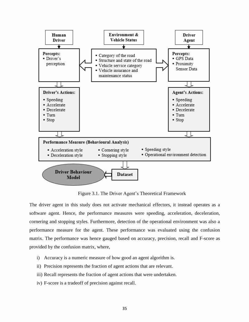
35

Figure 3.1. The Driver Agent’s Theoretical Framework

The driver agent in this study does not activate mechanical effectors, it instead operates as a

software agent. Hence, the performance measures were speeding, acceleration, deceleration,

cornering and stopping styles. Furthermore, detection of the operational environment was also a

performance measure for the agent. These performance was evaluated using the confusion

matrix. The performance was hence gauged based on accuracy, precision, recall and F-score as

provided by the confusion matrix, where,

i) Accuracy is a numeric measure of how good an agent algorithm is.

ii) Precision represents the fraction of agent actions that are relevant.

iii) Recall represents the fraction of agent actions that were undertaken.

iv) F-score is a tradeoff of precision against recall.

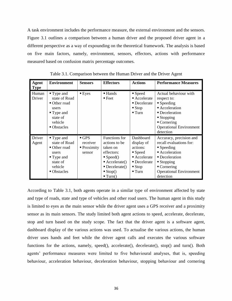
36

A task environment includes the performance measure, the external environment and the sensors.

Figure 3.1 outlines a comparison between a human driver and the proposed driver agent in a

different perspective as a way of expounding on the theoretical framework. The analysis is based

on five main factors, namely, environment, sensors, effectors, actions with performance

measured based on confusion matrix percentage outcomes.

Table 3.1. Comparison between the Human Driver and the Driver Agent

Agent

Type

Environment Sensors Effectors Actions Performance Measures

Human

Driver

Type and

state of Road

Other road

users

Type and

state of

vehicle

Obstacles

Eyes Hands

Feet

Speed

Accelerate

Decelerate

Stop

Turn

Actual behaviour with

respect to:

Speeding

Acceleration

Deceleration

Stopping

Cornering

Operational Environment

detection

Driver

Agent

Type and

state of Road

Other road

users

Type and

state of

vehicle

Obstacles

GPS

receiver

Proximity

sensor

Functions for

actions to be

taken on

effectors:

Speed()

Accelerate()

Decelerate()

Stop()

Turn()

Dashboard

display of

actions:

Speed

Accelerate

Decelerate

Stop

Turn

Accuracy, precision and

recall evaluations for:

Speeding

Acceleration

Deceleration

Stopping

Cornering

Operational Environment

detection

According to Table 3.1, both agents operate in a similar type of environment affected by state

and type of roads, state and type of vehicles and other road users. The human agent in this study

is limited to eyes as the main sensor while the driver agent uses a GPS receiver and a proximity

sensor as its main sensors. The study limited both agent actions to speed, accelerate, decelerate,

stop and turn based on the study scope. The fact that the driver agent is a software agent,

dashboard display of the various actions was used. To actualise the various actions, the human

driver uses hands and feet while the driver agent calls and executes the various software

functions for the actions, namely, speed(), accelerate(), decelerate(), stop() and turn(). Both

agents’ performance measures were limited to five behavioural analyses, that is, speeding

behaviour, acceleration behaviour, deceleration behaviour, stopping behaviour and cornering

37

behaviour. Another performance measure was the detection of the operational environment,

limited to road terrain and road pattern.

3.5 CONCEPTUAL FRAMEWORK

Figure 3.2 shows the conceptual framework, outlining independent, dependent and intervening

variables. The independent variables are GPS data collected by GPS receivers. These are

coordinates, speed, altitude, time, direction, and GPS signal strength. In addition, obstacle data

collected by the proximity sensor was also as an independent variable. These variables were

determined and selected through a prestudy mapping them to dependent variables. Since

behaviour is not measurable, the study made useful conclusions about a number of factors that

determine behaviour. The dependent variables hence included a measure of parameters that

contribute to the driving style of a human vehicle driver. These are speeding trends, acceleration

trends, deceleration trends, stopping trends and cornering trends. These trends founded the

driver’s profile that formulated a dataset that was used to train, evaluate and test the vehicle

driver agent. Detection of the vehicle driver’s operational environment, limited to road pattern

and road terrain was also a dependent variable. Intervening variables considered in this study

were road category that could be either dual carriageway, single carriageway or highway;

structure and state of the road with respect to straightness, corners, bumps, sloppiness and

condition of the road; vehicle service category that could be either public service or private

service and vehicle insurance and maintenance status that determines road worthiness.

38

Figure 3.2 Conceptual Framework

It is worth noting that each independent variable may have a direct effect, limited effect or no

effect at all over a given dependent variable. Table 3.2 outlines the effects of each independent

variable over the dependent variables. Similarly, Table 3.3 outlines the effects of intervening

variables over the dependent variables, where it clearly appears that all intervening variables

have a direct effect on driver behaviour but no effect on the determination of the operational

environment.

39

Table 3.2. Effects of Independent Variables over Dependent Variables

Independent Variable Effect of Dependent Variables

Coordinates Changes in coordinates directly affect the determination of the

operational environment.

Changes in coordinates have a limited effect to speeding, acceleration,

deceleration, cornering and stopping actions.

Speed Changes in speed directly affect speeding, acceleration, deceleration,

cornering and stopping actions.

Changes in speed have a limited effect on the determination of the


Direction Changes in direction directly affect the determination of the road

pattern.

Changes in coordinates have a limited effect to speeding, acceleration,

deceleration, cornering and stopping actions and no effect towards the

determination of the road terrain.

Altitude Changes is altitude directly affect the determination of the road

terrain.

Changes in altitude have a limited effect to speeding, acceleration,

deceleration, cornering and stopping actions and no effect towards the

determination of road pattern.

Time Changes in time directly affect determination of driver behaviour and


Obstacle data Obstacle data directly affect speeding, acceleration, deceleration,

cornering and stopping actions.

Obstacle data has no effect on the determination of the operational

environment.

GPS signal strength GPS signal strength at any given point in time directly affect

determination of driver behaviour and operational environment.

Table 3.3. Effects of Intervening Variables over Dependent Variables

Intervening Variable Effect of Dependent Variables

Category and structure of

the road

The category of the road directly affects speeding, acceleration,


The category of the road has no effect in the determination of the

operational environment with respect to road terrain and pattern.

Structure and state of the

road

The structure of the road directly affects speeding, acceleration,


The structure of road has no effect in the determination of the


Vehicle service category The vehicle service category directly affects speeding, acceleration,


The vehicle service category has no effect in the determination of the


Vehicle insurance and

maintenance state

The vehicle insurance and maintenance state directly affect speeding,

acceleration, deceleration, cornering and stopping actions.

The vehicle insurance and maintenance state has no effect in the

determination of the operational environment with respect to road

terrain and pattern.

40

3.6 SYSTEM MODEL

3.6.1 THE BLOCK DIAGRAM

The block diagram in Figure 3.3 outlines five major components that formulates the system

model, namely, GPS satellite, GPS receiver, Data Collection Unit (DCU), Server and Terminal.

According to the model, GPS satellites continuously transmit signals containing satellites’

positions (orbit), the time the signal is sent and other data. GPS receivers installed in sample

vehicles process the satellite signals to achieve position, time and other data parameters. A Data

Collection Unit connected to ultrasonic proximity sensors on the test vehicle determined obstacle

presence or absence. The DCU conveys sensor signals to the GPS receiver to complement GPS

data. Upon receipt of DCU data, the GPS receiver packages all the data in a single message then

transmits to a server via GPRS. The data is transmitted at varied intervals less than 5 seconds.

The server performs data analysis using specialised probabilistic methodologies to establish

patterns of vehicle driver behaviour. The software driver agent running on the terminal

periodically gets and displays analysed data as an indicator of human vehicle driver behavioural

probabilities and agent proposed actions.

Figure 3.3. The System Model

41

3.6.2 GPS TECHNOLOGY

The model adapts the GPS technology where Automatic Vehicle Location (AVL) is a technology

to track vehicles and relay location information to centralised monitoring locations [60]. A

variety of technologies can be used in this regard for instance satellite option that incorporates

GPS. GPS refers to a United States of America’s Government-operated network of earth-orbiting

satellites with ground control stations [61]. The network with approximately 24 active satellites

participating at any point in time continuously provides time and position information to

receiving stations and devices around the globe [61], [62].

A Global Position System is made up of three parts: GPS satellite, GPS receiver and a

monitoring station. A GPS satellite transmits a signal containing the satellite’s position (orbit),

the time the signal was sent and other data at a frequency of 1575.42MHz. A GPS receiver uses

the difference between the time the signal was sent and when it was received to calculate its

distance from the satellite. GPS positions [61], [63] are calculated through triangulation where

the known positions of at least three satellites overhead determine the position of a GPS

receiver/antenna pair on Earth. A signal from a fourth satellite is used for time corrections since

the clock in a GPS receiver is not as accurate as the atomic clock used by GPS satellites.

An algorithm that employs the doppler shift in the pseudo range signals from the satellites is

used to compute vehicle speeds. The doppler shift is directly proportional to the velocity of the

receiver along the direction to the satellite, regardless of the distance to the satellite [64]. For

better accuracy, speeds are updated at short intervals with readings normalized. Other parameters

supplied by the satellite include: date; time; and altitude. Upon acquisition of these data, a GPS

receiver sends the logged data updates to a monitoring station via GPRS for analysis. This event

occurs at some pre-set time intervals or upon a trigger.

3.6.3 THE LEARNING AGENT

A utility-based agent uses a model of the world, along with a utility function that measures its

preferences among states of the world [59]. It chooses actions that leads to the best-expected

utility, where expected utility is computed as an average of all possible outcome states, weighted

by the probability of the outcome. A rational utility-based agent chooses an action that

42

maximizes the expected utility of the action outcomes. Ingenious algorithms are required for

utility maximization. Despite these algorithms, perfect rationality is usually unachievable in

practice due to computational complexities [59]. The nature of the agent’s environment is

partially observable, multiagent, stochastic, sequential, dynamic, continuous, and unknown.

Mathematically, an agent’s behaviour is described by the agent function that maps any given

percept sequence to an action [59].

The research problem is a contingency kind of problem since exact prediction is impossible and

its solution requires a strategy, a contingency plan that specifies what action to take based on the

received percepts. Thus the use of utility functions to provide agent’s internal performance

measures in two main perspectives. Firstly, the function offers appropriate tradeoffs amongst

conflicting goals. Secondly, it weighs success likelihood against the importance of goals. If the

internal utility function and the external performance measures are in agreement [59], then it

chooses actions to maximize utility.

The intelligence of the agent is based on its dataset where the learning mechanism is a

combination of supervised and reinforcement learning subsystems. At the initial stages, it is

adapted to the dataset through supervised learning. The supervised learning is achieved through

the machine learning process, namely, training, validation and testing. Reinforcement learning is

gradually mainstreamed in the supervised learning at the point of validation and testing.

Reinforcement learning where the agent learns from a series of rewards or punishments that

attribute to reinforcement [59]. A reward is a form of feedback that makes the agent know

whether something good or bad has happened based on its actions. The reward-based approach

lead to formulation of an optimal behavioural pattern dataset. Learning allows the agent to

initially operate in unknown environments and to become more competent than its initial

knowledge. Figure 3.4 outlines the structure of a learning utility-based agent.

43

In an ideal case, learning agents act autonomously, operate in unknown environments, synthesise

rules and/or patterns from volumes of data, handle complex data as they improve their own

performance. This means that percepts are not only used for acting but for improvement on

future performance. A learning utility-based agent hence comprises of four key elements,

namely, a learning element, a critic, a performance element and a problem generator as

illustrated in Figure 3.4, where,

i) The performance element is responsible for selecting external actions. This actions are

based on percepts detected by the sensors. The performance element also takes in change

percepts from the learning element to decide on actions to be undertaken. Feedback from

the problem generator also acts as input to the performance element, facilitating

continuous learning. On the other hand, the performance element has two output

channels: knowledge to the learning element and action signals to effectors.

ii) The critic is responsible for providing feedback to the learning element. The feedback is

an outcome of processed input from sensors in comparison with objective performance

standards outside the agent. For a utility-based agent, as for the case of this study, an

external performance standard is critical to tell the critic if the agent’s action has a good

or bad effect on its environment.

Figure 3.4. The Structure of the Learning Utility-based Driver Agent

44

iii) The learning element is responsible for making improvements to the agent’s

performance. Learning is achieved through observing pairs of successive states in the

percept sequence. From this, the agent can learn how the world evolves. The element

uses feedback from the critic on how well the agent is doing. This feedback is used to

determine how the performance element should be modified as an improvement of the

agent for better performance in future. Furthermore, knowledge from the performance

element is also fed to the learning element for analysis aimed at future performance

improvements. There are two outcomes from the learning element that act as input to the

other elements. These are the change output that acts as input percept for the performance

element and the learning goals output that acts as input percepts to the problem generator.

iv) The problem generator suggests actions that lead to new and informative experiences.

This actions suggestions are continuously fed to the performance element as of when they

are determined. This makes the agent to keep learning and improving on performance.

The problem generator relies on learning goals generated by the learning element to make

its decisions.

3.7 DATA COLLECTION PROCESS

3.7.1 SOURCES OF DATA

Data was collected from drivers driving sample vehicles at different road segments. These

vehicles were instrumented with various sensors for data collection. The study used a GPS

receiver type capable of providing vehicle position coordinates, speed, direction (angle), altitude

and timestamp. A proximity sensor generated obstacle data with data transferred to the GPS

receiver for subsequent transmission to the server. On the other hand, operational rules per type

of road and driving region was based on regulations set out by the National Transport and Safety

Authority (NTSA) in Kenya and other World standard metrics.

3.7.2 TARGET POPULATION

Kenya has approximately 3,000,000 registered vehicles each of which could be assumed to be

operated by one or more licensed driver. Hence, the number of vehicle drivers is estimated to be

slightly above the number of registered vehicles. A target population refers to the collection of

45

individuals or regions to be used in a given investigation or study [65]. The target population for

this study were licensed vehicle drivers in Kenya. The study was based on a target sample

comprising 30 drivers subjected to two instrumented private cars and fifteen instrumented Public

Service Vehicles.

3.7.3 SAMPLING AND SAMPLE SIZE

A sample is a finite part of a statistical population to be investigated [65]. When dealing with

people, it can be defined as a set of respondents selected from a larger population for the purpose

of a survey. The choice of a sample influences the degree of accuracy of the results in a research

about a given phenomenon. Scholars have argued that where time and resources allow, the entire

population can be studied [65], [66]. While this may seem as the best possible approach, it is

practically impossible. The Cochran [67] provides one of the ideal methods for deriving a sample

size when given a desired level of precision, desired confidence level and the estimated

proportion of the attribute present in the population. The formula is considered appropriate in

situations with large population sizes. Equation (1) shows the Cochran formula.

𝑛0 =Z2𝑝𝑞

𝑒2 (1)

Where:

i) e is the desired level of precision, commonly referred to as the margin of error.

ii) p is the (estimated) proportion of the population having the attributes in question

iii) q is 1 – p.

iv) The z-value is found in the Z table.

Considering a confidence level of 95%, a Z value of 1.96 would be applicable as per the standard

Z table and a margin of error of 5%. The p was put at 0.5 which translates to a q of 0.5. Hence,

the n0 was determined to be 385 as outlined in equation (2).

𝑛0 =1.962(0.5)(1−0.5)

0.052 (2)

46

To try and fit the sample size determination to an approximate population of 3,000,000 licenced

drivers in Kenya, equation (3) was used to modify the sample size.

n =n0

1+(𝑛0−1)

𝑁

(3)

Where:

i) n0 is the Cochran’s sample size recommendation.

ii) N is the population size, in this case 3,000,000.

iii) n is the new adjusted sample size.

Hence, the resulting sample size after the modification was 384.95 which still rounds off to 385.

The computation is as outlined in equation (4). The small deviation of 0.05 is an indicator that

the initial Cochran formula fits in large populations, hence, the modification will have a

significance only on smaller populations.

n =385

1+(385−1)

3,000,000

(4)

Hair et al [68] argues that the sample size can range from 30 to 500 respondents but further states

that the use for analysis may also dictate the sample. In a later publication, Hair et al [69] notes

that if the sample size is less than 30, significant departures from normality can have a

substantial impact on the results. The minimum is to have at least five times as many

observations as the number of variables to be analysed [69], particularly in cases where factor

analysis is involved.

MacCullum et al [70] stated that where there is need to generalize the findings, as may be the

case in this study, sample size cannot be the sole determinant of generalizability of the results;

adequacy of a sample in such cases should be evaluated by examining the level of bias and the

level of data quality, which are two critical components. According to [71], studies of new ideas

often start small, sometimes even with an n of 1, due to cost and feasibility concerns. The cost of

the study is always impossible for researchers and funders to overlook in sample size

determination [71], [72].

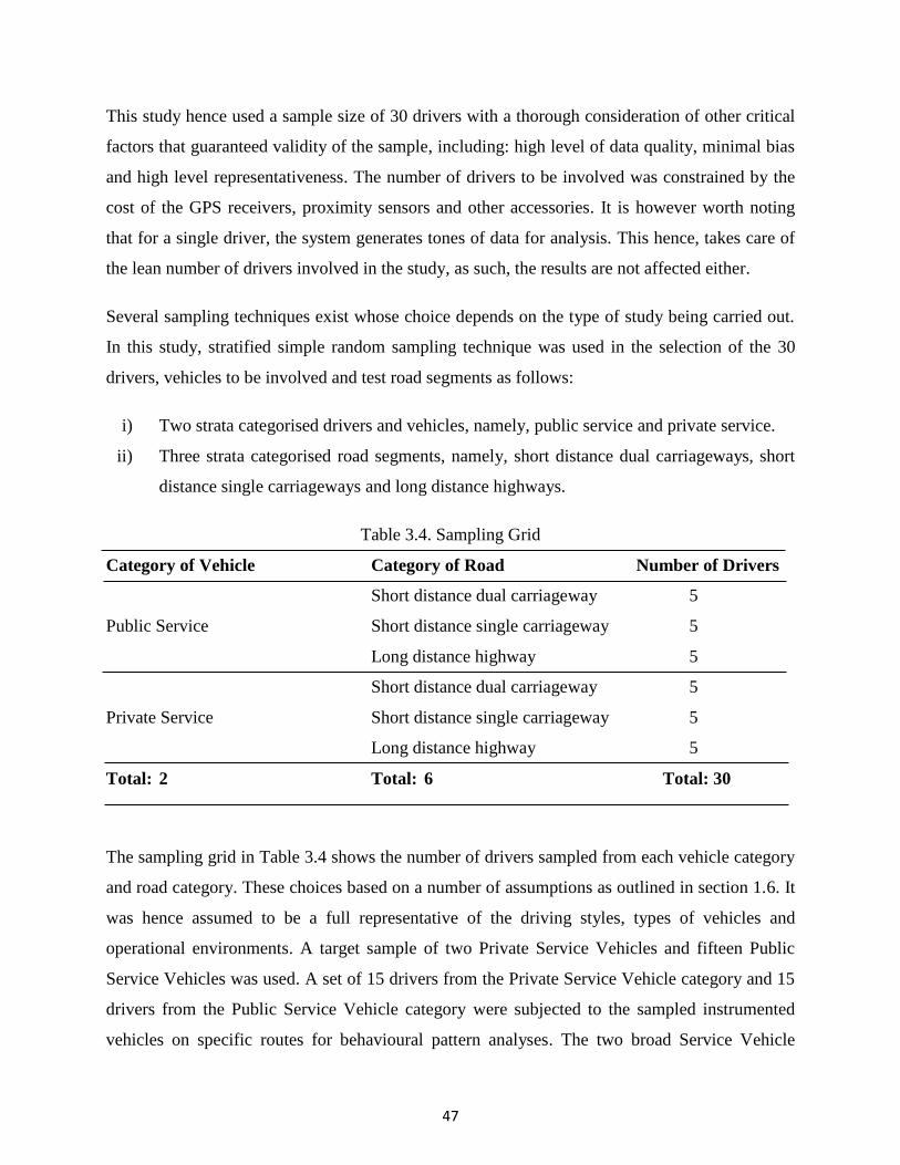
47

This study hence used a sample size of 30 drivers with a thorough consideration of other critical

factors that guaranteed validity of the sample, including: high level of data quality, minimal bias

and high level representativeness. The number of drivers to be involved was constrained by the

cost of the GPS receivers, proximity sensors and other accessories. It is however worth noting

that for a single driver, the system generates tones of data for analysis. This hence, takes care of

the lean number of drivers involved in the study, as such, the results are not affected either.

Several sampling techniques exist whose choice depends on the type of study being carried out.

In this study, stratified simple random sampling technique was used in the selection of the 30

drivers, vehicles to be involved and test road segments as follows:

i) Two strata categorised drivers and vehicles, namely, public service and private service.

ii) Three strata categorised road segments, namely, short distance dual carriageways, short

distance single carriageways and long distance highways.

Table 3.4. Sampling Grid

Category of Vehicle Category of Road Number of Drivers

Short distance dual carriageway 5

Public Service Short distance single carriageway 5

Long distance highway 5

Short distance dual carriageway 5

Private Service Short distance single carriageway 5

Long distance highway 5

Total: 2 Total: 6 Total: 30

The sampling grid in Table 3.4 shows the number of drivers sampled from each vehicle category

and road category. These choices based on a number of assumptions as outlined in section 1.6. It

was hence assumed to be a full representative of the driving styles, types of vehicles and

operational environments. A target sample of two Private Service Vehicles and fifteen Public

Service Vehicles was used. A set of 15 drivers from the Private Service Vehicle category and 15

drivers from the Public Service Vehicle category were subjected to the sampled instrumented

vehicles on specific routes for behavioural pattern analyses. The two broad Service Vehicle

48

categories accommodate light, heavy and commercial vehicle subcategories. A driver

behavioural pattern dataset was formulated purely from gathered and analysed GPS data. The

dataset from select drivers whose behaviour met the required conditions was used to train,

validate and test an agent modelling human vehicle driver behaviour. The full driver behaviour

model acts as a software driver agent with screen display of actions running in parallel with a

human vehicle driver without activating any mechanical effectors.

3.7.4 DATA COLLECTION TOOLS AND TECHNIQUES

A research data collection tool is defined as a testing device that measures a given phenomenon.

This study used real-time data collection using the following tools:

i) GPS Receiver

Continously receives GPS data from GPS satelittes and transmits to the GPS server for

analysis.

ii) Data Collection Unit (DCU)

Collects obstacle data to complement GPS data. It transmits obstacle signal data to the

GPS receiver for subsequent transmission to the GPS server.

iii) GPS Server

Receives data from GPS receivers and stores in the database for analysis.

DESIGN AND DEVELOPMENT OF DATA COLLECTION TOOLS

The prototype comprises of a GPS receiver, a Data Collection Unit and a GPS server. The study

used GPS receivers based on the GPRMC sentence format. These were sourced and used as per

the manufacturer’s specifications. It should be noted that the National Marine Electronics

Association (NMEA) 0183 standard defines dozens of sentence formats, but only a fraction

applies directly to GPS receivers [73]. NMEA 0183 data transmissions use plain text with the

characters coded using seven-bit American Standard Code for Information Interchange (ASCII)

[73]. The Recommended Minimum Specific GPS/Transmit Data (RMC) sentence contains

Coordinated Universal Time (UTC) date and time, the latitude and longitude of the position fix,

the ground speed, the course over the ground with respect to the true north, and the magnetic

declination [73]. The data is send as one sentence starting with $$ and ending with ## with the

49

various data parameters separated by commas [74]. The following is an example of the sentence

as transmitted by the GPS receiver:

$$1000000002???&A9955&B051006.000,A,0117.8458,S,03650.5808,E,30.00,090.38,200418,,,

A*79|0.9|&C0000011111&D0026:164&E10000000&Y00180000##

Where:

1000000002 Device unique identifier (Maximum of 15 characters)

A9955 Device board ID (Manufacturer specific)

051006.000 Time (hhmmss.ddd)

A Validity of the fix (A = Valid)

0117.8458 Latitude (ddmm.mmmm)

S Latitude hemisphere (S = Southern)

03650.5808 Longitude (dddmm.mmmm)

E Longitude hemisphere (E = Eastern)

30.00 Speed in knots (s.s)

090.38 Course in degrees (h.h)

200418 Date (ddmmyy)

‘$’ ‘,’ ‘?’ ‘&’ and ‘#’ Separator to the various data parameters

The string “A*79|0.9|&C0000011111&D0026:164&E1000 0000&Y00180000” represents

proprietary data that the device tracked along the way. This data is usually secreted by the device

manufacturers with *79 representing the checksum.

The format provided key data parameters required for driver behaviour monitoring. A custom-

made Data Collection Unit (DCU) complemented GPS receiver’s data with obstacle data. It was

50

based on an Arduino Microcontroller with an ultrasonic proximity sensor as outlined in Figure

3.5 with the source code for the program controlling the Arduino microcontroller outlined in

Appendix A.

The DCU periodically sends trigger signals to proximity sensors on test vehicle for

determination of obstacles in range. It then conveys sensor signals to the GPS receiver via a

power relay that completes the circuit if there is an obstacle otherwise it opens the circuit.

Microcontroller (Arduino Uno)

Arduino is an open-source computer hardware and software company, project and user

community that designs and manufactures kits for building digital devices and interactive objects

that can sense and control the physical world [75]. An Arduino board consists of an Atmel 8-bit

Alf and Vegard's RISC (AVR) microcontroller with complementary components that facilitate

programming and interfacing with other circuits through a specially designed printed circuit

Figure 3.5. Circuit Diagram for the Data Collection Unit

51

board (PCB) [75], [76]. The Arduino integrated development environment (IDE) is a Java-based

cross-platform application that includes a code editor that has features like other code editors.

The IDE facilitates writing, compiling and uploading of programs to the Arduino board. An

executable cyclic Arduino program requires a definition of only two functions, namely, setup

and loop functions as shown in the microcontroller program in Appendix A.

An Arduino board takes direct current (DC) from a DC power source or an AC-to-DC adapter. It

can also draw power through a Universal Serial Bus (USB) connection to any USB supported

device. The microcontroller is programmed using a C or C++ based Arduino programming

language. The wiring software library in the Arduino IDE makes many common input/output

operations much easier [75]. The main features of an Arduino Uno board are: ATmega328P

microcontroller, 7 – 12 input voltage, 14 digital input/output pins, 6 analog inputs, 32k flash

memory, 16Mhz quartz crystal clock speed, USB connection, Power jack, In-Circuit Serial

Programming (ICSP) header and the Reset button. Six out of the 14 digital input/output pins are

Pulse Width Modulation (PWM) outputs, allowing analog results to be retrieved through them.

Proximity Sensor (HC-SR04)

The HC-SR04 proximity sensor is an obstacle detection sensor type based on ultrasound

technology. It is a low cost sensor that provides 2cm to 400cm of non-contact measurement

functionality. The sensor supports a ranging accuracy that can reach up to 3mm. The HC-SR04

module is composed of an ultrasound transmitter, a receiver and a control circuit. It has 4 pins: a

5 volts’ pin for power, a trigger pin for trigger signal, an echo pin to receive the reflected signal

and a ground pin. Table 3.5 outlines the technical specifications for the HC-SR04 ultrasonic

sensor used in this study. This is as specified in the manufacturer’s product datasheet.

52

Table 3.5. HC-SR04 Technical Specifications

Description Rating

Working Voltage DC 5V

Working Current 15mA

Working Frequency 40Hz

Max Range 400cm

Min Range 2cm

Measuring Angle 15 degree

Trigger Input Signal 10 μS TTL pulse

Echo Output Signal Input TTL lever signal and the

range in proportion

Dimension 45*20*15mm

Power Relay (5V DC SPDT)

The 5 Volts Direct Current (DC) Single Pole Double Throw (SPDT) is a power relay module that

can be controlled directly by a wide range of microcontrollers. These microcontrollers include,

Arduino, Alf and Vegard's RISC (AVR), Peripheral Interface Controller (PIC), Advanced RISC

Machines (ARM) and Mixed Signal Processor (MSP) 430. The relay is suitable for numerous

applications in the range of domestic appliances, office machines, audio equipment, automobiles

among other appliances.

Figure 3.6. Internal Layout for a Power Relay

53

The 5V DC SPDT power relay has 5 pins as shown in Figure 3.6. These are the COM pin,

Normally Connected (NC) to COM pin, Normally Open (NO) to COM pin, two 5 volts’ COIL

pins. The NC and NO pins enable it to act as a power switch for driving high voltage devices.

The two COIL pins are supplied with 5 volts in either direction, creating a magnetic effect on the

COIL that facilitates switching between NO and NC pins through attraction and release as shown

in Figure 3.6. The COM to NO or NC connects to appliances or circuitries that supports high

voltages. In this case, they connect 12 volts’ power from the car battery to the GPS receiver. This

is used to denote presence or absence of an obstacle.

Microcontroller Program

The flowchart in Figure 3.7 outlines the flow of events as the microcontroller sends trigger

messages to the proximity sensor during the process of obstacle detection. An obstacle is

detected if it falls within a 4-meter range, that was the operational sensing distance for the

proximity sensor used in the study. Upon detection of an obstacle, the GPS trigger PIN is set to

HIGH. As a result, the GPS data sent to the server will include a value that indicates detection of

an obstacle. Otherwise the GPS trigger PIN is set LOW as an indicator that no obstacle is

detected. The process occurs as a continuous loop as long as the vehicle engine is on.

Figure 3.7. Microcontroller Communication with the Proximity Sensor

Yes No

distance < 4m?

Process echo signals

from the sensor

Continuously send

trigger signals to the

proximity sensor

Set GPS trigger

PIN to HIGH

Set GPS trigger

PIN to LOW

Start

54

The Arduino Uno microcontroller was programmed with the source code outlined in Appendix

A. Line 20 of the source code provides room for adjustment of obstacle sensing distances as a

way for calibration of the model. If an obstacle is detected within the specified distance range in

centimetres, then line 21 is executed. This would set the GPS trigger pin, in this case referred to

as the gpstrigpin, to HIGH. On the other hand, if no obstacle is detected within the range, line 24

will be executed setting the gpstrigpin to LOW.

GPS Receiver

The study used on-board units that use GPS technology to collect data from GPS satellites then

transmit the data to a GPS server for processing using GPRS technology. The choice of the

devices was informed by the required parameters that include vehicle speed, altitude, direction

and a timestamp.

GPS Server

The data transmitted by a GPS receiver ends up on a GPS server that has a receiver application

running continuously with a specific open port listening to incoming connections. A GPS server

was developed with two main components: -

i) Data Receiver TCP Application – the application interface receives data from GPS

receivers in National Marine Electronics Association (NMEA) format, interpret,

transform then route the data to the database for storage. The application uses socket

communication.

ii) SQL Based Database – the SQL-based database stores the data awaiting analysis.

A Data Receiver TCP application creates a specific type of socket used to listen to client

requests, in this case, GPS receiver connection requests. In case of a connection request, the

application creates a new socket through which exchange of data with the client using input and

output streams will be facilitated. The source and destination IP address, and port number

constitute a network socket. The process can be summarized as follows:-

55

i) The server process binds an IP address to a port then continuously listens to client

requests. The port must be opened on the router within the network that the server is

setup.

ii) The client, in this case, GPS receiver configured with the server IP address and port

number contacts the server by creating a client-local TCP socket, specifying IP address

and port number of the server. As a result of this, the client TCP establishes a connection

to the server TCP.

iii) When contacted, the server TCP creates a new socket for the server process to

communicate with the client there by allowing the GPS receiver to transmit data to the

server over the IP layer using either UDP or TCP. The GPS receivers used in this study

transmitted data using TCP. The transmission was via GPRS based on the mobile service

provider’s SIM used.

iv) The data receiver application receives the packets, validates them against authenticated

devices using a specific unique unit identifier and then stores in a database. The unique

identifier is always predefined in the database during initial unit setup.

The flow chart in Figure 3.8 outlines the functions of the GPS Data Receiver from the time GPS

data is received from the GPS receiver to the time it is routed to the GPS SQL-based database.

An SQL-based database was used since the data was relational. Ten tables were created to store

the various data elements. Appendix C outlines the ten tables with their respective attributes and

data types that formulates the database schema.

56

VALIDITY AND RELIABILITY OF DATA COLLECTION INSTRUMENTS

Measurement errors could arise from faults in the instruments, incorrect interpretations of

obtained values or instability in the behaviour of respondents or samples. These errors could be

systematic or random. Systematic errors or bias occur when the errors are made in one direction

away from the true score. Random errors on the other hand are attributable to chance factors.

Figure 3.8. Flowchart of Events at the Data Receiver

57

According to Mugenda [77], validity is the degree to which a research instrument measures what

it purports to measure. On the other hand, reliability is the extent to which results or observations

for a given experiment are consistent on any repeated trials [77]. Reliability in other words, is the

stability or consistency of scores over time or across raters.

In this study, the measurement instruments were on tested on five drivers in a pretest to check for

any inconsistencies and/or errors. After the pretest, relevant adjustments were made to the

instruments before use in the main study on the sampled subjects.

Data collection tools were validated through the following steps:

i) The first step involved face validity through dialog and brain storming with experts in the

transport industry and through research seminars. This led to the formulation of the driver

behaviour and environment probabilities per driving state chart as outlined in Table 0.1.

ii) A pilot study was then contacted involving 5 drivers on different road segments and

vehicle models that generated an intense prestudy dataset. Appendix D outlines sample

cleaned prestudy data. The dataset was cleaned and analysed using Principal Component

Analysis and Factor Analysis to ascertain whether the key variables were coming out

clearly. For instance, single factor, correlation and covariance ANOVA analyses were

established on a varied set of key data parameters that include, speed, altitude, direction

and change in time to determine the level of consistency and reliability before the actual

study. Sample analysis results are as presented in section 4.1.1.4 on validation of data

collection tools.

iii) Some revisions were made on the data collection tools. For instance, some thresholds

were adjusted in the driver behaviour and environment probabilities per driving state

chart as outlined in Table 0.1. Furthermore, GPS receivers were reconfigured to send data

at slightly short time intervals to help capture all driving style instances.

58

3.8 DATA ANALYSIS AND PRESENTATION

3.8.1 DATA MANAGEMENT

An important aspect of this research was in maintaining high quality standards in data collection

to ensure quality results. This was achieved through proper validation of data collection tools and

proper storage of the collected data. The realtime data logged at the server was kept as raw as

possible to facilitate proper analysis on the same. Most importantly, backups of the data were

created and protected to maintain high data integrity.

3.8.2 DATA SCREENING

Based on the nature of data collection that was purely realtime and using technology in data

collection, a check on missing values, normality and outliers in the data was done throughout the

entire study. This ensured that the fundamental characteristics of the data were available and

being collected appropriately.

MISSING VALUES

Given that data collection was electronic and automatically transmitted to the server by GPS

receivers, some instances could have delays that could lead to missing values, leading to

inconsistencies. A strategy was implemented to deal with such situations. This strategy involved

analysis of data using algorithms that subjected the data to time series analysis such that huge

gaps in time differences could lead to some data being eliminated from the analysis. The 2TBN

algorithm was heavily relied upon in this regard.

OUTLIERS

Data representing the independent variables was thoroughly scruitnised to ascertain whether it

was vital to influence the dependent variables. Instances in the data collection algorithms that

could lead to extreme data points as a form of outliers were spotted with the algorithms adjusted

accordingly to cleanse the data. It should be noted that the realtime nature of data collection

employed in this study was prone such instances, where, the data for a given independent

variable could have a huge deviation from other samples. During the entire study, outliers were

determined and eliminated through multivariate normality analysis. To further avoid outliers in

59

the main study, the 2TBN and Gaussian Mixture Model data analysis algorithms were adjusted

to detect huge variances in data values and automatically eliminate the data from the analysis.

ESTABLISHING VARIABLE NORMALITY

Hypothesis testing technique was used to assess the relationship among various variables

concurrently. Multivariate normality can be assumed [69], though the normality of the single

variables is not guaranteed. The research determined skewness and kurtosis as the methods of

normality. Skewness was used to measure the degree to which the distribution was symmetric,

whereby; a negative value showed that the left side of the histogram was lengthier associated to

the precise side. This is an optimistic worth demonstrating the opposite while a value zero

indicates that the distribution is balanced. Kurtosis on the other hand, unhurried the competent

highest of the unfriendly in the movement. Information distribution in high worth has the highest

height nearby the unfriendly and finished. Low kurtosis has a horizontal top neighboring the

unkind. Negative kurtosis showed platykurtic (flatter) distribution while positive values

leptokurtic (peaked) distribution. All resulting statistical tests are invalid from the normal

distribution if the variation is significantly larger [69]. This was applied throughout the study by

analyzing skewness and kurtosis levels provided through descriptive statistics results as depicted

in Chapter 5. At this point, some data was completely eliminated from the analysis for not

meeting the requirements.

FURTHER DATA VALIDITY

According to Mugenda [77], validity of data depends on the degree to which extraneous

variables have been controlled in the study to ensure that the change observed in the dependent

variable is actually as a result of the treatment. Hence, in addition to checks on missing values

and outliers, the following types of validity were considered:

1. Face Validity

Experts, research supervisors and other scholars were engaged in seminars and workshops to

ascertain whether the findings were valid.

60

2. Formative Validity

A discussion of research findings complemented by face and construct validity was used to

assesses how well the measures were able to provide information to help in driver behaviour

modelling.

3. Experimental Validity

Experimental validity was looked at in two perspectives, namely, internal validity and

external validity. Internal validity explored whether the independent variables influenced the

dependent variables. This was tested during the prestudy at the point of determining the

required data parameters that informed the selection of independent variables. The fact that

the prestudy yielded promising results, it was a clear indicator that the independent variables

were clearly affecting the dependent variables. Prestudy results are as outlined in Chapter 4,

section 4.1. On the other hand, external validity was used to ascertain whether study finding

could be generalized over the wider population. For instance, during the main study, several

experiments were carried out with correlation and covariance checked through ANOVA

analysis. This helped to determine the extent to which generalisabiliy could be spotted. The

various statistical analyses are as depicted throughout Chapter 4. Extraneous variables and

outside influences were hence controlled to avoid negative impact on research outcomes.

3.8.3 DATA ANALYSIS TOOLS AND TECHNIQUES

The study produced both quantitative and qualitative data, showing the various behavioural

parameters for a human vehicle driver. Data analysis used quantitative techniques with the

Microsoft Excel Application Software Package being used. The following tools and analysis

techniques were employed in addition to specialized algorithms:

i) ANOVA analysis tools – These utilized the single factor and two-factor analysis tools in

the determination of the fact that each sample was drawn from the same underlying

probability distribution against the alternative hypothesis that underlying probability

distributions are not the same for all samples. The tests were done at statistical significant

levels of p < 0.05.

ii) Descriptive statistics analysis tool – Generated a report of univariate statistics for data in

the input range for any given variables(s). It provided information about the central

61

tendency and variability in the data including the mean, mode, standard deviation,

kurtosis among others.

iii) Correlation and Covariance tools – Each tool gave an output matrix depicting the

correlation coefficient or covariance, respectively, between each pair of measurement

variables. The difference is that correlation coefficients are scaled to lie between -1 and

+1 inclusive. Corresponding covariance are not scaled. Both the correlation coefficient

and the covariance are measures of the extent to which two variables vary together.

3.8.4 DATA ANALYSIS ALGORITHMS

FORMULATION OF THE DRIVER BEHAVIOUR DATASET

The study relied on GPS data collected in realtime as drivers go along with their normal

operations. The main parameter required for profiling drivers are speed, altitude, direction,

timestamp and GPS signal strength data. These were complemented by proximity sensor data to

take care of presence or absence of obstacles in the driving environment. Drivers’ position in

form of coordinates is essential for any detailed report. The study was limited to five main

categories of driver behaviour: speeding, acceleration, deceleration, stopping and cornering.

Table 3.6 outlines possible attributes per category.

Table 3.6. Categories of Driver Behaviour Attributes

Profile Category Behavioural Attribute

Speeding Normal Speeding

High Speeding

Acceleration Normal Acceleration

Harsh Acceleration

Deceleration Normal Deceleration

Harsh Deceleration

Stopping Normal Braking to Stop

Harsh Braking to Stop

Cornering Normal Cornering

Harsh Cornering

62

The study established no existence of world standard braking and acceleration metrics. However,

some key metrics behind driver perception-reaction distance and braking distance leading to a

realisation of the stopping sight distance were used in this regard. Stopping sight distance is the

distance covered during two phases of stopping a vehicle: perception-reaction time (PRT), and

maneuver time (MT) [78]. Perception-reaction time is the time taken for a driver to realize that a

reaction is needed due to a given condition, decided what maneuver is appropriate (in this case,

stopping the vehicle), and start the maneuver (taking the foot off the accelerator and depressing

the brake pedal). On the other hand, maneuver time is the time taken to complete the maneuver

(decelerating and coming to a stop). The distance driven during perception-reaction time and

maneuver time is the sight distance needed. This may however vary due to the fact that different

vehicle models from different manufactures have varied strengths and capabilities. For instance,

some vehicles have a powerful braking system compared to others. Furthermore, other vehicles

have greater power picking levels allowing instant speed shifts. The study used a braking and

acceleration distance of less than 5 meters per square seconds to be normal. Any instances

greater than this limit should hence be treated to be harsh acceleration or braking behaviour.

Speeding metric could be set to international or national standards. For instance, according to the

Kenyan Traffic Act on speed limits, private motor vehicles are limited to 110km/h and 100km/h

on dual-carriage highways and on single carriage highways respectively. On the other hand,

commercial vehicles, passenger vehicles, omnibuses and other Public Service Vehicles are

limited to 80 km/h on any type of road. Furthermore, speed limited zones require slightly low

speed settings. For instance, built up area are always limited to maximum speeds of 50km/h

regardless of type of road or vehicle.

DETERMINATION OF BEHAVIOUR AND ENVIRONMENT

The study employed graphical probabilistic models to establish the behaviour and the nature of

operational environment based on possible probabilities given a set of variables. The study was

limited to five GPS data variables and obstacle data: speed, direction, altitude, time, signal

strength and obstacle presence signal. Two graphical models were considered: the Bayesian

Network (BN) and the Dynamic Bayesian Network (DBN).

63

Bayesian Network

The Bayesian Network is a probabilistic graphical model, a type of statistical model that maps a

set of variables and their conditional dependencies [79]. Figure 3.9 outlines a Bayesian Network

composed of five variables: change in speed, altitude, direction, obstacle and the GPS signal

strength. The time variable was incorporated in determining the various time slices in the DBN

described in the next section. Hence, not represented as a variable in the BN.

According to the graphical Bayesian Network in Figure 3.9, driver behaviour and nature of

environment depend on change in speed, altitude, direction and presence or absence of obstacles.

It is further evident that a change in speed is affected by changes in altitude and directions and

presence or absence of obstacles. Furthermore, the GPS signal strength affects changes in

altitude, speed and direction. The probabilities in the networks can be summarized as per

equation (5).

P(Behaviour & Environment) = P(∆Altitude | GPSSignalStrength) . P(Direction |

GPSSignalStrength) . P(Speed | Altitude, Direction, GPSSignalStrength, Obstacle)

(5)

The possible observations were represented in two sets: driver behaviour and nature of the

environment sets as shown in equation (6).

Figure 3.9. Bayesian Network of Five Variables

64

observations={

(‘normal_braking’, ‘harsh_braking’, ‘normal_acceleration’, ‘harsh_acceleration’,

‘normal_cornering’, ‘harsh_cornering’, ‘normal speeding’, ’high speeding’),

(‘meander’, ‘straight’, ‘up-hill’, ‘down-hill’)

} (6)

Dynamic Bayesian Network

Based on the dynamic natures of GPS data over time, it was necessary to consider the Dynamic

Bayesian Network representation. A DBN is a Bayesian Network that relates variables over

adjacent time steps [79]. It is hence often referred to as a 2-Time-slice Bayesian Networks

(2TBN). According to the 2TBN, at any given time t, the value of a variable can be calculated

from the internal regressors and immediate prior value at time t-1. In this case, the 2TBN could

be represented as depicted in Figure 3.10.

The model in the figure represents three copies of time-slices where each time-slice is a Bayesian

Network. According to the sample network, the probabilities for the three time-slices can be

summarized by equation (7) to (9), where, the difference between time t and t-1 depends upon

the time difference between two data points logged at the server.

𝑃(𝐵𝑒ℎ𝑎𝑣𝑖𝑜𝑢𝑟 & 𝐸𝑛𝑣𝑖𝑟𝑜𝑛𝑚𝑒𝑛𝑡𝑡−1)

= 𝑃(𝐴𝑙𝑡𝑖𝑡𝑢𝑑𝑒𝑡−1 | 𝐺𝑃𝑆𝑆𝑖𝑔𝑛𝑎𝑙𝑆𝑡𝑟𝑒𝑛𝑔𝑡ℎ𝑡−1) . 𝑃(𝐷𝑖𝑟𝑒𝑐𝑡𝑖𝑜𝑛𝑡−1 | 𝐺𝑃𝑆𝑆𝑖𝑔𝑛𝑎𝑙𝑆𝑡𝑟𝑒𝑛𝑔𝑡ℎ𝑡−1) . 𝑃(𝑆𝑝𝑒𝑒𝑑𝑡−1 | 𝐴𝑙𝑡𝑖𝑡𝑢𝑑𝑒𝑡−1, 𝐷𝑖𝑟𝑒𝑐𝑡𝑖𝑜𝑛𝑡−1, 𝑂𝑏𝑠𝑡𝑎𝑐𝑙𝑒𝑡−1 , 𝐺𝑃𝑆𝑆𝑖𝑔𝑛𝑎𝑙𝑆𝑡𝑟𝑒𝑛𝑔𝑡ℎ𝑡−1)

(7)

Figure 3.10. A 2TBN for Establishing Driver Behaviour and Operational Environment

65

𝑃(𝐵𝑒ℎ𝑎𝑣𝑖𝑜𝑢𝑟 & 𝐸𝑛𝑣𝑖𝑟𝑜𝑛𝑚𝑒𝑛𝑡𝑡)

= 𝑃(𝐴𝑙𝑡𝑖𝑡𝑢𝑑𝑒𝑡 | 𝐴𝑙𝑡𝑖𝑡𝑢𝑑𝑒𝑡−1, 𝐺𝑃𝑆𝑆𝑖𝑔𝑛𝑎𝑙𝑆𝑡𝑟𝑒𝑛𝑔𝑡ℎ𝑡) . 𝑃(𝐷𝑖𝑟𝑒𝑐𝑡𝑖𝑜𝑛𝑡 | 𝐷𝑖𝑟𝑒𝑐𝑡𝑖𝑜𝑛𝑡−1, 𝐺𝑃𝑆𝑆𝑖𝑔𝑛𝑎𝑙𝑆𝑡𝑟𝑒𝑛𝑔𝑡ℎ𝑡) . 𝑃(𝑆𝑝𝑒𝑒𝑑𝑡 | 𝑆𝑝𝑒𝑒𝑑𝑡−1, 𝐴𝑙𝑡𝑖𝑡𝑢𝑑𝑒𝑡 , 𝐴𝑙𝑡𝑖𝑡𝑢𝑑𝑒𝑡−1,

𝐷𝑖𝑟𝑒𝑐𝑡𝑖𝑜𝑛𝑡 , 𝐷𝑖𝑟𝑒𝑐𝑡𝑖𝑜𝑛𝑡−1, 𝑂𝑏𝑠𝑡𝑎𝑐𝑙𝑒𝑡 , 𝑂𝑏𝑠𝑡𝑎𝑐𝑙𝑒𝑡−1, 𝐺𝑃𝑆𝑆𝑖𝑔𝑛𝑎𝑙𝑆𝑡𝑟𝑒𝑛𝑔𝑡ℎ𝑡)

(8)

𝑃(𝐵𝑒ℎ𝑎𝑣𝑖𝑜𝑢𝑟 & 𝐸𝑛𝑣𝑖𝑟𝑜𝑛𝑚𝑒𝑛𝑡𝑡+1)

= 𝑃(𝐴𝑙𝑡𝑖𝑡𝑢𝑑𝑒𝑡+1 | 𝐴𝑙𝑡𝑖𝑡𝑢𝑑𝑒𝑡 , 𝐺𝑃𝑆𝑆𝑖𝑔𝑛𝑎𝑙𝑆𝑡𝑟𝑒𝑛𝑔𝑡ℎ𝑡+1) . 𝑃(𝐷𝑖𝑟𝑒𝑐𝑡𝑖𝑜𝑛𝑡+1 | 𝐷𝑖𝑟𝑒𝑐𝑡𝑖𝑜𝑛𝑡 , 𝐺𝑃𝑆𝑆𝑖𝑔𝑛𝑎𝑙𝑆𝑡𝑟𝑒𝑛𝑔𝑡ℎ𝑡+1) . 𝑃(𝑆𝑝𝑒𝑒𝑑𝑡+1 | 𝑆𝑝𝑒𝑒𝑑𝑡, 𝐴𝑙𝑡𝑖𝑡𝑢𝑑𝑒𝑡+1, 𝐴𝑙𝑡𝑖𝑡𝑢𝑑𝑒𝑡 ,𝐷𝑖𝑟𝑒𝑐𝑡𝑖𝑜𝑛𝑡+1, 𝐷𝑖𝑟𝑒𝑐𝑡𝑖𝑜𝑛𝑡 , 𝑂𝑏𝑠𝑡𝑎𝑐𝑙𝑒𝑡+1, 𝑂𝑏𝑠𝑡𝑎𝑐𝑙𝑒𝑡 , 𝐺𝑃𝑆𝑆𝑖𝑔𝑛𝑎𝑙𝑆𝑡𝑟𝑒𝑛𝑔𝑡ℎ𝑡+1)

(9)

This means that as time progresses, a new time-slice is generated. In which case, the value of

each of the five data variables is affected by the immediate previous value in the prior time-slice

except for GPS Signal Strength variable. There can be as many time-slices as the number of

times the change in time is recorded. This model is hence vital for mapping of GPS data since

such an analysis is a time series kind of analysis. It should hence be noted that a different

behaviour and environment is generated per time-slice. For effective driver profiling, an average

of time-slice behaviours for a journey has to be determined.

Such a DBN is defined as a pair, (BN, BN’), where BN is a Bayesian Network which defines the

prior P(λ1), and BN’ is a 2TBN that defines P(λt | λt-1) by means of a directed acyclic graph. This

is as summarised in (10). Da et al. [80] present a deeper elaboration of the Bayesian Network

model’s equation in a different way.

(10)

Equation (4) is referred to as a chain rule, where at any given time t, λkt is the k’th node while

Pr(λkt) are its parents in the graph. The nodes in the first slice of a 2TBN are not associated with

any parameters while each node in the second slice onwards has an associated conditional

probability distribution, hence for all times t greater than 1, we define P(λkt | Pr(λk

t)). It is worth

noting that the parent of a node can either be in the same or previous time-slice. The complete

joint distribution for j time-slices could hence be as defined in (11).

(11)

66

POSSIBLE STATES WITH PROFILING PROBABILITIES

Each time-slice could fall under one of the n possible driver states as outlined in Table 0.1 under

Appendix B, where n is total number of time-slices. The states have possible probabilities that

the 2TBN could use to determine the behaviour and nature of the driver’s environment. A 2TBN

is a generalization of the Hidden Markov Model (HMM). Hence, HMM could be applied to the

states outlined in the table to determine possible transitions and observation probabilities.

However, this will result to a complex state diagram due to the high number of states and

expected transition probabilities.

Any additions of variables to the states doubles or even triples the total number of probable states

hence contributing to the complexity of the entire network. For instance, if we factor weather in

the operational environment of the driver, then each of the current states will be duplicated to

take care of dry or wet. The set of states will hence shift from 128 to 256 states hence

complicating the environment further.

MACHINE LEARNING

This study started with supervised learning that entailed the use of training data that provided

examples of situations each with outcomes that helped the machine, in this case the driver agent,

to learn to predict outcomes of new data based on past examples. Validation and test data was

then used to refine and gauge the performance of the agent. Reinforcement learning in form of

rewards was involved to enable the machine to determine correct decisions made.

For effective machine learning, a huge set of data was collected from different environments and

drivers. Data for the 30 drivers whose maximum acceleration and deceleration margins were

within acceptable range of -5 to +5 m/s2 and whose driving speeds were less than or equals to 80

km/h or 100 km/h for Public Service Vehicles and Private Service Vehicles respectively was

considered for training, validation and testing of the agent. A compromise was however made for

instances here highest speeds did not exceed 5 km/h above the recommended speeds. The data

collected was divided into three sets: Training, validation and testing sets to serve the various

purposes for preparations of the driver agent.

67

A. Training Set

The training set was used for teaching the driver agent based on behavioural action patterns of a

human vehicle driver. This acted as a supervised learning paradigm. This approach employed

regression models over a time series as supervised learning algorithms. The 2TBN described in

the previous section was used as a representative of both an ensemble and time series algorithm.

The learning was probabilistic over a series of time.

The approach used first subjected drivers to drive tests as their behaviour was recorded. Data for

drivers with a commendable behaviour was used to build the training dataset for the agent.

Commendable behaviour in this case was determined by the level of consistency in behavioural

pattern. The training was done in such a manner that as a driver makes a real road trip, raw data

was captured and stored in the database. At the same time, automatic data pre-processing was

occurring behind the scenes to extract and log the following data parameters in a knowledge

base:

i) Latitude and Longitude

ii) Changes in speed

iii) Changes in time

iv) Changes in altitude

v) Changes in direction

vi) Average normal and harsh acceleration

vii) Average normal and harsh braking

viii) Average normal and harsh cornering

ix) Average straightness and meandering

x) Average uphill and downhill stretches

Each data point recorded in the knowledge base formed a Gaussian with the coordinates forming

the central point of the Gaussian. A single data point is composed of five to ten averaged human

vehicle driver behavioural data within the region forming the Gaussian. In this case, several

Gaussians are formulated as the training knowledge base is being formulated for a given road

segment. The Gaussians could be independent as some may overlap at different rates as shown in

68

Figure 3.11. The only limitations of this approach is the fact that all the Gaussians are formulated

with a similar radius hence they all form regions with equal perimeters.

Figure 3.11. Road Segment with Gaussians

The agent was then subjected to the data in the knowledge base to ascertain its actions in

comparison to actual driver actions in realtime. A commendable success rate was awarded a

reward as a sign to show that the agent got it right and that such actions have a positive impact in

future. For future analysis of the agent’s behaviour, all its actions were logged in another dataset

used during the validation phase.

B. Validation Set

After learning, the validation data set was then used to give an estimate of model skill while

tuning the model’s hyper parameters. This provided an unbiased evaluation of the agent on the

training dataset.

C. Test Set

The agent’s subsequent actions under dynamic conditions were then evaluated against sets of

performance standards using the test dataset. These performance standard were determined by

the thresholds for each of the behavioural categories as outlined in section 4.3.1 Table 4.15. The

dataset provided an unbiased evaluation of the final model fit on the training dataset. A reward

for best actions was issued in form of points and badges as a reinforcement kind of learning

paradigm.

69

Based on the nature of GPS data, supervised learning best fits since specific outcomes can be

deduced from example data. In this respect, probabilistic reasoning techniques that involve

Bayesian inferencing, mixture models, time series analysis, factor analysis and expectation

maximisation were used.

Probabilistic Reasoning Methodologies

Based on the stochastic nature of the driving environment, the intelligent agent relied on

probabilistic reasoning methodologies for both qualitative and quantitative analysis. The

algorithms behind the driver agent’s performance hence used probabilistic methodologies that

include Mixture models and Bayesian inferencing techniques for data analysis to facilitate

effective driver behaviour pattern recognition and matching. Factor Analysis statistically

described variability among observed, correlated variables. To effectively implement maximum

likelihood estimations for any given parameters, the Expectation Maximisation (EM) algorithm

was used as a soft K-Means clustering algorithm for determination of parameters of a mixture

with priorities given on number of components.

i) Factor Analysis

Factor analysis is a correlational technique used to find and describe underlying factors driving

outcome for a set of variables. The analysis targets to get the variance or covariance between the

observed variable in a population by a set of fewer unobserved factors and weightings. The

ANOVA single factor analysis was used to ascertain consistency in speeding, acceleration,

deceleration, cornering and stopping patterns, where random groups of experiments were

analysed over a control group.

To determine driver behaviour, the study employed factor analysis based primarily on two

observed GPS variables, namely, speed and angle. Changes in speed determined acceleration,

deceleration and stopping patterns as unobserved factors over time and good GPS signal

strength. On the other hand, angle changes determined cornering patterns as unobserved factors.

To determine the operational environment, factor analysis was founded on observed GPS angle

and altitude variables. The road pattern was determined by changes in direction based on GPS

70

angle variable over time and good GPS signal strength. On the other hand, road terrain was

determined by changes in altitude over time and good GPS signal strength.

The comparative analysis of observed speed, altitude and angle variable data was used in the

determination of cornering trends, road terrain and road pattern as unobserved factors. All these

unobserved factors cumulatively led to the determination of a vehicle driver’s behaviour hence

the formulation of the driver bahaviour dataset.

ii) Mixture Models

Mixture models are probabilistic sound ways of clustering, mostly soft clustering. Each cluster in

a mixture model corresponds to a probability distribution. The aim was to discover parameters of

each distribution, for instance, the mean and covariance of each distribution. The study used

Gaussian Mixture Models (GMM) with the Expectation Maximisation (EM) algorithm for point

assignment and Gaussian adjustment as follows:

a) Gaussian Mixture Models

The Gaussian Mixture Model (GMM) is a type of Mixture Model that clusters models as

Gaussian distributions and not just by their means. The GMM allows for formulation of more

than one cluster. The clusters could even overlap. To position data points to appropriate clusters,

the Expectation Maximisation algorithm was used since it uses probabilities as opposed to the K-

means that heavily rely on means.

Figure 3.12 outlines an example of a Gaussian Mixture Model with two overlapping Gaussians.

Based on the model, each data point was positioned to either Gaussian using probabilities. In

such cases, the log likelihood is heavily used in the determinations of the probabilities. This is

achieved using the Expectations Maximisation algorithm.

71

Figure 3.12. Example of a Gaussian Distribution

b) Expectation Maximisation

The Expectation Maximisation (EM) is a probabilistic distribution algorithm that allows for

automatic inferencing of parameter values in a mixture model. The algorithm places Gaussians

randomly by means and variances. For each point, EM tries to look for the probability of the

cluster it falls under. It then adjusts and fits points assigned to the various Gaussians. This is

iterated until convergence. The Expectation Maximisation is a soft clustering technique as

opposed to the K-means that uses hard clustering.

The study employed the GMM and EM in the determination of possible actions that the driver

agent could take. This came handy in machine learning for pattern determination in the training

dataset. Furthermore, they were applied in validation and testing of the driver agent model. For

instance, the agent determined whether to accelerate, decelerate, stop or turn based on positions

of detectable features and other agents within its environment. In such cases, one or more

Gaussians are virtually established hence rendering detected features to have probabilities that

distribute them among the Gaussians. These probabilities are established using the Expectation

Maximisation algorithm based on the log likelihood. As the agent moves, Gaussians keep

shifting positions based on the new detectable features as new probabilities keep being

generated.

72

iii) Bayesian Inferencing

The Dynamic Bayesian Network described in section 3.8.4.2 was also applied in machine

learning. The 2TBN technique used incorporated factor analysis.

iv) Decision Trees

Some instances used decision tree in the determination of actions to be performed by the driver

agent. Decision Tress were used in form of conditional control statements. They were heavily

relied upon in the identification of strategies likely to reach goals. For instance, the determination

of driver behaviour used the 2TBN implemented as Decision Trees using the if … else

conditional statement in the algorithm logic. Decision Tress further complemented Mixture

Models in machine learning for driver agent training, validation and testing.

AGENT EVALUATION METRICS FOR PERFORMANCE PARAMETERS

To realise the five behavioural parameters: speeding, acceleration; deceleration; cornering; and

stopping trends, it was necessary to understand key metrics behind driver perception-reaction

distance and braking distance that lead to a realisation of the stopping sight distance. Stopping

sight distance is the distance covered during two phases of stopping a vehicle: perception-

reaction time (PRT), and maneuver time (MT) [78]. Perception-reaction time is the time taken

for a driver to realize that a reaction is needed due to a given condition, decided what maneuver

is appropriate (in this case, stopping the vehicle), and start the maneuver (taking the foot off the

accelerator and depressing the brake pedal). On the other hand, maneuver time is the time taken

to complete the maneuver (decelerating and coming to a stop). The distance driven during

perception-reaction time and maneuver time is the sight distance needed. Hence, the agent’s

perception-reaction distance was computed using equation (12) and (13).

dPRT = 0.278 Vt (Metric) (12)

dPRT = 1.47 Vt (US Customary) (13)

Where:

dPRT = driver perception-reaction distance, m (ft)

V = design or initial speed, km/h (mph)

t = brake reaction time, in seconds

73

Based on different study results, 2.5 seconds has been chosen for a perception-reaction time

which accommodates approximately 90% of drivers when confronted with simple to moderately

complex situations [78]. For more complex cases, greater reaction time should be expected.

Braking Distance

Braking distance was based on equation (14) and (15)

dMT = 0.039 V2⁄a (Metric) (14)

dMT >= 1.075 V2⁄a (US Customary) (15)

Where:

dMT = braking distance, m (ft)

V = design or initial speed, km/h (mph)

a = deceleration rate, m/s2 (ft/s2)

Actual braking distances are affected by the vehicle type and condition, the original speed, the

incline of the road, the road surface, and numerous other factors. A deceleration rate of 3.4 m/s2

is used to determine stopping sight distance with approximately 90% of drivers experiencing

decelerations at rates greater than that [78]. These values are within most drivers' ability to stay

within the lane and maintain steering control. It should be noted that most wet road surfaces and

most vehicle braking systems are capable of providing enough braking force to exceed this

deceleration rate.

Stopping Sight Distance (SSD)

Stopping sight distance is hence the sum of reaction distance and braking distance as depicted in

equation (16) to (18)

SSD = dPRT + dMT (16)

SSD = 0.278 Vt + (0.039 V2) ⁄a (Metric) (17)

SSD = 1.47 Vt + (1.075 V2) ⁄a (US Customary) (18)

Proper performance of the driver agent was depended on a number of factors. Based on the

description of the stopping sight distance, the driving speed and time emerge to be key variables

in the determination of driver behavioural patterns. Fortunately, speed and time are data

74

parameters supplied by the type of GPS receivers used in this study. Data for obstacles in sight of

the driver was supplied proximity sensors through a Data Collection Unit interfaced to the GPS

receiver.

The research sought to formulate, implement and evaluate the effectiveness of a utility-based

driver agent that models a human vehicle driver’s behaviour under diverse conditions. Data was

collected in real-time using the GPS system. The system comprised GPS satellites, GPS

receivers, and a server. GPS receivers continuously acquired GPS data from GPS satellites. The

data was then relayed to the server via GPRS. GPS receiver’s data was complemented with

proximity sensor’s obstacle data from a custom-made Data Collection Unit (DCU).

The data collected by the system led to the formulation of a driver behaviour dataset that was

then subjected to a driver agent through three main stages: training, validation and testing. The

agent acted as a utility-based driver running in parallel with a human driver without activating

mechanical actuators. It instead operated as a software agent with screen display of actions. The

agent’s performance measures were limited to: speeding; acceleration; deceleration; cornering

and stopping trends and detection of road terrain and road pattern achieved through probabilistic

reasoning. Hence, stochastic methodologies that include Mixture Models with Bayesian

inference techniques were used for effective driver behaviour pattern recognition and matching.

The study was based on a target sample of 30 drivers subjected to instrumented vehicles

comprising of two private cars and fifteen Public Service Vehicles.

3.9 SUMMARY

The chapter discussed the research design and methodology, outlining the theoretical and

conceptual frameworks, data collection process, data analysis and presentation, validity and

reliability of the data collection instruments and analysis techniques used. The next chapter

brings out study results and their discussion.

75

CHAPTER 4

RESULTS AND DISCUSSIONS

This chapter presents study findings and their discussion for both the prestudy and the main

study. Main study results and their discussion are presented with respect to the study objectives.

The chapter concludes with a summary of the findings with respect to the study objectives,

research questions and the hypothesis.

4.1 PRESTUDY RESULTS

A prestudy was carried out at the initial phase of the research as a form of validation for both the

data collection tools, the independent variables and algorithms behind data analysis and

consistency in data collection and analysis. Several tests were done during the prestudy.

4.1.1 VALIDITY OF DATA COLLECTION TOOLS AND METHODS

The following analysis covers one of the prestudy tests as an indicator of how the entire model

ought to function towards achieving the research objectives.

BAYESIAN NETWORK ANALYSIS

Experiments were carried out considering both strata and different road segments. A sample of

these experiments is as outlined in Figure 4.1, with data in Appendix D, Table 0.2, during which

277 data points were logged at the GPS server. The experiment was carried out on a half-dual

and half-single carriageway road segment whose route map is as shown in Figure 4.1. The road

segment was composed of relatively straight stretches with few clear corners, some of which are

controlled by roundabouts. The road terrain was relatively flat with gentle slops at some point

and a steep slope over a very short stretch. Other factors included daytime, dry weather, a

mixture of both built-up and nonbuilt-up sections. Figure 4.2 – 4.7 outlines summaries of

experiment results.

76

Figure 4.1. Sample Half-Dual and Half-Single Carriageway

Analysis of Data Patterns

Considering graphical analysis outlined in Figures 4.2 – 4.6, promising data for speed, altitude,

direction and GPS Signal were collected.

Figure 4.2. Patterns for Acceleration and Deceleration

-3

-2.5

-2

-1.5

-1

-0.5

0

0.5

1

1.5

1 51 101 151 201 251

Ch

ange

in S

pee

d (

m/s

2)

Logged Data Points

Acceleration/Deceleration Trend

77

Acceleration and deceleration patterns depend on changes in speed. Such patterns are vital in the

determination of normal or harsh acceleration and deceleration behaviour. Based on the patterns,

the driver had behavioural patterns within a normal range. It should be noted that the study used

an acceleration and deceleration margin of less than or equal to 5 m/s2 to be normal. Any

instances greater than this limit are treated as harsh acceleration or deceleration behaviour. Based

on the results shown in Figure 4.2, none of the changes in acceleration exceeded 5 m/s2,

depicting normal driving behaviour.

Figure 4.3. Patterns for Speed Changes

Speed patterns help in the determination of speeding behaviour centered on preset speed limits

per road or vehicle type. Based on the results in Figure 4.3, the driver had speeds below 100

km/h, which was acceptable for the test road and vehicle type. This was a significance of normal

speeding behaviour.

0

20

40

60

80

100

1 51 101 151 201 251

Spee

d (

Km

/h)

Logged Data Points

Speed Trend

78

Figure 4.4. Patterns for Direction Changes

The study employed a GPS receiver that transmits data with an angle parameter whose value

ranges from 0 – 360 degrees. This is used to determine the direction that the vehicle is headed

centered on compass points where 00/3600, 450, 900, 1800 and 2700 signify North, East, South

and West respectively. The value was critical in the determination of road patterns, which was in

turn useful for establishment of cornering effects based on changes in the angle reading. Figure

4.4 shows the direction change trends where the values on the y axis could be interpreted as

follows:

N: 0

NE: 1 – 89

E: 90

SE: 91 – 179

S: 180 and -180

NW: -1 – -89

W: -90

SW: -91 – -179

Based on the results in Figure 4.4, the trip had sharp shifts in values at the beginning and towards

the end of the journey, a significance of sharp corners. The rest of the journey had relatively

small changes in direction values, an indicator of smooth changes in directions. Most of the

journey was headed towards the South, South East to be precise. The results match appropriately

with the route as traced in the map in Figure 4.1. This acts as a good prove on validity of data

collection tools.

-180-150-120

-90-60-30

0306090

120150180

1 51 101 151 201 251

Dir

ecti

on

(0 )

Logged Data Points

Direction Change Trend

79

Figure 4.5. Patterns for Altitude Changes

Altitude signifies the height above sea levels. The value, expressed in meters is critical in the

determination of road terrains. Hill climbing and rolling patterns could be represented by

increase or decrease in altitude values respectively. Flat terrains are signified by constant altitude

values hence gentle and steep levels depend on the magnitude of altitude changes. The results in

Figure 4.5 depict a road that is relatively flat.

Figure 4.6. Patterns for GPS Signal Strength

GPS signal strength is a horizontal dilution of precision (HDOP) value. HDOP is a measure of

the geometric quality of a GPS satellite configuration in the sky. It is a major factor in

determining the relative accuracy of a horizontal position for a GPS receiver. The smaller the

0

200

400

600

800

1000

1200

1400

1600

1800

2000

1 51 101 151 201 251

Alt

itu

de

(m)

Logged Data Points

Altitude Change Trend

0

1

2

3

4

5

6

7

8

9

1 51 101 151 201 251

GP

S Si

gnal

Str

engt

h (

HD

OP

)

Logged Data Points

GPS Signal Strength Change Trend

80

DOP number, the better the geometry. HDOP values less than 5 indicate a relatively good signal.

For instance, based on experiment results, the test experienced HDOP readings averaging to

approximately 0.8 after poor signal strengths for the first 31 data points. Hence, good GPS signal

strengths were recorded for the greater part of the journey as depicted in Figure 4.6. The major

shifts in the beginning of the trip occurred at the point when the signal strength was yet to

stabilize.

DBN BEHAVIOURAL ATTRIBUTES’ PROBABILITIES

The 2TBN for the entire journey as highlighted in Figure 4.1 would lead to 277 different time-

slices each with its own behavioural and environmental probabilities. This is due to the fact that

the journey recorded 277 different data points at progressing times but with varied time intervals.

Table 4.1 depicts sample data for the data points 45 to 60 for the journey with raw values from

the GPS receiver being latitude, longitude, speed, altitude, direction, gpstime and GPS signal.

The rest of the data values are computed to help subject them to the Bayesian Network. Each row

in the table represents a single time-slice. In this case, the 2TBN hence has a total of 15 time-

slices.

Table 4.1. Sample Data for the Journey

Data

Point Lat Lon

Speed

(km/h) Altitude

Dir

(o) GPSTime

GPS

Signal

Speed

(m/s)

∆Spd

(m/s2)

∆Dir

(o)

∆Alt

(m)

∆Time

(s)

Accl/

Deccl

(m/s2)

45 -1.299307 36.824097 7 1663 169 1516346394 0.8 1.94 1.94 4 -3.9 10 0.19

46 -1.299643 36.824242 25 1661.6 140 1516346402 0.8 6.94 5 -29 -1.4 8 0.63

47 -1.300125 36.824371 30 1660.1 179 1516346410 0.8 8.33 1.39 39 -1.5 8 0.17

48 -1.300463 36.824474 40 1660.3 157 1516346414 0.8 11.11 2.78 -22 0.2 4 0.7

49 -1.300983 36.824711 49 1661.1 155 1516346419 0.8 13.61 2.5 -2 0.8 5 0.5

50 -1.301447 36.824932 49 1661.2 155 1516346423 0.8 13.61 0 0 0.1 4 0

51 -1.30183 36.825108 39 1662.6 155 1516346427 0.8 10.83 -2.78 0 1.4 4 -0.7

52 -1.302402 36.825378 20 1661.8 155 1516346441 0.8 5.56 -5.27 0 -0.8 14 -0.38

53 -1.302548 36.825447 13 1661.6 157 1516346445 0.8 3.61 -1.95 2 -0.2 4 -0.49

54 -1.30269 36.825508 2 1660.8 154 1516346454 0.8 0.56 -3.05 -3 -0.8 9 -0.34

55 -1.302808 36.825565 3 1660 157 1516346464 0.8 0.83 0.27 3 -0.8 10 0.03

56 -1.302878 36.825596 7 1660.1 156 1516346473 0.8 1.94 1.11 -1 0.1 9 0.12

57 -1.303087 36.825691 4 1660.7 154 1516346484 0.8 1.11 -0.83 -2 0.6 11 -0.08

58 -1.30335 36.825794 13 1661.5 155 1516346503 0.8 3.61 2.5 1 0.8 19 0.13

59 -1.303622 36.825932 8 1661.4 156 1516346514 0.8 2.22 -1.39 1 -0.1 11 -0.13

60 -1.303683 36.825958 0 1660.5 159 1516346524 0.8 0 -2.22 3 -0.9 10 -0.22

81

SAMPLE DRIVER BEHAVIOUR ANALYSIS

Table 4.2 shows an analysis of probabilities of driver behaviour and nature of operational

environment for the road segment highlighted in Figure 4.1. Individual time-slice behavioural

and environmental probabilities were established based on changes in altitude, direction, speed

and time as outlined in Table 4.1 against the state probabilities in Table 0.1. Hence, the state

column in Table 4.2 matches each time-slice with its respective state in Table 0.1. The profiling

engine could generate an average for the entire journey based on individual time-slice

probabilities established by the Bayesian Network to generate a full driver profile.

Table 4.2. Driver Behaviour and Operational Environment Probabilities per Time-slice

Time-

slice

State

(Table

0.1)

Behaviour Environment Normal

Acceler

ation

Harsh

Acceleration

Normal

Braking

Harsh

Braking

Normal

Cornering

Harsh

Cornering

Meander Straight Up-Hill Down-

Hill

45 Nil Nil Nil Nil Nil Nil Nil Nil Nil Nil Nil

46 26 0.28 0.07 0.28 0.07 0.15 0.15 0.10 0.40 0.10 0.40

47 26 0.28 0.07 0.28 0.07 0.15 0.15 0.10 0.40 0.10 0.40

48 2 0.20 0.15 0.20 0.15 0.15 0.15 0.10 0.40 0.40 0.10

49 2 0.20 0.15 0.20 0.15 0.15 0.15 0.10 0.40 0.40 0.10

50 2 0.20 0.15 0.20 0.15 0.15 0.15 0.10 0.40 0.40 0.10

51 66 0.20 0.15 0.20 0.15 0.15 0.15 0.10 0.40 0.40 0.10

52 122 0.15 0.20 0.15 0.20 0.15 0.15 0.10 0.40 0.10 0.40

53 74 0.25 0.10 0.25 0.10 0.15 0.15 0.10 0.40 0.10 0.40

54 90 0.30 0.05 0.30 0.05 0.15 0.15 0.10 0.40 0.10 0.40

55 26 0.28 0.07 0.28 0.07 0.15 0.15 0.10 0.40 0.10 0.40

56 18 0.25 0.10 0.25 0.10 0.15 0.15 0.10 0.40 0.40 0.10

57 82 0.25 0.10 0.25 0.10 0.15 0.15 0.10 0.40 0.40 0.10

58 18 0.25 0.10 0.25 0.10 0.15 0.15 0.10 0.40 0.40 0.10

59 90 0.30 0.05 0.30 0.05 0.15 0.15 0.10 0.40 0.10 0.40

60 90 0.30 0.05 0.30 0.05 0.15 0.15 0.10 0.40 0.10 0.40

Average

Probability

0.25 0.10 0.25 0.10 0.15 0.15 0.10 0.40 0.24 0.26

The same approach could be subjected to the entire journey with probabilities of driver

behaviour and nature of operational environment being determined for all the 277 time-slices.

The resulting average probabilities would reflect the driver behaviour and operational

environment for the entire journey. The results are an indicator that the 2TBN is suitable for

analysis of data towards determination of driver behaviour.

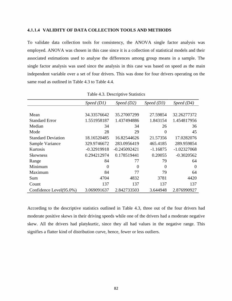
82

VALIDITY OF DATA COLLECTION TOOLS AND METHODS

To validate data collection tools for consistency, the ANOVA single factor analysis was

employed. ANOVA was chosen in this case since it is a collection of statistical models and their

associated estimations used to analyse the differences among group means in a sample. The

single factor analysis was used since the analysis in this case was based on speed as the main

independent variable over a set of four drivers. This was done for four drivers operating on the

same road as outlined in Table 4.3 to Table 4.4.

Table 4.3. Descriptive Statistics

Speed (D1) Speed (D2) Speed (D3) Speed (D4)

Mean 34.33576642 35.27007299 27.59854 32.26277372

Standard Error 1.551958187 1.437494886 1.843154 1.454817956

Median 34 34 26 36

Mode 28 29 0 45

Standard Deviation 18.16520485 16.82544626 21.57356 17.0282076

Sample Variance 329.9746672 283.0956419 465.4185 289.959854

Kurtosis -0.32919918 -0.245092421 -1.16875 -1.02327068

Skewness 0.294212974 0.178519441 0.20055 -0.3020562

Range 84 77 79 64

Minimum 0 0 0 0

Maximum 84 77 79 64

Sum 4704 4832 3781 4420

Count 137 137 137 137

Confidence Level(95.0%) 3.069091637 2.842733503 3.644948 2.876990927

According to the descriptive statistics outlined in Table 4.3, three out of the four drivers had

moderate positive skews in their driving speeds while one of the drivers had a moderate negative

skew. All the drivers had platykurtic, since they all had values in the negative range. This

signifies a flatter kind of distribution curve, hence, fewer or less outliers.

83

Table 4.4. ANOVA Single Factor Analysis

Source of

Variation SS df MS F P-value F crit

Between Groups 4802.254 3 1600.751 4.679 0.003 2.621

Within Groups 186109.022 544 342.112

Total 190911.276 547

Based on the ANOVA single factor results outlined in Table 4.4 and in relation to the null

hypothesis that states that the mean driving speed values of 4 different drivers are equal, since

the p-value is 0.003, which is less than the significance level of 0.05, we reject the null

hypothesis. This leads to the conclusion that some of the drivers have different driving speed

means. The fact that the F value is greater than F critical value, it is just an indicator that

something is significant in the results. This is the reality since human beings have different

behaviours that will definitely translate to differences in driving speed. This could further be

justified by Table 4.5 and Table 4.6 correlation and covariance results respectively that clearly

show the correlations and variances in speeding behaviour.

Table 4.5. Correlation Analysis


Speed (D1) 1

Speed (D2) 0.240422521 1

Speed (D3) 0.185235685 0.315943681 1

Speed (D4) 0.014498375 0.252875219 0.215458 1

Table 4.6. Covariance Analysis


Speed (D1) 327.566093

Speed (D2) 72.94581491 281.0292504

Speed (D3) 72.06180404 113.8456497 462.0213117

Speed (D4) 4.451915392 71.92173264 78.57264638 287.8434

84

In summary, the study tested reliability as follows:

1. Test retest reliability

A correlation of a set of human drivers and the agent subjected to a test on a similar road

segment twice was done in order to evaluate stability over time.

2. Parallel forms reliability

A correlation of a similar set of human drivers and the agent subjected to different road

segments was done in order to evaluate consistency of results.

3. Internal consistency reliability

This test complemented test retest and parallel form reliability tests. It was achieved through

following methods:

i) Average inter-item correlation

An average correlation of coefficients of pairs of behavioural parameters was

examined.

ii) Split-half reliability

Driver groups, behavioural parameters and/or test domains was split into halves then

subjected to tests with the correlation between the two total set scores being

determined.

4.1.2 DATA CONSISTENCY (RESULTS WITHOUT OBSTACLE SENSORS)

A further prestudy test involved experiments relying on GPS data variables only, without

obstacle data. This was in a move to ascertain the effectiveness of GPS data only in driver

behaviour analysis. The experiments further explored whether these data alone could inform

successful modelling of vehicle driver agent.

EXPERIMENT DESCRIPTION

The 2TBN probabilities in Table 0.1 were implemented in form of an algorithm for the driver

behaviour analysis system. A driver was monitored on different occasions and road segments.

The study first explored the driver’s behaviour on three different days, similar road segment,

driving in the same direction, almost same times of the day. Sample data for one of the three

experiments is as shown in Table 0.3 in Appendix D. The experiment was carried out on a single

85

carriageway road segment as shown in the route map in Figure 4.7. The road segment composed

of relatively straight stretches but with few sharp corners. The road terrain had relatively long

flat stretches with a short steep hill at one point. Other factors included morning hours, dry

weather, and busy road.

Figure 4.7. Sample Single Carriageway (Prestudy)

The results for the experiment included a summary of the driver behaviour for the analysis

period. This was founded on the 2TBN algorithm as discussed in section 3.8.4.2. The analysis

shows a snapshot of the driver behavour based on speeding, acceleration, braking and cornering

patterns. The analysis indicates driving styles in form of probabilities of normal versus harsh

behaviours. A higher probability is an indicator for the driver’s behaviour for the analysis item. It

further determines the driver’s operational environment centered on the road terrain and road

pattern. The terrain is expressed based on probability of uphill or downhill movements. The item

with the highest probability value determines the nature of the road terrain for the given road

segment. The same applies to the road pattern that is viewed from two perspectives, namely,

straight or meander.

86

Analysis of Data Patterns

Considering graphical analysis outlined in Figure 4.8 – 4.12, good data for speed, altitude,

direction and GPS Signal were collected. Good GPS signal strengths were recorded for the

greater part of the journey.

Figure 4.8. Patterns for Acceleration and Deceleration

Based on the patterns in Figure 4.8, the driver had acceleration and deceleration patterns within a

normal range. It should be noted that the study used an acceleration and deceleration less than or

equal to 5 m/s2 to be normal, otherwise, treated as harsh acceleration or deceleration behaviour.

Based on the results, none of the changes in acceleration exceeded 5 m/s2, depicting normal

driving behaviour.

-2.5

-2

-1.5

-1

-0.5

0

0.5

1

1.5

2

1 51 101 151

Acc

eler

atio

n /

Dec

ele

rati

on

(m

/s2)

Logged Data Points

Acceleration/Deceleration Trend

87

Figure 4.9. Patterns for Speed Changes

Speed patterns outlined in Figure 4.9, indicate a driving speed behaviour of below 80 km/h. This

is an acceptable behaviour based on the fact that the vehicle used was from a Private Service

Vehicle category limited to 110 km/h speeds. Furthermore, the road segment had no speed limits

specified.

Figure 4.10. Patterns for Direction Changes

0

10

20

30

40

50

60

70

80

1 51 101 151

Spee

d (

km/h

)

Logged Data Points

Speed Trend

-180-150-120

-90-60-30

0306090

120150180

1 51 101 151

Dir

ecti

on

(0)

Logged Data Points

Direction Change Trend

88

Figure 4.10 shows the direction change trends where the values on the y axis could be interpreted

as follows:

North (N): 0

North East (NE): 1 – 89

East (E): 90

South East (SE): 91 – 179

South (S): 180 and -180

North West (NW): -1 – -89

West (W): -90

South West (SW): -91 – -179

Based on the results in Figure 4.10, the entire trip had numerous sharp shifts in values, a

significance of many sharp corners. The results match appropriately with the route as traced on

the map in Figure 4.7 in which a number of sharp corners can be seen.

Figure 4.11. Patterns for Altitude Changes

The results in Figure 4.11 show a rise in value of altitude from the beginning of the journey to

the end, but some minor down shifts around data point 26. This is an indicator of a gentle hill

climb throughout the journey. The minor drop in altitude experienced a round data point 26 is an

indicator of some gentle slope then back to a climb.

1600

1650

1700

1750

1800

1850

1900

1 51 101 151

Alt

itu

de

(m)

Logged Data Points

Altitude Change Trend

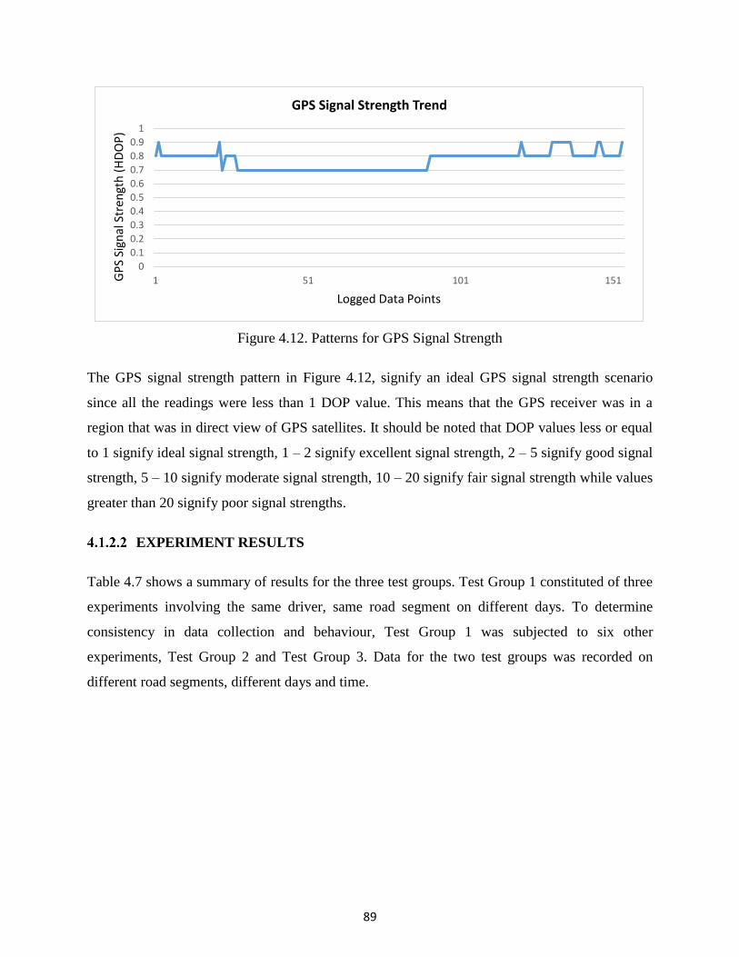
89

Figure 4.12. Patterns for GPS Signal Strength

The GPS signal strength pattern in Figure 4.12, signify an ideal GPS signal strength scenario

since all the readings were less than 1 DOP value. This means that the GPS receiver was in a

region that was in direct view of GPS satellites. It should be noted that DOP values less or equal

to 1 signify ideal signal strength, 1 – 2 signify excellent signal strength, 2 – 5 signify good signal

strength, 5 – 10 signify moderate signal strength, 10 – 20 signify fair signal strength while values

greater than 20 signify poor signal strengths.

EXPERIMENT RESULTS

Table 4.7 shows a summary of results for the three test groups. Test Group 1 constituted of three

experiments involving the same driver, same road segment on different days. To determine

consistency in data collection and behaviour, Test Group 1 was subjected to six other

experiments, Test Group 2 and Test Group 3. Data for the two test groups was recorded on

different road segments, different days and time.

0

0.1

0.2

0.3

0.4

0.5

0.6

0.7

0.8

0.9

1

1 51 101 151GP

S Si

gnal

Str

engt

h (

HD

OP

)

Logged Data Points

GPS Signal Strength Trend

90

Table 4.7. Driver Behaviour Analysis

Profile

Category

Behaviour

Attribute

Test Group 1 Test Group 2 Test Group 3

Exp

1

Exp

2

Exp

3 Avg

Exp

1

Exp

2

Exp

3 Avg

Exp

4

Exp

5

Exp

6 Avg

Speeding Lowest 0 0 0 0.00 0 0 0 0 0 0 0 0.00

Highest 69 68 74 70.33 94 107 114 105 124 80 74 95.75

Acceleration Normal 0.22 0.22 0.21 0.22 0.22 0.20 0.20 0.21 0.21 0.22 0.20 0.21

Harsh 0.10 0.10 0.09 0.10 0.09 0.08 0.08 0.08 0.08 0.09 0.08 0.08

Braking Normal 0.20 0.19 0.19 0.19 0.20 0.18 0.18 0.19 0.19 0.20 0.18 0.19

Harsh 0.12 0.12 0.12 0.12 0.11 0.10 0.10 0.10 0.10 0.11 0.10 0.10

Cornering Normal 0.13 0.13 0.13 0.13 0.13 0.12 0.12 0.12 0.12 0.13 0.12 0.12

Harsh 0.14 0.14 0.14 0.14 0.14 0.12 0.12 0.13 0.13 0.13 0.12 0.13

Road

Terrain

Uphill 0.28 0.29 0.27 0.28 0.21 0.20 0.20 0.20 0.22 0.22 0.21 0.21

Downhill 0.17 0.16 0.17 0.17 0.23 0.20 0.19 0.21 0.20 0.21 0.19 0.20

Road

Pattern

Straight 0.33 0.33 0.22 0.29 0.34 0.30 0.30 0.31 0.30 0.33 0.29 0.31

Meander 0.12 0.13 0.12 0.12 0.10 0.10 0.10 0.10 0.12 0.11 0.11 0.11

DISCUSSION OF RESULTS

Two main categories of observations can be made from the results for the consistency analysis

experiments:

1. Operational Environment

The driving environment had a terrain depicting a driver climbing i.e. rising altitudes.

The region had fairly straight stretches but with some corners.

2. Driver Behaviour

In such an environment, the driver has a high probability of driving at maximum

speeds of 70.33km/h.

The driver has a high probability of accelerating and braking normally.

The cornering behaviour may be normal or harsh with a tendency of being sharp

cornering.

Consistency in acceleration, braking, cornering and speeding was determined through an

ANOVA single factor analysis for two random groups of three experiments each over the Test

Group 1. The ANOVA single factor analysis for the same driver are as outlined in Table 4.8 to

Table 4.14. The descriptive statistic in Table 0.4 and Table 0.9 under Appendix D section show

91

normal distribution curves based on the skewness values in each case.

Table 4.8. Normal Acceleration Analysis (ANOVA Single Factor)

Source of Variation SS df MS F P-value F crit

Between Groups 0.0001556 2 7.778E-05 0.875 0.464033 5.143253

Within Groups 0.0005333 6 8.889E-05

Total 0.0006889 8

Table 4.9. Harsh Acceleration Analysis (ANOVA Single Factor)


Between Groups 0.0003556 2 0.0001778 5.333333 0.046656 5.143253

Within Groups 0.0002 6 3.333E-05

Total 0.0005556 8

Based on the results outlined in Table 4.8 and in relation to the null hypothesis that the means for

normal acceleration values for all the three test groups for the same driver are equal, since the p-

value is greater than the significance level of 0.05, we accept the null hypothesis. The fact that

the F value is less than the F critical value, makes it clear that there is nothing significant in the

results. On the other hand, based on the results outlined in Table 4.9 and in relation to the null

hypothesis that the means for harsh acceleration values for all the three test groups for the same

driver are equal, since the p-value is less than the significance level of 0.05, we reject the null

hypothesis. The fact that the F value is greater than the F critical value, makes it clear that there

is something significant in the results. This is the reality since a human vehicle driver is expected

to portray a certain consistent acceleration behaviour unless under critically uncertain conditions.

Table 4.10. Normal Braking Analysis (ANOVA Single Factor)


Between Groups 6.667E-05 2 3.333E-05 0.375 0.702332 5.143253

Within Groups 0.0005333 6 8.889E-05

Total 0.0006 8

92

Based on the results outlined in Table 4.10 and in relation to the null hypothesis that the means

for normal braking values for the two test groups against the control group for the three different

tests for the same driver are equal, since the p-value is greater than the significance level of 0.05,

we accept the null hypothesis. The fact that the F value is less than the F critical value, makes it

clear that there is nothing significant in the results. This is the reality since a human vehicle

driver is expected to portray a certain consistent braking behaviour unless under uncertain

conditions.

Table 4.11. Harsh Braking Analysis (ANOVA Single Factor)


Between Groups 0.0005556 2 0.0002778 12.5 0.007251 5.143253

Within Groups 0.0001333 6 2.222E-05

Total 0.0006889 8

On the other hand, the null hypothesis that the means for harsh braking behaviour values for the

two test groups against the control group for the same driver are equal, is rejected since the p-

value is less than the significance level of 0.05 as shown in Table 4.11. The fact that the F value

is way greater than the F critical value, makes it clear that there is something significant in the

results. This is the reality since a human vehicle driver is expected to portray normal braking

behaviour and that harsh braking should not be a normal day to day behaviour unless under

uncertain conditions.

Table 4.12. Highest Speed Analysis (ANOVA Single Factor)


Between Groups 1852.6667 2 926.33333 3.236413 0.111316 5.143253

Within Groups 1717.3333 6 286.22222

Total 3570 8

Based on the results outlined in Table 4.12 and in relation to the null hypothesis that the means

for highest speed values for the two test groups against the control group for the same driver are

equal, since the p-value is greater than the significance level of 0.05, we accept the null

93

hypothesis. The fact that the F value is less than the F critical value, makes it clear that there is

nothing significant in the results. This is the reality since a human vehicle driver is expected to

portray a certain consistent speeding behaviour unless under critically uncertain conditions.

Table 4.13. Normal Cornering Analysis (ANOVA Single Factor)


Between Groups 8.889E-05 2 4.444E-05 2 0.216 5.143253

Within Groups 0.0001333 6 2.222E-05

Total 0.0002222 8

Table 4.14. Harsh Cornering Analysis (ANOVA Single Factor)


Between Groups 0.0003556 2 0.0001778 3.2 0.113289 5.143253

Within Groups 0.0003333 6 5.556E-05

Total 0.0006889 8

Based on the results outlined in Table 4.13 and Table 4.14 and in relation to the null hypothesis

that the means for normal and harsh cornering values for the two test groups against the control

group for the three different tests for the same driver are equal, since the p-value in both cases

are greater than the significance level of 0.05, we accept the null hypothesis. The fact that both F

values are less than the F critical values, makes it clear that there is nothing significant in the

results. This is the reality since a human vehicle driver is expected to portray a certain consistent

cornering behaviour unless under critically uncertain conditions.

Considering the averages per category as outlined in Table 4.7, it could be concluded that the

driver accelerates and brakes normally. The driver may however approach corners normally or in

a harsh manner. Such a behaviour may be experienced in environments that are relatively

straight with some gentle to normal terrains.

94

4.1.3 DATA CONSISTENCY (RESULTS WITH OBSTACLE SENSORS)

The second phase of consistency test was composed of experiments including obstacle data. This

was in a move to ascertain how obstacle sensor data could complement GPS data for driver

behaviour analysis. The experiments further explored whether these two sets of data can inform

successful modelling of vehicle human driver behaviour through a software agent.

EXPERIMENT DESCRIPTION

A Data Collection Unit was designed using Arduino Uno Microcontroller and an ultrasonic

obstacle sensor as per the circuitry in Figure 3.5. The microcontroller code is as outlined in

Appendix A where the maximum obstacle distance was set to 4 meters. Initially, the experiment

used an LED to signify presence or absence of an obstacle within the range.

EXPERIMENT RESULTS

The LED was continuously on for distances greater than 2 meters. This was the case regardless

of whether there was an obstacle or not. This was an indicator that the obstacle sensor was

continuously sensing some obstacle within its vicinity.

For distances less than 2 meters, all seemed to work fine i.e. the LED turned on whenever there

was an obstacle otherwise it was off. This was however not consistent for actual road test

scenarios. For instance, at certain points during actual road test, it could delay abit to turn on

despite the obstacle being within the 2-meter range. For some instances, it could fail to turn on

completely even with an obstacle within range. Detection seemed to work only for driving

speeds below 10km/h.

DISCUSSION OF RESULTS

For the ultrasonic obstacle sensor to successfully detect an obstacle, it transmits sound waves to

the object and receives reflected sound from the object. Ultrasonic sound waves must be incident

on the object for it to reflect diffused incident energy. A fraction of the energy is reflected back

to the sensor in form of echoes. The longer the distance the longer it takes to detect the obstacle

and the weaker the reflected energy that may lead to failures in detection. The shorter the

distance, the faster the detection and the lower the chances of failures in detection. Ultrasonic

95

sensor calculate obstacle distances based on the speed of the ultrasonic wave and the time it takes

for the wave to get back to the sensor.

A thorough scrutiny of test results deduced the following findings:

i) The ultrasonic obstacle sensor sends trigger signals at a very wide angle, approximately

30 degrees. Hence, for distances greater than 2 meters, the continuous obstacle sensed

was the ground. A solution to this means that the sensor has to be raised too high for the

detection angle not to visualise the ground within it range.

ii) For an object to be detected, ultrasonic sound waves must be incident on the object for it

to reflect diffused incident energy, in cases of objects in motion, establishment of

incidence may fail to occur. Furthermore, reflected waves may fail to reach back to the

sensor due to changing distances. This may have contributed to the obstacle detection

inconsistencies for distances less than 2 meters during the test drive.

iii) The type and nature of surface that the ultrasonic sound wave hits has an effect on the

formulation of incidence and the strength of the reflected wave. In actual road test, the

types of objects detected varied widely i.e. some had wide surfaces, smooth surfaces,

among others. This may have also contributed to the obstacle detection inconsistencies.

In actual driving scenario, using a GPS receiver alone for data collection has a great potential in

determining the behaviour of the driver with probabilities relating to the operational

environment. The data gained from the sample test could act as training sets for an intelligent

agent aimed at modelling a driver’s behaviour. The ultrasonic obstacle sensor operating at less

than 2 meters’ detection distance and for speeds less than or equals to 10km/h will be too

limiting for driver behaviour analysis unless if used to only detect extremely risky behaviour

relating to driving at very close ranges to other vehicles. Such close range driving distances are

the norm in city scenarios especially during traffic jams. This may go against the norm for

profiling drivers based on risky behaviour as the results may not be a true reflection of the

driver’s behaviour.

96

4.1.4 PRESTUDY CHALLENGES AND THEIR EFFECTS TO THE MAIN STUDY

The success of the prestudy faced a number of unforeseen challenges, including but not limited

to:

1. The ultrasonic proximity sensor used was limited to detection distances less than 2 meters to

the obstacle as opposed to the earlier anticipated 10 meters’ range. The closer the sensor gets

to the obstacle, the better the accuracy of detection. The sensor type was heavily affected by

motion and interference from other environmental factors like wind. This created a major

challenge that led to many false positive detections. Unfortunately, these limitations were

tough to mitigate as they were beyond control in this study. The main study hence considered

obstacles detected at distances less than or equals to 2 meters.

2. Weather conditions on the other hand had an effect on proximity sensor’s functionality i.e.

the sensor was affected by the presence of humidity on the sensing surface. Hence, could

only function under low humidity levels to no humidity in the atmosphere. Proximity sensor

data was hence used in cases where the data was collected during times when humidity levels

were appropriate for the proximity sensor.

3. Drivers driving Public Service Vehicles for ferrying passengers tend to change for almost all

trips in a day. Most of the time, they drive to certain point of the journey then hand over to

other drivers. This posed a major challenge in monitoring a particular driver for a good

enough period for better pattern identification. The main study hence assumed that the

behaviour of a given set of Public Service Vehicle drivers could serve as a representation of

other drivers. However, the study had to introduce a categorization of Public Service Vehicle

drivers based on the operational environment i.e. town service driver or long distance driver.

This helped to avoid a generalization of behaviour over a large set of drivers operating under

varied environments.

4. It was extremely hard to use proximity sensors without drivers realizing that they were being

monitored. This was because, proximity sensors have to be physically fitted on the vehicle

hence visible to drivers. Hence, only one sample vehicle was instrumented to serve the

purpose of testing the model’s capability to detect obstacles and incorporate the data in driver

behaviour analysis during the main study.

97

4.1.5 CONCLUSION OF PRESTUDY RESULTS

The prestudy yielded stable, consistent and reliable results. These results helped in the validation

of data collection instruments and data analysis algorithms. Prestudy outcome led to the

publication of a research paper on the shortcomings of ultrasonic sensor technology for vehicle

driver assistance and profiling [81]. The paper basically outlines the fact that though the

technology is powerful for obstacle detection, it faces some challenges in certain applications

especially due to the wide beam width.

4.2 MAIN STUDY’S GENERAL AND DEMOGRAPHIC INFORMATION

The study samples were categorized based on different road categories and service vehicle

categories.

4.2.1 CATEGORIES OF ROADS IN KENYA

Kenyan roads have been adapted to a large range of structures and types in order to achieve a

common goal of transportation under varied conditions. The specific purpose, mode of transport,

and location of a road determine the characteristics it must have to maximize its usefulness.

Roads can be classified as generally private roads, lower capacity highways, higher capacity

highways, limited access grade-separated highways or multi modal. Lower capacity highways

are often single carriageways while higher capacity highways are often dual carriageways.

Kenya just like other countries in the world has different types and categories of roads spread

throughout the nation. This study focused on dual carriageways, single carriageways and

highways to represent the various categories of roads.

4.2.2 VEHICLE SERVICE CATEGORIES IN KENYA

All vehicles plying on Kenyan roads are categorized as either Private or Public Service Vehicles

(PSV). Private Service Vehicles are basically individually owned or attached to private

companies or organisations. Private Service Vehicles are the majority on Kenyan roads. On the

other hand, Public Service Vehicles are either Government owned or vehicles that are privately

owned but dedicated to serve the general public. A special category of Public Service Vehicles

well known in Kenya are “matatus”. Matatu is a Swahili name that refers to a category of

98

vehicles that serves to transport people from one location to another. Matatus are basically

passenger vehicle service group of vehicles.

4.2.3 SAMPLED DRIVERS

This study sampled drivers who operate on three categories of roads, namely, dual carriageways,

single carriageways and highways. The choice of roads also represented both urban and rural

settings. Furthermore, the sampled drivers also represented both service vehicle categories i.e.

Private Service Vehicles and Public Service Vehicles. Figure 4.13 depict the percentage of

drivers sampled per vehicle service category where 15 drivers were selected per vehicle service

category.

Figure 4.13. Sampled Drivers per Service Vehicle Category

To represent the three road categories, the 30 drivers were chosen from three categories such that

each category had a total of 10 drivers as shown in Figure 4.14. The 10 drivers per road category

were equally distributed to represent the two vehicle service categories.

Public Service Vehicles, 15, 50%

Private Service Vehicles, 15, 50%

Percentage of Drivers Per Vehicle Category

99

Figure 4.14. Sampled Drivers per Road Category

4.2.4 SAMPLED DRIVERS’ EXPERIENCE

According to the Kenyan Traffic Act, all vehicle drivers are required to possess a driving license.

This serves as a permit to drive a vehicle on Kenyan roads. Acquiring this vital document is a

predefined process guided by the Kenyan traffic laws. Driving licenses fall into different

categories, and are issued based on an individuals need upon successful training and passing of a

standard driving test. The driving test is facilitated by the Traffic Department of the Kenya

Police.

All the sampled drivers were licensed to drive vehicles on Kenyan roads with valid driving

licenses. Ascertaining experience level of a vehicle driver is deemed to be a complex process

since many parameters are required. To try and take care of this, the sampled drivers were

expected to portray evidence of active driving for at most one year from the point of selection.

Short distance, dual carriage way, 10, 34%

Short distance, single carriage way, 10, 33%

Long distance highway, 10, 33%

Percentage of Drivers Per Road Category

100

4.3 MAIN STUDY RESULTS AND DISCUSSION BASED ON OBJECTIVES

The overall motivation of the study was to contribute towards the efforts of understanding driver

behaviour and possibly aid in future strategies for minimising if not fully controlling the rate of

fatalities and road carnages worldwide. This was demonstrated through thorough monitoring and

analysis of human vehicle driver behaviour in comparison with a driver agent operating under

dynamic conditions. Two sets of performance measures were used to evaluate the behaviour of

human vehicle drivers and the driver agent. The first set was composed of five behavioural

analyses, that is, speeding behaviour, acceleration behaviour, deceleration behaviour, stopping

behaviour and cornering behaviour. The other set was the detection of the operational

environment, limited to road terrain and road pattern.

4.3.1 ESTABLISHMENT OF VEHICLE DRIVER BEHAVIOUR

Considering objective one and research question one, the study established that vehicle drivers

are agents that operate under partially observable; dynamic; nondeterministic; continuous;

sequential; multiagent; and unknown environments. Such environments are the most complex to

model. The study further established that a vehicle driver’s driving style depends on a number of

factors that include familiarity of the operational environment, type of road, road pattern, terrain

of the road, time of day, presence or absence of obstacles. Hence, driving styles may be

characterized based on different factors that include overtaking, speeding, acceleration, braking,

lane changing trends among other trends. The sunburst in Figure 4.15 summarises some of these

factors, where every slice represents a set of factors that could comprise a vehicle driver’s

environment.

101

Figure 4.15. A Sunburst Enumeration of Factors Characterizing a Vehicle Driver’s Environment

The categorizations are paired as follows:

i) Familiarity of the environment: familiar or unfamiliar.

ii) Type of road: single or dual carriageway

iii) Road pattern: meandering or straight

iv) Terrain of the road: hilly or flat

v) Time of day: day or night

vi) Obstacles: obstacle or no obstacle

Driver

Behaviour

102

Other layers of factors that could be considered in the driver’s operational environment include

mechanical condition of vehicles, vehicle model, weather condition, driving region, state of the

driver, and state of other road users among others.

DRIVER BEHAVIOUR PARAMETERS

To effectively determine the behaviour of vehicle drivers operating under diverse environments,

Table 4.15 presents parameters required per behavioural category while Table 0.1 under

Appendix B outlines behavioural probabilities that serve as metric thresholds for some

behaviour. The threshold column in Table 4.15 indicates the limits set out by authorising bodies

outlined in the authorisation column.

Table 4.15. Driver Behaviour Categorisation with their Respective Data Parameters

Category Behaviour Threshold Authorisation Parameters

Speeding Normality

in Speeding Non Built-up Areas

Single Carriageway:

Private cars: <=100km/h

Commercial: <=80km/h

Vehicles with Trailers:

<=65km/h

Dual Carriageway:

Private cars: <=110km/h

Commercial: <=80km/h

Vehicles with Trailers:

<=65km/h

Built-up Area

Recommended speed for

all vehicle categories is

50km/h or less in some

instances

Any values above the

recommended speeds per

region were considered to

be overspeeding instances

Standard metric set

out by National

Transport and

Safety Authority

(NTSA) in Kenya

Speed

Timestamp

Latitude

Longitude

Altitude

103


Acceleration

and

Deceleration

Normality

in

Acceleration

and

Deceleration

Speed increment against

time difference:

There are variable

thresholds based on

different factors:

o Vehicle type

o Vehicle strength

Accelerations ranging

from 0 to 5 meters per

square seconds were

considered to be normal

acceleration with any

values above 5 meters

per square seconds being

considered to be harsh

acceleration instances.

Decelerations ranging

from 0 to -5 meters per

square seconds were

considered to be normal

braking with any values

below -5 meters per

square seconds being

considered to be harsh

braking instances.

Vehicle

manufacturers

specifications

No standard metric

Speed

Timestamp

Latitude

Longitude

Altitude

Cornering Normality

in Cornering

Left or right angle

change against speed

levels were considered as

a measure.

A turn of less than 45

degrees was considered

to be a normal corner

while 45 and above

degrees turn qualified to

be a sharp corner.

Normal or harsh

cornering depends on

speeds against the degree

changes in addition to

altitude changes. This

was based on

probabilities as outlined

in Table 0.1.

Vehicle

manufacturers

specifications

No standard metric

Speed

Timestamp

Latitude

Longitude

Altitude

Direction

(angle)

Turn angle

Obstacle

data

104


Stopping Normality

in Braking

to an actual

Stop

Speed decrement against

time difference:

Stopping Sight Distance

(SSD) [78] was

considered:

SSD = (Perception-reaction

Distance) + (Braking Distance)

SSD = 0.278 Vt + (0.039 V2)/a

(Metric)

Where:

V = design or initial speed in

kilometers per hour (km/h)

a = deceleration rate in meter

per square seconds (m/s2)

t = brake reaction time, in

seconds (s)

World standard

metric on Stopping

Sight Distance

Speed

Timestamp

Latitude

Longitude

Altitude

Obstacle

data

A number of data analysis techniques exist. However, accuracy in the determination of driving

styles for behavioural analysis is dependent on data analysis methodologies and techniques used.

The study established that due to the stochastic, dynamic and partially observable nature of

drivers’ operational environment, appropriate data analysis techniques must involve elements of

probabilistic reasoning. The study hence settled on Bayesian Networks as the most suitable

methods. This was due to the following factors:

1. Bayesian Networks are probabilistic graphical models hence, represented by a graph

accompanied by a table of probabilities:

a) The graphical part of the Bayesian Network indicates the dependence or

independence between variables hence providing an easy to comprehend

visual knowledge representation tool [82].

b) The use of probabilities accommodates uncertainty in quantifying the

dependencies between variables [82].

2. Bayesian Networks are a type of statistical model that maps a set of variables and their

conditional dependencies.

3. Bayesian classification theories are useful analyses forms for prediction of future data

trends and intelligent decision-making [80].

105

It must however be noted that the behaviour of a vehicle driver varies greatly based on different

factors against time. Hence, successful analysis of driver behaviour should be kind of a time

series analysis. The study hence considers the power of Dynamic Bayesian Network (DBN) that

enables them to relate adjacent time steps. DBNs are therefore referred to as 2-Time-slice

Bayesian Network (2TBN). According to the 2TBN, at any given time t, the value of a variable

can be calculated from the internal regressors and immediate prior value at time t-1. This was

useful in the determination of driver behaviour per given time-slice with the average of several

time-slice behaviour constituting a full driver behaviour profile.

To determine actual driver behaviour, the study consider three categories of roads, namely, dual

carriageway, single carriage way and highways. A set of 15 drivers from the Private Service

Vehicle category and 15 drivers from the Public Service Vehicle category. The two broad

Service Vehicle categories accommodate light, heavy and commercial vehicle subcategories. The

sample of 30 drivers were all labelled D1 to D15 per Service Vehicle category. They were then

equally distributed in each of the three road categories, such that each category had 10 drivers, 5

from each Service Vehicle category as follows:

i) Dual carriageway: drivers D1, D2, D3, D4 and D5 from both Service Vehicle categories.

ii) Single carriageway: drivers D6, D7, D8, D9 and D10 from both Service Vehicle

categories.

iii) Highways: drivers D11, D12, D13, D14 and D15 from both Service Vehicle categories.

SPEEDING, ACCELERATION AND DECELERATION BEHAVIOUR: DUAL

CARRIAGEWAYS

Private Service Vehicle Drivers

The first set of five Private Service Vehicle drivers, labeled D1, D2, D3, D4 and D5, was

subjected to the Southern Bypass, a tarmac dual carriageway that connects Mombasa road to the

Waiyaki way. The road segment is as highlighted in Figure 4.16, ranging from Langata road

intersection all the way to the Waiyaki way intersection. The road segment was composed of

relatively straight stretches with few clear corners. The road terrain was relatively flat with

gentle slops at some point. The road had few gentle, speed breaker kind of bumps with no

106

potholes. Other factors included daytime, dry weather, a very short stretch of a built-up area,

Kikuyu, close to the Waiyaki way intersection.

Figure 4.16. Southern Bypass (Dual Carriageway)

The study established that Private Service Vehicle drivers tend to drive at relatively high speeds

on dual carriageways. This is as shown in Table 4.16 where average speeds were ranging from

lows of 74 km/h to highs of 99 km/h. The maximum speed ever recorded was 126 km/h. Only

one out of the five sampled drivers recorded the highest speed that was within the required speed

limit of 100 km/h without considering any speed limited zones.

Table 4.16. Speeding Behaviour for Private Service Drivers (Descriptive Statistics)

D1 D2 D3 D4 D5

Mean 89.79167 73.79167 98.95833 88.64583 90.60417

Standard Error 3.454229 2.772548 1.782987 1.945965 2.569899

Median 95.5 77 100 94 98

Mode 115 91 109 98 103

Standard Deviation 23.9316 19.20877 12.35289 13.48204 17.80478

Sample Variance 572.7216 368.977 152.594 181.7655 317.0102

Kurtosis -1.56065 -1.23649 -0.12686 0.984906 0.930629

Skewness -0.28926 -0.51333 -0.42931 -1.1307 -1.23422

Range 68 59 54 59 75

Minimum 48 39 72 46 36

Maximum 116 98 126 105 111

Sum 4310 3542 4750 4255 4349

Count 48 48 48 48 48

Confidence Level(95.0%) 6.949013 5.577646 3.586906 3.914778 5.169969

107

Table 4.17. Speeding Behaviour for Private Service Drivers (ANOVA Single Factor)


Between Groups 15922.97 4 3980.744 12.49395 3.13E-09 2.410058

Within Groups 74874.21 235 318.6137

Total 90797.18 239

The p-value that is significantly greater than 0.05 and F value significantly greater than F critical

are indicators that there is a significant difference in driving speed behaviour for any given set of

Private Service Vehicle drivers operating on dual carriageways. This is as depicted in Table 4.17.

This is however a complete inverse of the acceleration behaviour for the same set of drivers

using the same dataset as outlined in Table 4.18, where, the average acceleration and

deceleration falls between -0.025 and 0.171 meters per square seconds. Furthermore, the p-value

that is greater than 0.05 and F value that is less than the F critical is an indicator that there is

nothing significant in acceleration and deceleration behaviour for any given set of Private

Service Vehicle drivers operating on dual carriageways. This is as depicted in Table 4.19.


Statistics)

D1 D2 D3 D4 D5

Mean 0.059375 0.032292 0.012917 0.171458 -0.02521

Standard Error 0.06908 0.022869 0.052037 0.056644 0.06681

Median 0.16 0.045 0.095 0.14 0

Mode 0.28 0 0.14 0.14 0


Sample Variance 0.229057 0.025103 0.129979 0.154013 0.214251

Kurtosis 11.35035 -0.00562 1.011115 2.693319 3.200285

Skewness -2.78648 -0.32779 -1.01967 -0.52997 -1.31864

Range 2.98 0.73 1.61 2.22 2.6

Minimum -2.22 -0.37 -1.15 -1.2 -1.67

Maximum 0.76 0.36 0.46 1.02 0.93

Sum 2.85 1.55 0.62 8.23 -1.21

Count 48 48 48 48 48


108


Single Factor)


Between Groups 1.064877 4 0.266219 1.769127 0.135804 2.410058

Within Groups 35.36292 235 0.15048

Total 36.42779 239

Considering speeding, acceleration and deceleration trend analysis for Private Service Vehicle

drivers, it is emerging that the drivers tend to drive at significantly different high speeds on dual

carriageways but their acceleration and deceleration trends tend to converge. Both speeding and

acceleration analyses had platykurtic kind of distribution recorded for all the drivers based on the

kurtosis and skewness values except acceleration analyses for driver D1 and D5 that experienced

kurtosis values higher than 3 with slight skewness to the left.

Public Service Vehicle Drivers

The first set of five Public Service Vehicle drivers, labeled D1, D2, D3, D4 and D5, was

subjected to the Waiyaki Way, a tarmac dual carriage way ranging from Nairobi City to Limuru

Town as highlighted in Figure 4.17. The road segment was composed of relatively straight

stretches with few clear corners. The road terrain was relatively flat with gentle slops at some

point. The road had no bumps and no potholes. Other factors included daytime, dry weather,

composed of both built-up and nonbuilt-up sections.

Figure 4.17. Waiyaki Way (Dual Carriageway)

109

The study established that Public Service Vehicle drivers tend to drive at relatively low speeds

compared to Private Service Vehicle drivers on dual carriageways. The behaviour is however

limited to passenger Public Service Vehicle drivers. This is as shown in Table 4.20, where,

average speeds were ranging from lows of 53 km/h to highs of 72 km/h. The highest speed ever

recorded was 91 km/h. Surprisingly, all the five sampled drivers recorded maximum speeds that

were above the recommended speed limit of 80 km/h for Public Service Vehicles’ category in

Kenya.

Table 4.20. Speeding Behaviour for Public Service Drivers (Descriptive Statistics)

D1 D2 D3 D4 D5

Mean 59.33649 63.27014 53.42654 56.06635 72.27488

Standard Error 1.256328 0.975572 1.272379 1.20801 0.684946

Median 64 65 58 59 74

Mode 66 66 59 59 79


Sample Variance 333.0339 200.8172 341.5981 307.9099 98.99075

Kurtosis 0.782874 1.325255 0.771157 0.83857 1.255119

Skewness -1.21871 -0.92837 -1.1392 -1.06734 -0.95664

Range 78 85 79 80 58

Minimum 5 6 2 3 31

Maximum 83 91 81 83 89

Sum 12520 13350 11273 11830 15250

Count 211 211 211 211 211


Table 4.21. Speeding Behaviour for Public Service Drivers (ANOVA Single Factor)


Between Groups 45716.03 4 11429.01 44.56276 1.37E-34 2.380406

Within Groups 269293.5 1050 256.47

Total 315009.5 1054

Just like for the case of Private Service Vehicle drivers, speed analysis for the sampled set of

Public Service Vehicle drivers recorded a p-value greater than 0.05 and F value significantly

greater than F critical. This is an indicator that there is a significant difference in driving speed

behaviour for any given set of passenger Public Service Vehicle drivers operating on dual

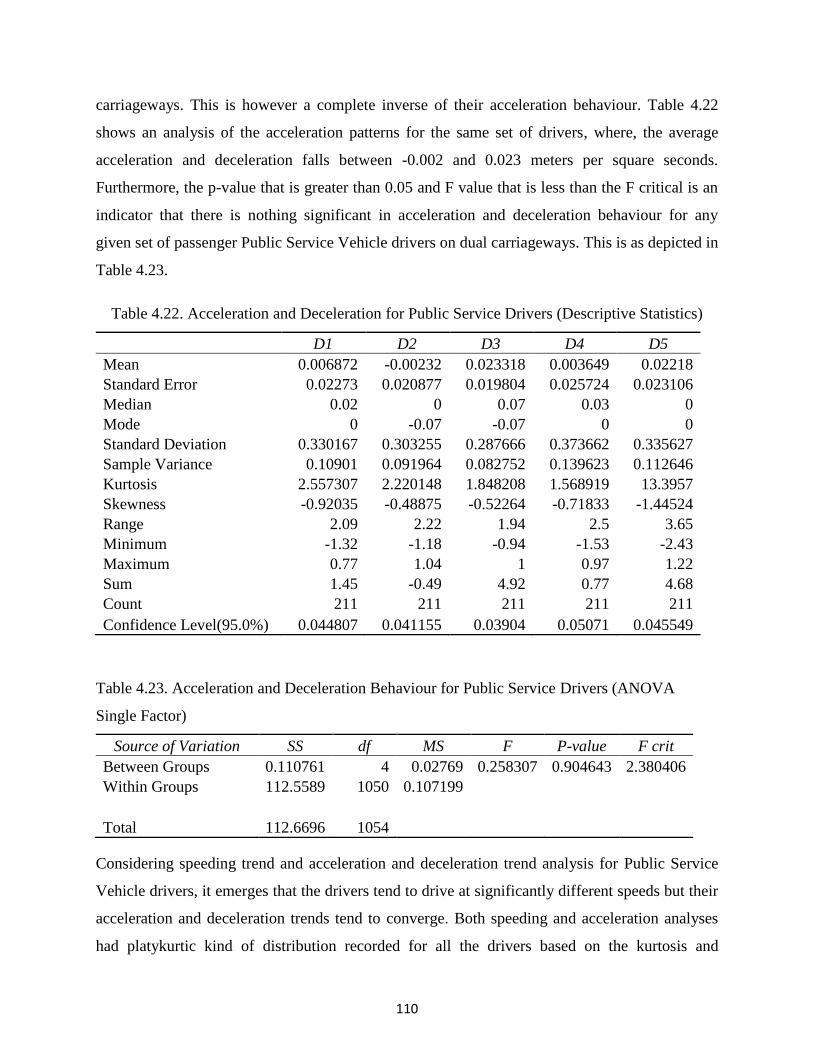
110

carriageways. This is however a complete inverse of their acceleration behaviour. Table 4.22

shows an analysis of the acceleration patterns for the same set of drivers, where, the average

acceleration and deceleration falls between -0.002 and 0.023 meters per square seconds.

Furthermore, the p-value that is greater than 0.05 and F value that is less than the F critical is an

indicator that there is nothing significant in acceleration and deceleration behaviour for any

given set of passenger Public Service Vehicle drivers on dual carriageways. This is as depicted in

Table 4.23.

Table 4.22. Acceleration and Deceleration for Public Service Drivers (Descriptive Statistics)

D1 D2 D3 D4 D5

Mean 0.006872 -0.00232 0.023318 0.003649 0.02218

Standard Error 0.02273 0.020877 0.019804 0.025724 0.023106

Median 0.02 0 0.07 0.03 0

Mode 0 -0.07 -0.07 0 0


Sample Variance 0.10901 0.091964 0.082752 0.139623 0.112646

Kurtosis 2.557307 2.220148 1.848208 1.568919 13.3957

Skewness -0.92035 -0.48875 -0.52264 -0.71833 -1.44524

Range 2.09 2.22 1.94 2.5 3.65

Minimum -1.32 -1.18 -0.94 -1.53 -2.43

Maximum 0.77 1.04 1 0.97 1.22

Sum 1.45 -0.49 4.92 0.77 4.68

Count 211 211 211 211 211



Single Factor)


Between Groups 0.110761 4 0.02769 0.258307 0.904643 2.380406

Within Groups 112.5589 1050 0.107199

Total 112.6696 1054

Considering speeding trend and acceleration and deceleration trend analysis for Public Service

Vehicle drivers, it emerges that the drivers tend to drive at significantly different speeds but their

acceleration and deceleration trends tend to converge. Both speeding and acceleration analyses

had platykurtic kind of distribution recorded for all the drivers based on the kurtosis and

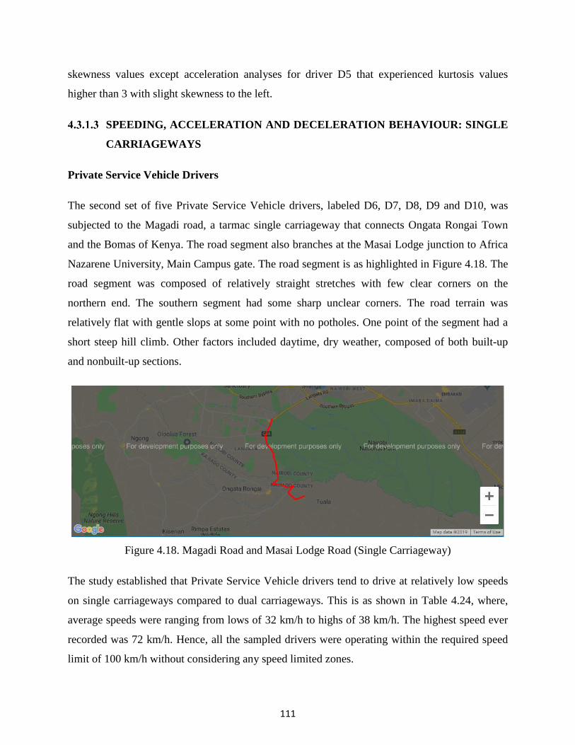
111

skewness values except acceleration analyses for driver D5 that experienced kurtosis values

higher than 3 with slight skewness to the left.

SPEEDING, ACCELERATION AND DECELERATION BEHAVIOUR: SINGLE

CARRIAGEWAYS


The second set of five Private Service Vehicle drivers, labeled D6, D7, D8, D9 and D10, was

subjected to the Magadi road, a tarmac single carriageway that connects Ongata Rongai Town

and the Bomas of Kenya. The road segment also branches at the Masai Lodge junction to Africa

Nazarene University, Main Campus gate. The road segment is as highlighted in Figure 4.18. The

road segment was composed of relatively straight stretches with few clear corners on the

northern end. The southern segment had some sharp unclear corners. The road terrain was

relatively flat with gentle slops at some point with no potholes. One point of the segment had a

short steep hill climb. Other factors included daytime, dry weather, composed of both built-up

and nonbuilt-up sections.

Figure 4.18. Magadi Road and Masai Lodge Road (Single Carriageway)

The study established that Private Service Vehicle drivers tend to drive at relatively low speeds

on single carriageways compared to dual carriageways. This is as shown in Table 4.24, where,

average speeds were ranging from lows of 32 km/h to highs of 38 km/h. The highest speed ever

recorded was 72 km/h. Hence, all the sampled drivers were operating within the required speed

limit of 100 km/h without considering any speed limited zones.

112


D6 D7 D8 D9 D10

Mean 31.72826 32.98913 32.91304 37.6087 35.08696

Standard Error 1.454198 1.450118 1.660411 1.56458 1.720541

Median 33.5 35 30.5 37.5 34

Mode 31 18 25 30 45


Sample Variance 194.5517 193.4614 253.6407 225.2078 272.344

Kurtosis -0.88554 -1.05655 -0.33991 -0.47977 -1.00674

Skewness -0.26857 -0.30264 0.534842 0.152712 0.02795

Range 54 51 65 63 62

Minimum 3 5 7 8 5

Maximum 57 56 72 71 67

Sum 2919 3035 3028 3460 3228

Count 92 92 92 92 92




Between Groups 1982.326 4 495.5815 2.175119 0.070835 2.391539

Within Groups 103667.7 455 227.8411

Total 105650 459

The p-value that is slightly greater than 0.05 and F value slightly less than F critical are

indicators that there is nothing significant in driving speed behaviour for any given set of Private

Service Vehicle drivers operating on single carriageways. This is as represented in Table 4.25.

The case is similar to the acceleration and deceleration behaviour for the same set of drivers

using the same dataset as outlined in Table 4.26, where, the average acceleration and

deceleration falls between 0.022 and 0.094 meters per square seconds. Furthermore, the p-value

that is greater than 0.05 and F value that is less than the F critical are indicators that there is


Service Vehicle drivers operating on a single carriageway. This is as shown in Table 4.27.

113


Statistics)

D6 D7 D8 D9 D10

Mean 0.041739 0.033152 0.094891 0.024239 0.022391

Standard Error 0.04819 0.039132 0.041861 0.043712 0.040778

Median 0.06 0.055 0.11 0.06 0.065

Mode 0 0 0 0.28 0.28


Sample Variance 0.213647 0.140883 0.161212 0.17579 0.152979

Kurtosis 1.706445 1.20754 5.315453 0.695908 1.634751

Skewness -0.49252 0.122686 -1.0756 -0.3724 -0.72573

Range 2.75 2.07 2.85 2.33 2.33

Minimum -1.5 -0.87 -1.83 -1.22 -1.46

Maximum 1.25 1.2 1.02 1.11 0.87

Sum 3.84 3.05 8.73 2.23 2.06

Count 92 92 92 92 92



Single Factor)


Between Groups 0.328216 4 0.082054 0.485808 0.746178 2.391539

Within Groups 76.85053 455 0.168902

Total 77.17874 459

Considering speeding, acceleration and deceleration trend analysis, it is emerging that Private

Service Vehicle drivers tend to drive at relatively slower speeds on single carriageways

compared to dual carriageways. However, there is nothing significantly different in their driving

speed, acceleration and deceleration trends. Both speeding and acceleration analyses had

platykurtic kind of distribution recorded for all the drivers based on the kurtosis and skewness

values.

114


The second set of five Private Service Vehicle drivers, labeled D6, D7, D8, D9 and D10, was

subjected to a tarmac single carriageway segment of the Nairobi – Nakuru Highway as

highlighted in Figure 4.19. The segment ranged from Kijabe to Gilgil. The road segment was

composed of relatively straight stretches with few clear corners. The road terrain was relatively

flat but with some regions with long sloping stretches. Several speed bumps existed in the

segment with no potholes. Other factors included daytime, dry weather, composed of both built-

up and nonbuilt-up sections.

Figure 4.19. Kijabe to Gilgil (Single Carriageway)

The study established that Public Service Vehicle drivers tend to drive at relatively high speeds

compared to Private Service Vehicle drivers while plying on single carriageways. This behaviour

is however limited to passenger Public Service Vehicle drivers. This is as shown in Table 4.28,

where, average speeds ranged from lows of 52 km/h to highs of 66 km/h. The highest speed ever

recorded was 94 km/h. Surprisingly, all the five sampled drivers recorded highest speeds that

were above the recommended speed limit of 80 km/h for Public Service Vehicles in Kenya. This

was a similar case for dual carriageways.

115


D6 D7 D8 D9 D10

Mean 64.68306 65.78962 53.28962 52.37432 60.78415

Standard Error 0.924783 0.987446 1.077689 1.250746 1.11426

Median 69 69 57 57 67

Mode 72 84 0 79 78


Sample Variance 313.0116 356.8679 425.0775 572.5581 454.4163

Kurtosis 2.529827 -0.4418 0.788044 -1.17459 -0.05975

Skewness -1.60974 -0.68537 -1.07583 -0.34912 -0.84441

Range 89 75 88 89 89

Minimum 0 19 0 0 0

Maximum 89 94 88 89 89

Sum 23674 24079 19504 19169 22247

Count 366 366 366 366 366


Table 4.29. Speeding Behaviour for Public Service Vehicle Drivers (ANOVA Single Factor)


Between Groups 57589.94 4 14397.48 33.92542 2.42E-27 2.376804

Within Groups 774505 1825 424.3863

Total 832094.9 1829


Public Service Vehicle drivers recorded a p-value significantly greater than 0.05 and F value

significantly greater than F critical as depicted in Table 4.29. This is an indicator that there is a

significant difference in driving speed behaviour for any given set of passenger Public Service

Vehicle drivers. This is however a complete inverse of the acceleration behaviour. Table 4.30

shows an analysis of the acceleration patterns for the same set of drivers where average

acceleration and deceleration falls between 0.0003 and 0.0104 meters per square seconds.

Furthermore, the p-value that is greater than 0.05 and F value that is less than the F critical are

indicators that there is nothing significant in acceleration and deceleration behaviour for any

given set of passenger Public Service Vehicle drivers operating on single carriageways. This is

as shown in Table 4.31.

116

Table 4.30. Acceleration and Deceleration Behaviour for Public Service Drivers (Descriptive

Statistics)

D6 D7 D8 D9 D10

Mean 0.010027 0.000301 0.007377 0.010137 0.010464

Standard Error 0.019159 0.01758 0.016444 0.018691 0.018021

Median 0 0 0 0.04 0

Mode 0 0 0 0 0


Sample Variance 0.134352 0.11312 0.098967 0.127858 0.118867

Kurtosis 6.34314 1.698256 4.178697 2.850152 3.034325

Skewness -0.9057 -0.25385 -0.68156 -1.13701 -0.27228

Range 3.65 2.29 2.92 2.49 2.56

Minimum -2.43 -1.11 -1.74 -1.72 -1.39

Maximum 1.22 1.18 1.18 0.77 1.17

Sum 3.67 0.11 2.7 3.71 3.83

Count 366 366 366 366 366



Single Factor)


Between Groups 0.027027 4 0.006757 0.056955 0.993979 2.376804

Within Groups 216.505 1825 0.118633

Total 216.532 1829

Considering speeding trend and acceleration and deceleration trend analysis it emerges that

Public Service Vehicle drivers operating on single carriageways tend to drive at significantly

different speeds but their acceleration and deceleration trends tend to converge. The case is

similar to the same category of drivers operating on dual carriageways. Both speeding and

acceleration analyses had platykurtic kind of distribution recorded for all the drivers based on the

kurtosis and skewness values except acceleration analyses for driver D6, D8 and D10 that

experienced kurtosis values higher than 3.

117

SPEEDING, ACCELERATION AND DECELERATION BEHAVIOUR: LONG

DISTANCE HIGHWAYS


The last set of five Private Service Vehicle drivers, labeled D11, D12, D13, D14 and D15, was

subjected to the Nairobi – Nakuru Highway. This was a 150 km tarmac highway that connects

Nairobi City and Nakuru Town. The highway was composed of both single carriageway and dual

carriageway segments with the longest stretch being single carriageway. The road segment

analysed is as highlighted in Figure 4.20. The road terrain was a mixed mode i.e. composed of a

mix of flat, sloping and hill climbing, clear and unclear corners. Several speed bumps existed at

different segment of the road with no potholes. Other factors included daytime, dry weather,


Figure 4.20. Nairobi – Nakuru Highway (Long Distance Highway)

The segment had relatively straight stretches with both clear and unclear corners spread

throughout. The road terrain was relatively flat but with some regions with long sloping

stretches. Several speed bumps existed in the segment. Other factors included daytime, dry

weather, composed of both built-up and nonbuilt-up sections.

The study established that Private Service Vehicle drivers tend to drive at relatively high speeds

on long distance highways. This is as shown in Table 4.32, where, average speeds were ranging

from lows of 44 km/h to highs of 63 km/h. The maximum speed ever recorded was 114 km/h

118

with only two out of the five sampled drivers recording highest speeds that were within the

required speed limit of 100 km/h without considering any speed limited zones.


D11 D12 D13 D14 D15

Mean 54.36921 43.9133 55.63378 63.00448 53.03438

Standard Error 0.859628 0.975585 0.859026 0.734885 0.996342

Median 55 48 56 65 52

Mode 54 0 43 64 52


Sample Variance 494.365 636.732 493.6726 361.2979 664.1141

Kurtosis -0.51406 -1.14656 -0.33493 0.468476 -0.5296

Skewness -0.2703 -0.20293 -0.05196 -0.65665 0.079605

Range 98 89 105 103 114

Minimum 2 0 0 0 0

Maximum 100 89 105 103 114

Sum 36373 29378 37219 42150 35480

Count 669 669 669 669 669




Between Groups 124808.5 4 31202.12 58.86789 4.32E-48 2.374593

Within Groups 1770321 3340 530.0363

Total 1895130 3344

The p-value that is significantly greater than 0.05 and F value greater than F critical are

indicators that there is a significant difference in driving speed behaviour for any given set of

Private Service Vehicle drivers operating on long distance highways. This is as depicted in

Table 4.33. It is however a complete inverse of the acceleration behaviour for the same set of

drivers using the same dataset as outlined in Table 4.34, where, the average acceleration and

deceleration falls between -0.006 and 0.025 meters per square seconds. Furthermore, the p-value

that is greater than 0.05 and F value that is less than the F critical are indicators that there is


Service Vehicle drivers. This is as depicted in Table 4.35.

119

Table 4.34. Acceleration and Deceleration Behaviour for Private Service Vehicle Drivers

(Descriptive Statistics)

D11 D12 D13 D14 D15

Mean 0.010972 0.020314 0.025336 -0.00607 0.020613

Standard Error 0.012836 0.011292 0.010748 0.014024 0.012703

Median 0.01 0.01 0.02 0 0.03

Mode 0 0 0 0 0


Sample Variance 0.11022 0.085304 0.077287 0.131583 0.107962

Kurtosis 3.115314 4.010804 5.788723 3.467327 4.178339

Skewness -0.95855 -0.98032 -1.21933 -0.841 -1.10151

Range 2.63 2.44 2.55 3.03 3.12

Minimum -1.57 -1.46 -1.55 -1.83 -2.15

Maximum 1.06 0.98 1 1.2 0.97

Sum 7.34 13.59 16.95 -4.06 13.79

Count 669 669 669 669 669



Single Factor)


Between Groups 0.417297 4 0.104324 1.018081 0.396474 2.374593

Within Groups 342.2544 3340 0.102471

Total 342.6717 3344

Considering speeding, acceleration and deceleration trend analysis for Private Service Vehicle

drivers, it is emerging that the drivers tend to drive at significantly different speeds on long

distance highways but their acceleration and deceleration trends tend to converge. Speeding

analyses had platykurtic kind of distribution recorded for all the drivers based on the kurtosis and

skewness values. However, acceleration analyses had leptokurtic kind of distributions based on

kurtosis values that were higher than 3.

120


The last set of five Public Service Vehicle drivers, labeled D11, D12, D13, D14 and D15, was

subjected to the Nairobi – Nakuru Highway. This is a 150 km tarmac highway that connects

Nairobi City and Nakuru Town. The highway is composed of both single carriageway and dual

carriageway segments with the longest stretch being single carriageway. The road segment

analysed is as highlighted in Figure 4.21. The road terrain was a mixed mode i.e. composed of a

mix of flat, sloping and hill climbing, clear and unclear corners. Several speed bumps existed at

different segment of the road with no potholes. Other factors included daytime, dry weather,


Figure 4.21. Nairobi – Nakuru Highway (Long Distance Highway)

The study established that Public Service Vehicle drivers tend to drive at relatively similar

speeds on single carriageways and long distance highways. This behaviour is however limited to

passenger Public Service Vehicle drivers. This is as shown in Table 4.36, where, average speeds

range from lows of 55 km/h to highs of 61 km/h. The maximum recorded speed was 98 km/h.

Surprisingly, all the five sampled drivers recorded maximum speeds that were above the

recommended speed limit of 80 km/h for Public Service Vehicles in Kenya.

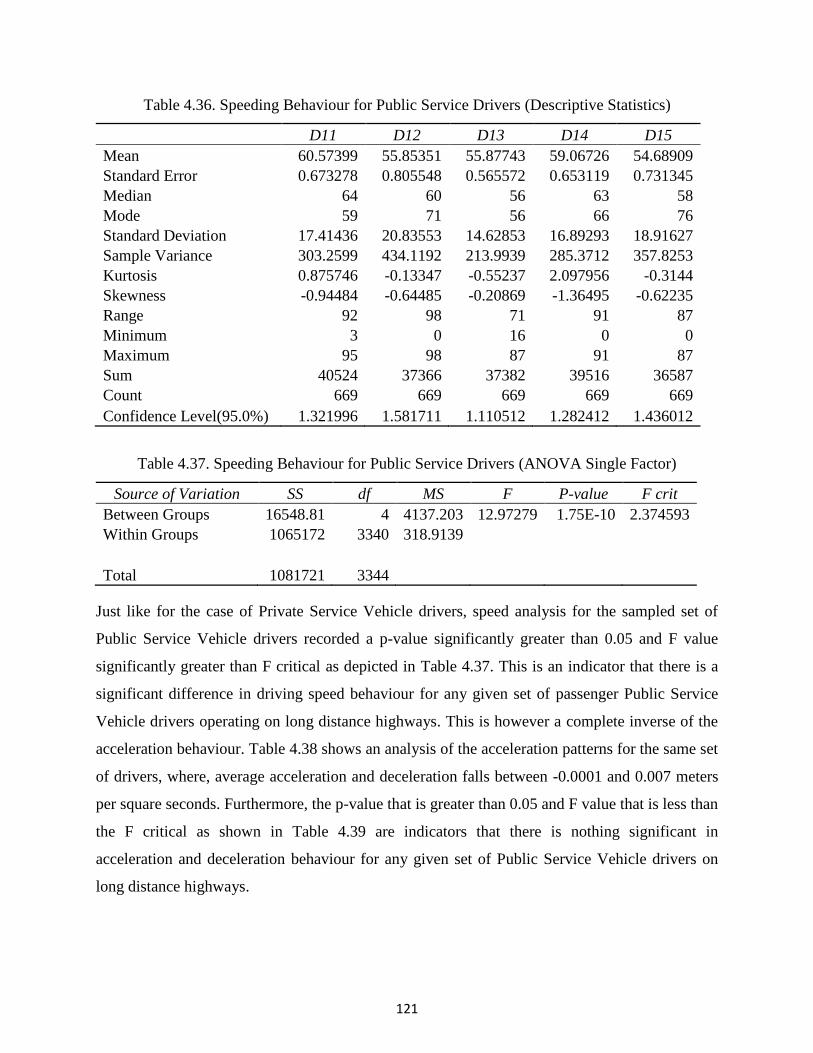
121


D11 D12 D13 D14 D15

Mean 60.57399 55.85351 55.87743 59.06726 54.68909

Standard Error 0.673278 0.805548 0.565572 0.653119 0.731345

Median 64 60 56 63 58

Mode 59 71 56 66 76


Sample Variance 303.2599 434.1192 213.9939 285.3712 357.8253

Kurtosis 0.875746 -0.13347 -0.55237 2.097956 -0.3144

Skewness -0.94484 -0.64485 -0.20869 -1.36495 -0.62235

Range 92 98 71 91 87

Minimum 3 0 16 0 0

Maximum 95 98 87 91 87

Sum 40524 37366 37382 39516 36587

Count 669 669 669 669 669


Table 4.37. Speeding Behaviour for Public Service Drivers (ANOVA Single Factor)


Between Groups 16548.81 4 4137.203 12.97279 1.75E-10 2.374593

Within Groups 1065172 3340 318.9139

Total 1081721 3344


Public Service Vehicle drivers recorded a p-value significantly greater than 0.05 and F value

significantly greater than F critical as depicted in Table 4.37. This is an indicator that there is a

significant difference in driving speed behaviour for any given set of passenger Public Service

Vehicle drivers operating on long distance highways. This is however a complete inverse of the

acceleration behaviour. Table 4.38 shows an analysis of the acceleration patterns for the same set

of drivers, where, average acceleration and deceleration falls between -0.0001 and 0.007 meters

per square seconds. Furthermore, the p-value that is greater than 0.05 and F value that is less than

the F critical as shown in Table 4.39 are indicators that there is nothing significant in

acceleration and deceleration behaviour for any given set of Public Service Vehicle drivers on

long distance highways.

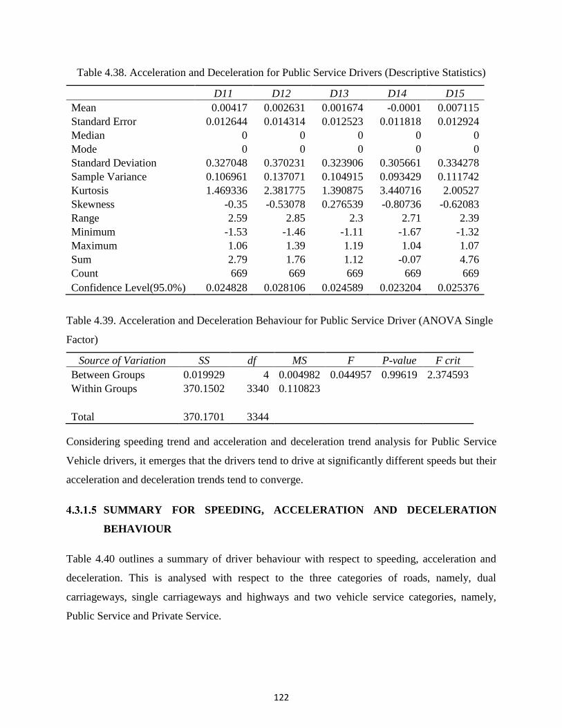
122

Table 4.38. Acceleration and Deceleration for Public Service Drivers (Descriptive Statistics)

D11 D12 D13 D14 D15

Mean 0.00417 0.002631 0.001674 -0.0001 0.007115

Standard Error 0.012644 0.014314 0.012523 0.011818 0.012924

Median 0 0 0 0 0

Mode 0 0 0 0 0


Sample Variance 0.106961 0.137071 0.104915 0.093429 0.111742

Kurtosis 1.469336 2.381775 1.390875 3.440716 2.00527

Skewness -0.35 -0.53078 0.276539 -0.80736 -0.62083

Range 2.59 2.85 2.3 2.71 2.39

Minimum -1.53 -1.46 -1.11 -1.67 -1.32

Maximum 1.06 1.39 1.19 1.04 1.07

Sum 2.79 1.76 1.12 -0.07 4.76

Count 669 669 669 669 669


Table 4.39. Acceleration and Deceleration Behaviour for Public Service Driver (ANOVA Single

Factor)


Between Groups 0.019929 4 0.004982 0.044957 0.99619 2.374593

Within Groups 370.1502 3340 0.110823

Total 370.1701 3344

Considering speeding trend and acceleration and deceleration trend analysis for Public Service

Vehicle drivers, it emerges that the drivers tend to drive at significantly different speeds but their

acceleration and deceleration trends tend to converge.

SUMMARY FOR SPEEDING, ACCELERATION AND DECELERATION

BEHAVIOUR

Table 4.40 outlines a summary of driver behaviour with respect to speeding, acceleration and

deceleration. This is analysed with respect to the three categories of roads, namely, dual

carriageways, single carriageways and highways and two vehicle service categories, namely,

Public Service and Private Service.

123

Table 4.40. Speeding, Acceleration and Deceleration Behaviour Summary

Dual Carriageway Single Carriageway Highway

Public Service Private Service Public Service Private Service Public Service Private Service

Average Speed 53 – 75 km/h 74 – 99 km/h 52 – 66 km/h 32 – 38 km/h 55 – 61 km/h 44 – 63 km/h

Highest Speed 91 km/h 126 km/h 94 km/h 72 km/h 98 km/h 114 km/h

Average Acceleration

/ Deceleration

-0.002 – 0.023

m/s2

-0.025 – 0.171

m/s2

0.0003 – 0.0104

m/s2

0.022 – 0.094

m/s2

-0.0001 – 0.007

m/s2

-0.006 – 0.025

m/s2

Highest Acceleration

Margin

1.22 m/s2 1.02 m/s2 1.22 m/s2 1.25 m/s2 1.39 m/s2 1.20 m/s2

Highest Deceleration

Margin

-2.43 m/s2 -2.22 m/s2 -2.43 m/s2 -1.87 m/s2 -1.67 m/s2 -2.15 m/s2

Conclusively, using road worthy vehicles on well-maintained, relatively flat dual carriageways

road category with gentle slops at some points, Private Service Vehicle drivers presented high

average driving speeds, acceleration and deceleration in comparison to Public Vehicle Service

drivers. This is based on the fact that Private Service Vehicle drivers average speed ranged

between 74 and 99 km/h with the highest speed being 126 km/h and average acceleration and

deceleration ranging between -0.025 and 0.171 m/s2 while Public Service Vehicle drivers

recorded average speeds between 53 and 75 km/h with the highest speed being 91 km/h and

average acceleration and deceleration ranging between -0.002 and 0.023 m/s2. Public Service

Vehicle drivers presented high acceleration and deceleration margins compared to Private

Service Vehicle drivers. This is evident by the fact that the highest acceleration margin recorded

for Private Service Vehicles drivers was 1.02 m/s2 compared to that of Public Service Vehicle

drivers that stood at 1.22 m/s2. Similarly, the highest deceleration margin recorded for Private

Service Vehicles drivers was -2.22 m/s2 compared to that of Public Service Vehicle drivers that

stood at -2.43 m/s2. Based on the analysis, datasets for driver D1, D3 and D4 under the Public

Service Vehicle category were considered for training the agent. Datasets for driver D2 and D4

of the Private Service Vehicle category were also considered in the training set for the driver

agent. The choices were based on the fact that all the drivers’ maximum acceleration and

deceleration margins were within acceptable ranges. A compromise was however made for

instances here highest speeds did not exceed 5 km/h above the recommended speeds.

On well-maintained single carriageways road category with a mix of flat, sloping and hill

climbing, clear and unclear corners, Public Service Vehicle drivers presented high average

driving speeds with low average acceleration and deceleration in comparison to Private Vehicle

124

Service drivers. This is based on the fact that Public Service Vehicle drivers average speed

ranged between 52 and 66 km/h with the highest speed being 94 km/h and average acceleration

and deceleration ranging between 0.0003 and 0.0104 m/s2 while Private Service Vehicle drivers

recorded average speeds between 32 and 38 km/h with the highest speed being 72 km/h and

average acceleration and deceleration ranging between 0.022 and 0.094 m/s2. Private Service

Vehicle drivers presented high acceleration margins compared to passenger Public Service

Vehicle drivers. This is evident by the fact that the highest acceleration margin recorded for

Private Service Vehicles drivers was 1.25 m/s2 compared to that of Public Service Vehicle

drivers that stood at 1.22 m/s2. On the contrary, Public Service Vehicle drivers presented high

deceleration margins compared to passenger Private Service Vehicle drivers. This is evident by

the fact that the highest deceleration margin recorded for Private Service Vehicles drivers was -

1.87 m/s2 compared to that of Public Service Vehicle drivers that stood at -2.43 m/s2. Based on

the analysis, datasets for all the sampled drivers under the Private Service Vehicle category were

included in the training set for the driver agent while none of the Public Service Vehicle drivers

was considered for inclusion in the training dataset. This was based on the fact that all Private

Service Vehicle drivers exhibited highest speeds within the required limits while all the Public

Service Vehicle drivers recorded highest speeds that were way above the allowable speed limits

for the service vehicle category.

On well-maintained long distance highways road category with a mix of flat, sloping and hill

climbing, clear and unclear corners, some stretches with bumps, Both Public Service Vehicle and

Private Service drivers presented overlapping average driving speeds. However, Private Service

Vehicle drivers presented high average acceleration and deceleration in comparison to Public

Vehicle Service drivers. This is based on the fact that Public Service Vehicle drivers average

speed ranged between 55 and 61 km/h with the highest speed being 98 km/h and average

acceleration and deceleration ranging between -0.0001 and 0.007 m/s2 while Private Service

Vehicle drivers recorded average speeds between 44 and 63 km/h with the highest speed being

114 km/h and average acceleration and deceleration ranging between -0.006 and 0.025 m/s2.

Public Service Vehicle drivers presented high acceleration margins compared to Private Service

Vehicle drivers. This is evident by the fact that the highest acceleration margin recorded for

Private Service Vehicles drivers was 1.20 m/s2 compared to that of Public Service Vehicle

drivers that stood at 1.39 m/s2. On the contrary, Private Service Vehicle drivers presented high

125

deceleration margins compared to passenger Public Service Vehicle drivers. This is evident by

the fact that the highest deceleration margin recorded for Private Service Vehicles drivers was -

2.15 m/s2 compared to that of Public Service Vehicle drivers that stood at -1.67 m/s2. Based on

the analysis, datasets for drivers D11, D12, D13 and D14 of the Private Service Vehicle category

were included in the training set for the driver agent while none of the Public Service Vehicle

drivers was considered for inclusion. This was based on the fact that four out of the five Private

Service Vehicle drivers exhibited highest speeds within the required limits while all the Public

Service Vehicle drivers recorded highest speeds that were way above the allowable speed limits

for the service vehicle category.

In summary, Private Service Vehicle drivers record high speeds on dual carriageways and

highways compared to single carriageways. Furthermore, they record high average speed ranges

on dual carriageways. On the other hand, Public Service Vehicle drivers record high acceleration

margins on dual carriageways and highways and high deceleration margins on dual carriageways

and single carriageways. On a general scale, Private Service Vehicle drivers present high average

acceleration / deceleration margins.

STOPPING BEHAVIOUR

Stopping behaviour was computed as a comparison of the actual distance taken to stop and the

distance established based on the standard Stopping Sight Distance metric as outlined in Table

4.15. Table 4.41 show a sample analysis for three drivers D1, D3 and D5 of the public service

vehicle category. Data for driver D2 and D4 did not have instances of stopping. The divers were

operating on a Dual carriageway. Considering the fact that Kenyan dual carriageway have a 100

km/h design speed, the Stopping Sight Distance based on this design speed is meant to be 184.21

meters. The study however based the Stopping Sight Distance on initial speeds as opposed to

design speed since a driver starts applying brakes when driving at varied speeds. Perception-

reaction time of 2.5 seconds and deceleration rate of 3.4 m/s2 were used in the determination of

Stopping Sight Distance. Under all circumstances, the Stopping Sight Distance based on initial

speed and the actual distance to stop were all below the Stopping Sight Distance based on design

speed since at no point did any driver brake from speeds of 100 km/h to 0 km/h.

126

Table 4.41. Stopping Behaviour Analysis

Driver D1

Data

Point

Speed

(km/h)

Change in

Time (s)

Deceleration

Rate (m/s2)

SSD Based on

Initial Speed (m)

Actual Distance

to Stop (m)

278 10 9 -1.2

279 0 12 -0.23 8.10 33.36

Driver D3

Data

Point

Speed

(km/h)

Change in

Time (s)

Deceleration

Rate (m/s2)

SSD Based on

Initial Speed (m)

Actual Distance

to Stop (m)

38 1 4 -0.35

39 0 17 -0.02 0.75 4.76

54 43 4 -0.28

55 0 12 -1 51.09 143.28

58 8 9 0.25

59 0 51 -0.04 6.29 113.22

64 6 10 0.08

65 0 10 -0.17 4.58 16.7

71 19 79 0.02

72 0 16 -0.33 17.35 84.48

83 16 10 0.22

84 0 10 -0.44 14.06 44.4

94 4 14 -0.52

95 0 6 -0.19 2.96 6.66

111 4 5 -0.61

112 0 10 -0.11 2.96 11.1

127 15 9 0.37

128 0 11 -0.38 13.01 45.87

133 2 6 -0.19

134 0 10 -0.06 1.46 5.6

136 4 10 0.03

137 0 10 -0.11 2.96 11.1

140 4 10 0.06

141 0 10 -0.11 2.96 11.1

147 3 6 0.05

148 0 10 -0.08 2.19 8.3

155 5 10 -0.03

156 0 10 -0.14 3.76 13.9

159 1 11 -0.15

160 0 10 -0.03 0.71 2.8

166 8 5 -0.06

127

Data

Point

Speed

(km/h)

Change in

Time (s)

Deceleration

Rate (m/s2)

SSD Based on

Initial Speed (m)

Actual Distance

to Stop (m)

167 0 10 -0.22 6.29 22.2

168 2 10 0.06

169 0 10 -0.06 1.41 5.6

174 5 5 0.06

175 0 5 -0.28 3.76 6.95

197 2 20 -0.03

198 0 10 -0.06 1.41 5.6

472 9 4 -0.56

473 0 11 -0.23 7.18 27.5

493 10 7 0.4

494 0 13 -0.21 8.10 36.14

Driver D5

Data

Point

Speed

(km/h)

Change in

Time (s)

Deceleration

Rate (m/s2)

SSD Based on

Initial Speed (m)

Actual Distance

to Stop (m)

67 39 4 -2.43

68 0 13 -0.83 44.55 140.79

71 6 9 0.19

72 0 11 -0.15 4.58 18.37

75 3 10 0.08

76 0 10 -0.08 2.19 8.3

279 15 5 -0.89

280 0 10 -0.42 13.01 41.7

It is evident that for all the three drivers’ stopping instances, the actual distance taken to stop was

greater than the standard Stopping Sight Distances computed based on initial speed. This was an

indicator that the driver’s braking to stopping behaviour was within acceptable standard margins.

A similar computation was done for all the 30 sampled drivers under the two categories i.e.

Public Service Vehicle category and Private Service Vehicle category. All the sampled drivers

presented stopping behaviour that was within acceptable margins, hence, qualifying the data

collected from them to be used for training the driver agent.

CORNERING BEHAVIOUR

The study established that there are no standard metrics for the determination of cornering

behaviour. The behaviour was hence determined using the margin of direction change in

comparison to time taken and speed. This behaviour was not monitored for human vehicle

128

drivers. It was however incorporated in the driver agent with a special algorithm used to

determine what could be termed as acceptable or unacceptable behaviour.

4.3.2 FORMULATION OF DRIVER BEHAVIOUR DATASET

Considering successful prestudy and main study results, in view of objective two and research

questions two, an effective dataset on driver behaviour patterns constitutes of the following raw

GPS data variables:

1. Coordinates (latitude and longitude)

2. Altitude

3. Speed

4. Direction

5. GPS time

6. GPS signal strength

These data variables lead to another key set of computed variables that are also critical for the

driver behaviour dataset. Majority of these computed variables are essential for use in the

Bayesian Network. These are:

1. Change in direction

2. Change in altitude

3. Change in time

4. Acceleration and deceleration

5. Stopping Sight Distance (SSD)

6. Distance to stop

A complete dataset on driver behaviour should also incorporate data on presence or absence of

obstacles in the operational environment of the driver. The study however excluded proximity

sensor data for the data set due to challenges and limitations outlined in the previous section.

However, a robotic vehicle agent could incorporate the proximity sensor if simulated on shorter

distances computed in centimeters.

A route map for the region constituting the dataset enhances the dataset by indicating a visual

perspective of the driving environment. To enhance the dataset further, a recorded video of real

129

diving environment and scenarios was also considered in some cases. This helps build

confidence in potential future users of the dataset.

A full dataset for both the prestudy and main study is available in a separate MS-Excel file.

However, Appendix E presents sample datasets for driver D1 and D4 of the Public Service

Vehicle and D2 and D4 of the Private Service Vehicle categories. The two drivers are part of the

fourteen drivers that were selected for training, validation and testing of the driver agent. The full

dataset for all the drivers that formulated the driver behaviour dataset will later be availed online

as an open access dataset for usage by interested parties.

4.3.3 DEVELOPMENT AND EVALUATION OF A VEHICLE DRIVER AGENT

The dataset formulated under objective two acted as a foundation for the development of the

vehicle driver agent in reference to objective three and four, with a focus on research question

three and four. An intelligent agent that models a human vehicle driver operating under

challenging diverse environments was hence developed. To better visualize the agent’s actions

under diverse environments, the study focused on a software agent.

The agent underwent three main phases: training, validation and testing. During the training

phase, the agent was subjected to the chosen dataset collected from human vehicle drivers to

facilitate learning. After successful training, the software agent underwent validation as an

unbiased evaluation of fitness while tuning the model’s hyper parameters. Finally, it was then put

in a real environment for the testing phase.

The study addressed a contingency kind of problem since exact prediction is impossible and its

solution requires a strategy, a contingency plan that specifies what action to take based on the

received percepts. This was achieved through utility functions to provide agent’s internal

performance measures in two main perspectives. Firstly, the function offers appropriate tradeoffs

amongst conflicting goals. Secondly, it weighs success likelihood against the importance of

goals. If the internal utility function and the external performance measures are in agreement,

then it chooses actions to maximize utility.

130

DESIGN OF THE DRIVER AGENT

A web based software agent was designed that operated in parallel with a human vehicle driver

without activating mechanical actuators. It instead operates as a software agent with screen

display of actions to be undertaken. The agent provided dashboard indicators for various actions

that include speeding, acceleration, deceleration, braking and turning. To achieve these actions,

the agent’s percepts were limited to GPS data and proximity sensor data gathered by various

sensors during actual vehicle operational period.

Figure 4.22 shows a sample dashboard for the software agent. The dashboard contains human

vehicle driver behaviour in form of probabilities where acceleration, braking and cornering

trends are each expressed in two perspectives, namely, normal and harsh. The perspective with

the highest probability depicts the behaviour of the driver at that moment. Also represented on

the dashboard is the driver agent actions that shows the action to be taken. The actions are in two

sets, where the first set provides indicator on speeding i.e. accelerate, decelerate or stop as the

second sets provides indicators on cornering actions i.e. turn right, turn left or move on. At the

bottom of the dashboard is a map with a marker showing the exact position of the vehicle. The

dashboard data values for both the human driver and the driver agent refresh at an interval of

1000 milliseconds.

131

Figure 4.22. Human Agent Verses Vehicle Driver Agent Dashboard

VALIDATION AND TESTING OF THE DRIVER AGENT

Agent testing was done under different road segments and conditions to ascertain stability. The

test environments encompassed roads with different states and patterns, dual and single

carriageways of different lengths and under varied times of the day and weather conditions. The

agent actions were evaluated against actions of the human vehicle driver. The variations in

environment types accommodated the fact that vehicle drivers operate under diverse, and

dynamic environments during which their actions may vary. One such an example is as outlined

in Figure 4.23 for a journey from Tuala to Langata. The road was composed of 90% single

carriageway with the remaining part being a dual carriageway. It had some uphill and downhill

132

sections, straight stretches and corners, with the experiment being carried out at daytime. The

location was a suitable choice since it represented a set of varied features that characterize the

operational environments of human vehicle drivers.

The test driver was chosen among the drivers that were used to formulate the training data set.

The driver had a valid driving license, a sign that he/she was legally permitted to drive vehicles

on Kenyan roads.

Figure 4.23. Driver Agent Test Environment

Table 0.16 under Appendix F shows sample data collected from a human vehicle driver on the

same route. This is part of the data that was used to train the driver agent. During agent training

on the route, several data points were logged in the agent training table in the database. Table

0.17 under Appendix F shows the data points for the sample route. Each data point formed the

center of a Gaussian that would inform the driver agent on the actions to take.

After agent training based on the training set, agent actions were now recorded on the route.

Table 4.42 shows actions of the driver agent at every point for half of the journey where the

speeding, cornering and terrain indicate the actions of the driver agent based on its percepts. The

agent operates as a software agent such that as the human vehicle driver was on the wheel, the

driver agent was indicating its actions on the dashboard at periodical intervals of 1000

milliseconds.

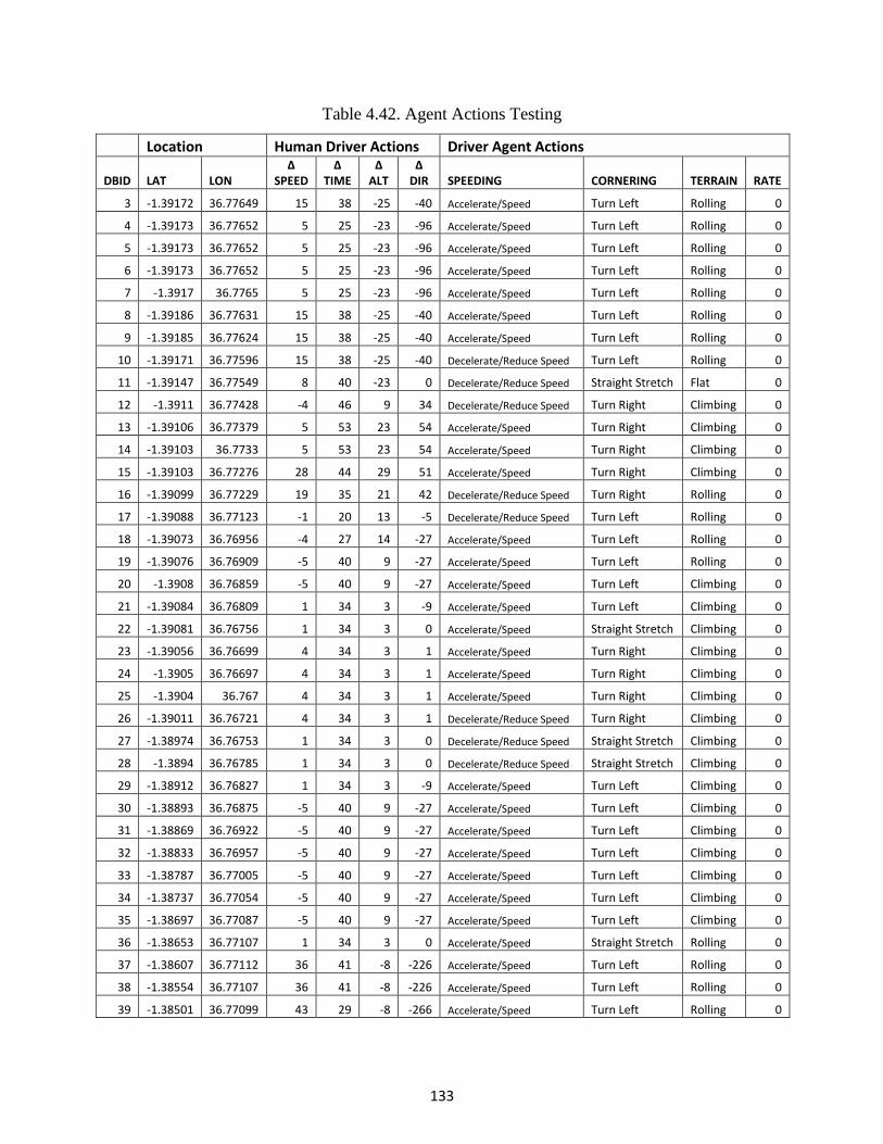
133

Table 4.42. Agent Actions Testing

Location Human Driver Actions Driver Agent Actions

DBID LAT LON ∆

SPEED ∆

TIME ∆

ALT ∆

DIR SPEEDING CORNERING TERRAIN RATE

3 -1.39172 36.77649 15 38 -25 -40 Accelerate/Speed Turn Left Rolling 0







10 -1.39171 36.77596 15 38 -25 -40 Decelerate/Reduce Speed Turn Left Rolling 0

11 -1.39147 36.77549 8 40 -23 0 Decelerate/Reduce Speed Straight Stretch Flat 0

12 -1.3911 36.77428 -4 46 9 34 Decelerate/Reduce Speed Turn Right Climbing 0

13 -1.39106 36.77379 5 53 23 54 Accelerate/Speed Turn Right Climbing 0



16 -1.39099 36.77229 19 35 21 42 Decelerate/Reduce Speed Turn Right Rolling 0

17 -1.39088 36.77123 -1 20 13 -5 Decelerate/Reduce Speed Turn Left Rolling 0

18 -1.39073 36.76956 -4 27 14 -27 Accelerate/Speed Turn Left Rolling 0

19 -1.39076 36.76909 -5 40 9 -27 Accelerate/Speed Turn Left Rolling 0

20 -1.3908 36.76859 -5 40 9 -27 Accelerate/Speed Turn Left Climbing 0

21 -1.39084 36.76809 1 34 3 -9 Accelerate/Speed Turn Left Climbing 0

22 -1.39081 36.76756 1 34 3 0 Accelerate/Speed Straight Stretch Climbing 0




26 -1.39011 36.76721 4 34 3 1 Decelerate/Reduce Speed Turn Right Climbing 0

27 -1.38974 36.76753 1 34 3 0 Decelerate/Reduce Speed Straight Stretch Climbing 0









36 -1.38653 36.77107 1 34 3 0 Accelerate/Speed Straight Stretch Rolling 0




134

EVALUATION OF THE DRIVER AGENT

The road segment had several turns or corners in the beginning. However, a good part of the road

was straight with gentle turns. Other corners were towards the end of the journey. From the

results for half of the journey as presented in Table 4.42, it is evident that the driver agent was

able to detect these corners and advised for turning as its recorded and displayed actions.

Instances of a hill climb and rolling were also correctly detected as these are physically present

on the road. The agent also advised on instances that required acceleration or deceleration. The

rate parameter gives room for human intervention as a way to reward the agent for good actions

taken. A complete set of agent actions for the entire journey is as outlined in Table 0.18 under

Appendix F. Figure 4.24 presents confusion matrices for acceleration, cornering and road terrain

actions of the agent in comparison to the actions by the human vehicle driver for the complete

journey. Performance of the agent was evaluated against four different measures, namely,

accuracy, precision, recall and F-score. This was based on four different elements that form the

confusion matrix i.e. True Positive (Tp), True Negative (Tn), False Positive (Fp) and False

Negative (Fn).

Accuracy is a numeric measure of how good an algorithm is. It represents how many correct

results the agent managed to identify, which is the proportion of true results among the total

number of cases that are examined. This was computed using equation (19).

Accuracy = (Tp+Tn)/(Tp+Tn+Fp+Fn) (19)

Precision represents the fraction of agent actions that are relevant. This was computed using

equation (20).

Precision = Tp/(Tp+Fp) (20)

Recall represents the fraction of agent actions that were undertaken. This was computed using

equation (21).

Recall = Tp/(Tp+Fn) (21)

F-score is a tradeoff of precision against recall. The higher the F-score value, the better the

algorithm. This was computed using equation (22).

F-Score = 2*Precision*Recall/(Precision + Recall) (22)

135

Figure 4.24 Confusion Matrices for Agent Testing

The driver agent test results clearly show the fact that the agent was able to display correct

actions under the three categories. For instance, acceleration actions were successfully detected

at accuracies of 68.7% while cornering and terrain action accuracies stood at 55.4% and 54.2%

respectively. The lower accuracy rate for terrain actions was attributed to the fact that the agent

was not flagging flat regions properly. Similarly, the agent was not flagging straight stretches

properly for cornering actions, hence the low accuracy rate. The success that was above 50% in

all cases is an indicator that probabilistic reasoning methodologies used properly determined the

vehicle driver behaviour leading to the formulation of a valid driver behaviour dataset. In

addition, all the three measures recorded an F-score value of over 70%, an indicator that the

algorithms used by the agent were appropriately good.

136

DRIVER AGENT MODEL

Figure 4.25 summarises how the agent operates. The agent’s state keeps changing as the journey

goes on. On the same note, its plan, context and actions also change progressively. A reward is

issued for agent actions that are commendable. This acts as a form of reinforcement learning

with reward. Agent state, plan and actions loop due to the dynamic nature of a vehicle driver’s


Figure 4.25. Driver Agent Model

4.4 SUMMARY OF STUDY FINDINGS

The findings in this chapter can hence be summarized as follows guided by the research

objectives.

The first objective sought to investigate how we could monitor and analyse behavioural

parameters for a human vehicle driver operating under diverse environments. This was looked at

from three perspectives:

1. What parameters are required to determine vehicle driver behaviour?

2. How can these parameters be established, collected or monitored?

3. How can the collected parameters be analysed to determine the behaviour of the driver?

Driving styles may be characterized based on different factors that include overtaking, speeding,

acceleration, braking, lane changing trends among others trends. It was determined that driver

137

behaviour is based on different factors that formulate the required parameters or variables. These

variables include speed, timestamp, latitude, longitude, altitude, direction (angle) and obstacle

data. The combined use of a GPS system, vehicle mounted monitoring systems and a server

application successfully facilitated the gathering and logging of these data parameters in real-

time. However, obstacle detection was not 100% successful due to major limitations based on

type of sensors used. From the findings, it is recommended that ultrasonic sensors could be

replaced by other sensors at the expense of cost or alternatively, sensor fusion be applied. To

determine the driver’s driving style, stochastic or probabilistic reasoning methodologies are

required. This led to the incorporation of special data analysis algorithms including, the Two-

Timeslice Bayesian Network (2TBN), Expectation Maximisation and the Gaussian Mixture

Model. The choice of these algorithms was due to the fact that the nature of the data required a

time series kind of analysis. The main outcome of this objective was the determination of a

vehicle driver’s profiles during and after a given journey.

The second objective sought to formulate a dataset on driver behavioural patterns. This was

achieved as an outcome of the profiles determined in the first objective. The collected and

analysed data that determined driver behaviour was used to formulate a driver behaviour dataset.

The dataset was built after numerous experiments that collected and analysed huge amounts of

data from different drivers operating under different environments. Such a dataset could find

many applications including informing future studies on transport and safety.

The last two objectives aimed at developing and evaluating a vehicle driver agent which can

operate in a complex environment. The study considered the three key phases of an intelligent

agent, namely, training, validation and testing. To achieve this, it was established that special

algorithms have to be fused to complement one another. The operation of the software agent was

hence founded on the Mixture Models, Factor Analysis, and Bayesian Inferencing. The Gaussian

Mixture Model supported by the Expectation Miximisation were critical in the determination of

agent action based on learning and other factors in its environment. The software driver agent

successfully operated in parallel with a human vehicle driver. The agent’s actions displayed on

the dashboard determined its performance.

138

Based on the findings, the study hypothesis stands accepted that “a utility-based agent can be

used as a basis for modelling human vehicle driver behaviour”.

Table 4.43 outlines a summary of the benchmark for the resulting model against an existing

closely related model, the UTDrive model.

Table 4.43. Model Benchmarking

Existing Models (UTDrive

Platform)

The Model in this Study

Motivation A research platform for in-vehicle

safety systems and driver behaviour

modelling

A platform for driver behaviour

modelling and operational

environment detection

Selected Key

Features

Focused more on an in-vehicle

environment driver behaviour

detection.

Can detect driver stress levels

and in-vehicle distractions.

The corpus used was gender

sensitive.

Purely focused on an out-vehicle

environment driver behaviour

detection.

Predicts operational environment:

terrain and pattern.

Includes a driver agent for driver

assistance.

Methodology Use of a mixture of algorithms due

to the incorporation of numerous

sensors.

Use of probabilistic reasoning and

intelligence methodologies:

Bayesian Networks

Gaussian Mixture Models

4.5 SUMMARY

The chapter outlined and discussed research findings with respect to the study objectives,

research questions and hypothesis. The next chapter concludes the study with recommendations

for further studies.

139

CHAPTER 5

CONCLUSION AND RECOMMENDATIONS

This chapter outlines the overall study conclusion and recommendations. Chapter content is

presented under three main sections, namely, conclusions, recommendations for further research

and recommendations for policy and practice.

5.1 CONCLUSION

Safety of road users is paramount globally with many renown organisations like the World

Health Organisation and the International Traffic Safety Data and Analysis Group advocating for

measures to reduce traffic injuries resulting from road accidents. Four main factors contribute to

road accidents, namely, structures of roads, states of roads, states of vehicles and behaviour of

vehicle drivers. A review of literature determined human vehicle driver behaviour as the major

cause of road accidents globally. Unfortunately, this happens to be the factor that has so far

proven to be the most difficult to monitor, analyse and model. This study established that driver

behaviour can be modelled using a utility-based agent where the research outcome showed that

the utility-based agent achieved mean performance accuracy rate of over 68%, +/- 5. This was a

clear indicator that probabilistic methodologies used correctly determined the vehicle driver

behaviour leading to the formulation of a valid driver behaviour dataset. Agent mean evaluation

F-score values of over 70%, +/-5 for detection of operational environments with respect to

corners and terrains and F-score values of over 80%, +/-5 for acceleration action were further

confirmations on the appropriateness of the algorithms used by the agent. These successful study

outcomes are an affirmation on the study hypothesis that a utility-based agent can be used as a

basis for modelling human vehicle driver behaviour.

5.2 RECOMMENDATIONS FOR FURTHER RESEARCH

5.2.1 RECOMMENDATIONS MADE DIRECTLY FROM DATA

Reliance on GPS data parameters with statistical probabilistic reasoning methodologies offers a

perfect approach for driver behaviour monitoring and analysis. Such analyses could be enhanced

further if more data parameters could be captured. For instance, inclusion of On-Board

140

Diagnostics (OBD) vehicle data could enrich the scope and accuracy in the determination of

driver behaviour. Further research should focus on full OBD data capture to complement GPS

data. Appropriate obstacle sensing could further improve on the results of such a study.

5.2.2 RECOMMENDATIONS BASED ON CHALLENGES

The study recommends the use of other types of obstacle sensors as opposed to ultrasonic

sensors for driver behaviour monitoring and profiling studies. This is centered on the major

challenge of long range obstacle sensing that came up as a major limitation in this study. This

was affected by the large beam width offered by ultrasonic sensors. To achieve better and

reliable results in obstacle detection, two considerations could be put in place:

i) Use of Alternative Technologies

Alternative obstacle detection technologies could be used. For instance, the Radio Detection and

Ranging (RADAR) and the laser-based Light Imaging Detection and Ranging (LIDAR).

However, both technologies come with pros and cons. Both technologies use the concept of

sending signals that bounce back upon hitting an obstacle, hence, the stronger the signal, the

better the reflection. The distance to the object is calculated based on the time taken for each

pulse to bounce back. RADAR technology is based on radio waves while laser-based LIDAR

technology uses laser light waves. It is worth noting that radio waves travel further than sound

waves and are undetectable to human sensory organs, as a result, they are best suited for long-

range obstacle detection compared to sound waves used by ultrasonic sensors. Both radio and

light waves have relatively same speeds though radio waves have less absorption compared to

light waves, a factor that makes radio waves propagate well in relatively longer distances. Smart

car makers prefer laser rangefinders since they are able to create a 3 dimensional image of the

obstacle. This makes it possible to determine the exact size of an object. However, laser waves

are affected by darkness and cloudy weather, hence, not suited for obstacle detection at night. In

addition, the technology is more expensive than RADAR.

The development of a RADAR based obstacle detection and warning system was pushed ahead

by Mercedes Benz in 90’s. Presently, automakers like Google, Uber, Tesla and Toyota use either

or both radio and laser wave technologies in addition to cameras, ultrasonic and infrared

141

technologies. RADAR technology is heavily used in airplanes, military vehicles, battleships and

marine equipment for long range obstacle detection. This is due to its suitability to operate at

daytime and nighttime and with less interference under varying weather conditions.

The frequency-modulated continuous-wave (FMCW) is an example of a RADAR technology

that uses electromagnetic waves transmitted by a front-end antenna system with the reflected

signal used to determine target distance and speed. The waves may be at microwave frequencies

or higher frequencies. FMCW radar sensors can change their operating frequency during

measurement, hence, the term frequency modulation. Such a technology is best suited for

environments with poor visibility. The waves have the capability to penetrate mud and sprays

and with an added advantage that allows for beam width adjustment to suite particular

applications. On the other hand, laser rangefinders send focused laser light beams, suited for long

range, high directionality and fast response time kinds of application scenarios. It is worth noting

that Laser light is monochromatic, directional, and coherent such that it is one wavelength

colour, with relatively narrow beams in one direction and the wavelengths are in phase in space

and time. Hence, this may solve the problem of detections of the ground as an obstacle, as was

the case for ultrasound waves. Unfortunately, laser lights are affected by poor environmental

visibility. This disadvantages the use of the technology under certain conditions like muddy

environments or environments with sprays. Unfortunately, rangefinders using either radio or

laser technology come at a high cost compared to ultrasound and infrared based rangefinders.

ii) Sensor Fusion

Sensor fusion is a concept that entails combining two or more technologies such that they

complement one another. For instance, if cost is a major issue, ultrasonic sensors could be

combined with infrared sensors to offer the following advantages:

i) Ultrasonic sensors could complement infrared sensors that fail under poor lighting

conditions such as smoke or fog and cannot detect transparent obstacles.

ii) On the other hand, infrared sensors could complement ultrasonic sensors that cannot

appropriately detect sound absorbing or soft surfaces. Such a sensor fusion can be quite

advantageous since both technologies are cheap as compared to other high cost

technologies like radio and laser. Unfortunately, such a fusion is limited to mid-range

142

detection hence cannot detect obstacles at far distances. This is a major drawback for

such a sensor fusion.

Radio waves and laser waves employed by RADAR and laser-based LIDAR sensors respectively

could also be fused to complement one another. This is best suited in cases where cost is not a

limiting factor. High accuracy, precision and reliability in obstacle detection could be achieved if

different technologies like radio waves, laser waves, ultrasonic waves and infrared waves could

all be fused. This kind of fusion is already being embraced by modern day automakers working

on smart cars. It is worth mentioning that the fusion is further enhanced by the use of

sophisticated cameras and data and image processing algorithms. Further research could explore

on the use of laser range sensing technology, a kind of technology heavily employed in the

Google self-driving car project and other smart car projects.

A proper and well-thought sensor fusion complemented by cameras and appropriate data

processing algorithms will definitely mitigate most of the challenges in obstacle detection. This

will address the cases of failed detections experienced particularly when both the sensor and

obstacles are in motion and when obstacles have differing unpredictable surface properties since

the different sensor technologies will complement one another’s shortcomings.

5.3 RECOMMENDATIONS FOR POLICY AND PRACTICE

From the study, there was a strong indication that driver behaviour is a leading factor to road

traffic injuries. This study therefore revealed issues that led to the following recommendations

that should inform on policy and practice, particularly for developing nations to help achieve

road safety through the adoption of the model:

1. There should be a mechanism in place for continuous monitoring of vehicle drivers’

behaviour as they go along with their day to day activities on world roads. This should come

in as a Governmental or Transport and Safety Authority policy.

2. The privacy policy should be reviewed to help accommodate the use of GPS technology for

driver behaviour monitoring and profiling.

143

3. It is advocated that the driver behaviour monitoring and analysis model be incorporated in

driver training schools. The model should also be a key tool that informs Traffic Departments

on whether to issue a driving permit to new drivers or not. It should also be used in making

decisions on possible revocations and/or cancelation of existing driving permits.

Full implementation of the model by Government agencies like the Transport and Safety

Authorities would require a policy to be put in place such that all employees be trained on how to

use the model. This would help in the understanding and utilisation of the data generated by use

of the model.

The resulting utility-based agent for vehicle driver modelling could be visualised in three

different perspectives, namely:

a) A model that establishes and profiles vehicle driver behaviour.

b) A dataset on vehicle driver behaviour.

c) A utility-based agent that models vehicle drivers.

Either of these study outcome perspectives could be adopted and implemented independently or

all could be adopted and implemented simultaneously. For instance, stakeholders interested in

determination of driver behaviour and profiling drivers based on their behaviour could only

adopt and implement the model that establishes and profiles vehicle driver behaviour. Such

stakeholders include but are not limited to insurance companies, transport and safety authorities,

traffic departments of the police force, organisations with large fleets, cab companies among

others. On the other hand, parties interested in Intelligent Transportation Systems for instance the

self-driving car technologies will find the utility-based agent for vehicle driver modelling vital as

a foundation worth exploration for extension.

Researchers and academia in the area of transport and driver behaviour will find the dataset on

driver behaviour a great avenue for their studies. Such beneficiaries could also adopt and

implement the model that determines and profiles vehicle drivers based on their behaviour. Such

a move could allow them to generate their own datasets on driver behaviour for specific

customized studies.

144

Adoption of either model or the full model could be supported or affected by several different

factors. Table 5.1 outlines a suggestion of key factors that could aid or hinder adoption of the

model in full. The rating per category of factors is based on the perception of the status of Kenya

as a Nation. This hence means that the rating may vary after a full study on the adoption of the

model is carried out.

Factors Rating

Availability of supporting technology 30%

Ease of use once implemented 30%

Aiding Factors Low cost of required devices 20%

Availability of skilled personnel 10%

Key stakeholders support 10%

Lack of modern day infrastructure 40%

High cost of internet or data bundles 30%

Hindering Factors Lack of trust in technology 10%

Lack of policy on privacy 10%

Enactment of National laws 10%

Table 5.1. Factors that Could Aid or Hinder Adoption of the Model

145

REFERENCES

[1] World Health Organisation, “Global status report on road safety 2013: supporting a

decade of action,” Geneva, 2013.

[2] World Health Organisation, “Global status report on road safety 2018,” Geneva, 2018.

[3] World Health Organisation, “Global status report on road safety 2015: supporting a

decade of action,” Geneva, 2015.

[4] World Health Organisation, “Global Status Report on Road Safety: Time for Action,”

Geneva, 2009.

[5] Road Safety Authority, “Road Safety Strategy 2013 - 2020,” Ireland, 2013.

[6] A. Nyamawe and E. Mbosso, “Road Safety: Adoption of ICT for Tracking Vehicles’

Over-speeding in Tanzania,” Int. J. Comput. …, 2014.

[7] D. Johnson and M. Trivedi, “Driving style recognition using a smartphone as a sensor

platform,” Intell. Transp. Syst. ( …, 2011.

[8] M. Moharrum and A. Al-Daraiseh, “Toward secure vehicular ad-hoc networks: a survey,”

IETE Tech. Rev., 2012.

[9] S. Fernandez and T. Ito, “Driver Behavior Model Based on Ontology for Intelligent

Transportation Systems,” 2015 IEEE 8th Int. Conf., 2015.

[10] C. Jeremiah and A. Nneka, “Issues and possibilities in Vehicular Ad-hoc Networks

(VANETs),” Comput. Control. Networking, 2015.

[11] E. Ohn-Bar and M. M. Trivedi, “Looking at Humans in the Age of Self-Driving and

Highly Automated Vehicles,” IEEE Trans. Intell. Veh., vol. 1, no. 1, pp. 90–104, 2016.

[12] S. Wakitani, Y. Yamauchi, T. Kinoshita, T. Yamamoto, M. Miyakoshi, and S. Harada,

“Design of a Vehicle Driver Model based on Database-Driven Control Approach,” IEEJ

Trans. Electron. Inf. Syst., vol. 138, no. 7, pp. 910–911, 2018.

[13] J. Morton, T. A. Wheeler, and M. J. Kochenderfer, “Analysis of Recurrent Neural

Networks for Probabilistic Modeling of Driver Behavior,” IEEE Trans. Intell. Transp.

Syst., vol. 18, no. 5, pp. 1289–1298, 2017.

[14] S. Schnelle, J. Wang, H. J. Su, and R. Jagacinski, “A Personalizable Driver Steering

Model Capable of Predicting Driver Behaviors in Vehicle Collision Avoidance

Maneuvers,” IEEE Trans. Human-Machine Syst., vol. 47, no. 5, pp. 625–635, 2017.

146

[15] S. Noh, B. Park, K. An, Y. Koo, and W. Han, “Co-Pilot Agent for Vehicle/Driver

Cooperative and Autonomous Driving,” ETRI J., vol. 37, no. 5, pp. 1032–1043, Oct. 2015.

[16] K. Takeda and J. Hansen, “International large-scale vehicle corpora for research on driver

behavior on the road,” Intell. …, 2011.

[17] K. Takeda, J. H. L. Hansen, H. Erdoǧan, and H. Abut, In-vehicle corpus and signal

processing for driver behavior. Boston, MA: Springer US, 2009.

[18] P. Angkititrakul, J. H. L. Hansen, S. Choi, T. Creek, J. Hayes, and J. Kim, “UTDrive: The

Smart Vehicle Project,” in In-Vehicle Corpus and Signal Processing for Driver Behavior,

Boston, MA: Springer US, 2009, pp. 55–67.

[19] N. Li, J. J. Jain, and C. Busso, “Modeling of Driver Behavior in Real World Scenarios

Using Multiple Noninvasive Sensors,” IEEE Trans. Multimed., vol. 15, no. 5, pp. 1213–

1225, 2012.

[20] A. Sathyanarayana, P. Boyraz, and J. H. L. Hansen, “Driver behavior analysis and route

recognition by hidden Markov models,” … Electron. Safety, …, 2008.

[21] A. Sathyanarayana, P. Boyraz, Z. Purohit, R. Lubag, and J. H. L. Hansen, “Driver

adaptive and context aware active safety systems using CAN-bus signals,” … (IV), 2010

IEEE, 2010.

[22] Z. Constantinescu, C. Marinoiu, and M. Vladoiu, “Driving style analysis using data

mining techniques,” researchgate.net, 2010.

[23] GPS.gov, “GPS accuracy.” [Online]. Available:

http://www.gps.gov/systems/gps/performance/accuracy/. [Accessed: 18-Sep-2014].

[24] International Traffic Safety Data and Analysis Group (IRTAD), “Road Safety Annual

Report 2018,” Paris, 2018.

[25] International Traffic Safety Data and Analysis Group (IRTAD), “Road Safety Annual

Report 2014,” Paris, 2014.

[26] A. Ellison, S. Greaves, and R. Daniels, “Profiling Drivers’ Risky Behaviour Towards All

Road Users,” Australas. Coll. Road …, 2012.

[27] G. N. Bifulco, F. Galante, L. Pariota, M. Russo Spena, and P. Del Gais, “Data Collection

for Traffic and Drivers’ Behaviour Studies: A Large-scale Survey,” Procedia - Soc.

Behav. Sci., vol. 111, pp. 721–730, Feb. 2014.

[28] J. De Winter and D. Dodou, “The Driver Behaviour Questionnaire as a predictor of

147

accidents: A meta-analysis,” J. Safety Res., 2010.

[29] J. Reason, A. Manstead, and S. Stradling, “Errors and violations on the roads: a real

distinction?,” Ergonomics, 1990.

[30] K. Jakobsen, S. C. H. Mouritsen, and K. Torp, “Evaluating eco-driving advice using

GPS/CANBus data,” in Proceedings of the 21st ACM SIGSPATIAL International

Conference on Advances in Geographic Information Systems - SIGSPATIAL’13, 2013, pp.

44–53.

[31] T. Toledo and T. Lotan, “In-vehicle data recorder for evaluation of driving behavior and

safety,” … J. Transp. Res. Board, 2006.

[32] N. Zhao, B. Mehler, B. Reimer, L. A. D’Ambrosio, A. Mehler, and J. F. Coughlin, “An

investigation of the relationship between the driving behavior questionnaire and objective

measures of highway driving behavior,” Transp. Res. Part F Traffic Psychol. Behav., vol.

15, no. 6, pp. 676–685, 2012.

[33] L. M. Martinussen, M. Møller, and C. G. Prato, “Assessing the relationship between the

Driver Behavior Questionnaire and the Driver Skill Inventory: Revealing sub-groups of

drivers,” Transp. Res. Part F Traffic Psychol. Behav., vol. 26, no. PART A, pp. 82–91,

2014.

[34] L. M. Martinussen, L. Hakamies-Blomqvist, M. Møller, T. Özkan, and T. Lajunen, “Age,

gender, mileage and the DBQ: The validity of the Driver Behavior Questionnaire in

different driver groups,” Accid. Anal. Prev., vol. 52, pp. 228–236, Mar. 2013.

[35] L. Guého, M. A. Granié, and J. C. Abric, “French validation of a new version of the

Driver Behavior Questionnaire (DBQ) for drivers of all ages and level of experiences,”

Accid. Anal. Prev., vol. 63, pp. 41–48, 2014.

[36] M. Mattsson, “Investigating the factorial invariance of the 28-item DBQ across genders

and age groups: An Exploratory Structural Equation Modeling Study,” Accid. Anal. Prev.,

vol. 48, pp. 379–396, 2012.

[37] P. Angkititrakul, M. Petracca, A. Sathyanarayana, and J. H. L. Hansen, “UTDrive: Driver

Behavior and Speech Interactive Systems for In-Vehicle Environments,” in 2007 IEEE

Intelligent Vehicles Symposium, 2007, pp. 566–569.

[38] B. Jensen, M. Skov, and N. Thiruravichandran, “Studying driver attention and behaviour

for three configurations of GPS navigation in real traffic driving,” Proc. SIGCHI …,

148

2010.

[39] J. Paefgen, F. Kehr, Y. Zhai, and F. Michahelles, “Driving behavior analysis with

smartphones: insights from a controlled field study,” Proc. 11th …, 2012.

[40] L. M. Bergasa, D. Almería, J. Almazán, J. J. Yebes, and R. Arroyo, “Drivesafe: An app

for alerting inattentive drivers and scoring driving behaviors,” Intell. Veh., 2014.

[41] H. Bořil, P. Boyraz, and J. Hansen, “Towards Multimodal Driver’s Stress Detection,”

Digit. signal Process. in-vehicle …, 2012.

[42] T. Yu and J. Hansen, “The ‘UTDrive’ in-vehicle voice activity detection system,” Intell.

Veh. Symp. (IV), 2010 …, 2010.

[43] J. Jain and C. Busso, “Analysis of driver behaviors during common tasks using frontal

video camera and CAN-Bus information,” Multimed. Expo (ICME), 2011 IEEE …, 2011.

[44] M. Lu, J. Wang, K. Li, T. Yamamura, N. Kuge, and T. Nakagawa, “Classification of

Longitudinal Driving Behaviour Based on Simulator Study,” ictct.org.

[45] C. You, M. Montes-de-Oca, and T. Bao, “CarSafe: a driver safety app that detects

dangerous driving behavior using dual-cameras on smartphones,” Proc. …, 2012.

[46] G. Castignani, R. Frank, and T. Engel, “Driver behavior profiling using smartphones,”

16th Int. IEEE …, 2013.

[47] M. Fazeen and B. Gozick, “Safe driving using mobile phones,” Intell. …, 2012.

[48] C. Arroyo, L. Bergasa, and E. Romera, “Adaptive fuzzy classifier to detect driving events

from the inertial sensors of a smartphone,” Syst. (ITSC), 2016 IEEE …, 2016.

[49] H. Eren, S. Makinist, and E. Akin, “Estimating driving behavior by a smartphone,” Veh.

Symp. (IV), …, 2012.

[50] G. Castignani, T. Derrmann, R. Frank, and T. Engel, “Driver behavior profiling using

smartphones: A low-cost platform for driver monitoring,” IEEE Intell., 2015.

[51] A. Singh and J. Bhasin, “A Variable Speed Limit (VSL) Based Model for Advanced

Traffic Management through VANETs,” 2016 30th Int. Conf., 2016.

[52] H. Moustafa and Y. Zhang, Vehicular networks: techniques, standards, and applications.

2009.

[53] J. Joshi, A. Singh, and L. Moitra, “DASITS: Driver Assistance System in Intelligent

Transport System,” 2016 30th Int., 2016.

[54] F. Martin-Fernández and P. Caballero-Gil, “An EXperimental Hybrid wIrelesS platform

149

for vehicular networks,” World of Wireless, 2016.

[55] K. Bayad, E. Bourhim, and M. Rziza, “Comparative study of topology-based routing

protocols in vehicular ad hoc network using IEEE802. 11p,” Electr., 2016.

[56] K. Abboud, H. Omar, and W. Zhuang, “Interworking of DSRC and Cellular Network

Technologies for V2X Communications: A Survey,” IEEE Trans., 2016.

[57] W. Devapriya and C. Babu, “Advance Driver Assistance System (ADAS): Speed bump

detection,” 2015 IEEE Int., 2015.

[58] V. Ramanishka, Y.-T. Chen, T. Misu, and K. Saenko, “Toward Driving Scene

Understanding: A Dataset for Learning Driver Behavior and Causal Reasoning.” pp.

7699–7707, 2018.

[59] S. J. Russell and P. Norvig, Artificial Intelligence : A Modern Approach. Malaysia;

Pearson Education Limited, 2016.

[60] S. Riter and J. McCoy, “Automatic Vehicle Location—An Overview,” IEEE Trans. Veh.

Technol., vol. 26, no. 1, pp. 7–11, 1977.

[61] R. Bajaj, S. L. Ranaweera, and D. P. Agrawal, “GPS: location-tracking technology,” IEEE

Comput., vol. 35, no. 4, pp. 92–94, May 2008.

[62] G. Djuknic and R. Richton, “Geolocation and assisted GPS,” IEEE Comput., vol. 34, no.

2, pp. 123–125, 2001.

[63] T. Yi, H. Li, and M. Gu, “Recent research and applications of GPS based technology for

bridge health monitoring,” Sci. China Technol. Sci., 2010.

[64] T. Chalko, “High accuracy speed measurement using GPS (Global Positioning System),”

NU J. Discov., 2007.

[65] O. Mugenda and A. Mugenda, Research methods: Quantitative and qualitative

approaches, 2 Rev Ed. Nairobi: Acts Press, 2003.

[66] C. R. Kothari, Quantitative Techniques, 3 Rev Ed. New Delhi: UBS Publishers, 2006.

[67] W. G. Cochran, Sampling Techniques, 2nd ed. New York, USA: John Wiley and Sons

Inc., 1963.

[68] J. F. Hair, W. C. Black, B. J. Babin, and R. E. Anderson, Multivariate Data Analysis. New

Jersey: Pearson Prentice Hall, 2010.

[69] J. F. Hair, W. C. Black, B. J. Babin, and R. E. Anderson, Multivariat Data Analysis:

Pearson New International Edition, 7 Ed. Essex: Pearson Education Limited, 2014.

150

[70] R. C. MacCallum, K. F. Widaman, S. Zhang, and S. Hong, “Sample size in factor

analysis.,” Am. Psychol. Assoc. Inc, psycnet.apa.org, vol. 4, no. 1, pp. 84–99, 1999.

[71] P. Bacchetti, S. G. Deeks, and J. M. McCune, “Breaking free of sample size dogma to

perform innovative translational research,” Sci. Transl. Med. stm.sciencemag.org, vol. 3,

no. 87 87ps24, 2011.

[72] P. Bacchetti, C. E. McCulloch, and M. R. Segal, “Simple, Defensible Sample Sizes Based

on Cost Efficiency,” Biometrics, vol. 64, no. 2, pp. 577–585, Jun. 2008.

[73] R. B. Langley, “NMEA 0183: A GPS receiver interface standard,” gauss.gge.unb.ca,

1995.

[74] J. Obuhuma and C. Moturi, “Use of GPS with road mapping for traffic analysis,” Int. J.

Sci. Technol., 2012.

[75] M. Bansode, S. Jadhav, and A. Kashyap, “Voice Recognition and Voice Navigation for

Blind using GPS,” Int. J. Innov., 2015.

[76] J. Sarik and I. Kymissis, “Lab kits using the Arduino prototyping platform,” 2010 IEEE

Front. Educ., 2010.

[77] A. G. Mugenda, “Social science research: Theory and principles,” Technol. Pedagog.

Educ., vol. 9, no. 3, pp. 319 – 342, 2008.

[78] D. B. Fambro, K. Fitzpatrick, and R. J. Koppa, “NCHRP Report 400: Determination of

stopping sight distances,” National Academy Press, Virginia, 1997.

[79] J. Pearl, Probabilistic Reasoning in Intelligent Systems: Networks of Plausible Inference.

San Francisco, CA, USA: Morgan Kaufmann Publishers Inc, 1988.

[80] M. Da, W. Wei, H. Hai-guang, G. J.-I. M. E. C. Sci, and undefined 2011, “The

application of Bayesian classification theories in distance education system,” mecs-

press.net.

[81] J. I. Obuhuma, H. O. Okoyo, and S. O. Mcoyowo, “Shortcomings of Ultrasonic Obstacle

Detection for Vehicle Driver Assistance and Profiling,” Int. J. Inf. Technol. Comput. Sci.,

vol. 11, no. 6, pp. 28–36, 2019.

[82] M. Tadlaoui, S. Aammou, … M. K.-I. J. of, and undefined 2016, “Learner modeling in

adaptive educational systems: a comparative study,” mecs-press.org.

[83] J. I. Obuhuma, H. O. Okoyo, and S. O. Mcoyowo, “Real-time Driver Advisory Model:

Intelligent Transportation Systems,” in IST-Africa 2018 Conference Proceedings, IEEE

151

Xplore, 2018.

[84] J. I. Obuhuma, H. O. Okoyo, and S. O. Mcoyowo, “Driver Behaviour Profiling Using

Dynamic Bayesian Network,” MECSJ. Mod. Educ. Comput. Sci., vol. 7, pp. 50–59, 2018.

152

APPENDICES

APPENDIX A: MICROCONTROLLER PROGRAM FOR PROXIMITY SENSORS

1. #define trigpin 2

2. #define echopin 3

3. #define gpstrigpin 4

4. void setup() {

5. Serial.begin(9600);

6. pinMode(trigpin, OUTPUT);

7. pinMode(echopin, INPUT);

8. pinMode(gpstrigpin, OUTPUT);

9. }

10. void loop() {

11. int distance, duration;

12. digitalWrite(trigpin, HIGH);

13. delayMicroseconds(1000);

14. digitalWrite(trigpin, LOW);

15. duration = pulseIn(echopin, HIGH);

16. distance = (duration/2)/29.1;

17. Serial.print(distance);

18. Serial.println(" cm");

19. delay(100);

20. if(distance>0 && distance<400){

21. digitalWrite(gpstrigpin, HIGH);

22. }

23. else{

24. digitalWrite(gpstrigpin, LOW);

25. }

26. }

153

APPENDIX B: BEHAVIOURAL PROBABILITIES

Table 0.1. Behaviour and Environment Probabilities per Driving State

State Behaviour Environment

∆Accl

(m/s2)

∆Tim

e (s)

∆Alt

(m)

∆Dir

(0)

Obst Normal

Accel

Harsh

Accel

Normal

Braking

Harsh

Braking

Normal

Corner

Harsh

Corner

Mean

der

Straight Up-

Hill

Dow

n-Hill

1 0 - 5 <=5 0 - 5 <+/-45 Yes 0.25 0.10 0.18 0.17 0.15 0.15 0.10 0.40 0.40 0.10

2 0 - 5 <=5 0 - 5 <+/-45 No 0.20 0.15 0.20 0.15 0.15 0.15 0.10 0.40 0.40 0.10

3 0 - 5 <=5 0 - 5 >=+/-45 Yes 0.25 0.10 0.18 0.17 0.10 0.20 0.40 0.10 0.40 0.10

4 0 - 5 <=5 0 - 5 >=+/-45 No 0.20 0.15 0.20 0.15 0.10 0.20 0.40 0.10 0.40 0.10

5 0 - 5 <=5 > 5 <+/-45 Yes 0.27 0.08 0.23 0.12 0.15 0.15 0.10 0.40 0.50 0.00

6 0 - 5 <=5 > 5 <+/-45 No 0.25 0.10 0.25 0.10 0.15 0.15 0.10 0.40 0.50 0.00

7 0 - 5 <=5 > 5 >=+/-45 Yes 0.27 0.08 0.23 0.12 0.20 0.10 0.40 0.10 0.50 0.00

8 0 - 5 <=5 > 5 >=+/-45 No 0.25 0.10 0.25 0.10 0.20 0.10 0.40 0.10 0.50 0.00

9 0 - 5 <=5 -0 - -5 <+/-45 Yes 0.27 0.08 0.23 0.12 0.15 0.15 0.10 0.40 0.10 0.40

10 0 - 5 <=5 -0 - -5 <+/-45 No 0.25 0.10 0.25 0.10 0.15 0.15 0.10 0.40 0.10 0.40

11 0 - 5 <=5 -0 - -5 >=+/-45 Yes 0.27 0.08 0.23 0.12 0.10 0.20 0.40 0.10 0.10 0.40

12 0 - 5 <=5 -0 - -5 >=+/-45 No 0.25 0.10 0.25 0.10 0.10 0.20 0.40 0.10 0.10 0.40

13 0 - 5 <=5 < -5 <+/-45 Yes 0.22 0.13 0.18 0.17 0.15 0.15 0.10 0.40 0.00 0.50

14 0 - 5 <=5 < -5 <+/-45 No 0.20 0.15 0.20 0.15 0.15 0.15 0.10 0.40 0.00 0.50

15 0 - 5 <=5 < -5 >=+/-45 Yes 0.22 0.13 0.18 0.17 0.10 0.20 0.40 0.10 0.00 0.50

16 0 - 5 <=5 < -5 >=+/-45 No 0.20 0.15 0.20 0.15 0.10 0.20 0.40 0.10 0.00 0.50

17 0 - 5 >5 0 - 5 <+/-45 Yes 0.27 0.08 0.23 0.12 0.15 0.15 0.10 0.40 0.40 0.10

18 0 - 5 >5 0 - 5 <+/-45 No 0.25 0.10 0.25 0.10 0.15 0.15 0.10 0.40 0.40 0.10

19 0 - 5 >5 0 - 5 >=+/-45 Yes 0.27 0.08 0.23 0.12 0.12 0.18 0.40 0.10 0.40 0.10

20 0 - 5 >5 0 - 5 >=+/-45 No 0.25 0.10 0.25 0.10 0.12 0.18 0.40 0.10 0.40 0.10

21 0 - 5 >5 > 5 <+/-45 Yes 0.30 0.05 0.27 0.08 0.15 0.15 0.10 0.40 0.50 0.00

22 0 - 5 >5 > 5 <+/-45 No 0.28 0.07 0.28 0.07 0.15 0.15 0.10 0.40 0.50 0.00

23 0 - 5 >5 > 5 >=+/-45 Yes 0.30 0.05 0.27 0.08 0.12 0.18 0.40 0.10 0.50 0.00

24 0 - 5 >5 > 5 >=+/-45 No 0.28 0.07 0.28 0.07 0.12 0.18 0.40 0.10 0.50 0.00

25 0 - 5 >5 -0 - -5 <+/-45 Yes 0.30 0.05 0.27 0.08 0.15 0.15 0.10 0.40 0.10 0.40

26 0 - 5 >5 -0 - -5 <+/-45 No 0.28 0.07 0.28 0.07 0.15 0.15 0.10 0.40 0.10 0.40

27 0 - 5 >5 -0 - -5 >=+/-45 Yes 0.30 0.05 0.27 0.08 0.12 0.18 0.40 0.10 0.10 0.40

28 0 - 5 >5 -0 - -5 >=+/-45 No 0.28 0.07 0.28 0.07 0.12 0.18 0.40 0.10 0.10 0.40

29 0 - 5 >5 < -5 <+/-45 Yes 0.27 0.08 0.23 0.12 0.15 0.15 0.10 0.40 0.00 0.50

30 0 - 5 >5 < -5 <+/-45 No 0.25 0.10 0.25 0.10 0.15 0.15 0.10 0.40 0.00 0.50

31 0 - 5 >5 < -5 >=+/-45 Yes 0.27 0.08 0.23 0.12 0.12 0.18 0.40 0.10 0.00 0.50

32 0 - 5 >5 < -5 >=+/-45 No 0.25 0.10 0.25 0.10 0.12 0.18 0.40 0.10 0.00 0.50

33 >5 <=5 0 - 5 <+/-45 Yes 0.15 0.20 0.10 0.25 0.15 0.15 0.10 0.40 0.40 0.10

34 >5 <=5 0 - 5 <+/-45 No 0.07 0.28 0.07 0.28 0.15 0.15 0.10 0.40 0.40 0.10

35 >5 <=5 0 - 5 >=+/-45 Yes 0.15 0.20 0.10 0.25 0.10 0.20 0.40 0.10 0.40 0.10

36 >5 <=5 0 - 5 >=+/-45 No 0.07 0.28 0.07 0.28 0.10 0.20 0.40 0.10 0.40 0.10

37 >5 <=5 > 5 <+/-45 Yes 0.17 0.18 0.18 0.17 0.15 0.15 0.10 0.40 0.50 0.00

38 >5 <=5 > 5 <+/-45 No 0.10 0.25 0.15 0.20 0.15 0.15 0.10 0.40 0.50 0.00

39 >5 <=5 > 5 >=+/-45 Yes 0.17 0.18 0.18 0.17 0.10 0.20 0.40 0.10 0.50 0.00

40 >5 <=5 > 5 >=+/-45 No 0.10 0.25 0.15 0.20 0.10 0.20 0.40 0.10 0.50 0.00

41 >5 <=5 -0 - -5 <+/-45 Yes 0.17 0.18 0.18 0.17 0.15 0.15 0.10 0.40 0.10 0.40

42 >5 <=5 -0 - -5 <+/-45 No 0.10 0.25 0.15 0.20 0.15 0.15 0.10 0.40 0.10 0.40

43 >5 <=5 -0 - -5 >=+/-45 Yes 0.17 0.18 0.18 0.17 0.07 0.23 0.40 0.10 0.10 0.40

44 >5 <=5 -0 - -5 >=+/-45 No 0.10 0.25 0.15 0.20 0.07 0.23 0.40 0.10 0.10 0.40

45 >5 <=5 < -5 <+/-45 Yes 0.05 0.30 0.08 0.27 0.15 0.15 0.10 0.40 0.00 0.50

46 >5 <=5 < -5 <+/-45 No 0.07 0.28 0.07 0.28 0.15 0.15 0.10 0.40 0.00 0.50

47 >5 <=5 < -5 >=+/-45 Yes 0.05 0.30 0.08 0.27 0.05 0.25 0.40 0.10 0.00 0.50

48 >5 <=5 < -5 >=+/-45 No 0.07 0.28 0.07 0.28 0.05 0.25 0.40 0.10 0.00 0.50

49 >5 >5 0 - 5 <+/-45 Yes 0.15 0.20 0.17 0.18 0.15 0.15 0.10 0.40 0.40 0.10

50 >5 >5 0 - 5 <+/-45 No 0.10 0.25 0.10 0.25 0.15 0.15 0.10 0.40 0.40 0.10

51 >5 >5 0 - 5 >=+/-45 Yes 0.15 0.20 0.17 0.18 0.18 0.22 0.40 0.10 0.40 0.10

52 >5 >5 0 - 5 >=+/-45 No 0.10 0.25 0.10 0.25 0.18 0.22 0.40 0.10 0.40 0.10

53 >5 >5 > 5 <+/-45 Yes 0.17 0.18 0.17 0.18 0.15 0.15 0.10 0.40 0.50 0.00

54 >5 >5 > 5 <+/-45 No 0.16 0.19 0.15 0.20 0.15 0.15 0.10 0.40 0.50 0.00

55 >5 >5 > 5 >=+/-45 Yes 0.17 0.18 0.17 0.18 0.17 0.23 0.40 0.10 0.50 0.00

56 >5 >5 > 5 >=+/-45 No 0.16 0.19 0.15 0.20 0.17 0.23 0.40 0.10 0.50 0.00

57 >5 >5 -0 - -5 <+/-45 Yes 0.15 0.20 0.15 0.20 0.15 0.15 0.10 0.40 0.10 0.40

58 >5 >5 -0 - -5 <+/-45 No 0.15 0.20 0.15 0.20 0.15 0.15 0.10 0.40 0.10 0.40

59 >5 >5 -0 - -5 >=+/-45 Yes 0.15 0.20 0.15 0.20 0.10 0.20 0.40 0.10 0.10 0.40

60 >5 >5 -0 - -5 >=+/-45 No 0.15 0.20 0.15 0.20 0.10 0.20 0.40 0.10 0.10 0.40

61 >5 >5 < -5 <+/-45 Yes 0.10 0.25 0.10 0.25 0.15 0.15 0.10 0.40 0.00 0.50

62 >5 >5 < -5 <+/-45 No 0.10 0.25 0.10 0.25 0.15 0.15 0.10 0.40 0.00 0.50

63 >5 >5 < -5 >=+/-45 Yes 0.10 0.25 0.10 0.25 0.05 0.25 0.40 0.10 0.00 0.50

64 >5 >5 < -5 >=+/-45 No 0.10 0.25 0.10 0.25 0.05 0.25 0.40 0.10 0.00 0.50

65 -0 - -5 <=5 0 - 5 <+/-45 Yes 0.20 0.15 0.20 0.15 0.15 0.15 0.10 0.40 0.40 0.10

66 -0 - -5 <=5 0 - 5 <+/-45 No 0.20 0.15 0.20 0.15 0.15 0.15 0.10 0.40 0.40 0.10

67 -0 - -5 <=5 0 - 5 >=+/-45 Yes 0.20 0.15 0.20 0.15 0.20 0.10 0.40 0.10 0.40 0.10

68 -0 - -5 <=5 0 - 5 >=+/-45 No 0.20 0.15 0.20 0.15 0.20 0.10 0.40 0.10 0.40 0.10

69 -0 - -5 <=5 > 5 <+/-45 Yes 0.25 0.10 0.25 0.10 0.15 0.15 0.10 0.40 0.50 0.00

154

70 -0 - -5 <=5 > 5 <+/-45 No 0.25 0.10 0.25 0.10 0.15 0.15 0.10 0.40 0.50 0.00

71 -0 - -5 <=5 > 5 >=+/-45 Yes 0.25 0.10 0.25 0.10 0.27 0.03 0.40 0.10 0.50 0.00

72 -0 - -5 <=5 > 5 >=+/-45 No 0.25 0.10 0.25 0.10 0.27 0.03 0.40 0.10 0.50 0.00

73 -0 - -5 <=5 -0 - -5 <+/-45 Yes 0.25 0.10 0.25 0.10 0.15 0.15 0.10 0.40 0.10 0.40

74 -0 - -5 <=5 -0 - -5 <+/-45 No 0.25 0.10 0.25 0.10 0.15 0.15 0.10 0.40 0.10 0.40

75 -0 - -5 <=5 -0 - -5 >=+/-45 Yes 0.25 0.10 0.25 0.10 0.25 0.05 0.40 0.10 0.10 0.40

76 -0 - -5 <=5 -0 - -5 >=+/-45 No 0.25 0.10 0.25 0.10 0.25 0.05 0.40 0.10 0.10 0.40

77 -0 - -5 <=5 < -5 <+/-45 Yes 0.20 0.15 0.20 0.15 0.15 0.15 0.10 0.40 0.00 0.50

78 -0 - -5 <=5 < -5 <+/-45 No 0.20 0.15 0.20 0.15 0.15 0.15 0.10 0.40 0.00 0.50

79 -0 - -5 <=5 < -5 >=+/-45 Yes 0.20 0.15 0.20 0.15 0.20 0.10 0.40 0.10 0.00 0.50

80 -0 - -5 <=5 < -5 >=+/-45 No 0.20 0.15 0.20 0.15 0.20 0.10 0.40 0.10 0.00 0.50

81 -0 - -5 >5 0 - 5 <+/-45 Yes 0.25 0.10 0.25 0.10 0.15 0.15 0.10 0.40 0.40 0.10

82 -0 - -5 >5 0 - 5 <+/-45 No 0.25 0.10 0.25 0.10 0.15 0.15 0.10 0.40 0.40 0.10

83 -0 - -5 >5 0 - 5 >=+/-45 Yes 0.25 0.10 0.25 0.10 0.20 0.10 0.40 0.10 0.40 0.10

84 -0 - -5 >5 0 - 5 >=+/-45 No 0.25 0.10 0.25 0.10 0.20 0.10 0.40 0.10 0.40 0.10

85 -0 - -5 >5 > 5 <+/-45 Yes 0.30 0.05 0.30 0.05 0.15 0.15 0.10 0.40 0.50 0.00

86 -0 - -5 >5 > 5 <+/-45 No 0.30 0.05 0.30 0.05 0.15 0.15 0.10 0.40 0.50 0.00

87 -0 - -5 >5 > 5 >=+/-45 Yes 0.30 0.05 0.30 0.05 0.27 0.03 0.40 0.10 0.50 0.00

88 -0 - -5 >5 > 5 >=+/-45 No 0.30 0.05 0.30 0.05 0.27 0.03 0.40 0.10 0.50 0.00

89 -0 - -5 >5 -0 - -5 <+/-45 Yes 0.30 0.05 0.30 0.05 0.15 0.15 0.10 0.40 0.10 0.40

90 -0 - -5 >5 -0 - -5 <+/-45 No 0.30 0.05 0.30 0.05 0.15 0.15 0.10 0.40 0.10 0.40

91 -0 - -5 >5 -0 - -5 >=+/-45 Yes 0.30 0.05 0.30 0.05 0.25 0.05 0.40 0.10 0.10 0.40

92 -0 - -5 >5 -0 - -5 >=+/-45 No 0.30 0.05 0.30 0.05 0.25 0.05 0.40 0.10 0.10 0.40

93 -0 - -5 >5 < -5 <+/-45 Yes 0.25 0.10 0.25 0.10 0.15 0.15 0.10 0.40 0.00 0.50

94 -0 - -5 >5 < -5 <+/-45 No 0.25 0.10 0.25 0.10 0.15 0.15 0.10 0.40 0.00 0.50

95 -0 - -5 >5 < -5 >=+/-45 Yes 0.25 0.10 0.25 0.10 0.20 0.10 0.40 0.10 0.00 0.50

96 -0 - -5 >5 < -5 >=+/-45 No 0.25 0.10 0.25 0.10 0.20 0.10 0.40 0.10 0.00 0.50

97 < -5 <=5 0 - 5 <+/-45 Yes 0.05 0.30 0.05 0.30 0.15 0.15 0.10 0.40 0.40 0.10

98 < -5 <=5 0 - 5 <+/-45 No 0.05 0.30 0.05 0.30 0.15 0.15 0.10 0.40 0.40 0.10

99 < -5 <=5 0 - 5 >=+/-45 Yes 0.05 0.30 0.05 0.30 0.20 0.10 0.40 0.10 0.40 0.10

100 < -5 <=5 0 - 5 >=+/-45 No 0.05 0.30 0.05 0.30 0.20 0.10 0.40 0.10 0.40 0.10

101 < -5 <=5 > 5 <+/-45 Yes 0.10 0.25 0.10 0.25 0.15 0.15 0.10 0.40 0.50 0.00

102 < -5 <=5 > 5 <+/-45 No 0.10 0.25 0.10 0.25 0.15 0.15 0.10 0.40 0.50 0.00

103 < -5 <=5 > 5 >=+/-45 Yes 0.10 0.25 0.10 0.25 0.27 0.03 0.40 0.10 0.50 0.00

104 < -5 <=5 > 5 >=+/-45 No 0.10 0.25 0.10 0.25 0.27 0.03 0.40 0.10 0.50 0.00

105 < -5 <=5 -0 - -5 <+/-45 Yes 0.10 0.25 0.10 0.25 0.15 0.15 0.10 0.40 0.10 0.40

106 < -5 <=5 -0 - -5 <+/-45 No 0.10 0.25 0.10 0.25 0.15 0.15 0.10 0.40 0.10 0.40

107 < -5 <=5 -0 - -5 >=+/-45 Yes 0.10 0.25 0.10 0.25 0.25 0.05 0.40 0.10 0.10 0.40

108 < -5 <=5 -0 - -5 >=+/-45 No 0.10 0.25 0.10 0.25 0.25 0.05 0.40 0.10 0.10 0.40

109 < -5 <=5 < -5 <+/-45 Yes 0.05 0.30 0.05 0.30 0.15 0.15 0.10 0.40 0.00 0.50

110 < -5 <=5 < -5 <+/-45 No 0.05 0.30 0.05 0.30 0.15 0.15 0.10 0.40 0.00 0.50

111 < -5 <=5 < -5 >=+/-45 Yes 0.05 0.30 0.05 0.30 0.20 0.10 0.40 0.10 0.00 0.50

112 < -5 <=5 < -5 >=+/-45 No 0.05 0.30 0.05 0.30 0.20 0.10 0.40 0.10 0.00 0.50

113 < -5 >5 0 - 5 <+/-45 Yes 0.10 0.25 0.10 0.25 0.15 0.15 0.10 0.40 0.40 0.10

114 < -5 >5 0 - 5 <+/-45 No 0.10 0.25 0.10 0.25 0.15 0.15 0.10 0.40 0.40 0.10

115 < -5 >5 0 - 5 >=+/-45 Yes 0.10 0.25 0.10 0.25 0.20 0.10 0.40 0.10 0.40 0.10

116 < -5 >5 0 - 5 >=+/-45 No 0.10 0.25 0.10 0.25 0.20 0.10 0.40 0.10 0.40 0.10

117 < -5 >5 > 5 <+/-45 Yes 0.15 0.20 0.15 0.20 0.15 0.15 0.10 0.40 0.50 0.00

118 < -5 >5 > 5 <+/-45 No 0.15 0.20 0.15 0.20 0.15 0.15 0.10 0.40 0.50 0.00

119 < -5 >5 > 5 >=+/-45 Yes 0.15 0.20 0.15 0.20 0.27 0.03 0.40 0.10 0.50 0.00

120 < -5 >5 > 5 >=+/-45 No 0.15 0.20 0.15 0.20 0.27 0.03 0.40 0.10 0.50 0.00

121 < -5 >5 -0 - -5 <+/-45 Yes 0.15 0.20 0.15 0.20 0.15 0.15 0.10 0.40 0.10 0.40

122 < -5 >5 -0 - -5 <+/-45 No 0.15 0.20 0.15 0.20 0.15 0.15 0.10 0.40 0.10 0.40

123 < -5 >5 -0 - -5 >=+/-45 Yes 0.15 0.20 0.15 0.20 0.25 0.05 0.40 0.10 0.10 0.40

124 < -5 >5 -0 - -5 >=+/-45 No 0.15 0.20 0.15 0.20 0.25 0.05 0.40 0.10 0.10 0.40

125 < -5 >5 < -5 <+/-45 Yes 0.10 0.25 0.10 0.25 0.15 0.15 0.10 0.40 0.00 0.50

126 < -5 >5 < -5 <+/-45 No 0.10 0.25 0.10 0.25 0.15 0.15 0.10 0.40 0.00 0.50

127 < -5 >5 < -5 >=+/-45 Yes 0.10 0.25 0.10 0.25 0.20 0.10 0.40 0.10 0.00 0.50

128 < -5 >5 < -5 >=+/-45 No 0.10 0.25 0.10 0.25 0.20 0.10 0.40 0.10 0.00 0.50

155

APPENDIX C: DATABASE SCHEMA

ts_admin Field Type Null Default

AdminId int(11) No

Username varchar(20) No

Password varchar(20) No

FName varchar(20) No

LName varchar(20) No

Name varchar(50) No

Photo varchar(500) No

SuperAdminId int(11) No

Status smallint(6) No

RoleId smallint(6) No

ts_agenttesting Field Type Null Default

dbID int(11) No

AssetUID varchar(20) No

Lat float(9,6) No

Lon float(9,6) No

GPSTime int(11) No

Speed int(11) No

ChgSpeed float No

ChgTime int(11) No

ChgAlt int(11) No

ChgDir smallint(6) No

AgentSpeeding varchar(30) No

AgentCornering varchar(30) No

AgentTerrain varchar(30) No

Distance float Yes NULL

Rate smallint(6) No

156

ts_agenttraining Field Type Null Default

dbID int(11) No


Lat float(9,6) No

Lon float(9,6) No

Speed int(11) No

ChgSpeed int(11) No

ChgTime int(11) No

ChgAlt int(11) No


avgnormaccl float(3,3) No

avgharshaccl float(3,3) No

avgnormbrake float(3,3) No

avgharshbrake float(3,3) No

avgnormcorner float(3,3) No

avgharshcorner float(3,3) No

avgmeander float(3,3) No

avgstraight float(3,3) No

avguphill float(3,3) No

avgdownhill float(3,3) No

ts_asset Field Type Null Default

dbID int(11) No

AssetReg varchar(20) No


AssetGSM varchar(20) Yes NULL

AssetType varchar(30) Yes NULL

AssetModel varchar(30) Yes NULL

MileageInit int(11) Yes NULL

LicenseNo varchar(50) No

GroupId int(11) No

AdminID int(11) No



157

ts_driver Field Type Null Default

LicenseNo varchar(50) No



Dob date No

LicenseExpDate date No

CellNo varchar(15) No

DriverEmail varchar(50) No


AdminId int(11) No

ts_driverbehaviour Field Type Null Default

dbID int(11) No


PrevTime int(11) No

CurTime int(11) No

PrevSpeed int(11) No

CurSpeed int(11) No

PrevAlt float No

CurAlt float No

PrevDir smallint(6) No

CurDir smallint(6) No

PrevObst smallint(6) No

CurObst smallint(6) No

ChgAccl float No

ChgTime int(11) No

ChgAlt float No


NormAccl float No

HarshAccl float No

NormBrake float No

HarshBrake float No

NormCorner float No

HarshCorner float No

Meander float No

Straight float No

UpHill float No

DownHill float No

158

ts_group Field Type Null Default

GroupId int(11) No

GroupName varchar(100) No

Description varchar(500) No

UserId int(11) No

AdminID int(11) No


ts_lastpositionlog Field Type Null Default

dbID int(11) No


GPSState tinyint(4) Yes NULL

GPSTime int(11) No

Lon float(9,6) Yes NULL

Lat float(9,6) Yes NULL

Speed tinyint(4) Yes NULL

Direction smallint(6) Yes NULL

EngineState smallint(6) Yes NULL

Mileage int(11) Yes NULL

Altitude float(9,2) Yes NULL

Hdop float(9,2) Yes NULL

Address varchar(500) Yes NULL

LicenseNo varchar(50) Yes NULL

159

ts_positionlog

Field Type Null Default

dbID int(11) No


GPSState tinyint(4) Yes NULL

GPSTime int(11) No

Lon float(9,6) Yes NULL

Lat float(9,6) Yes NULL

Speed tinyint(4) Yes NULL

Direction smallint(6) Yes NULL

EngineState smallint(6) Yes NULL

Mileage int(11) Yes NULL

Altitude float(9,2) Yes NULL

Hdop float(9,2) Yes NULL

IOState int(11) Yes NULL

Address varchar(500) Yes NULL

LicenseNo varchar(50) Yes NULL

ts_user Field Type Null Default

UserId int(11) No

Username varchar(20) No

Password varchar(20) No



Email varchar(50) No

PhoneNo varchar(13) No


AdminId int(11) No


RoleId smallint(6) No

160

APPENDIX D: SAMPLE PRESTUDY DATA

Table 0.2. Sample Data for a Test Segment in Figure 4.1 (Prestudy)

Data

Point Driver Lat Lon

Spd

(km/h) Alt Dir

Dir

(0) Time GPSTime

GPS

Signal

Strength

Spd

(m/s)

∆Spd

(m/s2)

∆Dir

(0)

∆Alt

(m) ∆Tm

(s)

Accel/

Decel

(m/s2)

1 D1 -1.291865 36.825642 0 1474.2 N 0 1/19/2018 10:14 1516346042 7.1 0

2 D1 -1.291808 36.825451 4 1659 NE 40 1/19/2018 10:14 1516346052 7.1 1.11 1.11 40 184.8 10 0.11

3 D1 -1.291725 36.82547 9 1658.5 NW 359 1/19/2018 10:14 1516346058 7.2 2.5 1.39 319 -0.5 6 0.23

4 D1 -1.291637 36.825451 7 1658 NW 348 1/19/2018 10:14 1516346062 7.2 1.94 -0.56 -11 -0.5 4 -0.14

5 D1 -1.291383 36.825264 4 1669.8 NW 308 1/19/2018 10:14 1516346077 7.2 1.11 -0.83 -40 11.8 15 -0.06

6 D1 -1.29143 36.82542 0 1665.9 NW 314 1/19/2018 10:14 1516346083 7.2 0 -1.11 6 -3.9 6 -0.19

7 D1 -1.291445 36.825455 0 1660.6 NW 314 1/19/2018 10:14 1516346093 7.3 0 0 0 -5.3 10 0

8 D1 -1.291427 36.825546 6 1658.6 NE 66 1/19/2018 10:15 1516346103 7.3 1.67 1.67 -248 -2 10 0.17

9 D1 -1.291498 36.825569 2 1667 SE 144 1/19/2018 10:15 1516346112 7.3 0.56 -1.11 78 8.4 9 -0.12

10 D1 -1.291502 36.825611 0 1673.5 SE 167 1/19/2018 10:15 1516346123 7.4 0 -0.56 23 6.5 11 -0.05

11 D1 -1.291463 36.825794 5 1666 NE 68 1/19/2018 10:15 1516346132 7.4 1.39 1.39 -99 -7.5 9 0.15

12 D1 -1.291317 36.825787 11 1665 NE 17 1/19/2018 10:15 1516346137 7.4 3.06 1.67 -51 -1 5 0.33

13 D1 -1.291128 36.825779 13 1665 NW 358 1/19/2018 10:15 1516346141 7.4 3.61 0.55 341 0 4 0.14

14 D1 -1.290865 36.825661 20 1671.1 NW 339 1/19/2018 10:15 1516346146 7.5 5.56 1.95 -19 6.1 5 0.39

15 D1 -1.290538 36.825336 21 1682.1 NW 329 1/19/2018 10:15 1516346151 3.7 5.83 0.27 -10 11 5 0.05

16 D1 -1.290403 36.825214 14 1686.9 NW 311 1/19/2018 10:15 1516346156 7.5 3.89 -1.94 -18 4.8 5 -0.39

17 D1 -1.290417 36.824944 22 1699.4 SW 264 1/19/2018 10:16 1516346163 7.5 6.11 2.22 -47 12.5 7 0.32

18 D1 -1.290852 36.824139 45 1704.4 SW 242 1/19/2018 10:16 1516346171 7.6 12.5 6.39 -22 5 8 0.8

19 D1 -1.291152 36.823692 51 1701.7 SW 240 1/19/2018 10:16 1516346175 7.6 14.17 1.67 -2 -2.7 4 0.42

20 D1 -1.291442 36.823219 54 1697.3 SW 239 1/19/2018 10:16 1516346179 7.6 15 0.83 -1 -4.4 4 0.21

21 D1 -1.291693 36.822746 48 1691.8 SW 242 1/19/2018 10:16 1516346183 7.6 13.33 -1.67 3 -5.5 4 -0.42

22 D1 -1.291905 36.822411 36 1686.5 SW 240 1/19/2018 10:16 1516346187 7.6 10 -3.33 -2 -5.3 4 -0.83

23 D1 -1.292103 36.822083 7 1678.1 SW 251 1/19/2018 10:16 1516346201 7.7 1.94 -8.06 11 -8.4 14 -0.58

24 D1 -1.292215 36.821957 9 1675.8 SW 219 1/19/2018 10:16 1516346213 7.7 2.5 0.56 -32 -2.3 12 0.05

25 D1 -1.292343 36.821873 10 1673.1 SW 219 1/19/2018 10:17 1516346220 7.8 2.78 0.28 0 -2.7 7 0.04

26 D1 -1.292442 36.821701 19 1672.9 SW 229 1/19/2018 10:17 1516346224 7.8 5.28 2.5 10 -0.2 4 0.63

27 D1 -1.29262 36.821445 25 1670 SW 231 1/19/2018 10:17 1516346228 7.8 6.94 1.66 2 -2.9 4 0.42

28 D1 -1.292905 36.82082 26 1656.2 SW 235 1/19/2018 10:17 1516346238 7.8 7.22 0.28 4 -13.8 10 0.03

29 D1 -1.293172 36.820782 18 1659.1 SE 172 1/19/2018 10:17 1516346244 7.9 5 -2.22 -63 2.9 6 -0.37

30 D1 -1.293417 36.820885 28 1660.3 SE 162 1/19/2018 10:17 1516346248 7.9 7.78 2.78 -10 1.2 4 0.7

31 D1 -1.294803 36.821705 34 1661.3 SE 153 1/19/2018 10:17 1516346262 2.2 9.44 1.66 -9 1 14 0.12

32 D1 -1.295043 36.821838 1 1662 SE 161 1/19/2018 10:17 1516346274 1.4 0.28 -9.16 8 0.7 12 -0.76

33 D1 -1.295222 36.821918 24 1670.2 SE 149 1/19/2018 10:18 1516346290 1.2 6.67 6.39 -12 8.2 16 0.4

34 D1 -1.295813 36.822273 36 1670.3 SE 148 1/19/2018 10:18 1516346298 1.2 10 3.33 -1 0.1 8 0.42

35 D1 -1.296475 36.822666 26 1666.4 SE 150 1/19/2018 10:18 1516346308 1.2 7.22 -2.78 2 -3.9 10 -0.28

36 D1 -1.297395 36.823219 32 1660.6 SE 149 1/19/2018 10:18 1516346322 1 8.89 1.67 -1 -5.8 14 0.12

37 D1 -1.29786 36.823494 39 1662.4 SE 150 1/19/2018 10:18 1516346328 1 10.83 1.94 1 1.8 6 0.32

38 D1 -1.298323 36.823765 42 1663.4 SE 150 1/19/2018 10:18 1516346333 1 11.67 0.84 0 1 5 0.17

39 D1 -1.298753 36.823956 37 1663.8 SE 161 1/19/2018 10:18 1516346338 1 10.28 -1.39 11 0.4 5 -0.28

40 D1 -1.299202 36.82407 25 1664.6 SE 168 1/19/2018 10:19 1516346344 1 6.94 -3.34 7 0.8 6 -0.56

41 D1 -1.299303 36.824085 0 1667.6 SE 165 1/19/2018 10:19 1516346354 1 0 -6.94 -3 3 10 -0.69

42 D1 -1.2993 36.824081 0 1666.9 SE 165 1/19/2018 10:19 1516346364 0.8 0 0 0 -0.7 10 0

43 D1 -1.2993 36.824081 0 1666.9 SE 165 1/19/2018 10:19 1516346374 0.8 0 0 0 0 10 0

44 D1 -1.2993 36.824081 0 1666.9 SE 165 1/19/2018 10:19 1516346384 0.8 0 0 0 0 10 0

45 D1 -1.299307 36.824097 7 1663 SE 169 1/19/2018 10:19 1516346394 0.8 1.94 1.94 4 -3.9 10 0.19

46 D1 -1.299643 36.824242 25 1661.6 SE 140 1/19/2018 10:20 1516346402 0.8 6.94 5 -29 -1.4 8 0.63

47 D1 -1.300125 36.824371 30 1660.1 SE 179 1/19/2018 10:20 1516346410 0.8 8.33 1.39 39 -1.5 8 0.17

48 D1 -1.300463 36.824474 40 1660.3 SE 157 1/19/2018 10:20 1516346414 0.8 11.11 2.78 -22 0.2 4 0.7

49 D1 -1.300983 36.824711 49 1661.1 SE 155 1/19/2018 10:20 1516346419 0.8 13.61 2.5 -2 0.8 5 0.5

50 D1 -1.301447 36.824932 49 1661.2 SE 155 1/19/2018 10:20 1516346423 0.8 13.61 0 0 0.1 4 0

51 D1 -1.30183 36.825108 39 1662.6 SE 155 1/19/2018 10:20 1516346427 0.8 10.83 -2.78 0 1.4 4 -0.7

52 D1 -1.302402 36.825378 20 1661.8 SE 155 1/19/2018 10:20 1516346441 0.8 5.56 -5.27 0 -0.8 14 -0.38

53 D1 -1.302548 36.825447 13 1661.6 SE 157 1/19/2018 10:20 1516346445 0.8 3.61 -1.95 2 -0.2 4 -0.49

54 D1 -1.30269 36.825508 2 1660.8 SE 154 1/19/2018 10:20 1516346454 0.8 0.56 -3.05 -3 -0.8 9 -0.34

55 D1 -1.302808 36.825565 3 1660 SE 157 1/19/2018 10:21 1516346464 0.8 0.83 0.27 3 -0.8 10 0.03

56 D1 -1.302878 36.825596 7 1660.1 SE 156 1/19/2018 10:21 1516346473 0.8 1.94 1.11 -1 0.1 9 0.12

57 D1 -1.303087 36.825691 4 1660.7 SE 154 1/19/2018 10:21 1516346484 0.8 1.11 -0.83 -2 0.6 11 -0.08

58 D1 -1.30335 36.825794 13 1661.5 SE 155 1/19/2018 10:21 1516346503 0.8 3.61 2.5 1 0.8 19 0.13

59 D1 -1.303622 36.825932 8 1661.4 SE 156 1/19/2018 10:21 1516346514 0.8 2.22 -1.39 1 -0.1 11 -0.13

60 D1 -1.303683 36.825958 0 1660.5 SE 159 1/19/2018 10:22 1516346524 0.8 0 -2.22 3 -0.9 10 -0.22

61 D1 -1.303685 36.825958 0 1660.9 SE 159 1/19/2018 10:22 1516346534 0.8 0 0 0 0.4 10 0

62 D1 -1.303688 36.825966 2 1661.2 SE 153 1/19/2018 10:22 1516346544 0.8 0.56 0.56 -6 0.3 10 0.06

63 D1 -1.303695 36.825977 0 1660.1 SE 152 1/19/2018 10:22 1516346554 0.8 0 -0.56 -1 -1.1 10 -0.06

64 D1 -1.3037 36.825981 3 1658.3 SE 156 1/19/2018 10:22 1516346564 0.8 0.83 0.83 4 -1.8 10 0.08

65 D1 -1.3038 36.826023 0 1657.7 SE 155 1/19/2018 10:22 1516346574 0.8 0 -0.83 -1 -0.6 10 -0.08

66 D1 -1.303815 36.826023 0 1657.5 SE 155 1/19/2018 10:23 1516346584 0.8 0 0 0 -0.2 10 0

67 D1 -1.303852 36.826038 7 1657.8 SE 157 1/19/2018 10:23 1516346595 0.8 1.94 1.94 2 0.3 11 0.18

68 D1 -1.303978 36.826092 2 1657.9 SE 156 1/19/2018 10:23 1516346605 0.8 0.56 -1.38 -1 0.1 10 -0.14

69 D1 -1.303985 36.826103 0 1657.4 SE 156 1/19/2018 10:23 1516346615 0.8 0 -0.56 0 -0.5 10 -0.06

70 D1 -1.304208 36.826206 7 1657.5 SE 163 1/19/2018 10:23 1516346625 0.8 1.94 1.94 7 0.1 10 0.19

71 D1 -1.304347 36.826271 3 1656.1 SE 161 1/19/2018 10:23 1516346635 0.8 0.83 -1.11 -2 -1.4 10 -0.11

72 D1 -1.304428 36.826233 4 1663.4 SE 156 1/19/2018 10:24 1516346645 0.8 1.11 0.28 -5 7.3 10 0.03

73 D1 -1.304473 36.826298 0 1663.3 SE 155 1/19/2018 10:24 1516346655 0.8 0 -1.11 -1 -0.1 10 -0.11

74 D1 -1.304473 36.826302 0 1663.4 SE 155 1/19/2018 10:24 1516346665 0.8 0 0 0 0.1 10 0

161

75 D1 -1.304473 36.826302 0 1663.4 SE 155 1/19/2018 10:24 1516346685 0.8 0 0 0 0 20 0

76 D1 -1.304493 36.826309 0 1661.2 SE 150 1/19/2018 10:24 1516346695 0.8 0 0 -5 -2.2 10 0

77 D1 -1.304493 36.826309 0 1661.2 SE 150 1/19/2018 10:25 1516346705 0.8 0 0 0 0 10 0

78 D1 -1.304533 36.826347 10 1660.2 SE 134 1/19/2018 10:25 1516346715 0.8 2.78 2.78 -16 -1 10 0.28

79 D1 -1.304633 36.826481 19 1660.2 SE 125 1/19/2018 10:25 1516346719 0.8 5.28 2.5 -9 0 4 0.63

80 D1 -1.304752 36.826611 9 1660.2 SE 141 1/19/2018 10:25 1516346723 0.8 2.5 -2.78 16 0 4 -0.7

81 D1 -1.304802 36.826649 5 1659.7 SE 156 1/19/2018 10:25 1516346727 0.8 1.39 -1.11 15 -0.5 4 -0.28

82 D1 -1.305202 36.826263 27 1658 SW 258 1/19/2018 10:25 1516346741 0.8 7.5 6.11 102 -1.7 14 0.44

83 D1 -1.305298 36.825962 34 1657.9 SW 250 1/19/2018 10:25 1516346745 0.8 9.44 1.94 -8 -0.1 4 0.49

84 D1 -1.30541 36.825626 33 1658 SW 255 1/19/2018 10:25 1516346749 0.8 9.17 -0.27 5 0.1 4 -0.07

85 D1 -1.305487 36.825279 20 1659 SW 261 1/19/2018 10:25 1516346755 0.8 5.56 -3.61 6 1 6 -0.6

86 D1 -1.305508 36.825096 20 1659.3 SW 263 1/19/2018 10:25 1516346759 0.8 5.56 0 2 0.3 4 0

87 D1 -1.305562 36.824684 33 1660.5 SW 262 1/19/2018 10:26 1516346765 0.8 9.17 3.61 -1 1.2 6 0.6

88 D1 -1.305612 36.824341 35 1660.8 SW 262 1/19/2018 10:26 1516346769 0.8 9.72 0.55 0 0.3 4 0.14

89 D1 -1.305675 36.82386 41 1662.8 SW 263 1/19/2018 10:26 1516346774 0.9 11.39 1.67 1 2 5 0.33

90 D1 -1.305755 36.823288 48 1663.8 SW 262 1/19/2018 10:26 1516346779 0.8 13.33 1.94 -1 1 5 0.39

91 D1 -1.305832 36.8228 50 1664 SW 261 1/19/2018 10:26 1516346783 0.8 13.89 0.56 -1 0.2 4 0.14

92 D1 -1.306437 36.820675 47 1664.6 SW 252 1/19/2018 10:26 1516346801 0.8 13.06 -0.83 -9 0.6 18 -0.05

93 D1 -1.306627 36.820263 46 1664.6 SW 241 1/19/2018 10:26 1516346805 0.8 12.78 -0.28 -11 0 4 -0.07

94 D1 -1.306943 36.81992 34 1665.5 SW 209 1/19/2018 10:26 1516346810 0.8 9.44 -3.34 -32 0.9 5 -0.67

95 D1 -1.307388 36.819599 25 1666.5 SW 238 1/19/2018 10:26 1516346819 0.8 6.94 -2.5 29 1 9 -0.28

96 D1 -1.307755 36.819389 34 1666.6 SW 205 1/19/2018 10:27 1516346825 0.8 9.44 2.5 -33 0.1 6 0.42

97 D1 -1.308095 36.819252 34 1666.6 SW 205 1/19/2018 10:27 1516346829 0.8 9.44 0 0 0 4 0

98 D1 -1.308602 36.819042 40 1666.5 SW 203 1/19/2018 10:27 1516346835 0.8 11.11 1.67 -2 -0.1 6 0.28

99 D1 -1.30909 36.81876 48 1666.2 SW 214 1/19/2018 10:27 1516346840 0.8 13.33 2.22 11 -0.3 5 0.44

100 D1 -1.309515 36.818451 54 1666 SW 217 1/19/2018 10:27 1516346844 0.8 15 1.67 3 -0.2 4 0.42

101 D1 -1.309972 36.818092 60 1665 SW 217 1/19/2018 10:27 1516346848 0.8 16.67 1.67 0 -1 4 0.42

102 D1 -1.311733 36.816715 59 1663.9 SW 218 1/19/2018 10:27 1516346862 0.8 16.39 -0.28 1 -1.1 14 -0.02

103 D1 -1.312185 36.816372 57 1664.1 SW 218 1/19/2018 10:27 1516346866 0.8 15.83 -0.56 0 0.2 4 -0.14

104 D1 -1.312577 36.816067 24 1665.6 SW 202 1/19/2018 10:27 1516346872 0.8 6.67 -9.16 -16 1.5 6 -1.53

105 D1 -1.312715 36.816044 7 1665.7 SW 194 1/19/2018 10:27 1516346876 0.8 1.94 -4.73 -8 0.1 4 -1.18

106 D1 -1.313008 36.815845 30 1668 SW 214 1/19/2018 10:28 1516346884 0.8 8.33 6.39 20 2.3 8 0.8

107 D1 -1.313427 36.815636 41 1668.9 SW 206 1/19/2018 10:28 1516346889 0.8 11.39 3.06 -8 0.9 5 0.61

108 D1 -1.313833 36.815441 46 1669.2 SW 207 1/19/2018 10:28 1516346893 0.8 12.78 1.39 1 0.3 4 0.35

109 D1 -1.314725 36.815002 49 1673.2 SW 207 1/19/2018 10:28 1516346901 0.8 13.61 0.83 0 4 8 0.1

110 D1 -1.315182 36.814762 52 1676 SW 210 1/19/2018 10:28 1516346905 0.8 14.44 0.83 3 2.8 4 0.21

111 D1 -1.315617 36.814453 54 1678.1 SW 219 1/19/2018 10:28 1516346909 0.8 15 0.56 9 2.1 4 0.14

112 D1 -1.316932 36.813156 46 1682 SW 223 1/19/2018 10:28 1516346923 0.8 12.78 -2.22 4 3.9 14 -0.16

113 D1 -1.317273 36.812813 50 1682.1 SW 226 1/19/2018 10:28 1516346927 0.8 13.89 1.11 3 0.1 4 0.28

114 D1 -1.31763 36.812443 53 1683 SW 227 1/19/2018 10:28 1516346931 0.8 14.72 0.83 1 0.9 4 0.21

115 D1 -1.318002 36.812038 57 1684.1 SW 228 1/19/2018 10:28 1516346935 0.8 15.83 1.11 1 1.1 4 0.28

116 D1 -1.318402 36.811607 60 1685.2 SW 226 1/19/2018 10:28 1516346939 0.8 16.67 0.84 -2 1.1 4 0.21

117 D1 -1.31885 36.811161 65 1686.2 SW 225 1/19/2018 10:29 1516346943 0.8 18.06 1.39 -1 1 4 0.35

118 D1 -1.31933 36.810692 69 1686.9 SW 224 1/19/2018 10:29 1516346947 0.8 19.17 1.11 -1 0.7 4 0.28

119 D1 -1.320382 36.809662 76 1687.6 SW 225 1/19/2018 10:29 1516346955 0.8 21.11 1.94 1 0.7 8 0.24

120 D1 -1.320938 36.809109 79 1688 SW 225 1/19/2018 10:29 1516346959 0.8 21.94 0.83 0 0.4 4 0.21

121 D1 -1.321987 36.807968 73 1689.8 SW 237 1/19/2018 10:29 1516346967 0.8 20.28 -1.66 12 1.8 8 -0.21

122 D1 -1.322815 36.804523 56 1690.3 SW 262 1/19/2018 10:29 1516346989 0.8 15.56 -4.72 25 0.5 22 -0.21

123 D1 -1.322885 36.803993 53 1691.4 SW 262 1/19/2018 10:29 1516346993 0.8 14.72 -0.84 0 1.1 4 -0.21

124 D1 -1.322962 36.803493 50 1692.4 SW 261 1/19/2018 10:29 1516346997 0.8 13.89 -0.83 -1 1 4 -0.21

125 D1 -1.323037 36.80302 49 1692.6 SW 260 1/19/2018 10:30 1516347001 0.8 13.61 -0.28 -1 0.2 4 -0.07

126 D1 -1.323125 36.802536 49 1692.8 SW 260 1/19/2018 10:30 1516347005 0.8 13.61 0 0 0.2 4 0

127 D1 -1.323222 36.802059 49 1692.8 SW 259 1/19/2018 10:30 1516347009 0.8 13.61 0 -1 0 4 0

128 D1 -1.323315 36.801567 51 1693 SW 258 1/19/2018 10:30 1516347013 0.8 14.17 0.56 -1 0.2 4 0.14

129 D1 -1.323432 36.801071 50 1693.2 SW 257 1/19/2018 10:30 1516347017 0.8 13.89 -0.28 -1 0.2 4 -0.07

130 D1 -1.323537 36.800575 51 1693.9 SW 259 1/19/2018 10:30 1516347021 0.8 14.17 0.28 2 0.7 4 0.07

131 D1 -1.323622 36.800091 50 1694.6 SW 260 1/19/2018 10:30 1516347025 0.8 13.89 -0.28 1 0.7 4 -0.07

132 D1 -1.323715 36.799622 48 1695 SW 258 1/19/2018 10:30 1516347029 0.8 13.33 -0.56 -2 0.4 4 -0.14

133 D1 -1.324033 36.798061 45 1699.3 SW 259 1/19/2018 10:30 1516347043 0.8 12.5 -0.83 1 4.3 14 -0.06

134 D1 -1.32415 36.797531 44 1701.8 SW 258 1/19/2018 10:30 1516347048 0.8 12.22 -0.28 -1 2.5 5 -0.06

135 D1 -1.324295 36.797009 44 1704 SW 251 1/19/2018 10:30 1516347053 0.8 12.22 0 -7 2.2 5 0

136 D1 -1.324523 36.796497 45 1706.1 SW 243 1/19/2018 10:30 1516347058 0.8 12.5 0.28 -8 2.1 5 0.06

137 D1 -1.324752 36.796097 47 1706.4 SW 241 1/19/2018 10:31 1516347062 0.8 13.06 0.56 -2 0.3 4 0.14

138 D1 -1.324992 36.795689 47 1708 SW 240 1/19/2018 10:31 1516347066 0.8 13.06 0 -1 1.6 4 0

139 D1 -1.325457 36.794888 45 1712.7 SW 240 1/19/2018 10:31 1516347074 0.8 12.5 -0.56 0 4.7 8 -0.07

140 D1 -1.326243 36.79353 47 1721.2 SW 241 1/19/2018 10:31 1516347088 0.8 13.06 0.56 1 8.5 14 0.04

141 D1 -1.327055 36.792103 47 1727.4 SW 240 1/19/2018 10:31 1516347102 0.8 13.06 0 -1 6.2 14 0

142 D1 -1.328035 36.790432 49 1735.7 SW 238 1/19/2018 10:31 1516347118 0.8 13.61 0.55 -2 8.3 16 0.03

143 D1 -1.328292 36.790016 49 1738.4 SW 240 1/19/2018 10:32 1516347122 0.8 13.61 0 2 2.7 4 0

144 D1 -1.328532 36.789597 49 1740.8 SW 240 1/19/2018 10:32 1516347126 0.8 13.61 0 0 2.4 4 0

145 D1 -1.328772 36.789165 50 1742.3 SW 241 1/19/2018 10:32 1516347130 0.8 13.89 0.28 1 1.5 4 0.07

146 D1 -1.329005 36.788715 51 1743.4 SW 243 1/19/2018 10:32 1516347134 0.8 14.17 0.28 2 1.1 4 0.07

147 D1 -1.329232 36.788265 50 1744.1 SW 242 1/19/2018 10:32 1516347138 0.8 13.89 -0.28 -1 0.7 4 -0.07

148 D1 -1.329468 36.78783 50 1744.9 SW 241 1/19/2018 10:32 1516347142 0.8 13.89 0 -1 0.8 4 0

149 D1 -1.329717 36.787384 51 1745.7 SW 241 1/19/2018 10:32 1516347146 0.8 14.17 0.28 0 0.8 4 0.07

150 D1 -1.331545 36.784103 64 1750.3 SW 241 1/19/2018 10:32 1516347172 0.8 17.78 3.61 0 4.6 26 0.14

151 D1 -1.331847 36.783569 61 1752 SW 241 1/19/2018 10:32 1516347176 0.8 16.94 -0.84 0 1.7 4 -0.21

152 D1 -1.332133 36.783058 57 1754.6 SW 241 1/19/2018 10:33 1516347180 0.8 15.83 -1.11 0 2.6 4 -0.28

153 D1 -1.332415 36.782581 56 1757.1 SW 240 1/19/2018 10:33 1516347184 0.8 15.56 -0.27 -1 2.5 4 -0.07

154 D1 -1.33272 36.782104 56 1759.8 SW 236 1/19/2018 10:33 1516347188 0.8 15.56 0 -4 2.7 4 0

155 D1 -1.333038 36.781635 56 1761.8 SW 238 1/19/2018 10:33 1516347192 0.8 15.56 0 2 2 4 0

156 D1 -1.333305 36.781162 55 1763.6 SW 241 1/19/2018 10:33 1516347196 0.8 15.28 -0.28 3 1.8 4 -0.07

157 D1 -1.333563 36.780685 54 1765.2 SW 242 1/19/2018 10:33 1516347200 0.8 15 -0.28 1 1.6 4 -0.07

158 D1 -1.33412 36.779743 55 1769.4 SW 238 1/19/2018 10:33 1516347208 0.8 15.28 0.28 -4 4.2 8 0.03

162

159 D1 -1.334712 36.778561 6 1776 SW 242 1/19/2018 10:33 1516347222 0.8 1.67 -13.61 4 6.6 14 -0.97

160 D1 -1.334733 36.778511 10 1776 SW 244 1/19/2018 10:33 1516347226 0.8 2.78 1.11 2 0 4 0.28

161 D1 -1.334967 36.778091 36 1777.9 SW 240 1/19/2018 10:33 1516347235 0.8 10 7.22 -4 1.9 9 0.8

162 D1 -1.33521 36.77766 43 1779 SW 242 1/19/2018 10:34 1516347240 0.8 11.94 1.94 2 1.1 5 0.39

163 D1 -1.33543 36.777267 46 1779.3 SW 241 1/19/2018 10:34 1516347244 0.8 12.78 0.84 -1 0.3 4 0.21

164 D1 -1.335688 36.77684 53 1780.4 SW 239 1/19/2018 10:34 1516347248 0.8 14.72 1.94 -2 1.1 4 0.49

165 D1 -1.33599 36.77636 59 1781 SW 238 1/19/2018 10:34 1516347252 0.8 16.39 1.67 -1 0.6 4 0.42

166 D1 -1.33634 36.775829 66 1780.4 SW 234 1/19/2018 10:34 1516347256 0.8 18.33 1.94 -4 -0.6 4 0.48

167 D1 -1.336788 36.775272 74 1778.6 SW 230 1/19/2018 10:34 1516347260 0.8 20.56 2.23 -4 -1.8 4 0.56

168 D1 -1.337248 36.774704 72 1776.6 SW 232 1/19/2018 10:34 1516347264 0.8 20 -0.56 2 -2 4 -0.14

169 D1 -1.337675 36.774166 64 1774.7 SW 232 1/19/2018 10:34 1516347268 0.8 17.78 -2.22 0 -1.9 4 -0.56

170 D1 -1.338685 36.772861 53 1778 SW 232 1/19/2018 10:34 1516347282 0.8 14.72 -3.06 0 3.3 14 -0.22

171 D1 -1.339023 36.77243 55 1778.8 SW 233 1/19/2018 10:34 1516347286 0.8 15.28 0.56 1 0.8 4 0.14

172 D1 -1.339387 36.771961 60 1782 SW 232 1/19/2018 10:34 1516347290 0.8 16.67 1.39 -1 3.2 4 0.35

173 D1 -1.339773 36.771484 62 1784.5 SW 231 1/19/2018 10:34 1516347294 0.8 17.22 0.55 -1 2.5 4 0.14

174 D1 -1.340167 36.770992 64 1786.7 SW 232 1/19/2018 10:34 1516347298 0.8 17.78 0.56 1 2.2 4 0.14

175 D1 -1.34056 36.770489 59 1788.5 SW 232 1/19/2018 10:35 1516347302 0.8 16.39 -1.39 0 1.8 4 -0.35

176 D1 -1.340742 36.770271 25 1789.3 SW 232 1/19/2018 10:35 1516347306 0.8 6.94 -9.45 0 0.8 4 -2.36

177 D1 -1.340935 36.770035 37 1789 SW 230 1/19/2018 10:35 1516347310 0.8 10.28 3.34 -2 -0.3 4 0.84

178 D1 -1.341275 36.7696 50 1789 SW 232 1/19/2018 10:35 1516347315 0.8 13.89 3.61 2 0 5 0.72

179 D1 -1.341608 36.769169 56 1789.1 SW 234 1/19/2018 10:35 1516347319 0.8 15.56 1.67 2 0.1 4 0.42

180 D1 -1.341947 36.768677 60 1789.6 SW 237 1/19/2018 10:35 1516347323 0.8 16.67 1.11 3 0.5 4 0.28

181 D1 -1.342228 36.768131 61 1790.8 SW 245 1/19/2018 10:35 1516347327 0.8 16.94 0.27 8 1.2 4 0.07

182 D1 -1.343518 36.766518 66 1798 SW 200 1/19/2018 10:35 1516347341 0.8 18.33 1.39 -45 7.2 14 0.1

183 D1 -1.344187 36.766304 70 1798.1 SW 198 1/19/2018 10:35 1516347345 0.8 19.44 1.11 -2 0.1 4 0.28

184 D1 -1.344855 36.766102 69 1798.2 SW 198 1/19/2018 10:35 1516347349 0.8 19.17 -0.27 0 0.1 4 -0.07

185 D1 -1.345458 36.765839 64 1798.2 SW 206 1/19/2018 10:35 1516347353 0.8 17.78 -1.39 8 0 4 -0.35

186 D1 -1.34591 36.765663 40 1798 SW 200 1/19/2018 10:35 1516347357 0.8 11.11 -6.67 -6 -0.2 4 -1.67

187 D1 -1.346368 36.765503 33 1796.6 SW 200 1/19/2018 10:36 1516347365 0.8 9.17 -1.94 0 -1.4 8 -0.24

188 D1 -1.346847 36.765339 45 1795.9 SW 199 1/19/2018 10:36 1516347370 0.8 12.5 3.33 -1 -0.7 5 0.67

189 D1 -1.347313 36.765171 51 1795.7 SW 200 1/19/2018 10:36 1516347374 0.8 14.17 1.67 1 -0.2 4 0.42

190 D1 -1.347827 36.764988 56 1795.1 SW 199 1/19/2018 10:36 1516347378 0.8 15.56 1.39 -1 -0.6 4 0.35

191 D1 -1.349707 36.764198 68 1789.2 SW 216 1/19/2018 10:36 1516347390 0.9 18.89 3.33 17 -5.9 12 0.28

192 D1 -1.350967 36.763306 39 1795.4 SW 214 1/19/2018 10:36 1516347404 0.8 10.83 -8.06 -2 6.2 14 -0.58

193 D1 -1.351378 36.763103 35 1795.9 SW 201 1/19/2018 10:36 1516347409 0.8 9.72 -1.11 -13 0.5 5 -0.22

194 D1 -1.351862 36.762974 34 1794.6 SW 195 1/19/2018 10:36 1516347415 0.8 9.44 -0.28 -6 -1.3 6 -0.05

195 D1 -1.35237 36.762875 27 1793.9 SW 194 1/19/2018 10:37 1516347424 0.8 7.5 -1.94 -1 -0.7 9 -0.22

196 D1 -1.352855 36.762733 48 1791.8 SW 203 1/19/2018 10:37 1516347429 0.8 13.33 5.83 9 -2.1 5 1.17

197 D1 -1.353355 36.762489 57 1790.8 SW 205 1/19/2018 10:37 1516347433 0.8 15.83 2.5 2 -1 4 0.63

198 D1 -1.353895 36.762238 58 1786.2 SW 205 1/19/2018 10:37 1516347437 0.8 16.11 0.28 0 -4.6 4 0.07

199 D1 -1.354415 36.762009 54 1784.5 SW 203 1/19/2018 10:37 1516347441 0.8 15 -1.11 -2 -1.7 4 -0.28

200 D1 -1.354888 36.761883 47 1787.2 SW 187 1/19/2018 10:37 1516347445 0.8 13.06 -1.94 -16 2.7 4 -0.49

201 D1 -1.355317 36.761925 43 1791.5 SE 170 1/19/2018 10:37 1516347449 0.8 11.94 -1.12 -17 4.3 4 -0.28

202 D1 -1.356217 36.762161 35 1795.4 SE 167 1/19/2018 10:37 1516347463 0.8 9.72 -2.22 -3 3.9 14 -0.16

203 D1 -1.35653 36.762241 30 1794.9 SE 164 1/19/2018 10:37 1516347467 0.8 8.33 -1.39 -3 -0.5 4 -0.35

204 D1 -1.356695 36.762291 15 1793.3 SE 166 1/19/2018 10:37 1516347471 0.8 4.17 -4.16 2 -1.6 4 -1.04

205 D1 -1.356927 36.762356 22 1791.8 SE 166 1/19/2018 10:37 1516347476 0.8 6.11 1.94 0 -1.5 5 0.39

206 D1 -1.357243 36.762428 29 1791.5 SE 167 1/19/2018 10:38 1516347481 0.8 8.06 1.95 1 -0.3 5 0.39

207 D1 -1.357655 36.762527 36 1791.3 SE 166 1/19/2018 10:38 1516347486 0.8 10 1.94 -1 -0.2 5 0.39

208 D1 -1.358127 36.762611 39 1792.3 SE 173 1/19/2018 10:38 1516347491 0.8 10.83 0.83 7 1 5 0.17

209 D1 -1.358643 36.762634 42 1793.1 SE 177 1/19/2018 10:38 1516347496 0.8 11.67 0.84 4 0.8 5 0.17

210 D1 -1.359183 36.762669 43 1793.6 SE 176 1/19/2018 10:38 1516347501 0.8 11.94 0.27 -1 0.5 5 0.05

211 D1 -1.359732 36.762695 45 1794.1 SE 176 1/19/2018 10:38 1516347506 0.8 12.5 0.56 0 0.5 5 0.11

212 D1 -1.36019 36.762733 45 1794.2 SE 175 1/19/2018 10:38 1516347510 0.8 12.5 0 -1 0.1 4 0

213 D1 -1.361612 36.763557 52 1792.1 SE 138 1/19/2018 10:38 1516347524 0.8 14.44 1.94 -37 -2.1 14 0.14

214 D1 -1.36202 36.763924 55 1791.7 SE 138 1/19/2018 10:38 1516347528 0.8 15.28 0.84 0 -0.4 4 0.21

215 D1 -1.362438 36.764301 55 1789.5 SE 139 1/19/2018 10:38 1516347532 0.8 15.28 0 1 -2.2 4 0

216 D1 -1.362847 36.764675 55 1788 SE 138 1/19/2018 10:38 1516347536 0.8 15.28 0 -1 -1.5 4 0

217 D1 -1.36325 36.765038 53 1786.8 SE 138 1/19/2018 10:39 1516347540 0.8 14.72 -0.56 0 -1.2 4 -0.14

218 D1 -1.363622 36.765373 50 1785.5 SE 137 1/19/2018 10:39 1516347544 0.8 13.89 -0.83 -1 -1.3 4 -0.21

219 D1 -1.364017 36.765713 36 1783.2 SE 140 1/19/2018 10:39 1516347549 0.8 10 -3.89 3 -2.3 5 -0.78

220 D1 -1.364267 36.765911 12 1780.6 SE 150 1/19/2018 10:39 1516347557 0.8 3.33 -6.67 10 -2.6 8 -0.83

221 D1 -1.364432 36.765999 17 1778.7 SE 145 1/19/2018 10:39 1516347562 0.8 4.72 1.39 -5 -1.9 5 0.28

222 D1 -1.364758 36.766209 39 1776.5 SE 150 1/19/2018 10:39 1516347567 0.8 10.83 6.11 5 -2.2 5 1.22

223 D1 -1.365772 36.766762 27 1775 SE 150 1/19/2018 10:39 1516347581 0.8 7.5 -3.33 0 -1.5 14 -0.24

224 D1 -1.366062 36.766918 16 1776.8 SE 151 1/19/2018 10:39 1516347587 0.8 4.44 -3.06 1 1.8 6 -0.51

225 D1 -1.366207 36.766987 11 1778.4 SE 152 1/19/2018 10:39 1516347594 0.8 3.06 -1.38 1 1.6 7 -0.2

226 D1 -1.366633 36.767223 25 1779.2 SE 151 1/19/2018 10:40 1516347603 0.8 6.94 3.88 -1 0.8 9 0.43

227 D1 -1.36686 36.767353 28 1779.2 SE 151 1/19/2018 10:40 1516347607 0.8 7.78 0.84 0 0 4 0.21

228 D1 -1.367135 36.767498 34 1779 SE 153 1/19/2018 10:40 1516347611 0.8 9.44 1.66 2 -0.2 4 0.42

229 D1 -1.367578 36.767662 40 1777.4 SE 166 1/19/2018 10:40 1516347616 0.8 11.11 1.67 13 -1.6 5 0.33

230 D1 -1.368127 36.7677 44 1778.9 SW 184 1/19/2018 10:40 1516347621 0.8 12.22 1.11 18 1.5 5 0.22

231 D1 -1.36867 36.767609 43 1781 SW 191 1/19/2018 10:40 1516347626 0.8 11.94 -0.28 7 2.1 5 -0.06

232 D1 -1.369092 36.767517 44 1781.3 SW 190 1/19/2018 10:40 1516347630 0.8 12.22 0.28 -1 0.3 4 0.07

233 D1 -1.370623 36.76786 51 1779.2 SE 153 1/19/2018 10:40 1516347644 0.8 14.17 1.95 -37 -2.1 14 0.14

234 D1 -1.37161 36.768356 52 1776.7 SE 153 1/19/2018 10:40 1516347652 0.8 14.44 0.27 0 -2.5 8 0.03

235 D1 -1.372058 36.768589 50 1774 SE 154 1/19/2018 10:40 1516347656 0.8 13.89 -0.55 1 -2.7 4 -0.14

236 D1 -1.372503 36.768814 50 1771.5 SE 153 1/19/2018 10:41 1516347660 0.8 13.89 0 -1 -2.5 4 0

237 D1 -1.372965 36.769035 53 1769.4 SE 155 1/19/2018 10:41 1516347664 0.8 14.72 0.83 2 -2.1 4 0.21

238 D1 -1.373443 36.769238 51 1767.2 SE 159 1/19/2018 10:41 1516347668 0.8 14.17 -0.55 4 -2.2 4 -0.14

239 D1 -1.373928 36.769402 50 1765.9 SE 163 1/19/2018 10:41 1516347672 0.8 13.89 -0.28 4 -1.3 4 -0.07

240 D1 -1.374387 36.769531 46 1765.8 SE 166 1/19/2018 10:41 1516347676 0.8 12.78 -1.11 3 -0.1 4 -0.28

241 D1 -1.374832 36.769619 45 1766.6 SE 170 1/19/2018 10:41 1516347680 0.8 12.5 -0.28 4 0.8 4 -0.07

242 D1 -1.37532 36.769684 36 1767.8 SE 171 1/19/2018 10:41 1516347685 0.8 10 -2.5 1 1.2 5 -0.5

163

243 D1 -1.375638 36.769714 31 1767.6 SE 172 1/19/2018 10:41 1516347689 0.8 8.61 -1.39 1 -0.2 4 -0.35

244 D1 -1.376472 36.769825 22 1761.6 SE 173 1/19/2018 10:41 1516347703 0.8 6.11 -2.5 1 -6 14 -0.18

245 D1 -1.376702 36.769852 23 1761.2 SE 171 1/19/2018 10:41 1516347707 0.8 6.39 0.28 -2 -0.4 4 0.07

246 D1 -1.37697 36.769897 21 1757.3 SE 171 1/19/2018 10:41 1516347712 0.8 5.83 -0.56 0 -3.9 5 -0.11

247 D1 -1.377277 36.769943 27 1754.9 SE 172 1/19/2018 10:41 1516347717 0.8 7.5 1.67 1 -2.4 5 0.33

248 D1 -1.37756 36.769985 30 1754.4 SE 172 1/19/2018 10:42 1516347721 0.8 8.33 0.83 0 -0.5 4 0.21

249 D1 -1.378063 36.770061 34 1746.4 SE 172 1/19/2018 10:42 1516347727 0.8 9.44 1.11 0 -8 6 0.19

250 D1 -1.37861 36.770149 40 1740.4 SE 173 1/19/2018 10:42 1516347733 0.8 11.11 1.67 1 -6 6 0.28

251 D1 -1.379003 36.770206 39 1739.4 SE 171 1/19/2018 10:42 1516347737 0.8 10.83 -0.28 -2 -1 4 -0.07

252 D1 -1.379403 36.770264 40 1735.1 SE 172 1/19/2018 10:42 1516347741 0.8 11.11 0.28 1 -4.3 4 0.07

253 D1 -1.379863 36.770325 33 1730.2 SE 172 1/19/2018 10:42 1516347746 0.8 9.17 -1.94 0 -4.9 5 -0.39

254 D1 -1.380172 36.770363 31 1730.1 SE 172 1/19/2018 10:42 1516347750 0.8 8.61 -0.56 0 -0.1 4 -0.14

255 D1 -1.380833 36.770451 12 1728.9 SE 169 1/19/2018 10:42 1516347764 0.8 3.33 -5.28 -3 -1.2 14 -0.38

256 D1 -1.381333 36.770523 28 1728.1 SE 173 1/19/2018 10:42 1516347774 0.8 7.78 4.45 4 -0.8 10 0.45

257 D1 -1.381622 36.770554 29 1727.9 SE 172 1/19/2018 10:42 1516347778 0.8 8.06 0.28 -1 -0.2 4 0.07

258 D1 -1.381903 36.770592 27 1727.2 SE 172 1/19/2018 10:43 1516347782 0.8 7.5 -0.56 0 -0.7 4 -0.14

259 D1 -1.382058 36.770481 21 1726.5 SW 257 1/19/2018 10:43 1516347786 0.8 5.83 -1.67 85 -0.7 4 -0.42

260 D1 -1.382078 36.770191 6 1727.2 SW 262 1/19/2018 10:43 1516347794 0.8 1.67 -4.16 5 0.7 8 -0.52

261 D1 -1.382075 36.770161 0 1727.3 SW 262 1/19/2018 10:43 1516347798 0.8 0 -1.67 0 0.1 4 -0.42

262 D1 -1.382072 36.770168 0 1726.4 SW 262 1/19/2018 10:43 1516347807 0.8 0 0 0 -0.9 9 0

263 D1 -1.382097 36.76989 19 1728.8 W 270 1/19/2018 10:43 1516347827 0.8 5.28 5.28 8 2.4 20 0.26

264 D1 -1.382087 36.769676 22 1728.9 NW 276 1/19/2018 10:43 1516347831 0.8 6.11 0.83 6 0.1 4 0.21

265 D1 -1.382077 36.769386 17 1729.5 SW 269 1/19/2018 10:43 1516347837 0.8 4.72 -1.39 -7 0.6 6 -0.23

266 D1 -1.382068 36.769161 17 1730.1 W 270 1/19/2018 10:44 1516347842 0.8 4.72 0 1 0.6 5 0

267 D1 -1.382073 36.768944 20 1730.9 NW 272 1/19/2018 10:44 1516347847 0.8 5.56 0.84 2 0.8 5 0.17

268 D1 -1.381895 36.7687 27 1730.4 NW 335 1/19/2018 10:44 1516347852 0.8 7.5 1.94 63 -0.5 5 0.39

269 D1 -1.381487 36.76862 33 1729.3 NW 351 1/19/2018 10:44 1516347857 0.8 9.17 1.67 16 -1.1 5 0.33

270 D1 -1.38111 36.768574 27 1729.4 NW 353 1/19/2018 10:44 1516347862 0.8 7.5 -1.67 2 0.1 5 -0.33

271 D1 -1.38075 36.768528 28 1730 NW 355 1/19/2018 10:44 1516347867 0.8 7.78 0.28 2 0.6 5 0.06

272 D1 -1.3802 36.768265 20 1732.1 SW 262 1/19/2018 10:44 1516347881 0.8 5.56 -2.22 -93 2.1 14 -0.16

273 D1 -1.380243 36.767921 21 1732.9 SW 264 1/19/2018 10:44 1516347887 0.8 5.83 0.27 2 0.8 6 0.05

274 D1 -1.380183 36.767792 12 1733.9 NW 328 1/19/2018 10:44 1516347892 0.8 3.33 -2.5 64 1 5 -0.5

275 D1 -1.380085 36.767704 8 1735.9 NW 281 1/19/2018 10:44 1516347897 0.8 2.22 -1.11 -47 2 5 -0.22

276 D1 -1.380038 36.767651 4 1736.3 NW 355 1/19/2018 10:45 1516347901 0.8 1.11 -1.11 74 0.4 4 -0.28

277 D1 -1.380028 36.767647 0 1739.2 NW 351 1/19/2018 10:45 1516347907 0.8 0 -1.11 -4 2.9 6 -0.19

164


Data


Spd

(km/h) Alt Dir

Dir

(0) Time GPSTime

GPS

Signal

Strength

Spd

(m/s)

∆Spd

(m/s2)

∆Dir

(0)

∆Alt

(m) ∆Tm

(s)

Accel/

Decel

(m/s2)

1 D1 -1.39172 36.77652 0 1712.4 SE 175 5/21/2018 7:40 1526874051 0.8 0

2 D1 -1.39169 36.77646 2 1709.5 W 270 5/21/2018 7:42 1526874175 0.9 0.56 0.56 95 -2.9 124 0

3 D1 -1.39166 36.77642 2 1709.1 NW 334 5/21/2018 7:43 1526874182 0.8 0.56 0 64 -0.4 7 0

4 D1 -1.39166 36.77642 5 1707.6 SW 192 5/21/2018 7:43 1526874197 0.8 1.39 0.83 -142 -1.5 15 0.06

5 D1 -1.39185 36.77636 9 1713.1 SW 262 5/21/2018 7:44 1526874253 0.8 2.5 1.11 70 5.5 56 0.02

6 D1 -1.39183 36.77627 21 1713.2 NW 294 5/21/2018 7:44 1526874255 0.8 5.83 3.33 32 0.1 2 1.67

7 D1 -1.39159 36.77582 38 1715.6 NW 300 5/21/2018 7:44 1526874261 0.8 10.56 4.73 6 2.4 6 0.79

8 D1 -1.39134 36.77536 39 1717.4 NW 298 5/21/2018 7:44 1526874266 0.8 10.83 0.27 -2 1.8 5 0.05

9 D1 -1.39114 36.77485 36 1718.7 NW 285 5/21/2018 7:44 1526874272 0.8 10 -0.83 -13 1.3 6 -0.14

10 D1 -1.39108 36.77434 31 1716.7 NW 276 5/21/2018 7:44 1526874278 0.8 8.61 -1.39 -9 -2 6 -0.23

11 D1 -1.39107 36.77336 14 1713 SW 269 5/21/2018 7:44 1526874294 0.8 3.89 -4.72 -7 -3.7 16 -0.3

12 D1 -1.39105 36.77284 36 1719.2 SW 268 5/21/2018 7:45 1526874302 0.8 10 6.11 -1 6.2 8 0.76

13 D1 -1.39102 36.77235 38 1720.9 NW 274 5/21/2018 7:45 1526874307 0.8 10.56 0.56 6 1.7 5 0.11

14 D1 -1.39098 36.77188 35 1720.3 NW 275 5/21/2018 7:45 1526874312 0.8 9.72 -0.84 1 -0.6 5 -0.17

15 D1 -1.39091 36.77134 36 1718.7 NW 277 5/21/2018 7:45 1526874318 0.8 10 0.28 2 -1.6 6 0.05

16 D1 -1.39086 36.77082 34 1718.9 NW 277 5/21/2018 7:45 1526874324 0.8 9.44 -0.56 0 0.2 6 -0.09

17 D1 -1.3908 36.77033 28 1722.5 NW 277 5/21/2018 7:45 1526874331 0.8 7.78 -1.66 0 3.6 7 -0.24

18 D1 -1.39076 36.76985 24 1722.6 NW 272 5/21/2018 7:45 1526874339 0.8 6.67 -1.11 -5 0.1 8 -0.14

19 D1 -1.3908 36.76861 32 1718.5 SW 264 5/21/2018 7:45 1526874354 0.8 8.89 2.22 -8 -4.1 15 0.15

20 D1 -1.39084 36.7681 19 1718 SW 267 5/21/2018 7:46 1526874364 0.8 5.28 -3.61 3 -0.5 10 -0.36

21 D1 -1.39083 36.76761 20 1716.7 NW 277 5/21/2018 7:46 1526874374 0.8 5.56 0.28 10 -1.3 10 0.03

22 D1 -1.39052 36.76697 11 1716.6 NW 346 5/21/2018 7:46 1526874414 0.9 3.06 -2.5 69 -0.1 40 -0.06

23 D1 -1.39043 36.76699 21 1716.7 NE 25 5/21/2018 7:46 1526874416 0.7 5.83 2.77 -321 0.1 2 1.39

24 D1 -1.39009 36.76726 41 1713.4 NE 39 5/21/2018 7:47 1526874421 0.8 11.39 5.56 14 -3.3 5 1.11

25 D1 -1.38966 36.76762 45 1708.8 NE 43 5/21/2018 7:47 1526874426 0.8 12.5 1.11 4 -4.6 5 0.22

26 D1 -1.38934 36.76796 46 1705.6 NE 51 5/21/2018 7:47 1526874430 0.8 12.78 0.28 8 -3.2 4 0.07

27 D1 -1.38909 36.76836 30 1702.8 NE 66 5/21/2018 7:47 1526874435 0.8 8.33 -4.45 15 -2.8 5 -0.89

28 D1 -1.38906 36.76844 3 1701.5 NE 70 5/21/2018 7:47 1526874439 0.7 0.83 -7.5 4 -1.3 4 -1.88

29 D1 -1.3889 36.76888 29 1702.8 NE 69 5/21/2018 7:47 1526874453 0.7 8.06 7.23 -1 1.3 14 0.52

30 D1 -1.3886 36.76934 41 1704.5 NE 49 5/21/2018 7:47 1526874459 0.7 11.39 3.33 -20 1.7 6 0.56

31 D1 -1.38751 36.77044 34 1706.4 NE 44 5/21/2018 7:47 1526874474 0.7 9.44 -1.95 -5 1.9 15 -0.13

32 D1 -1.38714 36.77078 27 1713.9 NE 38 5/21/2018 7:48 1526874481 0.7 7.5 -1.94 -6 7.5 7 -0.28

33 D1 -1.38672 36.77102 26 1716.2 NE 23 5/21/2018 7:48 1526874488 0.7 7.22 -0.28 -15 2.3 7 -0.04

34 D1 -1.3862 36.77111 26 1718.2 NE 4 5/21/2018 7:48 1526874496 0.7 7.22 0 -19 2 8 0

35 D1 -1.38609 36.7711 22 1718.3 NW 359 5/21/2018 7:48 1526874498 0.7 6.11 -1.11 355 0.1 2 -0.56

36 D1 -1.3857 36.77107 31 1719.8 NW 353 5/21/2018 7:48 1526874504 0.7 8.61 2.5 -6 1.5 6 0.42

37 D1 -1.38518 36.771 29 1719.6 NW 352 5/21/2018 7:48 1526874511 0.7 8.06 -0.55 -1 -0.2 7 -0.08

38 D1 -1.38469 36.77093 29 1718.7 NW 353 5/21/2018 7:48 1526874518 0.7 8.06 0 1 -0.9 7 0

39 D1 -1.38374 36.7708 22 1719.8 NW 352 5/21/2018 7:48 1526874535 0.7 6.11 -1.95 -1 1.1 17 -0.11

40 D1 -1.38322 36.77072 21 1719.3 NW 353 5/21/2018 7:49 1526874546 0.7 5.83 -0.28 1 -0.5 11 -0.03

41 D1 -1.38274 36.77067 21 1717.7 NW 352 5/21/2018 7:49 1526874555 0.7 5.83 0 -1 -1.6 9 0

42 D1 -1.38226 36.77059 28 1718.3 NW 352 5/21/2018 7:49 1526874562 0.7 7.78 1.95 0 0.6 7 0.28

43 D1 -1.38176 36.77053 16 1719.8 NW 353 5/21/2018 7:49 1526874571 0.7 4.44 -3.34 1 1.5 9 -0.37

44 D1 -1.38102 36.7704 11 1726 NW 354 5/21/2018 7:49 1526874595 0.7 3.06 -1.38 1 6.2 24 -0.06

45 D1 -1.38052 36.77033 29 1729.2 NW 353 5/21/2018 7:50 1526874606 0.7 8.06 5 -1 3.2 11 0.45

46 D1 -1.38004 36.77026 33 1731 NW 351 5/21/2018 7:50 1526874612 0.7 9.17 1.11 -2 1.8 6 0.19

47 D1 -1.37956 36.7702 11 1732.5 NW 351 5/21/2018 7:50 1526874621 0.7 3.06 -6.11 0 1.5 9 -0.68

48 D1 -1.37903 36.77012 28 1732.8 NW 354 5/21/2018 7:50 1526874635 0.7 7.78 4.72 3 0.3 14 0.34

49 D1 -1.37859 36.77006 26 1735.1 NW 349 5/21/2018 7:50 1526874643 0.7 7.22 -0.56 -5 2.3 8 -0.07

50 D1 -1.37807 36.76998 3 1735.4 NW 352 5/21/2018 7:50 1526874656 0.7 0.83 -6.39 3 0.3 13 -0.49

51 D1 -1.37746 36.7699 10 1738.3 NW 354 5/21/2018 7:51 1526874684 0.7 2.78 1.95 2 2.9 28 0.07

52 D1 -1.37695 36.76983 13 1744.3 NW 351 5/21/2018 7:51 1526874701 0.7 3.61 0.83 -3 6 17 0.05

53 D1 -1.37646 36.76976 16 1746.7 NW 350 5/21/2018 7:52 1526874721 0.7 4.44 0.83 -1 2.4 20 0.04

54 D1 -1.37591 36.76968 9 1750.5 NW 351 5/21/2018 7:52 1526874741 0.7 2.5 -1.94 1 3.8 20 -0.1

55 D1 -1.37538 36.76962 18 1756.8 NW 351 5/21/2018 7:52 1526874755 0.7 5 2.5 0 6.3 14 0.18

56 D1 -1.37436 36.76945 24 1764.6 NW 347 5/21/2018 7:52 1526874775 0.7 6.67 1.67 -4 7.8 20 0.08

57 D1 -1.37388 36.7693 29 1763.3 NW 343 5/21/2018 7:53 1526874782 0.7 8.06 1.39 -4 -1.3 7 0.2

58 D1 -1.37342 36.76915 28 1763.7 NW 339 5/21/2018 7:53 1526874789 0.7 7.78 -0.28 -4 0.4 7 -0.04

59 D1 -1.3729 36.76894 35 1766.2 NW 336 5/21/2018 7:53 1526874796 0.7 9.72 1.94 -3 2.5 7 0.28

60 D1 -1.37251 36.76868 28 1768.9 NW 306 5/21/2018 7:53 1526874802 0.7 7.78 -1.94 -30 2.7 6 -0.32

61 D1 -1.37231 36.76822 20 1773.8 NW 308 5/21/2018 7:53 1526874812 0.7 5.56 -2.22 2 4.9 10 -0.22

62 D1 -1.37224 36.76812 2 1774.4 SE 147 5/21/2018 7:57 1526875044 0.7 0.56 -5 -161 0.6 232 -0.02

63 D1 -1.37225 36.76813 3 1774.5 NW 330 5/21/2018 7:57 1526875052 0.7 0.83 0.27 183 0.1 8 0.03

64 D1 -1.37225 36.76813 4 1774.5 NE 10 5/21/2018 7:57 1526875054 0.7 1.11 0.28 -320 0 2 0.14

65 D1 -1.37156 36.76828 37 1772.8 NW 333 5/21/2018 7:57 1526875076 0.7 10.28 9.17 323 -1.7 22 0.42

66 D1 -1.37109 36.76803 44 1772.9 NW 333 5/21/2018 7:58 1526875081 0.7 12.22 1.94 0 0.1 5 0.39

67 D1 -1.37067 36.76782 49 1773.4 NW 333 5/21/2018 7:58 1526875085 0.7 13.61 1.39 0 0.5 4 0.35

68 D1 -1.37023 36.76761 48 1774.5 NW 334 5/21/2018 7:58 1526875089 0.7 13.33 -0.28 1 1.1 4 -0.07

69 D1 -1.36969 36.76742 44 1776.1 NW 349 5/21/2018 7:58 1526875094 0.7 12.22 -1.11 15 1.6 5 -0.22

70 D1 -1.36926 36.76741 42 1776.7 NE 3 5/21/2018 7:58 1526875098 0.7 11.67 -0.55 -346 0.6 4 -0.14

71 D1 -1.36906 36.76743 40 1776.6 NE 8 5/21/2018 7:58 1526875100 0.7 11.11 -0.56 5 -0.1 2 -0.28

72 D1 -1.36853 36.76754 34 1778.2 NE 12 5/21/2018 7:58 1526875106 0.7 9.44 -1.67 4 1.6 6 -0.28

73 D1 -1.36824 36.76757 26 1779.2 NW 349 5/21/2018 7:58 1526875110 0.7 7.22 -2.22 337 1 4 -0.56

74 D1 -1.36818 36.76749 23 1779.3 NW 295 5/21/2018 7:58 1526875112 0.7 6.39 -0.83 -54 0.1 2 -0.42

75 D1 -1.36798 36.76567 28 1783.9 NW 277 5/21/2018 7:58 1526875132 0.7 7.78 1.39 -18 4.6 20 0.07

76 D1 -1.36792 36.76518 33 1785.2 NW 277 5/21/2018 7:58 1526875139 0.7 9.17 1.39 0 1.3 7 0.2

77 D1 -1.36786 36.76468 44 1785.6 NW 277 5/21/2018 7:59 1526875144 0.7 12.22 3.05 0 0.4 5 0.61

78 D1 -1.36782 36.76421 49 1786.1 NW 274 5/21/2018 7:59 1526875148 0.7 13.61 1.39 -3 0.5 4 0.35

79 D1 -1.36783 36.7637 51 1786.3 SW 266 5/21/2018 7:59 1526875152 0.7 14.17 0.56 -8 0.2 4 0.14

165

80 D1 -1.36787 36.76318 50 1786.6 SW 265 5/21/2018 7:59 1526875156 0.7 13.89 -0.28 -1 0.3 4 -0.07

81 D1 -1.36791 36.76267 51 1786.4 SW 266 5/21/2018 7:59 1526875160 0.7 14.17 0.28 1 -0.2 4 0.07

82 D1 -1.36794 36.76216 33 1785.7 SW 266 5/21/2018 7:59 1526875165 0.7 9.17 -5 0 -0.7 5 -1

83 D1 -1.36799 36.7616 44 1786.4 SW 266 5/21/2018 7:59 1526875171 0.7 12.22 3.05 0 0.7 6 0.51

84 D1 -1.36802 36.76113 49 1787.2 SW 266 5/21/2018 7:59 1526875175 0.7 13.61 1.39 0 0.8 4 0.35

85 D1 -1.3681 36.76014 49 1788.3 SW 265 5/21/2018 7:59 1526875183 0.7 13.61 0 -1 1.1 8 0

86 D1 -1.36817 36.75885 45 1787.4 SW 266 5/21/2018 7:59 1526875197 0.7 12.5 -1.11 1 -0.9 14 -0.08

87 D1 -1.3682 36.75837 48 1787.3 SW 266 5/21/2018 8:00 1526875201 0.7 13.33 0.83 0 -0.1 4 0.21

88 D1 -1.36824 36.75787 50 1787.6 SW 266 5/21/2018 8:00 1526875205 0.7 13.89 0.56 0 0.3 4 0.14

89 D1 -1.36826 36.75739 46 1788.4 SW 267 5/21/2018 8:00 1526875209 0.7 12.78 -1.11 1 0.8 4 -0.28

90 D1 -1.3683 36.75685 40 1789.5 SW 264 5/21/2018 8:00 1526875214 0.7 11.11 -1.67 -3 1.1 5 -0.33

91 D1 -1.3683 36.75672 2 1791.1 SW 249 5/21/2018 8:00 1526875243 0.8 0.56 -10.55 -15 1.6 29 -0.36

92 D1 -1.36829 36.75647 11 1790.5 NW 303 5/21/2018 8:00 1526875254 0.8 3.06 2.5 54 -0.6 11 0.23

93 D1 -1.36822 36.75642 17 1790.6 NW 334 5/21/2018 8:00 1526875256 0.8 4.72 1.66 31 0.1 2 0.83

94 D1 -1.36807 36.75637 16 1791.4 NW 348 5/21/2018 8:01 1526875260 0.8 4.44 -0.28 14 0.8 4 -0.07

95 D1 -1.36723 36.75626 20 1791 NW 352 5/21/2018 8:01 1526875276 0.8 5.56 1.12 4 -0.4 16 0.07

96 D1 -1.36675 36.7562 28 1792.1 NW 355 5/21/2018 8:01 1526875283 0.8 7.78 2.22 3 1.1 7 0.32

97 D1 -1.36629 36.75612 19 1793.9 NW 351 5/21/2018 8:01 1526875290 0.8 5.28 -2.5 -4 1.8 7 -0.36

98 D1 -1.36578 36.75606 42 1795.2 NW 353 5/21/2018 8:01 1526875296 0.8 11.67 6.39 2 1.3 6 1.07

99 D1 -1.36527 36.756 41 1795.8 NW 354 5/21/2018 8:01 1526875301 0.8 11.39 -0.28 1 0.6 5 -0.06

100 D1 -1.36348 36.75578 27 1800.3 NW 353 5/21/2018 8:02 1526875329 0.8 7.5 -3.89 -1 4.5 28 -0.14

101 D1 -1.36312 36.75563 18 1802 NW 294 5/21/2018 8:02 1526875337 0.8 5 -2.5 -59 1.7 8 -0.31

102 D1 -1.36312 36.75554 12 1802.3 SW 267 5/21/2018 8:02 1526875340 0.8 3.33 -1.67 -27 0.3 3 -0.56

103 D1 -1.36319 36.75506 32 1801.2 SW 263 5/21/2018 8:02 1526875348 0.8 8.89 5.56 -4 -1.1 8 0.7

104 D1 -1.36326 36.75451 39 1800.7 SW 264 5/21/2018 8:02 1526875354 0.8 10.83 1.94 1 -0.5 6 0.32

105 D1 -1.36332 36.75403 38 1799.9 SW 263 5/21/2018 8:02 1526875359 0.8 10.56 -0.27 -1 -0.8 5 -0.05

106 D1 -1.36346 36.75311 36 1799.4 SW 263 5/21/2018 8:02 1526875374 0.8 10 -0.56 0 -0.5 15 -0.04

107 D1 -1.36355 36.75242 41 1798.6 SW 262 5/21/2018 8:03 1526875381 0.8 11.39 1.39 -1 -0.8 7 0.2

108 D1 -1.36362 36.7519 41 1798.9 SW 263 5/21/2018 8:03 1526875386 0.8 11.39 0 1 0.3 5 0

109 D1 -1.36367 36.75139 24 1799.4 SW 263 5/21/2018 8:03 1526875395 0.8 6.67 -4.72 0 0.5 9 -0.52

110 D1 -1.36373 36.7509 34 1799.1 SW 261 5/21/2018 8:03 1526875401 0.8 9.44 2.77 -2 -0.3 6 0.46

111 D1 -1.36385 36.74989 25 1798.5 SW 259 5/21/2018 8:03 1526875418 0.8 6.94 -2.5 -2 -0.6 17 -0.15

112 D1 -1.36392 36.74936 41 1799.5 SW 262 5/21/2018 8:03 1526875424 0.8 11.39 4.45 3 1 6 0.74

113 D1 -1.36412 36.7478 41 1797.9 SW 258 5/21/2018 8:03 1526875438 0.8 11.39 0 -4 -1.6 14 0

114 D1 -1.36424 36.74728 30 1800.6 SW 256 5/21/2018 8:04 1526875444 0.8 8.33 -3.06 -2 2.7 6 -0.51

115 D1 -1.36417 36.74704 11 1805.1 NW 348 5/21/2018 8:04 1526875451 0.8 3.06 -5.27 92 4.5 7 -0.75

116 D1 -1.36392 36.74716 37 1805.6 NE 34 5/21/2018 8:04 1526875455 0.8 10.28 7.22 -314 0.5 4 1.81

117 D1 -1.3634 36.74742 50 1804.7 NE 17 5/21/2018 8:04 1526875460 0.8 13.89 3.61 -17 -0.9 5 0.72

118 D1 -1.36303 36.74743 50 1805.5 NW 357 5/21/2018 8:04 1526875463 0.8 13.89 0 340 0.8 3 0

119 D1 -1.36279 36.74741 49 1806 NW 354 5/21/2018 8:04 1526875465 0.8 13.61 -0.28 -3 0.5 2 -0.14

120 D1 -1.36226 36.74733 39 1808.5 NW 352 5/21/2018 8:04 1526875470 0.8 10.83 -2.78 -2 2.5 5 -0.56

121 D1 -1.36172 36.74725 34 1808.9 NW 352 5/21/2018 8:04 1526875476 0.9 9.44 -1.39 0 0.4 6 -0.23

122 D1 -1.36125 36.74718 41 1810.8 NW 352 5/21/2018 8:04 1526875481 0.8 11.39 1.95 0 1.9 5 0.39

123 D1 -1.3574 36.74674 40 1811.2 NW 353 5/21/2018 8:05 1526875512 0.8 11.11 -0.28 1 0.4 31 -0.01

124 D1 -1.35688 36.74667 43 1813.1 NW 353 5/21/2018 8:05 1526875517 0.8 11.94 0.83 0 1.9 5 0.17

125 D1 -1.35633 36.74661 45 1813.8 NW 352 5/21/2018 8:05 1526875522 0.8 12.5 0.56 -1 0.7 5 0.11

126 D1 -1.35588 36.74655 46 1814.6 NW 353 5/21/2018 8:05 1526875526 0.8 12.78 0.28 1 0.8 4 0.07

127 D1 -1.35534 36.7465 41 1814.6 NW 357 5/21/2018 8:05 1526875531 0.8 11.39 -1.39 4 0 5 -0.28

128 D1 -1.35514 36.74651 39 1814.6 NE 1 5/21/2018 8:05 1526875533 0.8 10.83 -0.56 -356 0 2 -0.28

129 D1 -1.35487 36.74653 21 1814.1 NE 9 5/21/2018 8:05 1526875537 0.8 5.83 -5 8 -0.5 4 -1.25

130 D1 -1.3544 36.74342 25 1815.3 SW 263 5/21/2018 8:06 1526875597 0.8 6.94 1.11 254 1.2 60 0.02

131 D1 -1.35453 36.7425 21 1819.2 SW 261 5/21/2018 8:06 1526875617 0.9 5.83 -1.11 -2 3.9 20 -0.06

132 D1 -1.35458 36.74199 20 1822.3 SW 263 5/21/2018 8:07 1526875626 0.9 5.56 -0.27 2 3.1 9 -0.03

133 D1 -1.35465 36.74143 45 1824.5 SW 263 5/21/2018 8:07 1526875632 0.9 12.5 6.94 0 2.2 6 1.16

134 D1 -1.35472 36.74095 48 1825 SW 262 5/21/2018 8:07 1526875636 0.9 13.33 0.83 -1 0.5 4 0.21

135 D1 -1.35477 36.74042 53 1824.3 SW 264 5/21/2018 8:07 1526875640 0.9 14.72 1.39 2 -0.7 4 0.35

136 D1 -1.35481 36.73996 58 1823.7 SW 263 5/21/2018 8:07 1526875643 0.9 16.11 1.39 -1 -0.6 3 0.46

137 D1 -1.35488 36.73948 65 1824.3 SW 262 5/21/2018 8:07 1526875646 0.9 18.06 1.95 -1 0.6 3 0.65

138 D1 -1.35495 36.739 64 1825.1 SW 263 5/21/2018 8:07 1526875649 0.8 17.78 -0.28 1 0.8 3 -0.09

139 D1 -1.355 36.73852 65 1825.6 SW 264 5/21/2018 8:07 1526875652 0.8 18.06 0.28 1 0.5 3 0.09

140 D1 -1.35513 36.73747 69 1824.1 SW 264 5/21/2018 8:07 1526875658 0.8 19.17 1.11 0 -1.5 6 0.19

141 D1 -1.35524 36.73651 61 1823.9 SW 263 5/21/2018 8:07 1526875664 0.8 16.94 -2.23 -1 -0.2 6 -0.37

142 D1 -1.35542 36.73494 27 1826.5 SW 263 5/21/2018 8:07 1526875678 0.8 7.5 -9.44 0 2.6 14 -0.67

143 D1 -1.35549 36.73443 15 1826.6 SW 263 5/21/2018 8:08 1526875690 0.8 4.17 -3.33 0 0.1 12 -0.28

144 D1 -1.35555 36.7338 12 1828.5 SW 264 5/21/2018 8:08 1526875707 0.8 3.33 -0.84 1 1.9 17 -0.05

145 D1 -1.35561 36.73337 34 1829.6 SW 263 5/21/2018 8:08 1526875714 0.8 9.44 6.11 -1 1.1 7 0.87

146 D1 -1.35567 36.73289 32 1831 SW 262 5/21/2018 8:08 1526875720 0.9 8.89 -0.55 -1 1.4 6 -0.09

147 D1 -1.35574 36.73241 40 1830.3 SW 263 5/21/2018 8:08 1526875725 0.9 11.11 2.22 1 -0.7 5 0.44

148 D1 -1.35596 36.73037 60 1829.4 SW 264 5/21/2018 8:08 1526875739 0.8 16.67 5.56 1 -0.9 14 0.4

149 D1 -1.35593 36.72935 57 1833.5 NW 276 5/21/2018 8:09 1526875746 0.8 15.83 -0.84 12 4.1 7 -0.12

150 D1 -1.3558 36.72823 59 1832.9 NW 275 5/21/2018 8:09 1526875754 0.8 16.39 0.56 -1 -0.6 8 0.07

151 D1 -1.35583 36.72674 45 1840 SW 249 5/21/2018 8:09 1526875766 0.8 12.5 -3.89 -26 7.1 12 -0.32

152 D1 -1.35528 36.7264 29 1843.5 NE 3 5/21/2018 8:09 1526875780 0.8 8.06 -4.44 -246 3.5 14 -0.32

153 D1 -1.35511 36.72679 10 1839 NE 84 5/21/2018 8:09 1526875798 0.8 2.78 -5.28 81 -4.5 18 -0.29

154 D1 -1.35512 36.72712 0 1838.8 SW 254 5/21/2018 8:20 1526876456 0.9 0 -2.78 170 -0.2 658 0

166

Table 0.4. Normal Acceleration Analysis (Descriptive Statistics)


Mean 0.216666667 0.206666667 0.21

Standard Error 0.003333333 0.006666667 0.005773503

Median 0.22 0.2 0.21

Mode 0.22 0.2 #N/A

Standard Deviation 0.005773503 0.011547005 0.01

Sample Variance 3.33333E-05 0.000133333 1E-04

Kurtosis #DIV/0! #DIV/0! #DIV/0!

Skewness -1.732050808 1.732050808 1.19904E-14

Range 0.01 0.02 0.02

Minimum 0.21 0.2 0.2

Maximum 0.22 0.22 0.22

Sum 0.65 0.62 0.63

Count 3 3 3

Confidence Level(95.0%) 0.014342176 0.028684352 0.024841377

Table 0.5. Harsh Acceleration Analysis (Descriptive Statistics)


Mean 0.096666667 0.083333333 0.083333333

Standard Error 0.003333333 0.003333333 0.003333333

Median 0.1 0.08 0.08

Mode 0.1 0.08 0.08


Sample Variance 3.33333E-05 3.33333E-05 3.33333E-05


Skewness -1.732050808 1.732050808 1.732050808

Range 0.01 0.01 0.01

Minimum 0.09 0.08 0.08

Maximum 0.1 0.09 0.09

Sum 0.29 0.25 0.25

Count 3 3 3


167

Table 0.6. Speed Analysis (Descriptive Statistics)


Mean 70.33333333 105 92.66666667

Standard Error 1.855921454 5.859465277 15.76212056

Median 69 107 80

Mode #N/A #N/A #N/A


Sample Variance 10.33333333 103 745.3333333


Skewness 1.545392526

-

0.852357657 1.638409321

Range 6 20 50

Minimum 68 94 74

Maximum 74 114 124

Sum 211 315 278

Count 3 3 3


Table 0.7. Normal Braking Analysis (Descriptive Statistics)


Mean 0.193333333 0.186666667 0.19

Standard Error 0.003333333 0.006666667 0.005773503

Median 0.19 0.18 0.19

Mode 0.19 0.18 #N/A


Sample Variance 3.33333E-05 0.000133333 0.0001


Skewness 1.732050808 1.732050808 -2.44804E-14

Range 0.01 0.02 0.02

Minimum 0.19 0.18 0.18

Maximum 0.2 0.2 0.2

Sum 0.58 0.56 0.57

Count 3 3 3


168

Table 0.8. Harsh Braking Analysis (Descriptive Statistics)


Mean 0.12 0.103333333 0.103333333

Standard Error 0 0.003333333 0.003333333

Median 0.12 0.1 0.1

Mode 0.12 0.1 0.1

Standard Deviation 0 0.005773503 0.005773503

Sample Variance 0 3.33333E-05 3.33333E-05


Skewness #DIV/0! 1.732050808 1.732050808

Range 0 0.01 0.01

Minimum 0.12 0.1 0.1

Maximum 0.12 0.11 0.11

Sum 0.36 0.31 0.31

Count 3 3 3

Confidence Level(95.0%) 0 0.014342176 0.014342176

Table 0.9. Normal Cornering Analysis (Descriptive Statistics)


Mean 0.13 0.123333333 0.123333333

Standard Error 0 0.003333333 0.003333333

Median 0.13 0.12 0.12

Mode 0.13 0.12 0.12


Sample Variance 0 3.33333E-05 3.33333E-05


Skewness #DIV/0! 1.732050808 1.732050808

Range 0 0.01 0.01

Minimum 0.13 0.12 0.12

Maximum 0.13 0.13 0.13

Sum 0.39 0.37 0.37

Count 3 3 3


169

Table 0.10. Harsh Cornering Analysis (Descriptive Statistics)


Mean 0.14 0.126666667 0.126666667

Standard Error 0 0.006666667 0.003333333

Median 0.14 0.12 0.13

Mode 0.14 0.12 0.13


Sample Variance 0 0.000133333 3.33333E-05


Skewness #DIV/0! 1.732050808 -1.732050808

Range 0 0.02 0.01

Minimum 0.14 0.12 0.12

Maximum 0.14 0.14 0.13

Sum 0.42 0.38 0.38

Count 3 3 3


Figure 0.1. Sample Half-Dual and Half-Single Carriageway (Prestudy)

170


Data


Spd

(km/h) Alt Dir

Dir

(0) Time GPSTime

GPS

Signal

Strength

Spd

(m/s)

∆Spd

(m/s2)

∆Dir

(0)

∆Alt

(m)

∆Tm

(s)

Accel/

Decel

(m/s2)

1 D1 -1.39168 36.77649 0 1711.3 SW 194 5/16/2018 8:25 1526444758 0.8 0

2 D1 -1.39167 36.7765 2 1717 NW 299 5/16/2018 8:32 1526445128 0.8 0.56 0.56 105 5.7 370 0

3 D1 -1.39163 36.77645 3 1716.8 NW 348 5/16/2018 8:32 1526445137 0.8 0.83 0.27 49 -0.2 9 0.03

4 D1 -1.39163 36.77645 2 1716.1 SE 170 5/16/2018 8:32 1526445142 0.8 0.56 -0.27 -178 -0.7 5 -0.05

5 D1 -1.39185 36.77634 6 1712.5 SW 231 5/16/2018 8:32 1526445175 0.8 1.67 1.11 61 -3.6 33 0.03

6 D1 -1.39177 36.77615 24 1713.2 NW 299 5/16/2018 8:33 1526445180 0.8 6.67 5 68 0.7 5 1

7 D1 -1.39153 36.77569 31 1714.6 NW 299 5/16/2018 8:33 1526445187 0.8 8.61 1.94 0 1.4 7 0.28

8 D1 -1.39129 36.77522 29 1716.4 NW 298 5/16/2018 8:33 1526445194 0.9 8.06 -0.55 -1 1.8 7 -0.08

9 D1 -1.39113 36.77466 7 1719.8 NW 282 5/16/2018 8:33 1526445211 0.8 1.94 -6.12 -16 3.4 17 -0.36

10 D1 -1.39107 36.77411 24 1717.6 NW 274 5/16/2018 8:33 1526445224 0.9 6.67 4.73 -8 -2.2 13 0.36

11 D1 -1.39104 36.7729 34 1717.4 NW 271 5/16/2018 8:34 1526445241 0.8 9.44 2.77 -3 -0.2 17 0.16

12 D1 -1.39101 36.77239 34 1721.5 NW 274 5/16/2018 8:34 1526445247 0.8 9.44 0 3 4.1 6 0

13 D1 -1.39096 36.77192 36 1721.5 NW 275 5/16/2018 8:34 1526445252 0.8 10 0.56 1 0 5 0.11

14 D1 -1.39092 36.77144 38 1720.3 NW 275 5/16/2018 8:34 1526445257 0.8 10.56 0.56 0 -1.2 5 0.11

15 D1 -1.39087 36.77098 37 1720.7 NW 275 5/16/2018 8:34 1526445262 0.9 10.28 -0.28 0 0.4 5 -0.06

16 D1 -1.3908 36.77049 21 1726.7 NW 279 5/16/2018 8:34 1526445269 0.9 5.83 -4.45 4 6 7 -0.64

17 D1 -1.39075 36.76994 22 1722.6 NW 271 5/16/2018 8:34 1526445282 0.8 6.11 0.28 -8 -4.1 13 0.02

18 D1 -1.39079 36.76868 33 1725.2 SW 267 5/16/2018 8:35 1526445301 0.8 9.17 3.06 -4 2.6 19 0.16

19 D1 -1.39082 36.76817 34 1721.7 SW 268 5/16/2018 8:35 1526445307 0.8 9.44 0.27 1 -3.5 6 0.04

20 D1 -1.39083 36.76769 31 1718.3 NW 274 5/16/2018 8:35 1526445313 0.8 8.61 -0.83 6 -3.4 6 -0.14

21 D1 -1.39068 36.7672 4 1724.6 NW 292 5/16/2018 8:35 1526445349 0.8 1.11 -7.5 18 6.3 36 -0.21

22 D1 -1.3906 36.76704 12 1718.7 NW 335 5/16/2018 8:36 1526445392 0.8 3.33 2.22 43 -5.9 43 0.05

23 D1 -1.39053 36.76703 14 1718.7 NE 3 5/16/2018 8:36 1526445394 0.8 3.89 0.56 -332 0 2 0.28

24 D1 -1.39044 36.76706 18 1718.7 NE 27 5/16/2018 8:36 1526445396 0.8 5 1.11 24 0 2 0.56

25 D1 -1.38999 36.76738 41 1713.9 NE 38 5/16/2018 8:36 1526445403 0.8 11.39 6.39 11 -4.8 7 0.91

26 D1 -1.38955 36.76775 46 1708.6 NE 45 5/16/2018 8:36 1526445408 0.8 12.78 1.39 7 -5.3 5 0.28

27 D1 -1.38938 36.76794 49 1707.5 NE 49 5/16/2018 8:36 1526445410 0.8 13.61 0.83 4 -1.1 2 0.42

28 D1 -1.38854 36.76943 44 1706 NE 47 5/16/2018 8:37 1526445423 0.8 12.22 -1.39 -2 -1.5 13 -0.11

29 D1 -1.38816 36.76981 44 1705.7 NE 45 5/16/2018 8:37 1526445428 0.8 12.22 0 -2 -0.3 5 0

30 D1 -1.38776 36.77021 44 1707.3 NE 45 5/16/2018 8:37 1526445433 0.8 12.22 0 0 1.6 5 0

31 D1 -1.38736 36.77059 43 1708.7 NE 43 5/16/2018 8:37 1526445438 0.8 11.94 -0.28 -2 1.4 5 -0.06

32 D1 -1.38699 36.77089 36 1711.9 NE 35 5/16/2018 8:37 1526445443 0.8 10 -1.94 -8 3.2 5 -0.39

33 D1 -1.3865 36.77108 35 1714.8 NE 16 5/16/2018 8:37 1526445449 0.8 9.72 -0.28 -19 2.9 6 -0.05

34 D1 -1.38623 36.77111 37 1717.9 NE 4 5/16/2018 8:37 1526445452 0.8 10.28 0.56 -12 3.1 3 0.19

35 D1 -1.38603 36.77111 41 1719 NW 359 5/16/2018 8:37 1526445454 0.8 11.39 1.11 355 1.1 2 0.56

36 D1 -1.38548 36.77104 46 1722.6 NW 352 5/16/2018 8:37 1526445459 0.8 12.78 1.39 -7 3.6 5 0.28

37 D1 -1.38495 36.77096 41 1720.6 NW 352 5/16/2018 8:37 1526445464 0.8 11.39 -1.39 0 -2 5 -0.28

38 D1 -1.38341 36.77075 36 1716.3 NW 354 5/16/2018 8:38 1526445481 0.8 10 -1.39 2 -4.3 17 -0.08

39 D1 -1.38288 36.77068 30 1716.9 NW 353 5/16/2018 8:38 1526445489 0.8 8.33 -1.67 -1 0.6 8 -0.21

40 D1 -1.38238 36.77061 35 1717 NW 352 5/16/2018 8:38 1526445496 0.8 9.72 1.39 -1 0.1 7 0.2

41 D1 -1.3819 36.77054 39 1716.6 NW 352 5/16/2018 8:38 1526445501 0.8 10.83 1.11 0 -0.4 5 0.22

42 D1 -1.38143 36.77047 37 1716.6 NW 353 5/16/2018 8:38 1526445506 0.8 10.28 -0.55 1 0 5 -0.11

43 D1 -1.38092 36.7704 21 1719.4 NW 352 5/16/2018 8:38 1526445513 0.8 5.83 -4.45 -1 2.8 7 -0.64

44 D1 -1.38038 36.77031 36 1722.3 NW 350 5/16/2018 8:38 1526445522 0.8 10 4.17 -2 2.9 9 0.46

45 D1 -1.37988 36.77024 42 1724.5 NW 352 5/16/2018 8:38 1526445527 0.8 11.67 1.67 2 2.2 5 0.33

46 D1 -1.37828 36.77002 44 1725.8 NW 352 5/16/2018 8:39 1526445541 0.8 12.22 0.55 0 1.3 14 0.04

47 D1 -1.37776 36.76994 39 1735.4 NW 352 5/16/2018 8:39 1526445546 0.8 10.83 -1.39 0 9.6 5 -0.28

48 D1 -1.37726 36.76988 33 1741.6 NW 353 5/16/2018 8:39 1526445552 0.8 9.17 -1.66 1 6.2 6 -0.28

49 D1 -1.37675 36.76981 29 1748.6 NW 353 5/16/2018 8:39 1526445559 0.8 8.06 -1.11 0 7 7 -0.16

50 D1 -1.37625 36.76974 31 1754.5 NW 352 5/16/2018 8:39 1526445566 0.8 8.61 0.55 -1 5.9 7 0.08

51 D1 -1.37576 36.76968 34 1757.8 NW 352 5/16/2018 8:39 1526445572 0.8 9.44 0.83 0 3.3 6 0.14

52 D1 -1.37524 36.7696 27 1761.7 NW 350 5/16/2018 8:39 1526445580 0.8 7.5 -1.94 -2 3.9 8 -0.24

53 D1 -1.37475 36.76952 35 1763.2 NW 351 5/16/2018 8:39 1526445586 0.8 9.72 2.22 1 1.5 6 0.37

54 D1 -1.37303 36.76901 49 1764.8 NW 336 5/16/2018 8:40 1526445602 0.8 13.61 3.89 -15 1.6 16 0.24

55 D1 -1.37255 36.76878 37 1770.9 NW 334 5/16/2018 8:40 1526445607 0.8 10.28 -3.33 -2 6.1 5 -0.67

56 D1 -1.37208 36.76854 35 1772.1 NW 332 5/16/2018 8:40 1526445614 0.8 9.72 -0.56 -2 1.2 7 -0.08

57 D1 -1.37164 36.76832 42 1772.9 NW 333 5/16/2018 8:40 1526445619 0.8 11.67 1.95 1 0.8 5 0.39

58 D1 -1.37123 36.76811 48 1773.5 NW 334 5/16/2018 8:40 1526445623 0.8 13.33 1.66 1 0.6 4 0.42

59 D1 -1.37078 36.76788 51 1774.9 NW 333 5/16/2018 8:40 1526445627 0.8 14.17 0.84 -1 1.4 4 0.21

60 D1 -1.36986 36.76747 49 1776.6 NW 342 5/16/2018 8:40 1526445635 0.8 13.61 -0.56 9 1.7 8 -0.07

61 D1 -1.36937 36.76741 49 1776.9 NE 1 5/16/2018 8:40 1526445639 0.8 13.61 0 -341 0.3 4 0

62 D1 -1.3689 36.76747 46 1777.5 NE 10 5/16/2018 8:40 1526445643 0.8 12.78 -0.83 9 0.6 4 -0.21

63 D1 -1.36837 36.76757 43 1778.2 NE 11 5/16/2018 8:40 1526445648 0.8 11.94 -0.84 1 0.7 5 -0.17

64 D1 -1.36683 36.76729 45 1780.7 NW 332 5/16/2018 8:41 1526445662 0.8 12.5 0.56 321 2.5 14 0.04

65 D1 -1.3664 36.76706 37 1782.3 NW 330 5/16/2018 8:41 1526445667 0.8 10.28 -2.22 -2 1.6 5 -0.44

66 D1 -1.36595 36.7668 30 1782.3 NW 332 5/16/2018 8:41 1526445677 0.8 8.33 -1.95 2 0 10 -0.2

67 D1 -1.36549 36.76654 37 1780.2 NW 331 5/16/2018 8:41 1526445683 0.8 10.28 1.95 -1 -2.1 6 0.33

68 D1 -1.36508 36.76632 37 1779.3 NW 331 5/16/2018 8:41 1526445688 0.8 10.28 0 0 -0.9 5 0

69 D1 -1.36462 36.76607 32 1778.6 NW 331 5/16/2018 8:41 1526445694 0.8 8.89 -1.39 0 -0.7 6 -0.23

70 D1 -1.36418 36.76579 23 1780.6 NW 325 5/16/2018 8:41 1526445705 0.8 6.39 -2.5 -6 2 11 -0.23

71 D1 -1.3631 36.76484 43 1783.7 NW 319 5/16/2018 8:42 1526445722 0.8 11.94 5.55 -6 3.1 17 0.33

72 D1 -1.36268 36.76447 46 1785.2 NW 318 5/16/2018 8:42 1526445727 0.8 12.78 0.84 -1 1.5 5 0.17

73 D1 -1.36231 36.76415 49 1786.1 NW 318 5/16/2018 8:42 1526445731 0.8 13.61 0.83 0 0.9 4 0.21

74 D1 -1.36193 36.7638 52 1786.8 NW 318 5/16/2018 8:42 1526445735 0.8 14.44 0.83 0 0.7 4 0.21

75 D1 -1.36155 36.76346 49 1787.9 NW 318 5/16/2018 8:42 1526445739 0.8 13.61 -0.83 0 1.1 4 -0.21

76 D1 -1.36118 36.76314 48 1789.6 NW 319 5/16/2018 8:42 1526445743 0.8 13.33 -0.28 1 1.7 4 -0.07

77 D1 -1.36077 36.76284 50 1791.3 NW 331 5/16/2018 8:42 1526445747 0.8 13.89 0.56 12 1.7 4 0.14

78 D1 -1.36029 36.7627 49 1792.3 NW 349 5/16/2018 8:42 1526445751 0.8 13.61 -0.28 18 1 4 -0.07

79 D1 -1.3598 36.76264 52 1791.9 NW 355 5/16/2018 8:42 1526445755 0.8 14.44 0.83 6 -0.4 4 0.21

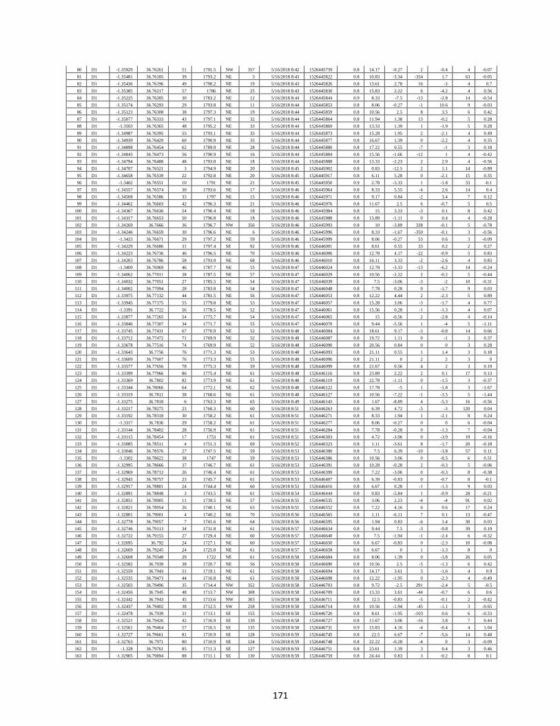
171

80 D1 -1.35929 36.76261 51 1791.5 NW 357 5/16/2018 8:42 1526445759 0.8 14.17 -0.27 2 -0.4 4 -0.07

81 D1 -1.35481 36.76185 39 1793.2 NE 3 5/16/2018 8:43 1526445822 0.8 10.83 -3.34 -354 1.7 63 -0.05

82 D1 -1.35436 36.76196 49 1790.2 NE 19 5/16/2018 8:43 1526445826 0.8 13.61 2.78 16 -3 4 0.7

83 D1 -1.35385 36.76217 57 1786 NE 25 5/16/2018 8:43 1526445830 0.8 15.83 2.22 6 -4.2 4 0.56

84 D1 -1.35225 36.76285 30 1783.2 NE 12 5/16/2018 8:44 1526445844 0.9 8.33 -7.5 -13 -2.8 14 -0.54

85 D1 -1.35174 36.76293 29 1793.8 NE 11 5/16/2018 8:44 1526445853 0.8 8.06 -0.27 -1 10.6 9 -0.03

86 D1 -1.35123 36.76308 38 1797.3 NE 19 5/16/2018 8:44 1526445859 0.8 10.56 2.5 8 3.5 6 0.42

87 D1 -1.35077 36.76333 43 1797.1 NE 32 5/16/2018 8:44 1526445864 0.8 11.94 1.38 13 -0.2 5 0.28

88 D1 -1.3503 36.76365 48 1795.2 NE 33 5/16/2018 8:44 1526445869 0.8 13.33 1.39 1 -1.9 5 0.28

89 D1 -1.34987 36.76395 55 1793.1 NE 35 5/16/2018 8:44 1526445873 0.8 15.28 1.95 2 -2.1 4 0.49

90 D1 -1.34939 36.76429 60 1790.9 NE 35 5/16/2018 8:44 1526445877 0.8 16.67 1.39 0 -2.2 4 0.35

91 D1 -1.34898 36.76454 62 1789.9 NE 28 5/16/2018 8:44 1526445880 0.8 17.22 0.55 -7 -1 3 0.18

92 D1 -1.34843 36.76473 56 1790.9 NE 16 5/16/2018 8:44 1526445884 0.8 15.56 -1.66 -12 1 4 -0.42

93 D1 -1.34794 36.76488 48 1793.8 NE 18 5/16/2018 8:44 1526445888 0.8 13.33 -2.23 2 2.9 4 -0.56

94 D1 -1.34707 36.76521 3 1794.9 NE 20 5/16/2018 8:45 1526445902 0.8 0.83 -12.5 2 1.1 14 -0.89

95 D1 -1.34658 36.76539 22 1792.8 NE 20 5/16/2018 8:45 1526445917 0.8 6.11 5.28 0 -2.1 15 0.35

96 D1 -1.3462 36.76551 10 1791 NE 21 5/16/2018 8:45 1526445950 0.9 2.78 -3.33 1 -1.8 33 -0.1

97 D1 -1.34557 36.76574 30 1793.6 NE 17 5/16/2018 8:46 1526445964 0.8 8.33 5.55 -4 2.6 14 0.4

98 D1 -1.34508 36.76586 33 1797 NE 15 5/16/2018 8:46 1526445971 0.8 9.17 0.84 -2 3.4 7 0.12

99 D1 -1.34462 36.76603 42 1796.3 NE 21 5/16/2018 8:46 1526445976 0.8 11.67 2.5 6 -0.7 5 0.5

100 D1 -1.34367 36.76636 54 1796.4 NE 18 5/16/2018 8:46 1526445984 0.8 15 3.33 -3 0.1 8 0.42

101 D1 -1.34317 36.76653 50 1796.8 NE 18 5/16/2018 8:46 1526445988 0.8 13.89 -1.11 0 0.4 4 -0.28

102 D1 -1.34269 36.7666 36 1796.7 NW 356 5/16/2018 8:46 1526445993 0.8 10 -3.89 338 -0.1 5 -0.78

103 D1 -1.34246 36.76659 30 1796.6 NE 6 5/16/2018 8:46 1526445996 0.8 8.33 -1.67 -350 -0.1 3 -0.56

104 D1 -1.3423 36.76671 29 1797.2 NE 59 5/16/2018 8:46 1526445999 0.8 8.06 -0.27 53 0.6 3 -0.09

105 D1 -1.34229 36.76686 31 1797.4 SE 92 5/16/2018 8:46 1526446001 0.8 8.61 0.55 33 0.2 2 0.27

106 D1 -1.34223 36.76736 46 1796.5 NE 70 5/16/2018 8:46 1526446006 0.8 12.78 4.17 -22 -0.9 5 0.83

107 D1 -1.34203 36.76786 58 1793.9 NE 68 5/16/2018 8:46 1526446010 0.8 16.11 3.33 -2 -2.6 4 0.83

108 D1 -1.3409 36.76969 46 1787.7 NE 55 5/16/2018 8:47 1526446024 0.8 12.78 -3.33 -13 -6.2 14 -0.24

109 D1 -1.34062 36.77011 38 1787.5 NE 57 5/16/2018 8:47 1526446029 0.8 10.56 -2.22 2 -0.2 5 -0.44

110 D1 -1.34032 36.77051 27 1785.5 NE 54 5/16/2018 8:47 1526446039 0.8 7.5 -3.06 -3 -2 10 -0.31

111 D1 -1.34002 36.77094 28 1783.8 NE 54 5/16/2018 8:47 1526446048 0.8 7.78 0.28 0 -1.7 9 0.03

112 D1 -1.33975 36.77132 44 1781.5 NE 56 5/16/2018 8:47 1526446053 0.8 12.22 4.44 2 -2.3 5 0.89

113 D1 -1.33945 36.77175 55 1779.8 NE 53 5/16/2018 8:47 1526446057 0.8 15.28 3.06 -3 -1.7 4 0.77

114 D1 -1.3391 36.7722 56 1778.5 NE 52 5/16/2018 8:47 1526446061 0.8 15.56 0.28 -1 -1.3 4 0.07

115 D1 -1.33877 36.77265 54 1775.7 NE 54 5/16/2018 8:47 1526446065 0.8 15 -0.56 2 -2.8 4 -0.14

116 D1 -1.33846 36.77307 34 1771.7 NE 55 5/16/2018 8:47 1526446070 0.8 9.44 -5.56 1 -4 5 -1.11

117 D1 -1.33745 36.77431 67 1770.9 NE 52 5/16/2018 8:48 1526446084 0.8 18.61 9.17 -3 -0.8 14 0.66

118 D1 -1.33712 36.77472 71 1769.9 NE 52 5/16/2018 8:48 1526446087 0.8 19.72 1.11 0 -1 3 0.37

119 D1 -1.33678 36.77516 74 1769.9 NE 52 5/16/2018 8:48 1526446090 0.8 20.56 0.84 0 0 3 0.28

120 D1 -1.33643 36.7756 76 1771.3 NE 53 5/16/2018 8:48 1526446093 0.8 21.11 0.55 1 1.4 3 0.18

121 D1 -1.33609 36.77607 76 1773.3 NE 55 5/16/2018 8:48 1526446096 0.8 21.11 0 2 2 3 0

122 D1 -1.33577 36.77656 78 1775.3 NE 59 5/16/2018 8:48 1526446099 0.8 21.67 0.56 4 2 3 0.19

123 D1 -1.33399 36.77966 86 1775.4 NE 61 5/16/2018 8:48 1526446116 0.8 23.89 2.22 2 0.1 17 0.13

124 D1 -1.33369 36.7802 82 1773.9 NE 61 5/16/2018 8:48 1526446119 0.8 22.78 -1.11 0 -1.5 3 -0.37

125 D1 -1.33344 36.78066 64 1772.1 NE 62 5/16/2018 8:48 1526446122 0.8 17.78 -5 1 -1.8 3 -1.67

126 D1 -1.33319 36.7811 38 1768.6 NE 61 5/16/2018 8:48 1526446127 0.8 10.56 -7.22 -1 -3.5 5 -1.44

127 D1 -1.33275 36.7818 6 1763.3 NE 65 5/16/2018 8:49 1526446143 0.8 1.67 -8.89 4 -5.3 16 -0.56

128 D1 -1.33217 36.78275 23 1760.3 NE 60 5/16/2018 8:51 1526446263 0.8 6.39 4.72 -5 -3 120 0.04

129 D1 -1.33192 36.78318 30 1758.2 NE 61 5/16/2018 8:51 1526446271 0.8 8.33 1.94 1 -2.1 8 0.24

130 D1 -1.3317 36.7836 29 1758.2 NE 61 5/16/2018 8:51 1526446277 0.8 8.06 -0.27 0 0 6 -0.04

131 D1 -1.33144 36.78402 28 1756.9 NE 61 5/16/2018 8:51 1526446284 0.8 7.78 -0.28 0 -1.3 7 -0.04

132 D1 -1.33115 36.78454 17 1753 NE 61 5/16/2018 8:51 1526446303 0.8 4.72 -3.06 0 -3.9 19 -0.16

133 D1 -1.33085 36.78511 4 1751.3 NE 69 5/16/2018 8:52 1526446323 0.8 1.11 -3.61 8 -1.7 20 -0.18

134 D1 -1.33046 36.78576 27 1747.5 NE 59 5/16/2018 8:53 1526446380 0.8 7.5 6.39 -10 -3.8 57 0.11

135 D1 -1.3302 36.78622 38 1747 NE 59 5/16/2018 8:53 1526446386 0.8 10.56 3.06 0 -0.5 6 0.51

136 D1 -1.32995 36.78666 37 1746.7 NE 61 5/16/2018 8:53 1526446391 0.8 10.28 -0.28 2 -0.3 5 -0.06

137 D1 -1.32969 36.78712 26 1746.4 NE 61 5/16/2018 8:53 1526446399 0.8 7.22 -3.06 0 -0.3 8 -0.38

138 D1 -1.32943 36.78757 23 1745.7 NE 61 5/16/2018 8:53 1526446407 0.8 6.39 -0.83 0 -0.7 8 -0.1

139 D1 -1.32917 36.78801 24 1744.4 NE 60 5/16/2018 8:53 1526446416 0.8 6.67 0.28 -1 -1.3 9 0.03

140 D1 -1.32891 36.78848 3 1743.5 NE 61 5/16/2018 8:54 1526446444 0.8 0.83 -5.84 1 -0.9 28 -0.21

141 D1 -1.32851 36.78905 11 1739.5 NE 57 5/16/2018 8:55 1526446535 0.8 3.06 2.23 -4 -4 91 0.02

142 D1 -1.32821 36.78954 26 1740.1 NE 63 5/16/2018 8:55 1526446552 0.8 7.22 4.16 6 0.6 17 0.24

143 D1 -1.32801 36.79001 4 1740.2 NE 70 5/16/2018 8:56 1526446565 0.8 1.11 -6.11 7 0.1 13 -0.47

144 D1 -1.32778 36.79057 7 1741.6 NE 64 5/16/2018 8:56 1526446595 0.8 1.94 0.83 -6 1.4 30 0.03

145 D1 -1.32746 36.79113 34 1731.8 NE 61 5/16/2018 8:57 1526446634 0.8 9.44 7.5 -3 -9.8 39 0.19

146 D1 -1.32722 36.79155 27 1729.4 NE 60 5/16/2018 8:57 1526446640 0.8 7.5 -1.94 -1 -2.4 6 -0.32

147 D1 -1.32695 36.792 24 1727.1 NE 60 5/16/2018 8:57 1526446650 0.8 6.67 -0.83 0 -2.3 10 -0.08

148 D1 -1.32669 36.79245 24 1725.8 NE 61 5/16/2018 8:57 1526446658 0.8 6.67 0 1 -1.3 8 0

149 D1 -1.32608 36.79348 29 1722 NE 61 5/16/2018 8:58 1526446684 0.8 8.06 1.39 0 -3.8 26 0.05

150 D1 -1.32582 36.7939 38 1720.7 NE 56 5/16/2018 8:58 1526446690 0.8 10.56 2.5 -5 -1.3 6 0.42

151 D1 -1.32559 36.7943 51 1719.1 NE 61 5/16/2018 8:58 1526446694 0.8 14.17 3.61 5 -1.6 4 0.9

152 D1 -1.32535 36.79473 44 1716.8 NE 61 5/16/2018 8:58 1526446698 0.8 12.22 -1.95 0 -2.3 4 -0.49

153 D1 -1.32503 36.79496 35 1714.4 NW 352 5/16/2018 8:58 1526446703 0.8 9.72 -2.5 291 -2.4 5 -0.5

154 D1 -1.32456 36.7945 48 1713.7 NW 308 5/16/2018 8:58 1526446709 0.8 13.33 3.61 -44 -0.7 6 0.6

155 D1 -1.32442 36.7943 45 1713.6 NW 303 5/16/2018 8:58 1526446711 0.8 12.5 -0.83 -5 -0.1 2 -0.42

156 D1 -1.32437 36.79402 38 1712.5 SW 258 5/16/2018 8:58 1526446714 0.8 10.56 -1.94 -45 -1.1 3 -0.65

157 D1 -1.32478 36.7939 31 1713.1 SE 155 5/16/2018 8:58 1526446720 0.8 8.61 -1.95 -103 0.6 6 -0.33

158 D1 -1.32521 36.79426 42 1716.9 SE 139 5/16/2018 8:58 1526446727 0.8 11.67 3.06 -16 3.8 7 0.44

159 D1 -1.32561 36.79464 57 1716.5 SE 135 5/16/2018 8:58 1526446731 0.9 15.83 4.16 -4 -0.4 4 1.04

160 D1 -1.32727 36.79661 81 1710.9 SE 128 5/16/2018 8:59 1526446745 0.8 22.5 6.67 -7 -5.6 14 0.48

161 D1 -1.32763 36.7971 80 1710.9 SE 124 5/16/2018 8:59 1526446748 0.8 22.22 -0.28 -4 0 3 -0.09

162 D1 -1.328 36.79761 85 1711.3 SE 127 5/16/2018 8:59 1526446751 0.8 23.61 1.39 3 0.4 3 0.46

163 D1 -1.32905 36.79894 88 1711.1 SE 130 5/16/2018 8:59 1526446759 0.8 24.44 0.83 3 -0.2 8 0.1

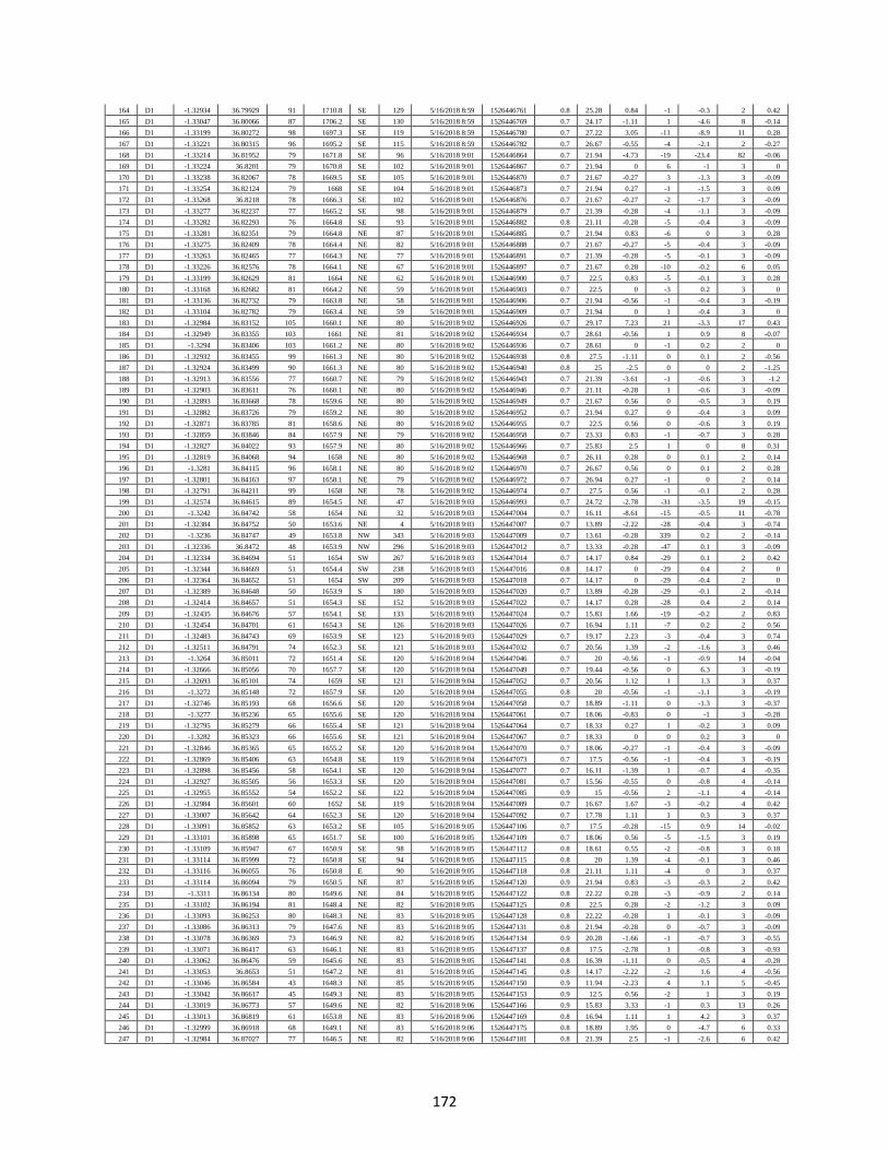
172

164 D1 -1.32934 36.79929 91 1710.8 SE 129 5/16/2018 8:59 1526446761 0.8 25.28 0.84 -1 -0.3 2 0.42

165 D1 -1.33047 36.80066 87 1706.2 SE 130 5/16/2018 8:59 1526446769 0.7 24.17 -1.11 1 -4.6 8 -0.14

166 D1 -1.33199 36.80272 98 1697.3 SE 119 5/16/2018 8:59 1526446780 0.7 27.22 3.05 -11 -8.9 11 0.28

167 D1 -1.33221 36.80315 96 1695.2 SE 115 5/16/2018 8:59 1526446782 0.7 26.67 -0.55 -4 -2.1 2 -0.27

168 D1 -1.33214 36.81952 79 1671.8 SE 96 5/16/2018 9:01 1526446864 0.7 21.94 -4.73 -19 -23.4 82 -0.06

169 D1 -1.33224 36.8201 79 1670.8 SE 102 5/16/2018 9:01 1526446867 0.7 21.94 0 6 -1 3 0

170 D1 -1.33238 36.82067 78 1669.5 SE 105 5/16/2018 9:01 1526446870 0.7 21.67 -0.27 3 -1.3 3 -0.09

171 D1 -1.33254 36.82124 79 1668 SE 104 5/16/2018 9:01 1526446873 0.7 21.94 0.27 -1 -1.5 3 0.09

172 D1 -1.33268 36.8218 78 1666.3 SE 102 5/16/2018 9:01 1526446876 0.7 21.67 -0.27 -2 -1.7 3 -0.09

173 D1 -1.33277 36.82237 77 1665.2 SE 98 5/16/2018 9:01 1526446879 0.7 21.39 -0.28 -4 -1.1 3 -0.09

174 D1 -1.33282 36.82293 76 1664.8 SE 93 5/16/2018 9:01 1526446882 0.8 21.11 -0.28 -5 -0.4 3 -0.09

175 D1 -1.33281 36.82351 79 1664.8 NE 87 5/16/2018 9:01 1526446885 0.7 21.94 0.83 -6 0 3 0.28

176 D1 -1.33275 36.82409 78 1664.4 NE 82 5/16/2018 9:01 1526446888 0.7 21.67 -0.27 -5 -0.4 3 -0.09

177 D1 -1.33263 36.82465 77 1664.3 NE 77 5/16/2018 9:01 1526446891 0.7 21.39 -0.28 -5 -0.1 3 -0.09

178 D1 -1.33226 36.82576 78 1664.1 NE 67 5/16/2018 9:01 1526446897 0.7 21.67 0.28 -10 -0.2 6 0.05

179 D1 -1.33199 36.82629 81 1664 NE 62 5/16/2018 9:01 1526446900 0.7 22.5 0.83 -5 -0.1 3 0.28

180 D1 -1.33168 36.82682 81 1664.2 NE 59 5/16/2018 9:01 1526446903 0.7 22.5 0 -3 0.2 3 0

181 D1 -1.33136 36.82732 79 1663.8 NE 58 5/16/2018 9:01 1526446906 0.7 21.94 -0.56 -1 -0.4 3 -0.19

182 D1 -1.33104 36.82782 79 1663.4 NE 59 5/16/2018 9:01 1526446909 0.7 21.94 0 1 -0.4 3 0

183 D1 -1.32984 36.83152 105 1660.1 NE 80 5/16/2018 9:02 1526446926 0.7 29.17 7.23 21 -3.3 17 0.43

184 D1 -1.32949 36.83355 103 1661 NE 81 5/16/2018 9:02 1526446934 0.7 28.61 -0.56 1 0.9 8 -0.07

185 D1 -1.3294 36.83406 103 1661.2 NE 80 5/16/2018 9:02 1526446936 0.7 28.61 0 -1 0.2 2 0

186 D1 -1.32932 36.83455 99 1661.3 NE 80 5/16/2018 9:02 1526446938 0.8 27.5 -1.11 0 0.1 2 -0.56

187 D1 -1.32924 36.83499 90 1661.3 NE 80 5/16/2018 9:02 1526446940 0.8 25 -2.5 0 0 2 -1.25

188 D1 -1.32913 36.83556 77 1660.7 NE 79 5/16/2018 9:02 1526446943 0.7 21.39 -3.61 -1 -0.6 3 -1.2

189 D1 -1.32903 36.83611 76 1660.1 NE 80 5/16/2018 9:02 1526446946 0.7 21.11 -0.28 1 -0.6 3 -0.09

190 D1 -1.32893 36.83668 78 1659.6 NE 80 5/16/2018 9:02 1526446949 0.7 21.67 0.56 0 -0.5 3 0.19

191 D1 -1.32882 36.83726 79 1659.2 NE 80 5/16/2018 9:02 1526446952 0.7 21.94 0.27 0 -0.4 3 0.09

192 D1 -1.32871 36.83785 81 1658.6 NE 80 5/16/2018 9:02 1526446955 0.7 22.5 0.56 0 -0.6 3 0.19

193 D1 -1.32859 36.83846 84 1657.9 NE 79 5/16/2018 9:02 1526446958 0.7 23.33 0.83 -1 -0.7 3 0.28

194 D1 -1.32827 36.84022 93 1657.9 NE 80 5/16/2018 9:02 1526446966 0.7 25.83 2.5 1 0 8 0.31

195 D1 -1.32819 36.84068 94 1658 NE 80 5/16/2018 9:02 1526446968 0.7 26.11 0.28 0 0.1 2 0.14

196 D1 -1.3281 36.84115 96 1658.1 NE 80 5/16/2018 9:02 1526446970 0.7 26.67 0.56 0 0.1 2 0.28

197 D1 -1.32801 36.84163 97 1658.1 NE 79 5/16/2018 9:02 1526446972 0.7 26.94 0.27 -1 0 2 0.14

198 D1 -1.32791 36.84211 99 1658 NE 78 5/16/2018 9:02 1526446974 0.7 27.5 0.56 -1 -0.1 2 0.28

199 D1 -1.32574 36.84615 89 1654.5 NE 47 5/16/2018 9:03 1526446993 0.7 24.72 -2.78 -31 -3.5 19 -0.15

200 D1 -1.3242 36.84742 58 1654 NE 32 5/16/2018 9:03 1526447004 0.7 16.11 -8.61 -15 -0.5 11 -0.78

201 D1 -1.32384 36.84752 50 1653.6 NE 4 5/16/2018 9:03 1526447007 0.7 13.89 -2.22 -28 -0.4 3 -0.74

202 D1 -1.3236 36.84747 49 1653.8 NW 343 5/16/2018 9:03 1526447009 0.7 13.61 -0.28 339 0.2 2 -0.14

203 D1 -1.32336 36.8472 48 1653.9 NW 296 5/16/2018 9:03 1526447012 0.7 13.33 -0.28 -47 0.1 3 -0.09

204 D1 -1.32334 36.84694 51 1654 SW 267 5/16/2018 9:03 1526447014 0.7 14.17 0.84 -29 0.1 2 0.42

205 D1 -1.32344 36.84669 51 1654.4 SW 238 5/16/2018 9:03 1526447016 0.8 14.17 0 -29 0.4 2 0

206 D1 -1.32364 36.84652 51 1654 SW 209 5/16/2018 9:03 1526447018 0.7 14.17 0 -29 -0.4 2 0

207 D1 -1.32389 36.84648 50 1653.9 S 180 5/16/2018 9:03 1526447020 0.7 13.89 -0.28 -29 -0.1 2 -0.14

208 D1 -1.32414 36.84657 51 1654.3 SE 152 5/16/2018 9:03 1526447022 0.7 14.17 0.28 -28 0.4 2 0.14

209 D1 -1.32435 36.84676 57 1654.1 SE 133 5/16/2018 9:03 1526447024 0.7 15.83 1.66 -19 -0.2 2 0.83

210 D1 -1.32454 36.84701 61 1654.3 SE 126 5/16/2018 9:03 1526447026 0.7 16.94 1.11 -7 0.2 2 0.56

211 D1 -1.32483 36.84743 69 1653.9 SE 123 5/16/2018 9:03 1526447029 0.7 19.17 2.23 -3 -0.4 3 0.74

212 D1 -1.32511 36.84791 74 1652.3 SE 121 5/16/2018 9:03 1526447032 0.7 20.56 1.39 -2 -1.6 3 0.46

213 D1 -1.3264 36.85011 72 1651.4 SE 120 5/16/2018 9:04 1526447046 0.7 20 -0.56 -1 -0.9 14 -0.04

214 D1 -1.32666 36.85056 70 1657.7 SE 120 5/16/2018 9:04 1526447049 0.7 19.44 -0.56 0 6.3 3 -0.19

215 D1 -1.32693 36.85101 74 1659 SE 121 5/16/2018 9:04 1526447052 0.7 20.56 1.12 1 1.3 3 0.37

216 D1 -1.3272 36.85148 72 1657.9 SE 120 5/16/2018 9:04 1526447055 0.8 20 -0.56 -1 -1.1 3 -0.19

217 D1 -1.32746 36.85193 68 1656.6 SE 120 5/16/2018 9:04 1526447058 0.7 18.89 -1.11 0 -1.3 3 -0.37

218 D1 -1.3277 36.85236 65 1655.6 SE 120 5/16/2018 9:04 1526447061 0.7 18.06 -0.83 0 -1 3 -0.28

219 D1 -1.32795 36.85279 66 1655.4 SE 121 5/16/2018 9:04 1526447064 0.7 18.33 0.27 1 -0.2 3 0.09

220 D1 -1.3282 36.85323 66 1655.6 SE 121 5/16/2018 9:04 1526447067 0.7 18.33 0 0 0.2 3 0

221 D1 -1.32846 36.85365 65 1655.2 SE 120 5/16/2018 9:04 1526447070 0.7 18.06 -0.27 -1 -0.4 3 -0.09

222 D1 -1.32869 36.85406 63 1654.8 SE 119 5/16/2018 9:04 1526447073 0.7 17.5 -0.56 -1 -0.4 3 -0.19

223 D1 -1.32898 36.85456 58 1654.1 SE 120 5/16/2018 9:04 1526447077 0.7 16.11 -1.39 1 -0.7 4 -0.35

224 D1 -1.32927 36.85505 56 1653.3 SE 120 5/16/2018 9:04 1526447081 0.7 15.56 -0.55 0 -0.8 4 -0.14

225 D1 -1.32955 36.85552 54 1652.2 SE 122 5/16/2018 9:04 1526447085 0.9 15 -0.56 2 -1.1 4 -0.14

226 D1 -1.32984 36.85601 60 1652 SE 119 5/16/2018 9:04 1526447089 0.7 16.67 1.67 -3 -0.2 4 0.42

227 D1 -1.33007 36.85642 64 1652.3 SE 120 5/16/2018 9:04 1526447092 0.7 17.78 1.11 1 0.3 3 0.37

228 D1 -1.33091 36.85852 63 1653.2 SE 105 5/16/2018 9:05 1526447106 0.7 17.5 -0.28 -15 0.9 14 -0.02

229 D1 -1.33101 36.85898 65 1651.7 SE 100 5/16/2018 9:05 1526447109 0.7 18.06 0.56 -5 -1.5 3 0.19

230 D1 -1.33109 36.85947 67 1650.9 SE 98 5/16/2018 9:05 1526447112 0.8 18.61 0.55 -2 -0.8 3 0.18

231 D1 -1.33114 36.85999 72 1650.8 SE 94 5/16/2018 9:05 1526447115 0.8 20 1.39 -4 -0.1 3 0.46

232 D1 -1.33116 36.86055 76 1650.8 E 90 5/16/2018 9:05 1526447118 0.8 21.11 1.11 -4 0 3 0.37

233 D1 -1.33114 36.86094 79 1650.5 NE 87 5/16/2018 9:05 1526447120 0.9 21.94 0.83 -3 -0.3 2 0.42

234 D1 -1.3311 36.86134 80 1649.6 NE 84 5/16/2018 9:05 1526447122 0.8 22.22 0.28 -3 -0.9 2 0.14

235 D1 -1.33102 36.86194 81 1648.4 NE 82 5/16/2018 9:05 1526447125 0.8 22.5 0.28 -2 -1.2 3 0.09

236 D1 -1.33093 36.86253 80 1648.3 NE 83 5/16/2018 9:05 1526447128 0.8 22.22 -0.28 1 -0.1 3 -0.09

237 D1 -1.33086 36.86313 79 1647.6 NE 83 5/16/2018 9:05 1526447131 0.8 21.94 -0.28 0 -0.7 3 -0.09

238 D1 -1.33078 36.86369 73 1646.9 NE 82 5/16/2018 9:05 1526447134 0.9 20.28 -1.66 -1 -0.7 3 -0.55

239 D1 -1.33071 36.86417 63 1646.1 NE 83 5/16/2018 9:05 1526447137 0.8 17.5 -2.78 1 -0.8 3 -0.93

240 D1 -1.33062 36.86476 59 1645.6 NE 83 5/16/2018 9:05 1526447141 0.8 16.39 -1.11 0 -0.5 4 -0.28

241 D1 -1.33053 36.8653 51 1647.2 NE 81 5/16/2018 9:05 1526447145 0.8 14.17 -2.22 -2 1.6 4 -0.56

242 D1 -1.33046 36.86584 43 1648.3 NE 85 5/16/2018 9:05 1526447150 0.9 11.94 -2.23 4 1.1 5 -0.45

243 D1 -1.33042 36.86617 45 1649.3 NE 83 5/16/2018 9:05 1526447153 0.9 12.5 0.56 -2 1 3 0.19

244 D1 -1.33019 36.86773 57 1649.6 NE 82 5/16/2018 9:06 1526447166 0.9 15.83 3.33 -1 0.3 13 0.26

245 D1 -1.33013 36.86819 61 1653.8 NE 83 5/16/2018 9:06 1526447169 0.8 16.94 1.11 1 4.2 3 0.37

246 D1 -1.32999 36.86918 68 1649.1 NE 83 5/16/2018 9:06 1526447175 0.8 18.89 1.95 0 -4.7 6 0.33

247 D1 -1.32984 36.87027 77 1646.5 NE 82 5/16/2018 9:06 1526447181 0.8 21.39 2.5 -1 -2.6 6 0.42

173

248 D1 -1.32971 36.87146 80 1643.2 NE 83 5/16/2018 9:06 1526447187 0.8 22.22 0.83 1 -3.3 6 0.14

249 D1 -1.32937 36.87386 80 1644.3 NE 82 5/16/2018 9:06 1526447199 0.8 22.22 0 -1 1.1 12 0

250 D1 -1.32928 36.87445 81 1646.1 NE 82 5/16/2018 9:06 1526447202 0.8 22.5 0.28 0 1.8 3 0.09

251 D1 -1.32921 36.87506 81 1647.4 NE 83 5/16/2018 9:06 1526447205 0.8 22.5 0 1 1.3 3 0

252 D1 -1.32913 36.87567 83 1647.8 NE 82 5/16/2018 9:06 1526447208 0.8 23.06 0.56 -1 0.4 3 0.19

253 D1 -1.32904 36.87629 84 1647.9 NE 82 5/16/2018 9:06 1526447211 0.8 23.33 0.27 0 0.1 3 0.09

254 D1 -1.3285 36.8804 84 1638.9 NE 84 5/16/2018 9:07 1526447230 0.8 23.33 0 2 -9 19 0

255 D1 -1.32848 36.88213 68 1636.5 SE 94 5/16/2018 9:07 1526447239 0.8 18.89 -4.44 10 -2.4 9 -0.49

256 D1 -1.32854 36.88273 62 1637.7 SE 98 5/16/2018 9:07 1526447243 0.8 17.22 -1.67 4 1.2 4 -0.42

257 D1 -1.32874 36.8837 70 1639.8 SE 104 5/16/2018 9:07 1526447249 0.8 19.44 2.22 6 2.1 6 0.37

258 D1 -1.32889 36.88424 75 1640.7 SE 107 5/16/2018 9:07 1526447252 0.8 20.83 1.39 3 0.9 3 0.46

259 D1 -1.32911 36.88477 78 1642 SE 113 5/16/2018 9:07 1526447255 0.8 21.67 0.84 6 1.3 3 0.28

260 D1 -1.32936 36.88532 81 1643.7 SE 115 5/16/2018 9:07 1526447258 0.8 22.5 0.83 2 1.7 3 0.28

261 D1 -1.32965 36.88587 83 1647.1 SE 119 5/16/2018 9:07 1526447261 0.8 23.06 0.56 4 3.4 3 0.19

262 D1 -1.32998 36.88641 85 1648.7 SE 122 5/16/2018 9:07 1526447264 0.8 23.61 0.55 3 1.6 3 0.18

263 D1 -1.33105 36.88774 86 1650.2 SE 130 5/16/2018 9:07 1526447272 0.8 23.89 0.28 8 1.5 8 0.04

264 D1 -1.33363 36.89069 74 1644.9 SE 131 5/16/2018 9:08 1526447291 0.8 20.56 -3.33 1 -5.3 19 -0.18

265 D1 -1.33395 36.89107 67 1644.9 SE 131 5/16/2018 9:08 1526447294 0.8 18.61 -1.95 0 0 3 -0.65

266 D1 -1.33428 36.89143 65 1644.4 SE 132 5/16/2018 9:08 1526447297 0.9 18.06 -0.55 1 -0.5 3 -0.18

267 D1 -1.33465 36.89187 56 1644.1 SE 132 5/16/2018 9:08 1526447301 0.8 15.56 -2.5 0 -0.3 4 -0.63

268 D1 -1.33504 36.8923 61 1643.6 SE 132 5/16/2018 9:08 1526447305 0.8 16.94 1.38 0 -0.5 4 0.35

269 D1 -1.33544 36.89275 59 1642.3 SE 131 5/16/2018 9:08 1526447309 0.8 16.39 -0.55 -1 -1.3 4 -0.14

270 D1 -1.3358 36.89316 52 1642.7 SE 131 5/16/2018 9:08 1526447313 0.8 14.44 -1.95 0 0.4 4 -0.49

271 D1 -1.33612 36.89353 49 1642.5 SE 129 5/16/2018 9:08 1526447317 0.8 13.61 -0.83 -2 -0.2 4 -0.21

272 D1 -1.33645 36.89394 53 1641 SE 130 5/16/2018 9:08 1526447321 0.8 14.72 1.11 1 -1.5 4 0.28

273 D1 -1.33682 36.89436 52 1639.7 SE 132 5/16/2018 9:08 1526447325 0.8 14.44 -0.28 2 -1.3 4 -0.07

274 D1 -1.33714 36.89472 48 1640.2 SE 131 5/16/2018 9:08 1526447329 0.8 13.33 -1.11 -1 0.5 4 -0.28

275 D1 -1.33748 36.8951 55 1640.5 SE 133 5/16/2018 9:08 1526447333 0.8 15.28 1.95 2 0.3 4 0.49

276 D1 -1.33901 36.89682 72 1640.7 SE 131 5/16/2018 9:09 1526447347 0.8 20 4.72 -2 0.2 14 0.34

277 D1 -1.33937 36.89723 75 1641 SE 131 5/16/2018 9:09 1526447350 0.8 20.83 0.83 0 0.3 3 0.28

278 D1 -1.33976 36.89766 77 1641.4 SE 131 5/16/2018 9:09 1526447353 0.8 21.39 0.56 0 0.4 3 0.19

279 D1 -1.34012 36.89807 69 1641.9 SE 131 5/16/2018 9:09 1526447356 0.8 19.17 -2.22 0 0.5 3 -0.74

280 D1 -1.34042 36.89845 63 1641.3 SE 128 5/16/2018 9:09 1526447359 0.8 17.5 -1.67 -3 -0.6 3 -0.56

281 D1 -1.34074 36.89882 66 1640.6 SE 131 5/16/2018 9:09 1526447362 0.8 18.33 0.83 3 -0.7 3 0.28

282 D1 -1.34107 36.8992 69 1641.2 SE 131 5/16/2018 9:09 1526447365 0.8 19.17 0.84 0 0.6 3 0.28

283 D1 -1.34143 36.8996 73 1642.2 SE 131 5/16/2018 9:09 1526447368 0.8 20.28 1.11 0 1 3 0.37

284 D1 -1.34181 36.90002 77 1642.8 SE 131 5/16/2018 9:09 1526447371 0.8 21.39 1.11 0 0.6 3 0.37

285 D1 -1.34221 36.90048 81 1643.5 SE 131 5/16/2018 9:09 1526447374 0.8 22.5 1.11 0 0.7 3 0.37

286 D1 -1.34264 36.90094 87 1644.9 SE 134 5/16/2018 9:09 1526447377 0.8 24.17 1.67 3 1.4 3 0.56

287 D1 -1.34386 36.90235 92 1644.8 SE 130 5/16/2018 9:09 1526447385 0.8 25.56 1.39 -4 -0.1 8 0.17

288 D1 -1.34416 36.90271 91 1644.6 SE 130 5/16/2018 9:09 1526447387 0.8 25.28 -0.28 0 -0.2 2 -0.14

289 D1 -1.34445 36.90305 91 1644.6 SE 131 5/16/2018 9:09 1526447389 0.8 25.28 0 1 0 2 0

290 D1 -1.34475 36.90339 90 1644.9 SE 132 5/16/2018 9:09 1526447391 0.8 25 -0.28 1 0.3 2 -0.14

291 D1 -1.34606 36.9068 64 1639.3 NE 84 5/16/2018 9:10 1526447411 0.8 17.78 -7.22 -48 -5.6 20 -0.36

292 D1 -1.34602 36.90733 49 1637.6 NE 88 5/16/2018 9:10 1526447415 0.8 13.61 -4.17 4 -1.7 4 -1.04

293 D1 -1.34594 36.90783 42 1637.1 NE 75 5/16/2018 9:10 1526447420 0.8 11.67 -1.94 -13 -0.5 5 -0.39

294 D1 -1.34586 36.9083 13 1632.4 SE 92 5/16/2018 9:10 1526447439 0.8 3.61 -8.06 17 -4.7 19 -0.42

295 D1 -1.34608 36.90879 35 1629.9 SE 126 5/16/2018 9:11 1526447511 0.8 9.72 6.11 34 -2.5 72 0.08

296 D1 -1.34658 36.91 41 1635.5 NE 82 5/16/2018 9:12 1526447526 0.9 11.39 1.67 -44 5.6 15 0.11

297 D1 -1.34647 36.91049 57 1634.1 NE 73 5/16/2018 9:12 1526447530 0.8 15.83 4.44 -9 -1.4 4 1.11

298 D1 -1.34628 36.91097 71 1633.7 NE 69 5/16/2018 9:12 1526447533 0.8 19.72 3.89 -4 -0.4 3 1.3

299 D1 -1.34605 36.91151 80 1633.2 NE 65 5/16/2018 9:12 1526447536 0.8 22.22 2.5 -4 -0.5 3 0.83

300 D1 -1.34575 36.91207 87 1632.8 NE 60 5/16/2018 9:12 1526447539 0.8 24.17 1.95 -5 -0.4 3 0.65

301 D1 -1.34467 36.91358 85 1631.4 NE 53 5/16/2018 9:12 1526447547 0.8 23.61 -0.56 -7 -1.4 8 -0.07

302 D1 -1.34436 36.91398 65 1630.6 NE 51 5/16/2018 9:12 1526447550 0.8 18.06 -5.55 -2 -0.8 3 -1.85

303 D1 -1.34416 36.91415 55 1630.1 NE 33 5/16/2018 9:12 1526447552 0.8 15.28 -2.78 -18 -0.5 2 -1.39

304 D1 -1.34392 36.91425 52 1629.3 NE 19 5/16/2018 9:12 1526447554 0.8 14.44 -0.84 -14 -0.8 2 -0.42

305 D1 -1.3437 36.91427 45 1628.3 N 360 5/16/2018 9:12 1526447556 0.8 12.5 -1.94 341 -1 2 -0.97

306 D1 -1.34338 36.91412 49 1627.5 NW 326 5/16/2018 9:12 1526447559 0.8 13.61 1.11 -34 -0.8 3 0.37

307 D1 -1.34293 36.91376 60 1628.2 NW 324 5/16/2018 9:12 1526447563 0.8 16.67 3.06 -2 0.7 4 0.77

308 D1 -1.34216 36.91317 65 1629 NW 324 5/16/2018 9:12 1526447569 0.8 18.06 1.39 0 0.8 6 0.23

309 D1 -1.34176 36.91288 65 1628.8 NW 324 5/16/2018 9:12 1526447572 0.8 18.06 0 0 -0.2 3 0

310 D1 -1.3403 36.91182 38 1630.4 NW 325 5/16/2018 9:13 1526447586 0.8 10.56 -7.5 1 1.6 14 -0.54

311 D1 -1.33995 36.91154 27 1631.3 NW 312 5/16/2018 9:13 1526447592 0.8 7.5 -3.06 -13 0.9 6 -0.51

312 D1 -1.3399 36.9114 32 1631.2 NW 285 5/16/2018 9:13 1526447594 0.8 8.89 1.39 -27 -0.1 2 0.7

313 D1 -1.33987 36.91105 38 1632 SW 265 5/16/2018 9:13 1526447598 0.9 10.56 1.67 -20 0.8 4 0.42

314 D1 -1.33993 36.91087 38 1632.1 SW 246 5/16/2018 9:13 1526447600 0.8 10.56 0 -19 0.1 2 0

315 D1 -1.34024 36.91046 40 1634.2 SW 233 5/16/2018 9:13 1526447605 0.8 11.11 0.55 -13 2.1 5 0.11

316 D1 -1.34053 36.91007 36 1632.9 SW 234 5/16/2018 9:13 1526447610 0.8 10 -1.11 1 -1.3 5 -0.22

317 D1 -1.34087 36.90971 31 1631.4 SW 227 5/16/2018 9:13 1526447616 0.8 8.61 -1.39 -7 -1.5 6 -0.23

318 D1 -1.34111 36.9093 22 1630.6 SW 240 5/16/2018 9:13 1526447624 0.8 6.11 -2.5 13 -0.8 8 -0.31

319 D1 -1.34146 36.90846 15 1631.2 SW 238 5/16/2018 9:14 1526447646 0.8 4.17 -1.94 -2 0.6 22 -0.09

320 D1 -1.34176 36.90806 17 1631.7 SW 231 5/16/2018 9:14 1526447658 0.8 4.72 0.55 -7 0.5 12 0.05

321 D1 -1.34194 36.90754 24 1632.1 SW 250 5/16/2018 9:14 1526447670 0.8 6.67 1.95 19 0.4 12 0.16

322 D1 -1.34207 36.90702 28 1633.9 SW 258 5/16/2018 9:14 1526447678 0.8 7.78 1.11 8 1.8 8 0.14

323 D1 -1.34221 36.90625 2 1636.7 NE 72 5/16/2018 9:16 1526447761 0.9 0.56 -7.22 -186 2.8 83 -0.09

324 D1 -1.34221 36.90625 1 1636.8 NE 78 5/16/2018 9:16 1526447764 0.9 0.28 -0.28 6 0.1 3 -0.09

325 D1 -1.34222 36.90626 2 1634.5 SW 243 5/16/2018 9:17 1526447858 0.9 0.56 0.28 165 -2.3 94 0

326 D1 -1.34225 36.90622 2 1636.1 NE 65 5/16/2018 9:18 1526447890 0.8 0.56 0 -178 1.6 32 0

327 D1 -1.34221 36.90624 2 1640.4 SW 251 5/16/2018 9:24 1526448281 0.9 0.56 0 186 4.3 391 0

328 D1 -1.34228 36.90607 4 1637.2 NW 296 5/16/2018 9:26 1526448363 0.9 1.11 0.55 45 -3.2 82 0.01

329 D1 -1.34228 36.90605 4 1637.2 NW 300 5/16/2018 9:26 1526448365 0.8 1.11 0 4 0 2 0

330 D1 -1.34219 36.90588 9 1643.3 NW 288 5/16/2018 9:26 1526448374 0.8 2.5 1.39 -12 6.1 9 0.15

331 D1 -1.34204 36.90527 4 1651.1 SW 234 5/16/2018 9:26 1526448408 0.8 1.11 -1.39 -54 7.8 34 -0.04

174

332 D1 -1.34205 36.90525 4 1649.9 SW 202 5/16/2018 9:26 1526448410 0.8 1.11 0 -32 -1.2 2 0

333 D1 -1.34207 36.90525 4 1647.5 SW 186 5/16/2018 9:26 1526448412 0.8 1.11 0 -16 -2.4 2 0

334 D1 -1.34236 36.90512 4 1638.9 SW 231 5/16/2018 9:27 1526448437 0.8 1.11 0 45 -8.6 25 0

335 D1 -1.3424 36.90511 3 1637.1 SE 177 5/16/2018 9:27 1526448443 0.8 0.83 -0.28 -54 -1.8 6 -0.05

336 D1 -1.34235 36.90509 0 1655.3 SE 158 5/16/2018 9:36 1526448967 0.8 0 -0.83 -19 18.2 524 0

337 D1 -1.34238 36.90511 0 1639.2 SE 158 5/16/2018 9:46 1526449568 0.7 0 0 0 -16.1 601 0

338 D1 -1.34238 36.90511 0 1639.2 SE 158 5/16/2018 9:56 1526450169 0.8 0 0 0 0 601 0

339 D1 -1.34238 36.90511 0 1639.2 SE 158 5/16/2018 10:06 1526450770 0.7 0 0 0 0 601 0

340 D1 -1.34238 36.90511 0 1639.2 SE 158 5/16/2018 10:16 1526451372 0.8 0 0 0 0 602 0

341 D1 -1.34238 36.90511 0 1639.2 SE 158 5/16/2018 10:26 1526451973 0.8 0 0 0 0 601 0

342 D1 -1.34238 36.90511 0 1639.2 SE 158 5/16/2018 10:36 1526452574 0.8 0 0 0 0 601 0

343 D1 -1.34238 36.90511 0 1639.2 SE 158 5/16/2018 10:46 1526453175 0.9 0 0 0 0 601 0

344 D1 -1.34238 36.90511 0 1639.2 SE 158 5/16/2018 10:56 1526453777 0.8 0 0 0 0 602 0

345 D1 -1.34238 36.90511 0 1639.2 SE 158 5/16/2018 11:06 1526454378 0.8 0 0 0 0 601 0

346 D1 -1.34238 36.90511 0 1639.2 SE 158 5/16/2018 11:16 1526454979 0.8 0 0 0 0 601 0

347 D1 -1.34238 36.90511 0 1639.2 SE 158 5/16/2018 11:26 1526455580 0.8 0 0 0 0 601 0

348 D1 -1.34242 36.90509 2 1639.9 NE 36 5/16/2018 11:28 1526455684 0.8 0.56 0.56 -122 0.7 104 0.01

349 D1 -1.34242 36.90509 5 1639.9 SW 229 5/16/2018 11:28 1526455689 0.8 1.39 0.83 193 0 5 0.17

350 D1 -1.34261 36.90493 5 1637.7 SE 144 5/16/2018 11:28 1526455703 0.8 1.39 0 -85 -2.2 14 0

351 D1 -1.34259 36.90494 2 1636.5 NW 319 5/16/2018 11:28 1526455708 0.8 0.56 -0.83 175 -1.2 5 -0.17

352 D1 -1.34255 36.90488 3 1633.3 SE 109 5/16/2018 11:28 1526455721 0.8 0.83 0.27 -210 -3.2 13 0.02

353 D1 -1.34255 36.90488 2 1631.3 NW 301 5/16/2018 11:28 1526455725 0.8 0.56 -0.27 192 -2 4 -0.07

354 D1 -1.34255 36.90486 3 1629.6 SE 96 5/16/2018 11:28 1526455735 0.8 0.83 0.27 -205 -1.7 10 0.03

355 D1 -1.34254 36.90487 6 1629.6 NE 50 5/16/2018 11:28 1526455737 0.9 1.67 0.84 -46 0 2 0.42

356 D1 -1.34204 36.90527 13 1636.4 NE 73 5/16/2018 11:29 1526455763 0.8 3.61 1.94 23 6.8 26 0.07

357 D1 -1.34204 36.90535 15 1636.4 SE 99 5/16/2018 11:29 1526455765 0.8 4.17 0.56 26 0 2 0.28

358 D1 -1.34217 36.90578 7 1627.6 SE 117 5/16/2018 11:29 1526455782 0.9 1.94 -2.23 18 -8.8 17 -0.13

359 D1 -1.34205 36.90683 21 1631.4 NE 78 5/16/2018 11:30 1526455823 0.8 5.83 3.89 -39 3.8 41 0.09

360 D1 -1.34194 36.90737 26 1634 NE 77 5/16/2018 11:30 1526455832 0.8 7.22 1.39 -1 2.6 9 0.15

361 D1 -1.3418 36.90789 26 1629.8 NE 74 5/16/2018 11:30 1526455840 0.9 7.22 0 -3 -4.2 8 0

362 D1 -1.34171 36.90809 21 1628.6 NE 52 5/16/2018 11:30 1526455844 0.8 5.83 -1.39 -22 -1.2 4 -0.35

363 D1 -1.34154 36.90832 18 1629.4 NE 54 5/16/2018 11:30 1526455851 0.8 5 -0.83 2 0.8 7 -0.12

364 D1 -1.34129 36.90875 19 1629.8 NE 67 5/16/2018 11:31 1526455862 0.8 5.28 0.28 13 0.4 11 0.03

365 D1 -1.34099 36.90955 19 1626.7 NE 73 5/16/2018 11:31 1526455883 0.8 5.28 0 6 -3.1 21 0

366 D1 -1.33929 36.9113 35 1632.7 NE 59 5/16/2018 11:31 1526455914 0.8 9.72 4.44 -14 6 31 0.14

367 D1 -1.33929 36.91155 35 1630.5 SE 111 5/16/2018 11:31 1526455917 0.8 9.72 0 52 -2.2 3 0

368 D1 -1.33951 36.91171 37 1629.5 SE 162 5/16/2018 11:32 1526455920 0.8 10.28 0.56 51 -1 3 0.19

369 D1 -1.34007 36.9118 46 1629.8 SE 164 5/16/2018 11:32 1526455925 0.8 12.78 2.5 2 0.3 5 0.5

370 D1 -1.34051 36.91204 50 1628.1 SE 148 5/16/2018 11:32 1526455929 0.8 13.89 1.11 -16 -1.7 4 0.28

371 D1 -1.3421 36.91316 57 1624.7 SE 144 5/16/2018 11:32 1526455943 0.8 15.83 1.94 -4 -3.4 14 0.14

372 D1 -1.34305 36.91384 57 1623.9 SE 144 5/16/2018 11:32 1526455951 0.8 15.83 0 0 -0.8 8 0

373 D1 -1.34347 36.91415 50 1623.8 SE 143 5/16/2018 11:32 1526455955 0.8 13.89 -1.94 -1 -0.1 4 -0.49

374 D1 -1.34364 36.91439 40 1624.2 SE 110 5/16/2018 11:32 1526455958 0.8 11.11 -2.78 -33 0.4 3 -0.93

375 D1 -1.34366 36.91459 42 1624.2 SE 93 5/16/2018 11:32 1526455960 0.8 11.67 0.56 -17 0 2 0.28

376 D1 -1.34368 36.91515 45 1625.1 SE 112 5/16/2018 11:32 1526455965 0.8 12.5 0.83 19 0.9 5 0.17

377 D1 -1.34384 36.91529 43 1625 SE 156 5/16/2018 11:32 1526455967 0.8 11.94 -0.56 44 -0.1 2 -0.28

378 D1 -1.34415 36.91525 44 1625.2 SW 201 5/16/2018 11:32 1526455970 0.8 12.22 0.28 45 0.2 3 0.09

379 D1 -1.34451 36.91493 49 1625.8 SW 234 5/16/2018 11:32 1526455974 0.8 13.61 1.39 33 0.6 4 0.35

380 D1 -1.34462 36.91469 50 1626 SW 252 5/16/2018 11:32 1526455976 0.8 13.89 0.28 18 0.2 2 0.14

381 D1 -1.34468 36.91444 51 1625.5 SW 254 5/16/2018 11:32 1526455978 0.8 14.17 0.28 2 -0.5 2 0.14

382 D1 -1.34496 36.91396 59 1625.3 SW 233 5/16/2018 11:33 1526455982 0.8 16.39 2.22 -21 -0.2 4 0.56

383 D1 -1.34524 36.91358 64 1625.1 SW 234 5/16/2018 11:33 1526455985 0.8 17.78 1.39 1 -0.2 3 0.46

384 D1 -1.34554 36.91317 68 1624.6 SW 234 5/16/2018 11:33 1526455988 0.8 18.89 1.11 0 -0.5 3 0.37

385 D1 -1.34584 36.91273 71 1624.2 SW 236 5/16/2018 11:33 1526455991 0.8 19.72 0.83 2 -0.4 3 0.28

386 D1 -1.34735 36.91057 78 1627.3 SW 238 5/16/2018 11:33 1526456005 0.8 21.67 1.95 2 3.1 14 0.14

387 D1 -1.34763 36.91005 79 1628.7 SW 244 5/16/2018 11:33 1526456008 0.8 21.94 0.27 6 1.4 3 0.09

388 D1 -1.34786 36.90949 79 1630.4 SW 249 5/16/2018 11:33 1526456011 0.8 21.94 0 5 1.7 3 0

389 D1 -1.34804 36.90892 80 1630.7 SW 254 5/16/2018 11:33 1526456014 0.8 22.22 0.28 5 0.3 3 0.09

390 D1 -1.34818 36.90834 81 1630.7 SW 259 5/16/2018 11:33 1526456017 0.8 22.5 0.28 5 0 3 0.09

391 D1 -1.34826 36.90773 82 1631 SW 263 5/16/2018 11:33 1526456020 0.8 22.78 0.28 4 0.3 3 0.09

392 D1 -1.34829 36.9071 84 1632.2 SW 269 5/16/2018 11:33 1526456023 0.8 23.33 0.55 6 1.2 3 0.18

393 D1 -1.34808 36.90537 90 1633.4 NW 283 5/16/2018 11:33 1526456031 0.8 25 1.67 14 1.2 8 0.21

394 D1 -1.34762 36.90407 92 1632.7 NW 293 5/16/2018 11:33 1526456037 0.8 25.56 0.56 10 -0.7 6 0.09

395 D1 -1.34741 36.90366 91 1632.2 NW 297 5/16/2018 11:33 1526456039 0.8 25.28 -0.28 4 -0.5 2 -0.14

396 D1 -1.34719 36.90327 89 1631.5 NW 301 5/16/2018 11:34 1526456041 0.8 24.72 -0.56 4 -0.7 2 -0.28

397 D1 -1.3468 36.90273 87 1631.3 NW 306 5/16/2018 11:34 1526456044 0.8 24.17 -0.55 5 -0.2 3 -0.18

398 D1 -1.34592 36.9018 85 1632.1 NW 317 5/16/2018 11:34 1526456050 0.8 23.61 -0.56 11 0.8 6 -0.09

399 D1 -1.34353 36.89961 76 1633.3 NW 315 5/16/2018 11:34 1526456067 0.8 21.11 -2.5 -2 1.2 17 -0.15

400 D1 -1.34311 36.89921 79 1632.7 NW 317 5/16/2018 11:34 1526456070 0.8 21.94 0.83 2 -0.6 3 0.28

401 D1 -1.34265 36.89882 81 1632.1 NW 319 5/16/2018 11:34 1526456073 0.8 22.5 0.56 2 -0.6 3 0.19

402 D1 -1.34218 36.8984 85 1631.8 NW 318 5/16/2018 11:34 1526456076 0.8 23.61 1.11 -1 -0.3 3 0.37

403 D1 -1.34087 36.89725 85 1632.2 NW 319 5/16/2018 11:34 1526456084 0.8 23.61 0 1 0.4 8 0

404 D1 -1.34041 36.89684 82 1632.2 NW 318 5/16/2018 11:34 1526456087 0.8 22.78 -0.83 -1 0 3 -0.28

405 D1 -1.33997 36.89644 80 1631.9 NW 318 5/16/2018 11:34 1526456090 0.8 22.22 -0.56 0 -0.3 3 -0.19

406 D1 -1.33953 36.89604 79 1631.6 NW 317 5/16/2018 11:34 1526456093 0.8 21.94 -0.28 -1 -0.3 3 -0.09

407 D1 -1.3387 36.89527 74 1630.7 NW 317 5/16/2018 11:34 1526456099 0.8 20.56 -1.38 0 -0.9 6 -0.23

408 D1 -1.33831 36.8949 72 1630.7 NW 316 5/16/2018 11:35 1526456102 0.8 20 -0.56 -1 0 3 -0.19

409 D1 -1.33793 36.89455 68 1630.8 NW 317 5/16/2018 11:35 1526456105 0.8 18.89 -1.11 1 0.1 3 -0.37

410 D1 -1.33757 36.89421 66 1631 NW 316 5/16/2018 11:35 1526456108 0.8 18.33 -0.56 -1 0.2 3 -0.19

411 D1 -1.33722 36.89387 66 1630.8 NW 315 5/16/2018 11:35 1526456111 0.8 18.33 0 -1 -0.2 3 0

412 D1 -1.33548 36.89213 75 1632.8 NW 314 5/16/2018 11:35 1526456125 0.8 20.83 2.5 -1 2 14 0.18

413 D1 -1.33508 36.89171 78 1632.9 NW 314 5/16/2018 11:35 1526456128 0.8 21.67 0.84 0 0.1 3 0.28

414 D1 -1.33468 36.89129 75 1632.8 NW 314 5/16/2018 11:35 1526456131 0.8 20.83 -0.84 0 -0.1 3 -0.28

415 D1 -1.33431 36.8909 70 1632.7 NW 313 5/16/2018 11:35 1526456134 0.8 19.44 -1.39 -1 -0.1 3 -0.46

175

416 D1 -1.33397 36.89053 66 1632.8 NW 313 5/16/2018 11:35 1526456137 0.8 18.33 -1.11 0 0.1 3 -0.37

417 D1 -1.33365 36.89018 63 1633 NW 312 5/16/2018 11:35 1526456140 0.8 17.5 -0.83 -1 0.2 3 -0.28

418 D1 -1.33334 36.88983 62 1633.3 NW 312 5/16/2018 11:35 1526456143 0.8 17.22 -0.28 0 0.3 3 -0.09

419 D1 -1.33302 36.88949 63 1633.3 NW 312 5/16/2018 11:35 1526456146 0.8 17.5 0.28 0 0 3 0.09

420 D1 -1.33263 36.88904 58 1633.6 NW 311 5/16/2018 11:35 1526456150 0.8 16.11 -1.39 -1 0.3 4 -0.35

421 D1 -1.33223 36.88859 64 1634.2 NW 312 5/16/2018 11:35 1526456154 0.8 17.78 1.67 1 0.6 4 0.42

422 D1 -1.3319 36.88821 67 1634.6 NW 312 5/16/2018 11:35 1526456157 0.8 18.61 0.83 0 0.4 3 0.28

423 D1 -1.33155 36.88783 70 1635 NW 312 5/16/2018 11:36 1526456160 0.8 19.44 0.83 0 0.4 3 0.28

424 D1 -1.33119 36.88744 71 1634.9 NW 312 5/16/2018 11:36 1526456163 0.8 19.72 0.28 0 -0.1 3 0.09

425 D1 -1.33084 36.88703 71 1634.9 NW 310 5/16/2018 11:36 1526456166 0.8 19.72 0 -2 0 3 0

426 D1 -1.33052 36.88661 47 1634.6 NW 305 5/16/2018 11:36 1526456170 0.8 13.06 -6.66 -5 -0.3 4 -1.67

427 D1 -1.33042 36.88648 34 1634.7 NW 304 5/16/2018 11:36 1526456172 0.8 9.44 -3.62 -1 0.1 2 -1.81

428 D1 -1.32997 36.88578 15 1635.4 NW 310 5/16/2018 11:36 1526456217 0.8 4.17 -5.27 6 0.7 45 -0.12

429 D1 -1.32974 36.88535 22 1635.3 NW 296 5/16/2018 11:37 1526456225 0.8 6.11 1.94 -14 -0.1 8 0.24

430 D1 -1.32943 36.88475 16 1636.7 NW 293 5/16/2018 11:37 1526456244 0.8 4.44 -1.67 -3 1.4 19 -0.09

431 D1 -1.32925 36.88428 14 1638.7 NW 289 5/16/2018 11:37 1526456255 0.8 3.89 -0.55 -4 2 11 -0.05

432 D1 -1.3291 36.88382 20 1640.6 NW 286 5/16/2018 11:37 1526456266 0.8 5.56 1.67 -3 1.9 11 0.15

433 D1 -1.32896 36.88325 16 1632.5 NW 283 5/16/2018 11:38 1526456286 0.8 4.44 -1.12 -3 -8.1 20 -0.06

434 D1 -1.32882 36.88224 28 1632.1 NW 276 5/16/2018 11:38 1526456304 0.8 7.78 3.34 -7 -0.4 18 0.19

435 D1 -1.3288 36.88177 33 1632.3 NW 274 5/16/2018 11:38 1526456310 0.8 9.17 1.39 -2 0.2 6 0.23

436 D1 -1.32879 36.88131 37 1632.2 W 270 5/16/2018 11:38 1526456315 0.8 10.28 1.11 -4 -0.1 5 0.22

437 D1 -1.32881 36.88075 39 1632.6 SW 266 5/16/2018 11:38 1526456321 0.8 10.83 0.55 -4 0.4 6 0.09

438 D1 -1.32885 36.88022 43 1634.2 SW 264 5/16/2018 11:38 1526456326 0.8 11.94 1.11 -2 1.6 5 0.22

439 D1 -1.32892 36.87967 45 1636 SW 262 5/16/2018 11:38 1526456331 0.8 12.5 0.56 -2 1.8 5 0.11

440 D1 -1.32897 36.87922 46 1637.3 SW 263 5/16/2018 11:38 1526456335 0.8 12.78 0.28 1 1.3 4 0.07

441 D1 -1.32904 36.87875 49 1638 SW 262 5/16/2018 11:38 1526456339 0.8 13.61 0.83 -1 0.7 4 0.21

442 D1 -1.32911 36.87823 53 1638.4 SW 262 5/16/2018 11:39 1526456343 0.8 14.72 1.11 0 0.4 4 0.28

443 D1 -1.32918 36.87773 48 1638.5 SW 262 5/16/2018 11:39 1526456347 0.8 13.33 -1.39 0 0.1 4 -0.35

444 D1 -1.32925 36.87724 50 1639.7 SW 262 5/16/2018 11:39 1526456351 0.8 13.89 0.56 0 1.2 4 0.14

445 D1 -1.32943 36.87565 45 1642.2 SW 263 5/16/2018 11:39 1526456365 0.8 12.5 -1.39 1 2.5 14 -0.1

446 D1 -1.3295 36.87515 36 1642.4 SW 262 5/16/2018 11:39 1526456370 0.9 10 -2.5 -1 0.2 5 -0.5

447 D1 -1.32957 36.87469 28 1642.8 SW 257 5/16/2018 11:39 1526456377 0.8 7.78 -2.22 -5 0.4 7 -0.32

448 D1 -1.32966 36.87418 22 1643.1 SW 264 5/16/2018 11:39 1526456385 0.8 6.11 -1.67 7 0.3 8 -0.21

449 D1 -1.32973 36.87368 23 1642.6 SW 263 5/16/2018 11:39 1526456399 0.8 6.39 0.28 -1 -0.5 14 0.02

450 D1 -1.3298 36.87317 24 1640.4 SW 263 5/16/2018 11:40 1526456407 0.8 6.67 0.28 0 -2.2 8 0.04

451 D1 -1.32993 36.87223 19 1638 SW 263 5/16/2018 11:40 1526456425 0.8 5.28 -1.39 0 -2.4 18 -0.08

452 D1 -1.32999 36.87171 18 1638.6 SW 264 5/16/2018 11:40 1526456439 0.8 5 -0.28 1 0.6 14 -0.02

453 D1 -1.33006 36.87116 17 1640.8 SW 261 5/16/2018 11:40 1526456458 0.8 4.72 -0.28 -3 2.2 19 -0.01

454 D1 -1.33015 36.87063 28 1640.7 SW 262 5/16/2018 11:41 1526456467 0.8 7.78 3.06 1 -0.1 9 0.34

455 D1 -1.3304 36.86894 46 1639.6 SW 262 5/16/2018 11:41 1526456484 0.8 12.78 5 0 -1.1 17 0.29

456 D1 -1.33047 36.86842 33 1639.9 SW 263 5/16/2018 11:41 1526456489 0.8 9.17 -3.61 1 0.3 5 -0.72

457 D1 -1.33054 36.86792 26 1638.8 SW 262 5/16/2018 11:41 1526456500 0.8 7.22 -1.95 -1 -1.1 11 -0.18

458 D1 -1.33061 36.8674 34 1639 SW 262 5/16/2018 11:41 1526456507 0.9 9.44 2.22 0 0.2 7 0.32

459 D1 -1.33068 36.86694 40 1638.8 SW 264 5/16/2018 11:41 1526456512 0.9 11.11 1.67 2 -0.2 5 0.33

460 D1 -1.33074 36.86641 44 1639.5 SW 265 5/16/2018 11:41 1526456517 0.8 12.22 1.11 1 0.7 5 0.22

461 D1 -1.33086 36.86541 48 1639.7 SW 262 5/16/2018 11:42 1526456526 0.8 13.33 1.11 -3 0.2 9 0.12

462 D1 -1.33093 36.86488 39 1640.6 SW 262 5/16/2018 11:42 1526456531 0.8 10.83 -2.5 0 0.9 5 -0.5

463 D1 -1.33114 36.8634 47 1640.6 SW 263 5/16/2018 11:42 1526456545 0.8 13.06 2.23 1 0 14 0.16

464 D1 -1.33121 36.86289 55 1641.3 SW 263 5/16/2018 11:42 1526456549 1 15.28 2.22 0 0.7 4 0.56

465 D1 -1.3313 36.8623 60 1641.9 SW 262 5/16/2018 11:42 1526456553 0.8 16.67 1.39 -1 0.6 4 0.35

466 D1 -1.33136 36.86184 61 1642.6 SW 262 5/16/2018 11:42 1526456556 0.8 16.94 0.27 0 0.7 3 0.09

467 D1 -1.33141 36.86138 64 1643.2 SW 264 5/16/2018 11:42 1526456559 0.8 17.78 0.84 2 0.6 3 0.28

468 D1 -1.33142 36.86089 68 1643.7 SW 269 5/16/2018 11:42 1526456562 0.8 18.89 1.11 5 0.5 3 0.37

469 D1 -1.33144 36.86038 68 1643.9 SW 269 5/16/2018 11:42 1526456565 0.8 18.89 0 0 0.2 3 0

470 D1 -1.33142 36.85988 67 1644 NW 273 5/16/2018 11:42 1526456568 0.8 18.61 -0.28 4 0.1 3 -0.09

471 D1 -1.33138 36.85937 68 1644.1 NW 277 5/16/2018 11:42 1526456571 0.8 18.89 0.28 4 0.1 3 0.09

472 D1 -1.33131 36.85888 65 1643.5 NW 280 5/16/2018 11:42 1526456574 0.8 18.06 -0.83 3 -0.6 3 -0.28

473 D1 -1.33123 36.85842 64 1642.7 NW 281 5/16/2018 11:42 1526456577 0.8 17.78 -0.28 1 -0.8 3 -0.09

474 D1 -1.33113 36.85799 58 1643 NW 286 5/16/2018 11:43 1526456580 0.8 16.11 -1.67 5 0.3 3 -0.56

475 D1 -1.33095 36.85745 58 1643.6 NW 290 5/16/2018 11:43 1526456584 0.8 16.11 0 4 0.6 4 0

476 D1 -1.3307 36.85691 60 1643.8 NW 294 5/16/2018 11:43 1526456588 0.8 16.67 0.56 4 0.2 4 0.14

477 D1 -1.3305 36.85649 63 1644.1 NW 296 5/16/2018 11:43 1526456591 0.9 17.5 0.83 2 0.3 3 0.28

478 D1 -1.32932 36.85444 71 1640.4 NW 303 5/16/2018 11:43 1526456605 0.8 19.72 2.22 7 -3.7 14 0.16

479 D1 -1.32904 36.85399 71 1640.2 NW 301 5/16/2018 11:43 1526456608 0.8 19.72 0 -2 -0.2 3 0

480 D1 -1.32877 36.85354 69 1639.5 NW 301 5/16/2018 11:43 1526456611 0.8 19.17 -0.55 0 -0.7 3 -0.18

481 D1 -1.32851 36.85311 66 1638.6 NW 300 5/16/2018 11:43 1526456614 0.8 18.33 -0.84 -1 -0.9 3 -0.28

482 D1 -1.32827 36.8527 64 1638.1 NW 300 5/16/2018 11:43 1526456617 0.8 17.78 -0.55 0 -0.5 3 -0.18

483 D1 -1.32804 36.8523 60 1638.2 NW 300 5/16/2018 11:43 1526456620 0.8 16.67 -1.11 0 0.1 3 -0.37

484 D1 -1.32777 36.85185 49 1639.2 NW 300 5/16/2018 11:43 1526456624 0.8 13.61 -3.06 0 1 4 -0.77

485 D1 -1.32754 36.85143 50 1639.3 NW 298 5/16/2018 11:43 1526456628 0.8 13.89 0.28 -2 0.1 4 0.07

486 D1 -1.32731 36.85103 45 1639.2 NW 301 5/16/2018 11:43 1526456632 0.8 12.5 -1.39 3 -0.1 4 -0.35

487 D1 -1.32704 36.85058 32 1638.7 NW 300 5/16/2018 11:43 1526456638 1 8.89 -3.61 -1 -0.5 6 -0.6

488 D1 -1.32678 36.8501 34 1639.1 NW 301 5/16/2018 11:44 1526456645 0.8 9.44 0.55 1 0.4 7 0.08

489 D1 -1.32652 36.84966 19 1640.2 NW 300 5/16/2018 11:44 1526456653 0.8 5.28 -4.16 -1 1.1 8 -0.52

490 D1 -1.32626 36.84921 31 1643.2 NW 301 5/16/2018 11:44 1526456670 0.8 8.61 3.33 1 3 17 0.2

491 D1 -1.32606 36.84873 47 1645.5 NW 300 5/16/2018 11:44 1526456675 0.8 13.06 4.45 -1 2.3 5 0.89

492 D1 -1.32581 36.8483 51 1645.4 NW 301 5/16/2018 11:44 1526456679 0.8 14.17 1.11 1 -0.1 4 0.28

493 D1 -1.32552 36.84786 55 1645.5 NW 303 5/16/2018 11:44 1526456683 0.8 15.28 1.11 2 0.1 4 0.28

494 D1 -1.32518 36.84736 62 1645.3 NW 301 5/16/2018 11:44 1526456687 0.8 17.22 1.94 -2 -0.2 4 0.49

495 D1 -1.32493 36.84697 60 1645.2 NW 302 5/16/2018 11:44 1526456690 1.2 16.67 -0.55 1 -0.1 3 -0.18

496 D1 -1.32462 36.84646 60 1643.7 NW 300 5/16/2018 11:44 1526456694 0.8 16.67 0 -2 -1.5 4 0

497 D1 -1.32437 36.84604 67 1642.8 NW 300 5/16/2018 11:44 1526456697 0.8 18.61 1.94 0 -0.9 3 0.65

498 D1 -1.32411 36.84557 74 1642.3 NW 299 5/16/2018 11:45 1526456700 0.8 20.56 1.95 -1 -0.5 3 0.65

499 D1 -1.3235 36.84456 80 1641.9 NW 300 5/16/2018 11:45 1526456706 0.8 22.22 1.66 1 -0.4 6 0.28

176

500 D1 -1.3232 36.84406 78 1642 NW 300 5/16/2018 11:45 1526456709 0.8 21.67 -0.55 0 0.1 3 -0.18

501 D1 -1.32185 36.84171 62 1646.2 NW 302 5/16/2018 11:45 1526456726 0.8 17.22 -4.45 2 4.2 17 -0.26

502 D1 -1.3216 36.84131 63 1645.9 NW 302 5/16/2018 11:45 1526456729 0.8 17.5 0.28 0 -0.3 3 0.09

503 D1 -1.32135 36.84091 64 1645.3 NW 301 5/16/2018 11:45 1526456732 0.8 17.78 0.28 -1 -0.6 3 0.09

504 D1 -1.3211 36.84052 61 1644.3 NW 302 5/16/2018 11:45 1526456735 0.8 16.94 -0.84 1 -1 3 -0.28

505 D1 -1.32078 36.84 61 1643.8 NW 303 5/16/2018 11:45 1526456739 0.8 16.94 0 1 -0.5 4 0

506 D1 -1.32051 36.8396 66 1643.3 NW 303 5/16/2018 11:45 1526456742 0.8 18.33 1.39 0 -0.5 3 0.46

507 D1 -1.32024 36.83916 71 1642.4 NW 302 5/16/2018 11:45 1526456745 0.8 19.72 1.39 -1 -0.9 3 0.46

508 D1 -1.31997 36.83872 68 1642.1 NW 302 5/16/2018 11:45 1526456748 0.8 18.89 -0.83 0 -0.3 3 -0.28

509 D1 -1.31972 36.83833 62 1642.3 NW 302 5/16/2018 11:45 1526456751 0.8 17.22 -1.67 0 0.2 3 -0.56

510 D1 -1.31941 36.83783 58 1643.1 NW 300 5/16/2018 11:45 1526456755 0.8 16.11 -1.11 -2 0.8 4 -0.28

511 D1 -1.31911 36.83734 59 1643.8 NW 301 5/16/2018 11:45 1526456759 0.8 16.39 0.28 1 0.7 4 0.07

512 D1 -1.31882 36.83685 55 1645 NW 301 5/16/2018 11:46 1526456763 0.8 15.28 -1.11 0 1.2 4 -0.28

513 D1 -1.31856 36.8364 55 1646.6 NW 301 5/16/2018 11:46 1526456767 0.8 15.28 0 0 1.6 4 0

514 D1 -1.31828 36.83593 53 1648.8 NW 301 5/16/2018 11:46 1526456771 0.8 14.72 -0.56 0 2.2 4 -0.14

515 D1 -1.31814 36.8357 55 1649.3 NW 300 5/16/2018 11:46 1526456773 0.8 15.28 0.56 -1 0.5 2 0.28

516 D1 -1.31704 36.83382 69 1653.6 NW 302 5/16/2018 11:46 1526456787 0.9 19.17 3.89 2 4.3 14 0.28

517 D1 -1.31679 36.83341 63 1653.9 NW 301 5/16/2018 11:46 1526456790 0.8 17.5 -1.67 -1 0.3 3 -0.56

518 D1 -1.31653 36.83302 63 1653.7 NW 303 5/16/2018 11:46 1526456793 0.8 17.5 0 2 -0.2 3 0

519 D1 -1.31624 36.83263 67 1653.8 NW 308 5/16/2018 11:46 1526456796 0.8 18.61 1.11 5 0.1 3 0.37

520 D1 -1.31591 36.83224 68 1654.2 NW 311 5/16/2018 11:46 1526456799 0.8 18.89 0.28 3 0.4 3 0.09

521 D1 -1.31554 36.83185 72 1654.9 NW 314 5/16/2018 11:46 1526456802 0.8 20 1.11 3 0.7 3 0.37

522 D1 -1.31513 36.83146 76 1655 NW 317 5/16/2018 11:46 1526456805 0.8 21.11 1.11 3 0.1 3 0.37

523 D1 -1.31468 36.83111 76 1654.6 NW 323 5/16/2018 11:46 1526456808 0.8 21.11 0 6 -0.4 3 0

524 D1 -1.31421 36.83079 76 1654.4 NW 327 5/16/2018 11:46 1526456811 0.8 21.11 0 4 -0.2 3 0

525 D1 -1.31373 36.8305 74 1654.7 NW 331 5/16/2018 11:46 1526456814 0.8 20.56 -0.55 4 0.3 3 -0.18

526 D1 -1.31323 36.83024 76 1655.2 NW 334 5/16/2018 11:46 1526456817 0.8 21.11 0.55 3 0.5 3 0.18

527 D1 -1.31271 36.82999 75 1656.4 NW 334 5/16/2018 11:47 1526456820 0.8 20.83 -0.28 0 1.2 3 -0.09

528 D1 -1.31221 36.82976 74 1657.4 NW 335 5/16/2018 11:47 1526456823 0.8 20.56 -0.27 1 1 3 -0.09

529 D1 -1.31169 36.82952 75 1657.6 NW 335 5/16/2018 11:47 1526456826 0.8 20.83 0.27 0 0.2 3 0.09

530 D1 -1.31118 36.82928 75 1657.3 NW 336 5/16/2018 11:47 1526456829 0.8 20.83 0 1 -0.3 3 0

531 D1 -1.31067 36.82906 72 1656.7 NW 335 5/16/2018 11:47 1526456832 0.8 20 -0.83 -1 -0.6 3 -0.28

532 D1 -1.30929 36.82843 8 1656.1 NW 335 5/16/2018 11:47 1526456846 0.8 2.22 -17.78 0 -0.6 14 -1.27

533 D1 -1.30929 36.82842 2 1656.9 NE 4 5/16/2018 11:47 1526456849 0.8 0.56 -1.66 -331 0.8 3 -0.55

534 D1 -1.30929 36.82843 2 1657.8 NW 319 5/16/2018 11:47 1526456855 0.8 0.56 0 315 0.9 6 0

535 D1 -1.30911 36.82834 2 1658.9 NE 14 5/16/2018 11:47 1526456871 0.8 0.56 0 -305 1.1 16 0

536 D1 -1.3091 36.82832 2 1662.6 NW 326 5/16/2018 11:48 1526456933 0.8 0.56 0 312 3.7 62 0

537 D1 -1.30808 36.82783 14 1655.1 NW 336 5/16/2018 11:51 1526457085 0.8 3.89 3.33 10 -7.5 152 0.02

538 D1 -1.30761 36.82761 28 1655.9 NW 335 5/16/2018 11:51 1526457095 0.8 7.78 3.89 -1 0.8 10 0.39

539 D1 -1.30713 36.82739 34 1656 NW 335 5/16/2018 11:51 1526457102 0.8 9.44 1.66 0 0.1 7 0.24

540 D1 -1.30669 36.82719 29 1655.5 NW 335 5/16/2018 11:51 1526457108 0.8 8.06 -1.38 0 -0.5 6 -0.23

541 D1 -1.30624 36.82699 18 1655.9 NW 336 5/16/2018 11:51 1526457116 0.8 5 -3.06 1 0.4 8 -0.38

542 D1 -1.30548 36.82671 15 1652.4 NW 330 5/16/2018 11:52 1526457172 0.8 4.17 -0.83 -6 -3.5 56 -0.01

543 D1 -1.30513 36.82632 16 1654.3 NW 316 5/16/2018 11:53 1526457186 0.8 4.44 0.27 -14 1.9 14 0.02

544 D1 -1.30492 36.82625 15 1657.7 N 0 5/16/2018 11:53 1526457191 0.8 4.17 -0.27 -316 3.4 5 -0.05

545 D1 -1.3047 36.82626 2 1665.4 NE 52 5/16/2018 11:53 1526457208 0.8 0.56 -3.61 52 7.7 17 -0.21

546 D1 -1.30466 36.82662 22 1658.3 NE 81 5/16/2018 11:54 1526457295 0.8 6.11 5.55 29 -7.1 87 0.06

547 D1 -1.30447 36.82706 24 1658.7 NE 63 5/16/2018 11:55 1526457302 0.8 6.67 0.56 -18 0.4 7 0.08

548 D1 -1.30426 36.82736 13 1656 NW 351 5/16/2018 11:55 1526457312 0.8 3.61 -3.06 288 -2.7 10 -0.31

549 D1 -1.30387 36.82721 11 1657.8 NW 340 5/16/2018 11:55 1526457326 0.8 3.06 -0.55 -11 1.8 14 -0.04

550 D1 -1.30339 36.82696 12 1656.5 NW 336 5/16/2018 11:55 1526457343 0.8 3.33 0.27 -4 -1.3 17 0.02

551 D1 -1.30294 36.82675 14 1654.2 NW 329 5/16/2018 11:55 1526457358 0.8 3.89 0.56 -7 -2.3 15 0.04

552 D1 -1.30271 36.82666 5 1654.8 NE 21 5/16/2018 11:56 1526457372 0.8 1.39 -2.5 -308 0.6 14 -0.18

553 D1 -1.30269 36.82668 4 1654.6 NE 64 5/16/2018 11:56 1526457374 0.8 1.11 -0.28 43 -0.2 2 -0.14

554 D1 -1.30265 36.82678 2 1663.9 NE 82 5/16/2018 11:57 1526457430 0.8 0.56 -0.55 18 9.3 56 -0.01

555 D1 -1.30266 36.82679 0 1661.3 SE 115 5/16/2018 12:06 1526457985 0.9 0 -0.56 33 -2.6 555 0

556 D1 -1.3026 36.82684 0 1657.2 SE 115 5/16/2018 12:16 1526458587 0.7 0 0 0 -4.1 602 0

557 D1 -1.3026 36.82684 0 1657.2 SE 115 5/16/2018 12:26 1526459188 0.7 0 0 0 0 601 0

558 D1 -1.3026 36.82684 0 1657.2 SE 115 5/16/2018 12:36 1526459786 0.7 0 0 0 0 598 0

559 D1 -1.30263 36.82683 2 1652.2 SW 204 5/16/2018 12:38 1526459895 0.8 0.56 0.56 89 -5 109 0.01

560 D1 -1.30264 36.82682 3 1652.5 SW 251 5/16/2018 12:39 1526459940 0.8 0.83 0.27 47 0.3 45 0.01

561 D1 -1.30263 36.82678 6 1652.2 NW 302 5/16/2018 12:39 1526459945 0.8 1.67 0.84 51 -0.3 5 0.17

562 D1 -1.30236 36.82658 14 1652.7 NW 331 5/16/2018 12:39 1526459955 0.8 3.89 2.22 29 0.5 10 0.22

563 D1 -1.30188 36.8263 11 1652.1 NW 335 5/16/2018 12:39 1526459971 0.9 3.06 -0.83 4 -0.6 16 -0.05

564 D1 -1.30141 36.82608 25 1652.5 NW 336 5/16/2018 12:39 1526459983 0.8 6.94 3.88 1 0.4 12 0.32

565 D1 -1.30094 36.82583 20 1653.9 NW 326 5/16/2018 12:39 1526459992 0.8 5.56 -1.38 -10 1.4 9 -0.15

566 D1 -1.30048 36.82563 17 1652.6 NW 336 5/16/2018 12:40 1526460002 0.8 4.72 -0.84 10 -1.3 10 -0.08

567 D1 -1.3 36.82538 20 1654.8 NW 335 5/16/2018 12:40 1526460017 0.8 5.56 0.84 -1 2.2 15 0.06

568 D1 -1.29968 36.82475 4 1651.4 SW 265 5/16/2018 12:40 1526460032 0.8 1.11 -4.45 -70 -3.4 15 -0.3

569 D1 -1.29989 36.82456 24 1666.1 SW 204 5/16/2018 12:41 1526460092 0.8 6.67 5.56 -61 14.7 60 0.09

570 D1 -1.3001 36.82448 29 1666.9 SW 196 5/16/2018 12:41 1526460095 0.8 8.06 1.39 -8 0.8 3 0.46

571 D1 -1.30054 36.82455 41 1669.8 SE 157 5/16/2018 12:41 1526460100 0.8 11.39 3.33 -39 2.9 5 0.67

572 D1 -1.30075 36.82464 46 1670.7 SE 156 5/16/2018 12:41 1526460102 0.8 12.78 1.39 -1 0.9 2 0.69

573 D1 -1.30121 36.82485 50 1674.8 SE 155 5/16/2018 12:41 1526460106 0.8 13.89 1.11 -1 4.1 4 0.28

574 D1 -1.30169 36.82506 49 1675.1 SE 155 5/16/2018 12:41 1526460110 0.8 13.61 -0.28 0 0.3 4 -0.07

575 D1 -1.30216 36.82525 46 1671.3 SE 155 5/16/2018 12:41 1526460114 0.8 12.78 -0.83 0 -3.8 4 -0.21

576 D1 -1.30264 36.82547 39 1666.2 SE 155 5/16/2018 12:41 1526460119 0.8 10.83 -1.95 0 -5.1 5 -0.39

577 D1 -1.30309 36.82568 29 1660.6 SE 155 5/16/2018 12:42 1526460125 0.8 8.06 -2.77 0 -5.6 6 -0.46

578 D1 -1.30355 36.82587 18 1656.5 SE 156 5/16/2018 12:42 1526460139 0.8 5 -3.06 1 -4.1 14 -0.22

579 D1 -1.30452 36.82639 12 1655.5 SE 133 5/16/2018 12:46 1526460363 0.8 3.33 -1.67 -23 -1 224 -0.01

580 D1 -1.30495 36.82669 20 1658.7 SW 186 5/16/2018 12:46 1526460376 0.8 5.56 2.23 53 3.2 13 0.17

581 D1 -1.30505 36.82665 19 1659 SW 213 5/16/2018 12:46 1526460378 0.8 5.28 -0.28 27 0.3 2 -0.14

582 D1 -1.30612 36.82153 60 1665.1 SW 255 5/16/2018 12:47 1526460436 0.8 16.67 11.39 42 6.1 58 0.2

583 D1 -1.30629 36.82097 61 1666.4 SW 254 5/16/2018 12:47 1526460440 0.8 16.94 0.27 -1 1.3 4 0.07

177

584 D1 -1.30721 36.81981 32 1665 SW 210 5/16/2018 12:47 1526460454 0.8 8.89 -8.05 -44 -1.4 14 -0.58

585 D1 -1.30757 36.81945 36 1662.7 SW 209 5/16/2018 12:47 1526460460 0.8 10 1.11 -1 -2.3 6 0.19

586 D1 -1.30809 36.81924 37 1662.7 SW 201 5/16/2018 12:47 1526460466 0.8 10.28 0.28 -8 0 6 0.05

587 D1 -1.3086 36.81903 49 1663.3 SW 203 5/16/2018 12:47 1526460471 0.8 13.61 3.33 2 0.6 5 0.67

588 D1 -1.30906 36.81876 54 1663.5 SW 213 5/16/2018 12:47 1526460475 0.8 15 1.39 10 0.2 4 0.35

589 D1 -1.30953 36.81842 59 1663.9 SW 218 5/16/2018 12:47 1526460479 0.8 16.39 1.39 5 0.4 4 0.35

590 D1 -1.30989 36.81814 59 1663.2 SW 218 5/16/2018 12:48 1526460482 0.9 16.39 0 0 -0.7 3 0

591 D1 -1.31025 36.81787 61 1662.2 SW 217 5/16/2018 12:48 1526460485 0.8 16.94 0.55 -1 -1 3 0.18

592 D1 -1.31098 36.81732 61 1661.3 SW 218 5/16/2018 12:48 1526460491 0.8 16.94 0 1 -0.9 6 0

593 D1 -1.31144 36.81695 57 1661.4 SW 218 5/16/2018 12:48 1526460495 0.8 15.83 -1.11 0 0.1 4 -0.28

594 D1 -1.3119 36.81662 56 1662.3 SW 213 5/16/2018 12:48 1526460499 0.9 15.56 -0.27 -5 0.9 4 -0.07

595 D1 -1.31241 36.81621 5 1667.4 SW 219 5/16/2018 12:48 1526460513 0.8 1.39 -14.17 6 5.1 14 -1.01

596 D1 -1.31291 36.81592 31 1675.3 SW 216 5/16/2018 12:48 1526460532 0.8 8.61 7.22 -3 7.9 19 0.38

597 D1 -1.31336 36.8157 40 1675 SW 205 5/16/2018 12:48 1526460537 0.9 11.11 2.5 -11 -0.3 5 0.5

598 D1 -1.31389 36.81546 48 1675.2 SW 206 5/16/2018 12:49 1526460542 0.9 13.33 2.22 1 0.2 5 0.44

599 D1 -1.31434 36.81525 50 1677.1 SW 205 5/16/2018 12:49 1526460546 0.8 13.89 0.56 -1 1.9 4 0.14

600 D1 -1.31481 36.81501 51 1678.6 SW 207 5/16/2018 12:49 1526460550 0.8 14.17 0.28 2 1.5 4 0.07

601 D1 -1.31527 36.81474 54 1679.3 SW 214 5/16/2018 12:49 1526460554 0.8 15 0.83 7 0.7 4 0.21

602 D1 -1.3157 36.81441 53 1680.1 SW 221 5/16/2018 12:49 1526460558 0.8 14.72 -0.28 7 0.8 4 -0.07

603 D1 -1.31719 36.81289 56 1680 SW 226 5/16/2018 12:49 1526460573 0.8 15.56 0.84 5 -0.1 15 0.06

604 D1 -1.31759 36.81248 57 1680.1 SW 226 5/16/2018 12:49 1526460577 0.8 15.83 0.27 0 0.1 4 0.07

605 D1 -1.31797 36.81207 56 1679.9 SW 227 5/16/2018 12:49 1526460581 0.8 15.56 -0.27 1 -0.2 4 -0.07

606 D1 -1.31835 36.81165 56 1679.8 SW 227 5/16/2018 12:49 1526460585 0.8 15.56 0 0 -0.1 4 0

607 D1 -1.31879 36.81123 63 1680.1 SW 223 5/16/2018 12:49 1526460589 0.8 17.5 1.94 -4 0.3 4 0.49

608 D1 -1.31915 36.81091 64 1680.1 SW 222 5/16/2018 12:49 1526460592 0.8 17.78 0.28 -1 0 3 0.09

609 D1 -1.31951 36.81058 63 1680.4 SW 223 5/16/2018 12:49 1526460595 0.8 17.5 -0.28 1 0.3 3 -0.09

610 D1 -1.31986 36.81025 64 1681.2 SW 224 5/16/2018 12:49 1526460598 0.8 17.78 0.28 1 0.8 3 0.09

611 D1 -1.3202 36.80992 64 1682.5 SW 224 5/16/2018 12:50 1526460601 1 17.78 0 0 1.3 3 0

612 D1 -1.32054 36.80959 63 1683 SW 225 5/16/2018 12:50 1526460604 0.8 17.5 -0.28 1 0.5 3 -0.09

613 D1 -1.32087 36.80927 62 1683.2 SW 225 5/16/2018 12:50 1526460607 0.8 17.22 -0.28 0 0.2 3 -0.09

614 D1 -1.3212 36.80895 61 1683.8 SW 225 5/16/2018 12:50 1526460610 0.8 16.94 -0.28 0 0.6 3 -0.09

615 D1 -1.32152 36.80862 62 1684.6 SW 225 5/16/2018 12:50 1526460613 0.8 17.22 0.28 0 0.8 3 0.09

616 D1 -1.32183 36.80827 62 1685.6 SW 230 5/16/2018 12:50 1526460616 0.8 17.22 0 5 1 3 0

617 D1 -1.3221 36.80788 62 1685.9 SW 240 5/16/2018 12:50 1526460619 0.8 17.22 0 10 0.3 3 0

618 D1 -1.32262 36.80579 59 1686 SW 259 5/16/2018 12:50 1526460633 0.8 16.39 -0.83 19 0.1 14 -0.06

619 D1 -1.32271 36.80523 57 1690 SW 261 5/16/2018 12:50 1526460637 0.8 15.83 -0.56 2 4 4 -0.14

620 D1 -1.32279 36.80468 55 1689.6 SW 263 5/16/2018 12:50 1526460641 0.8 15.28 -0.55 2 -0.4 4 -0.14

621 D1 -1.32293 36.80364 50 1688.7 SW 261 5/16/2018 12:50 1526460649 0.8 13.89 -1.39 -2 -0.9 8 -0.17

622 D1 -1.32302 36.80318 47 1688.7 SW 258 5/16/2018 12:50 1526460653 0.8 13.06 -0.83 -3 0 4 -0.21

623 D1 -1.32312 36.8027 50 1688.6 SW 260 5/16/2018 12:50 1526460657 0.8 13.89 0.83 2 -0.1 4 0.21

624 D1 -1.3232 36.80221 48 1688.3 SW 260 5/16/2018 12:51 1526460661 0.8 13.33 -0.56 0 -0.3 4 -0.14

625 D1 -1.3233 36.80175 47 1688.5 SW 258 5/16/2018 12:51 1526460665 0.8 13.06 -0.27 -2 0.2 4 -0.07

626 D1 -1.3234 36.80129 49 1690 SW 257 5/16/2018 12:51 1526460669 0.8 13.61 0.55 -1 1.5 4 0.14

627 D1 -1.3235 36.80077 54 1691.4 SW 259 5/16/2018 12:51 1526460673 0.8 15 1.39 2 1.4 4 0.35

628 D1 -1.32359 36.80024 54 1691.7 SW 260 5/16/2018 12:51 1526460677 0.8 15 0 1 0.3 4 0

629 D1 -1.32369 36.79971 54 1691.7 SW 259 5/16/2018 12:51 1526460681 0.8 15 0 -1 0 4 0

630 D1 -1.32409 36.79778 51 1698.2 SW 259 5/16/2018 12:51 1526460696 0.8 14.17 -0.83 0 6.5 15 -0.06

631 D1 -1.32421 36.79728 51 1700.8 SW 256 5/16/2018 12:51 1526460700 0.8 14.17 0 -3 2.6 4 0

632 D1 -1.32438 36.79684 48 1702.6 SW 247 5/16/2018 12:51 1526460704 0.8 13.33 -0.84 -9 1.8 4 -0.21

633 D1 -1.32459 36.79641 49 1705 SW 242 5/16/2018 12:51 1526460708 0.8 13.61 0.28 -5 2.4 4 0.07

634 D1 -1.32484 36.79598 51 1707 SW 242 5/16/2018 12:51 1526460712 0.8 14.17 0.56 0 2 4 0.14

635 D1 -1.32509 36.79551 53 1709.9 SW 242 5/16/2018 12:51 1526460716 0.8 14.72 0.55 0 2.9 4 0.14

636 D1 -1.32535 36.79505 54 1713.8 SW 241 5/16/2018 12:52 1526460720 0.8 15 0.28 -1 3.9 4 0.07

637 D1 -1.32561 36.79459 52 1717.8 SW 241 5/16/2018 12:52 1526460724 0.8 14.44 -0.56 0 4 4 -0.14

638 D1 -1.32587 36.79413 53 1720.7 SW 241 5/16/2018 12:52 1526460728 0.8 14.72 0.28 0 2.9 4 0.07

639 D1 -1.32614 36.79367 55 1722.3 SW 240 5/16/2018 12:52 1526460732 0.8 15.28 0.56 -1 1.6 4 0.14

640 D1 -1.32642 36.79318 58 1723.5 SW 240 5/16/2018 12:52 1526460736 0.8 16.11 0.83 0 1.2 4 0.21

641 D1 -1.32671 36.79267 59 1725.1 SW 241 5/16/2018 12:52 1526460740 0.8 16.39 0.28 1 1.6 4 0.07

642 D1 -1.32778 36.79087 60 1733.9 SW 241 5/16/2018 12:52 1526460754 0.8 16.67 0.28 0 8.8 14 0.02

643 D1 -1.328 36.79046 61 1735.3 SW 240 5/16/2018 12:52 1526460757 0.8 16.94 0.27 -1 1.4 3 0.09

644 D1 -1.32829 36.78996 57 1737 SW 240 5/16/2018 12:52 1526460761 0.8 15.83 -1.11 0 1.7 4 -0.28

645 D1 -1.32866 36.78906 15 1737.6 NW 315 5/16/2018 12:53 1526460800 0.8 4.17 -11.66 75 0.6 39 -0.3

646 D1 -1.32859 36.78904 16 1737.8 NE 6 5/16/2018 12:53 1526460802 0.8 4.44 0.27 -309 0.2 2 0.14

647 D1 -1.32786 36.79027 61 1738.2 NE 65 5/16/2018 12:53 1526460815 0.8 16.94 12.5 59 0.4 13 0.96

648 D1 -1.32764 36.79071 67 1737 NE 63 5/16/2018 12:53 1526460818 0.8 18.61 1.67 -2 -1.2 3 0.56

649 D1 -1.32739 36.79116 70 1735.5 NE 60 5/16/2018 12:53 1526460821 0.8 19.44 0.83 -3 -1.5 3 0.28

650 D1 -1.32713 36.79163 73 1733.5 NE 61 5/16/2018 12:53 1526460824 0.8 20.28 0.84 1 -2 3 0.28

651 D1 -1.32685 36.79211 73 1731.5 NE 60 5/16/2018 12:53 1526460827 0.8 20.28 0 -1 -2 3 0

652 D1 -1.32658 36.79258 72 1729.6 NE 60 5/16/2018 12:53 1526460830 0.8 20 -0.28 0 -1.9 3 -0.09

653 D1 -1.32503 36.79319 56 1717.8 NW 309 5/16/2018 12:54 1526460845 0.8 15.56 -4.44 249 -11.8 15 -0.3

654 D1 -1.32463 36.79277 59 1714.1 NW 329 5/16/2018 12:54 1526460849 0.8 16.39 0.83 20 -3.7 4 0.21

655 D1 -1.3242 36.79266 58 1711.4 NW 354 5/16/2018 12:54 1526460852 0.8 16.11 -0.28 25 -2.7 3 -0.09

656 D1 -1.32392 36.79263 56 1710.7 NW 355 5/16/2018 12:54 1526460854 0.8 15.56 -0.55 1 -0.7 2 -0.27

657 D1 -1.32342 36.79253 50 1708.7 NW 342 5/16/2018 12:54 1526460858 0.8 13.89 -1.67 -13 -2 4 -0.42

658 D1 -1.32118 36.79106 81 1708.6 NW 324 5/16/2018 12:54 1526460874 0.8 22.5 8.61 -18 -0.1 16 0.54

659 D1 -1.32067 36.7907 85 1709 NW 324 5/16/2018 12:54 1526460877 0.8 23.61 1.11 0 0.4 3 0.37

660 D1 -1.31809 36.78799 97 1716.4 NW 298 5/16/2018 12:54 1526460893 0.8 26.94 3.33 -26 7.4 16 0.21

661 D1 -1.31789 36.78755 98 1716.2 NW 293 5/16/2018 12:54 1526460895 0.8 27.22 0.28 -5 -0.2 2 0.14

662 D1 -1.31772 36.78709 97 1716.3 NW 289 5/16/2018 12:54 1526460897 0.8 26.94 -0.28 -4 0.1 2 -0.14

663 D1 -1.31754 36.78611 98 1718.8 NW 278 5/16/2018 12:55 1526460901 0.8 27.22 0.28 -11 2.5 4 0.07

664 D1 -1.31751 36.78561 99 1719.9 NW 273 5/16/2018 12:55 1526460903 0.8 27.5 0.28 -5 1.1 2 0.14

665 D1 -1.31752 36.78511 99 1721.1 SW 268 5/16/2018 12:55 1526460905 0.8 27.5 0 -5 1.2 2 0

666 D1 -1.31758 36.78462 100 1722.5 SW 263 5/16/2018 12:55 1526460907 0.8 27.78 0.28 -5 1.4 2 0.14

667 D1 -1.31768 36.78413 100 1724.1 SW 259 5/16/2018 12:55 1526460909 0.8 27.78 0 -4 1.6 2 0

178

668 D1 -1.3178 36.78364 100 1725.6 SW 256 5/16/2018 12:55 1526460911 0.8 27.78 0 -3 1.5 2 0

669 D1 -1.31793 36.78315 100 1727.2 SW 256 5/16/2018 12:55 1526460913 0.8 27.78 0 0 1.6 2 0

670 D1 -1.31805 36.78267 100 1729.2 SW 258 5/16/2018 12:55 1526460915 0.8 27.78 0 2 2 2 0

671 D1 -1.31815 36.78217 101 1731 SW 260 5/16/2018 12:55 1526460917 0.9 28.06 0.28 2 1.8 2 0.14

672 D1 -1.31824 36.78167 101 1731.6 SW 260 5/16/2018 12:55 1526460919 0.8 28.06 0 0 0.6 2 0

673 D1 -1.31832 36.78117 100 1732.1 SW 262 5/16/2018 12:55 1526460921 0.8 27.78 -0.28 2 0.5 2 -0.14

674 D1 -1.31837 36.78068 100 1733.1 SW 265 5/16/2018 12:55 1526460923 0.8 27.78 0 3 1 2 0

675 D1 -1.31899 36.7704 87 1771 SW 229 5/16/2018 12:56 1526460970 0.9 24.17 -3.61 -36 37.9 47 -0.08

676 D1 -1.31933 36.7701 89 1771.7 SW 221 5/16/2018 12:56 1526460972 0.9 24.72 0.55 -8 0.7 2 0.27

677 D1 -1.31967 36.76981 90 1773.1 SW 224 5/16/2018 12:56 1526460974 0.9 25 0.28 3 1.4 2 0.14

678 D1 -1.32014 36.76932 91 1776.8 SW 228 5/16/2018 12:56 1526460977 0.9 25.28 0.28 4 3.7 3 0.09

679 D1 -1.32044 36.76898 90 1777.8 SW 229 5/16/2018 12:56 1526460979 0.9 25 -0.28 1 1 2 -0.14

680 D1 -1.32072 36.76862 91 1779.7 SW 233 5/16/2018 12:56 1526460981 0.9 25.28 0.28 4 1.9 2 0.14

681 D1 -1.32098 36.76824 92 1781.4 SW 238 5/16/2018 12:56 1526460983 0.9 25.56 0.28 5 1.7 2 0.14

682 D1 -1.3218 36.76365 104 1792.8 SW 265 5/16/2018 12:56 1526461002 0.9 28.89 3.33 27 11.4 19 0.18

683 D1 -1.32242 36.76162 109 1794.7 SW 244 5/16/2018 12:56 1526461010 0.8 30.28 1.39 -21 1.9 8 0.17

684 D1 -1.32268 36.76114 110 1794.5 SW 240 5/16/2018 12:56 1526461012 0.8 30.56 0.28 -4 -0.2 2 0.14

685 D1 -1.32298 36.76067 111 1793.8 SW 236 5/16/2018 12:56 1526461014 0.8 30.83 0.27 -4 -0.7 2 0.14

686 D1 -1.32333 36.76024 112 1793.3 SW 232 5/16/2018 12:56 1526461016 0.8 31.11 0.28 -4 -0.5 2 0.14

687 D1 -1.32369 36.75979 113 1792.4 SW 232 5/16/2018 12:56 1526461018 0.8 31.39 0.28 0 -0.9 2 0.14

688 D1 -1.32402 36.75933 114 1791.5 SW 237 5/16/2018 12:57 1526461020 0.8 31.67 0.28 5 -0.9 2 0.14

689 D1 -1.32429 36.75883 114 1790.9 SW 243 5/16/2018 12:57 1526461022 0.8 31.67 0 6 -0.6 2 0

690 D1 -1.32452 36.75831 114 1790.7 SW 249 5/16/2018 12:57 1526461024 0.8 31.67 0 6 -0.2 2 0

691 D1 -1.32468 36.75776 114 1790.7 SW 255 5/16/2018 12:57 1526461026 0.8 31.67 0 6 0 2 0

692 D1 -1.32479 36.75721 112 1791.4 SW 260 5/16/2018 12:57 1526461028 0.8 31.11 -0.56 5 0.7 2 -0.28

693 D1 -1.32487 36.75668 107 1792.5 SW 261 5/16/2018 12:57 1526461030 0.8 29.72 -1.39 1 1.1 2 -0.7

694 D1 -1.32494 36.75617 102 1793.9 SW 262 5/16/2018 12:57 1526461032 0.8 28.33 -1.39 1 1.4 2 -0.7

695 D1 -1.32501 36.75568 100 1795 SW 261 5/16/2018 12:57 1526461034 0.8 27.78 -0.55 -1 1.1 2 -0.27

696 D1 -1.32509 36.75519 100 1796.1 SW 261 5/16/2018 12:57 1526461036 0.8 27.78 0 0 1.1 2 0

697 D1 -1.32516 36.75469 101 1797 SW 261 5/16/2018 12:57 1526461038 0.8 28.06 0.28 0 0.9 2 0.14

698 D1 -1.3253 36.7537 99 1798.3 SW 261 5/16/2018 12:57 1526461042 0.8 27.5 -0.56 0 1.3 4 -0.14

699 D1 -1.32592 36.74972 45 1806.6 SW 261 5/16/2018 12:57 1526461061 0.8 12.5 -15 0 8.3 19 -0.79

700 D1 -1.326 36.74923 36 1808.1 SW 261 5/16/2018 12:57 1526461067 0.8 10 -2.5 0 1.5 6 -0.42

701 D1 -1.32609 36.74866 55 1807.5 SW 261 5/16/2018 12:57 1526461072 0.8 15.28 5.28 0 -0.6 5 1.06

702 D1 -1.32617 36.7482 66 1807.2 SW 261 5/16/2018 12:57 1526461075 0.8 18.33 3.05 0 -0.3 3 1.02

703 D1 -1.32625 36.74768 72 1807.6 SW 260 5/16/2018 12:57 1526461078 0.8 20 1.67 -1 0.4 3 0.56

704 D1 -1.32638 36.74652 81 1808.4 SW 268 5/16/2018 12:58 1526461084 0.8 22.5 2.5 8 0.8 6 0.42

705 D1 -1.32635 36.74589 83 1808.9 NW 275 5/16/2018 12:58 1526461087 0.8 23.06 0.56 7 0.5 3 0.19

706 D1 -1.32625 36.74526 86 1810 NW 281 5/16/2018 12:58 1526461090 0.8 23.89 0.83 6 1.1 3 0.28

707 D1 -1.32565 36.74358 91 1811.8 NW 294 5/16/2018 12:58 1526461098 0.8 25.28 1.39 13 1.8 8 0.17

708 D1 -1.32546 36.74316 92 1811.8 NW 294 5/16/2018 12:58 1526461100 0.8 25.56 0.28 0 0 2 0.14

709 D1 -1.32527 36.74273 93 1811.8 NW 294 5/16/2018 12:58 1526461102 0.8 25.83 0.27 0 0 2 0.14

710 D1 -1.32339 36.73857 99 1809.2 NW 296 5/16/2018 12:58 1526461121 0.8 27.5 1.67 2 -2.6 19 0.09

711 D1 -1.32225 36.73694 100 1809.5 NW 313 5/16/2018 12:58 1526461129 0.8 27.78 0.28 17 0.3 8 0.04

712 D1 -1.32188 36.73659 101 1809.7 NW 317 5/16/2018 12:58 1526461131 0.8 28.06 0.28 4 0.2 2 0.14

713 D1 -1.3215 36.73626 100 1810.1 NW 319 5/16/2018 12:58 1526461133 0.8 27.78 -0.28 2 0.4 2 -0.14

714 D1 -1.32112 36.73594 100 1810.8 NW 319 5/16/2018 12:58 1526461135 0.8 27.78 0 0 0.7 2 0

715 D1 -1.32073 36.73562 100 1811.5 NW 319 5/16/2018 12:58 1526461137 0.8 27.78 0 0 0.7 2 0

716 D1 -1.32035 36.73529 100 1812.2 NW 319 5/16/2018 12:58 1526461139 0.8 27.78 0 0 0.7 2 0

717 D1 -1.31997 36.73497 100 1813 NW 319 5/16/2018 12:59 1526461141 0.8 27.78 0 0 0.8 2 0

718 D1 -1.31959 36.73465 100 1813.8 NW 319 5/16/2018 12:59 1526461143 0.8 27.78 0 0 0.8 2 0

719 D1 -1.3192 36.73432 100 1814.6 NW 319 5/16/2018 12:59 1526461145 0.8 27.78 0 0 0.8 2 0

720 D1 -1.31882 36.73399 100 1815.5 NW 319 5/16/2018 12:59 1526461147 0.8 27.78 0 0 0.9 2 0

721 D1 -1.31844 36.73367 102 1816.4 NW 319 5/16/2018 12:59 1526461149 0.8 28.33 0.55 0 0.9 2 0.27

722 D1 -1.31726 36.73265 105 1817.7 NW 319 5/16/2018 12:59 1526461155 0.8 29.17 0.84 0 1.3 6 0.14

723 D1 -1.31685 36.73231 107 1817.4 NW 320 5/16/2018 12:59 1526461157 0.8 29.72 0.55 1 -0.3 2 0.27

724 D1 -1.31642 36.73199 106 1816.9 NW 323 5/16/2018 12:59 1526461159 0.8 29.44 -0.28 3 -0.5 2 -0.14

725 D1 -1.31596 36.73171 107 1816.3 NW 329 5/16/2018 12:59 1526461161 0.8 29.72 0.28 6 -0.6 2 0.14

726 D1 -1.31548 36.73145 108 1816 NW 334 5/16/2018 12:59 1526461163 0.9 30 0.28 5 -0.3 2 0.14

727 D1 -1.3112 36.7296 77 1819.8 NW 317 5/16/2018 12:59 1526461182 0.8 21.39 -8.61 -17 3.8 19 -0.45

728 D1 -1.31086 36.72925 64 1820.9 NW 313 5/16/2018 12:59 1526461185 0.8 17.78 -3.61 -4 1.1 3 -1.2

729 D1 -1.31064 36.72878 51 1821.2 NW 284 5/16/2018 12:59 1526461189 0.8 14.17 -3.61 -29 0.3 4 -0.9

730 D1 -1.31065 36.72852 53 1821 SW 263 5/16/2018 12:59 1526461191 0.8 14.72 0.55 -21 -0.2 2 0.28

731 D1 -1.31076 36.72824 58 1821.3 SW 245 5/16/2018 12:59 1526461193 0.8 16.11 1.39 -18 0.3 2 0.69

732 D1 -1.31103 36.72785 62 1823.4 SW 237 5/16/2018 12:59 1526461196 0.8 17.22 1.11 -8 2.1 3 0.37

733 D1 -1.31118 36.72742 61 1824.5 SW 261 5/16/2018 12:59 1526461199 0.8 16.94 -0.28 24 1.1 3 -0.09

734 D1 -1.3111 36.72697 62 1824.7 NW 292 5/16/2018 1:00 1526461202 0.9 17.22 0.28 31 0.2 3 0.09

735 D1 -1.3109 36.72672 64 1825 NW 310 5/16/2018 1:00 1526461204 0.8 17.78 0.56 18 0.3 2 0.28

736 D1 -1.31068 36.7265 61 1824.9 NW 316 5/16/2018 1:00 1526461206 0.8 16.94 -0.84 6 -0.1 2 -0.42

737 D1 -1.31038 36.7261 44 1825.3 NW 288 5/16/2018 1:00 1526461210 0.8 12.22 -4.72 -28 0.4 4 -1.18

738 D1 -1.31036 36.72584 3 1828.3 SW 263 5/16/2018 1:00 1526461217 0.8 0.83 -11.39 -25 3 7 -1.63

739 D1 -1.31055 36.72524 4 1833.1 SW 247 5/16/2018 1:01 1526461319 0.8 1.11 0.28 -16 4.8 102 0

740 D1 -1.31125 36.72429 5 1834.7 SW 231 5/16/2018 1:04 1526461469 0.8 1.39 0.28 -16 1.6 150 0

741 D1 -1.31715 36.71972 6 1842.7 SE 99 5/16/2018 1:10 1526461800 0.9 1.67 0.28 -132 8 331 0

742 D1 -1.31721 36.71986 5 1840.9 SE 149 5/16/2018 1:10 1526461811 0.9 1.39 -0.28 50 -1.8 11 -0.03

743 D1 -1.31742 36.71985 2 1835.2 NE 4 5/16/2018 1:14 1526462078 0.9 0.56 -0.83 -145 -5.7 267 0

744 D1 -1.31742 36.71985 2 1835.2 SE 178 5/16/2018 1:14 1526462089 0.9 0.56 0 174 0 11 0

745 D1 -1.31744 36.71985 2 1835.6 SW 267 5/16/2018 1:15 1526462158 0.9 0.56 0 89 0.4 69 0

746 D1 -1.31744 36.71985 2 1835.9 SE 102 5/16/2018 1:16 1526462165 0.9 0.56 0 -165 0.3 7 0

747 D1 -1.31744 36.71985 0 1835.8 SE 111 5/16/2018 1:26 1526462795 0.9 0 -0.56 9 -0.1 630 0

748 D1 -1.31744 36.71985 0 1835.8 SE 111 5/16/2018 1:36 1526463397 0.9 0 0 0 0 602 0

749 D1 -1.31744 36.71985 0 1835.8 SE 111 5/16/2018 1:46 1526463998 0.9 0 0 0 0 601 0

750 D1 -1.31744 36.71985 0 1835.8 SE 111 5/16/2018 1:56 1526464599 0.9 0 0 0 0 601 0

751 D1 -1.31744 36.71985 0 1835.8 SE 111 5/16/2018 2:06 1526465200 0.9 0 0 0 0 601 0

179

752 D1 -1.31745 36.71989 0 1836.4 SE 111 5/16/2018 2:16 1526465802 0.9 0 0 0 0.6 602 0

753 D1 -1.31745 36.71989 0 1837.9 SE 111 5/16/2018 2:26 1526466403 0.8 0 0 0 1.5 601 0

754 D1 -1.31745 36.71989 0 1837.9 SE 111 5/16/2018 2:36 1526467004 0.8 0 0 0 0 601 0

755 D1 -1.31745 36.71989 0 1837.9 SE 111 5/16/2018 2:46 1526467605 0.8 0 0 0 0 601 0

756 D1 -1.31745 36.71989 0 1837.9 SE 111 5/16/2018 2:56 1526468207 0.8 0 0 0 0 602 0

757 D1 -1.31745 36.71989 0 1837.9 SE 111 5/16/2018 3:06 1526468808 0.8 0 0 0 0 601 0

758 D1 -1.31745 36.71989 0 1837.9 SE 111 5/16/2018 3:16 1526469409 0.8 0 0 0 0 601 0

759 D1 -1.31745 36.71989 0 1837.9 SE 111 5/16/2018 3:26 1526470010 0.8 0 0 0 0 601 0

760 D1 -1.31744 36.71988 2 1837.5 NW 292 5/16/2018 3:33 1526470385 0.8 0.56 0.56 181 -0.4 375 0

761 D1 -1.31743 36.71987 4 1837.7 NW 344 5/16/2018 3:33 1526470388 0.8 1.11 0.55 52 0.2 3 0.18

762 D1 -1.31741 36.71987 4 1837.8 NE 2 5/16/2018 3:33 1526470390 0.8 1.11 0 -342 0.1 2 0

763 D1 -1.31733 36.71986 2 1837.6 NW 348 5/16/2018 3:33 1526470414 0.8 0.56 -0.55 346 -0.2 24 -0.02

764 D1 -1.31722 36.7198 5 1836.6 NW 294 5/16/2018 3:33 1526470428 0.8 1.39 0.83 -54 -1 14 0.06

765 D1 -1.3172 36.71977 6 1836.9 NW 292 5/16/2018 3:33 1526470430 0.9 1.67 0.28 -2 0.3 2 0.14

766 D1 -1.31712 36.7193 3 1841.3 SW 245 5/16/2018 3:34 1526470463 0.8 0.83 -0.84 -47 4.4 33 -0.03

767 D1 -1.31717 36.71926 5 1840.5 SW 197 5/16/2018 3:34 1526470470 0.8 1.39 0.56 -48 -0.8 7 0.08

768 D1 -1.31741 36.71905 7 1838 NW 273 5/16/2018 3:34 1526470494 0.8 1.94 0.55 76 -2.5 24 0.02

769 D1 -1.3174 36.71895 12 1838.4 NW 278 5/16/2018 3:34 1526470497 0.8 3.33 1.39 5 0.4 3 0.46

770 D1 -1.31741 36.71876 13 1836.5 SW 208 5/16/2018 3:35 1526470516 0.8 3.61 0.28 -70 -1.9 19 0.01

771 D1 -1.31772 36.71869 32 1837.9 SW 189 5/16/2018 3:35 1526470521 0.8 8.89 5.28 -19 1.4 5 1.06

772 D1 -1.3182 36.71859 41 1841 SW 191 5/16/2018 3:35 1526470526 0.8 11.39 2.5 2 3.1 5 0.5

773 D1 -1.31877 36.71848 47 1843.3 SW 190 5/16/2018 3:35 1526470531 0.8 13.06 1.67 -1 2.3 5 0.33

774 D1 -1.31928 36.7184 52 1844.5 SW 189 5/16/2018 3:35 1526470535 0.8 14.44 1.38 -1 1.2 4 0.35

775 D1 -1.31982 36.71832 54 1845.6 SW 189 5/16/2018 3:35 1526470539 0.8 15 0.56 0 1.1 4 0.14

776 D1 -1.32188 36.718 54 1848.1 SW 190 5/16/2018 3:35 1526470554 0.8 15 0 1 2.5 15 0

777 D1 -1.32242 36.71792 55 1848.1 SW 188 5/16/2018 3:35 1526470558 0.8 15.28 0.28 -2 0 4 0.07

778 D1 -1.32297 36.71784 55 1848 SW 189 5/16/2018 3:36 1526470562 0.9 15.28 0 1 -0.1 4 0

779 D1 -1.32351 36.71776 54 1848.5 SW 189 5/16/2018 3:36 1526470566 0.8 15 -0.28 0 0.5 4 -0.07

780 D1 -1.32404 36.71768 54 1849.8 SW 189 5/16/2018 3:36 1526470570 0.8 15 0 0 1.3 4 0

781 D1 -1.32458 36.7176 54 1850.9 SW 188 5/16/2018 3:36 1526470574 0.8 15 0 -1 1.1 4 0

782 D1 -1.3251 36.71752 51 1851 SW 188 5/16/2018 3:36 1526470578 0.8 14.17 -0.83 0 0.1 4 -0.21

783 D1 -1.3256 36.71744 53 1850.8 SW 188 5/16/2018 3:36 1526470582 0.8 14.72 0.55 0 -0.2 4 0.14

784 D1 -1.32615 36.71736 57 1850.7 SW 189 5/16/2018 3:36 1526470586 0.8 15.83 1.11 1 -0.1 4 0.28

785 D1 -1.32672 36.71727 56 1850.3 SW 188 5/16/2018 3:36 1526470590 0.8 15.56 -0.27 -1 -0.4 4 -0.07

786 D1 -1.32727 36.71718 56 1849.7 SW 189 5/16/2018 3:36 1526470594 0.8 15.56 0 1 -0.6 4 0

787 D1 -1.3278 36.7171 53 1849.1 SW 189 5/16/2018 3:36 1526470598 0.8 14.72 -0.84 0 -0.6 4 -0.21

788 D1 -1.32823 36.71703 39 1849.6 SW 189 5/16/2018 3:36 1526470602 0.8 10.83 -3.89 0 0.5 4 -0.97

789 D1 -1.32964 36.71681 56 1849.6 SW 189 5/16/2018 3:36 1526470615 0.8 15.56 4.73 0 0 13 0.36

790 D1 -1.33023 36.71671 62 1851.6 SW 189 5/16/2018 3:36 1526470619 0.8 17.22 1.66 0 2 4 0.42

791 D1 -1.33072 36.71662 66 1852.3 SW 189 5/16/2018 3:37 1526470622 0.8 18.33 1.11 0 0.7 3 0.37

792 D1 -1.33124 36.71654 69 1852.4 SW 189 5/16/2018 3:37 1526470625 0.8 19.17 0.84 0 0.1 3 0.28

793 D1 -1.33176 36.71647 69 1852 SW 189 5/16/2018 3:37 1526470628 0.8 19.17 0 0 -0.4 3 0

794 D1 -1.33227 36.71639 68 1851.9 SW 189 5/16/2018 3:37 1526470631 0.8 18.89 -0.28 0 -0.1 3 -0.09

795 D1 -1.33273 36.71632 60 1851.8 SW 189 5/16/2018 3:37 1526470634 0.9 16.67 -2.22 0 -0.1 3 -0.74

796 D1 -1.33326 36.71628 31 1852 SW 186 5/16/2018 3:37 1526470640 0.8 8.61 -8.06 -3 0.2 6 -1.34

797 D1 -1.33382 36.71616 41 1855.3 SW 189 5/16/2018 3:37 1526470647 0.8 11.39 2.78 3 3.3 7 0.4

798 D1 -1.33428 36.71609 50 1857.5 SW 189 5/16/2018 3:37 1526470651 0.8 13.89 2.5 0 2.2 4 0.63

799 D1 -1.33483 36.716 57 1859.5 SW 189 5/16/2018 3:37 1526470655 0.9 15.83 1.94 0 2 4 0.49

800 D1 -1.33528 36.71593 63 1859.4 SW 188 5/16/2018 3:37 1526470658 0.8 17.5 1.67 -1 -0.1 3 0.56

801 D1 -1.33577 36.71586 66 1859.1 SW 189 5/16/2018 3:37 1526470661 0.9 18.33 0.83 1 -0.3 3 0.28

802 D1 -1.33798 36.71555 58 1858.9 SW 188 5/16/2018 3:37 1526470675 0.8 16.11 -2.22 -1 -0.2 14 -0.16

803 D1 -1.33855 36.71546 56 1860.2 SW 190 5/16/2018 3:37 1526470679 0.8 15.56 -0.55 2 1.3 4 -0.14

804 D1 -1.339 36.71524 51 1860.5 SW 216 5/16/2018 3:38 1526470683 0.8 14.17 -1.39 26 0.3 4 -0.35

805 D1 -1.33939 36.71488 56 1861.8 SW 222 5/16/2018 3:38 1526470687 0.8 15.56 1.39 6 1.3 4 0.35

806 D1 -1.33974 36.7146 60 1862 SW 218 5/16/2018 3:38 1526470690 0.8 16.67 1.11 -4 0.2 3 0.37

807 D1 -1.34076 36.7141 56 1859.8 SW 190 5/16/2018 3:38 1526470698 0.8 15.56 -1.11 -28 -2.2 8 -0.14

808 D1 -1.34129 36.71409 50 1858.5 SE 175 5/16/2018 3:38 1526470702 0.8 13.89 -1.67 -15 -1.3 4 -0.42

809 D1 -1.34152 36.71415 47 1858 SE 164 5/16/2018 3:38 1526470704 0.9 13.06 -0.83 -11 -0.5 2 -0.42

810 D1 -1.34178 36.71426 34 1855.7 SE 160 5/16/2018 3:38 1526470707 0.8 9.44 -3.62 -4 -2.3 3 -1.21

811 D1 -1.34225 36.71447 37 1853.6 SE 158 5/16/2018 3:38 1526470715 0.8 10.28 0.84 -2 -2.1 8 0.11

812 D1 -1.34368 36.71473 19 1853.6 SW 189 5/16/2018 3:38 1526470734 0.9 5.28 -5 31 0 19 -0.26

813 D1 -1.3442 36.71465 42 1854 SW 188 5/16/2018 3:39 1526470741 0.9 11.67 6.39 -1 0.4 7 0.91

814 D1 -1.34467 36.71458 49 1854.7 SW 188 5/16/2018 3:39 1526470745 0.8 13.61 1.94 0 0.7 4 0.49

815 D1 -1.3452 36.7145 55 1855.7 SW 189 5/16/2018 3:39 1526470749 0.9 15.28 1.67 1 1 4 0.42

816 D1 -1.34578 36.71442 60 1855.2 SW 188 5/16/2018 3:39 1526470753 0.9 16.67 1.39 -1 -0.5 4 0.35

817 D1 -1.34625 36.71435 62 1855.1 SW 188 5/16/2018 3:39 1526470756 0.9 17.22 0.55 0 -0.1 3 0.18

818 D1 -1.34673 36.71428 66 1854.8 SW 188 5/16/2018 3:39 1526470759 0.9 18.33 1.11 0 -0.3 3 0.37

819 D1 -1.34723 36.7142 70 1854.6 SW 189 5/16/2018 3:39 1526470762 0.9 19.44 1.11 1 -0.2 3 0.37

820 D1 -1.34777 36.71412 72 1854.6 SW 188 5/16/2018 3:39 1526470765 0.8 20 0.56 -1 0 3 0.19

821 D1 -1.34831 36.71403 71 1855.6 SW 188 5/16/2018 3:39 1526470768 0.9 19.72 -0.28 0 1 3 -0.09

822 D1 -1.34883 36.71396 69 1857.3 SW 188 5/16/2018 3:39 1526470771 1 19.17 -0.55 0 1.7 3 -0.18

823 D1 -1.34936 36.71389 71 1858.1 SW 188 5/16/2018 3:39 1526470774 0.9 19.72 0.55 0 0.8 3 0.18

824 D1 -1.3499 36.71381 73 1859.2 SW 188 5/16/2018 3:39 1526470777 0.8 20.28 0.56 0 1.1 3 0.19

825 D1 -1.35045 36.71372 74 1859.4 SW 188 5/16/2018 3:39 1526470780 0.9 20.56 0.28 0 0.2 3 0.09

826 D1 -1.35283 36.71336 60 1857.6 SW 188 5/16/2018 3:39 1526470794 0.9 16.67 -3.89 0 -1.8 14 -0.28

827 D1 -1.35331 36.71327 25 1859.1 SW 191 5/16/2018 3:39 1526470799 0.9 6.94 -9.73 3 1.5 5 -1.95

828 D1 -1.3538 36.71319 33 1860.1 SW 189 5/16/2018 3:40 1526470807 0.9 9.17 2.23 -2 1 8 0.28

829 D1 -1.35414 36.7133 22 1859.1 SE 118 5/16/2018 3:40 1526470813 0.9 6.11 -3.06 -71 -1 6 -0.51

830 D1 -1.35416 36.71343 18 1858.3 SE 96 5/16/2018 3:40 1526470816 0.9 5 -1.11 -22 -0.8 3 -0.37

831 D1 -1.35419 36.71396 43 1859.1 SE 96 5/16/2018 3:40 1526470822 0.9 11.94 6.94 0 0.8 6 1.16

832 D1 -1.35424 36.71446 50 1860.2 SE 96 5/16/2018 3:40 1526470826 0.9 13.89 1.95 0 1.1 4 0.49

833 D1 -1.3543 36.71499 55 1858.8 SE 97 5/16/2018 3:40 1526470830 0.9 15.28 1.39 1 -1.4 4 0.35

834 D1 -1.35437 36.71558 59 1854.6 SE 97 5/16/2018 3:40 1526470834 0.9 16.39 1.11 0 -4.2 4 0.28

835 D1 -1.35442 36.71604 62 1852.2 SE 96 5/16/2018 3:40 1526470837 0.9 17.22 0.83 -1 -2.4 3 0.28

180

836 D1 -1.35447 36.7165 62 1850.4 SE 97 5/16/2018 3:40 1526470840 0.9 17.22 0 1 -1.8 3 0

837 D1 -1.35467 36.71833 35 1845.7 SE 96 5/16/2018 3:40 1526470855 0.9 9.72 -7.5 -1 -4.7 15 -0.5

838 D1 -1.35473 36.7188 40 1846.4 SE 97 5/16/2018 3:41 1526470860 0.9 11.11 1.39 1 0.7 5 0.28

839 D1 -1.35479 36.71936 48 1847.1 SE 96 5/16/2018 3:41 1526470865 0.9 13.33 2.22 -1 0.7 5 0.44

840 D1 -1.35485 36.71985 48 1847 SE 96 5/16/2018 3:41 1526470869 0.9 13.33 0 0 -0.1 4 0

841 D1 -1.3549 36.72036 51 1846 SE 96 5/16/2018 3:41 1526470873 0.9 14.17 0.84 0 -1 4 0.21

842 D1 -1.35496 36.72087 51 1844.9 SE 97 5/16/2018 3:41 1526470877 0.9 14.17 0 1 -1.1 4 0

843 D1 -1.35501 36.72138 50 1844.5 SE 96 5/16/2018 3:41 1526470881 0.9 13.89 -0.28 -1 -0.4 4 -0.07

844 D1 -1.35505 36.7219 50 1844.4 SE 94 5/16/2018 3:41 1526470885 0.9 13.89 0 -2 -0.1 4 0

845 D1 -1.35511 36.7224 51 1844.7 SE 96 5/16/2018 3:41 1526470889 0.9 14.17 0.28 2 0.3 4 0.07

846 D1 -1.35517 36.7229 50 1843.5 SE 96 5/16/2018 3:41 1526470893 0.9 13.89 -0.28 0 -1.2 4 -0.07

847 D1 -1.35523 36.72348 49 1842.7 SE 96 5/16/2018 3:41 1526470898 0.9 13.61 -0.28 0 -0.8 5 -0.06

848 D1 -1.35529 36.72399 53 1843.1 SE 97 5/16/2018 3:41 1526470902 0.9 14.72 1.11 1 0.4 4 0.28

849 D1 -1.35581 36.72572 52 1840.1 SE 119 5/16/2018 3:41 1526470916 0.9 14.44 -0.28 22 -3 14 -0.02

850 D1 -1.35597 36.72616 44 1839.8 SE 96 5/16/2018 3:42 1526470920 0.9 12.22 -2.22 -23 -0.3 4 -0.56

851 D1 -1.35593 36.72638 27 1837.9 NE 63 5/16/2018 3:42 1526470923 0.9 7.5 -4.72 -33 -1.9 3 -1.57

852 D1 -1.35517 36.72712 3 1839.2 NW 358 5/16/2018 3:43 1526470983 0.9 0.83 -6.67 295 1.3 60 -0.11

853 D1 -1.35515 36.72712 4 1839.3 NE 5 5/16/2018 3:43 1526470986 0.9 1.11 0.28 -353 0.1 3 0.09

854 D1 -1.3551 36.72718 3 1835.3 SW 226 5/16/2018 3:43 1526470997 0.9 0.83 -0.28 221 -4 11 -0.03

855 D1 -1.35512 36.72712 0 1829.2 SW 253 5/16/2018 3:46 1526471213 0.9 0 -0.83 27 -6.1 216 0

856 D1 -1.35512 36.72712 0 1829.2 SW 253 5/16/2018 3:56 1526471814 0.9 0 0 0 0 601 0

857 D1 -1.35512 36.72712 0 1829.2 SW 253 5/16/2018 4:06 1526472415 0.9 0 0 0 0 601 0

858 D1 -1.35512 36.72712 0 1829.2 SW 253 5/16/2018 4:16 1526473017 1 0 0 0 0 602 0

859 D1 -1.35512 36.72712 0 1829.2 SW 253 5/16/2018 4:26 1526473618 1 0 0 0 0 601 0

860 D1 -1.35512 36.72712 0 1829.2 SW 253 5/16/2018 4:36 1526474219 0.9 0 0 0 0 601 0

861 D1 -1.35512 36.72712 0 1829.2 SW 253 5/16/2018 4:47 1526474820 0.9 0 0 0 0 601 0

862 D1 -1.35512 36.72713 0 1835.2 SW 253 5/16/2018 4:57 1526475422 0.8 0 0 0 6 602 0

863 D1 -1.35512 36.72711 0 1835.2 SW 253 5/16/2018 5:07 1526476023 0.7 0 0 0 0 601 0

864 D1 -1.35512 36.72711 0 1835.2 SW 253 5/16/2018 5:17 1526476624 0.7 0 0 0 0 601 0

865 D1 -1.35512 36.72711 0 1835.2 SW 253 5/16/2018 5:27 1526477225 0.8 0 0 0 0 601 0

866 D1 -1.35512 36.72711 0 1835.2 SW 253 5/16/2018 5:37 1526477827 0.8 0 0 0 0 602 0

867 D1 -1.35512 36.72711 0 1835.2 SW 253 5/16/2018 5:47 1526478428 0.9 0 0 0 0 601 0

868 D1 -1.35512 36.72711 0 1835.2 SW 253 5/16/2018 5:57 1526479029 0.8 0 0 0 0 601 0

869 D1 -1.35512 36.72711 0 1835.2 SW 253 5/16/2018 6:07 1526479630 0.8 0 0 0 0 601 0

870 D1 -1.35514 36.72709 4 1836.2 NW 278 5/16/2018 6:14 1526480085 0.8 1.11 1.11 25 1 455 0

871 D1 -1.35515 36.72665 4 1837.4 SW 262 5/16/2018 6:15 1526480109 0.8 1.11 0 -16 1.2 24 0

872 D1 -1.3552 36.72653 9 1838.9 SW 216 5/16/2018 6:15 1526480115 0.8 2.5 1.39 -46 1.5 6 0.23

873 D1 -1.35559 36.72643 18 1837.3 SW 191 5/16/2018 6:15 1526480124 0.8 5 2.5 -25 -1.6 9 0.28

874 D1 -1.35587 36.72641 10 1834.6 SE 166 5/16/2018 6:15 1526480132 0.8 2.78 -2.22 -25 -2.7 8 -0.28

875 D1 -1.35587 36.72661 21 1834.4 NE 67 5/16/2018 6:15 1526480138 0.8 5.83 3.05 -99 -0.2 6 0.51

876 D1 -1.35569 36.72709 33 1837.7 NE 75 5/16/2018 6:15 1526480145 0.8 9.17 3.34 8 3.3 7 0.48

877 D1 -1.35567 36.72757 39 1836.4 SE 94 5/16/2018 6:15 1526480150 0.8 10.83 1.66 19 -1.3 5 0.33

878 D1 -1.35572 36.7281 42 1834.6 SE 95 5/16/2018 6:15 1526480155 0.8 11.67 0.84 1 -1.8 5 0.17

879 D1 -1.35577 36.72865 46 1832.7 SE 95 5/16/2018 6:16 1526480160 0.8 12.78 1.11 0 -1.9 5 0.22

880 D1 -1.35591 36.7304 54 1833.3 NE 86 5/16/2018 6:16 1526480174 0.8 15 2.22 -9 0.6 14 0.16

881 D1 -1.35586 36.73094 54 1832.9 NE 84 5/16/2018 6:16 1526480178 0.8 15 0 -2 -0.4 4 0

882 D1 -1.3558 36.73146 51 1833.2 NE 83 5/16/2018 6:16 1526480182 0.8 14.17 -0.83 -1 0.3 4 -0.21

883 D1 -1.35575 36.73195 48 1834 NE 84 5/16/2018 6:16 1526480186 0.8 13.33 -0.84 1 0.8 4 -0.21

884 D1 -1.3557 36.73241 47 1833.8 NE 83 5/16/2018 6:16 1526480190 0.8 13.06 -0.27 -1 -0.2 4 -0.07

885 D1 -1.35563 36.73296 43 1833.1 NE 82 5/16/2018 6:16 1526480195 0.8 11.94 -1.12 -1 -0.7 5 -0.22

886 D1 -1.35556 36.73347 40 1832 NE 82 5/16/2018 6:16 1526480200 0.8 11.11 -0.83 0 -1.1 5 -0.17

887 D1 -1.3555 36.73398 30 1831.1 NE 82 5/16/2018 6:16 1526480207 0.8 8.33 -2.78 0 -0.9 7 -0.4

888 D1 -1.35545 36.73446 22 1830.3 NE 80 5/16/2018 6:16 1526480215 0.8 6.11 -2.22 -2 -0.8 8 -0.28

889 D1 -1.3554 36.73491 25 1829.8 NE 83 5/16/2018 6:17 1526480222 0.8 6.94 0.83 3 -0.5 7 0.12

890 D1 -1.35522 36.73638 52 1824.3 NE 82 5/16/2018 6:17 1526480236 0.8 14.44 7.5 -1 -5.5 14 0.54

891 D1 -1.35517 36.7369 53 1824.2 NE 83 5/16/2018 6:17 1526480240 0.8 14.72 0.28 1 -0.1 4 0.07

892 D1 -1.3551 36.73745 56 1824.4 NE 83 5/16/2018 6:17 1526480244 0.8 15.56 0.84 0 0.2 4 0.21

893 D1 -1.35504 36.73802 59 1824.1 NE 83 5/16/2018 6:17 1526480248 0.8 16.39 0.83 0 -0.3 4 0.21

894 D1 -1.35497 36.73863 62 1824.1 NE 82 5/16/2018 6:17 1526480252 0.8 17.22 0.83 -1 0 4 0.21

895 D1 -1.3549 36.7391 64 1823.9 NE 82 5/16/2018 6:17 1526480255 0.8 17.78 0.56 0 -0.2 3 0.19

896 D1 -1.35484 36.73959 65 1823.6 NE 82 5/16/2018 6:17 1526480258 0.8 18.06 0.28 0 -0.3 3 0.09

897 D1 -1.35478 36.74007 66 1823.3 NE 82 5/16/2018 6:17 1526480261 0.8 18.33 0.27 0 -0.3 3 0.09

898 D1 -1.35471 36.74056 65 1823.3 NE 82 5/16/2018 6:17 1526480264 0.8 18.06 -0.27 0 0 3 -0.09

899 D1 -1.35459 36.7416 56 1823.9 NE 81 5/16/2018 6:17 1526480271 0.8 15.56 -2.5 -1 0.6 7 -0.36

900 D1 -1.35452 36.74205 28 1823.6 NE 82 5/16/2018 6:17 1526480276 0.8 7.78 -7.78 1 -0.3 5 -1.56

901 D1 -1.3544 36.74311 21 1821.5 NE 79 5/16/2018 6:18 1526480294 0.8 5.83 -1.95 -3 -2.1 18 -0.11

902 D1 -1.35433 36.74361 37 1821.7 NE 83 5/16/2018 6:18 1526480300 0.8 10.28 4.45 4 0.2 6 0.74

903 D1 -1.35428 36.74414 35 1819.3 NE 84 5/16/2018 6:18 1526480309 0.8 9.72 -0.56 1 -2.4 9 -0.06

904 D1 -1.35422 36.74462 52 1818.1 NE 81 5/16/2018 6:18 1526480313 0.8 14.44 4.72 -3 -1.2 4 1.18

905 D1 -1.35414 36.74519 58 1817.5 NE 82 5/16/2018 6:18 1526480317 0.8 16.11 1.67 1 -0.6 4 0.42

906 D1 -1.35407 36.74577 56 1816.9 NE 83 5/16/2018 6:18 1526480321 0.8 15.56 -0.55 1 -0.6 4 -0.14

907 D1 -1.35438 36.74668 25 1813.1 SW 194 5/16/2018 6:19 1526480372 0.8 6.94 -8.62 111 -3.8 51 -0.17

908 D1 -1.35486 36.74657 16 1812.4 SW 187 5/16/2018 6:19 1526480383 0.8 4.44 -2.5 -7 -0.7 11 -0.23

909 D1 -1.35533 36.74654 39 1812.9 S 180 5/16/2018 6:19 1526480389 0.8 10.83 6.39 -7 0.5 6 1.07

910 D1 -1.3559 36.74661 48 1813.1 SE 173 5/16/2018 6:19 1526480394 0.8 13.33 2.5 -7 0.2 5 0.5

911 D1 -1.3564 36.74667 49 1812.9 SE 173 5/16/2018 6:19 1526480398 0.8 13.61 0.28 0 -0.2 4 0.07

912 D1 -1.35688 36.74674 46 1812.7 SE 173 5/16/2018 6:20 1526480402 0.8 12.78 -0.83 0 -0.2 4 -0.21

913 D1 -1.35844 36.74691 46 1811.3 SE 174 5/16/2018 6:20 1526480416 0.8 12.78 0 1 -1.4 14 0

914 D1 -1.3589 36.74697 46 1810.8 SE 173 5/16/2018 6:20 1526480420 0.8 12.78 0 -1 -0.5 4 0

915 D1 -1.35937 36.74703 47 1810.6 SE 173 5/16/2018 6:20 1526480424 0.8 13.06 0.28 0 -0.2 4 0.07

916 D1 -1.35984 36.74708 47 1810.2 SE 172 5/16/2018 6:20 1526480428 0.8 13.06 0 -1 -0.4 4 0

917 D1 -1.3603 36.74714 47 1809.9 SE 173 5/16/2018 6:20 1526480432 0.8 13.06 0 1 -0.3 4 0

918 D1 -1.36077 36.74719 46 1809.4 SE 174 5/16/2018 6:20 1526480436 0.8 12.78 -0.28 1 -0.5 4 -0.07

919 D1 -1.36126 36.74725 51 1809.2 SE 173 5/16/2018 6:20 1526480440 0.8 14.17 1.39 -1 -0.2 4 0.35

181

920 D1 -1.36179 36.74731 54 1809.2 SE 173 5/16/2018 6:20 1526480444 0.8 15 0.83 0 0 4 0.21

921 D1 -1.36232 36.74737 51 1809 SE 174 5/16/2018 6:20 1526480448 0.8 14.17 -0.83 1 -0.2 4 -0.21

922 D1 -1.36286 36.74744 40 1807.8 SE 171 5/16/2018 6:20 1526480453 0.8 11.11 -3.06 -3 -1.2 5 -0.61

923 D1 -1.36381 36.74999 18 1804.8 NE 87 5/16/2018 6:21 1526480497 0.8 5 -6.11 -84 -3 44 -0.14

924 D1 -1.3637 36.75091 41 1801.7 NE 85 5/16/2018 6:21 1526480510 0.8 11.39 6.39 -2 -3.1 13 0.49

925 D1 -1.36364 36.75153 17 1800.8 NE 86 5/16/2018 6:21 1526480517 0.8 4.72 -6.67 1 -0.9 7 -0.95

926 D1 -1.36341 36.75332 41 1801.6 NE 83 5/16/2018 6:22 1526480534 0.8 11.39 6.67 -3 0.8 17 0.39

927 D1 -1.36334 36.7539 38 1801.8 NE 82 5/16/2018 6:22 1526480543 0.8 10.56 -0.83 -1 0.2 9 -0.09

928 D1 -1.36327 36.7544 55 1801.9 NE 82 5/16/2018 6:22 1526480547 0.8 15.28 4.72 0 0.1 4 1.18

929 D1 -1.36321 36.75485 60 1802 NE 82 5/16/2018 6:22 1526480550 0.8 16.67 1.39 0 0.1 3 0.46

930 D1 -1.36314 36.75538 31 1801.1 NE 83 5/16/2018 6:22 1526480555 0.8 8.61 -8.06 1 -0.9 5 -1.61

931 D1 -1.36319 36.75579 26 1800.3 SE 136 5/16/2018 6:22 1526480565 0.8 7.22 -1.39 53 -0.8 10 -0.14

932 D1 -1.36332 36.75584 29 1800.7 SE 164 5/16/2018 6:22 1526480567 0.8 8.06 0.84 28 0.4 2 0.42

933 D1 -1.36386 36.7559 36 1802.2 SE 175 5/16/2018 6:22 1526480573 0.8 10 1.94 11 1.5 6 0.32

934 D1 -1.3647 36.75595 19 1796.6 SE 173 5/16/2018 6:23 1526480594 0.8 5.28 -4.72 -2 -5.6 21 -0.22

935 D1 -1.36522 36.75601 32 1800.8 SE 176 5/16/2018 6:23 1526480601 0.8 8.89 3.61 3 4.2 7 0.52

936 D1 -1.36574 36.75608 43 1799 SE 175 5/16/2018 6:23 1526480606 0.8 11.94 3.05 -1 -1.8 5 0.61

937 D1 -1.36622 36.75612 45 1796.1 SE 174 5/16/2018 6:23 1526480610 0.8 12.5 0.56 -1 -2.9 4 0.14

938 D1 -1.36675 36.7562 40 1791.9 SE 170 5/16/2018 6:23 1526480617 0.8 11.11 -1.39 -4 -4.2 7 -0.2

939 D1 -1.36725 36.75627 31 1790.8 SE 174 5/16/2018 6:23 1526480622 0.8 8.61 -2.5 4 -1.1 5 -0.5

940 D1 -1.36775 36.75633 32 1789 SE 174 5/16/2018 6:23 1526480630 0.8 8.89 0.28 0 -1.8 8 0.04

941 D1 -1.36823 36.75639 22 1787.8 SE 172 5/16/2018 6:24 1526480640 0.8 6.11 -2.78 -2 -1.2 10 -0.28

942 D1 -1.3696 36.75652 35 1789.4 SE 177 5/16/2018 6:24 1526480655 0.8 9.72 3.61 5 1.6 15 0.24

943 D1 -1.37014 36.75658 35 1789.1 SE 172 5/16/2018 6:24 1526480664 0.8 9.72 0 -5 -0.3 9 0

944 D1 -1.37059 36.75664 47 1790.8 SE 173 5/16/2018 6:24 1526480668 0.8 13.06 3.34 1 1.7 4 0.84

945 D1 -1.37111 36.75671 30 1790.4 SE 171 5/16/2018 6:24 1526480673 0.8 8.33 -4.73 -2 -0.4 5 -0.95

946 D1 -1.37222 36.75682 41 1790 SE 173 5/16/2018 6:24 1526480686 0.8 11.39 3.06 2 -0.4 13 0.24

947 D1 -1.37275 36.75689 31 1790.7 SE 174 5/16/2018 6:24 1526480694 0.8 8.61 -2.78 1 0.7 8 -0.35

948 D1 -1.37325 36.75696 29 1790.4 SE 171 5/16/2018 6:25 1526480700 0.8 8.06 -0.55 -3 -0.3 6 -0.09

949 D1 -1.3733 36.75772 24 1789.2 NE 84 5/16/2018 6:25 1526480715 0.8 6.67 -1.39 -87 -1.2 15 -0.09

950 D1 -1.37324 36.75822 24 1782.1 NE 84 5/16/2018 6:25 1526480723 0.8 6.67 0 0 -7.1 8 0

951 D1 -1.37318 36.7587 38 1781.8 NE 83 5/16/2018 6:25 1526480729 0.8 10.56 3.89 -1 -0.3 6 0.65

952 D1 -1.37312 36.75919 23 1779.8 NE 83 5/16/2018 6:25 1526480736 0.8 6.39 -4.17 0 -2 7 -0.6

953 D1 -1.37208 36.76795 6 1764.2 NE 84 5/16/2018 6:29 1526480956 0.8 1.67 -4.72 1 -15.6 220 -0.02

954 D1 -1.37211 36.76852 26 1768.1 SE 137 5/16/2018 6:34 1526481286 0.8 7.22 5.55 53 3.9 330 0.02

955 D1 -1.37286 36.76895 7 1769 SE 156 5/16/2018 6:37 1526481424 0.8 1.94 -5.28 19 0.9 138 -0.04

956 D1 -1.37322 36.7691 10 1768.4 SE 158 5/16/2018 6:37 1526481438 0.8 2.78 0.84 2 -0.6 14 0.06

957 D1 -1.37381 36.76933 12 1769 SE 163 5/16/2018 6:38 1526481481 0.9 3.33 0.55 5 0.6 43 0.01

958 D1 -1.37435 36.76949 22 1770.1 SE 166 5/16/2018 6:38 1526481496 0.8 6.11 2.78 3 1.1 15 0.19

959 D1 -1.37482 36.76959 26 1767.3 SE 170 5/16/2018 6:38 1526481504 0.8 7.22 1.11 4 -2.8 8 0.14

960 D1 -1.37533 36.76967 24 1763.7 SE 171 5/16/2018 6:38 1526481512 0.8 6.67 -0.55 1 -3.6 8 -0.07

961 D1 -1.37619 36.76978 15 1765.2 SE 172 5/16/2018 6:39 1526481556 0.8 4.17 -2.5 1 1.5 44 -0.06

962 D1 -1.37668 36.76984 16 1765.4 SE 172 5/16/2018 6:39 1526481567 0.8 4.44 0.27 0 0.2 11 0.02

963 D1 -1.37727 36.76994 12 1752.7 SE 171 5/16/2018 6:39 1526481598 0.8 3.33 -1.11 -1 -12.7 31 -0.04

964 D1 -1.37814 36.77005 22 1747.2 SE 172 5/16/2018 6:40 1526481617 0.8 6.11 2.78 1 -5.5 19 0.15

965 D1 -1.37869 36.77013 13 1742.4 SE 170 5/16/2018 6:40 1526481636 0.8 3.61 -2.5 -2 -4.8 19 -0.13

966 D1 -1.37942 36.77023 9 1744.9 SE 171 5/16/2018 6:41 1526481677 0.8 2.5 -1.11 1 2.5 41 -0.03

967 D1 -1.38132 36.77049 18 1722 SE 171 5/16/2018 6:42 1526481762 0.8 5 2.5 0 -22.9 85 0.03

968 D1 -1.38184 36.77057 7 1722.5 SE 173 5/16/2018 6:42 1526481779 0.8 1.94 -3.06 2 0.5 17 -0.18

969 D1 -1.38239 36.77065 8 1720.6 SE 173 5/16/2018 6:43 1526481797 0.8 2.22 0.28 0 -1.9 18 0.02

970 D1 -1.38299 36.77073 9 1724.8 SE 174 5/16/2018 6:46 1526482011 0.8 2.5 0.28 1 4.2 214 0

971 D1 -1.38309 36.77076 6 1724 SE 173 5/16/2018 6:47 1526482025 0.8 1.67 -0.83 -1 -0.8 14 -0.06

972 D1 -1.38334 36.77078 2 1725 SW 182 5/16/2018 6:47 1526482050 0.8 0.56 -1.11 9 1 25 -0.04

973 D1 -1.38407 36.77087 21 1724.1 SE 170 5/16/2018 6:48 1526482115 0.8 5.83 5.27 -12 -0.9 65 0.08

974 D1 -1.38456 36.77094 18 1724.2 SE 172 5/16/2018 6:48 1526482124 0.8 5 -0.83 2 0.1 9 -0.09

975 D1 -1.38561 36.77109 8 1727.2 SE 173 5/16/2018 6:49 1526482166 0.8 2.22 -2.78 1 3 42 -0.07

976 D1 -1.38674 36.77107 12 1715.2 SW 200 5/16/2018 6:50 1526482236 0.8 3.33 1.11 27 -12 70 0.02

977 D1 -1.38719 36.77078 12 1712.2 SW 220 5/16/2018 6:50 1526482252 0.8 3.33 0 20 -3 16 0

978 D1 -1.38767 36.77034 8 1709.7 SW 222 5/16/2018 6:52 1526482321 0.8 2.22 -1.11 2 -2.5 69 -0.02

979 D1 -1.38773 36.77028 9 1710.4 SW 229 5/16/2018 6:52 1526482325 0.8 2.5 0.28 7 0.7 4 0.07

980 D1 -1.38801 36.77002 9 1707.8 SW 222 5/16/2018 6:52 1526482341 0.8 2.5 0 -7 -2.6 16 0

981 D1 -1.38838 36.76965 9 1704.6 SW 222 5/16/2018 6:52 1526482358 0.8 2.5 0 0 -3.2 17 0

982 D1 -1.38885 36.76906 7 1700.7 SW 244 5/16/2018 6:53 1526482398 0.8 1.94 -0.56 22 -3.9 40 -0.01

983 D1 -1.38925 36.76819 12 1701.3 SW 243 5/16/2018 6:54 1526482458 0.8 3.33 1.39 -1 0.6 60 0.02

984 D1 -1.38964 36.76768 9 1698.2 SW 224 5/16/2018 6:55 1526482501 0.8 2.5 -0.83 -19 -3.1 43 -0.02

985 D1 -1.39021 36.76721 23 1709.4 SW 218 5/16/2018 6:55 1526482531 0.8 6.39 3.89 -6 11.2 30 0.13

986 D1 -1.39055 36.76703 10 1711.7 SE 171 5/16/2018 6:55 1526482540 0.8 2.78 -3.61 -47 2.3 9 -0.4

987 D1 -1.39062 36.76709 14 1711.7 SE 130 5/16/2018 6:55 1526482543 0.8 3.89 1.11 -41 0 3 0.37

988 D1 -1.39078 36.76761 23 1716.2 SE 101 5/16/2018 6:55 1526482557 0.8 6.39 2.5 -29 4.5 14 0.18

989 D1 -1.3908 36.76806 22 1716.4 SE 91 5/16/2018 6:56 1526482565 0.8 6.11 -0.28 -10 0.2 8 -0.03

990 D1 -1.39075 36.76876 14 1716.9 NE 84 5/16/2018 6:56 1526482579 0.8 3.89 -2.22 -7 0.5 14 -0.16

991 D1 -1.39071 36.76923 20 1718.6 NE 81 5/16/2018 6:56 1526482591 0.8 5.56 1.67 -3 1.7 12 0.14

992 D1 -1.3907 36.76933 19 1718.7 NE 84 5/16/2018 6:56 1526482593 0.8 5.28 -0.28 3 0.1 2 -0.14

993 D1 -1.39071 36.76984 16 1718.5 NE 86 5/16/2018 6:56 1526482606 0.8 4.44 -0.84 2 -0.2 13 -0.06

994 D1 -1.39075 36.77041 20 1717.4 SE 101 5/16/2018 6:57 1526482627 0.8 5.56 1.12 15 -1.1 21 0.05

995 D1 -1.39088 36.77133 39 1717.4 SE 96 5/16/2018 6:57 1526482641 0.8 10.83 5.27 -5 0 14 0.38

996 D1 -1.39093 36.77183 32 1716.2 SE 96 5/16/2018 6:57 1526482647 0.8 8.89 -1.94 0 -1.2 6 -0.32

997 D1 -1.39096 36.77232 32 1715.4 SE 94 5/16/2018 6:57 1526482653 0.8 8.89 0 -2 -0.8 6 0

998 D1 -1.391 36.7728 19 1714.4 SE 96 5/16/2018 6:57 1526482661 0.8 5.28 -3.61 2 -1 8 -0.45

999 D1 -1.39101 36.77343 11 1711.5 NE 88 5/16/2018 6:58 1526482686 0.8 3.06 -2.22 -8 -2.9 25 -0.09

1000 D1 -1.39105 36.77418 27 1712.5 SE 93 5/16/2018 6:58 1526482700 0.8 7.5 4.44 5 1 14 0.32

1001 D1 -1.39173 36.77643 0 1709.2 SE 109 5/16/2018 7:07 1526483238 0.8 0 -7.5 16 -3.3 538 -0.01

182

APPENDIX E: SAMPLE MAIN STUDY DATA (DRIVER BEHAVIOUR DATASET)

Table 0.12. Driver D1 of the Public Service Vehicle Category

Lat Lon

Speed

(km/h)

Altitud

e

Direction

(Angle

Changes) GPSTime

GPS

Signal

Strength

Spee

d

(m/s)

Chang

e in

Speed

(m/s)

Change

in

Direction

Change

in

Altitude

Change

in Time

(s)

Accl/Decl

(m/s2)

SSD

Based on

Initial

Speed

(m)

Actual

Distance

to Stop

(m)

1 -1.27357 36.81017 10 1682.4 310 1526640606 0.9 2.78

2 -1.27349 36.8101 6 1682.2 305 1526640611 0.8 1.67 -1.11 -5 -0.2 5 -0.22 8.10 13.9

3 -1.27345 36.81006 4 1681.1 305 1526640616 0.8 1.11 -0.56 0 -1.1 5 -0.11 4.58 8.35

4 -1.27342 36.81 6 1681.1 298 1526640626 0.9 1.67 0.56 -7 0 10 0.06 2.96 11.1

5 -1.27339 36.80993 6 1681.7 294 1526640631 0.8 1.67 0 -4 0.6 5 0 4.58 8.35

6 -1.27335 36.80984 7 1682.1 299 1526640636 0.9 1.94 0.27 5 0.4 5 0.05 4.58 8.35

7 -1.27313 36.80953 9 1683.5 310 1526640654 0.8 2.5 0.56 11 1.4 18 0.03 5.43 34.92

8 -1.27297 36.80935 8 1685.4 308 1526640668 0.8 2.22 -0.28 -2 1.9 14 -0.02 7.18 35

9 -1.27268 36.80899 6 1685 311 1526640710 0.8 1.67 -0.55 3 -0.4 42 -0.01 6.29 93.24

10 -1.27252 36.80874 8 1690.2 316 1526640722 0.8 2.22 0.55 5 5.2 12 0.05 4.58 20.04

11 -1.27228 36.80846 21 1689.8 317 1526640731 0.8 5.83 3.61 1 -0.4 9 0.4 6.29 19.98

12 -1.27175 36.80793 42 1687.7 319 1526640738 0.8 11.67 5.84 2 -2.1 7 0.83 19.65 40.81

13 -1.2714 36.80763 48 1686.8 319 1526640742 0.8 13.33 1.66 0 -0.9 4 0.42 49.42 46.68

14 -1.27098 36.80726 51 1685.8 316 1526640746 0.8 14.17 0.84 -3 -1 4 0.21 59.79 53.32

15 -1.2706 36.80692 49 1685.6 317 1526640750 0.8 13.61 -0.56 1 -0.2 4 -0.14 65.28 56.68

16 -1.27024 36.80662 45 1688.1 316 1526640754 0.9 12.5 -1.11 -1 2.5 4 -0.28 61.60 54.44

17 -1.26989 36.80631 50 1690.1 318 1526640758 0.8 13.89 1.39 2 2 4 0.35 54.50 50

18 -1.26463 36.80161 11 1717.8 352 1526640836 0.9 3.06 -10.83 34 27.7 78 -0.14 63.43 1083.42

19 -1.26408 36.80146 19 1711.6 329 1526640847 0.8 5.28 2.22 -23 -6.2 11 0.2 9.03 33.66

20 -1.2637 36.80117 20 1713.7 316 1526640864 0.8 5.56 0.28 -13 2.1 17 0.02 17.35 89.76

21 -1.26356 36.80106 23 1713.8 322 1526640867 0.8 6.39 0.83 6 0.1 3 0.28 18.49 16.68

22 -1.26344 36.80075 28 1718.8 317 1526640872 0.8 7.78 1.39 -5 5 5 0.28 22.05 31.95

23 -1.26303 36.80043 36 1724.6 318 1526640878 0.8 10 2.22 1 5.8 6 0.37 28.45 46.68

24 -1.26224 36.79978 45 1717.5 308 1526640887 0.8 12.5 2.5 -10 -7.1 9 0.28 39.89 90

25 -1.26197 36.79936 51 1717.2 298 1526640891 0.8 14.17 1.67 -10 -0.3 4 0.42 54.50 50

26 -1.26139 36.79764 40 1726.6 280 1526640906 0.9 11.11 -3.06 -18 9.4 15 -0.2 65.28 212.55

27 -1.26132 36.79723 3 1721.8 285 1526640919 0.8 0.83 -10.28 5 -4.8 13 -0.79 46.15 144.43

28 -1.2613 36.79717 6 1721.2 281 1526640923 0.8 1.67 0.84 -4 -0.6 4 0.21 2.19 3.32

29 -1.26129 36.79705 5 1720.4 274 1526640930 0.8 1.39 -0.28 -7 -0.8 7 -0.04 4.58 11.69

30 -1.26129 36.79691 4 1719.8 264 1526640937 0.8 1.11 -0.28 -10 -0.6 7 -0.04 3.76 9.73

31 -1.26124 36.79643 6 1727.8 282 1526640951 0.8 1.67 0.56 18 8 14 0.04 2.96 15.54

32 -1.26122 36.79625 6 1727.3 279 1526640957 0.8 1.67 0 -3 -0.5 6 0 4.58 10.02

33 -1.2612 36.7961 5 1730.1 273 1526640967 0.8 1.39 -0.28 -6 2.8 10 -0.03 4.58 16.7

34 -1.26117 36.79595 8 1732.8 282 1526640973 0.8 2.22 0.83 9 2.7 6 0.14 3.76 8.34

35 -1.26114 36.79579 11 1733.2 275 1526640977 0.8 3.06 0.84 -7 0.4 4 0.21 6.29 8.88

36 -1.26108 36.79549 6 1733.9 284 1526640987 0.8 1.67 -1.39 9 0.7 10 -0.14 9.03 30.6

37 -1.26106 36.79538 6 1734.2 287 1526640991 0.8 1.67 0 3 0.3 4 0 4.58 6.68

38 -1.26105 36.79519 8 1735.4 274 1526640997 0.8 2.22 0.55 -13 1.2 6 0.09 4.58 10.02

39 -1.26091 36.79363 5 1724.4 281 1526641076 0.8 1.39 -0.83 7 -11 79 -0.01 6.29 175.38

40 -1.26089 36.7934 7 1726.3 281 1526641086 0.8 1.94 0.55 0 1.9 10 0.06 3.76 13.9

41 -1.26086 36.79311 8 1726.5 276 1526641098 0.8 2.22 0.28 -5 0.2 12 0.02 5.43 23.28

42 -1.26081 36.79269 17 1727.9 278 1526641107 0.8 4.72 2.5 2 1.4 9 0.28 6.29 19.98

43 -1.26078 36.7925 11 1728.5 280 1526641112 0.8 3.06 -1.66 2 0.6 5 -0.33 15.13 23.6

44 -1.26074 36.79234 14 1728.8 283 1526641117 0.8 3.89 0.83 3 0.3 5 0.17 9.03 15.3

45 -1.26069 36.79204 3 1728.8 275 1526641131 0.8 0.83 -3.06 -8 0 14 -0.22 11.98 54.46

46 -1.26068 36.79193 7 1728.7 277 1526641137 0.8 1.94 1.11 2 -0.1 6 0.19 2.19 4.98

47 -1.26059 36.79164 2 1732.1 319 1526641149 0.8 0.56 -1.38 42 3.4 12 -0.12 5.43 23.28

48 -1.26054 36.7915 8 1735.3 289 1526641158 0.8 2.22 1.66 -30 3.2 9 0.18 1.44 5.04

49 -1.26055 36.79132 7 1740.1 293 1526641167 0.8 1.94 -0.28 4 4.8 9 -0.03 6.29 19.98

50 -1.2605 36.79096 23 1740.5 282 1526641173 0.8 6.39 4.45 -11 0.4 6 0.74 5.43 11.64

51 -1.26043 36.79076 19 1742.8 284 1526641177 0.9 5.28 -1.11 2 2.3 4 -0.28 22.05 25.56

52 -1.26016 36.78961 45 1745.9 279 1526641191 0.8 12.5 7.22 -5 3.1 14 0.52 17.35 73.92

53 -1.26009 36.78911 47 1751.9 278 1526641195 0.8 13.06 0.56 -1 6 4 0.14 54.50 50

54 -1.26003 36.78862 50 1752.2 276 1526641199 0.8 13.89 0.83 -2 0.3 4 0.21 58.00 52.24

55 -1.25998 36.78811 48 1753.2 276 1526641203 0.8 13.33 -0.56 0 1 4 -0.14 63.43 55.56

56 -1.25992 36.78756 55 1754.7 276 1526641207 0.8 15.28 1.95 0 1.5 4 0.49 59.79 53.32

57 -1.25986 36.78699 52 1754.9 275 1526641211 0.8 14.44 -0.84 -1 0.2 4 -0.21 72.92 61.12

58 -1.25969 36.78544 26 1756.8 278 1526641226 0.8 7.22 -7.22 3 1.9 15 -0.48 67.16 216.6

59 -1.25961 36.78495 9 1755.6 286 1526641236 0.8 2.5 -4.72 8 -1.2 10 -0.47 25.82 72.2

60 -1.2596 36.78482 11 1755.7 276 1526641240 0.8 3.06 0.56 -10 0.1 4 0.14 7.18 10

61 -1.25946 36.78368 30 1761 277 1526641259 0.8 8.33 5.27 1 5.3 19 0.28 9.03 58.14

62 -1.25949 36.78311 14 1782.8 261 1526641266 0.9 3.89 -4.44 -16 21.8 7 -0.63 31.17 58.31

63 -1.25934 36.78234 28 1778.5 278 1526641275 0.8 7.78 3.89 17 -4.3 9 0.43 11.98 35.01

64 -1.25925 36.78187 17 1774.4 276 1526641282 0.8 4.72 -3.06 -2 -4.1 7 -0.44 28.45 54.46

65 -1.25919 36.78139 21 1770.8 277 1526641292 0.8 5.83 1.11 1 -3.6 10 0.11 15.13 47.2

66 -1.25915 36.78084 12 1771.8 279 1526641306 0.8 3.33 -2.5 2 1 14 -0.18 19.65 81.62

67 -1.25911 36.78039 15 1774.3 276 1526641315 0.8 4.17 0.84 -3 2.5 9 0.09 9.99 29.97

68 -1.25903 36.78002 19 1773.4 275 1526641325 0.8 5.28 1.11 -1 -0.9 10 0.11 13.01 41.7

69 -1.259 36.77976 26 1773.2 276 1526641329 0.8 7.22 1.94 1 -0.2 4 0.49 17.35 21.12

70 -1.25899 36.7794 16 1772.5 271 1526641335 0.8 4.44 -2.78 -5 -0.7 6 -0.46 25.82 43.32

71 -1.25901 36.77928 8 1772.8 269 1526641339 0.8 2.22 -2.22 -2 0.3 4 -0.56 14.06 17.76

72 -1.25903 36.77926 5 1777.1 270 1526641345 0.8 1.39 -0.83 1 4.3 6 -0.14 6.29 13.32

73 -1.25901 36.77898 17 1777.1 268 1526641355 0.8 4.72 3.33 -2 0 10 0.33 3.76 13.9

183

74 -1.26031 36.77136 49 1784.3 258 1526641436 0.8 13.61 8.89 -10 7.2 81 0.11 15.13 382.32

75 -1.2606 36.77006 53 1789.1 257 1526641446 0.8 14.72 1.11 -1 4.8 10 0.11 61.60 136.1

76 -1.26087 36.76882 59 1793.7 257 1526641455 0.9 16.39 1.67 0 4.6 9 0.19 69.06 132.48

77 -1.26103 36.76822 64 1794 253 1526641459 0.9 17.78 1.39 -4 0.3 4 0.35 80.93 65.56

78 -1.26126 36.7676 68 1794.4 246 1526641463 0.9 18.89 1.11 -7 0.4 4 0.28 91.46 71.12

79 -1.26164 36.76699 72 1794.4 236 1526641467 0.9 20 1.11 -10 0 4 0.28 100.30 75.56

80 -1.26207 36.7664 73 1795.1 235 1526641471 0.8 20.28 0.28 -1 0.7 4 0.07 109.50 80

81 -1.2625 36.7658 73 1796.1 236 1526641475 0.8 20.28 0 1 1 4 0 111.86 81.12

82 -1.26287 36.76516 74 1796.6 243 1526641479 0.8 20.56 0.28 7 0.5 4 0.07 111.86 81.12

83 -1.26344 36.76268 72 1801.4 259 1526641493 0.8 20 -0.56 16 4.8 14 -0.04 114.24 287.84

84 -1.26357 36.76201 68 1802 259 1526641497 0.8 18.89 -1.11 0 0.6 4 -0.28 109.50 80

85 -1.26368 36.76139 61 1805.1 261 1526641501 0.8 16.94 -1.95 2 3.1 4 -0.49 100.30 75.56

86 -1.26377 36.76082 57 1808.3 262 1526641505 0.8 15.83 -1.11 1 3.2 4 -0.28 85.08 67.76

87 -1.26385 36.76023 61 1810.7 263 1526641509 0.8 16.94 1.11 1 2.4 4 0.28 76.88 63.32

88 -1.26391 36.75959 65 1811.3 265 1526641513 0.8 18.06 1.12 2 0.6 4 0.28 85.08 67.76

89 -1.26395 36.75892 66 1811.7 267 1526641517 0.8 18.33 0.27 2 0.4 4 0.07 93.64 72.24

90 -1.26401 36.75825 67 1812.3 264 1526641521 0.8 18.61 0.28 -3 0.6 4 0.07 95.84 73.32

91 -1.26408 36.75758 67 1814 263 1526641525 0.8 18.61 0 -1 1.7 4 0 98.06 74.44

92 -1.26416 36.75692 66 1816.7 265 1526641529 0.8 18.33 -0.28 2 2.7 4 -0.07 98.06 74.44

93 -1.26422 36.75631 59 1818.5 267 1526641533 0.8 16.39 -1.94 2 1.8 4 -0.48 95.84 73.32

94 -1.26424 36.75571 63 1819.1 268 1526641537 0.8 17.5 1.11 1 0.6 4 0.28 80.93 65.56

95 -1.26431 36.75383 48 1819.9 270 1526641551 0.8 13.33 -4.17 2 0.8 14 -0.3 89.31 245

96 -1.26429 36.75308 41 1820.3 271 1526641558 0.8 11.39 -1.94 1 0.4 7 -0.28 59.79 93.31

97 -1.26429 36.75255 42 1821 271 1526641563 0.8 11.67 0.28 0 0.7 5 0.06 47.78 56.95

98 -1.26427 36.75201 45 1822.7 270 1526641568 0.8 12.5 0.83 -1 1.7 5 0.17 49.42 58.35

99 -1.26428 36.75152 51 1823.2 271 1526641572 0.8 14.17 1.67 1 0.5 4 0.42 54.50 50

100 -1.26426 36.75096 58 1825.5 272 1526641576 0.8 16.11 1.94 1 2.3 4 0.49 65.28 56.68

101 -1.26426 36.75035 61 1828.4 268 1526641580 0.8 16.94 0.83 -4 2.9 4 0.21 78.90 64.44

102 -1.26429 36.7497 65 1830.5 268 1526641584 0.8 18.06 1.12 0 2.1 4 0.28 85.08 67.76

103 -1.26432 36.74903 66 1832.6 268 1526641588 0.8 18.33 0.27 0 2.1 4 0.07 93.64 72.24

104 -1.26432 36.74837 64 1834.5 269 1526641592 0.8 17.78 -0.55 1 1.9 4 -0.14 95.84 73.32

105 -1.26434 36.74775 60 1836.5 268 1526641596 0.8 16.67 -1.11 -1 2 4 -0.28 91.46 71.12

106 -1.26475 36.73675 60 1866 269 1526641682 0.8 16.67 0 1 29.5 86 0 82.99 1433.62

107 -1.26468 36.73537 59 1870.1 278 1526641691 0.8 16.39 -0.28 9 4.1 9 -0.03 82.99 150.03

108 -1.26462 36.73481 56 1870.6 276 1526641695 0.8 15.56 -0.83 -2 0.5 4 -0.21 80.93 65.56

109 -1.26453 36.73426 57 1872.5 279 1526641699 0.8 15.83 0.27 3 1.9 4 0.07 74.89 62.24

110 -1.26444 36.73368 59 1873.1 279 1526641703 0.8 16.39 0.56 0 0.6 4 0.14 76.88 63.32

111 -1.26437 36.73301 67 1873.7 276 1526641707 0.8 18.61 2.22 -3 0.6 4 0.56 80.93 65.56

112 -1.26417 36.73155 74 1874.1 277 1526641715 0.8 20.56 1.95 1 0.4 8 0.24 98.06 148.88

113 -1.26406 36.73083 70 1873.9 279 1526641719 0.8 19.44 -1.12 2 -0.2 4 -0.28 114.24 82.24

114 -1.26349 36.72872 60 1876.7 292 1526641733 0.8 16.67 -2.77 13 2.8 14 -0.2 104.86 272.16

115 -1.26323 36.72817 59 1876.9 297 1526641737 0.8 16.39 -0.28 5 0.2 4 -0.07 82.99 66.68

116 -1.26264 36.72711 59 1878 302 1526641745 0.8 16.39 0 5 1.1 8 0 80.93 131.12

117 -1.26234 36.72663 53 1879.1 304 1526641749 0.8 14.72 -1.67 2 1.1 4 -0.42 80.93 65.56

118 -1.26203 36.72619 51 1880.7 305 1526641753 0.8 14.17 -0.55 1 1.6 4 -0.14 69.06 58.88

119 -1.26173 36.72567 59 1881.3 299 1526641757 0.8 16.39 2.22 -6 0.6 4 0.56 65.28 56.68

120 -1.26142 36.72509 64 1882.6 298 1526641761 0.8 17.78 1.39 -1 1.3 4 0.35 80.93 65.56

121 -1.26113 36.72452 62 1885.3 297 1526641765 0.8 17.22 -0.56 -1 2.7 4 -0.14 91.46 71.12

122 -1.2609 36.7239 66 1888.6 290 1526641769 0.8 18.33 1.11 -7 3.3 4 0.28 87.18 68.88

123 -1.2607 36.72327 66 1890.7 287 1526641773 0.8 18.33 0 -3 2.1 4 0 95.84 73.32

124 -1.26052 36.72267 62 1891.9 285 1526641777 0.8 17.22 -1.11 -2 1.2 4 -0.28 95.84 73.32

125 -1.26028 36.72022 74 1901 270 1526641791 0.8 20.56 3.34 -15 9.1 14 0.24 87.18 241.08

126 -1.26032 36.71945 76 1901.2 266 1526641795 0.8 21.11 0.55 -4 0.2 4 0.14 114.24 82.24

127 -1.26042 36.71869 76 1902.2 261 1526641799 0.8 21.11 0 -5 1 4 0 119.07 84.44

128 -1.26057 36.71795 74 1903.9 259 1526641803 0.8 20.56 -0.55 -2 1.7 4 -0.14 119.07 84.44

129 -1.26072 36.71724 70 1906.5 258 1526641807 0.8 19.44 -1.12 -1 2.6 4 -0.28 114.24 82.24

130 -1.26087 36.71662 62 1908.8 258 1526641811 0.8 17.22 -2.22 0 2.3 4 -0.56 104.86 77.76

131 -1.26098 36.71599 65 1910.5 261 1526641815 0.8 18.06 0.84 3 1.7 4 0.21 87.18 68.88

132 -1.26106 36.71532 69 1911.5 265 1526641819 0.8 19.17 1.11 4 1 4 0.28 93.64 72.24

133 -1.26072 36.71247 73 1912.3 280 1526641835 0.8 20.28 1.11 15 0.8 16 0.07 102.57 306.72

134 -1.26006 36.70875 67 1920.6 280 1526641857 0.8 18.61 -1.67 0 8.3 22 -0.08 111.86 446.16

135 -1.25976 36.70685 73 1922.3 280 1526641868 0.8 20.28 1.67 0 1.7 11 0.15 98.06 204.71

136 -1.25936 36.70524 72 1925.8 286 1526641877 0.8 20 -0.28 6 3.5 9 -0.03 111.86 182.52

137 -1.25914 36.70453 75 1926.2 288 1526641881 0.8 20.83 0.83 2 0.4 4 0.21 109.50 80

138 -1.25813 36.70166 76 1934 290 1526641897 0.8 21.11 0.28 2 7.8 16 0.02 116.65 333.28

139 -1.25725 36.6992 77 1937.9 289 1526641911 0.8 21.39 0.28 -1 3.9 14 0.02 119.07 295.54

140 -1.257 36.69849 75 1938.3 289 1526641915 0.8 20.83 -0.56 0 0.4 4 -0.14 121.52 85.56

141 -1.25599 36.69563 78 1946.8 290 1526641931 0.8 21.67 0.84 1 8.5 16 0.05 116.65 333.28

142 -1.25575 36.69495 69 1949 289 1526641935 0.8 19.17 -2.5 -1 2.2 4 -0.63 124.00 86.68

143 -1.25556 36.69439 56 1950.3 289 1526641939 0.8 15.56 -3.61 0 1.3 4 -0.9 102.57 76.68

144 -1.25539 36.69391 51 1950.6 289 1526641943 0.8 14.17 -1.39 0 0.3 4 -0.35 74.89 62.24

145 -1.25523 36.69344 52 1950.8 290 1526641947 0.8 14.44 0.27 1 0.2 4 0.07 65.28 56.68

146 -1.25504 36.69292 56 1950.3 289 1526641951 0.8 15.56 1.12 -1 -0.5 4 0.28 67.16 57.76

147 -1.25485 36.6924 56 1949.5 289 1526641955 0.8 15.56 0 0 -0.8 4 0 74.89 62.24

148 -1.25338 36.68976 73 1951.5 304 1526641973 0.8 20.28 4.72 15 2 18 0.26 74.89 280.08

149 -1.25294 36.68914 76 1953.2 305 1526641977 0.8 21.11 0.83 1 1.7 4 0.21 111.86 81.12

150 -1.25182 36.68756 78 1956.3 305 1526641987 0.8 21.67 0.56 0 3.1 10 0.06 119.07 211.1

151 -1.25038 36.68552 75 1958.1 305 1526642000 0.8 20.83 -0.84 0 1.8 13 -0.06 124.00 281.71

152 -1.24996 36.68493 70 1958.8 304 1526642004 0.8 19.44 -1.39 -1 0.7 4 -0.35 116.65 83.32

153 -1.24957 36.68438 68 1959.6 306 1526642008 0.8 18.89 -0.55 2 0.8 4 -0.14 104.86 77.76

154 -1.24918 36.68383 68 1960.2 305 1526642012 0.8 18.89 0 -1 0.6 4 0 100.30 75.56

155 -1.2488 36.68329 66 1961.2 305 1526642016 0.8 18.33 -0.56 0 1 4 -0.14 100.30 75.56

156 -1.24843 36.68276 66 1962.3 305 1526642020 0.8 18.33 0 0 1.1 4 0 95.84 73.32

157 -1.24719 36.68095 64 1964.5 307 1526642034 0.8 17.78 -0.55 2 2.2 14 -0.04 95.84 256.62

184

158 -1.24676 36.68045 67 1964.8 312 1526642038 0.8 18.61 0.83 5 0.3 4 0.21 91.46 71.12

159 -1.24631 36.68 63 1966.1 315 1526642042 0.8 17.5 -1.11 3 1.3 4 -0.28 98.06 74.44

160 -1.24586 36.67959 61 1967.7 318 1526642046 0.8 16.94 -0.56 3 1.6 4 -0.14 89.31 70

161 -1.2454 36.67918 63 1969.8 320 1526642050 0.8 17.5 0.56 2 2.1 4 0.14 85.08 67.76

162 -1.24446 36.67835 61 1975.6 319 1526642058 0.8 16.94 -0.56 -1 5.8 8 -0.07 89.31 140

163 -1.24394 36.67793 28 1980 318 1526642065 0.8 7.78 -9.16 -1 4.4 7 -1.31 85.08 118.58

164 -1.24357 36.67766 19 1981.6 320 1526642078 0.8 5.28 -2.5 2 1.6 13 -0.19 28.45 101.14

165 -1.24252 36.67675 25 1980.9 319 1526642099 0.8 6.94 1.66 -1 -0.7 21 0.08 17.35 110.88

166 -1.2422 36.67649 24 1982.3 324 1526642106 0.8 6.67 -0.27 5 1.4 7 -0.04 24.54 48.58

167 -1.24187 36.67627 34 1982.1 328 1526642111 0.8 9.44 2.77 4 -0.2 5 0.55 23.29 33.35

168 -1.24145 36.67602 38 1981.9 332 1526642116 0.9 10.56 1.12 4 -0.2 5 0.22 36.89 47.2

169 -1.24103 36.67579 38 1982.5 332 1526642121 0.8 10.56 0 0 0.6 5 0 42.97 52.8

170 -1.24059 36.67555 40 1984.4 332 1526642126 0.8 11.11 0.55 0 1.9 5 0.11 42.97 52.8

171 -1.24013 36.67531 43 1987.1 332 1526642131 0.8 11.94 0.83 0 2.7 5 0.17 46.15 55.55

172 -1.23969 36.67508 51 1987.6 332 1526642135 0.8 14.17 2.23 0 0.5 4 0.56 51.09 47.76

173 -1.23918 36.67482 57 1990.4 332 1526642139 0.8 15.83 1.66 0 2.8 4 0.42 65.28 56.68

174 -1.23709 36.67371 76 1995.4 332 1526642153 0.8 21.11 5.28 0 5 14 0.38 76.88 221.62

175 -1.23644 36.67332 78 1995.8 326 1526642157 0.8 21.67 0.56 -6 0.4 4 0.14 119.07 84.44

176 -1.23585 36.67282 78 1997.9 314 1526642161 0.8 21.67 0 -12 2.1 4 0 124.00 86.68

177 -1.23535 36.67222 77 2001.1 307 1526642165 0.8 21.39 -0.28 -7 3.2 4 -0.07 124.00 86.68

178 -1.2349 36.6716 76 2005.4 305 1526642169 0.8 21.11 -0.28 -2 4.3 4 -0.07 121.52 85.56

179 -1.23406 36.67041 69 2014.8 305 1526642177 0.8 19.17 -1.94 0 9.4 8 -0.24 119.07 168.88

180 -1.23369 36.66987 64 2019.2 305 1526642181 0.8 17.78 -1.39 0 4.4 4 -0.35 102.57 76.68

181 -1.23333 36.66937 61 2023.2 304 1526642185 0.8 16.94 -0.84 -1 4 4 -0.21 91.46 71.12

182 -1.23296 36.66893 59 2027.5 315 1526642189 0.8 16.39 -0.55 11 4.3 4 -0.14 85.08 67.76

183 -1.23252 36.66855 58 2031.8 323 1526642193 0.8 16.11 -0.28 8 4.3 4 -0.07 80.93 65.56

184 -1.23204 36.66826 58 2035.5 332 1526642197 0.8 16.11 0 9 3.7 4 0 78.90 64.44

185 -1.22534 36.66379 26 2064.8 354 1526642273 0.8 7.22 -8.89 22 29.3 76 -0.12 78.90 1224.36

186 -1.22429 36.66365 49 2070.9 350 1526642284 0.8 13.61 6.39 -4 6.1 11 0.58 25.82 79.42

187 -1.22295 36.66346 65 2071.1 352 1526642293 0.8 18.06 4.45 2 0.2 9 0.49 61.60 122.49

188 -1.22224 36.66336 72 2075.6 353 1526642297 0.8 20 1.94 1 4.5 4 0.49 93.64 72.24

189 -1.22148 36.66325 77 2078.3 352 1526642301 0.8 21.39 1.39 -1 2.7 4 0.35 109.50 80

190 -1.22069 36.66315 78 2081.1 353 1526642305 0.8 21.67 0.28 1 2.8 4 0.07 121.52 85.56

191 -1.21989 36.66304 79 2082.4 352 1526642309 0.8 21.94 0.27 -1 1.3 4 0.07 124.00 86.68

192 -1.21909 36.66291 77 2082.9 352 1526642313 0.8 21.39 -0.55 0 0.5 4 -0.14 126.49 87.76

193 -1.21843 36.66281 60 2083 352 1526642317 0.8 16.67 -4.72 0 0.1 4 -1.18 121.52 85.56

194 -1.21633 36.66256 69 2084.7 351 1526642331 0.9 19.17 2.5 -1 1.7 14 0.18 82.99 233.38

195 -1.21565 36.6624 69 2084.5 345 1526642335 0.9 19.17 0 -6 -0.2 4 0 102.57 76.68

196 -1.215 36.66212 69 2081.4 332 1526642339 0.9 19.17 0 -13 -3.1 4 0 102.57 76.68

197 -1.21446 36.66174 66 2078.1 320 1526642343 0.9 18.33 -0.84 -12 -3.3 4 -0.21 102.57 76.68

198 -1.21402 36.66128 63 2075.1 312 1526642347 0.9 17.5 -0.83 -8 -3 4 -0.21 95.84 73.32

199 -1.21361 36.66078 65 2073.1 309 1526642351 0.8 18.06 0.56 -3 -2 4 0.14 89.31 70

200 -1.21321 36.66028 62 2073.3 308 1526642355 0.8 17.22 -0.84 -1 0.2 4 -0.21 93.64 72.24

201 -1.21281 36.65979 65 2074.2 311 1526642359 0.8 18.06 0.84 3 0.9 4 0.21 87.18 68.88

202 -1.21231 36.65933 70 2075.3 323 1526642363 0.8 19.44 1.38 12 1.1 4 0.35 93.64 72.24

203 -1.21169 36.65897 73 2076 333 1526642367 0.8 20.28 0.84 10 0.7 4 0.21 104.86 77.76

204 -1.21101 36.65867 74 2077.5 337 1526642371 0.8 20.56 0.28 4 1.5 4 0.07 111.86 81.12

205 -1.21031 36.65839 75 2080.4 338 1526642375 0.8 20.83 0.27 1 2.9 4 0.07 114.24 82.24

206 -1.20959 36.6581 77 2084.1 338 1526642379 0.8 21.39 0.56 0 3.7 4 0.14 116.65 83.32

207 -1.20693 36.65703 83 2092.7 338 1526642393 0.8 23.06 1.67 0 8.6 14 0.12 121.52 299.46

208 -1.20617 36.65672 81 2093 338 1526642397 0.8 22.5 -0.56 0 0.3 4 -0.14 136.71 92.24

209 -1.20542 36.65641 81 2093.3 338 1526642401 0.8 22.5 0 0 0.3 4 0 131.55 90

210 -1.20466 36.6561 82 2093.3 338 1526642405 0.8 22.78 0.28 0 0 4 0.07 131.55 90

211 -1.20389 36.65578 81 2093.5 338 1526642409 0.8 22.5 -0.28 0 0.2 4 -0.07 134.12 91.12

212 -1.20316 36.65549 78 2093.5 338 1526642413 0.8 21.67 -0.83 0 0 4 -0.21 131.55 90

213 -1.20247 36.65521 73 2092.9 338 1526642417 0.8 20.28 -1.39 0 -0.6 4 -0.35 124.00 86.68

214 -1.20181 36.65494 72 2092.3 338 1526642421 0.8 20 -0.28 0 -0.6 4 -0.07 111.86 81.12

215 -1.20113 36.65467 74 2092.1 337 1526642425 0.8 20.56 0.56 -1 -0.2 4 0.14 109.50 80

216 -1.20043 36.65439 75 2093 338 1526642429 0.8 20.83 0.27 1 0.9 4 0.07 114.24 82.24

217 -1.19972 36.6541 77 2094.9 338 1526642433 0.8 21.39 0.56 0 1.9 4 0.14 116.65 83.32

218 -1.19901 36.65382 76 2097.3 337 1526642437 0.8 21.11 -0.28 -1 2.4 4 -0.07 121.52 85.56

219 -1.1983 36.65353 75 2100.2 338 1526642441 0.8 20.83 -0.28 1 2.9 4 -0.07 119.07 84.44

220 -1.19577 36.65249 45 2103.4 335 1526642459 0.8 12.5 -8.33 -3 3.2 18 -0.46 116.65 374.94

221 -1.19397 36.65141 38 2127 325 1526642480 0.8 10.56 -1.94 -10 23.6 21 -0.09 54.50 262.5

222 -1.19319 36.65085 40 2130.3 323 1526642489 0.8 11.11 0.55 -2 3.3 9 0.06 42.97 95.04

223 -1.19276 36.65054 17 2131.5 324 1526642496 0.8 4.72 -6.39 1 1.2 7 -0.91 46.15 77.77

224 -1.19263 36.65045 17 2132 325 1526642500 0.8 4.72 0 1 0.5 4 0 15.13 18.88

225 -1.19181 36.64991 42 2129.2 328 1526642514 0.8 11.67 6.95 3 -2.8 14 0.5 15.13 66.08

226 -1.19137 36.64963 53 2129 329 1526642518 0.8 14.72 3.05 1 -0.2 4 0.76 49.42 46.68

227 -1.19083 36.64932 64 2129.7 330 1526642522 0.8 17.78 3.06 1 0.7 4 0.77 69.06 58.88

228 -1.19021 36.649 71 2131.3 334 1526642526 0.8 19.72 1.94 4 1.6 4 0.48 91.46 71.12

229 -1.18954 36.64867 72 2132.4 333 1526642530 0.8 20 0.28 -1 1.1 4 0.07 107.17 78.88

230 -1.18889 36.64833 70 2133 335 1526642534 0.8 19.44 -0.56 2 0.6 4 -0.14 109.50 80

231 -1.18827 36.64805 68 2133.4 333 1526642538 0.8 18.89 -0.55 -2 0.4 4 -0.14 104.86 77.76

232 -1.18763 36.64771 74 2133.5 333 1526642542 0.8 20.56 1.67 0 0.1 4 0.42 100.30 75.56

233 -1.18691 36.64737 81 2133 334 1526642546 0.8 22.5 1.94 1 -0.5 4 0.49 114.24 82.24

234 -1.18617 36.64701 81 2132 334 1526642550 0.8 22.5 0 0 -1 4 0 131.55 90

235 -1.18544 36.64665 81 2131 334 1526642554 0.8 22.5 0 0 -1 4 0 131.55 90

236 -1.18472 36.64631 79 2130.5 334 1526642558 0.8 21.94 -0.56 0 -0.5 4 -0.14 131.55 90

237 -1.17534 36.64217 48 2172.9 352 1526642631 0.8 13.33 -8.61 18 42.4 73 -0.12 126.49 1601.62

238 -1.17338 36.64188 65 2180.5 351 1526642644 0.8 18.06 4.73 -1 7.6 13 0.36 59.79 173.29

239 -1.17202 36.64166 55 2185.5 351 1526642653 0.8 15.28 -2.78 0 5 9 -0.31 93.64 162.54

240 -1.17145 36.64157 58 2186 351 1526642657 0.8 16.11 0.83 0 0.5 4 0.21 72.92 61.12

241 -1.17089 36.64148 56 2188.2 350 1526642661 0.8 15.56 -0.55 -1 2.2 4 -0.14 78.90 64.44

185

242 -1.17038 36.6414 50 2190.4 351 1526642665 0.8 13.89 -1.67 1 2.2 4 -0.42 74.89 62.24

243 -1.16986 36.64131 54 2192.2 351 1526642669 0.8 15 1.11 0 1.8 4 0.28 63.43 55.56

244 -1.16868 36.64111 63 2196.6 351 1526642677 0.8 17.5 2.5 0 4.4 8 0.31 70.98 120

245 -1.16803 36.64101 66 2199.4 350 1526642681 0.8 18.33 0.83 -1 2.8 4 0.21 89.31 70

246 -1.16563 36.64062 69 2209.5 351 1526642695 0.8 19.17 0.84 1 10.1 14 0.06 95.84 256.62

247 -1.16495 36.64051 69 2210.1 351 1526642699 0.8 19.17 0 0 0.6 4 0 102.57 76.68

248 -1.16434 36.64042 60 2212.7 350 1526642703 0.8 16.67 -2.5 -1 2.6 4 -0.63 102.57 76.68

249 -1.16376 36.64032 61 2215.7 350 1526642707 0.8 16.94 0.27 0 3 4 0.07 82.99 66.68

250 -1.16249 36.6401 65 2222 348 1526642715 0.8 18.06 1.12 -2 6.3 8 0.14 85.08 135.52

251 -1.16182 36.63997 69 2224.4 350 1526642719 0.8 19.17 1.11 2 2.4 4 0.28 93.64 72.24

252 -1.1611 36.63984 74 2226.4 351 1526642723 0.8 20.56 1.39 1 2 4 0.35 102.57 76.68

253 -1.16034 36.63973 76 2227.4 352 1526642727 0.8 21.11 0.55 1 1 4 0.14 114.24 82.24

254 -1.15956 36.63961 79 2227.7 351 1526642731 0.8 21.94 0.83 -1 0.3 4 0.21 119.07 84.44

255 -1.15875 36.63947 81 2227.6 351 1526642735 0.8 22.5 0.56 0 -0.1 4 0.14 126.49 87.76

256 -1.15794 36.63935 82 2228.2 352 1526642739 0.8 22.78 0.28 1 0.6 4 0.07 131.55 90

257 -1.15515 36.63886 81 2234.7 350 1526642753 0.8 22.5 -0.28 -2 6.5 14 -0.02 134.12 318.92

258 -1.15438 36.63873 75 2234.9 350 1526642757 0.8 20.83 -1.67 0 0.2 4 -0.42 131.55 90

259 -1.15373 36.63862 63 2236.8 351 1526642761 0.8 17.5 -3.33 1 1.9 4 -0.83 116.65 83.32

260 -1.15326 36.63856 44 2239.8 352 1526642765 0.8 12.22 -5.28 1 3 4 -1.32 89.31 70

261 -1.15274 36.63849 27 2245.3 351 1526642772 0.8 7.5 -4.72 -1 5.5 7 -0.67 52.79 85.54

262 -1.15227 36.63842 27 2247.3 350 1526642779 0.9 7.5 0 -1 2 7 0 27.13 52.5

263 -1.1518 36.63834 29 2248.7 350 1526642786 0.8 8.06 0.56 0 1.4 7 0.08 27.13 52.5

264 -1.15134 36.63827 32 2247.4 351 1526642792 0.8 8.89 0.83 1 -1.3 6 0.14 29.80 48.36

265 -1.15087 36.63818 29 2248 351 1526642798 0.8 8.06 -0.83 0 0.6 6 -0.14 33.99 53.34

266 -1.14345 36.63696 24 2263.8 349 1526642877 0.8 6.67 -1.39 -2 15.8 79 -0.02 29.80 636.74

267 -1.14262 36.63683 24 2265.8 352 1526642889 0.8 6.67 0 3 2 12 0 23.29 80.04

268 -1.14208 36.63675 30 2266.8 351 1526642898 0.8 8.33 1.66 -1 1 9 0.18 23.29 60.03

269 -1.14154 36.63667 32 2266.9 350 1526642905 0.8 8.89 0.56 -1 0.1 7 0.08 31.17 58.31

270 -1.14122 36.63661 34 2267.2 350 1526642909 0.8 9.44 0.55 0 0.3 4 0.14 33.99 35.56

271 -1.14083 36.63654 42 2267.7 349 1526642913 0.8 11.67 2.23 -1 0.5 4 0.56 36.89 37.76

272 -1.14033 36.63646 52 2267.3 349 1526642917 0.8 14.44 2.77 0 -0.4 4 0.69 49.42 46.68

273 -1.13977 36.63635 58 2267.5 349 1526642921 0.8 16.11 1.67 0 0.2 4 0.42 67.16 57.76

274 -1.13747 36.63592 76 2276.7 349 1526642935 0.8 21.11 5 0 9.2 14 0.36 78.90 225.54

275 -1.13677 36.63578 72 2277.2 349 1526642939 0.8 20 -1.11 0 0.5 4 -0.28 119.07 84.44

276 -1.13614 36.63566 61 2279.2 348 1526642943 0.8 16.94 -3.06 -1 2 4 -0.77 109.50 80

277 -1.13563 36.63556 49 2281.1 348 1526642947 0.8 13.61 -3.33 0 1.9 4 -0.83 85.08 67.76

278 -1.13515 36.63545 10 2285.5 346 1526642956 0.8 2.78 -10.83 -2 4.4 9 -1.2 61.60 122.49

279 -1.13497 36.63541 0 2286.4 347 1526642968 0.8 0 -2.78 1 0.9 12 -0.23 8.10 33.36

280 -1.1348 36.63537 17 2287 347 1526642978 0.8 4.72 4.72 0 0.6 10 0.47 0.00 0

281 -1.13455 36.63531 26 2285.1 348 1526642983 0.8 7.22 2.5 1 -1.9 5 0.5 15.13 23.6

282 -1.13331 36.63503 41 2284 347 1526642997 0.8 11.39 4.17 -1 -1.1 14 0.3 25.82 101.08

186

Table 0.13. Driver D4 of the Public Service Vehicle Category

Lat Lon

Speed

(km/h) Altitude

Direction

(Angle

Changes) GPSTime

GPS

Signal

Strength

Speed

(m/s)

Change

in

Speed

(m/s)

Change

in

Direction

Change

in

Altitude

Change

in

Time

(s)

Accl/Decl

(m/s2)

SSD Based

on Initial

Speed (m)

Actual

Distance

to Stop

(m)

1 -1.27372 36.81037 51 1683.5 334 1529133427 1.3 14.17 2 -1.27336 36.80998 54 1685.4 304 1529133431 1.3 15 0.83 -30 1.9 4 0.21 65.28 56.68

3 -1.27307 36.80953 54 1687.8 305 1529133435 1.3 15 0 1 2.4 4 0 70.98

60

4 -1.2727 36.80909 57 1687.5 310 1529133439 1.3 15.83 0.83 5 -0.3 4 0.21 70.98

60

5 -1.27234 36.80867 54 1687.8 313 1529133443 1.3 15 -0.83 3 0.3 4 -0.21 76.88

63.32

6 -1.27193 36.80827 60 1690.1 317 1529133447 1.3 16.67 1.67 4 2.3 4 0.42 70.98

60

7 -1.27146 36.80783 65 1693.6 317 1529133451 1.3 18.06 1.39 0 3.5 4 0.35 82.99

66.68

8 -1.26993 36.80646 68 1693.9 321 1529133463 1.3 18.89 0.83 4 0.3 12 0.07 93.64

216.72

9 -1.26943 36.80604 63 1695.6 317 1529133467 1.3 17.5 -1.39 -4 1.7 4 -0.35 100.30

75.56

10 -1.26897 36.80562 63 1699.2 319 1529133471 1.3 17.5 0 2 3.6 4 0 89.31

70

11 -1.26846 36.80517 66 1702.5 318 1529133475 1.3 18.33 0.83 -1 3.3 4 0.21 89.31

70

12 -1.26668 36.80366 68 1700 320 1529133489 1.3 18.89 0.56 2 -2.5 14 0.04 95.84

256.62

13 -1.26614 36.8032 72 1699.9 319 1529133493 1.3 20 1.11 -1 -0.1 4 0.28 100.30

75.56

14 -1.2656 36.80273 69 1699 319 1529133497 1.4 19.17 -0.83 0 -0.9 4 -0.21 109.50

80

15 -1.26516 36.80234 52 1699.6 316 1529133501 1.4 14.44 -4.73 -3 0.6 4 -1.18 102.57

76.68

16 -1.26481 36.80196 33 1700.4 302 1529133507 1.4 9.17 -5.27 -14 0.8 6 -0.88 67.16

86.64

17 -1.26446 36.80164 38 1702.4 339 1529133513 1.4 10.56 1.39 37 2 6 0.23 35.43

55.02

18 -1.264 36.80145 38 1704.5 333 1529133518 1.4 10.56 0 -6 2.1 5 0 42.97

52.8

19 -1.26371 36.80122 26 1710.3 317 1529133523 1.4 7.22 -3.34 -16 5.8 5 -0.67 42.97

52.8

20 -1.26357 36.80109 20 1711.9 323 1529133527 1.4 5.56 -1.66 6 1.6 4 -0.42 25.82

28.88

21 -1.26333 36.80088 29 1721.4 321 1529133533 1.4 8.06 2.5 -2 9.5 6 0.42 18.49

33.36

22 -1.26197 36.79951 65 1724.2 303 1529133547 1.4 18.06 10 -18 2.8 14 0.71 29.80

112.84

23 -1.26123 36.7973 80 1718 281 1529133559 1.4 22.22 4.16 -22 -6.2 12 0.35 93.64

216.72

24 -1.26112 36.79649 82 1713.9 277 1529133563 1.4 22.78 0.56 -4 -4.1 4 0.14 129.01

88.88

25 -1.26102 36.79566 83 1713.8 277 1529133567 1.4 23.06 0.28 0 -0.1 4 0.07 134.12

91.12

26 -1.26084 36.79322 72 1718.9 273 1529133579 1.4 20 -3.06 -4 5.1 12 -0.26 136.71

276.72

27 -1.26077 36.79256 66 1722.5 279 1529133583 1.5 18.33 -1.67 6 3.6 4 -0.42 109.50

80

28 -1.26064 36.79197 56 1724.9 285 1529133587 1.4 15.56 -2.77 6 2.4 4 -0.69 95.84

73.32

29 -1.26049 36.79147 42 1729.3 284 1529133592 1.4 11.67 -3.89 -1 4.4 5 -0.78 74.89

77.8

30 -1.26039 36.79108 43 1728.7 283 1529133596 1.4 11.94 0.27 -1 -0.6 4 0.07 49.42

46.68

31 -1.25943 36.78378 44 1745 278 1529133668 1.1 12.22 0.28 -5 16.3 72 0 51.09

859.68

32 -1.25937 36.7833 50 1745.1 277 1529133672 1.1 13.89 1.67 -1 0.1 4 0.42 52.79

48.88

33 -1.25931 36.78277 54 1745.8 277 1529133676 1.1 15 1.11 0 0.7 4 0.28 63.43

55.56

34 -1.25917 36.78162 61 1750.2 277 1529133684 1.1 16.94 1.94 0 4.4 8 0.24 70.98

120

35 -1.25911 36.78104 56 1752.2 277 1529133688 1.6 15.56 -1.38 0 2 4 -0.35 85.08

67.76

36 -1.259 36.78005 50 1757.5 274 1529133696 1.1 13.89 -1.67 -3 5.3 8 -0.21 74.89

124.48

37 -1.25897 36.77952 56 1761.7 272 1529133700 1.1 15.56 1.67 -2 4.2 4 0.42 63.43

55.56

38 -1.25898 36.77894 59 1764.6 270 1529133704 1.1 16.39 0.83 -2 2.9 4 0.21 74.89

62.24

39 -1.25919 36.77706 66 1769 261 1529133716 1.1 18.33 1.94 -9 4.4 12 0.16 80.93

196.68

40 -1.25955 36.77495 63 1768.1 261 1529133730 0.9 17.5 -0.83 0 -0.9 14 -0.06 95.84

256.62

41 -1.25965 36.77432 66 1768.1 261 1529133734 0.9 18.33 0.83 0 0 4 0.21 89.31

70

42 -1.25979 36.77367 67 1768.8 257 1529133738 0.9 18.61 0.28 -4 0.7 4 0.07 95.84

73.32

43 -1.26019 36.77183 59 1772.3 258 1529133750 0.9 16.39 -2.22 1 3.5 12 -0.19 98.06

223.32

44 -1.26031 36.77126 59 1773.4 258 1529133754 0.9 16.39 0 0 1.1 4 0 80.93

65.56

45 -1.26043 36.77075 54 1774.3 257 1529133758 0.9 15 -1.39 -1 0.9 4 -0.35 80.93

65.56

46 -1.26054 36.77026 51 1776.8 257 1529133762 0.9 14.17 -0.83 0 2.5 4 -0.21 70.98

60

47 -1.26066 36.76972 57 1780.9 259 1529133766 0.9 15.83 1.66 2 4.1 4 0.42 65.28

56.68

48 -1.26077 36.76915 59 1783.5 258 1529133770 0.9 16.39 0.56 -1 2.6 4 0.14 76.88

63.32

49 -1.26089 36.76862 51 1785.3 257 1529133774 0.9 14.17 -2.22 -1 1.8 4 -0.56 80.93

65.56

50 -1.26158 36.76703 55 1786.4 238 1529133788 0.9 15.28 1.11 -19 1.1 14 0.08 65.28

198.38

51 -1.26189 36.76659 52 1786.8 234 1529133792 0.9 14.44 -0.84 -4 0.4 4 -0.21 72.92

61.12

52 -1.26251 36.76573 58 1789.6 237 1529133800 0.9 16.11 1.67 3 2.8 8 0.21 67.16

115.52

53 -1.26279 36.76523 57 1790.3 244 1529133804 0.9 15.83 -0.28 7 0.7 4 -0.07 78.90

64.44

54 -1.263 36.7647 58 1790.9 251 1529133808 0.9 16.11 0.28 7 0.6 4 0.07 76.88

63.32

55 -1.26315 36.76416 56 1791.6 257 1529133812 0.9 15.56 -0.55 6 0.7 4 -0.14 78.90

64.44

56 -1.26326 36.76361 57 1792.9 259 1529133816 0.9 15.83 0.27 2 1.3 4 0.07 74.89

62.24

57 -1.26337 36.76303 59 1794.4 259 1529133820 0.9 16.39 0.56 0 1.5 4 0.14 76.88

63.32

58 -1.26347 36.76247 57 1795.6 260 1529133824 0.9 15.83 -0.56 1 1.2 4 -0.14 80.93

65.56

59 -1.26356 36.76196 51 1797.2 260 1529133828 0.9 14.17 -1.66 0 1.6 4 -0.42 76.88

63.32

60 -1.26365 36.76145 54 1799.7 261 1529133832 0.9 15 0.83 1 2.5 4 0.21 65.28

56.68

61 -1.26372 36.76099 43 1802.1 262 1529133836 0.9 11.94 -3.06 1 2.4 4 -0.77 70.98

60

62 -1.26393 36.75875 51 1805.1 266 1529133854 0.9 14.17 2.23 4 3 18 0.12 51.09

214.92

63 -1.26397 36.75827 46 1806.1 264 1529133858 0.9 12.78 -1.39 -2 1 4 -0.35 65.28

56.68

64 -1.26403 36.75775 34 1809 264 1529133864 0.9 9.44 -3.34 0 2.9 6 -0.56 56.24

76.68

65 -1.2641 36.75722 39 1810.1 263 1529133870 0.9 10.83 1.39 -1 1.1 6 0.23 36.89

56.64

66 -1.26413 36.75687 34 1810.3 264 1529133874 0.9 9.44 -1.39 1 0.2 4 -0.35 44.55

43.32

187

67 -1.26418 36.75653 35 1810.4 263 1529133878 0.9 9.72 0.28 -1 0.1 4 0.07 36.89

37.76

68 -1.26421 36.756 47 1809.4 269 1529133883 0.9 13.06 3.34 6 -1 5 0.67 38.38

48.6

69 -1.26422 36.75493 45 1809.3 269 1529133894 0.9 12.5 -0.56 0 -0.1 11 -0.05 58.00

143.66

70 -1.26426 36.75307 64 1809.1 270 1529133908 0.9 17.78 5.28 1 -0.2 14 0.38 54.50

175

71 -1.26427 36.75238 70 1809.2 270 1529133912 0.9 19.44 1.66 0 0.1 4 0.42 91.46

71.12

72 -1.26424 36.75168 68 1812.7 272 1529133916 0.9 18.89 -0.55 2 3.5 4 -0.14 104.86

77.76

73 -1.26423 36.75101 70 1816 270 1529133920 0.9 19.44 0.55 -2 3.3 4 0.14 100.30

75.56

74 -1.26424 36.7503 71 1819.1 269 1529133924 0.9 19.72 0.28 -1 3.1 4 0.07 104.86

77.76

75 -1.26424 36.74957 71 1822.7 269 1529133928 0.9 19.72 0 0 3.6 4 0 107.17

78.88

76 -1.26427 36.74886 71 1827 268 1529133932 1 19.72 0 -1 4.3 4 0 107.17

78.88

77 -1.26433 36.7468 54 1831.3 269 1529133944 0.9 15 -4.72 1 4.3 12 -0.39 107.17

236.64

188

Table 0.14. Driver D2 of the Private Service Vehicle Category

Lat Lon

Speed

(km/h) Altitude

Direction

(Angle

Changes) GPSTime

GPS

Signal

Strength

Speed

(m/s)

Change

in

Speed

(m/s)

Change

in

Direction

Change

in

Altitude

Change

in

Time

(s)

Accl/Decl

(m/s2)

SSD

Based

on

Initial

Speed

(m)

Actual

Distance

to Stop

(m)

1 -1.32201 36.79163 57 1710 324 1544874925 0.8 15.83

2 -1.31864 36.78887 64 1712.7 308 1544874956 0.7 17.78 1.95 -16 2.7 31 0.06 76.88 490.73

3 -1.31836 36.78846 67 1714.4 303 1544874959 0.7 18.61 0.83 -5 1.7 3 0.28 91.46

53.34

4 -1.3181 36.78802 69 1716.4 299 1544874962 0.7 19.17 0.56 -4 2 3 0.19 98.06

55.83

5 -1.31838 36.77944 41 1738.3 277 1544875017 0.7 11.39 -7.78 -22 21.9 55 -0.14 102.57

1054.35

6 -1.31827 36.77865 50 1739.8 278 1544875024 0.7 13.89 2.5 1 1.5 7 0.36 47.78

79.73

7 -1.31808 36.7777 48 1741.7 280 1544875032 0.8 13.33 -0.56 2 1.9 8 -0.07 63.43

111.12

8 -1.31796 36.77724 46 1743.2 285 1544875036 0.7 12.78 -0.55 5 1.5 4 -0.14 59.79

53.32

9 -1.31781 36.77668 47 1746.4 286 1544875041 0.8 13.06 0.28 1 3.2 5 0.06 56.24

63.9

10 -1.31767 36.77623 48 1748.3 286 1544875045 0.8 13.33 0.27 0 1.9 4 0.07 58.00

52.24

11 -1.31754 36.77574 51 1749.2 284 1544875049 0.7 14.17 0.84 -2 0.9 4 0.21 59.79

53.32

12 -1.31742 36.77522 55 1749.8 281 1544875053 0.7 15.28 1.11 -3 0.6 4 0.28 65.28

56.68

13 -1.31747 36.77305 67 1755.1 258 1544875067 0.8 18.61 3.33 -23 5.3 14 0.24 72.92

213.92

14 -1.31761 36.77256 68 1757.2 254 1544875070 0.8 18.89 0.28 -4 2.1 3 0.09 98.06

55.83

15 -1.31778 36.77208 67 1760.7 248 1544875073 0.8 18.61 -0.28 -6 3.5 3 -0.09 100.30

56.67

16 -1.32253 36.76132 91 1792.9 240 1544875140 0.8 25.28 6.67 -8 32.2 67 0.1 98.06

1246.87

17 -1.32351 36.76003 93 1793.1 232 1544875147 0.8 25.83 0.55 -8 0.2 7 0.08 158.23

176.96

18 -1.32379 36.75966 92 1793 235 1544875149 0.8 25.56 -0.27 3 -0.1 2 -0.14 163.84

51.66

19 -1.32404 36.75928 91 1792.7 239 1544875151 0.9 25.28 -0.28 4 -0.3 2 -0.14 161.03

51.12

20 -1.32426 36.75887 90 1792.4 244 1544875153 0.8 25 -0.28 5 -0.3 2 -0.14 158.23

50.56

21 -1.32444 36.75846 90 1792.4 248 1544875155 0.8 25 0 4 0 2 0 155.46

50

22 -1.32459 36.75803 90 1792.5 252 1544875157 0.8 25 0 4 0.1 2 0 155.46

50

23 -1.32471 36.75759 91 1793.3 256 1544875159 0.8 25.28 0.28 4 0.8 2 0.14 155.46

50

24 -1.3248 36.75715 91 1794.6 259 1544875161 0.8 25.28 0 3 1.3 2 0 158.23

50.56

25 -1.32495 36.75602 91 1796.1 261 1544875166 0.8 25.28 0 2 1.5 5 0 158.23

126.4

26 -1.32501 36.75557 91 1796.4 261 1544875168 0.8 25.28 0 0 0.3 2 0 158.23

50.56

27 -1.32511 36.75492 87 1796.6 261 1544875171 0.8 24.17 -1.11 0 0.2 3 -0.37 158.23

75.84

28 -1.32549 36.7523 72 1798.5 261 1544875185 0.8 20 -4.17 0 1.9 14 -0.3 147.29

338.38

29 -1.32591 36.74431 84 1810.1 290 1544875228 0.8 23.33 3.33 29 11.6 43 0.08 109.50

860

30 -1.3253 36.74292 88 1813 294 1544875235 0.8 24.44 1.11 4 2.9 7 0.16 139.32

163.31

31 -1.32408 36.74017 96 1813.4 294 1544875248 0.8 26.67 2.23 0 0.4 13 0.17 149.99

317.72

32 -1.32389 36.73972 97 1816.8 294 1544875250 0.8 26.94 0.27 0 3.4 2 0.14 172.43

53.34

33 -1.32369 36.73928 98 1816.9 294 1544875252 0.8 27.22 0.28 0 0.1 2 0.14 175.34

53.88

34 -1.32349 36.73883 97 1817 294 1544875254 0.8 26.94 -0.28 0 0.1 2 -0.14 178.27

54.44

35 -1.3228 36.7376 94 1816.8 304 1544875260 0.8 26.11 -0.83 10 -0.2 6 -0.14 175.34

161.64

36 -1.31227 36.73038 89 1819.3 334 1544875319 0.8 24.72 -1.39 30 2.5 59 -0.02 166.68

1540.49

37 -1.30845 36.72615 76 1825.3 302 1544875352 0.8 21.11 -3.61 -32 6 33 -0.11 152.71

815.76

38 -1.30779 36.72498 77 1827.6 298 1544875359 0.8 21.39 0.28 -4 2.3 7 0.04 119.07

147.77

39 -1.30753 36.72446 77 1829.2 296 1544875362 0.8 21.39 0 -2 1.6 3 0 121.52

64.17

40 -1.30729 36.72394 77 1831 295 1544875365 0.8 21.39 0 -1 1.8 3 0 121.52

64.17

41 -1.30684 36.72288 77 1834 292 1544875371 0.8 21.39 0 -3 3 6 0 121.52

128.34

42 -1.30643 36.72177 80 1836.1 288 1544875377 0.8 22.22 0.83 -4 2.1 6 0.14 121.52

128.34

43 -1.30625 36.72118 83 1836.9 287 1544875380 0.8 23.06 0.84 -1 0.8 3 0.28 129.01

66.66

44 -1.30577 36.71931 89 1839.2 283 1544875389 0.8 24.72 1.66 -4 2.3 9 0.18 136.71

207.54

45 -1.30434 36.71084 39 1862.1 276 1544875439 0.8 10.83 -13.89 -7 22.9 50 -0.28 152.71

1236

46 -1.30426 36.71014 42 1862.3 276 1544875446 0.8 11.67 0.84 0 0.2 7 0.12 44.55

75.81

47 -1.30421 36.70961 43 1865.7 276 1544875451 0.8 11.94 0.27 0 3.4 5 0.05 49.42

58.35

48 -1.30416 36.70906 46 1867.6 275 1544875456 0.8 12.78 0.84 -1 1.9 5 0.17 51.09

59.7

49 -1.3041 36.70849 45 1869.2 275 1544875461 0.8 12.5 -0.28 0 1.6 5 -0.06 56.24

63.9

50 -1.30385 36.70696 46 1871.2 285 1544875475 0.8 12.78 0.28 10 2 14 0.02 54.50

175

51 -1.30355 36.70612 55 1871.7 293 1544875482 0.9 15.28 2.5 8 0.5 7 0.36 56.24

89.46

52 -1.29758 36.69756 90 1870.5 287 1544875535 0.8 25 9.72 -6 -1.2 53 0.18 72.92

809.84

53 -1.29722 36.69608 88 1871.4 282 1544875542 0.8 24.44 -0.56 -5 0.9 7 -0.08 155.46

175

54 -1.29709 36.69543 89 1872.4 281 1544875545 0.8 24.72 0.28 -1 1 3 0.09 149.99

73.32

55 -1.29701 36.69498 91 1872.7 281 1544875547 0.8 25.28 0.56 0 0.3 2 0.28 152.71

49.44

56 -1.29693 36.69453 93 1873.3 280 1544875549 0.8 25.83 0.55 -1 0.6 2 0.27 158.23

50.56

57 -1.29685 36.69406 94 1873.9 281 1544875551 0.8 26.11 0.28 1 0.6 2 0.14 163.84

51.66

58 -1.29677 36.69359 95 1874.5 280 1544875553 0.8 26.39 0.28 -1 0.6 2 0.14 166.68

52.22

59 -1.29669 36.69313 94 1875.3 280 1544875555 0.8 26.11 -0.28 0 0.8 2 -0.14 169.55

52.78

60 -1.29661 36.69266 94 1876.6 281 1544875557 0.8 26.11 0 1 1.3 2 0 166.68

52.22

61 -1.29652 36.6922 93 1878.2 281 1544875559 0.8 25.83 -0.28 0 1.6 2 -0.14 166.68

52.22

62 -1.29643 36.69176 92 1879.7 282 1544875561 0.8 25.56 -0.27 1 1.5 2 -0.14 163.84

51.66

63 -1.29626 36.69112 88 1881.4 286 1544875564 0.8 24.44 -1.12 4 1.7 3 -0.37 161.03

76.68

64 -1.29608 36.69056 77 1882.2 288 1544875567 0.8 21.39 -3.05 2 0.8 3 -1.02 149.99

73.32

189

65 -1.29439 36.68755 59 1880 308 1544875591 0.8 16.39 -5 20 -2.2 24 -0.21 121.52

513.36

66 -1.29367 36.68675 63 1879.9 314 1544875598 0.8 17.5 1.11 6 -0.1 7 0.16 80.93

114.73

67 -1.29333 36.68641 65 1884 315 1544875601 0.8 18.06 0.56 1 4.1 3 0.19 89.31

52.5

68 -1.29296 36.68607 66 1886.1 318 1544875604 0.8 18.33 0.27 3 2.1 3 0.09 93.64

54.18

69 -1.29257 36.68575 68 1888.1 321 1544875607 0.8 18.89 0.56 3 2 3 0.19 95.84

54.99

70 -1.29215 36.68545 69 1889.5 324 1544875610 0.8 19.17 0.28 3 1.4 3 0.09 100.30

56.67

71 -1.29127 36.68487 70 1892 328 1544875616 0.8 19.44 0.27 4 2.5 6 0.04 102.57

115.02

72 -1.29037 36.68432 70 1896 329 1544875622 0.8 19.44 0 1 4 6 0 104.86

116.64

73 -1.28949 36.68376 67 1900 326 1544875628 0.8 18.61 -0.83 -3 4 6 -0.14 104.86

116.64

74 -1.28461 36.67733 62 1948.2 301 1544875679 0.8 17.22 -1.39 -25 48.2 51 -0.03 98.06

949.11

75 -1.28399 36.67645 64 1953.8 308 1544875686 0.8 17.78 0.56 7 5.6 7 0.08 87.18

120.54

76 -1.28368 36.67608 67 1955.5 311 1544875689 0.8 18.61 0.83 3 1.7 3 0.28 91.46

53.34

77 -1.28333 36.6757 68 1957.4 313 1544875692 0.8 18.89 0.28 2 1.9 3 0.09 98.06

55.83

78 -1.28297 36.67533 69 1959 315 1544875695 0.8 19.17 0.28 2 1.6 3 0.09 100.30

56.67

79 -1.28259 36.67497 72 1960.6 316 1544875698 0.8 20 0.83 1 1.6 3 0.28 102.57

57.51

80 -1.2822 36.67458 75 1962.3 315 1544875701 0.8 20.83 0.83 -1 1.7 3 0.28 109.50

60

81 -1.28178 36.67417 78 1963.7 315 1544875704 0.8 21.67 0.84 0 1.4 3 0.28 116.65

62.49

82 -1.28135 36.67374 80 1965.2 315 1544875707 0.8 22.22 0.55 0 1.5 3 0.18 124.00

65.01

83 -1.28093 36.67333 79 1966.6 315 1544875710 0.8 21.94 -0.28 0 1.4 3 -0.09 129.01

66.66

84 -1.27855 36.67098 80 1977.5 315 1544875727 0.8 22.22 0.28 0 10.9 17 0.02 126.49

372.98

85 -1.27812 36.67056 82 1979.2 316 1544875730 0.8 22.78 0.56 1 1.7 3 0.19 129.01

66.66

86 -1.27768 36.67012 83 1980.5 315 1544875733 0.8 23.06 0.28 -1 1.3 3 0.09 134.12

68.34

87 -1.27559 36.66797 87 1985.5 312 1544875747 0.8 24.17 1.11 -3 5 14 0.08 136.71

322.84

88 -1.2746 36.6668 89 1986.7 309 1544875754 0.8 24.72 0.55 -3 1.2 7 0.08 147.29

169.19

89 -1.27432 36.66645 91 1986.9 309 1544875756 0.8 25.28 0.56 0 0.2 2 0.28 152.71

49.44

90 -1.27404 36.66608 94 1987.1 308 1544875758 0.8 26.11 0.83 -1 0.2 2 0.41 158.23

50.56

91 -1.27375 36.6657 97 1987.2 308 1544875760 0.8 26.94 0.83 0 0.1 2 0.42 166.68

52.22

92 -1.27345 36.66531 97 1986.9 307 1544875762 0.8 26.94 0 -1 -0.3 2 0 175.34

53.88

93 -1.27315 36.66493 96 1986.5 308 1544875764 0.8 26.67 -0.27 1 -0.4 2 -0.14 175.34

53.88

94 -1.27286 36.66455 96 1986.1 308 1544875766 0.8 26.67 0 0 -0.4 2 0 172.43

53.34

95 -1.27257 36.66417 96 1985.7 307 1544875768 0.8 26.67 0 -1 -0.4 2 0 172.43

53.34

96 -1.27228 36.6638 94 1985.4 307 1544875770 0.8 26.11 -0.56 0 -0.3 2 -0.28 172.43

53.34

97 -1.27199 36.66342 94 1985.4 307 1544875772 0.8 26.11 0 0 0 2 0 166.68

52.22

98 -1.27141 36.66266 96 1985.2 307 1544875776 0.8 26.67 0.56 0 -0.2 4 0.14 166.68

104.44

99 -1.26895 36.66049 91 1986.2 330 1544875790 0.8 25.28 -1.39 23 1 14 -0.1 172.43

373.38

100 -1.25885 36.66182 89 2000.5 20 1544875838 0.8 24.72 -0.56 -310 14.3 48 -0.01 158.23

1213.44

101 -1.25842 36.66198 89 2003.9 20 1544875840 0.8 24.72 0 0 3.4 2 0 152.71

49.44

102 -1.2578 36.66221 89 2006.7 21 1544875843 0.8 24.72 0 1 2.8 3 0 152.71

74.16

103 -1.25674 36.66259 90 2008.9 20 1544875848 0.8 25 0.28 -1 2.2 5 0.06 152.71

123.6

104 -1.2557 36.66296 86 2011.3 19 1544875853 0.8 23.89 -1.11 -1 2.4 5 -0.22 155.46

125

105 -1.25454 36.66333 79 2014.6 17 1544875859 0.8 21.94 -1.95 -2 3.3 6 -0.33 144.61

143.34

106 -1.25338 36.66365 83 2015.3 15 1544875865 0.8 23.06 1.12 -2 0.7 6 0.19 126.49

131.64

107 -1.25216 36.66392 83 2014.4 13 1544875871 0.8 23.06 0 -2 -0.9 6 0 136.71

138.36

108 -1.24885 36.66453 81 2020.3 7 1544875888 1 22.5 -0.56 -6 5.9 17 -0.03 136.71

392.02

109 -1.2474 36.66467 83 2022.3 6 1544875895 0.9 23.06 0.56 -1 2 7 0.08 131.55

157.5

110 -1.24467 36.66505 84 2022.8 8 1544875908 0.8 23.33 0.27 2 0.5 13 0.02 136.71

299.78

111 -1.24405 36.66511 81 2029.2 5 1544875911 0.8 22.5 -0.83 -3 6.4 3 -0.28 139.32

69.99

112 -1.24347 36.66516 77 2031.8 7 1544875914 0.8 21.39 -1.11 2 2.6 3 -0.37 131.55

67.5

113 -1.24236 36.66532 77 2035 8 1544875920 0.8 21.39 0 1 3.2 6 0 121.52

128.34

114 -1.24113 36.66552 87 2032.5 10 1544875926 0.8 24.17 2.78 2 -2.5 6 0.46 121.52

128.34

115 -1.23936 36.6658 89 2029.1 11 1544875934 0.8 24.72 0.55 1 -3.4 8 0.07 147.29

193.36

116 -1.23234 36.66849 22 2038.8 336 1544875981 0.8 6.11 -18.61 325 9.7 47 -0.4 152.71

1161.84

190

Table 0.15. Driver D4 of the Private Service Vehicle Category

Lat Lon

Speed

(km/h) Altitude

Direction

(Angle

Changes) GPSTime

GPS

Signal

Strength

Speed

(m/s)

Change

in

Speed

(m/s)

Change

in

Direction

Change

in

Altitude

Change

in

Time

(s)

Accl/Decl

(m/s2)

SSD

Based

on

Initial

Speed

(m)

Actual

Distance

to Stop

(m)

1 -1.2356 36.66806 28 2033.9 247 1526649376 0.9 7.78

2 -1.2359 36.66769 46 2031.8 221 1526649381 0.9 12.78 5 -26 -2.1 5 1 28.45 38.9

3 -1.23633 36.66736 59 2030.2 218 1526649385 0.9 16.39 3.61 -3 -1.6 4 0.9 56.24

51.12

4 -1.23675 36.66705 70 2029.3 214 1526649388 0.9 19.44 3.05 -4 -0.9 3 1.02 80.93

49.17

5 -1.23722 36.66676 75 2029.3 211 1526649391 0.9 20.83 1.39 -3 0 3 0.46 104.86

58.32

6 -1.23773 36.66647 79 2029.8 207 1526649394 0.9 21.94 1.11 -4 0.5 3 0.37 116.65

62.49

7 -1.23829 36.66623 81 2030.4 201 1526649397 0.9 22.5 0.56 -6 0.6 3 0.19 126.49

65.82

8 -1.23889 36.66604 85 2030 196 1526649400 0.9 23.61 1.11 -5 -0.4 3 0.37 131.55

67.5

9 -1.24112 36.66569 95 2028.3 188 1526649410 0.9 26.39 2.78 -8 -1.7 10 0.28 141.95

236.1

10 -1.2416 36.66559 97 2027.8 192 1526649412 0.9 26.94 0.55 4 -0.5 2 0.28 169.55

52.78

11 -1.24209 36.66549 98 2027.8 192 1526649414 0.9 27.22 0.28 0 0 2 0.14 175.34

53.88

12 -1.24685 36.66485 104 2025.8 188 1526649433 0.9 28.89 1.67 -4 -2 19 0.09 178.27

517.18

13 -1.24884 36.66463 98 2023.2 185 1526649441 0.9 27.22 -1.67 -3 -2.6 8 -0.21 196.35

231.12

14 -1.24932 36.66457 98 2024.1 186 1526649443 0.9 27.22 0 1 0.9 2 0 178.27

54.44

15 -1.24981 36.66452 99 2025.2 187 1526649445 0.9 27.5 0.28 1 1.1 2 0.14 178.27

54.44

16 -1.2503 36.66444 100 2025.5 188 1526649447 0.9 27.78 0.28 1 0.3 2 0.14 181.23

55

17 -1.25325 36.66377 99 2016.8 194 1526649459 0.9 27.5 -0.28 6 -8.7 12 -0.02 184.21

333.36

18 -1.25514 36.66324 98 2013.1 197 1526649467 0.9 27.22 -0.28 3 -3.7 8 -0.04 181.23

220

19 -1.25706 36.66259 104 2009.2 200 1526649475 0.9 28.89 1.67 3 -3.9 8 0.21 178.27

217.76

20 -1.26331 36.66028 86 1993.7 199 1526649502 0.9 23.89 -5 -1 -15.5 27 -0.19 196.35

780.03

21 -1.26394 36.66008 87 1993.5 196 1526649505 0.9 24.17 0.28 -3 -0.2 3 0.09 144.61

71.67

22 -1.26457 36.65994 86 1993 192 1526649508 0.9 23.89 -0.28 -4 -0.5 3 -0.09 147.29

72.51

23 -1.2652 36.65986 84 1992.5 186 1526649511 0.9 23.33 -0.56 -6 -0.5 3 -0.19 144.61

71.67

24 -1.26584 36.65983 86 1993.2 181 1526649514 0.9 23.89 0.56 -5 0.7 3 0.19 139.32

69.99

25 -1.27007 36.66139 95 1989.6 143 1526649534 0.9 26.39 2.5 -38 -3.6 20 0.13 144.61

477.8

26 -1.27044 36.66171 98 1988.5 139 1526649536 0.9 27.22 0.83 -4 -1.1 2 0.41 169.55

52.78

27 -1.27533 36.66777 99 1988.4 130 1526649567 0.9 27.5 0.28 -9 -0.1 31 0.01 178.27

843.82

28 -1.27776 36.67033 100 1978 136 1526649581 0.9 27.78 0.28 6 -10.4 14 0.02 181.23

385

29 -1.27811 36.67067 100 1976.9 135 1526649583 0.9 27.78 0 -1 -1.1 2 0 184.21

55.56

30 -1.27847 36.67103 101 1976.1 135 1526649585 0.9 28.06 0.28 0 -0.8 2 0.14 184.21

55.56

31 -1.28029 36.67282 105 1969.9 135 1526649595 0.9 29.17 1.11 0 -6.2 10 0.11 187.21

280.6

32 -1.28368 36.6762 93 1958.1 132 1526649614 0.9 25.83 -3.34 -3 -11.8 19 -0.18 199.44

554.23

33 -1.2847 36.67751 73 1949.2 123 1526649622 0.9 20.28 -5.55 -9 -8.9 8 -0.69 163.84

206.64

34 -1.28493 36.6779 60 1946.4 120 1526649625 0.9 16.67 -3.61 -3 -2.8 3 -1.2 111.86

60.84

35 -1.28521 36.67845 68 1942.9 117 1526649629 0.9 18.89 2.22 -3 -3.5 4 0.56 82.99

66.68

36 -1.28545 36.67894 75 1940.7 117 1526649632 0.9 20.83 1.94 0 -2.2 3 0.65 100.30

56.67

37 -1.28571 36.67947 80 1938.5 117 1526649635 0.9 22.22 1.39 0 -2.2 3 0.46 116.65

62.49

38 -1.28599 36.68001 82 1935.7 118 1526649638 0.9 22.78 0.56 1 -2.8 3 0.19 129.01

66.66

39 -1.28694 36.68144 72 1925.8 127 1526649647 0.9 20 -2.78 9 -9.9 9 -0.31 134.12

205.02

40 -1.2873 36.68189 79 1923.2 129 1526649650 0.9 21.94 1.94 2 -2.6 3 0.65 109.50

60

41 -1.28771 36.68237 86 1920.1 131 1526649653 0.9 23.89 1.95 2 -3.1 3 0.65 126.49

65.82

42 -1.29064 36.68463 87 1905.8 148 1526649672 0.9 24.17 0.28 17 -14.3 19 0.01 144.61

453.91

43 -1.29103 36.68487 92 1904.7 148 1526649674 0.9 25.56 1.39 0 -1.1 2 0.69 147.29

48.34

44 -1.29186 36.68536 97 1900.4 148 1526649678 0.9 26.94 1.38 0 -4.3 4 0.35 161.03

102.24

45 -1.29574 36.68986 102 1884 115 1526649702 0.9 28.33 1.39 -33 -16.4 24 0.06 175.34

646.56

46 -1.29635 36.69171 97 1882.5 105 1526649710 0.9 26.94 -1.39 -10 -1.5 8 -0.17 190.23

226.64

47 -1.29646 36.69219 99 1882.2 102 1526649712 0.9 27.5 0.56 -3 -0.3 2 0.28 175.34

53.88

48 -1.29654 36.69268 100 1881.7 100 1526649714 0.9 27.78 0.28 -2 -0.5 2 0.14 181.23

55

49 -1.29663 36.69318 101 1880.7 101 1526649716 0.9 28.06 0.28 1 -1 2 0.14 184.21

55.56

50 -1.29761 36.69792 104 1876.4 106 1526649735 0.9 28.89 0.83 5 -4.3 19 0.04 187.21

533.14

51 -1.29837 36.69976 98 1874.4 116 1526649743 0.9 27.22 -1.67 10 -2 8 -0.21 196.35

231.12

52 -1.29859 36.70019 96 1874.4 118 1526649745 0.9 26.67 -0.55 2 0 2 -0.27 178.27

54.44

53 -1.29883 36.7006 94 1874.4 121 1526649747 0.9 26.11 -0.56 3 0 2 -0.28 172.43

53.34

54 -1.29908 36.701 95 1874.2 123 1526649749 0.9 26.39 0.28 2 -0.2 2 0.14 166.68

52.22

55 -1.29935 36.70139 96 1873.9 126 1526649751 0.9 26.67 0.28 3 -0.3 2 0.14 169.55

52.78

56 -1.30275 36.70506 102 1869.2 132 1526649771 0.9 28.33 1.66 6 -4.7 20 0.08 172.43

533.4

57 -1.30335 36.70588 102 1869.8 121 1526649775 0.9 28.33 0 -11 0.6 4 0 190.23

113.32

58 -1.30428 36.71064 105 1864.5 97 1526649794 0.9 29.17 0.84 -24 -5.3 19 0.04 190.23

538.27

59 -1.30454 36.71271 104 1857.4 98 1526649802 0.9 28.89 -0.28 1 -7.1 8 -0.04 199.44

233.36

60 -1.30461 36.71321 101 1857 98 1526649804 0.9 28.06 -0.83 0 -0.4 2 -0.42 196.35

57.78

61 -1.30467 36.71372 102 1856.5 97 1526649806 0.9 28.33 0.27 -1 -0.5 2 0.14 187.21

56.12

62 -1.30482 36.71473 103 1855.2 100 1526649810 0.9 28.61 0.28 3 -1.3 4 0.07 190.23

113.32

63 -1.30491 36.71524 106 1854.2 100 1526649812 0.9 29.44 0.83 0 -1 2 0.42 193.28

57.22

64 -1.305 36.71577 106 1853.2 101 1526649814 0.9 29.44 0 1 -1 2 0 202.55

58.88

191

65 -1.3051 36.71629 104 1852.1 101 1526649816 0.9 28.89 -0.55 0 -1.1 2 -0.28 202.55

58.88

66 -1.3053 36.7173 102 1849.6 102 1526649820 0.9 28.33 -0.56 1 -2.5 4 -0.14 196.35

115.56

67 -1.3054 36.7178 102 1848.9 102 1526649822 0.9 28.33 0 0 -0.7 2 0 190.23

56.66

68 -1.3055 36.71831 104 1848.6 101 1526649824 0.9 28.89 0.56 -1 -0.3 2 0.28 190.23

56.66

69 -1.30561 36.71883 106 1848.2 102 1526649826 0.9 29.44 0.55 1 -0.4 2 0.28 196.35

57.78

70 -1.30573 36.71937 111 1847.8 103 1526649828 0.9 30.83 1.39 1 -0.4 2 0.69 202.55

58.88

71 -1.30586 36.71992 115 1847.3 103 1526649830 0.9 31.94 1.11 0 -0.5 2 0.56 218.47

61.66

72 -1.30615 36.72108 122 1847.3 105 1526649834 0.9 33.89 1.95 2 0 4 0.49 231.62

127.76

73 -1.30632 36.72168 124 1847.1 107 1526649836 0.9 34.44 0.55 2 -0.2 2 0.27 255.52

67.78

74 -1.30857 36.72656 104 1827.9 121 1526649855 0.9 28.89 -5.55 14 -19.2 19 -0.29 262.55

654.36

75 -1.30958 36.728 77 1824.2 127 1526649863 0.9 21.39 -7.5 6 -3.7 8 -0.94 196.35

231.12

76 -1.30986 36.72839 61 1823.9 124 1526649866 0.9 16.94 -4.45 -3 -0.3 3 -1.48 121.52

64.17

77 -1.30995 36.72884 49 1823.3 90 1526649870 0.9 13.61 -3.33 -34 -0.6 4 -0.83 85.08

67.76

192

APPENDIX F: SAMPLE AGENT TRAINING, TESTING AND EVALUATION DATA

Table 0.16. Sample Agent Training Data

Data


Spd

(km/h) Alt Dir Dir (0) Time GPSTime

GPS

Signal

Strength

Spd

(m/s)

∆Spd

(m/s2)

∆Dir

(0)

∆Alt

(m)

∆Tm

(s)

Accel/

Decel

(m/s2)

1 Dr -1.39933 36.79036 0 1703.3 SE 137 1/19/2019 1:53 1547895232 0.8 0

2 Dr -1.39934 36.79033 4 1708.7 NW 345 1/19/2019 2:09 1547896145 0.8 1.11 1.11 208 5.4 913 0

3 Dr -1.39933 36.79033 3 1708.7 SW 258 1/19/2019 2:09 1547896150 0.8 0.83 -0.28 -87 0 5 -0.06

4 Dr -1.39946 36.78988 17 1694.1 SW 238 1/19/2019 2:09 1547896165 0.8 4.72 3.89 -20 -14.6 15 0.26

5 Dr -1.39971 36.78944 13 1692.1 SW 238 1/19/2019 2:09 1547896177 0.8 3.61 -1.11 0 -2 12 -0.09

6 Dr -1.39991 36.78923 14 1686 SW 206 1/19/2019 2:09 1547896185 0.9 3.89 0.28 -32 -6.1 8 0.04

7 Dr -1.40011 36.78917 12 1689.3 SW 214 1/19/2019 2:09 1547896191 0.8 3.33 -0.56 8 3.3 6 -0.09

8 Dr -1.40016 36.78909 11 1690.3 SW 254 1/19/2019 2:09 1547896194 0.8 3.06 -0.27 40 1 3 -0.09

9 Dr -1.4001 36.78895 3 1718.3 NW 331 1/19/2019 2:10 1547896240 0.8 0.83 -2.23 77 28 46 -0.05

10 Dr -1.39995 36.7888 12 1714.7 SW 269 1/19/2019 2:10 1547896249 0.8 3.33 2.5 -62 -3.6 9 0.28

11 Dr -1.40012 36.78824 6 1712.6 SW 248 1/19/2019 2:11 1547896266 0.8 1.67 -1.66 -21 -2.1 17 -0.1

12 Dr -1.4003 36.78773 18 1708.6 SW 250 1/19/2019 2:11 1547896281 0.8 5 3.33 2 -4 15 0.22

13 Dr -1.40046 36.78726 28 1709.8 SW 250 1/19/2019 2:11 1547896289 0.8 7.78 2.78 0 1.2 8 0.35

14 Dr -1.40065 36.78678 30 1708.5 SW 249 1/19/2019 2:11 1547896296 0.8 8.33 0.55 -1 -1.3 7 0.08

15 Dr -1.40084 36.78634 33 1708 SW 245 1/19/2019 2:11 1547896302 0.8 9.17 0.84 -4 -0.5 6 0.14

16 Dr -1.40107 36.78588 34 1709.3 SW 243 1/19/2019 2:11 1547896308 0.8 9.44 0.27 -2 1.3 6 0.04

17 Dr -1.4013 36.78539 36 1708.7 SW 245 1/19/2019 2:11 1547896314 0.8 10 0.56 2 -0.6 6 0.09

18 Dr -1.40167 36.78425 32 1711.1 SW 265 1/19/2019 2:12 1547896328 0.8 8.89 -1.11 20 2.4 14 -0.08

19 Dr -1.40154 36.78377 36 1712.7 NW 303 1/19/2019 2:12 1547896334 0.8 10 1.11 38 1.6 6 0.19

20 Dr -1.40121 36.7834 39 1714.8 NW 313 1/19/2019 2:12 1547896339 0.8 10.83 0.83 10 2.1 5 0.17

21 Dr -1.40093 36.78311 40 1716.3 NW 314 1/19/2019 2:12 1547896343 0.8 11.11 0.28 1 1.5 4 0.07

22 Dr -1.40079 36.78296 41 1716.5 NW 312 1/19/2019 2:12 1547896345 0.8 11.39 0.28 -2 0.2 2 0.14

23 Dr -1.40043 36.78258 43 1716.5 NW 314 1/19/2019 2:12 1547896350 0.8 11.94 0.55 2 0 5 0.11

24 Dr -1.40005 36.78221 43 1716.3 NW 314 1/19/2019 2:12 1547896355 0.8 11.94 0 0 -0.2 5 0

25 Dr -1.39967 36.78183 42 1716.7 NW 314 1/19/2019 2:12 1547896360 0.8 11.67 -0.27 0 0.4 5 -0.05

26 Dr -1.39929 36.78144 44 1719.4 NW 313 1/19/2019 2:12 1547896365 0.8 12.22 0.55 -1 2.7 5 0.11

27 Dr -1.39892 36.78104 43 1720.9 NW 312 1/19/2019 2:12 1547896370 0.8 11.94 -0.28 -1 1.5 5 -0.06

28 Dr -1.39771 36.77977 46 1722.9 NW 315 1/19/2019 2:13 1547896386 0.8 12.78 0.84 3 2 16 0.05

29 Dr -1.39738 36.77944 47 1722.3 NW 316 1/19/2019 2:13 1547896390 0.8 13.06 0.28 1 -0.6 4 0.07

30 Dr -1.3967 36.77875 36 1723.9 NW 313 1/19/2019 2:13 1547896399 0.8 10 -3.06 -3 1.6 9 -0.34

31 Dr -1.39651 36.77857 10 1724.2 NE 5 1/19/2019 2:13 1547896408 0.9 2.78 -7.22 -308 0.3 9 -0.8

32 Dr -1.39634 36.77874 24 1722.5 NE 51 1/19/2019 2:13 1547896413 0.8 6.67 3.89 46 -1.7 5 0.78

33 Dr -1.39603 36.77916 38 1722.4 NE 52 1/19/2019 2:13 1547896419 0.8 10.56 3.89 1 -0.1 6 0.65

34 Dr -1.39571 36.77959 44 1722.5 NE 53 1/19/2019 2:13 1547896424 0.8 12.22 1.66 1 0.1 5 0.33

35 Dr -1.3954 36.77993 47 1722.3 NE 43 1/19/2019 2:13 1547896428 0.8 13.06 0.84 -10 -0.2 4 0.21

36 Dr -1.39499 36.78019 47 1720.6 NE 28 1/19/2019 2:13 1547896432 0.8 13.06 0 -15 -1.7 4 0

37 Dr -1.39477 36.78029 47 1719.7 NE 24 1/19/2019 2:13 1547896434 0.8 13.06 0 -4 -0.9 2 0

38 Dr -1.39332 36.78114 44 1710.1 NE 44 1/19/2019 2:14 1547896448 0.8 12.22 -0.84 20 -9.6 14 -0.06

39 Dr -1.39296 36.78156 44 1712.2 NE 45 1/19/2019 2:14 1547896453 0.8 12.22 0 1 2.1 5 0

40 Dr -1.39255 36.78191 44 1713.8 NE 37 1/19/2019 2:14 1547896458 0.9 12.22 0 -8 1.6 5 0

41 Dr -1.39211 36.78217 36 1712.7 NE 27 1/19/2019 2:14 1547896463 0.9 10 -2.22 -10 -1.1 5 -0.44

42 Dr -1.39193 36.7822 14 1708.8 NW 351 1/19/2019 2:14 1547896467 0.8 3.89 -6.11 324 -3.9 4 -1.53

43 Dr -1.3919 36.78215 12 1707.4 NW 286 1/19/2019 2:14 1547896469 0.8 3.33 -0.56 -65 -1.4 2 -0.28

44 Dr -1.39199 36.78191 24 1699.9 SW 249 1/19/2019 2:14 1547896474 0.9 6.67 3.34 -37 -7.5 5 0.67

45 Dr -1.39214 36.78147 30 1689.8 SW 254 1/19/2019 2:14 1547896480 0.9 8.33 1.66 5 -10.1 6 0.28

46 Dr -1.39229 36.78096 19 1686 SW 255 1/19/2019 2:14 1547896492 0.9 5.28 -3.05 1 -3.8 12 -0.25

47 Dr -1.39257 36.78021 27 1682.1 SW 246 1/19/2019 2:15 1547896507 1 7.5 2.22 -9 -3.9 15 0.15

48 Dr -1.39278 36.77971 32 1677.1 SW 249 1/19/2019 2:15 1547896514 0.9 8.89 1.39 3 -5 7 0.2

49 Dr -1.39296 36.77923 11 1674.7 SW 251 1/19/2019 2:15 1547896528 0.9 3.06 -5.83 2 -2.4 14 -0.42

50 Dr -1.39307 36.77873 20 1685.8 SW 260 1/19/2019 2:15 1547896542 0.9 5.56 2.5 9 11.1 14 0.18

51 Dr -1.39305 36.77817 23 1690.7 NW 280 1/19/2019 2:15 1547896553 1 6.39 0.83 20 4.9 11 0.08

52 Dr -1.39252 36.77715 37 1700 NW 303 1/19/2019 2:16 1547896567 0.9 10.28 3.89 23 9.3 14 0.28

53 Dr -1.39224 36.77673 39 1703.5 NW 302 1/19/2019 2:16 1547896572 0.9 10.83 0.55 -1 3.5 5 0.11

54 Dr -1.39198 36.77633 39 1706.3 NW 302 1/19/2019 2:16 1547896577 0.9 10.83 0 0 2.8 5 0

55 Dr -1.39172 36.77593 39 1709.6 NW 302 1/19/2019 2:16 1547896582 0.9 10.83 0 0 3.3 5 0

56 Dr -1.39148 36.77552 36 1713 NW 298 1/19/2019 2:16 1547896587 0.9 10 -0.83 -4 3.4 5 -0.17

57 Dr -1.39112 36.7746 34 1721.5 NW 283 1/19/2019 2:16 1547896599 0.9 9.44 -0.56 -15 8.5 12 -0.05

58 Dr -1.39107 36.77413 38 1722.9 NW 275 1/19/2019 2:16 1547896604 0.9 10.56 1.12 -8 1.4 5 0.22

59 Dr -1.39105 36.77367 35 1723.8 NW 275 1/19/2019 2:16 1547896609 0.9 9.72 -0.84 0 0.9 5 -0.17

60 Dr -1.39102 36.77265 31 1721.8 NW 272 1/19/2019 2:17 1547896627 0.9 8.61 -1.11 -3 -2 18 -0.06

61 Dr -1.39097 36.77214 35 1724.2 NW 274 1/19/2019 2:17 1547896633 0.9 9.72 1.11 2 2.4 6 0.19

62 Dr -1.39093 36.77168 39 1726.3 NW 275 1/19/2019 2:17 1547896638 0.9 10.83 1.11 1 2.1 5 0.22

63 Dr -1.39089 36.77119 39 1727 NW 276 1/19/2019 2:17 1547896643 0.9 10.83 0 1 0.7 5 0

64 Dr -1.39082 36.77072 38 1729 NW 277 1/19/2019 2:17 1547896648 0.9 10.56 -0.27 1 2 5 -0.05

65 Dr -1.39077 36.77025 19 1732.3 NW 278 1/19/2019 2:17 1547896655 0.9 5.28 -5.28 1 3.3 7 -0.75

66 Dr -1.39075 36.76977 26 1732.3 SW 269 1/19/2019 2:17 1547896663 0.9 7.22 1.94 -9 0 8 0.24

67 Dr -1.39075 36.76925 26 1725.8 SW 264 1/19/2019 2:17 1547896671 0.9 7.22 0 -5 -6.5 8 0

68 Dr -1.39081 36.76811 30 1718.4 SW 268 1/19/2019 2:18 1547896687 0.9 8.33 1.11 4 -7.4 16 0.07

69 Dr -1.39079 36.76756 32 1715.5 NW 278 1/19/2019 2:18 1547896694 0.9 8.89 0.56 10 -2.9 7 0.08

70 Dr -1.39062 36.76707 12 1715.4 NW 291 1/19/2019 2:18 1547896706 0.9 3.33 -5.56 13 -0.1 12 -0.46

71 Dr -1.39053 36.76697 3 1714.8 NW 334 1/19/2019 2:18 1547896722 0.9 0.83 -2.5 43 -0.6 16 -0.16

72 Dr -1.39048 36.76696 10 1713.7 NE 11 1/19/2019 2:18 1547896726 0.9 2.78 1.95 -323 -1.1 4 0.49

73 Dr -1.39013 36.7672 33 1711.6 NE 39 1/19/2019 2:18 1547896733 0.9 9.17 6.39 28 -2.1 7 0.91

74 Dr -1.3891 36.76838 48 1707.3 NE 65 1/19/2019 2:19 1547896747 0.9 13.33 4.16 26 -4.3 14 0.3

193

75 Dr -1.38892 36.76882 46 1706.9 NE 68 1/19/2019 2:19 1547896751 0.9 12.78 -0.55 3 -0.4 4 -0.14

76 Dr -1.38869 36.76928 39 1706.9 NE 56 1/19/2019 2:19 1547896756 0.8 10.83 -1.95 -12 0 5 -0.39

77 Dr -1.38833 36.76967 33 1707.4 NE 46 1/19/2019 2:19 1547896762 0.8 9.17 -1.66 -10 0.5 6 -0.28

78 Dr -1.38796 36.77002 29 1710.5 NE 45 1/19/2019 2:19 1547896769 0.8 8.06 -1.11 -1 3.1 7 -0.16

79 Dr -1.38757 36.77041 33 1713.8 NE 45 1/19/2019 2:19 1547896776 0.8 9.17 1.11 0 3.3 7 0.16

80 Dr -1.38716 36.77076 29 1715.6 NE 40 1/19/2019 2:19 1547896783 0.8 8.06 -1.11 -5 1.8 7 -0.16

81 Dr -1.38675 36.77102 26 1721.7 NE 27 1/19/2019 2:19 1547896791 0.8 7.22 -0.84 -13 6.1 8 -0.11

82 Dr -1.38662 36.77107 26 1722.3 NE 21 1/19/2019 2:19 1547896793 0.8 7.22 0 -6 0.6 2 0

83 Dr -1.38341 36.77075 37 1725 NW 352 1/19/2019 2:20 1547896828 0.8 10.28 3.06 331 2.7 35 0.09

84 Dr -1.38293 36.77068 24 1718.7 NW 352 1/19/2019 2:20 1547896838 0.8 6.67 -3.61 0 -6.3 10 -0.36

85 Dr -1.38246 36.77062 28 1717.6 NW 353 1/19/2019 2:20 1547896846 0.8 7.78 1.11 1 -1.1 8 0.14

86 Dr -1.38199 36.77055 34 1718.7 NW 352 1/19/2019 2:20 1547896852 0.8 9.44 1.66 -1 1.1 6 0.28

87 Dr -1.38083 36.77038 19 1719.4 NW 353 1/19/2019 2:21 1547896867 0.8 5.28 -4.16 1 0.7 15 -0.28

88 Dr -1.38036 36.77031 28 1723.4 NW 351 1/19/2019 2:21 1547896875 0.9 7.78 2.5 -2 4 8 0.31

89 Dr -1.37987 36.77025 36 1725.4 NW 352 1/19/2019 2:21 1547896881 0.9 10 2.22 1 2 6 0.37

90 Dr -1.37938 36.77019 41 1727 NW 352 1/19/2019 2:21 1547896886 0.9 11.39 1.39 0 1.6 5 0.28

91 Dr -1.37887 36.77011 41 1729.2 NW 352 1/19/2019 2:21 1547896891 0.9 11.39 0 0 2.2 5 0

92 Dr -1.37839 36.77004 38 1732.7 NW 352 1/19/2019 2:21 1547896896 0.9 10.56 -0.83 0 3.5 5 -0.17

93 Dr -1.37785 36.76997 36 1739 NW 351 1/19/2019 2:21 1547896902 0.9 10 -0.56 -1 6.3 6 -0.09

94 Dr -1.37735 36.76989 25 1745.8 NW 352 1/19/2019 2:21 1547896909 0.9 6.94 -3.06 1 6.8 7 -0.44

95 Dr -1.37636 36.76977 33 1750.6 NW 349 1/19/2019 2:22 1547896927 0.9 9.17 2.23 -3 4.8 18 0.12

96 Dr -1.37592 36.76969 36 1760.6 NW 351 1/19/2019 2:22 1547896932 0.9 10 0.83 2 10 5 0.17

97 Dr -1.37543 36.76962 41 1764.6 NW 351 1/19/2019 2:22 1547896937 0.9 11.39 1.39 0 4 5 0.28

98 Dr -1.37491 36.76955 42 1767.2 NW 352 1/19/2019 2:22 1547896942 0.9 11.67 0.28 1 2.6 5 0.06

99 Dr -1.37436 36.76946 45 1766.8 NW 347 1/19/2019 2:22 1547896947 0.9 12.5 0.83 -5 -0.4 5 0.17

100 Dr -1.37391 36.76934 47 1765.2 NW 343 1/19/2019 2:22 1547896951 0.9 13.06 0.56 -4 -1.6 4 0.14

101 Dr -1.37337 36.76916 44 1763.1 NW 340 1/19/2019 2:22 1547896956 0.9 12.22 -0.84 -3 -2.1 5 -0.17

102 Dr -1.37287 36.76895 44 1764.9 NW 336 1/19/2019 2:22 1547896961 0.9 12.22 0 -4 1.8 5 0

103 Dr -1.37238 36.76871 43 1771.3 NW 334 1/19/2019 2:22 1547896966 0.9 11.94 -0.28 -2 6.4 5 -0.06

104 Dr -1.3719 36.76847 42 1777.4 NW 333 1/19/2019 2:22 1547896971 0.9 11.67 -0.27 -1 6.1 5 -0.05

105 Dr -1.37143 36.76823 42 1781.8 NW 333 1/19/2019 2:22 1547896976 0.9 11.67 0 0 4.4 5 0

106 Dr -1.37009 36.76757 43 1788 NW 336 1/19/2019 2:23 1547896990 0.9 11.94 0.27 3 6.2 14 0.02

107 Dr -1.36958 36.76743 42 1788.2 NW 353 1/19/2019 2:23 1547896995 0.9 11.67 -0.27 17 0.2 5 -0.05

108 Dr -1.36904 36.76746 43 1784.2 NE 8 1/19/2019 2:23 1547897000 0.9 11.94 0.27 -345 -4 5 0.05

109 Dr -1.36849 36.76757 45 1782.1 NE 12 1/19/2019 2:23 1547897005 0.9 12.5 0.56 4 -2.1 5 0.11

110 Dr -1.36795 36.76765 42 1782 NE 2 1/19/2019 2:23 1547897010 0.9 11.67 -0.83 -10 -0.1 5 -0.17

111 Dr -1.36742 36.76758 43 1781.3 NW 346 1/19/2019 2:23 1547897015 0.9 11.94 0.27 344 -0.7 5 0.05

112 Dr -1.36647 36.76711 40 1783.3 NW 331 1/19/2019 2:23 1547897025 0.9 11.11 -0.83 -15 2 10 -0.08

113 Dr -1.36604 36.76686 25 1782.5 NW 331 1/19/2019 2:23 1547897033 0.9 6.94 -4.17 0 -0.8 8 -0.52

114 Dr -1.36585 36.76675 32 1781.7 NW 332 1/19/2019 2:23 1547897036 0.9 8.89 1.95 1 -0.8 3 0.65

115 Dr -1.36469 36.7661 36 1774.7 NW 332 1/19/2019 2:24 1547897050 0.9 10 1.11 0 -7 14 0.08

116 Dr -1.36427 36.76586 17 1777.7 NW 328 1/19/2019 2:24 1547897058 0.9 4.72 -5.28 -4 3 8 -0.66

117 Dr -1.36384 36.76554 30 1780 NW 318 1/19/2019 2:24 1547897067 0.9 8.33 3.61 -10 2.3 9 0.4

118 Dr -1.36348 36.76522 34 1783.9 NW 318 1/19/2019 2:24 1547897073 0.9 9.44 1.11 0 3.9 6 0.19

119 Dr -1.36307 36.76484 40 1788.2 NW 318 1/19/2019 2:24 1547897079 0.9 11.11 1.67 0 4.3 6 0.28

120 Dr -1.3627 36.76451 39 1791.5 NW 318 1/19/2019 2:24 1547897084 0.9 10.83 -0.28 0 3.3 5 -0.06

121 Dr -1.36232 36.76416 41 1793.1 NW 318 1/19/2019 2:24 1547897089 0.9 11.39 0.56 0 1.6 5 0.11

122 Dr -1.36194 36.76379 43 1793.8 NW 317 1/19/2019 2:24 1547897094 0.9 11.94 0.55 -1 0.7 5 0.11

123 Dr -1.36086 36.76288 40 1795.6 NW 328 1/19/2019 2:25 1547897108 0.9 11.11 -0.83 11 1.8 14 -0.06

124 Dr -1.36037 36.7627 43 1796.1 NW 346 1/19/2019 2:25 1547897113 0.9 11.94 0.83 18 0.5 5 0.17

125 Dr -1.35983 36.76264 43 1793.3 NW 356 1/19/2019 2:25 1547897118 0.9 11.94 0 10 -2.8 5 0

126 Dr -1.3593 36.76261 42 1791 NW 357 1/19/2019 2:25 1547897123 0.9 11.67 -0.27 1 -2.3 5 -0.05

127 Dr -1.35877 36.76258 42 1789.6 NW 357 1/19/2019 2:25 1547897128 0.9 11.67 0 0 -1.4 5 0

128 Dr -1.35825 36.76255 41 1788.2 NW 356 1/19/2019 2:25 1547897133 0.9 11.39 -0.28 -1 -1.4 5 -0.06

129 Dr -1.35773 36.76248 41 1788.4 NW 349 1/19/2019 2:25 1547897138 0.9 11.39 0 -7 0.2 5 0

130 Dr -1.35723 36.76236 41 1787.5 NW 347 1/19/2019 2:25 1547897143 0.9 11.39 0 -2 -0.9 5 0

131 Dr -1.35677 36.76226 33 1786.9 NW 346 1/19/2019 2:25 1547897148 0.9 9.17 -2.22 -1 -0.6 5 -0.44

132 Dr -1.35557 36.76196 17 1788.2 NW 346 1/19/2019 2:26 1547897168 0.9 4.72 -4.45 0 1.3 20 -0.22

133 Dr -1.35501 36.76186 35 1787.8 NW 354 1/19/2019 2:26 1547897177 0.9 9.72 5 8 -0.4 9 0.56

134 Dr -1.35482 36.76186 39 1787.5 NE 1 1/19/2019 2:26 1547897179 0.9 10.83 1.11 -353 -0.3 2 0.56

135 Dr -1.3545 36.76191 45 1785.1 NE 14 1/19/2019 2:26 1547897182 0.9 12.5 1.67 13 -2.4 3 0.56

136 Dr -1.354 36.76211 56 1781.7 NE 24 1/19/2019 2:26 1547897186 0.9 15.56 3.06 10 -3.4 4 0.77

137 Dr -1.35346 36.76237 60 1779.3 NE 25 1/19/2019 2:26 1547897190 1 16.67 1.11 1 -2.4 4 0.28

138 Dr -1.35306 36.76257 59 1779.4 NE 26 1/19/2019 2:26 1547897193 0.9 16.39 -0.28 1 0.1 3 -0.09

139 Dr -1.35262 36.76278 45 1784.3 NE 22 1/19/2019 2:26 1547897197 0.9 12.5 -3.89 -4 4.9 4 -0.97

140 Dr -1.35215 36.76289 36 1790.9 NE 12 1/19/2019 2:26 1547897202 0.9 10 -2.5 -10 6.6 5 -0.5

141 Dr -1.35165 36.76296 34 1795.5 NE 11 1/19/2019 2:26 1547897208 0.9 9.44 -0.56 -1 4.6 6 -0.09

142 Dr -1.35117 36.7631 34 1798.8 NE 21 1/19/2019 2:26 1547897214 0.9 9.44 0 10 3.3 6 0

143 Dr -1.34988 36.76399 55 1794.5 NE 35 1/19/2019 2:27 1547897228 0.9 15.28 5.84 14 -4.3 14 0.42

144 Dr -1.34938 36.76433 61 1789.8 NE 35 1/19/2019 2:27 1547897232 0.9 16.94 1.66 0 -4.7 4 0.42

145 Dr -1.34898 36.76457 59 1789.1 NE 27 1/19/2019 2:27 1547897235 0.9 16.39 -0.55 -8 -0.7 3 -0.18

146 Dr -1.34848 36.76475 47 1790.8 NE 17 1/19/2019 2:27 1547897239 0.9 13.06 -3.33 -10 1.7 4 -0.83

147 Dr -1.34797 36.76489 41 1794.7 NE 17 1/19/2019 2:27 1547897244 0.9 11.39 -1.67 0 3.9 5 -0.33

148 Dr -1.34748 36.76506 43 1798.3 NE 20 1/19/2019 2:27 1547897249 0.9 11.94 0.55 3 3.6 5 0.11

149 Dr -1.34698 36.76524 43 1799.6 NE 21 1/19/2019 2:27 1547897254 0.9 11.94 0 1 1.3 5 0

150 Dr -1.34651 36.7654 15 1800.1 NE 20 1/19/2019 2:27 1547897263 0.9 4.17 -7.77 -1 0.5 9 -0.86

151 Dr -1.346 36.76558 24 1799.5 NE 20 1/19/2019 2:27 1547897273 0.9 6.67 2.5 0 -0.6 10 0.25

152 Dr -1.34522 36.76583 29 1798.3 NE 15 1/19/2019 2:28 1547897288 0.9 8.06 1.39 -5 -1.2 15 0.09

153 Dr -1.34475 36.76597 35 1795.1 NE 24 1/19/2019 2:28 1547897294 0.9 9.72 1.66 9 -3.2 6 0.28

154 Dr -1.3443 36.76617 26 1798.5 NE 22 1/19/2019 2:28 1547897300 0.9 7.22 -2.5 -2 3.4 6 -0.42

155 Dr -1.34381 36.76634 25 1798.9 NE 19 1/19/2019 2:28 1547897310 0.9 6.94 -0.28 -3 0.4 10 -0.03

156 Dr -1.34336 36.76648 35 1797.5 NE 19 1/19/2019 2:28 1547897316 0.9 9.72 2.78 0 -1.4 6 0.46

157 Dr -1.3429 36.76662 28 1795.1 NE 13 1/19/2019 2:28 1547897322 0.9 7.78 -1.94 -6 -2.4 6 -0.32

158 Dr -1.34278 36.76662 26 1794.5 NW 359 1/19/2019 2:28 1547897324 0.9 7.22 -0.56 346 -0.6 2 -0.28

194

159 Dr -1.34247 36.7666 24 1792.9 NE 2 1/19/2019 2:28 1547897329 0.9 6.67 -0.55 -357 -1.6 5 -0.11

160 Dr -1.34237 36.76665 23 1792.8 NE 32 1/19/2019 2:28 1547897331 0.9 6.39 -0.28 30 -0.1 2 -0.14

161 Dr -1.34231 36.76675 23 1793.2 NE 68 1/19/2019 2:28 1547897333 0.9 6.39 0 36 0.4 2 0

162 Dr -1.34195 36.7681 44 1792.7 NE 68 1/19/2019 2:29 1547897348 0.9 12.22 5.83 0 -0.5 15 0.39

163 Dr -1.34175 36.76852 47 1789 NE 61 1/19/2019 2:29 1547897352 0.9 13.06 0.84 -7 -3.7 4 0.21

164 Dr -1.34148 36.76893 48 1787.4 NE 54 1/19/2019 2:29 1547897356 0.9 13.33 0.27 -7 -1.6 4 0.07

165 Dr -1.3412 36.76933 49 1786.3 NE 55 1/19/2019 2:29 1547897360 0.9 13.61 0.28 1 -1.1 4 0.07

166 Dr -1.34089 36.76978 41 1785.7 NE 57 1/19/2019 2:29 1547897365 0.9 11.39 -2.22 2 -0.6 5 -0.44

167 Dr -1.34063 36.77017 37 1785.2 NE 56 1/19/2019 2:29 1547897370 0.9 10.28 -1.11 -1 -0.5 5 -0.22

168 Dr -1.34031 36.77058 30 1785.7 NE 53 1/19/2019 2:29 1547897379 0.9 8.33 -1.95 -3 0.5 9 -0.22

169 Dr -1.33999 36.771 28 1785.3 NE 50 1/19/2019 2:29 1547897387 0.9 7.78 -0.55 -3 -0.4 8 -0.07

170 Dr -1.33966 36.77143 40 1785.7 NE 52 1/19/2019 2:29 1547897393 0.9 11.11 3.33 2 0.4 6 0.56

171 Dr -1.33872 36.77261 34 1785.9 NE 54 1/19/2019 2:30 1547897408 0.9 9.44 -1.67 2 0.2 15 -0.11

172 Dr -1.33841 36.77302 17 1780.1 NE 54 1/19/2019 2:30 1547897417 0.9 4.72 -4.72 0 -5.8 9 -0.52

173 Dr -1.33812 36.77341 36 1781.3 NE 52 1/19/2019 2:30 1547897425 0.9 10 5.28 -2 1.2 8 0.66

174 Dr -1.33777 36.77385 50 1779.3 NE 53 1/19/2019 2:30 1547897430 0.9 13.89 3.89 1 -2 5 0.78

175 Dr -1.33744 36.7743 59 1777.6 NE 53 1/19/2019 2:30 1547897434 0.9 16.39 2.5 0 -1.7 4 0.63

176 Dr -1.33716 36.77467 63 1776.6 NE 52 1/19/2019 2:30 1547897437 0.9 17.5 1.11 -1 -1 3 0.37

177 Dr -1.33685 36.77504 66 1776.5 NE 51 1/19/2019 2:30 1547897440 0.9 18.33 0.83 -1 -0.1 3 0.28

178 Dr -1.33654 36.77544 67 1777.1 NE 52 1/19/2019 2:30 1547897443 0.9 18.61 0.28 1 0.6 3 0.09

179 Dr -1.33622 36.77585 69 1778.5 NE 53 1/19/2019 2:30 1547897446 0.9 19.17 0.56 1 1.4 3 0.19

180 Dr -1.33565 36.77673 69 1783.6 NE 59 1/19/2019 2:30 1547897452 1 19.17 0 6 5.1 6 0

181 Dr -1.3342 36.77927 70 1774.8 NE 61 1/19/2019 2:31 1547897469 0.9 19.44 0.27 2 -8.8 17 0.02

182 Dr -1.33395 36.77972 70 1773.2 NE 61 1/19/2019 2:31 1547897472 0.9 19.44 0 0 -1.6 3 0

183 Dr -1.33371 36.78014 63 1771.5 NE 61 1/19/2019 2:31 1547897475 0.9 17.5 -1.94 0 -1.7 3 -0.65

184 Dr -1.33345 36.78061 51 1769.5 NE 62 1/19/2019 2:31 1547897479 0.9 14.17 -3.33 1 -2 4 -0.83

185 Dr -1.3332 36.78107 24 1767.2 NE 61 1/19/2019 2:31 1547897486 0.9 6.67 -7.5 -1 -2.3 7 -1.07

186 Dr -1.33293 36.7815 31 1766.1 NE 46 1/19/2019 2:31 1547897493 0.9 8.61 1.94 -15 -1.1 7 0.28

187 Dr -1.33277 36.78153 31 1765.7 NE 8 1/19/2019 2:31 1547897495 0.9 8.61 0 -38 -0.4 2 0

188 Dr -1.33261 36.78149 32 1764.4 NW 341 1/19/2019 2:31 1547897497 0.9 8.89 0.28 333 -1.3 2 0.14

189 Dr -1.33245 36.78141 36 1763.3 NW 335 1/19/2019 2:31 1547897499 0.9 10 1.11 -6 -1.1 2 0.56

190 Dr -1.332 36.78118 41 1760.4 NW 334 1/19/2019 2:31 1547897504 0.9 11.39 1.39 -1 -2.9 5 0.28

191 Dr -1.33155 36.78096 39 1758.8 NW 335 1/19/2019 2:31 1547897509 0.9 10.83 -0.56 1 -1.6 5 -0.11

192 Dr -1.33114 36.78074 35 1758.9 NW 334 1/19/2019 2:31 1547897514 0.9 9.72 -1.11 -1 0.1 5 -0.22

193 Dr -1.3305 36.7804 14 1765 NW 337 1/19/2019 2:32 1547897529 0.9 3.89 -5.83 3 6.1 15 -0.39

194 Dr -1.32998 36.78024 24 1768.2 NW 343 1/19/2019 2:32 1547897540 0.9 6.67 2.78 6 3.2 11 0.25

195 Dr -1.32946 36.78011 19 1764.6 NW 350 1/19/2019 2:32 1547897555 0.9 5.28 -1.39 7 -3.6 15 -0.09

196 Dr -1.32892 36.78005 24 1764.2 NW 354 1/19/2019 2:32 1547897564 0.9 6.67 1.39 4 -0.4 9 0.15

197 Dr -1.32841 36.78001 35 1764 NW 359 1/19/2019 2:32 1547897571 0.9 9.72 3.05 5 -0.2 7 0.44

198 Dr -1.32823 36.78001 36 1763.7 N 0 1/19/2019 2:32 1547897573 0.9 10 0.28 -359 -0.3 2 0.14

199 Dr -1.32794 36.78001 40 1763 NE 3 1/19/2019 2:32 1547897576 0.9 11.11 1.11 3 -0.7 3 0.37

200 Dr -1.32664 36.78029 34 1762.1 NE 21 1/19/2019 2:33 1547897590 0.9 9.44 -1.67 18 -0.9 14 -0.12

201 Dr -1.32637 36.78033 27 1761.8 NW 356 1/19/2019 2:33 1547897594 0.9 7.5 -1.94 335 -0.3 4 -0.49

202 Dr -1.3262 36.78021 21 1762.1 NW 306 1/19/2019 2:33 1547897598 0.9 5.83 -1.67 -50 0.3 4 -0.42

203 Dr -1.32587 36.77996 16 1765.1 NW 355 1/19/2019 2:33 1547897609 0.9 4.44 -1.39 49 3 11 -0.13

204 Dr -1.32579 36.77996 15 1765.4 NW 359 1/19/2019 2:33 1547897611 0.9 4.17 -0.27 4 0.3 2 -0.14

205 Dr -1.32572 36.77996 14 1765.7 NE 1 1/19/2019 2:33 1547897613 0.9 3.89 -0.28 -358 0.3 2 -0.14

206 Dr -1.32529 36.77997 16 1763.1 NE 1 1/19/2019 2:33 1547897623 0.9 4.44 0.55 0 -2.6 10 0.06

207 Dr -1.32511 36.77997 15 1761.9 NW 358 1/19/2019 2:33 1547897628 0.9 4.17 -0.27 357 -1.2 5 -0.05

208 Dr -1.32499 36.77996 17 1761.6 NE 1 1/19/2019 2:33 1547897631 0.9 4.72 0.55 -357 -0.3 3 0.18

209 Dr -1.32484 36.77996 19 1761.1 N 360 1/19/2019 2:33 1547897634 0.9 5.28 0.56 359 -0.5 3 0.19

210 Dr -1.32474 36.77996 21 1760.9 NW 358 1/19/2019 2:33 1547897636 0.9 5.83 0.55 -2 -0.2 2 0.28

211 Dr -1.32399 36.77994 19 1761.1 N 360 1/19/2019 2:34 1547897650 0.9 5.28 -0.55 2 0.2 14 -0.04

212 Dr -1.32369 36.77988 10 1763.2 NW 308 1/19/2019 2:34 1547897658 0.9 2.78 -2.5 -52 2.1 8 -0.31

195

Table 0.17. Agent Training Data Points for Sample Route

dbID Lat Lon Speed

ChgS

peed

Chg

Time

ChgA

lt

ChgDi

r

avgno

rmacc

l

Avg

hars

haccl

Avg

normb

rake

Avg

hars

hbra

ke

Avg

norm

corne

r

Avg

harsh

corne

r

Avg

mean

der

avgst

raigh

t

avgu

phill

avgd

ownh

ill

38 -1.39933 36.79036 0 0 0 0 0 0 0 0 0 0 0 0 0 0 0

39 -1.39933 36.79036 0 0 -37430 2 0 0 0 0 0 0 0 0 0 0 0

40 -1.39934 36.79033 4 4 2715 7 208 0 0 0 0 0 0 0 0 0 0

41 -1.39933 36.79033 3 3 918 5 121 0 0 0 0 0 0 0 0 0 0

42 -1.39946 36.78988 17 17 40165 -9 101 0.27 0.02 0.05 0.02 0.03 0.03 0.02 0.08 0 0.1

43 -1.39971 36.78944 13 13 40177 -11 101 0.52 0.04 0.1 0.04 0.06 0.06 0.04 0.16 0.02 0.18

44 -1.39991 36.78923 14 10 40 -23 -139 0.79 0.05 0.14 0.07 0.09 0.09 0.06 0.24 0.02 0.28

45 -1.40011 36.78917 12 9 41 -19 -44 0.99 0.08 0.18 0.1 0.12 0.12 0.08 0.32 0.1 0.3

46 -1.40016 36.78909 11 -6 29 -4 16 0.999 0.11 0.22 0.13 0.15 0.15 0.1 0.4 0.18 0.32

47 -1.4001 36.78895 3 -10 63 26 93 0.999 0.12 0.23 0.12 0.16 0.14 0.16 0.34 0.28 0.22

48 -1.39995 36.7888 12 -2 64 29 63 0.999 0.11 0.23 0.12 0.15 0.15 0.22 0.28 0.28 0.22

49 -1.40012 36.78824 6 -6 75 23 34 0.999 0.11 0.23 0.12 0.15 0.15 0.22 0.28 0.3 0.2

50 -1.4003 36.78773 18 7 87 18 -4 0.999 0.09 0.25 0.1 0.15 0.15 0.22 0.28 0.24 0.26

51 -1.40046 36.78726 28 25 49 -9 -81 0.999 0.08 0.25 0.1 0.15 0.15 0.22 0.28 0.24 0.26

52 -1.40065 36.78678 30 18 47 -6 -20 0.999 0.07 0.26 0.09 0.14 0.16 0.16 0.34 0.16 0.34

53 -1.40084 36.78634 33 27 36 -5 -4 0.999 0.07 0.26 0.09 0.15 0.15 0.1 0.4 0.16 0.34

54 -1.40107 36.78588 34 16 27 1 -7 0.999 0.06 0.25 0.1 0.15 0.15 0.1 0.4 0.22 0.28

55 -1.4013 36.78539 36 8 25 -1 -5 0.999 0.06 0.25 0.1 0.15 0.15 0.1 0.4 0.22 0.28

56 -1.40167 36.78425 32 2 32 3 16 0.999 0.08 0.25 0.1 0.15 0.15 0.1 0.4 0.22 0.28

57 -1.40154 36.78377 36 3 32 5 58 0.999 0.08 0.24 0.11 0.15 0.15 0.1 0.4 0.28 0.22

58 -1.40121 36.7834 39 5 31 6 70 0.999 0.09 0.22 0.13 0.15 0.15 0.1 0.4 0.34 0.16

59 -1.40093 36.78311 40 4 29 8 69 0.999 0.1 0.21 0.14 0.15 0.15 0.1 0.4 0.34 0.16

60 -1.40079 36.78296 41 9 17 5 47 0.999 0.11 0.19 0.16 0.15 0.15 0.1 0.4 0.4 0.1

61 -1.40043 36.78258 43 7 16 4 11 0.999 0.08 0.15 0.13 0.12 0.12 0.08 0.32 0.32 0.08

62 -1.40005 36.78221 43 4 16 2 1 0.75 0.06 0.11 0.1 0.09 0.09 0.06 0.24 0.24 0.06

63 -1.39967 36.78183 42 2 17 0 0 0.7 0.07 0.11 0.1 0.09 0.09 0.06 0.24 0.24 0.06

64 -1.39929 36.78144 44 3 20 3 1 0.7 0.07 0.11 0.1 0.09 0.09 0.06 0.24 0.24 0.06

65 -1.39892 36.78104 43 0 20 4 -2 0.65 0.08 0.12 0.09 0.09 0.09 0.06 0.24 0.24 0.06

66 -1.39771 36.77977 46 3 31 7 1 0.92 0.1 0.16 0.12 0.12 0.12 0.08 0.32 0.32 0.08

67 -1.39738 36.77944 47 5 30 6 2 0.999 0.11 0.21 0.14 0.15 0.15 0.1 0.4 0.34 0.16

68 -1.3967 36.77875 36 -8 34 5 0 0.999 0.11 0.21 0.14 0.15 0.15 0.1 0.4 0.34 0.16

69 -1.39651 36.77857 10 -33 38 3 -307 0.999 0.12 0.21 0.14 0.14 0.16 0.16 0.34 0.34 0.16

70 -1.39634 36.77874 24 -22 27 0 -264 0.999 0.11 0.22 0.13 0.13 0.17 0.22 0.28 0.28 0.22

71 -1.39603 36.77916 38 -9 29 0 -264 0.999 0.1 0.23 0.12 0.13 0.17 0.22 0.28 0.22 0.28

72 -1.39571 36.77959 44 8 25 -1 -260 0.999 0.11 0.22 0.13 0.13 0.17 0.22 0.28 0.28 0.22

73 -1.3954 36.77993 47 37 20 -2 38 0.999 0.09 0.22 0.13 0.13 0.17 0.22 0.28 0.22 0.28

74 -1.39499 36.78019 47 23 19 -2 -23 0.999 0.06 0.18 0.1 0.11 0.13 0.14 0.26 0.14 0.26

75 -1.39477 36.78029 47 9 15 -3 -28 0.82 0.05 0.14 0.07 0.09 0.09 0.06 0.24 0.12 0.18

76 -1.39332 36.78114 44 0 24 -12 -9 0.72 0.07 0.12 0.09 0.09 0.09 0.06 0.24 0.1 0.2

77 -1.39296 36.78156 44 -3 25 -10 2 0.47 0.05 0.09 0.05 0.06 0.06 0.04 0.16 0.02 0.18

78 -1.39255 36.78191 44 -3 26 -7 9 0.2 0.03 0.04 0.03 0.03 0.03 0.02 0.08 0 0.1

79 -1.39211 36.78217 36 -11 29 -7 3 0.45 0.05 0.09 0.05 0.06 0.06 0.04 0.16 0.02 0.18

80 -1.39193 36.7822 14 -30 19 -1 307 0.7 0.07 0.14 0.07 0.08 0.1 0.12 0.18 0.04 0.26

81 -1.3919 36.78215 12 -32 16 -5 241 0.75 0.06 0.15 0.06 0.07 0.11 0.18 0.12 0.06 0.24

82 -1.39199 36.78191 24 -20 16 -14 212 0.97 0.09 0.19 0.09 0.1 0.14 0.2 0.2 0.06 0.34

83 -1.39214 36.78147 30 -6 17 -23 227 0.999 0.1 0.23 0.12 0.13 0.17 0.22 0.28 0.06 0.44

84 -1.39229 36.78096 19 5 25 -23 -96 0.999 0.1 0.23 0.12 0.13 0.17 0.22 0.28 0.06 0.44

85 -1.39257 36.78021 27 15 38 -25 -40 0.999 0.09 0.24 0.11 0.14 0.16 0.16 0.34 0.06 0.44

86 -1.39278 36.77971 32 8 40 -23 0 0.999 0.08 0.24 0.11 0.15 0.15 0.1 0.4 0.06 0.44

87 -1.39296 36.77923 11 -19 48 -15 -3 0.999 0.08 0.25 0.1 0.15 0.15 0.1 0.4 0.08 0.42

88 -1.39307 36.77873 20 1 50 0 5 0.999 0.07 0.26 0.09 0.15 0.15 0.1 0.4 0.18 0.32

89 -1.39305 36.77817 23 -4 46 9 34 0.999 0.07 0.26 0.09 0.15 0.15 0.1 0.4 0.24 0.26

90 -1.39252 36.77715 37 5 53 23 54 0.999 0.07 0.26 0.09 0.15 0.15 0.1 0.4 0.32 0.18

91 -1.39224 36.77673 39 28 44 29 51 0.999 0.08 0.24 0.11 0.15 0.15 0.1 0.4 0.38 0.12

92 -1.39198 36.77633 39 19 35 21 42 0.999 0.06 0.19 0.09 0.12 0.12 0.08 0.32 0.36 0.04

93 -1.39172 36.77593 39 16 29 19 22 0.82 0.05 0.14 0.07 0.09 0.09 0.06 0.24 0.26 0.04

94 -1.39148 36.77552 36 -1 20 13 -5 0.75 0.06 0.13 0.08 0.09 0.09 0.06 0.24 0.26 0.04

95 -1.39112 36.7746 34 -5 27 18 -19 0.7 0.07 0.13 0.08 0.09 0.09 0.06 0.24 0.26 0.04

96 -1.39107 36.77413 38 -1 27 17 -27 0.7 0.07 0.13 0.08 0.09 0.09 0.06 0.24 0.26 0.04

97 -1.39105 36.77367 35 -4 27 14 -27 0.9 0.1 0.17 0.11 0.12 0.12 0.08 0.32 0.34 0.06

98 -1.39102 36.77265 31 -5 40 9 -27 0.999 0.12 0.22 0.13 0.15 0.15 0.1 0.4 0.36 0.14

99 -1.39097 36.77214 35 1 34 3 -9 0.999 0.11 0.22 0.13 0.15 0.15 0.1 0.4 0.36 0.14

100 -1.39093 36.77168 39 1 34 3 0 0.999 0.11 0.21 0.14 0.15 0.15 0.1 0.4 0.34 0.16

101 -1.39089 36.77119 39 4 34 3 1 0.97 0.09 0.17 0.11 0.12 0.12 0.08 0.32 0.26 0.14

102 -1.39082 36.77072 38 7 21 7 5 0.97 0.09 0.17 0.11 0.12 0.12 0.08 0.32 0.26 0.14

103 -1.39077 36.77025 19 -16 22 8 4 0.92 0.1 0.16 0.12 0.12 0.12 0.08 0.32 0.32 0.08

104 -1.39075 36.76977 26 -13 25 6 -6 0.65 0.08 0.12 0.09 0.09 0.09 0.06 0.24 0.24 0.06

105 -1.39075 36.76925 26 -13 28 -1 -12 0.4 0.06 0.08 0.06 0.06 0.06 0.04 0.16 0.16 0.04

106 -1.39081 36.76811 30 -8 39 -11 -9 0.67 0.08 0.13 0.08 0.09 0.09 0.06 0.24 0.16 0.14

107 -1.39079 36.76756 32 13 39 -17 0 0.77 0.06 0.14 0.07 0.09 0.09 0.06 0.24 0.1 0.2

108 -1.39062 36.76707 12 -14 43 -17 22 0.82 0.05 0.15 0.06 0.09 0.09 0.06 0.24 0.04 0.26

109 -1.39053 36.76697 3 -23 51 -11 70 0.999 0.07 0.2 0.08 0.12 0.12 0.08 0.32 0.06 0.34

110 -1.39048 36.76696 10 -20 39 -5 -257 0.999 0.08 0.25 0.1 0.14 0.16 0.16 0.34 0.08 0.42

111 -1.39013 36.7672 33 1 39 -4 -239 0.999 0.08 0.25 0.1 0.14 0.16 0.16 0.34 0.1 0.4

112 -1.3891 36.76838 48 36 41 -8 -226 0.999 0.08 0.25 0.1 0.14 0.16 0.16 0.34 0.1 0.4

113 -1.38892 36.76882 46 43 29 -8 -266 0.999 0.08 0.25 0.1 0.14 0.16 0.16 0.34 0.1 0.4

114 -1.38869 36.76928 39 29 30 -7 45 0.999 0.06 0.2 0.08 0.11 0.13 0.14 0.26 0.08 0.32

115 -1.38833 36.76967 33 0 29 -4 7 0.999 0.07 0.2 0.08 0.12 0.12 0.08 0.32 0.14 0.26

196

116 -1.38796 36.77002 29 -19 22 3 -20 0.95 0.09 0.18 0.1 0.12 0.12 0.08 0.32 0.2 0.2

117 -1.38757 36.77041 33 -13 25 7 -23 0.92 0.1 0.18 0.1 0.12 0.12 0.08 0.32 0.26 0.14

118 -1.38716 36.77076 29 -10 27 9 -16 0.87 0.11 0.17 0.11 0.12 0.12 0.08 0.32 0.32 0.08

119 -1.38675 36.77102 26 -7 29 14 -19 0.999 0.13 0.22 0.13 0.15 0.15 0.1 0.4 0.42 0.08

120 -1.38662 36.77107 26 -3 24 12 -25 0.92 0.1 0.18 0.1 0.12 0.12 0.08 0.32 0.34 0.06

121 -1.38341 36.77075 37 4 52 11 307 0.99 0.08 0.18 0.1 0.11 0.13 0.14 0.26 0.34 0.06

122 -1.38293 36.77068 24 -5 55 3 312 0.92 0.1 0.18 0.1 0.11 0.13 0.14 0.26 0.26 0.14

123 -1.38246 36.77062 28 2 55 -4 326 0.999 0.08 0.19 0.09 0.11 0.13 0.14 0.26 0.2 0.2

124 -1.38199 36.77055 34 8 59 -4 331 0.999 0.07 0.19 0.09 0.11 0.13 0.14 0.26 0.18 0.22

125 -1.38083 36.77038 19 -18 39 -6 1 0.999 0.1 0.23 0.12 0.14 0.16 0.16 0.34 0.26 0.24

126 -1.38036 36.77031 28 4 37 5 -1 0.999 0.1 0.23 0.12 0.15 0.15 0.1 0.4 0.26 0.24

127 -1.37987 36.77025 36 8 35 8 -1 0.999 0.09 0.23 0.12 0.15 0.15 0.1 0.4 0.34 0.16

128 -1.37938 36.77019 41 7 34 8 0 0.999 0.1 0.21 0.14 0.15 0.15 0.1 0.4 0.4 0.1

129 -1.37887 36.77011 41 22 24 10 -1 0.99 0.08 0.17 0.11 0.12 0.12 0.08 0.32 0.32 0.08

130 -1.37839 36.77004 38 10 21 9 1 0.99 0.08 0.17 0.11 0.12 0.12 0.08 0.32 0.32 0.08

131 -1.37785 36.76997 36 0 21 14 -1 0.97 0.09 0.17 0.11 0.12 0.12 0.08 0.32 0.34 0.06

132 -1.37735 36.76989 25 -16 23 19 0 0.95 0.09 0.18 0.1 0.12 0.12 0.08 0.32 0.36 0.04

133 -1.37636 36.76977 33 -8 36 21 -3 0.97 0.09 0.19 0.09 0.12 0.12 0.08 0.32 0.36 0.04

134 -1.37592 36.76969 36 -2 36 28 -1 0.999 0.1 0.23 0.12 0.15 0.15 0.1 0.4 0.46 0.04

135 -1.37543 36.76962 41 5 35 26 0 0.999 0.09 0.23 0.12 0.15 0.15 0.1 0.4 0.46 0.04

136 -1.37491 36.76955 42 17 33 21 0 0.999 0.09 0.21 0.14 0.15 0.15 0.1 0.4 0.44 0.06

137 -1.37436 36.76946 45 12 20 16 -2 0.999 0.09 0.21 0.14 0.15 0.15 0.1 0.4 0.36 0.14

138 -1.37391 36.76934 47 11 19 5 -8 0.999 0.09 0.21 0.14 0.15 0.15 0.1 0.4 0.3 0.2

139 -1.37337 36.76916 44 3 19 -2 -11 0.999 0.09 0.21 0.14 0.15 0.15 0.1 0.4 0.22 0.28

140 -1.37287 36.76895 44 2 19 -2 -16 0.999 0.07 0.18 0.1 0.12 0.12 0.08 0.32 0.14 0.26

141 -1.37238 36.76871 43 -2 19 5 -13 0.999 0.07 0.19 0.09 0.12 0.12 0.08 0.32 0.16 0.24

142 -1.3719 36.76847 42 -5 20 12 -10 0.999 0.08 0.2 0.08 0.12 0.12 0.08 0.32 0.24 0.16

143 -1.37143 36.76823 42 -2 20 19 -7 0.75 0.06 0.15 0.06 0.09 0.09 0.06 0.24 0.22 0.08

144 -1.37009 36.76757 43 -1 29 23 0 0.8 0.05 0.15 0.06 0.09 0.09 0.06 0.24 0.3 0

145 -1.36958 36.76743 42 -1 29 17 19 0.999 0.08 0.19 0.09 0.12 0.12 0.08 0.32 0.38 0.02

146 -1.36904 36.76746 43 1 29 7 -325 0.999 0.08 0.19 0.09 0.11 0.13 0.14 0.26 0.3 0.1

147 -1.36849 36.76757 45 3 29 0 -321 0.999 0.07 0.19 0.09 0.11 0.13 0.14 0.26 0.22 0.18

148 -1.36795 36.76765 42 -1 20 -6 -334 0.999 0.09 0.24 0.11 0.14 0.16 0.16 0.34 0.24 0.26

149 -1.36742 36.76758 43 1 20 -7 -7 0.999 0.1 0.23 0.12 0.13 0.17 0.22 0.28 0.16 0.34

150 -1.36647 36.76711 40 -3 25 -1 323 0.999 0.1 0.23 0.12 0.13 0.17 0.22 0.28 0.16 0.34

151 -1.36604 36.76686 25 -20 28 0 319 0.999 0.1 0.23 0.12 0.14 0.16 0.16 0.34 0.16 0.34

152 -1.36585 36.76675 32 -10 26 0 330 0.999 0.1 0.23 0.12 0.14 0.16 0.16 0.34 0.16 0.34

153 -1.36469 36.7661 36 -7 35 -7 -14 0.999 0.1 0.23 0.12 0.14 0.16 0.16 0.34 0.14 0.36

154 -1.36427 36.76586 17 -23 33 -6 -3 0.999 0.11 0.22 0.13 0.15 0.15 0.1 0.4 0.2 0.3

155 -1.36384 36.76554 30 5 34 -3 -13 0.999 0.1 0.23 0.12 0.15 0.15 0.1 0.4 0.2 0.3

156 -1.36348 36.76522 34 2 37 2 -14 0.999 0.09 0.22 0.13 0.15 0.15 0.1 0.4 0.26 0.24

157 -1.36307 36.76484 40 4 29 14 -14 0.999 0.09 0.22 0.13 0.15 0.15 0.1 0.4 0.32 0.18

158 -1.3627 36.76451 39 22 26 14 -10 0.999 0.11 0.22 0.13 0.15 0.15 0.1 0.4 0.4 0.1

159 -1.36232 36.76416 41 11 22 13 0 0.999 0.1 0.21 0.14 0.15 0.15 0.1 0.4 0.4 0.1

160 -1.36194 36.76379 43 9 21 10 -1 0.999 0.1 0.2 0.15 0.15 0.15 0.1 0.4 0.4 0.1

161 -1.36086 36.76288 40 0 29 7 10 0.999 0.12 0.2 0.15 0.15 0.15 0.1 0.4 0.4 0.1

162 -1.36037 36.7627 43 4 29 5 28 0.999 0.12 0.19 0.16 0.15 0.15 0.1 0.4 0.4 0.1

163 -1.35983 36.76264 43 2 29 0 38 0.95 0.09 0.15 0.13 0.12 0.12 0.08 0.32 0.32 0.08

164 -1.3593 36.76261 42 -1 29 -3 40 0.95 0.09 0.16 0.12 0.12 0.12 0.08 0.32 0.26 0.14

165 -1.35877 36.76258 42 2 20 -6 29 0.7 0.07 0.13 0.08 0.09 0.09 0.06 0.24 0.18 0.12

166 -1.35825 36.76255 41 -2 20 -8 10 0.75 0.06 0.14 0.07 0.09 0.09 0.06 0.24 0.12 0.18

167 -1.35773 36.76248 41 -2 20 -5 -7 0.5 0.04 0.1 0.04 0.06 0.06 0.04 0.16 0.04 0.16

168 -1.35723 36.76236 41 -1 20 -4 -10 0.5 0.04 0.1 0.04 0.06 0.06 0.04 0.16 0.04 0.16

169 -1.35677 36.76226 33 -9 20 -3 -11 0.5 0.04 0.1 0.04 0.06 0.06 0.04 0.16 0.04 0.16

170 -1.35557 36.76196 17 -24 35 0 -10 0.7 0.07 0.14 0.07 0.09 0.09 0.06 0.24 0.12 0.18

171 -1.35501 36.76186 35 -6 39 -1 5 0.75 0.06 0.14 0.07 0.09 0.09 0.06 0.24 0.12 0.18

172 -1.35482 36.76186 39 -2 36 0 -346 0.999 0.08 0.19 0.09 0.11 0.13 0.14 0.26 0.14 0.26

173 -1.3545 36.76191 45 12 34 -2 -332 0.999 0.09 0.24 0.11 0.14 0.16 0.16 0.34 0.16 0.34

174 -1.354 36.76211 56 39 18 -7 -322 0.999 0.09 0.23 0.12 0.14 0.16 0.16 0.34 0.16 0.34

175 -1.35346 36.76237 60 25 13 -9 -329 0.999 0.07 0.24 0.11 0.14 0.16 0.16 0.34 0.1 0.4

176 -1.35306 36.76257 59 20 14 -8 25 0.999 0.09 0.22 0.13 0.14 0.16 0.16 0.34 0.16 0.34

177 -1.35262 36.76278 45 0 15 -1 8 0.999 0.11 0.22 0.13 0.15 0.15 0.1 0.4 0.22 0.28

178 -1.35215 36.76289 36 -20 16 9 -12 0.999 0.11 0.22 0.13 0.15 0.15 0.1 0.4 0.3 0.2

179 -1.35165 36.76296 34 -26 18 16 -14 0.999 0.13 0.22 0.13 0.15 0.15 0.1 0.4 0.36 0.14

180 -1.35117 36.7631 34 -25 21 19 -6 0.85 0.11 0.17 0.11 0.12 0.12 0.08 0.32 0.34 0.06

181 -1.34988 36.76399 55 10 31 10 13 0.95 0.09 0.18 0.1 0.12 0.12 0.08 0.32 0.28 0.12

182 -1.34938 36.76433 61 25 30 -1 23 0.999 0.08 0.19 0.09 0.12 0.12 0.08 0.32 0.22 0.18

183 -1.34898 36.76457 59 25 27 -6 16 0.999 0.08 0.19 0.09 0.12 0.12 0.08 0.32 0.14 0.26

184 -1.34848 36.76475 47 13 25 -8 -4 0.999 0.08 0.19 0.09 0.12 0.12 0.08 0.32 0.14 0.26

185 -1.34797 36.76489 41 -14 16 0 -18 0.999 0.11 0.23 0.12 0.15 0.15 0.1 0.4 0.22 0.28

186 -1.34748 36.76506 43 -18 17 9 -15 0.999 0.12 0.21 0.14 0.15 0.15 0.1 0.4 0.28 0.22

187 -1.34698 36.76524 43 -16 19 11 -6 0.9 0.1 0.17 0.11 0.12 0.12 0.08 0.32 0.26 0.14

188 -1.34651 36.7654 15 -32 24 9 3 0.85 0.11 0.16 0.12 0.12 0.12 0.08 0.32 0.32 0.08

189 -1.346 36.76558 24 -17 29 5 3 0.95 0.09 0.17 0.11 0.12 0.12 0.08 0.32 0.26 0.14

190 -1.34522 36.76583 29 -14 39 0 -5 0.999 0.07 0.18 0.1 0.12 0.12 0.08 0.32 0.2 0.2

191 -1.34475 36.76597 35 -8 40 -5 3 0.999 0.06 0.2 0.08 0.12 0.12 0.08 0.32 0.14 0.26

192 -1.3443 36.76617 26 11 37 -2 2 0.999 0.09 0.24 0.11 0.15 0.15 0.1 0.4 0.22 0.28

193 -1.34381 36.76634 25 1 37 -1 -1 0.999 0.09 0.24 0.11 0.15 0.15 0.1 0.4 0.22 0.28

194 -1.34336 36.76648 35 6 28 -1 4 0.999 0.09 0.24 0.11 0.15 0.15 0.1 0.4 0.22 0.28

195 -1.3429 36.76662 28 -7 28 0 -11 0.999 0.1 0.24 0.11 0.15 0.15 0.1 0.4 0.22 0.28

196 -1.34278 36.76662 26 0 24 -4 337 0.999 0.11 0.23 0.12 0.14 0.16 0.16 0.34 0.22 0.28

197 -1.34247 36.7666 24 -1 19 -6 -17 0.999 0.1 0.24 0.11 0.13 0.17 0.22 0.28 0.16 0.34

198 -1.34237 36.76665 23 -12 15 -5 13 0.999 0.09 0.25 0.1 0.13 0.17 0.22 0.28 0.1 0.4

199 -1.34231 36.76675 23 -5 11 -2 55 0.999 0.08 0.2 0.08 0.1 0.14 0.2 0.2 0.08 0.32

197

200 -1.34195 36.7681 44 18 24 -2 -292 0.999 0.07 0.2 0.08 0.1 0.14 0.2 0.2 0.08 0.32

201 -1.34175 36.76852 47 23 23 -4 59 0.999 0.07 0.2 0.08 0.11 0.13 0.14 0.26 0.08 0.32

202 -1.34148 36.76893 48 25 25 -5 22 0.999 0.06 0.2 0.08 0.12 0.12 0.08 0.32 0.08 0.32

203 -1.3412 36.76933 49 26 27 -7 -13 0.999 0.06 0.19 0.09 0.12 0.12 0.08 0.32 0.08 0.32

204 -1.34089 36.76978 41 -3 17 -7 -11 0.999 0.08 0.24 0.11 0.15 0.15 0.1 0.4 0.1 0.4

205 -1.34063 36.77017 37 -10 18 -4 -5 0.999 0.09 0.24 0.11 0.15 0.15 0.1 0.4 0.1 0.4

206 -1.34031 36.77058 30 -18 23 -2 -2 0.999 0.1 0.23 0.12 0.15 0.15 0.1 0.4 0.16 0.34

207 -1.33999 36.771 28 -21 27 -1 -5 0.999 0.11 0.24 0.11 0.15 0.15 0.1 0.4 0.16 0.34

208 -1.33966 36.77143 40 -1 28 0 -5 0.999 0.11 0.24 0.11 0.15 0.15 0.1 0.4 0.22 0.28

209 -1.33872 36.77261 34 -3 38 1 -2 0.999 0.12 0.23 0.12 0.15 0.15 0.1 0.4 0.28 0.22

210 -1.33841 36.77302 17 -13 38 -6 1 0.999 0.13 0.22 0.13 0.15 0.15 0.1 0.4 0.26 0.24

211 -1.33812 36.77341 36 8 38 -4 2 0.999 0.11 0.22 0.13 0.15 0.15 0.1 0.4 0.26 0.24

212 -1.33777 36.77385 50 10 37 -6 1 0.999 0.11 0.22 0.13 0.15 0.15 0.1 0.4 0.26 0.24

213 -1.33744 36.7743 59 25 26 -8 -1 0.999 0.11 0.22 0.13 0.15 0.15 0.1 0.4 0.2 0.3

214 -1.33716 36.77467 63 46 20 -4 -2 0.999 0.09 0.22 0.13 0.15 0.15 0.1 0.4 0.14 0.36

215 -1.33685 36.77504 66 30 15 -5 -1 0.999 0.08 0.23 0.12 0.15 0.15 0.1 0.4 0.16 0.34

216 -1.33654 36.77544 67 17 13 -2 -1 0.999 0.08 0.22 0.13 0.15 0.15 0.1 0.4 0.16 0.34

217 -1.33622 36.77585 69 10 12 1 0 0.999 0.09 0.21 0.14 0.15 0.15 0.1 0.4 0.22 0.28

218 -1.33565 36.77673 69 6 15 7 7 0.999 0.07 0.16 0.12 0.12 0.12 0.08 0.32 0.2 0.2

219 -1.3342 36.77927 70 4 29 -2 10 0.999 0.07 0.16 0.12 0.12 0.12 0.08 0.32 0.18 0.22

220 -1.33395 36.77972 70 3 29 -4 9 0.77 0.06 0.12 0.09 0.09 0.09 0.06 0.24 0.16 0.14

221 -1.33371 36.78014 63 -6 29 -7 8 0.77 0.06 0.13 0.08 0.09 0.09 0.06 0.24 0.1 0.2

222 -1.33345 36.78061 51 -18 27 -14 3 0.77 0.06 0.15 0.06 0.09 0.09 0.06 0.24 0.04 0.26

223 -1.3332 36.78107 24 -46 17 -8 0 0.999 0.08 0.2 0.08 0.12 0.12 0.08 0.32 0.06 0.34

224 -1.33293 36.7815 31 -39 21 -7 -15 0.999 0.07 0.2 0.08 0.12 0.12 0.08 0.32 0.08 0.32

225 -1.33277 36.78153 31 -32 20 -6 -53 0.999 0.07 0.2 0.08 0.12 0.12 0.08 0.32 0.08 0.32

226 -1.33261 36.78149 32 -19 18 -5 279 0.999 0.07 0.2 0.08 0.11 0.13 0.14 0.26 0.08 0.32

227 -1.33245 36.78141 36 12 13 -4 274 0.999 0.06 0.2 0.08 0.11 0.13 0.14 0.26 0.08 0.32

228 -1.332 36.78118 41 10 11 -6 288 0.999 0.06 0.19 0.09 0.11 0.13 0.14 0.26 0.08 0.32

229 -1.33155 36.78096 39 8 14 -7 327 0.999 0.07 0.19 0.09 0.11 0.13 0.14 0.26 0.08 0.32

230 -1.33114 36.78074 35 3 17 -6 -7 0.999 0.1 0.23 0.12 0.14 0.16 0.16 0.34 0.16 0.34

231 -1.3305 36.7804 14 -22 30 2 2 0.999 0.1 0.23 0.12 0.15 0.15 0.1 0.4 0.24 0.26

232 -1.32998 36.78024 24 -17 36 8 9 0.999 0.1 0.23 0.12 0.15 0.15 0.1 0.4 0.3 0.2

233 -1.32946 36.78011 19 -20 46 6 15 0.999 0.11 0.24 0.11 0.15 0.15 0.1 0.4 0.3 0.2

234 -1.32892 36.78005 24 -11 50 5 20 0.999 0.1 0.24 0.11 0.15 0.15 0.1 0.4 0.3 0.2

235 -1.32841 36.78001 35 21 42 -1 22 0.999 0.08 0.25 0.1 0.15 0.15 0.1 0.4 0.24 0.26

236 -1.32823 36.78001 36 12 33 -5 -343 0.999 0.07 0.25 0.1 0.14 0.16 0.16 0.34 0.16 0.34

237 -1.32794 36.78001 40 21 21 -2 -347 0.999 0.07 0.25 0.1 0.14 0.16 0.16 0.34 0.1 0.4

238 -1.32664 36.78029 34 10 26 -2 -333 0.999 0.07 0.25 0.1 0.14 0.16 0.16 0.34 0.1 0.4

239 -1.32637 36.78033 27 -8 23 -2 -3 0.999 0.08 0.25 0.1 0.13 0.17 0.22 0.28 0.1 0.4

240 -1.3262 36.78021 21 -15 25 -2 306 0.999 0.1 0.23 0.12 0.12 0.18 0.28 0.22 0.16 0.34

241 -1.32587 36.77996 16 -24 33 2 352 0.999 0.12 0.23 0.12 0.12 0.18 0.28 0.22 0.22 0.28

242 -1.32579 36.77996 15 -19 21 3 338 0.999 0.13 0.22 0.13 0.12 0.18 0.28 0.22 0.28 0.22

243 -1.32572 36.77996 14 -13 19 4 -355 0.999 0.14 0.21 0.14 0.11 0.19 0.34 0.16 0.34 0.16

244 -1.32529 36.77997 16 -5 25 1 -305 0.999 0.13 0.21 0.14 0.12 0.18 0.28 0.22 0.34 0.16

245 -1.32511 36.77997 15 -1 19 -3 3 0.999 0.12 0.22 0.13 0.12 0.18 0.28 0.22 0.28 0.22

246 -1.32499 36.77996 17 2 20 -4 -358 0.999 0.11 0.23 0.12 0.12 0.18 0.28 0.22 0.22 0.28

247 -1.32484 36.77996 19 5 21 -5 359 0.999 0.09 0.24 0.11 0.11 0.19 0.34 0.16 0.16 0.34

248 -1.32474 36.77996 21 5 13 -2 357 0.999 0.08 0.24 0.11 0.12 0.18 0.28 0.22 0.1 0.4

249 -1.32399 36.77994 19 4 22 -1 2 0.999 0.1 0.23 0.12 0.12 0.18 0.28 0.22 0.16 0.34

250 -1.32369 36.77988 10 -7 27 2 307 0.999 0.11 0.22 0.13 0.12 0.18 0.28 0.22 0.22 0.28

198

Table 0.18. Complete Agent Actions on Test Environment in Figure 4.23

DbId Lat Lon

Change

in

Speed

Change

in Time

Change

in Alt

Change

in Dir Speeding Cornering Terrain Rate









11 -1.39147 36.77549 8 40 -23 0 Decelerate/Reduce Speed Straight Stretch Flat 0






17 -1.39088 36.77123 -1 20 13 -5 Decelerate/Reduce Speed Turn Left Climbing 0























40 -1.38451 36.77091 29 30 -7 45 Accelerate/Speed Turn Right Flat 0











51 -1.37838 36.77005 2 55 -4 326 Decelerate/Reduce Speed Turn Right Flat 0

52 -1.37792 36.76998 8 59 -4 331 Accelerate/Speed Turn Right Flat 0

53 -1.37744 36.76991 -18 39 -6 1 Decelerate/Reduce Speed Turn Right Flat 0

54 -1.37634 36.76976 4 37 5 -1 Decelerate/Reduce Speed Turn Left Climbing 0





59 -1.37379 36.76931 0 21 14 -1 Decelerate/Reduce Speed Turn Left Climbing 0

60 -1.37329 36.76914 -16 23 19 0 Decelerate/Reduce Speed Straight Stretch Climbing 0













199





77 -1.36786 36.76418 -1 29 23 0 Decelerate/Reduce Speed Straight Stretch Climbing 0


79 -1.3679 36.76307 -3 25 -1 323 Decelerate/Reduce Speed Turn Right Flat 0


81 -1.3681 36.75633 -13 38 4 81 Accelerate/Speed Turn Right Climbing 0





200

APPENDIX G: AUTHOR ACADEMIC WRITING AND PUBLICATIONS

A. Recent Peer Reviewed Journal Research Publications

Title: Real-time Driver Advisory Model: Intelligent Transportation Systems [83]

Abstract: A vehicle driver is an agent operating under partially observable,

dynamic, nondeterministic and multiagent environments. This poses a challenge to drivers

operating on unfamiliar roads, hence compromised road safety. It is therefore paramount to

explore mechanisms for driver advisory on the status of roads ahead. This paper presents a model

for providing real-time advisory alerts to drivers approaching mapped points of interest (POIs)

and/or experiencing overspeeding behaviour. POIs include speed-limited zones, intersections,

bumps and black spots. Determination of driver’s approaching POIs used the K-Nearest

Neighbour algorithm centered on the Spherical Law of Cosines. A text-to-speech Android app

read text SMS alerts to avoid diversion of driver’s attention. The model is kind of a Vehicular

Ad-hoc Network as a low cost Vehicle-to-Driver communication using GPS, GSM and GIS. It is

applicable to low-end infrastructure in developing nations. Experiments for model validation

yielded positive results with success rates above 78% in terms of alert messages delivered to

drivers at good distances for better reaction times. The study was carried out as a technical test of

configurable technology that supports elements of Intelligent Transportation Systems, whose

implementation will influence on driving behaviour, hence improving on performance and road

safety.

Keywords: Intelligent Transportation Systems, VANET, Driver Advisory, Driver Assistance,

GPS.

201

Title: Driver Behaviour Profiling Using Dynamic Bayesian Network [84]

Abstract: In the recent past, there has been a rapid increase in the number of vehicles and

diversification of road networks worldwide. The biggest challenge now lies on how to monitor

and analyse behaviours of vehicle drivers as a catalyst to road safety. Driver behaviour depends

on the state and nature of the road, the state of the driver, vehicle conditions, and actions of other

road users among other factors. This paper illustrates the ability of Dynamic Bayesian Networks

towards determination of driving styles with respect to acceleration, cornering and braking

patterns. Bayesian Networks are probabilistic graphical models that map a set of variables and

their conditional dependencies. Sample test results showed that the 2-Time-slice Bayesian

Network model is suitable for generation of driver profiles using only four GPS data parameters

namely speed, altitude, direction and signal strength against time. The model classifies driver

profiles into two sets of observations: driver behaviour and nature of operational environment.

Adoption of the model could offer a cost effective, easy to implement and use solution that could

find many applications in vehicle driver recruiting firms, vehicle insurance companies and

transport and road safety authorities among other sectors.

Keywords: Driver Behaviour, Driver Profiling, GPS, Bayesian Network, Dynamic Bayesian

Network, 2TBN.

202

Title: Shortcomings of Ultrasonic Obstacle Detection for Vehicle Driver Assistance and

Profiling [81]

Abstract: Obstacle detection is a challenging problem that has attracted much attention recently,

especially in the context of research in self-driving car technologies. A number of obstacle

detection technologies exist. Ultrasound is among the commonly used technologies due to its low

cost compared to other technologies. This paper presents some findings on the research that has

been carried out by the authors with regard to vehicle driver assistance and profiling. It discusses

an experiment for detection of obstacles in a vehicle driver’s operational environment using

ultrasound technology. Experiment results clearly depict the capabilities and limitations of

ultrasound technology in detection of obstacles under motion and obstacles with varied surfaces.

Ultrasound’s wavelength, beam width, directionality among others are put into consideration.

Pros and cons of other technologies that could replace ultrasound, for instance RADAR and

LIDAR technologies are also discussed. The study recommends sensor fusion where several

types of sensor technologies are combined to complement one another. The study was a technical

test of configurable technology that could guide future studies on obstacle detection intending to

use infrared, sound, radio or laser technologies particularly when both the sensor and obstacle are

in motion and when obstacles have differing unpredictable surface properties.

Keywords: Obstacle Detection, Driver Profiling, Ultrasound, Ultrasonic Sensors, Bayesian

Network, 2TBN, Sensor Fusion, Driver Assistance.

203

B. In Press (Paper Presented in the IEEE AFRICON 2019 Conference)

Title: A Software Agent for Vehicle Driver Modeling

Abstract: The world is experiencing a paradigm shift towards intelligent agents in form of

machine learning for modelling any given task or process. Human vehicle drivers are agents that

operate under stochastic environments, full of other agents. Such environments are complex to

perceive and model. This study explores how a utility-based agent could be used to model human

vehicle drivers. The motivation behind this study was established on the assumption that a driver

agent founded on GPS data, Mixture Models and probabilistic reasoning methodologies could

effectively model human vehicle driver actions. The significance of the study is four-fold: First,

the function of the system could be extended to providing advisory services to drivers in real-

time. Second, data gathered from the system could be used by road safety stakeholders to vet

drivers and to diagnose causes of road accidents. Thirdly, the resulting knowledge-base could

establish standards of rationality in driving and/or formulate rules for use in driverless vehicle

control systems. Finally, the model could be used to build a dataset on driver behaviour for any

given vehicle driver and type and nature of operational environment.

Keywords: Driver Agent, Driver Model, Driver Behaviour, Probabilistic Reasoning, Mixture

Models.

204

C. Earlier Conferences and Publications in the Same Area

Title: Use of GPS with road mapping for traffic analysis [74]

Abstract: Traffic control and management requires high-tech computerized solutions as opposed

to the manual methods that commonly involve the use of traffic policemen, traffic lights and

safety cameras. Collection and analysis of road traffic data is a key requirement towards

establishment of traffic conditions on any given road segments. This paper explores the use of

the Global Positioning System (GPS) technology incorporated with road mapping focused at

traffic data collection and analysis of traffic conditions. A GPS data receiver application and

traffic analysis system was developed that collects GPS traffic data and provides the ability for

monitoring and analyzing traffic scenarios on the roads, for instance the speed of traffic. It also

provides planners on the road usage patterns for decision making. All these aspects can be

analysed both in real-time and historically basing on the fact that historical data is captured and

stored for future use. The system has an addition ability to trigger email alerts on speeding

vehicles. The results show that there is great need for real-time traffic information analysis due to

the tremendous variability in traffic scenarios in major cities like Nairobi, Kenya. The system has

been used to show changes in position, speed and directions of vehicles travelling on the Kenyan

roads with the speed of traffic algorithm developed and effectively put in place. The established

centralized GPS server database provides a means of various kinds of analysis. Using the

geographic components in the collected GPS data, and visualizing by mapping, provides a

clearer view of the traffic conditions for any given region. Challenges facing the existing systems

could be mitigated through the adoption of the GPS based system.

Keywords: GPS, Traffic Analysis, Road Usage Pattern, Road Mapping, Traffic Speed Analysis

205

APPENDIX H: RESEARCH SCHEDULE

Table 0.19. Monthly Task Research Schedule

206

APPENDIX I: RESEARCH BUDGET

Table 0.20. Yearly Itemised Research Budget

Item Name Year 1 Year 2 Year 3

1. Expendable Supplies

Printer Tonner 5,000 5,000 15,000

Printing Papers 5,000 5,000 10,000

Sub-Total 10,000 10,000 25,000

2. Software Requirements

GPS Server Application and Agent Development and Improvement 0 150,000 0

SPSS for Analysis 0 50,000 0

Sub-Total 0 200,000 0

3. Hardware Requirements

GPS Receivers (5 pieces) 0 100,000 0

GSM SIMs (5 pieces) 0 500 0

Proximity sensors (20 pieces) 0 100,000 0

Other Accessories:

Microcontroller – Arduino Uno (5 pieces)

40 Pin DIP IC Socket (10 pieces)

LCD 1602 Display – yellow (4 pieces)

LCD 1602 Serial Adapter (10 pieces)

Power supplies (5 pieces)

Tapes with Rubber Adhesive; Data Cables; Capacitors;

Resistors; LEDs, Jumper wires (male to female)

0

0

0

0

0

0

15,000

1,000

2,000

4,000

5,000

30,000

0

0

0

0

0

0

Sub-Total 0 257,500 0

4. Documentation and Publication Costs

4 Publications 5,000 5,000 10,000

4 Project Seminars 5,000 5,000 10,000

4 Conferences 5,000 5,000 10,000

Sub-total 15,000 15,000 30,000

5. Traveling Costs

Local traveling while collecting data 10,000 20,000 20,000

Sub-Total 10,000 20,000 20,000

6. Extra Personnel

4 Research assistants 0 80,000 80,000

2 Application developers 0 100,000 0

Sub-Total 0 180,000 80,000

7. Other Costs

GPS Receiver Installation (Man Power) 0 40,000 0

Mobile data 0 15,000 0

Internet Connectivity to the GPS Server 0 20,000 10,000

Sub-Total 0 75,000 10,000

Total Yearly budget 35,000 757,500 165,000

8. Miscellaneous

Miscellaneous (10% of Total Cost) 3,500 75,750 16,500

Grand Yearly Total 38,500 833,250 181,500

GRAND TOTAL 1,053,250

TOTAL BUDGET: One million fifty three thousand, two hundred and fifty only

207

APPENDIX J: RESEARCH APPROVAL AND PERMIT

Figure 0.2. Study Approval Letter by School of Graduate Studies, Maseno University

208

Figure 0.3. Research Permit (NACOSTI)

A UTILITY-BASED AGENT FOR VEHICLE DRIVER BEHAVIOUR ...

Documents

Transcript of A UTILITY-BASED AGENT FOR VEHICLE DRIVER BEHAVIOUR ...