A Study on Runoff-Infiltration

Characteristics of the Weathered Soil

Slope caused by a Squall

MARCH 5, 2010

Department of Urban Management

Graduate School of Engineering

Kyoto University

TOMONARI NIIMURA

i

Abstract

The occurrences of landslides due to rainfall have been reported all over the world and it is well

known that the landslide due to rainfall is one of the noticeable natural disasters. Furthermore,

recently in Japan, a number of locally-high intensity rainfall, namely “guerilla-like rainfall” occurs

frequently due to one of the effects of the climate change associated with global warming, and has

been highlighted as one of the most serious natural hazards that could cause slope failure.

This study aimed to clarify the mechanism of the rainfall infiltration into slopes during the

guerilla-like rainfall and the mechanism of the shallow slope failure due to guerilla-like rainfall.

For the purpose of these objectives, the field monitoring was conducted in Thailand, focusing

on the similarity between guerilla-like rainfall and squall in the tropics. Rainfall intensity,

volumetric water content, surface runoff, and pore water pressure were measured. Furthermore, this

study applied the numerical analysis, so-called Modified Multi-Tank Model, to evaluate the total

water mass balance in the slope including the amount of infiltration and runoff as well as the

variation of volumetric water content in unsaturated regions during the rainfall. The infiltration

characteristics, especially relationship between rainfall intensity and infiltration capacity, were

mainly discussed based on these measured results and application results of Modified Multi-Tank

Model.

Obtained results showed that infiltration characteristics from ground surface were related to not

only the soil characteristics but also the rainfall intensity and/or rainfall pattern. Furthermore, the

results also showed that the shallow region in the slope could become the saturated condition due to

the torrential rainfall.

This study led to a conclusion that the high-intensity rainfall could induce the large amount of

infiltration in short-term; the mechanism of the shallow slope failure at this monitoring slope was

that the infiltration water piled up at shallow region because the infiltration speed from ground

surface was quite larger than the infiltration speed in the shallow region.

ii

Acknowledgement

I would like to express my sincere appreciation to my supervisor, Prof. Hiroyasu Ohtsu,

Department of Urban Management, Graduate School of Engineering, Kyoto University, for his

generous encouragement and invaluable support. I have received quite a lot of advices. By his favor,

I have been able to finish completing my master thesis and grew up strong and spiritually rich. I

think he taught me not only the study but also way of life. I will devote myself to become the

engineer who is active internationally.

I sincerely thank to Associate Prof. Tomoki Shiotani, Department of Urban Management,

Graduate School of Engineering, Kyoto University, for his enthusiastic advice. It is invaluable

times to be taught the leading-edge study across the research area.

Thanks are due to all teachers of, Dr. Warakorn Mairiang, Dr. Suttisak Soralump, and Dr.

Apiniti Jotisankasa, Faculty of Engineering, Kasetsart University, for their kind advices and

cooperation. My master thesis could not have been accomplished without their fruitful advice;

moreover, I was able to learn not only the study but also culture in Thailand.

I would like to thank Assistant Prof. Shinya Inazumi, Department of Urban Management,

Graduate School of Engineering, Kyoto University, for his helping for my laboratory life.

Special thanks are due to Dr. Kenji Takahashi, Suimon Gijyutsu Consultant, for many

essential advices. By his favor, I could build up the core of my study.

I gratefully acknowledge Mr. Mitsuru Yabe, Dr. Nobusuke Hasegawa, Dr. Kazuki Nakamura,

and Mr. Tomohisa Iwasaki for their many kind of helps about the field monitoring.

I would like to thank technical adviser Mr. Takao Yano, Department of Urban and

Environmental Engineering, Graduate School of Engineering, Kyoto University for his advice

about the laboratory test.

Thanks a lot, Mr. Tawwphong Suksawat, Asian Institute of Technology for expeditious

handling about the adjustment of instruments. I would like to thank students of Geotechnical

Engineering Research and Development Center (GERD) for their friendly assistance for laboratory

tests and visiting Uttaradit. Moreover, sincerely thank to all staffs, Management Office in Tha Dan

Dam, for their kind cooperation; especially, Mr. Nui and his family supported fully about not only

the field monitoring but also the my life in Tha Dan city. Thank you, my พ่ีชาย.

I would like to thank Mr. Thamrongsak Suwanishwong for his kind concern. I wanted to study

iii

with him. I could finish completing my master thesis, although I often cause him worry.

I sincerely thank to Mr. Yohei Hotta, Taisei Corporation, for his great study and help. By his

advice, I could conduct the field monitoring project.

Thanks a lot, Ms. Mizue Kitamura and Ms. Hiromi Ito, laboratory’s secretary, for their

expeditious help especially about official trip about this study.

Thanks are due to all members, Construction Engineering Systems laboratory, Ms.

Chaleiwchalard Nipawan, Mr. Hiroki Arizono, Mr. Shimpei Yoshimi, Mr. Keisuke Kawai, Mr. Yuki

Tanizawa, Mr. Takuya Miki, Mr. Hiroyuki Yonezawa, Mr. Junnosuke Okawa, Mr. Ryoji Kawai, Mr.

Motoyoshi Goto, Yohei Fujita, and Mr. Yasuhiro Mita for spending a delightful laboratory life. I

would like to thank Ms. Chaleiwchalard Nipawan for checking my poor English. I also would like

to thank Mr. Hiroki Arizono and Shimpei Yoshimi for spending grateful days.

Finally, I wish to express my special thanks and respect to my beloved parents and my family

for the patience, encouragement, and supports to my study life. I would like to repay their

obligation as a member of society.

Thank you for everything.

ขอบคุณ มาก ครับ

iv

Table of Contents

Chapter 1. Introduction ................................................................................................................... 1

1.1 Background ............................................................................................................................. 1

1.2 Objectives ................................................................................................................................ 3

1.3 Compositions........................................................................................................................... 3

Chapter 2. Literature Review.......................................................................................................... 5

2.1 Field Monitoring of a Slope during Rainfall ........................................................................ 5

2.2 Infiltration Capacity............................................................................................................... 5

2.3 Soil Water Characteristic Curve ........................................................................................... 5

2.4 Tank Model ............................................................................................................................. 7

2.5 The Approach for Identification of Parameters Involved in Tank Model ......................... 8

2.6 Relationship between the Earlier Studies and This Study .................................................. 8

Chapter 3. Modified Multi-Tank Model ......................................................................................... 9

3.1 The Outline of Modified Multi-Tank Model ........................................................................ 9

3.1.1 Surface Tank Model ........................................................................................................ 9

3.1.2 Unsaturated Tank Model .............................................................................................. 10

3.2 Parameter Identification/Optimization Method.................................................................11

3.2.1 Kalman Filter Algorithm .............................................................................................. 12

3.2.2 Artificial Neural Networks ........................................................................................... 15

3.2.3 Error Calculation Method ............................................................................................ 16

Chapter 4. Field Monitoring Project at the Slope N.................................................................... 18

4.1 Geological Condition ............................................................................................................ 18

4.2 Rainfall Characteristics ....................................................................................................... 19

4.3 Field Monitoring System...................................................................................................... 21

4.3.1 Outline ............................................................................................................................ 21

4.3.2 Soil Moisture Meter....................................................................................................... 21

4.3.3 V-shaped Notch with Water Level Sensor ................................................................... 24

4.4 Results of Laboratory Tests ................................................................................................. 25

4.4.1 Slope Angle and Strength Constants ............................................................................ 25

4.4.2 Liquid Limit and Plastic Limit..................................................................................... 26

4.4.3 Grain Size Accumulation Curve................................................................................... 27

v

4.4.4 Geotechnical Classification........................................................................................... 28

4.4.5 Soil Water Characteristic Curve (SWCC) based on the Laboratory Test................ 29

4.5 Results of In-situ Measured Data........................................................................................ 29

4.5.1 Volumetric Water Content and Pore Water Pressure ................................................ 29

4.5.2 Runoff ............................................................................................................................. 38

4.5.3 Soil Water Characteristic Curve (SWCC) based on the In-situ Data....................... 41

4.5.4 Calculation of Water Mass Balance ............................................................................. 42

4.5.5 Amount of Runoff and Infiltration .............................................................................. 48

4.5.6 Observed Infiltration Rate ........................................................................................... 50

4.5.7 Rainfall Pattern which Has a Number of Rainfall Peaks .......................................... 51

4.6 Discussion based on the Laboratory Experiments ............................................................ 52

4.6.1 Slope Stability at Slope N .............................................................................................. 52

4.6.2 Soil Property .................................................................................................................. 52

4.7 Discussion based on Measured Results............................................................................... 53

4.7.1 Volumetric Water Content and the Pore Water Pressure .......................................... 53

4.7.2 The Difference of the Amount of Runoff ..................................................................... 54

4.7.3 In-situ Soil Water Characteristic Curve...................................................................... 55

4.7.4 Runoff-Infiltration Characteristics.............................................................................. 55

4.7.5 Mechanism of the Shallow Slope Failure due to Squall ............................................. 57

Chapter 5. Modified Multi-Tank Model ....................................................................................... 59

5.1 Framework of Modified Multi-Tank Model....................................................................... 59

5.1.1 Modified Multi-Tank Model at the Slope N ................................................................ 59

5.1.2 Modified Multi-Tank Model of One-Dimensional Column Infiltration Test ........... 60

5.1.3 Modified Multi-Tank Model at the Slope C ................................................................ 62

5.2 Analysis Results of the Modified Multi-Tank Model at the Slope N ................................ 63

5.2.1 Fitting Results ................................................................................................................ 63

5.2.2 Identified Results of the Surface Parameters ............................................................. 71

5.2.3 Identified Results of the Unsaturated Parameters ..................................................... 71

5.3 Discussion based on Modified Multi-Tank Model ............................................................. 75

5.3.1 Analysis Results of Surface Region .............................................................................. 75

5.3.2 Analysis Results of Unsaturated Region...................................................................... 79

5.3.3 Combination of the Analysis Results of Surface Region and Unsaturated Region . 81

5.3.4 Comparison of Parameters among Slope N, Slope C, and Column Test .................. 83

5.4 Infiltration Analysis due to the Difference of Rainfall Pattern ........................................ 84

vi

Chapter 6. Conclusion Remarks ................................................................................................... 88

6.1 Summaries and Conclusions................................................................................................ 88

6.1.1 Findings from the Field Monitoring at the Slope N, Thailand .................................. 88

6.1.2 Findings from the results of Modified Multi-Tank Model ......................................... 89

6.2 Future Prospects ................................................................................................................... 90

6.2.1 Monitoring Interval....................................................................................................... 90

6.2.2 Evaluation of Slope Stability against the Torrential Rainfall .................................... 93

References ........................................................................................................................... 95

1

Chapter 1. Introduction

1.1 Background The occurrences of landslides due to rainfall have been reported all over the world and it is well

known that the landslide due to rainfall is one of the noticeable natural disasters. Furthermore,

recently, in Japan, a number of locally-high intensity rainfalls, so-called “guerilla-like rainfall” as

shown in Figure 1.1, occurs frequently due to one of the effects of the climate change associated

with global warming, and has been highlighted as one of the most serious natural hazards that could

cause slope failure.

In addition, because many roads and railways in Japan have been constructed along

precipitous mountains, the countermeasures for road and railway slopes have been applied to

reinforce slopes (Ookubo, et al., 2008). As shown in Figure 1.2, however, private slopes, that is,

natural slopes outside administrators control often exist close to the slopes where countermeasures

have been constructed. Therefore, when landslide at outside their control natural slopes occurs, as a

result, road and railway administrators sometimes sustain damage such as traffic closure.

To cope with these problems, the concept of early warning system (Figure 1.3) has been

proposed and applied (Sugiyama and Nunokawa, 2007). This system defines the critical failure

criterion as the critical rainfall curves by associating statistically the accumulated rainfall with

hourly rainfall intensity. However, judgment of the critical failure criterion using hourly rainfall

intensity will be insufficient and sometimes inappropriate because guerilla-like rainfall intensively

occurs and does not last so long time. Furthermore, although this method is practical and useful as

the statistical method, this method does not consider the amount of rainwater infiltration into

subsoil. To evaluate instability of the slope caused by heavy rainfall, it is important and necessary

to consider the water mass balance and hydrological cycle in the slope.

Hydrological cycle in the slope caused by rainfall can be expressed as the following equation.

SIER QQQQ ++= (1.1)

where QR denotes the amount of rainfall, QE is the amount of evapotranspiration, QI is the amount

of infiltration, and QS is the amount of runoff.

In fact, it is essentially important, especially in the case of guerilla-like rainfall, to evaluate

geologically the amount of infiltration and runoff against the amount of rainfall as far as

rainfall-induced landslide is considered.

The laboratory tests and field monitoring to investigate the characteristics of the rainwater

2

infiltration into subsoil have been performed previously (Sugii, 2007; Thi et al., 2004). However, it

is difficult to monitor guerilla-like rainfall at the in-situ slopes and so far enough data has not be

obtained in Japan because the limitation of the occurrence of guerilla-like rainfall and there is

difficulty to forecast the guerilla-like rainfall including the location (“where”) and time (“when”).

Figure 1.2 Typical slope disaster near the road and railway

Figure 1.1 Frequency of torrential rainfall

3

1.2 Objectives This study aims to clarify the mechanism of the rainfall infiltration into slopes during the

guerilla-like rainfall including the unsaturated soil particles, and the mechanism of slope instability

and failure due to guerilla-like rainfall. Furthermore, this study aims to develop the numerical

analysis, so-called Modified Multi-Tank Model (MMTM), to evaluate the total water mass balance

in the slope including the amount of infiltration and runoff as well as the variation of volumetric

water content in unsaturated regions during the rainfall.

For the purpose of these objectives, this study mainly presents the results obtained from field

monitoring in Thailand, focusing on the similarity between guerilla-like rainfall and squall in the

tropics. It is relatively easy to obtain the data focused on the infiltration into slope subsoil caused

by torrential rainfall in tropic countries, because squall is observed frequently every day and

everywhere during the rainy season.

1.3 Compositions This thesis consists of six chapters. First, chapter 1 has stated this study’s background and

objectives.

The following chapter 2 provides literature review related to field monitoring of a slope, the

infiltration capacity, soil water characteristic curve, and tank model with its developments.

Chapter 3 explains a concept of MMTM, and the numerical methods related to the

Figure 1.3 Concept of early warning system

4

optimization of the parameters involved in MMTM, such as Kalman filter algorithm, Artificial

neural networks and error calculation method.

Chapter 4 presents the outline of field monitoring site in Thailand comparing with the

Japanese geological conditions and discusses the observation/measuring results. The

runoff-infiltration characteristics in the slope are also discussed.

Chapter 5 discusses the applicability of MMTM and the different infiltration characteristics

due to simulated rainfall patterns.

Finally, Chapter 6 draws conclusions of this study with the findings, obtained from this study

and issues for future studies.

5

Chapter 2. Literature Review

2.1 Field Monitoring of a Slope during Rainfall Rarely have the field monitoring projects been conducted for the purpose of discussion about

the mechanism of slope failure (Kitamura et al., 2000; Thi et al., 2004; Sako et al., 2006). Kitamura

et al. (2000) monitored matric suction and rainfall intensity at Kagoshima, Japan; the

characteristics of rainfall pattern and infiltration were qualitatively discussed. Thi et al. (2004)

measured the matric suction, volumetric water content, rainfall intensity, and the variation of

groundwater level every ten minutes at Hiroshima, Japan and discussed the relation between in-situ

volumetric water content and in-situ matric suction. Furthermore, Sako et al. (2006) have been

monitoring the matric suction, rainfall intensity and temperature at Kyoto, Japan and discussed the

relationship among the rainfall intensity, accumulated rainfall and tendency of the variation of the

pore water pressure.

2.2 Infiltration Capacity

It is estimated that the infiltration and runoff due to rainfall is related to the infiltration

capacity; for example, Horton (1940) proposed Horton infiltration equation based on the field test

as follows:

( ) ( ) ktcc effftf −−+= 0 (2.1)

where f(t) denotes the infiltration capacity at time step t, f0 is the initial infiltration capacity, fc is the

minimum constant infiltration capacity, and k is constant for a given curve.

This equation means the rate of runoff increases as time goes by, and finally reaches constant

maximum rate. This equation only focuses on the soil-specific infiltration capacity.

In response to this, Ishii (1974) proposed the new equation considering other factors such as

the rainfall intensity.

2.3 Soil Water Characteristic Curve Soil water characteristic curve (SWCC) represents the relation between the volumetric water

content and the matric suction. Characteristics of water retentivity in unsaturated soils are evaluated

by using SWCC. SWCC obtained from the laboratory test generally has characteristic of the

wetting process curve differ from the drying process curve (i.e., hysteresis) (Elrick and Bowman,

6

1964; Karube et al., 1995). Furthermore, SWCC is explained related to the unsaturated hydraulic

conductivity developed by Buckingham (1907) as shown in Figure 2.1, that is, the unsaturated

hydraulic conductivity decreases with decreasing the volumetric water content because the

Figure 2.2 Multi-Tank Model System

Figure 2.1 Typical soil water characteristic curves

7

cross-sectional area of passing water decreases.

According to Komine et al. (2009), SWCCs have different behaviors with different soil types.

For example, water retentivity of decomposed granite soil is relatively small but that of Akaboku

soil, Kuroboku soil and loamy soil in the Kanto Plain is relatively large. In addition, the increase of

matric suction against the decrease of volumetric water content is also different among soil types.

2.4 Tank Model

Sugawara (1960) had developed Tank Model for the purpose of the runoff analysis on regional

scale and applied Tank Model to many rivers in Japan since 1960.

After that, Takahashi et al. (2003) proposed Multi-Tank Model (MTM) based on Tank Model,

which enabled to treat the surface flow, the amount of infiltration and the variation of ground water

level in individual slope. Figure 2.2 shows the system of MTM, which is a triplet tank model that

consists of three one-dimensional two-tiered tanks. The calculation of MTM at middle part of the

slope, for example, is carried out using the following equations:

1111 MM Xq ⋅= β (2.2a)

( )1111 MMMM HXQ −⋅=α (2.2b)

( )2222 MMMM HXQ −⋅=α (2.2c)

( )3233 MMMM HXQ −⋅=α (2.2d)

where qM1 represents amount of infiltration from Tank M1 into Tank M2, QM1 denotes runoff from

Tank M1 to Tank L1, QM2 and QM3 denotes water flow from Tank M2. Moreover, αM1 is the

coefficient of runoff, αM2 and αM3 are the coefficients of water flow, and βM1 is the coefficient of

infiltration. X is water level in tanks and H is height of side outlet in tanks.

Considering water mass balance, the water level of Tank M1 and Tank M2 from time t to t+ Δt

is described as follows:

( ) ( ) ( ) ( ) ( ) ( ) ( )tqtQtQtEtRtXttX MMUMM 11111 −−+−+=Δ+ (2.3a)

( ) ( ) ( ) ( ) ( ) ( ) ( )tQtQtQtQtqtXttX UUMMMMM 3232122 ++−−+=Δ+ (2.3b)

where R and E represent the amount of rainfall and evapotranspiration, respectively.

The MTM was applied only in the saturated region of the slope. Therefore, Ohtsu et al. (2008)

proposed Modified Multi-Tank Model (MMTM) to estimate rainfall-induced movement of soil

water content not only in the saturated region but also in the unsaturated region.

8

2.5 The Approach for Identification of Parameters Involved in Tank Model Empirically-deduced parameters determined by the trial and error technique have been applied

to original Tank Model in order to simulate the amount of surface flow, infiltration and the variation

of groundwater level. Ichihara et al. (2000) applied the Kalman filter algorithm so as to identify the

parameters for three types of tank models. This optimization method enabled to identify the

parameters using real-time rainfall and runoff data without the data accumulated in the past, and

can be applied to the tank model with data including observation error.

Moreover, as was shown in earlier reports (Ohtsu et al., 2007; Ohtsu et al., 2008), Kalman

filter algorithm was applied to surface tanks of MMTM and Artificial neural networks were adapted

to unsaturated tanks of MMTM. Those studies enabled to simulate runoff-infiltration of the slope

surface region and the variation of volumetric water content in the unsaturated regions by using the

numerical parameters identified by Kalman filter algorithm and/or Artificial neural networks.

2.6 Relationship between the Earlier Studies and This Study

This section mentions the relationship between the earlier studies and this study.

First, about the field monitoring system, this study measures the rainfall intensity, volumetric

water content, surface runoff, and pore water pressure. Furthermore this study aims to conduct the

monitoring every ten minutes to cope with a short-term and high intensity rainfall such as squall

and/or guerilla-like rainfall.

In addition, this study focuses on the squall in Thailand, that is, short-term high intensity

rainfall; therefore, the rainfall intensity could influence the infiltration capacity as proposed by Ishii

(1974). Hence this study shows the relationship between the amount of runoff and rainfall, and

between the amount of infiltration and rainfall and discusses the infiltration characteristics against

due to squall.

Furthermore, the SWCC was commonly obtained from the laboratory tests using unsaturated

soils and in-situ measurement of the SWCC have not been sufficiently reported so far. Hence, this

study firstly focuses on the in-situ SWCC and in-situ hysteresis of SWCC because both of

volumetric water content and matric suction was measured and the season is obviously divided into

rainy (wetting process) and dry seasons (drying process) in Thailand. Furthermore this study also

takes note of the difference of SWCCs with depth in the slope.

Finally, based on earlier studies about MMTM, this study applies MMTM to some actual

slopes which is the same site by Hotta (2009) and this study discusses the parameters involved in

MMTM especially in terms of the relation with rainfall intensity and soil characteristics. Using

identified parameters, the difference of infiltration characteristics during assumed rainfall patterns

is discussed.

9

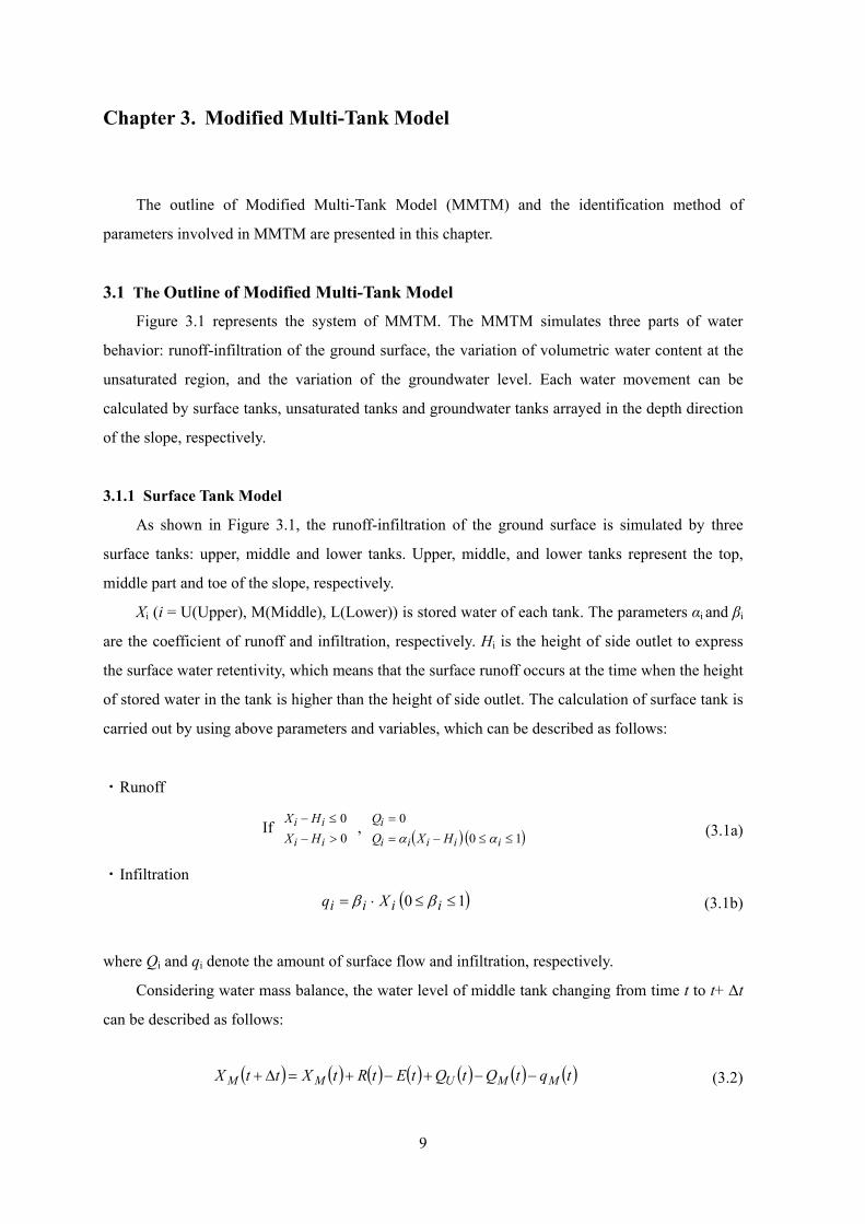
Chapter 3. Modified Multi-Tank Model

The outline of Modified Multi-Tank Model (MMTM) and the identification method of

parameters involved in MMTM are presented in this chapter.

3.1 The Outline of Modified Multi-Tank Model Figure 3.1 represents the system of MMTM. The MMTM simulates three parts of water

behavior: runoff-infiltration of the ground surface, the variation of volumetric water content at the

unsaturated region, and the variation of the groundwater level. Each water movement can be

calculated by surface tanks, unsaturated tanks and groundwater tanks arrayed in the depth direction

of the slope, respectively.

3.1.1 Surface Tank Model

As shown in Figure 3.1, the runoff-infiltration of the ground surface is simulated by three

surface tanks: upper, middle and lower tanks. Upper, middle, and lower tanks represent the top,

middle part and toe of the slope, respectively.

Xi (i = U(Upper), M(Middle), L(Lower)) is stored water of each tank. The parameters αi and βi

are the coefficient of runoff and infiltration, respectively. Hi is the height of side outlet to express

the surface water retentivity, which means that the surface runoff occurs at the time when the height

of stored water in the tank is higher than the height of side outlet. The calculation of surface tank is

carried out by using above parameters and variables, which can be described as follows:

・ Runoff

If 00

>−≤−

ii

iiHXHX , ( ) ( )10

0≤≤−=

=

iiiii

iHXQ

Qαα

(3.1a)

・ Infiltration

( )10 ≤≤⋅= iiii Xq ββ (3.1b)

where Qi and qi denote the amount of surface flow and infiltration, respectively.

Considering water mass balance, the water level of middle tank changing from time t to t+ Δt

can be described as follows:

( ) ( ) ( ) ( ) ( ) ( ) ( )tqtQtQtEtRtXttX MMUMM −−+−+=Δ+ (3.2)

10

where R is the amount of rainfall and E is the amount of evapotranspiration, which will be

negligible during rainfall.

3.1.2 Unsaturated Tank Model

As shown in Figure 3.1, the infiltration process in the unsaturated region of the slope is

simulated by some unsaturated tanks arrayed in the depth direction of the slope (e.g., five

unsaturated tanks were arrayed in Figure 3.1). The number of unsaturated tanks will depend on

Figure 3.2 The process of parameter identification

Figure 3.1 Modified Multi-Tank Model

11

unsaturated soil properties such as the characteristics of the variation of volumetric water content in

the unsaturated region.

Yi is stored water in the tank, which can be calculated using the following equation:

θ×= DY (3.3)

where D [mm] is the height of targeted unsaturated tank and θ is volumetric water content of

targeted depth.

Hij (j=1, 2, 3 ...) denotes the height of bottom outlet representing the water retention capacity

of soil particle in each layer which means that the infiltration will not take place unless the water

level in each tank exceeds the height of bottom outlet. The parameter βij denotes the coefficient of

infiltration. According to the empirical understandings on behavior of soil moisture content in the

unsaturated region, vertical flow is dominant comparing with the flow in the horizontal direction;

therefore, the unsaturated tanks have no side outlets.

In consequence, the calculation of the unsaturated tanks can be described as follows:

If 0

0

>−

≤−

ijij

jiij

HY

HY , ( ) ( )10

0

≤≤−=

=

ijijijiji

ij

HYq

q

ββ (3.4)

Considering water mass balance, the water level of the unsaturated tank changing from time t

to t+ Δt can also be described as follows:

If 21

>=

jj ,

( ) ( ) ( ) ( )( ) ( ) ( ) ( )tqtqtYttY

tqtqtYttY

ijijijij

iMii

−+=Δ+−+=Δ+

−1

111 (3.5)

3.2 Parameter Identification/Optimization Method Figure 3.2 shows the process of parameter identification and optimization for MMTM. In the

first step to identify parameters, back analyses, Kalman filter algorithm, and Artificial neural

networks, are adopted. Kalman filter algorithm and Artificial neural networks are applied to

identify the parameters related to the surface and the unsaturated tanks, respectively. As will

apparent below, the equations described the MMTM need to be linearized by Taylor expansion. In

the case of the unsaturated tanks, it is difficult to calculate by using the linearized data because the

variation of the volumetric water is relatively so small that linearized data becomes very small.

After the parameters have been extracted, the optimal parameters can be identified by using the

error calculation method.

12

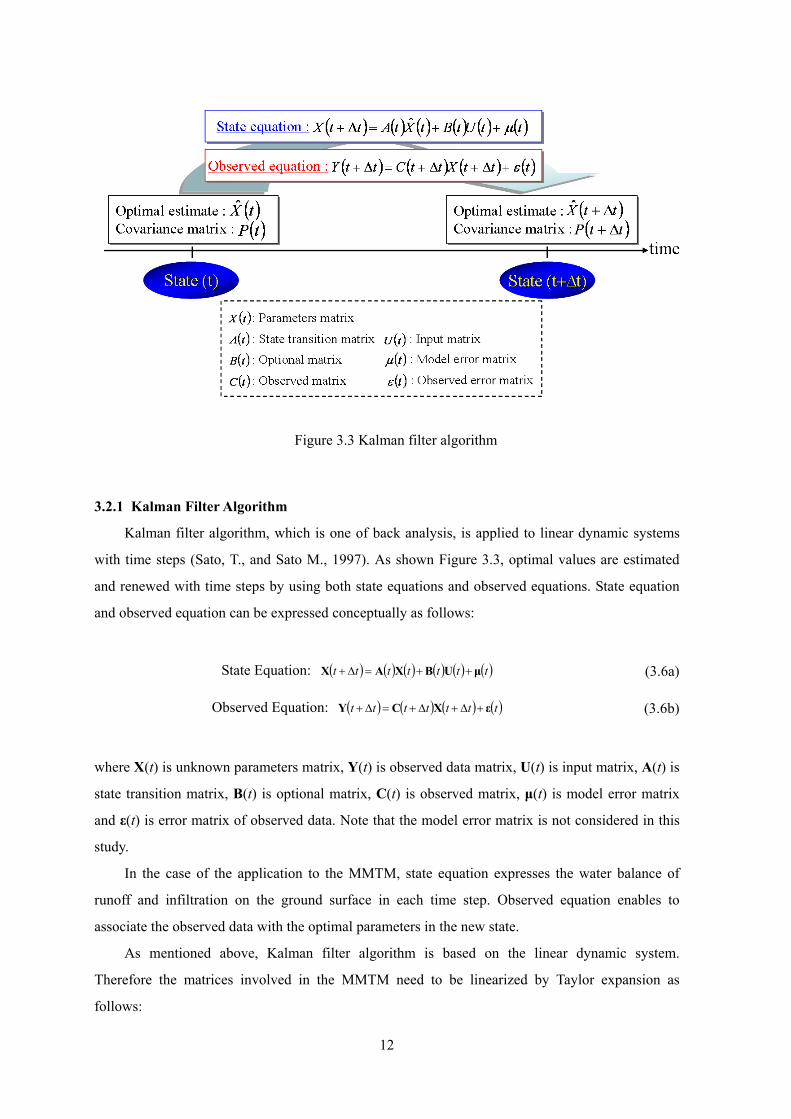
3.2.1 Kalman Filter Algorithm

Kalman filter algorithm, which is one of back analysis, is applied to linear dynamic systems

with time steps (Sato, T., and Sato M., 1997). As shown Figure 3.3, optimal values are estimated

and renewed with time steps by using both state equations and observed equations. State equation

and observed equation can be expressed conceptually as follows:

State Equation: ( ) ( ) ( ) ( ) ( ) ( )ttttttt μUBXAX ++=Δ+ (3.6a)

Observed Equation: ( ) ( ) ( ) ( )ttttttt εXCY +Δ+Δ+=Δ+ (3.6b)

where X(t) is unknown parameters matrix, Y(t) is observed data matrix, U(t) is input matrix, A(t) is

state transition matrix, B(t) is optional matrix, C(t) is observed matrix, μ(t) is model error matrix

and ε(t) is error matrix of observed data. Note that the model error matrix is not considered in this

study.

In the case of the application to the MMTM, state equation expresses the water balance of

runoff and infiltration on the ground surface in each time step. Observed equation enables to

associate the observed data with the optimal parameters in the new state.

As mentioned above, Kalman filter algorithm is based on the linear dynamic system.

Therefore the matrices involved in the MMTM need to be linearized by Taylor expansion as

follows:

Figure 3.3 Kalman filter algorithm

13

( ) ( ) ( )dt

tdXttXttX ⋅Δ+=Δ+ (3.7a)

( ) ( ) ( )dt

tdtttt ααα ⋅Δ+=Δ+ (3.7b)

( ) ( ) ( )dt

tdtttt βββ ⋅Δ+=Δ+ (3.7c)

As a result, the matrices of Kalman filter algorithm in the case of the MMTM can be derived

as follows:

( )T

LMULMULMU

dtd

dtd

dtd

dtd

dtd

dtd

dtdX

dtdX

dtdX

t ⎥⎦

⎤⎢⎣

⎡=

βββαααX (3.8a)

( )T

LMdt

dQdt

dqt ⎥⎦

⎤⎢⎣

⎡=Y (3.8b)

( )

( ) ( )( ) ( ) ( )

( ) ( ) ( )

⎥⎥⎥⎥⎥⎥⎥⎥⎥⎥⎥⎥

⎦

⎤

⎢⎢⎢⎢⎢⎢⎢⎢⎢⎢⎢⎢

⎣

⎡

−−−−+−−−−−+−

−−−+−

=

100000000010000000001000000000100000000010000000001000

00000000000000

LLMLLM

MMUMMU

UUUU

XHXHXXHXHX

XHX

t

βααβαα

βα

A

(3.8c)

( )

T

t⎥⎥⎥

⎦

⎤

⎢⎢⎢

⎣

⎡=

000000100000000010000000001

Β (3.8d)

( ) ⎥⎦

⎤⎢⎣

⎡−

=00000000000000

HXX

tLL

MM

αβ

C (3.8e)

( )( ) ( )

( ) ( ) ( )( ) ( ) ( ) ⎥

⎥⎥

⎦

⎤

⎢⎢⎢

⎣

⎡

⋅−−⋅−−⋅+−⋅−−⋅−−⋅+−

⋅−−⋅−−=

LLLLMM

MMMMUU

UUUU

XHXHXERXHXHXER

XHXERt

βααβαα

βαU (3.8f)

( ) ( )⎥⎦⎤

⎢⎣

⎡−⋅

⋅=

LLL

MM

HXX

tα

βε (3.8g)

Note that the height of side outlet is assumed to be constant and evapotranspiration during the

rainfall is assumed to be zero (negligible).

14

Observed data matrix Y is calculated from the amount of measured runoff and infiltration. The

amount of runoff is, for example, can be measured by V-shaped notch at the site. On the other hand,

the amount of infiltration can be calculated from the volumetric water content measured using the

soil moisture meter, because the amount of infiltration cannot be measured directly. The amount of

rainfall included in the input matrix U is measured using rainfall gauge with tipping-bucket. As

mentioned above, since Kalman filter algorithm estimates and renews the optimal parameters for

tank model at each time steps, this system requires the initial elements of matrices: initial values for

six coefficients, and initial water levels. Each tank has the same initial water level, 25 mm and the

initial values of each coefficient are assumed to be 0.2, 0.4, 0.6, 0.8 and 1.0. Hence, the number of

trials and errors in the calculation is 15,625(=56).

Figure 3.6 Flowchart of identifying the unsaturated parameters

Figure 3.4 Artificial Neural Networks Figure 3.5 Converting model

15

3.2.2 Artificial Neural Networks

Artificial neural networks are the complex signal process based on present understanding of

biological nervous systems (Sato, T., and Sato M., 1997). Figure 3.4 shows the basic concept of

Table 3.1 Leaning data

Figure 3.8 Error calculation method

16

Artificial neural networks. The input nodes are converted to the output nodes through the hidden

layer as shown in Figure 3.5. The input for the hidden layer is the summation of weighted input

signals, which can be derived as follows:

bwxSn

iii +=∑

=1 (3.9)

where S denotes the summation of weighted input signals, xi (i= 1, 2, ..., n) is input signals, wi is

weights and b is a bias term. Then, the output signals are read out through a non-linearity, which

calculates the difference between the summation and the certain threshold. The most typical

non-linearity will be the sigmoid function given by:

( )( )thSe

Sfyθα −−+

== *1

1 (3.10)

where y is the output signals, θth is the certain threshold and α∗ is a positive invariable.

In addition, this study adopts Artificial neural networks with supervised learning and the back

propagation algorithm, NEUROSIM/L(R) V4 (FUJITSU Corporation), which is applied as the

supervised learning.

Figure 3.6 shows the flowchart of identifying parameters for the unsaturated tanks by

Artificial neural networks together with supervised learning. Firstly, learning data is calculated as

shown in Table 3.1, that is, water level Y and variation of water level are calculated by the

coefficient of infiltration β and height of bottom outlet H set by random numbers in the MMTM.

Coefficient of infiltration is the random numbers between 0 and 1 and height of bottom outlet is the

random numbers between the minimum and maximum of measured water level. Then Artificial

neural networks are applied to pick up some parameter sets. Note that this identification method is

applied to the order of depth from the shallowest tank to the deepest tank.

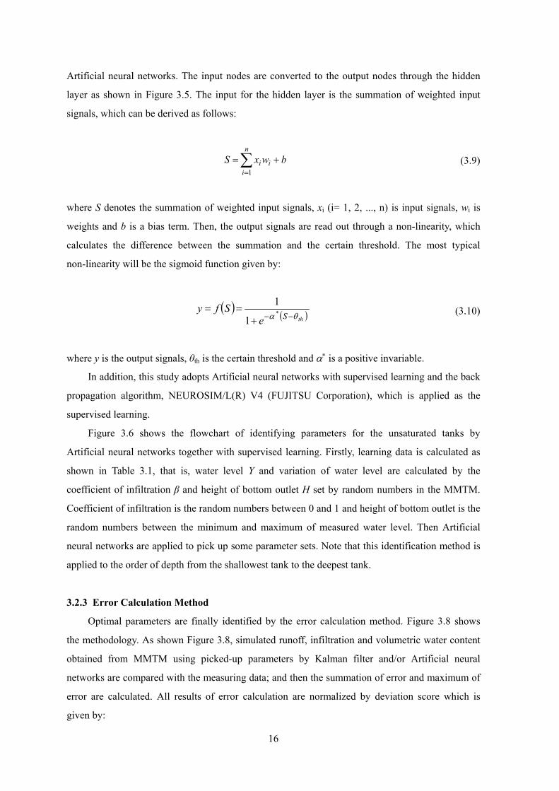
3.2.3 Error Calculation Method

Optimal parameters are finally identified by the error calculation method. Figure 3.8 shows

the methodology. As shown Figure 3.8, simulated runoff, infiltration and volumetric water content

obtained from MMTM using picked-up parameters by Kalman filter and/or Artificial neural

networks are compared with the measuring data; and then the summation of error and maximum of

error are calculated. All results of error calculation are normalized by deviation score which is

given by:

17

50)(10+

−=

er

erxy

σμ

(3.11)

where x denotes the each error, y is the deviation score, μer is the average of error and σer is standard

deviation of error.

Total amount of deviation scores can be derived as follows:

∑=

=1i

iyz (3.12)

where yi denotes each deviation score and z is total amount of deviation scores. Optimal parameter

set is defined as the parameter set in the case of minimum of the total amount of deviation scores.

18

Chapter 4. Field Monitoring Project at the Slope N

The comprehensive field monitoring at the slope N has been conducted in Thailand since

September, 2007 cooperating with Kasetsart University, Thailand. This chapter presents the

geological conditions, rainfall characteristics in the slope N, the monitoring system and laboratory

test; moreover, the measured results are discussed.

4.1 Geological Condition Slope N, whose geological layer consists of mud, sand and silt called Khorat group, which lies

in the northeast of Bangkok. Figure 4.1 shows the monitored slope, where landslide occurred in

August, 2004.

As shown in Figure 4.2, the soil type in this slope is laterite, which is typical surface formation

in hot and wet tropical regions. Laterite is formed by intensive and long weathering caused by high

temperature and heavy rainfall and includes rich iron and aluminum. Figure 4.3 shows the bedrock

outcrop consisting of rhyolite, which is volcanic rock with over 70 percent of silicon dioxide. This

monitored site is the soil slope composed by strongly weathered rhyolite.

Rhyolite and granite are also spread over the area of western Japan (Geological Survey of

Japan, National Institute of Advanced Industrial Science and Technology, 2009); the geological

feature of the slope N is similar to the weathered soil slope widely distributed in western Japan.

Figure 4.1 Monitoring slope N

19

4.2 Rainfall Characteristics Figure 4.4 (a), (b) and Figure 4.5 (a), (b)*) show the examples of rainfall pattern at the slope N

and in Japan, respectively. The accumulated rainfall and maximum rainfall intensity per 10 minutes

and 1 hour for each rainfall pattern are summarized as shown in Table 4.1. Comparing the rainfall

pattern in Thailand, a squall, with the one in Japan, “guerilla-like rainfall”, the maximum rainfall

intensity per 10 minutes is in the same range, 20-30 mm/10min. According to the accumulated

rainfall, the amount of rainfall of guerilla-like rainfall is larger than that of squall. This is because

the guerilla-like rainfall often lasts longer time and shows a few peaks of rain intensity although

tropical rainfall often shows one peak.

Although there are some differences between the squall and guerilla-like rainfall, it will be

appropriate to discuss these as the analogous phenomenon in terms of the maximum rainfall

intensity.

*) Japan Meteorological Agency (http://www.jma.go.jp/jma/index.html)

Figure 4.3 Bedrock outcrop (Rhyolite)

Figure 4.2 Surface formations (Laterite)

20

(a) City O, 29 August, 2008 (b) City H, 21 July, 2009

Figure 4.5 Example of rainfall pattern in Japan

(a) Slope N, 19 May, 2008 (b) Slope N, 30 July, 2008

Figure 4.4 Example of rainfall pattern in Thailand

Table 4.1 Comparison of rainfall pattern between Thailand and Japan

Slope N

(May, 08)

Slope N

(July, 08)

City O

(Aug., 08)

City H

(July, 09)

Accumulated Rainfall [mm] 66 81.5 302 275

Max. rainfall intensity [mm/10min] 20.5 19 30.5 18

Max. rainfall intensity [mm/1hr] 25 72.5 136 70.5

21

4.3 Field Monitoring System

4.3.1Outline

Figure 4.6 and Figure 4.7 show the cross-section and contour map of the field monitoring site,

respectively. The monitoring system consists of a rainfall gauge, two soil moisture meters, three

V-shaped notches with water level sensors to measure surface flow, a piezometer and two

tensiometers to measure pore water pressure and matric suction. One of the soil moisture meters

was installed at the middle part of the slope (No.1) and the other was installed at the toe of the

slope together with the rainfall gauge (No.2). Two V-shaped notches were constructed at the middle

part of the slope (No.11 and No.3) and one was constructed at the toe of the slope (No.2). These

measuring equipments were installed in September, 2007, and the data were recorded by every ten

minutes. The volumetric water content was measured by soil moisture meter which converted the

voltage of damp soil at the depth of GL-0.1 m, GL -0.2 m, GL-0.3 m, GL-0.4 m, GL-0.6 m and

GL-1.0 m .

Pore water pressure and matric suction were measured by the piezometer and tensiometers

installed by Kasetsart University (Jotisankasa and Mairaing, 2009). A piezometer was installed at

the toe of the slope in May, 2008 and the pore water pressure at the depth of GL-0.3 m, GL-0.6 m

and GL-1.0 m was measured. One of tensiometers was installed at the middle part of slope in

September, 2007 and measured the matric suction at the depth of GL-1.0 m, GL-1.5 m and GL-2.15

m. The other one was installed between the middle part and the toe of slope in June, 2009, which

measured matric suction at the depth of GL-0.76 m and GL-1.82 m. These measuring instruments

were set up to record every 1 day.

4.3.2 Soil Moisture Meter

Figure 4.8 shows the soil moisture meter and tripping bucket rainfall gauge. As mentioned

above, volumetric water content is calculated by converting the analogue output voltage of damp

soils which is measured by soil moisture meters (DELTA-T DEVICES, 2004). It is reported that the

relationship between volumetric water content and the analogue output voltage will be different

with different site condition (Sugii and Takeshita, 2007). Figure 4.9 shows the relationship

calibrated in the laboratory experiments (Ohtsu et al., 2008). In the laboratory experiments,

experimental volumetric water content obtained from undisturbed soil samples was compared with

the analogue output voltage. The volumetric water content can be calculated from the following

polynomial equation (4.1).

32 34.072.009.032.0 VVV ×−×+×−=θ (4.1)

22

Figure 4.7 Contour map of slope N

Figure 4.6 Cross-section of slope N and locations of measurement equipments

23

Figure 4.9 Relationship between volumetric water content and analogue output voltage

Figure 4.8 Soil moisture meter with rainfall gauge and data logger

24

where θ denotes the calculated volumetric water content and V [V] is the measured voltage.

The undisturbed soil samples were collected on 1 and 11 June, 2008 near the soil moisture

meter No.1 and No.2. The experimental volumetric water contents obtained from the first and the

second soil samples were distributed from about 40.0 to 70.0 %, and from about 30.0 to 50.0 %,

respectively, that is, variability of volumetric water content against a certain voltage was relatively

large. Therefore, it seems that equation (4.1) is well-rounded equation with errors.

4.3.3 V-shaped Notch with Water Level Sensor

The amount of surface runoff was measured by V-shaped notch with water level sensor. The

V-shaped notch No.1 and No.3 were constructed by wood, and No.2 was constructed by concrete as

shown in Figure 4.10 (a), (b). Note that current boards were constructed in the V-shaped notch No.2

because the turbulent flow was sometimes generated without the current boards since the amount of

Figure 4.11 Flow volume measurement method

Figure 4.10(a) Wooden V-shaped notch Figure 4.10(b) Concrete V-shaped notch

25

runoff at V-shaped notch No.2 was relatively large. Figure 4.11 shows the methodology to measure

the volume of surface flow. Water level is calculated by converting the absolute pressure which is

measured by the pressure transducer inside the water level sensor (OYO Corporation, 2005). Water

level is calculated as follows:

sow HHH −= (4.2)

where Hw [cm] denotes the water level of over flow, Ho [cm] is the measured water level and Hs

[cm] is the distance between notch and sensor.

Using the water level of over flow, the amount of runoff can be calculated using the following

equation (Japanese Industrial Standards Committee, 1990).

5.200084.0 wHQ ×= (4.3)

where Q [m3/min] denotes the amount of runoff.

4.4 Results of Laboratory Tests

4.4.1 Slope Angle and Strength Constants

The slope angle, total unit weight of soil, soil particle density, dry density, void ratio, and

strength constants related to factor of safety are summarized in Table 4.2. Soil particle density, dry

density and void ratio are the average value of the middle part of the slope at GL-0.6 m and the toe

of the slope at GL-0.6 m. Note that this slope was re-compacted after failing in August 2004 (with a

depth of failure ~ 2.0 m) due to heavy rainfall amounting to 344 mm over 4 days (Jotisankasa and

Mairaing, 2009) and the slope angle was about 45 degree when the measurement was performed.

Figure 4.12 shows the safety factor as a function of pore water pressure. The safety factor can be

calculated using the following equation assuming the slope is saturated and infinite:

( )ααγ

φαγcossin

tancos2

HuHc

FS w ′−+′= (4.4)

where FS denotes the safety factor, c’ [kPa] is effective cohesion, φ’ [deg] is effective friction angle,

γ [kN/m3] is total unit weight of soil, uw [kPa] is pore water pressure, H [m] is depth of slope failure,

α [deg] is the slope angle.

26

The depth of slope failure and slope angle was assumed to be 2.0 m, and 45 degree and 27.65

degree. The maximum pore water pressure measured at slope N was about 7 kPa. In the case of

safety factor (when the slope angle was 27.65 degree) was about 1.8.

4.4.2 Liquid Limit and Plastic Limit

Table 4.3 summarizes the liquid limit, plastic limit and plasticity index (Jotisankasa and

Mairaing, 2009). Note that plasticity index is defined as follows:

Figure 4.12 Factor of safety as a function of pore water pressure

Table 4.3 Liquid limit, plastic limit and plasticity index

Liquid limit [%] Plastic limit [%] Plasticity limit

46-51 6-18 33-40

Table 4.2 Parameters at slope N

Slope angle [deg] 27.65 Void ratio 1.05

Unit weight of soil [kN/m3] 17.66 Effective cohesion [kPa] 14.5

Soil particle density [g/cm3] 2.71 Effective friction angle [deg] 33.9

Dry density [g/cm3] 1.33

27

pLp wwI −= (4.5)

where Ip denotes plasticity index, wL is liquid limit and wp is plastic limit.

4.4.3 Grain Size Accumulation Curve

Figure 4.13 shows the grain size accumulation curves in the middle part of the slope at the

depth of GL-0.6 m and GL-1.0 m, and the toe of the slope at the depth of GL-0.6 m and GL-1.0 m.

Figure 4.14 Plasticity chart Figure 4.15 Triangle coordinate

Figure 4.13 Grain size accumulation curve

28

Note that not only sieve analysis but also sedimentation analysis were conducted in the experiments.

According to the test results, fine-grain fraction and viscous soil dominates at the slope N.

4.4.4 Geotechnical Classification

Figure 4.14 shows the plasticity chart based on liquid limit and plasticity index. The soil at the

slope N was classified intermediate between CL and CH which means clay of middle liquid limit.

Figure 4.15 shows the classification with the triangle coordinate. Soil samples of the middle

part of the slope at the depth of GL-0.6 m and GL-1.0 m were classified as sandy clay with gravel

(CLS-G) and sandy clay (CLS), respectively; soil samples of the toe of the slope at the depth of

Gl-0.6 m and GL-1.0 m were classified as cohesive sandy gravel (GCsS) and clay with sand gravel

(CL-SG), respectively.

Figure 4.18(a) Soil samples at GL-0.6 m Figure 4.18(b) Soil samples at GL-1.0 m

in the toe of the slope in the toe of the slope

Figure 4.16 SWCCs measured at slope N Figure 4.17 Comparison of SWCC between

the depths at the toe of the slope

29

4.4.5 Soil Water Characteristic Curve (SWCC) based on the Laboratory Test

Figure 4.16 shows the results of SWCCs obtained through the wetting/drying tests for the

middle part of the slope at GL-0.6 m, position between the middle part and toe of the slope at

GL-0.6 m and GL-1.0 m, and the toe of the slope at the depth of GL-0.6 m and GL-1.0 m (Ohtsu et

al., 2008). As mentioned above, soil type at the slope N was clay and water retentivity was

relatively large; therefore SWCCs ,of which volumetric water content were large, were obtained.

Figure 4.17 also shows the comparison of SWCC at the depth of GL-0.6 m with GL-1.0 m at the

toe of the slope. The SWCC at the depth of GL-0.6 m, matric suction increases 20 kPa with

decreasing the volumetric water content of 5 %. In contrast, case of the SWCC at the depth of

GL-1.0 m, matric suction increases only 10 kPa with increasing the volumetric water content of

5 %.

Figure 4.18(a), (b) show the soil samples obtained from the toe of the slope at the depth of

GL-0.6 m and GL-1.0 m, respectively. Aggregate structure and argillation is significant at deeper

part of the slope.

4.5 Results of In-situ Measured Data

4.5.1 Volumetric Water Content and Pore Water Pressure

Figure 4.19(a), (b) show the measured results of rainfall intensity and measured volumetric

water content per ten minutes in the middle part of the slope from September, 2007 to October,

2008 and from June, 2009 to September, 2009, respectively. Figure 4.20 (a), (b) show the measured

results at the toe of the slope from September, 2007 to October, 2008 and from June, 2009 to

September, 2009, respectively. Note that the measured data at GL-0.1 m and GL-0.6 m were not

able to be obtained due to an error of data logger. Furthermore, Figure 4.21(a), (b) illustrate the

observation results for rainfall intensity and measured pore water pressure per one day in the

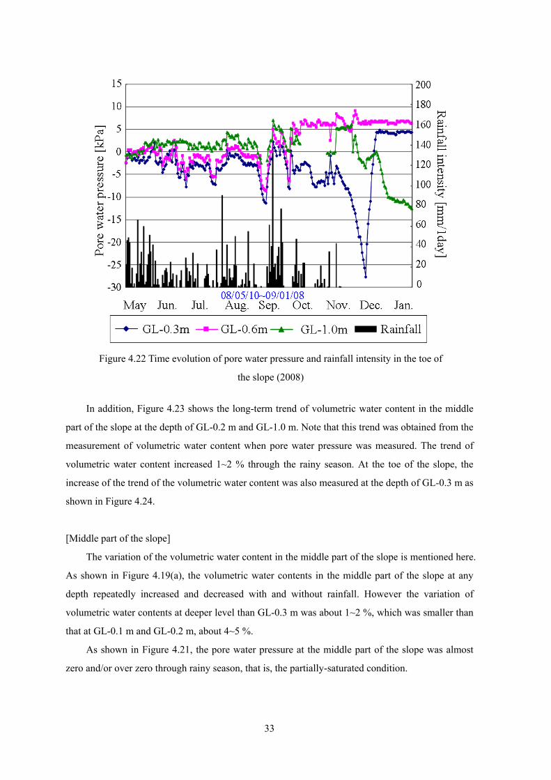
middle part of the slope in 2007 and 2008, respectively, and Figure 4.22 is the measured rainfall

intensity and pore water pressure per one day in the toe of the slope in 2008.

In Thailand, there are two seasons, so-called rainy season (from May to October) and dry

season (from November until April); therefore, no or very little rainfall can be observed after

November as shown in Figure 4.19, Figure 4.20, and Figure 4.21.

As mentioned above, since the soil types in the slope N are categorized as clay, the volumetric

water content at shallower level than GL-1.0 m is relatively larger. Hence, the volumetric water

content was more than 40 % even though the ground was dry condition at the beginning of rainy

season. At the beginning of the rainy season, the volumetric water content increased rapidly about

3 % in the middle part of the slope and 5 % at the toe of the slope.

30

Figure 4.19(b) Time evolution of volumetric water content and rainfall intensity at the middle

part of the slope (2009)

Figure 4.19(a) Time evolution of volumetric water content and rainfall intensity in the middle

part of the slope (2007, 2008)

31

Figure 4.20(b) Time evolution of volumetric water content and rainfall intensity in the toe of the

slope (2009)

Figure 4.20(a) Time evolution of volumetric water content and rainfall intensity in the toe of the

slope (2007, 2008)

32

Figure 4.21(b) Time evolution of pore water pressure and rainfall intensity in the middle part of

the slope (2008)

Figure 4.21(a) Time evolution of pore water pressure and rainfall intensity in the middle part of

the slope (2007)

33

In addition, Figure 4.23 shows the long-term trend of volumetric water content in the middle

part of the slope at the depth of GL-0.2 m and GL-1.0 m. Note that this trend was obtained from the

measurement of volumetric water content when pore water pressure was measured. The trend of

volumetric water content increased 1~2 % through the rainy season. At the toe of the slope, the

increase of the trend of the volumetric water content was also measured at the depth of GL-0.3 m as

shown in Figure 4.24.

[Middle part of the slope]

The variation of the volumetric water content in the middle part of the slope is mentioned here.

As shown in Figure 4.19(a), the volumetric water contents in the middle part of the slope at any

depth repeatedly increased and decreased with and without rainfall. However the variation of

volumetric water contents at deeper level than GL-0.3 m was about 1~2 %, which was smaller than

that at GL-0.1 m and GL-0.2 m, about 4~5 %.

As shown in Figure 4.21, the pore water pressure at the middle part of the slope was almost

zero and/or over zero through rainy season, that is, the partially-saturated condition.

Figure 4.22 Time evolution of pore water pressure and rainfall intensity in the toe of

the slope (2008)

34

[Toe of the slope]

The variation of the volumetric water content in the toe of the slope is mentioned. As shown in

Figure 4.20(a), the volumetric water content at shallower depth than GL-0.4m repeatedly increased

and decreased with and without rainfall. Especially the volumetric water content at the depth of

GL-0.3 m and GL-0.4 m often showed 60 % when a squall occurred. In the year 2008, the

Figure 4.24 Long-term trend of the volumetric water content at the toe of slope

Figure 4.23 Long-term trend of the volumetric water content at the middle part of the slope

35

volumetric water content at the depth of GL-0.2 m showed 60 % in September. This phenomenon

was significant in September, 2007.

On the other hand, at deeper level than GL-0.6m, the volumetric water content increased at the

beginning of the rainy season and kept almost constant value of about 60 %. As shown in Figure

4.22, the pore water pressure in the toe of the slope at the depth of GL-0.6 m and GL-1.0 m,

especially GL-1.0 m, was positive, that is, the saturated condition.

Figure 4.25(b) Time evolution of volumetric water content

at the toe part in September, 2008

Figure 4.25(a) Time evolution of volumetric water content

at the middle part in September, 2008

36

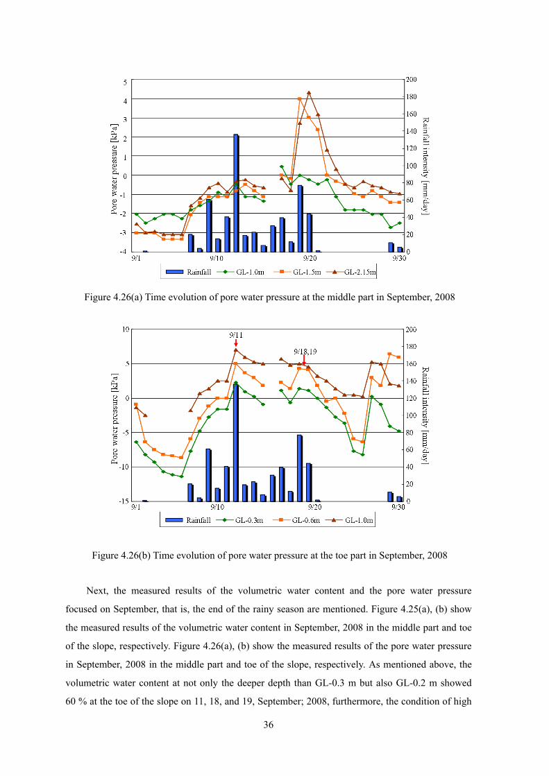
Next, the measured results of the volumetric water content and the pore water pressure

focused on September, that is, the end of the rainy season are mentioned. Figure 4.25(a), (b) show

the measured results of the volumetric water content in September, 2008 in the middle part and toe

of the slope, respectively. Figure 4.26(a), (b) show the measured results of the pore water pressure

in September, 2008 in the middle part and toe of the slope, respectively. As mentioned above, the

volumetric water content at not only the deeper depth than GL-0.3 m but also GL-0.2 m showed

60 % at the toe of the slope on 11, 18, and 19, September; 2008, furthermore, the condition of high

Figure 4.26(b) Time evolution of pore water pressure at the toe part in September, 2008

Figure 4.26(a) Time evolution of pore water pressure at the middle part in September, 2008

37

(a) Middle portion of slope (b) Toe of slope

Figure 4.29 Time evolution of the volumetric water content on 18, September, 2008

(a) Middle portion of slope (b) Toe of slope

Figure 4.28 Time evolution of the volumetric water content on 11, September, 2008

Figure 4.27 Difference of the total head between GL-0.3 m and GL-0.6 m at the part of the slope

38

volumetric water content lasted about from half a day to one day. In addition, the variation of the

volumetric water content at GL-0.2 m at the middle part of slope was relatively large on 18, 19,

September even though the rainfall intensity was not distinctly strong. The pore water pressure was

also relatively large on 18, 19, September, 2008, as shown in Figure 4.26(a), (b).

As the indicator of the permeability, Figure 4.27 shows the difference of the total head

between GL-0.3 m and GL-0.6 m at the toe of the slope calculated by using the measured results of

the pore water pressure. On 11, 18, and 19, September, 2008, as mentioned above, the difference of

the total head was relatively small, that is, the permeability between GL-0.3 m and GL-0.6 m was

low.

Figure 4.28(a), (b) show the behavior of volumetric water content on 11, September, 2008 in

the middle part and toe of the slope, respectively. Figure 4.29(a), (b) show the behavior on 18,

September, 2008 in the middle and toe of the slope, respectively. Figure 4.30(a), (b) show the

behavior on 19, September, 2008 in the middle and toe of the slope, respectively. Focused on the

behavior at the toe of the slope, the volumetric water content showed the constant value in order of

deeper part and the decrease of volumetric water content started in order of shallower part. In

addition, focused on Figure 4.29(a), the maximum value of the volumetric water content at GL-0.2

m was larger at the second rainfall peak.

4.5.2 Runoff

This subject presents the measuring results of surface runoff. The runoff in the middle part of

the slope was measured at the V-shaped notch No.11. As shown in Figure 4.7, the water catchment

area of middle part of the slope is A2, whose area is 150 m2. The surface runoff at the toe of the

slope was measured at the V-shaped notch No.2 and V-shaped notch No.3, which means that the

(a) Middle portion of slope (b) Toe of slope

Figure 4.30 Time evolution of the volumetric water content on 19, September, 2008

39

Figure 4.32 Runoff at the toe of the slope (2008)

Figure 4.31 Runoff at the middle part of the slope (2008)

40

amount of runoff at the toe of the slope can be calculated as follows:

32 QQQL −= (4.6)

where QL [L/10min] denotes the amount of runoff at the toe of the slope and Q2 [L/10min] and Q3

[L/10min] are the amount of measured runoff at the V-shaped notch No.2 and V-shaped notch No.3,

respectively.

Figure 4.33(b) In-situ SWCC at the toe of the slope (GL-1.0 m)

Figure 4.33(a) In-situ SWCC at the middle part of the slope (GL-1.0 m)

41

Since the amount of runoff generated outside the target area was measured at the V-shaped

notch No.3, the catchment area of the toe of the slope is A3 and A4 , whose total area is 425 m2.

In addition, the amount of runoff per ten minute can be calculated from the amount of runoff

per one minute as follows:

( ) 210 min,1min,1min,10 tttt QQQ Δ−+= (4.7)

where Q10min,t [L/10min] denotes the amount of runoff per ten minute from time step t- Δt to t,

Q1min,t and Q1min,t-Δt is the amount of observed runoff at time step t and t- Δt, respectively.

Figure 4.31 and Figure 4.32 show the measured results of the amount of runoff per ten

minutes in the middle and toe of the slope, respectively. As shown in Figure 4.31, the maximum

amount of runoff generated in the middle part of the slope was about 800 [L/10min]. By

considering the water catchment area in the middle part of the slope, the runoff can be calculated as

the maximum value about 5.5 litters per 10min and per area (0.55 litters per min per area).

On the other hand, as shown in Figure 4.32, the maximum amount of runoff generated in the

toe of the slope was about 6200 [L/10min]. By considering the water catchment area in the toe of

the slope, the runoff can be calculated as the maximum value about 15 litters per 10min and per

area (1.5 litters per min per area). The amount of runoff at the toe of the slope was three times as

large as that measured in the middle part of the slope.

4.5.3 Soil Water Characteristic Curve (SWCC) based on the In-situ Data

This subject presents the in-situ SWCC associated with the in-situ volumetric water content

and the in-situ pore water pressure. Note that the in-situ SWCC mentioned in this subject was

averaged behavior, because the pore water pressure was monitored once a day.

Figure 4.33(a), (b) show the in-situ SWCC at the depth of GL-1.0 m in the middle part and the

toe of the slope, respectively. Blue and green lines represent the SWCC measured from the end of

rainy season to dry season, and pink line represents the SWCC measured from the beginning of

rainy season to the middle of rainy season. Especially, in the middle part of the slope, large-scale

hysteresis can be observed between rainy and dry seasons in the in-situ SWCC.

In addition, routes of dry process had differences between the end of rainy season and dry

season in 2007 and the end of rainy season in 2008 to dry season in 2009 as shown in Figure

4.33(a).

Next, the in-situ SWCC in the middle part of the slope is compared with that in the toe of the

slope. By focusing on dry process, matric suction increased about 50~60 kPa with decreasing of

volumetric water content of 2 % in the middle part of the slope. On the other hand, matric suction

42

recovered only about 15 kPa with decreasing of volumetric water content of 4 % in the toe of the

slope, that is, the difference of behavior between the middle and the toe of the slope was measured

in the case of the in-situ SWCC though the difference of behavior of SWCC by the depth was

confirmed as shown in Figure 4.17 in the case of SWCC obtained from the laboratory tests.

4.5.4 Calculation of Water Mass Balance

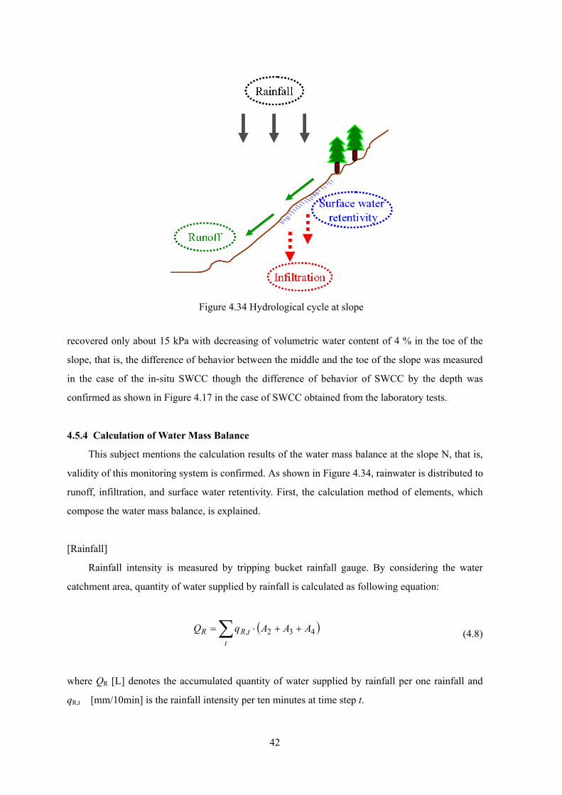
This subject mentions the calculation results of the water mass balance at the slope N, that is,

validity of this monitoring system is confirmed. As shown in Figure 4.34, rainwater is distributed to

runoff, infiltration, and surface water retentivity. First, the calculation method of elements, which

compose the water mass balance, is explained.

[Rainfall]

Rainfall intensity is measured by tripping bucket rainfall gauge. By considering the water

catchment area, quantity of water supplied by rainfall is calculated as following equation:

( )432, AAAqQt

tRR ++⋅=∑ (4.8)

where QR [L] denotes the accumulated quantity of water supplied by rainfall per one rainfall and

qR,t [mm/10min] is the rainfall intensity per ten minutes at time step t.

Figure 4.34 Hydrological cycle at slope

43

Figure 4.36 Concept of calculating infiltration by soil moisture meter

Figure 4.35 Surface water retentivity at the slope N

44

[Runoff]

The amount of runoff as a whole can be evaluated by the amount of the runoff at the toe of the

slope, that is, the accumulated quantity of runoff is obtained by counting up QL defined by equation

(4.6).

[Surface water retentivity]

Surface water retentivity means the accumulated rainfall when generating surface runoff is

first measured. It is estimated that surface water retentivity depends on the water-holding capability.

Hotta (2009) determined the surface water retentivity at the slope N by considering the amount of

runoff measured by each V-shaped notch and accumulated rainfall measured by rainfall gauge as

shown in Figure 4.35. Surface water retentivity is determined as 5 mm, that is, 2875 L by

considering the water catchment area.

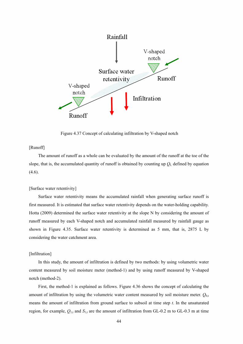
[Infiltration]

In this study, the amount of infiltration is defined by two methods: by using volumetric water

content measured by soil moisture meter (method-1) and by using runoff measured by V-shaped

notch (method-2).

First, the method-1 is explained as follows. Figure 4.36 shows the concept of calculating the

amount of infiltration by using the volumetric water content measured by soil moisture meter. Q0,t

means the amount of infiltration from ground surface to subsoil at time step t. In the unsaturated

region, for example, Q1,t and S1,t are the amount of infiltration from GL-0.2 m to GL-0.3 m at time

Figure 4.37 Concept of calculating infiltration by V-shaped notch

45

step t and the amount of retained water between GL-0.0 m and GL-0.2 m at time step t, respectively.

The amount of retained water is calculated by equation (3.3). For example, the amount of retained

water between GL-0.0 m and GL-0.2 m is calculated as following equation:

ttS ,2.0,1 200 θ⋅= (4.9)

where 200 [mm] means the layer thickness and θ0.2,t is the volumetric water content at the depth of

GL-0.2 m at time step t.

Furthermore, continuity equation of retained water from time step t to t+ 1 is described as

follows:

tttt QQSS ,1,0,11,1 −+=+ (4.10a)

tttt QQSS ,2,1,21,2 −+=+ (4.10b)

tttt QQSS ,3,2,31,3 −+=+ (4.10c)

tttt QQSS ,4,3,41,4 −+=+ (4.10d)

tttt QQSS ,5,4,51,5 −+=+ (4.10e)

The amount of infiltration from ground surface at time step t is calculated by substitute

Figure 4.38 Calculation results of water mass balance

46

equation (4.10e) into equation (4.10d), equation (4.10d) into equation (4.10c), equation (4.10c) into

equation (4.10b) and equation (4.10b) into equation (4.10a). Note that Q5,t is assumed to be zero

because Q5 can not be measured. Consequently, the amount of infiltration at time step t is

calculated as following equation:

( )∑=

+ −=5

1,1,,0

ititit SSQ (4.11)

By using equation (4.11), the unit amounts of infiltration in the middle part of the slope and

the toe of the slope are calculated; the whole amounts of infiltration are calculated as follows by

considering the water catchment area:

Middle part: ( )∑∑=

+ ⋅−=t i

titiMI ASSQ5

12,1,, (4.12a)

Toe part: ( ) ( )∑∑=

+ +⋅−=t i

titiLI AASSQ5

143,1,, (4.12b)

where QI,M and QI,L [L] denote the amount of infiltration per one rainfall in the middle part and the

toe of the slope, respectively.

Note that the amount of infiltration at the toe of slope could have some errors because the soil

moisture meter is installed outside the water catchment area at the toe of slope.

Second, method-2 is explained as follows. Figure 4.37 shows the concept of calculating the

amount of infiltration by using runoff obtained from V-shaped notch. The amounts of infiltration in

the middle part of the slope and the toe of the slope are described as follows:

Middle part: ∑∑ −−=t

ctt

tRMI QQqQ ,11,, (4.13a)

Toe part: ( ) ct t

tttt

tRLI QQQQqQ −−−+= ∑ ∑∑ ,3,2,11,, (4.13b)

where Q11,t, Q2,t, and Q3,t [L/10min] are the amounts of runoff at time step t measured by V-shaped

notch No.11, No.2, and No.3, respectively; Qc [L] is the amount of surface water retentivity. Note

that the amount of supply from the upper part to the middle part of the slope is neglected because

the amount of runoff at the upper part is not measured.

47

Figure 4.40 Relationship between the amount of rainfall and infiltration

Figure 4.39 Relationship between the amount of rainfall and runoff

48

Figure 4.38 shows the results of the water mass balance calculated from the 28 rainfall

patterns in 2008. Note that the amount of infiltration is used only in the method-1. The summation

of runoff, infiltration, and surface water retentivity had relatively nearly equal values with the

amount of rainfall. Hence this monitoring system can be used to observe the water mass balance

with high-accuracy.

4.5.5 Amount of Runoff and Infiltration

This subject shows the calculation results of the macroscopic amount of measured runoff and

infiltration due to rainfall by using the definition as mentioned preceding subject.

Figure 4.41(b) Unit amount of infiltration per one rainfall at the toe of the slope

Figure 4.41(a) Unit amount of infiltration per one rainfall at the middle part of the slope

49

Figure 4.39 and Figure 4.40 show the relationship between the amount of runoff and rainfall,

and the amount of infiltration and rainfall at the whole slope, respectively. Note that the amount of

infiltration is calculated by two methods as defined above. As shown in Figure 4.39 and Figure 4.40,

Figure 4.43 Relationship between the accumulated rainfall and the observed infiltration rate

categorized according to the progression of rainy season

Figure 4.42 Relationship between the accumulated rainfall and the observed infiltration rate

50

rainfalls, of which amount was from 10,000 to 40,000 [L], were mainly measured. This is because

the duration of squall was about 2~3 hours, and the maximum rainfall intensity was about

20mm/10min. The relationship between the runoff and rainfall as shown in Figure 4.39 can express

a quadratic function in all although a linear function can be fitted focused on the short-term rainfall.

Furthermore x-intercept means the surface water retentivity, 4000 [L]; this result corresponded to

the result as shown in Figure 4.35.

Next, as shown in Figure 4.40, the infiltration rate due to rainfall was distributed within the

range from 20 % to 65 %. Focusing on the short-term rainfall, the amount of infiltration was quite

different among the rainfall event even if the accumulated rainfall was almost the same.

Next, Figure 4.41 (a), (b) show the unit amount of infiltration per one rainfall in the middle

part and the toe part of the slope, respectively. Although the variability between method-1 and

method-2 was relatively large because the definition of the amount of infiltration was different, 15

[L/m2] infiltration was measured per one rainfall on average; therefore, if the duration of rainfall is

about 120 minutes, 1.3 [L/10min/m2] (i.e. 0.13 [L/min/m2]) infiltration is measured.

4.5.6 Observed Infiltration Rate

This subject shows the results of the relationship between the accumulated rainfall and the

measured infiltration rate. The infiltration in the middle part of the slope is focused on because the

middle part of the slope is treated as the representative part of infiltration characteristics.

Figure 4.42 shows the relationship between the accumulated rainfall and the measured

infiltration rate. To discuss about the rainfall-induced infiltration, the results are classified into

type-A, type-B, and type-C as will become apparent below in detail. Type-B1 and type-C1 are

examples of the rainfall results of type-B and type-C, respectively. Note that the measured

infiltration rate is defined as the ratio between the amount of infiltration calculated by method-1 as

mentioned above and the amount of water supplied by rainfall. The infiltration rate of the rainfall,

of which accumulated rainfall was about 10 to 80 mm, was widely distributed within the range

about from 0.03 to 0.42. The infiltration rate of the rainfall, of which accumulated rainfall was

Table 4.4 Accumulated rainfall, infiltration, and the infiltration rate

19, May 30, July 18, September

First Second First Second First Second

Rainfall 30.5 35 81 9 33 37

Infiltration 4.68 4.71 8.16 5.71 7.27 6.56

Infiltration rate 0.15 0.14 0.10 0.64 0.22 0.18

51

about 140 mm, was about 0.1, relatively small.

Figure 4.43 shows the relationship between the accumulated rainfall and the infiltration rate

categorized according to the progression of rainy season. Note that season-1 means the first half of

the rainy season (from May to August) and season-2 means the second half of the rainy season

(from September to November). Season-2 had a greater tendency to infiltrate than season-1.

4.5.7 Rainfall Pattern which Has a Number of Rainfall Peaks

This subject shows the measured results focused on the rainfall patterns which have a number

of rainfall peaks. Figure 4.44(a), (b), and (c) show the rainfall intensity and the accumulated

infiltration in the middle part of the slope. The rainfall patterns were divided into two peaks: the

first peak and the second peak. Table 4.4 shows the accumulated rainfall, infiltration, and the

infiltration rate of each rainfall and each peak. The infiltration rate of the second peak was almost

the same or larger than that of the first peak although samples were limited, and the rainfall pattern

and the rainfall intensity were different between the first peak and the second peak. At least the

infiltration rate of the second peak largely did not decrease in the case of the repeated squall.

(c) 18, September, 2008

Figure 4.44 Rainfall patterns which has a number of peaks with the accumulated infiltration

(a) 19, May, 2008 (b) 30, July, 2008

52

4.6 Discussion based on the Laboratory Experiments

This chapter mentions the discussion based on the laboratory experiments.

4.6.1 Slope Stability at Slope N

As mentioned in Figure 4.12, the present minimum safety factor was about 1.8, which means

that the slope N is stable and the possibility of slope failure is quite small currently. Slope N was

re-compacted after failing; accordingly the slope angle decreased compared to before. Therefore,

the current slope is relatively stable because the current slope angle (27.65 degree) is smaller than

the effective friction angle (33.9 degree), namely, repose angle.

4.6.2 Soil Property

As shown in Figure 4.13, the grain size accumulation curves mainly contained the viscous soil

were obtained and SWCCs, of which the volumetric water content was large, were obtained.

Compared these results with the results obtained from earlier studies in Japan, it would appear that

the grain size accumulation curves and SWCCs at the slope N is similar to Akaboku soil, volcanic

cohesive soil, at Oita, Japan (Komine et al., 2009), that is, there is really not much difference

between Thailand (slope N) and Japan in terms of the soil characteristics.

From the results of SWCCs, the soil at the slope N has relatively large water retentivity. In

addition, the difference of SWCC between GL-0.6 m and GL-1.0 m as mentioned in Figure 4.17

means that the restoration of matric suction related to the slope stability at GL-0.6 m is larger than

that at GL-1.0 m if the variation of volumetric water content is the same between GL-0.6 m and

GL-1.0 m. Furthermore, these results clearly show that the soil at GL-0.6 m allows moisture to

infiltrate easily, comparing with the soil at GL-1.0 m. It could be that this difference is caused by

the complex soil conditions among the depth as mentioned in Figure 4.18 caused by the weathering

Figure 4.45 Concept of slope weathering

53

(see Figure 4.45) and back-filling. Soil of the slope N sustains the weathering impact such as

torrential rainfall in the rainy season and wetting and drying through the rainy and dry seasons.

Furthermore, the slope N was re-compacted after failing. It could be that these combined factors

form such complex soil conditions.

4.7 Discussion based on Measured Results

The measured results are discussed in this section. First, the variation characteristics of the

volumetric water content, the runoff, and in-situ SWCC at the slope N are discussed. Next, the

amount of runoff-infiltration quantified by the measured data is discussed; especially, infiltration

characteristics depending on the rainfall intensity and the progression of the rainy season are

discussed. Finally, the behavior of the volumetric water content at the shallow region due to

infiltration water is discussed in detail; the mechanism of the shallow slope failure in the case of the

torrential rainfall is pointed out.

4.7.1 Volumetric Water Content and the Pore Water Pressure

The variation characteristics of the volumetric water content and the pore water pressure are

discussed.

First, long-term variation of the volumetric water content is discussed. At the beginning of the

rainy season, the volumetric water content immediately increased. It is inferred that infiltration

water was consumed in adsorption to dry and unsaturated soil particle because no rainfall was

observed in the dry season, that is, the adsorption water decreased due to long-term dry condition.

After the rainy season started, as shown in Figure 4.23 and Figure 4.24, the volumetric water

content gradually increased through the rainy season. It is estimated that this phenomenon means

that the amount of retentive water increased caused by repeated squall. As mentioned above, the

soil type at the slope N is clay, that is, the water retentivity is relatively large; it could be that

repeated rainfall had a much greater impact on water retentive condition comparing the sandy soil.

[Middle part of the slope]

The variation characteristics of the volumetric water content in the middle part of the slope are

discussed. The variations of volumetric water content at deeper level than GL-0.3 m were about

1~2 %, which were smaller than that at GL-0.1 m and GL-0.2 m. This phenomenon clearly shows

that the variation of rainfall intensity strongly affects on the variation of volumetric water content at

shallower region of the slope. Moreover, as shown in Table 4.2, the average of the void ratio in the

slope N is 1.05, which means that the saturated volumetric water content is about 50 %. Hence, in

the deeper level in the slope such as GL-0.3 m~ GL-1.0 m can be estimated to be nearly-saturated

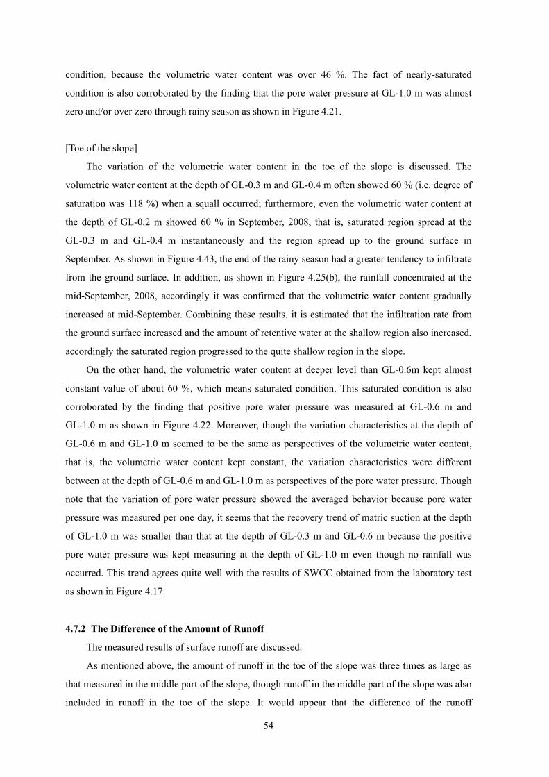
54

condition, because the volumetric water content was over 46 %. The fact of nearly-saturated

condition is also corroborated by the finding that the pore water pressure at GL-1.0 m was almost

zero and/or over zero through rainy season as shown in Figure 4.21.

[Toe of the slope]

The variation of the volumetric water content in the toe of the slope is discussed. The

volumetric water content at the depth of GL-0.3 m and GL-0.4 m often showed 60 % (i.e. degree of

saturation was 118 %) when a squall occurred; furthermore, even the volumetric water content at

the depth of GL-0.2 m showed 60 % in September, 2008, that is, saturated region spread at the

GL-0.3 m and GL-0.4 m instantaneously and the region spread up to the ground surface in

September. As shown in Figure 4.43, the end of the rainy season had a greater tendency to infiltrate

from the ground surface. In addition, as shown in Figure 4.25(b), the rainfall concentrated at the

mid-September, 2008, accordingly it was confirmed that the volumetric water content gradually

increased at mid-September. Combining these results, it is estimated that the infiltration rate from

the ground surface increased and the amount of retentive water at the shallow region also increased,

accordingly the saturated region progressed to the quite shallow region in the slope.

On the other hand, the volumetric water content at deeper level than GL-0.6m kept almost

constant value of about 60 %，which means saturated condition. This saturated condition is also

corroborated by the finding that positive pore water pressure was measured at GL-0.6 m and

GL-1.0 m as shown in Figure 4.22. Moreover, though the variation characteristics at the depth of

GL-0.6 m and GL-1.0 m seemed to be the same as perspectives of the volumetric water content,

that is, the volumetric water content kept constant, the variation characteristics were different

between at the depth of GL-0.6 m and GL-1.0 m as perspectives of the pore water pressure. Though

note that the variation of pore water pressure showed the averaged behavior because pore water

pressure was measured per one day, it seems that the recovery trend of matric suction at the depth

of GL-1.0 m was smaller than that at the depth of GL-0.3 m and GL-0.6 m because the positive

pore water pressure was kept measuring at the depth of GL-1.0 m even though no rainfall was

occurred. This trend agrees quite well with the results of SWCC obtained from the laboratory test

as shown in Figure 4.17.

4.7.2 The Difference of the Amount of Runoff

The measured results of surface runoff are discussed.

As mentioned above, the amount of runoff in the toe of the slope was three times as large as

that measured in the middle part of the slope, though runoff in the middle part of the slope was also

included in runoff in the toe of the slope. It would appear that the difference of the runoff

55

characteristics between the middle and toe of the slope was caused by the difference of the

vegetation. The vegetation in the toe of the slope mainly consists of low grasses. In the middle part

of the slope, on the other hand, some medium-tall trees with low grasses were observed. Since the

soil type of this slope is clay, it is estimated that water permeability in this slope will be relatively

low; therefore, the-runoff infiltration mechanisms may be strongly affected by the difference of

vegetation.

4.7.3 In-situ Soil Water Characteristic Curve

The in-situ SWCC associated with the in-situ volumetric water content and the in-situ pore

water pressure is discussed. It is noticed that SWCC based on the laboratory tests shows the

stationary SWCC depending on the geological conditions; on the other hand, the in-situ SWCC

means the nonstationary SWCC affected by the weathering and repeated torrential rainfall.

As shown in Figure 4.33, large-scale hysteresis can be measured. In rainy season, torrential

rainfall was repeated; hence, the in-situ SWCC, whose variation of pore water pressure was

relatively small, was obtained because the pore water pressure was almost always large. Moreover

it is estimated that the rainwater infiltration from ground surface to subsoil (i.e. vertical downward

water flow) was a major part of water flow. In dry season, on the other hand, little rainfall was

occurred; therefore, the in-situ SWCC, whose variation of pore water pressure was larger than that

in rainy season, was obtained. Moreover, the evapotranspiration from subsoil to ground surface (i.e.

vertical upward water flow) was a major part of water flow. It is inferred that rainfall interval and

the difference of direction of water flow between the rainy season and dry season caused the

large-scale hysteresis between rainy and dry seasons.

In addition, it could be that the difference of the routes of dry process as shown in Figure

4.33(a) was caused by annual range such as difference of the amount of annual rainfall, vegetation,

especially the change of root zone and affection of weathering.

Next, the difference of the behavior of the in-situ SWCC between in the middle part and toe of

the slope as shown in Figure 4.33 mentions that if the variation of volumetric water content was the

same between in the middle part of the slope and in the toe of the slope, the restoration of matric

suction related to resistance for slope failure in the middle part of the slope is larger than that in the

toe of the slope, that is, the toe of the slope could trigger the landslide. Furthermore these results

clearly show that the soil at GL-0.6 m in the toe of the slope allows moisture to infiltrate easily,

comparing with the soil at GL-1.0 m in the toe of the slope.

4.7.4 Runoff-Infiltration Characteristics

Surface runoff and surface infiltration due to rainfall are discussed.

56

As shown in Figure 4.40, in the macroscopic viewpoint combining the short-term rainfall and

the long-term rainfall, it is inferred that the infiltration capacity converged against the duration of

rainfall; this results correspond to the concept of Horton infiltration capacity as referred in chapter

2. However, focusing on the short-term rainfall, the amount of infiltration was quite different

among the rainfall event even if the accumulated rainfall was almost the same; therefore, it is

inferred that the infiltration characteristics could change in consequence of the rainfall pattern

and/or the rainfall intensity focusing on the short-term rainfall.

To discuss about the short-term rainfall in detail, relationship as shown in Figure 4.42 is

focused on. Based on this relationship, it is inferred that the envelope curve can be described; in

addition, the rainfall type is divided into three types: high-intensity and low accumulation rainfall

(type-A), high-intensity and middle accumulation rainfall (type-B), and low-intensity and high

accumulation rainfall (type-C). Rainfall of type-A has one-shot period of high rainfall intensity, and

rainfall of type-B has a number of high intensity rainfalls, accordingly the accumulated rainfall is

relatively large. Rainfall of type-C, which is rare case in squall in Thailand, has a number of

periods of low rainfall intensity or a number of periods of low rainfall intensity with some periods

of middle rainfall intensity; the duration of rainfall is long.

The infiltration rate of the rainfall of type-C was relatively small; it is very likely that this

result mention that the amount of infiltration does not increase very much even if low intensity

rainfall lasts. Rainfall of type-A has one-shot period; the infiltration rate of rainfall type-A was

slightly smaller than that of rainfall of type-B and the accumulated rainfall was small; accordingly

the amount of rainfall was small. On the other hand, the rainfall of type-B had a number of periods

of the high rainfall intensity; accordingly it is estimated that infiltration rate of that was relatively

high. Rainfall of type-B has large value of the infiltration rate and large amount of rainfall;

accordingly, the amount of infiltration becomes large.

Next, rainfall of type-B1 is compared with rainfall of type-C1 as the specific example. Note

that rainfall of type-B1 and type-C1 are examples of the observed results as shown in Figure 4.42.

First, the accumulated rainfall and the infiltration rate of rainfall of type-B1 were 46 mm and 0.42,

respectively; therefore, the accumulated infiltration was about 19 mm. On the other hand, the

accumulated rainfall and the infiltration rate of rainfall of type-C1 were 136.5 mm and 0.08,

respectively; hence, the accumulated infiltration was about 11 mm. The accumulated infiltration of

the rainfall of type-B1 was larger than that of type-C1 even though the accumulated rainfall of the

rainfall of type-C1 was quite larger than that of the rainfall of type-B1. Considering the duration of

the rainfall (i.e. the duration of rainfall of type-B1 and type-C1 are 130 minutes and 1300 min,

respectively), in the case of the rainfall of type-B1, the infiltration is intensively generated in short

term.

57

In summary, the rainfall of type-B is relatively dangerous in terms of the slope stability

because high-intensity rainfall induces the large amount of infiltration in short term. In addition, it

is inferred that the infiltration capacity is affected by not only the soil characteristics but also the

rainfall intensity and/or rainfall pattern.

Next, the variability of the infiltration rate among the rainfall of type-B is discussed. As shown

in Figure 4.43, it could be that the infiltration capacity increased affected by the progression of the

rainy season. As mentioned in Figure 4.23, the trend of the volumetric water content increases with

progressing the rainy season. As referred in chapter 2, the permeability increases with increasing

the degree of saturation. At the beginning of the rainy season, it is difficult for the rainwater

reached on the ground surface to infiltrate into the subsoil due to the pore air; altogether, rainwater

infiltrates with getting around the void filled with the air. At the end of rainy season, it could be that

the pore air contained in surface soil decreases due to the repeated squall through the rainy season;

therefore, rainwater smoothly infiltrate into the subsoil. Considering this result, it could be that the

guerilla-like rainfall as shown in Figure 4.5(b) (i.e. there are a number of rainfall peaks) sufficiently

infiltrates from the second rainfall peaks because the pore air decreases at the first rainfall peak.

This result could imply that soil water infiltration characteristics have the hysteresis. Moreover, as

the other reason, it could be that the root systems of the vegetation grow up through the rainy

season, accordingly the water smoothly infiltrates along the root system.

Next, infiltration characteristics in the case of the rainfall pattern which has a number of

rainfall peaks are discussed. As this result, at least the infiltration rate of the second peak largely did

not decrease. Considering the soil type at slope N, the influence of the infiltration water at the first

peak remains at the shallow region when the second rainfall occurs; accordingly it could be that the

cumulative rainwater due to repeated squall destabilizes the slope.

4.7.5 Mechanism of the Shallow Slope Failure due to Squall

In preceding subject, the risk of the cumulative rainwater due to repeated squall was pointed

out. In this subject, the rainfall patterns in September, 2008 are specifically discussed by using

Figure 4.28, Figure 4.29, and Figure 4.30, and the hypothesis of the mechanism of the shallow

slope failure due to squall is pointed out.

First, the behavior in the toe of the slope is focused on (11, 18, and 19, September, 2008). As

pointed out above, the volumetric water content showed the constant value in order of deeper part

and kept constant. Considering the results of Figure 4.27, that is, the total head was relatively small,

it is inferred that the infiltration water piles up in order of deeper part. The fact that the piling up of

the water starts in order of deeper part correspond to the result that ability to conduct water at the

deeper part is smaller than that at the shallower part as pointed out in Figure 4.17.

58

Next, the behavior in the middle part of the slope is focused on. As shown in Figure 4.29(a),

the maximum volumetric water content at GL-0.2 m at the first rainfall peak was about 47 % and

that at the second peak was about 48 %. This reason is estimated as follows. The water which

infiltrated at the first peak retains at the shallow part; the infiltration water was continuously

generated by the second rainfall peak with remaining the influence of the infiltration water at the

first peak. Therefore it could be that the piling up progressed till GL-0.2 m, that is, this result is the

same phenomenon with the phenomenon in the toe of the slope.

In summary, this phenomenon could be explained as shown in Figure 4.46. As mentioned

above, the short-term rainfall sufficiently infiltrates into subsoil; however, the infiltration speed in

the subsoil at the slope N is relatively small due to the soil type and complex soil condition;

accordingly, the infiltration water piles up at the shallow region because the infiltration speed from

the ground surface in larger than that at the subsoil. It seems that progression of the saturated zone

to the shallower region generates the positive pore water pressure, and this is the mechanism of the

shallow slope failure due to squall.

It would appear that this phenomenon occurs even the sand slope (i.e. the permeability is

relatively large.) when the infiltration speed from the ground surface due to the torrential rainfall

exceeds the permeability of the sandy ground.

Figure 4.46 Mechanism of the shallow slope failure

59

Chapter 5. Modified Multi-Tank Model

This chapter mentions the applicability of MMTM. This study applies MMTM to the

measured results at the slope N and discusses the identified parameters in detail. In addition, the

identified parameters at the slope N is compared with the identified parameters at other

experimental result and monitoring site, that is, one-dimensional column infiltration test and field

monitoring at slope C simulated in earlier study (Hotta, 2009). Furthermore, the difference of

infiltration characteristics related to rainfall pattern is discussed by using the identified parameters.

5.1 Framework of Modified Multi-Tank Model

5.1.1Modified Multi-Tank Model at the Slope N

First, the framework of the surface tank at the slope N is mentioned as shown in Figure 5.1.

Middle and lower tanks simulate the runoff-infiltration in the middle part and toe of the slope.

Upper tank, which has no measured results, is assumed to simulate the runoff-infiltration in the top

of the slope.

As for the parameters related to the surface tank, the height of side outlet shows the surface

water retentivity; therefore, this parameter is set to be 5 mm as shown in Figure 4.35. The

coefficient of infiltration and the coefficient of runoff were determined by back analysis, Kalman

filter algorithm as mentioned above. As the input data of Kalman filter algorithm, the runoff in the

toe of the slope and the infiltration in the middle of the slope were applied. The input data also is

needed to be treated as the unit value because MMTM simulates the unit amount of runoff and

infiltration; therefore, the runoff in the toe of slope as defined in equation (4.6) is inputted as

following equation:

( )43 AAQq LL += (5.1)

where qL [mm/10min] denotes the unit amount of runoff in the toe of the slope per ten minutes. The

unit amount of runoff is similarly defined as following equation:

211 AQqM = (5.2)

where qM [mm/10min] denotes the unit amount of runoff in the middle part of the slope per ten

minutes and Q11 [L/10min] is the amount of measured runoff at V-shaped notch No.11.

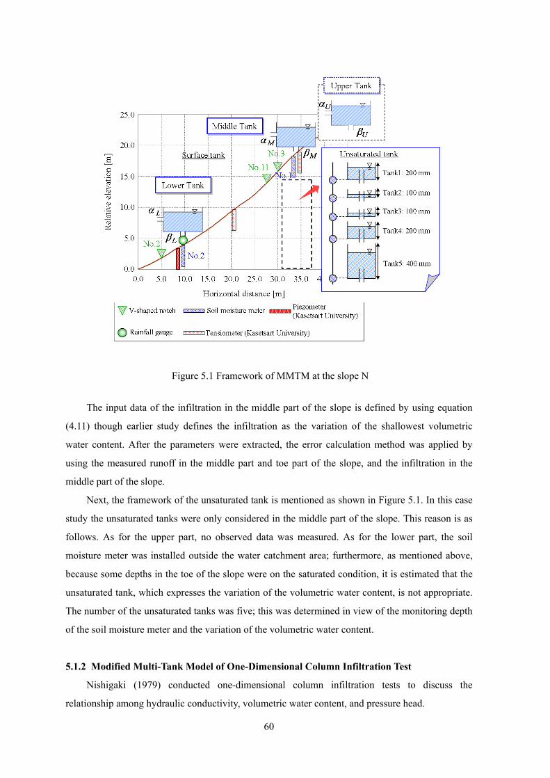
60

The input data of the infiltration in the middle part of the slope is defined by using equation

(4.11) though earlier study defines the infiltration as the variation of the shallowest volumetric

water content. After the parameters were extracted, the error calculation method was applied by

using the measured runoff in the middle part and toe part of the slope, and the infiltration in the

middle part of the slope.

Next, the framework of the unsaturated tank is mentioned as shown in Figure 5.1. In this case

study the unsaturated tanks were only considered in the middle part of the slope. This reason is as

follows. As for the upper part, no observed data was measured. As for the lower part, the soil

moisture meter was installed outside the water catchment area; furthermore, as mentioned above,

because some depths in the toe of the slope were on the saturated condition, it is estimated that the

unsaturated tank, which expresses the variation of the volumetric water content, is not appropriate.

The number of the unsaturated tanks was five; this was determined in view of the monitoring depth

of the soil moisture meter and the variation of the volumetric water content.

5.1.2 Modified Multi-Tank Model of One-Dimensional Column Infiltration Test

Nishigaki (1979) conducted one-dimensional column infiltration tests to discuss the

relationship among hydraulic conductivity, volumetric water content, and pressure head.

Figure 5.1 Framework of MMTM at the slope N

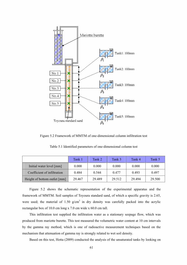
61

Figure 5.2 shows the schematic representation of the experimental apparatus and the

framework of MMTM. Soil samples of Toyoura standard sand, of which a specific gravity is 2.65,

were used; the material of 1.50 g/cm3 in dry density was carefully packed into the acrylic

rectangular box of 10.0 cm long x 7.0 cm wide x 60.0 cm tall.

This infiltration test supplied the infiltration water as a stationary seepage flow, which was

produced from mariotte burette. This test measured the volumetric water content at 10 cm intervals

by the gamma ray method, which is one of radioactive measurement techniques based on the

mechanism that attenuation of gamma ray is strongly related to wet soil density.

Based on this test, Hotta (2009) conducted the analysis of the unsaturated tanks by looking on

Table 5.1 Identified parameters of one-dimensional column test

Tank 1 Tank 2 Tank 3 Tank 4 Tank 5

Initial water level [mm] 0.000 0.000 0.000 0.000 0.000

Coefficient of infiltration 0.484 0.544 0.477 0.493 0.497

Height of bottom outlet [mm] 29.467 29.489 29.512 29.494 29.500

Figure 5.2 Framework of MMTM of one-dimensional column infiltration test

62

the sand column as the unsaturated region as shown in Figure 5.2.

Table 5.1 shows the identified optimal parameters of one-dimensional column test by MMTM.

The variability of coefficient of infiltration and the height of bottom outlet was relatively small

among the tanks.

5.1.3 Modified Multi-Tank Model at the Slope C

Kasetsart University conducted the field test at the slope C, Thailand, 29 and 30, July, 2007.

The investigated area at the slope C is 5 x 5 m2. Figure 5.3 shows the monitoring outline and the

framework of MMTM at the slope C; this site had three tensiometers, four sprinklers, and

hexahedron tub.

Hotta (2009) applied MMTM to the slope C. Four sprinklers played role of constant intensity

rainfall, of which maximum is 0.3 mm/min (i.e. 3 mm/10min) and hexahedron tub enabled to

Table 5.2 Identified parameters at slope C

Upper tank Middle tank Lower tank

Runoff Infiltration Runoff Infiltration Runoff Infiltration

Part-1 0.988 0.487 0.498 0.127 0.663 0.489

Part-2 0.987 0.488 0.497 0.126 0.661 0.490

Figure 5.3 Framework of MMTM at slope C

63

measure the surface runoff. In addition, the volumetric water content was not measured at the slope

C; therefore, it was indirectly estimated by using the matric suction and SWCC obtained from the

slope C. This study focuses attention on the identified surface parameters.

MMTM were applied to two rainfalls. Table 5.2 shows the identified optimal parameters at the

slope C. As shown in Table 5.2, the coefficient of infiltration in the middle tank at the slope C was

relatively small.

5.2 Analysis Results of the Modified Multi-Tank Model at the Slope N

5.2.1 Fitting Results

This subject shows the fitting results. This study applied MMTM to 26 rainfall patterns

measured from 19, May, 2008 to 4, Nov., 2008. In addition, as mentioned above, the definition of

infiltration related to the input data of Kalman filter algorithm was changed from earlier study

(Hotta, 2009).

First, the surface fitting results are mentioned. Table 5.3 shows the input data of Kalman filter

algorithm.

Figure 5.4, Figure 5.5 show the results of fitting analysis of the runoff in the middle part and

toe of the slope, respectively; Figure 5.6 shows the results of fitting analysis of the infiltration in

the middle part of the slope.

First, the results of fitting analysis of the runoff are mentioned. As shown in Figure 5.4, the

results of the runoff analysis in the middle part of the slope can simulate wave shape of the increase

and decrease of the amount of runoff although the amount of peak runoff can not be simulated in

some cases (e.g. 19, May, 30, May; 30, July; 3, August; 21, August; 19, September).

As shown in Figure 5.5, the results of the runoff analysis in the toe of the slope can simulate

not only wave shape but also the amount of peak runoff.

Table 5.3 Input data to Kalman filter algorithm (Part-1)

Rainfall

[mm/10min]

ΔRunoff

[mm/10min]

ΔInfiltration

[mm/10min]

Rainfall

[mm/10min]

ΔRunoff

[mm/10min]

ΔInfiltration

[mm/10min]

5/19 17:30 0.0 0.000 0.001 5/21 21:00 0.0 0.000 0.000

5/19 17:40 4.0 0.915 0.351 5/21 21:10 4.0 0.000 0.081

5/19 17:50 3.0 0.812 1.819 5/21 21:20 8.5 1.580 0.365

5/19 18:00 13.0 4.829 -3.300 5/21 21:30 4.0 0.899 -0.005

5/19 18:10 3.5 1.071 0.530 5/21 22:40 2.0 -1.208 -0.241

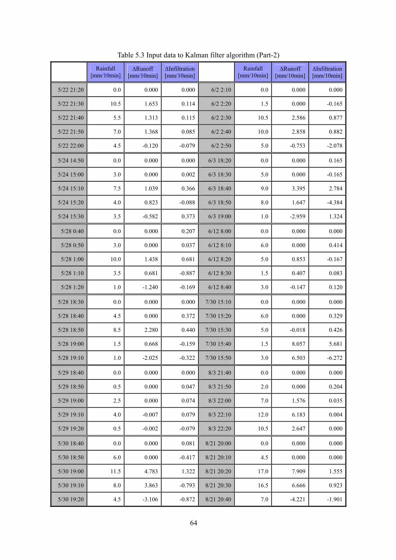
64

Table 5.3 Input data to Kalman filter algorithm (Part-2)

Rainfall [mm/10min]

ΔRunoff [mm/10min]

ΔInfiltration [mm/10min] Rainfall

[mm/10min]ΔRunoff

[mm/10min] ΔInfiltration [mm/10min]

5/22 21:20 0.0 0.000 0.000 6/2 2:10 0.0 0.000 0.000

5/22 21:30 10.5 1.653 0.114 6/2 2:20 1.5 0.000 -0.165

5/22 21:40 5.5 1.313 0.115 6/2 2:30 10.5 2.586 0.877

5/22 21:50 7.0 1.368 0.085 6/2 2:40 10.0 2.858 0.882

5/22 22:00 4.5 -0.120 -0.079 6/2 2:50 5.0 -0.753 -2.078

5/24 14:50 0.0 0.000 0.000 6/3 18:20 0.0 0.000 0.165

5/24 15:00 3.0 0.000 0.002 6/3 18:30 5.0 0.000 -0.165

5/24 15:10 7.5 1.039 0.366 6/3 18:40 9.0 3.395 2.784

5/24 15:20 4.0 0.823 -0.088 6/3 18:50 8.0 1.647 -4.384

5/24 15:30 3.5 -0.582 0.373 6/3 19:00 1.0 -2.959 1.324

5/28 0:40 0.0 0.000 0.207 6/12 8:00 0.0 0.000 0.000

5/28 0:50 3.0 0.000 0.037 6/12 8:10 6.0 0.000 0.414

5/28 1:00 10.0 1.438 0.681 6/12 8:20 5.0 0.853 -0.167

5/28 1:10 3.5 0.681 -0.887 6/12 8:30 1.5 0.407 0.083

5/28 1:20 1.0 -1.240 -0.169 6/12 8:40 3.0 -0.147 0.120

5/28 18:30 0.0 0.000 0.000 7/30 15:10 0.0 0.000 0.000

5/28 18:40 4.5 0.000 0.372 7/30 15:20 6.0 0.000 0.329

5/28 18:50 8.5 2.280 0.440 7/30 15:30 5.0 -0.018 0.426

5/28 19:00 1.5 0.668 -0.159 7/30 15:40 1.5 8.057 5.681

5/28 19:10 1.0 -2.025 -0.322 7/30 15:50 3.0 6.503 -6.272

5/29 18:40 0.0 0.000 0.000 8/3 21:40 0.0 0.000 0.000

5/29 18:50 0.5 0.000 0.047 8/3 21:50 2.0 0.000 0.204

5/29 19:00 2.5 0.000 0.074 8/3 22:00 7.0 1.576 0.035

5/29 19:10 4.0 -0.007 0.079 8/3 22:10 12.0 6.183 0.004

5/29 19:20 0.5 -0.002 -0.079 8/3 22:20 10.5 2.647 0.000

5/30 18:40 0.0 0.000 0.081 8/21 20:00 0.0 0.000 0.000

5/30 18:50 6.0 0.000 -0.417 8/21 20:10 4.5 0.000 0.000

5/30 19:00 11.5 4.783 1.322 8/21 20:20 17.0 7.909 1.555

5/30 19:10 8.0 3.863 -0.793 8/21 20:30 16.5 6.666 0.923

5/30 19:20 4.5 -3.106 -0.872 8/21 20:40 7.0 -4.221 -1.901

65

Table 5.3 Input data to Kalman filter algorithm (Part-3)

Rainfall [mm/10min]

ΔRunoff [mm/10min]

ΔInfiltration [mm/10min] Rainfall

[mm/10min]ΔRunoff

[mm/10min] ΔInfiltration [mm/10min]

8/27 1:30 0.0 0.000 -0.041 9/19 22:30 0.0 0.000 0.868

8/27 1:40 0.5 0.000 -0.287 9/19 22:40 2.0 0.000 -0.496

8/27 1:50 7.0 1.010 0.449 9/19 22:50 6.0 2.361 3.332

8/27 2:00 7.0 2.701 -0.163 9/19 23:00 3.5 1.449 -1.179

8/27 2:10 3.0 -0.226 0.126 9/19 23:10 5.5 0.954 -0.231

9/6 15:40 0.0 0.000 0.000 9/30 13:50 0.0 0.000 -0.004

9/6 15:50 7.5 0.000 0.244 9/30 14:00 0.5 0.000 0.088

9/6 16:00 11.5 2.079 0.249 9/30 14:10 11.0 2.621 6.219

9/6 16:10 0.5 0.278 -0.129 9/30 14:20 6.0 1.132 -8.802

9/6 16:20 0.5 -2.008 0.092 9/30 14:30 0.0 -2.444 2.467

9/8 11:50 0.0 0.000 0.000 10/1 12:50 0.0 0.000 -0.121

9/8 12:00 1.0 0.000 0.493 10/1 13:00 8.0 1.674 5.828

9/8 12:10 6.5 -0.466 0.038 10/1 13:10 6.5 0.805 -7.390

9/8 12:20 7.5 2.361 -0.162 10/1 13:20 4.0 2.708 11.239

9/8 12:30 4.0 1.717 0.000 10/1 13:30 15.5 2.136 -14.801

9/11 9:50 0.0 0.000 0.000 10/22 16:30 0.0 0.000 0.000

9/11 10:00 2.0 0.011 0.000 10/22 16:40 3.5 0.000 0.084

9/11 10:10 5.0 1.572 0.080 10/22 16:50 7.5 1.828 2.665

9/11 10:20 2.5 1.382 0.250 10/22 17:00 1.5 0.548 -3.644

9/11 10:30 1.5 -0.564 -0.086 10/22 17:10 0.5 -1.758 0.901

9/15 20:40 0.0 0.000 0.000 10/29 13:20 0.0 0.000 0.000

9/15 20:50 0.5 0.000 0.417 10/29 13:30 1.0 0.000 0.284

9/15 21:00 3.5 0.000 0.163 10/29 13:40 11.5 5.763 8.666

9/15 21:10 4.5 2.227 4.882 10/29 13:50 16.0 3.760 -9.911

9/15 21:20 7.0 2.545 -6.575 10/29 14:00 4.0 -4.938 -2.006

9/18 22:20 0.0 0.000 0.000 11/4 12:20 0.0 0.000 0.000

9/18 22:30 8.5 2.832 5.165 11/4 12:30 2.0 0.000 1.268

9/18 22:40 4.5 1.218 -5.576 11/4 12:40 1.0 0.000 -0.614

9/18 22:50 5.5 -0.447 2.559 11/4 12:50 0.5 0.000 5.117

9/18 23:00 6.5 1.534 -2.475 11/4 13:00 7.0 1.578 -8.527

66

Figure 5.4 Runoff analyses in the middle part of the slope

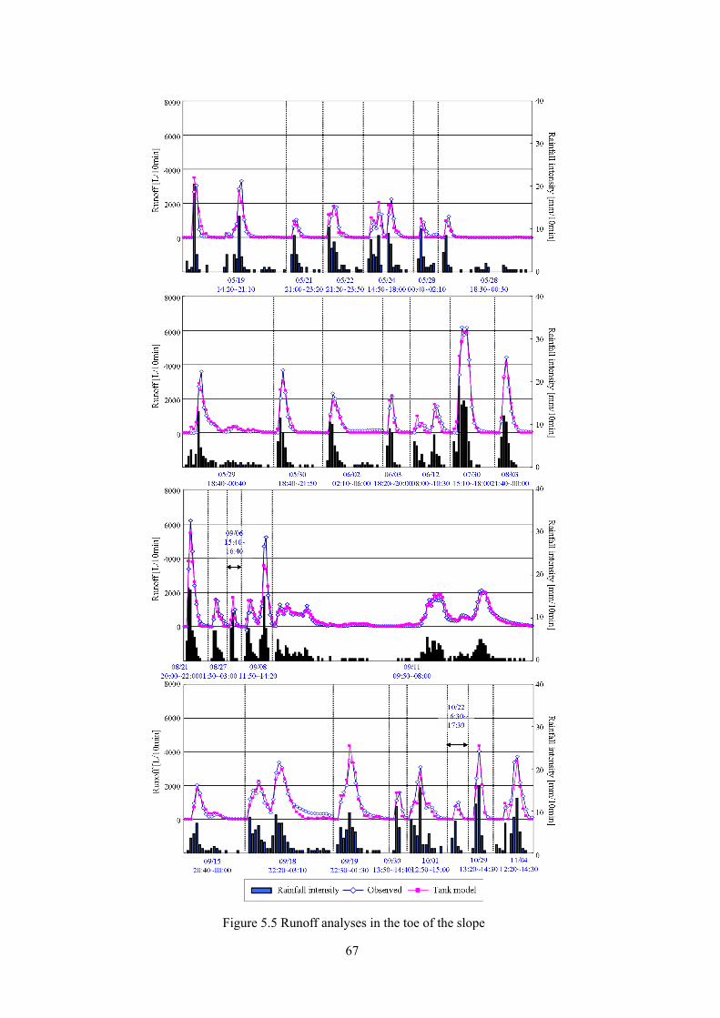
67

Figure 5.5 Runoff analyses in the toe of the slope

68

Figure 5.6 Infiltration analyses in the middle part of the slope

69

Figure 5.7(a) Seepage analyses in the middle part of the slope (GL-0.2m, -0.3m)

70

Figure 5.7(b) Seepage analyses in the middle part of the slope (GL-0.4m, -0.6m,-1.0m)

71

As shown in Figure 5.6, the results of infiltration analysis in the middle part of the slope can

not sufficiently simulate the behavior, although the wave shape sometimes can be simulated.

Next, the fitting analyses of the variation of the volumetric water content are mentioned.

Figure 5.7(a), (b) show the seepage analyses in the middle part of the slope.

As shown in Figure 5.7(a), the variation range at the depth of GL-0.2 m was relatively large,

of which the maximum was about 4 %. Even though the variation was large and rapid, MMTM can

sufficiently simulate the behavior. However, when there were a number of peaks of the variation of

volumetric water content (e.g. 15, September, 4, November), the fitting results sometimes showed

well-rounded behavior.

As shown in Figure 5.7(b), MMTM can sufficiently simulate the behavior of the variation at

deeper depth than GL-0.3 although the variation range was relatively small. In addition, for

example, in the case of 4, November, 2008, the variation of the volumetric water content deeper

depth than GL-0.3 m started after time elapsed from the beginning of the rainfall although the

volumetric water content at the depth of GL-0.2 m changed as soon as the rainfall started. This

results show the time-delay of the infiltration. MMTM can sufficiently simulate the delay of the

variation of the volumetric water content although the peak value of the volumetric water content is

overestimated.

5.2.2 Identified Results of the Surface Parameters

This subject shows the identified surface parameters.

Figure 5.8(a), (b), (c) show the relationship between the coefficients of infiltration and runoff

at the upper, middle, and lower tanks, respectively. Note that the parameters were classified as N-1

and N-2. N-1 and N-2 were defined in terms of the maximum rainfall intensity. The rainfall, of

which the maximum intensity is more than 10mm/10min, was defined as rainfall pattern N-1; the

rainfall, of which the maximum intensity is less than 10mm/10min, was defined rainfall pattern N-2.

The parameters at the upper tank, especially the coefficient of runoff were widely distributed as

shown in Figure 5.8(a). As shown in Figure 5.8（b）, both of the coefficient of infiltration and runoff

in the case of N-1, high-intensity rainfall, were larger than both of those in the case of N-2, low

intensity rainfall. Moreover, as shown in Figure 5.8(c), the variability of lower parameters was

relatively small; the coefficients of infiltration were distributed within the range of 0.0 to 0.4, and

the coefficients of runoff are distributed within the range of 0.3 to 0.6.

5.2.3 Identified Results of the Unsaturated Parameters

This subject shows the identified unsaturated parameters in the middle part of the slope.

Figure 5.9(a), (b), (c), (d), and (e) show the relationship between the coefficient of infiltration

72

Figure 5.8(c) Surface parameters at lower tank

Figure 5.8(b) Surface parameters at middle tank

Figure 5.8(a) Surface parameters at upper tank

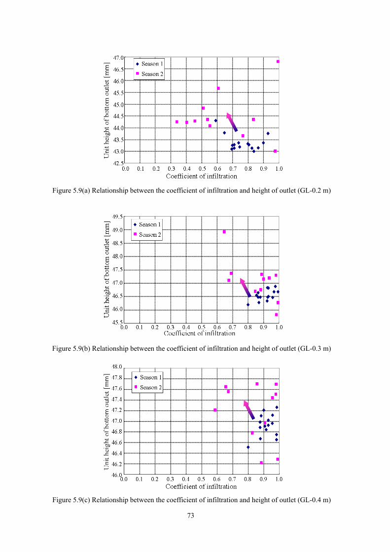
73

Figure 5.9(c) Relationship between the coefficient of infiltration and height of outlet (GL-0.4 m)

Figure 5.9(b) Relationship between the coefficient of infiltration and height of outlet (GL-0.3 m)

Figure 5.9(a) Relationship between the coefficient of infiltration and height of outlet (GL-0.2 m)

74

and the unit height of the bottom outlet at the depth of GL-0.2 m, GL-0.3 m, GL-0.4 m, GL-0.6 m,

and GL -1.0 m, respectively. Unit height of bottom outlet means the height of bottom outlet per 100

mm of the height of tank. Considering the variation caused by progression of rainy season, the

season was divided into two seasons as mentioned above: season-1 (from May to August), season-2

(from September to November). At any depth, the height of bottom outlet increased as rainy season

progresses.

In addition, Table 5.4 shows average value of the unit height of the bottom outlet at season-1

and season-2. In each season, the height of bottom outlet was different among the depths.

Next, Figure 5.10 shows the relationship between the coefficient of infiltration and the depth.

At the deeper depth than GL-0.3 m, the coefficients of infiltration were mainly distributed within

the range of 0.8 to 1.0. These coefficients of infiltration mean that the infiltration water supplied

Figure 5.9(e) Relationship between the coefficient of infiltration and height of outlet (GL-1.0 m)

Figure 5.9(d) Relationship between the coefficient of infiltration and height of outlet (GL-0.6 m)

75

from shallower part was largely permeated to deeper part.

On the other hand, the coefficients of infiltration at the depth of GL-0.2 m were widely

distributed within the range of 0.3 to 1.0. The small coefficients of infiltration mean that the

infiltration water was held at the depth.

5.3 Discussion based on Modified Multi-Tank Model The analysis results are discussed in this subject. First, the analysis results of the surface

region are discussed. Next, the analysis results of the unsaturated region are discussed. Moreover,

discussion combined the results of the surface region and the unsaturated region is conducted; the

parameters identified based on slope N, slope C, and one-dimensional column test are compared.

5.3.1 Analysis Results of Surface Region

The analysis results of the surface region are discussed in this subject.

First, the results of fitting analysis of the runoff are discussed. As shown in Figure 5.4, the

Figure 5.10 Relationship between the coefficient of infiltration and height of outlet (GL-1.0 m)

Table 5.4 Average value of the unit height of bottom outlet

GL-0.2m GL-0.3m GL-0.4m GL-0.6m GL-1.0m

Season-1 43.36 46.55 46.92 48.60 46.33

Season-2 44.50 47.08 47.18 49.10 47.15

76

runoff in the middle part of the slope was overestimated in some cases. Overestimation was mainly

confirmed in the case of rainfall pattern N-1. As shown in Figure 5.8(b), the coefficients of runoff

of N-1 (0.3~0.6) were larger than those of N-2 (0.1~0.3), that is, it is estimated that smaller

coefficient of runoff in the middle part is appropriate even in the case of N-1, focusing on only the

amount of runoff in the middle part of the slope. However, the parameters involved in MMTM are

identified to minimize the whole errors. The runoff in middle part also means the water supply in

terms of the lower tank; therefore, for example, if the amount of runoff in the toe of the slope was

relatively large, the amount of runoff in the toe part can be fitted by using not only the supply from

the rainfall but also runoff in the middle part. Accordingly, the whole error sometimes becomes

small though the error of the runoff in the middle part increases. Moreover, in the middle part of the

slope, at the phase of error calculation method to identify the optimal parameter, both the runoff

and the infiltration are considered; therefore, the parameter considered the relationship between the

coefficient of runoff and infiltration is determined.

As shown in Figure 5.5, the runoff in the toe of the slope can be simulated with very high

accuracy. In the toe of the slope, when the optimal parameters are determined, only the runoff is

considered because the amount of infiltration in the toe part is not measured as mentioned above.

Therefore, the latitude to set the coefficient of runoff is large because parameters can set only

considering the amount of runoff. Conversely, it is estimated that the coefficient of infiltration is

adjusted to fit the runoff, that is, the coefficient of infiltration has limited physical meaning as will

become apparent below.

As shown in Figure 5.6, the results off infiltration analysis in the middle part of the slope can

not sufficiently simulate the behavior. The infiltration was not directly measured but calculated by

equation (4.11) based on the measured volumetric water content although the runoff was directly

Figure 5.11 Relationship the maximum rainfall intensity and the middle coefficient of infiltration

77

measured by V-shaped notch. Therefore, it could be that reliability of the infiltration as measured

data is relatively small comparing the measured runoff. Especially, the infiltration defined by

equation (4.11) was calculated by the difference value of the volumetric water content; therefore,

when the volumetric water content decreased, the infiltration was evaluated to be negative value; in

this case, the amount of infiltration was assumed to be zero for descriptive purposes. Hence, the

variation of the amount of infiltration at the end of a rainfall can not be evaluated precisely

although the variation of the amount of infiltration at the beginning of rainfall is relatively

evaluated precisely.

Next, the identified surface parameters are discussed.

First, the parameters at the upper tank are discussed. Upper parameters were widely

distributed as shown in Figure 5.8(a). As mentioned above, upper tank was the assumed tank which

was not inputted any measuring data. Therefore, it is estimated that the upper parameters adjust the

whole water mass balance, especially the water mass balance of the middle and lower tank.

Second, the parameters at the middle tank are discussed. It is estimated that the middle part of

the slope especially is treated as the representative part of infiltration characteristics. As shown in

Figure 5.8（b）, coefficients of infiltration of N-1 were larger than those of N-2. Large values of

coefficient of infiltration in the case of N-1 mean that the high-intensity rainfall has a greater

tendency to infiltrate than low-intensity rainfall. This tendency is supported by the relationship

between the maximum rainfall intensity and the coefficient of infiltration in the middle part of the

slope as shown in Figure 5.11, that is, the coefficient of infiltration increased with increasing the

maximum rainfall intensity. On the other hand, it is estimated that the coefficient of runoff adjusts

the runoff in the toe of the slope as mentioned above; therefore, the increase of the coefficient of

Figure 5.12 Relationship between runoff at the toe of slope

and coefficient of runoff at the middle tank (N-1)

78

runoff at the middle tank has limited physical meaning in terms of the runoff in the middle part of

the slope although this essentially means the increase of the amount of runoff. This is supported by

the relationship between the accumulated runoff in the toe of the slope and the coefficient of runoff

at the middle tank as shown in Figure 5.12, that is, the coefficient of runoff increased with

increasing the accumulated runoff in the toe of the slope to supply the water to the toe part.

Third, the parameters at the lower tank are discussed. It is estimated that the toe of the slope

especially is treated as the representative part of runoff characteristics. As mentioned above, the

infiltration in the toe of the slope had no measured data; therefore, it is estimated that the

coefficient of infiltration at the lower tank performed as the coefficient to adjust the simulation of

Figure 5.14 Relationship between runoff at the toe of slope

and coefficient of infiltration at the toe tank

Figure 5.13 Relationship between runoff at the toe of slope

and coefficient of runoff at the toe tank

79

runoff in the toe of the slope. Figure 5.13 and Figure 5.14 show the relationship between the

accumulated runoff in the toe of the slope and the coefficient of runoff at the lower tank, and

relationship between the accumulated runoff in the toe of the slope and the coefficient of infiltration,

respectively. As shown in Figure 5.13, correlativity between the accumulated runoff in the toe of

the slope and the coefficient of runoff at the lower tank is small; on the other hand, as shown in

Figure 5.14, the coefficients of infiltration at the lower tank decreased with increasing the

accumulated runoff in the toe of the slope. By comparison Figure 5.13 with Figure 5.14, it is

estimated that the simulation of runoff at the lower tank is mainly adjusted to change the coefficient

of infiltration at the lower tank.

5.3.2 Analysis Results of Unsaturated Region

The analysis results of the unsaturated region are discussed in this subject.

As shown in Figure 5.7(a), MMTM can sufficiently simulate the behavior at GL-0.2m and

GL-0.3 m. However, when there were a number of peaks of volumetric water content (e.g. 15,

September, 4, November), the fitting results sometimes showed well-rounded behavior. This reason

is estimated as follows. The parameters identified by Artificial neural network stay constant

through the rainfall; therefore, the variation of infiltration characteristics can not be considered;

therefore, it is estimated that the well-rounded results are obtained to minimize the whole error.

As shown in Figure 5.7(b), MMTM can sufficiently simulate the behavior at deeper depth than

GL-0.4m. Moreover, as shown in the rainfall pattern on 4, November, 2008, MMTM can also

simulate the delay of the variation of the volumetric water content. MMTM considers the

time-delay of the variation of the volumetric water content as the height of the bottom outlet. This

Figure 5.15 Concept of the unsaturated tank at deeper depth

80

result shows that the bottom outlet sufficiently fulfill a function as the parameter which simulates

the time-delay.

Next, the identified unsaturated parameters are discussed.

First, as mentioned in Figure 5.9, the height of bottom outlet increased through the rainy

season. As mentioned above, the height of bottom outlet means the water retention, that is, the

results that the height of bottom outlet increased is compatible with the fact that the volumetric

water content gradually increased thorough the rainy season because of the repeated squall as

shown in Figure 4.23. Hence it is estimated that MMTM can simulate the long-term increase of the

volumetric water content as the increase of the height of bottom outlet.

As shown in Table 5.4, the height of bottom outlet was different among the depths. As

mentioned above, the soil at the slope N is affected by the weathering caused by repeated rainfall,

high temperature and back-filling; therefore, the values of the volumetric water content was a little

different among the depths because of the nonhomogeneity of the soil characteristics. MMTM can

evaluate this nonhomogeneity as the difference of the height of bottom outlet.

Next, the unsaturated coefficients of infiltration are discussed. At the deeper depth than

GL-0.3 m, the coefficients of infiltration were mainly distributed within the range of 0.8 to 1.0.

These coefficients of infiltration mean that the infiltration water supplied from shallower part was

largely permeated to deeper part. As mentioned above, the variation of the volumetric water content

at the deeper depth than GL-0.3 m was very small, that is, these depths already showed

Figure 5.16 Relationship between the coefficient of infiltration and the variation rate of the

volumetric water content (GL-0.2 m)

81

partially-saturated condition. Hence MMTM simulates this phenomenon by enlarging the

coefficient of infiltration as shown in Figure 5.15.

On the other hand, the coefficients of infiltration at the depth of GL-0.2 m were widely

distributed. The small coefficients of infiltration mean that the infiltration water was held at the

depth. Therefore, as shown in Figure 5.16, the coefficients of infiltration at the depth of GL-0.2 m

decreased with increasing the variation rate of the volumetric water content at the depth of GL-0.2

m. MMTM simulates the increase of the volumetric water content by becoming small the

coefficient of infiltration, that is, the infiltration to the deeper region is controlled.

5.3.3 Combination of the Analysis Results of Surface Region and Unsaturated Region

This subject discusses the analysis results of the infiltration characteristics combining the

identified surface parameters with unsaturated parameters. As mentioned in Figure 5.11, the surface

coefficients of infiltration in the middle part increased with increasing the maximum rainfall

intensity. In addition, as shown in Figure 5.16, the coefficient of infiltration at shallowest

unsaturated tank (GL-0.2 m) decreased with increasing the variation rate of the volumetric water

content at the depth of GL-0.2 m. Based on these results, the relationship between the surface

coefficient of infiltration at the middle tank and the unsaturated coefficient of infiltration at the

depth of GL-0.2 m is illustrated as shown in Figure 5.17. This relationship is conceptually

illustrated as shown in Figure 5.18. Altogether, this relationship means that the retentive water at

Figure 5.17 Relationship between the unsaturated coefficient of infiltration at GL-0.2 m and the

surface coefficient of infiltration at middle tank

82

Figure 5.19 Variation of water mass balance simulated by MMTM (19, September, 2008)

Figure 5.18 Relationship between the surface coefficient of infiltration and the unsaturated

coefficient of infiltration

83

shallow part increases with increasing the amount of infiltration from ground surface. Moreover,

Figure 5.19 shows the example of the variation of water mass balance against rainfall simulated by

MMTM. This example is the result simulated against the rainfall on 19, September, 2008. Only the

water level at the depth of GL-0.2 m largely changed against rainfall-induced infiltration. These

simulation results correspond to the actual phenomenon as follows. High-intensity rainfall induces

the large amount of infiltration; on the other hand, the soil type at the slope N is clay (i.e. the

permeability is low) and the deeper depth than GL-0.3 m is partially-saturated condition. Therefore,

the infiltration speed from the ground surface is larger than the infiltration speed in the subsoil,

accordingly the rainwater is retained the shallow unsaturated region. This phenomenon is one of the

mechanisms of shallow slope failure as mentioned in chapter 4. Hence, it is estimated that MMTM

can simulate the behavior of the rainwater and infiltration water in the case of the shallow slope

failure caused by high-intensity rainfall.

5.3.4 Comparison of Parameters among Slope N, Slope C, and Column Test

Identified parameters among slope N, slope C, and one-dimensional column test are compared

and discussed in this subject.

First, the surface parameters are compared and discussed focused on slope N and slope C. As

shown in Table 5.2, the coefficients of infiltration at the middle tank in the slope C were relatively

small. It could be that these results were caused by the low-intensity rainfall generated by sprinklers.

In the case of the slope N, as shown in Figure 5.11, the coefficients of infiltration at the middle tank

increase with increasing the maximum rainfall intensity, that is, high-intensity rainfall has greater

tendency to infiltrate than low-intensity rainfall. The identified results at the slope C correspond to

the tendency at the slope N, that is, the rainfall intensity generated by sprinklers is relatively low;

therefore, the coefficient of infiltration at middle tank is small.

Next, the unsaturated parameters are compared and discussed focused on the slope N and

one-dimensional column test. As shown in Table 5.1, the variability of coefficient of infiltration and

the height of bottom outlet in one-dimensional test was relatively small among the tanks. This

reason is estimated as follows. As mentioned above, one-dimensional column test was conducted

by using Toyoura standard sand, and a stationary seepage flow; that is, it is estimated that the

infiltration characteristics were not different among the depth. Therefore, the coefficient of

infiltration and the height of bottom outlet, which control the infiltration characteristics on the

model, had small variability among the tank.

On the other hand, as mentioned in Figure 5.9 and Table 5.4, both the coefficient of infiltration

and the height of bottom outlet have some variability among the depth. As mentioned above, soil

water characteristics were different among the depth at the slope N due to the weathering and

84

back-filling.

Hence, MMTM can treat not only the homogenous soil water characteristics but also the

heterogeneous soil water characteristics to set the suitable parameters.

5.4 Infiltration Analysis due to the Difference of Rainfall Pattern This section mentions the variation of the infiltration characteristics due to the difference of

rainfall pattern by using MMTM. As mentioned above, it is pointed out that MMTM can simulate

Table 5.5(a) Surface parameters

Upper tank Middle tank Lower tank

Runoff Infiltration Runoff Infiltration Runoff Infiltration

Surface 0.123 0.594 0.575 0.651 0.638 0.020

(c) Back type rainfall pattern (d) Constant type rainfall pattern

Figure 5.20 Inputted rainfall pattern

(a) Actual rainfall pattern (b) Front type rainfall pattern

85

the variation of water mass balance in the case of high-intensity rainfall. In this section,

guerilla-like rainfall confirmed in Japan is inputted to MMTM with identified parameters at the

slope N, and the infiltration characteristics are discussed by changing the rainfall pattern.

The guerilla-like rainfall which was generated on 29, August, 2009, at city O in Japan was

applied to MMTM as the input assumed rainfall. The actual rainfall pattern is illustrated as shown

(c) Back type rainfall pattern (d) Constant type rainfall pattern

Figure 5.21 Rainfall intensity and the surface infiltration intensity

(a) Actual rainfall pattern (b) Front type rainfall pattern

Table 5.5(b) Unsaturated parameters

Tank 1 Tank 2 Tank 3 Tank 4 Tank 5

Initial water level [mm] 88.773 47.025 47.440 99.222 189.928

Initial volumetric water content [%] 43.886 47.025 47.440 49.611 47.482

Coefficient of infiltration 0.403 0.936 0.980 0.920 0.960

Height of bottom outlet [mm] 88.456 47.183 47.504 99.297 190.222

86

in Figure 5.20(a). To evaluate the difference of the infiltration characteristics due to the difference

of rainfall pattern, the four rainfall pattern which had the same amount of accumulated rainfall with

the actual rainfall pattern were assumed: front type (Figure 5.20(b)), back type (Figure 5.20(c)), and

constant type (Figure 5.20(d)). The initial condition and the parameters identified by the measured

data on 19, September, 2008 at the slope N were applied as summarized in Table 5.5(a), (b).

Figure 5.21(a), (b), (c), and (d) show the rainfall intensity and the surface infiltration intensity

in the case of the actual rainfall, front type rainfall, back type rainfall, and constant type rainfall,

respectively. First, the infiltration intensity in the case of constant type rainfall was smaller any

other rainfall pattern. The water level of the surface tank was relatively small through the rainfall;

accordingly the infiltration intensity became small. It is inferred that this results paradoxically

substantiate that the coefficient of infiltration at the slope C, where rainfall intensity was constant,

was small. Second, as shown in Figure 5.21(b), the peak of infiltration intensity only in the case of

front type rainfall pattern did not conform to the peak of rainfall intensity. This reason is estimated

as follows. In the case of front type rainfall pattern, highest-intensity rainfall suddenly occurred as

(c) Back type rainfall pattern (d) Constant type rainfall pattern

Figure 5.22 Rainfall intensity and the variation of the volumetric water content

(a) Actual rainfall pattern (b) Front type rainfall pattern

87

soon as rainfall started; therefore, the infiltration occurred without water due to antecedent rainfall

in the surface tank. At the next time step, when the second highest-intensity rainfall, the infiltration

intensity was maximized because there was the water due to antecedent highest-intensity rainfall in

the tank. In the case of the back type rainfall pattern, the infiltration intensity was maximized at

time step, when the highest-intensity rainfall occurred because there were some amounts of water

in the tank before highest-intensity rainfall occurred. Hence, the maximum value of the infiltration

intensity in the case of the back type rainfall pattern is larger than that in the case of the front type

rainfall pattern.

Figure 5.22(a), (b), (c), and (d) show the rainfall intensity and the variation of the volumetric

water content in the case of the actual rainfall pattern, front type rainfall pattern,, back type rainfall

pattern, and constant type rainfall pattern, respectively. First, the variation of the volumetric water

content except for the depth of GL-0.2 m was relatively small. This is why the infiltration water

was retained at shallow region as mentioned above. Second, the maximum value of the volumetric

water content at the depth of GL-0.2 m in the case of the back type rainfall pattern was larger than

that in the case of the front type rainfall pattern. Considering matric suction related to resistance for

slope failure decreases with increasing the volumetric water content, it is estimated that the back

type rainfall pattern is more dangerous than the front type rainfall pattern in terms of the slope

stability. In addition, the variation of the volumetric water content was relatively small in the case

of the constant type rainfall pattern. It remains possible that the experiment used the constant

rainfall intensity can not evaluate the infiltration characteristics and slope stability.

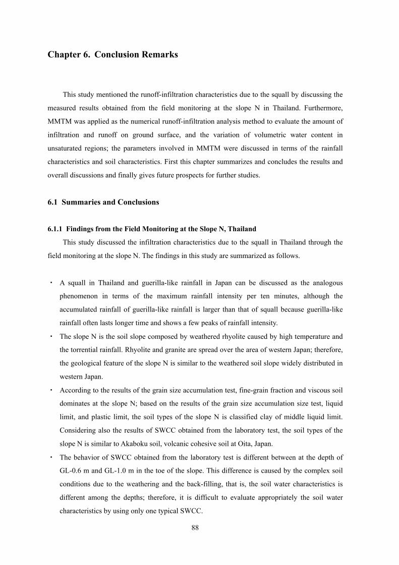
88

Chapter 6. Conclusion Remarks

This study mentioned the runoff-infiltration characteristics due to the squall by discussing the

measured results obtained from the field monitoring at the slope N in Thailand. Furthermore,

MMTM was applied as the numerical runoff-infiltration analysis method to evaluate the amount of

infiltration and runoff on ground surface, and the variation of volumetric water content in

unsaturated regions; the parameters involved in MMTM were discussed in terms of the rainfall

characteristics and soil characteristics. First this chapter summarizes and concludes the results and

overall discussions and finally gives future prospects for further studies.

6.1 Summaries and Conclusions

6.1.1 Findings from the Field Monitoring at the Slope N, Thailand

This study discussed the infiltration characteristics due to the squall in Thailand through the

field monitoring at the slope N. The findings in this study are summarized as follows.

・ A squall in Thailand and guerilla-like rainfall in Japan can be discussed as the analogous

phenomenon in terms of the maximum rainfall intensity per ten minutes, although the

accumulated rainfall of guerilla-like rainfall is larger than that of squall because guerilla-like

rainfall often lasts longer time and shows a few peaks of rainfall intensity.

・ The slope N is the soil slope composed by weathered rhyolite caused by high temperature and

the torrential rainfall. Rhyolite and granite are spread over the area of western Japan; therefore,

the geological feature of the slope N is similar to the weathered soil slope widely distributed in

western Japan.

・ According to the results of the grain size accumulation test, fine-grain fraction and viscous soil

dominates at the slope N; based on the results of the grain size accumulation size test, liquid

limit, and plastic limit, the soil types of the slope N is classified clay of middle liquid limit.

Considering also the results of SWCC obtained from the laboratory test, the soil types of the

slope N is similar to Akaboku soil, volcanic cohesive soil at Oita, Japan.

・ The behavior of SWCC obtained from the laboratory test is different between at the depth of

GL-0.6 m and GL-1.0 m in the toe of the slope. This difference is caused by the complex soil

conditions due to the weathering and the back-filling, that is, the soil water characteristics is

different among the depths; therefore, it is difficult to evaluate appropriately the soil water

characteristics by using only one typical SWCC.

89

・ Measured volumetric water content at the slope N has different behavior among the depths and

between the middle part of the slope and the toe of the slope. Especially in the toe of the slope,

the volumetric water contents at the depth of GL-0.2 m, GL-0.3 m, and GL-0.4 m show 60 %

(saturated condition), that is, saturated region spread instantaneously up to the ground surface

due to the torrential rainfall. On the other hand, the volumetric water contents at the depth of

GL-0.6 m and GL-1.0 m keep constant value of about 60 % (saturated condition), and positive

pore water pressure is measured at these depths. This surface saturated condition is related to

the high rainfall intensity and low permeability of subsoil.

・ The in-situ SWCC has different behavior between in the middle part of the slope and the toe of

the slope; as a result, the toe of the slope triggers the landslide.

・ This monitoring system can measure the appropriate water mass balance; on that basis, the

macroscopic infiltration rate in the whole is distributed within the range from 20 % to 65 %.

・ Focusing on the infiltration rate in the middle part of the slope, the infiltration rate changes

affected by the rainfall intensity and the progress of the rainy season. The infiltration

characteristics have the hysteresis. Moreover, in the case of the rainfall pattern which has a

number of rainfall peaks, the infiltration rate of the second peak is sufficiently almost the same

as that of the first peak.

・ The mechanism of the shallow slope failure assumed by the results in the slope N is

summarized as follows. Torrential rainfall induces large amount of infiltration water from the

ground surface; on the other hand, the infiltration speed is relatively small because of the clay

(low permeability). Accordingly the saturated region spreads in the shallow region due to piling

up the water because the infiltration speed from the ground surface is quite larger than that of

subsoil.

6.1.2 Findings from the results of Modified Multi-Tank Model

This study applied measured results to Modified Multi-Tank Model. The findings in this study

are summarized as follows.

・ The surface runoff in the toe of the slope can precisely be simulated. On the other hand, the

surface runoff in the middle part of the slope can not be simulated in terms of the peak runoff in

some cases. The variation of the volumetric water content in the middle part of the slope can be

simulated even though the variation is large and rapid. However, when there are some peaks of

the variation of the volumetric water content, the fitting results show well-rounded behavior.

・ The surface parameters are classified into two types of parameters: the parameters which have

physical meaning and the parameters which adjust the water mass balance of the system. The

90

coefficient of infiltration in the middle tank is the former type and related to the rainfall

intensity. On the other hand, the parameters involved in the upper tank adjust the whole water

mass balance; furthermore, the coefficient of runoff in the middle tank and the coefficient of

infiltration in the lower tank adjust the water mass balance, especially, the runoff in the toe of

the slope.

・ The unsaturated coefficients of infiltration at deeper depth than GL-0.3 m have large values to

keep the constant volumetric water content; on the other hand, the unsaturated coefficients of

infiltration at the depth of GL-0.2 m are widely distributed, that is, the unsaturated coefficients

of infiltration at the depth of GL-0.2 m decreases with increasing the volumetric water content

at the depth of GL-0.2 m.

・ Modified Multi-Tank Model can simulate the behavior of the rainwater and infiltration water in

the case of the shallow slope failure caused by squall.

・ The maximum volumetric water content in a rainfall is different among the rainfall patterns

even if the amount of rainfall is the same; back type rainfall pattern is the most dangerous in

term of slope stability.

6.2 Future Prospects

6.2.1 Monitoring Interval This study discussed the runoff-infiltration characteristics by using the measured results every

ten minutes to cope with a short-term and high intensity rainfall such as squall or guerilla-like

rainfall. This subject shows the measured results of one minute interval monitoring which was

probatively conducted from 18 to 24 September, 2008 and compares the results of one minute

interval monitoring with the results of ten minute interval monitoring.

Figure 6.1(a), (b) show the measured results of one minute rainfall intensity measured by

rainfall gauge with tripping bucket on 18 and 19 September, 2008, respectively; Figure 6.2(a), (b)

show the measured results of ten minute rainfall intensity on 18 and 19 September, 2008,

respectively. In the case of ten minute interval monitoring, rainfall intensity were measured every

ten minutes discretely, therefore one rainfall peak was sometimes divided into two measured time

steps especially as shown in Figure 6.1(a) (22:20~ 22:40 on 18 September, 2009). In such a case, it

is estimated that the variation of rainfall intensity can not be evaluated appropriately.

However, it is estimated that the particular problem of one minute interval monitoring exists,

that is, monitoring interval is not appropriate in terms of resolution capability of rainfall gauge; for

example, if the rainfall pattern as shown in Figure 6.3 was confirmed, it is estimated that it does not

mean no rainfall was generated in t=1 and suddenly 0.5 mm rainfall was generated in t=2 as an

91

actual phenomenon. This should be interpreted that 0.5 mm rainfall was generated in two time steps

in the case of one minute interval monitoring. Tripping bucket rainfall gauge measures rainfall

intensity by counting the number of trip of bucket which impounds rainfall. This gauge trips when

0.5 mm rainfall is impounded in the box, hence the measured results show no rainfall was

generated if the amount of rainfall was less than 0.5 mm per one minute.

Needless to say, it is needed to adopt the rainfall gauge with higher resolution to cope with this

problem; however, it is estimated to be possible to evaluate the one minute rainfall intensity to

define the approximative one minute rainfall as following equations.

If 0,,0,00,00,0

21

11

≠==≠=≠≠

===

+==+==

ittt

itititit

rrrtrorrr

Λ , ( )

irRRRrrRR

itittt

itititit

====

+==+==

===

+==

21

11 2 (6.1)

(a) 18 September, 2008 (b) 19 September, 2008

Figure 6.2 Observed results of ten minute rainfall intensity

(a) 18 September, 2008 (b) 19 September, 2008

Figure 6.1 Observed results of one minute rainfall intensity

92

where rt=i means the one minute rainfall intensity at t=i observed by tripping bucket rainfall gauge

and Rt=i means the approximative one minute rainfall intensity at t=i.

By this concept, the rainfall data as shown in Figure 6.3 can be revised as shown in Figure 6.4,

that is, Rt=1 and Rt=2 are calculated by the average of rt=1 and rt=2, and Rt=3, Rt=4 and Rt=5 are

calculated by the average of rt=3, rt=4 and rt=5.

In addition, Figure 6.5(a), (b) show the comparison of the measured results of one minute

interval monitoring with ten minute monitoring in the middle part of the slope at the depth of

GL-0.1 m and GL-0.2 m on 18 and 19, September, 2008, respectively. As shown in Figure 6.5(a),

(b), compared with one minute interval monitoring, ten minute interval monitoring can express the

(a) 18 September, 2008 (b) 19 September, 2008

Figure 6.5 Comparison of the volumetric water content

between the one minute monitoring and ten minute monitoring

Figure 6.4 Approximative rainfall intensity

Figure 6.3 Rainfall intensity measured by

rainfall gauge

93

rough variation of volumetric water content although one hour interval can not express the variation

of volumetric water content due to the squall (Hotta, 2009). However, when the rainfall started and

the volumetric water content changed rapidly, ten minute interval monitoring can only express the

average variation of the volumetric water content; therefore, it is estimated that one minute interval

monitoring is effective in the case of focusing on the variation of the volumetric water content the

right from the beginning of the rainfall.

Finally, Figure 6.6(a), (b) show the approximative rainfall intensity and variation of the

volumetric water content in the middle part of the slope on 18 and 19, September, 2008,

respectively. It is estimated that the definition of approximative rainfall intensity is appropriate

because increase and decrease of approximative rainfall intensity relatively corresponds to the

variation of volumetric water content.

Next, the issue assumed in term of the application of one-minute measured results to MMTM

is mentioned. Considering the relationship between the infiltration speed and the time step interval,

it could be that the number of the unsaturated tanks is needed to increase to estimate the volumetric

water content precisely.

6.2.2 Evaluation of Slope Stability against the Torrential Rainfall

In this monitoring site, the region of which volumetric water content was constant at high

value was showed. This study pointed out that these regions have already become the saturated

condition and moving up of the saturated region to surface region caused the surface landslide due

to torrential rainfall, that is, it is estimated that this kind of landslide occurs not in the unsaturated

condition but in the saturated condition. Therefore not only the short-interval monitoring of the

(a) 18 September, 2008 (b) 19 September, 2008

Figure 6.6 Results of the volumetric water content of one minute monitoring

with approximative rainfall intensity

94

volumetric water content but also the short-interval monitoring of the pore water pressure is needed

because the volumetric water content is constant in the saturated condition although the pore water

pressure can change even in the saturated condition. In addition, the model to estimate the variation

of the positive pore water pressure is needed to estimate the slope stability under the saturated

condition. In the case of the unsaturated slope stability, it can be evaluated by associating matric

suction with volumetric water content by SWCC fitting model (van Genuchten M, 1980). On the

other hand, the positive pore water pressure related to the saturated slope can not be estimated by

using the volumetric water content because the volumetric water content is constant in the saturated

condition.

95

References

Buckingham, E.: Studies on the Movement of Soil Moisture, Bulletin 38. U.S. Department of

Agriculture Bureau of Soils Washington D.C., 1907.

DELTA-T DEVICES: User Manual for the Profile Probe, Delta-T Devices, Cambridge, UK, 2004.

Elrick, D. E., and Bowman, D. H.: Note on an improved apparatus for soil moisture flow

measurements, Soil Sci. Soc. Am. Proc., 28, pp. 450-453, 1964.

FUJITSU Corporation: NEUROSIM/L(R) V4. (in Japanese)

Geological Survey of Japan, National Institute of Advanced Industrial Science and Technology:

Geological Survey of Japan, AIST (ed.). 2009. Seamless digital geological map of Japan 1: 200,000.

Dec 15, 2009 version. Research Information Database DB084, 2009. (in Japanese)

Horton, E. R.: An approach toward a physical interpretation of infiltration-capacity, Soil Sci. Soc.

Am. Proc., 5, pp. 399-417, 1940.

Hotta, Y.: Evaluation of Unsaturated Soil Slope Stability against Heavy Rainfall Using Modified

Multi-Tank Model System, Dissertation of Kyoto University, 2009.

Ichihara, K., Toyokawa, K., Sawaguchi, I. and Kawashima, H.: Real time runoff forecasting with

tank models whose parameter values are identified by Kalman Filter, J Jpn. For. Soc., 82, pp.

125-131, 2000. (in Japanese)

Ishii, M.: Studies on the Runoff Mechanism in Slope (I): A Few Studies on HORTON’s Infiltration

Capacity, Journal of the Japanese Forestry Society, Vol. 56, No.3, pp. 90-96, 1974. (in Japanese)

Japanese Industrial Standards Committee: The Formula for Estimation of Amount of Water Flow by

V-shaped Notch, Japanese Industrial Standards (JIS) B 8302-1990. (in Japanese)

Jotisankasa, A., and Mairaing, W.: Suction-monitored direct shear testing of residual soils from

landslide-prone areas, Journal of Geotechnical and Geoenvironmental Engineering, ASCE, Vol. 1,

pp. 119-138, 2009

96

Karube, D., Kato, S., Hamada, K., and Honda, M.: The Relationship between the Mechanical

Behavior and the State of Porewater in Unsaturated Soil, Proceedings of JSCE, Vol. 535, No. iii-34,

pp. 83-92, 1996. (in Japanese)

Kitamura, R., Kawaida, M., Abe, H., Jomoto, K. and Terachi, T.: Development of Field Measuring

System For Suction in Unsaturated Soil with Rainfall, Proceedings of JSCE, Vol. 652, No. III-51,

pp. 287-292, 2000. (in Japanese)

Komine, H., Yasuhara, K., Murakami, S., and Uchida, Y.: Simplified Evaluation on Vulnerability of

River Levee and Bank by Torrential Rainfall from the Viewpoint of Water Retentivity of Some

Soils (<Theme>Global Warming and Freak Weather), The Japanese Geotechnical Society, Vol. 57,

No. 4, pp. 22-25, 2009. (in Japanese)

Nishihgaki, M.: Research on Behavior of Groundwater and Its Application to Foundation

Engineering, Dissertation of Kyoto University, 1979. (in Japanese)

Ohtsu, H., Akagi, M., and Takahashi, K.: Identification of Parameters Involved in Multi-Tank

Model System Using Artificial Network, Proceedings of the EIT-JSCE International Seminar on

Rock Engineering 2007, pp. 149-154, 2007.

Ohtsu, H., Hotta, Y., Takahashi, K., and Nakamura, K.: A Study on Applicability of Modified

Multi-Tank Model for Unsaturated Soil Slope, Proceedings of the EIT-JSCE joint International

Seminar on Rock Engineering 2008, 184-191, 2008.

Ookubo, K., Fujioka, K., and Takemoto, M.: Maintenance on Earth Structure of Express Network

in Japan (<Theme> Maintenance and Renewal), Soil mechanics and foundation engineering, Vol.

56, No.2, pp. 2-3, 2008. (in Japanese)

OYO Corporation: User Manual for S&DL mini, 2005. (in Japanese)

Sako, K., Fukagawa, R., Iwasaki, K., Satomi, T., and Yasukawa, I.: Field Monitoring on Slope

around Important Cultural Asset in order to Prevent Slope Disasters due to Rainfall, Japanese

Geotechnical Journal, Vol. 1, No.3, pp. 57-69, 2006. (in Japanese)

97

Sato, T., and Sato, M.: Structural Identification using Neural Network and Kalman Filter

Algorithms, Journal of structural mechanics and earthquake engineering, JSCE, Vol. 563, No. I-39,

pp. 1-10, 1997. (in Japanese)

Sugawara, M.: On the Analysis of Runoff Structure about Several Japanese Rivers, Japanese

Journal of Geophysics, 2, No.4, 1961.

Sugii, T., and Takeshita, Y.: Engineering Technique for Evaluating the Hydraulic Properties of

Unsaturated Soils (Theme: Monitoring Techniques of Slope Stability in the Rain), Soil mechanics

and foundation engineering, 55 (9), pp. 20-22, 2007. (in Japanese)

Sugiyama, T. and Nunokawa, O.: Risk Estimation for Railway Slope Failure and Train Operation

Control during Rainfall (Theme: Monitoring Techniques of Slope Stability in the Rain), Soil

mechanics and foundation engineering, 55(9), pp. 14-16, 2007. (in Japanese)

Takahashi, K., Ohtsu, H. and Ohnishi, Y.: Research on the Slope Risk Evaluation in Consideration

of Groundwater Behavior Using the Storage Tank Model (<Theme> Geotechnical Risk

Management), Soil mechanics and foundation engineering, 51 (10), pp. 15-17, 2003. (in Japanese)

Thi, H., Sasaki, Y., Moriwaki, T., Kano, S., Yamamoto, M., Sato, T. and Uekuma, H.: Monitoring

System to Trance Rainfall Induced Moisture Change in a Masado Slope, Bulletin of the Graduate

School of Engineering, Hiroshima University, Vol. 53, No.1, 2004. (in Japanese)

Van Genuchten M, Th.: A Closed Form Equation for Predicting the Hydraulic Conductivity of

Unsaturated Soils, Soil Sci. Soc. Am. J., pp. 892-898, 1980.

98

謝辞

最後になりましたが，本論文を締めくくるにあたり，本研究にご協力いただいた方々に

感謝の意を表します．

3 年間，親身なご指導を賜りました京都大学大学院工学研究科・大津宏康教授に心より

感謝致します．数々のご助言を賜りましたが，今でも忘れられないことは，09 年 9 月に学

生のみで計測機器の再設置をすることになり，不安がっていた私に，「失敗してもいいから，

とにかく考えた通りに好きにやってきなさい．」とおっしゃっていただいたことです．その

後押し，期待にどれほどまで応えることができたか正直自信はありませんが，先生という

絶対的な支えがあったお陰で，3 年前に配属された時には想像できない程，私自身成長で

きたと感じています．研究以外では，例えば今後の進路に悩んでいた際に，「鶏口となるも

牛後となるなかれって諺は間違いでな，牛の口を目指しなさい．」とおっしゃっていただい

たことが強く記憶に残っています．先生には，研究に留まらず，学生から社会人になる過

渡期にある私に人生の生き方も教えていただいたと感じています．就職してからも先生に

教えていただいた数々のことを胸に，土木に携わって関西地方の暮らしを支え，また世界

で活躍できる技術者を目指して日々精進してまいりますので，今後ともご指導ご鞭撻よろ

しくお願い申し上げます．

京都大学大学院工学研究科・塩谷智基准教授には熱心なご助言を頂きましたこと深謝致

します．研究内容の垣根を越えて多くの最新の研究のお話をお伺いすることができたこと

は，私にとって大変刺激になり，研究に取り組む意欲に繋がりました．また，研究以外の

相談についても時にはお酒を交えてお話を聞いていただき，有意義な時間を過ごすことが

できました．心から感謝致します．

また，カセサート大学工学研究科・Dr. Warakorn Mairaing，Dr. Suttisak Soralump，および

Dr. Apiniti Jotisankasa には特に現地滞在中数々のご支援を賜りました．改めて御礼申し上げ

ます．Dr. Warakorn Mairaing は，暖かく研究室に迎え入れて頂き，実験室の使用等数々の

ご配慮いただきました．御礼申し上げます．Dr. Suttisak Soralump には現地滞在中に度々電

話をいただき，進捗状況について気にかけて頂いたと共に，同大学の学生と交流する機会

を積極的に作っていただき，大変有意義な時間を過ごすことができました．厚く御礼申し

上げます．Dr. Apiniti Jotisankasa には数々の貴重なデータを提供していただいただけでなく，

様々なトラブルに対しても迅速かつ丁寧に対応していただきました．重ねて御礼申し上げ

ます．

京都大学大学院工学研究科・稲積真哉助教には研究室生活を有意義に過ごす上で多くの

ご支援を頂きましたと共に，研究面でも貴重なご意見を賜りました．大変感謝致します．

水文技術コンサルタント株式会社・高橋健二氏には研究の本質に関わる部分で多くの貴

99

重なご助言を頂きましたことに，心より御礼申し上げます．遅々として進まない私の研究

に対して，大変本質的なご指摘を数々頂きましたことで，本研究の核となる部分を形作る

ことができました．また，現地視察として Uttaradit までご同行いただいただけでなく，灼

熱の中での Nakhon Nayok における作業にご協力いただきましたことに，改めて感謝致し

ます．

応用地質株式会社・矢部満氏，長谷川信介氏，中村一樹氏，および岩崎智久氏には貴重

な計測機器を提供いただくと共に数多くのご助言を賜りました．矢部満氏には Nakhon

Nayok での現地作業，Uttaradit への現地視察にご協力いただいたと共に，計器トラブル発

生時や計測機器に関する質問にも迅速に対応していただきました．特に 09 年 9 月に学生二

人で再設置作業のために現地に赴く直前に，京都までご足労頂き，設置の上での留意点等

をご指導いただきました．厚く御礼申し上げます．長谷川信介氏には，Nakhon Nayok の現

地作業，Uttaradit の視察におきまして多大なるご協力を頂いたのみならず，研究室の先輩

として親しくさせていただきました．心より御礼申し上げます．中村一樹氏には Nakhon

Nayok 現地作業において，多大なるご支援をいただきました．特に私が現地に始めて滞在

した際にご同行いただき，大変心強かったです．深謝致します．岩崎智久氏には Nakhon

Nayok での現地作業において多大なるご支援いただきました．改めて御礼申し上げます．

京都大学大学院工学研究科・矢野隆夫技術専門員には室内実験のご指導を頂きましたこ

と心より感謝いたします．

アジア工科大学・Mr. Taweephong Suksawat，カセサート大学学生諸氏，タダンダム管理

事務所の現地スタッフの皆様に心より感謝致します．Mr. Taweephong Suksawat には計器ト

ラブルの対応のために何度も現地に赴いて頂き，迅速に対応して頂きましたと共に，現地

作業のサポートもしていただきました．大変感謝しております．カセサート大学学生諸氏

には滞在期間を配慮し，実験機器を利用させていただいたと共に，Uttaradit の視察にもご

同行いただきました．御礼申し上げます．タダンダム管理事務所の皆様には，滞在中事務

所の一角をご好意でお貸しいただき，研究を進めさせていただきました．特に，Mr. Nui

には現地作業において多大なるご支援をいただきました．彼無しでの研究の完遂は無かっ

たといっても過言ではありません．また，家族ぐるみでの付き合いもさせていただき，タ

イの文化に触れると共に，「君は私の弟のような存在だよ．」と懇意にしていただき，大変

充実した日々を過ごすことができました．心より感謝致します．

Mr. Thamrongsak Suwanishwong には生前大変お世話になりました．初めて学生一人でタ

イに行く私を心配し，「空港に着くくらいの時間とホテルに到着する時間ぐらいに電話する

からね．」と多くを気遣ってくれたこと決して忘れません．もっと共に研究にしたかったで

す．心配ばかりかけていた後輩でしたが，ここに論文を完成することができました．心よ

り御礼申し上げます．

大成建設株式会社・堀田洋平氏には本研究の先行研究者として多くの貴重なデータを提

100

供して頂き，また共に現地に赴いた際には，次年度以降のことを見越して厳しく指導して

頂きました．今年になってその理由が本当に身にしみ，助かりました．共に研究室で過ご

させて頂いた 2 年間は大変有意義で楽しい時間でした．心より御礼申し上げます．

また，京都大学工学研究科・北村瑞絵前秘書，ならびに伊東宏美秘書にはタイ出張に関

する様々な手続きを迅速に進めていただき，大変感謝しております．ここに御礼申し上げ

ます．

また，京都大学工学研究科都市社会工学専攻土木施工システム分野・Chaleiwchalard

Nipawan さん，有薗大樹君，吉見晋平君，河合啓介君，谷澤勇気君，幹拓也君，米澤裕之

君，大川淳之介君，川合良治君，後藤基芳君，および藤田洋平君，京都大学経営管理大学

院・箕田康宏君には共に有意義な学生生活を過ごさせていただきました．特に

Chaleiwchalard Nipawan さんには本論文の校閲を始め，現地との連絡等数々のご支援をいた

だきました．また，有薗大樹君，吉見晋平君とは同期として研究のみならず，公私共に多

くの時間を共有し有意義な研究室生活を送ることができました．皆様との研究室生活での

全てがいい思い出でこれからも共に刺激し合い，頑張っていく仲間でありたいと思います．

ここに，改めて感謝致します．

最後になりますが，大学院まで進学させていただき，不自由なく学業に没頭する環境を

与えてくれた両親に心より感謝致します．その偉大な存在に感謝し，これからの長い人生

をかけて少しずつではありますが，恩返ししていきたいと思います．

全ての皆様へ改めて，

本当にありがとうございました，thank you very much, and ขอบคุณ มาก ครับ