WRRC Bulletin 43

Modeling the Infiltration Component of the Rainfall-Runoff Process

by

Russell G Mein Research Assistant

Department of Agricultural Engineering

and

Curtis L Larson Professor

Department of Agricultural Engineering

University of Minnesota

The work reported in this bulletin was supported primarily by funds provided by the Minnesota tuml Experimcnt Station Institnte of Agriculture University of JVlinnesota The publication of this bul lctin was supported in part by funds provided bl the United States Department of the Interior as

authorized under the Vater Rcsources Research Act of 1964 Publie Law 88-3i9

September 1971

Minneapolis Minnesota

WATER RESOURCES RESEARCH CENTER

UNIVERSITY OF MINNESOTA GRADUATF SCHOOl

TABLE OF CONTENTS

1 INTRODUCTION bull Watershed Models The Infiltration Component

II THE INFILTRATION PROCESS bull Definitions bull Infiltration - The Ideal Soil Hysteresis Infiltration - The Natural Soil Rainfall Intensity bullbull

III EXISTING INFILTRATION MODELS Empirical Algebraic Equations Theoretically Derived Algebraic Equations The Soil Moisture Flow Equationbullbull The Need for a SimDle Model - The Research Plan

IV DEVELOPMENT OF AN INFILTRATION MODEL bull Prediction of the Infiltration Volume Prior to Runoff The Capillary Potential at the Wetting Front (Sav) Prediction of the Infiltration After Runoff Begins Summary of Model bull bull bull bull bull bull bull

v NUMERICAL SOLUTION OF THE HOISTURE FLOW EQUATION Fonnulation of Basic Finite Difference Scheme Solution of Equation 27 for Each Time Step Depth Increment bullbull Time Increment bull The Computer Program

VI GENERATION OF INFILTRATION DATA The Soils Used bull Choice of Initial Hoisture Content Results bullbullbullbullbullbullbull

VII ANALYSIS - TEST OF PROPOSED HODEL Prediction of Fs

and Rainfall Intensity

Prediction of Infiltration After Surface Saturation

VIII CONCLUSION bull Summary Conclusions General Applicability of Results Suggestions for Further Study

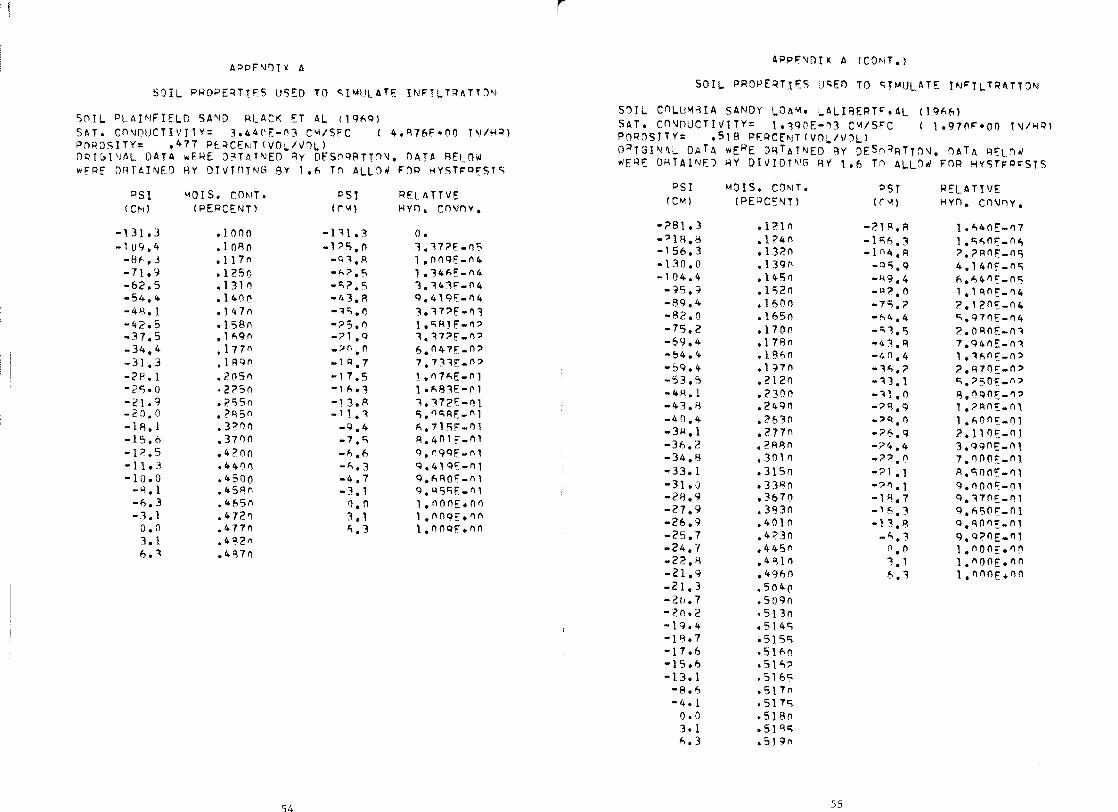
APPENDIX A Soil Properties Used to Simulate Infiltration

APPENDIX B Generated Infiltration Data

i

PAGE

1 1 2

3 3 3 5 7 7

9 9

10 13 14

15 15 17 18 20

21 21 26 27 28 29

30 30 31 31

39 39 43

47 47 48 48 49

54

59

LIST OF FIGURES

FIGURE PAGE

1 Capillary suction and relative conductivity as a function of moisture content for a typical soil (Saturated moisture con ten t bull5 ) bull bull bull bull bull bull bull bull bull bull bull bull bull 4

2 Hypothetical moisture profile development under a constant rainfall rate (After Childs Ref 7 Fig 1213) 6

3 Infiftration rate vs time corresponding to Fig 2 6

4 Typical textbook infiltration curvebull 8

5 Infiltration curves for different rainfall intensities II 13 and bull bull 8

6 Definition diagram for Green and Ampt formula 11

7 Typical capil suction vs moisture content for (1) sandy soil (2) clay soil bull bull bull bull 11

8 A typical moisture content profile at the moment of saturation 16

9 The assumed moisture content profile for derivation of the infiltration capacity equation 16

10 Behaviour of infiltration capacity vs infiltration volume relationship as predicted by Eq 19 For const IHD (II and 13 are different rainfall intensities) 19

11 Definition diagram for finite difference scheme 23

12 Capillary suction vs moisture content for the selected soils (Absorption data - points listed in Appendix A) 32

13 Capillary suction vs relative conductivity for the selected soils (Absorption data - points listed in Appendix A) 33

14 Infiltration rate vs time for Columbia Sandy Loam showing effect of initial moisture content E1 4Ks ) 35

15 Infil tration rate vs time for Columbia Sandy Loam showing effect of initial moisture content (I 8Ks) bull 35

16 Dimensionless infiltration rate vs time for Columbia Sandy Loam showing effect of rainfall intensity (IHC 125) bull 36

17 Dimensionless infiltration rate vs infiltration volume [or Columbia Sandy Loam showing effect of rainfall intensity (IHC = 125) bull 36

LIST OF FIGURES (continued)

FIGURE PAGE LIST OF TABLES

18 Dimensionless infiltration rate vs time showing effect of rainfall intensity

for Ida Silt Loam (IMC ~ 4) 37 TABLE PAGE

19 Dimensionless infiltration rate vs infiltration volume for 1 increments used in the finite difference scheme 28

Ida Silt Loam showing effect of rainfall intensity (IMC ~ 4) bull 37 2 Soils selected for the study 30

20 Soil moisture profiles for Columbia Sandy Loam at (i) 472 sec 3 Values of obtained from Eq 17 and Fig 13 39

- the moment (IMC = 2 I

of surface saturation = 4Kc)

(ii) 1450 secs 38 4 Predicted and Computed Infiltration Volume to Surface Saturshy

ation (cm) for Plainfield Sand bull bull bull 40

21 Soil moisture profiles for Ida Silt Loam at (i) 7277 secs the moment of surface saturation (ii) 40340 secs (IMC 25 I ~ 4Ks) bull 38

5 Predicted and ation (cm) for

Infiltration Volume to Surface SaturshyColumbia Sandy Loam bull bull bull 40

22 Predicted volume to saturation

to saturation (Eq 23) vs (Eq 27) for all soils

computed volume 43

6 Predicted and Computed Infiltration Volume ation (cm) for Guelph Loam bull bull

to Surface Saturshybull 41

23 Comparison of infiltration volume

(Eq 23) and observed values of the at surface saturation ) for columns of

7 Predicted and Computed Infiltration Volume to Surface Saturshyation (cm) for Ida Silt Loam bullbull 41

Rehovot Sand (Experimental data from Rubin and Steinhardt Ref 43 Fig 2) bull bull bull bull bull 44

8 Predicted and Computed Infiltration Volume to Surface Saturshyation (cm) for Yolo Light Clay bull bull 42

24 Predicted vs computed values of for all soils 46 9 General Comparison of Infiltration Volumes given by Eq 24

25 Predicted vs computed values of F for all soils 46 and the Finite Difference Solution to the Richards Equation (Eq 28) bullbullbullbullbullbull 45

App A Soil Properties Used to Simulate Infiltration 54

App B Generated Infiltration Data 59

iii

SYMBOL

a

A

b

f

F

Fp

i

I

HIC

HID

j

k

kr

K

K s

L

LHS

m

n

RAIN

SYMBOLS USED

MEANING

Parameter in Kostyakov and Holtan equations

Parameter in Philip equation

Tridiagonal matrix in finite difference scheme

Parameter in Kostyakov equation

Infiltration rate

Equilibrium or steady infiltration capacity

Infiltration capacity

Initial infiltration capacity (Horton)

Infiltration volume

potential infiltration volume (Holtan)

Infiltration volume to start of runoff

Subscript denoting depth node

Rainfall intensity

Initial moisture content

Initial moisture deficit

Subscript denoting time node

Parameter in Horton equation

Relative conductivity

Capillary conductivity

Saturated capillary conductivity

Depth to equivalent wetting front

Vector in finite difference scheme

Number of increments used at each

Wettable porosity in Green Ampt equation

time step

Rainfall intensity used in finite difference program

v

SYMBOL

s

S

Sav

SL

t

t s

v

z

yenav

yen

ltJ

SYMBOLS USED (cont)

MEANING

Sorptivity in Philip equation

Capillary suction (= -yen)

Capillary suction at the wetting front

Slope of the S-O curve

Time from start of rainfall

Adjusted time to allow for rainfall infiltration

Time to start of runoff

Darcy fluid velocity

Distance below soil surface (positive downwards)

Moisture content (volvol)

Initial moisture content

Saturated moisture content

Average capillary potential at wetting front

Capillary potential

Total potential

vi

FOREWORD

This Bulletin is published in furtherance of the purposes of the Water Resources Research Act of 1964 The purpose of the Act is to stimulate sponsor provide for and supplement present programs for the conduct of research investigations experiments and the training of scientists in the field of water and resources which affect water The Act is promoting a more adequate national program of water resources research by furnishing financial assistance to non-Federal research

The Act provides for establishment of Water Resources Research Insti shytutes or Centers at Universities throughout the Nation On September I 1964 a Water Resources Research Center was established in the Graduate School as an interdisciplinary component of the University of Minnesota The Center has the responsibility for unifying and stimulating University water resources research through the administration of funds covered in the Act and made available by other sources coordinating University reshysearch w-i th water resources programs of local State and Federal agencies and private throughout the State and assisting in training additional scientists for work in the field of water resources through research

This report is the forty-third in a series of publLcations designed to present information bearing on water resources research in Minnesota and the results of some of the research sponsored by the Center In this study a simple infiltration model is proposed for the idealized case of a constant intensity rainfall infiltrating into a homogeneous soil at unishyform initial moisture content

This bulletin represents a research effort completed under Project 12-55 of the Minnesota Agricultural Experiment Station entitled Hydrology of Small WaterSheds in the Department of Agricul tural Engineering Russhysell G Mein served as Research Assistant and Curtis L Larson is Project Leader Computer time was furnished by the University of Minnesota Compushyter Center

The work reported herein was done in partial fulfillment of the reshyqui rements for the degree of Doctor of Philosophy granted to Russell G Mein by the Graduate School University of Minnesota August 1971

~ I

MODELING THE INFILTRATION COMPONENT OF THE RAINFALL-RUNOFF PROCESS

I iNTRODUCTION

Hydrology is a broad science which deals with those processes of the hydrologiC or water cycle which occur on land The elements of the hydrologic cycle have been qualitatively understood for several centuri~s (10) but an adequate quantitative description of each component and its interaction with other components has yet to be achieved

The classic problem in hydrology is the prediction of both amount and rate of watershed runoff caused by rainfall Such prediction is vital for the correct design of all types of hydraulic structures large or small For medium and large watersheds the hydrologist frequently has rainfall and stream flow data to work with but for small watersheds most commonly there is no streamflow data To make predictions of rUnshyoff for small watersheds design engineers have been forced to use one of the many empirical formulas found in the literature (9) These formulas are generally entirely empirical giving the peak flow as a function of the rainfall intensity watershed area and perhaps other watershed factors representation of the actual rainfal1shyrunoff process is neither attempted nor achieved

The advent of the high speed digital computer has been of tremendous significance in hydrology On one hand it has enabled fast storage and retrieval of hydrological records whose sheer bulk had long before reached unmanageable proportions On the other hand computational techniques preViously impractical because of the number of calculations involved can now be used for the simulation of hydrologic processes

It is not surprlslng therefore that computers should be applied in hydrology to simulate the actual processes involved in rainfall-runoff on a watershed The best known mathematical model is the Stanford Watershed JIodel (11) which takes hourly rainfall data as input and accounts for interception infil tration interflow groundwater flow evaporation and overland flow and gives the runoff hydrograph as outshyput Unfortunately this model has several empirical constants which must be fitted to the watershed thus historical records of rainfall and runoff are necessary If some way could be found of predicting these parameters from watershed characteristics then the model could be applied to ungaged watersheds which have no records

In recent years many other watershed models have been proposed eg (12) (29)middot (48) and tested against measured runoff hydrographs Almost invariably there are several parameters to be fitted a severe limitashytion for any watershed model again because of the lack of data avail shyable for most watersheds

I I I

II

I II I II II

For the continental United States approximately 30 of the total precipitation becomes streamflow (10) From this figure one can argue that more than 70 of the annual precipitation infiltrates into the soil for both interflow and groundwater contribute to streamflow after infilshytration But for individual storms the percentage varies widely rangshying from 100 when all of the rainfall infiltrates to perhaps 30-50 for a high runoff storm It is apparent therefore that a watershed model must describe infiltration accurately to have any chance of proshyducing valid and useful results The watershed model must also include soil moisture redistribution drainage and evapotranspiration since the moisture level prior to a storm is a dominant factor in the infilshytration rates observed Recent work in redistribution drainage and evapotranspiration models shows promise (see References (1) (17) and (18raquo and may well lead to a good soil accounting mois lure model

Despite its importance the infiltration component in all of the current watershed models is usually represented by empirical relationshyships of one form or another Typically an equation needing one or more fitted parameters is used Huggins and Monke (29) showed that the choice of infiltration parameter employed in their watershed model had more influence than any of his other parameters on the outflow hydroshygraph which again emphasizes the desirability of a valid infiltration

model

It is evident that there is a pressing need for an improved infiltrashytion model one which will better represent the actual infiltration proshycess utilizing parameters that are physically meaningful and capable of being measured The model must be sufficiently flexible to be useable under different rainfall conditions and should not require a large amoun t of computing time The study reported herein was carried out with these objectives in mind This report is essentially the same as the PhD dissertation by Mein (34) with the junior author as major adviser

The infiltration process is a complex one for it is influenced by many soil and water properties Even when the soil is completely homoshygeneous (a rare occurrence in nature) and the fluid properties are known it is a difficult phenomenom to describe This chapter is devoted to a discussion of the major factors which influence infiltration and of some of the problems involved in the formulation of any infiltration model

Definitions

Throughout this bulletin the following terminology and units will be used

The process of water entry into a soil through the soi

Infiltration rate (f) The rate at which water moves through the soil surface (Units emsec)

The maximum rate at which the soil can (Units emsec)

The total volume of infiltration from the event (Units cm)

Hydraulic head due to capillary forces

The same as capillary potential but with oppos positive suction represents a negative hydraulic head water)

Capillary conductivi ty (K) The volume rate of flow of water through the soil under a unit gradient which is dependent on the soil moisture content Sometimes referred to as conductivity or hydraulic conductivshy

(Units cmsec)

The capillary conductivity when the

Relative conductivity (kr ) Capillary conductivity for a given moisture content divided by the saturated conductivity (Dimensionless)

For the purpose of discussion the ideal soil is considered to be one which is homogeneous throughout the profile and in which all of the pores are interconnected by capillaries In addition it is assumed that

3

the applied rainfall falls uniformly over the soil surface (natural rainshyfall is discussed later) Because the movement of water into the soil is areally uniform the infiltration process can be considered to be oneshydimensional

For this ideal case perhaps the most important factors which affect the infiltration capacity are soil type and moisture content The soil type determines the size and number of the capillaries through which the water must flow The moisture content determines the capillary potential in the soil and the relative conductivity as shown for a typical soil in Fig 1 For a low moisture content the suctions are high and the conducshytivity low At high moisture contents near saturation the soil suction is low and the relative conductivity high

One can now examine a typical infiltration event rainfall falling on a dry soil Because the initial moisture content is low the relative conductivity (Fig 1) is small This implies that the moisture level must be higher before water will move further into the soil mass Beshycause of this a distinct wetting front will form with the moisture conshytent ahead of the front still low and the soil behind the front virtually saturated A considerable capillary suction exists at the wetting front

10

(1600

Relative500 conduclivlty---

Ii 400

w

gt5 M w

0

U ~

M 300 W U

0 u ~

~ w ~

200 ~ M

aJ cc ()

100 ---- Vl I f

o 1 2 3 4 5

0- Moisture content (volvol)

Fig 1 Capillary suction and relative conductivity as a function of moisture content for a typical soil (Saturated moisture conshytent = 5)

At the onset of rainfall the potential gradient causing moisture movement is very high for the potential difference between the wetting front and the soil surface acts over a very small distance At this stage the infiltration capacity is higher than the rainfall rate so the infiltration rate is limited to the rainfall rate Figs 2 and 3 illusshytrate the phenomenom which corresponds to curves 1 2 and 3

As more and more water enters the soil the thickness of the wet zone becomes larger and the potential gradient is reduced The infiltrashytion capacity decreases until it is just equal to the rainfall rate shythis moment corresponds to curve 4 in Fig 2 and point 4 in Fig 3 and occurs at the moment when the surface becomes saturated

The potential gradient continues to lessen as the wetted depth inshycreases so that the infiltration capacity is reduced with time (corresshyponding to 5 and 6 in Figs 2 and 3) Theoretically the potential gradient will be unity after an infinite time for then the case is the same as saturated flow under the influence of gravity and the infiltrashytion capacity is equal to the saturated conductivity In practice the infiltration rate is asymptotic to the saturated conductivity line (Fig 3) but does not reach it

The prediction of point 4 (Fig 3) is of vital concern to the hydroshylogist for it is then that runoff will begin Also it is the beginning of f = fp instead of f = I However for a given soil type this moment depends not only on the initial moisture content of the soil but also on the rainfall rate The shape o( the subsequent curve 4-5-6 likewise depends on the initial moisture content and rainfall rate

The capillary moisture content curve is different (or wetting the soil than it is dewatering the soil The curves shown in Fig 1 demonstrate this phenomenom--these are called the boundary wetting and boundary drying curves applicable for continuous wetting or continuous drying respectively However between these curves there are an infinite number of possible paths or scanning curves depending on the wetting and drying history of the soil Thus even though infiltration is a wetting phenomena it cannot invariably be assumed that the suction is following the boundary wetting curve

There are several methods of handling the hysteresis complication in soil moisture computations A suitable numerical scheme is given by Ibrahim and Brutsaert (30) in the form of a triangular suction table However in this study because the scanning curves were not available hysteresis is not be considered and the starting point is assumed to be On the wetting curve

gt

Moisture content 8 Infiltration - The Natural Soil

G 8 Surface I t oa 7 i s The variability in natural soils makes a difficult situation virtually

ClJ u qj ~ H l Ul

o

~ ~

N

impossible as far as soil profile descriptions are concerned The surshyface condition which has a vital influence on infiltration capacities can vary over a watershed from complete vegetative cover to bare soil The latter case is subject to surface sealing by raindrop compaction shown to significantly alter the infiltration characteristics (13) A plowed surface results in much greater infiltration almost 20 times more in one test (6)

A complete description of all the factors which influence infiltrashytion on a natural watershed (cracking vegetation layering etc) will not be included here For that the reader is referred to articles by Parr and Bertrand (38) or Erie (15) Suffice it to say that the varshyiability is so significant even in seemingly uniform soils that soil samples from the same site often do not exhibit the same properties (22)

It follows then that a simple infiltration model which will be accurate for natural soils is not possible for the complete description of the soil itself is impracticable One can only hope to produce a model which will give a reasonable estimate of the infiltration behavior That is the goal of this study

Fig 2 Hypothetical moisture profile development under a constant rainfall rate (After Childs Ref 7 Fig 1213) Rainfall Intensity

III

I

Most textbook infiltration curves (eg Ref 33) are of the form shown in Fig 4 which assumes a saturated surface at time zero While in flood irrigation this condition can occur under rainfall or sprinkler irrigation it rarely occurs Almost always there is at least a brief period when in Fig 5

all the rainfall infiltrates as shown in curves 1 2 3

There are 3 general cases of infiltration under rainfall

Q) w qj H

~ 0

H W qj H w rl H ~

~ H

~ K s

rate Case A I lt Ks The rainfall rate is less than the saturated conducshy

tivity curve 4 In Fig 5 shows this condition For a deep homogeneous soil runoff will never occur under this condition for all of the rainshyfall will infiltrate regardless of the duration As far as a watershed model is concerned such a rain must still be accounted for because the soil moisture level is being altered

Case B Ks lt I lt f The rainfall rate is greater than the saturated conductlvlty but less than the infiltration capacity This condition corresponds to the horizontal portion of curves 1 2 3 in Fig 5 Note that the period of time from zero to surface saturation (ts ) is different for the different intensities

Fig 3 Infiltration rate

t _ time

vs time corresponding to Fig 2

Case C I gt f The rainfall intensity is greater than the infiltrashytion capaclty Only under this condition can runoff occur Fig 4 and the decreaSing portions of curves 1 2 and 3 (Fig 5) illustrate this and show the dependence of the curve shape on the initial rainfall intenshySity

6 7

- - -shy -shy - Rainfall

Infiltration Runoff

1i Because the major interest of the hydrologist is to predict runoff

most work has involved study of Case C It is the contention of the writers that Case B is just as vital since it almost always precedes and influences the behavior in Case C This argument will be strengthened further in later sections

aJ w til

P o w til

w r-l l

P H

-

t - time

Fig 4 Typical textbook infiltration curve

I 1

aJ w til

P 0 w til

i 1 (3) 3- P

H

14-4 K s

14

t sat l

ig 5 Infiltration curves for different rainfall intenshysities I 12 13 and

~ -1 - shy

~-~--

t sat2 tsat3

t - time

8

III

Many different infiltration equations have been published in the literature In this chapter the more important of these are presented with a brief discussion of tIle derivation attributes and deficiencies of each Because infiltration can be thought of as the surface boundary condition of soil moisture movement it can also be predicted from the equations which describe soil moisture flow Development of this latter approach suggests an alternative method of deriving a useful infiltration model

As mentioned in the previous chapter the infiltration capacity decreases as the volume of water in the profile increases So it is not surprising that early attempts to produce a field infiltration equation merely fitted the characteristic curve shape by a decay-type function

The Kostyakov Equation

The general form of the infiltration expression put forward by Kostyakov in 1932 as cited by Rode (42) is

F atb (1)

where F is the total infiltration volume t is the time from the onset of infiltration and a and b are constants (Oltbltl) The form of this expression is simple but the constants a and b cannot be predicted in advance There is no provision for predicting when runoff will begin under a rainfall input (the transition from Case B to Case C given in Chapt 1)

The simplicity has encouraged the use of this equation in flood irrigation studies eg Fok (16) for which the normal procedure is to (it a and b (rom test data on the plot concerned A modified time varshyiable was proposed by Kincaid et al (31) to use this equation for sprinkler irrigation for which the initial infiltration capacity of the soil exceeded the application rate The modification improved the fit markedly but the Constants a (which depends on the initial moisture content as well as the soil type) and b (which depends on the soil type) still had to be fitted

The Horton Equation

Possibly the best known infiltration expression is that known as Hortons equation (7) which he proposed in 1940 The equation is

fp fc + (fo - fc) e-kt (2)

~here fp is the infiltration capacity at any time t fo is the initial lnfiltration capacity fc is the final or equilibrium infiltration capacshy

ity fc is the final or equilibrium infiltration capacity and k is a constant dependent on soil type and the initial moisture content The feature of Eq 2 is its and good fit to experimental data but fc and k have all to be fitted 1beoretically fc should be a constant for a location but Burman (5) found better fits to experimental data by varying it too from one storm to another This would indicate that the good fit possible with Eq 2 might be due more to the fact that it has three parameters rather than because of its representation of the infiltration process The Horton equation likeshywise cannot be used for an event beginning as Case B

The Holtan Equation

A more recent expression is that of Holtan (27) from a substantial volume of field data

n+ aFp (3)

where fp is the infiltration is again the final infiltration capacity Fp is infiltration volume (equal to the initial available moisture storage minus the volume of water already infiltrated) a is a constant between 025 and 080 and n is a constant dependent on soil type This expression is well suited for inclusion in a watershed model because it links infiltration capacity to the soil moisture level and is not time dependent An expansion of this idea into an infiltration-drainage-evaporation-runoff model was made Holtan et al (28) by conceptually the soil storage into capillary storage and free water storage

Use of this formula has been made by Huggins and Monke (29) who used the effective storage depth of the soil as a parameter to be fitted The depths used ranged from 3 to 16 without explanation This illustrates the major of the Holtan model for the control

specified has a influence on the prediction of infiltration

There are many equations derived from applying Darcys Law to the wetted zone in the soil using the fact that a distinct wetting front exists Green and Ampt (20) were the first with this approach and their

will be given here

The Green and Ampt Equation

The equation derived by Green and Ampt in 1911 assumes that the soil surface is covered by a pool of water whose depth can be neglected Referring to Fig 6 and assuming that the conductivity in the wetted zone is Ks Darcys law can be applied to give

(4)fp

II)

Water Negligible depth I

L

~ Wetting front

Dry soil

Fig 6 Definition diagram for Green and Ampt formula

VJ

r 0

M u

(1)~ I Ul

Moisture content

Fig 7 Typical capillary suction VS moisture content for

-

(1) sandy soil (2) clay soil

11

where L is the distance from the soil surface to the wetting front and S is the capillary suction at the wetting front By continuity nL F where n is the initial moisture deficit (Os - ) and F is the volume of infiltration Thus writing dFdt

dF Ks (1 + F)dt (5)

Integrating and substituting F o at t o

f - Sn (6)Kst

This form of the G A law is more convenient than Eq 4 for watershed

CWi modeling for it relates the infiltration volume to the time from the start ot infiltration From it one can obtain the volume for any given time or vice versa Ibe advantage of Eq 6 is that all of the parameters are properties of the soil-water system and can be measured Estimation of S for a soil represented by curve 2 (Fig 7) is difficult however since the capillary suction always varies with moisture content The resultant suction for such a soil will be some kind of average taken over the whole wetting front This point is discussed in later sections Note that the equations do not account for the ci rcumshystance of rainfall intensity being less than the infiltration capacity (Case B)

Several other workers have derived equations similar to Eqs 4 and 6 using Darcys law and the law of conservation of mass Rode (42) lists Alekseev (1948) Budagovskii (1955) and Subnitsyn (1964) to which we can add Philip (1954) and Hall (1956) although the latter author failed to include the capillary force at the wetting front (23 25 39)

Interest in the Green and Ampt formula has revived and the results have been very encouraging Bouwer has developed apparatus to measure S in the field (2) and shown how to extend the analysis to a layered soil (3) Laboratory tests and the G - A theory for layered soils have shown excellent agreement (8) None of these tests however were made for the rainfall condition at the surface (Case B)

Ibe Philip Equation

For a homogeneous soil with a uniform initial moisture content and an excess water supply at the surface Philip has solved the partial differential equation of soil moisture flow (Eq 8 - discussed in the next section) The solution is in the form of an infinite series but because of the convergence only the first two terms need to be considered (41) giving

F + At (7)

where F is the volume of infiltration to time t and s and A are constants depending on the soil and its initial moisture content

12

The form of this equation is convenient and s and A can be predicted in advance but the method of finding their correct values is and beyond the scope of a simple watershed model The rainfall condition (Case B) is not simulated by Eq 7

Tests of the above equations have been made against field data Skaggs et al (44) fitted all of the equations and found them all satisshyfactory particularly for short times Such a test may show that the equation has the right form if the constants are correct but still does not answer the question of the constants A test of the Green-Ampt CEq 6) and Philip (Eq equations was made by Whisler and Bouwer (47) who concluded that the G - A equation was not only to use but also gave better results experienced considerable difficulty in predicting s and A for Eq 7

A combination of Darcys law (applied to unsaturated f low) and the equation of continuity results in the second-order non-linear partial differential equation eg Ref (7)

8 3S(0raquo)K 0 -- shy3z () dZ Z (8)

where 0 is volumetric moisture content t is time Z is the distance beshylow the surface S(O) is the capillary suction and K((l) is the unsatshyurated conductivity Equation 8 is sometimes referred to as the Richards equation and also as the diffusion equation

The solution of this equation for unsteady flow is difficult the analytic solution proposed by Philip (40) is complex and applicable only to homogeneous soils with a unifonn ini tial moisture content and an excess water supply at the surface For other boundary and initial conshyditions numerical analysis techniques (usually finite differences) are necessary and the required computation is far from simple as shown in the followin2 section

It remains to be shown here that Eq 8 is a valid model for soil moisture flow one which is suitable to generate infiltration data under a variety of input conditions

There are many examples of solutions of Eq 8 being compared with field tests Neilson et al (36) after stating that Eq 8 is valid for laboratory soils compared results given by Eq 8 with observed field moisture profiles in Monona silt loam and Ida silt loam Agreement was termed adequate especially when the depth of water penetration was in the homogeneous soil layer Whisler and Bouwer (47) in the tes ts cited earlier judged Eq 8 good better than the other infiltration equations tested

Seepage of water from a pond was simulated Green et al (21) USing Eq 8 and compared with a field test A non-homogeneous soil was

13

modeled by Wang and Lakshminarayana (46) and good agreement found with a field trial

The above examples are cited as validation of the Richards equation I t is unfortunate that its complexity and its requirement of the f-()

and K-0 curves as input data rule it out for inclusion in a practical watershed model

The Need for a Simple Model - The Research Plan

It was shown in Section II that there are three distinct cases of rainfall intensity as related to infiltration and runoff There were as given previously cases

(A) IltKs (B) KsltIltfp (C) Igtfp

For the hydrologist concerned with predicting the volume and timing of runoff (A) need not be considered except as a source of soil moisture for future events For most natural runoff events the infiltration proshycess starts in Case B and when the surface becomes saturated mov~s to Case C and runoff begins The important point here is that the behavior in (C) is markedly influenced by the volume infiltrated in (n) For this there are no simple infiltration equations

The principal objective of this study was to develop a simple method of predicting the time between the start of rainfall and the beginning of runoff using measurable properties of the soil and rainfall intensity The infiltration decay portion of the curve was studied with the intent of modifying the Green and Arnpt equation to allow for the infiltration volume prior to surface saturation and the hope of determining the appropriate capillary suction value for the soil

The proposed model was tested against solutions of the Richards equation for several soils each with several different initial moisture contents and a number of rainfall intensity levels Experimental and field data were used for testing to the extent available

IV DEVELOPMENT OF AN INFILTRATION MODEL

Both saturated and unsaturated fluid flow through soils can be desshycribed by Darcys law providing the appropriate conductivity value is used However as shown in Sec II the capillary conductivity is highly dependent on the moisture content which is a considerable complication To derive simple expressions for infiltration based on Darcys law some assump tions about the and movement of the wetting front are necshyessary These assumptions are explained in the development of the infilshytration model

The situation to be examined here is that of a constant intensity rainfall which initially completely infiltrates into the soil but which eventually produces runoff The two stages in the process previously designated Case B and Case C are considered in the following discussion

=-=-==c~=--c==-==-=~c~~~=-~~~~ (Case B)

As stated in Sec II the moisture content at the surface increases during the rainfall until surface saturation is reached Although Darcys law is applicable at any time during the process it is at the moment of saturation that a useful relationship can be developed for at that moment the surface moisture content and conductivity are known

A typical profile at the moment of surface saturation is shown in Fig 8 (It should be noted that the shape and extent of the profile depends on the soil properties and the rainfall intensity) The shaded area is equal in volume to the volume of infiltration up to surface saturation Darcys law will be applied to the shaded area in other words we are assuming an abrupt wetting front with the soil beyond at the initial moisture content and the soil behind at saturation

Darcys law can be written

q = -K (0) z

where q is the flow rate in depth per unit of time K(O) is the capillary conductivity is the potential and z is the depth

In finite difference form this can be written

q =- -K(G)

in which the subscripts 1 and 2 refer to the surface and wetting front respectively At the moment of saturation the infiltration rate is still equal to the rainfall rate so we can put q I Applying Eq 10 to Fig 8 we see 22 zl = Ls The potential at the surface ~l is arbitrarily taken as zero so the potential at the wetting front will be

+ Sav) where Sav is the average capillary potential discussed later

15

I

o - Moisture content 8

~ gt gt s

Surface

ill ()

cU 4-lt ~ l Ul

o ~

rl ill n c w p ill ~

N

II II Fig 8 A typical moisture content profile at the moment

of saturation

o - Moisture content

OsUi Surface

ill ()

cU 4-lt ~ l Ul

~ o rl ill n c w p ill ~

N

F - F s

L

Ls

Fig 9 The assumed moisture content profile for derivation of the infiltration capacity equation

1(

The capillary conductivity is assumed to be equal to the saturated conshyductivity Making these substitutions Eq 10 becomes

Sav + LsI = Ks (11)

Ls

From Fig 8

volume infiltrated FsL

initial moisture deficit IMD (12)

where the initial moisture deficit IMD Os - 0i

Substituting Eq 12 into Eq 11 and rearranging terms we obtain

Fs Sav (UID) (IKs)-l (l3)

which can be used to predict the volume of infiltration prior to runoff Intuitively (Eq 13) is satisfactory for if IMD = 0 (soil saturated) there is no infiltration prior to runoff (Fs = 0) When IlKs ~ 1 Fs ~ 00 for all of the rainfall at this low intensity will infiltrate

A relationship similar to equation 13 was proposed as part of the predicted intake volume to saturation by Rubin and Steinhardt (43) for a soil with a well defined ~ubbling pressure (the capillary potential at which the soil begins to desaturate) In their case Sav was equal to the bubbling pressure Since many soils do not exhibit a well defined bubbling pressure the determination of Sav in the following way is conshysidered substantially more general

The Capillary Potential at the Wetting Front (Sav)

There would appear to be two alternative ways of determining the average suction at the wetting front from the S - 0 relationship or from the S - K relationship for the soil in question Examination of these curves for a soil shows that the former is not acceptable Take Fig 1 for example It shows that the capillary conductivity is effectively zero at a moisture content of about 30 For moisture conshytents below this level soil moisture movement is comparitively very slow despite the high suctions in this region Since we are interested in the moving front it would seem that the average capillary suction is best determined from the S - K curve It is proposed therefore that Sav be determined by

fK(Os)

SdK(O) - K(Oj)Sav

K(Os) - K(Oi) (14)

17

It is more convenient to use the relative conductivities kr instead of the absolute conductivity K(O)

kr(e) (IS)

Substituting Eq IS into Eq 14 and noting that K(Os)

Sav (16)

initial moisture content before a rainfall event is such field capacity) so that we can write kr error Then

Sav ~lSdkY (17)

or slmpiy the area under the S - kr curve between kr 0 and kr l In practice the S - relationship near kr = 0 is hard to define so in this the area in the range kr = 01 to kr 1 was used

Prediction of the Infiltration Capacity After Runoff Begins C)

Let us assume that some time after the surface has saturated the moisture profile can be represented by Fig 9 Darcys law can be again noting that the infiltration rate is now equal to the infiltration capacity (fp) to give

+ L fp =

(18)

As in Eq 12 Ls Similarly L = (F shy

Hence IMD fp Ks (1 + )

F (19)

Note that in this equation the infiltration capacity is not inshyfluenced by the infiltration volume up to surface saturation In other words Eq 19 a relationship as shown in in which the infiltration constant in position for dif rainfall intensities data presented by Rubin and Steinhardt (43) is very similar to Fig 10

It may sometimes be more useful to have the cumulative infiltration as a function of the time since the beginning of the rainfall By f dFdt in Eq 19 and separating the variables we obtain p

18

(JJ

- C1i H

o ~

H +J C1i I-

- r-1 H ~

H

F 1 s3

_ FInfiltration volume

Fig 10 Behaviour of infiltration capacity vs infiltration volume relattonship as predicted by Eq 19 For const It-m and b are different rainfall intensities)

ftF dt (20)IFs ts

which can be reduced to

Ks (t - t s ) F (IMD) Savloge[Fs + It-ID bull

- 18 + (IMD) loge [Fs + IMD savl

If we call the equivalent time to infiltrate volume under saturated surface conditions Eq 21 can be maninulated to

F + (IMD) Sav)Ks (t - ts + F Sav ( (It-ID) bull Sav (22)

which is similar to the Green and Ampt expression given in Eq 6 but with an adjusted tilne scale Eq 22 can be solved directly for the actual time t or bv iteration for F

19

Summary of Model V NUMERICAL SOLUTION OF THE MOISTURE FLOW EQUATION

It has been proposed in this section that a suitable model for inshyfiltration of a constant intensity rainfall (IgtKs) into a soil of uniform The soil moisture flow equation CEq 8) is a second - order nonshymoisture content can be expressed in the following form linear partial differential equation An ideal solution would be an

analytic one but except for a few special cases no general analytic f I until F = Fs given by solution is available To obtain solutions for situations which approxshy

o imate real-life conditions several researchers have employed finite difference methods of one form or another and programmed a computer for

- 1 (23) the repetitive and tedious computations involved

and Smith (45) examined many of the published methods in an attempt to develop one which both satisfied the law of continuity and predicted a

for F gt f given by smooth infiltration curve whose shape agreed with field observations The numerical scheme developed below is a method based on the Crank shy(1 + (IMD)

(24) Nicholson finite difference scheme and is similar to that adopted byF Smith Additional refinements and modifications have been made and the

resulting program is suitable for infiltration under any constant rainshyfall rate into any homogeneous soil type and for any initial moisture distribution Layered soils and rainfall of non-constant intensity can be simulated with simple modifications to the program

Interior Nodes

For convenience Eq 8 will be rewritten here

Z (K(G) 3S(0raquo)t dZ - (25)

The conductivity K(G) can be written as K (0) = Ks kr where Ks is the saturated hydraulic conductivity and kr is the relative conducshytivity (This form is more convenient for interpretation since kr reshypresents the fraction of the maximum conductivity possible for the soil in question) Also using the chain rule of calculus

at) )S d isect) - Ks t as at dZ dZ (26)

Replacing the differential expressions by their corresponding finite difference approximations one obtains

lk118 r A II (k I1S ) - K

I1S lit uZ r 6z s 6z (27)

There are two dependent variables in this equation 8 and S It can be reduced to an expression with S as the only dependent variable noting that S is the slope of the G vs S curve at some appropriate point Writing S as SL and multiplying both sides by [12

6zlS _ Ks [11 (k r ) - I1kr ] (28) I1t Z

2120

To evaluate the difference expression the notation demonstrated in Fig 11 will be used All nodes on the time - distance plane are numbered with the subscript i referring to the depth dimension and the subscript j to the time dimension Thus i 1 and j 1 refer to zero depth and Zero time respectively The time and depth increments are not necessarily constant(discussed later) so the node spacings shown in Fig 11 are uneven The depth node i is assumed to represent the soil thickshyness I which extends from the midpoint of zi and zi-l to the midpoint of zi zi+l These midpoints will be designated minus (-) and (+) respectively in the notation In the finite difference approximashytion the distance-averaged quantities will be evaluated at the midpoint of the time step tt Eq 28 becomes

-l j j_z(SL)~ Llzi (S~ - S]-l) - Ks ( tS+ kr1 At 1 1 Z+ LI Z_

J-2 J--1 )1 (29)+ kr+ - k r _

Now we can write

j j-l(Si+l + Si+l S~ - S~-l) 2

1 1

(sj + Sj-l - sj S~-l) 2i i i-l 1-1 (30)

bull 1 1

The terms kJ - and kJ -2 could be evaluated as being conductivitiesr+ r-

corresponding to the suctions S~-~2 and S~_12 respectively or the average1+2 1_

conductivity taken from th~ Four surrounding node points A third alternative is to select kJ2 as a time-averaged conductivity from the node from which flow to noae i is originating It was found that the latter assumption improves convergence although there is no appreciable difference from the results obtained by the other two methods Thereshyfore let

kj-12 (k j j-l+ k r- ri-l ri-l

and

r+ (kt + ktl) 2 (31)

Substituting Eq 30 into Eq 29 we obtain

1 _[zi (j j-l) _ [j (S~ + s~ - s~-l)(SL)i At Si - Si - - Ks kr+ 1+1 i+l 1 1 _

26z+

sj-l - sj 1 2 j-l)k J- ( Sf +

i i-l - Si_l + kr+ shyr- (32)2tz_ ~-]

22

r time

t j - 1 t j Ti=lJ=l j=2 Surface

Nt i=2

()) U tU

44 j zi_1l CIl

--- LIt I--

sj-l sji 1 1 1

4 j -1 j tS

Z S -

I fLI Z -1

LI Z+

j-1 j ~si+l Si+l

- Zi_1 ~ 0 rl ())

0

c Zi+1u ())

A

Zi+ l

Fig 11 Definition diagram (or finite difference scheme

23

Placing the unknown values on the right hand side as before resultsThe unknown terms are the sjs - these will be placed on the right hand side of the equation in

j-l j-l( 1)j-~ lIzl Sj-l + K 1lt (S2 - Sl + Zliz+)

j-~ lIzi j-l j (j-l j-l ) - jJ 1 rt 1 s-r+ - RAINSHl - Si + 2l1z+ _-(S1)i ~ Si + Ks kr+ -z+

2l1z+ sj (Ks~+ _ (S1)j~ j (Kskr+ )

-1 -1 1 2ts 1- S2 ~j-~ ) + LH (37)K kj-~ (si -Sl-l + 2iz_ ) r shysj ( + s r+ 2iz_ i-l z_ or

j-~2 j-~ j jK kj-~ 1HSl ~ blSl + c S2 (38)sj (Kskr+ + Kskr - + s r- _ (S1)j-~ lIZi) l i 2l1z+ Zli z+ LZZ i Ft shy

j-~ This is the first equation of the tridiagonal matrix (Eq 35) for the sj rainfall condition at the surface(Ksk~ )Hl (33)

Upper Boundary Condition-Case C which can be written more simply in the form

When the surface layer is saturated (the transition from unsaturated to saturated is discussed later) the capillary suction S1 is set equal1HSi ~ ai s1_l + b i Sl + Sl+l (34)c i to zero which assumes there is no significant ponding on the surface Thus we skip node 1 and start computation at node 2 Because sj is

An equation of the form of Eq 34 can be written for the upper and known ( 0) Eq34 becomes 1lower boundary conditions (see next section) and for each inter lying

R

depth mode resulting in a set of m equations for m unknown values of S j j1HS2 ~ S2 + c2 S3 (39)In matrix form this can be written as

-+ which is the first equation of the tridiagonal matrix (Eq 35) for a

[AJ S 1HS (35) saturated surface

where tAJ is a tri-diagonal matrix a form which can be solved rapidly with a simple numerical algorithm The upper and lower boundary condishy 10wer Boundary Conditiontions should now be examined For the upper boundary there are two possibilities either the surface is unsaturated (rainfall condition _ In the early stages of infiltration the wetting front has notCase B) or the surface is saturated (Case C) penetrated far into the profile It is more economical in computation

time if the nodes which have not yet been reached by the wetting front are excluded from the calculation Therefore the matrix [AJ is

Upper Boundary Condition-Case B I truncated For this condition at the appropriate node m one can say

For this case the surface layer is unsaturated and the extra term S~ = s~-l Hence Eq 34 becomes the rainfall rate must be added to the continuity equation for the

(40)nodes i ~ 1 Following the same procedure as before an equation 1HSm = ~ S~_l + S~bm analagous to Eq 32 can be written for the surface node

Which is the final equation in the m x m tridiagonal matrix j_~ lIzl j j -l j j-l

(S1) 1 Fi (Sl - ) = - K k Sl - S2 s r+ + 1) z+ Initial Conditions

+ RAIN (36) The required initial conditions are the initial moisture content for

where RAIN is the rainfall intensity each node and whether or not the surface is to be instantaneously satshyurated at time zero All cases simulated in the study involved infiltrashytion under rainfall into a soil with a uniform initial moisture content

I 11

24

I I

Solution of Eq 29 for Each Time Step

Soil Properties

It is necessary at every step to compute the values of ~ and SL corresponding to the capillary suction at each node To expedite this the 8 vs Sand kr vs S relationships for the soil are stored in the computer as tables of data points These points are chosen such that an insignificant error is incurred by assuming a straight line between successive points By this method the appropriate values of e and kr can be determined efficiently by linear interpolation To compute (S1)j-2 the 8-S table is scanned for the data point nearest the value

of the midpoint of si-l and sl The slope is determined by fitting a

parabola to this and its adjacent data points If the difference beshy

tween si-l and Sf is greater than a specified value then the slope of

j-l j-l j jthe chord joining (0i Si ) and (8 bull Si ) is usedi

Requirement of Iteration

To solve Eq 29 for a given time step it is necessary to use the correct values of kr and SL at each node However to obtain these values the corresponding S-values (which it is required to find) have to be known Thus an iterative procedure is needed whereby the Sshyvalues are estimated and kr and (S1) determined for these estimated values Equation 33 is then solved for the new S-values which are comshypared with the estimated values If the estimated and new S-values at each node do not correspond to within a specified error tolerance the process is repeated using the new S-values as the new estimates

Transition from Unsaturated to Saturated Surface

As infiltration under a rainfall rate gtKs proceeds the surface layer becomes wetter and the transition from Case B to Case C occurs A constant check is kept of the moisture level in the surface node and when saturation is reached the time step is adjusted so that the phenomenom occurs just at the end of the time increment and the step recomputed Subsequent time steps are then assumed to have a saturated surface condition prevailing

Acceleration of Convergence

The convergence for the iterative procedure described above can be accelerated using Aitkens A2 - method (26) which predicts an improved value from the result of the previous three iterations The formula can be stated thus

26

(Sn+l - Sn)2SSn+2 n (Sn+2 - 2Sn+l + Sn) (41)

where S Sn+l S +2 are the values of S from the previous three iterashytions nSn+2 hopeyenully is an improved estimate which will jump several iteratio~s Some tests of the numerical solution showed that when the Aitken A - method was applied to those nodes which had not converged the average saving in computation was two iteration steps for each time step The method was not applied to the first iteration stepbut to every three thereafter for it is not suitable unless convergence is occurring

Computation of Infiltration

After convergence is achieved the cumulative infiltration is computed from the change in the soil moisture level since the beginning of the event That is

m jF r t zl - (42)

i=l

The average infiltration rate over the time interval is simply

Fj-lf

t (43)

For the unsaturated surface condition a continuity check is possible by comparing the cumulative infiltration volume from Eq 42 with the rainfall volume in the same time Such a check was made for each computer run and the maximum error was of the order of 1 but generally much less

Qepth Increment

Many published finite difference schemes for solving Eq 25 have a fixed depth increment (eg Ref 24) Smith (45) showed that the choice of depth increment has a considerable influence on the results and proposed that increments be small near the soil surface where the suction gradients are higher and where it is necessary to accurately preshydict surface saturation and larger at points deeper in the soil where gradients are smaller Palmer (37) reached the same conclusion

In the work reported here the same pattern of depth increments was used for all soils These values are shown in Table 1

27

Table I Depth increments used in the finite difference scheme

Depth Range (cm) Increment Size (cm) No of Increments

o shy 1 20 5 1 - 8 25 28 I

8 - 10 50 4 1

10 - 15 100 5 15 ~ 25 200 5 25 - 500 3

These depth increments are a compromise based on the results of Smith (45) Palmer (37) and several tests by the senior author It was found that by halving the depth increment a smaller time to surface saturation was predicted A second halving of the increment resulted in a yet smaller predicted time but the discrepancy was approximately half of the previous difference Thus the depth increment must be reduced until the difference between successive predicted values is an acceptable one For the choice given above the estimated error is of the order of 5 (Note that if the depth increment is halved the comshyputation time is more than doubled)

Time Increment

Eq 25 is non-linear because SL and kr are functions of S As mentioned before it is solved by assuming that kr and SL are constant over the particular time step Tests with the numerical solution showed that errors in computation of SL produced continuity errors and that the solution was far more sensitive to SL than k bullr

The initial time step was arbitrarily chosen as the time needed to fill 10 of the available storage in the uppermost soil layer Larger initial steps caused instability in the solution Hence the time step was computed from a prediction of the slope change for each node over the new time step This prediction was based on the change over the previous time step and the curvature of the 8-S curve at that point A secondary factor in the choice of the time step was the number of iterations involved Too large a time step means many iterations and poorer accuracy while too small a step means few iterations but many more time steps for the same event time An increase of the time step by 20 was made if the iterations on the previous step were less than four and the time step was halved if more than twenty iterations were needed

Generally for each run the time step increased reasonably uniformshyly to a predetermined maximum value

28

The Computer Program

The program was written in FORTRAN IV and was run on the CDC 6600 computer at the University of Minnesota Computer Center The complete program was given by Mein (34) It is written as a series of subroutines for maximum flexibility Briefly the data input is handled in DATIN and the initial conditions are computed in CALC Subroutine MAIN solves the basic soil moisture equation and CONS computes the infiltration elapsed time depth of wetting and the new time step PLOTT is an option to plot the moisture content or capillary potential as a function of depth while INTERP and SLOPE are used to interpolate the soil data curves and calculate the slope of the 8-S curve respectively

For an average run the compile time was 4 seconds and the run time 15 seconds

29

VI GENERATION OF INFILTRATION DATA

Discussion of the Richards Equation in Sec III showed that it is considered the best available mathematical description of moisture flow in soils With numerical solution of this equation one can therefore generate any number of infiltration events simply by using the appropriate soil properties and the desired values of initial moisture content and rainfall intensity In this manner the influence of any factor on the infiltration behavior can be studied by systematically changing its value Such a technique is extremely difficult in both field and laboratory experiments

The Soils Used

It was desired to generate infiltration data for a range of soil types The soils selected from published data and lis ted below in Table 2 vary in texture from a sand to a light

Table 2 Soils selected for the study

Soil Porosity

Plainfield Sand (disturbed sample)

477

Columbia Sandy Loam (disturbed s

(32) 1 39 x 10-3 518

Guelph Loam (air dried sieved)

(14) 367 x 10-4 523

Ida Sil t Loam (undisturbed sample)

(19) 292 x 10-5 530

Yolo Light Clay (disturbed sample)

(35) 1 23 x 10-5 499

The published data for the first 3 soils in Table 2 were desorption data but because infiltration is an absorption process it is important to use the absorption or wetting curve of the soil characteristic curves A reasonable estimate of the wetting curve can be obtained by the drying curve S - values a factor approximately equal to 16 (D A Farrell Research Soil Scientist Agricultural Research Service private communication) For spherical particles Rode (42) shows that the ratio of Sdes to Sabs is about 18 but it would be somewhat less for non-spherical particles Examination of published hystereSis data showed different values of the ratio of Sdes to Sabs ranging from 15 to 18 over most of the curve In this study a constant ratio of 16 was used ie for the sand sandy loam and loam the S values for the S-EJ and S-K curves were divided by 16 to obtain wetting data

30

The S-EJ and S-kr curves for the five soils listed in Table 2 are shown in 12 and 13 Note that a wide variability in soil propershyties is by these curves Complete details of the input data for each soil are given in Appendix A

Choice of Initial Moisture Contents and Rainfall Intensities

The moisture contents used in the study for each soil were somewhat arbitrarily chosen but in all cases the highest initial moisture conshytent was such that the relative conductivity at that moisture level was small laquo5) With this as the upper limit a number of values spread over the remaining soil data range were selected for each soil (In natural soil drainage after rainfall can reduce the moisture content fairly rapidly to a point where the conductivity is low so the choice of the upper limi t above is realis tic)

Rainfall intensities were chosen as fixed multiples of the saturated conductivity for each soil values of 4 and 8 were used for all soils

Columbia Sandy Loam and Ida Silt Loam were singled out for more extensive testing both to save a substantial number of computer runs on the other 3 soils and because represent two completely differshyent soil types Additional rainfall intensities (2 Ks and 6 Ks) and extra moisture levels of moisture content were used for these two soils

Results

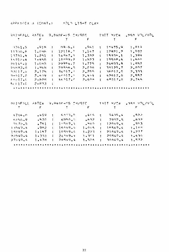
A number of graphs and figures representative of the infiltration data generated for each soil will be presented in this chapter Addishytional data are in Appendix B

given in Sec VII and the complete results are listed

Graphs of iin Figs 14 and

nfiltration rates vs time for Columbia Sand15 the effect of initial moisture

y Loam content

are on

given the

shape of the infiltration capacity curve As one would expect the time to surface saturation is larger when the initial moisture level is less Note also that the infiltration curve is steeper the sooner that surface saturation is reached and that the slope of the tail of each curve becomes small even though the infiltration rate is significantly greater than Ks

Figs 16 and 17 are different ways of plotting the results for Columbia Sandy Loam Fig 16 clearly shows the effect that rainfall intensity has on both the shape and position of the resulting infiltrashytion capacity curve However as shown in Fig 17 by plotting infilshytration volume on the abscissa the infiltration capacities for each run fallon the same curve Similar data for Ida Silt Loam are shown in Figs 18 and 19 although in the latter the infiltration capacity curves do not quite coincide The implication of the common infiltration capacity vs infiltration volume curve and a possible explashynation of the Ida Silt Loam discrepancy is discussed in the next section

31

I 11 bull i f 1 J j fI I 1 1111 LJl111 111 1f 111 II

-t-

I ~ I I I Iii I 11 I Iii i ~ I I I I I I I I I I I

1

x Plainfield Sand 6 Ida Silt Loam o Columbia Sandy Loam c Yolo Light Clay + Guelph Loam

140 ~ J I plusmnr 1- I IT 11 r11 t i 111 r jTIll I I Hi 1i II 11I 1

120 -+Hl-

I 11

100 ~ i i

s u 80+---+ 1-iamp ill II 11 j I 1i ~I

1

I I 1j ~ II I I

~ k q

o 60-u ~~~

U If Ii I I I I I1

l Ul ~ I

I I gt H til ~ ~ rl ~ bull I rlP 40 I -I~middot

~I 1-0 _~til l I I I IU i ( bull I I I 1 BI i i I i middot d _I +

bull

I - ~0-o [ I - ~

j I t j t

1 i I20-+shy bull -~ xtii -

il I If ~j 1+~1-

t bull 1 tl + bull + - t +- ~I

r -

I I I lampl 01 02 03 04 05

Moisture content (volvol)

Fig 12 Capillary Suction vs moisture content for the selected

soils (Absorbtion data - points listed in Appendix A)

32

t+ t j ~fF--r-ffEHf+- - - I t 1 -+ +- bull

(if tt+-+ tHljltH~t- _+t- Ifr---cf - ~ j - 1+-1-T - bull 1 II - I 1-1-~T~1-1- -- shy --1----+----+

140 ~+~]hHt-H fhrtlt I ~l L - I j j

I I )c Plainfield Sand I120

0 Columbia Sandy Loam ~ j + Guelph Loam j i i 4 II A Ida Silt Loam I

--It~ +--L-+ - 0 Yolo Light Clay0 + + + jshy

1 t I j j )11 1 11 [~~-1)-rLL-l100

80

s u

60

0

-M -u U l Ul

gt H til rl rlP til

U

20

o o 2 4 6 8 10

Relative conductivity

Fig 13 Capillary suction vs relative conductivity for the selshy

ected soils (Absorbtion data - pOints listed in Appendix A)

(page39) It should also be mentioned that of the five soil types used the coincidence of the infilt~ation capacity vs infiltration volume curves was best for Columbia Sandy Loam and poorest for Ida Silt Loam the examshyples shown in Figs 17 and 19 These results illustrate the fact that infiltration capacity is best expressed in terms of prior infiltration volume and initial moisture content rather than by the usual empiric~l equations which give infiltration capacity as a function of time

Along with the infiltration data the soil moisture profile at each time step was obtained Figs 20 and 21 show the profile at the instant of surface saturation and at a later time for Columbia Sandy Loam and Ida Silt Loam respectively

A general observation on the depth of wetting is worth noting here The program to generate the infiltration event halted when a specified event time had elapsed or the wetting front reached 30 cm whichever happened first For the loam silt loam and light clay the former criterion stopped the run whilst the latter criterion caused many of the sand and sandy loam runs to terminate In all cases the infiltration rate had fallen to the portion of the curve where the infiltration capacshyity was decreasing slowly The corresponding depths of the wetting front ranged from around 8 cm for the clay to 30 cm for the sand This obsershyvation has important implications which are given in Sec VIII

~

CJ III

--ltII

S CJ

4

III - tll 1-1

t1 2 o

- tll 1-1 - - I I I-r~ 0 II

o 200 400 600 800 1000 Time (sec )

Fig 14 Infiltration rate VS time for Columbia Sandy Loam showing effect of ini tial moisture content (1= 4Ks)

0 200 400 600 800 Time (sec)

Fig 15 Infiltration rate vs time for Columbia Sandy Loam showing effect of initial moisture content (I =

lO~

x IMC= 125 + IMC~2

t IMC=318 8

U III ltIl -shys

6CJ

I 0 e-

III - tll 1-1

0 - til 1-1 middottmiddotmiddot I-

-

Ir t1 +-_~___ i

H j

I I

01 j I 1 j bull 1 1060

2

o

----A - -Igt A I bull ~

- ~ I

Rainfall Intensity

~A ah0-1amp

- jAb

1

Ib __ --j -shy 00

4

x o A

Imiddotmiddotmiddot~ 1middotmiddot AI)rbull- vtmiddot i V 0 I 1_bull +~~+- ---

j I

L

8 I Intensity

)( 4K

6 0 6Ks

A 8Ks s

5amp-~i

4~+1--

3

o 400 600 800

8

7

6

5

flK s

4

3

22

o 1000 2000 3000 4000 5000 1000 Time (sec)

Time (sec) Fig 18 Dimensionless infiltration rate VS time for Ida Silt

Fig 16 Dimensionless infiltration rate vs time for Columbia Loam showing effect of rainfall intensity (IMC 4) Sandy Loam showing effect of rainfall (IMC= 125)

x o Igt

It

f30- ~txkmiddot~~ I i ~ ~-- +

i ~~~~ X~ ~~ bullbullbullbullbull 1 bullbullbullbull

1 bullbullbullbullbullbull 7bullbull

I 8~+__t--A~ bull II

7 JIimiddot~middot __ ~L A I+~middotmiddot~+middot+bullbullbull t Rainfall Intensity I i

6IA-~--0 G~Q~ lt I 1 j ~

I I I I i

5

flK I-j ~~~1i~J-fT~III s

I 1~ t~hO_t I I

4 J)(-c-J l X )( )(__~)( bull A ~ i

j ~~ t I j j11W~ 1

3 ----4~~~+-~~-+ bull-~ t -~-t~+ I t 4+---lt- - ~ I Q~1I4

~~

II2 - --1

a 1 2 3 4 52 3 4 5 Infiltration volume (cm)Infiltration Volume (em)

Fig 17 Dimensionless infiltration rate vs infiltration volume for Fig 19 Dimensionless infiltration rate vs infiltration volume Columbia Sandy Loam showing effect of rainfall for Ida Silt Loam showing effect of rainfall intensity (IHC= 125) (IMC=4)

ill 37

Moisture content (volvol)1 2 3 4 5

Pig 20 Soil moisture profiles for Columbia Sandy Loam at (i) 472 sees - the moment of surface saturation (ii) 1450 sees

0

ltI) ()

10 I- I m

~ rl

ltI) 0

c 20 ltI) 0

30

(IMC = 2 I = 4Ks)

-

~

1 2 ltI) () ltII

4-lt I- l m

~ rl

ltI) 10 0

c ltI) o

20

Fig 21 Soil (i) 7277 sees - the

at

(ii) 40340 sees (IMC = 25 I = 4Ks)

Moisture content (volvol) 3 4

moment of surface saturation

38

VII

In this section the infiltration behavior predicted independently by the proposed model 23 and 24) is with the data generated by the finite difference approximation to the Richards equation (Eq 28) There are two parts to the model prediction of the moment of surface saturation which is the end of the stage for which infiltration rate equals the rainfall intensity and prediction of the infiltration capacshyity of the soil when the infiltration rate falls below the rainfall rate A further test of the former stage is made using published experimental data

Prediction of Fs

To predict the infiltration volume prior to surface saturation (Fs) Eq 23 is used llowever the parameter Sav must first be evaluated using Eq 17 and the curve for each soi1 shown in Fig 13 111e values obtained for each soil are given in Table 3

Table 3 Values of Sav obtained from Eq 17 and Fig 13

Soil Save ern)

Plainfield Sand 1173

Columbia Loam 2383 Loam 31 38

Ida Silt Loam 743

Yolo Light 2236

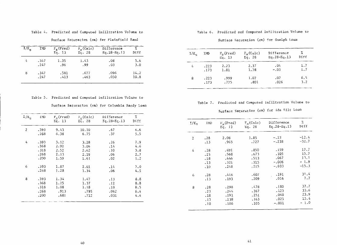
With the appropriate value of Sav in Eq 23 the volume of water uptake to the point of surface saturation can be The values obtained for the five soils for a variety of rainfall intensities and initial moisture contents are compared with the corresponding values computed by Eq 28 in Tables 4 to 8

In view of the assumptions involved in the derivation of Eq 23 the agreement obtained between Eq 23 and Eq 28 for all of the soils except Ida Silt Loam is very good If one considers the error in the resul ts from the Richards equation due to a finite depth increment (discussed in Sec V) and realizing that this tends to increase the value of Fs obtained the results look better still

Table 7 shows comparatively large percentage for Ida Silt Loam although absolute differences are small The explanation may be that the different soil properties near saturation (See Fig 12) render less valid the assumption of a rectangular wetting front protile made in deriving part of Eq 23 Certainly the soil moisture profile for this soil at saturation bull 21) is vastly different from that of Columshybia Sandy Loam (Fig 20) Further investigation should be directed at

39

Table 4 Predicted and Computed Infiltration Volume to Table 6 Predicted and Computed Infiltration Volume to

Surface Saturation (em) for Plainfield Sand Surface Saturation (em) for Guelph Loam

IlKs HID Fs (Pred) Fs (Calc) Difference Eq 13 Eq 28 Eq28-Eq13 Diff IlL IMD Fs(Pred) Fs (Calc) Difference

4 347 135 143 08 56 Eq 13 Eq 28 Eq28-Eq13 Diff

247 96 99 03 30 4 223 223 237 04 17 173 181 1 78 -03 17

8 347 581 677 096 142 247 413 463 050 108 8 223 999 107 07 65

173 775 801 026 32

Table 5 Predicted and Computed Infiltration Volume to

Surface Saturation (em) for Columbia Sandy Loam Table 7 Predicted and Computed Infiltration Volume to

Surface Saturation (em) for Ida Silt Loam

IlKs

2

IMD

393

(Pred) 13

943

Fs (Ca1c) Eq 28

1010

Difference Eq28-Eq13

67

Diff

66

IlKs IMD Fs(Pred) Eq 13

F s (Ca1c) Eq 28

Difference Eq 2 8-Eq bull 13

Diff

268 638 675 37 55 2 28 208 185 -23 -124

4 393 312 328 26 79 13 965 727 -238 -327 368 292 306 14 46 318 252 262 10 38 4 28 691 850 159 177 268 213 219 06 27 23 568 673 105 157 200 159 161 02 12 18 446 513 067 131

13 321 315 -006 - 19 6 393 187 201 14 70 10 248 215 033 -153

268 1 28 134 06 45 6 28 416 607 191 314

8 393 134 1 47 13 88 13 193 209 016 77 368 125 1 37 12 88 318 108 118 10 85 8 28 298 478 180 377 268 913 795 062 64 23 244 367 123 336 200 681 712 031 44 18 191 251 060 239

13 138 163 025 154

10 106 105 -001 - 10

4140

this apparent anomaly

All of the results in Tables 4 to 8 for two large values in Table 5) are plotted in Fig 22 for a visual comparison between results from Eqs 23 and 28 agreement is

A further test of Eq 23 can be made against data published by Rubin and Steinhardt (43) for rainfall infiltration into columns of air-dry Rehovot Sand Because the actual moment of surface saturation (defined in this study as the moment when the suction at the surface is just zero) is difficult to observe Rubin and Steinhardt noted three stages visible retardation of rainfall just apparent (Stage A) about 13 of surface just covered by water ( P) and surface just completely covered (Stage C) They reasoned that surface saturation should occur someshywhere between stages A and P The experimental points corresponding to stages A and P are plotted for several rainfall intensities in Fig 23

From their published data for Rehovot sand the were noted The is 387 (volvol) the is 479 cmhr the initial moisture content (air dry) was taken to be 025 (volvol) and was computed to be 161 cm The values predicted

Eq 23 for the rainfall intensities are plotted with the data in Fig 23 The good agreement between the observed

and predicted infiltration volume to surface saturation is further proof of the validity of Eq 23

Table 8 Predicted and Computed Infiltration Volume to Surface Saturation (cm) for Yolo Light Clay

IKs urn bull 13 Diff

4 249

149

8 249

149

186 1 90 04 21 111 966 -14 -15

797 918 121 131

477 459 -018 39

I

I b

s U

rJl I-lt

0 ltll +-l U rl 0 ltll

P-lt

4~__~~~+-~~

3

2

1 0 Plainfjeld Sand x Columbia Sandy Loam Il Guelph Loam + Ida Silt Loam a Yolo Light

o r I I I I I I I o 1 2 3 4

Computed (cm)

Fig 22 Predicted volume to saturation (Eq 23) vs computed volume to saturation (Eq 27) for all soils bull

Prediction of Infiltration Capacity After Surface Saturation

There are two possible methods for testing this portion of the proshyposed model (Eq 24) The model predictions could be calculated using the point of saturation from Eq 26 as the starting point ie indeshypendently of the first stage of the model given above or could be comshyputed from the predicted point of saturation Because Eq 23 is a necessary part of the model and also because it would be a more severe test it was decided to use the latter approach

For each value of IlKs and IMD given in Tables 4 to 8 an infiltrashytion capacity curve was obtained The data points for these curves are given in Appendix B A point by point comparison of the data points against values predicted by Eq 24 has been made but would be too volumshyinous to present here Instead two or three points were picked from each curve and the predicted and computed values plotted in Figs 24 and 25 The scatter in the fpKs plot in Fig 24 is small but is even less on the plot of infiltration volumes in Fig 25

200

150

c s u

100 raquo

M til

~ i

M

r- 50 r-

ltU H

~ ltU ~

o o

I i I I I I I II

I t T

11 t- t I

I i I I I i 5 10 15 20

Infiltration volume (em)

Fig 23 Comparison of predicted (Eq 23) and observed values of the infiltration volume at surface saturation (Fs) for columns Rehovot Sand (Experimental data from Rubin and Steinhardt Ref 43 Fig 2)

Stage A - the moment at which visible retardation of the rainfall is first observed

Stage P - the point at which 13 of the soil surface is covered by water

A assessment of the comparison of observed and predicted values for each soil is presented in Table 9 Errors up to about 10 were considered acceptable

It should be noted that the error increased slowly with time In practice the rainfall events would not persist for the times simshyulated so that the increasing error is not considered to be a major objection to the model A further point to note here is that because the prediction from the first stage of the model is used as the starting point the error here is actually the comhined error from both steps ie the modeL

44

Table 9 General Comparison of Infiltration Volumes given by Eq 24 and the Finite Difference Solution to the Richards Equation (Eq 28)

Soil Comments

Plainfield Sand Agreement excellent-largest error obtained was 36

Columbia Sandy Loam Agreement excellent-for most runs less than 2 difference

34

Guelph Loam Agreement excellent - largest error 44

Ida Silt Loam Agreement fair - error genershyally less than 10 but some as hil2h as 20

Yolo Light Clay Agreement - satisfactory shyerrors up to maximum of 11

Again the Ida Silt Loam was the soil for which the proposed model gave the poorest results Examination of 21 may show why In the development of Eq 24 it was assumed that the shape of the wetting front was essentially unchanged after surface saturation occurred For Columbia Sandy Loam (Fig 20) this appears to be a good assumption but for Ida Silt Loam (Fig 21) it is not Consequently the infiltration rate vs infiltration volume data points for different intensities for Ida Silt Loam (Fig 19) do not fall quite on the same curve as predicted by Eq 24 (see Fig 10) Contrast this result with those obtained for Colu~bia Sandy Loam 17) for which the points do fallon the same curve

The authors are not awareof any field data with which the proposed model can be tested Although many many infiltration tests have been published it is uncommon for a range of rainfall intensities to be

and rare indeed for the suction - conductivity curve to be available for the soils In 1911 Green and Ampt (20) urged that soils be classified in terms of the parameters permeability porosity and capillary Unfortunately this excellent advice has not been followed

__

8 t 11amp1 + )78_ t--I~-~-O- ----~tl

i - )leI _ i A A Itt

6 r-JLI-~_)X i 1 1 I i I Ie middot middot1middotmiddot - CiX +

N -r

1 ~ I middotr~+~ I 1 t --- t i -- I 0 middotWl oj b I

i it i J gtI

bullbulllt~ bull ~- I~~~+-~- --~+----- t 1--cJ 4 ltl -I-l U

rlt I ~~ Ii 1I4 --cJ - 1- t + ltl I- p Ii Ii i~1 bull 0 Plainfield Sand

Ul ~

P -~~r-~-- x Columbia Sandy Loam-- 2 4-lt J~ imiddot A Guelph Loam

1X i + Ida Silt Loam X c Yolo Light Clay

o V I 1 o 2 4 6 8

Fig 24

8

f1 u 6

r- N

4 0 ~

0 ltl -I-li U

0 Plainfield Sand-I

gtlt Columbia Sandy Loamltl I-

0 middotmiddotA~2 D Guelph Loam

rx p bull bull + I

1- Ida S 11 t Loam c Yolo Light Clay

F Computed (Eq ltem )

Fig 25 Predicted vs Computed values of r for all soils

Predicted vs

I I I

t -

CEq 27)

all soils

r VIII CONCLUSION

Sunnnary

Infiltration is probably the most important hydrologic process affecting watershed runoff from a storm but to date it has been the weakest component of most current watershed models The major problem has been the prediction of the start of runoff during a storm and of the infiltration capacity vs time relationship after runoff has begun Both of these stages in the rainfall-infiltration-runoff process depend strongly on soil type rainfall intensity and the initial soil moisture content

Based on this study a simple infiltration model is proposed for the idealized case of a constant intensity rainfall infiltrating into a homogeneous soil at uniform initial moisture content The infiltration volume prior to the beginning of runoff is predicted from a modified form of Darcys Law The succeeding infiltration capacity decay curve is described by the Green and Ampt equation with a correction included to allow for the volume of infiltration prior to surface saturation All parameters in the model can be obtained from the rainfall intensity and measurable properties of the soil no fitting is required

The model equations were tested against numerous solutions of the diffusion equation for soil moisture flow Comparisons were made for five different soil types (sand sandy loam loam silt loam light clay) and for a variety of rainfall intensities and initial soil moisture levels A further independent tes t of the prediction of the water upshytake before runoff was made against published experimental observations Good to excellent agreement was obtained for all tests except in the case of the silt loam for which agreement was fair

The proposed model for I Ks is as follows

f I until F = Fs given by

Sav (IMD) Fs IKs - 1 (44)

and following thiS when F gt f given by

Ks (1 + --=--shy (45 )

Where f is the infiltration rate (cmsec) fp is the infiltration capacity (cmsec) F is the infiltration volume from start of rainfall (cm) Fs is the infiltration volume to time of surface saturation (cm) IMD is the initial moisture deficit = porosity - initial moisture

content

47

~Cl r is the saturated hydraulic conguctivity (cmsec) is the rainfall intensity (cmsec)

Sav is the average capillary suction at the wetting front obtained from the S - K relationshin for the soil

Conclusions

For the idealized conditions assumed for this (constant rainshyfall intensity homogeneous soil uniform initial moisture content) the following specific conclusions can be drawn

1 For a rainfall intensity greater than the saturated conductivity but less than the infiltration capacity the volume of infiltration prior to the commencement of runoff (surface just saturated) can be reasonably predicted by Eq 44 for soil types ranging from sand to at least a light

2 For a soil with a saturated surface condition capacity less than rainfall the decline of infiltration capac ty can be predicted by Eq 45 for a wide range of soil types (sand to

3 The appropriate value of the capillary suction at the wetting front can be determined by simply taking the area under the S - Kr curve for the range 001 lt kr lt 10 if the initial capillary conductivity is small compared to saturated conductivity

A more general conclusion is that it is far more meaningful to relate infiltration capacity to the prior infiltration volume and the initial moisture content rather than to express it as a function of time

It would be a rare circumstance for which one would find a rainfall of constant onto a truly soil of uniform moisture content as was assumed in this study But examination of each assumption shows that they are less restrictive than it would first appear

The derivation of the first stage of the model (Eq 44) assumed a constant rainfall intensity After that so long as the intensity exshyceeds the infiltration capacity (I ~ fp) it makes no difference what the rainfall is (a note on surface sealing is made later) Now we see that many storms could fit the requirements - all that is needed is a period of constant or perhaps nearly intensity rainfall until the surface is saturated

The next assumption to look at is that It was noted in Section VI that the depth reached by the during the inshyfiltration event was comparitively small- 5 cm for to 35-30 cm for the sand That is it is the upper layer which determines the infiltration behavior of a soil It is this laver onlv which we have

assumed to be homogeneous an assumption which can be made for many soils bullbull For example the long term effect of tillage tends to mix the topsoil into a more homogeneous layer (The short term effect of tillage can often be thought of as a creation of depression storage -- possibly one could apply the infiltration model to the soil below the plow depth)

TIle difficulty with any soil is to determine the appropriate S - K to use (Note that it is difficult to experimentally determine this relationship even for an ideal There are several reported mathematical models to predict the S - K curve from the S - 0 curve eg Ref 4 and recent work with this (Farrell communication) Because of

44 and 45 may have to be fitted to find Note however that once Sav is determined for the soil the model is le for different moisture contents and intensities There is no need to redetermine parashymeters as is the case with most empirical infiltration equations

The assumption of uniform moisture content is also softened somewhat by the discussion of the influencing depth of soil above It may well be that the moisture content in the upper soil is non-uniform in many cases Thusinfluence of non-uniform initial moisture content should be studied further

The condition of the soil surface is known to be an important factor in surface sealing by raindrop compaction can have a big influence Soil cracking root holes etc can also affect the infil shytration I t is not claimed here that the model proposed above will account for this kind of natural It is only hoped that this model with measurable parameters is an improvement over many of the existing models

Suggestions for Further Study

Several possibilities exist for the applicability of the model discussed in the previous section

1 It should be possible to extend the analysiS to layered soils as has been done for the Green-Ampt equation (Refs 3 8) Further work is needed on this

2 The assumption of uniform initial moisture content is limiting for the model but a good possibility exists that the division of the soil mass into layers of uniform initial moisture content would give good results

3 Some investigation of non-uniform rainfall intensity should be made for the first stage of the model to see how a reasonable estimate of the moment of surface saturation could be made for this case

Finally a series of field tests would be desirable to test the model further

49

T 1

2

3

4

5

6

7

8

9

10

11

12

13

14

Black 1 A Gardner W R and Thurtell G W (1969) The prediction of evaporation and soil water storage for a bare soil Soil Sci Soc Am Proc 21 655-660

Bouwer H (1966) Rapid field measurement of value and hydraulic conductivity of soil as significant parameters in flow system analysis Water Resources Research l 729-738

Bouwer H (1969) Infiltration of water into nonuniform soil Proc ASCE (IR) 22 451-462

Brooks R H and Corey A T (1964) Hydraulic properties of porous media Hydrology No3 Colorado State University Fort Collins Colorado

Burman R D (1969) Plot runoff using kinematic wave theory and parameter optimization Unpub PhD thesis Cornell

Burwell R E Allmaras R R and Sloneker L L Strucshy tural alteration of soil surfaces by tillage and rainfall J Soil and Water Cons (2) 61-63

Childs E C (1969) An introduction to the basis of soil water phenomena J and Sons Ltd 493 pp

Childs E C and M (1969) The vertical movement of water in a stratified porous material 1 Infiltration Water Resources Research 2 (2) 446-459

determination of waterway areas for of structures in small basins Univ

of Illinois Eng Expt Station Bull 462

Chow V T (1964) and its development Section I in Handbook of Hydrology (Chow Ed) McGraw Hill NY 1418 pp

Crawford N H and R K (1962) The is of conshytinuous stream flow hydrographs on a digital computer Dept of Civ Eng Stanford Univ Tech Report No 12

(1968) Rainfall-runoff model for small basin simulation lASH Pub No8 The use of analog

computers in hydrology Vol 11 347-355

Edwards W M and W E (1968) Infiltration of water into soils as influenced by surface seal development ASAE Paper 68-212 Summer Meeting Trans ASAE 12 (4) 463-465 470

Elrick D E and Bowman D H (1964) Note on an improved apparashytus for soil moisture flow measurements Soil Sci Am Proc 28 450-453 shy

15 Erie L J (1962) Evaluation of infiltration measurements Trans ASAE 5 (1) 11-13

16 Fok Y-S (1967) Infiltration in exponential forms Trans ASCE (IR4) 125-135

17 Gardner W R Hillel D movement of soil water 1

851-861

18 Gardner W R Hillel D movement of soil water 2

and Benyamini Y (1970) Post-Irrigation Redistribution Water Resources Research

and Benyamini Y (1970) Post-irrigation Simultaneous redistribution and evaporashy

tion Water Resources Research 6 1148-1153

19 Green R E (1962) Infiltration of water into soils as influenced by antecedent moisture Unpub PhD Thesis Iowa State Univ Iowa

20 Green W H and Ampt G A (1911) Studies on soil I The flow of air and water through soils J Agric Sci i3 1-24

21 Green D W Dibiri H C F and Prill R(1970) Numerical modeling of unsaturated groundwater flow and comparison of the model to a field experiment Water Resources Research 6 (3) 862-874

22 Haan C T Barfield B J and Phillips R E (1970) Influence of moisture content-potential-diffusivity relations on tate infiltration Paper 70-235 ASAE Summer Meeting (Minneapolis)

23 Hall W A (1956) and infiltration in one-dimensional infiltration in a uniform soil AGU Trans 602-604

24 Hanks R J and Bowers S A (1962) Numerical solution of the moisture flow equation for infiltration into layered soils Soil Sci Soc Am Proc ~ 530-534

25 Hansen V E (1955) Inffl tration and soil water movement Soil Science (2) 93-105

26 llenrici P (1964) Elements of numerical analysis J and Sons NY 336 pp

27 Holtan H N (1961) A concept for infiltration estimates in watershyshed engineering ARS paper 41-51

28 Holtan H N England C B and Allen Jr W H (1967) Hydrologic capacities of soils in watershed engineering Proc Int Hydrol Symp (Fort Collins t 1967) 1 218-226

29 Huggins L Fbull and Manke E J (1966) The mathematical simulation of the hydrology of small watersheds Tech Report No1 Water Resources Research Center Purdue

r 30 Ibrahim H A and Brutsaert A M (1968) Intermittent infiltrashy

tion into soils with hysteresis Trans ASCE 94 (RYl) 113-137

31 Kincaid D C Heerman D F and Kruse E G (1969) Application rates and runoff in center-pivot sprinkler irrigation Trans ASAE ~ 790-797

32 Laliberte G E Corey A T and Brooks R H (1966) Properties of unsaturated porous media Hydrol Paper 17 Colorado State Univ Fort Collins Colorado

33 Linsley R A Kohler M S and Paulus JLM (1949) Applied hydrology McGraw Hill NY 689 pp

34 Mein R G (1971) Modeling of the Infiltration component of the rainfall-runoff process Unpub PhD Thesis University of Minnesota Minneapolis Minnesota

35 Moore R E (1939) Water conduction from shallow water tables Hilgardia 12 (6) 383-426

36 Nielson D R Kirkham D and Van Wijk W R (1961) Diffusion equation calculation of field soil water infiltration profiles Soil Sci Soc Am Proc 165-168

37 Palmer R G (1967) Infiltration of water into Marshall soils as related to selected hydrologic characteristics Unpub PhD thesis Iowa State Univ Iowa

38 Parr J F and Bertrand A R (1960) Water infiltration into soils Advanc Agron 311-363

39 Philip J R (1954) An infiltration equation with physical significance Soil Sci ~ 153-157

40 Philip J R (1957) The theory of infiltration 1 The infiltrashytration equation and its solution Soil Sci 83 345-357

41 Philip J R (1957) The theory of infiltration 4 Sorptivity and algebraic infiltration equations Soil Sci 84 257-264

42 Rode A A (1965) Theory of soil moisture Vol 1 (Translated from Russian) Published for USDA and NSF by the Israel Program for Scientific Translation Jerusalem (1969)

43 Rubin J and Steinhardt R (1964) Soil water relations during rain infiltration Ill Water uptake at incipient ponding Soil Sci Soc Am Proc 28 614-619

44 Skaggs R W Huggins L F Monke E J and Foster G R (1968) Experimental evaluation of infiltration equations Trans ASAE 12 (6) 622-628

45 Smith R E (1970) Mathematical simulation of infiltrating watershysheds Unpub PhD ThesiS Colorado State Univ Fort Collins Colorado

46 Wang F C and Lakshminarayana V (1968) Mathematical simulation of water movement through unsaturated non-homogeneous soils Soi Sci Soc Am Proc ~ 329-334

47 Whisler F D and Bouwer H (1970) Comparison of methods for calculating vertical infiltration and drainage in soils J Hydrol 10 1-19

48 Wooding R A (1965) A hydraulic model for the catchment stream problem I Kinematic Wave Theory J Hydro12 254-267 II Numerical Solutions J Hydro 1 2 268-272 III Comparison with Runoff Observations J Hydrol plusmn (1966) 21-37

53

r

APPFJDTl( A

SOIL PROPEQTtFS USED TO ltIMliLATE INFTLTRlTlD~j

SOIL PLAINFIELD SAND RLACK ET AL (19~QI

SAT cnNDUCTIVITY 344rE-n3 C~SFC 4A7~FOO TJHQI POROSITY= 477 PtRCENT(VOl~~Ll ORIGINAL DATA wERE ~3TATNED ~Y DEsnRATT~N OAT RElO~ WFRE ORTAINEQ RY Dt~IOTNG BY 16 Tn ALLO~ FOR HYSTFQESTS

PSI fgt10IS CO~IT bull PST RELATIVE (CM) (PERCENT) ( rIA) HYD cnIJI)Y

-1313 1000 -1113 o -1U94 10Ao -1150 117E_n -Sf3 117 -qlA 1009E-n4 -71 ltI 12Se -hgt~ 1 bull 14f~ - r14 -625 bull 1 31 n -5gt5 l141E_04 -544 140(1 -438 94191-04 -481 1470 -150 117f-l1 -425 15BI1 -1511 1RJf-nraquo -37 5 bull 1 69 n -gt1 Q 1 111E_raquo -344 171 _no 6 047F_0 -313 1A9 - 1 A 7 1111E_I1gt -281 205n -175 1117E-nl -250 middot225n -1 1 181E-nl -219 255n - 38 17E-nl -200 2A5 n -111 AE-1I1 -lA1 32110 -94 1115E-1I1 -1gt6 3700 _1 A4 0 1FOl -P5 4200 -(-6 Q9Qf-1 -113 441)n -(-3 Q419Emiddotnl -100 4500 -47 QFAOI=-nl

-Rl 45Ar -31 QIltCE-1l1 -63 41gtSI 00 11100EOO -31 4721 31 1nOQE+ln

00 477n 3 ln09E+nn 31 4l211 63 41171)

4

APPFNDI)( A (CO~jTl

SOIL PRO~ERTIFS ultED TO ltIMULAT INFILTRATTON

SOIL cnLU~~IA SANDY LOA~ LALI8ERTFAL (19~6l SAT cnNOUCTI~tTY= 1190E-113 C~SFC (1970FOO tN~R) PORnSITY 518 PERCENT(VOLVOLI ORTGIN~L DATA WERE ORTAINED 9Y DESnRRTTON nATA REL~~ WERE OHTAINED RY DI~IDING BY 16 Tn ALLO~ FOR HYSTFRFSIS

PSI MOIS CO~jT bull PST RELATIVE (CM) (PE~CNT) laquo(-I HYI) cnJIIY

-Bl3 121n -2188 1140E-n7 -raquo1f-lH bull 1 4n -11)3 1FnE_n-1563 bull 1320 -l n 4A IAoE_n -1300 139(1 -QSQ 4140f_ n ~1044 1451) -lt94 640E-oS

-9lt9 15211 -~O 11AOE_4 -694- 160n -7lt2 212 01_(14 -B20 1650 -h44 970E-n4 -752 1700 -S 20AOE-Ol -694 17An -41A 7Q40E-n1 -~4 4 1n -4(14 160E-0gt -594 1 HO -162 2A70E-0gt -535 21211 -111 I50E_nraquo -4R1 bull nOn -110 A1)9 0E-lgt -43B 249n -1119 111101_01 -4fl4 2amp3(1 -gtAn 1100E-01 -3Rl 271(1 -gt69 211oE-n] -362 28Bn -44 39QOE-Ol -34R 301n -no 71I00E_tll -331 3151) - 11 ACiOOE-nl -310 33Rn -Ill 91l00t-n -2139 3670 -1 B7 Q170E-1l1 -279 3130 -11 9650E_Ol -269 4010 -1A QAonE_ol -257 4230 -61 9QgtdegE-1I1-24 ( 4451i (10 1 nOOEn) -2211 4Fll0 11 1 n OOEon -219 496(1 61 11I00Eno -213 504( -207 5090 -202 513n -194- 514 -lR7 515r -176 511gt -156 5111 -131 5l6e -86 517 -4 517

00 58n 301 51~

13 519(1

55

TABLE OF CONTENTS

1 INTRODUCTION bull Watershed Models The Infiltration Component

II THE INFILTRATION PROCESS bull Definitions bull Infiltration - The Ideal Soil Hysteresis Infiltration - The Natural Soil Rainfall Intensity bullbull

III EXISTING INFILTRATION MODELS Empirical Algebraic Equations Theoretically Derived Algebraic Equations The Soil Moisture Flow Equationbullbull The Need for a SimDle Model - The Research Plan

IV DEVELOPMENT OF AN INFILTRATION MODEL bull Prediction of the Infiltration Volume Prior to Runoff The Capillary Potential at the Wetting Front (Sav) Prediction of the Infiltration After Runoff Begins Summary of Model bull bull bull bull bull bull bull

v NUMERICAL SOLUTION OF THE HOISTURE FLOW EQUATION Fonnulation of Basic Finite Difference Scheme Solution of Equation 27 for Each Time Step Depth Increment bullbull Time Increment bull The Computer Program

VI GENERATION OF INFILTRATION DATA The Soils Used bull Choice of Initial Hoisture Content Results bullbullbullbullbullbullbull

VII ANALYSIS - TEST OF PROPOSED HODEL Prediction of Fs

and Rainfall Intensity

Prediction of Infiltration After Surface Saturation

VIII CONCLUSION bull Summary Conclusions General Applicability of Results Suggestions for Further Study

APPENDIX A Soil Properties Used to Simulate Infiltration

APPENDIX B Generated Infiltration Data

i

PAGE

1 1 2

3 3 3 5 7 7

9 9

10 13 14

15 15 17 18 20

21 21 26 27 28 29

30 30 31 31

39 39 43

47 47 48 48 49

54

59

LIST OF FIGURES

FIGURE PAGE

1 Capillary suction and relative conductivity as a function of moisture content for a typical soil (Saturated moisture con ten t bull5 ) bull bull bull bull bull bull bull bull bull bull bull bull bull 4

2 Hypothetical moisture profile development under a constant rainfall rate (After Childs Ref 7 Fig 1213) 6

3 Infiftration rate vs time corresponding to Fig 2 6

4 Typical textbook infiltration curvebull 8

5 Infiltration curves for different rainfall intensities II 13 and bull bull 8

6 Definition diagram for Green and Ampt formula 11

7 Typical capil suction vs moisture content for (1) sandy soil (2) clay soil bull bull bull bull 11

8 A typical moisture content profile at the moment of saturation 16

9 The assumed moisture content profile for derivation of the infiltration capacity equation 16

10 Behaviour of infiltration capacity vs infiltration volume relationship as predicted by Eq 19 For const IHD (II and 13 are different rainfall intensities) 19

11 Definition diagram for finite difference scheme 23

12 Capillary suction vs moisture content for the selected soils (Absorption data - points listed in Appendix A) 32

13 Capillary suction vs relative conductivity for the selected soils (Absorption data - points listed in Appendix A) 33

14 Infiltration rate vs time for Columbia Sandy Loam showing effect of initial moisture content E1 4Ks ) 35

15 Infil tration rate vs time for Columbia Sandy Loam showing effect of initial moisture content (I 8Ks) bull 35

16 Dimensionless infiltration rate vs time for Columbia Sandy Loam showing effect of rainfall intensity (IHC 125) bull 36

17 Dimensionless infiltration rate vs infiltration volume [or Columbia Sandy Loam showing effect of rainfall intensity (IHC = 125) bull 36

LIST OF FIGURES (continued)

FIGURE PAGE LIST OF TABLES

18 Dimensionless infiltration rate vs time showing effect of rainfall intensity

for Ida Silt Loam (IMC ~ 4) 37 TABLE PAGE

19 Dimensionless infiltration rate vs infiltration volume for 1 increments used in the finite difference scheme 28

Ida Silt Loam showing effect of rainfall intensity (IMC ~ 4) bull 37 2 Soils selected for the study 30

20 Soil moisture profiles for Columbia Sandy Loam at (i) 472 sec 3 Values of obtained from Eq 17 and Fig 13 39

- the moment (IMC = 2 I

of surface saturation = 4Kc)

(ii) 1450 secs 38 4 Predicted and Computed Infiltration Volume to Surface Saturshy

ation (cm) for Plainfield Sand bull bull bull 40

21 Soil moisture profiles for Ida Silt Loam at (i) 7277 secs the moment of surface saturation (ii) 40340 secs (IMC 25 I ~ 4Ks) bull 38

5 Predicted and ation (cm) for

Infiltration Volume to Surface SaturshyColumbia Sandy Loam bull bull bull 40

22 Predicted volume to saturation

to saturation (Eq 23) vs (Eq 27) for all soils

computed volume 43

6 Predicted and Computed Infiltration Volume ation (cm) for Guelph Loam bull bull

to Surface Saturshybull 41

23 Comparison of infiltration volume

(Eq 23) and observed values of the at surface saturation ) for columns of

7 Predicted and Computed Infiltration Volume to Surface Saturshyation (cm) for Ida Silt Loam bullbull 41

Rehovot Sand (Experimental data from Rubin and Steinhardt Ref 43 Fig 2) bull bull bull bull bull 44

8 Predicted and Computed Infiltration Volume to Surface Saturshyation (cm) for Yolo Light Clay bull bull 42

24 Predicted vs computed values of for all soils 46 9 General Comparison of Infiltration Volumes given by Eq 24

25 Predicted vs computed values of F for all soils 46 and the Finite Difference Solution to the Richards Equation (Eq 28) bullbullbullbullbullbull 45

App A Soil Properties Used to Simulate Infiltration 54

App B Generated Infiltration Data 59

iii

SYMBOL

a

A

b

f

F

Fp

i

I

HIC

HID

j

k

kr

K

K s

L

LHS

m

n

RAIN

SYMBOLS USED

MEANING

Parameter in Kostyakov and Holtan equations

Parameter in Philip equation

Tridiagonal matrix in finite difference scheme

Parameter in Kostyakov equation

Infiltration rate

Equilibrium or steady infiltration capacity

Infiltration capacity

Initial infiltration capacity (Horton)

Infiltration volume

potential infiltration volume (Holtan)

Infiltration volume to start of runoff

Subscript denoting depth node

Rainfall intensity

Initial moisture content

Initial moisture deficit

Subscript denoting time node

Parameter in Horton equation

Relative conductivity

Capillary conductivity

Saturated capillary conductivity

Depth to equivalent wetting front

Vector in finite difference scheme

Number of increments used at each

Wettable porosity in Green Ampt equation

time step

Rainfall intensity used in finite difference program

v

SYMBOL

s

S

Sav

SL

t

t s

v

z

yenav

yen

ltJ

SYMBOLS USED (cont)

MEANING

Sorptivity in Philip equation

Capillary suction (= -yen)

Capillary suction at the wetting front

Slope of the S-O curve

Time from start of rainfall

Adjusted time to allow for rainfall infiltration

Time to start of runoff

Darcy fluid velocity

Distance below soil surface (positive downwards)

Moisture content (volvol)

Initial moisture content

Saturated moisture content

Average capillary potential at wetting front

Capillary potential

Total potential

vi

FOREWORD

This Bulletin is published in furtherance of the purposes of the Water Resources Research Act of 1964 The purpose of the Act is to stimulate sponsor provide for and supplement present programs for the conduct of research investigations experiments and the training of scientists in the field of water and resources which affect water The Act is promoting a more adequate national program of water resources research by furnishing financial assistance to non-Federal research

The Act provides for establishment of Water Resources Research Insti shytutes or Centers at Universities throughout the Nation On September I 1964 a Water Resources Research Center was established in the Graduate School as an interdisciplinary component of the University of Minnesota The Center has the responsibility for unifying and stimulating University water resources research through the administration of funds covered in the Act and made available by other sources coordinating University reshysearch w-i th water resources programs of local State and Federal agencies and private throughout the State and assisting in training additional scientists for work in the field of water resources through research

This report is the forty-third in a series of publLcations designed to present information bearing on water resources research in Minnesota and the results of some of the research sponsored by the Center In this study a simple infiltration model is proposed for the idealized case of a constant intensity rainfall infiltrating into a homogeneous soil at unishyform initial moisture content

This bulletin represents a research effort completed under Project 12-55 of the Minnesota Agricultural Experiment Station entitled Hydrology of Small WaterSheds in the Department of Agricul tural Engineering Russhysell G Mein served as Research Assistant and Curtis L Larson is Project Leader Computer time was furnished by the University of Minnesota Compushyter Center

The work reported herein was done in partial fulfillment of the reshyqui rements for the degree of Doctor of Philosophy granted to Russell G Mein by the Graduate School University of Minnesota August 1971

~ I

MODELING THE INFILTRATION COMPONENT OF THE RAINFALL-RUNOFF PROCESS

I iNTRODUCTION

Hydrology is a broad science which deals with those processes of the hydrologiC or water cycle which occur on land The elements of the hydrologic cycle have been qualitatively understood for several centuri~s (10) but an adequate quantitative description of each component and its interaction with other components has yet to be achieved

The classic problem in hydrology is the prediction of both amount and rate of watershed runoff caused by rainfall Such prediction is vital for the correct design of all types of hydraulic structures large or small For medium and large watersheds the hydrologist frequently has rainfall and stream flow data to work with but for small watersheds most commonly there is no streamflow data To make predictions of rUnshyoff for small watersheds design engineers have been forced to use one of the many empirical formulas found in the literature (9) These formulas are generally entirely empirical giving the peak flow as a function of the rainfall intensity watershed area and perhaps other watershed factors representation of the actual rainfal1shyrunoff process is neither attempted nor achieved

The advent of the high speed digital computer has been of tremendous significance in hydrology On one hand it has enabled fast storage and retrieval of hydrological records whose sheer bulk had long before reached unmanageable proportions On the other hand computational techniques preViously impractical because of the number of calculations involved can now be used for the simulation of hydrologic processes

It is not surprlslng therefore that computers should be applied in hydrology to simulate the actual processes involved in rainfall-runoff on a watershed The best known mathematical model is the Stanford Watershed JIodel (11) which takes hourly rainfall data as input and accounts for interception infil tration interflow groundwater flow evaporation and overland flow and gives the runoff hydrograph as outshyput Unfortunately this model has several empirical constants which must be fitted to the watershed thus historical records of rainfall and runoff are necessary If some way could be found of predicting these parameters from watershed characteristics then the model could be applied to ungaged watersheds which have no records

In recent years many other watershed models have been proposed eg (12) (29)middot (48) and tested against measured runoff hydrographs Almost invariably there are several parameters to be fitted a severe limitashytion for any watershed model again because of the lack of data avail shyable for most watersheds

I I I

II

I II I II II

For the continental United States approximately 30 of the total precipitation becomes streamflow (10) From this figure one can argue that more than 70 of the annual precipitation infiltrates into the soil for both interflow and groundwater contribute to streamflow after infilshytration But for individual storms the percentage varies widely rangshying from 100 when all of the rainfall infiltrates to perhaps 30-50 for a high runoff storm It is apparent therefore that a watershed model must describe infiltration accurately to have any chance of proshyducing valid and useful results The watershed model must also include soil moisture redistribution drainage and evapotranspiration since the moisture level prior to a storm is a dominant factor in the infilshytration rates observed Recent work in redistribution drainage and evapotranspiration models shows promise (see References (1) (17) and (18raquo and may well lead to a good soil accounting mois lure model

Despite its importance the infiltration component in all of the current watershed models is usually represented by empirical relationshyships of one form or another Typically an equation needing one or more fitted parameters is used Huggins and Monke (29) showed that the choice of infiltration parameter employed in their watershed model had more influence than any of his other parameters on the outflow hydroshygraph which again emphasizes the desirability of a valid infiltration

model

It is evident that there is a pressing need for an improved infiltrashytion model one which will better represent the actual infiltration proshycess utilizing parameters that are physically meaningful and capable of being measured The model must be sufficiently flexible to be useable under different rainfall conditions and should not require a large amoun t of computing time The study reported herein was carried out with these objectives in mind This report is essentially the same as the PhD dissertation by Mein (34) with the junior author as major adviser

The infiltration process is a complex one for it is influenced by many soil and water properties Even when the soil is completely homoshygeneous (a rare occurrence in nature) and the fluid properties are known it is a difficult phenomenom to describe This chapter is devoted to a discussion of the major factors which influence infiltration and of some of the problems involved in the formulation of any infiltration model

Definitions

Throughout this bulletin the following terminology and units will be used

The process of water entry into a soil through the soi

Infiltration rate (f) The rate at which water moves through the soil surface (Units emsec)

The maximum rate at which the soil can (Units emsec)

The total volume of infiltration from the event (Units cm)

Hydraulic head due to capillary forces

The same as capillary potential but with oppos positive suction represents a negative hydraulic head water)

Capillary conductivi ty (K) The volume rate of flow of water through the soil under a unit gradient which is dependent on the soil moisture content Sometimes referred to as conductivity or hydraulic conductivshy

(Units cmsec)

The capillary conductivity when the

Relative conductivity (kr ) Capillary conductivity for a given moisture content divided by the saturated conductivity (Dimensionless)

For the purpose of discussion the ideal soil is considered to be one which is homogeneous throughout the profile and in which all of the pores are interconnected by capillaries In addition it is assumed that

3

the applied rainfall falls uniformly over the soil surface (natural rainshyfall is discussed later) Because the movement of water into the soil is areally uniform the infiltration process can be considered to be oneshydimensional

For this ideal case perhaps the most important factors which affect the infiltration capacity are soil type and moisture content The soil type determines the size and number of the capillaries through which the water must flow The moisture content determines the capillary potential in the soil and the relative conductivity as shown for a typical soil in Fig 1 For a low moisture content the suctions are high and the conducshytivity low At high moisture contents near saturation the soil suction is low and the relative conductivity high

One can now examine a typical infiltration event rainfall falling on a dry soil Because the initial moisture content is low the relative conductivity (Fig 1) is small This implies that the moisture level must be higher before water will move further into the soil mass Beshycause of this a distinct wetting front will form with the moisture conshytent ahead of the front still low and the soil behind the front virtually saturated A considerable capillary suction exists at the wetting front

10

(1600

Relative500 conduclivlty---

Ii 400

w

gt5 M w

0

U ~

M 300 W U

0 u ~

~ w ~

200 ~ M

aJ cc ()

100 ---- Vl I f

o 1 2 3 4 5

0- Moisture content (volvol)

Fig 1 Capillary suction and relative conductivity as a function of moisture content for a typical soil (Saturated moisture conshytent = 5)

At the onset of rainfall the potential gradient causing moisture movement is very high for the potential difference between the wetting front and the soil surface acts over a very small distance At this stage the infiltration capacity is higher than the rainfall rate so the infiltration rate is limited to the rainfall rate Figs 2 and 3 illusshytrate the phenomenom which corresponds to curves 1 2 and 3

As more and more water enters the soil the thickness of the wet zone becomes larger and the potential gradient is reduced The infiltrashytion capacity decreases until it is just equal to the rainfall rate shythis moment corresponds to curve 4 in Fig 2 and point 4 in Fig 3 and occurs at the moment when the surface becomes saturated

The potential gradient continues to lessen as the wetted depth inshycreases so that the infiltration capacity is reduced with time (corresshyponding to 5 and 6 in Figs 2 and 3) Theoretically the potential gradient will be unity after an infinite time for then the case is the same as saturated flow under the influence of gravity and the infiltrashytion capacity is equal to the saturated conductivity In practice the infiltration rate is asymptotic to the saturated conductivity line (Fig 3) but does not reach it

The prediction of point 4 (Fig 3) is of vital concern to the hydroshylogist for it is then that runoff will begin Also it is the beginning of f = fp instead of f = I However for a given soil type this moment depends not only on the initial moisture content of the soil but also on the rainfall rate The shape o( the subsequent curve 4-5-6 likewise depends on the initial moisture content and rainfall rate

The capillary moisture content curve is different (or wetting the soil than it is dewatering the soil The curves shown in Fig 1 demonstrate this phenomenom--these are called the boundary wetting and boundary drying curves applicable for continuous wetting or continuous drying respectively However between these curves there are an infinite number of possible paths or scanning curves depending on the wetting and drying history of the soil Thus even though infiltration is a wetting phenomena it cannot invariably be assumed that the suction is following the boundary wetting curve

There are several methods of handling the hysteresis complication in soil moisture computations A suitable numerical scheme is given by Ibrahim and Brutsaert (30) in the form of a triangular suction table However in this study because the scanning curves were not available hysteresis is not be considered and the starting point is assumed to be On the wetting curve

gt

Moisture content 8 Infiltration - The Natural Soil

G 8 Surface I t oa 7 i s The variability in natural soils makes a difficult situation virtually

ClJ u qj ~ H l Ul

o

~ ~

N

impossible as far as soil profile descriptions are concerned The surshyface condition which has a vital influence on infiltration capacities can vary over a watershed from complete vegetative cover to bare soil The latter case is subject to surface sealing by raindrop compaction shown to significantly alter the infiltration characteristics (13) A plowed surface results in much greater infiltration almost 20 times more in one test (6)

A complete description of all the factors which influence infiltrashytion on a natural watershed (cracking vegetation layering etc) will not be included here For that the reader is referred to articles by Parr and Bertrand (38) or Erie (15) Suffice it to say that the varshyiability is so significant even in seemingly uniform soils that soil samples from the same site often do not exhibit the same properties (22)

It follows then that a simple infiltration model which will be accurate for natural soils is not possible for the complete description of the soil itself is impracticable One can only hope to produce a model which will give a reasonable estimate of the infiltration behavior That is the goal of this study

Fig 2 Hypothetical moisture profile development under a constant rainfall rate (After Childs Ref 7 Fig 1213) Rainfall Intensity

III

I

Most textbook infiltration curves (eg Ref 33) are of the form shown in Fig 4 which assumes a saturated surface at time zero While in flood irrigation this condition can occur under rainfall or sprinkler irrigation it rarely occurs Almost always there is at least a brief period when in Fig 5

all the rainfall infiltrates as shown in curves 1 2 3

There are 3 general cases of infiltration under rainfall

Q) w qj H

~ 0

H W qj H w rl H ~

~ H

~ K s

rate Case A I lt Ks The rainfall rate is less than the saturated conducshy

tivity curve 4 In Fig 5 shows this condition For a deep homogeneous soil runoff will never occur under this condition for all of the rainshyfall will infiltrate regardless of the duration As far as a watershed model is concerned such a rain must still be accounted for because the soil moisture level is being altered

Case B Ks lt I lt f The rainfall rate is greater than the saturated conductlvlty but less than the infiltration capacity This condition corresponds to the horizontal portion of curves 1 2 3 in Fig 5 Note that the period of time from zero to surface saturation (ts ) is different for the different intensities

Fig 3 Infiltration rate

t _ time

vs time corresponding to Fig 2

Case C I gt f The rainfall intensity is greater than the infiltrashytion capaclty Only under this condition can runoff occur Fig 4 and the decreaSing portions of curves 1 2 and 3 (Fig 5) illustrate this and show the dependence of the curve shape on the initial rainfall intenshySity

6 7

- - -shy -shy - Rainfall

Infiltration Runoff

1i Because the major interest of the hydrologist is to predict runoff

most work has involved study of Case C It is the contention of the writers that Case B is just as vital since it almost always precedes and influences the behavior in Case C This argument will be strengthened further in later sections

aJ w til

P o w til

w r-l l

P H

-

t - time

Fig 4 Typical textbook infiltration curve

I 1

aJ w til

P 0 w til

i 1 (3) 3- P

H

14-4 K s

14

t sat l

ig 5 Infiltration curves for different rainfall intenshysities I 12 13 and

~ -1 - shy

~-~--

t sat2 tsat3

t - time

8

III

Many different infiltration equations have been published in the literature In this chapter the more important of these are presented with a brief discussion of tIle derivation attributes and deficiencies of each Because infiltration can be thought of as the surface boundary condition of soil moisture movement it can also be predicted from the equations which describe soil moisture flow Development of this latter approach suggests an alternative method of deriving a useful infiltration model

As mentioned in the previous chapter the infiltration capacity decreases as the volume of water in the profile increases So it is not surprising that early attempts to produce a field infiltration equation merely fitted the characteristic curve shape by a decay-type function

The Kostyakov Equation

The general form of the infiltration expression put forward by Kostyakov in 1932 as cited by Rode (42) is

F atb (1)

where F is the total infiltration volume t is the time from the onset of infiltration and a and b are constants (Oltbltl) The form of this expression is simple but the constants a and b cannot be predicted in advance There is no provision for predicting when runoff will begin under a rainfall input (the transition from Case B to Case C given in Chapt 1)

The simplicity has encouraged the use of this equation in flood irrigation studies eg Fok (16) for which the normal procedure is to (it a and b (rom test data on the plot concerned A modified time varshyiable was proposed by Kincaid et al (31) to use this equation for sprinkler irrigation for which the initial infiltration capacity of the soil exceeded the application rate The modification improved the fit markedly but the Constants a (which depends on the initial moisture content as well as the soil type) and b (which depends on the soil type) still had to be fitted

The Horton Equation

Possibly the best known infiltration expression is that known as Hortons equation (7) which he proposed in 1940 The equation is

fp fc + (fo - fc) e-kt (2)

~here fp is the infiltration capacity at any time t fo is the initial lnfiltration capacity fc is the final or equilibrium infiltration capacshy

ity fc is the final or equilibrium infiltration capacity and k is a constant dependent on soil type and the initial moisture content The feature of Eq 2 is its and good fit to experimental data but fc and k have all to be fitted 1beoretically fc should be a constant for a location but Burman (5) found better fits to experimental data by varying it too from one storm to another This would indicate that the good fit possible with Eq 2 might be due more to the fact that it has three parameters rather than because of its representation of the infiltration process The Horton equation likeshywise cannot be used for an event beginning as Case B

The Holtan Equation

A more recent expression is that of Holtan (27) from a substantial volume of field data

n+ aFp (3)

where fp is the infiltration is again the final infiltration capacity Fp is infiltration volume (equal to the initial available moisture storage minus the volume of water already infiltrated) a is a constant between 025 and 080 and n is a constant dependent on soil type This expression is well suited for inclusion in a watershed model because it links infiltration capacity to the soil moisture level and is not time dependent An expansion of this idea into an infiltration-drainage-evaporation-runoff model was made Holtan et al (28) by conceptually the soil storage into capillary storage and free water storage

Use of this formula has been made by Huggins and Monke (29) who used the effective storage depth of the soil as a parameter to be fitted The depths used ranged from 3 to 16 without explanation This illustrates the major of the Holtan model for the control

specified has a influence on the prediction of infiltration

There are many equations derived from applying Darcys Law to the wetted zone in the soil using the fact that a distinct wetting front exists Green and Ampt (20) were the first with this approach and their

will be given here

The Green and Ampt Equation

The equation derived by Green and Ampt in 1911 assumes that the soil surface is covered by a pool of water whose depth can be neglected Referring to Fig 6 and assuming that the conductivity in the wetted zone is Ks Darcys law can be applied to give

(4)fp

II)

Water Negligible depth I

L

~ Wetting front

Dry soil

Fig 6 Definition diagram for Green and Ampt formula

VJ

r 0

M u

(1)~ I Ul

Moisture content

Fig 7 Typical capillary suction VS moisture content for

-

(1) sandy soil (2) clay soil

11

where L is the distance from the soil surface to the wetting front and S is the capillary suction at the wetting front By continuity nL F where n is the initial moisture deficit (Os - ) and F is the volume of infiltration Thus writing dFdt

dF Ks (1 + F)dt (5)

Integrating and substituting F o at t o

f - Sn (6)Kst

This form of the G A law is more convenient than Eq 4 for watershed

CWi modeling for it relates the infiltration volume to the time from the start ot infiltration From it one can obtain the volume for any given time or vice versa Ibe advantage of Eq 6 is that all of the parameters are properties of the soil-water system and can be measured Estimation of S for a soil represented by curve 2 (Fig 7) is difficult however since the capillary suction always varies with moisture content The resultant suction for such a soil will be some kind of average taken over the whole wetting front This point is discussed in later sections Note that the equations do not account for the ci rcumshystance of rainfall intensity being less than the infiltration capacity (Case B)

Several other workers have derived equations similar to Eqs 4 and 6 using Darcys law and the law of conservation of mass Rode (42) lists Alekseev (1948) Budagovskii (1955) and Subnitsyn (1964) to which we can add Philip (1954) and Hall (1956) although the latter author failed to include the capillary force at the wetting front (23 25 39)

Interest in the Green and Ampt formula has revived and the results have been very encouraging Bouwer has developed apparatus to measure S in the field (2) and shown how to extend the analysis to a layered soil (3) Laboratory tests and the G - A theory for layered soils have shown excellent agreement (8) None of these tests however were made for the rainfall condition at the surface (Case B)

Ibe Philip Equation

For a homogeneous soil with a uniform initial moisture content and an excess water supply at the surface Philip has solved the partial differential equation of soil moisture flow (Eq 8 - discussed in the next section) The solution is in the form of an infinite series but because of the convergence only the first two terms need to be considered (41) giving

F + At (7)

where F is the volume of infiltration to time t and s and A are constants depending on the soil and its initial moisture content

12

The form of this equation is convenient and s and A can be predicted in advance but the method of finding their correct values is and beyond the scope of a simple watershed model The rainfall condition (Case B) is not simulated by Eq 7

Tests of the above equations have been made against field data Skaggs et al (44) fitted all of the equations and found them all satisshyfactory particularly for short times Such a test may show that the equation has the right form if the constants are correct but still does not answer the question of the constants A test of the Green-Ampt CEq 6) and Philip (Eq equations was made by Whisler and Bouwer (47) who concluded that the G - A equation was not only to use but also gave better results experienced considerable difficulty in predicting s and A for Eq 7

A combination of Darcys law (applied to unsaturated f low) and the equation of continuity results in the second-order non-linear partial differential equation eg Ref (7)

8 3S(0raquo)K 0 -- shy3z () dZ Z (8)

where 0 is volumetric moisture content t is time Z is the distance beshylow the surface S(O) is the capillary suction and K((l) is the unsatshyurated conductivity Equation 8 is sometimes referred to as the Richards equation and also as the diffusion equation

The solution of this equation for unsteady flow is difficult the analytic solution proposed by Philip (40) is complex and applicable only to homogeneous soils with a unifonn ini tial moisture content and an excess water supply at the surface For other boundary and initial conshyditions numerical analysis techniques (usually finite differences) are necessary and the required computation is far from simple as shown in the followin2 section

It remains to be shown here that Eq 8 is a valid model for soil moisture flow one which is suitable to generate infiltration data under a variety of input conditions

There are many examples of solutions of Eq 8 being compared with field tests Neilson et al (36) after stating that Eq 8 is valid for laboratory soils compared results given by Eq 8 with observed field moisture profiles in Monona silt loam and Ida silt loam Agreement was termed adequate especially when the depth of water penetration was in the homogeneous soil layer Whisler and Bouwer (47) in the tes ts cited earlier judged Eq 8 good better than the other infiltration equations tested

Seepage of water from a pond was simulated Green et al (21) USing Eq 8 and compared with a field test A non-homogeneous soil was

13

modeled by Wang and Lakshminarayana (46) and good agreement found with a field trial

The above examples are cited as validation of the Richards equation I t is unfortunate that its complexity and its requirement of the f-()

and K-0 curves as input data rule it out for inclusion in a practical watershed model

The Need for a Simple Model - The Research Plan

It was shown in Section II that there are three distinct cases of rainfall intensity as related to infiltration and runoff There were as given previously cases

(A) IltKs (B) KsltIltfp (C) Igtfp

For the hydrologist concerned with predicting the volume and timing of runoff (A) need not be considered except as a source of soil moisture for future events For most natural runoff events the infiltration proshycess starts in Case B and when the surface becomes saturated mov~s to Case C and runoff begins The important point here is that the behavior in (C) is markedly influenced by the volume infiltrated in (n) For this there are no simple infiltration equations

The principal objective of this study was to develop a simple method of predicting the time between the start of rainfall and the beginning of runoff using measurable properties of the soil and rainfall intensity The infiltration decay portion of the curve was studied with the intent of modifying the Green and Arnpt equation to allow for the infiltration volume prior to surface saturation and the hope of determining the appropriate capillary suction value for the soil

The proposed model was tested against solutions of the Richards equation for several soils each with several different initial moisture contents and a number of rainfall intensity levels Experimental and field data were used for testing to the extent available

IV DEVELOPMENT OF AN INFILTRATION MODEL

Both saturated and unsaturated fluid flow through soils can be desshycribed by Darcys law providing the appropriate conductivity value is used However as shown in Sec II the capillary conductivity is highly dependent on the moisture content which is a considerable complication To derive simple expressions for infiltration based on Darcys law some assump tions about the and movement of the wetting front are necshyessary These assumptions are explained in the development of the infilshytration model

The situation to be examined here is that of a constant intensity rainfall which initially completely infiltrates into the soil but which eventually produces runoff The two stages in the process previously designated Case B and Case C are considered in the following discussion

=-=-==c~=--c==-==-=~c~~~=-~~~~ (Case B)

As stated in Sec II the moisture content at the surface increases during the rainfall until surface saturation is reached Although Darcys law is applicable at any time during the process it is at the moment of saturation that a useful relationship can be developed for at that moment the surface moisture content and conductivity are known

A typical profile at the moment of surface saturation is shown in Fig 8 (It should be noted that the shape and extent of the profile depends on the soil properties and the rainfall intensity) The shaded area is equal in volume to the volume of infiltration up to surface saturation Darcys law will be applied to the shaded area in other words we are assuming an abrupt wetting front with the soil beyond at the initial moisture content and the soil behind at saturation

Darcys law can be written

q = -K (0) z

where q is the flow rate in depth per unit of time K(O) is the capillary conductivity is the potential and z is the depth

In finite difference form this can be written

q =- -K(G)

in which the subscripts 1 and 2 refer to the surface and wetting front respectively At the moment of saturation the infiltration rate is still equal to the rainfall rate so we can put q I Applying Eq 10 to Fig 8 we see 22 zl = Ls The potential at the surface ~l is arbitrarily taken as zero so the potential at the wetting front will be

+ Sav) where Sav is the average capillary potential discussed later

15

I

o - Moisture content 8

~ gt gt s

Surface

ill ()

cU 4-lt ~ l Ul

o ~

rl ill n c w p ill ~

N

II II Fig 8 A typical moisture content profile at the moment

of saturation

o - Moisture content

OsUi Surface

ill ()

cU 4-lt ~ l Ul

~ o rl ill n c w p ill ~

N

F - F s

L

Ls

Fig 9 The assumed moisture content profile for derivation of the infiltration capacity equation

1(

The capillary conductivity is assumed to be equal to the saturated conshyductivity Making these substitutions Eq 10 becomes

Sav + LsI = Ks (11)

Ls

From Fig 8

volume infiltrated FsL

initial moisture deficit IMD (12)

where the initial moisture deficit IMD Os - 0i

Substituting Eq 12 into Eq 11 and rearranging terms we obtain

Fs Sav (UID) (IKs)-l (l3)

which can be used to predict the volume of infiltration prior to runoff Intuitively (Eq 13) is satisfactory for if IMD = 0 (soil saturated) there is no infiltration prior to runoff (Fs = 0) When IlKs ~ 1 Fs ~ 00 for all of the rainfall at this low intensity will infiltrate

A relationship similar to equation 13 was proposed as part of the predicted intake volume to saturation by Rubin and Steinhardt (43) for a soil with a well defined ~ubbling pressure (the capillary potential at which the soil begins to desaturate) In their case Sav was equal to the bubbling pressure Since many soils do not exhibit a well defined bubbling pressure the determination of Sav in the following way is conshysidered substantially more general

The Capillary Potential at the Wetting Front (Sav)

There would appear to be two alternative ways of determining the average suction at the wetting front from the S - 0 relationship or from the S - K relationship for the soil in question Examination of these curves for a soil shows that the former is not acceptable Take Fig 1 for example It shows that the capillary conductivity is effectively zero at a moisture content of about 30 For moisture conshytents below this level soil moisture movement is comparitively very slow despite the high suctions in this region Since we are interested in the moving front it would seem that the average capillary suction is best determined from the S - K curve It is proposed therefore that Sav be determined by

fK(Os)

SdK(O) - K(Oj)Sav

K(Os) - K(Oi) (14)

17

It is more convenient to use the relative conductivities kr instead of the absolute conductivity K(O)

kr(e) (IS)

Substituting Eq IS into Eq 14 and noting that K(Os)

Sav (16)

initial moisture content before a rainfall event is such field capacity) so that we can write kr error Then

Sav ~lSdkY (17)

or slmpiy the area under the S - kr curve between kr 0 and kr l In practice the S - relationship near kr = 0 is hard to define so in this the area in the range kr = 01 to kr 1 was used

Prediction of the Infiltration Capacity After Runoff Begins C)

Let us assume that some time after the surface has saturated the moisture profile can be represented by Fig 9 Darcys law can be again noting that the infiltration rate is now equal to the infiltration capacity (fp) to give

+ L fp =

(18)

As in Eq 12 Ls Similarly L = (F shy

Hence IMD fp Ks (1 + )

F (19)

Note that in this equation the infiltration capacity is not inshyfluenced by the infiltration volume up to surface saturation In other words Eq 19 a relationship as shown in in which the infiltration constant in position for dif rainfall intensities data presented by Rubin and Steinhardt (43) is very similar to Fig 10

It may sometimes be more useful to have the cumulative infiltration as a function of the time since the beginning of the rainfall By f dFdt in Eq 19 and separating the variables we obtain p

18

(JJ

- C1i H

o ~

H +J C1i I-

- r-1 H ~

H

F 1 s3

_ FInfiltration volume

Fig 10 Behaviour of infiltration capacity vs infiltration volume relattonship as predicted by Eq 19 For const It-m and b are different rainfall intensities)

ftF dt (20)IFs ts

which can be reduced to

Ks (t - t s ) F (IMD) Savloge[Fs + It-ID bull

- 18 + (IMD) loge [Fs + IMD savl

If we call the equivalent time to infiltrate volume under saturated surface conditions Eq 21 can be maninulated to

F + (IMD) Sav)Ks (t - ts + F Sav ( (It-ID) bull Sav (22)

which is similar to the Green and Ampt expression given in Eq 6 but with an adjusted tilne scale Eq 22 can be solved directly for the actual time t or bv iteration for F

19

Summary of Model V NUMERICAL SOLUTION OF THE MOISTURE FLOW EQUATION

It has been proposed in this section that a suitable model for inshyfiltration of a constant intensity rainfall (IgtKs) into a soil of uniform The soil moisture flow equation CEq 8) is a second - order nonshymoisture content can be expressed in the following form linear partial differential equation An ideal solution would be an

analytic one but except for a few special cases no general analytic f I until F = Fs given by solution is available To obtain solutions for situations which approxshy

o imate real-life conditions several researchers have employed finite difference methods of one form or another and programmed a computer for

- 1 (23) the repetitive and tedious computations involved

and Smith (45) examined many of the published methods in an attempt to develop one which both satisfied the law of continuity and predicted a

for F gt f given by smooth infiltration curve whose shape agreed with field observations The numerical scheme developed below is a method based on the Crank shy(1 + (IMD)

(24) Nicholson finite difference scheme and is similar to that adopted byF Smith Additional refinements and modifications have been made and the

resulting program is suitable for infiltration under any constant rainshyfall rate into any homogeneous soil type and for any initial moisture distribution Layered soils and rainfall of non-constant intensity can be simulated with simple modifications to the program

Interior Nodes

For convenience Eq 8 will be rewritten here

Z (K(G) 3S(0raquo)t dZ - (25)

The conductivity K(G) can be written as K (0) = Ks kr where Ks is the saturated hydraulic conductivity and kr is the relative conducshytivity (This form is more convenient for interpretation since kr reshypresents the fraction of the maximum conductivity possible for the soil in question) Also using the chain rule of calculus

at) )S d isect) - Ks t as at dZ dZ (26)

Replacing the differential expressions by their corresponding finite difference approximations one obtains

lk118 r A II (k I1S ) - K

I1S lit uZ r 6z s 6z (27)

There are two dependent variables in this equation 8 and S It can be reduced to an expression with S as the only dependent variable noting that S is the slope of the G vs S curve at some appropriate point Writing S as SL and multiplying both sides by [12

6zlS _ Ks [11 (k r ) - I1kr ] (28) I1t Z

2120

To evaluate the difference expression the notation demonstrated in Fig 11 will be used All nodes on the time - distance plane are numbered with the subscript i referring to the depth dimension and the subscript j to the time dimension Thus i 1 and j 1 refer to zero depth and Zero time respectively The time and depth increments are not necessarily constant(discussed later) so the node spacings shown in Fig 11 are uneven The depth node i is assumed to represent the soil thickshyness I which extends from the midpoint of zi and zi-l to the midpoint of zi zi+l These midpoints will be designated minus (-) and (+) respectively in the notation In the finite difference approximashytion the distance-averaged quantities will be evaluated at the midpoint of the time step tt Eq 28 becomes

-l j j_z(SL)~ Llzi (S~ - S]-l) - Ks ( tS+ kr1 At 1 1 Z+ LI Z_

J-2 J--1 )1 (29)+ kr+ - k r _

Now we can write

j j-l(Si+l + Si+l S~ - S~-l) 2

1 1

(sj + Sj-l - sj S~-l) 2i i i-l 1-1 (30)

bull 1 1

The terms kJ - and kJ -2 could be evaluated as being conductivitiesr+ r-

corresponding to the suctions S~-~2 and S~_12 respectively or the average1+2 1_

conductivity taken from th~ Four surrounding node points A third alternative is to select kJ2 as a time-averaged conductivity from the node from which flow to noae i is originating It was found that the latter assumption improves convergence although there is no appreciable difference from the results obtained by the other two methods Thereshyfore let

kj-12 (k j j-l+ k r- ri-l ri-l

and

r+ (kt + ktl) 2 (31)

Substituting Eq 30 into Eq 29 we obtain

1 _[zi (j j-l) _ [j (S~ + s~ - s~-l)(SL)i At Si - Si - - Ks kr+ 1+1 i+l 1 1 _

26z+

sj-l - sj 1 2 j-l)k J- ( Sf +

i i-l - Si_l + kr+ shyr- (32)2tz_ ~-]

22

r time

t j - 1 t j Ti=lJ=l j=2 Surface

Nt i=2

()) U tU

44 j zi_1l CIl

--- LIt I--

sj-l sji 1 1 1

4 j -1 j tS

Z S -

I fLI Z -1

LI Z+

j-1 j ~si+l Si+l

- Zi_1 ~ 0 rl ())

0

c Zi+1u ())

A

Zi+ l

Fig 11 Definition diagram (or finite difference scheme

23

Placing the unknown values on the right hand side as before resultsThe unknown terms are the sjs - these will be placed on the right hand side of the equation in

j-l j-l( 1)j-~ lIzl Sj-l + K 1lt (S2 - Sl + Zliz+)

j-~ lIzi j-l j (j-l j-l ) - jJ 1 rt 1 s-r+ - RAINSHl - Si + 2l1z+ _-(S1)i ~ Si + Ks kr+ -z+

2l1z+ sj (Ks~+ _ (S1)j~ j (Kskr+ )

-1 -1 1 2ts 1- S2 ~j-~ ) + LH (37)K kj-~ (si -Sl-l + 2iz_ ) r shysj ( + s r+ 2iz_ i-l z_ or

j-~2 j-~ j jK kj-~ 1HSl ~ blSl + c S2 (38)sj (Kskr+ + Kskr - + s r- _ (S1)j-~ lIZi) l i 2l1z+ Zli z+ LZZ i Ft shy

j-~ This is the first equation of the tridiagonal matrix (Eq 35) for the sj rainfall condition at the surface(Ksk~ )Hl (33)

Upper Boundary Condition-Case C which can be written more simply in the form

When the surface layer is saturated (the transition from unsaturated to saturated is discussed later) the capillary suction S1 is set equal1HSi ~ ai s1_l + b i Sl + Sl+l (34)c i to zero which assumes there is no significant ponding on the surface Thus we skip node 1 and start computation at node 2 Because sj is

An equation of the form of Eq 34 can be written for the upper and known ( 0) Eq34 becomes 1lower boundary conditions (see next section) and for each inter lying

R

depth mode resulting in a set of m equations for m unknown values of S j j1HS2 ~ S2 + c2 S3 (39)In matrix form this can be written as

-+ which is the first equation of the tridiagonal matrix (Eq 35) for a

[AJ S 1HS (35) saturated surface

where tAJ is a tri-diagonal matrix a form which can be solved rapidly with a simple numerical algorithm The upper and lower boundary condishy 10wer Boundary Conditiontions should now be examined For the upper boundary there are two possibilities either the surface is unsaturated (rainfall condition _ In the early stages of infiltration the wetting front has notCase B) or the surface is saturated (Case C) penetrated far into the profile It is more economical in computation

time if the nodes which have not yet been reached by the wetting front are excluded from the calculation Therefore the matrix [AJ is

Upper Boundary Condition-Case B I truncated For this condition at the appropriate node m one can say

For this case the surface layer is unsaturated and the extra term S~ = s~-l Hence Eq 34 becomes the rainfall rate must be added to the continuity equation for the

(40)nodes i ~ 1 Following the same procedure as before an equation 1HSm = ~ S~_l + S~bm analagous to Eq 32 can be written for the surface node

Which is the final equation in the m x m tridiagonal matrix j_~ lIzl j j -l j j-l

(S1) 1 Fi (Sl - ) = - K k Sl - S2 s r+ + 1) z+ Initial Conditions

+ RAIN (36) The required initial conditions are the initial moisture content for

where RAIN is the rainfall intensity each node and whether or not the surface is to be instantaneously satshyurated at time zero All cases simulated in the study involved infiltrashytion under rainfall into a soil with a uniform initial moisture content

I 11

24

I I

Solution of Eq 29 for Each Time Step

Soil Properties

It is necessary at every step to compute the values of ~ and SL corresponding to the capillary suction at each node To expedite this the 8 vs Sand kr vs S relationships for the soil are stored in the computer as tables of data points These points are chosen such that an insignificant error is incurred by assuming a straight line between successive points By this method the appropriate values of e and kr can be determined efficiently by linear interpolation To compute (S1)j-2 the 8-S table is scanned for the data point nearest the value

of the midpoint of si-l and sl The slope is determined by fitting a

parabola to this and its adjacent data points If the difference beshy

tween si-l and Sf is greater than a specified value then the slope of

j-l j-l j jthe chord joining (0i Si ) and (8 bull Si ) is usedi

Requirement of Iteration

To solve Eq 29 for a given time step it is necessary to use the correct values of kr and SL at each node However to obtain these values the corresponding S-values (which it is required to find) have to be known Thus an iterative procedure is needed whereby the Sshyvalues are estimated and kr and (S1) determined for these estimated values Equation 33 is then solved for the new S-values which are comshypared with the estimated values If the estimated and new S-values at each node do not correspond to within a specified error tolerance the process is repeated using the new S-values as the new estimates

Transition from Unsaturated to Saturated Surface

As infiltration under a rainfall rate gtKs proceeds the surface layer becomes wetter and the transition from Case B to Case C occurs A constant check is kept of the moisture level in the surface node and when saturation is reached the time step is adjusted so that the phenomenom occurs just at the end of the time increment and the step recomputed Subsequent time steps are then assumed to have a saturated surface condition prevailing

Acceleration of Convergence

The convergence for the iterative procedure described above can be accelerated using Aitkens A2 - method (26) which predicts an improved value from the result of the previous three iterations The formula can be stated thus

26

(Sn+l - Sn)2SSn+2 n (Sn+2 - 2Sn+l + Sn) (41)

where S Sn+l S +2 are the values of S from the previous three iterashytions nSn+2 hopeyenully is an improved estimate which will jump several iteratio~s Some tests of the numerical solution showed that when the Aitken A - method was applied to those nodes which had not converged the average saving in computation was two iteration steps for each time step The method was not applied to the first iteration stepbut to every three thereafter for it is not suitable unless convergence is occurring

Computation of Infiltration

After convergence is achieved the cumulative infiltration is computed from the change in the soil moisture level since the beginning of the event That is

m jF r t zl - (42)

i=l

The average infiltration rate over the time interval is simply

Fj-lf

t (43)

For the unsaturated surface condition a continuity check is possible by comparing the cumulative infiltration volume from Eq 42 with the rainfall volume in the same time Such a check was made for each computer run and the maximum error was of the order of 1 but generally much less

Qepth Increment

Many published finite difference schemes for solving Eq 25 have a fixed depth increment (eg Ref 24) Smith (45) showed that the choice of depth increment has a considerable influence on the results and proposed that increments be small near the soil surface where the suction gradients are higher and where it is necessary to accurately preshydict surface saturation and larger at points deeper in the soil where gradients are smaller Palmer (37) reached the same conclusion

In the work reported here the same pattern of depth increments was used for all soils These values are shown in Table 1

27

Table I Depth increments used in the finite difference scheme

Depth Range (cm) Increment Size (cm) No of Increments

o shy 1 20 5 1 - 8 25 28 I

8 - 10 50 4 1

10 - 15 100 5 15 ~ 25 200 5 25 - 500 3

These depth increments are a compromise based on the results of Smith (45) Palmer (37) and several tests by the senior author It was found that by halving the depth increment a smaller time to surface saturation was predicted A second halving of the increment resulted in a yet smaller predicted time but the discrepancy was approximately half of the previous difference Thus the depth increment must be reduced until the difference between successive predicted values is an acceptable one For the choice given above the estimated error is of the order of 5 (Note that if the depth increment is halved the comshyputation time is more than doubled)

Time Increment

Eq 25 is non-linear because SL and kr are functions of S As mentioned before it is solved by assuming that kr and SL are constant over the particular time step Tests with the numerical solution showed that errors in computation of SL produced continuity errors and that the solution was far more sensitive to SL than k bullr

The initial time step was arbitrarily chosen as the time needed to fill 10 of the available storage in the uppermost soil layer Larger initial steps caused instability in the solution Hence the time step was computed from a prediction of the slope change for each node over the new time step This prediction was based on the change over the previous time step and the curvature of the 8-S curve at that point A secondary factor in the choice of the time step was the number of iterations involved Too large a time step means many iterations and poorer accuracy while too small a step means few iterations but many more time steps for the same event time An increase of the time step by 20 was made if the iterations on the previous step were less than four and the time step was halved if more than twenty iterations were needed

Generally for each run the time step increased reasonably uniformshyly to a predetermined maximum value

28

The Computer Program

The program was written in FORTRAN IV and was run on the CDC 6600 computer at the University of Minnesota Computer Center The complete program was given by Mein (34) It is written as a series of subroutines for maximum flexibility Briefly the data input is handled in DATIN and the initial conditions are computed in CALC Subroutine MAIN solves the basic soil moisture equation and CONS computes the infiltration elapsed time depth of wetting and the new time step PLOTT is an option to plot the moisture content or capillary potential as a function of depth while INTERP and SLOPE are used to interpolate the soil data curves and calculate the slope of the 8-S curve respectively

For an average run the compile time was 4 seconds and the run time 15 seconds

29

VI GENERATION OF INFILTRATION DATA

Discussion of the Richards Equation in Sec III showed that it is considered the best available mathematical description of moisture flow in soils With numerical solution of this equation one can therefore generate any number of infiltration events simply by using the appropriate soil properties and the desired values of initial moisture content and rainfall intensity In this manner the influence of any factor on the infiltration behavior can be studied by systematically changing its value Such a technique is extremely difficult in both field and laboratory experiments

The Soils Used

It was desired to generate infiltration data for a range of soil types The soils selected from published data and lis ted below in Table 2 vary in texture from a sand to a light

Table 2 Soils selected for the study

Soil Porosity

Plainfield Sand (disturbed sample)

477

Columbia Sandy Loam (disturbed s

(32) 1 39 x 10-3 518

Guelph Loam (air dried sieved)

(14) 367 x 10-4 523

Ida Sil t Loam (undisturbed sample)

(19) 292 x 10-5 530

Yolo Light Clay (disturbed sample)

(35) 1 23 x 10-5 499

The published data for the first 3 soils in Table 2 were desorption data but because infiltration is an absorption process it is important to use the absorption or wetting curve of the soil characteristic curves A reasonable estimate of the wetting curve can be obtained by the drying curve S - values a factor approximately equal to 16 (D A Farrell Research Soil Scientist Agricultural Research Service private communication) For spherical particles Rode (42) shows that the ratio of Sdes to Sabs is about 18 but it would be somewhat less for non-spherical particles Examination of published hystereSis data showed different values of the ratio of Sdes to Sabs ranging from 15 to 18 over most of the curve In this study a constant ratio of 16 was used ie for the sand sandy loam and loam the S values for the S-EJ and S-K curves were divided by 16 to obtain wetting data

30

The S-EJ and S-kr curves for the five soils listed in Table 2 are shown in 12 and 13 Note that a wide variability in soil propershyties is by these curves Complete details of the input data for each soil are given in Appendix A

Choice of Initial Moisture Contents and Rainfall Intensities

The moisture contents used in the study for each soil were somewhat arbitrarily chosen but in all cases the highest initial moisture conshytent was such that the relative conductivity at that moisture level was small laquo5) With this as the upper limit a number of values spread over the remaining soil data range were selected for each soil (In natural soil drainage after rainfall can reduce the moisture content fairly rapidly to a point where the conductivity is low so the choice of the upper limi t above is realis tic)

Rainfall intensities were chosen as fixed multiples of the saturated conductivity for each soil values of 4 and 8 were used for all soils

Columbia Sandy Loam and Ida Silt Loam were singled out for more extensive testing both to save a substantial number of computer runs on the other 3 soils and because represent two completely differshyent soil types Additional rainfall intensities (2 Ks and 6 Ks) and extra moisture levels of moisture content were used for these two soils

Results

A number of graphs and figures representative of the infiltration data generated for each soil will be presented in this chapter Addishytional data are in Appendix B

given in Sec VII and the complete results are listed

Graphs of iin Figs 14 and

nfiltration rates vs time for Columbia Sand15 the effect of initial moisture

y Loam content

are on

given the

shape of the infiltration capacity curve As one would expect the time to surface saturation is larger when the initial moisture level is less Note also that the infiltration curve is steeper the sooner that surface saturation is reached and that the slope of the tail of each curve becomes small even though the infiltration rate is significantly greater than Ks

Figs 16 and 17 are different ways of plotting the results for Columbia Sandy Loam Fig 16 clearly shows the effect that rainfall intensity has on both the shape and position of the resulting infiltrashytion capacity curve However as shown in Fig 17 by plotting infilshytration volume on the abscissa the infiltration capacities for each run fallon the same curve Similar data for Ida Silt Loam are shown in Figs 18 and 19 although in the latter the infiltration capacity curves do not quite coincide The implication of the common infiltration capacity vs infiltration volume curve and a possible explashynation of the Ida Silt Loam discrepancy is discussed in the next section

31

I 11 bull i f 1 J j fI I 1 1111 LJl111 111 1f 111 II

-t-

I ~ I I I Iii I 11 I Iii i ~ I I I I I I I I I I I

1

x Plainfield Sand 6 Ida Silt Loam o Columbia Sandy Loam c Yolo Light Clay + Guelph Loam

140 ~ J I plusmnr 1- I IT 11 r11 t i 111 r jTIll I I Hi 1i II 11I 1

120 -+Hl-

I 11

100 ~ i i

s u 80+---+ 1-iamp ill II 11 j I 1i ~I

1

I I 1j ~ II I I

~ k q

o 60-u ~~~

U If Ii I I I I I1

l Ul ~ I

I I gt H til ~ ~ rl ~ bull I rlP 40 I -I~middot

~I 1-0 _~til l I I I IU i ( bull I I I 1 BI i i I i middot d _I +

bull

I - ~0-o [ I - ~

j I t j t

1 i I20-+shy bull -~ xtii -

il I If ~j 1+~1-

t bull 1 tl + bull + - t +- ~I

r -

I I I lampl 01 02 03 04 05

Moisture content (volvol)

Fig 12 Capillary Suction vs moisture content for the selected

soils (Absorbtion data - points listed in Appendix A)

32

t+ t j ~fF--r-ffEHf+- - - I t 1 -+ +- bull

(if tt+-+ tHljltH~t- _+t- Ifr---cf - ~ j - 1+-1-T - bull 1 II - I 1-1-~T~1-1- -- shy --1----+----+

140 ~+~]hHt-H fhrtlt I ~l L - I j j

I I )c Plainfield Sand I120

0 Columbia Sandy Loam ~ j + Guelph Loam j i i 4 II A Ida Silt Loam I

--It~ +--L-+ - 0 Yolo Light Clay0 + + + jshy

1 t I j j )11 1 11 [~~-1)-rLL-l100

80

s u

60

0

-M -u U l Ul

gt H til rl rlP til

U

20

o o 2 4 6 8 10

Relative conductivity

Fig 13 Capillary suction vs relative conductivity for the selshy

ected soils (Absorbtion data - pOints listed in Appendix A)

(page39) It should also be mentioned that of the five soil types used the coincidence of the infilt~ation capacity vs infiltration volume curves was best for Columbia Sandy Loam and poorest for Ida Silt Loam the examshyples shown in Figs 17 and 19 These results illustrate the fact that infiltration capacity is best expressed in terms of prior infiltration volume and initial moisture content rather than by the usual empiric~l equations which give infiltration capacity as a function of time

Along with the infiltration data the soil moisture profile at each time step was obtained Figs 20 and 21 show the profile at the instant of surface saturation and at a later time for Columbia Sandy Loam and Ida Silt Loam respectively

A general observation on the depth of wetting is worth noting here The program to generate the infiltration event halted when a specified event time had elapsed or the wetting front reached 30 cm whichever happened first For the loam silt loam and light clay the former criterion stopped the run whilst the latter criterion caused many of the sand and sandy loam runs to terminate In all cases the infiltration rate had fallen to the portion of the curve where the infiltration capacshyity was decreasing slowly The corresponding depths of the wetting front ranged from around 8 cm for the clay to 30 cm for the sand This obsershyvation has important implications which are given in Sec VIII

~

CJ III

--ltII

S CJ

4

III - tll 1-1

t1 2 o

- tll 1-1 - - I I I-r~ 0 II

o 200 400 600 800 1000 Time (sec )

Fig 14 Infiltration rate VS time for Columbia Sandy Loam showing effect of ini tial moisture content (1= 4Ks)

0 200 400 600 800 Time (sec)

Fig 15 Infiltration rate vs time for Columbia Sandy Loam showing effect of initial moisture content (I =

lO~

x IMC= 125 + IMC~2

t IMC=318 8

U III ltIl -shys

6CJ

I 0 e-

III - tll 1-1

0 - til 1-1 middottmiddotmiddot I-

-

Ir t1 +-_~___ i

H j

I I

01 j I 1 j bull 1 1060

2

o

----A - -Igt A I bull ~

- ~ I

Rainfall Intensity

~A ah0-1amp

- jAb

1

Ib __ --j -shy 00

4

x o A

Imiddotmiddotmiddot~ 1middotmiddot AI)rbull- vtmiddot i V 0 I 1_bull +~~+- ---

j I

L

8 I Intensity

)( 4K

6 0 6Ks

A 8Ks s

5amp-~i

4~+1--

3

o 400 600 800

8

7

6

5

flK s

4

3

22

o 1000 2000 3000 4000 5000 1000 Time (sec)

Time (sec) Fig 18 Dimensionless infiltration rate VS time for Ida Silt

Fig 16 Dimensionless infiltration rate vs time for Columbia Loam showing effect of rainfall intensity (IMC 4) Sandy Loam showing effect of rainfall (IMC= 125)

x o Igt

It

f30- ~txkmiddot~~ I i ~ ~-- +

i ~~~~ X~ ~~ bullbullbullbullbull 1 bullbullbullbull

1 bullbullbullbullbullbull 7bullbull

I 8~+__t--A~ bull II

7 JIimiddot~middot __ ~L A I+~middotmiddot~+middot+bullbullbull t Rainfall Intensity I i

6IA-~--0 G~Q~ lt I 1 j ~

I I I I i

5

flK I-j ~~~1i~J-fT~III s

I 1~ t~hO_t I I

4 J)(-c-J l X )( )(__~)( bull A ~ i

j ~~ t I j j11W~ 1

3 ----4~~~+-~~-+ bull-~ t -~-t~+ I t 4+---lt- - ~ I Q~1I4

~~

II2 - --1

a 1 2 3 4 52 3 4 5 Infiltration volume (cm)Infiltration Volume (em)

Fig 17 Dimensionless infiltration rate vs infiltration volume for Fig 19 Dimensionless infiltration rate vs infiltration volume Columbia Sandy Loam showing effect of rainfall for Ida Silt Loam showing effect of rainfall intensity (IHC= 125) (IMC=4)

ill 37

Moisture content (volvol)1 2 3 4 5

Pig 20 Soil moisture profiles for Columbia Sandy Loam at (i) 472 sees - the moment of surface saturation (ii) 1450 sees

0

ltI) ()

10 I- I m

~ rl

ltI) 0

c 20 ltI) 0

30

(IMC = 2 I = 4Ks)

-

~

1 2 ltI) () ltII

4-lt I- l m

~ rl

ltI) 10 0

c ltI) o

20

Fig 21 Soil (i) 7277 sees - the

at

(ii) 40340 sees (IMC = 25 I = 4Ks)

Moisture content (volvol) 3 4

moment of surface saturation

38

VII

In this section the infiltration behavior predicted independently by the proposed model 23 and 24) is with the data generated by the finite difference approximation to the Richards equation (Eq 28) There are two parts to the model prediction of the moment of surface saturation which is the end of the stage for which infiltration rate equals the rainfall intensity and prediction of the infiltration capacshyity of the soil when the infiltration rate falls below the rainfall rate A further test of the former stage is made using published experimental data

Prediction of Fs

To predict the infiltration volume prior to surface saturation (Fs) Eq 23 is used llowever the parameter Sav must first be evaluated using Eq 17 and the curve for each soi1 shown in Fig 13 111e values obtained for each soil are given in Table 3

Table 3 Values of Sav obtained from Eq 17 and Fig 13

Soil Save ern)

Plainfield Sand 1173

Columbia Loam 2383 Loam 31 38

Ida Silt Loam 743

Yolo Light 2236

With the appropriate value of Sav in Eq 23 the volume of water uptake to the point of surface saturation can be The values obtained for the five soils for a variety of rainfall intensities and initial moisture contents are compared with the corresponding values computed by Eq 28 in Tables 4 to 8

In view of the assumptions involved in the derivation of Eq 23 the agreement obtained between Eq 23 and Eq 28 for all of the soils except Ida Silt Loam is very good If one considers the error in the resul ts from the Richards equation due to a finite depth increment (discussed in Sec V) and realizing that this tends to increase the value of Fs obtained the results look better still

Table 7 shows comparatively large percentage for Ida Silt Loam although absolute differences are small The explanation may be that the different soil properties near saturation (See Fig 12) render less valid the assumption of a rectangular wetting front protile made in deriving part of Eq 23 Certainly the soil moisture profile for this soil at saturation bull 21) is vastly different from that of Columshybia Sandy Loam (Fig 20) Further investigation should be directed at

39

Table 4 Predicted and Computed Infiltration Volume to Table 6 Predicted and Computed Infiltration Volume to

Surface Saturation (em) for Plainfield Sand Surface Saturation (em) for Guelph Loam

IlKs HID Fs (Pred) Fs (Calc) Difference Eq 13 Eq 28 Eq28-Eq13 Diff IlL IMD Fs(Pred) Fs (Calc) Difference

4 347 135 143 08 56 Eq 13 Eq 28 Eq28-Eq13 Diff

247 96 99 03 30 4 223 223 237 04 17 173 181 1 78 -03 17

8 347 581 677 096 142 247 413 463 050 108 8 223 999 107 07 65

173 775 801 026 32

Table 5 Predicted and Computed Infiltration Volume to

Surface Saturation (em) for Columbia Sandy Loam Table 7 Predicted and Computed Infiltration Volume to

Surface Saturation (em) for Ida Silt Loam

IlKs

2

IMD

393

(Pred) 13

943

Fs (Ca1c) Eq 28

1010

Difference Eq28-Eq13

67

Diff

66

IlKs IMD Fs(Pred) Eq 13

F s (Ca1c) Eq 28

Difference Eq 2 8-Eq bull 13

Diff

268 638 675 37 55 2 28 208 185 -23 -124

4 393 312 328 26 79 13 965 727 -238 -327 368 292 306 14 46 318 252 262 10 38 4 28 691 850 159 177 268 213 219 06 27 23 568 673 105 157 200 159 161 02 12 18 446 513 067 131

13 321 315 -006 - 19 6 393 187 201 14 70 10 248 215 033 -153

268 1 28 134 06 45 6 28 416 607 191 314

8 393 134 1 47 13 88 13 193 209 016 77 368 125 1 37 12 88 318 108 118 10 85 8 28 298 478 180 377 268 913 795 062 64 23 244 367 123 336 200 681 712 031 44 18 191 251 060 239

13 138 163 025 154

10 106 105 -001 - 10

4140

this apparent anomaly

All of the results in Tables 4 to 8 for two large values in Table 5) are plotted in Fig 22 for a visual comparison between results from Eqs 23 and 28 agreement is

A further test of Eq 23 can be made against data published by Rubin and Steinhardt (43) for rainfall infiltration into columns of air-dry Rehovot Sand Because the actual moment of surface saturation (defined in this study as the moment when the suction at the surface is just zero) is difficult to observe Rubin and Steinhardt noted three stages visible retardation of rainfall just apparent (Stage A) about 13 of surface just covered by water ( P) and surface just completely covered (Stage C) They reasoned that surface saturation should occur someshywhere between stages A and P The experimental points corresponding to stages A and P are plotted for several rainfall intensities in Fig 23

From their published data for Rehovot sand the were noted The is 387 (volvol) the is 479 cmhr the initial moisture content (air dry) was taken to be 025 (volvol) and was computed to be 161 cm The values predicted

Eq 23 for the rainfall intensities are plotted with the data in Fig 23 The good agreement between the observed

and predicted infiltration volume to surface saturation is further proof of the validity of Eq 23

Table 8 Predicted and Computed Infiltration Volume to Surface Saturation (cm) for Yolo Light Clay

IKs urn bull 13 Diff

4 249

149

8 249

149

186 1 90 04 21 111 966 -14 -15

797 918 121 131

477 459 -018 39

I

I b

s U

rJl I-lt

0 ltll +-l U rl 0 ltll

P-lt

4~__~~~+-~~

3

2

1 0 Plainfjeld Sand x Columbia Sandy Loam Il Guelph Loam + Ida Silt Loam a Yolo Light

o r I I I I I I I o 1 2 3 4

Computed (cm)

Fig 22 Predicted volume to saturation (Eq 23) vs computed volume to saturation (Eq 27) for all soils bull

Prediction of Infiltration Capacity After Surface Saturation

There are two possible methods for testing this portion of the proshyposed model (Eq 24) The model predictions could be calculated using the point of saturation from Eq 26 as the starting point ie indeshypendently of the first stage of the model given above or could be comshyputed from the predicted point of saturation Because Eq 23 is a necessary part of the model and also because it would be a more severe test it was decided to use the latter approach

For each value of IlKs and IMD given in Tables 4 to 8 an infiltrashytion capacity curve was obtained The data points for these curves are given in Appendix B A point by point comparison of the data points against values predicted by Eq 24 has been made but would be too volumshyinous to present here Instead two or three points were picked from each curve and the predicted and computed values plotted in Figs 24 and 25 The scatter in the fpKs plot in Fig 24 is small but is even less on the plot of infiltration volumes in Fig 25

200

150

c s u

100 raquo

M til

~ i

M

r- 50 r-

ltU H

~ ltU ~

o o

I i I I I I I II

I t T

11 t- t I

I i I I I i 5 10 15 20

Infiltration volume (em)

Fig 23 Comparison of predicted (Eq 23) and observed values of the infiltration volume at surface saturation (Fs) for columns Rehovot Sand (Experimental data from Rubin and Steinhardt Ref 43 Fig 2)

Stage A - the moment at which visible retardation of the rainfall is first observed

Stage P - the point at which 13 of the soil surface is covered by water

A assessment of the comparison of observed and predicted values for each soil is presented in Table 9 Errors up to about 10 were considered acceptable

It should be noted that the error increased slowly with time In practice the rainfall events would not persist for the times simshyulated so that the increasing error is not considered to be a major objection to the model A further point to note here is that because the prediction from the first stage of the model is used as the starting point the error here is actually the comhined error from both steps ie the modeL

44

Table 9 General Comparison of Infiltration Volumes given by Eq 24 and the Finite Difference Solution to the Richards Equation (Eq 28)

Soil Comments

Plainfield Sand Agreement excellent-largest error obtained was 36

Columbia Sandy Loam Agreement excellent-for most runs less than 2 difference

34

Guelph Loam Agreement excellent - largest error 44

Ida Silt Loam Agreement fair - error genershyally less than 10 but some as hil2h as 20

Yolo Light Clay Agreement - satisfactory shyerrors up to maximum of 11

Again the Ida Silt Loam was the soil for which the proposed model gave the poorest results Examination of 21 may show why In the development of Eq 24 it was assumed that the shape of the wetting front was essentially unchanged after surface saturation occurred For Columbia Sandy Loam (Fig 20) this appears to be a good assumption but for Ida Silt Loam (Fig 21) it is not Consequently the infiltration rate vs infiltration volume data points for different intensities for Ida Silt Loam (Fig 19) do not fall quite on the same curve as predicted by Eq 24 (see Fig 10) Contrast this result with those obtained for Colu~bia Sandy Loam 17) for which the points do fallon the same curve

The authors are not awareof any field data with which the proposed model can be tested Although many many infiltration tests have been published it is uncommon for a range of rainfall intensities to be

and rare indeed for the suction - conductivity curve to be available for the soils In 1911 Green and Ampt (20) urged that soils be classified in terms of the parameters permeability porosity and capillary Unfortunately this excellent advice has not been followed

__

8 t 11amp1 + )78_ t--I~-~-O- ----~tl

i - )leI _ i A A Itt

6 r-JLI-~_)X i 1 1 I i I Ie middot middot1middotmiddot - CiX +

N -r

1 ~ I middotr~+~ I 1 t --- t i -- I 0 middotWl oj b I

i it i J gtI

bullbulllt~ bull ~- I~~~+-~- --~+----- t 1--cJ 4 ltl -I-l U

rlt I ~~ Ii 1I4 --cJ - 1- t + ltl I- p Ii Ii i~1 bull 0 Plainfield Sand

Ul ~

P -~~r-~-- x Columbia Sandy Loam-- 2 4-lt J~ imiddot A Guelph Loam

1X i + Ida Silt Loam X c Yolo Light Clay

o V I 1 o 2 4 6 8

Fig 24

8

f1 u 6

r- N

4 0 ~

0 ltl -I-li U

0 Plainfield Sand-I

gtlt Columbia Sandy Loamltl I-

0 middotmiddotA~2 D Guelph Loam

rx p bull bull + I

1- Ida S 11 t Loam c Yolo Light Clay

F Computed (Eq ltem )

Fig 25 Predicted vs Computed values of r for all soils

Predicted vs

I I I

t -

CEq 27)

all soils

r VIII CONCLUSION

Sunnnary

Infiltration is probably the most important hydrologic process affecting watershed runoff from a storm but to date it has been the weakest component of most current watershed models The major problem has been the prediction of the start of runoff during a storm and of the infiltration capacity vs time relationship after runoff has begun Both of these stages in the rainfall-infiltration-runoff process depend strongly on soil type rainfall intensity and the initial soil moisture content

Based on this study a simple infiltration model is proposed for the idealized case of a constant intensity rainfall infiltrating into a homogeneous soil at uniform initial moisture content The infiltration volume prior to the beginning of runoff is predicted from a modified form of Darcys Law The succeeding infiltration capacity decay curve is described by the Green and Ampt equation with a correction included to allow for the volume of infiltration prior to surface saturation All parameters in the model can be obtained from the rainfall intensity and measurable properties of the soil no fitting is required

The model equations were tested against numerous solutions of the diffusion equation for soil moisture flow Comparisons were made for five different soil types (sand sandy loam loam silt loam light clay) and for a variety of rainfall intensities and initial soil moisture levels A further independent tes t of the prediction of the water upshytake before runoff was made against published experimental observations Good to excellent agreement was obtained for all tests except in the case of the silt loam for which agreement was fair

The proposed model for I Ks is as follows

f I until F = Fs given by

Sav (IMD) Fs IKs - 1 (44)

and following thiS when F gt f given by

Ks (1 + --=--shy (45 )

Where f is the infiltration rate (cmsec) fp is the infiltration capacity (cmsec) F is the infiltration volume from start of rainfall (cm) Fs is the infiltration volume to time of surface saturation (cm) IMD is the initial moisture deficit = porosity - initial moisture

content

47

~Cl r is the saturated hydraulic conguctivity (cmsec) is the rainfall intensity (cmsec)

Sav is the average capillary suction at the wetting front obtained from the S - K relationshin for the soil

Conclusions

For the idealized conditions assumed for this (constant rainshyfall intensity homogeneous soil uniform initial moisture content) the following specific conclusions can be drawn

1 For a rainfall intensity greater than the saturated conductivity but less than the infiltration capacity the volume of infiltration prior to the commencement of runoff (surface just saturated) can be reasonably predicted by Eq 44 for soil types ranging from sand to at least a light

2 For a soil with a saturated surface condition capacity less than rainfall the decline of infiltration capac ty can be predicted by Eq 45 for a wide range of soil types (sand to

3 The appropriate value of the capillary suction at the wetting front can be determined by simply taking the area under the S - Kr curve for the range 001 lt kr lt 10 if the initial capillary conductivity is small compared to saturated conductivity

A more general conclusion is that it is far more meaningful to relate infiltration capacity to the prior infiltration volume and the initial moisture content rather than to express it as a function of time

It would be a rare circumstance for which one would find a rainfall of constant onto a truly soil of uniform moisture content as was assumed in this study But examination of each assumption shows that they are less restrictive than it would first appear

The derivation of the first stage of the model (Eq 44) assumed a constant rainfall intensity After that so long as the intensity exshyceeds the infiltration capacity (I ~ fp) it makes no difference what the rainfall is (a note on surface sealing is made later) Now we see that many storms could fit the requirements - all that is needed is a period of constant or perhaps nearly intensity rainfall until the surface is saturated

The next assumption to look at is that It was noted in Section VI that the depth reached by the during the inshyfiltration event was comparitively small- 5 cm for to 35-30 cm for the sand That is it is the upper layer which determines the infiltration behavior of a soil It is this laver onlv which we have

assumed to be homogeneous an assumption which can be made for many soils bullbull For example the long term effect of tillage tends to mix the topsoil into a more homogeneous layer (The short term effect of tillage can often be thought of as a creation of depression storage -- possibly one could apply the infiltration model to the soil below the plow depth)

TIle difficulty with any soil is to determine the appropriate S - K to use (Note that it is difficult to experimentally determine this relationship even for an ideal There are several reported mathematical models to predict the S - K curve from the S - 0 curve eg Ref 4 and recent work with this (Farrell communication) Because of

44 and 45 may have to be fitted to find Note however that once Sav is determined for the soil the model is le for different moisture contents and intensities There is no need to redetermine parashymeters as is the case with most empirical infiltration equations

The assumption of uniform moisture content is also softened somewhat by the discussion of the influencing depth of soil above It may well be that the moisture content in the upper soil is non-uniform in many cases Thusinfluence of non-uniform initial moisture content should be studied further

The condition of the soil surface is known to be an important factor in surface sealing by raindrop compaction can have a big influence Soil cracking root holes etc can also affect the infil shytration I t is not claimed here that the model proposed above will account for this kind of natural It is only hoped that this model with measurable parameters is an improvement over many of the existing models

Suggestions for Further Study

Several possibilities exist for the applicability of the model discussed in the previous section

1 It should be possible to extend the analysiS to layered soils as has been done for the Green-Ampt equation (Refs 3 8) Further work is needed on this

2 The assumption of uniform initial moisture content is limiting for the model but a good possibility exists that the division of the soil mass into layers of uniform initial moisture content would give good results

3 Some investigation of non-uniform rainfall intensity should be made for the first stage of the model to see how a reasonable estimate of the moment of surface saturation could be made for this case

Finally a series of field tests would be desirable to test the model further

49

T 1

2

3

4

5

6

7

8

9

10

11

12

13

14

Black 1 A Gardner W R and Thurtell G W (1969) The prediction of evaporation and soil water storage for a bare soil Soil Sci Soc Am Proc 21 655-660

Bouwer H (1966) Rapid field measurement of value and hydraulic conductivity of soil as significant parameters in flow system analysis Water Resources Research l 729-738

Bouwer H (1969) Infiltration of water into nonuniform soil Proc ASCE (IR) 22 451-462

Brooks R H and Corey A T (1964) Hydraulic properties of porous media Hydrology No3 Colorado State University Fort Collins Colorado

Burman R D (1969) Plot runoff using kinematic wave theory and parameter optimization Unpub PhD thesis Cornell

Burwell R E Allmaras R R and Sloneker L L Strucshy tural alteration of soil surfaces by tillage and rainfall J Soil and Water Cons (2) 61-63

Childs E C (1969) An introduction to the basis of soil water phenomena J and Sons Ltd 493 pp

Childs E C and M (1969) The vertical movement of water in a stratified porous material 1 Infiltration Water Resources Research 2 (2) 446-459

determination of waterway areas for of structures in small basins Univ

of Illinois Eng Expt Station Bull 462

Chow V T (1964) and its development Section I in Handbook of Hydrology (Chow Ed) McGraw Hill NY 1418 pp

Crawford N H and R K (1962) The is of conshytinuous stream flow hydrographs on a digital computer Dept of Civ Eng Stanford Univ Tech Report No 12

(1968) Rainfall-runoff model for small basin simulation lASH Pub No8 The use of analog

computers in hydrology Vol 11 347-355

Edwards W M and W E (1968) Infiltration of water into soils as influenced by surface seal development ASAE Paper 68-212 Summer Meeting Trans ASAE 12 (4) 463-465 470

Elrick D E and Bowman D H (1964) Note on an improved apparashytus for soil moisture flow measurements Soil Sci Am Proc 28 450-453 shy

15 Erie L J (1962) Evaluation of infiltration measurements Trans ASAE 5 (1) 11-13

16 Fok Y-S (1967) Infiltration in exponential forms Trans ASCE (IR4) 125-135

17 Gardner W R Hillel D movement of soil water 1

851-861

18 Gardner W R Hillel D movement of soil water 2

and Benyamini Y (1970) Post-Irrigation Redistribution Water Resources Research

and Benyamini Y (1970) Post-irrigation Simultaneous redistribution and evaporashy

tion Water Resources Research 6 1148-1153

19 Green R E (1962) Infiltration of water into soils as influenced by antecedent moisture Unpub PhD Thesis Iowa State Univ Iowa

20 Green W H and Ampt G A (1911) Studies on soil I The flow of air and water through soils J Agric Sci i3 1-24

21 Green D W Dibiri H C F and Prill R(1970) Numerical modeling of unsaturated groundwater flow and comparison of the model to a field experiment Water Resources Research 6 (3) 862-874

22 Haan C T Barfield B J and Phillips R E (1970) Influence of moisture content-potential-diffusivity relations on tate infiltration Paper 70-235 ASAE Summer Meeting (Minneapolis)

23 Hall W A (1956) and infiltration in one-dimensional infiltration in a uniform soil AGU Trans 602-604

24 Hanks R J and Bowers S A (1962) Numerical solution of the moisture flow equation for infiltration into layered soils Soil Sci Soc Am Proc ~ 530-534

25 Hansen V E (1955) Inffl tration and soil water movement Soil Science (2) 93-105

26 llenrici P (1964) Elements of numerical analysis J and Sons NY 336 pp

27 Holtan H N (1961) A concept for infiltration estimates in watershyshed engineering ARS paper 41-51

28 Holtan H N England C B and Allen Jr W H (1967) Hydrologic capacities of soils in watershed engineering Proc Int Hydrol Symp (Fort Collins t 1967) 1 218-226

29 Huggins L Fbull and Manke E J (1966) The mathematical simulation of the hydrology of small watersheds Tech Report No1 Water Resources Research Center Purdue

r 30 Ibrahim H A and Brutsaert A M (1968) Intermittent infiltrashy

tion into soils with hysteresis Trans ASCE 94 (RYl) 113-137

31 Kincaid D C Heerman D F and Kruse E G (1969) Application rates and runoff in center-pivot sprinkler irrigation Trans ASAE ~ 790-797

32 Laliberte G E Corey A T and Brooks R H (1966) Properties of unsaturated porous media Hydrol Paper 17 Colorado State Univ Fort Collins Colorado

33 Linsley R A Kohler M S and Paulus JLM (1949) Applied hydrology McGraw Hill NY 689 pp

34 Mein R G (1971) Modeling of the Infiltration component of the rainfall-runoff process Unpub PhD Thesis University of Minnesota Minneapolis Minnesota

35 Moore R E (1939) Water conduction from shallow water tables Hilgardia 12 (6) 383-426

36 Nielson D R Kirkham D and Van Wijk W R (1961) Diffusion equation calculation of field soil water infiltration profiles Soil Sci Soc Am Proc 165-168

37 Palmer R G (1967) Infiltration of water into Marshall soils as related to selected hydrologic characteristics Unpub PhD thesis Iowa State Univ Iowa

38 Parr J F and Bertrand A R (1960) Water infiltration into soils Advanc Agron 311-363

39 Philip J R (1954) An infiltration equation with physical significance Soil Sci ~ 153-157

40 Philip J R (1957) The theory of infiltration 1 The infiltrashytration equation and its solution Soil Sci 83 345-357

41 Philip J R (1957) The theory of infiltration 4 Sorptivity and algebraic infiltration equations Soil Sci 84 257-264

42 Rode A A (1965) Theory of soil moisture Vol 1 (Translated from Russian) Published for USDA and NSF by the Israel Program for Scientific Translation Jerusalem (1969)

43 Rubin J and Steinhardt R (1964) Soil water relations during rain infiltration Ill Water uptake at incipient ponding Soil Sci Soc Am Proc 28 614-619

44 Skaggs R W Huggins L F Monke E J and Foster G R (1968) Experimental evaluation of infiltration equations Trans ASAE 12 (6) 622-628

45 Smith R E (1970) Mathematical simulation of infiltrating watershysheds Unpub PhD ThesiS Colorado State Univ Fort Collins Colorado

46 Wang F C and Lakshminarayana V (1968) Mathematical simulation of water movement through unsaturated non-homogeneous soils Soi Sci Soc Am Proc ~ 329-334

47 Whisler F D and Bouwer H (1970) Comparison of methods for calculating vertical infiltration and drainage in soils J Hydrol 10 1-19

48 Wooding R A (1965) A hydraulic model for the catchment stream problem I Kinematic Wave Theory J Hydro12 254-267 II Numerical Solutions J Hydro 1 2 268-272 III Comparison with Runoff Observations J Hydrol plusmn (1966) 21-37

53

r

APPFJDTl( A

SOIL PROPEQTtFS USED TO ltIMliLATE INFTLTRlTlD~j

SOIL PLAINFIELD SAND RLACK ET AL (19~QI

SAT cnNDUCTIVITY 344rE-n3 C~SFC 4A7~FOO TJHQI POROSITY= 477 PtRCENT(VOl~~Ll ORIGINAL DATA wERE ~3TATNED ~Y DEsnRATT~N OAT RElO~ WFRE ORTAINEQ RY Dt~IOTNG BY 16 Tn ALLO~ FOR HYSTFQESTS

PSI fgt10IS CO~IT bull PST RELATIVE (CM) (PERCENT) ( rIA) HYD cnIJI)Y

-1313 1000 -1113 o -1U94 10Ao -1150 117E_n -Sf3 117 -qlA 1009E-n4 -71 ltI 12Se -hgt~ 1 bull 14f~ - r14 -625 bull 1 31 n -5gt5 l141E_04 -544 140(1 -438 94191-04 -481 1470 -150 117f-l1 -425 15BI1 -1511 1RJf-nraquo -37 5 bull 1 69 n -gt1 Q 1 111E_raquo -344 171 _no 6 047F_0 -313 1A9 - 1 A 7 1111E_I1gt -281 205n -175 1117E-nl -250 middot225n -1 1 181E-nl -219 255n - 38 17E-nl -200 2A5 n -111 AE-1I1 -lA1 32110 -94 1115E-1I1 -1gt6 3700 _1 A4 0 1FOl -P5 4200 -(-6 Q9Qf-1 -113 441)n -(-3 Q419Emiddotnl -100 4500 -47 QFAOI=-nl

-Rl 45Ar -31 QIltCE-1l1 -63 41gtSI 00 11100EOO -31 4721 31 1nOQE+ln

00 477n 3 ln09E+nn 31 4l211 63 41171)

4

APPFNDI)( A (CO~jTl

SOIL PRO~ERTIFS ultED TO ltIMULAT INFILTRATTON

SOIL cnLU~~IA SANDY LOA~ LALI8ERTFAL (19~6l SAT cnNOUCTI~tTY= 1190E-113 C~SFC (1970FOO tN~R) PORnSITY 518 PERCENT(VOLVOLI ORTGIN~L DATA WERE ORTAINED 9Y DESnRRTTON nATA REL~~ WERE OHTAINED RY DI~IDING BY 16 Tn ALLO~ FOR HYSTFRFSIS

PSI MOIS CO~jT bull PST RELATIVE (CM) (PE~CNT) laquo(-I HYI) cnJIIY

-Bl3 121n -2188 1140E-n7 -raquo1f-lH bull 1 4n -11)3 1FnE_n-1563 bull 1320 -l n 4A IAoE_n -1300 139(1 -QSQ 4140f_ n ~1044 1451) -lt94 640E-oS

-9lt9 15211 -~O 11AOE_4 -694- 160n -7lt2 212 01_(14 -B20 1650 -h44 970E-n4 -752 1700 -S 20AOE-Ol -694 17An -41A 7Q40E-n1 -~4 4 1n -4(14 160E-0gt -594 1 HO -162 2A70E-0gt -535 21211 -111 I50E_nraquo -4R1 bull nOn -110 A1)9 0E-lgt -43B 249n -1119 111101_01 -4fl4 2amp3(1 -gtAn 1100E-01 -3Rl 271(1 -gt69 211oE-n] -362 28Bn -44 39QOE-Ol -34R 301n -no 71I00E_tll -331 3151) - 11 ACiOOE-nl -310 33Rn -Ill 91l00t-n -2139 3670 -1 B7 Q170E-1l1 -279 3130 -11 9650E_Ol -269 4010 -1A QAonE_ol -257 4230 -61 9QgtdegE-1I1-24 ( 4451i (10 1 nOOEn) -2211 4Fll0 11 1 n OOEon -219 496(1 61 11I00Eno -213 504( -207 5090 -202 513n -194- 514 -lR7 515r -176 511gt -156 5111 -131 5l6e -86 517 -4 517

00 58n 301 51~

13 519(1

55

LIST OF FIGURES (continued)

FIGURE PAGE LIST OF TABLES

18 Dimensionless infiltration rate vs time showing effect of rainfall intensity

for Ida Silt Loam (IMC ~ 4) 37 TABLE PAGE

19 Dimensionless infiltration rate vs infiltration volume for 1 increments used in the finite difference scheme 28

Ida Silt Loam showing effect of rainfall intensity (IMC ~ 4) bull 37 2 Soils selected for the study 30

20 Soil moisture profiles for Columbia Sandy Loam at (i) 472 sec 3 Values of obtained from Eq 17 and Fig 13 39

- the moment (IMC = 2 I

of surface saturation = 4Kc)

(ii) 1450 secs 38 4 Predicted and Computed Infiltration Volume to Surface Saturshy

ation (cm) for Plainfield Sand bull bull bull 40

21 Soil moisture profiles for Ida Silt Loam at (i) 7277 secs the moment of surface saturation (ii) 40340 secs (IMC 25 I ~ 4Ks) bull 38

5 Predicted and ation (cm) for

Infiltration Volume to Surface SaturshyColumbia Sandy Loam bull bull bull 40

22 Predicted volume to saturation

to saturation (Eq 23) vs (Eq 27) for all soils

computed volume 43

6 Predicted and Computed Infiltration Volume ation (cm) for Guelph Loam bull bull

to Surface Saturshybull 41

23 Comparison of infiltration volume

(Eq 23) and observed values of the at surface saturation ) for columns of

7 Predicted and Computed Infiltration Volume to Surface Saturshyation (cm) for Ida Silt Loam bullbull 41

Rehovot Sand (Experimental data from Rubin and Steinhardt Ref 43 Fig 2) bull bull bull bull bull 44

8 Predicted and Computed Infiltration Volume to Surface Saturshyation (cm) for Yolo Light Clay bull bull 42

24 Predicted vs computed values of for all soils 46 9 General Comparison of Infiltration Volumes given by Eq 24

25 Predicted vs computed values of F for all soils 46 and the Finite Difference Solution to the Richards Equation (Eq 28) bullbullbullbullbullbull 45

App A Soil Properties Used to Simulate Infiltration 54

App B Generated Infiltration Data 59

iii

SYMBOL

a

A

b

f

F

Fp

i

I

HIC

HID

j

k

kr

K

K s

L

LHS

m

n

RAIN

SYMBOLS USED

MEANING

Parameter in Kostyakov and Holtan equations

Parameter in Philip equation

Tridiagonal matrix in finite difference scheme

Parameter in Kostyakov equation

Infiltration rate

Equilibrium or steady infiltration capacity

Infiltration capacity

Initial infiltration capacity (Horton)

Infiltration volume

potential infiltration volume (Holtan)

Infiltration volume to start of runoff

Subscript denoting depth node

Rainfall intensity

Initial moisture content

Initial moisture deficit

Subscript denoting time node

Parameter in Horton equation

Relative conductivity

Capillary conductivity

Saturated capillary conductivity

Depth to equivalent wetting front

Vector in finite difference scheme

Number of increments used at each

Wettable porosity in Green Ampt equation

time step

Rainfall intensity used in finite difference program

v

SYMBOL

s

S

Sav

SL

t

t s

v

z

yenav

yen

ltJ

SYMBOLS USED (cont)

MEANING

Sorptivity in Philip equation

Capillary suction (= -yen)

Capillary suction at the wetting front

Slope of the S-O curve

Time from start of rainfall

Adjusted time to allow for rainfall infiltration

Time to start of runoff

Darcy fluid velocity

Distance below soil surface (positive downwards)

Moisture content (volvol)

Initial moisture content

Saturated moisture content

Average capillary potential at wetting front

Capillary potential

Total potential

vi

FOREWORD

This Bulletin is published in furtherance of the purposes of the Water Resources Research Act of 1964 The purpose of the Act is to stimulate sponsor provide for and supplement present programs for the conduct of research investigations experiments and the training of scientists in the field of water and resources which affect water The Act is promoting a more adequate national program of water resources research by furnishing financial assistance to non-Federal research

The Act provides for establishment of Water Resources Research Insti shytutes or Centers at Universities throughout the Nation On September I 1964 a Water Resources Research Center was established in the Graduate School as an interdisciplinary component of the University of Minnesota The Center has the responsibility for unifying and stimulating University water resources research through the administration of funds covered in the Act and made available by other sources coordinating University reshysearch w-i th water resources programs of local State and Federal agencies and private throughout the State and assisting in training additional scientists for work in the field of water resources through research

This report is the forty-third in a series of publLcations designed to present information bearing on water resources research in Minnesota and the results of some of the research sponsored by the Center In this study a simple infiltration model is proposed for the idealized case of a constant intensity rainfall infiltrating into a homogeneous soil at unishyform initial moisture content

This bulletin represents a research effort completed under Project 12-55 of the Minnesota Agricultural Experiment Station entitled Hydrology of Small WaterSheds in the Department of Agricul tural Engineering Russhysell G Mein served as Research Assistant and Curtis L Larson is Project Leader Computer time was furnished by the University of Minnesota Compushyter Center

The work reported herein was done in partial fulfillment of the reshyqui rements for the degree of Doctor of Philosophy granted to Russell G Mein by the Graduate School University of Minnesota August 1971

~ I

MODELING THE INFILTRATION COMPONENT OF THE RAINFALL-RUNOFF PROCESS

I iNTRODUCTION

Hydrology is a broad science which deals with those processes of the hydrologiC or water cycle which occur on land The elements of the hydrologic cycle have been qualitatively understood for several centuri~s (10) but an adequate quantitative description of each component and its interaction with other components has yet to be achieved

The classic problem in hydrology is the prediction of both amount and rate of watershed runoff caused by rainfall Such prediction is vital for the correct design of all types of hydraulic structures large or small For medium and large watersheds the hydrologist frequently has rainfall and stream flow data to work with but for small watersheds most commonly there is no streamflow data To make predictions of rUnshyoff for small watersheds design engineers have been forced to use one of the many empirical formulas found in the literature (9) These formulas are generally entirely empirical giving the peak flow as a function of the rainfall intensity watershed area and perhaps other watershed factors representation of the actual rainfal1shyrunoff process is neither attempted nor achieved

The advent of the high speed digital computer has been of tremendous significance in hydrology On one hand it has enabled fast storage and retrieval of hydrological records whose sheer bulk had long before reached unmanageable proportions On the other hand computational techniques preViously impractical because of the number of calculations involved can now be used for the simulation of hydrologic processes

It is not surprlslng therefore that computers should be applied in hydrology to simulate the actual processes involved in rainfall-runoff on a watershed The best known mathematical model is the Stanford Watershed JIodel (11) which takes hourly rainfall data as input and accounts for interception infil tration interflow groundwater flow evaporation and overland flow and gives the runoff hydrograph as outshyput Unfortunately this model has several empirical constants which must be fitted to the watershed thus historical records of rainfall and runoff are necessary If some way could be found of predicting these parameters from watershed characteristics then the model could be applied to ungaged watersheds which have no records

In recent years many other watershed models have been proposed eg (12) (29)middot (48) and tested against measured runoff hydrographs Almost invariably there are several parameters to be fitted a severe limitashytion for any watershed model again because of the lack of data avail shyable for most watersheds

I I I

II

I II I II II

For the continental United States approximately 30 of the total precipitation becomes streamflow (10) From this figure one can argue that more than 70 of the annual precipitation infiltrates into the soil for both interflow and groundwater contribute to streamflow after infilshytration But for individual storms the percentage varies widely rangshying from 100 when all of the rainfall infiltrates to perhaps 30-50 for a high runoff storm It is apparent therefore that a watershed model must describe infiltration accurately to have any chance of proshyducing valid and useful results The watershed model must also include soil moisture redistribution drainage and evapotranspiration since the moisture level prior to a storm is a dominant factor in the infilshytration rates observed Recent work in redistribution drainage and evapotranspiration models shows promise (see References (1) (17) and (18raquo and may well lead to a good soil accounting mois lure model

Despite its importance the infiltration component in all of the current watershed models is usually represented by empirical relationshyships of one form or another Typically an equation needing one or more fitted parameters is used Huggins and Monke (29) showed that the choice of infiltration parameter employed in their watershed model had more influence than any of his other parameters on the outflow hydroshygraph which again emphasizes the desirability of a valid infiltration

model

It is evident that there is a pressing need for an improved infiltrashytion model one which will better represent the actual infiltration proshycess utilizing parameters that are physically meaningful and capable of being measured The model must be sufficiently flexible to be useable under different rainfall conditions and should not require a large amoun t of computing time The study reported herein was carried out with these objectives in mind This report is essentially the same as the PhD dissertation by Mein (34) with the junior author as major adviser

The infiltration process is a complex one for it is influenced by many soil and water properties Even when the soil is completely homoshygeneous (a rare occurrence in nature) and the fluid properties are known it is a difficult phenomenom to describe This chapter is devoted to a discussion of the major factors which influence infiltration and of some of the problems involved in the formulation of any infiltration model

Definitions

Throughout this bulletin the following terminology and units will be used

The process of water entry into a soil through the soi

Infiltration rate (f) The rate at which water moves through the soil surface (Units emsec)

The maximum rate at which the soil can (Units emsec)

The total volume of infiltration from the event (Units cm)

Hydraulic head due to capillary forces

The same as capillary potential but with oppos positive suction represents a negative hydraulic head water)

Capillary conductivi ty (K) The volume rate of flow of water through the soil under a unit gradient which is dependent on the soil moisture content Sometimes referred to as conductivity or hydraulic conductivshy

(Units cmsec)

The capillary conductivity when the

Relative conductivity (kr ) Capillary conductivity for a given moisture content divided by the saturated conductivity (Dimensionless)

For the purpose of discussion the ideal soil is considered to be one which is homogeneous throughout the profile and in which all of the pores are interconnected by capillaries In addition it is assumed that

3

the applied rainfall falls uniformly over the soil surface (natural rainshyfall is discussed later) Because the movement of water into the soil is areally uniform the infiltration process can be considered to be oneshydimensional

For this ideal case perhaps the most important factors which affect the infiltration capacity are soil type and moisture content The soil type determines the size and number of the capillaries through which the water must flow The moisture content determines the capillary potential in the soil and the relative conductivity as shown for a typical soil in Fig 1 For a low moisture content the suctions are high and the conducshytivity low At high moisture contents near saturation the soil suction is low and the relative conductivity high

One can now examine a typical infiltration event rainfall falling on a dry soil Because the initial moisture content is low the relative conductivity (Fig 1) is small This implies that the moisture level must be higher before water will move further into the soil mass Beshycause of this a distinct wetting front will form with the moisture conshytent ahead of the front still low and the soil behind the front virtually saturated A considerable capillary suction exists at the wetting front

10

(1600

Relative500 conduclivlty---

Ii 400

w

gt5 M w

0

U ~

M 300 W U

0 u ~

~ w ~

200 ~ M

aJ cc ()

100 ---- Vl I f

o 1 2 3 4 5

0- Moisture content (volvol)

Fig 1 Capillary suction and relative conductivity as a function of moisture content for a typical soil (Saturated moisture conshytent = 5)

At the onset of rainfall the potential gradient causing moisture movement is very high for the potential difference between the wetting front and the soil surface acts over a very small distance At this stage the infiltration capacity is higher than the rainfall rate so the infiltration rate is limited to the rainfall rate Figs 2 and 3 illusshytrate the phenomenom which corresponds to curves 1 2 and 3

As more and more water enters the soil the thickness of the wet zone becomes larger and the potential gradient is reduced The infiltrashytion capacity decreases until it is just equal to the rainfall rate shythis moment corresponds to curve 4 in Fig 2 and point 4 in Fig 3 and occurs at the moment when the surface becomes saturated

The potential gradient continues to lessen as the wetted depth inshycreases so that the infiltration capacity is reduced with time (corresshyponding to 5 and 6 in Figs 2 and 3) Theoretically the potential gradient will be unity after an infinite time for then the case is the same as saturated flow under the influence of gravity and the infiltrashytion capacity is equal to the saturated conductivity In practice the infiltration rate is asymptotic to the saturated conductivity line (Fig 3) but does not reach it

The prediction of point 4 (Fig 3) is of vital concern to the hydroshylogist for it is then that runoff will begin Also it is the beginning of f = fp instead of f = I However for a given soil type this moment depends not only on the initial moisture content of the soil but also on the rainfall rate The shape o( the subsequent curve 4-5-6 likewise depends on the initial moisture content and rainfall rate

The capillary moisture content curve is different (or wetting the soil than it is dewatering the soil The curves shown in Fig 1 demonstrate this phenomenom--these are called the boundary wetting and boundary drying curves applicable for continuous wetting or continuous drying respectively However between these curves there are an infinite number of possible paths or scanning curves depending on the wetting and drying history of the soil Thus even though infiltration is a wetting phenomena it cannot invariably be assumed that the suction is following the boundary wetting curve

There are several methods of handling the hysteresis complication in soil moisture computations A suitable numerical scheme is given by Ibrahim and Brutsaert (30) in the form of a triangular suction table However in this study because the scanning curves were not available hysteresis is not be considered and the starting point is assumed to be On the wetting curve

gt

Moisture content 8 Infiltration - The Natural Soil

G 8 Surface I t oa 7 i s The variability in natural soils makes a difficult situation virtually

ClJ u qj ~ H l Ul

o

~ ~

N

impossible as far as soil profile descriptions are concerned The surshyface condition which has a vital influence on infiltration capacities can vary over a watershed from complete vegetative cover to bare soil The latter case is subject to surface sealing by raindrop compaction shown to significantly alter the infiltration characteristics (13) A plowed surface results in much greater infiltration almost 20 times more in one test (6)

A complete description of all the factors which influence infiltrashytion on a natural watershed (cracking vegetation layering etc) will not be included here For that the reader is referred to articles by Parr and Bertrand (38) or Erie (15) Suffice it to say that the varshyiability is so significant even in seemingly uniform soils that soil samples from the same site often do not exhibit the same properties (22)

It follows then that a simple infiltration model which will be accurate for natural soils is not possible for the complete description of the soil itself is impracticable One can only hope to produce a model which will give a reasonable estimate of the infiltration behavior That is the goal of this study

Fig 2 Hypothetical moisture profile development under a constant rainfall rate (After Childs Ref 7 Fig 1213) Rainfall Intensity

III

I

Most textbook infiltration curves (eg Ref 33) are of the form shown in Fig 4 which assumes a saturated surface at time zero While in flood irrigation this condition can occur under rainfall or sprinkler irrigation it rarely occurs Almost always there is at least a brief period when in Fig 5

all the rainfall infiltrates as shown in curves 1 2 3

There are 3 general cases of infiltration under rainfall

Q) w qj H

~ 0

H W qj H w rl H ~

~ H

~ K s

rate Case A I lt Ks The rainfall rate is less than the saturated conducshy

tivity curve 4 In Fig 5 shows this condition For a deep homogeneous soil runoff will never occur under this condition for all of the rainshyfall will infiltrate regardless of the duration As far as a watershed model is concerned such a rain must still be accounted for because the soil moisture level is being altered

Case B Ks lt I lt f The rainfall rate is greater than the saturated conductlvlty but less than the infiltration capacity This condition corresponds to the horizontal portion of curves 1 2 3 in Fig 5 Note that the period of time from zero to surface saturation (ts ) is different for the different intensities

Fig 3 Infiltration rate

t _ time

vs time corresponding to Fig 2

Case C I gt f The rainfall intensity is greater than the infiltrashytion capaclty Only under this condition can runoff occur Fig 4 and the decreaSing portions of curves 1 2 and 3 (Fig 5) illustrate this and show the dependence of the curve shape on the initial rainfall intenshySity

6 7

- - -shy -shy - Rainfall

Infiltration Runoff

1i Because the major interest of the hydrologist is to predict runoff

most work has involved study of Case C It is the contention of the writers that Case B is just as vital since it almost always precedes and influences the behavior in Case C This argument will be strengthened further in later sections

aJ w til

P o w til

w r-l l

P H

-

t - time

Fig 4 Typical textbook infiltration curve

I 1

aJ w til

P 0 w til

i 1 (3) 3- P

H

14-4 K s

14

t sat l

ig 5 Infiltration curves for different rainfall intenshysities I 12 13 and

~ -1 - shy

~-~--

t sat2 tsat3

t - time

8

III

Many different infiltration equations have been published in the literature In this chapter the more important of these are presented with a brief discussion of tIle derivation attributes and deficiencies of each Because infiltration can be thought of as the surface boundary condition of soil moisture movement it can also be predicted from the equations which describe soil moisture flow Development of this latter approach suggests an alternative method of deriving a useful infiltration model

As mentioned in the previous chapter the infiltration capacity decreases as the volume of water in the profile increases So it is not surprising that early attempts to produce a field infiltration equation merely fitted the characteristic curve shape by a decay-type function

The Kostyakov Equation

The general form of the infiltration expression put forward by Kostyakov in 1932 as cited by Rode (42) is

F atb (1)

where F is the total infiltration volume t is the time from the onset of infiltration and a and b are constants (Oltbltl) The form of this expression is simple but the constants a and b cannot be predicted in advance There is no provision for predicting when runoff will begin under a rainfall input (the transition from Case B to Case C given in Chapt 1)

The simplicity has encouraged the use of this equation in flood irrigation studies eg Fok (16) for which the normal procedure is to (it a and b (rom test data on the plot concerned A modified time varshyiable was proposed by Kincaid et al (31) to use this equation for sprinkler irrigation for which the initial infiltration capacity of the soil exceeded the application rate The modification improved the fit markedly but the Constants a (which depends on the initial moisture content as well as the soil type) and b (which depends on the soil type) still had to be fitted

The Horton Equation

Possibly the best known infiltration expression is that known as Hortons equation (7) which he proposed in 1940 The equation is

fp fc + (fo - fc) e-kt (2)

~here fp is the infiltration capacity at any time t fo is the initial lnfiltration capacity fc is the final or equilibrium infiltration capacshy

ity fc is the final or equilibrium infiltration capacity and k is a constant dependent on soil type and the initial moisture content The feature of Eq 2 is its and good fit to experimental data but fc and k have all to be fitted 1beoretically fc should be a constant for a location but Burman (5) found better fits to experimental data by varying it too from one storm to another This would indicate that the good fit possible with Eq 2 might be due more to the fact that it has three parameters rather than because of its representation of the infiltration process The Horton equation likeshywise cannot be used for an event beginning as Case B

The Holtan Equation

A more recent expression is that of Holtan (27) from a substantial volume of field data

n+ aFp (3)

where fp is the infiltration is again the final infiltration capacity Fp is infiltration volume (equal to the initial available moisture storage minus the volume of water already infiltrated) a is a constant between 025 and 080 and n is a constant dependent on soil type This expression is well suited for inclusion in a watershed model because it links infiltration capacity to the soil moisture level and is not time dependent An expansion of this idea into an infiltration-drainage-evaporation-runoff model was made Holtan et al (28) by conceptually the soil storage into capillary storage and free water storage

Use of this formula has been made by Huggins and Monke (29) who used the effective storage depth of the soil as a parameter to be fitted The depths used ranged from 3 to 16 without explanation This illustrates the major of the Holtan model for the control

specified has a influence on the prediction of infiltration

There are many equations derived from applying Darcys Law to the wetted zone in the soil using the fact that a distinct wetting front exists Green and Ampt (20) were the first with this approach and their

will be given here

The Green and Ampt Equation

The equation derived by Green and Ampt in 1911 assumes that the soil surface is covered by a pool of water whose depth can be neglected Referring to Fig 6 and assuming that the conductivity in the wetted zone is Ks Darcys law can be applied to give

(4)fp

II)

Water Negligible depth I

L

~ Wetting front

Dry soil

Fig 6 Definition diagram for Green and Ampt formula

VJ

r 0

M u

(1)~ I Ul

Moisture content

Fig 7 Typical capillary suction VS moisture content for

-

(1) sandy soil (2) clay soil

11

where L is the distance from the soil surface to the wetting front and S is the capillary suction at the wetting front By continuity nL F where n is the initial moisture deficit (Os - ) and F is the volume of infiltration Thus writing dFdt

dF Ks (1 + F)dt (5)

Integrating and substituting F o at t o

f - Sn (6)Kst

This form of the G A law is more convenient than Eq 4 for watershed

CWi modeling for it relates the infiltration volume to the time from the start ot infiltration From it one can obtain the volume for any given time or vice versa Ibe advantage of Eq 6 is that all of the parameters are properties of the soil-water system and can be measured Estimation of S for a soil represented by curve 2 (Fig 7) is difficult however since the capillary suction always varies with moisture content The resultant suction for such a soil will be some kind of average taken over the whole wetting front This point is discussed in later sections Note that the equations do not account for the ci rcumshystance of rainfall intensity being less than the infiltration capacity (Case B)

Several other workers have derived equations similar to Eqs 4 and 6 using Darcys law and the law of conservation of mass Rode (42) lists Alekseev (1948) Budagovskii (1955) and Subnitsyn (1964) to which we can add Philip (1954) and Hall (1956) although the latter author failed to include the capillary force at the wetting front (23 25 39)

Interest in the Green and Ampt formula has revived and the results have been very encouraging Bouwer has developed apparatus to measure S in the field (2) and shown how to extend the analysis to a layered soil (3) Laboratory tests and the G - A theory for layered soils have shown excellent agreement (8) None of these tests however were made for the rainfall condition at the surface (Case B)

Ibe Philip Equation

For a homogeneous soil with a uniform initial moisture content and an excess water supply at the surface Philip has solved the partial differential equation of soil moisture flow (Eq 8 - discussed in the next section) The solution is in the form of an infinite series but because of the convergence only the first two terms need to be considered (41) giving

F + At (7)

where F is the volume of infiltration to time t and s and A are constants depending on the soil and its initial moisture content

12

The form of this equation is convenient and s and A can be predicted in advance but the method of finding their correct values is and beyond the scope of a simple watershed model The rainfall condition (Case B) is not simulated by Eq 7

Tests of the above equations have been made against field data Skaggs et al (44) fitted all of the equations and found them all satisshyfactory particularly for short times Such a test may show that the equation has the right form if the constants are correct but still does not answer the question of the constants A test of the Green-Ampt CEq 6) and Philip (Eq equations was made by Whisler and Bouwer (47) who concluded that the G - A equation was not only to use but also gave better results experienced considerable difficulty in predicting s and A for Eq 7

A combination of Darcys law (applied to unsaturated f low) and the equation of continuity results in the second-order non-linear partial differential equation eg Ref (7)

8 3S(0raquo)K 0 -- shy3z () dZ Z (8)

where 0 is volumetric moisture content t is time Z is the distance beshylow the surface S(O) is the capillary suction and K((l) is the unsatshyurated conductivity Equation 8 is sometimes referred to as the Richards equation and also as the diffusion equation

The solution of this equation for unsteady flow is difficult the analytic solution proposed by Philip (40) is complex and applicable only to homogeneous soils with a unifonn ini tial moisture content and an excess water supply at the surface For other boundary and initial conshyditions numerical analysis techniques (usually finite differences) are necessary and the required computation is far from simple as shown in the followin2 section

It remains to be shown here that Eq 8 is a valid model for soil moisture flow one which is suitable to generate infiltration data under a variety of input conditions

There are many examples of solutions of Eq 8 being compared with field tests Neilson et al (36) after stating that Eq 8 is valid for laboratory soils compared results given by Eq 8 with observed field moisture profiles in Monona silt loam and Ida silt loam Agreement was termed adequate especially when the depth of water penetration was in the homogeneous soil layer Whisler and Bouwer (47) in the tes ts cited earlier judged Eq 8 good better than the other infiltration equations tested

Seepage of water from a pond was simulated Green et al (21) USing Eq 8 and compared with a field test A non-homogeneous soil was

13

modeled by Wang and Lakshminarayana (46) and good agreement found with a field trial

The above examples are cited as validation of the Richards equation I t is unfortunate that its complexity and its requirement of the f-()

and K-0 curves as input data rule it out for inclusion in a practical watershed model

The Need for a Simple Model - The Research Plan

It was shown in Section II that there are three distinct cases of rainfall intensity as related to infiltration and runoff There were as given previously cases

(A) IltKs (B) KsltIltfp (C) Igtfp

For the hydrologist concerned with predicting the volume and timing of runoff (A) need not be considered except as a source of soil moisture for future events For most natural runoff events the infiltration proshycess starts in Case B and when the surface becomes saturated mov~s to Case C and runoff begins The important point here is that the behavior in (C) is markedly influenced by the volume infiltrated in (n) For this there are no simple infiltration equations

The principal objective of this study was to develop a simple method of predicting the time between the start of rainfall and the beginning of runoff using measurable properties of the soil and rainfall intensity The infiltration decay portion of the curve was studied with the intent of modifying the Green and Arnpt equation to allow for the infiltration volume prior to surface saturation and the hope of determining the appropriate capillary suction value for the soil

The proposed model was tested against solutions of the Richards equation for several soils each with several different initial moisture contents and a number of rainfall intensity levels Experimental and field data were used for testing to the extent available

IV DEVELOPMENT OF AN INFILTRATION MODEL

Both saturated and unsaturated fluid flow through soils can be desshycribed by Darcys law providing the appropriate conductivity value is used However as shown in Sec II the capillary conductivity is highly dependent on the moisture content which is a considerable complication To derive simple expressions for infiltration based on Darcys law some assump tions about the and movement of the wetting front are necshyessary These assumptions are explained in the development of the infilshytration model

The situation to be examined here is that of a constant intensity rainfall which initially completely infiltrates into the soil but which eventually produces runoff The two stages in the process previously designated Case B and Case C are considered in the following discussion

=-=-==c~=--c==-==-=~c~~~=-~~~~ (Case B)

As stated in Sec II the moisture content at the surface increases during the rainfall until surface saturation is reached Although Darcys law is applicable at any time during the process it is at the moment of saturation that a useful relationship can be developed for at that moment the surface moisture content and conductivity are known

A typical profile at the moment of surface saturation is shown in Fig 8 (It should be noted that the shape and extent of the profile depends on the soil properties and the rainfall intensity) The shaded area is equal in volume to the volume of infiltration up to surface saturation Darcys law will be applied to the shaded area in other words we are assuming an abrupt wetting front with the soil beyond at the initial moisture content and the soil behind at saturation

Darcys law can be written

q = -K (0) z

where q is the flow rate in depth per unit of time K(O) is the capillary conductivity is the potential and z is the depth

In finite difference form this can be written

q =- -K(G)

in which the subscripts 1 and 2 refer to the surface and wetting front respectively At the moment of saturation the infiltration rate is still equal to the rainfall rate so we can put q I Applying Eq 10 to Fig 8 we see 22 zl = Ls The potential at the surface ~l is arbitrarily taken as zero so the potential at the wetting front will be

+ Sav) where Sav is the average capillary potential discussed later

15

I

o - Moisture content 8

~ gt gt s

Surface

ill ()

cU 4-lt ~ l Ul

o ~

rl ill n c w p ill ~

N

II II Fig 8 A typical moisture content profile at the moment

of saturation

o - Moisture content

OsUi Surface

ill ()

cU 4-lt ~ l Ul

~ o rl ill n c w p ill ~

N

F - F s

L

Ls

Fig 9 The assumed moisture content profile for derivation of the infiltration capacity equation

1(

The capillary conductivity is assumed to be equal to the saturated conshyductivity Making these substitutions Eq 10 becomes

Sav + LsI = Ks (11)

Ls

From Fig 8

volume infiltrated FsL

initial moisture deficit IMD (12)

where the initial moisture deficit IMD Os - 0i

Substituting Eq 12 into Eq 11 and rearranging terms we obtain

Fs Sav (UID) (IKs)-l (l3)

which can be used to predict the volume of infiltration prior to runoff Intuitively (Eq 13) is satisfactory for if IMD = 0 (soil saturated) there is no infiltration prior to runoff (Fs = 0) When IlKs ~ 1 Fs ~ 00 for all of the rainfall at this low intensity will infiltrate

A relationship similar to equation 13 was proposed as part of the predicted intake volume to saturation by Rubin and Steinhardt (43) for a soil with a well defined ~ubbling pressure (the capillary potential at which the soil begins to desaturate) In their case Sav was equal to the bubbling pressure Since many soils do not exhibit a well defined bubbling pressure the determination of Sav in the following way is conshysidered substantially more general

The Capillary Potential at the Wetting Front (Sav)

There would appear to be two alternative ways of determining the average suction at the wetting front from the S - 0 relationship or from the S - K relationship for the soil in question Examination of these curves for a soil shows that the former is not acceptable Take Fig 1 for example It shows that the capillary conductivity is effectively zero at a moisture content of about 30 For moisture conshytents below this level soil moisture movement is comparitively very slow despite the high suctions in this region Since we are interested in the moving front it would seem that the average capillary suction is best determined from the S - K curve It is proposed therefore that Sav be determined by

fK(Os)

SdK(O) - K(Oj)Sav

K(Os) - K(Oi) (14)

17

It is more convenient to use the relative conductivities kr instead of the absolute conductivity K(O)

kr(e) (IS)

Substituting Eq IS into Eq 14 and noting that K(Os)

Sav (16)

initial moisture content before a rainfall event is such field capacity) so that we can write kr error Then

Sav ~lSdkY (17)

or slmpiy the area under the S - kr curve between kr 0 and kr l In practice the S - relationship near kr = 0 is hard to define so in this the area in the range kr = 01 to kr 1 was used

Prediction of the Infiltration Capacity After Runoff Begins C)

Let us assume that some time after the surface has saturated the moisture profile can be represented by Fig 9 Darcys law can be again noting that the infiltration rate is now equal to the infiltration capacity (fp) to give

+ L fp =

(18)

As in Eq 12 Ls Similarly L = (F shy

Hence IMD fp Ks (1 + )

F (19)

Note that in this equation the infiltration capacity is not inshyfluenced by the infiltration volume up to surface saturation In other words Eq 19 a relationship as shown in in which the infiltration constant in position for dif rainfall intensities data presented by Rubin and Steinhardt (43) is very similar to Fig 10

It may sometimes be more useful to have the cumulative infiltration as a function of the time since the beginning of the rainfall By f dFdt in Eq 19 and separating the variables we obtain p

18

(JJ

- C1i H

o ~

H +J C1i I-

- r-1 H ~

H

F 1 s3

_ FInfiltration volume

Fig 10 Behaviour of infiltration capacity vs infiltration volume relattonship as predicted by Eq 19 For const It-m and b are different rainfall intensities)

ftF dt (20)IFs ts

which can be reduced to

Ks (t - t s ) F (IMD) Savloge[Fs + It-ID bull

- 18 + (IMD) loge [Fs + IMD savl

If we call the equivalent time to infiltrate volume under saturated surface conditions Eq 21 can be maninulated to

F + (IMD) Sav)Ks (t - ts + F Sav ( (It-ID) bull Sav (22)

which is similar to the Green and Ampt expression given in Eq 6 but with an adjusted tilne scale Eq 22 can be solved directly for the actual time t or bv iteration for F

19

Summary of Model V NUMERICAL SOLUTION OF THE MOISTURE FLOW EQUATION

It has been proposed in this section that a suitable model for inshyfiltration of a constant intensity rainfall (IgtKs) into a soil of uniform The soil moisture flow equation CEq 8) is a second - order nonshymoisture content can be expressed in the following form linear partial differential equation An ideal solution would be an

analytic one but except for a few special cases no general analytic f I until F = Fs given by solution is available To obtain solutions for situations which approxshy

o imate real-life conditions several researchers have employed finite difference methods of one form or another and programmed a computer for

- 1 (23) the repetitive and tedious computations involved

and Smith (45) examined many of the published methods in an attempt to develop one which both satisfied the law of continuity and predicted a

for F gt f given by smooth infiltration curve whose shape agreed with field observations The numerical scheme developed below is a method based on the Crank shy(1 + (IMD)

(24) Nicholson finite difference scheme and is similar to that adopted byF Smith Additional refinements and modifications have been made and the

resulting program is suitable for infiltration under any constant rainshyfall rate into any homogeneous soil type and for any initial moisture distribution Layered soils and rainfall of non-constant intensity can be simulated with simple modifications to the program

Interior Nodes

For convenience Eq 8 will be rewritten here

Z (K(G) 3S(0raquo)t dZ - (25)

The conductivity K(G) can be written as K (0) = Ks kr where Ks is the saturated hydraulic conductivity and kr is the relative conducshytivity (This form is more convenient for interpretation since kr reshypresents the fraction of the maximum conductivity possible for the soil in question) Also using the chain rule of calculus

at) )S d isect) - Ks t as at dZ dZ (26)

Replacing the differential expressions by their corresponding finite difference approximations one obtains

lk118 r A II (k I1S ) - K

I1S lit uZ r 6z s 6z (27)

There are two dependent variables in this equation 8 and S It can be reduced to an expression with S as the only dependent variable noting that S is the slope of the G vs S curve at some appropriate point Writing S as SL and multiplying both sides by [12

6zlS _ Ks [11 (k r ) - I1kr ] (28) I1t Z

2120

To evaluate the difference expression the notation demonstrated in Fig 11 will be used All nodes on the time - distance plane are numbered with the subscript i referring to the depth dimension and the subscript j to the time dimension Thus i 1 and j 1 refer to zero depth and Zero time respectively The time and depth increments are not necessarily constant(discussed later) so the node spacings shown in Fig 11 are uneven The depth node i is assumed to represent the soil thickshyness I which extends from the midpoint of zi and zi-l to the midpoint of zi zi+l These midpoints will be designated minus (-) and (+) respectively in the notation In the finite difference approximashytion the distance-averaged quantities will be evaluated at the midpoint of the time step tt Eq 28 becomes

-l j j_z(SL)~ Llzi (S~ - S]-l) - Ks ( tS+ kr1 At 1 1 Z+ LI Z_

J-2 J--1 )1 (29)+ kr+ - k r _

Now we can write

j j-l(Si+l + Si+l S~ - S~-l) 2

1 1

(sj + Sj-l - sj S~-l) 2i i i-l 1-1 (30)

bull 1 1

The terms kJ - and kJ -2 could be evaluated as being conductivitiesr+ r-

corresponding to the suctions S~-~2 and S~_12 respectively or the average1+2 1_

conductivity taken from th~ Four surrounding node points A third alternative is to select kJ2 as a time-averaged conductivity from the node from which flow to noae i is originating It was found that the latter assumption improves convergence although there is no appreciable difference from the results obtained by the other two methods Thereshyfore let

kj-12 (k j j-l+ k r- ri-l ri-l

and

r+ (kt + ktl) 2 (31)

Substituting Eq 30 into Eq 29 we obtain

1 _[zi (j j-l) _ [j (S~ + s~ - s~-l)(SL)i At Si - Si - - Ks kr+ 1+1 i+l 1 1 _

26z+

sj-l - sj 1 2 j-l)k J- ( Sf +

i i-l - Si_l + kr+ shyr- (32)2tz_ ~-]

22

r time

t j - 1 t j Ti=lJ=l j=2 Surface

Nt i=2

()) U tU

44 j zi_1l CIl

--- LIt I--

sj-l sji 1 1 1

4 j -1 j tS

Z S -

I fLI Z -1

LI Z+

j-1 j ~si+l Si+l

- Zi_1 ~ 0 rl ())

0

c Zi+1u ())

A

Zi+ l

Fig 11 Definition diagram (or finite difference scheme

23

Placing the unknown values on the right hand side as before resultsThe unknown terms are the sjs - these will be placed on the right hand side of the equation in

j-l j-l( 1)j-~ lIzl Sj-l + K 1lt (S2 - Sl + Zliz+)

j-~ lIzi j-l j (j-l j-l ) - jJ 1 rt 1 s-r+ - RAINSHl - Si + 2l1z+ _-(S1)i ~ Si + Ks kr+ -z+

2l1z+ sj (Ks~+ _ (S1)j~ j (Kskr+ )

-1 -1 1 2ts 1- S2 ~j-~ ) + LH (37)K kj-~ (si -Sl-l + 2iz_ ) r shysj ( + s r+ 2iz_ i-l z_ or

j-~2 j-~ j jK kj-~ 1HSl ~ blSl + c S2 (38)sj (Kskr+ + Kskr - + s r- _ (S1)j-~ lIZi) l i 2l1z+ Zli z+ LZZ i Ft shy

j-~ This is the first equation of the tridiagonal matrix (Eq 35) for the sj rainfall condition at the surface(Ksk~ )Hl (33)

Upper Boundary Condition-Case C which can be written more simply in the form

When the surface layer is saturated (the transition from unsaturated to saturated is discussed later) the capillary suction S1 is set equal1HSi ~ ai s1_l + b i Sl + Sl+l (34)c i to zero which assumes there is no significant ponding on the surface Thus we skip node 1 and start computation at node 2 Because sj is

An equation of the form of Eq 34 can be written for the upper and known ( 0) Eq34 becomes 1lower boundary conditions (see next section) and for each inter lying

R

depth mode resulting in a set of m equations for m unknown values of S j j1HS2 ~ S2 + c2 S3 (39)In matrix form this can be written as

-+ which is the first equation of the tridiagonal matrix (Eq 35) for a

[AJ S 1HS (35) saturated surface

where tAJ is a tri-diagonal matrix a form which can be solved rapidly with a simple numerical algorithm The upper and lower boundary condishy 10wer Boundary Conditiontions should now be examined For the upper boundary there are two possibilities either the surface is unsaturated (rainfall condition _ In the early stages of infiltration the wetting front has notCase B) or the surface is saturated (Case C) penetrated far into the profile It is more economical in computation

time if the nodes which have not yet been reached by the wetting front are excluded from the calculation Therefore the matrix [AJ is

Upper Boundary Condition-Case B I truncated For this condition at the appropriate node m one can say

For this case the surface layer is unsaturated and the extra term S~ = s~-l Hence Eq 34 becomes the rainfall rate must be added to the continuity equation for the

(40)nodes i ~ 1 Following the same procedure as before an equation 1HSm = ~ S~_l + S~bm analagous to Eq 32 can be written for the surface node

Which is the final equation in the m x m tridiagonal matrix j_~ lIzl j j -l j j-l

(S1) 1 Fi (Sl - ) = - K k Sl - S2 s r+ + 1) z+ Initial Conditions

+ RAIN (36) The required initial conditions are the initial moisture content for

where RAIN is the rainfall intensity each node and whether or not the surface is to be instantaneously satshyurated at time zero All cases simulated in the study involved infiltrashytion under rainfall into a soil with a uniform initial moisture content

I 11

24

I I

Solution of Eq 29 for Each Time Step

Soil Properties

It is necessary at every step to compute the values of ~ and SL corresponding to the capillary suction at each node To expedite this the 8 vs Sand kr vs S relationships for the soil are stored in the computer as tables of data points These points are chosen such that an insignificant error is incurred by assuming a straight line between successive points By this method the appropriate values of e and kr can be determined efficiently by linear interpolation To compute (S1)j-2 the 8-S table is scanned for the data point nearest the value

of the midpoint of si-l and sl The slope is determined by fitting a

parabola to this and its adjacent data points If the difference beshy

tween si-l and Sf is greater than a specified value then the slope of

j-l j-l j jthe chord joining (0i Si ) and (8 bull Si ) is usedi

Requirement of Iteration

To solve Eq 29 for a given time step it is necessary to use the correct values of kr and SL at each node However to obtain these values the corresponding S-values (which it is required to find) have to be known Thus an iterative procedure is needed whereby the Sshyvalues are estimated and kr and (S1) determined for these estimated values Equation 33 is then solved for the new S-values which are comshypared with the estimated values If the estimated and new S-values at each node do not correspond to within a specified error tolerance the process is repeated using the new S-values as the new estimates

Transition from Unsaturated to Saturated Surface

As infiltration under a rainfall rate gtKs proceeds the surface layer becomes wetter and the transition from Case B to Case C occurs A constant check is kept of the moisture level in the surface node and when saturation is reached the time step is adjusted so that the phenomenom occurs just at the end of the time increment and the step recomputed Subsequent time steps are then assumed to have a saturated surface condition prevailing

Acceleration of Convergence

The convergence for the iterative procedure described above can be accelerated using Aitkens A2 - method (26) which predicts an improved value from the result of the previous three iterations The formula can be stated thus

26

(Sn+l - Sn)2SSn+2 n (Sn+2 - 2Sn+l + Sn) (41)

where S Sn+l S +2 are the values of S from the previous three iterashytions nSn+2 hopeyenully is an improved estimate which will jump several iteratio~s Some tests of the numerical solution showed that when the Aitken A - method was applied to those nodes which had not converged the average saving in computation was two iteration steps for each time step The method was not applied to the first iteration stepbut to every three thereafter for it is not suitable unless convergence is occurring

Computation of Infiltration

After convergence is achieved the cumulative infiltration is computed from the change in the soil moisture level since the beginning of the event That is

m jF r t zl - (42)

i=l

The average infiltration rate over the time interval is simply

Fj-lf

t (43)

For the unsaturated surface condition a continuity check is possible by comparing the cumulative infiltration volume from Eq 42 with the rainfall volume in the same time Such a check was made for each computer run and the maximum error was of the order of 1 but generally much less

Qepth Increment

Many published finite difference schemes for solving Eq 25 have a fixed depth increment (eg Ref 24) Smith (45) showed that the choice of depth increment has a considerable influence on the results and proposed that increments be small near the soil surface where the suction gradients are higher and where it is necessary to accurately preshydict surface saturation and larger at points deeper in the soil where gradients are smaller Palmer (37) reached the same conclusion

In the work reported here the same pattern of depth increments was used for all soils These values are shown in Table 1

27

Table I Depth increments used in the finite difference scheme

Depth Range (cm) Increment Size (cm) No of Increments

o shy 1 20 5 1 - 8 25 28 I

8 - 10 50 4 1

10 - 15 100 5 15 ~ 25 200 5 25 - 500 3

These depth increments are a compromise based on the results of Smith (45) Palmer (37) and several tests by the senior author It was found that by halving the depth increment a smaller time to surface saturation was predicted A second halving of the increment resulted in a yet smaller predicted time but the discrepancy was approximately half of the previous difference Thus the depth increment must be reduced until the difference between successive predicted values is an acceptable one For the choice given above the estimated error is of the order of 5 (Note that if the depth increment is halved the comshyputation time is more than doubled)

Time Increment

Eq 25 is non-linear because SL and kr are functions of S As mentioned before it is solved by assuming that kr and SL are constant over the particular time step Tests with the numerical solution showed that errors in computation of SL produced continuity errors and that the solution was far more sensitive to SL than k bullr

The initial time step was arbitrarily chosen as the time needed to fill 10 of the available storage in the uppermost soil layer Larger initial steps caused instability in the solution Hence the time step was computed from a prediction of the slope change for each node over the new time step This prediction was based on the change over the previous time step and the curvature of the 8-S curve at that point A secondary factor in the choice of the time step was the number of iterations involved Too large a time step means many iterations and poorer accuracy while too small a step means few iterations but many more time steps for the same event time An increase of the time step by 20 was made if the iterations on the previous step were less than four and the time step was halved if more than twenty iterations were needed

Generally for each run the time step increased reasonably uniformshyly to a predetermined maximum value

28

The Computer Program

The program was written in FORTRAN IV and was run on the CDC 6600 computer at the University of Minnesota Computer Center The complete program was given by Mein (34) It is written as a series of subroutines for maximum flexibility Briefly the data input is handled in DATIN and the initial conditions are computed in CALC Subroutine MAIN solves the basic soil moisture equation and CONS computes the infiltration elapsed time depth of wetting and the new time step PLOTT is an option to plot the moisture content or capillary potential as a function of depth while INTERP and SLOPE are used to interpolate the soil data curves and calculate the slope of the 8-S curve respectively

For an average run the compile time was 4 seconds and the run time 15 seconds

29

VI GENERATION OF INFILTRATION DATA

Discussion of the Richards Equation in Sec III showed that it is considered the best available mathematical description of moisture flow in soils With numerical solution of this equation one can therefore generate any number of infiltration events simply by using the appropriate soil properties and the desired values of initial moisture content and rainfall intensity In this manner the influence of any factor on the infiltration behavior can be studied by systematically changing its value Such a technique is extremely difficult in both field and laboratory experiments

The Soils Used

It was desired to generate infiltration data for a range of soil types The soils selected from published data and lis ted below in Table 2 vary in texture from a sand to a light

Table 2 Soils selected for the study

Soil Porosity

Plainfield Sand (disturbed sample)

477

Columbia Sandy Loam (disturbed s

(32) 1 39 x 10-3 518

Guelph Loam (air dried sieved)

(14) 367 x 10-4 523

Ida Sil t Loam (undisturbed sample)

(19) 292 x 10-5 530

Yolo Light Clay (disturbed sample)

(35) 1 23 x 10-5 499

The published data for the first 3 soils in Table 2 were desorption data but because infiltration is an absorption process it is important to use the absorption or wetting curve of the soil characteristic curves A reasonable estimate of the wetting curve can be obtained by the drying curve S - values a factor approximately equal to 16 (D A Farrell Research Soil Scientist Agricultural Research Service private communication) For spherical particles Rode (42) shows that the ratio of Sdes to Sabs is about 18 but it would be somewhat less for non-spherical particles Examination of published hystereSis data showed different values of the ratio of Sdes to Sabs ranging from 15 to 18 over most of the curve In this study a constant ratio of 16 was used ie for the sand sandy loam and loam the S values for the S-EJ and S-K curves were divided by 16 to obtain wetting data

30

The S-EJ and S-kr curves for the five soils listed in Table 2 are shown in 12 and 13 Note that a wide variability in soil propershyties is by these curves Complete details of the input data for each soil are given in Appendix A

Choice of Initial Moisture Contents and Rainfall Intensities

The moisture contents used in the study for each soil were somewhat arbitrarily chosen but in all cases the highest initial moisture conshytent was such that the relative conductivity at that moisture level was small laquo5) With this as the upper limit a number of values spread over the remaining soil data range were selected for each soil (In natural soil drainage after rainfall can reduce the moisture content fairly rapidly to a point where the conductivity is low so the choice of the upper limi t above is realis tic)

Rainfall intensities were chosen as fixed multiples of the saturated conductivity for each soil values of 4 and 8 were used for all soils

Columbia Sandy Loam and Ida Silt Loam were singled out for more extensive testing both to save a substantial number of computer runs on the other 3 soils and because represent two completely differshyent soil types Additional rainfall intensities (2 Ks and 6 Ks) and extra moisture levels of moisture content were used for these two soils

Results

A number of graphs and figures representative of the infiltration data generated for each soil will be presented in this chapter Addishytional data are in Appendix B

given in Sec VII and the complete results are listed

Graphs of iin Figs 14 and

nfiltration rates vs time for Columbia Sand15 the effect of initial moisture

y Loam content

are on

given the

shape of the infiltration capacity curve As one would expect the time to surface saturation is larger when the initial moisture level is less Note also that the infiltration curve is steeper the sooner that surface saturation is reached and that the slope of the tail of each curve becomes small even though the infiltration rate is significantly greater than Ks

Figs 16 and 17 are different ways of plotting the results for Columbia Sandy Loam Fig 16 clearly shows the effect that rainfall intensity has on both the shape and position of the resulting infiltrashytion capacity curve However as shown in Fig 17 by plotting infilshytration volume on the abscissa the infiltration capacities for each run fallon the same curve Similar data for Ida Silt Loam are shown in Figs 18 and 19 although in the latter the infiltration capacity curves do not quite coincide The implication of the common infiltration capacity vs infiltration volume curve and a possible explashynation of the Ida Silt Loam discrepancy is discussed in the next section

31

I 11 bull i f 1 J j fI I 1 1111 LJl111 111 1f 111 II

-t-

I ~ I I I Iii I 11 I Iii i ~ I I I I I I I I I I I

1

x Plainfield Sand 6 Ida Silt Loam o Columbia Sandy Loam c Yolo Light Clay + Guelph Loam

140 ~ J I plusmnr 1- I IT 11 r11 t i 111 r jTIll I I Hi 1i II 11I 1

120 -+Hl-

I 11

100 ~ i i

s u 80+---+ 1-iamp ill II 11 j I 1i ~I

1

I I 1j ~ II I I

~ k q

o 60-u ~~~

U If Ii I I I I I1

l Ul ~ I

I I gt H til ~ ~ rl ~ bull I rlP 40 I -I~middot

~I 1-0 _~til l I I I IU i ( bull I I I 1 BI i i I i middot d _I +

bull

I - ~0-o [ I - ~

j I t j t

1 i I20-+shy bull -~ xtii -

il I If ~j 1+~1-

t bull 1 tl + bull + - t +- ~I

r -

I I I lampl 01 02 03 04 05

Moisture content (volvol)

Fig 12 Capillary Suction vs moisture content for the selected

soils (Absorbtion data - points listed in Appendix A)

32

t+ t j ~fF--r-ffEHf+- - - I t 1 -+ +- bull

(if tt+-+ tHljltH~t- _+t- Ifr---cf - ~ j - 1+-1-T - bull 1 II - I 1-1-~T~1-1- -- shy --1----+----+

140 ~+~]hHt-H fhrtlt I ~l L - I j j

I I )c Plainfield Sand I120

0 Columbia Sandy Loam ~ j + Guelph Loam j i i 4 II A Ida Silt Loam I

--It~ +--L-+ - 0 Yolo Light Clay0 + + + jshy

1 t I j j )11 1 11 [~~-1)-rLL-l100

80

s u

60

0

-M -u U l Ul

gt H til rl rlP til

U

20

o o 2 4 6 8 10

Relative conductivity

Fig 13 Capillary suction vs relative conductivity for the selshy

ected soils (Absorbtion data - pOints listed in Appendix A)

(page39) It should also be mentioned that of the five soil types used the coincidence of the infilt~ation capacity vs infiltration volume curves was best for Columbia Sandy Loam and poorest for Ida Silt Loam the examshyples shown in Figs 17 and 19 These results illustrate the fact that infiltration capacity is best expressed in terms of prior infiltration volume and initial moisture content rather than by the usual empiric~l equations which give infiltration capacity as a function of time

Along with the infiltration data the soil moisture profile at each time step was obtained Figs 20 and 21 show the profile at the instant of surface saturation and at a later time for Columbia Sandy Loam and Ida Silt Loam respectively

A general observation on the depth of wetting is worth noting here The program to generate the infiltration event halted when a specified event time had elapsed or the wetting front reached 30 cm whichever happened first For the loam silt loam and light clay the former criterion stopped the run whilst the latter criterion caused many of the sand and sandy loam runs to terminate In all cases the infiltration rate had fallen to the portion of the curve where the infiltration capacshyity was decreasing slowly The corresponding depths of the wetting front ranged from around 8 cm for the clay to 30 cm for the sand This obsershyvation has important implications which are given in Sec VIII

~

CJ III

--ltII

S CJ

4

III - tll 1-1

t1 2 o

- tll 1-1 - - I I I-r~ 0 II

o 200 400 600 800 1000 Time (sec )

Fig 14 Infiltration rate VS time for Columbia Sandy Loam showing effect of ini tial moisture content (1= 4Ks)

0 200 400 600 800 Time (sec)

Fig 15 Infiltration rate vs time for Columbia Sandy Loam showing effect of initial moisture content (I =

lO~

x IMC= 125 + IMC~2

t IMC=318 8

U III ltIl -shys

6CJ

I 0 e-

III - tll 1-1

0 - til 1-1 middottmiddotmiddot I-

-

Ir t1 +-_~___ i

H j

I I

01 j I 1 j bull 1 1060

2

o

----A - -Igt A I bull ~

- ~ I

Rainfall Intensity

~A ah0-1amp

- jAb

1

Ib __ --j -shy 00

4

x o A

Imiddotmiddotmiddot~ 1middotmiddot AI)rbull- vtmiddot i V 0 I 1_bull +~~+- ---

j I

L

8 I Intensity

)( 4K

6 0 6Ks

A 8Ks s

5amp-~i

4~+1--

3

o 400 600 800

8

7

6

5

flK s

4

3

22

o 1000 2000 3000 4000 5000 1000 Time (sec)

Time (sec) Fig 18 Dimensionless infiltration rate VS time for Ida Silt

Fig 16 Dimensionless infiltration rate vs time for Columbia Loam showing effect of rainfall intensity (IMC 4) Sandy Loam showing effect of rainfall (IMC= 125)

x o Igt

It

f30- ~txkmiddot~~ I i ~ ~-- +

i ~~~~ X~ ~~ bullbullbullbullbull 1 bullbullbullbull

1 bullbullbullbullbullbull 7bullbull

I 8~+__t--A~ bull II

7 JIimiddot~middot __ ~L A I+~middotmiddot~+middot+bullbullbull t Rainfall Intensity I i

6IA-~--0 G~Q~ lt I 1 j ~

I I I I i

5

flK I-j ~~~1i~J-fT~III s

I 1~ t~hO_t I I

4 J)(-c-J l X )( )(__~)( bull A ~ i

j ~~ t I j j11W~ 1

3 ----4~~~+-~~-+ bull-~ t -~-t~+ I t 4+---lt- - ~ I Q~1I4

~~

II2 - --1

a 1 2 3 4 52 3 4 5 Infiltration volume (cm)Infiltration Volume (em)

Fig 17 Dimensionless infiltration rate vs infiltration volume for Fig 19 Dimensionless infiltration rate vs infiltration volume Columbia Sandy Loam showing effect of rainfall for Ida Silt Loam showing effect of rainfall intensity (IHC= 125) (IMC=4)

ill 37

Moisture content (volvol)1 2 3 4 5

Pig 20 Soil moisture profiles for Columbia Sandy Loam at (i) 472 sees - the moment of surface saturation (ii) 1450 sees

0

ltI) ()

10 I- I m

~ rl

ltI) 0

c 20 ltI) 0

30

(IMC = 2 I = 4Ks)

-

~

1 2 ltI) () ltII

4-lt I- l m

~ rl

ltI) 10 0

c ltI) o

20

Fig 21 Soil (i) 7277 sees - the

at

(ii) 40340 sees (IMC = 25 I = 4Ks)

Moisture content (volvol) 3 4

moment of surface saturation

38

VII

In this section the infiltration behavior predicted independently by the proposed model 23 and 24) is with the data generated by the finite difference approximation to the Richards equation (Eq 28) There are two parts to the model prediction of the moment of surface saturation which is the end of the stage for which infiltration rate equals the rainfall intensity and prediction of the infiltration capacshyity of the soil when the infiltration rate falls below the rainfall rate A further test of the former stage is made using published experimental data

Prediction of Fs

To predict the infiltration volume prior to surface saturation (Fs) Eq 23 is used llowever the parameter Sav must first be evaluated using Eq 17 and the curve for each soi1 shown in Fig 13 111e values obtained for each soil are given in Table 3

Table 3 Values of Sav obtained from Eq 17 and Fig 13

Soil Save ern)

Plainfield Sand 1173

Columbia Loam 2383 Loam 31 38

Ida Silt Loam 743

Yolo Light 2236

With the appropriate value of Sav in Eq 23 the volume of water uptake to the point of surface saturation can be The values obtained for the five soils for a variety of rainfall intensities and initial moisture contents are compared with the corresponding values computed by Eq 28 in Tables 4 to 8

In view of the assumptions involved in the derivation of Eq 23 the agreement obtained between Eq 23 and Eq 28 for all of the soils except Ida Silt Loam is very good If one considers the error in the resul ts from the Richards equation due to a finite depth increment (discussed in Sec V) and realizing that this tends to increase the value of Fs obtained the results look better still

Table 7 shows comparatively large percentage for Ida Silt Loam although absolute differences are small The explanation may be that the different soil properties near saturation (See Fig 12) render less valid the assumption of a rectangular wetting front protile made in deriving part of Eq 23 Certainly the soil moisture profile for this soil at saturation bull 21) is vastly different from that of Columshybia Sandy Loam (Fig 20) Further investigation should be directed at

39

Table 4 Predicted and Computed Infiltration Volume to Table 6 Predicted and Computed Infiltration Volume to

Surface Saturation (em) for Plainfield Sand Surface Saturation (em) for Guelph Loam

IlKs HID Fs (Pred) Fs (Calc) Difference Eq 13 Eq 28 Eq28-Eq13 Diff IlL IMD Fs(Pred) Fs (Calc) Difference

4 347 135 143 08 56 Eq 13 Eq 28 Eq28-Eq13 Diff

247 96 99 03 30 4 223 223 237 04 17 173 181 1 78 -03 17

8 347 581 677 096 142 247 413 463 050 108 8 223 999 107 07 65

173 775 801 026 32

Table 5 Predicted and Computed Infiltration Volume to

Surface Saturation (em) for Columbia Sandy Loam Table 7 Predicted and Computed Infiltration Volume to

Surface Saturation (em) for Ida Silt Loam

IlKs

2

IMD

393

(Pred) 13

943

Fs (Ca1c) Eq 28

1010

Difference Eq28-Eq13

67

Diff

66

IlKs IMD Fs(Pred) Eq 13

F s (Ca1c) Eq 28

Difference Eq 2 8-Eq bull 13

Diff

268 638 675 37 55 2 28 208 185 -23 -124

4 393 312 328 26 79 13 965 727 -238 -327 368 292 306 14 46 318 252 262 10 38 4 28 691 850 159 177 268 213 219 06 27 23 568 673 105 157 200 159 161 02 12 18 446 513 067 131

13 321 315 -006 - 19 6 393 187 201 14 70 10 248 215 033 -153

268 1 28 134 06 45 6 28 416 607 191 314

8 393 134 1 47 13 88 13 193 209 016 77 368 125 1 37 12 88 318 108 118 10 85 8 28 298 478 180 377 268 913 795 062 64 23 244 367 123 336 200 681 712 031 44 18 191 251 060 239

13 138 163 025 154

10 106 105 -001 - 10

4140

this apparent anomaly

All of the results in Tables 4 to 8 for two large values in Table 5) are plotted in Fig 22 for a visual comparison between results from Eqs 23 and 28 agreement is

A further test of Eq 23 can be made against data published by Rubin and Steinhardt (43) for rainfall infiltration into columns of air-dry Rehovot Sand Because the actual moment of surface saturation (defined in this study as the moment when the suction at the surface is just zero) is difficult to observe Rubin and Steinhardt noted three stages visible retardation of rainfall just apparent (Stage A) about 13 of surface just covered by water ( P) and surface just completely covered (Stage C) They reasoned that surface saturation should occur someshywhere between stages A and P The experimental points corresponding to stages A and P are plotted for several rainfall intensities in Fig 23

From their published data for Rehovot sand the were noted The is 387 (volvol) the is 479 cmhr the initial moisture content (air dry) was taken to be 025 (volvol) and was computed to be 161 cm The values predicted

Eq 23 for the rainfall intensities are plotted with the data in Fig 23 The good agreement between the observed

and predicted infiltration volume to surface saturation is further proof of the validity of Eq 23

Table 8 Predicted and Computed Infiltration Volume to Surface Saturation (cm) for Yolo Light Clay

IKs urn bull 13 Diff

4 249

149

8 249

149

186 1 90 04 21 111 966 -14 -15

797 918 121 131

477 459 -018 39

I

I b

s U

rJl I-lt

0 ltll +-l U rl 0 ltll

P-lt

4~__~~~+-~~

3

2

1 0 Plainfjeld Sand x Columbia Sandy Loam Il Guelph Loam + Ida Silt Loam a Yolo Light

o r I I I I I I I o 1 2 3 4

Computed (cm)

Fig 22 Predicted volume to saturation (Eq 23) vs computed volume to saturation (Eq 27) for all soils bull

Prediction of Infiltration Capacity After Surface Saturation

There are two possible methods for testing this portion of the proshyposed model (Eq 24) The model predictions could be calculated using the point of saturation from Eq 26 as the starting point ie indeshypendently of the first stage of the model given above or could be comshyputed from the predicted point of saturation Because Eq 23 is a necessary part of the model and also because it would be a more severe test it was decided to use the latter approach

For each value of IlKs and IMD given in Tables 4 to 8 an infiltrashytion capacity curve was obtained The data points for these curves are given in Appendix B A point by point comparison of the data points against values predicted by Eq 24 has been made but would be too volumshyinous to present here Instead two or three points were picked from each curve and the predicted and computed values plotted in Figs 24 and 25 The scatter in the fpKs plot in Fig 24 is small but is even less on the plot of infiltration volumes in Fig 25

200

150

c s u

100 raquo

M til

~ i

M

r- 50 r-

ltU H

~ ltU ~

o o

I i I I I I I II

I t T

11 t- t I

I i I I I i 5 10 15 20

Infiltration volume (em)

Fig 23 Comparison of predicted (Eq 23) and observed values of the infiltration volume at surface saturation (Fs) for columns Rehovot Sand (Experimental data from Rubin and Steinhardt Ref 43 Fig 2)

Stage A - the moment at which visible retardation of the rainfall is first observed

Stage P - the point at which 13 of the soil surface is covered by water

A assessment of the comparison of observed and predicted values for each soil is presented in Table 9 Errors up to about 10 were considered acceptable

It should be noted that the error increased slowly with time In practice the rainfall events would not persist for the times simshyulated so that the increasing error is not considered to be a major objection to the model A further point to note here is that because the prediction from the first stage of the model is used as the starting point the error here is actually the comhined error from both steps ie the modeL

44

Table 9 General Comparison of Infiltration Volumes given by Eq 24 and the Finite Difference Solution to the Richards Equation (Eq 28)

Soil Comments

Plainfield Sand Agreement excellent-largest error obtained was 36

Columbia Sandy Loam Agreement excellent-for most runs less than 2 difference

34

Guelph Loam Agreement excellent - largest error 44

Ida Silt Loam Agreement fair - error genershyally less than 10 but some as hil2h as 20

Yolo Light Clay Agreement - satisfactory shyerrors up to maximum of 11

Again the Ida Silt Loam was the soil for which the proposed model gave the poorest results Examination of 21 may show why In the development of Eq 24 it was assumed that the shape of the wetting front was essentially unchanged after surface saturation occurred For Columbia Sandy Loam (Fig 20) this appears to be a good assumption but for Ida Silt Loam (Fig 21) it is not Consequently the infiltration rate vs infiltration volume data points for different intensities for Ida Silt Loam (Fig 19) do not fall quite on the same curve as predicted by Eq 24 (see Fig 10) Contrast this result with those obtained for Colu~bia Sandy Loam 17) for which the points do fallon the same curve

The authors are not awareof any field data with which the proposed model can be tested Although many many infiltration tests have been published it is uncommon for a range of rainfall intensities to be

and rare indeed for the suction - conductivity curve to be available for the soils In 1911 Green and Ampt (20) urged that soils be classified in terms of the parameters permeability porosity and capillary Unfortunately this excellent advice has not been followed

__

8 t 11amp1 + )78_ t--I~-~-O- ----~tl

i - )leI _ i A A Itt

6 r-JLI-~_)X i 1 1 I i I Ie middot middot1middotmiddot - CiX +

N -r

1 ~ I middotr~+~ I 1 t --- t i -- I 0 middotWl oj b I

i it i J gtI

bullbulllt~ bull ~- I~~~+-~- --~+----- t 1--cJ 4 ltl -I-l U

rlt I ~~ Ii 1I4 --cJ - 1- t + ltl I- p Ii Ii i~1 bull 0 Plainfield Sand

Ul ~

P -~~r-~-- x Columbia Sandy Loam-- 2 4-lt J~ imiddot A Guelph Loam

1X i + Ida Silt Loam X c Yolo Light Clay

o V I 1 o 2 4 6 8

Fig 24

8

f1 u 6

r- N

4 0 ~

0 ltl -I-li U

0 Plainfield Sand-I

gtlt Columbia Sandy Loamltl I-

0 middotmiddotA~2 D Guelph Loam

rx p bull bull + I

1- Ida S 11 t Loam c Yolo Light Clay

F Computed (Eq ltem )

Fig 25 Predicted vs Computed values of r for all soils

Predicted vs

I I I

t -

CEq 27)

all soils

r VIII CONCLUSION

Sunnnary

Infiltration is probably the most important hydrologic process affecting watershed runoff from a storm but to date it has been the weakest component of most current watershed models The major problem has been the prediction of the start of runoff during a storm and of the infiltration capacity vs time relationship after runoff has begun Both of these stages in the rainfall-infiltration-runoff process depend strongly on soil type rainfall intensity and the initial soil moisture content

Based on this study a simple infiltration model is proposed for the idealized case of a constant intensity rainfall infiltrating into a homogeneous soil at uniform initial moisture content The infiltration volume prior to the beginning of runoff is predicted from a modified form of Darcys Law The succeeding infiltration capacity decay curve is described by the Green and Ampt equation with a correction included to allow for the volume of infiltration prior to surface saturation All parameters in the model can be obtained from the rainfall intensity and measurable properties of the soil no fitting is required

The model equations were tested against numerous solutions of the diffusion equation for soil moisture flow Comparisons were made for five different soil types (sand sandy loam loam silt loam light clay) and for a variety of rainfall intensities and initial soil moisture levels A further independent tes t of the prediction of the water upshytake before runoff was made against published experimental observations Good to excellent agreement was obtained for all tests except in the case of the silt loam for which agreement was fair

The proposed model for I Ks is as follows

f I until F = Fs given by

Sav (IMD) Fs IKs - 1 (44)

and following thiS when F gt f given by

Ks (1 + --=--shy (45 )

Where f is the infiltration rate (cmsec) fp is the infiltration capacity (cmsec) F is the infiltration volume from start of rainfall (cm) Fs is the infiltration volume to time of surface saturation (cm) IMD is the initial moisture deficit = porosity - initial moisture

content

47

~Cl r is the saturated hydraulic conguctivity (cmsec) is the rainfall intensity (cmsec)

Sav is the average capillary suction at the wetting front obtained from the S - K relationshin for the soil

Conclusions

For the idealized conditions assumed for this (constant rainshyfall intensity homogeneous soil uniform initial moisture content) the following specific conclusions can be drawn

1 For a rainfall intensity greater than the saturated conductivity but less than the infiltration capacity the volume of infiltration prior to the commencement of runoff (surface just saturated) can be reasonably predicted by Eq 44 for soil types ranging from sand to at least a light

2 For a soil with a saturated surface condition capacity less than rainfall the decline of infiltration capac ty can be predicted by Eq 45 for a wide range of soil types (sand to

3 The appropriate value of the capillary suction at the wetting front can be determined by simply taking the area under the S - Kr curve for the range 001 lt kr lt 10 if the initial capillary conductivity is small compared to saturated conductivity

A more general conclusion is that it is far more meaningful to relate infiltration capacity to the prior infiltration volume and the initial moisture content rather than to express it as a function of time

It would be a rare circumstance for which one would find a rainfall of constant onto a truly soil of uniform moisture content as was assumed in this study But examination of each assumption shows that they are less restrictive than it would first appear

The derivation of the first stage of the model (Eq 44) assumed a constant rainfall intensity After that so long as the intensity exshyceeds the infiltration capacity (I ~ fp) it makes no difference what the rainfall is (a note on surface sealing is made later) Now we see that many storms could fit the requirements - all that is needed is a period of constant or perhaps nearly intensity rainfall until the surface is saturated

The next assumption to look at is that It was noted in Section VI that the depth reached by the during the inshyfiltration event was comparitively small- 5 cm for to 35-30 cm for the sand That is it is the upper layer which determines the infiltration behavior of a soil It is this laver onlv which we have

assumed to be homogeneous an assumption which can be made for many soils bullbull For example the long term effect of tillage tends to mix the topsoil into a more homogeneous layer (The short term effect of tillage can often be thought of as a creation of depression storage -- possibly one could apply the infiltration model to the soil below the plow depth)

TIle difficulty with any soil is to determine the appropriate S - K to use (Note that it is difficult to experimentally determine this relationship even for an ideal There are several reported mathematical models to predict the S - K curve from the S - 0 curve eg Ref 4 and recent work with this (Farrell communication) Because of

44 and 45 may have to be fitted to find Note however that once Sav is determined for the soil the model is le for different moisture contents and intensities There is no need to redetermine parashymeters as is the case with most empirical infiltration equations

The assumption of uniform moisture content is also softened somewhat by the discussion of the influencing depth of soil above It may well be that the moisture content in the upper soil is non-uniform in many cases Thusinfluence of non-uniform initial moisture content should be studied further

The condition of the soil surface is known to be an important factor in surface sealing by raindrop compaction can have a big influence Soil cracking root holes etc can also affect the infil shytration I t is not claimed here that the model proposed above will account for this kind of natural It is only hoped that this model with measurable parameters is an improvement over many of the existing models

Suggestions for Further Study

Several possibilities exist for the applicability of the model discussed in the previous section

1 It should be possible to extend the analysiS to layered soils as has been done for the Green-Ampt equation (Refs 3 8) Further work is needed on this

2 The assumption of uniform initial moisture content is limiting for the model but a good possibility exists that the division of the soil mass into layers of uniform initial moisture content would give good results

3 Some investigation of non-uniform rainfall intensity should be made for the first stage of the model to see how a reasonable estimate of the moment of surface saturation could be made for this case

Finally a series of field tests would be desirable to test the model further

49

T 1

2

3

4

5

6

7

8

9

10

11

12

13

14

Black 1 A Gardner W R and Thurtell G W (1969) The prediction of evaporation and soil water storage for a bare soil Soil Sci Soc Am Proc 21 655-660

Bouwer H (1966) Rapid field measurement of value and hydraulic conductivity of soil as significant parameters in flow system analysis Water Resources Research l 729-738

Bouwer H (1969) Infiltration of water into nonuniform soil Proc ASCE (IR) 22 451-462

Brooks R H and Corey A T (1964) Hydraulic properties of porous media Hydrology No3 Colorado State University Fort Collins Colorado

Burman R D (1969) Plot runoff using kinematic wave theory and parameter optimization Unpub PhD thesis Cornell

Burwell R E Allmaras R R and Sloneker L L Strucshy tural alteration of soil surfaces by tillage and rainfall J Soil and Water Cons (2) 61-63

Childs E C (1969) An introduction to the basis of soil water phenomena J and Sons Ltd 493 pp

Childs E C and M (1969) The vertical movement of water in a stratified porous material 1 Infiltration Water Resources Research 2 (2) 446-459

determination of waterway areas for of structures in small basins Univ

of Illinois Eng Expt Station Bull 462

Chow V T (1964) and its development Section I in Handbook of Hydrology (Chow Ed) McGraw Hill NY 1418 pp

Crawford N H and R K (1962) The is of conshytinuous stream flow hydrographs on a digital computer Dept of Civ Eng Stanford Univ Tech Report No 12

(1968) Rainfall-runoff model for small basin simulation lASH Pub No8 The use of analog

computers in hydrology Vol 11 347-355

Edwards W M and W E (1968) Infiltration of water into soils as influenced by surface seal development ASAE Paper 68-212 Summer Meeting Trans ASAE 12 (4) 463-465 470

Elrick D E and Bowman D H (1964) Note on an improved apparashytus for soil moisture flow measurements Soil Sci Am Proc 28 450-453 shy

15 Erie L J (1962) Evaluation of infiltration measurements Trans ASAE 5 (1) 11-13

16 Fok Y-S (1967) Infiltration in exponential forms Trans ASCE (IR4) 125-135

17 Gardner W R Hillel D movement of soil water 1

851-861

18 Gardner W R Hillel D movement of soil water 2

and Benyamini Y (1970) Post-Irrigation Redistribution Water Resources Research

and Benyamini Y (1970) Post-irrigation Simultaneous redistribution and evaporashy

tion Water Resources Research 6 1148-1153

19 Green R E (1962) Infiltration of water into soils as influenced by antecedent moisture Unpub PhD Thesis Iowa State Univ Iowa

20 Green W H and Ampt G A (1911) Studies on soil I The flow of air and water through soils J Agric Sci i3 1-24

21 Green D W Dibiri H C F and Prill R(1970) Numerical modeling of unsaturated groundwater flow and comparison of the model to a field experiment Water Resources Research 6 (3) 862-874

22 Haan C T Barfield B J and Phillips R E (1970) Influence of moisture content-potential-diffusivity relations on tate infiltration Paper 70-235 ASAE Summer Meeting (Minneapolis)

23 Hall W A (1956) and infiltration in one-dimensional infiltration in a uniform soil AGU Trans 602-604

24 Hanks R J and Bowers S A (1962) Numerical solution of the moisture flow equation for infiltration into layered soils Soil Sci Soc Am Proc ~ 530-534

25 Hansen V E (1955) Inffl tration and soil water movement Soil Science (2) 93-105

26 llenrici P (1964) Elements of numerical analysis J and Sons NY 336 pp

27 Holtan H N (1961) A concept for infiltration estimates in watershyshed engineering ARS paper 41-51

28 Holtan H N England C B and Allen Jr W H (1967) Hydrologic capacities of soils in watershed engineering Proc Int Hydrol Symp (Fort Collins t 1967) 1 218-226

29 Huggins L Fbull and Manke E J (1966) The mathematical simulation of the hydrology of small watersheds Tech Report No1 Water Resources Research Center Purdue

r 30 Ibrahim H A and Brutsaert A M (1968) Intermittent infiltrashy

tion into soils with hysteresis Trans ASCE 94 (RYl) 113-137

31 Kincaid D C Heerman D F and Kruse E G (1969) Application rates and runoff in center-pivot sprinkler irrigation Trans ASAE ~ 790-797

32 Laliberte G E Corey A T and Brooks R H (1966) Properties of unsaturated porous media Hydrol Paper 17 Colorado State Univ Fort Collins Colorado

33 Linsley R A Kohler M S and Paulus JLM (1949) Applied hydrology McGraw Hill NY 689 pp

34 Mein R G (1971) Modeling of the Infiltration component of the rainfall-runoff process Unpub PhD Thesis University of Minnesota Minneapolis Minnesota

35 Moore R E (1939) Water conduction from shallow water tables Hilgardia 12 (6) 383-426

36 Nielson D R Kirkham D and Van Wijk W R (1961) Diffusion equation calculation of field soil water infiltration profiles Soil Sci Soc Am Proc 165-168

37 Palmer R G (1967) Infiltration of water into Marshall soils as related to selected hydrologic characteristics Unpub PhD thesis Iowa State Univ Iowa

38 Parr J F and Bertrand A R (1960) Water infiltration into soils Advanc Agron 311-363

39 Philip J R (1954) An infiltration equation with physical significance Soil Sci ~ 153-157

40 Philip J R (1957) The theory of infiltration 1 The infiltrashytration equation and its solution Soil Sci 83 345-357

41 Philip J R (1957) The theory of infiltration 4 Sorptivity and algebraic infiltration equations Soil Sci 84 257-264

42 Rode A A (1965) Theory of soil moisture Vol 1 (Translated from Russian) Published for USDA and NSF by the Israel Program for Scientific Translation Jerusalem (1969)

43 Rubin J and Steinhardt R (1964) Soil water relations during rain infiltration Ill Water uptake at incipient ponding Soil Sci Soc Am Proc 28 614-619

44 Skaggs R W Huggins L F Monke E J and Foster G R (1968) Experimental evaluation of infiltration equations Trans ASAE 12 (6) 622-628

45 Smith R E (1970) Mathematical simulation of infiltrating watershysheds Unpub PhD ThesiS Colorado State Univ Fort Collins Colorado

46 Wang F C and Lakshminarayana V (1968) Mathematical simulation of water movement through unsaturated non-homogeneous soils Soi Sci Soc Am Proc ~ 329-334

47 Whisler F D and Bouwer H (1970) Comparison of methods for calculating vertical infiltration and drainage in soils J Hydrol 10 1-19

48 Wooding R A (1965) A hydraulic model for the catchment stream problem I Kinematic Wave Theory J Hydro12 254-267 II Numerical Solutions J Hydro 1 2 268-272 III Comparison with Runoff Observations J Hydrol plusmn (1966) 21-37

53

r

APPFJDTl( A

SOIL PROPEQTtFS USED TO ltIMliLATE INFTLTRlTlD~j

SOIL PLAINFIELD SAND RLACK ET AL (19~QI

SAT cnNDUCTIVITY 344rE-n3 C~SFC 4A7~FOO TJHQI POROSITY= 477 PtRCENT(VOl~~Ll ORIGINAL DATA wERE ~3TATNED ~Y DEsnRATT~N OAT RElO~ WFRE ORTAINEQ RY Dt~IOTNG BY 16 Tn ALLO~ FOR HYSTFQESTS

PSI fgt10IS CO~IT bull PST RELATIVE (CM) (PERCENT) ( rIA) HYD cnIJI)Y

-1313 1000 -1113 o -1U94 10Ao -1150 117E_n -Sf3 117 -qlA 1009E-n4 -71 ltI 12Se -hgt~ 1 bull 14f~ - r14 -625 bull 1 31 n -5gt5 l141E_04 -544 140(1 -438 94191-04 -481 1470 -150 117f-l1 -425 15BI1 -1511 1RJf-nraquo -37 5 bull 1 69 n -gt1 Q 1 111E_raquo -344 171 _no 6 047F_0 -313 1A9 - 1 A 7 1111E_I1gt -281 205n -175 1117E-nl -250 middot225n -1 1 181E-nl -219 255n - 38 17E-nl -200 2A5 n -111 AE-1I1 -lA1 32110 -94 1115E-1I1 -1gt6 3700 _1 A4 0 1FOl -P5 4200 -(-6 Q9Qf-1 -113 441)n -(-3 Q419Emiddotnl -100 4500 -47 QFAOI=-nl

-Rl 45Ar -31 QIltCE-1l1 -63 41gtSI 00 11100EOO -31 4721 31 1nOQE+ln

00 477n 3 ln09E+nn 31 4l211 63 41171)

4

APPFNDI)( A (CO~jTl

SOIL PRO~ERTIFS ultED TO ltIMULAT INFILTRATTON

SOIL cnLU~~IA SANDY LOA~ LALI8ERTFAL (19~6l SAT cnNOUCTI~tTY= 1190E-113 C~SFC (1970FOO tN~R) PORnSITY 518 PERCENT(VOLVOLI ORTGIN~L DATA WERE ORTAINED 9Y DESnRRTTON nATA REL~~ WERE OHTAINED RY DI~IDING BY 16 Tn ALLO~ FOR HYSTFRFSIS

PSI MOIS CO~jT bull PST RELATIVE (CM) (PE~CNT) laquo(-I HYI) cnJIIY

-Bl3 121n -2188 1140E-n7 -raquo1f-lH bull 1 4n -11)3 1FnE_n-1563 bull 1320 -l n 4A IAoE_n -1300 139(1 -QSQ 4140f_ n ~1044 1451) -lt94 640E-oS

-9lt9 15211 -~O 11AOE_4 -694- 160n -7lt2 212 01_(14 -B20 1650 -h44 970E-n4 -752 1700 -S 20AOE-Ol -694 17An -41A 7Q40E-n1 -~4 4 1n -4(14 160E-0gt -594 1 HO -162 2A70E-0gt -535 21211 -111 I50E_nraquo -4R1 bull nOn -110 A1)9 0E-lgt -43B 249n -1119 111101_01 -4fl4 2amp3(1 -gtAn 1100E-01 -3Rl 271(1 -gt69 211oE-n] -362 28Bn -44 39QOE-Ol -34R 301n -no 71I00E_tll -331 3151) - 11 ACiOOE-nl -310 33Rn -Ill 91l00t-n -2139 3670 -1 B7 Q170E-1l1 -279 3130 -11 9650E_Ol -269 4010 -1A QAonE_ol -257 4230 -61 9QgtdegE-1I1-24 ( 4451i (10 1 nOOEn) -2211 4Fll0 11 1 n OOEon -219 496(1 61 11I00Eno -213 504( -207 5090 -202 513n -194- 514 -lR7 515r -176 511gt -156 5111 -131 5l6e -86 517 -4 517

00 58n 301 51~

13 519(1

55

SYMBOL

a

A

b

f

F

Fp

i

I

HIC

HID

j

k

kr

K

K s

L

LHS

m

n

RAIN

SYMBOLS USED

MEANING

Parameter in Kostyakov and Holtan equations

Parameter in Philip equation

Tridiagonal matrix in finite difference scheme

Parameter in Kostyakov equation

Infiltration rate

Equilibrium or steady infiltration capacity

Infiltration capacity

Initial infiltration capacity (Horton)

Infiltration volume

potential infiltration volume (Holtan)

Infiltration volume to start of runoff

Subscript denoting depth node

Rainfall intensity

Initial moisture content

Initial moisture deficit

Subscript denoting time node

Parameter in Horton equation

Relative conductivity

Capillary conductivity

Saturated capillary conductivity

Depth to equivalent wetting front

Vector in finite difference scheme

Number of increments used at each

Wettable porosity in Green Ampt equation

time step

Rainfall intensity used in finite difference program

v

SYMBOL

s

S

Sav

SL

t

t s

v

z

yenav

yen

ltJ

SYMBOLS USED (cont)

MEANING

Sorptivity in Philip equation

Capillary suction (= -yen)

Capillary suction at the wetting front

Slope of the S-O curve

Time from start of rainfall

Adjusted time to allow for rainfall infiltration

Time to start of runoff

Darcy fluid velocity

Distance below soil surface (positive downwards)

Moisture content (volvol)

Initial moisture content

Saturated moisture content

Average capillary potential at wetting front

Capillary potential

Total potential

vi

FOREWORD

This Bulletin is published in furtherance of the purposes of the Water Resources Research Act of 1964 The purpose of the Act is to stimulate sponsor provide for and supplement present programs for the conduct of research investigations experiments and the training of scientists in the field of water and resources which affect water The Act is promoting a more adequate national program of water resources research by furnishing financial assistance to non-Federal research

The Act provides for establishment of Water Resources Research Insti shytutes or Centers at Universities throughout the Nation On September I 1964 a Water Resources Research Center was established in the Graduate School as an interdisciplinary component of the University of Minnesota The Center has the responsibility for unifying and stimulating University water resources research through the administration of funds covered in the Act and made available by other sources coordinating University reshysearch w-i th water resources programs of local State and Federal agencies and private throughout the State and assisting in training additional scientists for work in the field of water resources through research

This report is the forty-third in a series of publLcations designed to present information bearing on water resources research in Minnesota and the results of some of the research sponsored by the Center In this study a simple infiltration model is proposed for the idealized case of a constant intensity rainfall infiltrating into a homogeneous soil at unishyform initial moisture content

This bulletin represents a research effort completed under Project 12-55 of the Minnesota Agricultural Experiment Station entitled Hydrology of Small WaterSheds in the Department of Agricul tural Engineering Russhysell G Mein served as Research Assistant and Curtis L Larson is Project Leader Computer time was furnished by the University of Minnesota Compushyter Center

The work reported herein was done in partial fulfillment of the reshyqui rements for the degree of Doctor of Philosophy granted to Russell G Mein by the Graduate School University of Minnesota August 1971

~ I

MODELING THE INFILTRATION COMPONENT OF THE RAINFALL-RUNOFF PROCESS

I iNTRODUCTION

Hydrology is a broad science which deals with those processes of the hydrologiC or water cycle which occur on land The elements of the hydrologic cycle have been qualitatively understood for several centuri~s (10) but an adequate quantitative description of each component and its interaction with other components has yet to be achieved

The classic problem in hydrology is the prediction of both amount and rate of watershed runoff caused by rainfall Such prediction is vital for the correct design of all types of hydraulic structures large or small For medium and large watersheds the hydrologist frequently has rainfall and stream flow data to work with but for small watersheds most commonly there is no streamflow data To make predictions of rUnshyoff for small watersheds design engineers have been forced to use one of the many empirical formulas found in the literature (9) These formulas are generally entirely empirical giving the peak flow as a function of the rainfall intensity watershed area and perhaps other watershed factors representation of the actual rainfal1shyrunoff process is neither attempted nor achieved

The advent of the high speed digital computer has been of tremendous significance in hydrology On one hand it has enabled fast storage and retrieval of hydrological records whose sheer bulk had long before reached unmanageable proportions On the other hand computational techniques preViously impractical because of the number of calculations involved can now be used for the simulation of hydrologic processes

It is not surprlslng therefore that computers should be applied in hydrology to simulate the actual processes involved in rainfall-runoff on a watershed The best known mathematical model is the Stanford Watershed JIodel (11) which takes hourly rainfall data as input and accounts for interception infil tration interflow groundwater flow evaporation and overland flow and gives the runoff hydrograph as outshyput Unfortunately this model has several empirical constants which must be fitted to the watershed thus historical records of rainfall and runoff are necessary If some way could be found of predicting these parameters from watershed characteristics then the model could be applied to ungaged watersheds which have no records

In recent years many other watershed models have been proposed eg (12) (29)middot (48) and tested against measured runoff hydrographs Almost invariably there are several parameters to be fitted a severe limitashytion for any watershed model again because of the lack of data avail shyable for most watersheds

I I I

II

I II I II II

For the continental United States approximately 30 of the total precipitation becomes streamflow (10) From this figure one can argue that more than 70 of the annual precipitation infiltrates into the soil for both interflow and groundwater contribute to streamflow after infilshytration But for individual storms the percentage varies widely rangshying from 100 when all of the rainfall infiltrates to perhaps 30-50 for a high runoff storm It is apparent therefore that a watershed model must describe infiltration accurately to have any chance of proshyducing valid and useful results The watershed model must also include soil moisture redistribution drainage and evapotranspiration since the moisture level prior to a storm is a dominant factor in the infilshytration rates observed Recent work in redistribution drainage and evapotranspiration models shows promise (see References (1) (17) and (18raquo and may well lead to a good soil accounting mois lure model

Despite its importance the infiltration component in all of the current watershed models is usually represented by empirical relationshyships of one form or another Typically an equation needing one or more fitted parameters is used Huggins and Monke (29) showed that the choice of infiltration parameter employed in their watershed model had more influence than any of his other parameters on the outflow hydroshygraph which again emphasizes the desirability of a valid infiltration

model

It is evident that there is a pressing need for an improved infiltrashytion model one which will better represent the actual infiltration proshycess utilizing parameters that are physically meaningful and capable of being measured The model must be sufficiently flexible to be useable under different rainfall conditions and should not require a large amoun t of computing time The study reported herein was carried out with these objectives in mind This report is essentially the same as the PhD dissertation by Mein (34) with the junior author as major adviser

The infiltration process is a complex one for it is influenced by many soil and water properties Even when the soil is completely homoshygeneous (a rare occurrence in nature) and the fluid properties are known it is a difficult phenomenom to describe This chapter is devoted to a discussion of the major factors which influence infiltration and of some of the problems involved in the formulation of any infiltration model

Definitions

Throughout this bulletin the following terminology and units will be used

The process of water entry into a soil through the soi

Infiltration rate (f) The rate at which water moves through the soil surface (Units emsec)

The maximum rate at which the soil can (Units emsec)

The total volume of infiltration from the event (Units cm)

Hydraulic head due to capillary forces

The same as capillary potential but with oppos positive suction represents a negative hydraulic head water)

Capillary conductivi ty (K) The volume rate of flow of water through the soil under a unit gradient which is dependent on the soil moisture content Sometimes referred to as conductivity or hydraulic conductivshy

(Units cmsec)

The capillary conductivity when the

Relative conductivity (kr ) Capillary conductivity for a given moisture content divided by the saturated conductivity (Dimensionless)

For the purpose of discussion the ideal soil is considered to be one which is homogeneous throughout the profile and in which all of the pores are interconnected by capillaries In addition it is assumed that

3

the applied rainfall falls uniformly over the soil surface (natural rainshyfall is discussed later) Because the movement of water into the soil is areally uniform the infiltration process can be considered to be oneshydimensional

For this ideal case perhaps the most important factors which affect the infiltration capacity are soil type and moisture content The soil type determines the size and number of the capillaries through which the water must flow The moisture content determines the capillary potential in the soil and the relative conductivity as shown for a typical soil in Fig 1 For a low moisture content the suctions are high and the conducshytivity low At high moisture contents near saturation the soil suction is low and the relative conductivity high

One can now examine a typical infiltration event rainfall falling on a dry soil Because the initial moisture content is low the relative conductivity (Fig 1) is small This implies that the moisture level must be higher before water will move further into the soil mass Beshycause of this a distinct wetting front will form with the moisture conshytent ahead of the front still low and the soil behind the front virtually saturated A considerable capillary suction exists at the wetting front

10

(1600

Relative500 conduclivlty---

Ii 400

w

gt5 M w

0

U ~

M 300 W U

0 u ~

~ w ~

200 ~ M

aJ cc ()

100 ---- Vl I f

o 1 2 3 4 5

0- Moisture content (volvol)

Fig 1 Capillary suction and relative conductivity as a function of moisture content for a typical soil (Saturated moisture conshytent = 5)

At the onset of rainfall the potential gradient causing moisture movement is very high for the potential difference between the wetting front and the soil surface acts over a very small distance At this stage the infiltration capacity is higher than the rainfall rate so the infiltration rate is limited to the rainfall rate Figs 2 and 3 illusshytrate the phenomenom which corresponds to curves 1 2 and 3

As more and more water enters the soil the thickness of the wet zone becomes larger and the potential gradient is reduced The infiltrashytion capacity decreases until it is just equal to the rainfall rate shythis moment corresponds to curve 4 in Fig 2 and point 4 in Fig 3 and occurs at the moment when the surface becomes saturated

The potential gradient continues to lessen as the wetted depth inshycreases so that the infiltration capacity is reduced with time (corresshyponding to 5 and 6 in Figs 2 and 3) Theoretically the potential gradient will be unity after an infinite time for then the case is the same as saturated flow under the influence of gravity and the infiltrashytion capacity is equal to the saturated conductivity In practice the infiltration rate is asymptotic to the saturated conductivity line (Fig 3) but does not reach it

The prediction of point 4 (Fig 3) is of vital concern to the hydroshylogist for it is then that runoff will begin Also it is the beginning of f = fp instead of f = I However for a given soil type this moment depends not only on the initial moisture content of the soil but also on the rainfall rate The shape o( the subsequent curve 4-5-6 likewise depends on the initial moisture content and rainfall rate

The capillary moisture content curve is different (or wetting the soil than it is dewatering the soil The curves shown in Fig 1 demonstrate this phenomenom--these are called the boundary wetting and boundary drying curves applicable for continuous wetting or continuous drying respectively However between these curves there are an infinite number of possible paths or scanning curves depending on the wetting and drying history of the soil Thus even though infiltration is a wetting phenomena it cannot invariably be assumed that the suction is following the boundary wetting curve

There are several methods of handling the hysteresis complication in soil moisture computations A suitable numerical scheme is given by Ibrahim and Brutsaert (30) in the form of a triangular suction table However in this study because the scanning curves were not available hysteresis is not be considered and the starting point is assumed to be On the wetting curve

gt

Moisture content 8 Infiltration - The Natural Soil

G 8 Surface I t oa 7 i s The variability in natural soils makes a difficult situation virtually

ClJ u qj ~ H l Ul

o

~ ~

N

impossible as far as soil profile descriptions are concerned The surshyface condition which has a vital influence on infiltration capacities can vary over a watershed from complete vegetative cover to bare soil The latter case is subject to surface sealing by raindrop compaction shown to significantly alter the infiltration characteristics (13) A plowed surface results in much greater infiltration almost 20 times more in one test (6)

A complete description of all the factors which influence infiltrashytion on a natural watershed (cracking vegetation layering etc) will not be included here For that the reader is referred to articles by Parr and Bertrand (38) or Erie (15) Suffice it to say that the varshyiability is so significant even in seemingly uniform soils that soil samples from the same site often do not exhibit the same properties (22)

It follows then that a simple infiltration model which will be accurate for natural soils is not possible for the complete description of the soil itself is impracticable One can only hope to produce a model which will give a reasonable estimate of the infiltration behavior That is the goal of this study

Fig 2 Hypothetical moisture profile development under a constant rainfall rate (After Childs Ref 7 Fig 1213) Rainfall Intensity

III

I

Most textbook infiltration curves (eg Ref 33) are of the form shown in Fig 4 which assumes a saturated surface at time zero While in flood irrigation this condition can occur under rainfall or sprinkler irrigation it rarely occurs Almost always there is at least a brief period when in Fig 5

all the rainfall infiltrates as shown in curves 1 2 3

There are 3 general cases of infiltration under rainfall

Q) w qj H

~ 0

H W qj H w rl H ~

~ H

~ K s

rate Case A I lt Ks The rainfall rate is less than the saturated conducshy

tivity curve 4 In Fig 5 shows this condition For a deep homogeneous soil runoff will never occur under this condition for all of the rainshyfall will infiltrate regardless of the duration As far as a watershed model is concerned such a rain must still be accounted for because the soil moisture level is being altered

Case B Ks lt I lt f The rainfall rate is greater than the saturated conductlvlty but less than the infiltration capacity This condition corresponds to the horizontal portion of curves 1 2 3 in Fig 5 Note that the period of time from zero to surface saturation (ts ) is different for the different intensities

Fig 3 Infiltration rate

t _ time

vs time corresponding to Fig 2

Case C I gt f The rainfall intensity is greater than the infiltrashytion capaclty Only under this condition can runoff occur Fig 4 and the decreaSing portions of curves 1 2 and 3 (Fig 5) illustrate this and show the dependence of the curve shape on the initial rainfall intenshySity

6 7

- - -shy -shy - Rainfall

Infiltration Runoff

1i Because the major interest of the hydrologist is to predict runoff

most work has involved study of Case C It is the contention of the writers that Case B is just as vital since it almost always precedes and influences the behavior in Case C This argument will be strengthened further in later sections

aJ w til

P o w til

w r-l l

P H

-

t - time

Fig 4 Typical textbook infiltration curve

I 1

aJ w til

P 0 w til

i 1 (3) 3- P

H

14-4 K s

14

t sat l

ig 5 Infiltration curves for different rainfall intenshysities I 12 13 and

~ -1 - shy

~-~--

t sat2 tsat3

t - time

8

III

Many different infiltration equations have been published in the literature In this chapter the more important of these are presented with a brief discussion of tIle derivation attributes and deficiencies of each Because infiltration can be thought of as the surface boundary condition of soil moisture movement it can also be predicted from the equations which describe soil moisture flow Development of this latter approach suggests an alternative method of deriving a useful infiltration model

As mentioned in the previous chapter the infiltration capacity decreases as the volume of water in the profile increases So it is not surprising that early attempts to produce a field infiltration equation merely fitted the characteristic curve shape by a decay-type function

The Kostyakov Equation

The general form of the infiltration expression put forward by Kostyakov in 1932 as cited by Rode (42) is

F atb (1)

where F is the total infiltration volume t is the time from the onset of infiltration and a and b are constants (Oltbltl) The form of this expression is simple but the constants a and b cannot be predicted in advance There is no provision for predicting when runoff will begin under a rainfall input (the transition from Case B to Case C given in Chapt 1)

The simplicity has encouraged the use of this equation in flood irrigation studies eg Fok (16) for which the normal procedure is to (it a and b (rom test data on the plot concerned A modified time varshyiable was proposed by Kincaid et al (31) to use this equation for sprinkler irrigation for which the initial infiltration capacity of the soil exceeded the application rate The modification improved the fit markedly but the Constants a (which depends on the initial moisture content as well as the soil type) and b (which depends on the soil type) still had to be fitted

The Horton Equation

Possibly the best known infiltration expression is that known as Hortons equation (7) which he proposed in 1940 The equation is

fp fc + (fo - fc) e-kt (2)

~here fp is the infiltration capacity at any time t fo is the initial lnfiltration capacity fc is the final or equilibrium infiltration capacshy

ity fc is the final or equilibrium infiltration capacity and k is a constant dependent on soil type and the initial moisture content The feature of Eq 2 is its and good fit to experimental data but fc and k have all to be fitted 1beoretically fc should be a constant for a location but Burman (5) found better fits to experimental data by varying it too from one storm to another This would indicate that the good fit possible with Eq 2 might be due more to the fact that it has three parameters rather than because of its representation of the infiltration process The Horton equation likeshywise cannot be used for an event beginning as Case B

The Holtan Equation

A more recent expression is that of Holtan (27) from a substantial volume of field data

n+ aFp (3)

where fp is the infiltration is again the final infiltration capacity Fp is infiltration volume (equal to the initial available moisture storage minus the volume of water already infiltrated) a is a constant between 025 and 080 and n is a constant dependent on soil type This expression is well suited for inclusion in a watershed model because it links infiltration capacity to the soil moisture level and is not time dependent An expansion of this idea into an infiltration-drainage-evaporation-runoff model was made Holtan et al (28) by conceptually the soil storage into capillary storage and free water storage

Use of this formula has been made by Huggins and Monke (29) who used the effective storage depth of the soil as a parameter to be fitted The depths used ranged from 3 to 16 without explanation This illustrates the major of the Holtan model for the control

specified has a influence on the prediction of infiltration

There are many equations derived from applying Darcys Law to the wetted zone in the soil using the fact that a distinct wetting front exists Green and Ampt (20) were the first with this approach and their

will be given here

The Green and Ampt Equation

The equation derived by Green and Ampt in 1911 assumes that the soil surface is covered by a pool of water whose depth can be neglected Referring to Fig 6 and assuming that the conductivity in the wetted zone is Ks Darcys law can be applied to give

(4)fp

II)

Water Negligible depth I

L

~ Wetting front

Dry soil

Fig 6 Definition diagram for Green and Ampt formula

VJ

r 0

M u

(1)~ I Ul

Moisture content

Fig 7 Typical capillary suction VS moisture content for

-

(1) sandy soil (2) clay soil

11

where L is the distance from the soil surface to the wetting front and S is the capillary suction at the wetting front By continuity nL F where n is the initial moisture deficit (Os - ) and F is the volume of infiltration Thus writing dFdt

dF Ks (1 + F)dt (5)

Integrating and substituting F o at t o

f - Sn (6)Kst

This form of the G A law is more convenient than Eq 4 for watershed

CWi modeling for it relates the infiltration volume to the time from the start ot infiltration From it one can obtain the volume for any given time or vice versa Ibe advantage of Eq 6 is that all of the parameters are properties of the soil-water system and can be measured Estimation of S for a soil represented by curve 2 (Fig 7) is difficult however since the capillary suction always varies with moisture content The resultant suction for such a soil will be some kind of average taken over the whole wetting front This point is discussed in later sections Note that the equations do not account for the ci rcumshystance of rainfall intensity being less than the infiltration capacity (Case B)

Several other workers have derived equations similar to Eqs 4 and 6 using Darcys law and the law of conservation of mass Rode (42) lists Alekseev (1948) Budagovskii (1955) and Subnitsyn (1964) to which we can add Philip (1954) and Hall (1956) although the latter author failed to include the capillary force at the wetting front (23 25 39)

Interest in the Green and Ampt formula has revived and the results have been very encouraging Bouwer has developed apparatus to measure S in the field (2) and shown how to extend the analysis to a layered soil (3) Laboratory tests and the G - A theory for layered soils have shown excellent agreement (8) None of these tests however were made for the rainfall condition at the surface (Case B)

Ibe Philip Equation

For a homogeneous soil with a uniform initial moisture content and an excess water supply at the surface Philip has solved the partial differential equation of soil moisture flow (Eq 8 - discussed in the next section) The solution is in the form of an infinite series but because of the convergence only the first two terms need to be considered (41) giving

F + At (7)

where F is the volume of infiltration to time t and s and A are constants depending on the soil and its initial moisture content

12

The form of this equation is convenient and s and A can be predicted in advance but the method of finding their correct values is and beyond the scope of a simple watershed model The rainfall condition (Case B) is not simulated by Eq 7

Tests of the above equations have been made against field data Skaggs et al (44) fitted all of the equations and found them all satisshyfactory particularly for short times Such a test may show that the equation has the right form if the constants are correct but still does not answer the question of the constants A test of the Green-Ampt CEq 6) and Philip (Eq equations was made by Whisler and Bouwer (47) who concluded that the G - A equation was not only to use but also gave better results experienced considerable difficulty in predicting s and A for Eq 7

A combination of Darcys law (applied to unsaturated f low) and the equation of continuity results in the second-order non-linear partial differential equation eg Ref (7)

8 3S(0raquo)K 0 -- shy3z () dZ Z (8)

where 0 is volumetric moisture content t is time Z is the distance beshylow the surface S(O) is the capillary suction and K((l) is the unsatshyurated conductivity Equation 8 is sometimes referred to as the Richards equation and also as the diffusion equation

The solution of this equation for unsteady flow is difficult the analytic solution proposed by Philip (40) is complex and applicable only to homogeneous soils with a unifonn ini tial moisture content and an excess water supply at the surface For other boundary and initial conshyditions numerical analysis techniques (usually finite differences) are necessary and the required computation is far from simple as shown in the followin2 section

It remains to be shown here that Eq 8 is a valid model for soil moisture flow one which is suitable to generate infiltration data under a variety of input conditions

There are many examples of solutions of Eq 8 being compared with field tests Neilson et al (36) after stating that Eq 8 is valid for laboratory soils compared results given by Eq 8 with observed field moisture profiles in Monona silt loam and Ida silt loam Agreement was termed adequate especially when the depth of water penetration was in the homogeneous soil layer Whisler and Bouwer (47) in the tes ts cited earlier judged Eq 8 good better than the other infiltration equations tested

Seepage of water from a pond was simulated Green et al (21) USing Eq 8 and compared with a field test A non-homogeneous soil was

13

modeled by Wang and Lakshminarayana (46) and good agreement found with a field trial

The above examples are cited as validation of the Richards equation I t is unfortunate that its complexity and its requirement of the f-()

and K-0 curves as input data rule it out for inclusion in a practical watershed model

The Need for a Simple Model - The Research Plan

It was shown in Section II that there are three distinct cases of rainfall intensity as related to infiltration and runoff There were as given previously cases

(A) IltKs (B) KsltIltfp (C) Igtfp

For the hydrologist concerned with predicting the volume and timing of runoff (A) need not be considered except as a source of soil moisture for future events For most natural runoff events the infiltration proshycess starts in Case B and when the surface becomes saturated mov~s to Case C and runoff begins The important point here is that the behavior in (C) is markedly influenced by the volume infiltrated in (n) For this there are no simple infiltration equations

The principal objective of this study was to develop a simple method of predicting the time between the start of rainfall and the beginning of runoff using measurable properties of the soil and rainfall intensity The infiltration decay portion of the curve was studied with the intent of modifying the Green and Arnpt equation to allow for the infiltration volume prior to surface saturation and the hope of determining the appropriate capillary suction value for the soil

The proposed model was tested against solutions of the Richards equation for several soils each with several different initial moisture contents and a number of rainfall intensity levels Experimental and field data were used for testing to the extent available

IV DEVELOPMENT OF AN INFILTRATION MODEL

Both saturated and unsaturated fluid flow through soils can be desshycribed by Darcys law providing the appropriate conductivity value is used However as shown in Sec II the capillary conductivity is highly dependent on the moisture content which is a considerable complication To derive simple expressions for infiltration based on Darcys law some assump tions about the and movement of the wetting front are necshyessary These assumptions are explained in the development of the infilshytration model

The situation to be examined here is that of a constant intensity rainfall which initially completely infiltrates into the soil but which eventually produces runoff The two stages in the process previously designated Case B and Case C are considered in the following discussion

=-=-==c~=--c==-==-=~c~~~=-~~~~ (Case B)

As stated in Sec II the moisture content at the surface increases during the rainfall until surface saturation is reached Although Darcys law is applicable at any time during the process it is at the moment of saturation that a useful relationship can be developed for at that moment the surface moisture content and conductivity are known

A typical profile at the moment of surface saturation is shown in Fig 8 (It should be noted that the shape and extent of the profile depends on the soil properties and the rainfall intensity) The shaded area is equal in volume to the volume of infiltration up to surface saturation Darcys law will be applied to the shaded area in other words we are assuming an abrupt wetting front with the soil beyond at the initial moisture content and the soil behind at saturation

Darcys law can be written

q = -K (0) z

where q is the flow rate in depth per unit of time K(O) is the capillary conductivity is the potential and z is the depth

In finite difference form this can be written

q =- -K(G)

in which the subscripts 1 and 2 refer to the surface and wetting front respectively At the moment of saturation the infiltration rate is still equal to the rainfall rate so we can put q I Applying Eq 10 to Fig 8 we see 22 zl = Ls The potential at the surface ~l is arbitrarily taken as zero so the potential at the wetting front will be

+ Sav) where Sav is the average capillary potential discussed later

15

I

o - Moisture content 8

~ gt gt s

Surface

ill ()

cU 4-lt ~ l Ul

o ~

rl ill n c w p ill ~

N

II II Fig 8 A typical moisture content profile at the moment

of saturation

o - Moisture content

OsUi Surface

ill ()

cU 4-lt ~ l Ul

~ o rl ill n c w p ill ~

N

F - F s

L

Ls

Fig 9 The assumed moisture content profile for derivation of the infiltration capacity equation

1(

The capillary conductivity is assumed to be equal to the saturated conshyductivity Making these substitutions Eq 10 becomes

Sav + LsI = Ks (11)

Ls

From Fig 8

volume infiltrated FsL

initial moisture deficit IMD (12)

where the initial moisture deficit IMD Os - 0i

Substituting Eq 12 into Eq 11 and rearranging terms we obtain

Fs Sav (UID) (IKs)-l (l3)

which can be used to predict the volume of infiltration prior to runoff Intuitively (Eq 13) is satisfactory for if IMD = 0 (soil saturated) there is no infiltration prior to runoff (Fs = 0) When IlKs ~ 1 Fs ~ 00 for all of the rainfall at this low intensity will infiltrate

A relationship similar to equation 13 was proposed as part of the predicted intake volume to saturation by Rubin and Steinhardt (43) for a soil with a well defined ~ubbling pressure (the capillary potential at which the soil begins to desaturate) In their case Sav was equal to the bubbling pressure Since many soils do not exhibit a well defined bubbling pressure the determination of Sav in the following way is conshysidered substantially more general

The Capillary Potential at the Wetting Front (Sav)

There would appear to be two alternative ways of determining the average suction at the wetting front from the S - 0 relationship or from the S - K relationship for the soil in question Examination of these curves for a soil shows that the former is not acceptable Take Fig 1 for example It shows that the capillary conductivity is effectively zero at a moisture content of about 30 For moisture conshytents below this level soil moisture movement is comparitively very slow despite the high suctions in this region Since we are interested in the moving front it would seem that the average capillary suction is best determined from the S - K curve It is proposed therefore that Sav be determined by

fK(Os)

SdK(O) - K(Oj)Sav

K(Os) - K(Oi) (14)

17

It is more convenient to use the relative conductivities kr instead of the absolute conductivity K(O)

kr(e) (IS)

Substituting Eq IS into Eq 14 and noting that K(Os)

Sav (16)

initial moisture content before a rainfall event is such field capacity) so that we can write kr error Then

Sav ~lSdkY (17)

or slmpiy the area under the S - kr curve between kr 0 and kr l In practice the S - relationship near kr = 0 is hard to define so in this the area in the range kr = 01 to kr 1 was used

Prediction of the Infiltration Capacity After Runoff Begins C)

Let us assume that some time after the surface has saturated the moisture profile can be represented by Fig 9 Darcys law can be again noting that the infiltration rate is now equal to the infiltration capacity (fp) to give

+ L fp =

(18)

As in Eq 12 Ls Similarly L = (F shy

Hence IMD fp Ks (1 + )

F (19)

Note that in this equation the infiltration capacity is not inshyfluenced by the infiltration volume up to surface saturation In other words Eq 19 a relationship as shown in in which the infiltration constant in position for dif rainfall intensities data presented by Rubin and Steinhardt (43) is very similar to Fig 10

It may sometimes be more useful to have the cumulative infiltration as a function of the time since the beginning of the rainfall By f dFdt in Eq 19 and separating the variables we obtain p

18

(JJ

- C1i H

o ~

H +J C1i I-

- r-1 H ~

H

F 1 s3

_ FInfiltration volume

Fig 10 Behaviour of infiltration capacity vs infiltration volume relattonship as predicted by Eq 19 For const It-m and b are different rainfall intensities)

ftF dt (20)IFs ts

which can be reduced to

Ks (t - t s ) F (IMD) Savloge[Fs + It-ID bull

- 18 + (IMD) loge [Fs + IMD savl

If we call the equivalent time to infiltrate volume under saturated surface conditions Eq 21 can be maninulated to

F + (IMD) Sav)Ks (t - ts + F Sav ( (It-ID) bull Sav (22)

which is similar to the Green and Ampt expression given in Eq 6 but with an adjusted tilne scale Eq 22 can be solved directly for the actual time t or bv iteration for F

19

Summary of Model V NUMERICAL SOLUTION OF THE MOISTURE FLOW EQUATION

It has been proposed in this section that a suitable model for inshyfiltration of a constant intensity rainfall (IgtKs) into a soil of uniform The soil moisture flow equation CEq 8) is a second - order nonshymoisture content can be expressed in the following form linear partial differential equation An ideal solution would be an

analytic one but except for a few special cases no general analytic f I until F = Fs given by solution is available To obtain solutions for situations which approxshy

o imate real-life conditions several researchers have employed finite difference methods of one form or another and programmed a computer for

- 1 (23) the repetitive and tedious computations involved

and Smith (45) examined many of the published methods in an attempt to develop one which both satisfied the law of continuity and predicted a

for F gt f given by smooth infiltration curve whose shape agreed with field observations The numerical scheme developed below is a method based on the Crank shy(1 + (IMD)

(24) Nicholson finite difference scheme and is similar to that adopted byF Smith Additional refinements and modifications have been made and the

resulting program is suitable for infiltration under any constant rainshyfall rate into any homogeneous soil type and for any initial moisture distribution Layered soils and rainfall of non-constant intensity can be simulated with simple modifications to the program

Interior Nodes

For convenience Eq 8 will be rewritten here

Z (K(G) 3S(0raquo)t dZ - (25)

The conductivity K(G) can be written as K (0) = Ks kr where Ks is the saturated hydraulic conductivity and kr is the relative conducshytivity (This form is more convenient for interpretation since kr reshypresents the fraction of the maximum conductivity possible for the soil in question) Also using the chain rule of calculus

at) )S d isect) - Ks t as at dZ dZ (26)

Replacing the differential expressions by their corresponding finite difference approximations one obtains

lk118 r A II (k I1S ) - K

I1S lit uZ r 6z s 6z (27)

There are two dependent variables in this equation 8 and S It can be reduced to an expression with S as the only dependent variable noting that S is the slope of the G vs S curve at some appropriate point Writing S as SL and multiplying both sides by [12

6zlS _ Ks [11 (k r ) - I1kr ] (28) I1t Z

2120

To evaluate the difference expression the notation demonstrated in Fig 11 will be used All nodes on the time - distance plane are numbered with the subscript i referring to the depth dimension and the subscript j to the time dimension Thus i 1 and j 1 refer to zero depth and Zero time respectively The time and depth increments are not necessarily constant(discussed later) so the node spacings shown in Fig 11 are uneven The depth node i is assumed to represent the soil thickshyness I which extends from the midpoint of zi and zi-l to the midpoint of zi zi+l These midpoints will be designated minus (-) and (+) respectively in the notation In the finite difference approximashytion the distance-averaged quantities will be evaluated at the midpoint of the time step tt Eq 28 becomes

-l j j_z(SL)~ Llzi (S~ - S]-l) - Ks ( tS+ kr1 At 1 1 Z+ LI Z_

J-2 J--1 )1 (29)+ kr+ - k r _

Now we can write

j j-l(Si+l + Si+l S~ - S~-l) 2

1 1

(sj + Sj-l - sj S~-l) 2i i i-l 1-1 (30)

bull 1 1

The terms kJ - and kJ -2 could be evaluated as being conductivitiesr+ r-

corresponding to the suctions S~-~2 and S~_12 respectively or the average1+2 1_

conductivity taken from th~ Four surrounding node points A third alternative is to select kJ2 as a time-averaged conductivity from the node from which flow to noae i is originating It was found that the latter assumption improves convergence although there is no appreciable difference from the results obtained by the other two methods Thereshyfore let

kj-12 (k j j-l+ k r- ri-l ri-l

and

r+ (kt + ktl) 2 (31)

Substituting Eq 30 into Eq 29 we obtain

1 _[zi (j j-l) _ [j (S~ + s~ - s~-l)(SL)i At Si - Si - - Ks kr+ 1+1 i+l 1 1 _

26z+

sj-l - sj 1 2 j-l)k J- ( Sf +

i i-l - Si_l + kr+ shyr- (32)2tz_ ~-]

22

r time

t j - 1 t j Ti=lJ=l j=2 Surface

Nt i=2

()) U tU

44 j zi_1l CIl

--- LIt I--

sj-l sji 1 1 1

4 j -1 j tS

Z S -

I fLI Z -1

LI Z+

j-1 j ~si+l Si+l

- Zi_1 ~ 0 rl ())

0

c Zi+1u ())

A

Zi+ l

Fig 11 Definition diagram (or finite difference scheme

23

Placing the unknown values on the right hand side as before resultsThe unknown terms are the sjs - these will be placed on the right hand side of the equation in

j-l j-l( 1)j-~ lIzl Sj-l + K 1lt (S2 - Sl + Zliz+)

j-~ lIzi j-l j (j-l j-l ) - jJ 1 rt 1 s-r+ - RAINSHl - Si + 2l1z+ _-(S1)i ~ Si + Ks kr+ -z+

2l1z+ sj (Ks~+ _ (S1)j~ j (Kskr+ )

-1 -1 1 2ts 1- S2 ~j-~ ) + LH (37)K kj-~ (si -Sl-l + 2iz_ ) r shysj ( + s r+ 2iz_ i-l z_ or

j-~2 j-~ j jK kj-~ 1HSl ~ blSl + c S2 (38)sj (Kskr+ + Kskr - + s r- _ (S1)j-~ lIZi) l i 2l1z+ Zli z+ LZZ i Ft shy

j-~ This is the first equation of the tridiagonal matrix (Eq 35) for the sj rainfall condition at the surface(Ksk~ )Hl (33)

Upper Boundary Condition-Case C which can be written more simply in the form

When the surface layer is saturated (the transition from unsaturated to saturated is discussed later) the capillary suction S1 is set equal1HSi ~ ai s1_l + b i Sl + Sl+l (34)c i to zero which assumes there is no significant ponding on the surface Thus we skip node 1 and start computation at node 2 Because sj is

An equation of the form of Eq 34 can be written for the upper and known ( 0) Eq34 becomes 1lower boundary conditions (see next section) and for each inter lying

R

depth mode resulting in a set of m equations for m unknown values of S j j1HS2 ~ S2 + c2 S3 (39)In matrix form this can be written as

-+ which is the first equation of the tridiagonal matrix (Eq 35) for a

[AJ S 1HS (35) saturated surface

where tAJ is a tri-diagonal matrix a form which can be solved rapidly with a simple numerical algorithm The upper and lower boundary condishy 10wer Boundary Conditiontions should now be examined For the upper boundary there are two possibilities either the surface is unsaturated (rainfall condition _ In the early stages of infiltration the wetting front has notCase B) or the surface is saturated (Case C) penetrated far into the profile It is more economical in computation

time if the nodes which have not yet been reached by the wetting front are excluded from the calculation Therefore the matrix [AJ is

Upper Boundary Condition-Case B I truncated For this condition at the appropriate node m one can say

For this case the surface layer is unsaturated and the extra term S~ = s~-l Hence Eq 34 becomes the rainfall rate must be added to the continuity equation for the

(40)nodes i ~ 1 Following the same procedure as before an equation 1HSm = ~ S~_l + S~bm analagous to Eq 32 can be written for the surface node

Which is the final equation in the m x m tridiagonal matrix j_~ lIzl j j -l j j-l

(S1) 1 Fi (Sl - ) = - K k Sl - S2 s r+ + 1) z+ Initial Conditions

+ RAIN (36) The required initial conditions are the initial moisture content for

where RAIN is the rainfall intensity each node and whether or not the surface is to be instantaneously satshyurated at time zero All cases simulated in the study involved infiltrashytion under rainfall into a soil with a uniform initial moisture content

I 11

24

I I

Solution of Eq 29 for Each Time Step

Soil Properties

It is necessary at every step to compute the values of ~ and SL corresponding to the capillary suction at each node To expedite this the 8 vs Sand kr vs S relationships for the soil are stored in the computer as tables of data points These points are chosen such that an insignificant error is incurred by assuming a straight line between successive points By this method the appropriate values of e and kr can be determined efficiently by linear interpolation To compute (S1)j-2 the 8-S table is scanned for the data point nearest the value

of the midpoint of si-l and sl The slope is determined by fitting a

parabola to this and its adjacent data points If the difference beshy

tween si-l and Sf is greater than a specified value then the slope of

j-l j-l j jthe chord joining (0i Si ) and (8 bull Si ) is usedi

Requirement of Iteration

To solve Eq 29 for a given time step it is necessary to use the correct values of kr and SL at each node However to obtain these values the corresponding S-values (which it is required to find) have to be known Thus an iterative procedure is needed whereby the Sshyvalues are estimated and kr and (S1) determined for these estimated values Equation 33 is then solved for the new S-values which are comshypared with the estimated values If the estimated and new S-values at each node do not correspond to within a specified error tolerance the process is repeated using the new S-values as the new estimates

Transition from Unsaturated to Saturated Surface

As infiltration under a rainfall rate gtKs proceeds the surface layer becomes wetter and the transition from Case B to Case C occurs A constant check is kept of the moisture level in the surface node and when saturation is reached the time step is adjusted so that the phenomenom occurs just at the end of the time increment and the step recomputed Subsequent time steps are then assumed to have a saturated surface condition prevailing

Acceleration of Convergence

The convergence for the iterative procedure described above can be accelerated using Aitkens A2 - method (26) which predicts an improved value from the result of the previous three iterations The formula can be stated thus

26

(Sn+l - Sn)2SSn+2 n (Sn+2 - 2Sn+l + Sn) (41)

where S Sn+l S +2 are the values of S from the previous three iterashytions nSn+2 hopeyenully is an improved estimate which will jump several iteratio~s Some tests of the numerical solution showed that when the Aitken A - method was applied to those nodes which had not converged the average saving in computation was two iteration steps for each time step The method was not applied to the first iteration stepbut to every three thereafter for it is not suitable unless convergence is occurring

Computation of Infiltration

After convergence is achieved the cumulative infiltration is computed from the change in the soil moisture level since the beginning of the event That is

m jF r t zl - (42)

i=l

The average infiltration rate over the time interval is simply

Fj-lf

t (43)

For the unsaturated surface condition a continuity check is possible by comparing the cumulative infiltration volume from Eq 42 with the rainfall volume in the same time Such a check was made for each computer run and the maximum error was of the order of 1 but generally much less

Qepth Increment

Many published finite difference schemes for solving Eq 25 have a fixed depth increment (eg Ref 24) Smith (45) showed that the choice of depth increment has a considerable influence on the results and proposed that increments be small near the soil surface where the suction gradients are higher and where it is necessary to accurately preshydict surface saturation and larger at points deeper in the soil where gradients are smaller Palmer (37) reached the same conclusion

In the work reported here the same pattern of depth increments was used for all soils These values are shown in Table 1

27

Table I Depth increments used in the finite difference scheme

Depth Range (cm) Increment Size (cm) No of Increments

o shy 1 20 5 1 - 8 25 28 I

8 - 10 50 4 1

10 - 15 100 5 15 ~ 25 200 5 25 - 500 3

These depth increments are a compromise based on the results of Smith (45) Palmer (37) and several tests by the senior author It was found that by halving the depth increment a smaller time to surface saturation was predicted A second halving of the increment resulted in a yet smaller predicted time but the discrepancy was approximately half of the previous difference Thus the depth increment must be reduced until the difference between successive predicted values is an acceptable one For the choice given above the estimated error is of the order of 5 (Note that if the depth increment is halved the comshyputation time is more than doubled)

Time Increment

Eq 25 is non-linear because SL and kr are functions of S As mentioned before it is solved by assuming that kr and SL are constant over the particular time step Tests with the numerical solution showed that errors in computation of SL produced continuity errors and that the solution was far more sensitive to SL than k bullr

The initial time step was arbitrarily chosen as the time needed to fill 10 of the available storage in the uppermost soil layer Larger initial steps caused instability in the solution Hence the time step was computed from a prediction of the slope change for each node over the new time step This prediction was based on the change over the previous time step and the curvature of the 8-S curve at that point A secondary factor in the choice of the time step was the number of iterations involved Too large a time step means many iterations and poorer accuracy while too small a step means few iterations but many more time steps for the same event time An increase of the time step by 20 was made if the iterations on the previous step were less than four and the time step was halved if more than twenty iterations were needed

Generally for each run the time step increased reasonably uniformshyly to a predetermined maximum value

28

The Computer Program

The program was written in FORTRAN IV and was run on the CDC 6600 computer at the University of Minnesota Computer Center The complete program was given by Mein (34) It is written as a series of subroutines for maximum flexibility Briefly the data input is handled in DATIN and the initial conditions are computed in CALC Subroutine MAIN solves the basic soil moisture equation and CONS computes the infiltration elapsed time depth of wetting and the new time step PLOTT is an option to plot the moisture content or capillary potential as a function of depth while INTERP and SLOPE are used to interpolate the soil data curves and calculate the slope of the 8-S curve respectively

For an average run the compile time was 4 seconds and the run time 15 seconds

29

VI GENERATION OF INFILTRATION DATA

Discussion of the Richards Equation in Sec III showed that it is considered the best available mathematical description of moisture flow in soils With numerical solution of this equation one can therefore generate any number of infiltration events simply by using the appropriate soil properties and the desired values of initial moisture content and rainfall intensity In this manner the influence of any factor on the infiltration behavior can be studied by systematically changing its value Such a technique is extremely difficult in both field and laboratory experiments

The Soils Used

It was desired to generate infiltration data for a range of soil types The soils selected from published data and lis ted below in Table 2 vary in texture from a sand to a light

Table 2 Soils selected for the study

Soil Porosity

Plainfield Sand (disturbed sample)

477

Columbia Sandy Loam (disturbed s

(32) 1 39 x 10-3 518

Guelph Loam (air dried sieved)

(14) 367 x 10-4 523

Ida Sil t Loam (undisturbed sample)

(19) 292 x 10-5 530

Yolo Light Clay (disturbed sample)

(35) 1 23 x 10-5 499

The published data for the first 3 soils in Table 2 were desorption data but because infiltration is an absorption process it is important to use the absorption or wetting curve of the soil characteristic curves A reasonable estimate of the wetting curve can be obtained by the drying curve S - values a factor approximately equal to 16 (D A Farrell Research Soil Scientist Agricultural Research Service private communication) For spherical particles Rode (42) shows that the ratio of Sdes to Sabs is about 18 but it would be somewhat less for non-spherical particles Examination of published hystereSis data showed different values of the ratio of Sdes to Sabs ranging from 15 to 18 over most of the curve In this study a constant ratio of 16 was used ie for the sand sandy loam and loam the S values for the S-EJ and S-K curves were divided by 16 to obtain wetting data

30

The S-EJ and S-kr curves for the five soils listed in Table 2 are shown in 12 and 13 Note that a wide variability in soil propershyties is by these curves Complete details of the input data for each soil are given in Appendix A

Choice of Initial Moisture Contents and Rainfall Intensities

The moisture contents used in the study for each soil were somewhat arbitrarily chosen but in all cases the highest initial moisture conshytent was such that the relative conductivity at that moisture level was small laquo5) With this as the upper limit a number of values spread over the remaining soil data range were selected for each soil (In natural soil drainage after rainfall can reduce the moisture content fairly rapidly to a point where the conductivity is low so the choice of the upper limi t above is realis tic)

Rainfall intensities were chosen as fixed multiples of the saturated conductivity for each soil values of 4 and 8 were used for all soils

Columbia Sandy Loam and Ida Silt Loam were singled out for more extensive testing both to save a substantial number of computer runs on the other 3 soils and because represent two completely differshyent soil types Additional rainfall intensities (2 Ks and 6 Ks) and extra moisture levels of moisture content were used for these two soils

Results

A number of graphs and figures representative of the infiltration data generated for each soil will be presented in this chapter Addishytional data are in Appendix B

given in Sec VII and the complete results are listed

Graphs of iin Figs 14 and

nfiltration rates vs time for Columbia Sand15 the effect of initial moisture

y Loam content

are on

given the

shape of the infiltration capacity curve As one would expect the time to surface saturation is larger when the initial moisture level is less Note also that the infiltration curve is steeper the sooner that surface saturation is reached and that the slope of the tail of each curve becomes small even though the infiltration rate is significantly greater than Ks

Figs 16 and 17 are different ways of plotting the results for Columbia Sandy Loam Fig 16 clearly shows the effect that rainfall intensity has on both the shape and position of the resulting infiltrashytion capacity curve However as shown in Fig 17 by plotting infilshytration volume on the abscissa the infiltration capacities for each run fallon the same curve Similar data for Ida Silt Loam are shown in Figs 18 and 19 although in the latter the infiltration capacity curves do not quite coincide The implication of the common infiltration capacity vs infiltration volume curve and a possible explashynation of the Ida Silt Loam discrepancy is discussed in the next section

31

I 11 bull i f 1 J j fI I 1 1111 LJl111 111 1f 111 II

-t-

I ~ I I I Iii I 11 I Iii i ~ I I I I I I I I I I I

1

x Plainfield Sand 6 Ida Silt Loam o Columbia Sandy Loam c Yolo Light Clay + Guelph Loam

140 ~ J I plusmnr 1- I IT 11 r11 t i 111 r jTIll I I Hi 1i II 11I 1

120 -+Hl-

I 11

100 ~ i i

s u 80+---+ 1-iamp ill II 11 j I 1i ~I

1

I I 1j ~ II I I

~ k q

o 60-u ~~~

U If Ii I I I I I1

l Ul ~ I

I I gt H til ~ ~ rl ~ bull I rlP 40 I -I~middot

~I 1-0 _~til l I I I IU i ( bull I I I 1 BI i i I i middot d _I +

bull

I - ~0-o [ I - ~

j I t j t

1 i I20-+shy bull -~ xtii -

il I If ~j 1+~1-

t bull 1 tl + bull + - t +- ~I

r -

I I I lampl 01 02 03 04 05

Moisture content (volvol)

Fig 12 Capillary Suction vs moisture content for the selected

soils (Absorbtion data - points listed in Appendix A)

32

t+ t j ~fF--r-ffEHf+- - - I t 1 -+ +- bull

(if tt+-+ tHljltH~t- _+t- Ifr---cf - ~ j - 1+-1-T - bull 1 II - I 1-1-~T~1-1- -- shy --1----+----+

140 ~+~]hHt-H fhrtlt I ~l L - I j j

I I )c Plainfield Sand I120

0 Columbia Sandy Loam ~ j + Guelph Loam j i i 4 II A Ida Silt Loam I

--It~ +--L-+ - 0 Yolo Light Clay0 + + + jshy

1 t I j j )11 1 11 [~~-1)-rLL-l100

80

s u

60

0

-M -u U l Ul

gt H til rl rlP til

U

20

o o 2 4 6 8 10

Relative conductivity

Fig 13 Capillary suction vs relative conductivity for the selshy

ected soils (Absorbtion data - pOints listed in Appendix A)

(page39) It should also be mentioned that of the five soil types used the coincidence of the infilt~ation capacity vs infiltration volume curves was best for Columbia Sandy Loam and poorest for Ida Silt Loam the examshyples shown in Figs 17 and 19 These results illustrate the fact that infiltration capacity is best expressed in terms of prior infiltration volume and initial moisture content rather than by the usual empiric~l equations which give infiltration capacity as a function of time

Along with the infiltration data the soil moisture profile at each time step was obtained Figs 20 and 21 show the profile at the instant of surface saturation and at a later time for Columbia Sandy Loam and Ida Silt Loam respectively

A general observation on the depth of wetting is worth noting here The program to generate the infiltration event halted when a specified event time had elapsed or the wetting front reached 30 cm whichever happened first For the loam silt loam and light clay the former criterion stopped the run whilst the latter criterion caused many of the sand and sandy loam runs to terminate In all cases the infiltration rate had fallen to the portion of the curve where the infiltration capacshyity was decreasing slowly The corresponding depths of the wetting front ranged from around 8 cm for the clay to 30 cm for the sand This obsershyvation has important implications which are given in Sec VIII

~

CJ III

--ltII

S CJ

4

III - tll 1-1

t1 2 o

- tll 1-1 - - I I I-r~ 0 II

o 200 400 600 800 1000 Time (sec )

Fig 14 Infiltration rate VS time for Columbia Sandy Loam showing effect of ini tial moisture content (1= 4Ks)

0 200 400 600 800 Time (sec)

Fig 15 Infiltration rate vs time for Columbia Sandy Loam showing effect of initial moisture content (I =

lO~

x IMC= 125 + IMC~2

t IMC=318 8

U III ltIl -shys

6CJ

I 0 e-

III - tll 1-1

0 - til 1-1 middottmiddotmiddot I-

-

Ir t1 +-_~___ i

H j

I I

01 j I 1 j bull 1 1060

2

o

----A - -Igt A I bull ~

- ~ I

Rainfall Intensity

~A ah0-1amp

- jAb

1

Ib __ --j -shy 00

4

x o A

Imiddotmiddotmiddot~ 1middotmiddot AI)rbull- vtmiddot i V 0 I 1_bull +~~+- ---

j I

L

8 I Intensity

)( 4K

6 0 6Ks

A 8Ks s

5amp-~i

4~+1--

3

o 400 600 800

8

7

6

5

flK s

4

3

22

o 1000 2000 3000 4000 5000 1000 Time (sec)

Time (sec) Fig 18 Dimensionless infiltration rate VS time for Ida Silt

Fig 16 Dimensionless infiltration rate vs time for Columbia Loam showing effect of rainfall intensity (IMC 4) Sandy Loam showing effect of rainfall (IMC= 125)

x o Igt

It

f30- ~txkmiddot~~ I i ~ ~-- +

i ~~~~ X~ ~~ bullbullbullbullbull 1 bullbullbullbull

1 bullbullbullbullbullbull 7bullbull

I 8~+__t--A~ bull II

7 JIimiddot~middot __ ~L A I+~middotmiddot~+middot+bullbullbull t Rainfall Intensity I i

6IA-~--0 G~Q~ lt I 1 j ~

I I I I i

5

flK I-j ~~~1i~J-fT~III s

I 1~ t~hO_t I I

4 J)(-c-J l X )( )(__~)( bull A ~ i

j ~~ t I j j11W~ 1

3 ----4~~~+-~~-+ bull-~ t -~-t~+ I t 4+---lt- - ~ I Q~1I4

~~

II2 - --1

a 1 2 3 4 52 3 4 5 Infiltration volume (cm)Infiltration Volume (em)

Fig 17 Dimensionless infiltration rate vs infiltration volume for Fig 19 Dimensionless infiltration rate vs infiltration volume Columbia Sandy Loam showing effect of rainfall for Ida Silt Loam showing effect of rainfall intensity (IHC= 125) (IMC=4)

ill 37

Moisture content (volvol)1 2 3 4 5

Pig 20 Soil moisture profiles for Columbia Sandy Loam at (i) 472 sees - the moment of surface saturation (ii) 1450 sees

0

ltI) ()

10 I- I m

~ rl

ltI) 0

c 20 ltI) 0

30

(IMC = 2 I = 4Ks)

-

~

1 2 ltI) () ltII

4-lt I- l m

~ rl

ltI) 10 0

c ltI) o

20

Fig 21 Soil (i) 7277 sees - the

at

(ii) 40340 sees (IMC = 25 I = 4Ks)

Moisture content (volvol) 3 4

moment of surface saturation

38

VII

In this section the infiltration behavior predicted independently by the proposed model 23 and 24) is with the data generated by the finite difference approximation to the Richards equation (Eq 28) There are two parts to the model prediction of the moment of surface saturation which is the end of the stage for which infiltration rate equals the rainfall intensity and prediction of the infiltration capacshyity of the soil when the infiltration rate falls below the rainfall rate A further test of the former stage is made using published experimental data

Prediction of Fs

To predict the infiltration volume prior to surface saturation (Fs) Eq 23 is used llowever the parameter Sav must first be evaluated using Eq 17 and the curve for each soi1 shown in Fig 13 111e values obtained for each soil are given in Table 3

Table 3 Values of Sav obtained from Eq 17 and Fig 13

Soil Save ern)

Plainfield Sand 1173

Columbia Loam 2383 Loam 31 38

Ida Silt Loam 743

Yolo Light 2236

With the appropriate value of Sav in Eq 23 the volume of water uptake to the point of surface saturation can be The values obtained for the five soils for a variety of rainfall intensities and initial moisture contents are compared with the corresponding values computed by Eq 28 in Tables 4 to 8

In view of the assumptions involved in the derivation of Eq 23 the agreement obtained between Eq 23 and Eq 28 for all of the soils except Ida Silt Loam is very good If one considers the error in the resul ts from the Richards equation due to a finite depth increment (discussed in Sec V) and realizing that this tends to increase the value of Fs obtained the results look better still

Table 7 shows comparatively large percentage for Ida Silt Loam although absolute differences are small The explanation may be that the different soil properties near saturation (See Fig 12) render less valid the assumption of a rectangular wetting front protile made in deriving part of Eq 23 Certainly the soil moisture profile for this soil at saturation bull 21) is vastly different from that of Columshybia Sandy Loam (Fig 20) Further investigation should be directed at

39

Table 4 Predicted and Computed Infiltration Volume to Table 6 Predicted and Computed Infiltration Volume to

Surface Saturation (em) for Plainfield Sand Surface Saturation (em) for Guelph Loam

IlKs HID Fs (Pred) Fs (Calc) Difference Eq 13 Eq 28 Eq28-Eq13 Diff IlL IMD Fs(Pred) Fs (Calc) Difference

4 347 135 143 08 56 Eq 13 Eq 28 Eq28-Eq13 Diff

247 96 99 03 30 4 223 223 237 04 17 173 181 1 78 -03 17

8 347 581 677 096 142 247 413 463 050 108 8 223 999 107 07 65

173 775 801 026 32

Table 5 Predicted and Computed Infiltration Volume to

Surface Saturation (em) for Columbia Sandy Loam Table 7 Predicted and Computed Infiltration Volume to

Surface Saturation (em) for Ida Silt Loam

IlKs

2

IMD

393

(Pred) 13

943

Fs (Ca1c) Eq 28

1010

Difference Eq28-Eq13

67

Diff

66

IlKs IMD Fs(Pred) Eq 13

F s (Ca1c) Eq 28

Difference Eq 2 8-Eq bull 13

Diff

268 638 675 37 55 2 28 208 185 -23 -124

4 393 312 328 26 79 13 965 727 -238 -327 368 292 306 14 46 318 252 262 10 38 4 28 691 850 159 177 268 213 219 06 27 23 568 673 105 157 200 159 161 02 12 18 446 513 067 131

13 321 315 -006 - 19 6 393 187 201 14 70 10 248 215 033 -153

268 1 28 134 06 45 6 28 416 607 191 314

8 393 134 1 47 13 88 13 193 209 016 77 368 125 1 37 12 88 318 108 118 10 85 8 28 298 478 180 377 268 913 795 062 64 23 244 367 123 336 200 681 712 031 44 18 191 251 060 239

13 138 163 025 154

10 106 105 -001 - 10

4140

this apparent anomaly

All of the results in Tables 4 to 8 for two large values in Table 5) are plotted in Fig 22 for a visual comparison between results from Eqs 23 and 28 agreement is

A further test of Eq 23 can be made against data published by Rubin and Steinhardt (43) for rainfall infiltration into columns of air-dry Rehovot Sand Because the actual moment of surface saturation (defined in this study as the moment when the suction at the surface is just zero) is difficult to observe Rubin and Steinhardt noted three stages visible retardation of rainfall just apparent (Stage A) about 13 of surface just covered by water ( P) and surface just completely covered (Stage C) They reasoned that surface saturation should occur someshywhere between stages A and P The experimental points corresponding to stages A and P are plotted for several rainfall intensities in Fig 23

From their published data for Rehovot sand the were noted The is 387 (volvol) the is 479 cmhr the initial moisture content (air dry) was taken to be 025 (volvol) and was computed to be 161 cm The values predicted

Eq 23 for the rainfall intensities are plotted with the data in Fig 23 The good agreement between the observed

and predicted infiltration volume to surface saturation is further proof of the validity of Eq 23

Table 8 Predicted and Computed Infiltration Volume to Surface Saturation (cm) for Yolo Light Clay

IKs urn bull 13 Diff

4 249

149

8 249

149

186 1 90 04 21 111 966 -14 -15

797 918 121 131

477 459 -018 39

I

I b

s U

rJl I-lt

0 ltll +-l U rl 0 ltll

P-lt

4~__~~~+-~~

3

2

1 0 Plainfjeld Sand x Columbia Sandy Loam Il Guelph Loam + Ida Silt Loam a Yolo Light

o r I I I I I I I o 1 2 3 4

Computed (cm)

Fig 22 Predicted volume to saturation (Eq 23) vs computed volume to saturation (Eq 27) for all soils bull

Prediction of Infiltration Capacity After Surface Saturation

There are two possible methods for testing this portion of the proshyposed model (Eq 24) The model predictions could be calculated using the point of saturation from Eq 26 as the starting point ie indeshypendently of the first stage of the model given above or could be comshyputed from the predicted point of saturation Because Eq 23 is a necessary part of the model and also because it would be a more severe test it was decided to use the latter approach

For each value of IlKs and IMD given in Tables 4 to 8 an infiltrashytion capacity curve was obtained The data points for these curves are given in Appendix B A point by point comparison of the data points against values predicted by Eq 24 has been made but would be too volumshyinous to present here Instead two or three points were picked from each curve and the predicted and computed values plotted in Figs 24 and 25 The scatter in the fpKs plot in Fig 24 is small but is even less on the plot of infiltration volumes in Fig 25

200

150

c s u

100 raquo

M til

~ i

M

r- 50 r-

ltU H

~ ltU ~

o o

I i I I I I I II

I t T

11 t- t I

I i I I I i 5 10 15 20

Infiltration volume (em)

Fig 23 Comparison of predicted (Eq 23) and observed values of the infiltration volume at surface saturation (Fs) for columns Rehovot Sand (Experimental data from Rubin and Steinhardt Ref 43 Fig 2)

Stage A - the moment at which visible retardation of the rainfall is first observed

Stage P - the point at which 13 of the soil surface is covered by water

A assessment of the comparison of observed and predicted values for each soil is presented in Table 9 Errors up to about 10 were considered acceptable

It should be noted that the error increased slowly with time In practice the rainfall events would not persist for the times simshyulated so that the increasing error is not considered to be a major objection to the model A further point to note here is that because the prediction from the first stage of the model is used as the starting point the error here is actually the comhined error from both steps ie the modeL

44

Table 9 General Comparison of Infiltration Volumes given by Eq 24 and the Finite Difference Solution to the Richards Equation (Eq 28)

Soil Comments

Plainfield Sand Agreement excellent-largest error obtained was 36

Columbia Sandy Loam Agreement excellent-for most runs less than 2 difference

34

Guelph Loam Agreement excellent - largest error 44

Ida Silt Loam Agreement fair - error genershyally less than 10 but some as hil2h as 20

Yolo Light Clay Agreement - satisfactory shyerrors up to maximum of 11

Again the Ida Silt Loam was the soil for which the proposed model gave the poorest results Examination of 21 may show why In the development of Eq 24 it was assumed that the shape of the wetting front was essentially unchanged after surface saturation occurred For Columbia Sandy Loam (Fig 20) this appears to be a good assumption but for Ida Silt Loam (Fig 21) it is not Consequently the infiltration rate vs infiltration volume data points for different intensities for Ida Silt Loam (Fig 19) do not fall quite on the same curve as predicted by Eq 24 (see Fig 10) Contrast this result with those obtained for Colu~bia Sandy Loam 17) for which the points do fallon the same curve

The authors are not awareof any field data with which the proposed model can be tested Although many many infiltration tests have been published it is uncommon for a range of rainfall intensities to be

and rare indeed for the suction - conductivity curve to be available for the soils In 1911 Green and Ampt (20) urged that soils be classified in terms of the parameters permeability porosity and capillary Unfortunately this excellent advice has not been followed

__

8 t 11amp1 + )78_ t--I~-~-O- ----~tl

i - )leI _ i A A Itt

6 r-JLI-~_)X i 1 1 I i I Ie middot middot1middotmiddot - CiX +

N -r

1 ~ I middotr~+~ I 1 t --- t i -- I 0 middotWl oj b I

i it i J gtI

bullbulllt~ bull ~- I~~~+-~- --~+----- t 1--cJ 4 ltl -I-l U

rlt I ~~ Ii 1I4 --cJ - 1- t + ltl I- p Ii Ii i~1 bull 0 Plainfield Sand

Ul ~

P -~~r-~-- x Columbia Sandy Loam-- 2 4-lt J~ imiddot A Guelph Loam

1X i + Ida Silt Loam X c Yolo Light Clay

o V I 1 o 2 4 6 8

Fig 24

8

f1 u 6

r- N

4 0 ~

0 ltl -I-li U

0 Plainfield Sand-I

gtlt Columbia Sandy Loamltl I-

0 middotmiddotA~2 D Guelph Loam

rx p bull bull + I

1- Ida S 11 t Loam c Yolo Light Clay

F Computed (Eq ltem )

Fig 25 Predicted vs Computed values of r for all soils

Predicted vs

I I I

t -

CEq 27)

all soils

r VIII CONCLUSION

Sunnnary

Infiltration is probably the most important hydrologic process affecting watershed runoff from a storm but to date it has been the weakest component of most current watershed models The major problem has been the prediction of the start of runoff during a storm and of the infiltration capacity vs time relationship after runoff has begun Both of these stages in the rainfall-infiltration-runoff process depend strongly on soil type rainfall intensity and the initial soil moisture content

Based on this study a simple infiltration model is proposed for the idealized case of a constant intensity rainfall infiltrating into a homogeneous soil at uniform initial moisture content The infiltration volume prior to the beginning of runoff is predicted from a modified form of Darcys Law The succeeding infiltration capacity decay curve is described by the Green and Ampt equation with a correction included to allow for the volume of infiltration prior to surface saturation All parameters in the model can be obtained from the rainfall intensity and measurable properties of the soil no fitting is required

The model equations were tested against numerous solutions of the diffusion equation for soil moisture flow Comparisons were made for five different soil types (sand sandy loam loam silt loam light clay) and for a variety of rainfall intensities and initial soil moisture levels A further independent tes t of the prediction of the water upshytake before runoff was made against published experimental observations Good to excellent agreement was obtained for all tests except in the case of the silt loam for which agreement was fair

The proposed model for I Ks is as follows

f I until F = Fs given by

Sav (IMD) Fs IKs - 1 (44)

and following thiS when F gt f given by

Ks (1 + --=--shy (45 )

Where f is the infiltration rate (cmsec) fp is the infiltration capacity (cmsec) F is the infiltration volume from start of rainfall (cm) Fs is the infiltration volume to time of surface saturation (cm) IMD is the initial moisture deficit = porosity - initial moisture

content

47

~Cl r is the saturated hydraulic conguctivity (cmsec) is the rainfall intensity (cmsec)

Sav is the average capillary suction at the wetting front obtained from the S - K relationshin for the soil

Conclusions

For the idealized conditions assumed for this (constant rainshyfall intensity homogeneous soil uniform initial moisture content) the following specific conclusions can be drawn

1 For a rainfall intensity greater than the saturated conductivity but less than the infiltration capacity the volume of infiltration prior to the commencement of runoff (surface just saturated) can be reasonably predicted by Eq 44 for soil types ranging from sand to at least a light

2 For a soil with a saturated surface condition capacity less than rainfall the decline of infiltration capac ty can be predicted by Eq 45 for a wide range of soil types (sand to

3 The appropriate value of the capillary suction at the wetting front can be determined by simply taking the area under the S - Kr curve for the range 001 lt kr lt 10 if the initial capillary conductivity is small compared to saturated conductivity

A more general conclusion is that it is far more meaningful to relate infiltration capacity to the prior infiltration volume and the initial moisture content rather than to express it as a function of time

It would be a rare circumstance for which one would find a rainfall of constant onto a truly soil of uniform moisture content as was assumed in this study But examination of each assumption shows that they are less restrictive than it would first appear

The derivation of the first stage of the model (Eq 44) assumed a constant rainfall intensity After that so long as the intensity exshyceeds the infiltration capacity (I ~ fp) it makes no difference what the rainfall is (a note on surface sealing is made later) Now we see that many storms could fit the requirements - all that is needed is a period of constant or perhaps nearly intensity rainfall until the surface is saturated

The next assumption to look at is that It was noted in Section VI that the depth reached by the during the inshyfiltration event was comparitively small- 5 cm for to 35-30 cm for the sand That is it is the upper layer which determines the infiltration behavior of a soil It is this laver onlv which we have

assumed to be homogeneous an assumption which can be made for many soils bullbull For example the long term effect of tillage tends to mix the topsoil into a more homogeneous layer (The short term effect of tillage can often be thought of as a creation of depression storage -- possibly one could apply the infiltration model to the soil below the plow depth)

TIle difficulty with any soil is to determine the appropriate S - K to use (Note that it is difficult to experimentally determine this relationship even for an ideal There are several reported mathematical models to predict the S - K curve from the S - 0 curve eg Ref 4 and recent work with this (Farrell communication) Because of

44 and 45 may have to be fitted to find Note however that once Sav is determined for the soil the model is le for different moisture contents and intensities There is no need to redetermine parashymeters as is the case with most empirical infiltration equations

The assumption of uniform moisture content is also softened somewhat by the discussion of the influencing depth of soil above It may well be that the moisture content in the upper soil is non-uniform in many cases Thusinfluence of non-uniform initial moisture content should be studied further

The condition of the soil surface is known to be an important factor in surface sealing by raindrop compaction can have a big influence Soil cracking root holes etc can also affect the infil shytration I t is not claimed here that the model proposed above will account for this kind of natural It is only hoped that this model with measurable parameters is an improvement over many of the existing models

Suggestions for Further Study

Several possibilities exist for the applicability of the model discussed in the previous section

1 It should be possible to extend the analysiS to layered soils as has been done for the Green-Ampt equation (Refs 3 8) Further work is needed on this

2 The assumption of uniform initial moisture content is limiting for the model but a good possibility exists that the division of the soil mass into layers of uniform initial moisture content would give good results

3 Some investigation of non-uniform rainfall intensity should be made for the first stage of the model to see how a reasonable estimate of the moment of surface saturation could be made for this case

Finally a series of field tests would be desirable to test the model further

49

T 1

2

3

4

5

6

7

8

9

10

11

12

13

14

Black 1 A Gardner W R and Thurtell G W (1969) The prediction of evaporation and soil water storage for a bare soil Soil Sci Soc Am Proc 21 655-660

Bouwer H (1966) Rapid field measurement of value and hydraulic conductivity of soil as significant parameters in flow system analysis Water Resources Research l 729-738

Bouwer H (1969) Infiltration of water into nonuniform soil Proc ASCE (IR) 22 451-462

Brooks R H and Corey A T (1964) Hydraulic properties of porous media Hydrology No3 Colorado State University Fort Collins Colorado

Burman R D (1969) Plot runoff using kinematic wave theory and parameter optimization Unpub PhD thesis Cornell

Burwell R E Allmaras R R and Sloneker L L Strucshy tural alteration of soil surfaces by tillage and rainfall J Soil and Water Cons (2) 61-63

Childs E C (1969) An introduction to the basis of soil water phenomena J and Sons Ltd 493 pp

Childs E C and M (1969) The vertical movement of water in a stratified porous material 1 Infiltration Water Resources Research 2 (2) 446-459

determination of waterway areas for of structures in small basins Univ

of Illinois Eng Expt Station Bull 462

Chow V T (1964) and its development Section I in Handbook of Hydrology (Chow Ed) McGraw Hill NY 1418 pp

Crawford N H and R K (1962) The is of conshytinuous stream flow hydrographs on a digital computer Dept of Civ Eng Stanford Univ Tech Report No 12

(1968) Rainfall-runoff model for small basin simulation lASH Pub No8 The use of analog

computers in hydrology Vol 11 347-355

Edwards W M and W E (1968) Infiltration of water into soils as influenced by surface seal development ASAE Paper 68-212 Summer Meeting Trans ASAE 12 (4) 463-465 470

Elrick D E and Bowman D H (1964) Note on an improved apparashytus for soil moisture flow measurements Soil Sci Am Proc 28 450-453 shy

15 Erie L J (1962) Evaluation of infiltration measurements Trans ASAE 5 (1) 11-13

16 Fok Y-S (1967) Infiltration in exponential forms Trans ASCE (IR4) 125-135

17 Gardner W R Hillel D movement of soil water 1

851-861

18 Gardner W R Hillel D movement of soil water 2

and Benyamini Y (1970) Post-Irrigation Redistribution Water Resources Research

and Benyamini Y (1970) Post-irrigation Simultaneous redistribution and evaporashy

tion Water Resources Research 6 1148-1153

19 Green R E (1962) Infiltration of water into soils as influenced by antecedent moisture Unpub PhD Thesis Iowa State Univ Iowa

20 Green W H and Ampt G A (1911) Studies on soil I The flow of air and water through soils J Agric Sci i3 1-24

21 Green D W Dibiri H C F and Prill R(1970) Numerical modeling of unsaturated groundwater flow and comparison of the model to a field experiment Water Resources Research 6 (3) 862-874

22 Haan C T Barfield B J and Phillips R E (1970) Influence of moisture content-potential-diffusivity relations on tate infiltration Paper 70-235 ASAE Summer Meeting (Minneapolis)

23 Hall W A (1956) and infiltration in one-dimensional infiltration in a uniform soil AGU Trans 602-604

24 Hanks R J and Bowers S A (1962) Numerical solution of the moisture flow equation for infiltration into layered soils Soil Sci Soc Am Proc ~ 530-534

25 Hansen V E (1955) Inffl tration and soil water movement Soil Science (2) 93-105

26 llenrici P (1964) Elements of numerical analysis J and Sons NY 336 pp

27 Holtan H N (1961) A concept for infiltration estimates in watershyshed engineering ARS paper 41-51

28 Holtan H N England C B and Allen Jr W H (1967) Hydrologic capacities of soils in watershed engineering Proc Int Hydrol Symp (Fort Collins t 1967) 1 218-226

29 Huggins L Fbull and Manke E J (1966) The mathematical simulation of the hydrology of small watersheds Tech Report No1 Water Resources Research Center Purdue

r 30 Ibrahim H A and Brutsaert A M (1968) Intermittent infiltrashy

tion into soils with hysteresis Trans ASCE 94 (RYl) 113-137

31 Kincaid D C Heerman D F and Kruse E G (1969) Application rates and runoff in center-pivot sprinkler irrigation Trans ASAE ~ 790-797

32 Laliberte G E Corey A T and Brooks R H (1966) Properties of unsaturated porous media Hydrol Paper 17 Colorado State Univ Fort Collins Colorado

33 Linsley R A Kohler M S and Paulus JLM (1949) Applied hydrology McGraw Hill NY 689 pp

34 Mein R G (1971) Modeling of the Infiltration component of the rainfall-runoff process Unpub PhD Thesis University of Minnesota Minneapolis Minnesota

35 Moore R E (1939) Water conduction from shallow water tables Hilgardia 12 (6) 383-426

36 Nielson D R Kirkham D and Van Wijk W R (1961) Diffusion equation calculation of field soil water infiltration profiles Soil Sci Soc Am Proc 165-168

37 Palmer R G (1967) Infiltration of water into Marshall soils as related to selected hydrologic characteristics Unpub PhD thesis Iowa State Univ Iowa

38 Parr J F and Bertrand A R (1960) Water infiltration into soils Advanc Agron 311-363

39 Philip J R (1954) An infiltration equation with physical significance Soil Sci ~ 153-157

40 Philip J R (1957) The theory of infiltration 1 The infiltrashytration equation and its solution Soil Sci 83 345-357

41 Philip J R (1957) The theory of infiltration 4 Sorptivity and algebraic infiltration equations Soil Sci 84 257-264

42 Rode A A (1965) Theory of soil moisture Vol 1 (Translated from Russian) Published for USDA and NSF by the Israel Program for Scientific Translation Jerusalem (1969)

43 Rubin J and Steinhardt R (1964) Soil water relations during rain infiltration Ill Water uptake at incipient ponding Soil Sci Soc Am Proc 28 614-619

44 Skaggs R W Huggins L F Monke E J and Foster G R (1968) Experimental evaluation of infiltration equations Trans ASAE 12 (6) 622-628

45 Smith R E (1970) Mathematical simulation of infiltrating watershysheds Unpub PhD ThesiS Colorado State Univ Fort Collins Colorado

46 Wang F C and Lakshminarayana V (1968) Mathematical simulation of water movement through unsaturated non-homogeneous soils Soi Sci Soc Am Proc ~ 329-334

47 Whisler F D and Bouwer H (1970) Comparison of methods for calculating vertical infiltration and drainage in soils J Hydrol 10 1-19

48 Wooding R A (1965) A hydraulic model for the catchment stream problem I Kinematic Wave Theory J Hydro12 254-267 II Numerical Solutions J Hydro 1 2 268-272 III Comparison with Runoff Observations J Hydrol plusmn (1966) 21-37

53

r

APPFJDTl( A

SOIL PROPEQTtFS USED TO ltIMliLATE INFTLTRlTlD~j

SOIL PLAINFIELD SAND RLACK ET AL (19~QI

SAT cnNDUCTIVITY 344rE-n3 C~SFC 4A7~FOO TJHQI POROSITY= 477 PtRCENT(VOl~~Ll ORIGINAL DATA wERE ~3TATNED ~Y DEsnRATT~N OAT RElO~ WFRE ORTAINEQ RY Dt~IOTNG BY 16 Tn ALLO~ FOR HYSTFQESTS

PSI fgt10IS CO~IT bull PST RELATIVE (CM) (PERCENT) ( rIA) HYD cnIJI)Y

-1313 1000 -1113 o -1U94 10Ao -1150 117E_n -Sf3 117 -qlA 1009E-n4 -71 ltI 12Se -hgt~ 1 bull 14f~ - r14 -625 bull 1 31 n -5gt5 l141E_04 -544 140(1 -438 94191-04 -481 1470 -150 117f-l1 -425 15BI1 -1511 1RJf-nraquo -37 5 bull 1 69 n -gt1 Q 1 111E_raquo -344 171 _no 6 047F_0 -313 1A9 - 1 A 7 1111E_I1gt -281 205n -175 1117E-nl -250 middot225n -1 1 181E-nl -219 255n - 38 17E-nl -200 2A5 n -111 AE-1I1 -lA1 32110 -94 1115E-1I1 -1gt6 3700 _1 A4 0 1FOl -P5 4200 -(-6 Q9Qf-1 -113 441)n -(-3 Q419Emiddotnl -100 4500 -47 QFAOI=-nl

-Rl 45Ar -31 QIltCE-1l1 -63 41gtSI 00 11100EOO -31 4721 31 1nOQE+ln

00 477n 3 ln09E+nn 31 4l211 63 41171)

4

APPFNDI)( A (CO~jTl

SOIL PRO~ERTIFS ultED TO ltIMULAT INFILTRATTON

SOIL cnLU~~IA SANDY LOA~ LALI8ERTFAL (19~6l SAT cnNOUCTI~tTY= 1190E-113 C~SFC (1970FOO tN~R) PORnSITY 518 PERCENT(VOLVOLI ORTGIN~L DATA WERE ORTAINED 9Y DESnRRTTON nATA REL~~ WERE OHTAINED RY DI~IDING BY 16 Tn ALLO~ FOR HYSTFRFSIS

PSI MOIS CO~jT bull PST RELATIVE (CM) (PE~CNT) laquo(-I HYI) cnJIIY

-Bl3 121n -2188 1140E-n7 -raquo1f-lH bull 1 4n -11)3 1FnE_n-1563 bull 1320 -l n 4A IAoE_n -1300 139(1 -QSQ 4140f_ n ~1044 1451) -lt94 640E-oS

-9lt9 15211 -~O 11AOE_4 -694- 160n -7lt2 212 01_(14 -B20 1650 -h44 970E-n4 -752 1700 -S 20AOE-Ol -694 17An -41A 7Q40E-n1 -~4 4 1n -4(14 160E-0gt -594 1 HO -162 2A70E-0gt -535 21211 -111 I50E_nraquo -4R1 bull nOn -110 A1)9 0E-lgt -43B 249n -1119 111101_01 -4fl4 2amp3(1 -gtAn 1100E-01 -3Rl 271(1 -gt69 211oE-n] -362 28Bn -44 39QOE-Ol -34R 301n -no 71I00E_tll -331 3151) - 11 ACiOOE-nl -310 33Rn -Ill 91l00t-n -2139 3670 -1 B7 Q170E-1l1 -279 3130 -11 9650E_Ol -269 4010 -1A QAonE_ol -257 4230 -61 9QgtdegE-1I1-24 ( 4451i (10 1 nOOEn) -2211 4Fll0 11 1 n OOEon -219 496(1 61 11I00Eno -213 504( -207 5090 -202 513n -194- 514 -lR7 515r -176 511gt -156 5111 -131 5l6e -86 517 -4 517

00 58n 301 51~

13 519(1

55

FOREWORD

This Bulletin is published in furtherance of the purposes of the Water Resources Research Act of 1964 The purpose of the Act is to stimulate sponsor provide for and supplement present programs for the conduct of research investigations experiments and the training of scientists in the field of water and resources which affect water The Act is promoting a more adequate national program of water resources research by furnishing financial assistance to non-Federal research

The Act provides for establishment of Water Resources Research Insti shytutes or Centers at Universities throughout the Nation On September I 1964 a Water Resources Research Center was established in the Graduate School as an interdisciplinary component of the University of Minnesota The Center has the responsibility for unifying and stimulating University water resources research through the administration of funds covered in the Act and made available by other sources coordinating University reshysearch w-i th water resources programs of local State and Federal agencies and private throughout the State and assisting in training additional scientists for work in the field of water resources through research

This report is the forty-third in a series of publLcations designed to present information bearing on water resources research in Minnesota and the results of some of the research sponsored by the Center In this study a simple infiltration model is proposed for the idealized case of a constant intensity rainfall infiltrating into a homogeneous soil at unishyform initial moisture content

This bulletin represents a research effort completed under Project 12-55 of the Minnesota Agricultural Experiment Station entitled Hydrology of Small WaterSheds in the Department of Agricul tural Engineering Russhysell G Mein served as Research Assistant and Curtis L Larson is Project Leader Computer time was furnished by the University of Minnesota Compushyter Center

The work reported herein was done in partial fulfillment of the reshyqui rements for the degree of Doctor of Philosophy granted to Russell G Mein by the Graduate School University of Minnesota August 1971

~ I

MODELING THE INFILTRATION COMPONENT OF THE RAINFALL-RUNOFF PROCESS

I iNTRODUCTION

Hydrology is a broad science which deals with those processes of the hydrologiC or water cycle which occur on land The elements of the hydrologic cycle have been qualitatively understood for several centuri~s (10) but an adequate quantitative description of each component and its interaction with other components has yet to be achieved

The classic problem in hydrology is the prediction of both amount and rate of watershed runoff caused by rainfall Such prediction is vital for the correct design of all types of hydraulic structures large or small For medium and large watersheds the hydrologist frequently has rainfall and stream flow data to work with but for small watersheds most commonly there is no streamflow data To make predictions of rUnshyoff for small watersheds design engineers have been forced to use one of the many empirical formulas found in the literature (9) These formulas are generally entirely empirical giving the peak flow as a function of the rainfall intensity watershed area and perhaps other watershed factors representation of the actual rainfal1shyrunoff process is neither attempted nor achieved

The advent of the high speed digital computer has been of tremendous significance in hydrology On one hand it has enabled fast storage and retrieval of hydrological records whose sheer bulk had long before reached unmanageable proportions On the other hand computational techniques preViously impractical because of the number of calculations involved can now be used for the simulation of hydrologic processes

It is not surprlslng therefore that computers should be applied in hydrology to simulate the actual processes involved in rainfall-runoff on a watershed The best known mathematical model is the Stanford Watershed JIodel (11) which takes hourly rainfall data as input and accounts for interception infil tration interflow groundwater flow evaporation and overland flow and gives the runoff hydrograph as outshyput Unfortunately this model has several empirical constants which must be fitted to the watershed thus historical records of rainfall and runoff are necessary If some way could be found of predicting these parameters from watershed characteristics then the model could be applied to ungaged watersheds which have no records

In recent years many other watershed models have been proposed eg (12) (29)middot (48) and tested against measured runoff hydrographs Almost invariably there are several parameters to be fitted a severe limitashytion for any watershed model again because of the lack of data avail shyable for most watersheds

I I I

II

I II I II II

For the continental United States approximately 30 of the total precipitation becomes streamflow (10) From this figure one can argue that more than 70 of the annual precipitation infiltrates into the soil for both interflow and groundwater contribute to streamflow after infilshytration But for individual storms the percentage varies widely rangshying from 100 when all of the rainfall infiltrates to perhaps 30-50 for a high runoff storm It is apparent therefore that a watershed model must describe infiltration accurately to have any chance of proshyducing valid and useful results The watershed model must also include soil moisture redistribution drainage and evapotranspiration since the moisture level prior to a storm is a dominant factor in the infilshytration rates observed Recent work in redistribution drainage and evapotranspiration models shows promise (see References (1) (17) and (18raquo and may well lead to a good soil accounting mois lure model

Despite its importance the infiltration component in all of the current watershed models is usually represented by empirical relationshyships of one form or another Typically an equation needing one or more fitted parameters is used Huggins and Monke (29) showed that the choice of infiltration parameter employed in their watershed model had more influence than any of his other parameters on the outflow hydroshygraph which again emphasizes the desirability of a valid infiltration

model

It is evident that there is a pressing need for an improved infiltrashytion model one which will better represent the actual infiltration proshycess utilizing parameters that are physically meaningful and capable of being measured The model must be sufficiently flexible to be useable under different rainfall conditions and should not require a large amoun t of computing time The study reported herein was carried out with these objectives in mind This report is essentially the same as the PhD dissertation by Mein (34) with the junior author as major adviser

The infiltration process is a complex one for it is influenced by many soil and water properties Even when the soil is completely homoshygeneous (a rare occurrence in nature) and the fluid properties are known it is a difficult phenomenom to describe This chapter is devoted to a discussion of the major factors which influence infiltration and of some of the problems involved in the formulation of any infiltration model

Definitions

Throughout this bulletin the following terminology and units will be used

The process of water entry into a soil through the soi

Infiltration rate (f) The rate at which water moves through the soil surface (Units emsec)

The maximum rate at which the soil can (Units emsec)

The total volume of infiltration from the event (Units cm)

Hydraulic head due to capillary forces

The same as capillary potential but with oppos positive suction represents a negative hydraulic head water)

Capillary conductivi ty (K) The volume rate of flow of water through the soil under a unit gradient which is dependent on the soil moisture content Sometimes referred to as conductivity or hydraulic conductivshy

(Units cmsec)

The capillary conductivity when the

Relative conductivity (kr ) Capillary conductivity for a given moisture content divided by the saturated conductivity (Dimensionless)

For the purpose of discussion the ideal soil is considered to be one which is homogeneous throughout the profile and in which all of the pores are interconnected by capillaries In addition it is assumed that

3

the applied rainfall falls uniformly over the soil surface (natural rainshyfall is discussed later) Because the movement of water into the soil is areally uniform the infiltration process can be considered to be oneshydimensional

For this ideal case perhaps the most important factors which affect the infiltration capacity are soil type and moisture content The soil type determines the size and number of the capillaries through which the water must flow The moisture content determines the capillary potential in the soil and the relative conductivity as shown for a typical soil in Fig 1 For a low moisture content the suctions are high and the conducshytivity low At high moisture contents near saturation the soil suction is low and the relative conductivity high

One can now examine a typical infiltration event rainfall falling on a dry soil Because the initial moisture content is low the relative conductivity (Fig 1) is small This implies that the moisture level must be higher before water will move further into the soil mass Beshycause of this a distinct wetting front will form with the moisture conshytent ahead of the front still low and the soil behind the front virtually saturated A considerable capillary suction exists at the wetting front

10

(1600

Relative500 conduclivlty---

Ii 400

w

gt5 M w

0

U ~

M 300 W U

0 u ~

~ w ~

200 ~ M

aJ cc ()

100 ---- Vl I f

o 1 2 3 4 5

0- Moisture content (volvol)

Fig 1 Capillary suction and relative conductivity as a function of moisture content for a typical soil (Saturated moisture conshytent = 5)

At the onset of rainfall the potential gradient causing moisture movement is very high for the potential difference between the wetting front and the soil surface acts over a very small distance At this stage the infiltration capacity is higher than the rainfall rate so the infiltration rate is limited to the rainfall rate Figs 2 and 3 illusshytrate the phenomenom which corresponds to curves 1 2 and 3

As more and more water enters the soil the thickness of the wet zone becomes larger and the potential gradient is reduced The infiltrashytion capacity decreases until it is just equal to the rainfall rate shythis moment corresponds to curve 4 in Fig 2 and point 4 in Fig 3 and occurs at the moment when the surface becomes saturated

The potential gradient continues to lessen as the wetted depth inshycreases so that the infiltration capacity is reduced with time (corresshyponding to 5 and 6 in Figs 2 and 3) Theoretically the potential gradient will be unity after an infinite time for then the case is the same as saturated flow under the influence of gravity and the infiltrashytion capacity is equal to the saturated conductivity In practice the infiltration rate is asymptotic to the saturated conductivity line (Fig 3) but does not reach it

The prediction of point 4 (Fig 3) is of vital concern to the hydroshylogist for it is then that runoff will begin Also it is the beginning of f = fp instead of f = I However for a given soil type this moment depends not only on the initial moisture content of the soil but also on the rainfall rate The shape o( the subsequent curve 4-5-6 likewise depends on the initial moisture content and rainfall rate

The capillary moisture content curve is different (or wetting the soil than it is dewatering the soil The curves shown in Fig 1 demonstrate this phenomenom--these are called the boundary wetting and boundary drying curves applicable for continuous wetting or continuous drying respectively However between these curves there are an infinite number of possible paths or scanning curves depending on the wetting and drying history of the soil Thus even though infiltration is a wetting phenomena it cannot invariably be assumed that the suction is following the boundary wetting curve

There are several methods of handling the hysteresis complication in soil moisture computations A suitable numerical scheme is given by Ibrahim and Brutsaert (30) in the form of a triangular suction table However in this study because the scanning curves were not available hysteresis is not be considered and the starting point is assumed to be On the wetting curve

gt

Moisture content 8 Infiltration - The Natural Soil

G 8 Surface I t oa 7 i s The variability in natural soils makes a difficult situation virtually

ClJ u qj ~ H l Ul

o

~ ~

N

impossible as far as soil profile descriptions are concerned The surshyface condition which has a vital influence on infiltration capacities can vary over a watershed from complete vegetative cover to bare soil The latter case is subject to surface sealing by raindrop compaction shown to significantly alter the infiltration characteristics (13) A plowed surface results in much greater infiltration almost 20 times more in one test (6)

A complete description of all the factors which influence infiltrashytion on a natural watershed (cracking vegetation layering etc) will not be included here For that the reader is referred to articles by Parr and Bertrand (38) or Erie (15) Suffice it to say that the varshyiability is so significant even in seemingly uniform soils that soil samples from the same site often do not exhibit the same properties (22)

It follows then that a simple infiltration model which will be accurate for natural soils is not possible for the complete description of the soil itself is impracticable One can only hope to produce a model which will give a reasonable estimate of the infiltration behavior That is the goal of this study

Fig 2 Hypothetical moisture profile development under a constant rainfall rate (After Childs Ref 7 Fig 1213) Rainfall Intensity

III

I

Most textbook infiltration curves (eg Ref 33) are of the form shown in Fig 4 which assumes a saturated surface at time zero While in flood irrigation this condition can occur under rainfall or sprinkler irrigation it rarely occurs Almost always there is at least a brief period when in Fig 5

all the rainfall infiltrates as shown in curves 1 2 3

There are 3 general cases of infiltration under rainfall

Q) w qj H

~ 0

H W qj H w rl H ~

~ H

~ K s

rate Case A I lt Ks The rainfall rate is less than the saturated conducshy

tivity curve 4 In Fig 5 shows this condition For a deep homogeneous soil runoff will never occur under this condition for all of the rainshyfall will infiltrate regardless of the duration As far as a watershed model is concerned such a rain must still be accounted for because the soil moisture level is being altered

Case B Ks lt I lt f The rainfall rate is greater than the saturated conductlvlty but less than the infiltration capacity This condition corresponds to the horizontal portion of curves 1 2 3 in Fig 5 Note that the period of time from zero to surface saturation (ts ) is different for the different intensities

Fig 3 Infiltration rate

t _ time

vs time corresponding to Fig 2

Case C I gt f The rainfall intensity is greater than the infiltrashytion capaclty Only under this condition can runoff occur Fig 4 and the decreaSing portions of curves 1 2 and 3 (Fig 5) illustrate this and show the dependence of the curve shape on the initial rainfall intenshySity

6 7

- - -shy -shy - Rainfall

Infiltration Runoff

1i Because the major interest of the hydrologist is to predict runoff

most work has involved study of Case C It is the contention of the writers that Case B is just as vital since it almost always precedes and influences the behavior in Case C This argument will be strengthened further in later sections

aJ w til

P o w til

w r-l l

P H

-

t - time

Fig 4 Typical textbook infiltration curve

I 1

aJ w til

P 0 w til

i 1 (3) 3- P

H

14-4 K s

14

t sat l

ig 5 Infiltration curves for different rainfall intenshysities I 12 13 and

~ -1 - shy

~-~--

t sat2 tsat3

t - time

8

III

Many different infiltration equations have been published in the literature In this chapter the more important of these are presented with a brief discussion of tIle derivation attributes and deficiencies of each Because infiltration can be thought of as the surface boundary condition of soil moisture movement it can also be predicted from the equations which describe soil moisture flow Development of this latter approach suggests an alternative method of deriving a useful infiltration model

As mentioned in the previous chapter the infiltration capacity decreases as the volume of water in the profile increases So it is not surprising that early attempts to produce a field infiltration equation merely fitted the characteristic curve shape by a decay-type function

The Kostyakov Equation

The general form of the infiltration expression put forward by Kostyakov in 1932 as cited by Rode (42) is

F atb (1)

where F is the total infiltration volume t is the time from the onset of infiltration and a and b are constants (Oltbltl) The form of this expression is simple but the constants a and b cannot be predicted in advance There is no provision for predicting when runoff will begin under a rainfall input (the transition from Case B to Case C given in Chapt 1)

The simplicity has encouraged the use of this equation in flood irrigation studies eg Fok (16) for which the normal procedure is to (it a and b (rom test data on the plot concerned A modified time varshyiable was proposed by Kincaid et al (31) to use this equation for sprinkler irrigation for which the initial infiltration capacity of the soil exceeded the application rate The modification improved the fit markedly but the Constants a (which depends on the initial moisture content as well as the soil type) and b (which depends on the soil type) still had to be fitted

The Horton Equation

Possibly the best known infiltration expression is that known as Hortons equation (7) which he proposed in 1940 The equation is

fp fc + (fo - fc) e-kt (2)

~here fp is the infiltration capacity at any time t fo is the initial lnfiltration capacity fc is the final or equilibrium infiltration capacshy

ity fc is the final or equilibrium infiltration capacity and k is a constant dependent on soil type and the initial moisture content The feature of Eq 2 is its and good fit to experimental data but fc and k have all to be fitted 1beoretically fc should be a constant for a location but Burman (5) found better fits to experimental data by varying it too from one storm to another This would indicate that the good fit possible with Eq 2 might be due more to the fact that it has three parameters rather than because of its representation of the infiltration process The Horton equation likeshywise cannot be used for an event beginning as Case B

The Holtan Equation

A more recent expression is that of Holtan (27) from a substantial volume of field data

n+ aFp (3)

where fp is the infiltration is again the final infiltration capacity Fp is infiltration volume (equal to the initial available moisture storage minus the volume of water already infiltrated) a is a constant between 025 and 080 and n is a constant dependent on soil type This expression is well suited for inclusion in a watershed model because it links infiltration capacity to the soil moisture level and is not time dependent An expansion of this idea into an infiltration-drainage-evaporation-runoff model was made Holtan et al (28) by conceptually the soil storage into capillary storage and free water storage

Use of this formula has been made by Huggins and Monke (29) who used the effective storage depth of the soil as a parameter to be fitted The depths used ranged from 3 to 16 without explanation This illustrates the major of the Holtan model for the control

specified has a influence on the prediction of infiltration

There are many equations derived from applying Darcys Law to the wetted zone in the soil using the fact that a distinct wetting front exists Green and Ampt (20) were the first with this approach and their

will be given here

The Green and Ampt Equation

The equation derived by Green and Ampt in 1911 assumes that the soil surface is covered by a pool of water whose depth can be neglected Referring to Fig 6 and assuming that the conductivity in the wetted zone is Ks Darcys law can be applied to give

(4)fp

II)

Water Negligible depth I

L

~ Wetting front

Dry soil

Fig 6 Definition diagram for Green and Ampt formula

VJ

r 0

M u

(1)~ I Ul

Moisture content

Fig 7 Typical capillary suction VS moisture content for

-

(1) sandy soil (2) clay soil

11

where L is the distance from the soil surface to the wetting front and S is the capillary suction at the wetting front By continuity nL F where n is the initial moisture deficit (Os - ) and F is the volume of infiltration Thus writing dFdt

dF Ks (1 + F)dt (5)

Integrating and substituting F o at t o

f - Sn (6)Kst

This form of the G A law is more convenient than Eq 4 for watershed

CWi modeling for it relates the infiltration volume to the time from the start ot infiltration From it one can obtain the volume for any given time or vice versa Ibe advantage of Eq 6 is that all of the parameters are properties of the soil-water system and can be measured Estimation of S for a soil represented by curve 2 (Fig 7) is difficult however since the capillary suction always varies with moisture content The resultant suction for such a soil will be some kind of average taken over the whole wetting front This point is discussed in later sections Note that the equations do not account for the ci rcumshystance of rainfall intensity being less than the infiltration capacity (Case B)

Several other workers have derived equations similar to Eqs 4 and 6 using Darcys law and the law of conservation of mass Rode (42) lists Alekseev (1948) Budagovskii (1955) and Subnitsyn (1964) to which we can add Philip (1954) and Hall (1956) although the latter author failed to include the capillary force at the wetting front (23 25 39)

Interest in the Green and Ampt formula has revived and the results have been very encouraging Bouwer has developed apparatus to measure S in the field (2) and shown how to extend the analysis to a layered soil (3) Laboratory tests and the G - A theory for layered soils have shown excellent agreement (8) None of these tests however were made for the rainfall condition at the surface (Case B)

Ibe Philip Equation

For a homogeneous soil with a uniform initial moisture content and an excess water supply at the surface Philip has solved the partial differential equation of soil moisture flow (Eq 8 - discussed in the next section) The solution is in the form of an infinite series but because of the convergence only the first two terms need to be considered (41) giving

F + At (7)

where F is the volume of infiltration to time t and s and A are constants depending on the soil and its initial moisture content

12

The form of this equation is convenient and s and A can be predicted in advance but the method of finding their correct values is and beyond the scope of a simple watershed model The rainfall condition (Case B) is not simulated by Eq 7

Tests of the above equations have been made against field data Skaggs et al (44) fitted all of the equations and found them all satisshyfactory particularly for short times Such a test may show that the equation has the right form if the constants are correct but still does not answer the question of the constants A test of the Green-Ampt CEq 6) and Philip (Eq equations was made by Whisler and Bouwer (47) who concluded that the G - A equation was not only to use but also gave better results experienced considerable difficulty in predicting s and A for Eq 7

A combination of Darcys law (applied to unsaturated f low) and the equation of continuity results in the second-order non-linear partial differential equation eg Ref (7)

8 3S(0raquo)K 0 -- shy3z () dZ Z (8)

where 0 is volumetric moisture content t is time Z is the distance beshylow the surface S(O) is the capillary suction and K((l) is the unsatshyurated conductivity Equation 8 is sometimes referred to as the Richards equation and also as the diffusion equation

The solution of this equation for unsteady flow is difficult the analytic solution proposed by Philip (40) is complex and applicable only to homogeneous soils with a unifonn ini tial moisture content and an excess water supply at the surface For other boundary and initial conshyditions numerical analysis techniques (usually finite differences) are necessary and the required computation is far from simple as shown in the followin2 section

It remains to be shown here that Eq 8 is a valid model for soil moisture flow one which is suitable to generate infiltration data under a variety of input conditions

There are many examples of solutions of Eq 8 being compared with field tests Neilson et al (36) after stating that Eq 8 is valid for laboratory soils compared results given by Eq 8 with observed field moisture profiles in Monona silt loam and Ida silt loam Agreement was termed adequate especially when the depth of water penetration was in the homogeneous soil layer Whisler and Bouwer (47) in the tes ts cited earlier judged Eq 8 good better than the other infiltration equations tested

Seepage of water from a pond was simulated Green et al (21) USing Eq 8 and compared with a field test A non-homogeneous soil was

13

modeled by Wang and Lakshminarayana (46) and good agreement found with a field trial

The above examples are cited as validation of the Richards equation I t is unfortunate that its complexity and its requirement of the f-()

and K-0 curves as input data rule it out for inclusion in a practical watershed model

The Need for a Simple Model - The Research Plan

It was shown in Section II that there are three distinct cases of rainfall intensity as related to infiltration and runoff There were as given previously cases

(A) IltKs (B) KsltIltfp (C) Igtfp

For the hydrologist concerned with predicting the volume and timing of runoff (A) need not be considered except as a source of soil moisture for future events For most natural runoff events the infiltration proshycess starts in Case B and when the surface becomes saturated mov~s to Case C and runoff begins The important point here is that the behavior in (C) is markedly influenced by the volume infiltrated in (n) For this there are no simple infiltration equations

The principal objective of this study was to develop a simple method of predicting the time between the start of rainfall and the beginning of runoff using measurable properties of the soil and rainfall intensity The infiltration decay portion of the curve was studied with the intent of modifying the Green and Arnpt equation to allow for the infiltration volume prior to surface saturation and the hope of determining the appropriate capillary suction value for the soil

The proposed model was tested against solutions of the Richards equation for several soils each with several different initial moisture contents and a number of rainfall intensity levels Experimental and field data were used for testing to the extent available

IV DEVELOPMENT OF AN INFILTRATION MODEL

Both saturated and unsaturated fluid flow through soils can be desshycribed by Darcys law providing the appropriate conductivity value is used However as shown in Sec II the capillary conductivity is highly dependent on the moisture content which is a considerable complication To derive simple expressions for infiltration based on Darcys law some assump tions about the and movement of the wetting front are necshyessary These assumptions are explained in the development of the infilshytration model

The situation to be examined here is that of a constant intensity rainfall which initially completely infiltrates into the soil but which eventually produces runoff The two stages in the process previously designated Case B and Case C are considered in the following discussion

=-=-==c~=--c==-==-=~c~~~=-~~~~ (Case B)

As stated in Sec II the moisture content at the surface increases during the rainfall until surface saturation is reached Although Darcys law is applicable at any time during the process it is at the moment of saturation that a useful relationship can be developed for at that moment the surface moisture content and conductivity are known

A typical profile at the moment of surface saturation is shown in Fig 8 (It should be noted that the shape and extent of the profile depends on the soil properties and the rainfall intensity) The shaded area is equal in volume to the volume of infiltration up to surface saturation Darcys law will be applied to the shaded area in other words we are assuming an abrupt wetting front with the soil beyond at the initial moisture content and the soil behind at saturation

Darcys law can be written

q = -K (0) z

where q is the flow rate in depth per unit of time K(O) is the capillary conductivity is the potential and z is the depth

In finite difference form this can be written

q =- -K(G)

in which the subscripts 1 and 2 refer to the surface and wetting front respectively At the moment of saturation the infiltration rate is still equal to the rainfall rate so we can put q I Applying Eq 10 to Fig 8 we see 22 zl = Ls The potential at the surface ~l is arbitrarily taken as zero so the potential at the wetting front will be

+ Sav) where Sav is the average capillary potential discussed later

15

I

o - Moisture content 8

~ gt gt s

Surface

ill ()

cU 4-lt ~ l Ul

o ~

rl ill n c w p ill ~

N

II II Fig 8 A typical moisture content profile at the moment

of saturation

o - Moisture content

OsUi Surface

ill ()

cU 4-lt ~ l Ul

~ o rl ill n c w p ill ~

N

F - F s

L

Ls

Fig 9 The assumed moisture content profile for derivation of the infiltration capacity equation

1(

The capillary conductivity is assumed to be equal to the saturated conshyductivity Making these substitutions Eq 10 becomes

Sav + LsI = Ks (11)

Ls

From Fig 8

volume infiltrated FsL

initial moisture deficit IMD (12)

where the initial moisture deficit IMD Os - 0i

Substituting Eq 12 into Eq 11 and rearranging terms we obtain

Fs Sav (UID) (IKs)-l (l3)

which can be used to predict the volume of infiltration prior to runoff Intuitively (Eq 13) is satisfactory for if IMD = 0 (soil saturated) there is no infiltration prior to runoff (Fs = 0) When IlKs ~ 1 Fs ~ 00 for all of the rainfall at this low intensity will infiltrate

A relationship similar to equation 13 was proposed as part of the predicted intake volume to saturation by Rubin and Steinhardt (43) for a soil with a well defined ~ubbling pressure (the capillary potential at which the soil begins to desaturate) In their case Sav was equal to the bubbling pressure Since many soils do not exhibit a well defined bubbling pressure the determination of Sav in the following way is conshysidered substantially more general

The Capillary Potential at the Wetting Front (Sav)

There would appear to be two alternative ways of determining the average suction at the wetting front from the S - 0 relationship or from the S - K relationship for the soil in question Examination of these curves for a soil shows that the former is not acceptable Take Fig 1 for example It shows that the capillary conductivity is effectively zero at a moisture content of about 30 For moisture conshytents below this level soil moisture movement is comparitively very slow despite the high suctions in this region Since we are interested in the moving front it would seem that the average capillary suction is best determined from the S - K curve It is proposed therefore that Sav be determined by

fK(Os)

SdK(O) - K(Oj)Sav

K(Os) - K(Oi) (14)

17

It is more convenient to use the relative conductivities kr instead of the absolute conductivity K(O)

kr(e) (IS)

Substituting Eq IS into Eq 14 and noting that K(Os)

Sav (16)

initial moisture content before a rainfall event is such field capacity) so that we can write kr error Then

Sav ~lSdkY (17)

or slmpiy the area under the S - kr curve between kr 0 and kr l In practice the S - relationship near kr = 0 is hard to define so in this the area in the range kr = 01 to kr 1 was used

Prediction of the Infiltration Capacity After Runoff Begins C)

Let us assume that some time after the surface has saturated the moisture profile can be represented by Fig 9 Darcys law can be again noting that the infiltration rate is now equal to the infiltration capacity (fp) to give

+ L fp =

(18)

As in Eq 12 Ls Similarly L = (F shy

Hence IMD fp Ks (1 + )

F (19)

Note that in this equation the infiltration capacity is not inshyfluenced by the infiltration volume up to surface saturation In other words Eq 19 a relationship as shown in in which the infiltration constant in position for dif rainfall intensities data presented by Rubin and Steinhardt (43) is very similar to Fig 10

It may sometimes be more useful to have the cumulative infiltration as a function of the time since the beginning of the rainfall By f dFdt in Eq 19 and separating the variables we obtain p

18

(JJ

- C1i H

o ~

H +J C1i I-

- r-1 H ~

H

F 1 s3

_ FInfiltration volume

Fig 10 Behaviour of infiltration capacity vs infiltration volume relattonship as predicted by Eq 19 For const It-m and b are different rainfall intensities)

ftF dt (20)IFs ts

which can be reduced to

Ks (t - t s ) F (IMD) Savloge[Fs + It-ID bull

- 18 + (IMD) loge [Fs + IMD savl

If we call the equivalent time to infiltrate volume under saturated surface conditions Eq 21 can be maninulated to

F + (IMD) Sav)Ks (t - ts + F Sav ( (It-ID) bull Sav (22)

which is similar to the Green and Ampt expression given in Eq 6 but with an adjusted tilne scale Eq 22 can be solved directly for the actual time t or bv iteration for F

19

Summary of Model V NUMERICAL SOLUTION OF THE MOISTURE FLOW EQUATION

It has been proposed in this section that a suitable model for inshyfiltration of a constant intensity rainfall (IgtKs) into a soil of uniform The soil moisture flow equation CEq 8) is a second - order nonshymoisture content can be expressed in the following form linear partial differential equation An ideal solution would be an

analytic one but except for a few special cases no general analytic f I until F = Fs given by solution is available To obtain solutions for situations which approxshy

o imate real-life conditions several researchers have employed finite difference methods of one form or another and programmed a computer for

- 1 (23) the repetitive and tedious computations involved

and Smith (45) examined many of the published methods in an attempt to develop one which both satisfied the law of continuity and predicted a

for F gt f given by smooth infiltration curve whose shape agreed with field observations The numerical scheme developed below is a method based on the Crank shy(1 + (IMD)

(24) Nicholson finite difference scheme and is similar to that adopted byF Smith Additional refinements and modifications have been made and the

resulting program is suitable for infiltration under any constant rainshyfall rate into any homogeneous soil type and for any initial moisture distribution Layered soils and rainfall of non-constant intensity can be simulated with simple modifications to the program

Interior Nodes

For convenience Eq 8 will be rewritten here

Z (K(G) 3S(0raquo)t dZ - (25)

The conductivity K(G) can be written as K (0) = Ks kr where Ks is the saturated hydraulic conductivity and kr is the relative conducshytivity (This form is more convenient for interpretation since kr reshypresents the fraction of the maximum conductivity possible for the soil in question) Also using the chain rule of calculus

at) )S d isect) - Ks t as at dZ dZ (26)

Replacing the differential expressions by their corresponding finite difference approximations one obtains

lk118 r A II (k I1S ) - K

I1S lit uZ r 6z s 6z (27)

There are two dependent variables in this equation 8 and S It can be reduced to an expression with S as the only dependent variable noting that S is the slope of the G vs S curve at some appropriate point Writing S as SL and multiplying both sides by [12

6zlS _ Ks [11 (k r ) - I1kr ] (28) I1t Z

2120

To evaluate the difference expression the notation demonstrated in Fig 11 will be used All nodes on the time - distance plane are numbered with the subscript i referring to the depth dimension and the subscript j to the time dimension Thus i 1 and j 1 refer to zero depth and Zero time respectively The time and depth increments are not necessarily constant(discussed later) so the node spacings shown in Fig 11 are uneven The depth node i is assumed to represent the soil thickshyness I which extends from the midpoint of zi and zi-l to the midpoint of zi zi+l These midpoints will be designated minus (-) and (+) respectively in the notation In the finite difference approximashytion the distance-averaged quantities will be evaluated at the midpoint of the time step tt Eq 28 becomes

-l j j_z(SL)~ Llzi (S~ - S]-l) - Ks ( tS+ kr1 At 1 1 Z+ LI Z_

J-2 J--1 )1 (29)+ kr+ - k r _

Now we can write

j j-l(Si+l + Si+l S~ - S~-l) 2

1 1

(sj + Sj-l - sj S~-l) 2i i i-l 1-1 (30)

bull 1 1

The terms kJ - and kJ -2 could be evaluated as being conductivitiesr+ r-

corresponding to the suctions S~-~2 and S~_12 respectively or the average1+2 1_

conductivity taken from th~ Four surrounding node points A third alternative is to select kJ2 as a time-averaged conductivity from the node from which flow to noae i is originating It was found that the latter assumption improves convergence although there is no appreciable difference from the results obtained by the other two methods Thereshyfore let

kj-12 (k j j-l+ k r- ri-l ri-l

and

r+ (kt + ktl) 2 (31)

Substituting Eq 30 into Eq 29 we obtain

1 _[zi (j j-l) _ [j (S~ + s~ - s~-l)(SL)i At Si - Si - - Ks kr+ 1+1 i+l 1 1 _

26z+

sj-l - sj 1 2 j-l)k J- ( Sf +

i i-l - Si_l + kr+ shyr- (32)2tz_ ~-]

22

r time

t j - 1 t j Ti=lJ=l j=2 Surface

Nt i=2

()) U tU

44 j zi_1l CIl

--- LIt I--

sj-l sji 1 1 1

4 j -1 j tS

Z S -

I fLI Z -1

LI Z+

j-1 j ~si+l Si+l

- Zi_1 ~ 0 rl ())

0

c Zi+1u ())

A

Zi+ l

Fig 11 Definition diagram (or finite difference scheme

23

Placing the unknown values on the right hand side as before resultsThe unknown terms are the sjs - these will be placed on the right hand side of the equation in

j-l j-l( 1)j-~ lIzl Sj-l + K 1lt (S2 - Sl + Zliz+)

j-~ lIzi j-l j (j-l j-l ) - jJ 1 rt 1 s-r+ - RAINSHl - Si + 2l1z+ _-(S1)i ~ Si + Ks kr+ -z+

2l1z+ sj (Ks~+ _ (S1)j~ j (Kskr+ )

-1 -1 1 2ts 1- S2 ~j-~ ) + LH (37)K kj-~ (si -Sl-l + 2iz_ ) r shysj ( + s r+ 2iz_ i-l z_ or

j-~2 j-~ j jK kj-~ 1HSl ~ blSl + c S2 (38)sj (Kskr+ + Kskr - + s r- _ (S1)j-~ lIZi) l i 2l1z+ Zli z+ LZZ i Ft shy

j-~ This is the first equation of the tridiagonal matrix (Eq 35) for the sj rainfall condition at the surface(Ksk~ )Hl (33)

Upper Boundary Condition-Case C which can be written more simply in the form

When the surface layer is saturated (the transition from unsaturated to saturated is discussed later) the capillary suction S1 is set equal1HSi ~ ai s1_l + b i Sl + Sl+l (34)c i to zero which assumes there is no significant ponding on the surface Thus we skip node 1 and start computation at node 2 Because sj is

An equation of the form of Eq 34 can be written for the upper and known ( 0) Eq34 becomes 1lower boundary conditions (see next section) and for each inter lying

R

depth mode resulting in a set of m equations for m unknown values of S j j1HS2 ~ S2 + c2 S3 (39)In matrix form this can be written as

-+ which is the first equation of the tridiagonal matrix (Eq 35) for a

[AJ S 1HS (35) saturated surface

where tAJ is a tri-diagonal matrix a form which can be solved rapidly with a simple numerical algorithm The upper and lower boundary condishy 10wer Boundary Conditiontions should now be examined For the upper boundary there are two possibilities either the surface is unsaturated (rainfall condition _ In the early stages of infiltration the wetting front has notCase B) or the surface is saturated (Case C) penetrated far into the profile It is more economical in computation

time if the nodes which have not yet been reached by the wetting front are excluded from the calculation Therefore the matrix [AJ is

Upper Boundary Condition-Case B I truncated For this condition at the appropriate node m one can say

For this case the surface layer is unsaturated and the extra term S~ = s~-l Hence Eq 34 becomes the rainfall rate must be added to the continuity equation for the

(40)nodes i ~ 1 Following the same procedure as before an equation 1HSm = ~ S~_l + S~bm analagous to Eq 32 can be written for the surface node

Which is the final equation in the m x m tridiagonal matrix j_~ lIzl j j -l j j-l

(S1) 1 Fi (Sl - ) = - K k Sl - S2 s r+ + 1) z+ Initial Conditions

+ RAIN (36) The required initial conditions are the initial moisture content for

where RAIN is the rainfall intensity each node and whether or not the surface is to be instantaneously satshyurated at time zero All cases simulated in the study involved infiltrashytion under rainfall into a soil with a uniform initial moisture content

I 11

24

I I

Solution of Eq 29 for Each Time Step

Soil Properties

It is necessary at every step to compute the values of ~ and SL corresponding to the capillary suction at each node To expedite this the 8 vs Sand kr vs S relationships for the soil are stored in the computer as tables of data points These points are chosen such that an insignificant error is incurred by assuming a straight line between successive points By this method the appropriate values of e and kr can be determined efficiently by linear interpolation To compute (S1)j-2 the 8-S table is scanned for the data point nearest the value

of the midpoint of si-l and sl The slope is determined by fitting a

parabola to this and its adjacent data points If the difference beshy

tween si-l and Sf is greater than a specified value then the slope of

j-l j-l j jthe chord joining (0i Si ) and (8 bull Si ) is usedi

Requirement of Iteration

To solve Eq 29 for a given time step it is necessary to use the correct values of kr and SL at each node However to obtain these values the corresponding S-values (which it is required to find) have to be known Thus an iterative procedure is needed whereby the Sshyvalues are estimated and kr and (S1) determined for these estimated values Equation 33 is then solved for the new S-values which are comshypared with the estimated values If the estimated and new S-values at each node do not correspond to within a specified error tolerance the process is repeated using the new S-values as the new estimates

Transition from Unsaturated to Saturated Surface

As infiltration under a rainfall rate gtKs proceeds the surface layer becomes wetter and the transition from Case B to Case C occurs A constant check is kept of the moisture level in the surface node and when saturation is reached the time step is adjusted so that the phenomenom occurs just at the end of the time increment and the step recomputed Subsequent time steps are then assumed to have a saturated surface condition prevailing

Acceleration of Convergence

The convergence for the iterative procedure described above can be accelerated using Aitkens A2 - method (26) which predicts an improved value from the result of the previous three iterations The formula can be stated thus

26

(Sn+l - Sn)2SSn+2 n (Sn+2 - 2Sn+l + Sn) (41)

where S Sn+l S +2 are the values of S from the previous three iterashytions nSn+2 hopeyenully is an improved estimate which will jump several iteratio~s Some tests of the numerical solution showed that when the Aitken A - method was applied to those nodes which had not converged the average saving in computation was two iteration steps for each time step The method was not applied to the first iteration stepbut to every three thereafter for it is not suitable unless convergence is occurring

Computation of Infiltration

After convergence is achieved the cumulative infiltration is computed from the change in the soil moisture level since the beginning of the event That is

m jF r t zl - (42)

i=l

The average infiltration rate over the time interval is simply

Fj-lf

t (43)

For the unsaturated surface condition a continuity check is possible by comparing the cumulative infiltration volume from Eq 42 with the rainfall volume in the same time Such a check was made for each computer run and the maximum error was of the order of 1 but generally much less

Qepth Increment

Many published finite difference schemes for solving Eq 25 have a fixed depth increment (eg Ref 24) Smith (45) showed that the choice of depth increment has a considerable influence on the results and proposed that increments be small near the soil surface where the suction gradients are higher and where it is necessary to accurately preshydict surface saturation and larger at points deeper in the soil where gradients are smaller Palmer (37) reached the same conclusion

In the work reported here the same pattern of depth increments was used for all soils These values are shown in Table 1

27

Table I Depth increments used in the finite difference scheme

Depth Range (cm) Increment Size (cm) No of Increments

o shy 1 20 5 1 - 8 25 28 I

8 - 10 50 4 1

10 - 15 100 5 15 ~ 25 200 5 25 - 500 3

These depth increments are a compromise based on the results of Smith (45) Palmer (37) and several tests by the senior author It was found that by halving the depth increment a smaller time to surface saturation was predicted A second halving of the increment resulted in a yet smaller predicted time but the discrepancy was approximately half of the previous difference Thus the depth increment must be reduced until the difference between successive predicted values is an acceptable one For the choice given above the estimated error is of the order of 5 (Note that if the depth increment is halved the comshyputation time is more than doubled)

Time Increment

Eq 25 is non-linear because SL and kr are functions of S As mentioned before it is solved by assuming that kr and SL are constant over the particular time step Tests with the numerical solution showed that errors in computation of SL produced continuity errors and that the solution was far more sensitive to SL than k bullr

The initial time step was arbitrarily chosen as the time needed to fill 10 of the available storage in the uppermost soil layer Larger initial steps caused instability in the solution Hence the time step was computed from a prediction of the slope change for each node over the new time step This prediction was based on the change over the previous time step and the curvature of the 8-S curve at that point A secondary factor in the choice of the time step was the number of iterations involved Too large a time step means many iterations and poorer accuracy while too small a step means few iterations but many more time steps for the same event time An increase of the time step by 20 was made if the iterations on the previous step were less than four and the time step was halved if more than twenty iterations were needed

Generally for each run the time step increased reasonably uniformshyly to a predetermined maximum value

28

The Computer Program

The program was written in FORTRAN IV and was run on the CDC 6600 computer at the University of Minnesota Computer Center The complete program was given by Mein (34) It is written as a series of subroutines for maximum flexibility Briefly the data input is handled in DATIN and the initial conditions are computed in CALC Subroutine MAIN solves the basic soil moisture equation and CONS computes the infiltration elapsed time depth of wetting and the new time step PLOTT is an option to plot the moisture content or capillary potential as a function of depth while INTERP and SLOPE are used to interpolate the soil data curves and calculate the slope of the 8-S curve respectively

For an average run the compile time was 4 seconds and the run time 15 seconds

29

VI GENERATION OF INFILTRATION DATA

Discussion of the Richards Equation in Sec III showed that it is considered the best available mathematical description of moisture flow in soils With numerical solution of this equation one can therefore generate any number of infiltration events simply by using the appropriate soil properties and the desired values of initial moisture content and rainfall intensity In this manner the influence of any factor on the infiltration behavior can be studied by systematically changing its value Such a technique is extremely difficult in both field and laboratory experiments

The Soils Used

It was desired to generate infiltration data for a range of soil types The soils selected from published data and lis ted below in Table 2 vary in texture from a sand to a light

Table 2 Soils selected for the study

Soil Porosity

Plainfield Sand (disturbed sample)

477

Columbia Sandy Loam (disturbed s

(32) 1 39 x 10-3 518

Guelph Loam (air dried sieved)

(14) 367 x 10-4 523

Ida Sil t Loam (undisturbed sample)

(19) 292 x 10-5 530

Yolo Light Clay (disturbed sample)

(35) 1 23 x 10-5 499

The published data for the first 3 soils in Table 2 were desorption data but because infiltration is an absorption process it is important to use the absorption or wetting curve of the soil characteristic curves A reasonable estimate of the wetting curve can be obtained by the drying curve S - values a factor approximately equal to 16 (D A Farrell Research Soil Scientist Agricultural Research Service private communication) For spherical particles Rode (42) shows that the ratio of Sdes to Sabs is about 18 but it would be somewhat less for non-spherical particles Examination of published hystereSis data showed different values of the ratio of Sdes to Sabs ranging from 15 to 18 over most of the curve In this study a constant ratio of 16 was used ie for the sand sandy loam and loam the S values for the S-EJ and S-K curves were divided by 16 to obtain wetting data

30

The S-EJ and S-kr curves for the five soils listed in Table 2 are shown in 12 and 13 Note that a wide variability in soil propershyties is by these curves Complete details of the input data for each soil are given in Appendix A

Choice of Initial Moisture Contents and Rainfall Intensities

The moisture contents used in the study for each soil were somewhat arbitrarily chosen but in all cases the highest initial moisture conshytent was such that the relative conductivity at that moisture level was small laquo5) With this as the upper limit a number of values spread over the remaining soil data range were selected for each soil (In natural soil drainage after rainfall can reduce the moisture content fairly rapidly to a point where the conductivity is low so the choice of the upper limi t above is realis tic)

Rainfall intensities were chosen as fixed multiples of the saturated conductivity for each soil values of 4 and 8 were used for all soils

Columbia Sandy Loam and Ida Silt Loam were singled out for more extensive testing both to save a substantial number of computer runs on the other 3 soils and because represent two completely differshyent soil types Additional rainfall intensities (2 Ks and 6 Ks) and extra moisture levels of moisture content were used for these two soils

Results

A number of graphs and figures representative of the infiltration data generated for each soil will be presented in this chapter Addishytional data are in Appendix B

given in Sec VII and the complete results are listed

Graphs of iin Figs 14 and

nfiltration rates vs time for Columbia Sand15 the effect of initial moisture

y Loam content

are on

given the

shape of the infiltration capacity curve As one would expect the time to surface saturation is larger when the initial moisture level is less Note also that the infiltration curve is steeper the sooner that surface saturation is reached and that the slope of the tail of each curve becomes small even though the infiltration rate is significantly greater than Ks

Figs 16 and 17 are different ways of plotting the results for Columbia Sandy Loam Fig 16 clearly shows the effect that rainfall intensity has on both the shape and position of the resulting infiltrashytion capacity curve However as shown in Fig 17 by plotting infilshytration volume on the abscissa the infiltration capacities for each run fallon the same curve Similar data for Ida Silt Loam are shown in Figs 18 and 19 although in the latter the infiltration capacity curves do not quite coincide The implication of the common infiltration capacity vs infiltration volume curve and a possible explashynation of the Ida Silt Loam discrepancy is discussed in the next section

31

I 11 bull i f 1 J j fI I 1 1111 LJl111 111 1f 111 II

-t-

I ~ I I I Iii I 11 I Iii i ~ I I I I I I I I I I I

1

x Plainfield Sand 6 Ida Silt Loam o Columbia Sandy Loam c Yolo Light Clay + Guelph Loam

140 ~ J I plusmnr 1- I IT 11 r11 t i 111 r jTIll I I Hi 1i II 11I 1

120 -+Hl-

I 11

100 ~ i i

s u 80+---+ 1-iamp ill II 11 j I 1i ~I

1

I I 1j ~ II I I

~ k q

o 60-u ~~~

U If Ii I I I I I1

l Ul ~ I

I I gt H til ~ ~ rl ~ bull I rlP 40 I -I~middot

~I 1-0 _~til l I I I IU i ( bull I I I 1 BI i i I i middot d _I +

bull

I - ~0-o [ I - ~

j I t j t

1 i I20-+shy bull -~ xtii -

il I If ~j 1+~1-

t bull 1 tl + bull + - t +- ~I

r -

I I I lampl 01 02 03 04 05

Moisture content (volvol)

Fig 12 Capillary Suction vs moisture content for the selected

soils (Absorbtion data - points listed in Appendix A)

32

t+ t j ~fF--r-ffEHf+- - - I t 1 -+ +- bull

(if tt+-+ tHljltH~t- _+t- Ifr---cf - ~ j - 1+-1-T - bull 1 II - I 1-1-~T~1-1- -- shy --1----+----+

140 ~+~]hHt-H fhrtlt I ~l L - I j j

I I )c Plainfield Sand I120

0 Columbia Sandy Loam ~ j + Guelph Loam j i i 4 II A Ida Silt Loam I

--It~ +--L-+ - 0 Yolo Light Clay0 + + + jshy

1 t I j j )11 1 11 [~~-1)-rLL-l100

80

s u

60

0

-M -u U l Ul

gt H til rl rlP til

U

20

o o 2 4 6 8 10

Relative conductivity

Fig 13 Capillary suction vs relative conductivity for the selshy

ected soils (Absorbtion data - pOints listed in Appendix A)

(page39) It should also be mentioned that of the five soil types used the coincidence of the infilt~ation capacity vs infiltration volume curves was best for Columbia Sandy Loam and poorest for Ida Silt Loam the examshyples shown in Figs 17 and 19 These results illustrate the fact that infiltration capacity is best expressed in terms of prior infiltration volume and initial moisture content rather than by the usual empiric~l equations which give infiltration capacity as a function of time

Along with the infiltration data the soil moisture profile at each time step was obtained Figs 20 and 21 show the profile at the instant of surface saturation and at a later time for Columbia Sandy Loam and Ida Silt Loam respectively

A general observation on the depth of wetting is worth noting here The program to generate the infiltration event halted when a specified event time had elapsed or the wetting front reached 30 cm whichever happened first For the loam silt loam and light clay the former criterion stopped the run whilst the latter criterion caused many of the sand and sandy loam runs to terminate In all cases the infiltration rate had fallen to the portion of the curve where the infiltration capacshyity was decreasing slowly The corresponding depths of the wetting front ranged from around 8 cm for the clay to 30 cm for the sand This obsershyvation has important implications which are given in Sec VIII

~

CJ III

--ltII

S CJ

4

III - tll 1-1

t1 2 o

- tll 1-1 - - I I I-r~ 0 II

o 200 400 600 800 1000 Time (sec )

Fig 14 Infiltration rate VS time for Columbia Sandy Loam showing effect of ini tial moisture content (1= 4Ks)

0 200 400 600 800 Time (sec)

Fig 15 Infiltration rate vs time for Columbia Sandy Loam showing effect of initial moisture content (I =

lO~

x IMC= 125 + IMC~2

t IMC=318 8

U III ltIl -shys

6CJ

I 0 e-

III - tll 1-1

0 - til 1-1 middottmiddotmiddot I-

-

Ir t1 +-_~___ i

H j

I I

01 j I 1 j bull 1 1060

2

o

----A - -Igt A I bull ~

- ~ I

Rainfall Intensity

~A ah0-1amp

- jAb

1

Ib __ --j -shy 00

4

x o A

Imiddotmiddotmiddot~ 1middotmiddot AI)rbull- vtmiddot i V 0 I 1_bull +~~+- ---

j I

L

8 I Intensity

)( 4K

6 0 6Ks

A 8Ks s

5amp-~i

4~+1--

3

o 400 600 800

8

7

6

5

flK s

4

3

22

o 1000 2000 3000 4000 5000 1000 Time (sec)

Time (sec) Fig 18 Dimensionless infiltration rate VS time for Ida Silt

Fig 16 Dimensionless infiltration rate vs time for Columbia Loam showing effect of rainfall intensity (IMC 4) Sandy Loam showing effect of rainfall (IMC= 125)

x o Igt

It

f30- ~txkmiddot~~ I i ~ ~-- +

i ~~~~ X~ ~~ bullbullbullbullbull 1 bullbullbullbull

1 bullbullbullbullbullbull 7bullbull

I 8~+__t--A~ bull II

7 JIimiddot~middot __ ~L A I+~middotmiddot~+middot+bullbullbull t Rainfall Intensity I i

6IA-~--0 G~Q~ lt I 1 j ~

I I I I i

5

flK I-j ~~~1i~J-fT~III s

I 1~ t~hO_t I I

4 J)(-c-J l X )( )(__~)( bull A ~ i

j ~~ t I j j11W~ 1

3 ----4~~~+-~~-+ bull-~ t -~-t~+ I t 4+---lt- - ~ I Q~1I4

~~

II2 - --1

a 1 2 3 4 52 3 4 5 Infiltration volume (cm)Infiltration Volume (em)

Fig 17 Dimensionless infiltration rate vs infiltration volume for Fig 19 Dimensionless infiltration rate vs infiltration volume Columbia Sandy Loam showing effect of rainfall for Ida Silt Loam showing effect of rainfall intensity (IHC= 125) (IMC=4)

ill 37

Moisture content (volvol)1 2 3 4 5

Pig 20 Soil moisture profiles for Columbia Sandy Loam at (i) 472 sees - the moment of surface saturation (ii) 1450 sees

0

ltI) ()

10 I- I m

~ rl

ltI) 0

c 20 ltI) 0

30

(IMC = 2 I = 4Ks)

-

~

1 2 ltI) () ltII

4-lt I- l m

~ rl

ltI) 10 0

c ltI) o

20

Fig 21 Soil (i) 7277 sees - the

at

(ii) 40340 sees (IMC = 25 I = 4Ks)

Moisture content (volvol) 3 4

moment of surface saturation

38

VII

In this section the infiltration behavior predicted independently by the proposed model 23 and 24) is with the data generated by the finite difference approximation to the Richards equation (Eq 28) There are two parts to the model prediction of the moment of surface saturation which is the end of the stage for which infiltration rate equals the rainfall intensity and prediction of the infiltration capacshyity of the soil when the infiltration rate falls below the rainfall rate A further test of the former stage is made using published experimental data

Prediction of Fs

To predict the infiltration volume prior to surface saturation (Fs) Eq 23 is used llowever the parameter Sav must first be evaluated using Eq 17 and the curve for each soi1 shown in Fig 13 111e values obtained for each soil are given in Table 3

Table 3 Values of Sav obtained from Eq 17 and Fig 13

Soil Save ern)

Plainfield Sand 1173

Columbia Loam 2383 Loam 31 38

Ida Silt Loam 743

Yolo Light 2236

With the appropriate value of Sav in Eq 23 the volume of water uptake to the point of surface saturation can be The values obtained for the five soils for a variety of rainfall intensities and initial moisture contents are compared with the corresponding values computed by Eq 28 in Tables 4 to 8

In view of the assumptions involved in the derivation of Eq 23 the agreement obtained between Eq 23 and Eq 28 for all of the soils except Ida Silt Loam is very good If one considers the error in the resul ts from the Richards equation due to a finite depth increment (discussed in Sec V) and realizing that this tends to increase the value of Fs obtained the results look better still

Table 7 shows comparatively large percentage for Ida Silt Loam although absolute differences are small The explanation may be that the different soil properties near saturation (See Fig 12) render less valid the assumption of a rectangular wetting front protile made in deriving part of Eq 23 Certainly the soil moisture profile for this soil at saturation bull 21) is vastly different from that of Columshybia Sandy Loam (Fig 20) Further investigation should be directed at

39

Table 4 Predicted and Computed Infiltration Volume to Table 6 Predicted and Computed Infiltration Volume to

Surface Saturation (em) for Plainfield Sand Surface Saturation (em) for Guelph Loam

IlKs HID Fs (Pred) Fs (Calc) Difference Eq 13 Eq 28 Eq28-Eq13 Diff IlL IMD Fs(Pred) Fs (Calc) Difference

4 347 135 143 08 56 Eq 13 Eq 28 Eq28-Eq13 Diff

247 96 99 03 30 4 223 223 237 04 17 173 181 1 78 -03 17

8 347 581 677 096 142 247 413 463 050 108 8 223 999 107 07 65

173 775 801 026 32

Table 5 Predicted and Computed Infiltration Volume to

Surface Saturation (em) for Columbia Sandy Loam Table 7 Predicted and Computed Infiltration Volume to

Surface Saturation (em) for Ida Silt Loam

IlKs

2

IMD

393

(Pred) 13

943

Fs (Ca1c) Eq 28

1010

Difference Eq28-Eq13

67

Diff

66

IlKs IMD Fs(Pred) Eq 13

F s (Ca1c) Eq 28

Difference Eq 2 8-Eq bull 13

Diff

268 638 675 37 55 2 28 208 185 -23 -124

4 393 312 328 26 79 13 965 727 -238 -327 368 292 306 14 46 318 252 262 10 38 4 28 691 850 159 177 268 213 219 06 27 23 568 673 105 157 200 159 161 02 12 18 446 513 067 131

13 321 315 -006 - 19 6 393 187 201 14 70 10 248 215 033 -153

268 1 28 134 06 45 6 28 416 607 191 314

8 393 134 1 47 13 88 13 193 209 016 77 368 125 1 37 12 88 318 108 118 10 85 8 28 298 478 180 377 268 913 795 062 64 23 244 367 123 336 200 681 712 031 44 18 191 251 060 239

13 138 163 025 154

10 106 105 -001 - 10

4140

this apparent anomaly

All of the results in Tables 4 to 8 for two large values in Table 5) are plotted in Fig 22 for a visual comparison between results from Eqs 23 and 28 agreement is

A further test of Eq 23 can be made against data published by Rubin and Steinhardt (43) for rainfall infiltration into columns of air-dry Rehovot Sand Because the actual moment of surface saturation (defined in this study as the moment when the suction at the surface is just zero) is difficult to observe Rubin and Steinhardt noted three stages visible retardation of rainfall just apparent (Stage A) about 13 of surface just covered by water ( P) and surface just completely covered (Stage C) They reasoned that surface saturation should occur someshywhere between stages A and P The experimental points corresponding to stages A and P are plotted for several rainfall intensities in Fig 23

From their published data for Rehovot sand the were noted The is 387 (volvol) the is 479 cmhr the initial moisture content (air dry) was taken to be 025 (volvol) and was computed to be 161 cm The values predicted

Eq 23 for the rainfall intensities are plotted with the data in Fig 23 The good agreement between the observed

and predicted infiltration volume to surface saturation is further proof of the validity of Eq 23

Table 8 Predicted and Computed Infiltration Volume to Surface Saturation (cm) for Yolo Light Clay

IKs urn bull 13 Diff

4 249

149

8 249

149

186 1 90 04 21 111 966 -14 -15

797 918 121 131

477 459 -018 39

I

I b

s U

rJl I-lt

0 ltll +-l U rl 0 ltll

P-lt

4~__~~~+-~~

3

2

1 0 Plainfjeld Sand x Columbia Sandy Loam Il Guelph Loam + Ida Silt Loam a Yolo Light

o r I I I I I I I o 1 2 3 4

Computed (cm)

Fig 22 Predicted volume to saturation (Eq 23) vs computed volume to saturation (Eq 27) for all soils bull

Prediction of Infiltration Capacity After Surface Saturation

There are two possible methods for testing this portion of the proshyposed model (Eq 24) The model predictions could be calculated using the point of saturation from Eq 26 as the starting point ie indeshypendently of the first stage of the model given above or could be comshyputed from the predicted point of saturation Because Eq 23 is a necessary part of the model and also because it would be a more severe test it was decided to use the latter approach

For each value of IlKs and IMD given in Tables 4 to 8 an infiltrashytion capacity curve was obtained The data points for these curves are given in Appendix B A point by point comparison of the data points against values predicted by Eq 24 has been made but would be too volumshyinous to present here Instead two or three points were picked from each curve and the predicted and computed values plotted in Figs 24 and 25 The scatter in the fpKs plot in Fig 24 is small but is even less on the plot of infiltration volumes in Fig 25

200

150

c s u

100 raquo

M til

~ i

M

r- 50 r-

ltU H

~ ltU ~

o o

I i I I I I I II

I t T

11 t- t I

I i I I I i 5 10 15 20

Infiltration volume (em)

Fig 23 Comparison of predicted (Eq 23) and observed values of the infiltration volume at surface saturation (Fs) for columns Rehovot Sand (Experimental data from Rubin and Steinhardt Ref 43 Fig 2)

Stage A - the moment at which visible retardation of the rainfall is first observed

Stage P - the point at which 13 of the soil surface is covered by water

A assessment of the comparison of observed and predicted values for each soil is presented in Table 9 Errors up to about 10 were considered acceptable

It should be noted that the error increased slowly with time In practice the rainfall events would not persist for the times simshyulated so that the increasing error is not considered to be a major objection to the model A further point to note here is that because the prediction from the first stage of the model is used as the starting point the error here is actually the comhined error from both steps ie the modeL

44

Table 9 General Comparison of Infiltration Volumes given by Eq 24 and the Finite Difference Solution to the Richards Equation (Eq 28)

Soil Comments

Plainfield Sand Agreement excellent-largest error obtained was 36

Columbia Sandy Loam Agreement excellent-for most runs less than 2 difference

34

Guelph Loam Agreement excellent - largest error 44

Ida Silt Loam Agreement fair - error genershyally less than 10 but some as hil2h as 20

Yolo Light Clay Agreement - satisfactory shyerrors up to maximum of 11

Again the Ida Silt Loam was the soil for which the proposed model gave the poorest results Examination of 21 may show why In the development of Eq 24 it was assumed that the shape of the wetting front was essentially unchanged after surface saturation occurred For Columbia Sandy Loam (Fig 20) this appears to be a good assumption but for Ida Silt Loam (Fig 21) it is not Consequently the infiltration rate vs infiltration volume data points for different intensities for Ida Silt Loam (Fig 19) do not fall quite on the same curve as predicted by Eq 24 (see Fig 10) Contrast this result with those obtained for Colu~bia Sandy Loam 17) for which the points do fallon the same curve

The authors are not awareof any field data with which the proposed model can be tested Although many many infiltration tests have been published it is uncommon for a range of rainfall intensities to be

and rare indeed for the suction - conductivity curve to be available for the soils In 1911 Green and Ampt (20) urged that soils be classified in terms of the parameters permeability porosity and capillary Unfortunately this excellent advice has not been followed

__

8 t 11amp1 + )78_ t--I~-~-O- ----~tl

i - )leI _ i A A Itt

6 r-JLI-~_)X i 1 1 I i I Ie middot middot1middotmiddot - CiX +

N -r

1 ~ I middotr~+~ I 1 t --- t i -- I 0 middotWl oj b I

i it i J gtI

bullbulllt~ bull ~- I~~~+-~- --~+----- t 1--cJ 4 ltl -I-l U

rlt I ~~ Ii 1I4 --cJ - 1- t + ltl I- p Ii Ii i~1 bull 0 Plainfield Sand

Ul ~

P -~~r-~-- x Columbia Sandy Loam-- 2 4-lt J~ imiddot A Guelph Loam

1X i + Ida Silt Loam X c Yolo Light Clay

o V I 1 o 2 4 6 8

Fig 24

8

f1 u 6

r- N

4 0 ~

0 ltl -I-li U

0 Plainfield Sand-I

gtlt Columbia Sandy Loamltl I-

0 middotmiddotA~2 D Guelph Loam

rx p bull bull + I

1- Ida S 11 t Loam c Yolo Light Clay

F Computed (Eq ltem )

Fig 25 Predicted vs Computed values of r for all soils

Predicted vs

I I I

t -

CEq 27)

all soils

r VIII CONCLUSION

Sunnnary

Infiltration is probably the most important hydrologic process affecting watershed runoff from a storm but to date it has been the weakest component of most current watershed models The major problem has been the prediction of the start of runoff during a storm and of the infiltration capacity vs time relationship after runoff has begun Both of these stages in the rainfall-infiltration-runoff process depend strongly on soil type rainfall intensity and the initial soil moisture content

Based on this study a simple infiltration model is proposed for the idealized case of a constant intensity rainfall infiltrating into a homogeneous soil at uniform initial moisture content The infiltration volume prior to the beginning of runoff is predicted from a modified form of Darcys Law The succeeding infiltration capacity decay curve is described by the Green and Ampt equation with a correction included to allow for the volume of infiltration prior to surface saturation All parameters in the model can be obtained from the rainfall intensity and measurable properties of the soil no fitting is required

The model equations were tested against numerous solutions of the diffusion equation for soil moisture flow Comparisons were made for five different soil types (sand sandy loam loam silt loam light clay) and for a variety of rainfall intensities and initial soil moisture levels A further independent tes t of the prediction of the water upshytake before runoff was made against published experimental observations Good to excellent agreement was obtained for all tests except in the case of the silt loam for which agreement was fair

The proposed model for I Ks is as follows

f I until F = Fs given by

Sav (IMD) Fs IKs - 1 (44)

and following thiS when F gt f given by

Ks (1 + --=--shy (45 )

Where f is the infiltration rate (cmsec) fp is the infiltration capacity (cmsec) F is the infiltration volume from start of rainfall (cm) Fs is the infiltration volume to time of surface saturation (cm) IMD is the initial moisture deficit = porosity - initial moisture

content

47

~Cl r is the saturated hydraulic conguctivity (cmsec) is the rainfall intensity (cmsec)

Sav is the average capillary suction at the wetting front obtained from the S - K relationshin for the soil

Conclusions

For the idealized conditions assumed for this (constant rainshyfall intensity homogeneous soil uniform initial moisture content) the following specific conclusions can be drawn

1 For a rainfall intensity greater than the saturated conductivity but less than the infiltration capacity the volume of infiltration prior to the commencement of runoff (surface just saturated) can be reasonably predicted by Eq 44 for soil types ranging from sand to at least a light

2 For a soil with a saturated surface condition capacity less than rainfall the decline of infiltration capac ty can be predicted by Eq 45 for a wide range of soil types (sand to

3 The appropriate value of the capillary suction at the wetting front can be determined by simply taking the area under the S - Kr curve for the range 001 lt kr lt 10 if the initial capillary conductivity is small compared to saturated conductivity

A more general conclusion is that it is far more meaningful to relate infiltration capacity to the prior infiltration volume and the initial moisture content rather than to express it as a function of time

It would be a rare circumstance for which one would find a rainfall of constant onto a truly soil of uniform moisture content as was assumed in this study But examination of each assumption shows that they are less restrictive than it would first appear

The derivation of the first stage of the model (Eq 44) assumed a constant rainfall intensity After that so long as the intensity exshyceeds the infiltration capacity (I ~ fp) it makes no difference what the rainfall is (a note on surface sealing is made later) Now we see that many storms could fit the requirements - all that is needed is a period of constant or perhaps nearly intensity rainfall until the surface is saturated

The next assumption to look at is that It was noted in Section VI that the depth reached by the during the inshyfiltration event was comparitively small- 5 cm for to 35-30 cm for the sand That is it is the upper layer which determines the infiltration behavior of a soil It is this laver onlv which we have

assumed to be homogeneous an assumption which can be made for many soils bullbull For example the long term effect of tillage tends to mix the topsoil into a more homogeneous layer (The short term effect of tillage can often be thought of as a creation of depression storage -- possibly one could apply the infiltration model to the soil below the plow depth)

TIle difficulty with any soil is to determine the appropriate S - K to use (Note that it is difficult to experimentally determine this relationship even for an ideal There are several reported mathematical models to predict the S - K curve from the S - 0 curve eg Ref 4 and recent work with this (Farrell communication) Because of

44 and 45 may have to be fitted to find Note however that once Sav is determined for the soil the model is le for different moisture contents and intensities There is no need to redetermine parashymeters as is the case with most empirical infiltration equations

The assumption of uniform moisture content is also softened somewhat by the discussion of the influencing depth of soil above It may well be that the moisture content in the upper soil is non-uniform in many cases Thusinfluence of non-uniform initial moisture content should be studied further

The condition of the soil surface is known to be an important factor in surface sealing by raindrop compaction can have a big influence Soil cracking root holes etc can also affect the infil shytration I t is not claimed here that the model proposed above will account for this kind of natural It is only hoped that this model with measurable parameters is an improvement over many of the existing models

Suggestions for Further Study

Several possibilities exist for the applicability of the model discussed in the previous section

1 It should be possible to extend the analysiS to layered soils as has been done for the Green-Ampt equation (Refs 3 8) Further work is needed on this

2 The assumption of uniform initial moisture content is limiting for the model but a good possibility exists that the division of the soil mass into layers of uniform initial moisture content would give good results

3 Some investigation of non-uniform rainfall intensity should be made for the first stage of the model to see how a reasonable estimate of the moment of surface saturation could be made for this case

Finally a series of field tests would be desirable to test the model further

49

T 1

2

3

4

5

6

7

8

9

10

11

12

13

14

Black 1 A Gardner W R and Thurtell G W (1969) The prediction of evaporation and soil water storage for a bare soil Soil Sci Soc Am Proc 21 655-660

Bouwer H (1966) Rapid field measurement of value and hydraulic conductivity of soil as significant parameters in flow system analysis Water Resources Research l 729-738

Bouwer H (1969) Infiltration of water into nonuniform soil Proc ASCE (IR) 22 451-462

Brooks R H and Corey A T (1964) Hydraulic properties of porous media Hydrology No3 Colorado State University Fort Collins Colorado

Burman R D (1969) Plot runoff using kinematic wave theory and parameter optimization Unpub PhD thesis Cornell

Burwell R E Allmaras R R and Sloneker L L Strucshy tural alteration of soil surfaces by tillage and rainfall J Soil and Water Cons (2) 61-63

Childs E C (1969) An introduction to the basis of soil water phenomena J and Sons Ltd 493 pp

Childs E C and M (1969) The vertical movement of water in a stratified porous material 1 Infiltration Water Resources Research 2 (2) 446-459

determination of waterway areas for of structures in small basins Univ

of Illinois Eng Expt Station Bull 462

Chow V T (1964) and its development Section I in Handbook of Hydrology (Chow Ed) McGraw Hill NY 1418 pp

Crawford N H and R K (1962) The is of conshytinuous stream flow hydrographs on a digital computer Dept of Civ Eng Stanford Univ Tech Report No 12

(1968) Rainfall-runoff model for small basin simulation lASH Pub No8 The use of analog

computers in hydrology Vol 11 347-355

Edwards W M and W E (1968) Infiltration of water into soils as influenced by surface seal development ASAE Paper 68-212 Summer Meeting Trans ASAE 12 (4) 463-465 470

Elrick D E and Bowman D H (1964) Note on an improved apparashytus for soil moisture flow measurements Soil Sci Am Proc 28 450-453 shy

15 Erie L J (1962) Evaluation of infiltration measurements Trans ASAE 5 (1) 11-13

16 Fok Y-S (1967) Infiltration in exponential forms Trans ASCE (IR4) 125-135

17 Gardner W R Hillel D movement of soil water 1

851-861

18 Gardner W R Hillel D movement of soil water 2

and Benyamini Y (1970) Post-Irrigation Redistribution Water Resources Research

and Benyamini Y (1970) Post-irrigation Simultaneous redistribution and evaporashy

tion Water Resources Research 6 1148-1153

19 Green R E (1962) Infiltration of water into soils as influenced by antecedent moisture Unpub PhD Thesis Iowa State Univ Iowa

20 Green W H and Ampt G A (1911) Studies on soil I The flow of air and water through soils J Agric Sci i3 1-24

21 Green D W Dibiri H C F and Prill R(1970) Numerical modeling of unsaturated groundwater flow and comparison of the model to a field experiment Water Resources Research 6 (3) 862-874

22 Haan C T Barfield B J and Phillips R E (1970) Influence of moisture content-potential-diffusivity relations on tate infiltration Paper 70-235 ASAE Summer Meeting (Minneapolis)

23 Hall W A (1956) and infiltration in one-dimensional infiltration in a uniform soil AGU Trans 602-604

24 Hanks R J and Bowers S A (1962) Numerical solution of the moisture flow equation for infiltration into layered soils Soil Sci Soc Am Proc ~ 530-534

25 Hansen V E (1955) Inffl tration and soil water movement Soil Science (2) 93-105

26 llenrici P (1964) Elements of numerical analysis J and Sons NY 336 pp

27 Holtan H N (1961) A concept for infiltration estimates in watershyshed engineering ARS paper 41-51

28 Holtan H N England C B and Allen Jr W H (1967) Hydrologic capacities of soils in watershed engineering Proc Int Hydrol Symp (Fort Collins t 1967) 1 218-226

29 Huggins L Fbull and Manke E J (1966) The mathematical simulation of the hydrology of small watersheds Tech Report No1 Water Resources Research Center Purdue

r 30 Ibrahim H A and Brutsaert A M (1968) Intermittent infiltrashy

tion into soils with hysteresis Trans ASCE 94 (RYl) 113-137

31 Kincaid D C Heerman D F and Kruse E G (1969) Application rates and runoff in center-pivot sprinkler irrigation Trans ASAE ~ 790-797

32 Laliberte G E Corey A T and Brooks R H (1966) Properties of unsaturated porous media Hydrol Paper 17 Colorado State Univ Fort Collins Colorado

33 Linsley R A Kohler M S and Paulus JLM (1949) Applied hydrology McGraw Hill NY 689 pp

34 Mein R G (1971) Modeling of the Infiltration component of the rainfall-runoff process Unpub PhD Thesis University of Minnesota Minneapolis Minnesota

35 Moore R E (1939) Water conduction from shallow water tables Hilgardia 12 (6) 383-426

36 Nielson D R Kirkham D and Van Wijk W R (1961) Diffusion equation calculation of field soil water infiltration profiles Soil Sci Soc Am Proc 165-168

37 Palmer R G (1967) Infiltration of water into Marshall soils as related to selected hydrologic characteristics Unpub PhD thesis Iowa State Univ Iowa

38 Parr J F and Bertrand A R (1960) Water infiltration into soils Advanc Agron 311-363

39 Philip J R (1954) An infiltration equation with physical significance Soil Sci ~ 153-157

40 Philip J R (1957) The theory of infiltration 1 The infiltrashytration equation and its solution Soil Sci 83 345-357

41 Philip J R (1957) The theory of infiltration 4 Sorptivity and algebraic infiltration equations Soil Sci 84 257-264

42 Rode A A (1965) Theory of soil moisture Vol 1 (Translated from Russian) Published for USDA and NSF by the Israel Program for Scientific Translation Jerusalem (1969)

43 Rubin J and Steinhardt R (1964) Soil water relations during rain infiltration Ill Water uptake at incipient ponding Soil Sci Soc Am Proc 28 614-619

44 Skaggs R W Huggins L F Monke E J and Foster G R (1968) Experimental evaluation of infiltration equations Trans ASAE 12 (6) 622-628

45 Smith R E (1970) Mathematical simulation of infiltrating watershysheds Unpub PhD ThesiS Colorado State Univ Fort Collins Colorado

46 Wang F C and Lakshminarayana V (1968) Mathematical simulation of water movement through unsaturated non-homogeneous soils Soi Sci Soc Am Proc ~ 329-334

47 Whisler F D and Bouwer H (1970) Comparison of methods for calculating vertical infiltration and drainage in soils J Hydrol 10 1-19

48 Wooding R A (1965) A hydraulic model for the catchment stream problem I Kinematic Wave Theory J Hydro12 254-267 II Numerical Solutions J Hydro 1 2 268-272 III Comparison with Runoff Observations J Hydrol plusmn (1966) 21-37

53

r

APPFJDTl( A

SOIL PROPEQTtFS USED TO ltIMliLATE INFTLTRlTlD~j

SOIL PLAINFIELD SAND RLACK ET AL (19~QI

SAT cnNDUCTIVITY 344rE-n3 C~SFC 4A7~FOO TJHQI POROSITY= 477 PtRCENT(VOl~~Ll ORIGINAL DATA wERE ~3TATNED ~Y DEsnRATT~N OAT RElO~ WFRE ORTAINEQ RY Dt~IOTNG BY 16 Tn ALLO~ FOR HYSTFQESTS

PSI fgt10IS CO~IT bull PST RELATIVE (CM) (PERCENT) ( rIA) HYD cnIJI)Y

-1313 1000 -1113 o -1U94 10Ao -1150 117E_n -Sf3 117 -qlA 1009E-n4 -71 ltI 12Se -hgt~ 1 bull 14f~ - r14 -625 bull 1 31 n -5gt5 l141E_04 -544 140(1 -438 94191-04 -481 1470 -150 117f-l1 -425 15BI1 -1511 1RJf-nraquo -37 5 bull 1 69 n -gt1 Q 1 111E_raquo -344 171 _no 6 047F_0 -313 1A9 - 1 A 7 1111E_I1gt -281 205n -175 1117E-nl -250 middot225n -1 1 181E-nl -219 255n - 38 17E-nl -200 2A5 n -111 AE-1I1 -lA1 32110 -94 1115E-1I1 -1gt6 3700 _1 A4 0 1FOl -P5 4200 -(-6 Q9Qf-1 -113 441)n -(-3 Q419Emiddotnl -100 4500 -47 QFAOI=-nl

-Rl 45Ar -31 QIltCE-1l1 -63 41gtSI 00 11100EOO -31 4721 31 1nOQE+ln

00 477n 3 ln09E+nn 31 4l211 63 41171)

4

APPFNDI)( A (CO~jTl

SOIL PRO~ERTIFS ultED TO ltIMULAT INFILTRATTON

SOIL cnLU~~IA SANDY LOA~ LALI8ERTFAL (19~6l SAT cnNOUCTI~tTY= 1190E-113 C~SFC (1970FOO tN~R) PORnSITY 518 PERCENT(VOLVOLI ORTGIN~L DATA WERE ORTAINED 9Y DESnRRTTON nATA REL~~ WERE OHTAINED RY DI~IDING BY 16 Tn ALLO~ FOR HYSTFRFSIS

PSI MOIS CO~jT bull PST RELATIVE (CM) (PE~CNT) laquo(-I HYI) cnJIIY

-Bl3 121n -2188 1140E-n7 -raquo1f-lH bull 1 4n -11)3 1FnE_n-1563 bull 1320 -l n 4A IAoE_n -1300 139(1 -QSQ 4140f_ n ~1044 1451) -lt94 640E-oS

-9lt9 15211 -~O 11AOE_4 -694- 160n -7lt2 212 01_(14 -B20 1650 -h44 970E-n4 -752 1700 -S 20AOE-Ol -694 17An -41A 7Q40E-n1 -~4 4 1n -4(14 160E-0gt -594 1 HO -162 2A70E-0gt -535 21211 -111 I50E_nraquo -4R1 bull nOn -110 A1)9 0E-lgt -43B 249n -1119 111101_01 -4fl4 2amp3(1 -gtAn 1100E-01 -3Rl 271(1 -gt69 211oE-n] -362 28Bn -44 39QOE-Ol -34R 301n -no 71I00E_tll -331 3151) - 11 ACiOOE-nl -310 33Rn -Ill 91l00t-n -2139 3670 -1 B7 Q170E-1l1 -279 3130 -11 9650E_Ol -269 4010 -1A QAonE_ol -257 4230 -61 9QgtdegE-1I1-24 ( 4451i (10 1 nOOEn) -2211 4Fll0 11 1 n OOEon -219 496(1 61 11I00Eno -213 504( -207 5090 -202 513n -194- 514 -lR7 515r -176 511gt -156 5111 -131 5l6e -86 517 -4 517

00 58n 301 51~

13 519(1

55

I I I

II

I II I II II

For the continental United States approximately 30 of the total precipitation becomes streamflow (10) From this figure one can argue that more than 70 of the annual precipitation infiltrates into the soil for both interflow and groundwater contribute to streamflow after infilshytration But for individual storms the percentage varies widely rangshying from 100 when all of the rainfall infiltrates to perhaps 30-50 for a high runoff storm It is apparent therefore that a watershed model must describe infiltration accurately to have any chance of proshyducing valid and useful results The watershed model must also include soil moisture redistribution drainage and evapotranspiration since the moisture level prior to a storm is a dominant factor in the infilshytration rates observed Recent work in redistribution drainage and evapotranspiration models shows promise (see References (1) (17) and (18raquo and may well lead to a good soil accounting mois lure model

Despite its importance the infiltration component in all of the current watershed models is usually represented by empirical relationshyships of one form or another Typically an equation needing one or more fitted parameters is used Huggins and Monke (29) showed that the choice of infiltration parameter employed in their watershed model had more influence than any of his other parameters on the outflow hydroshygraph which again emphasizes the desirability of a valid infiltration

model

It is evident that there is a pressing need for an improved infiltrashytion model one which will better represent the actual infiltration proshycess utilizing parameters that are physically meaningful and capable of being measured The model must be sufficiently flexible to be useable under different rainfall conditions and should not require a large amoun t of computing time The study reported herein was carried out with these objectives in mind This report is essentially the same as the PhD dissertation by Mein (34) with the junior author as major adviser

The infiltration process is a complex one for it is influenced by many soil and water properties Even when the soil is completely homoshygeneous (a rare occurrence in nature) and the fluid properties are known it is a difficult phenomenom to describe This chapter is devoted to a discussion of the major factors which influence infiltration and of some of the problems involved in the formulation of any infiltration model

Definitions

Throughout this bulletin the following terminology and units will be used

The process of water entry into a soil through the soi

Infiltration rate (f) The rate at which water moves through the soil surface (Units emsec)

The maximum rate at which the soil can (Units emsec)

The total volume of infiltration from the event (Units cm)

Hydraulic head due to capillary forces

The same as capillary potential but with oppos positive suction represents a negative hydraulic head water)

Capillary conductivi ty (K) The volume rate of flow of water through the soil under a unit gradient which is dependent on the soil moisture content Sometimes referred to as conductivity or hydraulic conductivshy

(Units cmsec)

The capillary conductivity when the

Relative conductivity (kr ) Capillary conductivity for a given moisture content divided by the saturated conductivity (Dimensionless)

For the purpose of discussion the ideal soil is considered to be one which is homogeneous throughout the profile and in which all of the pores are interconnected by capillaries In addition it is assumed that

3

the applied rainfall falls uniformly over the soil surface (natural rainshyfall is discussed later) Because the movement of water into the soil is areally uniform the infiltration process can be considered to be oneshydimensional

For this ideal case perhaps the most important factors which affect the infiltration capacity are soil type and moisture content The soil type determines the size and number of the capillaries through which the water must flow The moisture content determines the capillary potential in the soil and the relative conductivity as shown for a typical soil in Fig 1 For a low moisture content the suctions are high and the conducshytivity low At high moisture contents near saturation the soil suction is low and the relative conductivity high

One can now examine a typical infiltration event rainfall falling on a dry soil Because the initial moisture content is low the relative conductivity (Fig 1) is small This implies that the moisture level must be higher before water will move further into the soil mass Beshycause of this a distinct wetting front will form with the moisture conshytent ahead of the front still low and the soil behind the front virtually saturated A considerable capillary suction exists at the wetting front

10

(1600

Relative500 conduclivlty---

Ii 400

w

gt5 M w

0

U ~

M 300 W U

0 u ~

~ w ~

200 ~ M

aJ cc ()

100 ---- Vl I f

o 1 2 3 4 5

0- Moisture content (volvol)

Fig 1 Capillary suction and relative conductivity as a function of moisture content for a typical soil (Saturated moisture conshytent = 5)

At the onset of rainfall the potential gradient causing moisture movement is very high for the potential difference between the wetting front and the soil surface acts over a very small distance At this stage the infiltration capacity is higher than the rainfall rate so the infiltration rate is limited to the rainfall rate Figs 2 and 3 illusshytrate the phenomenom which corresponds to curves 1 2 and 3

As more and more water enters the soil the thickness of the wet zone becomes larger and the potential gradient is reduced The infiltrashytion capacity decreases until it is just equal to the rainfall rate shythis moment corresponds to curve 4 in Fig 2 and point 4 in Fig 3 and occurs at the moment when the surface becomes saturated

The potential gradient continues to lessen as the wetted depth inshycreases so that the infiltration capacity is reduced with time (corresshyponding to 5 and 6 in Figs 2 and 3) Theoretically the potential gradient will be unity after an infinite time for then the case is the same as saturated flow under the influence of gravity and the infiltrashytion capacity is equal to the saturated conductivity In practice the infiltration rate is asymptotic to the saturated conductivity line (Fig 3) but does not reach it

The prediction of point 4 (Fig 3) is of vital concern to the hydroshylogist for it is then that runoff will begin Also it is the beginning of f = fp instead of f = I However for a given soil type this moment depends not only on the initial moisture content of the soil but also on the rainfall rate The shape o( the subsequent curve 4-5-6 likewise depends on the initial moisture content and rainfall rate

The capillary moisture content curve is different (or wetting the soil than it is dewatering the soil The curves shown in Fig 1 demonstrate this phenomenom--these are called the boundary wetting and boundary drying curves applicable for continuous wetting or continuous drying respectively However between these curves there are an infinite number of possible paths or scanning curves depending on the wetting and drying history of the soil Thus even though infiltration is a wetting phenomena it cannot invariably be assumed that the suction is following the boundary wetting curve

There are several methods of handling the hysteresis complication in soil moisture computations A suitable numerical scheme is given by Ibrahim and Brutsaert (30) in the form of a triangular suction table However in this study because the scanning curves were not available hysteresis is not be considered and the starting point is assumed to be On the wetting curve

gt

Moisture content 8 Infiltration - The Natural Soil

G 8 Surface I t oa 7 i s The variability in natural soils makes a difficult situation virtually

ClJ u qj ~ H l Ul

o

~ ~

N

impossible as far as soil profile descriptions are concerned The surshyface condition which has a vital influence on infiltration capacities can vary over a watershed from complete vegetative cover to bare soil The latter case is subject to surface sealing by raindrop compaction shown to significantly alter the infiltration characteristics (13) A plowed surface results in much greater infiltration almost 20 times more in one test (6)

A complete description of all the factors which influence infiltrashytion on a natural watershed (cracking vegetation layering etc) will not be included here For that the reader is referred to articles by Parr and Bertrand (38) or Erie (15) Suffice it to say that the varshyiability is so significant even in seemingly uniform soils that soil samples from the same site often do not exhibit the same properties (22)

It follows then that a simple infiltration model which will be accurate for natural soils is not possible for the complete description of the soil itself is impracticable One can only hope to produce a model which will give a reasonable estimate of the infiltration behavior That is the goal of this study

Fig 2 Hypothetical moisture profile development under a constant rainfall rate (After Childs Ref 7 Fig 1213) Rainfall Intensity

III

I

Most textbook infiltration curves (eg Ref 33) are of the form shown in Fig 4 which assumes a saturated surface at time zero While in flood irrigation this condition can occur under rainfall or sprinkler irrigation it rarely occurs Almost always there is at least a brief period when in Fig 5

all the rainfall infiltrates as shown in curves 1 2 3

There are 3 general cases of infiltration under rainfall

Q) w qj H

~ 0

H W qj H w rl H ~

~ H

~ K s

rate Case A I lt Ks The rainfall rate is less than the saturated conducshy

tivity curve 4 In Fig 5 shows this condition For a deep homogeneous soil runoff will never occur under this condition for all of the rainshyfall will infiltrate regardless of the duration As far as a watershed model is concerned such a rain must still be accounted for because the soil moisture level is being altered

Case B Ks lt I lt f The rainfall rate is greater than the saturated conductlvlty but less than the infiltration capacity This condition corresponds to the horizontal portion of curves 1 2 3 in Fig 5 Note that the period of time from zero to surface saturation (ts ) is different for the different intensities

Fig 3 Infiltration rate

t _ time

vs time corresponding to Fig 2

Case C I gt f The rainfall intensity is greater than the infiltrashytion capaclty Only under this condition can runoff occur Fig 4 and the decreaSing portions of curves 1 2 and 3 (Fig 5) illustrate this and show the dependence of the curve shape on the initial rainfall intenshySity

6 7

- - -shy -shy - Rainfall

Infiltration Runoff

1i Because the major interest of the hydrologist is to predict runoff

most work has involved study of Case C It is the contention of the writers that Case B is just as vital since it almost always precedes and influences the behavior in Case C This argument will be strengthened further in later sections

aJ w til

P o w til

w r-l l

P H

-

t - time

Fig 4 Typical textbook infiltration curve

I 1

aJ w til

P 0 w til

i 1 (3) 3- P

H

14-4 K s

14

t sat l

ig 5 Infiltration curves for different rainfall intenshysities I 12 13 and

~ -1 - shy

~-~--

t sat2 tsat3

t - time

8

III

Many different infiltration equations have been published in the literature In this chapter the more important of these are presented with a brief discussion of tIle derivation attributes and deficiencies of each Because infiltration can be thought of as the surface boundary condition of soil moisture movement it can also be predicted from the equations which describe soil moisture flow Development of this latter approach suggests an alternative method of deriving a useful infiltration model

As mentioned in the previous chapter the infiltration capacity decreases as the volume of water in the profile increases So it is not surprising that early attempts to produce a field infiltration equation merely fitted the characteristic curve shape by a decay-type function

The Kostyakov Equation

The general form of the infiltration expression put forward by Kostyakov in 1932 as cited by Rode (42) is

F atb (1)

where F is the total infiltration volume t is the time from the onset of infiltration and a and b are constants (Oltbltl) The form of this expression is simple but the constants a and b cannot be predicted in advance There is no provision for predicting when runoff will begin under a rainfall input (the transition from Case B to Case C given in Chapt 1)

The simplicity has encouraged the use of this equation in flood irrigation studies eg Fok (16) for which the normal procedure is to (it a and b (rom test data on the plot concerned A modified time varshyiable was proposed by Kincaid et al (31) to use this equation for sprinkler irrigation for which the initial infiltration capacity of the soil exceeded the application rate The modification improved the fit markedly but the Constants a (which depends on the initial moisture content as well as the soil type) and b (which depends on the soil type) still had to be fitted

The Horton Equation

Possibly the best known infiltration expression is that known as Hortons equation (7) which he proposed in 1940 The equation is

fp fc + (fo - fc) e-kt (2)

~here fp is the infiltration capacity at any time t fo is the initial lnfiltration capacity fc is the final or equilibrium infiltration capacshy

ity fc is the final or equilibrium infiltration capacity and k is a constant dependent on soil type and the initial moisture content The feature of Eq 2 is its and good fit to experimental data but fc and k have all to be fitted 1beoretically fc should be a constant for a location but Burman (5) found better fits to experimental data by varying it too from one storm to another This would indicate that the good fit possible with Eq 2 might be due more to the fact that it has three parameters rather than because of its representation of the infiltration process The Horton equation likeshywise cannot be used for an event beginning as Case B

The Holtan Equation

A more recent expression is that of Holtan (27) from a substantial volume of field data

n+ aFp (3)

where fp is the infiltration is again the final infiltration capacity Fp is infiltration volume (equal to the initial available moisture storage minus the volume of water already infiltrated) a is a constant between 025 and 080 and n is a constant dependent on soil type This expression is well suited for inclusion in a watershed model because it links infiltration capacity to the soil moisture level and is not time dependent An expansion of this idea into an infiltration-drainage-evaporation-runoff model was made Holtan et al (28) by conceptually the soil storage into capillary storage and free water storage

Use of this formula has been made by Huggins and Monke (29) who used the effective storage depth of the soil as a parameter to be fitted The depths used ranged from 3 to 16 without explanation This illustrates the major of the Holtan model for the control

specified has a influence on the prediction of infiltration

There are many equations derived from applying Darcys Law to the wetted zone in the soil using the fact that a distinct wetting front exists Green and Ampt (20) were the first with this approach and their

will be given here

The Green and Ampt Equation

The equation derived by Green and Ampt in 1911 assumes that the soil surface is covered by a pool of water whose depth can be neglected Referring to Fig 6 and assuming that the conductivity in the wetted zone is Ks Darcys law can be applied to give

(4)fp

II)

Water Negligible depth I

L

~ Wetting front

Dry soil

Fig 6 Definition diagram for Green and Ampt formula

VJ

r 0

M u

(1)~ I Ul

Moisture content

Fig 7 Typical capillary suction VS moisture content for

-

(1) sandy soil (2) clay soil

11

where L is the distance from the soil surface to the wetting front and S is the capillary suction at the wetting front By continuity nL F where n is the initial moisture deficit (Os - ) and F is the volume of infiltration Thus writing dFdt

dF Ks (1 + F)dt (5)

Integrating and substituting F o at t o

f - Sn (6)Kst

This form of the G A law is more convenient than Eq 4 for watershed

CWi modeling for it relates the infiltration volume to the time from the start ot infiltration From it one can obtain the volume for any given time or vice versa Ibe advantage of Eq 6 is that all of the parameters are properties of the soil-water system and can be measured Estimation of S for a soil represented by curve 2 (Fig 7) is difficult however since the capillary suction always varies with moisture content The resultant suction for such a soil will be some kind of average taken over the whole wetting front This point is discussed in later sections Note that the equations do not account for the ci rcumshystance of rainfall intensity being less than the infiltration capacity (Case B)

Several other workers have derived equations similar to Eqs 4 and 6 using Darcys law and the law of conservation of mass Rode (42) lists Alekseev (1948) Budagovskii (1955) and Subnitsyn (1964) to which we can add Philip (1954) and Hall (1956) although the latter author failed to include the capillary force at the wetting front (23 25 39)

Interest in the Green and Ampt formula has revived and the results have been very encouraging Bouwer has developed apparatus to measure S in the field (2) and shown how to extend the analysis to a layered soil (3) Laboratory tests and the G - A theory for layered soils have shown excellent agreement (8) None of these tests however were made for the rainfall condition at the surface (Case B)

Ibe Philip Equation

For a homogeneous soil with a uniform initial moisture content and an excess water supply at the surface Philip has solved the partial differential equation of soil moisture flow (Eq 8 - discussed in the next section) The solution is in the form of an infinite series but because of the convergence only the first two terms need to be considered (41) giving

F + At (7)

where F is the volume of infiltration to time t and s and A are constants depending on the soil and its initial moisture content

12

The form of this equation is convenient and s and A can be predicted in advance but the method of finding their correct values is and beyond the scope of a simple watershed model The rainfall condition (Case B) is not simulated by Eq 7

Tests of the above equations have been made against field data Skaggs et al (44) fitted all of the equations and found them all satisshyfactory particularly for short times Such a test may show that the equation has the right form if the constants are correct but still does not answer the question of the constants A test of the Green-Ampt CEq 6) and Philip (Eq equations was made by Whisler and Bouwer (47) who concluded that the G - A equation was not only to use but also gave better results experienced considerable difficulty in predicting s and A for Eq 7

A combination of Darcys law (applied to unsaturated f low) and the equation of continuity results in the second-order non-linear partial differential equation eg Ref (7)

8 3S(0raquo)K 0 -- shy3z () dZ Z (8)

where 0 is volumetric moisture content t is time Z is the distance beshylow the surface S(O) is the capillary suction and K((l) is the unsatshyurated conductivity Equation 8 is sometimes referred to as the Richards equation and also as the diffusion equation

The solution of this equation for unsteady flow is difficult the analytic solution proposed by Philip (40) is complex and applicable only to homogeneous soils with a unifonn ini tial moisture content and an excess water supply at the surface For other boundary and initial conshyditions numerical analysis techniques (usually finite differences) are necessary and the required computation is far from simple as shown in the followin2 section

It remains to be shown here that Eq 8 is a valid model for soil moisture flow one which is suitable to generate infiltration data under a variety of input conditions

There are many examples of solutions of Eq 8 being compared with field tests Neilson et al (36) after stating that Eq 8 is valid for laboratory soils compared results given by Eq 8 with observed field moisture profiles in Monona silt loam and Ida silt loam Agreement was termed adequate especially when the depth of water penetration was in the homogeneous soil layer Whisler and Bouwer (47) in the tes ts cited earlier judged Eq 8 good better than the other infiltration equations tested

Seepage of water from a pond was simulated Green et al (21) USing Eq 8 and compared with a field test A non-homogeneous soil was

13

modeled by Wang and Lakshminarayana (46) and good agreement found with a field trial

The above examples are cited as validation of the Richards equation I t is unfortunate that its complexity and its requirement of the f-()

and K-0 curves as input data rule it out for inclusion in a practical watershed model

The Need for a Simple Model - The Research Plan

It was shown in Section II that there are three distinct cases of rainfall intensity as related to infiltration and runoff There were as given previously cases

(A) IltKs (B) KsltIltfp (C) Igtfp

For the hydrologist concerned with predicting the volume and timing of runoff (A) need not be considered except as a source of soil moisture for future events For most natural runoff events the infiltration proshycess starts in Case B and when the surface becomes saturated mov~s to Case C and runoff begins The important point here is that the behavior in (C) is markedly influenced by the volume infiltrated in (n) For this there are no simple infiltration equations

The principal objective of this study was to develop a simple method of predicting the time between the start of rainfall and the beginning of runoff using measurable properties of the soil and rainfall intensity The infiltration decay portion of the curve was studied with the intent of modifying the Green and Arnpt equation to allow for the infiltration volume prior to surface saturation and the hope of determining the appropriate capillary suction value for the soil

The proposed model was tested against solutions of the Richards equation for several soils each with several different initial moisture contents and a number of rainfall intensity levels Experimental and field data were used for testing to the extent available

IV DEVELOPMENT OF AN INFILTRATION MODEL

Both saturated and unsaturated fluid flow through soils can be desshycribed by Darcys law providing the appropriate conductivity value is used However as shown in Sec II the capillary conductivity is highly dependent on the moisture content which is a considerable complication To derive simple expressions for infiltration based on Darcys law some assump tions about the and movement of the wetting front are necshyessary These assumptions are explained in the development of the infilshytration model

The situation to be examined here is that of a constant intensity rainfall which initially completely infiltrates into the soil but which eventually produces runoff The two stages in the process previously designated Case B and Case C are considered in the following discussion

=-=-==c~=--c==-==-=~c~~~=-~~~~ (Case B)

As stated in Sec II the moisture content at the surface increases during the rainfall until surface saturation is reached Although Darcys law is applicable at any time during the process it is at the moment of saturation that a useful relationship can be developed for at that moment the surface moisture content and conductivity are known

A typical profile at the moment of surface saturation is shown in Fig 8 (It should be noted that the shape and extent of the profile depends on the soil properties and the rainfall intensity) The shaded area is equal in volume to the volume of infiltration up to surface saturation Darcys law will be applied to the shaded area in other words we are assuming an abrupt wetting front with the soil beyond at the initial moisture content and the soil behind at saturation

Darcys law can be written

q = -K (0) z

where q is the flow rate in depth per unit of time K(O) is the capillary conductivity is the potential and z is the depth

In finite difference form this can be written

q =- -K(G)

in which the subscripts 1 and 2 refer to the surface and wetting front respectively At the moment of saturation the infiltration rate is still equal to the rainfall rate so we can put q I Applying Eq 10 to Fig 8 we see 22 zl = Ls The potential at the surface ~l is arbitrarily taken as zero so the potential at the wetting front will be

+ Sav) where Sav is the average capillary potential discussed later

15

I

o - Moisture content 8

~ gt gt s

Surface

ill ()

cU 4-lt ~ l Ul

o ~

rl ill n c w p ill ~

N

II II Fig 8 A typical moisture content profile at the moment

of saturation

o - Moisture content

OsUi Surface

ill ()

cU 4-lt ~ l Ul

~ o rl ill n c w p ill ~

N

F - F s

L

Ls

Fig 9 The assumed moisture content profile for derivation of the infiltration capacity equation

1(

The capillary conductivity is assumed to be equal to the saturated conshyductivity Making these substitutions Eq 10 becomes

Sav + LsI = Ks (11)

Ls

From Fig 8

volume infiltrated FsL

initial moisture deficit IMD (12)

where the initial moisture deficit IMD Os - 0i

Substituting Eq 12 into Eq 11 and rearranging terms we obtain

Fs Sav (UID) (IKs)-l (l3)

which can be used to predict the volume of infiltration prior to runoff Intuitively (Eq 13) is satisfactory for if IMD = 0 (soil saturated) there is no infiltration prior to runoff (Fs = 0) When IlKs ~ 1 Fs ~ 00 for all of the rainfall at this low intensity will infiltrate

A relationship similar to equation 13 was proposed as part of the predicted intake volume to saturation by Rubin and Steinhardt (43) for a soil with a well defined ~ubbling pressure (the capillary potential at which the soil begins to desaturate) In their case Sav was equal to the bubbling pressure Since many soils do not exhibit a well defined bubbling pressure the determination of Sav in the following way is conshysidered substantially more general

The Capillary Potential at the Wetting Front (Sav)

There would appear to be two alternative ways of determining the average suction at the wetting front from the S - 0 relationship or from the S - K relationship for the soil in question Examination of these curves for a soil shows that the former is not acceptable Take Fig 1 for example It shows that the capillary conductivity is effectively zero at a moisture content of about 30 For moisture conshytents below this level soil moisture movement is comparitively very slow despite the high suctions in this region Since we are interested in the moving front it would seem that the average capillary suction is best determined from the S - K curve It is proposed therefore that Sav be determined by

fK(Os)

SdK(O) - K(Oj)Sav

K(Os) - K(Oi) (14)

17

It is more convenient to use the relative conductivities kr instead of the absolute conductivity K(O)

kr(e) (IS)

Substituting Eq IS into Eq 14 and noting that K(Os)

Sav (16)

initial moisture content before a rainfall event is such field capacity) so that we can write kr error Then

Sav ~lSdkY (17)

or slmpiy the area under the S - kr curve between kr 0 and kr l In practice the S - relationship near kr = 0 is hard to define so in this the area in the range kr = 01 to kr 1 was used

Prediction of the Infiltration Capacity After Runoff Begins C)

Let us assume that some time after the surface has saturated the moisture profile can be represented by Fig 9 Darcys law can be again noting that the infiltration rate is now equal to the infiltration capacity (fp) to give

+ L fp =

(18)

As in Eq 12 Ls Similarly L = (F shy

Hence IMD fp Ks (1 + )

F (19)

Note that in this equation the infiltration capacity is not inshyfluenced by the infiltration volume up to surface saturation In other words Eq 19 a relationship as shown in in which the infiltration constant in position for dif rainfall intensities data presented by Rubin and Steinhardt (43) is very similar to Fig 10

It may sometimes be more useful to have the cumulative infiltration as a function of the time since the beginning of the rainfall By f dFdt in Eq 19 and separating the variables we obtain p

18

(JJ

- C1i H

o ~

H +J C1i I-

- r-1 H ~

H

F 1 s3

_ FInfiltration volume

Fig 10 Behaviour of infiltration capacity vs infiltration volume relattonship as predicted by Eq 19 For const It-m and b are different rainfall intensities)

ftF dt (20)IFs ts

which can be reduced to

Ks (t - t s ) F (IMD) Savloge[Fs + It-ID bull

- 18 + (IMD) loge [Fs + IMD savl

If we call the equivalent time to infiltrate volume under saturated surface conditions Eq 21 can be maninulated to

F + (IMD) Sav)Ks (t - ts + F Sav ( (It-ID) bull Sav (22)

which is similar to the Green and Ampt expression given in Eq 6 but with an adjusted tilne scale Eq 22 can be solved directly for the actual time t or bv iteration for F

19

Summary of Model V NUMERICAL SOLUTION OF THE MOISTURE FLOW EQUATION

It has been proposed in this section that a suitable model for inshyfiltration of a constant intensity rainfall (IgtKs) into a soil of uniform The soil moisture flow equation CEq 8) is a second - order nonshymoisture content can be expressed in the following form linear partial differential equation An ideal solution would be an

analytic one but except for a few special cases no general analytic f I until F = Fs given by solution is available To obtain solutions for situations which approxshy

o imate real-life conditions several researchers have employed finite difference methods of one form or another and programmed a computer for

- 1 (23) the repetitive and tedious computations involved

and Smith (45) examined many of the published methods in an attempt to develop one which both satisfied the law of continuity and predicted a

for F gt f given by smooth infiltration curve whose shape agreed with field observations The numerical scheme developed below is a method based on the Crank shy(1 + (IMD)

(24) Nicholson finite difference scheme and is similar to that adopted byF Smith Additional refinements and modifications have been made and the

resulting program is suitable for infiltration under any constant rainshyfall rate into any homogeneous soil type and for any initial moisture distribution Layered soils and rainfall of non-constant intensity can be simulated with simple modifications to the program

Interior Nodes

For convenience Eq 8 will be rewritten here

Z (K(G) 3S(0raquo)t dZ - (25)

The conductivity K(G) can be written as K (0) = Ks kr where Ks is the saturated hydraulic conductivity and kr is the relative conducshytivity (This form is more convenient for interpretation since kr reshypresents the fraction of the maximum conductivity possible for the soil in question) Also using the chain rule of calculus

at) )S d isect) - Ks t as at dZ dZ (26)

Replacing the differential expressions by their corresponding finite difference approximations one obtains

lk118 r A II (k I1S ) - K

I1S lit uZ r 6z s 6z (27)

There are two dependent variables in this equation 8 and S It can be reduced to an expression with S as the only dependent variable noting that S is the slope of the G vs S curve at some appropriate point Writing S as SL and multiplying both sides by [12

6zlS _ Ks [11 (k r ) - I1kr ] (28) I1t Z

2120

To evaluate the difference expression the notation demonstrated in Fig 11 will be used All nodes on the time - distance plane are numbered with the subscript i referring to the depth dimension and the subscript j to the time dimension Thus i 1 and j 1 refer to zero depth and Zero time respectively The time and depth increments are not necessarily constant(discussed later) so the node spacings shown in Fig 11 are uneven The depth node i is assumed to represent the soil thickshyness I which extends from the midpoint of zi and zi-l to the midpoint of zi zi+l These midpoints will be designated minus (-) and (+) respectively in the notation In the finite difference approximashytion the distance-averaged quantities will be evaluated at the midpoint of the time step tt Eq 28 becomes

-l j j_z(SL)~ Llzi (S~ - S]-l) - Ks ( tS+ kr1 At 1 1 Z+ LI Z_

J-2 J--1 )1 (29)+ kr+ - k r _

Now we can write

j j-l(Si+l + Si+l S~ - S~-l) 2

1 1

(sj + Sj-l - sj S~-l) 2i i i-l 1-1 (30)

bull 1 1

The terms kJ - and kJ -2 could be evaluated as being conductivitiesr+ r-

corresponding to the suctions S~-~2 and S~_12 respectively or the average1+2 1_

conductivity taken from th~ Four surrounding node points A third alternative is to select kJ2 as a time-averaged conductivity from the node from which flow to noae i is originating It was found that the latter assumption improves convergence although there is no appreciable difference from the results obtained by the other two methods Thereshyfore let

kj-12 (k j j-l+ k r- ri-l ri-l

and

r+ (kt + ktl) 2 (31)

Substituting Eq 30 into Eq 29 we obtain

1 _[zi (j j-l) _ [j (S~ + s~ - s~-l)(SL)i At Si - Si - - Ks kr+ 1+1 i+l 1 1 _

26z+

sj-l - sj 1 2 j-l)k J- ( Sf +

i i-l - Si_l + kr+ shyr- (32)2tz_ ~-]

22

r time

t j - 1 t j Ti=lJ=l j=2 Surface

Nt i=2

()) U tU

44 j zi_1l CIl

--- LIt I--

sj-l sji 1 1 1

4 j -1 j tS

Z S -

I fLI Z -1

LI Z+

j-1 j ~si+l Si+l

- Zi_1 ~ 0 rl ())

0

c Zi+1u ())

A

Zi+ l

Fig 11 Definition diagram (or finite difference scheme

23

Placing the unknown values on the right hand side as before resultsThe unknown terms are the sjs - these will be placed on the right hand side of the equation in

j-l j-l( 1)j-~ lIzl Sj-l + K 1lt (S2 - Sl + Zliz+)

j-~ lIzi j-l j (j-l j-l ) - jJ 1 rt 1 s-r+ - RAINSHl - Si + 2l1z+ _-(S1)i ~ Si + Ks kr+ -z+

2l1z+ sj (Ks~+ _ (S1)j~ j (Kskr+ )

-1 -1 1 2ts 1- S2 ~j-~ ) + LH (37)K kj-~ (si -Sl-l + 2iz_ ) r shysj ( + s r+ 2iz_ i-l z_ or

j-~2 j-~ j jK kj-~ 1HSl ~ blSl + c S2 (38)sj (Kskr+ + Kskr - + s r- _ (S1)j-~ lIZi) l i 2l1z+ Zli z+ LZZ i Ft shy

j-~ This is the first equation of the tridiagonal matrix (Eq 35) for the sj rainfall condition at the surface(Ksk~ )Hl (33)

Upper Boundary Condition-Case C which can be written more simply in the form

When the surface layer is saturated (the transition from unsaturated to saturated is discussed later) the capillary suction S1 is set equal1HSi ~ ai s1_l + b i Sl + Sl+l (34)c i to zero which assumes there is no significant ponding on the surface Thus we skip node 1 and start computation at node 2 Because sj is

An equation of the form of Eq 34 can be written for the upper and known ( 0) Eq34 becomes 1lower boundary conditions (see next section) and for each inter lying

R

depth mode resulting in a set of m equations for m unknown values of S j j1HS2 ~ S2 + c2 S3 (39)In matrix form this can be written as

-+ which is the first equation of the tridiagonal matrix (Eq 35) for a

[AJ S 1HS (35) saturated surface

where tAJ is a tri-diagonal matrix a form which can be solved rapidly with a simple numerical algorithm The upper and lower boundary condishy 10wer Boundary Conditiontions should now be examined For the upper boundary there are two possibilities either the surface is unsaturated (rainfall condition _ In the early stages of infiltration the wetting front has notCase B) or the surface is saturated (Case C) penetrated far into the profile It is more economical in computation

time if the nodes which have not yet been reached by the wetting front are excluded from the calculation Therefore the matrix [AJ is

Upper Boundary Condition-Case B I truncated For this condition at the appropriate node m one can say

For this case the surface layer is unsaturated and the extra term S~ = s~-l Hence Eq 34 becomes the rainfall rate must be added to the continuity equation for the

(40)nodes i ~ 1 Following the same procedure as before an equation 1HSm = ~ S~_l + S~bm analagous to Eq 32 can be written for the surface node

Which is the final equation in the m x m tridiagonal matrix j_~ lIzl j j -l j j-l

(S1) 1 Fi (Sl - ) = - K k Sl - S2 s r+ + 1) z+ Initial Conditions

+ RAIN (36) The required initial conditions are the initial moisture content for

where RAIN is the rainfall intensity each node and whether or not the surface is to be instantaneously satshyurated at time zero All cases simulated in the study involved infiltrashytion under rainfall into a soil with a uniform initial moisture content

I 11

24

I I

Solution of Eq 29 for Each Time Step

Soil Properties

It is necessary at every step to compute the values of ~ and SL corresponding to the capillary suction at each node To expedite this the 8 vs Sand kr vs S relationships for the soil are stored in the computer as tables of data points These points are chosen such that an insignificant error is incurred by assuming a straight line between successive points By this method the appropriate values of e and kr can be determined efficiently by linear interpolation To compute (S1)j-2 the 8-S table is scanned for the data point nearest the value

of the midpoint of si-l and sl The slope is determined by fitting a

parabola to this and its adjacent data points If the difference beshy

tween si-l and Sf is greater than a specified value then the slope of

j-l j-l j jthe chord joining (0i Si ) and (8 bull Si ) is usedi

Requirement of Iteration

To solve Eq 29 for a given time step it is necessary to use the correct values of kr and SL at each node However to obtain these values the corresponding S-values (which it is required to find) have to be known Thus an iterative procedure is needed whereby the Sshyvalues are estimated and kr and (S1) determined for these estimated values Equation 33 is then solved for the new S-values which are comshypared with the estimated values If the estimated and new S-values at each node do not correspond to within a specified error tolerance the process is repeated using the new S-values as the new estimates

Transition from Unsaturated to Saturated Surface

As infiltration under a rainfall rate gtKs proceeds the surface layer becomes wetter and the transition from Case B to Case C occurs A constant check is kept of the moisture level in the surface node and when saturation is reached the time step is adjusted so that the phenomenom occurs just at the end of the time increment and the step recomputed Subsequent time steps are then assumed to have a saturated surface condition prevailing

Acceleration of Convergence

The convergence for the iterative procedure described above can be accelerated using Aitkens A2 - method (26) which predicts an improved value from the result of the previous three iterations The formula can be stated thus

26

(Sn+l - Sn)2SSn+2 n (Sn+2 - 2Sn+l + Sn) (41)

where S Sn+l S +2 are the values of S from the previous three iterashytions nSn+2 hopeyenully is an improved estimate which will jump several iteratio~s Some tests of the numerical solution showed that when the Aitken A - method was applied to those nodes which had not converged the average saving in computation was two iteration steps for each time step The method was not applied to the first iteration stepbut to every three thereafter for it is not suitable unless convergence is occurring

Computation of Infiltration

After convergence is achieved the cumulative infiltration is computed from the change in the soil moisture level since the beginning of the event That is

m jF r t zl - (42)

i=l

The average infiltration rate over the time interval is simply

Fj-lf

t (43)

For the unsaturated surface condition a continuity check is possible by comparing the cumulative infiltration volume from Eq 42 with the rainfall volume in the same time Such a check was made for each computer run and the maximum error was of the order of 1 but generally much less

Qepth Increment

Many published finite difference schemes for solving Eq 25 have a fixed depth increment (eg Ref 24) Smith (45) showed that the choice of depth increment has a considerable influence on the results and proposed that increments be small near the soil surface where the suction gradients are higher and where it is necessary to accurately preshydict surface saturation and larger at points deeper in the soil where gradients are smaller Palmer (37) reached the same conclusion

In the work reported here the same pattern of depth increments was used for all soils These values are shown in Table 1

27

Table I Depth increments used in the finite difference scheme

Depth Range (cm) Increment Size (cm) No of Increments

o shy 1 20 5 1 - 8 25 28 I

8 - 10 50 4 1

10 - 15 100 5 15 ~ 25 200 5 25 - 500 3

These depth increments are a compromise based on the results of Smith (45) Palmer (37) and several tests by the senior author It was found that by halving the depth increment a smaller time to surface saturation was predicted A second halving of the increment resulted in a yet smaller predicted time but the discrepancy was approximately half of the previous difference Thus the depth increment must be reduced until the difference between successive predicted values is an acceptable one For the choice given above the estimated error is of the order of 5 (Note that if the depth increment is halved the comshyputation time is more than doubled)

Time Increment

Eq 25 is non-linear because SL and kr are functions of S As mentioned before it is solved by assuming that kr and SL are constant over the particular time step Tests with the numerical solution showed that errors in computation of SL produced continuity errors and that the solution was far more sensitive to SL than k bullr

The initial time step was arbitrarily chosen as the time needed to fill 10 of the available storage in the uppermost soil layer Larger initial steps caused instability in the solution Hence the time step was computed from a prediction of the slope change for each node over the new time step This prediction was based on the change over the previous time step and the curvature of the 8-S curve at that point A secondary factor in the choice of the time step was the number of iterations involved Too large a time step means many iterations and poorer accuracy while too small a step means few iterations but many more time steps for the same event time An increase of the time step by 20 was made if the iterations on the previous step were less than four and the time step was halved if more than twenty iterations were needed

Generally for each run the time step increased reasonably uniformshyly to a predetermined maximum value

28

The Computer Program

The program was written in FORTRAN IV and was run on the CDC 6600 computer at the University of Minnesota Computer Center The complete program was given by Mein (34) It is written as a series of subroutines for maximum flexibility Briefly the data input is handled in DATIN and the initial conditions are computed in CALC Subroutine MAIN solves the basic soil moisture equation and CONS computes the infiltration elapsed time depth of wetting and the new time step PLOTT is an option to plot the moisture content or capillary potential as a function of depth while INTERP and SLOPE are used to interpolate the soil data curves and calculate the slope of the 8-S curve respectively

For an average run the compile time was 4 seconds and the run time 15 seconds

29

VI GENERATION OF INFILTRATION DATA

Discussion of the Richards Equation in Sec III showed that it is considered the best available mathematical description of moisture flow in soils With numerical solution of this equation one can therefore generate any number of infiltration events simply by using the appropriate soil properties and the desired values of initial moisture content and rainfall intensity In this manner the influence of any factor on the infiltration behavior can be studied by systematically changing its value Such a technique is extremely difficult in both field and laboratory experiments

The Soils Used

It was desired to generate infiltration data for a range of soil types The soils selected from published data and lis ted below in Table 2 vary in texture from a sand to a light

Table 2 Soils selected for the study

Soil Porosity

Plainfield Sand (disturbed sample)

477

Columbia Sandy Loam (disturbed s

(32) 1 39 x 10-3 518

Guelph Loam (air dried sieved)

(14) 367 x 10-4 523

Ida Sil t Loam (undisturbed sample)

(19) 292 x 10-5 530

Yolo Light Clay (disturbed sample)

(35) 1 23 x 10-5 499

The published data for the first 3 soils in Table 2 were desorption data but because infiltration is an absorption process it is important to use the absorption or wetting curve of the soil characteristic curves A reasonable estimate of the wetting curve can be obtained by the drying curve S - values a factor approximately equal to 16 (D A Farrell Research Soil Scientist Agricultural Research Service private communication) For spherical particles Rode (42) shows that the ratio of Sdes to Sabs is about 18 but it would be somewhat less for non-spherical particles Examination of published hystereSis data showed different values of the ratio of Sdes to Sabs ranging from 15 to 18 over most of the curve In this study a constant ratio of 16 was used ie for the sand sandy loam and loam the S values for the S-EJ and S-K curves were divided by 16 to obtain wetting data

30

The S-EJ and S-kr curves for the five soils listed in Table 2 are shown in 12 and 13 Note that a wide variability in soil propershyties is by these curves Complete details of the input data for each soil are given in Appendix A

Choice of Initial Moisture Contents and Rainfall Intensities

The moisture contents used in the study for each soil were somewhat arbitrarily chosen but in all cases the highest initial moisture conshytent was such that the relative conductivity at that moisture level was small laquo5) With this as the upper limit a number of values spread over the remaining soil data range were selected for each soil (In natural soil drainage after rainfall can reduce the moisture content fairly rapidly to a point where the conductivity is low so the choice of the upper limi t above is realis tic)

Rainfall intensities were chosen as fixed multiples of the saturated conductivity for each soil values of 4 and 8 were used for all soils

Columbia Sandy Loam and Ida Silt Loam were singled out for more extensive testing both to save a substantial number of computer runs on the other 3 soils and because represent two completely differshyent soil types Additional rainfall intensities (2 Ks and 6 Ks) and extra moisture levels of moisture content were used for these two soils

Results

A number of graphs and figures representative of the infiltration data generated for each soil will be presented in this chapter Addishytional data are in Appendix B

given in Sec VII and the complete results are listed

Graphs of iin Figs 14 and

nfiltration rates vs time for Columbia Sand15 the effect of initial moisture

y Loam content

are on

given the

shape of the infiltration capacity curve As one would expect the time to surface saturation is larger when the initial moisture level is less Note also that the infiltration curve is steeper the sooner that surface saturation is reached and that the slope of the tail of each curve becomes small even though the infiltration rate is significantly greater than Ks

Figs 16 and 17 are different ways of plotting the results for Columbia Sandy Loam Fig 16 clearly shows the effect that rainfall intensity has on both the shape and position of the resulting infiltrashytion capacity curve However as shown in Fig 17 by plotting infilshytration volume on the abscissa the infiltration capacities for each run fallon the same curve Similar data for Ida Silt Loam are shown in Figs 18 and 19 although in the latter the infiltration capacity curves do not quite coincide The implication of the common infiltration capacity vs infiltration volume curve and a possible explashynation of the Ida Silt Loam discrepancy is discussed in the next section

31

I 11 bull i f 1 J j fI I 1 1111 LJl111 111 1f 111 II

-t-

I ~ I I I Iii I 11 I Iii i ~ I I I I I I I I I I I

1

x Plainfield Sand 6 Ida Silt Loam o Columbia Sandy Loam c Yolo Light Clay + Guelph Loam

140 ~ J I plusmnr 1- I IT 11 r11 t i 111 r jTIll I I Hi 1i II 11I 1

120 -+Hl-

I 11

100 ~ i i

s u 80+---+ 1-iamp ill II 11 j I 1i ~I

1

I I 1j ~ II I I

~ k q

o 60-u ~~~

U If Ii I I I I I1

l Ul ~ I

I I gt H til ~ ~ rl ~ bull I rlP 40 I -I~middot

~I 1-0 _~til l I I I IU i ( bull I I I 1 BI i i I i middot d _I +

bull

I - ~0-o [ I - ~

j I t j t

1 i I20-+shy bull -~ xtii -

il I If ~j 1+~1-

t bull 1 tl + bull + - t +- ~I

r -

I I I lampl 01 02 03 04 05

Moisture content (volvol)

Fig 12 Capillary Suction vs moisture content for the selected

soils (Absorbtion data - points listed in Appendix A)

32

t+ t j ~fF--r-ffEHf+- - - I t 1 -+ +- bull

(if tt+-+ tHljltH~t- _+t- Ifr---cf - ~ j - 1+-1-T - bull 1 II - I 1-1-~T~1-1- -- shy --1----+----+

140 ~+~]hHt-H fhrtlt I ~l L - I j j

I I )c Plainfield Sand I120

0 Columbia Sandy Loam ~ j + Guelph Loam j i i 4 II A Ida Silt Loam I

--It~ +--L-+ - 0 Yolo Light Clay0 + + + jshy

1 t I j j )11 1 11 [~~-1)-rLL-l100

80

s u

60

0

-M -u U l Ul

gt H til rl rlP til

U

20

o o 2 4 6 8 10

Relative conductivity

Fig 13 Capillary suction vs relative conductivity for the selshy

ected soils (Absorbtion data - pOints listed in Appendix A)

(page39) It should also be mentioned that of the five soil types used the coincidence of the infilt~ation capacity vs infiltration volume curves was best for Columbia Sandy Loam and poorest for Ida Silt Loam the examshyples shown in Figs 17 and 19 These results illustrate the fact that infiltration capacity is best expressed in terms of prior infiltration volume and initial moisture content rather than by the usual empiric~l equations which give infiltration capacity as a function of time

Along with the infiltration data the soil moisture profile at each time step was obtained Figs 20 and 21 show the profile at the instant of surface saturation and at a later time for Columbia Sandy Loam and Ida Silt Loam respectively

A general observation on the depth of wetting is worth noting here The program to generate the infiltration event halted when a specified event time had elapsed or the wetting front reached 30 cm whichever happened first For the loam silt loam and light clay the former criterion stopped the run whilst the latter criterion caused many of the sand and sandy loam runs to terminate In all cases the infiltration rate had fallen to the portion of the curve where the infiltration capacshyity was decreasing slowly The corresponding depths of the wetting front ranged from around 8 cm for the clay to 30 cm for the sand This obsershyvation has important implications which are given in Sec VIII

~

CJ III

--ltII

S CJ

4

III - tll 1-1

t1 2 o

- tll 1-1 - - I I I-r~ 0 II

o 200 400 600 800 1000 Time (sec )

Fig 14 Infiltration rate VS time for Columbia Sandy Loam showing effect of ini tial moisture content (1= 4Ks)

0 200 400 600 800 Time (sec)

Fig 15 Infiltration rate vs time for Columbia Sandy Loam showing effect of initial moisture content (I =

lO~

x IMC= 125 + IMC~2

t IMC=318 8

U III ltIl -shys

6CJ

I 0 e-

III - tll 1-1

0 - til 1-1 middottmiddotmiddot I-

-

Ir t1 +-_~___ i

H j

I I

01 j I 1 j bull 1 1060

2

o

----A - -Igt A I bull ~

- ~ I

Rainfall Intensity

~A ah0-1amp

- jAb

1

Ib __ --j -shy 00

4

x o A

Imiddotmiddotmiddot~ 1middotmiddot AI)rbull- vtmiddot i V 0 I 1_bull +~~+- ---

j I

L

8 I Intensity

)( 4K

6 0 6Ks

A 8Ks s

5amp-~i

4~+1--

3

o 400 600 800

8

7

6

5

flK s

4

3

22

o 1000 2000 3000 4000 5000 1000 Time (sec)

Time (sec) Fig 18 Dimensionless infiltration rate VS time for Ida Silt

Fig 16 Dimensionless infiltration rate vs time for Columbia Loam showing effect of rainfall intensity (IMC 4) Sandy Loam showing effect of rainfall (IMC= 125)

x o Igt

It

f30- ~txkmiddot~~ I i ~ ~-- +

i ~~~~ X~ ~~ bullbullbullbullbull 1 bullbullbullbull

1 bullbullbullbullbullbull 7bullbull

I 8~+__t--A~ bull II

7 JIimiddot~middot __ ~L A I+~middotmiddot~+middot+bullbullbull t Rainfall Intensity I i

6IA-~--0 G~Q~ lt I 1 j ~

I I I I i

5

flK I-j ~~~1i~J-fT~III s

I 1~ t~hO_t I I

4 J)(-c-J l X )( )(__~)( bull A ~ i

j ~~ t I j j11W~ 1

3 ----4~~~+-~~-+ bull-~ t -~-t~+ I t 4+---lt- - ~ I Q~1I4

~~

II2 - --1

a 1 2 3 4 52 3 4 5 Infiltration volume (cm)Infiltration Volume (em)

Fig 17 Dimensionless infiltration rate vs infiltration volume for Fig 19 Dimensionless infiltration rate vs infiltration volume Columbia Sandy Loam showing effect of rainfall for Ida Silt Loam showing effect of rainfall intensity (IHC= 125) (IMC=4)

ill 37

Moisture content (volvol)1 2 3 4 5

Pig 20 Soil moisture profiles for Columbia Sandy Loam at (i) 472 sees - the moment of surface saturation (ii) 1450 sees

0

ltI) ()

10 I- I m

~ rl

ltI) 0

c 20 ltI) 0

30

(IMC = 2 I = 4Ks)

-

~

1 2 ltI) () ltII

4-lt I- l m

~ rl

ltI) 10 0

c ltI) o

20

Fig 21 Soil (i) 7277 sees - the

at

(ii) 40340 sees (IMC = 25 I = 4Ks)

Moisture content (volvol) 3 4

moment of surface saturation

38

VII

In this section the infiltration behavior predicted independently by the proposed model 23 and 24) is with the data generated by the finite difference approximation to the Richards equation (Eq 28) There are two parts to the model prediction of the moment of surface saturation which is the end of the stage for which infiltration rate equals the rainfall intensity and prediction of the infiltration capacshyity of the soil when the infiltration rate falls below the rainfall rate A further test of the former stage is made using published experimental data

Prediction of Fs

To predict the infiltration volume prior to surface saturation (Fs) Eq 23 is used llowever the parameter Sav must first be evaluated using Eq 17 and the curve for each soi1 shown in Fig 13 111e values obtained for each soil are given in Table 3

Table 3 Values of Sav obtained from Eq 17 and Fig 13

Soil Save ern)

Plainfield Sand 1173

Columbia Loam 2383 Loam 31 38

Ida Silt Loam 743

Yolo Light 2236

With the appropriate value of Sav in Eq 23 the volume of water uptake to the point of surface saturation can be The values obtained for the five soils for a variety of rainfall intensities and initial moisture contents are compared with the corresponding values computed by Eq 28 in Tables 4 to 8

In view of the assumptions involved in the derivation of Eq 23 the agreement obtained between Eq 23 and Eq 28 for all of the soils except Ida Silt Loam is very good If one considers the error in the resul ts from the Richards equation due to a finite depth increment (discussed in Sec V) and realizing that this tends to increase the value of Fs obtained the results look better still

Table 7 shows comparatively large percentage for Ida Silt Loam although absolute differences are small The explanation may be that the different soil properties near saturation (See Fig 12) render less valid the assumption of a rectangular wetting front protile made in deriving part of Eq 23 Certainly the soil moisture profile for this soil at saturation bull 21) is vastly different from that of Columshybia Sandy Loam (Fig 20) Further investigation should be directed at

39

Table 4 Predicted and Computed Infiltration Volume to Table 6 Predicted and Computed Infiltration Volume to

Surface Saturation (em) for Plainfield Sand Surface Saturation (em) for Guelph Loam

IlKs HID Fs (Pred) Fs (Calc) Difference Eq 13 Eq 28 Eq28-Eq13 Diff IlL IMD Fs(Pred) Fs (Calc) Difference

4 347 135 143 08 56 Eq 13 Eq 28 Eq28-Eq13 Diff

247 96 99 03 30 4 223 223 237 04 17 173 181 1 78 -03 17

8 347 581 677 096 142 247 413 463 050 108 8 223 999 107 07 65

173 775 801 026 32

Table 5 Predicted and Computed Infiltration Volume to

Surface Saturation (em) for Columbia Sandy Loam Table 7 Predicted and Computed Infiltration Volume to

Surface Saturation (em) for Ida Silt Loam

IlKs

2

IMD

393

(Pred) 13

943

Fs (Ca1c) Eq 28

1010

Difference Eq28-Eq13

67

Diff

66

IlKs IMD Fs(Pred) Eq 13

F s (Ca1c) Eq 28

Difference Eq 2 8-Eq bull 13

Diff

268 638 675 37 55 2 28 208 185 -23 -124

4 393 312 328 26 79 13 965 727 -238 -327 368 292 306 14 46 318 252 262 10 38 4 28 691 850 159 177 268 213 219 06 27 23 568 673 105 157 200 159 161 02 12 18 446 513 067 131

13 321 315 -006 - 19 6 393 187 201 14 70 10 248 215 033 -153

268 1 28 134 06 45 6 28 416 607 191 314

8 393 134 1 47 13 88 13 193 209 016 77 368 125 1 37 12 88 318 108 118 10 85 8 28 298 478 180 377 268 913 795 062 64 23 244 367 123 336 200 681 712 031 44 18 191 251 060 239

13 138 163 025 154

10 106 105 -001 - 10

4140

this apparent anomaly

All of the results in Tables 4 to 8 for two large values in Table 5) are plotted in Fig 22 for a visual comparison between results from Eqs 23 and 28 agreement is

A further test of Eq 23 can be made against data published by Rubin and Steinhardt (43) for rainfall infiltration into columns of air-dry Rehovot Sand Because the actual moment of surface saturation (defined in this study as the moment when the suction at the surface is just zero) is difficult to observe Rubin and Steinhardt noted three stages visible retardation of rainfall just apparent (Stage A) about 13 of surface just covered by water ( P) and surface just completely covered (Stage C) They reasoned that surface saturation should occur someshywhere between stages A and P The experimental points corresponding to stages A and P are plotted for several rainfall intensities in Fig 23

From their published data for Rehovot sand the were noted The is 387 (volvol) the is 479 cmhr the initial moisture content (air dry) was taken to be 025 (volvol) and was computed to be 161 cm The values predicted

Eq 23 for the rainfall intensities are plotted with the data in Fig 23 The good agreement between the observed

and predicted infiltration volume to surface saturation is further proof of the validity of Eq 23

Table 8 Predicted and Computed Infiltration Volume to Surface Saturation (cm) for Yolo Light Clay

IKs urn bull 13 Diff

4 249

149

8 249

149

186 1 90 04 21 111 966 -14 -15

797 918 121 131

477 459 -018 39

I

I b

s U

rJl I-lt

0 ltll +-l U rl 0 ltll

P-lt

4~__~~~+-~~

3

2

1 0 Plainfjeld Sand x Columbia Sandy Loam Il Guelph Loam + Ida Silt Loam a Yolo Light

o r I I I I I I I o 1 2 3 4

Computed (cm)

Fig 22 Predicted volume to saturation (Eq 23) vs computed volume to saturation (Eq 27) for all soils bull

Prediction of Infiltration Capacity After Surface Saturation

There are two possible methods for testing this portion of the proshyposed model (Eq 24) The model predictions could be calculated using the point of saturation from Eq 26 as the starting point ie indeshypendently of the first stage of the model given above or could be comshyputed from the predicted point of saturation Because Eq 23 is a necessary part of the model and also because it would be a more severe test it was decided to use the latter approach

For each value of IlKs and IMD given in Tables 4 to 8 an infiltrashytion capacity curve was obtained The data points for these curves are given in Appendix B A point by point comparison of the data points against values predicted by Eq 24 has been made but would be too volumshyinous to present here Instead two or three points were picked from each curve and the predicted and computed values plotted in Figs 24 and 25 The scatter in the fpKs plot in Fig 24 is small but is even less on the plot of infiltration volumes in Fig 25

200

150

c s u

100 raquo

M til

~ i

M

r- 50 r-

ltU H

~ ltU ~

o o

I i I I I I I II

I t T

11 t- t I

I i I I I i 5 10 15 20

Infiltration volume (em)

Fig 23 Comparison of predicted (Eq 23) and observed values of the infiltration volume at surface saturation (Fs) for columns Rehovot Sand (Experimental data from Rubin and Steinhardt Ref 43 Fig 2)

Stage A - the moment at which visible retardation of the rainfall is first observed

Stage P - the point at which 13 of the soil surface is covered by water

A assessment of the comparison of observed and predicted values for each soil is presented in Table 9 Errors up to about 10 were considered acceptable

It should be noted that the error increased slowly with time In practice the rainfall events would not persist for the times simshyulated so that the increasing error is not considered to be a major objection to the model A further point to note here is that because the prediction from the first stage of the model is used as the starting point the error here is actually the comhined error from both steps ie the modeL

44

Table 9 General Comparison of Infiltration Volumes given by Eq 24 and the Finite Difference Solution to the Richards Equation (Eq 28)

Soil Comments

Plainfield Sand Agreement excellent-largest error obtained was 36

Columbia Sandy Loam Agreement excellent-for most runs less than 2 difference

34

Guelph Loam Agreement excellent - largest error 44

Ida Silt Loam Agreement fair - error genershyally less than 10 but some as hil2h as 20

Yolo Light Clay Agreement - satisfactory shyerrors up to maximum of 11

Again the Ida Silt Loam was the soil for which the proposed model gave the poorest results Examination of 21 may show why In the development of Eq 24 it was assumed that the shape of the wetting front was essentially unchanged after surface saturation occurred For Columbia Sandy Loam (Fig 20) this appears to be a good assumption but for Ida Silt Loam (Fig 21) it is not Consequently the infiltration rate vs infiltration volume data points for different intensities for Ida Silt Loam (Fig 19) do not fall quite on the same curve as predicted by Eq 24 (see Fig 10) Contrast this result with those obtained for Colu~bia Sandy Loam 17) for which the points do fallon the same curve

The authors are not awareof any field data with which the proposed model can be tested Although many many infiltration tests have been published it is uncommon for a range of rainfall intensities to be

and rare indeed for the suction - conductivity curve to be available for the soils In 1911 Green and Ampt (20) urged that soils be classified in terms of the parameters permeability porosity and capillary Unfortunately this excellent advice has not been followed

__

8 t 11amp1 + )78_ t--I~-~-O- ----~tl

i - )leI _ i A A Itt

6 r-JLI-~_)X i 1 1 I i I Ie middot middot1middotmiddot - CiX +

N -r

1 ~ I middotr~+~ I 1 t --- t i -- I 0 middotWl oj b I

i it i J gtI

bullbulllt~ bull ~- I~~~+-~- --~+----- t 1--cJ 4 ltl -I-l U

rlt I ~~ Ii 1I4 --cJ - 1- t + ltl I- p Ii Ii i~1 bull 0 Plainfield Sand

Ul ~

P -~~r-~-- x Columbia Sandy Loam-- 2 4-lt J~ imiddot A Guelph Loam

1X i + Ida Silt Loam X c Yolo Light Clay

o V I 1 o 2 4 6 8

Fig 24

8

f1 u 6

r- N

4 0 ~

0 ltl -I-li U

0 Plainfield Sand-I

gtlt Columbia Sandy Loamltl I-

0 middotmiddotA~2 D Guelph Loam

rx p bull bull + I

1- Ida S 11 t Loam c Yolo Light Clay

F Computed (Eq ltem )

Fig 25 Predicted vs Computed values of r for all soils

Predicted vs

I I I

t -

CEq 27)

all soils

r VIII CONCLUSION

Sunnnary

Infiltration is probably the most important hydrologic process affecting watershed runoff from a storm but to date it has been the weakest component of most current watershed models The major problem has been the prediction of the start of runoff during a storm and of the infiltration capacity vs time relationship after runoff has begun Both of these stages in the rainfall-infiltration-runoff process depend strongly on soil type rainfall intensity and the initial soil moisture content

Based on this study a simple infiltration model is proposed for the idealized case of a constant intensity rainfall infiltrating into a homogeneous soil at uniform initial moisture content The infiltration volume prior to the beginning of runoff is predicted from a modified form of Darcys Law The succeeding infiltration capacity decay curve is described by the Green and Ampt equation with a correction included to allow for the volume of infiltration prior to surface saturation All parameters in the model can be obtained from the rainfall intensity and measurable properties of the soil no fitting is required

The model equations were tested against numerous solutions of the diffusion equation for soil moisture flow Comparisons were made for five different soil types (sand sandy loam loam silt loam light clay) and for a variety of rainfall intensities and initial soil moisture levels A further independent tes t of the prediction of the water upshytake before runoff was made against published experimental observations Good to excellent agreement was obtained for all tests except in the case of the silt loam for which agreement was fair

The proposed model for I Ks is as follows

f I until F = Fs given by

Sav (IMD) Fs IKs - 1 (44)

and following thiS when F gt f given by

Ks (1 + --=--shy (45 )

Where f is the infiltration rate (cmsec) fp is the infiltration capacity (cmsec) F is the infiltration volume from start of rainfall (cm) Fs is the infiltration volume to time of surface saturation (cm) IMD is the initial moisture deficit = porosity - initial moisture

content

47

~Cl r is the saturated hydraulic conguctivity (cmsec) is the rainfall intensity (cmsec)

Sav is the average capillary suction at the wetting front obtained from the S - K relationshin for the soil

Conclusions

For the idealized conditions assumed for this (constant rainshyfall intensity homogeneous soil uniform initial moisture content) the following specific conclusions can be drawn

1 For a rainfall intensity greater than the saturated conductivity but less than the infiltration capacity the volume of infiltration prior to the commencement of runoff (surface just saturated) can be reasonably predicted by Eq 44 for soil types ranging from sand to at least a light

2 For a soil with a saturated surface condition capacity less than rainfall the decline of infiltration capac ty can be predicted by Eq 45 for a wide range of soil types (sand to

3 The appropriate value of the capillary suction at the wetting front can be determined by simply taking the area under the S - Kr curve for the range 001 lt kr lt 10 if the initial capillary conductivity is small compared to saturated conductivity

A more general conclusion is that it is far more meaningful to relate infiltration capacity to the prior infiltration volume and the initial moisture content rather than to express it as a function of time

It would be a rare circumstance for which one would find a rainfall of constant onto a truly soil of uniform moisture content as was assumed in this study But examination of each assumption shows that they are less restrictive than it would first appear

The derivation of the first stage of the model (Eq 44) assumed a constant rainfall intensity After that so long as the intensity exshyceeds the infiltration capacity (I ~ fp) it makes no difference what the rainfall is (a note on surface sealing is made later) Now we see that many storms could fit the requirements - all that is needed is a period of constant or perhaps nearly intensity rainfall until the surface is saturated

The next assumption to look at is that It was noted in Section VI that the depth reached by the during the inshyfiltration event was comparitively small- 5 cm for to 35-30 cm for the sand That is it is the upper layer which determines the infiltration behavior of a soil It is this laver onlv which we have

assumed to be homogeneous an assumption which can be made for many soils bullbull For example the long term effect of tillage tends to mix the topsoil into a more homogeneous layer (The short term effect of tillage can often be thought of as a creation of depression storage -- possibly one could apply the infiltration model to the soil below the plow depth)

TIle difficulty with any soil is to determine the appropriate S - K to use (Note that it is difficult to experimentally determine this relationship even for an ideal There are several reported mathematical models to predict the S - K curve from the S - 0 curve eg Ref 4 and recent work with this (Farrell communication) Because of

44 and 45 may have to be fitted to find Note however that once Sav is determined for the soil the model is le for different moisture contents and intensities There is no need to redetermine parashymeters as is the case with most empirical infiltration equations

The assumption of uniform moisture content is also softened somewhat by the discussion of the influencing depth of soil above It may well be that the moisture content in the upper soil is non-uniform in many cases Thusinfluence of non-uniform initial moisture content should be studied further

The condition of the soil surface is known to be an important factor in surface sealing by raindrop compaction can have a big influence Soil cracking root holes etc can also affect the infil shytration I t is not claimed here that the model proposed above will account for this kind of natural It is only hoped that this model with measurable parameters is an improvement over many of the existing models

Suggestions for Further Study

Several possibilities exist for the applicability of the model discussed in the previous section

1 It should be possible to extend the analysiS to layered soils as has been done for the Green-Ampt equation (Refs 3 8) Further work is needed on this

2 The assumption of uniform initial moisture content is limiting for the model but a good possibility exists that the division of the soil mass into layers of uniform initial moisture content would give good results

3 Some investigation of non-uniform rainfall intensity should be made for the first stage of the model to see how a reasonable estimate of the moment of surface saturation could be made for this case

Finally a series of field tests would be desirable to test the model further

49

T 1

2

3

4

5

6

7

8

9

10

11

12

13

14

Black 1 A Gardner W R and Thurtell G W (1969) The prediction of evaporation and soil water storage for a bare soil Soil Sci Soc Am Proc 21 655-660

Bouwer H (1966) Rapid field measurement of value and hydraulic conductivity of soil as significant parameters in flow system analysis Water Resources Research l 729-738

Bouwer H (1969) Infiltration of water into nonuniform soil Proc ASCE (IR) 22 451-462

Brooks R H and Corey A T (1964) Hydraulic properties of porous media Hydrology No3 Colorado State University Fort Collins Colorado

Burman R D (1969) Plot runoff using kinematic wave theory and parameter optimization Unpub PhD thesis Cornell

Burwell R E Allmaras R R and Sloneker L L Strucshy tural alteration of soil surfaces by tillage and rainfall J Soil and Water Cons (2) 61-63

Childs E C (1969) An introduction to the basis of soil water phenomena J and Sons Ltd 493 pp

Childs E C and M (1969) The vertical movement of water in a stratified porous material 1 Infiltration Water Resources Research 2 (2) 446-459

determination of waterway areas for of structures in small basins Univ

of Illinois Eng Expt Station Bull 462

Chow V T (1964) and its development Section I in Handbook of Hydrology (Chow Ed) McGraw Hill NY 1418 pp

Crawford N H and R K (1962) The is of conshytinuous stream flow hydrographs on a digital computer Dept of Civ Eng Stanford Univ Tech Report No 12

(1968) Rainfall-runoff model for small basin simulation lASH Pub No8 The use of analog

computers in hydrology Vol 11 347-355

Edwards W M and W E (1968) Infiltration of water into soils as influenced by surface seal development ASAE Paper 68-212 Summer Meeting Trans ASAE 12 (4) 463-465 470

Elrick D E and Bowman D H (1964) Note on an improved apparashytus for soil moisture flow measurements Soil Sci Am Proc 28 450-453 shy

15 Erie L J (1962) Evaluation of infiltration measurements Trans ASAE 5 (1) 11-13

16 Fok Y-S (1967) Infiltration in exponential forms Trans ASCE (IR4) 125-135

17 Gardner W R Hillel D movement of soil water 1

851-861

18 Gardner W R Hillel D movement of soil water 2

and Benyamini Y (1970) Post-Irrigation Redistribution Water Resources Research

and Benyamini Y (1970) Post-irrigation Simultaneous redistribution and evaporashy

tion Water Resources Research 6 1148-1153

19 Green R E (1962) Infiltration of water into soils as influenced by antecedent moisture Unpub PhD Thesis Iowa State Univ Iowa

20 Green W H and Ampt G A (1911) Studies on soil I The flow of air and water through soils J Agric Sci i3 1-24

21 Green D W Dibiri H C F and Prill R(1970) Numerical modeling of unsaturated groundwater flow and comparison of the model to a field experiment Water Resources Research 6 (3) 862-874

22 Haan C T Barfield B J and Phillips R E (1970) Influence of moisture content-potential-diffusivity relations on tate infiltration Paper 70-235 ASAE Summer Meeting (Minneapolis)

23 Hall W A (1956) and infiltration in one-dimensional infiltration in a uniform soil AGU Trans 602-604

24 Hanks R J and Bowers S A (1962) Numerical solution of the moisture flow equation for infiltration into layered soils Soil Sci Soc Am Proc ~ 530-534

25 Hansen V E (1955) Inffl tration and soil water movement Soil Science (2) 93-105

26 llenrici P (1964) Elements of numerical analysis J and Sons NY 336 pp

27 Holtan H N (1961) A concept for infiltration estimates in watershyshed engineering ARS paper 41-51

28 Holtan H N England C B and Allen Jr W H (1967) Hydrologic capacities of soils in watershed engineering Proc Int Hydrol Symp (Fort Collins t 1967) 1 218-226

29 Huggins L Fbull and Manke E J (1966) The mathematical simulation of the hydrology of small watersheds Tech Report No1 Water Resources Research Center Purdue

r 30 Ibrahim H A and Brutsaert A M (1968) Intermittent infiltrashy

tion into soils with hysteresis Trans ASCE 94 (RYl) 113-137

31 Kincaid D C Heerman D F and Kruse E G (1969) Application rates and runoff in center-pivot sprinkler irrigation Trans ASAE ~ 790-797

32 Laliberte G E Corey A T and Brooks R H (1966) Properties of unsaturated porous media Hydrol Paper 17 Colorado State Univ Fort Collins Colorado

33 Linsley R A Kohler M S and Paulus JLM (1949) Applied hydrology McGraw Hill NY 689 pp

34 Mein R G (1971) Modeling of the Infiltration component of the rainfall-runoff process Unpub PhD Thesis University of Minnesota Minneapolis Minnesota

35 Moore R E (1939) Water conduction from shallow water tables Hilgardia 12 (6) 383-426

36 Nielson D R Kirkham D and Van Wijk W R (1961) Diffusion equation calculation of field soil water infiltration profiles Soil Sci Soc Am Proc 165-168

37 Palmer R G (1967) Infiltration of water into Marshall soils as related to selected hydrologic characteristics Unpub PhD thesis Iowa State Univ Iowa

38 Parr J F and Bertrand A R (1960) Water infiltration into soils Advanc Agron 311-363

39 Philip J R (1954) An infiltration equation with physical significance Soil Sci ~ 153-157

40 Philip J R (1957) The theory of infiltration 1 The infiltrashytration equation and its solution Soil Sci 83 345-357

41 Philip J R (1957) The theory of infiltration 4 Sorptivity and algebraic infiltration equations Soil Sci 84 257-264

42 Rode A A (1965) Theory of soil moisture Vol 1 (Translated from Russian) Published for USDA and NSF by the Israel Program for Scientific Translation Jerusalem (1969)

43 Rubin J and Steinhardt R (1964) Soil water relations during rain infiltration Ill Water uptake at incipient ponding Soil Sci Soc Am Proc 28 614-619

44 Skaggs R W Huggins L F Monke E J and Foster G R (1968) Experimental evaluation of infiltration equations Trans ASAE 12 (6) 622-628

45 Smith R E (1970) Mathematical simulation of infiltrating watershysheds Unpub PhD ThesiS Colorado State Univ Fort Collins Colorado

46 Wang F C and Lakshminarayana V (1968) Mathematical simulation of water movement through unsaturated non-homogeneous soils Soi Sci Soc Am Proc ~ 329-334

47 Whisler F D and Bouwer H (1970) Comparison of methods for calculating vertical infiltration and drainage in soils J Hydrol 10 1-19

48 Wooding R A (1965) A hydraulic model for the catchment stream problem I Kinematic Wave Theory J Hydro12 254-267 II Numerical Solutions J Hydro 1 2 268-272 III Comparison with Runoff Observations J Hydrol plusmn (1966) 21-37

53

r

APPFJDTl( A

SOIL PROPEQTtFS USED TO ltIMliLATE INFTLTRlTlD~j

SOIL PLAINFIELD SAND RLACK ET AL (19~QI

SAT cnNDUCTIVITY 344rE-n3 C~SFC 4A7~FOO TJHQI POROSITY= 477 PtRCENT(VOl~~Ll ORIGINAL DATA wERE ~3TATNED ~Y DEsnRATT~N OAT RElO~ WFRE ORTAINEQ RY Dt~IOTNG BY 16 Tn ALLO~ FOR HYSTFQESTS

PSI fgt10IS CO~IT bull PST RELATIVE (CM) (PERCENT) ( rIA) HYD cnIJI)Y

-1313 1000 -1113 o -1U94 10Ao -1150 117E_n -Sf3 117 -qlA 1009E-n4 -71 ltI 12Se -hgt~ 1 bull 14f~ - r14 -625 bull 1 31 n -5gt5 l141E_04 -544 140(1 -438 94191-04 -481 1470 -150 117f-l1 -425 15BI1 -1511 1RJf-nraquo -37 5 bull 1 69 n -gt1 Q 1 111E_raquo -344 171 _no 6 047F_0 -313 1A9 - 1 A 7 1111E_I1gt -281 205n -175 1117E-nl -250 middot225n -1 1 181E-nl -219 255n - 38 17E-nl -200 2A5 n -111 AE-1I1 -lA1 32110 -94 1115E-1I1 -1gt6 3700 _1 A4 0 1FOl -P5 4200 -(-6 Q9Qf-1 -113 441)n -(-3 Q419Emiddotnl -100 4500 -47 QFAOI=-nl

-Rl 45Ar -31 QIltCE-1l1 -63 41gtSI 00 11100EOO -31 4721 31 1nOQE+ln

00 477n 3 ln09E+nn 31 4l211 63 41171)

4

APPFNDI)( A (CO~jTl

SOIL PRO~ERTIFS ultED TO ltIMULAT INFILTRATTON

SOIL cnLU~~IA SANDY LOA~ LALI8ERTFAL (19~6l SAT cnNOUCTI~tTY= 1190E-113 C~SFC (1970FOO tN~R) PORnSITY 518 PERCENT(VOLVOLI ORTGIN~L DATA WERE ORTAINED 9Y DESnRRTTON nATA REL~~ WERE OHTAINED RY DI~IDING BY 16 Tn ALLO~ FOR HYSTFRFSIS

PSI MOIS CO~jT bull PST RELATIVE (CM) (PE~CNT) laquo(-I HYI) cnJIIY

-Bl3 121n -2188 1140E-n7 -raquo1f-lH bull 1 4n -11)3 1FnE_n-1563 bull 1320 -l n 4A IAoE_n -1300 139(1 -QSQ 4140f_ n ~1044 1451) -lt94 640E-oS

-9lt9 15211 -~O 11AOE_4 -694- 160n -7lt2 212 01_(14 -B20 1650 -h44 970E-n4 -752 1700 -S 20AOE-Ol -694 17An -41A 7Q40E-n1 -~4 4 1n -4(14 160E-0gt -594 1 HO -162 2A70E-0gt -535 21211 -111 I50E_nraquo -4R1 bull nOn -110 A1)9 0E-lgt -43B 249n -1119 111101_01 -4fl4 2amp3(1 -gtAn 1100E-01 -3Rl 271(1 -gt69 211oE-n] -362 28Bn -44 39QOE-Ol -34R 301n -no 71I00E_tll -331 3151) - 11 ACiOOE-nl -310 33Rn -Ill 91l00t-n -2139 3670 -1 B7 Q170E-1l1 -279 3130 -11 9650E_Ol -269 4010 -1A QAonE_ol -257 4230 -61 9QgtdegE-1I1-24 ( 4451i (10 1 nOOEn) -2211 4Fll0 11 1 n OOEon -219 496(1 61 11I00Eno -213 504( -207 5090 -202 513n -194- 514 -lR7 515r -176 511gt -156 5111 -131 5l6e -86 517 -4 517

00 58n 301 51~

13 519(1

55

the applied rainfall falls uniformly over the soil surface (natural rainshyfall is discussed later) Because the movement of water into the soil is areally uniform the infiltration process can be considered to be oneshydimensional

For this ideal case perhaps the most important factors which affect the infiltration capacity are soil type and moisture content The soil type determines the size and number of the capillaries through which the water must flow The moisture content determines the capillary potential in the soil and the relative conductivity as shown for a typical soil in Fig 1 For a low moisture content the suctions are high and the conducshytivity low At high moisture contents near saturation the soil suction is low and the relative conductivity high

One can now examine a typical infiltration event rainfall falling on a dry soil Because the initial moisture content is low the relative conductivity (Fig 1) is small This implies that the moisture level must be higher before water will move further into the soil mass Beshycause of this a distinct wetting front will form with the moisture conshytent ahead of the front still low and the soil behind the front virtually saturated A considerable capillary suction exists at the wetting front

10

(1600

Relative500 conduclivlty---

Ii 400

w

gt5 M w

0

U ~

M 300 W U

0 u ~

~ w ~

200 ~ M

aJ cc ()

100 ---- Vl I f

o 1 2 3 4 5

0- Moisture content (volvol)

Fig 1 Capillary suction and relative conductivity as a function of moisture content for a typical soil (Saturated moisture conshytent = 5)

At the onset of rainfall the potential gradient causing moisture movement is very high for the potential difference between the wetting front and the soil surface acts over a very small distance At this stage the infiltration capacity is higher than the rainfall rate so the infiltration rate is limited to the rainfall rate Figs 2 and 3 illusshytrate the phenomenom which corresponds to curves 1 2 and 3

As more and more water enters the soil the thickness of the wet zone becomes larger and the potential gradient is reduced The infiltrashytion capacity decreases until it is just equal to the rainfall rate shythis moment corresponds to curve 4 in Fig 2 and point 4 in Fig 3 and occurs at the moment when the surface becomes saturated

The potential gradient continues to lessen as the wetted depth inshycreases so that the infiltration capacity is reduced with time (corresshyponding to 5 and 6 in Figs 2 and 3) Theoretically the potential gradient will be unity after an infinite time for then the case is the same as saturated flow under the influence of gravity and the infiltrashytion capacity is equal to the saturated conductivity In practice the infiltration rate is asymptotic to the saturated conductivity line (Fig 3) but does not reach it

The prediction of point 4 (Fig 3) is of vital concern to the hydroshylogist for it is then that runoff will begin Also it is the beginning of f = fp instead of f = I However for a given soil type this moment depends not only on the initial moisture content of the soil but also on the rainfall rate The shape o( the subsequent curve 4-5-6 likewise depends on the initial moisture content and rainfall rate

The capillary moisture content curve is different (or wetting the soil than it is dewatering the soil The curves shown in Fig 1 demonstrate this phenomenom--these are called the boundary wetting and boundary drying curves applicable for continuous wetting or continuous drying respectively However between these curves there are an infinite number of possible paths or scanning curves depending on the wetting and drying history of the soil Thus even though infiltration is a wetting phenomena it cannot invariably be assumed that the suction is following the boundary wetting curve

There are several methods of handling the hysteresis complication in soil moisture computations A suitable numerical scheme is given by Ibrahim and Brutsaert (30) in the form of a triangular suction table However in this study because the scanning curves were not available hysteresis is not be considered and the starting point is assumed to be On the wetting curve

gt

Moisture content 8 Infiltration - The Natural Soil

G 8 Surface I t oa 7 i s The variability in natural soils makes a difficult situation virtually

ClJ u qj ~ H l Ul

o

~ ~

N

impossible as far as soil profile descriptions are concerned The surshyface condition which has a vital influence on infiltration capacities can vary over a watershed from complete vegetative cover to bare soil The latter case is subject to surface sealing by raindrop compaction shown to significantly alter the infiltration characteristics (13) A plowed surface results in much greater infiltration almost 20 times more in one test (6)

A complete description of all the factors which influence infiltrashytion on a natural watershed (cracking vegetation layering etc) will not be included here For that the reader is referred to articles by Parr and Bertrand (38) or Erie (15) Suffice it to say that the varshyiability is so significant even in seemingly uniform soils that soil samples from the same site often do not exhibit the same properties (22)

It follows then that a simple infiltration model which will be accurate for natural soils is not possible for the complete description of the soil itself is impracticable One can only hope to produce a model which will give a reasonable estimate of the infiltration behavior That is the goal of this study

Fig 2 Hypothetical moisture profile development under a constant rainfall rate (After Childs Ref 7 Fig 1213) Rainfall Intensity

III

I

Most textbook infiltration curves (eg Ref 33) are of the form shown in Fig 4 which assumes a saturated surface at time zero While in flood irrigation this condition can occur under rainfall or sprinkler irrigation it rarely occurs Almost always there is at least a brief period when in Fig 5

all the rainfall infiltrates as shown in curves 1 2 3

There are 3 general cases of infiltration under rainfall

Q) w qj H

~ 0

H W qj H w rl H ~

~ H

~ K s

rate Case A I lt Ks The rainfall rate is less than the saturated conducshy

tivity curve 4 In Fig 5 shows this condition For a deep homogeneous soil runoff will never occur under this condition for all of the rainshyfall will infiltrate regardless of the duration As far as a watershed model is concerned such a rain must still be accounted for because the soil moisture level is being altered

Case B Ks lt I lt f The rainfall rate is greater than the saturated conductlvlty but less than the infiltration capacity This condition corresponds to the horizontal portion of curves 1 2 3 in Fig 5 Note that the period of time from zero to surface saturation (ts ) is different for the different intensities

Fig 3 Infiltration rate

t _ time

vs time corresponding to Fig 2

Case C I gt f The rainfall intensity is greater than the infiltrashytion capaclty Only under this condition can runoff occur Fig 4 and the decreaSing portions of curves 1 2 and 3 (Fig 5) illustrate this and show the dependence of the curve shape on the initial rainfall intenshySity

6 7

- - -shy -shy - Rainfall

Infiltration Runoff

1i Because the major interest of the hydrologist is to predict runoff

most work has involved study of Case C It is the contention of the writers that Case B is just as vital since it almost always precedes and influences the behavior in Case C This argument will be strengthened further in later sections

aJ w til

P o w til

w r-l l

P H

-

t - time

Fig 4 Typical textbook infiltration curve

I 1

aJ w til

P 0 w til

i 1 (3) 3- P

H

14-4 K s

14

t sat l

ig 5 Infiltration curves for different rainfall intenshysities I 12 13 and

~ -1 - shy

~-~--

t sat2 tsat3

t - time

8

III

Many different infiltration equations have been published in the literature In this chapter the more important of these are presented with a brief discussion of tIle derivation attributes and deficiencies of each Because infiltration can be thought of as the surface boundary condition of soil moisture movement it can also be predicted from the equations which describe soil moisture flow Development of this latter approach suggests an alternative method of deriving a useful infiltration model

As mentioned in the previous chapter the infiltration capacity decreases as the volume of water in the profile increases So it is not surprising that early attempts to produce a field infiltration equation merely fitted the characteristic curve shape by a decay-type function

The Kostyakov Equation

The general form of the infiltration expression put forward by Kostyakov in 1932 as cited by Rode (42) is

F atb (1)

where F is the total infiltration volume t is the time from the onset of infiltration and a and b are constants (Oltbltl) The form of this expression is simple but the constants a and b cannot be predicted in advance There is no provision for predicting when runoff will begin under a rainfall input (the transition from Case B to Case C given in Chapt 1)

The simplicity has encouraged the use of this equation in flood irrigation studies eg Fok (16) for which the normal procedure is to (it a and b (rom test data on the plot concerned A modified time varshyiable was proposed by Kincaid et al (31) to use this equation for sprinkler irrigation for which the initial infiltration capacity of the soil exceeded the application rate The modification improved the fit markedly but the Constants a (which depends on the initial moisture content as well as the soil type) and b (which depends on the soil type) still had to be fitted

The Horton Equation

Possibly the best known infiltration expression is that known as Hortons equation (7) which he proposed in 1940 The equation is

fp fc + (fo - fc) e-kt (2)

~here fp is the infiltration capacity at any time t fo is the initial lnfiltration capacity fc is the final or equilibrium infiltration capacshy

ity fc is the final or equilibrium infiltration capacity and k is a constant dependent on soil type and the initial moisture content The feature of Eq 2 is its and good fit to experimental data but fc and k have all to be fitted 1beoretically fc should be a constant for a location but Burman (5) found better fits to experimental data by varying it too from one storm to another This would indicate that the good fit possible with Eq 2 might be due more to the fact that it has three parameters rather than because of its representation of the infiltration process The Horton equation likeshywise cannot be used for an event beginning as Case B

The Holtan Equation

A more recent expression is that of Holtan (27) from a substantial volume of field data

n+ aFp (3)

where fp is the infiltration is again the final infiltration capacity Fp is infiltration volume (equal to the initial available moisture storage minus the volume of water already infiltrated) a is a constant between 025 and 080 and n is a constant dependent on soil type This expression is well suited for inclusion in a watershed model because it links infiltration capacity to the soil moisture level and is not time dependent An expansion of this idea into an infiltration-drainage-evaporation-runoff model was made Holtan et al (28) by conceptually the soil storage into capillary storage and free water storage

Use of this formula has been made by Huggins and Monke (29) who used the effective storage depth of the soil as a parameter to be fitted The depths used ranged from 3 to 16 without explanation This illustrates the major of the Holtan model for the control

specified has a influence on the prediction of infiltration

There are many equations derived from applying Darcys Law to the wetted zone in the soil using the fact that a distinct wetting front exists Green and Ampt (20) were the first with this approach and their

will be given here

The Green and Ampt Equation

The equation derived by Green and Ampt in 1911 assumes that the soil surface is covered by a pool of water whose depth can be neglected Referring to Fig 6 and assuming that the conductivity in the wetted zone is Ks Darcys law can be applied to give

(4)fp

II)

Water Negligible depth I

L

~ Wetting front

Dry soil

Fig 6 Definition diagram for Green and Ampt formula

VJ

r 0

M u

(1)~ I Ul

Moisture content

Fig 7 Typical capillary suction VS moisture content for

-

(1) sandy soil (2) clay soil

11

where L is the distance from the soil surface to the wetting front and S is the capillary suction at the wetting front By continuity nL F where n is the initial moisture deficit (Os - ) and F is the volume of infiltration Thus writing dFdt

dF Ks (1 + F)dt (5)

Integrating and substituting F o at t o

f - Sn (6)Kst

This form of the G A law is more convenient than Eq 4 for watershed

CWi modeling for it relates the infiltration volume to the time from the start ot infiltration From it one can obtain the volume for any given time or vice versa Ibe advantage of Eq 6 is that all of the parameters are properties of the soil-water system and can be measured Estimation of S for a soil represented by curve 2 (Fig 7) is difficult however since the capillary suction always varies with moisture content The resultant suction for such a soil will be some kind of average taken over the whole wetting front This point is discussed in later sections Note that the equations do not account for the ci rcumshystance of rainfall intensity being less than the infiltration capacity (Case B)

Several other workers have derived equations similar to Eqs 4 and 6 using Darcys law and the law of conservation of mass Rode (42) lists Alekseev (1948) Budagovskii (1955) and Subnitsyn (1964) to which we can add Philip (1954) and Hall (1956) although the latter author failed to include the capillary force at the wetting front (23 25 39)

Interest in the Green and Ampt formula has revived and the results have been very encouraging Bouwer has developed apparatus to measure S in the field (2) and shown how to extend the analysis to a layered soil (3) Laboratory tests and the G - A theory for layered soils have shown excellent agreement (8) None of these tests however were made for the rainfall condition at the surface (Case B)

Ibe Philip Equation

For a homogeneous soil with a uniform initial moisture content and an excess water supply at the surface Philip has solved the partial differential equation of soil moisture flow (Eq 8 - discussed in the next section) The solution is in the form of an infinite series but because of the convergence only the first two terms need to be considered (41) giving

F + At (7)

where F is the volume of infiltration to time t and s and A are constants depending on the soil and its initial moisture content

12

The form of this equation is convenient and s and A can be predicted in advance but the method of finding their correct values is and beyond the scope of a simple watershed model The rainfall condition (Case B) is not simulated by Eq 7

Tests of the above equations have been made against field data Skaggs et al (44) fitted all of the equations and found them all satisshyfactory particularly for short times Such a test may show that the equation has the right form if the constants are correct but still does not answer the question of the constants A test of the Green-Ampt CEq 6) and Philip (Eq equations was made by Whisler and Bouwer (47) who concluded that the G - A equation was not only to use but also gave better results experienced considerable difficulty in predicting s and A for Eq 7

A combination of Darcys law (applied to unsaturated f low) and the equation of continuity results in the second-order non-linear partial differential equation eg Ref (7)

8 3S(0raquo)K 0 -- shy3z () dZ Z (8)

where 0 is volumetric moisture content t is time Z is the distance beshylow the surface S(O) is the capillary suction and K((l) is the unsatshyurated conductivity Equation 8 is sometimes referred to as the Richards equation and also as the diffusion equation

The solution of this equation for unsteady flow is difficult the analytic solution proposed by Philip (40) is complex and applicable only to homogeneous soils with a unifonn ini tial moisture content and an excess water supply at the surface For other boundary and initial conshyditions numerical analysis techniques (usually finite differences) are necessary and the required computation is far from simple as shown in the followin2 section

It remains to be shown here that Eq 8 is a valid model for soil moisture flow one which is suitable to generate infiltration data under a variety of input conditions

There are many examples of solutions of Eq 8 being compared with field tests Neilson et al (36) after stating that Eq 8 is valid for laboratory soils compared results given by Eq 8 with observed field moisture profiles in Monona silt loam and Ida silt loam Agreement was termed adequate especially when the depth of water penetration was in the homogeneous soil layer Whisler and Bouwer (47) in the tes ts cited earlier judged Eq 8 good better than the other infiltration equations tested

Seepage of water from a pond was simulated Green et al (21) USing Eq 8 and compared with a field test A non-homogeneous soil was

13

modeled by Wang and Lakshminarayana (46) and good agreement found with a field trial

The above examples are cited as validation of the Richards equation I t is unfortunate that its complexity and its requirement of the f-()

and K-0 curves as input data rule it out for inclusion in a practical watershed model

The Need for a Simple Model - The Research Plan

It was shown in Section II that there are three distinct cases of rainfall intensity as related to infiltration and runoff There were as given previously cases

(A) IltKs (B) KsltIltfp (C) Igtfp

For the hydrologist concerned with predicting the volume and timing of runoff (A) need not be considered except as a source of soil moisture for future events For most natural runoff events the infiltration proshycess starts in Case B and when the surface becomes saturated mov~s to Case C and runoff begins The important point here is that the behavior in (C) is markedly influenced by the volume infiltrated in (n) For this there are no simple infiltration equations

The principal objective of this study was to develop a simple method of predicting the time between the start of rainfall and the beginning of runoff using measurable properties of the soil and rainfall intensity The infiltration decay portion of the curve was studied with the intent of modifying the Green and Arnpt equation to allow for the infiltration volume prior to surface saturation and the hope of determining the appropriate capillary suction value for the soil

The proposed model was tested against solutions of the Richards equation for several soils each with several different initial moisture contents and a number of rainfall intensity levels Experimental and field data were used for testing to the extent available

IV DEVELOPMENT OF AN INFILTRATION MODEL

Both saturated and unsaturated fluid flow through soils can be desshycribed by Darcys law providing the appropriate conductivity value is used However as shown in Sec II the capillary conductivity is highly dependent on the moisture content which is a considerable complication To derive simple expressions for infiltration based on Darcys law some assump tions about the and movement of the wetting front are necshyessary These assumptions are explained in the development of the infilshytration model

The situation to be examined here is that of a constant intensity rainfall which initially completely infiltrates into the soil but which eventually produces runoff The two stages in the process previously designated Case B and Case C are considered in the following discussion

=-=-==c~=--c==-==-=~c~~~=-~~~~ (Case B)

As stated in Sec II the moisture content at the surface increases during the rainfall until surface saturation is reached Although Darcys law is applicable at any time during the process it is at the moment of saturation that a useful relationship can be developed for at that moment the surface moisture content and conductivity are known

A typical profile at the moment of surface saturation is shown in Fig 8 (It should be noted that the shape and extent of the profile depends on the soil properties and the rainfall intensity) The shaded area is equal in volume to the volume of infiltration up to surface saturation Darcys law will be applied to the shaded area in other words we are assuming an abrupt wetting front with the soil beyond at the initial moisture content and the soil behind at saturation

Darcys law can be written

q = -K (0) z

where q is the flow rate in depth per unit of time K(O) is the capillary conductivity is the potential and z is the depth

In finite difference form this can be written

q =- -K(G)

in which the subscripts 1 and 2 refer to the surface and wetting front respectively At the moment of saturation the infiltration rate is still equal to the rainfall rate so we can put q I Applying Eq 10 to Fig 8 we see 22 zl = Ls The potential at the surface ~l is arbitrarily taken as zero so the potential at the wetting front will be

+ Sav) where Sav is the average capillary potential discussed later

15

I

o - Moisture content 8

~ gt gt s

Surface

ill ()

cU 4-lt ~ l Ul

o ~

rl ill n c w p ill ~

N

II II Fig 8 A typical moisture content profile at the moment

of saturation

o - Moisture content

OsUi Surface

ill ()

cU 4-lt ~ l Ul

~ o rl ill n c w p ill ~

N

F - F s

L

Ls

Fig 9 The assumed moisture content profile for derivation of the infiltration capacity equation

1(

The capillary conductivity is assumed to be equal to the saturated conshyductivity Making these substitutions Eq 10 becomes

Sav + LsI = Ks (11)

Ls

From Fig 8

volume infiltrated FsL

initial moisture deficit IMD (12)

where the initial moisture deficit IMD Os - 0i

Substituting Eq 12 into Eq 11 and rearranging terms we obtain

Fs Sav (UID) (IKs)-l (l3)

which can be used to predict the volume of infiltration prior to runoff Intuitively (Eq 13) is satisfactory for if IMD = 0 (soil saturated) there is no infiltration prior to runoff (Fs = 0) When IlKs ~ 1 Fs ~ 00 for all of the rainfall at this low intensity will infiltrate

A relationship similar to equation 13 was proposed as part of the predicted intake volume to saturation by Rubin and Steinhardt (43) for a soil with a well defined ~ubbling pressure (the capillary potential at which the soil begins to desaturate) In their case Sav was equal to the bubbling pressure Since many soils do not exhibit a well defined bubbling pressure the determination of Sav in the following way is conshysidered substantially more general

The Capillary Potential at the Wetting Front (Sav)

There would appear to be two alternative ways of determining the average suction at the wetting front from the S - 0 relationship or from the S - K relationship for the soil in question Examination of these curves for a soil shows that the former is not acceptable Take Fig 1 for example It shows that the capillary conductivity is effectively zero at a moisture content of about 30 For moisture conshytents below this level soil moisture movement is comparitively very slow despite the high suctions in this region Since we are interested in the moving front it would seem that the average capillary suction is best determined from the S - K curve It is proposed therefore that Sav be determined by

fK(Os)

SdK(O) - K(Oj)Sav

K(Os) - K(Oi) (14)

17

It is more convenient to use the relative conductivities kr instead of the absolute conductivity K(O)

kr(e) (IS)

Substituting Eq IS into Eq 14 and noting that K(Os)

Sav (16)

initial moisture content before a rainfall event is such field capacity) so that we can write kr error Then

Sav ~lSdkY (17)

or slmpiy the area under the S - kr curve between kr 0 and kr l In practice the S - relationship near kr = 0 is hard to define so in this the area in the range kr = 01 to kr 1 was used

Prediction of the Infiltration Capacity After Runoff Begins C)

Let us assume that some time after the surface has saturated the moisture profile can be represented by Fig 9 Darcys law can be again noting that the infiltration rate is now equal to the infiltration capacity (fp) to give

+ L fp =

(18)

As in Eq 12 Ls Similarly L = (F shy

Hence IMD fp Ks (1 + )

F (19)

Note that in this equation the infiltration capacity is not inshyfluenced by the infiltration volume up to surface saturation In other words Eq 19 a relationship as shown in in which the infiltration constant in position for dif rainfall intensities data presented by Rubin and Steinhardt (43) is very similar to Fig 10

It may sometimes be more useful to have the cumulative infiltration as a function of the time since the beginning of the rainfall By f dFdt in Eq 19 and separating the variables we obtain p

18

(JJ

- C1i H

o ~

H +J C1i I-

- r-1 H ~

H

F 1 s3

_ FInfiltration volume

Fig 10 Behaviour of infiltration capacity vs infiltration volume relattonship as predicted by Eq 19 For const It-m and b are different rainfall intensities)

ftF dt (20)IFs ts

which can be reduced to

Ks (t - t s ) F (IMD) Savloge[Fs + It-ID bull

- 18 + (IMD) loge [Fs + IMD savl

If we call the equivalent time to infiltrate volume under saturated surface conditions Eq 21 can be maninulated to

F + (IMD) Sav)Ks (t - ts + F Sav ( (It-ID) bull Sav (22)

which is similar to the Green and Ampt expression given in Eq 6 but with an adjusted tilne scale Eq 22 can be solved directly for the actual time t or bv iteration for F

19

Summary of Model V NUMERICAL SOLUTION OF THE MOISTURE FLOW EQUATION

It has been proposed in this section that a suitable model for inshyfiltration of a constant intensity rainfall (IgtKs) into a soil of uniform The soil moisture flow equation CEq 8) is a second - order nonshymoisture content can be expressed in the following form linear partial differential equation An ideal solution would be an

analytic one but except for a few special cases no general analytic f I until F = Fs given by solution is available To obtain solutions for situations which approxshy

o imate real-life conditions several researchers have employed finite difference methods of one form or another and programmed a computer for

- 1 (23) the repetitive and tedious computations involved

and Smith (45) examined many of the published methods in an attempt to develop one which both satisfied the law of continuity and predicted a

for F gt f given by smooth infiltration curve whose shape agreed with field observations The numerical scheme developed below is a method based on the Crank shy(1 + (IMD)

(24) Nicholson finite difference scheme and is similar to that adopted byF Smith Additional refinements and modifications have been made and the

resulting program is suitable for infiltration under any constant rainshyfall rate into any homogeneous soil type and for any initial moisture distribution Layered soils and rainfall of non-constant intensity can be simulated with simple modifications to the program

Interior Nodes

For convenience Eq 8 will be rewritten here

Z (K(G) 3S(0raquo)t dZ - (25)

The conductivity K(G) can be written as K (0) = Ks kr where Ks is the saturated hydraulic conductivity and kr is the relative conducshytivity (This form is more convenient for interpretation since kr reshypresents the fraction of the maximum conductivity possible for the soil in question) Also using the chain rule of calculus

at) )S d isect) - Ks t as at dZ dZ (26)

Replacing the differential expressions by their corresponding finite difference approximations one obtains

lk118 r A II (k I1S ) - K

I1S lit uZ r 6z s 6z (27)

There are two dependent variables in this equation 8 and S It can be reduced to an expression with S as the only dependent variable noting that S is the slope of the G vs S curve at some appropriate point Writing S as SL and multiplying both sides by [12

6zlS _ Ks [11 (k r ) - I1kr ] (28) I1t Z

2120

To evaluate the difference expression the notation demonstrated in Fig 11 will be used All nodes on the time - distance plane are numbered with the subscript i referring to the depth dimension and the subscript j to the time dimension Thus i 1 and j 1 refer to zero depth and Zero time respectively The time and depth increments are not necessarily constant(discussed later) so the node spacings shown in Fig 11 are uneven The depth node i is assumed to represent the soil thickshyness I which extends from the midpoint of zi and zi-l to the midpoint of zi zi+l These midpoints will be designated minus (-) and (+) respectively in the notation In the finite difference approximashytion the distance-averaged quantities will be evaluated at the midpoint of the time step tt Eq 28 becomes

-l j j_z(SL)~ Llzi (S~ - S]-l) - Ks ( tS+ kr1 At 1 1 Z+ LI Z_

J-2 J--1 )1 (29)+ kr+ - k r _

Now we can write

j j-l(Si+l + Si+l S~ - S~-l) 2

1 1

(sj + Sj-l - sj S~-l) 2i i i-l 1-1 (30)

bull 1 1

The terms kJ - and kJ -2 could be evaluated as being conductivitiesr+ r-

corresponding to the suctions S~-~2 and S~_12 respectively or the average1+2 1_

conductivity taken from th~ Four surrounding node points A third alternative is to select kJ2 as a time-averaged conductivity from the node from which flow to noae i is originating It was found that the latter assumption improves convergence although there is no appreciable difference from the results obtained by the other two methods Thereshyfore let

kj-12 (k j j-l+ k r- ri-l ri-l

and

r+ (kt + ktl) 2 (31)

Substituting Eq 30 into Eq 29 we obtain

1 _[zi (j j-l) _ [j (S~ + s~ - s~-l)(SL)i At Si - Si - - Ks kr+ 1+1 i+l 1 1 _

26z+

sj-l - sj 1 2 j-l)k J- ( Sf +

i i-l - Si_l + kr+ shyr- (32)2tz_ ~-]

22

r time

t j - 1 t j Ti=lJ=l j=2 Surface

Nt i=2

()) U tU

44 j zi_1l CIl

--- LIt I--

sj-l sji 1 1 1

4 j -1 j tS

Z S -

I fLI Z -1

LI Z+

j-1 j ~si+l Si+l

- Zi_1 ~ 0 rl ())

0

c Zi+1u ())

A

Zi+ l

Fig 11 Definition diagram (or finite difference scheme

23

Placing the unknown values on the right hand side as before resultsThe unknown terms are the sjs - these will be placed on the right hand side of the equation in

j-l j-l( 1)j-~ lIzl Sj-l + K 1lt (S2 - Sl + Zliz+)

j-~ lIzi j-l j (j-l j-l ) - jJ 1 rt 1 s-r+ - RAINSHl - Si + 2l1z+ _-(S1)i ~ Si + Ks kr+ -z+

2l1z+ sj (Ks~+ _ (S1)j~ j (Kskr+ )

-1 -1 1 2ts 1- S2 ~j-~ ) + LH (37)K kj-~ (si -Sl-l + 2iz_ ) r shysj ( + s r+ 2iz_ i-l z_ or

j-~2 j-~ j jK kj-~ 1HSl ~ blSl + c S2 (38)sj (Kskr+ + Kskr - + s r- _ (S1)j-~ lIZi) l i 2l1z+ Zli z+ LZZ i Ft shy

j-~ This is the first equation of the tridiagonal matrix (Eq 35) for the sj rainfall condition at the surface(Ksk~ )Hl (33)

Upper Boundary Condition-Case C which can be written more simply in the form

When the surface layer is saturated (the transition from unsaturated to saturated is discussed later) the capillary suction S1 is set equal1HSi ~ ai s1_l + b i Sl + Sl+l (34)c i to zero which assumes there is no significant ponding on the surface Thus we skip node 1 and start computation at node 2 Because sj is

An equation of the form of Eq 34 can be written for the upper and known ( 0) Eq34 becomes 1lower boundary conditions (see next section) and for each inter lying

R

depth mode resulting in a set of m equations for m unknown values of S j j1HS2 ~ S2 + c2 S3 (39)In matrix form this can be written as

-+ which is the first equation of the tridiagonal matrix (Eq 35) for a

[AJ S 1HS (35) saturated surface

where tAJ is a tri-diagonal matrix a form which can be solved rapidly with a simple numerical algorithm The upper and lower boundary condishy 10wer Boundary Conditiontions should now be examined For the upper boundary there are two possibilities either the surface is unsaturated (rainfall condition _ In the early stages of infiltration the wetting front has notCase B) or the surface is saturated (Case C) penetrated far into the profile It is more economical in computation

time if the nodes which have not yet been reached by the wetting front are excluded from the calculation Therefore the matrix [AJ is

Upper Boundary Condition-Case B I truncated For this condition at the appropriate node m one can say

For this case the surface layer is unsaturated and the extra term S~ = s~-l Hence Eq 34 becomes the rainfall rate must be added to the continuity equation for the

(40)nodes i ~ 1 Following the same procedure as before an equation 1HSm = ~ S~_l + S~bm analagous to Eq 32 can be written for the surface node

Which is the final equation in the m x m tridiagonal matrix j_~ lIzl j j -l j j-l

(S1) 1 Fi (Sl - ) = - K k Sl - S2 s r+ + 1) z+ Initial Conditions

+ RAIN (36) The required initial conditions are the initial moisture content for

where RAIN is the rainfall intensity each node and whether or not the surface is to be instantaneously satshyurated at time zero All cases simulated in the study involved infiltrashytion under rainfall into a soil with a uniform initial moisture content

I 11

24

I I

Solution of Eq 29 for Each Time Step

Soil Properties

It is necessary at every step to compute the values of ~ and SL corresponding to the capillary suction at each node To expedite this the 8 vs Sand kr vs S relationships for the soil are stored in the computer as tables of data points These points are chosen such that an insignificant error is incurred by assuming a straight line between successive points By this method the appropriate values of e and kr can be determined efficiently by linear interpolation To compute (S1)j-2 the 8-S table is scanned for the data point nearest the value

of the midpoint of si-l and sl The slope is determined by fitting a

parabola to this and its adjacent data points If the difference beshy

tween si-l and Sf is greater than a specified value then the slope of

j-l j-l j jthe chord joining (0i Si ) and (8 bull Si ) is usedi

Requirement of Iteration

To solve Eq 29 for a given time step it is necessary to use the correct values of kr and SL at each node However to obtain these values the corresponding S-values (which it is required to find) have to be known Thus an iterative procedure is needed whereby the Sshyvalues are estimated and kr and (S1) determined for these estimated values Equation 33 is then solved for the new S-values which are comshypared with the estimated values If the estimated and new S-values at each node do not correspond to within a specified error tolerance the process is repeated using the new S-values as the new estimates

Transition from Unsaturated to Saturated Surface

As infiltration under a rainfall rate gtKs proceeds the surface layer becomes wetter and the transition from Case B to Case C occurs A constant check is kept of the moisture level in the surface node and when saturation is reached the time step is adjusted so that the phenomenom occurs just at the end of the time increment and the step recomputed Subsequent time steps are then assumed to have a saturated surface condition prevailing

Acceleration of Convergence

The convergence for the iterative procedure described above can be accelerated using Aitkens A2 - method (26) which predicts an improved value from the result of the previous three iterations The formula can be stated thus

26

(Sn+l - Sn)2SSn+2 n (Sn+2 - 2Sn+l + Sn) (41)

where S Sn+l S +2 are the values of S from the previous three iterashytions nSn+2 hopeyenully is an improved estimate which will jump several iteratio~s Some tests of the numerical solution showed that when the Aitken A - method was applied to those nodes which had not converged the average saving in computation was two iteration steps for each time step The method was not applied to the first iteration stepbut to every three thereafter for it is not suitable unless convergence is occurring

Computation of Infiltration

After convergence is achieved the cumulative infiltration is computed from the change in the soil moisture level since the beginning of the event That is

m jF r t zl - (42)

i=l

The average infiltration rate over the time interval is simply

Fj-lf

t (43)

For the unsaturated surface condition a continuity check is possible by comparing the cumulative infiltration volume from Eq 42 with the rainfall volume in the same time Such a check was made for each computer run and the maximum error was of the order of 1 but generally much less

Qepth Increment

Many published finite difference schemes for solving Eq 25 have a fixed depth increment (eg Ref 24) Smith (45) showed that the choice of depth increment has a considerable influence on the results and proposed that increments be small near the soil surface where the suction gradients are higher and where it is necessary to accurately preshydict surface saturation and larger at points deeper in the soil where gradients are smaller Palmer (37) reached the same conclusion

In the work reported here the same pattern of depth increments was used for all soils These values are shown in Table 1

27

Table I Depth increments used in the finite difference scheme

Depth Range (cm) Increment Size (cm) No of Increments

o shy 1 20 5 1 - 8 25 28 I

8 - 10 50 4 1

10 - 15 100 5 15 ~ 25 200 5 25 - 500 3

These depth increments are a compromise based on the results of Smith (45) Palmer (37) and several tests by the senior author It was found that by halving the depth increment a smaller time to surface saturation was predicted A second halving of the increment resulted in a yet smaller predicted time but the discrepancy was approximately half of the previous difference Thus the depth increment must be reduced until the difference between successive predicted values is an acceptable one For the choice given above the estimated error is of the order of 5 (Note that if the depth increment is halved the comshyputation time is more than doubled)

Time Increment

Eq 25 is non-linear because SL and kr are functions of S As mentioned before it is solved by assuming that kr and SL are constant over the particular time step Tests with the numerical solution showed that errors in computation of SL produced continuity errors and that the solution was far more sensitive to SL than k bullr

The initial time step was arbitrarily chosen as the time needed to fill 10 of the available storage in the uppermost soil layer Larger initial steps caused instability in the solution Hence the time step was computed from a prediction of the slope change for each node over the new time step This prediction was based on the change over the previous time step and the curvature of the 8-S curve at that point A secondary factor in the choice of the time step was the number of iterations involved Too large a time step means many iterations and poorer accuracy while too small a step means few iterations but many more time steps for the same event time An increase of the time step by 20 was made if the iterations on the previous step were less than four and the time step was halved if more than twenty iterations were needed

Generally for each run the time step increased reasonably uniformshyly to a predetermined maximum value

28

The Computer Program

The program was written in FORTRAN IV and was run on the CDC 6600 computer at the University of Minnesota Computer Center The complete program was given by Mein (34) It is written as a series of subroutines for maximum flexibility Briefly the data input is handled in DATIN and the initial conditions are computed in CALC Subroutine MAIN solves the basic soil moisture equation and CONS computes the infiltration elapsed time depth of wetting and the new time step PLOTT is an option to plot the moisture content or capillary potential as a function of depth while INTERP and SLOPE are used to interpolate the soil data curves and calculate the slope of the 8-S curve respectively

For an average run the compile time was 4 seconds and the run time 15 seconds

29

VI GENERATION OF INFILTRATION DATA

Discussion of the Richards Equation in Sec III showed that it is considered the best available mathematical description of moisture flow in soils With numerical solution of this equation one can therefore generate any number of infiltration events simply by using the appropriate soil properties and the desired values of initial moisture content and rainfall intensity In this manner the influence of any factor on the infiltration behavior can be studied by systematically changing its value Such a technique is extremely difficult in both field and laboratory experiments

The Soils Used

It was desired to generate infiltration data for a range of soil types The soils selected from published data and lis ted below in Table 2 vary in texture from a sand to a light

Table 2 Soils selected for the study

Soil Porosity

Plainfield Sand (disturbed sample)

477

Columbia Sandy Loam (disturbed s

(32) 1 39 x 10-3 518

Guelph Loam (air dried sieved)

(14) 367 x 10-4 523

Ida Sil t Loam (undisturbed sample)

(19) 292 x 10-5 530

Yolo Light Clay (disturbed sample)

(35) 1 23 x 10-5 499

The published data for the first 3 soils in Table 2 were desorption data but because infiltration is an absorption process it is important to use the absorption or wetting curve of the soil characteristic curves A reasonable estimate of the wetting curve can be obtained by the drying curve S - values a factor approximately equal to 16 (D A Farrell Research Soil Scientist Agricultural Research Service private communication) For spherical particles Rode (42) shows that the ratio of Sdes to Sabs is about 18 but it would be somewhat less for non-spherical particles Examination of published hystereSis data showed different values of the ratio of Sdes to Sabs ranging from 15 to 18 over most of the curve In this study a constant ratio of 16 was used ie for the sand sandy loam and loam the S values for the S-EJ and S-K curves were divided by 16 to obtain wetting data

30

The S-EJ and S-kr curves for the five soils listed in Table 2 are shown in 12 and 13 Note that a wide variability in soil propershyties is by these curves Complete details of the input data for each soil are given in Appendix A

Choice of Initial Moisture Contents and Rainfall Intensities

The moisture contents used in the study for each soil were somewhat arbitrarily chosen but in all cases the highest initial moisture conshytent was such that the relative conductivity at that moisture level was small laquo5) With this as the upper limit a number of values spread over the remaining soil data range were selected for each soil (In natural soil drainage after rainfall can reduce the moisture content fairly rapidly to a point where the conductivity is low so the choice of the upper limi t above is realis tic)

Rainfall intensities were chosen as fixed multiples of the saturated conductivity for each soil values of 4 and 8 were used for all soils

Columbia Sandy Loam and Ida Silt Loam were singled out for more extensive testing both to save a substantial number of computer runs on the other 3 soils and because represent two completely differshyent soil types Additional rainfall intensities (2 Ks and 6 Ks) and extra moisture levels of moisture content were used for these two soils

Results

A number of graphs and figures representative of the infiltration data generated for each soil will be presented in this chapter Addishytional data are in Appendix B

given in Sec VII and the complete results are listed

Graphs of iin Figs 14 and

nfiltration rates vs time for Columbia Sand15 the effect of initial moisture

y Loam content

are on

given the

shape of the infiltration capacity curve As one would expect the time to surface saturation is larger when the initial moisture level is less Note also that the infiltration curve is steeper the sooner that surface saturation is reached and that the slope of the tail of each curve becomes small even though the infiltration rate is significantly greater than Ks

Figs 16 and 17 are different ways of plotting the results for Columbia Sandy Loam Fig 16 clearly shows the effect that rainfall intensity has on both the shape and position of the resulting infiltrashytion capacity curve However as shown in Fig 17 by plotting infilshytration volume on the abscissa the infiltration capacities for each run fallon the same curve Similar data for Ida Silt Loam are shown in Figs 18 and 19 although in the latter the infiltration capacity curves do not quite coincide The implication of the common infiltration capacity vs infiltration volume curve and a possible explashynation of the Ida Silt Loam discrepancy is discussed in the next section

31

I 11 bull i f 1 J j fI I 1 1111 LJl111 111 1f 111 II

-t-

I ~ I I I Iii I 11 I Iii i ~ I I I I I I I I I I I

1

x Plainfield Sand 6 Ida Silt Loam o Columbia Sandy Loam c Yolo Light Clay + Guelph Loam

140 ~ J I plusmnr 1- I IT 11 r11 t i 111 r jTIll I I Hi 1i II 11I 1

120 -+Hl-

I 11

100 ~ i i

s u 80+---+ 1-iamp ill II 11 j I 1i ~I

1

I I 1j ~ II I I

~ k q

o 60-u ~~~

U If Ii I I I I I1

l Ul ~ I

I I gt H til ~ ~ rl ~ bull I rlP 40 I -I~middot

~I 1-0 _~til l I I I IU i ( bull I I I 1 BI i i I i middot d _I +

bull

I - ~0-o [ I - ~

j I t j t

1 i I20-+shy bull -~ xtii -

il I If ~j 1+~1-

t bull 1 tl + bull + - t +- ~I

r -

I I I lampl 01 02 03 04 05

Moisture content (volvol)

Fig 12 Capillary Suction vs moisture content for the selected

soils (Absorbtion data - points listed in Appendix A)

32

t+ t j ~fF--r-ffEHf+- - - I t 1 -+ +- bull

(if tt+-+ tHljltH~t- _+t- Ifr---cf - ~ j - 1+-1-T - bull 1 II - I 1-1-~T~1-1- -- shy --1----+----+

140 ~+~]hHt-H fhrtlt I ~l L - I j j

I I )c Plainfield Sand I120

0 Columbia Sandy Loam ~ j + Guelph Loam j i i 4 II A Ida Silt Loam I

--It~ +--L-+ - 0 Yolo Light Clay0 + + + jshy

1 t I j j )11 1 11 [~~-1)-rLL-l100

80

s u

60

0

-M -u U l Ul

gt H til rl rlP til

U

20

o o 2 4 6 8 10

Relative conductivity

Fig 13 Capillary suction vs relative conductivity for the selshy

ected soils (Absorbtion data - pOints listed in Appendix A)

(page39) It should also be mentioned that of the five soil types used the coincidence of the infilt~ation capacity vs infiltration volume curves was best for Columbia Sandy Loam and poorest for Ida Silt Loam the examshyples shown in Figs 17 and 19 These results illustrate the fact that infiltration capacity is best expressed in terms of prior infiltration volume and initial moisture content rather than by the usual empiric~l equations which give infiltration capacity as a function of time

Along with the infiltration data the soil moisture profile at each time step was obtained Figs 20 and 21 show the profile at the instant of surface saturation and at a later time for Columbia Sandy Loam and Ida Silt Loam respectively

A general observation on the depth of wetting is worth noting here The program to generate the infiltration event halted when a specified event time had elapsed or the wetting front reached 30 cm whichever happened first For the loam silt loam and light clay the former criterion stopped the run whilst the latter criterion caused many of the sand and sandy loam runs to terminate In all cases the infiltration rate had fallen to the portion of the curve where the infiltration capacshyity was decreasing slowly The corresponding depths of the wetting front ranged from around 8 cm for the clay to 30 cm for the sand This obsershyvation has important implications which are given in Sec VIII

~

CJ III

--ltII

S CJ

4

III - tll 1-1

t1 2 o

- tll 1-1 - - I I I-r~ 0 II

o 200 400 600 800 1000 Time (sec )

Fig 14 Infiltration rate VS time for Columbia Sandy Loam showing effect of ini tial moisture content (1= 4Ks)

0 200 400 600 800 Time (sec)

Fig 15 Infiltration rate vs time for Columbia Sandy Loam showing effect of initial moisture content (I =

lO~

x IMC= 125 + IMC~2

t IMC=318 8

U III ltIl -shys

6CJ

I 0 e-

III - tll 1-1

0 - til 1-1 middottmiddotmiddot I-

-

Ir t1 +-_~___ i

H j

I I

01 j I 1 j bull 1 1060

2

o

----A - -Igt A I bull ~

- ~ I

Rainfall Intensity

~A ah0-1amp

- jAb

1

Ib __ --j -shy 00

4

x o A

Imiddotmiddotmiddot~ 1middotmiddot AI)rbull- vtmiddot i V 0 I 1_bull +~~+- ---

j I

L

8 I Intensity

)( 4K

6 0 6Ks

A 8Ks s

5amp-~i

4~+1--

3

o 400 600 800

8

7

6

5

flK s

4

3

22

o 1000 2000 3000 4000 5000 1000 Time (sec)

Time (sec) Fig 18 Dimensionless infiltration rate VS time for Ida Silt

Fig 16 Dimensionless infiltration rate vs time for Columbia Loam showing effect of rainfall intensity (IMC 4) Sandy Loam showing effect of rainfall (IMC= 125)

x o Igt

It

f30- ~txkmiddot~~ I i ~ ~-- +

i ~~~~ X~ ~~ bullbullbullbullbull 1 bullbullbullbull

1 bullbullbullbullbullbull 7bullbull

I 8~+__t--A~ bull II

7 JIimiddot~middot __ ~L A I+~middotmiddot~+middot+bullbullbull t Rainfall Intensity I i

6IA-~--0 G~Q~ lt I 1 j ~

I I I I i

5

flK I-j ~~~1i~J-fT~III s

I 1~ t~hO_t I I

4 J)(-c-J l X )( )(__~)( bull A ~ i

j ~~ t I j j11W~ 1

3 ----4~~~+-~~-+ bull-~ t -~-t~+ I t 4+---lt- - ~ I Q~1I4

~~

II2 - --1

a 1 2 3 4 52 3 4 5 Infiltration volume (cm)Infiltration Volume (em)

Fig 17 Dimensionless infiltration rate vs infiltration volume for Fig 19 Dimensionless infiltration rate vs infiltration volume Columbia Sandy Loam showing effect of rainfall for Ida Silt Loam showing effect of rainfall intensity (IHC= 125) (IMC=4)

ill 37

Moisture content (volvol)1 2 3 4 5

Pig 20 Soil moisture profiles for Columbia Sandy Loam at (i) 472 sees - the moment of surface saturation (ii) 1450 sees

0

ltI) ()

10 I- I m

~ rl

ltI) 0

c 20 ltI) 0

30

(IMC = 2 I = 4Ks)

-

~

1 2 ltI) () ltII

4-lt I- l m

~ rl

ltI) 10 0

c ltI) o

20

Fig 21 Soil (i) 7277 sees - the

at

(ii) 40340 sees (IMC = 25 I = 4Ks)

Moisture content (volvol) 3 4

moment of surface saturation

38

VII

In this section the infiltration behavior predicted independently by the proposed model 23 and 24) is with the data generated by the finite difference approximation to the Richards equation (Eq 28) There are two parts to the model prediction of the moment of surface saturation which is the end of the stage for which infiltration rate equals the rainfall intensity and prediction of the infiltration capacshyity of the soil when the infiltration rate falls below the rainfall rate A further test of the former stage is made using published experimental data

Prediction of Fs

To predict the infiltration volume prior to surface saturation (Fs) Eq 23 is used llowever the parameter Sav must first be evaluated using Eq 17 and the curve for each soi1 shown in Fig 13 111e values obtained for each soil are given in Table 3

Table 3 Values of Sav obtained from Eq 17 and Fig 13

Soil Save ern)

Plainfield Sand 1173

Columbia Loam 2383 Loam 31 38

Ida Silt Loam 743

Yolo Light 2236

With the appropriate value of Sav in Eq 23 the volume of water uptake to the point of surface saturation can be The values obtained for the five soils for a variety of rainfall intensities and initial moisture contents are compared with the corresponding values computed by Eq 28 in Tables 4 to 8

In view of the assumptions involved in the derivation of Eq 23 the agreement obtained between Eq 23 and Eq 28 for all of the soils except Ida Silt Loam is very good If one considers the error in the resul ts from the Richards equation due to a finite depth increment (discussed in Sec V) and realizing that this tends to increase the value of Fs obtained the results look better still

Table 7 shows comparatively large percentage for Ida Silt Loam although absolute differences are small The explanation may be that the different soil properties near saturation (See Fig 12) render less valid the assumption of a rectangular wetting front protile made in deriving part of Eq 23 Certainly the soil moisture profile for this soil at saturation bull 21) is vastly different from that of Columshybia Sandy Loam (Fig 20) Further investigation should be directed at

39

Table 4 Predicted and Computed Infiltration Volume to Table 6 Predicted and Computed Infiltration Volume to

Surface Saturation (em) for Plainfield Sand Surface Saturation (em) for Guelph Loam

IlKs HID Fs (Pred) Fs (Calc) Difference Eq 13 Eq 28 Eq28-Eq13 Diff IlL IMD Fs(Pred) Fs (Calc) Difference

4 347 135 143 08 56 Eq 13 Eq 28 Eq28-Eq13 Diff

247 96 99 03 30 4 223 223 237 04 17 173 181 1 78 -03 17

8 347 581 677 096 142 247 413 463 050 108 8 223 999 107 07 65

173 775 801 026 32

Table 5 Predicted and Computed Infiltration Volume to

Surface Saturation (em) for Columbia Sandy Loam Table 7 Predicted and Computed Infiltration Volume to

Surface Saturation (em) for Ida Silt Loam

IlKs

2

IMD

393

(Pred) 13

943

Fs (Ca1c) Eq 28

1010

Difference Eq28-Eq13

67

Diff

66

IlKs IMD Fs(Pred) Eq 13

F s (Ca1c) Eq 28

Difference Eq 2 8-Eq bull 13

Diff

268 638 675 37 55 2 28 208 185 -23 -124

4 393 312 328 26 79 13 965 727 -238 -327 368 292 306 14 46 318 252 262 10 38 4 28 691 850 159 177 268 213 219 06 27 23 568 673 105 157 200 159 161 02 12 18 446 513 067 131

13 321 315 -006 - 19 6 393 187 201 14 70 10 248 215 033 -153

268 1 28 134 06 45 6 28 416 607 191 314

8 393 134 1 47 13 88 13 193 209 016 77 368 125 1 37 12 88 318 108 118 10 85 8 28 298 478 180 377 268 913 795 062 64 23 244 367 123 336 200 681 712 031 44 18 191 251 060 239

13 138 163 025 154

10 106 105 -001 - 10

4140

this apparent anomaly

All of the results in Tables 4 to 8 for two large values in Table 5) are plotted in Fig 22 for a visual comparison between results from Eqs 23 and 28 agreement is

A further test of Eq 23 can be made against data published by Rubin and Steinhardt (43) for rainfall infiltration into columns of air-dry Rehovot Sand Because the actual moment of surface saturation (defined in this study as the moment when the suction at the surface is just zero) is difficult to observe Rubin and Steinhardt noted three stages visible retardation of rainfall just apparent (Stage A) about 13 of surface just covered by water ( P) and surface just completely covered (Stage C) They reasoned that surface saturation should occur someshywhere between stages A and P The experimental points corresponding to stages A and P are plotted for several rainfall intensities in Fig 23

From their published data for Rehovot sand the were noted The is 387 (volvol) the is 479 cmhr the initial moisture content (air dry) was taken to be 025 (volvol) and was computed to be 161 cm The values predicted

Eq 23 for the rainfall intensities are plotted with the data in Fig 23 The good agreement between the observed

and predicted infiltration volume to surface saturation is further proof of the validity of Eq 23

Table 8 Predicted and Computed Infiltration Volume to Surface Saturation (cm) for Yolo Light Clay

IKs urn bull 13 Diff

4 249

149

8 249

149

186 1 90 04 21 111 966 -14 -15

797 918 121 131

477 459 -018 39

I

I b

s U

rJl I-lt

0 ltll +-l U rl 0 ltll

P-lt

4~__~~~+-~~

3

2

1 0 Plainfjeld Sand x Columbia Sandy Loam Il Guelph Loam + Ida Silt Loam a Yolo Light

o r I I I I I I I o 1 2 3 4

Computed (cm)

Fig 22 Predicted volume to saturation (Eq 23) vs computed volume to saturation (Eq 27) for all soils bull

Prediction of Infiltration Capacity After Surface Saturation

There are two possible methods for testing this portion of the proshyposed model (Eq 24) The model predictions could be calculated using the point of saturation from Eq 26 as the starting point ie indeshypendently of the first stage of the model given above or could be comshyputed from the predicted point of saturation Because Eq 23 is a necessary part of the model and also because it would be a more severe test it was decided to use the latter approach

For each value of IlKs and IMD given in Tables 4 to 8 an infiltrashytion capacity curve was obtained The data points for these curves are given in Appendix B A point by point comparison of the data points against values predicted by Eq 24 has been made but would be too volumshyinous to present here Instead two or three points were picked from each curve and the predicted and computed values plotted in Figs 24 and 25 The scatter in the fpKs plot in Fig 24 is small but is even less on the plot of infiltration volumes in Fig 25

200

150

c s u

100 raquo

M til

~ i

M

r- 50 r-

ltU H

~ ltU ~

o o

I i I I I I I II

I t T

11 t- t I

I i I I I i 5 10 15 20

Infiltration volume (em)

Fig 23 Comparison of predicted (Eq 23) and observed values of the infiltration volume at surface saturation (Fs) for columns Rehovot Sand (Experimental data from Rubin and Steinhardt Ref 43 Fig 2)

Stage A - the moment at which visible retardation of the rainfall is first observed

Stage P - the point at which 13 of the soil surface is covered by water

A assessment of the comparison of observed and predicted values for each soil is presented in Table 9 Errors up to about 10 were considered acceptable

It should be noted that the error increased slowly with time In practice the rainfall events would not persist for the times simshyulated so that the increasing error is not considered to be a major objection to the model A further point to note here is that because the prediction from the first stage of the model is used as the starting point the error here is actually the comhined error from both steps ie the modeL

44

Table 9 General Comparison of Infiltration Volumes given by Eq 24 and the Finite Difference Solution to the Richards Equation (Eq 28)

Soil Comments

Plainfield Sand Agreement excellent-largest error obtained was 36

Columbia Sandy Loam Agreement excellent-for most runs less than 2 difference

34

Guelph Loam Agreement excellent - largest error 44

Ida Silt Loam Agreement fair - error genershyally less than 10 but some as hil2h as 20

Yolo Light Clay Agreement - satisfactory shyerrors up to maximum of 11

Again the Ida Silt Loam was the soil for which the proposed model gave the poorest results Examination of 21 may show why In the development of Eq 24 it was assumed that the shape of the wetting front was essentially unchanged after surface saturation occurred For Columbia Sandy Loam (Fig 20) this appears to be a good assumption but for Ida Silt Loam (Fig 21) it is not Consequently the infiltration rate vs infiltration volume data points for different intensities for Ida Silt Loam (Fig 19) do not fall quite on the same curve as predicted by Eq 24 (see Fig 10) Contrast this result with those obtained for Colu~bia Sandy Loam 17) for which the points do fallon the same curve

The authors are not awareof any field data with which the proposed model can be tested Although many many infiltration tests have been published it is uncommon for a range of rainfall intensities to be

and rare indeed for the suction - conductivity curve to be available for the soils In 1911 Green and Ampt (20) urged that soils be classified in terms of the parameters permeability porosity and capillary Unfortunately this excellent advice has not been followed

__

8 t 11amp1 + )78_ t--I~-~-O- ----~tl

i - )leI _ i A A Itt

6 r-JLI-~_)X i 1 1 I i I Ie middot middot1middotmiddot - CiX +

N -r

1 ~ I middotr~+~ I 1 t --- t i -- I 0 middotWl oj b I

i it i J gtI

bullbulllt~ bull ~- I~~~+-~- --~+----- t 1--cJ 4 ltl -I-l U

rlt I ~~ Ii 1I4 --cJ - 1- t + ltl I- p Ii Ii i~1 bull 0 Plainfield Sand

Ul ~

P -~~r-~-- x Columbia Sandy Loam-- 2 4-lt J~ imiddot A Guelph Loam

1X i + Ida Silt Loam X c Yolo Light Clay

o V I 1 o 2 4 6 8

Fig 24

8

f1 u 6

r- N

4 0 ~

0 ltl -I-li U

0 Plainfield Sand-I

gtlt Columbia Sandy Loamltl I-

0 middotmiddotA~2 D Guelph Loam

rx p bull bull + I

1- Ida S 11 t Loam c Yolo Light Clay

F Computed (Eq ltem )

Fig 25 Predicted vs Computed values of r for all soils

Predicted vs

I I I

t -

CEq 27)

all soils

r VIII CONCLUSION

Sunnnary

Infiltration is probably the most important hydrologic process affecting watershed runoff from a storm but to date it has been the weakest component of most current watershed models The major problem has been the prediction of the start of runoff during a storm and of the infiltration capacity vs time relationship after runoff has begun Both of these stages in the rainfall-infiltration-runoff process depend strongly on soil type rainfall intensity and the initial soil moisture content

Based on this study a simple infiltration model is proposed for the idealized case of a constant intensity rainfall infiltrating into a homogeneous soil at uniform initial moisture content The infiltration volume prior to the beginning of runoff is predicted from a modified form of Darcys Law The succeeding infiltration capacity decay curve is described by the Green and Ampt equation with a correction included to allow for the volume of infiltration prior to surface saturation All parameters in the model can be obtained from the rainfall intensity and measurable properties of the soil no fitting is required

The model equations were tested against numerous solutions of the diffusion equation for soil moisture flow Comparisons were made for five different soil types (sand sandy loam loam silt loam light clay) and for a variety of rainfall intensities and initial soil moisture levels A further independent tes t of the prediction of the water upshytake before runoff was made against published experimental observations Good to excellent agreement was obtained for all tests except in the case of the silt loam for which agreement was fair

The proposed model for I Ks is as follows

f I until F = Fs given by

Sav (IMD) Fs IKs - 1 (44)

and following thiS when F gt f given by

Ks (1 + --=--shy (45 )

Where f is the infiltration rate (cmsec) fp is the infiltration capacity (cmsec) F is the infiltration volume from start of rainfall (cm) Fs is the infiltration volume to time of surface saturation (cm) IMD is the initial moisture deficit = porosity - initial moisture

content

47

~Cl r is the saturated hydraulic conguctivity (cmsec) is the rainfall intensity (cmsec)

Sav is the average capillary suction at the wetting front obtained from the S - K relationshin for the soil

Conclusions

For the idealized conditions assumed for this (constant rainshyfall intensity homogeneous soil uniform initial moisture content) the following specific conclusions can be drawn

1 For a rainfall intensity greater than the saturated conductivity but less than the infiltration capacity the volume of infiltration prior to the commencement of runoff (surface just saturated) can be reasonably predicted by Eq 44 for soil types ranging from sand to at least a light

2 For a soil with a saturated surface condition capacity less than rainfall the decline of infiltration capac ty can be predicted by Eq 45 for a wide range of soil types (sand to

3 The appropriate value of the capillary suction at the wetting front can be determined by simply taking the area under the S - Kr curve for the range 001 lt kr lt 10 if the initial capillary conductivity is small compared to saturated conductivity

A more general conclusion is that it is far more meaningful to relate infiltration capacity to the prior infiltration volume and the initial moisture content rather than to express it as a function of time

It would be a rare circumstance for which one would find a rainfall of constant onto a truly soil of uniform moisture content as was assumed in this study But examination of each assumption shows that they are less restrictive than it would first appear

The derivation of the first stage of the model (Eq 44) assumed a constant rainfall intensity After that so long as the intensity exshyceeds the infiltration capacity (I ~ fp) it makes no difference what the rainfall is (a note on surface sealing is made later) Now we see that many storms could fit the requirements - all that is needed is a period of constant or perhaps nearly intensity rainfall until the surface is saturated

The next assumption to look at is that It was noted in Section VI that the depth reached by the during the inshyfiltration event was comparitively small- 5 cm for to 35-30 cm for the sand That is it is the upper layer which determines the infiltration behavior of a soil It is this laver onlv which we have

assumed to be homogeneous an assumption which can be made for many soils bullbull For example the long term effect of tillage tends to mix the topsoil into a more homogeneous layer (The short term effect of tillage can often be thought of as a creation of depression storage -- possibly one could apply the infiltration model to the soil below the plow depth)

TIle difficulty with any soil is to determine the appropriate S - K to use (Note that it is difficult to experimentally determine this relationship even for an ideal There are several reported mathematical models to predict the S - K curve from the S - 0 curve eg Ref 4 and recent work with this (Farrell communication) Because of

44 and 45 may have to be fitted to find Note however that once Sav is determined for the soil the model is le for different moisture contents and intensities There is no need to redetermine parashymeters as is the case with most empirical infiltration equations

The assumption of uniform moisture content is also softened somewhat by the discussion of the influencing depth of soil above It may well be that the moisture content in the upper soil is non-uniform in many cases Thusinfluence of non-uniform initial moisture content should be studied further

The condition of the soil surface is known to be an important factor in surface sealing by raindrop compaction can have a big influence Soil cracking root holes etc can also affect the infil shytration I t is not claimed here that the model proposed above will account for this kind of natural It is only hoped that this model with measurable parameters is an improvement over many of the existing models

Suggestions for Further Study

Several possibilities exist for the applicability of the model discussed in the previous section

1 It should be possible to extend the analysiS to layered soils as has been done for the Green-Ampt equation (Refs 3 8) Further work is needed on this

2 The assumption of uniform initial moisture content is limiting for the model but a good possibility exists that the division of the soil mass into layers of uniform initial moisture content would give good results

3 Some investigation of non-uniform rainfall intensity should be made for the first stage of the model to see how a reasonable estimate of the moment of surface saturation could be made for this case

Finally a series of field tests would be desirable to test the model further

49

T 1

2

3

4

5

6

7

8

9

10

11

12

13

14

Black 1 A Gardner W R and Thurtell G W (1969) The prediction of evaporation and soil water storage for a bare soil Soil Sci Soc Am Proc 21 655-660

Bouwer H (1966) Rapid field measurement of value and hydraulic conductivity of soil as significant parameters in flow system analysis Water Resources Research l 729-738

Bouwer H (1969) Infiltration of water into nonuniform soil Proc ASCE (IR) 22 451-462

Brooks R H and Corey A T (1964) Hydraulic properties of porous media Hydrology No3 Colorado State University Fort Collins Colorado

Burman R D (1969) Plot runoff using kinematic wave theory and parameter optimization Unpub PhD thesis Cornell

Burwell R E Allmaras R R and Sloneker L L Strucshy tural alteration of soil surfaces by tillage and rainfall J Soil and Water Cons (2) 61-63

Childs E C (1969) An introduction to the basis of soil water phenomena J and Sons Ltd 493 pp

Childs E C and M (1969) The vertical movement of water in a stratified porous material 1 Infiltration Water Resources Research 2 (2) 446-459

determination of waterway areas for of structures in small basins Univ

of Illinois Eng Expt Station Bull 462

Chow V T (1964) and its development Section I in Handbook of Hydrology (Chow Ed) McGraw Hill NY 1418 pp

Crawford N H and R K (1962) The is of conshytinuous stream flow hydrographs on a digital computer Dept of Civ Eng Stanford Univ Tech Report No 12

(1968) Rainfall-runoff model for small basin simulation lASH Pub No8 The use of analog

computers in hydrology Vol 11 347-355

Edwards W M and W E (1968) Infiltration of water into soils as influenced by surface seal development ASAE Paper 68-212 Summer Meeting Trans ASAE 12 (4) 463-465 470

Elrick D E and Bowman D H (1964) Note on an improved apparashytus for soil moisture flow measurements Soil Sci Am Proc 28 450-453 shy

15 Erie L J (1962) Evaluation of infiltration measurements Trans ASAE 5 (1) 11-13

16 Fok Y-S (1967) Infiltration in exponential forms Trans ASCE (IR4) 125-135

17 Gardner W R Hillel D movement of soil water 1

851-861

18 Gardner W R Hillel D movement of soil water 2

and Benyamini Y (1970) Post-Irrigation Redistribution Water Resources Research

and Benyamini Y (1970) Post-irrigation Simultaneous redistribution and evaporashy

tion Water Resources Research 6 1148-1153

19 Green R E (1962) Infiltration of water into soils as influenced by antecedent moisture Unpub PhD Thesis Iowa State Univ Iowa

20 Green W H and Ampt G A (1911) Studies on soil I The flow of air and water through soils J Agric Sci i3 1-24

21 Green D W Dibiri H C F and Prill R(1970) Numerical modeling of unsaturated groundwater flow and comparison of the model to a field experiment Water Resources Research 6 (3) 862-874

22 Haan C T Barfield B J and Phillips R E (1970) Influence of moisture content-potential-diffusivity relations on tate infiltration Paper 70-235 ASAE Summer Meeting (Minneapolis)

23 Hall W A (1956) and infiltration in one-dimensional infiltration in a uniform soil AGU Trans 602-604

24 Hanks R J and Bowers S A (1962) Numerical solution of the moisture flow equation for infiltration into layered soils Soil Sci Soc Am Proc ~ 530-534

25 Hansen V E (1955) Inffl tration and soil water movement Soil Science (2) 93-105

26 llenrici P (1964) Elements of numerical analysis J and Sons NY 336 pp

27 Holtan H N (1961) A concept for infiltration estimates in watershyshed engineering ARS paper 41-51

28 Holtan H N England C B and Allen Jr W H (1967) Hydrologic capacities of soils in watershed engineering Proc Int Hydrol Symp (Fort Collins t 1967) 1 218-226

29 Huggins L Fbull and Manke E J (1966) The mathematical simulation of the hydrology of small watersheds Tech Report No1 Water Resources Research Center Purdue

r 30 Ibrahim H A and Brutsaert A M (1968) Intermittent infiltrashy

tion into soils with hysteresis Trans ASCE 94 (RYl) 113-137

31 Kincaid D C Heerman D F and Kruse E G (1969) Application rates and runoff in center-pivot sprinkler irrigation Trans ASAE ~ 790-797

32 Laliberte G E Corey A T and Brooks R H (1966) Properties of unsaturated porous media Hydrol Paper 17 Colorado State Univ Fort Collins Colorado

33 Linsley R A Kohler M S and Paulus JLM (1949) Applied hydrology McGraw Hill NY 689 pp

34 Mein R G (1971) Modeling of the Infiltration component of the rainfall-runoff process Unpub PhD Thesis University of Minnesota Minneapolis Minnesota

35 Moore R E (1939) Water conduction from shallow water tables Hilgardia 12 (6) 383-426

36 Nielson D R Kirkham D and Van Wijk W R (1961) Diffusion equation calculation of field soil water infiltration profiles Soil Sci Soc Am Proc 165-168

37 Palmer R G (1967) Infiltration of water into Marshall soils as related to selected hydrologic characteristics Unpub PhD thesis Iowa State Univ Iowa

38 Parr J F and Bertrand A R (1960) Water infiltration into soils Advanc Agron 311-363

39 Philip J R (1954) An infiltration equation with physical significance Soil Sci ~ 153-157

40 Philip J R (1957) The theory of infiltration 1 The infiltrashytration equation and its solution Soil Sci 83 345-357

41 Philip J R (1957) The theory of infiltration 4 Sorptivity and algebraic infiltration equations Soil Sci 84 257-264

42 Rode A A (1965) Theory of soil moisture Vol 1 (Translated from Russian) Published for USDA and NSF by the Israel Program for Scientific Translation Jerusalem (1969)

43 Rubin J and Steinhardt R (1964) Soil water relations during rain infiltration Ill Water uptake at incipient ponding Soil Sci Soc Am Proc 28 614-619

44 Skaggs R W Huggins L F Monke E J and Foster G R (1968) Experimental evaluation of infiltration equations Trans ASAE 12 (6) 622-628

45 Smith R E (1970) Mathematical simulation of infiltrating watershysheds Unpub PhD ThesiS Colorado State Univ Fort Collins Colorado

46 Wang F C and Lakshminarayana V (1968) Mathematical simulation of water movement through unsaturated non-homogeneous soils Soi Sci Soc Am Proc ~ 329-334

47 Whisler F D and Bouwer H (1970) Comparison of methods for calculating vertical infiltration and drainage in soils J Hydrol 10 1-19

48 Wooding R A (1965) A hydraulic model for the catchment stream problem I Kinematic Wave Theory J Hydro12 254-267 II Numerical Solutions J Hydro 1 2 268-272 III Comparison with Runoff Observations J Hydrol plusmn (1966) 21-37

53

r

APPFJDTl( A

SOIL PROPEQTtFS USED TO ltIMliLATE INFTLTRlTlD~j

SOIL PLAINFIELD SAND RLACK ET AL (19~QI

SAT cnNDUCTIVITY 344rE-n3 C~SFC 4A7~FOO TJHQI POROSITY= 477 PtRCENT(VOl~~Ll ORIGINAL DATA wERE ~3TATNED ~Y DEsnRATT~N OAT RElO~ WFRE ORTAINEQ RY Dt~IOTNG BY 16 Tn ALLO~ FOR HYSTFQESTS

PSI fgt10IS CO~IT bull PST RELATIVE (CM) (PERCENT) ( rIA) HYD cnIJI)Y

-1313 1000 -1113 o -1U94 10Ao -1150 117E_n -Sf3 117 -qlA 1009E-n4 -71 ltI 12Se -hgt~ 1 bull 14f~ - r14 -625 bull 1 31 n -5gt5 l141E_04 -544 140(1 -438 94191-04 -481 1470 -150 117f-l1 -425 15BI1 -1511 1RJf-nraquo -37 5 bull 1 69 n -gt1 Q 1 111E_raquo -344 171 _no 6 047F_0 -313 1A9 - 1 A 7 1111E_I1gt -281 205n -175 1117E-nl -250 middot225n -1 1 181E-nl -219 255n - 38 17E-nl -200 2A5 n -111 AE-1I1 -lA1 32110 -94 1115E-1I1 -1gt6 3700 _1 A4 0 1FOl -P5 4200 -(-6 Q9Qf-1 -113 441)n -(-3 Q419Emiddotnl -100 4500 -47 QFAOI=-nl

-Rl 45Ar -31 QIltCE-1l1 -63 41gtSI 00 11100EOO -31 4721 31 1nOQE+ln

00 477n 3 ln09E+nn 31 4l211 63 41171)

4

APPFNDI)( A (CO~jTl

SOIL PRO~ERTIFS ultED TO ltIMULAT INFILTRATTON

SOIL cnLU~~IA SANDY LOA~ LALI8ERTFAL (19~6l SAT cnNOUCTI~tTY= 1190E-113 C~SFC (1970FOO tN~R) PORnSITY 518 PERCENT(VOLVOLI ORTGIN~L DATA WERE ORTAINED 9Y DESnRRTTON nATA REL~~ WERE OHTAINED RY DI~IDING BY 16 Tn ALLO~ FOR HYSTFRFSIS

PSI MOIS CO~jT bull PST RELATIVE (CM) (PE~CNT) laquo(-I HYI) cnJIIY

-Bl3 121n -2188 1140E-n7 -raquo1f-lH bull 1 4n -11)3 1FnE_n-1563 bull 1320 -l n 4A IAoE_n -1300 139(1 -QSQ 4140f_ n ~1044 1451) -lt94 640E-oS

-9lt9 15211 -~O 11AOE_4 -694- 160n -7lt2 212 01_(14 -B20 1650 -h44 970E-n4 -752 1700 -S 20AOE-Ol -694 17An -41A 7Q40E-n1 -~4 4 1n -4(14 160E-0gt -594 1 HO -162 2A70E-0gt -535 21211 -111 I50E_nraquo -4R1 bull nOn -110 A1)9 0E-lgt -43B 249n -1119 111101_01 -4fl4 2amp3(1 -gtAn 1100E-01 -3Rl 271(1 -gt69 211oE-n] -362 28Bn -44 39QOE-Ol -34R 301n -no 71I00E_tll -331 3151) - 11 ACiOOE-nl -310 33Rn -Ill 91l00t-n -2139 3670 -1 B7 Q170E-1l1 -279 3130 -11 9650E_Ol -269 4010 -1A QAonE_ol -257 4230 -61 9QgtdegE-1I1-24 ( 4451i (10 1 nOOEn) -2211 4Fll0 11 1 n OOEon -219 496(1 61 11I00Eno -213 504( -207 5090 -202 513n -194- 514 -lR7 515r -176 511gt -156 5111 -131 5l6e -86 517 -4 517

00 58n 301 51~

13 519(1

55

Moisture content 8 Infiltration - The Natural Soil

G 8 Surface I t oa 7 i s The variability in natural soils makes a difficult situation virtually

ClJ u qj ~ H l Ul

o

~ ~

N

impossible as far as soil profile descriptions are concerned The surshyface condition which has a vital influence on infiltration capacities can vary over a watershed from complete vegetative cover to bare soil The latter case is subject to surface sealing by raindrop compaction shown to significantly alter the infiltration characteristics (13) A plowed surface results in much greater infiltration almost 20 times more in one test (6)

A complete description of all the factors which influence infiltrashytion on a natural watershed (cracking vegetation layering etc) will not be included here For that the reader is referred to articles by Parr and Bertrand (38) or Erie (15) Suffice it to say that the varshyiability is so significant even in seemingly uniform soils that soil samples from the same site often do not exhibit the same properties (22)

It follows then that a simple infiltration model which will be accurate for natural soils is not possible for the complete description of the soil itself is impracticable One can only hope to produce a model which will give a reasonable estimate of the infiltration behavior That is the goal of this study

Fig 2 Hypothetical moisture profile development under a constant rainfall rate (After Childs Ref 7 Fig 1213) Rainfall Intensity

III

I

Most textbook infiltration curves (eg Ref 33) are of the form shown in Fig 4 which assumes a saturated surface at time zero While in flood irrigation this condition can occur under rainfall or sprinkler irrigation it rarely occurs Almost always there is at least a brief period when in Fig 5

all the rainfall infiltrates as shown in curves 1 2 3

There are 3 general cases of infiltration under rainfall

Q) w qj H

~ 0

H W qj H w rl H ~

~ H

~ K s

rate Case A I lt Ks The rainfall rate is less than the saturated conducshy

tivity curve 4 In Fig 5 shows this condition For a deep homogeneous soil runoff will never occur under this condition for all of the rainshyfall will infiltrate regardless of the duration As far as a watershed model is concerned such a rain must still be accounted for because the soil moisture level is being altered

Case B Ks lt I lt f The rainfall rate is greater than the saturated conductlvlty but less than the infiltration capacity This condition corresponds to the horizontal portion of curves 1 2 3 in Fig 5 Note that the period of time from zero to surface saturation (ts ) is different for the different intensities

Fig 3 Infiltration rate

t _ time

vs time corresponding to Fig 2

Case C I gt f The rainfall intensity is greater than the infiltrashytion capaclty Only under this condition can runoff occur Fig 4 and the decreaSing portions of curves 1 2 and 3 (Fig 5) illustrate this and show the dependence of the curve shape on the initial rainfall intenshySity

6 7

- - -shy -shy - Rainfall

Infiltration Runoff

1i Because the major interest of the hydrologist is to predict runoff

most work has involved study of Case C It is the contention of the writers that Case B is just as vital since it almost always precedes and influences the behavior in Case C This argument will be strengthened further in later sections

aJ w til

P o w til

w r-l l

P H

-

t - time

Fig 4 Typical textbook infiltration curve

I 1

aJ w til

P 0 w til

i 1 (3) 3- P

H

14-4 K s

14

t sat l

ig 5 Infiltration curves for different rainfall intenshysities I 12 13 and

~ -1 - shy

~-~--

t sat2 tsat3

t - time

8

III

Many different infiltration equations have been published in the literature In this chapter the more important of these are presented with a brief discussion of tIle derivation attributes and deficiencies of each Because infiltration can be thought of as the surface boundary condition of soil moisture movement it can also be predicted from the equations which describe soil moisture flow Development of this latter approach suggests an alternative method of deriving a useful infiltration model

As mentioned in the previous chapter the infiltration capacity decreases as the volume of water in the profile increases So it is not surprising that early attempts to produce a field infiltration equation merely fitted the characteristic curve shape by a decay-type function

The Kostyakov Equation

The general form of the infiltration expression put forward by Kostyakov in 1932 as cited by Rode (42) is

F atb (1)

where F is the total infiltration volume t is the time from the onset of infiltration and a and b are constants (Oltbltl) The form of this expression is simple but the constants a and b cannot be predicted in advance There is no provision for predicting when runoff will begin under a rainfall input (the transition from Case B to Case C given in Chapt 1)

The simplicity has encouraged the use of this equation in flood irrigation studies eg Fok (16) for which the normal procedure is to (it a and b (rom test data on the plot concerned A modified time varshyiable was proposed by Kincaid et al (31) to use this equation for sprinkler irrigation for which the initial infiltration capacity of the soil exceeded the application rate The modification improved the fit markedly but the Constants a (which depends on the initial moisture content as well as the soil type) and b (which depends on the soil type) still had to be fitted

The Horton Equation

Possibly the best known infiltration expression is that known as Hortons equation (7) which he proposed in 1940 The equation is

fp fc + (fo - fc) e-kt (2)

~here fp is the infiltration capacity at any time t fo is the initial lnfiltration capacity fc is the final or equilibrium infiltration capacshy

ity fc is the final or equilibrium infiltration capacity and k is a constant dependent on soil type and the initial moisture content The feature of Eq 2 is its and good fit to experimental data but fc and k have all to be fitted 1beoretically fc should be a constant for a location but Burman (5) found better fits to experimental data by varying it too from one storm to another This would indicate that the good fit possible with Eq 2 might be due more to the fact that it has three parameters rather than because of its representation of the infiltration process The Horton equation likeshywise cannot be used for an event beginning as Case B

The Holtan Equation

A more recent expression is that of Holtan (27) from a substantial volume of field data

n+ aFp (3)

where fp is the infiltration is again the final infiltration capacity Fp is infiltration volume (equal to the initial available moisture storage minus the volume of water already infiltrated) a is a constant between 025 and 080 and n is a constant dependent on soil type This expression is well suited for inclusion in a watershed model because it links infiltration capacity to the soil moisture level and is not time dependent An expansion of this idea into an infiltration-drainage-evaporation-runoff model was made Holtan et al (28) by conceptually the soil storage into capillary storage and free water storage

Use of this formula has been made by Huggins and Monke (29) who used the effective storage depth of the soil as a parameter to be fitted The depths used ranged from 3 to 16 without explanation This illustrates the major of the Holtan model for the control

specified has a influence on the prediction of infiltration

There are many equations derived from applying Darcys Law to the wetted zone in the soil using the fact that a distinct wetting front exists Green and Ampt (20) were the first with this approach and their

will be given here

The Green and Ampt Equation

The equation derived by Green and Ampt in 1911 assumes that the soil surface is covered by a pool of water whose depth can be neglected Referring to Fig 6 and assuming that the conductivity in the wetted zone is Ks Darcys law can be applied to give

(4)fp

II)

Water Negligible depth I

L

~ Wetting front

Dry soil

Fig 6 Definition diagram for Green and Ampt formula

VJ

r 0

M u

(1)~ I Ul

Moisture content

Fig 7 Typical capillary suction VS moisture content for

-

(1) sandy soil (2) clay soil

11

where L is the distance from the soil surface to the wetting front and S is the capillary suction at the wetting front By continuity nL F where n is the initial moisture deficit (Os - ) and F is the volume of infiltration Thus writing dFdt

dF Ks (1 + F)dt (5)

Integrating and substituting F o at t o

f - Sn (6)Kst

This form of the G A law is more convenient than Eq 4 for watershed

CWi modeling for it relates the infiltration volume to the time from the start ot infiltration From it one can obtain the volume for any given time or vice versa Ibe advantage of Eq 6 is that all of the parameters are properties of the soil-water system and can be measured Estimation of S for a soil represented by curve 2 (Fig 7) is difficult however since the capillary suction always varies with moisture content The resultant suction for such a soil will be some kind of average taken over the whole wetting front This point is discussed in later sections Note that the equations do not account for the ci rcumshystance of rainfall intensity being less than the infiltration capacity (Case B)

Several other workers have derived equations similar to Eqs 4 and 6 using Darcys law and the law of conservation of mass Rode (42) lists Alekseev (1948) Budagovskii (1955) and Subnitsyn (1964) to which we can add Philip (1954) and Hall (1956) although the latter author failed to include the capillary force at the wetting front (23 25 39)

Interest in the Green and Ampt formula has revived and the results have been very encouraging Bouwer has developed apparatus to measure S in the field (2) and shown how to extend the analysis to a layered soil (3) Laboratory tests and the G - A theory for layered soils have shown excellent agreement (8) None of these tests however were made for the rainfall condition at the surface (Case B)

Ibe Philip Equation

For a homogeneous soil with a uniform initial moisture content and an excess water supply at the surface Philip has solved the partial differential equation of soil moisture flow (Eq 8 - discussed in the next section) The solution is in the form of an infinite series but because of the convergence only the first two terms need to be considered (41) giving

F + At (7)

where F is the volume of infiltration to time t and s and A are constants depending on the soil and its initial moisture content

12

The form of this equation is convenient and s and A can be predicted in advance but the method of finding their correct values is and beyond the scope of a simple watershed model The rainfall condition (Case B) is not simulated by Eq 7

Tests of the above equations have been made against field data Skaggs et al (44) fitted all of the equations and found them all satisshyfactory particularly for short times Such a test may show that the equation has the right form if the constants are correct but still does not answer the question of the constants A test of the Green-Ampt CEq 6) and Philip (Eq equations was made by Whisler and Bouwer (47) who concluded that the G - A equation was not only to use but also gave better results experienced considerable difficulty in predicting s and A for Eq 7

A combination of Darcys law (applied to unsaturated f low) and the equation of continuity results in the second-order non-linear partial differential equation eg Ref (7)

8 3S(0raquo)K 0 -- shy3z () dZ Z (8)

where 0 is volumetric moisture content t is time Z is the distance beshylow the surface S(O) is the capillary suction and K((l) is the unsatshyurated conductivity Equation 8 is sometimes referred to as the Richards equation and also as the diffusion equation

The solution of this equation for unsteady flow is difficult the analytic solution proposed by Philip (40) is complex and applicable only to homogeneous soils with a unifonn ini tial moisture content and an excess water supply at the surface For other boundary and initial conshyditions numerical analysis techniques (usually finite differences) are necessary and the required computation is far from simple as shown in the followin2 section

It remains to be shown here that Eq 8 is a valid model for soil moisture flow one which is suitable to generate infiltration data under a variety of input conditions

There are many examples of solutions of Eq 8 being compared with field tests Neilson et al (36) after stating that Eq 8 is valid for laboratory soils compared results given by Eq 8 with observed field moisture profiles in Monona silt loam and Ida silt loam Agreement was termed adequate especially when the depth of water penetration was in the homogeneous soil layer Whisler and Bouwer (47) in the tes ts cited earlier judged Eq 8 good better than the other infiltration equations tested

Seepage of water from a pond was simulated Green et al (21) USing Eq 8 and compared with a field test A non-homogeneous soil was

13

modeled by Wang and Lakshminarayana (46) and good agreement found with a field trial

The above examples are cited as validation of the Richards equation I t is unfortunate that its complexity and its requirement of the f-()

and K-0 curves as input data rule it out for inclusion in a practical watershed model

The Need for a Simple Model - The Research Plan

It was shown in Section II that there are three distinct cases of rainfall intensity as related to infiltration and runoff There were as given previously cases

(A) IltKs (B) KsltIltfp (C) Igtfp

For the hydrologist concerned with predicting the volume and timing of runoff (A) need not be considered except as a source of soil moisture for future events For most natural runoff events the infiltration proshycess starts in Case B and when the surface becomes saturated mov~s to Case C and runoff begins The important point here is that the behavior in (C) is markedly influenced by the volume infiltrated in (n) For this there are no simple infiltration equations

The principal objective of this study was to develop a simple method of predicting the time between the start of rainfall and the beginning of runoff using measurable properties of the soil and rainfall intensity The infiltration decay portion of the curve was studied with the intent of modifying the Green and Arnpt equation to allow for the infiltration volume prior to surface saturation and the hope of determining the appropriate capillary suction value for the soil

The proposed model was tested against solutions of the Richards equation for several soils each with several different initial moisture contents and a number of rainfall intensity levels Experimental and field data were used for testing to the extent available

IV DEVELOPMENT OF AN INFILTRATION MODEL

Both saturated and unsaturated fluid flow through soils can be desshycribed by Darcys law providing the appropriate conductivity value is used However as shown in Sec II the capillary conductivity is highly dependent on the moisture content which is a considerable complication To derive simple expressions for infiltration based on Darcys law some assump tions about the and movement of the wetting front are necshyessary These assumptions are explained in the development of the infilshytration model

The situation to be examined here is that of a constant intensity rainfall which initially completely infiltrates into the soil but which eventually produces runoff The two stages in the process previously designated Case B and Case C are considered in the following discussion

=-=-==c~=--c==-==-=~c~~~=-~~~~ (Case B)

As stated in Sec II the moisture content at the surface increases during the rainfall until surface saturation is reached Although Darcys law is applicable at any time during the process it is at the moment of saturation that a useful relationship can be developed for at that moment the surface moisture content and conductivity are known

A typical profile at the moment of surface saturation is shown in Fig 8 (It should be noted that the shape and extent of the profile depends on the soil properties and the rainfall intensity) The shaded area is equal in volume to the volume of infiltration up to surface saturation Darcys law will be applied to the shaded area in other words we are assuming an abrupt wetting front with the soil beyond at the initial moisture content and the soil behind at saturation

Darcys law can be written

q = -K (0) z

where q is the flow rate in depth per unit of time K(O) is the capillary conductivity is the potential and z is the depth

In finite difference form this can be written

q =- -K(G)

in which the subscripts 1 and 2 refer to the surface and wetting front respectively At the moment of saturation the infiltration rate is still equal to the rainfall rate so we can put q I Applying Eq 10 to Fig 8 we see 22 zl = Ls The potential at the surface ~l is arbitrarily taken as zero so the potential at the wetting front will be

+ Sav) where Sav is the average capillary potential discussed later

15

I

o - Moisture content 8

~ gt gt s

Surface

ill ()

cU 4-lt ~ l Ul

o ~

rl ill n c w p ill ~

N

II II Fig 8 A typical moisture content profile at the moment

of saturation

o - Moisture content

OsUi Surface

ill ()

cU 4-lt ~ l Ul

~ o rl ill n c w p ill ~

N

F - F s

L

Ls

Fig 9 The assumed moisture content profile for derivation of the infiltration capacity equation

1(

The capillary conductivity is assumed to be equal to the saturated conshyductivity Making these substitutions Eq 10 becomes

Sav + LsI = Ks (11)

Ls

From Fig 8

volume infiltrated FsL

initial moisture deficit IMD (12)

where the initial moisture deficit IMD Os - 0i

Substituting Eq 12 into Eq 11 and rearranging terms we obtain

Fs Sav (UID) (IKs)-l (l3)

which can be used to predict the volume of infiltration prior to runoff Intuitively (Eq 13) is satisfactory for if IMD = 0 (soil saturated) there is no infiltration prior to runoff (Fs = 0) When IlKs ~ 1 Fs ~ 00 for all of the rainfall at this low intensity will infiltrate

A relationship similar to equation 13 was proposed as part of the predicted intake volume to saturation by Rubin and Steinhardt (43) for a soil with a well defined ~ubbling pressure (the capillary potential at which the soil begins to desaturate) In their case Sav was equal to the bubbling pressure Since many soils do not exhibit a well defined bubbling pressure the determination of Sav in the following way is conshysidered substantially more general

The Capillary Potential at the Wetting Front (Sav)

There would appear to be two alternative ways of determining the average suction at the wetting front from the S - 0 relationship or from the S - K relationship for the soil in question Examination of these curves for a soil shows that the former is not acceptable Take Fig 1 for example It shows that the capillary conductivity is effectively zero at a moisture content of about 30 For moisture conshytents below this level soil moisture movement is comparitively very slow despite the high suctions in this region Since we are interested in the moving front it would seem that the average capillary suction is best determined from the S - K curve It is proposed therefore that Sav be determined by

fK(Os)

SdK(O) - K(Oj)Sav

K(Os) - K(Oi) (14)

17

It is more convenient to use the relative conductivities kr instead of the absolute conductivity K(O)

kr(e) (IS)

Substituting Eq IS into Eq 14 and noting that K(Os)

Sav (16)

initial moisture content before a rainfall event is such field capacity) so that we can write kr error Then

Sav ~lSdkY (17)

or slmpiy the area under the S - kr curve between kr 0 and kr l In practice the S - relationship near kr = 0 is hard to define so in this the area in the range kr = 01 to kr 1 was used

Prediction of the Infiltration Capacity After Runoff Begins C)

Let us assume that some time after the surface has saturated the moisture profile can be represented by Fig 9 Darcys law can be again noting that the infiltration rate is now equal to the infiltration capacity (fp) to give

+ L fp =

(18)

As in Eq 12 Ls Similarly L = (F shy

Hence IMD fp Ks (1 + )

F (19)

Note that in this equation the infiltration capacity is not inshyfluenced by the infiltration volume up to surface saturation In other words Eq 19 a relationship as shown in in which the infiltration constant in position for dif rainfall intensities data presented by Rubin and Steinhardt (43) is very similar to Fig 10

It may sometimes be more useful to have the cumulative infiltration as a function of the time since the beginning of the rainfall By f dFdt in Eq 19 and separating the variables we obtain p

18

(JJ

- C1i H

o ~

H +J C1i I-

- r-1 H ~

H

F 1 s3

_ FInfiltration volume

Fig 10 Behaviour of infiltration capacity vs infiltration volume relattonship as predicted by Eq 19 For const It-m and b are different rainfall intensities)

ftF dt (20)IFs ts

which can be reduced to

Ks (t - t s ) F (IMD) Savloge[Fs + It-ID bull

- 18 + (IMD) loge [Fs + IMD savl

If we call the equivalent time to infiltrate volume under saturated surface conditions Eq 21 can be maninulated to

F + (IMD) Sav)Ks (t - ts + F Sav ( (It-ID) bull Sav (22)

which is similar to the Green and Ampt expression given in Eq 6 but with an adjusted tilne scale Eq 22 can be solved directly for the actual time t or bv iteration for F

19

Summary of Model V NUMERICAL SOLUTION OF THE MOISTURE FLOW EQUATION

It has been proposed in this section that a suitable model for inshyfiltration of a constant intensity rainfall (IgtKs) into a soil of uniform The soil moisture flow equation CEq 8) is a second - order nonshymoisture content can be expressed in the following form linear partial differential equation An ideal solution would be an

analytic one but except for a few special cases no general analytic f I until F = Fs given by solution is available To obtain solutions for situations which approxshy

o imate real-life conditions several researchers have employed finite difference methods of one form or another and programmed a computer for

- 1 (23) the repetitive and tedious computations involved

and Smith (45) examined many of the published methods in an attempt to develop one which both satisfied the law of continuity and predicted a

for F gt f given by smooth infiltration curve whose shape agreed with field observations The numerical scheme developed below is a method based on the Crank shy(1 + (IMD)

(24) Nicholson finite difference scheme and is similar to that adopted byF Smith Additional refinements and modifications have been made and the

resulting program is suitable for infiltration under any constant rainshyfall rate into any homogeneous soil type and for any initial moisture distribution Layered soils and rainfall of non-constant intensity can be simulated with simple modifications to the program

Interior Nodes

For convenience Eq 8 will be rewritten here

Z (K(G) 3S(0raquo)t dZ - (25)

The conductivity K(G) can be written as K (0) = Ks kr where Ks is the saturated hydraulic conductivity and kr is the relative conducshytivity (This form is more convenient for interpretation since kr reshypresents the fraction of the maximum conductivity possible for the soil in question) Also using the chain rule of calculus

at) )S d isect) - Ks t as at dZ dZ (26)

Replacing the differential expressions by their corresponding finite difference approximations one obtains

lk118 r A II (k I1S ) - K

I1S lit uZ r 6z s 6z (27)

There are two dependent variables in this equation 8 and S It can be reduced to an expression with S as the only dependent variable noting that S is the slope of the G vs S curve at some appropriate point Writing S as SL and multiplying both sides by [12

6zlS _ Ks [11 (k r ) - I1kr ] (28) I1t Z

2120

To evaluate the difference expression the notation demonstrated in Fig 11 will be used All nodes on the time - distance plane are numbered with the subscript i referring to the depth dimension and the subscript j to the time dimension Thus i 1 and j 1 refer to zero depth and Zero time respectively The time and depth increments are not necessarily constant(discussed later) so the node spacings shown in Fig 11 are uneven The depth node i is assumed to represent the soil thickshyness I which extends from the midpoint of zi and zi-l to the midpoint of zi zi+l These midpoints will be designated minus (-) and (+) respectively in the notation In the finite difference approximashytion the distance-averaged quantities will be evaluated at the midpoint of the time step tt Eq 28 becomes

-l j j_z(SL)~ Llzi (S~ - S]-l) - Ks ( tS+ kr1 At 1 1 Z+ LI Z_

J-2 J--1 )1 (29)+ kr+ - k r _

Now we can write

j j-l(Si+l + Si+l S~ - S~-l) 2

1 1

(sj + Sj-l - sj S~-l) 2i i i-l 1-1 (30)

bull 1 1

The terms kJ - and kJ -2 could be evaluated as being conductivitiesr+ r-

corresponding to the suctions S~-~2 and S~_12 respectively or the average1+2 1_

conductivity taken from th~ Four surrounding node points A third alternative is to select kJ2 as a time-averaged conductivity from the node from which flow to noae i is originating It was found that the latter assumption improves convergence although there is no appreciable difference from the results obtained by the other two methods Thereshyfore let

kj-12 (k j j-l+ k r- ri-l ri-l

and

r+ (kt + ktl) 2 (31)

Substituting Eq 30 into Eq 29 we obtain

1 _[zi (j j-l) _ [j (S~ + s~ - s~-l)(SL)i At Si - Si - - Ks kr+ 1+1 i+l 1 1 _

26z+

sj-l - sj 1 2 j-l)k J- ( Sf +

i i-l - Si_l + kr+ shyr- (32)2tz_ ~-]

22

r time

t j - 1 t j Ti=lJ=l j=2 Surface

Nt i=2

()) U tU

44 j zi_1l CIl

--- LIt I--

sj-l sji 1 1 1

4 j -1 j tS

Z S -

I fLI Z -1

LI Z+

j-1 j ~si+l Si+l

- Zi_1 ~ 0 rl ())

0

c Zi+1u ())

A

Zi+ l

Fig 11 Definition diagram (or finite difference scheme

23

Placing the unknown values on the right hand side as before resultsThe unknown terms are the sjs - these will be placed on the right hand side of the equation in

j-l j-l( 1)j-~ lIzl Sj-l + K 1lt (S2 - Sl + Zliz+)

j-~ lIzi j-l j (j-l j-l ) - jJ 1 rt 1 s-r+ - RAINSHl - Si + 2l1z+ _-(S1)i ~ Si + Ks kr+ -z+

2l1z+ sj (Ks~+ _ (S1)j~ j (Kskr+ )

-1 -1 1 2ts 1- S2 ~j-~ ) + LH (37)K kj-~ (si -Sl-l + 2iz_ ) r shysj ( + s r+ 2iz_ i-l z_ or

j-~2 j-~ j jK kj-~ 1HSl ~ blSl + c S2 (38)sj (Kskr+ + Kskr - + s r- _ (S1)j-~ lIZi) l i 2l1z+ Zli z+ LZZ i Ft shy

j-~ This is the first equation of the tridiagonal matrix (Eq 35) for the sj rainfall condition at the surface(Ksk~ )Hl (33)

Upper Boundary Condition-Case C which can be written more simply in the form

When the surface layer is saturated (the transition from unsaturated to saturated is discussed later) the capillary suction S1 is set equal1HSi ~ ai s1_l + b i Sl + Sl+l (34)c i to zero which assumes there is no significant ponding on the surface Thus we skip node 1 and start computation at node 2 Because sj is

An equation of the form of Eq 34 can be written for the upper and known ( 0) Eq34 becomes 1lower boundary conditions (see next section) and for each inter lying

R

depth mode resulting in a set of m equations for m unknown values of S j j1HS2 ~ S2 + c2 S3 (39)In matrix form this can be written as

-+ which is the first equation of the tridiagonal matrix (Eq 35) for a

[AJ S 1HS (35) saturated surface

where tAJ is a tri-diagonal matrix a form which can be solved rapidly with a simple numerical algorithm The upper and lower boundary condishy 10wer Boundary Conditiontions should now be examined For the upper boundary there are two possibilities either the surface is unsaturated (rainfall condition _ In the early stages of infiltration the wetting front has notCase B) or the surface is saturated (Case C) penetrated far into the profile It is more economical in computation

time if the nodes which have not yet been reached by the wetting front are excluded from the calculation Therefore the matrix [AJ is

Upper Boundary Condition-Case B I truncated For this condition at the appropriate node m one can say

For this case the surface layer is unsaturated and the extra term S~ = s~-l Hence Eq 34 becomes the rainfall rate must be added to the continuity equation for the

(40)nodes i ~ 1 Following the same procedure as before an equation 1HSm = ~ S~_l + S~bm analagous to Eq 32 can be written for the surface node

Which is the final equation in the m x m tridiagonal matrix j_~ lIzl j j -l j j-l

(S1) 1 Fi (Sl - ) = - K k Sl - S2 s r+ + 1) z+ Initial Conditions

+ RAIN (36) The required initial conditions are the initial moisture content for

where RAIN is the rainfall intensity each node and whether or not the surface is to be instantaneously satshyurated at time zero All cases simulated in the study involved infiltrashytion under rainfall into a soil with a uniform initial moisture content

I 11

24

I I

Solution of Eq 29 for Each Time Step

Soil Properties

It is necessary at every step to compute the values of ~ and SL corresponding to the capillary suction at each node To expedite this the 8 vs Sand kr vs S relationships for the soil are stored in the computer as tables of data points These points are chosen such that an insignificant error is incurred by assuming a straight line between successive points By this method the appropriate values of e and kr can be determined efficiently by linear interpolation To compute (S1)j-2 the 8-S table is scanned for the data point nearest the value

of the midpoint of si-l and sl The slope is determined by fitting a

parabola to this and its adjacent data points If the difference beshy

tween si-l and Sf is greater than a specified value then the slope of

j-l j-l j jthe chord joining (0i Si ) and (8 bull Si ) is usedi

Requirement of Iteration

To solve Eq 29 for a given time step it is necessary to use the correct values of kr and SL at each node However to obtain these values the corresponding S-values (which it is required to find) have to be known Thus an iterative procedure is needed whereby the Sshyvalues are estimated and kr and (S1) determined for these estimated values Equation 33 is then solved for the new S-values which are comshypared with the estimated values If the estimated and new S-values at each node do not correspond to within a specified error tolerance the process is repeated using the new S-values as the new estimates

Transition from Unsaturated to Saturated Surface

As infiltration under a rainfall rate gtKs proceeds the surface layer becomes wetter and the transition from Case B to Case C occurs A constant check is kept of the moisture level in the surface node and when saturation is reached the time step is adjusted so that the phenomenom occurs just at the end of the time increment and the step recomputed Subsequent time steps are then assumed to have a saturated surface condition prevailing

Acceleration of Convergence

The convergence for the iterative procedure described above can be accelerated using Aitkens A2 - method (26) which predicts an improved value from the result of the previous three iterations The formula can be stated thus

26

(Sn+l - Sn)2SSn+2 n (Sn+2 - 2Sn+l + Sn) (41)

where S Sn+l S +2 are the values of S from the previous three iterashytions nSn+2 hopeyenully is an improved estimate which will jump several iteratio~s Some tests of the numerical solution showed that when the Aitken A - method was applied to those nodes which had not converged the average saving in computation was two iteration steps for each time step The method was not applied to the first iteration stepbut to every three thereafter for it is not suitable unless convergence is occurring

Computation of Infiltration

After convergence is achieved the cumulative infiltration is computed from the change in the soil moisture level since the beginning of the event That is

m jF r t zl - (42)

i=l

The average infiltration rate over the time interval is simply

Fj-lf

t (43)

For the unsaturated surface condition a continuity check is possible by comparing the cumulative infiltration volume from Eq 42 with the rainfall volume in the same time Such a check was made for each computer run and the maximum error was of the order of 1 but generally much less

Qepth Increment

Many published finite difference schemes for solving Eq 25 have a fixed depth increment (eg Ref 24) Smith (45) showed that the choice of depth increment has a considerable influence on the results and proposed that increments be small near the soil surface where the suction gradients are higher and where it is necessary to accurately preshydict surface saturation and larger at points deeper in the soil where gradients are smaller Palmer (37) reached the same conclusion

In the work reported here the same pattern of depth increments was used for all soils These values are shown in Table 1

27

Table I Depth increments used in the finite difference scheme

Depth Range (cm) Increment Size (cm) No of Increments

o shy 1 20 5 1 - 8 25 28 I

8 - 10 50 4 1

10 - 15 100 5 15 ~ 25 200 5 25 - 500 3

These depth increments are a compromise based on the results of Smith (45) Palmer (37) and several tests by the senior author It was found that by halving the depth increment a smaller time to surface saturation was predicted A second halving of the increment resulted in a yet smaller predicted time but the discrepancy was approximately half of the previous difference Thus the depth increment must be reduced until the difference between successive predicted values is an acceptable one For the choice given above the estimated error is of the order of 5 (Note that if the depth increment is halved the comshyputation time is more than doubled)

Time Increment

Eq 25 is non-linear because SL and kr are functions of S As mentioned before it is solved by assuming that kr and SL are constant over the particular time step Tests with the numerical solution showed that errors in computation of SL produced continuity errors and that the solution was far more sensitive to SL than k bullr

The initial time step was arbitrarily chosen as the time needed to fill 10 of the available storage in the uppermost soil layer Larger initial steps caused instability in the solution Hence the time step was computed from a prediction of the slope change for each node over the new time step This prediction was based on the change over the previous time step and the curvature of the 8-S curve at that point A secondary factor in the choice of the time step was the number of iterations involved Too large a time step means many iterations and poorer accuracy while too small a step means few iterations but many more time steps for the same event time An increase of the time step by 20 was made if the iterations on the previous step were less than four and the time step was halved if more than twenty iterations were needed

Generally for each run the time step increased reasonably uniformshyly to a predetermined maximum value

28

The Computer Program

The program was written in FORTRAN IV and was run on the CDC 6600 computer at the University of Minnesota Computer Center The complete program was given by Mein (34) It is written as a series of subroutines for maximum flexibility Briefly the data input is handled in DATIN and the initial conditions are computed in CALC Subroutine MAIN solves the basic soil moisture equation and CONS computes the infiltration elapsed time depth of wetting and the new time step PLOTT is an option to plot the moisture content or capillary potential as a function of depth while INTERP and SLOPE are used to interpolate the soil data curves and calculate the slope of the 8-S curve respectively

For an average run the compile time was 4 seconds and the run time 15 seconds

29

VI GENERATION OF INFILTRATION DATA

Discussion of the Richards Equation in Sec III showed that it is considered the best available mathematical description of moisture flow in soils With numerical solution of this equation one can therefore generate any number of infiltration events simply by using the appropriate soil properties and the desired values of initial moisture content and rainfall intensity In this manner the influence of any factor on the infiltration behavior can be studied by systematically changing its value Such a technique is extremely difficult in both field and laboratory experiments

The Soils Used

It was desired to generate infiltration data for a range of soil types The soils selected from published data and lis ted below in Table 2 vary in texture from a sand to a light

Table 2 Soils selected for the study

Soil Porosity

Plainfield Sand (disturbed sample)

477

Columbia Sandy Loam (disturbed s

(32) 1 39 x 10-3 518

Guelph Loam (air dried sieved)

(14) 367 x 10-4 523

Ida Sil t Loam (undisturbed sample)

(19) 292 x 10-5 530

Yolo Light Clay (disturbed sample)

(35) 1 23 x 10-5 499

The published data for the first 3 soils in Table 2 were desorption data but because infiltration is an absorption process it is important to use the absorption or wetting curve of the soil characteristic curves A reasonable estimate of the wetting curve can be obtained by the drying curve S - values a factor approximately equal to 16 (D A Farrell Research Soil Scientist Agricultural Research Service private communication) For spherical particles Rode (42) shows that the ratio of Sdes to Sabs is about 18 but it would be somewhat less for non-spherical particles Examination of published hystereSis data showed different values of the ratio of Sdes to Sabs ranging from 15 to 18 over most of the curve In this study a constant ratio of 16 was used ie for the sand sandy loam and loam the S values for the S-EJ and S-K curves were divided by 16 to obtain wetting data

30

The S-EJ and S-kr curves for the five soils listed in Table 2 are shown in 12 and 13 Note that a wide variability in soil propershyties is by these curves Complete details of the input data for each soil are given in Appendix A

Choice of Initial Moisture Contents and Rainfall Intensities

The moisture contents used in the study for each soil were somewhat arbitrarily chosen but in all cases the highest initial moisture conshytent was such that the relative conductivity at that moisture level was small laquo5) With this as the upper limit a number of values spread over the remaining soil data range were selected for each soil (In natural soil drainage after rainfall can reduce the moisture content fairly rapidly to a point where the conductivity is low so the choice of the upper limi t above is realis tic)

Rainfall intensities were chosen as fixed multiples of the saturated conductivity for each soil values of 4 and 8 were used for all soils

Columbia Sandy Loam and Ida Silt Loam were singled out for more extensive testing both to save a substantial number of computer runs on the other 3 soils and because represent two completely differshyent soil types Additional rainfall intensities (2 Ks and 6 Ks) and extra moisture levels of moisture content were used for these two soils

Results

A number of graphs and figures representative of the infiltration data generated for each soil will be presented in this chapter Addishytional data are in Appendix B

given in Sec VII and the complete results are listed

Graphs of iin Figs 14 and

nfiltration rates vs time for Columbia Sand15 the effect of initial moisture

y Loam content

are on

given the

shape of the infiltration capacity curve As one would expect the time to surface saturation is larger when the initial moisture level is less Note also that the infiltration curve is steeper the sooner that surface saturation is reached and that the slope of the tail of each curve becomes small even though the infiltration rate is significantly greater than Ks

Figs 16 and 17 are different ways of plotting the results for Columbia Sandy Loam Fig 16 clearly shows the effect that rainfall intensity has on both the shape and position of the resulting infiltrashytion capacity curve However as shown in Fig 17 by plotting infilshytration volume on the abscissa the infiltration capacities for each run fallon the same curve Similar data for Ida Silt Loam are shown in Figs 18 and 19 although in the latter the infiltration capacity curves do not quite coincide The implication of the common infiltration capacity vs infiltration volume curve and a possible explashynation of the Ida Silt Loam discrepancy is discussed in the next section

31

I 11 bull i f 1 J j fI I 1 1111 LJl111 111 1f 111 II

-t-

I ~ I I I Iii I 11 I Iii i ~ I I I I I I I I I I I

1

x Plainfield Sand 6 Ida Silt Loam o Columbia Sandy Loam c Yolo Light Clay + Guelph Loam

140 ~ J I plusmnr 1- I IT 11 r11 t i 111 r jTIll I I Hi 1i II 11I 1

120 -+Hl-

I 11

100 ~ i i

s u 80+---+ 1-iamp ill II 11 j I 1i ~I

1

I I 1j ~ II I I

~ k q

o 60-u ~~~

U If Ii I I I I I1

l Ul ~ I

I I gt H til ~ ~ rl ~ bull I rlP 40 I -I~middot

~I 1-0 _~til l I I I IU i ( bull I I I 1 BI i i I i middot d _I +

bull

I - ~0-o [ I - ~

j I t j t

1 i I20-+shy bull -~ xtii -

il I If ~j 1+~1-

t bull 1 tl + bull + - t +- ~I

r -

I I I lampl 01 02 03 04 05

Moisture content (volvol)

Fig 12 Capillary Suction vs moisture content for the selected

soils (Absorbtion data - points listed in Appendix A)

32

t+ t j ~fF--r-ffEHf+- - - I t 1 -+ +- bull

(if tt+-+ tHljltH~t- _+t- Ifr---cf - ~ j - 1+-1-T - bull 1 II - I 1-1-~T~1-1- -- shy --1----+----+

140 ~+~]hHt-H fhrtlt I ~l L - I j j

I I )c Plainfield Sand I120

0 Columbia Sandy Loam ~ j + Guelph Loam j i i 4 II A Ida Silt Loam I

--It~ +--L-+ - 0 Yolo Light Clay0 + + + jshy

1 t I j j )11 1 11 [~~-1)-rLL-l100

80

s u

60

0

-M -u U l Ul

gt H til rl rlP til

U

20

o o 2 4 6 8 10

Relative conductivity

Fig 13 Capillary suction vs relative conductivity for the selshy

ected soils (Absorbtion data - pOints listed in Appendix A)

(page39) It should also be mentioned that of the five soil types used the coincidence of the infilt~ation capacity vs infiltration volume curves was best for Columbia Sandy Loam and poorest for Ida Silt Loam the examshyples shown in Figs 17 and 19 These results illustrate the fact that infiltration capacity is best expressed in terms of prior infiltration volume and initial moisture content rather than by the usual empiric~l equations which give infiltration capacity as a function of time

Along with the infiltration data the soil moisture profile at each time step was obtained Figs 20 and 21 show the profile at the instant of surface saturation and at a later time for Columbia Sandy Loam and Ida Silt Loam respectively

A general observation on the depth of wetting is worth noting here The program to generate the infiltration event halted when a specified event time had elapsed or the wetting front reached 30 cm whichever happened first For the loam silt loam and light clay the former criterion stopped the run whilst the latter criterion caused many of the sand and sandy loam runs to terminate In all cases the infiltration rate had fallen to the portion of the curve where the infiltration capacshyity was decreasing slowly The corresponding depths of the wetting front ranged from around 8 cm for the clay to 30 cm for the sand This obsershyvation has important implications which are given in Sec VIII

~

CJ III

--ltII

S CJ

4

III - tll 1-1

t1 2 o

- tll 1-1 - - I I I-r~ 0 II

o 200 400 600 800 1000 Time (sec )

Fig 14 Infiltration rate VS time for Columbia Sandy Loam showing effect of ini tial moisture content (1= 4Ks)

0 200 400 600 800 Time (sec)

Fig 15 Infiltration rate vs time for Columbia Sandy Loam showing effect of initial moisture content (I =

lO~

x IMC= 125 + IMC~2

t IMC=318 8

U III ltIl -shys

6CJ

I 0 e-

III - tll 1-1

0 - til 1-1 middottmiddotmiddot I-

-

Ir t1 +-_~___ i

H j

I I

01 j I 1 j bull 1 1060

2

o

----A - -Igt A I bull ~

- ~ I

Rainfall Intensity

~A ah0-1amp

- jAb

1

Ib __ --j -shy 00

4

x o A

Imiddotmiddotmiddot~ 1middotmiddot AI)rbull- vtmiddot i V 0 I 1_bull +~~+- ---

j I

L

8 I Intensity

)( 4K

6 0 6Ks

A 8Ks s

5amp-~i

4~+1--

3

o 400 600 800

8

7

6

5

flK s

4

3

22

o 1000 2000 3000 4000 5000 1000 Time (sec)

Time (sec) Fig 18 Dimensionless infiltration rate VS time for Ida Silt

Fig 16 Dimensionless infiltration rate vs time for Columbia Loam showing effect of rainfall intensity (IMC 4) Sandy Loam showing effect of rainfall (IMC= 125)

x o Igt

It

f30- ~txkmiddot~~ I i ~ ~-- +

i ~~~~ X~ ~~ bullbullbullbullbull 1 bullbullbullbull

1 bullbullbullbullbullbull 7bullbull

I 8~+__t--A~ bull II

7 JIimiddot~middot __ ~L A I+~middotmiddot~+middot+bullbullbull t Rainfall Intensity I i

6IA-~--0 G~Q~ lt I 1 j ~

I I I I i

5

flK I-j ~~~1i~J-fT~III s

I 1~ t~hO_t I I

4 J)(-c-J l X )( )(__~)( bull A ~ i

j ~~ t I j j11W~ 1

3 ----4~~~+-~~-+ bull-~ t -~-t~+ I t 4+---lt- - ~ I Q~1I4

~~

II2 - --1

a 1 2 3 4 52 3 4 5 Infiltration volume (cm)Infiltration Volume (em)

Fig 17 Dimensionless infiltration rate vs infiltration volume for Fig 19 Dimensionless infiltration rate vs infiltration volume Columbia Sandy Loam showing effect of rainfall for Ida Silt Loam showing effect of rainfall intensity (IHC= 125) (IMC=4)

ill 37

Moisture content (volvol)1 2 3 4 5

Pig 20 Soil moisture profiles for Columbia Sandy Loam at (i) 472 sees - the moment of surface saturation (ii) 1450 sees

0

ltI) ()

10 I- I m

~ rl

ltI) 0

c 20 ltI) 0

30

(IMC = 2 I = 4Ks)

-

~

1 2 ltI) () ltII

4-lt I- l m

~ rl

ltI) 10 0

c ltI) o

20

Fig 21 Soil (i) 7277 sees - the

at

(ii) 40340 sees (IMC = 25 I = 4Ks)

Moisture content (volvol) 3 4

moment of surface saturation

38

VII

In this section the infiltration behavior predicted independently by the proposed model 23 and 24) is with the data generated by the finite difference approximation to the Richards equation (Eq 28) There are two parts to the model prediction of the moment of surface saturation which is the end of the stage for which infiltration rate equals the rainfall intensity and prediction of the infiltration capacshyity of the soil when the infiltration rate falls below the rainfall rate A further test of the former stage is made using published experimental data

Prediction of Fs

To predict the infiltration volume prior to surface saturation (Fs) Eq 23 is used llowever the parameter Sav must first be evaluated using Eq 17 and the curve for each soi1 shown in Fig 13 111e values obtained for each soil are given in Table 3

Table 3 Values of Sav obtained from Eq 17 and Fig 13

Soil Save ern)

Plainfield Sand 1173

Columbia Loam 2383 Loam 31 38

Ida Silt Loam 743

Yolo Light 2236

With the appropriate value of Sav in Eq 23 the volume of water uptake to the point of surface saturation can be The values obtained for the five soils for a variety of rainfall intensities and initial moisture contents are compared with the corresponding values computed by Eq 28 in Tables 4 to 8

In view of the assumptions involved in the derivation of Eq 23 the agreement obtained between Eq 23 and Eq 28 for all of the soils except Ida Silt Loam is very good If one considers the error in the resul ts from the Richards equation due to a finite depth increment (discussed in Sec V) and realizing that this tends to increase the value of Fs obtained the results look better still

Table 7 shows comparatively large percentage for Ida Silt Loam although absolute differences are small The explanation may be that the different soil properties near saturation (See Fig 12) render less valid the assumption of a rectangular wetting front protile made in deriving part of Eq 23 Certainly the soil moisture profile for this soil at saturation bull 21) is vastly different from that of Columshybia Sandy Loam (Fig 20) Further investigation should be directed at

39

Table 4 Predicted and Computed Infiltration Volume to Table 6 Predicted and Computed Infiltration Volume to

Surface Saturation (em) for Plainfield Sand Surface Saturation (em) for Guelph Loam

IlKs HID Fs (Pred) Fs (Calc) Difference Eq 13 Eq 28 Eq28-Eq13 Diff IlL IMD Fs(Pred) Fs (Calc) Difference

4 347 135 143 08 56 Eq 13 Eq 28 Eq28-Eq13 Diff

247 96 99 03 30 4 223 223 237 04 17 173 181 1 78 -03 17

8 347 581 677 096 142 247 413 463 050 108 8 223 999 107 07 65

173 775 801 026 32

Table 5 Predicted and Computed Infiltration Volume to

Surface Saturation (em) for Columbia Sandy Loam Table 7 Predicted and Computed Infiltration Volume to

Surface Saturation (em) for Ida Silt Loam

IlKs

2

IMD

393

(Pred) 13

943

Fs (Ca1c) Eq 28

1010

Difference Eq28-Eq13

67

Diff

66

IlKs IMD Fs(Pred) Eq 13

F s (Ca1c) Eq 28

Difference Eq 2 8-Eq bull 13

Diff

268 638 675 37 55 2 28 208 185 -23 -124

4 393 312 328 26 79 13 965 727 -238 -327 368 292 306 14 46 318 252 262 10 38 4 28 691 850 159 177 268 213 219 06 27 23 568 673 105 157 200 159 161 02 12 18 446 513 067 131

13 321 315 -006 - 19 6 393 187 201 14 70 10 248 215 033 -153

268 1 28 134 06 45 6 28 416 607 191 314

8 393 134 1 47 13 88 13 193 209 016 77 368 125 1 37 12 88 318 108 118 10 85 8 28 298 478 180 377 268 913 795 062 64 23 244 367 123 336 200 681 712 031 44 18 191 251 060 239

13 138 163 025 154

10 106 105 -001 - 10

4140

this apparent anomaly

All of the results in Tables 4 to 8 for two large values in Table 5) are plotted in Fig 22 for a visual comparison between results from Eqs 23 and 28 agreement is

A further test of Eq 23 can be made against data published by Rubin and Steinhardt (43) for rainfall infiltration into columns of air-dry Rehovot Sand Because the actual moment of surface saturation (defined in this study as the moment when the suction at the surface is just zero) is difficult to observe Rubin and Steinhardt noted three stages visible retardation of rainfall just apparent (Stage A) about 13 of surface just covered by water ( P) and surface just completely covered (Stage C) They reasoned that surface saturation should occur someshywhere between stages A and P The experimental points corresponding to stages A and P are plotted for several rainfall intensities in Fig 23

From their published data for Rehovot sand the were noted The is 387 (volvol) the is 479 cmhr the initial moisture content (air dry) was taken to be 025 (volvol) and was computed to be 161 cm The values predicted

Eq 23 for the rainfall intensities are plotted with the data in Fig 23 The good agreement between the observed

and predicted infiltration volume to surface saturation is further proof of the validity of Eq 23

Table 8 Predicted and Computed Infiltration Volume to Surface Saturation (cm) for Yolo Light Clay

IKs urn bull 13 Diff

4 249

149

8 249

149

186 1 90 04 21 111 966 -14 -15

797 918 121 131

477 459 -018 39

I

I b

s U

rJl I-lt

0 ltll +-l U rl 0 ltll

P-lt

4~__~~~+-~~

3

2

1 0 Plainfjeld Sand x Columbia Sandy Loam Il Guelph Loam + Ida Silt Loam a Yolo Light

o r I I I I I I I o 1 2 3 4

Computed (cm)

Fig 22 Predicted volume to saturation (Eq 23) vs computed volume to saturation (Eq 27) for all soils bull

Prediction of Infiltration Capacity After Surface Saturation

There are two possible methods for testing this portion of the proshyposed model (Eq 24) The model predictions could be calculated using the point of saturation from Eq 26 as the starting point ie indeshypendently of the first stage of the model given above or could be comshyputed from the predicted point of saturation Because Eq 23 is a necessary part of the model and also because it would be a more severe test it was decided to use the latter approach

For each value of IlKs and IMD given in Tables 4 to 8 an infiltrashytion capacity curve was obtained The data points for these curves are given in Appendix B A point by point comparison of the data points against values predicted by Eq 24 has been made but would be too volumshyinous to present here Instead two or three points were picked from each curve and the predicted and computed values plotted in Figs 24 and 25 The scatter in the fpKs plot in Fig 24 is small but is even less on the plot of infiltration volumes in Fig 25

200

150

c s u

100 raquo

M til

~ i

M

r- 50 r-

ltU H

~ ltU ~

o o

I i I I I I I II

I t T

11 t- t I

I i I I I i 5 10 15 20

Infiltration volume (em)

Fig 23 Comparison of predicted (Eq 23) and observed values of the infiltration volume at surface saturation (Fs) for columns Rehovot Sand (Experimental data from Rubin and Steinhardt Ref 43 Fig 2)

Stage A - the moment at which visible retardation of the rainfall is first observed

Stage P - the point at which 13 of the soil surface is covered by water

A assessment of the comparison of observed and predicted values for each soil is presented in Table 9 Errors up to about 10 were considered acceptable

It should be noted that the error increased slowly with time In practice the rainfall events would not persist for the times simshyulated so that the increasing error is not considered to be a major objection to the model A further point to note here is that because the prediction from the first stage of the model is used as the starting point the error here is actually the comhined error from both steps ie the modeL

44

Table 9 General Comparison of Infiltration Volumes given by Eq 24 and the Finite Difference Solution to the Richards Equation (Eq 28)

Soil Comments

Plainfield Sand Agreement excellent-largest error obtained was 36

Columbia Sandy Loam Agreement excellent-for most runs less than 2 difference

34

Guelph Loam Agreement excellent - largest error 44

Ida Silt Loam Agreement fair - error genershyally less than 10 but some as hil2h as 20

Yolo Light Clay Agreement - satisfactory shyerrors up to maximum of 11

Again the Ida Silt Loam was the soil for which the proposed model gave the poorest results Examination of 21 may show why In the development of Eq 24 it was assumed that the shape of the wetting front was essentially unchanged after surface saturation occurred For Columbia Sandy Loam (Fig 20) this appears to be a good assumption but for Ida Silt Loam (Fig 21) it is not Consequently the infiltration rate vs infiltration volume data points for different intensities for Ida Silt Loam (Fig 19) do not fall quite on the same curve as predicted by Eq 24 (see Fig 10) Contrast this result with those obtained for Colu~bia Sandy Loam 17) for which the points do fallon the same curve

The authors are not awareof any field data with which the proposed model can be tested Although many many infiltration tests have been published it is uncommon for a range of rainfall intensities to be

and rare indeed for the suction - conductivity curve to be available for the soils In 1911 Green and Ampt (20) urged that soils be classified in terms of the parameters permeability porosity and capillary Unfortunately this excellent advice has not been followed

__

8 t 11amp1 + )78_ t--I~-~-O- ----~tl

i - )leI _ i A A Itt

6 r-JLI-~_)X i 1 1 I i I Ie middot middot1middotmiddot - CiX +

N -r

1 ~ I middotr~+~ I 1 t --- t i -- I 0 middotWl oj b I

i it i J gtI

bullbulllt~ bull ~- I~~~+-~- --~+----- t 1--cJ 4 ltl -I-l U

rlt I ~~ Ii 1I4 --cJ - 1- t + ltl I- p Ii Ii i~1 bull 0 Plainfield Sand

Ul ~

P -~~r-~-- x Columbia Sandy Loam-- 2 4-lt J~ imiddot A Guelph Loam

1X i + Ida Silt Loam X c Yolo Light Clay

o V I 1 o 2 4 6 8

Fig 24

8

f1 u 6

r- N

4 0 ~

0 ltl -I-li U

0 Plainfield Sand-I

gtlt Columbia Sandy Loamltl I-

0 middotmiddotA~2 D Guelph Loam

rx p bull bull + I

1- Ida S 11 t Loam c Yolo Light Clay

F Computed (Eq ltem )

Fig 25 Predicted vs Computed values of r for all soils

Predicted vs

I I I

t -

CEq 27)

all soils

r VIII CONCLUSION

Sunnnary

Infiltration is probably the most important hydrologic process affecting watershed runoff from a storm but to date it has been the weakest component of most current watershed models The major problem has been the prediction of the start of runoff during a storm and of the infiltration capacity vs time relationship after runoff has begun Both of these stages in the rainfall-infiltration-runoff process depend strongly on soil type rainfall intensity and the initial soil moisture content

Based on this study a simple infiltration model is proposed for the idealized case of a constant intensity rainfall infiltrating into a homogeneous soil at uniform initial moisture content The infiltration volume prior to the beginning of runoff is predicted from a modified form of Darcys Law The succeeding infiltration capacity decay curve is described by the Green and Ampt equation with a correction included to allow for the volume of infiltration prior to surface saturation All parameters in the model can be obtained from the rainfall intensity and measurable properties of the soil no fitting is required

The model equations were tested against numerous solutions of the diffusion equation for soil moisture flow Comparisons were made for five different soil types (sand sandy loam loam silt loam light clay) and for a variety of rainfall intensities and initial soil moisture levels A further independent tes t of the prediction of the water upshytake before runoff was made against published experimental observations Good to excellent agreement was obtained for all tests except in the case of the silt loam for which agreement was fair

The proposed model for I Ks is as follows

f I until F = Fs given by

Sav (IMD) Fs IKs - 1 (44)

and following thiS when F gt f given by

Ks (1 + --=--shy (45 )

Where f is the infiltration rate (cmsec) fp is the infiltration capacity (cmsec) F is the infiltration volume from start of rainfall (cm) Fs is the infiltration volume to time of surface saturation (cm) IMD is the initial moisture deficit = porosity - initial moisture

content

47

~Cl r is the saturated hydraulic conguctivity (cmsec) is the rainfall intensity (cmsec)

Sav is the average capillary suction at the wetting front obtained from the S - K relationshin for the soil

Conclusions

For the idealized conditions assumed for this (constant rainshyfall intensity homogeneous soil uniform initial moisture content) the following specific conclusions can be drawn

1 For a rainfall intensity greater than the saturated conductivity but less than the infiltration capacity the volume of infiltration prior to the commencement of runoff (surface just saturated) can be reasonably predicted by Eq 44 for soil types ranging from sand to at least a light

2 For a soil with a saturated surface condition capacity less than rainfall the decline of infiltration capac ty can be predicted by Eq 45 for a wide range of soil types (sand to

3 The appropriate value of the capillary suction at the wetting front can be determined by simply taking the area under the S - Kr curve for the range 001 lt kr lt 10 if the initial capillary conductivity is small compared to saturated conductivity

A more general conclusion is that it is far more meaningful to relate infiltration capacity to the prior infiltration volume and the initial moisture content rather than to express it as a function of time

It would be a rare circumstance for which one would find a rainfall of constant onto a truly soil of uniform moisture content as was assumed in this study But examination of each assumption shows that they are less restrictive than it would first appear

The derivation of the first stage of the model (Eq 44) assumed a constant rainfall intensity After that so long as the intensity exshyceeds the infiltration capacity (I ~ fp) it makes no difference what the rainfall is (a note on surface sealing is made later) Now we see that many storms could fit the requirements - all that is needed is a period of constant or perhaps nearly intensity rainfall until the surface is saturated

The next assumption to look at is that It was noted in Section VI that the depth reached by the during the inshyfiltration event was comparitively small- 5 cm for to 35-30 cm for the sand That is it is the upper layer which determines the infiltration behavior of a soil It is this laver onlv which we have

assumed to be homogeneous an assumption which can be made for many soils bullbull For example the long term effect of tillage tends to mix the topsoil into a more homogeneous layer (The short term effect of tillage can often be thought of as a creation of depression storage -- possibly one could apply the infiltration model to the soil below the plow depth)

TIle difficulty with any soil is to determine the appropriate S - K to use (Note that it is difficult to experimentally determine this relationship even for an ideal There are several reported mathematical models to predict the S - K curve from the S - 0 curve eg Ref 4 and recent work with this (Farrell communication) Because of

44 and 45 may have to be fitted to find Note however that once Sav is determined for the soil the model is le for different moisture contents and intensities There is no need to redetermine parashymeters as is the case with most empirical infiltration equations

The assumption of uniform moisture content is also softened somewhat by the discussion of the influencing depth of soil above It may well be that the moisture content in the upper soil is non-uniform in many cases Thusinfluence of non-uniform initial moisture content should be studied further

The condition of the soil surface is known to be an important factor in surface sealing by raindrop compaction can have a big influence Soil cracking root holes etc can also affect the infil shytration I t is not claimed here that the model proposed above will account for this kind of natural It is only hoped that this model with measurable parameters is an improvement over many of the existing models

Suggestions for Further Study

Several possibilities exist for the applicability of the model discussed in the previous section

1 It should be possible to extend the analysiS to layered soils as has been done for the Green-Ampt equation (Refs 3 8) Further work is needed on this

2 The assumption of uniform initial moisture content is limiting for the model but a good possibility exists that the division of the soil mass into layers of uniform initial moisture content would give good results

3 Some investigation of non-uniform rainfall intensity should be made for the first stage of the model to see how a reasonable estimate of the moment of surface saturation could be made for this case

Finally a series of field tests would be desirable to test the model further

49

T 1

2

3

4

5

6

7

8

9

10

11

12

13

14

Black 1 A Gardner W R and Thurtell G W (1969) The prediction of evaporation and soil water storage for a bare soil Soil Sci Soc Am Proc 21 655-660

Bouwer H (1966) Rapid field measurement of value and hydraulic conductivity of soil as significant parameters in flow system analysis Water Resources Research l 729-738

Bouwer H (1969) Infiltration of water into nonuniform soil Proc ASCE (IR) 22 451-462

Brooks R H and Corey A T (1964) Hydraulic properties of porous media Hydrology No3 Colorado State University Fort Collins Colorado

Burman R D (1969) Plot runoff using kinematic wave theory and parameter optimization Unpub PhD thesis Cornell

Burwell R E Allmaras R R and Sloneker L L Strucshy tural alteration of soil surfaces by tillage and rainfall J Soil and Water Cons (2) 61-63

Childs E C (1969) An introduction to the basis of soil water phenomena J and Sons Ltd 493 pp

Childs E C and M (1969) The vertical movement of water in a stratified porous material 1 Infiltration Water Resources Research 2 (2) 446-459

determination of waterway areas for of structures in small basins Univ

of Illinois Eng Expt Station Bull 462

Chow V T (1964) and its development Section I in Handbook of Hydrology (Chow Ed) McGraw Hill NY 1418 pp

Crawford N H and R K (1962) The is of conshytinuous stream flow hydrographs on a digital computer Dept of Civ Eng Stanford Univ Tech Report No 12

(1968) Rainfall-runoff model for small basin simulation lASH Pub No8 The use of analog

computers in hydrology Vol 11 347-355

Edwards W M and W E (1968) Infiltration of water into soils as influenced by surface seal development ASAE Paper 68-212 Summer Meeting Trans ASAE 12 (4) 463-465 470

Elrick D E and Bowman D H (1964) Note on an improved apparashytus for soil moisture flow measurements Soil Sci Am Proc 28 450-453 shy

15 Erie L J (1962) Evaluation of infiltration measurements Trans ASAE 5 (1) 11-13

16 Fok Y-S (1967) Infiltration in exponential forms Trans ASCE (IR4) 125-135

17 Gardner W R Hillel D movement of soil water 1

851-861

18 Gardner W R Hillel D movement of soil water 2

and Benyamini Y (1970) Post-Irrigation Redistribution Water Resources Research

and Benyamini Y (1970) Post-irrigation Simultaneous redistribution and evaporashy

tion Water Resources Research 6 1148-1153

19 Green R E (1962) Infiltration of water into soils as influenced by antecedent moisture Unpub PhD Thesis Iowa State Univ Iowa

20 Green W H and Ampt G A (1911) Studies on soil I The flow of air and water through soils J Agric Sci i3 1-24

21 Green D W Dibiri H C F and Prill R(1970) Numerical modeling of unsaturated groundwater flow and comparison of the model to a field experiment Water Resources Research 6 (3) 862-874

22 Haan C T Barfield B J and Phillips R E (1970) Influence of moisture content-potential-diffusivity relations on tate infiltration Paper 70-235 ASAE Summer Meeting (Minneapolis)

23 Hall W A (1956) and infiltration in one-dimensional infiltration in a uniform soil AGU Trans 602-604

24 Hanks R J and Bowers S A (1962) Numerical solution of the moisture flow equation for infiltration into layered soils Soil Sci Soc Am Proc ~ 530-534

25 Hansen V E (1955) Inffl tration and soil water movement Soil Science (2) 93-105

26 llenrici P (1964) Elements of numerical analysis J and Sons NY 336 pp

27 Holtan H N (1961) A concept for infiltration estimates in watershyshed engineering ARS paper 41-51

28 Holtan H N England C B and Allen Jr W H (1967) Hydrologic capacities of soils in watershed engineering Proc Int Hydrol Symp (Fort Collins t 1967) 1 218-226

29 Huggins L Fbull and Manke E J (1966) The mathematical simulation of the hydrology of small watersheds Tech Report No1 Water Resources Research Center Purdue

r 30 Ibrahim H A and Brutsaert A M (1968) Intermittent infiltrashy

tion into soils with hysteresis Trans ASCE 94 (RYl) 113-137

31 Kincaid D C Heerman D F and Kruse E G (1969) Application rates and runoff in center-pivot sprinkler irrigation Trans ASAE ~ 790-797

32 Laliberte G E Corey A T and Brooks R H (1966) Properties of unsaturated porous media Hydrol Paper 17 Colorado State Univ Fort Collins Colorado

33 Linsley R A Kohler M S and Paulus JLM (1949) Applied hydrology McGraw Hill NY 689 pp

34 Mein R G (1971) Modeling of the Infiltration component of the rainfall-runoff process Unpub PhD Thesis University of Minnesota Minneapolis Minnesota

35 Moore R E (1939) Water conduction from shallow water tables Hilgardia 12 (6) 383-426

36 Nielson D R Kirkham D and Van Wijk W R (1961) Diffusion equation calculation of field soil water infiltration profiles Soil Sci Soc Am Proc 165-168

37 Palmer R G (1967) Infiltration of water into Marshall soils as related to selected hydrologic characteristics Unpub PhD thesis Iowa State Univ Iowa

38 Parr J F and Bertrand A R (1960) Water infiltration into soils Advanc Agron 311-363

39 Philip J R (1954) An infiltration equation with physical significance Soil Sci ~ 153-157

40 Philip J R (1957) The theory of infiltration 1 The infiltrashytration equation and its solution Soil Sci 83 345-357

41 Philip J R (1957) The theory of infiltration 4 Sorptivity and algebraic infiltration equations Soil Sci 84 257-264

42 Rode A A (1965) Theory of soil moisture Vol 1 (Translated from Russian) Published for USDA and NSF by the Israel Program for Scientific Translation Jerusalem (1969)

43 Rubin J and Steinhardt R (1964) Soil water relations during rain infiltration Ill Water uptake at incipient ponding Soil Sci Soc Am Proc 28 614-619

44 Skaggs R W Huggins L F Monke E J and Foster G R (1968) Experimental evaluation of infiltration equations Trans ASAE 12 (6) 622-628

45 Smith R E (1970) Mathematical simulation of infiltrating watershysheds Unpub PhD ThesiS Colorado State Univ Fort Collins Colorado

46 Wang F C and Lakshminarayana V (1968) Mathematical simulation of water movement through unsaturated non-homogeneous soils Soi Sci Soc Am Proc ~ 329-334

47 Whisler F D and Bouwer H (1970) Comparison of methods for calculating vertical infiltration and drainage in soils J Hydrol 10 1-19

48 Wooding R A (1965) A hydraulic model for the catchment stream problem I Kinematic Wave Theory J Hydro12 254-267 II Numerical Solutions J Hydro 1 2 268-272 III Comparison with Runoff Observations J Hydrol plusmn (1966) 21-37

53

r

APPFJDTl( A

SOIL PROPEQTtFS USED TO ltIMliLATE INFTLTRlTlD~j

SOIL PLAINFIELD SAND RLACK ET AL (19~QI

SAT cnNDUCTIVITY 344rE-n3 C~SFC 4A7~FOO TJHQI POROSITY= 477 PtRCENT(VOl~~Ll ORIGINAL DATA wERE ~3TATNED ~Y DEsnRATT~N OAT RElO~ WFRE ORTAINEQ RY Dt~IOTNG BY 16 Tn ALLO~ FOR HYSTFQESTS

PSI fgt10IS CO~IT bull PST RELATIVE (CM) (PERCENT) ( rIA) HYD cnIJI)Y

-1313 1000 -1113 o -1U94 10Ao -1150 117E_n -Sf3 117 -qlA 1009E-n4 -71 ltI 12Se -hgt~ 1 bull 14f~ - r14 -625 bull 1 31 n -5gt5 l141E_04 -544 140(1 -438 94191-04 -481 1470 -150 117f-l1 -425 15BI1 -1511 1RJf-nraquo -37 5 bull 1 69 n -gt1 Q 1 111E_raquo -344 171 _no 6 047F_0 -313 1A9 - 1 A 7 1111E_I1gt -281 205n -175 1117E-nl -250 middot225n -1 1 181E-nl -219 255n - 38 17E-nl -200 2A5 n -111 AE-1I1 -lA1 32110 -94 1115E-1I1 -1gt6 3700 _1 A4 0 1FOl -P5 4200 -(-6 Q9Qf-1 -113 441)n -(-3 Q419Emiddotnl -100 4500 -47 QFAOI=-nl

-Rl 45Ar -31 QIltCE-1l1 -63 41gtSI 00 11100EOO -31 4721 31 1nOQE+ln

00 477n 3 ln09E+nn 31 4l211 63 41171)

4

APPFNDI)( A (CO~jTl

SOIL PRO~ERTIFS ultED TO ltIMULAT INFILTRATTON

SOIL cnLU~~IA SANDY LOA~ LALI8ERTFAL (19~6l SAT cnNOUCTI~tTY= 1190E-113 C~SFC (1970FOO tN~R) PORnSITY 518 PERCENT(VOLVOLI ORTGIN~L DATA WERE ORTAINED 9Y DESnRRTTON nATA REL~~ WERE OHTAINED RY DI~IDING BY 16 Tn ALLO~ FOR HYSTFRFSIS

PSI MOIS CO~jT bull PST RELATIVE (CM) (PE~CNT) laquo(-I HYI) cnJIIY

-Bl3 121n -2188 1140E-n7 -raquo1f-lH bull 1 4n -11)3 1FnE_n-1563 bull 1320 -l n 4A IAoE_n -1300 139(1 -QSQ 4140f_ n ~1044 1451) -lt94 640E-oS

-9lt9 15211 -~O 11AOE_4 -694- 160n -7lt2 212 01_(14 -B20 1650 -h44 970E-n4 -752 1700 -S 20AOE-Ol -694 17An -41A 7Q40E-n1 -~4 4 1n -4(14 160E-0gt -594 1 HO -162 2A70E-0gt -535 21211 -111 I50E_nraquo -4R1 bull nOn -110 A1)9 0E-lgt -43B 249n -1119 111101_01 -4fl4 2amp3(1 -gtAn 1100E-01 -3Rl 271(1 -gt69 211oE-n] -362 28Bn -44 39QOE-Ol -34R 301n -no 71I00E_tll -331 3151) - 11 ACiOOE-nl -310 33Rn -Ill 91l00t-n -2139 3670 -1 B7 Q170E-1l1 -279 3130 -11 9650E_Ol -269 4010 -1A QAonE_ol -257 4230 -61 9QgtdegE-1I1-24 ( 4451i (10 1 nOOEn) -2211 4Fll0 11 1 n OOEon -219 496(1 61 11I00Eno -213 504( -207 5090 -202 513n -194- 514 -lR7 515r -176 511gt -156 5111 -131 5l6e -86 517 -4 517

00 58n 301 51~

13 519(1

55

1i Because the major interest of the hydrologist is to predict runoff

most work has involved study of Case C It is the contention of the writers that Case B is just as vital since it almost always precedes and influences the behavior in Case C This argument will be strengthened further in later sections

aJ w til

P o w til

w r-l l

P H

-

t - time

Fig 4 Typical textbook infiltration curve

I 1

aJ w til

P 0 w til

i 1 (3) 3- P

H

14-4 K s

14

t sat l

ig 5 Infiltration curves for different rainfall intenshysities I 12 13 and

~ -1 - shy

~-~--

t sat2 tsat3

t - time

8

III

Many different infiltration equations have been published in the literature In this chapter the more important of these are presented with a brief discussion of tIle derivation attributes and deficiencies of each Because infiltration can be thought of as the surface boundary condition of soil moisture movement it can also be predicted from the equations which describe soil moisture flow Development of this latter approach suggests an alternative method of deriving a useful infiltration model

As mentioned in the previous chapter the infiltration capacity decreases as the volume of water in the profile increases So it is not surprising that early attempts to produce a field infiltration equation merely fitted the characteristic curve shape by a decay-type function

The Kostyakov Equation

The general form of the infiltration expression put forward by Kostyakov in 1932 as cited by Rode (42) is

F atb (1)

where F is the total infiltration volume t is the time from the onset of infiltration and a and b are constants (Oltbltl) The form of this expression is simple but the constants a and b cannot be predicted in advance There is no provision for predicting when runoff will begin under a rainfall input (the transition from Case B to Case C given in Chapt 1)

The simplicity has encouraged the use of this equation in flood irrigation studies eg Fok (16) for which the normal procedure is to (it a and b (rom test data on the plot concerned A modified time varshyiable was proposed by Kincaid et al (31) to use this equation for sprinkler irrigation for which the initial infiltration capacity of the soil exceeded the application rate The modification improved the fit markedly but the Constants a (which depends on the initial moisture content as well as the soil type) and b (which depends on the soil type) still had to be fitted

The Horton Equation

Possibly the best known infiltration expression is that known as Hortons equation (7) which he proposed in 1940 The equation is

fp fc + (fo - fc) e-kt (2)

~here fp is the infiltration capacity at any time t fo is the initial lnfiltration capacity fc is the final or equilibrium infiltration capacshy

ity fc is the final or equilibrium infiltration capacity and k is a constant dependent on soil type and the initial moisture content The feature of Eq 2 is its and good fit to experimental data but fc and k have all to be fitted 1beoretically fc should be a constant for a location but Burman (5) found better fits to experimental data by varying it too from one storm to another This would indicate that the good fit possible with Eq 2 might be due more to the fact that it has three parameters rather than because of its representation of the infiltration process The Horton equation likeshywise cannot be used for an event beginning as Case B

The Holtan Equation

A more recent expression is that of Holtan (27) from a substantial volume of field data

n+ aFp (3)

where fp is the infiltration is again the final infiltration capacity Fp is infiltration volume (equal to the initial available moisture storage minus the volume of water already infiltrated) a is a constant between 025 and 080 and n is a constant dependent on soil type This expression is well suited for inclusion in a watershed model because it links infiltration capacity to the soil moisture level and is not time dependent An expansion of this idea into an infiltration-drainage-evaporation-runoff model was made Holtan et al (28) by conceptually the soil storage into capillary storage and free water storage

Use of this formula has been made by Huggins and Monke (29) who used the effective storage depth of the soil as a parameter to be fitted The depths used ranged from 3 to 16 without explanation This illustrates the major of the Holtan model for the control

specified has a influence on the prediction of infiltration

There are many equations derived from applying Darcys Law to the wetted zone in the soil using the fact that a distinct wetting front exists Green and Ampt (20) were the first with this approach and their

will be given here

The Green and Ampt Equation

The equation derived by Green and Ampt in 1911 assumes that the soil surface is covered by a pool of water whose depth can be neglected Referring to Fig 6 and assuming that the conductivity in the wetted zone is Ks Darcys law can be applied to give

(4)fp

II)

Water Negligible depth I

L

~ Wetting front

Dry soil

Fig 6 Definition diagram for Green and Ampt formula

VJ

r 0

M u

(1)~ I Ul

Moisture content

Fig 7 Typical capillary suction VS moisture content for

-

(1) sandy soil (2) clay soil

11

where L is the distance from the soil surface to the wetting front and S is the capillary suction at the wetting front By continuity nL F where n is the initial moisture deficit (Os - ) and F is the volume of infiltration Thus writing dFdt

dF Ks (1 + F)dt (5)

Integrating and substituting F o at t o

f - Sn (6)Kst

This form of the G A law is more convenient than Eq 4 for watershed

CWi modeling for it relates the infiltration volume to the time from the start ot infiltration From it one can obtain the volume for any given time or vice versa Ibe advantage of Eq 6 is that all of the parameters are properties of the soil-water system and can be measured Estimation of S for a soil represented by curve 2 (Fig 7) is difficult however since the capillary suction always varies with moisture content The resultant suction for such a soil will be some kind of average taken over the whole wetting front This point is discussed in later sections Note that the equations do not account for the ci rcumshystance of rainfall intensity being less than the infiltration capacity (Case B)

Several other workers have derived equations similar to Eqs 4 and 6 using Darcys law and the law of conservation of mass Rode (42) lists Alekseev (1948) Budagovskii (1955) and Subnitsyn (1964) to which we can add Philip (1954) and Hall (1956) although the latter author failed to include the capillary force at the wetting front (23 25 39)

Interest in the Green and Ampt formula has revived and the results have been very encouraging Bouwer has developed apparatus to measure S in the field (2) and shown how to extend the analysis to a layered soil (3) Laboratory tests and the G - A theory for layered soils have shown excellent agreement (8) None of these tests however were made for the rainfall condition at the surface (Case B)

Ibe Philip Equation

For a homogeneous soil with a uniform initial moisture content and an excess water supply at the surface Philip has solved the partial differential equation of soil moisture flow (Eq 8 - discussed in the next section) The solution is in the form of an infinite series but because of the convergence only the first two terms need to be considered (41) giving

F + At (7)

where F is the volume of infiltration to time t and s and A are constants depending on the soil and its initial moisture content

12

The form of this equation is convenient and s and A can be predicted in advance but the method of finding their correct values is and beyond the scope of a simple watershed model The rainfall condition (Case B) is not simulated by Eq 7

Tests of the above equations have been made against field data Skaggs et al (44) fitted all of the equations and found them all satisshyfactory particularly for short times Such a test may show that the equation has the right form if the constants are correct but still does not answer the question of the constants A test of the Green-Ampt CEq 6) and Philip (Eq equations was made by Whisler and Bouwer (47) who concluded that the G - A equation was not only to use but also gave better results experienced considerable difficulty in predicting s and A for Eq 7

A combination of Darcys law (applied to unsaturated f low) and the equation of continuity results in the second-order non-linear partial differential equation eg Ref (7)

8 3S(0raquo)K 0 -- shy3z () dZ Z (8)

where 0 is volumetric moisture content t is time Z is the distance beshylow the surface S(O) is the capillary suction and K((l) is the unsatshyurated conductivity Equation 8 is sometimes referred to as the Richards equation and also as the diffusion equation

The solution of this equation for unsteady flow is difficult the analytic solution proposed by Philip (40) is complex and applicable only to homogeneous soils with a unifonn ini tial moisture content and an excess water supply at the surface For other boundary and initial conshyditions numerical analysis techniques (usually finite differences) are necessary and the required computation is far from simple as shown in the followin2 section

It remains to be shown here that Eq 8 is a valid model for soil moisture flow one which is suitable to generate infiltration data under a variety of input conditions

There are many examples of solutions of Eq 8 being compared with field tests Neilson et al (36) after stating that Eq 8 is valid for laboratory soils compared results given by Eq 8 with observed field moisture profiles in Monona silt loam and Ida silt loam Agreement was termed adequate especially when the depth of water penetration was in the homogeneous soil layer Whisler and Bouwer (47) in the tes ts cited earlier judged Eq 8 good better than the other infiltration equations tested

Seepage of water from a pond was simulated Green et al (21) USing Eq 8 and compared with a field test A non-homogeneous soil was

13

modeled by Wang and Lakshminarayana (46) and good agreement found with a field trial

The above examples are cited as validation of the Richards equation I t is unfortunate that its complexity and its requirement of the f-()

and K-0 curves as input data rule it out for inclusion in a practical watershed model

The Need for a Simple Model - The Research Plan

It was shown in Section II that there are three distinct cases of rainfall intensity as related to infiltration and runoff There were as given previously cases

(A) IltKs (B) KsltIltfp (C) Igtfp

For the hydrologist concerned with predicting the volume and timing of runoff (A) need not be considered except as a source of soil moisture for future events For most natural runoff events the infiltration proshycess starts in Case B and when the surface becomes saturated mov~s to Case C and runoff begins The important point here is that the behavior in (C) is markedly influenced by the volume infiltrated in (n) For this there are no simple infiltration equations

The principal objective of this study was to develop a simple method of predicting the time between the start of rainfall and the beginning of runoff using measurable properties of the soil and rainfall intensity The infiltration decay portion of the curve was studied with the intent of modifying the Green and Arnpt equation to allow for the infiltration volume prior to surface saturation and the hope of determining the appropriate capillary suction value for the soil

The proposed model was tested against solutions of the Richards equation for several soils each with several different initial moisture contents and a number of rainfall intensity levels Experimental and field data were used for testing to the extent available

IV DEVELOPMENT OF AN INFILTRATION MODEL

Both saturated and unsaturated fluid flow through soils can be desshycribed by Darcys law providing the appropriate conductivity value is used However as shown in Sec II the capillary conductivity is highly dependent on the moisture content which is a considerable complication To derive simple expressions for infiltration based on Darcys law some assump tions about the and movement of the wetting front are necshyessary These assumptions are explained in the development of the infilshytration model

The situation to be examined here is that of a constant intensity rainfall which initially completely infiltrates into the soil but which eventually produces runoff The two stages in the process previously designated Case B and Case C are considered in the following discussion

=-=-==c~=--c==-==-=~c~~~=-~~~~ (Case B)

As stated in Sec II the moisture content at the surface increases during the rainfall until surface saturation is reached Although Darcys law is applicable at any time during the process it is at the moment of saturation that a useful relationship can be developed for at that moment the surface moisture content and conductivity are known

A typical profile at the moment of surface saturation is shown in Fig 8 (It should be noted that the shape and extent of the profile depends on the soil properties and the rainfall intensity) The shaded area is equal in volume to the volume of infiltration up to surface saturation Darcys law will be applied to the shaded area in other words we are assuming an abrupt wetting front with the soil beyond at the initial moisture content and the soil behind at saturation

Darcys law can be written

q = -K (0) z

where q is the flow rate in depth per unit of time K(O) is the capillary conductivity is the potential and z is the depth

In finite difference form this can be written

q =- -K(G)

in which the subscripts 1 and 2 refer to the surface and wetting front respectively At the moment of saturation the infiltration rate is still equal to the rainfall rate so we can put q I Applying Eq 10 to Fig 8 we see 22 zl = Ls The potential at the surface ~l is arbitrarily taken as zero so the potential at the wetting front will be

+ Sav) where Sav is the average capillary potential discussed later

15

I

o - Moisture content 8

~ gt gt s

Surface

ill ()

cU 4-lt ~ l Ul

o ~

rl ill n c w p ill ~

N

II II Fig 8 A typical moisture content profile at the moment

of saturation

o - Moisture content

OsUi Surface

ill ()

cU 4-lt ~ l Ul

~ o rl ill n c w p ill ~

N

F - F s

L

Ls

Fig 9 The assumed moisture content profile for derivation of the infiltration capacity equation

1(

The capillary conductivity is assumed to be equal to the saturated conshyductivity Making these substitutions Eq 10 becomes

Sav + LsI = Ks (11)

Ls

From Fig 8

volume infiltrated FsL

initial moisture deficit IMD (12)

where the initial moisture deficit IMD Os - 0i

Substituting Eq 12 into Eq 11 and rearranging terms we obtain

Fs Sav (UID) (IKs)-l (l3)

which can be used to predict the volume of infiltration prior to runoff Intuitively (Eq 13) is satisfactory for if IMD = 0 (soil saturated) there is no infiltration prior to runoff (Fs = 0) When IlKs ~ 1 Fs ~ 00 for all of the rainfall at this low intensity will infiltrate

A relationship similar to equation 13 was proposed as part of the predicted intake volume to saturation by Rubin and Steinhardt (43) for a soil with a well defined ~ubbling pressure (the capillary potential at which the soil begins to desaturate) In their case Sav was equal to the bubbling pressure Since many soils do not exhibit a well defined bubbling pressure the determination of Sav in the following way is conshysidered substantially more general

The Capillary Potential at the Wetting Front (Sav)

There would appear to be two alternative ways of determining the average suction at the wetting front from the S - 0 relationship or from the S - K relationship for the soil in question Examination of these curves for a soil shows that the former is not acceptable Take Fig 1 for example It shows that the capillary conductivity is effectively zero at a moisture content of about 30 For moisture conshytents below this level soil moisture movement is comparitively very slow despite the high suctions in this region Since we are interested in the moving front it would seem that the average capillary suction is best determined from the S - K curve It is proposed therefore that Sav be determined by

fK(Os)

SdK(O) - K(Oj)Sav

K(Os) - K(Oi) (14)

17

It is more convenient to use the relative conductivities kr instead of the absolute conductivity K(O)

kr(e) (IS)

Substituting Eq IS into Eq 14 and noting that K(Os)

Sav (16)

initial moisture content before a rainfall event is such field capacity) so that we can write kr error Then

Sav ~lSdkY (17)

or slmpiy the area under the S - kr curve between kr 0 and kr l In practice the S - relationship near kr = 0 is hard to define so in this the area in the range kr = 01 to kr 1 was used

Prediction of the Infiltration Capacity After Runoff Begins C)

Let us assume that some time after the surface has saturated the moisture profile can be represented by Fig 9 Darcys law can be again noting that the infiltration rate is now equal to the infiltration capacity (fp) to give

+ L fp =

(18)

As in Eq 12 Ls Similarly L = (F shy

Hence IMD fp Ks (1 + )

F (19)

Note that in this equation the infiltration capacity is not inshyfluenced by the infiltration volume up to surface saturation In other words Eq 19 a relationship as shown in in which the infiltration constant in position for dif rainfall intensities data presented by Rubin and Steinhardt (43) is very similar to Fig 10

It may sometimes be more useful to have the cumulative infiltration as a function of the time since the beginning of the rainfall By f dFdt in Eq 19 and separating the variables we obtain p

18

(JJ

- C1i H

o ~

H +J C1i I-

- r-1 H ~

H

F 1 s3

_ FInfiltration volume

Fig 10 Behaviour of infiltration capacity vs infiltration volume relattonship as predicted by Eq 19 For const It-m and b are different rainfall intensities)

ftF dt (20)IFs ts

which can be reduced to

Ks (t - t s ) F (IMD) Savloge[Fs + It-ID bull

- 18 + (IMD) loge [Fs + IMD savl

If we call the equivalent time to infiltrate volume under saturated surface conditions Eq 21 can be maninulated to

F + (IMD) Sav)Ks (t - ts + F Sav ( (It-ID) bull Sav (22)

which is similar to the Green and Ampt expression given in Eq 6 but with an adjusted tilne scale Eq 22 can be solved directly for the actual time t or bv iteration for F

19

Summary of Model V NUMERICAL SOLUTION OF THE MOISTURE FLOW EQUATION

It has been proposed in this section that a suitable model for inshyfiltration of a constant intensity rainfall (IgtKs) into a soil of uniform The soil moisture flow equation CEq 8) is a second - order nonshymoisture content can be expressed in the following form linear partial differential equation An ideal solution would be an

analytic one but except for a few special cases no general analytic f I until F = Fs given by solution is available To obtain solutions for situations which approxshy

o imate real-life conditions several researchers have employed finite difference methods of one form or another and programmed a computer for

- 1 (23) the repetitive and tedious computations involved

and Smith (45) examined many of the published methods in an attempt to develop one which both satisfied the law of continuity and predicted a

for F gt f given by smooth infiltration curve whose shape agreed with field observations The numerical scheme developed below is a method based on the Crank shy(1 + (IMD)

(24) Nicholson finite difference scheme and is similar to that adopted byF Smith Additional refinements and modifications have been made and the

resulting program is suitable for infiltration under any constant rainshyfall rate into any homogeneous soil type and for any initial moisture distribution Layered soils and rainfall of non-constant intensity can be simulated with simple modifications to the program

Interior Nodes

For convenience Eq 8 will be rewritten here

Z (K(G) 3S(0raquo)t dZ - (25)

The conductivity K(G) can be written as K (0) = Ks kr where Ks is the saturated hydraulic conductivity and kr is the relative conducshytivity (This form is more convenient for interpretation since kr reshypresents the fraction of the maximum conductivity possible for the soil in question) Also using the chain rule of calculus

at) )S d isect) - Ks t as at dZ dZ (26)

Replacing the differential expressions by their corresponding finite difference approximations one obtains

lk118 r A II (k I1S ) - K

I1S lit uZ r 6z s 6z (27)

There are two dependent variables in this equation 8 and S It can be reduced to an expression with S as the only dependent variable noting that S is the slope of the G vs S curve at some appropriate point Writing S as SL and multiplying both sides by [12

6zlS _ Ks [11 (k r ) - I1kr ] (28) I1t Z

2120

To evaluate the difference expression the notation demonstrated in Fig 11 will be used All nodes on the time - distance plane are numbered with the subscript i referring to the depth dimension and the subscript j to the time dimension Thus i 1 and j 1 refer to zero depth and Zero time respectively The time and depth increments are not necessarily constant(discussed later) so the node spacings shown in Fig 11 are uneven The depth node i is assumed to represent the soil thickshyness I which extends from the midpoint of zi and zi-l to the midpoint of zi zi+l These midpoints will be designated minus (-) and (+) respectively in the notation In the finite difference approximashytion the distance-averaged quantities will be evaluated at the midpoint of the time step tt Eq 28 becomes

-l j j_z(SL)~ Llzi (S~ - S]-l) - Ks ( tS+ kr1 At 1 1 Z+ LI Z_

J-2 J--1 )1 (29)+ kr+ - k r _

Now we can write

j j-l(Si+l + Si+l S~ - S~-l) 2

1 1

(sj + Sj-l - sj S~-l) 2i i i-l 1-1 (30)

bull 1 1

The terms kJ - and kJ -2 could be evaluated as being conductivitiesr+ r-

corresponding to the suctions S~-~2 and S~_12 respectively or the average1+2 1_

conductivity taken from th~ Four surrounding node points A third alternative is to select kJ2 as a time-averaged conductivity from the node from which flow to noae i is originating It was found that the latter assumption improves convergence although there is no appreciable difference from the results obtained by the other two methods Thereshyfore let

kj-12 (k j j-l+ k r- ri-l ri-l

and

r+ (kt + ktl) 2 (31)

Substituting Eq 30 into Eq 29 we obtain

1 _[zi (j j-l) _ [j (S~ + s~ - s~-l)(SL)i At Si - Si - - Ks kr+ 1+1 i+l 1 1 _

26z+

sj-l - sj 1 2 j-l)k J- ( Sf +

i i-l - Si_l + kr+ shyr- (32)2tz_ ~-]

22

r time

t j - 1 t j Ti=lJ=l j=2 Surface

Nt i=2

()) U tU

44 j zi_1l CIl

--- LIt I--

sj-l sji 1 1 1

4 j -1 j tS

Z S -

I fLI Z -1

LI Z+

j-1 j ~si+l Si+l

- Zi_1 ~ 0 rl ())

0

c Zi+1u ())

A

Zi+ l

Fig 11 Definition diagram (or finite difference scheme

23

Placing the unknown values on the right hand side as before resultsThe unknown terms are the sjs - these will be placed on the right hand side of the equation in

j-l j-l( 1)j-~ lIzl Sj-l + K 1lt (S2 - Sl + Zliz+)

j-~ lIzi j-l j (j-l j-l ) - jJ 1 rt 1 s-r+ - RAINSHl - Si + 2l1z+ _-(S1)i ~ Si + Ks kr+ -z+

2l1z+ sj (Ks~+ _ (S1)j~ j (Kskr+ )

-1 -1 1 2ts 1- S2 ~j-~ ) + LH (37)K kj-~ (si -Sl-l + 2iz_ ) r shysj ( + s r+ 2iz_ i-l z_ or

j-~2 j-~ j jK kj-~ 1HSl ~ blSl + c S2 (38)sj (Kskr+ + Kskr - + s r- _ (S1)j-~ lIZi) l i 2l1z+ Zli z+ LZZ i Ft shy

j-~ This is the first equation of the tridiagonal matrix (Eq 35) for the sj rainfall condition at the surface(Ksk~ )Hl (33)

Upper Boundary Condition-Case C which can be written more simply in the form

When the surface layer is saturated (the transition from unsaturated to saturated is discussed later) the capillary suction S1 is set equal1HSi ~ ai s1_l + b i Sl + Sl+l (34)c i to zero which assumes there is no significant ponding on the surface Thus we skip node 1 and start computation at node 2 Because sj is

An equation of the form of Eq 34 can be written for the upper and known ( 0) Eq34 becomes 1lower boundary conditions (see next section) and for each inter lying

R

depth mode resulting in a set of m equations for m unknown values of S j j1HS2 ~ S2 + c2 S3 (39)In matrix form this can be written as

-+ which is the first equation of the tridiagonal matrix (Eq 35) for a

[AJ S 1HS (35) saturated surface

where tAJ is a tri-diagonal matrix a form which can be solved rapidly with a simple numerical algorithm The upper and lower boundary condishy 10wer Boundary Conditiontions should now be examined For the upper boundary there are two possibilities either the surface is unsaturated (rainfall condition _ In the early stages of infiltration the wetting front has notCase B) or the surface is saturated (Case C) penetrated far into the profile It is more economical in computation

time if the nodes which have not yet been reached by the wetting front are excluded from the calculation Therefore the matrix [AJ is

Upper Boundary Condition-Case B I truncated For this condition at the appropriate node m one can say

For this case the surface layer is unsaturated and the extra term S~ = s~-l Hence Eq 34 becomes the rainfall rate must be added to the continuity equation for the

(40)nodes i ~ 1 Following the same procedure as before an equation 1HSm = ~ S~_l + S~bm analagous to Eq 32 can be written for the surface node

Which is the final equation in the m x m tridiagonal matrix j_~ lIzl j j -l j j-l

(S1) 1 Fi (Sl - ) = - K k Sl - S2 s r+ + 1) z+ Initial Conditions

+ RAIN (36) The required initial conditions are the initial moisture content for

where RAIN is the rainfall intensity each node and whether or not the surface is to be instantaneously satshyurated at time zero All cases simulated in the study involved infiltrashytion under rainfall into a soil with a uniform initial moisture content

I 11

24

I I

Solution of Eq 29 for Each Time Step

Soil Properties

It is necessary at every step to compute the values of ~ and SL corresponding to the capillary suction at each node To expedite this the 8 vs Sand kr vs S relationships for the soil are stored in the computer as tables of data points These points are chosen such that an insignificant error is incurred by assuming a straight line between successive points By this method the appropriate values of e and kr can be determined efficiently by linear interpolation To compute (S1)j-2 the 8-S table is scanned for the data point nearest the value

of the midpoint of si-l and sl The slope is determined by fitting a

parabola to this and its adjacent data points If the difference beshy

tween si-l and Sf is greater than a specified value then the slope of

j-l j-l j jthe chord joining (0i Si ) and (8 bull Si ) is usedi

Requirement of Iteration

To solve Eq 29 for a given time step it is necessary to use the correct values of kr and SL at each node However to obtain these values the corresponding S-values (which it is required to find) have to be known Thus an iterative procedure is needed whereby the Sshyvalues are estimated and kr and (S1) determined for these estimated values Equation 33 is then solved for the new S-values which are comshypared with the estimated values If the estimated and new S-values at each node do not correspond to within a specified error tolerance the process is repeated using the new S-values as the new estimates

Transition from Unsaturated to Saturated Surface

As infiltration under a rainfall rate gtKs proceeds the surface layer becomes wetter and the transition from Case B to Case C occurs A constant check is kept of the moisture level in the surface node and when saturation is reached the time step is adjusted so that the phenomenom occurs just at the end of the time increment and the step recomputed Subsequent time steps are then assumed to have a saturated surface condition prevailing

Acceleration of Convergence

The convergence for the iterative procedure described above can be accelerated using Aitkens A2 - method (26) which predicts an improved value from the result of the previous three iterations The formula can be stated thus

26

(Sn+l - Sn)2SSn+2 n (Sn+2 - 2Sn+l + Sn) (41)

where S Sn+l S +2 are the values of S from the previous three iterashytions nSn+2 hopeyenully is an improved estimate which will jump several iteratio~s Some tests of the numerical solution showed that when the Aitken A - method was applied to those nodes which had not converged the average saving in computation was two iteration steps for each time step The method was not applied to the first iteration stepbut to every three thereafter for it is not suitable unless convergence is occurring

Computation of Infiltration

After convergence is achieved the cumulative infiltration is computed from the change in the soil moisture level since the beginning of the event That is

m jF r t zl - (42)

i=l

The average infiltration rate over the time interval is simply

Fj-lf

t (43)

For the unsaturated surface condition a continuity check is possible by comparing the cumulative infiltration volume from Eq 42 with the rainfall volume in the same time Such a check was made for each computer run and the maximum error was of the order of 1 but generally much less

Qepth Increment

Many published finite difference schemes for solving Eq 25 have a fixed depth increment (eg Ref 24) Smith (45) showed that the choice of depth increment has a considerable influence on the results and proposed that increments be small near the soil surface where the suction gradients are higher and where it is necessary to accurately preshydict surface saturation and larger at points deeper in the soil where gradients are smaller Palmer (37) reached the same conclusion

In the work reported here the same pattern of depth increments was used for all soils These values are shown in Table 1

27

Table I Depth increments used in the finite difference scheme

Depth Range (cm) Increment Size (cm) No of Increments

o shy 1 20 5 1 - 8 25 28 I

8 - 10 50 4 1

10 - 15 100 5 15 ~ 25 200 5 25 - 500 3

These depth increments are a compromise based on the results of Smith (45) Palmer (37) and several tests by the senior author It was found that by halving the depth increment a smaller time to surface saturation was predicted A second halving of the increment resulted in a yet smaller predicted time but the discrepancy was approximately half of the previous difference Thus the depth increment must be reduced until the difference between successive predicted values is an acceptable one For the choice given above the estimated error is of the order of 5 (Note that if the depth increment is halved the comshyputation time is more than doubled)

Time Increment

Eq 25 is non-linear because SL and kr are functions of S As mentioned before it is solved by assuming that kr and SL are constant over the particular time step Tests with the numerical solution showed that errors in computation of SL produced continuity errors and that the solution was far more sensitive to SL than k bullr

The initial time step was arbitrarily chosen as the time needed to fill 10 of the available storage in the uppermost soil layer Larger initial steps caused instability in the solution Hence the time step was computed from a prediction of the slope change for each node over the new time step This prediction was based on the change over the previous time step and the curvature of the 8-S curve at that point A secondary factor in the choice of the time step was the number of iterations involved Too large a time step means many iterations and poorer accuracy while too small a step means few iterations but many more time steps for the same event time An increase of the time step by 20 was made if the iterations on the previous step were less than four and the time step was halved if more than twenty iterations were needed

Generally for each run the time step increased reasonably uniformshyly to a predetermined maximum value

28

The Computer Program

The program was written in FORTRAN IV and was run on the CDC 6600 computer at the University of Minnesota Computer Center The complete program was given by Mein (34) It is written as a series of subroutines for maximum flexibility Briefly the data input is handled in DATIN and the initial conditions are computed in CALC Subroutine MAIN solves the basic soil moisture equation and CONS computes the infiltration elapsed time depth of wetting and the new time step PLOTT is an option to plot the moisture content or capillary potential as a function of depth while INTERP and SLOPE are used to interpolate the soil data curves and calculate the slope of the 8-S curve respectively

For an average run the compile time was 4 seconds and the run time 15 seconds

29

VI GENERATION OF INFILTRATION DATA

Discussion of the Richards Equation in Sec III showed that it is considered the best available mathematical description of moisture flow in soils With numerical solution of this equation one can therefore generate any number of infiltration events simply by using the appropriate soil properties and the desired values of initial moisture content and rainfall intensity In this manner the influence of any factor on the infiltration behavior can be studied by systematically changing its value Such a technique is extremely difficult in both field and laboratory experiments

The Soils Used

It was desired to generate infiltration data for a range of soil types The soils selected from published data and lis ted below in Table 2 vary in texture from a sand to a light

Table 2 Soils selected for the study

Soil Porosity

Plainfield Sand (disturbed sample)

477

Columbia Sandy Loam (disturbed s

(32) 1 39 x 10-3 518

Guelph Loam (air dried sieved)

(14) 367 x 10-4 523

Ida Sil t Loam (undisturbed sample)

(19) 292 x 10-5 530

Yolo Light Clay (disturbed sample)

(35) 1 23 x 10-5 499

The published data for the first 3 soils in Table 2 were desorption data but because infiltration is an absorption process it is important to use the absorption or wetting curve of the soil characteristic curves A reasonable estimate of the wetting curve can be obtained by the drying curve S - values a factor approximately equal to 16 (D A Farrell Research Soil Scientist Agricultural Research Service private communication) For spherical particles Rode (42) shows that the ratio of Sdes to Sabs is about 18 but it would be somewhat less for non-spherical particles Examination of published hystereSis data showed different values of the ratio of Sdes to Sabs ranging from 15 to 18 over most of the curve In this study a constant ratio of 16 was used ie for the sand sandy loam and loam the S values for the S-EJ and S-K curves were divided by 16 to obtain wetting data

30

The S-EJ and S-kr curves for the five soils listed in Table 2 are shown in 12 and 13 Note that a wide variability in soil propershyties is by these curves Complete details of the input data for each soil are given in Appendix A

Choice of Initial Moisture Contents and Rainfall Intensities

The moisture contents used in the study for each soil were somewhat arbitrarily chosen but in all cases the highest initial moisture conshytent was such that the relative conductivity at that moisture level was small laquo5) With this as the upper limit a number of values spread over the remaining soil data range were selected for each soil (In natural soil drainage after rainfall can reduce the moisture content fairly rapidly to a point where the conductivity is low so the choice of the upper limi t above is realis tic)

Rainfall intensities were chosen as fixed multiples of the saturated conductivity for each soil values of 4 and 8 were used for all soils

Columbia Sandy Loam and Ida Silt Loam were singled out for more extensive testing both to save a substantial number of computer runs on the other 3 soils and because represent two completely differshyent soil types Additional rainfall intensities (2 Ks and 6 Ks) and extra moisture levels of moisture content were used for these two soils

Results

A number of graphs and figures representative of the infiltration data generated for each soil will be presented in this chapter Addishytional data are in Appendix B

given in Sec VII and the complete results are listed

Graphs of iin Figs 14 and

nfiltration rates vs time for Columbia Sand15 the effect of initial moisture

y Loam content

are on

given the

shape of the infiltration capacity curve As one would expect the time to surface saturation is larger when the initial moisture level is less Note also that the infiltration curve is steeper the sooner that surface saturation is reached and that the slope of the tail of each curve becomes small even though the infiltration rate is significantly greater than Ks

Figs 16 and 17 are different ways of plotting the results for Columbia Sandy Loam Fig 16 clearly shows the effect that rainfall intensity has on both the shape and position of the resulting infiltrashytion capacity curve However as shown in Fig 17 by plotting infilshytration volume on the abscissa the infiltration capacities for each run fallon the same curve Similar data for Ida Silt Loam are shown in Figs 18 and 19 although in the latter the infiltration capacity curves do not quite coincide The implication of the common infiltration capacity vs infiltration volume curve and a possible explashynation of the Ida Silt Loam discrepancy is discussed in the next section

31

I 11 bull i f 1 J j fI I 1 1111 LJl111 111 1f 111 II

-t-

I ~ I I I Iii I 11 I Iii i ~ I I I I I I I I I I I

1

x Plainfield Sand 6 Ida Silt Loam o Columbia Sandy Loam c Yolo Light Clay + Guelph Loam

140 ~ J I plusmnr 1- I IT 11 r11 t i 111 r jTIll I I Hi 1i II 11I 1

120 -+Hl-

I 11

100 ~ i i

s u 80+---+ 1-iamp ill II 11 j I 1i ~I

1

I I 1j ~ II I I

~ k q

o 60-u ~~~

U If Ii I I I I I1

l Ul ~ I

I I gt H til ~ ~ rl ~ bull I rlP 40 I -I~middot

~I 1-0 _~til l I I I IU i ( bull I I I 1 BI i i I i middot d _I +

bull

I - ~0-o [ I - ~

j I t j t

1 i I20-+shy bull -~ xtii -

il I If ~j 1+~1-

t bull 1 tl + bull + - t +- ~I

r -

I I I lampl 01 02 03 04 05

Moisture content (volvol)

Fig 12 Capillary Suction vs moisture content for the selected

soils (Absorbtion data - points listed in Appendix A)

32

t+ t j ~fF--r-ffEHf+- - - I t 1 -+ +- bull

(if tt+-+ tHljltH~t- _+t- Ifr---cf - ~ j - 1+-1-T - bull 1 II - I 1-1-~T~1-1- -- shy --1----+----+

140 ~+~]hHt-H fhrtlt I ~l L - I j j

I I )c Plainfield Sand I120

0 Columbia Sandy Loam ~ j + Guelph Loam j i i 4 II A Ida Silt Loam I

--It~ +--L-+ - 0 Yolo Light Clay0 + + + jshy

1 t I j j )11 1 11 [~~-1)-rLL-l100

80

s u

60

0

-M -u U l Ul

gt H til rl rlP til

U

20

o o 2 4 6 8 10

Relative conductivity

Fig 13 Capillary suction vs relative conductivity for the selshy

ected soils (Absorbtion data - pOints listed in Appendix A)

(page39) It should also be mentioned that of the five soil types used the coincidence of the infilt~ation capacity vs infiltration volume curves was best for Columbia Sandy Loam and poorest for Ida Silt Loam the examshyples shown in Figs 17 and 19 These results illustrate the fact that infiltration capacity is best expressed in terms of prior infiltration volume and initial moisture content rather than by the usual empiric~l equations which give infiltration capacity as a function of time

Along with the infiltration data the soil moisture profile at each time step was obtained Figs 20 and 21 show the profile at the instant of surface saturation and at a later time for Columbia Sandy Loam and Ida Silt Loam respectively

A general observation on the depth of wetting is worth noting here The program to generate the infiltration event halted when a specified event time had elapsed or the wetting front reached 30 cm whichever happened first For the loam silt loam and light clay the former criterion stopped the run whilst the latter criterion caused many of the sand and sandy loam runs to terminate In all cases the infiltration rate had fallen to the portion of the curve where the infiltration capacshyity was decreasing slowly The corresponding depths of the wetting front ranged from around 8 cm for the clay to 30 cm for the sand This obsershyvation has important implications which are given in Sec VIII

~

CJ III

--ltII

S CJ

4

III - tll 1-1

t1 2 o

- tll 1-1 - - I I I-r~ 0 II

o 200 400 600 800 1000 Time (sec )

Fig 14 Infiltration rate VS time for Columbia Sandy Loam showing effect of ini tial moisture content (1= 4Ks)

0 200 400 600 800 Time (sec)

Fig 15 Infiltration rate vs time for Columbia Sandy Loam showing effect of initial moisture content (I =

lO~

x IMC= 125 + IMC~2

t IMC=318 8

U III ltIl -shys

6CJ

I 0 e-

III - tll 1-1

0 - til 1-1 middottmiddotmiddot I-

-

Ir t1 +-_~___ i

H j

I I

01 j I 1 j bull 1 1060

2

o

----A - -Igt A I bull ~

- ~ I

Rainfall Intensity

~A ah0-1amp

- jAb

1

Ib __ --j -shy 00

4

x o A

Imiddotmiddotmiddot~ 1middotmiddot AI)rbull- vtmiddot i V 0 I 1_bull +~~+- ---

j I

L

8 I Intensity

)( 4K

6 0 6Ks

A 8Ks s

5amp-~i

4~+1--

3

o 400 600 800

8

7

6

5

flK s

4

3

22

o 1000 2000 3000 4000 5000 1000 Time (sec)

Time (sec) Fig 18 Dimensionless infiltration rate VS time for Ida Silt

Fig 16 Dimensionless infiltration rate vs time for Columbia Loam showing effect of rainfall intensity (IMC 4) Sandy Loam showing effect of rainfall (IMC= 125)

x o Igt

It

f30- ~txkmiddot~~ I i ~ ~-- +

i ~~~~ X~ ~~ bullbullbullbullbull 1 bullbullbullbull

1 bullbullbullbullbullbull 7bullbull

I 8~+__t--A~ bull II

7 JIimiddot~middot __ ~L A I+~middotmiddot~+middot+bullbullbull t Rainfall Intensity I i

6IA-~--0 G~Q~ lt I 1 j ~

I I I I i

5

flK I-j ~~~1i~J-fT~III s

I 1~ t~hO_t I I

4 J)(-c-J l X )( )(__~)( bull A ~ i

j ~~ t I j j11W~ 1

3 ----4~~~+-~~-+ bull-~ t -~-t~+ I t 4+---lt- - ~ I Q~1I4

~~

II2 - --1

a 1 2 3 4 52 3 4 5 Infiltration volume (cm)Infiltration Volume (em)

Fig 17 Dimensionless infiltration rate vs infiltration volume for Fig 19 Dimensionless infiltration rate vs infiltration volume Columbia Sandy Loam showing effect of rainfall for Ida Silt Loam showing effect of rainfall intensity (IHC= 125) (IMC=4)

ill 37

Moisture content (volvol)1 2 3 4 5

Pig 20 Soil moisture profiles for Columbia Sandy Loam at (i) 472 sees - the moment of surface saturation (ii) 1450 sees

0

ltI) ()

10 I- I m

~ rl

ltI) 0

c 20 ltI) 0

30

(IMC = 2 I = 4Ks)

-

~

1 2 ltI) () ltII

4-lt I- l m

~ rl

ltI) 10 0

c ltI) o

20

Fig 21 Soil (i) 7277 sees - the

at

(ii) 40340 sees (IMC = 25 I = 4Ks)

Moisture content (volvol) 3 4

moment of surface saturation

38

VII

In this section the infiltration behavior predicted independently by the proposed model 23 and 24) is with the data generated by the finite difference approximation to the Richards equation (Eq 28) There are two parts to the model prediction of the moment of surface saturation which is the end of the stage for which infiltration rate equals the rainfall intensity and prediction of the infiltration capacshyity of the soil when the infiltration rate falls below the rainfall rate A further test of the former stage is made using published experimental data

Prediction of Fs

To predict the infiltration volume prior to surface saturation (Fs) Eq 23 is used llowever the parameter Sav must first be evaluated using Eq 17 and the curve for each soi1 shown in Fig 13 111e values obtained for each soil are given in Table 3

Table 3 Values of Sav obtained from Eq 17 and Fig 13

Soil Save ern)

Plainfield Sand 1173

Columbia Loam 2383 Loam 31 38

Ida Silt Loam 743

Yolo Light 2236

With the appropriate value of Sav in Eq 23 the volume of water uptake to the point of surface saturation can be The values obtained for the five soils for a variety of rainfall intensities and initial moisture contents are compared with the corresponding values computed by Eq 28 in Tables 4 to 8

In view of the assumptions involved in the derivation of Eq 23 the agreement obtained between Eq 23 and Eq 28 for all of the soils except Ida Silt Loam is very good If one considers the error in the resul ts from the Richards equation due to a finite depth increment (discussed in Sec V) and realizing that this tends to increase the value of Fs obtained the results look better still

Table 7 shows comparatively large percentage for Ida Silt Loam although absolute differences are small The explanation may be that the different soil properties near saturation (See Fig 12) render less valid the assumption of a rectangular wetting front protile made in deriving part of Eq 23 Certainly the soil moisture profile for this soil at saturation bull 21) is vastly different from that of Columshybia Sandy Loam (Fig 20) Further investigation should be directed at

39

Table 4 Predicted and Computed Infiltration Volume to Table 6 Predicted and Computed Infiltration Volume to

Surface Saturation (em) for Plainfield Sand Surface Saturation (em) for Guelph Loam

IlKs HID Fs (Pred) Fs (Calc) Difference Eq 13 Eq 28 Eq28-Eq13 Diff IlL IMD Fs(Pred) Fs (Calc) Difference

4 347 135 143 08 56 Eq 13 Eq 28 Eq28-Eq13 Diff

247 96 99 03 30 4 223 223 237 04 17 173 181 1 78 -03 17

8 347 581 677 096 142 247 413 463 050 108 8 223 999 107 07 65

173 775 801 026 32

Table 5 Predicted and Computed Infiltration Volume to

Surface Saturation (em) for Columbia Sandy Loam Table 7 Predicted and Computed Infiltration Volume to

Surface Saturation (em) for Ida Silt Loam

IlKs

2

IMD

393

(Pred) 13

943

Fs (Ca1c) Eq 28

1010

Difference Eq28-Eq13

67

Diff

66

IlKs IMD Fs(Pred) Eq 13

F s (Ca1c) Eq 28

Difference Eq 2 8-Eq bull 13

Diff

268 638 675 37 55 2 28 208 185 -23 -124

4 393 312 328 26 79 13 965 727 -238 -327 368 292 306 14 46 318 252 262 10 38 4 28 691 850 159 177 268 213 219 06 27 23 568 673 105 157 200 159 161 02 12 18 446 513 067 131

13 321 315 -006 - 19 6 393 187 201 14 70 10 248 215 033 -153

268 1 28 134 06 45 6 28 416 607 191 314

8 393 134 1 47 13 88 13 193 209 016 77 368 125 1 37 12 88 318 108 118 10 85 8 28 298 478 180 377 268 913 795 062 64 23 244 367 123 336 200 681 712 031 44 18 191 251 060 239

13 138 163 025 154

10 106 105 -001 - 10

4140

this apparent anomaly

All of the results in Tables 4 to 8 for two large values in Table 5) are plotted in Fig 22 for a visual comparison between results from Eqs 23 and 28 agreement is

A further test of Eq 23 can be made against data published by Rubin and Steinhardt (43) for rainfall infiltration into columns of air-dry Rehovot Sand Because the actual moment of surface saturation (defined in this study as the moment when the suction at the surface is just zero) is difficult to observe Rubin and Steinhardt noted three stages visible retardation of rainfall just apparent (Stage A) about 13 of surface just covered by water ( P) and surface just completely covered (Stage C) They reasoned that surface saturation should occur someshywhere between stages A and P The experimental points corresponding to stages A and P are plotted for several rainfall intensities in Fig 23

From their published data for Rehovot sand the were noted The is 387 (volvol) the is 479 cmhr the initial moisture content (air dry) was taken to be 025 (volvol) and was computed to be 161 cm The values predicted

Eq 23 for the rainfall intensities are plotted with the data in Fig 23 The good agreement between the observed

and predicted infiltration volume to surface saturation is further proof of the validity of Eq 23

Table 8 Predicted and Computed Infiltration Volume to Surface Saturation (cm) for Yolo Light Clay

IKs urn bull 13 Diff

4 249

149

8 249

149

186 1 90 04 21 111 966 -14 -15

797 918 121 131

477 459 -018 39

I

I b

s U

rJl I-lt

0 ltll +-l U rl 0 ltll

P-lt

4~__~~~+-~~

3

2

1 0 Plainfjeld Sand x Columbia Sandy Loam Il Guelph Loam + Ida Silt Loam a Yolo Light

o r I I I I I I I o 1 2 3 4

Computed (cm)

Fig 22 Predicted volume to saturation (Eq 23) vs computed volume to saturation (Eq 27) for all soils bull

Prediction of Infiltration Capacity After Surface Saturation

There are two possible methods for testing this portion of the proshyposed model (Eq 24) The model predictions could be calculated using the point of saturation from Eq 26 as the starting point ie indeshypendently of the first stage of the model given above or could be comshyputed from the predicted point of saturation Because Eq 23 is a necessary part of the model and also because it would be a more severe test it was decided to use the latter approach

For each value of IlKs and IMD given in Tables 4 to 8 an infiltrashytion capacity curve was obtained The data points for these curves are given in Appendix B A point by point comparison of the data points against values predicted by Eq 24 has been made but would be too volumshyinous to present here Instead two or three points were picked from each curve and the predicted and computed values plotted in Figs 24 and 25 The scatter in the fpKs plot in Fig 24 is small but is even less on the plot of infiltration volumes in Fig 25

200

150

c s u

100 raquo

M til

~ i

M

r- 50 r-

ltU H

~ ltU ~

o o

I i I I I I I II

I t T

11 t- t I

I i I I I i 5 10 15 20

Infiltration volume (em)

Fig 23 Comparison of predicted (Eq 23) and observed values of the infiltration volume at surface saturation (Fs) for columns Rehovot Sand (Experimental data from Rubin and Steinhardt Ref 43 Fig 2)

Stage A - the moment at which visible retardation of the rainfall is first observed

Stage P - the point at which 13 of the soil surface is covered by water

A assessment of the comparison of observed and predicted values for each soil is presented in Table 9 Errors up to about 10 were considered acceptable

It should be noted that the error increased slowly with time In practice the rainfall events would not persist for the times simshyulated so that the increasing error is not considered to be a major objection to the model A further point to note here is that because the prediction from the first stage of the model is used as the starting point the error here is actually the comhined error from both steps ie the modeL

44

Table 9 General Comparison of Infiltration Volumes given by Eq 24 and the Finite Difference Solution to the Richards Equation (Eq 28)

Soil Comments

Plainfield Sand Agreement excellent-largest error obtained was 36

Columbia Sandy Loam Agreement excellent-for most runs less than 2 difference

34

Guelph Loam Agreement excellent - largest error 44

Ida Silt Loam Agreement fair - error genershyally less than 10 but some as hil2h as 20

Yolo Light Clay Agreement - satisfactory shyerrors up to maximum of 11

Again the Ida Silt Loam was the soil for which the proposed model gave the poorest results Examination of 21 may show why In the development of Eq 24 it was assumed that the shape of the wetting front was essentially unchanged after surface saturation occurred For Columbia Sandy Loam (Fig 20) this appears to be a good assumption but for Ida Silt Loam (Fig 21) it is not Consequently the infiltration rate vs infiltration volume data points for different intensities for Ida Silt Loam (Fig 19) do not fall quite on the same curve as predicted by Eq 24 (see Fig 10) Contrast this result with those obtained for Colu~bia Sandy Loam 17) for which the points do fallon the same curve

The authors are not awareof any field data with which the proposed model can be tested Although many many infiltration tests have been published it is uncommon for a range of rainfall intensities to be

and rare indeed for the suction - conductivity curve to be available for the soils In 1911 Green and Ampt (20) urged that soils be classified in terms of the parameters permeability porosity and capillary Unfortunately this excellent advice has not been followed

__

8 t 11amp1 + )78_ t--I~-~-O- ----~tl

i - )leI _ i A A Itt

6 r-JLI-~_)X i 1 1 I i I Ie middot middot1middotmiddot - CiX +

N -r

1 ~ I middotr~+~ I 1 t --- t i -- I 0 middotWl oj b I

i it i J gtI

bullbulllt~ bull ~- I~~~+-~- --~+----- t 1--cJ 4 ltl -I-l U

rlt I ~~ Ii 1I4 --cJ - 1- t + ltl I- p Ii Ii i~1 bull 0 Plainfield Sand

Ul ~

P -~~r-~-- x Columbia Sandy Loam-- 2 4-lt J~ imiddot A Guelph Loam

1X i + Ida Silt Loam X c Yolo Light Clay

o V I 1 o 2 4 6 8

Fig 24

8

f1 u 6

r- N

4 0 ~

0 ltl -I-li U

0 Plainfield Sand-I

gtlt Columbia Sandy Loamltl I-

0 middotmiddotA~2 D Guelph Loam

rx p bull bull + I

1- Ida S 11 t Loam c Yolo Light Clay

F Computed (Eq ltem )

Fig 25 Predicted vs Computed values of r for all soils

Predicted vs

I I I

t -

CEq 27)

all soils

r VIII CONCLUSION

Sunnnary

Infiltration is probably the most important hydrologic process affecting watershed runoff from a storm but to date it has been the weakest component of most current watershed models The major problem has been the prediction of the start of runoff during a storm and of the infiltration capacity vs time relationship after runoff has begun Both of these stages in the rainfall-infiltration-runoff process depend strongly on soil type rainfall intensity and the initial soil moisture content

Based on this study a simple infiltration model is proposed for the idealized case of a constant intensity rainfall infiltrating into a homogeneous soil at uniform initial moisture content The infiltration volume prior to the beginning of runoff is predicted from a modified form of Darcys Law The succeeding infiltration capacity decay curve is described by the Green and Ampt equation with a correction included to allow for the volume of infiltration prior to surface saturation All parameters in the model can be obtained from the rainfall intensity and measurable properties of the soil no fitting is required

The model equations were tested against numerous solutions of the diffusion equation for soil moisture flow Comparisons were made for five different soil types (sand sandy loam loam silt loam light clay) and for a variety of rainfall intensities and initial soil moisture levels A further independent tes t of the prediction of the water upshytake before runoff was made against published experimental observations Good to excellent agreement was obtained for all tests except in the case of the silt loam for which agreement was fair

The proposed model for I Ks is as follows

f I until F = Fs given by

Sav (IMD) Fs IKs - 1 (44)

and following thiS when F gt f given by

Ks (1 + --=--shy (45 )

Where f is the infiltration rate (cmsec) fp is the infiltration capacity (cmsec) F is the infiltration volume from start of rainfall (cm) Fs is the infiltration volume to time of surface saturation (cm) IMD is the initial moisture deficit = porosity - initial moisture

content

47

~Cl r is the saturated hydraulic conguctivity (cmsec) is the rainfall intensity (cmsec)

Sav is the average capillary suction at the wetting front obtained from the S - K relationshin for the soil

Conclusions

For the idealized conditions assumed for this (constant rainshyfall intensity homogeneous soil uniform initial moisture content) the following specific conclusions can be drawn

1 For a rainfall intensity greater than the saturated conductivity but less than the infiltration capacity the volume of infiltration prior to the commencement of runoff (surface just saturated) can be reasonably predicted by Eq 44 for soil types ranging from sand to at least a light

2 For a soil with a saturated surface condition capacity less than rainfall the decline of infiltration capac ty can be predicted by Eq 45 for a wide range of soil types (sand to

3 The appropriate value of the capillary suction at the wetting front can be determined by simply taking the area under the S - Kr curve for the range 001 lt kr lt 10 if the initial capillary conductivity is small compared to saturated conductivity

A more general conclusion is that it is far more meaningful to relate infiltration capacity to the prior infiltration volume and the initial moisture content rather than to express it as a function of time

It would be a rare circumstance for which one would find a rainfall of constant onto a truly soil of uniform moisture content as was assumed in this study But examination of each assumption shows that they are less restrictive than it would first appear

The derivation of the first stage of the model (Eq 44) assumed a constant rainfall intensity After that so long as the intensity exshyceeds the infiltration capacity (I ~ fp) it makes no difference what the rainfall is (a note on surface sealing is made later) Now we see that many storms could fit the requirements - all that is needed is a period of constant or perhaps nearly intensity rainfall until the surface is saturated

The next assumption to look at is that It was noted in Section VI that the depth reached by the during the inshyfiltration event was comparitively small- 5 cm for to 35-30 cm for the sand That is it is the upper layer which determines the infiltration behavior of a soil It is this laver onlv which we have

assumed to be homogeneous an assumption which can be made for many soils bullbull For example the long term effect of tillage tends to mix the topsoil into a more homogeneous layer (The short term effect of tillage can often be thought of as a creation of depression storage -- possibly one could apply the infiltration model to the soil below the plow depth)

TIle difficulty with any soil is to determine the appropriate S - K to use (Note that it is difficult to experimentally determine this relationship even for an ideal There are several reported mathematical models to predict the S - K curve from the S - 0 curve eg Ref 4 and recent work with this (Farrell communication) Because of

44 and 45 may have to be fitted to find Note however that once Sav is determined for the soil the model is le for different moisture contents and intensities There is no need to redetermine parashymeters as is the case with most empirical infiltration equations

The assumption of uniform moisture content is also softened somewhat by the discussion of the influencing depth of soil above It may well be that the moisture content in the upper soil is non-uniform in many cases Thusinfluence of non-uniform initial moisture content should be studied further

The condition of the soil surface is known to be an important factor in surface sealing by raindrop compaction can have a big influence Soil cracking root holes etc can also affect the infil shytration I t is not claimed here that the model proposed above will account for this kind of natural It is only hoped that this model with measurable parameters is an improvement over many of the existing models

Suggestions for Further Study

Several possibilities exist for the applicability of the model discussed in the previous section

1 It should be possible to extend the analysiS to layered soils as has been done for the Green-Ampt equation (Refs 3 8) Further work is needed on this

2 The assumption of uniform initial moisture content is limiting for the model but a good possibility exists that the division of the soil mass into layers of uniform initial moisture content would give good results

3 Some investigation of non-uniform rainfall intensity should be made for the first stage of the model to see how a reasonable estimate of the moment of surface saturation could be made for this case

Finally a series of field tests would be desirable to test the model further

49

T 1

2

3

4

5

6

7

8

9

10

11

12

13

14

Black 1 A Gardner W R and Thurtell G W (1969) The prediction of evaporation and soil water storage for a bare soil Soil Sci Soc Am Proc 21 655-660

Bouwer H (1966) Rapid field measurement of value and hydraulic conductivity of soil as significant parameters in flow system analysis Water Resources Research l 729-738

Bouwer H (1969) Infiltration of water into nonuniform soil Proc ASCE (IR) 22 451-462

Brooks R H and Corey A T (1964) Hydraulic properties of porous media Hydrology No3 Colorado State University Fort Collins Colorado

Burman R D (1969) Plot runoff using kinematic wave theory and parameter optimization Unpub PhD thesis Cornell

Burwell R E Allmaras R R and Sloneker L L Strucshy tural alteration of soil surfaces by tillage and rainfall J Soil and Water Cons (2) 61-63

Childs E C (1969) An introduction to the basis of soil water phenomena J and Sons Ltd 493 pp

Childs E C and M (1969) The vertical movement of water in a stratified porous material 1 Infiltration Water Resources Research 2 (2) 446-459

determination of waterway areas for of structures in small basins Univ

of Illinois Eng Expt Station Bull 462

Chow V T (1964) and its development Section I in Handbook of Hydrology (Chow Ed) McGraw Hill NY 1418 pp

Crawford N H and R K (1962) The is of conshytinuous stream flow hydrographs on a digital computer Dept of Civ Eng Stanford Univ Tech Report No 12

(1968) Rainfall-runoff model for small basin simulation lASH Pub No8 The use of analog

computers in hydrology Vol 11 347-355

Edwards W M and W E (1968) Infiltration of water into soils as influenced by surface seal development ASAE Paper 68-212 Summer Meeting Trans ASAE 12 (4) 463-465 470

Elrick D E and Bowman D H (1964) Note on an improved apparashytus for soil moisture flow measurements Soil Sci Am Proc 28 450-453 shy

15 Erie L J (1962) Evaluation of infiltration measurements Trans ASAE 5 (1) 11-13

16 Fok Y-S (1967) Infiltration in exponential forms Trans ASCE (IR4) 125-135

17 Gardner W R Hillel D movement of soil water 1

851-861

18 Gardner W R Hillel D movement of soil water 2

and Benyamini Y (1970) Post-Irrigation Redistribution Water Resources Research

and Benyamini Y (1970) Post-irrigation Simultaneous redistribution and evaporashy

tion Water Resources Research 6 1148-1153

19 Green R E (1962) Infiltration of water into soils as influenced by antecedent moisture Unpub PhD Thesis Iowa State Univ Iowa

20 Green W H and Ampt G A (1911) Studies on soil I The flow of air and water through soils J Agric Sci i3 1-24

21 Green D W Dibiri H C F and Prill R(1970) Numerical modeling of unsaturated groundwater flow and comparison of the model to a field experiment Water Resources Research 6 (3) 862-874

22 Haan C T Barfield B J and Phillips R E (1970) Influence of moisture content-potential-diffusivity relations on tate infiltration Paper 70-235 ASAE Summer Meeting (Minneapolis)

23 Hall W A (1956) and infiltration in one-dimensional infiltration in a uniform soil AGU Trans 602-604

24 Hanks R J and Bowers S A (1962) Numerical solution of the moisture flow equation for infiltration into layered soils Soil Sci Soc Am Proc ~ 530-534

25 Hansen V E (1955) Inffl tration and soil water movement Soil Science (2) 93-105

26 llenrici P (1964) Elements of numerical analysis J and Sons NY 336 pp

27 Holtan H N (1961) A concept for infiltration estimates in watershyshed engineering ARS paper 41-51

28 Holtan H N England C B and Allen Jr W H (1967) Hydrologic capacities of soils in watershed engineering Proc Int Hydrol Symp (Fort Collins t 1967) 1 218-226

29 Huggins L Fbull and Manke E J (1966) The mathematical simulation of the hydrology of small watersheds Tech Report No1 Water Resources Research Center Purdue

r 30 Ibrahim H A and Brutsaert A M (1968) Intermittent infiltrashy

tion into soils with hysteresis Trans ASCE 94 (RYl) 113-137

31 Kincaid D C Heerman D F and Kruse E G (1969) Application rates and runoff in center-pivot sprinkler irrigation Trans ASAE ~ 790-797

32 Laliberte G E Corey A T and Brooks R H (1966) Properties of unsaturated porous media Hydrol Paper 17 Colorado State Univ Fort Collins Colorado

33 Linsley R A Kohler M S and Paulus JLM (1949) Applied hydrology McGraw Hill NY 689 pp

34 Mein R G (1971) Modeling of the Infiltration component of the rainfall-runoff process Unpub PhD Thesis University of Minnesota Minneapolis Minnesota

35 Moore R E (1939) Water conduction from shallow water tables Hilgardia 12 (6) 383-426

36 Nielson D R Kirkham D and Van Wijk W R (1961) Diffusion equation calculation of field soil water infiltration profiles Soil Sci Soc Am Proc 165-168

37 Palmer R G (1967) Infiltration of water into Marshall soils as related to selected hydrologic characteristics Unpub PhD thesis Iowa State Univ Iowa

38 Parr J F and Bertrand A R (1960) Water infiltration into soils Advanc Agron 311-363

39 Philip J R (1954) An infiltration equation with physical significance Soil Sci ~ 153-157

40 Philip J R (1957) The theory of infiltration 1 The infiltrashytration equation and its solution Soil Sci 83 345-357

41 Philip J R (1957) The theory of infiltration 4 Sorptivity and algebraic infiltration equations Soil Sci 84 257-264

42 Rode A A (1965) Theory of soil moisture Vol 1 (Translated from Russian) Published for USDA and NSF by the Israel Program for Scientific Translation Jerusalem (1969)

43 Rubin J and Steinhardt R (1964) Soil water relations during rain infiltration Ill Water uptake at incipient ponding Soil Sci Soc Am Proc 28 614-619

44 Skaggs R W Huggins L F Monke E J and Foster G R (1968) Experimental evaluation of infiltration equations Trans ASAE 12 (6) 622-628

45 Smith R E (1970) Mathematical simulation of infiltrating watershysheds Unpub PhD ThesiS Colorado State Univ Fort Collins Colorado

46 Wang F C and Lakshminarayana V (1968) Mathematical simulation of water movement through unsaturated non-homogeneous soils Soi Sci Soc Am Proc ~ 329-334

47 Whisler F D and Bouwer H (1970) Comparison of methods for calculating vertical infiltration and drainage in soils J Hydrol 10 1-19

48 Wooding R A (1965) A hydraulic model for the catchment stream problem I Kinematic Wave Theory J Hydro12 254-267 II Numerical Solutions J Hydro 1 2 268-272 III Comparison with Runoff Observations J Hydrol plusmn (1966) 21-37

53

r

APPFJDTl( A

SOIL PROPEQTtFS USED TO ltIMliLATE INFTLTRlTlD~j

SOIL PLAINFIELD SAND RLACK ET AL (19~QI

SAT cnNDUCTIVITY 344rE-n3 C~SFC 4A7~FOO TJHQI POROSITY= 477 PtRCENT(VOl~~Ll ORIGINAL DATA wERE ~3TATNED ~Y DEsnRATT~N OAT RElO~ WFRE ORTAINEQ RY Dt~IOTNG BY 16 Tn ALLO~ FOR HYSTFQESTS

PSI fgt10IS CO~IT bull PST RELATIVE (CM) (PERCENT) ( rIA) HYD cnIJI)Y

-1313 1000 -1113 o -1U94 10Ao -1150 117E_n -Sf3 117 -qlA 1009E-n4 -71 ltI 12Se -hgt~ 1 bull 14f~ - r14 -625 bull 1 31 n -5gt5 l141E_04 -544 140(1 -438 94191-04 -481 1470 -150 117f-l1 -425 15BI1 -1511 1RJf-nraquo -37 5 bull 1 69 n -gt1 Q 1 111E_raquo -344 171 _no 6 047F_0 -313 1A9 - 1 A 7 1111E_I1gt -281 205n -175 1117E-nl -250 middot225n -1 1 181E-nl -219 255n - 38 17E-nl -200 2A5 n -111 AE-1I1 -lA1 32110 -94 1115E-1I1 -1gt6 3700 _1 A4 0 1FOl -P5 4200 -(-6 Q9Qf-1 -113 441)n -(-3 Q419Emiddotnl -100 4500 -47 QFAOI=-nl

-Rl 45Ar -31 QIltCE-1l1 -63 41gtSI 00 11100EOO -31 4721 31 1nOQE+ln

00 477n 3 ln09E+nn 31 4l211 63 41171)

4

APPFNDI)( A (CO~jTl

SOIL PRO~ERTIFS ultED TO ltIMULAT INFILTRATTON

SOIL cnLU~~IA SANDY LOA~ LALI8ERTFAL (19~6l SAT cnNOUCTI~tTY= 1190E-113 C~SFC (1970FOO tN~R) PORnSITY 518 PERCENT(VOLVOLI ORTGIN~L DATA WERE ORTAINED 9Y DESnRRTTON nATA REL~~ WERE OHTAINED RY DI~IDING BY 16 Tn ALLO~ FOR HYSTFRFSIS

PSI MOIS CO~jT bull PST RELATIVE (CM) (PE~CNT) laquo(-I HYI) cnJIIY

-Bl3 121n -2188 1140E-n7 -raquo1f-lH bull 1 4n -11)3 1FnE_n-1563 bull 1320 -l n 4A IAoE_n -1300 139(1 -QSQ 4140f_ n ~1044 1451) -lt94 640E-oS

-9lt9 15211 -~O 11AOE_4 -694- 160n -7lt2 212 01_(14 -B20 1650 -h44 970E-n4 -752 1700 -S 20AOE-Ol -694 17An -41A 7Q40E-n1 -~4 4 1n -4(14 160E-0gt -594 1 HO -162 2A70E-0gt -535 21211 -111 I50E_nraquo -4R1 bull nOn -110 A1)9 0E-lgt -43B 249n -1119 111101_01 -4fl4 2amp3(1 -gtAn 1100E-01 -3Rl 271(1 -gt69 211oE-n] -362 28Bn -44 39QOE-Ol -34R 301n -no 71I00E_tll -331 3151) - 11 ACiOOE-nl -310 33Rn -Ill 91l00t-n -2139 3670 -1 B7 Q170E-1l1 -279 3130 -11 9650E_Ol -269 4010 -1A QAonE_ol -257 4230 -61 9QgtdegE-1I1-24 ( 4451i (10 1 nOOEn) -2211 4Fll0 11 1 n OOEon -219 496(1 61 11I00Eno -213 504( -207 5090 -202 513n -194- 514 -lR7 515r -176 511gt -156 5111 -131 5l6e -86 517 -4 517

00 58n 301 51~

13 519(1

55

ity fc is the final or equilibrium infiltration capacity and k is a constant dependent on soil type and the initial moisture content The feature of Eq 2 is its and good fit to experimental data but fc and k have all to be fitted 1beoretically fc should be a constant for a location but Burman (5) found better fits to experimental data by varying it too from one storm to another This would indicate that the good fit possible with Eq 2 might be due more to the fact that it has three parameters rather than because of its representation of the infiltration process The Horton equation likeshywise cannot be used for an event beginning as Case B

The Holtan Equation

A more recent expression is that of Holtan (27) from a substantial volume of field data

n+ aFp (3)

where fp is the infiltration is again the final infiltration capacity Fp is infiltration volume (equal to the initial available moisture storage minus the volume of water already infiltrated) a is a constant between 025 and 080 and n is a constant dependent on soil type This expression is well suited for inclusion in a watershed model because it links infiltration capacity to the soil moisture level and is not time dependent An expansion of this idea into an infiltration-drainage-evaporation-runoff model was made Holtan et al (28) by conceptually the soil storage into capillary storage and free water storage

Use of this formula has been made by Huggins and Monke (29) who used the effective storage depth of the soil as a parameter to be fitted The depths used ranged from 3 to 16 without explanation This illustrates the major of the Holtan model for the control

specified has a influence on the prediction of infiltration

There are many equations derived from applying Darcys Law to the wetted zone in the soil using the fact that a distinct wetting front exists Green and Ampt (20) were the first with this approach and their

will be given here

The Green and Ampt Equation

The equation derived by Green and Ampt in 1911 assumes that the soil surface is covered by a pool of water whose depth can be neglected Referring to Fig 6 and assuming that the conductivity in the wetted zone is Ks Darcys law can be applied to give

(4)fp

II)

Water Negligible depth I

L

~ Wetting front

Dry soil

Fig 6 Definition diagram for Green and Ampt formula

VJ

r 0

M u

(1)~ I Ul

Moisture content

Fig 7 Typical capillary suction VS moisture content for

-

(1) sandy soil (2) clay soil

11

where L is the distance from the soil surface to the wetting front and S is the capillary suction at the wetting front By continuity nL F where n is the initial moisture deficit (Os - ) and F is the volume of infiltration Thus writing dFdt

dF Ks (1 + F)dt (5)

Integrating and substituting F o at t o

f - Sn (6)Kst

This form of the G A law is more convenient than Eq 4 for watershed

CWi modeling for it relates the infiltration volume to the time from the start ot infiltration From it one can obtain the volume for any given time or vice versa Ibe advantage of Eq 6 is that all of the parameters are properties of the soil-water system and can be measured Estimation of S for a soil represented by curve 2 (Fig 7) is difficult however since the capillary suction always varies with moisture content The resultant suction for such a soil will be some kind of average taken over the whole wetting front This point is discussed in later sections Note that the equations do not account for the ci rcumshystance of rainfall intensity being less than the infiltration capacity (Case B)

Several other workers have derived equations similar to Eqs 4 and 6 using Darcys law and the law of conservation of mass Rode (42) lists Alekseev (1948) Budagovskii (1955) and Subnitsyn (1964) to which we can add Philip (1954) and Hall (1956) although the latter author failed to include the capillary force at the wetting front (23 25 39)

Interest in the Green and Ampt formula has revived and the results have been very encouraging Bouwer has developed apparatus to measure S in the field (2) and shown how to extend the analysis to a layered soil (3) Laboratory tests and the G - A theory for layered soils have shown excellent agreement (8) None of these tests however were made for the rainfall condition at the surface (Case B)

Ibe Philip Equation

For a homogeneous soil with a uniform initial moisture content and an excess water supply at the surface Philip has solved the partial differential equation of soil moisture flow (Eq 8 - discussed in the next section) The solution is in the form of an infinite series but because of the convergence only the first two terms need to be considered (41) giving

F + At (7)

where F is the volume of infiltration to time t and s and A are constants depending on the soil and its initial moisture content

12

The form of this equation is convenient and s and A can be predicted in advance but the method of finding their correct values is and beyond the scope of a simple watershed model The rainfall condition (Case B) is not simulated by Eq 7

Tests of the above equations have been made against field data Skaggs et al (44) fitted all of the equations and found them all satisshyfactory particularly for short times Such a test may show that the equation has the right form if the constants are correct but still does not answer the question of the constants A test of the Green-Ampt CEq 6) and Philip (Eq equations was made by Whisler and Bouwer (47) who concluded that the G - A equation was not only to use but also gave better results experienced considerable difficulty in predicting s and A for Eq 7

A combination of Darcys law (applied to unsaturated f low) and the equation of continuity results in the second-order non-linear partial differential equation eg Ref (7)

8 3S(0raquo)K 0 -- shy3z () dZ Z (8)

where 0 is volumetric moisture content t is time Z is the distance beshylow the surface S(O) is the capillary suction and K((l) is the unsatshyurated conductivity Equation 8 is sometimes referred to as the Richards equation and also as the diffusion equation

The solution of this equation for unsteady flow is difficult the analytic solution proposed by Philip (40) is complex and applicable only to homogeneous soils with a unifonn ini tial moisture content and an excess water supply at the surface For other boundary and initial conshyditions numerical analysis techniques (usually finite differences) are necessary and the required computation is far from simple as shown in the followin2 section

It remains to be shown here that Eq 8 is a valid model for soil moisture flow one which is suitable to generate infiltration data under a variety of input conditions

There are many examples of solutions of Eq 8 being compared with field tests Neilson et al (36) after stating that Eq 8 is valid for laboratory soils compared results given by Eq 8 with observed field moisture profiles in Monona silt loam and Ida silt loam Agreement was termed adequate especially when the depth of water penetration was in the homogeneous soil layer Whisler and Bouwer (47) in the tes ts cited earlier judged Eq 8 good better than the other infiltration equations tested

Seepage of water from a pond was simulated Green et al (21) USing Eq 8 and compared with a field test A non-homogeneous soil was

13

modeled by Wang and Lakshminarayana (46) and good agreement found with a field trial

The above examples are cited as validation of the Richards equation I t is unfortunate that its complexity and its requirement of the f-()

and K-0 curves as input data rule it out for inclusion in a practical watershed model

The Need for a Simple Model - The Research Plan

It was shown in Section II that there are three distinct cases of rainfall intensity as related to infiltration and runoff There were as given previously cases

(A) IltKs (B) KsltIltfp (C) Igtfp

For the hydrologist concerned with predicting the volume and timing of runoff (A) need not be considered except as a source of soil moisture for future events For most natural runoff events the infiltration proshycess starts in Case B and when the surface becomes saturated mov~s to Case C and runoff begins The important point here is that the behavior in (C) is markedly influenced by the volume infiltrated in (n) For this there are no simple infiltration equations

The principal objective of this study was to develop a simple method of predicting the time between the start of rainfall and the beginning of runoff using measurable properties of the soil and rainfall intensity The infiltration decay portion of the curve was studied with the intent of modifying the Green and Arnpt equation to allow for the infiltration volume prior to surface saturation and the hope of determining the appropriate capillary suction value for the soil

The proposed model was tested against solutions of the Richards equation for several soils each with several different initial moisture contents and a number of rainfall intensity levels Experimental and field data were used for testing to the extent available

IV DEVELOPMENT OF AN INFILTRATION MODEL

Both saturated and unsaturated fluid flow through soils can be desshycribed by Darcys law providing the appropriate conductivity value is used However as shown in Sec II the capillary conductivity is highly dependent on the moisture content which is a considerable complication To derive simple expressions for infiltration based on Darcys law some assump tions about the and movement of the wetting front are necshyessary These assumptions are explained in the development of the infilshytration model

The situation to be examined here is that of a constant intensity rainfall which initially completely infiltrates into the soil but which eventually produces runoff The two stages in the process previously designated Case B and Case C are considered in the following discussion

=-=-==c~=--c==-==-=~c~~~=-~~~~ (Case B)

As stated in Sec II the moisture content at the surface increases during the rainfall until surface saturation is reached Although Darcys law is applicable at any time during the process it is at the moment of saturation that a useful relationship can be developed for at that moment the surface moisture content and conductivity are known

A typical profile at the moment of surface saturation is shown in Fig 8 (It should be noted that the shape and extent of the profile depends on the soil properties and the rainfall intensity) The shaded area is equal in volume to the volume of infiltration up to surface saturation Darcys law will be applied to the shaded area in other words we are assuming an abrupt wetting front with the soil beyond at the initial moisture content and the soil behind at saturation

Darcys law can be written

q = -K (0) z

where q is the flow rate in depth per unit of time K(O) is the capillary conductivity is the potential and z is the depth

In finite difference form this can be written

q =- -K(G)

in which the subscripts 1 and 2 refer to the surface and wetting front respectively At the moment of saturation the infiltration rate is still equal to the rainfall rate so we can put q I Applying Eq 10 to Fig 8 we see 22 zl = Ls The potential at the surface ~l is arbitrarily taken as zero so the potential at the wetting front will be

+ Sav) where Sav is the average capillary potential discussed later

15

I

o - Moisture content 8

~ gt gt s

Surface

ill ()

cU 4-lt ~ l Ul

o ~

rl ill n c w p ill ~

N

II II Fig 8 A typical moisture content profile at the moment

of saturation

o - Moisture content

OsUi Surface

ill ()

cU 4-lt ~ l Ul

~ o rl ill n c w p ill ~

N

F - F s

L

Ls

Fig 9 The assumed moisture content profile for derivation of the infiltration capacity equation

1(

The capillary conductivity is assumed to be equal to the saturated conshyductivity Making these substitutions Eq 10 becomes

Sav + LsI = Ks (11)

Ls

From Fig 8

volume infiltrated FsL

initial moisture deficit IMD (12)

where the initial moisture deficit IMD Os - 0i

Substituting Eq 12 into Eq 11 and rearranging terms we obtain

Fs Sav (UID) (IKs)-l (l3)

which can be used to predict the volume of infiltration prior to runoff Intuitively (Eq 13) is satisfactory for if IMD = 0 (soil saturated) there is no infiltration prior to runoff (Fs = 0) When IlKs ~ 1 Fs ~ 00 for all of the rainfall at this low intensity will infiltrate

A relationship similar to equation 13 was proposed as part of the predicted intake volume to saturation by Rubin and Steinhardt (43) for a soil with a well defined ~ubbling pressure (the capillary potential at which the soil begins to desaturate) In their case Sav was equal to the bubbling pressure Since many soils do not exhibit a well defined bubbling pressure the determination of Sav in the following way is conshysidered substantially more general

The Capillary Potential at the Wetting Front (Sav)

There would appear to be two alternative ways of determining the average suction at the wetting front from the S - 0 relationship or from the S - K relationship for the soil in question Examination of these curves for a soil shows that the former is not acceptable Take Fig 1 for example It shows that the capillary conductivity is effectively zero at a moisture content of about 30 For moisture conshytents below this level soil moisture movement is comparitively very slow despite the high suctions in this region Since we are interested in the moving front it would seem that the average capillary suction is best determined from the S - K curve It is proposed therefore that Sav be determined by

fK(Os)

SdK(O) - K(Oj)Sav

K(Os) - K(Oi) (14)

17

It is more convenient to use the relative conductivities kr instead of the absolute conductivity K(O)

kr(e) (IS)

Substituting Eq IS into Eq 14 and noting that K(Os)

Sav (16)

initial moisture content before a rainfall event is such field capacity) so that we can write kr error Then

Sav ~lSdkY (17)

or slmpiy the area under the S - kr curve between kr 0 and kr l In practice the S - relationship near kr = 0 is hard to define so in this the area in the range kr = 01 to kr 1 was used

Prediction of the Infiltration Capacity After Runoff Begins C)

Let us assume that some time after the surface has saturated the moisture profile can be represented by Fig 9 Darcys law can be again noting that the infiltration rate is now equal to the infiltration capacity (fp) to give

+ L fp =

(18)

As in Eq 12 Ls Similarly L = (F shy

Hence IMD fp Ks (1 + )

F (19)

Note that in this equation the infiltration capacity is not inshyfluenced by the infiltration volume up to surface saturation In other words Eq 19 a relationship as shown in in which the infiltration constant in position for dif rainfall intensities data presented by Rubin and Steinhardt (43) is very similar to Fig 10

It may sometimes be more useful to have the cumulative infiltration as a function of the time since the beginning of the rainfall By f dFdt in Eq 19 and separating the variables we obtain p

18

(JJ

- C1i H

o ~

H +J C1i I-

- r-1 H ~

H

F 1 s3

_ FInfiltration volume

Fig 10 Behaviour of infiltration capacity vs infiltration volume relattonship as predicted by Eq 19 For const It-m and b are different rainfall intensities)

ftF dt (20)IFs ts

which can be reduced to

Ks (t - t s ) F (IMD) Savloge[Fs + It-ID bull

- 18 + (IMD) loge [Fs + IMD savl

If we call the equivalent time to infiltrate volume under saturated surface conditions Eq 21 can be maninulated to

F + (IMD) Sav)Ks (t - ts + F Sav ( (It-ID) bull Sav (22)

which is similar to the Green and Ampt expression given in Eq 6 but with an adjusted tilne scale Eq 22 can be solved directly for the actual time t or bv iteration for F

19

Summary of Model V NUMERICAL SOLUTION OF THE MOISTURE FLOW EQUATION

It has been proposed in this section that a suitable model for inshyfiltration of a constant intensity rainfall (IgtKs) into a soil of uniform The soil moisture flow equation CEq 8) is a second - order nonshymoisture content can be expressed in the following form linear partial differential equation An ideal solution would be an

analytic one but except for a few special cases no general analytic f I until F = Fs given by solution is available To obtain solutions for situations which approxshy

o imate real-life conditions several researchers have employed finite difference methods of one form or another and programmed a computer for

- 1 (23) the repetitive and tedious computations involved

and Smith (45) examined many of the published methods in an attempt to develop one which both satisfied the law of continuity and predicted a

for F gt f given by smooth infiltration curve whose shape agreed with field observations The numerical scheme developed below is a method based on the Crank shy(1 + (IMD)

(24) Nicholson finite difference scheme and is similar to that adopted byF Smith Additional refinements and modifications have been made and the

resulting program is suitable for infiltration under any constant rainshyfall rate into any homogeneous soil type and for any initial moisture distribution Layered soils and rainfall of non-constant intensity can be simulated with simple modifications to the program

Interior Nodes

For convenience Eq 8 will be rewritten here

Z (K(G) 3S(0raquo)t dZ - (25)

The conductivity K(G) can be written as K (0) = Ks kr where Ks is the saturated hydraulic conductivity and kr is the relative conducshytivity (This form is more convenient for interpretation since kr reshypresents the fraction of the maximum conductivity possible for the soil in question) Also using the chain rule of calculus

at) )S d isect) - Ks t as at dZ dZ (26)

Replacing the differential expressions by their corresponding finite difference approximations one obtains

lk118 r A II (k I1S ) - K

I1S lit uZ r 6z s 6z (27)

There are two dependent variables in this equation 8 and S It can be reduced to an expression with S as the only dependent variable noting that S is the slope of the G vs S curve at some appropriate point Writing S as SL and multiplying both sides by [12

6zlS _ Ks [11 (k r ) - I1kr ] (28) I1t Z

2120

To evaluate the difference expression the notation demonstrated in Fig 11 will be used All nodes on the time - distance plane are numbered with the subscript i referring to the depth dimension and the subscript j to the time dimension Thus i 1 and j 1 refer to zero depth and Zero time respectively The time and depth increments are not necessarily constant(discussed later) so the node spacings shown in Fig 11 are uneven The depth node i is assumed to represent the soil thickshyness I which extends from the midpoint of zi and zi-l to the midpoint of zi zi+l These midpoints will be designated minus (-) and (+) respectively in the notation In the finite difference approximashytion the distance-averaged quantities will be evaluated at the midpoint of the time step tt Eq 28 becomes

-l j j_z(SL)~ Llzi (S~ - S]-l) - Ks ( tS+ kr1 At 1 1 Z+ LI Z_

J-2 J--1 )1 (29)+ kr+ - k r _

Now we can write

j j-l(Si+l + Si+l S~ - S~-l) 2

1 1

(sj + Sj-l - sj S~-l) 2i i i-l 1-1 (30)

bull 1 1

The terms kJ - and kJ -2 could be evaluated as being conductivitiesr+ r-

corresponding to the suctions S~-~2 and S~_12 respectively or the average1+2 1_

conductivity taken from th~ Four surrounding node points A third alternative is to select kJ2 as a time-averaged conductivity from the node from which flow to noae i is originating It was found that the latter assumption improves convergence although there is no appreciable difference from the results obtained by the other two methods Thereshyfore let

kj-12 (k j j-l+ k r- ri-l ri-l

and

r+ (kt + ktl) 2 (31)

Substituting Eq 30 into Eq 29 we obtain

1 _[zi (j j-l) _ [j (S~ + s~ - s~-l)(SL)i At Si - Si - - Ks kr+ 1+1 i+l 1 1 _

26z+

sj-l - sj 1 2 j-l)k J- ( Sf +

i i-l - Si_l + kr+ shyr- (32)2tz_ ~-]

22

r time

t j - 1 t j Ti=lJ=l j=2 Surface

Nt i=2

()) U tU

44 j zi_1l CIl

--- LIt I--

sj-l sji 1 1 1

4 j -1 j tS

Z S -

I fLI Z -1

LI Z+

j-1 j ~si+l Si+l

- Zi_1 ~ 0 rl ())

0

c Zi+1u ())

A

Zi+ l

Fig 11 Definition diagram (or finite difference scheme

23

Placing the unknown values on the right hand side as before resultsThe unknown terms are the sjs - these will be placed on the right hand side of the equation in

j-l j-l( 1)j-~ lIzl Sj-l + K 1lt (S2 - Sl + Zliz+)

j-~ lIzi j-l j (j-l j-l ) - jJ 1 rt 1 s-r+ - RAINSHl - Si + 2l1z+ _-(S1)i ~ Si + Ks kr+ -z+

2l1z+ sj (Ks~+ _ (S1)j~ j (Kskr+ )

-1 -1 1 2ts 1- S2 ~j-~ ) + LH (37)K kj-~ (si -Sl-l + 2iz_ ) r shysj ( + s r+ 2iz_ i-l z_ or

j-~2 j-~ j jK kj-~ 1HSl ~ blSl + c S2 (38)sj (Kskr+ + Kskr - + s r- _ (S1)j-~ lIZi) l i 2l1z+ Zli z+ LZZ i Ft shy

j-~ This is the first equation of the tridiagonal matrix (Eq 35) for the sj rainfall condition at the surface(Ksk~ )Hl (33)

Upper Boundary Condition-Case C which can be written more simply in the form

When the surface layer is saturated (the transition from unsaturated to saturated is discussed later) the capillary suction S1 is set equal1HSi ~ ai s1_l + b i Sl + Sl+l (34)c i to zero which assumes there is no significant ponding on the surface Thus we skip node 1 and start computation at node 2 Because sj is

An equation of the form of Eq 34 can be written for the upper and known ( 0) Eq34 becomes 1lower boundary conditions (see next section) and for each inter lying

R

depth mode resulting in a set of m equations for m unknown values of S j j1HS2 ~ S2 + c2 S3 (39)In matrix form this can be written as

-+ which is the first equation of the tridiagonal matrix (Eq 35) for a

[AJ S 1HS (35) saturated surface

where tAJ is a tri-diagonal matrix a form which can be solved rapidly with a simple numerical algorithm The upper and lower boundary condishy 10wer Boundary Conditiontions should now be examined For the upper boundary there are two possibilities either the surface is unsaturated (rainfall condition _ In the early stages of infiltration the wetting front has notCase B) or the surface is saturated (Case C) penetrated far into the profile It is more economical in computation

time if the nodes which have not yet been reached by the wetting front are excluded from the calculation Therefore the matrix [AJ is

Upper Boundary Condition-Case B I truncated For this condition at the appropriate node m one can say

For this case the surface layer is unsaturated and the extra term S~ = s~-l Hence Eq 34 becomes the rainfall rate must be added to the continuity equation for the

(40)nodes i ~ 1 Following the same procedure as before an equation 1HSm = ~ S~_l + S~bm analagous to Eq 32 can be written for the surface node

Which is the final equation in the m x m tridiagonal matrix j_~ lIzl j j -l j j-l

(S1) 1 Fi (Sl - ) = - K k Sl - S2 s r+ + 1) z+ Initial Conditions

+ RAIN (36) The required initial conditions are the initial moisture content for

where RAIN is the rainfall intensity each node and whether or not the surface is to be instantaneously satshyurated at time zero All cases simulated in the study involved infiltrashytion under rainfall into a soil with a uniform initial moisture content

I 11

24

I I

Solution of Eq 29 for Each Time Step

Soil Properties

It is necessary at every step to compute the values of ~ and SL corresponding to the capillary suction at each node To expedite this the 8 vs Sand kr vs S relationships for the soil are stored in the computer as tables of data points These points are chosen such that an insignificant error is incurred by assuming a straight line between successive points By this method the appropriate values of e and kr can be determined efficiently by linear interpolation To compute (S1)j-2 the 8-S table is scanned for the data point nearest the value

of the midpoint of si-l and sl The slope is determined by fitting a

parabola to this and its adjacent data points If the difference beshy

tween si-l and Sf is greater than a specified value then the slope of

j-l j-l j jthe chord joining (0i Si ) and (8 bull Si ) is usedi

Requirement of Iteration

To solve Eq 29 for a given time step it is necessary to use the correct values of kr and SL at each node However to obtain these values the corresponding S-values (which it is required to find) have to be known Thus an iterative procedure is needed whereby the Sshyvalues are estimated and kr and (S1) determined for these estimated values Equation 33 is then solved for the new S-values which are comshypared with the estimated values If the estimated and new S-values at each node do not correspond to within a specified error tolerance the process is repeated using the new S-values as the new estimates

Transition from Unsaturated to Saturated Surface

As infiltration under a rainfall rate gtKs proceeds the surface layer becomes wetter and the transition from Case B to Case C occurs A constant check is kept of the moisture level in the surface node and when saturation is reached the time step is adjusted so that the phenomenom occurs just at the end of the time increment and the step recomputed Subsequent time steps are then assumed to have a saturated surface condition prevailing

Acceleration of Convergence

The convergence for the iterative procedure described above can be accelerated using Aitkens A2 - method (26) which predicts an improved value from the result of the previous three iterations The formula can be stated thus

26

(Sn+l - Sn)2SSn+2 n (Sn+2 - 2Sn+l + Sn) (41)

where S Sn+l S +2 are the values of S from the previous three iterashytions nSn+2 hopeyenully is an improved estimate which will jump several iteratio~s Some tests of the numerical solution showed that when the Aitken A - method was applied to those nodes which had not converged the average saving in computation was two iteration steps for each time step The method was not applied to the first iteration stepbut to every three thereafter for it is not suitable unless convergence is occurring

Computation of Infiltration

After convergence is achieved the cumulative infiltration is computed from the change in the soil moisture level since the beginning of the event That is

m jF r t zl - (42)

i=l

The average infiltration rate over the time interval is simply

Fj-lf

t (43)

For the unsaturated surface condition a continuity check is possible by comparing the cumulative infiltration volume from Eq 42 with the rainfall volume in the same time Such a check was made for each computer run and the maximum error was of the order of 1 but generally much less

Qepth Increment

Many published finite difference schemes for solving Eq 25 have a fixed depth increment (eg Ref 24) Smith (45) showed that the choice of depth increment has a considerable influence on the results and proposed that increments be small near the soil surface where the suction gradients are higher and where it is necessary to accurately preshydict surface saturation and larger at points deeper in the soil where gradients are smaller Palmer (37) reached the same conclusion

In the work reported here the same pattern of depth increments was used for all soils These values are shown in Table 1

27

Table I Depth increments used in the finite difference scheme

Depth Range (cm) Increment Size (cm) No of Increments

o shy 1 20 5 1 - 8 25 28 I

8 - 10 50 4 1

10 - 15 100 5 15 ~ 25 200 5 25 - 500 3

These depth increments are a compromise based on the results of Smith (45) Palmer (37) and several tests by the senior author It was found that by halving the depth increment a smaller time to surface saturation was predicted A second halving of the increment resulted in a yet smaller predicted time but the discrepancy was approximately half of the previous difference Thus the depth increment must be reduced until the difference between successive predicted values is an acceptable one For the choice given above the estimated error is of the order of 5 (Note that if the depth increment is halved the comshyputation time is more than doubled)

Time Increment

Eq 25 is non-linear because SL and kr are functions of S As mentioned before it is solved by assuming that kr and SL are constant over the particular time step Tests with the numerical solution showed that errors in computation of SL produced continuity errors and that the solution was far more sensitive to SL than k bullr

The initial time step was arbitrarily chosen as the time needed to fill 10 of the available storage in the uppermost soil layer Larger initial steps caused instability in the solution Hence the time step was computed from a prediction of the slope change for each node over the new time step This prediction was based on the change over the previous time step and the curvature of the 8-S curve at that point A secondary factor in the choice of the time step was the number of iterations involved Too large a time step means many iterations and poorer accuracy while too small a step means few iterations but many more time steps for the same event time An increase of the time step by 20 was made if the iterations on the previous step were less than four and the time step was halved if more than twenty iterations were needed

Generally for each run the time step increased reasonably uniformshyly to a predetermined maximum value

28

The Computer Program

The program was written in FORTRAN IV and was run on the CDC 6600 computer at the University of Minnesota Computer Center The complete program was given by Mein (34) It is written as a series of subroutines for maximum flexibility Briefly the data input is handled in DATIN and the initial conditions are computed in CALC Subroutine MAIN solves the basic soil moisture equation and CONS computes the infiltration elapsed time depth of wetting and the new time step PLOTT is an option to plot the moisture content or capillary potential as a function of depth while INTERP and SLOPE are used to interpolate the soil data curves and calculate the slope of the 8-S curve respectively

For an average run the compile time was 4 seconds and the run time 15 seconds

29

VI GENERATION OF INFILTRATION DATA

Discussion of the Richards Equation in Sec III showed that it is considered the best available mathematical description of moisture flow in soils With numerical solution of this equation one can therefore generate any number of infiltration events simply by using the appropriate soil properties and the desired values of initial moisture content and rainfall intensity In this manner the influence of any factor on the infiltration behavior can be studied by systematically changing its value Such a technique is extremely difficult in both field and laboratory experiments

The Soils Used

It was desired to generate infiltration data for a range of soil types The soils selected from published data and lis ted below in Table 2 vary in texture from a sand to a light

Table 2 Soils selected for the study

Soil Porosity

Plainfield Sand (disturbed sample)

477

Columbia Sandy Loam (disturbed s

(32) 1 39 x 10-3 518

Guelph Loam (air dried sieved)

(14) 367 x 10-4 523

Ida Sil t Loam (undisturbed sample)

(19) 292 x 10-5 530

Yolo Light Clay (disturbed sample)

(35) 1 23 x 10-5 499

The published data for the first 3 soils in Table 2 were desorption data but because infiltration is an absorption process it is important to use the absorption or wetting curve of the soil characteristic curves A reasonable estimate of the wetting curve can be obtained by the drying curve S - values a factor approximately equal to 16 (D A Farrell Research Soil Scientist Agricultural Research Service private communication) For spherical particles Rode (42) shows that the ratio of Sdes to Sabs is about 18 but it would be somewhat less for non-spherical particles Examination of published hystereSis data showed different values of the ratio of Sdes to Sabs ranging from 15 to 18 over most of the curve In this study a constant ratio of 16 was used ie for the sand sandy loam and loam the S values for the S-EJ and S-K curves were divided by 16 to obtain wetting data

30

The S-EJ and S-kr curves for the five soils listed in Table 2 are shown in 12 and 13 Note that a wide variability in soil propershyties is by these curves Complete details of the input data for each soil are given in Appendix A

Choice of Initial Moisture Contents and Rainfall Intensities

The moisture contents used in the study for each soil were somewhat arbitrarily chosen but in all cases the highest initial moisture conshytent was such that the relative conductivity at that moisture level was small laquo5) With this as the upper limit a number of values spread over the remaining soil data range were selected for each soil (In natural soil drainage after rainfall can reduce the moisture content fairly rapidly to a point where the conductivity is low so the choice of the upper limi t above is realis tic)

Rainfall intensities were chosen as fixed multiples of the saturated conductivity for each soil values of 4 and 8 were used for all soils

Columbia Sandy Loam and Ida Silt Loam were singled out for more extensive testing both to save a substantial number of computer runs on the other 3 soils and because represent two completely differshyent soil types Additional rainfall intensities (2 Ks and 6 Ks) and extra moisture levels of moisture content were used for these two soils

Results

A number of graphs and figures representative of the infiltration data generated for each soil will be presented in this chapter Addishytional data are in Appendix B

given in Sec VII and the complete results are listed

Graphs of iin Figs 14 and

nfiltration rates vs time for Columbia Sand15 the effect of initial moisture

y Loam content

are on

given the

shape of the infiltration capacity curve As one would expect the time to surface saturation is larger when the initial moisture level is less Note also that the infiltration curve is steeper the sooner that surface saturation is reached and that the slope of the tail of each curve becomes small even though the infiltration rate is significantly greater than Ks

Figs 16 and 17 are different ways of plotting the results for Columbia Sandy Loam Fig 16 clearly shows the effect that rainfall intensity has on both the shape and position of the resulting infiltrashytion capacity curve However as shown in Fig 17 by plotting infilshytration volume on the abscissa the infiltration capacities for each run fallon the same curve Similar data for Ida Silt Loam are shown in Figs 18 and 19 although in the latter the infiltration capacity curves do not quite coincide The implication of the common infiltration capacity vs infiltration volume curve and a possible explashynation of the Ida Silt Loam discrepancy is discussed in the next section

31

I 11 bull i f 1 J j fI I 1 1111 LJl111 111 1f 111 II

-t-

I ~ I I I Iii I 11 I Iii i ~ I I I I I I I I I I I

1

x Plainfield Sand 6 Ida Silt Loam o Columbia Sandy Loam c Yolo Light Clay + Guelph Loam

140 ~ J I plusmnr 1- I IT 11 r11 t i 111 r jTIll I I Hi 1i II 11I 1

120 -+Hl-

I 11

100 ~ i i

s u 80+---+ 1-iamp ill II 11 j I 1i ~I

1

I I 1j ~ II I I

~ k q

o 60-u ~~~

U If Ii I I I I I1

l Ul ~ I

I I gt H til ~ ~ rl ~ bull I rlP 40 I -I~middot

~I 1-0 _~til l I I I IU i ( bull I I I 1 BI i i I i middot d _I +

bull

I - ~0-o [ I - ~

j I t j t

1 i I20-+shy bull -~ xtii -

il I If ~j 1+~1-

t bull 1 tl + bull + - t +- ~I

r -

I I I lampl 01 02 03 04 05

Moisture content (volvol)

Fig 12 Capillary Suction vs moisture content for the selected

soils (Absorbtion data - points listed in Appendix A)

32

t+ t j ~fF--r-ffEHf+- - - I t 1 -+ +- bull

(if tt+-+ tHljltH~t- _+t- Ifr---cf - ~ j - 1+-1-T - bull 1 II - I 1-1-~T~1-1- -- shy --1----+----+

140 ~+~]hHt-H fhrtlt I ~l L - I j j

I I )c Plainfield Sand I120

0 Columbia Sandy Loam ~ j + Guelph Loam j i i 4 II A Ida Silt Loam I

--It~ +--L-+ - 0 Yolo Light Clay0 + + + jshy

1 t I j j )11 1 11 [~~-1)-rLL-l100

80

s u

60

0

-M -u U l Ul

gt H til rl rlP til

U

20

o o 2 4 6 8 10

Relative conductivity

Fig 13 Capillary suction vs relative conductivity for the selshy

ected soils (Absorbtion data - pOints listed in Appendix A)

(page39) It should also be mentioned that of the five soil types used the coincidence of the infilt~ation capacity vs infiltration volume curves was best for Columbia Sandy Loam and poorest for Ida Silt Loam the examshyples shown in Figs 17 and 19 These results illustrate the fact that infiltration capacity is best expressed in terms of prior infiltration volume and initial moisture content rather than by the usual empiric~l equations which give infiltration capacity as a function of time

Along with the infiltration data the soil moisture profile at each time step was obtained Figs 20 and 21 show the profile at the instant of surface saturation and at a later time for Columbia Sandy Loam and Ida Silt Loam respectively

A general observation on the depth of wetting is worth noting here The program to generate the infiltration event halted when a specified event time had elapsed or the wetting front reached 30 cm whichever happened first For the loam silt loam and light clay the former criterion stopped the run whilst the latter criterion caused many of the sand and sandy loam runs to terminate In all cases the infiltration rate had fallen to the portion of the curve where the infiltration capacshyity was decreasing slowly The corresponding depths of the wetting front ranged from around 8 cm for the clay to 30 cm for the sand This obsershyvation has important implications which are given in Sec VIII

~

CJ III

--ltII

S CJ

4

III - tll 1-1

t1 2 o

- tll 1-1 - - I I I-r~ 0 II

o 200 400 600 800 1000 Time (sec )

Fig 14 Infiltration rate VS time for Columbia Sandy Loam showing effect of ini tial moisture content (1= 4Ks)

0 200 400 600 800 Time (sec)

Fig 15 Infiltration rate vs time for Columbia Sandy Loam showing effect of initial moisture content (I =

lO~

x IMC= 125 + IMC~2

t IMC=318 8

U III ltIl -shys

6CJ

I 0 e-

III - tll 1-1

0 - til 1-1 middottmiddotmiddot I-

-

Ir t1 +-_~___ i

H j

I I

01 j I 1 j bull 1 1060

2

o

----A - -Igt A I bull ~

- ~ I

Rainfall Intensity

~A ah0-1amp

- jAb

1

Ib __ --j -shy 00

4

x o A

Imiddotmiddotmiddot~ 1middotmiddot AI)rbull- vtmiddot i V 0 I 1_bull +~~+- ---

j I

L

8 I Intensity

)( 4K

6 0 6Ks

A 8Ks s

5amp-~i

4~+1--

3

o 400 600 800

8

7

6

5

flK s

4

3

22

o 1000 2000 3000 4000 5000 1000 Time (sec)

Time (sec) Fig 18 Dimensionless infiltration rate VS time for Ida Silt

Fig 16 Dimensionless infiltration rate vs time for Columbia Loam showing effect of rainfall intensity (IMC 4) Sandy Loam showing effect of rainfall (IMC= 125)

x o Igt

It

f30- ~txkmiddot~~ I i ~ ~-- +

i ~~~~ X~ ~~ bullbullbullbullbull 1 bullbullbullbull

1 bullbullbullbullbullbull 7bullbull

I 8~+__t--A~ bull II

7 JIimiddot~middot __ ~L A I+~middotmiddot~+middot+bullbullbull t Rainfall Intensity I i

6IA-~--0 G~Q~ lt I 1 j ~

I I I I i

5

flK I-j ~~~1i~J-fT~III s

I 1~ t~hO_t I I

4 J)(-c-J l X )( )(__~)( bull A ~ i

j ~~ t I j j11W~ 1

3 ----4~~~+-~~-+ bull-~ t -~-t~+ I t 4+---lt- - ~ I Q~1I4

~~

II2 - --1

a 1 2 3 4 52 3 4 5 Infiltration volume (cm)Infiltration Volume (em)

Fig 17 Dimensionless infiltration rate vs infiltration volume for Fig 19 Dimensionless infiltration rate vs infiltration volume Columbia Sandy Loam showing effect of rainfall for Ida Silt Loam showing effect of rainfall intensity (IHC= 125) (IMC=4)

ill 37

Moisture content (volvol)1 2 3 4 5

Pig 20 Soil moisture profiles for Columbia Sandy Loam at (i) 472 sees - the moment of surface saturation (ii) 1450 sees

0

ltI) ()

10 I- I m

~ rl

ltI) 0

c 20 ltI) 0

30

(IMC = 2 I = 4Ks)

-

~

1 2 ltI) () ltII

4-lt I- l m

~ rl

ltI) 10 0

c ltI) o

20

Fig 21 Soil (i) 7277 sees - the

at

(ii) 40340 sees (IMC = 25 I = 4Ks)

Moisture content (volvol) 3 4

moment of surface saturation

38

VII

In this section the infiltration behavior predicted independently by the proposed model 23 and 24) is with the data generated by the finite difference approximation to the Richards equation (Eq 28) There are two parts to the model prediction of the moment of surface saturation which is the end of the stage for which infiltration rate equals the rainfall intensity and prediction of the infiltration capacshyity of the soil when the infiltration rate falls below the rainfall rate A further test of the former stage is made using published experimental data

Prediction of Fs

To predict the infiltration volume prior to surface saturation (Fs) Eq 23 is used llowever the parameter Sav must first be evaluated using Eq 17 and the curve for each soi1 shown in Fig 13 111e values obtained for each soil are given in Table 3

Table 3 Values of Sav obtained from Eq 17 and Fig 13

Soil Save ern)

Plainfield Sand 1173

Columbia Loam 2383 Loam 31 38

Ida Silt Loam 743

Yolo Light 2236

With the appropriate value of Sav in Eq 23 the volume of water uptake to the point of surface saturation can be The values obtained for the five soils for a variety of rainfall intensities and initial moisture contents are compared with the corresponding values computed by Eq 28 in Tables 4 to 8

In view of the assumptions involved in the derivation of Eq 23 the agreement obtained between Eq 23 and Eq 28 for all of the soils except Ida Silt Loam is very good If one considers the error in the resul ts from the Richards equation due to a finite depth increment (discussed in Sec V) and realizing that this tends to increase the value of Fs obtained the results look better still

Table 7 shows comparatively large percentage for Ida Silt Loam although absolute differences are small The explanation may be that the different soil properties near saturation (See Fig 12) render less valid the assumption of a rectangular wetting front protile made in deriving part of Eq 23 Certainly the soil moisture profile for this soil at saturation bull 21) is vastly different from that of Columshybia Sandy Loam (Fig 20) Further investigation should be directed at

39

Table 4 Predicted and Computed Infiltration Volume to Table 6 Predicted and Computed Infiltration Volume to

Surface Saturation (em) for Plainfield Sand Surface Saturation (em) for Guelph Loam

IlKs HID Fs (Pred) Fs (Calc) Difference Eq 13 Eq 28 Eq28-Eq13 Diff IlL IMD Fs(Pred) Fs (Calc) Difference

4 347 135 143 08 56 Eq 13 Eq 28 Eq28-Eq13 Diff

247 96 99 03 30 4 223 223 237 04 17 173 181 1 78 -03 17

8 347 581 677 096 142 247 413 463 050 108 8 223 999 107 07 65

173 775 801 026 32

Table 5 Predicted and Computed Infiltration Volume to

Surface Saturation (em) for Columbia Sandy Loam Table 7 Predicted and Computed Infiltration Volume to

Surface Saturation (em) for Ida Silt Loam

IlKs

2

IMD

393

(Pred) 13

943

Fs (Ca1c) Eq 28

1010

Difference Eq28-Eq13

67

Diff

66

IlKs IMD Fs(Pred) Eq 13

F s (Ca1c) Eq 28

Difference Eq 2 8-Eq bull 13

Diff

268 638 675 37 55 2 28 208 185 -23 -124

4 393 312 328 26 79 13 965 727 -238 -327 368 292 306 14 46 318 252 262 10 38 4 28 691 850 159 177 268 213 219 06 27 23 568 673 105 157 200 159 161 02 12 18 446 513 067 131

13 321 315 -006 - 19 6 393 187 201 14 70 10 248 215 033 -153

268 1 28 134 06 45 6 28 416 607 191 314

8 393 134 1 47 13 88 13 193 209 016 77 368 125 1 37 12 88 318 108 118 10 85 8 28 298 478 180 377 268 913 795 062 64 23 244 367 123 336 200 681 712 031 44 18 191 251 060 239

13 138 163 025 154

10 106 105 -001 - 10

4140

this apparent anomaly

All of the results in Tables 4 to 8 for two large values in Table 5) are plotted in Fig 22 for a visual comparison between results from Eqs 23 and 28 agreement is

A further test of Eq 23 can be made against data published by Rubin and Steinhardt (43) for rainfall infiltration into columns of air-dry Rehovot Sand Because the actual moment of surface saturation (defined in this study as the moment when the suction at the surface is just zero) is difficult to observe Rubin and Steinhardt noted three stages visible retardation of rainfall just apparent (Stage A) about 13 of surface just covered by water ( P) and surface just completely covered (Stage C) They reasoned that surface saturation should occur someshywhere between stages A and P The experimental points corresponding to stages A and P are plotted for several rainfall intensities in Fig 23

From their published data for Rehovot sand the were noted The is 387 (volvol) the is 479 cmhr the initial moisture content (air dry) was taken to be 025 (volvol) and was computed to be 161 cm The values predicted

Eq 23 for the rainfall intensities are plotted with the data in Fig 23 The good agreement between the observed

and predicted infiltration volume to surface saturation is further proof of the validity of Eq 23

Table 8 Predicted and Computed Infiltration Volume to Surface Saturation (cm) for Yolo Light Clay

IKs urn bull 13 Diff

4 249

149

8 249

149

186 1 90 04 21 111 966 -14 -15

797 918 121 131

477 459 -018 39

I

I b

s U

rJl I-lt

0 ltll +-l U rl 0 ltll

P-lt

4~__~~~+-~~

3

2

1 0 Plainfjeld Sand x Columbia Sandy Loam Il Guelph Loam + Ida Silt Loam a Yolo Light

o r I I I I I I I o 1 2 3 4

Computed (cm)

Fig 22 Predicted volume to saturation (Eq 23) vs computed volume to saturation (Eq 27) for all soils bull

Prediction of Infiltration Capacity After Surface Saturation

There are two possible methods for testing this portion of the proshyposed model (Eq 24) The model predictions could be calculated using the point of saturation from Eq 26 as the starting point ie indeshypendently of the first stage of the model given above or could be comshyputed from the predicted point of saturation Because Eq 23 is a necessary part of the model and also because it would be a more severe test it was decided to use the latter approach

For each value of IlKs and IMD given in Tables 4 to 8 an infiltrashytion capacity curve was obtained The data points for these curves are given in Appendix B A point by point comparison of the data points against values predicted by Eq 24 has been made but would be too volumshyinous to present here Instead two or three points were picked from each curve and the predicted and computed values plotted in Figs 24 and 25 The scatter in the fpKs plot in Fig 24 is small but is even less on the plot of infiltration volumes in Fig 25

200

150

c s u

100 raquo

M til

~ i

M

r- 50 r-

ltU H

~ ltU ~

o o

I i I I I I I II

I t T

11 t- t I

I i I I I i 5 10 15 20

Infiltration volume (em)

Fig 23 Comparison of predicted (Eq 23) and observed values of the infiltration volume at surface saturation (Fs) for columns Rehovot Sand (Experimental data from Rubin and Steinhardt Ref 43 Fig 2)

Stage A - the moment at which visible retardation of the rainfall is first observed

Stage P - the point at which 13 of the soil surface is covered by water

A assessment of the comparison of observed and predicted values for each soil is presented in Table 9 Errors up to about 10 were considered acceptable

It should be noted that the error increased slowly with time In practice the rainfall events would not persist for the times simshyulated so that the increasing error is not considered to be a major objection to the model A further point to note here is that because the prediction from the first stage of the model is used as the starting point the error here is actually the comhined error from both steps ie the modeL

44

Table 9 General Comparison of Infiltration Volumes given by Eq 24 and the Finite Difference Solution to the Richards Equation (Eq 28)

Soil Comments

Plainfield Sand Agreement excellent-largest error obtained was 36

Columbia Sandy Loam Agreement excellent-for most runs less than 2 difference

34

Guelph Loam Agreement excellent - largest error 44

Ida Silt Loam Agreement fair - error genershyally less than 10 but some as hil2h as 20

Yolo Light Clay Agreement - satisfactory shyerrors up to maximum of 11

Again the Ida Silt Loam was the soil for which the proposed model gave the poorest results Examination of 21 may show why In the development of Eq 24 it was assumed that the shape of the wetting front was essentially unchanged after surface saturation occurred For Columbia Sandy Loam (Fig 20) this appears to be a good assumption but for Ida Silt Loam (Fig 21) it is not Consequently the infiltration rate vs infiltration volume data points for different intensities for Ida Silt Loam (Fig 19) do not fall quite on the same curve as predicted by Eq 24 (see Fig 10) Contrast this result with those obtained for Colu~bia Sandy Loam 17) for which the points do fallon the same curve

The authors are not awareof any field data with which the proposed model can be tested Although many many infiltration tests have been published it is uncommon for a range of rainfall intensities to be

and rare indeed for the suction - conductivity curve to be available for the soils In 1911 Green and Ampt (20) urged that soils be classified in terms of the parameters permeability porosity and capillary Unfortunately this excellent advice has not been followed

__

8 t 11amp1 + )78_ t--I~-~-O- ----~tl

i - )leI _ i A A Itt

6 r-JLI-~_)X i 1 1 I i I Ie middot middot1middotmiddot - CiX +

N -r

1 ~ I middotr~+~ I 1 t --- t i -- I 0 middotWl oj b I

i it i J gtI

bullbulllt~ bull ~- I~~~+-~- --~+----- t 1--cJ 4 ltl -I-l U

rlt I ~~ Ii 1I4 --cJ - 1- t + ltl I- p Ii Ii i~1 bull 0 Plainfield Sand

Ul ~

P -~~r-~-- x Columbia Sandy Loam-- 2 4-lt J~ imiddot A Guelph Loam

1X i + Ida Silt Loam X c Yolo Light Clay

o V I 1 o 2 4 6 8

Fig 24

8

f1 u 6

r- N

4 0 ~

0 ltl -I-li U

0 Plainfield Sand-I

gtlt Columbia Sandy Loamltl I-

0 middotmiddotA~2 D Guelph Loam

rx p bull bull + I

1- Ida S 11 t Loam c Yolo Light Clay

F Computed (Eq ltem )

Fig 25 Predicted vs Computed values of r for all soils

Predicted vs

I I I

t -

CEq 27)

all soils

r VIII CONCLUSION

Sunnnary

Infiltration is probably the most important hydrologic process affecting watershed runoff from a storm but to date it has been the weakest component of most current watershed models The major problem has been the prediction of the start of runoff during a storm and of the infiltration capacity vs time relationship after runoff has begun Both of these stages in the rainfall-infiltration-runoff process depend strongly on soil type rainfall intensity and the initial soil moisture content

Based on this study a simple infiltration model is proposed for the idealized case of a constant intensity rainfall infiltrating into a homogeneous soil at uniform initial moisture content The infiltration volume prior to the beginning of runoff is predicted from a modified form of Darcys Law The succeeding infiltration capacity decay curve is described by the Green and Ampt equation with a correction included to allow for the volume of infiltration prior to surface saturation All parameters in the model can be obtained from the rainfall intensity and measurable properties of the soil no fitting is required

The model equations were tested against numerous solutions of the diffusion equation for soil moisture flow Comparisons were made for five different soil types (sand sandy loam loam silt loam light clay) and for a variety of rainfall intensities and initial soil moisture levels A further independent tes t of the prediction of the water upshytake before runoff was made against published experimental observations Good to excellent agreement was obtained for all tests except in the case of the silt loam for which agreement was fair

The proposed model for I Ks is as follows

f I until F = Fs given by

Sav (IMD) Fs IKs - 1 (44)

and following thiS when F gt f given by

Ks (1 + --=--shy (45 )

Where f is the infiltration rate (cmsec) fp is the infiltration capacity (cmsec) F is the infiltration volume from start of rainfall (cm) Fs is the infiltration volume to time of surface saturation (cm) IMD is the initial moisture deficit = porosity - initial moisture

content

47

~Cl r is the saturated hydraulic conguctivity (cmsec) is the rainfall intensity (cmsec)

Sav is the average capillary suction at the wetting front obtained from the S - K relationshin for the soil

Conclusions

For the idealized conditions assumed for this (constant rainshyfall intensity homogeneous soil uniform initial moisture content) the following specific conclusions can be drawn

1 For a rainfall intensity greater than the saturated conductivity but less than the infiltration capacity the volume of infiltration prior to the commencement of runoff (surface just saturated) can be reasonably predicted by Eq 44 for soil types ranging from sand to at least a light

2 For a soil with a saturated surface condition capacity less than rainfall the decline of infiltration capac ty can be predicted by Eq 45 for a wide range of soil types (sand to

3 The appropriate value of the capillary suction at the wetting front can be determined by simply taking the area under the S - Kr curve for the range 001 lt kr lt 10 if the initial capillary conductivity is small compared to saturated conductivity

A more general conclusion is that it is far more meaningful to relate infiltration capacity to the prior infiltration volume and the initial moisture content rather than to express it as a function of time

It would be a rare circumstance for which one would find a rainfall of constant onto a truly soil of uniform moisture content as was assumed in this study But examination of each assumption shows that they are less restrictive than it would first appear

The derivation of the first stage of the model (Eq 44) assumed a constant rainfall intensity After that so long as the intensity exshyceeds the infiltration capacity (I ~ fp) it makes no difference what the rainfall is (a note on surface sealing is made later) Now we see that many storms could fit the requirements - all that is needed is a period of constant or perhaps nearly intensity rainfall until the surface is saturated

The next assumption to look at is that It was noted in Section VI that the depth reached by the during the inshyfiltration event was comparitively small- 5 cm for to 35-30 cm for the sand That is it is the upper layer which determines the infiltration behavior of a soil It is this laver onlv which we have

assumed to be homogeneous an assumption which can be made for many soils bullbull For example the long term effect of tillage tends to mix the topsoil into a more homogeneous layer (The short term effect of tillage can often be thought of as a creation of depression storage -- possibly one could apply the infiltration model to the soil below the plow depth)

TIle difficulty with any soil is to determine the appropriate S - K to use (Note that it is difficult to experimentally determine this relationship even for an ideal There are several reported mathematical models to predict the S - K curve from the S - 0 curve eg Ref 4 and recent work with this (Farrell communication) Because of

44 and 45 may have to be fitted to find Note however that once Sav is determined for the soil the model is le for different moisture contents and intensities There is no need to redetermine parashymeters as is the case with most empirical infiltration equations

The assumption of uniform moisture content is also softened somewhat by the discussion of the influencing depth of soil above It may well be that the moisture content in the upper soil is non-uniform in many cases Thusinfluence of non-uniform initial moisture content should be studied further

The condition of the soil surface is known to be an important factor in surface sealing by raindrop compaction can have a big influence Soil cracking root holes etc can also affect the infil shytration I t is not claimed here that the model proposed above will account for this kind of natural It is only hoped that this model with measurable parameters is an improvement over many of the existing models

Suggestions for Further Study

Several possibilities exist for the applicability of the model discussed in the previous section

1 It should be possible to extend the analysiS to layered soils as has been done for the Green-Ampt equation (Refs 3 8) Further work is needed on this

2 The assumption of uniform initial moisture content is limiting for the model but a good possibility exists that the division of the soil mass into layers of uniform initial moisture content would give good results

3 Some investigation of non-uniform rainfall intensity should be made for the first stage of the model to see how a reasonable estimate of the moment of surface saturation could be made for this case

Finally a series of field tests would be desirable to test the model further

49

T 1

2

3

4

5

6

7

8

9

10

11

12

13

14

Black 1 A Gardner W R and Thurtell G W (1969) The prediction of evaporation and soil water storage for a bare soil Soil Sci Soc Am Proc 21 655-660

Bouwer H (1966) Rapid field measurement of value and hydraulic conductivity of soil as significant parameters in flow system analysis Water Resources Research l 729-738

Bouwer H (1969) Infiltration of water into nonuniform soil Proc ASCE (IR) 22 451-462

Brooks R H and Corey A T (1964) Hydraulic properties of porous media Hydrology No3 Colorado State University Fort Collins Colorado

Burman R D (1969) Plot runoff using kinematic wave theory and parameter optimization Unpub PhD thesis Cornell

Burwell R E Allmaras R R and Sloneker L L Strucshy tural alteration of soil surfaces by tillage and rainfall J Soil and Water Cons (2) 61-63

Childs E C (1969) An introduction to the basis of soil water phenomena J and Sons Ltd 493 pp

Childs E C and M (1969) The vertical movement of water in a stratified porous material 1 Infiltration Water Resources Research 2 (2) 446-459

determination of waterway areas for of structures in small basins Univ

of Illinois Eng Expt Station Bull 462

Chow V T (1964) and its development Section I in Handbook of Hydrology (Chow Ed) McGraw Hill NY 1418 pp

Crawford N H and R K (1962) The is of conshytinuous stream flow hydrographs on a digital computer Dept of Civ Eng Stanford Univ Tech Report No 12

(1968) Rainfall-runoff model for small basin simulation lASH Pub No8 The use of analog

computers in hydrology Vol 11 347-355

Edwards W M and W E (1968) Infiltration of water into soils as influenced by surface seal development ASAE Paper 68-212 Summer Meeting Trans ASAE 12 (4) 463-465 470

Elrick D E and Bowman D H (1964) Note on an improved apparashytus for soil moisture flow measurements Soil Sci Am Proc 28 450-453 shy

15 Erie L J (1962) Evaluation of infiltration measurements Trans ASAE 5 (1) 11-13

16 Fok Y-S (1967) Infiltration in exponential forms Trans ASCE (IR4) 125-135

17 Gardner W R Hillel D movement of soil water 1

851-861

18 Gardner W R Hillel D movement of soil water 2

and Benyamini Y (1970) Post-Irrigation Redistribution Water Resources Research

and Benyamini Y (1970) Post-irrigation Simultaneous redistribution and evaporashy

tion Water Resources Research 6 1148-1153

19 Green R E (1962) Infiltration of water into soils as influenced by antecedent moisture Unpub PhD Thesis Iowa State Univ Iowa

20 Green W H and Ampt G A (1911) Studies on soil I The flow of air and water through soils J Agric Sci i3 1-24

21 Green D W Dibiri H C F and Prill R(1970) Numerical modeling of unsaturated groundwater flow and comparison of the model to a field experiment Water Resources Research 6 (3) 862-874

22 Haan C T Barfield B J and Phillips R E (1970) Influence of moisture content-potential-diffusivity relations on tate infiltration Paper 70-235 ASAE Summer Meeting (Minneapolis)

23 Hall W A (1956) and infiltration in one-dimensional infiltration in a uniform soil AGU Trans 602-604

24 Hanks R J and Bowers S A (1962) Numerical solution of the moisture flow equation for infiltration into layered soils Soil Sci Soc Am Proc ~ 530-534

25 Hansen V E (1955) Inffl tration and soil water movement Soil Science (2) 93-105

26 llenrici P (1964) Elements of numerical analysis J and Sons NY 336 pp

27 Holtan H N (1961) A concept for infiltration estimates in watershyshed engineering ARS paper 41-51

28 Holtan H N England C B and Allen Jr W H (1967) Hydrologic capacities of soils in watershed engineering Proc Int Hydrol Symp (Fort Collins t 1967) 1 218-226

29 Huggins L Fbull and Manke E J (1966) The mathematical simulation of the hydrology of small watersheds Tech Report No1 Water Resources Research Center Purdue

r 30 Ibrahim H A and Brutsaert A M (1968) Intermittent infiltrashy

tion into soils with hysteresis Trans ASCE 94 (RYl) 113-137

31 Kincaid D C Heerman D F and Kruse E G (1969) Application rates and runoff in center-pivot sprinkler irrigation Trans ASAE ~ 790-797

32 Laliberte G E Corey A T and Brooks R H (1966) Properties of unsaturated porous media Hydrol Paper 17 Colorado State Univ Fort Collins Colorado

33 Linsley R A Kohler M S and Paulus JLM (1949) Applied hydrology McGraw Hill NY 689 pp

34 Mein R G (1971) Modeling of the Infiltration component of the rainfall-runoff process Unpub PhD Thesis University of Minnesota Minneapolis Minnesota

35 Moore R E (1939) Water conduction from shallow water tables Hilgardia 12 (6) 383-426

36 Nielson D R Kirkham D and Van Wijk W R (1961) Diffusion equation calculation of field soil water infiltration profiles Soil Sci Soc Am Proc 165-168

37 Palmer R G (1967) Infiltration of water into Marshall soils as related to selected hydrologic characteristics Unpub PhD thesis Iowa State Univ Iowa

38 Parr J F and Bertrand A R (1960) Water infiltration into soils Advanc Agron 311-363

39 Philip J R (1954) An infiltration equation with physical significance Soil Sci ~ 153-157

40 Philip J R (1957) The theory of infiltration 1 The infiltrashytration equation and its solution Soil Sci 83 345-357

41 Philip J R (1957) The theory of infiltration 4 Sorptivity and algebraic infiltration equations Soil Sci 84 257-264

42 Rode A A (1965) Theory of soil moisture Vol 1 (Translated from Russian) Published for USDA and NSF by the Israel Program for Scientific Translation Jerusalem (1969)

43 Rubin J and Steinhardt R (1964) Soil water relations during rain infiltration Ill Water uptake at incipient ponding Soil Sci Soc Am Proc 28 614-619

44 Skaggs R W Huggins L F Monke E J and Foster G R (1968) Experimental evaluation of infiltration equations Trans ASAE 12 (6) 622-628

45 Smith R E (1970) Mathematical simulation of infiltrating watershysheds Unpub PhD ThesiS Colorado State Univ Fort Collins Colorado

46 Wang F C and Lakshminarayana V (1968) Mathematical simulation of water movement through unsaturated non-homogeneous soils Soi Sci Soc Am Proc ~ 329-334

47 Whisler F D and Bouwer H (1970) Comparison of methods for calculating vertical infiltration and drainage in soils J Hydrol 10 1-19

48 Wooding R A (1965) A hydraulic model for the catchment stream problem I Kinematic Wave Theory J Hydro12 254-267 II Numerical Solutions J Hydro 1 2 268-272 III Comparison with Runoff Observations J Hydrol plusmn (1966) 21-37

53

r

APPFJDTl( A

SOIL PROPEQTtFS USED TO ltIMliLATE INFTLTRlTlD~j

SOIL PLAINFIELD SAND RLACK ET AL (19~QI

SAT cnNDUCTIVITY 344rE-n3 C~SFC 4A7~FOO TJHQI POROSITY= 477 PtRCENT(VOl~~Ll ORIGINAL DATA wERE ~3TATNED ~Y DEsnRATT~N OAT RElO~ WFRE ORTAINEQ RY Dt~IOTNG BY 16 Tn ALLO~ FOR HYSTFQESTS

PSI fgt10IS CO~IT bull PST RELATIVE (CM) (PERCENT) ( rIA) HYD cnIJI)Y

-1313 1000 -1113 o -1U94 10Ao -1150 117E_n -Sf3 117 -qlA 1009E-n4 -71 ltI 12Se -hgt~ 1 bull 14f~ - r14 -625 bull 1 31 n -5gt5 l141E_04 -544 140(1 -438 94191-04 -481 1470 -150 117f-l1 -425 15BI1 -1511 1RJf-nraquo -37 5 bull 1 69 n -gt1 Q 1 111E_raquo -344 171 _no 6 047F_0 -313 1A9 - 1 A 7 1111E_I1gt -281 205n -175 1117E-nl -250 middot225n -1 1 181E-nl -219 255n - 38 17E-nl -200 2A5 n -111 AE-1I1 -lA1 32110 -94 1115E-1I1 -1gt6 3700 _1 A4 0 1FOl -P5 4200 -(-6 Q9Qf-1 -113 441)n -(-3 Q419Emiddotnl -100 4500 -47 QFAOI=-nl

-Rl 45Ar -31 QIltCE-1l1 -63 41gtSI 00 11100EOO -31 4721 31 1nOQE+ln

00 477n 3 ln09E+nn 31 4l211 63 41171)

4

APPFNDI)( A (CO~jTl

SOIL PRO~ERTIFS ultED TO ltIMULAT INFILTRATTON

SOIL cnLU~~IA SANDY LOA~ LALI8ERTFAL (19~6l SAT cnNOUCTI~tTY= 1190E-113 C~SFC (1970FOO tN~R) PORnSITY 518 PERCENT(VOLVOLI ORTGIN~L DATA WERE ORTAINED 9Y DESnRRTTON nATA REL~~ WERE OHTAINED RY DI~IDING BY 16 Tn ALLO~ FOR HYSTFRFSIS

PSI MOIS CO~jT bull PST RELATIVE (CM) (PE~CNT) laquo(-I HYI) cnJIIY

-Bl3 121n -2188 1140E-n7 -raquo1f-lH bull 1 4n -11)3 1FnE_n-1563 bull 1320 -l n 4A IAoE_n -1300 139(1 -QSQ 4140f_ n ~1044 1451) -lt94 640E-oS

-9lt9 15211 -~O 11AOE_4 -694- 160n -7lt2 212 01_(14 -B20 1650 -h44 970E-n4 -752 1700 -S 20AOE-Ol -694 17An -41A 7Q40E-n1 -~4 4 1n -4(14 160E-0gt -594 1 HO -162 2A70E-0gt -535 21211 -111 I50E_nraquo -4R1 bull nOn -110 A1)9 0E-lgt -43B 249n -1119 111101_01 -4fl4 2amp3(1 -gtAn 1100E-01 -3Rl 271(1 -gt69 211oE-n] -362 28Bn -44 39QOE-Ol -34R 301n -no 71I00E_tll -331 3151) - 11 ACiOOE-nl -310 33Rn -Ill 91l00t-n -2139 3670 -1 B7 Q170E-1l1 -279 3130 -11 9650E_Ol -269 4010 -1A QAonE_ol -257 4230 -61 9QgtdegE-1I1-24 ( 4451i (10 1 nOOEn) -2211 4Fll0 11 1 n OOEon -219 496(1 61 11I00Eno -213 504( -207 5090 -202 513n -194- 514 -lR7 515r -176 511gt -156 5111 -131 5l6e -86 517 -4 517

00 58n 301 51~

13 519(1

55

where L is the distance from the soil surface to the wetting front and S is the capillary suction at the wetting front By continuity nL F where n is the initial moisture deficit (Os - ) and F is the volume of infiltration Thus writing dFdt

dF Ks (1 + F)dt (5)

Integrating and substituting F o at t o

f - Sn (6)Kst

This form of the G A law is more convenient than Eq 4 for watershed

CWi modeling for it relates the infiltration volume to the time from the start ot infiltration From it one can obtain the volume for any given time or vice versa Ibe advantage of Eq 6 is that all of the parameters are properties of the soil-water system and can be measured Estimation of S for a soil represented by curve 2 (Fig 7) is difficult however since the capillary suction always varies with moisture content The resultant suction for such a soil will be some kind of average taken over the whole wetting front This point is discussed in later sections Note that the equations do not account for the ci rcumshystance of rainfall intensity being less than the infiltration capacity (Case B)

Several other workers have derived equations similar to Eqs 4 and 6 using Darcys law and the law of conservation of mass Rode (42) lists Alekseev (1948) Budagovskii (1955) and Subnitsyn (1964) to which we can add Philip (1954) and Hall (1956) although the latter author failed to include the capillary force at the wetting front (23 25 39)

Interest in the Green and Ampt formula has revived and the results have been very encouraging Bouwer has developed apparatus to measure S in the field (2) and shown how to extend the analysis to a layered soil (3) Laboratory tests and the G - A theory for layered soils have shown excellent agreement (8) None of these tests however were made for the rainfall condition at the surface (Case B)

Ibe Philip Equation

For a homogeneous soil with a uniform initial moisture content and an excess water supply at the surface Philip has solved the partial differential equation of soil moisture flow (Eq 8 - discussed in the next section) The solution is in the form of an infinite series but because of the convergence only the first two terms need to be considered (41) giving

F + At (7)

where F is the volume of infiltration to time t and s and A are constants depending on the soil and its initial moisture content

12

The form of this equation is convenient and s and A can be predicted in advance but the method of finding their correct values is and beyond the scope of a simple watershed model The rainfall condition (Case B) is not simulated by Eq 7

Tests of the above equations have been made against field data Skaggs et al (44) fitted all of the equations and found them all satisshyfactory particularly for short times Such a test may show that the equation has the right form if the constants are correct but still does not answer the question of the constants A test of the Green-Ampt CEq 6) and Philip (Eq equations was made by Whisler and Bouwer (47) who concluded that the G - A equation was not only to use but also gave better results experienced considerable difficulty in predicting s and A for Eq 7

A combination of Darcys law (applied to unsaturated f low) and the equation of continuity results in the second-order non-linear partial differential equation eg Ref (7)

8 3S(0raquo)K 0 -- shy3z () dZ Z (8)

where 0 is volumetric moisture content t is time Z is the distance beshylow the surface S(O) is the capillary suction and K((l) is the unsatshyurated conductivity Equation 8 is sometimes referred to as the Richards equation and also as the diffusion equation

The solution of this equation for unsteady flow is difficult the analytic solution proposed by Philip (40) is complex and applicable only to homogeneous soils with a unifonn ini tial moisture content and an excess water supply at the surface For other boundary and initial conshyditions numerical analysis techniques (usually finite differences) are necessary and the required computation is far from simple as shown in the followin2 section

It remains to be shown here that Eq 8 is a valid model for soil moisture flow one which is suitable to generate infiltration data under a variety of input conditions

There are many examples of solutions of Eq 8 being compared with field tests Neilson et al (36) after stating that Eq 8 is valid for laboratory soils compared results given by Eq 8 with observed field moisture profiles in Monona silt loam and Ida silt loam Agreement was termed adequate especially when the depth of water penetration was in the homogeneous soil layer Whisler and Bouwer (47) in the tes ts cited earlier judged Eq 8 good better than the other infiltration equations tested

Seepage of water from a pond was simulated Green et al (21) USing Eq 8 and compared with a field test A non-homogeneous soil was

13

modeled by Wang and Lakshminarayana (46) and good agreement found with a field trial

The above examples are cited as validation of the Richards equation I t is unfortunate that its complexity and its requirement of the f-()

and K-0 curves as input data rule it out for inclusion in a practical watershed model

The Need for a Simple Model - The Research Plan

It was shown in Section II that there are three distinct cases of rainfall intensity as related to infiltration and runoff There were as given previously cases

(A) IltKs (B) KsltIltfp (C) Igtfp

For the hydrologist concerned with predicting the volume and timing of runoff (A) need not be considered except as a source of soil moisture for future events For most natural runoff events the infiltration proshycess starts in Case B and when the surface becomes saturated mov~s to Case C and runoff begins The important point here is that the behavior in (C) is markedly influenced by the volume infiltrated in (n) For this there are no simple infiltration equations

The principal objective of this study was to develop a simple method of predicting the time between the start of rainfall and the beginning of runoff using measurable properties of the soil and rainfall intensity The infiltration decay portion of the curve was studied with the intent of modifying the Green and Arnpt equation to allow for the infiltration volume prior to surface saturation and the hope of determining the appropriate capillary suction value for the soil

The proposed model was tested against solutions of the Richards equation for several soils each with several different initial moisture contents and a number of rainfall intensity levels Experimental and field data were used for testing to the extent available

IV DEVELOPMENT OF AN INFILTRATION MODEL

Both saturated and unsaturated fluid flow through soils can be desshycribed by Darcys law providing the appropriate conductivity value is used However as shown in Sec II the capillary conductivity is highly dependent on the moisture content which is a considerable complication To derive simple expressions for infiltration based on Darcys law some assump tions about the and movement of the wetting front are necshyessary These assumptions are explained in the development of the infilshytration model

The situation to be examined here is that of a constant intensity rainfall which initially completely infiltrates into the soil but which eventually produces runoff The two stages in the process previously designated Case B and Case C are considered in the following discussion

=-=-==c~=--c==-==-=~c~~~=-~~~~ (Case B)

As stated in Sec II the moisture content at the surface increases during the rainfall until surface saturation is reached Although Darcys law is applicable at any time during the process it is at the moment of saturation that a useful relationship can be developed for at that moment the surface moisture content and conductivity are known

A typical profile at the moment of surface saturation is shown in Fig 8 (It should be noted that the shape and extent of the profile depends on the soil properties and the rainfall intensity) The shaded area is equal in volume to the volume of infiltration up to surface saturation Darcys law will be applied to the shaded area in other words we are assuming an abrupt wetting front with the soil beyond at the initial moisture content and the soil behind at saturation

Darcys law can be written

q = -K (0) z

where q is the flow rate in depth per unit of time K(O) is the capillary conductivity is the potential and z is the depth

In finite difference form this can be written

q =- -K(G)

in which the subscripts 1 and 2 refer to the surface and wetting front respectively At the moment of saturation the infiltration rate is still equal to the rainfall rate so we can put q I Applying Eq 10 to Fig 8 we see 22 zl = Ls The potential at the surface ~l is arbitrarily taken as zero so the potential at the wetting front will be

+ Sav) where Sav is the average capillary potential discussed later

15

I

o - Moisture content 8

~ gt gt s

Surface

ill ()

cU 4-lt ~ l Ul

o ~

rl ill n c w p ill ~

N

II II Fig 8 A typical moisture content profile at the moment

of saturation

o - Moisture content

OsUi Surface

ill ()

cU 4-lt ~ l Ul

~ o rl ill n c w p ill ~

N

F - F s

L

Ls

Fig 9 The assumed moisture content profile for derivation of the infiltration capacity equation

1(

The capillary conductivity is assumed to be equal to the saturated conshyductivity Making these substitutions Eq 10 becomes

Sav + LsI = Ks (11)

Ls

From Fig 8

volume infiltrated FsL

initial moisture deficit IMD (12)

where the initial moisture deficit IMD Os - 0i

Substituting Eq 12 into Eq 11 and rearranging terms we obtain

Fs Sav (UID) (IKs)-l (l3)

which can be used to predict the volume of infiltration prior to runoff Intuitively (Eq 13) is satisfactory for if IMD = 0 (soil saturated) there is no infiltration prior to runoff (Fs = 0) When IlKs ~ 1 Fs ~ 00 for all of the rainfall at this low intensity will infiltrate

A relationship similar to equation 13 was proposed as part of the predicted intake volume to saturation by Rubin and Steinhardt (43) for a soil with a well defined ~ubbling pressure (the capillary potential at which the soil begins to desaturate) In their case Sav was equal to the bubbling pressure Since many soils do not exhibit a well defined bubbling pressure the determination of Sav in the following way is conshysidered substantially more general

The Capillary Potential at the Wetting Front (Sav)

There would appear to be two alternative ways of determining the average suction at the wetting front from the S - 0 relationship or from the S - K relationship for the soil in question Examination of these curves for a soil shows that the former is not acceptable Take Fig 1 for example It shows that the capillary conductivity is effectively zero at a moisture content of about 30 For moisture conshytents below this level soil moisture movement is comparitively very slow despite the high suctions in this region Since we are interested in the moving front it would seem that the average capillary suction is best determined from the S - K curve It is proposed therefore that Sav be determined by

fK(Os)

SdK(O) - K(Oj)Sav

K(Os) - K(Oi) (14)

17

It is more convenient to use the relative conductivities kr instead of the absolute conductivity K(O)

kr(e) (IS)

Substituting Eq IS into Eq 14 and noting that K(Os)

Sav (16)

initial moisture content before a rainfall event is such field capacity) so that we can write kr error Then

Sav ~lSdkY (17)

or slmpiy the area under the S - kr curve between kr 0 and kr l In practice the S - relationship near kr = 0 is hard to define so in this the area in the range kr = 01 to kr 1 was used

Prediction of the Infiltration Capacity After Runoff Begins C)

Let us assume that some time after the surface has saturated the moisture profile can be represented by Fig 9 Darcys law can be again noting that the infiltration rate is now equal to the infiltration capacity (fp) to give

+ L fp =

(18)

As in Eq 12 Ls Similarly L = (F shy

Hence IMD fp Ks (1 + )

F (19)

Note that in this equation the infiltration capacity is not inshyfluenced by the infiltration volume up to surface saturation In other words Eq 19 a relationship as shown in in which the infiltration constant in position for dif rainfall intensities data presented by Rubin and Steinhardt (43) is very similar to Fig 10

It may sometimes be more useful to have the cumulative infiltration as a function of the time since the beginning of the rainfall By f dFdt in Eq 19 and separating the variables we obtain p

18

(JJ

- C1i H

o ~

H +J C1i I-

- r-1 H ~

H

F 1 s3

_ FInfiltration volume

Fig 10 Behaviour of infiltration capacity vs infiltration volume relattonship as predicted by Eq 19 For const It-m and b are different rainfall intensities)

ftF dt (20)IFs ts

which can be reduced to

Ks (t - t s ) F (IMD) Savloge[Fs + It-ID bull

- 18 + (IMD) loge [Fs + IMD savl

If we call the equivalent time to infiltrate volume under saturated surface conditions Eq 21 can be maninulated to

F + (IMD) Sav)Ks (t - ts + F Sav ( (It-ID) bull Sav (22)

which is similar to the Green and Ampt expression given in Eq 6 but with an adjusted tilne scale Eq 22 can be solved directly for the actual time t or bv iteration for F

19

Summary of Model V NUMERICAL SOLUTION OF THE MOISTURE FLOW EQUATION

It has been proposed in this section that a suitable model for inshyfiltration of a constant intensity rainfall (IgtKs) into a soil of uniform The soil moisture flow equation CEq 8) is a second - order nonshymoisture content can be expressed in the following form linear partial differential equation An ideal solution would be an

analytic one but except for a few special cases no general analytic f I until F = Fs given by solution is available To obtain solutions for situations which approxshy

o imate real-life conditions several researchers have employed finite difference methods of one form or another and programmed a computer for

- 1 (23) the repetitive and tedious computations involved

and Smith (45) examined many of the published methods in an attempt to develop one which both satisfied the law of continuity and predicted a

for F gt f given by smooth infiltration curve whose shape agreed with field observations The numerical scheme developed below is a method based on the Crank shy(1 + (IMD)

(24) Nicholson finite difference scheme and is similar to that adopted byF Smith Additional refinements and modifications have been made and the

resulting program is suitable for infiltration under any constant rainshyfall rate into any homogeneous soil type and for any initial moisture distribution Layered soils and rainfall of non-constant intensity can be simulated with simple modifications to the program

Interior Nodes

For convenience Eq 8 will be rewritten here

Z (K(G) 3S(0raquo)t dZ - (25)

The conductivity K(G) can be written as K (0) = Ks kr where Ks is the saturated hydraulic conductivity and kr is the relative conducshytivity (This form is more convenient for interpretation since kr reshypresents the fraction of the maximum conductivity possible for the soil in question) Also using the chain rule of calculus

at) )S d isect) - Ks t as at dZ dZ (26)

Replacing the differential expressions by their corresponding finite difference approximations one obtains

lk118 r A II (k I1S ) - K

I1S lit uZ r 6z s 6z (27)

There are two dependent variables in this equation 8 and S It can be reduced to an expression with S as the only dependent variable noting that S is the slope of the G vs S curve at some appropriate point Writing S as SL and multiplying both sides by [12

6zlS _ Ks [11 (k r ) - I1kr ] (28) I1t Z

2120

To evaluate the difference expression the notation demonstrated in Fig 11 will be used All nodes on the time - distance plane are numbered with the subscript i referring to the depth dimension and the subscript j to the time dimension Thus i 1 and j 1 refer to zero depth and Zero time respectively The time and depth increments are not necessarily constant(discussed later) so the node spacings shown in Fig 11 are uneven The depth node i is assumed to represent the soil thickshyness I which extends from the midpoint of zi and zi-l to the midpoint of zi zi+l These midpoints will be designated minus (-) and (+) respectively in the notation In the finite difference approximashytion the distance-averaged quantities will be evaluated at the midpoint of the time step tt Eq 28 becomes

-l j j_z(SL)~ Llzi (S~ - S]-l) - Ks ( tS+ kr1 At 1 1 Z+ LI Z_

J-2 J--1 )1 (29)+ kr+ - k r _

Now we can write

j j-l(Si+l + Si+l S~ - S~-l) 2

1 1

(sj + Sj-l - sj S~-l) 2i i i-l 1-1 (30)

bull 1 1

The terms kJ - and kJ -2 could be evaluated as being conductivitiesr+ r-

corresponding to the suctions S~-~2 and S~_12 respectively or the average1+2 1_

conductivity taken from th~ Four surrounding node points A third alternative is to select kJ2 as a time-averaged conductivity from the node from which flow to noae i is originating It was found that the latter assumption improves convergence although there is no appreciable difference from the results obtained by the other two methods Thereshyfore let

kj-12 (k j j-l+ k r- ri-l ri-l

and

r+ (kt + ktl) 2 (31)

Substituting Eq 30 into Eq 29 we obtain

1 _[zi (j j-l) _ [j (S~ + s~ - s~-l)(SL)i At Si - Si - - Ks kr+ 1+1 i+l 1 1 _

26z+

sj-l - sj 1 2 j-l)k J- ( Sf +

i i-l - Si_l + kr+ shyr- (32)2tz_ ~-]

22

r time

t j - 1 t j Ti=lJ=l j=2 Surface

Nt i=2

()) U tU

44 j zi_1l CIl

--- LIt I--

sj-l sji 1 1 1

4 j -1 j tS

Z S -

I fLI Z -1

LI Z+

j-1 j ~si+l Si+l

- Zi_1 ~ 0 rl ())

0

c Zi+1u ())

A

Zi+ l

Fig 11 Definition diagram (or finite difference scheme

23

Placing the unknown values on the right hand side as before resultsThe unknown terms are the sjs - these will be placed on the right hand side of the equation in

j-l j-l( 1)j-~ lIzl Sj-l + K 1lt (S2 - Sl + Zliz+)

j-~ lIzi j-l j (j-l j-l ) - jJ 1 rt 1 s-r+ - RAINSHl - Si + 2l1z+ _-(S1)i ~ Si + Ks kr+ -z+

2l1z+ sj (Ks~+ _ (S1)j~ j (Kskr+ )

-1 -1 1 2ts 1- S2 ~j-~ ) + LH (37)K kj-~ (si -Sl-l + 2iz_ ) r shysj ( + s r+ 2iz_ i-l z_ or

j-~2 j-~ j jK kj-~ 1HSl ~ blSl + c S2 (38)sj (Kskr+ + Kskr - + s r- _ (S1)j-~ lIZi) l i 2l1z+ Zli z+ LZZ i Ft shy

j-~ This is the first equation of the tridiagonal matrix (Eq 35) for the sj rainfall condition at the surface(Ksk~ )Hl (33)

Upper Boundary Condition-Case C which can be written more simply in the form

When the surface layer is saturated (the transition from unsaturated to saturated is discussed later) the capillary suction S1 is set equal1HSi ~ ai s1_l + b i Sl + Sl+l (34)c i to zero which assumes there is no significant ponding on the surface Thus we skip node 1 and start computation at node 2 Because sj is

An equation of the form of Eq 34 can be written for the upper and known ( 0) Eq34 becomes 1lower boundary conditions (see next section) and for each inter lying

R

depth mode resulting in a set of m equations for m unknown values of S j j1HS2 ~ S2 + c2 S3 (39)In matrix form this can be written as

-+ which is the first equation of the tridiagonal matrix (Eq 35) for a

[AJ S 1HS (35) saturated surface

where tAJ is a tri-diagonal matrix a form which can be solved rapidly with a simple numerical algorithm The upper and lower boundary condishy 10wer Boundary Conditiontions should now be examined For the upper boundary there are two possibilities either the surface is unsaturated (rainfall condition _ In the early stages of infiltration the wetting front has notCase B) or the surface is saturated (Case C) penetrated far into the profile It is more economical in computation

time if the nodes which have not yet been reached by the wetting front are excluded from the calculation Therefore the matrix [AJ is

Upper Boundary Condition-Case B I truncated For this condition at the appropriate node m one can say

For this case the surface layer is unsaturated and the extra term S~ = s~-l Hence Eq 34 becomes the rainfall rate must be added to the continuity equation for the

(40)nodes i ~ 1 Following the same procedure as before an equation 1HSm = ~ S~_l + S~bm analagous to Eq 32 can be written for the surface node

Which is the final equation in the m x m tridiagonal matrix j_~ lIzl j j -l j j-l

(S1) 1 Fi (Sl - ) = - K k Sl - S2 s r+ + 1) z+ Initial Conditions

+ RAIN (36) The required initial conditions are the initial moisture content for

where RAIN is the rainfall intensity each node and whether or not the surface is to be instantaneously satshyurated at time zero All cases simulated in the study involved infiltrashytion under rainfall into a soil with a uniform initial moisture content

I 11

24

I I

Solution of Eq 29 for Each Time Step

Soil Properties

It is necessary at every step to compute the values of ~ and SL corresponding to the capillary suction at each node To expedite this the 8 vs Sand kr vs S relationships for the soil are stored in the computer as tables of data points These points are chosen such that an insignificant error is incurred by assuming a straight line between successive points By this method the appropriate values of e and kr can be determined efficiently by linear interpolation To compute (S1)j-2 the 8-S table is scanned for the data point nearest the value

of the midpoint of si-l and sl The slope is determined by fitting a

parabola to this and its adjacent data points If the difference beshy

tween si-l and Sf is greater than a specified value then the slope of

j-l j-l j jthe chord joining (0i Si ) and (8 bull Si ) is usedi

Requirement of Iteration

To solve Eq 29 for a given time step it is necessary to use the correct values of kr and SL at each node However to obtain these values the corresponding S-values (which it is required to find) have to be known Thus an iterative procedure is needed whereby the Sshyvalues are estimated and kr and (S1) determined for these estimated values Equation 33 is then solved for the new S-values which are comshypared with the estimated values If the estimated and new S-values at each node do not correspond to within a specified error tolerance the process is repeated using the new S-values as the new estimates

Transition from Unsaturated to Saturated Surface

As infiltration under a rainfall rate gtKs proceeds the surface layer becomes wetter and the transition from Case B to Case C occurs A constant check is kept of the moisture level in the surface node and when saturation is reached the time step is adjusted so that the phenomenom occurs just at the end of the time increment and the step recomputed Subsequent time steps are then assumed to have a saturated surface condition prevailing

Acceleration of Convergence

The convergence for the iterative procedure described above can be accelerated using Aitkens A2 - method (26) which predicts an improved value from the result of the previous three iterations The formula can be stated thus

26

(Sn+l - Sn)2SSn+2 n (Sn+2 - 2Sn+l + Sn) (41)

where S Sn+l S +2 are the values of S from the previous three iterashytions nSn+2 hopeyenully is an improved estimate which will jump several iteratio~s Some tests of the numerical solution showed that when the Aitken A - method was applied to those nodes which had not converged the average saving in computation was two iteration steps for each time step The method was not applied to the first iteration stepbut to every three thereafter for it is not suitable unless convergence is occurring

Computation of Infiltration

After convergence is achieved the cumulative infiltration is computed from the change in the soil moisture level since the beginning of the event That is

m jF r t zl - (42)

i=l

The average infiltration rate over the time interval is simply

Fj-lf

t (43)

For the unsaturated surface condition a continuity check is possible by comparing the cumulative infiltration volume from Eq 42 with the rainfall volume in the same time Such a check was made for each computer run and the maximum error was of the order of 1 but generally much less

Qepth Increment

Many published finite difference schemes for solving Eq 25 have a fixed depth increment (eg Ref 24) Smith (45) showed that the choice of depth increment has a considerable influence on the results and proposed that increments be small near the soil surface where the suction gradients are higher and where it is necessary to accurately preshydict surface saturation and larger at points deeper in the soil where gradients are smaller Palmer (37) reached the same conclusion

In the work reported here the same pattern of depth increments was used for all soils These values are shown in Table 1

27

Table I Depth increments used in the finite difference scheme

Depth Range (cm) Increment Size (cm) No of Increments

o shy 1 20 5 1 - 8 25 28 I

8 - 10 50 4 1

10 - 15 100 5 15 ~ 25 200 5 25 - 500 3

These depth increments are a compromise based on the results of Smith (45) Palmer (37) and several tests by the senior author It was found that by halving the depth increment a smaller time to surface saturation was predicted A second halving of the increment resulted in a yet smaller predicted time but the discrepancy was approximately half of the previous difference Thus the depth increment must be reduced until the difference between successive predicted values is an acceptable one For the choice given above the estimated error is of the order of 5 (Note that if the depth increment is halved the comshyputation time is more than doubled)

Time Increment

Eq 25 is non-linear because SL and kr are functions of S As mentioned before it is solved by assuming that kr and SL are constant over the particular time step Tests with the numerical solution showed that errors in computation of SL produced continuity errors and that the solution was far more sensitive to SL than k bullr

The initial time step was arbitrarily chosen as the time needed to fill 10 of the available storage in the uppermost soil layer Larger initial steps caused instability in the solution Hence the time step was computed from a prediction of the slope change for each node over the new time step This prediction was based on the change over the previous time step and the curvature of the 8-S curve at that point A secondary factor in the choice of the time step was the number of iterations involved Too large a time step means many iterations and poorer accuracy while too small a step means few iterations but many more time steps for the same event time An increase of the time step by 20 was made if the iterations on the previous step were less than four and the time step was halved if more than twenty iterations were needed

Generally for each run the time step increased reasonably uniformshyly to a predetermined maximum value

28

The Computer Program

The program was written in FORTRAN IV and was run on the CDC 6600 computer at the University of Minnesota Computer Center The complete program was given by Mein (34) It is written as a series of subroutines for maximum flexibility Briefly the data input is handled in DATIN and the initial conditions are computed in CALC Subroutine MAIN solves the basic soil moisture equation and CONS computes the infiltration elapsed time depth of wetting and the new time step PLOTT is an option to plot the moisture content or capillary potential as a function of depth while INTERP and SLOPE are used to interpolate the soil data curves and calculate the slope of the 8-S curve respectively

For an average run the compile time was 4 seconds and the run time 15 seconds

29

VI GENERATION OF INFILTRATION DATA

Discussion of the Richards Equation in Sec III showed that it is considered the best available mathematical description of moisture flow in soils With numerical solution of this equation one can therefore generate any number of infiltration events simply by using the appropriate soil properties and the desired values of initial moisture content and rainfall intensity In this manner the influence of any factor on the infiltration behavior can be studied by systematically changing its value Such a technique is extremely difficult in both field and laboratory experiments

The Soils Used

It was desired to generate infiltration data for a range of soil types The soils selected from published data and lis ted below in Table 2 vary in texture from a sand to a light

Table 2 Soils selected for the study

Soil Porosity

Plainfield Sand (disturbed sample)

477

Columbia Sandy Loam (disturbed s

(32) 1 39 x 10-3 518

Guelph Loam (air dried sieved)

(14) 367 x 10-4 523

Ida Sil t Loam (undisturbed sample)

(19) 292 x 10-5 530

Yolo Light Clay (disturbed sample)

(35) 1 23 x 10-5 499

The published data for the first 3 soils in Table 2 were desorption data but because infiltration is an absorption process it is important to use the absorption or wetting curve of the soil characteristic curves A reasonable estimate of the wetting curve can be obtained by the drying curve S - values a factor approximately equal to 16 (D A Farrell Research Soil Scientist Agricultural Research Service private communication) For spherical particles Rode (42) shows that the ratio of Sdes to Sabs is about 18 but it would be somewhat less for non-spherical particles Examination of published hystereSis data showed different values of the ratio of Sdes to Sabs ranging from 15 to 18 over most of the curve In this study a constant ratio of 16 was used ie for the sand sandy loam and loam the S values for the S-EJ and S-K curves were divided by 16 to obtain wetting data

30

The S-EJ and S-kr curves for the five soils listed in Table 2 are shown in 12 and 13 Note that a wide variability in soil propershyties is by these curves Complete details of the input data for each soil are given in Appendix A

Choice of Initial Moisture Contents and Rainfall Intensities

The moisture contents used in the study for each soil were somewhat arbitrarily chosen but in all cases the highest initial moisture conshytent was such that the relative conductivity at that moisture level was small laquo5) With this as the upper limit a number of values spread over the remaining soil data range were selected for each soil (In natural soil drainage after rainfall can reduce the moisture content fairly rapidly to a point where the conductivity is low so the choice of the upper limi t above is realis tic)

Rainfall intensities were chosen as fixed multiples of the saturated conductivity for each soil values of 4 and 8 were used for all soils

Columbia Sandy Loam and Ida Silt Loam were singled out for more extensive testing both to save a substantial number of computer runs on the other 3 soils and because represent two completely differshyent soil types Additional rainfall intensities (2 Ks and 6 Ks) and extra moisture levels of moisture content were used for these two soils

Results

A number of graphs and figures representative of the infiltration data generated for each soil will be presented in this chapter Addishytional data are in Appendix B

given in Sec VII and the complete results are listed

Graphs of iin Figs 14 and

nfiltration rates vs time for Columbia Sand15 the effect of initial moisture

y Loam content

are on

given the

shape of the infiltration capacity curve As one would expect the time to surface saturation is larger when the initial moisture level is less Note also that the infiltration curve is steeper the sooner that surface saturation is reached and that the slope of the tail of each curve becomes small even though the infiltration rate is significantly greater than Ks

Figs 16 and 17 are different ways of plotting the results for Columbia Sandy Loam Fig 16 clearly shows the effect that rainfall intensity has on both the shape and position of the resulting infiltrashytion capacity curve However as shown in Fig 17 by plotting infilshytration volume on the abscissa the infiltration capacities for each run fallon the same curve Similar data for Ida Silt Loam are shown in Figs 18 and 19 although in the latter the infiltration capacity curves do not quite coincide The implication of the common infiltration capacity vs infiltration volume curve and a possible explashynation of the Ida Silt Loam discrepancy is discussed in the next section

31

I 11 bull i f 1 J j fI I 1 1111 LJl111 111 1f 111 II

-t-

I ~ I I I Iii I 11 I Iii i ~ I I I I I I I I I I I

1

x Plainfield Sand 6 Ida Silt Loam o Columbia Sandy Loam c Yolo Light Clay + Guelph Loam

140 ~ J I plusmnr 1- I IT 11 r11 t i 111 r jTIll I I Hi 1i II 11I 1

120 -+Hl-

I 11

100 ~ i i

s u 80+---+ 1-iamp ill II 11 j I 1i ~I

1

I I 1j ~ II I I

~ k q

o 60-u ~~~

U If Ii I I I I I1

l Ul ~ I

I I gt H til ~ ~ rl ~ bull I rlP 40 I -I~middot

~I 1-0 _~til l I I I IU i ( bull I I I 1 BI i i I i middot d _I +

bull

I - ~0-o [ I - ~

j I t j t

1 i I20-+shy bull -~ xtii -

il I If ~j 1+~1-

t bull 1 tl + bull + - t +- ~I

r -

I I I lampl 01 02 03 04 05

Moisture content (volvol)

Fig 12 Capillary Suction vs moisture content for the selected

soils (Absorbtion data - points listed in Appendix A)

32

t+ t j ~fF--r-ffEHf+- - - I t 1 -+ +- bull

(if tt+-+ tHljltH~t- _+t- Ifr---cf - ~ j - 1+-1-T - bull 1 II - I 1-1-~T~1-1- -- shy --1----+----+

140 ~+~]hHt-H fhrtlt I ~l L - I j j

I I )c Plainfield Sand I120

0 Columbia Sandy Loam ~ j + Guelph Loam j i i 4 II A Ida Silt Loam I

--It~ +--L-+ - 0 Yolo Light Clay0 + + + jshy

1 t I j j )11 1 11 [~~-1)-rLL-l100

80

s u

60

0

-M -u U l Ul

gt H til rl rlP til

U

20

o o 2 4 6 8 10

Relative conductivity

Fig 13 Capillary suction vs relative conductivity for the selshy

ected soils (Absorbtion data - pOints listed in Appendix A)

(page39) It should also be mentioned that of the five soil types used the coincidence of the infilt~ation capacity vs infiltration volume curves was best for Columbia Sandy Loam and poorest for Ida Silt Loam the examshyples shown in Figs 17 and 19 These results illustrate the fact that infiltration capacity is best expressed in terms of prior infiltration volume and initial moisture content rather than by the usual empiric~l equations which give infiltration capacity as a function of time

Along with the infiltration data the soil moisture profile at each time step was obtained Figs 20 and 21 show the profile at the instant of surface saturation and at a later time for Columbia Sandy Loam and Ida Silt Loam respectively

A general observation on the depth of wetting is worth noting here The program to generate the infiltration event halted when a specified event time had elapsed or the wetting front reached 30 cm whichever happened first For the loam silt loam and light clay the former criterion stopped the run whilst the latter criterion caused many of the sand and sandy loam runs to terminate In all cases the infiltration rate had fallen to the portion of the curve where the infiltration capacshyity was decreasing slowly The corresponding depths of the wetting front ranged from around 8 cm for the clay to 30 cm for the sand This obsershyvation has important implications which are given in Sec VIII

~

CJ III

--ltII

S CJ

4

III - tll 1-1

t1 2 o

- tll 1-1 - - I I I-r~ 0 II

o 200 400 600 800 1000 Time (sec )

Fig 14 Infiltration rate VS time for Columbia Sandy Loam showing effect of ini tial moisture content (1= 4Ks)

0 200 400 600 800 Time (sec)

Fig 15 Infiltration rate vs time for Columbia Sandy Loam showing effect of initial moisture content (I =

lO~

x IMC= 125 + IMC~2

t IMC=318 8

U III ltIl -shys

6CJ

I 0 e-

III - tll 1-1

0 - til 1-1 middottmiddotmiddot I-

-

Ir t1 +-_~___ i

H j

I I

01 j I 1 j bull 1 1060

2

o

----A - -Igt A I bull ~

- ~ I

Rainfall Intensity

~A ah0-1amp

- jAb

1

Ib __ --j -shy 00

4

x o A

Imiddotmiddotmiddot~ 1middotmiddot AI)rbull- vtmiddot i V 0 I 1_bull +~~+- ---

j I

L

8 I Intensity

)( 4K

6 0 6Ks

A 8Ks s

5amp-~i

4~+1--

3

o 400 600 800

8

7

6

5

flK s

4

3

22

o 1000 2000 3000 4000 5000 1000 Time (sec)

Time (sec) Fig 18 Dimensionless infiltration rate VS time for Ida Silt

Fig 16 Dimensionless infiltration rate vs time for Columbia Loam showing effect of rainfall intensity (IMC 4) Sandy Loam showing effect of rainfall (IMC= 125)

x o Igt

It

f30- ~txkmiddot~~ I i ~ ~-- +

i ~~~~ X~ ~~ bullbullbullbullbull 1 bullbullbullbull

1 bullbullbullbullbullbull 7bullbull

I 8~+__t--A~ bull II

7 JIimiddot~middot __ ~L A I+~middotmiddot~+middot+bullbullbull t Rainfall Intensity I i

6IA-~--0 G~Q~ lt I 1 j ~

I I I I i

5

flK I-j ~~~1i~J-fT~III s

I 1~ t~hO_t I I

4 J)(-c-J l X )( )(__~)( bull A ~ i

j ~~ t I j j11W~ 1

3 ----4~~~+-~~-+ bull-~ t -~-t~+ I t 4+---lt- - ~ I Q~1I4

~~

II2 - --1

a 1 2 3 4 52 3 4 5 Infiltration volume (cm)Infiltration Volume (em)

Fig 17 Dimensionless infiltration rate vs infiltration volume for Fig 19 Dimensionless infiltration rate vs infiltration volume Columbia Sandy Loam showing effect of rainfall for Ida Silt Loam showing effect of rainfall intensity (IHC= 125) (IMC=4)

ill 37

Moisture content (volvol)1 2 3 4 5

Pig 20 Soil moisture profiles for Columbia Sandy Loam at (i) 472 sees - the moment of surface saturation (ii) 1450 sees

0

ltI) ()

10 I- I m

~ rl

ltI) 0

c 20 ltI) 0

30

(IMC = 2 I = 4Ks)

-

~

1 2 ltI) () ltII

4-lt I- l m

~ rl

ltI) 10 0

c ltI) o

20

Fig 21 Soil (i) 7277 sees - the

at

(ii) 40340 sees (IMC = 25 I = 4Ks)

Moisture content (volvol) 3 4

moment of surface saturation

38

VII

In this section the infiltration behavior predicted independently by the proposed model 23 and 24) is with the data generated by the finite difference approximation to the Richards equation (Eq 28) There are two parts to the model prediction of the moment of surface saturation which is the end of the stage for which infiltration rate equals the rainfall intensity and prediction of the infiltration capacshyity of the soil when the infiltration rate falls below the rainfall rate A further test of the former stage is made using published experimental data

Prediction of Fs

To predict the infiltration volume prior to surface saturation (Fs) Eq 23 is used llowever the parameter Sav must first be evaluated using Eq 17 and the curve for each soi1 shown in Fig 13 111e values obtained for each soil are given in Table 3

Table 3 Values of Sav obtained from Eq 17 and Fig 13

Soil Save ern)

Plainfield Sand 1173

Columbia Loam 2383 Loam 31 38

Ida Silt Loam 743

Yolo Light 2236

With the appropriate value of Sav in Eq 23 the volume of water uptake to the point of surface saturation can be The values obtained for the five soils for a variety of rainfall intensities and initial moisture contents are compared with the corresponding values computed by Eq 28 in Tables 4 to 8

In view of the assumptions involved in the derivation of Eq 23 the agreement obtained between Eq 23 and Eq 28 for all of the soils except Ida Silt Loam is very good If one considers the error in the resul ts from the Richards equation due to a finite depth increment (discussed in Sec V) and realizing that this tends to increase the value of Fs obtained the results look better still

Table 7 shows comparatively large percentage for Ida Silt Loam although absolute differences are small The explanation may be that the different soil properties near saturation (See Fig 12) render less valid the assumption of a rectangular wetting front protile made in deriving part of Eq 23 Certainly the soil moisture profile for this soil at saturation bull 21) is vastly different from that of Columshybia Sandy Loam (Fig 20) Further investigation should be directed at

39

Table 4 Predicted and Computed Infiltration Volume to Table 6 Predicted and Computed Infiltration Volume to

Surface Saturation (em) for Plainfield Sand Surface Saturation (em) for Guelph Loam

IlKs HID Fs (Pred) Fs (Calc) Difference Eq 13 Eq 28 Eq28-Eq13 Diff IlL IMD Fs(Pred) Fs (Calc) Difference

4 347 135 143 08 56 Eq 13 Eq 28 Eq28-Eq13 Diff

247 96 99 03 30 4 223 223 237 04 17 173 181 1 78 -03 17

8 347 581 677 096 142 247 413 463 050 108 8 223 999 107 07 65

173 775 801 026 32

Table 5 Predicted and Computed Infiltration Volume to

Surface Saturation (em) for Columbia Sandy Loam Table 7 Predicted and Computed Infiltration Volume to

Surface Saturation (em) for Ida Silt Loam

IlKs

2

IMD

393

(Pred) 13

943

Fs (Ca1c) Eq 28

1010

Difference Eq28-Eq13

67

Diff

66

IlKs IMD Fs(Pred) Eq 13

F s (Ca1c) Eq 28

Difference Eq 2 8-Eq bull 13

Diff

268 638 675 37 55 2 28 208 185 -23 -124

4 393 312 328 26 79 13 965 727 -238 -327 368 292 306 14 46 318 252 262 10 38 4 28 691 850 159 177 268 213 219 06 27 23 568 673 105 157 200 159 161 02 12 18 446 513 067 131

13 321 315 -006 - 19 6 393 187 201 14 70 10 248 215 033 -153

268 1 28 134 06 45 6 28 416 607 191 314

8 393 134 1 47 13 88 13 193 209 016 77 368 125 1 37 12 88 318 108 118 10 85 8 28 298 478 180 377 268 913 795 062 64 23 244 367 123 336 200 681 712 031 44 18 191 251 060 239

13 138 163 025 154

10 106 105 -001 - 10

4140

this apparent anomaly

All of the results in Tables 4 to 8 for two large values in Table 5) are plotted in Fig 22 for a visual comparison between results from Eqs 23 and 28 agreement is

A further test of Eq 23 can be made against data published by Rubin and Steinhardt (43) for rainfall infiltration into columns of air-dry Rehovot Sand Because the actual moment of surface saturation (defined in this study as the moment when the suction at the surface is just zero) is difficult to observe Rubin and Steinhardt noted three stages visible retardation of rainfall just apparent (Stage A) about 13 of surface just covered by water ( P) and surface just completely covered (Stage C) They reasoned that surface saturation should occur someshywhere between stages A and P The experimental points corresponding to stages A and P are plotted for several rainfall intensities in Fig 23

From their published data for Rehovot sand the were noted The is 387 (volvol) the is 479 cmhr the initial moisture content (air dry) was taken to be 025 (volvol) and was computed to be 161 cm The values predicted

Eq 23 for the rainfall intensities are plotted with the data in Fig 23 The good agreement between the observed

and predicted infiltration volume to surface saturation is further proof of the validity of Eq 23

Table 8 Predicted and Computed Infiltration Volume to Surface Saturation (cm) for Yolo Light Clay

IKs urn bull 13 Diff

4 249

149

8 249

149

186 1 90 04 21 111 966 -14 -15

797 918 121 131

477 459 -018 39

I

I b

s U

rJl I-lt

0 ltll +-l U rl 0 ltll

P-lt

4~__~~~+-~~

3

2

1 0 Plainfjeld Sand x Columbia Sandy Loam Il Guelph Loam + Ida Silt Loam a Yolo Light

o r I I I I I I I o 1 2 3 4

Computed (cm)

Fig 22 Predicted volume to saturation (Eq 23) vs computed volume to saturation (Eq 27) for all soils bull

Prediction of Infiltration Capacity After Surface Saturation

There are two possible methods for testing this portion of the proshyposed model (Eq 24) The model predictions could be calculated using the point of saturation from Eq 26 as the starting point ie indeshypendently of the first stage of the model given above or could be comshyputed from the predicted point of saturation Because Eq 23 is a necessary part of the model and also because it would be a more severe test it was decided to use the latter approach

For each value of IlKs and IMD given in Tables 4 to 8 an infiltrashytion capacity curve was obtained The data points for these curves are given in Appendix B A point by point comparison of the data points against values predicted by Eq 24 has been made but would be too volumshyinous to present here Instead two or three points were picked from each curve and the predicted and computed values plotted in Figs 24 and 25 The scatter in the fpKs plot in Fig 24 is small but is even less on the plot of infiltration volumes in Fig 25

200

150

c s u

100 raquo

M til

~ i

M

r- 50 r-

ltU H

~ ltU ~

o o

I i I I I I I II

I t T

11 t- t I

I i I I I i 5 10 15 20

Infiltration volume (em)

Fig 23 Comparison of predicted (Eq 23) and observed values of the infiltration volume at surface saturation (Fs) for columns Rehovot Sand (Experimental data from Rubin and Steinhardt Ref 43 Fig 2)

Stage A - the moment at which visible retardation of the rainfall is first observed

Stage P - the point at which 13 of the soil surface is covered by water

A assessment of the comparison of observed and predicted values for each soil is presented in Table 9 Errors up to about 10 were considered acceptable

It should be noted that the error increased slowly with time In practice the rainfall events would not persist for the times simshyulated so that the increasing error is not considered to be a major objection to the model A further point to note here is that because the prediction from the first stage of the model is used as the starting point the error here is actually the comhined error from both steps ie the modeL

44

Table 9 General Comparison of Infiltration Volumes given by Eq 24 and the Finite Difference Solution to the Richards Equation (Eq 28)

Soil Comments

Plainfield Sand Agreement excellent-largest error obtained was 36

Columbia Sandy Loam Agreement excellent-for most runs less than 2 difference

34

Guelph Loam Agreement excellent - largest error 44

Ida Silt Loam Agreement fair - error genershyally less than 10 but some as hil2h as 20

Yolo Light Clay Agreement - satisfactory shyerrors up to maximum of 11

Again the Ida Silt Loam was the soil for which the proposed model gave the poorest results Examination of 21 may show why In the development of Eq 24 it was assumed that the shape of the wetting front was essentially unchanged after surface saturation occurred For Columbia Sandy Loam (Fig 20) this appears to be a good assumption but for Ida Silt Loam (Fig 21) it is not Consequently the infiltration rate vs infiltration volume data points for different intensities for Ida Silt Loam (Fig 19) do not fall quite on the same curve as predicted by Eq 24 (see Fig 10) Contrast this result with those obtained for Colu~bia Sandy Loam 17) for which the points do fallon the same curve

The authors are not awareof any field data with which the proposed model can be tested Although many many infiltration tests have been published it is uncommon for a range of rainfall intensities to be

and rare indeed for the suction - conductivity curve to be available for the soils In 1911 Green and Ampt (20) urged that soils be classified in terms of the parameters permeability porosity and capillary Unfortunately this excellent advice has not been followed

__

8 t 11amp1 + )78_ t--I~-~-O- ----~tl

i - )leI _ i A A Itt

6 r-JLI-~_)X i 1 1 I i I Ie middot middot1middotmiddot - CiX +

N -r

1 ~ I middotr~+~ I 1 t --- t i -- I 0 middotWl oj b I

i it i J gtI

bullbulllt~ bull ~- I~~~+-~- --~+----- t 1--cJ 4 ltl -I-l U

rlt I ~~ Ii 1I4 --cJ - 1- t + ltl I- p Ii Ii i~1 bull 0 Plainfield Sand

Ul ~

P -~~r-~-- x Columbia Sandy Loam-- 2 4-lt J~ imiddot A Guelph Loam

1X i + Ida Silt Loam X c Yolo Light Clay

o V I 1 o 2 4 6 8

Fig 24

8

f1 u 6

r- N

4 0 ~

0 ltl -I-li U

0 Plainfield Sand-I

gtlt Columbia Sandy Loamltl I-

0 middotmiddotA~2 D Guelph Loam

rx p bull bull + I

1- Ida S 11 t Loam c Yolo Light Clay

F Computed (Eq ltem )

Fig 25 Predicted vs Computed values of r for all soils

Predicted vs

I I I

t -

CEq 27)

all soils

r VIII CONCLUSION

Sunnnary

Infiltration is probably the most important hydrologic process affecting watershed runoff from a storm but to date it has been the weakest component of most current watershed models The major problem has been the prediction of the start of runoff during a storm and of the infiltration capacity vs time relationship after runoff has begun Both of these stages in the rainfall-infiltration-runoff process depend strongly on soil type rainfall intensity and the initial soil moisture content

Based on this study a simple infiltration model is proposed for the idealized case of a constant intensity rainfall infiltrating into a homogeneous soil at uniform initial moisture content The infiltration volume prior to the beginning of runoff is predicted from a modified form of Darcys Law The succeeding infiltration capacity decay curve is described by the Green and Ampt equation with a correction included to allow for the volume of infiltration prior to surface saturation All parameters in the model can be obtained from the rainfall intensity and measurable properties of the soil no fitting is required

The model equations were tested against numerous solutions of the diffusion equation for soil moisture flow Comparisons were made for five different soil types (sand sandy loam loam silt loam light clay) and for a variety of rainfall intensities and initial soil moisture levels A further independent tes t of the prediction of the water upshytake before runoff was made against published experimental observations Good to excellent agreement was obtained for all tests except in the case of the silt loam for which agreement was fair

The proposed model for I Ks is as follows

f I until F = Fs given by

Sav (IMD) Fs IKs - 1 (44)

and following thiS when F gt f given by

Ks (1 + --=--shy (45 )

Where f is the infiltration rate (cmsec) fp is the infiltration capacity (cmsec) F is the infiltration volume from start of rainfall (cm) Fs is the infiltration volume to time of surface saturation (cm) IMD is the initial moisture deficit = porosity - initial moisture

content

47

~Cl r is the saturated hydraulic conguctivity (cmsec) is the rainfall intensity (cmsec)

Sav is the average capillary suction at the wetting front obtained from the S - K relationshin for the soil

Conclusions

For the idealized conditions assumed for this (constant rainshyfall intensity homogeneous soil uniform initial moisture content) the following specific conclusions can be drawn

1 For a rainfall intensity greater than the saturated conductivity but less than the infiltration capacity the volume of infiltration prior to the commencement of runoff (surface just saturated) can be reasonably predicted by Eq 44 for soil types ranging from sand to at least a light

2 For a soil with a saturated surface condition capacity less than rainfall the decline of infiltration capac ty can be predicted by Eq 45 for a wide range of soil types (sand to

3 The appropriate value of the capillary suction at the wetting front can be determined by simply taking the area under the S - Kr curve for the range 001 lt kr lt 10 if the initial capillary conductivity is small compared to saturated conductivity

A more general conclusion is that it is far more meaningful to relate infiltration capacity to the prior infiltration volume and the initial moisture content rather than to express it as a function of time

It would be a rare circumstance for which one would find a rainfall of constant onto a truly soil of uniform moisture content as was assumed in this study But examination of each assumption shows that they are less restrictive than it would first appear

The derivation of the first stage of the model (Eq 44) assumed a constant rainfall intensity After that so long as the intensity exshyceeds the infiltration capacity (I ~ fp) it makes no difference what the rainfall is (a note on surface sealing is made later) Now we see that many storms could fit the requirements - all that is needed is a period of constant or perhaps nearly intensity rainfall until the surface is saturated

The next assumption to look at is that It was noted in Section VI that the depth reached by the during the inshyfiltration event was comparitively small- 5 cm for to 35-30 cm for the sand That is it is the upper layer which determines the infiltration behavior of a soil It is this laver onlv which we have

assumed to be homogeneous an assumption which can be made for many soils bullbull For example the long term effect of tillage tends to mix the topsoil into a more homogeneous layer (The short term effect of tillage can often be thought of as a creation of depression storage -- possibly one could apply the infiltration model to the soil below the plow depth)

TIle difficulty with any soil is to determine the appropriate S - K to use (Note that it is difficult to experimentally determine this relationship even for an ideal There are several reported mathematical models to predict the S - K curve from the S - 0 curve eg Ref 4 and recent work with this (Farrell communication) Because of

44 and 45 may have to be fitted to find Note however that once Sav is determined for the soil the model is le for different moisture contents and intensities There is no need to redetermine parashymeters as is the case with most empirical infiltration equations

The assumption of uniform moisture content is also softened somewhat by the discussion of the influencing depth of soil above It may well be that the moisture content in the upper soil is non-uniform in many cases Thusinfluence of non-uniform initial moisture content should be studied further

The condition of the soil surface is known to be an important factor in surface sealing by raindrop compaction can have a big influence Soil cracking root holes etc can also affect the infil shytration I t is not claimed here that the model proposed above will account for this kind of natural It is only hoped that this model with measurable parameters is an improvement over many of the existing models

Suggestions for Further Study

Several possibilities exist for the applicability of the model discussed in the previous section

1 It should be possible to extend the analysiS to layered soils as has been done for the Green-Ampt equation (Refs 3 8) Further work is needed on this

2 The assumption of uniform initial moisture content is limiting for the model but a good possibility exists that the division of the soil mass into layers of uniform initial moisture content would give good results

3 Some investigation of non-uniform rainfall intensity should be made for the first stage of the model to see how a reasonable estimate of the moment of surface saturation could be made for this case

Finally a series of field tests would be desirable to test the model further

49

T 1

2

3

4

5

6

7

8

9

10

11

12

13

14

Black 1 A Gardner W R and Thurtell G W (1969) The prediction of evaporation and soil water storage for a bare soil Soil Sci Soc Am Proc 21 655-660

Bouwer H (1966) Rapid field measurement of value and hydraulic conductivity of soil as significant parameters in flow system analysis Water Resources Research l 729-738

Bouwer H (1969) Infiltration of water into nonuniform soil Proc ASCE (IR) 22 451-462

Brooks R H and Corey A T (1964) Hydraulic properties of porous media Hydrology No3 Colorado State University Fort Collins Colorado

Burman R D (1969) Plot runoff using kinematic wave theory and parameter optimization Unpub PhD thesis Cornell

Burwell R E Allmaras R R and Sloneker L L Strucshy tural alteration of soil surfaces by tillage and rainfall J Soil and Water Cons (2) 61-63

Childs E C (1969) An introduction to the basis of soil water phenomena J and Sons Ltd 493 pp

Childs E C and M (1969) The vertical movement of water in a stratified porous material 1 Infiltration Water Resources Research 2 (2) 446-459

determination of waterway areas for of structures in small basins Univ

of Illinois Eng Expt Station Bull 462

Chow V T (1964) and its development Section I in Handbook of Hydrology (Chow Ed) McGraw Hill NY 1418 pp

Crawford N H and R K (1962) The is of conshytinuous stream flow hydrographs on a digital computer Dept of Civ Eng Stanford Univ Tech Report No 12

(1968) Rainfall-runoff model for small basin simulation lASH Pub No8 The use of analog

computers in hydrology Vol 11 347-355

Edwards W M and W E (1968) Infiltration of water into soils as influenced by surface seal development ASAE Paper 68-212 Summer Meeting Trans ASAE 12 (4) 463-465 470

Elrick D E and Bowman D H (1964) Note on an improved apparashytus for soil moisture flow measurements Soil Sci Am Proc 28 450-453 shy

15 Erie L J (1962) Evaluation of infiltration measurements Trans ASAE 5 (1) 11-13

16 Fok Y-S (1967) Infiltration in exponential forms Trans ASCE (IR4) 125-135

17 Gardner W R Hillel D movement of soil water 1

851-861

18 Gardner W R Hillel D movement of soil water 2

and Benyamini Y (1970) Post-Irrigation Redistribution Water Resources Research

and Benyamini Y (1970) Post-irrigation Simultaneous redistribution and evaporashy

tion Water Resources Research 6 1148-1153

19 Green R E (1962) Infiltration of water into soils as influenced by antecedent moisture Unpub PhD Thesis Iowa State Univ Iowa

20 Green W H and Ampt G A (1911) Studies on soil I The flow of air and water through soils J Agric Sci i3 1-24

21 Green D W Dibiri H C F and Prill R(1970) Numerical modeling of unsaturated groundwater flow and comparison of the model to a field experiment Water Resources Research 6 (3) 862-874

22 Haan C T Barfield B J and Phillips R E (1970) Influence of moisture content-potential-diffusivity relations on tate infiltration Paper 70-235 ASAE Summer Meeting (Minneapolis)

23 Hall W A (1956) and infiltration in one-dimensional infiltration in a uniform soil AGU Trans 602-604

24 Hanks R J and Bowers S A (1962) Numerical solution of the moisture flow equation for infiltration into layered soils Soil Sci Soc Am Proc ~ 530-534

25 Hansen V E (1955) Inffl tration and soil water movement Soil Science (2) 93-105

26 llenrici P (1964) Elements of numerical analysis J and Sons NY 336 pp

27 Holtan H N (1961) A concept for infiltration estimates in watershyshed engineering ARS paper 41-51

28 Holtan H N England C B and Allen Jr W H (1967) Hydrologic capacities of soils in watershed engineering Proc Int Hydrol Symp (Fort Collins t 1967) 1 218-226

29 Huggins L Fbull and Manke E J (1966) The mathematical simulation of the hydrology of small watersheds Tech Report No1 Water Resources Research Center Purdue

r 30 Ibrahim H A and Brutsaert A M (1968) Intermittent infiltrashy

tion into soils with hysteresis Trans ASCE 94 (RYl) 113-137

31 Kincaid D C Heerman D F and Kruse E G (1969) Application rates and runoff in center-pivot sprinkler irrigation Trans ASAE ~ 790-797

32 Laliberte G E Corey A T and Brooks R H (1966) Properties of unsaturated porous media Hydrol Paper 17 Colorado State Univ Fort Collins Colorado

33 Linsley R A Kohler M S and Paulus JLM (1949) Applied hydrology McGraw Hill NY 689 pp

34 Mein R G (1971) Modeling of the Infiltration component of the rainfall-runoff process Unpub PhD Thesis University of Minnesota Minneapolis Minnesota

35 Moore R E (1939) Water conduction from shallow water tables Hilgardia 12 (6) 383-426

36 Nielson D R Kirkham D and Van Wijk W R (1961) Diffusion equation calculation of field soil water infiltration profiles Soil Sci Soc Am Proc 165-168

37 Palmer R G (1967) Infiltration of water into Marshall soils as related to selected hydrologic characteristics Unpub PhD thesis Iowa State Univ Iowa

38 Parr J F and Bertrand A R (1960) Water infiltration into soils Advanc Agron 311-363

39 Philip J R (1954) An infiltration equation with physical significance Soil Sci ~ 153-157

40 Philip J R (1957) The theory of infiltration 1 The infiltrashytration equation and its solution Soil Sci 83 345-357

41 Philip J R (1957) The theory of infiltration 4 Sorptivity and algebraic infiltration equations Soil Sci 84 257-264

42 Rode A A (1965) Theory of soil moisture Vol 1 (Translated from Russian) Published for USDA and NSF by the Israel Program for Scientific Translation Jerusalem (1969)

43 Rubin J and Steinhardt R (1964) Soil water relations during rain infiltration Ill Water uptake at incipient ponding Soil Sci Soc Am Proc 28 614-619

44 Skaggs R W Huggins L F Monke E J and Foster G R (1968) Experimental evaluation of infiltration equations Trans ASAE 12 (6) 622-628

45 Smith R E (1970) Mathematical simulation of infiltrating watershysheds Unpub PhD ThesiS Colorado State Univ Fort Collins Colorado

46 Wang F C and Lakshminarayana V (1968) Mathematical simulation of water movement through unsaturated non-homogeneous soils Soi Sci Soc Am Proc ~ 329-334

47 Whisler F D and Bouwer H (1970) Comparison of methods for calculating vertical infiltration and drainage in soils J Hydrol 10 1-19

48 Wooding R A (1965) A hydraulic model for the catchment stream problem I Kinematic Wave Theory J Hydro12 254-267 II Numerical Solutions J Hydro 1 2 268-272 III Comparison with Runoff Observations J Hydrol plusmn (1966) 21-37

53

r

APPFJDTl( A

SOIL PROPEQTtFS USED TO ltIMliLATE INFTLTRlTlD~j

SOIL PLAINFIELD SAND RLACK ET AL (19~QI

SAT cnNDUCTIVITY 344rE-n3 C~SFC 4A7~FOO TJHQI POROSITY= 477 PtRCENT(VOl~~Ll ORIGINAL DATA wERE ~3TATNED ~Y DEsnRATT~N OAT RElO~ WFRE ORTAINEQ RY Dt~IOTNG BY 16 Tn ALLO~ FOR HYSTFQESTS

PSI fgt10IS CO~IT bull PST RELATIVE (CM) (PERCENT) ( rIA) HYD cnIJI)Y

-1313 1000 -1113 o -1U94 10Ao -1150 117E_n -Sf3 117 -qlA 1009E-n4 -71 ltI 12Se -hgt~ 1 bull 14f~ - r14 -625 bull 1 31 n -5gt5 l141E_04 -544 140(1 -438 94191-04 -481 1470 -150 117f-l1 -425 15BI1 -1511 1RJf-nraquo -37 5 bull 1 69 n -gt1 Q 1 111E_raquo -344 171 _no 6 047F_0 -313 1A9 - 1 A 7 1111E_I1gt -281 205n -175 1117E-nl -250 middot225n -1 1 181E-nl -219 255n - 38 17E-nl -200 2A5 n -111 AE-1I1 -lA1 32110 -94 1115E-1I1 -1gt6 3700 _1 A4 0 1FOl -P5 4200 -(-6 Q9Qf-1 -113 441)n -(-3 Q419Emiddotnl -100 4500 -47 QFAOI=-nl

-Rl 45Ar -31 QIltCE-1l1 -63 41gtSI 00 11100EOO -31 4721 31 1nOQE+ln

00 477n 3 ln09E+nn 31 4l211 63 41171)

4

APPFNDI)( A (CO~jTl

SOIL PRO~ERTIFS ultED TO ltIMULAT INFILTRATTON

SOIL cnLU~~IA SANDY LOA~ LALI8ERTFAL (19~6l SAT cnNOUCTI~tTY= 1190E-113 C~SFC (1970FOO tN~R) PORnSITY 518 PERCENT(VOLVOLI ORTGIN~L DATA WERE ORTAINED 9Y DESnRRTTON nATA REL~~ WERE OHTAINED RY DI~IDING BY 16 Tn ALLO~ FOR HYSTFRFSIS

PSI MOIS CO~jT bull PST RELATIVE (CM) (PE~CNT) laquo(-I HYI) cnJIIY

-Bl3 121n -2188 1140E-n7 -raquo1f-lH bull 1 4n -11)3 1FnE_n-1563 bull 1320 -l n 4A IAoE_n -1300 139(1 -QSQ 4140f_ n ~1044 1451) -lt94 640E-oS

-9lt9 15211 -~O 11AOE_4 -694- 160n -7lt2 212 01_(14 -B20 1650 -h44 970E-n4 -752 1700 -S 20AOE-Ol -694 17An -41A 7Q40E-n1 -~4 4 1n -4(14 160E-0gt -594 1 HO -162 2A70E-0gt -535 21211 -111 I50E_nraquo -4R1 bull nOn -110 A1)9 0E-lgt -43B 249n -1119 111101_01 -4fl4 2amp3(1 -gtAn 1100E-01 -3Rl 271(1 -gt69 211oE-n] -362 28Bn -44 39QOE-Ol -34R 301n -no 71I00E_tll -331 3151) - 11 ACiOOE-nl -310 33Rn -Ill 91l00t-n -2139 3670 -1 B7 Q170E-1l1 -279 3130 -11 9650E_Ol -269 4010 -1A QAonE_ol -257 4230 -61 9QgtdegE-1I1-24 ( 4451i (10 1 nOOEn) -2211 4Fll0 11 1 n OOEon -219 496(1 61 11I00Eno -213 504( -207 5090 -202 513n -194- 514 -lR7 515r -176 511gt -156 5111 -131 5l6e -86 517 -4 517

00 58n 301 51~

13 519(1

55

modeled by Wang and Lakshminarayana (46) and good agreement found with a field trial

The above examples are cited as validation of the Richards equation I t is unfortunate that its complexity and its requirement of the f-()

and K-0 curves as input data rule it out for inclusion in a practical watershed model

The Need for a Simple Model - The Research Plan

It was shown in Section II that there are three distinct cases of rainfall intensity as related to infiltration and runoff There were as given previously cases

(A) IltKs (B) KsltIltfp (C) Igtfp

For the hydrologist concerned with predicting the volume and timing of runoff (A) need not be considered except as a source of soil moisture for future events For most natural runoff events the infiltration proshycess starts in Case B and when the surface becomes saturated mov~s to Case C and runoff begins The important point here is that the behavior in (C) is markedly influenced by the volume infiltrated in (n) For this there are no simple infiltration equations

The principal objective of this study was to develop a simple method of predicting the time between the start of rainfall and the beginning of runoff using measurable properties of the soil and rainfall intensity The infiltration decay portion of the curve was studied with the intent of modifying the Green and Arnpt equation to allow for the infiltration volume prior to surface saturation and the hope of determining the appropriate capillary suction value for the soil

The proposed model was tested against solutions of the Richards equation for several soils each with several different initial moisture contents and a number of rainfall intensity levels Experimental and field data were used for testing to the extent available

IV DEVELOPMENT OF AN INFILTRATION MODEL

Both saturated and unsaturated fluid flow through soils can be desshycribed by Darcys law providing the appropriate conductivity value is used However as shown in Sec II the capillary conductivity is highly dependent on the moisture content which is a considerable complication To derive simple expressions for infiltration based on Darcys law some assump tions about the and movement of the wetting front are necshyessary These assumptions are explained in the development of the infilshytration model

The situation to be examined here is that of a constant intensity rainfall which initially completely infiltrates into the soil but which eventually produces runoff The two stages in the process previously designated Case B and Case C are considered in the following discussion

=-=-==c~=--c==-==-=~c~~~=-~~~~ (Case B)

As stated in Sec II the moisture content at the surface increases during the rainfall until surface saturation is reached Although Darcys law is applicable at any time during the process it is at the moment of saturation that a useful relationship can be developed for at that moment the surface moisture content and conductivity are known

A typical profile at the moment of surface saturation is shown in Fig 8 (It should be noted that the shape and extent of the profile depends on the soil properties and the rainfall intensity) The shaded area is equal in volume to the volume of infiltration up to surface saturation Darcys law will be applied to the shaded area in other words we are assuming an abrupt wetting front with the soil beyond at the initial moisture content and the soil behind at saturation

Darcys law can be written

q = -K (0) z

where q is the flow rate in depth per unit of time K(O) is the capillary conductivity is the potential and z is the depth

In finite difference form this can be written

q =- -K(G)

in which the subscripts 1 and 2 refer to the surface and wetting front respectively At the moment of saturation the infiltration rate is still equal to the rainfall rate so we can put q I Applying Eq 10 to Fig 8 we see 22 zl = Ls The potential at the surface ~l is arbitrarily taken as zero so the potential at the wetting front will be

+ Sav) where Sav is the average capillary potential discussed later

15

I

o - Moisture content 8

~ gt gt s

Surface

ill ()

cU 4-lt ~ l Ul

o ~

rl ill n c w p ill ~

N

II II Fig 8 A typical moisture content profile at the moment

of saturation

o - Moisture content

OsUi Surface

ill ()

cU 4-lt ~ l Ul

~ o rl ill n c w p ill ~

N

F - F s

L

Ls

Fig 9 The assumed moisture content profile for derivation of the infiltration capacity equation

1(

The capillary conductivity is assumed to be equal to the saturated conshyductivity Making these substitutions Eq 10 becomes

Sav + LsI = Ks (11)

Ls

From Fig 8

volume infiltrated FsL

initial moisture deficit IMD (12)

where the initial moisture deficit IMD Os - 0i

Substituting Eq 12 into Eq 11 and rearranging terms we obtain

Fs Sav (UID) (IKs)-l (l3)

which can be used to predict the volume of infiltration prior to runoff Intuitively (Eq 13) is satisfactory for if IMD = 0 (soil saturated) there is no infiltration prior to runoff (Fs = 0) When IlKs ~ 1 Fs ~ 00 for all of the rainfall at this low intensity will infiltrate

A relationship similar to equation 13 was proposed as part of the predicted intake volume to saturation by Rubin and Steinhardt (43) for a soil with a well defined ~ubbling pressure (the capillary potential at which the soil begins to desaturate) In their case Sav was equal to the bubbling pressure Since many soils do not exhibit a well defined bubbling pressure the determination of Sav in the following way is conshysidered substantially more general

The Capillary Potential at the Wetting Front (Sav)

There would appear to be two alternative ways of determining the average suction at the wetting front from the S - 0 relationship or from the S - K relationship for the soil in question Examination of these curves for a soil shows that the former is not acceptable Take Fig 1 for example It shows that the capillary conductivity is effectively zero at a moisture content of about 30 For moisture conshytents below this level soil moisture movement is comparitively very slow despite the high suctions in this region Since we are interested in the moving front it would seem that the average capillary suction is best determined from the S - K curve It is proposed therefore that Sav be determined by

fK(Os)

SdK(O) - K(Oj)Sav

K(Os) - K(Oi) (14)

17

It is more convenient to use the relative conductivities kr instead of the absolute conductivity K(O)

kr(e) (IS)

Substituting Eq IS into Eq 14 and noting that K(Os)

Sav (16)

initial moisture content before a rainfall event is such field capacity) so that we can write kr error Then

Sav ~lSdkY (17)

or slmpiy the area under the S - kr curve between kr 0 and kr l In practice the S - relationship near kr = 0 is hard to define so in this the area in the range kr = 01 to kr 1 was used

Prediction of the Infiltration Capacity After Runoff Begins C)

Let us assume that some time after the surface has saturated the moisture profile can be represented by Fig 9 Darcys law can be again noting that the infiltration rate is now equal to the infiltration capacity (fp) to give

+ L fp =

(18)

As in Eq 12 Ls Similarly L = (F shy

Hence IMD fp Ks (1 + )

F (19)

Note that in this equation the infiltration capacity is not inshyfluenced by the infiltration volume up to surface saturation In other words Eq 19 a relationship as shown in in which the infiltration constant in position for dif rainfall intensities data presented by Rubin and Steinhardt (43) is very similar to Fig 10

It may sometimes be more useful to have the cumulative infiltration as a function of the time since the beginning of the rainfall By f dFdt in Eq 19 and separating the variables we obtain p

18

(JJ

- C1i H

o ~

H +J C1i I-

- r-1 H ~

H

F 1 s3

_ FInfiltration volume

Fig 10 Behaviour of infiltration capacity vs infiltration volume relattonship as predicted by Eq 19 For const It-m and b are different rainfall intensities)

ftF dt (20)IFs ts

which can be reduced to

Ks (t - t s ) F (IMD) Savloge[Fs + It-ID bull

- 18 + (IMD) loge [Fs + IMD savl

If we call the equivalent time to infiltrate volume under saturated surface conditions Eq 21 can be maninulated to

F + (IMD) Sav)Ks (t - ts + F Sav ( (It-ID) bull Sav (22)

which is similar to the Green and Ampt expression given in Eq 6 but with an adjusted tilne scale Eq 22 can be solved directly for the actual time t or bv iteration for F

19

Summary of Model V NUMERICAL SOLUTION OF THE MOISTURE FLOW EQUATION

It has been proposed in this section that a suitable model for inshyfiltration of a constant intensity rainfall (IgtKs) into a soil of uniform The soil moisture flow equation CEq 8) is a second - order nonshymoisture content can be expressed in the following form linear partial differential equation An ideal solution would be an

analytic one but except for a few special cases no general analytic f I until F = Fs given by solution is available To obtain solutions for situations which approxshy

o imate real-life conditions several researchers have employed finite difference methods of one form or another and programmed a computer for

- 1 (23) the repetitive and tedious computations involved

and Smith (45) examined many of the published methods in an attempt to develop one which both satisfied the law of continuity and predicted a

for F gt f given by smooth infiltration curve whose shape agreed with field observations The numerical scheme developed below is a method based on the Crank shy(1 + (IMD)

(24) Nicholson finite difference scheme and is similar to that adopted byF Smith Additional refinements and modifications have been made and the

resulting program is suitable for infiltration under any constant rainshyfall rate into any homogeneous soil type and for any initial moisture distribution Layered soils and rainfall of non-constant intensity can be simulated with simple modifications to the program

Interior Nodes

For convenience Eq 8 will be rewritten here

Z (K(G) 3S(0raquo)t dZ - (25)

The conductivity K(G) can be written as K (0) = Ks kr where Ks is the saturated hydraulic conductivity and kr is the relative conducshytivity (This form is more convenient for interpretation since kr reshypresents the fraction of the maximum conductivity possible for the soil in question) Also using the chain rule of calculus

at) )S d isect) - Ks t as at dZ dZ (26)

Replacing the differential expressions by their corresponding finite difference approximations one obtains

lk118 r A II (k I1S ) - K

I1S lit uZ r 6z s 6z (27)

There are two dependent variables in this equation 8 and S It can be reduced to an expression with S as the only dependent variable noting that S is the slope of the G vs S curve at some appropriate point Writing S as SL and multiplying both sides by [12

6zlS _ Ks [11 (k r ) - I1kr ] (28) I1t Z

2120

To evaluate the difference expression the notation demonstrated in Fig 11 will be used All nodes on the time - distance plane are numbered with the subscript i referring to the depth dimension and the subscript j to the time dimension Thus i 1 and j 1 refer to zero depth and Zero time respectively The time and depth increments are not necessarily constant(discussed later) so the node spacings shown in Fig 11 are uneven The depth node i is assumed to represent the soil thickshyness I which extends from the midpoint of zi and zi-l to the midpoint of zi zi+l These midpoints will be designated minus (-) and (+) respectively in the notation In the finite difference approximashytion the distance-averaged quantities will be evaluated at the midpoint of the time step tt Eq 28 becomes

-l j j_z(SL)~ Llzi (S~ - S]-l) - Ks ( tS+ kr1 At 1 1 Z+ LI Z_

J-2 J--1 )1 (29)+ kr+ - k r _

Now we can write

j j-l(Si+l + Si+l S~ - S~-l) 2

1 1

(sj + Sj-l - sj S~-l) 2i i i-l 1-1 (30)

bull 1 1

The terms kJ - and kJ -2 could be evaluated as being conductivitiesr+ r-

corresponding to the suctions S~-~2 and S~_12 respectively or the average1+2 1_

conductivity taken from th~ Four surrounding node points A third alternative is to select kJ2 as a time-averaged conductivity from the node from which flow to noae i is originating It was found that the latter assumption improves convergence although there is no appreciable difference from the results obtained by the other two methods Thereshyfore let

kj-12 (k j j-l+ k r- ri-l ri-l

and

r+ (kt + ktl) 2 (31)

Substituting Eq 30 into Eq 29 we obtain

1 _[zi (j j-l) _ [j (S~ + s~ - s~-l)(SL)i At Si - Si - - Ks kr+ 1+1 i+l 1 1 _

26z+

sj-l - sj 1 2 j-l)k J- ( Sf +

i i-l - Si_l + kr+ shyr- (32)2tz_ ~-]

22

r time

t j - 1 t j Ti=lJ=l j=2 Surface

Nt i=2

()) U tU

44 j zi_1l CIl

--- LIt I--

sj-l sji 1 1 1

4 j -1 j tS

Z S -

I fLI Z -1

LI Z+

j-1 j ~si+l Si+l

- Zi_1 ~ 0 rl ())

0

c Zi+1u ())

A

Zi+ l

Fig 11 Definition diagram (or finite difference scheme

23

Placing the unknown values on the right hand side as before resultsThe unknown terms are the sjs - these will be placed on the right hand side of the equation in

j-l j-l( 1)j-~ lIzl Sj-l + K 1lt (S2 - Sl + Zliz+)

j-~ lIzi j-l j (j-l j-l ) - jJ 1 rt 1 s-r+ - RAINSHl - Si + 2l1z+ _-(S1)i ~ Si + Ks kr+ -z+

2l1z+ sj (Ks~+ _ (S1)j~ j (Kskr+ )

-1 -1 1 2ts 1- S2 ~j-~ ) + LH (37)K kj-~ (si -Sl-l + 2iz_ ) r shysj ( + s r+ 2iz_ i-l z_ or

j-~2 j-~ j jK kj-~ 1HSl ~ blSl + c S2 (38)sj (Kskr+ + Kskr - + s r- _ (S1)j-~ lIZi) l i 2l1z+ Zli z+ LZZ i Ft shy

j-~ This is the first equation of the tridiagonal matrix (Eq 35) for the sj rainfall condition at the surface(Ksk~ )Hl (33)

Upper Boundary Condition-Case C which can be written more simply in the form

When the surface layer is saturated (the transition from unsaturated to saturated is discussed later) the capillary suction S1 is set equal1HSi ~ ai s1_l + b i Sl + Sl+l (34)c i to zero which assumes there is no significant ponding on the surface Thus we skip node 1 and start computation at node 2 Because sj is

An equation of the form of Eq 34 can be written for the upper and known ( 0) Eq34 becomes 1lower boundary conditions (see next section) and for each inter lying

R

depth mode resulting in a set of m equations for m unknown values of S j j1HS2 ~ S2 + c2 S3 (39)In matrix form this can be written as

-+ which is the first equation of the tridiagonal matrix (Eq 35) for a

[AJ S 1HS (35) saturated surface

where tAJ is a tri-diagonal matrix a form which can be solved rapidly with a simple numerical algorithm The upper and lower boundary condishy 10wer Boundary Conditiontions should now be examined For the upper boundary there are two possibilities either the surface is unsaturated (rainfall condition _ In the early stages of infiltration the wetting front has notCase B) or the surface is saturated (Case C) penetrated far into the profile It is more economical in computation

time if the nodes which have not yet been reached by the wetting front are excluded from the calculation Therefore the matrix [AJ is

Upper Boundary Condition-Case B I truncated For this condition at the appropriate node m one can say

For this case the surface layer is unsaturated and the extra term S~ = s~-l Hence Eq 34 becomes the rainfall rate must be added to the continuity equation for the

(40)nodes i ~ 1 Following the same procedure as before an equation 1HSm = ~ S~_l + S~bm analagous to Eq 32 can be written for the surface node

Which is the final equation in the m x m tridiagonal matrix j_~ lIzl j j -l j j-l

(S1) 1 Fi (Sl - ) = - K k Sl - S2 s r+ + 1) z+ Initial Conditions

+ RAIN (36) The required initial conditions are the initial moisture content for

where RAIN is the rainfall intensity each node and whether or not the surface is to be instantaneously satshyurated at time zero All cases simulated in the study involved infiltrashytion under rainfall into a soil with a uniform initial moisture content

I 11

24

I I

Solution of Eq 29 for Each Time Step

Soil Properties

It is necessary at every step to compute the values of ~ and SL corresponding to the capillary suction at each node To expedite this the 8 vs Sand kr vs S relationships for the soil are stored in the computer as tables of data points These points are chosen such that an insignificant error is incurred by assuming a straight line between successive points By this method the appropriate values of e and kr can be determined efficiently by linear interpolation To compute (S1)j-2 the 8-S table is scanned for the data point nearest the value

of the midpoint of si-l and sl The slope is determined by fitting a

parabola to this and its adjacent data points If the difference beshy

tween si-l and Sf is greater than a specified value then the slope of

j-l j-l j jthe chord joining (0i Si ) and (8 bull Si ) is usedi

Requirement of Iteration

To solve Eq 29 for a given time step it is necessary to use the correct values of kr and SL at each node However to obtain these values the corresponding S-values (which it is required to find) have to be known Thus an iterative procedure is needed whereby the Sshyvalues are estimated and kr and (S1) determined for these estimated values Equation 33 is then solved for the new S-values which are comshypared with the estimated values If the estimated and new S-values at each node do not correspond to within a specified error tolerance the process is repeated using the new S-values as the new estimates

Transition from Unsaturated to Saturated Surface

As infiltration under a rainfall rate gtKs proceeds the surface layer becomes wetter and the transition from Case B to Case C occurs A constant check is kept of the moisture level in the surface node and when saturation is reached the time step is adjusted so that the phenomenom occurs just at the end of the time increment and the step recomputed Subsequent time steps are then assumed to have a saturated surface condition prevailing

Acceleration of Convergence

The convergence for the iterative procedure described above can be accelerated using Aitkens A2 - method (26) which predicts an improved value from the result of the previous three iterations The formula can be stated thus

26

(Sn+l - Sn)2SSn+2 n (Sn+2 - 2Sn+l + Sn) (41)

where S Sn+l S +2 are the values of S from the previous three iterashytions nSn+2 hopeyenully is an improved estimate which will jump several iteratio~s Some tests of the numerical solution showed that when the Aitken A - method was applied to those nodes which had not converged the average saving in computation was two iteration steps for each time step The method was not applied to the first iteration stepbut to every three thereafter for it is not suitable unless convergence is occurring

Computation of Infiltration

After convergence is achieved the cumulative infiltration is computed from the change in the soil moisture level since the beginning of the event That is

m jF r t zl - (42)

i=l

The average infiltration rate over the time interval is simply

Fj-lf

t (43)

For the unsaturated surface condition a continuity check is possible by comparing the cumulative infiltration volume from Eq 42 with the rainfall volume in the same time Such a check was made for each computer run and the maximum error was of the order of 1 but generally much less

Qepth Increment

Many published finite difference schemes for solving Eq 25 have a fixed depth increment (eg Ref 24) Smith (45) showed that the choice of depth increment has a considerable influence on the results and proposed that increments be small near the soil surface where the suction gradients are higher and where it is necessary to accurately preshydict surface saturation and larger at points deeper in the soil where gradients are smaller Palmer (37) reached the same conclusion

In the work reported here the same pattern of depth increments was used for all soils These values are shown in Table 1

27

Table I Depth increments used in the finite difference scheme

Depth Range (cm) Increment Size (cm) No of Increments

o shy 1 20 5 1 - 8 25 28 I

8 - 10 50 4 1

10 - 15 100 5 15 ~ 25 200 5 25 - 500 3

These depth increments are a compromise based on the results of Smith (45) Palmer (37) and several tests by the senior author It was found that by halving the depth increment a smaller time to surface saturation was predicted A second halving of the increment resulted in a yet smaller predicted time but the discrepancy was approximately half of the previous difference Thus the depth increment must be reduced until the difference between successive predicted values is an acceptable one For the choice given above the estimated error is of the order of 5 (Note that if the depth increment is halved the comshyputation time is more than doubled)

Time Increment

Eq 25 is non-linear because SL and kr are functions of S As mentioned before it is solved by assuming that kr and SL are constant over the particular time step Tests with the numerical solution showed that errors in computation of SL produced continuity errors and that the solution was far more sensitive to SL than k bullr

The initial time step was arbitrarily chosen as the time needed to fill 10 of the available storage in the uppermost soil layer Larger initial steps caused instability in the solution Hence the time step was computed from a prediction of the slope change for each node over the new time step This prediction was based on the change over the previous time step and the curvature of the 8-S curve at that point A secondary factor in the choice of the time step was the number of iterations involved Too large a time step means many iterations and poorer accuracy while too small a step means few iterations but many more time steps for the same event time An increase of the time step by 20 was made if the iterations on the previous step were less than four and the time step was halved if more than twenty iterations were needed

Generally for each run the time step increased reasonably uniformshyly to a predetermined maximum value

28

The Computer Program

The program was written in FORTRAN IV and was run on the CDC 6600 computer at the University of Minnesota Computer Center The complete program was given by Mein (34) It is written as a series of subroutines for maximum flexibility Briefly the data input is handled in DATIN and the initial conditions are computed in CALC Subroutine MAIN solves the basic soil moisture equation and CONS computes the infiltration elapsed time depth of wetting and the new time step PLOTT is an option to plot the moisture content or capillary potential as a function of depth while INTERP and SLOPE are used to interpolate the soil data curves and calculate the slope of the 8-S curve respectively

For an average run the compile time was 4 seconds and the run time 15 seconds

29

VI GENERATION OF INFILTRATION DATA

Discussion of the Richards Equation in Sec III showed that it is considered the best available mathematical description of moisture flow in soils With numerical solution of this equation one can therefore generate any number of infiltration events simply by using the appropriate soil properties and the desired values of initial moisture content and rainfall intensity In this manner the influence of any factor on the infiltration behavior can be studied by systematically changing its value Such a technique is extremely difficult in both field and laboratory experiments

The Soils Used

It was desired to generate infiltration data for a range of soil types The soils selected from published data and lis ted below in Table 2 vary in texture from a sand to a light

Table 2 Soils selected for the study

Soil Porosity

Plainfield Sand (disturbed sample)

477

Columbia Sandy Loam (disturbed s

(32) 1 39 x 10-3 518

Guelph Loam (air dried sieved)

(14) 367 x 10-4 523

Ida Sil t Loam (undisturbed sample)

(19) 292 x 10-5 530

Yolo Light Clay (disturbed sample)

(35) 1 23 x 10-5 499

The published data for the first 3 soils in Table 2 were desorption data but because infiltration is an absorption process it is important to use the absorption or wetting curve of the soil characteristic curves A reasonable estimate of the wetting curve can be obtained by the drying curve S - values a factor approximately equal to 16 (D A Farrell Research Soil Scientist Agricultural Research Service private communication) For spherical particles Rode (42) shows that the ratio of Sdes to Sabs is about 18 but it would be somewhat less for non-spherical particles Examination of published hystereSis data showed different values of the ratio of Sdes to Sabs ranging from 15 to 18 over most of the curve In this study a constant ratio of 16 was used ie for the sand sandy loam and loam the S values for the S-EJ and S-K curves were divided by 16 to obtain wetting data

30

The S-EJ and S-kr curves for the five soils listed in Table 2 are shown in 12 and 13 Note that a wide variability in soil propershyties is by these curves Complete details of the input data for each soil are given in Appendix A

Choice of Initial Moisture Contents and Rainfall Intensities

The moisture contents used in the study for each soil were somewhat arbitrarily chosen but in all cases the highest initial moisture conshytent was such that the relative conductivity at that moisture level was small laquo5) With this as the upper limit a number of values spread over the remaining soil data range were selected for each soil (In natural soil drainage after rainfall can reduce the moisture content fairly rapidly to a point where the conductivity is low so the choice of the upper limi t above is realis tic)

Rainfall intensities were chosen as fixed multiples of the saturated conductivity for each soil values of 4 and 8 were used for all soils

Columbia Sandy Loam and Ida Silt Loam were singled out for more extensive testing both to save a substantial number of computer runs on the other 3 soils and because represent two completely differshyent soil types Additional rainfall intensities (2 Ks and 6 Ks) and extra moisture levels of moisture content were used for these two soils

Results

A number of graphs and figures representative of the infiltration data generated for each soil will be presented in this chapter Addishytional data are in Appendix B

given in Sec VII and the complete results are listed

Graphs of iin Figs 14 and

nfiltration rates vs time for Columbia Sand15 the effect of initial moisture

y Loam content

are on

given the

shape of the infiltration capacity curve As one would expect the time to surface saturation is larger when the initial moisture level is less Note also that the infiltration curve is steeper the sooner that surface saturation is reached and that the slope of the tail of each curve becomes small even though the infiltration rate is significantly greater than Ks

Figs 16 and 17 are different ways of plotting the results for Columbia Sandy Loam Fig 16 clearly shows the effect that rainfall intensity has on both the shape and position of the resulting infiltrashytion capacity curve However as shown in Fig 17 by plotting infilshytration volume on the abscissa the infiltration capacities for each run fallon the same curve Similar data for Ida Silt Loam are shown in Figs 18 and 19 although in the latter the infiltration capacity curves do not quite coincide The implication of the common infiltration capacity vs infiltration volume curve and a possible explashynation of the Ida Silt Loam discrepancy is discussed in the next section

31

I 11 bull i f 1 J j fI I 1 1111 LJl111 111 1f 111 II

-t-

I ~ I I I Iii I 11 I Iii i ~ I I I I I I I I I I I

1

x Plainfield Sand 6 Ida Silt Loam o Columbia Sandy Loam c Yolo Light Clay + Guelph Loam

140 ~ J I plusmnr 1- I IT 11 r11 t i 111 r jTIll I I Hi 1i II 11I 1

120 -+Hl-

I 11

100 ~ i i

s u 80+---+ 1-iamp ill II 11 j I 1i ~I

1

I I 1j ~ II I I

~ k q

o 60-u ~~~

U If Ii I I I I I1

l Ul ~ I

I I gt H til ~ ~ rl ~ bull I rlP 40 I -I~middot

~I 1-0 _~til l I I I IU i ( bull I I I 1 BI i i I i middot d _I +

bull

I - ~0-o [ I - ~

j I t j t

1 i I20-+shy bull -~ xtii -

il I If ~j 1+~1-

t bull 1 tl + bull + - t +- ~I

r -

I I I lampl 01 02 03 04 05

Moisture content (volvol)

Fig 12 Capillary Suction vs moisture content for the selected

soils (Absorbtion data - points listed in Appendix A)

32

t+ t j ~fF--r-ffEHf+- - - I t 1 -+ +- bull

(if tt+-+ tHljltH~t- _+t- Ifr---cf - ~ j - 1+-1-T - bull 1 II - I 1-1-~T~1-1- -- shy --1----+----+

140 ~+~]hHt-H fhrtlt I ~l L - I j j

I I )c Plainfield Sand I120

0 Columbia Sandy Loam ~ j + Guelph Loam j i i 4 II A Ida Silt Loam I

--It~ +--L-+ - 0 Yolo Light Clay0 + + + jshy

1 t I j j )11 1 11 [~~-1)-rLL-l100

80

s u

60

0

-M -u U l Ul

gt H til rl rlP til

U

20

o o 2 4 6 8 10

Relative conductivity

Fig 13 Capillary suction vs relative conductivity for the selshy

ected soils (Absorbtion data - pOints listed in Appendix A)

(page39) It should also be mentioned that of the five soil types used the coincidence of the infilt~ation capacity vs infiltration volume curves was best for Columbia Sandy Loam and poorest for Ida Silt Loam the examshyples shown in Figs 17 and 19 These results illustrate the fact that infiltration capacity is best expressed in terms of prior infiltration volume and initial moisture content rather than by the usual empiric~l equations which give infiltration capacity as a function of time

Along with the infiltration data the soil moisture profile at each time step was obtained Figs 20 and 21 show the profile at the instant of surface saturation and at a later time for Columbia Sandy Loam and Ida Silt Loam respectively

A general observation on the depth of wetting is worth noting here The program to generate the infiltration event halted when a specified event time had elapsed or the wetting front reached 30 cm whichever happened first For the loam silt loam and light clay the former criterion stopped the run whilst the latter criterion caused many of the sand and sandy loam runs to terminate In all cases the infiltration rate had fallen to the portion of the curve where the infiltration capacshyity was decreasing slowly The corresponding depths of the wetting front ranged from around 8 cm for the clay to 30 cm for the sand This obsershyvation has important implications which are given in Sec VIII

~

CJ III

--ltII

S CJ

4

III - tll 1-1

t1 2 o

- tll 1-1 - - I I I-r~ 0 II

o 200 400 600 800 1000 Time (sec )

Fig 14 Infiltration rate VS time for Columbia Sandy Loam showing effect of ini tial moisture content (1= 4Ks)

0 200 400 600 800 Time (sec)

Fig 15 Infiltration rate vs time for Columbia Sandy Loam showing effect of initial moisture content (I =

lO~

x IMC= 125 + IMC~2

t IMC=318 8

U III ltIl -shys

6CJ

I 0 e-

III - tll 1-1

0 - til 1-1 middottmiddotmiddot I-

-

Ir t1 +-_~___ i

H j

I I

01 j I 1 j bull 1 1060

2

o

----A - -Igt A I bull ~

- ~ I

Rainfall Intensity

~A ah0-1amp

- jAb

1

Ib __ --j -shy 00

4

x o A

Imiddotmiddotmiddot~ 1middotmiddot AI)rbull- vtmiddot i V 0 I 1_bull +~~+- ---

j I

L

8 I Intensity

)( 4K

6 0 6Ks

A 8Ks s

5amp-~i

4~+1--

3

o 400 600 800

8

7

6

5

flK s

4

3

22

o 1000 2000 3000 4000 5000 1000 Time (sec)

Time (sec) Fig 18 Dimensionless infiltration rate VS time for Ida Silt

Fig 16 Dimensionless infiltration rate vs time for Columbia Loam showing effect of rainfall intensity (IMC 4) Sandy Loam showing effect of rainfall (IMC= 125)

x o Igt

It

f30- ~txkmiddot~~ I i ~ ~-- +

i ~~~~ X~ ~~ bullbullbullbullbull 1 bullbullbullbull

1 bullbullbullbullbullbull 7bullbull

I 8~+__t--A~ bull II

7 JIimiddot~middot __ ~L A I+~middotmiddot~+middot+bullbullbull t Rainfall Intensity I i

6IA-~--0 G~Q~ lt I 1 j ~

I I I I i

5

flK I-j ~~~1i~J-fT~III s

I 1~ t~hO_t I I

4 J)(-c-J l X )( )(__~)( bull A ~ i

j ~~ t I j j11W~ 1

3 ----4~~~+-~~-+ bull-~ t -~-t~+ I t 4+---lt- - ~ I Q~1I4

~~

II2 - --1

a 1 2 3 4 52 3 4 5 Infiltration volume (cm)Infiltration Volume (em)

Fig 17 Dimensionless infiltration rate vs infiltration volume for Fig 19 Dimensionless infiltration rate vs infiltration volume Columbia Sandy Loam showing effect of rainfall for Ida Silt Loam showing effect of rainfall intensity (IHC= 125) (IMC=4)

ill 37

Moisture content (volvol)1 2 3 4 5

Pig 20 Soil moisture profiles for Columbia Sandy Loam at (i) 472 sees - the moment of surface saturation (ii) 1450 sees

0

ltI) ()

10 I- I m

~ rl

ltI) 0

c 20 ltI) 0

30

(IMC = 2 I = 4Ks)

-

~

1 2 ltI) () ltII

4-lt I- l m

~ rl

ltI) 10 0

c ltI) o

20

Fig 21 Soil (i) 7277 sees - the

at

(ii) 40340 sees (IMC = 25 I = 4Ks)

Moisture content (volvol) 3 4

moment of surface saturation

38

VII

In this section the infiltration behavior predicted independently by the proposed model 23 and 24) is with the data generated by the finite difference approximation to the Richards equation (Eq 28) There are two parts to the model prediction of the moment of surface saturation which is the end of the stage for which infiltration rate equals the rainfall intensity and prediction of the infiltration capacshyity of the soil when the infiltration rate falls below the rainfall rate A further test of the former stage is made using published experimental data

Prediction of Fs

To predict the infiltration volume prior to surface saturation (Fs) Eq 23 is used llowever the parameter Sav must first be evaluated using Eq 17 and the curve for each soi1 shown in Fig 13 111e values obtained for each soil are given in Table 3

Table 3 Values of Sav obtained from Eq 17 and Fig 13

Soil Save ern)

Plainfield Sand 1173

Columbia Loam 2383 Loam 31 38

Ida Silt Loam 743

Yolo Light 2236

With the appropriate value of Sav in Eq 23 the volume of water uptake to the point of surface saturation can be The values obtained for the five soils for a variety of rainfall intensities and initial moisture contents are compared with the corresponding values computed by Eq 28 in Tables 4 to 8

In view of the assumptions involved in the derivation of Eq 23 the agreement obtained between Eq 23 and Eq 28 for all of the soils except Ida Silt Loam is very good If one considers the error in the resul ts from the Richards equation due to a finite depth increment (discussed in Sec V) and realizing that this tends to increase the value of Fs obtained the results look better still

Table 7 shows comparatively large percentage for Ida Silt Loam although absolute differences are small The explanation may be that the different soil properties near saturation (See Fig 12) render less valid the assumption of a rectangular wetting front protile made in deriving part of Eq 23 Certainly the soil moisture profile for this soil at saturation bull 21) is vastly different from that of Columshybia Sandy Loam (Fig 20) Further investigation should be directed at

39

Table 4 Predicted and Computed Infiltration Volume to Table 6 Predicted and Computed Infiltration Volume to

Surface Saturation (em) for Plainfield Sand Surface Saturation (em) for Guelph Loam

IlKs HID Fs (Pred) Fs (Calc) Difference Eq 13 Eq 28 Eq28-Eq13 Diff IlL IMD Fs(Pred) Fs (Calc) Difference

4 347 135 143 08 56 Eq 13 Eq 28 Eq28-Eq13 Diff

247 96 99 03 30 4 223 223 237 04 17 173 181 1 78 -03 17

8 347 581 677 096 142 247 413 463 050 108 8 223 999 107 07 65

173 775 801 026 32

Table 5 Predicted and Computed Infiltration Volume to

Surface Saturation (em) for Columbia Sandy Loam Table 7 Predicted and Computed Infiltration Volume to

Surface Saturation (em) for Ida Silt Loam

IlKs

2

IMD

393

(Pred) 13

943

Fs (Ca1c) Eq 28

1010

Difference Eq28-Eq13

67

Diff

66

IlKs IMD Fs(Pred) Eq 13

F s (Ca1c) Eq 28

Difference Eq 2 8-Eq bull 13

Diff

268 638 675 37 55 2 28 208 185 -23 -124

4 393 312 328 26 79 13 965 727 -238 -327 368 292 306 14 46 318 252 262 10 38 4 28 691 850 159 177 268 213 219 06 27 23 568 673 105 157 200 159 161 02 12 18 446 513 067 131

13 321 315 -006 - 19 6 393 187 201 14 70 10 248 215 033 -153

268 1 28 134 06 45 6 28 416 607 191 314

8 393 134 1 47 13 88 13 193 209 016 77 368 125 1 37 12 88 318 108 118 10 85 8 28 298 478 180 377 268 913 795 062 64 23 244 367 123 336 200 681 712 031 44 18 191 251 060 239

13 138 163 025 154

10 106 105 -001 - 10

4140

this apparent anomaly

All of the results in Tables 4 to 8 for two large values in Table 5) are plotted in Fig 22 for a visual comparison between results from Eqs 23 and 28 agreement is

A further test of Eq 23 can be made against data published by Rubin and Steinhardt (43) for rainfall infiltration into columns of air-dry Rehovot Sand Because the actual moment of surface saturation (defined in this study as the moment when the suction at the surface is just zero) is difficult to observe Rubin and Steinhardt noted three stages visible retardation of rainfall just apparent (Stage A) about 13 of surface just covered by water ( P) and surface just completely covered (Stage C) They reasoned that surface saturation should occur someshywhere between stages A and P The experimental points corresponding to stages A and P are plotted for several rainfall intensities in Fig 23

From their published data for Rehovot sand the were noted The is 387 (volvol) the is 479 cmhr the initial moisture content (air dry) was taken to be 025 (volvol) and was computed to be 161 cm The values predicted

Eq 23 for the rainfall intensities are plotted with the data in Fig 23 The good agreement between the observed

and predicted infiltration volume to surface saturation is further proof of the validity of Eq 23

Table 8 Predicted and Computed Infiltration Volume to Surface Saturation (cm) for Yolo Light Clay

IKs urn bull 13 Diff

4 249

149

8 249

149

186 1 90 04 21 111 966 -14 -15

797 918 121 131

477 459 -018 39

I

I b

s U

rJl I-lt

0 ltll +-l U rl 0 ltll

P-lt

4~__~~~+-~~

3

2

1 0 Plainfjeld Sand x Columbia Sandy Loam Il Guelph Loam + Ida Silt Loam a Yolo Light

o r I I I I I I I o 1 2 3 4

Computed (cm)

Fig 22 Predicted volume to saturation (Eq 23) vs computed volume to saturation (Eq 27) for all soils bull

Prediction of Infiltration Capacity After Surface Saturation

There are two possible methods for testing this portion of the proshyposed model (Eq 24) The model predictions could be calculated using the point of saturation from Eq 26 as the starting point ie indeshypendently of the first stage of the model given above or could be comshyputed from the predicted point of saturation Because Eq 23 is a necessary part of the model and also because it would be a more severe test it was decided to use the latter approach

For each value of IlKs and IMD given in Tables 4 to 8 an infiltrashytion capacity curve was obtained The data points for these curves are given in Appendix B A point by point comparison of the data points against values predicted by Eq 24 has been made but would be too volumshyinous to present here Instead two or three points were picked from each curve and the predicted and computed values plotted in Figs 24 and 25 The scatter in the fpKs plot in Fig 24 is small but is even less on the plot of infiltration volumes in Fig 25

200

150

c s u

100 raquo

M til

~ i

M

r- 50 r-

ltU H

~ ltU ~

o o

I i I I I I I II

I t T

11 t- t I

I i I I I i 5 10 15 20

Infiltration volume (em)

Fig 23 Comparison of predicted (Eq 23) and observed values of the infiltration volume at surface saturation (Fs) for columns Rehovot Sand (Experimental data from Rubin and Steinhardt Ref 43 Fig 2)

Stage A - the moment at which visible retardation of the rainfall is first observed

Stage P - the point at which 13 of the soil surface is covered by water

A assessment of the comparison of observed and predicted values for each soil is presented in Table 9 Errors up to about 10 were considered acceptable

It should be noted that the error increased slowly with time In practice the rainfall events would not persist for the times simshyulated so that the increasing error is not considered to be a major objection to the model A further point to note here is that because the prediction from the first stage of the model is used as the starting point the error here is actually the comhined error from both steps ie the modeL

44

Table 9 General Comparison of Infiltration Volumes given by Eq 24 and the Finite Difference Solution to the Richards Equation (Eq 28)

Soil Comments

Plainfield Sand Agreement excellent-largest error obtained was 36

Columbia Sandy Loam Agreement excellent-for most runs less than 2 difference

34

Guelph Loam Agreement excellent - largest error 44

Ida Silt Loam Agreement fair - error genershyally less than 10 but some as hil2h as 20

Yolo Light Clay Agreement - satisfactory shyerrors up to maximum of 11

Again the Ida Silt Loam was the soil for which the proposed model gave the poorest results Examination of 21 may show why In the development of Eq 24 it was assumed that the shape of the wetting front was essentially unchanged after surface saturation occurred For Columbia Sandy Loam (Fig 20) this appears to be a good assumption but for Ida Silt Loam (Fig 21) it is not Consequently the infiltration rate vs infiltration volume data points for different intensities for Ida Silt Loam (Fig 19) do not fall quite on the same curve as predicted by Eq 24 (see Fig 10) Contrast this result with those obtained for Colu~bia Sandy Loam 17) for which the points do fallon the same curve

The authors are not awareof any field data with which the proposed model can be tested Although many many infiltration tests have been published it is uncommon for a range of rainfall intensities to be

and rare indeed for the suction - conductivity curve to be available for the soils In 1911 Green and Ampt (20) urged that soils be classified in terms of the parameters permeability porosity and capillary Unfortunately this excellent advice has not been followed

__

8 t 11amp1 + )78_ t--I~-~-O- ----~tl

i - )leI _ i A A Itt

6 r-JLI-~_)X i 1 1 I i I Ie middot middot1middotmiddot - CiX +

N -r

1 ~ I middotr~+~ I 1 t --- t i -- I 0 middotWl oj b I

i it i J gtI

bullbulllt~ bull ~- I~~~+-~- --~+----- t 1--cJ 4 ltl -I-l U

rlt I ~~ Ii 1I4 --cJ - 1- t + ltl I- p Ii Ii i~1 bull 0 Plainfield Sand

Ul ~

P -~~r-~-- x Columbia Sandy Loam-- 2 4-lt J~ imiddot A Guelph Loam

1X i + Ida Silt Loam X c Yolo Light Clay

o V I 1 o 2 4 6 8

Fig 24

8

f1 u 6

r- N

4 0 ~

0 ltl -I-li U

0 Plainfield Sand-I

gtlt Columbia Sandy Loamltl I-

0 middotmiddotA~2 D Guelph Loam

rx p bull bull + I

1- Ida S 11 t Loam c Yolo Light Clay

F Computed (Eq ltem )

Fig 25 Predicted vs Computed values of r for all soils

Predicted vs

I I I

t -

CEq 27)

all soils

r VIII CONCLUSION

Sunnnary

Infiltration is probably the most important hydrologic process affecting watershed runoff from a storm but to date it has been the weakest component of most current watershed models The major problem has been the prediction of the start of runoff during a storm and of the infiltration capacity vs time relationship after runoff has begun Both of these stages in the rainfall-infiltration-runoff process depend strongly on soil type rainfall intensity and the initial soil moisture content

Based on this study a simple infiltration model is proposed for the idealized case of a constant intensity rainfall infiltrating into a homogeneous soil at uniform initial moisture content The infiltration volume prior to the beginning of runoff is predicted from a modified form of Darcys Law The succeeding infiltration capacity decay curve is described by the Green and Ampt equation with a correction included to allow for the volume of infiltration prior to surface saturation All parameters in the model can be obtained from the rainfall intensity and measurable properties of the soil no fitting is required

The model equations were tested against numerous solutions of the diffusion equation for soil moisture flow Comparisons were made for five different soil types (sand sandy loam loam silt loam light clay) and for a variety of rainfall intensities and initial soil moisture levels A further independent tes t of the prediction of the water upshytake before runoff was made against published experimental observations Good to excellent agreement was obtained for all tests except in the case of the silt loam for which agreement was fair

The proposed model for I Ks is as follows

f I until F = Fs given by

Sav (IMD) Fs IKs - 1 (44)

and following thiS when F gt f given by

Ks (1 + --=--shy (45 )

Where f is the infiltration rate (cmsec) fp is the infiltration capacity (cmsec) F is the infiltration volume from start of rainfall (cm) Fs is the infiltration volume to time of surface saturation (cm) IMD is the initial moisture deficit = porosity - initial moisture

content

47

~Cl r is the saturated hydraulic conguctivity (cmsec) is the rainfall intensity (cmsec)

Sav is the average capillary suction at the wetting front obtained from the S - K relationshin for the soil

Conclusions

For the idealized conditions assumed for this (constant rainshyfall intensity homogeneous soil uniform initial moisture content) the following specific conclusions can be drawn

1 For a rainfall intensity greater than the saturated conductivity but less than the infiltration capacity the volume of infiltration prior to the commencement of runoff (surface just saturated) can be reasonably predicted by Eq 44 for soil types ranging from sand to at least a light

2 For a soil with a saturated surface condition capacity less than rainfall the decline of infiltration capac ty can be predicted by Eq 45 for a wide range of soil types (sand to

3 The appropriate value of the capillary suction at the wetting front can be determined by simply taking the area under the S - Kr curve for the range 001 lt kr lt 10 if the initial capillary conductivity is small compared to saturated conductivity

A more general conclusion is that it is far more meaningful to relate infiltration capacity to the prior infiltration volume and the initial moisture content rather than to express it as a function of time

It would be a rare circumstance for which one would find a rainfall of constant onto a truly soil of uniform moisture content as was assumed in this study But examination of each assumption shows that they are less restrictive than it would first appear

The derivation of the first stage of the model (Eq 44) assumed a constant rainfall intensity After that so long as the intensity exshyceeds the infiltration capacity (I ~ fp) it makes no difference what the rainfall is (a note on surface sealing is made later) Now we see that many storms could fit the requirements - all that is needed is a period of constant or perhaps nearly intensity rainfall until the surface is saturated

The next assumption to look at is that It was noted in Section VI that the depth reached by the during the inshyfiltration event was comparitively small- 5 cm for to 35-30 cm for the sand That is it is the upper layer which determines the infiltration behavior of a soil It is this laver onlv which we have

assumed to be homogeneous an assumption which can be made for many soils bullbull For example the long term effect of tillage tends to mix the topsoil into a more homogeneous layer (The short term effect of tillage can often be thought of as a creation of depression storage -- possibly one could apply the infiltration model to the soil below the plow depth)

TIle difficulty with any soil is to determine the appropriate S - K to use (Note that it is difficult to experimentally determine this relationship even for an ideal There are several reported mathematical models to predict the S - K curve from the S - 0 curve eg Ref 4 and recent work with this (Farrell communication) Because of

44 and 45 may have to be fitted to find Note however that once Sav is determined for the soil the model is le for different moisture contents and intensities There is no need to redetermine parashymeters as is the case with most empirical infiltration equations

The assumption of uniform moisture content is also softened somewhat by the discussion of the influencing depth of soil above It may well be that the moisture content in the upper soil is non-uniform in many cases Thusinfluence of non-uniform initial moisture content should be studied further

The condition of the soil surface is known to be an important factor in surface sealing by raindrop compaction can have a big influence Soil cracking root holes etc can also affect the infil shytration I t is not claimed here that the model proposed above will account for this kind of natural It is only hoped that this model with measurable parameters is an improvement over many of the existing models

Suggestions for Further Study

Several possibilities exist for the applicability of the model discussed in the previous section

1 It should be possible to extend the analysiS to layered soils as has been done for the Green-Ampt equation (Refs 3 8) Further work is needed on this

2 The assumption of uniform initial moisture content is limiting for the model but a good possibility exists that the division of the soil mass into layers of uniform initial moisture content would give good results

3 Some investigation of non-uniform rainfall intensity should be made for the first stage of the model to see how a reasonable estimate of the moment of surface saturation could be made for this case

Finally a series of field tests would be desirable to test the model further

49

T 1

2

3

4

5

6

7

8

9

10

11

12

13

14

Black 1 A Gardner W R and Thurtell G W (1969) The prediction of evaporation and soil water storage for a bare soil Soil Sci Soc Am Proc 21 655-660

Bouwer H (1966) Rapid field measurement of value and hydraulic conductivity of soil as significant parameters in flow system analysis Water Resources Research l 729-738

Bouwer H (1969) Infiltration of water into nonuniform soil Proc ASCE (IR) 22 451-462

Brooks R H and Corey A T (1964) Hydraulic properties of porous media Hydrology No3 Colorado State University Fort Collins Colorado

Burman R D (1969) Plot runoff using kinematic wave theory and parameter optimization Unpub PhD thesis Cornell

Burwell R E Allmaras R R and Sloneker L L Strucshy tural alteration of soil surfaces by tillage and rainfall J Soil and Water Cons (2) 61-63

Childs E C (1969) An introduction to the basis of soil water phenomena J and Sons Ltd 493 pp

Childs E C and M (1969) The vertical movement of water in a stratified porous material 1 Infiltration Water Resources Research 2 (2) 446-459

determination of waterway areas for of structures in small basins Univ

of Illinois Eng Expt Station Bull 462

Chow V T (1964) and its development Section I in Handbook of Hydrology (Chow Ed) McGraw Hill NY 1418 pp

Crawford N H and R K (1962) The is of conshytinuous stream flow hydrographs on a digital computer Dept of Civ Eng Stanford Univ Tech Report No 12

(1968) Rainfall-runoff model for small basin simulation lASH Pub No8 The use of analog

computers in hydrology Vol 11 347-355

Edwards W M and W E (1968) Infiltration of water into soils as influenced by surface seal development ASAE Paper 68-212 Summer Meeting Trans ASAE 12 (4) 463-465 470

Elrick D E and Bowman D H (1964) Note on an improved apparashytus for soil moisture flow measurements Soil Sci Am Proc 28 450-453 shy

15 Erie L J (1962) Evaluation of infiltration measurements Trans ASAE 5 (1) 11-13

16 Fok Y-S (1967) Infiltration in exponential forms Trans ASCE (IR4) 125-135

17 Gardner W R Hillel D movement of soil water 1

851-861

18 Gardner W R Hillel D movement of soil water 2

and Benyamini Y (1970) Post-Irrigation Redistribution Water Resources Research

and Benyamini Y (1970) Post-irrigation Simultaneous redistribution and evaporashy

tion Water Resources Research 6 1148-1153

19 Green R E (1962) Infiltration of water into soils as influenced by antecedent moisture Unpub PhD Thesis Iowa State Univ Iowa

20 Green W H and Ampt G A (1911) Studies on soil I The flow of air and water through soils J Agric Sci i3 1-24

21 Green D W Dibiri H C F and Prill R(1970) Numerical modeling of unsaturated groundwater flow and comparison of the model to a field experiment Water Resources Research 6 (3) 862-874

22 Haan C T Barfield B J and Phillips R E (1970) Influence of moisture content-potential-diffusivity relations on tate infiltration Paper 70-235 ASAE Summer Meeting (Minneapolis)

23 Hall W A (1956) and infiltration in one-dimensional infiltration in a uniform soil AGU Trans 602-604

24 Hanks R J and Bowers S A (1962) Numerical solution of the moisture flow equation for infiltration into layered soils Soil Sci Soc Am Proc ~ 530-534

25 Hansen V E (1955) Inffl tration and soil water movement Soil Science (2) 93-105

26 llenrici P (1964) Elements of numerical analysis J and Sons NY 336 pp

27 Holtan H N (1961) A concept for infiltration estimates in watershyshed engineering ARS paper 41-51

28 Holtan H N England C B and Allen Jr W H (1967) Hydrologic capacities of soils in watershed engineering Proc Int Hydrol Symp (Fort Collins t 1967) 1 218-226

29 Huggins L Fbull and Manke E J (1966) The mathematical simulation of the hydrology of small watersheds Tech Report No1 Water Resources Research Center Purdue

r 30 Ibrahim H A and Brutsaert A M (1968) Intermittent infiltrashy

tion into soils with hysteresis Trans ASCE 94 (RYl) 113-137

31 Kincaid D C Heerman D F and Kruse E G (1969) Application rates and runoff in center-pivot sprinkler irrigation Trans ASAE ~ 790-797

32 Laliberte G E Corey A T and Brooks R H (1966) Properties of unsaturated porous media Hydrol Paper 17 Colorado State Univ Fort Collins Colorado

33 Linsley R A Kohler M S and Paulus JLM (1949) Applied hydrology McGraw Hill NY 689 pp

34 Mein R G (1971) Modeling of the Infiltration component of the rainfall-runoff process Unpub PhD Thesis University of Minnesota Minneapolis Minnesota

35 Moore R E (1939) Water conduction from shallow water tables Hilgardia 12 (6) 383-426

36 Nielson D R Kirkham D and Van Wijk W R (1961) Diffusion equation calculation of field soil water infiltration profiles Soil Sci Soc Am Proc 165-168

37 Palmer R G (1967) Infiltration of water into Marshall soils as related to selected hydrologic characteristics Unpub PhD thesis Iowa State Univ Iowa

38 Parr J F and Bertrand A R (1960) Water infiltration into soils Advanc Agron 311-363

39 Philip J R (1954) An infiltration equation with physical significance Soil Sci ~ 153-157

40 Philip J R (1957) The theory of infiltration 1 The infiltrashytration equation and its solution Soil Sci 83 345-357

41 Philip J R (1957) The theory of infiltration 4 Sorptivity and algebraic infiltration equations Soil Sci 84 257-264

42 Rode A A (1965) Theory of soil moisture Vol 1 (Translated from Russian) Published for USDA and NSF by the Israel Program for Scientific Translation Jerusalem (1969)

43 Rubin J and Steinhardt R (1964) Soil water relations during rain infiltration Ill Water uptake at incipient ponding Soil Sci Soc Am Proc 28 614-619

44 Skaggs R W Huggins L F Monke E J and Foster G R (1968) Experimental evaluation of infiltration equations Trans ASAE 12 (6) 622-628

45 Smith R E (1970) Mathematical simulation of infiltrating watershysheds Unpub PhD ThesiS Colorado State Univ Fort Collins Colorado

46 Wang F C and Lakshminarayana V (1968) Mathematical simulation of water movement through unsaturated non-homogeneous soils Soi Sci Soc Am Proc ~ 329-334

47 Whisler F D and Bouwer H (1970) Comparison of methods for calculating vertical infiltration and drainage in soils J Hydrol 10 1-19

48 Wooding R A (1965) A hydraulic model for the catchment stream problem I Kinematic Wave Theory J Hydro12 254-267 II Numerical Solutions J Hydro 1 2 268-272 III Comparison with Runoff Observations J Hydrol plusmn (1966) 21-37

53

r

APPFJDTl( A

SOIL PROPEQTtFS USED TO ltIMliLATE INFTLTRlTlD~j

SOIL PLAINFIELD SAND RLACK ET AL (19~QI

SAT cnNDUCTIVITY 344rE-n3 C~SFC 4A7~FOO TJHQI POROSITY= 477 PtRCENT(VOl~~Ll ORIGINAL DATA wERE ~3TATNED ~Y DEsnRATT~N OAT RElO~ WFRE ORTAINEQ RY Dt~IOTNG BY 16 Tn ALLO~ FOR HYSTFQESTS

PSI fgt10IS CO~IT bull PST RELATIVE (CM) (PERCENT) ( rIA) HYD cnIJI)Y

-1313 1000 -1113 o -1U94 10Ao -1150 117E_n -Sf3 117 -qlA 1009E-n4 -71 ltI 12Se -hgt~ 1 bull 14f~ - r14 -625 bull 1 31 n -5gt5 l141E_04 -544 140(1 -438 94191-04 -481 1470 -150 117f-l1 -425 15BI1 -1511 1RJf-nraquo -37 5 bull 1 69 n -gt1 Q 1 111E_raquo -344 171 _no 6 047F_0 -313 1A9 - 1 A 7 1111E_I1gt -281 205n -175 1117E-nl -250 middot225n -1 1 181E-nl -219 255n - 38 17E-nl -200 2A5 n -111 AE-1I1 -lA1 32110 -94 1115E-1I1 -1gt6 3700 _1 A4 0 1FOl -P5 4200 -(-6 Q9Qf-1 -113 441)n -(-3 Q419Emiddotnl -100 4500 -47 QFAOI=-nl

-Rl 45Ar -31 QIltCE-1l1 -63 41gtSI 00 11100EOO -31 4721 31 1nOQE+ln

00 477n 3 ln09E+nn 31 4l211 63 41171)

4

APPFNDI)( A (CO~jTl

SOIL PRO~ERTIFS ultED TO ltIMULAT INFILTRATTON

SOIL cnLU~~IA SANDY LOA~ LALI8ERTFAL (19~6l SAT cnNOUCTI~tTY= 1190E-113 C~SFC (1970FOO tN~R) PORnSITY 518 PERCENT(VOLVOLI ORTGIN~L DATA WERE ORTAINED 9Y DESnRRTTON nATA REL~~ WERE OHTAINED RY DI~IDING BY 16 Tn ALLO~ FOR HYSTFRFSIS

PSI MOIS CO~jT bull PST RELATIVE (CM) (PE~CNT) laquo(-I HYI) cnJIIY

-Bl3 121n -2188 1140E-n7 -raquo1f-lH bull 1 4n -11)3 1FnE_n-1563 bull 1320 -l n 4A IAoE_n -1300 139(1 -QSQ 4140f_ n ~1044 1451) -lt94 640E-oS

-9lt9 15211 -~O 11AOE_4 -694- 160n -7lt2 212 01_(14 -B20 1650 -h44 970E-n4 -752 1700 -S 20AOE-Ol -694 17An -41A 7Q40E-n1 -~4 4 1n -4(14 160E-0gt -594 1 HO -162 2A70E-0gt -535 21211 -111 I50E_nraquo -4R1 bull nOn -110 A1)9 0E-lgt -43B 249n -1119 111101_01 -4fl4 2amp3(1 -gtAn 1100E-01 -3Rl 271(1 -gt69 211oE-n] -362 28Bn -44 39QOE-Ol -34R 301n -no 71I00E_tll -331 3151) - 11 ACiOOE-nl -310 33Rn -Ill 91l00t-n -2139 3670 -1 B7 Q170E-1l1 -279 3130 -11 9650E_Ol -269 4010 -1A QAonE_ol -257 4230 -61 9QgtdegE-1I1-24 ( 4451i (10 1 nOOEn) -2211 4Fll0 11 1 n OOEon -219 496(1 61 11I00Eno -213 504( -207 5090 -202 513n -194- 514 -lR7 515r -176 511gt -156 5111 -131 5l6e -86 517 -4 517

00 58n 301 51~

13 519(1

55

I

o - Moisture content 8

~ gt gt s

Surface

ill ()

cU 4-lt ~ l Ul

o ~

rl ill n c w p ill ~

N

II II Fig 8 A typical moisture content profile at the moment

of saturation

o - Moisture content

OsUi Surface

ill ()

cU 4-lt ~ l Ul

~ o rl ill n c w p ill ~

N

F - F s

L

Ls

Fig 9 The assumed moisture content profile for derivation of the infiltration capacity equation

1(

The capillary conductivity is assumed to be equal to the saturated conshyductivity Making these substitutions Eq 10 becomes

Sav + LsI = Ks (11)

Ls

From Fig 8

volume infiltrated FsL

initial moisture deficit IMD (12)

where the initial moisture deficit IMD Os - 0i

Substituting Eq 12 into Eq 11 and rearranging terms we obtain

Fs Sav (UID) (IKs)-l (l3)

which can be used to predict the volume of infiltration prior to runoff Intuitively (Eq 13) is satisfactory for if IMD = 0 (soil saturated) there is no infiltration prior to runoff (Fs = 0) When IlKs ~ 1 Fs ~ 00 for all of the rainfall at this low intensity will infiltrate

A relationship similar to equation 13 was proposed as part of the predicted intake volume to saturation by Rubin and Steinhardt (43) for a soil with a well defined ~ubbling pressure (the capillary potential at which the soil begins to desaturate) In their case Sav was equal to the bubbling pressure Since many soils do not exhibit a well defined bubbling pressure the determination of Sav in the following way is conshysidered substantially more general

The Capillary Potential at the Wetting Front (Sav)

There would appear to be two alternative ways of determining the average suction at the wetting front from the S - 0 relationship or from the S - K relationship for the soil in question Examination of these curves for a soil shows that the former is not acceptable Take Fig 1 for example It shows that the capillary conductivity is effectively zero at a moisture content of about 30 For moisture conshytents below this level soil moisture movement is comparitively very slow despite the high suctions in this region Since we are interested in the moving front it would seem that the average capillary suction is best determined from the S - K curve It is proposed therefore that Sav be determined by

fK(Os)

SdK(O) - K(Oj)Sav

K(Os) - K(Oi) (14)

17

It is more convenient to use the relative conductivities kr instead of the absolute conductivity K(O)

kr(e) (IS)

Substituting Eq IS into Eq 14 and noting that K(Os)

Sav (16)

initial moisture content before a rainfall event is such field capacity) so that we can write kr error Then

Sav ~lSdkY (17)

or slmpiy the area under the S - kr curve between kr 0 and kr l In practice the S - relationship near kr = 0 is hard to define so in this the area in the range kr = 01 to kr 1 was used

Prediction of the Infiltration Capacity After Runoff Begins C)

Let us assume that some time after the surface has saturated the moisture profile can be represented by Fig 9 Darcys law can be again noting that the infiltration rate is now equal to the infiltration capacity (fp) to give

+ L fp =

(18)

As in Eq 12 Ls Similarly L = (F shy

Hence IMD fp Ks (1 + )

F (19)

Note that in this equation the infiltration capacity is not inshyfluenced by the infiltration volume up to surface saturation In other words Eq 19 a relationship as shown in in which the infiltration constant in position for dif rainfall intensities data presented by Rubin and Steinhardt (43) is very similar to Fig 10

It may sometimes be more useful to have the cumulative infiltration as a function of the time since the beginning of the rainfall By f dFdt in Eq 19 and separating the variables we obtain p

18

(JJ

- C1i H

o ~

H +J C1i I-

- r-1 H ~

H

F 1 s3

_ FInfiltration volume

Fig 10 Behaviour of infiltration capacity vs infiltration volume relattonship as predicted by Eq 19 For const It-m and b are different rainfall intensities)

ftF dt (20)IFs ts

which can be reduced to

Ks (t - t s ) F (IMD) Savloge[Fs + It-ID bull

- 18 + (IMD) loge [Fs + IMD savl

If we call the equivalent time to infiltrate volume under saturated surface conditions Eq 21 can be maninulated to

F + (IMD) Sav)Ks (t - ts + F Sav ( (It-ID) bull Sav (22)

which is similar to the Green and Ampt expression given in Eq 6 but with an adjusted tilne scale Eq 22 can be solved directly for the actual time t or bv iteration for F

19

Summary of Model V NUMERICAL SOLUTION OF THE MOISTURE FLOW EQUATION

It has been proposed in this section that a suitable model for inshyfiltration of a constant intensity rainfall (IgtKs) into a soil of uniform The soil moisture flow equation CEq 8) is a second - order nonshymoisture content can be expressed in the following form linear partial differential equation An ideal solution would be an

analytic one but except for a few special cases no general analytic f I until F = Fs given by solution is available To obtain solutions for situations which approxshy

o imate real-life conditions several researchers have employed finite difference methods of one form or another and programmed a computer for

- 1 (23) the repetitive and tedious computations involved

and Smith (45) examined many of the published methods in an attempt to develop one which both satisfied the law of continuity and predicted a

for F gt f given by smooth infiltration curve whose shape agreed with field observations The numerical scheme developed below is a method based on the Crank shy(1 + (IMD)

(24) Nicholson finite difference scheme and is similar to that adopted byF Smith Additional refinements and modifications have been made and the

resulting program is suitable for infiltration under any constant rainshyfall rate into any homogeneous soil type and for any initial moisture distribution Layered soils and rainfall of non-constant intensity can be simulated with simple modifications to the program

Interior Nodes

For convenience Eq 8 will be rewritten here

Z (K(G) 3S(0raquo)t dZ - (25)

The conductivity K(G) can be written as K (0) = Ks kr where Ks is the saturated hydraulic conductivity and kr is the relative conducshytivity (This form is more convenient for interpretation since kr reshypresents the fraction of the maximum conductivity possible for the soil in question) Also using the chain rule of calculus

at) )S d isect) - Ks t as at dZ dZ (26)

Replacing the differential expressions by their corresponding finite difference approximations one obtains

lk118 r A II (k I1S ) - K

I1S lit uZ r 6z s 6z (27)

There are two dependent variables in this equation 8 and S It can be reduced to an expression with S as the only dependent variable noting that S is the slope of the G vs S curve at some appropriate point Writing S as SL and multiplying both sides by [12

6zlS _ Ks [11 (k r ) - I1kr ] (28) I1t Z

2120

To evaluate the difference expression the notation demonstrated in Fig 11 will be used All nodes on the time - distance plane are numbered with the subscript i referring to the depth dimension and the subscript j to the time dimension Thus i 1 and j 1 refer to zero depth and Zero time respectively The time and depth increments are not necessarily constant(discussed later) so the node spacings shown in Fig 11 are uneven The depth node i is assumed to represent the soil thickshyness I which extends from the midpoint of zi and zi-l to the midpoint of zi zi+l These midpoints will be designated minus (-) and (+) respectively in the notation In the finite difference approximashytion the distance-averaged quantities will be evaluated at the midpoint of the time step tt Eq 28 becomes

-l j j_z(SL)~ Llzi (S~ - S]-l) - Ks ( tS+ kr1 At 1 1 Z+ LI Z_

J-2 J--1 )1 (29)+ kr+ - k r _

Now we can write

j j-l(Si+l + Si+l S~ - S~-l) 2

1 1

(sj + Sj-l - sj S~-l) 2i i i-l 1-1 (30)

bull 1 1

The terms kJ - and kJ -2 could be evaluated as being conductivitiesr+ r-

corresponding to the suctions S~-~2 and S~_12 respectively or the average1+2 1_

conductivity taken from th~ Four surrounding node points A third alternative is to select kJ2 as a time-averaged conductivity from the node from which flow to noae i is originating It was found that the latter assumption improves convergence although there is no appreciable difference from the results obtained by the other two methods Thereshyfore let

kj-12 (k j j-l+ k r- ri-l ri-l

and

r+ (kt + ktl) 2 (31)

Substituting Eq 30 into Eq 29 we obtain

1 _[zi (j j-l) _ [j (S~ + s~ - s~-l)(SL)i At Si - Si - - Ks kr+ 1+1 i+l 1 1 _

26z+

sj-l - sj 1 2 j-l)k J- ( Sf +

i i-l - Si_l + kr+ shyr- (32)2tz_ ~-]

22

r time

t j - 1 t j Ti=lJ=l j=2 Surface

Nt i=2

()) U tU

44 j zi_1l CIl

--- LIt I--

sj-l sji 1 1 1

4 j -1 j tS

Z S -

I fLI Z -1

LI Z+

j-1 j ~si+l Si+l

- Zi_1 ~ 0 rl ())

0

c Zi+1u ())

A

Zi+ l

Fig 11 Definition diagram (or finite difference scheme

23

Placing the unknown values on the right hand side as before resultsThe unknown terms are the sjs - these will be placed on the right hand side of the equation in

j-l j-l( 1)j-~ lIzl Sj-l + K 1lt (S2 - Sl + Zliz+)

j-~ lIzi j-l j (j-l j-l ) - jJ 1 rt 1 s-r+ - RAINSHl - Si + 2l1z+ _-(S1)i ~ Si + Ks kr+ -z+

2l1z+ sj (Ks~+ _ (S1)j~ j (Kskr+ )

-1 -1 1 2ts 1- S2 ~j-~ ) + LH (37)K kj-~ (si -Sl-l + 2iz_ ) r shysj ( + s r+ 2iz_ i-l z_ or

j-~2 j-~ j jK kj-~ 1HSl ~ blSl + c S2 (38)sj (Kskr+ + Kskr - + s r- _ (S1)j-~ lIZi) l i 2l1z+ Zli z+ LZZ i Ft shy

j-~ This is the first equation of the tridiagonal matrix (Eq 35) for the sj rainfall condition at the surface(Ksk~ )Hl (33)

Upper Boundary Condition-Case C which can be written more simply in the form

When the surface layer is saturated (the transition from unsaturated to saturated is discussed later) the capillary suction S1 is set equal1HSi ~ ai s1_l + b i Sl + Sl+l (34)c i to zero which assumes there is no significant ponding on the surface Thus we skip node 1 and start computation at node 2 Because sj is

An equation of the form of Eq 34 can be written for the upper and known ( 0) Eq34 becomes 1lower boundary conditions (see next section) and for each inter lying

R

depth mode resulting in a set of m equations for m unknown values of S j j1HS2 ~ S2 + c2 S3 (39)In matrix form this can be written as

-+ which is the first equation of the tridiagonal matrix (Eq 35) for a

[AJ S 1HS (35) saturated surface

where tAJ is a tri-diagonal matrix a form which can be solved rapidly with a simple numerical algorithm The upper and lower boundary condishy 10wer Boundary Conditiontions should now be examined For the upper boundary there are two possibilities either the surface is unsaturated (rainfall condition _ In the early stages of infiltration the wetting front has notCase B) or the surface is saturated (Case C) penetrated far into the profile It is more economical in computation

time if the nodes which have not yet been reached by the wetting front are excluded from the calculation Therefore the matrix [AJ is

Upper Boundary Condition-Case B I truncated For this condition at the appropriate node m one can say

For this case the surface layer is unsaturated and the extra term S~ = s~-l Hence Eq 34 becomes the rainfall rate must be added to the continuity equation for the

(40)nodes i ~ 1 Following the same procedure as before an equation 1HSm = ~ S~_l + S~bm analagous to Eq 32 can be written for the surface node

Which is the final equation in the m x m tridiagonal matrix j_~ lIzl j j -l j j-l

(S1) 1 Fi (Sl - ) = - K k Sl - S2 s r+ + 1) z+ Initial Conditions

+ RAIN (36) The required initial conditions are the initial moisture content for

where RAIN is the rainfall intensity each node and whether or not the surface is to be instantaneously satshyurated at time zero All cases simulated in the study involved infiltrashytion under rainfall into a soil with a uniform initial moisture content

I 11

24

I I

Solution of Eq 29 for Each Time Step

Soil Properties

It is necessary at every step to compute the values of ~ and SL corresponding to the capillary suction at each node To expedite this the 8 vs Sand kr vs S relationships for the soil are stored in the computer as tables of data points These points are chosen such that an insignificant error is incurred by assuming a straight line between successive points By this method the appropriate values of e and kr can be determined efficiently by linear interpolation To compute (S1)j-2 the 8-S table is scanned for the data point nearest the value

of the midpoint of si-l and sl The slope is determined by fitting a

parabola to this and its adjacent data points If the difference beshy

tween si-l and Sf is greater than a specified value then the slope of

j-l j-l j jthe chord joining (0i Si ) and (8 bull Si ) is usedi

Requirement of Iteration

To solve Eq 29 for a given time step it is necessary to use the correct values of kr and SL at each node However to obtain these values the corresponding S-values (which it is required to find) have to be known Thus an iterative procedure is needed whereby the Sshyvalues are estimated and kr and (S1) determined for these estimated values Equation 33 is then solved for the new S-values which are comshypared with the estimated values If the estimated and new S-values at each node do not correspond to within a specified error tolerance the process is repeated using the new S-values as the new estimates

Transition from Unsaturated to Saturated Surface

As infiltration under a rainfall rate gtKs proceeds the surface layer becomes wetter and the transition from Case B to Case C occurs A constant check is kept of the moisture level in the surface node and when saturation is reached the time step is adjusted so that the phenomenom occurs just at the end of the time increment and the step recomputed Subsequent time steps are then assumed to have a saturated surface condition prevailing

Acceleration of Convergence

The convergence for the iterative procedure described above can be accelerated using Aitkens A2 - method (26) which predicts an improved value from the result of the previous three iterations The formula can be stated thus

26

(Sn+l - Sn)2SSn+2 n (Sn+2 - 2Sn+l + Sn) (41)

where S Sn+l S +2 are the values of S from the previous three iterashytions nSn+2 hopeyenully is an improved estimate which will jump several iteratio~s Some tests of the numerical solution showed that when the Aitken A - method was applied to those nodes which had not converged the average saving in computation was two iteration steps for each time step The method was not applied to the first iteration stepbut to every three thereafter for it is not suitable unless convergence is occurring

Computation of Infiltration

After convergence is achieved the cumulative infiltration is computed from the change in the soil moisture level since the beginning of the event That is

m jF r t zl - (42)

i=l

The average infiltration rate over the time interval is simply

Fj-lf

t (43)

For the unsaturated surface condition a continuity check is possible by comparing the cumulative infiltration volume from Eq 42 with the rainfall volume in the same time Such a check was made for each computer run and the maximum error was of the order of 1 but generally much less

Qepth Increment

Many published finite difference schemes for solving Eq 25 have a fixed depth increment (eg Ref 24) Smith (45) showed that the choice of depth increment has a considerable influence on the results and proposed that increments be small near the soil surface where the suction gradients are higher and where it is necessary to accurately preshydict surface saturation and larger at points deeper in the soil where gradients are smaller Palmer (37) reached the same conclusion

In the work reported here the same pattern of depth increments was used for all soils These values are shown in Table 1

27

Table I Depth increments used in the finite difference scheme

Depth Range (cm) Increment Size (cm) No of Increments

o shy 1 20 5 1 - 8 25 28 I

8 - 10 50 4 1

10 - 15 100 5 15 ~ 25 200 5 25 - 500 3

These depth increments are a compromise based on the results of Smith (45) Palmer (37) and several tests by the senior author It was found that by halving the depth increment a smaller time to surface saturation was predicted A second halving of the increment resulted in a yet smaller predicted time but the discrepancy was approximately half of the previous difference Thus the depth increment must be reduced until the difference between successive predicted values is an acceptable one For the choice given above the estimated error is of the order of 5 (Note that if the depth increment is halved the comshyputation time is more than doubled)

Time Increment

Eq 25 is non-linear because SL and kr are functions of S As mentioned before it is solved by assuming that kr and SL are constant over the particular time step Tests with the numerical solution showed that errors in computation of SL produced continuity errors and that the solution was far more sensitive to SL than k bullr

The initial time step was arbitrarily chosen as the time needed to fill 10 of the available storage in the uppermost soil layer Larger initial steps caused instability in the solution Hence the time step was computed from a prediction of the slope change for each node over the new time step This prediction was based on the change over the previous time step and the curvature of the 8-S curve at that point A secondary factor in the choice of the time step was the number of iterations involved Too large a time step means many iterations and poorer accuracy while too small a step means few iterations but many more time steps for the same event time An increase of the time step by 20 was made if the iterations on the previous step were less than four and the time step was halved if more than twenty iterations were needed

Generally for each run the time step increased reasonably uniformshyly to a predetermined maximum value

28

The Computer Program

The program was written in FORTRAN IV and was run on the CDC 6600 computer at the University of Minnesota Computer Center The complete program was given by Mein (34) It is written as a series of subroutines for maximum flexibility Briefly the data input is handled in DATIN and the initial conditions are computed in CALC Subroutine MAIN solves the basic soil moisture equation and CONS computes the infiltration elapsed time depth of wetting and the new time step PLOTT is an option to plot the moisture content or capillary potential as a function of depth while INTERP and SLOPE are used to interpolate the soil data curves and calculate the slope of the 8-S curve respectively

For an average run the compile time was 4 seconds and the run time 15 seconds

29

VI GENERATION OF INFILTRATION DATA

Discussion of the Richards Equation in Sec III showed that it is considered the best available mathematical description of moisture flow in soils With numerical solution of this equation one can therefore generate any number of infiltration events simply by using the appropriate soil properties and the desired values of initial moisture content and rainfall intensity In this manner the influence of any factor on the infiltration behavior can be studied by systematically changing its value Such a technique is extremely difficult in both field and laboratory experiments

The Soils Used

It was desired to generate infiltration data for a range of soil types The soils selected from published data and lis ted below in Table 2 vary in texture from a sand to a light

Table 2 Soils selected for the study

Soil Porosity

Plainfield Sand (disturbed sample)

477

Columbia Sandy Loam (disturbed s

(32) 1 39 x 10-3 518

Guelph Loam (air dried sieved)

(14) 367 x 10-4 523

Ida Sil t Loam (undisturbed sample)

(19) 292 x 10-5 530

Yolo Light Clay (disturbed sample)

(35) 1 23 x 10-5 499

The published data for the first 3 soils in Table 2 were desorption data but because infiltration is an absorption process it is important to use the absorption or wetting curve of the soil characteristic curves A reasonable estimate of the wetting curve can be obtained by the drying curve S - values a factor approximately equal to 16 (D A Farrell Research Soil Scientist Agricultural Research Service private communication) For spherical particles Rode (42) shows that the ratio of Sdes to Sabs is about 18 but it would be somewhat less for non-spherical particles Examination of published hystereSis data showed different values of the ratio of Sdes to Sabs ranging from 15 to 18 over most of the curve In this study a constant ratio of 16 was used ie for the sand sandy loam and loam the S values for the S-EJ and S-K curves were divided by 16 to obtain wetting data

30

The S-EJ and S-kr curves for the five soils listed in Table 2 are shown in 12 and 13 Note that a wide variability in soil propershyties is by these curves Complete details of the input data for each soil are given in Appendix A

Choice of Initial Moisture Contents and Rainfall Intensities

The moisture contents used in the study for each soil were somewhat arbitrarily chosen but in all cases the highest initial moisture conshytent was such that the relative conductivity at that moisture level was small laquo5) With this as the upper limit a number of values spread over the remaining soil data range were selected for each soil (In natural soil drainage after rainfall can reduce the moisture content fairly rapidly to a point where the conductivity is low so the choice of the upper limi t above is realis tic)

Rainfall intensities were chosen as fixed multiples of the saturated conductivity for each soil values of 4 and 8 were used for all soils

Columbia Sandy Loam and Ida Silt Loam were singled out for more extensive testing both to save a substantial number of computer runs on the other 3 soils and because represent two completely differshyent soil types Additional rainfall intensities (2 Ks and 6 Ks) and extra moisture levels of moisture content were used for these two soils

Results

A number of graphs and figures representative of the infiltration data generated for each soil will be presented in this chapter Addishytional data are in Appendix B

given in Sec VII and the complete results are listed

Graphs of iin Figs 14 and

nfiltration rates vs time for Columbia Sand15 the effect of initial moisture

y Loam content

are on

given the

shape of the infiltration capacity curve As one would expect the time to surface saturation is larger when the initial moisture level is less Note also that the infiltration curve is steeper the sooner that surface saturation is reached and that the slope of the tail of each curve becomes small even though the infiltration rate is significantly greater than Ks

Figs 16 and 17 are different ways of plotting the results for Columbia Sandy Loam Fig 16 clearly shows the effect that rainfall intensity has on both the shape and position of the resulting infiltrashytion capacity curve However as shown in Fig 17 by plotting infilshytration volume on the abscissa the infiltration capacities for each run fallon the same curve Similar data for Ida Silt Loam are shown in Figs 18 and 19 although in the latter the infiltration capacity curves do not quite coincide The implication of the common infiltration capacity vs infiltration volume curve and a possible explashynation of the Ida Silt Loam discrepancy is discussed in the next section

31

I 11 bull i f 1 J j fI I 1 1111 LJl111 111 1f 111 II

-t-

I ~ I I I Iii I 11 I Iii i ~ I I I I I I I I I I I

1

x Plainfield Sand 6 Ida Silt Loam o Columbia Sandy Loam c Yolo Light Clay + Guelph Loam

140 ~ J I plusmnr 1- I IT 11 r11 t i 111 r jTIll I I Hi 1i II 11I 1

120 -+Hl-

I 11

100 ~ i i

s u 80+---+ 1-iamp ill II 11 j I 1i ~I

1

I I 1j ~ II I I

~ k q

o 60-u ~~~

U If Ii I I I I I1

l Ul ~ I

I I gt H til ~ ~ rl ~ bull I rlP 40 I -I~middot

~I 1-0 _~til l I I I IU i ( bull I I I 1 BI i i I i middot d _I +

bull

I - ~0-o [ I - ~

j I t j t

1 i I20-+shy bull -~ xtii -

il I If ~j 1+~1-

t bull 1 tl + bull + - t +- ~I

r -

I I I lampl 01 02 03 04 05

Moisture content (volvol)

Fig 12 Capillary Suction vs moisture content for the selected

soils (Absorbtion data - points listed in Appendix A)

32

t+ t j ~fF--r-ffEHf+- - - I t 1 -+ +- bull

(if tt+-+ tHljltH~t- _+t- Ifr---cf - ~ j - 1+-1-T - bull 1 II - I 1-1-~T~1-1- -- shy --1----+----+

140 ~+~]hHt-H fhrtlt I ~l L - I j j

I I )c Plainfield Sand I120

0 Columbia Sandy Loam ~ j + Guelph Loam j i i 4 II A Ida Silt Loam I

--It~ +--L-+ - 0 Yolo Light Clay0 + + + jshy

1 t I j j )11 1 11 [~~-1)-rLL-l100

80

s u

60

0

-M -u U l Ul

gt H til rl rlP til

U

20

o o 2 4 6 8 10

Relative conductivity

Fig 13 Capillary suction vs relative conductivity for the selshy

ected soils (Absorbtion data - pOints listed in Appendix A)

(page39) It should also be mentioned that of the five soil types used the coincidence of the infilt~ation capacity vs infiltration volume curves was best for Columbia Sandy Loam and poorest for Ida Silt Loam the examshyples shown in Figs 17 and 19 These results illustrate the fact that infiltration capacity is best expressed in terms of prior infiltration volume and initial moisture content rather than by the usual empiric~l equations which give infiltration capacity as a function of time

Along with the infiltration data the soil moisture profile at each time step was obtained Figs 20 and 21 show the profile at the instant of surface saturation and at a later time for Columbia Sandy Loam and Ida Silt Loam respectively

A general observation on the depth of wetting is worth noting here The program to generate the infiltration event halted when a specified event time had elapsed or the wetting front reached 30 cm whichever happened first For the loam silt loam and light clay the former criterion stopped the run whilst the latter criterion caused many of the sand and sandy loam runs to terminate In all cases the infiltration rate had fallen to the portion of the curve where the infiltration capacshyity was decreasing slowly The corresponding depths of the wetting front ranged from around 8 cm for the clay to 30 cm for the sand This obsershyvation has important implications which are given in Sec VIII

~

CJ III

--ltII

S CJ

4

III - tll 1-1

t1 2 o

- tll 1-1 - - I I I-r~ 0 II

o 200 400 600 800 1000 Time (sec )

Fig 14 Infiltration rate VS time for Columbia Sandy Loam showing effect of ini tial moisture content (1= 4Ks)

0 200 400 600 800 Time (sec)

Fig 15 Infiltration rate vs time for Columbia Sandy Loam showing effect of initial moisture content (I =

lO~

x IMC= 125 + IMC~2

t IMC=318 8

U III ltIl -shys

6CJ

I 0 e-

III - tll 1-1

0 - til 1-1 middottmiddotmiddot I-

-

Ir t1 +-_~___ i

H j

I I

01 j I 1 j bull 1 1060

2

o

----A - -Igt A I bull ~

- ~ I

Rainfall Intensity

~A ah0-1amp

- jAb

1

Ib __ --j -shy 00

4

x o A

Imiddotmiddotmiddot~ 1middotmiddot AI)rbull- vtmiddot i V 0 I 1_bull +~~+- ---

j I

L

8 I Intensity

)( 4K

6 0 6Ks

A 8Ks s

5amp-~i

4~+1--

3

o 400 600 800

8

7

6

5

flK s

4

3

22

o 1000 2000 3000 4000 5000 1000 Time (sec)

Time (sec) Fig 18 Dimensionless infiltration rate VS time for Ida Silt

Fig 16 Dimensionless infiltration rate vs time for Columbia Loam showing effect of rainfall intensity (IMC 4) Sandy Loam showing effect of rainfall (IMC= 125)

x o Igt

It

f30- ~txkmiddot~~ I i ~ ~-- +

i ~~~~ X~ ~~ bullbullbullbullbull 1 bullbullbullbull

1 bullbullbullbullbullbull 7bullbull

I 8~+__t--A~ bull II

7 JIimiddot~middot __ ~L A I+~middotmiddot~+middot+bullbullbull t Rainfall Intensity I i

6IA-~--0 G~Q~ lt I 1 j ~

I I I I i

5

flK I-j ~~~1i~J-fT~III s

I 1~ t~hO_t I I

4 J)(-c-J l X )( )(__~)( bull A ~ i

j ~~ t I j j11W~ 1

3 ----4~~~+-~~-+ bull-~ t -~-t~+ I t 4+---lt- - ~ I Q~1I4

~~

II2 - --1

a 1 2 3 4 52 3 4 5 Infiltration volume (cm)Infiltration Volume (em)

Fig 17 Dimensionless infiltration rate vs infiltration volume for Fig 19 Dimensionless infiltration rate vs infiltration volume Columbia Sandy Loam showing effect of rainfall for Ida Silt Loam showing effect of rainfall intensity (IHC= 125) (IMC=4)

ill 37

Moisture content (volvol)1 2 3 4 5

Pig 20 Soil moisture profiles for Columbia Sandy Loam at (i) 472 sees - the moment of surface saturation (ii) 1450 sees

0

ltI) ()

10 I- I m

~ rl

ltI) 0

c 20 ltI) 0

30

(IMC = 2 I = 4Ks)

-

~

1 2 ltI) () ltII

4-lt I- l m

~ rl

ltI) 10 0

c ltI) o

20

Fig 21 Soil (i) 7277 sees - the

at

(ii) 40340 sees (IMC = 25 I = 4Ks)

Moisture content (volvol) 3 4

moment of surface saturation

38

VII

In this section the infiltration behavior predicted independently by the proposed model 23 and 24) is with the data generated by the finite difference approximation to the Richards equation (Eq 28) There are two parts to the model prediction of the moment of surface saturation which is the end of the stage for which infiltration rate equals the rainfall intensity and prediction of the infiltration capacshyity of the soil when the infiltration rate falls below the rainfall rate A further test of the former stage is made using published experimental data

Prediction of Fs

To predict the infiltration volume prior to surface saturation (Fs) Eq 23 is used llowever the parameter Sav must first be evaluated using Eq 17 and the curve for each soi1 shown in Fig 13 111e values obtained for each soil are given in Table 3

Table 3 Values of Sav obtained from Eq 17 and Fig 13

Soil Save ern)

Plainfield Sand 1173

Columbia Loam 2383 Loam 31 38

Ida Silt Loam 743

Yolo Light 2236

With the appropriate value of Sav in Eq 23 the volume of water uptake to the point of surface saturation can be The values obtained for the five soils for a variety of rainfall intensities and initial moisture contents are compared with the corresponding values computed by Eq 28 in Tables 4 to 8

In view of the assumptions involved in the derivation of Eq 23 the agreement obtained between Eq 23 and Eq 28 for all of the soils except Ida Silt Loam is very good If one considers the error in the resul ts from the Richards equation due to a finite depth increment (discussed in Sec V) and realizing that this tends to increase the value of Fs obtained the results look better still

Table 7 shows comparatively large percentage for Ida Silt Loam although absolute differences are small The explanation may be that the different soil properties near saturation (See Fig 12) render less valid the assumption of a rectangular wetting front protile made in deriving part of Eq 23 Certainly the soil moisture profile for this soil at saturation bull 21) is vastly different from that of Columshybia Sandy Loam (Fig 20) Further investigation should be directed at

39

Table 4 Predicted and Computed Infiltration Volume to Table 6 Predicted and Computed Infiltration Volume to

Surface Saturation (em) for Plainfield Sand Surface Saturation (em) for Guelph Loam

IlKs HID Fs (Pred) Fs (Calc) Difference Eq 13 Eq 28 Eq28-Eq13 Diff IlL IMD Fs(Pred) Fs (Calc) Difference

4 347 135 143 08 56 Eq 13 Eq 28 Eq28-Eq13 Diff

247 96 99 03 30 4 223 223 237 04 17 173 181 1 78 -03 17

8 347 581 677 096 142 247 413 463 050 108 8 223 999 107 07 65

173 775 801 026 32

Table 5 Predicted and Computed Infiltration Volume to

Surface Saturation (em) for Columbia Sandy Loam Table 7 Predicted and Computed Infiltration Volume to

Surface Saturation (em) for Ida Silt Loam

IlKs

2

IMD

393

(Pred) 13

943

Fs (Ca1c) Eq 28

1010

Difference Eq28-Eq13

67

Diff

66

IlKs IMD Fs(Pred) Eq 13

F s (Ca1c) Eq 28

Difference Eq 2 8-Eq bull 13

Diff

268 638 675 37 55 2 28 208 185 -23 -124

4 393 312 328 26 79 13 965 727 -238 -327 368 292 306 14 46 318 252 262 10 38 4 28 691 850 159 177 268 213 219 06 27 23 568 673 105 157 200 159 161 02 12 18 446 513 067 131

13 321 315 -006 - 19 6 393 187 201 14 70 10 248 215 033 -153

268 1 28 134 06 45 6 28 416 607 191 314

8 393 134 1 47 13 88 13 193 209 016 77 368 125 1 37 12 88 318 108 118 10 85 8 28 298 478 180 377 268 913 795 062 64 23 244 367 123 336 200 681 712 031 44 18 191 251 060 239

13 138 163 025 154

10 106 105 -001 - 10

4140

this apparent anomaly

All of the results in Tables 4 to 8 for two large values in Table 5) are plotted in Fig 22 for a visual comparison between results from Eqs 23 and 28 agreement is

A further test of Eq 23 can be made against data published by Rubin and Steinhardt (43) for rainfall infiltration into columns of air-dry Rehovot Sand Because the actual moment of surface saturation (defined in this study as the moment when the suction at the surface is just zero) is difficult to observe Rubin and Steinhardt noted three stages visible retardation of rainfall just apparent (Stage A) about 13 of surface just covered by water ( P) and surface just completely covered (Stage C) They reasoned that surface saturation should occur someshywhere between stages A and P The experimental points corresponding to stages A and P are plotted for several rainfall intensities in Fig 23

From their published data for Rehovot sand the were noted The is 387 (volvol) the is 479 cmhr the initial moisture content (air dry) was taken to be 025 (volvol) and was computed to be 161 cm The values predicted

Eq 23 for the rainfall intensities are plotted with the data in Fig 23 The good agreement between the observed

and predicted infiltration volume to surface saturation is further proof of the validity of Eq 23

Table 8 Predicted and Computed Infiltration Volume to Surface Saturation (cm) for Yolo Light Clay

IKs urn bull 13 Diff

4 249

149

8 249

149

186 1 90 04 21 111 966 -14 -15

797 918 121 131

477 459 -018 39

I

I b

s U

rJl I-lt

0 ltll +-l U rl 0 ltll

P-lt

4~__~~~+-~~

3

2

1 0 Plainfjeld Sand x Columbia Sandy Loam Il Guelph Loam + Ida Silt Loam a Yolo Light

o r I I I I I I I o 1 2 3 4

Computed (cm)

Fig 22 Predicted volume to saturation (Eq 23) vs computed volume to saturation (Eq 27) for all soils bull

Prediction of Infiltration Capacity After Surface Saturation

There are two possible methods for testing this portion of the proshyposed model (Eq 24) The model predictions could be calculated using the point of saturation from Eq 26 as the starting point ie indeshypendently of the first stage of the model given above or could be comshyputed from the predicted point of saturation Because Eq 23 is a necessary part of the model and also because it would be a more severe test it was decided to use the latter approach

For each value of IlKs and IMD given in Tables 4 to 8 an infiltrashytion capacity curve was obtained The data points for these curves are given in Appendix B A point by point comparison of the data points against values predicted by Eq 24 has been made but would be too volumshyinous to present here Instead two or three points were picked from each curve and the predicted and computed values plotted in Figs 24 and 25 The scatter in the fpKs plot in Fig 24 is small but is even less on the plot of infiltration volumes in Fig 25

200

150

c s u

100 raquo

M til

~ i

M

r- 50 r-

ltU H

~ ltU ~

o o

I i I I I I I II

I t T

11 t- t I

I i I I I i 5 10 15 20

Infiltration volume (em)

Fig 23 Comparison of predicted (Eq 23) and observed values of the infiltration volume at surface saturation (Fs) for columns Rehovot Sand (Experimental data from Rubin and Steinhardt Ref 43 Fig 2)

Stage A - the moment at which visible retardation of the rainfall is first observed

Stage P - the point at which 13 of the soil surface is covered by water

A assessment of the comparison of observed and predicted values for each soil is presented in Table 9 Errors up to about 10 were considered acceptable

It should be noted that the error increased slowly with time In practice the rainfall events would not persist for the times simshyulated so that the increasing error is not considered to be a major objection to the model A further point to note here is that because the prediction from the first stage of the model is used as the starting point the error here is actually the comhined error from both steps ie the modeL

44

Table 9 General Comparison of Infiltration Volumes given by Eq 24 and the Finite Difference Solution to the Richards Equation (Eq 28)

Soil Comments

Plainfield Sand Agreement excellent-largest error obtained was 36

Columbia Sandy Loam Agreement excellent-for most runs less than 2 difference

34

Guelph Loam Agreement excellent - largest error 44

Ida Silt Loam Agreement fair - error genershyally less than 10 but some as hil2h as 20

Yolo Light Clay Agreement - satisfactory shyerrors up to maximum of 11

Again the Ida Silt Loam was the soil for which the proposed model gave the poorest results Examination of 21 may show why In the development of Eq 24 it was assumed that the shape of the wetting front was essentially unchanged after surface saturation occurred For Columbia Sandy Loam (Fig 20) this appears to be a good assumption but for Ida Silt Loam (Fig 21) it is not Consequently the infiltration rate vs infiltration volume data points for different intensities for Ida Silt Loam (Fig 19) do not fall quite on the same curve as predicted by Eq 24 (see Fig 10) Contrast this result with those obtained for Colu~bia Sandy Loam 17) for which the points do fallon the same curve

The authors are not awareof any field data with which the proposed model can be tested Although many many infiltration tests have been published it is uncommon for a range of rainfall intensities to be

and rare indeed for the suction - conductivity curve to be available for the soils In 1911 Green and Ampt (20) urged that soils be classified in terms of the parameters permeability porosity and capillary Unfortunately this excellent advice has not been followed

__

8 t 11amp1 + )78_ t--I~-~-O- ----~tl

i - )leI _ i A A Itt

6 r-JLI-~_)X i 1 1 I i I Ie middot middot1middotmiddot - CiX +

N -r

1 ~ I middotr~+~ I 1 t --- t i -- I 0 middotWl oj b I

i it i J gtI

bullbulllt~ bull ~- I~~~+-~- --~+----- t 1--cJ 4 ltl -I-l U

rlt I ~~ Ii 1I4 --cJ - 1- t + ltl I- p Ii Ii i~1 bull 0 Plainfield Sand

Ul ~

P -~~r-~-- x Columbia Sandy Loam-- 2 4-lt J~ imiddot A Guelph Loam

1X i + Ida Silt Loam X c Yolo Light Clay

o V I 1 o 2 4 6 8

Fig 24

8

f1 u 6

r- N

4 0 ~

0 ltl -I-li U

0 Plainfield Sand-I

gtlt Columbia Sandy Loamltl I-

0 middotmiddotA~2 D Guelph Loam

rx p bull bull + I

1- Ida S 11 t Loam c Yolo Light Clay

F Computed (Eq ltem )

Fig 25 Predicted vs Computed values of r for all soils

Predicted vs

I I I

t -

CEq 27)

all soils

r VIII CONCLUSION

Sunnnary

Infiltration is probably the most important hydrologic process affecting watershed runoff from a storm but to date it has been the weakest component of most current watershed models The major problem has been the prediction of the start of runoff during a storm and of the infiltration capacity vs time relationship after runoff has begun Both of these stages in the rainfall-infiltration-runoff process depend strongly on soil type rainfall intensity and the initial soil moisture content

Based on this study a simple infiltration model is proposed for the idealized case of a constant intensity rainfall infiltrating into a homogeneous soil at uniform initial moisture content The infiltration volume prior to the beginning of runoff is predicted from a modified form of Darcys Law The succeeding infiltration capacity decay curve is described by the Green and Ampt equation with a correction included to allow for the volume of infiltration prior to surface saturation All parameters in the model can be obtained from the rainfall intensity and measurable properties of the soil no fitting is required

The model equations were tested against numerous solutions of the diffusion equation for soil moisture flow Comparisons were made for five different soil types (sand sandy loam loam silt loam light clay) and for a variety of rainfall intensities and initial soil moisture levels A further independent tes t of the prediction of the water upshytake before runoff was made against published experimental observations Good to excellent agreement was obtained for all tests except in the case of the silt loam for which agreement was fair

The proposed model for I Ks is as follows

f I until F = Fs given by

Sav (IMD) Fs IKs - 1 (44)

and following thiS when F gt f given by

Ks (1 + --=--shy (45 )

Where f is the infiltration rate (cmsec) fp is the infiltration capacity (cmsec) F is the infiltration volume from start of rainfall (cm) Fs is the infiltration volume to time of surface saturation (cm) IMD is the initial moisture deficit = porosity - initial moisture

content

47

~Cl r is the saturated hydraulic conguctivity (cmsec) is the rainfall intensity (cmsec)

Sav is the average capillary suction at the wetting front obtained from the S - K relationshin for the soil

Conclusions

For the idealized conditions assumed for this (constant rainshyfall intensity homogeneous soil uniform initial moisture content) the following specific conclusions can be drawn

1 For a rainfall intensity greater than the saturated conductivity but less than the infiltration capacity the volume of infiltration prior to the commencement of runoff (surface just saturated) can be reasonably predicted by Eq 44 for soil types ranging from sand to at least a light

2 For a soil with a saturated surface condition capacity less than rainfall the decline of infiltration capac ty can be predicted by Eq 45 for a wide range of soil types (sand to

3 The appropriate value of the capillary suction at the wetting front can be determined by simply taking the area under the S - Kr curve for the range 001 lt kr lt 10 if the initial capillary conductivity is small compared to saturated conductivity

A more general conclusion is that it is far more meaningful to relate infiltration capacity to the prior infiltration volume and the initial moisture content rather than to express it as a function of time

It would be a rare circumstance for which one would find a rainfall of constant onto a truly soil of uniform moisture content as was assumed in this study But examination of each assumption shows that they are less restrictive than it would first appear

The derivation of the first stage of the model (Eq 44) assumed a constant rainfall intensity After that so long as the intensity exshyceeds the infiltration capacity (I ~ fp) it makes no difference what the rainfall is (a note on surface sealing is made later) Now we see that many storms could fit the requirements - all that is needed is a period of constant or perhaps nearly intensity rainfall until the surface is saturated

The next assumption to look at is that It was noted in Section VI that the depth reached by the during the inshyfiltration event was comparitively small- 5 cm for to 35-30 cm for the sand That is it is the upper layer which determines the infiltration behavior of a soil It is this laver onlv which we have

assumed to be homogeneous an assumption which can be made for many soils bullbull For example the long term effect of tillage tends to mix the topsoil into a more homogeneous layer (The short term effect of tillage can often be thought of as a creation of depression storage -- possibly one could apply the infiltration model to the soil below the plow depth)

TIle difficulty with any soil is to determine the appropriate S - K to use (Note that it is difficult to experimentally determine this relationship even for an ideal There are several reported mathematical models to predict the S - K curve from the S - 0 curve eg Ref 4 and recent work with this (Farrell communication) Because of

44 and 45 may have to be fitted to find Note however that once Sav is determined for the soil the model is le for different moisture contents and intensities There is no need to redetermine parashymeters as is the case with most empirical infiltration equations

The assumption of uniform moisture content is also softened somewhat by the discussion of the influencing depth of soil above It may well be that the moisture content in the upper soil is non-uniform in many cases Thusinfluence of non-uniform initial moisture content should be studied further

The condition of the soil surface is known to be an important factor in surface sealing by raindrop compaction can have a big influence Soil cracking root holes etc can also affect the infil shytration I t is not claimed here that the model proposed above will account for this kind of natural It is only hoped that this model with measurable parameters is an improvement over many of the existing models

Suggestions for Further Study

Several possibilities exist for the applicability of the model discussed in the previous section

1 It should be possible to extend the analysiS to layered soils as has been done for the Green-Ampt equation (Refs 3 8) Further work is needed on this

2 The assumption of uniform initial moisture content is limiting for the model but a good possibility exists that the division of the soil mass into layers of uniform initial moisture content would give good results

3 Some investigation of non-uniform rainfall intensity should be made for the first stage of the model to see how a reasonable estimate of the moment of surface saturation could be made for this case

Finally a series of field tests would be desirable to test the model further

49

T 1

2

3

4

5

6

7

8

9

10

11

12

13

14

Black 1 A Gardner W R and Thurtell G W (1969) The prediction of evaporation and soil water storage for a bare soil Soil Sci Soc Am Proc 21 655-660

Bouwer H (1966) Rapid field measurement of value and hydraulic conductivity of soil as significant parameters in flow system analysis Water Resources Research l 729-738

Bouwer H (1969) Infiltration of water into nonuniform soil Proc ASCE (IR) 22 451-462

Brooks R H and Corey A T (1964) Hydraulic properties of porous media Hydrology No3 Colorado State University Fort Collins Colorado

Burman R D (1969) Plot runoff using kinematic wave theory and parameter optimization Unpub PhD thesis Cornell

Burwell R E Allmaras R R and Sloneker L L Strucshy tural alteration of soil surfaces by tillage and rainfall J Soil and Water Cons (2) 61-63

Childs E C (1969) An introduction to the basis of soil water phenomena J and Sons Ltd 493 pp

Childs E C and M (1969) The vertical movement of water in a stratified porous material 1 Infiltration Water Resources Research 2 (2) 446-459

determination of waterway areas for of structures in small basins Univ

of Illinois Eng Expt Station Bull 462

Chow V T (1964) and its development Section I in Handbook of Hydrology (Chow Ed) McGraw Hill NY 1418 pp

Crawford N H and R K (1962) The is of conshytinuous stream flow hydrographs on a digital computer Dept of Civ Eng Stanford Univ Tech Report No 12

(1968) Rainfall-runoff model for small basin simulation lASH Pub No8 The use of analog

computers in hydrology Vol 11 347-355

Edwards W M and W E (1968) Infiltration of water into soils as influenced by surface seal development ASAE Paper 68-212 Summer Meeting Trans ASAE 12 (4) 463-465 470

Elrick D E and Bowman D H (1964) Note on an improved apparashytus for soil moisture flow measurements Soil Sci Am Proc 28 450-453 shy

15 Erie L J (1962) Evaluation of infiltration measurements Trans ASAE 5 (1) 11-13

16 Fok Y-S (1967) Infiltration in exponential forms Trans ASCE (IR4) 125-135

17 Gardner W R Hillel D movement of soil water 1

851-861

18 Gardner W R Hillel D movement of soil water 2

and Benyamini Y (1970) Post-Irrigation Redistribution Water Resources Research

and Benyamini Y (1970) Post-irrigation Simultaneous redistribution and evaporashy

tion Water Resources Research 6 1148-1153

19 Green R E (1962) Infiltration of water into soils as influenced by antecedent moisture Unpub PhD Thesis Iowa State Univ Iowa

20 Green W H and Ampt G A (1911) Studies on soil I The flow of air and water through soils J Agric Sci i3 1-24

21 Green D W Dibiri H C F and Prill R(1970) Numerical modeling of unsaturated groundwater flow and comparison of the model to a field experiment Water Resources Research 6 (3) 862-874

22 Haan C T Barfield B J and Phillips R E (1970) Influence of moisture content-potential-diffusivity relations on tate infiltration Paper 70-235 ASAE Summer Meeting (Minneapolis)

23 Hall W A (1956) and infiltration in one-dimensional infiltration in a uniform soil AGU Trans 602-604

24 Hanks R J and Bowers S A (1962) Numerical solution of the moisture flow equation for infiltration into layered soils Soil Sci Soc Am Proc ~ 530-534

25 Hansen V E (1955) Inffl tration and soil water movement Soil Science (2) 93-105

26 llenrici P (1964) Elements of numerical analysis J and Sons NY 336 pp

27 Holtan H N (1961) A concept for infiltration estimates in watershyshed engineering ARS paper 41-51

28 Holtan H N England C B and Allen Jr W H (1967) Hydrologic capacities of soils in watershed engineering Proc Int Hydrol Symp (Fort Collins t 1967) 1 218-226

29 Huggins L Fbull and Manke E J (1966) The mathematical simulation of the hydrology of small watersheds Tech Report No1 Water Resources Research Center Purdue

r 30 Ibrahim H A and Brutsaert A M (1968) Intermittent infiltrashy

tion into soils with hysteresis Trans ASCE 94 (RYl) 113-137

31 Kincaid D C Heerman D F and Kruse E G (1969) Application rates and runoff in center-pivot sprinkler irrigation Trans ASAE ~ 790-797

32 Laliberte G E Corey A T and Brooks R H (1966) Properties of unsaturated porous media Hydrol Paper 17 Colorado State Univ Fort Collins Colorado

33 Linsley R A Kohler M S and Paulus JLM (1949) Applied hydrology McGraw Hill NY 689 pp

34 Mein R G (1971) Modeling of the Infiltration component of the rainfall-runoff process Unpub PhD Thesis University of Minnesota Minneapolis Minnesota

35 Moore R E (1939) Water conduction from shallow water tables Hilgardia 12 (6) 383-426

36 Nielson D R Kirkham D and Van Wijk W R (1961) Diffusion equation calculation of field soil water infiltration profiles Soil Sci Soc Am Proc 165-168

37 Palmer R G (1967) Infiltration of water into Marshall soils as related to selected hydrologic characteristics Unpub PhD thesis Iowa State Univ Iowa

38 Parr J F and Bertrand A R (1960) Water infiltration into soils Advanc Agron 311-363

39 Philip J R (1954) An infiltration equation with physical significance Soil Sci ~ 153-157

40 Philip J R (1957) The theory of infiltration 1 The infiltrashytration equation and its solution Soil Sci 83 345-357

41 Philip J R (1957) The theory of infiltration 4 Sorptivity and algebraic infiltration equations Soil Sci 84 257-264

42 Rode A A (1965) Theory of soil moisture Vol 1 (Translated from Russian) Published for USDA and NSF by the Israel Program for Scientific Translation Jerusalem (1969)

43 Rubin J and Steinhardt R (1964) Soil water relations during rain infiltration Ill Water uptake at incipient ponding Soil Sci Soc Am Proc 28 614-619

44 Skaggs R W Huggins L F Monke E J and Foster G R (1968) Experimental evaluation of infiltration equations Trans ASAE 12 (6) 622-628

45 Smith R E (1970) Mathematical simulation of infiltrating watershysheds Unpub PhD ThesiS Colorado State Univ Fort Collins Colorado

46 Wang F C and Lakshminarayana V (1968) Mathematical simulation of water movement through unsaturated non-homogeneous soils Soi Sci Soc Am Proc ~ 329-334

47 Whisler F D and Bouwer H (1970) Comparison of methods for calculating vertical infiltration and drainage in soils J Hydrol 10 1-19

48 Wooding R A (1965) A hydraulic model for the catchment stream problem I Kinematic Wave Theory J Hydro12 254-267 II Numerical Solutions J Hydro 1 2 268-272 III Comparison with Runoff Observations J Hydrol plusmn (1966) 21-37

53

r

APPFJDTl( A

SOIL PROPEQTtFS USED TO ltIMliLATE INFTLTRlTlD~j

SOIL PLAINFIELD SAND RLACK ET AL (19~QI

SAT cnNDUCTIVITY 344rE-n3 C~SFC 4A7~FOO TJHQI POROSITY= 477 PtRCENT(VOl~~Ll ORIGINAL DATA wERE ~3TATNED ~Y DEsnRATT~N OAT RElO~ WFRE ORTAINEQ RY Dt~IOTNG BY 16 Tn ALLO~ FOR HYSTFQESTS

PSI fgt10IS CO~IT bull PST RELATIVE (CM) (PERCENT) ( rIA) HYD cnIJI)Y

-1313 1000 -1113 o -1U94 10Ao -1150 117E_n -Sf3 117 -qlA 1009E-n4 -71 ltI 12Se -hgt~ 1 bull 14f~ - r14 -625 bull 1 31 n -5gt5 l141E_04 -544 140(1 -438 94191-04 -481 1470 -150 117f-l1 -425 15BI1 -1511 1RJf-nraquo -37 5 bull 1 69 n -gt1 Q 1 111E_raquo -344 171 _no 6 047F_0 -313 1A9 - 1 A 7 1111E_I1gt -281 205n -175 1117E-nl -250 middot225n -1 1 181E-nl -219 255n - 38 17E-nl -200 2A5 n -111 AE-1I1 -lA1 32110 -94 1115E-1I1 -1gt6 3700 _1 A4 0 1FOl -P5 4200 -(-6 Q9Qf-1 -113 441)n -(-3 Q419Emiddotnl -100 4500 -47 QFAOI=-nl

-Rl 45Ar -31 QIltCE-1l1 -63 41gtSI 00 11100EOO -31 4721 31 1nOQE+ln

00 477n 3 ln09E+nn 31 4l211 63 41171)

4

APPFNDI)( A (CO~jTl

SOIL PRO~ERTIFS ultED TO ltIMULAT INFILTRATTON

SOIL cnLU~~IA SANDY LOA~ LALI8ERTFAL (19~6l SAT cnNOUCTI~tTY= 1190E-113 C~SFC (1970FOO tN~R) PORnSITY 518 PERCENT(VOLVOLI ORTGIN~L DATA WERE ORTAINED 9Y DESnRRTTON nATA REL~~ WERE OHTAINED RY DI~IDING BY 16 Tn ALLO~ FOR HYSTFRFSIS

PSI MOIS CO~jT bull PST RELATIVE (CM) (PE~CNT) laquo(-I HYI) cnJIIY

-Bl3 121n -2188 1140E-n7 -raquo1f-lH bull 1 4n -11)3 1FnE_n-1563 bull 1320 -l n 4A IAoE_n -1300 139(1 -QSQ 4140f_ n ~1044 1451) -lt94 640E-oS

-9lt9 15211 -~O 11AOE_4 -694- 160n -7lt2 212 01_(14 -B20 1650 -h44 970E-n4 -752 1700 -S 20AOE-Ol -694 17An -41A 7Q40E-n1 -~4 4 1n -4(14 160E-0gt -594 1 HO -162 2A70E-0gt -535 21211 -111 I50E_nraquo -4R1 bull nOn -110 A1)9 0E-lgt -43B 249n -1119 111101_01 -4fl4 2amp3(1 -gtAn 1100E-01 -3Rl 271(1 -gt69 211oE-n] -362 28Bn -44 39QOE-Ol -34R 301n -no 71I00E_tll -331 3151) - 11 ACiOOE-nl -310 33Rn -Ill 91l00t-n -2139 3670 -1 B7 Q170E-1l1 -279 3130 -11 9650E_Ol -269 4010 -1A QAonE_ol -257 4230 -61 9QgtdegE-1I1-24 ( 4451i (10 1 nOOEn) -2211 4Fll0 11 1 n OOEon -219 496(1 61 11I00Eno -213 504( -207 5090 -202 513n -194- 514 -lR7 515r -176 511gt -156 5111 -131 5l6e -86 517 -4 517

00 58n 301 51~

13 519(1

55

It is more convenient to use the relative conductivities kr instead of the absolute conductivity K(O)

kr(e) (IS)

Substituting Eq IS into Eq 14 and noting that K(Os)

Sav (16)

initial moisture content before a rainfall event is such field capacity) so that we can write kr error Then

Sav ~lSdkY (17)

or slmpiy the area under the S - kr curve between kr 0 and kr l In practice the S - relationship near kr = 0 is hard to define so in this the area in the range kr = 01 to kr 1 was used

Prediction of the Infiltration Capacity After Runoff Begins C)

Let us assume that some time after the surface has saturated the moisture profile can be represented by Fig 9 Darcys law can be again noting that the infiltration rate is now equal to the infiltration capacity (fp) to give

+ L fp =

(18)

As in Eq 12 Ls Similarly L = (F shy

Hence IMD fp Ks (1 + )

F (19)

Note that in this equation the infiltration capacity is not inshyfluenced by the infiltration volume up to surface saturation In other words Eq 19 a relationship as shown in in which the infiltration constant in position for dif rainfall intensities data presented by Rubin and Steinhardt (43) is very similar to Fig 10

It may sometimes be more useful to have the cumulative infiltration as a function of the time since the beginning of the rainfall By f dFdt in Eq 19 and separating the variables we obtain p

18

(JJ

- C1i H

o ~

H +J C1i I-

- r-1 H ~

H

F 1 s3

_ FInfiltration volume

Fig 10 Behaviour of infiltration capacity vs infiltration volume relattonship as predicted by Eq 19 For const It-m and b are different rainfall intensities)

ftF dt (20)IFs ts

which can be reduced to

Ks (t - t s ) F (IMD) Savloge[Fs + It-ID bull

- 18 + (IMD) loge [Fs + IMD savl

If we call the equivalent time to infiltrate volume under saturated surface conditions Eq 21 can be maninulated to

F + (IMD) Sav)Ks (t - ts + F Sav ( (It-ID) bull Sav (22)

which is similar to the Green and Ampt expression given in Eq 6 but with an adjusted tilne scale Eq 22 can be solved directly for the actual time t or bv iteration for F

19

Summary of Model V NUMERICAL SOLUTION OF THE MOISTURE FLOW EQUATION

It has been proposed in this section that a suitable model for inshyfiltration of a constant intensity rainfall (IgtKs) into a soil of uniform The soil moisture flow equation CEq 8) is a second - order nonshymoisture content can be expressed in the following form linear partial differential equation An ideal solution would be an

analytic one but except for a few special cases no general analytic f I until F = Fs given by solution is available To obtain solutions for situations which approxshy

o imate real-life conditions several researchers have employed finite difference methods of one form or another and programmed a computer for

- 1 (23) the repetitive and tedious computations involved

and Smith (45) examined many of the published methods in an attempt to develop one which both satisfied the law of continuity and predicted a

for F gt f given by smooth infiltration curve whose shape agreed with field observations The numerical scheme developed below is a method based on the Crank shy(1 + (IMD)

(24) Nicholson finite difference scheme and is similar to that adopted byF Smith Additional refinements and modifications have been made and the

resulting program is suitable for infiltration under any constant rainshyfall rate into any homogeneous soil type and for any initial moisture distribution Layered soils and rainfall of non-constant intensity can be simulated with simple modifications to the program

Interior Nodes

For convenience Eq 8 will be rewritten here

Z (K(G) 3S(0raquo)t dZ - (25)

The conductivity K(G) can be written as K (0) = Ks kr where Ks is the saturated hydraulic conductivity and kr is the relative conducshytivity (This form is more convenient for interpretation since kr reshypresents the fraction of the maximum conductivity possible for the soil in question) Also using the chain rule of calculus

at) )S d isect) - Ks t as at dZ dZ (26)

Replacing the differential expressions by their corresponding finite difference approximations one obtains

lk118 r A II (k I1S ) - K

I1S lit uZ r 6z s 6z (27)

There are two dependent variables in this equation 8 and S It can be reduced to an expression with S as the only dependent variable noting that S is the slope of the G vs S curve at some appropriate point Writing S as SL and multiplying both sides by [12

6zlS _ Ks [11 (k r ) - I1kr ] (28) I1t Z

2120

To evaluate the difference expression the notation demonstrated in Fig 11 will be used All nodes on the time - distance plane are numbered with the subscript i referring to the depth dimension and the subscript j to the time dimension Thus i 1 and j 1 refer to zero depth and Zero time respectively The time and depth increments are not necessarily constant(discussed later) so the node spacings shown in Fig 11 are uneven The depth node i is assumed to represent the soil thickshyness I which extends from the midpoint of zi and zi-l to the midpoint of zi zi+l These midpoints will be designated minus (-) and (+) respectively in the notation In the finite difference approximashytion the distance-averaged quantities will be evaluated at the midpoint of the time step tt Eq 28 becomes

-l j j_z(SL)~ Llzi (S~ - S]-l) - Ks ( tS+ kr1 At 1 1 Z+ LI Z_

J-2 J--1 )1 (29)+ kr+ - k r _

Now we can write

j j-l(Si+l + Si+l S~ - S~-l) 2

1 1

(sj + Sj-l - sj S~-l) 2i i i-l 1-1 (30)

bull 1 1

The terms kJ - and kJ -2 could be evaluated as being conductivitiesr+ r-

corresponding to the suctions S~-~2 and S~_12 respectively or the average1+2 1_

conductivity taken from th~ Four surrounding node points A third alternative is to select kJ2 as a time-averaged conductivity from the node from which flow to noae i is originating It was found that the latter assumption improves convergence although there is no appreciable difference from the results obtained by the other two methods Thereshyfore let

kj-12 (k j j-l+ k r- ri-l ri-l

and

r+ (kt + ktl) 2 (31)

Substituting Eq 30 into Eq 29 we obtain

1 _[zi (j j-l) _ [j (S~ + s~ - s~-l)(SL)i At Si - Si - - Ks kr+ 1+1 i+l 1 1 _

26z+

sj-l - sj 1 2 j-l)k J- ( Sf +

i i-l - Si_l + kr+ shyr- (32)2tz_ ~-]

22

r time

t j - 1 t j Ti=lJ=l j=2 Surface

Nt i=2

()) U tU

44 j zi_1l CIl

--- LIt I--

sj-l sji 1 1 1

4 j -1 j tS

Z S -

I fLI Z -1

LI Z+

j-1 j ~si+l Si+l

- Zi_1 ~ 0 rl ())

0

c Zi+1u ())

A

Zi+ l

Fig 11 Definition diagram (or finite difference scheme

23

Placing the unknown values on the right hand side as before resultsThe unknown terms are the sjs - these will be placed on the right hand side of the equation in

j-l j-l( 1)j-~ lIzl Sj-l + K 1lt (S2 - Sl + Zliz+)

j-~ lIzi j-l j (j-l j-l ) - jJ 1 rt 1 s-r+ - RAINSHl - Si + 2l1z+ _-(S1)i ~ Si + Ks kr+ -z+

2l1z+ sj (Ks~+ _ (S1)j~ j (Kskr+ )

-1 -1 1 2ts 1- S2 ~j-~ ) + LH (37)K kj-~ (si -Sl-l + 2iz_ ) r shysj ( + s r+ 2iz_ i-l z_ or

j-~2 j-~ j jK kj-~ 1HSl ~ blSl + c S2 (38)sj (Kskr+ + Kskr - + s r- _ (S1)j-~ lIZi) l i 2l1z+ Zli z+ LZZ i Ft shy

j-~ This is the first equation of the tridiagonal matrix (Eq 35) for the sj rainfall condition at the surface(Ksk~ )Hl (33)

Upper Boundary Condition-Case C which can be written more simply in the form

When the surface layer is saturated (the transition from unsaturated to saturated is discussed later) the capillary suction S1 is set equal1HSi ~ ai s1_l + b i Sl + Sl+l (34)c i to zero which assumes there is no significant ponding on the surface Thus we skip node 1 and start computation at node 2 Because sj is

An equation of the form of Eq 34 can be written for the upper and known ( 0) Eq34 becomes 1lower boundary conditions (see next section) and for each inter lying

R

depth mode resulting in a set of m equations for m unknown values of S j j1HS2 ~ S2 + c2 S3 (39)In matrix form this can be written as

-+ which is the first equation of the tridiagonal matrix (Eq 35) for a

[AJ S 1HS (35) saturated surface

where tAJ is a tri-diagonal matrix a form which can be solved rapidly with a simple numerical algorithm The upper and lower boundary condishy 10wer Boundary Conditiontions should now be examined For the upper boundary there are two possibilities either the surface is unsaturated (rainfall condition _ In the early stages of infiltration the wetting front has notCase B) or the surface is saturated (Case C) penetrated far into the profile It is more economical in computation

time if the nodes which have not yet been reached by the wetting front are excluded from the calculation Therefore the matrix [AJ is

Upper Boundary Condition-Case B I truncated For this condition at the appropriate node m one can say

For this case the surface layer is unsaturated and the extra term S~ = s~-l Hence Eq 34 becomes the rainfall rate must be added to the continuity equation for the

(40)nodes i ~ 1 Following the same procedure as before an equation 1HSm = ~ S~_l + S~bm analagous to Eq 32 can be written for the surface node

Which is the final equation in the m x m tridiagonal matrix j_~ lIzl j j -l j j-l

(S1) 1 Fi (Sl - ) = - K k Sl - S2 s r+ + 1) z+ Initial Conditions

+ RAIN (36) The required initial conditions are the initial moisture content for

where RAIN is the rainfall intensity each node and whether or not the surface is to be instantaneously satshyurated at time zero All cases simulated in the study involved infiltrashytion under rainfall into a soil with a uniform initial moisture content

I 11

24

I I

Solution of Eq 29 for Each Time Step

Soil Properties

It is necessary at every step to compute the values of ~ and SL corresponding to the capillary suction at each node To expedite this the 8 vs Sand kr vs S relationships for the soil are stored in the computer as tables of data points These points are chosen such that an insignificant error is incurred by assuming a straight line between successive points By this method the appropriate values of e and kr can be determined efficiently by linear interpolation To compute (S1)j-2 the 8-S table is scanned for the data point nearest the value

of the midpoint of si-l and sl The slope is determined by fitting a

parabola to this and its adjacent data points If the difference beshy

tween si-l and Sf is greater than a specified value then the slope of

j-l j-l j jthe chord joining (0i Si ) and (8 bull Si ) is usedi

Requirement of Iteration

To solve Eq 29 for a given time step it is necessary to use the correct values of kr and SL at each node However to obtain these values the corresponding S-values (which it is required to find) have to be known Thus an iterative procedure is needed whereby the Sshyvalues are estimated and kr and (S1) determined for these estimated values Equation 33 is then solved for the new S-values which are comshypared with the estimated values If the estimated and new S-values at each node do not correspond to within a specified error tolerance the process is repeated using the new S-values as the new estimates

Transition from Unsaturated to Saturated Surface

As infiltration under a rainfall rate gtKs proceeds the surface layer becomes wetter and the transition from Case B to Case C occurs A constant check is kept of the moisture level in the surface node and when saturation is reached the time step is adjusted so that the phenomenom occurs just at the end of the time increment and the step recomputed Subsequent time steps are then assumed to have a saturated surface condition prevailing

Acceleration of Convergence

The convergence for the iterative procedure described above can be accelerated using Aitkens A2 - method (26) which predicts an improved value from the result of the previous three iterations The formula can be stated thus

26

(Sn+l - Sn)2SSn+2 n (Sn+2 - 2Sn+l + Sn) (41)

where S Sn+l S +2 are the values of S from the previous three iterashytions nSn+2 hopeyenully is an improved estimate which will jump several iteratio~s Some tests of the numerical solution showed that when the Aitken A - method was applied to those nodes which had not converged the average saving in computation was two iteration steps for each time step The method was not applied to the first iteration stepbut to every three thereafter for it is not suitable unless convergence is occurring

Computation of Infiltration

After convergence is achieved the cumulative infiltration is computed from the change in the soil moisture level since the beginning of the event That is

m jF r t zl - (42)

i=l

The average infiltration rate over the time interval is simply

Fj-lf

t (43)

For the unsaturated surface condition a continuity check is possible by comparing the cumulative infiltration volume from Eq 42 with the rainfall volume in the same time Such a check was made for each computer run and the maximum error was of the order of 1 but generally much less

Qepth Increment

Many published finite difference schemes for solving Eq 25 have a fixed depth increment (eg Ref 24) Smith (45) showed that the choice of depth increment has a considerable influence on the results and proposed that increments be small near the soil surface where the suction gradients are higher and where it is necessary to accurately preshydict surface saturation and larger at points deeper in the soil where gradients are smaller Palmer (37) reached the same conclusion

In the work reported here the same pattern of depth increments was used for all soils These values are shown in Table 1

27

Table I Depth increments used in the finite difference scheme

Depth Range (cm) Increment Size (cm) No of Increments

o shy 1 20 5 1 - 8 25 28 I

8 - 10 50 4 1

10 - 15 100 5 15 ~ 25 200 5 25 - 500 3

These depth increments are a compromise based on the results of Smith (45) Palmer (37) and several tests by the senior author It was found that by halving the depth increment a smaller time to surface saturation was predicted A second halving of the increment resulted in a yet smaller predicted time but the discrepancy was approximately half of the previous difference Thus the depth increment must be reduced until the difference between successive predicted values is an acceptable one For the choice given above the estimated error is of the order of 5 (Note that if the depth increment is halved the comshyputation time is more than doubled)

Time Increment

Eq 25 is non-linear because SL and kr are functions of S As mentioned before it is solved by assuming that kr and SL are constant over the particular time step Tests with the numerical solution showed that errors in computation of SL produced continuity errors and that the solution was far more sensitive to SL than k bullr

The initial time step was arbitrarily chosen as the time needed to fill 10 of the available storage in the uppermost soil layer Larger initial steps caused instability in the solution Hence the time step was computed from a prediction of the slope change for each node over the new time step This prediction was based on the change over the previous time step and the curvature of the 8-S curve at that point A secondary factor in the choice of the time step was the number of iterations involved Too large a time step means many iterations and poorer accuracy while too small a step means few iterations but many more time steps for the same event time An increase of the time step by 20 was made if the iterations on the previous step were less than four and the time step was halved if more than twenty iterations were needed

Generally for each run the time step increased reasonably uniformshyly to a predetermined maximum value

28

The Computer Program

The program was written in FORTRAN IV and was run on the CDC 6600 computer at the University of Minnesota Computer Center The complete program was given by Mein (34) It is written as a series of subroutines for maximum flexibility Briefly the data input is handled in DATIN and the initial conditions are computed in CALC Subroutine MAIN solves the basic soil moisture equation and CONS computes the infiltration elapsed time depth of wetting and the new time step PLOTT is an option to plot the moisture content or capillary potential as a function of depth while INTERP and SLOPE are used to interpolate the soil data curves and calculate the slope of the 8-S curve respectively

For an average run the compile time was 4 seconds and the run time 15 seconds

29

VI GENERATION OF INFILTRATION DATA

Discussion of the Richards Equation in Sec III showed that it is considered the best available mathematical description of moisture flow in soils With numerical solution of this equation one can therefore generate any number of infiltration events simply by using the appropriate soil properties and the desired values of initial moisture content and rainfall intensity In this manner the influence of any factor on the infiltration behavior can be studied by systematically changing its value Such a technique is extremely difficult in both field and laboratory experiments

The Soils Used

It was desired to generate infiltration data for a range of soil types The soils selected from published data and lis ted below in Table 2 vary in texture from a sand to a light

Table 2 Soils selected for the study

Soil Porosity

Plainfield Sand (disturbed sample)

477

Columbia Sandy Loam (disturbed s

(32) 1 39 x 10-3 518

Guelph Loam (air dried sieved)

(14) 367 x 10-4 523

Ida Sil t Loam (undisturbed sample)

(19) 292 x 10-5 530

Yolo Light Clay (disturbed sample)

(35) 1 23 x 10-5 499

The published data for the first 3 soils in Table 2 were desorption data but because infiltration is an absorption process it is important to use the absorption or wetting curve of the soil characteristic curves A reasonable estimate of the wetting curve can be obtained by the drying curve S - values a factor approximately equal to 16 (D A Farrell Research Soil Scientist Agricultural Research Service private communication) For spherical particles Rode (42) shows that the ratio of Sdes to Sabs is about 18 but it would be somewhat less for non-spherical particles Examination of published hystereSis data showed different values of the ratio of Sdes to Sabs ranging from 15 to 18 over most of the curve In this study a constant ratio of 16 was used ie for the sand sandy loam and loam the S values for the S-EJ and S-K curves were divided by 16 to obtain wetting data

30

The S-EJ and S-kr curves for the five soils listed in Table 2 are shown in 12 and 13 Note that a wide variability in soil propershyties is by these curves Complete details of the input data for each soil are given in Appendix A

Choice of Initial Moisture Contents and Rainfall Intensities

The moisture contents used in the study for each soil were somewhat arbitrarily chosen but in all cases the highest initial moisture conshytent was such that the relative conductivity at that moisture level was small laquo5) With this as the upper limit a number of values spread over the remaining soil data range were selected for each soil (In natural soil drainage after rainfall can reduce the moisture content fairly rapidly to a point where the conductivity is low so the choice of the upper limi t above is realis tic)

Rainfall intensities were chosen as fixed multiples of the saturated conductivity for each soil values of 4 and 8 were used for all soils

Columbia Sandy Loam and Ida Silt Loam were singled out for more extensive testing both to save a substantial number of computer runs on the other 3 soils and because represent two completely differshyent soil types Additional rainfall intensities (2 Ks and 6 Ks) and extra moisture levels of moisture content were used for these two soils

Results

A number of graphs and figures representative of the infiltration data generated for each soil will be presented in this chapter Addishytional data are in Appendix B

given in Sec VII and the complete results are listed

Graphs of iin Figs 14 and

nfiltration rates vs time for Columbia Sand15 the effect of initial moisture

y Loam content

are on

given the

shape of the infiltration capacity curve As one would expect the time to surface saturation is larger when the initial moisture level is less Note also that the infiltration curve is steeper the sooner that surface saturation is reached and that the slope of the tail of each curve becomes small even though the infiltration rate is significantly greater than Ks

Figs 16 and 17 are different ways of plotting the results for Columbia Sandy Loam Fig 16 clearly shows the effect that rainfall intensity has on both the shape and position of the resulting infiltrashytion capacity curve However as shown in Fig 17 by plotting infilshytration volume on the abscissa the infiltration capacities for each run fallon the same curve Similar data for Ida Silt Loam are shown in Figs 18 and 19 although in the latter the infiltration capacity curves do not quite coincide The implication of the common infiltration capacity vs infiltration volume curve and a possible explashynation of the Ida Silt Loam discrepancy is discussed in the next section

31

I 11 bull i f 1 J j fI I 1 1111 LJl111 111 1f 111 II

-t-

I ~ I I I Iii I 11 I Iii i ~ I I I I I I I I I I I

1

x Plainfield Sand 6 Ida Silt Loam o Columbia Sandy Loam c Yolo Light Clay + Guelph Loam

140 ~ J I plusmnr 1- I IT 11 r11 t i 111 r jTIll I I Hi 1i II 11I 1

120 -+Hl-

I 11

100 ~ i i

s u 80+---+ 1-iamp ill II 11 j I 1i ~I

1

I I 1j ~ II I I

~ k q

o 60-u ~~~

U If Ii I I I I I1

l Ul ~ I

I I gt H til ~ ~ rl ~ bull I rlP 40 I -I~middot

~I 1-0 _~til l I I I IU i ( bull I I I 1 BI i i I i middot d _I +

bull

I - ~0-o [ I - ~

j I t j t

1 i I20-+shy bull -~ xtii -

il I If ~j 1+~1-

t bull 1 tl + bull + - t +- ~I

r -

I I I lampl 01 02 03 04 05

Moisture content (volvol)

Fig 12 Capillary Suction vs moisture content for the selected

soils (Absorbtion data - points listed in Appendix A)

32

t+ t j ~fF--r-ffEHf+- - - I t 1 -+ +- bull

(if tt+-+ tHljltH~t- _+t- Ifr---cf - ~ j - 1+-1-T - bull 1 II - I 1-1-~T~1-1- -- shy --1----+----+

140 ~+~]hHt-H fhrtlt I ~l L - I j j

I I )c Plainfield Sand I120

0 Columbia Sandy Loam ~ j + Guelph Loam j i i 4 II A Ida Silt Loam I

--It~ +--L-+ - 0 Yolo Light Clay0 + + + jshy

1 t I j j )11 1 11 [~~-1)-rLL-l100

80

s u

60

0

-M -u U l Ul

gt H til rl rlP til

U

20

o o 2 4 6 8 10

Relative conductivity

Fig 13 Capillary suction vs relative conductivity for the selshy

ected soils (Absorbtion data - pOints listed in Appendix A)

(page39) It should also be mentioned that of the five soil types used the coincidence of the infilt~ation capacity vs infiltration volume curves was best for Columbia Sandy Loam and poorest for Ida Silt Loam the examshyples shown in Figs 17 and 19 These results illustrate the fact that infiltration capacity is best expressed in terms of prior infiltration volume and initial moisture content rather than by the usual empiric~l equations which give infiltration capacity as a function of time

Along with the infiltration data the soil moisture profile at each time step was obtained Figs 20 and 21 show the profile at the instant of surface saturation and at a later time for Columbia Sandy Loam and Ida Silt Loam respectively

A general observation on the depth of wetting is worth noting here The program to generate the infiltration event halted when a specified event time had elapsed or the wetting front reached 30 cm whichever happened first For the loam silt loam and light clay the former criterion stopped the run whilst the latter criterion caused many of the sand and sandy loam runs to terminate In all cases the infiltration rate had fallen to the portion of the curve where the infiltration capacshyity was decreasing slowly The corresponding depths of the wetting front ranged from around 8 cm for the clay to 30 cm for the sand This obsershyvation has important implications which are given in Sec VIII

~

CJ III

--ltII

S CJ

4

III - tll 1-1

t1 2 o

- tll 1-1 - - I I I-r~ 0 II

o 200 400 600 800 1000 Time (sec )

Fig 14 Infiltration rate VS time for Columbia Sandy Loam showing effect of ini tial moisture content (1= 4Ks)

0 200 400 600 800 Time (sec)

Fig 15 Infiltration rate vs time for Columbia Sandy Loam showing effect of initial moisture content (I =

lO~

x IMC= 125 + IMC~2

t IMC=318 8

U III ltIl -shys

6CJ

I 0 e-

III - tll 1-1

0 - til 1-1 middottmiddotmiddot I-

-

Ir t1 +-_~___ i

H j

I I

01 j I 1 j bull 1 1060

2

o

----A - -Igt A I bull ~

- ~ I

Rainfall Intensity

~A ah0-1amp

- jAb

1

Ib __ --j -shy 00

4

x o A

Imiddotmiddotmiddot~ 1middotmiddot AI)rbull- vtmiddot i V 0 I 1_bull +~~+- ---

j I

L

8 I Intensity

)( 4K

6 0 6Ks

A 8Ks s

5amp-~i

4~+1--

3

o 400 600 800

8

7

6

5

flK s

4

3

22

o 1000 2000 3000 4000 5000 1000 Time (sec)

Time (sec) Fig 18 Dimensionless infiltration rate VS time for Ida Silt

Fig 16 Dimensionless infiltration rate vs time for Columbia Loam showing effect of rainfall intensity (IMC 4) Sandy Loam showing effect of rainfall (IMC= 125)

x o Igt

It

f30- ~txkmiddot~~ I i ~ ~-- +

i ~~~~ X~ ~~ bullbullbullbullbull 1 bullbullbullbull

1 bullbullbullbullbullbull 7bullbull

I 8~+__t--A~ bull II

7 JIimiddot~middot __ ~L A I+~middotmiddot~+middot+bullbullbull t Rainfall Intensity I i

6IA-~--0 G~Q~ lt I 1 j ~

I I I I i

5

flK I-j ~~~1i~J-fT~III s

I 1~ t~hO_t I I

4 J)(-c-J l X )( )(__~)( bull A ~ i

j ~~ t I j j11W~ 1

3 ----4~~~+-~~-+ bull-~ t -~-t~+ I t 4+---lt- - ~ I Q~1I4

~~

II2 - --1

a 1 2 3 4 52 3 4 5 Infiltration volume (cm)Infiltration Volume (em)

Fig 17 Dimensionless infiltration rate vs infiltration volume for Fig 19 Dimensionless infiltration rate vs infiltration volume Columbia Sandy Loam showing effect of rainfall for Ida Silt Loam showing effect of rainfall intensity (IHC= 125) (IMC=4)

ill 37

Moisture content (volvol)1 2 3 4 5

Pig 20 Soil moisture profiles for Columbia Sandy Loam at (i) 472 sees - the moment of surface saturation (ii) 1450 sees

0

ltI) ()

10 I- I m

~ rl

ltI) 0

c 20 ltI) 0

30

(IMC = 2 I = 4Ks)

-

~

1 2 ltI) () ltII

4-lt I- l m

~ rl

ltI) 10 0

c ltI) o

20

Fig 21 Soil (i) 7277 sees - the

at

(ii) 40340 sees (IMC = 25 I = 4Ks)

Moisture content (volvol) 3 4

moment of surface saturation

38

VII

In this section the infiltration behavior predicted independently by the proposed model 23 and 24) is with the data generated by the finite difference approximation to the Richards equation (Eq 28) There are two parts to the model prediction of the moment of surface saturation which is the end of the stage for which infiltration rate equals the rainfall intensity and prediction of the infiltration capacshyity of the soil when the infiltration rate falls below the rainfall rate A further test of the former stage is made using published experimental data

Prediction of Fs

To predict the infiltration volume prior to surface saturation (Fs) Eq 23 is used llowever the parameter Sav must first be evaluated using Eq 17 and the curve for each soi1 shown in Fig 13 111e values obtained for each soil are given in Table 3

Table 3 Values of Sav obtained from Eq 17 and Fig 13

Soil Save ern)

Plainfield Sand 1173

Columbia Loam 2383 Loam 31 38

Ida Silt Loam 743

Yolo Light 2236

With the appropriate value of Sav in Eq 23 the volume of water uptake to the point of surface saturation can be The values obtained for the five soils for a variety of rainfall intensities and initial moisture contents are compared with the corresponding values computed by Eq 28 in Tables 4 to 8

In view of the assumptions involved in the derivation of Eq 23 the agreement obtained between Eq 23 and Eq 28 for all of the soils except Ida Silt Loam is very good If one considers the error in the resul ts from the Richards equation due to a finite depth increment (discussed in Sec V) and realizing that this tends to increase the value of Fs obtained the results look better still

Table 7 shows comparatively large percentage for Ida Silt Loam although absolute differences are small The explanation may be that the different soil properties near saturation (See Fig 12) render less valid the assumption of a rectangular wetting front protile made in deriving part of Eq 23 Certainly the soil moisture profile for this soil at saturation bull 21) is vastly different from that of Columshybia Sandy Loam (Fig 20) Further investigation should be directed at

39

Table 4 Predicted and Computed Infiltration Volume to Table 6 Predicted and Computed Infiltration Volume to

Surface Saturation (em) for Plainfield Sand Surface Saturation (em) for Guelph Loam

IlKs HID Fs (Pred) Fs (Calc) Difference Eq 13 Eq 28 Eq28-Eq13 Diff IlL IMD Fs(Pred) Fs (Calc) Difference

4 347 135 143 08 56 Eq 13 Eq 28 Eq28-Eq13 Diff

247 96 99 03 30 4 223 223 237 04 17 173 181 1 78 -03 17

8 347 581 677 096 142 247 413 463 050 108 8 223 999 107 07 65

173 775 801 026 32

Table 5 Predicted and Computed Infiltration Volume to

Surface Saturation (em) for Columbia Sandy Loam Table 7 Predicted and Computed Infiltration Volume to

Surface Saturation (em) for Ida Silt Loam

IlKs

2

IMD

393

(Pred) 13

943

Fs (Ca1c) Eq 28

1010

Difference Eq28-Eq13

67

Diff

66

IlKs IMD Fs(Pred) Eq 13

F s (Ca1c) Eq 28

Difference Eq 2 8-Eq bull 13

Diff

268 638 675 37 55 2 28 208 185 -23 -124

4 393 312 328 26 79 13 965 727 -238 -327 368 292 306 14 46 318 252 262 10 38 4 28 691 850 159 177 268 213 219 06 27 23 568 673 105 157 200 159 161 02 12 18 446 513 067 131

13 321 315 -006 - 19 6 393 187 201 14 70 10 248 215 033 -153

268 1 28 134 06 45 6 28 416 607 191 314

8 393 134 1 47 13 88 13 193 209 016 77 368 125 1 37 12 88 318 108 118 10 85 8 28 298 478 180 377 268 913 795 062 64 23 244 367 123 336 200 681 712 031 44 18 191 251 060 239

13 138 163 025 154

10 106 105 -001 - 10

4140

this apparent anomaly

All of the results in Tables 4 to 8 for two large values in Table 5) are plotted in Fig 22 for a visual comparison between results from Eqs 23 and 28 agreement is

A further test of Eq 23 can be made against data published by Rubin and Steinhardt (43) for rainfall infiltration into columns of air-dry Rehovot Sand Because the actual moment of surface saturation (defined in this study as the moment when the suction at the surface is just zero) is difficult to observe Rubin and Steinhardt noted three stages visible retardation of rainfall just apparent (Stage A) about 13 of surface just covered by water ( P) and surface just completely covered (Stage C) They reasoned that surface saturation should occur someshywhere between stages A and P The experimental points corresponding to stages A and P are plotted for several rainfall intensities in Fig 23

From their published data for Rehovot sand the were noted The is 387 (volvol) the is 479 cmhr the initial moisture content (air dry) was taken to be 025 (volvol) and was computed to be 161 cm The values predicted

Eq 23 for the rainfall intensities are plotted with the data in Fig 23 The good agreement between the observed

and predicted infiltration volume to surface saturation is further proof of the validity of Eq 23

Table 8 Predicted and Computed Infiltration Volume to Surface Saturation (cm) for Yolo Light Clay

IKs urn bull 13 Diff

4 249

149

8 249

149

186 1 90 04 21 111 966 -14 -15

797 918 121 131

477 459 -018 39

I

I b

s U

rJl I-lt

0 ltll +-l U rl 0 ltll

P-lt

4~__~~~+-~~

3

2

1 0 Plainfjeld Sand x Columbia Sandy Loam Il Guelph Loam + Ida Silt Loam a Yolo Light

o r I I I I I I I o 1 2 3 4

Computed (cm)

Fig 22 Predicted volume to saturation (Eq 23) vs computed volume to saturation (Eq 27) for all soils bull

Prediction of Infiltration Capacity After Surface Saturation

There are two possible methods for testing this portion of the proshyposed model (Eq 24) The model predictions could be calculated using the point of saturation from Eq 26 as the starting point ie indeshypendently of the first stage of the model given above or could be comshyputed from the predicted point of saturation Because Eq 23 is a necessary part of the model and also because it would be a more severe test it was decided to use the latter approach

For each value of IlKs and IMD given in Tables 4 to 8 an infiltrashytion capacity curve was obtained The data points for these curves are given in Appendix B A point by point comparison of the data points against values predicted by Eq 24 has been made but would be too volumshyinous to present here Instead two or three points were picked from each curve and the predicted and computed values plotted in Figs 24 and 25 The scatter in the fpKs plot in Fig 24 is small but is even less on the plot of infiltration volumes in Fig 25

200

150

c s u

100 raquo

M til

~ i

M

r- 50 r-

ltU H

~ ltU ~

o o

I i I I I I I II

I t T

11 t- t I

I i I I I i 5 10 15 20

Infiltration volume (em)

Fig 23 Comparison of predicted (Eq 23) and observed values of the infiltration volume at surface saturation (Fs) for columns Rehovot Sand (Experimental data from Rubin and Steinhardt Ref 43 Fig 2)

Stage A - the moment at which visible retardation of the rainfall is first observed

Stage P - the point at which 13 of the soil surface is covered by water

A assessment of the comparison of observed and predicted values for each soil is presented in Table 9 Errors up to about 10 were considered acceptable

It should be noted that the error increased slowly with time In practice the rainfall events would not persist for the times simshyulated so that the increasing error is not considered to be a major objection to the model A further point to note here is that because the prediction from the first stage of the model is used as the starting point the error here is actually the comhined error from both steps ie the modeL

44

Table 9 General Comparison of Infiltration Volumes given by Eq 24 and the Finite Difference Solution to the Richards Equation (Eq 28)

Soil Comments

Plainfield Sand Agreement excellent-largest error obtained was 36

Columbia Sandy Loam Agreement excellent-for most runs less than 2 difference

34

Guelph Loam Agreement excellent - largest error 44

Ida Silt Loam Agreement fair - error genershyally less than 10 but some as hil2h as 20

Yolo Light Clay Agreement - satisfactory shyerrors up to maximum of 11

Again the Ida Silt Loam was the soil for which the proposed model gave the poorest results Examination of 21 may show why In the development of Eq 24 it was assumed that the shape of the wetting front was essentially unchanged after surface saturation occurred For Columbia Sandy Loam (Fig 20) this appears to be a good assumption but for Ida Silt Loam (Fig 21) it is not Consequently the infiltration rate vs infiltration volume data points for different intensities for Ida Silt Loam (Fig 19) do not fall quite on the same curve as predicted by Eq 24 (see Fig 10) Contrast this result with those obtained for Colu~bia Sandy Loam 17) for which the points do fallon the same curve

The authors are not awareof any field data with which the proposed model can be tested Although many many infiltration tests have been published it is uncommon for a range of rainfall intensities to be

and rare indeed for the suction - conductivity curve to be available for the soils In 1911 Green and Ampt (20) urged that soils be classified in terms of the parameters permeability porosity and capillary Unfortunately this excellent advice has not been followed

__

8 t 11amp1 + )78_ t--I~-~-O- ----~tl

i - )leI _ i A A Itt

6 r-JLI-~_)X i 1 1 I i I Ie middot middot1middotmiddot - CiX +

N -r

1 ~ I middotr~+~ I 1 t --- t i -- I 0 middotWl oj b I

i it i J gtI

bullbulllt~ bull ~- I~~~+-~- --~+----- t 1--cJ 4 ltl -I-l U

rlt I ~~ Ii 1I4 --cJ - 1- t + ltl I- p Ii Ii i~1 bull 0 Plainfield Sand

Ul ~

P -~~r-~-- x Columbia Sandy Loam-- 2 4-lt J~ imiddot A Guelph Loam

1X i + Ida Silt Loam X c Yolo Light Clay

o V I 1 o 2 4 6 8

Fig 24

8

f1 u 6

r- N

4 0 ~

0 ltl -I-li U

0 Plainfield Sand-I

gtlt Columbia Sandy Loamltl I-

0 middotmiddotA~2 D Guelph Loam

rx p bull bull + I

1- Ida S 11 t Loam c Yolo Light Clay

F Computed (Eq ltem )

Fig 25 Predicted vs Computed values of r for all soils

Predicted vs

I I I

t -

CEq 27)

all soils

r VIII CONCLUSION

Sunnnary

Infiltration is probably the most important hydrologic process affecting watershed runoff from a storm but to date it has been the weakest component of most current watershed models The major problem has been the prediction of the start of runoff during a storm and of the infiltration capacity vs time relationship after runoff has begun Both of these stages in the rainfall-infiltration-runoff process depend strongly on soil type rainfall intensity and the initial soil moisture content

Based on this study a simple infiltration model is proposed for the idealized case of a constant intensity rainfall infiltrating into a homogeneous soil at uniform initial moisture content The infiltration volume prior to the beginning of runoff is predicted from a modified form of Darcys Law The succeeding infiltration capacity decay curve is described by the Green and Ampt equation with a correction included to allow for the volume of infiltration prior to surface saturation All parameters in the model can be obtained from the rainfall intensity and measurable properties of the soil no fitting is required

The model equations were tested against numerous solutions of the diffusion equation for soil moisture flow Comparisons were made for five different soil types (sand sandy loam loam silt loam light clay) and for a variety of rainfall intensities and initial soil moisture levels A further independent tes t of the prediction of the water upshytake before runoff was made against published experimental observations Good to excellent agreement was obtained for all tests except in the case of the silt loam for which agreement was fair

The proposed model for I Ks is as follows

f I until F = Fs given by

Sav (IMD) Fs IKs - 1 (44)

and following thiS when F gt f given by

Ks (1 + --=--shy (45 )

Where f is the infiltration rate (cmsec) fp is the infiltration capacity (cmsec) F is the infiltration volume from start of rainfall (cm) Fs is the infiltration volume to time of surface saturation (cm) IMD is the initial moisture deficit = porosity - initial moisture

content

47

~Cl r is the saturated hydraulic conguctivity (cmsec) is the rainfall intensity (cmsec)

Sav is the average capillary suction at the wetting front obtained from the S - K relationshin for the soil

Conclusions

For the idealized conditions assumed for this (constant rainshyfall intensity homogeneous soil uniform initial moisture content) the following specific conclusions can be drawn

1 For a rainfall intensity greater than the saturated conductivity but less than the infiltration capacity the volume of infiltration prior to the commencement of runoff (surface just saturated) can be reasonably predicted by Eq 44 for soil types ranging from sand to at least a light

2 For a soil with a saturated surface condition capacity less than rainfall the decline of infiltration capac ty can be predicted by Eq 45 for a wide range of soil types (sand to

3 The appropriate value of the capillary suction at the wetting front can be determined by simply taking the area under the S - Kr curve for the range 001 lt kr lt 10 if the initial capillary conductivity is small compared to saturated conductivity

A more general conclusion is that it is far more meaningful to relate infiltration capacity to the prior infiltration volume and the initial moisture content rather than to express it as a function of time

It would be a rare circumstance for which one would find a rainfall of constant onto a truly soil of uniform moisture content as was assumed in this study But examination of each assumption shows that they are less restrictive than it would first appear

The derivation of the first stage of the model (Eq 44) assumed a constant rainfall intensity After that so long as the intensity exshyceeds the infiltration capacity (I ~ fp) it makes no difference what the rainfall is (a note on surface sealing is made later) Now we see that many storms could fit the requirements - all that is needed is a period of constant or perhaps nearly intensity rainfall until the surface is saturated

The next assumption to look at is that It was noted in Section VI that the depth reached by the during the inshyfiltration event was comparitively small- 5 cm for to 35-30 cm for the sand That is it is the upper layer which determines the infiltration behavior of a soil It is this laver onlv which we have

assumed to be homogeneous an assumption which can be made for many soils bullbull For example the long term effect of tillage tends to mix the topsoil into a more homogeneous layer (The short term effect of tillage can often be thought of as a creation of depression storage -- possibly one could apply the infiltration model to the soil below the plow depth)

TIle difficulty with any soil is to determine the appropriate S - K to use (Note that it is difficult to experimentally determine this relationship even for an ideal There are several reported mathematical models to predict the S - K curve from the S - 0 curve eg Ref 4 and recent work with this (Farrell communication) Because of

44 and 45 may have to be fitted to find Note however that once Sav is determined for the soil the model is le for different moisture contents and intensities There is no need to redetermine parashymeters as is the case with most empirical infiltration equations

The assumption of uniform moisture content is also softened somewhat by the discussion of the influencing depth of soil above It may well be that the moisture content in the upper soil is non-uniform in many cases Thusinfluence of non-uniform initial moisture content should be studied further

The condition of the soil surface is known to be an important factor in surface sealing by raindrop compaction can have a big influence Soil cracking root holes etc can also affect the infil shytration I t is not claimed here that the model proposed above will account for this kind of natural It is only hoped that this model with measurable parameters is an improvement over many of the existing models

Suggestions for Further Study

Several possibilities exist for the applicability of the model discussed in the previous section

1 It should be possible to extend the analysiS to layered soils as has been done for the Green-Ampt equation (Refs 3 8) Further work is needed on this

2 The assumption of uniform initial moisture content is limiting for the model but a good possibility exists that the division of the soil mass into layers of uniform initial moisture content would give good results

3 Some investigation of non-uniform rainfall intensity should be made for the first stage of the model to see how a reasonable estimate of the moment of surface saturation could be made for this case

Finally a series of field tests would be desirable to test the model further

49

T 1

2

3

4

5

6

7

8

9

10

11

12

13

14

Black 1 A Gardner W R and Thurtell G W (1969) The prediction of evaporation and soil water storage for a bare soil Soil Sci Soc Am Proc 21 655-660

Bouwer H (1966) Rapid field measurement of value and hydraulic conductivity of soil as significant parameters in flow system analysis Water Resources Research l 729-738

Bouwer H (1969) Infiltration of water into nonuniform soil Proc ASCE (IR) 22 451-462

Brooks R H and Corey A T (1964) Hydraulic properties of porous media Hydrology No3 Colorado State University Fort Collins Colorado

Burman R D (1969) Plot runoff using kinematic wave theory and parameter optimization Unpub PhD thesis Cornell

Burwell R E Allmaras R R and Sloneker L L Strucshy tural alteration of soil surfaces by tillage and rainfall J Soil and Water Cons (2) 61-63

Childs E C (1969) An introduction to the basis of soil water phenomena J and Sons Ltd 493 pp

Childs E C and M (1969) The vertical movement of water in a stratified porous material 1 Infiltration Water Resources Research 2 (2) 446-459

determination of waterway areas for of structures in small basins Univ

of Illinois Eng Expt Station Bull 462

Chow V T (1964) and its development Section I in Handbook of Hydrology (Chow Ed) McGraw Hill NY 1418 pp

Crawford N H and R K (1962) The is of conshytinuous stream flow hydrographs on a digital computer Dept of Civ Eng Stanford Univ Tech Report No 12

(1968) Rainfall-runoff model for small basin simulation lASH Pub No8 The use of analog

computers in hydrology Vol 11 347-355

Edwards W M and W E (1968) Infiltration of water into soils as influenced by surface seal development ASAE Paper 68-212 Summer Meeting Trans ASAE 12 (4) 463-465 470

Elrick D E and Bowman D H (1964) Note on an improved apparashytus for soil moisture flow measurements Soil Sci Am Proc 28 450-453 shy

15 Erie L J (1962) Evaluation of infiltration measurements Trans ASAE 5 (1) 11-13

16 Fok Y-S (1967) Infiltration in exponential forms Trans ASCE (IR4) 125-135

17 Gardner W R Hillel D movement of soil water 1

851-861

18 Gardner W R Hillel D movement of soil water 2

and Benyamini Y (1970) Post-Irrigation Redistribution Water Resources Research

and Benyamini Y (1970) Post-irrigation Simultaneous redistribution and evaporashy

tion Water Resources Research 6 1148-1153

19 Green R E (1962) Infiltration of water into soils as influenced by antecedent moisture Unpub PhD Thesis Iowa State Univ Iowa

20 Green W H and Ampt G A (1911) Studies on soil I The flow of air and water through soils J Agric Sci i3 1-24

21 Green D W Dibiri H C F and Prill R(1970) Numerical modeling of unsaturated groundwater flow and comparison of the model to a field experiment Water Resources Research 6 (3) 862-874

22 Haan C T Barfield B J and Phillips R E (1970) Influence of moisture content-potential-diffusivity relations on tate infiltration Paper 70-235 ASAE Summer Meeting (Minneapolis)

23 Hall W A (1956) and infiltration in one-dimensional infiltration in a uniform soil AGU Trans 602-604

24 Hanks R J and Bowers S A (1962) Numerical solution of the moisture flow equation for infiltration into layered soils Soil Sci Soc Am Proc ~ 530-534

25 Hansen V E (1955) Inffl tration and soil water movement Soil Science (2) 93-105

26 llenrici P (1964) Elements of numerical analysis J and Sons NY 336 pp

27 Holtan H N (1961) A concept for infiltration estimates in watershyshed engineering ARS paper 41-51

28 Holtan H N England C B and Allen Jr W H (1967) Hydrologic capacities of soils in watershed engineering Proc Int Hydrol Symp (Fort Collins t 1967) 1 218-226

29 Huggins L Fbull and Manke E J (1966) The mathematical simulation of the hydrology of small watersheds Tech Report No1 Water Resources Research Center Purdue

r 30 Ibrahim H A and Brutsaert A M (1968) Intermittent infiltrashy

tion into soils with hysteresis Trans ASCE 94 (RYl) 113-137

31 Kincaid D C Heerman D F and Kruse E G (1969) Application rates and runoff in center-pivot sprinkler irrigation Trans ASAE ~ 790-797

32 Laliberte G E Corey A T and Brooks R H (1966) Properties of unsaturated porous media Hydrol Paper 17 Colorado State Univ Fort Collins Colorado

33 Linsley R A Kohler M S and Paulus JLM (1949) Applied hydrology McGraw Hill NY 689 pp

34 Mein R G (1971) Modeling of the Infiltration component of the rainfall-runoff process Unpub PhD Thesis University of Minnesota Minneapolis Minnesota

35 Moore R E (1939) Water conduction from shallow water tables Hilgardia 12 (6) 383-426

36 Nielson D R Kirkham D and Van Wijk W R (1961) Diffusion equation calculation of field soil water infiltration profiles Soil Sci Soc Am Proc 165-168

37 Palmer R G (1967) Infiltration of water into Marshall soils as related to selected hydrologic characteristics Unpub PhD thesis Iowa State Univ Iowa

38 Parr J F and Bertrand A R (1960) Water infiltration into soils Advanc Agron 311-363

39 Philip J R (1954) An infiltration equation with physical significance Soil Sci ~ 153-157

40 Philip J R (1957) The theory of infiltration 1 The infiltrashytration equation and its solution Soil Sci 83 345-357

41 Philip J R (1957) The theory of infiltration 4 Sorptivity and algebraic infiltration equations Soil Sci 84 257-264

42 Rode A A (1965) Theory of soil moisture Vol 1 (Translated from Russian) Published for USDA and NSF by the Israel Program for Scientific Translation Jerusalem (1969)

43 Rubin J and Steinhardt R (1964) Soil water relations during rain infiltration Ill Water uptake at incipient ponding Soil Sci Soc Am Proc 28 614-619

44 Skaggs R W Huggins L F Monke E J and Foster G R (1968) Experimental evaluation of infiltration equations Trans ASAE 12 (6) 622-628

45 Smith R E (1970) Mathematical simulation of infiltrating watershysheds Unpub PhD ThesiS Colorado State Univ Fort Collins Colorado

46 Wang F C and Lakshminarayana V (1968) Mathematical simulation of water movement through unsaturated non-homogeneous soils Soi Sci Soc Am Proc ~ 329-334

47 Whisler F D and Bouwer H (1970) Comparison of methods for calculating vertical infiltration and drainage in soils J Hydrol 10 1-19

48 Wooding R A (1965) A hydraulic model for the catchment stream problem I Kinematic Wave Theory J Hydro12 254-267 II Numerical Solutions J Hydro 1 2 268-272 III Comparison with Runoff Observations J Hydrol plusmn (1966) 21-37

53

r

APPFJDTl( A

SOIL PROPEQTtFS USED TO ltIMliLATE INFTLTRlTlD~j

SOIL PLAINFIELD SAND RLACK ET AL (19~QI

SAT cnNDUCTIVITY 344rE-n3 C~SFC 4A7~FOO TJHQI POROSITY= 477 PtRCENT(VOl~~Ll ORIGINAL DATA wERE ~3TATNED ~Y DEsnRATT~N OAT RElO~ WFRE ORTAINEQ RY Dt~IOTNG BY 16 Tn ALLO~ FOR HYSTFQESTS

PSI fgt10IS CO~IT bull PST RELATIVE (CM) (PERCENT) ( rIA) HYD cnIJI)Y

-1313 1000 -1113 o -1U94 10Ao -1150 117E_n -Sf3 117 -qlA 1009E-n4 -71 ltI 12Se -hgt~ 1 bull 14f~ - r14 -625 bull 1 31 n -5gt5 l141E_04 -544 140(1 -438 94191-04 -481 1470 -150 117f-l1 -425 15BI1 -1511 1RJf-nraquo -37 5 bull 1 69 n -gt1 Q 1 111E_raquo -344 171 _no 6 047F_0 -313 1A9 - 1 A 7 1111E_I1gt -281 205n -175 1117E-nl -250 middot225n -1 1 181E-nl -219 255n - 38 17E-nl -200 2A5 n -111 AE-1I1 -lA1 32110 -94 1115E-1I1 -1gt6 3700 _1 A4 0 1FOl -P5 4200 -(-6 Q9Qf-1 -113 441)n -(-3 Q419Emiddotnl -100 4500 -47 QFAOI=-nl

-Rl 45Ar -31 QIltCE-1l1 -63 41gtSI 00 11100EOO -31 4721 31 1nOQE+ln

00 477n 3 ln09E+nn 31 4l211 63 41171)

4

APPFNDI)( A (CO~jTl

SOIL PRO~ERTIFS ultED TO ltIMULAT INFILTRATTON

SOIL cnLU~~IA SANDY LOA~ LALI8ERTFAL (19~6l SAT cnNOUCTI~tTY= 1190E-113 C~SFC (1970FOO tN~R) PORnSITY 518 PERCENT(VOLVOLI ORTGIN~L DATA WERE ORTAINED 9Y DESnRRTTON nATA REL~~ WERE OHTAINED RY DI~IDING BY 16 Tn ALLO~ FOR HYSTFRFSIS

PSI MOIS CO~jT bull PST RELATIVE (CM) (PE~CNT) laquo(-I HYI) cnJIIY

-Bl3 121n -2188 1140E-n7 -raquo1f-lH bull 1 4n -11)3 1FnE_n-1563 bull 1320 -l n 4A IAoE_n -1300 139(1 -QSQ 4140f_ n ~1044 1451) -lt94 640E-oS

-9lt9 15211 -~O 11AOE_4 -694- 160n -7lt2 212 01_(14 -B20 1650 -h44 970E-n4 -752 1700 -S 20AOE-Ol -694 17An -41A 7Q40E-n1 -~4 4 1n -4(14 160E-0gt -594 1 HO -162 2A70E-0gt -535 21211 -111 I50E_nraquo -4R1 bull nOn -110 A1)9 0E-lgt -43B 249n -1119 111101_01 -4fl4 2amp3(1 -gtAn 1100E-01 -3Rl 271(1 -gt69 211oE-n] -362 28Bn -44 39QOE-Ol -34R 301n -no 71I00E_tll -331 3151) - 11 ACiOOE-nl -310 33Rn -Ill 91l00t-n -2139 3670 -1 B7 Q170E-1l1 -279 3130 -11 9650E_Ol -269 4010 -1A QAonE_ol -257 4230 -61 9QgtdegE-1I1-24 ( 4451i (10 1 nOOEn) -2211 4Fll0 11 1 n OOEon -219 496(1 61 11I00Eno -213 504( -207 5090 -202 513n -194- 514 -lR7 515r -176 511gt -156 5111 -131 5l6e -86 517 -4 517

00 58n 301 51~

13 519(1

55

Summary of Model V NUMERICAL SOLUTION OF THE MOISTURE FLOW EQUATION

It has been proposed in this section that a suitable model for inshyfiltration of a constant intensity rainfall (IgtKs) into a soil of uniform The soil moisture flow equation CEq 8) is a second - order nonshymoisture content can be expressed in the following form linear partial differential equation An ideal solution would be an

analytic one but except for a few special cases no general analytic f I until F = Fs given by solution is available To obtain solutions for situations which approxshy

o imate real-life conditions several researchers have employed finite difference methods of one form or another and programmed a computer for

- 1 (23) the repetitive and tedious computations involved

and Smith (45) examined many of the published methods in an attempt to develop one which both satisfied the law of continuity and predicted a

for F gt f given by smooth infiltration curve whose shape agreed with field observations The numerical scheme developed below is a method based on the Crank shy(1 + (IMD)

(24) Nicholson finite difference scheme and is similar to that adopted byF Smith Additional refinements and modifications have been made and the

resulting program is suitable for infiltration under any constant rainshyfall rate into any homogeneous soil type and for any initial moisture distribution Layered soils and rainfall of non-constant intensity can be simulated with simple modifications to the program

Interior Nodes

For convenience Eq 8 will be rewritten here

Z (K(G) 3S(0raquo)t dZ - (25)

The conductivity K(G) can be written as K (0) = Ks kr where Ks is the saturated hydraulic conductivity and kr is the relative conducshytivity (This form is more convenient for interpretation since kr reshypresents the fraction of the maximum conductivity possible for the soil in question) Also using the chain rule of calculus

at) )S d isect) - Ks t as at dZ dZ (26)

Replacing the differential expressions by their corresponding finite difference approximations one obtains

lk118 r A II (k I1S ) - K

I1S lit uZ r 6z s 6z (27)

There are two dependent variables in this equation 8 and S It can be reduced to an expression with S as the only dependent variable noting that S is the slope of the G vs S curve at some appropriate point Writing S as SL and multiplying both sides by [12

6zlS _ Ks [11 (k r ) - I1kr ] (28) I1t Z

2120

To evaluate the difference expression the notation demonstrated in Fig 11 will be used All nodes on the time - distance plane are numbered with the subscript i referring to the depth dimension and the subscript j to the time dimension Thus i 1 and j 1 refer to zero depth and Zero time respectively The time and depth increments are not necessarily constant(discussed later) so the node spacings shown in Fig 11 are uneven The depth node i is assumed to represent the soil thickshyness I which extends from the midpoint of zi and zi-l to the midpoint of zi zi+l These midpoints will be designated minus (-) and (+) respectively in the notation In the finite difference approximashytion the distance-averaged quantities will be evaluated at the midpoint of the time step tt Eq 28 becomes

-l j j_z(SL)~ Llzi (S~ - S]-l) - Ks ( tS+ kr1 At 1 1 Z+ LI Z_

J-2 J--1 )1 (29)+ kr+ - k r _

Now we can write

j j-l(Si+l + Si+l S~ - S~-l) 2

1 1

(sj + Sj-l - sj S~-l) 2i i i-l 1-1 (30)

bull 1 1

The terms kJ - and kJ -2 could be evaluated as being conductivitiesr+ r-

corresponding to the suctions S~-~2 and S~_12 respectively or the average1+2 1_

conductivity taken from th~ Four surrounding node points A third alternative is to select kJ2 as a time-averaged conductivity from the node from which flow to noae i is originating It was found that the latter assumption improves convergence although there is no appreciable difference from the results obtained by the other two methods Thereshyfore let

kj-12 (k j j-l+ k r- ri-l ri-l

and

r+ (kt + ktl) 2 (31)

Substituting Eq 30 into Eq 29 we obtain

1 _[zi (j j-l) _ [j (S~ + s~ - s~-l)(SL)i At Si - Si - - Ks kr+ 1+1 i+l 1 1 _

26z+

sj-l - sj 1 2 j-l)k J- ( Sf +

i i-l - Si_l + kr+ shyr- (32)2tz_ ~-]

22

r time

t j - 1 t j Ti=lJ=l j=2 Surface

Nt i=2

()) U tU

44 j zi_1l CIl

--- LIt I--

sj-l sji 1 1 1

4 j -1 j tS

Z S -

I fLI Z -1

LI Z+

j-1 j ~si+l Si+l

- Zi_1 ~ 0 rl ())

0

c Zi+1u ())

A

Zi+ l

Fig 11 Definition diagram (or finite difference scheme

23

Placing the unknown values on the right hand side as before resultsThe unknown terms are the sjs - these will be placed on the right hand side of the equation in

j-l j-l( 1)j-~ lIzl Sj-l + K 1lt (S2 - Sl + Zliz+)

j-~ lIzi j-l j (j-l j-l ) - jJ 1 rt 1 s-r+ - RAINSHl - Si + 2l1z+ _-(S1)i ~ Si + Ks kr+ -z+

2l1z+ sj (Ks~+ _ (S1)j~ j (Kskr+ )

-1 -1 1 2ts 1- S2 ~j-~ ) + LH (37)K kj-~ (si -Sl-l + 2iz_ ) r shysj ( + s r+ 2iz_ i-l z_ or

j-~2 j-~ j jK kj-~ 1HSl ~ blSl + c S2 (38)sj (Kskr+ + Kskr - + s r- _ (S1)j-~ lIZi) l i 2l1z+ Zli z+ LZZ i Ft shy

j-~ This is the first equation of the tridiagonal matrix (Eq 35) for the sj rainfall condition at the surface(Ksk~ )Hl (33)

Upper Boundary Condition-Case C which can be written more simply in the form

When the surface layer is saturated (the transition from unsaturated to saturated is discussed later) the capillary suction S1 is set equal1HSi ~ ai s1_l + b i Sl + Sl+l (34)c i to zero which assumes there is no significant ponding on the surface Thus we skip node 1 and start computation at node 2 Because sj is

An equation of the form of Eq 34 can be written for the upper and known ( 0) Eq34 becomes 1lower boundary conditions (see next section) and for each inter lying

R

depth mode resulting in a set of m equations for m unknown values of S j j1HS2 ~ S2 + c2 S3 (39)In matrix form this can be written as

-+ which is the first equation of the tridiagonal matrix (Eq 35) for a

[AJ S 1HS (35) saturated surface

where tAJ is a tri-diagonal matrix a form which can be solved rapidly with a simple numerical algorithm The upper and lower boundary condishy 10wer Boundary Conditiontions should now be examined For the upper boundary there are two possibilities either the surface is unsaturated (rainfall condition _ In the early stages of infiltration the wetting front has notCase B) or the surface is saturated (Case C) penetrated far into the profile It is more economical in computation

time if the nodes which have not yet been reached by the wetting front are excluded from the calculation Therefore the matrix [AJ is

Upper Boundary Condition-Case B I truncated For this condition at the appropriate node m one can say

For this case the surface layer is unsaturated and the extra term S~ = s~-l Hence Eq 34 becomes the rainfall rate must be added to the continuity equation for the

(40)nodes i ~ 1 Following the same procedure as before an equation 1HSm = ~ S~_l + S~bm analagous to Eq 32 can be written for the surface node

Which is the final equation in the m x m tridiagonal matrix j_~ lIzl j j -l j j-l

(S1) 1 Fi (Sl - ) = - K k Sl - S2 s r+ + 1) z+ Initial Conditions

+ RAIN (36) The required initial conditions are the initial moisture content for

where RAIN is the rainfall intensity each node and whether or not the surface is to be instantaneously satshyurated at time zero All cases simulated in the study involved infiltrashytion under rainfall into a soil with a uniform initial moisture content

I 11

24

I I

Solution of Eq 29 for Each Time Step

Soil Properties

It is necessary at every step to compute the values of ~ and SL corresponding to the capillary suction at each node To expedite this the 8 vs Sand kr vs S relationships for the soil are stored in the computer as tables of data points These points are chosen such that an insignificant error is incurred by assuming a straight line between successive points By this method the appropriate values of e and kr can be determined efficiently by linear interpolation To compute (S1)j-2 the 8-S table is scanned for the data point nearest the value

of the midpoint of si-l and sl The slope is determined by fitting a

parabola to this and its adjacent data points If the difference beshy

tween si-l and Sf is greater than a specified value then the slope of

j-l j-l j jthe chord joining (0i Si ) and (8 bull Si ) is usedi

Requirement of Iteration

To solve Eq 29 for a given time step it is necessary to use the correct values of kr and SL at each node However to obtain these values the corresponding S-values (which it is required to find) have to be known Thus an iterative procedure is needed whereby the Sshyvalues are estimated and kr and (S1) determined for these estimated values Equation 33 is then solved for the new S-values which are comshypared with the estimated values If the estimated and new S-values at each node do not correspond to within a specified error tolerance the process is repeated using the new S-values as the new estimates

Transition from Unsaturated to Saturated Surface

As infiltration under a rainfall rate gtKs proceeds the surface layer becomes wetter and the transition from Case B to Case C occurs A constant check is kept of the moisture level in the surface node and when saturation is reached the time step is adjusted so that the phenomenom occurs just at the end of the time increment and the step recomputed Subsequent time steps are then assumed to have a saturated surface condition prevailing

Acceleration of Convergence

The convergence for the iterative procedure described above can be accelerated using Aitkens A2 - method (26) which predicts an improved value from the result of the previous three iterations The formula can be stated thus

26

(Sn+l - Sn)2SSn+2 n (Sn+2 - 2Sn+l + Sn) (41)

where S Sn+l S +2 are the values of S from the previous three iterashytions nSn+2 hopeyenully is an improved estimate which will jump several iteratio~s Some tests of the numerical solution showed that when the Aitken A - method was applied to those nodes which had not converged the average saving in computation was two iteration steps for each time step The method was not applied to the first iteration stepbut to every three thereafter for it is not suitable unless convergence is occurring

Computation of Infiltration

After convergence is achieved the cumulative infiltration is computed from the change in the soil moisture level since the beginning of the event That is

m jF r t zl - (42)

i=l

The average infiltration rate over the time interval is simply

Fj-lf

t (43)

For the unsaturated surface condition a continuity check is possible by comparing the cumulative infiltration volume from Eq 42 with the rainfall volume in the same time Such a check was made for each computer run and the maximum error was of the order of 1 but generally much less

Qepth Increment

Many published finite difference schemes for solving Eq 25 have a fixed depth increment (eg Ref 24) Smith (45) showed that the choice of depth increment has a considerable influence on the results and proposed that increments be small near the soil surface where the suction gradients are higher and where it is necessary to accurately preshydict surface saturation and larger at points deeper in the soil where gradients are smaller Palmer (37) reached the same conclusion

In the work reported here the same pattern of depth increments was used for all soils These values are shown in Table 1

27

Table I Depth increments used in the finite difference scheme

Depth Range (cm) Increment Size (cm) No of Increments

o shy 1 20 5 1 - 8 25 28 I

8 - 10 50 4 1

10 - 15 100 5 15 ~ 25 200 5 25 - 500 3

These depth increments are a compromise based on the results of Smith (45) Palmer (37) and several tests by the senior author It was found that by halving the depth increment a smaller time to surface saturation was predicted A second halving of the increment resulted in a yet smaller predicted time but the discrepancy was approximately half of the previous difference Thus the depth increment must be reduced until the difference between successive predicted values is an acceptable one For the choice given above the estimated error is of the order of 5 (Note that if the depth increment is halved the comshyputation time is more than doubled)

Time Increment

Eq 25 is non-linear because SL and kr are functions of S As mentioned before it is solved by assuming that kr and SL are constant over the particular time step Tests with the numerical solution showed that errors in computation of SL produced continuity errors and that the solution was far more sensitive to SL than k bullr

The initial time step was arbitrarily chosen as the time needed to fill 10 of the available storage in the uppermost soil layer Larger initial steps caused instability in the solution Hence the time step was computed from a prediction of the slope change for each node over the new time step This prediction was based on the change over the previous time step and the curvature of the 8-S curve at that point A secondary factor in the choice of the time step was the number of iterations involved Too large a time step means many iterations and poorer accuracy while too small a step means few iterations but many more time steps for the same event time An increase of the time step by 20 was made if the iterations on the previous step were less than four and the time step was halved if more than twenty iterations were needed

Generally for each run the time step increased reasonably uniformshyly to a predetermined maximum value

28

The Computer Program

The program was written in FORTRAN IV and was run on the CDC 6600 computer at the University of Minnesota Computer Center The complete program was given by Mein (34) It is written as a series of subroutines for maximum flexibility Briefly the data input is handled in DATIN and the initial conditions are computed in CALC Subroutine MAIN solves the basic soil moisture equation and CONS computes the infiltration elapsed time depth of wetting and the new time step PLOTT is an option to plot the moisture content or capillary potential as a function of depth while INTERP and SLOPE are used to interpolate the soil data curves and calculate the slope of the 8-S curve respectively

For an average run the compile time was 4 seconds and the run time 15 seconds

29

VI GENERATION OF INFILTRATION DATA

Discussion of the Richards Equation in Sec III showed that it is considered the best available mathematical description of moisture flow in soils With numerical solution of this equation one can therefore generate any number of infiltration events simply by using the appropriate soil properties and the desired values of initial moisture content and rainfall intensity In this manner the influence of any factor on the infiltration behavior can be studied by systematically changing its value Such a technique is extremely difficult in both field and laboratory experiments

The Soils Used

It was desired to generate infiltration data for a range of soil types The soils selected from published data and lis ted below in Table 2 vary in texture from a sand to a light

Table 2 Soils selected for the study

Soil Porosity

Plainfield Sand (disturbed sample)

477

Columbia Sandy Loam (disturbed s

(32) 1 39 x 10-3 518

Guelph Loam (air dried sieved)

(14) 367 x 10-4 523

Ida Sil t Loam (undisturbed sample)

(19) 292 x 10-5 530

Yolo Light Clay (disturbed sample)

(35) 1 23 x 10-5 499

The published data for the first 3 soils in Table 2 were desorption data but because infiltration is an absorption process it is important to use the absorption or wetting curve of the soil characteristic curves A reasonable estimate of the wetting curve can be obtained by the drying curve S - values a factor approximately equal to 16 (D A Farrell Research Soil Scientist Agricultural Research Service private communication) For spherical particles Rode (42) shows that the ratio of Sdes to Sabs is about 18 but it would be somewhat less for non-spherical particles Examination of published hystereSis data showed different values of the ratio of Sdes to Sabs ranging from 15 to 18 over most of the curve In this study a constant ratio of 16 was used ie for the sand sandy loam and loam the S values for the S-EJ and S-K curves were divided by 16 to obtain wetting data

30

The S-EJ and S-kr curves for the five soils listed in Table 2 are shown in 12 and 13 Note that a wide variability in soil propershyties is by these curves Complete details of the input data for each soil are given in Appendix A

Choice of Initial Moisture Contents and Rainfall Intensities

The moisture contents used in the study for each soil were somewhat arbitrarily chosen but in all cases the highest initial moisture conshytent was such that the relative conductivity at that moisture level was small laquo5) With this as the upper limit a number of values spread over the remaining soil data range were selected for each soil (In natural soil drainage after rainfall can reduce the moisture content fairly rapidly to a point where the conductivity is low so the choice of the upper limi t above is realis tic)

Rainfall intensities were chosen as fixed multiples of the saturated conductivity for each soil values of 4 and 8 were used for all soils

Columbia Sandy Loam and Ida Silt Loam were singled out for more extensive testing both to save a substantial number of computer runs on the other 3 soils and because represent two completely differshyent soil types Additional rainfall intensities (2 Ks and 6 Ks) and extra moisture levels of moisture content were used for these two soils

Results

A number of graphs and figures representative of the infiltration data generated for each soil will be presented in this chapter Addishytional data are in Appendix B

given in Sec VII and the complete results are listed

Graphs of iin Figs 14 and

nfiltration rates vs time for Columbia Sand15 the effect of initial moisture

y Loam content

are on

given the

shape of the infiltration capacity curve As one would expect the time to surface saturation is larger when the initial moisture level is less Note also that the infiltration curve is steeper the sooner that surface saturation is reached and that the slope of the tail of each curve becomes small even though the infiltration rate is significantly greater than Ks

Figs 16 and 17 are different ways of plotting the results for Columbia Sandy Loam Fig 16 clearly shows the effect that rainfall intensity has on both the shape and position of the resulting infiltrashytion capacity curve However as shown in Fig 17 by plotting infilshytration volume on the abscissa the infiltration capacities for each run fallon the same curve Similar data for Ida Silt Loam are shown in Figs 18 and 19 although in the latter the infiltration capacity curves do not quite coincide The implication of the common infiltration capacity vs infiltration volume curve and a possible explashynation of the Ida Silt Loam discrepancy is discussed in the next section

31

I 11 bull i f 1 J j fI I 1 1111 LJl111 111 1f 111 II

-t-

I ~ I I I Iii I 11 I Iii i ~ I I I I I I I I I I I

1

x Plainfield Sand 6 Ida Silt Loam o Columbia Sandy Loam c Yolo Light Clay + Guelph Loam

140 ~ J I plusmnr 1- I IT 11 r11 t i 111 r jTIll I I Hi 1i II 11I 1

120 -+Hl-

I 11

100 ~ i i

s u 80+---+ 1-iamp ill II 11 j I 1i ~I

1

I I 1j ~ II I I

~ k q

o 60-u ~~~

U If Ii I I I I I1

l Ul ~ I

I I gt H til ~ ~ rl ~ bull I rlP 40 I -I~middot

~I 1-0 _~til l I I I IU i ( bull I I I 1 BI i i I i middot d _I +

bull

I - ~0-o [ I - ~

j I t j t

1 i I20-+shy bull -~ xtii -

il I If ~j 1+~1-

t bull 1 tl + bull + - t +- ~I

r -

I I I lampl 01 02 03 04 05

Moisture content (volvol)

Fig 12 Capillary Suction vs moisture content for the selected

soils (Absorbtion data - points listed in Appendix A)

32

t+ t j ~fF--r-ffEHf+- - - I t 1 -+ +- bull

(if tt+-+ tHljltH~t- _+t- Ifr---cf - ~ j - 1+-1-T - bull 1 II - I 1-1-~T~1-1- -- shy --1----+----+

140 ~+~]hHt-H fhrtlt I ~l L - I j j

I I )c Plainfield Sand I120

0 Columbia Sandy Loam ~ j + Guelph Loam j i i 4 II A Ida Silt Loam I

--It~ +--L-+ - 0 Yolo Light Clay0 + + + jshy

1 t I j j )11 1 11 [~~-1)-rLL-l100

80

s u

60

0

-M -u U l Ul

gt H til rl rlP til

U

20

o o 2 4 6 8 10

Relative conductivity

Fig 13 Capillary suction vs relative conductivity for the selshy

ected soils (Absorbtion data - pOints listed in Appendix A)

(page39) It should also be mentioned that of the five soil types used the coincidence of the infilt~ation capacity vs infiltration volume curves was best for Columbia Sandy Loam and poorest for Ida Silt Loam the examshyples shown in Figs 17 and 19 These results illustrate the fact that infiltration capacity is best expressed in terms of prior infiltration volume and initial moisture content rather than by the usual empiric~l equations which give infiltration capacity as a function of time

Along with the infiltration data the soil moisture profile at each time step was obtained Figs 20 and 21 show the profile at the instant of surface saturation and at a later time for Columbia Sandy Loam and Ida Silt Loam respectively

A general observation on the depth of wetting is worth noting here The program to generate the infiltration event halted when a specified event time had elapsed or the wetting front reached 30 cm whichever happened first For the loam silt loam and light clay the former criterion stopped the run whilst the latter criterion caused many of the sand and sandy loam runs to terminate In all cases the infiltration rate had fallen to the portion of the curve where the infiltration capacshyity was decreasing slowly The corresponding depths of the wetting front ranged from around 8 cm for the clay to 30 cm for the sand This obsershyvation has important implications which are given in Sec VIII

~

CJ III

--ltII

S CJ

4

III - tll 1-1

t1 2 o

- tll 1-1 - - I I I-r~ 0 II

o 200 400 600 800 1000 Time (sec )

Fig 14 Infiltration rate VS time for Columbia Sandy Loam showing effect of ini tial moisture content (1= 4Ks)

0 200 400 600 800 Time (sec)

Fig 15 Infiltration rate vs time for Columbia Sandy Loam showing effect of initial moisture content (I =

lO~

x IMC= 125 + IMC~2

t IMC=318 8

U III ltIl -shys

6CJ

I 0 e-

III - tll 1-1

0 - til 1-1 middottmiddotmiddot I-

-

Ir t1 +-_~___ i

H j

I I

01 j I 1 j bull 1 1060

2

o

----A - -Igt A I bull ~

- ~ I

Rainfall Intensity

~A ah0-1amp

- jAb

1

Ib __ --j -shy 00

4

x o A

Imiddotmiddotmiddot~ 1middotmiddot AI)rbull- vtmiddot i V 0 I 1_bull +~~+- ---

j I

L

8 I Intensity

)( 4K

6 0 6Ks

A 8Ks s

5amp-~i

4~+1--

3

o 400 600 800

8

7

6

5

flK s

4

3

22

o 1000 2000 3000 4000 5000 1000 Time (sec)

Time (sec) Fig 18 Dimensionless infiltration rate VS time for Ida Silt

Fig 16 Dimensionless infiltration rate vs time for Columbia Loam showing effect of rainfall intensity (IMC 4) Sandy Loam showing effect of rainfall (IMC= 125)

x o Igt

It

f30- ~txkmiddot~~ I i ~ ~-- +

i ~~~~ X~ ~~ bullbullbullbullbull 1 bullbullbullbull

1 bullbullbullbullbullbull 7bullbull

I 8~+__t--A~ bull II

7 JIimiddot~middot __ ~L A I+~middotmiddot~+middot+bullbullbull t Rainfall Intensity I i

6IA-~--0 G~Q~ lt I 1 j ~

I I I I i

5

flK I-j ~~~1i~J-fT~III s

I 1~ t~hO_t I I

4 J)(-c-J l X )( )(__~)( bull A ~ i

j ~~ t I j j11W~ 1

3 ----4~~~+-~~-+ bull-~ t -~-t~+ I t 4+---lt- - ~ I Q~1I4

~~

II2 - --1

a 1 2 3 4 52 3 4 5 Infiltration volume (cm)Infiltration Volume (em)

Fig 17 Dimensionless infiltration rate vs infiltration volume for Fig 19 Dimensionless infiltration rate vs infiltration volume Columbia Sandy Loam showing effect of rainfall for Ida Silt Loam showing effect of rainfall intensity (IHC= 125) (IMC=4)

ill 37

Moisture content (volvol)1 2 3 4 5

Pig 20 Soil moisture profiles for Columbia Sandy Loam at (i) 472 sees - the moment of surface saturation (ii) 1450 sees

0

ltI) ()

10 I- I m

~ rl

ltI) 0

c 20 ltI) 0

30

(IMC = 2 I = 4Ks)

-

~

1 2 ltI) () ltII

4-lt I- l m

~ rl

ltI) 10 0

c ltI) o

20

Fig 21 Soil (i) 7277 sees - the

at

(ii) 40340 sees (IMC = 25 I = 4Ks)

Moisture content (volvol) 3 4

moment of surface saturation

38

VII

In this section the infiltration behavior predicted independently by the proposed model 23 and 24) is with the data generated by the finite difference approximation to the Richards equation (Eq 28) There are two parts to the model prediction of the moment of surface saturation which is the end of the stage for which infiltration rate equals the rainfall intensity and prediction of the infiltration capacshyity of the soil when the infiltration rate falls below the rainfall rate A further test of the former stage is made using published experimental data

Prediction of Fs

To predict the infiltration volume prior to surface saturation (Fs) Eq 23 is used llowever the parameter Sav must first be evaluated using Eq 17 and the curve for each soi1 shown in Fig 13 111e values obtained for each soil are given in Table 3

Table 3 Values of Sav obtained from Eq 17 and Fig 13

Soil Save ern)

Plainfield Sand 1173

Columbia Loam 2383 Loam 31 38

Ida Silt Loam 743

Yolo Light 2236

With the appropriate value of Sav in Eq 23 the volume of water uptake to the point of surface saturation can be The values obtained for the five soils for a variety of rainfall intensities and initial moisture contents are compared with the corresponding values computed by Eq 28 in Tables 4 to 8

In view of the assumptions involved in the derivation of Eq 23 the agreement obtained between Eq 23 and Eq 28 for all of the soils except Ida Silt Loam is very good If one considers the error in the resul ts from the Richards equation due to a finite depth increment (discussed in Sec V) and realizing that this tends to increase the value of Fs obtained the results look better still

Table 7 shows comparatively large percentage for Ida Silt Loam although absolute differences are small The explanation may be that the different soil properties near saturation (See Fig 12) render less valid the assumption of a rectangular wetting front protile made in deriving part of Eq 23 Certainly the soil moisture profile for this soil at saturation bull 21) is vastly different from that of Columshybia Sandy Loam (Fig 20) Further investigation should be directed at

39

Table 4 Predicted and Computed Infiltration Volume to Table 6 Predicted and Computed Infiltration Volume to

Surface Saturation (em) for Plainfield Sand Surface Saturation (em) for Guelph Loam

IlKs HID Fs (Pred) Fs (Calc) Difference Eq 13 Eq 28 Eq28-Eq13 Diff IlL IMD Fs(Pred) Fs (Calc) Difference

4 347 135 143 08 56 Eq 13 Eq 28 Eq28-Eq13 Diff

247 96 99 03 30 4 223 223 237 04 17 173 181 1 78 -03 17

8 347 581 677 096 142 247 413 463 050 108 8 223 999 107 07 65

173 775 801 026 32

Table 5 Predicted and Computed Infiltration Volume to

Surface Saturation (em) for Columbia Sandy Loam Table 7 Predicted and Computed Infiltration Volume to

Surface Saturation (em) for Ida Silt Loam

IlKs

2

IMD

393

(Pred) 13

943

Fs (Ca1c) Eq 28

1010

Difference Eq28-Eq13

67

Diff

66

IlKs IMD Fs(Pred) Eq 13

F s (Ca1c) Eq 28

Difference Eq 2 8-Eq bull 13

Diff

268 638 675 37 55 2 28 208 185 -23 -124

4 393 312 328 26 79 13 965 727 -238 -327 368 292 306 14 46 318 252 262 10 38 4 28 691 850 159 177 268 213 219 06 27 23 568 673 105 157 200 159 161 02 12 18 446 513 067 131

13 321 315 -006 - 19 6 393 187 201 14 70 10 248 215 033 -153

268 1 28 134 06 45 6 28 416 607 191 314

8 393 134 1 47 13 88 13 193 209 016 77 368 125 1 37 12 88 318 108 118 10 85 8 28 298 478 180 377 268 913 795 062 64 23 244 367 123 336 200 681 712 031 44 18 191 251 060 239

13 138 163 025 154

10 106 105 -001 - 10

4140

this apparent anomaly

All of the results in Tables 4 to 8 for two large values in Table 5) are plotted in Fig 22 for a visual comparison between results from Eqs 23 and 28 agreement is

A further test of Eq 23 can be made against data published by Rubin and Steinhardt (43) for rainfall infiltration into columns of air-dry Rehovot Sand Because the actual moment of surface saturation (defined in this study as the moment when the suction at the surface is just zero) is difficult to observe Rubin and Steinhardt noted three stages visible retardation of rainfall just apparent (Stage A) about 13 of surface just covered by water ( P) and surface just completely covered (Stage C) They reasoned that surface saturation should occur someshywhere between stages A and P The experimental points corresponding to stages A and P are plotted for several rainfall intensities in Fig 23

From their published data for Rehovot sand the were noted The is 387 (volvol) the is 479 cmhr the initial moisture content (air dry) was taken to be 025 (volvol) and was computed to be 161 cm The values predicted

Eq 23 for the rainfall intensities are plotted with the data in Fig 23 The good agreement between the observed

and predicted infiltration volume to surface saturation is further proof of the validity of Eq 23

Table 8 Predicted and Computed Infiltration Volume to Surface Saturation (cm) for Yolo Light Clay

IKs urn bull 13 Diff

4 249

149

8 249

149

186 1 90 04 21 111 966 -14 -15

797 918 121 131

477 459 -018 39

I

I b

s U

rJl I-lt

0 ltll +-l U rl 0 ltll

P-lt

4~__~~~+-~~

3

2

1 0 Plainfjeld Sand x Columbia Sandy Loam Il Guelph Loam + Ida Silt Loam a Yolo Light

o r I I I I I I I o 1 2 3 4

Computed (cm)

Fig 22 Predicted volume to saturation (Eq 23) vs computed volume to saturation (Eq 27) for all soils bull

Prediction of Infiltration Capacity After Surface Saturation

There are two possible methods for testing this portion of the proshyposed model (Eq 24) The model predictions could be calculated using the point of saturation from Eq 26 as the starting point ie indeshypendently of the first stage of the model given above or could be comshyputed from the predicted point of saturation Because Eq 23 is a necessary part of the model and also because it would be a more severe test it was decided to use the latter approach

For each value of IlKs and IMD given in Tables 4 to 8 an infiltrashytion capacity curve was obtained The data points for these curves are given in Appendix B A point by point comparison of the data points against values predicted by Eq 24 has been made but would be too volumshyinous to present here Instead two or three points were picked from each curve and the predicted and computed values plotted in Figs 24 and 25 The scatter in the fpKs plot in Fig 24 is small but is even less on the plot of infiltration volumes in Fig 25

200

150

c s u

100 raquo

M til

~ i

M

r- 50 r-

ltU H

~ ltU ~

o o

I i I I I I I II

I t T

11 t- t I

I i I I I i 5 10 15 20

Infiltration volume (em)

Fig 23 Comparison of predicted (Eq 23) and observed values of the infiltration volume at surface saturation (Fs) for columns Rehovot Sand (Experimental data from Rubin and Steinhardt Ref 43 Fig 2)

Stage A - the moment at which visible retardation of the rainfall is first observed

Stage P - the point at which 13 of the soil surface is covered by water

A assessment of the comparison of observed and predicted values for each soil is presented in Table 9 Errors up to about 10 were considered acceptable

It should be noted that the error increased slowly with time In practice the rainfall events would not persist for the times simshyulated so that the increasing error is not considered to be a major objection to the model A further point to note here is that because the prediction from the first stage of the model is used as the starting point the error here is actually the comhined error from both steps ie the modeL

44

Table 9 General Comparison of Infiltration Volumes given by Eq 24 and the Finite Difference Solution to the Richards Equation (Eq 28)

Soil Comments

Plainfield Sand Agreement excellent-largest error obtained was 36

Columbia Sandy Loam Agreement excellent-for most runs less than 2 difference

34

Guelph Loam Agreement excellent - largest error 44

Ida Silt Loam Agreement fair - error genershyally less than 10 but some as hil2h as 20

Yolo Light Clay Agreement - satisfactory shyerrors up to maximum of 11

Again the Ida Silt Loam was the soil for which the proposed model gave the poorest results Examination of 21 may show why In the development of Eq 24 it was assumed that the shape of the wetting front was essentially unchanged after surface saturation occurred For Columbia Sandy Loam (Fig 20) this appears to be a good assumption but for Ida Silt Loam (Fig 21) it is not Consequently the infiltration rate vs infiltration volume data points for different intensities for Ida Silt Loam (Fig 19) do not fall quite on the same curve as predicted by Eq 24 (see Fig 10) Contrast this result with those obtained for Colu~bia Sandy Loam 17) for which the points do fallon the same curve

The authors are not awareof any field data with which the proposed model can be tested Although many many infiltration tests have been published it is uncommon for a range of rainfall intensities to be

and rare indeed for the suction - conductivity curve to be available for the soils In 1911 Green and Ampt (20) urged that soils be classified in terms of the parameters permeability porosity and capillary Unfortunately this excellent advice has not been followed

__

8 t 11amp1 + )78_ t--I~-~-O- ----~tl

i - )leI _ i A A Itt

6 r-JLI-~_)X i 1 1 I i I Ie middot middot1middotmiddot - CiX +

N -r

1 ~ I middotr~+~ I 1 t --- t i -- I 0 middotWl oj b I

i it i J gtI

bullbulllt~ bull ~- I~~~+-~- --~+----- t 1--cJ 4 ltl -I-l U

rlt I ~~ Ii 1I4 --cJ - 1- t + ltl I- p Ii Ii i~1 bull 0 Plainfield Sand

Ul ~

P -~~r-~-- x Columbia Sandy Loam-- 2 4-lt J~ imiddot A Guelph Loam

1X i + Ida Silt Loam X c Yolo Light Clay

o V I 1 o 2 4 6 8

Fig 24

8

f1 u 6

r- N

4 0 ~

0 ltl -I-li U

0 Plainfield Sand-I

gtlt Columbia Sandy Loamltl I-

0 middotmiddotA~2 D Guelph Loam

rx p bull bull + I

1- Ida S 11 t Loam c Yolo Light Clay

F Computed (Eq ltem )

Fig 25 Predicted vs Computed values of r for all soils

Predicted vs

I I I

t -

CEq 27)

all soils

r VIII CONCLUSION

Sunnnary

Infiltration is probably the most important hydrologic process affecting watershed runoff from a storm but to date it has been the weakest component of most current watershed models The major problem has been the prediction of the start of runoff during a storm and of the infiltration capacity vs time relationship after runoff has begun Both of these stages in the rainfall-infiltration-runoff process depend strongly on soil type rainfall intensity and the initial soil moisture content

Based on this study a simple infiltration model is proposed for the idealized case of a constant intensity rainfall infiltrating into a homogeneous soil at uniform initial moisture content The infiltration volume prior to the beginning of runoff is predicted from a modified form of Darcys Law The succeeding infiltration capacity decay curve is described by the Green and Ampt equation with a correction included to allow for the volume of infiltration prior to surface saturation All parameters in the model can be obtained from the rainfall intensity and measurable properties of the soil no fitting is required

The model equations were tested against numerous solutions of the diffusion equation for soil moisture flow Comparisons were made for five different soil types (sand sandy loam loam silt loam light clay) and for a variety of rainfall intensities and initial soil moisture levels A further independent tes t of the prediction of the water upshytake before runoff was made against published experimental observations Good to excellent agreement was obtained for all tests except in the case of the silt loam for which agreement was fair

The proposed model for I Ks is as follows

f I until F = Fs given by

Sav (IMD) Fs IKs - 1 (44)

and following thiS when F gt f given by

Ks (1 + --=--shy (45 )

Where f is the infiltration rate (cmsec) fp is the infiltration capacity (cmsec) F is the infiltration volume from start of rainfall (cm) Fs is the infiltration volume to time of surface saturation (cm) IMD is the initial moisture deficit = porosity - initial moisture

content

47

~Cl r is the saturated hydraulic conguctivity (cmsec) is the rainfall intensity (cmsec)

Sav is the average capillary suction at the wetting front obtained from the S - K relationshin for the soil

Conclusions

For the idealized conditions assumed for this (constant rainshyfall intensity homogeneous soil uniform initial moisture content) the following specific conclusions can be drawn

1 For a rainfall intensity greater than the saturated conductivity but less than the infiltration capacity the volume of infiltration prior to the commencement of runoff (surface just saturated) can be reasonably predicted by Eq 44 for soil types ranging from sand to at least a light

2 For a soil with a saturated surface condition capacity less than rainfall the decline of infiltration capac ty can be predicted by Eq 45 for a wide range of soil types (sand to

3 The appropriate value of the capillary suction at the wetting front can be determined by simply taking the area under the S - Kr curve for the range 001 lt kr lt 10 if the initial capillary conductivity is small compared to saturated conductivity

A more general conclusion is that it is far more meaningful to relate infiltration capacity to the prior infiltration volume and the initial moisture content rather than to express it as a function of time

It would be a rare circumstance for which one would find a rainfall of constant onto a truly soil of uniform moisture content as was assumed in this study But examination of each assumption shows that they are less restrictive than it would first appear

The derivation of the first stage of the model (Eq 44) assumed a constant rainfall intensity After that so long as the intensity exshyceeds the infiltration capacity (I ~ fp) it makes no difference what the rainfall is (a note on surface sealing is made later) Now we see that many storms could fit the requirements - all that is needed is a period of constant or perhaps nearly intensity rainfall until the surface is saturated

The next assumption to look at is that It was noted in Section VI that the depth reached by the during the inshyfiltration event was comparitively small- 5 cm for to 35-30 cm for the sand That is it is the upper layer which determines the infiltration behavior of a soil It is this laver onlv which we have

assumed to be homogeneous an assumption which can be made for many soils bullbull For example the long term effect of tillage tends to mix the topsoil into a more homogeneous layer (The short term effect of tillage can often be thought of as a creation of depression storage -- possibly one could apply the infiltration model to the soil below the plow depth)

TIle difficulty with any soil is to determine the appropriate S - K to use (Note that it is difficult to experimentally determine this relationship even for an ideal There are several reported mathematical models to predict the S - K curve from the S - 0 curve eg Ref 4 and recent work with this (Farrell communication) Because of

44 and 45 may have to be fitted to find Note however that once Sav is determined for the soil the model is le for different moisture contents and intensities There is no need to redetermine parashymeters as is the case with most empirical infiltration equations

The assumption of uniform moisture content is also softened somewhat by the discussion of the influencing depth of soil above It may well be that the moisture content in the upper soil is non-uniform in many cases Thusinfluence of non-uniform initial moisture content should be studied further

The condition of the soil surface is known to be an important factor in surface sealing by raindrop compaction can have a big influence Soil cracking root holes etc can also affect the infil shytration I t is not claimed here that the model proposed above will account for this kind of natural It is only hoped that this model with measurable parameters is an improvement over many of the existing models

Suggestions for Further Study

Several possibilities exist for the applicability of the model discussed in the previous section

1 It should be possible to extend the analysiS to layered soils as has been done for the Green-Ampt equation (Refs 3 8) Further work is needed on this

2 The assumption of uniform initial moisture content is limiting for the model but a good possibility exists that the division of the soil mass into layers of uniform initial moisture content would give good results

3 Some investigation of non-uniform rainfall intensity should be made for the first stage of the model to see how a reasonable estimate of the moment of surface saturation could be made for this case

Finally a series of field tests would be desirable to test the model further

49

T 1

2

3

4

5

6

7

8

9

10

11

12

13

14

Black 1 A Gardner W R and Thurtell G W (1969) The prediction of evaporation and soil water storage for a bare soil Soil Sci Soc Am Proc 21 655-660

Bouwer H (1966) Rapid field measurement of value and hydraulic conductivity of soil as significant parameters in flow system analysis Water Resources Research l 729-738

Bouwer H (1969) Infiltration of water into nonuniform soil Proc ASCE (IR) 22 451-462

Brooks R H and Corey A T (1964) Hydraulic properties of porous media Hydrology No3 Colorado State University Fort Collins Colorado

Burman R D (1969) Plot runoff using kinematic wave theory and parameter optimization Unpub PhD thesis Cornell

Burwell R E Allmaras R R and Sloneker L L Strucshy tural alteration of soil surfaces by tillage and rainfall J Soil and Water Cons (2) 61-63

Childs E C (1969) An introduction to the basis of soil water phenomena J and Sons Ltd 493 pp

Childs E C and M (1969) The vertical movement of water in a stratified porous material 1 Infiltration Water Resources Research 2 (2) 446-459

determination of waterway areas for of structures in small basins Univ

of Illinois Eng Expt Station Bull 462

Chow V T (1964) and its development Section I in Handbook of Hydrology (Chow Ed) McGraw Hill NY 1418 pp

Crawford N H and R K (1962) The is of conshytinuous stream flow hydrographs on a digital computer Dept of Civ Eng Stanford Univ Tech Report No 12

(1968) Rainfall-runoff model for small basin simulation lASH Pub No8 The use of analog

computers in hydrology Vol 11 347-355

Edwards W M and W E (1968) Infiltration of water into soils as influenced by surface seal development ASAE Paper 68-212 Summer Meeting Trans ASAE 12 (4) 463-465 470

Elrick D E and Bowman D H (1964) Note on an improved apparashytus for soil moisture flow measurements Soil Sci Am Proc 28 450-453 shy

15 Erie L J (1962) Evaluation of infiltration measurements Trans ASAE 5 (1) 11-13

16 Fok Y-S (1967) Infiltration in exponential forms Trans ASCE (IR4) 125-135

17 Gardner W R Hillel D movement of soil water 1

851-861

18 Gardner W R Hillel D movement of soil water 2

and Benyamini Y (1970) Post-Irrigation Redistribution Water Resources Research

and Benyamini Y (1970) Post-irrigation Simultaneous redistribution and evaporashy

tion Water Resources Research 6 1148-1153

19 Green R E (1962) Infiltration of water into soils as influenced by antecedent moisture Unpub PhD Thesis Iowa State Univ Iowa

20 Green W H and Ampt G A (1911) Studies on soil I The flow of air and water through soils J Agric Sci i3 1-24

21 Green D W Dibiri H C F and Prill R(1970) Numerical modeling of unsaturated groundwater flow and comparison of the model to a field experiment Water Resources Research 6 (3) 862-874

22 Haan C T Barfield B J and Phillips R E (1970) Influence of moisture content-potential-diffusivity relations on tate infiltration Paper 70-235 ASAE Summer Meeting (Minneapolis)

23 Hall W A (1956) and infiltration in one-dimensional infiltration in a uniform soil AGU Trans 602-604

24 Hanks R J and Bowers S A (1962) Numerical solution of the moisture flow equation for infiltration into layered soils Soil Sci Soc Am Proc ~ 530-534

25 Hansen V E (1955) Inffl tration and soil water movement Soil Science (2) 93-105

26 llenrici P (1964) Elements of numerical analysis J and Sons NY 336 pp

27 Holtan H N (1961) A concept for infiltration estimates in watershyshed engineering ARS paper 41-51

28 Holtan H N England C B and Allen Jr W H (1967) Hydrologic capacities of soils in watershed engineering Proc Int Hydrol Symp (Fort Collins t 1967) 1 218-226

29 Huggins L Fbull and Manke E J (1966) The mathematical simulation of the hydrology of small watersheds Tech Report No1 Water Resources Research Center Purdue

r 30 Ibrahim H A and Brutsaert A M (1968) Intermittent infiltrashy

tion into soils with hysteresis Trans ASCE 94 (RYl) 113-137

31 Kincaid D C Heerman D F and Kruse E G (1969) Application rates and runoff in center-pivot sprinkler irrigation Trans ASAE ~ 790-797

32 Laliberte G E Corey A T and Brooks R H (1966) Properties of unsaturated porous media Hydrol Paper 17 Colorado State Univ Fort Collins Colorado

33 Linsley R A Kohler M S and Paulus JLM (1949) Applied hydrology McGraw Hill NY 689 pp

34 Mein R G (1971) Modeling of the Infiltration component of the rainfall-runoff process Unpub PhD Thesis University of Minnesota Minneapolis Minnesota

35 Moore R E (1939) Water conduction from shallow water tables Hilgardia 12 (6) 383-426

36 Nielson D R Kirkham D and Van Wijk W R (1961) Diffusion equation calculation of field soil water infiltration profiles Soil Sci Soc Am Proc 165-168

37 Palmer R G (1967) Infiltration of water into Marshall soils as related to selected hydrologic characteristics Unpub PhD thesis Iowa State Univ Iowa

38 Parr J F and Bertrand A R (1960) Water infiltration into soils Advanc Agron 311-363

39 Philip J R (1954) An infiltration equation with physical significance Soil Sci ~ 153-157

40 Philip J R (1957) The theory of infiltration 1 The infiltrashytration equation and its solution Soil Sci 83 345-357

41 Philip J R (1957) The theory of infiltration 4 Sorptivity and algebraic infiltration equations Soil Sci 84 257-264

42 Rode A A (1965) Theory of soil moisture Vol 1 (Translated from Russian) Published for USDA and NSF by the Israel Program for Scientific Translation Jerusalem (1969)

43 Rubin J and Steinhardt R (1964) Soil water relations during rain infiltration Ill Water uptake at incipient ponding Soil Sci Soc Am Proc 28 614-619

44 Skaggs R W Huggins L F Monke E J and Foster G R (1968) Experimental evaluation of infiltration equations Trans ASAE 12 (6) 622-628

45 Smith R E (1970) Mathematical simulation of infiltrating watershysheds Unpub PhD ThesiS Colorado State Univ Fort Collins Colorado

46 Wang F C and Lakshminarayana V (1968) Mathematical simulation of water movement through unsaturated non-homogeneous soils Soi Sci Soc Am Proc ~ 329-334

47 Whisler F D and Bouwer H (1970) Comparison of methods for calculating vertical infiltration and drainage in soils J Hydrol 10 1-19

48 Wooding R A (1965) A hydraulic model for the catchment stream problem I Kinematic Wave Theory J Hydro12 254-267 II Numerical Solutions J Hydro 1 2 268-272 III Comparison with Runoff Observations J Hydrol plusmn (1966) 21-37

53

r

APPFJDTl( A

SOIL PROPEQTtFS USED TO ltIMliLATE INFTLTRlTlD~j

SOIL PLAINFIELD SAND RLACK ET AL (19~QI

SAT cnNDUCTIVITY 344rE-n3 C~SFC 4A7~FOO TJHQI POROSITY= 477 PtRCENT(VOl~~Ll ORIGINAL DATA wERE ~3TATNED ~Y DEsnRATT~N OAT RElO~ WFRE ORTAINEQ RY Dt~IOTNG BY 16 Tn ALLO~ FOR HYSTFQESTS

PSI fgt10IS CO~IT bull PST RELATIVE (CM) (PERCENT) ( rIA) HYD cnIJI)Y

-1313 1000 -1113 o -1U94 10Ao -1150 117E_n -Sf3 117 -qlA 1009E-n4 -71 ltI 12Se -hgt~ 1 bull 14f~ - r14 -625 bull 1 31 n -5gt5 l141E_04 -544 140(1 -438 94191-04 -481 1470 -150 117f-l1 -425 15BI1 -1511 1RJf-nraquo -37 5 bull 1 69 n -gt1 Q 1 111E_raquo -344 171 _no 6 047F_0 -313 1A9 - 1 A 7 1111E_I1gt -281 205n -175 1117E-nl -250 middot225n -1 1 181E-nl -219 255n - 38 17E-nl -200 2A5 n -111 AE-1I1 -lA1 32110 -94 1115E-1I1 -1gt6 3700 _1 A4 0 1FOl -P5 4200 -(-6 Q9Qf-1 -113 441)n -(-3 Q419Emiddotnl -100 4500 -47 QFAOI=-nl

-Rl 45Ar -31 QIltCE-1l1 -63 41gtSI 00 11100EOO -31 4721 31 1nOQE+ln

00 477n 3 ln09E+nn 31 4l211 63 41171)

4

APPFNDI)( A (CO~jTl

SOIL PRO~ERTIFS ultED TO ltIMULAT INFILTRATTON

SOIL cnLU~~IA SANDY LOA~ LALI8ERTFAL (19~6l SAT cnNOUCTI~tTY= 1190E-113 C~SFC (1970FOO tN~R) PORnSITY 518 PERCENT(VOLVOLI ORTGIN~L DATA WERE ORTAINED 9Y DESnRRTTON nATA REL~~ WERE OHTAINED RY DI~IDING BY 16 Tn ALLO~ FOR HYSTFRFSIS

PSI MOIS CO~jT bull PST RELATIVE (CM) (PE~CNT) laquo(-I HYI) cnJIIY

-Bl3 121n -2188 1140E-n7 -raquo1f-lH bull 1 4n -11)3 1FnE_n-1563 bull 1320 -l n 4A IAoE_n -1300 139(1 -QSQ 4140f_ n ~1044 1451) -lt94 640E-oS

-9lt9 15211 -~O 11AOE_4 -694- 160n -7lt2 212 01_(14 -B20 1650 -h44 970E-n4 -752 1700 -S 20AOE-Ol -694 17An -41A 7Q40E-n1 -~4 4 1n -4(14 160E-0gt -594 1 HO -162 2A70E-0gt -535 21211 -111 I50E_nraquo -4R1 bull nOn -110 A1)9 0E-lgt -43B 249n -1119 111101_01 -4fl4 2amp3(1 -gtAn 1100E-01 -3Rl 271(1 -gt69 211oE-n] -362 28Bn -44 39QOE-Ol -34R 301n -no 71I00E_tll -331 3151) - 11 ACiOOE-nl -310 33Rn -Ill 91l00t-n -2139 3670 -1 B7 Q170E-1l1 -279 3130 -11 9650E_Ol -269 4010 -1A QAonE_ol -257 4230 -61 9QgtdegE-1I1-24 ( 4451i (10 1 nOOEn) -2211 4Fll0 11 1 n OOEon -219 496(1 61 11I00Eno -213 504( -207 5090 -202 513n -194- 514 -lR7 515r -176 511gt -156 5111 -131 5l6e -86 517 -4 517

00 58n 301 51~

13 519(1

55

To evaluate the difference expression the notation demonstrated in Fig 11 will be used All nodes on the time - distance plane are numbered with the subscript i referring to the depth dimension and the subscript j to the time dimension Thus i 1 and j 1 refer to zero depth and Zero time respectively The time and depth increments are not necessarily constant(discussed later) so the node spacings shown in Fig 11 are uneven The depth node i is assumed to represent the soil thickshyness I which extends from the midpoint of zi and zi-l to the midpoint of zi zi+l These midpoints will be designated minus (-) and (+) respectively in the notation In the finite difference approximashytion the distance-averaged quantities will be evaluated at the midpoint of the time step tt Eq 28 becomes

-l j j_z(SL)~ Llzi (S~ - S]-l) - Ks ( tS+ kr1 At 1 1 Z+ LI Z_

J-2 J--1 )1 (29)+ kr+ - k r _

Now we can write

j j-l(Si+l + Si+l S~ - S~-l) 2

1 1

(sj + Sj-l - sj S~-l) 2i i i-l 1-1 (30)

bull 1 1

The terms kJ - and kJ -2 could be evaluated as being conductivitiesr+ r-

corresponding to the suctions S~-~2 and S~_12 respectively or the average1+2 1_

conductivity taken from th~ Four surrounding node points A third alternative is to select kJ2 as a time-averaged conductivity from the node from which flow to noae i is originating It was found that the latter assumption improves convergence although there is no appreciable difference from the results obtained by the other two methods Thereshyfore let

kj-12 (k j j-l+ k r- ri-l ri-l

and

r+ (kt + ktl) 2 (31)

Substituting Eq 30 into Eq 29 we obtain

1 _[zi (j j-l) _ [j (S~ + s~ - s~-l)(SL)i At Si - Si - - Ks kr+ 1+1 i+l 1 1 _

26z+

sj-l - sj 1 2 j-l)k J- ( Sf +

i i-l - Si_l + kr+ shyr- (32)2tz_ ~-]

22

r time

t j - 1 t j Ti=lJ=l j=2 Surface

Nt i=2

()) U tU

44 j zi_1l CIl

--- LIt I--

sj-l sji 1 1 1

4 j -1 j tS

Z S -

I fLI Z -1

LI Z+

j-1 j ~si+l Si+l

- Zi_1 ~ 0 rl ())

0

c Zi+1u ())

A

Zi+ l

Fig 11 Definition diagram (or finite difference scheme

23

Placing the unknown values on the right hand side as before resultsThe unknown terms are the sjs - these will be placed on the right hand side of the equation in

j-l j-l( 1)j-~ lIzl Sj-l + K 1lt (S2 - Sl + Zliz+)

j-~ lIzi j-l j (j-l j-l ) - jJ 1 rt 1 s-r+ - RAINSHl - Si + 2l1z+ _-(S1)i ~ Si + Ks kr+ -z+

2l1z+ sj (Ks~+ _ (S1)j~ j (Kskr+ )

-1 -1 1 2ts 1- S2 ~j-~ ) + LH (37)K kj-~ (si -Sl-l + 2iz_ ) r shysj ( + s r+ 2iz_ i-l z_ or

j-~2 j-~ j jK kj-~ 1HSl ~ blSl + c S2 (38)sj (Kskr+ + Kskr - + s r- _ (S1)j-~ lIZi) l i 2l1z+ Zli z+ LZZ i Ft shy

j-~ This is the first equation of the tridiagonal matrix (Eq 35) for the sj rainfall condition at the surface(Ksk~ )Hl (33)

Upper Boundary Condition-Case C which can be written more simply in the form

When the surface layer is saturated (the transition from unsaturated to saturated is discussed later) the capillary suction S1 is set equal1HSi ~ ai s1_l + b i Sl + Sl+l (34)c i to zero which assumes there is no significant ponding on the surface Thus we skip node 1 and start computation at node 2 Because sj is

An equation of the form of Eq 34 can be written for the upper and known ( 0) Eq34 becomes 1lower boundary conditions (see next section) and for each inter lying

R

depth mode resulting in a set of m equations for m unknown values of S j j1HS2 ~ S2 + c2 S3 (39)In matrix form this can be written as

-+ which is the first equation of the tridiagonal matrix (Eq 35) for a

[AJ S 1HS (35) saturated surface

where tAJ is a tri-diagonal matrix a form which can be solved rapidly with a simple numerical algorithm The upper and lower boundary condishy 10wer Boundary Conditiontions should now be examined For the upper boundary there are two possibilities either the surface is unsaturated (rainfall condition _ In the early stages of infiltration the wetting front has notCase B) or the surface is saturated (Case C) penetrated far into the profile It is more economical in computation

time if the nodes which have not yet been reached by the wetting front are excluded from the calculation Therefore the matrix [AJ is

Upper Boundary Condition-Case B I truncated For this condition at the appropriate node m one can say

For this case the surface layer is unsaturated and the extra term S~ = s~-l Hence Eq 34 becomes the rainfall rate must be added to the continuity equation for the

(40)nodes i ~ 1 Following the same procedure as before an equation 1HSm = ~ S~_l + S~bm analagous to Eq 32 can be written for the surface node

Which is the final equation in the m x m tridiagonal matrix j_~ lIzl j j -l j j-l

(S1) 1 Fi (Sl - ) = - K k Sl - S2 s r+ + 1) z+ Initial Conditions

+ RAIN (36) The required initial conditions are the initial moisture content for

where RAIN is the rainfall intensity each node and whether or not the surface is to be instantaneously satshyurated at time zero All cases simulated in the study involved infiltrashytion under rainfall into a soil with a uniform initial moisture content

I 11

24

I I

Solution of Eq 29 for Each Time Step

Soil Properties

It is necessary at every step to compute the values of ~ and SL corresponding to the capillary suction at each node To expedite this the 8 vs Sand kr vs S relationships for the soil are stored in the computer as tables of data points These points are chosen such that an insignificant error is incurred by assuming a straight line between successive points By this method the appropriate values of e and kr can be determined efficiently by linear interpolation To compute (S1)j-2 the 8-S table is scanned for the data point nearest the value

of the midpoint of si-l and sl The slope is determined by fitting a

parabola to this and its adjacent data points If the difference beshy

tween si-l and Sf is greater than a specified value then the slope of

j-l j-l j jthe chord joining (0i Si ) and (8 bull Si ) is usedi

Requirement of Iteration

To solve Eq 29 for a given time step it is necessary to use the correct values of kr and SL at each node However to obtain these values the corresponding S-values (which it is required to find) have to be known Thus an iterative procedure is needed whereby the Sshyvalues are estimated and kr and (S1) determined for these estimated values Equation 33 is then solved for the new S-values which are comshypared with the estimated values If the estimated and new S-values at each node do not correspond to within a specified error tolerance the process is repeated using the new S-values as the new estimates

Transition from Unsaturated to Saturated Surface

As infiltration under a rainfall rate gtKs proceeds the surface layer becomes wetter and the transition from Case B to Case C occurs A constant check is kept of the moisture level in the surface node and when saturation is reached the time step is adjusted so that the phenomenom occurs just at the end of the time increment and the step recomputed Subsequent time steps are then assumed to have a saturated surface condition prevailing

Acceleration of Convergence

The convergence for the iterative procedure described above can be accelerated using Aitkens A2 - method (26) which predicts an improved value from the result of the previous three iterations The formula can be stated thus

26

(Sn+l - Sn)2SSn+2 n (Sn+2 - 2Sn+l + Sn) (41)

where S Sn+l S +2 are the values of S from the previous three iterashytions nSn+2 hopeyenully is an improved estimate which will jump several iteratio~s Some tests of the numerical solution showed that when the Aitken A - method was applied to those nodes which had not converged the average saving in computation was two iteration steps for each time step The method was not applied to the first iteration stepbut to every three thereafter for it is not suitable unless convergence is occurring

Computation of Infiltration

After convergence is achieved the cumulative infiltration is computed from the change in the soil moisture level since the beginning of the event That is

m jF r t zl - (42)

i=l

The average infiltration rate over the time interval is simply

Fj-lf

t (43)

For the unsaturated surface condition a continuity check is possible by comparing the cumulative infiltration volume from Eq 42 with the rainfall volume in the same time Such a check was made for each computer run and the maximum error was of the order of 1 but generally much less

Qepth Increment

Many published finite difference schemes for solving Eq 25 have a fixed depth increment (eg Ref 24) Smith (45) showed that the choice of depth increment has a considerable influence on the results and proposed that increments be small near the soil surface where the suction gradients are higher and where it is necessary to accurately preshydict surface saturation and larger at points deeper in the soil where gradients are smaller Palmer (37) reached the same conclusion

In the work reported here the same pattern of depth increments was used for all soils These values are shown in Table 1

27

Table I Depth increments used in the finite difference scheme

Depth Range (cm) Increment Size (cm) No of Increments

o shy 1 20 5 1 - 8 25 28 I

8 - 10 50 4 1

10 - 15 100 5 15 ~ 25 200 5 25 - 500 3

These depth increments are a compromise based on the results of Smith (45) Palmer (37) and several tests by the senior author It was found that by halving the depth increment a smaller time to surface saturation was predicted A second halving of the increment resulted in a yet smaller predicted time but the discrepancy was approximately half of the previous difference Thus the depth increment must be reduced until the difference between successive predicted values is an acceptable one For the choice given above the estimated error is of the order of 5 (Note that if the depth increment is halved the comshyputation time is more than doubled)

Time Increment

Eq 25 is non-linear because SL and kr are functions of S As mentioned before it is solved by assuming that kr and SL are constant over the particular time step Tests with the numerical solution showed that errors in computation of SL produced continuity errors and that the solution was far more sensitive to SL than k bullr

The initial time step was arbitrarily chosen as the time needed to fill 10 of the available storage in the uppermost soil layer Larger initial steps caused instability in the solution Hence the time step was computed from a prediction of the slope change for each node over the new time step This prediction was based on the change over the previous time step and the curvature of the 8-S curve at that point A secondary factor in the choice of the time step was the number of iterations involved Too large a time step means many iterations and poorer accuracy while too small a step means few iterations but many more time steps for the same event time An increase of the time step by 20 was made if the iterations on the previous step were less than four and the time step was halved if more than twenty iterations were needed

Generally for each run the time step increased reasonably uniformshyly to a predetermined maximum value

28

The Computer Program

The program was written in FORTRAN IV and was run on the CDC 6600 computer at the University of Minnesota Computer Center The complete program was given by Mein (34) It is written as a series of subroutines for maximum flexibility Briefly the data input is handled in DATIN and the initial conditions are computed in CALC Subroutine MAIN solves the basic soil moisture equation and CONS computes the infiltration elapsed time depth of wetting and the new time step PLOTT is an option to plot the moisture content or capillary potential as a function of depth while INTERP and SLOPE are used to interpolate the soil data curves and calculate the slope of the 8-S curve respectively

For an average run the compile time was 4 seconds and the run time 15 seconds

29

VI GENERATION OF INFILTRATION DATA

Discussion of the Richards Equation in Sec III showed that it is considered the best available mathematical description of moisture flow in soils With numerical solution of this equation one can therefore generate any number of infiltration events simply by using the appropriate soil properties and the desired values of initial moisture content and rainfall intensity In this manner the influence of any factor on the infiltration behavior can be studied by systematically changing its value Such a technique is extremely difficult in both field and laboratory experiments

The Soils Used

It was desired to generate infiltration data for a range of soil types The soils selected from published data and lis ted below in Table 2 vary in texture from a sand to a light

Table 2 Soils selected for the study

Soil Porosity

Plainfield Sand (disturbed sample)

477

Columbia Sandy Loam (disturbed s

(32) 1 39 x 10-3 518

Guelph Loam (air dried sieved)

(14) 367 x 10-4 523

Ida Sil t Loam (undisturbed sample)

(19) 292 x 10-5 530

Yolo Light Clay (disturbed sample)

(35) 1 23 x 10-5 499

The published data for the first 3 soils in Table 2 were desorption data but because infiltration is an absorption process it is important to use the absorption or wetting curve of the soil characteristic curves A reasonable estimate of the wetting curve can be obtained by the drying curve S - values a factor approximately equal to 16 (D A Farrell Research Soil Scientist Agricultural Research Service private communication) For spherical particles Rode (42) shows that the ratio of Sdes to Sabs is about 18 but it would be somewhat less for non-spherical particles Examination of published hystereSis data showed different values of the ratio of Sdes to Sabs ranging from 15 to 18 over most of the curve In this study a constant ratio of 16 was used ie for the sand sandy loam and loam the S values for the S-EJ and S-K curves were divided by 16 to obtain wetting data

30

The S-EJ and S-kr curves for the five soils listed in Table 2 are shown in 12 and 13 Note that a wide variability in soil propershyties is by these curves Complete details of the input data for each soil are given in Appendix A

Choice of Initial Moisture Contents and Rainfall Intensities

The moisture contents used in the study for each soil were somewhat arbitrarily chosen but in all cases the highest initial moisture conshytent was such that the relative conductivity at that moisture level was small laquo5) With this as the upper limit a number of values spread over the remaining soil data range were selected for each soil (In natural soil drainage after rainfall can reduce the moisture content fairly rapidly to a point where the conductivity is low so the choice of the upper limi t above is realis tic)

Rainfall intensities were chosen as fixed multiples of the saturated conductivity for each soil values of 4 and 8 were used for all soils

Columbia Sandy Loam and Ida Silt Loam were singled out for more extensive testing both to save a substantial number of computer runs on the other 3 soils and because represent two completely differshyent soil types Additional rainfall intensities (2 Ks and 6 Ks) and extra moisture levels of moisture content were used for these two soils

Results

A number of graphs and figures representative of the infiltration data generated for each soil will be presented in this chapter Addishytional data are in Appendix B

given in Sec VII and the complete results are listed

Graphs of iin Figs 14 and

nfiltration rates vs time for Columbia Sand15 the effect of initial moisture

y Loam content

are on

given the

shape of the infiltration capacity curve As one would expect the time to surface saturation is larger when the initial moisture level is less Note also that the infiltration curve is steeper the sooner that surface saturation is reached and that the slope of the tail of each curve becomes small even though the infiltration rate is significantly greater than Ks

Figs 16 and 17 are different ways of plotting the results for Columbia Sandy Loam Fig 16 clearly shows the effect that rainfall intensity has on both the shape and position of the resulting infiltrashytion capacity curve However as shown in Fig 17 by plotting infilshytration volume on the abscissa the infiltration capacities for each run fallon the same curve Similar data for Ida Silt Loam are shown in Figs 18 and 19 although in the latter the infiltration capacity curves do not quite coincide The implication of the common infiltration capacity vs infiltration volume curve and a possible explashynation of the Ida Silt Loam discrepancy is discussed in the next section

31

I 11 bull i f 1 J j fI I 1 1111 LJl111 111 1f 111 II

-t-

I ~ I I I Iii I 11 I Iii i ~ I I I I I I I I I I I

1

x Plainfield Sand 6 Ida Silt Loam o Columbia Sandy Loam c Yolo Light Clay + Guelph Loam

140 ~ J I plusmnr 1- I IT 11 r11 t i 111 r jTIll I I Hi 1i II 11I 1

120 -+Hl-

I 11

100 ~ i i

s u 80+---+ 1-iamp ill II 11 j I 1i ~I

1

I I 1j ~ II I I

~ k q

o 60-u ~~~

U If Ii I I I I I1

l Ul ~ I

I I gt H til ~ ~ rl ~ bull I rlP 40 I -I~middot

~I 1-0 _~til l I I I IU i ( bull I I I 1 BI i i I i middot d _I +

bull

I - ~0-o [ I - ~

j I t j t

1 i I20-+shy bull -~ xtii -

il I If ~j 1+~1-

t bull 1 tl + bull + - t +- ~I

r -

I I I lampl 01 02 03 04 05

Moisture content (volvol)

Fig 12 Capillary Suction vs moisture content for the selected

soils (Absorbtion data - points listed in Appendix A)

32

t+ t j ~fF--r-ffEHf+- - - I t 1 -+ +- bull

(if tt+-+ tHljltH~t- _+t- Ifr---cf - ~ j - 1+-1-T - bull 1 II - I 1-1-~T~1-1- -- shy --1----+----+

140 ~+~]hHt-H fhrtlt I ~l L - I j j

I I )c Plainfield Sand I120

0 Columbia Sandy Loam ~ j + Guelph Loam j i i 4 II A Ida Silt Loam I

--It~ +--L-+ - 0 Yolo Light Clay0 + + + jshy

1 t I j j )11 1 11 [~~-1)-rLL-l100

80

s u

60

0

-M -u U l Ul

gt H til rl rlP til

U

20

o o 2 4 6 8 10

Relative conductivity

Fig 13 Capillary suction vs relative conductivity for the selshy

ected soils (Absorbtion data - pOints listed in Appendix A)

(page39) It should also be mentioned that of the five soil types used the coincidence of the infilt~ation capacity vs infiltration volume curves was best for Columbia Sandy Loam and poorest for Ida Silt Loam the examshyples shown in Figs 17 and 19 These results illustrate the fact that infiltration capacity is best expressed in terms of prior infiltration volume and initial moisture content rather than by the usual empiric~l equations which give infiltration capacity as a function of time

Along with the infiltration data the soil moisture profile at each time step was obtained Figs 20 and 21 show the profile at the instant of surface saturation and at a later time for Columbia Sandy Loam and Ida Silt Loam respectively

A general observation on the depth of wetting is worth noting here The program to generate the infiltration event halted when a specified event time had elapsed or the wetting front reached 30 cm whichever happened first For the loam silt loam and light clay the former criterion stopped the run whilst the latter criterion caused many of the sand and sandy loam runs to terminate In all cases the infiltration rate had fallen to the portion of the curve where the infiltration capacshyity was decreasing slowly The corresponding depths of the wetting front ranged from around 8 cm for the clay to 30 cm for the sand This obsershyvation has important implications which are given in Sec VIII

~

CJ III

--ltII

S CJ

4

III - tll 1-1

t1 2 o

- tll 1-1 - - I I I-r~ 0 II

o 200 400 600 800 1000 Time (sec )

Fig 14 Infiltration rate VS time for Columbia Sandy Loam showing effect of ini tial moisture content (1= 4Ks)

0 200 400 600 800 Time (sec)

Fig 15 Infiltration rate vs time for Columbia Sandy Loam showing effect of initial moisture content (I =

lO~

x IMC= 125 + IMC~2

t IMC=318 8

U III ltIl -shys

6CJ

I 0 e-

III - tll 1-1

0 - til 1-1 middottmiddotmiddot I-

-

Ir t1 +-_~___ i

H j

I I

01 j I 1 j bull 1 1060

2

o

----A - -Igt A I bull ~

- ~ I

Rainfall Intensity

~A ah0-1amp

- jAb

1

Ib __ --j -shy 00

4

x o A

Imiddotmiddotmiddot~ 1middotmiddot AI)rbull- vtmiddot i V 0 I 1_bull +~~+- ---

j I

L

8 I Intensity

)( 4K

6 0 6Ks

A 8Ks s

5amp-~i

4~+1--

3

o 400 600 800

8

7

6

5

flK s

4

3

22

o 1000 2000 3000 4000 5000 1000 Time (sec)

Time (sec) Fig 18 Dimensionless infiltration rate VS time for Ida Silt

Fig 16 Dimensionless infiltration rate vs time for Columbia Loam showing effect of rainfall intensity (IMC 4) Sandy Loam showing effect of rainfall (IMC= 125)

x o Igt

It

f30- ~txkmiddot~~ I i ~ ~-- +

i ~~~~ X~ ~~ bullbullbullbullbull 1 bullbullbullbull

1 bullbullbullbullbullbull 7bullbull

I 8~+__t--A~ bull II

7 JIimiddot~middot __ ~L A I+~middotmiddot~+middot+bullbullbull t Rainfall Intensity I i

6IA-~--0 G~Q~ lt I 1 j ~

I I I I i

5

flK I-j ~~~1i~J-fT~III s

I 1~ t~hO_t I I

4 J)(-c-J l X )( )(__~)( bull A ~ i

j ~~ t I j j11W~ 1

3 ----4~~~+-~~-+ bull-~ t -~-t~+ I t 4+---lt- - ~ I Q~1I4

~~

II2 - --1

a 1 2 3 4 52 3 4 5 Infiltration volume (cm)Infiltration Volume (em)

Fig 17 Dimensionless infiltration rate vs infiltration volume for Fig 19 Dimensionless infiltration rate vs infiltration volume Columbia Sandy Loam showing effect of rainfall for Ida Silt Loam showing effect of rainfall intensity (IHC= 125) (IMC=4)

ill 37

Moisture content (volvol)1 2 3 4 5

Pig 20 Soil moisture profiles for Columbia Sandy Loam at (i) 472 sees - the moment of surface saturation (ii) 1450 sees

0

ltI) ()

10 I- I m

~ rl

ltI) 0

c 20 ltI) 0

30

(IMC = 2 I = 4Ks)

-

~

1 2 ltI) () ltII

4-lt I- l m

~ rl

ltI) 10 0

c ltI) o

20

Fig 21 Soil (i) 7277 sees - the

at

(ii) 40340 sees (IMC = 25 I = 4Ks)

Moisture content (volvol) 3 4

moment of surface saturation

38

VII

In this section the infiltration behavior predicted independently by the proposed model 23 and 24) is with the data generated by the finite difference approximation to the Richards equation (Eq 28) There are two parts to the model prediction of the moment of surface saturation which is the end of the stage for which infiltration rate equals the rainfall intensity and prediction of the infiltration capacshyity of the soil when the infiltration rate falls below the rainfall rate A further test of the former stage is made using published experimental data

Prediction of Fs

To predict the infiltration volume prior to surface saturation (Fs) Eq 23 is used llowever the parameter Sav must first be evaluated using Eq 17 and the curve for each soi1 shown in Fig 13 111e values obtained for each soil are given in Table 3

Table 3 Values of Sav obtained from Eq 17 and Fig 13

Soil Save ern)

Plainfield Sand 1173

Columbia Loam 2383 Loam 31 38

Ida Silt Loam 743

Yolo Light 2236

With the appropriate value of Sav in Eq 23 the volume of water uptake to the point of surface saturation can be The values obtained for the five soils for a variety of rainfall intensities and initial moisture contents are compared with the corresponding values computed by Eq 28 in Tables 4 to 8

In view of the assumptions involved in the derivation of Eq 23 the agreement obtained between Eq 23 and Eq 28 for all of the soils except Ida Silt Loam is very good If one considers the error in the resul ts from the Richards equation due to a finite depth increment (discussed in Sec V) and realizing that this tends to increase the value of Fs obtained the results look better still

Table 7 shows comparatively large percentage for Ida Silt Loam although absolute differences are small The explanation may be that the different soil properties near saturation (See Fig 12) render less valid the assumption of a rectangular wetting front protile made in deriving part of Eq 23 Certainly the soil moisture profile for this soil at saturation bull 21) is vastly different from that of Columshybia Sandy Loam (Fig 20) Further investigation should be directed at

39

Table 4 Predicted and Computed Infiltration Volume to Table 6 Predicted and Computed Infiltration Volume to

Surface Saturation (em) for Plainfield Sand Surface Saturation (em) for Guelph Loam

IlKs HID Fs (Pred) Fs (Calc) Difference Eq 13 Eq 28 Eq28-Eq13 Diff IlL IMD Fs(Pred) Fs (Calc) Difference

4 347 135 143 08 56 Eq 13 Eq 28 Eq28-Eq13 Diff

247 96 99 03 30 4 223 223 237 04 17 173 181 1 78 -03 17

8 347 581 677 096 142 247 413 463 050 108 8 223 999 107 07 65

173 775 801 026 32

Table 5 Predicted and Computed Infiltration Volume to

Surface Saturation (em) for Columbia Sandy Loam Table 7 Predicted and Computed Infiltration Volume to

Surface Saturation (em) for Ida Silt Loam

IlKs

2

IMD

393

(Pred) 13

943

Fs (Ca1c) Eq 28

1010

Difference Eq28-Eq13

67

Diff

66

IlKs IMD Fs(Pred) Eq 13

F s (Ca1c) Eq 28

Difference Eq 2 8-Eq bull 13

Diff

268 638 675 37 55 2 28 208 185 -23 -124

4 393 312 328 26 79 13 965 727 -238 -327 368 292 306 14 46 318 252 262 10 38 4 28 691 850 159 177 268 213 219 06 27 23 568 673 105 157 200 159 161 02 12 18 446 513 067 131

13 321 315 -006 - 19 6 393 187 201 14 70 10 248 215 033 -153

268 1 28 134 06 45 6 28 416 607 191 314

8 393 134 1 47 13 88 13 193 209 016 77 368 125 1 37 12 88 318 108 118 10 85 8 28 298 478 180 377 268 913 795 062 64 23 244 367 123 336 200 681 712 031 44 18 191 251 060 239

13 138 163 025 154

10 106 105 -001 - 10

4140

this apparent anomaly

All of the results in Tables 4 to 8 for two large values in Table 5) are plotted in Fig 22 for a visual comparison between results from Eqs 23 and 28 agreement is

A further test of Eq 23 can be made against data published by Rubin and Steinhardt (43) for rainfall infiltration into columns of air-dry Rehovot Sand Because the actual moment of surface saturation (defined in this study as the moment when the suction at the surface is just zero) is difficult to observe Rubin and Steinhardt noted three stages visible retardation of rainfall just apparent (Stage A) about 13 of surface just covered by water ( P) and surface just completely covered (Stage C) They reasoned that surface saturation should occur someshywhere between stages A and P The experimental points corresponding to stages A and P are plotted for several rainfall intensities in Fig 23

From their published data for Rehovot sand the were noted The is 387 (volvol) the is 479 cmhr the initial moisture content (air dry) was taken to be 025 (volvol) and was computed to be 161 cm The values predicted

Eq 23 for the rainfall intensities are plotted with the data in Fig 23 The good agreement between the observed

and predicted infiltration volume to surface saturation is further proof of the validity of Eq 23

Table 8 Predicted and Computed Infiltration Volume to Surface Saturation (cm) for Yolo Light Clay

IKs urn bull 13 Diff

4 249

149

8 249

149

186 1 90 04 21 111 966 -14 -15

797 918 121 131

477 459 -018 39

I

I b

s U

rJl I-lt

0 ltll +-l U rl 0 ltll

P-lt

4~__~~~+-~~

3

2

1 0 Plainfjeld Sand x Columbia Sandy Loam Il Guelph Loam + Ida Silt Loam a Yolo Light

o r I I I I I I I o 1 2 3 4

Computed (cm)

Fig 22 Predicted volume to saturation (Eq 23) vs computed volume to saturation (Eq 27) for all soils bull

Prediction of Infiltration Capacity After Surface Saturation

There are two possible methods for testing this portion of the proshyposed model (Eq 24) The model predictions could be calculated using the point of saturation from Eq 26 as the starting point ie indeshypendently of the first stage of the model given above or could be comshyputed from the predicted point of saturation Because Eq 23 is a necessary part of the model and also because it would be a more severe test it was decided to use the latter approach

For each value of IlKs and IMD given in Tables 4 to 8 an infiltrashytion capacity curve was obtained The data points for these curves are given in Appendix B A point by point comparison of the data points against values predicted by Eq 24 has been made but would be too volumshyinous to present here Instead two or three points were picked from each curve and the predicted and computed values plotted in Figs 24 and 25 The scatter in the fpKs plot in Fig 24 is small but is even less on the plot of infiltration volumes in Fig 25

200

150

c s u

100 raquo

M til

~ i

M

r- 50 r-

ltU H

~ ltU ~

o o

I i I I I I I II

I t T

11 t- t I

I i I I I i 5 10 15 20

Infiltration volume (em)

Fig 23 Comparison of predicted (Eq 23) and observed values of the infiltration volume at surface saturation (Fs) for columns Rehovot Sand (Experimental data from Rubin and Steinhardt Ref 43 Fig 2)

Stage A - the moment at which visible retardation of the rainfall is first observed

Stage P - the point at which 13 of the soil surface is covered by water

A assessment of the comparison of observed and predicted values for each soil is presented in Table 9 Errors up to about 10 were considered acceptable

It should be noted that the error increased slowly with time In practice the rainfall events would not persist for the times simshyulated so that the increasing error is not considered to be a major objection to the model A further point to note here is that because the prediction from the first stage of the model is used as the starting point the error here is actually the comhined error from both steps ie the modeL

44

Table 9 General Comparison of Infiltration Volumes given by Eq 24 and the Finite Difference Solution to the Richards Equation (Eq 28)

Soil Comments

Plainfield Sand Agreement excellent-largest error obtained was 36

Columbia Sandy Loam Agreement excellent-for most runs less than 2 difference

34

Guelph Loam Agreement excellent - largest error 44

Ida Silt Loam Agreement fair - error genershyally less than 10 but some as hil2h as 20

Yolo Light Clay Agreement - satisfactory shyerrors up to maximum of 11

Again the Ida Silt Loam was the soil for which the proposed model gave the poorest results Examination of 21 may show why In the development of Eq 24 it was assumed that the shape of the wetting front was essentially unchanged after surface saturation occurred For Columbia Sandy Loam (Fig 20) this appears to be a good assumption but for Ida Silt Loam (Fig 21) it is not Consequently the infiltration rate vs infiltration volume data points for different intensities for Ida Silt Loam (Fig 19) do not fall quite on the same curve as predicted by Eq 24 (see Fig 10) Contrast this result with those obtained for Colu~bia Sandy Loam 17) for which the points do fallon the same curve

The authors are not awareof any field data with which the proposed model can be tested Although many many infiltration tests have been published it is uncommon for a range of rainfall intensities to be

and rare indeed for the suction - conductivity curve to be available for the soils In 1911 Green and Ampt (20) urged that soils be classified in terms of the parameters permeability porosity and capillary Unfortunately this excellent advice has not been followed

__

8 t 11amp1 + )78_ t--I~-~-O- ----~tl

i - )leI _ i A A Itt

6 r-JLI-~_)X i 1 1 I i I Ie middot middot1middotmiddot - CiX +

N -r

1 ~ I middotr~+~ I 1 t --- t i -- I 0 middotWl oj b I

i it i J gtI

bullbulllt~ bull ~- I~~~+-~- --~+----- t 1--cJ 4 ltl -I-l U

rlt I ~~ Ii 1I4 --cJ - 1- t + ltl I- p Ii Ii i~1 bull 0 Plainfield Sand

Ul ~

P -~~r-~-- x Columbia Sandy Loam-- 2 4-lt J~ imiddot A Guelph Loam

1X i + Ida Silt Loam X c Yolo Light Clay

o V I 1 o 2 4 6 8

Fig 24

8

f1 u 6

r- N

4 0 ~

0 ltl -I-li U

0 Plainfield Sand-I

gtlt Columbia Sandy Loamltl I-

0 middotmiddotA~2 D Guelph Loam

rx p bull bull + I

1- Ida S 11 t Loam c Yolo Light Clay

F Computed (Eq ltem )

Fig 25 Predicted vs Computed values of r for all soils

Predicted vs

I I I

t -

CEq 27)

all soils

r VIII CONCLUSION

Sunnnary

Infiltration is probably the most important hydrologic process affecting watershed runoff from a storm but to date it has been the weakest component of most current watershed models The major problem has been the prediction of the start of runoff during a storm and of the infiltration capacity vs time relationship after runoff has begun Both of these stages in the rainfall-infiltration-runoff process depend strongly on soil type rainfall intensity and the initial soil moisture content

Based on this study a simple infiltration model is proposed for the idealized case of a constant intensity rainfall infiltrating into a homogeneous soil at uniform initial moisture content The infiltration volume prior to the beginning of runoff is predicted from a modified form of Darcys Law The succeeding infiltration capacity decay curve is described by the Green and Ampt equation with a correction included to allow for the volume of infiltration prior to surface saturation All parameters in the model can be obtained from the rainfall intensity and measurable properties of the soil no fitting is required

The model equations were tested against numerous solutions of the diffusion equation for soil moisture flow Comparisons were made for five different soil types (sand sandy loam loam silt loam light clay) and for a variety of rainfall intensities and initial soil moisture levels A further independent tes t of the prediction of the water upshytake before runoff was made against published experimental observations Good to excellent agreement was obtained for all tests except in the case of the silt loam for which agreement was fair

The proposed model for I Ks is as follows

f I until F = Fs given by

Sav (IMD) Fs IKs - 1 (44)

and following thiS when F gt f given by

Ks (1 + --=--shy (45 )

Where f is the infiltration rate (cmsec) fp is the infiltration capacity (cmsec) F is the infiltration volume from start of rainfall (cm) Fs is the infiltration volume to time of surface saturation (cm) IMD is the initial moisture deficit = porosity - initial moisture

content

47

~Cl r is the saturated hydraulic conguctivity (cmsec) is the rainfall intensity (cmsec)

Sav is the average capillary suction at the wetting front obtained from the S - K relationshin for the soil

Conclusions

For the idealized conditions assumed for this (constant rainshyfall intensity homogeneous soil uniform initial moisture content) the following specific conclusions can be drawn

1 For a rainfall intensity greater than the saturated conductivity but less than the infiltration capacity the volume of infiltration prior to the commencement of runoff (surface just saturated) can be reasonably predicted by Eq 44 for soil types ranging from sand to at least a light

2 For a soil with a saturated surface condition capacity less than rainfall the decline of infiltration capac ty can be predicted by Eq 45 for a wide range of soil types (sand to

3 The appropriate value of the capillary suction at the wetting front can be determined by simply taking the area under the S - Kr curve for the range 001 lt kr lt 10 if the initial capillary conductivity is small compared to saturated conductivity

A more general conclusion is that it is far more meaningful to relate infiltration capacity to the prior infiltration volume and the initial moisture content rather than to express it as a function of time

It would be a rare circumstance for which one would find a rainfall of constant onto a truly soil of uniform moisture content as was assumed in this study But examination of each assumption shows that they are less restrictive than it would first appear

The derivation of the first stage of the model (Eq 44) assumed a constant rainfall intensity After that so long as the intensity exshyceeds the infiltration capacity (I ~ fp) it makes no difference what the rainfall is (a note on surface sealing is made later) Now we see that many storms could fit the requirements - all that is needed is a period of constant or perhaps nearly intensity rainfall until the surface is saturated

The next assumption to look at is that It was noted in Section VI that the depth reached by the during the inshyfiltration event was comparitively small- 5 cm for to 35-30 cm for the sand That is it is the upper layer which determines the infiltration behavior of a soil It is this laver onlv which we have

assumed to be homogeneous an assumption which can be made for many soils bullbull For example the long term effect of tillage tends to mix the topsoil into a more homogeneous layer (The short term effect of tillage can often be thought of as a creation of depression storage -- possibly one could apply the infiltration model to the soil below the plow depth)

TIle difficulty with any soil is to determine the appropriate S - K to use (Note that it is difficult to experimentally determine this relationship even for an ideal There are several reported mathematical models to predict the S - K curve from the S - 0 curve eg Ref 4 and recent work with this (Farrell communication) Because of

44 and 45 may have to be fitted to find Note however that once Sav is determined for the soil the model is le for different moisture contents and intensities There is no need to redetermine parashymeters as is the case with most empirical infiltration equations

The assumption of uniform moisture content is also softened somewhat by the discussion of the influencing depth of soil above It may well be that the moisture content in the upper soil is non-uniform in many cases Thusinfluence of non-uniform initial moisture content should be studied further

The condition of the soil surface is known to be an important factor in surface sealing by raindrop compaction can have a big influence Soil cracking root holes etc can also affect the infil shytration I t is not claimed here that the model proposed above will account for this kind of natural It is only hoped that this model with measurable parameters is an improvement over many of the existing models

Suggestions for Further Study

Several possibilities exist for the applicability of the model discussed in the previous section

1 It should be possible to extend the analysiS to layered soils as has been done for the Green-Ampt equation (Refs 3 8) Further work is needed on this

2 The assumption of uniform initial moisture content is limiting for the model but a good possibility exists that the division of the soil mass into layers of uniform initial moisture content would give good results

3 Some investigation of non-uniform rainfall intensity should be made for the first stage of the model to see how a reasonable estimate of the moment of surface saturation could be made for this case

Finally a series of field tests would be desirable to test the model further

49

T 1

2

3

4

5

6

7

8

9

10

11

12

13

14

Black 1 A Gardner W R and Thurtell G W (1969) The prediction of evaporation and soil water storage for a bare soil Soil Sci Soc Am Proc 21 655-660

Bouwer H (1966) Rapid field measurement of value and hydraulic conductivity of soil as significant parameters in flow system analysis Water Resources Research l 729-738

Bouwer H (1969) Infiltration of water into nonuniform soil Proc ASCE (IR) 22 451-462

Brooks R H and Corey A T (1964) Hydraulic properties of porous media Hydrology No3 Colorado State University Fort Collins Colorado

Burman R D (1969) Plot runoff using kinematic wave theory and parameter optimization Unpub PhD thesis Cornell

Burwell R E Allmaras R R and Sloneker L L Strucshy tural alteration of soil surfaces by tillage and rainfall J Soil and Water Cons (2) 61-63

Childs E C (1969) An introduction to the basis of soil water phenomena J and Sons Ltd 493 pp

Childs E C and M (1969) The vertical movement of water in a stratified porous material 1 Infiltration Water Resources Research 2 (2) 446-459

determination of waterway areas for of structures in small basins Univ

of Illinois Eng Expt Station Bull 462

Chow V T (1964) and its development Section I in Handbook of Hydrology (Chow Ed) McGraw Hill NY 1418 pp

Crawford N H and R K (1962) The is of conshytinuous stream flow hydrographs on a digital computer Dept of Civ Eng Stanford Univ Tech Report No 12

(1968) Rainfall-runoff model for small basin simulation lASH Pub No8 The use of analog

computers in hydrology Vol 11 347-355

Edwards W M and W E (1968) Infiltration of water into soils as influenced by surface seal development ASAE Paper 68-212 Summer Meeting Trans ASAE 12 (4) 463-465 470

Elrick D E and Bowman D H (1964) Note on an improved apparashytus for soil moisture flow measurements Soil Sci Am Proc 28 450-453 shy

15 Erie L J (1962) Evaluation of infiltration measurements Trans ASAE 5 (1) 11-13

16 Fok Y-S (1967) Infiltration in exponential forms Trans ASCE (IR4) 125-135

17 Gardner W R Hillel D movement of soil water 1

851-861

18 Gardner W R Hillel D movement of soil water 2

and Benyamini Y (1970) Post-Irrigation Redistribution Water Resources Research

and Benyamini Y (1970) Post-irrigation Simultaneous redistribution and evaporashy

tion Water Resources Research 6 1148-1153

19 Green R E (1962) Infiltration of water into soils as influenced by antecedent moisture Unpub PhD Thesis Iowa State Univ Iowa

20 Green W H and Ampt G A (1911) Studies on soil I The flow of air and water through soils J Agric Sci i3 1-24

21 Green D W Dibiri H C F and Prill R(1970) Numerical modeling of unsaturated groundwater flow and comparison of the model to a field experiment Water Resources Research 6 (3) 862-874

22 Haan C T Barfield B J and Phillips R E (1970) Influence of moisture content-potential-diffusivity relations on tate infiltration Paper 70-235 ASAE Summer Meeting (Minneapolis)

23 Hall W A (1956) and infiltration in one-dimensional infiltration in a uniform soil AGU Trans 602-604

24 Hanks R J and Bowers S A (1962) Numerical solution of the moisture flow equation for infiltration into layered soils Soil Sci Soc Am Proc ~ 530-534

25 Hansen V E (1955) Inffl tration and soil water movement Soil Science (2) 93-105

26 llenrici P (1964) Elements of numerical analysis J and Sons NY 336 pp

27 Holtan H N (1961) A concept for infiltration estimates in watershyshed engineering ARS paper 41-51

28 Holtan H N England C B and Allen Jr W H (1967) Hydrologic capacities of soils in watershed engineering Proc Int Hydrol Symp (Fort Collins t 1967) 1 218-226

29 Huggins L Fbull and Manke E J (1966) The mathematical simulation of the hydrology of small watersheds Tech Report No1 Water Resources Research Center Purdue

r 30 Ibrahim H A and Brutsaert A M (1968) Intermittent infiltrashy

tion into soils with hysteresis Trans ASCE 94 (RYl) 113-137

31 Kincaid D C Heerman D F and Kruse E G (1969) Application rates and runoff in center-pivot sprinkler irrigation Trans ASAE ~ 790-797

32 Laliberte G E Corey A T and Brooks R H (1966) Properties of unsaturated porous media Hydrol Paper 17 Colorado State Univ Fort Collins Colorado

33 Linsley R A Kohler M S and Paulus JLM (1949) Applied hydrology McGraw Hill NY 689 pp

34 Mein R G (1971) Modeling of the Infiltration component of the rainfall-runoff process Unpub PhD Thesis University of Minnesota Minneapolis Minnesota

35 Moore R E (1939) Water conduction from shallow water tables Hilgardia 12 (6) 383-426

36 Nielson D R Kirkham D and Van Wijk W R (1961) Diffusion equation calculation of field soil water infiltration profiles Soil Sci Soc Am Proc 165-168

37 Palmer R G (1967) Infiltration of water into Marshall soils as related to selected hydrologic characteristics Unpub PhD thesis Iowa State Univ Iowa

38 Parr J F and Bertrand A R (1960) Water infiltration into soils Advanc Agron 311-363

39 Philip J R (1954) An infiltration equation with physical significance Soil Sci ~ 153-157

40 Philip J R (1957) The theory of infiltration 1 The infiltrashytration equation and its solution Soil Sci 83 345-357

41 Philip J R (1957) The theory of infiltration 4 Sorptivity and algebraic infiltration equations Soil Sci 84 257-264

42 Rode A A (1965) Theory of soil moisture Vol 1 (Translated from Russian) Published for USDA and NSF by the Israel Program for Scientific Translation Jerusalem (1969)

43 Rubin J and Steinhardt R (1964) Soil water relations during rain infiltration Ill Water uptake at incipient ponding Soil Sci Soc Am Proc 28 614-619

44 Skaggs R W Huggins L F Monke E J and Foster G R (1968) Experimental evaluation of infiltration equations Trans ASAE 12 (6) 622-628

45 Smith R E (1970) Mathematical simulation of infiltrating watershysheds Unpub PhD ThesiS Colorado State Univ Fort Collins Colorado

46 Wang F C and Lakshminarayana V (1968) Mathematical simulation of water movement through unsaturated non-homogeneous soils Soi Sci Soc Am Proc ~ 329-334

47 Whisler F D and Bouwer H (1970) Comparison of methods for calculating vertical infiltration and drainage in soils J Hydrol 10 1-19

48 Wooding R A (1965) A hydraulic model for the catchment stream problem I Kinematic Wave Theory J Hydro12 254-267 II Numerical Solutions J Hydro 1 2 268-272 III Comparison with Runoff Observations J Hydrol plusmn (1966) 21-37

53

r

APPFJDTl( A

SOIL PROPEQTtFS USED TO ltIMliLATE INFTLTRlTlD~j

SOIL PLAINFIELD SAND RLACK ET AL (19~QI

SAT cnNDUCTIVITY 344rE-n3 C~SFC 4A7~FOO TJHQI POROSITY= 477 PtRCENT(VOl~~Ll ORIGINAL DATA wERE ~3TATNED ~Y DEsnRATT~N OAT RElO~ WFRE ORTAINEQ RY Dt~IOTNG BY 16 Tn ALLO~ FOR HYSTFQESTS

PSI fgt10IS CO~IT bull PST RELATIVE (CM) (PERCENT) ( rIA) HYD cnIJI)Y

-1313 1000 -1113 o -1U94 10Ao -1150 117E_n -Sf3 117 -qlA 1009E-n4 -71 ltI 12Se -hgt~ 1 bull 14f~ - r14 -625 bull 1 31 n -5gt5 l141E_04 -544 140(1 -438 94191-04 -481 1470 -150 117f-l1 -425 15BI1 -1511 1RJf-nraquo -37 5 bull 1 69 n -gt1 Q 1 111E_raquo -344 171 _no 6 047F_0 -313 1A9 - 1 A 7 1111E_I1gt -281 205n -175 1117E-nl -250 middot225n -1 1 181E-nl -219 255n - 38 17E-nl -200 2A5 n -111 AE-1I1 -lA1 32110 -94 1115E-1I1 -1gt6 3700 _1 A4 0 1FOl -P5 4200 -(-6 Q9Qf-1 -113 441)n -(-3 Q419Emiddotnl -100 4500 -47 QFAOI=-nl

-Rl 45Ar -31 QIltCE-1l1 -63 41gtSI 00 11100EOO -31 4721 31 1nOQE+ln

00 477n 3 ln09E+nn 31 4l211 63 41171)

4

APPFNDI)( A (CO~jTl

SOIL PRO~ERTIFS ultED TO ltIMULAT INFILTRATTON

SOIL cnLU~~IA SANDY LOA~ LALI8ERTFAL (19~6l SAT cnNOUCTI~tTY= 1190E-113 C~SFC (1970FOO tN~R) PORnSITY 518 PERCENT(VOLVOLI ORTGIN~L DATA WERE ORTAINED 9Y DESnRRTTON nATA REL~~ WERE OHTAINED RY DI~IDING BY 16 Tn ALLO~ FOR HYSTFRFSIS

PSI MOIS CO~jT bull PST RELATIVE (CM) (PE~CNT) laquo(-I HYI) cnJIIY

-Bl3 121n -2188 1140E-n7 -raquo1f-lH bull 1 4n -11)3 1FnE_n-1563 bull 1320 -l n 4A IAoE_n -1300 139(1 -QSQ 4140f_ n ~1044 1451) -lt94 640E-oS

-9lt9 15211 -~O 11AOE_4 -694- 160n -7lt2 212 01_(14 -B20 1650 -h44 970E-n4 -752 1700 -S 20AOE-Ol -694 17An -41A 7Q40E-n1 -~4 4 1n -4(14 160E-0gt -594 1 HO -162 2A70E-0gt -535 21211 -111 I50E_nraquo -4R1 bull nOn -110 A1)9 0E-lgt -43B 249n -1119 111101_01 -4fl4 2amp3(1 -gtAn 1100E-01 -3Rl 271(1 -gt69 211oE-n] -362 28Bn -44 39QOE-Ol -34R 301n -no 71I00E_tll -331 3151) - 11 ACiOOE-nl -310 33Rn -Ill 91l00t-n -2139 3670 -1 B7 Q170E-1l1 -279 3130 -11 9650E_Ol -269 4010 -1A QAonE_ol -257 4230 -61 9QgtdegE-1I1-24 ( 4451i (10 1 nOOEn) -2211 4Fll0 11 1 n OOEon -219 496(1 61 11I00Eno -213 504( -207 5090 -202 513n -194- 514 -lR7 515r -176 511gt -156 5111 -131 5l6e -86 517 -4 517

00 58n 301 51~

13 519(1

55

Placing the unknown values on the right hand side as before resultsThe unknown terms are the sjs - these will be placed on the right hand side of the equation in

j-l j-l( 1)j-~ lIzl Sj-l + K 1lt (S2 - Sl + Zliz+)

j-~ lIzi j-l j (j-l j-l ) - jJ 1 rt 1 s-r+ - RAINSHl - Si + 2l1z+ _-(S1)i ~ Si + Ks kr+ -z+

2l1z+ sj (Ks~+ _ (S1)j~ j (Kskr+ )

-1 -1 1 2ts 1- S2 ~j-~ ) + LH (37)K kj-~ (si -Sl-l + 2iz_ ) r shysj ( + s r+ 2iz_ i-l z_ or

j-~2 j-~ j jK kj-~ 1HSl ~ blSl + c S2 (38)sj (Kskr+ + Kskr - + s r- _ (S1)j-~ lIZi) l i 2l1z+ Zli z+ LZZ i Ft shy

j-~ This is the first equation of the tridiagonal matrix (Eq 35) for the sj rainfall condition at the surface(Ksk~ )Hl (33)

Upper Boundary Condition-Case C which can be written more simply in the form

When the surface layer is saturated (the transition from unsaturated to saturated is discussed later) the capillary suction S1 is set equal1HSi ~ ai s1_l + b i Sl + Sl+l (34)c i to zero which assumes there is no significant ponding on the surface Thus we skip node 1 and start computation at node 2 Because sj is

An equation of the form of Eq 34 can be written for the upper and known ( 0) Eq34 becomes 1lower boundary conditions (see next section) and for each inter lying

R

depth mode resulting in a set of m equations for m unknown values of S j j1HS2 ~ S2 + c2 S3 (39)In matrix form this can be written as

-+ which is the first equation of the tridiagonal matrix (Eq 35) for a

[AJ S 1HS (35) saturated surface

where tAJ is a tri-diagonal matrix a form which can be solved rapidly with a simple numerical algorithm The upper and lower boundary condishy 10wer Boundary Conditiontions should now be examined For the upper boundary there are two possibilities either the surface is unsaturated (rainfall condition _ In the early stages of infiltration the wetting front has notCase B) or the surface is saturated (Case C) penetrated far into the profile It is more economical in computation

time if the nodes which have not yet been reached by the wetting front are excluded from the calculation Therefore the matrix [AJ is

Upper Boundary Condition-Case B I truncated For this condition at the appropriate node m one can say

For this case the surface layer is unsaturated and the extra term S~ = s~-l Hence Eq 34 becomes the rainfall rate must be added to the continuity equation for the

(40)nodes i ~ 1 Following the same procedure as before an equation 1HSm = ~ S~_l + S~bm analagous to Eq 32 can be written for the surface node

Which is the final equation in the m x m tridiagonal matrix j_~ lIzl j j -l j j-l

(S1) 1 Fi (Sl - ) = - K k Sl - S2 s r+ + 1) z+ Initial Conditions

+ RAIN (36) The required initial conditions are the initial moisture content for

where RAIN is the rainfall intensity each node and whether or not the surface is to be instantaneously satshyurated at time zero All cases simulated in the study involved infiltrashytion under rainfall into a soil with a uniform initial moisture content

I 11

24

I I

Solution of Eq 29 for Each Time Step

Soil Properties

It is necessary at every step to compute the values of ~ and SL corresponding to the capillary suction at each node To expedite this the 8 vs Sand kr vs S relationships for the soil are stored in the computer as tables of data points These points are chosen such that an insignificant error is incurred by assuming a straight line between successive points By this method the appropriate values of e and kr can be determined efficiently by linear interpolation To compute (S1)j-2 the 8-S table is scanned for the data point nearest the value

of the midpoint of si-l and sl The slope is determined by fitting a

parabola to this and its adjacent data points If the difference beshy

tween si-l and Sf is greater than a specified value then the slope of

j-l j-l j jthe chord joining (0i Si ) and (8 bull Si ) is usedi

Requirement of Iteration

To solve Eq 29 for a given time step it is necessary to use the correct values of kr and SL at each node However to obtain these values the corresponding S-values (which it is required to find) have to be known Thus an iterative procedure is needed whereby the Sshyvalues are estimated and kr and (S1) determined for these estimated values Equation 33 is then solved for the new S-values which are comshypared with the estimated values If the estimated and new S-values at each node do not correspond to within a specified error tolerance the process is repeated using the new S-values as the new estimates

Transition from Unsaturated to Saturated Surface

As infiltration under a rainfall rate gtKs proceeds the surface layer becomes wetter and the transition from Case B to Case C occurs A constant check is kept of the moisture level in the surface node and when saturation is reached the time step is adjusted so that the phenomenom occurs just at the end of the time increment and the step recomputed Subsequent time steps are then assumed to have a saturated surface condition prevailing

Acceleration of Convergence

The convergence for the iterative procedure described above can be accelerated using Aitkens A2 - method (26) which predicts an improved value from the result of the previous three iterations The formula can be stated thus

26

(Sn+l - Sn)2SSn+2 n (Sn+2 - 2Sn+l + Sn) (41)

where S Sn+l S +2 are the values of S from the previous three iterashytions nSn+2 hopeyenully is an improved estimate which will jump several iteratio~s Some tests of the numerical solution showed that when the Aitken A - method was applied to those nodes which had not converged the average saving in computation was two iteration steps for each time step The method was not applied to the first iteration stepbut to every three thereafter for it is not suitable unless convergence is occurring

Computation of Infiltration

After convergence is achieved the cumulative infiltration is computed from the change in the soil moisture level since the beginning of the event That is

m jF r t zl - (42)

i=l

The average infiltration rate over the time interval is simply

Fj-lf

t (43)

For the unsaturated surface condition a continuity check is possible by comparing the cumulative infiltration volume from Eq 42 with the rainfall volume in the same time Such a check was made for each computer run and the maximum error was of the order of 1 but generally much less

Qepth Increment

Many published finite difference schemes for solving Eq 25 have a fixed depth increment (eg Ref 24) Smith (45) showed that the choice of depth increment has a considerable influence on the results and proposed that increments be small near the soil surface where the suction gradients are higher and where it is necessary to accurately preshydict surface saturation and larger at points deeper in the soil where gradients are smaller Palmer (37) reached the same conclusion

In the work reported here the same pattern of depth increments was used for all soils These values are shown in Table 1

27

Table I Depth increments used in the finite difference scheme

Depth Range (cm) Increment Size (cm) No of Increments

o shy 1 20 5 1 - 8 25 28 I

8 - 10 50 4 1

10 - 15 100 5 15 ~ 25 200 5 25 - 500 3

These depth increments are a compromise based on the results of Smith (45) Palmer (37) and several tests by the senior author It was found that by halving the depth increment a smaller time to surface saturation was predicted A second halving of the increment resulted in a yet smaller predicted time but the discrepancy was approximately half of the previous difference Thus the depth increment must be reduced until the difference between successive predicted values is an acceptable one For the choice given above the estimated error is of the order of 5 (Note that if the depth increment is halved the comshyputation time is more than doubled)

Time Increment

Eq 25 is non-linear because SL and kr are functions of S As mentioned before it is solved by assuming that kr and SL are constant over the particular time step Tests with the numerical solution showed that errors in computation of SL produced continuity errors and that the solution was far more sensitive to SL than k bullr

The initial time step was arbitrarily chosen as the time needed to fill 10 of the available storage in the uppermost soil layer Larger initial steps caused instability in the solution Hence the time step was computed from a prediction of the slope change for each node over the new time step This prediction was based on the change over the previous time step and the curvature of the 8-S curve at that point A secondary factor in the choice of the time step was the number of iterations involved Too large a time step means many iterations and poorer accuracy while too small a step means few iterations but many more time steps for the same event time An increase of the time step by 20 was made if the iterations on the previous step were less than four and the time step was halved if more than twenty iterations were needed

Generally for each run the time step increased reasonably uniformshyly to a predetermined maximum value

28

The Computer Program

The program was written in FORTRAN IV and was run on the CDC 6600 computer at the University of Minnesota Computer Center The complete program was given by Mein (34) It is written as a series of subroutines for maximum flexibility Briefly the data input is handled in DATIN and the initial conditions are computed in CALC Subroutine MAIN solves the basic soil moisture equation and CONS computes the infiltration elapsed time depth of wetting and the new time step PLOTT is an option to plot the moisture content or capillary potential as a function of depth while INTERP and SLOPE are used to interpolate the soil data curves and calculate the slope of the 8-S curve respectively

For an average run the compile time was 4 seconds and the run time 15 seconds

29

VI GENERATION OF INFILTRATION DATA

Discussion of the Richards Equation in Sec III showed that it is considered the best available mathematical description of moisture flow in soils With numerical solution of this equation one can therefore generate any number of infiltration events simply by using the appropriate soil properties and the desired values of initial moisture content and rainfall intensity In this manner the influence of any factor on the infiltration behavior can be studied by systematically changing its value Such a technique is extremely difficult in both field and laboratory experiments

The Soils Used

It was desired to generate infiltration data for a range of soil types The soils selected from published data and lis ted below in Table 2 vary in texture from a sand to a light

Table 2 Soils selected for the study

Soil Porosity

Plainfield Sand (disturbed sample)

477

Columbia Sandy Loam (disturbed s

(32) 1 39 x 10-3 518

Guelph Loam (air dried sieved)

(14) 367 x 10-4 523

Ida Sil t Loam (undisturbed sample)

(19) 292 x 10-5 530

Yolo Light Clay (disturbed sample)

(35) 1 23 x 10-5 499

The published data for the first 3 soils in Table 2 were desorption data but because infiltration is an absorption process it is important to use the absorption or wetting curve of the soil characteristic curves A reasonable estimate of the wetting curve can be obtained by the drying curve S - values a factor approximately equal to 16 (D A Farrell Research Soil Scientist Agricultural Research Service private communication) For spherical particles Rode (42) shows that the ratio of Sdes to Sabs is about 18 but it would be somewhat less for non-spherical particles Examination of published hystereSis data showed different values of the ratio of Sdes to Sabs ranging from 15 to 18 over most of the curve In this study a constant ratio of 16 was used ie for the sand sandy loam and loam the S values for the S-EJ and S-K curves were divided by 16 to obtain wetting data

30

The S-EJ and S-kr curves for the five soils listed in Table 2 are shown in 12 and 13 Note that a wide variability in soil propershyties is by these curves Complete details of the input data for each soil are given in Appendix A

Choice of Initial Moisture Contents and Rainfall Intensities

The moisture contents used in the study for each soil were somewhat arbitrarily chosen but in all cases the highest initial moisture conshytent was such that the relative conductivity at that moisture level was small laquo5) With this as the upper limit a number of values spread over the remaining soil data range were selected for each soil (In natural soil drainage after rainfall can reduce the moisture content fairly rapidly to a point where the conductivity is low so the choice of the upper limi t above is realis tic)

Rainfall intensities were chosen as fixed multiples of the saturated conductivity for each soil values of 4 and 8 were used for all soils

Columbia Sandy Loam and Ida Silt Loam were singled out for more extensive testing both to save a substantial number of computer runs on the other 3 soils and because represent two completely differshyent soil types Additional rainfall intensities (2 Ks and 6 Ks) and extra moisture levels of moisture content were used for these two soils

Results

A number of graphs and figures representative of the infiltration data generated for each soil will be presented in this chapter Addishytional data are in Appendix B

given in Sec VII and the complete results are listed

Graphs of iin Figs 14 and

nfiltration rates vs time for Columbia Sand15 the effect of initial moisture

y Loam content

are on

given the

shape of the infiltration capacity curve As one would expect the time to surface saturation is larger when the initial moisture level is less Note also that the infiltration curve is steeper the sooner that surface saturation is reached and that the slope of the tail of each curve becomes small even though the infiltration rate is significantly greater than Ks

Figs 16 and 17 are different ways of plotting the results for Columbia Sandy Loam Fig 16 clearly shows the effect that rainfall intensity has on both the shape and position of the resulting infiltrashytion capacity curve However as shown in Fig 17 by plotting infilshytration volume on the abscissa the infiltration capacities for each run fallon the same curve Similar data for Ida Silt Loam are shown in Figs 18 and 19 although in the latter the infiltration capacity curves do not quite coincide The implication of the common infiltration capacity vs infiltration volume curve and a possible explashynation of the Ida Silt Loam discrepancy is discussed in the next section

31

I 11 bull i f 1 J j fI I 1 1111 LJl111 111 1f 111 II

-t-

I ~ I I I Iii I 11 I Iii i ~ I I I I I I I I I I I

1

x Plainfield Sand 6 Ida Silt Loam o Columbia Sandy Loam c Yolo Light Clay + Guelph Loam

140 ~ J I plusmnr 1- I IT 11 r11 t i 111 r jTIll I I Hi 1i II 11I 1

120 -+Hl-

I 11

100 ~ i i

s u 80+---+ 1-iamp ill II 11 j I 1i ~I

1

I I 1j ~ II I I

~ k q

o 60-u ~~~

U If Ii I I I I I1

l Ul ~ I

I I gt H til ~ ~ rl ~ bull I rlP 40 I -I~middot

~I 1-0 _~til l I I I IU i ( bull I I I 1 BI i i I i middot d _I +

bull

I - ~0-o [ I - ~

j I t j t

1 i I20-+shy bull -~ xtii -

il I If ~j 1+~1-

t bull 1 tl + bull + - t +- ~I

r -

I I I lampl 01 02 03 04 05

Moisture content (volvol)

Fig 12 Capillary Suction vs moisture content for the selected

soils (Absorbtion data - points listed in Appendix A)

32

t+ t j ~fF--r-ffEHf+- - - I t 1 -+ +- bull

(if tt+-+ tHljltH~t- _+t- Ifr---cf - ~ j - 1+-1-T - bull 1 II - I 1-1-~T~1-1- -- shy --1----+----+

140 ~+~]hHt-H fhrtlt I ~l L - I j j

I I )c Plainfield Sand I120

0 Columbia Sandy Loam ~ j + Guelph Loam j i i 4 II A Ida Silt Loam I

--It~ +--L-+ - 0 Yolo Light Clay0 + + + jshy

1 t I j j )11 1 11 [~~-1)-rLL-l100

80

s u

60

0

-M -u U l Ul

gt H til rl rlP til

U

20

o o 2 4 6 8 10

Relative conductivity

Fig 13 Capillary suction vs relative conductivity for the selshy

ected soils (Absorbtion data - pOints listed in Appendix A)

(page39) It should also be mentioned that of the five soil types used the coincidence of the infilt~ation capacity vs infiltration volume curves was best for Columbia Sandy Loam and poorest for Ida Silt Loam the examshyples shown in Figs 17 and 19 These results illustrate the fact that infiltration capacity is best expressed in terms of prior infiltration volume and initial moisture content rather than by the usual empiric~l equations which give infiltration capacity as a function of time

Along with the infiltration data the soil moisture profile at each time step was obtained Figs 20 and 21 show the profile at the instant of surface saturation and at a later time for Columbia Sandy Loam and Ida Silt Loam respectively

A general observation on the depth of wetting is worth noting here The program to generate the infiltration event halted when a specified event time had elapsed or the wetting front reached 30 cm whichever happened first For the loam silt loam and light clay the former criterion stopped the run whilst the latter criterion caused many of the sand and sandy loam runs to terminate In all cases the infiltration rate had fallen to the portion of the curve where the infiltration capacshyity was decreasing slowly The corresponding depths of the wetting front ranged from around 8 cm for the clay to 30 cm for the sand This obsershyvation has important implications which are given in Sec VIII

~

CJ III

--ltII

S CJ

4

III - tll 1-1

t1 2 o

- tll 1-1 - - I I I-r~ 0 II

o 200 400 600 800 1000 Time (sec )

Fig 14 Infiltration rate VS time for Columbia Sandy Loam showing effect of ini tial moisture content (1= 4Ks)

0 200 400 600 800 Time (sec)

Fig 15 Infiltration rate vs time for Columbia Sandy Loam showing effect of initial moisture content (I =

lO~

x IMC= 125 + IMC~2

t IMC=318 8

U III ltIl -shys

6CJ

I 0 e-

III - tll 1-1

0 - til 1-1 middottmiddotmiddot I-

-

Ir t1 +-_~___ i

H j

I I

01 j I 1 j bull 1 1060

2

o

----A - -Igt A I bull ~

- ~ I

Rainfall Intensity

~A ah0-1amp

- jAb

1

Ib __ --j -shy 00

4

x o A

Imiddotmiddotmiddot~ 1middotmiddot AI)rbull- vtmiddot i V 0 I 1_bull +~~+- ---

j I

L

8 I Intensity

)( 4K

6 0 6Ks

A 8Ks s

5amp-~i

4~+1--

3

o 400 600 800

8

7

6

5

flK s

4

3

22

o 1000 2000 3000 4000 5000 1000 Time (sec)

Time (sec) Fig 18 Dimensionless infiltration rate VS time for Ida Silt

Fig 16 Dimensionless infiltration rate vs time for Columbia Loam showing effect of rainfall intensity (IMC 4) Sandy Loam showing effect of rainfall (IMC= 125)

x o Igt

It

f30- ~txkmiddot~~ I i ~ ~-- +

i ~~~~ X~ ~~ bullbullbullbullbull 1 bullbullbullbull

1 bullbullbullbullbullbull 7bullbull

I 8~+__t--A~ bull II

7 JIimiddot~middot __ ~L A I+~middotmiddot~+middot+bullbullbull t Rainfall Intensity I i

6IA-~--0 G~Q~ lt I 1 j ~

I I I I i

5

flK I-j ~~~1i~J-fT~III s

I 1~ t~hO_t I I

4 J)(-c-J l X )( )(__~)( bull A ~ i

j ~~ t I j j11W~ 1

3 ----4~~~+-~~-+ bull-~ t -~-t~+ I t 4+---lt- - ~ I Q~1I4

~~

II2 - --1

a 1 2 3 4 52 3 4 5 Infiltration volume (cm)Infiltration Volume (em)

Fig 17 Dimensionless infiltration rate vs infiltration volume for Fig 19 Dimensionless infiltration rate vs infiltration volume Columbia Sandy Loam showing effect of rainfall for Ida Silt Loam showing effect of rainfall intensity (IHC= 125) (IMC=4)

ill 37

Moisture content (volvol)1 2 3 4 5

Pig 20 Soil moisture profiles for Columbia Sandy Loam at (i) 472 sees - the moment of surface saturation (ii) 1450 sees

0

ltI) ()

10 I- I m

~ rl

ltI) 0

c 20 ltI) 0

30

(IMC = 2 I = 4Ks)

-

~

1 2 ltI) () ltII

4-lt I- l m

~ rl

ltI) 10 0

c ltI) o

20

Fig 21 Soil (i) 7277 sees - the

at

(ii) 40340 sees (IMC = 25 I = 4Ks)

Moisture content (volvol) 3 4

moment of surface saturation

38

VII

In this section the infiltration behavior predicted independently by the proposed model 23 and 24) is with the data generated by the finite difference approximation to the Richards equation (Eq 28) There are two parts to the model prediction of the moment of surface saturation which is the end of the stage for which infiltration rate equals the rainfall intensity and prediction of the infiltration capacshyity of the soil when the infiltration rate falls below the rainfall rate A further test of the former stage is made using published experimental data

Prediction of Fs

To predict the infiltration volume prior to surface saturation (Fs) Eq 23 is used llowever the parameter Sav must first be evaluated using Eq 17 and the curve for each soi1 shown in Fig 13 111e values obtained for each soil are given in Table 3

Table 3 Values of Sav obtained from Eq 17 and Fig 13

Soil Save ern)

Plainfield Sand 1173

Columbia Loam 2383 Loam 31 38

Ida Silt Loam 743

Yolo Light 2236

With the appropriate value of Sav in Eq 23 the volume of water uptake to the point of surface saturation can be The values obtained for the five soils for a variety of rainfall intensities and initial moisture contents are compared with the corresponding values computed by Eq 28 in Tables 4 to 8

In view of the assumptions involved in the derivation of Eq 23 the agreement obtained between Eq 23 and Eq 28 for all of the soils except Ida Silt Loam is very good If one considers the error in the resul ts from the Richards equation due to a finite depth increment (discussed in Sec V) and realizing that this tends to increase the value of Fs obtained the results look better still

Table 7 shows comparatively large percentage for Ida Silt Loam although absolute differences are small The explanation may be that the different soil properties near saturation (See Fig 12) render less valid the assumption of a rectangular wetting front protile made in deriving part of Eq 23 Certainly the soil moisture profile for this soil at saturation bull 21) is vastly different from that of Columshybia Sandy Loam (Fig 20) Further investigation should be directed at

39

Table 4 Predicted and Computed Infiltration Volume to Table 6 Predicted and Computed Infiltration Volume to

Surface Saturation (em) for Plainfield Sand Surface Saturation (em) for Guelph Loam

IlKs HID Fs (Pred) Fs (Calc) Difference Eq 13 Eq 28 Eq28-Eq13 Diff IlL IMD Fs(Pred) Fs (Calc) Difference

4 347 135 143 08 56 Eq 13 Eq 28 Eq28-Eq13 Diff

247 96 99 03 30 4 223 223 237 04 17 173 181 1 78 -03 17

8 347 581 677 096 142 247 413 463 050 108 8 223 999 107 07 65

173 775 801 026 32

Table 5 Predicted and Computed Infiltration Volume to

Surface Saturation (em) for Columbia Sandy Loam Table 7 Predicted and Computed Infiltration Volume to

Surface Saturation (em) for Ida Silt Loam

IlKs

2

IMD

393

(Pred) 13

943

Fs (Ca1c) Eq 28

1010

Difference Eq28-Eq13

67

Diff

66

IlKs IMD Fs(Pred) Eq 13

F s (Ca1c) Eq 28

Difference Eq 2 8-Eq bull 13

Diff

268 638 675 37 55 2 28 208 185 -23 -124

4 393 312 328 26 79 13 965 727 -238 -327 368 292 306 14 46 318 252 262 10 38 4 28 691 850 159 177 268 213 219 06 27 23 568 673 105 157 200 159 161 02 12 18 446 513 067 131

13 321 315 -006 - 19 6 393 187 201 14 70 10 248 215 033 -153

268 1 28 134 06 45 6 28 416 607 191 314

8 393 134 1 47 13 88 13 193 209 016 77 368 125 1 37 12 88 318 108 118 10 85 8 28 298 478 180 377 268 913 795 062 64 23 244 367 123 336 200 681 712 031 44 18 191 251 060 239

13 138 163 025 154

10 106 105 -001 - 10

4140

this apparent anomaly

All of the results in Tables 4 to 8 for two large values in Table 5) are plotted in Fig 22 for a visual comparison between results from Eqs 23 and 28 agreement is

A further test of Eq 23 can be made against data published by Rubin and Steinhardt (43) for rainfall infiltration into columns of air-dry Rehovot Sand Because the actual moment of surface saturation (defined in this study as the moment when the suction at the surface is just zero) is difficult to observe Rubin and Steinhardt noted three stages visible retardation of rainfall just apparent (Stage A) about 13 of surface just covered by water ( P) and surface just completely covered (Stage C) They reasoned that surface saturation should occur someshywhere between stages A and P The experimental points corresponding to stages A and P are plotted for several rainfall intensities in Fig 23

From their published data for Rehovot sand the were noted The is 387 (volvol) the is 479 cmhr the initial moisture content (air dry) was taken to be 025 (volvol) and was computed to be 161 cm The values predicted

Eq 23 for the rainfall intensities are plotted with the data in Fig 23 The good agreement between the observed

and predicted infiltration volume to surface saturation is further proof of the validity of Eq 23

Table 8 Predicted and Computed Infiltration Volume to Surface Saturation (cm) for Yolo Light Clay

IKs urn bull 13 Diff

4 249

149

8 249

149

186 1 90 04 21 111 966 -14 -15

797 918 121 131

477 459 -018 39

I

I b

s U

rJl I-lt

0 ltll +-l U rl 0 ltll

P-lt

4~__~~~+-~~

3

2

1 0 Plainfjeld Sand x Columbia Sandy Loam Il Guelph Loam + Ida Silt Loam a Yolo Light

o r I I I I I I I o 1 2 3 4

Computed (cm)

Fig 22 Predicted volume to saturation (Eq 23) vs computed volume to saturation (Eq 27) for all soils bull

Prediction of Infiltration Capacity After Surface Saturation

There are two possible methods for testing this portion of the proshyposed model (Eq 24) The model predictions could be calculated using the point of saturation from Eq 26 as the starting point ie indeshypendently of the first stage of the model given above or could be comshyputed from the predicted point of saturation Because Eq 23 is a necessary part of the model and also because it would be a more severe test it was decided to use the latter approach

For each value of IlKs and IMD given in Tables 4 to 8 an infiltrashytion capacity curve was obtained The data points for these curves are given in Appendix B A point by point comparison of the data points against values predicted by Eq 24 has been made but would be too volumshyinous to present here Instead two or three points were picked from each curve and the predicted and computed values plotted in Figs 24 and 25 The scatter in the fpKs plot in Fig 24 is small but is even less on the plot of infiltration volumes in Fig 25

200

150

c s u

100 raquo

M til

~ i

M

r- 50 r-

ltU H

~ ltU ~

o o

I i I I I I I II

I t T

11 t- t I

I i I I I i 5 10 15 20

Infiltration volume (em)

Fig 23 Comparison of predicted (Eq 23) and observed values of the infiltration volume at surface saturation (Fs) for columns Rehovot Sand (Experimental data from Rubin and Steinhardt Ref 43 Fig 2)

Stage A - the moment at which visible retardation of the rainfall is first observed

Stage P - the point at which 13 of the soil surface is covered by water

A assessment of the comparison of observed and predicted values for each soil is presented in Table 9 Errors up to about 10 were considered acceptable

It should be noted that the error increased slowly with time In practice the rainfall events would not persist for the times simshyulated so that the increasing error is not considered to be a major objection to the model A further point to note here is that because the prediction from the first stage of the model is used as the starting point the error here is actually the comhined error from both steps ie the modeL

44

Table 9 General Comparison of Infiltration Volumes given by Eq 24 and the Finite Difference Solution to the Richards Equation (Eq 28)

Soil Comments

Plainfield Sand Agreement excellent-largest error obtained was 36

Columbia Sandy Loam Agreement excellent-for most runs less than 2 difference

34

Guelph Loam Agreement excellent - largest error 44

Ida Silt Loam Agreement fair - error genershyally less than 10 but some as hil2h as 20

Yolo Light Clay Agreement - satisfactory shyerrors up to maximum of 11

Again the Ida Silt Loam was the soil for which the proposed model gave the poorest results Examination of 21 may show why In the development of Eq 24 it was assumed that the shape of the wetting front was essentially unchanged after surface saturation occurred For Columbia Sandy Loam (Fig 20) this appears to be a good assumption but for Ida Silt Loam (Fig 21) it is not Consequently the infiltration rate vs infiltration volume data points for different intensities for Ida Silt Loam (Fig 19) do not fall quite on the same curve as predicted by Eq 24 (see Fig 10) Contrast this result with those obtained for Colu~bia Sandy Loam 17) for which the points do fallon the same curve

The authors are not awareof any field data with which the proposed model can be tested Although many many infiltration tests have been published it is uncommon for a range of rainfall intensities to be

and rare indeed for the suction - conductivity curve to be available for the soils In 1911 Green and Ampt (20) urged that soils be classified in terms of the parameters permeability porosity and capillary Unfortunately this excellent advice has not been followed

__

8 t 11amp1 + )78_ t--I~-~-O- ----~tl

i - )leI _ i A A Itt

6 r-JLI-~_)X i 1 1 I i I Ie middot middot1middotmiddot - CiX +

N -r

1 ~ I middotr~+~ I 1 t --- t i -- I 0 middotWl oj b I

i it i J gtI

bullbulllt~ bull ~- I~~~+-~- --~+----- t 1--cJ 4 ltl -I-l U

rlt I ~~ Ii 1I4 --cJ - 1- t + ltl I- p Ii Ii i~1 bull 0 Plainfield Sand

Ul ~

P -~~r-~-- x Columbia Sandy Loam-- 2 4-lt J~ imiddot A Guelph Loam

1X i + Ida Silt Loam X c Yolo Light Clay

o V I 1 o 2 4 6 8

Fig 24

8

f1 u 6

r- N

4 0 ~

0 ltl -I-li U

0 Plainfield Sand-I

gtlt Columbia Sandy Loamltl I-

0 middotmiddotA~2 D Guelph Loam

rx p bull bull + I

1- Ida S 11 t Loam c Yolo Light Clay

F Computed (Eq ltem )

Fig 25 Predicted vs Computed values of r for all soils

Predicted vs

I I I

t -

CEq 27)

all soils

r VIII CONCLUSION

Sunnnary

Infiltration is probably the most important hydrologic process affecting watershed runoff from a storm but to date it has been the weakest component of most current watershed models The major problem has been the prediction of the start of runoff during a storm and of the infiltration capacity vs time relationship after runoff has begun Both of these stages in the rainfall-infiltration-runoff process depend strongly on soil type rainfall intensity and the initial soil moisture content

Based on this study a simple infiltration model is proposed for the idealized case of a constant intensity rainfall infiltrating into a homogeneous soil at uniform initial moisture content The infiltration volume prior to the beginning of runoff is predicted from a modified form of Darcys Law The succeeding infiltration capacity decay curve is described by the Green and Ampt equation with a correction included to allow for the volume of infiltration prior to surface saturation All parameters in the model can be obtained from the rainfall intensity and measurable properties of the soil no fitting is required

The model equations were tested against numerous solutions of the diffusion equation for soil moisture flow Comparisons were made for five different soil types (sand sandy loam loam silt loam light clay) and for a variety of rainfall intensities and initial soil moisture levels A further independent tes t of the prediction of the water upshytake before runoff was made against published experimental observations Good to excellent agreement was obtained for all tests except in the case of the silt loam for which agreement was fair

The proposed model for I Ks is as follows

f I until F = Fs given by

Sav (IMD) Fs IKs - 1 (44)

and following thiS when F gt f given by

Ks (1 + --=--shy (45 )

Where f is the infiltration rate (cmsec) fp is the infiltration capacity (cmsec) F is the infiltration volume from start of rainfall (cm) Fs is the infiltration volume to time of surface saturation (cm) IMD is the initial moisture deficit = porosity - initial moisture

content

47

~Cl r is the saturated hydraulic conguctivity (cmsec) is the rainfall intensity (cmsec)

Sav is the average capillary suction at the wetting front obtained from the S - K relationshin for the soil

Conclusions

For the idealized conditions assumed for this (constant rainshyfall intensity homogeneous soil uniform initial moisture content) the following specific conclusions can be drawn

1 For a rainfall intensity greater than the saturated conductivity but less than the infiltration capacity the volume of infiltration prior to the commencement of runoff (surface just saturated) can be reasonably predicted by Eq 44 for soil types ranging from sand to at least a light

2 For a soil with a saturated surface condition capacity less than rainfall the decline of infiltration capac ty can be predicted by Eq 45 for a wide range of soil types (sand to

3 The appropriate value of the capillary suction at the wetting front can be determined by simply taking the area under the S - Kr curve for the range 001 lt kr lt 10 if the initial capillary conductivity is small compared to saturated conductivity

A more general conclusion is that it is far more meaningful to relate infiltration capacity to the prior infiltration volume and the initial moisture content rather than to express it as a function of time

It would be a rare circumstance for which one would find a rainfall of constant onto a truly soil of uniform moisture content as was assumed in this study But examination of each assumption shows that they are less restrictive than it would first appear

The derivation of the first stage of the model (Eq 44) assumed a constant rainfall intensity After that so long as the intensity exshyceeds the infiltration capacity (I ~ fp) it makes no difference what the rainfall is (a note on surface sealing is made later) Now we see that many storms could fit the requirements - all that is needed is a period of constant or perhaps nearly intensity rainfall until the surface is saturated

The next assumption to look at is that It was noted in Section VI that the depth reached by the during the inshyfiltration event was comparitively small- 5 cm for to 35-30 cm for the sand That is it is the upper layer which determines the infiltration behavior of a soil It is this laver onlv which we have

assumed to be homogeneous an assumption which can be made for many soils bullbull For example the long term effect of tillage tends to mix the topsoil into a more homogeneous layer (The short term effect of tillage can often be thought of as a creation of depression storage -- possibly one could apply the infiltration model to the soil below the plow depth)

TIle difficulty with any soil is to determine the appropriate S - K to use (Note that it is difficult to experimentally determine this relationship even for an ideal There are several reported mathematical models to predict the S - K curve from the S - 0 curve eg Ref 4 and recent work with this (Farrell communication) Because of

44 and 45 may have to be fitted to find Note however that once Sav is determined for the soil the model is le for different moisture contents and intensities There is no need to redetermine parashymeters as is the case with most empirical infiltration equations

The assumption of uniform moisture content is also softened somewhat by the discussion of the influencing depth of soil above It may well be that the moisture content in the upper soil is non-uniform in many cases Thusinfluence of non-uniform initial moisture content should be studied further

The condition of the soil surface is known to be an important factor in surface sealing by raindrop compaction can have a big influence Soil cracking root holes etc can also affect the infil shytration I t is not claimed here that the model proposed above will account for this kind of natural It is only hoped that this model with measurable parameters is an improvement over many of the existing models

Suggestions for Further Study

Several possibilities exist for the applicability of the model discussed in the previous section

1 It should be possible to extend the analysiS to layered soils as has been done for the Green-Ampt equation (Refs 3 8) Further work is needed on this

2 The assumption of uniform initial moisture content is limiting for the model but a good possibility exists that the division of the soil mass into layers of uniform initial moisture content would give good results

3 Some investigation of non-uniform rainfall intensity should be made for the first stage of the model to see how a reasonable estimate of the moment of surface saturation could be made for this case

Finally a series of field tests would be desirable to test the model further

49

T 1

2

3

4

5

6

7

8

9

10

11

12

13

14

Black 1 A Gardner W R and Thurtell G W (1969) The prediction of evaporation and soil water storage for a bare soil Soil Sci Soc Am Proc 21 655-660

Bouwer H (1966) Rapid field measurement of value and hydraulic conductivity of soil as significant parameters in flow system analysis Water Resources Research l 729-738

Bouwer H (1969) Infiltration of water into nonuniform soil Proc ASCE (IR) 22 451-462

Brooks R H and Corey A T (1964) Hydraulic properties of porous media Hydrology No3 Colorado State University Fort Collins Colorado

Burman R D (1969) Plot runoff using kinematic wave theory and parameter optimization Unpub PhD thesis Cornell

Burwell R E Allmaras R R and Sloneker L L Strucshy tural alteration of soil surfaces by tillage and rainfall J Soil and Water Cons (2) 61-63

Childs E C (1969) An introduction to the basis of soil water phenomena J and Sons Ltd 493 pp

Childs E C and M (1969) The vertical movement of water in a stratified porous material 1 Infiltration Water Resources Research 2 (2) 446-459

determination of waterway areas for of structures in small basins Univ

of Illinois Eng Expt Station Bull 462

Chow V T (1964) and its development Section I in Handbook of Hydrology (Chow Ed) McGraw Hill NY 1418 pp

Crawford N H and R K (1962) The is of conshytinuous stream flow hydrographs on a digital computer Dept of Civ Eng Stanford Univ Tech Report No 12

(1968) Rainfall-runoff model for small basin simulation lASH Pub No8 The use of analog

computers in hydrology Vol 11 347-355

Edwards W M and W E (1968) Infiltration of water into soils as influenced by surface seal development ASAE Paper 68-212 Summer Meeting Trans ASAE 12 (4) 463-465 470

Elrick D E and Bowman D H (1964) Note on an improved apparashytus for soil moisture flow measurements Soil Sci Am Proc 28 450-453 shy

15 Erie L J (1962) Evaluation of infiltration measurements Trans ASAE 5 (1) 11-13

16 Fok Y-S (1967) Infiltration in exponential forms Trans ASCE (IR4) 125-135

17 Gardner W R Hillel D movement of soil water 1

851-861

18 Gardner W R Hillel D movement of soil water 2

and Benyamini Y (1970) Post-Irrigation Redistribution Water Resources Research

and Benyamini Y (1970) Post-irrigation Simultaneous redistribution and evaporashy

tion Water Resources Research 6 1148-1153

19 Green R E (1962) Infiltration of water into soils as influenced by antecedent moisture Unpub PhD Thesis Iowa State Univ Iowa

20 Green W H and Ampt G A (1911) Studies on soil I The flow of air and water through soils J Agric Sci i3 1-24

21 Green D W Dibiri H C F and Prill R(1970) Numerical modeling of unsaturated groundwater flow and comparison of the model to a field experiment Water Resources Research 6 (3) 862-874

22 Haan C T Barfield B J and Phillips R E (1970) Influence of moisture content-potential-diffusivity relations on tate infiltration Paper 70-235 ASAE Summer Meeting (Minneapolis)

23 Hall W A (1956) and infiltration in one-dimensional infiltration in a uniform soil AGU Trans 602-604

24 Hanks R J and Bowers S A (1962) Numerical solution of the moisture flow equation for infiltration into layered soils Soil Sci Soc Am Proc ~ 530-534

25 Hansen V E (1955) Inffl tration and soil water movement Soil Science (2) 93-105

26 llenrici P (1964) Elements of numerical analysis J and Sons NY 336 pp

27 Holtan H N (1961) A concept for infiltration estimates in watershyshed engineering ARS paper 41-51

28 Holtan H N England C B and Allen Jr W H (1967) Hydrologic capacities of soils in watershed engineering Proc Int Hydrol Symp (Fort Collins t 1967) 1 218-226

29 Huggins L Fbull and Manke E J (1966) The mathematical simulation of the hydrology of small watersheds Tech Report No1 Water Resources Research Center Purdue

r 30 Ibrahim H A and Brutsaert A M (1968) Intermittent infiltrashy

tion into soils with hysteresis Trans ASCE 94 (RYl) 113-137

31 Kincaid D C Heerman D F and Kruse E G (1969) Application rates and runoff in center-pivot sprinkler irrigation Trans ASAE ~ 790-797

32 Laliberte G E Corey A T and Brooks R H (1966) Properties of unsaturated porous media Hydrol Paper 17 Colorado State Univ Fort Collins Colorado

33 Linsley R A Kohler M S and Paulus JLM (1949) Applied hydrology McGraw Hill NY 689 pp

34 Mein R G (1971) Modeling of the Infiltration component of the rainfall-runoff process Unpub PhD Thesis University of Minnesota Minneapolis Minnesota

35 Moore R E (1939) Water conduction from shallow water tables Hilgardia 12 (6) 383-426

36 Nielson D R Kirkham D and Van Wijk W R (1961) Diffusion equation calculation of field soil water infiltration profiles Soil Sci Soc Am Proc 165-168

37 Palmer R G (1967) Infiltration of water into Marshall soils as related to selected hydrologic characteristics Unpub PhD thesis Iowa State Univ Iowa

38 Parr J F and Bertrand A R (1960) Water infiltration into soils Advanc Agron 311-363

39 Philip J R (1954) An infiltration equation with physical significance Soil Sci ~ 153-157

40 Philip J R (1957) The theory of infiltration 1 The infiltrashytration equation and its solution Soil Sci 83 345-357

41 Philip J R (1957) The theory of infiltration 4 Sorptivity and algebraic infiltration equations Soil Sci 84 257-264

42 Rode A A (1965) Theory of soil moisture Vol 1 (Translated from Russian) Published for USDA and NSF by the Israel Program for Scientific Translation Jerusalem (1969)

43 Rubin J and Steinhardt R (1964) Soil water relations during rain infiltration Ill Water uptake at incipient ponding Soil Sci Soc Am Proc 28 614-619

44 Skaggs R W Huggins L F Monke E J and Foster G R (1968) Experimental evaluation of infiltration equations Trans ASAE 12 (6) 622-628

45 Smith R E (1970) Mathematical simulation of infiltrating watershysheds Unpub PhD ThesiS Colorado State Univ Fort Collins Colorado

46 Wang F C and Lakshminarayana V (1968) Mathematical simulation of water movement through unsaturated non-homogeneous soils Soi Sci Soc Am Proc ~ 329-334

47 Whisler F D and Bouwer H (1970) Comparison of methods for calculating vertical infiltration and drainage in soils J Hydrol 10 1-19

48 Wooding R A (1965) A hydraulic model for the catchment stream problem I Kinematic Wave Theory J Hydro12 254-267 II Numerical Solutions J Hydro 1 2 268-272 III Comparison with Runoff Observations J Hydrol plusmn (1966) 21-37

53

r

APPFJDTl( A

SOIL PROPEQTtFS USED TO ltIMliLATE INFTLTRlTlD~j

SOIL PLAINFIELD SAND RLACK ET AL (19~QI

SAT cnNDUCTIVITY 344rE-n3 C~SFC 4A7~FOO TJHQI POROSITY= 477 PtRCENT(VOl~~Ll ORIGINAL DATA wERE ~3TATNED ~Y DEsnRATT~N OAT RElO~ WFRE ORTAINEQ RY Dt~IOTNG BY 16 Tn ALLO~ FOR HYSTFQESTS

PSI fgt10IS CO~IT bull PST RELATIVE (CM) (PERCENT) ( rIA) HYD cnIJI)Y

-1313 1000 -1113 o -1U94 10Ao -1150 117E_n -Sf3 117 -qlA 1009E-n4 -71 ltI 12Se -hgt~ 1 bull 14f~ - r14 -625 bull 1 31 n -5gt5 l141E_04 -544 140(1 -438 94191-04 -481 1470 -150 117f-l1 -425 15BI1 -1511 1RJf-nraquo -37 5 bull 1 69 n -gt1 Q 1 111E_raquo -344 171 _no 6 047F_0 -313 1A9 - 1 A 7 1111E_I1gt -281 205n -175 1117E-nl -250 middot225n -1 1 181E-nl -219 255n - 38 17E-nl -200 2A5 n -111 AE-1I1 -lA1 32110 -94 1115E-1I1 -1gt6 3700 _1 A4 0 1FOl -P5 4200 -(-6 Q9Qf-1 -113 441)n -(-3 Q419Emiddotnl -100 4500 -47 QFAOI=-nl

-Rl 45Ar -31 QIltCE-1l1 -63 41gtSI 00 11100EOO -31 4721 31 1nOQE+ln

00 477n 3 ln09E+nn 31 4l211 63 41171)

4

APPFNDI)( A (CO~jTl

SOIL PRO~ERTIFS ultED TO ltIMULAT INFILTRATTON

SOIL cnLU~~IA SANDY LOA~ LALI8ERTFAL (19~6l SAT cnNOUCTI~tTY= 1190E-113 C~SFC (1970FOO tN~R) PORnSITY 518 PERCENT(VOLVOLI ORTGIN~L DATA WERE ORTAINED 9Y DESnRRTTON nATA REL~~ WERE OHTAINED RY DI~IDING BY 16 Tn ALLO~ FOR HYSTFRFSIS

PSI MOIS CO~jT bull PST RELATIVE (CM) (PE~CNT) laquo(-I HYI) cnJIIY

-Bl3 121n -2188 1140E-n7 -raquo1f-lH bull 1 4n -11)3 1FnE_n-1563 bull 1320 -l n 4A IAoE_n -1300 139(1 -QSQ 4140f_ n ~1044 1451) -lt94 640E-oS

-9lt9 15211 -~O 11AOE_4 -694- 160n -7lt2 212 01_(14 -B20 1650 -h44 970E-n4 -752 1700 -S 20AOE-Ol -694 17An -41A 7Q40E-n1 -~4 4 1n -4(14 160E-0gt -594 1 HO -162 2A70E-0gt -535 21211 -111 I50E_nraquo -4R1 bull nOn -110 A1)9 0E-lgt -43B 249n -1119 111101_01 -4fl4 2amp3(1 -gtAn 1100E-01 -3Rl 271(1 -gt69 211oE-n] -362 28Bn -44 39QOE-Ol -34R 301n -no 71I00E_tll -331 3151) - 11 ACiOOE-nl -310 33Rn -Ill 91l00t-n -2139 3670 -1 B7 Q170E-1l1 -279 3130 -11 9650E_Ol -269 4010 -1A QAonE_ol -257 4230 -61 9QgtdegE-1I1-24 ( 4451i (10 1 nOOEn) -2211 4Fll0 11 1 n OOEon -219 496(1 61 11I00Eno -213 504( -207 5090 -202 513n -194- 514 -lR7 515r -176 511gt -156 5111 -131 5l6e -86 517 -4 517

00 58n 301 51~

13 519(1

55

I I

Solution of Eq 29 for Each Time Step

Soil Properties

It is necessary at every step to compute the values of ~ and SL corresponding to the capillary suction at each node To expedite this the 8 vs Sand kr vs S relationships for the soil are stored in the computer as tables of data points These points are chosen such that an insignificant error is incurred by assuming a straight line between successive points By this method the appropriate values of e and kr can be determined efficiently by linear interpolation To compute (S1)j-2 the 8-S table is scanned for the data point nearest the value

of the midpoint of si-l and sl The slope is determined by fitting a

parabola to this and its adjacent data points If the difference beshy

tween si-l and Sf is greater than a specified value then the slope of

j-l j-l j jthe chord joining (0i Si ) and (8 bull Si ) is usedi

Requirement of Iteration

To solve Eq 29 for a given time step it is necessary to use the correct values of kr and SL at each node However to obtain these values the corresponding S-values (which it is required to find) have to be known Thus an iterative procedure is needed whereby the Sshyvalues are estimated and kr and (S1) determined for these estimated values Equation 33 is then solved for the new S-values which are comshypared with the estimated values If the estimated and new S-values at each node do not correspond to within a specified error tolerance the process is repeated using the new S-values as the new estimates

Transition from Unsaturated to Saturated Surface

As infiltration under a rainfall rate gtKs proceeds the surface layer becomes wetter and the transition from Case B to Case C occurs A constant check is kept of the moisture level in the surface node and when saturation is reached the time step is adjusted so that the phenomenom occurs just at the end of the time increment and the step recomputed Subsequent time steps are then assumed to have a saturated surface condition prevailing

Acceleration of Convergence

The convergence for the iterative procedure described above can be accelerated using Aitkens A2 - method (26) which predicts an improved value from the result of the previous three iterations The formula can be stated thus

26

(Sn+l - Sn)2SSn+2 n (Sn+2 - 2Sn+l + Sn) (41)

where S Sn+l S +2 are the values of S from the previous three iterashytions nSn+2 hopeyenully is an improved estimate which will jump several iteratio~s Some tests of the numerical solution showed that when the Aitken A - method was applied to those nodes which had not converged the average saving in computation was two iteration steps for each time step The method was not applied to the first iteration stepbut to every three thereafter for it is not suitable unless convergence is occurring

Computation of Infiltration

After convergence is achieved the cumulative infiltration is computed from the change in the soil moisture level since the beginning of the event That is

m jF r t zl - (42)

i=l

The average infiltration rate over the time interval is simply

Fj-lf

t (43)

For the unsaturated surface condition a continuity check is possible by comparing the cumulative infiltration volume from Eq 42 with the rainfall volume in the same time Such a check was made for each computer run and the maximum error was of the order of 1 but generally much less

Qepth Increment

Many published finite difference schemes for solving Eq 25 have a fixed depth increment (eg Ref 24) Smith (45) showed that the choice of depth increment has a considerable influence on the results and proposed that increments be small near the soil surface where the suction gradients are higher and where it is necessary to accurately preshydict surface saturation and larger at points deeper in the soil where gradients are smaller Palmer (37) reached the same conclusion

In the work reported here the same pattern of depth increments was used for all soils These values are shown in Table 1

27

Table I Depth increments used in the finite difference scheme

Depth Range (cm) Increment Size (cm) No of Increments

o shy 1 20 5 1 - 8 25 28 I

8 - 10 50 4 1

10 - 15 100 5 15 ~ 25 200 5 25 - 500 3

These depth increments are a compromise based on the results of Smith (45) Palmer (37) and several tests by the senior author It was found that by halving the depth increment a smaller time to surface saturation was predicted A second halving of the increment resulted in a yet smaller predicted time but the discrepancy was approximately half of the previous difference Thus the depth increment must be reduced until the difference between successive predicted values is an acceptable one For the choice given above the estimated error is of the order of 5 (Note that if the depth increment is halved the comshyputation time is more than doubled)

Time Increment

Eq 25 is non-linear because SL and kr are functions of S As mentioned before it is solved by assuming that kr and SL are constant over the particular time step Tests with the numerical solution showed that errors in computation of SL produced continuity errors and that the solution was far more sensitive to SL than k bullr

The initial time step was arbitrarily chosen as the time needed to fill 10 of the available storage in the uppermost soil layer Larger initial steps caused instability in the solution Hence the time step was computed from a prediction of the slope change for each node over the new time step This prediction was based on the change over the previous time step and the curvature of the 8-S curve at that point A secondary factor in the choice of the time step was the number of iterations involved Too large a time step means many iterations and poorer accuracy while too small a step means few iterations but many more time steps for the same event time An increase of the time step by 20 was made if the iterations on the previous step were less than four and the time step was halved if more than twenty iterations were needed

Generally for each run the time step increased reasonably uniformshyly to a predetermined maximum value

28

The Computer Program

The program was written in FORTRAN IV and was run on the CDC 6600 computer at the University of Minnesota Computer Center The complete program was given by Mein (34) It is written as a series of subroutines for maximum flexibility Briefly the data input is handled in DATIN and the initial conditions are computed in CALC Subroutine MAIN solves the basic soil moisture equation and CONS computes the infiltration elapsed time depth of wetting and the new time step PLOTT is an option to plot the moisture content or capillary potential as a function of depth while INTERP and SLOPE are used to interpolate the soil data curves and calculate the slope of the 8-S curve respectively

For an average run the compile time was 4 seconds and the run time 15 seconds

29

VI GENERATION OF INFILTRATION DATA

Discussion of the Richards Equation in Sec III showed that it is considered the best available mathematical description of moisture flow in soils With numerical solution of this equation one can therefore generate any number of infiltration events simply by using the appropriate soil properties and the desired values of initial moisture content and rainfall intensity In this manner the influence of any factor on the infiltration behavior can be studied by systematically changing its value Such a technique is extremely difficult in both field and laboratory experiments

The Soils Used

It was desired to generate infiltration data for a range of soil types The soils selected from published data and lis ted below in Table 2 vary in texture from a sand to a light

Table 2 Soils selected for the study

Soil Porosity

Plainfield Sand (disturbed sample)

477

Columbia Sandy Loam (disturbed s

(32) 1 39 x 10-3 518

Guelph Loam (air dried sieved)

(14) 367 x 10-4 523

Ida Sil t Loam (undisturbed sample)

(19) 292 x 10-5 530

Yolo Light Clay (disturbed sample)

(35) 1 23 x 10-5 499

The published data for the first 3 soils in Table 2 were desorption data but because infiltration is an absorption process it is important to use the absorption or wetting curve of the soil characteristic curves A reasonable estimate of the wetting curve can be obtained by the drying curve S - values a factor approximately equal to 16 (D A Farrell Research Soil Scientist Agricultural Research Service private communication) For spherical particles Rode (42) shows that the ratio of Sdes to Sabs is about 18 but it would be somewhat less for non-spherical particles Examination of published hystereSis data showed different values of the ratio of Sdes to Sabs ranging from 15 to 18 over most of the curve In this study a constant ratio of 16 was used ie for the sand sandy loam and loam the S values for the S-EJ and S-K curves were divided by 16 to obtain wetting data

30

The S-EJ and S-kr curves for the five soils listed in Table 2 are shown in 12 and 13 Note that a wide variability in soil propershyties is by these curves Complete details of the input data for each soil are given in Appendix A

Choice of Initial Moisture Contents and Rainfall Intensities

The moisture contents used in the study for each soil were somewhat arbitrarily chosen but in all cases the highest initial moisture conshytent was such that the relative conductivity at that moisture level was small laquo5) With this as the upper limit a number of values spread over the remaining soil data range were selected for each soil (In natural soil drainage after rainfall can reduce the moisture content fairly rapidly to a point where the conductivity is low so the choice of the upper limi t above is realis tic)

Rainfall intensities were chosen as fixed multiples of the saturated conductivity for each soil values of 4 and 8 were used for all soils

Columbia Sandy Loam and Ida Silt Loam were singled out for more extensive testing both to save a substantial number of computer runs on the other 3 soils and because represent two completely differshyent soil types Additional rainfall intensities (2 Ks and 6 Ks) and extra moisture levels of moisture content were used for these two soils

Results

A number of graphs and figures representative of the infiltration data generated for each soil will be presented in this chapter Addishytional data are in Appendix B

given in Sec VII and the complete results are listed

Graphs of iin Figs 14 and

nfiltration rates vs time for Columbia Sand15 the effect of initial moisture

y Loam content

are on

given the

shape of the infiltration capacity curve As one would expect the time to surface saturation is larger when the initial moisture level is less Note also that the infiltration curve is steeper the sooner that surface saturation is reached and that the slope of the tail of each curve becomes small even though the infiltration rate is significantly greater than Ks

Figs 16 and 17 are different ways of plotting the results for Columbia Sandy Loam Fig 16 clearly shows the effect that rainfall intensity has on both the shape and position of the resulting infiltrashytion capacity curve However as shown in Fig 17 by plotting infilshytration volume on the abscissa the infiltration capacities for each run fallon the same curve Similar data for Ida Silt Loam are shown in Figs 18 and 19 although in the latter the infiltration capacity curves do not quite coincide The implication of the common infiltration capacity vs infiltration volume curve and a possible explashynation of the Ida Silt Loam discrepancy is discussed in the next section

31

I 11 bull i f 1 J j fI I 1 1111 LJl111 111 1f 111 II

-t-

I ~ I I I Iii I 11 I Iii i ~ I I I I I I I I I I I

1

x Plainfield Sand 6 Ida Silt Loam o Columbia Sandy Loam c Yolo Light Clay + Guelph Loam

140 ~ J I plusmnr 1- I IT 11 r11 t i 111 r jTIll I I Hi 1i II 11I 1

120 -+Hl-

I 11

100 ~ i i

s u 80+---+ 1-iamp ill II 11 j I 1i ~I

1

I I 1j ~ II I I

~ k q

o 60-u ~~~

U If Ii I I I I I1

l Ul ~ I

I I gt H til ~ ~ rl ~ bull I rlP 40 I -I~middot

~I 1-0 _~til l I I I IU i ( bull I I I 1 BI i i I i middot d _I +

bull

I - ~0-o [ I - ~

j I t j t

1 i I20-+shy bull -~ xtii -

il I If ~j 1+~1-

t bull 1 tl + bull + - t +- ~I

r -

I I I lampl 01 02 03 04 05

Moisture content (volvol)

Fig 12 Capillary Suction vs moisture content for the selected

soils (Absorbtion data - points listed in Appendix A)

32

t+ t j ~fF--r-ffEHf+- - - I t 1 -+ +- bull

(if tt+-+ tHljltH~t- _+t- Ifr---cf - ~ j - 1+-1-T - bull 1 II - I 1-1-~T~1-1- -- shy --1----+----+

140 ~+~]hHt-H fhrtlt I ~l L - I j j

I I )c Plainfield Sand I120

0 Columbia Sandy Loam ~ j + Guelph Loam j i i 4 II A Ida Silt Loam I

--It~ +--L-+ - 0 Yolo Light Clay0 + + + jshy

1 t I j j )11 1 11 [~~-1)-rLL-l100

80

s u

60

0

-M -u U l Ul

gt H til rl rlP til

U

20

o o 2 4 6 8 10

Relative conductivity

Fig 13 Capillary suction vs relative conductivity for the selshy

ected soils (Absorbtion data - pOints listed in Appendix A)

(page39) It should also be mentioned that of the five soil types used the coincidence of the infilt~ation capacity vs infiltration volume curves was best for Columbia Sandy Loam and poorest for Ida Silt Loam the examshyples shown in Figs 17 and 19 These results illustrate the fact that infiltration capacity is best expressed in terms of prior infiltration volume and initial moisture content rather than by the usual empiric~l equations which give infiltration capacity as a function of time

Along with the infiltration data the soil moisture profile at each time step was obtained Figs 20 and 21 show the profile at the instant of surface saturation and at a later time for Columbia Sandy Loam and Ida Silt Loam respectively

A general observation on the depth of wetting is worth noting here The program to generate the infiltration event halted when a specified event time had elapsed or the wetting front reached 30 cm whichever happened first For the loam silt loam and light clay the former criterion stopped the run whilst the latter criterion caused many of the sand and sandy loam runs to terminate In all cases the infiltration rate had fallen to the portion of the curve where the infiltration capacshyity was decreasing slowly The corresponding depths of the wetting front ranged from around 8 cm for the clay to 30 cm for the sand This obsershyvation has important implications which are given in Sec VIII

~

CJ III

--ltII

S CJ

4

III - tll 1-1

t1 2 o

- tll 1-1 - - I I I-r~ 0 II

o 200 400 600 800 1000 Time (sec )

Fig 14 Infiltration rate VS time for Columbia Sandy Loam showing effect of ini tial moisture content (1= 4Ks)

0 200 400 600 800 Time (sec)

Fig 15 Infiltration rate vs time for Columbia Sandy Loam showing effect of initial moisture content (I =

lO~

x IMC= 125 + IMC~2

t IMC=318 8

U III ltIl -shys

6CJ

I 0 e-

III - tll 1-1

0 - til 1-1 middottmiddotmiddot I-

-

Ir t1 +-_~___ i

H j

I I

01 j I 1 j bull 1 1060

2

o

----A - -Igt A I bull ~

- ~ I

Rainfall Intensity

~A ah0-1amp

- jAb

1

Ib __ --j -shy 00

4

x o A

Imiddotmiddotmiddot~ 1middotmiddot AI)rbull- vtmiddot i V 0 I 1_bull +~~+- ---

j I

L

8 I Intensity

)( 4K

6 0 6Ks

A 8Ks s

5amp-~i

4~+1--

3

o 400 600 800

8

7

6

5

flK s

4

3

22

o 1000 2000 3000 4000 5000 1000 Time (sec)

Time (sec) Fig 18 Dimensionless infiltration rate VS time for Ida Silt

Fig 16 Dimensionless infiltration rate vs time for Columbia Loam showing effect of rainfall intensity (IMC 4) Sandy Loam showing effect of rainfall (IMC= 125)

x o Igt

It

f30- ~txkmiddot~~ I i ~ ~-- +

i ~~~~ X~ ~~ bullbullbullbullbull 1 bullbullbullbull

1 bullbullbullbullbullbull 7bullbull

I 8~+__t--A~ bull II

7 JIimiddot~middot __ ~L A I+~middotmiddot~+middot+bullbullbull t Rainfall Intensity I i

6IA-~--0 G~Q~ lt I 1 j ~

I I I I i

5

flK I-j ~~~1i~J-fT~III s

I 1~ t~hO_t I I

4 J)(-c-J l X )( )(__~)( bull A ~ i

j ~~ t I j j11W~ 1

3 ----4~~~+-~~-+ bull-~ t -~-t~+ I t 4+---lt- - ~ I Q~1I4

~~

II2 - --1

a 1 2 3 4 52 3 4 5 Infiltration volume (cm)Infiltration Volume (em)

Fig 17 Dimensionless infiltration rate vs infiltration volume for Fig 19 Dimensionless infiltration rate vs infiltration volume Columbia Sandy Loam showing effect of rainfall for Ida Silt Loam showing effect of rainfall intensity (IHC= 125) (IMC=4)

ill 37

Moisture content (volvol)1 2 3 4 5

Pig 20 Soil moisture profiles for Columbia Sandy Loam at (i) 472 sees - the moment of surface saturation (ii) 1450 sees

0

ltI) ()

10 I- I m

~ rl

ltI) 0

c 20 ltI) 0

30

(IMC = 2 I = 4Ks)

-

~

1 2 ltI) () ltII

4-lt I- l m

~ rl

ltI) 10 0

c ltI) o

20

Fig 21 Soil (i) 7277 sees - the

at

(ii) 40340 sees (IMC = 25 I = 4Ks)

Moisture content (volvol) 3 4

moment of surface saturation

38

VII

In this section the infiltration behavior predicted independently by the proposed model 23 and 24) is with the data generated by the finite difference approximation to the Richards equation (Eq 28) There are two parts to the model prediction of the moment of surface saturation which is the end of the stage for which infiltration rate equals the rainfall intensity and prediction of the infiltration capacshyity of the soil when the infiltration rate falls below the rainfall rate A further test of the former stage is made using published experimental data

Prediction of Fs

To predict the infiltration volume prior to surface saturation (Fs) Eq 23 is used llowever the parameter Sav must first be evaluated using Eq 17 and the curve for each soi1 shown in Fig 13 111e values obtained for each soil are given in Table 3

Table 3 Values of Sav obtained from Eq 17 and Fig 13

Soil Save ern)

Plainfield Sand 1173

Columbia Loam 2383 Loam 31 38

Ida Silt Loam 743

Yolo Light 2236

With the appropriate value of Sav in Eq 23 the volume of water uptake to the point of surface saturation can be The values obtained for the five soils for a variety of rainfall intensities and initial moisture contents are compared with the corresponding values computed by Eq 28 in Tables 4 to 8

In view of the assumptions involved in the derivation of Eq 23 the agreement obtained between Eq 23 and Eq 28 for all of the soils except Ida Silt Loam is very good If one considers the error in the resul ts from the Richards equation due to a finite depth increment (discussed in Sec V) and realizing that this tends to increase the value of Fs obtained the results look better still

Table 7 shows comparatively large percentage for Ida Silt Loam although absolute differences are small The explanation may be that the different soil properties near saturation (See Fig 12) render less valid the assumption of a rectangular wetting front protile made in deriving part of Eq 23 Certainly the soil moisture profile for this soil at saturation bull 21) is vastly different from that of Columshybia Sandy Loam (Fig 20) Further investigation should be directed at

39

Table 4 Predicted and Computed Infiltration Volume to Table 6 Predicted and Computed Infiltration Volume to

Surface Saturation (em) for Plainfield Sand Surface Saturation (em) for Guelph Loam

IlKs HID Fs (Pred) Fs (Calc) Difference Eq 13 Eq 28 Eq28-Eq13 Diff IlL IMD Fs(Pred) Fs (Calc) Difference

4 347 135 143 08 56 Eq 13 Eq 28 Eq28-Eq13 Diff

247 96 99 03 30 4 223 223 237 04 17 173 181 1 78 -03 17

8 347 581 677 096 142 247 413 463 050 108 8 223 999 107 07 65

173 775 801 026 32

Table 5 Predicted and Computed Infiltration Volume to

Surface Saturation (em) for Columbia Sandy Loam Table 7 Predicted and Computed Infiltration Volume to

Surface Saturation (em) for Ida Silt Loam

IlKs

2

IMD

393

(Pred) 13

943

Fs (Ca1c) Eq 28

1010

Difference Eq28-Eq13

67

Diff

66

IlKs IMD Fs(Pred) Eq 13

F s (Ca1c) Eq 28

Difference Eq 2 8-Eq bull 13

Diff

268 638 675 37 55 2 28 208 185 -23 -124

4 393 312 328 26 79 13 965 727 -238 -327 368 292 306 14 46 318 252 262 10 38 4 28 691 850 159 177 268 213 219 06 27 23 568 673 105 157 200 159 161 02 12 18 446 513 067 131

13 321 315 -006 - 19 6 393 187 201 14 70 10 248 215 033 -153

268 1 28 134 06 45 6 28 416 607 191 314

8 393 134 1 47 13 88 13 193 209 016 77 368 125 1 37 12 88 318 108 118 10 85 8 28 298 478 180 377 268 913 795 062 64 23 244 367 123 336 200 681 712 031 44 18 191 251 060 239

13 138 163 025 154

10 106 105 -001 - 10

4140

this apparent anomaly

All of the results in Tables 4 to 8 for two large values in Table 5) are plotted in Fig 22 for a visual comparison between results from Eqs 23 and 28 agreement is

A further test of Eq 23 can be made against data published by Rubin and Steinhardt (43) for rainfall infiltration into columns of air-dry Rehovot Sand Because the actual moment of surface saturation (defined in this study as the moment when the suction at the surface is just zero) is difficult to observe Rubin and Steinhardt noted three stages visible retardation of rainfall just apparent (Stage A) about 13 of surface just covered by water ( P) and surface just completely covered (Stage C) They reasoned that surface saturation should occur someshywhere between stages A and P The experimental points corresponding to stages A and P are plotted for several rainfall intensities in Fig 23

From their published data for Rehovot sand the were noted The is 387 (volvol) the is 479 cmhr the initial moisture content (air dry) was taken to be 025 (volvol) and was computed to be 161 cm The values predicted

Eq 23 for the rainfall intensities are plotted with the data in Fig 23 The good agreement between the observed

and predicted infiltration volume to surface saturation is further proof of the validity of Eq 23

Table 8 Predicted and Computed Infiltration Volume to Surface Saturation (cm) for Yolo Light Clay

IKs urn bull 13 Diff

4 249

149

8 249

149

186 1 90 04 21 111 966 -14 -15

797 918 121 131

477 459 -018 39

I

I b

s U

rJl I-lt

0 ltll +-l U rl 0 ltll

P-lt

4~__~~~+-~~

3

2

1 0 Plainfjeld Sand x Columbia Sandy Loam Il Guelph Loam + Ida Silt Loam a Yolo Light

o r I I I I I I I o 1 2 3 4

Computed (cm)

Fig 22 Predicted volume to saturation (Eq 23) vs computed volume to saturation (Eq 27) for all soils bull

Prediction of Infiltration Capacity After Surface Saturation

There are two possible methods for testing this portion of the proshyposed model (Eq 24) The model predictions could be calculated using the point of saturation from Eq 26 as the starting point ie indeshypendently of the first stage of the model given above or could be comshyputed from the predicted point of saturation Because Eq 23 is a necessary part of the model and also because it would be a more severe test it was decided to use the latter approach

For each value of IlKs and IMD given in Tables 4 to 8 an infiltrashytion capacity curve was obtained The data points for these curves are given in Appendix B A point by point comparison of the data points against values predicted by Eq 24 has been made but would be too volumshyinous to present here Instead two or three points were picked from each curve and the predicted and computed values plotted in Figs 24 and 25 The scatter in the fpKs plot in Fig 24 is small but is even less on the plot of infiltration volumes in Fig 25

200

150

c s u

100 raquo

M til

~ i

M

r- 50 r-

ltU H

~ ltU ~

o o

I i I I I I I II

I t T

11 t- t I

I i I I I i 5 10 15 20

Infiltration volume (em)

Fig 23 Comparison of predicted (Eq 23) and observed values of the infiltration volume at surface saturation (Fs) for columns Rehovot Sand (Experimental data from Rubin and Steinhardt Ref 43 Fig 2)

Stage A - the moment at which visible retardation of the rainfall is first observed

Stage P - the point at which 13 of the soil surface is covered by water

A assessment of the comparison of observed and predicted values for each soil is presented in Table 9 Errors up to about 10 were considered acceptable

It should be noted that the error increased slowly with time In practice the rainfall events would not persist for the times simshyulated so that the increasing error is not considered to be a major objection to the model A further point to note here is that because the prediction from the first stage of the model is used as the starting point the error here is actually the comhined error from both steps ie the modeL

44

Table 9 General Comparison of Infiltration Volumes given by Eq 24 and the Finite Difference Solution to the Richards Equation (Eq 28)

Soil Comments

Plainfield Sand Agreement excellent-largest error obtained was 36

Columbia Sandy Loam Agreement excellent-for most runs less than 2 difference

34

Guelph Loam Agreement excellent - largest error 44

Ida Silt Loam Agreement fair - error genershyally less than 10 but some as hil2h as 20

Yolo Light Clay Agreement - satisfactory shyerrors up to maximum of 11

Again the Ida Silt Loam was the soil for which the proposed model gave the poorest results Examination of 21 may show why In the development of Eq 24 it was assumed that the shape of the wetting front was essentially unchanged after surface saturation occurred For Columbia Sandy Loam (Fig 20) this appears to be a good assumption but for Ida Silt Loam (Fig 21) it is not Consequently the infiltration rate vs infiltration volume data points for different intensities for Ida Silt Loam (Fig 19) do not fall quite on the same curve as predicted by Eq 24 (see Fig 10) Contrast this result with those obtained for Colu~bia Sandy Loam 17) for which the points do fallon the same curve

The authors are not awareof any field data with which the proposed model can be tested Although many many infiltration tests have been published it is uncommon for a range of rainfall intensities to be

and rare indeed for the suction - conductivity curve to be available for the soils In 1911 Green and Ampt (20) urged that soils be classified in terms of the parameters permeability porosity and capillary Unfortunately this excellent advice has not been followed

__

8 t 11amp1 + )78_ t--I~-~-O- ----~tl

i - )leI _ i A A Itt

6 r-JLI-~_)X i 1 1 I i I Ie middot middot1middotmiddot - CiX +

N -r

1 ~ I middotr~+~ I 1 t --- t i -- I 0 middotWl oj b I

i it i J gtI

bullbulllt~ bull ~- I~~~+-~- --~+----- t 1--cJ 4 ltl -I-l U

rlt I ~~ Ii 1I4 --cJ - 1- t + ltl I- p Ii Ii i~1 bull 0 Plainfield Sand

Ul ~

P -~~r-~-- x Columbia Sandy Loam-- 2 4-lt J~ imiddot A Guelph Loam

1X i + Ida Silt Loam X c Yolo Light Clay

o V I 1 o 2 4 6 8

Fig 24

8

f1 u 6

r- N

4 0 ~

0 ltl -I-li U

0 Plainfield Sand-I

gtlt Columbia Sandy Loamltl I-

0 middotmiddotA~2 D Guelph Loam

rx p bull bull + I

1- Ida S 11 t Loam c Yolo Light Clay

F Computed (Eq ltem )

Fig 25 Predicted vs Computed values of r for all soils

Predicted vs

I I I

t -

CEq 27)

all soils

r VIII CONCLUSION

Sunnnary

Infiltration is probably the most important hydrologic process affecting watershed runoff from a storm but to date it has been the weakest component of most current watershed models The major problem has been the prediction of the start of runoff during a storm and of the infiltration capacity vs time relationship after runoff has begun Both of these stages in the rainfall-infiltration-runoff process depend strongly on soil type rainfall intensity and the initial soil moisture content

Based on this study a simple infiltration model is proposed for the idealized case of a constant intensity rainfall infiltrating into a homogeneous soil at uniform initial moisture content The infiltration volume prior to the beginning of runoff is predicted from a modified form of Darcys Law The succeeding infiltration capacity decay curve is described by the Green and Ampt equation with a correction included to allow for the volume of infiltration prior to surface saturation All parameters in the model can be obtained from the rainfall intensity and measurable properties of the soil no fitting is required

The model equations were tested against numerous solutions of the diffusion equation for soil moisture flow Comparisons were made for five different soil types (sand sandy loam loam silt loam light clay) and for a variety of rainfall intensities and initial soil moisture levels A further independent tes t of the prediction of the water upshytake before runoff was made against published experimental observations Good to excellent agreement was obtained for all tests except in the case of the silt loam for which agreement was fair

The proposed model for I Ks is as follows

f I until F = Fs given by

Sav (IMD) Fs IKs - 1 (44)

and following thiS when F gt f given by

Ks (1 + --=--shy (45 )

Where f is the infiltration rate (cmsec) fp is the infiltration capacity (cmsec) F is the infiltration volume from start of rainfall (cm) Fs is the infiltration volume to time of surface saturation (cm) IMD is the initial moisture deficit = porosity - initial moisture

content

47

~Cl r is the saturated hydraulic conguctivity (cmsec) is the rainfall intensity (cmsec)

Sav is the average capillary suction at the wetting front obtained from the S - K relationshin for the soil

Conclusions

For the idealized conditions assumed for this (constant rainshyfall intensity homogeneous soil uniform initial moisture content) the following specific conclusions can be drawn

1 For a rainfall intensity greater than the saturated conductivity but less than the infiltration capacity the volume of infiltration prior to the commencement of runoff (surface just saturated) can be reasonably predicted by Eq 44 for soil types ranging from sand to at least a light

2 For a soil with a saturated surface condition capacity less than rainfall the decline of infiltration capac ty can be predicted by Eq 45 for a wide range of soil types (sand to

3 The appropriate value of the capillary suction at the wetting front can be determined by simply taking the area under the S - Kr curve for the range 001 lt kr lt 10 if the initial capillary conductivity is small compared to saturated conductivity

A more general conclusion is that it is far more meaningful to relate infiltration capacity to the prior infiltration volume and the initial moisture content rather than to express it as a function of time

It would be a rare circumstance for which one would find a rainfall of constant onto a truly soil of uniform moisture content as was assumed in this study But examination of each assumption shows that they are less restrictive than it would first appear

The derivation of the first stage of the model (Eq 44) assumed a constant rainfall intensity After that so long as the intensity exshyceeds the infiltration capacity (I ~ fp) it makes no difference what the rainfall is (a note on surface sealing is made later) Now we see that many storms could fit the requirements - all that is needed is a period of constant or perhaps nearly intensity rainfall until the surface is saturated

The next assumption to look at is that It was noted in Section VI that the depth reached by the during the inshyfiltration event was comparitively small- 5 cm for to 35-30 cm for the sand That is it is the upper layer which determines the infiltration behavior of a soil It is this laver onlv which we have

assumed to be homogeneous an assumption which can be made for many soils bullbull For example the long term effect of tillage tends to mix the topsoil into a more homogeneous layer (The short term effect of tillage can often be thought of as a creation of depression storage -- possibly one could apply the infiltration model to the soil below the plow depth)

TIle difficulty with any soil is to determine the appropriate S - K to use (Note that it is difficult to experimentally determine this relationship even for an ideal There are several reported mathematical models to predict the S - K curve from the S - 0 curve eg Ref 4 and recent work with this (Farrell communication) Because of

44 and 45 may have to be fitted to find Note however that once Sav is determined for the soil the model is le for different moisture contents and intensities There is no need to redetermine parashymeters as is the case with most empirical infiltration equations

The assumption of uniform moisture content is also softened somewhat by the discussion of the influencing depth of soil above It may well be that the moisture content in the upper soil is non-uniform in many cases Thusinfluence of non-uniform initial moisture content should be studied further

The condition of the soil surface is known to be an important factor in surface sealing by raindrop compaction can have a big influence Soil cracking root holes etc can also affect the infil shytration I t is not claimed here that the model proposed above will account for this kind of natural It is only hoped that this model with measurable parameters is an improvement over many of the existing models

Suggestions for Further Study

Several possibilities exist for the applicability of the model discussed in the previous section

1 It should be possible to extend the analysiS to layered soils as has been done for the Green-Ampt equation (Refs 3 8) Further work is needed on this

2 The assumption of uniform initial moisture content is limiting for the model but a good possibility exists that the division of the soil mass into layers of uniform initial moisture content would give good results

3 Some investigation of non-uniform rainfall intensity should be made for the first stage of the model to see how a reasonable estimate of the moment of surface saturation could be made for this case

Finally a series of field tests would be desirable to test the model further

49

T 1

2

3

4

5

6

7

8

9

10

11

12

13

14

Black 1 A Gardner W R and Thurtell G W (1969) The prediction of evaporation and soil water storage for a bare soil Soil Sci Soc Am Proc 21 655-660

Bouwer H (1966) Rapid field measurement of value and hydraulic conductivity of soil as significant parameters in flow system analysis Water Resources Research l 729-738

Bouwer H (1969) Infiltration of water into nonuniform soil Proc ASCE (IR) 22 451-462

Brooks R H and Corey A T (1964) Hydraulic properties of porous media Hydrology No3 Colorado State University Fort Collins Colorado

Burman R D (1969) Plot runoff using kinematic wave theory and parameter optimization Unpub PhD thesis Cornell

Burwell R E Allmaras R R and Sloneker L L Strucshy tural alteration of soil surfaces by tillage and rainfall J Soil and Water Cons (2) 61-63

Childs E C (1969) An introduction to the basis of soil water phenomena J and Sons Ltd 493 pp

Childs E C and M (1969) The vertical movement of water in a stratified porous material 1 Infiltration Water Resources Research 2 (2) 446-459

determination of waterway areas for of structures in small basins Univ

of Illinois Eng Expt Station Bull 462

Chow V T (1964) and its development Section I in Handbook of Hydrology (Chow Ed) McGraw Hill NY 1418 pp

Crawford N H and R K (1962) The is of conshytinuous stream flow hydrographs on a digital computer Dept of Civ Eng Stanford Univ Tech Report No 12

(1968) Rainfall-runoff model for small basin simulation lASH Pub No8 The use of analog

computers in hydrology Vol 11 347-355

Edwards W M and W E (1968) Infiltration of water into soils as influenced by surface seal development ASAE Paper 68-212 Summer Meeting Trans ASAE 12 (4) 463-465 470

Elrick D E and Bowman D H (1964) Note on an improved apparashytus for soil moisture flow measurements Soil Sci Am Proc 28 450-453 shy

15 Erie L J (1962) Evaluation of infiltration measurements Trans ASAE 5 (1) 11-13

16 Fok Y-S (1967) Infiltration in exponential forms Trans ASCE (IR4) 125-135

17 Gardner W R Hillel D movement of soil water 1

851-861

18 Gardner W R Hillel D movement of soil water 2

and Benyamini Y (1970) Post-Irrigation Redistribution Water Resources Research

and Benyamini Y (1970) Post-irrigation Simultaneous redistribution and evaporashy

tion Water Resources Research 6 1148-1153

19 Green R E (1962) Infiltration of water into soils as influenced by antecedent moisture Unpub PhD Thesis Iowa State Univ Iowa

20 Green W H and Ampt G A (1911) Studies on soil I The flow of air and water through soils J Agric Sci i3 1-24

21 Green D W Dibiri H C F and Prill R(1970) Numerical modeling of unsaturated groundwater flow and comparison of the model to a field experiment Water Resources Research 6 (3) 862-874

22 Haan C T Barfield B J and Phillips R E (1970) Influence of moisture content-potential-diffusivity relations on tate infiltration Paper 70-235 ASAE Summer Meeting (Minneapolis)

23 Hall W A (1956) and infiltration in one-dimensional infiltration in a uniform soil AGU Trans 602-604

24 Hanks R J and Bowers S A (1962) Numerical solution of the moisture flow equation for infiltration into layered soils Soil Sci Soc Am Proc ~ 530-534

25 Hansen V E (1955) Inffl tration and soil water movement Soil Science (2) 93-105

26 llenrici P (1964) Elements of numerical analysis J and Sons NY 336 pp

27 Holtan H N (1961) A concept for infiltration estimates in watershyshed engineering ARS paper 41-51

28 Holtan H N England C B and Allen Jr W H (1967) Hydrologic capacities of soils in watershed engineering Proc Int Hydrol Symp (Fort Collins t 1967) 1 218-226

29 Huggins L Fbull and Manke E J (1966) The mathematical simulation of the hydrology of small watersheds Tech Report No1 Water Resources Research Center Purdue

r 30 Ibrahim H A and Brutsaert A M (1968) Intermittent infiltrashy

tion into soils with hysteresis Trans ASCE 94 (RYl) 113-137

31 Kincaid D C Heerman D F and Kruse E G (1969) Application rates and runoff in center-pivot sprinkler irrigation Trans ASAE ~ 790-797

32 Laliberte G E Corey A T and Brooks R H (1966) Properties of unsaturated porous media Hydrol Paper 17 Colorado State Univ Fort Collins Colorado

33 Linsley R A Kohler M S and Paulus JLM (1949) Applied hydrology McGraw Hill NY 689 pp

34 Mein R G (1971) Modeling of the Infiltration component of the rainfall-runoff process Unpub PhD Thesis University of Minnesota Minneapolis Minnesota

35 Moore R E (1939) Water conduction from shallow water tables Hilgardia 12 (6) 383-426

36 Nielson D R Kirkham D and Van Wijk W R (1961) Diffusion equation calculation of field soil water infiltration profiles Soil Sci Soc Am Proc 165-168

37 Palmer R G (1967) Infiltration of water into Marshall soils as related to selected hydrologic characteristics Unpub PhD thesis Iowa State Univ Iowa

38 Parr J F and Bertrand A R (1960) Water infiltration into soils Advanc Agron 311-363

39 Philip J R (1954) An infiltration equation with physical significance Soil Sci ~ 153-157

40 Philip J R (1957) The theory of infiltration 1 The infiltrashytration equation and its solution Soil Sci 83 345-357

41 Philip J R (1957) The theory of infiltration 4 Sorptivity and algebraic infiltration equations Soil Sci 84 257-264

42 Rode A A (1965) Theory of soil moisture Vol 1 (Translated from Russian) Published for USDA and NSF by the Israel Program for Scientific Translation Jerusalem (1969)

43 Rubin J and Steinhardt R (1964) Soil water relations during rain infiltration Ill Water uptake at incipient ponding Soil Sci Soc Am Proc 28 614-619

44 Skaggs R W Huggins L F Monke E J and Foster G R (1968) Experimental evaluation of infiltration equations Trans ASAE 12 (6) 622-628

45 Smith R E (1970) Mathematical simulation of infiltrating watershysheds Unpub PhD ThesiS Colorado State Univ Fort Collins Colorado

46 Wang F C and Lakshminarayana V (1968) Mathematical simulation of water movement through unsaturated non-homogeneous soils Soi Sci Soc Am Proc ~ 329-334

47 Whisler F D and Bouwer H (1970) Comparison of methods for calculating vertical infiltration and drainage in soils J Hydrol 10 1-19

48 Wooding R A (1965) A hydraulic model for the catchment stream problem I Kinematic Wave Theory J Hydro12 254-267 II Numerical Solutions J Hydro 1 2 268-272 III Comparison with Runoff Observations J Hydrol plusmn (1966) 21-37

53

r

APPFJDTl( A

SOIL PROPEQTtFS USED TO ltIMliLATE INFTLTRlTlD~j

SOIL PLAINFIELD SAND RLACK ET AL (19~QI

SAT cnNDUCTIVITY 344rE-n3 C~SFC 4A7~FOO TJHQI POROSITY= 477 PtRCENT(VOl~~Ll ORIGINAL DATA wERE ~3TATNED ~Y DEsnRATT~N OAT RElO~ WFRE ORTAINEQ RY Dt~IOTNG BY 16 Tn ALLO~ FOR HYSTFQESTS

PSI fgt10IS CO~IT bull PST RELATIVE (CM) (PERCENT) ( rIA) HYD cnIJI)Y

-1313 1000 -1113 o -1U94 10Ao -1150 117E_n -Sf3 117 -qlA 1009E-n4 -71 ltI 12Se -hgt~ 1 bull 14f~ - r14 -625 bull 1 31 n -5gt5 l141E_04 -544 140(1 -438 94191-04 -481 1470 -150 117f-l1 -425 15BI1 -1511 1RJf-nraquo -37 5 bull 1 69 n -gt1 Q 1 111E_raquo -344 171 _no 6 047F_0 -313 1A9 - 1 A 7 1111E_I1gt -281 205n -175 1117E-nl -250 middot225n -1 1 181E-nl -219 255n - 38 17E-nl -200 2A5 n -111 AE-1I1 -lA1 32110 -94 1115E-1I1 -1gt6 3700 _1 A4 0 1FOl -P5 4200 -(-6 Q9Qf-1 -113 441)n -(-3 Q419Emiddotnl -100 4500 -47 QFAOI=-nl

-Rl 45Ar -31 QIltCE-1l1 -63 41gtSI 00 11100EOO -31 4721 31 1nOQE+ln

00 477n 3 ln09E+nn 31 4l211 63 41171)

4

APPFNDI)( A (CO~jTl

SOIL PRO~ERTIFS ultED TO ltIMULAT INFILTRATTON

SOIL cnLU~~IA SANDY LOA~ LALI8ERTFAL (19~6l SAT cnNOUCTI~tTY= 1190E-113 C~SFC (1970FOO tN~R) PORnSITY 518 PERCENT(VOLVOLI ORTGIN~L DATA WERE ORTAINED 9Y DESnRRTTON nATA REL~~ WERE OHTAINED RY DI~IDING BY 16 Tn ALLO~ FOR HYSTFRFSIS

PSI MOIS CO~jT bull PST RELATIVE (CM) (PE~CNT) laquo(-I HYI) cnJIIY

-Bl3 121n -2188 1140E-n7 -raquo1f-lH bull 1 4n -11)3 1FnE_n-1563 bull 1320 -l n 4A IAoE_n -1300 139(1 -QSQ 4140f_ n ~1044 1451) -lt94 640E-oS

-9lt9 15211 -~O 11AOE_4 -694- 160n -7lt2 212 01_(14 -B20 1650 -h44 970E-n4 -752 1700 -S 20AOE-Ol -694 17An -41A 7Q40E-n1 -~4 4 1n -4(14 160E-0gt -594 1 HO -162 2A70E-0gt -535 21211 -111 I50E_nraquo -4R1 bull nOn -110 A1)9 0E-lgt -43B 249n -1119 111101_01 -4fl4 2amp3(1 -gtAn 1100E-01 -3Rl 271(1 -gt69 211oE-n] -362 28Bn -44 39QOE-Ol -34R 301n -no 71I00E_tll -331 3151) - 11 ACiOOE-nl -310 33Rn -Ill 91l00t-n -2139 3670 -1 B7 Q170E-1l1 -279 3130 -11 9650E_Ol -269 4010 -1A QAonE_ol -257 4230 -61 9QgtdegE-1I1-24 ( 4451i (10 1 nOOEn) -2211 4Fll0 11 1 n OOEon -219 496(1 61 11I00Eno -213 504( -207 5090 -202 513n -194- 514 -lR7 515r -176 511gt -156 5111 -131 5l6e -86 517 -4 517

00 58n 301 51~

13 519(1

55

Table I Depth increments used in the finite difference scheme

Depth Range (cm) Increment Size (cm) No of Increments

o shy 1 20 5 1 - 8 25 28 I

8 - 10 50 4 1

10 - 15 100 5 15 ~ 25 200 5 25 - 500 3

These depth increments are a compromise based on the results of Smith (45) Palmer (37) and several tests by the senior author It was found that by halving the depth increment a smaller time to surface saturation was predicted A second halving of the increment resulted in a yet smaller predicted time but the discrepancy was approximately half of the previous difference Thus the depth increment must be reduced until the difference between successive predicted values is an acceptable one For the choice given above the estimated error is of the order of 5 (Note that if the depth increment is halved the comshyputation time is more than doubled)

Time Increment

Eq 25 is non-linear because SL and kr are functions of S As mentioned before it is solved by assuming that kr and SL are constant over the particular time step Tests with the numerical solution showed that errors in computation of SL produced continuity errors and that the solution was far more sensitive to SL than k bullr

The initial time step was arbitrarily chosen as the time needed to fill 10 of the available storage in the uppermost soil layer Larger initial steps caused instability in the solution Hence the time step was computed from a prediction of the slope change for each node over the new time step This prediction was based on the change over the previous time step and the curvature of the 8-S curve at that point A secondary factor in the choice of the time step was the number of iterations involved Too large a time step means many iterations and poorer accuracy while too small a step means few iterations but many more time steps for the same event time An increase of the time step by 20 was made if the iterations on the previous step were less than four and the time step was halved if more than twenty iterations were needed

Generally for each run the time step increased reasonably uniformshyly to a predetermined maximum value

28

The Computer Program

The program was written in FORTRAN IV and was run on the CDC 6600 computer at the University of Minnesota Computer Center The complete program was given by Mein (34) It is written as a series of subroutines for maximum flexibility Briefly the data input is handled in DATIN and the initial conditions are computed in CALC Subroutine MAIN solves the basic soil moisture equation and CONS computes the infiltration elapsed time depth of wetting and the new time step PLOTT is an option to plot the moisture content or capillary potential as a function of depth while INTERP and SLOPE are used to interpolate the soil data curves and calculate the slope of the 8-S curve respectively

For an average run the compile time was 4 seconds and the run time 15 seconds

29

VI GENERATION OF INFILTRATION DATA

Discussion of the Richards Equation in Sec III showed that it is considered the best available mathematical description of moisture flow in soils With numerical solution of this equation one can therefore generate any number of infiltration events simply by using the appropriate soil properties and the desired values of initial moisture content and rainfall intensity In this manner the influence of any factor on the infiltration behavior can be studied by systematically changing its value Such a technique is extremely difficult in both field and laboratory experiments

The Soils Used

It was desired to generate infiltration data for a range of soil types The soils selected from published data and lis ted below in Table 2 vary in texture from a sand to a light

Table 2 Soils selected for the study

Soil Porosity

Plainfield Sand (disturbed sample)

477

Columbia Sandy Loam (disturbed s

(32) 1 39 x 10-3 518

Guelph Loam (air dried sieved)

(14) 367 x 10-4 523

Ida Sil t Loam (undisturbed sample)

(19) 292 x 10-5 530

Yolo Light Clay (disturbed sample)

(35) 1 23 x 10-5 499

The published data for the first 3 soils in Table 2 were desorption data but because infiltration is an absorption process it is important to use the absorption or wetting curve of the soil characteristic curves A reasonable estimate of the wetting curve can be obtained by the drying curve S - values a factor approximately equal to 16 (D A Farrell Research Soil Scientist Agricultural Research Service private communication) For spherical particles Rode (42) shows that the ratio of Sdes to Sabs is about 18 but it would be somewhat less for non-spherical particles Examination of published hystereSis data showed different values of the ratio of Sdes to Sabs ranging from 15 to 18 over most of the curve In this study a constant ratio of 16 was used ie for the sand sandy loam and loam the S values for the S-EJ and S-K curves were divided by 16 to obtain wetting data

30

The S-EJ and S-kr curves for the five soils listed in Table 2 are shown in 12 and 13 Note that a wide variability in soil propershyties is by these curves Complete details of the input data for each soil are given in Appendix A

Choice of Initial Moisture Contents and Rainfall Intensities

The moisture contents used in the study for each soil were somewhat arbitrarily chosen but in all cases the highest initial moisture conshytent was such that the relative conductivity at that moisture level was small laquo5) With this as the upper limit a number of values spread over the remaining soil data range were selected for each soil (In natural soil drainage after rainfall can reduce the moisture content fairly rapidly to a point where the conductivity is low so the choice of the upper limi t above is realis tic)

Rainfall intensities were chosen as fixed multiples of the saturated conductivity for each soil values of 4 and 8 were used for all soils

Columbia Sandy Loam and Ida Silt Loam were singled out for more extensive testing both to save a substantial number of computer runs on the other 3 soils and because represent two completely differshyent soil types Additional rainfall intensities (2 Ks and 6 Ks) and extra moisture levels of moisture content were used for these two soils

Results

A number of graphs and figures representative of the infiltration data generated for each soil will be presented in this chapter Addishytional data are in Appendix B

given in Sec VII and the complete results are listed

Graphs of iin Figs 14 and

nfiltration rates vs time for Columbia Sand15 the effect of initial moisture

y Loam content

are on

given the

shape of the infiltration capacity curve As one would expect the time to surface saturation is larger when the initial moisture level is less Note also that the infiltration curve is steeper the sooner that surface saturation is reached and that the slope of the tail of each curve becomes small even though the infiltration rate is significantly greater than Ks

Figs 16 and 17 are different ways of plotting the results for Columbia Sandy Loam Fig 16 clearly shows the effect that rainfall intensity has on both the shape and position of the resulting infiltrashytion capacity curve However as shown in Fig 17 by plotting infilshytration volume on the abscissa the infiltration capacities for each run fallon the same curve Similar data for Ida Silt Loam are shown in Figs 18 and 19 although in the latter the infiltration capacity curves do not quite coincide The implication of the common infiltration capacity vs infiltration volume curve and a possible explashynation of the Ida Silt Loam discrepancy is discussed in the next section

31

I 11 bull i f 1 J j fI I 1 1111 LJl111 111 1f 111 II

-t-

I ~ I I I Iii I 11 I Iii i ~ I I I I I I I I I I I

1

x Plainfield Sand 6 Ida Silt Loam o Columbia Sandy Loam c Yolo Light Clay + Guelph Loam

140 ~ J I plusmnr 1- I IT 11 r11 t i 111 r jTIll I I Hi 1i II 11I 1

120 -+Hl-

I 11

100 ~ i i

s u 80+---+ 1-iamp ill II 11 j I 1i ~I

1

I I 1j ~ II I I

~ k q

o 60-u ~~~

U If Ii I I I I I1

l Ul ~ I

I I gt H til ~ ~ rl ~ bull I rlP 40 I -I~middot

~I 1-0 _~til l I I I IU i ( bull I I I 1 BI i i I i middot d _I +

bull

I - ~0-o [ I - ~

j I t j t

1 i I20-+shy bull -~ xtii -

il I If ~j 1+~1-

t bull 1 tl + bull + - t +- ~I

r -

I I I lampl 01 02 03 04 05

Moisture content (volvol)

Fig 12 Capillary Suction vs moisture content for the selected

soils (Absorbtion data - points listed in Appendix A)

32

t+ t j ~fF--r-ffEHf+- - - I t 1 -+ +- bull

(if tt+-+ tHljltH~t- _+t- Ifr---cf - ~ j - 1+-1-T - bull 1 II - I 1-1-~T~1-1- -- shy --1----+----+

140 ~+~]hHt-H fhrtlt I ~l L - I j j

I I )c Plainfield Sand I120

0 Columbia Sandy Loam ~ j + Guelph Loam j i i 4 II A Ida Silt Loam I

--It~ +--L-+ - 0 Yolo Light Clay0 + + + jshy

1 t I j j )11 1 11 [~~-1)-rLL-l100

80

s u

60

0

-M -u U l Ul

gt H til rl rlP til

U

20

o o 2 4 6 8 10

Relative conductivity

Fig 13 Capillary suction vs relative conductivity for the selshy

ected soils (Absorbtion data - pOints listed in Appendix A)

(page39) It should also be mentioned that of the five soil types used the coincidence of the infilt~ation capacity vs infiltration volume curves was best for Columbia Sandy Loam and poorest for Ida Silt Loam the examshyples shown in Figs 17 and 19 These results illustrate the fact that infiltration capacity is best expressed in terms of prior infiltration volume and initial moisture content rather than by the usual empiric~l equations which give infiltration capacity as a function of time

Along with the infiltration data the soil moisture profile at each time step was obtained Figs 20 and 21 show the profile at the instant of surface saturation and at a later time for Columbia Sandy Loam and Ida Silt Loam respectively

A general observation on the depth of wetting is worth noting here The program to generate the infiltration event halted when a specified event time had elapsed or the wetting front reached 30 cm whichever happened first For the loam silt loam and light clay the former criterion stopped the run whilst the latter criterion caused many of the sand and sandy loam runs to terminate In all cases the infiltration rate had fallen to the portion of the curve where the infiltration capacshyity was decreasing slowly The corresponding depths of the wetting front ranged from around 8 cm for the clay to 30 cm for the sand This obsershyvation has important implications which are given in Sec VIII

~

CJ III

--ltII

S CJ

4

III - tll 1-1

t1 2 o

- tll 1-1 - - I I I-r~ 0 II

o 200 400 600 800 1000 Time (sec )

Fig 14 Infiltration rate VS time for Columbia Sandy Loam showing effect of ini tial moisture content (1= 4Ks)

0 200 400 600 800 Time (sec)

Fig 15 Infiltration rate vs time for Columbia Sandy Loam showing effect of initial moisture content (I =

lO~

x IMC= 125 + IMC~2

t IMC=318 8

U III ltIl -shys

6CJ

I 0 e-

III - tll 1-1

0 - til 1-1 middottmiddotmiddot I-

-

Ir t1 +-_~___ i

H j

I I

01 j I 1 j bull 1 1060

2

o

----A - -Igt A I bull ~

- ~ I

Rainfall Intensity

~A ah0-1amp

- jAb

1

Ib __ --j -shy 00

4

x o A

Imiddotmiddotmiddot~ 1middotmiddot AI)rbull- vtmiddot i V 0 I 1_bull +~~+- ---

j I

L

8 I Intensity

)( 4K

6 0 6Ks

A 8Ks s

5amp-~i

4~+1--

3

o 400 600 800

8

7

6

5

flK s

4

3

22

o 1000 2000 3000 4000 5000 1000 Time (sec)

Time (sec) Fig 18 Dimensionless infiltration rate VS time for Ida Silt

Fig 16 Dimensionless infiltration rate vs time for Columbia Loam showing effect of rainfall intensity (IMC 4) Sandy Loam showing effect of rainfall (IMC= 125)

x o Igt

It

f30- ~txkmiddot~~ I i ~ ~-- +

i ~~~~ X~ ~~ bullbullbullbullbull 1 bullbullbullbull

1 bullbullbullbullbullbull 7bullbull

I 8~+__t--A~ bull II

7 JIimiddot~middot __ ~L A I+~middotmiddot~+middot+bullbullbull t Rainfall Intensity I i

6IA-~--0 G~Q~ lt I 1 j ~

I I I I i

5

flK I-j ~~~1i~J-fT~III s

I 1~ t~hO_t I I

4 J)(-c-J l X )( )(__~)( bull A ~ i

j ~~ t I j j11W~ 1

3 ----4~~~+-~~-+ bull-~ t -~-t~+ I t 4+---lt- - ~ I Q~1I4

~~

II2 - --1

a 1 2 3 4 52 3 4 5 Infiltration volume (cm)Infiltration Volume (em)

Fig 17 Dimensionless infiltration rate vs infiltration volume for Fig 19 Dimensionless infiltration rate vs infiltration volume Columbia Sandy Loam showing effect of rainfall for Ida Silt Loam showing effect of rainfall intensity (IHC= 125) (IMC=4)

ill 37

Moisture content (volvol)1 2 3 4 5

Pig 20 Soil moisture profiles for Columbia Sandy Loam at (i) 472 sees - the moment of surface saturation (ii) 1450 sees

0

ltI) ()

10 I- I m

~ rl

ltI) 0

c 20 ltI) 0

30

(IMC = 2 I = 4Ks)

-

~

1 2 ltI) () ltII

4-lt I- l m

~ rl

ltI) 10 0

c ltI) o

20

Fig 21 Soil (i) 7277 sees - the

at

(ii) 40340 sees (IMC = 25 I = 4Ks)

Moisture content (volvol) 3 4

moment of surface saturation

38

VII

In this section the infiltration behavior predicted independently by the proposed model 23 and 24) is with the data generated by the finite difference approximation to the Richards equation (Eq 28) There are two parts to the model prediction of the moment of surface saturation which is the end of the stage for which infiltration rate equals the rainfall intensity and prediction of the infiltration capacshyity of the soil when the infiltration rate falls below the rainfall rate A further test of the former stage is made using published experimental data

Prediction of Fs

To predict the infiltration volume prior to surface saturation (Fs) Eq 23 is used llowever the parameter Sav must first be evaluated using Eq 17 and the curve for each soi1 shown in Fig 13 111e values obtained for each soil are given in Table 3

Table 3 Values of Sav obtained from Eq 17 and Fig 13

Soil Save ern)

Plainfield Sand 1173

Columbia Loam 2383 Loam 31 38

Ida Silt Loam 743

Yolo Light 2236

With the appropriate value of Sav in Eq 23 the volume of water uptake to the point of surface saturation can be The values obtained for the five soils for a variety of rainfall intensities and initial moisture contents are compared with the corresponding values computed by Eq 28 in Tables 4 to 8

In view of the assumptions involved in the derivation of Eq 23 the agreement obtained between Eq 23 and Eq 28 for all of the soils except Ida Silt Loam is very good If one considers the error in the resul ts from the Richards equation due to a finite depth increment (discussed in Sec V) and realizing that this tends to increase the value of Fs obtained the results look better still

Table 7 shows comparatively large percentage for Ida Silt Loam although absolute differences are small The explanation may be that the different soil properties near saturation (See Fig 12) render less valid the assumption of a rectangular wetting front protile made in deriving part of Eq 23 Certainly the soil moisture profile for this soil at saturation bull 21) is vastly different from that of Columshybia Sandy Loam (Fig 20) Further investigation should be directed at

39

Table 4 Predicted and Computed Infiltration Volume to Table 6 Predicted and Computed Infiltration Volume to

Surface Saturation (em) for Plainfield Sand Surface Saturation (em) for Guelph Loam

IlKs HID Fs (Pred) Fs (Calc) Difference Eq 13 Eq 28 Eq28-Eq13 Diff IlL IMD Fs(Pred) Fs (Calc) Difference

4 347 135 143 08 56 Eq 13 Eq 28 Eq28-Eq13 Diff

247 96 99 03 30 4 223 223 237 04 17 173 181 1 78 -03 17

8 347 581 677 096 142 247 413 463 050 108 8 223 999 107 07 65

173 775 801 026 32

Table 5 Predicted and Computed Infiltration Volume to

Surface Saturation (em) for Columbia Sandy Loam Table 7 Predicted and Computed Infiltration Volume to

Surface Saturation (em) for Ida Silt Loam

IlKs

2

IMD

393

(Pred) 13

943

Fs (Ca1c) Eq 28

1010

Difference Eq28-Eq13

67

Diff

66

IlKs IMD Fs(Pred) Eq 13

F s (Ca1c) Eq 28

Difference Eq 2 8-Eq bull 13

Diff

268 638 675 37 55 2 28 208 185 -23 -124

4 393 312 328 26 79 13 965 727 -238 -327 368 292 306 14 46 318 252 262 10 38 4 28 691 850 159 177 268 213 219 06 27 23 568 673 105 157 200 159 161 02 12 18 446 513 067 131

13 321 315 -006 - 19 6 393 187 201 14 70 10 248 215 033 -153

268 1 28 134 06 45 6 28 416 607 191 314

8 393 134 1 47 13 88 13 193 209 016 77 368 125 1 37 12 88 318 108 118 10 85 8 28 298 478 180 377 268 913 795 062 64 23 244 367 123 336 200 681 712 031 44 18 191 251 060 239

13 138 163 025 154

10 106 105 -001 - 10

4140

this apparent anomaly

All of the results in Tables 4 to 8 for two large values in Table 5) are plotted in Fig 22 for a visual comparison between results from Eqs 23 and 28 agreement is

A further test of Eq 23 can be made against data published by Rubin and Steinhardt (43) for rainfall infiltration into columns of air-dry Rehovot Sand Because the actual moment of surface saturation (defined in this study as the moment when the suction at the surface is just zero) is difficult to observe Rubin and Steinhardt noted three stages visible retardation of rainfall just apparent (Stage A) about 13 of surface just covered by water ( P) and surface just completely covered (Stage C) They reasoned that surface saturation should occur someshywhere between stages A and P The experimental points corresponding to stages A and P are plotted for several rainfall intensities in Fig 23

From their published data for Rehovot sand the were noted The is 387 (volvol) the is 479 cmhr the initial moisture content (air dry) was taken to be 025 (volvol) and was computed to be 161 cm The values predicted

Eq 23 for the rainfall intensities are plotted with the data in Fig 23 The good agreement between the observed

and predicted infiltration volume to surface saturation is further proof of the validity of Eq 23

Table 8 Predicted and Computed Infiltration Volume to Surface Saturation (cm) for Yolo Light Clay

IKs urn bull 13 Diff

4 249

149

8 249

149

186 1 90 04 21 111 966 -14 -15

797 918 121 131

477 459 -018 39

I

I b

s U

rJl I-lt

0 ltll +-l U rl 0 ltll

P-lt

4~__~~~+-~~

3

2

1 0 Plainfjeld Sand x Columbia Sandy Loam Il Guelph Loam + Ida Silt Loam a Yolo Light

o r I I I I I I I o 1 2 3 4

Computed (cm)

Fig 22 Predicted volume to saturation (Eq 23) vs computed volume to saturation (Eq 27) for all soils bull

Prediction of Infiltration Capacity After Surface Saturation

There are two possible methods for testing this portion of the proshyposed model (Eq 24) The model predictions could be calculated using the point of saturation from Eq 26 as the starting point ie indeshypendently of the first stage of the model given above or could be comshyputed from the predicted point of saturation Because Eq 23 is a necessary part of the model and also because it would be a more severe test it was decided to use the latter approach

For each value of IlKs and IMD given in Tables 4 to 8 an infiltrashytion capacity curve was obtained The data points for these curves are given in Appendix B A point by point comparison of the data points against values predicted by Eq 24 has been made but would be too volumshyinous to present here Instead two or three points were picked from each curve and the predicted and computed values plotted in Figs 24 and 25 The scatter in the fpKs plot in Fig 24 is small but is even less on the plot of infiltration volumes in Fig 25

200

150

c s u

100 raquo

M til

~ i

M

r- 50 r-

ltU H

~ ltU ~

o o

I i I I I I I II

I t T

11 t- t I

I i I I I i 5 10 15 20

Infiltration volume (em)

Fig 23 Comparison of predicted (Eq 23) and observed values of the infiltration volume at surface saturation (Fs) for columns Rehovot Sand (Experimental data from Rubin and Steinhardt Ref 43 Fig 2)

Stage A - the moment at which visible retardation of the rainfall is first observed

Stage P - the point at which 13 of the soil surface is covered by water

A assessment of the comparison of observed and predicted values for each soil is presented in Table 9 Errors up to about 10 were considered acceptable

It should be noted that the error increased slowly with time In practice the rainfall events would not persist for the times simshyulated so that the increasing error is not considered to be a major objection to the model A further point to note here is that because the prediction from the first stage of the model is used as the starting point the error here is actually the comhined error from both steps ie the modeL

44

Table 9 General Comparison of Infiltration Volumes given by Eq 24 and the Finite Difference Solution to the Richards Equation (Eq 28)

Soil Comments

Plainfield Sand Agreement excellent-largest error obtained was 36

Columbia Sandy Loam Agreement excellent-for most runs less than 2 difference

34

Guelph Loam Agreement excellent - largest error 44

Ida Silt Loam Agreement fair - error genershyally less than 10 but some as hil2h as 20

Yolo Light Clay Agreement - satisfactory shyerrors up to maximum of 11

Again the Ida Silt Loam was the soil for which the proposed model gave the poorest results Examination of 21 may show why In the development of Eq 24 it was assumed that the shape of the wetting front was essentially unchanged after surface saturation occurred For Columbia Sandy Loam (Fig 20) this appears to be a good assumption but for Ida Silt Loam (Fig 21) it is not Consequently the infiltration rate vs infiltration volume data points for different intensities for Ida Silt Loam (Fig 19) do not fall quite on the same curve as predicted by Eq 24 (see Fig 10) Contrast this result with those obtained for Colu~bia Sandy Loam 17) for which the points do fallon the same curve

The authors are not awareof any field data with which the proposed model can be tested Although many many infiltration tests have been published it is uncommon for a range of rainfall intensities to be

and rare indeed for the suction - conductivity curve to be available for the soils In 1911 Green and Ampt (20) urged that soils be classified in terms of the parameters permeability porosity and capillary Unfortunately this excellent advice has not been followed

__

8 t 11amp1 + )78_ t--I~-~-O- ----~tl

i - )leI _ i A A Itt

6 r-JLI-~_)X i 1 1 I i I Ie middot middot1middotmiddot - CiX +

N -r

1 ~ I middotr~+~ I 1 t --- t i -- I 0 middotWl oj b I

i it i J gtI

bullbulllt~ bull ~- I~~~+-~- --~+----- t 1--cJ 4 ltl -I-l U

rlt I ~~ Ii 1I4 --cJ - 1- t + ltl I- p Ii Ii i~1 bull 0 Plainfield Sand

Ul ~

P -~~r-~-- x Columbia Sandy Loam-- 2 4-lt J~ imiddot A Guelph Loam

1X i + Ida Silt Loam X c Yolo Light Clay

o V I 1 o 2 4 6 8

Fig 24

8

f1 u 6

r- N

4 0 ~

0 ltl -I-li U

0 Plainfield Sand-I

gtlt Columbia Sandy Loamltl I-

0 middotmiddotA~2 D Guelph Loam

rx p bull bull + I

1- Ida S 11 t Loam c Yolo Light Clay

F Computed (Eq ltem )

Fig 25 Predicted vs Computed values of r for all soils

Predicted vs

I I I

t -

CEq 27)

all soils

r VIII CONCLUSION

Sunnnary

Infiltration is probably the most important hydrologic process affecting watershed runoff from a storm but to date it has been the weakest component of most current watershed models The major problem has been the prediction of the start of runoff during a storm and of the infiltration capacity vs time relationship after runoff has begun Both of these stages in the rainfall-infiltration-runoff process depend strongly on soil type rainfall intensity and the initial soil moisture content

Based on this study a simple infiltration model is proposed for the idealized case of a constant intensity rainfall infiltrating into a homogeneous soil at uniform initial moisture content The infiltration volume prior to the beginning of runoff is predicted from a modified form of Darcys Law The succeeding infiltration capacity decay curve is described by the Green and Ampt equation with a correction included to allow for the volume of infiltration prior to surface saturation All parameters in the model can be obtained from the rainfall intensity and measurable properties of the soil no fitting is required

The model equations were tested against numerous solutions of the diffusion equation for soil moisture flow Comparisons were made for five different soil types (sand sandy loam loam silt loam light clay) and for a variety of rainfall intensities and initial soil moisture levels A further independent tes t of the prediction of the water upshytake before runoff was made against published experimental observations Good to excellent agreement was obtained for all tests except in the case of the silt loam for which agreement was fair

The proposed model for I Ks is as follows

f I until F = Fs given by

Sav (IMD) Fs IKs - 1 (44)

and following thiS when F gt f given by

Ks (1 + --=--shy (45 )

Where f is the infiltration rate (cmsec) fp is the infiltration capacity (cmsec) F is the infiltration volume from start of rainfall (cm) Fs is the infiltration volume to time of surface saturation (cm) IMD is the initial moisture deficit = porosity - initial moisture

content

47

~Cl r is the saturated hydraulic conguctivity (cmsec) is the rainfall intensity (cmsec)

Sav is the average capillary suction at the wetting front obtained from the S - K relationshin for the soil

Conclusions

For the idealized conditions assumed for this (constant rainshyfall intensity homogeneous soil uniform initial moisture content) the following specific conclusions can be drawn

1 For a rainfall intensity greater than the saturated conductivity but less than the infiltration capacity the volume of infiltration prior to the commencement of runoff (surface just saturated) can be reasonably predicted by Eq 44 for soil types ranging from sand to at least a light

2 For a soil with a saturated surface condition capacity less than rainfall the decline of infiltration capac ty can be predicted by Eq 45 for a wide range of soil types (sand to

3 The appropriate value of the capillary suction at the wetting front can be determined by simply taking the area under the S - Kr curve for the range 001 lt kr lt 10 if the initial capillary conductivity is small compared to saturated conductivity

A more general conclusion is that it is far more meaningful to relate infiltration capacity to the prior infiltration volume and the initial moisture content rather than to express it as a function of time

It would be a rare circumstance for which one would find a rainfall of constant onto a truly soil of uniform moisture content as was assumed in this study But examination of each assumption shows that they are less restrictive than it would first appear

The derivation of the first stage of the model (Eq 44) assumed a constant rainfall intensity After that so long as the intensity exshyceeds the infiltration capacity (I ~ fp) it makes no difference what the rainfall is (a note on surface sealing is made later) Now we see that many storms could fit the requirements - all that is needed is a period of constant or perhaps nearly intensity rainfall until the surface is saturated

The next assumption to look at is that It was noted in Section VI that the depth reached by the during the inshyfiltration event was comparitively small- 5 cm for to 35-30 cm for the sand That is it is the upper layer which determines the infiltration behavior of a soil It is this laver onlv which we have

assumed to be homogeneous an assumption which can be made for many soils bullbull For example the long term effect of tillage tends to mix the topsoil into a more homogeneous layer (The short term effect of tillage can often be thought of as a creation of depression storage -- possibly one could apply the infiltration model to the soil below the plow depth)

TIle difficulty with any soil is to determine the appropriate S - K to use (Note that it is difficult to experimentally determine this relationship even for an ideal There are several reported mathematical models to predict the S - K curve from the S - 0 curve eg Ref 4 and recent work with this (Farrell communication) Because of

44 and 45 may have to be fitted to find Note however that once Sav is determined for the soil the model is le for different moisture contents and intensities There is no need to redetermine parashymeters as is the case with most empirical infiltration equations

The assumption of uniform moisture content is also softened somewhat by the discussion of the influencing depth of soil above It may well be that the moisture content in the upper soil is non-uniform in many cases Thusinfluence of non-uniform initial moisture content should be studied further

The condition of the soil surface is known to be an important factor in surface sealing by raindrop compaction can have a big influence Soil cracking root holes etc can also affect the infil shytration I t is not claimed here that the model proposed above will account for this kind of natural It is only hoped that this model with measurable parameters is an improvement over many of the existing models

Suggestions for Further Study

Several possibilities exist for the applicability of the model discussed in the previous section

1 It should be possible to extend the analysiS to layered soils as has been done for the Green-Ampt equation (Refs 3 8) Further work is needed on this

2 The assumption of uniform initial moisture content is limiting for the model but a good possibility exists that the division of the soil mass into layers of uniform initial moisture content would give good results

3 Some investigation of non-uniform rainfall intensity should be made for the first stage of the model to see how a reasonable estimate of the moment of surface saturation could be made for this case

Finally a series of field tests would be desirable to test the model further

49

T 1

2

3

4

5

6

7

8

9

10

11

12

13

14

Black 1 A Gardner W R and Thurtell G W (1969) The prediction of evaporation and soil water storage for a bare soil Soil Sci Soc Am Proc 21 655-660

Bouwer H (1966) Rapid field measurement of value and hydraulic conductivity of soil as significant parameters in flow system analysis Water Resources Research l 729-738

Bouwer H (1969) Infiltration of water into nonuniform soil Proc ASCE (IR) 22 451-462

Brooks R H and Corey A T (1964) Hydraulic properties of porous media Hydrology No3 Colorado State University Fort Collins Colorado

Burman R D (1969) Plot runoff using kinematic wave theory and parameter optimization Unpub PhD thesis Cornell

Burwell R E Allmaras R R and Sloneker L L Strucshy tural alteration of soil surfaces by tillage and rainfall J Soil and Water Cons (2) 61-63

Childs E C (1969) An introduction to the basis of soil water phenomena J and Sons Ltd 493 pp

Childs E C and M (1969) The vertical movement of water in a stratified porous material 1 Infiltration Water Resources Research 2 (2) 446-459

determination of waterway areas for of structures in small basins Univ

of Illinois Eng Expt Station Bull 462

Chow V T (1964) and its development Section I in Handbook of Hydrology (Chow Ed) McGraw Hill NY 1418 pp

Crawford N H and R K (1962) The is of conshytinuous stream flow hydrographs on a digital computer Dept of Civ Eng Stanford Univ Tech Report No 12

(1968) Rainfall-runoff model for small basin simulation lASH Pub No8 The use of analog

computers in hydrology Vol 11 347-355

Edwards W M and W E (1968) Infiltration of water into soils as influenced by surface seal development ASAE Paper 68-212 Summer Meeting Trans ASAE 12 (4) 463-465 470

Elrick D E and Bowman D H (1964) Note on an improved apparashytus for soil moisture flow measurements Soil Sci Am Proc 28 450-453 shy

15 Erie L J (1962) Evaluation of infiltration measurements Trans ASAE 5 (1) 11-13

16 Fok Y-S (1967) Infiltration in exponential forms Trans ASCE (IR4) 125-135

17 Gardner W R Hillel D movement of soil water 1

851-861

18 Gardner W R Hillel D movement of soil water 2

and Benyamini Y (1970) Post-Irrigation Redistribution Water Resources Research

and Benyamini Y (1970) Post-irrigation Simultaneous redistribution and evaporashy

tion Water Resources Research 6 1148-1153

19 Green R E (1962) Infiltration of water into soils as influenced by antecedent moisture Unpub PhD Thesis Iowa State Univ Iowa

20 Green W H and Ampt G A (1911) Studies on soil I The flow of air and water through soils J Agric Sci i3 1-24

21 Green D W Dibiri H C F and Prill R(1970) Numerical modeling of unsaturated groundwater flow and comparison of the model to a field experiment Water Resources Research 6 (3) 862-874

22 Haan C T Barfield B J and Phillips R E (1970) Influence of moisture content-potential-diffusivity relations on tate infiltration Paper 70-235 ASAE Summer Meeting (Minneapolis)

23 Hall W A (1956) and infiltration in one-dimensional infiltration in a uniform soil AGU Trans 602-604

24 Hanks R J and Bowers S A (1962) Numerical solution of the moisture flow equation for infiltration into layered soils Soil Sci Soc Am Proc ~ 530-534

25 Hansen V E (1955) Inffl tration and soil water movement Soil Science (2) 93-105

26 llenrici P (1964) Elements of numerical analysis J and Sons NY 336 pp

27 Holtan H N (1961) A concept for infiltration estimates in watershyshed engineering ARS paper 41-51

28 Holtan H N England C B and Allen Jr W H (1967) Hydrologic capacities of soils in watershed engineering Proc Int Hydrol Symp (Fort Collins t 1967) 1 218-226

29 Huggins L Fbull and Manke E J (1966) The mathematical simulation of the hydrology of small watersheds Tech Report No1 Water Resources Research Center Purdue

r 30 Ibrahim H A and Brutsaert A M (1968) Intermittent infiltrashy

tion into soils with hysteresis Trans ASCE 94 (RYl) 113-137

31 Kincaid D C Heerman D F and Kruse E G (1969) Application rates and runoff in center-pivot sprinkler irrigation Trans ASAE ~ 790-797

32 Laliberte G E Corey A T and Brooks R H (1966) Properties of unsaturated porous media Hydrol Paper 17 Colorado State Univ Fort Collins Colorado

33 Linsley R A Kohler M S and Paulus JLM (1949) Applied hydrology McGraw Hill NY 689 pp

34 Mein R G (1971) Modeling of the Infiltration component of the rainfall-runoff process Unpub PhD Thesis University of Minnesota Minneapolis Minnesota

35 Moore R E (1939) Water conduction from shallow water tables Hilgardia 12 (6) 383-426

36 Nielson D R Kirkham D and Van Wijk W R (1961) Diffusion equation calculation of field soil water infiltration profiles Soil Sci Soc Am Proc 165-168

37 Palmer R G (1967) Infiltration of water into Marshall soils as related to selected hydrologic characteristics Unpub PhD thesis Iowa State Univ Iowa

38 Parr J F and Bertrand A R (1960) Water infiltration into soils Advanc Agron 311-363

39 Philip J R (1954) An infiltration equation with physical significance Soil Sci ~ 153-157

40 Philip J R (1957) The theory of infiltration 1 The infiltrashytration equation and its solution Soil Sci 83 345-357

41 Philip J R (1957) The theory of infiltration 4 Sorptivity and algebraic infiltration equations Soil Sci 84 257-264

42 Rode A A (1965) Theory of soil moisture Vol 1 (Translated from Russian) Published for USDA and NSF by the Israel Program for Scientific Translation Jerusalem (1969)

43 Rubin J and Steinhardt R (1964) Soil water relations during rain infiltration Ill Water uptake at incipient ponding Soil Sci Soc Am Proc 28 614-619

44 Skaggs R W Huggins L F Monke E J and Foster G R (1968) Experimental evaluation of infiltration equations Trans ASAE 12 (6) 622-628

45 Smith R E (1970) Mathematical simulation of infiltrating watershysheds Unpub PhD ThesiS Colorado State Univ Fort Collins Colorado

46 Wang F C and Lakshminarayana V (1968) Mathematical simulation of water movement through unsaturated non-homogeneous soils Soi Sci Soc Am Proc ~ 329-334

47 Whisler F D and Bouwer H (1970) Comparison of methods for calculating vertical infiltration and drainage in soils J Hydrol 10 1-19

48 Wooding R A (1965) A hydraulic model for the catchment stream problem I Kinematic Wave Theory J Hydro12 254-267 II Numerical Solutions J Hydro 1 2 268-272 III Comparison with Runoff Observations J Hydrol plusmn (1966) 21-37

53

r

APPFJDTl( A

SOIL PROPEQTtFS USED TO ltIMliLATE INFTLTRlTlD~j

SOIL PLAINFIELD SAND RLACK ET AL (19~QI

SAT cnNDUCTIVITY 344rE-n3 C~SFC 4A7~FOO TJHQI POROSITY= 477 PtRCENT(VOl~~Ll ORIGINAL DATA wERE ~3TATNED ~Y DEsnRATT~N OAT RElO~ WFRE ORTAINEQ RY Dt~IOTNG BY 16 Tn ALLO~ FOR HYSTFQESTS

PSI fgt10IS CO~IT bull PST RELATIVE (CM) (PERCENT) ( rIA) HYD cnIJI)Y

-1313 1000 -1113 o -1U94 10Ao -1150 117E_n -Sf3 117 -qlA 1009E-n4 -71 ltI 12Se -hgt~ 1 bull 14f~ - r14 -625 bull 1 31 n -5gt5 l141E_04 -544 140(1 -438 94191-04 -481 1470 -150 117f-l1 -425 15BI1 -1511 1RJf-nraquo -37 5 bull 1 69 n -gt1 Q 1 111E_raquo -344 171 _no 6 047F_0 -313 1A9 - 1 A 7 1111E_I1gt -281 205n -175 1117E-nl -250 middot225n -1 1 181E-nl -219 255n - 38 17E-nl -200 2A5 n -111 AE-1I1 -lA1 32110 -94 1115E-1I1 -1gt6 3700 _1 A4 0 1FOl -P5 4200 -(-6 Q9Qf-1 -113 441)n -(-3 Q419Emiddotnl -100 4500 -47 QFAOI=-nl

-Rl 45Ar -31 QIltCE-1l1 -63 41gtSI 00 11100EOO -31 4721 31 1nOQE+ln

00 477n 3 ln09E+nn 31 4l211 63 41171)

4

APPFNDI)( A (CO~jTl

SOIL PRO~ERTIFS ultED TO ltIMULAT INFILTRATTON

SOIL cnLU~~IA SANDY LOA~ LALI8ERTFAL (19~6l SAT cnNOUCTI~tTY= 1190E-113 C~SFC (1970FOO tN~R) PORnSITY 518 PERCENT(VOLVOLI ORTGIN~L DATA WERE ORTAINED 9Y DESnRRTTON nATA REL~~ WERE OHTAINED RY DI~IDING BY 16 Tn ALLO~ FOR HYSTFRFSIS

PSI MOIS CO~jT bull PST RELATIVE (CM) (PE~CNT) laquo(-I HYI) cnJIIY

-Bl3 121n -2188 1140E-n7 -raquo1f-lH bull 1 4n -11)3 1FnE_n-1563 bull 1320 -l n 4A IAoE_n -1300 139(1 -QSQ 4140f_ n ~1044 1451) -lt94 640E-oS

-9lt9 15211 -~O 11AOE_4 -694- 160n -7lt2 212 01_(14 -B20 1650 -h44 970E-n4 -752 1700 -S 20AOE-Ol -694 17An -41A 7Q40E-n1 -~4 4 1n -4(14 160E-0gt -594 1 HO -162 2A70E-0gt -535 21211 -111 I50E_nraquo -4R1 bull nOn -110 A1)9 0E-lgt -43B 249n -1119 111101_01 -4fl4 2amp3(1 -gtAn 1100E-01 -3Rl 271(1 -gt69 211oE-n] -362 28Bn -44 39QOE-Ol -34R 301n -no 71I00E_tll -331 3151) - 11 ACiOOE-nl -310 33Rn -Ill 91l00t-n -2139 3670 -1 B7 Q170E-1l1 -279 3130 -11 9650E_Ol -269 4010 -1A QAonE_ol -257 4230 -61 9QgtdegE-1I1-24 ( 4451i (10 1 nOOEn) -2211 4Fll0 11 1 n OOEon -219 496(1 61 11I00Eno -213 504( -207 5090 -202 513n -194- 514 -lR7 515r -176 511gt -156 5111 -131 5l6e -86 517 -4 517

00 58n 301 51~

13 519(1

55

VI GENERATION OF INFILTRATION DATA

Discussion of the Richards Equation in Sec III showed that it is considered the best available mathematical description of moisture flow in soils With numerical solution of this equation one can therefore generate any number of infiltration events simply by using the appropriate soil properties and the desired values of initial moisture content and rainfall intensity In this manner the influence of any factor on the infiltration behavior can be studied by systematically changing its value Such a technique is extremely difficult in both field and laboratory experiments

The Soils Used

It was desired to generate infiltration data for a range of soil types The soils selected from published data and lis ted below in Table 2 vary in texture from a sand to a light

Table 2 Soils selected for the study

Soil Porosity

Plainfield Sand (disturbed sample)

477

Columbia Sandy Loam (disturbed s

(32) 1 39 x 10-3 518

Guelph Loam (air dried sieved)

(14) 367 x 10-4 523

Ida Sil t Loam (undisturbed sample)

(19) 292 x 10-5 530

Yolo Light Clay (disturbed sample)

(35) 1 23 x 10-5 499

The published data for the first 3 soils in Table 2 were desorption data but because infiltration is an absorption process it is important to use the absorption or wetting curve of the soil characteristic curves A reasonable estimate of the wetting curve can be obtained by the drying curve S - values a factor approximately equal to 16 (D A Farrell Research Soil Scientist Agricultural Research Service private communication) For spherical particles Rode (42) shows that the ratio of Sdes to Sabs is about 18 but it would be somewhat less for non-spherical particles Examination of published hystereSis data showed different values of the ratio of Sdes to Sabs ranging from 15 to 18 over most of the curve In this study a constant ratio of 16 was used ie for the sand sandy loam and loam the S values for the S-EJ and S-K curves were divided by 16 to obtain wetting data

30

The S-EJ and S-kr curves for the five soils listed in Table 2 are shown in 12 and 13 Note that a wide variability in soil propershyties is by these curves Complete details of the input data for each soil are given in Appendix A

Choice of Initial Moisture Contents and Rainfall Intensities

The moisture contents used in the study for each soil were somewhat arbitrarily chosen but in all cases the highest initial moisture conshytent was such that the relative conductivity at that moisture level was small laquo5) With this as the upper limit a number of values spread over the remaining soil data range were selected for each soil (In natural soil drainage after rainfall can reduce the moisture content fairly rapidly to a point where the conductivity is low so the choice of the upper limi t above is realis tic)

Rainfall intensities were chosen as fixed multiples of the saturated conductivity for each soil values of 4 and 8 were used for all soils

Columbia Sandy Loam and Ida Silt Loam were singled out for more extensive testing both to save a substantial number of computer runs on the other 3 soils and because represent two completely differshyent soil types Additional rainfall intensities (2 Ks and 6 Ks) and extra moisture levels of moisture content were used for these two soils

Results

A number of graphs and figures representative of the infiltration data generated for each soil will be presented in this chapter Addishytional data are in Appendix B

given in Sec VII and the complete results are listed

Graphs of iin Figs 14 and

nfiltration rates vs time for Columbia Sand15 the effect of initial moisture

y Loam content

are on

given the

shape of the infiltration capacity curve As one would expect the time to surface saturation is larger when the initial moisture level is less Note also that the infiltration curve is steeper the sooner that surface saturation is reached and that the slope of the tail of each curve becomes small even though the infiltration rate is significantly greater than Ks

Figs 16 and 17 are different ways of plotting the results for Columbia Sandy Loam Fig 16 clearly shows the effect that rainfall intensity has on both the shape and position of the resulting infiltrashytion capacity curve However as shown in Fig 17 by plotting infilshytration volume on the abscissa the infiltration capacities for each run fallon the same curve Similar data for Ida Silt Loam are shown in Figs 18 and 19 although in the latter the infiltration capacity curves do not quite coincide The implication of the common infiltration capacity vs infiltration volume curve and a possible explashynation of the Ida Silt Loam discrepancy is discussed in the next section

31

I 11 bull i f 1 J j fI I 1 1111 LJl111 111 1f 111 II

-t-

I ~ I I I Iii I 11 I Iii i ~ I I I I I I I I I I I

1

x Plainfield Sand 6 Ida Silt Loam o Columbia Sandy Loam c Yolo Light Clay + Guelph Loam

140 ~ J I plusmnr 1- I IT 11 r11 t i 111 r jTIll I I Hi 1i II 11I 1

120 -+Hl-

I 11

100 ~ i i

s u 80+---+ 1-iamp ill II 11 j I 1i ~I

1

I I 1j ~ II I I

~ k q

o 60-u ~~~

U If Ii I I I I I1

l Ul ~ I

I I gt H til ~ ~ rl ~ bull I rlP 40 I -I~middot

~I 1-0 _~til l I I I IU i ( bull I I I 1 BI i i I i middot d _I +

bull

I - ~0-o [ I - ~

j I t j t

1 i I20-+shy bull -~ xtii -

il I If ~j 1+~1-

t bull 1 tl + bull + - t +- ~I

r -

I I I lampl 01 02 03 04 05

Moisture content (volvol)

Fig 12 Capillary Suction vs moisture content for the selected

soils (Absorbtion data - points listed in Appendix A)

32

t+ t j ~fF--r-ffEHf+- - - I t 1 -+ +- bull

(if tt+-+ tHljltH~t- _+t- Ifr---cf - ~ j - 1+-1-T - bull 1 II - I 1-1-~T~1-1- -- shy --1----+----+

140 ~+~]hHt-H fhrtlt I ~l L - I j j

I I )c Plainfield Sand I120

0 Columbia Sandy Loam ~ j + Guelph Loam j i i 4 II A Ida Silt Loam I

--It~ +--L-+ - 0 Yolo Light Clay0 + + + jshy

1 t I j j )11 1 11 [~~-1)-rLL-l100

80

s u

60

0

-M -u U l Ul

gt H til rl rlP til

U

20

o o 2 4 6 8 10

Relative conductivity

Fig 13 Capillary suction vs relative conductivity for the selshy

ected soils (Absorbtion data - pOints listed in Appendix A)

(page39) It should also be mentioned that of the five soil types used the coincidence of the infilt~ation capacity vs infiltration volume curves was best for Columbia Sandy Loam and poorest for Ida Silt Loam the examshyples shown in Figs 17 and 19 These results illustrate the fact that infiltration capacity is best expressed in terms of prior infiltration volume and initial moisture content rather than by the usual empiric~l equations which give infiltration capacity as a function of time

Along with the infiltration data the soil moisture profile at each time step was obtained Figs 20 and 21 show the profile at the instant of surface saturation and at a later time for Columbia Sandy Loam and Ida Silt Loam respectively

A general observation on the depth of wetting is worth noting here The program to generate the infiltration event halted when a specified event time had elapsed or the wetting front reached 30 cm whichever happened first For the loam silt loam and light clay the former criterion stopped the run whilst the latter criterion caused many of the sand and sandy loam runs to terminate In all cases the infiltration rate had fallen to the portion of the curve where the infiltration capacshyity was decreasing slowly The corresponding depths of the wetting front ranged from around 8 cm for the clay to 30 cm for the sand This obsershyvation has important implications which are given in Sec VIII

~

CJ III

--ltII

S CJ

4

III - tll 1-1

t1 2 o

- tll 1-1 - - I I I-r~ 0 II

o 200 400 600 800 1000 Time (sec )

Fig 14 Infiltration rate VS time for Columbia Sandy Loam showing effect of ini tial moisture content (1= 4Ks)

0 200 400 600 800 Time (sec)

Fig 15 Infiltration rate vs time for Columbia Sandy Loam showing effect of initial moisture content (I =

lO~

x IMC= 125 + IMC~2

t IMC=318 8

U III ltIl -shys

6CJ

I 0 e-

III - tll 1-1

0 - til 1-1 middottmiddotmiddot I-

-

Ir t1 +-_~___ i

H j

I I

01 j I 1 j bull 1 1060

2

o

----A - -Igt A I bull ~

- ~ I

Rainfall Intensity

~A ah0-1amp

- jAb

1

Ib __ --j -shy 00

4

x o A

Imiddotmiddotmiddot~ 1middotmiddot AI)rbull- vtmiddot i V 0 I 1_bull +~~+- ---

j I

L

8 I Intensity

)( 4K

6 0 6Ks

A 8Ks s

5amp-~i

4~+1--

3

o 400 600 800

8

7

6

5

flK s

4

3

22

o 1000 2000 3000 4000 5000 1000 Time (sec)

Time (sec) Fig 18 Dimensionless infiltration rate VS time for Ida Silt

Fig 16 Dimensionless infiltration rate vs time for Columbia Loam showing effect of rainfall intensity (IMC 4) Sandy Loam showing effect of rainfall (IMC= 125)

x o Igt

It

f30- ~txkmiddot~~ I i ~ ~-- +

i ~~~~ X~ ~~ bullbullbullbullbull 1 bullbullbullbull

1 bullbullbullbullbullbull 7bullbull

I 8~+__t--A~ bull II

7 JIimiddot~middot __ ~L A I+~middotmiddot~+middot+bullbullbull t Rainfall Intensity I i

6IA-~--0 G~Q~ lt I 1 j ~

I I I I i

5

flK I-j ~~~1i~J-fT~III s

I 1~ t~hO_t I I

4 J)(-c-J l X )( )(__~)( bull A ~ i

j ~~ t I j j11W~ 1

3 ----4~~~+-~~-+ bull-~ t -~-t~+ I t 4+---lt- - ~ I Q~1I4

~~

II2 - --1

a 1 2 3 4 52 3 4 5 Infiltration volume (cm)Infiltration Volume (em)

Fig 17 Dimensionless infiltration rate vs infiltration volume for Fig 19 Dimensionless infiltration rate vs infiltration volume Columbia Sandy Loam showing effect of rainfall for Ida Silt Loam showing effect of rainfall intensity (IHC= 125) (IMC=4)

ill 37

Moisture content (volvol)1 2 3 4 5

Pig 20 Soil moisture profiles for Columbia Sandy Loam at (i) 472 sees - the moment of surface saturation (ii) 1450 sees

0

ltI) ()

10 I- I m

~ rl

ltI) 0

c 20 ltI) 0

30

(IMC = 2 I = 4Ks)

-

~

1 2 ltI) () ltII

4-lt I- l m

~ rl

ltI) 10 0

c ltI) o

20

Fig 21 Soil (i) 7277 sees - the

at

(ii) 40340 sees (IMC = 25 I = 4Ks)

Moisture content (volvol) 3 4

moment of surface saturation

38

VII

In this section the infiltration behavior predicted independently by the proposed model 23 and 24) is with the data generated by the finite difference approximation to the Richards equation (Eq 28) There are two parts to the model prediction of the moment of surface saturation which is the end of the stage for which infiltration rate equals the rainfall intensity and prediction of the infiltration capacshyity of the soil when the infiltration rate falls below the rainfall rate A further test of the former stage is made using published experimental data

Prediction of Fs

To predict the infiltration volume prior to surface saturation (Fs) Eq 23 is used llowever the parameter Sav must first be evaluated using Eq 17 and the curve for each soi1 shown in Fig 13 111e values obtained for each soil are given in Table 3

Table 3 Values of Sav obtained from Eq 17 and Fig 13

Soil Save ern)

Plainfield Sand 1173

Columbia Loam 2383 Loam 31 38

Ida Silt Loam 743

Yolo Light 2236

With the appropriate value of Sav in Eq 23 the volume of water uptake to the point of surface saturation can be The values obtained for the five soils for a variety of rainfall intensities and initial moisture contents are compared with the corresponding values computed by Eq 28 in Tables 4 to 8

In view of the assumptions involved in the derivation of Eq 23 the agreement obtained between Eq 23 and Eq 28 for all of the soils except Ida Silt Loam is very good If one considers the error in the resul ts from the Richards equation due to a finite depth increment (discussed in Sec V) and realizing that this tends to increase the value of Fs obtained the results look better still

Table 7 shows comparatively large percentage for Ida Silt Loam although absolute differences are small The explanation may be that the different soil properties near saturation (See Fig 12) render less valid the assumption of a rectangular wetting front protile made in deriving part of Eq 23 Certainly the soil moisture profile for this soil at saturation bull 21) is vastly different from that of Columshybia Sandy Loam (Fig 20) Further investigation should be directed at

39

Table 4 Predicted and Computed Infiltration Volume to Table 6 Predicted and Computed Infiltration Volume to

Surface Saturation (em) for Plainfield Sand Surface Saturation (em) for Guelph Loam

IlKs HID Fs (Pred) Fs (Calc) Difference Eq 13 Eq 28 Eq28-Eq13 Diff IlL IMD Fs(Pred) Fs (Calc) Difference

4 347 135 143 08 56 Eq 13 Eq 28 Eq28-Eq13 Diff

247 96 99 03 30 4 223 223 237 04 17 173 181 1 78 -03 17

8 347 581 677 096 142 247 413 463 050 108 8 223 999 107 07 65

173 775 801 026 32

Table 5 Predicted and Computed Infiltration Volume to

Surface Saturation (em) for Columbia Sandy Loam Table 7 Predicted and Computed Infiltration Volume to

Surface Saturation (em) for Ida Silt Loam

IlKs

2

IMD

393

(Pred) 13

943

Fs (Ca1c) Eq 28

1010

Difference Eq28-Eq13

67

Diff

66

IlKs IMD Fs(Pred) Eq 13

F s (Ca1c) Eq 28

Difference Eq 2 8-Eq bull 13

Diff

268 638 675 37 55 2 28 208 185 -23 -124

4 393 312 328 26 79 13 965 727 -238 -327 368 292 306 14 46 318 252 262 10 38 4 28 691 850 159 177 268 213 219 06 27 23 568 673 105 157 200 159 161 02 12 18 446 513 067 131

13 321 315 -006 - 19 6 393 187 201 14 70 10 248 215 033 -153

268 1 28 134 06 45 6 28 416 607 191 314

8 393 134 1 47 13 88 13 193 209 016 77 368 125 1 37 12 88 318 108 118 10 85 8 28 298 478 180 377 268 913 795 062 64 23 244 367 123 336 200 681 712 031 44 18 191 251 060 239

13 138 163 025 154

10 106 105 -001 - 10

4140

this apparent anomaly

All of the results in Tables 4 to 8 for two large values in Table 5) are plotted in Fig 22 for a visual comparison between results from Eqs 23 and 28 agreement is

A further test of Eq 23 can be made against data published by Rubin and Steinhardt (43) for rainfall infiltration into columns of air-dry Rehovot Sand Because the actual moment of surface saturation (defined in this study as the moment when the suction at the surface is just zero) is difficult to observe Rubin and Steinhardt noted three stages visible retardation of rainfall just apparent (Stage A) about 13 of surface just covered by water ( P) and surface just completely covered (Stage C) They reasoned that surface saturation should occur someshywhere between stages A and P The experimental points corresponding to stages A and P are plotted for several rainfall intensities in Fig 23

From their published data for Rehovot sand the were noted The is 387 (volvol) the is 479 cmhr the initial moisture content (air dry) was taken to be 025 (volvol) and was computed to be 161 cm The values predicted

Eq 23 for the rainfall intensities are plotted with the data in Fig 23 The good agreement between the observed

and predicted infiltration volume to surface saturation is further proof of the validity of Eq 23

Table 8 Predicted and Computed Infiltration Volume to Surface Saturation (cm) for Yolo Light Clay

IKs urn bull 13 Diff

4 249

149

8 249

149

186 1 90 04 21 111 966 -14 -15

797 918 121 131

477 459 -018 39

I

I b

s U

rJl I-lt

0 ltll +-l U rl 0 ltll

P-lt

4~__~~~+-~~

3

2

1 0 Plainfjeld Sand x Columbia Sandy Loam Il Guelph Loam + Ida Silt Loam a Yolo Light

o r I I I I I I I o 1 2 3 4

Computed (cm)

Fig 22 Predicted volume to saturation (Eq 23) vs computed volume to saturation (Eq 27) for all soils bull

Prediction of Infiltration Capacity After Surface Saturation

There are two possible methods for testing this portion of the proshyposed model (Eq 24) The model predictions could be calculated using the point of saturation from Eq 26 as the starting point ie indeshypendently of the first stage of the model given above or could be comshyputed from the predicted point of saturation Because Eq 23 is a necessary part of the model and also because it would be a more severe test it was decided to use the latter approach

For each value of IlKs and IMD given in Tables 4 to 8 an infiltrashytion capacity curve was obtained The data points for these curves are given in Appendix B A point by point comparison of the data points against values predicted by Eq 24 has been made but would be too volumshyinous to present here Instead two or three points were picked from each curve and the predicted and computed values plotted in Figs 24 and 25 The scatter in the fpKs plot in Fig 24 is small but is even less on the plot of infiltration volumes in Fig 25

200

150

c s u

100 raquo

M til

~ i

M

r- 50 r-

ltU H

~ ltU ~

o o

I i I I I I I II

I t T

11 t- t I

I i I I I i 5 10 15 20

Infiltration volume (em)

Fig 23 Comparison of predicted (Eq 23) and observed values of the infiltration volume at surface saturation (Fs) for columns Rehovot Sand (Experimental data from Rubin and Steinhardt Ref 43 Fig 2)

Stage A - the moment at which visible retardation of the rainfall is first observed

Stage P - the point at which 13 of the soil surface is covered by water

A assessment of the comparison of observed and predicted values for each soil is presented in Table 9 Errors up to about 10 were considered acceptable

It should be noted that the error increased slowly with time In practice the rainfall events would not persist for the times simshyulated so that the increasing error is not considered to be a major objection to the model A further point to note here is that because the prediction from the first stage of the model is used as the starting point the error here is actually the comhined error from both steps ie the modeL

44

Table 9 General Comparison of Infiltration Volumes given by Eq 24 and the Finite Difference Solution to the Richards Equation (Eq 28)

Soil Comments

Plainfield Sand Agreement excellent-largest error obtained was 36

Columbia Sandy Loam Agreement excellent-for most runs less than 2 difference

34

Guelph Loam Agreement excellent - largest error 44

Ida Silt Loam Agreement fair - error genershyally less than 10 but some as hil2h as 20

Yolo Light Clay Agreement - satisfactory shyerrors up to maximum of 11

Again the Ida Silt Loam was the soil for which the proposed model gave the poorest results Examination of 21 may show why In the development of Eq 24 it was assumed that the shape of the wetting front was essentially unchanged after surface saturation occurred For Columbia Sandy Loam (Fig 20) this appears to be a good assumption but for Ida Silt Loam (Fig 21) it is not Consequently the infiltration rate vs infiltration volume data points for different intensities for Ida Silt Loam (Fig 19) do not fall quite on the same curve as predicted by Eq 24 (see Fig 10) Contrast this result with those obtained for Colu~bia Sandy Loam 17) for which the points do fallon the same curve

The authors are not awareof any field data with which the proposed model can be tested Although many many infiltration tests have been published it is uncommon for a range of rainfall intensities to be

and rare indeed for the suction - conductivity curve to be available for the soils In 1911 Green and Ampt (20) urged that soils be classified in terms of the parameters permeability porosity and capillary Unfortunately this excellent advice has not been followed

__

8 t 11amp1 + )78_ t--I~-~-O- ----~tl

i - )leI _ i A A Itt

6 r-JLI-~_)X i 1 1 I i I Ie middot middot1middotmiddot - CiX +

N -r

1 ~ I middotr~+~ I 1 t --- t i -- I 0 middotWl oj b I

i it i J gtI

bullbulllt~ bull ~- I~~~+-~- --~+----- t 1--cJ 4 ltl -I-l U

rlt I ~~ Ii 1I4 --cJ - 1- t + ltl I- p Ii Ii i~1 bull 0 Plainfield Sand

Ul ~

P -~~r-~-- x Columbia Sandy Loam-- 2 4-lt J~ imiddot A Guelph Loam

1X i + Ida Silt Loam X c Yolo Light Clay

o V I 1 o 2 4 6 8

Fig 24

8

f1 u 6

r- N

4 0 ~

0 ltl -I-li U

0 Plainfield Sand-I

gtlt Columbia Sandy Loamltl I-

0 middotmiddotA~2 D Guelph Loam

rx p bull bull + I

1- Ida S 11 t Loam c Yolo Light Clay

F Computed (Eq ltem )

Fig 25 Predicted vs Computed values of r for all soils

Predicted vs

I I I

t -

CEq 27)

all soils

r VIII CONCLUSION

Sunnnary

Infiltration is probably the most important hydrologic process affecting watershed runoff from a storm but to date it has been the weakest component of most current watershed models The major problem has been the prediction of the start of runoff during a storm and of the infiltration capacity vs time relationship after runoff has begun Both of these stages in the rainfall-infiltration-runoff process depend strongly on soil type rainfall intensity and the initial soil moisture content

Based on this study a simple infiltration model is proposed for the idealized case of a constant intensity rainfall infiltrating into a homogeneous soil at uniform initial moisture content The infiltration volume prior to the beginning of runoff is predicted from a modified form of Darcys Law The succeeding infiltration capacity decay curve is described by the Green and Ampt equation with a correction included to allow for the volume of infiltration prior to surface saturation All parameters in the model can be obtained from the rainfall intensity and measurable properties of the soil no fitting is required

The model equations were tested against numerous solutions of the diffusion equation for soil moisture flow Comparisons were made for five different soil types (sand sandy loam loam silt loam light clay) and for a variety of rainfall intensities and initial soil moisture levels A further independent tes t of the prediction of the water upshytake before runoff was made against published experimental observations Good to excellent agreement was obtained for all tests except in the case of the silt loam for which agreement was fair

The proposed model for I Ks is as follows

f I until F = Fs given by

Sav (IMD) Fs IKs - 1 (44)

and following thiS when F gt f given by

Ks (1 + --=--shy (45 )

Where f is the infiltration rate (cmsec) fp is the infiltration capacity (cmsec) F is the infiltration volume from start of rainfall (cm) Fs is the infiltration volume to time of surface saturation (cm) IMD is the initial moisture deficit = porosity - initial moisture

content

47

~Cl r is the saturated hydraulic conguctivity (cmsec) is the rainfall intensity (cmsec)

Sav is the average capillary suction at the wetting front obtained from the S - K relationshin for the soil

Conclusions

For the idealized conditions assumed for this (constant rainshyfall intensity homogeneous soil uniform initial moisture content) the following specific conclusions can be drawn

1 For a rainfall intensity greater than the saturated conductivity but less than the infiltration capacity the volume of infiltration prior to the commencement of runoff (surface just saturated) can be reasonably predicted by Eq 44 for soil types ranging from sand to at least a light

2 For a soil with a saturated surface condition capacity less than rainfall the decline of infiltration capac ty can be predicted by Eq 45 for a wide range of soil types (sand to

3 The appropriate value of the capillary suction at the wetting front can be determined by simply taking the area under the S - Kr curve for the range 001 lt kr lt 10 if the initial capillary conductivity is small compared to saturated conductivity

A more general conclusion is that it is far more meaningful to relate infiltration capacity to the prior infiltration volume and the initial moisture content rather than to express it as a function of time

It would be a rare circumstance for which one would find a rainfall of constant onto a truly soil of uniform moisture content as was assumed in this study But examination of each assumption shows that they are less restrictive than it would first appear

The derivation of the first stage of the model (Eq 44) assumed a constant rainfall intensity After that so long as the intensity exshyceeds the infiltration capacity (I ~ fp) it makes no difference what the rainfall is (a note on surface sealing is made later) Now we see that many storms could fit the requirements - all that is needed is a period of constant or perhaps nearly intensity rainfall until the surface is saturated

The next assumption to look at is that It was noted in Section VI that the depth reached by the during the inshyfiltration event was comparitively small- 5 cm for to 35-30 cm for the sand That is it is the upper layer which determines the infiltration behavior of a soil It is this laver onlv which we have

assumed to be homogeneous an assumption which can be made for many soils bullbull For example the long term effect of tillage tends to mix the topsoil into a more homogeneous layer (The short term effect of tillage can often be thought of as a creation of depression storage -- possibly one could apply the infiltration model to the soil below the plow depth)

TIle difficulty with any soil is to determine the appropriate S - K to use (Note that it is difficult to experimentally determine this relationship even for an ideal There are several reported mathematical models to predict the S - K curve from the S - 0 curve eg Ref 4 and recent work with this (Farrell communication) Because of

44 and 45 may have to be fitted to find Note however that once Sav is determined for the soil the model is le for different moisture contents and intensities There is no need to redetermine parashymeters as is the case with most empirical infiltration equations

The assumption of uniform moisture content is also softened somewhat by the discussion of the influencing depth of soil above It may well be that the moisture content in the upper soil is non-uniform in many cases Thusinfluence of non-uniform initial moisture content should be studied further

The condition of the soil surface is known to be an important factor in surface sealing by raindrop compaction can have a big influence Soil cracking root holes etc can also affect the infil shytration I t is not claimed here that the model proposed above will account for this kind of natural It is only hoped that this model with measurable parameters is an improvement over many of the existing models

Suggestions for Further Study

Several possibilities exist for the applicability of the model discussed in the previous section

1 It should be possible to extend the analysiS to layered soils as has been done for the Green-Ampt equation (Refs 3 8) Further work is needed on this

2 The assumption of uniform initial moisture content is limiting for the model but a good possibility exists that the division of the soil mass into layers of uniform initial moisture content would give good results

3 Some investigation of non-uniform rainfall intensity should be made for the first stage of the model to see how a reasonable estimate of the moment of surface saturation could be made for this case

Finally a series of field tests would be desirable to test the model further

49

T 1

2

3

4

5

6

7

8

9

10

11

12

13

14

Black 1 A Gardner W R and Thurtell G W (1969) The prediction of evaporation and soil water storage for a bare soil Soil Sci Soc Am Proc 21 655-660

Bouwer H (1966) Rapid field measurement of value and hydraulic conductivity of soil as significant parameters in flow system analysis Water Resources Research l 729-738

Bouwer H (1969) Infiltration of water into nonuniform soil Proc ASCE (IR) 22 451-462

Brooks R H and Corey A T (1964) Hydraulic properties of porous media Hydrology No3 Colorado State University Fort Collins Colorado

Burman R D (1969) Plot runoff using kinematic wave theory and parameter optimization Unpub PhD thesis Cornell

Burwell R E Allmaras R R and Sloneker L L Strucshy tural alteration of soil surfaces by tillage and rainfall J Soil and Water Cons (2) 61-63

Childs E C (1969) An introduction to the basis of soil water phenomena J and Sons Ltd 493 pp

Childs E C and M (1969) The vertical movement of water in a stratified porous material 1 Infiltration Water Resources Research 2 (2) 446-459

determination of waterway areas for of structures in small basins Univ

of Illinois Eng Expt Station Bull 462

Chow V T (1964) and its development Section I in Handbook of Hydrology (Chow Ed) McGraw Hill NY 1418 pp

Crawford N H and R K (1962) The is of conshytinuous stream flow hydrographs on a digital computer Dept of Civ Eng Stanford Univ Tech Report No 12

(1968) Rainfall-runoff model for small basin simulation lASH Pub No8 The use of analog

computers in hydrology Vol 11 347-355

Edwards W M and W E (1968) Infiltration of water into soils as influenced by surface seal development ASAE Paper 68-212 Summer Meeting Trans ASAE 12 (4) 463-465 470

Elrick D E and Bowman D H (1964) Note on an improved apparashytus for soil moisture flow measurements Soil Sci Am Proc 28 450-453 shy

15 Erie L J (1962) Evaluation of infiltration measurements Trans ASAE 5 (1) 11-13

16 Fok Y-S (1967) Infiltration in exponential forms Trans ASCE (IR4) 125-135

17 Gardner W R Hillel D movement of soil water 1

851-861

18 Gardner W R Hillel D movement of soil water 2

and Benyamini Y (1970) Post-Irrigation Redistribution Water Resources Research

and Benyamini Y (1970) Post-irrigation Simultaneous redistribution and evaporashy

tion Water Resources Research 6 1148-1153

19 Green R E (1962) Infiltration of water into soils as influenced by antecedent moisture Unpub PhD Thesis Iowa State Univ Iowa

20 Green W H and Ampt G A (1911) Studies on soil I The flow of air and water through soils J Agric Sci i3 1-24

21 Green D W Dibiri H C F and Prill R(1970) Numerical modeling of unsaturated groundwater flow and comparison of the model to a field experiment Water Resources Research 6 (3) 862-874

22 Haan C T Barfield B J and Phillips R E (1970) Influence of moisture content-potential-diffusivity relations on tate infiltration Paper 70-235 ASAE Summer Meeting (Minneapolis)

23 Hall W A (1956) and infiltration in one-dimensional infiltration in a uniform soil AGU Trans 602-604

24 Hanks R J and Bowers S A (1962) Numerical solution of the moisture flow equation for infiltration into layered soils Soil Sci Soc Am Proc ~ 530-534

25 Hansen V E (1955) Inffl tration and soil water movement Soil Science (2) 93-105

26 llenrici P (1964) Elements of numerical analysis J and Sons NY 336 pp

27 Holtan H N (1961) A concept for infiltration estimates in watershyshed engineering ARS paper 41-51

28 Holtan H N England C B and Allen Jr W H (1967) Hydrologic capacities of soils in watershed engineering Proc Int Hydrol Symp (Fort Collins t 1967) 1 218-226

29 Huggins L Fbull and Manke E J (1966) The mathematical simulation of the hydrology of small watersheds Tech Report No1 Water Resources Research Center Purdue

r 30 Ibrahim H A and Brutsaert A M (1968) Intermittent infiltrashy

tion into soils with hysteresis Trans ASCE 94 (RYl) 113-137

31 Kincaid D C Heerman D F and Kruse E G (1969) Application rates and runoff in center-pivot sprinkler irrigation Trans ASAE ~ 790-797

32 Laliberte G E Corey A T and Brooks R H (1966) Properties of unsaturated porous media Hydrol Paper 17 Colorado State Univ Fort Collins Colorado

33 Linsley R A Kohler M S and Paulus JLM (1949) Applied hydrology McGraw Hill NY 689 pp

34 Mein R G (1971) Modeling of the Infiltration component of the rainfall-runoff process Unpub PhD Thesis University of Minnesota Minneapolis Minnesota

35 Moore R E (1939) Water conduction from shallow water tables Hilgardia 12 (6) 383-426

36 Nielson D R Kirkham D and Van Wijk W R (1961) Diffusion equation calculation of field soil water infiltration profiles Soil Sci Soc Am Proc 165-168

37 Palmer R G (1967) Infiltration of water into Marshall soils as related to selected hydrologic characteristics Unpub PhD thesis Iowa State Univ Iowa

38 Parr J F and Bertrand A R (1960) Water infiltration into soils Advanc Agron 311-363

39 Philip J R (1954) An infiltration equation with physical significance Soil Sci ~ 153-157

40 Philip J R (1957) The theory of infiltration 1 The infiltrashytration equation and its solution Soil Sci 83 345-357

41 Philip J R (1957) The theory of infiltration 4 Sorptivity and algebraic infiltration equations Soil Sci 84 257-264

42 Rode A A (1965) Theory of soil moisture Vol 1 (Translated from Russian) Published for USDA and NSF by the Israel Program for Scientific Translation Jerusalem (1969)

43 Rubin J and Steinhardt R (1964) Soil water relations during rain infiltration Ill Water uptake at incipient ponding Soil Sci Soc Am Proc 28 614-619

44 Skaggs R W Huggins L F Monke E J and Foster G R (1968) Experimental evaluation of infiltration equations Trans ASAE 12 (6) 622-628

45 Smith R E (1970) Mathematical simulation of infiltrating watershysheds Unpub PhD ThesiS Colorado State Univ Fort Collins Colorado

46 Wang F C and Lakshminarayana V (1968) Mathematical simulation of water movement through unsaturated non-homogeneous soils Soi Sci Soc Am Proc ~ 329-334

47 Whisler F D and Bouwer H (1970) Comparison of methods for calculating vertical infiltration and drainage in soils J Hydrol 10 1-19

48 Wooding R A (1965) A hydraulic model for the catchment stream problem I Kinematic Wave Theory J Hydro12 254-267 II Numerical Solutions J Hydro 1 2 268-272 III Comparison with Runoff Observations J Hydrol plusmn (1966) 21-37

53

r

APPFJDTl( A

SOIL PROPEQTtFS USED TO ltIMliLATE INFTLTRlTlD~j

SOIL PLAINFIELD SAND RLACK ET AL (19~QI

SAT cnNDUCTIVITY 344rE-n3 C~SFC 4A7~FOO TJHQI POROSITY= 477 PtRCENT(VOl~~Ll ORIGINAL DATA wERE ~3TATNED ~Y DEsnRATT~N OAT RElO~ WFRE ORTAINEQ RY Dt~IOTNG BY 16 Tn ALLO~ FOR HYSTFQESTS

PSI fgt10IS CO~IT bull PST RELATIVE (CM) (PERCENT) ( rIA) HYD cnIJI)Y

-1313 1000 -1113 o -1U94 10Ao -1150 117E_n -Sf3 117 -qlA 1009E-n4 -71 ltI 12Se -hgt~ 1 bull 14f~ - r14 -625 bull 1 31 n -5gt5 l141E_04 -544 140(1 -438 94191-04 -481 1470 -150 117f-l1 -425 15BI1 -1511 1RJf-nraquo -37 5 bull 1 69 n -gt1 Q 1 111E_raquo -344 171 _no 6 047F_0 -313 1A9 - 1 A 7 1111E_I1gt -281 205n -175 1117E-nl -250 middot225n -1 1 181E-nl -219 255n - 38 17E-nl -200 2A5 n -111 AE-1I1 -lA1 32110 -94 1115E-1I1 -1gt6 3700 _1 A4 0 1FOl -P5 4200 -(-6 Q9Qf-1 -113 441)n -(-3 Q419Emiddotnl -100 4500 -47 QFAOI=-nl

-Rl 45Ar -31 QIltCE-1l1 -63 41gtSI 00 11100EOO -31 4721 31 1nOQE+ln

00 477n 3 ln09E+nn 31 4l211 63 41171)

4

APPFNDI)( A (CO~jTl

SOIL PRO~ERTIFS ultED TO ltIMULAT INFILTRATTON

SOIL cnLU~~IA SANDY LOA~ LALI8ERTFAL (19~6l SAT cnNOUCTI~tTY= 1190E-113 C~SFC (1970FOO tN~R) PORnSITY 518 PERCENT(VOLVOLI ORTGIN~L DATA WERE ORTAINED 9Y DESnRRTTON nATA REL~~ WERE OHTAINED RY DI~IDING BY 16 Tn ALLO~ FOR HYSTFRFSIS

PSI MOIS CO~jT bull PST RELATIVE (CM) (PE~CNT) laquo(-I HYI) cnJIIY

-Bl3 121n -2188 1140E-n7 -raquo1f-lH bull 1 4n -11)3 1FnE_n-1563 bull 1320 -l n 4A IAoE_n -1300 139(1 -QSQ 4140f_ n ~1044 1451) -lt94 640E-oS

-9lt9 15211 -~O 11AOE_4 -694- 160n -7lt2 212 01_(14 -B20 1650 -h44 970E-n4 -752 1700 -S 20AOE-Ol -694 17An -41A 7Q40E-n1 -~4 4 1n -4(14 160E-0gt -594 1 HO -162 2A70E-0gt -535 21211 -111 I50E_nraquo -4R1 bull nOn -110 A1)9 0E-lgt -43B 249n -1119 111101_01 -4fl4 2amp3(1 -gtAn 1100E-01 -3Rl 271(1 -gt69 211oE-n] -362 28Bn -44 39QOE-Ol -34R 301n -no 71I00E_tll -331 3151) - 11 ACiOOE-nl -310 33Rn -Ill 91l00t-n -2139 3670 -1 B7 Q170E-1l1 -279 3130 -11 9650E_Ol -269 4010 -1A QAonE_ol -257 4230 -61 9QgtdegE-1I1-24 ( 4451i (10 1 nOOEn) -2211 4Fll0 11 1 n OOEon -219 496(1 61 11I00Eno -213 504( -207 5090 -202 513n -194- 514 -lR7 515r -176 511gt -156 5111 -131 5l6e -86 517 -4 517

00 58n 301 51~

13 519(1

55

I 11 bull i f 1 J j fI I 1 1111 LJl111 111 1f 111 II

-t-

I ~ I I I Iii I 11 I Iii i ~ I I I I I I I I I I I

1

x Plainfield Sand 6 Ida Silt Loam o Columbia Sandy Loam c Yolo Light Clay + Guelph Loam

140 ~ J I plusmnr 1- I IT 11 r11 t i 111 r jTIll I I Hi 1i II 11I 1

120 -+Hl-

I 11

100 ~ i i

s u 80+---+ 1-iamp ill II 11 j I 1i ~I

1

I I 1j ~ II I I

~ k q

o 60-u ~~~

U If Ii I I I I I1

l Ul ~ I

I I gt H til ~ ~ rl ~ bull I rlP 40 I -I~middot

~I 1-0 _~til l I I I IU i ( bull I I I 1 BI i i I i middot d _I +

bull

I - ~0-o [ I - ~

j I t j t

1 i I20-+shy bull -~ xtii -

il I If ~j 1+~1-

t bull 1 tl + bull + - t +- ~I

r -

I I I lampl 01 02 03 04 05

Moisture content (volvol)

Fig 12 Capillary Suction vs moisture content for the selected

soils (Absorbtion data - points listed in Appendix A)

32

t+ t j ~fF--r-ffEHf+- - - I t 1 -+ +- bull

(if tt+-+ tHljltH~t- _+t- Ifr---cf - ~ j - 1+-1-T - bull 1 II - I 1-1-~T~1-1- -- shy --1----+----+

140 ~+~]hHt-H fhrtlt I ~l L - I j j

I I )c Plainfield Sand I120

0 Columbia Sandy Loam ~ j + Guelph Loam j i i 4 II A Ida Silt Loam I

--It~ +--L-+ - 0 Yolo Light Clay0 + + + jshy

1 t I j j )11 1 11 [~~-1)-rLL-l100

80

s u

60

0

-M -u U l Ul

gt H til rl rlP til

U

20

o o 2 4 6 8 10

Relative conductivity

Fig 13 Capillary suction vs relative conductivity for the selshy

ected soils (Absorbtion data - pOints listed in Appendix A)

(page39) It should also be mentioned that of the five soil types used the coincidence of the infilt~ation capacity vs infiltration volume curves was best for Columbia Sandy Loam and poorest for Ida Silt Loam the examshyples shown in Figs 17 and 19 These results illustrate the fact that infiltration capacity is best expressed in terms of prior infiltration volume and initial moisture content rather than by the usual empiric~l equations which give infiltration capacity as a function of time

Along with the infiltration data the soil moisture profile at each time step was obtained Figs 20 and 21 show the profile at the instant of surface saturation and at a later time for Columbia Sandy Loam and Ida Silt Loam respectively

A general observation on the depth of wetting is worth noting here The program to generate the infiltration event halted when a specified event time had elapsed or the wetting front reached 30 cm whichever happened first For the loam silt loam and light clay the former criterion stopped the run whilst the latter criterion caused many of the sand and sandy loam runs to terminate In all cases the infiltration rate had fallen to the portion of the curve where the infiltration capacshyity was decreasing slowly The corresponding depths of the wetting front ranged from around 8 cm for the clay to 30 cm for the sand This obsershyvation has important implications which are given in Sec VIII

~

CJ III

--ltII

S CJ

4

III - tll 1-1

t1 2 o

- tll 1-1 - - I I I-r~ 0 II

o 200 400 600 800 1000 Time (sec )

Fig 14 Infiltration rate VS time for Columbia Sandy Loam showing effect of ini tial moisture content (1= 4Ks)

0 200 400 600 800 Time (sec)

Fig 15 Infiltration rate vs time for Columbia Sandy Loam showing effect of initial moisture content (I =

lO~

x IMC= 125 + IMC~2

t IMC=318 8

U III ltIl -shys

6CJ

I 0 e-

III - tll 1-1

0 - til 1-1 middottmiddotmiddot I-

-

Ir t1 +-_~___ i

H j

I I

01 j I 1 j bull 1 1060

2

o

----A - -Igt A I bull ~

- ~ I

Rainfall Intensity

~A ah0-1amp

- jAb

1

Ib __ --j -shy 00

4

x o A

Imiddotmiddotmiddot~ 1middotmiddot AI)rbull- vtmiddot i V 0 I 1_bull +~~+- ---

j I

L

8 I Intensity

)( 4K

6 0 6Ks

A 8Ks s

5amp-~i

4~+1--

3

o 400 600 800

8

7

6

5

flK s

4

3

22

o 1000 2000 3000 4000 5000 1000 Time (sec)

Time (sec) Fig 18 Dimensionless infiltration rate VS time for Ida Silt

Fig 16 Dimensionless infiltration rate vs time for Columbia Loam showing effect of rainfall intensity (IMC 4) Sandy Loam showing effect of rainfall (IMC= 125)

x o Igt

It

f30- ~txkmiddot~~ I i ~ ~-- +

i ~~~~ X~ ~~ bullbullbullbullbull 1 bullbullbullbull

1 bullbullbullbullbullbull 7bullbull

I 8~+__t--A~ bull II

7 JIimiddot~middot __ ~L A I+~middotmiddot~+middot+bullbullbull t Rainfall Intensity I i

6IA-~--0 G~Q~ lt I 1 j ~

I I I I i

5

flK I-j ~~~1i~J-fT~III s

I 1~ t~hO_t I I

4 J)(-c-J l X )( )(__~)( bull A ~ i

j ~~ t I j j11W~ 1

3 ----4~~~+-~~-+ bull-~ t -~-t~+ I t 4+---lt- - ~ I Q~1I4

~~

II2 - --1

a 1 2 3 4 52 3 4 5 Infiltration volume (cm)Infiltration Volume (em)

Fig 17 Dimensionless infiltration rate vs infiltration volume for Fig 19 Dimensionless infiltration rate vs infiltration volume Columbia Sandy Loam showing effect of rainfall for Ida Silt Loam showing effect of rainfall intensity (IHC= 125) (IMC=4)

ill 37

Moisture content (volvol)1 2 3 4 5

Pig 20 Soil moisture profiles for Columbia Sandy Loam at (i) 472 sees - the moment of surface saturation (ii) 1450 sees

0

ltI) ()

10 I- I m

~ rl

ltI) 0

c 20 ltI) 0

30

(IMC = 2 I = 4Ks)

-

~

1 2 ltI) () ltII

4-lt I- l m

~ rl

ltI) 10 0

c ltI) o

20

Fig 21 Soil (i) 7277 sees - the

at

(ii) 40340 sees (IMC = 25 I = 4Ks)

Moisture content (volvol) 3 4

moment of surface saturation

38

VII

In this section the infiltration behavior predicted independently by the proposed model 23 and 24) is with the data generated by the finite difference approximation to the Richards equation (Eq 28) There are two parts to the model prediction of the moment of surface saturation which is the end of the stage for which infiltration rate equals the rainfall intensity and prediction of the infiltration capacshyity of the soil when the infiltration rate falls below the rainfall rate A further test of the former stage is made using published experimental data

Prediction of Fs

To predict the infiltration volume prior to surface saturation (Fs) Eq 23 is used llowever the parameter Sav must first be evaluated using Eq 17 and the curve for each soi1 shown in Fig 13 111e values obtained for each soil are given in Table 3

Table 3 Values of Sav obtained from Eq 17 and Fig 13

Soil Save ern)

Plainfield Sand 1173

Columbia Loam 2383 Loam 31 38

Ida Silt Loam 743

Yolo Light 2236

With the appropriate value of Sav in Eq 23 the volume of water uptake to the point of surface saturation can be The values obtained for the five soils for a variety of rainfall intensities and initial moisture contents are compared with the corresponding values computed by Eq 28 in Tables 4 to 8

In view of the assumptions involved in the derivation of Eq 23 the agreement obtained between Eq 23 and Eq 28 for all of the soils except Ida Silt Loam is very good If one considers the error in the resul ts from the Richards equation due to a finite depth increment (discussed in Sec V) and realizing that this tends to increase the value of Fs obtained the results look better still

Table 7 shows comparatively large percentage for Ida Silt Loam although absolute differences are small The explanation may be that the different soil properties near saturation (See Fig 12) render less valid the assumption of a rectangular wetting front protile made in deriving part of Eq 23 Certainly the soil moisture profile for this soil at saturation bull 21) is vastly different from that of Columshybia Sandy Loam (Fig 20) Further investigation should be directed at

39

Table 4 Predicted and Computed Infiltration Volume to Table 6 Predicted and Computed Infiltration Volume to

Surface Saturation (em) for Plainfield Sand Surface Saturation (em) for Guelph Loam

IlKs HID Fs (Pred) Fs (Calc) Difference Eq 13 Eq 28 Eq28-Eq13 Diff IlL IMD Fs(Pred) Fs (Calc) Difference

4 347 135 143 08 56 Eq 13 Eq 28 Eq28-Eq13 Diff

247 96 99 03 30 4 223 223 237 04 17 173 181 1 78 -03 17

8 347 581 677 096 142 247 413 463 050 108 8 223 999 107 07 65

173 775 801 026 32

Table 5 Predicted and Computed Infiltration Volume to

Surface Saturation (em) for Columbia Sandy Loam Table 7 Predicted and Computed Infiltration Volume to

Surface Saturation (em) for Ida Silt Loam

IlKs

2

IMD

393

(Pred) 13

943

Fs (Ca1c) Eq 28

1010

Difference Eq28-Eq13

67

Diff

66

IlKs IMD Fs(Pred) Eq 13

F s (Ca1c) Eq 28

Difference Eq 2 8-Eq bull 13

Diff

268 638 675 37 55 2 28 208 185 -23 -124

4 393 312 328 26 79 13 965 727 -238 -327 368 292 306 14 46 318 252 262 10 38 4 28 691 850 159 177 268 213 219 06 27 23 568 673 105 157 200 159 161 02 12 18 446 513 067 131

13 321 315 -006 - 19 6 393 187 201 14 70 10 248 215 033 -153

268 1 28 134 06 45 6 28 416 607 191 314

8 393 134 1 47 13 88 13 193 209 016 77 368 125 1 37 12 88 318 108 118 10 85 8 28 298 478 180 377 268 913 795 062 64 23 244 367 123 336 200 681 712 031 44 18 191 251 060 239

13 138 163 025 154

10 106 105 -001 - 10

4140

this apparent anomaly

All of the results in Tables 4 to 8 for two large values in Table 5) are plotted in Fig 22 for a visual comparison between results from Eqs 23 and 28 agreement is

A further test of Eq 23 can be made against data published by Rubin and Steinhardt (43) for rainfall infiltration into columns of air-dry Rehovot Sand Because the actual moment of surface saturation (defined in this study as the moment when the suction at the surface is just zero) is difficult to observe Rubin and Steinhardt noted three stages visible retardation of rainfall just apparent (Stage A) about 13 of surface just covered by water ( P) and surface just completely covered (Stage C) They reasoned that surface saturation should occur someshywhere between stages A and P The experimental points corresponding to stages A and P are plotted for several rainfall intensities in Fig 23

From their published data for Rehovot sand the were noted The is 387 (volvol) the is 479 cmhr the initial moisture content (air dry) was taken to be 025 (volvol) and was computed to be 161 cm The values predicted

Eq 23 for the rainfall intensities are plotted with the data in Fig 23 The good agreement between the observed

and predicted infiltration volume to surface saturation is further proof of the validity of Eq 23

Table 8 Predicted and Computed Infiltration Volume to Surface Saturation (cm) for Yolo Light Clay

IKs urn bull 13 Diff

4 249

149

8 249

149

186 1 90 04 21 111 966 -14 -15

797 918 121 131

477 459 -018 39

I

I b

s U

rJl I-lt

0 ltll +-l U rl 0 ltll

P-lt

4~__~~~+-~~

3

2

1 0 Plainfjeld Sand x Columbia Sandy Loam Il Guelph Loam + Ida Silt Loam a Yolo Light

o r I I I I I I I o 1 2 3 4

Computed (cm)

Fig 22 Predicted volume to saturation (Eq 23) vs computed volume to saturation (Eq 27) for all soils bull

Prediction of Infiltration Capacity After Surface Saturation

There are two possible methods for testing this portion of the proshyposed model (Eq 24) The model predictions could be calculated using the point of saturation from Eq 26 as the starting point ie indeshypendently of the first stage of the model given above or could be comshyputed from the predicted point of saturation Because Eq 23 is a necessary part of the model and also because it would be a more severe test it was decided to use the latter approach

For each value of IlKs and IMD given in Tables 4 to 8 an infiltrashytion capacity curve was obtained The data points for these curves are given in Appendix B A point by point comparison of the data points against values predicted by Eq 24 has been made but would be too volumshyinous to present here Instead two or three points were picked from each curve and the predicted and computed values plotted in Figs 24 and 25 The scatter in the fpKs plot in Fig 24 is small but is even less on the plot of infiltration volumes in Fig 25

200

150

c s u

100 raquo

M til

~ i

M

r- 50 r-

ltU H

~ ltU ~

o o

I i I I I I I II

I t T

11 t- t I

I i I I I i 5 10 15 20

Infiltration volume (em)

Fig 23 Comparison of predicted (Eq 23) and observed values of the infiltration volume at surface saturation (Fs) for columns Rehovot Sand (Experimental data from Rubin and Steinhardt Ref 43 Fig 2)

Stage A - the moment at which visible retardation of the rainfall is first observed

Stage P - the point at which 13 of the soil surface is covered by water

A assessment of the comparison of observed and predicted values for each soil is presented in Table 9 Errors up to about 10 were considered acceptable

It should be noted that the error increased slowly with time In practice the rainfall events would not persist for the times simshyulated so that the increasing error is not considered to be a major objection to the model A further point to note here is that because the prediction from the first stage of the model is used as the starting point the error here is actually the comhined error from both steps ie the modeL

44

Table 9 General Comparison of Infiltration Volumes given by Eq 24 and the Finite Difference Solution to the Richards Equation (Eq 28)

Soil Comments

Plainfield Sand Agreement excellent-largest error obtained was 36

Columbia Sandy Loam Agreement excellent-for most runs less than 2 difference

34

Guelph Loam Agreement excellent - largest error 44

Ida Silt Loam Agreement fair - error genershyally less than 10 but some as hil2h as 20

Yolo Light Clay Agreement - satisfactory shyerrors up to maximum of 11

Again the Ida Silt Loam was the soil for which the proposed model gave the poorest results Examination of 21 may show why In the development of Eq 24 it was assumed that the shape of the wetting front was essentially unchanged after surface saturation occurred For Columbia Sandy Loam (Fig 20) this appears to be a good assumption but for Ida Silt Loam (Fig 21) it is not Consequently the infiltration rate vs infiltration volume data points for different intensities for Ida Silt Loam (Fig 19) do not fall quite on the same curve as predicted by Eq 24 (see Fig 10) Contrast this result with those obtained for Colu~bia Sandy Loam 17) for which the points do fallon the same curve

The authors are not awareof any field data with which the proposed model can be tested Although many many infiltration tests have been published it is uncommon for a range of rainfall intensities to be

and rare indeed for the suction - conductivity curve to be available for the soils In 1911 Green and Ampt (20) urged that soils be classified in terms of the parameters permeability porosity and capillary Unfortunately this excellent advice has not been followed

__

8 t 11amp1 + )78_ t--I~-~-O- ----~tl

i - )leI _ i A A Itt

6 r-JLI-~_)X i 1 1 I i I Ie middot middot1middotmiddot - CiX +

N -r

1 ~ I middotr~+~ I 1 t --- t i -- I 0 middotWl oj b I

i it i J gtI

bullbulllt~ bull ~- I~~~+-~- --~+----- t 1--cJ 4 ltl -I-l U

rlt I ~~ Ii 1I4 --cJ - 1- t + ltl I- p Ii Ii i~1 bull 0 Plainfield Sand

Ul ~

P -~~r-~-- x Columbia Sandy Loam-- 2 4-lt J~ imiddot A Guelph Loam

1X i + Ida Silt Loam X c Yolo Light Clay

o V I 1 o 2 4 6 8

Fig 24

8

f1 u 6

r- N

4 0 ~

0 ltl -I-li U

0 Plainfield Sand-I

gtlt Columbia Sandy Loamltl I-

0 middotmiddotA~2 D Guelph Loam

rx p bull bull + I

1- Ida S 11 t Loam c Yolo Light Clay

F Computed (Eq ltem )

Fig 25 Predicted vs Computed values of r for all soils

Predicted vs

I I I

t -

CEq 27)

all soils

r VIII CONCLUSION

Sunnnary

Infiltration is probably the most important hydrologic process affecting watershed runoff from a storm but to date it has been the weakest component of most current watershed models The major problem has been the prediction of the start of runoff during a storm and of the infiltration capacity vs time relationship after runoff has begun Both of these stages in the rainfall-infiltration-runoff process depend strongly on soil type rainfall intensity and the initial soil moisture content

Based on this study a simple infiltration model is proposed for the idealized case of a constant intensity rainfall infiltrating into a homogeneous soil at uniform initial moisture content The infiltration volume prior to the beginning of runoff is predicted from a modified form of Darcys Law The succeeding infiltration capacity decay curve is described by the Green and Ampt equation with a correction included to allow for the volume of infiltration prior to surface saturation All parameters in the model can be obtained from the rainfall intensity and measurable properties of the soil no fitting is required

The model equations were tested against numerous solutions of the diffusion equation for soil moisture flow Comparisons were made for five different soil types (sand sandy loam loam silt loam light clay) and for a variety of rainfall intensities and initial soil moisture levels A further independent tes t of the prediction of the water upshytake before runoff was made against published experimental observations Good to excellent agreement was obtained for all tests except in the case of the silt loam for which agreement was fair

The proposed model for I Ks is as follows

f I until F = Fs given by

Sav (IMD) Fs IKs - 1 (44)

and following thiS when F gt f given by

Ks (1 + --=--shy (45 )

Where f is the infiltration rate (cmsec) fp is the infiltration capacity (cmsec) F is the infiltration volume from start of rainfall (cm) Fs is the infiltration volume to time of surface saturation (cm) IMD is the initial moisture deficit = porosity - initial moisture

content

47

~Cl r is the saturated hydraulic conguctivity (cmsec) is the rainfall intensity (cmsec)

Sav is the average capillary suction at the wetting front obtained from the S - K relationshin for the soil

Conclusions

For the idealized conditions assumed for this (constant rainshyfall intensity homogeneous soil uniform initial moisture content) the following specific conclusions can be drawn

1 For a rainfall intensity greater than the saturated conductivity but less than the infiltration capacity the volume of infiltration prior to the commencement of runoff (surface just saturated) can be reasonably predicted by Eq 44 for soil types ranging from sand to at least a light

2 For a soil with a saturated surface condition capacity less than rainfall the decline of infiltration capac ty can be predicted by Eq 45 for a wide range of soil types (sand to

3 The appropriate value of the capillary suction at the wetting front can be determined by simply taking the area under the S - Kr curve for the range 001 lt kr lt 10 if the initial capillary conductivity is small compared to saturated conductivity

A more general conclusion is that it is far more meaningful to relate infiltration capacity to the prior infiltration volume and the initial moisture content rather than to express it as a function of time

It would be a rare circumstance for which one would find a rainfall of constant onto a truly soil of uniform moisture content as was assumed in this study But examination of each assumption shows that they are less restrictive than it would first appear

The derivation of the first stage of the model (Eq 44) assumed a constant rainfall intensity After that so long as the intensity exshyceeds the infiltration capacity (I ~ fp) it makes no difference what the rainfall is (a note on surface sealing is made later) Now we see that many storms could fit the requirements - all that is needed is a period of constant or perhaps nearly intensity rainfall until the surface is saturated

The next assumption to look at is that It was noted in Section VI that the depth reached by the during the inshyfiltration event was comparitively small- 5 cm for to 35-30 cm for the sand That is it is the upper layer which determines the infiltration behavior of a soil It is this laver onlv which we have

assumed to be homogeneous an assumption which can be made for many soils bullbull For example the long term effect of tillage tends to mix the topsoil into a more homogeneous layer (The short term effect of tillage can often be thought of as a creation of depression storage -- possibly one could apply the infiltration model to the soil below the plow depth)

TIle difficulty with any soil is to determine the appropriate S - K to use (Note that it is difficult to experimentally determine this relationship even for an ideal There are several reported mathematical models to predict the S - K curve from the S - 0 curve eg Ref 4 and recent work with this (Farrell communication) Because of

44 and 45 may have to be fitted to find Note however that once Sav is determined for the soil the model is le for different moisture contents and intensities There is no need to redetermine parashymeters as is the case with most empirical infiltration equations

The assumption of uniform moisture content is also softened somewhat by the discussion of the influencing depth of soil above It may well be that the moisture content in the upper soil is non-uniform in many cases Thusinfluence of non-uniform initial moisture content should be studied further

The condition of the soil surface is known to be an important factor in surface sealing by raindrop compaction can have a big influence Soil cracking root holes etc can also affect the infil shytration I t is not claimed here that the model proposed above will account for this kind of natural It is only hoped that this model with measurable parameters is an improvement over many of the existing models

Suggestions for Further Study

Several possibilities exist for the applicability of the model discussed in the previous section

1 It should be possible to extend the analysiS to layered soils as has been done for the Green-Ampt equation (Refs 3 8) Further work is needed on this

2 The assumption of uniform initial moisture content is limiting for the model but a good possibility exists that the division of the soil mass into layers of uniform initial moisture content would give good results

3 Some investigation of non-uniform rainfall intensity should be made for the first stage of the model to see how a reasonable estimate of the moment of surface saturation could be made for this case

Finally a series of field tests would be desirable to test the model further

49

T 1

2

3

4

5

6

7

8

9

10

11

12

13

14

Black 1 A Gardner W R and Thurtell G W (1969) The prediction of evaporation and soil water storage for a bare soil Soil Sci Soc Am Proc 21 655-660

Bouwer H (1966) Rapid field measurement of value and hydraulic conductivity of soil as significant parameters in flow system analysis Water Resources Research l 729-738

Bouwer H (1969) Infiltration of water into nonuniform soil Proc ASCE (IR) 22 451-462

Brooks R H and Corey A T (1964) Hydraulic properties of porous media Hydrology No3 Colorado State University Fort Collins Colorado

Burman R D (1969) Plot runoff using kinematic wave theory and parameter optimization Unpub PhD thesis Cornell

Burwell R E Allmaras R R and Sloneker L L Strucshy tural alteration of soil surfaces by tillage and rainfall J Soil and Water Cons (2) 61-63

Childs E C (1969) An introduction to the basis of soil water phenomena J and Sons Ltd 493 pp

Childs E C and M (1969) The vertical movement of water in a stratified porous material 1 Infiltration Water Resources Research 2 (2) 446-459

determination of waterway areas for of structures in small basins Univ

of Illinois Eng Expt Station Bull 462

Chow V T (1964) and its development Section I in Handbook of Hydrology (Chow Ed) McGraw Hill NY 1418 pp

Crawford N H and R K (1962) The is of conshytinuous stream flow hydrographs on a digital computer Dept of Civ Eng Stanford Univ Tech Report No 12

(1968) Rainfall-runoff model for small basin simulation lASH Pub No8 The use of analog

computers in hydrology Vol 11 347-355

Edwards W M and W E (1968) Infiltration of water into soils as influenced by surface seal development ASAE Paper 68-212 Summer Meeting Trans ASAE 12 (4) 463-465 470

Elrick D E and Bowman D H (1964) Note on an improved apparashytus for soil moisture flow measurements Soil Sci Am Proc 28 450-453 shy

15 Erie L J (1962) Evaluation of infiltration measurements Trans ASAE 5 (1) 11-13

16 Fok Y-S (1967) Infiltration in exponential forms Trans ASCE (IR4) 125-135

17 Gardner W R Hillel D movement of soil water 1

851-861

18 Gardner W R Hillel D movement of soil water 2

and Benyamini Y (1970) Post-Irrigation Redistribution Water Resources Research

and Benyamini Y (1970) Post-irrigation Simultaneous redistribution and evaporashy

tion Water Resources Research 6 1148-1153

19 Green R E (1962) Infiltration of water into soils as influenced by antecedent moisture Unpub PhD Thesis Iowa State Univ Iowa

20 Green W H and Ampt G A (1911) Studies on soil I The flow of air and water through soils J Agric Sci i3 1-24

21 Green D W Dibiri H C F and Prill R(1970) Numerical modeling of unsaturated groundwater flow and comparison of the model to a field experiment Water Resources Research 6 (3) 862-874

22 Haan C T Barfield B J and Phillips R E (1970) Influence of moisture content-potential-diffusivity relations on tate infiltration Paper 70-235 ASAE Summer Meeting (Minneapolis)

23 Hall W A (1956) and infiltration in one-dimensional infiltration in a uniform soil AGU Trans 602-604

24 Hanks R J and Bowers S A (1962) Numerical solution of the moisture flow equation for infiltration into layered soils Soil Sci Soc Am Proc ~ 530-534

25 Hansen V E (1955) Inffl tration and soil water movement Soil Science (2) 93-105

26 llenrici P (1964) Elements of numerical analysis J and Sons NY 336 pp

27 Holtan H N (1961) A concept for infiltration estimates in watershyshed engineering ARS paper 41-51

28 Holtan H N England C B and Allen Jr W H (1967) Hydrologic capacities of soils in watershed engineering Proc Int Hydrol Symp (Fort Collins t 1967) 1 218-226

29 Huggins L Fbull and Manke E J (1966) The mathematical simulation of the hydrology of small watersheds Tech Report No1 Water Resources Research Center Purdue

r 30 Ibrahim H A and Brutsaert A M (1968) Intermittent infiltrashy

tion into soils with hysteresis Trans ASCE 94 (RYl) 113-137

31 Kincaid D C Heerman D F and Kruse E G (1969) Application rates and runoff in center-pivot sprinkler irrigation Trans ASAE ~ 790-797

32 Laliberte G E Corey A T and Brooks R H (1966) Properties of unsaturated porous media Hydrol Paper 17 Colorado State Univ Fort Collins Colorado

33 Linsley R A Kohler M S and Paulus JLM (1949) Applied hydrology McGraw Hill NY 689 pp

34 Mein R G (1971) Modeling of the Infiltration component of the rainfall-runoff process Unpub PhD Thesis University of Minnesota Minneapolis Minnesota

35 Moore R E (1939) Water conduction from shallow water tables Hilgardia 12 (6) 383-426

36 Nielson D R Kirkham D and Van Wijk W R (1961) Diffusion equation calculation of field soil water infiltration profiles Soil Sci Soc Am Proc 165-168

37 Palmer R G (1967) Infiltration of water into Marshall soils as related to selected hydrologic characteristics Unpub PhD thesis Iowa State Univ Iowa

38 Parr J F and Bertrand A R (1960) Water infiltration into soils Advanc Agron 311-363

39 Philip J R (1954) An infiltration equation with physical significance Soil Sci ~ 153-157

40 Philip J R (1957) The theory of infiltration 1 The infiltrashytration equation and its solution Soil Sci 83 345-357

41 Philip J R (1957) The theory of infiltration 4 Sorptivity and algebraic infiltration equations Soil Sci 84 257-264

42 Rode A A (1965) Theory of soil moisture Vol 1 (Translated from Russian) Published for USDA and NSF by the Israel Program for Scientific Translation Jerusalem (1969)

43 Rubin J and Steinhardt R (1964) Soil water relations during rain infiltration Ill Water uptake at incipient ponding Soil Sci Soc Am Proc 28 614-619

44 Skaggs R W Huggins L F Monke E J and Foster G R (1968) Experimental evaluation of infiltration equations Trans ASAE 12 (6) 622-628

45 Smith R E (1970) Mathematical simulation of infiltrating watershysheds Unpub PhD ThesiS Colorado State Univ Fort Collins Colorado

46 Wang F C and Lakshminarayana V (1968) Mathematical simulation of water movement through unsaturated non-homogeneous soils Soi Sci Soc Am Proc ~ 329-334

47 Whisler F D and Bouwer H (1970) Comparison of methods for calculating vertical infiltration and drainage in soils J Hydrol 10 1-19

48 Wooding R A (1965) A hydraulic model for the catchment stream problem I Kinematic Wave Theory J Hydro12 254-267 II Numerical Solutions J Hydro 1 2 268-272 III Comparison with Runoff Observations J Hydrol plusmn (1966) 21-37

53

r

APPFJDTl( A

SOIL PROPEQTtFS USED TO ltIMliLATE INFTLTRlTlD~j

SOIL PLAINFIELD SAND RLACK ET AL (19~QI

SAT cnNDUCTIVITY 344rE-n3 C~SFC 4A7~FOO TJHQI POROSITY= 477 PtRCENT(VOl~~Ll ORIGINAL DATA wERE ~3TATNED ~Y DEsnRATT~N OAT RElO~ WFRE ORTAINEQ RY Dt~IOTNG BY 16 Tn ALLO~ FOR HYSTFQESTS

PSI fgt10IS CO~IT bull PST RELATIVE (CM) (PERCENT) ( rIA) HYD cnIJI)Y

-1313 1000 -1113 o -1U94 10Ao -1150 117E_n -Sf3 117 -qlA 1009E-n4 -71 ltI 12Se -hgt~ 1 bull 14f~ - r14 -625 bull 1 31 n -5gt5 l141E_04 -544 140(1 -438 94191-04 -481 1470 -150 117f-l1 -425 15BI1 -1511 1RJf-nraquo -37 5 bull 1 69 n -gt1 Q 1 111E_raquo -344 171 _no 6 047F_0 -313 1A9 - 1 A 7 1111E_I1gt -281 205n -175 1117E-nl -250 middot225n -1 1 181E-nl -219 255n - 38 17E-nl -200 2A5 n -111 AE-1I1 -lA1 32110 -94 1115E-1I1 -1gt6 3700 _1 A4 0 1FOl -P5 4200 -(-6 Q9Qf-1 -113 441)n -(-3 Q419Emiddotnl -100 4500 -47 QFAOI=-nl

-Rl 45Ar -31 QIltCE-1l1 -63 41gtSI 00 11100EOO -31 4721 31 1nOQE+ln

00 477n 3 ln09E+nn 31 4l211 63 41171)

4

APPFNDI)( A (CO~jTl

SOIL PRO~ERTIFS ultED TO ltIMULAT INFILTRATTON

SOIL cnLU~~IA SANDY LOA~ LALI8ERTFAL (19~6l SAT cnNOUCTI~tTY= 1190E-113 C~SFC (1970FOO tN~R) PORnSITY 518 PERCENT(VOLVOLI ORTGIN~L DATA WERE ORTAINED 9Y DESnRRTTON nATA REL~~ WERE OHTAINED RY DI~IDING BY 16 Tn ALLO~ FOR HYSTFRFSIS

PSI MOIS CO~jT bull PST RELATIVE (CM) (PE~CNT) laquo(-I HYI) cnJIIY

-Bl3 121n -2188 1140E-n7 -raquo1f-lH bull 1 4n -11)3 1FnE_n-1563 bull 1320 -l n 4A IAoE_n -1300 139(1 -QSQ 4140f_ n ~1044 1451) -lt94 640E-oS

-9lt9 15211 -~O 11AOE_4 -694- 160n -7lt2 212 01_(14 -B20 1650 -h44 970E-n4 -752 1700 -S 20AOE-Ol -694 17An -41A 7Q40E-n1 -~4 4 1n -4(14 160E-0gt -594 1 HO -162 2A70E-0gt -535 21211 -111 I50E_nraquo -4R1 bull nOn -110 A1)9 0E-lgt -43B 249n -1119 111101_01 -4fl4 2amp3(1 -gtAn 1100E-01 -3Rl 271(1 -gt69 211oE-n] -362 28Bn -44 39QOE-Ol -34R 301n -no 71I00E_tll -331 3151) - 11 ACiOOE-nl -310 33Rn -Ill 91l00t-n -2139 3670 -1 B7 Q170E-1l1 -279 3130 -11 9650E_Ol -269 4010 -1A QAonE_ol -257 4230 -61 9QgtdegE-1I1-24 ( 4451i (10 1 nOOEn) -2211 4Fll0 11 1 n OOEon -219 496(1 61 11I00Eno -213 504( -207 5090 -202 513n -194- 514 -lR7 515r -176 511gt -156 5111 -131 5l6e -86 517 -4 517

00 58n 301 51~

13 519(1

55

(page39) It should also be mentioned that of the five soil types used the coincidence of the infilt~ation capacity vs infiltration volume curves was best for Columbia Sandy Loam and poorest for Ida Silt Loam the examshyples shown in Figs 17 and 19 These results illustrate the fact that infiltration capacity is best expressed in terms of prior infiltration volume and initial moisture content rather than by the usual empiric~l equations which give infiltration capacity as a function of time

Along with the infiltration data the soil moisture profile at each time step was obtained Figs 20 and 21 show the profile at the instant of surface saturation and at a later time for Columbia Sandy Loam and Ida Silt Loam respectively

A general observation on the depth of wetting is worth noting here The program to generate the infiltration event halted when a specified event time had elapsed or the wetting front reached 30 cm whichever happened first For the loam silt loam and light clay the former criterion stopped the run whilst the latter criterion caused many of the sand and sandy loam runs to terminate In all cases the infiltration rate had fallen to the portion of the curve where the infiltration capacshyity was decreasing slowly The corresponding depths of the wetting front ranged from around 8 cm for the clay to 30 cm for the sand This obsershyvation has important implications which are given in Sec VIII

~

CJ III

--ltII

S CJ

4

III - tll 1-1

t1 2 o

- tll 1-1 - - I I I-r~ 0 II

o 200 400 600 800 1000 Time (sec )

Fig 14 Infiltration rate VS time for Columbia Sandy Loam showing effect of ini tial moisture content (1= 4Ks)

0 200 400 600 800 Time (sec)

Fig 15 Infiltration rate vs time for Columbia Sandy Loam showing effect of initial moisture content (I =

lO~

x IMC= 125 + IMC~2

t IMC=318 8

U III ltIl -shys

6CJ

I 0 e-

III - tll 1-1

0 - til 1-1 middottmiddotmiddot I-

-

Ir t1 +-_~___ i

H j

I I

01 j I 1 j bull 1 1060

2

o

----A - -Igt A I bull ~

- ~ I

Rainfall Intensity

~A ah0-1amp

- jAb

1

Ib __ --j -shy 00

4

x o A

Imiddotmiddotmiddot~ 1middotmiddot AI)rbull- vtmiddot i V 0 I 1_bull +~~+- ---

j I

L

8 I Intensity

)( 4K

6 0 6Ks

A 8Ks s

5amp-~i

4~+1--

3

o 400 600 800

8

7

6

5

flK s

4

3

22

o 1000 2000 3000 4000 5000 1000 Time (sec)

Time (sec) Fig 18 Dimensionless infiltration rate VS time for Ida Silt

Fig 16 Dimensionless infiltration rate vs time for Columbia Loam showing effect of rainfall intensity (IMC 4) Sandy Loam showing effect of rainfall (IMC= 125)

x o Igt

It

f30- ~txkmiddot~~ I i ~ ~-- +

i ~~~~ X~ ~~ bullbullbullbullbull 1 bullbullbullbull

1 bullbullbullbullbullbull 7bullbull

I 8~+__t--A~ bull II

7 JIimiddot~middot __ ~L A I+~middotmiddot~+middot+bullbullbull t Rainfall Intensity I i

6IA-~--0 G~Q~ lt I 1 j ~

I I I I i

5

flK I-j ~~~1i~J-fT~III s

I 1~ t~hO_t I I

4 J)(-c-J l X )( )(__~)( bull A ~ i

j ~~ t I j j11W~ 1

3 ----4~~~+-~~-+ bull-~ t -~-t~+ I t 4+---lt- - ~ I Q~1I4

~~

II2 - --1

a 1 2 3 4 52 3 4 5 Infiltration volume (cm)Infiltration Volume (em)

Fig 17 Dimensionless infiltration rate vs infiltration volume for Fig 19 Dimensionless infiltration rate vs infiltration volume Columbia Sandy Loam showing effect of rainfall for Ida Silt Loam showing effect of rainfall intensity (IHC= 125) (IMC=4)

ill 37

Moisture content (volvol)1 2 3 4 5

Pig 20 Soil moisture profiles for Columbia Sandy Loam at (i) 472 sees - the moment of surface saturation (ii) 1450 sees

0

ltI) ()

10 I- I m

~ rl

ltI) 0

c 20 ltI) 0

30

(IMC = 2 I = 4Ks)

-

~

1 2 ltI) () ltII

4-lt I- l m

~ rl

ltI) 10 0

c ltI) o

20

Fig 21 Soil (i) 7277 sees - the

at

(ii) 40340 sees (IMC = 25 I = 4Ks)

Moisture content (volvol) 3 4

moment of surface saturation

38

VII

In this section the infiltration behavior predicted independently by the proposed model 23 and 24) is with the data generated by the finite difference approximation to the Richards equation (Eq 28) There are two parts to the model prediction of the moment of surface saturation which is the end of the stage for which infiltration rate equals the rainfall intensity and prediction of the infiltration capacshyity of the soil when the infiltration rate falls below the rainfall rate A further test of the former stage is made using published experimental data

Prediction of Fs

To predict the infiltration volume prior to surface saturation (Fs) Eq 23 is used llowever the parameter Sav must first be evaluated using Eq 17 and the curve for each soi1 shown in Fig 13 111e values obtained for each soil are given in Table 3

Table 3 Values of Sav obtained from Eq 17 and Fig 13

Soil Save ern)

Plainfield Sand 1173

Columbia Loam 2383 Loam 31 38

Ida Silt Loam 743

Yolo Light 2236

With the appropriate value of Sav in Eq 23 the volume of water uptake to the point of surface saturation can be The values obtained for the five soils for a variety of rainfall intensities and initial moisture contents are compared with the corresponding values computed by Eq 28 in Tables 4 to 8

In view of the assumptions involved in the derivation of Eq 23 the agreement obtained between Eq 23 and Eq 28 for all of the soils except Ida Silt Loam is very good If one considers the error in the resul ts from the Richards equation due to a finite depth increment (discussed in Sec V) and realizing that this tends to increase the value of Fs obtained the results look better still

Table 7 shows comparatively large percentage for Ida Silt Loam although absolute differences are small The explanation may be that the different soil properties near saturation (See Fig 12) render less valid the assumption of a rectangular wetting front protile made in deriving part of Eq 23 Certainly the soil moisture profile for this soil at saturation bull 21) is vastly different from that of Columshybia Sandy Loam (Fig 20) Further investigation should be directed at

39

Table 4 Predicted and Computed Infiltration Volume to Table 6 Predicted and Computed Infiltration Volume to

Surface Saturation (em) for Plainfield Sand Surface Saturation (em) for Guelph Loam

IlKs HID Fs (Pred) Fs (Calc) Difference Eq 13 Eq 28 Eq28-Eq13 Diff IlL IMD Fs(Pred) Fs (Calc) Difference

4 347 135 143 08 56 Eq 13 Eq 28 Eq28-Eq13 Diff

247 96 99 03 30 4 223 223 237 04 17 173 181 1 78 -03 17

8 347 581 677 096 142 247 413 463 050 108 8 223 999 107 07 65

173 775 801 026 32

Table 5 Predicted and Computed Infiltration Volume to

Surface Saturation (em) for Columbia Sandy Loam Table 7 Predicted and Computed Infiltration Volume to

Surface Saturation (em) for Ida Silt Loam

IlKs

2

IMD

393

(Pred) 13

943

Fs (Ca1c) Eq 28

1010

Difference Eq28-Eq13

67

Diff

66

IlKs IMD Fs(Pred) Eq 13

F s (Ca1c) Eq 28

Difference Eq 2 8-Eq bull 13

Diff

268 638 675 37 55 2 28 208 185 -23 -124

4 393 312 328 26 79 13 965 727 -238 -327 368 292 306 14 46 318 252 262 10 38 4 28 691 850 159 177 268 213 219 06 27 23 568 673 105 157 200 159 161 02 12 18 446 513 067 131

13 321 315 -006 - 19 6 393 187 201 14 70 10 248 215 033 -153

268 1 28 134 06 45 6 28 416 607 191 314

8 393 134 1 47 13 88 13 193 209 016 77 368 125 1 37 12 88 318 108 118 10 85 8 28 298 478 180 377 268 913 795 062 64 23 244 367 123 336 200 681 712 031 44 18 191 251 060 239

13 138 163 025 154

10 106 105 -001 - 10

4140

this apparent anomaly

All of the results in Tables 4 to 8 for two large values in Table 5) are plotted in Fig 22 for a visual comparison between results from Eqs 23 and 28 agreement is

A further test of Eq 23 can be made against data published by Rubin and Steinhardt (43) for rainfall infiltration into columns of air-dry Rehovot Sand Because the actual moment of surface saturation (defined in this study as the moment when the suction at the surface is just zero) is difficult to observe Rubin and Steinhardt noted three stages visible retardation of rainfall just apparent (Stage A) about 13 of surface just covered by water ( P) and surface just completely covered (Stage C) They reasoned that surface saturation should occur someshywhere between stages A and P The experimental points corresponding to stages A and P are plotted for several rainfall intensities in Fig 23

From their published data for Rehovot sand the were noted The is 387 (volvol) the is 479 cmhr the initial moisture content (air dry) was taken to be 025 (volvol) and was computed to be 161 cm The values predicted

Eq 23 for the rainfall intensities are plotted with the data in Fig 23 The good agreement between the observed

and predicted infiltration volume to surface saturation is further proof of the validity of Eq 23

Table 8 Predicted and Computed Infiltration Volume to Surface Saturation (cm) for Yolo Light Clay

IKs urn bull 13 Diff

4 249

149

8 249

149

186 1 90 04 21 111 966 -14 -15

797 918 121 131

477 459 -018 39

I

I b

s U

rJl I-lt

0 ltll +-l U rl 0 ltll

P-lt

4~__~~~+-~~

3

2

1 0 Plainfjeld Sand x Columbia Sandy Loam Il Guelph Loam + Ida Silt Loam a Yolo Light

o r I I I I I I I o 1 2 3 4

Computed (cm)

Fig 22 Predicted volume to saturation (Eq 23) vs computed volume to saturation (Eq 27) for all soils bull

Prediction of Infiltration Capacity After Surface Saturation

There are two possible methods for testing this portion of the proshyposed model (Eq 24) The model predictions could be calculated using the point of saturation from Eq 26 as the starting point ie indeshypendently of the first stage of the model given above or could be comshyputed from the predicted point of saturation Because Eq 23 is a necessary part of the model and also because it would be a more severe test it was decided to use the latter approach

For each value of IlKs and IMD given in Tables 4 to 8 an infiltrashytion capacity curve was obtained The data points for these curves are given in Appendix B A point by point comparison of the data points against values predicted by Eq 24 has been made but would be too volumshyinous to present here Instead two or three points were picked from each curve and the predicted and computed values plotted in Figs 24 and 25 The scatter in the fpKs plot in Fig 24 is small but is even less on the plot of infiltration volumes in Fig 25

200

150

c s u

100 raquo

M til

~ i

M

r- 50 r-

ltU H

~ ltU ~

o o

I i I I I I I II

I t T

11 t- t I

I i I I I i 5 10 15 20

Infiltration volume (em)

Fig 23 Comparison of predicted (Eq 23) and observed values of the infiltration volume at surface saturation (Fs) for columns Rehovot Sand (Experimental data from Rubin and Steinhardt Ref 43 Fig 2)

Stage A - the moment at which visible retardation of the rainfall is first observed

Stage P - the point at which 13 of the soil surface is covered by water

A assessment of the comparison of observed and predicted values for each soil is presented in Table 9 Errors up to about 10 were considered acceptable

It should be noted that the error increased slowly with time In practice the rainfall events would not persist for the times simshyulated so that the increasing error is not considered to be a major objection to the model A further point to note here is that because the prediction from the first stage of the model is used as the starting point the error here is actually the comhined error from both steps ie the modeL

44

Table 9 General Comparison of Infiltration Volumes given by Eq 24 and the Finite Difference Solution to the Richards Equation (Eq 28)

Soil Comments

Plainfield Sand Agreement excellent-largest error obtained was 36

Columbia Sandy Loam Agreement excellent-for most runs less than 2 difference

34

Guelph Loam Agreement excellent - largest error 44

Ida Silt Loam Agreement fair - error genershyally less than 10 but some as hil2h as 20

Yolo Light Clay Agreement - satisfactory shyerrors up to maximum of 11

Again the Ida Silt Loam was the soil for which the proposed model gave the poorest results Examination of 21 may show why In the development of Eq 24 it was assumed that the shape of the wetting front was essentially unchanged after surface saturation occurred For Columbia Sandy Loam (Fig 20) this appears to be a good assumption but for Ida Silt Loam (Fig 21) it is not Consequently the infiltration rate vs infiltration volume data points for different intensities for Ida Silt Loam (Fig 19) do not fall quite on the same curve as predicted by Eq 24 (see Fig 10) Contrast this result with those obtained for Colu~bia Sandy Loam 17) for which the points do fallon the same curve

The authors are not awareof any field data with which the proposed model can be tested Although many many infiltration tests have been published it is uncommon for a range of rainfall intensities to be

and rare indeed for the suction - conductivity curve to be available for the soils In 1911 Green and Ampt (20) urged that soils be classified in terms of the parameters permeability porosity and capillary Unfortunately this excellent advice has not been followed

__

8 t 11amp1 + )78_ t--I~-~-O- ----~tl

i - )leI _ i A A Itt

6 r-JLI-~_)X i 1 1 I i I Ie middot middot1middotmiddot - CiX +

N -r

1 ~ I middotr~+~ I 1 t --- t i -- I 0 middotWl oj b I

i it i J gtI

bullbulllt~ bull ~- I~~~+-~- --~+----- t 1--cJ 4 ltl -I-l U

rlt I ~~ Ii 1I4 --cJ - 1- t + ltl I- p Ii Ii i~1 bull 0 Plainfield Sand

Ul ~

P -~~r-~-- x Columbia Sandy Loam-- 2 4-lt J~ imiddot A Guelph Loam

1X i + Ida Silt Loam X c Yolo Light Clay

o V I 1 o 2 4 6 8

Fig 24

8

f1 u 6

r- N

4 0 ~

0 ltl -I-li U

0 Plainfield Sand-I

gtlt Columbia Sandy Loamltl I-

0 middotmiddotA~2 D Guelph Loam

rx p bull bull + I

1- Ida S 11 t Loam c Yolo Light Clay

F Computed (Eq ltem )

Fig 25 Predicted vs Computed values of r for all soils

Predicted vs

I I I

t -

CEq 27)

all soils

r VIII CONCLUSION

Sunnnary

Infiltration is probably the most important hydrologic process affecting watershed runoff from a storm but to date it has been the weakest component of most current watershed models The major problem has been the prediction of the start of runoff during a storm and of the infiltration capacity vs time relationship after runoff has begun Both of these stages in the rainfall-infiltration-runoff process depend strongly on soil type rainfall intensity and the initial soil moisture content

Based on this study a simple infiltration model is proposed for the idealized case of a constant intensity rainfall infiltrating into a homogeneous soil at uniform initial moisture content The infiltration volume prior to the beginning of runoff is predicted from a modified form of Darcys Law The succeeding infiltration capacity decay curve is described by the Green and Ampt equation with a correction included to allow for the volume of infiltration prior to surface saturation All parameters in the model can be obtained from the rainfall intensity and measurable properties of the soil no fitting is required

The model equations were tested against numerous solutions of the diffusion equation for soil moisture flow Comparisons were made for five different soil types (sand sandy loam loam silt loam light clay) and for a variety of rainfall intensities and initial soil moisture levels A further independent tes t of the prediction of the water upshytake before runoff was made against published experimental observations Good to excellent agreement was obtained for all tests except in the case of the silt loam for which agreement was fair

The proposed model for I Ks is as follows

f I until F = Fs given by

Sav (IMD) Fs IKs - 1 (44)

and following thiS when F gt f given by

Ks (1 + --=--shy (45 )

Where f is the infiltration rate (cmsec) fp is the infiltration capacity (cmsec) F is the infiltration volume from start of rainfall (cm) Fs is the infiltration volume to time of surface saturation (cm) IMD is the initial moisture deficit = porosity - initial moisture

content

47

~Cl r is the saturated hydraulic conguctivity (cmsec) is the rainfall intensity (cmsec)

Sav is the average capillary suction at the wetting front obtained from the S - K relationshin for the soil

Conclusions

For the idealized conditions assumed for this (constant rainshyfall intensity homogeneous soil uniform initial moisture content) the following specific conclusions can be drawn

1 For a rainfall intensity greater than the saturated conductivity but less than the infiltration capacity the volume of infiltration prior to the commencement of runoff (surface just saturated) can be reasonably predicted by Eq 44 for soil types ranging from sand to at least a light

2 For a soil with a saturated surface condition capacity less than rainfall the decline of infiltration capac ty can be predicted by Eq 45 for a wide range of soil types (sand to

3 The appropriate value of the capillary suction at the wetting front can be determined by simply taking the area under the S - Kr curve for the range 001 lt kr lt 10 if the initial capillary conductivity is small compared to saturated conductivity

A more general conclusion is that it is far more meaningful to relate infiltration capacity to the prior infiltration volume and the initial moisture content rather than to express it as a function of time

It would be a rare circumstance for which one would find a rainfall of constant onto a truly soil of uniform moisture content as was assumed in this study But examination of each assumption shows that they are less restrictive than it would first appear

The derivation of the first stage of the model (Eq 44) assumed a constant rainfall intensity After that so long as the intensity exshyceeds the infiltration capacity (I ~ fp) it makes no difference what the rainfall is (a note on surface sealing is made later) Now we see that many storms could fit the requirements - all that is needed is a period of constant or perhaps nearly intensity rainfall until the surface is saturated

The next assumption to look at is that It was noted in Section VI that the depth reached by the during the inshyfiltration event was comparitively small- 5 cm for to 35-30 cm for the sand That is it is the upper layer which determines the infiltration behavior of a soil It is this laver onlv which we have

assumed to be homogeneous an assumption which can be made for many soils bullbull For example the long term effect of tillage tends to mix the topsoil into a more homogeneous layer (The short term effect of tillage can often be thought of as a creation of depression storage -- possibly one could apply the infiltration model to the soil below the plow depth)

TIle difficulty with any soil is to determine the appropriate S - K to use (Note that it is difficult to experimentally determine this relationship even for an ideal There are several reported mathematical models to predict the S - K curve from the S - 0 curve eg Ref 4 and recent work with this (Farrell communication) Because of

44 and 45 may have to be fitted to find Note however that once Sav is determined for the soil the model is le for different moisture contents and intensities There is no need to redetermine parashymeters as is the case with most empirical infiltration equations

The assumption of uniform moisture content is also softened somewhat by the discussion of the influencing depth of soil above It may well be that the moisture content in the upper soil is non-uniform in many cases Thusinfluence of non-uniform initial moisture content should be studied further

The condition of the soil surface is known to be an important factor in surface sealing by raindrop compaction can have a big influence Soil cracking root holes etc can also affect the infil shytration I t is not claimed here that the model proposed above will account for this kind of natural It is only hoped that this model with measurable parameters is an improvement over many of the existing models

Suggestions for Further Study

Several possibilities exist for the applicability of the model discussed in the previous section

1 It should be possible to extend the analysiS to layered soils as has been done for the Green-Ampt equation (Refs 3 8) Further work is needed on this

2 The assumption of uniform initial moisture content is limiting for the model but a good possibility exists that the division of the soil mass into layers of uniform initial moisture content would give good results

3 Some investigation of non-uniform rainfall intensity should be made for the first stage of the model to see how a reasonable estimate of the moment of surface saturation could be made for this case

Finally a series of field tests would be desirable to test the model further

49

T 1

2

3

4

5

6

7

8

9

10

11

12

13

14

Black 1 A Gardner W R and Thurtell G W (1969) The prediction of evaporation and soil water storage for a bare soil Soil Sci Soc Am Proc 21 655-660

Bouwer H (1966) Rapid field measurement of value and hydraulic conductivity of soil as significant parameters in flow system analysis Water Resources Research l 729-738

Bouwer H (1969) Infiltration of water into nonuniform soil Proc ASCE (IR) 22 451-462

Brooks R H and Corey A T (1964) Hydraulic properties of porous media Hydrology No3 Colorado State University Fort Collins Colorado

Burman R D (1969) Plot runoff using kinematic wave theory and parameter optimization Unpub PhD thesis Cornell

Burwell R E Allmaras R R and Sloneker L L Strucshy tural alteration of soil surfaces by tillage and rainfall J Soil and Water Cons (2) 61-63

Childs E C (1969) An introduction to the basis of soil water phenomena J and Sons Ltd 493 pp

Childs E C and M (1969) The vertical movement of water in a stratified porous material 1 Infiltration Water Resources Research 2 (2) 446-459

determination of waterway areas for of structures in small basins Univ

of Illinois Eng Expt Station Bull 462

Chow V T (1964) and its development Section I in Handbook of Hydrology (Chow Ed) McGraw Hill NY 1418 pp

Crawford N H and R K (1962) The is of conshytinuous stream flow hydrographs on a digital computer Dept of Civ Eng Stanford Univ Tech Report No 12

(1968) Rainfall-runoff model for small basin simulation lASH Pub No8 The use of analog

computers in hydrology Vol 11 347-355

Edwards W M and W E (1968) Infiltration of water into soils as influenced by surface seal development ASAE Paper 68-212 Summer Meeting Trans ASAE 12 (4) 463-465 470

Elrick D E and Bowman D H (1964) Note on an improved apparashytus for soil moisture flow measurements Soil Sci Am Proc 28 450-453 shy

15 Erie L J (1962) Evaluation of infiltration measurements Trans ASAE 5 (1) 11-13

16 Fok Y-S (1967) Infiltration in exponential forms Trans ASCE (IR4) 125-135

17 Gardner W R Hillel D movement of soil water 1

851-861

18 Gardner W R Hillel D movement of soil water 2

and Benyamini Y (1970) Post-Irrigation Redistribution Water Resources Research

and Benyamini Y (1970) Post-irrigation Simultaneous redistribution and evaporashy

tion Water Resources Research 6 1148-1153

19 Green R E (1962) Infiltration of water into soils as influenced by antecedent moisture Unpub PhD Thesis Iowa State Univ Iowa

20 Green W H and Ampt G A (1911) Studies on soil I The flow of air and water through soils J Agric Sci i3 1-24

21 Green D W Dibiri H C F and Prill R(1970) Numerical modeling of unsaturated groundwater flow and comparison of the model to a field experiment Water Resources Research 6 (3) 862-874

22 Haan C T Barfield B J and Phillips R E (1970) Influence of moisture content-potential-diffusivity relations on tate infiltration Paper 70-235 ASAE Summer Meeting (Minneapolis)

23 Hall W A (1956) and infiltration in one-dimensional infiltration in a uniform soil AGU Trans 602-604

24 Hanks R J and Bowers S A (1962) Numerical solution of the moisture flow equation for infiltration into layered soils Soil Sci Soc Am Proc ~ 530-534

25 Hansen V E (1955) Inffl tration and soil water movement Soil Science (2) 93-105

26 llenrici P (1964) Elements of numerical analysis J and Sons NY 336 pp

27 Holtan H N (1961) A concept for infiltration estimates in watershyshed engineering ARS paper 41-51

28 Holtan H N England C B and Allen Jr W H (1967) Hydrologic capacities of soils in watershed engineering Proc Int Hydrol Symp (Fort Collins t 1967) 1 218-226

29 Huggins L Fbull and Manke E J (1966) The mathematical simulation of the hydrology of small watersheds Tech Report No1 Water Resources Research Center Purdue

r 30 Ibrahim H A and Brutsaert A M (1968) Intermittent infiltrashy

tion into soils with hysteresis Trans ASCE 94 (RYl) 113-137

31 Kincaid D C Heerman D F and Kruse E G (1969) Application rates and runoff in center-pivot sprinkler irrigation Trans ASAE ~ 790-797

32 Laliberte G E Corey A T and Brooks R H (1966) Properties of unsaturated porous media Hydrol Paper 17 Colorado State Univ Fort Collins Colorado

33 Linsley R A Kohler M S and Paulus JLM (1949) Applied hydrology McGraw Hill NY 689 pp

34 Mein R G (1971) Modeling of the Infiltration component of the rainfall-runoff process Unpub PhD Thesis University of Minnesota Minneapolis Minnesota

35 Moore R E (1939) Water conduction from shallow water tables Hilgardia 12 (6) 383-426

36 Nielson D R Kirkham D and Van Wijk W R (1961) Diffusion equation calculation of field soil water infiltration profiles Soil Sci Soc Am Proc 165-168

37 Palmer R G (1967) Infiltration of water into Marshall soils as related to selected hydrologic characteristics Unpub PhD thesis Iowa State Univ Iowa

38 Parr J F and Bertrand A R (1960) Water infiltration into soils Advanc Agron 311-363

39 Philip J R (1954) An infiltration equation with physical significance Soil Sci ~ 153-157

40 Philip J R (1957) The theory of infiltration 1 The infiltrashytration equation and its solution Soil Sci 83 345-357

41 Philip J R (1957) The theory of infiltration 4 Sorptivity and algebraic infiltration equations Soil Sci 84 257-264

42 Rode A A (1965) Theory of soil moisture Vol 1 (Translated from Russian) Published for USDA and NSF by the Israel Program for Scientific Translation Jerusalem (1969)

43 Rubin J and Steinhardt R (1964) Soil water relations during rain infiltration Ill Water uptake at incipient ponding Soil Sci Soc Am Proc 28 614-619

44 Skaggs R W Huggins L F Monke E J and Foster G R (1968) Experimental evaluation of infiltration equations Trans ASAE 12 (6) 622-628

45 Smith R E (1970) Mathematical simulation of infiltrating watershysheds Unpub PhD ThesiS Colorado State Univ Fort Collins Colorado

46 Wang F C and Lakshminarayana V (1968) Mathematical simulation of water movement through unsaturated non-homogeneous soils Soi Sci Soc Am Proc ~ 329-334

47 Whisler F D and Bouwer H (1970) Comparison of methods for calculating vertical infiltration and drainage in soils J Hydrol 10 1-19

48 Wooding R A (1965) A hydraulic model for the catchment stream problem I Kinematic Wave Theory J Hydro12 254-267 II Numerical Solutions J Hydro 1 2 268-272 III Comparison with Runoff Observations J Hydrol plusmn (1966) 21-37

53

r

APPFJDTl( A

SOIL PROPEQTtFS USED TO ltIMliLATE INFTLTRlTlD~j

SOIL PLAINFIELD SAND RLACK ET AL (19~QI

SAT cnNDUCTIVITY 344rE-n3 C~SFC 4A7~FOO TJHQI POROSITY= 477 PtRCENT(VOl~~Ll ORIGINAL DATA wERE ~3TATNED ~Y DEsnRATT~N OAT RElO~ WFRE ORTAINEQ RY Dt~IOTNG BY 16 Tn ALLO~ FOR HYSTFQESTS

PSI fgt10IS CO~IT bull PST RELATIVE (CM) (PERCENT) ( rIA) HYD cnIJI)Y

-1313 1000 -1113 o -1U94 10Ao -1150 117E_n -Sf3 117 -qlA 1009E-n4 -71 ltI 12Se -hgt~ 1 bull 14f~ - r14 -625 bull 1 31 n -5gt5 l141E_04 -544 140(1 -438 94191-04 -481 1470 -150 117f-l1 -425 15BI1 -1511 1RJf-nraquo -37 5 bull 1 69 n -gt1 Q 1 111E_raquo -344 171 _no 6 047F_0 -313 1A9 - 1 A 7 1111E_I1gt -281 205n -175 1117E-nl -250 middot225n -1 1 181E-nl -219 255n - 38 17E-nl -200 2A5 n -111 AE-1I1 -lA1 32110 -94 1115E-1I1 -1gt6 3700 _1 A4 0 1FOl -P5 4200 -(-6 Q9Qf-1 -113 441)n -(-3 Q419Emiddotnl -100 4500 -47 QFAOI=-nl

-Rl 45Ar -31 QIltCE-1l1 -63 41gtSI 00 11100EOO -31 4721 31 1nOQE+ln

00 477n 3 ln09E+nn 31 4l211 63 41171)

4

APPFNDI)( A (CO~jTl

SOIL PRO~ERTIFS ultED TO ltIMULAT INFILTRATTON

SOIL cnLU~~IA SANDY LOA~ LALI8ERTFAL (19~6l SAT cnNOUCTI~tTY= 1190E-113 C~SFC (1970FOO tN~R) PORnSITY 518 PERCENT(VOLVOLI ORTGIN~L DATA WERE ORTAINED 9Y DESnRRTTON nATA REL~~ WERE OHTAINED RY DI~IDING BY 16 Tn ALLO~ FOR HYSTFRFSIS

PSI MOIS CO~jT bull PST RELATIVE (CM) (PE~CNT) laquo(-I HYI) cnJIIY

-Bl3 121n -2188 1140E-n7 -raquo1f-lH bull 1 4n -11)3 1FnE_n-1563 bull 1320 -l n 4A IAoE_n -1300 139(1 -QSQ 4140f_ n ~1044 1451) -lt94 640E-oS

-9lt9 15211 -~O 11AOE_4 -694- 160n -7lt2 212 01_(14 -B20 1650 -h44 970E-n4 -752 1700 -S 20AOE-Ol -694 17An -41A 7Q40E-n1 -~4 4 1n -4(14 160E-0gt -594 1 HO -162 2A70E-0gt -535 21211 -111 I50E_nraquo -4R1 bull nOn -110 A1)9 0E-lgt -43B 249n -1119 111101_01 -4fl4 2amp3(1 -gtAn 1100E-01 -3Rl 271(1 -gt69 211oE-n] -362 28Bn -44 39QOE-Ol -34R 301n -no 71I00E_tll -331 3151) - 11 ACiOOE-nl -310 33Rn -Ill 91l00t-n -2139 3670 -1 B7 Q170E-1l1 -279 3130 -11 9650E_Ol -269 4010 -1A QAonE_ol -257 4230 -61 9QgtdegE-1I1-24 ( 4451i (10 1 nOOEn) -2211 4Fll0 11 1 n OOEon -219 496(1 61 11I00Eno -213 504( -207 5090 -202 513n -194- 514 -lR7 515r -176 511gt -156 5111 -131 5l6e -86 517 -4 517

00 58n 301 51~

13 519(1

55