A STUDY OF TRACER TRANSPORTS BY PLANETARY SCALE WAVES

IN THE MIT STRATOSPHERIC GENERAL CIRCULATION MODEL

by

GARY EDWARD MOORE

B.S., Walla Walla College(1973)

SUBMITTED IN PARTIAL FULFILLMENT

OF THE REQUIREMENTS FOR THE

DEGREE OF

MASTER OF SCIENCE

at the

MASSACHUSETTS INSTITUTE OF TECHNOLOGY

(AUGUST, 1977)

Signature of Author

[,.11- epartment of Meteorology, August 29, 1977

Certified byThesis Supervisor

Accepted by.............................................................Chairman, Department Committee

WIT Ial

A Study of Tracer Transports by Planetary Scale Wavesin the MIT Stratospheric General Circulation Model

by

Gary Edward Moore

Submitted to the Department of Meteorology on August 29, 1977, in partialfulfillment of the requirements for the degree of Master of Science.

ABSTRACT

The quasi-geostrophic global stratospheric model at MIT developed byD. Cunnold, F. Alyea, N. Phillips, and R. Prinn is used to study the zonaland time-averaged transport of potential temperature and ozone by the plane-tary zonal wavenumbers 1-6. Several types of covariances between the winds,geopotential, and the tracers are calculated in order to evaluate the direc-tions and strength of the fluxes and the winds causing the fluxes.

The eddy covariances show that, in the lower stratosphere, ozone andpotential temperature b6th move polewards and downwards in longitudes oflow geopotential, in agreement with observations. In the upper stratosphereand lower mesosphereozone and potential temperature are negatively corre-lated. In the midlatitudes of this region the eddy flux of potential tem-perature horizontally diverges; with downwards eddy fluxes occuring in lowlatitudes and upwards fluxes occurring in high latitudes.

The meridional eddy flux of ozone is found to be only 1-3% efficientsince the meridional wind and ozone waves are nearly 900 out of phase.Another contributing factor to the inefficiency of the eddy transport isthe tendency for the transient eddy flux to nearly cancel the standing eddyflux in the lowest layers of the stratosphere. The total flux of ozone isfurther diminished in some regions of the atmosphere by the opposition ofthe eddy fluxes to the mean circulation flux.

In the final chapters, some of the calculated covariances are appliedin an attempt to calculate the eddy diffusivities. Because of the unsuita-bility of the mathematical form of the equation used to define the eddydiffusivity, Kyy, and the uncertainties in the averaged covariances; Kyycould not be estimated in a straightforward manner with any accuracy. Theeddy diffusivity Kyy is then assumed to be the product of the meridionalEKE and the timescale typical of the mixing processes taking place. Thetimescale was calculated two ways. One used the LaGrangian integral time-scale of Taylor's dispersion theorem. The other was an attempt to find thetimescale typical of the advective processes by using a mean length scaleand the mean zonal wind. Both results showed reasonable agreement of thetimescale with previously observed timescales in the atmosphere.

Thesis Supervisor: Ronald PrinnTitle: Associate Professor

TABLE OF CONTENTS

Page

INTRODUCTION

1. The stratosphere: a descriptive review of its behavior

2. Representation of the eddy fluxes

3. A consistent model of tracer transport in the stratosphere

4. Introduction to the MIT stratospheric GCM

5. A comparison of

6. The behavior of

velocities

7. A survey of the

in the model

8. A survey of the

tracers

9. Introduction to

10. A first attempt

selected model covariances with observation

the meridional and vertical eddy wind

eddy fluxes of ozone and potential temperature

phase difference between the winds and the

the mixing length hypothesis

at obtaining eddy diffusivities

11. The use of Taylor's dispersion theorem in determining eddy

diffusivities

12. Conclusions and summary

ACKNOWLEDGMENTS

APPENDIX

REFERENCES

TABLE I

FIGURE CAPTIONS

FIGURES

-1-Introducion

A large numerical general circulation model(GCM) such as the

stratospheric model developed by Cunnold et al. (1975) allows a study

of the simulated atmosphere to an extent not achieved by observation.

Physical transport processes associated with certain mathematical terms

can easily be switched on and off for the purposes of study. Furthermore,

the predicted variables are easily analyzed without having to be modified

as observations like radiosonde data are.

A diagnostic study of the eddy transport of tracers such as potential

temperature and ozone in the MIT Stratospheric GCM should be helpful

in determining whether the simulations of the atmosphere bear a resemblance

to observations. Secondly;'the diagnostic study should be helpful in both

the interpretation and as a guide for future observations such as improved

remote sensing by satellite.

The average transport by the eddies of such tracers as momentum, heat

and certain chemical species presently remains one of the least understood

of the processes occurring in the general circulation. The actual eddy

transport of a tracer is the result of the little understood complex interactions

occurring between the zonal waves which shears, stretches, and deforms

parcels of air. The wave interactions are reflected in the behavior of the

tracer and wind variation's amplitude, and in the variation of the phase

angle between the two. By making a diagnostic study of the behavior of the

wind and tracer amplitudes and their phase differences, as a function of

zonal wavenumber, one might possibly find a simple means of roughly describing

the tracer transport done by the long planetary waves.

-2-

1. The Stratosphere: A Descriptive Review of its Behavior

A great body of observational studies of the stratosphere have been

done by members of the Planetary Circulations Project at MIT. Historically,

some of the first statistically significant studies were conducted on the

IGY (1957-1958) data collected in the region 10-100 mb. The result of

these investigations are detailed quite thoroughly in Barnes' (1962) report.

Further data for the region 2-200 mb have been summed up quite neatly in a

report given by Newell et al. (1974). Newell has also organized and summar-

ized the observations of tracer transports in the lower stratosphere in an

earlier paper (Newell, 1963).

The mean temperature field shows a surprising feature in that the 10-

200 mb layer generally has warm poles and a cold equator, despite radiation-

al cooling at high and midlatitudes, and warming in low latitudes. The

stratospheric profile exhibits its greatest complexity during the winter.

Above 100 mb during this period, the pole becomes cooler than midlatitudes.

Consequently one finds a CWC pattern on traveling from the pole to the

equator.

The observed zonal wind field is dominated by a winter polar jet which

increases at 40* from a minimum near 50 mb to what appears to be a maximum

at about .2 mb. During the summer, easterlies extend upwards from around

30 mb at the midlatitudes to a broad core which Murgatroyd (1969a) shows to

close at .2 mb.

The zonal averaged meridional circulation was once a source of contro-

versy until the eddy heat flux observations presented by Newell et al. (1974)

were used by Louis (1974) to deduce the circulation from the thermodynamic

equation. The circulation shows a winter Hadley cell which extends into

-3-

the lower stratosphere. The Ferrel cells of both hemispheres also penetrate

the stratosphere. Thus a two-cell circulation operates in the stratosphere

with a direct cell in low and midlatitudes, and an indirect cell at high and

midlatitudes.

As one compares a 50 mb geopotential map with a 500 mb map, it becomes

evident that there is a qualitative difference between the stratospheric

and tropospheric eddies. The smaller eddies of the troposphere disappear,

leaving only planetary scale waves 1-3 to dominate at 50 mb. Sawyer (1965),

in an address to the Royal Meteorological Society, mentioned some work done

by G. R. Benwell that showed a phase relationship between 50 and 500 mb,

but there was no apparent correlation of the amplitudes of the waves between

the two levels.

White (1954) was the first to note that the horizontal heat flux in

the lower stratosphere was counter gradient. Peng (1963) and Newell (1965,1972)

firmly established that the eddy heat flux is northwards in the lower stratosphere

right up to high latitudes where a minor southward flux occurs. A counter-

gradient heat transport by the eddies directly implies that EAPE is being

converted to ZAPE which maintains the positive zonally averaged temperature

gradient. Unfortunately the vertical transient eddy heat flux cannot be

directly measured. However, Oort and Rasmussen (1971) found that the stand-

ing eddies in the lower stratosphere transport heat downwards towards the

tropopause.

In the lower stratosphere the diabatic heating is sufficiently small

to allow the calculation of adiabatic vertical velocities from the thermo-

dynamic equation. Jensen (1961) made a pilot study and found a downward

motion of less dense (warm) parcels and an upward motion of denser (cooler)

parcels. Oort (1964) also found a convergence of the vertical transport of

-4-

geopotential. Such a convergence means that pressure forces are doing work

on the stratospheric air mass. One might draw the tentative conclusion

that the stratosphere appears to be driven from the tropospheric motions

in a fashion that Newell calls a "refrigerator" mode.

Loisel and Molla (1962) found that by using adiabatic vertical velo-

cities the vertical and northward wind components of the transient eddies

are negatively correlated in the lower stratosphere, but positively corre-

lated in the troposphere. Further work by Newell et al. (1974) found that

negative values of the standing eddy covariance between V and W occur up to

10 mb.

Dickipson (1962) discussed the momentum budget of the IGY wind data.

The data show a horizontal convergence of angular momentum into the regions

of maximum zonal flow by the eddies. Newell (1972) used five years of wind

data to study the northward eddy transport of angular momentum. He also

found a maximum of northward eddy momentum flux just south of the polar

night jet which fluctuated as a function of the jet velocity. The counter-

gradient flux-of momentum indicates that a conversion of EKE to ZKE is taking place.

Of all the tracers measured, the distribution of ozone in the lower

stratosphere has probably been studied the most. It was once surmised that

ozone was in photochemical equilibrium; but the ozonesonde network observa-

tions show that the maximum total columnar amounts of ozone are found in

high latitudes during the spring. Such observations are in direct contra-

diction to the photochemical equalibrium theory which implies an equatorial

maximum of ozone during the summer.

Martin (1956) found from observations of the horizontal eddy ozone

fluxes that ozone must be removed from the low latitude and moved northwards.

Newell (1963) used IGY data to find that the meridional flux by the transient

-5-

and standing eddies is predominantly polewards in midlatitudes.

The spread of radioactive tungsten 185 from equatorial nuclear tests

has been studies by Stebbins (1960), Feeley and Spar (1960), and Newell

(1963). Feely and Spar (1960) used a Gaussian model to simulate the spread

of the debris in the lower stratosphere. They found eddy diffusivities in

the horizontal of 1-106 m2 sec-1 and in the vertical of the magnitude

1-40 m2 sec~ . Newell (1963) published meridional-vertical distributions

of tungsten 185 which showed the northward and downward spread of the center

of gravity of the radioactive debris cloud in the lower stratosphere.

-6-

2. Representation of the Eddy Fluxes

In the atmosphere there are four types of wave motion. Waves are

classified as to whether they are standing or traveling waves or steady or

transient waves. Standing waves are geostationary and are distinctly rela-

ted to forcing features of topography and heating at the ground. Traveling

waves are generally will-o'-the-wisps since their source of energy fluctuates

as a function of longitude and time. It is impossible to separate transient

standing wave amplitudes from steady traveling wave amplitudes; thus only

steady stationary waves can be separated from the total eddy quantity.

The model of Cunnold et al. (1975) that is used in this study specifies

the wave components as spherical harmonics at a given level. The eddy

amplitudes at a given latitude, level, and instant of time can be written

as a zonal Fourier series, i.e.,

In this study six zonal wavenumbers plus the zonal mean are used to repre-

sent a variable in the model.

The averaging scheme of Starr and White (1951) will be applied in

describing the covariances of variables. The zonal averaging operator is

denoted by brackets, <( )>. The zonal deviation from the mean is shown by

a star, ( )*. The time operator shall appear an an overbar, ( ), while the

time deviation is represented by a prime, ( )'. The order of applying the

averaging operators results in different kinds of eddy products. If the

time operator is applied first, the product of two variables A and B is

written following Starr and White (1951) as:

-7-

) 3) (2.2)

Term 1 of (2.2) is simple the product of the time-zonal means. The second

term represents the eddy product due to standing steady waves. The third

term represents the contribution due to the transient standing waves and

both. the transient and steady traveling waves.

If the zonal-averaging operator is used before the time-averaging

operator, the two-variable product, AB, becomes:

<AI3> =-<A> <0e> + <A><1'> +,Af~t (2.3)'(1 Q) (3)

The first term of (2.3) is the product of the zonal-time averaged terms

and it does not equal the first term in (2.2). The second term is the pro-

duct resulting from correlations between transients in the zonally averaged

variables. The last term contains the amplitude contributions from all

four types of waves.

The second term of (2.2) is calculated by taking time averages of the

B and C coefficients of (2.1). Since the longitudinally dependent terms of

the Fourier series are orthogonal, the zonally-averaged product of two vari-

ables, P and Q, can be written as:

6(pf > s Z ( 60 %89Ph c- Qc)

nh (2.4)

The third term of (2.2) is calculated as a residual by subtracting the first

two terms on the right-hand side of (2.2) from the total covariance.

-8-

The amplitude of a given zonal wavenumber is given by the relation:

W~I = -S BQ ,+ ) (2.5)IN % 16,(2.5)

The phase angle of a given zonal wavenumber is found from the relation:

0 V,1 rt gIC1 (2.6)

The amplitude and phase angle contain all of the information to be known

about the waves.

The cpvariance of two quantities A and B can also be found directly by

going from a spherical harmonic representation to a Gaussian-weighted grid

space via a Fourier transformation. Once on the grid, the multiplication

of the two variables can be carried out. An exponential filter is used to

smooth the grid field so that the truncation of the product will not result

in significant negative overshoot. The exponential filter has the added

advantage of no phase shift and the conservation horizontally averaged AB

value. After filtering, the reverse Fourier transformation is used to trans-

form back to spherical harmonics. The transformation automatically truncates

the product and eliminates aliasing. The zeroth order harmonic becomes the

zonal average of AB that is desired. The spectral-grid-spectral method

(SPS) has the advantage of not specifying more information in the meridional

direction than the spherical harmonics allow, as is sometimes the case with

the zonal Fourier series technique (ZFS).

-9-

3. A Consistent Model of Tracer Transport in the Stratosphere

After reviewing previous observations, Newell (1964) proposed a logi-

* * *cally consistent model based on the phase relations between T , V , W , and

*

03 . Newell spoke of the tracer transports in the lower stratosphere as

arising naturally from the motions and temperature patterns of the tropo-

sphere.

In a midlatitude amplifying disturbance the temperature wave lags the

geopotential wave by 0-ff radians. The lag results in perturbation potential

energy generation and a westward slope of the lines of constant phase with

height. The disturbance amplifies due to cold advection beneath the upper

tropospheric trough, and warm advection under the upper tropospheric ridge.

The vertical motions must be downwards in the air behind the midtropospheric

trough and upwards ahead of the trough so that the divergent motions can

make the necessary geostrophic vorticity change in the upper troposphere.

* *The results pattern of winds imply positive correlations between V , W

*and T . Geopotential and meridional velocity are negatively correlated,

while the vertical velocity is positively correlated with geopotential.

Figure 1 shows the typical phase relations of a geostrophic disturbance in

the troposphere. Note that in mid-troposphere the perturbation mixing

*ratio ozone, X , is generally positively correlated with temperature, so

that its eddy flux is generally polewards and upwards.

In the lower stratosphere the vertically propagating waves phase -still slopes

westwards with height. Temperature, ozone, and the meridional winds of the

disturbance are still positively correlated. The crucial difference, shown

*in Figure 1, is that the lines of constant phase for W do not slope west-

*wards at the same slope the V lines do. As a result, in the lower

-10-

* *stratosphere the vertical velocity advances in phase relative to V , T

*and X so that all of the correlations are negative. The phase relation

between the geopotential and the winds remains of the same sign as in the

upper troposphere. Newell (1963) likened the lower stratosphere to a

"refrigerator". In this region warm parcels are further adiabatically

warmed as they are forced to descend down the temperature gradient into the

upper troposphere, thus warming it. Cooler upper tropospheric parcels are

forced up the temperature gradient, adiabatically cooling as they go, to

where they end up cooling the lower stratosphere.

An interesting question is: why does the vertical velocity's phase

change relative to the cool trough as one goes from the troposphere to the

stratosphere? It would seem that the air motions are trying to occur in

such a manner as to decrease the stability of the lower stratosphere. The

decrease of stability implies an increase in potential energy due to the

tropospheric waves. Thus an upwards eddy geopotential flux, <W 4> >0,

should result. Sawyer (1965) addressed this question with a comment on the

w equation. If diffusion is neglected, and there is to be a small merid-

ional circulation, then the differential vorticity advection term in the

w equation has to oppose the thickness heating term in order for the

equation to be balanced. For such an opposition to occur in a cooling layer,

there must be a negative correlation between vorticity and vertical velocity.

Thus rising motion occurs above the geopotential maxima and sinking motion

above the minima. The result, again shown in Figure 1, is consistent for

a mechanically cooled lower stratosphere.

In the case at hand it is of interest to discover whether geostrophic

disturbances of limited zonal wavenumber can explain the observations pre-

sented. Although the phase model proposed seems, by observation, to

-11-

physically hang together, it has by no means been proven to be the only con-

sistent scheme. A GCM might uncover different relationships. The limited

set of physics in the GCM make is possible to deduce a physical mechanism

whereby a batter parameterization can be deduced. The GCM can also produce

those correlations that are the "missing links" in the observations. An

example would be the direct calculation of all covariances that contain

the vertical velocity. The GCM has a final obvious advantage in that it

can be extended to regions that are not easily observed.

-12-

4. Introduction to the MIT Stratospheric GCM

The data used in this study come from various runs of the quasi-geo-

strophic model of Cunnold et al. (1975). The reader is referred to the

referenced cited for a more detailed explanation of the dynamical and

chemical formulations in the model. At best only a simple physical descrip-

tion of the model will be given in this section.

The model has 25 prediction levels in the vertical axis which is in

increments of log pressure. The lowest level is the ground and the highest

level is centered at 71 km. The model uses a global spectral technique and

represents each variable at a level with 79 spherical harmonics. The

longitudinal truncation only allows zonal waves of up to wavenumber six.

The set of dynamical equations used are the energetically consistent

balance equation set described by Lorenz (1960). The model does not pre-

dict the globally-averaged temperature, but rather it is externally speci-

fied. Another simplification is that the horizontal advection due to the

nondivergent wind is neglected. Vertical transport of ozone and momentum

by the subspectral scale eddies is simulated with a specified vertical

eddy diffusivity. Frictional stress, topography, and all types of thermal

forcing are included as terms in the vorticity and thermodynamic equations.

The ozone mixing ratio is predicted from two equations which separately

predict the globally-averaged ozone mixing ratio and its deviation from

the global mean. The coupling between both prediction equations comes

only through a single term in the global average prediction equation. This

term is the vertical divergence of the globally-averaged flux due to the

product of the deviations of ozone mixing ratio and the vertical wind from

the global mean.

-13-

The photochemistry in the model includes reactions of odd nitrogen and

water vapor with odd oxygen. The photochemistry and the dynamics are

coupled through both the temperature dependent reaction rates and the

diabatic heating due to solar radiation absorption by ozone.

-14-

5. A Comparison of Selected Model Covariances with Observation

* *Of crucial importance to the phase model is the <V W > covariance

* *which sums up the phase relation between V and W for all classes of

eddies. Because of equatorial symmetry, only the winter and spring northern

hemispheric seasonal averages are presented in Figures 2 and 3 respectively.

* *A positive average correlation exists between V and W during both

the summer and winter months in the troposphere. The positive correlation

indicates that upward and poleward motions are taking place in the model as

they do in the observed atmosphere. The winter hemisphere has correspond-

* *ingly larger covariances due to the increased magnitudes of the V , W

winds. The region of 200-30 mb possesses a negative average correlation

* *between V and W for both summer and winter seasons. The observed adia-

batic vertical wind correlations are in a sense justified since it seems

that long planetary waves with geostrophic winds can have velocity compon-

ents that result in the negative correlations. In the winter season a

maximum covariance of one-half the magnitude of the upper troposphere occurs

at about 90 mb at 40-50*. In the summer the maximum still lies at 90 mb,

but it is shifted much closer to the equator, having a peak near 20-30*.

While the lower stratospheric maximum is about the same magnitude as the

peak in the winter, it is almost five times larger than the upper tropo-

spheric covariances. This fact indicates that the lower stratosphere has

much less seasonal variability of the mixing slopes than the troposphere.

Above 30 mb the covariance patterns again change. The winter season

* *undergoes a shift back to positive average covariances between V and W

The positive covariances are about as large as those in the lower strato-

sphere up at about .5 mb. It is not apparent at this point whether the

-15-

vertical velocity's phase has slipped back to that of the troposphere, or

whether it has advanced in phase half a vertical wavelength. The summer

**hemisphere maintains the negative V ,W correlation through the stratosphere

at high to midlatitudes. At equatorial latitudes a slight positive corre-

lation eixsts up to .5 mb.

Above .5 mb, the low latitude winter season correlations again become

negative. In the summer season the positive correlation in the equatorial

regions also go negative.

* *After this once over of the V ,W average covariances, one sees several

unique regions in the vertical, namely 1000-200 mb, 200-30 mb, 30-.5 mb,

and above ,.5 mb., The regions are quite distinct especially in the spring

and fall. These two seasons have nearly symmetric covariances that are

almost identical to one another. In the upper stratosphere there appears

to be two distinct latitudinal regions. The regions in the vertical are

represented by dominantly positive (1000-200 mb), negative (200-30 mb), and

positive (30-.5 mb) covariances. The +,-,+,-, pattern looks suspiciously

as if it might have its roots in vertically periodic motions.

* *The vertical flux of geopotential by the eddies, <W $ >, indicates

the upwards or downwards export of potential energy. A vertical conver-

gence of this covariance indicates that a source of energy within the layer

exports eddy pressure work to other regions.

Figures 4 and 5 show the vertical eddy flux of geopotential. During

the winter season, eddy potential energy propagates vertically upwards at

high to midlatitudes clear to the top of the model. Vertical divergence of

the eddy covariance occurs in the troposphere. This result is hardly sur-

prising in view of the present knowledge of the energy cycle of the tropo-

sphere. Convergence occurs from 200 mb to about 25 mb. Such a finding

-16-

reinforces Oort's (1964) analysis which found the lower stratosphere to be

driven by the troposphere and not by internal energy sources. Divergence

occurs above 25 mb up to about 2 mb at 300 and .3 mb at 70*. Convergence

occurs above the region of divergence. One would expect to find conver-

gence near the upper boundary as pressure forces propagating from below do

work on the layer adjacent to the rigid lid.

The most peculiar feature in the winter hemisphere is the strong region

of divergence in the low latitude region .1-.5 mb. In the lower mesosphere

the mean temperature has a maximum at midlatitudes and minima at the poles

and equator. Although the eddy heat fluxes are directed along slopes going

northwards and downwards, the eddy heat flux at low latitudes is downgradi-

ent like the stratosphere. An examination of the mean temperature and zonal

wind gradients in both the vertical and horizontal did not seem to reveal

any favorable conditions for baroclinic instability as a source for the

downwards propagating eddy potential energy flux below this region. How-

ever a growing disturbance might occur if the ozone radiative-dynamical

coupling described by Leovy (1964) occurs. If significant coupling occurs,

EKE is generated when parcels carry excess ozone on the downward side of

their trajectory and undergo a net heating due to solar absorption. Some-

times the EKE generation outstrips the radiational damping of the wave

motions. Barotropic instability cannot be ruled out either. Since the

region of the presumed instability occurs southwards of the polar night jet

where large positive horizontal shears can make a change of sign in the

potential vorticity gradient. The question can be settled only by looking

at more covariances and their divergences.

The summer season looks much like the winter season and high to midlati-

tudes; the only difference is that the magnitudes of the convergences and

-17-

divergences are much smaller than in the winter. The low latitudes of the

summer season lack the odd feature of the winter season in the upper strato-

sphere and lower mesosphere.

During the spring and fall seasons there is still an upwards eddy flux

of geopotential in midlatitudes. Also there is still convergence in the

lower stratosphere, divergence from 20 mb to the stratopause, and convergence

above that. At high latitudes there are downward eddy fluxes of geopotential

for both hemispheric seasons.

It is of interest to check on the sign of the average producE of the

vertical and horizontal eddy fluxes in order to determine the direction of

the slope 'along which the eddies are moving ozone. Figures 6 and 7 show the

* * * *seasonally-averaged eddy covariance, <V W 03 03 >.

During the winter season ozone is generally transported downwards and

equatorwards in the troposphere. In the lower stratosphere at midlatitudes,

ozone is transported downwards and polewards in the region up to 30 mb. The

maximum covariance occurs near 100 mb at 50*. Thus it is quite possible for

large amounts of ozone to be brought into the troposphere during the forma-

tion of an upper tropospheric thermally-indirect front. Danielson (1968)

found from analyzed observations that ozone-rich air is brought down into

the troposphere during a frontal occurrence.

Above 30 mb, the midlatitude winter season shows a tendency to have

ozone brought upwards and polewards with a slope sign like that of the

troposphere. In the low to midlatitude mesosphere, the slope of the ozone

fluxes appears to be directed downwards and polewards. Ozone convergence

is taking place in this region.

In the summer hemisphere the tropospheric and lower stratospheric

covariances are smaller; however, the direction of the slope remains unchanged.

--18-

The only significant difference is that the polewards and downwards slopes

extend to the top of the model throughout almost all the hemisphere.

During the spring and fall seasons there are still polewards and up-

wards directed flux slopes in the troposphere, and poleward-downwards

slopes in the lower stratosphere. In the region 1-20 mb, a polewards and

upwards slope occurs in midlatitudes for both the spring and fall seasons.

The sign of the average product of the horizontal and vertical eddy

fluxes of temperature are also calculated in order to note the thermal

behavior of certain regions. Figures 8 and 9 show the seasonal averages

of <V W T T >. A connection can be drawn between these covariances and

* *the <W # > dovariance by remembering that Eliassen and Palm (1960 -

* *Equation 10.12) showed that positive <W $ > directly implies a poleward

heat flux for quasi-geostrophic waves.

The winter season shows the eddies in the troposphere to be dominated

by mainly polewards and upwards slopes along which heat is transferred. In

the upper troposphere near the tropopause gap the direction of the flux

slopes changes from polewards and upwards to polewards and downwards. The

change in the direction of the slope is lower than in the case of ozone.

The lower stratosphere up to about 30 mb has a polewards and downwards

slope along which the eddies move heat. This result is consistent with

Newell's (1964) concept of the behavior of the lower stratosphere. Since

the horizontal eddy flux direction is counter to the average temperature

gradient the region sppears to be destroying EAPE and converting it to ZAPE.

At the same time the vertical eddy flux is downgradient which indicates a

conversion of EKE to EAPE.

At very high latitudes the polewards and downwards slope, along which

sensible heat is moved, persists up into the mesosphere. The covariance

-19-

increases steadily with height from about 50 mb on up.

Above 20 mb in the high to midlatitudes, the direction of the potential

temperature fluxes tends upwards and polewards. In the low to midlatitudes

an upwards and equatorwards direction of the heat flux is evident. A

large heat source is implied at midlatitudes to balance the divergence of

heat.

The most interesting feature of the winter hemisphere is the strong

region of an equatorwards and downwards flux of heat centered near 3 mb and

* *200. This feature appears to be connected with the <W # > feature during

the winter season.

The summer season shows the polewards and upwards flux of temperature

in the mid to lower troposphere. While the stratosphere and the mesosphere

have the expected polewards and downwards flux slopes that are opposed to

those in the troposphere, the covariances in the stratosphere are miniscule

compared to the winter season as the observations dempnstate.

The spring and fall seasons present a confusing situation in regard to

the direction of the heat fluxes. The lower stratosphere up to 30 mb of

both spring and fall have polewards and downwards eddy flux slopes. Above

30 mb both seasons possess a polewards and downwards flux slope at low and

high latitudes which continues on up into the mesosphere. The midlatitudes

for both seasons have a polewards and upwards flux slope above 30 mb. This

behavior is similar to that in the troposphere.

It is interesting to see how the two tracers correlate. A positive

correlation is expected in the lower stratosphere due to the similarities

of the source regions. The covariance of ozone to potential temperature is

shown in Figures 10 and 11.

-20-

The winter season shows ozone to be dominantly positively correlated

to temperature below 3 mb. Above 3 mb the only positive correlation that

extends into the mesosphere occurs only at very high latitudes. The only

remaining region where a negative correlation exists is in the lower tropical

troposphere where ozone is quite scarce since there is no significant

local source, while the temperatures are quite large.

In the summer season the positive correlation extends up to 5 mb)and

above 5 mb a negative correlation exists. It should be noted that for both

winter and summer seasons the changeover in the sign of the correlation

occurs at about 10 mb near the equator.

The spring season has a predominantly negative ozone-temperature co-

relation in the lower to midtroposphere. Above 300 mb a positive correla-

tion exists up to about 5 mb. Above 5 mb the correlation becomes negative.

The fall season has a negative ozone-temperature correlation only in the

low latitude troposphere. The region of positive correlation extends up to

5 mb. The region above 5 mb and equatorwards of 600 has a negative ozone-

temperature correlation.

The negative correlation above 5 mb is probably due to the fact that

the rate constants for the production and destruction of ozone are dependent

on the exponential of the inverse temperature. As temperature decreases,

the production rate increases slightly, while the destruction rate due to

NO,0 decreases. In the region below 5 mb the bulk of the ozone is produced

near the tropics; however, dynamical motions move ozone into warmer regions,

thus making the correlation positive in the stratosphere.

-21-

6. The Behavior of the Meridional and Vertical Eddy Wind Velocities

A study of the eddy winds themselves is of prime importance since the

winds make up one-half of the amplitude factor of a flux. For a given

*phase lag between a tracer, Q , and the wind, the strength of the meridion-

al wind of the eddies determines in part the size of the poleward flux

which is of primary importance in this study. Another reason for the

interest in the eddy winds stems from the need to compare the modeled eddy

winds with the observations in order to see if the winds in the model are

of sufficient accuracy so as to result in the proper eddy fluxes. A final

reason for investigating the meridional wind amplitudes is that the decay

and growth rates of the amplitudes of zonally propagating waves can be re-

lated to eddy diffusivities in a crude fashion as Green (1970) has pointed

out.

The model makes use- of only the horizontally nondivergent wind, V$,

for the horizontal advection of heat or ozone. Thus the advection by the

eddies will be considered to be done entirely by the nondivergent wind.

Under these circumstances the nondivergent meridional wind relations of the

form:

(6.1)

can be written.

Figures 12, 13, and 14 show the area weighted variances <V2 > <(V 2 >9

22and <(V')2> respectively for the months of June and December of Run 26.

The <V and <(V')2 > are the steady standing wave, and residual transient

eddy components respectively.

-22-

The total meridional EKE, <V >, has a winter maximum at 200-500 mb and

500 which is about three times greater than the summer maximum at 500. The

observed winter maximum according to Oort and Rasmussen (1971) is about

2 2 2 2320 m /sec compared with the model's 700 m /sec2. The summer maximum is

2 2 2 2observed to be 195 m /sec compared to the model's 263 m /sec2. One dis-

tinct difference between the model's tropospheric meridional wind variances

and the observed variances occurs in the equatorial regions. At the equator

the observed total variance <V2> equals about 65 m2/sec2 compared with the

model's huge value of 250 m 2/sec2

The difference in the variance can be ascribed to the fact that the

model is a quasi-geostraphic model. Near the equator, the assumptions in-

volved in the quasi-geostrophic approximation do not hold. The Rossby

number near the equator becomes of order 1 or greater, therefore making it

impossible to balance the Coriolis term with the pressure gradient term.

The balance should occur between the pressure gradient term and the inertial

term. By using the Coriolis force, the wind in the waves is strongly over-

estimated. These spuriously large amplitude eddies make it quite difficult

to calculate the interhemispheric tropospheric transport.

The lower stratosphere of the model exhibits a strong dropoff in the

EKE as one progresses from the troposphere to the lower stratosphere. At

650 and 50 mb, the winter observations show a variance of 210 m 2/sec 2, but

2 2the model gives a value of only 150 m /sec2. The dropoff of EKE with

height during the summer is even greater. Summer observations at 55* and

2 2 2 250 mb show values of 26 m /sec while the model has a value of 50 m /sec .

The highest analyzed observations by Newell (1972) show the total

winter meridional wind variance to be 225 m 2/sec2 at 10 mb and 600 while

the model has a value of 240 m 2/sec2 at this location. Thus in the winter

-23-

hemisphere the tropospheric eddies are two times too strong; while in the

lower stratosphere they are too weak. By about the altitude of 10 mb the

eddies appear to be about the right strength.

The equatorial regions suffer from quasi-geostrophic theory breakdown;

but despite the fact that the tropospheric meridional EKE is five times

too strong, the variance at 10 mb of 10 m 2/sec2 agrees quite well with the

values found by Newell (1972). On the average the summer hemisphere shows

a tendency for the modeled meridional EKE to be one to two times greater

than the observations.

By studying the analysis of observations made by Oort and Rasmussen

(1971), one finds that in the region 200-500 mb the ratio of the transient

wave EKE to the steady standing wave EKE is about six during the winter,

and it increases to about 25 during the summer. The midlatitude ratio ob-

served in the model is slightly more erratic but it is generally in the

range of four to ten during the winter and increases in the summer midlati-

tude regions to about 25 to 35. The tropospheric ratio of the standing EKE

to the transient EKE seems to agree with observations in a satisfactory

manner at midlatitudes.

In the summer hemisphere, at 50 mb, the midlatitude steady standing

wave EKE is greater by an order of magnitude than what is observed. The

transient EKE appears to be twice the observed value as was the case in

the lower troposphere. Above 50 mb both types of eddy variances fall off

rapidly and settle down to a transient to standing wave ratio of five to ten.

In the winter hemisphere the standing waves appear to be attenuated

much too rapidly in the high to midlatitudes. At 50 mb and 600 the observa-

tions show an EKE of 50 m 2/sec2 while the model has an EKE of 60 m 2/sec2

yet the standing EKE in the troposphere is two times too large. It seems

-24-

that the standing waves are sufficiently trapped so as to allow only the

amount of variance that is observed. The transient waves are strongly

trapped so that at 50 mb only the amount of variance comparable to the

observations exists; despite the fact that in the troposphere the tran-

sient variance is two times too large. Above 50 mb the transient wave to

standing wave amplitude ratio is about five to ten in midlatitudes.

The standing wave spectra are plotted in Figures 15, 16, and 17 as

a function of zonal wavenumber. Each spectrum has been plotted so that the

summation over the zonal wavenumbers of all the amplitudes equals one. Thus

what is plotted is the fractional contribution to the total variance. The

132, 40, 12, 1, pnd .089 mb levels are of particular interest since the

levels each occur in a distinctly differently behaving section of the atmo-

sphere. The horizontal resolution is limited to the equatorial region and

the midlatitudes at 40*.

The winter hemisphere standing wave spectrum exhibits a spectral gap

at wavenumber 4 in the lower stratosphere. In this region, maxima occur at

wavenumbers 3 and 5. In the upper stratosphere the gap disappears and wave-

number 5 strongly dominates. As one progresses up into the mesosphere the

peak moves to wavenumber 3 at 1 mb and finally to wavenumber 1 at .089.

The shift to dominant lower wavenumbers is both observed and expected from

theory.

At the equator a spectral gap still appears at wavenumber 4 in the

lower stratosphere. The maxima occur at wavenumbers 2 and 5, with wavenum-

ber 2 being very dominant by 40 mb. It is not clear why a spectral gap

should appear at the stationary wavenumber 4 since sources for the forcing

of wavenumber 4 should be about the same as wavenumber 5. There is a possi-

bility that wave energy is being reflected from the truncation at zonal

-25-

wavenumber 6, which makes wavenumbers 5 and 6 too large.

The summer hemisphere exhibits maxima at wavenumbers 2 and 4 in the

midlatitude lower stratosphere. In the upper stratosphere the maxima

shifts to wavenumbers 1 and 3. At the altitude of 1 mb wavenumber 3 is

very dominant. Upon progressing upwards to .089 mb an even more unusual

spectrum exists where wavenumbers 1 and 6 dominate. The seeming dominance

of wavenumber 6 may again be due to the spectral truncation.

Figure 18 shows the energy-weighted zonal wavenumber contours. The

weighted wavenumber is defined through the relation:

L~~ Yvxv*>''/ I (6.2)

A comparison of Figure 18 with Figures 15, 16 and 17 shows that the addition

of the transient wave variance weights the zonal wavenumber center of moment

towards a higher wavenumber. In figure 18 one can see the Eulerian spec-

trum characteristic baroclinic peak near zonal wavenumber 5. The shift of

the spectrum towards lower zonal wavenumber shows up quite strongly at high

latitudes and altitudes. The trapping of wavenumbers greater than 2 appears

to be stronger during summer than winter. This fact is probably due to the

easterlies and the zero line in the zonal wind field.

The average phase change of the standing waves as a function of height

is also of interest. Van Loon et al. (1973) show that the zonal wavenumbers

1 and 2 vary roughly as ff and n/2 radians per 30 km respectively. At mid-

latitudes the observed phase of wavenumber 1 varies linearly with height.

Wavenumber 2 at midlatitudes shows a larger rate of phase variation near the

ground.

-26-

Figures 19, 20, and 21 show the phase in radians as a function of

height for wavenumbers 1, 2, and 3 respectively during the winter. At lati-

tude 40 during winter, wavenumber 1 appears to vary 27r radians in 30 km.

Furthermore its phase becomes constant with height above 1 mb. This con-

stancy of the phase with height could be due to a standing wave pattern

caused by upward propagating waves reflecting off the regions of large <U>

and the lid. Possibly the Newtonian cooling is not large enough to prevent

the wave reflection off the jet. Simmons (1974) found that the <U> and the

presence of Newtonian cooling are critical in avoiding the reflecting wave.

In winter, stationary wavenumber 2 calculated by the model also exhi-

bits abouta 2n radians shift per 30 km and a constancy of phase above 5 mb.

During the summer, the phase shift is only ff radians per 30 km at midlati-

tudes, but reflection is still apparent above 5 mb. Notice that in both

wavenumbers 1 and 2 the further polewards one goes, the lower the level

drops at which the constancy of phase appears. This effect could be the

result of either ducting or the change in the resulting damping rate of the

wave. Wavenumber 3 has again a winter midlatitude 2ff radian phase shift

per 30 km and again it exhibits a changeover to constant phase at 5 mb. In

the summer hemisphere the phase shift is only ff radians per 30 km.

Matsuno (1970) used a quasi-geostrophic model in spherical coordinates

and found that the standing waves are attenuated much too strongly. Second-

ly, he found that his model gave phase shifts of ff radians and nearly 1.5ff

radians per 30 km for wavenumbers 1 and 2 respectively. Matsuno also found

very little southward tilt of the isophases which indicated little or no

ducting of waves towards to equatorial zero line. This result could stem

from the fact he was using a hemispheric, not a global model.

-27-

The excessive phase tilt in the lower 30 km of the model in this study

can be due to either an excessive southward phase shift or too much vorti-

city advection which, when balanced by vortex stretching, leads to a reduced

vertical wavelength for the waves.

In the equatorial regions all wavenumbers show that most of the phase

shift takes place above 50 mb where the zero line for <U> reaches the equa-

tor. This fact suggests that ducting of the wave phase from different lati-

tudes could be responsible for this apparent shift.

Figure 22 shows the total vertical velocity variance due to the eddies.

There is not much to say about the variance except that it has a very strong

similarity, to the <V 2>. One other note of interest is that in the upper

atmosphere, the maximum in the variance occurs equatorward of the polar

night jet. The summer hemispheric atmosphere above 30 mb has little or no

vertical eddy velocities to speak of.

The only way to get at what the transient eddies are doing is to plot

and study the time histories of the phase and the amplitude of the wave. A

preliminary study was made by making a time history for the month of Decem-

ber at the 12 mb level and at latitude 40 for wavenumbers 1, 3, and 5.

These histories are shown in Figures 23, 24, and 25.

The purpose of such a plot was merely to look at the typical behavior

*

of the amplitude and phase of V as a function of time. From such a plot

the velocity of the wave with respect to a fixed point can be found. Second-

ly, it was unknown whether or not discontinuities would occur in the wave

history due to the daily sampling. The failure to sample often enough has

been thought to be a problem for the higher wave numbers in particular.

Wavenumber 1 seems well-behaved in both amplitude and phase. A definite

30-day decay in the trend of the wave amplitude shows up. The phase exhibits

-28-

a general westward motion with no great discontinuities. The average

phase velocity is about -9 m/sec with respect to the ground.

Wavenumber 3 appears to hesitate between going from a decaying mode to

a growing mode near days 2-4. The variations in amplitude are greater than

in the wavenumber 1 case. The phase shifts very quickly westward with

respect to the ground. It moves at an average velocity of about -30 m/sec.

From the Rossby wave dispersion relation, the latitudinal scale of this

wave must be quite large in order to produce the large retrogression.

Wavenumber 5 has very large amplitude changes with a period of roughly

7 days. Note that near day 6 the sampling of the wave seems to catch a

wave in the.act of switching from a decaying to a growing mode, which causes

a spurious "bump" in the amplitude. The phase motion of the wave is east-

wards with an average phase speed of about 4 m/sec.

A calculation was made of the average mixing slope defined by Reed and

German (1965) as <W /V >. Unfortunately the mixing slope covariance shows

a large amount of point-to-point variation. The problems appears to be too

short an averaging interval, and an improper grid and spectral representa-

*tion which allowed small values of V to dominate the covariance.

Another less "noisy", but possibly less legitimate estimate of the mix-

ing slope can be formed by taking the ratio <VW>/<VV>. This approximation

assumes that Kyy = T<V2> and Kyz = T<VW> instead of Reed and German's

* *relation L(Y) = L(Z)(W /V ). T is a time scale that is not necessarily

velocity independent, but is characteristic of the exchange of parcels. A

more developed discussion of this matter will be given in a later chapter.

Figure 26. Shows the mixing slope defined by <VW>/<VV>. The dominant

feature below 20 mb is the downwards-polewards slopes in the lower strato-

sphere and the upwards-polewards slopes in the troposphere. The typical

-29-

stratospheric slope is 2-4.E-04 radians, Reed and German (1965) found

slopes of the same magnitude. In the troposphere, Hantel and Baader (1976)

found slope maxima of 1.OE-3 radians which are also reproduced in Figure 26.

In the summer hemisphere, the rest of the atmosphere above 20 mb has a

downwards-polewards slope that has a maximum near midlatitudes and minima

at the poles and the equator as one would expect. The winter hemisphere

shows downwards-equatorwards slopes in the upper stratosphere and lower

mesosphere of the same sign as the troposphere. The maximum slope is cen-

* *tered near the region where the <W $ > anomaly exists in the mesosphere.

Above 1 mb, in the low to midlatitudes the downwards-polewards slopes

again dominate.

-30-

7. A Survey of the Eddy Fluxes of Ozone and Potential Temperature in the

Model

The poleward fluxes of ozone are of particular interest in this study.

These fluxes are responsible for the ozone number density maximum which

appear in the lower stratospheric high latitudes. One can observe these

maxima in Figure 27 where <03> is shown. The ozone number densities simu-

lated by the model appear to agree reasonably well with the observations

analyzed by Wilcox et al. (1977).

The total meridional ozone flux due to the eddies is shown in Figure 28.

All fluxesthat are presented are area-weighted to give an idea of their true

contribution to the global flux budget. The winter hemisphere shows an

equatorward flux of ozone at high to midlatitudes in the lowest part of the

mesosphere near 1 mb. This flux is downgradient according to Figure 27.

Everywhere else in the winter hemisphere, down to the 30 mb level, a pole-

ward flux exists which comes to a maximum between 10 to 20 mb and 400.

Below 30 mb a confusing region occurs. Here the eddies act to cause

alternating signs in the flux in going from level to level. At midlatitudes

the vertical average of the fluxes between 50 and 150 mb in midlatitudes are

actually of the same size as those near 20 mb. Proof of this is shown in

Figure 29 where the average flux of the 50-150 mb layer is shown. Notice

that large interhemispheric transports appear to be occurring. The direc-

tion of the flux is towards the winter hemisphere, and this kind of export

is expected due to the exchange of stratospheric air with the troposphere

at midlatitudes. Below 150 mb, the eddy ozone flux decreases, but it re-

mains polewards at high to midlatitudes. In the equatorial troposphere the

eddy flux is directed equatorwards, which implies downgradient transport

-31-

into the tropical ozone-poor air shown in Figure 27.

In the summer hemisphere, the mesospheric horizontal ozone eddy flux is

generally directed equatorwards. The midlatitude upper stratosphere main-

tains its poleward flux. The lower summer stratosphere in the 50 to 150 mb

region has poleward fluxes north of 500, and net equatorwards fluxes south

of 50*. It will be shown later that the vertical transient eddy flux is

responsible for the change of direction of the flux from one season to

another since it changes the mixing surface's slope from horizontally up-

gradient to downgradient fluxes. The upper troposphere has poleward fluxes

of ozone, but the lower troposphere has equatorward directed fluxes. This

behavior is reflected in the changeover of the horizontal ozone gradient

shown in Figure 27.

A further breakdown of the eddy ozone flux was made. The steady stand-

ing wave flux and the residual transient wave flux are shown in Figures 30

and 31 respectively. In winter the region from 30 mb up to the stratopause

has a transient eddy flux that dominates over the standing eddy flux by

factors of five to ten. Both the eddy flux components are directed polewards.

Below 50 mb in winter, the two eddy components are much larger than the

total eddy flux. However, at many places they nearly cancel each other and

leave only a small residual. This behavior is quite puzzling. Somehow the

transient eddies are tied to the standing eddies in such a manner that

causes them to oDnose one another systematically over a large number of

points. The interhemispheric flux in the 50 to 150 mb region seems control-

led by the transient eddies which win out in the tug-of-war going on between

the standing and the transient eddies.

In the summer hemisphere the opposition of the flux components occurs

from the troposphere clear up to 30 mb. At high latitudes the cancellation

-32-

effect continues up to the stratopause. At midlatitudes in the upper

stratosphere and lower mesosphere, the transient eddy flux dominates over

the standing eddies by at least a factor of two.

The total vertical flux of ozone, including the mean circulation, is

shown in Figure 32. The winter hemisphere shows a strong downwards flux

of ozone throughout the whole vertical extent of the atmosphere from 10-50*.

The maximum in the flux occurs near the tropopause. This result agrees

with the flux directions given by the tropopause gap mechanism of Daniel-

sen (1968) and the downward Hadley-Ferrel cell branches of the mean circu-

lation. At very high latitudes ozone is moved upwards at all levels.

The summer lemisphere troposphere has a downwards total flux of ozone

in the 20-40* belt, and an upwards flux in the 50-60* belt. Upon comparing

the total flux in Figure 32 with the standing and transient fluxes in

Figures 33 and 34, one finds that the mean circulation transport of ozone

tends to oppose the transient eddy fluxes, and actually dominates the verti-

cal fluxes in some regions. Mahlman (1973) showed that this opposition of

the mean circulation and transient eddy fluxes also occurs in a primitive

equation model.

In summer, the total vertical flux of ozone in the midlatitude lower

stratosphere is directed upwards. The upwards flux is due to the action of

the eddies, mainly the transient eddies and not the mean circulation. This

direction of eddy flux is completely opposite to the winter hemisphere and

its cause is not clearly understood at the present. At low latitudes in

the summer mid-stratosphere the total vertical flux is directed upwards.

However in this case the eddies have a combined downwards flux, but the

Hadley circulation opposes and wins out over the eddies. Higher up, near

5 mb, the summer season midlatitude transient eddies are upwards and

-33-

dominate the eddy flux budget over the standing eddies by as much as a fac-

tor of ten. In the low and high latitude regions the eddy ozone flux is

downward. The domination of the vertical eddy flux by the transient eddies

is probably due to the fact that tropospheric-forced steady stationary

waves are trapped by the easterlies and the zero wind line. Again, when

looking at the zonally-averaged streamfunction of Cunnold et al. (1975)

above 5 mb, one sees that the eddy flux is in opposition to the mean

circulation flux.

In the winter hemisphere for the low to midlatitudes, the 5 to 20 mb

layer has upwards transient eddy fluxes. The high latitudes of this layer

show downward flpxes. In winter, the 50 to 200 mb region shows downwards

transient eddy fluxes at most latitudes. In the troposphere the transient

eddy fluxes can best be described as everywhere opposing the mean circula-

tion transport.

The standing eddies in the winter hemisphere compete with the transient

eddies up to the 1 mb level where they abruptly taper off due to the fact

that the lines of constant phase become vertical at this level. The 5 to

30 mb region at midlatitudes exhibits an upwards eddy flux which generally

acts to aid the transient eddies in opposing the mean circulation. In the

tropical lower stratosphere a curious standing eddy flux pattern appears.

A downwards flux of ozone due to the standing waves appear in the summer

hemisphere, and an upwards flux appears in the winter hemisphere.

The horizontal flux of potential temperature due to all the eddies is

shown in Figure 35. The flux of temperature is polewards clear to the top

of the model in the winter hemisphere throughout the high and midlatitudes.

This type of flux is expected if the wave disturbances are to propagate

vertically.

-34-

In the mid-troposphere, there occurs a convergence of heat into the

equator coupled to a divergence at the tropopause. This feature also

appeared in Manabe and Mahlman's (1976) primitive equation model. They

suggested that the flux was due to the gravity-Rossby wave modes. The

quasi-geostrophic model can roughly simulate such modes at the equator,

and if they are forced by the applied heating they could be responsible for

the feature.

The most exciting feature by far is the equatorward flux of heat near

.5 mb in the low latitude winter hemisphere. This flux appears to be rela-

* *ted to the strong low latitude divergence of <W $ >. The 20-40* belt exhi-

bits a strpng divergence of heat. Solar heating by ozone appears to be the

only significant source of heat for this region. The equatorwards flux of

heat according to Eliassen and Palm (1960) would cause a downwards eddy

geopotential flux.

The vertical flux of potential temperature by all the eddies is shown

in Figure 36. The vertical potential temperature flux is directed upwards

in most of the troposphere for both summer and winter as Oort and Rasmussen

(1971) show. Above 10 mb, the high to midlatitude winter upper stratosphere

and mesosphere exhibit an upwards eddy flux of potential temperature. In

the low latitudes, the winter upper stratosphere and mesosphere exhibit a

downwards eddy flux of potential temperature.

The lower stratosphere at high to midlatitudes of both seasons shows a

downgradient downward flux of potential temperature. The negative correla-

tion between potential temperature and vertical wind velocity comes from the

tendency for the vertical motions to respond to the diabatic cooling in a

manner that causes downward motions to occur in cyclonic regions.

-35-

The tropical tropopause region shows an eddy upwards flux of potential

temperature in the summer hemisphere and a downwards flux in the winter

hemisphere. These features appear to be related to the strong horizontal

convergence of heat by the eddies into this region.

In order to determine which wavenumbers are doing most of the transport,

the total eddy fluxes of ozone were broken down by wavenumber for the levels

132, 40, 12 and 1 mb for the latitudes 80*N, 40*N, 0*, 40*S, and 80*S. The

fraction of the total covariance as a function of wavenumber is plotted in

Figures 37 and 38. At 80* both December and June show that the flux is

extremely dominated by wavenumbers 1 and 2 at all levels. During the winter

the eddy ftux at 40* in the lower stratosphere is divided fairly evenly

between wavenumbers 1, 5, and 6. During the winter, wavenumbers 5 and 6

contribute significantly to the eddy flux up to 12 mb. In the lower meso-

sphere, however, only wavenumber 1 makes a significant contribution.

At the equator there appears to be a tendency for all the wavenumbers

to contribute a flux in the same direction. This is in contrast to mid-

latitudes where various wavenumbers of significant contribution tend to

oppose one another. The lower equatorial mesosphere curiously enough has

a strong contribution to the total flux made by wavenumber 4. This contri-

bution probably comes from the mixed mode Rossby wave.

During the summer, the midlatitude fluxes are either dominated by or

strongly influenced by a strong wavenumber 4 component at all levels. The

contribution to the flux by wavenumber 4 is in the same direction at all

levels. Wavenumbers 1 and 2 become significant only above 12 mb.

In all the months the midlatitudes do not show a dominant wavenumber

that would be useful in aiding a parameterization of the flux. Only at

high latitudes and mesospheric altitudes would such a scheme work. The only

-36-

hope for a useful parameterization in terms of phase would occur only if

all the wavenumbers had nearly the same phase difference between ozone and

the wind. However, this hope is also destroyed as one sees that there is

significant opposition in the fluxes as a function of wavenumber. One

apparently cannot restrict the parameterization scheme to one zonal wave-

number.

-37-

8. A Survey of the Phase Difference Between the' Winds and the Tracers

The particular eddy flux of interest in this study is the poleward

flux of ozone. Consequently the study of the phase lags for the time being

* *will be limited to V and 03.

In order to ascertain the gross "efficiency" of the eddies in trans-

porting ozone, the average phase angle defined by

was calculated. This phase angle contains not only the information on the

average size of the phase difference between V and 03 but also the corre-

lation between the amplitude size and the phase difference. The expression

is unsuitable in trying to get an idea of the phase difference. Neverthe-

less it does give one an idea of the average "efficiency" at which the

eddies transport ozone.

The phase difference, y, is shown in Figure 39. It can be seen that

the eddies are very poor transporters of ozone. Only about 1-3% of the

total possible transport is realized since the phase angle is nearly always

near 7r/2 radians on the average. The 50 to 200 mb region is notoriously

inefficient. This result is to be expected since the net flux in this region

is about the flux one finds for a layer one-third the thickness near 20 mb.

The most efficient regions of transport can muster only about a 5% efficiency.

* *The average phase difference between 03 and V for the standing waves

at levels 132, 12, 1 and .089 mb are plotted as a function of zonal wave-

number in Figures 40 and 41. The most obvious fact is that the standing

eddies have a phase difference much greater than the gross phase difference.

-38-

This result should be expected since the standing eddy wind variance is

much smaller than that of the transient eddies, yet the standing eddy

fluxes are nearly able to cancel the transient eddy fluxes in some places.

This kind of behavior then implies that the phase difference should be

* *fairly large. The phase difference between V and 03 is quite random in

the sense that the phase difference randomly fluctuates back and forth

across the 900 line as a function of wavenumber. There doesn't appear to

be any particular "spectrum" of phase differences that can easily be fitted

by a simple relation.

* *Phase histories of V and 03 for the first three zonal wavenumbers

at 12 mb and latitude 40 are shown in Figures 42, 43 and 44. The time

period for the histories is set in the winter month of December.

Zonal wavenumber 1 shows a fairly constant leading of the ozone wave

which on the average has a phase difference of 1.86 radians. Wavenumber 2

shows ozone still to be leading, however the phase difference shows a larger

amount of variance. On the average the phase difference is about 1.71 radi-

ans. Wavenumber 3 retrogrades rapidly with a westward motion, but the ozone

wave still leads the wind. The variance of the phase difference grows still

larger, and it is found that this trend continues out to wavenumber 6. The

average phase difference for wavenumber 3 is about 1.81 radians.

In summary one can see that the transient eddies have phase differences

which are very close to 1.57 radians on the average. The meridional wind

and the ozone in these eddies appear to be almost completely out of phase.

The standing waves on the other hand exhibit larger phase differences, but

in many cases the different wavenumbers show a tendency to cancel one another.

The transient waves show a fair amount of constancy in the phase difference

as a function of zonal wavenumber, while the stationary waves do not. At

-39-

this point it is not exactly clear what the transient wave phase difference

depends on so that one can write these phase differences in terms of averag-

ed quantities.

-40-

9. Introduction to the Mixing Length Hypothesis

The gradient law approximation to the mixing length hypothesis has

been reviewed elsewhere, i.e., see Corrsin (1969). For any question about

the historical development and the validity of usage of the mixing length

hypothesis one is referred to the previous reference cited and to Launder

(1974).

The mixing length hypothesis is at best a physically meaningless

analog to molecular diffusion. One of the main drawbacks in parameterizing

the fluxes by eddy diffusion is a lack of physical guidance in calculating

the eddy-diffusion coefficients K(I,J) = <L(I) V"(J)>.

Stone (1973) found functional expressions for Kyy in terms of the mean

state variables. However this case is misleading since the eddy diffusivi-

ties really result from the explicit expressions for the heat fluxes, with

the fluxes, who needs the eddy diffusivities?

There are two approaches to getting eddy diffusivities. The first is

to simply fit or "tune" the eddy diffusivities to the observed fluxes.

The second way is to use statistical methods like Kao (1965) to deduce the

mean behavior of an ensemble of parcels.

Reed and German (1965) were the first to discuss relations between the

different elements of the two-dimensional eddy diffusivity tensor. In

the two-dimensional case, a perturbation in the tracer field, Q" = Q - <Q>,

can be written to first order terms as:

-41-

Reed and German assumed that the turbulence to be approximately isotropic

so that V"L = W"L . This assumption allowed the definition of a mixing

slope as being the wind ratio of the form:

S=P(9.2)

By multiplying (9.1) by V" and both zonally and time averaging one can

arrive at the relation:

(9.3)

where % , and where e equals the density.

The triple covariance in (9.3) can be expanded if V"L is treated as a

single variable. By ignoring the correlations between variations in <o>

and <V"Ly>, the resulting form of (9.3) can be written as:

where Kyy = <V"LY>.

The same kind of manipulation can be done for the vertical flux corre-

lation with the result:

Reed and German (1965) were the first to use a direct method of deter-

mining two-dimensional eddy diffusivities from the wind and tracer statistics.

The method in reality is just a direct way of tuning the eddy diffusivities

as opposed to tuning them in a model by trial and error.

-42-

The eddy diffusivity of the midlatitude mid-tropospheric disturbances

was found by using Eady's (1949) approximation that for heat, mixing tends

to occur along slopes one-half that of the mean isentropes. This approxi-

mation plus the observed eddy heat flux allows the direct calculation of

Kyy at that point.

The eddy diffusivity, Kyy, is extrapolated to other regions by the

use of Prandtl's (1945) improved assumption that the eddy diffusivities

are proportional to the variance of the wind. By using observed horizontal

eddy heat fluxes, Reed and German were able to calculate <a>. They also

assumed <a> to vanish at the equator so that the ratio Kzz/Kyy equals

<a'a'> which is then held constant everywhere.

Unfortunately Gudiksen et al. (1968) found that the eddy diffusivities

were much too large and had to be reduced by factors to 5 to 10 so that the

modeled distribution of tungsten 185 would fit the observations. By using

five years of data on the heat fluxes and wind variances, Luther (1973)

made a set of eddy diffusivities. Luther extrapolated the values of Kyy

above the region of observation by assuming that the upward propagating

wave motions have a constant energy density so that the wind variances

increase by the inverse square root of the density. Later)Louis (1974)

used a meridional circulation that he deduced and the observed ozone dis-

tribution to get improved estimates for Kyy.

-43-

10. A First Attempt at Obtaining Eddy Diffusivities

The model of Cunnold et al. (1975) can be facilitated to calculate all

of the variables in (9.4) except Kyy for the cases of ozone and potential

temperature. If one substitutes < > = -3<Q>/Y/3<Q>/DZ, and makes some

mathematical arrangements, Equation (9.4) can be solved by Kyy by the ex-

pression:

4KI> 4 V (10.1)

Equatiqn (10.1) presents some problems mathematically since it becomes

singular as <a> = <f> . In the case that the tracer is potential tempera-

ture the possibility of a singularity becomes inevitable. In the tropo-

sphere <at> < < > since the disturbances are generally of a baroclinic

nature. While in the stratosphere <O> > <> since the motions behave like

a "refrigerator" and EKE is changed to EAPE. Somewhere in between the mid-

troposphere and the lower stratosphere <a> = . In the equatorial

regions <a> and <f> become quite small and they tend to equal one another.

The smallest amount of error in either <ct> or <6> can cause a large spurious

Kyy. Several calculations using both the ozone mixing ratio and potential

temperature showed singularity problems in both these regions, and also at

high latitudes in the stratosphere.

The vertical eddy flux relation (9.5) also has the same problem of

singularities when <a><I > . Computations again showed the same

problem in approximately the same regions. The uncertainty in the average

values tend to make it impossible to exclude even the pseudo-singularities

from occurring in (10.1).

-44-

Another, more basic complication in the direct computation stems from

the uncertainty in the average values. One cannot time-average over an

infinite number of winter seasons to get a true winter average. Each aver-

age value has a finite level of uncertainty. The standard error gives a

measure of the random "noise" that the average is buried in. The standard

error is not really a true measure of the amount of variation which takes

place about the mean since the spectrum of the winds is not a constant as

a function of frequency. A better indicator of the uncertainty might come

from using a high order Markov process instead of a random process. However,

it is a line of analysis that would be complicated, and for the effort the

estimate of the uncertainty is provided well enough by a random model.

The standard error is given by a//N, where a is the standard deviation

of the uncertain variable and N is the number of independent samples of the

variable. Averaging over a season instead of a month decreases the error

only by a factor of .58, while averaging over a year reduces it by a factor

of .29.

The standard error strongly reflects the effect of beginning and ending

in a small averaging interval. If one averages over 30 days and the devia-

tions from the average are on the average 30 times larger than the average,

then if there are one or two more positive deviations than negative ones,

due to the point of beginning and ending, large errors are possible because

the standard error is of the order of the average value.

Confidence limits can be established by using the T statistic defined

by <(>/a/Ar. A confidence level of 95% can be set by using a T statistic

of two which is simply twice the standard error. The 95% confidence limits

* * *f* -were set for <V 03 >, <V V >, <ca>, and <03>. The appropriate monthly

-45-

values and their uncertainties are shown in Table 1 for selected levels

and latitudes.

* *From looking at Table 1, one can note that for the covariance <V 03 >

even the sign cannot be accurately ascertained in many cases. The uncer-

tainties in the covariance are particularly large at level 21 and at high

and low latitudes. An even worse case is the mixing surface slopes, <a>.

Sometimes the uncertainties are nearly a factor of two larger than the aver-

age value.

Variances and single variables fared much better. Note that for

* *<V V > the uncertainty is at least a factor of three less than the average

value, while for<0 3> at high altitudes, the uncertainty is one-tenth the

average. In the case of <0 3> one can see the distinct increase of the uncer-

tainty to average ratio as one progresses from level 15 to 21. The increase

in the uncertainty is probably due to the increased importance of the diver-

gence of the eddy fluxes in determining the mean value.

From the uncertainties in the mixing slopes and the fluxes, it looks

as though only monthly averages taken from nine years of data will signifi-

cantly reduce the uncertainties anywhere near to the fractional level of un-

* *certainty in <V V > and <03> . Unfortunately only three years are simulated

per experiment. The first year is generally evolutionary towards the steady

yearly oscillation. Run 26, which appears to be the most successful to

date, has only two years of simulation, thus only one month at a time can

be simulated. Nevertheless one can at least make a preliminary study from

the small amount of data at hand.

As an example to illustrate what sort of problem uncertainty is in the

calculation of Kyy from (10.1), a specific calculation of the Kyy uncertain-

ty was made for Level 15 and 400 S. The uncertainty relation for Kyy is

-46-

derived in Appendix 1. Substituting in the values from Table 1 along with

the ozone gradients gives the result: Kyy = 2.45E+6 ± 6.63E+6. The uncer-

tainty can be seen to be so large as to make it difficult to determine even

the sign of Kyy.

In the past, the assumption that Kyy is proportional to L<(V')2> +

-*2<(V ) >) has been used quite often. It is of interest to find out what the

size of the constant of proportionality is: whether it is 1 minute, 1 day,

or 1 week. Secondly, one might ask if perhaps a different power of

<(V) 2> + <(V ) 2> might work better.

A test was conducted to see what the variance-gradient produce relation

* *was to the, fluxes. Y was set equal to -<V e > and X was set equal to

V* [7 . A scatter plot of X versus Y was made and shown in

Figure 45. The region chosen included the levels 15-19 and the latitudes

30-60*S for the northern hemispheric month of June.

A polynomial regression was made of X on Y. The largest reduction of

variance was only .15 which indicated a large amount of random scatter.

The result when the Y intercept was zeroed indicated that the reduction of

variance was accomplished mainly by a linear fit with the slope of 1.lE+5 sec.

The large uncertainties in the Y's are the cause of the scatter and the nega-

tive X values which tend to detract from the validity of the plot, however

not much can be done about it.

In the troposphere, Schneider and Dickinson (1976) interpreted the

proportionality factor in Kyy <(V) 2> + <(V )2> to be roughly the in-

verse of the growth rate of the most unstable wave. The growth rate goes

approximately as f/v/R'I, where f is the Coriolis parameter and RI is the

Richardson number. For the midlatitude troposphere the inverse of the

growth rate is roughly three days. In comparing this result with the lower

-47-

stratosphere the proportionality coefficient does not seem to differ much

despite the different dynamics of the two regions. This is encouraging,

6since if the slope had been on the order of 10 sec, the proportionality

argument would be much less credible.

One could find the proportionality coefficient by using Reed and Ger-

man's (1965) technique, however it would be better if the coefficient could

be calculated directly. There are two ways of doing this. One way is to

make use of Taylor's dispersion theory which is discussed in the next sec-

tion. The other way is to try to formalize the physical mechanism which

controls the proportionality coefficient of interest.

By taking a, cue from the growth of a tropospheric growing baroclinic

eddy, one can obtain some physical insight as to what the proportionality

time constant means. The growth of the eddy basically comes from the tem-

perature advection. The advection must in a sense be "localized" so that

the advective processes will preserve the scale of the disturbance and not

*try to distort it beyond recognition. If the phase difference between V

*and T is close to 7r/2 radians, the advective scale can be thought to be

of the order of one-half the wavelength. If the phase relation holds for

most wavenumbers, then the distance would be about one-half the meridional

EKE weighted wavelength.

The rate at which parcels are brought into a disturbance and taken

out, in an average sense is roughly determined by the absolute value of the

average zonal wind. The coefficient of proportionality, which shall be

henceforth called T, is regulated directly by the advective scale, and

inversely by the zonal wind. The idea is simply that the larger the wind,

the shorter the time it takes for a parcel to move the advective length

scale. The coefficient T can be tentatively written as

-48-

pd (10.2)

The constant C is simply a small constant to avoid singularities near

II| = 0.T tends to remain constant in the vertical. As one goes to higher

levels in the stratosphere, the zonal wind velocity increases, but the

meridional EKE weighted zonal wavelength also increases. As one goes from

the equator to the pole the zonal wind velocity reaches a maximum near 50*.

The weighted zonal wavenumber on the other hand tends to remain constant.

One expects -some, latitudinal variation with T reaching a minimum at mid-

latitudes as Murgatroyd (1969) found.

Several experiemtns were conducted with this formula. One experiment

was conducted on Run 17 data with the intent of getting well-behaved Kyy

eddy diffusivities. In this experiment the advection length was not calcu-

lated explicitly, but rather was artificially fixed by specifying the Kyy

value at 50*. The value chosen was Kyy = 2.6E+5 m 2/sec for both winter

and spring northern hemispheric seasons. The Kyy eddy diffusivities calcu-

lated arehown in Figures 46 and 47 respectively for the case C = 5 m/sec.

*Run 17 variances of V were found to be roughly four times larger than

observation due to the lack of significant subspectral diffusion. Secondly,

a large computational two-level oscillation showed up.

Compared with those of Gudiksen et al. (1968), the Kyy's show a much

wider range of values. While the Gudiksen et al. set show only variations

of a factor of five in the troposphere, the values in Figure 46 show the

tropospheric variation to be about a factor of ten. In the troposphere

several features are common to both sets. These are the tropospheric

-49-

inimum at 20-30*N and the maxima near the jet core and at the equator.

Also appearing in both sets is the minimum in the lower troposphere of the

equatorial regions.

The Gudiksen et al. Kyy's decrease slightly in midlatitude from the

tropopause maximum to a minimum near 25 km of about 4.OE+5 m 2/sec. The

model Kyy's also exhibit a minimum in this region of about the same size,

but the decrease is about a factor of ten. In going upwards from 50 mb,

the Gudiksen et al. values of Kyy increase much more rapidly at high lati-

tudes than the model Kyy's do. The equatorial regions exhibit a rapid

decrease in Kyy in the lower stratosphere for both sets. However, the

minimum of the model Kyy's is about 3.OE+5 while the Gudiksen et al. value

is more than three times smaller. For a further comparison one is referred

to the CIAP Monograph Vol. 1 (1975) for other sets of Kyy eddy diffusivities.

Another experiment was run using the meridional EKE weighted zonal

wavenumber found from (6.1). The northern hemispheric month of June from

Run 26 was used in order to calculate T. The result is shown in Figure 48.

The factor C was arbitrarily set to 2 m/sec.

T does not seem so constant as was anticipated. T varies about an

order of magnitude at most. Fortunately the only sharp gradients in T occur

near the equator, and in the lower troposphere. Upon looking at the pattern

of T one finds a strong inverse proportionality of T with (<V'V'> + <V V >).

Minima occur in T where maxima occur in the variance. One might be led to

redefine the formula for Kyy as:

k= C1 (V v.> + < (10.3)

where n falls in the range .5 to 1.0 and C2 is a true constant, say the

space-averaged T.

-50-

11. The Use of Taylor's Dispersion Theorem in Determining Eddy Diffusivities

Taylor (1921) demonstrated the relation of the distance dispersion,

22<fi2>, to the velocity variance, V 2and the velocity autocorrelation

coefficient, R(T). If <. 2> is the square of the distance the particles

have diffused in a time period T, the dispersion rate can be expressed by

the now well-known Taylor relation:

< >y-Z , S C) /e3 z < V> (1.1

As t, goes to infinity, the integral in (11.1) becomes what is known

as the LaGrangian integral time scale (LIT). Generally the time period t

is taken as an averaging time period much greater than the lifetime of the

individual eddies so that in most cases the integral in (11.1) closely

approximates the LIT. The most important eddy diffusivity component Kyy

can be expressed as

r:.v9(11.2)

where T is now used to denote the LIT.

The LaGrangian frame of reference has been used in the discussion. In

many cases the LaGrangian variables are computationally awkward since one

must work with moving particle trajectories, rather than the handy instan-

taneous point sampling of radiosondes. In order to make use of the Euler-

ian variables, Hay and Pasquill (1959) proposed the following Eulerian-

LaGrangian transformation:

-51-

R Lpe) =4(1)(11.3)

where RL AND RE are the LaGrangian and Eulerian autocorrelation coeffi-

cients. The parameter S is a scale dependent parameter linking the

integral timescales by the relation L = E'

Kao (1965) proposed a relation for the associated with Rossby

waves. The relation takes into account the Doppler shifting effect of

the zonal wasterly wind which tends to move the energy spectrum peak

towards lower frequencies. The average S which is independent over wave-

number cap .be expressed by the relation:

p~ lxc~ -ai 2/~ic9) (11.4)

where LW 2 is the square of the meridional EKE weighted mean zonal wave-

number of the turbulence.

A plot of 3 is shown in Figure 49 for the northern hemispheric month

of June. At midlatitudes 3 appears to be about 0.5. This value agrees

quite well with the set of 1 made by Murgatroyd (1969b). 1 as a whole

tends to have an inverse proportionality with the zonal wind profile,

with strong westerlies appearing as low 1 regions, and the strong easter-

lies show 1 to be one or larger. In the troposphere 1 is generally about

0.5. The jets appear as minima. While at high latitudes the cos$3 term

becomes quite small; giving values of unity or greater. The summer hemi-

sphere stratosphere exhibits an almost uniform region of 1 of the range

of 1-2 equatorwards of 60*.

-52-

In order to calculate T , the Eulerian integral timescale TE is

calculated by taking the sum over all time lags of the autocorrelation

coefficient R vv(t). Unfortunately the accuracy of the estimate of the

*R vv(t) is limited by the length of the time record of V , and the time-

scale of the dominant eddies. The length of the record must be at least

five times longer than the dominant eddy timescales. Secondly, one must

be careful of how the longest time lag is ended. Otherwise the ending of

the record on a large R vv(t) will prevent accurate estimate of the LIT.

Figure 50 shows the autocorrelation coefficient at 12 mb and 40*

for the month of December. The form of the autocorrelation coefficient

* *as a function of time is somewhat like R (t) = exp(-P t)cos(Q t).

vv

Murgatroyd (1969b) used this form for R vv(t) in his study. This relation

for R (t) is simply the Fourier transformation of a spectrum with a peak.vv

P and Q are parameters that adjust the frequency and strength of the spec-

tral peak. In the autocorrelation coefficient case at hand, the dominant

period seems to be about 12 to 14 days.

The meridional winds that went to make up the autocorrelation coeffi-

cients were preprocessed to remove any linear trend that would bias the

autocorrelation coefficient. The 32-day time period seems to be insuffi-

cient in many regions for estimating the LaGrangina integral timesacle.

At 12 mb the autocorrelation shows a dominant period of about 12 days.

Obviously a 32-day sample cannot represent this frequency well. Secondly,

at the 3 1 st day lag, the autocorrelation coefficient is still quite large.

This indicates that a very long period is biasing the total area under the

R vv(t) curve. This problem is compounded by the fact that TL is quite

small compared with any given R vv(t) that goes into making the sum for T .

-53-

The LaGrangian timescale was plotted for those regions in which it

was felt that there was some significance in the TL obtained. The LIT,

TL, is shown in Figure 51. The timescale is meant for the northern hemi-

spheric month of June.

The timescale seems to have a maximum near 80 mb and a minimum in

the mid-troposphere. Murgatroyd (1969a) also found the same kind of pro-

file. Murgatroyd's values for TL are about one-half the values calculated

from the model data. The variation in TL calculated range by a factor of

three between 400 and 50 mb.

The comparison of the calculated TL with the T shown in Figure 48

shows a rough smilarity. In both cases there is a mid-tropospheric

minimum, a 50 mb maximum, and a maximum in the lowest part of the tropo-

sphere.

-54-

12. Conclusions and Summary

One of the basic purposes of this diagnostic study on the data from

the MIT stratospheric GCM was to compare the observations of the eddy fluxes

of ozone and potential temperature with the model simulation. Another pur-

pose was to present findings from the model in regions where observations

have not yet been made so that the results can act as a guide to future ob-

servations. The study conducted on Runs 17 and 26 of the model has several

significant conclusions which can be made. An attempt shall be made to

present the more important points of the study by type of analysis and by

region of the atmosphere.

In themidlatitude troposphere the surfaces along which ozone and poten-

tial temperature mix are directed polewards and upwards. The slopes of the

mixing surfaces are of the same size (5.OE-4 radians) as those observed in

the troposphere. In the troposphere the mean circulation fluxes tend to

oppose the eddy fluxes of ozone and heat.

In the troposphere the ratio of the meridional transient EKE to that of

the standing eddies is about that observed by Oort and Rasmussen (1971).

The midlatitude meridional EKE for both the transient and the standing eddies

is about twice that observed.

In the mid-troposphere the equatorial region behaves quite differently

from midlatitudes in that it exhibits an equatorward eddy flux of heat con-

verging into the euqator, while ozone appears to be diverging. The merid-

ional EKE is spuriously large at the equator also.

The stratosphere in the 10 to 150 mb region has some similarities and

some differences from the troposphere. In the midlatitudes, the stratospheric

temperature flux remains polewards, and the vertical flux of geopotential is

-55-

positive like the upper troposphere. The convergence of the vertical eddy

flux of geopotential, along with the downwards vertical eddy flux of tem-

perature agrees with Oort's (1964) analysis which found the stratosphere

was forced by the pressure forces from the troposphere, and that the EKE of

the wave motions is being converted to EAPE.

Both ozone and potential temperature in the lower midlatitude winter

stratosphere have polewards and downwards fluxes that tend to occur in

longitudes of low geopotential. The slopes of the mixing surfaces are about

the right size (4.OE-4 radians) and exhibit a maximum at midlatitudes as

previous estimates by Reed and German (1965) have shown.

The horizontal steady stationary wave fluxes of ozone tend to cancel

the transient eddy ozone fluxes in the lower stratosphere. Each flux com-

ponent is much larger than the total eddy flux. In the 50 to 150 mb

region the large variability makes the total eddy flux of ozone undergo

changes from polewards to equator-wards directed fluxes from level to level,

although the total eddy flux in this region is directed polewards during

the winter. The vertical eddy fluxes ofozone also show a tendency to oppose

the mean circulation fluxes.

The meridional EKE for both the stationary and transient waves decreases

to about the observed values at 30 mb for most latitudes. The only excep-

tion occurs at high latitudes where the steady stationary wave variances

decrease instead of increase as the observations show to be the case.

The vertical scale of the nondivergent meridional standing wave wind

seems to be roughly twice as small as it should be in the lower stratosphere.

This standing wave also exhibits a constant phase with height above 10 mb.

As one goes polewards and upwards, both the transient and standing wave

motions show a spectral shift towards lower wavenumber. The fluxes of ozone

-56-

also exhibit this spectral shift. The only true exception is near the

equator where wavenumber 4, due possibly to the mixed-mode Rossby wave,

dominates the transient eddy fluxes.

The waves as a whole show ozone and the meridional wind to be nearly

900 out of phase so that only 1-3% of the total potential flux of ozone

is realized. The traveling wave fluxes of ozone seem to have better

behaved phase differences between ozone and the meridional wind than the

steady stationary eddy fluxes.

The region from .5 to 10 mb shows some interesting behavior in the

winter hemisphere. The mixing slopes change sign with respect to the rest

of the stratosphere, and possess a sign simialr to that of the troposphere.

In the lowest part of the mesosphere the potential temperature fluxes are

mainly equatorwards on the low latitude side of 400 and polewards on the

high latitude side. Heat diverges out of the region about 40*. The verti-

cal fluxes of potential temperature equatorwards of 40* are downwards,

while those polewards of 40* are upwards.

The winter transient vertical eddy fluxes of ozone equatorwards of 40* are

upwards, while those polewards of 40* are downwards. The horizontal eddy

fluxes of ozone show a convergence into the midlatitudes. The convergence

is even strong enough to produce equatorward eddy fluxes of ozone near 1 mb

in midlatitudes.

Because of the tropospherically similar mean temperature gradients in

the vertical and horizontal, the high latitude mesospheric regions could

quite possibly be baroclinically unstable. The downwards directed eddy

geopotential flux in the low latitudes is quite interesting, for in this

region one cannot rule out barotropic instabilities due to the large hori-

zontal zonal wind shears on the low latitude side of the polar night jet.

-57-

Of course, further studies on the energetics of both regions would have to

be done in order to show conclusively the energy conversions going on.

However, the general directions of the mean gradients of wind, temperature,

and the eddy fluxes suggest the possibilities for instability to the extent

that such further study is highly encouraged.

The region above .5 mb seems to behave much like the 20 to 150 mb

region. The mixing slopes tilt so that the eddy fluxes of potential tem-

perature are directed downwards and polewards. The only significant dif-

ference between the two regions is that ozone and temperature are negatively

correlated.

The later part of the study which was directed towards obtaining eddy

diffusivities demonstrated several points. The first one is that one can-

not use the eddy flux equation to get the eddy diffusivities without running

into serious difficulties with singularities. Secondly, the daily varia-

tion of the fluxes is so large that one needs at least 300 samples in a

particular timespan of averaging in order to reduce the uncertainty of an

average to an acceptable level. The uncertainty has a tendency to mask

any relation between Kyy and the meridional EKE.

Several approaches of finding the time scale relating the meridional

EKE and Kyy were tried. The first method involved the finding of the

typical advective timescale due to all the waves. The second method used

Taylor's dispersion theorem to calculate the LaGrangian integral timescale.

The model's Eulerian variables were transformed to LaGrangian ones via a

Hays and Pasquill (1959) type transformation specifically derived for

Rossby waves.

The first method gave Kyy eddy diffusivities that compared favorably

-58-

with the Gudiksen et al. (1968) values. The timescales found from both

methods compared favorably with those of Murgatroyd (1969b). A longer

averaging period is needed in order to make a good estimate of the

Lagrangian integral timescale for the whole atmosphere. By using the

<a>, <a2>, the <v2> and the T from the model it seems quite possible for

one to calculate meaningful eddy diffusivities.

-59-

ACKNOWLEDGEMENTS

The author would like to acknowledge the helpful discussions

that he had with Derek Cunnold and Fred Alyea. He would also like to acknow-

ledge the patient and helpful editing of this thesis by his advisor, Professor

Ron Prinn. A special acknowledgement should go to the author's wife, Layla,

who put up with the long sessions he spent with the computer. The author was

supported by a research assistantship under Grant No. rQ 4 ASA

-60-

APPENDIX

Equation (10.1) can be expressed in the form

k b - - A (1 -ic (A. 1)

where

AY <V'*>

The uncertainty of (A.1) can be expressed by taking logarithms of

(A.1) and then differentiating, leaving

= _ t CD) (A.2)

The uncertainty, 6(B + CD), can further be simplified if broken up onto

6B and 6CD. The two uncertainties are simply additive. The uncertainty

6CD can be written as 6CD = CD(6C/C + 6D/D). By combining these results

and substituting into (A.2) one arrives at the result

I Sk~ (Ct~~Zf(t~t ii (A.3)

( V M C'C CC(AL-

-61-

The uncertainty of the derivatives are calculated by assuming

a centered finite difference approximation that makes the uncertainty

6( ) = 2-6<Q>/DN, where DN = DPHI, DZ, etc. Given A, B, C, D and the

uncertainties of the type in Table 1, the uncertainty 6Kyy can be

calculated.

-62-

References

Barnes, A. A., Jr., 1962: Kinetic and potential energy between 100 mb and10 mb during the first six months of the IGY. Final Report, Departmentof Meteorology, Massachusetts Institute of Technology, 8-131.

ClAP Monograph 1, 1974: The natural stratosphere of 1974. Department ofTransportation final report, DOT-TST-75-51.

Corrsin, S., 1974: Limitations of gradient transport models in randomwalks and in turbulence. Advances in Geophysics, 18a, 25-60.

Cunnold, D., F. Alyea, N. Phillips, and R. Prinn, 1975: A three-dimensionaldynamical-chemical model of atmospheric ozone. J. Atmos. Sci., 32,170-194.

Danielsen, E. F., 1968: Stratospheric-tropospheric exchange based onradioactivity, ozone and potential vorticity. J. Atmos. Sci., 25,501-518.

Dickinson, R. E., 1962: Momentum balance of the stratosphere during the IGY.Final Report, Department of Meteorology, Massachusetts Institute ofTechnology, Cambridge.

Eady, E. T., 1949: Long waves and cyclone waves. Tellus, 1, 33-52.

Eliassen, A., and E. Palm, 1960: On the transfer of energy in stationarymountain waves. Geofys. Publ., 22, No.3, 22 pp.

Feely, H. and J. Spar, 1960: Tungsten-185 from nuclear bomb test as atracer for stratosphere meteorology. Nature, 188, 1062-1065.

Hantel, M. and H.-R. Baader, 1976: On the vertical eddy heat flux in thenorthern atmosphere. Beitrffge zur Physik der Atmosph~re, 49,1-12.

Hay, J. S., and F. Pasquill, 1959: Diffusion from a continuous source inrelation to the spectrum and scale of turbulence. Advances inGeophysics, 6, Academic Press, New York, 345-365.

Green, J. S. A., 1960: A problem in baroclinic stability. Quart. J. Roy.Met. Soc., 86, 237-251.

Green, J. S. A., 1970: Transfer properties of the large-scale eddies andthe general circulation of the stratosphere. Quart. J. Roy. Met. Soc.,96, 157-185.

Gudiksen, P. H., A. W. Fairhall, and R. J. Reed, 1968: Roles of mean merid-ional circulation and eddy diffusion in the transports of trace sub-stances in the lower stratosphere. J. Geophys. Res., 73, 4461-4473.

-63-

Jensen, C. E., 1961: Energy transformation and vertical flux processes overthe northern hemisphere. J. Geophys. Res., 66, 1145-1156.

Launder, B. E., and D. B. Spalding, 1972: Lecture in Mathematical Modelsof Turbulence, Academic Press, London and New York.

Leovy, C., 1964: Simple models of thermally-driven mesospheric circulation.J. Atmos. Sci., 21, 327-351.

Lorenz, E. N., 1960: Energy and numerical weather prediction. Tellus, 12,364-373.

Louis, J. F., 1974:

Ph.D. Thesis, Department of Geoastrophysics, University of Colorado.

Luther, F. M., 1973: Monthly mean values of eddy diffusion coefficients inlower stratosphere. AIAA Paper No. 73-498, Paper presented at theAIAA/AMS International Conference on the Environmental Impact ofAerospace Operations in the High Atmosphere, Denver, Colorado.

Kao, S. K., 1965: Some aspects of the large-scale turbulence and diffusionin the atmosphere.' Quart. J. Roy. Met. Soc., 91, 10-17.

Mahlman, J. D., 1973: Preliminary results from a three-dimensional general-circulation/tracer model. Proc. Second Conf. on the Climatic ImpactAssessment Program, Report No. DOT-TSC-OST-73-4, U.S. Department ofTransportation, 321-337.

Manabe, S., and J. D. Mahlman, 1976: Simulation of the seasonal and inter-hemispheric variations in the stratospheric circulation. J. Atmos.Sci., 33, 2185, 2217.

Martin, D. W., 1956: Contribution to the study of the atmospheric ozone.Sci. Rep. No. 6, Department of Meteorology, Massachusetts Institute ofTechnology, 49 pp.

Matsuno, T., 1971: A dynamical model of the stratospheric sudden warming.J. Atmos. Sci., 28, 1479-1493.

Molla, A. C., and C. J. Loisel, 1962: On the hemispheric correlations ofvertical and meridional wind components. Geof. Pura e Appl., 51,166-170.

Murgatroyd, R. J., 1969a: The structure and dynamics of the stratosphere.In The Global Circulation of the Stratosphere, edited by G. Corby,

pp. 154-195, Royal Meteorological Society, London.

Murgatroyd, R. J., 1969b: Estimates from geostrophic trajectories of hori-zontal diffusivity in the mid-latitude troposphere and lower strato-sphere. Quart. J. Roy. Met. Soc., 95, 40-62.

-64-

Newell, R. E., 1963: Transfer through the tropopause and within thestratosphere. Quart. J. Roy. Met. Soc., 89, 167-204.

Newell, R. E., 1965: A review of studies of eddy fluxes in the stratosphereand mesosphere. Department of Meteorology, Planetary CirculationsProject, Report No. 12, Massachusetts Institute of Technology.

Newell, R. E., J. W. Kidson, D. G. Vincent, and G. J. Boer, 1972: TheGeneral Circulation of the Tropical Atmosphere, Vol. 1, MIT Press,Cambridge.

Newell, R. E., J. W. Kidson, D. G. Vincent, and G. J. Boer, 1974a: TheGeneral Circulation of the Tropical Atmosphere, Vol. 2, MIT Press,Cambridge.

Newell, R. E., G. F. Herman, J. W. Fullmer, W. R. Tahnk, and M. Tanaka,1974b: Diagnostic studies of the general circulation of the strato-sphere. Department of Meteorology, Massachusetts Institute ofTechnology, Report No. COO-2195-11.

Oort, A. H., 1964: On the energetics of the mean and eddy circulations inthe lower stratosphere. Tellus, 16, 309-327.

Oort, A. H., and E. M. Rasmussen, 1971: Atmospheric circulation statics.NOAA Prof. Paper No. 5, Geophysical Fluid Dynamics Laboratory,Princeton, New Jersey.

Peng, J., 1963: Stratospheric wind, temperature and isobaric height condi-tions during the IGY period Part II. Department of Meteorology,Planetary Circulations Project, Report No. 10, Massachusetts Instituteof Technology.

Prandtl, L. 1925: Bericht Uber Untersuchungen zur ausgebildeten turbulenz.ZAMM, 5, 139.

Prandtl, L. 1945: tber ein neues formelsystem fUr die ausgebildete turbu-lenz. Nachrichten von der Akad. der Wissenschaft in G8ttigen.

Reed, R. J., and K. E. German, 1965: A contribution to the problem ofstratospheric diffusion by large-scale mixing. Mon. Wea. Rev., 93,313-321.

Sawyer, J. S., 1965: The dynamical problems of the lower stratosphere.Quart. J. Roy. Met. Soc., 91, 407-424.

Schneider, S. H., and R. E. Dickinson, 1974: Climatic modelling. Rev.Geophys. Space Phys., 12, 447-493.

Simmons, A. J., 1974: Planetary scale disturbances in the polar winterstratosphere. Quart. J. Roy. Met. Soc., 100, 76-108.

Starr, V. P., and R. M. White, 1951: A hemispherical study of the atmo-spheric angular momentum balance. Quart. J. Roy. Met. Soc., 77,215-225.

-65-

S'tebbins, A. K., III, 1960: Progress report on the high altitude samplingprogram. DASA 532B, H.Q. Defence Atomic Support Agency.

Stone, P. H., 1973: The effect of large-scale eddies on climatic change,J. Atmos. Sci., 30, 521-529.

Taylor, G. I., 1921: Diffusion by continuous movements. Proc. LondonMath. Soc., 20, 196.

White, R. M., 1954: The countergradient flux of sensible heat in thelower stratosphere. Tellus, 6, 177-179.

Wilcox, R. W., G. D. Nastrom, and A. D. Belmont, 1977: Periodic variationof total ozone and its vertical distribution. J. Appl. Met., 7,290-298.

Van Loon, H., R. L. Jenne, and K. Labitzke, 1973: The zonal harmonicstanding waves. J. Geophys. Res., 78, 4463-4471.

1.44E6±7.18E6

-2.71E7±2.23E8

5.68E10±1.45E10

-6.16E11±7.15Ell

T A B L

40*N

-8.29E7±4.86E7

-1.97E9±8.34E8

5.24E10±2.22E10

3.74E12±8.36E12

00

-6.78E7±7.9.1E7

-1.03E9±1.07E9

-1.21Ell±3.7E10

-2.67E12±8.8E12

400S

-5.53E7±5.6E7

2.0E10±1.13E10

-2.85E11±1.04E11

-3.43E12±8.60E12

80*S

-1.17E7±9.66E7

3.65E9±3.37E9

3.91E9±3.19E10

-2.02E12±5.61E11

9.38±1.43

4.37±.66

3. 23±. 65

11.9±2.11

1.03E9±1.17E8

6.4E10±3.73E8

1.95E12±4.42E10

2.4E12±9.41E11

-1.3E-4±1.2E-4

-1.2E-4±1.3E-4

-7.7E-5±1.6E-4

-1.5E-4±2.7E-4

28.5±6.90

5. 30±1.13

5. 96±.65

221±29. 7

1.22E9±6.60E7

7.61E10±3.30E8

2.88E12±2.16E10

1.04E12±4.57E11

-6.2E-5±6.7E-5

-1.2E-5±1.4E-4

-2.6E-5±1.lE-4

-6.6E-5±1.7E-4

253±7.07

32.3±8.38

10.2±1.30

170±32.0

1.21E9±2.02E7

8.38E10±3.32E8

2.75E12 2.21E10

1.OE11±3.59Ell

-3.OE-6±4.6E-5

1.1E-4±3.1E-4

-5.8E-5±1.OE-4

1.OE-4±5.6E-5

202±48. 7

132±26.1

98. 8±17.0

414±85.0

7.53E8±1.14E8

1.12E11±2.55E9

1.41E12±2.03E10

1.41E12±3.15E11

1.6E-4±1.6E-4

1.lE-4±3.5E-4

-2.lE-5±3.9E-5

-2.9E-5±1.lE-4

60.6±20.4

13.0±1.79

35.3±5.33

14.0±3.18

4.25E9±2.24E9

2.19E11±1.03E10

1.30E12±5.18E10

4.18E12±1.28E12

-8.9E-5±8.5E-5

-1.5E-4±1.8E-4

-4.8E-5±1.7E-4

7.9E-4±1.7E-3

V 0380*N

V v

0 3

-67-

Figure Captions

1. The phase relations as implied by observations.

* *2. The <V W > covariance from run 17 for the northern hemispheric winter.

-2 2 -2Units are 10 m sec .

* *3. The <V W > covariance from run 17 for the northern hemispheric spring.

-2 2 -2Units are 10 m sec .

* *4. The <W # > covariance from run 17 for the northern hemispheric winter.

3 -3Units are m sec .

* *5. The <W $ > covariance from run 17 for the northern hemispheric spring.

3 3Units are m sec .

* * * *6.. The <W V 03 03 > covariance from run 17 for the northern hemispheric

22 2 2 -6 -2winter. Units are 10 m molecules cm sec .

* * * *7. The <W V 0 0 > covariance from run 17 for the norther hemispheric

222 2 -6 -2spring. Units are 10 m molecules cm sec

8. The <W V T T > covariance from run 17 for the northern hemispheric

1 2 2 -2winter. Units are 10 m K sec

* * * *9. The <W V T T > covariance from run 17 for the northern hemispheric

1l2 2 -2spring. Units are 10 m *K sec .

* *10. The <03 e > covariance from run 17 for the northern hemispheric winter.

Units are 10 13molecules cm- 3K.

* *11. The <03 0 > covariance from run 17 for the northern hemispheric spring.

Units are 101molecules cm K.

12. The area-weighted <VV> covariance from run 26 for the northern hemi-

2 -2spheric month of June. Units are m sec

13. The area-weighted <V V > covariance from run 26 for the northern hemi-

2 -2.spheric month of June. Units are m sec

-68-

14. The area-weighted <V'V'> covariance from run 26 for the northern hemispheric

2 -2month of June; units are m -sec

15. The normalized variance spectrum of <V*V*> from run 26 at 40*S for the

northern hemispheric month of June

16. The normalized variance spectrum of <V*V*> from run 26 at the equator for

the northern hemispheric month of June

17. The normalized variance spectrum of <V*V*> from run 26 at 40*N the northern

hemispheric month of June

18. The <V*V*> weighted zonal wavenumber from run 26 for the northern hemispheric

month of June.

19. The phaseof the steady stationary zonal wavenumber 1 V* amplitude from

run 26 for the northern hemispheric month of June

20. The same as 19 for zonal wavenumber 2

21. The same as 19 for zonal wavenumber 3

22. The area-weighted <W*W*> covariance form run 26 for the northern hemisphric

-6 2 -2month of June; units are 10 m sec

23. The amplitude and phase history for days 450-480 of run 26 for the zonal

wavenumber 1 meridional wind V* at 40*S and 12 mb.

24. The same as 23 for zonal wavenumber 3

25. The same as 23 for zonal wavenumber 5

26. The mixing slope <VW>/<VV> from run 26 for the northern hemispheric month

of June; units are 10 4radians

27. The number density of ozone <0 3> from run 26 for the northern hemispheric

month of June; units are 1011 molecules cm-3

28. The area-weighted <VO3> covariance from run 26 for the northern hemispheric

11 -3 -1month of June; units are 10 m-molecules-cm sec

29. The total area weighted horizontal eddy flux of ozone for the 50-150 mb

layer from run 26 for the northern hemispheric month of June; units are

-69-

11 -3 -110 m-molecules-cm sec

30. The area-weighted <V'O'> covariance from run 26 for the northern hemispheric311 -3 -1month of June; units are 10 m-molecules-cm sec

31. The area-weighted <V'0 3'> covariance from run 26 for the northern hemispheric

11 -3 -lmonth of June; units are 10 m molecules cm sec

32. The area-weighted <WO 3> covariance from run 26 for the northern hemispheric

8 -3 -1month of June; units are 10 m molecules cm sec

33. The area-weighted <W'0 3'> covariance from run 26 for the northern hemispheric

8 -3 -1month of June; units are 10 m molecules cm sec

34. The area-weighted <W*0 3*> covariance from run 26 for the northern hemispheric

8 -3 -1month of June; units are 10 m molecule cm sec

35. The area-weighted <V*0*> covariance from run 26 for the northern hemispheric

month of June; units are 101 m *K sec~1

36. The area-weighted <W*®*> covariance from run 26 for the northern hemispheric

month of June; units are 10-2 m *K sec~1

37. The fractional contribution of each zonal wavenumber to the total meridional

eddy ozone flux <V*0 3*> as a function of zonal wavenumber. The covariznce

<V*0 3*> is from run 26 for the northern hemispheric month of June

38. Same as 37

39. The phase angle, y from run 26 for the northern hemispheric month of June,

the units are 10-2 radians.

40. The phase difference in degrees between ozone and the meridional wind for

the standing waves as a function of zonal wavenumber. The phase angles

are from run 26 for the northern hemispheric month of June

41. Same as 40

42. The phase angles of IV*I and 103*1 for wavenumber 1 at 400S and 12 mb

-70-

during the days 450-480 from run 26 for the northern hemispheric month of

June; units are degrees

43. The same for wavenumber 2

44. The same for wavenumber 3

45. A plot of -<V*O*> versus <V*V*> [3<>/aD# + <a>3<0>/3z]

46. The eddy diffusivity K from run 17 for the northern hemispheric winter;yy

.4 2 -lunits are 10 m sec

47. The eddy diffusivity K from run 17 for the northern hemispheric spring;

4 2 -lunits are 10 m sec

48. The timescale T with C 1=2 m/sec from run 26 for the northern hemispheric

4month of June; units are 10 sec

49. the Eulerian-Langrangian conversion factor from run 26 for the northern

hemispheric month of June, units-none.

50. The auto correlation coefficient R (t) for days 450-480 from run 26 atvv

400S and 12 mb for the northern hemispheric month of June.

51. The Lagrangian integral time scale from run 26 for the northern hemispheric

month of June; units are 101 days.

+1

50MB

-1

P

+1

500 MB

-I

WEST

-STRATOSPHERE

-TROPOSPHERE

EAST

PHASE ANGLE (RADIANS)

T i.-ure ,. .

WINTER60N 40N 20N 0 20S

SUMMER40S 60S

0.05

0.1

0.2

0.5

1.0

E 2 .0

60N 40N 20N 0 20S 40S 60S 80S

LATITUDE

figure 2.

80N 80S

70

60

50

E40

30

20

I0

5.0

10

20

50

100

200

500

00080N

SPRING20N 0 20S 40S 60S 80S

' i-10

I I I - I I I I

u 1.... - 0 ~0-- / - -\ ~

80N 60N 40N 20N 20S 40S 60S 80S

70

0.1-

0.2-

0.5-

1.0-

LATITUDE

f i;ure 3.

80N 60N 40N0.05-

60

50

E-40-

30bJ

20

-10

0

2.0

L 5.0-

n

U 20-

50-

100-

200-

500-

1000

FA LL

80N 60N 40N 20N 0 20S 40S 60S 80S

0.05 1 1 I- -70

0.1-

0.2 -60

0.5- -50

-5

E 2.0 0 -- 40

U5.0-0

n10- -30 (

w 20--a_,t CLU5U0- 2

500 0I

i 1 -J - 1 1 01000 80N 60N 40N 20N 0 20S 40S 60S 80S

LATITUDE

f ure 4.

SUMMERWINTER

FALL40N 20N 0 20S 40S 60S

80N 60N 40N 20N 0 20S 40S 60SLATITUDE

80S

80S

0.05

0.1

0.2

0.5

1.0.

E 2.0

figure .

80N 60N

-70

-60

-50

40

-30

20

10

0

5.0

10

20

50

100

200-

500-

1000

SPRING

WINTER SUMMER

60N 40N 20N 0 20S 40SI I , 60S

-70

-60

-50

E

0

0J

0LATITUDE

figure r .

20S

80N

SPRING FALL80N 60N 40N 20N 0 20S 40S 60S 80S

0.05 --70

0.1-

0.2 Q 60- 00

1.0 0 0 05

E 2.0 --40

u 5.0 -

cl) 30

J20- 0 0 uJ

50 -- 20100 dI200-

0 010

500-

1000 - i 080N 60N 40N 20N 0 20S 40S 60S 80SLATITUDE

f i t:u re 7.

SUMMER

20N

110100

( 5 5 -

-00 -10

In5 1

0.05-

0.1-

0.2-

0.5-

1.0-

E 2.0-

i 5.0-

r

S20-L

50~

100-

200-

500~

100020N 0

LATITUDE

f i gure .

80N 60N 40N 20S 40S 60S 80S

I ~~~ ~ 1- )

-70

~60

-50

E40

--30

a:

20

-10

080N 60N 40N 20 S 40S

,-Is

60 S 80S

0

WINTER

SPRING FALL8ON 60N 40N 20N 0 20S 40S 60S 80S

0.05- -70

0.I-1 -5 \Yt o5

0.2- 100 0 5 50 -60

0.5-50

1.0- 50 5

E 2.0-- -10 0 0 E-. 0 - 40-

5.0 -5)cr-I 5 ~--

10O 0Cf)

120 82

AI0T050- 20

100- 00

200-0-1

500- 0iiI

8ON 60N 40N 20N 0 20S 40S 60S 8S 0LATITUDE

f i u re '.

SUMMER

60N 40N 20N 20S 40S 60SI I

0

____I

0~ ~

I I I I I I 1 I~ I I I I I I IL

60N 40N 20N 0 20SLATITUDE

40S 60S

80NI I I I. I

80S0.05-

0.1-

0.2-

0.5-

1.0-

E2.0-.

5.0-

10-

20-

50-

100-

200-

500-

1000

-70

-60

-50

E-40

30F

-20

- 10

0

-0-.

80N

0

80S

<Z2 2-

WINTER

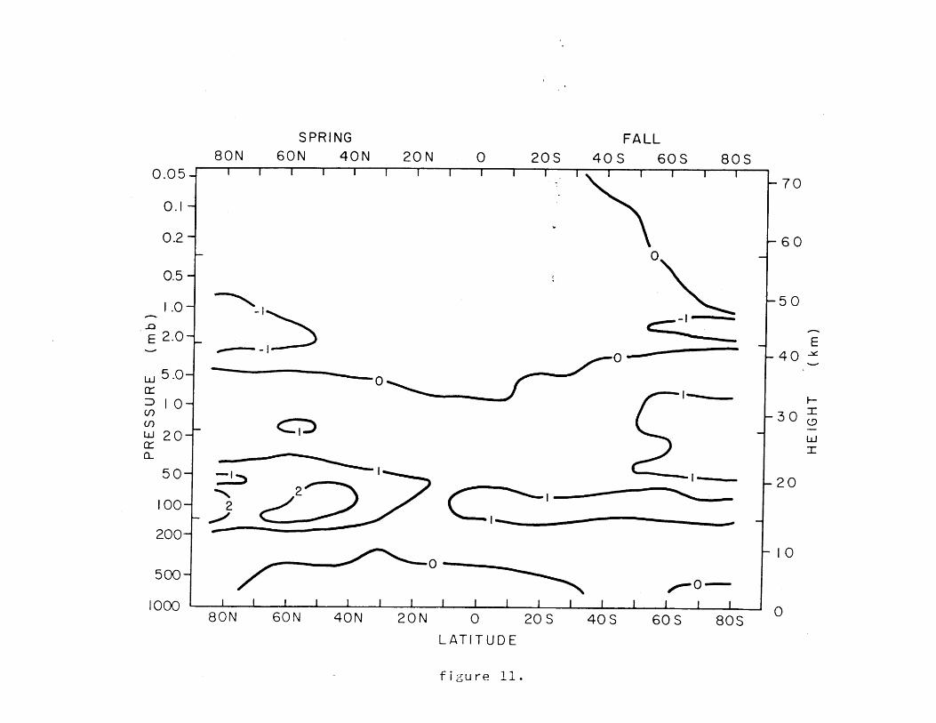
SPRING80N 60N 40N

I I I I I

20N 20SI I

40SI I I I

0

0

0

-~I I I I I I I I I I I I I J~

80N 60N 40N 20N 0 20SLATITUDE

40S

60S 80SI I I

0

1'~ ___

60S 80S

figure 11.

0.05-

0.1-

0.2-

0.5-

1.0-

E 2 .0-

5.0 -

Dio-

J 20-

50-

100-

200-

500-

1000

70

-60

-50

40

-30

-20

10

0--

FALL

c 7-044 *-

' T a jnl--,!-

O SO8 S09 SOP SO2 0 NO2 NOV N09 NO8

0o 00001 oo

-009

ooog01 001c oot,00 001

001 09

0 F,00_-02 ofU

00 /~02-c

-01m

~0 t3 0, Z 3-

09- S -O

0900

09- *

0 z -Foo~

S OP SO2 0 NO2 NOpSOB SO9 NO9 NO8

, T o j n c. -

0 NO2I- - I I I I I I I I I

NOt' NO9 NOBI I I I I I

SOt' SO2 0 NO2 NOt?

SO8 S09 S O7 S oz

01-

02-

OtP -

09-

09-

-1'O

-90-0

0001

-009

-OO

-001

-09

-OZ mU)

Ocn-01 m:

-0*l9

-9'0

I I I I I I I I I I I I I * I _ _NO9 NO8SO8 SO9

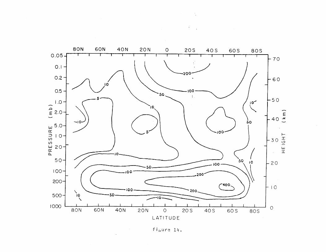
80N 60N 40N 20N 203 40S 60S SOS

o 50I

-I40N 20N 0 20S

I I I I I

40S 60S 80SLATITUDE

figure 14.

I I U I I Ii0.05-

0.1-

0.2-

0.5-

1.0-

10

I s-

2.0 -L

Ll 5.0-

D I0-

U 20-

L

50-

100-

200-

500-

1000

10

0

-70

60

-5 0

-40

-I30- w

LI

-20

10

080N 60N

80N 60N 40N 20N 20S 40S 60S 80S

40* De

-6.

.089mb

.4 -mb

40 mb.2 132mb

S2 3 4 5

Zonol Wavenumber

figure 15

2 3 4 5

Zonal Wavenumber

figure 1b.

.6-

I mb

.4-

13

12mb

2 -

40mb

2 3 4Zonal Wavenumber

figure 17.

80N 60N 40N 20NJUNE

0 20S 40S 60S

8ON 60N 40N 20N 0 20S 40S 60SLATITUDE

80S

80S

u~j

:DzuJ

z0

Lu

figure 1..

-70

-60

-50

E40

30

20

10

0

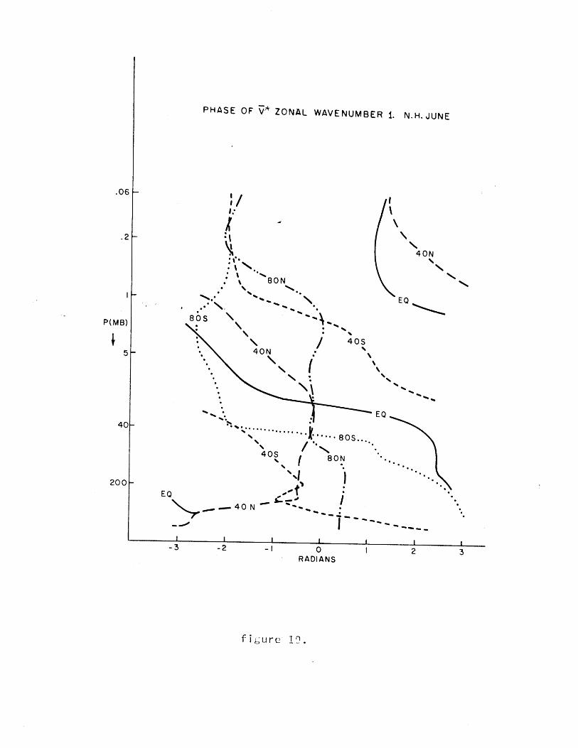
PHASE OF V*

:1

:' *%%

N.P(MB)

- \ 40S5 -. 40N

40-

I..........0S....

200N

200- \1EQ

.- 40 N

-3 -2 -0 ORADIANS

ZONAL WAVENUMBER I. N.H.JUNE

40N

0N

EQ

8

f ii.ure 12.

.06

.2

PHASE OF V ZONAL WAVENUMBER 2.

40S

80N

\EQ*

40N

40S

\ -.

B8N

figure 20.

.06

.2

P (MB)

5

40N

80S

40 k

200 k

N

EQ

40N

-3 -2 -1 0 I 2 3RADIANS

N.H. JUNE

8SS

PHASE OF V* ZONAL WAVENUMBER 3. N.H. JUNE

40N64

EQ

4 0 S4o

80N

I- - -

40S-

4% N

EQ

0N

-80.S

40N

figure 21.

.06

.2

P(MB)

5

40 H

200

80N

80N

II.-3 -2 -I 0 1 2 3

RADIANS

80S

308e 309 St7 sO, 0 NO0 N 0 t7 ",09 N UU 000 1

009

01 -0

-001

009-09

OZm(I)

02- (n

001~

09-

09- o

SOP SO2 0 NO2 NOV

l'O

90*0SO8 SO9NO9 NOB

40* WinterWavenumber I

5-

4- -400*

<v I v->m/sec

34 ---

300 *

2-200*

%%- -00

Doys

f i g-u re

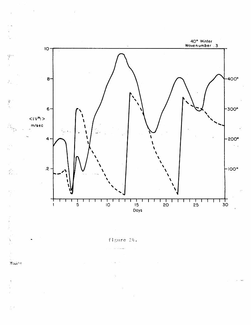
40* WinterWavenumber 3

8- 400*

6- P \-300*

<I V*l >

m/sec

4 -200*

<2- -L1000

I 5 lO 15 20 25 30Days

figure 24.

400 Winter'Wawenumber 5

5 0 15 20 25 30Days

fii Li re

10

8

<1 V*I>m/sec

6

4

2

40S

60N 40N 20 N 20S 40 S 60 S 80S

0.05

0.|

0.2

0.5

|.0

E 2.0

I I ;ure ~

.70

-60

.50

E40

30

20

I0

0

5.0

10

20

50

100

200

500

10008ON

80N 60N 40N 20N 20S 60S 80S

209 209 S20P O 0 N0OF NOt& N09 NU9u 0001

009

0z of 001

09

m 009

00m -Z

0*9

0* 109g

09-

£09 £09 s OV £0 ? 0 N0Z NOV' N09 N08

80N GON 40N 20N 20S 40S 60S 805I I I I I

0

0

0-22

0

55

I I I I I I ~ I I I I I I I I I

40N 20N

LATITUDE

fi ure .

0.05-

0 .-

0.2-

0.5-

1.0-

~/2

2.0 -{_

5.0-

1I0-

-' 20-

50-

100-

200-

500-

1000

7 0

-60

50

E40

30

20

- 0

080N 60N 20 S 40S 60S 80S

80N 60N 40N 20N 20S 40S 60S 80S

1.0

IV03)

M-MOLCM SEC'

0

-5-

-1.0-

40S EQ 40N

f iure 2J.

80N 60N 40N 20N 203 403 603 803I I I I I I I I I I a I I I0.05-

0.1-

0.2-

0.5-

1.0-

80NI I I I I I~

60N 40N 20N 20S

LATITUDE

fir-ure 3 .

'O . 0

02.0-L

5.0-

1 0-

20-

50-

100-

200-

500-

000

70

60

50

E-40

-30

-20

10

0

-~-~0 Na I

40S 60S 80S

60N 40N 20N 20S 40S 60S 80S80N

80N 60N 40N 20N 0 20S 40S 60S 80S

0.0 5- -7 0

0.1-

0.2 - 60

0.5-0-50

1.0 N

E 2 .0 -- E40

5.0 -

D1 0 - -3 02n 0 C

50 - 220-

a--

500-C 100000

80N 60N 40N 20N 0 20S 40S 60S 80S

LATITUDE

f i ure 1.

80N 60N 40N 20N 0 20S 40S 60S 80S0.05- 70

0.1-

0.2- 0 0 60

0.5-

1.0- 050

E 2.0 E-40

5.0-.5 -5

1 0- 'O-0IO 30 3QDcn.

W20- -10 wi0

50- -20

100- 10 - 20

200- 5 55

1000 080N 60N 40N 20N 0 20S 40S 60S 80S

LATITUDE

f i. ure 3 .

80N 60N 40N 20N 0 20S 40S 60S 80S0.05- -70

0.1-

0.2- 60

0.5 --50

1.0-

E 2.0-_- E-40

w 5.0-

D1 - 5 3cn 0 -30ct 0

50 20

00

200-0 00

500-

1000 0 I I I I_80N 60N 40N 20N 0 20S 40S 60S 80S

LATITUDE

i ure 33.

40S

_-----o \ 0,-

0

-0

0 o ~~~

--------- 0

80N 60N 40N 20N 0 20S 40S 60S 80S

LATITUDE

f igu re 314.

0.05

0.1

0.2

0.5

1.0

p2.0

10

100

200

500

1000

70

60

50

E4 0

30ui

20

10

0

60S 80S40N 20N 20S80N 60N

S09S OP

.. /

/i

0 NOZI I I I I

I II I I

SOV SO 0 NO2 NOV

NOtpN09NO8I I i I I I 0

01-

OP -

09-

09-

0001

-009

-001

-09

-OZ m()

-Qc

-' m

-0* 1

-9'0

-rlO

.,ISOB SO9NO9 NO9

*r

i fi n i

S ~z 0 N0ZSO S0 S I I I

-~.

-a I I I I I II I I I I I I I I I I II I I I

.I

SOBSO9SO17NOPN09NOB

0

O9v-

09-

09-

1O

-90,0

0001

-009

-001

-09

-OZ

-01 m:

-O'9m

-90

SOB SO9NO9 NO8 SO SO O o N O2 N Ot?

L'I ~rK~i4

ALTI

03sol?-

qwot

~I I-

Jyisoot,

qwZ21

No09NoOt'

, .5

No08NoOt7s008

i~' c Jn2I

03

qwI

TTFT

qw -I

38

1'

N008N0017sIOotpS00 8

No08

T E FII -r

No Ot'soot,sooe

SO SO9 S ot s 0 02 NO& N9 NO 000

C 009

01

-O9z

~02- 00 cI

-A 00

C-., 0*1-Z

09 ~

OL- ..,

0 NO2 NOVNO9 NO9 S OtpSO2 SOB SO9

80S

100-

1 6

EQ.

100-

1 6 1 6

EQ.

1 6

100'-

I-

fi:;u r~ 4r~~*

132 mb

40S 40N 8 ON

0

100-

8 0S

IL40 mb

40S

1 6ulil1 6

40N 8 0 I

1 6

100-

1 6 1 6 1 6

Tt ~JflKI4

q Lu O

9 1.1

sod

*qwJ T

t~m

IE-(9'01T.0 T

8

-~juT

NO11 0

NO tiSetn

lei ti

12 mb.40' winterwavenumber 1

301-

V

ia1 15 20 25

Days

f i gUre 42.

12 mib.40'winterwavenumber 2

300

V

200--

100

Days

figure 43.

12 ib.40' winterwavenumber 3

300-

200 -

V

10 06-

3

I I I |5 10 15 20

Da ys

figuro 44.

0I-'

03-93G-N~

09

01oixg

>i19? 3-V loIxg-

t7-

ari GJi

£09 £09 sO ot 0sO 0 NO0 N OP N09 N08 00

001 00

009

01 O0 i ~

cos- ~~001 -0

099

099 (N?

02 -of____

S Op SO2 0 NO2 N OV SOB SO9NO9 NOB

s09 £09 sO £t Oz 0 NQ0 N Ot? J N 0 8 oI

001 009

01 -0 001 00 oo

001 09 ()0 0 1

0I F 09

-01 .........

o 12 -..........

09 n.

001 -0*1

0 9

0001

01

S O, SO2 0 N02 N OVNO9 NOB SOe SO9

-3l?1in''

0i I I I I I I I

NO2NOVN09sI I I I I

S08 £09 sot, SO~ 0 NO~ NOP N09 N08

S09SO17SOeN08

0 1-

OP

09-

OIL -

SO9

190

SO otNO9 NO9

0001

-009

00Z

001

-09

-OZ cC/)

-0-9 m

cr

-OI

-9'0

SO2 O N O2 N OV SOe SO9

£09 £09 sot £OZ 0 NO0 N Ot N3D9 N0O CG,

0 1

-009

/1009

01 -7, 01c

--O m

n Bn/E02 -0 1

090L

09-

\~9P- / ( 0*0

09- 9 0£ OP z0* 0ONP N0

-G; oji nr i

NO9 NO9 O NO2 NOV SO2 SOB SO9S 017

1.0

. . I1

-.

a

Iu re

TC ir!l

£09sO t selOI I I I I I I I

i~ GfiI-,-v7

0I I I I I T I -I I

I I I I I I I I I I I I I

~C)RN 0N OPN09N090

01 -

OP, -

09-

09-

OL -

0001

-009

-ooZ

-001

-09

-O' mC/)

-01icx

0*

9*0

'O

-90*0 I I

NO9 NO9 0 NO2N Ot? SOe SO9SO t S OF,