A Study of TOC Supply Chain Replenishment System in LED ...

INTERNATIONAL JOURNAL OF ACADEMIC RESEARCH IN ACCOUNTING, FINANCE AND

MANAGEMENT SCIENCES

Vol. 1 0 , No. 3, 2020, E-ISSN: 2225-8329 © 2020 HRMARS

527

Full Terms & Conditions of access and use can be found at

http://hrmars.com/index.php/pages/detail/publication-ethics

A Study of TOC Supply Chain Replenishment System in LED Chip Manufacturing Plant

Horng-Huei Wu, Liang-Ying Wei, Chih-Hung Tsai, Yi-Chan Chung, Shu-Fang Lin

To Link this Article: http://dx.doi.org/10.6007/IJARAFMS/v10-i3/8398 DOI:10.6007/IJARAFMS /v10-i3/8398

Received: 10 July 2020, Revised: 11 August 2020, Accepted: 30 August 2020

Published Online: 24 September 2020

In-Text Citation: (Wu et al., 2020) To Cite this Article: Wu, H.-H., Wei, L.-Y., Tsai, C.-H., Chung, Y.-C., & Lin, S.-F. (2020). A Study of TOC Supply Chain

Replenishment System in LED Chip Manufacturing Plant. International Journal of Academic Research in Accounting Finance and Management Sciences, 10(3), 527–543.

Copyright: © 2020 The Author(s)

Published by Human Resource Management Academic Research Society (www.hrmars.com) This article is published under the Creative Commons Attribution (CC BY 4.0) license. Anyone may reproduce, distribute, translate and create derivative works of this article (for both commercial and non-commercial purposes), subject to full attribution to the original publication and authors. The full terms of this license may be seen at: http://creativecommons.org/licences/by/4.0/legalcode

Vol. 10, No. 3, 2020, Pg. 527 - 543

http://hrmars.com/index.php/pages/detail/IJARAFMS JOURNAL HOMEPAGE

http://creativecommons.org/licences/by/4.0/legalcode


MANAGEMENT SCIENCES


528

A Study of TOC Supply Chain Replenishment System in LED Chip Manufacturing Plant

Horng-Huei Wu1, Liang-Ying Wei2, Chih-Hung Tsai3, Yi-Chan Chung4, Shu-Fang Lin5

1Department of Business Administration, Chung-Hua University, Hsin-Chu, Taiwan 2,3Department of Information Management, Yuanpei University of Medical Technology, Hsin-Chu,

Taiwan, 4,5Graduate Institute of Business Administration, Yuanpei University of Medical Technology, Hsin-Chu, Taiwan

2Email: [email protected]

Abstract The LED chip manufacturing (LED-CM) is an important process in the LED supply chain. To meet

the severely competitive pressure these years, the issue of inventory risk for the variety of products is an imperative task for the LED-CM plant. The TOC supply chain replenishment system (TOC-SCRS) is one of the potential solutions to effectively manage inventory in the industry. However, the special features of the unstable production output and a product composed of the chips of different Bins exist in the LED-CM plant. Therefore, the application of TOC-SCRS to the LED-CM plant will encounter the following issues: (1) How to determine the optimal inventory buffer of the chips in the different Bins because a product can be composed of different combination of the chips in the feasible Bins? This paper proposed optimal Bin allocation models to resolve this problem. The optimal Bins inventory combination of a case is further performed via LINGO system and utilized to demonstrate the feasibility of these models. Employing the proposed models will facilitate LED-CM plants to improve their throughput and competitiveness. Keywords: LED Chip Manufacturing, Unstable Production Output, TOC Supply Chain Replenishment System (TOC-SCRS), Bin Allocation, Optimization Model. Introduction

Light-emitting diode (LED) is the most popular green energy industry in recent years, the output value of global LED packaging is about 13.363 billion US dollars, of which Taiwan's output accounted for 21% of the global industry, and the ranking of Taiwan’s output is second in the world (Lee et al., 2011). Therefore, Taiwan's LED industry relative to global industry not only occupies an important position but also has a competitive advantage potential. Taiwan’s LED industry has still growth space every year. Taiwan government deems that LED industry is one of important industries, and actively fosters it after semiconductor and panel industry. However, technical and capital thresholds for the LED industry are not high. Recently, many manufacturers investment LED industry in the mainland


MANAGEMENT SCIENCES


529

China, and LED industry has had oversupply phenomenon. Taiwan manufacturers would think how to improve competitiveness by R&D technology and manufacturing management capacity. It would be the key point for industry to continually maintain the current advantages and face the serious challenges.

LED industry can be divided into four major processes: raw materials, upstream, middle and downstream (Lee et al., 2011). The main raw material production part is to produce sapphire substrate and silicon substrate crystal column. The substrate is an important raw material for the production of Epi wafer. There are some industries in Taiwan, such as Wafer Works Corporation and Sino-American Silicon Products. The upstream process is mainly Epi wafer manufacturing, and the middle process is the manufacture of LED grain. Manufacturers generally integrate upstream and middle process. Domestic industries are EPISTAR Corporation and OptoTech Corporation. The downstream process is LED package and module factory. The process is mainly based on the different needs of the terminal application to package or modularize grain for subsequent applications. Domestic industries are Everlight electronic corporation, LITE-ON technology corporation, and Kingbright electronic corporation. Production process of LED Chip Manufacturer (LED-CM) is not only complex but also unstable. Product’s quality would determine the pros and cons of LED applications. Therefore, the grain factory is an important part for the LED industry, and it is the object (scope) for this study to be investigated.

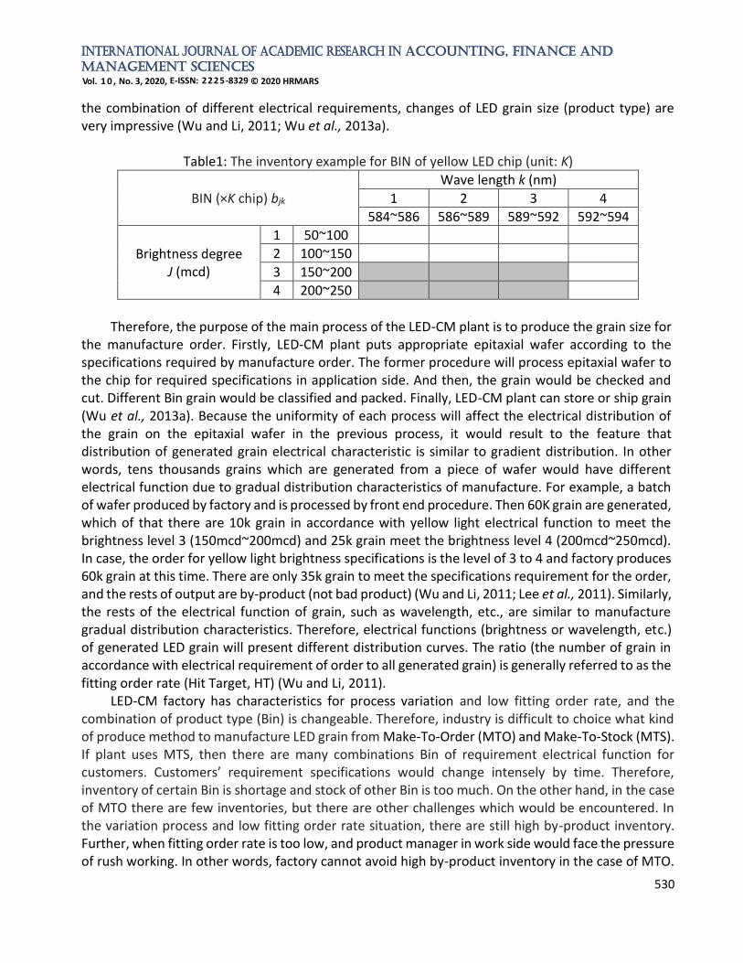
Basically, epitaxial wafer (EPI) is the input material of the LED-CM plant, and the output product is grain (Chip or Die). A chip can be produced thousands to tens thousands of the grain by grain size. The structure and size of grain is determined by electrical function. The major electrical function is brightness and wavelength. The other electrical functions are voltage and other conditions required by individual customer. Due to different applications have the different electrical function requirement, for example, the wavelength of the yellow LED is 584nm~594nm and the brightness is 100mcd ~ 300mcd. However, some customers want LED to be more yellow and bright, and the specifications for the LED will be 586nm~588nm and 200mcd~250mcd. Other customers would want the specifications to be 588nm~590nm and 150mcd~200mcd. Therefore, the LED-CM factory would indicate electrical function of grain by different Bin (section) as shown in Table 1. From Table 1, take yellow LED grain for example, the wavelength is divided into 4 bands (ie k = 1, 2, .., K, K = 4), and the brightness is divided into four levels (j = 1, 2, .., J, J = 4). Therefore, there are 16 types of Bins. The specifications of order made by customer are marked with the electrical range, and production manager converts order to the corresponding Bin in compliance with the specification. Then, manager processes the order to subsequent steps according to Bin. For example, manager would assess whether these inventories are sufficient of Bin. Perhaps, manager decides the most suitable Epi wafer and production process depending on the combination of these Bin. For example, customer makes 100k grain orders under a specification for the yellow light wavelength 583~593nm and brightness of 140~260mcd. Because the grain size of the shipment cannot be greater than the specifications of the customer requirements. Therefore, according to the Bin table in Table 1, the production manager can detect the feasible wavelengths of bands 1 to 3 and the brightness levels of 3 to 4, so there are six kinds of Bin can be satisfied, namely (j, k), j = 3~4 , K = 1~3, as shown in Table 1, the gray section. Subsequently, manager reevaluates whether these six kinds of Bin's inventory is enough. If inventory is not enough, manager must make a command to produce. Therefore, under


MANAGEMENT SCIENCES


530

the combination of different electrical requirements, changes of LED grain size (product type) are very impressive (Wu and Li, 2011; Wu et al., 2013a).

Table1: The inventory example for BIN of yellow LED chip (unit: K)

BIN (×K chip) bjk

Wave length k (nm)

1 2 3 4

584~586 586~589 589~592 592~594

Brightness degree J (mcd)

1 50~100

2 100~150

3 150~200

4 200~250

Therefore, the purpose of the main process of the LED-CM plant is to produce the grain size for

the manufacture order. Firstly, LED-CM plant puts appropriate epitaxial wafer according to the specifications required by manufacture order. The former procedure will process epitaxial wafer to the chip for required specifications in application side. And then, the grain would be checked and cut. Different Bin grain would be classified and packed. Finally, LED-CM plant can store or ship grain (Wu et al., 2013a). Because the uniformity of each process will affect the electrical distribution of the grain on the epitaxial wafer in the previous process, it would result to the feature that distribution of generated grain electrical characteristic is similar to gradient distribution. In other words, tens thousands grains which are generated from a piece of wafer would have different electrical function due to gradual distribution characteristics of manufacture. For example, a batch of wafer produced by factory and is processed by front end procedure. Then 60K grain are generated, which of that there are 10k grain in accordance with yellow light electrical function to meet the brightness level 3 (150mcd~200mcd) and 25k grain meet the brightness level 4 (200mcd~250mcd). In case, the order for yellow light brightness specifications is the level of 3 to 4 and factory produces 60k grain at this time. There are only 35k grain to meet the specifications requirement for the order, and the rests of output are by-product (not bad product) (Wu and Li, 2011; Lee et al., 2011). Similarly, the rests of the electrical function of grain, such as wavelength, etc., are similar to manufacture gradual distribution characteristics. Therefore, electrical functions (brightness or wavelength, etc.) of generated LED grain will present different distribution curves. The ratio (the number of grain in accordance with electrical requirement of order to all generated grain) is generally referred to as the fitting order rate (Hit Target, HT) (Wu and Li, 2011).

LED-CM factory has characteristics for process variation and low fitting order rate, and the combination of product type (Bin) is changeable. Therefore, industry is difficult to choice what kind of produce method to manufacture LED grain from Make-To-Order (MTO) and Make-To-Stock (MTS). If plant uses MTS, then there are many combinations Bin of requirement electrical function for customers. Customers’ requirement specifications would change intensely by time. Therefore, inventory of certain Bin is shortage and stock of other Bin is too much. On the other hand, in the case of MTO there are few inventories, but there are other challenges which would be encountered. In the variation process and low fitting order rate situation, there are still high by-product inventory. Further, when fitting order rate is too low, and product manager in work side would face the pressure of rush working. In other words, factory cannot avoid high by-product inventory in the case of MTO.


MANAGEMENT SCIENCES


531

In the worst situation, assembly order is insufficient causing by unstable manufacture process, product manager should use supplementary material or shift other product order to meet the urgent need (Wu and Li, 2011; Wu et al., 2013a; Wu et al., 2013b). It would result to work in a rush, and factory cannot avoid delay order schedule.

LED-CM factory is in unstable manufacture process environment and faces a great challenge while using MTO. MTO is now widely used for LED-CM factory. The major reason is that while using MTS, the Bin's inventory management is very complex and difficult to control, which will cause inventory to rise endlessly or inventory shortage problems. Recently, LED manufactures of mainland China produce mass products, LED industry has had oversupply phenomenon. To enhance competitiveness, Taiwanese manufacturers are forced to significantly shorten the manufacturing lead time. In the past, normal shipping time was 24 days and shipping time of urgent order was 16 days. Nowadays, shipping time is shortened for a week or factory is asked for immediate shipping, and even some customers have asked to provide Vendor-Managed Inventory (VMI) services (Levi et al., 2008). Therefore, LED-CM factory has faced the need to change MTS. How to reduce the inventory caused by MTS is the management problem that LED-CM factory must face.

In many viable practical approaches, theory of constraint-supply chain replenishment system (TOC-SCRS) is one of the effective solutions (Cole and Jacob, 1994; Goldratt, 1994). The system is widely accepted by industry at present (Holt, 1999; Perez, 1997; Simatupang et al., 2004; Smith, 2001). Its main content consists two parts, namely, replenishment mechanism and monitoring mechanism (Wu et al., 2013c; Cole and Jacob, 1994; Wu et al., 2010). Within TOC-SCRS replenishment mechanism, factory retains the largest stock occurred in replenishment period and its replenishment is only double number of sale volume during the two replenishment periods. Therefore, the policy of TOC-SCRS can ensure the lowest inventory. Further, TOC-SCRS method also monitors influence level of unexpected situations within TOC-SCRS monitoring mechanism. System would make emergency replenishment requirements while it is necessary. Therefore, factory can avoid out of stock. According to the general response of the company implemented TOC supply chain solution (Belvedere and Grando, 2005; Blackstone, 2001; Hoffman and Cardarelli, 2002; Kendall, 2004; Novotny, 1997; Patnode, 1999; Sharma, 1997; Waite et al., 1998; Watson and Polito, 2003), the benefits are that inventory are substantially reduced, the level of service is increased significantly(or out of stock rate is significantly reduced), overdue goods are declined, factory can fast react market changes and so on.

Due to the output variation of the LED-CM plant and the diversification of the product (or diversification of Bin combination), the following problems are encountered when applying TOC-SCRS method. TOC-SCRS considers each product category as an object for replenishment and monitoring. In other words, each product must establish its inventory level, parameters of replenishment and buffer management. Although LED-CM factory defines products by specifications for order or shipping, but the different specifications of the products are composed of different Bin grain compositions, and the combinations are unlimited because of customers’ requirement (different Bin grain can be combined into a large number of specification products). Therefore, if factory uses product specifications as the management object, not only the product category will expend endless, but also different product specifications cannot be shared (unless product be send back work side and be reworked, but the cost will increase a lot ). The results would cause inventory too high. Therefore, according to the postponement or delayed differentiation (Beamon, 1998; Levi et al.,


MANAGEMENT SCIENCES


532

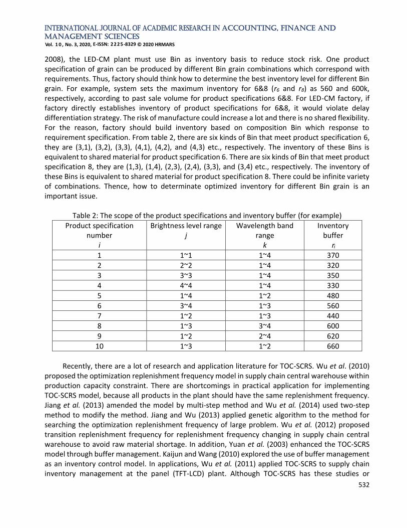
2008), the LED-CM plant must use Bin as inventory basis to reduce stock risk. One product specification of grain can be produced by different Bin grain combinations which correspond with requirements. Thus, factory should think how to determine the best inventory level for different Bin grain. For example, system sets the maximum inventory for 6&8 (r6 and r8) as 560 and 600k, respectively, according to past sale volume for product specifications 6&8. For LED-CM factory, if factory directly establishes inventory of product specifications for 6&8, it would violate delay differentiation strategy. The risk of manufacture could increase a lot and there is no shared flexibility. For the reason, factory should build inventory based on composition Bin which response to requirement specification. From table 2, there are six kinds of Bin that meet product specification 6, they are (3,1), (3,2), (3,3), (4,1), (4,2), and (4,3) etc., respectively. The inventory of these Bins is equivalent to shared material for product specification 6. There are six kinds of Bin that meet product specification 8, they are (1,3), (1,4), (2,3), (2,4), (3,3), and (3,4) etc., respectively. The inventory of these Bins is equivalent to shared material for product specification 8. There could be infinite variety of combinations. Thence, how to determinate optimized inventory for different Bin grain is an important issue.

Table 2: The scope of the product specifications and inventory buffer (for example)

Product specification number

i

Brightness level range j

Wavelength band range

k

Inventory buffer

ri

1 1~1 1~4 370

2 2~2 1~4 320

3 3~3 1~4 350

4 4~4 1~4 330

5 1~4 1~2 480

6 3~4 1~3 560

7 1~2 1~3 440

8 1~3 3~4 600

9 1~2 2~4 620

10 1~3 1~2 660

Recently, there are a lot of research and application literature for TOC-SCRS. Wu et al. (2010)

proposed the optimization replenishment frequency model in supply chain central warehouse within production capacity constraint. There are shortcomings in practical application for implementing TOC-SCRS model, because all products in the plant should have the same replenishment frequency. Jiang et al. (2013) amended the model by multi-step method and Wu et al. (2014) used two-step method to modify the method. Jiang and Wu (2013) applied genetic algorithm to the method for searching the optimization replenishment frequency of large problem. Wu et al. (2012) proposed transition replenishment frequency for replenishment frequency changing in supply chain central warehouse to avoid raw material shortage. In addition, Yuan et al. (2003) enhanced the TOC-SCRS model through buffer management. Kaijun and Wang (2010) explored the use of buffer management as an inventory control model. In applications, Wu et al. (2011) applied TOC-SCRS to supply chain inventory management at the panel (TFT-LCD) plant. Although TOC-SCRS has these studies or


MANAGEMENT SCIENCES


533

applications, there are no formal research literatures to show how to apply TOC-SCRS method to LED-CM plant. Therefore, if this study can provide solutions for problems mentioned above, it will make the TOC-SCRS replenishment mechanism more perfect and widely used. The research results would contribute to practical application of industry and promote academic to perform further research by using TOC-SCRS method.

Based on the above problems and requirements, the purpose of this study is to provide a feasible solution for the establishment of TOC-SCRS application model in order to strengthen the current TOC-SCRS. Thence, this paper proposes the Bin inventory buffer model which integrates product specifications and optimization Bin. Proposed model not only provide the conversion mode for product specification inventory buffer and Bin inventory buffer, but also can add incremental function of popular product specification according to company’s future needs. For the reason that proposed model can further establish optimization Bin inventory buffer mode.

Conversion Problem for Product Specifications Inventory Buffer and Bin Inventory Buffer Symbol Description

The required symbols for this study are as follows: bm: The inventory buffer of each Bin, m=1,2,.., M. dim: Inventory of No. m Bin grain converted from inventory buffer of product specification i, i =1,

2,.., I; m=1, 2,.., M. I: Quantity of product specifications type. i: Product specifications of category i, i =1, 2,.., I. J: The maximum range of brightness levels j: Brightness level number, j=1, 2,.., J. K: The maximum range of wavelength bands k: Wavelength band number, k=1, 2,.., K. lli: The lower limit of the brightness range of product specification i, i =1, 2,.., I. lui: The upper limit of the brightness range of product specification i, i =1, 2,.., I. M: The total number of Bin, M= J*(J - 1) + K. m: The number of each Bin, m=1,2,.., M. ri: Obtained maximum inventory buffer for product specifications i by TOC-SCRS, i =1, 2,.., I. wli: The lower limit of the wavelength range of product specification i, i =1, 2,.., I. wui: The upper limit of the wavelength range of product specification i, i =1, 2,.., I. β: In order to avoid the occurrence of the specification upgrade, minimum proportion of

compulsory shipment for each product specification Bin, 0<β<1.

Problem Description Because the order of the LED-CM factory is based on the product specifications, the inventory

buffer of each product specification can be evaluated according to the TOC-SCRS model (Wu et al., 2010). However, inventory of the LED-CM plant must be based on Grain inventory of Bin. Proposed model mainly utilizes inventory buffer of each product specification obtained by TOC-SCRS to further convert optimization inventory buffer of each Bin, as shown in Figure 1. Therefore, the input data for proposed model is the inventory buffer (ri) of each product specification, and the output data is the


MANAGEMENT SCIENCES


534

optimization stock buffer of each Bin (bm). Secondly, proposed model is built on the following environment: (1) The specifications of the LED grain only contain the main lightness and the wavelength, where the

brightness is divided into J grades and the wavelengths are divided into K wavebands. (2) There are J x K Bin, each Bin number and relationships for brightness level and wavelength band

as shown in equation (1).

KkJjkjJm ..2,1,,..2,1,)1(* ==+−= ( 1 )

(3) The feasible brightness level and wavelength band for each product specification, as shown in equation (2). In other words, the grain of each order must consist of the grain of its available specifications Bin. FBi ={(j,k), ll i≦j≦lui, wl i≦k≦wui}={m, m=J*(j-1)+k, ll i≦j≦lui, wl i≦k≦wui}, i=1,2, ..,I (2)

(4) In order to avoid the problem of order specification upgrade, the number of grains for per viable bin of each order must not be less than a lower limit (β), which is determined by the consensus between the LED-CM and the customer. The value of β is from 0% to 10%.

Figure1: The framework of Optimization Bin inventory buffer model

Conversion method for Product specifications inventory buffer and Bin inventory buffer Conversion matrix of Bin inventory buffer

The so-called conversion matrix of Bin inventory buffer as shown in Table 3, it is used to convert the inventory buffer of each product specifications into each Bin inventory buffer matrix. The two lines on the left side are divided into the product specifications and their inventory buffer, and the first column is the Bin number. The middle shadow part is the applicable Bin number rage for each product specification, such as feasible Bin number of product specification 1 is numbered No. 1 to No. 4. The number displayed on shadows is the inventory buffer conversion (assignment) of the product specifications and is the amount of inventory buffer for each available Bin. For example, the inventory buffer of product specification 1 is 370k grain, and Table 3 shows the example that the assigned grain number are 92k, 92k, 93k and 93k, respectively for No. 1 to No4 Bin. According to the product specifications assigned to the available Bin grain, the total number of grains of the Bin is obtained by summing up the grains of the same Bin, as shown in the bottom row of Table 3. For example, the total number of grains in No. 1 Bin is 335k, which is the inventory buffer for the No.1 bin. Therefore, the inventory buffer of each product specification (in the left two lines) can be converted to be inventory buffer for each Bin by Bin inventory buffer conversion matrix, as shown in the last column of Table 3.

Optimization Bin

inventory buffer

conversion mode

TOC-SCRS

model

Optimization

inventory

buffer for

each Bin

Inventory

buffer of each

product

specification

Historical sales

information of

each product

specification

The scope of this study


MANAGEMENT SCIENCES


535

Table 3: Bin inventory buffer conversion matrix

Product specificati

on #(i)

Bin#(m)

1 2 3 4 5 6 7 8 9 10

11

12

13

14

15

16

Sum

1 370 92 92 93 93

370

2 320 80 80 80 80

320

3 350 87 87 88 88

350

4 330 82 82 83 83

330

5 480 60 60 60 60 60 60 60 60

480

6 560 93 93 93 93 94 94

560

7 440 73 73 73 73 74 74

440

8 600 100 100 100 100 100 100

600

9 620 103 103 103 103 104 104

620

10 660 110 110 110 110 110 110

660

The amount of inventory buffer for each Bin (bm)

335 438 369 296 323 427 358 284 350 350 281 188 235 236 177 83 4730

Design Steps of Bin Inventory Buffer Conversion Matrix Step 1: Acquire basic information of Bin inventory bugger conversion matrix, content includes

number and product specification of the left two lines, inventory buffer of product specification, Bin number of the previous column, and the possible Bin combination of the product specifications of the middle shade part and so on.

Step 2: Formulate the distribution rules for each product specification inventory buffer allocation to each available Bin inventory.

Step 3: According to distribution rule, system allocates each product specification inventory buffer to each available Bin inventory. Each Bin allocated inventory must meet the following two conditions: (1) The sum of the number of grains allocated to each feasible Bin should be equal to the

inventory buffer of the product specification, as shown in equation (3)

IirdiFBm

iim ,..2,1, ==

( 3 )

Inventory buffer of each

product specification (ri)

Conversion amount

for each Bin(dim)


MANAGEMENT SCIENCES


536

(2) The number of grains allocated to each feasible Bin must be greater than one lower limit (

ir ) to avoid the problem of upgrading the order specification, as shown in equation

(4).

iiim FBmIird = ,..2,1, ( 4 )

Step 4: Cumulate number of grain of each Bin allocated from each product specification inventory buffer to the last column, as shown in equation (5)

MmdbI

i

imm ...,2,1,1

===

( 5 )

Step 5: Check whether the sum of the inventory buffers for each Bin is equal to the sum of the inventory buffer of each product specification, as shown in equation (6). If the formula (6) is satisfied, then end; otherwise return to step 3 and reallocate or correct.

+−

= =

KJJ

m

I

i

im rb)1(*

1 1

( 6 )

Case Description

As shown in Table 2. In this case, there are 10 kinds of LED grain product specifications (I = 10), and the main product specifications are brightness and wavelength, which is divided into four levels of brightness (J = 4) and 4 bands of wavelength (K = 4). So this case has 16 (= J × K) Bin, and the feasibility ranges of each product specification as shown in Table 2. Secondly, in order to avoid the problem of order upgrade, this case requires that the lower limit of the number of grains allocated to each available Bin is 5% (β= 0.05).Through the evaluation of past orders, the inventory buffer (ri) required for each product specification is shown in Table 2. In order to obtain the Bin's inventory buffer, the design steps according to Bin inventory buffer conversion matrix are as follows: Step 1: Acquire basic data of the Bin inventory buffer conversion matrix, content includes the number

of product specifications of the left two lines and the inventory buffer of each product specification, the Bin number of the last column, and the applicable Bin combination of the product specifications of the middle shade, and so on, as shown in Table 3.

Step 2: The used distribution method is average distribution method which allocates inventory of product specification to acceptable Bin. If there is a remainder and then system randomly assigns 1k to any feasible Bin, until dispatch is finished

Step 3: In the case of product specification 1, the inventory buffer is 370k grain, and there are four feasible Bin (No. 1 ~ No. 4), so each feasible Bin evenly allocates 92k (= 370k / 4) grains. As a result of the balance of 2k, then system randomly assigns 1k to No. 3 and No. 4 Bin. The last No. 1, No. 2, No. 3 and No. 4 Bin are assigned 92k, 92k, 93k and 93k grain. Since the allocated grains of each available Bin for product specification 1 satisfy the conditions of equations (3) and (4). The next product specification is allocated continually until the inventory buffers of the 10 product specifications are allocated to the respective feasible Bin. The results are shown in Table 3 (The number of middle shadows).

Step 4: Take No. 1 Bin as an example, according to equation (5), b1=d11 + d51 + d71 + d101 = (92 + 60 + 73 + 110) = 335. Similarly, we can calculate the rest of the Bin's inventory buffer, as shown in the bottom row of Table 3.


MANAGEMENT SCIENCES


537

Step 5：Due to the sum of the inventory buffers of each Bin is 4,730k grains, and the sum of the product specifications inventory buffers is also 4,730k grains. The condition of the equation (6) is satisfied and therefore the process is finished.

Optimization Bin inventory Buffer Model Model Description

Basically, the inventory buffer of each Bin converted by Bin inventory buffer conversion matrix from inventory buffer of each product specification is only feasible solution. Subsequently, this study will further propose the optimization Bin inventory buffer model. Proposed model not only meet the largest inventory requirement of existing product specification, but also have elasticity to cope with future combination changes of product specification. Therefore, plant can exert the effect of delay differentiation. Flexibility defined in this study is measured by the amount of growth that can be met in the future for certain popular product specifications (H). In order to meet the needs of sales growth, feasible Bin inventory of popular product specification is bigger and better or elastic increment (△s) of inventory is bigger and better. In other words, in the case of satisfying the maximum inventory requirement of the existing product specifications, if the (Δs) is larger, it means that elasticity which is respond to popular product specification( )Hi sale increasing in future is

greater. Therefore, target equation of whole model is as follows, equation (7), and the constraint equations are as follows: equation (8) to (14).

Target equation：

sMax ( 7 )

Constraint equation：

IirdiFBm

iim ,..2,1, ==

( 8 )

iiim FBmIird = ,..2,1, ( 9 )

MmdbI

i

imm ...,2,1,1

===

( 1 0 )

+−

= =

KJJ

m

I

i

im rb)1(*

1 1

( 1 1 )

),(,

imFBmHi

rbfsi

= ( 1 2 )

imd and mb are nonnegative integer, i=1,2.. I, m=1,2..,M (13)

0 < β < 0 . 1 ( 1 4 ) First, constraint equation (8) means that sum of allocated inventory for each feasible Bin of

satisfying product specification should be equal to inventory buffer requirement of product specification i. Equation (9) is to avoid the problem of upgrading the specification, and the amount of inventory allocated by each feasible Bin must be greater than product specifications inventory buffer minimum ratio requirement. Equation (10) is the inventory of each Bin and is the sum of the stocks allocated by the feasible bin that satisfies the respective product specification. Equation (11)


MANAGEMENT SCIENCES


538

is to formulate that sum of inventory for all Bins cannot be less than sum of required inventory for all product specifications. Equation (12) is an incremental function that should satisfy future popular product specifications. Equation (13) regulates the inventory of each Bin as a non-negative integer, and equation (14) formulates minimum lower limit ratio from 0 to 0.1 to avoid specification upgrading problem.

Case Description

The case of this section continues the case in section 3.3. Due to company is optimistic about the future potential of product specification 3 and manager expects the product specifications to have the greatest flexibility in the future. In other words, product specification No. 3 would be popular product in future that is H = {3}, and feasible Bins of product specification No.3 are No. 9-12 Bin, that is FB3= {9,10,11,12}. If factory want to have largest shipments of product specification No.3 in future, it must have the largest inventory of No. 5 to No. 8 Bin. Therefore, incremental equation △s (equation (12)) can be expressed as shown in equation (15), and the target equation is asked to be the maximum value.

3

12

9,

)( rbrbsm

m

FBmHi

im −=−= =

( 1 5 )

Table 4 shows that the optimization Bin inventory buffer generated by LINGO program from optimization inventory buffer model mentioned above. The inventory buffers of b9, b10, b11 and b12

are 853k, 103k, 1166k and 48k respectively. Hence, △s= (2170k - 350k)= 1,820k. In other words, there are 6.2 times (= 2170k/350k) product for product specification No. 3 or factory has the flexibility to ship extra 1820k product in future. Table 5 shows the comparison results for optimization Bin inventory buffer of product specification No.3 in Table 4 which has maximum elasticity (shipping volume) and general Bin inventory buffer in Table 3. The future increment of product specification 3 of the optimization Bin inventory buffer model is 1820k, and the future increment of product specification 3 of general Bin inventory buffer model is only 819k. In other words, the flexibility of product specification No. 3 increases again 2.2 times (= 1820k / 819k) under the optimization model.

Therefore, the product specification inventory buffer and Bin inventory buffer conversion model proposed in this study not only can obtain required reasonable Bin inventory buffer of product specification inventory buffer, but also can add incremental formula of popular product specification according to company’s future needs. Company can further establish the optimization Bin inventory buffer model, and you can get, optimization Bin inventory buffer of required product specifications inventory buffer under company's future needs.


MANAGEMENT SCIENCES


539

Table 4: Optimization Bin inventory buffers which make product specification No.3 in Table 3 have

maximum flexibility (shipments) in future

product specificati

on #(i)

Bin#(m)

1 2 3 4 5 6 7 8 9 10 11 12 13 14 15 16 Sum

1 370 19 19 313 19 37

0

2 320 16 16 272 16 32

0

3 350 18 18 296 18 35

0

4 330 17 17 279 17 33

0

5 480 24 24 24 24 312 24 24 24 48

0

6 560 28 28 420 28 28 28 56

0

7 440 22 22 330 22 22 22 44

0

8 600 30 30 30 30 450 30 60

0

9 620 31 31 465 31 31 31 62

0

10 660 33 33 33 33 495 33 66

0

Inventory buffer of Bin(bm) 98 129 704 514 95 126 355 77 853 103 1166

48 69 69 307 17 4730

Table 5: Comparison of the optimal Bin inventory buffer (Table 4) with the general Bin inventory

buffer (Table 3)

Inventory buffer of product

specification No. 3(r3)

Feasible Bin inventory buffer of product specification No.3 Incremental

value △s

Elastic ratio

b9 b10 b11 b12 Sum

Table 3 (general model)

350 350 350 281 188 1169 819 3.34

Table 4 (Optimization model)

350 853 103 1166 48 2170 1820 6.2

‘

Inventory buffer of

product specification (ri)

Amount of bin

conversion (dim)


MANAGEMENT SCIENCES


540

Conclusions LED grain manufacturing (LED-CM) plant is an important part of the LED industry. In response to

market demand for intense competition, inventory pressure of product diversification is an inevitable key issue for LED-CM factory. Although TOC-SCRS is an effective solution, however LED-CM plant has process output variation and characteristic that product specifications are composed of grains in different sections (Bin). If factory sets directly inventory according to product specification, there would be unlimited variety of product specification due to customers’ requirements (different Bin grain can be combined into a large number of product specifications). It will lead to high inventory and low elasticity. Therefore, LED-CM factory must use Bin as inventory’s unit. However, in LED-CM factory, orders, shipping and production must be based on product specification, and the reason would cause that the same product specification could be composed by different Bin grains while implementing TOC-SCRS method. Thence, how to determine the optimal inventory level for different Bin grains is an important research issue. This study aims at the establishment of TOC-SCRS application model to provide a feasible solution and strengthens the current TOC-SCRS deficiencies. This paper proposes a model integrating product specification and optimal Bin inventory buffer of Bin. Proposed model not only provides conversion method for product specifications inventory buffer and Bin inventory buffer, but also can add an incremental formula of popular product specification. Factory can further establish the optimal Bin inventory buffer mode by proposed model.

In this study, proposed conversion model for product specifications inventory buffer and Bin inventory buffer can obtain reasonable Bin inventory buffer of required product specification inventory buffer. According to the company's future requirements, factory can add popular product specifications incremental function. Company can utilize generated optimal Bin inventory buffer model to obtain Product specifications inventory buffer required for the optimal Bin inventory buffer by LINGO program in the company's future needs. Research results of this study will be available as reference for LED grain factory to enhance its effective output and competitiveness.

To summarize, the contributions of the study are that this paper builds TOC-SCRS model to offer feasible and strengthens TOC-SCRS deficiencies at present. Proposed model can set up best solution of Bin inventory buffer mode for factory. Then company can obtain Product specifications inventory buffer required by LINGO program in future needs. Research results could increase production capacity of LED grain factory.

Acknowledgements

The authors would like to thank the Ministry of Science and Technology of the Republic of China in Taiwan for partially supporting this research under Contract No. 102-2221-E-216 -027-MY3. Corresponding Author Liang-Ying Wei, PhD Department of Information Management, Yuanpei University of Medical Technology, No. 306, Yuanpei Street, Hsin-Chu, Taiwan 30015 Email: [email protected]


MANAGEMENT SCIENCES


541

References Aytug, H., Lawley, M. A., Mckay, K., Mohan, S., and Uzsoy, R. (2005), “Executing production schedules

in the face of uncertainties: A review and some future directions,” European Journal of Operational Research, Vol. 161, No. 1, pp.86-110.

Beamon, B. M. (1998), “Supply chain design and analysis: Models and methods. International Journal of Production Economics, Vol. 55, No. 3, pp.281-294.

Belvedere, V., and Grando, A. (2005), “Implementing a pull system in batch/mix process industry through theory of constraints: A case-study,” Human Systems Management, Vol. 24, No. 1, pp.3-12.

Blackstone, J. H. (2001), “Theory of constraints –a status report,” International Journal of Production Research, Vol. 39, No. 6, pp.1053-1080.

Cole, H., and Jacob, D. (1994), “Introduction to TOC Supply Chain, USA: AGI institute (2002). Goldratt, E.M., (1994), “It’s Not Luck,” England: Gower. Hoffman, G., and Cardarelli, H. (2002), “Implementing TOC Supply Chain: A Detailed Case Study –

MACtac,” USA: AGI Institute. Holt, J. R. (1999), “TOC in Supply Chain management,” 1999 Constraints Management Symposium

Proceedings, pp.85-87, March 22-23, Pheonix, AZ, U.S.A, USA: APPICS. Jiang, X. Y., and Wu, H. H. (2013), "Optimization of setup frequency for TOC supply chain

replenishment system with capacity constraints," Neural Computing and Applications, Vol. 23, No. 6, pp.1831-1838.

Jiang, X. Y., Wu, H. H., and Tsai, T. P. (2013), "A Study of Diverse Replenishment Frequency Model for TOC Supply Chain Replenishment Systems under Capacity Constraint," International Journal of Modelling, Identification and Control, Vol. 19, No. 3, pp.248-256.

Kendall, G. I. (2004), “Viable Vision - Transforming Total Sales into Net Profits,” USA: J. Ross Publishing, Inc.

Kaijun, L., and Wang, Y. (2010), “Research on inventory control policies for nonstationary demand based on TOC,” International Journal of Computational Intelligence Systems, Suppl. 1, pp.114-128.

Lee, C. W., Chien, C. F., and Zheng, J. N. (2011), “The Optimal Decision System of LED Chip Releasing and Purchasing,” Proceedings of the 2011 Annual Conference of the Chinese Institute of Industrial Engineers, Hsin-Chu, Taiwan.

Levi, D. S., Kaminsky, P., and Levi, E. S. (2008), “Designing and Managing the Supply Chain- Concepts, Strategies and Case Studies,” McGraw-Hill Companies, Inc.

Novotny, D. J. (1997), “TOC Supply Chain Case Study,” 1997 APICS Constraints Management Symposium Proceedings, pp.78-79, April 17-18, Denver, Colorado, U.S.A, USA: APPICS.

Patnode, N. H. (1999), “Providing Responsive Logistics Support: Applying LEAN Thinking to Logistics,” 1999 Constraints Management Symposium Proceedings, pp.93-96, March 22-23, Pheonix, AZ, U.S.A, USA: APICS,

Perez, J. L. (1997), “TOC for world class global supply chain management,” Computers & Industrial Engineering, Vol. 33, pp.289-293.

Schragenheim, E. M. (2002), “Make-to-Stock under Drum-Buffer-Rope and Buffer Management Methodology,” 2002 International Conference Proceedings, APICS~ The Educational Society for Resource Management.


MANAGEMENT SCIENCES


542

Schragenheim, E., and Dettmer, H. W. (2001), “Manufacturing at Warp Speed: Optimizing Supply Chain Financial Performance,” Florida: St. Lucie Press, U.S.A.

Schragenheim, E., and Ronen, B. (1991), “Buffer management: a diagnostic tool for production control,” Production and Inventory Management Journal (second quarter), pp.74-79.

Sharma, K. (1997), “TOC Supply Chain Implementation: System Strategies,” 1997 APICS Constraints Management Symposium Proceedings, pp.66-74, April 17-18, Denver, Colorado, U.S.A, USA: APICS.

Simatupang, T. M., Wright, A. C., and Sridharan, N. (2004), “Applying the theory of constraints to supply chain collaboration,” Supply Chain Management: An International Journal, Vol. 9, No. 1, pp.57-70.

Smith, D. A. (2001), “Linking the Supply Chain Using the Theory of Constraints Logistical Applications and a New Understanding of the Role of Inventory/Buffer Management, “ 2001 Constraints Management Technical Conference Proceedings, pp.64-67, March 19-20, San Antonio, Texas, U.S.A, USA: APICS.

Waite, J., Gupta, S., and Hill, E. (1998), “Meritor HVS Story,” 1998 APICS Constraints Management Symposium Proceedings, pp.1-9, April 16-17, Seattle Washington, AZ, U.S.A, USA: APICS.

Watson, K., and Polito, T. (2003), “Comparison of DRP and TOC financial performance within a multi-product, multi-echelon physical distribution environment,” International Journal of Production Research, Vol. 41, No. 4, pp.741-765.

Wu, H. H., Chen, C. P., Tsai, C. H., and Tsai, T. P. (2010), “A Study of an Enhanced Simulation Model for TOC Supply Chain Replenishment System under Capacity Constrain,” Expert Systems with Applications, Vol. 37, No. 9, pp.6435-6440.

Wu, H. H., and Li, M. F. (2011), “A study of the order fulfillment and production model for the LED die manufacturer,” Proceedings of the 2011 Annual Conference of the Chinese Institute of Industrial Engineers, Hsin-Chu, Taiwan.

Wu, H. H., Tsai, S. H., Tsai, C. H., Tsai, R., and Liao, M. Y. (2011), “A study of supply chain replenishment system of theory of constraints for thin film transistor liquid crystal display (TFT-LCD) plants,” African Journal of Business Management, Vol. 5, No. 21, pp.8617-8633.

Wu, H. H., Huang, H. H., and Jen, W. T. (2012), “A Study of the Elongated Replenishment Frequency of TOC Supply Chain Replenishment Systems in Plants,” International Journal of Production Research, Vol. 50, No. 19, pp.5567-5581.

Wu, H. H., Li, M. F., and Hsu, T. F. (2013a), “An order fulfillment model for the LED chip manufacturing plant, “Advanced Materials Research, Vols. 694-697, pp.3446-3452.

Wu, H. H., Li, M. F., and Yeh, C. H. (2013b), “A Study of the Material Re-issued Models for an Insufficient Output of the LED Chip Manufacturing Plant,” Advanced Materials Research, Vols. 694-697, pp.3434-3440.

Wu, H. H., Li, M. F., and Hsu, T. F. (2013c), “A Study of an order fulfillment model for the LED chip manufacturing plant,” Advanced Materials Research, Vols. 694-697, pp.3446-3452.

Wu, H. H., Lee, A. H. I., and Tsai, T. P. (2014), “A two-level replenishment frequency model for TOC supply chain replenishment systems under capacity constraint,” Computers & Industrial Engineering, Vol. 72, No. 2, pp.152-159.

Yuan, K. J., Chang, S. H. and Li, R. K. (2003), “Enhancement of theory of constraints replenishment using a novel generic buffer management procedure,” International Journal of Production


MANAGEMENT SCIENCES


543

Research, Vol. 41, No. 4, pp.725-740.

A Study of TOC Supply Chain Replenishment System in LED ...

Documents

Transcript of A Study of TOC Supply Chain Replenishment System in LED ...