A review of high frequency surface wave radar for ...

Turk J Elec Eng & Comp Sci, Vol.18, No.3, 2010, c© TUBITAK

doi:10.3906/elk-0912-331

A review of high frequency surface wave radar for

detection and tracking of ships

Anthony M. PONSFORD, Jian WANGRaytheon Canada Limited, 400 Phillip Street, Waterloo Ontario,

N2L 6R7, CANADAe-mail: tony [email protected], jian [email protected]

Abstract

In today’s resource-driven economy, maritime nations are claiming economic borders that extend beyond

the continental shelf or the 200 nautical mile (nm) Exclusive Economic Zone (EEZ). However, claiming such

large economic area places responsibilities on the parent nation to exercise jurisdiction through surveillance

and enforcement.

The requirement to see beyond the horizon has long been a goal of maritime security forces. Today,

this is largely dependent on cooperative vessels voluntarily communicating their intentions to local shore-side

authorities, as well as on those vessel sightings reported by patrollers. Recent advances in technology provide

maritime nations with options to provide more systematic surveillance of both cooperative and non-cooperative

targets.

This paper presents an overview of a land-based High Frequency Surface Wave Radar (HFSWR) used to

provide persistent, active, surveillance. The paper demonstrates that these radars have now reached a level

of maturity where their performance is predictable and that they can, within known limits, reliably detect and

track ocean going vessels throughout the EEZ.

1. Introduction

This paper provides an overview of factors that affect the performance of HFSWR and how these systems canbe most effectively used to provide real-time, persistent and active surveillance of the 200 nm EEZ maritimeboundaries.

HFSWR refers to a classification of radar that utilizes the surface-wave mode of propagation and thatoperate in the 3 MHz to 30 MHz frequency range; surface waves have the following characteristics:

(a) they attenuate directly as functions of distance (range), frequency and surface roughness;

(b) they propagate efficiently in vertical polarization only; and

(c) they require a conducting surface, such as a saline ocean, to propagate.

HFSWR detection range is dependent on many factors [1], [2]]. For our initial discussion it is sufficientto state that the range obtainable is dependent on the frequency of operation, radiated power and vessel size as

409

Turk J Elec Eng & Comp Sci, Vol.18, No.3, 2010

well as the prevailing environmental conditions. The radar signal will experience a greater rate of attenuationas the radar frequency is increased or, for a given frequency, the sea state increases.

Detection of vessels by HFSWR fall in to two distinct categories: those smaller vessels (typically less

than 1000 tons) whose detection range is limited by the presence of ocean clutter and those larger vessels

(typically greater 1000 tons) whose maximum detection range is limited by external noise. In the former case,the detection range can only be increased by reducing the area of the radar clutter cell, whilst in the latter casethe detection range can also be extended by increasing the effective radiated power.

1.1. Paper overview

This paper presents an overview of factors that influence the successful detection and subsequent tracking ofvessels using HFSWR. Section 2, introduces the basics of an HFSWR system and presents an example of thelayout of a typical radar site. This is followed in Section 3 by a review of propagation losses as a function ofboth radar frequency and sea state.

The scattering of the radar signal from the ocean and the resulting ocean clutter spectrum is discussed inSection 4. Section 5 reviews vessel detection using HFSWR and presents a method for approximating the radarcross section (RCS) of a vessel at HF. The performance of HFSWR is ultimately limited by external noise andthis is discussed in Section 6. The impact on performance of unwanted signals such as self generated ionosphericclutter is presented in Section 7. A key factor in specifying radar performance is the Probability of Detection;this is discussed in Section 8, whilst Section 9 presents an overview of tracking and the associated Probabilityof Track. Conclusions are presented in Section 10.

2. HFSWR basics

HFSWRs that are used for long-range vessel tracking typically operate in a pulse-Doppler mode, where theradar emits a coherent pulse train. Vessels, which are within the area illuminated by the radar, reflect thesepulses back to the radar, where the echoes are received by a linear array of antennas. The signal receivedon each antenna is digitally processed to enhance the signal-to-interference ratio, where the term interferenceincludes all unwanted signals such as sea clutter, external noise, ionospheric reflection as well as interference fromother users of the band. The returned echoes are processed and sorted according to range, velocity (Doppler)and bearing. The echoes are then compared against a detection threshold chosen to achieve a predeterminedconstant-false-alarm-rate (CFAR). If the magnitude of an echo exceeds the threshold it is declared a detection.These detections are then forwarded to a tracking algorithm that associates consecutive detections in to tracks.

An example of a monostatic radar site is illustrated in Figure 1. It can be observed that in thisconfiguration the transmit and receive arrays are co-located and share a common site. The length of the receivearray is a compromise between the desire to maximize the directive gain and resolution whilst minimizing real-estate requirements. This typically limits the number of element pairs to 16 spaced at 1/2λ increments. Boththe transmit antenna and individual doublet-pairs generate antenna patterns that cover the desired search area.

410

PONSFORD, WANG : A review of high frequency surface wave radar for...,

� � � ��

��

��

��

��

Figure 1. Typical radar site layout for a monostatic installation.

2.1. Radar coverage area

For a monostatic radar, the area of coverage is symmetrical around the radar boresight, where the boresightis perpendicular to the axis of the array. When using a linear array, returns from beyond +/-60 degrees inazimuth are typically not displayed, due to rapid falloff in system performance as well as the potential forleft/right ambiguity due to the presence of unwanted grating lobes.

Within the azimuth coverage region, the radar signal processor synthesizers multiple narrow receivebeams. These receive beams are “electronically steered” to simultaneously cover the desired search area. Asillustrated in Figure 2, as a beam is steered away from boresight it becomes both broader and more lossy.

�! �! "! #! ! #! "! �! �! $!

#%

#!

�%

�!

%

!

&'�(��)��

�*

��*�� $+#��,-(�.��*� � ��

!��)+�!��)+

�! �! "! #! ! #! "! �! �! $!

#%

#!

�%

�!

%

!

&'�(��)��

�*

��*�� "+��,-(�.��*� � ��

!��)+�!��)+

Figure 2. Comparison of receive synthesized beam pattern at boresight and +60 degree for operating frequencies of 3.2

and 4.1 MHz.

411


When specifying the performance of a HFSWR, it is typical to assume an azimuth-averaged gain of thecombined transmit and receive antenna patterns.

3. Propagation losses

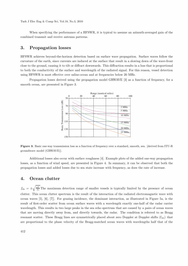
HFSWR achieves beyond-the-horizon detection based on surface wave propagation. Surface waves follow thecurvature of the earth, since currents are induced at the surface that result in a slowing down of the wave-frontclose to the ground, causing it to tilt or diffract downwards. This diffraction results in a loss that is proportionalto both the conductivity of the surface and wavelength of the radiated signal. For this reason, vessel detectionusing HFSWR is most effective over saline-ocean and at frequencies below 20 MHz.

Propagation losses derived using the propagation model GRWAVE [3] as a function of frequency, for asmooth ocean, are presented in Figure 3.

�� )��/ ��0

%!

1!

�!

��!

�$!

�%!

*��

��

��

��

��

�2��

��/�

*0

#��,-%��,-

�!��,-

�%��,-

#!��,-

#%��,-

!��#!��"!��!��!��!!

Figure 3. Basic one-way transmission loss as a function of frequency over a standard, smooth, sea. [derived from ITU-R

groundwave model (GRWAVE)].

Additional losses also occur with surface roughness [4]. Example plots of the added one-way propagationlosses, as a function of wind speed, are presented in Figure 4. In summary, it can be observed that both thepropagation losses and added losses due to sea state increase with frequency, as does the rate of increase.

4. Ocean clutter

fds = ±√

gfc

πc The maximum detection range of smaller vessels is typically limited by the presence of ocean

clutter. This ocean clutter spectrum is the result of the interaction of the radiated electromagnetic wave withocean waves [5], [6], [7]]. For grazing incidence, the dominant interaction, as illustrated in Figure 5a, is theresult of first-order scatter from ocean surface waves with a wavelength exactly one-half of the radar carrierwavelength. This results in two large peaks in the sea echo spectrum that are caused by a pairs of ocean wavesthat are moving directly away from, and directly towards, the radar. The condition is referred to as Braggresonant scatter. These Bragg lines are symmetrically placed about zero Doppler at Doppler shifts (fds) thatare proportional to the phase velocity of the Bragg-matched ocean waves with wavelengths half that of the

412


radar carrier frequency (fc).

fds = ∓√

gfc

πc(1)

wherec is speed of light andg is the acceleration due to gravity.

!

%

�!

�%

#!

�� )��/ ��0

��

��2

��/�

*0

!

#

"

�

�

�!

�#

�"

!��#%��%!��1%��!!!# %% !1 %� !!�� )��/ ��0

��

��2

��/�

*0

�!��,- #!��,-

%��3�

�!��3�

�%��3�

#!��3�

�!��3�

�%��3�

#!��3�

Figure 4. Added loss due to surface roughness (wind speed = 5 m/s, corresponding to sea state 3;10 m/s, sea state 5;

15 m/s, sea state 7; and 20 m/s, sea state 8).

Figure 5. Electromagnetic and ocean wave Interaction that result in both first-order and second-order resonant scatter.

Ocean waves are trochoidal and contain multiple frequencies, and thus Bragg resonant scatter will alsooccur at harmonics of the principal wavelength. This results in second-order peaks in the ocean spectrum. Also,

413


since the ocean surface consists of a random collection of sea waves, and the detailed configuration of the oceansurface varies in an irregular manner, additional scattering occurs that results in a continuum.

4.1. Ocean clutter continuum

The ocean clutter continuum is the result of second-order scatter. As illustrated in Figure 5b, if the effectivespacing of ocean waves (as seen by the radar) is equal to one-half the radar wavelength, then diffractive scatteringwill occur along the surface of the specular reflection angle. If these scattered radar waves encounter a secondsea wave of suitable wavelength and direction, then the radar signal will be returned to the radar.

A second source of second-order scatter, illustrated in Figure 5c, is the result of interaction betweencrossing sea waves. If these crossing sea waves generate a third sea wave having a wavelength equal to one-halfthe radar wavelength, then Bragg resonance scatter will occur.

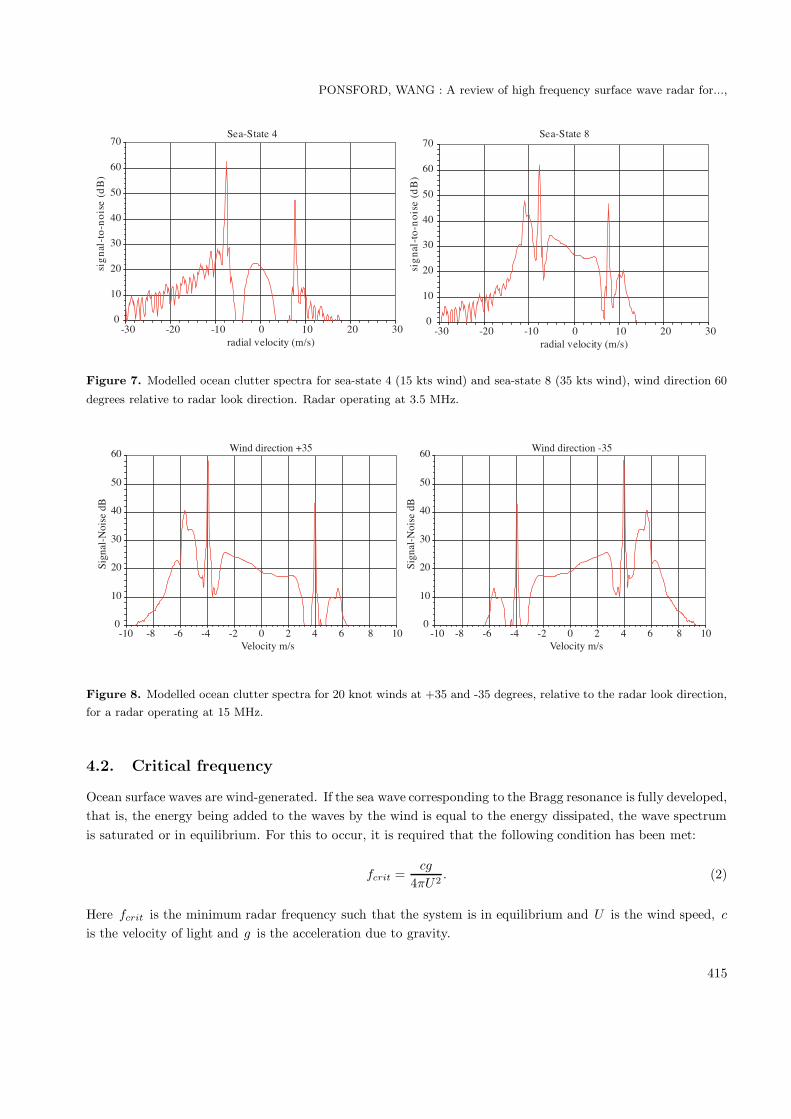
A modeled power spectrum [8] showing the relative contribution of first- and second-order ocean scatteringas observed by an HF Radar is presented in Figure 6. In the figure, the clutter power spectrum has been plottedrelative to the equivalent radial speed of a vessel, and where by convention a positive velocity is associatedwith a vessel approaching the radar. As illustrated in Figure 7, the energy contained within the second-ordercontinuum is related to sea-state and hence surface wind speed.

!

�!

#!

$!

"!

%!

�!

�!�� "�� #��!��#��"��!4��3�

�)

�� 5

��

��*

Figure 6. Relative contribution of first (blue trace) and second (red trace) order clutter to the HF radar doppler

spectrum radar simulation of a radar operating at 15 MHz at 100 km range, sea-state 8.

In addition, since the wind has a cardioid distribution pattern, the distribution of the energy containedwithin the second-order continuum will be dependent on the wind direction. For example, Figure 8 comparesthe theoretical clutter spectrum for winds blowing at +35 and –35 degrees relative to the radar look direction.It can be observed that the spectra are mirror images about zero. For the +35◦ case, the clutter spectrum hasthe majority of the energy contained in the negative half of the spectrum, whilst for the –35◦ wind-direction itis in the positive half. Hence, in the former case, the maximum range at which a small outbound vessel will bedetected will be less than for the same vessel when inbound, the opposite being true for the –35◦ wind.

414


!

�!

#!

$!

"!

%!

�!

1!

$! #! �! ! �! #! $!�� /�3�0

�) �

� ��

�

��/�

*0

�� " ��

!

�!

#!

$!

"!

%!

�!

1!

$! #! �! ! �! #! $!�� /�3�0

�) �

� ��

�

��/�

*0

Figure 7. Modelled ocean clutter spectra for sea-state 4 (15 kts wind) and sea-state 8 (35 kts wind), wind direction 60

degrees relative to radar look direction. Radar operating at 3.5 MHz.

6 �� 7$%

!

�!

#!

$!

"!

%!

�!

�!�� "�� #��!��#��"��!4��3�

�)

�� 5

��

��*

!

�!

#!

$!

"!

%!

�!

�!�� "�� #��!��#��"��!4��3�

�)

�� 5

��

��*

6 �� $%

Figure 8. Modelled ocean clutter spectra for 20 knot winds at +35 and -35 degrees, relative to the radar look direction,

for a radar operating at 15 MHz.

4.2. Critical frequency

Ocean surface waves are wind-generated. If the sea wave corresponding to the Bragg resonance is fully developed,that is, the energy being added to the waves by the wind is equal to the energy dissipated, the wave spectrumis saturated or in equilibrium. For this to occur, it is required that the following condition has been met:

fcrit =cg

4πU2. (2)

Here fcrit is the minimum radar frequency such that the system is in equilibrium and U is the wind speed, c

is the velocity of light and g is the acceleration due to gravity.

415


The spectra presented in this report all assume that the sea state is sufficient such that the radar isoperating above the critical frequency. If the radar is operated at a frequency below the critical frequency, thesea will not be fully developed, and the energy contained within the Bragg wave and associated continuumwill be significantly less. Under such conditions it is not unusual to detect small vessels to significantly greaterranges.

5. Vessel detection

HFSWRs are coherent devices that discriminate between echoes originating from surface vessels and the usuallymore dominant sea echo, on the basis of their differing Doppler shifts.

fdt = 2V fc

cAt HF, the dominant return from surface vessels is the result of reflections from vertical

superstructure. These echoes will experience a Doppler shift fdt that is proportional to the vessel’s radialvelocity V with respect to the radar look direction:

fdt =2V fc

c(3)

5.1. Vessel detection within the ocean clutter spectrum

Ocean-clutter usually limits the detection range of small to medium size vessels. For vessel detection, themagnitude of the clutter against which the vessel is detected is determined by the magnitude of the continuumat the radial velocity corresponding to that of the vessel, this being determined by the radar frequency as wellas the wind speed and direction relative to the radar. Detection of smaller, low-speed vessels will therefore beheavily influenced by the continuum level and hence wind-speed and wind direction. In the specification of theradar performance, it is typical to assume a Doppler averaged value for the continuum for all wind directions.

Once the sea reaches a fully developed state, an increase in wind speed or surface roughness results inan increase in the extent of the continuum and, since the sea is in equilibrium, does not result in an increasein magnitude. However, for a clutter-limited vessel, there will be a reduction in detection range due to theincrease in propagation loss [9]. In addition, at higher frequencies and higher sea states, harmonics associatedwith Bragg resonant scatter begin to appear.

5.2. Radar blind velocity

It can be observed that returns from the Bragg-matched ocean wave result in a pair of blind velocities equalto the apparent velocity of the Bragg wave. From equation (3) it can be observed that the Doppler shiftof an echo originating from a surface vessel is proportional to the radar carrier frequency. However, fromequation (1) the Doppler shift of the Bragg-matched wave is proportional to the square-root of the radar carrierfrequency. Therefore, as illustrated in Figure 9, to avoid radar blind velocity zones, the radar can be operatedsimultaneously on two frequencies that are separated according to the formula

fc2 ≥(√

fc1 + nfres

√πc

g

)2

or fc2 ≤(√

fc1 − nfres

√πc

g

)2

(4)

416


where fc1 and fc2 are the two carrier frequencies, fres is the Doppler resolution bin, and n is the requirednumber of separation in Doppler from Bragg lines in order for a target to be detected.

Figure 9. Comparison of the radar ocean clutter spectrum for operation at 3.2 MHz (blue trace) and 4.4 MHz (red

trace) in sea-state 7 for a wind direction of 160 degrees relative to the radar look direction.

5.3. Doppler resolution

The Doppler resolution, and hence the radial velocity resolution, is inversely proportional to the coherentintegration interval (CII). A sufficient CII must be used to resolve the vessel echo from the more dominantBragg-matched echo. The CII must also provide enough gain to lift the coherent return from the vessel abovethat of the non-coherent background noise. In general, it is better to maximize the CII to the limit where thetarget remains within the given radar resolution cell (range, azimuth, Doppler) and does not suffer either rangewalk or Doppler smearing.

The limiting factor in setting the duration of the CII is generally determined by the vessel speed andapparent radial acceleration when moving perpendicular to the radar look direction [10]. As illustrated in Figure10, when the vessel is tangential to the radar look direction, its relative radial velocity and hence Doppler iszero. As the vessel continues on its path it will experience radial acceleration. This radial acceleration willin turn set a limit on the maximum CII if Doppler smearing and corresponding loss of coherent gain is to beavoided.

In summary, the CII is a compromise between various conflicting requirements. It is desirable, in a multi-target environment, to maximize the CII to provide sufficient Doppler resolution as well as provide sufficientprocessing gain to detect vessels at greater range. However, this has to be traded against the requirement forthe vessel response to remain within a radar resolution cell to prevent either range-walk or Doppler smearing.[11]. To overcome these conflicting requirements, the received data can be split and processed, within the signalprocessing architecture, using multiple CII’s.

417


��

8��

��

��&��

��&��

�

��&��

��4��

Figure 10. Vessel with a tangential path to the radar look direction.

5.4. Radar cross-section of marine vessels

There are a number of conventions used in defining the radar cross-section (RCS) of a vessel, depending on howthe ground plane on which it is situated is treated. This report defines the RCS as if it were measured in freespace.

For a vessel to be detected, its radar cross section must be greater than that of the contending RCS ofthe ocean clutter continuum at the vessel Doppler frequency, The magnitude of the clutter RCS is given by theRCS of the unit patch area multiplied by the area of the radar patch.

The radar cross section of vessels at HF is complex and has been treated extensively by others [12], [13],

[14]]. However, it has been shown [15] that the RCS of larger vessels (>1000 tons) can be approximated by theempirical formula

σ = 52fD3/2 m2 (5)

where σ is the vessel’s Free Space RCS, f is the radar frequency in MHz and D = ship size in ×103 metrictons.

The RCS of smaller vessels can be approximated as discussed in the following section.

5.5. Radar cross section of small vessels

The RCS of small vessels is dominated by their vertical metallic superstructure. If this superstructure isgrounded to the ocean surface, then the RCS of the vessel can be approximated to that of a grounded monopoleantenna [16]. When the metallic vertical superstructure is isolated from the ground, then the RCS can beapproximated to that of a dipole antenna. Multiple structures will produce additive effects that can result inhigher peaks in the RCS value as well as deeper nulls.

Small craft without significant vertical superstructures will have very small RCS, and may only be detectedagainst a noise background. This requires that the boat travels at a radial velocity sufficient such that theresultant Doppler shift is well removed from that of the ocean clutter.

418


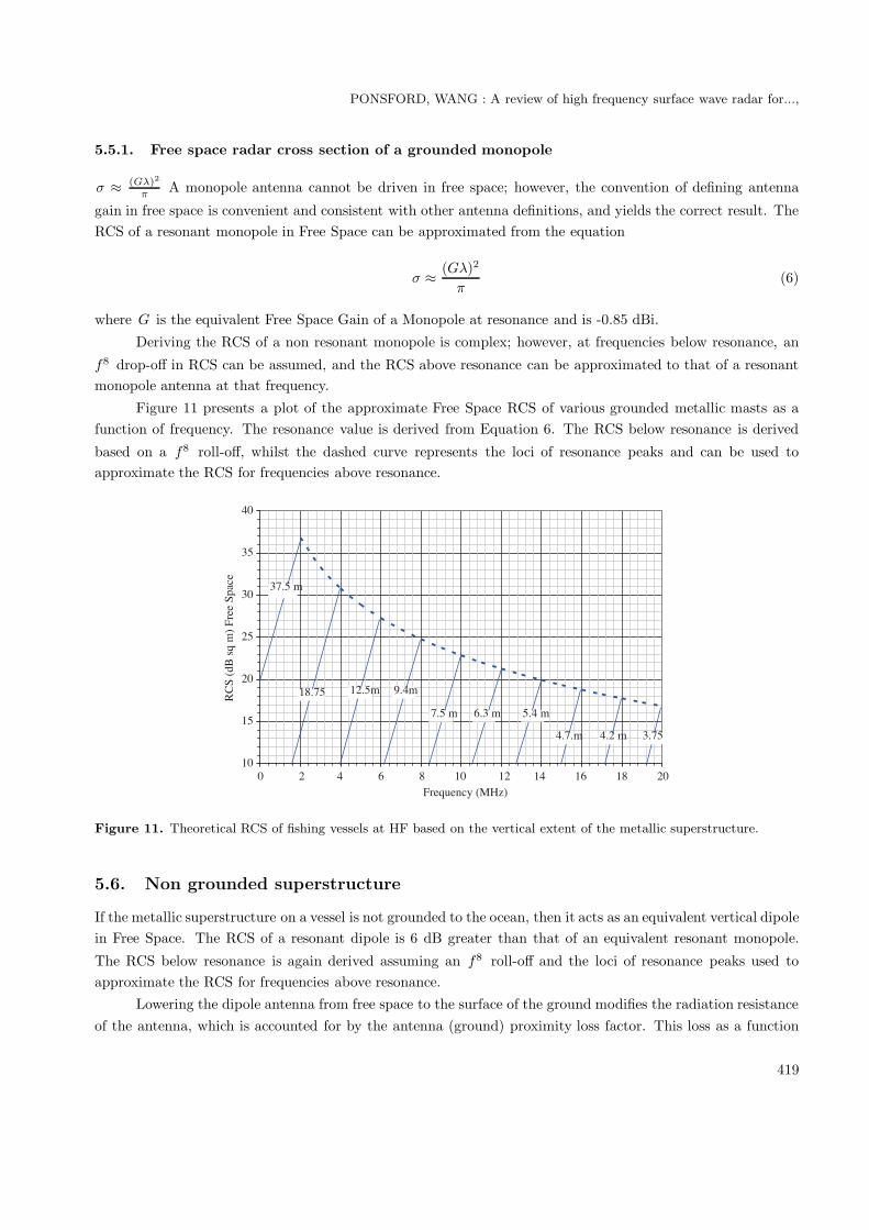
5.5.1. Free space radar cross section of a grounded monopole

σ ≈ (Gλ)2

πA monopole antenna cannot be driven in free space; however, the convention of defining antenna

gain in free space is convenient and consistent with other antenna definitions, and yields the correct result. TheRCS of a resonant monopole in Free Space can be approximated from the equation

σ ≈ (Gλ)2

π(6)

where G is the equivalent Free Space Gain of a Monopole at resonance and is -0.85 dBi.

Deriving the RCS of a non resonant monopole is complex; however, at frequencies below resonance, an

f8 drop-off in RCS can be assumed, and the RCS above resonance can be approximated to that of a resonantmonopole antenna at that frequency.

Figure 11 presents a plot of the approximate Free Space RCS of various grounded metallic masts as afunction of frequency. The resonance value is derived from Equation 6. The RCS below resonance is derived

based on a f8 roll-off, whilst the dashed curve represents the loci of resonance peaks and can be used toapproximate the RCS for frequencies above resonance.

�!

�%

#!

#%

$!

$%

"!

!��#��"��!��#��"��#!9�� /�,-0

�.

��/�*

��

�0�9��

��

��

�+"��#+%�

$1+%��

��+1%

1+%�� +$�� %+"��

"+1+� "+#�� $+1%

Figure 11. Theoretical RCS of fishing vessels at HF based on the vertical extent of the metallic superstructure.

5.6. Non grounded superstructure

If the metallic superstructure on a vessel is not grounded to the ocean, then it acts as an equivalent vertical dipolein Free Space. The RCS of a resonant dipole is 6 dB greater than that of an equivalent resonant monopole.

The RCS below resonance is again derived assuming an f8 roll-off and the loci of resonance peaks used toapproximate the RCS for frequencies above resonance.

Lowering the dipole antenna from free space to the surface of the ground modifies the radiation resistanceof the antenna, which is accounted for by the antenna (ground) proximity loss factor. This loss as a function

419


of height above the ground is plotted in Figure 12. Since the vertical superstructure acts as both receive andtransmit antenna, this effect must be entered twice to arrive at the approximation of the RCS. As can be seen,when the dipole is bisected by the ground, it has the same equivalent gain as that of a monopole antenna.

$+%

$

#+%

#

�+%

�

!+%

!

!+%

�

!��!+��!+#��!+$��!+"��!+%��!+��!+1��!+��!+��,�)��:��)�� /6�� )��0

��

��2

��

��

��

��&

��

��

�9��

��

��

Figure 12. Ground proximity effect showing added loss relative to a dipole antenna in free space as the antenna

approaches and eventually dissects the conducting plane.

5.7. Aspect angle dependency

The Radar Cross Section is the sum of reflections of the radar signal from vertical structures. As illustrated inFigure 13, if the apparent distance between these vertical structures as seen by the radar is equal to an evennumber of quarter wavelengths, then constructive interference takes place. If the apparent distance is equal toan odd number of quarter wavelengths, then destructive interference occurs.

$+%

$

#+%

#

�+%

�

!+%

!

!+%

�

!��!+��!+#��!+$��!+"��!+%��!+��!+1��!+��!+��,�)��:��)�� /6�� )��0

��

��2

��

��

��

��&

��

��

�9��

��

��

Figure 13. Aspect angle dependence of RCS: constructive and destructive interference.

In summary, HFSWR radiate a vertically polarized wave, and for smaller vessels the RCS is dominatedby their vertical superstructure. For larger vessels, the RCS increases with the size of the vessel. Constructiveand destructive reflections result in the RCS value changing with the vessel aspect angle relative to the radar

420


look direction. In general, for larger vessels the broadside RCS is larger than the bow-on or stern-on RCS. Inthe specification of the RCS of a vessel, it is usual to quote an aspect-angle averaged value for the RCS.

It can be noted that a significant fluctuation in RCS of smaller vessels also occurs as a function of seastate. In higher sea conditions, the pitching and rolling of the vessels reduces the average effective verticalheight of the metallic superstructure as observed over the coherent integration interval.

6. External noise

The level of the external noise ultimately limits the maximum detection range of larger vessels. External noiseconsists of both the irreducible natural noise and the incidental man-made noise. The natural noise is the sumof the atmospheric noise (which is frequency-, location-, season- and time-of-day dependent) and galactic noise

(which is frequency-dependent). The level of the man-made noise is determined by frequency and proximity tolocal noise-generating sources such as industry, power lines and highways. Typical relationships between thevarious noise sources, as a function of frequency, for a European location are presented in Figure 14.

#!

#%

$!

$%

"!

"%

%!

%%

�!

�%

# $ " % � 1 � � �

�� 5�� 5�� 5�� 5�� )��

9�� ,-

�*;�<

�*

!

�� 5�� 5�� 5�� 5�� )��

Figure 14. Relationship between the various noise sources as a function of frequency at a European location.

It can be observed that the man-made noise level will typically dominate the day-time noise level; however,at night the atmospheric noise level will usually dominate. Both atmospheric and man-made noise decreaseas a function of frequencies; above approximately 15 MHz there is little day/night dependency. It can also beobserved that at frequencies below 10 MHz the contribution of galactic noise can be ignored.

6.1. Man-made noise

The daytime noise level at a site will typically be dominated by man-made noise. Man-made noise is dependenton the level of human activity, and can be approximated by [17] the relation

Nm = c − d log 10f − 204dBW, (7)

where Nm denotes man-made noise power in decibels below 1 W in a 1 Hz bandwidth, f is frequency in MHz,and c,d are constants derived from measurements.

421


Constants c and d have been derived by the Comite Consultatif International des Radio Communications(CCIR) as shown in Table 1.

Table 1. Constants c and d derived by the Comite Consultatif International des Radio Communications (CCIR).

Environmental Category c dBusiness Stores, offices, industrial parks, etc 76.8 27.7

Residential > 5 dwellings / Hectare 72.5 27.7Rural < 0.5 dwellings / Hectare 67.2 27.7

Quiet rural 53.6 28.6

It is preferable to select an HF Radar site where the level of man-made noise is low, and it is general toinitially specify HFSWR performance relative to that of a typical rural site occurring in the summer month.

Figure 15 presents the predicted atmospheric noise level at 3.5 MHz for a location in Europe. It can beobserved that the night time atmospheric noise is considerably greater than the day time atmospheric noise (in

this example ∼10dB), where the increase is due to impulsive noise arising as the result of lightening, and isgreatest at the equator and minimal at the poles. It can also be noted that there is also a fluctuation in noisebetween the seasons, with the lower noise levels occurring in the summer month.

"!

"%

%!

%%

�!

�%

!!!! !"!! !"!! !�!! !�!! �#!! �#!! ��!! ��!! #!!! #!!! #"!!��*��<�/2��0

9��/�*

�;�<

�*

0

6 �� ) ��

Figure 15. Example estimate of the atmospheric noise level at 3.5 MHz for a location in Europe as a function of time,

day and season.

In summary, the background noise level ultimately limits the detection range of larger vessels. In thespecification of radar performance, it is usual to present detection range for both day and night using noisevalues that are averaged over the seasons and time blocks.

7. Ionospheric clutter

Not all the energy emitted by the HF radar propagates along the surface as a surface wave. Some of thisenergy is directed upwards and may reflect from the ionosphere [1, [18]]. During daylight hours the absorptiveproperties of the D-layer prevents significant energy being returned to the earth. However, at night this layerdisappears and energy is returned via the F-layer.

422


There are three main categories of ionospheric clutter: a single-reflection or first-order scatter that isthe result of a single overhead reflection; second-order scatter, where the signal is initially reflected from theionosphere, back to the ocean, and forward as a surface wave back to the radar (or vice versa); and third-order scatter, where the signal is reflected via the ionosphere onto the ocean, and from the ocean back to theionosphere, and subsequently back to the radar.

Typically, due to the geometry of the third-order scatter, the total path length places this clutter beyondthe maximum range of the radar, and appears as range-wrap, where the radar receives returns from previouspulses while collecting data on the current transmit pulse. This type of clutter can be readily removed bychanging the phase codes of successive pulses of the coherent pulse chain; the second-time-around echo will beheavily attenuated by the filter that is matched to the current pulse, and not the previous.

For second-order ionospheric clutter to be of concern, the total path length must be less that the maximumrange of the radar. This limits the reflective angle to near-vertical incidence. For strong reflections to occurfrom the ocean, it is required that the condition of Bragg resonant scatter is met. At near-vertical illuminationthis requires ocean waves that have a wavelength that is now equal to that of the radar wavelength. At thelower end of the HF band this implies very high sea states. Strong second-order ionospheric clutter is generallyobserved in the radar data during periods of high sea-states. It occurs at a range that is equal to the height ofthe ionospheric F-layer, and extends out in range whilst maintaining approximately the same signal strength.

First-order ionospheric scatter appears at a narrow band of ranges corresponding to the height of eitherthe E- or F-layers. Options for combating this clutter are limited, but it can be alleviated by using multipleradar frequencies that may be returned from slightly different heights [19]. Other options include increasingthe radar carrier frequency to above the layer-critical frequency, such that the radar signal penetrates the layerinstead of reflecting from it. This typically requires operating at a frequency above 10 MHz. However, theadditional surface wave propagation loss may result in the maximum detection range of the radar to be lessthan the range at which ionospheric clutter occurs.

8. Probability of detection

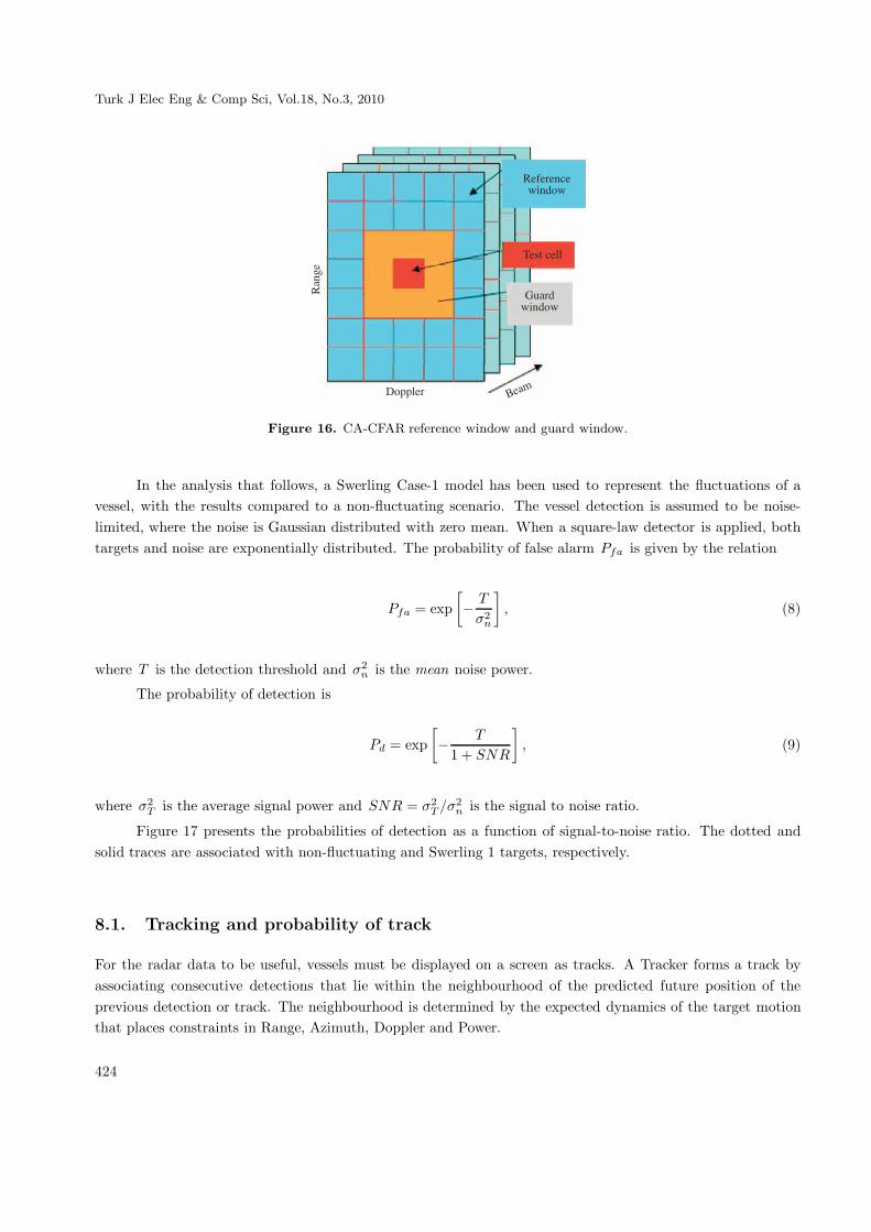
The previous sections have described the basic radar performance as well as the signal environment. For thedata to be useful, it is necessary that the returns from the vessels must be extracted from this environment witha high degree of probability. This is achieved by comparing each radar pixel that is bounded in Azimuth, Rangeand Doppler, to that of its neighbour. A typical HFSWR may have in the order of 10 million pixels per CII.An efficient detector for determining the presence of a vessel return is the Constant False Alarm Rate (CFAR)algorithm, where a threshold is set such that the rate at which the false alarm occurs due to noise crossing thethreshold (in the absence of signal) is constant.

A basic CFAR algorithm is illustrated in Figure 16. The pixel under test is centred in the middle ofthe range/Doppler/azimuth space. A guard window is employed to ensure that the target is not present in theregion used to estimate the noise floor.

In specifying the performance of the radar, it is required that the probability of falsely declaring thepresence of a vessel is specified, as well as the probability of correctly declaring the presence of a vessel. Thisis usually achieved based on theoretical analysis, and requires that appropriate models are used to characteriseboth the vessel and the environment.

423


��=�� > ��>

��

��> ��>

&�� *��

��

)�

Figure 16. CA-CFAR reference window and guard window.

In the analysis that follows, a Swerling Case-1 model has been used to represent the fluctuations of avessel, with the results compared to a non-fluctuating scenario. The vessel detection is assumed to be noise-limited, where the noise is Gaussian distributed with zero mean. When a square-law detector is applied, bothtargets and noise are exponentially distributed. The probability of false alarm Pfa is given by the relation

Pfa = exp[− T

σ2n

], (8)

where T is the detection threshold and σ2n is the mean noise power.

The probability of detection is

Pd = exp[− T

1 + SNR

], (9)

where σ2T is the average signal power and SNR = σ2

T /σ2n is the signal to noise ratio.

Figure 17 presents the probabilities of detection as a function of signal-to-noise ratio. The dotted andsolid traces are associated with non-fluctuating and Swerling 1 targets, respectively.

8.1. Tracking and probability of track

For the radar data to be useful, vessels must be displayed on a screen as tracks. A Tracker forms a track byassociating consecutive detections that lie within the neighbourhood of the predicted future position of theprevious detection or track. The neighbourhood is determined by the expected dynamics of the target motionthat places constraints in Range, Azimuth, Doppler and Power.

424


% ! % �! �% #! #% $!!

!+�

!+#

!+$

!+"

!+%

!+�

!+1

!+�

!+�

�

?��:

�:�

��

=�&

��

��

�) ��5��/�*0

� =�� )(�=�@"+%� %�>�� )��(�=�@"+%� % � =�� )(�=�@�+�� $�>�� )��(�=�@�+�� $

Figure 17. The probability of detection as a function of signal-to-noise ratio.

When a vessel is detected for the first time, a track initiation process is commenced, as illustrated inFigure 18.

A ��&�� # ��B�� :�� B��

A ��?�� 5�)�:�� # ��?�� ?��2��

5�>5�)�:��

$��?��

?��2�� :�� <

Figure 18. Track initiation process.

Based on the radar parameters, and the limits set on the vessel dynamics, a neighbourhood is drawnaround the initial plot or detection. The neighbourhood is not centred on the plot, since the plot also has aDoppler associated with it. For example, if this Doppler is significantly positive, then the vessel is approachingthe radar. Therefore, it is reasonable to predict that the next return from this vessel will be at a range that iscloser to the radar by an amount that is related to the measured Doppler. Since the radar only measures theradial component, the vessel may be travelling to the left or right of the radar; consequently, the direction oftravel can not be determined until at least two updates have been received. The Tracker outputs a “smoothed”target location based on the weighted average of the predicted and measured locations.

To minimize false track rates, a deferred decision Tracker can be used, where the tracker employs threelevels of track promotion logic:

425


1. Potential tracks (P): single detection

2. Tentative tracks (T): 0-X update tracks

3. Confirmed tracks (C): track is deleted after a defined number of consecutive misses.

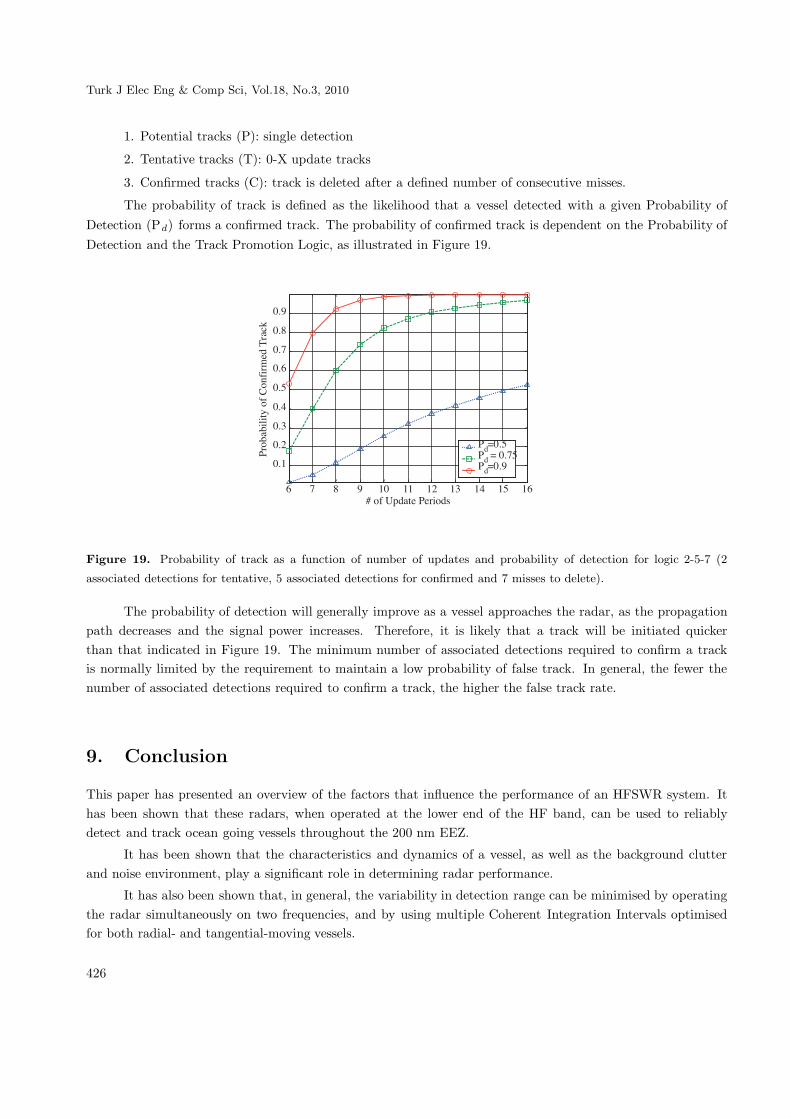
The probability of track is defined as the likelihood that a vessel detected with a given Probability ofDetection (Pd) forms a confirmed track. The probability of confirmed track is dependent on the Probability ofDetection and the Track Promotion Logic, as illustrated in Figure 19.

� 1 � � �! �� # �$ �" �% ��

!+�

!+#

!+$

!+"

!+%

!+�

!+1

!+�

!+�

C �= B�� ?��

?��:

�:�

��=

.�

=��

��

�<

?�@!+%?� @ !+1%?�@!+�

Figure 19. Probability of track as a function of number of updates and probability of detection for logic 2-5-7 (2

associated detections for tentative, 5 associated detections for confirmed and 7 misses to delete).

The probability of detection will generally improve as a vessel approaches the radar, as the propagationpath decreases and the signal power increases. Therefore, it is likely that a track will be initiated quickerthan that indicated in Figure 19. The minimum number of associated detections required to confirm a trackis normally limited by the requirement to maintain a low probability of false track. In general, the fewer thenumber of associated detections required to confirm a track, the higher the false track rate.

9. Conclusion

This paper has presented an overview of the factors that influence the performance of an HFSWR system. Ithas been shown that these radars, when operated at the lower end of the HF band, can be used to reliablydetect and track ocean going vessels throughout the 200 nm EEZ.

It has been shown that the characteristics and dynamics of a vessel, as well as the background clutterand noise environment, play a significant role in determining radar performance.

It has also been shown that, in general, the variability in detection range can be minimised by operatingthe radar simultaneously on two frequencies, and by using multiple Coherent Integration Intervals optimisedfor both radial- and tangential-moving vessels.

426


Acknowledgements

The authors would like to acknowledge and thank Defence Research and Development Canada (DRDC), fortheir consistent support in the development and testing of High Frequency Surface Wave Radar.

References

[1] L. Sevgi, A. Ponsford, A. Chan, “An integrated maritime surveillance system based on high frequency surface wave

radars, Part 1 - Theory of operation”, IEEE Proc. Ant. And Prop., Vol. 43, Aug. 2001.

[2] A. Ponsford, L. Sevgi, A. Chan, “An integrated maritime surveillance system based on high frequency surface wave

radars, Part 2 - Operational status and system performance”, IEEE Proc. Ant. And Prop., Vol. 43, Oct 2001.

[3] GRWAVE available from http://www.itu.int/ITU-R/study-groups/software/rsg3-grwave.zip.

[4] D. E. Barrick, ”Theory of HF and VHF propagation across the rough sea”, Parts 1 and 3, Radio Science., Vol. 6,

no. 5, pp 517-533, 1971.

[5] D. E. Barrick, “Remote sensing of sea state by radar”, Remote Sensing of Troposphere, V.E. Derr, Ed., GPO,

Washington, DC, Ch.12 1972.

[6] E. D. R. Shearman, “Propagation and scattering in MF/HF ground wave radar”, Proc. IEE, Part F, Vol. 130, no.

7, pp 579-590, 1983.

[7] S. K. Srivastava, ”Scattering of high frequency electromagnetic waves from an ocean surface: An alternative

approach incorporating a dipole source”, Ph.D. Thesis, Memorial University, Newfoundland, 1984.

[8] D. S. Bryant, A. M. Ponsford, S. K. Srivastava, “A computer package for the parameter optimization of ground

wave radar”, Proc. OCEANS’88 Conference, USA, Vol. 2, pp 485-490, 1988.

[9] H. Leong, A. Ponsford, “The effects of sea clutter on the performance of HF surface wave radar in ship detection”,

IEEE Radar Conference, Italy 2008.

[10] R. M. Dizaji, A. Ponsford, “Optimum coherent integration time for a surface target with periodic acceleration”,

IEEE CCECE 2003, Montreal, May 2003.

[11] A. M. Ponsford, “Detection and tracking of go-fast boats using HFSWR”, SPIE Defence and Security Symposium,

Orlando ,17 April 2004.

[12] L. Sevgi, “Target reflectivity and RCS interactions in integrated maritime surveillance systems based on surface

wave high frequency radars”, IEEE Ant and Prop Mag, Vol. 43, No 1, Feb 2001.

[13] C. W. Trueman, S. J. Kubina, “RCS of fundamental scatterers in the HF band”, 7 th Annual Review of Progress

in Applied Computational Electromagnetics of the Applied Electromagnetics Computational Society, Monterey,

California, March 18-22, 1991.

[14] H. Leong, H. Wilson, “An estimation and verification of vessel radar cross sections for HFSWR”, IEEE Ant and

Prop Mag, Vol. 48, no. 2, pp. 11-6, Apr. 2006.

427


[15] A. M. Ponsford, “Surveillance of the 200 nautical mile exclusive economic zone (EEZ) using high frequency surface

wave radar (HFSWR)” , Canadian Journal of Remote Sensing, Vol. 27, No. 4, Aug. 2001, Special Issue on Ship

Detection in Coastal Waters, pp. 354-360.

[16] R. W. Bogle, D. B. Trizna, “Small boat HF radar cross sections”, NRL Memorandum Report 3322, July 1976.

[17] CCIR, “Man-made radio noise”, Report 258-4, CCIR, ITU, Geneva, 1986.

[18] A. Ponsford, R. M. Dizaji, R. McKerracher, “HF surface wave radar operation in adverse conditions”, IEEE Proc.

Of the Int. Conf. On Radar, Adelaide, Australia, 3-5 Sept. 2003

[19] H. Leong, A. Ponsford, “The advantage of dual-frequency operation in ship tracking by HF surface wave radar”,

International Radar Conference 2004, Toulouse, France, 19-21 Oct. 2004.

428

A review of high frequency surface wave radar for ...

Documents

Transcript of A review of high frequency surface wave radar for ...