A Regional Trade Model with Ricardian Productivity

Gains and Multi-technology Electricity Supply

Frank Pothen∗ and Michael Hubler†

Hannover Economic Papers (HEP) No. 585

ISSN 0949-9962

March 10, 2017

Abstract

This article presents an applied general equilibrium model which combines the the-

oretical foundations of an Eaton-Kortum type model of international trade with the

complexity of a global multi-region, multi-sector Computable General Equilibrium

(CGE) model of production and consumption. The Eaton-Kortum model features

endogenous trade-induced productivity gains via Ricardian specialization and takes

non-tariff trade costs into account. Model regions and sectors can be disaggregated,

e.g., representing technology-specific electricity generation. The models is tailored

to explicitly study the German Federal State of Lower Saxony, a prime location for

renewable electricity generation in Germany with ambitious climate policy goals. The

calibration utilizes the structural estimation of a gravity model with constraints, while

the disaggregation adapts methods used in regional science and energy economics.

With these features the model goes beyond standard CGE models and provides new

insights in the nexus between trade policy and climate policy. Simulations suggest

that the removal of tariffs creates smaller welfare gains than a comparable reduction of

non-tariff barriers to trade but also a slightly smaller increase in global CO2 emissions.

Trade policy-induced productivity gains and renewable energy subsidies significantly

reduce carbon leakage from the EU to the rest of the world by making the EU more

CO2-efficient. With its large wind power potential, Lower Saxony is less susceptible

to negative effects of climate policy than the rest of Germany.

JEL Classifications: C68; F10; F18; Q40

Keywords: international trade; regional model; climate policy; renewable energy; CGE

∗Corresponding main author, email: pothen@iuw.uni-hannover.de, tel: +49-511-762-14575, fax: +49-511-762-2667, Leibniz Universitat Hannover, Institute for Environmental Economics and World Trade,Konigsworther Platz 1, 30167 Hannover, Germany.†Leibniz Universitat Hannover, Institute for Environmental Economics and World Trade.

1

1 Introduction

The 2015 United Nations Climate Change Conference in Paris was an important step

towards a climate policy solution with global coverage. In an increasingly internationalized

world economy, global coverage of climate policy appears to be inevitable in order to

achieve ambitious climate policy goals. The share of merchandise trade in GDP, for

instance, rose from 17.5% in 1960 to 50% in 2014 (World Bank, 2016).

Unilateral actions are, nevertheless, dominating international climate policy. They are

not only implemented by nations or the European Union, but also by sub-national bodies.

The German Federal State of Lower Saxony, for instance, investigates whether it will by

able to satisfy its energy demand completely from renewable sources by 2050 (NMUEK,

2016). These regional climate policy initiatives are not only highly intertwined with global

climate policy but also interact with trade policy. Trade-induced sectoral specialisation or

productivity gains might affect sub-national regions like Lower Lower Saxony differently

than the country as a whole, increasing or decreasing costs of their climate policy.

Trade policy and climate policy can affect each other in various ways. On the one

hand, a reduction of trade barriers enlarges trade volumes and production, which is likely

to increase CO2 emissions and carbon leakage1 (Frankel and Rose, 2005; Peters and Her-

twich, 2008; Bohringer et al., 2012), whereas increased specialization can in- or decrease

emissions and leakage via structural change across sectors and productivity gains within

sectors. On the other hand, carbon pricing and renewable energy support affect trade and

specialization. The implications for productivity as well as carbon leakage are unclear ex

ante. The interactions between these two policies have hardly been considered by scholars

and policy makers so far. Hence, this article sheds light on relevant interactions.

This article introduces a novel general equilibrium model which is tailored to study

these interactions between climate and trade policy. By revealing the underlying economic

mechanisms, it provides qualitative and quantitative inference on how these policy fields

affect each other. The model combines the trade-theoretic foundations of the Eaton and

Kortum (2002) model,2 including endogenous Ricardian specialization and productivity

gains, with the flexibility and expandability of a Computable General Equilibrium (CGE)

model (e.g. Bohringer and Loschel, 2006; Chen et al., 2015).

In the Eaton and Kortum (2002) model, sectors produce a continuum of differentiated

1The increase in CO2 emissions in other regions due to the introduction of a CO2 price in one region.2The seminal general equilibrium model by Eaton and Kortum (2002) explains international trade flows

via a combination of technology differentials, relative input costs and iceberg trade costs.

2

varieties of their goods. Neither firms nor consumers have preferences over an individual

variety from specific regions. They purchase a variety from the region offering it for the

least price. This assumption is particularly plausible for relatively homogeneous energy

and resource-intensive upstream goods. Hence, the Eaton and Kortum (2002) model is

an appealing alternative to the Armington (1969) model for studying energy and climate

policies.

The trade model is calibrated by using a structural estimation approach (drawing

on Balistreri and Hillberry, 2007; Balistreri et al., 2011), in which the market clearing

conditions of the model enter a gravity model estimation as side constraints. Unlike

unconstrained gravity models, this approach ensures that the baseline constitutes a general

equilibrium of the model.

Our model allows for a technology-specific representation of the electricity sector

(Bohringer, 1998; Bohringer and Loschel, 2006). Renewable electricity generation can re-

act endogenously to trade and climate policy, taking into consideration regional differences

in the potential for expanding renewable power generation. A constrained optimization

technique following Sue Wing (2008) is implemented to disaggregate the electricity sector.

The overwhelming majority of general equilibrium models represents nations or group

of nations (for an exception see Bosello and Standardi, 2015). To study climate policy in

Lower Saxony, we disaggregate Germany into two regions: Lower Saxony and the Rest

of Germany. Taking Lower Saxony as example, the model is not only able to investigate

climate policies by sub-national regions but also to study differences in how international

trade and climate policy affects regions within a country. The disaggregation utilizes a

regional science approach (based on Kronenberg, 2009; Tobben and Kronenberg, 2014).

The application of the model to the European Union (EU) is particularly interesting

because of the EU’s regional heterogeneity as well as the implementation of climate and

energy policies at different political levels (EU, national states, federal states etc.). The

European Union Emissions Trading System (EU ETS) is Europe’s key climate policy

instrument (Ellerman et al., 2010) covering around 11,000 installations and 45% of the

EU’s CO2 emissions. Within the EU, we focus on Germany because it is a front-runner

in the transition towards a low-carbon economy and has heavily subsidized renewable

energy. Within Germany, the federal state of Lower Saxony is the prime location for

installing wind power plants, while its population density is lower than and the sectoral

composition is different from the German average. Lower Saxony’s shares of agriculture

and food production in total production, for example, are relatively high but there is no

3

coal extraction.

We implement two sets of policy scenarios which highlight the interaction between

climate and trade policy. In the global trade policy scenarios, we remove either tariffs

and trade subsidies or we reduce non-tariff barriers to an equivalent extent. In both

trade policy scenarios, we find the following results. The share of renewables in the

electricity sectors of Lower Saxony and the rest of Germany increases by about 16%

because lower trade costs enhance output and thus carbon emissions. The allowances

price in the EU ETS rises in response to increasing output, creating a price signal that

shifts power generation towards renewables. Due to its large wind power potential and

the corresponding low abatement costs, Lower Saxony’s resulting emissions reduction

of over 16% is twice the reduction in the rest of Germany. While the estimated trade

policy-induced welfare gains stay below 1%, the reduction of non-tariff barriers creates

larger gains than the removal of subsidies and tariffs in all model regions including Lower

Saxony and the rest of German.

In South Korea, on the contrary, trade-induced specialization shifts production towards

energy-intensive sectors so that CO2 emissions rise by one third. When removing tariffs,

the former Soviet Union region experiences a 20% increase in total factor productivity.

Notwithstanding, as a major fossil energy exporter, it experiences a 2% welfare drop

because it refrains from exerting power on fossil fuel markets. This loss turns into an

8% welfare gain when removing non-tariff barriers which constitute a mere inefficiency

without tax revenues.

With reduced non-tariff barriers, the EU climate policy is also responsible for less car-

bon leakage to the rest of the world, because the reduction of non-tariff barriers supports

structural change towards less energy-intensive industries and thus eases decarbonization

within the EU. On the opposite, driven by policy-induced structural change, total factor

productivity becomes slightly lower and global emissions slightly higher when non-tariff

barriers are reduced than when tariffs are removed.

In the EU climate policy scenarios, we first tighten the emissions cap by 13% relative

to 2011 which corresponds to the reduction scheduled for 2020. Then, we add subsidies

for wind and solar power as in practice in Germany. Faced with higher input costs due

to the tighter emissions cap, Germany specializes in goods and varieties of goods which it

can produce efficiently. Thereby, climate policy induces productivity gains for Germany.

In the other model regions, on the contrary, the induced productivity effects are negative.

Lower Saxony experiences a welfare drop of 0.14% due to the more restrictive climate

4

policy target. Welfare falls twice as much in the rest of Germany. With its large potential

for renewable energy generation, in particular wind power, and its sectoral structure

exhibiting higher agricultural and smaller manufacturing shares, Lower Saxony is less

susceptible to negative effects of climate policy. The application of renewable energy

subsidies reduces carbon leakage and global emissions and creates minor welfare gains,

especially for Germany and Italy.

Because of its strong link between theory and empirics, the Eaton and Kortum (2002)

model has been frequently extended and applied (Eaton and Kortum, 2012). Applications

range from theory-consistent measurement of competitiveness (Costinot et al., 2011), the

determinants of productivity (Levchenko and Zhang, 2016) and impacts of expanding

transport infrastructure (Donaldson, 2010) to the welfare effects of international trade

agreements (Caliendo and Parro, 2015). Our model setup draws on the work by Eaton

and Kortum (2002), Alvarez and Lucas (2007), Caliendo et al. (2014) and Caliendo and

Parro (2015).

So far Eaton and Kortum (2002) type models have hardly been used to study climate

change-related issues. A notable exception is the work by Costinot et al. (2016) who

investigate how climate change alters comparative advantages in agriculture and how

this, in turn, affects GDP. Our article describes, to our knowledge, the first climate or

energy policy application. Furthermore, besides a subnational representation of the United

States in the study by Caliendo et al. (2014), Eaton and Kortum type models have, to

our knowledge, not been calibrated to regionally or technologically disaggregated data.

Models based on Eaton and Kortum (2002) usually assume Cobb-Douglas production

functions.3 These imply that all intermediate inputs can be substituted with each other

in the same manner and that the elasticity of substitution between them equals unity.

This simplification is problematic when studying climate and energy policies, because the

substitutability of energy carriers among each other or with value added is heterogeneous

and crucial for the magnitude of policy effects. Therefore, we add to the Eaton and Kortum

literature by implementing nested Constant Elasticity of Substitution (CES) production

and consumption functions (following van der Werf, 2008), which are common in the CGE

policy modeling literature (e.g. Bohringer and Loschel, 2006; Chen et al., 2015) and which

allow the substitutability to vary between inputs. As usual in this literature, our main

data source is the Global Trade Analysis Project (GTAP) database.

3Caliendo et al. (2014) present a variant of their model with Constant Elasticity of Substitution pro-duction functions. It is, to our knowledge, the only study which employs CES production functions in theEaton and Kortum (2002) literature.

5

The article proceeds as follows. Section 2 presents the theoretical model. Section 3

describes the structural estimation and disaggregation procedure. Section 4 defines the

policy scenarios and interprets the simulation results. Section 5 concludes with policy

implications and a discussion.

2 Model

In the course of this section, the model is set up and solved.

2.1 Overview

We begin with a narrative and a technical overview of the model structure.

2.1.1 Summary

The model presented in this study is a static Ricardian general equilibrium model based

on Eaton and Kortum (2002) as well as Caliendo et al. (2014) and Caliendo and Parro

(2015). There is one representative consumer per region (subsection 2.2). A representative

firm per sector and region produces a continuum of differentiated varieties of the sector’s

good (subsection 2.3). Individual varieties from different regions are perfect substitutes.

The steel sector in the USA, for instance, produces a large number of steel varieties (which

are termed grades in steelmaking). But if an individual variety is selected, it is irrelevant

if it was produced in the United States or in China because it serves the same purpose in

production. Likewise, the representative consumer of each region has no preferences over

varieties from different countries.

The varieties are combined via a CES function to produce the sector’s output (sub-

section 2.3). The pattern of international trade depends on sector-specific absolute pro-

ductivities, variety-specific probabilistic productivities, and trade costs (subsection 2.4).

Based on these productivities, Ricardian specialization in varieties creates endogenous

(productivity) gains from trade. This is an important advancement compared to the fa-

miliar Armington (1969) type model of trade which is commonly used in Computable

General Equilibrium (CGE) models. In Armington models, gains from trade via Ricar-

dian specialization are determined by the benchmark data and do not adjust endogenously

in counterfactuals. We assume constant returns to scale and perfect competition in all

markets. Hence, firms do not earn profits.

The model allows for regional disaggregation below the national level (for the calibra-

tion see section 3). It allows for sectoral disaggregation as well. The electricity sector is

6

disaggregated in various emitting and non-emitting generation technologies (subsection

2.3.2). As a consequence, climate and energy policy does not only affect energy use in

production and consumption but also the decarbonization of electricity supply.

Three primary production factors are considered in the model: labor, capital, and

natural resources. Labor and capital can move freely across sectors but are internationally

immobile. Natural resources are specific to the corresponding extractive industries such

as crude oil production or mining. Under climate policy with carbon pricing, fossil fuel

inputs require corresponding inputs of emissions allowances.

2.1.2 Structure

The model differentiates between sectors indexed i or j as well as regions indexed r, s or

rr. The index r usually represents the producing or exporting region while s represents the

consuming or importing region. Regions can be individual countries, groups of countries,

or German Federal States. The indices i and j encompass all industries of the economy

including the sectors electricity, transportation and services. All variables and parameters,

which concern individual varieties, are written in lower-case latin letters. Lower case greek

letters denote relative values such as tax rates or input shares. Variables and parameters

of sectors are denoted in upper-case letters.

An equilibrium of the model is reached if a set of 13 equilibrium conditions are simulta-

neously fulfilled.4 Table 1 lists the equilibrium conditions and the corresponding equation

numbers as well as the associated endogenous variables, their symbols and dimensions

(see subsection 2.5 for market clearing conditions in individual markets).5

The model setup encompasses five types of equilibrium conditions. The income balance

condition, zero-profit conditions and market clearing conditions are standard elements

of CGE models written as a Mixed Complementarity Problem (MCP). The Eaton and

Kortum (2002) type trade model contributes additional equations which determine goods’

prices and trade shares. If climate policy with the possibility to allocate allowances for free

is taken into account, a corresponding market clearing condition for emissions allowances

and a policy condition which represents the free allocation of allowances will be required.

The model is implemented as a Mixed Complementarity Problem in GAMS (General

Algebraic Modeling System; Bussieck and Meeraus, 2004) and solved by using the PATH

4See Alvarez and Lucas (2007) for a proof of the existence and the uniqueness of an equilibrium in theEaton and Kortum (2002) model.

5Theses variables are directly determined by the model solution; further variables are derived fromthem.

7

algorithm (Dirkse and Ferris, 1995). Demand and per-unit cost functions are formulated in

the calibrated share form (Bohringer et al., 2003) which normalizes the baseline variables

to unity to ease the model solution and interpretation.

Table 1Equilibrium conditions and variables

Variable Equation Symbol Dimension

Income balance condition:Consumer income MQ (1) (2) Yr R

Zero-profit conditions:Intern. transport services MQ (2) (6) XT

h HPer-unit input costs MQ (4) (8) ci,r I ×RSectoral goods price index MQ (5) (9) Pi,r I ×R

Trade flows:Bilateral trade shares MQ (6) (11) πi,r,s I ×R×R

Market clearing conditions:Prices of intern. transp. serv. MQ (3) (16) P Th HFactor prices MQ (7) (13) PFf,r F ×RResource prices MQ (8) (14) PRESi,r I ×RPrices of the fixed factors MQ (9) (15) PFFEGg,r G×ROutput of goods/sectors MQ (10) (19) Xi,r I ×RTotal Demand MQ (11) (18) Di,r I ×REmissions price MQ (12) (20) PETS 1

Policy condition:Subsidy for free allowances MQ (13) (21) φETSi,r I ×R

r/s = region, i = sector, h = transport service sector, f = factor, g = electricity generation technology,R = number of regions, I = number of sectors, H = number of transport service sectors, F = numberof factors, G = number of technologies, ETS = emissions trading scheme, MQ = model equation.

2.2 Consumption

In each region, a representative consumer s chooses the optimal bundle of goods Ci,s from

sectors i which maximizes her utility Us. Pi,s denotes the price of good i in s. τ ci,s is an

ad-valorem consumption tax rate. We assume that the representative consumer spends a

fixed fraction ξs of her income Ys on consumption. The remainder is invested.

maxCi,s

Us = Us (C1,s, C2,s, . . . ) subject to (1)

ξsYs =∑i

Pi,sCi,s(1 + τ ci,s)

Consumers have nested CES preferences over sectors’ goods. In the nested CES func-

tion depicted by figure 1 goods are combined step-wise to allow for differentiated degrees

of substitutability between them. A higher elasticity of substitution σ implies better

substitutability.

8

Figure 1Nesting structure of the consumer’s utility function

Us

σC

CEs

σCE

NGASi,s

CNGAS,s ACO2NGAS,s

. . . PETRi,s

CPETR,s ACO2PETR,s

CNs

σCN

C 1,s C ...,s C I,s

The representative consumer in s combines energy goods into an energy aggregate

CEs . It comprises the consumption of coal (COALs), crude oil (CRUDs), gas (NGASs),

refined petroleum (PETRs), and electricity (ELECs). The elasticity of substitution

between energy goods is denoted σCE .

Consumers emit carbon dioxide when they burn fossil fuels. To reflect these emissions,

the consumption of fossil fuels Ci,s ∀i ∈ COAL,CRUD,NGAS,PETR,ELEC is con-

nected with CO2 ACO2i,s . The nest of natural gas inputs NGASs, for instance, consists of

purchases from the natural gas sector CNGAS,s and the corresponding emissions ACO2NGAS,s.

Fossil fuels and emissions are combined in fixed proportions via Leontief functions because

the carbon content of each good is physically determined.

The other goods are combined into a non-energy aggregate CNs with an elasticity of

substitution σCN . Energy and non-energy aggregates are subsequently aggregated to total

consumption. The elasticity of substitution between them is σC .

The representative consumer is endowed with exogenous region-specific quantities of

the factors labor, capital, natural resources and fixed factors for electricity generation

(see figure 3 below). She supplies them inelastically on factor markets and receives factor

income. She, furthermore, receives income from net taxes and selling emissions allowances.

The representative consumer’s current account deficit or surplus is held constant.

Equation (2) is a stylized version of the income equation representing model equa-

tion MQ (1), in which PFf,s indicates a factor price and Nf,s the exogenous endowment

with factor f in region s. Θs symbolizes the endogenous sum of net tax revenues (tax

9

revenues minus subsidy payments) and ∆s the exogenous current account deficit of s.

Ys =∑f

PFf,sNf,s + Θs + ∆s (2)

We define real consumption ξsYscCs

as the welfare measure for policy analyses where cCs

denotes the true-cost-of-living index, the price index of the optimal consumption bundle

implied by the CES utility function depicted in figure 1.

2.3 Production

The production side features varieties of each good, CES functions and technologies.

2.3.1 Varieties

In each sector i, a representative firm produces a continuum of differentiated varieties of

the sector’s good. Constant returns to scale and perfect competition imply that firms earn

no profits and the number of firms in equilibrium is neither determined nor important.

The representative firm combines primary factors and intermediate inputs according

to a CES nest structure as explained in the next subsection (see figures 2 and 3). Equation

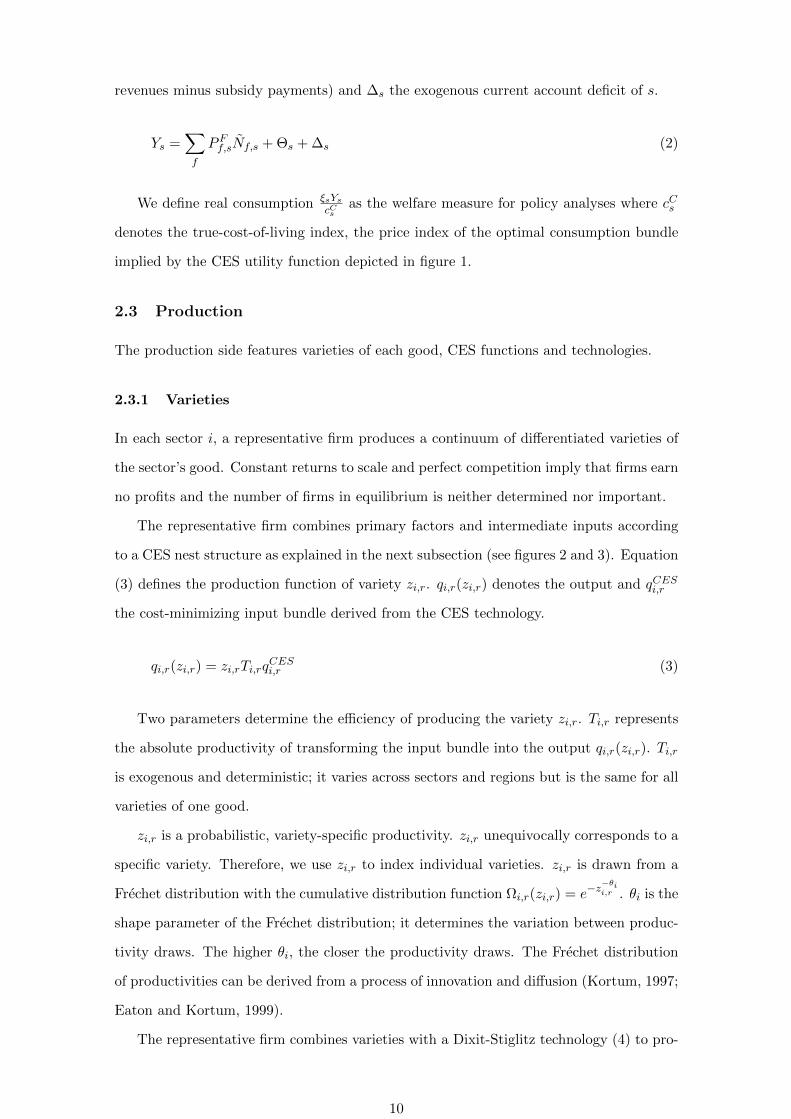
(3) defines the production function of variety zi,r. qi,r(zi,r) denotes the output and qCESi,r

the cost-minimizing input bundle derived from the CES technology.

qi,r(zi,r) = zi,rTi,rqCESi,r (3)

Two parameters determine the efficiency of producing the variety zi,r. Ti,r represents

the absolute productivity of transforming the input bundle into the output qi,r(zi,r). Ti,r

is exogenous and deterministic; it varies across sectors and regions but is the same for all

varieties of one good.

zi,r is a probabilistic, variety-specific productivity. zi,r unequivocally corresponds to a

specific variety. Therefore, we use zi,r to index individual varieties. zi,r is drawn from a

Frechet distribution with the cumulative distribution function Ωi,r(zi,r) = e−z−θii,r . θi is the

shape parameter of the Frechet distribution; it determines the variation between produc-

tivity draws. The higher θi, the closer the productivity draws. The Frechet distribution

of productivities can be derived from a process of innovation and diffusion (Kortum, 1997;

Eaton and Kortum, 1999).

The representative firm combines varieties with a Dixit-Stiglitz technology (4) to pro-

10

duce the sectoral output Qi,r. σ is the elasticity of substitution between varieties.

Qi,r =

[∫qi,r(zi)

σ−1σ ωi(zi) dzi

] σσ−1

(4)

2.3.2 Technologies

Most models based upon Eaton and Kortum (2002) assume Cobb-Douglas production

functions.6 We implement a nested CES production structure which allows for different

degrees of substitutability between fossil fuels and other inputs.

Figure 2Nesting structure of all sectors except electricity

Qi,r

σRES

KLEMi,r

σKLEM

KLEi,rσKLE

KLi,rσKL

Ki,r Li,r

ENi,r

σEN

Zi,ELEC,rFFi,rσFF

COALi,r

ZCOAL,i,r ACO2COAL,i,r

CRUDi,r

ZCRUD,i,r ACO2CRUD,i,r

NGASi,r

ZNGAS,i,r ACO2NGAS,i,r

PETRi,r

ZPETR,i,r ACO2PETR,i,r

Zi,rσz

Z1,i,r Z...,i,r ZI,i,r

RESi,r

Figure 2 depicts the nesting of all goods i except the electricity sector. It shows how

primary factors and intermediate inputs Zj,i,r are combined to produce a quantity Qi,r.

Let’s take the capital-and-labor nest KLi,r as an example for the interpretation of figure 2.

Sector i in r combines inputs of capital Ki,r and labor Li,r. σKL represents the elasticity

6Intermediate inputs are aggregated by using a Cobb-Douglas technology, so are primary factors. Theintermediate aggregate and value added are combined by another Cobb-Douglas function.

11

of substitution between these inputs. A higher elasticity of substitution implies better

substitutability, and a larger input share a higher importance of the corresponding factor

for production.

The fossil fuels nest combines inputs of coal (COALi,r), natural gas (NGASi,r), refined

petroleum (PETRi,r), and crude oil (CRUDi,r). The elasticity of substitution between

fossil fuels is denoted σFF . Each fossil fuel nest is a combination between the intermediate

input of the corresponding sector, Zj,i,r, and CO2 emissions from burning them, ACO2j,i,r .

They are combined by using a Leontief production function.

In the energy nest EN i,r, the fossil fuel aggregate is combined with the input of

electricity Zi,ELEC,r. This reflects that electricity drives electric machines and generates

light, while fossil fuels drive combustion engines and generate heat. The capital and

labor aggregate KLi,r and the energy aggregate are combined in the KLEi,r nest with an

elasticity of substitution of σKLE . A production structure, in which value added can be

substituted for energy, has proven to be empirically convincing (van der Werf, 2008).

The KLEi,r nest is combined with intermediate inputs of non-energy goods.

The non-energy intermediate nest Zi,r aggregates intermediate inputs Zj,i,r ∀j 6=

COAL,NGAS,PETR,CRUD,ELEC with the elasticity of substitution σz.

Resource-extracting sectors (coal, crude oil, natural gas, and other mining) use an

additional primary factor of production, a sector-specific natural resource RESi,r, which

is combined with the KLEM i,r nest to produce output Qi,r.

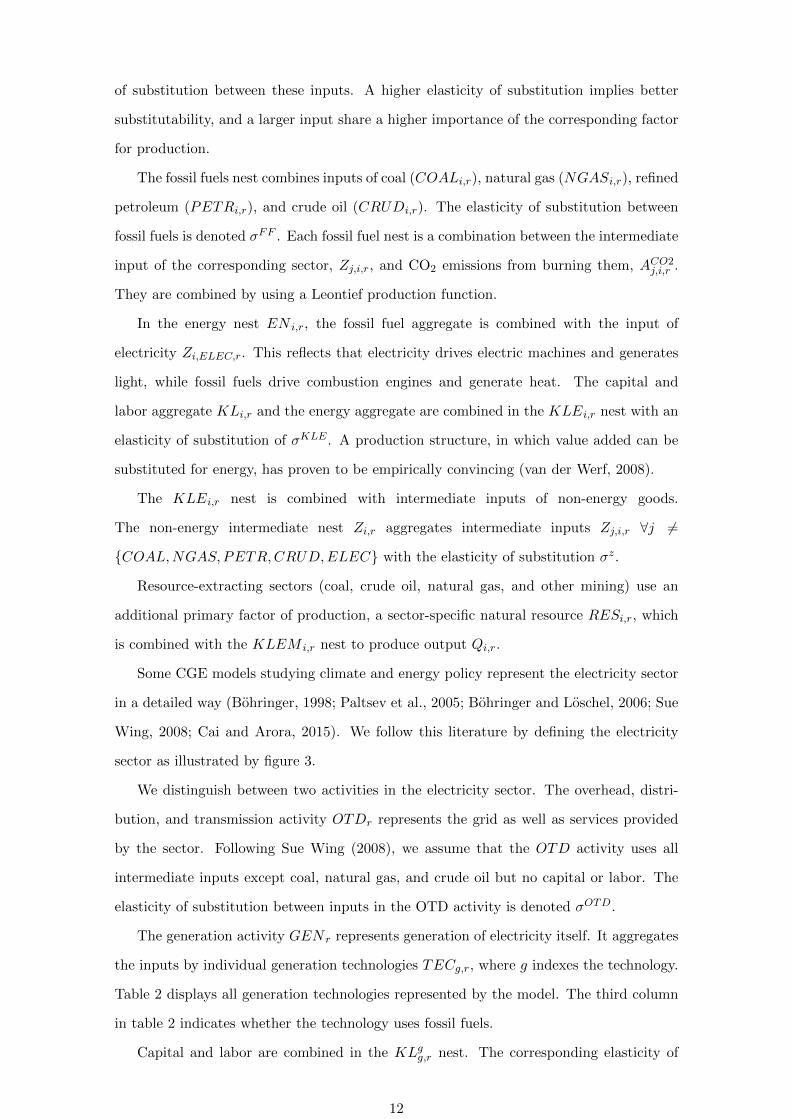
Some CGE models studying climate and energy policy represent the electricity sector

in a detailed way (Bohringer, 1998; Paltsev et al., 2005; Bohringer and Loschel, 2006; Sue

Wing, 2008; Cai and Arora, 2015). We follow this literature by defining the electricity

sector as illustrated by figure 3.

We distinguish between two activities in the electricity sector. The overhead, distri-

bution, and transmission activity OTDr represents the grid as well as services provided

by the sector. Following Sue Wing (2008), we assume that the OTD activity uses all

intermediate inputs except coal, natural gas, and crude oil but no capital or labor. The

elasticity of substitution between inputs in the OTD activity is denoted σOTD.

The generation activity GEN r represents generation of electricity itself. It aggregates

the inputs by individual generation technologies TECg,r, where g indexes the technology.

Table 2 displays all generation technologies represented by the model. The third column

in table 2 indicates whether the technology uses fossil fuels.

Capital and labor are combined in the KLgg,r nest. The corresponding elasticity of

12

Figure 3Nesting structure of the electricity sector

ELEC r

σELE

OTDr

σOTD

Z1,ELEC,r Z...,ELEC,r ZI,ELEC,r

GEN r

σGEN

TEC1,r

σTEC1,r

TECg,r

σTECg,r

KLFg,rσKLF

KLgg,rσKLg

Kg,r Lg,r

FFgg,rσFFg

COALg,r

ZCOAL,g,r ACO2g,r

CRUDg,r

ZCRUD,g,r ACO2g,r

NGASg,r

ZNGAS,g,r ACO2g,r

FFEGg,r

TEC...,r

σTEC...,r

substitution is σKLg. The inputs of coal, natural gas, and crude oil are combined within the

FF gg,r nest. They include the inputs of the fossil fuels, Zj,g,r, as well as the corresponding

CO2 emissions, ACO2j,g,r . Following Paltsev et al. (2005), we assume that refined petroleum

is not used to generate electricity. The capital-labor aggregate and the fossil fuels are

combined in the KLF g,r nest.

Usually, a technology does not employ more than one fossil fuel. Coal-fired power

plants use coal, gas-fired plants natural gas. In regions, for which we do not disaggregate

the generation technologies, we use an aggregate technology which uses coal, gas, and

crude oil (gAGG). In this case, we assume an elasticity of substitution σFFg between

fossil fuels.

Capital, labor and fuels are combined with a fixed factor in electricity generation

(FFEGg,r) in the TECg,r nest. It represents barriers to the expansion of individual

technologies. The interpretation of the fixed factor differs by technology. For wind power,

13

Table 2Power generation technologies

g Description Fossil

gCOA Coal-fired plants YesgOIL Oil-fired plants YesgGAS Gas-fired plants YesgNUK Nuclear fission NogHY D Hydroelectric plants NogWND Onshore and offshore wind NogSOL Photovoltaics and thermo-solar plant NogGET Geothermal and wave sources NogBIO Biomass and waste NogAGG Aggregate in r without Yes

technology-specific generation

for instance, it represents the limited availability of suitable sites for wind turbines. For

nuclear power plants and, to a lesser degree, other conventional technologies, the fixed

factor represents political restrictions to an expansion of production.

Note that the elasticity of substitution between KLF g,r and FFEGg,r, σTECg,r , can

differ by technology g and region r. This allows, for instance, to assume stronger political

constraints for building new nuclear power plants than for building new coal-fired plants.

Furthermore, regional differences in potentials for renewable energy can be accounted for.

2.4 Trade

Drawing upon the varieties and technologies defined in the previous subsection, this sub-

section sets up the Eaton and Kortum (2002) type trade model. It starts by defining trade

costs and proceeds by deriving price indices and trade shares.

2.4.1 Costs

Determining price differentials between regions, trade costs are a crucial part of the model.

Multiplicative trade costs δi,r,s are associated with the flow of good i from region r to

region s. Unlike in the Melitz (2003) model, there are no fixed costs of exporting. Thus,

international trade does not generate (additional) economies of scale and profits. Trade

within a region is assumed to be costless (δi,s,s = 1).

The functional form of the overall trade costs δi,r,s is defined by equation (5). We

differentiate between four components of trade costs: First, import tariffs τmi,r,s. Second,

transport margins ψh,i,r,s · P Th . Third, export subsidies τ ei,r,s. Fourth, iceberg trade costs

14

δi,r,s. The components are multiplied by each other because they affect price differentials

simultaneously and interactively.

δi,r,s = (1 + τmi,r,s)(1 +∑h

ψh,i,r,sPTh )(1− τ ei,r,s)δi,r,s (5)

τmi,r,s denotes the ad-valorem tariff (rate) imposed on imports of i from region r to

region s. Likewise, τ ei,r,s stands for an ad-valorem subsidy (rate) for exports of i from r to

s. The former is collected by region s, the latter is paid by region r. (Export subsidies can

also be negative and thus equivalent to export taxes.) Both τmi,r,s and τ ei,r,s are exogenous.

δi,r,s is interpreted as iceberg trade costs. They represent costs other than tariffs and

transportation costs which firms incur when they export their products. They include

transaction costs due to differences in language and regulation or other non-tariff barriers

to trade. The intuition for iceberg costs is that part of a good “melts away” when it is

shipped abroad. Iceberg costs imply that the transaction costs involve the same input

bundle and production technology as the traded good.

ψh,i,r,s is the international transport margin. For each unit of good i shipped from

region r to region s, ψh,i,r,s units of international transport services provided by sector h ∈ i

are needed. h indexes the transport sectors. The model considers one transport sector

(TRNS) but the underlying data allows to distinguish between up to three transport

sectors: air transport, water transport, and other transport. The explicit representation

of international transport services isolates how the demand for transport services reacts

to policy changes or exogenous shocks.

ψh,i,r,s is multiplied by the price of international transport services P Th . If the price of

international transport services falls, for instance due to technological improvements, the

trade costs δi,r,s fall as well. While ψh,i,r,s is exogenous, P Th is endogenous in the model.

International transport services are provided by a global transport sector. Using a

Cobb-Douglas technology, the production function of this sector combines inputs from

transport sectors h of all regions r.7

The following zero-profit condition (6) applies to the global transport sector and

represents MQ (2). It determines the output of international transport services, Fh.

Output is chosen such that the price for the international transport services P Th equals

the per-unit input costs∏r

(Ph,rζh,r

)ζh,rimplied by the Cobb-Douglas production function.

7It is not observable in the data which regions provide the international transport services to ship agood, for instance, from China to the United States. Assuming international transport services to be aglobal aggregate is a common solution to cope with this lack of data.

15

ζh,r is the exogenous input share of region r in international transport services.

P Th,r −∏r

(Ph,rζh,r

)ζh,r= 0 (6)

2.4.2 Prices

In this subsection, we exploit the properties of the Frechet distribution and the previous

assumptions to derive a simple expression for the sectoral prices Pi,s. We draw upon

Caliendo et al. (2014) who detail a simpler yet similar model. Let ci,r denote the per per-

unit input costs of sector i in r and τxi,r an output tax. Then, under perfect competition,

the price pi,r,s(zi,r) of variety zi,r in region s equals:

pi,r,s(zi,r) =ci,rδi,r,s

zi,rTi,r(1− τxi,r)(7)

With productivity varying between varieties, endogenous (Ricardian) productivity

gains from trade via specialization arise. Imagine, for example, a counterfactual sce-

nario in which European steel producers face fiercer competition from China, because the

Chinese steel sector experiences a positive productivity shock. As a consequence, Europe

imports more of the cheap Chinese varieties and shifts production to steel varieties, for

which it has the highest productivity zi,r. Thus, the increased competitive pressure from

abroad (China) induces a productivity gain at home (Europe).

Let ci,r denote the per per-unit input costs of sector i in r. Equation 8 below is a

stylized formulation of the per-unit input costs of producers in non-electricity sectors. It

constitutes the fourth model equation MQ (4). cxi,r represents the per-unit input costs of

nest x in sector i in r. The nesting structure is displayed in figure 2. The dots represent

the corresponding prices including taxes of intermediate inputs and primary factor inputs.

ci,r = cKLEMi,r

[cKLEi,r

[cKLi,r [. . . ] , cEi,r

[. . . , cFFi,r [. . . ]

]], cZi,r [. . . ]

](8)

It can be shown that the sectoral price Pi,s can be written as in equation (9); see

appendix C as well as Caliendo et al. (2014) for details. Equation (9) is denoted MQ (5)

which together with MQ (4), determines the sectoral prices in the model. γi is a constant.

Pi,s = γi

[∑r

T θii,r(1− τxi,r)

θi(ci,rδi,r,s)−θi

]− 1θi

(9)

A region s is in autarky if the trade costs equal infinity, δi,r,s = ∞ ∀ r 6= s. In this

16

case, the price only depends on the productivity, per-unit input costs, and taxes in s. If

s can trade with other regions r, their productivities Ti,r, per-unit input costs ci,r, and

taxes τxi,r as well as the bilateral trade costs δi,r,s influence the price in s.

High per-unit input costs ci,r lead to an increase in the price. The same is true for

the trade costs δi,r,s. The more costly it is to ship good i from r to s, the higher the price

in region s. High trade costs impede consumers and firms in region s from purchasing

efficiently produced varieties from region r which leads to higher prices. A high absolute

productivity, Ti,r, implies that sector i in region r uses its input bundle efficiently. Thus,

prices decrease in Ti,r. Furthermore, high output taxes τxi,r increase the price Pi,s.

θi is the shape parameter of the Frechet distribution. A high θi implies that produc-

tivity draws are similar. If productivities are similar, gains from trade are smaller because

a region finds it harder to replace inefficiently produced domestic varieties by more effi-

ciently produced imported ones. Therefore, the sectoral price Pi,s increases in θi, ceteris

paribus.

Next, a trade share πi,r,s can be derived. It denotes the share of destination region

s’s demand for good i which is supplied by origin region r. The trade share πi,r,s can

be written as follows. See appendix C as well as Caliendo et al. (2014) for the detailed

derivation.

πi,r,s =T θii,r(1− τxi,r)θi (ci,rδi,r,s)

−θi∑rr T

θii,rr(1− τxi,rr)θi(ci,rrδi,rr,s)−θi

(10)

The trade share πi,r,s measures the share of varieties of good i which region s purchases

from region r. Eaton and Kortum (2002) show that πi,r,s also corresponds to the share of

expenditure on i in s (Di,s) which is spent on goods from r. The trade share of region r

in s equals r’s contribution to the price index.8

Plugging the price equation (9) into equation (10) leads to an alternative expression

for the determination of trade shares which serves as model equation MQ (6).

πi,r,s =

[Ti,r(1− τxi,r)Pi,s

γici,rδi,r,s

]θi(11)

Equations (10) and (11) illustrate how the trade share of good i from origin region r

8Equation (10) reveals that the trade share of good i between regions r and s can only equal zero intwo cases. First, if the absolute productivity Ti,r of sector i in r equals zero. In this case, r is unable toproduce good i. Second, if the trade costs equal infinity (δi,r,s = ∞) and trade between the regions isimpossible. In the numerical solution, however, sufficiently small values are treated as zeros. Therefore,zero trade flows can occur in the model.

17

to destination region s reacts to a positive shock of the absolute productivity Ti,r. Ti,r

enters equation (11) directly, leading to an increase of r’s share in s’s demand for i. At

the same time, the improved productivity Ti,r also lowers the price index Pi,s (equation

9) leading indirectly to a decrease in the trade share. In summary, a higher Ti,r implies

an increase in πi,r,s.

For the interpretation of policy effects, let us derive the following elasticity of the trade

share πi,r,s with respect to a change in trade costs δi,r,s.

ηπi,r,s,δi,r,s =∂πi,r,s∂δi,r,s

δi,r,sπi,r,s

= −θi(1− πi,r,s) (12)

The negative sign indicates that higher sector-specific trade costs reduce the corre-

sponding trade share. A larger θi and a smaller initial πi,r,s go along with stronger policy

effects. A high θi implies small productivity differences between varieties and thus little

leeway for re-allocation as a response to higher trade costs.

2.5 Markets

A well-defined model solution requires that factor, transport, goods and emissions markets

are in equilibrium so that all markets clear.

2.5.1 Factors

Consumers supply their endowments of labor and capital inelastically on the factor mar-

kets. A market clearing condition determines factor prices PFf,r by equating the supply

and the demand from all sectors. f indexes primary factors, Nf,r denotes the exogenous

endowment with factor f in r.

Factor demand is derived from the CES production functions displayed in figures 2

and 3. Note that sectors’ input bundles do not differ by variety. Thus, the demand for

factor f equals the usual CES demand functions (Caliendo et al., 2014). The market

clearing conditions MQ (7) for the factors labor and capital read as follows. Vf,i,r is

the endogenous input of factor f in the production of good i in region r.

Nf,r =∑i

Vf,i,r ∀f ∈ L,K (13)

Four sectors employ a sector-specific natural resource in their production: coal

(COAL), gas (NGAS), oil (CRUD), and mining (MINE). The market clearing con-

dition MQ (8) expressed by equation (14) below, determines the price of the natural

18

resource used by sector i in r, PRESi,r . It equates the exogenous supply of the resource

NRES,i,r with the demand from the corresponding sector RESi,r.

NRES,i,r = RESi,r ∀i ∈ COAL,NGAS,CRUD,MINE (14)

The next market clearing condition MQ (9) determines the price for the

technology-specific fixed factor in electricity generation, PFFEGg,r as characterized by equa-

tion (15). Here, the exogenous supply of the fixed factor NFFEG,g,r is equated with the

demand from technology g in r, FFEGg,r.

NFFEG,g,r = FFEGg,r (15)

2.5.2 Transport

The market clearing condition (16) below constitutes MQ (3). It determines the price

P Th,r by equating supply and demand for international transport services. The demand for

international transport services, which we denote ZTh,i,r,s, depends on trade volumes and

on ψh,i,r,s.

Fh =∑i,r,s

ZTh,i,r,s (16)

Let Fh,r denote the demand for transportation services from country r by the global

transportation sector h. Since the global transportation sector combines its inputs ac-

cording to a Cobb-Douglas function, the expenditure on transportation services from r

can be expressed as:

Fh,rPh,r = ζh,rPTh,rFh (17)

Let Di,s denote the total expenditure of region s on good i. As equation (18) shows,

Di,s equals the sum of final (Ci,r) and intermediate demand for i (Zi,j,r). It enters the

model as MQ (10).

Di,s =∑j

Zi,j,s + Ci,s (18)

19

2.5.3 Goods

Goods markets clear when the sales by sector i in region r, Xi,r, equal the expenditures

on its goods in all regions s. Equation (19) shows the market clearing condition MQ

(10).

Xi,r =∑s

πi,r,sDi,s

(1 + τmi,r,s)(1 +∑

h ψh,i,r,sPTh )(1− τ ei,r,s)

(19)

The expression πi,r,sDi,s corresponds to the expenditure on goods from i in r by region

s. It encompasses both intermediate and final demand. Expenditures on imported goods

include trade costs. The denominator of equation (19) corrects the expenditures for export

subsidies, international transport margins, and import tariffs. Therefore, the right hand

side of equation (19) equals the demand for sector i’s goods net of tariffs and international

transport margins.

Additional demand for transport services is generated by the global transport services

sector. Thus for transport services sectors h ∈ i, the term ζh,rPTh,rFh, derived from the

demand function (17), is added to the right hand side of (19).

2.5.4 Emissions

The EU Emissions Trading System (EU ETS) is the key instrument of the European

climate policy. Established in 2005, the EU ETS encompasses some 11,000 stationary

installations in the EU plus Iceland, Liechtenstein, and Norway. Since 2012 it has also

captured parts of the aviation sector. Around 45% of the European Union’s CO2 emissions

are covered by the EU ETS (see Ellerman et al., 2010, for an overview).

The price for allowances in the EU ETS, PETS , is determined by the following market

clearing condition MQ (12) in equation (20). It equates the exogenous supply of

allowances NETS with the CO2 emissions by sector i in region r burning fuel j, ACO2j,i,r , j ∈

COAL,CRUD,NGAS4. This demand is modeled by combining the input of fossil fuels

in the nested CES production function with an input of CO2 allowances in a Leontief nest

as illustrated in figures 2 and 3. Note that we restrict the sectors i and regions r to subsets

iets and rets. The former encompasses all sectors which are part of the EU ETS and the

latter all regions which are part of it.

NETS =∑j

∑i∈iets

∑r∈rets

AETSj,i,r (20)

20

In the second phase of the EU ETS, between 2008 and 2012, the overwhelming major-

ity of initial allowances were allocated to firms for free. Let αfai,r denote the share of freely

allocated allowances in sector i in r. To replicate free allocation, we introduce an endoge-

nous output subsidy φETSi,r which compensates producers for the sector-specific share αfai,r

of their expenditures on allowances.

φETSi,r Xi,r = αfai,r∑j

PETSACO2j,i,r (21)

This policy condition MQ (13) completes the model setup.

3 Calibration

This section describes the calibration procedure and the required data.

3.1 Overview

The advanced trade model as well as the disaggregation of regions and sectors go beyond

standard input-output datasets and require elaborated calibration techniques (subsection

3.2). For the trade model, the absolute productivities (Ti,r) and the iceberg trade costs

(δi,r,s) need to be calibrated via a structural estimation approach. This is a key difference

to Armington (1969) based CGE models, in which baseline trade flows are replicated by

assuming that they reflect preferences for goods produced in individual regions.

Most other parameter values of the model, such as input shares of CES functions

(including Cobb-Douglas and Leontief functions) describing production and consumption

as well as tax and subsidy rates, can directly be calibrated to input-output data (subsection

3.3), such as the GTAP dataset (see, for example, Bohringer et al., 2003). Other parameter

values, like elasticities of substitution or the share parameter of the Frechet distribution

(θi) are taken from the literature.

For the regional disaggregation (subsection 3.4), we adapt and employ a regional sci-

ence approach (Kronenberg, 2009). Likewise, for the individual representation of the

technologies in the electricity sector (subsection 3.5), additional data on the electricity

mix and technology-specific inputs are required. A consistent dataset is ensured via a

constrained optimization model (following Sue Wing, 2008).

The implementation of the emissions trading scheme involves some specialties, too

(subsection 3.6). Beside emissions targets, the regional and sectoral coverage of the scheme

as well as the shares of freely allocated allowances must be fixed.

21

3.2 Trade model

The following subsections explain the structural estimation and the recovery of absolute

productivities for the calibration of the trade model.

3.2.1 Structural estimation

Following Eaton and Kortum (2002), we begin by normalizing the trade share πi,r,s, the

share of good i which region s purchases from region r. We divide it by the share of s’s

consumption of i which is supplied by the domestic industry (πi,s,s).

πi,r,sπi,s,s

=T θii,r(1− τxi,r)θi (ci,rδi,r,s)

−θi

T θii,s(1− τxi,s)θic−θii,s

(22)

The normalized trade share only depends on parameters of either r or s. It is indepen-

dent of productivities or trade costs in other regions. Bilateral trade flows and the total

demand for good i are observable. Therefore,πi,r,sπi,s,s

is observable. We linearize equation

(22) by taking logs.

log

[πi,r,sπi,s,s

]= log

[Tβi,rθii,r (1− τxi,r)θic

−θii,r

]− (23)

log[Tβi,sθii,s (1− τxi,s)θic

−θii,s

]− θi log [δi,r,s]

Recall that the trade costs δi,r,s consist of four components (equation 5). Export

subsidies (τ ei,r,s), international transport margins (ψh,i,r,sPTh ), and import tariffs (τmi,r,s)

are observable. Only iceberg trade costs δi,r,s need to be estimated.

We use the econometric specification (24) below for the iceberg trade costs. distancer,s

denotes the distance between regions r and s. We normalize distancer,s by the shortest

distance between two regions in our sample. µi is the elasticity of the iceberg costs with

respect to distance. Dummy variables capture the effect of sharing a border (borderr,s),

having a common language (languager,s), having colonial ties (colonyr,s), being part of

a regional trade agreements (rtrader,s), and having a common currency (currencyr,s).

The parameter pipelinei,r,s is specific to the natural gas sector and captures whether two

regions are connected by a gas pipeline.

log δi,r,s =µi log distancer,s + β1i borderr,s + β2i languager,s + β3i colonyr,s (24)

+ β4i rtrader,s + β5i currencyr,s + β6i pipelinei,r,s

22

Equation (23) can be interpreted as a gravity model of trade (Eaton and Kortum,

2002). It contains technology-cum-input-cost terms for the exporting and the importing

nation. We define an exporter fixed effect ei,r = log[T θii,r(1− τxi,r)θic

−θii,r

]and an importer

fixed effect mi,s = log[T θii,s(1− τxi,s)θic

−θii,s

]which we plug into equation (23). Adding an

error term εi,r,s yields the following estimation equation. The value of θi is taken from

the literature.

logπi,r,sπi,s,s

= ei,r −mi,s − θi log δi,r,s + εi,r,s (25)

Adding the market clearing condition (19) as a side constraint to the estimation prob-

lem ensures that the parameter estimates and, thus, the model’s baseline constitute an

equilibrium of the model (Balistreri and Hillberry, 2007; Balistreri et al., 2011; Pothen

and Balistreri, 2017).

The exporter fixed effect in the United States is assumed zero, ei,USA = 0. This implies

that we estimate the technology-cum-input-cost terms relative to the USA.

Si,r = exp(ei,r) =T θii,r(1− τxi,r)θic

−θii,r

T θii,USA(1− τxi,USA)θic−θii,USA

. (26)

With the help of this expression, we are able to rewrite equation (10) to obtain an

expression for πi,r,s that solely depends on the trade costs and on Si,r.

πi,r,s =Si,rδ

−θii,r,s∑

rr Si,rrδ−θii,rr,s

(27)

In combination with the market clearing condition (19), we obtain a set of equations

that we can estimate via Ordenary Least Squares (OLS) (see Appendix D).

3.2.2 Recovering the absolute productivity

Equipped with the estimates of Si,r and δi,r,s, we calculate relative prices. First, we

combine δi,r,s with data on import and export tariffs as well as international transport

margin to compute the total trade costs δi,r,s.

The price of good i in region s relative to its United States’ counterpart can be written

23

as follows.9

Pi,s = Pi,USA

[ ∑r Si,rδ

−θii,r,s∑

r Si,rδ−θii,r,USA

]−1/θi(28)

We conveniently choose units such that the USA’s price equals unity in each sector

(Pi,USA = 1). Thereby, we can calculate the prices for all regions. Factor prices PFf,r are

computed by dividing the factor compensation by physical inputs of labor and capital.

Prices for the sector-specific natural resources and for the technology-specific fixed factors

are normalized to unity. Having derived the sectoral prices, we are able to compute the

per-unit input costs ci,r.

After computing the per-unit input costs, we can derive the total factor productivity

(TFP) Λi,r. It can be shown that the TFP can be expressed as Λi,r =ci,r

Pi,r(1−τxi,r).10 We

plug the TFP term into the expression for trade shares in (11) to obtain:

πi,r,s =

[Λi,rγiTi,r

]−θi(29)

Solving (29) for Ti,r yields the absolute productivities Ti,r.11

Ti,r = γiΛi,rπ1θii,r,s (30)

3.3 Inputs and outputs

The overall model is designed to match a global input-output dataset as described in the

first subsection. The second subsection deals with other data sources.

3.3.1 GTAP data

The most common and most important dataset used for the model calibration is the Global

Trade Analysis Project (GTAP) database, version 9 (Aguiar et al., 2016). We calibrate

the model to the benchmark year 2011, the most recent one in GTAP 9. The database

9Shikher (2012) as well as Levchenko and Zhang (2016) use the formulaPi,s

Pi,USA=

[πi,s,s

πi,USA,USA

1Si,s

] 1θi .

Our approach yields the same results but is also applicable to sectors which do not produce and, thus,have Si,s = 0.

10See, for instance, Caliendo et al. (2014).11Note that estimation problem (47) will lead to different trade flows than those observed in the data.

Two adjustments to the data are necessary to balance the inputs and outputs. First, demand for interna-tional transportation services is altered due to changing trade flows. We introduce a balancing parameterin the market clearing condition for the international transportation sector to ensure that supply equalsdemand. Second, the export subsidies paid and the import tariffs received also change. We adjust incomesaccordingly.

24

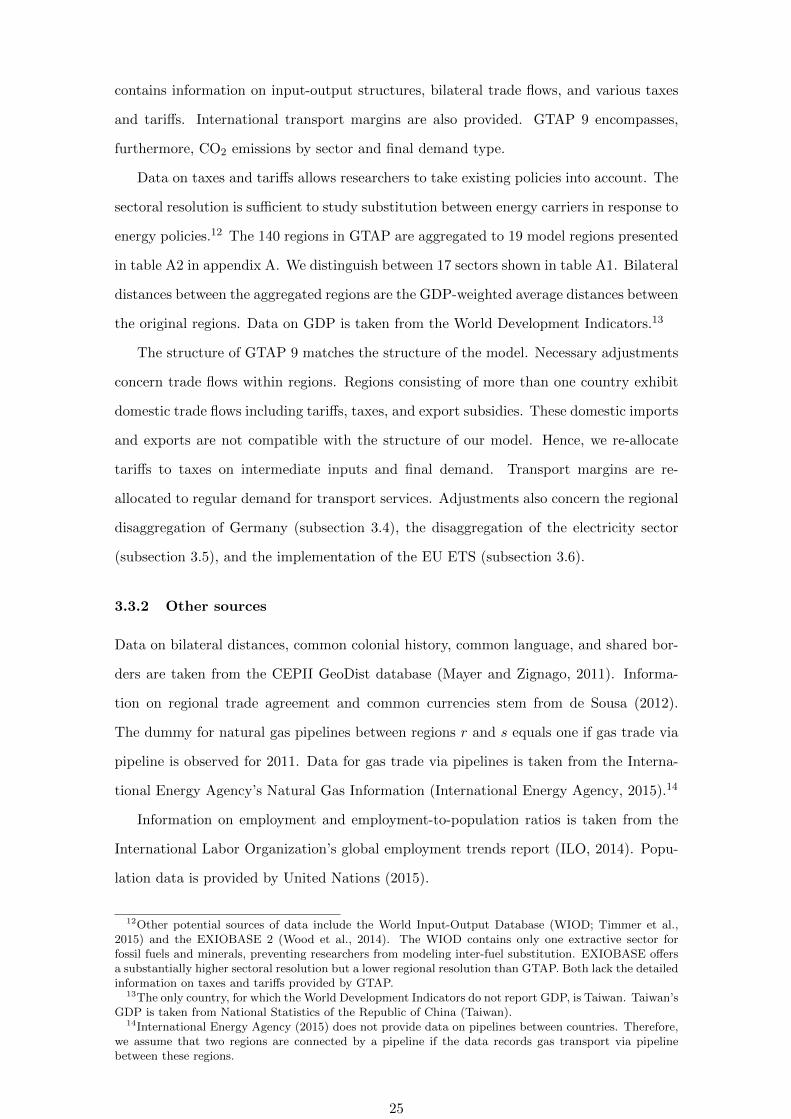
contains information on input-output structures, bilateral trade flows, and various taxes

and tariffs. International transport margins are also provided. GTAP 9 encompasses,

furthermore, CO2 emissions by sector and final demand type.

Data on taxes and tariffs allows researchers to take existing policies into account. The

sectoral resolution is sufficient to study substitution between energy carriers in response to

energy policies.12 The 140 regions in GTAP are aggregated to 19 model regions presented

in table A2 in appendix A. We distinguish between 17 sectors shown in table A1. Bilateral

distances between the aggregated regions are the GDP-weighted average distances between

the original regions. Data on GDP is taken from the World Development Indicators.13

The structure of GTAP 9 matches the structure of the model. Necessary adjustments

concern trade flows within regions. Regions consisting of more than one country exhibit

domestic trade flows including tariffs, taxes, and export subsidies. These domestic imports

and exports are not compatible with the structure of our model. Hence, we re-allocate

tariffs to taxes on intermediate inputs and final demand. Transport margins are re-

allocated to regular demand for transport services. Adjustments also concern the regional

disaggregation of Germany (subsection 3.4), the disaggregation of the electricity sector

(subsection 3.5), and the implementation of the EU ETS (subsection 3.6).

3.3.2 Other sources

Data on bilateral distances, common colonial history, common language, and shared bor-

ders are taken from the CEPII GeoDist database (Mayer and Zignago, 2011). Informa-

tion on regional trade agreement and common currencies stem from de Sousa (2012).

The dummy for natural gas pipelines between regions r and s equals one if gas trade via

pipeline is observed for 2011. Data for gas trade via pipelines is taken from the Interna-

tional Energy Agency’s Natural Gas Information (International Energy Agency, 2015).14

Information on employment and employment-to-population ratios is taken from the

International Labor Organization’s global employment trends report (ILO, 2014). Popu-

lation data is provided by United Nations (2015).

12Other potential sources of data include the World Input-Output Database (WIOD; Timmer et al.,2015) and the EXIOBASE 2 (Wood et al., 2014). The WIOD contains only one extractive sector forfossil fuels and minerals, preventing researchers from modeling inter-fuel substitution. EXIOBASE offersa substantially higher sectoral resolution but a lower regional resolution than GTAP. Both lack the detailedinformation on taxes and tariffs provided by GTAP.

13The only country, for which the World Development Indicators do not report GDP, is Taiwan. Taiwan’sGDP is taken from National Statistics of the Republic of China (Taiwan).

14International Energy Agency (2015) does not provide data on pipelines between countries. Therefore,we assume that two regions are connected by a pipeline if the data records gas transport via pipelinebetween these regions.

25

The elasticities of substitution are taken from the MIT EPPA (Emissions Prediction

and Policy Analysis) model (Paltsev et al., 2005). They are listed in appendix B.

3.4 Regional disaggregation

We decompose the German input-output data from GTAP into the Federal State of Lower

Saxony (Niedersachsen) and the Rest of Germany. Lower Saxony (LSX) is a large north-

ern state with a high potential for utilizing wind power. We employ the Cross-Hauling

Adjusted Regionalization Method (CHARM; Kronenberg, 2009) in the modified version

by Tobben and Kronenberg (2014) to separate Lower Saxony from the Rest of Germany

(ROG). Details can be found in appendix E.1.

Lower Saxony’s sectoral composition differs notably from the one in the Rest of Ger-

many (see table E1 in appendix E). Agriculture (AGRI) and food production (FOOD)

account for 1.9% and 3.3% of value added in Lower Saxony compared to 1.2% and 2.4% in

the Rest of Germany. Furthermore, the electricity sector (ELEC) share of 1.5% is slightly

higher than in the Rest of Germany. The share of non-energy intensive manufacturing

(MANU) and services (SERV ) is smaller in Lower Saxony than in the Rest of Germany.

3.5 Sectoral disaggregation

The disaggregation of the electricity sector enables an endogenous adjustment of the elec-

tricity mix and hence the decarbonization of energy supply induced by climate policy.

The technology-specific representation of the electricity generation outlined in subsection

2.3.2 does not have an empirical counterpart in the GTAP data. Hence, we utilize an

approach based on Sue Wing (2008) to disaggregate the GTAP data of the electricity

sector by generation technology. The required data on electricity output and input shares

by technology are taken from the literature. For the following analysis, we disaggregate

the electricity sector of Lower Saxony, Rest of Germany, France, Italy and United King-

dom. The full list of regions with and without a disaggregated the electricity sector, is

presented in table A2. For other regions, we model an aggregate technology (gAGG)

which represents all generation technologies. We disaggregate the generation technology

by using an algorithm which fits the output of individual technologies and the inputs

of labor and value added to the observed data while satisfying the market clearing and

zero-profit conditions. The details of the disaggregation are presented in appendix E.2.

26

3.6 Emissions trading

The EU ETS has been in force since 2005. The GTAP benchmark year 2011 belongs

to the EU ETS’s second phase which lasted from 2008 to 2012. The GTAP data need

to be modified to account for the EU ETS. We combine CO2 emissions recorded in the

GTAP with price data to identify payments for certificates. Furthermore, we calibrate a

subsidy φETSi,r which ensures that a free allocation of 90% of the allowances is achieved in

the baseline. Details are presented in Appendix F.

4 Policies

The model is tailored to analyze the interaction of trade and climate policy in a globalizing

world. Trade liberalization is expected to affect CO2 emissions and climate policy costs;

vice versa climate policy is expected to affect trade and the related productivity gains from

specialization. To study these interconnections, in the following subsections we simulate

two sets of counterfactual scenarios. First, we study a worldwide reduction of trade costs

in terms of tariffs or non-tariff barriers (subsection 4.1). Second, we study the reduction

of CO2 allowances in the EU ETS as well as renewable energy support (subsection 4.2).

4.1 Trade policy

In the first set of simulations, we study how changes in trade costs affect welfare and

CO2 emissions. Recall that the trade costs are defined as follows: δi,r,s = (1 + τmi,r,s)(1 +∑h ψh,i,r,sP

Th )(1−τ ei,r,s)δi,r,s (equation 5). We implement two scenarios in which we reduce

the trade costs.

In the noTariffs scenario, τmi,r,s and τ ei,r,s are set to zero, i.e., all import and export

tariffs or subsidies are abolished in all regions and sectors. The noTariffs scenario resem-

bles classical (multilateral) trade agreements under GATT or the auspices of the WTO.

Tariffs and subsidies are also one element of currently debated trade agreements, such

as the Trans-Atlantic Trade and Investment Partnership (TTIP), or the Trans-Pacific

Partnership (TPP).

Table 3 shows the resulting percentage reductions in overall trade costs δi,r,s of sectoral

trade from r to s in the scenarios noTariffs and lessIceberg. The reductions range from

1.8% in France to 7.3% in India. For most regions, the drop in trade costs is around two

to three per cent.

In recent debates on trade agreements, the reduction of non-tariff trade barriers, such

27

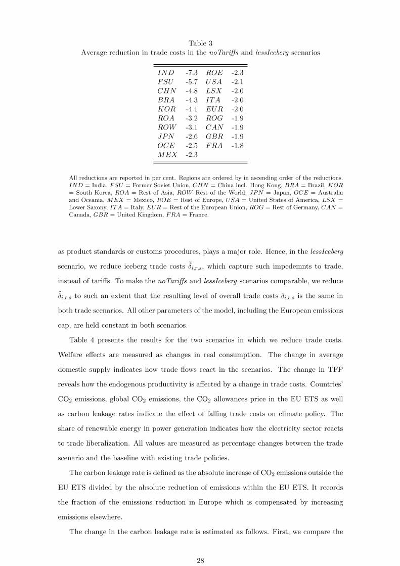
Table 3Average reduction in trade costs in the noTariffs and lessIceberg scenarios

IND -7.3 ROE -2.3FSU -5.7 USA -2.1CHN -4.8 LSX -2.0BRA -4.3 ITA -2.0KOR -4.1 EUR -2.0ROA -3.2 ROG -1.9ROW -3.1 CAN -1.9JPN -2.6 GBR -1.9OCE -2.5 FRA -1.8MEX -2.3

All reductions are reported in per cent. Regions are ordered by in ascending order of the reductions.IND = India, FSU = Former Soviet Union, CHN = China incl. Hong Kong, BRA = Brazil, KOR= South Korea, ROA = Rest of Asia, ROW Rest of the World, JPN = Japan, OCE = Australiaand Oceania, MEX = Mexico, ROE = Rest of Europe, USA = United States of America, LSX =Lower Saxony, ITA = Italy, EUR = Rest of the European Union, ROG = Rest of Germany, CAN =Canada, GBR = United Kingdom, FRA = France.

as product standards or customs procedures, plays a major role. Hence, in the lessIceberg

scenario, we reduce iceberg trade costs δi,r,s, which capture such impedemnts to trade,

instead of tariffs. To make the noTariffs and lessIceberg scenarios comparable, we reduce

δi,r,s to such an extent that the resulting level of overall trade costs δi,r,s is the same in

both trade scenarios. All other parameters of the model, including the European emissions

cap, are held constant in both scenarios.

Table 4 presents the results for the two scenarios in which we reduce trade costs.

Welfare effects are measured as changes in real consumption. The change in average

domestic supply indicates how trade flows react in the scenarios. The change in TFP

reveals how the endogenous productivity is affected by a change in trade costs. Countries’

CO2 emissions, global CO2 emissions, the CO2 allowances price in the EU ETS as well

as carbon leakage rates indicate the effect of falling trade costs on climate policy. The

share of renewable energy in power generation indicates how the electricity sector reacts

to trade liberalization. All values are measured as percentage changes between the trade

scenario and the baseline with existing trade policies.

The carbon leakage rate is defined as the absolute increase of CO2 emissions outside the

EU ETS divided by the absolute reduction of emissions within the EU ETS. It records

the fraction of the emissions reduction in Europe which is compensated by increasing

emissions elsewhere.

The change in the carbon leakage rate is estimated as follows. First, we compare the

28

baseline with a simulation in which the number of allowances is drastically increased such

that the carbon price drops to zero. This yields the carbon leakage rate in the baseline.

Second, we compute the carbon leakage rate for the trade policy scenario with reduced

trade costs in the analogous way. Then we compute the percentage change between the

leakage rates in the trade policy and baseline scenario.

Table 4 reports the results for six selected regions. The evaluation of Lower Saxony

(LSX) with its large wind power potential in comparison to the Rest of Germany (ROG)

shows how far the regional disaggregation matters. China (CHN) is chosen as the biggest

emerging economy, while the USA are the world’s largest economy. Korea (KOR) repre-

sents the “Asian Tigers” that have developed with an amazing pace. The Former Soviet

Union (FSU) is a major gas supplier to Europe and represents fossil fuel exporters.

In the noTariffs scenario, we observe small welfare increases compared to the baseline

in most regions. Lower Saxony, the Rest of Germany, China, and the USA exhibit welfare

gains of less than one per cent. Korea’s welfare increases by 4.3%, which is the strongest

rise among all model regions. Its gross income increases by 2.7%, while its true-cost-of-

living price index cCs falls by 1.6%. Falling trade costs enhance specialization, both within

(cf. Finicelli et al., 2013) and between sectors. This specialization causes welfare gains

in almost all model regions. Korea benefits particularly from the increased specialization

possibilities.

Tariffs can serve as an instrument to exploit power on international markets.15 If re-

gions abolish welfare-enhancing beggar-thy-neighbor tariffs, they can incur welfare losses.

The Former Soviet Union exemplifies this effect. It loses about 2.0% of its welfare due to

the removed tariffs.

The average domestic supply, the share of good i, which region r supplies to the

domestic market, falls in all regions. Countries increasingly specialize in those activities in

which they are productive and import other goods. Consequently, total factor productivity

rises in almost all regions in response to removing trade taxes and subsidies. The Former

Soviet Union achieves the strongest gain: its TFP grows by 20.9%. To illustrate the

specialization gains in a formal way, we solve equation (30) for total factor productivity

Λi,r and obtain the following expression:

Λi,r = γ−1iTi,r

π1/θii,r,r

(31)

15See Alvarez and Lucas (2007) who study optimal tariffs in an Eaton and Kortum model.

29

Table 4Results of the trade policy scenarios

noTariffs lessIceberg

Welfare

LSX 0.46 0.85ROG 0.11 0.50CHN 0.22 3.09FSU -2.03 8.55KOR 4.33 11.57USA 0.20 0.50

LSX -5.67 -6.01ROG -3.78 -4.12

Average CHN -5.33 -5.41domestic supply FSU -11.14 -10.60

KOR -15.13 -14.99USA -2.28 -2.55

LSX -0.74 -0.88ROG 1.03 0.93

Total Factor CHN 3.47 2.82Productivity FSU 20.93 8.77

KOR 3.77 3.52USA -0.43 -0.67

CO2 emissions

LSX -16.38 -16.88ROG -8.50 -8.72CHN -1.74 -2.32FSU -7.94 -2.83KOR 34.38 38.64USA 1.22 1.34

Renewables share

LSX 15.76 15.61ROG 14.45 14.60CHN - -FSU - -KOR - -USA - -

Global CO2 emissions 2.73 3.40CO2 price EU ETS 160 163Carbon leakage rate -0.09 -6.07

All changes are compared to the baseline with existing trade costs and reported in per cent. TFP =total factor productivity, LSX = Lower Saxony, ROG = Rest of Germany, CHN = China, FSU =Former Soviet Union, KOR = South Korea, USA = United States of America.

Equation 31 shows that falling domestic supply πi,r,r increases total factor productivity

ceteris paribus. Sectors specialize in varieties which they manufacture efficiently. This

Ricardian selection process (Finicelli et al., 2013) raises TFP.

Some regions, such as Lower Saxony or the United States, experience trade-induced

changes in sectoral composition towards less efficient industries. Faced with cheaper for-

30

eign competition, these regions expand their production in sectors such as services which

have a lower TFP.

The noTariffs scenario affects Lower Saxony and the Rest of Germany to different

extents. While Lower Saxony exhibits a welfare gain of 0.5%, the Rest of Germany

experiences a gain of only 0.1%. The average domestic supply falls more significantly

in Lower Saxony than in the Rest of Germany. Apparently, Lower Saxony’s economy

specializes more intensively in response to falling trade costs. The decline in TFP of 0.7%

indicates that Lower Saxony’s economy shifts toward less productive sectors.

CO2 emissions change substantially in response to abolishing tariffs and trade subsi-

dies. In Lower Saxony, they fall by over 16%, which is about twice the reduction of over

8% in the Rest of Germany. This drastic reduction is driven by Lower Saxony’s large wind

power potential and the resulting low mitigation costs. In the Rest of Germany, China,

and the Former Soviet Union, CO2 emissions fall by less than 10%. On the other hand, the

USA and South Korea exhibit rising emissions. In total, global carbon emissions rise by

2.7% due to trade liberalization, while the climate policy-induced carbon leakage rate in

the noTariffs scenario is almost identical to the one in the baseline.16 Due to the induced

expansion of economic activity, the allowances price in the EU ETS increases by 160%

compared to the baseline.

South Korea, whose carbon emissions increase by more than a third, exemplifies how

structural change can affect a country’s CO2 emissions. Gross output of the Korean

chemicals industry increases by 36%. Other sectors, such as iron and steel, non-ferrous

metals and power generation, increase their gross output by more than 20%. Thus Korea’s

rising CO2 emissions are driven by structural change in favor of energy-intensive industries.

Table 4 also displays how the share of renewables in power generation changes in

response to falling trade costs in Lower Saxony and the Rest of Germany. In the baseline,

Lower Saxony has a renewables share in electricity generation of about 30%. The Rest

of Germany has a share of about 20%. In both regions, the share of renewables rises by

about 16% compared to the baseline. Falling trade costs enhance output and thus carbon

emissions. This is reflected by the higher CO2 price in the EU ETS. The electricity sector

reacts to the higher CO2 price by shifting generation to renewables.

In the lessIceberg scenario, the overall trade costs δi,r,s are reduced by the same amount

as in the noTariffs scenario, but the reduction is caused by falling iceberg costs instead

16This means, due to trade liberalization emissions rise with and without climate policy so that theleakage rate measured between them stays roughly constant.

31

of abolished tariffs. Table 4 reveals that reducing the iceberg costs leads to higher welfare

gains than dropping tariffs. Welfare gains in the lessIceberg scenario are more than twice

as high as in the noTariffs scenario. Even the Former Soviet Union, which incurred a

welfare loss from dropping tariffs, exhibits a welfare gain of 8.6% if iceberg costs are

reduced.

The key difference between tariffs and iceberg costs is that tariffs generate revenues

which are distributed to the representative consumer, whereas iceberg costs δi,r,s consti-

tutes a mere inefficiency. Because regions do not relinquish revenue, their removal leads

to stronger welfare gains than eliminating tariffs.

The effects for average domestic supply in the lessIceberg scenario are in the same

ballpark as in the noTariffs scenario. Because trade costs change by the same amount,

the trade shares evolve similarly. The TFP grows less substantially when iceberg costs

are reduced than when tariffs are abolished. This affect is mainly driven by trade-induced

structural change towards sectors with smaller potential for productivity gains: the ser-

vices sector, for instance, expands more under lessIceberg than noTariffs.

Within the EU ETS, regional CO2 emissions fall and the allowances price rises as

in the noTariffs scenario but with a slightly higher magnitude. Compared to noTariffs,

renewable power generation slightly shifts from Lower Saxony to the Rest of Germany.

Worldwide carbon emissions rise by 3.4% due to the reduction in iceberg costs, which is

about 0.7 percentage points higher than under the removal of tariffs.

The climate policy-induced carbon leakage rate falls by 6.1% in the lessIceberg sce-

nario compared to the baseline. In the noTariffs scenario, on the contrary, we observe an

insignificant decrease. With reduced iceberg costs, the EU climate policy is responsible

for less carbon leakage to the rest of the world because the reduction of non-tariff barriers

supports structural change towards less energy-intensive industries in Europe. This struc-

tural change improves energy and carbon efficiency and eases decarbonization within the

EU induced by climate policy.

4.2 Climate policy

In the second set of counterfactual simulations, we study how a reduction of allowances

in the EU ETS affects welfare, trade, and global CO2 emissions. All scenarios in this

subsection study a 13% reduction of allowances relative to the year 2011. The EU Com-

mission has codified this reduction for the third phase of the EU ETS. The number of

allowances will be reduced from 2,084 billion tons in 2011 to 1,816 billion tons in 2020

32

(EU Commission, 2015). This corresponds to a reduction of emissions covered by the EU

ETS by 21% compared to 2005 or 13% compared to 2011.

Four simulations are computed. The first, denoted ETS20, corresponds to the 13%

reduction of allowances in the EU ETS. All other parameters of the model remain at

baseline levels. In other words, the EU ETS’s cap is applied to the original baseline data

for the year 2011. We do not impose a carbon tax on non-ETS sectors.

In the ETS20sub scenario, the reduction of allowances is accompanied by a subsidy for

wind power and solar power in the regions Lower Saxony, Rest of Germany, France, Italy

and United Kingdom. This scenario reflects that the European 20-20-20 climate policy

strategy relies on a mix of instruments. In the EU, particularly in Germany, renewable

energies, especially wind and solar power, have been heavily subsidized; in Germany re-

newable energy levies account for over 20% of households’ electricity (Bundesnetzagentur

and Bundeskartellamt, 2016). Taking into consideration that the magnitude of support

shall be reduced and that the benchmark data already incorporate general taxes and sub-

sidies, we assume a subsidy rate of 10%. In the model, however, electricity generation

is not subject to any market failure which would theoretically justify a subsidy (Tinber-

gen, 1952). Consequently, any additional policy instrument, such as a renewable energy

subsidy, is expected to raise the costs of reaching a given emissions target.

The ETS20gr scenario takes into account that the emission reduction is envisaged for

2020 and that the economy will grow until then. We assume that the world economy

grows by 1.3% per year between 2011 and 2020 (consistent with assumptions for Europe

in EU Commission, 2016). This corresponds to an overall growth of 12.3% compared to

2011, i.e., all inputs, outputs, and endowments rise by 12.3%. In the ETS20gr scenario,

we implement the same absolute reduction goal in the EU ETS as in the ETS20 scenario.

The last scenario, denoted ETS20subgr, combines economic growth and the emissions

reduction with a 10% subsidy on wind and solar power in the EU.

Table 5 presents the results of the four scenarios in which the number of allowances

in the EU ETS is reduced. It shows changes in welfare (real consumption), average

domestic supply, TFP, regions’ and global CO2 emissions, the renewables share in power

generation, the allowances’ price in the EU ETS, and the carbon leakage rate. All values

are expressed as percentage changes relative to the baseline. We display the same regions

as in the previous section, except replacing South Korea by France (FRA), the second

biggest European economy and member of the EU ETS.

The first column shows the outcomes of the ETS20 scenario. The emissions reduction

33

does not have major impacts on real consumption. The welfare loss in Lower Saxony

amounts to 0.14% and to 0.28% in the Rest of Germany. Welfare falls by only 0.02%

in France; with a large nuclear power share, France is hardly affected by the tighter

emissions cap. Welfare in Europe’s major trade partners such as the USA and China is

quasi unaffected. The Former Soviet Union sustains a very small welfare loss due to falling

demand for fossil fuels.

Lower Saxony and the Rest of Germany experience a reduction in their average domes-

tic supply by 2.02% and 0.17%, respectively because stricter climate policy raises costs for

their industries. Higher costs of carbon make European exports less competitive in other

markets such as the Former Soviet Union. These markets display increasing domestic

supply, driven by less competition from their European trade partners. The changes in

TFP correspond to the changes in average domestic supply (see equation 31): they rise

in Lower Saxony and the Rest of Germany but fall in the other regions. This implies

climate policy-induced productivity (efficiency) gains in Germany but productivity reduc-

tions outside Germany. These policy-induced changes in trade and productivity affect

regional emissions and carbon leakage as discussed in the following paragraphs.

CO2 emissions fall by 18.28% compared to the baseline in Lower Saxony and by 8.32%

in the Rest of Germany. Thus, more emissions are abated in Lower Saxony with it’s large

wind power potential than in the Rest of Germany. The allowances price in the ETS rises

by 139% in response to the lower cap. This equals a price of about 45 USD per ton of

CO2. Global CO2 emissions decrease by 0.27%. Furthermore, the share of renewabales

in electricity generation rises in all regions which are subject to the EU ETS. France is

less affected than Lower Saxony and the Rest of Germany because its electricity sector is

dominated by carbon-free nuclear power. As a result, France’s carbon emissions decrease

by 2.79%. Slightly increasing emissions in other parts of the world imply carbon leakage.

Carbon leakage under the ETS20 climate policy exceeds the baseline rate by 17.03%.

In the ETS20sub scenario, the emissions reduction is accompanied by a 10% subsidy

on wind and solar power. Effects on welfare and TFP are almost identical to the ETS20

scenario. According to our results, the additional policy instrument creates insignificant

or minor positive welfare effects. Particularly the Rest of Germany and Italy (not shown

in the table) exhibit smaller welfare losses than in the ETS20 scenario. This effect can be

attributed to the interaction with existing taxes and subsidies: in the presence of existing

distortions, the welfare effect of a newly introduced instrument is indeterminate ex-ante

(Lipsey and Lancaster, 1956). Because electricity inputs in production and consumption

34

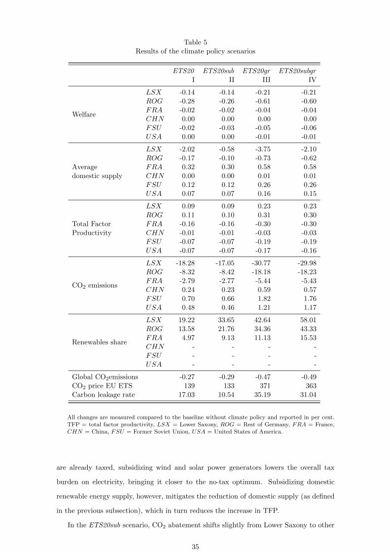
Table 5Results of the climate policy scenarios

ETS20 ETS20sub ETS20gr ETS20subgrI II III IV

Welfare

LSX -0.14 -0.14 -0.21 -0.21ROG -0.28 -0.26 -0.61 -0.60FRA -0.02 -0.02 -0.04 -0.04CHN 0.00 0.00 0.00 0.00FSU -0.02 -0.03 -0.05 -0.06USA 0.00 0.00 -0.01 -0.01

LSX -2.02 -0.58 -3.75 -2.10ROG -0.17 -0.10 -0.73 -0.62

Average FRA 0.32 0.30 0.58 0.58domestic supply CHN 0.00 0.00 0.01 0.01

FSU 0.12 0.12 0.26 0.26USA 0.07 0.07 0.16 0.15

LSX 0.09 0.09 0.23 0.23ROG 0.11 0.10 0.31 0.30

Total Factor FRA -0.16 -0.16 -0.30 -0.30Productivity CHN -0.01 -0.01 -0.03 -0.03

FSU -0.07 -0.07 -0.19 -0.19USA -0.07 -0.07 -0.17 -0.16

CO2 emissions

LSX -18.28 -17.05 -30.77 -29.98ROG -8.32 -8.42 -18.18 -18.23FRA -2.79 -2.77 -5.44 -5.43CHN 0.24 0.23 0.59 0.57FSU 0.70 0.66 1.82 1.76USA 0.48 0.46 1.21 1.17

Renewables share

LSX 19.22 33.65 42.64 58.01ROG 13.58 21.76 34.36 43.33FRA 4.97 9.13 11.13 15.53CHN - - - -FSU - - - -USA - - - -

Global CO2emissions -0.27 -0.29 -0.47 -0.49CO2 price EU ETS 139 133 371 363Carbon leakage rate 17.03 10.54 35.19 31.04

All changes are measured compared to the baseline without climate policy and reported in per cent.TFP = total factor productivity, LSX = Lower Saxony, ROG = Rest of Germany, FRA = France,CHN = China, FSU = Former Soviet Union, USA = United States of America.

are already taxed, subsidizing wind and solar power generators lowers the overall tax

burden on electricity, bringing it closer to the no-tax optimum. Subsidizing domestic

renewable energy supply, however, mitigates the reduction of domestic supply (as defined

in the previous subsection), which in turn reduces the increase in TFP.

In the ETS20sub scenario, CO2 abatement shifts slightly from Lower Saxony to other

35

regions of Europe, including the Rest of Germany. The share of renewables in electricity

generation rises substantially in all regions subject to the EU ETS so that the allowances

price rises less strongly than in the ETS20 scenario. The subsidy encourages the ex-

pansion of renewable electricity sources, reducing the price signal needed to achieve the

emissions target. In this scenario, we find a reduction of global carbon emissions of 0.29%

compared to the baseline without climate policy. This corresponds to an additional reduc-

tion of 0.02 percentage points compared to an isolated reduction in the ETS cap (ETS20

scenario). The renewable energy subsidy reduces the European emissions intensity and

lowers mitigation costs. Therefore, the carbon leakage rate under ETS20sub increases

only by 10.54% compared to the baseline, which is substantially lower than in the ETS20

scenario.

The ETS20gr scenario combines the same absolute emissions reduction as in the pre-

vious scenarios with a growing economy over the time horizon 2011 to 2020. The welfare

costs of achieving the same absolute emissions level are higher when considering economic

growth. Real consumption in Lower Saxony falls by 0.21% and by 0.61% in the Rest

of Germany. We do not observe notable welfare changes outside the EU; in the Former

Soviet Union, for example, welfare declines by 0.05%.

CO2 abatement is more pronounced in the ETS20gr scenario than in the ETS20

scenario because CO2 emissions have to fall more substantially to reach the same absolute

emission level as in the previous scenarios. In Lower Saxony, carbon emissions fall by

30.77%. Reductions in the Rest of Germany are lower. The allowances price increases by

4.7 times to 88 USD per ton of CO2. The share of renewables in electricity generation

rises by 42.64% in Lower Saxony and 34.36% in the Rest of Germany, but only by 11.13%

in France compared to the baseline. We find an increase in the carbon leakage rate of

35.19% compared to the baseline.

Implementing a 10% subsidy for wind and solar power in the ETS20subgr scenario has

similar effects as in the ETS20sub scenario: welfare remains almost unchanged, carbon

abatement shifts from Lower Saxony to other parts of Europe, and the allowances price

rises less strongly than without the subsidy.

Figure 4 illustrates how the electricity mix in Lower Saxony changes in response to the

more ambitious climate policy. The values represent the changes in technology g’s value

share in electricity generation in per cent compared to the baseline.

In the ETS20 scenario, the share of electricity generated from coal-fired power plants

(gCOA) declines by about 26.6% because coal is the technology with the highest emissions

36

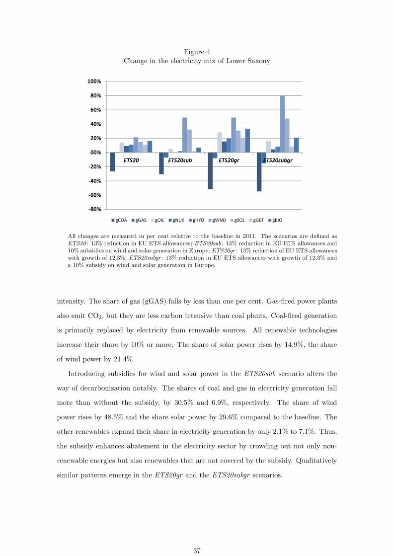
Figure 4Change in the electricity mix of Lower Saxony

-80%

-60%

-40%

-20%

00%

20%

40%

60%

80%

100%

ETS20 ETS20sub ETS20gr ETS20subgr

gCOA gGAS gOIL gNUK gHYD gWND gSOL gGET gBIO

All changes are measured in per cent relative to the baseline in 2011. The scenarios are defined asETS20 : 13% reduction in EU ETS allowances; ETS20sub: 13% reduction in EU ETS allowances and10% subsidies on wind and solar generation in Europe; ETS20gr : 13% reduction of EU ETS allowanceswith growth of 12.3%; ETS20subgr : 13% reduction in EU ETS allowances with growth of 12.3% anda 10% subsidy on wind and solar generation in Europe.

intensity. The share of gas (gGAS) falls by less than one per cent. Gas-fired power plants

also emit CO2, but they are less carbon intensive than coal plants. Coal-fired generation

is primarily replaced by electricity from renewable sources. All renewable technologies

increase their share by 10% or more. The share of solar power rises by 14.9%, the share

of wind power by 21.4%.

Introducing subsidies for wind and solar power in the ETS20sub scenario alters the

way of decarbonization notably. The shares of coal and gas in electricity generation fall

more than without the subsidy, by 30.5% and 6.9%, respectively. The share of wind

power rises by 48.5% and the share solar power by 29.6% compared to the baseline. The

other renewables expand their share in electricity generation by only 2.1% to 7.1%. Thus,

the subsidy enhances abatement in the electricity sector by crowding out not only non-

renewable energies but also renewables that are not covered by the subsidy. Qualitatively

similar patterns emerge in the ETS20gr and the ETS20subgr scenarios.

37

5 Conclusion

This article has introduced a complex general equilibrium model tailored for studying the

interaction between energy and climate policy on the one hand and international trade pol-

icy on the other hand. It combines the theoretical foundations of a Ricardian trade model

(Eaton and Kortum, 2002) with the flexibility and expandability of a Computable General

Equilibrium model. Notable extensions include Constant Elasticity of Substitution (CES)

production and utility functions as well as regional and sectoral disaggregation.

In the currently debated trade agreements, the reduction of non-tariff trade barriers

receives more attention than the removal of tariffs. Our results emphasize the benefits of

tackling non-tariff barriers. They indicate that the reduction of non-tariff barriers gener-

ates larger welfare gains than an equivalent tariff reduction. The worldwide reduction of

non-tariff barriers, however, also results in slightly higher CO2 emissions than the removal

of subsidies and tariffs. Nonetheless, there is also good news from an environmental per-

spective: the reduction of non-tariff barriers induces significant efficiency improvements

via specialization, which eases the achievement of the EU emissions cap. This, in turn,

reduces carbon leakage from the EU to the rest of the world. Consequently, climate pol-

icy negotiators should strive for emissions targets for all important trading economies, as

envisaged by the Paris agreement, in order to avoid increasing emissions induced by the

removal of non-tariff barriers.

The model distinguishes between the German Federal State of Lower Saxony and the

rest of Germany. Lower Saxony is a prime location for renewable electricity generation

in Europe and has a notably different sectoral structure than the rest of Germany. It,

furthermore, is developing ambitious climate policies (NMUEK, 2016) which are expected

to interact with national and international climate policy initiatives as well as with trade

policy. Therefore, Lower Saxony constitutes an excellent subject for studying the role of

sub-national entities in climate policy.

In both, the trade policy and the climate policy simulations, Lower Saxony is affected

to a different extent than the rest of Germany. Its welfare increases more when trade is

liberalized while it simultaneously reduces CO2 emissions by twice as much as the rest of

Germany. Due to its large potential for renewable electricity generation and its sectoral

structure, Lower Saxony reacts with substantially larger CO2 abatement to a reduction

of allowances in the EU ETS.

As long as there is no global climate policy regime implemented, according to our

results, renewable energy support (via a subsidy for wind and solar power) significantly

38

reduces carbon leakage of the European climate policy and slightly reduces global emis-

sions, while the welfare effects are negligible or (in Germany and Italy) slightly positive.

These surprising welfare effects can be attributed to the reduction of existing (tax) dis-

tortions in a second-best world. Renewable energy support in the EU, however, impairs

competition from other regions, which mitigates trade-induced productivity gains from

specialization. Such interconnections of climate and trade policy have so far been widely

overlooked by economic research and policy.

Like in other numerical model analyses, the estimated magnitudes of policy effects de-

pend on the elasticities of substitution in the CES production and consumption functions

and the shape parameter of the Frechet distribution, which we take from the literature.

Thus, we focus on qualitative insights which are robust across different choices of parame-

ter values. In future research, the model can be applied to the analysis of specific regional

trade agreements and their effects on CO2 emissions. Model regions and sectors can be

further disaggregated so that, for example, more German federal states and more power

generation technologies are visible.

6 Acknowledgement

We gratefully acknowledge funding for the project “NEDS – Nachhaltige Energiever-

sorgung Niedersachsen” supported by the Lower Saxony Ministry of Science and Culture

through the “Niedersachsisches Vorab” grant programme (grant ZN3043).

7 References

Aguiar, A., Narayanan, B., and McDougall., R. (2016). An Overview of the GTAP 9 DataBase. Journal of Global Economic Analysis, 1(1):181–208.

Alvarez, F. and Lucas, R. E. (2007). General Equilibrium Analysis of the Eaton-KortumModel of International Trade. Journal of Monetary Economics, 54(6):1726–1768.

Armington, P. S. (1969). A Theory of Demand for Products Distinguished by Place ofProduction. IMF Staff Papers, 16(1):159–178.

Balistreri, E. J. and Hillberry, R. H. (2007). Structural Estimation and the Border Puzzle.Journal of International Economics, 72(2):451–463.

Balistreri, E. J., Hillberry, R. H., and Rutherford, T. F. (2011). Structural Estimationand Solution of International Trade Models with Heterogeneous Firms. Journal ofInternational Economics, 83(2):95–108.

Bohringer, C. (1998). The Synthesis of Bottom-up and Top-down in Energy Policy Mod-eling. Energy Economics, 20(3):233–248.

39

Bohringer, C., Carbone, J. C., and Rutherford, T. F. (2012). Unilateral Climate Pol-icy Design: Efficiency and Equity Implications of Alternative Instruments to ReduceCarbon Leakage. Energy Economics, 34:S208–S217.

Bohringer, C. and Loschel, A. (2006). Promoting Renewable Energy in Europe: A HybridComputable General Equilibrium Approach. Energy Journal, 27(SI):135–150.

Bohringer, C., Rutherford, T. F., and Wiegard, W. (2003). Computable General Equilib-rium Analysis: Opening a Black Box. ZEW Discussion Paper, 03-56.

Bosello, F. and Standardi, G. (2015). A Sub-national CGE model for the EuropeanMediterranean Countries. Research Paper CMCC, RP0274.

Bundesnetzagentur and Bundeskartellamt (2016). Monitoringbericht 2016. Monitoring-bericht gemaß § 63 Abs. 3 i. V. m. § 35 EnWG und § 48 Abs. 3 i. V. m. § 53 Abs.3 GWB. Stand: 30. November 2016. Bundesnetzagentur, Bundeskartellamt, Bonn,Germany.

Bussieck, M. R. and Meeraus, A. (2004). General Algebraic Modeling System (GAMS). InKallrath, J., editor, Modeling Languages in Mathematical Optimization, pages 137–157.Springer US, Boston, MA.

Cai, Y. and Arora, V. (2015). Disaggregating Electricity Generation Technologies in CGEModels: A Revised Technology Bundle Approach with an Application to the U.S. CleanPower Plan. Applied Energy, 154:543–555.

Caliendo, L. and Parro, F. (2015). Estimates of the Trade and Welfare Effects of NAFTA.Review of Economic Studies, 82(1):1–44.

Caliendo, L., Rossi-Hansberg, E., Parro, F., and Sarte, P.-D. (2014). The Impact ofRegional and Sectoral Productivity Changes on the US Economy. NBER WorkingPaper, 20168.

Chen, Y.-H. H., Paltsev, S., Reilly, J. M., Morris, J. F., and Babiker, M. H. (2015). TheMIT EPPA6 Model: Economic Growth, Energy Use, and Food Consumption. JointProgram on the Science and Policy of Global Change Reports, 278.

Costinot, A., Donaldson, D., and Komunjer, I. (2011). What Goods Do Countries Trade?A Quantitative Exploration of Ricardo’s Ideas. Review of Economic Studies, 79:581–608.

Costinot, A., Donaldson, D., and Smith, C. (2016). Evolving Comparative Advantageand the Impact of Climate Change in Agricultural Markets: Evidence from 1.7 MillionFields around the World. Journal of Political Economy, 124(1):205–248.

de Sousa, J. (2012). The Currency Union Effect on Trade is Decreasing over Time.Economics Letters, 117(3):917–920.

Dirkse, S. P. and Ferris, M. C. (1995). The PATH Solver: A Non-Monotone StabilizationScheme for Mixed Complementarity Problems. Optimization Methods and Software,5(2):123–156.

Donaldson, D. (2010). Railroads of the Raj: Estimating the Impact of TransportationInfrastructure. NBER Working Paper, 16487.

Eaton, J. and Kortum, S. (1999). International Technology Diffusion: Theory and Mea-surement. International Economic Review, 40(3):537–570.

Eaton, J. and Kortum, S. (2002). Technology, Geography, and Trade. Econometrica,70(5):1741–1779.

40

Eaton, J. and Kortum, S. (2012). Putting Ricardo to Work. Journal of Economic Per-spectives, 26(2):65–89.

Ellerman, A. D., Convery, F. J., and de Perthuis, C. (2010). Pricing Carbon: The EuropeanUnion Emissions Trading Scheme. Cambridge University Press, Cambridge.

EU Commission (2015). EU ETS Handbook.

EU Commission (2016). EU Reference Scenario 2016. Energy, Transport and GHG Emis-sions. Trends to 2050. Publications Office of the European Union, Luxembourg, Lux-embourg.

Finicelli, A., Pagano, P., and Sbracia, M. (2013). Ricardian Selection. Journal of Inter-national Economics, 89(1):96–109.

Frankel, J. A. and Rose, A. K. (2005). Is Trade Good or Bad for the Environment?Sorting Out the Causality. Review of Economics and Statistics, 87(1):85–91.

ILO (2014). Global Employment Trends 2014: The Risk of a Jobless Recovery. Interna-tional Labour Office, Geneva, Switzerland.

International Energy Agency (2015). Natural Gas Information 2015. International EnergyAgency, Paris, France.

Kortum, S. S. (1997). Research, Patenting, and Technological Change. Econometrica,65(6):1389–1419.

Kronenberg, T. (2009). Construction of Regional Input-Output Tables Using NonsurveyMethods. The Role of Cross-Hauling. International Regional Science Review, 32(1):40–64.

Levchenko, A. A. and Zhang, J. (2016). The Evolution of Comparative Advantage: Mea-surement and Welfare Implications. Journal of Monetary Economics, 78:96–111.

Lipsey, R. G. and Lancaster, K. (1956). The General Theory of Second Best. Review ofEconomic Studies, 24(1):11–32.

Mayer, T. and Zignago, S. (2011). Notes on CEPII’s Distances Measures: The GeoDistDatabase. CEPII Working Paper, 2011-25.

Melitz, M. J. (2003). The Impact of Trade on Intra-Industry Reallocations and AggregateIndustry Productivity. Econometrica, 71(6):1695–1725.

NMUEK (Niedersachsische Ministerium fr Umwelt, Energie und Klimaschutz) (2016).Szenarien zur Energieversorgung in Niedersachsen im Jahr 2050. Hannover, Germany.URL: http://www.umwelt.niedersachsen.de/download/106468/Szenarien_zur_

Energieversorgung_in_Niedersachsen_im_Jahr_2050_-_Gutachten_-_April_

2016_.pdf.

Paltsev, S., Reilly, J. M., Jacoby, H. D., Eckaus, R. S., McFarland, J., Sarofim, M., andBabiker, M. A. M. (2005). The MIT Emissions Prediction and Policy Analysis (EPPA)Model: Version 4. Joint Program on the Science and Policy of Global Change Reports,125.

Peters, G. P. and Hertwich, E. G. (2008). CO2 Embodied in International Trade with Im-plications for Global Climate Policy. Environmental Science & Technology, 42(5):1401–1407.

Pothen, F. and Balistreri, E. J. (2017). Decomposing the Measure of Ignorance: TotalFactor Productivity and Ricardian Selection in the World Economy. Mimeo.

41

Shikher, S. (2012). Putting Industries into the Eaton-Kortum Model. Journal of Inter-national Trade & Economic Development, 21(6):807–837.

Sue Wing, I. (2008). The Synthesis of Bottom-up and Top-down Approaches to ClimatePolicy Modeling: Electric Power Technology Detail in a Social Accounting Framework.Energy Economics, 30(2):547–573.

Timmer, M. P., Dietzenbacher, E., Los, B., Stehrer, R., and de Vries, G. J. (2015).An Illustrated User Guide to the World Input-Output Database: the Case of GlobalAutomotive Production. Review of International Economics, 23(3):575–605.

Tinbergen, J. (1952). On the Theory of Economic Policy. North-Holland PublishingCompany, Amsterdam, Netherlands.

Tobben, J. and Kronenberg, T. (2014). Construction of Multi-Regional Input-OutputTables using the CHARM method. Economic Systems Research, 27(4):487–507.

United Nations (2015). World Population Prospects: The 2015 Revision. United Nations,New York, USA. URL: https://esa.un.org/unpd/wpp/.

van der Werf, E. (2008). Production functions for climate policy modeling: An empiricalanalysis. Energy Economics, 30(6):2964–2979.

Wood, R., Stadler, K., Bulavskaya, T., Lutter, S., Giljum, S., de Koning, A., Kuenen,J., Schutz, H., Acosta-Fernandez, J., Usubiaga, A., Simas, M., Ivanova, O., Weinzettel,J., Schmidt, J., Merciai, S., and Tukker, A. (2014). Global Sustainability Accounting -Developing EXIOBASE for Multi-Regional Footprint Analysis. Sustainability, 7(1):138–163.

World Bank (2016). World Development Indicators 2016. Washington, DC, USA. URL:http://data.worldbank.org/data-catalog/world-development-indicators.

42

Supplementary online appendix

A Definition of sectors and regions

Table A1 lists all sectors between whom we differentiate in the model as well as whether

they are part of the EU ETS.

Table A1Sectors in the model

i Description ETS

AGRI Agriculture NoCOAL Coal NoCRUD Crude oil NoNGAS Natural gas NoPETR Refined petroleum YesFOOD Food production NoMINE Mining NoPAPR Paper and pulp YesCHEM Chemical products YesNMMS Mineral products nec YesIRST Iron and steel YesNFMS Non-ferrous metals YesMANU Manufacturing NoELEC Electricity YesTRNS Transport NoCONS Construction NoSERV Services No

The regions considered in the model are displayed in table A2. The column Disagg

indicates whether a technology-specific electricity generation is considered in region r.

Table A2Regions in the model

r Description Disagg r Description Disagg

LSX Lower Saxony Yes CAN Canada NoROG Rest of Germany Yes KOR Korea NoUSA United States No FSU Former Soviet Union NoCHN China incl. Hong Kong No OCE Australia and Oceania NoJPN Japan No MEX Mexico NoGBR United Kingdom Yes EUR Rest of the European Union NoFRA France Yes ROE Rest of Europe NoIND India No ROA Rest of Asia NoITA Italy Yes ROW Rest of the World NoBRA Brazil No

43

B Elasticities of substitution

Table B1 lists all elasticities of substitution in the model and their values. The values

are taken from (Paltsev et al., 2005). When Paltsev et al. (2005) assume a range of

elasticities, the lowest value is chosen. The elasticity of substitution between activities

in the electricity sector, σELE , is assumed to be zero. This reflects that changes in the

electricity grid cannot compensate for changes in electricity demand or supply, at least

in the short run. The elasticity of substitution between the fixed factor in electricity

generation and the KLF nest ranges from 0.1 (nuclear generation) to 0.6 (wind and solar

power).

Table B1Elasticities of substitution

Elasticity of substitution between Value

Final demand and...

σCE Energy goods 0.4

σCN Non-energy goods 0.25

σC Energy and non-energy aggregates 0.25

Production (non-electricity) and...

σRES KLEM and natural resource 0.6

σKLEM KLE and intermediates 0

σKLE Value added and energy 0.4

σZ Non-energy intermediates 0

σKL Capital and labor 1

σE Electricity and fossil fuels 0.5

σFF Fossil fuels 1

Production (electricity) and...

σELE Activities 0

σOTD Inputs in OTD 0

σGEN Technologies 3

σTECg,r KLF and the fixed factor 0.1-0.6

σKLF Value added and fossil fuels 0.4

σKLg Capital and labor in generation 1

σFFg Fossil fuels in generation 0.3

σ Varieties 2

C Sectoral price index

The productivity of manufacturing a variety zi,r is a random variable. It is Frechet

distributed with the cumulative distribution function Ωi,r = Pr [zi,r ≤ z] = exp[−z−θi

].

44

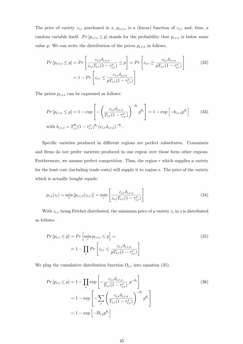
The price of variety zi,r purchased in s, pi,r,s, is a (linear) function of zi,r and, thus, a

random variable itself. Pr [pi,r,s ≤ p] stands for the probability that pi,r,s is below some

value p. We can write the distribution of the prices pi,r,s as follows.

Pr [pi,r,s ≤ p] = Pr

[ci,rδi,r,s

zi,rTi,r(1− τxi,r)≤ p

]= Pr

[zi,r ≥

ci,rδi,r,spTi,r(1− τxi,r)

](32)

= 1− Pr

[zi,r ≤

ci,rδi,r,spTi,r(1− τxi,r)

]

The prices pi,r,s can be expressed as follows:

Pr [pi,r,s ≤ p] = 1− exp

−( ci,rδi,r,sTi,r(1− τxi,r)

)−θipθi

= 1− exp[−bi,r,spθi

](33)

with bi,r,s = T θii,r(1− τxi,r)

θi (ci,rδi,r,s)−θi .

Specific varieties produced in different regions are perfect substitutes. Consumers

and firms do not prefer varieties produced in one region over those form other regions.

Furthermore, we assume perfect competition. Thus, the region r which supplies a variety

for the least cost (including trade costs) will supply it to region s. The price of the variety

which is actually bought equals:

pi,s(zi) = minr

[pi,r,s(zi,r)] = minr

[ci,rδi,r,s

zi,rTi,r(1− τxi,r)

](34)

With zi,r being Frechet distributed, the minimum price of a variety zi in s is distributed

as follows.

Pr [pi,s ≤ p] = Pr[minrpi,r,s ≤ p

]= (35)

= 1−∏r

Pr

[zi,r ≤

ci,rδi,r,spTi,r(1− τxi,r)

]

We plug the cumulative distribution function Ωi,r into equation (35).

Pr [pi,s ≤ p] = 1−∏r

exp

[− ci,rδi,r,sTi,r(1− τxi,r)

p−θi

](36)

= 1− exp

−∑r

(ci,rδi,r,s

Ti,r(1− τxi,r)

)−θipθi

= 1− exp

[−Bi,spθi

]

45

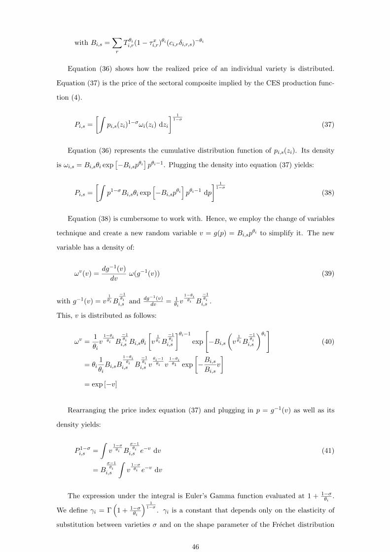
with Bi,s =∑r

T θii,r(1− τxi,r)

θi(ci,rδi,r,s)−θi

Equation (36) shows how the realized price of an individual variety is distributed.

Equation (37) is the price of the sectoral composite implied by the CES production func-

tion (4).

Pi,s =

[∫pi,s(zi)

1−σωi(zi) dzi

] 11−σ

(37)

Equation (36) represents the cumulative distribution function of pi,s(zi). Its density

is ωi,s = Bi,sθi exp[−Bi,spθi

]pθi−1. Plugging the density into equation (37) yields:

Pi,s =

[∫p1−σBi,sθi exp

[−Bi,spθi

]pθi−1 dp

] 11−σ

(38)

Equation (38) is cumbersome to work with. Hence, we employ the change of variables

technique and create a new random variable v = g(p) = Bi,spθi to simplify it. The new

variable has a density of:

ωv(v) =dg−1(v)

dvω(g−1(v)) (39)

with g−1(v) = v1θiB

−1θii,s and dg−1(v)

dv = 1θiv

1−θiθi B

−1θii,s .

This, v is distributed as follows:

ωv =1

θiv

1−θiθi B

−1θii,s Bi,sθi

[v

1θiB

−1θii,s

]θi−1exp

[−Bi,s

(v

1θiB

−1θii,s

)θi](40)

= θi1

θiBi,sB

1−θiθi

i,s B−1θii,s v

θi−1

θi v1−θiθ1 exp

[−Bi,sBi,s

v

]= exp [−v]

Rearranging the price index equation (37) and plugging in p = g−1(v) as well as its

density yields:

P 1−σi,s =

∫v

1−σθi B

σ−1θii,s e−v dv (41)

= Bσ−1θii,s

∫v

1−σθi e−v dv

The expression under the integral is Euler’s Gamma function evaluated at 1 + 1−σθi

.

We define γi = Γ(

1 + 1−σθi

) 11−σ

. γi is a constant that depends only on the elasticity of

substitution between varieties σ and on the shape parameter of the Frechet distribution

46

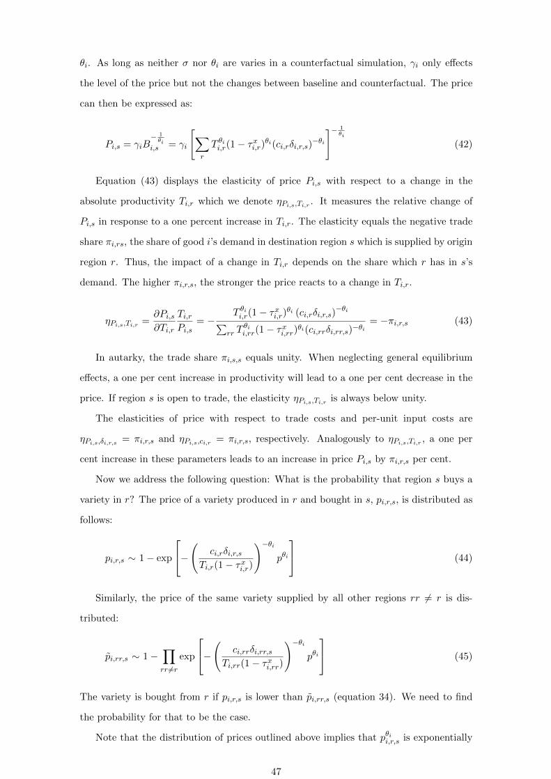
θi. As long as neither σ nor θi are varies in a counterfactual simulation, γi only effects

the level of the price but not the changes between baseline and counterfactual. The price

can then be expressed as:

Pi,s = γiB− 1θi

i,s = γi

[∑r

T θii,r(1− τxi,r)

θi(ci,rδi,r,s)−θi

]− 1θi

(42)

Equation (43) displays the elasticity of price Pi,s with respect to a change in the

absolute productivity Ti,r which we denote ηPi,s,Ti,r . It measures the relative change of

Pi,s in response to a one percent increase in Ti,r. The elasticity equals the negative trade

share πi,rs, the share of good i’s demand in destination region s which is supplied by origin

region r. Thus, the impact of a change in Ti,r depends on the share which r has in s’s

demand. The higher πi,r,s, the stronger the price reacts to a change in Ti,r.

ηPi,s,Ti,r =∂Pi,s∂Ti,r

Ti,rPi,s

= −T θii,r(1− τxi,r)θi (ci,rδi,r,s)

−θi∑rr T

θii,rr(1− τxi,rr)θi(ci,rrδi,rr,s)−θi

= −πi,r,s (43)

In autarky, the trade share πi,s,s equals unity. When neglecting general equilibrium

effects, a one per cent increase in productivity will lead to a one per cent decrease in the

price. If region s is open to trade, the elasticity ηPi,s,Ti,r is always below unity.

The elasticities of price with respect to trade costs and per-unit input costs are

ηPi,s,δi,r,s = πi,r,s and ηPi,s,ci,r = πi,r,s, respectively. Analogously to ηPi,s,Ti,r , a one per

cent increase in these parameters leads to an increase in price Pi,s by πi,r,s per cent.

Now we address the following question: What is the probability that region s buys a

variety in r? The price of a variety produced in r and bought in s, pi,r,s, is distributed as

follows:

pi,r,s ∼ 1− exp

−( ci,rδi,r,sTi,r(1− τxi,r)

)−θipθi

(44)

Similarly, the price of the same variety supplied by all other regions rr 6= r is dis-

tributed:

pi,rr,s ∼ 1−∏rr 6=r

exp

−( ci,rrδi,rr,sTi,rr(1− τxi,rr)

)−θipθi

(45)

The variety is bought from r if pi,r,s is lower than pi,rr,s (equation 34). We need to find

the probability for that to be the case.

Note that the distribution of prices outlined above implies that pθii,r,s is exponentially

47

distributed with the parameter bi,r,s. Analogously, pθii,rr,s is exponentially distributed with

the parameter Bi,s =[∑

rr 6=r Tθii,rr(1− τxi,rr)θi(ci,rrδi,rr,s)−θi

]. We can exploit the following

property of the exponential distribution: if pθii,r,s ∼ exp [bi,s] and pθii,rr,s ∼ exp[Bi,r,s

]are both independently exponentially distributed, then Pr

(pθii,r,s < pθii,rr,s

)=

bi,r,sbi,r,s+Bi,r,s

.

Therefore, the probability that a variety is supplied by r in s is:

πi,r,s = Pr

[pi,r,s ≤ min

rr 6=rpi,rr,s

]=bi,r,sBi,s

(46)

=T θii,r(1− τxi,r)θi (ci,rδi,r,s)

−θi∑rr T

θii,rr(1− τxi,rr)θi(ci,rrδi,rr,s)−θi

D Structural estimation problem

The following set of equations characterizes the structural estimation problem of the trade

model under non-linear restrictions. It is implemented as a Non-Linear Programming

(NLP) problem in GAMS and solved by using the CONOPT algorithm (Drud, 1985). For

sectors which do not produce, we assume Ti,r = 0. Trade shares smaller than 10−8 are

excluded from the optimization criterion to avoid numerical problems. The solution yields

estimates for Si,r and δi,r,s.

min∑i,r,s

[log

πi,r,sπi,s,s

− (ei,r −mi,s − θi log δi,r,s)

]2subject to

log δi,r,s = log(1 + τmi,r,s) + log(1 +∑h

ψh,i,r,s) + log(1− τ ei,r,s) + log δi,r,s

log δi,r,s = µi log distancer,s + β1i borderr,s + β2i languager,s + β3i colonyr,s

+ β4i rtrader,s + β5i currencyr,s + β6i pipelinei,r,s

Si,r = exp(ei,r)

πi,r,s =Si,rδ

−θii,r,s∑

rr Si,rrδ−θii,rr,s

Xi,r =∑s

πi,r,sDi,s

(1 + τmi,r,s)(1 +∑

h ψh,i,r,sPTtr)(1− τ ei,r,s)

+ ζi,rFi

ei,USA = 0

(47)

48

E Disaggregation procedure

E.1 Regional disaggregation

This subsection describes how Germany (DEU) is decomposed into Lower Saxony (LSX)

and the Rest of Germany (ROG). GTAP does not provide data on subnational regions.

The latest input-output table for a German Federal State provided by a statistical agency

is available for Baden-Wuerttemberg in 1990. Furthermore, some scholars have com-

piled recent input-output tables for selected Federal States. Examples include North

Rhine-Westphalia (Kronenberg, 2009), Mecklenburg-Vorpommern (Kronenberg, 2010),

Thuringia (Dettmer and Sauer, 2014), and Baden-Wuerttemberg (Heindl and Voigt, 2012).

Schulte in den Baumen et al. (2015) present research based upon regionally disaggregated

input-output data for Germany; the table itself is, however, not publicly available.

We employ a non-survey approach to derive input-output data for Lower Saxony.

Non-survey methods have been developed to compile subnational input-output tables

with limited primary data, avoiding costly and time-consuming surveys. We rely upon

the Cross-Hauling Adjusted Regionalization Method (CHARM; Kronenberg, 2009) in the

modified version by Tobben and Kronenberg (2014).

E.1.1 Inputs and outputs

We begin by disaggregating final demand. Data on final consumption and investment

by Federal State is available at Arbeitskreis Volkswirtschaftliche Gesamtrechnungen der

Lander (2015b). We use this data to compute Lower Saxony’s shares in final consumption

and investment and split them accordingly.17 The consumption shares in Lower Saxony

and in the Rest of Germany are assumed to be the same.

In the next step, we split the gross output of each sector, Xi,DEU . Data on gross

outputs by sector and Federal State is not recorded in Germany. For the oil and gas

sectors, physical outputs by Federal State are published by Wirtschaftsverband Erdol-

und Erdgasgewinnung (2012). For electricity generation, the physical output share is

computed based upon data from Landerarbeitskreis Energiebilanzen (2016b). For other

sectors, we use Lower Saxony’s employment share to split the sectors. Employment is mea-

sured as the number of employees subject to social insurance contributions (“Sozialver-

17An alternative way to compute Lower Saxony’s final demand is to employ household survey data suchas the Einkommens- und Verbrauchsstichprobe (EVS). It can be used to decompose final consumption byprivate households, the most important component of final demand (Kronenberg, 2010; Heindl and Voigt,2012).

49

sicherungspflichtig Beschaftigte”). Data is compiled by the German Federal Employment

Agency (Bundesagentur fur Arbeit, 2016a,b).18

We assume that all sectors i in Lower Saxony and the Rest of Germany use the same

mix of intermediate inputs and primary factors. The intermediate input of good j in

sector i in Lower Saxony Zj,i,LSX can then be computed by scaling down the intermediate

input of the German sectors (Zj,i,DEU ) according to Lower Saxony’s share in output of i:

Zj,i,LSX =Xi,LSXXi,DEU

Zj,i,DEU . The same procedure is applied to primary factor inputs. We

assume that the same tax rates apply in Lower Saxony and in the Rest of Germany.

Table E1 reports the sector shares in value added of Lower Saxony and the Rest of

Germany as represented by the model in per cent.

Table E1Regional sector shares

i Description LSX ROG

AGRI Agriculture 1.9 1.2COAL Coal 0.0 0.5CRUD Crude oil 0.1 0.0NGAS Natural gas 0.2 0.1PETR Refined petroleum 0.1 0.2FOOD Food production 3.3 2.4MINE Mining 0.3 0.1PAPR Paper and pulp 1.8 1.6CHEM Chemical products 3.5 3.5NMMS Mineral products nec 0.8 0.8IRST Iron and steel 0.5 0.6NFMS Non-ferrous metals 0.4 0.5MANU Manufacturing 13.6 15.2ELEC Electricity 1.5 1.2TRNS Transport 4.1 3.2CONS Construction 5.0 4.3SERV Services 62.9 64.7

Sector shares in value added of Lower Saxony (LSX) and the Rest of Germany (ROG) in per cent.Value added includes payments for natural resources and the fixed factor in the electricity sector.

E.1.2 Trade flows

The next step is to estimate the trade flows of Lower Saxony and the Rest of Germany.

Lower Saxony’s net exports Ni,LSX can be computed by subtracting total demand from

gross outputs (equation 48). Both gross outputs Xi,LSX and total demand Di,LSX are

18For some sectors, in particular agricultural and food-producing industries, the sectoral resolution islower in the employment data than in GTAP. We use the same share of the more aggregate sector inthe employment data for all GTAP sectors. The GTAP sector “dwellings” represents imputed rents. Asthere is no employment data for this sector, we use Lower Saxony’s share in GDP to split it (ArbeitskreisVolkswirtschaftliche Gesamtrechnungen der Lander, 2015a).

50

already estimated. The net exports in the Rest of Germany are computed analogously.

Ni,LSX = Xi,LSX −Di,LSX = Xi,LSX −

∑j

Zi,j,LSX + Ci,LSX

(48)

To calibrate the model, gross trade flows for the new regions need to be estimated. We

differentiate between Germany’s trade flows and the trade flows between the new regions,

Lower Saxony (LSX) the rest of Germany (ROG).

The gross trade flows of Lower Saxony and the Rest of Germany with all other regions

are quantified. Data on exports and imports by Federal States for selected goods is

available at the German statistical office.19 We use this data to compute the shares which

the two regions have in Germany’s imports and exports and split trade flows accordingly.

For sectors without primary data, imports are split according to Lower Saxony’s share in

Germany’s total demand for i (Di,LSX/Di,DEU ) and exports according to Lower Saxony’s

share in Germany’s sales (Xi,LSX/Xi,DEU ).

The Cross-Hauling Adjusted Regionalization Method (CHARM; Tobben and Kronen-

berg, 2014) is used to estimate the gross trade flows of Lower Saxony and the Rest of

Germany. Cross hauling quantifies the simultaneous exports and imports of good i in

r (Flegg et al., 2014). Cross hauling is also known as intra-industry trade in the trade

literature.

Cross hauling or intra-industry trade accounts for a substantial share of international

trade. If measured at the 5-digit Standard International Trade Classification (SITC), 27%

of world merchandise trade was intra-industry trade. If measured at the 3-digit level, this

share increases to 44% (Brulhart, 2009). With regions specializing in varieties within

sectors, our model allows for intra-industry trade.

Let Hi,r denote the cross hauling with good i in region r. Hi,r is defined as the sum of

exports and imports of i less the absolute value of the net export (equation 49). In other

words, it equals the trade volume of i in r minus the absolute value of the net exports.

Ei,r,s =πi,r,sDi,s

(1+τmi,r,s)(1+∑h ψh,i,r,sP

Ttr)(1−τei,r,s)

denotes the absolute export of good i from r to s.

Mi,s,r = πi,s,rDi,r is the absolute import of i from s into r.

Hi,r = (∑s

Ei,r,s +∑s

Mi,s,r)︸ ︷︷ ︸Trade volume

− |∑s

Ei,r,s −∑s

Mi,s,r)|︸ ︷︷ ︸Net exports

(49)

19Destatis genesis database, “Aus- und Einfuhr (Außenhandel): Bundeslander, Jahre, Lander, Waren-systematik”. Code 51000-0036.

51

For any given trade volume, cross hauling or intra-industry trade reaches its maximum

when imports and exports offset each other (∑

sEi,r,s =∑

sMi,s,r). Hi,r equals zero if

region r only imports or only exports a good.

Let Hpi,LSX,ROG denote the bilateral cross hauling potential between Lower Saxony

and the Rest of Germany. It records the upper limit to intra-industry trade between

these two regions. It is determined by the minimum of four terms (equation 50): first,

the output of good i in Lower Saxony minus exports in all other regions (Xi,LSX −∑s 6=LSX,ROGEi,LSX,s). Second, the demand for good i in Lower Saxony minus imports

from all other regions (Di,LSX −∑

s 6=LSX,ROGMi,s,LSX). Third, the output of good i in

the Rest of Germany minus exports in all other regions (Xi,ROG−∑

s 6=LSX,ROGEi,ROG,s).

Fourth, the demand for good i in the Rest of Germany minus imports from all other regions

(Di,ROG−∑

s 6=LSX,ROGMi,s,ROG). Note that the minimum in equation (50) is multiplied

by two. This is necessary because bilateral cross hauling is always double-counted, once

as exports and once as imports.

Hpi,LSX,ROG = 2 min(Xi,LSX −

∑s 6=LSX,ROG

Ei,LSX,s; (50)

Di,LSX −∑

s 6=LSX,ROGMi,s,LSX ;

Xi,ROG −∑

s 6=LSX,ROGEi,ROG,s;

Di,ROG −∑

s 6=LSX,ROGMi,s,ROG)

For Germany as a whole, gross trade flows, production and demand for each good

i are observable. Hence, we can compute Germany’s cross hauling Hi,DEU and its cross

hauling potential. Let χi,DEU denote the share of Germany’s cross hauling potential which

is realized.

χi,DEU =Hi,DEU

2 min (Xi,DEU ;Di,DEU )(51)

As an illustration assume, for instance, that Germany has a cross hauling potential of

one billion US$ in some sector i. This potential is computed by taking the minimum

of Germany’s production and total demand for i. Assume, furthermore, that German

intra-industry trade with i amounts to 500 million US$. In this example, χi,r = 0.5 which

means that Germany realizes 50% of its cross hauling potential.

We now assume that each region in Germany realizes the same fraction of its cross

52

hauling potential as Germany as whole does (χi,DEU = χi,LSX = χi,ROG). Under this

assumption, bilateral cross hauling between LSX and ROG equals:

Hi,LSX,ROG = 2χi,DEU Hpi,LSX,ROG (52)

With bilateral cross hauling quantified, we can compute gross exports of i from Lower

Saxony to the Rest of Germany, Ei,LSX,ROG. Bilateral cross hauling is defined as Hi,r,s =

Ei,r,s + Mi,s,r − |Ni,r|. Solving for the trade volume yields Ei,r,s + Mi,s,r = Hi,r + |Ni,r|.

Furthermore, the gross exports of region r can be expressed as Ei,r,s =Ei,r,s+Mi,s,r+Ni,r

2 .

Plugging in the trade volume leads to the following formula which we use to compute

Ei,LSX,ROG. It only contains known parameters. Gross exports of the Rest of Germany

are computed analogously.

Ei,LSX,ROG =Hi,LSX,ROG + |Ni,LSX | +Ni,LSX

2(53)

This step completes the disaggregation of Germany into Lower Saxony and the Rest

of Germany.

E.2 Sectoral disaggregation

In the first step of the disaggregation of the electricity sector, all intermediate inputs

except coal (COAL), natural gas (NGAS), and crude oil (CRUD) are allocated to an

overhead, transmission, and distribution (OTD) activity. See figure 3 which displays the

allocation of intermediate and primary factor inputs to the activities in the electricity

sector. The input of coal, natural gas, crude oil, as well as value added is distributed

among the generation technologies.

To satisfy the accounting identities, the disaggregated electricity sector has to fulfill

three sets of restrictions. First, the sum of inputs of factor f in all technologies g, Vf,g,r,

has to equal the input of f into the electricity sector, Vf,ELEC,r.

Vf,ELEC,r =∑g

Vf,g,r (54)

Analogously, the input of coal, gas, and crude oil into the technologies g (Zj,g,r) has

to equal the input into the electricity sector (Zj,ELEC,r). We allocate each of them to one

technology. The input of coal is allocated to coal-fired plants (gCOA), the input of crude

53

oil to oil-fired plants (gOIL) and the input of gas to gas-fired plants (gGAS).

Zj,ELEC,r =∑g

Zj,g,r ∀j ∈ COAL,NGAS,CRUD (55)

The third restriction concerns the outputs. The gross output of all technologies (Xg,r)

as well as of the OTD activity (XOTD,r) have to equal the output of the electricity sector

in GTAP (XELEC,r).20

XELEC,r = XOTD,r +∑g

Xg,r (56)

We implement two criteria which operationalize the difference between the data and

the disaggregated electricity sector (Sue Wing, 2008). Let αtecg,r denote the share of tech-

nology g in the total electricity generation of region r. Furthermore, let αvf,g,r denote the

input share of primary factor f in technology g.21 We minimize the following expression

(57). Both αtecg,r and αvf,g,r are exogenous parameters. To avoid outliers in the estimated

output shares we add the constraint |αtecg,r| ≤ εα (with εα = 0.2).

minXg,r,Vu,g,r

κ∑g

[1

αtecg,r

Xg,r∑ggXgg,r

− 1

]2+ (57)

(1− κ)∑g,f

1

αvf,g,r

Vf,g,r

(1 + τvf,g,r

)Xg,r

2

The first sum in equation (57) measures the squared difference between g’s share in

electricity generation in the data and the share of technology g in the total sales of the

electricity sector after the disaggregation. Note that αtecg,r is calculated based upon the

physical electricity generation, whileXg,r∑gg Xgg,r

is the share of g in electricity sales.

The second sum records the differences between the input shares from the data, αvf,g,r,

and the input share in the disaggregated GTAP data. κ is a weighting parameter which

we assume to be 0.9. The problem is implemented as a Non-Linear Programming (NLP)

problem in GAMS and solved by using the CONOPT algorithm.

For the disaggregation, we draw on the following data source. The electricity output

by technology is taken from the extended world energy balances provided by Interna-

tional Energy Agency (2015). For Germany, we used data on gross electricity generation

20The output of technology g is defined as Xg,r =∑f Vf,g,r(1+τvf,g,r)+

∑j Zj,g,r(1+τzj,g,r). Analogously,

the output of the OTD activity is XOTD,r =∑j Zj,OTD,r(1 + τzj,OTD,r).

21We do not introduce a criterion for the inputs of fossil primary energy carriers. Their inputs areallocated to the respective technology, rendering this criterion uninformative.

54

by technology and Federal State from Landerarbeitskreis Energiebilanzen (2016a) and

Landerarbeitskreis Energiebilanzen (2016b).

The input shares in electricity generation are approximated by input shares in the

levelized cost of electricity (LCoE). Schroder et al. (2013) conduct a literature overview

and propose a harmonized dataset of LCoE estimates. It contains estimates for the time

from 2010 to 2050 and is focused on electricity generation in Europe. Therefore, we use

their shares to quantify αvu,g,r.

The optimization procedure leads to an electricity mix which is close to the mix re-

ported by the statistical data.

F Emissions trading

This subsection describes the process which is used to implement the European Union

Emissions Trading System (EU ETS) as well as the data employed. The CO2 emissions

by sector are taken from the GTAP database. According to the EU Commission, in

2011“7.9 billion allowances were traded, with a value of $147.9 billion” (EU Commission,

2012). This implies an average allowances price of 18.72 USD per ton of CO2.

In phase I and II of the EU ETS, the overall cap on CO2 was determined in a bottom-

up manner. Member states submitted national allocation plans to the EU Commission

which reviewed and then either confirmed or rejected them. The final emissions caps

per region added up to 2.08 billion tons of CO2 per year (EU Commission, 2007) in the

second phase. We assume that income from selling allowances is distributed according to

the share of each region in the overall cap. The data on the emissions caps by country is

taken from EU Commission (2007). We split Germany’s cap according to Lower Saxony’s

share in population.

Based upon this data, the GTAP database is modified in three steps. The first step is

to allocate the input of allowances to the fossil fuel nests in the EU ETS sectors. Figures

2 and 3 show how the how allowances and intermediate inputs of fuels are combined.22

The following sectors are part of the EU ETS: refined petroleum (PETR), paper and

pulp (PAPR), chemical products (CHEM), mineral products not elsewhere classified

(NMMS), iron and steel (IRST ), non-ferrous metals (NFMS), and electricity (ELEC).

22Table A1 shows which sectors are assumed to be part of the EU ETS. We assume that the sectorsas a whole are covered by the emissions trading scheme. The sectors in the EU ETS are energy-intensiveindustries dominated by large companies which account for the vast majority of the emissions. Ignoringsmall firms which are part of these industries but not subject to the EU ETS is unlikely to bias the results.

55

The second step is to quantify the output subsidy φETSi,r . It reflects that the majority

allowances were allocated freely to the sectors in the second phase of the EU ETS. We

assume that 90% of allowances are freely allocated.23

The third step is to balance the ETS sectors’ taxes. According to the European System

of Accounts 2010 (Eurostat, 2013), payments for allowances are classified as output taxes.

In the model, payments for allowances are effectively (endogenous) taxes on fossil fuel

inputs. We therefore adjust the output tax rate τxi,r to equate payments to the government.

For the sectors which are not part of the EU ETS, we assume that no additional

climate policy is introduced beyond measures in force in 2011. Taxes on fossil fuel inputs

are recorded in the GTAP data.

G References of the appendix

Arbeitskreis Volkswirtschaftliche Gesamtrechnungen der Lander (2015a). Bruttoinland-sprodukt, Bruttowertschopfung in den Landern der Bundesrepublik Deutschland 2000bis 2014. Reihe 1, Band 1. Statistisches Landesamt Baden-Wurttemberg, Stuttgart,Germany. URL: http://www.vgrdl.de/.

Arbeitskreis Volkswirtschaftliche Gesamtrechnungen der Lander (2015b). Entstehung,Verteilung und Verwendung des Bruttoinlandsprodukts in den Landern der Bundesre-publik Deutschland. 1991 bis 2014. Reihe 1, Band 5. Statistisches Landesamt Baden-Wurttemberg, Stuttgart, Germany. URL: http://www.vgrdl.de/.

Brulhart, M. (2009). An Account of Global Intra-industry Trade, 1962-2006. WorldEconomy, 32(3):401–459.

Bundesagentur fur Arbeit (2016a). Sozialversicherungspflichtig und geringfugigBeschaftigte nach Wirtschaftszweigen der WZ 2008 in Deutschland. Statistikder Bundesagentur fur Arbeit, Nurnberg, Germany. URL: http://statistik.

arbeitsagentur.de.

Bundesagentur fur Arbeit (2016b). Sozialversicherungspflichtig und geringfugigBeschaftigte nach Wirtschaftszweigen der WZ 2008 in Niedersachsen. Statistikder Bundesagentur fur Arbeit, Nurnberg, Germany. URL: http://statistik.

arbeitsagentur.de.

Dettmer, B. and Sauer, T. (2014). Regionalokonomische Auswirkungen eines geplantenPumpspeicherkraftwerks: Eine Input-Output-Analyse fur den Freistaat Thuringen.Zeitschrift fur Energiewirtschaft, 38(4):255–268.

Drud, A. (1985). CONOPT: A GRG Code for Large Sparse Dynamic Nonlinear Opti-mization Problems. Mathematical Programming, 31(2):153–191.

23The European Environment Agency provides data on both freely allocated allowances and verifiedemissions. These cannot easily be translated into a share of free allocation for two reasons. First, datais recorded by installation and not by sector. Second, the data implies a share of free allocation greaterthen 100% for most types of installations. The allowances which they received for free exceeded their totalemissions.

56

EU Commission (2007). Emissions trading: EU-wide cap for 2008-2012 set at 2.08 billionallowances after assessment of national plans for Bulgaria. European Commission PressReleases Database, IP/07/1614.

EU Commission (2012). EU ETS 2005-2012. URL: https://ec.europa.eu/clima/

policies/ets/pre2013.

Eurostat (2013). European System of Accounts 2010. Publications Office of the EuropeanUnion, Luxembourg, Luxembourg.

Flegg, A. T., Huang, Y., and Tohmo, T. (2014). Cross-Hauling and Regional Input-Output Tables: The Case of the Province of Hubei, China. University of the West ofEngland. Economics Working Paper Series, 1310.

Heindl, P. and Voigt, S. (2012). Employment Effects of Regional Climate Policy: The Caseof Renewable Energy Promotion by Feed-In Tariffs. ZEW Discussion Paper, 12-066.

International Energy Agency (2015). Extended World Energy Balances. 2015 Edition.International Energy Agency, Paris, France.

Kronenberg, T. (2009). Construction of Regional Input-Output Tables Using NonsurveyMethods. The Role of Cross-Hauling. International Regional Science Review, 32(1):40–64.

Kronenberg, T. (2010). Erstellung einer Input-Output-Tabelle fur Mecklenburg-Vorpommern. AStA Wirtschafts- und Sozialstatistisches Archiv, 4(3):223–248.

Landerarbeitskreis Energiebilanzen (2016a). Bruttostromerzeugung aus Erneuer-baren Energietragern in GWh (Stand 31.03.2016). Statistisches Landesamt Bre-men, Bremen, Germany. URL: http://www.lak-energiebilanzen.de/dseiten/

energiebilanzenAktuelleErgebnisse.cfm.

Landerarbeitskreis Energiebilanzen (2016b). Bruttostromerzeugung nach En-ergietragern in GWh (Stand 31.03.2016). Statistisches Landesamt Bremen,Bremen, Germany. URL: http://www.lak-energiebilanzen.de/dseiten/

energiebilanzenAktuelleErgebnisse.cfm.

Paltsev, S., Reilly, J. M., Jacoby, H. D., Eckaus, R. S., McFarland, J., Sarofim, M., andBabiker, M. A. M. (2005). The MIT Emissions Prediction and Policy Analysis (EPPA)Model: Version 4. Joint Program on the Science and Policy of Global Change Reports,125.

Schroder, A., Kunz, F., Meiss, J., Mendelevitch, R., and von Hirschhausen, C. (2013).Current and Prospective Costs of Electricity Generation until 2050. DIW Data Docu-mentation, 68.

Schulte in den Baumen, H., Tobben, J., and Lenzen, M. (2015). Labour Forced Impactsand Production Losses due to the 2013 Flood in Germany. Journal of Hydrology,527:142–150.

Sue Wing, I. (2008). The Synthesis of Bottom-up and Top-down Approaches to ClimatePolicy Modeling: Electric Power Technology Detail in a Social Accounting Framework.Energy Economics, 30(2):547–573.

Tobben, J. and Kronenberg, T. (2014). Construction of Multi-Regional Input-OutputTables using the CHARM method. Economic Systems Research, 27(4):487–507.

Wirtschaftsverband Erdol- und Erdgasgewinnung (2012). Jahresberichte Zahlen undFakten 2012. Wirtschaftsverband Erdol- und Erdgasgewinnung e. V., Han-nover, Germany. URL: http://www.bveg.de/content/download/3720/38766/file/WEG-Jahresbericht2012.pdf.

57