![Agricultural Productivity, Comparative Advantage, and ...lib.cufe.edu.cn/upload_files/other/4_20140530024310_[59]matsuyama... · Agricultural Productivity, Comparative Advantage,](https://static.fdocuments.us/doc/165x107/5b1eab367f8b9a22028bd7eb/agricultural-productivity-comparative-advantage-and-libcufeeducnuploadfilesother42014053002431059matsuyama.jpg)
Chapter 3 Labor Productivity and Comparative...
114
Chapter 3 Labor Productivity and Comparative Advantage: The Ricardian Model
Transcript of Chapter 3 Labor Productivity and Comparative...
Chapter 3
Labor Productivity and Comparative Advantage: The Ricardian Model
Copyright ©2015 Pearson Education, Inc. All rights reserved. 3-2
Preview
• Opportunity costs and comparative advantage• Production possibilities• Relative supply, relative demand & relative prices• Trade possibilities and gains from trade• Wages and trade• Misconceptions about comparative advantage• Transportation costs and non-traded goods• Empirical evidence
Copyright ©2015 Pearson Education, Inc. All rights reserved. 3-3
Introduction
• Sources of differences across countries that lead to gains from trade:– The Ricardian model (Chapter 3) examines
differences in the productivity of labor (due to differences in technology) between countries.
– The Heckscher-Ohlin model (Chapter 5) examines differences in labor, labor skills, physical capital, land, or other factors of production between countries.
Copyright ©2015 Pearson Education, Inc. All rights reserved. 3-4
Ricardian Model Assumptions
1. Two countries: domestic and foreign. 2. Two goods: wine and cheese.3. Labor is the only resource needed for production.4. Labor productivity is constant.5. Labor productivity varies across countries due to
differences in technology.6. The supply of labor in each country is constant.7. Labor markets are competitive.8. Workers are mobile across sectors.
Copyright ©2015 Pearson Education, Inc. All rights reserved. 3-5
Comparative Advantage
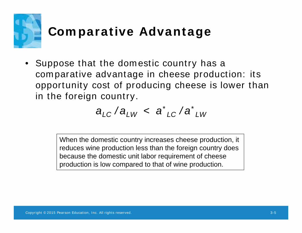
• Suppose that the domestic country has a comparative advantage in cheese production: its opportunity cost of producing cheese is lower than in the foreign country.
aLC /aLW < a*LC /a*
LW
When the domestic country increases cheese production, it reduces wine production less than the foreign country does because the domestic unit labor requirement of cheese production is low compared to that of wine production.
Copyright ©2015 Pearson Education, Inc. All rights reserved. 3-6
Comparative Advantage
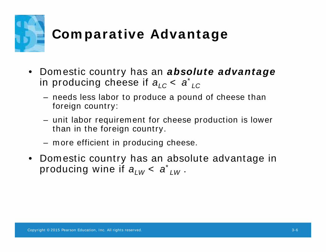
• Domestic country has an absolute advantagein producing cheese if aLC < a*
LC
– needs less labor to produce a pound of cheese than foreign country:
– unit labor requirement for cheese production is lower than in the foreign country.
– more efficient in producing cheese.
• Domestic country has an absolute advantage in producing wine if aLW < a*
LW .
Copyright ©2015 Pearson Education, Inc. All rights reserved. 3-7
Comparative Advantage
• Even a country that is the most (or least) efficient producer of all goods still can benefit from trade.– Even a (rich, developed) country with an absolute
advantage in both goods will have a comparative advantage in only one good — the good where its absolute advantage is larger.
– Even a (poor, developing) country with an absolute disadvantage in both goods will have a comparative advantage in producing something — the good where its absolute disadvantage is smaller.
Copyright ©2015 Pearson Education, Inc. All rights reserved. 3-8
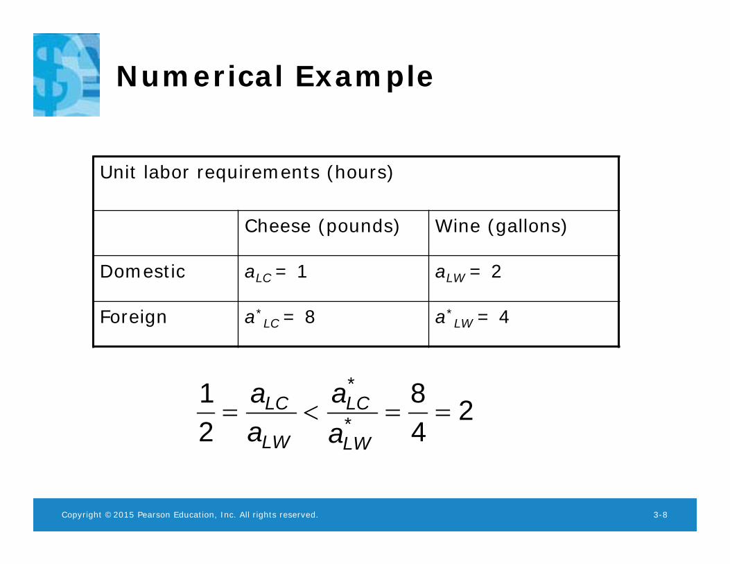
Numerical Example
Unit labor requirements (hours)
Cheese (pounds) Wine (gallons)
Domestic aLC = 1 aLW = 2
Foreign a*LC = 8 a*
LW = 4
248
21
*
*
LW
LC
LW
LC
aa
aa
Copyright ©2015 Pearson Education, Inc. All rights reserved. 3-9
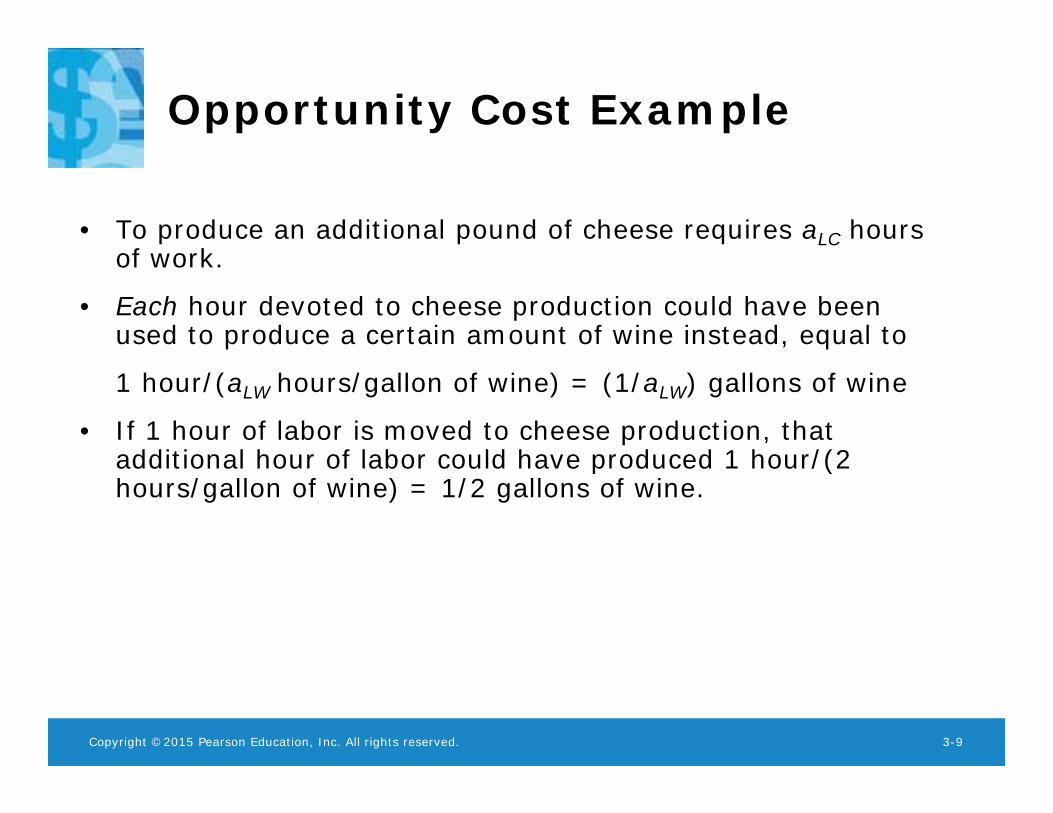
Opportunity Cost Example
• To produce an additional pound of cheese requires aLC hours of work.
• Each hour devoted to cheese production could have been used to produce a certain amount of wine instead, equal to
1 hour/(aLW hours/gallon of wine) = (1/aLW) gallons of wine
• If 1 hour of labor is moved to cheese production, that additional hour of labor could have produced 1 hour/(2 hours/gallon of wine) = 1/2 gallons of wine.
Copyright ©2015 Pearson Education, Inc. All rights reserved. 3-10
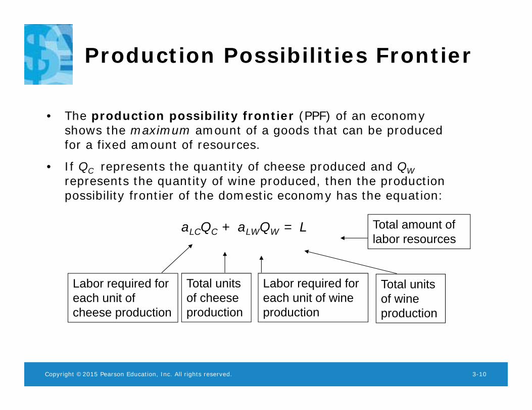
Production Possibilities Frontier
• The production possibility frontier (PPF) of an economy shows the maximum amount of a goods that can be produced for a fixed amount of resources.
• If QC represents the quantity of cheese produced and QWrepresents the quantity of wine produced, then the production possibility frontier of the domestic economy has the equation:
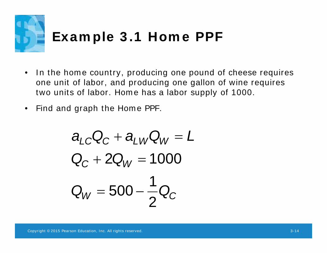
aLCQC + aLWQW = L
Total units of wine production
Labor required for each unit of cheese production
Total units of cheese production
Labor required for each unit of wine production
Total amount of labor resources
Copyright ©2015 Pearson Education, Inc. All rights reserved. 3-11
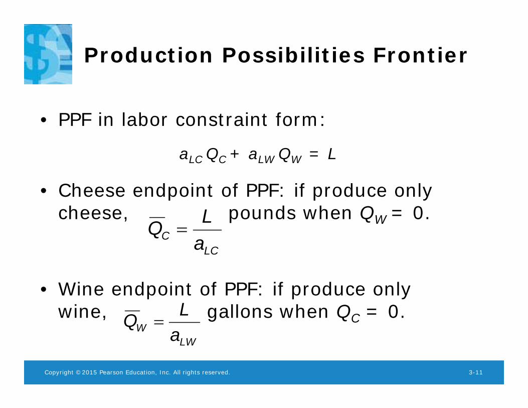
Production Possibilities Frontier
• PPF in labor constraint form:
aLC QC + aLW QW = L
• Cheese endpoint of PPF: if produce only cheese, pounds when QW = 0.
• Wine endpoint of PPF: if produce only wine, gallons when QC = 0.
LCC a
LQ
LWW a
LQ
Copyright ©2015 Pearson Education, Inc. All rights reserved. 3-12
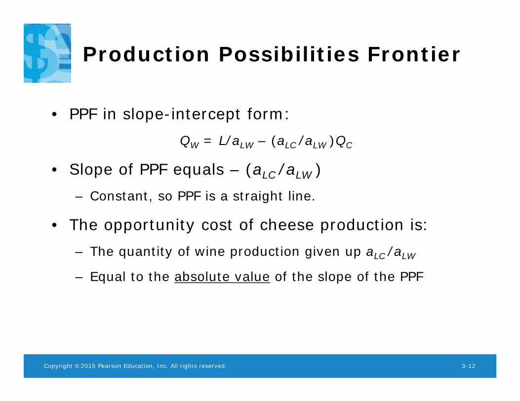
Production Possibilities Frontier
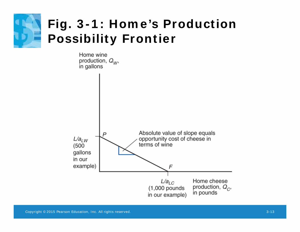
• PPF in slope-intercept form:QW = L/aLW – (aLC /aLW )QC
• Slope of PPF equals – (aLC /aLW )– Constant, so PPF is a straight line.
• The opportunity cost of cheese production is:– The quantity of wine production given up aLC /aLW
– Equal to the absolute value of the slope of the PPF
Copyright ©2015 Pearson Education, Inc. All rights reserved. 3-13
Fig. 3-1: Home’s Production Possibility Frontier
Copyright ©2015 Pearson Education, Inc. All rights reserved. 3-14
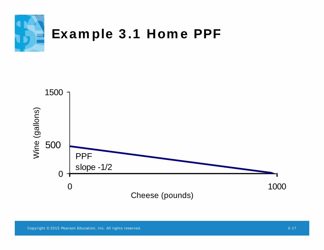
Example 3.1 Home PPF
• In the home country, producing one pound of cheese requires one unit of labor, and producing one gallon of wine requires two units of labor. Home has a labor supply of 1000.
• Find and graph the Home PPF.
CW
WC
WLWCLC
QQLQaQa
21500
10002
Copyright ©2015 Pearson Education, Inc. All rights reserved. 3-15
Example 3.1 Home PPF
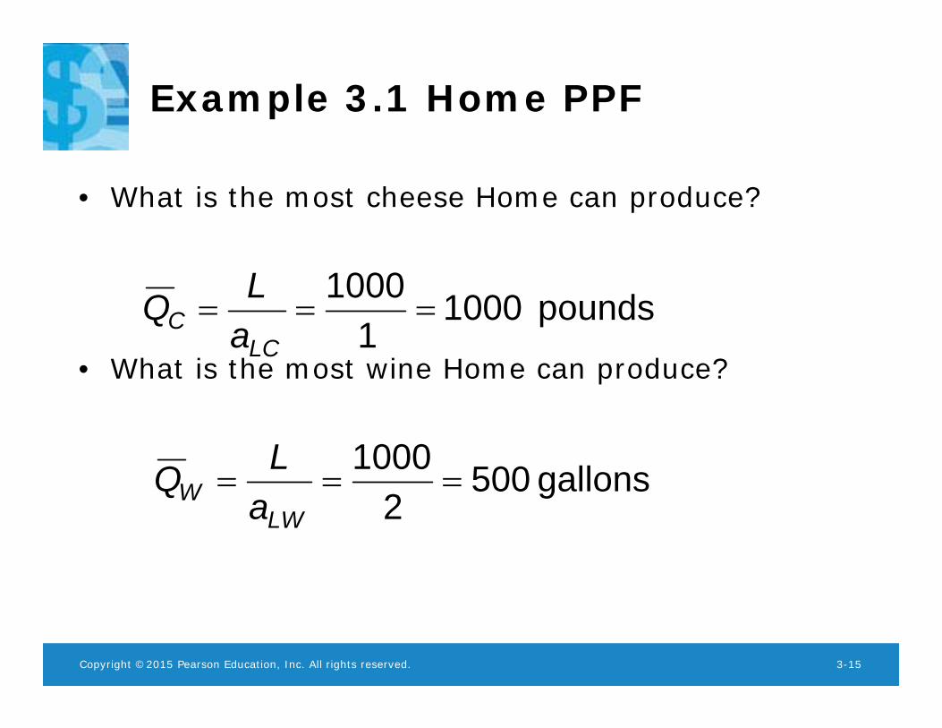
• What is the most cheese Home can produce?
• What is the most wine Home can produce?
pounds 10001
1000
LCC a
LQ
gallons 5002
1000
LWW a
LQ
Copyright ©2015 Pearson Education, Inc. All rights reserved. 3-16
Example 3.1 Home PPF
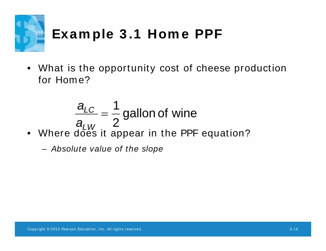
• What is the opportunity cost of cheese production for Home?
• Where does it appear in the PPF equation?– Absolute value of the slope
wineof gallon 21
LW
LC
aa
Copyright ©2015 Pearson Education, Inc. All rights reserved. 3-17
Example 3.1 Home PPF
0
1500
0 1000Cheese (pounds)
Win
e (g
allo
ns)
PPFslope -1/2
500
Copyright ©2015 Pearson Education, Inc. All rights reserved. 3-18
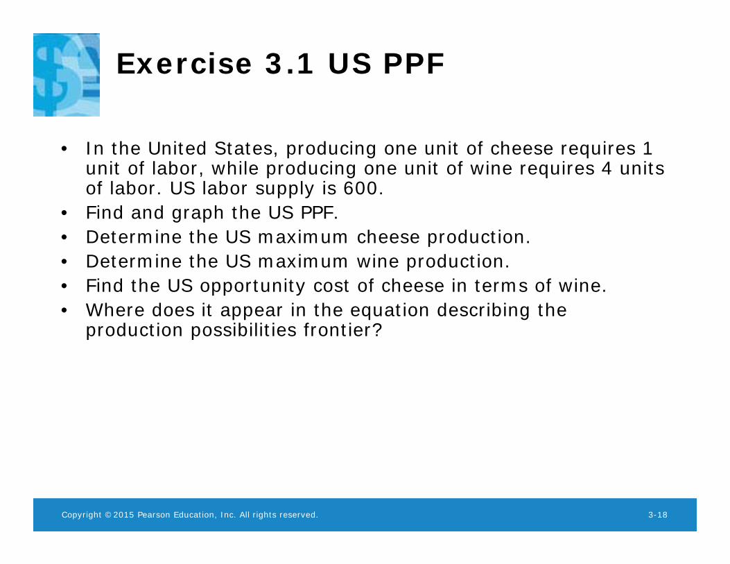
Exercise 3.1 US PPF
• In the United States, producing one unit of cheese requires 1 unit of labor, while producing one unit of wine requires 4 units of labor. US labor supply is 600.
• Find and graph the US PPF.• Determine the US maximum cheese production.• Determine the US maximum wine production.• Find the US opportunity cost of cheese in terms of wine. • Where does it appear in the equation describing the
production possibilities frontier?
Copyright ©2015 Pearson Education, Inc. All rights reserved. 3-19
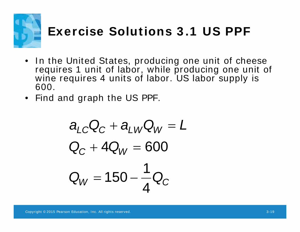
Exercise Solutions 3.1 US PPF
• In the United States, producing one unit of cheese requires 1 unit of labor, while producing one unit of wine requires 4 units of labor. US labor supply is 600.
• Find and graph the US PPF.
CW
WC
WLWCLC
QQLQaQa
41150
6004
Copyright ©2015 Pearson Education, Inc. All rights reserved. 3-20
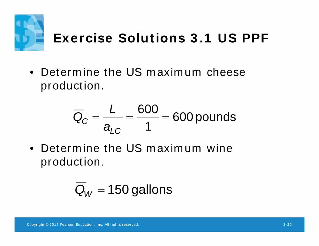
Exercise Solutions 3.1 US PPF
• Determine the US maximum cheese production.
• Determine the US maximum wine production.
pounds 6001
600
LCC a
LQ
gallons 150WQ
Copyright ©2015 Pearson Education, Inc. All rights reserved. 3-21
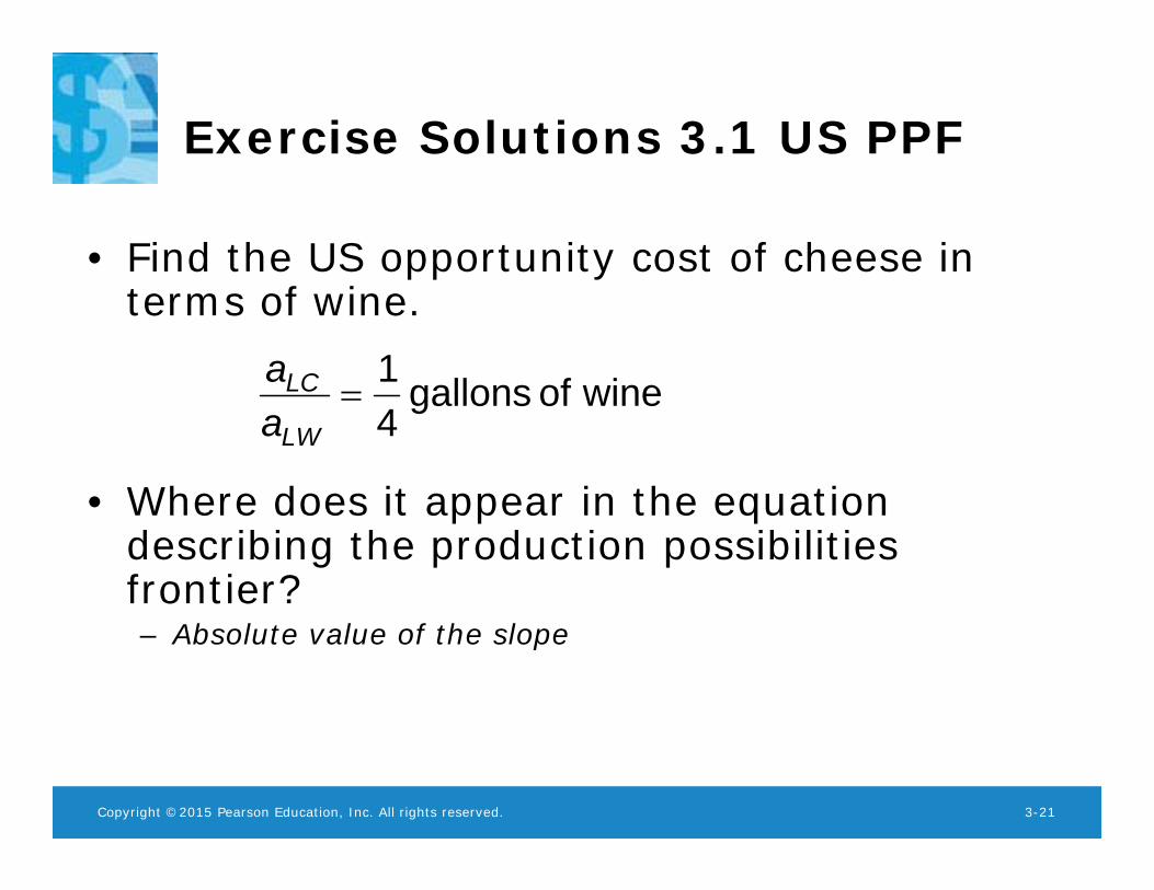
Exercise Solutions 3.1 US PPF
• Find the US opportunity cost of cheese in terms of wine.
• Where does it appear in the equation describing the production possibilities frontier?– Absolute value of the slope
wineof gallons 41
LW
LC
aa
Copyright ©2015 Pearson Education, Inc. All rights reserved. 3-22
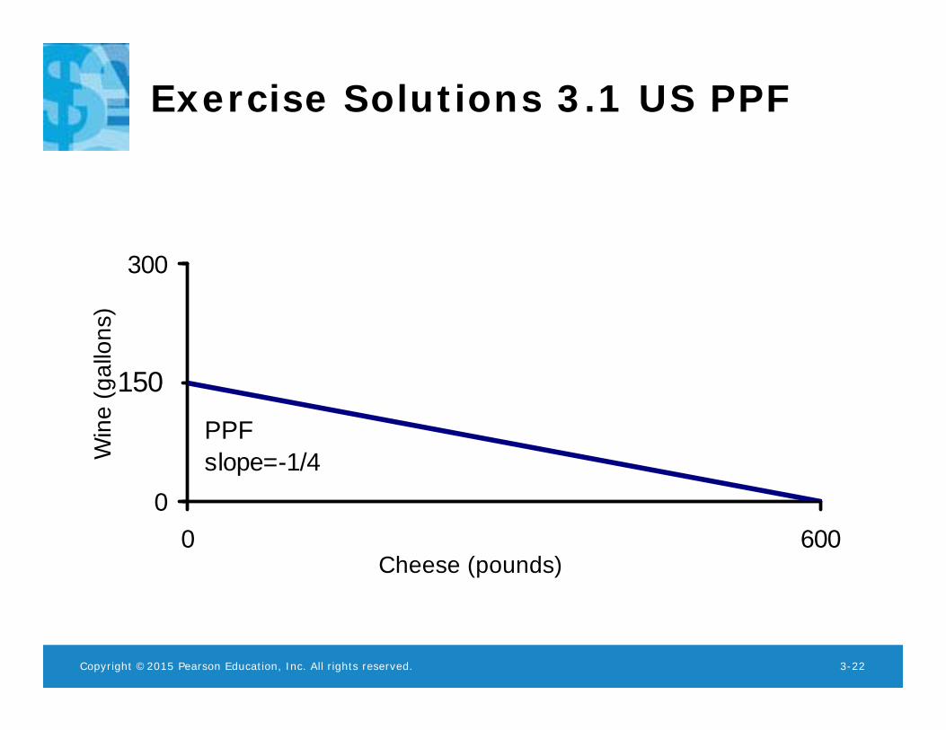
Exercise Solutions 3.1 US PPF
0
300
0 600Cheese (pounds)
Win
e (g
allo
ns)
PPFslope=-1/4
150
Copyright ©2015 Pearson Education, Inc. All rights reserved. 3-23
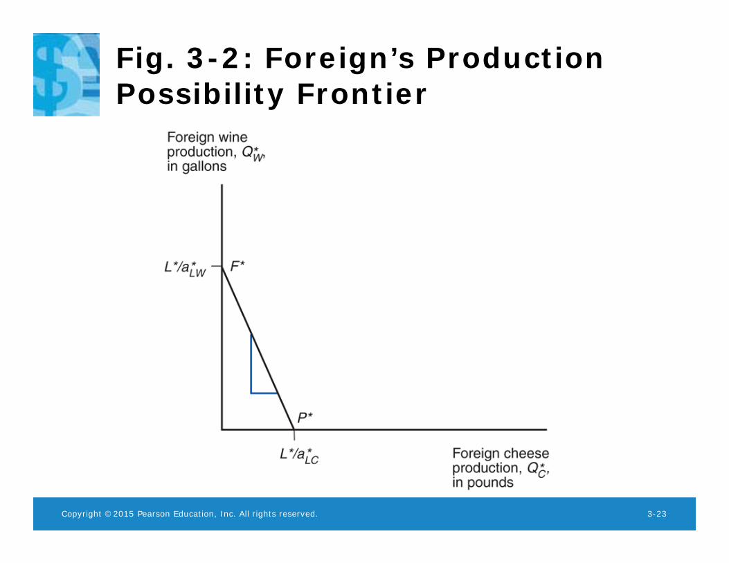
Fig. 3-2: Foreign’s Production Possibility Frontier
Copyright ©2015 Pearson Education, Inc. All rights reserved. 3-24
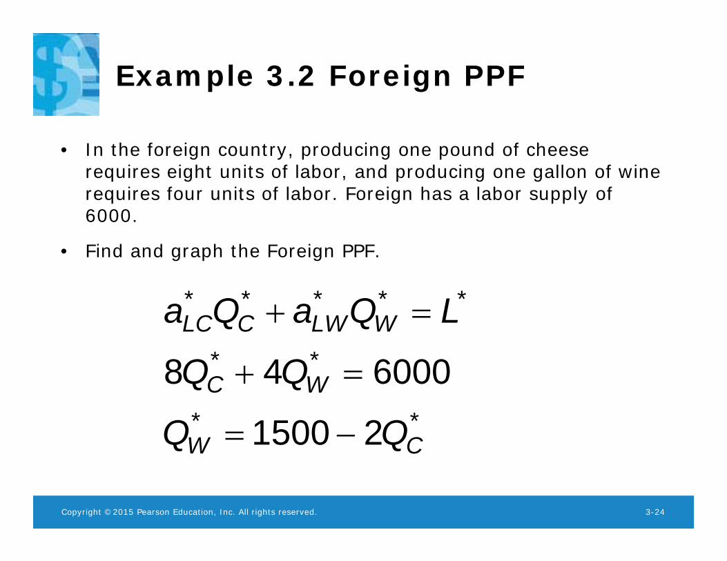
Example 3.2 Foreign PPF
• In the foreign country, producing one pound of cheese requires eight units of labor, and producing one gallon of wine requires four units of labor. Foreign has a labor supply of 6000.
• Find and graph the Foreign PPF.
**
**
*****
21500
600048
CW
WC
WLWCLC
LQaQa
Copyright ©2015 Pearson Education, Inc. All rights reserved. 3-25
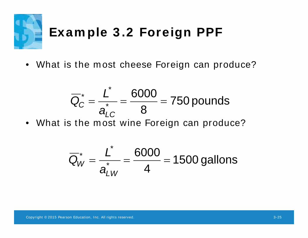
Example 3.2 Foreign PPF
• What is the most cheese Foreign can produce?
• What is the most wine Foreign can produce?
pounds 7508
6000*
**
LCC a
LQ
gallons 15004
6000*
**
LWW a
LQ
Copyright ©2015 Pearson Education, Inc. All rights reserved. 3-26
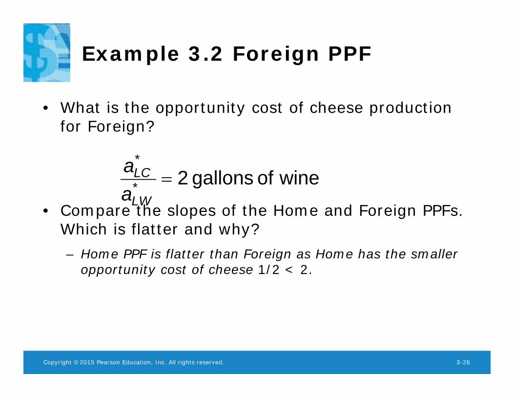
Example 3.2 Foreign PPF
• What is the opportunity cost of cheese production for Foreign?
• Compare the slopes of the Home and Foreign PPFs. Which is flatter and why?– Home PPF is flatter than Foreign as Home has the smaller
opportunity cost of cheese 1/2 < 2.
wineof gallons 2*
*
LW
LC
aa
Copyright ©2015 Pearson Education, Inc. All rights reserved. 3-27
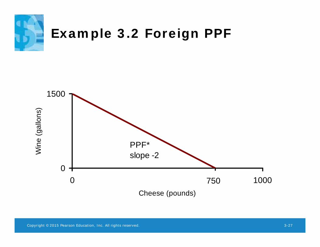
Example 3.2 Foreign PPF
0
1500
0 1000Cheese (pounds)
Win
e (g
allo
ns)
PPF*slope -2
750
Copyright ©2015 Pearson Education, Inc. All rights reserved. 3-28
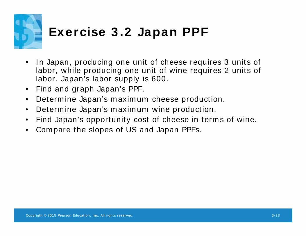
Exercise 3.2 Japan PPF
• In Japan, producing one unit of cheese requires 3 units of labor, while producing one unit of wine requires 2 units of labor. Japan’s labor supply is 600.
• Find and graph Japan’s PPF.• Determine Japan’s maximum cheese production.• Determine Japan’s maximum wine production.• Find Japan’s opportunity cost of cheese in terms of wine.• Compare the slopes of US and Japan PPFs.
Copyright ©2015 Pearson Education, Inc. All rights reserved. 3-29
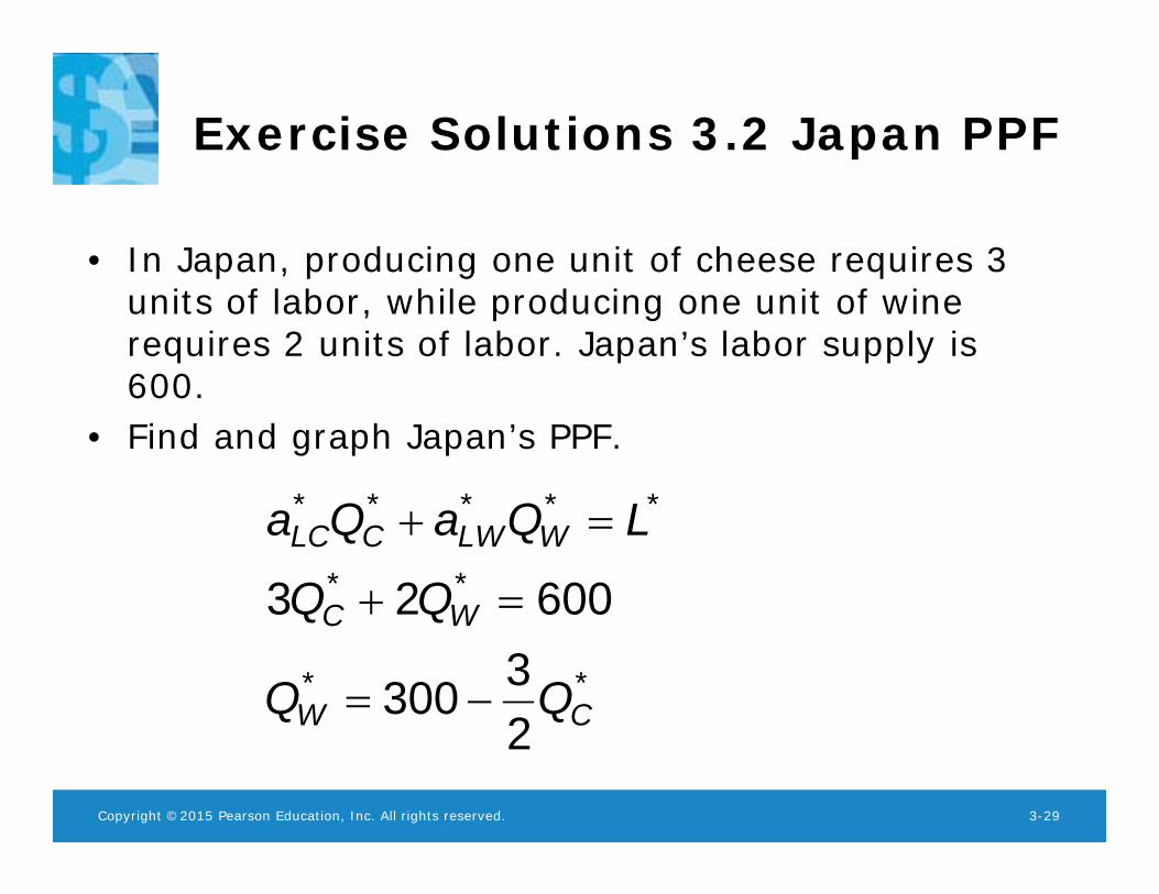
Exercise Solutions 3.2 Japan PPF
• In Japan, producing one unit of cheese requires 3 units of labor, while producing one unit of wine requires 2 units of labor. Japan’s labor supply is 600.
• Find and graph Japan’s PPF.
**
**
*****
23300
60023
CW
WC
WLWCLC
LQaQa
Copyright ©2015 Pearson Education, Inc. All rights reserved. 3-30
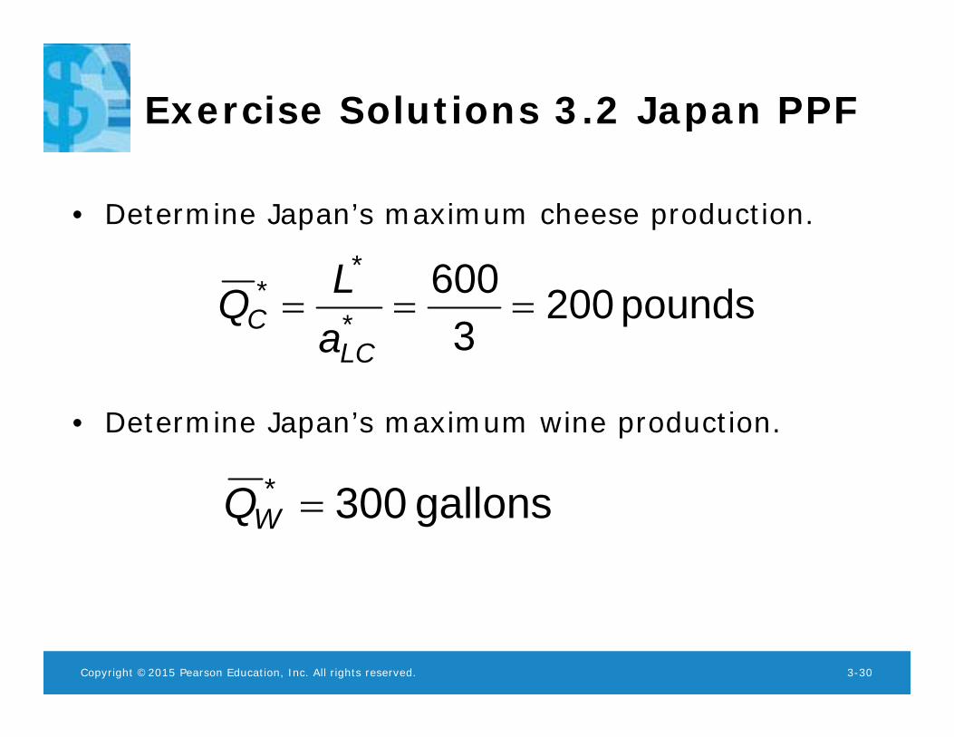
Exercise Solutions 3.2 Japan PPF
• Determine Japan’s maximum cheese production.
• Determine Japan’s maximum wine production.
pounds 2003
600*
**
LCC a
LQ
gallons 300* WQ
Copyright ©2015 Pearson Education, Inc. All rights reserved. 3-31
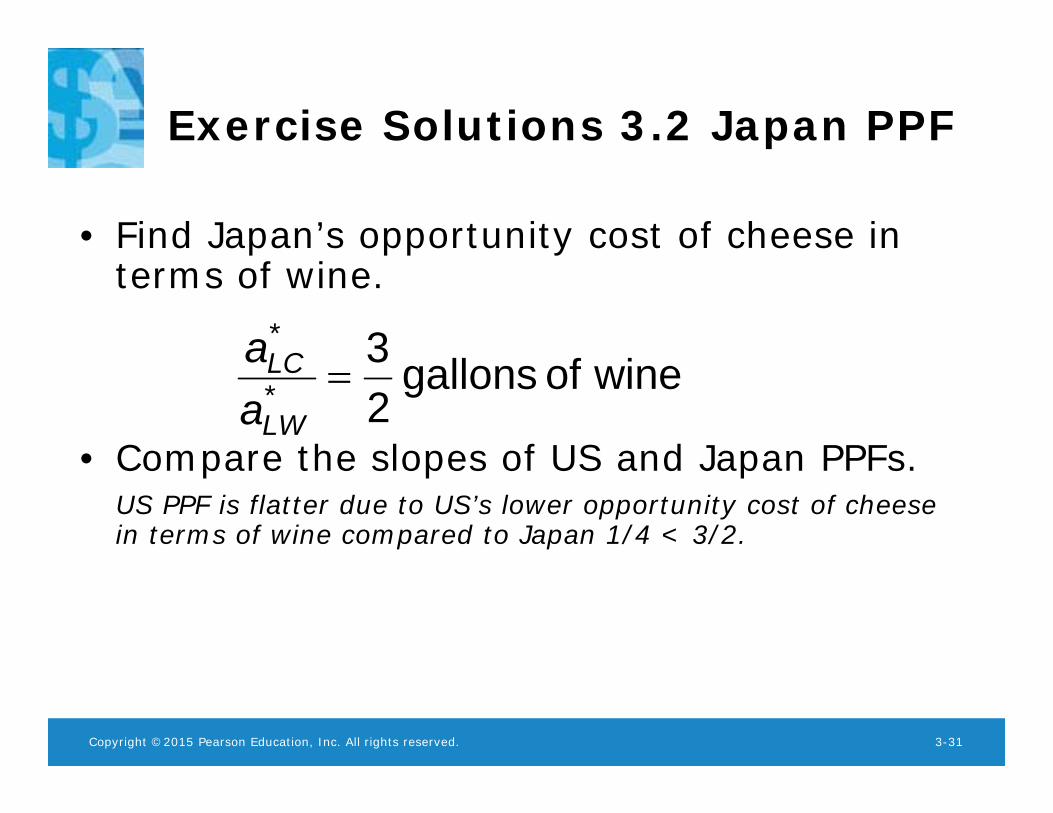
Exercise Solutions 3.2 Japan PPF
• Find Japan’s opportunity cost of cheese in terms of wine.
• Compare the slopes of US and Japan PPFs.US PPF is flatter due to US’s lower opportunity cost of cheese in terms of wine compared to Japan 1/4 < 3/2.
wineof gallons 23
*
*
LW
LC
aa
Copyright ©2015 Pearson Education, Inc. All rights reserved. 3-32
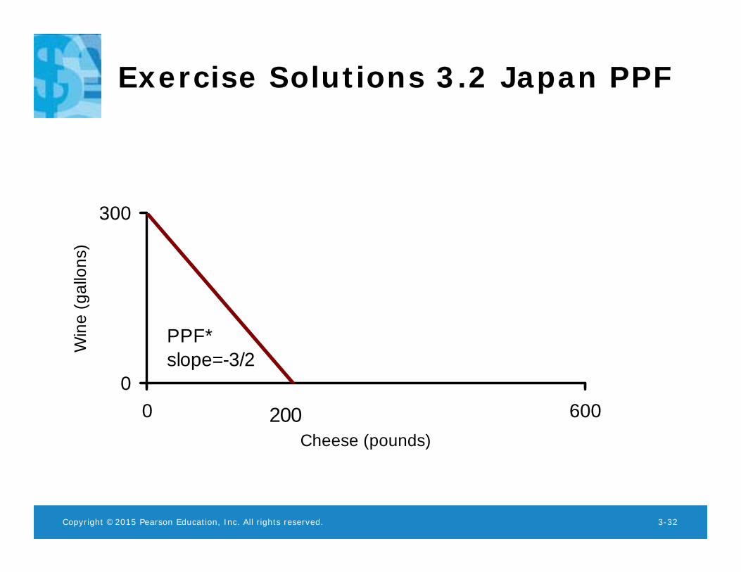
Exercise Solutions 3.2 Japan PPF
0
300
0 600Cheese (pounds)
Win
e (g
allo
ns)
PPF*slope=-3/2
200
Copyright ©2015 Pearson Education, Inc. All rights reserved. 3-33
Production, Prices and Wages
• Let PC be the price of cheese and PW be the price of wine.
• Wage equals value of the marginal product of labor– Wages of cheese makers equal the market value of the cheese
produced: wC = PC /aLC
– Wages of wine makers equal the market value of the wine produced: wW = PW /aLW
• Workers are attracted to whichever industry pays a higher wage.
Copyright ©2015 Pearson Education, Inc. All rights reserved. 3-34
Production, Prices and Wages
• If PC /aLC > PW/aLW , workers will make only cheese.– The economy will specialize in cheese production if the
price of cheese relative to the price of wine exceeds the opportunity cost of producing cheese.
• If PC /aLC < PW /aLW , workers will make only wine.– The economy will specialize in wine production if the price of wine
relative to the price of cheese exceeds the opportunity cost of producing wine.
Copyright ©2015 Pearson Education, Inc. All rights reserved. 3-35
Production, Prices and Wages
• If the domestic country wants to consume both wine and cheese (in the absence of international trade), relative prices must adjust so that wages are equal in the wine and cheese industries. – When the relative price of a good equals the
opportunity cost of producing that goodPC /aLC = PW/aLW
wages are equal across sectors wC = wW
Copyright ©2015 Pearson Education, Inc. All rights reserved. 3-36
Relative Supply and Relative Demand
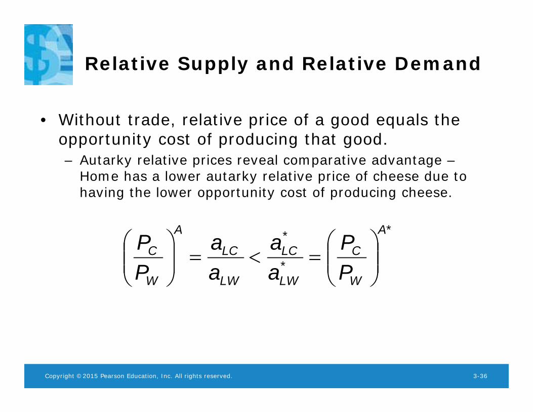
• Without trade, relative price of a good equals the opportunity cost of producing that good.– Autarky relative prices reveal comparative advantage –
Home has a lower autarky relative price of cheese due to having the lower opportunity cost of producing cheese.
*
*
* A
W
C
LW
LC
LW
LC
A
W
C
PP
aa
aa
PP
Copyright ©2015 Pearson Education, Inc. All rights reserved. 3-37
Relative Supply and Relative Demand
• To see how all countries can benefit from trade, we calculate relative prices when trade exists.
• The free trade relative price of cheese to wine adjusts to make world relative supply of cheese to wine equal world relative demand of cheese to wine.
RD = RS
Copyright ©2015 Pearson Education, Inc. All rights reserved. 3-38
Relative Supply and Relative Demand
• World relative supply of cheese to wine is the quantity of cheese supplied by all countries relative to the quantity of wine supplied by all countries at each relative price of cheese to wine.
RS = (QC+QC*)/(QW+QW*)
– Usually increases as the relative price of cheese increases, but will have a special “step” shape in this model.
Copyright ©2015 Pearson Education, Inc. All rights reserved. 3-39
Relative Supply
• If the relative price of cheese to wine were to fall below Home’s opportunity cost
PC /PW < aLC /aLW < a*LC /a*
LW – Both countries would produce only wine,– No cheese would be produced anywhere,– Cannot be an equilibrium
Copyright ©2015 Pearson Education, Inc. All rights reserved. 3-40
Relative Supply
• When the relative price of cheese to wine equals Home’s opportunity cost,
PC /PW = aLC /aLW < a*LC /a*
LW
– Domestic workers indifferent between producing wine or cheese
– Foreign workers produce only wine.
Copyright ©2015 Pearson Education, Inc. All rights reserved. 3-41
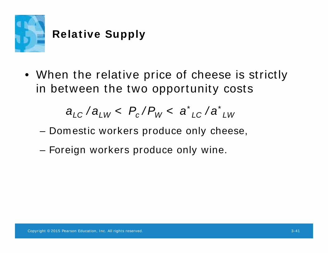
Relative Supply
• When the relative price of cheese is strictly in between the two opportunity costs
aLC /aLW < Pc /PW < a*LC /a*
LW
– Domestic workers produce only cheese,
– Foreign workers produce only wine.
Copyright ©2015 Pearson Education, Inc. All rights reserved. 3-42
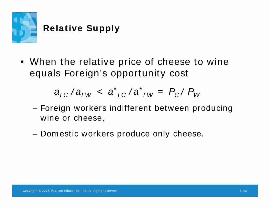
Relative Supply
• When the relative price of cheese to wine equals Foreign’s opportunity cost
aLC /aLW < a*LC /a*
LW = PC / PW
– Foreign workers indifferent between producing wine or cheese,
– Domestic workers produce only cheese.
Copyright ©2015 Pearson Education, Inc. All rights reserved. 3-43
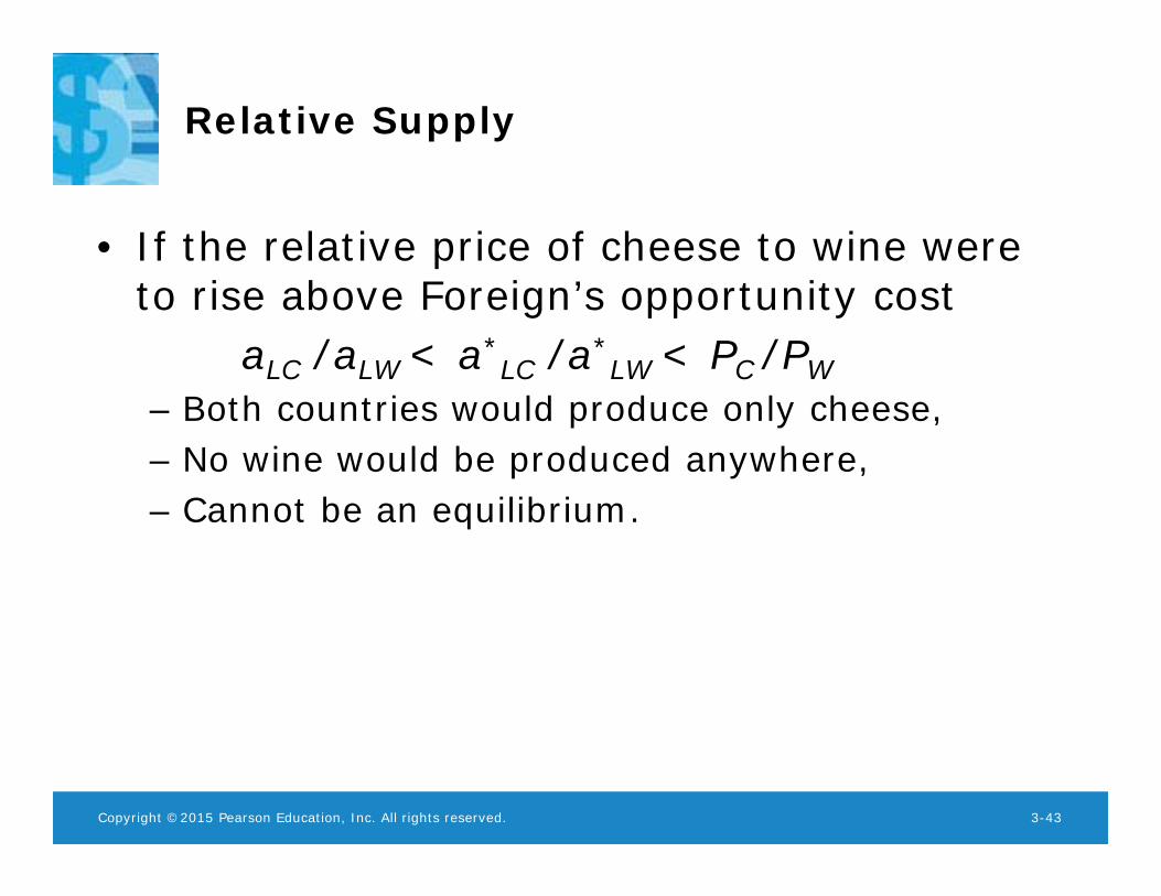
Relative Supply
• If the relative price of cheese to wine were to rise above Foreign’s opportunity cost
aLC /aLW < a*LC /a*
LW < PC /PW– Both countries would produce only cheese,– No wine would be produced anywhere,– Cannot be an equilibrium.
Copyright ©2015 Pearson Education, Inc. All rights reserved. 3-44
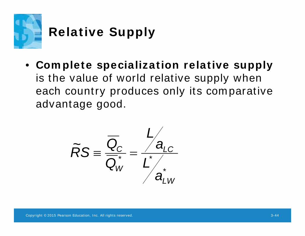
Relative Supply
• Complete specialization relative supplyis the value of world relative supply when each country produces only its comparative advantage good.
***
~
LW
LC
W
C
aL
aL
QQSR
Copyright ©2015 Pearson Education, Inc. All rights reserved. 3-45
Relative Supply
• World relative supply is a step function:– First step aLC/aLW is Home opportunity cost of
cheese– Second step aLC*/aLW* is Foreign opportunity
cost of cheese– Jump occurs at complete specialization relative
supply
Copyright ©2015 Pearson Education, Inc. All rights reserved. 3-46
Relative Demand
• World relative demand of cheese to wine is the quantity of cheese demanded in all countries relative to the quantity of wine demanded in all countries at each relative price of cheese to wine RD = (DC+DC*)/(DW+DW*).– Usually consumers purchase less cheese and more wine as
relative price of cheese to wine rises, so the relative quantity of cheese demanded falls.
Copyright ©2015 Pearson Education, Inc. All rights reserved. 3-47
Relative Demand
• A common specification for relative demand is to make relative demand for cheese to wine proportional to inverse of relative price of cheese to wine.
W
CC
W
PPP
PRD 1
Copyright ©2015 Pearson Education, Inc. All rights reserved. 3-48
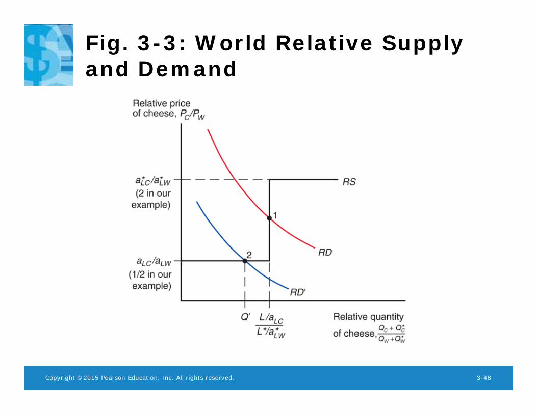
Fig. 3-3: World Relative Supply and Demand
Copyright ©2015 Pearson Education, Inc. All rights reserved. 3-49
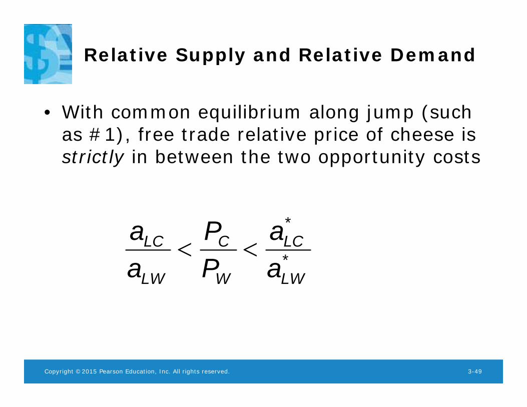
Relative Supply and Relative Demand
• With common equilibrium along jump (such as #1), free trade relative price of cheese is strictly in between the two opportunity costs
*
*
LW
LC
W
C
LW
LC
aa
PP
aa
Copyright ©2015 Pearson Education, Inc. All rights reserved. 3-50
Relative Supply and Relative Demand
• However, depending on strength of relative demand for cheese, an equilibrium can occur along either step, such as #2.
• Free trade relative price of cheese may equal Home or Foreign opportunity costs.
Copyright ©2015 Pearson Education, Inc. All rights reserved. 3-51
Example 3.3 Relative Supply and Demand
• Recall under complete specialization according to comparative advantage, Home produces 1000 pounds of cheese and no wine.
• Foreign produces 1500 gallons of wine and no cheese.
• Home’s opportunity cost of cheese is 1/2, and Foreign’s is 2.
Copyright ©2015 Pearson Education, Inc. All rights reserved. 3-52
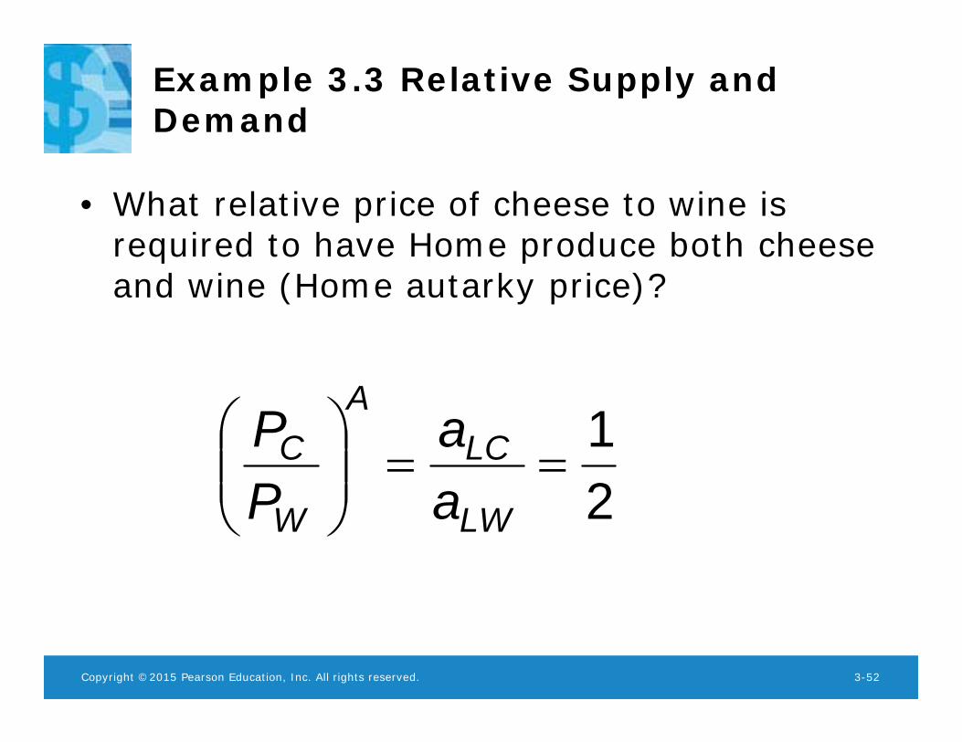
Example 3.3 Relative Supply and Demand
• What relative price of cheese to wine is required to have Home produce both cheese and wine (Home autarky price)?
21
LW
LCA
W
C
aa
PP
Copyright ©2015 Pearson Education, Inc. All rights reserved. 3-53
Example 3.3 Relative Supply and Demand
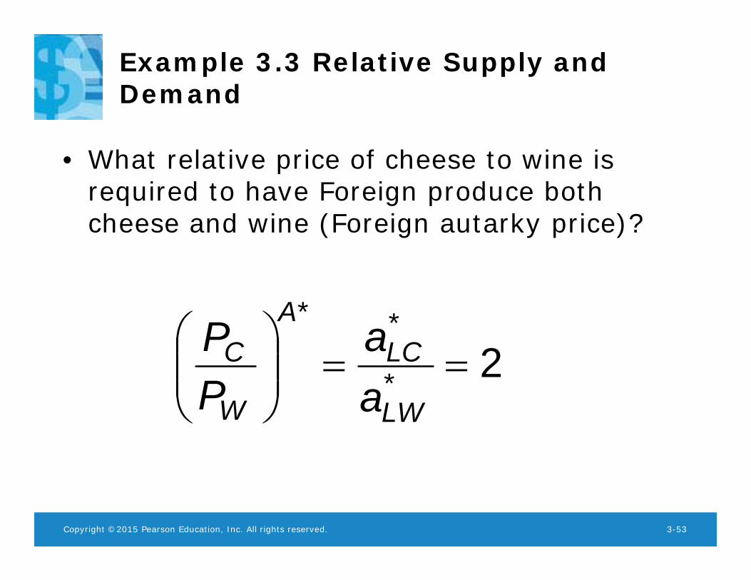
• What relative price of cheese to wine is required to have Foreign produce both cheese and wine (Foreign autarky price)?
2*
**
LW
LCA
W
C
aa
PP
Copyright ©2015 Pearson Education, Inc. All rights reserved. 3-54
Example 3.3 Relative Supply and Demand
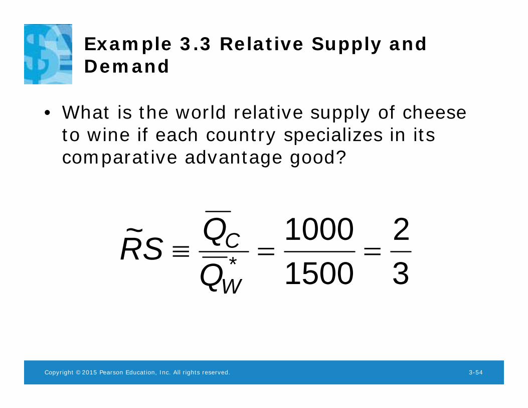
• What is the world relative supply of cheese to wine if each country specializes in its comparative advantage good?
32
15001000~
* W
C
QQSR
Copyright ©2015 Pearson Education, Inc. All rights reserved. 3-55
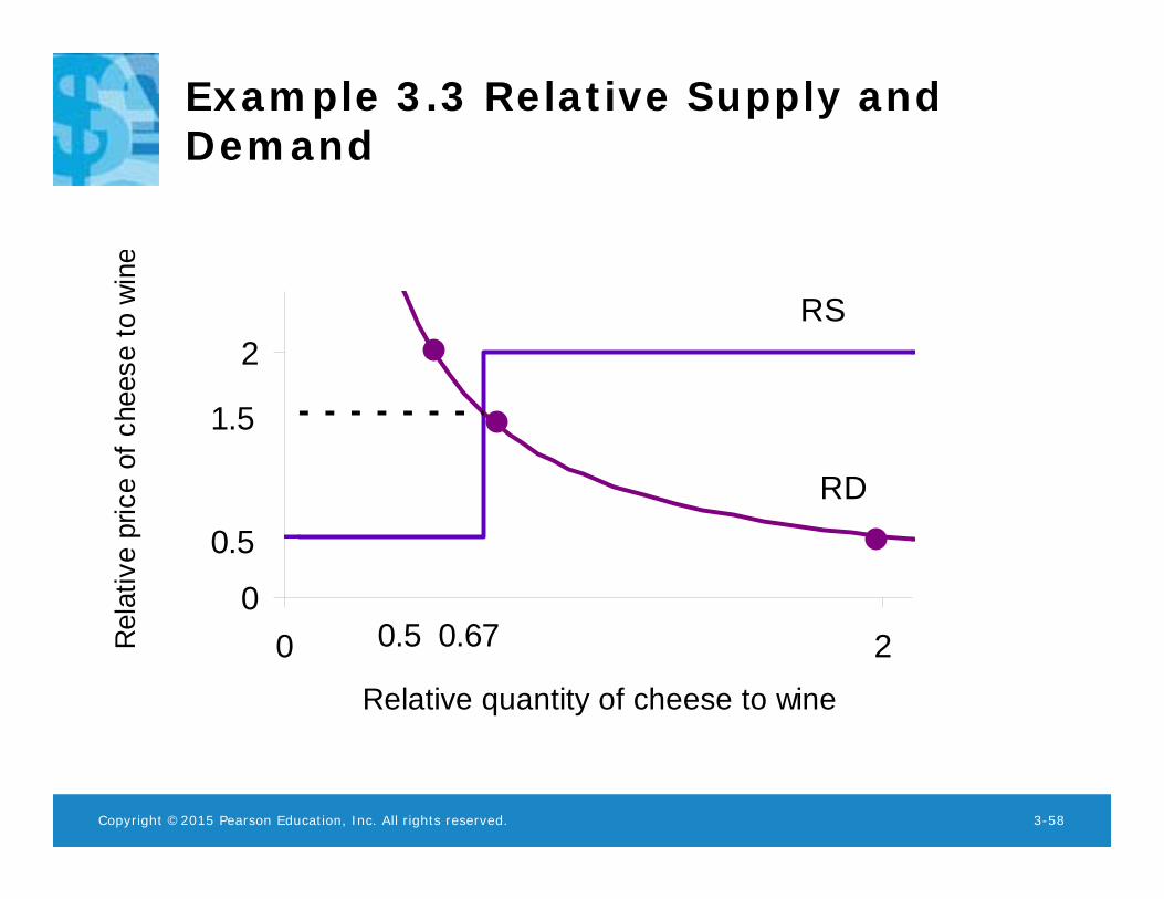
Example 3.3 Relative Supply and Demand
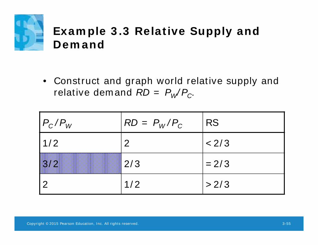
• Construct and graph world relative supply and relative demand RD = PW/PC.
PC /PW RD = PW /PC RS
1/2 2 <2/3
3/2 2/3 =2/3
2 1/2 >2/3
Copyright ©2015 Pearson Education, Inc. All rights reserved. 3-56
Example 3.3 Relative Supply and Demand
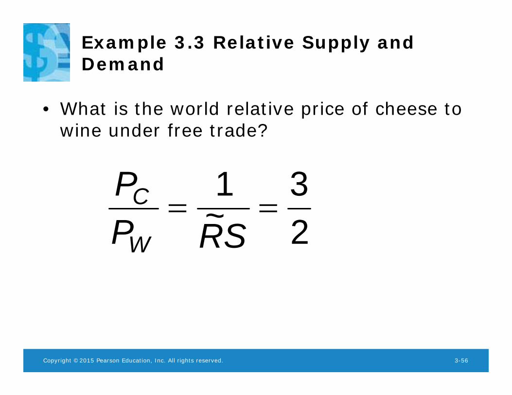
• What is the world relative price of cheese to wine under free trade?
23
~1
SRP
PW
C
Copyright ©2015 Pearson Education, Inc. All rights reserved. 3-57
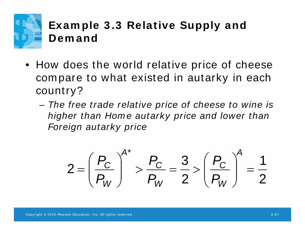
Example 3.3 Relative Supply and Demand
• How does the world relative price of cheese compare to what existed in autarky in each country? – The free trade relative price of cheese to wine is
higher than Home autarky price and lower than Foreign autarky price
21
232
*
A
W
C
W
CA
W
C
PP
PP
PP
Copyright ©2015 Pearson Education, Inc. All rights reserved. 3-58
Example 3.3 Relative Supply and Demand
0
2
0 2Relative quantity of cheese to wine
Rel
ativ
e pr
ice
of c
hees
e to
win
e
RS
RD
1.5
0.5
0.5 0.67
Copyright ©2015 Pearson Education, Inc. All rights reserved. 3-59
Exercise 3.3 World Equilibrium
• Find the relative price of cheese to wine required to have the United States produce both cheese and wine.
• Find the relative price of cheese to wine required to have Japan produce both cheese and wine.
• Find the world relative supply of cheese to wine if both countries specialize in their comparative advantage good.
Copyright ©2015 Pearson Education, Inc. All rights reserved. 3-60
Exercise 3.3 World Equilibrium
• Construct and graph world relative supply and demand RD = PW/PC.
• Find the equilibrium relative price of cheese to wine under free trade.
• Compare the free trade relative price of cheese to each country’s autarky relative price.
Copyright ©2015 Pearson Education, Inc. All rights reserved. 3-61
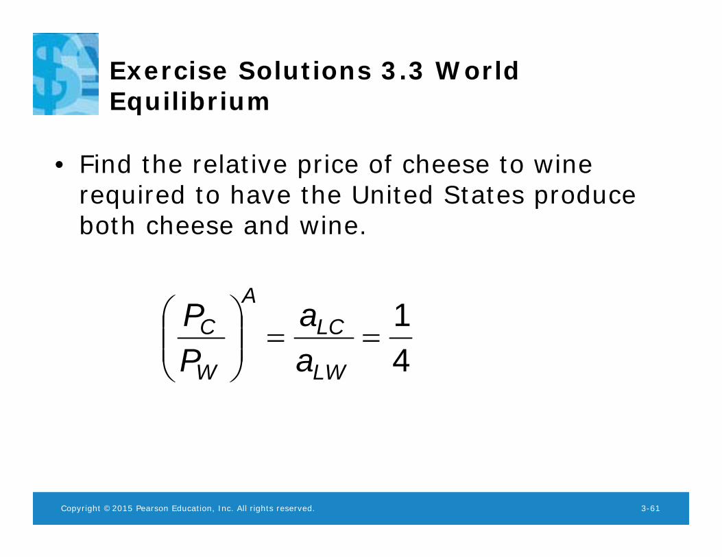
Exercise Solutions 3.3 World Equilibrium
• Find the relative price of cheese to wine required to have the United States produce both cheese and wine.
41
LW
LCA
W
C
aa
PP
Copyright ©2015 Pearson Education, Inc. All rights reserved. 3-62
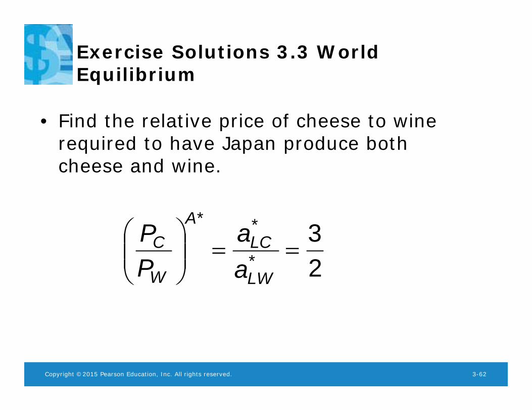
Exercise Solutions 3.3 World Equilibrium
• Find the relative price of cheese to wine required to have Japan produce both cheese and wine.
23
*
**
LW
LCA
W
C
aa
PP
Copyright ©2015 Pearson Education, Inc. All rights reserved. 3-63
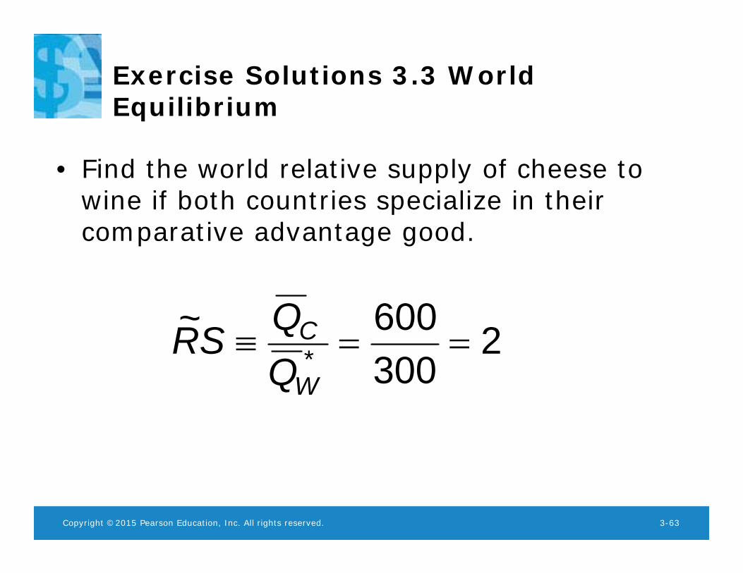
Exercise Solutions 3.3 World Equilibrium
• Find the world relative supply of cheese to wine if both countries specialize in their comparative advantage good.
2300600~
* W
C
QQSR
Copyright ©2015 Pearson Education, Inc. All rights reserved. 3-64
Exercise Solutions 3.3 World Equilibrium
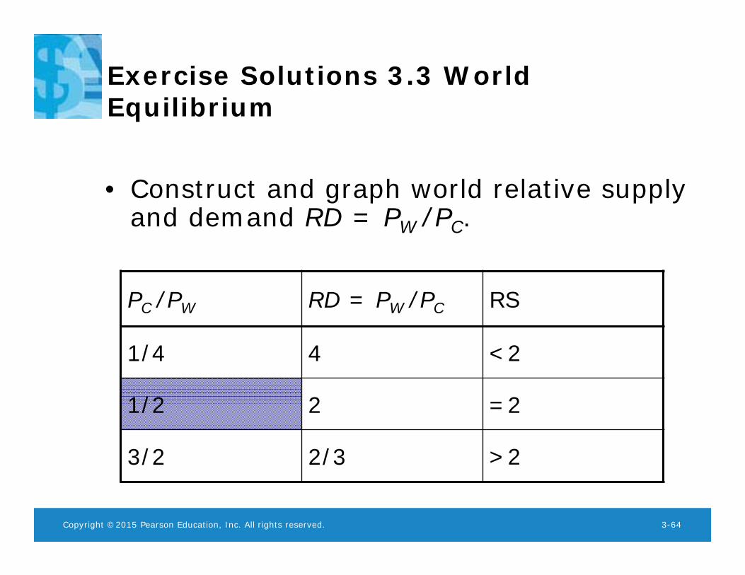
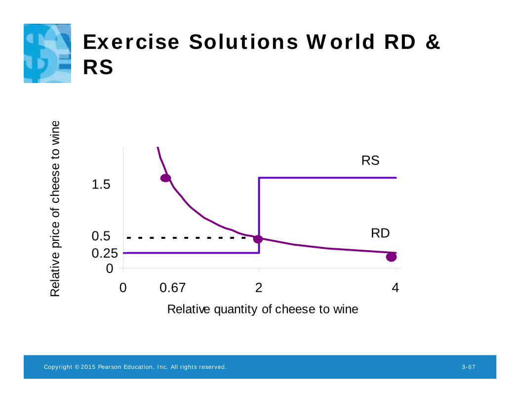
• Construct and graph world relative supply and demand RD = PW /PC.
PC /PW RD = PW /PC RS
1/4 4 <2
1/2 2 =2
3/2 2/3 >2
Copyright ©2015 Pearson Education, Inc. All rights reserved. 3-65
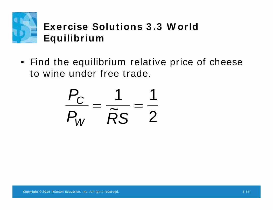
Exercise Solutions 3.3 World Equilibrium
• Find the equilibrium relative price of cheese to wine under free trade.
21
~1
SRP
PW
C
Copyright ©2015 Pearson Education, Inc. All rights reserved. 3-66
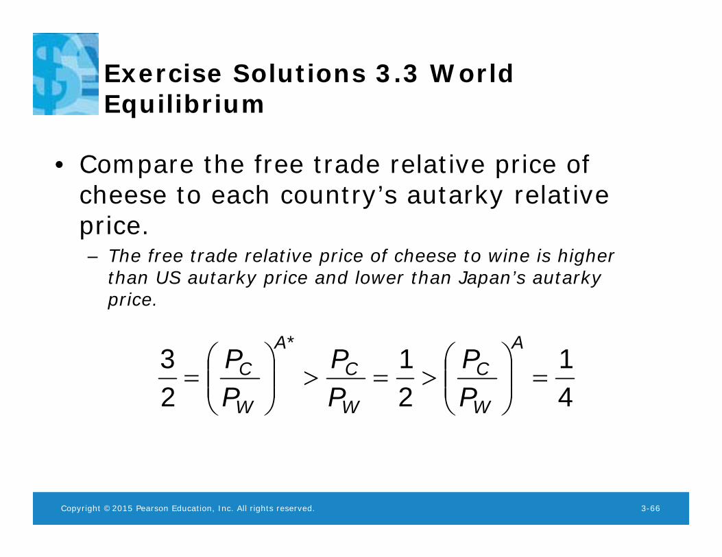
Exercise Solutions 3.3 World Equilibrium
• Compare the free trade relative price of cheese to each country’s autarky relative price.– The free trade relative price of cheese to wine is higher
than US autarky price and lower than Japan’s autarky price.
41
21
23
*
A
W
C
W
CA
W
C
PP
PP
PP
Copyright ©2015 Pearson Education, Inc. All rights reserved. 3-67
Exercise Solutions World RD & RS
00 2 4
Relative quantity of cheese to wine
Rel
ativ
e pr
ice
of c
hees
e to
win
e
RS
RD
1.5
0.50.25
0.67
Copyright ©2015 Pearson Education, Inc. All rights reserved. 3-68
World Production Efficiency
• World production is efficient if it is not possible to increase the world production of cheese without reducing the world production of wine.– Free trade equilibrium is efficient as at least one
country specializes in its comparative advantage good
– Autarky is not - neither specialized
Copyright ©2015 Pearson Education, Inc. All rights reserved. 3-69
Gains from Trade
• Gains from trade come from specializing in production that use resources most efficiently (comparative advantage good), and using the income generated from that production to buy the goods and services that countries desire.
Copyright ©2015 Pearson Education, Inc. All rights reserved. 3-70
Gains from Trade
• Domestic workers earn a higher income from cheese production because the relative price of cheese increases with trade.
• Foreign workers earn a higher income from wine production because the relative price of cheese decreases with trade (making cheese cheaper) and the relative price of wine increases with trade.
Copyright ©2015 Pearson Education, Inc. All rights reserved. 3-71
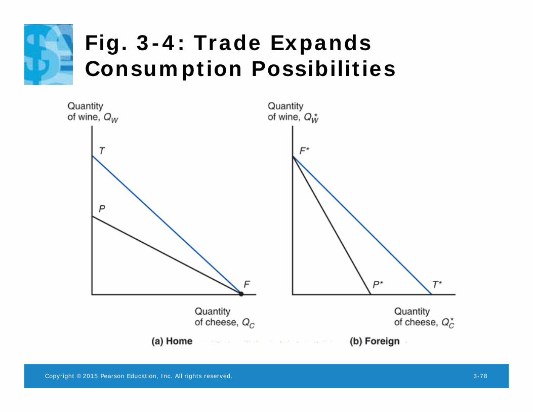
Gains from Trade
• Think of trade as an indirect method of production or a new technology that converts cheese into wine or vice versa.
• Without trade, a country has to allocate resources to produce all of the goods that it wants to consume (autarky).
• With trade, a country can specialize its production and trade the products for the goods that it wants to consume.
• Allowing trade expands consumption possibilities beyond production possibilities.
Copyright ©2015 Pearson Education, Inc. All rights reserved. 3-72
Gains from Trade
• If international trade leads to a relative price of cheese to wine that differs from Home’s autarky price, then Home gains from trade.
• Similarly, if international trade leads to a relative price of cheese to wine that differs from Foreign’s autarky price, then Foreign gains from trade.
Copyright ©2015 Pearson Education, Inc. All rights reserved. 3-73
Gains from Trade
• Typically both countries gain from trade.• Possible for one of the countries to not gain.
– If so, other country gains even more.• At least one country always gains since
there are gains at the world level.• If gain from trade, TPF outside PPF.
Copyright ©2015 Pearson Education, Inc. All rights reserved. 3-74
Trade Possibilities Frontier
• The trade possibilities frontier (TPF) of an economy shows the maximumamount of a goods that can be consumed by trading the optimal production bundle at world prices under free trade.
Copyright ©2015 Pearson Education, Inc. All rights reserved. 3-75
Trade Possibilities Frontier
• If DC represents the quantity of cheese consumed and DW represents the quantity of wine consumed, then the trade possibility frontier of the domestic economy has the equation:
PCDC + PWDW = PCQC + PWQW
Copyright ©2015 Pearson Education, Inc. All rights reserved. 3-76
Trade Possibilities Frontier
• Assuming complete specialization in cheese, Home trade possibilities frontier in income-expenditure form simplifies to
CW
CWC
W
C QPPDD
PP
Copyright ©2015 Pearson Education, Inc. All rights reserved. 3-77
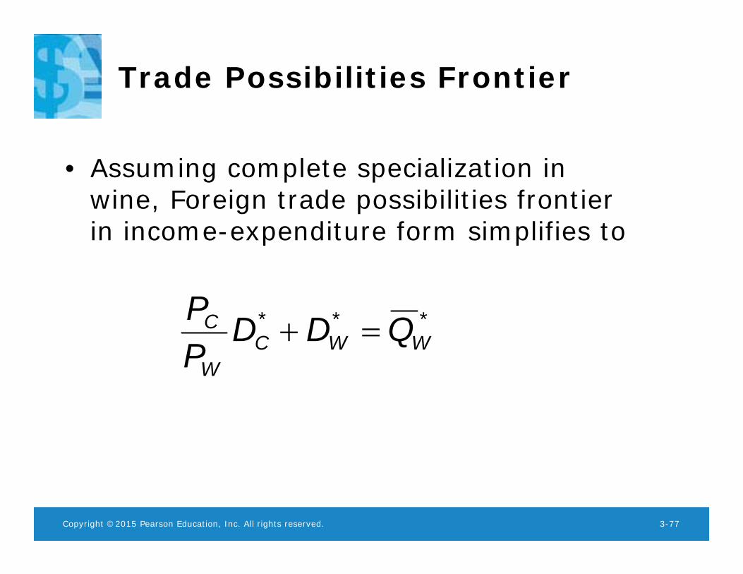
Trade Possibilities Frontier
• Assuming complete specialization in wine, Foreign trade possibilities frontier in income-expenditure form simplifies to
***WWC
W
C QDDPP
Copyright ©2015 Pearson Education, Inc. All rights reserved. 3-78
Fig. 3-4: Trade Expands Consumption Possibilities
Copyright ©2015 Pearson Education, Inc. All rights reserved. 3-79
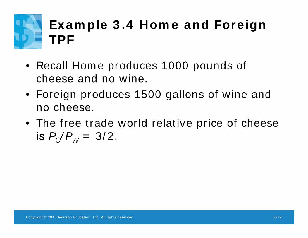
Example 3.4 Home and Foreign TPF
• Recall Home produces 1000 pounds of cheese and no wine.
• Foreign produces 1500 gallons of wine and no cheese.
• The free trade world relative price of cheese is PC/PW = 3/2.
Copyright ©2015 Pearson Education, Inc. All rights reserved. 3-80
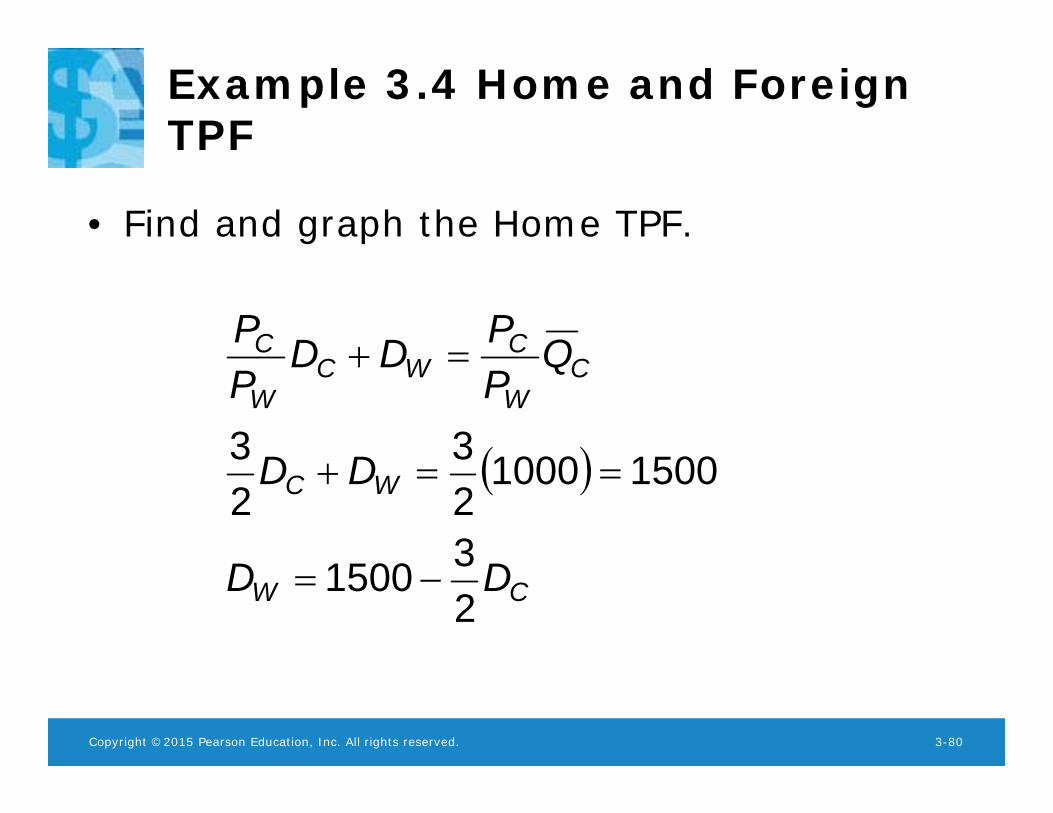
Example 3.4 Home and Foreign TPF
• Find and graph the Home TPF.
CW
WC
CW
CWC
W
C
DD
DD
QPPDD
PP
231500
1500100023
23
Copyright ©2015 Pearson Education, Inc. All rights reserved. 3-81
Example 3.4 Home and Foreign TPF
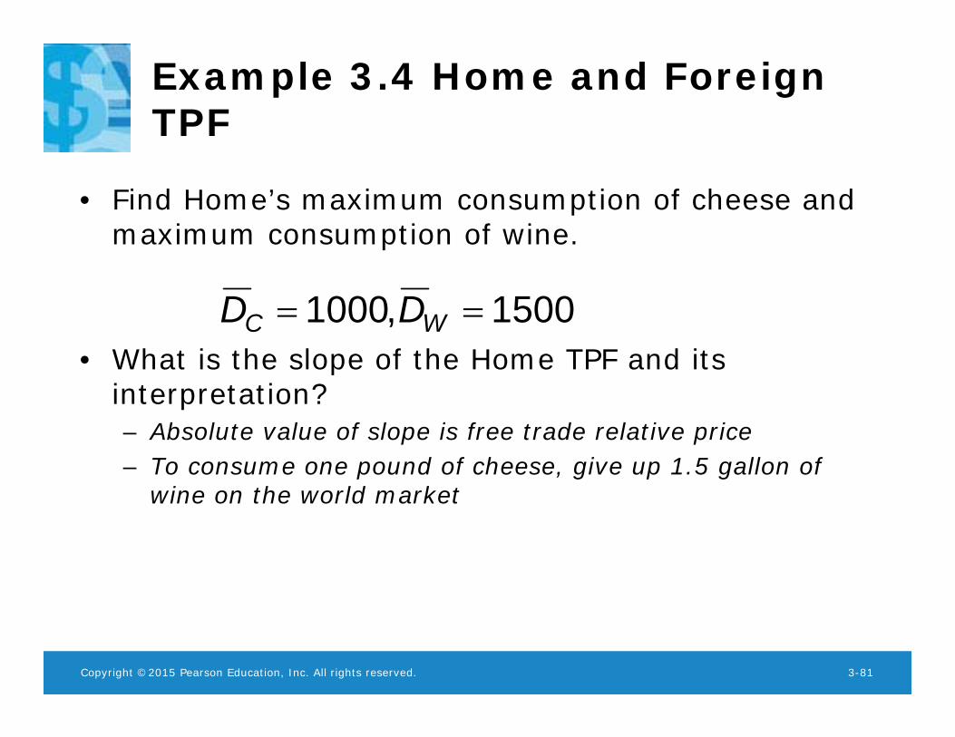
• Find Home’s maximum consumption of cheese and maximum consumption of wine.
• What is the slope of the Home TPF and its interpretation?– Absolute value of slope is free trade relative price– To consume one pound of cheese, give up 1.5 gallon of
wine on the world market
1500,1000 WC DD
Copyright ©2015 Pearson Education, Inc. All rights reserved. 3-82
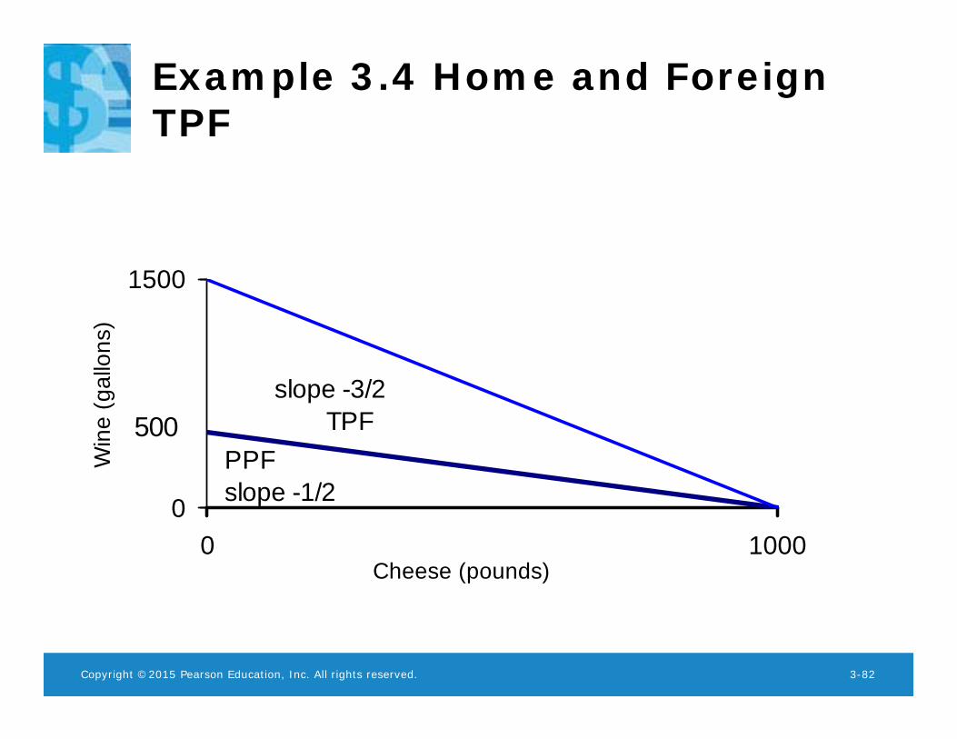
Example 3.4 Home and Foreign TPF
0
1500
0 1000Cheese (pounds)
Win
e (g
allo
ns)
PPFslope -1/2
slope -3/2 TPF500
Copyright ©2015 Pearson Education, Inc. All rights reserved. 3-83
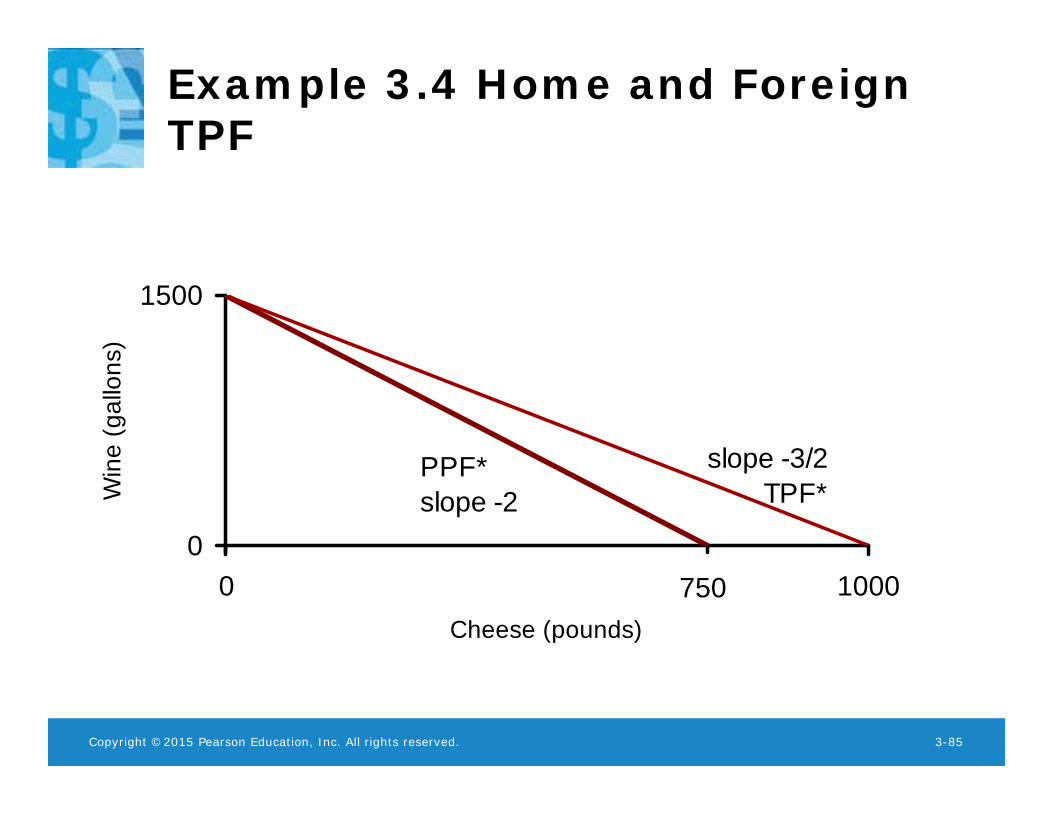
Example 3.4 Home and Foreign TPF
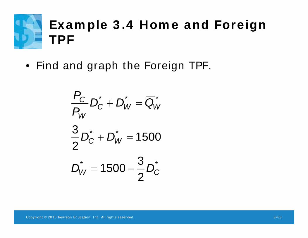
• Find and graph the Foreign TPF.
**
**
***
231500
150023
CW
WC
WWCW
C
DD
DD
QDDPP
Copyright ©2015 Pearson Education, Inc. All rights reserved. 3-84
Example 3.4 Home and Foreign TPF
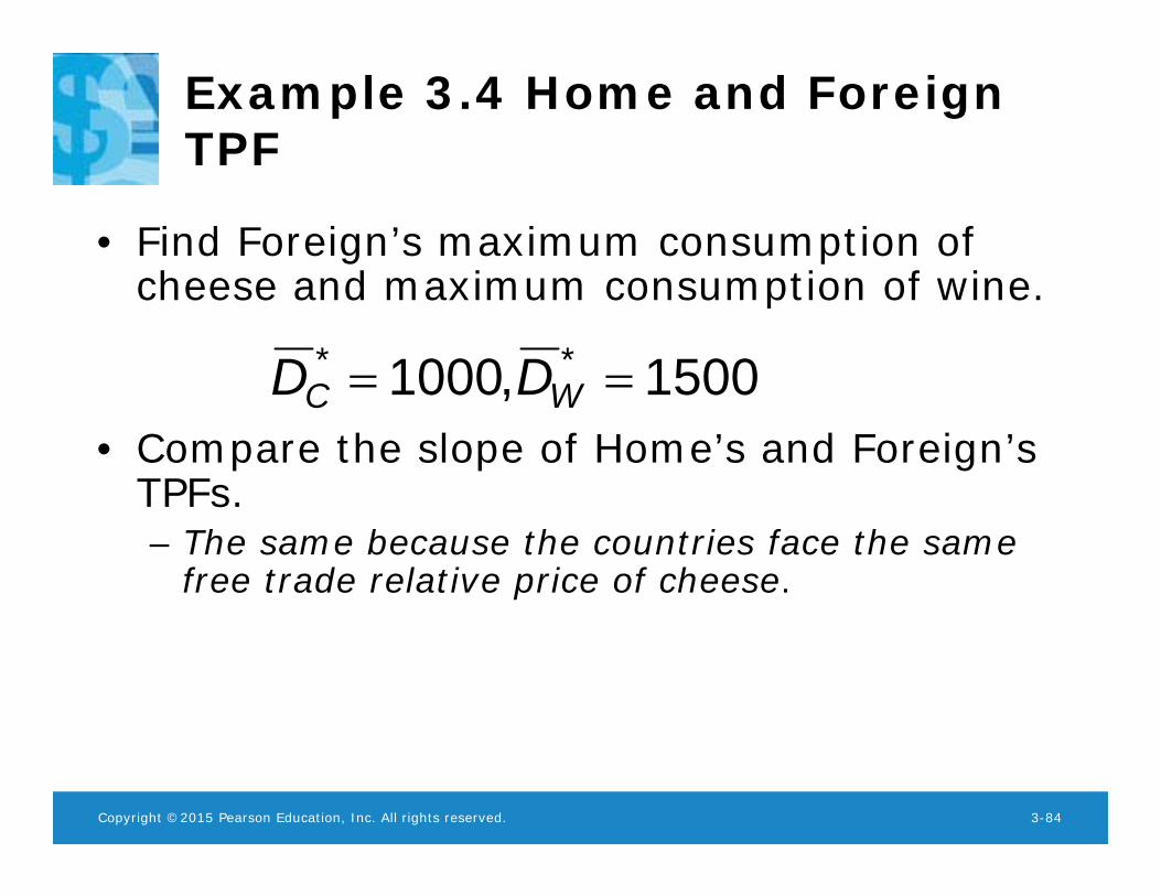
• Find Foreign’s maximum consumption of cheese and maximum consumption of wine.
• Compare the slope of Home’s and Foreign’s TPFs.– The same because the countries face the same
free trade relative price of cheese.
1500,1000 ** WC DD
Copyright ©2015 Pearson Education, Inc. All rights reserved. 3-85
Example 3.4 Home and Foreign TPF
0
1500
0 1000Cheese (pounds)
Win
e (g
allo
ns)
PPF*slope -2
slope -3/2 TPF*
750
Copyright ©2015 Pearson Education, Inc. All rights reserved. 3-86
Exercise 3.4 US and Japan TPF
• Find and graph the US TPF.• Determine US maximum cheese
consumption and US maximum wine consumption.
• Find the slope of the US TPF.• What does the slope of the US TPF
represent?
Copyright ©2015 Pearson Education, Inc. All rights reserved. 3-87
Exercise 3.4 US and Japan TPF
• Find and graph Japan’s TPF.• Determine Japan’s maximum cheese
consumption and maximum wine consumption.
• Find the slope of Japan’s TPF. • Compare the slopes of US and Japan TPFs.
Copyright ©2015 Pearson Education, Inc. All rights reserved. 3-88
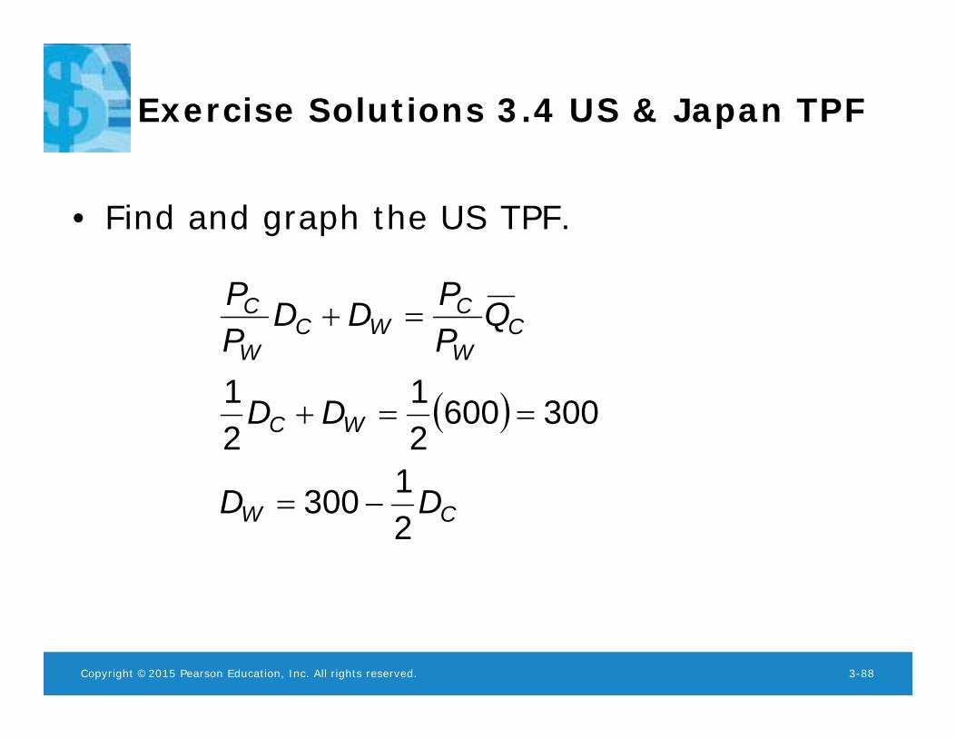
Exercise Solutions 3.4 US & Japan TPF
• Find and graph the US TPF.
CW
WC
CW
CWC
W
C
DD
DD
QPPDD
PP
21300
30060021
21
Copyright ©2015 Pearson Education, Inc. All rights reserved. 3-89
Exercise Solutions 3.4 US & Japan TPF
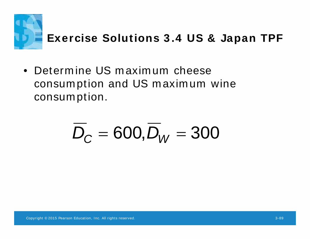
• Determine US maximum cheese consumption and US maximum wine consumption.
300,600 WC DD
Copyright ©2015 Pearson Education, Inc. All rights reserved. 3-90
Exercise Solutions 3.4 US & Japan TPF
• Find the slope of the US TPF.– Slope is -1/2.
• What does the slope of the US TPF represent?– Absolute value of slope is free trade relative price
– give up 1/2 gallon of wine to buy one pound of cheese on world market.
Copyright ©2015 Pearson Education, Inc. All rights reserved. 3-91
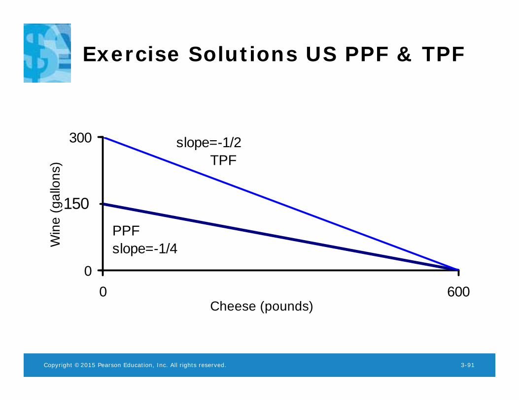
Exercise Solutions US PPF & TPF
0
300
0 600Cheese (pounds)
Win
e (g
allo
ns)
PPFslope=-1/4
slope=-1/2 TPF
150
Copyright ©2015 Pearson Education, Inc. All rights reserved. 3-92
Exercise Solutions 3.4 US & Japan TPF
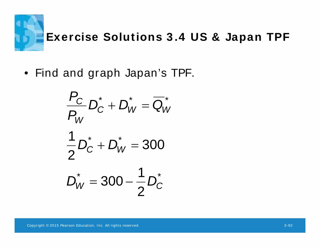
• Find and graph Japan’s TPF.
**
**
***
21300
30021
CW
WC
WWCW
C
DD
DD
QDDPP
Copyright ©2015 Pearson Education, Inc. All rights reserved. 3-93
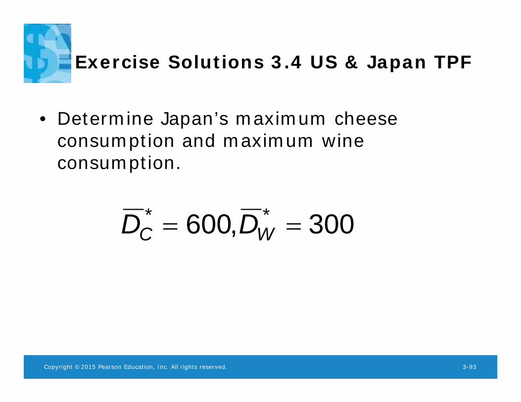
Exercise Solutions 3.4 US & Japan TPF
• Determine Japan’s maximum cheese consumption and maximum wine consumption.
300,600 ** WC DD
Copyright ©2015 Pearson Education, Inc. All rights reserved. 3-94
Exercise Solutions 3.4 US & Japan TPF
• Find the slope of Japan’s TPF. – Slope is -1/2.
• Compare the slopes of US and Japan TPFs.– The same because the countries face the same
free trade relative price of cheese.
Copyright ©2015 Pearson Education, Inc. All rights reserved. 3-95
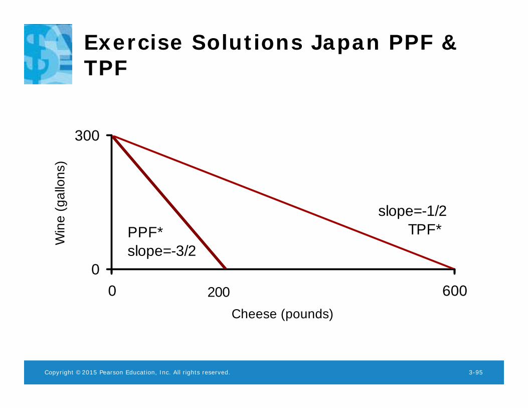
Exercise Solutions Japan PPF & TPF
0
300
0 600Cheese (pounds)
Win
e (g
allo
ns)
PPF*slope=-3/2
slope=-1/2 TPF*
200
Copyright ©2015 Pearson Education, Inc. All rights reserved. 3-96
Trade Pattern
• The trade pattern indicates the direction of trade; description of which countries import and export which goods.
• Each country exports its comparative advantage good.– Home exports cheese and imports wine.– Foreign exports wine and imports cheese.
Copyright ©2015 Pearson Education, Inc. All rights reserved. 3-97
Three Possible Equilibria
1. Free trade relative price can equal Home autarky relative price
– Home produces both goods, Foreign only wine– Foreign gains, Home does not
2. Free trade relative price can equal Foreign autarky relative price
– Foreign produces both goods, Home only cheese– Home gains, Foreign does not
Copyright ©2015 Pearson Education, Inc. All rights reserved. 3-98
Three Possible Equilibria
3. Free trade relative price can be strictly in between autarky relative prices
– Home produces only cheese, Foreign only wine (complete specialization according to comparative advantage)
– Both Home and Foreign gain• Home always exports cheese, Foreign
always exports wine.
Copyright ©2015 Pearson Education, Inc. All rights reserved. 3-99
Relative Wages
• Relative wages are the wages of the domestic country relative to the wages in the foreign country.
• Productivity (technological) differences determine wage differences in the Ricardian model.– A country with absolute advantage in producing a good will enjoy
a higher wage in that industry after trade.
• Both countries have a cost advantage in production.– The cost of high wages can be offset by high productivity.– The cost of low productivity can be offset by low wages.
Copyright ©2015 Pearson Education, Inc. All rights reserved. 3-100
Common Misconceptions
1. Free trade is beneficial only if a country is more productive than foreign countries.– Even an unproductive country benefits from free
trade.
– The benefits of free trade do not depend on absolute advantage, rather they depend on comparative advantage: specializing in industries that use resources most efficiently.
Copyright ©2015 Pearson Education, Inc. All rights reserved. 3-101
Common Misconceptions
2. Free trade with countries that pay low wages hurts high wage countries.– Not unfair competition: low wages reflect low productivity
so production costs might not be low.– Consumers benefit because they can purchase goods
more cheaply (more wine in exchange for cheese).– Producers/workers benefit by earning a higher income (by
using resources more efficiently and through higher prices/wages).
Copyright ©2015 Pearson Education, Inc. All rights reserved. 3-102
Common Misconceptions
3. Free trade exploits less productive countries.– While labor standards in some countries are less than
exemplary compared to Western standards, they are so with or without trade.
– Deeper poverty and exploitation may result without exports.
– Consumers benefit from free trade by having access to cheaply (efficiently) produced goods.
– Producers/workers benefit from having higher profits/wages—higher compared to the alternative.
Copyright ©2015 Pearson Education, Inc. All rights reserved. 3-103
Transportation Costs and Non-traded Goods
• The production specialization predicted by the Ricardian model rarely happens:1. More than one factor of production reduces
the tendency of specialization (chapter 4)2. Protectionism (chapter 8)3. Transportation costs reduce or prevent
trade, which may cause each country to produce the same good or service
Copyright ©2015 Pearson Education, Inc. All rights reserved. 3-104
Transportation Costs and Non-traded Goods
• Non-traded goods and services (e.g., haircuts and auto repairs) exist due to high transportation costs.– Countries tend to spend a large fraction of national income
on non-traded goods and services.
– This fact has implications for the gravity model and for models that consider how income transfers across countries affect trade.
Copyright ©2015 Pearson Education, Inc. All rights reserved. 3-105
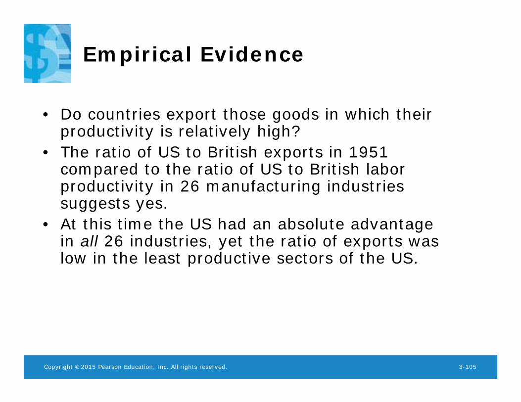
Empirical Evidence
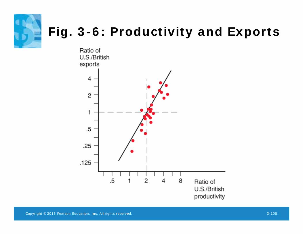
• Do countries export those goods in which their productivity is relatively high?
• The ratio of US to British exports in 1951 compared to the ratio of US to British labor productivity in 26 manufacturing industries suggests yes.
• At this time the US had an absolute advantage in all 26 industries, yet the ratio of exports was low in the least productive sectors of the US.
Copyright ©2015 Pearson Education, Inc. All rights reserved. 3-106
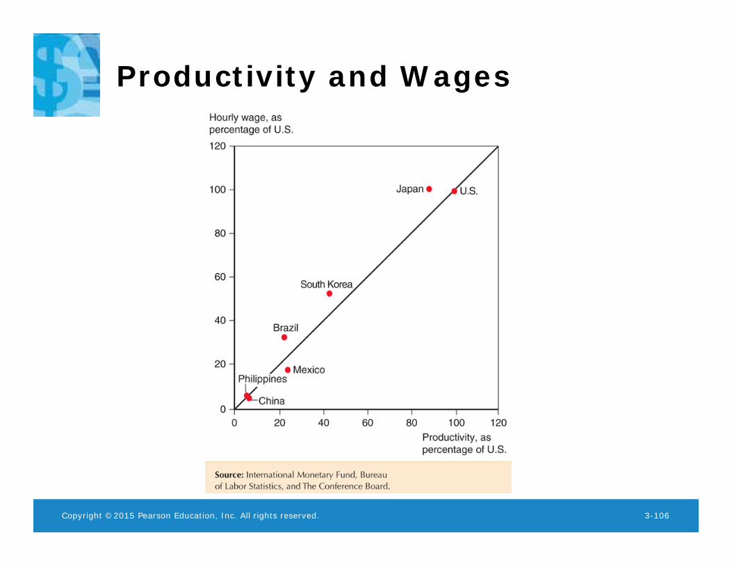
Productivity and Wages
Copyright ©2015 Pearson Education, Inc. All rights reserved. 3-107
Do Wages Reflect Productivity?
• Other evidence shows that wages rise as productivity rises.– In 2000, South Korea’s labor productivity was 35% of
the US level and its average wages were about 38% of US average wages.
– After the Korean War, South Korea was one of the poorest countries in the world, and its labor productivity was very low. In 1975, average wages in South Korea were still only 5% of US average wages.
Copyright ©2015 Pearson Education, Inc. All rights reserved. 3-108
Fig. 3-6: Productivity and Exports
Copyright ©2015 Pearson Education, Inc. All rights reserved. 3-109
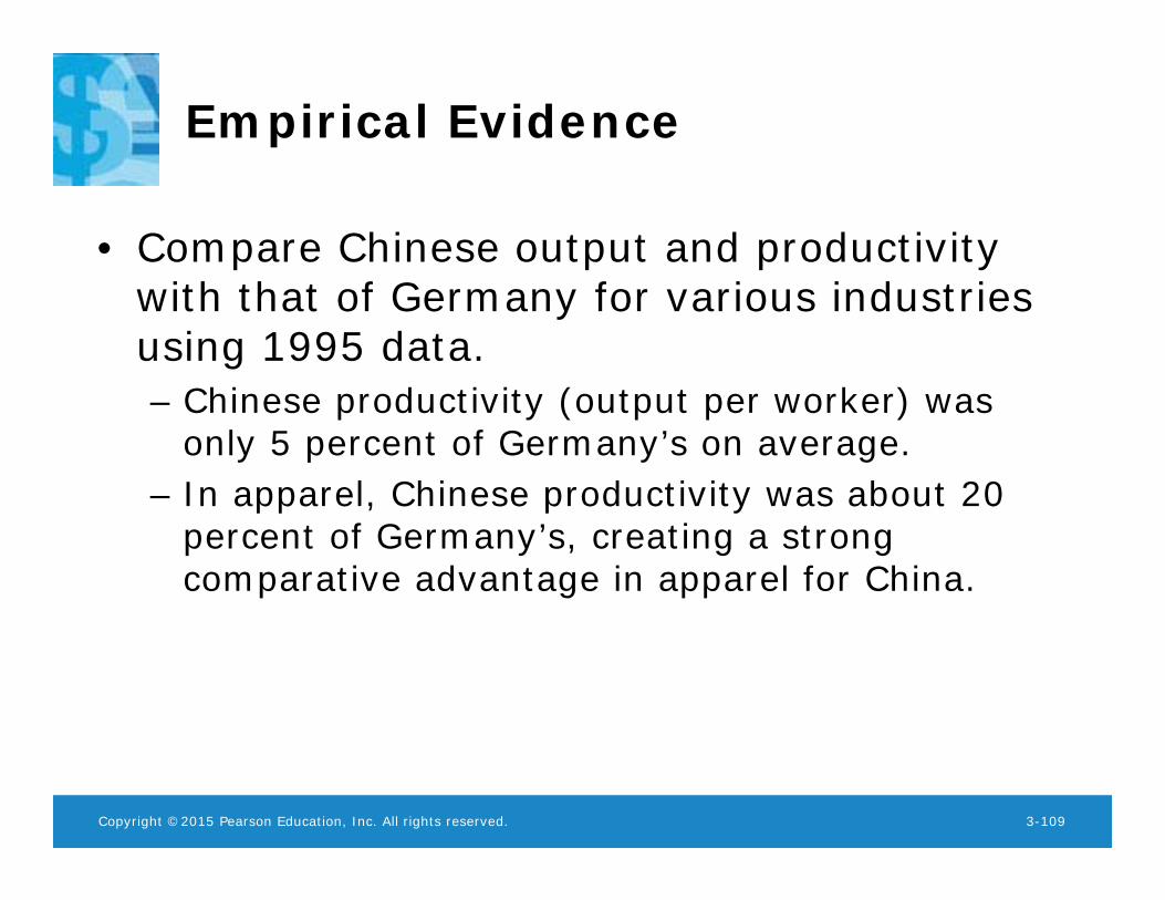
Empirical Evidence
• Compare Chinese output and productivity with that of Germany for various industries using 1995 data.– Chinese productivity (output per worker) was
only 5 percent of Germany’s on average.– In apparel, Chinese productivity was about 20
percent of Germany’s, creating a strong comparative advantage in apparel for China.
Copyright ©2015 Pearson Education, Inc. All rights reserved. 3-110
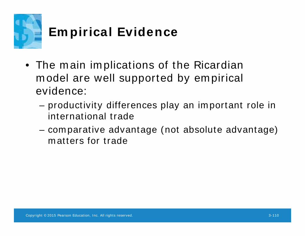
Empirical Evidence
• The main implications of the Ricardian model are well supported by empirical evidence:– productivity differences play an important role in
international trade– comparative advantage (not absolute advantage)
matters for trade
Copyright ©2015 Pearson Education, Inc. All rights reserved. 3-111
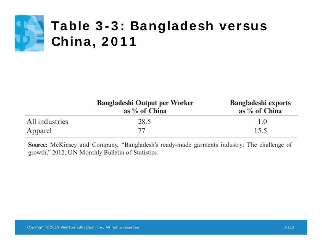
Table 3-3: Bangladesh versus China, 2011
Copyright ©2015 Pearson Education, Inc. All rights reserved. 3-112
Summary
1. Differences in the productivity of labor across countries generate comparative advantage.
2. A country has a comparative advantage in producing a good when its opportunity cost of producing that good is lower than in other countries.
Copyright ©2015 Pearson Education, Inc. All rights reserved. 3-113
Summary (cont.)
3. Countries export goods in which they have a comparative advantage - high productivity or low wages give countries a cost advantage.
4. With trade, the relative price settles in between what the relative prices were in each country before trade.
Copyright ©2015 Pearson Education, Inc. All rights reserved. 3-114
Summary (cont.)
5. Trade benefits all countries due to the relative price of the exported good rising: income for workers who produce exports rises, and imported goods become less expensive.
6. Empirical evidence supports trade based on comparative advantage, although transportation costs and other factors prevent complete specialization in production.