A Referenced Empirical Ground-Motion Model for Arias ...

A Referenced Empirical Ground-Motion Modelfor Arias Intensity and Cumulative AbsoluteVelocity Based on the NGA-East Database

Ali Farhadi1 and Shahram Pezeshk*1

ABSTRACTIn this study, we use the referenced empirical method of Atkinson (2008) to develop aground-motion model (GMM) for estimating Arias intensity (IA) and cumulative absolutevelocity (CAV) for the central and eastern North America. We use Campbell and Bozorgnia(2019) as the reference model. To achieve the objectives of this study, we begin with com-puting the geometric mean of the IA and CAV from the two as-recorded horizontal com-ponents of the motion for the recording motions in the Next Generation Attenuation-Eaststrong-motion database. Then, we calculate the residuals of Campbell and Bozorgnia(2019) reference GMM for both IA and CAV. Next, we use the mixed-effect regressionapproach introduced by Abrahamson and Youngs (1992) to define adjustment factorsto the Campbell and Bozorgnia (2019) model. Finally, we evaluate the proposed referencedempirical model by performing a set of residual analyses and comparing model predictionswith observed data. The proposed model shows no apparent residual trend for magnitudeor distance and implicitly accounts for the site term using the site factors proposed byCampbell and Bozorgnia (2019) model. The valid distance and magnitude range of the pro-posedmodel is the same as the selected referencemodel. In addition, we consider our newmodel to be applicable for time-averaged shear-wave velocity in the upper 30 m (VS30)between 150 and 2000 m= s.

KEY POINTS• We developed a referenced empirical model for IA and

CAV based on the NGA-East database.• Our model shows no apparent magnitude or distance

residual trend, and implicitly accounts for the site term.• The proposed model is applicable to future seismic hazard

studies in the CENA region.

INTRODUCTIONFrom the engineers’ point of view, three characteristics of stronggroundmotion, including the amplitude, frequency content, andduration, are of great importance (Kramer, 1996). In practice,more than one ground-motion intensity measure (GMIM)may be required to fully describe such features. Arias intensity(IA) and cumulative absolute velocity (CAV) are two instrumen-tal GMIMs because they reflect more than one key aspect of thestrong ground motion at the same time. These GMIMs includecumulative effects of ground-motion duration and intensity.The key advantage of IA and CAV over peak response param-eters is evident from their mathematical expressions given by thefollowing equations (Arias, 1970; Electrical Power ResearchInstitute, 1988; Reed and Kassawara, 1990):

EQ-TARGET;temp:intralink-;df1;320;365IA � π

2g

Ztmax

0a�t�2dt �1�

and

EQ-TARGET;temp:intralink-;df2;320;316CAV �Z

tmax

0ja�t�jdt; �2�

in which g is the gravitational rate of acceleration (9:81 m=s2),a�t� is the amplitude of the acceleration time history at time t,ja�t�j is the absolute value of a�t�, and tmax is the total durationof time history.

Ground-motion models (GMMs) with simple to complexfunctional forms are often used to predict GMIMs, includingIA and CAV. In the central and eastern North America (CENA),researchers have mainly focused on developing GMMs for pre-dicting amplitude-based and spectrum-based GMIMs such as

1. Department of Civil Engineering, The University of Memphis, Memphis, Tennessee,U.S.A.

*Corresponding author: [email protected]

Cite this article as Farhadi, A., and S. Pezeshk (2020). A Referenced EmpiricalGround-Motion Model for Arias Intensity and Cumulative Absolute Velocity Based onthe NGA-East Database, Bull. Seismol. Soc. Am. 110, 508–518, doi: 10.1785/0120190267

© Seismological Society of America

508 • Bulletin of the Seismological Society of America www.bssaonline.org Volume 110 Number 2 April 2020

Downloaded from http://pubs.geoscienceworld.org/ssa/bssa/article-pdf/110/2/508/4972700/bssa-2019267.1.pdfby 16550 on 03 December 2020

https://doi.org/10.1785/0120190267

https://doi.org/10.1785/0120190267

peak ground acceleration (PGA) and spectral acceleration (SA).These GMIMs describe the amplitude and the frequency contentof the ground motion but fail to capture the cumulative effectof ground-motion duration and intensity. Cumulative-basedGMIMs, in particular, IA and CAV could be used in line withamplitude-based and spectrum-based GMIMs to fully character-ize strong groundmotion. Therefore, the need to develop GMMsfor predicting duration-related ground-motion parameters inCENA is warranted.

In the data-poor region of CENA, it is impossible to estab-lish robust empirical models over a wide magnitude–distancerange. To develop reliable GMMs for such a region, severalresearchers have used the popular method of stochastic sim-ulation (Atkinson and Boore, 1995, 2006, 2011; Toro et al.,1997; Silva et al., 2002). In this method, GMMs are developedbased on synthetic records generated from simple seismologi-cal models in which underlying source, path, and site param-eters were calibrated in accordance with the insufficient localdata. Campbell (2003) and Atkinson (2008) proposed thehybrid empirical and referenced empirical approaches, respec-tively, as alternatives methods to the stochastic simulationapproach. In both approaches, predictions in the target region(data-poor region) are linked to the experience from the hostregion (data-rich region). The idea behind the hybrid empiricalapproach is to adjust robust GMMs from the host region todevelop GMMs for the target region. In the hybrid empiricalmethod, adjustment factors are computed from the ratio ofsynthetic ground-motion records generated for the target regionto those generated for the host region. In the referenced empiri-cal method, adjustment factors are purely empirical, obtainedfrom the ratio of the observed data in the target region to theircorresponding predictions in the host region. The hybridmethod has been successfully implemented by some researchersto develop GMMs for CENA region (e.g., Tavakoli and Pezeshk,2005; Pezeshk et al., 2011, 2018). Atkinson (2008, 2010),Atkinson and Boore (2011), Atkinson and Motazedian (2013),and Hassani and Atkinson (2015) are examples of application ofthe referenced empirical approach for developing GMMs ineastern North America, Hawaii, and Puerto Rico.

In this study, we used the referenced empirical method(Atkinson, 2008) to develop a GMM model for estimatingIA and CAV for CENA, relative to the reference model ofCampbell and Bozorgnia (2019; hereafter, CB19). We adoptedthis method to fully utilize the CENA data in computing adjust-ment factors required for developing GMMs for CENA. In thisstudy, we implemented a single methodology to develop a modelfor IA and CAV. In our view, it is prudent to develop alternativemodels using other approaches to better quantify epistemicuncertainty.

Both IA and CAV have been extensively used in previousstudies to assess the impact of strong-motion duration on slopestability, soil liquefaction, building damage, and/or seismicresponse of bridges (Electrical Power Research Institute, 1988,

1991; Cabañas et al., 1997; Kayen and Mitchell, 1997; Mackieand Stojadinovic, 2001; Kramer and Mitchell, 2006; Jibson,2007). IA and CAV are well correlated with engineering demandparameters considered for buildings and bridges, and severalstudies suggested their inclusion in selecting acceleration timeseries required for time-history analyses (Tothong and Luco,2007; Tarbali and Bradley, 2015; Kiani and Pezeshk, 2017;Du and Wang, 2018; Kiani et al., 2018). The reference to similarstudies, discussions on the applicability of IA and CAV for quan-tifying damage on structural and geotechnical systems, andthe advantages of one measure over another can be found inCampbell and Bozorgnia (2010, 2011, 2012, 2019).

STRONG GROUND MOTION DATASETGoulet et al. (2014) performed a comprehensive study to com-pile Next Generation Attenuation-East (NGA-East) databasefrom CENA earthquakes since 1988, in addition to the 1982Miramichi and the 1985 Nahanni strong-motion records. Theirdataset contains more than 29,000 ground-motion records from81 earthquakes and 1379 recording stations. Events in theNGA-East database have moment magnitudes larger thanM 2.5and distances up to 1500 km. The NGA-East database providespeak-based and spectrum-based GMIMs for RotD50 (Boore,2010), in addition to several seismological parameters for eachreported ground-motion record. We computed the geometricmean of the IA and CAV from the two as-recorded horizontalcomponents of the motion. We could have used RotD50 insteadof the geometric mean for computing IA and CAV to be con-sistent with the preferred definition of component combinationin the NGA-East database. However, the definition of ground-motion parameter used in the reference model is geometricmean, and converting from one-component definition intoanother would introduce a source of uncertainty. To be consis-tent with the applicability range of the selected reference model,we used the NGA-East database of available CENA recordingswith M ≥ 3:3, Rrup < 300 km, and the time-averaged shear-wave velocity (VS) in the top 30 m (VS30) above 150 m=s.It should be noted that the generating dataset of the referencemodel (CB19) contains a single recording site withVS30 > 1500 m=s. Consequently, the maximum VS30 value thatthe reference model should be used for is 1500 m=s. However,the NGA-East dataset contains many stations with VS30 valuesabove 1500 m=s. Neglecting these stations will sharply reducethe number of records for the regression analysis. Therefore,we included these sites in our evaluations, and we will explainhow this may affect the result while evaluating the proposed ref-erenced empirical model. Moreover, we excluded earthquakesand recording stations in the Gulf Coast region, which have beenshown to exhibit significantly different ground-motion attenu-ation because of the thick sediments in the region (Dreiling et al.,2014). In addition, we only retained events with at least threerecorded motions. Overall, we used 771 records from 44 earth-quakes and 267 recording stations in our analyses. Table 1 gives

Volume 110 Number 2 April 2020 www.bssaonline.org Bulletin of the Seismological Society of America • 509


a list of 44 earthquakes used for the regression analyses. Thistable also provides information about the date, the magnitude,the number of records per event, and the geographical locationof these events.

A map, including earthquakes used in this study and theirrecording stations within the study region, is illustrated inFigure 1. This figure also shows the Gulf Coast region that wasnot considered in this analysis. Based on Q observations fromUSArray, Cramer (2018) characterized a boundary differentfrom the NGA-East (Dreiling et al., 2014) to distinguish the

Gulf Coast region from the midcontinental regions in the cen-tral and eastern United States. However, we adopted the inter-pretation of Dreiling et al. (2014) because the developers of theNGA-East database (Goulet et al., 2014) used this study fordividing CENA into different subregions, including the GulfCoast region.

Figure 2 shows the distribution of magnitude data versusrupture distance. Based on Figure 2, the database is sparse inshort distances and large magnitudes (M > 5 and distances<100 km). A large number of ground-motion records provided

TABLE 1Events Used to Develop Ground-Motion Model for Arias Intensity (IA) and Cumulative Absolute Velocity (CAV)

Event Name Date (yyyy/mm/dd) Latitude (°) Longitude (°) Magnitude Number of Records

Saguenay 1988/11/25 48.117 −71.184 5.85 16LaMalbaie 1997/10/28 47.672 −69.905 4.29 6CapRouge 1997/11/06 46.801 −71.424 4.45 8Laurentide 2000/07/12 47.551 −71.078 3.65 8Ashtabula 2001/01/26 41.872 −80.796 3.85 3AuSableForks 2002/04/20 44.513 −73.699 4.99 15Caborn 2002/06/18 37.983 −87.795 4.55 6Charleston 2002/11/11 32.404 −79.936 4.03 11FtPayne 2003/04/29 34.494 −85.629 4.62 6LaMalbaie 2003/06/13 47.703 −70.087 3.53 10BarkLake 2003/10/12 47.005 −76.362 3.82 12Jefferson 2003/12/09 37.774 −78.1 4.25 7RiviereDuLoup 2005/03/06 47.7528 −69.7321 4.65 28Thurso 2006/02/25 45.652 −75.23 3.7 19BaieStPaul 2006/04/07 47.3748 −70.4769 3.72 14Acadia 2006/10/03 44.3453 −68.1453 3.87 4MtCarmel 2008/04/18 38.45 −87.89 5.3 20MtCarmel Aftershock 2008/04/18 38.48 −87.89 4.64 22MtCarmel 2008/04/21 38.473 −87.824 4.03 20MtCarmel 2008/04/25 38.45 −87.87 3.75 26RiviereDuLoup 2008/11/15 47.739 −69.735 3.57 12Jones 2010/01/15 35.592 −97.258 3.84 30Lincoln 2010/02/27 35.553 −96.752 4.18 30ValDesBois 2010/06/23 45.904 −75.497 5.1 21StFlavien 2010/07/23 46.584 −71.665 3.51 11MontLaurier 1990/10/19 46.474 −75.591 4.47 3Montgomery 2010/07/16 39.167 −77.252 3.42 12Slaughterville 2010/10/13 35.202 −97.309 4.36 62Guy 2010/10/15 35.276 −92.322 3.86 15Nahanni 1985/12/23 62.187 −124.243 6.76 3Arcadia 2010/11/24 35.627 −97.246 3.96 61Greentown 2010/12/30 40.427 −85.888 3.85 11Guy 2010/11/20 35.316 −92.317 3.9 17Greenbrier 2011/02/28 35.265 −92.34 4.68 29Sullivan 2011/06/07 38.121 −90.933 3.89 46EagleLake 2006/07/14 46.9247 −68.6807 3.46 12Hawkesbury 2011/03/16 45.581 −74.553 3.59 15Charlevoix 2001/05/22 47.654 −69.92 3.6 8Mineral 2011/08/23 37.905 −77.975 5.74 18Mineral 2011/08/25 37.94 −77.896 3.97 17Sparks 2011/11/05 35.57 −96.703 4.73 37Sparks 2011/11/06 35.537 −96.747 5.68 28Saguenay 1988/11/23 48.13 −71.2 4.19 6Saguenay 1988/11/26 48.14 −71.3 3.53 6



in the NGA-East database gives an excellent opportunity to pro-vide meaningful comparisons between earthquakes in westernand eastern United States at regional distances. In Figure 2, wegrouped ground-motion records based on VS30 at their recordingstations into five National Earthquake Hazards ReductionProgram (NEHRP) site classes (class A: VS30 ≥ 1500 m=s,

class B: 760≤VS30≤1500m=s,class C: 360 ≤ VS30 ≤ 760 m=s,class D: 180≤VS30≤360m=s,and class E: VS30 ≤ 180 m=s).According to this figure, thenumber of records from siteclass D is not very large, andonly four records represent siteclass E.

METHODOLOGYDeveloping GMMs using refer-enced empirical method couldbe done in few steps. First stepis to define the target and hostregions. The target region inour study is the data-poorregion of CENA. In addition,we selected the western UnitedStates as the host regionbecause numerous strong-motion records exist for thisregion. The second and thecritical step in the referencedempirical method is selectingthe reference GMM. The refer-

ence model should be established from data representing thehost region. Furthermore, this model should capture complexground-motion scaling effects using few seismological param-eters. A set of models have been developed for the westernUnited States because of the availability of abundant data overa wide magnitude–distance range. Campbell and Bozorgnia(2010, 2012, 2019), Bustos and Stafford (2012), Foulser-Piggott and Stafford (2012), Du and Wang (2013), andAbrahamson et al. (2016) are GMMs that have been developedfor IA and/or CAV using global data dominantly constructedfrom California earthquakes. Campbell and Bozorgnia (2010)and Du and Wang (2013) used the NGA-West1 global data-base to develop a set of GMMs for CAV. Foulser-Piggott andStafford (2012), as well as Campbell and Bozorgnia (2012),used the same dataset to develop their GMMs for IA.Bustos and Stafford (2012) developed a GMM for IA as a func-tion of PGA and some other predictor variables using a subsetof the NGA-West1 global database. Abrahamson et al. (2016)developed a conditional model for IA in terms of PGA, SA atthe period of T � 1:0 s, VS30, and magnitude using the NGA-West2 database. They combined their model with the fiveNGAmodels summarized in Bozorgnia et al. (2014) to developfive GMMs for the median and standard deviation of the IA.Campbell and Bozorgnia (2019) updated their GMMs for bothIA and CAV (i.e., Campbell and Bozorgnia 2010, 2012) usingthe same functional form and database they used to developtheir NGA-West2 model (Campbell and Bozorgnia, 2014)

Figure 2. Magnitude–distance distribution of the database. The color versionof this figure is available only in the electronic edition.

Figure 1. Central and eastern North America earthquakes selected from the Next Generation Attenuation-Eastground-motion database for present study. The 1985 Nahanni earthquake is off this map and hence notshown. The color version of this figure is available only in the electronic edition.



for amplitude-based and spectrum-based GMIMs. Campbelland Bozorgnia (2019) is the only model that has been devel-oped for both IA and CAV for the host region. In addition, thismodel captures complex ground-motion scaling effects usinga comprehensive set of seismological and site parameters inits functional form. Moreover, the NGA-West2 database thathas been used to develop this model is rich for events withmagnitude as small asM 3.3 and distances up to 300 km, mak-ing the comparisons to CENA data robust.

The final step in the referenced empirical method is todevelop a model for estimating adjustment factors from theratio of the observed data in the target region to their corre-sponding predictions provided by the reference model. To thisgoal, we first computed the natural logarithm of the residualsfrom the following equation:

EQ-TARGET;temp:intralink-;df3;53;274 ln�Residuals� � ln�Obsij� − ln�Preij�; �3�

in which Obsij is the observed GMIM for the ith earthquake andjth recording station in the target region, and Predij representsthe prediction provided by the Campbell and Bozorgnia (2019)model for the same observation.

The Campbell and Bozorgnia (2019) global model is appli-cable to several shallow crustal subregions including California,China, Italy, Japan, and Turkey. In this study, we applied theCampbell and Bozorgnia (2019) model proposed for theCalifornia region to the NGA-East database because this modelis constrained primarily from California data for M < 6.Furthermore, the Campbell and Bozorgnia (2019) modelrequires a set of input parameters that are not available in theNGA-East database (e.g., depth-to-top of rupture and depth toVS equal to 2:5 km=s). This model lets the users to estimate

poorly constrained inputparameters using a set of rela-tions introduced in Campbelland Bozorgnia (2014). Forexample, depth to VS equal to2:5 km=s can be estimated fromequation (33) in Campbell andBozorgnia (2014) and depth-to-top of rupture can beapproximated from equa-tions (4) and (5) in Chiou andYoungs (2014). Assuming rea-sonable values for unknownparameters would reduce thepossibility of coming up withbiased predictions.

Figure 3 shows the distribu-tion of the CB19 model resid-uals versus distance for bothIA and CAV. In this figure,observed data are grouped into

four magnitude and eight distance bins. Moreover, a curve witha simple functional form is fitted to the residuals. This fit canbe used to define adjustment factors to the Campbell andBozorgnia (2019) model. We have tried several trial functionalforms to come up with the best fit to the residuals. We startedwith more complex functional forms and dropped insignificantterms to come up with a curve shape that better fits the resid-uals. Finally, we used mixed-effect regression approach intro-duced by Abrahamson and Youngs (1992) to solve thefollowing functional form that provides the best fit to the resid-uals

EQ-TARGET;temp:intralink-;df4;320;328 ln�FCENA�ij � C0 � C1 ×Mi × ln��R2rupij � h2

q� � C2

× �ln��R2rupij � h2

q�2 � ηi � εij; �4�

in which FCENA is the adjustment factor to adjust prediction ofthe Campbell and Bozorgnia (2019) model for CENA, i and jare indexes that represent earthquakes and recording motions,M is the moment magnitude, Rrup is the closest distance fromthe site to the ruptured area. In this equation, C0, C1, and C2

are fixed-effects coefficients determined from regression analy-ses, and h has different values for IA and CAV and is fixed to beequal to coefficient c7 determined by Campbell and Bozorgnia(2019). In addition, ηi represents the random event term for ithearthquake, and εij is the within-event residuals for jth record-ing motion in ith earthquake. ηi and εij follow normal distri-butions with zero means and the standard deviations of τ andφ, respectively. τ and φ can be combined using the followingequation to compute the total standard deviation (σ):

EQ-TARGET;temp:intralink-;df5;320;80σ ��τ2 � φ2

q: �5�

Figure 3. Residuals of Campbell and Bozorgnia (2019) reference ground-motion model (GMM) in natural log for Ariasintensity (IA) and cumulative absolute velocity (CAV). The residuals are coded by magnitude size. Squares show theaverage residuals in equally log-spaced distance bins with their corresponding standard deviation, and dashed linesshow the fitted line to residuals (equation 4). The color version of this figure is available only in the electronic edition.



Table 2 summarizes the coefficients discussed previously forIA and CAV. In this table, all sigma components are expressedin natural logarithms. As is clear from Table 2, we obtainedrelatively large sigma values because we included data froma wide magnitude–distance range and a variety of site classesin the generating dataset. Small-to-moderate magnitude datafrom larger distances contributes the most to the NGA-Eastdatabase (Fig. 2) and Boore et al. (2014), as well asCampbell and Bozorgnia (2014), indicated that such a combi-nation of data would result in higher variability. To reduce thevariability of the proposed model, we imposed more restrictivecriteria (M > 4 and Rrup < 100 km) on selecting data from theNGA-East database, but we found no significant reduction.This could be attributed to the paucity of data for such a mag-nitude–distance range in the study region. In Table 2, sigma forCAV is comparable with those obtained by Hassani andAtkinson (2015) and Pezeshk et al. (2018) for intensity measuresother than IA and CAV. Moreover, the standard deviation for IAis approximately double that of CAV (Table 2). The large stan-dard deviation associated with IA is consistent with findings ofCampbell and Bozorgnia (2012, 2019). They obtained signifi-cantly larger sigma value for IA than CAV and noticed thatIA has the highest standard deviation among all GMIMs theyconsidered. It should be noted that the sigma components ofTable 2 are not dependent on the magnitude, distance, andVS30.

EVALUATION OF THE PROPOSED MODELWe perform a set of residual analyses to evaluate the perfor-mance of the proposed model (hereafter, FP20). To this end,we first adjust predictions provided by the Campbell andBozorgnia (2019) model to obtain predictions for CENA usingthe following equation:

EQ-TARGET;temp:intralink-;df6;41;224YCENA � YCB19 × FCENA: �6�

In the above equation, YCENA is the predicted duration-relatedGMIM for CENA, YCB19 is the predicted value for the sameground-motion parameter using the model of Campbell andBozorgnia (2019), and FCENA is the adjustment factor proposedin equation (4) of the present study.

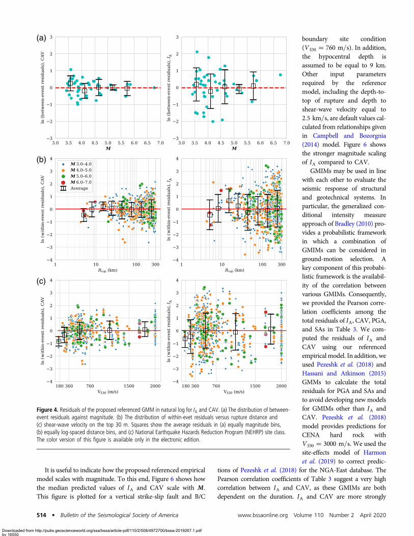
In Figure 4, the residuals of the FP20 referenced empiricalmodel are plotted versus magnitude, distance, and VS forboth IA and CAV. This figure shows the distribution ofbetween-event residuals versus magnitude and within-eventresiduals versus rupture distance (Rrup) and VS. In Figure 4a,

we grouped magnitude data into five groups and averaged overthe residuals in the same bin. We followed a similar procedureand divided distance data into eight groups in Figure 4b.In addition, we categorized recording motions to the fiveNEHRP site classifications while plotting within-event residualsagainst the VS in Figure 4c. Overall, no significant residualtrend is apparent from this figure, which confirms the suitabilityof the proposed model. In addition, the distribution of residualsversus all independent variables indicate that the modeldeveloped for CAV has higher predictive capability than thatof IA, which is consistent with the findings of Campbell andBozorgnia (2012, 2019). According to Figure 4, there is no dis-cernable residual trend for within-event residuals versus the VS

except for the NEHRP site classes D and E. This is an interestingobservation because we used the site factors proposed byCampbell and Bozorgnia (2019) to implicitly account for thesite term in our model. The small tendency to smaller averageresiduals for softer sites (classes D and E) is probably due to thesensitivity of the reference model to the basin effects. Moreover,for the site class E, only four records are available that may notbe sufficient to account for complex site-response characteristicsand potential for nonlinear site effects in this class. As it is clearfrom Figure 4, we used the reference model outside its validityrange to consider class A sites (VS30 > 1500 m=s) in our eval-uations. The inspection of the within-event residuals showsno apparent trend corresponding to VS30 above 1500 m=s.Consequently, we consider our new model to be valid for VS30

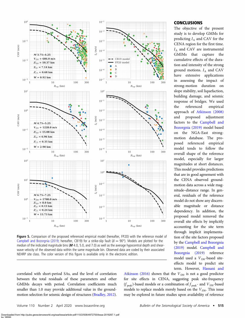
values between 150 and 2000 m=s.In Figure 5, we compared the proposed referenced empirical

model (FP20) with the reference model (CB19) and observeddata for various magnitudes and across rupture distances up to300 km. In this figure, models are plotted for the median of theindicated magnitude bins (M 4.0, 5.0, and 7.0) as well as theaverage VS of the observed data within the same magnitudebin. Increasing magnitude would result in a significantreduction in the observed data. For the last magnitude bin(M 6.75–7.25), there are only three recording motions fromthe 1985 Nahanni earthquake. Figure 5 illustrates that the pro-posed model works well in matching the observed data inCENA region confirming the adequacy of the adjustment fac-tors proposed to CB19 model by the FP20 model for the CENAground-motion data. The FP20 model proposed for CENAprovides higher predictions for GMIMs compared to theCB19 model. However, the FP20 model tends to behave similarto the CB19 model for larger magnitudes at short distances. Asis clear from Figure 5, there is a smooth kink in curves given byboth GMMs at 80 km due to the way the anelastic attenuationhas been modeled in the CB19 model. The CB19 model con-siders different attenuation trend for distances below andabove 80 km. Such a kink is sharper for the proposed modelthan that of the reference model because the difference in theattenuation trend between CENA and California is more high-lighted at regional distances.

TABLE 2Regression Coefficients of the Proposed Model

GMIM C0 C1 C2 h τ φ σ

IA 1.069 −0.162 0.232 4.869 0.82 1.27 1.52CAV 0.707 −0.051 0.092 6.325 0.41 0.61 0.74

GMIM, ground-motion intensity measure.



It is useful to indicate how the proposed referenced empiricalmodel scales with magnitude. To this end, Figure 6 shows howthe median predicted values of IA and CAV scale with M.This figure is plotted for a vertical strike-slip fault and B/C

boundary site condition(VS30 � 760 m=s). In addition,the hypocentral depth isassumed to be equal to 9 km.Other input parametersrequired by the referencemodel, including the depth-to-top of rupture and depth toshear-wave velocity equal to2:5 km=s, are default values cal-culated from relationships givenin Campbell and Bozorgnia(2014) model. Figure 6 showsthe stronger magnitude scalingof IA compared to CAV.

GMIMs may be used in linewith each other to evaluate theseismic response of structuraland geotechnical systems. Inparticular, the generalized con-ditional intensity measureapproach of Bradley (2010) pro-vides a probabilistic frameworkin which a combination ofGMIMs can be considered inground-motion selection. Akey component of this probabi-listic framework is the availabil-ity of the correlation betweenvarious GMIMs. Consequently,we provided the Pearson corre-lation coefficients among thetotal residuals of IA, CAV, PGA,and SAs in Table 3. We com-puted the residuals of IA andCAV using our referencedempirical model. In addition, weused Pezeshk et al. (2018) andHassani and Atkinson (2015)GMMs to calculate the totalresiduals for PGA and SAs andto avoid developing new modelsfor GMIMs other than IA andCAV. Pezeshk et al. (2018)model provides predictions forCENA hard rock withVS30 � 3000 m=s. We used thesite-effects model of Harmonet al. (2019) to correct predic-

tions of Pezeshk et al. (2018) for the NGA-East database. ThePearson correlation coefficients of Table 3 suggest a very highcorrelation between IA and CAV, as these GMIMs are bothdependent on the duration. IA and CAV are more strongly

(a)

(b)

(c)

Figure 4. Residuals of the proposed referenced GMM in natural log for IA and CAV. (a) The distribution of between-event residuals against magnitude. (b) The distribution of within-evet residuals versus rupture distance and(c) shear-wave velocity on the top 30 m. Squares show the average residuals in (a) equally magnitude bins,(b) equally log-spaced distance bins, and (c) National Earthquake Hazards Reduction Program (NEHRP) site class.The color version of this figure is available only in the electronic edition.



correlated with short-period SAs, and the level of correlationbetween the total residuals of these parameters and otherGMIMs decays with period. Correlation coefficients muchsmaller than 1.0 may provide additional value in the ground-motion selection for seismic design of structures (Bradley, 2012).

CONCLUSIONSThe objective of the presentstudy is to develop GMMs forpredicting IA and CAV for theCENA region for the first time.IA and CAV are instrumentalGMIMs that capture thecumulative effects of the dura-tion and intensity of the strongground motions. IA and CAVhave extensive applicationsin assessing the impact ofstrong-motion duration onslope stability, soil liquefaction,building damage, and seismicresponse of bridges. We usedthe referenced empiricalapproach of Atkinson (2008)and proposed adjustmentfactors to the Campbell andBozorgnia (2019) model basedon the NGA-East strong-motion database. The pro-posed referenced empiricalmodel tends to follow theoverall shape of the referencemodel, especially for largermagnitudes at short distances.This model provides predictionsthat are in good agreement withthe CENA observed ground-motion data across a wide mag-nitude–distance range. In gen-eral, residuals of the referencemodel do not show any discern-able magnitude or distancedependency. In addition, theproposed model removed theoverall site effects by implicitlyaccounting for the site termthrough implicit implementa-tion of the site factors proposedby the Campbell and Bozorgnia(2019) model. Campbell andBozorgnia (2019) referencemodel used a VS30-based site-effects model to predict siteterm. However, Hassani and

Atkinson (2016) shown that the VS30 is not a good predictorfor site effects in CENA, suggesting peak site-frequency(f peak)-based models or a combination of f peak- and VS30-basedmodels to replace models merely based on the VS30. This issuemay be explored in future studies upon availability of reference

Figure 5. Comparison of the proposed referenced empirical model (hereafter, FP20) with the reference model ofCampbell and Bozorgnia (2019; hereafter, CB19) for a strike-slip fault (δ � 90°). Models are plotted for themedian of the indicated magnitude bins (M 4.0, 5.0, and 7.0) as well as the average hypocentral depth and shear-wave velocity of the observed data within the same magnitude bin. Observed data are coded by their associatedNEHRP site class. The color version of this figure is available only in the electronic edition.



models based on f peak or the combination of f peak and VS30. Wesuggest the proposed referenced empirical model to be used forestimating IA and CAV within the CENA region for magnitudesabove M 3.30, and rupture distances up to 300 km and VS30

values between 150 and 2000 m=s. There are very limitedground-motion observations for magnitudes above M 5.8 in

the NGA-East strong-motiondatabase. Therefore, a largeamount of epistemic uncer-tainty is associated with themedian predictions of the pro-posed referenced empiricalmodel for the magnitude–distance range of engineeringinterest. To adequately addressthis epistemic uncertainty, otherapproaches should be used todevelop alternative models forpredicting IA and CAV.

DATA AND RESOURCESThe Next Generation Attenuation-East (NGA-East) flat-file usedin this study could be accessed from

(www.peer.berkeley.edu; last accessed October 2019). In addition, weused the acceleration time histories to compute Arias intensity (IA)and cumulative absolute velocity (CAV) values not presented in theNGA-East database. Figure 1 was prepared using ArcMap 10.5.1.Moreover, we used Python 3.7 libraries including Matplotlib,Numpy, Pandas, Seaborn, and Statsmodels to perform linear mixed-effects regression and make Figures 2–6.

ACKNOWLEDGMENTSThis study benefited from the constructive and insightful comments oftwo anonymous reviewers as well as Associate Editor Ivan G. Wong.

REFERENCESAbrahamson, C., H.-J. M. Shi, and B. Yang (2016). Ground-motion pre-

diction equations for Arias intensity consistent with the NGA-West2ground-motion models, PEER Report 2016/05, Pacific EarthquakeEngineering Research Center, University of California, Berkeley.

Abrahamson, N. A., and R. R. Youngs (1992). A stable algorithm forregression analyses using the random-effects model, Bull. Seismol.Soc. Am. 82, 505–510.

Arias, A. (1970). A measure of earthquake intensity, in Seismic Designfor Nuclear Power Plants, R. J. Hansen (Editor), The MIT Press,Cambridge, Massachusetts, 438–483.

Atkinson, G. (2008). Ground-motion prediction equations for easternNorth America from a referenced empirical approach: Implicationsfor epistemic uncertainty, Bull. Seismol. Soc. Am. 98, 1304–1318.

Atkinson, G. (2010). Ground-motion prediction equations for Hawaiifrom a referenced empirical approach, Bull. Seismol. Soc. Am. 101,1304–1318.

Atkinson, G., and D. Boore (1995). New ground motion relations foreastern North America, Bull. Seismol. Soc. Am. 85, 17–30.

Atkinson, G., and D. Boore (2006). Ground motion prediction equa-tions for earthquakes in eastern North America, Bull. Seismol.Soc. Am. 96, 2181–2205.

Atkinson, G., and D. Boore (2011). Modifications to existing ground-motion prediction equations in light of new data, Bull. Seismol. Soc.Am. 101, 1121–1135.

Figure 6. Scaling of Arias intensity and CAV with the moment magnitude for a vertical strike-slip earthquake.

TABLE 3Summary of the Pearson Correlation Coefficients of theTotal Residuals

HA15 GMM PZCT18 GMM

GMIM CAV IA CAV IA

PGA 0.804 0.791 0.833 0.8480.05 0.825 0.803 0.820 0.8200.075 0.805 0.781 0.826 0.8090.10 0.751 0.744 0.796 0.7910.15 0.681 0.689 0.753 0.7540.20 0.633 0.641 0.701 0.6930.25 0.591 0.596 0.580 0.6020.30 0.568 0.577 0.513 0.5520.40 0.506 0.515 0.502 0.5180.50 0.462 0.474 0.411 0.4370.75 0.404 0.422 0.350 0.3861.0 0.367 0.389 0.288 0.3441.50 0.340 0.376 0.269 0.3302.0 0.316 0.362 0.246 0.3143.0 0.270 0.330 0.211 0.2824.0 0.220 0.290 0.172 0.2455.0 0.215 0.293 0.169 0.2457.5 0.260 0.332 0.216 0.28410 0.291 0.358 0.261 0.321CAV 1.000 0.959 1.000 0.959IA 0.959 1.000 0.959 1.000

GMIM, ground-motion intensity measure; GMM, ground-motion model; HA15,Hassani and Atkinson (2015) GMM; PGA, peak ground acceleration; PZCT18,Pezeshk et al. (2018) GMM.



www.peer.berkeley.edu




Atkinson, G., and D. Motazedian (2013). Ground-motion amplitudes forearthquakes in Puerto Rico, Bull. Seismol. Soc. Am. 103, 1846–1859.

Boore, D. M. (2010). Orientation-independent, nongeometric-meanmeasures of seismic intensity from two horizontal componentsof motion, Bull. Seismol. Soc. Am. 100, 1830–1835.

Boore, D. M., J. P. Stewart, E. Seyhan, and G. M. Atkinson (2014).NGA-West2 equations for predicting PGA, PGV, and 5% dampedPSA for shallow crustal earthquakes, Earthq. Spectra 30, no. 3,1057–1085.

Bozorgnia, Y., N. Abrahamson, L. Al Atik, T. Ancheta, G. Atkinson, J.Baker, A. Baltay, D. Boore, K. Campbell, B. Chiou, et al. (2014).NGA-West 2 research project, Earthq. Spectra 30, 973–987.

Bradley, B. A. (2010). A generalized conditional intensity measureapproach and holistic ground motion selection, Earthq. Eng. Struct.Dynam. 39, 1321–1342.

Bradley, B. A. (2012). Empirical correlations between cumulativeabsolute velocity and amplitude-based ground motion intensitymeasures, Earthq. Spectra 28, 37–54.

Bustos, A. G., and P. J. Stafford (2012). On the use of Arias intensity asa lower bound in the hazard integration process of a PSHA, Proc.15th World Conf. on Earthquake Engineering, Vol. 12, Lisbon,Portugal, 24–28 September 2012, 9011–9020.

Cabañas, L., B. Benito, and M. Herráiz (1997). An approach to themeasurement of the potential structural damage of earthquakeground motions, Earthq. Eng. Struct. Dynam. 26, 79–92.

Campbell, K. W. (2003). Prediction of strong ground motion using thehybrid empirical method and its use in the development of groundmotion (attenuation) relations in eastern North America, Bull.Seismol. Soc. Am. 93, 1012–1033.

Campbell, K. W., and Y. Bozorgnia (2010). A ground motion predic-tion equation for the horizontal component of cumulative absolutevelocity (CAV) using the PEER-NGA database, Earthq. Spectra 26,635–650.

Campbell, K. W., and Y. Bozorgnia (2011). Predictive equations forthe horizontal component of standardized cumulative absolutevelocity as adapted for use in the shutdown of U.S. nuclear powerplants, Nucl. Eng. Des. 241, 2558–2569.

Campbell, K. W., and Y. Bozorgnia (2012). A comparison of groundmotion prediction equations for Arias intensity and cumulativeabsolute velocity developed using a consistent database and func-tional form, Earthq. Spectra 28, 931–941.

Campbell, K. W., and Y. Bozorgnia (2014). NGA-West2 groundmotion model for the average horizontal components of PGA,PGV, and 5%-damped linear acceleration response spectra,Earthq. Spectra 30, 1087–1115.

Campbell, K. W., and Y. Bozorgnia (2019). Ground motion models forthe horizontal components of Arias intensity (AI) and cumulativeabsolute velocity (CAV) using the NGA-West2 database, Earthq.Spectra 35, 1289–1310.

Chiou, B. S.-J., and R. R. Youngs (2014). Update of the Chiou andYoungs NGA model for the average horizontal component of peakgroundmotion and response spectra, Earthq. Spectra 30, 1117–1153.

Cramer, C. H. (2018). Gulf Coast regional Q boundaries fromUSArray data, Bull. Seismol. Soc. Am. 108, 427–449.

Dreiling, J., M. P. Isken, W. D. Mooney, M. C. Chapman, and R. W.Godbee (2014). NGA-East regionalization report: Comparison offour crustal regions within Central and Eastern North America

using waveform modeling and 5%-damped pseudo-spectral accel-eration response, PEER Report No. 2014/15, Pacific EarthquakeEngineering Research Center (PEER), University of California,Berkeley, California.

Du, W., and G. Wang (2013). A simple ground-motion predictionmodel for cumulative absolute velocity and model validation,Earthq. Eng. Struct. Dynam. 42, 1189–1202.

Du, W., and G. Wang (2018). Ground motion selection for seismicslope displacement analysis using a generalized intensity measuredistribution method, Earthq. Eng. Struct. Dynam. 45, 1352–1359.

Electrical Power Research Institute (1988). A criterion for determin-ing exceedance of the operating basis earthquake, Report EPRI NP-5930, Palo Alto, California.

Electrical Power Research Institute (1991). Standardization of thecumulative absolute velocity, Report No. EPRI TR-100082-T2,Palo Alto, California.

Foulser-Piggott, R., and P. J. Stafford (2012). A predictive modelfor Arias intensity at multiple sites and consideration of spatialcorrelations, Earthq. Eng. Struct. Dynam. 41, 431–451.

Goulet, C. A., T. Kishida, T. D. Ancheta, C. H. Cramer, R. B. Darragh,W. J. Silva, Y. M. A. Hashash, J. Harmon, J. P. Stewart, K. E.Wooddell, et al. (2014). PEER NGA-East database, PEER ReportNo. 2014/17, Pacific Earthquake Engineering Research Center(PEER), University of California, Berkeley, California.

Harmon, J. A., Y. M. A. Hashash, J. P. Stewart, E. M. Rathje, K. W.Campbell, W. J. Silva, B. Xu, M. Musgrove, and O. Ilhan (2019).Site amplification functions for central and eastern North America—Part II: Modular simulation-based models, Earthq. Spectra 35,815–847.

Hassani, B., and G. M. Atkinson (2015). Referenced empirical ground-motion model for eastern North America, Seismol. Res. Lett. 86,477–491.

Hassani, B., and G. M. Atkinson (2016). Applicability of the NGA-West2 site-effects model for central and eastern North America,Bull. Seismol. Soc. Am. 106, 1331–1341.

Jibson, R. W. (2007). Regression models for estimating coseismiclandslide displacement, Eng. Geol. 91, 209–218.

Kayen, R. E., and J. K. Mitchell (1997). Assessment of liquefactionpotential during earthquakes by Arias intensity, J. Geotech.Geoenviron. Eng. 123, 1162–1174.

Kiani, J., and S. Pezeshk (2017). Sensitivity analysis of the seismicdemands of RC moment resisting frames to different aspects ofground motions, Earthq. Eng. Struct. Dynam. 46, doi: 10.1002/eqe.2928.

Kiani, J., C. Camp, and S. Pezeshk (2018). Role of conditioning inten-sity measure in the influence of ground motion duration on thestructural response, Soil Dynam. Earthq. Eng. 104, 408–417.

Kramer, S. L. (1996). Geotechnical Earthquake Engineering, PrenticeHall, Inc., Upper Saddle River, New Jersey, 653 pp.

Kramer, S. L., and R. A. Mitchell (2006). Ground motion intensitymeasures for liquefaction hazard evaluation, Earthq. Spectra 22,413–438.

Mackie, K., and B. Stojadinovic (2001). Probabilistic seismic demandmodel for California highway bridges, J. Bridge Eng. 6, 468–481.

Pezeshk, S., A. Zandieh, K. W. Campbell, and B. Tavakoli (2018).Ground-motion prediction equations for central and easternNorth America using the hybrid empirical method and



http://dx.doi.org/10.1002/eqe.2928

http://dx.doi.org/10.1002/eqe.2928

NGA-West2 empirical ground-motion models, Bull. Seismol. Soc.Am. 108, 2278–2304.

Pezeshk, S., A. Zandieh, and B. Tavakoli (2011). Hybrid empiricalground motion prediction equations for eastern North Americausing NGA models and updated seismological parameters, Bull.Seismol. Soc. Am. 101, 1859–1870.

Reed, J. W., and R. P. Kassawara (1990). A criterion for determiningexceedance of the operating basis earthquake, Nucl. Eng. Des. 123,387–396.

Silva, W., N. Gregor, and R. Darragh (2002). Development of regionalhard rock attenuation relations for central and eastern NorthAmerica, Technical Report, Pacific Engineering and Analysis, ElCerrito, California.

Tarbali, K., and B. A. Bradley (2015). Ground motion selection forscenario ruptures using the generalized conditional intensity

measure (GCIM) method, Earthq. Eng. Struct. Dynam. 44,1601–1621.

Tavakoli, B., and S. Pezeshk (2005). Empirical-stochastic ground-motion prediction for eastern North America, Bull. Seismol.Soc. Am. 95, 2283–2296.

Toro, G. R., N. A. Abrahamson, and J. F. Schneider (1997). Model ofstrong ground motions from earthquakes in central and easternNorth America: Best estimates and uncertainties, Seismol. Res.Lett. 68, 41–57.

Tothong, P., and N. Luco (2007). Probabilistic seismic demand analy-sis using advanced ground motion intensity measures, Earthq. Eng.Struct. Dynam. 36, 1837–1860.

Manuscript received 16 October 2019

Published online 3 March 2020



A Referenced Empirical Ground-Motion Model for Arias ...

Documents

Transcript of A Referenced Empirical Ground-Motion Model for Arias ...