A Partial-Order-Based Model to Estimate Individual ... · PDF fileA Partial-Order-Based Model...
55
A Partial-Order-Based Model to Estimate Individual Preferences using Panel Data Srikanth Jagabathula Leonard N. Stern School of Business, New York University, New York, NY 10012, [email protected] Gustavo Vulcano Leonard N. Stern School of Business, New York University, New York, NY 10012, [email protected], School of Business, Torcuato di Tella University, Buenos Aires, Argentina In retail operations, customer choices may be affected by stockout and promotion events. Given panel data with the transaction history of customers, and product availability and promotion data, our goal is to predict future individual purchases. We use a general nonparametric framework in which we represent customers by partial orders of prefer- ences. In each store visit, each customer samples a full preference list of the products consistent with her partial order, forms a consideration set, and then chooses to purchase the most preferred product among the considered ones. Our approach involves: (a) defining behavioral models to build consideration sets as subsets of the products on offer, (b) proposing a clustering algorithm for determining customer segments, and (c) deriving marginal distributions for partial preferences under the multinomial logit (MNL) model. Numerical experiments on real-world panel data show that our approach allows more accurate, fine-grained predictions for individual purchase behavior compared to state-of-the-art alternative methods. Key words : nonparametric choice models, inertia in choice, brand loyalty, panel data. Original version: February 2015. Revisions: January 2016, July 2016, September 2016. 1. Introduction Demand estimates are key inputs for inventory control and price optimization models used in retail operations and revenue management (RM). 1 In the last decade, there has been a trend of switching from independent demand models to choice-based models of demand in both the academia and the industry practice. For simplicity, the traditional approach assumed that each product has its own independent stream of demand. However, if products are substitutes and their availabilities vary over time, then the demand for each product will be a function of the set of alternatives available to consumers when they make their purchase decisions, so that ignoring stockout and substitution effects that occur over time can introduce biases in the estimation process. The building block for estimating customer choice is the specification of a choice model, either parametric or nonparametric. Most of the proposals in the operations-related literature have been 1 For instance, a field study in the airline RM practice suggests that a 20% reduction of forecast error can translate into a 1% additional revenues (P¨ olt [34]). 1
Transcript of A Partial-Order-Based Model to Estimate Individual ... · PDF fileA Partial-Order-Based Model...
A Partial-Order-Based Model to EstimateIndividual Preferences using Panel Data
Srikanth JagabathulaLeonard N. Stern School of Business, New York University, New York, NY 10012, [email protected]
Gustavo VulcanoLeonard N. Stern School of Business, New York University, New York, NY 10012, [email protected],
School of Business, Torcuato di Tella University, Buenos Aires, Argentina
In retail operations, customer choices may be affected by stockout and promotion events. Given panel
data with the transaction history of customers, and product availability and promotion data, our goal is to
predict future individual purchases.
We use a general nonparametric framework in which we represent customers by partial orders of prefer-
ences. In each store visit, each customer samples a full preference list of the products consistent with her
partial order, forms a consideration set, and then chooses to purchase the most preferred product among
the considered ones. Our approach involves: (a) defining behavioral models to build consideration sets as
subsets of the products on offer, (b) proposing a clustering algorithm for determining customer segments,
and (c) deriving marginal distributions for partial preferences under the multinomial logit (MNL) model.
Numerical experiments on real-world panel data show that our approach allows more accurate, fine-grained
predictions for individual purchase behavior compared to state-of-the-art alternative methods.
Key words : nonparametric choice models, inertia in choice, brand loyalty, panel data.
Original version: February 2015. Revisions: January 2016, July 2016, September 2016.
1. Introduction
Demand estimates are key inputs for inventory control and price optimization models used in retail
operations and revenue management (RM).1 In the last decade, there has been a trend of switching
from independent demand models to choice-based models of demand in both the academia and the
industry practice. For simplicity, the traditional approach assumed that each product has its own
independent stream of demand. However, if products are substitutes and their availabilities vary
over time, then the demand for each product will be a function of the set of alternatives available
to consumers when they make their purchase decisions, so that ignoring stockout and substitution
effects that occur over time can introduce biases in the estimation process.
The building block for estimating customer choice is the specification of a choice model, either
parametric or nonparametric. Most of the proposals in the operations-related literature have been
1 For instance, a field study in the airline RM practice suggests that a 20% reduction of forecast error can translateinto a 1% additional revenues (Polt [34]).
1
Jagabathula and Vulcano: Estimating Individual Customer Preferences2 Article submitted to Management Science; manuscript no.
on the former for both estimation and assortment optimization (e.g., Kok and Fisher [27], Musalem
et al. [31]). By parametric, we mean that the number of parameters that describe the family of
underlying distributions is fixed and independent of the training data set volume. The parameter-
ized model structure relates product attributes to the utility values or choice probabilities of the
different options. The greatest advantage of parametric models is the ability to include covariates,
such as product features and price, that can help explain consumer preferences for alternatives.
This also enables parametric models like the multinomial logit (MNL) or nested logit (NL) with
linear-in-parameters utilities to extrapolate choice predictions to new alternatives that have not
been observed in historical data and to predict how changes in product attributes such as price
affect choice outcomes. Yet, the drawback of any parametric model is that one must make assump-
tions about the structure of preferences and the relevant covariates that influence it, which requires
expert judgment and trial-and-error testing to determine an appropriate specification.
Recently, with the rise of business analytics and data-driven approaches, there has been a growing
interest in revenue predictions and demand estimation derived from nonparametric choice models
(e.g., Farias and Jagabathula [15], Haensel and Koole [18], van Ryzin and Vulcano [44]) that provide
inputs for various optimization problems (see discussion in Section 1.2). These operations-related,
nonparametric proposals specify customer types defined by their rank ordering of all alternatives
(along with the no-purchase alternative).2 When faced with a choice from an offer set, a customer
is assumed to purchase the available product that ranks highest in her preference list – or to quit
without purchasing. The flexibility of this non-parametric choice model comes at a price: The
potential number of preference lists (customer types) in this rank-based choice model is factorial
in the number of alternatives, which challenges the estimation procedure.
The empirical evidence both in academia and industry practices strongly sustains choice-based
demand models over the independent demand assumption (e.g., Ratliff et al. [36], Newman et
al. [32], Vulcano et al. [45]) when the data source consists of product availability and sales trans-
action data. Yet, these models overlook two important features: First, they ignore the repeated
interactions of a given customer with the firm and treats every transaction as coming from a dif-
ferent individual; and second, they usually assume that the items evaluated by a given customer
in any store visit are all the available ones within a category (or subcategory) of products, which
likely overestimates the size of the true consideration set. The first limitation can be addressed by
keeping track of the repeated interactions between a customer and the firm by tagging transactions
2 In the rank-based choice model of demand, the modeler should estimate a discrete probability mass function (pmf) onthe set of customer types. The number of parameters (i.e., the number of customer types with non-zero probabilities)grows with the number of products, customers, and the volume of data, and hence the labeling as a nonparametricmodel.

Jagabathula and Vulcano: Estimating Individual Customer PreferencesArticle submitted to Management Science; manuscript no. 3
with customer id. This information, popularly referred to as panel data, can be used subsequently to
learn the preferences of individual customers. The canonical example is customers buying groceries
on a weekly basis from a grocery retailer, but more broadly the setting includes any application in
which customers exhibit loyalty through repeated purchases be it apparel, hotel, airline, etc. This
type of data is very common in practical settings because of the proliferation of loyalty cards and
other marketing programs, and can later be used to customize the offering (e.g., via personalized
assortments and prices -Clifford [13]-, or personalized mobile phone coupons -Danaher et al. [14]-).
The limitation on the unobserved consideration set of the customer requires building a behavioral
model of choice that captures individual bounded rationality.
In this paper we contribute to the literature by proposing a nonparametric, choice-based
demand framework that overcomes the two limitations discussed above, and that incorporates
both operations- and marketing-related components. We infer individual customer preferences from
panel data in a setting where: i) products are not always available (e.g., due to stock-outs or
deliberate scarcity introduced by the firm), ii) preferences may be altered by price or display pro-
motions, and iii) customers exhibit bounded rationality in the sense that they cannot evaluate all
the products on offer, and their consideration sets are unobservable. For the purpose of estimation,
the framework can accommodate both parametric and non-parametric models.
1.1. Summary of results
We propose a choice-based demand model that is a generalization of the aforementioned rank-
based model, which typically associates each customer with a fixed preference list that remains
constant over time. In our model, we focus on a fixed set of m customers who visit a firm repeatedly
and make purchases from a particular category or subcategory of products (e.g., coffee, shampoo,
etc). The full assortment is defined by a set of products, together with the no-purchase option.
Each customer belongs to a market segment and is characterized by a set of partial preferences,
represented by a directed acyclic graph (DAG) with products as nodes. The DAG captures partial
preferences of the form “product a is preferred to product b” through a directed edge from product a
to product b, but typically does not provide a full ranking of the products. Upon each store visit,
the customer samples a full ranking consistent with her DAG according to a distribution specified
for her particular market segment, and chooses the product within her consideration set that ranks
highest in her preference list. Of course, neither the customer’s DAG nor her sampled preference list
nor her consideration set are observable. For each customer id, the firm only observes a collection of
revealed preferences: the offered products at the moment of purchasing and the chosen product. As
a consequence, our estimation procedure involves three sequential phases: 1) Building the DAG for
each customer, 2) Clustering the DAGs into a pre-specified number of segments, and 3) Estimating
distributions over preference lists that best explain the purchasing patterns of the customers.

Jagabathula and Vulcano: Estimating Individual Customer Preferences4 Article submitted to Management Science; manuscript no.
The first phase requires a key element of our work: the modeling of behavioral biases of each
individual customer. Existing literature has established several behavioral biases that are common
in customer choice behavior. We focus on one such bias that is relevant to the construction of
consideration sets, namely, inertia in choice. Inertia in choice – also referred to as short-term
brand loyalty by Jeuland [25] – claims that when facing frequently purchased consumer goods,
customers tend to stick to the same option rather than evaluate all products on offer in each
store visit. We capture the effect of such inertia in choice by assuming that customers tend to
purchase what they bought previously until there is a “trigger event” that forces them to consider
other products on offer. We distinguish two important trigger events: stock-out of the previously
purchased product (which induces the customer to re-evaluate all products on offer), and existence
of product promotions (in particular, display and price promotions). Based on these behavioral
assumptions, we define a set of behavioral rules that allow us to dynamically build the customer’s
DAG as we keep track of the sequence of her interactions with the firm and she reveals her
preferences through her purchasing patterns.
Next, in order to better capture customer heterogeneity, we cluster the m DAGs into K classes,
where K is a predetermined small number (e.g., K = 5). We formulate this clustering problem as
an integer program (IP) to systematically capture the idea that the DAGs of individual customers
assigned to the same class are “close” to each other (according to a distance metric).
Finally, in the estimation phase, we calibrate a multinomial logit (MNL) model to assess prob-
abilistic distributions over preference lists consistent with the DAGs of the first phase and the
clustering of the second phase.
The predictive performance of our method is demonstrated through an exhaustive set of numeri-
cal experiments using real-world panel data on the purchase of 29 grocery categories across two big
US markets in year 2007. We divide our data set in two pieces. On the first part (i.e., the training
data), we perform the three phases summarized above. Then, on the second part (i.e., the hold-out
sample), we predict what the customer would purchase when confronted with the offer sets and
products on promotion, and compare with the recorded purchase. We observe that our method
with behavioral rules and clustering obtains up to 40% improvement in prediction accuracy on
standard metrics over state-of-the-art benchmarks based on variants of the MNL, commonly used
in the current industry practice.
1.2. Positioning in the literature
Our work has several connections to the literature in both operations and marketing. While existing
work in operations has largely focused on using transaction data aggregated over all customers
to estimate choice models, literature in marketing has extensively used panel data to fit choice

Jagabathula and Vulcano: Estimating Individual Customer PreferencesArticle submitted to Management Science; manuscript no. 5
models. The latter extends all the way back to the seminal work of Guadagni and Little [16], in
which they fit a MNL model to household panel data on the purchases of regular ground coffee,
and which has paved the way for choice modeling in marketing using scanner panel data3; see
Chandukala et. al. [8] and Wierenga [46] for a detailed overview of choice modeling using panel
data in the area of marketing. Much of this work focuses on understanding how various panel
covariates influence individual choice making. For that, a model is specified that relates the panel
covariates to a distribution over preference lists (induced, for instance, by the MNL model) that
describes the preferences of each customer. The model is then estimated from choice data assuming
that different choices of the same customer are characterized by independent draws of preference
lists from the same distribution.
Our work tightens this assumption by allowing customers to be ‘partially consistent’ in their
preferences across different choice instances, so that the draws of preference lists are no longer fully
independent but are compatible with the customer’s DAG. This additional structure allows our
model to capture individual preferences more accurately, especially when observations are sparse.
In the context of the operations-related literature, rank-based choice models of demand have been
used as inputs in retail operations proposals, pioneered by the work of Mahajan and van Ryzin [29],
who analyze a single-period, stochastic inventory model in which a sequence of customers described
by preference lists substitute among product variants within a retail assortment while inventory is
depleted. Other recent retail operations papers dealing with variants of rank-based choice models
include Rusmevichientong et al. [38], Smith et al. [39], Honhon et al. [20], Honhon et al. [21],
and Jagabathula and Rusmevichientong [23]. Rank-based models also reached the airline-related
RM literature (e.g., see Zhang and Cooper [47], Chen and Homem-de-Mello [10], Chaneton and
Vulcano [9], and Kunnumkal [28]). All these proposals assume that data is obtained at the market
level, and do not take into account the repeated interaction of a customer with a firm. Therefore,
its applicability to make fine-grained, individual level predictions of purchasing patterns is unclear.
Finally, our work has rich methodological connections to the area that studies distributions over
rankings in Statistics and Machine Learning. We discuss these connections in Sections 3 and 5.
2. Model description
We start this section with a description of the general modeling framework, where we introduce
basic notation and formally define the DAGs that represent the customers. We continue with
a discussion of the model assumptions, where we position our framework with respect to the
traditional approaches towards customer choice. Next, we describe the type of data needed by our
framework, and finish with a detailed explanation of the DAGs’ construction process.
3 In fact, we use a variant of the model by Guadagni and Little [16] as one of our benchmarks in Section 5.

Jagabathula and Vulcano: Estimating Individual Customer Preferences6 Article submitted to Management Science; manuscript no.
2.1. General modeling framework
We model consumer preferences using a general rank-based choice model of demand. The product
universe N consists of n products {a1, a2, . . . , an}. The ‘no-purchase’ or ‘outside’ alternative is
denoted by 0. Preferences over the universe of products are captured by an anti-reflexive, anti-
symmetric, and transitive relation �, which induces a total ordering or ranking over all the products
in the universe, and we write a� b to mean “a is preferred to b”. Preferences can also be represented
through rankings or permutations. Each preference list σ specifies a rank ordering over the n+ 1
products in the universe N ∪{0}, with σ(a) denoting the preference rank of product a. Lower ranks
indicate higher preference so that a customer described by σ prefers product a to product b if and
only if σ(a)<σ(b), or equivalently, if a�σ b.
The population consists of m customers who make purchases over T discrete time periods.
We assume that the set of customers and the set of products remain constant over time. Each
customer i is described by a general partial order Di. A general partial order specifies a collection
of pairwise preference relations, Di ⊂ {(aj, aj′) : 0≤ j, j′ ≤ n, j 6= j′}, so that product aj is preferred
to product aj′ for any (aj, aj′) ∈Di. In addition, the customer belongs to one of K segments in
the market, where segment k is characterized by a probability distribution λk over preference lists.
In every interaction with the firm, the customer will sample a full ranking consistent with Di
according to the distribution λk. We say that a preference list σ is consistent with partial order Di
if and only if σ(aj)<σ(aj′) for each (aj, aj′)∈Di. The partial order Di could be empty (i.e., have
no arcs), in which case the consistency requirement is vacuous.
To illustrate, suppose n= 3 and take a customer of type k with partial order D= {(1,2), (3,2)}.
For ease of exposition, we ignore here the no-purchase alternative.4 There are two possible rankings
consistent with D in this case: 1 � 3 � 2, and 3 � 1 � 2. The distribution λk specifies the point
probabilities for each of the six possible rankings. Now, since D = {(1,2), (3,2)}, the customer
consistently prefers both 1 and 3 over 2 in every choice instance. Hence, conditioned on D, she
samples the preference list 1� 3� 2 or 3� 1� 2, say with probabilities 0.6 and 0.4, respectively.
The choice process proceeds as follows. In each purchase or choice instance, customer i of type k is
offered a subset S of products. She focuses on a consideration set C ⊂ S∪{0}, samples a preference
list σ according to distribution λk from her collection of rankings consistent with Di, and purchases
from C the most preferred product according to σ, i.e., arg minaj∈C σ(aj). Different choice instances
for customer i are independent but always consistent with her own collection of preference lists
described by her partial order Di. Thus, in the previous example, and assuming that the customer
considers all products on offer, if the subset S = {1,2} is offered, the customer chooses product 1
4 This example could be used to model the preferences of a coffee customer who always prefers decaf (product 1and 3) to non-decaf (product 2). One may readily construct other such examples.

Jagabathula and Vulcano: Estimating Individual Customer PreferencesArticle submitted to Management Science; manuscript no. 7
for sure. If S = {1,2,3} is offered, then the customer purchases 1 with probability 0.6 (if 1� 3� 2
is sampled), and 3 with probability 0.4 (if 3� 1� 2 is sampled).
The model described above is quite general and requires further restrictions to be estimable from
data. The model is specified by the partial order Di for each customer i, the number of customer
classes K, the class membership of each of the customers, and the distribution λk over prefer-
ence lists for each class k. The partial orders are built dynamically as we keep track of the store
visits of each customer recorded in the training dataset, as explained later in Section 2.4. Their
construction requires a behavioral model relating the observed choices to underlying preferences.
Next, for an input parameter K, we determine the class membership of each of the customers
through a clustering technique described in Section 4. Broadly speaking, the clustering technique
clusters together customers with similar partial preferences. The distributions λk can in principle
be induced by any of the commonly used choice models. In this paper, we focus on the most com-
monly used model: the MNL model, which has been extensively applied in operations, marketing,
economics, and transportation science. As shown in Section 3, the MNL model allows for tractable
(or approximately tractable) estimation from general partial orders.
2.2. Discussion of model assumptions
The inference of the customers’ partial orders assumes that both the population of customers and
the product universe remain constant along the horizon T . Our approach can be repeated from time
to time (e.g., once a year) in order to collect new data points and update both the customer base
and their preferences. In the meantime, new items in the category could be considered within the
scope of an existing product, which is our minimal level of aggregation in the analysis to establish
preferences.5
The potential benefit of the DAGs is the boost in accuracy it could provide for fine-grained
individual-level predictions. These gains could be particularly significant for cases in which only a
small sample of information is available for each customer, and customers are endowed with con-
sistent preferences, like brand-loyal customers. In such cases, it is impractical to fit a choice model
separately to each customer. For this reason, one must make distributional assumptions relating
the preferences of the different customers, while retaining sufficient customer-level heterogeneity.
A common approach is to assume that customers belong to K classes/segments and all customers
in class k are homogeneous in the sense that they sample preferences from the same distribu-
tion λk, though the distributions are different across different classes. For instance, all customers
of class k may sample preferences from the same multinomial logit (MNL) distribution, but the
MNL parameters are different across different classes.
5 We explain later in Section 5 how we aggregate different Universal Product Codes (UPCs) in the dataset.

Jagabathula and Vulcano: Estimating Individual Customer Preferences8 Article submitted to Management Science; manuscript no.
A challenge in implementing this approach is setting the appropriate value for the number
of segments K. On the one hand, smaller values of K result in parsimonious models that can
be efficiently fit to available data. On the other hand, larger values of K can better capture
customer-level heterogeneity. Our model avoids this difficulty by providing an additional lever to
capture heterogeneity while retaining parsimony. Specifically, even if customers are not segmented
and are assumed to sample preferences from the same distribution (e.g., a single class MNL),
our model captures customer-level heterogeneity by allowing the partial orders to differ across
customers. When computing the probability of customer i choosing a particular option, we use the
demand estimates but also condition on the customer being characterized by Di, which imposes
additional structure (and constraints) on the utility drawn for the different products. The DAGs
are inferred from small sample data and typically require significantly less computational effort
than the estimation of a multi-class demand model. Recall that our model is quite general in the
sense that if the DAGs are empty (i.e., the nodes are isolated), no structure is superimposed and we
recover a standard, unconstrained, choice-based demand model (e.g., a typical, single-class MNL).
On the other hand, we expect the gains to be subdued or non-existent for customers who are
variety-seeking and inconsistent in their preferences across multiple purchase instances. Such cus-
tomers are readily identified with only a few observations (we would quickly identify products a
and b such that a is purchased over b in one instance, and b is purchased over a in another instance).
These customers will be represented with empty DAGs, and traditional techniques may be applied.
It is also worth pointing out that using the transitivity of the pair preferences captured by arcs
in the DAGs (e.g., a� b and b� c) allows to infer a richer set of preferences not directly revealed
(e.g., a� c), and that are not explicitly subsumed in traditional models.
Finally, note that our model for customer choice behavior is consistent with the Random Utility
Maximization (RUM) class of models. These models assume that each customer samples utilities
for each of the considered products and chooses to purchase the product with the maximum
utility. A particular model specification consists of a definition of the distribution from which
utilities are drawn. Since each realization of utilities induces a preference list with higher utility
products preferred to lower utility products, the RUM model can be equivalently specified through
a distribution over preference lists (e.g., see Strauss [41], and Mahajan and van Ryzin [29, Section 2]
for further discussion). In a similar fashion, our model assumes that in each choice instance, a
customer samples a preference list according to a distribution over preference lists (conditioned
on her DAG) and chooses the most preferred product. Consequently, our model description of
customer choice behavior is consistent with that of a RUM class.
Jagabathula and Vulcano: Estimating Individual Customer PreferencesArticle submitted to Management Science; manuscript no. 9
2.3. Data model
We assume access to panel data with the panel consisting of m customers purchasing over T periods.
In particular, the purchases of customer i are tracked over Ti discrete time periods for a given
category of products. To simplify notation, we relabel the periods on a per customer basis: t= 1
corresponds to his first visit to the store, t= 2 corresponds to his second visit to the store, and Ti
corresponds to the last one in the training dataset. For each customer i, the basic data consist of
purchases of the customer over time, denoted by tuples (ajit , Sit) for t= 1,2, . . . , Ti, where Sit ⊂Ndenotes the subset of products on offer in period t, and ajit ∈ Sit denotes the product purchased in
period t.
In addition, the dataset includes information about the products Pit ⊂ Sit that were on pro-
motion in period t. A product may be on display promotion (prominently displayed on the store
shelves) or on price promotion (offered at a discounted price). In either case, the product exhibits
a distinctive feature that makes it stand out from the others on offer, potentially impacting the
purchase behavior of the customer (more on this below). To simplify the analysis, we consider the
promotion feature as a binary attribute of a product. However, our model could be extended to
distinguish a finite number of price discount depths and display formats.
2.4. Building the customers’ partial orders
We dynamically build customers’ partial orders from the panel data by keeping track of the
sequences of interactions between the customers and the firm. Specifically, for each customer i, we
start with the empty DAG Di (i.e., a DAG with isolated nodes), and sequentially add preference
arcs (pairwise comparisons) inferred from the sequence of purchase observations of the customer.
To explain how we infer the preference arcs, consider the store visit corresponding to the pur-
chase observation (transaction) (aj, S) of a customer, in which product aj was purchased from the
subset S ∪ {0}. Let σ denote the preference list used by the customer for this purchase instance.
The classical assumption is that the customer considers all the offered products and decides to
purchase the most preferred one. In other words, when offered subset S, the customer purchases
arg mina`∈S∪{0} σ(a`). This classical assumption then implies that since aj is the observed purchase,
the underlying preference list σ is such that aj = arg mina`∈S∪{0} σ(a`), so that σ(aj)<σ(a`) for all
a` ∈ S∪{0}, ` 6= j. But customers are rationally bounded and may not consider all the products on
offer. A typical supermarket carries tens (or even hundreds) of products under each category. Fur-
ther, the customer may not adopt a complex purchase process for frequently purchased products.
Given this, it is unreasonable to expect the customer to evaluate all the products offered on the
shelves. As a result, we assume that customers evaluate only a subset of the offered products, often
called the consideration set. Existing literature provides evidence for various behavioral heuristics
that customers use to construct consideration sets (e.g., see the recent survey by Hauser [19]).

Jagabathula and Vulcano: Estimating Individual Customer Preferences10 Article submitted to Management Science; manuscript no.
Now, if customers only evaluate the products in a consideration set, the purchased product aj
would belong to and only be preferred to all other products in the consideration set. Let C ⊂
S ∪ {0} denote the consideration set. We must then have that σ(aj)< σ(a`) for all a` ∈ C \ {aj},
and therefore we would add the arcs: D←D ∪ {(aj, a`) : ∀a` ∈C \ {aj}}. Note that ignoring the
consideration set results in inferring spurious comparisons of the form σ(aj) < σ(a`), for a` ∈
(S ∪{0}) \C.
Unfortunately, the consideration set in each store visit is unobservable. As a result, we must infer
it from the observed transaction in a sequential basis. We face the following challenge: on one hand,
incorrectly assuming a large consideration set (say C = S∪{0}) increases both the number of correct
and spurious comparisons, whereas conservatively assuming a small consideration set decreases
both types of comparisons. Hence, we must balance the requirement of maximizing the number
of correct pairwise comparisons (to obtain a more accurate estimate of the underlying preference
distribution) and minimizing the number of spurious pairwise comparisons (which introduce biases
in the estimates). In order to address this challenge, we focus on the three consideration set
definitions below. In all of them, during the DAG building process, as soon as the addition of arcs
from aji,t to Cit implies the creation of a cycle in Di, then we stop, delete all the arcs, and keep Di
as the empty DAG.
1. Standard model, where the consideration set is the same as the offer set. More precisely, for
customer i in period t, we define the consideration set Cit = Sit ∪ {0}, i.e., the customer
evaluates all the products on offer, even ignoring the effect of promotions. This assumption is
reasonable for product categories in which the number of offered products is relatively small, or
for a customer who goes through an exhaustive purchase process before making the purchase
decision. Stores with selective offerings and high-priced product categories are good examples.
2. Inertial model, designed to capture the inertia of choice or short-term brand loyalty. The key
intuition behind this model is that customers will continue to purchase the same product
unless there is a “trigger event” that forces them to consider other products. Starting from
Ci1 = Si1 ∪ {0}, for t= 2, . . . , Ti, we do: given the previous product purchased by customer i,
aji,t−1, and given the set of promoted products in period t, Pit ⊂ Sit, her consideration set in
period t is
Cit =
{aji,t−1
}∪Pit ∪{0} if aji,t−1
∈ Sit and aji,t 6∈ PitSit ∪{0} if aji,t−1
6∈ Sit and aji,t 6∈ PitPit if aji,t ∈ Pit.
(1)
In words, we are modeling two trigger events: promotions and stock-outs. We first assume that
if the previous purchase is in stock and the current purchase is not on promotion, then the
customer is expected to stick to the previous purchase, i.e., it is expected that aji,t = aji,t−1.
In this case, the customer considers only the previously purchased product in addition to

Jagabathula and Vulcano: Estimating Individual Customer PreferencesArticle submitted to Management Science; manuscript no. 11
any other products that are on promotion. In the second case, if the previously purchased
product is stocked-out, then the customer is forced to evaluate all products on offer in order
to determine the “new” best product. Finally, the customer buys a product on promotion –
despite the fact that the previous purchase is in stock – which is consistent with existing work
that notes that promotions induce trials from customers (e.g., Gupta [17], Chintagunta [12]).
In any case, the inertial model attempts to explain any “switches” (current purchase is
different from previous purchase) due to either a stockout or promotion. The customer will
set the last purchase (either on promotion or not) as her sticky product for the next purchase.
This model is reasonable for frequently purchased products in instances in which customers
tend to repeat their selection.
Similar to the case of adding a cycle to Di, under the inertial model it could happen that
the observed transaction is not consistent with any of the three cases in (1). In that situation
we stop, delete all the arcs, and keep Di as the empty DAG.
3. Censored model, which extends the inertial model by allowing customers to randomly deviate
from it. Thus, the censored model can capture customers whose “switches” are not explained
either by a stockout or a promotion but rather by idiosyncratic reasons, i.e., ajit 6= aji,t−1, but
aji,t−1∈ Sit and ajit 6∈ Pit. In such cases, the consideration set cannot be inferred from the
inertial principles, and we set Cit = {ajit}. In other words, the model is a relaxed version of
the inertial definition, and does not infer any pairwise comparisons in time period t when the
choice instance cannot be explained by the consideration set definition in (1).
Figure 1 illustrates the construction of a DAG Di under the standard and inertial models for the
same sequence of transactions of a given customer. The horizon has Ti = 3 periods, and there are
n= 6 products in the category. For the standard model, Cit = Sit ∪ {0}, for all t. For the inertial
model, the consideration set captures the sticky principle which is only altered by stock-out or
promotion events. We always start from the empty DAG and proceed similarly to the standard
model when t= 1 (second case of (1)). When t= 2, the promotion effect prevails according to the
third case in (1). Finally, when t= 3, the sticky principle dominates, illustrating the first case in (1).
The customer’s preferences are then described by the final DAG in the corresponding sequence
(either standard or inertial).
Figure 2 illustrates a DAG construction under the censored model in a case where the inertial
model cannot explain the purchasing behavior of a given customer. In the second period, the
customer is expected to buy either 2 (her sticky product) or 1 (which is on promotion). However,
the customer chooses 4. This is set as the new sticky product for the customer, and without adding
any arc to the DAG, we proceed to the next period.

Jagabathula and Vulcano: Estimating Individual Customer Preferences12 Article submitted to Management Science; manuscript no.
t=1 Offer set Si1={1, 2, 3} Promotion set Pi1={3} Purchase a1i1= 2
1
2
3 0
Standardmodel Iner-almodel
1
2
3 0
t=2 Offer set Si2={2, 4, 6} Promotion set Pi2={4, 6} Purchase a2i2= 4
1
2
3 0
6
4
1
2
3 0 6
4
t=3 Offer set Si3={4, 5, 6} Promotion set Pi3={5} Purchase a3i3= 4
1
2
3 0
6
4
1
2
3 0 6
4
5
Inference
Choiceinstance
Inference
Inference
Ci1={1, 2, 3, 0} Ci1={1, 2, 3, 0}
Ci2={2, 4, 6, 0} Ci2={4, 6}
Ci3={4, 5, 6, 0} Ci3={4, 5, 0}
5
4
5
6
4
5
6
5
5
Figure 1 Construction of a DAG for a given customer under the standard and inertial models, with Ti = 3 and n= 6.
The first column describes the offer set Sit, the promotion set Pit, and the observed purchase aji,t of each choice instance.
The second and third columns show the evolution of the construction of the DAGs under the standard and inertial models,
respectively.
Note that our procedure to build the DAGs under each of the consideration set definitions is
designed so that at the end of the process, for each arc that is present there is evidence in the data
to include it, and at the same time no evidence to exclude it. Overall, this cautious approach tends
to maximize the number of meaningful edges in each DAG.
Finally, we point out that the aforementioned consideration set definitions are only three plausible
ones among many others that the modeler can propose in order to better explain the purchasing
pattern of the customers and predict future transactions. For instance, in the extreme case where
we only assess that Cit ={aji,t
}, all DAGs will be empty, which brings us back to the typical
unconstrained, choice-based demand model (e.g., the single class MNL).
3. Analysis: Partial order-based MNL likelihoods
In what follows, we derive the probabilities of certain classes of partial orders under the
MNL/Plackett-Luce model, which specifies distributions over complete orderings. We will use these
results later in Section 5 for the estimation of parameters using the maximum likelihood criterion.
In order to streamline our discussion, in this section we ignore the no-purchase option labeled 0
and without loss of generality focus on the standard consideration set definition where Cit = Sit.

Jagabathula and Vulcano: Estimating Individual Customer PreferencesArticle submitted to Management Science; manuscript no. 13
t=1 Offer set Si1={1, 2, 3} Promotion set Pi1={3} Purchase a1i1= 2
0
2
3 1
Iner%almodel Censoredmodel
0
2
3 1
t=2 Offer set Si2={1, 2, 4} Promotion set Pi2={1} Purchase a2i2= 4
0
2
3 1
Inference
Choiceinstance
Inference
Ci1={1, 2, 3, 0} Ci1={1, 2, 3, 0}
Ci2={1, 2} Ci2={4}
The inertial model cannot explain this purchase behavior.
Arcs are deleted and process stops.
t=3 Offer set Si3={1, 3, 4} Promotion set Pi3={3} Purchase a3i3= 4
0
2
3 1
Inference
Ci3={3, 4, 0} 4
0
2
3 1
4 4
4 4
Figure 2 Construction of a DAG for a given customer under the inertial and Censored models, with Ti = 3 and n= 4.
When t= 2, the inertial model cannot explain the purchase behavior, the building process stops, and the customer is
represented with the empty DAG.
Different probability distributions can be defined over the set of rankings (e.g., see Marden [30]).
We will focus on specification of such probabilities under the MNL model. Let λ(σ) denote the
probability assigned to a full ranking σ. We can then extend the calculation of probabilities to
partial orders defined on the same set of products N . More specifically, we can interpret any partial
order D as a censored observation of an underlying full ranking σ sampled by a customer according
to the distribution over the total orders. Hence, if we define SD = {σ : σ(a)<σ(b) whenever (a, b)∈D} as the collection of full rankings consistent with D, then we can compute the probability
λ(D) =∑σ∈SD
λ(σ).
From this expression, it follows that computing the likelihood of a general partial order D is #P-
hard because counting the number of full rankings consistent with D is indeed #P-hard (Brightwell
and Winkler [6]). Given this, we will restrict our attention to a particular class of partial orders
(specified below) and derive computationally tractable, closed-form expressions for its likelihood.
3.1. MNL/Plackett-Luce model
The Plackett-Luce model (e.g., see Marden [30]) is a distribution over rankings defined on the
universe of items N with parameter va > 0 for item a. For a given ranking σ, the likelihood of σ
under this model is
λ(σ) =n∏r=1
vσr∑n
j=r vσj.

Jagabathula and Vulcano: Estimating Individual Customer Preferences14 Article submitted to Management Science; manuscript no.
For a given indexing of the products, we also use vj to denote the parameter associated with
product aj.
We highlight here that the Plackett-Luce model is defined by a distribution over rankings that
leads to choice probabilities consistent with the MNL choice probabilities. Appendix A1 provides
a self-contained collection of preliminary results that serve as building block for the next ones.
Here, we start from a corollary that states the probability of choosing a particular product from a
subset S ⊂N .
Corollary 3.1. For a given subset S ⊂N , the choice probability for ai ∈ S under the Plackett-
Luce model is
P(ai|S) =vi∑aj∈S
vj.
As proved in the Appendix, Corollary 3.1 follows from the results of Propositions A1.2 and A1.3
therein. This result specifies the probability of an important special class of DAG: the star graph.
The choice probability corresponds to the probability that a particular product is top-ranked among
a subset S of products. The partial preference that prefers product a to all other products in
set S can be represented as a star graph with directed edges from node a to all the other nodes in
S \ {a}. The expression for the probability of a star graph under the Plackett-Luce model is the
well-known choice probability expression under the MNL model (see Ben-Akiva and Lerman [4]).
While traditionally, the choice probability under the MNL model is derived using the random
utility specification of the model, our development here presents an alternate proof starting from
the primitive of the distribution of a specific ranking.
We now consider a class of DAGs that can be represented as a forest of directed trees6 with
unique roots. In order to aid our development, we introduce the concept of reachability of an acyclic
directed graph. Any DAG D can be equivalently represented by its reachability function Ψ that
specifies all the nodes that can be reached from each node in the graph. More precisely, Ψ(a) =
{b : there is a directed path from a to b in D}. We implicitly assume that a node is reachable from
itself so that a∈Ψ(a) for all a. Hence, Ψ(a) is never empty and is a singleton set if the out-degree
of a node is zero. Further, we assume that for a given DAG D, we have already computed its unique
transitive reduction, i.e., a graph with as few edges as possible that has the same reachability
relation as D (e.g., see Aho et al. [2]).
Now, we will focus on the class of connected DAGs that are directed trees. In particular, we will
constrain to directed trees with exactly one node that has no incoming arc. We call that node the
root of the tree. Equivalently, a directed tree can be described as a hierarchical tree, where each
6 A directed tree is a connected and directed graph which would still be an acyclic graph if the directions on theedges were ignored.

Jagabathula and Vulcano: Estimating Individual Customer PreferencesArticle submitted to Management Science; manuscript no. 15
level k is defined by the nodes that are at distance k from the root. The probability of a given
directed tree D under the MNL/Plackett-Luce model is provided in the next proposition.
Proposition 3.1. Consider a directed tree D with a unique root defined over elements in S ⊂N .
Then, under the Plackett-Luce model, the likelihood of D is given by
λ(D) =∏a∈N
va∑a′∈Ψ(a) va′
The above result can be extended to a forest of directed trees, each with a unique root, by invoking
the result of Corollary A1.1 in the Appendix. Specifically, we have the following new result.
Proposition 3.2. Consider a forest D of directed trees, each with a unique root defined over
elements in S ⊂N . Then, under the Plackett-Luce model, the likelihood of D is given by
λ(D) =∏a∈N
va∑a′∈Ψ(a) va′
Finally, we derive the expression for the probability that a customer chooses a specific product
from an offer set S conditioned on the partial order that describes the preferences of the customer.
We use this expression to make individual-level purchase predictions once we infer the underlying
partial orders of each of the customers. More precisely, we are interested in the probability that
product aj from set S will be chosen given that the sampled preference list is consistent with
DAG D. For that, let C(aj, S) denote the star graph with root aj. Then, our goal is to compute
the probability
f(aj, S,D)∆= Pr(SC(aj ,S) | SD) =
Pr(SD ∩SC(aj ,S))
Pr(SD),
where the second equality above follows from a straightforward application of Bayes rule. The next
result computes the conditional choice probability when D and S satisfy some conditions, for which
we need to define hD(S)⊂ S as the subset of “heads” (i.e. the set of nodes without parents) in the
subgraph of D restricted to S.
Proposition 3.3. Suppose we are given a DAG D that is a forest of directed trees, each with a
unique root. Let S be a collection of products, and further assume that all nodes in hD(S) are also
roots in D. Then, under the Plackett-Luce model, the probability of choosing product aj from offer
set S conditioned on the fact that the sampled preference list is consistent with DAG D is given by
f(aj, S,D) =Pr(SC(aj ,S) ∩SD)
Pr(SD)=
{ vΨ(aj)∑a`∈hD(S) vΨ(a`)
, if aj ∈ hD(S),
0, otherwise,
where Ψ is the reachability function of D, and vA∆=∑
a∈A va for any subset A of products.

Jagabathula and Vulcano: Estimating Individual Customer Preferences16 Article submitted to Management Science; manuscript no.
The proposition above states that given a DAG D, the customer will only purchase products
in hD(S) when offered subset S. In principle, the customer may choose any product in hD(S),
and Proposition 3.3 specifies the conditional probability of the customer choosing each of the
products there. The expression for the probability has an intuitive form that is consistent with
the unconditional choice probability given in Corollary 3.1, with the “weight” va of each product
replaced by the “weight” vΨ(a) of the entire subtree “hanging” from node a.
4. Clustering individuals
We now discuss how to account for heterogeneity in customer preferences. If we had sufficient data
for each customer, then we can fit a model separately for each customer. However, in practice,
data are sparse, and we typically have only a few observations for each customer. We overcome the
data sparsity issue by assuming that customers -represented by their respective DAGs- belong to a
small, predetermined number of classes, where customers belonging to the same class k are “close”
to a full preference list σk. In this section, we formulate an integer program (IP) that segments
the DAGs into K classes, and compute the corresponding central orders σk, k = 1, . . . ,K. In a
follow-up step (Section 5) we will further estimate a separate distribution λk over preference lists
for each cluster.
As a preprocessing step, given a collection of DAGs where customer c is represented by DAG Dc,
we augment the arcs in each DAG by taking its transitive closure: we add edge (aj, aj′) whenever
there is a directed path from node aj to aj′ in the original graph. The transitive closure of any
directed graph with O(n) nodes can be computed with O(n3) computational complexity using the
Floyd-Warshall algorithm. Given this, we let Dc denote the graph obtained after completing the
transitive closure.
We measure similarity between DAGs using a distance function based on the level of conflict
of each customer assigned to cluster k with respect to the centroid σk. For each DAG Dc, the
preference of aj over aj′ described by an edge (aj, aj′) is either verified in the total order σk, or it
is violated. Then, we define the distance between customer c and the centroid of the cluster, σk, as
dist(c,σk) = (number of edges in Dc in disagreement)− (number of edges in Dc in agreement).
Denoting |Ec| the total number of edges in Dc, and since any edge is either in agreement or
disagreement, we can substitute above and get
dist(c,σk) = 2× (number of edges in Dc in disagreement)− |Ec|.
This distance measure penalizes the number of disagreements between a customer assigned to
cluster k and σk, and at the same time rewards the number of agreements. 7 Given the level of
7 Even though we use the term distance, its interpretation should be taken with caution because it could lead tonegative values. This measure is a linear transformation of the Kendall-Tau distance, which counts the number ofpairs of elements that are ranked opposite in two total orders. See Stanley [40].

Jagabathula and Vulcano: Estimating Individual Customer PreferencesArticle submitted to Management Science; manuscript no. 17
conflict of a customer, the optimal clustering of the DAGs into K classes minimizes the aggregate
level of conflict of all customers.
The (IP) is formulated as follows. Define binary linear ordering variables δhjk, which are equal
to 1 if product ah goes before aj in the sequence (i.e., preference list) for cluster k, and equal to zero
otherwise. In addition, define binary variables Tck, which are equal to 1 if customer c is assigned
to cluster k, and equal to zero otherwise. Finally, let whjc be a binary indicator of disagreement
for edge (ah, aj) ∈Dc with respect to the total order that characterizes the cluster to which the
customer was assigned. The IP is given by:
minm∑c=1
∑(h,j)∈Dc
(2whjc − 1)
s.t.:K∑k=1
Tck = 1,∀c,
δhjk + δjhk = 1, ∀h≤ j,∀k,
δhrk + δrjk + δjhk ≤ 2, ∀h, r, j, h 6= r 6= j,∀k, (2)
δjhk +Tck−whjc ≤ 1, ∀(h, j)∈Dc,∀k, c,
δhjk,whjc, Tck ∈ {0,1}, ∀h, j, k, c.
Overall, there are O(n2(m+K)+mK) binary variables and O(n3K+n2mK) constraints. The first
set of equalities guarantees that any customer c is assigned to exactly one cluster k. The second
set of equalities ensures that for any cluster k, either product ah goes before product aj in the
preference list, or product aj goes before product ah. The third set of constraints ensure a linear
ordering among three products. The last set of constraints counts conflicts: when customer c is
assigned to cluster k, and product aj goes before product ah in the total order associated with
cluster k, then edge (ah, aj)∈Dc must be counted as a conflict (i.e., whjc = 1). The objective is to
minimize the aggregate level of conflict across all clusters. The final position of product aj in the
total order σk, σk(aj), can be determined from: σk(aj) =∑
i:i6=j δijk + 1.
We note that the development above can be formalized using the Maximum Likelihood Esti-
mation (MLE) framework when the underlying preferences of the customers are described by a
Mallows model.8
Solving the IP to optimality is challenging in general. It has a very poor linear programming
relaxation where all variables whjc take value zero, and in our experience becomes very hard to
8 The Mallows model has been extensively used in machine learning and directly specifies distributions over rankings.In particular, when the underlying customer DAGs have a particular structure (denoted partitioned preferences),maximizing the log-likelihood function of the DAGs under the Mallows model is equivalent to solving our IP (2).When the conditions above are not satisfied, our IP formulation can be treated as performing approximate MLE. SeeJagabathula and Vulcano [24] for further details.

Jagabathula and Vulcano: Estimating Individual Customer Preferences18 Article submitted to Management Science; manuscript no.
solve to optimality. In order to ease the computational process, we develop a heuristic that provides
a nontrivial initial solution. The heuristic is of the greedy-type. It starts by sorting all the DAGs in
decreasing order of number of edges. The DAG with the largest number of edges, D(1), is assigned to
cluster 1. Then, it picks the (K−1) DAGs with the most number of conflicts with D(1), and assigns
them to corresponding clusters k = 2, . . . ,K. Finally, it goes sequentially over all the remaining
DAGs (following the decreasing number of edges), and counts the total number of conflicts between
an unassigned DAG and all the DAGs of each cluster k = 1, . . . ,K. It assigns the DAG to the
cluster with least conflicts.
Clustering & centroid calculation heuristic
Input Given a collection of DAGs {D1, . . . ,Dm} and a number of clusters K, do:
Step 1 Sort the customers in decreasing order of number of edges |Ec|. Let (D(1), . . . ,D(m)) be the new order.
Step 2 Pick D(1) and assign it to cluster 1. Mark D(1) as an assigned customer.
Step 3 Count the number of conflicts between each DAG in {D(2), . . . ,D(m)} and D(1). Then, pick the (K−1) DAGs
with the most number of conflicts, and assign each of them to the empty clusters k= 2, . . . ,K. Mark the selected K−1
customers as assigned.
Step 4 For c := 1 to m do
If customer D(c) was not assigned before, do:
Mark customer D(c) as assigned.
For k := 1 to K do
Count the number of conflicted edges between D(c) and all the DAGS already assigned to cluster k
Endfor
Assign D(c) to the cluster with minimum number of conflicts
Endif
Step 5 For k := 1 to K do:
Solve the IP (2) for cluster k (assuming K = 1) and come up with a ranking σk.
Step 6 Stop.
For a single cluster, the problem is the generalization of the Kemeny optimization problem -
defined for total orders - to partial orders (e.g., see Ali and Melia [3]).
5. Case study on the IRI Academic Dataset
In this section, we present the results from a case study using the IRI Academic dataset (Bronnen-
berg et al. [7]), which consists of real-world purchase transactions from grocery and drug stores.
Our computations were carried out on a computer with Intel Core i7 (4th Gen), 2 GHz processor,
and 8Gb of RAM.
The purpose of the case study is two-fold: (a) to demonstrate the application of our predictive
method to a real-world setting and determine the accuracy of the assessments, and (b) to pit our
framework in a horse-race against three popular benchmarks which are variations of the MNL

Jagabathula and Vulcano: Estimating Individual Customer PreferencesArticle submitted to Management Science; manuscript no. 19
model: we start with the latent class MNL (LC-MNL) and the Random Parameters Logit (RPL)
models9, followed by the MNL model of brand choice proposed by Guadagni and Little [16]. We
tested all the approaches on the accuracy of two prediction measures on hold-out data, and find
that our methods outperform the benchmarks in most of the categories analyzed.
5.1. Data analysis
We considered one year (calendar year 2007) of data on the sales of consumer packaged goods
(CPG) for chains of grocery stores in the two largest Behavior Scan markets. We focused on a total
of 29 categories, listed in Table 1. The data consist of 1.2M records of weekly sales transactions
from 84K customers spanning 52 weeks.10 For each purchase transaction, we have the week and the
store id of the purchase, the Universal Product Code (UPC) of the purchased item, the panel id of
the purchasing customer, quantity purchased, price paid, and an indicator of whether the purchased
item is on price/display promotion. Because there is no explicit information about the assortment
faced by each consumer upon her visit, the offer set is “approximately built” by aggregating all
the transactions within a given category observed from the same store during a particular week.
We split the transaction data into the training set – consisting of the first 26 weeks of trans-
actions – and the test/hold-out set – consisting of the last 26 weeks of transactions. We focused
on customers with at least two purchases over the training period. This resulted in a total of 64K
customers and 1.1M transactions. In order to address data sparsity, we aggregated the sales data
by vendor as follows. Each purchased item in the data is identified by its collapsed UPC code,
which is a 13-digit-long code. We aggregated all the items with the same vendor code (comprising
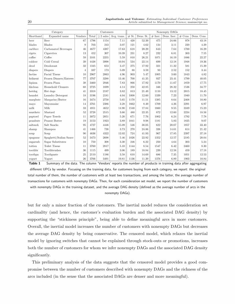
digits 3 through 7) into a single “product”. A detailed summary of the data is provided in Table 1.
We note from Table 1 that we observed nonempty DAGs for 31.2% of the customers under the
standard, 38.5% under the inertial, and 71.4% under the censored consideration set definitions.
The DAGs for the remaining customers were empty because of the appearance of directed cycles
during the construction of their DAGs or deviations from the assumptions of the inertial model.
These numbers confirm our discussion in Section 2.4: The standard consideration set appears
to be restrictive in the sense of imposing a heavy computational burden on the customer side
by assuming that a transaction implies the evaluation of all products on offer, potentially adding
several spurious arcs to the DAGs (as verified in the ‘Dens. St.’ column), and resulting in directed
cycles for the majority of the individuals. Consequently, we infer nonempty DAGs that are denser
9 The RPL model is also referred to in the literature as the Random Coefficients model (e.g., see Train [42, Chap-ter 6.2]).
10 The data consist of 5K unique customers/panelists whose purchases span the 29 categories. Because we analyzed thecategories separately, we treat each customer-category combination as a “customer”. There were two more categoriesin the dataset, “photography supplies” and “razors”, that we ignore due to data sparsity.
Jagabathula and Vulcano: Estimating Individual Customer Preferences20 Article submitted to Management Science; manuscript no.
Category Customers Nonempty DAGs
Shorthand Expanded name Vendors Total ≥ 2 sales Avg. trans. # St. Dens. St. # Iner. Dens. Iner. # Cens. Dens. Cens.
beer Beer 67 1796 1154 7.11 420 52.39 475 24.66 978 43.18
blades Blades 9 703 243 3.07 121 4.62 134 3.11 220 4.29
carbbev Carbonated Beverages 46 4677 4387 17.63 618 20.29 643 7.64 1700 16.29
cigets Cigarettes 13 452 307 10.39 231 8.27 232 6.81 303 7.55
coffee Coffee 59 3101 2255 5.59 810 26.21 1071 16.19 1886 22.27
coldcer Cold Cereal 39 4438 3998 10.94 534 22.14 699 12.18 1948 19.36
deod Deodorant 32 1345 653 3.47 275 17.92 321 11.32 581 15.39
diapers Diapers 4 337 173 5.09 88 3.59 93 2.52 152 3.44
factiss Facial Tissue 10 2967 2063 4.96 903 5.47 1005 3.60 1843 4.82
fzdinent Frozen Dinners/Entrees 77 3707 3288 13.46 700 41.35 927 23.41 1799 40.05
fzpizza Frozen Pizza 38 3460 2946 7.83 866 17.92 1170 11.67 1859 17.75
hhclean Household Cleaners 68 2725 1699 4.14 250 42.85 346 28.32 1536 34.77
hotdog Hot dogs 41 3318 2187 3.82 813 21.49 1110 13.12 2015 18.45
laundet Laundry Detergent 18 3196 2181 4.04 1008 12.60 1339 7.23 1940 11.70
margbutr Margarine/Butter 16 3474 2750 5.65 1170 11.51 1385 8.64 2468 10.80
mayo Mayonnaise 14 3761 2386 3.28 1662 8.49 1709 4.26 2291 6.97
milk Milk 33 4851 4652 14.90 1540 17.84 1660 9.55 3349 15.23
mustketc Mustard 52 3728 2515 3.66 480 22.35 872 12.60 2234 18.56
paptowl Paper Towels 11 3072 2051 5.20 671 7.76 1002 6.24 1792 7.78
peanbutr Peanut Butter 19 3153 1923 3.89 1041 9.98 1181 5.83 1825 9.07
saltsnck Salt Snacks 95 4727 4446 15.09 546 38.05 622 20.67 1857 33.40
shamp Shampoo 41 1466 738 3.73 270 24.86 338 14.61 614 21.42
soup Soup 90 4636 4322 12.02 724 41.93 967 17.85 2397 37.18
spagsauc Spaghetti/Italian Sauce 52 3473 2698 5.46 1026 22.92 1352 12.57 2185 20.04
sugarsub Sugar Substitutes 10 750 308 3.30 246 6.22 250 4.64 303 5.24
toitisu Toilet Tissue 11 3760 2817 5.10 1144 8.54 1547 6.42 2460 8.30
toothbr Toothbrushes 36 1115 499 3.06 189 18.84 239 12.58 459 17.18
toothpa Toothpaste 25 2110 1186 3.58 610 14.69 686 7.35 1051 12.53
yogurt Yogurt 26 3766 3491 19.81 1136 11.39 1376 6.89 1903 10.84
Table 1 Summary of the data. The column ‘Vendors’ reports the number of products in training data after aggregating
different UPCs by vendor. Focusing on the training data, for customers buying from each category, we report: the original
total number of them, the number of customers with at least two transactions, and among the latter, the average number of
transactions for customers with nonempty DAGs. Then, for each consideration set model, we report the number of customers
with nonempty DAGs in the training dataset, and the average DAG density (defined as the average number of arcs in the
nonempty DAGs).
but for only a minor fraction of the customers. The inertial model reduces the consideration set
cardinality (and hence, the customer’s evaluation burden and the associated DAG density) by
supporting the “stickiness principle”, being able to define meaningful arcs in more customers.
Overall, the inertial model increases the number of customers with nonempty DAGs but decreases
the average DAG density by being conservative. The censored model, which relaxes the inertial
model by ignoring switches that cannot be explained through stock-outs or promotions, increases
both the number of customers for whom we infer nonempty DAGs and the associated DAG density
significantly.
This preliminary analysis of the data suggests that the censored model provides a good com-
promise between the number of customers described with nonempty DAGs and the richness of the
arcs included (in the sense that the associated DAGs are denser and more meaningful).

Jagabathula and Vulcano: Estimating Individual Customer PreferencesArticle submitted to Management Science; manuscript no. 21
Our benchmarking study focuses on the customers with nonempty DAGs in order to assess the
additional benefit that can be obtained from the DAG structure. When a customer has an empty
DAG, our model reduces to a classical RUM model; therefore, customers with empty DAGs can
be analyzed with well-established methods (e.g., MNL, latent class MNL, etc).
5.2. Models compared
First, we pitted our partial order MNL (PO-MNL) method against two popular benchmarks based
on the MNL model: the latent class MNL (LC-MNL) and the Random Parameters Logit (RPL)
models. All three models belong to the general random utility maximization (RUM) model class,
which assumes that a customer samples product utilities in each purchase instance, and chooses the
product giving the highest one. The difference is that in our model the draws are independent but
conditioned on being consistent with the customer partial order across different purchase instances.
Within the RUM class, the single-class MNL model is the most popular member, with several
other sophisticated models being extensions of it. The MNL model assumes that customers assign
utility Uj = uj + εj to product j and choose the product with the maximum utility. The error
terms εj are Gumbel distributed with location parameter 0 and scale parameter 1. The nominal
utility uj for product j is usually assumed to depend on covariates xj` in a linear-in-parameter
form: uj = β0 +∑
` β`xj`. However, because we train and test on the same universe of products, we
directly estimate the nominal utilities uj from transactions without requiring attribute selection.
This approach is common in operations-related applications, where the product universe is fixed
and attribute selection is non-trivial.11 Nevertheless, we emphasize that like in the case of the
benchmarks, our PO-MNL method allows the incorporation of covariates. Next, we briefly describe
how we fit each of the models to data.
5.2.1. Model fit according to our method. Once we infer the DAGs according to the
consideration sets models described in Section 2, we have two different treatments: i) the whole
population as a single class of customers, and ii) the case where we cluster the individuals. In order
to cluster the DAGs we solve the IP described in (2) with a time limit of five minutes on MATLAB
combined with ILOG CPLEX callable library (v12.4). We tried K = 1, . . . ,5, classes, and retain
the solutions attaining the largest objective function value in (2).
The output of the clustering is used to estimate a K latent-class PO-MNL in which we assume
that each customer belongs to one of the K (latent) classes, with K = 1 for treatment (i). A
customer belonging to class h samples her DAG according to an MNL model with parameters βh.
11 For instance, Sabre Airline Solutions, one of the leading RM software providers for airlines, with a tradition of highquality R&D, implemented a proprietary version of the procedure described in Ratliff et al. [36] for a single classMNL model.

Jagabathula and Vulcano: Estimating Individual Customer Preferences22 Article submitted to Management Science; manuscript no.
A priori, a customer has a probability γh of belonging to class h, where γh ≥ 0 and∑K
h=1 γh =
1. We approximate the likelihood of a DAG under a single-class PO-MNL with the expression
described in Proposition 3.2, which becomes exact when the DAG is a forest of directed trees. After
marginalizing the likelihood of the DAG over all possible latent classes, the regularized maximum
likelihood estimation problem that we need to solve can be written as
maxβ,γ
m∑i=1
log
[K∑h=1
γh
n∏j=1
exp(βhj)
1 +∑
a`∈Ψi(aj)exp(βh`)
]−α
K∑h=1
‖βh‖1,
where Ψi(aj) denotes the set of nodes that can be reached from aj in DAG Di (recall, always
including aj). Note that the estimation relies only on the DAGs of individual customers and not
on their detailed purchase transactions.
The above estimation problem can be shown to be non-concave for K > 1, even for a fixed value
of α. To overcome the complexity of directly solving it, we used the EM algorithm. As part of the
EM initialization, we used the output from the clustering in Section 4 as our starting point. More
precisely, the clustering yields subsets D1,D2, . . . ,DK , which form a partition of the collection of
all the customer DAGs. In order to get a parameter vector β(0)h , we fit a PO-MNL model to each
subset of DAGs Dh by solving the following single-class PO-MNL maximum likelihood estimation
problem:
maxβh
∑i∈Dh
n∑j=1
βhj − log
1 +∑
a`∈Ψi(aj)
exp(βh`)
−α‖βh‖1. (3)
We tuned the value of α by 5-fold cross-validation, as described in Appendix A2.1. We also set
γ(0)h = |Dh|/
(∑K
`=1 |D`|)
. Then, using {γ(0), (β(0)h )Kh=1} as the starting point, we carried out EM
iterations. Further details are provided in Appendix A2.1.2.
Prediction. Given the parameter estimates, we make predictions as follows. For a customer i with
DAG Di, and defining vhj = exp(βhj), we estimate the posterior membership probabilities γih, for
each h, at the beginning of the holdout sample horizon, and make the prediction:
fi(aj, S) =K∑h=1
γihfh(aj, S,Di), where γih =γh∏n
j=1 vhj/(
1 +∑
`∈Ψi(aj)vh`
)∑K
d=1 γd∏n
j=1 vdj/(
1 +∑
`∈Ψi(aj)vd`
) ,where fh(aj, S,Di) is the approximation from Proposition 3.3 for predicting the choice probability
for an individual described by parameters vh. Similar to estimation, the prediction relies only on
the DAG structure of customer i and not on detailed transaction information.

Jagabathula and Vulcano: Estimating Individual Customer PreferencesArticle submitted to Management Science; manuscript no. 23
5.2.2. Benchmark models fit according to the classical approach. The two MNL-based
benchmarks are briefly described here, with further details in Appendix A2.1. The first model is
the k-latent-class MNL (LC-MNL) model12, where each customer belongs to one of k unobservable
classes, k= 1, . . . ,10, and remains there during the whole horizon. We keep track of the customer id
in the panel data to estimate the nominal utilities, and treat transactions as independent realiza-
tions. This model makes individual-level predictions by averaging the predictions from k single-class
models, weighted by the posterior probability of class-membership. We fit the model with k classes,
and for each performance metric (to be introduced in Section 5.3), we report the best performance
from these 10 models. In our case, the estimation requires assessing the value of k n parameters.
The second model is the random parameters logit (RPL) model, which captures heterogeneity
in customer preferences by assuming that each customer samples the β parameters of the utilities
according to some distribution and makes choices according to a single-class MNL model with
parameter vector β. The key distinction from the LC-MNL model is that the distribution describing
the parameter vector β may be continuous and not just discrete with finite support. In our case, we
assume that β is sampled according to N(µ,Σ), which denotes the multivariate normal distribution
with mean µ and variance-covariance matrix Σ, where Σ is a diagonal matrix with the jth diagonal
entry equal to σ2j . RPL requires the estimation of 2n parameters within a computationally intensive
sample average approximation approach.
For both benchmarks, and following the common practice, we use the standard consideration set
definition. Given the parameter estimates, we make individual level predictions by updating the
class membership probabilities at the beginning of the holdout sample horizon.
5.3. Experimental setup
We test the predictive power of the models on a one-step ahead prediction experiment in each
category under two different metrics: chi-square and miss rates. Here, the periods are labeled over
the hold-out horizon as t= 1,2, . . . , T . For each customer i, the objective is to predict the product
she will purchase in period t+ 1 when given the last purchase of the customer up to period t and
offer set St+1 and promoted products Pt+1 she faces in period t+ 1.
For each (category, consideration set definition) combination, there is a specific subset of cus-
tomers described with nonempty DAGs (see Table 1), and for that specific subset, we calibrate the
two benchmarks and our PO-MNL model.
12 Here we use k to refer to the number of latent classes, which could be different from K -the number of clustersfrom Section 4-.

Jagabathula and Vulcano: Estimating Individual Customer Preferences24 Article submitted to Management Science; manuscript no.
Both metrics considered rely on the definition of the indicator function yi(aj, t), taking the
value 1 if customer i makes a purchase in period t and product aj has the highest predicted choice
probability, and 0 otherwise, i.e.,
yi(aj, t) = I {customer i makes a purchase in period t and fi(aj, St)≥ fi(a`, St) ∀ `∈ St} .
The first metric computes the following “chi-square” score:
X2 score =1
|N | |U |∑
i∈U,aj∈N
(nij − nij)2
0.5 + nij, where nij =
T∑t=1
yi(aj, t), (4)
where U is the set of all individuals, and nij is the observed number of times individual i purchased
product aj during the horizon of length T . The term nij denotes the aggregate predicted number
of purchases of product aj by individual i.
To make the prediction, each model combination defined as the pair (choice model, consideration
set definition) is given the offer set St+1; promoted products Pt+1; the set of individuals Ut+1 who
purchase in period t+ 1; and all the purchase transactions of all the individuals, offer sets, and
promoted products up to time period t. Using this information, each model combination provides
choice probabilities for each of the offered products.
The score in (4) is similar to the popular chi-square measure of goodness-of-fit of the form
(O−E)2/E, where O refers to the observed value and E refers to the expected value. The use of
this score in our setting is justified by considering the observed counts nij as the realization of the
sum of independent (but not identically distributed) Bernoulli random variables.13 We add 0.5 to
the denominator to smooth the score and deal with undefined instances. The score measures the
ability of the model combinations to predict aggregate market shares, with lower scores indicating
better predictive accuracy.
We also measure the miss-rate of the model combinations, defined as
miss rate =1
|U | |T |∑i∈U
T∑t=1
I {customer i makes a purchase in period t and yi(ajit , t) = 0} , (5)
where I[A] is the indicator function taking value 1 if A is true and 0 otherwise. Recall that ajit
denotes the product purchased by individual i in period t. Again, lower miss rates are better. Note
that the miss-rate measure is very stringent, since it rewards or penalizes the assessment of the
right customer purchase on a per period basis (rather than aggregating over the whole horizon as
in the X2 case).
13 Since the offer sets change and predictions are conditioned on them, there random variables are not identicallydistributed across time.
Jagabathula and Vulcano: Estimating Individual Customer PreferencesArticle submitted to Management Science; manuscript no. 25
PO + Standard PO + Inertial PO + Censored
impr clustering = 8.85%
impr no clustering = 8.24%
impr clustering = 4.68%
impr no clustering = 4.02%
impr clustering = 36.73%
impr no clustering = 35.2%
impr clustering = 34.71%
impr no clustering = 33.11%
impr clustering = 41.46%
impr no clustering = 40.19%
impr clustering = 38.3%
impr no clustering = 37.02%
0.0
0.2
0.4
0.6
0.0
0.2
0.4
0.6
LC
-MN
L+
Sta
nd
ard
RP
L+
Stan
dard
0.0 0.2 0.4 0.6 0.0 0.2 0.4 0.6 0.0 0.2 0.4 0.6PO X2 score
Ben
chm
ark
X2
scor
e
clustering no clustering
Figure 3 Scatterplot of the average X2 scores of all 29 categories under the PO and the (LC-MNL, standard)
and (RPL, standard) benchmarks for both single class and clustering cases. Lower is better; therefore, we
outperform the benchmark for points above the 45◦ line.
The above experimental setup is reflective of the practical prediction problem that a firm faces.
Both measures are computed conditioning on a purchase event. Predicting the set of customers
who will purchase in a given period t can be done separately using classical time-series models that
capture any periodicity and seasonality in customer store visits.
5.4. Results and discussion
We compare the predictive performance of the two benchmark models (LC-MNL and RPL under
the standard consideration set definition) with three variants of our model class: PO-MNL (also
labeled just PO from here onwards) under the standard, inertial, and censored consideration set
definitions.
Figure 3 presents scatterplots of the X2 scores of LC-MNL and RPL (under the standard model)
versus X2 scores of the three combinations of PO and the consideration set definitions, across
the 29 product categories, including both single-class and clustering cases. We observe that our
PO method dominates both (LC-MNL, standard) and (RPL, standard) benchmarks across the
board. The charts allow to isolate three concurrent effects that favor our proposal. First, when
considering the left column in Figure 3, we are focusing on the standard consideration set definition
and comparing our PO versus both benchmarks. For the no clustering case, the X2 score from PO

Jagabathula and Vulcano: Estimating Individual Customer Preferences26 Article submitted to Management Science; manuscript no.
exhibits an average improvement of 8.24% over LC-MNL and 4.02% over RPL. This improvement
can be attributed to the effectiveness of the DAGs capturing partial preferences of the customers,
which is remarkable because both benchmark models have more parameters and explicitly account
for customer-level heterogeneity. It takes only around 10 seconds to fit the PO model as opposed
to 67 minutes to fit the RPL model (which in turn dominates LC-MNL). The key reason for
the superior performance of PO is that even without explicit clustering, the model accounts for
heterogeneous customer preferences through their partial orders, making more efficient use of the
limited data.
The second effect stems from the behavioral biases captured by non standard consideration
set definitions: the (PO, inertial) combination allows to boost the X2 score performance to the
range 33%-35%, and the (PO, censored) pair pushes it further to 40%. This outstanding improve-
ment reveals the significant explanatory power displayed by partial preferences (represented by
DAGs) jointly with the behavioral biases that determine the construction of such DAGs.
The third effect is captured by the clustering IP in Section 4 that groups together users with
similar preferences. It can further boost the performance by 0.6 percentage points (pp) under
the standard model, to around 1.4 pp under the behavioral (i.e., inertial and censored) models.
Our results indicate that identifying similar customers has a more significant impact under the
behavioral models, where DAGs are more informative since they are built upon fewer spurious
edges. Thus, at the expense of some additional computational effort, clustering into only a few
classes can further boost our performance.
In Figure 4 we report the loyalty score of each category (left panel), and explore possible cor-
relations between X2 scores and loyalty scores (right panel). To compute the loyalty score of a
category, we calculate the fraction of the total purchases coming from the most frequently pur-
chased product (i.e., vendor) of each customer buying from that category, and take the average of
those fractions across customers purchasing from the category. There is a clear positive correlation
between X2 scores and loyalty scores. That is, the X2 performance leveraged by the DAGs (versus
the most competitive benchmark, i.e., (RPL, standard)) is further emphasized for high brand loyal
categories, and it is even more emphasized under behavioral models that highlight the stickiness
principle (i.e., both inertial and censored models show a higher slope). This observation is further
investigated in Appendix A2.2 (see Figure A2 therein). For categories with high loyalty indices we
can obtain a huge improvement in the X2 score by accounting for individual partial preferences
under the three consideration set definitions.
Figure 5 presents scatterplots of the miss rates following a display format similar to Figure 3.
Recall that this is a more stringent predictive measure, since it rewards or penalizes the sum of
individual transaction assessments (see definition (5)). We observe that our model combinations
Jagabathula and Vulcano: Estimating Individual Customer PreferencesArticle submitted to Management Science; manuscript no. 27
hhclean
mustketc
saltsnck
fzdinent
coldcer
soup
toothbr
hotdog
fzpizza
shamp
paptowl
coffee
deod
spagsauc
factiss
toitisu
carbbev
laundet
beer
milk
margbutr
toothpa
blades
peanbutr
yogurt
diapers
mayo
sugarsub
cigets
0.00 0.25 0.50 0.75loyalty score
PO + Standard PO + Inertial PO + Censored
% impr. = -0.27 + 0.43 loyalty % impr. = -0.48 + 1.13 loyalty % impr. = -0.67 + 1.45 loyalty
0.0
0.2
0.4
0.6
0.8
0.6 0.7 0.8 0.9 0.6 0.7 0.8 0.9 0.6 0.7 0.8 0.9loyalty score
%im
pr.
of
X2
score
over
RP
L+
Sta
ndar
d
Figure 4 Left panel: Loyalty scores across categories, sorted in descending order. Right panel: Scatter plot and
linear regression of X2 score of PO over (RPL, standard), for each consideration set definition.
obtain improvements of between 2% and 6% over the benchmarks in four of the six panels, when
using the clustering procedure. In the remaining two (lower right) panels, our performance is similar
to the benchmarks (most points lie on the 45◦ line). The same three aforementioned effects play a
role here (although the behavioral bias effect is diminished when compared with (RPL, standard)).
The charts in the left column reveal the value delivered by capturing partial preferences under the
standard consideration set definition, providing gains between 2.6% and 5.6%. Clustering still plays
a role in boosting performance, resulting in improvements close to 1 pp in some cases. As noted, the
behavioral models are just as good as the (RPL, standard) model in terms of the miss-rates. This
may be explained by noting that the stickiness assumption can lead to double penalization: missing
first when the customer deviates from purchasing the “loyal” brand, and missing again when the
customer returns to the “loyal” brand because the sticky product is updated to the latest purchase.
This observation suggests that if the objective is to increase accuracy of immediate predictions,
it may be best to increase the chances of a hit by expanding the consideration set to the entire
offer-set, in order to account for possible deviations from the inertial assumption.
We also investigated the correlation between percentage improvement of PO over (RPL, stan-
dard) with respect to the miss rates (see Figure A3 in Appendix A2.2). As we said, the miss rate
measure is quite stringent, but better results are obtained under PO for high loyalty categories,
mainly under the standard but also under the censored consideration set definitions.
Jagabathula and Vulcano: Estimating Individual Customer Preferences28 Article submitted to Management Science; manuscript no.
PO + Standard PO + Inertial PO + Censored
impr clustering = 5.99%
impr no clustering = 5.62%
impr clustering = 3.04%
impr no clustering = 2.65%
impr clustering = 2.01%
impr no clustering = 1.36%
impr clustering = 0.52%
impr no clustering = -0.13%
impr clustering = 4.49%
impr no clustering = 3.87%
impr clustering = 0.8%
impr no clustering = 0.13%
0.0
0.2
0.4
0.6
0.8
0.0
0.2
0.4
0.6
0.8
LC
-MN
L+
Sta
nd
ard
RP
L+
Stan
dard
0.0 0.2 0.4 0.6 0.8 0.0 0.2 0.4 0.6 0.8 0.0 0.2 0.4 0.6 0.8PO miss rates
Ben
chm
ark
mis
sra
tes
clustering no clustering
Figure 5 Scatterplot of the average miss rates of all 29 categories under the PO and the (LC-MNL, standard)
and (RPL, standard) benchmarks for both single class and clustering cases. Lower is better; therefore, we
outperform the benchmark for points above the 45◦ line.
Overall, the combination (PO-MNL, censored) seems to provide the best performance under
X2 scores, and a better or comparable performance with respect to miss rates, which is quite
remarkable since when building individual DAGs under the censored consideration set definition we
could describe the behavior of 71% of the customer base with nonempty DAGs. The performance
is further boosted when we apply (PO-MNL, censored) over categories with high loyalty score.
However, if the focus is mainly on miss rates, the combination (PO-MNL, standard) appears to be
the best option.
5.5. Comparison with the Guadagni-Little model
The final benchmark study is to compare our method with the proposal by Guadagni and Little [16],
denoted GL onwards. Guandagni and Little calibrated an MNL model of brand choice, based
on panel data, over the “regular ground coffee” category. They formulated a linear-in-parameters
utility model that captures covariates such as full price, indicator for brand promotion, price cut for
products on promotion, indicator to keep track of the promotion status of the last two purchases,
and two additional covariates to capture loyalty effects: in terms of coffee brand, and in terms of
packaging size. For them, loyalty is taken to be the exponentially weighted average of past purchases
of the brand and the packaging size, treated as 0-1 variables. However, their loyalty scores do not
Jagabathula and Vulcano: Estimating Individual Customer PreferencesArticle submitted to Management Science; manuscript no. 29
PO + Standard PO + Inertial PO + Censored
impr clustering = -37.9%
impr no clustering = -38.89%
impr clustering = 11.74%
impr no clustering = 9.67%
impr clustering = 19.68%
impr no clustering = 17.57%
0.0
0.2
0.4
0.6
GL
+S
tan
dard
0.0 0.2 0.4 0.6 0.0 0.2 0.4 0.6 0.0 0.2 0.4 0.6PO X2 score
Ben
chm
ark
X2
scor
e
clustering no clustering
Figure 6 Scatterplot of the average X2 scores of all 29 categories under the PO and the GL+Standard
benchmark for both single class and clustering cases. Lower is better; therefore, we outperform the benchmark for
points above the 45◦ line.
reflect stock-outs: the no-purchase of a product because of a stock-out is treated as a regular switch
to a different brand. For the purposes of our study, we implemented a variation of the GL model,
adapted to the variables present in our dataset; for details, see Appendix A2.1.
Even though the GL model is tailored to capture loyalty, as our inertial and censored models
are, there is a fundamental difference between both approaches: GL maintains a richer state via
the utility function of their MNL model, which is updated dynamically as promotions arise, both
in the training and holdout samples, whereas we maintain a limited state via the consideration
set definition, also in both the training and holdout samples (though in the holdout sample we do
not update the DAGs). More specifically, GL maintains the promotion status of the current and
the previous two purchases and longer term loyalty information through an exponential smoothing
reflecting recency and frequency of purchases. Instead, we maintain the promotion status of current
purchase and only short-term loyalty information in the form of the previous purchase. Therefore,
the comparison should be taken with caution.14
Guadagni and Little [16] provide evidence for the remarkable performance of their method in
predicting product market shares for “regular ground coffee.” The X2 score captures the accu-
racy of a method in predicting these market shares. Figure 6 shows that GL generally beats the
performance of the standard model (which is not aimed at capturing brand loyalty), but also high-
lights the good performance that we achieve with (PO, inertial) and (PO, censored), with our X2
14 The previous benchmarks LC-MNL and RPL, where we did not consider covariates either, are more suitable forcomparison. Those results allowed us to show the value of building the DAGs over a MNL model, allowing us toquantify the value of superimposing such incremental structure.
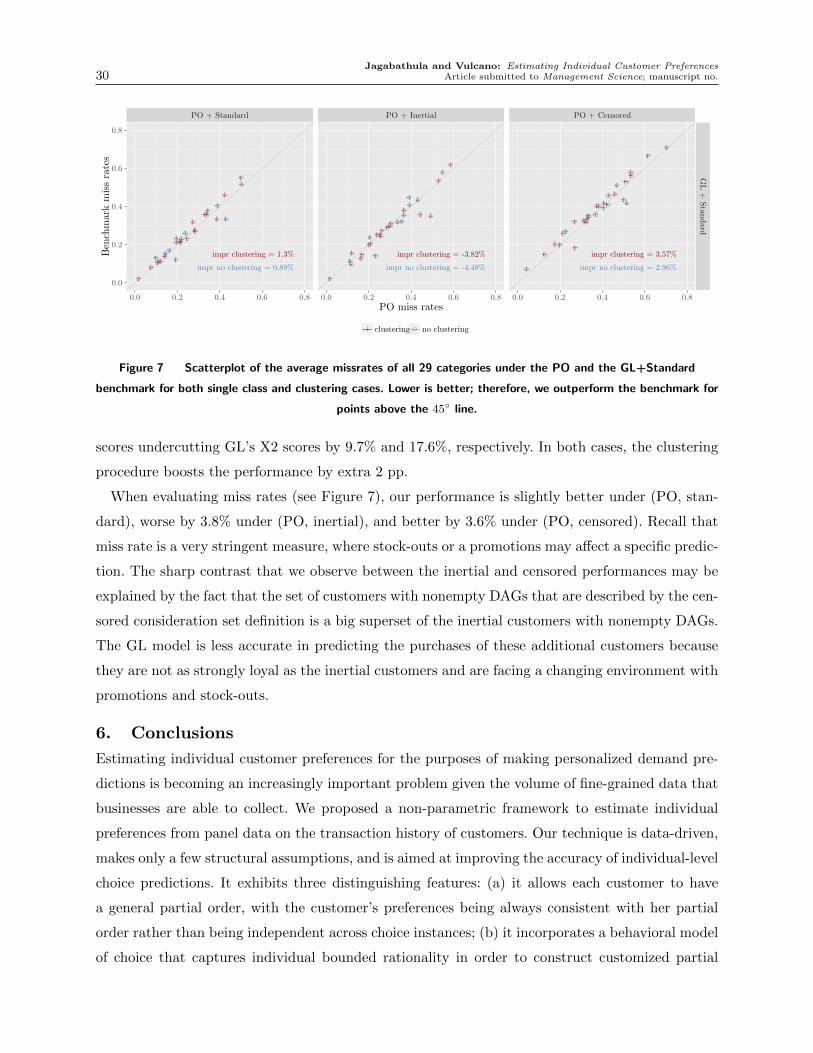
Jagabathula and Vulcano: Estimating Individual Customer Preferences30 Article submitted to Management Science; manuscript no.
PO + Standard PO + Inertial PO + Censored
impr clustering = 1.3%
impr no clustering = 0.89%
impr clustering = -3.82%
impr no clustering = -4.48%
impr clustering = 3.57%
impr no clustering = 2.96%
0.0
0.2
0.4
0.6
0.8
GL
+S
tan
dard
0.0 0.2 0.4 0.6 0.8 0.0 0.2 0.4 0.6 0.8 0.0 0.2 0.4 0.6 0.8PO miss rates
Ben
chm
ark
mis
sra
tes
clustering no clustering
Figure 7 Scatterplot of the average missrates of all 29 categories under the PO and the GL+Standard
benchmark for both single class and clustering cases. Lower is better; therefore, we outperform the benchmark for
points above the 45◦ line.
scores undercutting GL’s X2 scores by 9.7% and 17.6%, respectively. In both cases, the clustering
procedure boosts the performance by extra 2 pp.
When evaluating miss rates (see Figure 7), our performance is slightly better under (PO, stan-
dard), worse by 3.8% under (PO, inertial), and better by 3.6% under (PO, censored). Recall that
miss rate is a very stringent measure, where stock-outs or a promotions may affect a specific predic-
tion. The sharp contrast that we observe between the inertial and censored performances may be
explained by the fact that the set of customers with nonempty DAGs that are described by the cen-
sored consideration set definition is a big superset of the inertial customers with nonempty DAGs.
The GL model is less accurate in predicting the purchases of these additional customers because
they are not as strongly loyal as the inertial customers and are facing a changing environment with
promotions and stock-outs.
6. Conclusions
Estimating individual customer preferences for the purposes of making personalized demand pre-
dictions is becoming an increasingly important problem given the volume of fine-grained data that
businesses are able to collect. We proposed a non-parametric framework to estimate individual
preferences from panel data on the transaction history of customers. Our technique is data-driven,
makes only a few structural assumptions, and is aimed at improving the accuracy of individual-level
choice predictions. It exhibits three distinguishing features: (a) it allows each customer to have
a general partial order, with the customer’s preferences being always consistent with her partial
order rather than being independent across choice instances; (b) it incorporates a behavioral model
of choice that captures individual bounded rationality in order to construct customized partial

Jagabathula and Vulcano: Estimating Individual Customer PreferencesArticle submitted to Management Science; manuscript no. 31
orders from purchase records; and (c) it allows to group customers by preference similarities. We
demonstrate on real-world data that accounting for partial order and behavioral aspects of choice
significantly improves the accuracy of individual-level predictions over existing state-of-the-art
methods.
Our work opens the door for many exciting future research directions. A key theoretical contri-
bution of our work is deriving the likelihood expressions for general classes of partial orders under
the MNL/Plackett-Luce model. Existing work has mainly considered classes of partial orders (such
as top-k rankings, partitioned preferences, etc.) that commonly arise when data are collected on
the web. However, onsite transactions often yield choice data, resulting in partial orders that lack
the types of structure already studied. Our work has introduced a new class of partial orders - for-
est of directed trees with unique roots - and has shown that it affords closed-form expression for
likelihood under the MNL/Plackett-Luce model. Identifying other general classes of partial orders
for which likelihoods can be computed in a tractable manner under different popular choice models
(such as variants of the MNL) is an exciting future direction. In addition, investigating properties
of the clustering IP to derive theoretical guarantees for general classes of partial orders can result
in significant contributions to this problem.
Finally, the comparison of the performance of our method versus the classical Guadagni and
Little [16] approach suggests that capturing state dependence via a parameterized utility function
could be a means to further boost the potential of partial-order based preferences.
References[1] Yaser S Abu-Mostafa, Malik Magdon-Ismail, and Hsuan-Tien Lin. Learning from data. AMLBook, 2012.
[2] A. Aho, M. Garey, and J. Ullman. The transitive reduction of a directed graph. SIAM Journal on Computing,1(2):131–137, 1972.
[3] A. Ali and M. Melia. Experiments with kemeny ranking: What works when? Mathematical Social Sciences,64:28–40, 2012.
[4] M. Ben-Akiva and S. Lerman. Discrete Choice Analysis: Theory and Applications to Travel Demand. The MITPress, Cambridge, MA, sixth edition, 1994.
[5] Stephen Boyd and Lieven Vandenberghe. Convex optimization. Cambridge university press, 2009.
[6] G. Brightwell and P. Winkler. Counting linear extensions is #P-complete. In STOC ’91 Proceedings of thetwenty-third annual ACM Symposium on Theory of Computing, pages 175–181, 1991.
[7] B. Bronnenberg, M. Kruger, and C. Mela. The IRI academic dataset. Management Science, 27(4):745–748, 2008.
[8] Sandeep R Chandukala, Jaehwan Kim, and Thomas Otter. Choice models in marketing, 2008.
[9] J. Chaneton and G. Vulcano. Computing bid-prices for revenue management under customer choice behavior.M&SOM, 13(4):452–470, 2011.
[10] L. Chen and T. Homem de Mello. Mathematical programming models for revenue management under customerchoice. European Journal of Operational Research, 203:294–305, 2010.
[11] Siddhartha Chib and Edward Greenberg. Markov chain monte carlo simulation methods in econometrics. Econo-metric theory, 12(03):409–431, 1996.
[12] P. Chintagunta. Investigating purchase incidence, brand choice and purchase quantity decisions on households.Marketing Science, 12:184–208, 1993.
[13] S. Clifford. Shopper alert: Price may drop just for you alone. New York Times, August 9 2012.
[14] P. Danaher, M. Smith, K. Ranasinghe, and T. Danaher. Where, when, and how long: Factors that influence theredemption of mobile phone cupons. Journal of Marketing Research, 52:710–725, 2015.
[15] V. Farias, S. Jagabathula, and D. Shah. A new approach to modeling choice with limited data. ManagementScience, 59(2):305–322, 2013.

Jagabathula and Vulcano: Estimating Individual Customer Preferences32 Article submitted to Management Science; manuscript no.
[16] P. Guadagni and J. Little. A logit model of brand choice calibrated on scanner data. Marketing Science, 2:203–238, 1983.
[17] S. Gupta. Impact of sales promotions on when, what, and how much to buy. Journal of Marketing Research,25:342–355, November 1988.
[18] A. Haensel and G. Koole. Estimating unconstrained demand rate functions using customer choice sets. Journalof Revenue and Pricing Management, 10(5):438–454, 2011.
[19] J. Hauser. Consideration-set heuristics. Working paper, MIT Sloan School of Management, April 2013.
[20] D. Honhon, V. Gaur, and S. Seshadri. Assortment planning and inventory decisions under stockout-based sub-stitution. Operations Research, 58(5):1364–1379, 2010.
[21] D. Honhon, S. Jonnalagedda, and X. Pan. Optimal algorithms for assortment selection under ranking-basedconsumer choice models. Management Science, 12(2):279–289, 2012.
[22] D. Hunter. MM algorithms for generalized Bradley-Terry models. The Annals of Statistics, 32(1):384–406, 2004.
[23] S. Jagabathula and P. Rusmevichientong. A two-stage model of consideration set and choice: Learning, revenueprediction, and applications. Working paper, Leonard N. Stern School of Business, 2014.
[24] S. Jagabathula and G. Vulcano. A partial-order-based Mallows model of discrete choice. Working paper, NewYork University, 2016.
[25] A. Jeuland. Brand choice inertia as one aspect of the notion of brand loyalty. Management Science, 25(7):671–682,1979.
[26] Eric Jones, Travis Oliphant, Pearu Peterson, et al. SciPy: Open source scientific tools for Python, 2001–. [Online;accessed 2015-08-21].
[27] G. Kok and M. Fisher. Demand estimation and assortment optimization under substitution: Methodology andapplication. Operations Research, 55:1001–1021, 2007.
[28] S. Kunnumkal. Randomization approaches for network revenue management with customer choice behavior.POMS, 23(9):1617–1633, 2014.
[29] S. Mahajan and G.J. van Ryzin. Stocking retail assortments under dynamic consumer substitution. OperationsResearch, 49:334–351, 2001.
[30] J. Marden. Analyzing and modeling rank data. Chapman and Hall, 1995.
[31] A. Musalem, M. Olivares, E. Bradlow, C. Terwiesch, and D. Corsten. Structural estimation of the effect ofout-of-stocks. Management Science, 56:1180–1197, 2010.
[32] J. Newman, M. Ferguson, L. Garrow, and T. Jacobs. Estimation of choice-based models using sales data from asingle firm. M&SOM, 16(2):184–197, 2014.
[33] Jorge Nocedal and Stephen Wright. Numerical optimization. Springer Science & Business Media, 2006.
[34] S. Polt. Forecasting is difficult –especially if it refers to the future. In Revenue Management and DistributionStudy Group Annual Meeting, Melbourne, Australia, May 1998. AGIFORS.
[35] William H Press, Saul A Teukolsky, William T Vetterling, and Brian P Flannery. Numerical recipes: The art ofscientific computing. 3rd. New York: Cambridge University Press, 2007.
[36] R. Ratliff, B. Rao, C. Narayan, and K. Yellepeddi. A multi-flight recapture heuristic for estimating unconstraineddemand from airline bookings. Journal of Revenue and Pricing Management, 7:153–171, 2008.
[37] Peter E Rossi, Greg M Allenby, and Rob McCulloch. Bayesian statistics and marketing. John Wiley & Sons,2012.
[38] P. Rusmevichientong, B. van Roy, and P. Glynn. A nonparametric approach to multiproduct pricing. OperationsResearch, 54(1):82–98, 2006.
[39] J. Smith, C. Lim, and A. Alptekinoglu. New product introduction against a predator: A bilevel mixed-integerprogramming. Naval Research Logistics, 56(8):714–729, 2009.
[40] R. Stanley. Enumerative Combinatorics, volume 1. Cambridge University Press, 2000.
[41] D. Strauss. Some results on random utility models. Journal of Mathematical Psychology, 20:35–52, 1979.
[42] K. Train. Discrete choice methods with simulation. Cambridge University Press, New York, NY, second edition,2009.
[43] Kenneth Train and Garrett Sonnier. Mixed logit with bounded distributions of partworths. Applications ofSimulation Methods in Environmental Resource Economics, edited by A. Alberini and R. Scarpa. New York:Kluwer Academic, 2003.
[44] G. van Ryzin and G. Vulcano. A market discovery algorithm to estimate a general class of non-parametricchoice models. Decision, Risk and Operations Division, Columbia Business School. Forthcoming in ManagementScience, 2014.
[45] G. Vulcano, G. van Ryzin, and W. Chaar. Choice-based revenue management: An empirical study of estimationand optimization. M&SOM, 12(3):371–392, 2010.
[46] Berend Wierenga. Handbook of Marketing Decision Models. Springer Science + Business Media, New York,January 2008.

Jagabathula and Vulcano: Estimating Individual Customer PreferencesArticle submitted to Management Science; manuscript no. 33
[47] D. Zhang and W. Cooper. Revenue management for parallel flights with customer-choice behavior. OperationsResearch, 53(3):415–431, 2005.

Jagabathula and Vulcano: Estimating Individual Customer PreferencesArticle submitted to Management Science; manuscript no. A1
A Partial Order-Based Model to Estimate
Individual Preferences using Panel Data
Appendix
Srikanth Jagabathula
Leonard N. Stern School of Business, New York University, New York, NY 10012,
Gustavo Vulcano
Leonard N. Stern School of Business, New York University, New York, NY 10012,
School of Business, Torcuato di Tella University, Buenos Aires, Argentina
A1. The MNL/Plackett-Luce model under DAGs
In order to streamline our discussion, in this section we ignore the no-purchase option labeled 0
and without loss of generality focus on the standard consideration set definition where Cit = Sit.
We also augment the notation as follows. For any two integers i < j, let [i, j] denote the set
{i, i+ 1, . . . , j}. When i= 1, we drop it from the notation so that [j] denotes the set {1,2, . . . , j}
for any positive integer j. A complete ranking (or simply, a ranking) is a bijection σ : N → [n]
that maps each product a ∈N to its rank σ(a) ∈ [n]. We let Sn denote the space of all complete
rankings over n items. It follows from our notation that σ−1(i) (or, to simplify, σi) denotes the
product that is ranked at position i. Thus, σ1σ2 . . . σn is the list of products written in increasing
order of their ranks.
Different probability distributions can be defined over the set of rankings (e.g., see Marden [30]).
We will focus on specification of such probabilities under the MNL model. Let λ(σ) denote the
probability assigned to a full ranking σ. We can then extend the calculation of probabilities to
partial orders defined on the same set of products N . More specifically, we can interpret any
partial order D as a censored observation of an underlying full ranking σ sampled by a customer
according to the distribution over the total orders. Hence, if we define SD = {σ ∈ Sn : σ(a) <
σ(b) whenever (a, b)∈D} as the collection of full rankings consistent with D, then we can compute
the probability
λ(D) =∑σ∈SD
λ(σ).
From this expression, it follows that computing the likelihood of a general partial order D is #P-
hard because counting the number of full rankings consistent with D is indeed #P-hard (Brightwell
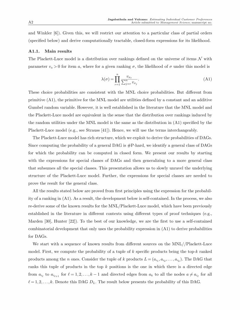
Jagabathula and Vulcano: Estimating Individual Customer PreferencesA2 Article submitted to Management Science; manuscript no.
and Winkler [6]). Given this, we will restrict our attention to a particular class of partial orders
(specified below) and derive computationally tractable, closed-form expressions for its likelihood.
A1.1. Main results
The Plackett-Luce model is a distribution over rankings defined on the universe of items N with
parameter va > 0 for item a, where for a given ranking σ, the likelihood of σ under this model is
λ(σ) =n∏r=1
vσr∑n
j=r vσj. (A1)
These choice probabilities are consistent with the MNL choice probabilities. But different from
primitive (A1), the primitive for the MNL model are utilities defined by a constant and an additive
Gumbel random variable. However, it is well established in the literature that the MNL model and
the Plackett-Luce model are equivalent in the sense that the distribution over rankings induced by
the random utilities under the MNL model is the same as the distribution in (A1) specified by the
Plackett-Luce model (e.g., see Strauss [41]). Hence, we will use the terms interchangeably.
The Plackett-Luce model has rich structure, which we exploit to derive the probabilities of DAGs.
Since computing the probability of a general DAG is #P-hard, we identify a general class of DAGs
for which the probability can be computed in closed form. We present our results by starting
with the expressions for special classes of DAGs and then generalizing to a more general class
that subsumes all the special classes. This presentation allows us to slowly unravel the underlying
structure of the Plackett-Luce model. Further, the expressions for special classes are needed to
prove the result for the general class.
All the results stated below are proved from first principles using the expression for the probabil-
ity of a ranking in (A1). As a result, the development below is self-contained. In the process, we also
re-derive some of the known results for the MNL/Plackett-Luce model, which have been previously
established in the literature in different contexts using different types of proof techniques (e.g.,
Marden [30], Hunter [22]). To the best of our knowledge, we are the first to use a self-contained
combinatorial development that only uses the probability expression in (A1) to derive probabilities
for DAGs.
We start with a sequence of known results from different sources on the MNL//Plackett-Luce
model. First, we compute the probability of a tuple of k specific products being the top-k ranked
products among the n ones. Consider the tuple of k products L= (ai1 , ai2 , . . . , aik). The DAG that
ranks this tuple of products in the top k positions is the one in which there is a directed edge
from ai` to ai`+1for `= 1,2, . . . , k − 1 and directed edges from ak to all the nodes a 6= ai` for all
`= 1,2, . . . , k. Denote this DAG DL. The result below presents the probability of this DAG.

Jagabathula and Vulcano: Estimating Individual Customer PreferencesArticle submitted to Management Science; manuscript no. A3
Proposition A1.1. Let L= (ai1 , ai2 , . . . , aik) be a tuple of k products. Consider a DAG DL that
ranks this tuple of products in the top k positions among the n ones, and where there is no ranking
among the remaining n− k. Then, the probability of observing DL under a Plackett-Luce model is
given by
λ(DL) = P(σ(ai1) = 1, σ(ai2) = 2, . . . , σ(aik) = k) =k∏r=1
vir∑aj∈Lc
vj +∑k
j=r vij,
where Lc =N \{ai1 , ai2 , . . . , aik
}.
The partial order corresponding to top-k rankings commonly arises in the online context in which
users are typically presented with top-k results for some k in response to a search query. Hence,
data are typically available in the form of top-k rankings for different users. The above result states
that a Plackett-Luce model can be conveniently used in this context because it has a closed-form
expression for the probability λ(DL).
The next results considers the case in which partial orders are specified only over a subset S ⊂N
of products. Specifically, we focus on the probability of a partial order that only specifies a total
ordering over a subset S of products. The result states that for a given subset S ⊂N of size k, the
probability of a (short) rank π defined over S is given by the sum of the likelihoods of all full ranks
consistent with π, and characterizes a closed-form for it that only depends on the products in S.
That is, the probability of a ranking on a subset only depends on the relative order of the elements
in the subset. This property is referred to as internal consistency by Hunter [22], who provides an
outline of the proof. We include in the Appendix a detailed version.
Proposition A1.2. For any subset S of k products, let π be a ranking over the elements of S.
Let σ(π) denote the set of full rankings over N defined as
σ(π) = {σ : σ(ai)<σ(aj) whenever π(ai)<π(aj) for all ai, aj ∈ S} .
Then, we must have
λ(π) =∑σ∈σ(π)
λ(σ) =k∏r=1
vπr∑k
j=r vπj.
The previous result applies when we define a ranking over a subset of the product universe N .
Now, consider two disjoint subsets S1 and S2, and two corresponding rankings π1 and π2. The
following proposition establishes that the probability of all rankings on S1 ∪S2 consistent with π1
and π2 is just the product of the probabilities of both rankings on the respective subsets.

Jagabathula and Vulcano: Estimating Individual Customer PreferencesA4 Article submitted to Management Science; manuscript no.
Proposition A1.3. Consider two disjoint subsets S1, S2 ⊂ N , and two rankings π1 and π2
defined over the respective subsets. Then, λ(π1, π2) =∑
σ∈σ(π1,π2) λ(σ) = λ(π1)λ(π2), where σ(π1, π2)
denotes the collection of rankings that are consistent with both π1 and π2 i.e.,
σ(π1, π2) = {σ : σ(ai)<σ(aj) whenever π1(ai)<π1(aj) or π2(ai)<π2(aj) for all ai, aj ∈ S1 ∪S2} .
The result of Proposition A1.3 immediately results in the following corollary.
Corollary A1.1. Let G be a collection of DAGs defined over N , with G= {G1, . . . ,GL} such
that G` ∩G`′ = ∅ for ` 6= `′. Then, λ(G) =∑
σ∈SGλ(σ) =
∏L
`=1 λ(G`).
The results in Propositions A1.2 and A1.3 are critical in deriving the probability of general DAGs.
Specifically, the results establish two key structural properties: (i) once we restrict our attention to
partial rankings over a subset of products S, we can ignore the remaining products, and pretend as
if the Plackett-Luce model is specified only the products in S; and (ii) the probability of a disjoint
collection of DAGs decomposes into the product of the probabilities of the individual DAGs. These
“independence” properties allow us to deal with DAGs that may be defined over disjoint subsets
of products where each subset may comprise only a small subset of the universe. Such DAGs are
commonly occur in practice because customers may not consider all the products in the universe.
As shown below, we use the two properties above to derive our results.
A1.2. Technical proofs
Proof of Proposition A1.1
We prove this result by induction on k. The result follows from the definition for k= n. We assume
the result is true for k+ 1 and prove it for k.
Given L, since products in L must be ranked top-k, the (k+ 1)th position must be occupied by
one of the products in Lc. Thus, denoting the tuple (ai1 , ai2 , . . . , aik , aj) by <L,aj >, we can write
λ(DL) =∑aj∈Lc
P(<L,aj >) =∑aj∈Lc
vj∑a`∈Lc
v`
k∏r=1
vir∑a`∈Lc
v` +∑k
`=r vi`
=k∏r=1
vir∑a`∈Lc
v` +∑k
`=r vi`
∑aj∈Lc
vj∑a`∈Lc
v`
=k∏r=1
vir∑a`∈Lc
v` +∑k
`=r vi`,
where the second equality follows from the induction hypothesis. The result now follows by induc-
tion.
Proof of Proposition A1.2

Jagabathula and Vulcano: Estimating Individual Customer PreferencesArticle submitted to Management Science; manuscript no. A5
We prove this result by backward induction on the size of the subset k. The result follows from
definition for k= n. Assuming the result is true for all subsets of size k+ 1, we prove the result for
subsets of size k.
Consider a subset S of size k and a ranking π over the elements of S. Let Sc denote the set
N \ S. Fix a product aj ∈ Sc and let S+ denote the set S ∪ {aj}. Starting from π, we now create
k+ 1 different rankings π1, π2, . . . , πk+1 over the elements of the subset S+ defined as
π` = (π1, π2, . . . , π`−1, aj, π`, . . . , πk), for `= 1,2, . . . , k+ 1,
where we have represented a ranking using a tuple with the products listed in decreasing order of
preference. With this definition, it is now easy to see that
σ(π`)∩σ(π`′) = ∅ for ` 6= `′, and σ(π) =
k+1⋃`=1
σ(π`).
The disjointness is easy to see because the position of aj relative to the elements of S is different
for different values of `. The fact that σ(π) decomposes into the union of the set σ(π`) follows from
the fact that product aj must be placed in one of the k+ 1 positions relative to the elements of
set S as specified above. We now invoke the induction hypothesis to write
P(σ(π)) =k+1∑`=1
P(σ(π`)) =k+1∑`=1
k+1∏r=1
vπ`r∑k+1
`′=r vπ``′
.
Note that the elements in π` other than aj are independent of `. Then, we could establish the
sequence of equalities
P(σ(π)) =k+1∑`=1
(l−1∏r=1
vπr
vj +∑k
`′=r vπ`′
)vj
vj +∑k
`′=l vπ`′
(k∏r=l
vπr∑k
`′=r vπ`′
)
=k+1∑`=1
(l−1∏r=1
vπr∑k
`′=r vπ`′
∑k
`′=r vπ`′
vj +∑k
`′=r vπ`′
)vj
vj +∑k
`′=l vπ`′
(k∏r=l
vπr∑k
`′=r vπ`′
)
=k+1∑`=1
(k∏r=1
vπr∑k
`′=r vπ`′
)vj
vj +∑k
`′=l vπ`′
(l−1∏r=1
∑k
`′=r vπ`′
vj +∑k
`′=r vπ`′
).
We simplify the expression by denoting the first inner factor by
X∆=
k∏r=1
vπr∑k
`′=r vπ`′,
and also define for 1≤ `≤ k,
F (`)∆=∏r=1
∑k
`′=r vπ`′
vj +∑k
`′=r vπ`′.

Jagabathula and Vulcano: Estimating Individual Customer PreferencesA6 Article submitted to Management Science; manuscript no.
Also, let F (0)∆= 1 and F (k+ 1)
∆= 0. We now note the following:
F (`−1)−F (`) = F (`−1)
(1− F (`)
F (`− 1)
)= F (`−1)
(1−
∑k
`′=` vπ`′
vj +∑k
`′=` vπ`′
)= F (`−1)
vj
vj +∑k
`′=` vπ`′.
We can now write
P(σ(π)) =k+1∑`=1
Xvj
vj +∑k
`′=l vπ`′F (`− 1)
= Xk+1∑`=1
(F (`− 1)−F (`))
= X (F (0)−F (k+ 1)) =X.
The result of the proposition now follows by induction.
Proof of Proposition A1.3
We start with a preliminary result.
Lemma A1. Consider two subsets S1, S2 ⊂ N with S1 ∩ S2 = ∅. Let π1 be a ranking
over S1, and π2 be a ranking over S2. Assume w.l.o.g. that π1 = (a1,1, a1,2, . . . , a1,k1) and π2 =
(a2,1, a2,2, . . . , a2,k2). For a fixed i, 0≤ i≤ k1, let Si(π1, π2) be the set of rankings in Sn consistent
with both π1 and π2, where the head of π2 is located after the ith element of π1, i.e.,
Si(π1, π2) = {σ ∈Sn : σ ∈ σ(π1)∩σ(π2), with σ(a2,1)≥ i+ 1}.
Then,
λ(Si(π1, π2)) =i∏
j=1
v1,j∑k1
j′=j v1,j′ +∑
a2,j′∈S2v2,j′
k1∏j=i+1
v1,j∑k1
j′=j v1,j′λ(π2).
Proof. Note that from Proposition A1.2, we can restrict to rankings defined over the set S1∪S2.
We fix the cardinality of S1 at k1 and show the result by induction on the cardinality of S2, k2.
Note that for k2 = 0, the result follows from Proposition A1.2, assuming λ(∅) = 1. For k2 = 1, the
argument reduces to the proof of Proposition A1.2, with S = S1, and Sc = S2 = {a2,1}. Assuming
the result is true for S2 = k2, we prove it for k2 + 1.
For index ` ≥ i in π1, insert the top ranked element a2,1 in π2, between positions ` and `+ 1
in π1. Denote π`+11 and π−2 the rankings after this shift. Since the cardinality of S2 reduces by one,
we can apply the induction hypothesis and get
λ(S`(π`+11 , π−2 )) =
∏j=1
v1,j∑k1
j′=j v1,j′ +∑
a2,j′∈S2v2,j′
v2,1∑k1
j′=`+1 v1,j′ +∑
a2,j′∈S2v2,j′
k1∏j=`+1
v1,j∑k1
j′=j v1,j′λ(π−2 ).
With this definition, we can see that
σ(π`+11 , π−2 )∩σ(π`
′+11 , π−2 ) = ∅ for ` 6= `′, and σ(π1, π2) =
k1⋃`=0
σ(π`+11 , π−2 ).

Jagabathula and Vulcano: Estimating Individual Customer PreferencesArticle submitted to Management Science; manuscript no. A7
We can now invoke the induction hypothesis to write
P(Si(π1, π2)) =
k1∑`=i
P(σ(π`+11 , π−2 )),
and establish the following sequence of equalities:
P(Si(π1, π2)) =
k1∑`=i
P(σ(π`+11 , π−2 ))
=
k1∑`=i
`∏j=1
v1,j∑k1j′=j v1,j′ +
∑a2,j′∈S2
v2,j′
v2,1∑k1j′=`+1 v1,j′ +
∑a2,j′∈S2
v2,j′
k1∏j=`+1
v1,j∑k1j′=j v1,j′
λ(π−2 )
=
k1∑`=i
i∏j=1
v1,j∑k1j′=j v1,j′ +
∑a2,j′∈S2
v2,j′
∏j=i+1
v1,j∑k1j′=j v1,j′ +
∑a2,j′∈S2
v2,j′
k1∏j=`+1
v1,j∑k1j′=j v1,j′
× v2,1∑k1j′=`+1 v1,j′ +
∑a2,j′∈S2
v2,j′
λ(π−2 )
= λ(π−2 )
i∏j=1
v1,j∑k1j′=j v1,j′ +
∑a2,j′∈S2
v2,j′
k1∏j=i+1
v1,j∑k1j′=j v1,j′
×k1∑`=i
∏j=i+1
v1,j∑k1j′=j v1,j′ +
∑a2,j′∈S2
v2,j′
∏j=i+1
∑k1j′=j v1,j′
v1,j
v2,1∑a2,j′∈S2
v2,j′
∑a2,j′∈S2
v2,j′∑k1j′=`+1 v1,j′ +
∑a2,j′∈S2
v2,j′
= λ(π2)
i∏j=1
v1,j∑k1j′=j v1,j′ +
∑a2,j′∈S2
v2,j′
k1∏j=i+1
v1,j∑k1j′=j v1,j′
×k1∑`=i
`∏j=i+1
v1,j∑k1j′=j v1,j′ +
∑a2,j′∈S2
v2,j′
`∏j=i+1
∑k1j′=j v1,j′
v1,j
∑a2,j′∈S2
v2,j′∑k1j′=`+1 v1,j′ +
∑a2,j′∈S2
v2,j′
= λ(π2)
i∏j=1
v1,j∑k1j′=j v1,j′ +
∑a2,j′∈S2
v2,j′
k1∏j=i+1
v1,j∑k1j′=j v1,j′
×k1∑`=i
∏j=i+1
∑k1j′=j v1,j′∑k1
j′=j v1,j′ +∑
a2,j′∈S2v2,j′
∑a2,j′∈S2
v2,j′∑k1j′=`+1 v1,j′ +
∑a2,j′∈S2
v2,j′
,
where the second last equality follows from the fact that λ(π) =(v2,1/
∑a2,j′∈S2
v2,j′
)λ(π−2 ) since
a2,1 is the top-ranked product in π2 and π−2 is the ranking with a2,1 removed. Define a function
F (·) such that F (i) = 1, F (k1 + 1) = 0, and for i+ 1≤ `≤ k1,
F (`) =∏j=i+1
∑k1
j′=j v1,j′∑k1
j′=j v1,j′ +∑
aj′∈S2v2,j′
.
Note that
F (`)−F (`+ 1) = F (`)
(1− F (`+ 1)
F (`)
)
= F (`)
1−∑k1
j′=`+1 v1,j′∑k1
j′=`+1 v1,j′ +∑
aj′∈S2v2,j′

Jagabathula and Vulcano: Estimating Individual Customer PreferencesA8 Article submitted to Management Science; manuscript no.
= F (`)
∑aj′∈S2
v2,j′∑k1
j′=`+1 v1,j′ +∑
aj′∈S2v2,j′
.
Now, we can write
P(Si(π1, π2)) =
k1∑`=i
P(σ(π`+11 , π−2 )
= λ(π2)i∏
j=1
v1,j∑k1
j′=j v1,j′ +∑
a2,j′∈S2v2,j′
k1∏j=i+1
v1,j∑k1
j′=j v1,j′
k1∑`=i
F (`)
∑aj′∈S2
v2,j′∑k1
j′=`+1 v1,j′ +∑
aj′∈S2v2,j′
= λ(π2)i∏
j=1
v1,j∑k1
j′=j v1,j′ +∑
a2,j′∈S2v2,j′
k1∏j=i+1
v1,j∑k1
j′=j v1,j′
k1∑`=i
(F (`)−F (`+ 1))
= λ(π2)i∏
j=1
v1,j∑k1
j′=j v1,j′ +∑
a2,j′∈S2v2,j′
k1∏j=i+1
v1,j∑k1
j′=j v1,j′
because∑k1
`=i (F (`)−F (`+ 1)) = F (i)−F (k1 + 1) = 1. The result of the lemma now follows.
To conclude the proof of the proposition, we apply the previous lemma from a distinctive posi-
tion i = 0 in ranking π1 in order to get all possible rankings in Sn consistent with π1 and π2.
Proof of Corollary A1.1
The argument follows by induction. We prove the base case L= 2. Consider a full rank σ consistent
with G, i.e., σ ∈ SG. We can establish the following sequence of equalities for π1 and π2 defined
over the elements of G1 and G2, respectively:
λ(G) =∑
σ∈SG1∩SG2
λ(σ) =∑
π1∈SG1π2∈SG2
∑σ∈σ(π1,π2)
λ(σ)
=∑
π1∈SG1
∑π2∈SG2
∑σ∈σ(π1,π2)
λ(σ)
=∑
π1∈SG1
∑π2∈SG2
λ(π1)λ(π2)
=∑
π1∈SG1
λ(π1)∑
π2∈SG2
λ(π2)
= λ(G1)λ(G2),
where the second to last equality in the chain follows from the fact that the probability of σ in SG1
just depends on the elements in G1 (c.f., Proposition A1.3).
Defining G1,2 =G1∪G2, the induction continues by applying the argument above to G1,2 and G3,
and repeating up to GL.

Jagabathula and Vulcano: Estimating Individual Customer PreferencesArticle submitted to Management Science; manuscript no. A9
Proof of Corollary 3.1
The proof follows from Propositions A1.1 and A1.2. Specifically, let Ai denote the set of (short)
rankings π over the products in set S that rank product ai at the top, with |S|= k. Further, let
D denote the star DAG with ai as the root node and directed edges from ai to nodes a∈ S \ {ai}.
It can then be seen that the collection of rankings σ that are consistent with D can be written as
the disjoint union SD =⋃π∈Ai
σ(π). It follows that
P(ai|S) =∑σ∈D
λ(σ) =∑π∈Ai
∑σ∈σ(π)
λ(σ) =∑π∈Ai
k∏r=1
vπr∑k
j=r vπj,
where the last equality follows from Proposition A1.2. Since every ranking π ∈Ai ranks product
ai at the top, we can write π =< ai, π′ > where π′ is any ranking over the collection of products
S \ {ai}. Therefore, we must have that π1 = ai and∑k
j=1 vπj =∑
aj∈Svj. Isolating the first term
from the inner product above we can write
P(ai|S) =vi∑aj∈S
vj
∑π′
k−1∏r=1
vπ′r∑k−1
j=r vπ′j
,
where we define π′j = πj+1 for any j = 1,2, . . . , k− 1. It now follows from (A1) that the summation
term above is the sum of the probabilities of all possible permutations restricted to the set S \{ai},
which equals 1.
The result now follows.
Proof of Proposition 3.1
The proof follows by induction on the height k of a directed tree, where we define the height (or
the diameter) of a directed tree as the longest distance between the root and the leaf node. For
k = 1, the DAG is a star graph with ar as the root node. This DAG corresponds to ar being the
most preferred product from the set S. Thus, the result follows from invoking Corollary 3.1, which
specifies the probability of ar being chosen from the subset S.
Suppose the result holds for a directed tree of height at most k, and consider a directed tree D
of height k+ 1, with root ar, and child nodes ar1 , . . . , arL of the root. Let D` be the directed tree
“hanging” from ar` , with root ar` .
We first suppose that S =N , so that there is at least one edge in D that is incident to/from
every product in N . Now consider a ranking σ ∈ SD. Since the DAG D is defined over all the
products and there is a directed path from the root ar to every other node in N , the ranking σ has
ar as the top-most product. Hence, we can write σ= (ar, σ′), where σ′ is a short ranking (of length
n− 1) defined over the set of n− 1 products N \ {ar} such that σ′ ∈⋂L
`=1 SD` with SD` being the

Jagabathula and Vulcano: Estimating Individual Customer PreferencesA10 Article submitted to Management Science; manuscript no.
collection of (short) rankings (of length n−1) that are consistent with DAG D`. Further, it follows
from the definition of λ(·) that
λ(σ) =vr∑
aj∈Ψ(ar) vjλ(σ′),
where λ is the distribution induced over the n− 1 products in the set N \{ar} with parameter vj
for product aj. We can now write
λ(D) =∑σ∈SD
λ(σ) =∑
σ′∈⋂L`=1 SD`
vr∑aj∈Ψ(ar) vj
λ(σ′)
=vr∑
aj∈Ψ(ar) vj
∑σ′∈
⋂L`=1 SD`
λ(σ′) =vr∑
aj∈Ψ(ar) vj
L∏`=1
λ(D`),
where the last equality follows from Corollary A1.1 applied over the disjoint collection of DAGs D`
defined on the n− 1 products N \ {ar}. Since each DAG D` is a directed tree of height less than
or equal to k, we can invoke the induction hypothesis to write
λ(D`) =∏ai
vi∑aj∈Ψ(ai)
vj,
which completes the proof for the case when S =N .
For a general subset S ⊂N , we can invoke Proposition A1.2 to restrict our attention to only the
products in S and repeat the above induction step arguments.
The result of the proposition now follows by induction.
Proof of Proposition 3.3
It is clear that if aj /∈ hD(S), then product aj will never be chosen by a ranking that is consistent
with D. Hence, we assume that aj ∈ hD(S). To simplify notation, let C denote the DAG C(aj, S).
We prove this result by deriving the expression for the probability Pr(σ ∈ SD ∩SC) of sampling a
ranked list that is consistent with both D and C. For that, we first introduce the concept of the
merge of two DAGs.
Given any two DAGs D1 and D2, we define their merge D1 ]D2 as the graph that is obtained
by taking the union of the two graphs and then completing the transitive closures. We assume that
the two DAGs are consistent, so that the union of the graphs results in a DAG. We prove below
that under the hypothesis of the proposition, the merge C ]D has structure that can be exploited
to first show that SD]C = SD ∩SC and then derive a compact expression for the probability that
σ ∈ SD ∩SC .
Using the concept of the merge of two DAGs, we prove the result of the proposition in three
steps as follows. We first derive the reachability function ΨM(·) of the merge M = D ]C of the

Jagabathula and Vulcano: Estimating Individual Customer PreferencesArticle submitted to Management Science; manuscript no. A11
two DAGs D and C. We then argue that SD]C = SD ∩SC . Finally, we use the hypothesis that the
collection of products in hD(S) are roots of trees in D to derive the expression for the conditional
choice probability. We assume that D has been reduced so that D is already its unique transitive
reduction. Let Ψ and ΨM denote the reachability functions of D and M , respectively.
Step 1: Expression for the reachability function ΨM(·). For aj being the root of C(aj, S), we show
that the reachability function is given by
ΨM(a) =
Ψ(a)∪ΨM(aj), if aj ∈Ψ(a), a 6= aj,
∪a′∈ΨC(aj)Ψ(a′) if a= aj,
Ψ(a), if aj 6∈Ψ(a),
(A2)
where ΨC is the reachability function of DAG C. Thus, the reachability in D ] C is that same
as the reachability in D (case 3 in (A2)), except for node aj (case 2) and its predecessors in D
(case 1). In order to prove the above result, first note that Ψ(a)⊆ΨM(a) for any node a because
D ] C contains the graph D, so that every node that can be reached from a in D can also be
reached in D]C.
For the third case in (A2), consider a node a that is not “upstream” of aj so that aj /∈Ψ(a). Since
Ψ(a)⊆ΨM(a), it is sufficient to argue that ΨM(a)⊆Ψ(a). In order to arrive at a contradiction,
suppose there exists an a′ such that a′ ∈ ΨM(a), but a′ /∈ Ψ(a). Since a′ ∈ ΨM(a), there exists a
directed path a= `0, `1, `2, . . . , `k, `k+1 = a′ such that the edges (`i, `i+1) ∈D ]C for i= 0,1, . . . , k.
Now since a′ /∈Ψ(a), the edges (`i, `i+1), i= 0,1, . . . , k cannot all belong to D. Hence, there is at
least one edge in the path `0, `1, . . . , `k+1 that is in C but not in D. Let (`i∗ , `i∗+1) be the edge in C
with the smallest i∗ so that every edge (`i, `i+1) for i < i∗ is in D. It then follows that since every
edge in C is of the form (aj, b) for some node b, it must be that `i∗ = aj. This implies that aj is
reachable from a in D through the path `0, `1, . . . , `i∗ . This contradicts the fact that aj /∈Ψ(a). We
have thus established that ΨM(a) = Ψ(a) for any node a such that aj /∈Ψ(a).
For the first case in (A2), consider a node a such that aj ∈Ψ(a), aj 6= a. (i) We first claim that
Ψ(a)∪ΨM(aj)⊆ΨM(a). We have already argued above that Ψ(a)⊂ΨM(a). Since aj ∈Ψ(a), we
can reach node aj from a in D ]C and subsequently every node that can be reached from aj in
D ]C. It must thus be true that every node reachable from aj in D ]C is also reachable from a.
This implies that ΨM(aj)⊂ΨM(a), proving the claim above.
(ii) We now prove that ΨM(a)⊆Ψ(a)∪ΨM(aj). For that, as above consider a node a′ ∈ΨM(a)
and any directed path a= `0, `1, `2, . . . , `k, `k+1 = a′ with edges (`i, `i+1) ∈D ]C for i= 0,1, . . . , k.
Now, every edge (`i, `i+1) is in D or C. If all the edges are in D, then it is clear that a′ is reachable
from a in D, so that a′ ∈ Ψ(a). On the other hand, suppose not all edges (`i, `i+1) are in D.
Then, there will be exactly one edge in C because every node in C is of the form (aj, b) for some
node b. Let (`i∗ , `i∗+1) be the edge in C. It then follows that node a′ is reachable from aj in

Jagabathula and Vulcano: Estimating Individual Customer PreferencesA12 Article submitted to Management Science; manuscript no.
D ] C, so that a′ ∈ ΨM(aj). It thus follows that a′ ∈ Ψ(a) ∪ΨM(aj). We have thus shown that
ΨM(a)⊆Ψ(a)∪ΨM(aj). This, combined with the claim proved above that Ψ(a)∪ΨM(aj)⊆ΨM(a)
establishes that ΨM(a) = Ψ(a)∪ΨM(aj) for node a such that aj ∈Ψ(a).
Finally, for the second case in (A2), consider the node aj. We want to show that ΨM(aj) =
∪a∈ΨC(aj)Ψ(a). First consider any node a′ ∈Ψ(a) for some a∈ΨC(aj). Since node a′ can be reached
from a in DAG D and a can be reached from aj in DAG C, a′ is reachable from aj in DAG M ,
which contains edges in both D and C. Thus, it follows that ∪a∈ΨC(aj)Ψ(a)⊆ΨM(aj). Conversely,
consider any a′ ∈ ΨM(aj). Again consider any directed path aj = `0, `1, `2, . . . , `k, `k+1 = a′ with
edges (`i, `i+1)∈D]C for i= 0,1, . . . , k. If none of the edges (`i, `i+1) is in C, then it follows from
definition that a′ ∈Ψ(aj). Since aj ∈ΨC(aj), we have that a′ ∈∪a∈ΨC(aj)Ψ(a). On the other hand,
suppose one of the edges belongs to C. Then, as argued above, it must be the edge (`0, `1) because
`0 = aj and every edge in C is incident away from aj. This implies that a′ ∈Ψ(`1). Since `1 ∈ΨC(aj),
we have thus shown that a′ ∈ ∪a∈ΨC(aj)Ψ(a). It now follows that ΨM(aj) ⊆ ∪a∈ΨC(aj)Ψ(a). The
result that ΨM(aj) =∪a∈ΨC(aj)Ψ(a) now follows.
Step 2: SD]C = SD ∩SC. We now show that the class SD]C of rankings σ that are consistent with
D]C is the same as the class of rankings that are consistent with both D and C. For that, recall
that for any DAG D, σ ∈ SD if and only if σ(a)<σ(b) for any b∈Ψ(a) and b 6= a.
(i) Consider any σ ∈ SD]C , so that σ(a) < σ(b) for any b ∈ ΨM(a), b 6= a. For any node b that
can be reached from a in D, we must have that b ∈ Ψ(a) ⊆ ΨM(a), so that σ(a) < σ(b).
Since σ(a)< σ(b) for any two nodes b 6= a such that b ∈Ψ(a), it follows that σ ∈ SD. Using
a symmetric argument, we can show that σ ∈ SC because it follows from Step 1 above that
ΨC(a) ⊂ ΨM(a) for all a. We have thus shown that whenever σ ∈ SD]C , it must be that
σ ∈ SD ∩SC , which implies that SD]C ⊆ SD ∩SC .
(ii) Conversely, suppose σ ∈ SD ∩SC and consider distinct nodes b 6= a such that b ∈ΨM(a). We
want to show that σ(a)< σ(b), which will imply that the ranking σ is also consistent with
the DAG M , and hence σ ∈ SD]C .
• If aj /∈Ψ(a), we know from Step 1 that Ψ(a) = ΨM(a)3 b, which implies that σ(a)<σ(b).
• Suppose aj ∈ Ψ(a), aj 6= a. Then, we know from Step 1 that ΨM(a) = Ψ(a) ∪ΨM(aj).
Now if b∈Ψ(a), we are done because σ ∈ SD, which implies that σ(a)<σ(b). Instead, suppose
that b ∈ΨM(aj). Since ΨM(aj) = ∪a′∈ΨC(aj)Ψ(a′) (from Step 1), there exists an a′ ∈ΨC(aj)
such that b ∈Ψ(a′). We must now have that σ(aj)< σ(a′)< σ(b), where the first inequality
follows from σ ∈ SC and the second inequality follows from σ ∈ SD. Finally, aj ∈Ψ(a) implies
that σ(a)<σ(aj). We can now conclude that σ(a)<σ(b).
• Finally, suppose aj = a. Again, from Step 1, since b∈ΨM(a), there exists an a′ ∈ΨC(aj)
such that b ∈Ψ(a′). We must now have that σ(aj)< σ(a′)< σ(b), where the first inequality

Jagabathula and Vulcano: Estimating Individual Customer PreferencesArticle submitted to Management Science; manuscript no. A13
follows from σ ∈ SC and the second inequality follows from σ ∈ SD. Since aj = a, we have
σ(a)<σ(b).
The result that SD]C = SD1∩SD2
now follows.
Step 3: Expression for conditional choice probability. We are now ready to derive the expression for
the conditional choice probability. Given hD(S) and the additional hypothesis that all the nodes
therein are roots of directed trees in DAG D, we argue that the transitive reduction of the merge
D]C is a forest of directed trees with unique roots.
To see that, let R denote the collection of root nodes of D and let Tr denote a tree with r as
the root. We claim that the transitive reduction of the merge D]C is the collection T of directed
trees including
• Tr for r ∈R \hD(S),
• ThD(S), defined as the tree with root node aj, children a ∈ hD(S) \ {aj} of the root node, and
subtrees Ta hanging from each of the children.
Since the trees Ta are disjoint, it follows from our definition that ThD(S) is indeed a directed tree.
Figure A1 illustrates the construction of DAG ThD(S).
hD(S)
R\hD(S) aj a a’
b2 b3
b1
T4 T5
ThD(S)
aj
a a’ b1 b2 b3
(a) Star graph C(aj,S)
T1 T2 T3
aj a a’
b1 b2 b3
(b) Subgraph of D restricted to subset of nodes S
(c) ConstrucBon of DAG T
Figure A1 Construction of DAG T . Given a forest of directed trees D comprising DAGs {T1, . . . , T5}, and the
star graph C(aj , S) (panel (a)), first we compute the subgraph of D restricted to the subset of nodes S
(panel (b)). We further assume that all heads in this restricted graph (i.e., the set hD(S)) are heads in D. The
directed tree ThD(S) is defined by adding arcs as shown in panel (c). We finalize by adding the isolated directed
trees T4 and T5 to have tree T .
To prove that T is the transitive reduction of D ]C, we argue here that they have the same
reachability functions ΨM(a) = ΨT (a).

Jagabathula and Vulcano: Estimating Individual Customer PreferencesA14 Article submitted to Management Science; manuscript no.
• First, note since aj is a root node in D, then aj 6∈Ψ(a) for any other a. By focusing on the
root aj, for a 6= aj, it follows from (A2) (case (3)) that ΨM(a) = Ψ(a). At the same time, for a 6= aj,
and given that T is obtained from D by adding only incoming edges to nodes in hD(S) \ {aj}, it
must be that ΨT (a) = Ψ(a). It thus follows that ΨT (a) = Ψ(a) = ΨM(a) for any a 6= aj.
• Now, consider the node aj. It follows from the definition that ΨT (aj) =∪a∈hD(S)Ψ(a). Also, it
follows from Step 1 that ΨM(aj) =∪a∈ΨC(aj)Ψ(a). In our case, ΨC(aj) = S since C corresponds to
the star DAG with directed edges from aj to a′ ∈ S \{aj}. Therefore, we have ΨM(aj) =∪a∈SΨ(a).
Now consider a′ ∈ S \hD(S). The node a′ cannot be a root in D, and has to be part of a tree Ta
hanging below aj. Then, it follows by the definition of hD(S) that there is a node a′′ ∈ hD(S)
such that a′ ∈ Ψ(a′′), which implies that Ψ(a′) ⊂ Ψ(a′′). Due to this containment, we can write
∪a∈SΨ(a) = ∪a∈hD(S)Ψ(a) because for any a ∈ S \ hD(S) we can find a node a′ ∈ hD(S) such that
Ψ(a)⊂Ψ(a′). Hence, we have shown that
ΨM(aj) =∪a∈hD(S)Ψ(a). (A3)
It thus follows that ΨM(aj) = ΨT (aj).
As a result, we have shown that the reachability under both T and D ]C are the same. Further,
T is a collection of directed trees with unique roots. Therefore, T must be the transitive reduction
of D]C.
Now that we have shown that D]C is a forest of directed trees with unique roots, we can invoke
the result of Proposition 3.2 to write
λ(D]C) =∏a∈M
va∑a′∈ΨM (a) va′
.
Given that D]C is a forest of directed trees, then D (which is obtained from D]C by removing
edges) must also be a forest of directed trees. Invoking again Proposition 3.2, we can write
λ(D) =∏a∈D
va∑a′∈Ψ(a) va′
,
Since both D and M span the same set of nodes, we must have that
f(aj, S,D) =Pr(SD ∩SC)
Pr(SD)=λ(D]C)
λ(D)=∏a∈D
∑a′∈Ψ(a) va′∑a′∈ΨM (a) va′
,
where the second equality follows from Step 2 above.
We now invoke Step 1 to simplify the product expression above. Specifically, since aj is a root
in D, then aj ∈Ψ(a) for any other a. Thus, invoking Step 1 (case (3)), we have that ΨM(a) = Ψ(a)
for any a 6= aj. Therefore, all terms involving a 6= aj cancel out, leading to
f(aj, S,D) =
∑a∈Ψ(aj)
va∑a∈ΨM (aj)
va.

Jagabathula and Vulcano: Estimating Individual Customer PreferencesArticle submitted to Management Science; manuscript no. A15
Now consider ΨM(aj). According to (A3), we have that ΨM(aj) = ∪a∈hD(S)Ψ(a). Further, since
all the nodes in hD(S) are roots of trees in D, we have that for a,a′ ∈ hD(S), a 6= a′, Ψ(a)∩Ψ(a′) =
∅. Hence, we have∑
a∈ΨM (aj)va =
∑a∈hD(S)
∑a′∈Ψ(a) va′ =
∑a∈hD(S) vΨ(a), where we are using the
notation vA to denote∑
a∈A va for any subset A. With this simplifcation, we can write
f(aj, S,D) =vΨ(aj)∑
a∈hD(S) vΨ(a)
.
The result of the Proposition now follows.
A2. Supplement to case study on the IRI Academic Dataset
A2.1. Estimation: Implementation details
We present some additional implementation details for fitting the three benchmarks and our pro-
posed model described in Section 5.
A2.1.1. Benchmark models fit We start by describing the details for fitting the two bench-
mark models, LC-MNL and RPL, to the transaction data. Following the common practice, we
assume a standard consideration set definition.
k-class LC-MNL model. For a fixed integer k > 0, the k-class LC-MNL model captures pref-
erence heterogeneity among customers by allowing them to belong to k different (unobservable)
classes. Customers belonging to class h make choices according to a single-class MNL model with
parameter vector βh, so that the probability of choosing item aj from offer set S is equal to
vhj/(1 +
∑`∈S vh`
), where vh` = exp(βh`). The likelihood of the sequence of purchase observa-
tions (ajit , Sit) for 1≤ t≤ Ti, where ajit is purchased from offer set Sit by customer i, is equal to∑k
h=1 γh∏Tit=1
vhjit1+
∑`∈Sit
vh`, where we marginalize over all possible class memberships because the
class membership is latent. We estimated the model parameters by solving the following regularized
maximum likelihood problem for k= 1,2, . . . ,10:
maxβ,γ
m∑i=1
log
(k∑h=1
γh
Ti∏t=1
exp(βhjit)
1 +∑
`∈Sitexp(βh`)
)−α
k∑h=1
‖βh‖1, (A4)
where α> 0 is the penalty term. When the value of α is fixed and k= 1, it can be shown that the
optimization problem in (A4) is globally concave and therefore can be solved efficiently (Train [42]).
More generally, for k > 1, even with the value of α fixed, the problem becomes non-concave.
Hence, we used the expectation-maximization (EM) algorithm described in Train [42] for parameter
estimation.
We initialize the EM with a random allocation of customers to one of the k classes, leading to an
initial allocation D1,D2, . . . ,Dk, which form a partition of the collection of all the customer DAGs.

Jagabathula and Vulcano: Estimating Individual Customer PreferencesA16 Article submitted to Management Science; manuscript no.
We set γ(0)h = |Dh|/
(∑k
`=1 |D`|)
. In order to get a parameter vector β(0)h , we fit a MNL model to
each subset of DAGs Dh by solving the following single-class MNL maximum likelihood estimation
problem:
maxβh
∑i∈Dh
Ti∑t=1
[βhjit − log
(1 +
∑a`∈Sit
exp(βh`)
)]−α‖βh‖1.
We tuned the value of α by 5-fold cross-validation, as described later. Then, using {γ(0), (β(0)h )Kh=1}
as the starting point, we carried out EM iterations until convergence. We point out here that even
though the convergence is not guaranteed a priori, it was verified consistently in all our experiments.
In iteration q, q= 1,2, . . ., we solve the E-step followed by the M-step.
E-step. Compute P(q)ih , the probability that customer i belongs to class h conditioned on the current
estimates {γ(q−1), (β(q−1)h )Kh=1} and observed data Oi = (jit, Sit)
Tit=1 for the customer:
P(q)ih = P(i belongs to class h | {γ(q−1), (β
(q−1)h )Kh=1},Oi)
=P(Oi | {γ(q−1), (β
(q−1)h )Kh=1}, i belongs to class h)×P(i belongs to class h | {γ(q−1), (β
(q−1)h )Kh=1})
P(Oi | {γ(q−1), (β(q−1)h )Kh=1})
=P(Oi | {γ(q−1), (β
(q−1)h )Kh=1}, i belongs to class h)×P(i belongs to class h | {γ(q−1), (β
(q−1)h )Kh=1})∑K
d=1 P(Oi | {γ(q−1), (β(q−1)h )Kh=1}, i belongs to class d)×P(i belongs to class d | {γ(q−1), (β
(q−1)h )Kh=1})
=γ
(q−1)h
∏Ti
t=1 exp(β(q−1)hjit
)/(
1 +∑
a`∈Sitexp(β
(q−1)h` )
)∑K
d=1 γ(q−1)d
∏Ti
t=1 exp(β(q−1)djit
)/(
1 +∑
a`∈Sitexp(β
(q−1)d` )
) .
M-step. For each latent class h, we update parameters as follows:
γ(q)h =
∑m
i=1P(q)ih
m,
and to get β(q)h we solve
maxβh
m∑i=1
P(q)ih
Ti∑t=1
[βhjit − log
(1 +
∑a`∈Sit
exp(βh`)
)]−α‖βh‖1.
We tuned the value of α by 5-fold cross-validation.
Prediction. Given the parameter estimates, we make individual level predictions by updating the
class membership probabilities as follows.1 For each customer i, we compute the posterior prob-
ability γih of belonging to class h, conditioned on the training observations Oi = {(jit, Sit)Tit=1}as
γih =γh∏Tit=1 vhjit/
[1 +
∑`∈Sit
vh`
]∑K
d=1 γd∏Tit=1 vdjit/
[1 +
∑`∈Sit
vd`
]1 Due to computational tractability purposes and in the interest of a fair comparison, the update of the class mem-bership probabilities is conducted only once at the beginning of the holdout sample transactions. Note that a morefrequent update in the case of our PO-MNL model would imply a change in the DAG structure of the customers.

Jagabathula and Vulcano: Estimating Individual Customer PreferencesArticle submitted to Management Science; manuscript no. A17
Finally, we make the individual level prediction (see Train [42] for details)
fi(aj, S) =K∑h=1
γihvhj∑`∈S vh`
.
Regularization for maximum likelihood estimation. We used regularization to avoid overfitting and
deal with data sparsity that results in identification issues. Regularization can be thought of as
imposing ‘priors’ on model parameters. We used the popular `1 regularization technique, which
can be thought of as either choosing a sparse parameter vector (“most” of the parameters are
zero) from the multiple optima or imposing the prior that the parameter vector is sparse. Sparsity
is a commonly used prior (Abu-Mostafa et al. [1]), which in our setting corresponds to the prior
assumption that the customer is indifferent among “most” of the products, except maybe a “few”.
Note that the value of the penalty term α is not known. Choosing the value of α is equivalent
to ‘model selection’, in which each value of α corresponds to a different instance of the model.
We use cross-validation – a popular tool for model selection – for choosing the ‘optimal’ value
of α. In particular, our goal is to choose α such that the fitted model has a low generalization
error, i.e., has good predictive performance on data that was not seen during model estimation.
For that, we constructed a function F (α) that provides a measure of the generalization error
of the model for the given choice of α. Specifically, given α, we computed F (α) by arbitrarily
partitioning the training data into 5 parts of roughly the same size. We then estimated model
parameters by solving the corresponding estimation problem (e.g., (A4)) using only data from the
first four parts and computed the log likelihood of the ‘validation’ data (in the fifth part) under the
estimated parameter vector β. We repeated this process five times with each of the parts used as
validation data exactly once. We assigned the average of the negative of the log likelihoods on the
five validation datasets to F (α). Thus, the lower the value of F (α), the better is the quality of fit.
We expect F (·) to be unimodal due to the bias-variance tradeoff (Abu-Mostafa et al. [1]). Then,
we carried out Golden Section Search (Press et al. [35]) (with the assumption that F (·) is strictly
unimodal) to determine the optimal value α∗ that minimizes F (·). We then used the value α∗ and
solved the corresponding estimation problem to get the parameter vectors βh for h = 1,2, . . . , k.
Note that this last step is necessary in order to have the estimates for (β,γ) over the whole training
dataset.
Random Parameters Logit model. This model captures heterogeneity in customer preferences
by assuming that each customer samples β according to some distribution and makes choices
according to a single-class MNL model with parameter vector β. The key distinction from the LC-
MNL model class is that the distribution describing the parameter vectors β may be continuous

Jagabathula and Vulcano: Estimating Individual Customer PreferencesA18 Article submitted to Management Science; manuscript no.
and not just discrete with finite support. We assume that β is sampled according to N(µ,Σ), which
denotes the multivariate normal distribution with mean µ and variance-covariance matrix Σ. We
assume that Σ is a diagonal matrix with the jth diagonal entry equal to σ2j . With these assumptions,
the likelihood of the sequence of purchase observations (ajt , St) for 1≤ t≤ T for a given customer
is equal to∫ [∏T
t=1eβjt
1+∑`∈St e
β`
]φ(β)dβ, where φ(·) denotes the density of N(µ,Σ).
We estimated the model parameters µ and Σ through the method of maximum simulated likeli-
hood estimation (MSLE) in which the log-likelihood of the data is approximated through simulated
probabilities. In particular, if ξ1,ξ2, . . . ,ξR are R draws according to an n-dimensional multivariate
standard normal distribution, then we solve the following maximum simulated likelihood problem:
maxµ,Σ
m∑i=1
log
(1
R
R∑r=1
Ti∏t=1
exp(βrjit)
1 +∑
`∈Sitexp(βr` )
), where βr` = µ` + ξr`σ`, for any `= 1,2, . . . , n.
The above optimization problem is non-convex. We chose R= 400 and used a general non-linear
solver2 to reach a stationary point.
Prediction. Given the parameter estimates µ and Σ, we made predictions as follows. For customer i
with training observations Hi = {(ajit , Sit) : 1≤ t≤ Ti}, we make the prediction
fi(aj, S) =
∫exp(βj)∑`∈S exp(β`)
φ(β|Hi;µ,Σ)dβ, (A5)
where φ(·|Hi,µ,Σ) is the posterior distribution of the individual MNL parameter vector β condi-
tioned on the observed choices Hi and the population prior.
There is no closed-form expression for the posterior. So, we used the Metropolis-Hastings (MH)
algorithm (see Chib and Greenberg [11]) to generate 8,000 samples according to the posterior
distribution and approximated the integral in (A5) as the average of the predictions from the
samples. We describe the implementation details for a generic customer with observations H ={(ajt , St) : 1≤ t≤ T
}where in choice instance t, product ajt is picked from offer set St. The cus-
tomer makes choices according to an MNL model whose parameter vector is sampled according
to a multivariate normal prior N(µ,Σ) with mean vector µ and a diagonal variance-covariance
matrix Σ, with Σjj = σ2j for j = 1,2, . . . , n. Given H and the population prior parameters µ and Σ,
our goal is to draw samples from the posterior distribution of the MNL parameter vector. For that,
we implemented the procedure described in Train and Sonnier [43]. Let s be a parameter that will
be set later and β0 be the current draw; the new draw β1 is obtained as follows:
1. Draw ξ according to a standard multivariate normal distribution N(0, In), where In is the
n×n identity matrix. Compute δ= sξ.
2 The BFGS algorithm (see Nocedal and Wright [33]) implemented in the Python SciPy library (Jones et. al. [26]).

Jagabathula and Vulcano: Estimating Individual Customer PreferencesArticle submitted to Management Science; manuscript no. A19
2. Construct the proposed new draw β∆=β0 + δ.
3. Compare the posterior at β with the posterior at β0:
ρ=φ(β)
∏T
t=1
[exp(βjt)/
(1 +
∑`∈St exp(β`)
)]φ(β0)
∏T
t=1
[exp(β0jt)/
(1 +
∑`∈St exp(β0`)
)] ,where φ(·) denotes the density of N(µ,Σ).
4. Draw ζ from standard uniform distribution over [0,1].
5. If ζ < ρ, accept the proposal and set β1 = β. Otherwise, reject the draw and use the previous
draw as the current draw: β1 =β0.
We took the initial draw to be the mean vector µ. We generated a total of 10,000 draws for each
customer, of which the first 2,000 were “burned-in” (to get close to the stationary distribution)
and we retained the remaining 8,000 draws. The parameter s affects the acceptance rate in the
MH algorithm. Following Rossi et al. [37], we set it as s= 2.93/√n.
Guadagni-Little model. Based on the proposal in Guadagni and Little [16], we used the following
utility specification: the utility Uijt assigned by customer i to product j in purchase instance t is
given by Uijt = uijt(β) + εijt, where
uijt(β) = βj+βp ·I {j ∈ Pit}+βp−1 ·I {ji,t−1 = j; j ∈ Pi,t−1}+βp−2 ·I {ji,t−2 = j; j ∈ Pi,t−2}+βloyal ·xloyal
ijt ,
β denotes the vector of parameters((βj)
nj=1, β
p, βp−1, βp−2, β
loyal), xloyal
ijt is the loyalty score of cus-
tomer i for product j at time t, defined as
xloyalijt = αb ·xloyal
i,j,t−1 + (1−αb) · I {ji,t−1 = j} ,
and εijt are standard Gumbel random variables that are i.i.d. across different customers, products,
and time periods. Following Guadagni and Little [16], we initialize the loyalty index by setting
xij1 = αb if product j was the first purchase of customer i and xij1 = (1−αb)/(n− 1), otherwise.
This ensures that the sum of the loyalty indices across the different products is always 1. The
parameter αb was tuned through cross-validation.
The coefficient βj captures the product specific utility, βp a customer’s promotion sensitivity, βp−1
and βp−2 the propensity to repurchase a product that was purchased on promotion in one or both
of the previous two purchase instances, and βloyal the product loyalty. Note that the coefficient βj
is alternative specific and the coefficients βp, βp−1, βp−2, and βloyal are common across alternatives.
As a result, there are a total of n+ 4 parameters to be estimated from data.
Guadagni and Little [16] also include variables corresponding to size loyalty (in addition to brand
loyalty), price, and depth of promotion. These variables are not readily available in our case study

Jagabathula and Vulcano: Estimating Individual Customer PreferencesA20 Article submitted to Management Science; manuscript no.
because of the aggregation of individual UPCs into corresponding vendors. Consequently, we don’t
include them.
With the above utility specification, we estimated the model parameters by solving the following
maximum likelihood estimation problem:
maxβ
m∑i=1
Ti∑t=1
[uiji,tt(β)− log
(1 +
∑j∈Sit
euijt(β)
)](A6)
When the value of αb is fixed, it can be shown that the optimization problem in (A6) is globally
concave and, hence, can be solved efficiently (Train [42]).
Prediction. Once the parameters β are computed, we make individual-level predictions by updating
the product utilities uijt(β) for each time period and then computing
fi(aj, S) =euijt(β)∑`∈S e
ui`t(β).
A2.1.2. Models fit according to our method.
We describe here the EM algorithm to estimate the parameters of our K PO-MNL model. For
completeness, we repeat here the initialization described in the main body of the paper, followed
by the specification of the iterations.
Initialization. Let D1,D2, . . . ,DK be the output of the clustering algorithm, forming a partition of
the collection of all customer DAGs. In order to get a parameter vector β(0)h , we fit a PO-MNL
model to each subset of DAGs Dh by solving the following single-class PO-MNL MLE problem:
maxβh
∑i∈Dh
n∑j=1
βhj − log
∑a`∈Ψi(aj)
exp(βh`)
−α‖βh‖1. (A7)
With the value of α fixed, the objective function in (A7) can be shown to be concave (Boyd
and Vandenberghe [5]) and hence can be solved efficiently. We tuned the value of α by 5-fold
cross-validation, as described in Appendix A2.1. We also set γ(0)h = |Dh|/
(∑K
`=1 |D`|)
. Then, using
{γ(0), (β(0)h )Kh=1} as the starting point, we iterate until convergence. We point out here that even
though the convergence is not guaranteed a priori, it was verified consistently in all our experiments.
In iteration q, q= 1,2, . . ., we solve the E-step followed by the M-step.
E-step. Compute P(q)ih , the probability that customer i belongs to class h conditioned on the current
estimates {γ(q−1), (β(q−1)h )Kh=1} and observed DAG Di for the customer:
P(q)ih = P(i belongs to class h | {γ(q−1), (β
(q−1)h )Kh=1},Di)
=P(Di | {γ(q−1), (β
(q−1)h )Kh=1}, i belongs to class h)×P(i belongs to class h | {γ(q−1), (β
(q−1)h )Kh=1})
P(Di | {γ(q−1), (β(q−1)h )Kh=1})

Jagabathula and Vulcano: Estimating Individual Customer PreferencesArticle submitted to Management Science; manuscript no. A21
=P(Di | {γ(q−1), (β
(q−1)h )Kh=1}, i belongs to class h)×P(i belongs to class h | {γ(q−1), (β
(q−1)h )Kh=1})∑K
d=1 P(Di | {γ(q−1), (β(q−1)h )Kh=1}, i belongs to class d)×P(i belongs to class d | {γ(q−1), (β
(q−1)h )Kh=1})
=γ
(q−1)h
∏n
j=1 exp(β(q−1)hj )/
(1 +
∑`∈Ψi(aj) exp(β
(q−1)h` )
)∑K
d=1 γ(q−1)d
∏n
j=1 exp(β(q−1)dj )/
(1 +
∑`∈Ψi(aj) exp(β
(q−1)d` )
) .
M-step. For each latent class h, we update parameters as follows:
γ(q)h =
∑m
i=1P(q)ih
m,
and to get β(q)h we solve
maxβh
m∑i=1
P(q)ih
n∑j=1
βhj − log
1 +∑
a`∈Ψi(aj)
exp(βh`)
−α‖βh‖1.We tuned the value of α by 5-fold cross-validation.
A2.2. Supplement to numerical results
Figure A2 shows the trade-off between the relative improvement in X2 performance and the cov-
erage, defined as the set of top k categories ranked according to loyalty index from highest to
lowest, for k= 1, . . . ,29, for the analysis with clustering. The deep decreasing trend of the charts,
especially for small values of k, reveals that for categories with high loyalty indices we can obtain
a huge improvement in the X2 performance by accounting for individual partial preferences under
the three consideration set definitions.
Figure A3 plots miss rates of PO over (RPL, Standard) for each consideration set definition, for
the analysis with clustering, analogously to what was done for the X2 score in Figure 4. It shows
a positive correlation between loyalty scores and the improvement along miss rates over (RPL,
Standard) for the cases (PO, Standard) and (PO, Censored).
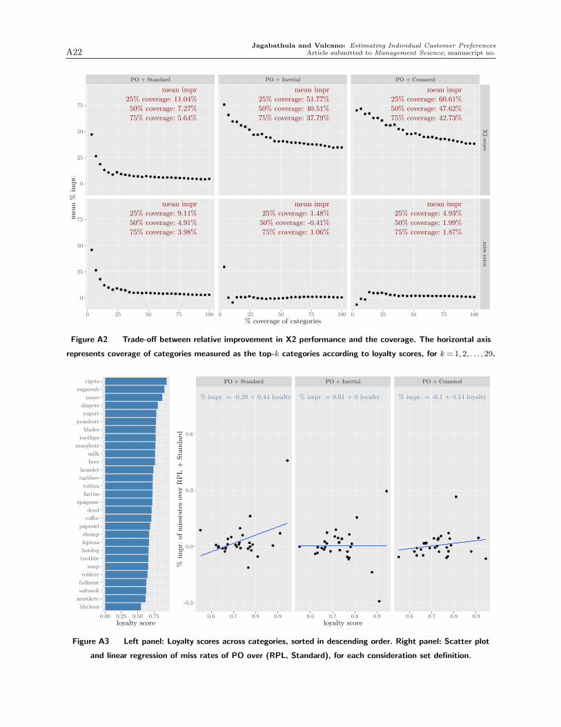
Jagabathula and Vulcano: Estimating Individual Customer PreferencesA22 Article submitted to Management Science; manuscript no.
PO + Standard PO + Inertial PO + Censored
mean impr
25% coverage: 11.04%
50% coverage: 7.27%
75% coverage: 5.64%
mean impr
25% coverage: 9.11%
50% coverage: 4.91%
75% coverage: 3.98%
mean impr
25% coverage: 51.77%
50% coverage: 40.51%
75% coverage: 37.79%
mean impr
25% coverage: 1.48%
50% coverage: -0.41%
75% coverage: 1.06%
mean impr
25% coverage: 60.61%
50% coverage: 47.62%
75% coverage: 42.73%
mean impr
25% coverage: 4.93%
50% coverage: 1.99%
75% coverage: 1.87%
0
25
50
75
0
25
50
75
X2
scorem
issrates
0 25 50 75 100 0 25 50 75 100 0 25 50 75 100% coverage of categories
mea
n%
impr.
Figure A2 Trade-off between relative improvement in X2 performance and the coverage. The horizontal axis
represents coverage of categories measured as the top-k categories according to loyalty scores, for k= 1,2, . . . ,29.
hhclean
mustketc
saltsnck
fzdinent
coldcer
soup
toothbr
hotdog
fzpizza
shamp
paptowl
coffee
deod
spagsauc
factiss
toitisu
carbbev
laundet
beer
milk
margbutr
toothpa
blades
peanbutr
yogurt
diapers
mayo
sugarsub
cigets
0.00 0.25 0.50 0.75loyalty score
PO + Standard PO + Inertial PO + Censored
% impr. = -0.29 + 0.44 loyalty % impr. = 0.01 + 0 loyalty % impr. = -0.1 + 0.14 loyalty
-0.3
0.0
0.3
0.6
0.6 0.7 0.8 0.9 0.6 0.7 0.8 0.9 0.6 0.7 0.8 0.9loyalty score
%im
pr.
ofm
issr
ate
sov
erR
PL
+Sta
ndar
d
Figure A3 Left panel: Loyalty scores across categories, sorted in descending order. Right panel: Scatter plot
and linear regression of miss rates of PO over (RPL, Standard), for each consideration set definition.