INVESTIGATION OF LAYERED LROC IMAGERY AND …€¦ · · 2017-03-01THE GLOBAL ENVIRONMENTAL...
57
INVESTIGATION OF LAYERED LUNAR MARE LAVA FLOWS THROUGH LROC IMAGERY AND TERRESTRIAL ANALOGS A THESIS SUBMITTED TO THE GLOBAL ENVIRONMENTAL SCIENCE UNDERGRATE DIVISION IN PARTIAL FULFILLMENT OF THE REQUIREMENTS FOR THE DEGREE OF BACHELOR OF SCIENCE IN GLOBAL ENVIRONMENTAL SCIENCE MAY 2014 By Heidi Needham Thesis Advisor Dr. Sarah Fagents
Transcript of INVESTIGATION OF LAYERED LROC IMAGERY AND …€¦ · · 2017-03-01THE GLOBAL ENVIRONMENTAL...
INVESTIGATION OF LAYERED
LUNAR MARE LAVA FLOWS THROUGH
LROC IMAGERY AND TERRESTRIAL ANALOGS
A THESIS SUBMITTED TO
THE GLOBAL ENVIRONMENTAL SCIENCE
UNDERGRATE DIVISION IN PARTIAL FULFILLMENT
OF THE REQUIREMENTS FOR THE DEGREE OF
BACHELOR OF SCIENCE
IN
GLOBAL ENVIRONMENTAL SCIENCE
MAY 2014
By
Heidi Needham
Thesis Advisor
Dr. Sarah Fagents

ii
I certify that I have read this thesis and that, in my opinion, it is satisfactory in scope and
quality as a thesis for the degree of Bachelor of Science in Global Environmental
Science.
THESIS ADVISOR
Dr. Sarah Fagents
Hawaiʻi Institute of Geophysics and Planetology

iii
ACKNOWLEDGEMENTS
I would like to thank the NASA Space Grant Consortium at the University of
Hawaiʻi at Mānoa for offering this project as an undergraduate research opportunity. The
skills I have gained in both research and educational knowledge will follow me
throughout my research and career goals. I would also like to thank the McNair Scholar’s
Program for their financial support which allowed me to continue working on this project
through the summer and their counsel and guidance in following my educational and
career goals. I would especially like to thank my mentor Dr. Sarah Fagents and Dr. Elise
Rumpf for their guidance and help throughout this project. The personnel in the HIGP
and the staff in the NASA Space Grant office also deserve a thank you for providing the
support needed to complete this project.

iv
ABSTRACT
The lunar surface contains considerable amounts of information regarding the
formation of the Solar System and more recently the Earth-Moon system. This makes it
the ideal place to “Expand scientific understanding of the Earth and the universe in which
we live,” a primary goal stated by NASA. The main objective of this project was to
estimate the number and thicknesses of specific mare flow locations on the Moon visible
within the walls of impact craters in Lunar Reconnaissance Orbiter Camera (LROC)
Narrow Angle Camera (NAC) images. This work was motivated by a need to understand
flow thicknesses in models of mare flow emplacement and cooling. We focused
primarily on layered deposits exposed in the walls of impact craters consistent with
stacked lava flows. Our approach involved mapping inferred flow units in LROC data
and determining the average thickness of flows using Lunar Orbiter Laser Altimeter
(LOLA). However, image resolution prevents determination of whether each mapped
layer contains a single flow unit or several flows. The precision of this method is
therefore difficult to determine without ground-truth confirmation. To further examine
the accuracy of this method to determine remotely sensed flow thicknesses, this study
was complemented with analysis of Earth-based satellite imagery of Hawaiian basalt lava
flows as analogs to lunar mare lava flows. Through field analysis, ground-truthed data
for the terrestrial imagery was obtained to assess the accuracy of the inferences acquired
from the LROC images. The terrestrial analog study of satellite images showed average
flow thicknesses of 2.0 to 7.7 m. Measurements collected in the field yielded thicknesses
ranging from 1.6 to 2.0 m. The lunar results compiled from Dawes Crater show an
average mare flow thicknesses of 5.7 ± 4.7 m to 18.1 ± 8.9 m. Based on the terrestrial

v
analog study, the image-derived flow thicknesses were overestimated by factors ranging
from 1.0 to 4.5. This was primarily due to the difficulty of identifying all flow contacts
in the images. Although flow thicknesses can be better constrained with the high
resolution LRO images, these estimates are most likely larger than true flow thicknesses.

vi
Table of Contents
ACKNOWLEDGEMENTS ............................................................................................................ iii
ABSTRACT .................................................................................................................................... iv
LIST OF TABLES ......................................................................................................................... vii
LIST OF FIGURES ...................................................................................................................... viii
LIST OF ABBREVIATIONS ......................................................................................................... ix
CHAPTER 1: INTRODUCTION .................................................................................................... 1
CHAPTER 2: BACKGROUND ...................................................................................................... 5
2.1 Brief History of the Moon ...................................................................................................... 5
2.2 Previous Flow Thickness Measurements ............................................................................... 8
2.3 Hawaiian Lava Flow Successions as Planetary Analogs ..................................................... 12
2.4 Lunar Missions and Instrumentation.................................................................................... 14
2.5 Terrestrial Instruments and Data Sets .................................................................................. 15
2.6 Significance of this Study .................................................................................................... 17
CHAPTER 3: METHODS ............................................................................................................. 19
3.1 Selection of Lunar Data ....................................................................................................... 19
3.2 Selection of Terrestrial Data ................................................................................................ 22
3.3 Image Processing and Analysis ........................................................................................... 24
3.4 Field Analysis ...................................................................................................................... 29
CHAPTER 4: RESULTS ............................................................................................................... 31
4.1 Flow Thicknesses Interpreted from LRO/KAGUYA Data .................................................. 31
4.2 Flow Thicknesses Interpreted from WorldView 2 Data ...................................................... 32
4.3 Field Measurements of Flow Thicknesses ........................................................................... 35
CHAPTER 5: DISCUSSION ......................................................................................................... 37
CHAPTER 6: CONCLUSION ...................................................................................................... 42
REFERENCES .............................................................................................................................. 44

vii
LIST OF TABLES
Table 1. List of images utilized in the Dawes Crater mosaic. ..................................................... 21
Table 2. Summary of mapped layered deposits in Dawes Crater using Lunar Reconnaissance
Orbiter data. ................................................................................................................................... 33
Table 3. Summary of mapped layered deposits on O‘ahu, Hawai‘i using WorldView-2 satellite
images. ........................................................................................................................................... 34
Table 4. Summary of field observations from the three terrestrial study sites. ............................ 36

viii
LIST OF FIGURES
Figure 1. Comparison between lunar and terrestrial satellite images. ............................................ 3
Figure 2. Process of Regolith Formation ........................................................................................ 7
Figure 3. Determining Shadow Measurement of a Mare Flow. .................................................... 10
Figure 4. Geologic map of the Wai'anae Range. .......................................................................... 12
Figure 5. WorldView 2 image of Oahu, HI. ................................................................................ 16
Figure 6. Layered deposits in Dawes Crater. ............................................................................... 18
Figure 7. Image of the Moon with study sites marked. ................................................................ 19
Figure 8. Geologic Map of West Oahu. ....................................................................................... 23
Figure 9. Dawes Image Mosaic. ................................................................................................... 25
Figure 10. Dawes Study Sites ...................................................................................................... 27
Figure 11. Satellite Image of Pu’u Heleakala. ............................................................................. 28
Figure 12. Study Sites on Oahu ................................................................................................... 30
Figure 13. Layered hillside Makapuʻu. ........................................................................................ 38

ix
LIST OF ABBREVIATIONS
CCMA Center for Coastal Monitoring and Assessment
DEM Digital Elevation Model
DOE Diffractive Optical Element
DTM Digital Terrain Model
ESRI Environmental Systems Research Institute
GCR Galatic Cosmic Rays
GIS Geographic Information Systems
ISIS Integrated Software for Imagers and Spectrometers
JAXA Japan Aerospace Exploration Agency
LOLA Lunar Orbiter Laser Altimeter
LRO Lunar Reconnaissance Orbiter
LROC Lunar Reconnaissance Orbiter Camera
NAC Narrow Angle Camera
PDS Planetary Data Services
RDR Reduced Data Record
SELENE Selenological and Engineering Explorer
TC Terrain Camera
USDA United States Department of Agriculture
USGS United States Geological Survey
WAC Wide Angle Camera

1
CHAPTER 1
INTRODUCTION
In the layered surface of the Moon there lies an important record of the history of
the Solar System. Of key importance is the information we can obtain about the origins
of the Earth-Moon system and evolution of the Sun. The lunar surface has been exposed
to the space environment since its formation billions of years ago. As such, it can be
viewed as a record of events that occurred in space after the Moon’s formation. Surface
regolith deposits incorporate solar wind and solar flare particles, along with cosmogenic
products of galactic cosmic ray (GCR) impacts (Armstrong et al., 2002). The lunar
surface may also contain ejecta from large impacts on Earth and other planetary bodies
(Spudis, 1996). Lunar lava flows that were emplaced over surface regoliths would have
acted as a shield protecting from continued bombardment the ancient deposits that may
hold clues to the Solar System’s history. Identification of layered lava flows and
intercalated regolith deposits provides a time-series of snapshots of the lunar
environment, and measurements of flow thicknesses can be used as inputs to models of
lava–substrate heating that predict the depths in buried paleoregolith deposits at which
implanted particles will avoid being volatilized by the heat of the overlying flow (Fagents
et al., 2010; Rumpf et al., 2013).
Technological improvements in satellite instrumentation have led to increasingly
detailed views of the lunar surface. The Lunar Reconnaissance Orbiter Camera (LROC)
Narrow Angle Camera (NAC) imagery resolution of 0.5 m/pixel allows for more precise
measurements of lunar lava flows than was previously possible with lower resolution

2
images. These flows are commonly found exposed in the walls of impact craters on the
lunar surface. However, it is unclear whether the LROC NAC image resolution is
sufficient to determine whether each layer identified in an image contains a single flow or
an outcrop of multiple stacked flows. Although higher resolution imagery has improved
our ability to estimate lava flow thickness, it may be insufficient to determine flow
thicknesses with confidence. Illumination geometry, spacecraft viewing angles, and
shadowing influence the appearance of the exposed lava flows, making it difficult to
determine exact thicknesses. Outcrops of lava flows can also be altered over time by
mass wasting and obscured by talus deposits (Robinson et al., 2012). Hence the accuracy
of thickness measurements based on remotely sensed methods is difficult to determine
without some other means of verification.
In seeking a method to determine the accuracy of measurements made using
Lunar Reconnaissance Orbiter (LRO) data, we conducted a terrestrial analog study using
satellite and topographic data on the island of Oahu, Hawaiʻi. The Hawaiian Islands offer
a unique place to study long term effusive eruptions of low-viscosity basalt flows. A
study by Mouginis-Mark and Rowland (2008) noted the similarities in morphology and
degradation of lava flows exposed in the eroded Koolau volcano on Southeast Oahu with
those of deposits in images of Arsia Mons Volcano on Mars. This study confirmed that
Hawaiian basalt flows are appropriate analogs to low-viscosity lava flows elsewhere in
the Solar System. The Waiʻanae Range on Western Oahu contains deposits of ponded
caldera lavas and flank flows in close proximity to each other. In this study, flows visible
in satellite images of Oahu were compared with layered deposits of stacked lava flows in
the walls of impact craters, pit craters and large boulders on the lunar surface. The
3
terrestrial comparison study constrained the accuracy of the thickness measurements
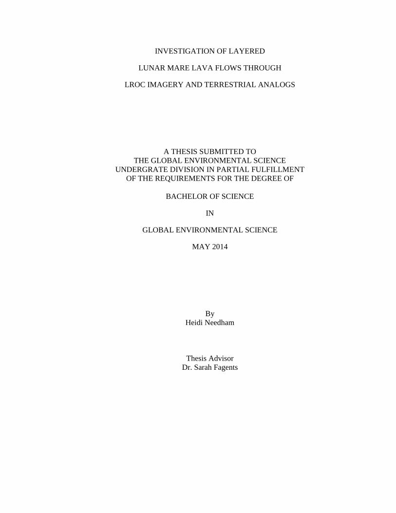
acquired from the analysis of LROC images. A comparison between lunar and terrestrial
stacked lava sequences from the Waiʻanae Range is shown in Figure 1.
Comparisons of LROC imagery with analysis of Earth-based satellite imagery
allow for the accuracy of the analyses to be assessed. This was accomplished by
obtaining ground-truthing data through field analysis from the sites examined in the
terrestrial imagery. The terrestrial analog study allows for inferences to be drawn
regarding the uncertainties associated with thickness measurements made using LRO data
sets. Determining the accuracy of flow thickness measurements allows for assessment of
the uncertainty in modeled preservation depths of extra-lunar volatiles in buried regoliths
heated by overlying lava flows (Fagents et al., 2010; Rumpf et al., 2013). The results of
this project are also relevant to models of lunar lava flow dynamics that seek to relate
eruption conditions to flow dimensions, which ultimately contributes to furthering our
understanding of the volcanological history of the Moon.
Figure 1. Comparison between lunar and terrestrial satellite images.
Left image shows layered deposits on Dawes crater and right image shows layered lava flows from
West Oahu, HI. Lunar image is LROC NAC image M180994913LC and the terrestrial images is a
WorldView 2 satellite image.

4
In the following chapters, I first provide additional detail on the history of the
Moon and lunar surface processes (Chapter 2). This includes background on the
evolution of lunar volcanism and other surface processes that make it an important record
of early Solar System events. Also discussed are the different methods used to determine
lava flow thicknesses on planetary bodies and the importance of accurate thickness
measurements. For the terrestrial analog study, the volcanic history of Hawaiian shield
volcanoes is discussed, including the evolution of the Waiʻanae and Koʻolau Volcanoes
on Oahu.
Methodology for the study is covered in Chapter 3, which details the procedures,
instrumentation and remote sensing datasets that were used for this study. Methods for
measuring lava flows in the field are also discussed. The results from satellite and field
measurements are provided in Chapter 4, and Chapter 5 discusses the implications of the
research results.
5
CHAPTER 2
BACKGROUND
2.1 Brief History of the Moon
Lunar scientists believe that the Moon was created from the impact of the Earth
by another planetary body approximately 4.6 billion years ago (Frankel, 1996). The
other planetary body, roughly the size of Mars, would have excavated a large portion of
the Earth’s surface and interior. Some of this material from Earth along with the debris
from the breakup of the other planetary body would have been ejected into orbit around
the Earth forming a ring (Rothery et al., 2011). Gravitational forces would cause Earth
to reclaim some of the ejecta with the remaining accreting to form the Moon. Evidence
for this theory is based on analysis of lunar samples that show similar geochemical and
isotopic signatures for both the Earth and the Moon (Rothery et al., 2011). Following its
formation the Moon underwent a period of heavy bombardment by cosmic debris
between 4.2 and 3.8 million years ago (Frankel, 1996). After the heavy bombardment,
melting episodes generated by radioactive heating led to the volcanism that created the
dark mare regions still visible today. This time frame, known as the Epoc of Mare
Flooding, occurred approximately 3.8 – 3.2 billion years ago (Hiesinger, 2000). After
this period, volcanism diminished and the lunar surface has remained fairly stable
showing two main surface types, the darker maria and the brighter, more heavily cratered
highlands. The latter represent the older crust of the Moon and contain a cratered record
of the heavy bombardment early in the Moon’s history.

6
The two distinct surfaces of the Moon appear differently due to chemical
differences. The older highland regions have lower FeO and TiO2 and lower CaO/Al2O3
ratios than mare basalts (Taylor et al., 1991). The younger mare lava flows cover
approximately 6 million square kilometers or one third of the Moon’s surface and have a
large variation in TiO2 concentrations (Taylor et al., 1991). The concentrations can range
from high-Ti (>9 wt.% TiO2), to low-Ti (1.5-9 wt.% TiO2), to very low-Ti (<1.5 wt.%
TiO2) (Taylor et al., 1991). Mare flows are thought to have had high eruption
temperatures, exceeding 1200°C, and low viscosities (Hörz et al., 1991).
Of the nine locations on the Moon sampled by Apollo astronauts, the youngest
was dated at 3.2 billion years old (Vaniman et al., 1991). An important difference
between the mineralogy of the Earth and Moon is that rocks on the Moon are not recycled
by plate tectonics (Carrier et al., 1991). Lacking an atmosphere, the Moon retains
significantly fewer volatiles than Earth and has been found to contain only small amount
of water (Saal et al., 2008; Anand, 2010). This restricts the types of minerals that can
form. Using various methods, including analysis of Apollo lunar samples, only one
hundred mineral species have been found on the lunar surface, very different from the
over two thousand found on Earth (Frankel, 1996). The main species of minerals found
on the Moon are pyroxenes, feldspars, olivines, magnetite, ilmenite, quartz and zircons
(Rothery et al., 2011).
Over time the lunar surface has been modified due to its continuous exposure to
space. Continually bombarded by macro and micrometeorites, the surface of the Moon
has been fragmented into a poorly sorted fine grained material called regolith. Regolith
up to several meters thick covers the entire lunar surface, with solid bedrock and lava
7
flows only visible in areas that are uncovered due to impacts exposing the underlying
bedrock. In some cases, layered sections of bedrock are exposed, which have been
interpreted as stacks of lava flows (Mckay et al., 1991). These layers are significant as
they may hold an important record of early Solar System processes buried in between the
lava flow layers (Hörz et al., 1991).
The lunar surface has also been impacted by a variety of particles originating
from solar flares, solar wind, and galactic cosmic rays. As micrometeorites impact the
surface they cause localized melting and agglutinate formation that traps these particles
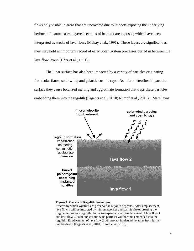
embedding them into the regolith (Fagents et al., 2010; Rumpf et al., 2013). Mare lavas
Figure 2. Process of Regolith Formation
Process by which volatiles are preserved in regolith deposits. After emplacement,
lava flow 1 will be impacted by micrometeorites and cosmic fluxes creating the
fragmented surface regolith. In the timespan between emplacement of lava flow 1
and lava flow 2, solar and cosmic wind particles will become embedded into the
regolith. Emplacement of lava flow 2 will protect implanted volatiles from further
bombardment (Fagents et al., 2010; Rumpf et al., 2013).

8
that flowed over older regolith deposits would have acted as a shield protecting these
former surfaces (Figure 2). A succession of lava flows and intercalated regolith deposits
generates a time series of solar wind and cosmic ray samples (Fagents et al., 2010;
Rumpf et al., 2013). Mare lava flow layers preserving these volatiles can be dated using
radiometric techniques to define an approximate age and exposure duration for the
intervening regolith. Acquisition and analysis of such samples during future missions
would permit assessment of variations in the strength and composition of solar wind,
solar flare and cosmic particle fluxes since the formation of the Moon.
The survivability of preserved volatiles is dependent on how deeply into the
underlying regolith heat will be transferred when it is covered by a layer of lava. The
thicker the overlying lava, the deeper into the regolith vaporization and outgassing
occurs, thereby destroying the implanted volatiles. Establishing improved estimates on
the thickness of lunar lava flows will allow lunar scientists to better determine
appropriate locations and depths from which to collect samples during future manned or
robotic missions.
2.2 Previous Flow Thickness Measurements
Understanding lava flow thicknesses on the Moon is important for determining
the volume and eruption rates of mare flows and the survivability of trapped volatiles in
the underlying regolith. This knowledge enhances planetary scientist’s overall
comprehension of the geologic and thermal evolution of the Moon. There are several
methods that have been used to estimate thicknesses of lava flows on the Moon. Previous
approaches include analyzing crater excavation depths within individual flows (Platz et

9
al., 2010), in-situ observations made by Apollo astronauts near Hadley Rille (Howard et
al., 1972), crater size-frequency distributions (Hiesinger and Head, 2002), and analysis of
Clementine multispectral data (Weider et al., 2010). Observations of lunar mare
thicknesses have also been studied using Digital Elevation Models (DEM) and
photoclinometry to reconstruct flow fronts from variations in surface reflectance (Kirk et
al., 2003). Others have utilized shadow measurements on flow front scarps to obtain a
flow thickness (Yingst and Head, 1997; Head et al., 2002; Hiesinger et al., 2002; Platz et
al., 2010). Determining lunar flow thicknesses from these methods relies heavily on the
resolution and quality of the data used for the measurements.
The most accurate method of determining the thicknesses of lunar lava flows
would be field measurements from the Moon. This was not possible at most Apollo
landing sites, however Apollo 15 astronauts photographed layering within the upper walls
of Hadley Rille. Estimates from these images show lava layers that were on the order of
1-10 m thick (Spudis et al., 1988; Vaniman et al., 1991). However, the quality of the
photographs hindered accurate determination of whether the flows were single events or
multiple flows from the same eruption (Howard et al., 1972). Since Hadley Rille is just
one location, additional methods have been used to determine thickness in other localities
on the Moon.
Flow thicknesses at multiple sites have been determined from crater size-
frequency distributions (Head et al., 2002; Hiesinger et al., 2002; Platz et al., 2010).
Utilizing techniques that examined distribution curves of crater size-frequency, Head et
al. (2002) determined a characteristic point in the curve that signified a separation of time
between two different lava flows. From this method average flow thicknesses of
10
approximately 30 – 60 m were determined (Head et al., 2002). This approach is useful in
determining thickness and volume estimates in images where there is a low sun angle or
places were flows are partially obscured.
Another approach that applies data from crater size-frequency distribution is a
method which utilizes partially buried craters to determine the thickness of an overlaying
deposit (Platz et al., 2010). This technique requires the crater size-frequency distribution
of a crater of interest and its associated underlying crater to extrapolate a layer thickness.
Although this method was utilized to determine thicknesses on Mars, it has the potential
to be used on other planetary bodies.
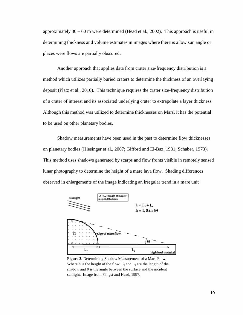
Shadow measurements have been used in the past to determine flow thicknesses
on planetary bodies (Hiesinger et al., 2007; Gifford and El-Baz, 1981; Schaber, 1973).
This method uses shadows generated by scarps and flow fronts visible in remotely sensed
lunar photography to determine the height of a mare lava flow. Shading differences
observed in enlargements of the image indicating an irregular trend in a mare unit
Figure 3. Determining Shadow Measurement of a Mare Flow.
Where h is the height of the flow, Lf and Ls are the length of the
shadow and θ is the angle between the surface and the incident
sunlight. Image from Yingst and Head, 1997.

11
(Gifford and El-Baz, 1981). This shading difference allows for determination of the flow
front and the shadow generated from the light angle is measured. A flow height can be
determined from these measurement by determining the overall length of the shadow and
multiplying by the tangent of the incident angle (Figure 3). Using this method Gifford
and El-Baz, (1981) found mare flow heights ranging from 1-96 m with an overall average
of 21 m in their study. Other shadow measurements have found average heights of 30-35
m (Schaber, 1973). This method is limited by the resolution of the images and shape of
the flow. It is often hard to accurately locate the exact edge of the shadow and it is
commonly assumed that the thickness is uniform across the flow (Gifford and El-Baz,
1981).
Another method employed to determine mare lava flow thicknesses is
photoclinometry, sometimes called shape-from-shading. This technique determines the
surface shape from image gray values and computer software to generate 3-D surface
topography (Lohse et al., 2006). Lobe thicknesses measured from the resulting
topographic profiles, indicate approximate thicknesses of 40 to 60 m (Garry et al., 2010).
Limitations in this method are attributed to the assumption that the surface underlying the
flow is flat, and that there are negligible variations in albedo within the image (Garry et
al., 2010).
Technological improvements in satellite instrumentation have led to increasingly
detailed views of the lunar surface, which allows for improvements in thickness
estimates. Using LROC imagery, lunar mare lava flow thicknesses have been measured
within the rims of pit craters (Robinson et al., 2012) and more recently in impact craters
(Enns and Robinson, 2013). Lava flows in pit craters have been observed to have

12
thicknesses ranging from 3-14 m and average thicknesses of ~10 m (Robinson et al.,
2012). Recent work conducted on 50 select impact craters in nearside mare, involving a
methodology similar to that of this study, showed flow thicknesses ranging between 6
and 25 m (Enns and Robinson, 2013). Studies on impact craters using the higher
resolution LROC imagery will increase the accuracy of thickness measurements of lunar
mare lava flows, compared to studies using previous data sets.
2.3 Hawaiian Lava Flow Successions as Planetary Analogs
An important element of this research is the terrestrial analog study to assess the
accuracy of lunar flow thickness measurements. On Oahu outcrops of stacked lava flows
Figure 4. Geologic map of the Waiʻanae Range.
Shows the four different members and the two study sites. Thin black line is the old caldera
complex. Geology and map from John Sinton, unpublished.

13
exhibit morphologies similar to those observed in planetary image data sets (Mouginis-
Mark and Rowland, 2008), making them a useful analog for layered lunar lavas. The
Waiʻanae Volcano makes up the western portion of the island of Oahu in Hawaiʻi.
Exposed Waiʻanae lavas range in age from approximately 3.9 to 2.8 Ma (McDougall,
1963, Funkhouser et al., 1968; Doell and Dalrymple, 1973; Presley et al., 1997). The
rock units comprising the Waiʻanae Range are known as the Waiʻanae Volcanics. These
have been grouped into four separate units or members, two pre-shield members and two
post-shield members (Presley et al., 1997). The Lualualei Member consists of the oldest
exposed lavas dominated by tholeiitic olivine basalts. It is mainly exposed near Puʻu
Heleakalā and Puʻu o Hulu, two ridges on the south side of Lualualei Valley. The
Kamaileʻunu Member erupted ~3.55 – 3.06 Ma ago during the caldera filling period,
producing plagioclase-bearing tholeiitic lavas, alkalic basalts and some basaltic
hawaiites. This member is exposed in various locations throughout the old caldera
complex, Lualualei Valley and along rift zones outside of the caldera complex. The two
younger members, Pālehua and Kolekole, are post-shield stage and consist of various
types of more alkalic lavas like hawaiites and rare mugearites (Presley et al., 1997).
The two study sites located in the Waiʻanae Range consist of layered tholeiitic
basalts emplaced during the shield-building stage of the volcano. Puʻu Heleakalā
consists of the Lualualei Member, and Puʻu Kepauala consists of Kamaileʻunu Member
lavas, making a deposition age of approximately 3.05 – 3.55 million years ago (Guillou et
al., 2000). The location of these two study sites relative to the Waiʻanae Volcano and the
old caldera complex is shown in Figure 4.
14
The study site at Makapuʻu is situated on the southeastern point of the island of
Oahu. Koʻolau Range consists almost entirely of tholeiitic basalt lavas ranging in age
from 1.8 to 2.6 million years. The Makapuʻu section of the Koʻolau Range contains
shield stage lavas dipping down slope from northeast facing cliffs which make up the
Koʻolau Pali. Field sites occurred at the top of the Pali cliffs and across a valley along
the Makapuʻu trail.
2.4 Lunar Missions and Instrumentation
This project relied heavily on data acquired by instruments onboard the Lunar
Reconnaissance Orbiter (LRO). The LRO spacecraft entered orbit around the Moon in
June of 2009. The main objectives of the spacecraft are to return high resolution imagery
to identify potential landing sites and to completely map the polar regions of the Moon to
identify areas in permanent shadow that may host water ice (Robinson et al., 2010). The
imaging system has both a wide angle camera (WAC) and two narrow angle cameras
(NAC). The NAC system has been mapping the surface of the Moon on scales of less
than a meter, allowing for a robust inspection of surface features. This work utilized
these high resolution images of the lunar surface to investigate lava flow thickness within
the walls of impact craters.
In addition to imaging data, topographic data are acquired on the LRO spacecraft
by the Lunar Orbiter Laser Altimeter (LOLA). LOLA is an instrument that pulses a
single laser through a Diffractive Optical Element (DOE) to produce a signal with five
beams that illuminates the surface of the Moon (LOLA website:
http://lunar.gsfc.nasa.gov/lola/about.html) (Smith et al., 2010). With each beam LOLA
15
measures the range, generated from time of flight, the surface roughness and surface
reflectance generated from the transmitted and returned energy. From the data LOLA
gathers from the surface the instrument is able to determine the slope along and across
the track. LOLA data are used to produce topographic elevation models of the lunar
surface as well as models of surface slope, lunar gravity, surface roughness and surface
brightness (Smith et al., 2010).
An additional data set used for the lunar analysis was the Digital Terrain Model
(DTM) generated from the stereo images of the Terrain Camera (TC) on the KAGUYA
SELENE instrument. KAGUYA has a Main Orbiter at 100 km altitude and two small
satellites in polar orbit. The scientific instruments on board are used for the global
mapping of lunar surface, magnetic field measurement, and gravity field measurement
together with the instruments. The main mission objective, like the LRO mission, is
future lunar exploration. The KAYGUA DTM was constructed using mosaic images,
mapped from combinations of several images, with no overlap between files (JAXA
website: http://www.kaguya.jaxa.jp/en/greeting/index.htm). The DTM has a resolution
of 10 m and was used as a base layer in the mosaic of Dawes Crater as described in
Chapter 3.
2.5 Terrestrial Instruments and Data Sets
WorldView 2 satellite images obtained from the United States Department of
Agriculture (USDA) were used for this project (Figure 5). The WorldView 2 satellite
was launched by Satellite Imaging Group in October of 2009 and provides 0.5 m
panchromatic mono and stereo satellite image data. Information on these data can be
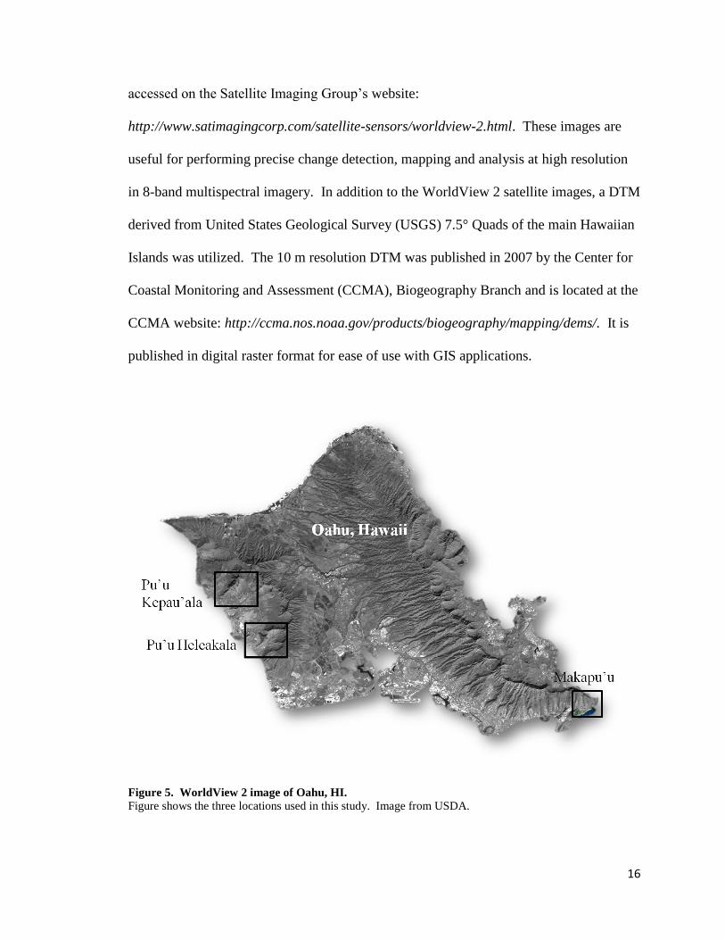
16
accessed on the Satellite Imaging Group’s website:
http://www.satimagingcorp.com/satellite-sensors/worldview-2.html. These images are
useful for performing precise change detection, mapping and analysis at high resolution
in 8-band multispectral imagery. In addition to the WorldView 2 satellite images, a DTM
derived from United States Geological Survey (USGS) 7.5° Quads of the main Hawaiian
Islands was utilized. The 10 m resolution DTM was published in 2007 by the Center for
Coastal Monitoring and Assessment (CCMA), Biogeography Branch and is located at the
CCMA website: http://ccma.nos.noaa.gov/products/biogeography/mapping/dems/. It is
published in digital raster format for ease of use with GIS applications.
Figure 5. WorldView 2 image of Oahu, HI. Figure shows the three locations used in this study. Image from USDA.

17
2.6 Significance of this Study
The need for this study was established by previous modeling investigations, in
which uncertainties in flow thicknesses had significant implications for the validity of the
results (Fagents et al, 2010; Rumpf et al, 2013). Accurate knowledge of lunar lava flow
thicknesses is important for determining correct boundaries and constraints in volcanic
flux estimates throughout the thermal evolution of the Moon. Previous measurements of
lava flow thicknesses have suffered inaccuracies due to the limitations in the resolution of
remotely sensed imagery. In addition, flow morphologies are typically indistinct as a
result of billions of years of space weathering and regolith formation since their
emplacement making it hard to determine thicknesses accurately (Hörz et al., 1991).
Mare lava flow rheology and dynamics are commonly studied through numerical
modeling in order to understand the volcanic evolution of the Moon. Two important
factors in understanding the rheology of lunar lava flows is the viscosity (η) and yield
strength (Y). For example, one expression commonly used to relate flow conditions to
flow thickness is the Jefferys equation:
𝑉 =𝑔𝑑2𝜌 𝑆𝑖𝑛|𝛼|
3𝜂
Where (g) is the lunar acceleration of gravity 1.622 m/s2, (d) is the thickness of
the flow, (ρ) is the density of the flow, (α) is the slope angle of the surface and (V) is the
flow velocity. The thickness of the lava flow (d) can have a significant effect on the
18
calculated viscosity and velocity because of the dependence of these values on the square
of the flow thickness.
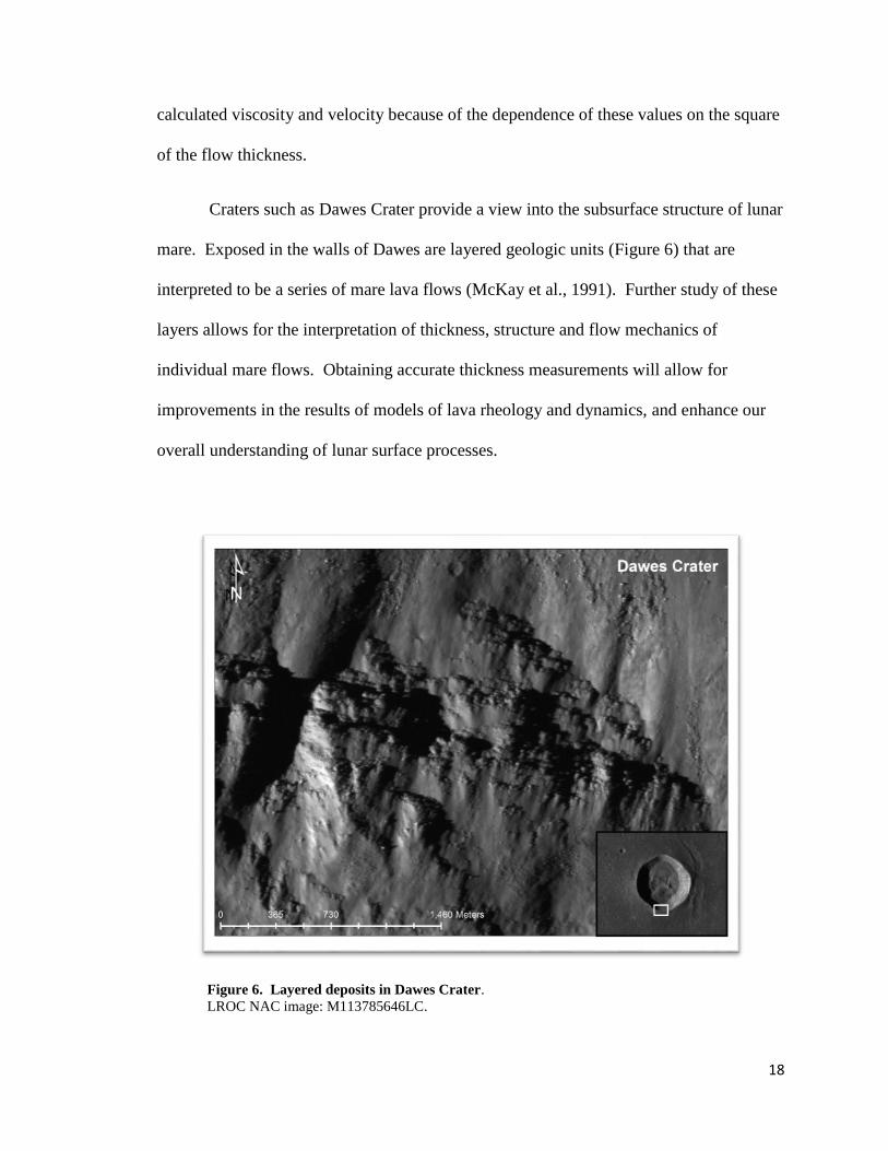
Craters such as Dawes Crater provide a view into the subsurface structure of lunar
mare. Exposed in the walls of Dawes are layered geologic units (Figure 6) that are
interpreted to be a series of mare lava flows (McKay et al., 1991). Further study of these
layers allows for the interpretation of thickness, structure and flow mechanics of
individual mare flows. Obtaining accurate thickness measurements will allow for
improvements in the results of models of lava rheology and dynamics, and enhance our
overall understanding of lunar surface processes.
Figure 6. Layered deposits in Dawes Crater.
LROC NAC image: M113785646LC.
19
CHAPTER 3
METHODS
3.1 Selection of Lunar Data
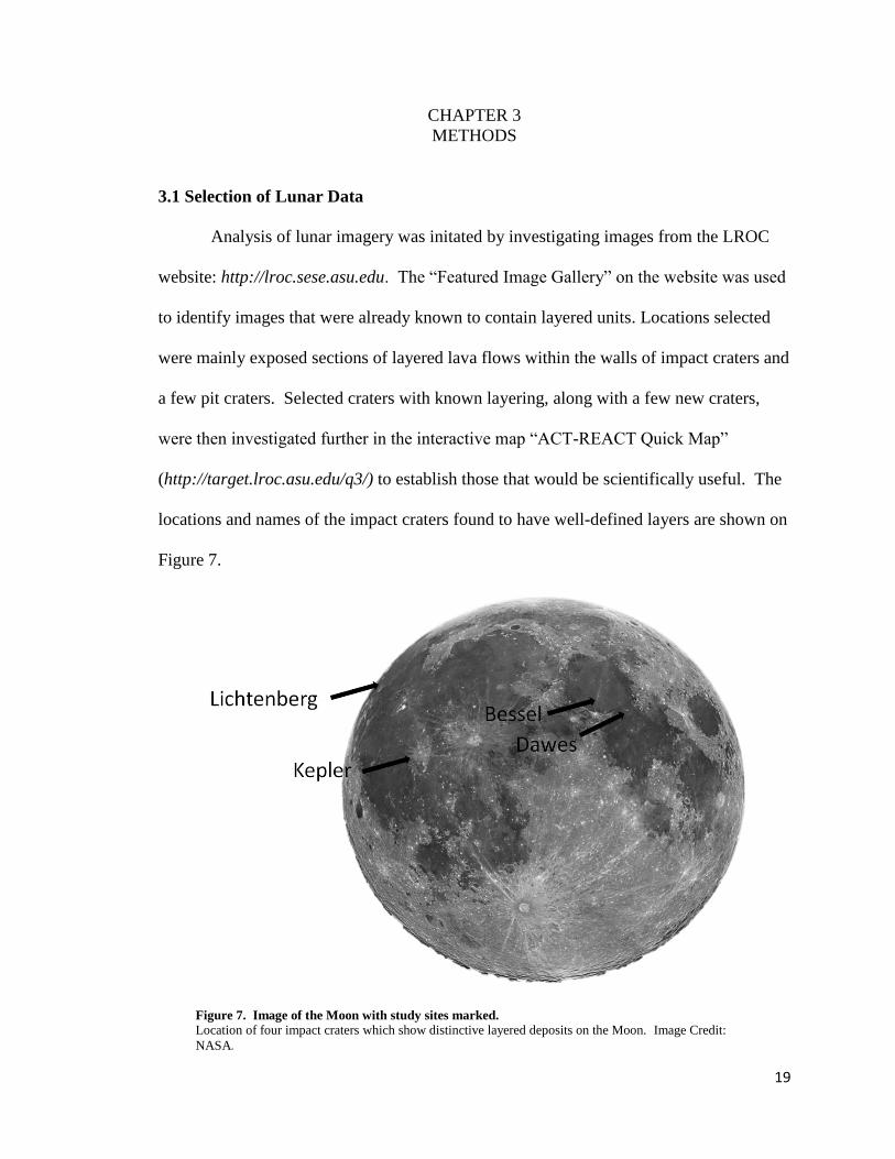
Analysis of lunar imagery was initated by investigating images from the LROC
website: http://lroc.sese.asu.edu. The “Featured Image Gallery” on the website was used
to identify images that were already known to contain layered units. Locations selected
were mainly exposed sections of layered lava flows within the walls of impact craters and
a few pit craters. Selected craters with known layering, along with a few new craters,
were then investigated further in the interactive map “ACT-REACT Quick Map”
(http://target.lroc.asu.edu/q3/) to establish those that would be scientifically useful. The
locations and names of the impact craters found to have well-defined layers are shown on
Figure 7.
Figure 7. Image of the Moon with study sites marked.
Location of four impact craters which show distinctive layered deposits on the Moon. Image Credit:
NASA.

20
For this study Dawes Crater was chosen because of the numerous sections of
visible layering identified within the crater wall. It is located between Mare Serenitatis
and Mare Tranquilitatis at 17.2 °N latitude and 26.3 ° E longitude. Additional
information on Dawes was gathered using an interactive search tool in “ACT-REACT
Quick Map” that allowed for selecting and highlighting the entire crater. Once selected, a
query search was conducted that returned all LROC products for the highlighted area
listed by their product number. The data list returned from the query search and
associated metadata were exported to an Excel spreadsheet. All images listed were
examined in detail on the LROC website to determine usability for this project. Images
that were useable were selected for downloading and images that were not suitable were
noted as not useable. These included images that were too dark, along with any that
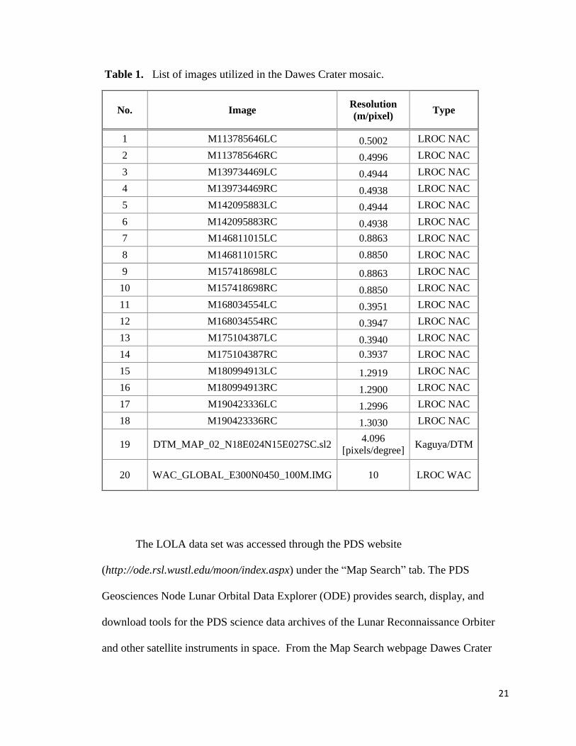
contained only small sections along the rim of Dawes with no visible layering. A list of
the images utilized is shown in Table 1.
Using the Planetary Data Services (PDS) Archive Interface’s product search from
the LROC website (http://wms.lroc.asu.edu/lroc/search) and the query list of image
identification numbers, NAC and WAC images for Dawes were downloaded and saved
into a master file for Dawes Crater. Both LROC and KAGUYA TC (Terrain Camera)
DTMs were examined for downloading. The KAGUYA TC DTM was chosen due to its
10 meters per pixel coverage and downloaded from the KAGUYA Selene website:
http://l2db.selene.darts.isas.jaxa.jp/index.html.en.
21
Table 1. List of images utilized in the Dawes Crater mosaic.
No. Image Resolution
(m/pixel) Type
1 M113785646LC 0.5002 LROC NAC
2 M113785646RC 0.4996 LROC NAC
3 M139734469LC 0.4944 LROC NAC
4 M139734469RC 0.4938 LROC NAC
5 M142095883LC 0.4944 LROC NAC
6 M142095883RC 0.4938 LROC NAC
7 M146811015LC 0.8863 LROC NAC
8 M146811015RC 0.8850 LROC NAC
9 M157418698LC 0.8863 LROC NAC
10 M157418698RC 0.8850 LROC NAC
11 M168034554LC 0.3951 LROC NAC
12 M168034554RC 0.3947 LROC NAC
13 M175104387LC 0.3940 LROC NAC
14 M175104387RC 0.3937 LROC NAC
15 M180994913LC 1.2919 LROC NAC
16 M180994913RC 1.2900 LROC NAC
17 M190423336LC 1.2996 LROC NAC
18 M190423336RC 1.3030 LROC NAC
19 DTM_MAP_02_N18E024N15E027SC.sl2 4.096
[pixels/degree] Kaguya/DTM
20 WAC_GLOBAL_E300N0450_100M.IMG 10 LROC WAC
The LOLA data set was accessed through the PDS website
(http://ode.rsl.wustl.edu/moon/index.aspx) under the “Map Search” tab. The PDS
Geosciences Node Lunar Orbital Data Explorer (ODE) provides search, display, and
download tools for the PDS science data archives of the Lunar Reconnaissance Orbiter
and other satellite instruments in space. From the Map Search webpage Dawes Crater

22
was selected and a query search was conducted. The search returned numerous results
for various LOLA data products. For this study the LOLA Reduced Data Record (RDR)
shapefiles were downloaded and used for analysis by layering them on top of the image
mosaic to determine elevation points and distances along transect lines.
3.2 Selection of Terrestrial Data
Given the similar resolution to LROC NAC images, WorldView 2 satellite images
of Oahu were acquired through the Coastal Geology Group at the University of Hawaiʻi.
This imagery was made available by the USDA (United States Department of
Agriculture) and has a resolution of 0.5 meters per pixel, analogous to the LROC NAC
images. The images were saved onto an external hard drive for ease of use. The
WorldView 2 satellite images were then examined to find locations that would be most
analogous to the lunar study sites. The ten locations identified were located mainly on
the south west end of the old Waiʻanae Range and are shown in Figure 8.
Reconnaissance fieldwork was then conducted at the selected locations to determine
whether they were valuable scientifically, as well as accessible for study in the field.
Following the reconnaissance work, the locations at Nanakuli (Site 3) and one in the
Makaha (Site 6), shown in Figure 8, were chosen as study sites. One additional study site
on the Eastern side of Oahu at Makapuʻu was also selected (Figure 5).

23
Figure 8. Geologic Map of West Oahu. Shows potential field sites examined in both satellite imagery and in the field. Sites 3 and 6 were chosen
for further analysis.

24
3.3 Image Processing and Analysis
Once the necessary lunar and terrestrial images were downloaded they were
further processed to combine them into a useable mosaic. This was completed using the
Environmental Systems Research Institute (ESRI) software package ArcGIS 10.1,
located online at http://www.arcgis.com/. ArcGIS provides a platform for creating maps
and processing geospatial information within a single database. The KAGUYA DTM
and WAC images were first processed in the “Integrated Software for Imagers and
Spectrometers” (ISIS) before they were added as base layers for the crater mosaic. ISIS
is a free image processing and analysis software package that is distributed by the
Astrogeology Branch of the United States Geological Survey (USGS) and can be
accessed via the ISIS website at http://isis.astrogeology.usgs.gov/. ISIS was used to crop
and remove the unnecessary portions of the images while keeping the associated
georeferencing within the imagery. A bash script was used to unzip the files and convert
them from .img image files into .cub cube files. Then the program was used to place
appropriate coordinates onto the image cubes and mosaic them into a predefined size.
All LROC images first required processing in ArcCatalog before they could be
added as a mapped layer. Each image was opened in ArcCatalog in order to build raster
pyramid layers. Pyramids are reduced resolution layers of the raster dataset. Building
pyramids allows for improved performance while viewing large files in ArcGIS. The
images were further processed to update the spatial referencing to GSC Moon 2000, a
geographic coordinate system for the Moon. NAC images had to be geo-referenced
before they could be overlain on the LROC and KAGUYA DTM base layers. This step
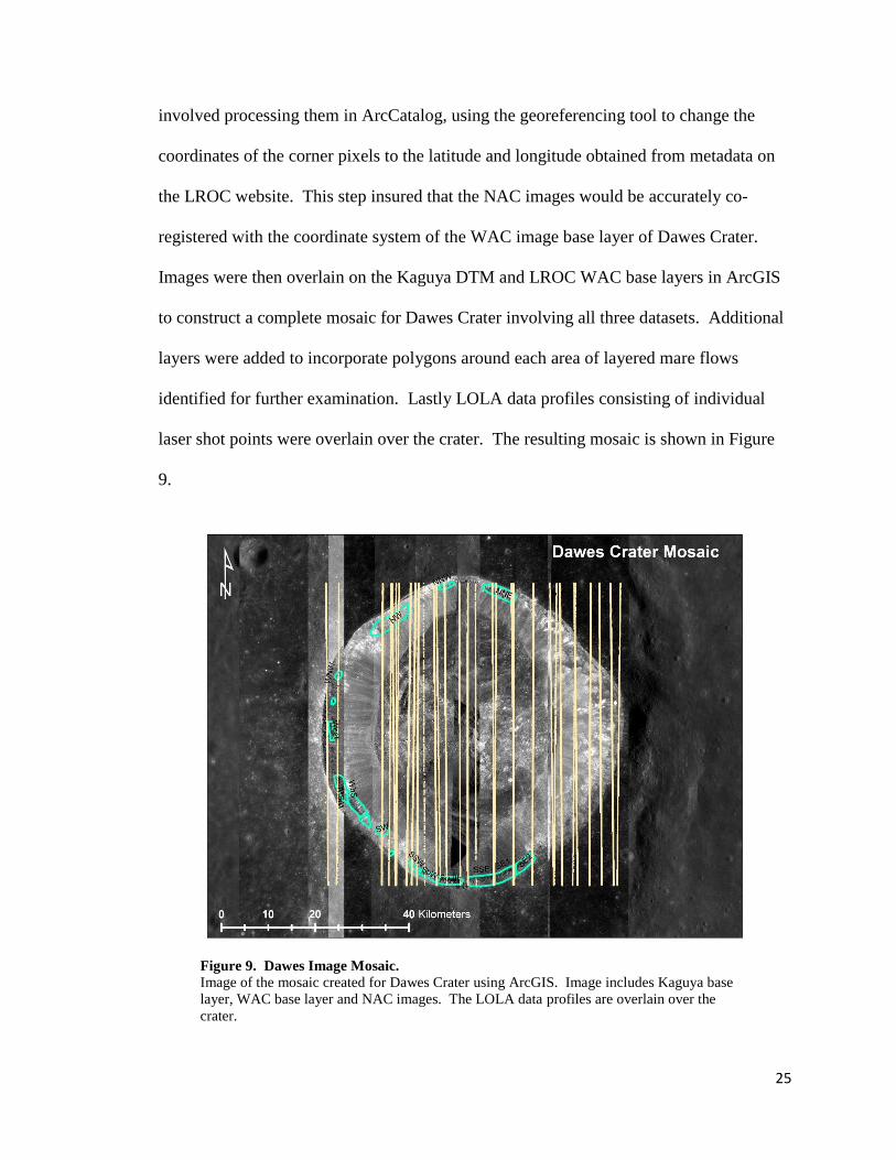
25
involved processing them in ArcCatalog, using the georeferencing tool to change the
coordinates of the corner pixels to the latitude and longitude obtained from metadata on
the LROC website. This step insured that the NAC images would be accurately co-
registered with the coordinate system of the WAC image base layer of Dawes Crater.
Images were then overlain on the Kaguya DTM and LROC WAC base layers in ArcGIS
to construct a complete mosaic for Dawes Crater involving all three datasets. Additional
layers were added to incorporate polygons around each area of layered mare flows
identified for further examination. Lastly LOLA data profiles consisting of individual
laser shot points were overlain over the crater. The resulting mosaic is shown in Figure
9.
Figure 9. Dawes Image Mosaic. Image of the mosaic created for Dawes Crater using ArcGIS. Image includes Kaguya base
layer, WAC base layer and NAC images. The LOLA data profiles are overlain over the
crater.
26
From the mosaics, potential contacts between lava flows were delineated on the
images using an editor in ArcGIS to draw polylines on top of possible flows. These
contacts were mapped by two individuals to compare differences in the interpretation of
lava flows in the images. Utilizing the spatial referencing available in the image, the
numbers of individual lava flows within a given vertical section were counted and
incorporated into a data table. Using both the LOLA data and NAC stereo DEMs for
each crater we established the dimensions of the section being studied by determining the
elevation difference between the top and bottom of the section. Thickness estimates were
established by dividing the number of delineated flow layers by the elevation change
along each transect. An example of this step is shown in Figure 10, which shows the six
main localities within Dawes Crater. Sites are labeled according to their location around
the crater wall, starting from the top Northeastern section (a) rotating counter-clockwise
to the Southeastern bottom section (f). Sections analyzed were limited to those where
LOLA data points ran across visibly stratified areas. Transects were drawn between two
LOLA shot points to establish the elevation change. Potential lava flows were mapped
with the solid and dashed lines. The solid lines indicate a moderate degree of confidence
that the underlying layer is a lava flow contact and dashed lines represent those were
there is a greater amount of uncertainty. The maximum count for the number of layers
took into account both sets of lines mapped. The minimum count only included the solid
lines in the section.
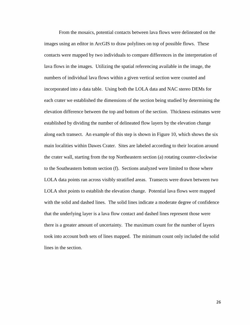
27
Figure 10. Dawes Study Sites
Six different localities where layers in Dawes Crater were analyzed. Figures appear in a counter-
clockwise fashion with (a) Section NNE starting at the top of Dawes Crater and ending at (f)
towards the bottom of the crater, as shown in the transects.

28
In a similar method to that applied to the lunar imagery, the terrestrial WorldView
2 images were assimilated into usable mosaics in ArcGIS. The WorldView 2 satellite
images were overlain on the USGS 10 m DTM of Oahu, Hawaiʻi. Images were already
in required format and did not need to be further processed. Possible layered flows were
delineated for the entire hillside in preparation for fieldwork, as accessibility for specific
areas was uncertain. Prospective transects where fieldwork was to ensue were placed in
the mosaic and layers along the transect were counted. Thickness measurements were
made by dividing the elevation change along the transect, given by the DTM data, and
the number of flows counted in the image. Figure 11 shows a portion of the WorldView
2 mosaic of West Oahu hillside, Puʻu Heleakalā.
Figure 11. Satellite Image of Puʻu Heleakala.
Shows a WorldView 2 base layer (Upper Left) and zoomed in satellite imagery from the
terrestrial mosaic. West Oahu, Hawaiʻi (WorldView 2 image: 11JAN11213026-P3DM_R5C3-
052390565220_01_P001.TIF)

29
3.4 Field Analysis
Once potential lava flows were mapped in the terrestrial image mosaic, field work
was conducted at the chosen study sites. Field work took place along four different
transects that were mapped out in the terrestrial mosaic. Two were located on the West
side of Oahu in Waiʻanae Range and two were located at Makapuʻu on the southeastern
point of the island (Figure 5). Field transects were located on hillsides with outcrops of
underlying bedrock visible between vegetation, with some outcrops containing multiple
layered flow units. Ground vegetation was similar in both locations and was comprised
mainly of low lying grass and small shrubs. Most of the field work was conducted during
the dry season when the vegetation was drier and sparser than during the wet season.
In the field, the accessible portions of the outcrops were examined to determine
the numbers and thicknesses of flows. Within each section, data was gathered on flow
morphology, texture and location. Measurements were taken with a 50 meter measuring
tape from the top of the outcrop to the bottom of the exposed lava flows. GPS waypoints
were taken from the bottom of each outcrop where measurements and morphology were
noted. On returning from the field, the resulting GPS points were downloaded and
plotted on the satellite image to provide a comparison of each lava flow unit measured in
the field with the lava flow layers delineated in the image. The product of this processing
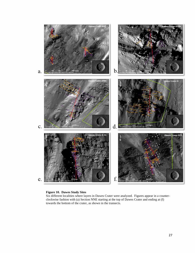
and field work is shown for one field site in Figure 12. Images (a) and (b) in Figure 12
show the two localities on the leeward side of Oahu. Images (c) and (d) show data for
Makapuʻu, on east Oahu.
30
Figure 12. Study Sites on Oahu
Images of the four terrestrial study sites from Oahu, Hawaiʻi. Lava flows are delineated and transects are
marked in red. a. Puʻu Heleakalā, and b. Puʻu Kepauʻala, c. Makapuʻu Section 1 and d. Makapuʻu Section
2.
31
CHAPTER 4
RESULTS
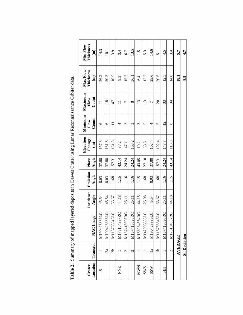
4.1 Flow Thicknesses Interpreted from LRO/KAGUYA Data
A summary of all the study sites that were investigated within Dawes Crater is
shown in Table 1. There were six total sites identified that had layered deposits and were
also positioned under LOLA data tracks. Sites were situated around the crater and were
identified by locations labeled according to their position in the crater. At two sites the
same transect is mapped in two different images, labeled (a) and (b), where the layered
deposits appeared differently in the two images due to differences in the resolution,
incidence, emission and phase angles associated with the images. The maximum and
minimum average flow thickness at each site is given along with the overall average.
Also given is the maximum and minimum average flow thickness for the entire crater
along with the standard deviation from the average.
Analysis of the data gathered shows an overall average flow thickness from
Dawes Crater of 11.9 m with maximum thickness of 18.1 ± 8.9 m and a minimum
thickness of 5.7 ± 4.7 m. The maximum and minimum average flow thicknesses for
each vertical transect were determined by dividing the elevation change by the total
number of flows along the transect. The minimum flow count includes only layers that
were clearly discernable in the LROC NAC images. The maximum flow count includes
both the minimum flow count and layers that appeared to be flows but were ambiguous in
the image. Such ambiguous identifications occur, for instance, when a section of a flow
appears on both sides of the transect line but was obscured right at the transect line due to
shadowing or being partially covered by talus deposits. For both locations S and SSW,

32
the flows were mapped and counted at the same locality in two NAC images. Layering
was discernable in both images but differences in appearance due to resolution,
illumination angle and shadowing led to different numbers of flows being mapped. For
instance, in location S image 2 a, which had a resolution of 1.3 m/pixel, had a maximum
count of 18 flows where image 2 b, with a resolution of 0.5 m/pixel, had a maximum
flow count of 47.
4.2 Flow Thicknesses Interpreted from WorldView 2 Data
Results derived from interpretation of WorldView 2 images of the three terrestrial
study sites are shown in Table 3. For each study site the WorldView 2 image number is
given along with the number of transects that were overlain on the image. The elevation
change in meters is given for each transect, together with a minimum and maximum flow
count. A minimum and maximum average flow thickness was generated by dividing the
elevation change along the transect by the maximum and minimum flow count,
respectively. For each site flow thickness averages are given along with the standard
deviation from the average.
The average of both the maximum and minimum thicknesses is given for each
location. Flows counted at study site Puʻu Heleakalā showed a maximum average
thickness of 7.4 ± 4.3 m and a minimum average thickness of 4.2 ± 1.6 m. The
maximum average flow thickness at Puʻu Kepauʻala was 7.7 ± 2.0 m with a minimum of
4.4 ± 0.9 m. Makapuʻu flows had maximum average flow thickness of 3.2 ± 0.5 m and a
minimum average flow thickness of 2.0 ± 0.5 m.
Tab
le 2
. S
um
mar
y o
f m
apped
layer
ed d
eposi
ts i
n D
awes
Cra
ter
usi
ng L
un
ar R
econn
aiss
ance
Orb
iter
dat
a.
Cra
ter
Lo
cati
on
T
ran
sect
N
AC
Im
ag
e
Inci
den
ce
An
gle
Em
issi
on
An
gle
Ph
ase
An
gle
Ele
va
tio
n
Ch
an
ge
(m)
Min
imu
m
Flo
w
Co
un
t
Ma
xim
um
Flo
w
Co
un
t
Ma
x F
low
Th
ick
nes
s
(m)
Min
Flo
w
Th
ick
nes
s
(m)
S
1
M1
90
42
333
6L
C
45
.54
8.0
3
37
.88
1
57
.3
6
11
26
.2
14
.3
2
a M
19
042
333
6L
C
45
.54
8.0
3
37
.88
1
81
.8
6
18
30
.3
10
.1
2
b
M1
13
78
564
6L
C
55
.67
1.6
8
57
.3
18
1.8
1
1
47
16
.5
3.9
NN
E
1
M1
75
10
438
7R
C
44
.18
1.1
5
43
.14
3
7.2
4
1
1
9.3
3
.4
2
M
15
741
869
8R
C
25
.11
1.1
6
24
.24
4
7.1
3
7
1
5.7
6
.7
3
M
15
741
869
8R
C
25
.11
1.1
6
24
.24
1
08
.2
3
8
36
.1
13
.5
WW
N
1
M1
68
03
455
4R
C
44
.15
1.1
5
43
.05
1
9.2
3
1
3
6.4
1
.5
SW
S
1
M1
42
09
588
3L
C
25
.98
1.6
8
27
.18
6
8.5
5
1
3
13
.7
5.3
SS
W
1a
M1
90
42
333
6L
C
45
.54
8.0
3
37
.88
1
02
.4
4
7
25
.6
14
.6
1
b
M1
13
78
564
6L
C
55
.67
1.6
8
57
.3
10
2.4
5
2
0
20
.5
5.1
SE
1
1
M1
57
41
869
8R
C
25
.11
1.1
6
24
.24
1
47
.7
12
33
12
.3
4.5
2
M
17
510
438
7R
C
44
.18
1.1
5
43
.14
1
16
.9
8
34
14
.6
3.4
AV
ER
AG
E
18
.1
5.7
St.
Dev
iati
on
8
.9
4.7

Tab
le 3
. S
um
mar
y o
f m
apped
layer
ed d
eposi
ts o
n O
‘ahu,
Haw
aiʻi
usi
ng W
orl
dV
iew
-2 s
atel
lite
im
ages
.
Loca
tion
W
orl
dV
iew
-2 I
mag
e
Nu
mb
er
Ele
vati
on
Ch
an
ge
(m)
Min
Flo
w
Cou
nt
Max
Flo
w
Cou
nt
Max
Flo
w
Flo
w
Th
ick
nes
s
(m)
Min
Flo
w
Flo
w
Th
ick
nes
s
(m)
Pu
‘u
Hel
eak
alā
1
1JA
N1
12
13
02
6-P
3D
M_
R5
C3
-
05
23
90
56
52
20
_0
1_P
001
1
47
.0
12
17
3.9
2
.8
2
1
61.0
1
6
32
10
.1
5.0
A
VE
RA
GE
7
.4
4.2
S
t. D
evia
tio
n
4.3
1
.6
Pu
‘u
Kep
au
‘ala
1
1JA
N1
12
13
02
6-P
3D
M_
R4
C2
-
05
23
90
56
52
20
_0
1_P
001
1
10
2.5
1
1
22
9.3
4
.7
2
5
2
8
11
6.5
4
.7
3
22
4
7
5.5
3
.1
A
VE
RA
GE
7
.7
4.4
S
t. D
evia
tio
n
2.0
0
.9
Mak
ap
u‘u
1
1JA
N1
12
13
02
6-P
3D
M_
R6
C9
-
05
23
90
56
52
20
_0
1_P
001
Bea
ch 1
1
7
6
11
2.8
1
.5
B
each
2
29
9
13
3.2
2
.2
Go
rge
15
4
6
3.8
2
.5
A
VE
RA
GE
3
.2
2.0
S
t. D
evia
tio
n
0.5
0
.5

4.3 Field Measurements of Flow Thicknesses
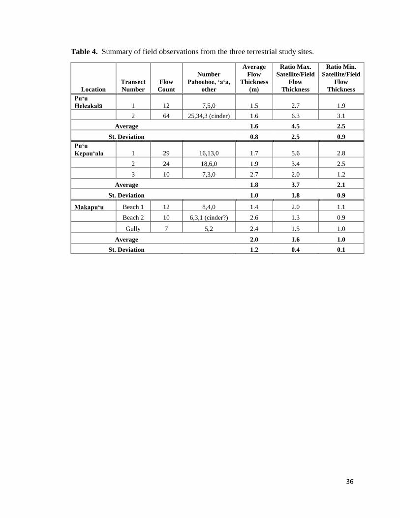
A summary of all field observations for the three terrestrial study sites is shown in
Table 4. This table includes in-situ flow counts and measured flow thicknesses. In
addition, an average thickness is given for each site, along with the standard deviation
from the average for that site. Ratios of thicknesses derived from satellite images and
field data are given for each transect. Average minimum and maximum ratios and the
standard deviation of each is also given.
Field measurements of flows at Puʻu Heleakalā indicate an average flow thickness
of 1.6 ± 0.8 m. Puʻu Kepau’ala flows had an average thickness of 1.8 ± 1.0 m, and
Makapuʻu flows had an average flow thickness of 2.0 ± 1.2 m. These flow thicknesses
are significantly less than those interpreted from the WorldView 2 satellite imagery.
Average flow thicknesses observed in the field established that the flow
thicknesses derived from the remote sensing data led to an overestimation of layer
thickness for all three study sites. When comparing the ratio of image derived to field
thickness data, flow thicknesses at Puʻu Heleakalā were overestimated by factors ranging
from a minimum of 2.5 to a maximum of 4.5. These results are similar to the comparison
at the Puʻu Kepauʻala site which showed a minimum overestimation factor of 2.1 to a
maximum of 3.7. Makapuʻu flows were slightly less overestimated, with a factor
minimum of 1.0 ranging to 1.6. One site at Makapuʻu, Beach 2, was slightly
underestimated by a factor of 0.9.
36
Table 4. Summary of field observations from the three terrestrial study sites.
Location
Transect
Number
Flow
Count
Number
Pahoehoe, ‘a‘a,
other
Average
Flow
Thickness
(m)
Ratio Max.
Satellite/Field
Flow
Thickness
Ratio Min.
Satellite/Field
Flow
Thickness
Pu‘u
Heleakalā 1 12 7,5,0 1.5 2.7 1.9
2 64 25,34,3 (cinder) 1.6 6.3 3.1
Average 1.6 4.5 2.5
St. Deviation 0.8 2.5 0.9
Pu‘u
Kepau‘ala 1 29 16,13,0 1.7 5.6 2.8
2 24 18,6,0 1.9 3.4 2.5
3 10 7,3,0 2.7 2.0 1.2
Average 1.8 3.7 2.1
St. Deviation 1.0 1.8 0.9
Makapu‘u Beach 1 12 8,4,0 1.4 2.0 1.1
Beach 2 10 6,3,1 (cinder?) 2.6 1.3 0.9
Gully 7 5,2 2.4 1.5 1.0
Average 2.0 1.6 1.0
St. Deviation 1.2 0.4 0.1
37
CHAPTER 5
DISCUSSION
The three different localities used in the terrestrial analog study showed average
image-derived flow thicknesses of 2.1 to 3.8 m for the minimum flow thickness and
average maximum thicknesses that ranged between 2.4 and 4.3 m. When compared to
the thickness measured in the field of 1.0 to 2.5 m, the image-derived flow thicknesses
were overestimated by a maximum factor of 4.5 ± 2.5 m and a minimum factor of 2.5 ±
0.9 m for Puʻu Heleakalā, a maximum of 3.7 ± 1.8 m with a minimum of 2.1 ± 0.9 m for
Puʻu Kepauʻala, and a maximum of 1.6 ± 0.4 m and a minimum of 1.0 ± 0.1 m for
Makapuʻu. Overestimation in flow thicknesses is mainly due to the difficulty of
identifying all flows in the images. Field observations showed that there are commonly
multiple individual flows within a single outcrop. For example, one outcrop at Puʻu
Heleakalā contained five individual lava flows that were identified as just a single flow in
the satellite image. This disparity occurred along every field transect except Transect 1 at
the Puʻu Heleakalā study site. Identification of multiple flows within each outcrop
resulted in higher flow counts and smaller flow thicknesses in the field than those derived
from the satellite images.
The presence of multiple stacked flow units in a single outcrop is a common
feature resulting from normal erosional patterns for layered flows of both ʼa’a and
pāhoehoe lavas. Due to the stratified nature of the flows and slope of the hillside,
erosional processes tend to remove the exposed frontal exposed section of stacked lavas.
The terrestrial sites utilized for this study often had a stepped appearance as shown in

38
Figure 13. This may occur because ʻaʻa clinker and weaker pāhoehoe flows are more
readily eroded than dense ʻaʻa flow cores when they are the exposed top layer.
One limitation experienced during fieldwork was the interpretation of the
layering. Outcrops which contained multiple or indeterminate layering were commonly
counted as complex. Pāhoehoe flow contacts tended to be convoluted and at times folded
in on themselves appearing as more than one layer. Flows that were separated by a clear
contact were easily discernable, however there was not always a clear or continuous
contact between each flow. It was also difficult to walk directly along the chosen transect
due to the steepness of the terrain. Some of the larger flows were over 9 m thick and
required climbing and interpretation of flow contacts from the bottom of the unit.
Alternately, other outcrops were low and rubbly, making them hard to discern in the
Figure 13. Layered hillside Makapuʻu.
The northeast facing side of Makapuʻu Location 1. Image shows the layered deposits of tholeiitic basalt
lavas in the southern most section of the Koʻolau Range.

39
field. Ground vegetation also masked lava flows in the terrestrial images, and talus had a
similar obscuring effect in both lunar and terrestrial cases.
The lunar study included measurements observed from lava layers in Dawes
Crater. Average flow thickness for study sites along the rim of Dawes Crater was 11.9 m
with maximum thicknesses of 18.1 ± 8.9 m and a minimum thickness of 5.7 ± 4.7 m.
The lunar basalt flows were thicker than those found on Oahu. However when compared
with thickness measurements reported in the literature, the results of this study showed
thickness estimates less than reported in the past based on lower resolution datasets, but
similar to thicknesses recently reported using LROC imagery (Enns and Robinson, 2013;
Robinson et al., 2012).
Improved estimates of lunar lava flow thicknesses will help constrain estimates of
volcanic flux estimates utilized in lunar flow modeling and studies on the petrogenesis of
lunar mare basalts. Accurate thickness estimates hold significance for lunar scientists
and planetary geologists who utilize such data to understand the evolution of volcanism
on the Moon. Understanding lunar volcanism from layered deposits is important in
determining flow mechanisms, cooling history and regolith development between flows
(Robinson et al., 2012). The thickness of individual volcanic units on the lunar surface is
a key factor needed to accurately constrain estimates of the viscosity (η) and velocity (V)
of mare lava flows. For example, the Jefferys Equation relates those parameters by the
following expression.
𝑉 =𝑔𝑑2𝜌 𝑆𝑖𝑛|𝛼|
3𝜂
40
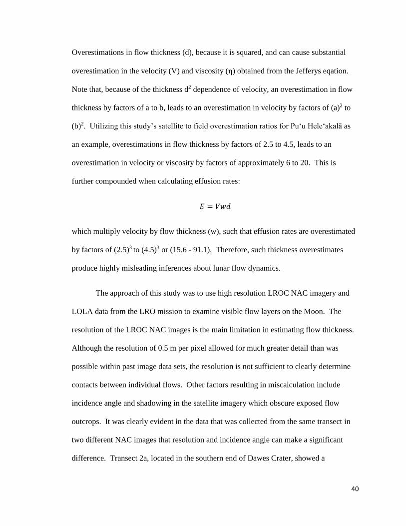
Overestimations in flow thickness (d), because it is squared, and can cause substantial
overestimation in the velocity (V) and viscosity (η) obtained from the Jefferys eqation.
Note that, because of the thickness d2 dependence of velocity, an overestimation in flow
thickness by factors of a to b, leads to an overestimation in velocity by factors of (a)2 to
(b)2. Utilizing this study’s satellite to field overestimation ratios for Puʻu Heleʻakalā as
an example, overestimations in flow thickness by factors of 2.5 to 4.5, leads to an
overestimation in velocity or viscosity by factors of approximately 6 to 20. This is
further compounded when calculating effusion rates:
𝐸 = 𝑉𝑤𝑑
which multiply velocity by flow thickness (w), such that effusion rates are overestimated
by factors of (2.5)3 to (4.5)3 or (15.6 - 91.1). Therefore, such thickness overestimates
produce highly misleading inferences about lunar flow dynamics.
The approach of this study was to use high resolution LROC NAC imagery and
LOLA data from the LRO mission to examine visible flow layers on the Moon. The
resolution of the LROC NAC images is the main limitation in estimating flow thickness.
Although the resolution of 0.5 m per pixel allowed for much greater detail than was
possible within past image data sets, the resolution is not sufficient to clearly determine
contacts between individual flows. Other factors resulting in miscalculation include
incidence angle and shadowing in the satellite imagery which obscure exposed flow
outcrops. It was clearly evident in the data that was collected from the same transect in
two different NAC images that resolution and incidence angle can make a significant
difference. Transect 2a, located in the southern end of Dawes Crater, showed a

41
maximum flow count of 18 in image M190423336LC. The same transect (2b) in image
M113785646LC showed a maximum flow count of 47 flows. This discrepancy indicates
that it is best to take image resolution, and the incidence and emission angles into
consideration when make mare lava flow thickness determination.
The lunar results are interpreted from only one crater on the Moon, Dawes. This
study could be improved by examining exposed mare lava flows in a greater number of
craters. The results from the terrestrial analog study show that layer thicknesses derived
from remotely sensed imagery tend to be overestimated. This implies that lunar lava
flow thicknesses may be similarly overestimated and previous measurements may need to
be reevaluated with the newer higher resolution imagery available. Estimates of lunar
lava flow thicknesses made from remotely sensed imagery should be considered
maximum possible thicknesses when being used in models for effusion rates and
rheology of lunar volcanism.
42
CHAPTER 6
CONCLUSIONS
Approximately half of the layers identified in terrestrial satellite images of
exposed lava flow sequences contain more than one flow unit when measured in the field.
We therefore conclude that the numbers of individual flows in an exposure are
underestimated using remote sensing data. This results in overestimations of flow
thicknesses by factors ranging from an average of 1.0 ± 0.1 and 4.5 ± 2.5 at the terrestrial
study sites and we argue that flow thicknesses may be similarly overestimated using the
LRO data for the Moon. Overestimation of flow thicknesses has important implications
for our understanding of effusive volcanism on the Moon. For instance, inaccurate flow
thicknesses will affect the interpretation of rheology and effusion rates in models of lava
dynamics. In addition, the thickness of a lava flow overlying a regolith deposit strongly
influences the extent to which implanted volatiles would be volatilized and lost from the
regolith (Fagents et al., 2010; Rumpf et al., 2013). Inaccurate flow thicknesses would
thus provide misleading recommendations for sampling depths during future lunar
missions.
This study shows that terrestrial analogs can be used to test interpretations of
lunar volcanic deposits. However, thickness estimates should be used as a baseline,
taking into consideration any inadequacies in the data being used. The resolution of
remotely sensed imagery is the main limitation in estimating flow thickness. Other
factors counting towards miscalculation include illumination angle and shadowing in the
satellite imagery. Ground vegetation also obscured flow units in the terrestrial images,
and talus had a similar obscuring effect in both lunar and terrestrial cases. Flow thickness
measurements based on remotely sensed imagery should be considered the upper limits

43
on flow thicknesses, as individual flow units are almost certainly not all identified using
current data sets. A key conclusion is that there is no substitute for human or rover
validation in the field to verify outcrop-scale inferences drawn from remote sensing data.
44
REFERENCES
Anand, M. 2010. Lunar Water: A Brief Review. Earth Moon Planets. DOI
10.1007/s11038-010-9377-9
Armstrong, J.C., Wells, L.E. and Gonzales, G. 2002. Rummaging through the Earth’s
attic for remains of ancient life. Icarus, 160, 183-196.
Carrier, D.W. III, Olheoft, G.R., Mendell, W., 1991. Physical Properties of the Lunar
Surface. In: Heiken, G.H. ed., Vaniman, D.T. ed., French, B.M. ed., The Lunar
Source Book: A Users Guide to the Moon. Cambridge University Press, 475-
594.
Doell, R.R., Dalrymple, G.B., 1973. Potassium–argon ages and paleomagnetism of the
Waianae and Koolau Volcanic series, Oahu, Hawaii. Geol. Soc. Am. Bull. 84,
1217–1242.
Enns, A.C., Robinson, M.S., 2013. Basaltic Layers Exposed in Lunar Mare Craters. 44th
Lunar and Planetary Science Conference.
Fagents, S.A., Rumpf, M.E., Crawford, I.A., Joy, K.H. 2010. Preservation potential of
implanted solar wind volatiles in lunar paleoregolith deposits buried by lava
flows. Icarus, 207, 595-604.
Fink, J. H., Zimbelman, J. R., 1983. Rheology of the 1983 Royal Gardens basalt flows,
Kilauea Volcano, Hawaii. Bull. Volcanol. 48, 87-96.
Frankel, C. 1996. Volcanoes of the Solar System. Cambridge University Press.
Funkhouser, J.G., Barnes, I.L., Naughton, J.J., 1968. The determination of a series of
ages of Hawaiian volcanoes by potassium-argon method. Pac. Sci. 22, 369-372.
Garry, W. B., Robinson, M. S., and the LROC Team. 2010. Observations of Flow Lobes
in the Phase I Lavas, Mare Imbrium, the Moon. 41st Lunar and Planetary Science
Conference.
45
Gifford, A.W., El-Baz, F. 1981. Thicknesses of Lunar Mare Flow Fronts. The Moon
and the Planets. 24, 391-398.
Guillou, H., Sinton, J., Laj, C., Kissel, C., Szeremeta, N., 2000. New K-Ar ages of shield
lavas from Waianae Volcano, Oahu, Hawaii Archipelago. J. Volcanol. Res., 96,
229-242.
Haskin, L., Warren, P., 1991. Lunar Chemistry. In: In: Heiken, G.H. ed., Vaniman,
D.T. ed., French, B.M. ed., The Lunar Source Book: A Users Guide to the Moon.
Cambridge University Press. 357-474.
Hiesinger, H., Jaumann, R., Neukum, G., Head III, J.W., 2000. Ages of mare basalts on
the lunar nearside. J. Geophys. Res., 105, E12, doi: 10.1029/2000JE001244
Hiesinger H., Jaumann R., Neukum G. and Head J. W. III. 2000. Ages of mare basalts on
the lunar nearside. Journal of Geophysical Research 105: 29239–29275.
Hiesinger, H., J. W. Head III, and G. Neukum (2007), Young lava flows on the eastern
flank of Ascraeus Mons: Rheological properties derived from High Resolution
Stereo Camera (HRSC) images and Mars Orbiter Laser Altimeter (MOLA)
data, J. Geophys. Res., 112, E05011, doi: 10.1029/2006JE002717.
Hörz, F, Grieve, R., Heiken, G., Spudis, P., Binder, A., 1991. Lunar Surface Processes.
In: Heiken, G.H. ed., Vaniman, D.T. ed., French, B.M. ed., The Lunar Source
Book: A Users Guide to the Moon. Cambridge University Press, 61-120.
Howard, K. A., Head, J.W., Swann, G.A. 1972. Geology of Hadley Rille. Proceedings
of the Third Lunar Science Conference. Suppl. 3, Vol. 1, 1-14.
Kirk, R. L., Barrett, J. M., and Soderblom, L. A. (2003). Photoclinometry made
simple…? In Advances in Planetary Mapping 2003. Houston, TX: Lunar and
Planetary Institute.
Lohse, V., Heipke, C., Kirk, R.L. 2006. Derivation of planetary topography using mulit-
image shape-from-shading. Planet. Space Sci., 54, 661-674.
McDougall, I., 1963. Potassium–Argon ages from western Oahu, Hawaii. Nature, 197,
344–345.
46
Mckay et al., 1991. The Lunar Regolith. In: Heiken, G.H. ed., Vaniman, D.T. ed.,
French, B.M. ed., The Lunar Source Book: A Users Guide to the Moon.
Cambridge University Press, 285-356.
Mouginis-Mark, P.J., Rowland, S.K., 2008. Lava flows at Arsia Mons, Mars: Insights
from a graben imaged by HiRISE. Icarus, 198, 27-36.
Platz, T., Michael, G.G., Neukum, G., 2010. Confident thickness estimates for planetary
surface deposits from concealed crater populations. Earth Planet. Sci. Lett., 293,
388-395.
Presley, T. K., Sinton, J. M., Pringle, M. 1997. Postshield volcanism and catastrophic
erosion of the Waianae Volcano, Oahu, Hi. Bull. Volcanol., 58, 597-616.
Robinson, M.S., et al., 2010. Lunar Reconnaissance Orbiter Camera (LROC).
Instrument Overview. Space Sci. Rev., 150, 81–124
Robinson, M.S., et al., 2012. Confirmation of sublunarean voids and thin layering in
mare deposits. Planet. Space Sci., 69, 18-27.
Rothery, D. A., McBride, N., Gilman, I. 2011. An Introduction to the Solar System.
Cambridge University Press.
Rumpf, M.E., S.A. Fagents, I.A. Crawford, and K.H. Joy (2013). Numerical modeling of
lava-regolith heat transfer on the Moon and implications for the preservation of
implanted volatiles. J. Geophy. Res. Planets, 18, 382-397.
Saal, A. E., et al. 2008. Volatile content of lunar volcanic glasses and the presence of
water in the Moon’s interior. Nature. 454, 192-195.
Schaber, G.G. 1973. Lava flows in Mare Imbrium: Geologic evaluation from Apollo
orbital photography. Proceedings of the Lunar Science Conference. Vol. 1, Sup.
4, Pgs. 73-92.
Sharpton, V.L., 2014. Outcrops on lunar crater rims: Implications for rim construction
mechanisms, ejecta volumes and excavation depths. J Geophys. Res. Planets.
119, 154-168.
47
Smith et al., 2009. The Lunnar Orbiter Laser Altimeter Investigation on the Lunar
Reconnaissance Orbiter Mission. Space Sci. Rev., 150, 209-241.
Spudis, P.D., Swann, G.A., Greeley, R. 1988. The Formation of Hadley Rille and
Implications for the Geology of the Apollo 15 Region. Proceedings of Lunar and
Planetary Sci. Conf., 18, 243-254.
Spudis, P.D. 1996. The Once and Future Moon. Simthsonian Institution Press.
Washington D.C.
Taylor, J.G., Warren, P., Ryder, G., Delano, J., Pieters, C., Lofgren, G., 1991. Lunar
Rocks. In: Heiken, G.H. ed., Vaniman, D.T. ed., French, B.M. ed., The Lunar
Source Book: A Users Guide to the Moon. Cambridge University Press, 183-
284.
Vaniman, D., Dietrich, J. Taylor, J., Heiken, G., 1991. Explorations, Samples, and
Recent Concepts of the Moon. In: Heiken, G.H. ed., Vaniman, D.T. ed., French,
B.M. ed., The Lunar Source Book: A Users Guide to the Moon. Cambridge
University Press, 5-26.
Weider, S.Z., Crawford, I.A., Joy, K.H., 2010. Individual lava flow thicknesses in
Oceanus Procellarum and Mare Serenitatis determined from Clementine
multispectral data, Icarus, 209, 2, 323-336.
Yingst, R. A., and J. W. Head III (1997), Volumes of lunar lava ponds in South Pole-
Aitken and Orientale Basins: Implications for eruption conditions, transport
mechanisms, and magma source regions, J. Geophys. Res., 102(E5), 10909–
10931, doi:10.1029/97JE00717.

48