A NOVEL METHOD TO IMPROVE QUANTITATIVE SUSCEPTIBILITY ... · PDF filethe use of very short TEs...

Ph.D. Thesis – Sagar Buch McMaster – School of Biomedical Engineering

A NOVEL METHOD TO IMPROVE QUANTITATIVE

SUSCEPTIBILITY MAPPING WITH AN APPLICATION

FOR MEASURING CHANGES IN BRAIN OXYGEN

SATURATION IN THE PRESENCE OF CAFFEINE

AND DIAMOX


i

A NOVEL METHOD TO IMPROVE QUANTITATIVE

SUSCEPTIBILITY MAPPING WITH AN APPLICATION FOR

MEASURING CHANGES IN BRAIN OXYGEN SATURATION IN THE

PRESENCE OF CAFFEINE AND DIAMOX

BY

SAGAR BUCH

A Thesis

Submitted to the School of Graduate Studies

in Partial Fulfillment of the Requirements

for the Degree of Ph.D.

(Doctor of Philosophy)

in Biomedical Engineering

McMaster University

© Copyright by Sagar Buch, April 2015


ii

Ph.D. (2015) McMaster University

(Biomedical Engineering) Hamilton, ON, Canada

TITLE: A Novel Method to Improve Quantitative Susceptibility Mapping

with an Application for Measuring Changes in Brain Oxygen Saturation in

the Presence of Caffeine and Diamox

AUTHOR: Sagar Buch, M.A.Sc.

SUPERVISOR: Dr. E. Mark Haacke

NUMBER OF PAGES: xvi, 116


iii

Abstract

Magnetic Resonance Imaging (MRI) is a widely used, non-invasive imaging technique

that provides a means to reveal structural and functional information of different body

tissues in detail. Susceptibility Weighted Imaging (SWI) is a field in MRI that utilizes the

information from the magnetic susceptibility property of different tissues using the gradient

echo phase information. Although longer echo times (TEs) have been widely used in

applications involving SWI, there are a few problems related with the long TE data, such

as the strong blooming effect and phase aliasing even at macroscopic levels. In this thesis,

the use of very short TEs is proposed to study susceptibility mapping. The short TEs can

be used to study structures with susceptibilities an order of magnitude larger (such as air

and bones in and around the brain sinuses, skull and teeth) than those within soft tissue.

Using the phase replacement technique that we recently developed, it becomes possible to

map the geometry of such structures, which to date has proven difficult due to the lack of

water content (for sinuses) or due to very short T2* (for bones).

The method of phase replacement inside the sinuses proposed in this thesis provides

more accurate phase information for the inversion than assuming zero or some arbitrary

constant inside these structures. The first and second iterations were responsible for most

of the changes in mapping out the susceptibility values. The mean susceptibility value in

the sphenoid sinus is calculated as +9.3 ± 1.1ppm, close to the expected value of +9.4ppm

for air. The reconstruction of the teeth in the in-vivo data provides a mean Δχ(teeth-tissue)=–

3.3ppm, thanks to the preserved phase inside the jaw. This is in agreement with the


iv

susceptibility value measured from a tooth phantom (Δχ(tooth-phantom)=–3.1ppm). The mean

susceptibility inside a relatively homogeneous region of the skull bone was measured to be

Δχ(bone-tissue)=–2.1ppm. Finally, these susceptibilities can be used to help remove the

unwanted background fields prior to applying either SHARP or HPF.

In addition, the effects of the background field gradient on flow compensation are

studied. Due to the presence of these background gradients, an unwanted phase term is

induced by the blood flow inside the vessels. Using a 3D numerical model and in vivo data,

the background gradients were estimated to be as large as 1.5mT/m close to the air-tissue

interfaces and 0.7mT/m inside the brain (leading to a potential signal loss of up to 15%).

The quantitative susceptibility mapping (QSM) results were improved in the entire image

after removing the confounding arterial phase thanks to the reduced ringing artifacts.

Lastly, a novel approach to improve the susceptibility mapping results was introduced

and utilized to monitor the changes in venous oxygen saturation levels as well as the

changes in oxygen extraction fraction instigated by the vasodynamic agents, caffeine and

acetazolamide. The internal streaking artifacts in the susceptibility maps were reduced by

giving an initial susceptibility value uniformly to the structure-of-interest, based on the a

priori information. For veins, the iterative results, when the initial value of 0.45 ppm was

used, were the best in terms of the highest accuracy in the mean susceptibility value (0.453

ppm) and the lowest standard deviation (0.013 ppm). Using this technique, the venous

oxygen saturation levels (inside the internal cerebral veins (ICVs)) for normal

physiological conditions, post-caffeine and post-Diamox for the first volunteer were


v

calculated as (mean ± standard deviation): YNormal = 69.1 ± 3.3 %, YCaffeine = 60.5 ± 2.8

% and YDiamox = 79.1 ± 4.0%.

For the caffeine challenge, the percentage change in oxygen extraction fraction (OEF)

for pre and post caffeine results was calculated as +27.0 ± 3.8%; and for the Diamox

challenge, the percentage change in OEF was calculated as −32.6 ± 2.1 % for the ICVs.

These vascular effects of Diamox and caffeine were large enough to be easily measured

with susceptibility mapping and can serve as a sensitive biomarker for measuring

reductions in cerebro-vascular reserve through abnormal vascular response, an increase in

oxygen consumption during reperfusion hyperoxia or locally varying oxygen saturation

levels in regions surrounding damaged tissue.

In conclusion, our new approach to QSM offers a means to monitor venous oxygen

saturation reasonably accurately and may provide a new means to study neurovascular

diseases where there are changes in perfusion that affect the oxygen extraction fraction.


vi

Acknowledgements

I would like to sincerely thank my supervisor, Dr. E. Mark Haacke, for encouraging my

research and for allowing me to grow as a researcher. He invariably finds time for his

students and collaborators to sort out their problems and gives them new, interesting ideas

to think about. Dr. Haacke and his works have been and will always be a huge source

inspiration for me. It has been an unbelievable privilege to work under your guidance.

I am very thankful to Dr. Michael Noseworthy, for his continuous support, motivation

and enthusiasm during my graduate career. His extremely informative and insightful

approach of teaching the students is very instrumental in our progress and attending his

courses has always been a delight. I cannot thank my supervisory committee members, Dr.

Maureen MacDonald and Dr. Qiyin Fang, enough for their extremely helpful comments

and guidance. Your words of encouragement has brought me to where I am right now.

I would also like to acknowledge Dr. Yu-Chung Norman Cheng, Dr. Jaladhar Neelavalli

and Dr. Yongquan Ye at Wayne State University, for their help and time they spent in

clearing my doubts. I wish to thank my colleague at McMaster University, Saifeng Liu,

for sharing his knowledge and experiences that has been instrumental in my research work.

I wish to thank my parents, my mother, Dr. Bharati Buch and my father, Dr. Yatrik

Buch, for the immense love and support they gave me throughout my life. I could not have

come so far without them. This thesis is dedicated to them.


vii

Table of Contents

Chapter 1: Introduction ....................................................................................................... 1

Chapter 2: Basics Of Mr Phase Signal And Magnetic Susceptibility ................................. 7

2.1 Larmor Frequency And Free Induction Decay ......................................................... 7

2.2 Magnetic Susceptibility ............................................................................................. 9

2.3 Gradient Echo Imaging ........................................................................................... 13

2.4 Magnetic Field Perturbations (ΔB(r)) ..................................................................... 19

2.5 Background Field Removal ..................................................................................... 24

2.6 Forward Method For Calculating Field Perturbations ............................................ 27

2.7 Susceptibility Mapping ........................................................................................... 30

Chapter 3: Susceptibility Mapping Of Air, Bone And Calcium In The Head .................. 39

3.1 Introduction ............................................................................................................. 39

3.2 Methods ................................................................................................................... 41

3.3 Results ..................................................................................................................... 49

3.4 Discussion And Conclusions ................................................................................... 58

Chapter 4: Estimation Of Phase Change Induced By Blood Flow In Presence Of

Background Gradients (𝐺’) ............................................................................................... 67

4.1 Introduction ............................................................................................................. 67

4.2 Theory ..................................................................................................................... 69


viii

4.3 Methods ................................................................................................................... 73

4.4 Results ..................................................................................................................... 75

4.5 Discussion And Conclusions ................................................................................... 81

Chapter 5: Measuring The Changes In Cerebral Oxygen Extraction Fraction ................. 87

5.1 Introduction ............................................................................................................. 87

5.2 Theory ..................................................................................................................... 89

5.3 Methods ................................................................................................................... 90

5.4 Results ..................................................................................................................... 93

5.5 Discussion And Conclusions ................................................................................. 101

Chapter 6: Future Directions ........................................................................................... 111


ix

List of Figures

Chapter 2:

Figure 2.1. The precession of a spin after the application of an RF pulse, a), which

generates an observable NMR signal called free induction decay (FID) signal in the

absence of any magnetic gradients, b). ............................................................................... 9

Figure 2.2. Basics of a gradient echo sequence. a) The effects of applying a positive or

negative gradient field in presence of the main external magnetic field (B0), b) A simple

representation of a gradient-echo pulse sequence. ............................................................ 14

Figure 2.3. Pulse sequence diagram for a 3D gradient echo MR acquisition with flow

compensation in all three directions to reduce the effects of pulsatility effects of the blood

or cerebrospinal fluid flow. The pulse sequence includes first order gradient moment

nulling in readout (Gr) and slice-select (Gs) directions. The partition encoding and phase

encoding (Gp) gradients are velocity compensated with respect to the echo. ................... 17

Figure 2.4. Complex representation of an MR signal acquired through ‘Real’ and

‘Imaginary’ channels. |S| represents the magnitude and φ is the phase component of an

MR signal. ......................................................................................................................... 19

Figure 2.5. A cylinder with a radius ‘a’ placed at an angle θ to the external magnetic field

B0 and is the polar angle in the x-y plane of the point ‘p’ relative to the external field. The

magnetic field variation outside the cylinder at a point ‘p’ with a distance ρ can be defined

by Eq. 2.17. ....................................................................................................................... 23


x

Figure 2.6. a) Original unfiltered phase image with imaging parameters: TE=20ms, B0=3T

with 0.5×0.5×0.5mm3 resolution and b) Homodyne high pass filtered phase image with

filter size of 64×64 pixels, c) phase images processed with SHARP algorithm (radius=6

pixels and th=0.05). The filtered phase images in b) and c) shows the underlying tissue

information much clearly due to the reduced background field variations. ..................... 26

Figure 2.7. a) Original susceptibility map (SM) of a 3D brain model, b) Simulated phase

generated by using the forward calculation of the magnetic field perturbations (Eq. 2.31)

at TE=20ms and B0=3T, c) SM reconstructed from phase information in b) using the

inverse process (Eq. 2.32 and Eq. 2.33). ........................................................................... 32

Figure 2.8. Susceptibility maps before and after the iterative method using veins as the

structure-of-interest. a) Original susceptibility map in sagittal view, b) Iterative result of a)

after three iterations, c) The difference map of a) and b), d) Same original susceptibility

map as a) in coronal view, e) Iterative result of a) after three iterations in coronal view, f)

The difference map of d) and e). White arrows indicate the streaking artifacts seen in the

original susceptibility maps a) and d). The difference maps demonstrate that this streaking

noise is almost completely removed after three iterations of iterative method. ............... 34

Chapter 3:

Figure 3.1. Illustration of the proposed sinus mapping process using short TE and phase

replacement method. Phase replacement steps are repeated until the relative change of the

mean susceptibility inside the sinuses is less than some chosen value of β. The mask, Mhead,

is used to remove the noisy pixels from phase images, whereas Mair/bone represents the mask


xi

of structures-of-interest for phase replacement process (in this case: sinuses, bones and

teeth). ................................................................................................................................ 47

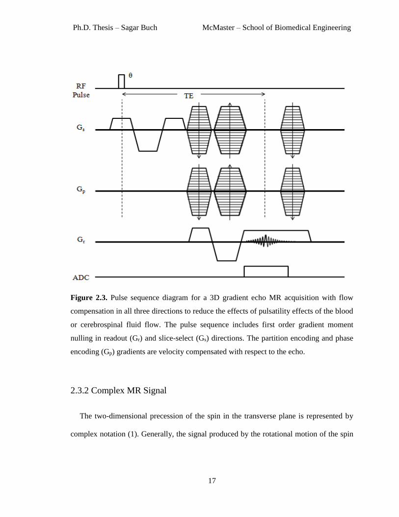
Figure 3.2. Simulation of the phase behavior using a 3D numerical model. a) In vivo T1-

weighted data used to generate the 3D model, b) 3D numerical brain model, and c)

simulated phase of the air-tissue interfaces using Eq. 9. .................................................. 49

Figure 3.3. a) 3D brain model used to test the proposed concept; b) simulated phase image

generated from a) by using a forward calculation (TE=2.5ms and B0=3T); c) brain mask

(Mbrain); d) head mask (Mhead); e) measured susceptibility map resulting from the phase

simulation keeping phase only inside the brain, by using the Mbrain mask; and f) measured

susceptibility map resulting from the phase simulation using phase information from all

tissues surrounding the sinuses inside the head, by using the Mhead mask. Note the major

improvement in the shape and susceptibility of the ethmoid sinus. ................................. 50

Figure 3.4. Susceptibility reconstruction of the tooth phantom. a) Original phase image at

TE=2.5ms, b) processed phase image and c) reconstructed susceptibility map of the tooth

phantom generated after five phase replacement iterations. The mean susceptibility value

inside the tooth is measured as Δχ(teeth-tissue)= –3.1 ± 1.2. .................................................. 50

Figure 3.5. Comparison of the magnitude images (a, b and c) and susceptibility maps (d, e

and f) in all three views, showing agreement spatially between the sinuses and teeth in the

original magnitude images and their reconstruction in the susceptibility maps. Structures

are identified by the white arrows: 1 – Frontal sinus, 2 – maxillary sinus, 3 – teeth, 4 –

mastoid sinus, 5 – ear canal, 6 – ethmoid sinus, 7 – occipital skull bone. ........................ 52


xii

Figure 3.6. Measured mean susceptibility values and standard deviations inside the

sphenoid sinus from the brain model (a and b); along with sphenoid sinus (c and d), teeth

(e and f) and bone (g and h) from the in vivo data. .......................................................... 53

Figure 3.7. Background field removal using extracted susceptibility distributions inside

the sinuses, bones and teeth for two different volunteers: (a-d) volunteer 1 and (e-h)

volunteer 2. a) and e) original phase data acquired at TE = 7.5ms, b) and f) predicted

magnetic perturbations TE=7.5ms and B0=3T, c) and g) resultant phase information

produced after subtracting the predicted phase from original phase images. The phase

profile plots (d and h), along the black lines, demonstrate that the predicted phase agrees

well with the original phase behavior outside the sinuses. ............................................... 55

Figure 3.8. Improvement in phase processing using susceptibility maps of sinuses and

bones. The phase images shown in this figure are acquired at TE=7.5ms and field strength

of 3T. a) Conventional homodyne high pass (HP) filtering with 32x32 filter size, b)

homodyne HP filtered image (32x32 filter size) applied after subtracting the forward

modeled phase generated from susceptibility maps of sinuses and bones, c) filtered phase

image generated using SHARP method. d), e) and f) are the resultant susceptibility maps

generated from phase images shown in a), b) and c), respectively. The white arrows

demonstrate the areas of improvement using the forward modeled phase, namely the

preservation of SSS (long arrow) and significant reduction of phase behavior caused by the

air-tissue interfaces (short arrow). The effect of the improper boundary conditions due to

the erosion of the brain near the SSS in the SHARP processed phase images is indicated

by the black arrows. .......................................................................................................... 57


xiii

Chapter 4:

Figure 4.1. A negative background gradient (Gx’) in the readout direction and the induced

echo shift. The center of the sampling period represents the ideal echo time, TE. However,

in presence of an extraneous gradient (Gx’), the shifted echo occurs at the time TE’. ...... 71

Figure 4.2. Calculated background gradient deviations along three dimensions: (a, d and

g) along x-direction,Gx′; (b, e and h) along y-direction, Gy′; and (c, f and i) along z-

direction, Gz′; shown in transverse, sagittal and coronal planes. The profiles in j), k) and l)

were measured along the black lines shown in a), b) and c), respectively. ...................... 76

Figure 4.3. Phase accumulation due to flow in presence of the background gradient (G′)

in: a) x-direction (left-right), b) y-direction (up-down) and c) in z-direction (perpendicular

to the plane of the image); for blood flow velocity of 60cm/s and TE = 20ms. ............... 77

Figure 4.4. a) Original, low resolution, unwrapped phase image (TE = 2.5ms), b) sinus

maps generated from a, c) the predicted field (∆B) generated from the sinus shown in b, d)

frequency profiles generated along the black line in a and c. Note the agreement between

the original phase and predicted field. .............................................................................. 77

Figure 4.5. a) Original, high resolution, magnitude image with b) homodyne high-pass

filtered 32×32 (TE=17.5ms), c) simulated maps representing background gradient induced

phase (in x-direction, i.e. Gx′), assuming the blood flow velocity of MCAs is v = 60cm/s

and TE = 17.5ms; and d) resultant phase image after correcting the flow-induced phase

inside left and right MCAs (identified by the black and white arrows, respectively,

representing opposite flow directions). ............................................................................. 79


xiv

Figure 4.6. Background gradients generated from field inhomogeneities caused by the

veins. Susceptibility maps are shown in a) transverse and b) sagittal views. Red crosses are

used to identify the vein of Galen. The background gradients were measured primarily in

c) y-direction and d) z-direction. ...................................................................................... 79

Figure 4.7. Phase images and susceptibility maps with and without the suppression of

phase from the arteries. a) SHARP processed result using the original phase images, b)

susceptibility map produced from a), c) SHARP processed result using the phase images

generated after setting the phase inside the arteries to zero, d) susceptibility map produced

from c). .............................................................................................................................. 80

Chapter 5:

Figure 5.1. Simulated susceptibility maps produced from a 3D numerical model using a)

conventional iterative algorithm, b) the proposed method by assigning 450ppb to veins and

c) by assigning 700ppb to veins. Images d, e and f are contrast modified versions of a, b,

and c to visualize the extent of internal streaking artifacts. .............................................. 94

Figure 5.2. Mean (a) and standard deviation (b) of the susceptibility measured inside the

superior sagittal sinus at each iteration of the iterative SWIM algorithm. Different initial

values (χ0) were set to the veins. Independent of the choice of starting point, the values

tend to converge close to the expected susceptibility of 0.45 ppm. The use of proper initial

value reduces the streaking artifacts inside the veins. ...................................................... 94

Figure 5.3. a) Susceptibility maps generated using the conventional iterative technique,

and b) susceptibility maps generated using the forced value iterative method. Note the


xv

improvement in the susceptibility distribution, inside the veins of different sizes, in d) with

respect to the conventional iterative SWIM results in c). ................................................. 96

Figure 5.4. Evaluation of dynamic changes in venous susceptibility distribution due to the

administration of caffeine and Diamox. Phase data is acquired for four time points after the

drug ingestion, at an interval of 15 minutes. a) and f) Susceptibility maps for the data

acquired before caffeine and Diamox intake, respectively, b-e) susceptibility maps for the

data at four times points after caffeine intake, g-j) susceptibility maps the data at four times

points after Diamox intake. ............................................................................................... 97

Figure 5.5. Susceptibility maps generated from the data acquired: a) post-Diamox

administration, b and c) pre-Diamox and pre-caffeine administration, d) post-caffeine

administration for healthy volunteers. The profile plot demonstrates the variation in

susceptibility values across the internal cerebral veins caused by these altered brain states.

........................................................................................................................................... 98

Figure 5.6. Susceptibility values measured inside the major cerebral veins across five

healthy volunteers. The phase data was acquired before and after the administration of

Diamox and Caffeine with TE = 15ms and voxel resolution = (0.5mm)3. Each drug test

was performed on separate days. The susceptibility values generated from the data acquired

pre-administration of these drugs were averaged. R-ICV, L-ICV: right and left internal

cerebral veins; R-TSV, L-TSV: right and left thalamo-striate veins; R-SV, L-SV: right and

left septal veins; VoG: Vein of Galen; StrS: Straight sinus. ............................................. 99


xvi

List of Tables

Chapter 3:

Table 3.1. Mean susceptibility value (Δχ(sinus-tissue)), standard deviation and relative change,

inside the sphenoid sinus of a healthy volunteer, as a function of the number of phase

replacement iterations. ...................................................................................................... 52

Table 3.2. Measured susceptibility distributions (mean ± standard deviation) inside the

various sinuses (Δχ(sinus-tissue)), skull bone (Δχ(bone-tissue)) and teeth (Δχ(teeth-tissue)) from the 3D

brain model and from the four healthy volunteers. These results were produced with five

iterations of phase replacement method. ........................................................................... 54

Chapter 5:

Table 5.1. Mean ± standard deviation of the percentage change in oxygen extraction

fraction for cerebral veins of different vessel sizes, across five healthy subjects, measured

before and after administration of Diamox and caffeine. R-ICV, L-ICV: right and left

internal cerebral veins; R-TSV, L-TSV: right and left thalamo-striate veins; R-SV, L-SV:

right and left septal veins; VoG: Vein of Galen; StrS: Straight sinus. ........................... 100


1

Chapter 1: Introduction

Magnetic Resonance Imaging (MRI) is a widely used, non-invasive imaging technique

that provides a means to reveal structural and functional information of different body

tissues in detail. The MR magnitude information has been primarily used in MRI for

clinical diagnosis due to the soft tissue contrast provided by the images. Depending on the

application, a variety of contrasts can be generated between different tissues of interest in

the magnitude images by altering the imaging parameters (1). For example, different

contrasts are created by spin density, T1 and T2 weighted sequences.

Apart from a few applications such as flow quantification, phase sensitive inversion

recovery or MRI thermometry, the phase signal had been ignored in obtaining structural

information from different tissues (2–5). Susceptibility Weighted Imaging (SWI) is a field

in MRI that utilizes the gradient echo phase information to create filtered phase images that

are used to enhance contrast in the magnitude images (2,6). The phase signal is dependent

on the magnetic susceptibility distribution of a given tissue sample, hence, the phase

images offer a unique image contrast. The applications of the phase images include


2

studying the progress of neurodegenerative diseases like multiple sclerosis by detection of

iron deposition in the brain, and the presence of calcium deposition in breast tissue and

quantifying oxygen saturation in veins using the susceptibility maps (7–9). Susceptibility

mapping technique utilizes the phase information around an object to reconstruct the

susceptibility properties across a given tissue (6,10–13).

The strength of phase behavior is dependent on the time of echo, where higher echo

times will produce a stronger, more discernible signal. Currently, the focus of phase

imaging and susceptibility mapping has been on using longer TEs on the order of T2* (~20

to 30ms) to enhance susceptibility effects for small structures or objects with low

susceptibility (14). However, the macroscopic and microscopic phase wrapping or phase

aliasing at higher echo times leads to T2* signal loss and blooming artifacts that makes the

object appear larger than its actual size. This, in turn, leads to an underestimation of the

measured susceptibility. Therefore, in this thesis, use of relatively shorter TEs (~2.5ms) is

proposed, especially when studying structures with much stronger susceptibilities in the

brain.

The potential applications of utilizing short TEs includes imaging of high iron content

in stroke and traumatic brain injury as well as mineralization in Parkinson’s disease;

imaging of major veins in the body to measure oxygen saturation (2). Furthermore, by

preserving the signal outside the brain itself, phase images at short echo times provide a

new approach for imaging high susceptibility objects such as sinuses, bones and teeth that

have no or unreliable MR signal. Regions which have no signal cannot benefit from any of

the usual tissue properties except for susceptibility which usually affects tissues outside the


3

source. This thesis introduces the phase replacement method, which updates the predicted

phase inside an object iteratively in order to improve the susceptibility reconstruction (15).

The resulting images for air and bones are not only of interest in and of themselves, but

also can be used to model and remove the unwanted background phase to better evaluate

local tissue anomalies at long TEs.

Recently, a variety of multi-echo gradient echo sequences have been used for

simultaneous MR angiography and venography, susceptibility weighted imaging (SWI)

and susceptibility mapping (10,16,17). However, these flow compensated sequences are

still highly sensitive to flow artifacts, especially at the longer echo times. The presence of

flow induced phase will hamper the quality of SWI images and create artifacts in

quantitative susceptibility mapping (QSM). Therefore, it is critical to understand these

potential sources of error and then eventually remove them if viable. For the second major

part of this thesis, the unwanted phase induced by blood flow in presence of the background

gradients is studied and evaluated. This unique approach also suggests that the magnitude

images from the first echo can be used as a means to remove spurious phase for QSM

calculations.

A recently developed iterative algorithm helps in reducing the streaking artifacts caused

by the ill-posed nature (singularity region within the inverse Green’s function) of the

susceptibility mapping process (18). However, the streaking artifacts inside a structure are

carried forward to the final results. For structures with high susceptibility, these artifacts

can be stronger and deleterious. The final part of this thesis introduces a method to further

improve the susceptibility mapping by reducing the streaking artifacts both inside and


4

outside a structure-of-interest. This method is then used for measuring the cerebral venous

oxygen saturation levels. In this work, the ability of this approach is to demonstrate the

quantification of the blood oxygenation level of cerebral veins (Yv) in vivo, not only under

normal physiological conditions but also by challenging the physiologic conditions,

induced by vasodynamic agents such as caffeine or acetazolamide, which affect the

cerebral venous blood oxygenation level (19–22). For each of the above mentioned

approaches, a 3D numerical brain model was used to predict and validate the associated

errors.

References

1. Haacke EM. Magnetic resonance imaging: physical principles and sequence design.

New York, NY [u.a.: Wiley-Liss; 1999.

2. Haacke EM, Mittal S, Wu Z, Neelavalli J, Cheng Y-CN. Susceptibility-Weighted

Imaging: Technical Aspects and Clinical Applications, Part 1. Am J Neuroradiol.

2009 Jan 1;30(1):19–30.

3. De Poorter J. Noninvasive MRI thermometry with the proton resonance frequency

method: study of susceptibility effects. Magn Reson Med Off J Soc Magn Reson Med

Soc Magn Reson Med. 1995 Sep;34(3):359–67.

4. Evans AJ, Iwai F, Grist TA, Sostman HD, Hedlund LW, Spritzer CE, et al. Magnetic

resonance imaging of blood flow with a phase subtraction technique. In vitro and in

vivo validation. Invest Radiol. 1993 Feb;28(2):109–15.

5. Hou P, Hasan KM, Sitton CW, Wolinsky JS, Narayana PA. Phase-sensitive T1

inversion recovery imaging: a time-efficient interleaved technique for improved

tissue contrast in neuroimaging. AJNR Am J Neuroradiol. 2005 Jul;26(6):1432–8.

6. Haacke EM, Reichenbach JR. Susceptibility Weighted Imaging in MRI: Basic

Concepts and Clinical Applications. John Wiley & Sons; 2014. 916 p.


5

7. Haacke EM, Garbern J, Miao Y, Habib C, Liu M. Iron stores and cerebral veins in

MS studied by susceptibility weighted imaging. Int Angiol J Int Union Angiol. 2010

Apr;29(2):149–57.

8. Fatemi-Ardekani A, Boylan C, Noseworthy MD. Identification of breast calcification

using magnetic resonance imaging. Med Phys. 2009 Dec;36(12):5429–36.

9. Haacke EM, Tang J, Neelavalli J, Cheng YCN. Susceptibility mapping as a means to

visualize veins and quantify oxygen saturation. J Magn Reson Imaging JMRI. 2010

Sep;32(3):663–76.

10. Haacke EM, Liu S, Buch S, Zheng W, Wu D, Ye Y. Quantitative susceptibility

mapping: current status and future directions. Magn Reson Imaging. 2015

Jan;33(1):1–25.

11. Marques J p., Bowtell R. Application of a Fourier-based method for rapid calculation

of field inhomogeneity due to spatial variation of magnetic susceptibility. Concepts

Magn Reson Part B Magn Reson Eng. 2005 Apr 1;25B(1):65–78.

12. Salomir R, de Senneville BD, Moonen CT. A fast calculation method for magnetic

field inhomogeneity due to an arbitrary distribution of bulk susceptibility. Concepts

Magn Reson Part B Magn Reson Eng. 2003 Jan 1;19B(1):26–34.

13. Haacke EM, Lai S, Reichenbach JR, Kuppusamy K, Hoogenraad FG, Takeichi H, et

al. In vivo measurement of blood oxygen saturation using magnetic resonance

imaging: a direct validation of the blood oxygen level-dependent concept in

functional brain imaging. Hum Brain Mapp. 1997;5(5):341–6.

14. Haacke EM, Xu Y, Cheng Y-CN, Reichenbach JR. Susceptibility weighted imaging

(SWI). Magn Reson Med. 2004;52(3):612–8.

15. Buch S, Liu S, Ye Y, Cheng Y-CN, Neelavalli J, Haacke EM. Susceptibility mapping

of air, bone, and calcium in the head. Magn Reson Med Off J Soc Magn Reson Med

Soc Magn Reson Med. 2014 Jul 7;

16. Ye Y, Hu J, Wu D, Haacke EM. Noncontrast-enhanced magnetic resonance

angiography and venography imaging with enhanced angiography. J Magn Reson

Imaging JMRI. 2013 Dec;38(6):1539–48.

17. Feng W, Neelavalli J, Haacke EM. Catalytic multiecho phase unwrapping scheme

(CAMPUS) in multiecho gradient echo imaging: removing phase wraps on a voxel-

by-voxel basis. Magn Reson Med Off J Soc Magn Reson Med Soc Magn Reson Med.

2013 Jul;70(1):117–26.


6

18. Tang J, Liu S, Neelavalli J, Cheng YCN, Buch S, Haacke EM. Improving

susceptibility mapping using a threshold-based K-space/image domain iterative

reconstruction approach. Magn Reson Med Off J Soc Magn Reson Med Soc Magn

Reson Med. 2013 May;69(5):1396–407.

19. Cameron OG, Modell JG, Hariharan M. Caffeine and human cerebral blood flow: a

positron emission tomography study. Life Sci. 1990;47(13):1141–6.

20. Chen Y, Parrish TB. Caffeine’s effects on cerebrovascular reactivity and coupling

between cerebral blood flow and oxygen metabolism. NeuroImage. 2009 Feb

1;44(3):647–52.

21. Okazawa H, Yamauchi H, Sugimoto K, Toyoda H, Kishibe Y, Takahashi M. Effects

of acetazolamide on cerebral blood flow, blood volume, and oxygen metabolism: a

positron emission tomography study with healthy volunteers. J Cereb Blood Flow

Metab Off J Int Soc Cereb Blood Flow Metab. 2001 Dec;21(12):1472–9.

22. Grossmann WM, Koeberle B. The dose-response relationship of acetazolamide on

the cerebral blood flow in normal subjects. Cerebrovasc Dis Basel Switz. 2000

Feb;10(1):65–9.


1Most of the contents of this chapter have been adapted from: Haacke et al, “Magnetic

Resonance Imaging: Physical Principles and Sequence Design,” 1st Ed., Wiley-

Liss;1999.

7

Chapter 2: Basics of MR Phase Signal

and Magnetic Susceptibility1

The phase component of the magnetic resonance imaging (MRI) signal has been

increasingly employed to improve image contrast, to depict normal or abnormal tissues and

to image veins based on the tissue magnetic susceptibility property. In this chapter, the

major purpose will be to describe introductory physics of MR phase signal. Furthermore,

the post-processing techniques for the phase data as well as the method for susceptibility

mapping are described.

2.1 Larmor Frequency and Free Induction Decay

MRI is a technique based on the interaction of the external main magnetic field with the

nuclear spin. One component of this interaction is the precession of the spins about the

magnetic field (1). Nuclear spin is a quantum mechanical intrinsic property of a particle

which represents the intrinsic angular momentum of that particle (1).


8

The frequency of the spin precession around the external magnetic field for a right

handed system is given by:

ω0 = γ ∙ B0 [2.1]

where, ω0 is the frequency of spin precession or the Larmor frequency, γ is the constant

known as the gyromagnetic ratio (for a hydrogen proton γ =2.68×108rad/s/Tesla) and B0 is

the external field strength. In the presence of an external magnetic field, the net

magnetization of the spins in a tissue is in the direction of the main field. After a time much

larger than the T1 (spin-lattice) relaxation time, this magnetization is known as the

equilibrium magnetization (M0) (1). Even though, the external magnetic field tends to align

the protons along the direction of the main field, only a fraction of the total number of spins

orient themselves in the direction parallel to the main field.

The three major components of an MRI machine include the main magnet that generates

a static external magnetic field, the radio frequency (RF) coils that excite a tissue sample

using an RF pulse and receive MRI signal and the gradient coils that help in spatial selection

of the region of interest(2). Application of a Radio-Frequency (RF) pulse enables the spin

of hydrogen protons to orient away from the main field direction. Due to short temporary

presence of this RF pulse, the spin will then collectively precess towards the main field

direction (2). The process of redirecting themselves parallel to the external field is shown

in Figure 2.1. The decay of the transverse magnetization (magnetization in x-y plane) is

called the Free Induction Decay. This helps in regaining the equilibrium state of the

magnetization in the presence of the external field, B0.


9

Time-varying magnetic field derived from the sum of all precessing protons spin fields

would induce an emf (electro-motive force) which is detected through the corresponding

flux changes by a receiver coil, as seen in the Figure 2.1 (1).

Figure 2.1. The precession of a spin after the application of an RF pulse, a), which

generates an observable NMR signal called free induction decay (FID) signal in the absence

of any magnetic gradients, b).

2.2 Magnetic Susceptibility

Several sources of magnetic field variation can be found in the body which can cause

signal distortion, loss of signal, image artifacts and T2* losses. Extracorporeal objects

include surgically implanted objects, iron-based tattoos, and certain cosmetic products like

eye shadows; and also the internal magnetic susceptibility differences found between the

tissues in the body (1). While the extracorporeal objects create distortion artifacts, the


10

internal susceptibility differences can be used to provide a unique contrast in the phase

images (3). This attribute may provide special information about tissues, such as

distinguishing lesions from normal tissue (3).

Magnetic susceptibility can be defined as the property of a substance, when placed

within an external uniform magnetic field, which measures its tendency to get magnetized

and alter the magnetic field around it (1).

The physical magnetic field (measured in Tesla) is given by:

B = μ H [2.2]

where, μ is the permeability constant of the substance and �� is measured in Ampere/meter

(A/m) which is approximately the same as �� field when there is no substance present (1).

A relative permeability of a substance can be defined as 𝜇r = 𝜇 / 𝜇0, where for free space 𝜇

=𝜇0 = 4𝜋 × 10−7Tm/A, a universal constant. The induced magnetic field �� inside a

substance is given by

B = μ0 (H + M ) [2.3]

where �� is induced magnetization serving as a macroscopic source of internal field

contribution of the electron spin inside the substance (1).

Magnetic susceptibility is viewed as the proportionality constant (𝜒) for the relation

between the induced magnetization in a temporarily magnetized substance and an external

magnetic field; and the value of this dimensionless constant describes the magnetic

property of the substance (3).


11

M = χ ∙ H [2.4]

This provides the expression for an induced magnetic field in presence of the external

magnetic field and the induced magnetization for a given object with susceptibility𝜒 (1).

Eq. 2.3 can be written as:

B = μ0 (1 + χ)H

and, B = μ0 (1 + χ

χ) M

Hence, M = [χ ∙ B

μ0(1+χ)] ≈ (χ ∙ B )/μ0 (when χ<<1) [2.5]

2.2.1 Types of Magnetic Susceptibility

Substances can be classified into diamagnetic, paramagnetic and ferromagnetic

materials based on their macroscopic influence over the external magnetic field (1). The

magnetization depends on the magnetic susceptibility of the object. For empty space, the

value of χ is zero, whereas a negative value of χ represents a diamagnetic material, if the

value of χ is positive the material is paramagnetic (1). The terms ‘paramagnetic’ and

‘diamagnetic’ are used relative to the susceptibility of the water rather than vacuum, in MRI

field. For ferromagnetic materials, the value of 𝜒 is much larger than 1 (1). Eq. 2.3 is more

suitable expression for the ferromagnetic materials, and, generally, the relevant information

for human tissue imaging comes from susceptibility values which are relatively very small

(1,3,4).


12

Diamagnetic substances:

Human tissues contain a significant amount of water, making most of the soft tissues

diamagnetic in nature. Inert gases, crystal salts, such as NaCl, most organic molecules, and

water are some examples of diamagnetic substances. Bone is slightly more diamagnetic

than most of the soft tissues in the body (1).

Paramagnetic substances:

Iron is strongly paramagnetic so that even small amounts can be detected (1).

Gadolinium is another good example of a paramagnetic substance and it is combined with

a chelating agent to reduce its toxicity, so it can be used in MRI as a contrast agent to depict

the vascular network in different regions. Copper, manganese, and dysprosium, are some

other examples of paramagnetic ions that are used for MRI applications. Molecular oxygen

is also slightly paramagnetic in nature (4).

Ferromagnetic substances:

Ferromagnetic materials, like a horseshoe magnet, can achieve constant magnetization

even at a room temperature (4). Ferromagnetism arises from the individual atomic magnetic

moments but results in much stronger induced magnetization, than paramagnetic materials,

because of their special structural arrangement. The spins are arranged parallel to each other

preferentially, making it a lower energy state. The presence of ferromagnetic materials in

human tissues is rare compared to diamagnetic or paramagnetic substances. Most of the

ferromagnetic signals in MRI originate from an external source rather than a biological

tissue (4).


13

2.3 Gradient Echo Imaging

Although, MRI signal is acquired using the receiver coils, the signal is generated using

a special set of steps that modify and direct the orientations of spin precession. The free

induction decay generates an emf signal (1).

A series of RF pulses are applied to the region of interest which tip the equilibrium

magnetization (M0) away from the external magnetic field and generate a signal, other than

the free induction decay, in form of an echo which can be easily acquired by the receiver

coils(1). A pulse sequence is the pattern of applying these RF pulses to generate the desired

echo signal, and this pattern varies with the particular type of image to be produced. In

MRI, additional external gradients coils are applied to the tissue sample in order to produce

spatially dependent signal from a given tissue sample (2).

Gradient coils are used to induce linear variations in the main magnetic field (Bo)

(Figure 2.2a)). There are three imaging gradient coils, one for each direction. The variation

in the magnetic field permits localization of image slices as well as phase encoding and

frequency encoding (2).

Gradient echo (GRE) imaging is one of the most important sequence types used in MRI

today. GRE sequence has been used to rapidly acquire MRI data with high spatial resolution

and low RF power deposition (5,6).


14

a)

b)

Figure 2.2. Basics of a gradient echo sequence. a) The effects of applying a positive or

negative gradient field in presence of the main external magnetic field (B0), b) A simple

representation of a gradient-echo pulse sequence.

A simple gradient echo sequence diagram can be seen in Figure 2.2b). The RF

excitation pulse is followed by a negative gradient signal applied from time t1 to t2 along

the direction of the main magnetic field (B0). The net magnetization vector that is tipped

onto the transverse plane shows a linear change in precession frequencies (larmor

frequencies) at different z-locations (1). This can be understood by referring to Eq. 2.1 that


15

shows the relationship between the precession frequency and the main magnetic field acting

on the spin. The presence of a gradient field causes a linear change in the magnetic field

with respect to the position in z-direction (2). The transverse components of spins at

different z-locations are shown projected onto the x-y plane below the negative gradient in

Figure 2.2b) illustrating the dephasing of the signal (2).

Another gradient with reverse polarity is applied to the imaging sample from time t3 to

t4. The gradient being opposite in polarity induces rephasing of the signal causing an echo

as shown below the positive gradient in Figure 2.2b). The time between the RF pulse

excitation and maximum gradient echo signal is called the Echo time (TE). This way the

gradient echo permits the recovery of the signal using the gradients.

2.3.1 SWI Pulse Sequence

Gradient echo-based MRI is considered a conventional technique and is routinely used

for nearly every medical application in both 2D and 3D data acquisition modes (4). For

Susceptibility Weighted Imaging (SWI) data acquisition, a 3D, RF spoiled, velocity

compensated, gradient echo sequence is used (Please refer to Figure 2.3) (4). The signal of

this gradient echo sequence also depends on tissue properties like T1, T2* relaxation times,

and the spin density (3).

Gradient moment nulling (GMN) is a method used to modify a gradient waveform in

order to suppress the motion sensitivity of a pulse sequence (2). Gradient moments are

values calculated from the integral of a given gradient waveform with time (2):

mn = ∫[tn ∙ G (t)]dt [2.6]


16

where, mn is the nth gradient moment of the gradient waveform G(t). Gradient moments of

a gradient waveform can be nulled, depending on the application, to various degrees and

orders. Signal variations that lead to artifacts in the image are caused by the rapid and

pulsatile flow of blood and cerebrospinal fluid. These artifacts include signal loss due to

flow-induced dephasing, misregistration artifacts and the velocity induced phase (1,2,4).

The phase for a spin moving with a constant velocity (ν) for a bipolar pulse Gx of duration

2τ is given by:

φ = γGx ∙ ν τ2 [2.7]

Motion or flow with constant velocity is compensated with first order GMN, by nulling

the first moment of a gradient waveform, and is also called velocity compensation or flow

compensation (1). For a velocity compensated pulse sequence, the velocity induced phase

(given by Eq. 2.7) disappears, which leaves the desired susceptibility induced phase

information (4).

Figure 2.3 represents the original pulse sequence used for SWI data acquisition. A

volume with several centimeters of slab thickness is excited using an RF pulse of low flip

angle, which is then spatially resolved in 3D space by applying the frequency encoding,

phase encoding and partition encoding gradients (1). Velocity compensation is applied in

all three spatial directions- slice-select (Gs), phase-encoding (Gp) and readout (Gr)

directions to eliminate oblique flow artifacts (1). The partition gradients in slice-select and

phase encoding directions are rewound after sampling the echo signal, whereas the readout

gradient remains to dephase the spins (1).


17

Figure 2.3. Pulse sequence diagram for a 3D gradient echo MR acquisition with flow

compensation in all three directions to reduce the effects of pulsatility effects of the blood

or cerebrospinal fluid flow. The pulse sequence includes first order gradient moment

nulling in readout (Gr) and slice-select (Gs) directions. The partition encoding and phase

encoding (Gp) gradients are velocity compensated with respect to the echo.

2.3.2 Complex MR Signal

The two-dimensional precession of the spin in the transverse plane is represented by

complex notation (1). Generally, the signal produced by the rotational motion of the spin


18

precession in presence of a constant magnetic field is acquired by two channels representing

real and imaginary parts of a complex signal:

Sxy(t) = Sx(t) + i Sy(t) [2.8]

where, Sx and Sy represent the real and imaginary channels of the signal (Please refer to

Figure 2.4). This equation can be rewritten as:

Sxy(t) = |Sxy(0)| ∙ eiφ(r ,t) [2.9]

where, |𝑆𝑥𝑦|=√𝑆𝑥2 + 𝑆𝑦

2 is the magnitude and φ = tan−1(Sy

Sx) is the phase component of

an MR signal. The phase component of the MR signal is dependent on the position of the

spin and the phase accumulation with time (1). For a right handed system:

φ(r , t) = −ωo ∙ t + γ(B(r ))t

or, φ(r , t) = −γ(B0 − B(r ))t [2.10]

As seen in the Eq. 2.10, the phase accumulated at time (t) depends on the larmor

frequency (ω0) and the variations in the main magnetic field due to local variation (B(r ))

(4). The variations in the main magnetic field are introduced by the external linear fields or

structural susceptibility effects which are explained later.

2.3.3 Phase Aliasing

In MR imaging, phase is used to encode spatial information at a position (r ). However,

in addition to the position-dependent phase created by the spatial encoding gradients, there

are unavoidably other forms of remnant or background phase present (1,3). These unwanted


19

spurious phase effects also need to be understood and dealt with before useful information

from MR phase images can be extracted. A general change of phase over time is studied

by simplifying the Eq. 2.10: φ(t) = Δω ∙ t, where, Δω represents the effective frequency

that includes the original larmor frequency and magnetic field variation components.

Figure 2.4. Complex representation of an MR signal acquired through ‘Real’ and

‘Imaginary’ channels. |𝑆| represents the magnitude and 𝜑 is the phase component of an

MR signal.

Figure 2.4 shows the phase evolution in a complex domain. It is evident that the phase

values lie within the range of -π to +π. Therefore, any phase values outside this interval are

wrapped back within the interval of (-π, +π). This phase wrapping is also called phase

aliasing and the aliasing of phase continues as ‘t’ increases (See Figure 2.6a)) (1).

2.4 Magnetic Field Perturbations (ΔB(�� ))

The main magnetic field (B0) should ideally be homogeneous at all the parts of the

sample. But, practically, there are local magnetic field variations found in the sample,


20

which can be caused by the imperfect gradient functioning, eddy currents, motion or

susceptibility changes between the tissues (1,3,4).

As mentioned before, the phase information can be written as a function of the difference

between the uniform field B0 and the local field B(r ) variation at position r and time t. We

can rewrite Eq. 2.10 as:

φ(r, t) = −γ(∆B(r )) ∙ t [2.11]

where, ΔB(r ) represents the variation in the main magnetic field due to the presence of local

magnetic field. The MR signal is acquired in form of an echo signal, and as mentioned

before the time at which the center of the echo is received is represented as TE (Echo time)

(1,2). Hence, the phase accumulated is given as:

φ(r , t) = −γ ∙ (∆B(r )) ∙ TE [2.12]

The above expression shows the dependence of the accumulated phase signal on the

echo time (TE), static main magnetic field (B0) and the nonhomogeneous, spatially varying,

local field distribution (ΔB(r )).

SWI uses very high spatial resolution and it incorporates the phase into the final image.

The phase difference in the local tissue between two neighbouring voxels:

∆φ = −γ(∆B)TE [2.13]

The magnetic susceptibility difference is perhaps the only source at this detail to affect

the magnetic field. Due to the high spatial resolution, the background field inside a voxel

can be regarded as homogeneous (7). The magnetic field variations in Eq. 2.13 can be


21

represented as the product of the magnetic susceptibility difference (∆𝜒) between the two

voxels and the main magnetic field.

∆φ = −γ(∆χ ∙ B0)TE [2.14]

The dependence of phase signal on the magnetic susceptibility distribution of a given

tissue sample, the phase images offer a unique contrast between the tissue structures such

the veins and the surrounding tissue due to the susceptibility difference between the

deoxygenated blood in the veins and surrounding tissues is Δχ≈0.45ppm in SI units (3,4).

2.4.1 Selection of the echo time

According to Eq. 2.14, the phase signal is proportional to time. Hence, in order to obtain

a stronger phase response, a higher echo time should be chosen ideally. Usually the focus

of phase imaging is to study veins (8,9) and iron deposition (10–12) by acquiring at long

TEs (~20ms). However, this long TE approach leads to both macroscopic and microscopic

(subpixel size) aliasing. For imaging the veins, an echo time of 20 ms is usually used at 3T

so that the phase for a vein parallel to the main magnetic field is close to π (4,13). For a

vessel perpendicular to the main field, the phase is −π/2 inside the vein, and the maximum

is 3π/2 at the edge of this vein. Hence, phase aliasing occurs at the edge of this vein. Due

to partial volume effects, both the phase inside and outside the vein will be integrated across

the voxel leading to increased T2* effects. This causes signal loss and the blooming artifact

that makes the object appear larger than it really is. Consequently, the smaller veins will

appear thicker (up to the size of the voxel) in the magnitude image than it really is and the

phase will be an inaccurate estimate of the real phase (14–16). This increase in apparent


22

size leads to a concomitant underestimate of susceptibility. Despite this, the magnetic

moment (proportional to the product of the susceptibility times the volume of the object)

will remain an invariant and can be correctly predicted (15–17). If absolute susceptibility

is the goal, it would seem more appropriate to set as priority an echo time at which no intra-

voxel phase aliasing will occur. Hence, for the structures with strong susceptibility, such as

the air/bone-tissue interfaces, lower TEs are more suitable (18). This topic is covered in

detail in Chapter 3.

2.4.2 Geometric dependence

The net magnetization in an object within a uniform external magnetic field distorts the

uniform field outside the object due to its magnetic susceptibility. The expression of phase

difference in Eq. 2.14 shows the phase variation between two voxels due to the

susceptibility difference between them, but for a bigger region of interest the field

variations can be given as (19):

∆B(r ) = go∆χB0 [2.15]

where, go is factor dependent on the geometry of an object. Therefore, the spatial

distribution of this deviation in the external applied field is a function of the geometry of

the object (19). The local field deviation inside and around an object is of interest because

it gives rise to local phase differences in MR imaging.

and, ∆φ = −γ ∙ (go∆χB0) ∙ TE [2.16]


23

When discussing the effects of geometry on local field variations, we usually neglect the

background field and assume that χ ≪ 1 (4). If information of the object shape is

analytically known, we can generate the effective phase information inside and outside the

object. For example, the effective variations in the magnetic field, calculated using the

Lorentz spherical term and Green’s function, inside and outside a cylinder that makes an

angle θ to the main field are given by:

∆Bin =∆χ ∙ B0(3cos2θ−1)

6 ,

∆Bout = ∆χ ∙ B0sin2θ cos 2ϕ

a2

ρ2 [2.17]

where, Δχ = χi – χe, χi and χe are the susceptibilities inside and outside the cylinder,

respectively (See Figure 2.5). The derivation of these solutions can be found in literature

(1,20). The analytical solution for a cylinder can be used to understand the field variations

for a blood vessel by using the appropriate susceptibility values.

Figure 2.5. A cylinder with a radius ‘a’ placed

at an angle θ to the external magnetic field B0

and is the polar angle in the x-y plane of the

point ‘p’ relative to the external field. The

magnetic field variation outside the cylinder at

a point ‘p’ with a distance ρ can be defined by

Eq. 2.17.


24

For more complicated non-uniform structures, the expressions for magnetic field

variations around the object are not so straightforward, hence are not available easily

(1,3,4). The solution for finding the magnetic field perturbations due to non-uniform

geometries will be discussed later in this chapter.

2.5 Background Field Removal

The phase images contain information about all magnetic fields, microscopic and

macroscopic. The microscopic field information consists of the local susceptibility

distribution and the macroscopic field includes the field changes caused by the geometry

of the object, such air-tissue interface around the sinuses in the brain, and by

inhomogeneities in the main magnetic field. The effective phase behavior can be written as

the summation of these fields (1,3,20):

φ = −γ(∆Bmain field + ∆Bcs + ∆Bglobal geometry + ∆Blocal field) [2.18]

where, ΔBcs represents the field variations due to the chemical shift effects. The field

variations due to chemical shift are different from the local field variations due to the

susceptibility differences, since the latter depends on the geometry of the object (3).

In order to remove the field variations due to the inhomogeneities in the main magnetic

field and the global geometries, processing techniques such as Homodyne High pass (HP)

filter and sophisticated harmonic artifact reduction for phase data (SHARP) can be applied

to the original phase images (3,4,21,22) (See Figure 2.6).


25

2.5.1 Homodyne high pass filter

HP-filtered image, ρ'(r), is obtained by complex dividing the original image ρ(r) by a

complex image (ρm(r)) generated from truncating the central n × n pixels from the original

complex image and zero-filling the elements outside the central n × n elements to get the

same dimensions as the original image.

ρ′(r) = ρ(r)/ρm(r) [2.19]

The central part of k-space, or frequency domain of the complex image, will contain the

low frequency spatial changes of the main magnetic field (22). By generating an image

based on the central part of the k-space and complex dividing it from the original complex

data, we should get rid of main field inhomogeneity effects. This would also remove most

of the unwanted field variations due to global geometries. Figure 2.6b) shows that most of

the low frequency spatially varying fields that obscure the local inter-tissue phase

differences of interest are removed after applying the homodyne high pass filter.

The filtered-phase images, with the background field changes almost completely

removed in them, have been very helpful in differentiating one tissue from one another,

depending on their susceptibilities (4). However, apart from removing the background field

effects, the HP filter also tends to remove some of the physiologically relevant phase

information from larger anatomic structures (3,4). This limits the use of filter size larger

than 64×64 since it introduces adverse effects on bigger objects with homogeneous

distribution of susceptibility values inside them.


26

Figure 2.6. a) Original unfiltered phase image with imaging parameters: TE=20ms, B0=3T

with 0.5×0.5×0.5mm3 resolution and b) Homodyne high pass filtered phase image with

filter size of 64×64 pixels, c) phase images processed with SHARP algorithm (radius=6

pixels and th=0.05). The filtered phase images in b) and c) shows the underlying tissue

information much clearly due to the reduced background field variations.

2.5.2 Sophisticated harmonic artifact reduction for phase data (SHARP)

The field variation, which can be extracted from the phase images using Eq. 2.13, can

be considered as a combination of the background field (∆Bb(r )) and the local field

(∆B𝑙(r )) as:

∆B(r ) = ∆Bb(r ) + ∆B𝑙(r ) [2.20]

SHARP algorithm works on the principal that the background field variations can be

approximated as a harmonic component of the phase data in the region of homogeneous

susceptibility. Recognizing the background field as a harmonic function, recent studies


27

have suggested using the spherical mean value property (21,23). The spherical mean value

property of the background field implies that:

∆Bb(r ) = ∆Bb(r ) ∗ s [2.21]

where, s represents a normalized spherical kernel. Applying the spherical kernel to Eq. 2.20

and subtracting it from the original phase, we get

∆B′(r ) = ∆B(r ) − ∆B(r ) ∗ 𝑠 = ∆B𝑙(r ) − ∆B𝑙(r ) ∗ 𝑠 [2.22]

The term ∆Bb(r ) will cancel out due to the relation shown in Eq. 2.21. The result of Eq.

2.22 is deconvolved to compensate for the signal loss to the local field variation caused by

the spherical filtering as follows:

∆B𝑙(r ) = ∆B′(r ) ∗ (𝛿 − 𝑠)−1 [2.23]

where, (𝛿 − 𝑠)−1 represents the regularized inverse kernel. An eroded mask of the brain,

for example, is applied to remove any unreliable convolution results close to the boundary.

The accuracy of the SHARP processed phase images is dependent on both the size of the

spherical kernel and the regularization in the deconvolution process. The phase data

processed using SHARP algorithm (Figure 2.6c)) shows the preservation of the local field

variations, unlike the considerable loss to the phase of large structures (such as the globus

pallidus) caused by the homodyne high pass filter.

2.6 Forward Method for Calculating Field Perturbations

As explained earlier, changes in local magnetic field due to relative differences in

biological tissue magnetic susceptibilities can provide a unique tissue contrast. The field


28

variations are dependent on the susceptibility differences and geometry of the object of

interest. Hence, methods for estimating this induced static field inhomogeneity due to the

presence of an arbitrarily shaped biological tissue in an external homogeneous magnetic

field have been of considerable interest right from the early days of MR imaging (24,25).

Apart from data correction, such methods can also help us better understand the tissue

properties observed in MR experiments through better mathematical simulation of the

tissue and its properties. A forward method is used where the induced field perturbation is

calculated by convolving the susceptibility distribution with an analytically derived kernel;

and this method can be rapidly implemented using fast Fourier transform (FFT) (26,27).

An object, when placed in an external magnetic field (B0), develops an induced

magnetization, M, owing to its magnetic susceptibility property, χ, as mentioned briefly in

the earlier part of this chapter. The z-component of the induced magnetization is in the

direction of the main magnetic field therefore it is much larger than x and y components.

For magnetic materials, the net magnetic field Bz(r ) and induced magnetization Mz(r ) are

related by using Eq. 2.5,

Mz(r ) ≈χ(r )

μ0B0z [2.24]

where, μ0 is the absolute permittivity of free space. The expression for the resulting net

magnetic field distribution at any point ‘r’ due to the presence of induced magnetization

M(��) can be expressed by (4,26):

Bz(r ) = B0 +μ0

4π∫ d3r ′ {

3Mz(r ) ∙ (𝑧 −𝑧 ′)2

|r −r ′|5−

Mz(r ′)

|r −r ′|3}

v′ [2.25]


29

We need to find out the field deviation which can be expressed as Bdz(r ) = Bz(r ) – B0.

Substituting Eq. 2.24 in the Eq. 2.25 we get,

Bdz(r ) = B0

4π∫ d3r ′ {

3χ(r) ∙ (𝑧 −𝑧 ′)2

|r −r ′|5−

χ(r ′)

|r −r ′|3}

v′ [2.26]

The above equation can be expressed as a convolution between the susceptibility

distribution and a 3D Green’s function (4):

Bdz(r ) = B0

4π∫ d3r ′(χ(r ) × g(r )) v′

[2.27]

where, g(r ) = 1

4π∙ (3cos2θ − r2)/ r5 [2.28]

In the Fourier domain, the Green’s function can be evaluated as (4,20):

g(k) =1

3−

kz2

k2 [2.29]

where, k2=kx2+ky

2+kz2 and kx, ky and kz are the coordinates in k-space. Using the Fourier

Transformation (FT) and Inverse Fourier Transform (FT-1), Eq. 2.25 can be rewritten as:

Bdz(𝑟 ) = B0 ∙ FT−1 [FT(χ(𝑟 )) ∙ (1

3−

kz2

kx2+ky

2+kz2)] [2.30]

The deviations in the magnetic field can now be used to predict the phase behavior using

Eq. 2.13.

φ = −γB0TE ∙ FT−1 [FT(χ(𝑟 )) ∙ (1

3−

kz2

kx2+ky

2+kz2)] [2.31]


30

The derivation shown above is valid for any arbitrarily shaped, finite, three-dimensional

source structure (4,27). This expression is utilized on the brain model to simulate the phase

images from the susceptibility maps generated for various geometries in the brain.

The continuous Green’s function is derived assuming an infinite field of view. However,

all the acquired MR data have a finite field of view (FOV) and are discretized. Thus, we

always have a discretized object and a finite FOV to begin with while making such field

estimation calculations (4). Hence, to obtain consistent results, a discrete Green’s function

should be used which is calculated using the finite discrete Fourier transformation of the

spatial Green’s functions.

The magnetic fields calculated based on a discrete Green’s function are aliased (albeit

to a lesser degree) in k-space due to finite FOV. The aliasing will increase when the object

size increases and becomes comparable to FOV. The problem due to the finite sampling

can be alleviated by increasing the size of the field of view relative to the object size

(26,28). The forward method can be used accurately even when the object size (i.e.,

diameter) is as large as 60% of the field of view (4,20).

2.7 Susceptibility Mapping

The ability to quantify local magnetic susceptibility makes it possible to measure the

amount of calcium or iron in the body whether it is calcium in breast (29) or iron in the

form of non-heme iron (such as ferritin or hemosiderin) or heme iron (deoxy-hemoglobin)

(3). Susceptibility maps are produced using the SWI phase data which utilize the


31

information about the phase behavior around the objects to reconstruct the susceptibility

distribution in that region (8).

The expression for reconstructing susceptibility distributions can be derived by

rearranging the terms in the Eq. 2.31.

χ(r ) =FT−1[g−1(k) ∙ φ(k)]

γ ∙ B0 ∙ TE [2.32]

where χ(r) is the reconstructed susceptibility map, φ(k) is the phase information (filtered or

unfiltered), g−1(k) is inverse of the Green’s function g(k) given in Eq. 2.29.

2.7.1 Regularized inverse process

The inverse process, however, produces a region in k-space which consists of unreliable

information. This region is defined by the condition when g(k) = 0, i.e. points on or near

the conical regions defined by kx2+ky

2−2kz2=0. Thus, the inverse process requires

regularization to estimate the susceptibility map (8).

The simplest way to solve this inverse problem is to define a k-space truncation

threshold (8,30) and construct a regularized inverse filter (𝐺𝑟𝑒𝑔−1 (𝑘))as:

Greg−1 (k) = {

(1

3−

kz2

k2)−1

, when |1

3−

kz2

k2| > th

sgn (1

3−

kz2

k2) (1

3−

kz2

k2)2

th−3 , when |1

3−

kz2

k2| ≤ th

[2.33]

Greg−1 (k) is gradually reduced to 0 as |

1

3−

kz2

k2| approaches 0. The region |1

3−

kz2

k2| ≤ th in k-

space is referred to as the “cone of singularities” in this thesis. Although constrained

regularizations (21,31–33) have shown good overall results, they require longer


32

reconstruction times and assumptions about the contrast around a given object. Threshold-

based, single orientation regularization methods (TBSO) (22,27,8,30) provide the least

acquisition time and the shortest computational time to calculate susceptibility maps.

However, their calculated susceptibility maps lead to underestimated susceptibility values

(χ) and display severe streaking artifacts especially around structures with significant

susceptibility differences, such as veins or parts of the basal ganglia such as globus pallidus.

Figure 2.7. a) Original susceptibility map (SM) of a 3D brain model, b) Simulated phase

generated by using the forward calculation of the magnetic field perturbations (Eq. 2.31) at

TE=20ms and B0=3T, c) SM reconstructed from phase information in b) using the inverse

process (Eq. 2.32 and Eq. 2.33).

Figure 2.7 demonstrates a simple example of the forward and inverse process to

generate simulated phase images and reconstructed susceptibility maps. As we can see, the

reconstructed SM is not exactly the same as the original SM (Figure 2.7a) and 2.7c)). The

next chapter introduces a simulated brain model that is used to understand more about the

general phase behavior in a human brain and to demonstrate how accurately the

transformation of phase to susceptibility takes place.


33

2.7.2 Iterative SWIM

Due to the ill-posed nature of the inverse problem, streaking artifacts maybe present

both outside and inside the object of interest, depending on the regularization process that

is used (See Eq. 2.33). Streaking artifacts will cause blurring of the edges, and may even

be misinterpreted as certain structures when they appear in anatomical regions where such

an object may be expected (9). Streaking artifacts can also lead to errors in quantifying the

susceptibilities (9). Applying the geometry constrained iterative SWIM method, where the

k-space/image domain approach iteratively fills in the relevant information inside the

singularity region of the inverse filter, reduces the external streaking artifacts found in the

original susceptibility map (9).

The initial susceptibility map is used to threshold the structure(s) of interest. The binary

mask extracts the reconstructed susceptibility distribution inside the structure from the

initial susceptibility map. The streaking artifacts associated with the structure are usually

outside the structure; with less artifacts in the extracted susceptibility map. The k-space of

the extracted susceptibility map is used to replace the singularity region in the k-space of

the initial susceptibility map. This replacement will provide realistic data points in the

singularity region and reconstruction of this new k-space using inverse Fourier

transformation will produce a new susceptibility map with significantly reduced streaking

artifacts. This procedure is repeated, by considering the new susceptibility map as the initial

susceptibility map, until the error in the susceptibility value of the structure of interest

between two consecutive iterations converges.


34

Figure 2.8 c) and 2.8e) demonstrates the reduction in streaking artifacts around the

vessels. The iterative method can be used to remove streaking artifacts associated with not

only vessels but also other brain structures by selecting the binary masks of different

regions of interest, including the basal ganglia structures. The main advantages of this

iterative algorithm are its time efficiency and the preservation of susceptibility variation of

the veins and other structures with high susceptibility values that are handled by the various

thresholds.

Figure 2.8. Susceptibility maps before and after the iterative method using veins as the

structure-of-interest. a) Original susceptibility map in sagittal view, b) Iterative result of a)

after three iterations, c) The difference map of a) and b), d) Same original susceptibility

map as a) in coronal view, e) Iterative result of a) after three iterations in coronal view, f)

The difference map of d) and e). White arrows indicate the streaking artifacts seen in the

original susceptibility maps a) and d). The difference maps demonstrate that this streaking

noise is almost completely removed after three iterations of iterative method.


35

References


New York, NY [u.a.: Wiley-Liss]; 1999.

2. Bernstein MA, King KF, Zhou XJ. Handbook of MRI Pulse Sequences. Elsevier;

2004. 1041 p.



2009 Jan 1;30(1):19–30.



5. Edelstein WA, Hutchison JM, Johnson G, Redpath T. Spin warp NMR imaging and

applications to human whole-body imaging. Phys Med Biol. 1980 Jul;25(4):751–6.

6. Haase A, Frahm J, Matthaei D, Hänicke W, Merboldt K-D. FLASH imaging: Rapid

NMR imaging using low flip-angle pulses. J Magn Reson. 2011 Dec;213(2):533–41.

7. Reichenbach JR, Venkatesan R, Yablonskiy DA, Thompson MR, Lai S, Haacke EM.

Theory and application of static field inhomogeneity effects in gradient-echo imaging.

J Magn Reson Imaging JMRI. 1997 Apr;7(2):266–79.



Sep;32(3):663–76.



reconstruction approach. Magn Reson Med. 2013 May;69(5):1396–407.


36

10. Schweser F, Deistung A, Lehr BW, Reichenbach JR. Quantitative imaging of intrinsic

magnetic tissue properties using MRI signal phase: an approach to in vivo brain iron

metabolism? NeuroImage. 2011 Feb 14;54(4):2789–807.

11. Liu T, Khalidov I, de Rochefort L, Spincemaille P, Liu J, Tsiouris AJ, et al. A novel

background field removal method for MRI using projection onto dipole fields (PDF).

NMR Biomed. 2011 Nov;24(9):1129–36.

12. Li W, Wu B, Liu C. Quantitative susceptibility mapping of human brain reflects

spatial variation in tissue composition. NeuroImage. 2011 Apr 15;55(4):1645–56.

13. Reichenbach JR, Barth M, Haacke EM, Klarhöfer M, Kaiser WA, Moser E. High-

resolution MR venography at 3.0 Tesla. J Comput Assist Tomogr. 2000

Dec;24(6):949–57.

14. Cheng Y-CN, Hsieh C-Y, Neelavalli J, Liu Q, Dawood MS, Haacke EM. A complex

sum method of quantifying susceptibilities in cylindrical objects: the first step toward

quantitative diagnosis of small objects in MRI. Magn Reson Imaging. 2007

Oct;25(8):1171–80.

15. Schweser F, Deistung A, Lehr BW, Reichenbach JR. Differentiation between

diamagnetic and paramagnetic cerebral lesions based on magnetic susceptibility

mapping. Med Phys. 2010 Oct;37(10):5165–78.

16. Liu T, Surapaneni K, Lou M, Cheng L, Spincemaille P, Wang Y. Cerebral

microbleeds: burden assessment by using quantitative susceptibility mapping.

Radiology. 2012 Jan;262(1):269–78.

17. Liu S, Neelavalli J, Cheng Y-CN, Tang J, Mark Haacke E. Quantitative susceptibility

mapping of small objects using volume constraints. Magn Reson Med. 2013 Mar

1;69(3):716–23.


37


of air, bone, and calcium in the head. Magn Reson Med. 2014 Jul 7;

19. Chu SC, Xu Y, Balschi JA, Springer CS. Bulk magnetic susceptibility shifts in NMR

studies of compartmentalized samples: use of paramagnetic reagents. Magn Reson

Med. 1990 Feb;13(2):239–62.

20. Cheng Y-CN, Neelavalli J, Haacke EM. Limitations of calculating field distributions

and magnetic susceptibilities in MRI using a Fourier based method. Phys Med Biol.

2009 Mar 7;54(5):1169–89.

21. De Rochefort L, Liu T, Kressler B, Liu J, Spincemaille P, Lebon V, et al. Quantitative

susceptibility map reconstruction from MR phase data using bayesian regularization:

validation and application to brain imaging. Magn Reson Med. 2010 Jan;63(1):194–

206.

22. Wang Y, Yu Y, Li D, Bae KT, Brown JJ, Lin W, et al. Artery and vein separation

using susceptibility-dependent phase in contrast-enhanced MRA. J Magn Reson

Imaging JMRI. 2000 Nov;12(5):661–70.

23. Sun H, Wilman AH. Background field removal using spherical mean value filtering

and Tikhonov regularization. Magn Reson Med. 2014 Mar 1;71(3):1151–7.

24. Case TA, Durney CH, Ailion DC, Cutillo AG, Morris AH. A mathematical model of

diamagnetic line broadening in lung tissue and similar heterogeneous systems:

Calculations and measurements. J Magn Reson 1969. 1987 Jun 15;73(2):304–14.

25. Durney CH, Bertolina J, Ailion DC, Christman R, Cutillo AG, Morris AH, et al.

Calculation and interpretation of inhomogeneous line broadening in models of lungs

and other heterogeneous structures. J Magn Reson 1969. 1989 Dec;85(3):554–70.


38

26. Salomir R, de Senneville BD, Moonen CT. A fast calculation method for magnetic

field inhomogeneity due to an arbitrary distribution of bulk susceptibility. Concepts

Magn Reson Part B Magn Reson Eng. 2003 Jan 1;19B(1):26–34.

27. Neelavalli J, Cheng Y-CN, Jiang J, Haacke EM. Removing background phase

variations in susceptibility-weighted imaging using a fast, forward-field calculation. J

Magn Reson Imaging JMRI. 2009 Apr;29(4):937–48.




29. Fatemi-Ardekani A, Boylan C, Noseworthy MD. Identification of breast calcification

using magnetic resonance imaging. Med Phys. 2009 Dec;36(12):5429–36.

30. Shmueli K, de Zwart JA, van Gelderen P, Li T-Q, Dodd SJ, Duyn JH. Magnetic

susceptibility mapping of brain tissue in vivo using MRI phase data. Magn Reson

Med. 2009 Dec;62(6):1510–22.

31. Kressler B, de Rochefort L, Liu T, Spincemaille P, Jiang Q, Wang Y. Nonlinear

Regularization for Per Voxel Estimation of Magnetic Susceptibility Distributions

from MRI Field Maps. IEEE Trans Med Imaging. 2010 Feb;29(2):273–81.

32. Liu T, Liu J, de Rochefort L, Spincemaille P, Khalidov I, Ledoux JR, et al.

Morphology enabled dipole inversion (MEDI) from a single-angle acquisition:

comparison with COSMOS in human brain imaging. Magn Reson Med. 2011

Sep;66(3):777–83.

33. Wharton S, Schäfer A, Bowtell R. Susceptibility mapping in the human brain using

threshold-based k-space division. Magn Reson Med. 2010 May 1;63(5):1292–304.


2Most of the contents of this chapter have been adapted with permission (license number:

3618941429267) from: Buch S, Liu S, Ye Y, Cheng YC, Neelavalli J, Haacke EM. Susceptibility mapping of air, bone, and calcium in the head. Magn Reson Med. 2014 Jul

7. doi: 10.1002/mrm.25350. 39

Chapter 3: Susceptibility Mapping of

Air, Bone and Calcium in the Head2

3.1 INTRODUCTION

Proton magnetic resonance (MR) imaging provides excellent contrast between tissues

thanks to the presence of water as well as numerous independent tissue properties such as

relaxation times, magnetization exchange, motion, chemical shift and magnetic

susceptibility. The presence of proton molecules in the form of water is imperative to

generate an MR signal in human imaging. Regions, such as brain sinuses, which have no

signal cannot benefit from any of the usual tissue properties listed above except for

susceptibility which usually affects tissues outside the source. Bones, on the other hand,

generally have a very short T2*, except for diploe, the internal spongy part present between

the compact layers of flat bones.


40

This causes considerable signal loss at conventional echo times (TEs) of greater than

10ms. However, at short TEs (~2.5ms), some signal is evident in the diploe. In this paper,

we wish to image structures that have little to no MR signal, but are of clinical interest such

as sinuses, bones and teeth. MR phase images contain essential information about local

magnetic susceptibility sources in the brain (1–3). Appropriately processed, the phase

images can be used to reconstruct the local susceptibility sources creating a new type of

contrast in the form of susceptibility maps (4–6). Usually, the focus of susceptibility

mapping has been on structures within the brain such as the basal ganglia, midbrain, veins

and grey matter (5,7,8). Compared with these structures, the sinuses and the bones outside

the brain have much stronger response to the magnetic field (9). These strong susceptibility

sources, especially the air in the sinuses, usually create major non-local phase components,

confounding the extraction of the phase information of the local tissues in the brain (4). In

the past, every effort has been made to reduce such “phase artifacts” introduced by the

sinuses (4,9–11). In fact, the susceptibility maps of these sinuses can be generated from the

phase as well.

Previous studies have utilized the phase inside the brain (excluding the skull) only to

generate a distribution of all the dipole sources outside the brain which is then used to

remove the background field (11). However, the resulting susceptibility distribution does

not reflect the susceptibilities of those various structures outside the brain accurately, since

it represents susceptibility distribution generated only from phase behavior found in

intracranial tissues. The main advances presented herein include: preserving the phase

information within the tissue outside the brain (i.e., the skull and its associated tissue which


41

is usually discarded) and using an iterative susceptibility mapping approach that we

introduce in this work by iteratively updating the predicted phase inside an object which

has no signal. Specifically, we show that the susceptibility distributions of the sinuses,

bones and teeth can be estimated using phase images that come from a high bandwidth

gradient echo sequence with a short echo time on the order of few milliseconds to avoid

distortion and signal loss at the air-tissue interfaces.

3.2 METHODS

3.2.1 3D brain model simulations

In order to test this concept, phase images were simulated for a 3D brain model which

includes the basal ganglia, midbrain structures, major veins, grey matter (GM), white

matter (WM), cerebrospinal fluid (CSF), the sinuses (Δχsinus-water = +9.4ppm) and the teeth

(Δχteeth-water = –3ppm). Susceptibility values of the structures were taken from former

studies (7,12) and from the susceptibility maps of in vivo human data (in ppm): red nucleus

= 0.08, substantia nigra = 0.13, thalamus = 0.03, caudate nucleus = 0.06, putamen = 0.09,

globus pallidus = 0.16, veins = 0.45, GM = 0.02, WM = –0.033 and CSF = 0 (susceptibility

values are reported relative to that of cerebrospinal fluid). Absolute susceptibility of air,

χ(v,air), is ~0.35ppm while χ(CSF) is close to that of water χ(water) = –9.05ppm at 293K (13).

The brain model was created in a 512×512×512 matrix. The field variation induced by the

brain model was calculated through the forward modeling approach (9,14,15), which can

be expressed as:

𝜑(r ) = 𝛾𝐵0𝑇𝐸 ∙ [𝜒(r ) ∗ (1

4𝜋∙3∙𝑐𝑜𝑠2𝜃−1

𝑟3 )] [3.1],


42

for a left-handed system. θ is the azimuthal angle in the spherical coordinate system, r2 =

x2 + y2 + z2, and “∗” represents the convolution operator (See Chapter 2, section 2.6) (16).

The susceptibility maps of the brain model were zero padded to 10243 in the forward

calculation. Phase images were calculated for B0 = 3T and TE = 2.5ms. No filtering or other

processing methods were applied to the simulated phase.

Susceptibility maps (χ(r )) were generated from the phase images (φ(r )) using a single

orientation QSM method by applying the regularized inverse filter with a truncation

threshold of 0.1 (8):

χ(r ) =FT−1[g−1(k) ∙ φ(k)]

γ ∙ B0 ∙ TE [2],

where FT represents Fourier transformation and φ(k) = FT[φ(r )]. The Green’s function in

the Fourier domain can be represented as g(k) = 1/3 – kz2/k2, where k2 = kx

2+ky2+kz

2 and

g−1(k) represents the regularized inverse of the Green’s function in the Fourier domain. In

order to reduce the streaking artifacts induced by the singularities in the inverse process, a

k-space/image domain iterative algorithm was used to replace the k-space data in the

singularity region with reliable information derived from the geometry of the structures of

interest (6,8).

3.2.2 Phase preservation outside the object of interest

One of the key features of our method is the inclusion of the phase in the tissue

surrounding the sinuses. This is achieved by creating a mask, Mhead, which is unity for brain

and extra-cerebral tissues and zero for all other regions. The original magnitude images


43

acquired at an echo time of 2.5ms were utilized to generate Mhead by keeping only the pixels

whose intensities were above a given value, determined by the noise level in magnitude

images. This mask was used to maintain the actual phase around the sinuses and bones.

Another mask, Mbrain, was set to one for brain tissue and zero for other regions.

Susceptibility maps were generated by applying the brain mask, Mbrain, or the head mask,

Mhead, to the simulated phase images and were compared to demonstrate the importance of

preserving the extra-cerebral phase. Similarly, a mask, Mair/bone, was generated which is set

to unity inside the sinuses and bones, and zero otherwise.

3.2.3 Phase replacement method

Although the iterative algorithm clearly improves the initial inversion results by

increasing the accuracy of the susceptibility values and reducing the streaking artifacts,

there is a considerable underestimation/bias seen in the measured Δχ values inside the

sinuses. The phase inside the sinuses is nulled using the Mhead mask to generate:

𝜑′ = 𝜑 ∙ 𝑀ℎ𝑒𝑎𝑑. The external phase provides only partial information to reconstruct the

local susceptibility.

In order to further improve the inversion result, the missing phase information inside the

sinuses (𝜑𝑠(𝑖𝑛𝑠𝑖𝑑𝑒)′ ) was replaced with that generated from the forward field calculation

using the current susceptibility distribution (𝜒𝑖) of the sinuses (9). The phase inside the

structures is replaced iteratively until the susceptibility value inside the object converged.

In each phase replacement step, the k-space/image domain algorithm was applied. The

susceptibility distributions of the sinuses, bones and teeth were extracted using the mask


44

Mair/bone. The k-space information of these extracted structures was used to update the

missing k-space data inside the singularity region, i.e., where |g(k)| < 0.1. This process

reduces the streaking artifacts caused by the sinuses, which would otherwise contaminate

the susceptibility values inside other structures surrounding the sinuses, especially the teeth.

3.2.4 Tooth Phantom

In order to evaluate the accuracy of the reconstruction inside an object with no apparent

signal, a phantom consisting of a premolar human tooth embedded in 6% agarose gel was

made. The calcium in teeth has a very short T2* and low proton density (17,18). The

imaging parameters were: TE1 = 2.5ms, TE2 = 5ms, TE3 = 7.5ms, FA = 15°, TR = 12ms,

BW = 473Hz/pixel and voxel size = 0.7×0.7×1.4mm3.

3.2.5 In vivo MR data acquisition

The in vivo MRI data were acquired from four healthy volunteers at three in-phase TE

values for water and fat signals. The scans were run sagittally using a standard 3D SWI

sequence, with whole neck-brain coverage on a 3T Verio scanner (Siemens Healthcare,

Erlangen, Germany). The imaging parameters were the same as those in the tooth phantom

study.

3.2.6 In vivo data processing

The following steps were performed to generate susceptibility maps for the sinuses,

bones and teeth (see Figure 3.1):


45

1) For in vivo data, there is a spatially-variable phase offset term (𝜑0) present, along

with the TE dependent phase (𝜑), which will affect the accuracy of the QSM

reconstruction (10,19,20).

φ′ = φ + φ0 [3],

The multi-echo sequence uses a rephased-dephased-rephased readout gradient pattern.

We selected the two echoes with rephased readout gradient to eliminate any

inconsistencies in the phase offset term and the eddy current effects. 𝜑0 can be calculated

using the phase data acquired at TE = 2.5ms (𝜑2.5′ ) and TE = 7.5ms (𝜑7.5

′ ) through

complex division:

𝜑0 = [arg (𝑒𝑖∙3∙𝜑2.5

′

𝑒𝑖∙𝜑7.5′⁄ )] /2 [4],

A 3 by 3 median filter was applied to reduce the noise. Then, 𝜑0 was removed from the

original TE = 2.5ms data:

𝜑2.5 = arg (𝑒𝑖∙𝜑2.5

′

𝑒𝑖∙𝜑0⁄ ) [5].

A 3D guided phase unwrapping algorithm was used to unwrap the resultant 2.5ms data

(21). The remnant phase effects due to global geometry of the head were reduced by

quadratic fitting. Using higher order fit may remove relevant phase behavior of the

global structures, such as sinuses.

2) A mask with zero for regions inside the sinuses and regions outside the head, and

unity for brain tissue and extra-cerebral tissues, Mhead, was generated from the original


46

magnitude images using a threshold determined by the noise level. This mask was

applied to remove noisy pixels from the phase data;

3) Susceptibility maps were generated using the resultant phase images from Step 2,

using Equation [2] with the regularization threshold of 0.1 (8). As mentioned in Chapter

2, the geometry constrained iterative method was utilized, where the k-space/image

domain approach iteratively fills in the relevant information inside the singularity region

of the inverse filter reducing the streaking artifacts found in the original susceptibility

map. This relevant information is extracted from a structure of interest and as the filled

in information is only pertaining to that particular structure, it should not change the

distribution of the other structures nor does it use a low pass filter which would cause

blurring. The phase inside the sinuses, bones and teeth was updated using the forward

calculated phase at each iteration step, as described in section 3.2.3.

The mask, Mair/bone, generated using the magnitude images was used as a constraint to

keep only those parts of the 3D data that were clearly sinus/bone but not tissue. The iterative

algorithm was stopped when the relative change (β) between the susceptibility maps

obtained from previous and from the current iteration was sufficiently small at less than

5%. The relative change in the susceptibility maps was calculated as: (χi − χi−1)/χi, where

χi and χi−1 are the mean values of the susceptibility distributions inside a region-of-interest

(ROI) within the sinuses, for the current and the previous iterations, respectively. Mean

susceptibility values of sinuses, bones and teeth were measured using predefined ROIs. The

original magnitude images were used as a reference for the ROIs as the sinuses, bones and

teeth have no discernible MR signal in the magnitude image.


47

Figure 3.1. Illustration of the proposed sinus mapping process using short TE and phase

replacement method. Phase replacement steps are repeated until the relative change of the

mean susceptibility inside the sinuses is less than some chosen value of β. The mask, Mhead,

is used to remove the noisy pixels from phase images, whereas Mair/bone represents the mask

of structures-of-interest for phase replacement process (in this case: sinuses, bones and

teeth).


48

3.2.7 Background field removal

Outside of mapping the sinuses, bones and teeth, another application of this method is

the removal of global phase effects caused by these strong susceptibility sources. Magnetic

field perturbations induced by the extracted sinuses and bones were predicted by using the

forward process (see Eq. (1)) with TE = 7.5ms and B0 = 3T (9,14). The predicted phase

was subtracted from the original phase data acquired at TE = 7.5ms.

In the final step, the conventional homodyne high pass filtering (with 32x32 filter size)

and sophisticated harmonic artifact reduction for phase (SHARP) data algorithm results

were compared with the improved result after subtracting the background field predicted

from the susceptibility maps of sinuses and bones (10,22).


49

3.3 RESULTS

Figure 3.2a shows a T1 image as part of the 3D dataset that is used to create a 3D

numerical model (Figure 3.2b)). The predicted field perturbation are shown in Figure 3.2c)

that are generated using Eq. 3.1. The results from the brain model simulations using

different masks for the brain only, Mbrain, versus whole head, Mhead, are shown in Figure

3.3. Clearly, keeping the information from the skull region outside the brain has a major

impact on the reconstruction of the sinus and bone susceptibilities.

Susceptibility maps generated from the tooth phantom showed a range of susceptibility

values inside the tooth of Δχ(teeth-tissue) = – 3.1 ± 1.2 ppm (Figure 3.4). Similar to the

simulation result shown in Figure 3.6, the first and second iterations were responsible for

most of the changes in mapping out the susceptibility values inside the tooth.

Figure 3.2. Simulation of the phase behavior using a 3D numerical model. a) In vivo T1-

weighted data used to generate the 3D model, b) 3D numerical brain model, and c)

simulated phase of the air-tissue interfaces using Eq. 9.


50

Figure 3.3. a) 3D brain model used to test the proposed concept; b) simulated phase image

generated from a) by using a forward calculation (TE=2.5ms and B0=3T); c) brain mask

(Mbrain); d) head mask (Mhead); e) measured susceptibility map resulting from the phase

simulation keeping phase only inside the brain, by using the Mbrain mask; and f) measured

susceptibility map resulting from the phase simulation using phase information from all

tissues surrounding the sinuses inside the head, by using the Mhead mask. Note the major

improvement in the shape and susceptibility of the ethmoid sinus.

Figure 3.4. Susceptibility reconstruction of the tooth phantom. a) Original phase image at

TE=2.5ms, b) processed phase image and c) reconstructed susceptibility map of the tooth


51

phantom generated after five phase replacement iterations. The mean susceptibility value

inside the tooth is measured as Δχ(teeth-tissue)= –3.1 ± 1.2.

The reconstructed susceptibility maps, along with the magnitude images for the in vivo

data are shown in Figure 3.5. The sagittal whole brain coverage provides more phase

information especially around the mastoid sinuses. The measured susceptibility value

inside the sinuses was increased in each iteration step, as shown in Figure 3.6.

The mean susceptibility converged at around +9.4ppm, the value originally assigned to

the sinuses in the numerical brain model. It was noted that the standard deviation of the

distribution was the least after the fourth iteration. This is confirmed by the results from the

in vivo data shown in Table 3.1, which demonstrates the change in the susceptibility

reconstruction with respect to the number of phase replacement iterations. According to

this table, the relative change of 10%, 5% and 1% will require two, three and five phase

replacement iterations, respectively. For this study, the phase replacement step was

terminated after five iterations. Each iteration of the phase replacement method takes

approximately 38 seconds for a matrix size of 512×512×256 on MATLAB (64-bit

Windows system, 16GB RAM, Intel i7 CPU with 3.4GHz speed).


52

Figure 3.5. Comparison of the magnitude images (a, b and c) and susceptibility maps (d, e

and f) in all three views, showing agreement spatially between the sinuses and teeth in the

original magnitude images and their reconstruction in the susceptibility maps. Structures

are identified by the white arrows: 1 – Frontal sinus, 2 – maxillary sinus, 3 – teeth, 4 –

mastoid sinus, 5 – ear canal, 6 – ethmoid sinus, 7 – occipital skull bone.

Table 3.1. Mean susceptibility value (Δχ(sinus-tissue)), standard deviation and relative change,

inside the sphenoid sinus of a healthy volunteer, as a function of the number of phase

replacement iterations.

Phase replacement iterations

Initial

result 1 2 3 4 5

Mean susceptibility (in ppm) 6.28 7.90 8.60 8.89 9.10 9.16

Standard deviation (in ppm) 1.9 1.8 1.7 1.7 1.6 1.5

Relative change of the mean (in %) 23.8 8.9 3.4 2.2 0.7


53

Figure 3.6. Measured mean susceptibility values and standard deviations inside the

sphenoid sinus from the brain model (a and b); along with sphenoid sinus (c and d), teeth

(e and f) and bone (g and h) from the in vivo data.

The results from the actual imaging data show good delineation of sinuses and teeth due

to the preservation of phase in the skull and by updating the internal phase. Table 3.2 shows

the susceptibility values for the different structures in four different healthy subjects.


54

Table 3.2. Measured susceptibility distributions (mean ± standard deviation) inside the

various sinuses (Δχ(sinus-tissue)), skull bone (Δχ(bone-tissue)) and teeth (Δχ(teeth-tissue)) from the 3D

brain model and from the four healthy volunteers. These results were produced with five

iterations of phase replacement method.

Structures

Brain

Model

Healthy volunteers

1 2 3 4

Measured Δχ

(in ppm)

Measured Δχ

(in ppm)

Measured Δχ

(in ppm)

Measured Δχ

(in ppm)

Measured Δχ

(in ppm)

Sphenoid sinus 9.3 ± 0.6 9.1 ± 1.3 9.2 ± 0.6 9.2 ± 1.0 9.3 ± 1.1

Maxillary sinus 9.3 ± 0.7 9.5 ± 1.5 9.2 ± 0.9 9.2 ± 1.0 9.4 ± 1.5

Ethmoid sinus 9.2 ± 0.8 9.0 ± 1.8 9.2 ± 0.9 8.7 ± 1.4 8.8 ± 1.5

Frontal sinus 7.5 ± 1.1 7.4 ± 1.4 4.2 ± 1.6 5.1 ± 1.9 7.9 ± 1.6

Mastoid sinus 9.0 ± 0.6 6.5 ± 1.3 6.6 ± 1.2 6.3 ± 0.9 6.6 ± 1.5

Ear canal - 9.2 ± 1.5 9.0 ± 1.1 9.1 ± 1.4 8.9 ± 1.6

Teeth –2.9 ± 0.4 –3.2 ± 1.1 –3.1 ± 1.0 –3.2 ± 1.2 –3.2 ± 1.1

Skull – Occipital - –2.0 ± 0.6 –2.2 ± 0.6 –2.1 ± 0.6 –2.1 ± 0.7

Skull – Mandible - –2.1 ± 0.4 –2.0 ± 0.7 –2.1 ± 0.6 –2.1 ± 0.5

Initially, susceptibility values of Δχ(sinus-tissue)= +9.4ppm and Δχ(teeth-tissue)= –3.0ppm were

assigned to the sinuses and the teeth for the brain model, respectively. Skull bone was not

included in the brain model.


55

The mean susceptibility values in all the sinuses are much higher than other areas of the

brain as expected. The mean susceptibility values in the ethmoid, maxillary and sphenoid

sinuses range from +8.7ppm to +9.5ppm, while those in the mastoid and frontal sinuses are

close to +7ppm. These are all close to the expected value of +9.4ppm for air. The

reconstruction of the teeth provides a mean Δχ(teeth-tissue) = –3.3ppm, thanks to the preserved

phase inside the jaw. This agrees with the susceptibility value measured from the tooth

phantom. The mean susceptibility inside a relatively homogeneous region of the skull bone

was measured to be Δχ(bone-tissue) = -2.1ppm. This agrees with the susceptibility found in a

previous study (23). Figure 3.7 demonstrates the removal of the global field caused by the

strong susceptibility structures, such as sinuses and teeth. The profile plots (Figure 3.7d

and 3.7h) show the agreement between the original phase behavior at TE = 7.5ms and the

predicted field generated from susceptibility maps as depicted in Figure 3.5.

Figure 3.7. Background field removal using extracted susceptibility distributions inside the

sinuses, bones and teeth for two different volunteers: (a-d) volunteer 1 and (e-h) volunteer

2. a) and e) original phase data acquired at TE = 7.5ms, b) and f) predicted magnetic

perturbations TE=7.5ms and B0=3T, c) and g) resultant phase information produced after


56

subtracting the predicted phase from original phase images. The phase profile plots (d and

h), along the black lines, demonstrate that the predicted phase agrees with the original phase

behavior outside the sinuses.

Figure 3.8 demonstrates the advantages of using the susceptibility distribution of

sinuses and bones for background field removal over conventional homodyne high-pass

filtering and SHARP. In Figure 3.8a and 3.8b, we can see that the remnant background

field in the high-pass filtered results has been significantly reduced after the removal of the

field predicted using the susceptibility distribution of sinuses and bones (short white

arrows). The edges of the brain were eroded in the SHARP processed phase image, but

were preserved when a mild high-pass filter was used (long white arrows in Figure 3.8b)

and 3.8c). In addition, a remnant low-spatial frequency background phase component near

the superior sagittal sinus (SSS) can be observed from the SHARP processed phase image

(black arrow in Figure 3.8c).

The amplitude of this artifact was evaluated by measuring the background tissue in three

regions adjacent to the SSS each with 200 pixels. The measured mean and standard error

of the affected region (black arrow in Figure 3.8f) was 99 ± 4ppb in the SHARP processed

QSM image and –21 ± 4ppb in the HPF version, while the mean and standard deviations

of the mean in the two adjacent regions were 60 ± 5ppb and –10 ± 6ppb for SHARP

processed QSM whereas, for the HPF results they were –10 ± 4ppb and –12 ± 4ppb.

Clearly, there is a consistent susceptibility response for the background tissue for the HPF

case but not for the SHARP filtered case (black arrows in Figure 3.8b) and 3.8e)).


57

Figure 3.8. Improvement in phase processing using susceptibility maps of sinuses and

bones. The phase images shown in this figure are acquired at TE=7.5ms and field strength

of 3T. a) Conventional homodyne high pass (HP) filtering with 32x32 filter size, b)

homodyne HP filtered image (32x32 filter size) applied after subtracting the forward

modeled phase generated from susceptibility maps of sinuses and bones, c) filtered phase

image generated using SHARP method. d), e) and f) are the resultant susceptibility maps

generated from phase images shown in a), b) and c), respectively. The white arrows

demonstrate the areas of improvement using the forward modeled phase, namely the

preservation of SSS (long arrow) and significant reduction of phase behavior caused by the

air-tissue interfaces (short arrow). The effect of the improper boundary conditions due to

the erosion of the brain near the SSS in the SHARP processed phase images is indicated by

the black arrows.


58

3.4 DISCUSSION AND CONCLUSIONS

The problem with using phase images directly from a single echo has generally been the

presence of unwanted background fields, originating from the air-tissue interfaces, as these

effects confound the local phase changes in tissue caused by local susceptibility variations.

In this paper, we have focused on imaging these confounding sources such as air (sinuses),

bone and calcium (what one might call the A, B, Cs of QSM). Using both simulated and real

data, we have shown that one can image these objects even though there is no signal inside

them in most circumstances.

In this work, we proposed using relatively shorter echo times than the usual echo times

used in QSM data acquisition when studying tissue susceptibilities in the brain. Usually the

focus of phase imaging and quantitative susceptibility mapping is to study cerebral venous

oxygen saturation (4,8) and iron deposition (5,7,24,25). This requires using long TEs

(~20ms). However, there are practical problems with this long TE approach leading to both

macroscopic and microscopic (relative to pixel size) aliasing. The former can be corrected

while the latter leads to T2* signal loss and the blooming artifact that makes the object

appear larger than it really is, especially for strong susceptibility objects. This increase in

apparent size leads to a concomitant underestimate of susceptibility (26). For the in vivo

data, the information in the skull is often lost or irrecoverable at long echo times but remains

viable at very short echo times. With a high bandwidth sequence using a TE of 2.5ms, we

were able to extract the susceptibility distribution while avoiding severe geometric

distortion and T2* signal loss in the tissue regions surrounding the sinuses.


59

One key feature of this method is the use of the phase information around the structure

of interest, which plays a critical role in better estimating the susceptibility value of the

structure even when there is no signal inside the structure itself. The main idea here is to

preserve the phase information surrounding a given structure in the skull and tissue, which

is removed in routine QSM methods. By including structures near the edge of the

susceptibility sources, a more complete set of phase (field) information is available and the

inversion process works much better. To evaluate this concept, we used a 3D human brain

model to produce susceptibility maps with and without the phase surrounding the sinuses.

Due to the relatively large size of the sinuses and bones, removal of the internal phase, and

using only the phase outside the structures (i.e., in the brain only) for QSM, the calculated

susceptibility is prone to underestimation. The more spatial phase information provided to

the inverse process, the more accurate the estimated susceptibility for the sinuses and bones.

The inclusion of the extra-cerebral tissue also makes this technique unique over other

susceptibility mapping/background removal techniques, in which the main goal was to

remove the field induced by the susceptibility sources outside the brain and thus does not

produce faithful geometry information of the sinuses (11). The shape and position of the

sinuses as they appear in the susceptibility maps using our approach will depend on the

binary masks generated from the magnitude images.

Air has a significantly higher susceptibility than other tissues in the brain. The streaking

artifacts associated with the sinuses may contaminate the estimation of the susceptibility

distribution inside the surrounding bones and teeth. We found that, using the geometry of

the sinuses, the k-space/image domain iterative susceptibility algorithm can largely reduce


60

the streaking artifacts of the sinuses. This leads to better delineation of the susceptibility

distributions of bones and teeth.

The method of phase replacement inside the sinuses provides more accurate phase

information for the inversion than assuming zero or some arbitrary constant inside these

structures. Because of their short T2*, teeth do not possess adequate signal. The resultant

susceptibility maps of the tooth phantom that are generated using our method helps to

validate the method of replacing the internal phase and to demonstrate the potential for

imaging materials with no signal. The bone or calcium measurements are generally

calculated using computed tomography (CT) (27). The results presented in Figure 3.5 show

that we can image the presence of bone and show its diamagnetic behavior, although we

make no claim as to the ability to measure bone mineral density with this method at this

stage.

Bones are more diamagnetic with respect to other tissues or water. The value we

obtained agrees with the magnetic susceptibility of the bones, Δχbone-tissue = −2.5ppm, found

in previous studies (17,24). In addition, the teeth contain a calcified tissue called dentine.

The collagen in the bones appears in the form of a trabecular framework, which is absent

in teeth, making teeth inherently stronger and denser. Calcium hydroxyapatite (HA) is one

of the major constituents of bones and teeth, and as shown in (23) it contributes to the

greater diamagnetism in these structures. Teeth are composed of enamel, dentine and

cementum. Enamel which is the outermost layer has higher concentration of HA than

dentine and bones. Hence, as expected, the susceptibility maps reveal that the teeth are

more diamagnetic than bones.


61

Similarly, keeping signal from tissues around the sinuses made it possible to create

realistic susceptibility maps of the sinuses. The mastoid cavity showed lower

susceptibilities than the rest of the sinuses. This may be caused in part by the trabecular

pattern and the involvement of the air-cells within the sinuses that effectively reduce the

overall susceptibility. The presence of a varying amount of sinus fluid should be

considered, which will affect the overall susceptibility of the sinus. This can vary from

person to person but should be easily handled with the approach described in this paper.

The proposed method has shown promising results on the numerical brain model for all the

sinuses, except for the frontal sinus (Table 3.2). The fact that the frontal sinus is closer to

being parallel to the main magnetic field leads to little or no phase information outside the

sinus; and hence shows reduced accuracy in the estimated susceptibility. The residual phase

due to imperfect prediction of the forward field surrounding the frontal sinus can be seen

in Figure 3.8. This orientation dependent drawback can be overcome by acquiring two

acquisitions in different orientations (28).

There are several potential applications for mapping high susceptibility tissues outside

of air, bones and calcium. First, this approach can be used to predict the air-tissue interface

induced field variations and remove their phase effects from the original images. This

would allow the use of a much smaller high-pass filter or even no high-pass filter at all.

The predicted field using the sinus maps generated from a short echo can be used to process

the phase images at any echo time, followed by a mild homodyne high pass filtering. This

is particularly efficient for processing multi-echo phase data. On the other hand, processing

using SHARP will require phase unwrapping at each echo. Background variation removal


62

using sophisticated methods, such as SHARP, has the disadvantage of losing the phase

information at the edge of the extracted brain. This erosion, which is dependent on the

kernel size, discards some important tissues in the cortex of the brain or major veins such

as superior sagittal sinus and other cortical veins. Furthermore, unwanted remnant

background field can be caused by the improper generation of the brain mask and the

inclusion of noisy pixels with unreliable phase values. This can be corrected by the removal

of the field predicted using the susceptibility distribution of sinuses and bones prior to

applying SHARP. In addition, the accuracy of SHARP also depends on the deconvolution

process (29) which may fail due to the erosion of the brain which leaves behind a low

spatial frequency background phase component in the processed phase images (30), as

observed near the SSS in the SHARP processed phase images (black arrow in Figure 3.8c).

On the other hand, the use of a mild high-pass filter after the removal of the field induced

by the sinuses and bones provides a more uniform response in the processed phase images.

This could be advantageous in estimating the susceptibilities of the brain near the SSS.

Second, this approach makes it possible to better image the spine and regions surrounding

the eyes, which has not yet been done with great success using SWI, QSM or QSM based

SWI (31,32). Third, one might consider studying inclusion in material science even for

materials that contain no protons as long as they show susceptibility differences compared

to the surrounding materials.

In conclusion, by preserving the signal outside the brain itself, phase images at short

echo times provide a new approach for imaging high susceptibility objects such as sinuses,

bones and teeth in the head. By replacing the phase inside these structures with the predicted


63

phase from the estimated field and using an iterative reconstruction approach, it is possible

to provide a good estimate of the susceptibilities. Finally, these susceptibilities can be used

to help remove the unwanted background fields prior to applying either SHARP or HPF.

References

1. Haacke EM, Xu Y, Cheng Y-CN, Reichenbach JR. Susceptibility weighted imaging

(SWI). Magn Reson Med. 2004;52(3):612–8.

2. Wu Z, Mittal S, Kish K, Yu Y, Hu J, Haacke EM. Identification of calcification with

MRI using susceptibility-weighted imaging: A case study. J Magn Reson Imaging.

2009;29(1): 177–82.


First edition; Wiley-Liss; 1999.


visualize veins and quantify oxygen saturation. J Magn Reson Imaging.

2010;32(3):663–76.

5. Shmueli K, de Zwart JA, van Gelderen P, Li T-Q, Dodd SJ, Duyn JH. Magnetic

susceptibility mapping of brain tissue in vivo using MRI phase data. Magn Reson

Med. 2009;62(6):1510–22.

6. Liu J, Liu T, de Rochefort L, et al. Morphology enabled dipole inversion for

quantitative susceptibility mapping using structural consistency between the

magnitude image and the susceptibility map. NeuroImage. 2012;59(3):2560–8.

7. Wharton S, Bowtell R. Whole-brain susceptibility mapping at high field: a

comparison of multiple- and single-orientation methods. NeuroImage.

2010;53(2):515–25.


64



reconstruction approach. Magn Reson Med. 2013;69(5):1396–407.



Magn Reson Imaging. 2009;29(4):937–48.



metabolism? NeuroImage. 2011;54(4):2789–807.

11. Liu T, Khalidov I, de Rochefort L, Spincemaille P, Liu J, Tsiouris AJ, Wang Y. A

novel background field removal method for MRI using projection onto dipole fields

(PDF). NMR Biomed. 2011;24(9):1129–36.

12. Li W, Wu B, Liu C. Quantitative Susceptibility Mapping of Human Brain Reflects

Spatial Variation in Tissue Composition. NeuroImage. 2011;55(4):1645–56.

13. Lide DR. CRC Handbook of Chemistry and Physics, 87th Edition. CRC Press; 2006.

2608 p.

14. Koch KM, Papademetris X, Rothman DL, de Graaf RA. Rapid calculations of

susceptibility-induced magnetostatic field perturbations for in vivo magnetic

resonance. Phys Med Biol. 2006;51(24):6381–402.



Magn Reson Part B Magn Reson Eng. 2005;25B(1):65–78.



2009;54(5):1169–89.


65

17. Horch RA, Nyman JS, Gochberg DF, Dortch RD, Does MD. Characterization of 1H

NMR Signal in Human Cortical Bone for Magnetic Resonance Imaging. Magn Reson

Med. 2010;64(3):680–7.

18. De Rochefort L, Brown R, Prince MR, Wang Y. Quantitative MR susceptibility

mapping using piece-wise constant regularized inversion of the magnetic field. Magn

Reson Med. 2008;60(4):1003–9.

19. Haacke EM, Petropoulos LS, Nilges EW, Wu DH. Extraction of conductivity and

permittivity using magnetic resonance imaging. Phys Med Biol. 1991;36(6):723.

20. Kim D-H, Choi N, Gho S-M, Shin J, Liu C. Simultaneous imaging of in vivo

conductivity and susceptibility. Magn Reson Med. 2013; doi: 10.1002/mrm.24759.

21. Arevalillo-Herráez M, Gdeisat MA, Burton DR. Hybrid robust and fast algorithm for

three-dimensional phase unwrapping. Appl Opt. 2009;48(32):6313–23.

22. Wang Y, Yu Y, Li D, Bae KT, Brown JJ, Lin W, Haacke EM. Artery and vein

separation using susceptibility-dependent phase in contrast-enhanced MRA. J Magn

Reson Imaging. 2000;12(5):661–70.

23. Hopkins JA, Wehrli FW. Magnetic susceptibility measurement of insoluble solids by

NMR: magnetic susceptibility of bone. Magn Reson Med. 1997;37(4):494–500.

24. Haacke EM, Cheng NYC, House MJ, Liu Q, Neelavalli J, Ogg RJ, Khan A, Ayaz M,

Kirsch W, Obenaus A. Imaging iron stores in the brain using magnetic resonance

imaging. Magn Reson Imaging. 2005;23(1):1–25.

25. Zheng W, Nichol H, Liu S, Cheng Y-CN, Haacke EM. Measuring iron in the brain

using quantitative susceptibility mapping and X-ray fluorescence imaging.

NeuroImage. 2013;78:68–74.

26. Liu S, Neelavalli J, Cheng Y-CN, Tang J, Mark Haacke E. Quantitative susceptibility

mapping of small objects using volume constraints. Magn Reson Med.

2013;69(3):716–23.


66

27. Homolka P, Beer A, Birkfellner W, Nowotny R, Gahleitner A, Tschabitscher M,

Bergmann H. Bone mineral density measurement with dental quantitative CT prior to

dental implant placement in cadaver mandibles: pilot study. Radiology.

2002;224(1):247–52.

28. Liu T, Spincemaille P, de Rochefort L, Kressler B, Wang Y. Calculation of

susceptibility through multiple orientation sampling (COSMOS): a method for

conditioning the inverse problem from measured magnetic field map to susceptibility

source image in MRI. Magn Reson Med. 2009;61(1):196–204.

29. Sun H, Wilman AH. Background field removal using spherical mean value filtering

and Tikhonov regularization. Magn Reson Med. 2014;71(3):1151–7.

30. Zhou D, Liu T, Spincemaille P, Wang Y. Background field removal by solving the

Laplacian boundary value problem. NMR Biomed. 2014;27(3):312–9.

31. Liu S, Mok K, Neelavalli J, Cheng Y-CN, Tang J, Ye Y, Haacke EM. Improved MR

venography using quantitative susceptibility-weighted imaging. J Magn Reson

Imaging. 2013; doi: 10.1002/jmri.24413.

32. Gho SM, Liu C, Li W, Jang U, Kim EY, Hwang D, Kim DH. Susceptibility map-

weighted imaging (SMWI) for neuroimaging. Magn Reson Med. 2013; doi:

10.1002/mrm.24920.


67

Chapter 4: Estimation of Phase

Change Induced by Blood Flow in

Presence of Background Gradients

(𝑮’)

4.1 INTRODUCTION

Susceptibility weighted imaging (SWI) has been widely used to image venous blood,

microbleeds, iron, calcium and any other substances that lead to local susceptibility

changes. The MR phase data obtained from a gradient-echo sequence has also been used to

perform quantitative susceptibility mapping (1–3). The internal phase for blood vessels is

constituted by the moving spins based on the blood flow and it given by Eq. 2.7 (4,5).

However, in order to study the local variations caused by susceptibility differences, the


68

phase term due to flow needs to be suppressed. Therefore, the zeroth as well as first

moments of the imaging gradients are nulled for the SWI sequence (4) (See Figure 2.3 in

Chapter 2).

Although the phase accumulation due to constant velocity in the presence of imaging

gradients is designed to be zero, there are other sources of phase shift for a blood vessel

that need to be studied. One of the major sources comes from the perturbations in the main

magnetic field induced by the magnetic susceptibility changes at the air/bone-tissue

interfaces. These inhomogeneities will lead to an extraneous gradient, despite the perfectly

designed flow compensation sequence.

In this chapter, this internal phase term due to blood flow, in presence of these additional

unwanted background gradients, was studied using a 3D numerical model, which consists

of air-tissue interfaces. In addition, the simulation results were validated using in vivo data

(double-echo sequence) by using the phase replacement method to generate sinus/bone

susceptibility maps (See Chapter 3, sections 3.2.3 and 3.2.6) (6). Furthermore, the

magnitude data of the first echo were used to identify the major arteries and generate masks.

Using the arterial masks, the phase for arteries can be nulled to reduce flow induced artifacts

in quantitative susceptibility mapping.


69

4.2 THEORY

4.2.1 Evaluating the effect of background gradients on flow compensation

In this section, it is assumed that first gradient moment nulling is applied, and only the

components in x direction are considered for simplicity. The field inhomogeneity

(∆B(x(t))) induced phase of the moving isochromat can be calculated, for a left-handed

system, as (4):

φ(t) = γ∫ ∆B(x(t))dtt

0 [4.1]

For a velocity v , the position of the spin isochromat is x(t) = x0 + v (x0)t, where x0 is

the initial position. Assuming the velocity is locally constant in time up to TE, we get x(t) =

x(TE) + v (x0)(t − TE). Eq. 4.1 becomes:

φ(t) = γ∫ ∆B(x(TE) + v (x0)(t − TE))dtTE

0

φ(TE) = γ∆B(x(TE))TE −1

2[γv (x0) G′ (x(TE)) TE2] [4.2]

where, G’ (x(TE)) represents the gradient of field inhomogeneities at x(TE):

G′ (x(TE)) = ∇ (∆B(x(TE))) [4.3]

Traditionally, the phase of an isochromat of spins with motion due to the applied

gradient is compensated through gradient moment nulling. However, even with full flow

compensation, there is still remnant phase due to the presence of main field

inhomogeneities. For a left-handed system, the phase inside a vessel on the phase images

acquired with a flow compensated gradient-echo sequence, from Eq. 4.2, is given as:


70

φ(𝐫) = γ∆B(𝐫)TE −1

2γv ∙ 𝐆′ (𝐫)TE2 [4.4]

assuming local constant velocity v , and G’ (r) is the background field gradient.

The first term is the phase of stationary tissue, while the second term represents the extra

flow-related phase due to the background field gradient G′ (r). It is this phase term that

causes failure in flow compensation as well as possible signal decay due to the phase

dispersion across a voxel. In the head, 𝐆’ (𝐫) is dominantly attributed to the air/bone tissue

interfaces induced field variations. In order to study the effects of G’ , the field variation

caused by air/bone-tissue interfaces in the head must be determined. In this chapter, small

field variations due to imperfectly shimmed fields are ignored.

4.2.2 Echo shift in the presence of the background gradients

Due to the presence of an extraneous gradient, the acquired echo is shifted from the

center of the k-space. Figure 4.1 shows a simplified, typical read gradient which produces

a gradient echo at time TE. When a negative background gradient (Gx’) is superimposed to

the imaging gradient (Gx), the effective dephasing gradient becomes −(Gx + Gx′) whereas

the rephasing gradient during the readout, becomes (Gx − Gx′). Thus in this case, the

resultant echo time shifts to the right and increases to TE’. Similarly, in case of a positive

background gradient of same strength, the echo time will shift to the left.


71

Figure 4.1. A negative background gradient (𝐺𝑥’) in the readout direction and the induced

echo shift. The center of the sampling period represents the ideal echo time, TE. However,

in presence of an extraneous gradient (𝐺𝑥’), the shifted echo occurs at the time 𝑇𝐸’.

Assuming that n = N/2, where N is the total number of sampling points, and the sampling

interval, ∆𝑡 = Ts/N, where Ts is the total sampling time. The ideal time of echo, TE, can be

expressed as: TE = t1 + n∆t, where t1 marks the beginning of the sampling period (See

Figure 4.1).

When the echo occurs at t = TE’, the effects of dephasing and rephasing gradients null

each other, such that:

∫ Gxtotal(t)dt

TE′

0= 0, [4.5]

where, TE′ = t1 + n′∆t [4.6]

Solving for equality in Eq. 4.5 by referring to Figure 4.1:


72

−Gxn∆t + Gxn′∆t + Gx

′ (t1 + n∆t) = 0 [4.7]

From Eqs. 4.6 and 4.7, TE’ is given by

TE′ =Gx

Gx+Gx′ ∙ (t1 + n∆t) =

Gx

Gx+Gx′ ∙ TE [4.8]

Assuming that nshift is the number of sample points by which the echo is shifted,

(nshift∆t = TE′ − TE). From Eq. 4.8, we get

nshift∆t = −Gx

′

Gx + Gx′∙ TE

For |𝐺𝑥 |>>|𝐺𝑥′ |, 𝑛𝑠ℎ𝑖𝑓𝑡 ≈

𝐺𝑥′𝑇𝐸

𝐺𝑥∆𝑡 [4.9]

When |nshift| ≥ 2n, the echo will be completely out of the sampling window. This will cause

the voxel signal to disappear.

An echo shift of nshift∆t corresponds to a shift in k-space by, kshift = nshift∆k (4).

According to the Fourier transform shift theorem, a shift in k-space causes a phase

dispersion across a given voxel by:

∆φ = −2πkshift∆x = −2πnshift/N [4.10]

Due to the phase distribution ∆𝜑 (ranging from −∆φ/2 to +∆φ/2) across the voxel, the

resultant voxel signal is dephased signal:

ρn = ρ0 [1

∆φ∫ eiφdφ

∆φ

−∆φ] = ρ0sinc(∆φ/2) [4.11]

where, 𝜌0 is the homogeneous spin density.


73

4.3 METHODS

4.3.1 Background gradient simulations

In the head, the background field is mainly induced by the air-tissue interfaces. In order

to study these phase changes due to the presence of background gradients (G′), the effects

of global field changes caused by air-tissue interfaces in the head must be evaluated (small

field variations due to imperfectly shimmed fields are ignored).

In order to study these background gradients, a map of field perturbations was simulated

from a 3D model of the susceptibility (χ(r )) generated from a T1-MPRAGE data of a

normal brain, by assuming the susceptibility difference of Δχair-water = +9.4ppm. Absolute

susceptibility of air, χ(v,air), is ~0.35ppm while χ(CSF) which is close to that of water, χ(v,water)

= –9.05ppm at 293oK (7). The brain model is created using a 512×512×512 matrix. The

field variation induced by the brain model can be calculated through the forward modeling

approach (8–10), which is expressed as:

∆B(r ) = [χ(r ) ∗ (1

4π∙3cos2θ−1

r3)] [4.12]

for a left-handed system. Here, θ is the azimuthal angle in the spherical coordinate system,

r2 = x2 + y2 + z2, and “∗” represents the convolution operator (11).

The background gradient G′ can be calculated from the field maps, using Eq. 4.3. The

phase induced by the blood flow in presence of background gradient G′ inside a vessel were

generated as:

φG′ = −1

2γ[Gx

′ ∙ vx + Gy′ ∙ vy + Gz

′ ∙ vz] TE2. [4.13].


74

4.3.2 Validation using in vivo data

Two double-echo data were acquired for 1) predicting the background gradients and,

hence, 2) validating the prediction of the flow induced internal phase for the arteries in a

data acquired using a flow-compensated sequence. The first double-echo data was collected

with a relatively lower resolution of 1.3×1.3×1.3mm3 and no flow-compensation, to

generate the sinus maps. The imaging parameters used were: TE1/TE2 = 2.5/5ms, TR =

20ms, FA = 13o, bandwidth = 531 Hz/pxl. The second double-echo data was acquired with

higher resolution of 0.63×0.63×1.3mm3, fully flow-compensated with imaging

parameters: TE1/TE2 = 7.5/17.5ms, TR = 25ms, FA=15o, receiver bandwidth = 480Hz/pixel

(for each TE) and matrix size of 384×384×144. The echo shifts was corrected by detecting

the maximum value across k-space of the given data, and shifting the k-space such that this

peak value, representing the center of the echo, was assigned to central element of the

matrix (12).

The sinus/bone susceptibility maps were produced from the low resolution, short TE

data using the phase replacement method (6). The sinus maps were registered and

interpolated to match the imaging resolution and FOV of the high resolution flow-

compensated data. The background gradient maps were generated using the predicted field,

calculated from the susceptibility reconstruction of the air-tissue and air-bones interfaces.

Based on Eq. 4.13, the flow-induced changes in phase were simulated from these

background gradient maps, assuming v = 60cm/s for middle cerebral arteries (MCAs) (13–

15). The directional vector of the blood velocity was calculated by manually measuring the

angles in different sections of the MCAs.


75

In order to suppress this confounding arterial phase, a binary mask segmenting the

arteries was created by setting a threshold to the magnitude images at the shorter TE. To

generate better susceptibility maps, the phase inside the arteries was set to zero using the

arterial mask after the background field was removed using sophisticated harmonic artifact

reduction for phase data (SHARP) (16). Next, susceptibility maps were generated using the

geometry constrained susceptibility mapping (iterative SWIM) algorithm (17).

4.4 RESULTS

4.4.1 Numerical Simulations of the background gradients (G’)

The field perturbations were simulated using the 3D numerical model, as shown in

Chapter 3, Figure 3.2. Figure 4.2 demonstrates the background gradient components

calculated from the field maps (as described in Eq. 4.3). The background gradient is much

higher near the air-tissue interfaces, where some of the major blood vessels are situated

such as the MCAs. The background gradient peaked at 1.5mT/m, measured at a distance of

1.5mm from the air-tissue interface. The values inside the brain, 4mm away from the

ethmoid sinus, the background gradient was measured as high as 0.7mT/m (Figure 4.2j) to

4.2l)). The predicted phase induced by flow in presence of the background gradients are

shown in Figure 4.3.


76

Figure 4.2. Calculated background gradient deviations along three dimensions: (a, d and

g) along x-direction,𝐺𝑥′ ; (b, e and h) along y-direction, 𝐺𝑦

′ ; and (c, f and i) along z-direction,

𝐺𝑧′; shown in transverse, sagittal and coronal planes. The profiles in j), k) and l) were

measured along the black lines shown in a), b) and c), respectively.


77

Figure 4.3. Phase accumulation due to flow in presence of the background gradient (𝐺′)

in: a) x-direction (left-right), b) y-direction (up-down) and c) in z-direction (perpendicular

to the plane of the image); for blood flow velocity of 60cm/s and TE = 20ms.

Figure 4.4. a) Original, low resolution, unwrapped phase image (TE = 2.5ms), b) sinus

maps generated from a, c) the predicted field (∆𝐵) generated from the sinus shown in b, d)

frequency profiles generated along the black line in a and c. Note the agreement between

the original phase and predicted field.


78

4.4.2 In vivo data analysis

The susceptibility distributions of the air or sinuses and bones (Figure 4.4b) are

generated from the low resolution, non-flow compensated, short TE (TE=2.5ms) phase

images (Figure 4.4a). The predicted field (Figure 4.4c) produced from these sinus maps

are in good agreement with the original phase image, as demonstrated in Figure 4.4d.

The background gradient maps produced from the predicted field are validated by

comparing the flow-induced phase maps generated in the presence of these background

gradients with the high resolution data acquired using a fully flow compensated sequence.

The phase image in Figure 4.5b attests the aforementioned flow-induced phase in the

left and right MCAs (L-MCA and R-MCA). The arteries can be easily distinguished using

the magnitude images (Figure 4.5a) with relatively high signal due to the time-of-flight

(TOF) effect. The arteries were extracted using a simple intensity-based threshold to

generate a binary mask. Using this mask, the predicted flow effects were extracted from

Figure 4.5c to correct the internal phase offset for L-MCA and R-MCA, as demonstrated

in Figure 4.5d.


79

Figure 4.5. a) Original, high

resolution, magnitude image with

b) homodyne high-pass filtered

32×32 (TE=17.5ms), c) simulated

maps representing background

gradient induced phase (in 𝑥-

direction, i.e. 𝐺𝑥′ ), assuming the

blood flow velocity of MCAs is ��

= 60cm/s and TE = 17.5ms; and d)

resultant phase image after

correcting the flow-induced phase

inside left and right MCAs

(identified by the black and white

arrows, respectively, representing

opposite flow directions).

Figure 4.6. Background gradients generated from field inhomogeneities caused by the

veins. Susceptibility maps are shown in a) transverse and b) sagittal views. Red crosses are

used to identify the vein of Galen. The background gradients were measured primarily in

c) y-direction and d) z-direction.


80

The background gradient strength due to the local structures such as veins, which has

relatively higher susceptibility than other brain tissues, were analyzed from the flow-

compensated data. The G’ gradients inside the vein of Galen were measured in y and z

directions: 𝐺𝑦′ ≈0.4mT/m and 𝐺𝑧

′ ≈0.3mT/m (Figure 4.6). In addition, arterial phase

suppression improves the quality of QSM data, as demonstrated in Figure 4.7. While the

blood flow induces unwanted phase inside arteries causing false enhancement, it also

produces non-local streaking artifacts in the susceptibility maps.

Figure 4.7. Phase images and susceptibility maps with and without the suppression of

phase from the arteries. a) SHARP processed result using the original phase images, b)

susceptibility map produced from a), c) SHARP processed result using the phase images

generated after setting the phase inside the arteries to zero, d) susceptibility map produced

from c).


81


The quality and accuracy of QSM depend on proper flow compensation, as any flow

induced phase will cause false enhancement of the vessels phase images and bias and

streaking artifacts in the susceptibility maps. In this chapter, the effects of the background

field gradient were evaluated quantitatively. This study also demonstrated the potential to

predict the flow induced phase from the background field gradient.

As shown in Figures 4.4, the unwanted phase accumulated inside a blood vessel due to

blood flow in the presence of background gradients are much stronger near the air-tissue

interfaces. For every 2𝜋 wrap on the predicted flow-induced phase behavior in Figure 4.4

(at v = 60cm/s), we can predict that even for 1/10th of the velocity, i.e. for v = 6cm/s, there

will be the corresponding 18o shift in phase inside a vessel in presence of the background

gradients. For example, in presence of this small velocity, with the hematocrit of 44% and

venous oxygen saturation of 70%, the predicted phase inside the vein parallel to the main

field can be 0.1π at an echo time of 17.5ms at 3T. On the other hand, the predicted phase

due to the susceptibility of venous blood is around 0.3π (4,18). Therefore, even with this

small speed, there is an approximately 30% error in the phase inside the vein and therefore

a 30% error in the estimated susceptibility, if solely the phase inside the vein was used for

susceptibility quantification. However, for veins in the central part of the brain (as shown

in Figure 4.6) it is not expected that the G′-velocity phase will have a significant impact on

the phase measurement or susceptibility quantification of the vein, because of the relatively

small background field gradient and slow flow.


82

The geometric configurations of water and air compartments are the major factors

generating the global susceptibility-induced field distortion in the human head. Therefore,

for our computer simulations, only the susceptibility differences of water and air were

included. The calculated background gradients are simulated with the assumption of a

homogeneous main magnetic field. These background gradients can also be determined by

various background field removal algorithms (16,19). However, this approach will

introduce another source of errors in the phase of the veins, especially in regions close to

the edge of the brain, even though the actual background field gradient is small (20).

In practice, the field distortions due to the geometrical effect may be partially

compensated by proper shimming of the static magnetic field. However, removing static

magnetic field variations due to the air/tissue interfaces would be hard to accomplish with

the current shimming methods. The background gradient measured from the high resolution

3D numerical model was as high as 0.7mT/m inside the brain, 4mm away from the ethmoid

sinus. According to Eq. 4.9, for a high resolution data with (0.5mm)3 resolution, BW/pixel

= 400Hz/pxl, TE = 17.5ms, Nx = 512 and Gx′ = 0.7mT/m acquired with a symmetric echo

readout, the effective echo can occur at a shift of nshift≈158 sample points from center of

the sampling window. This leads to a uniform phase dispersion of −0.62π across a voxel

and a signal loss of 15% (4).

There are a few limitations in this study. Due to the nonlinear nature of blood flow,

remnant phase maybe present in regions where acceleration can no longer be neglected.

However, for an accurate estimate of the acceleration induced phase requires knowledge of

the flow pattern and the geometry of the arteries. Furthermore, the flow in the vessels is not


83

uniform flow, and any spatial variation of the velocity may cause extra signal decay (4).

The extent of which needs to be studied further. The predictions were made using mean

velocities throughout the cardiac cycle for the MCAs. The upper and lower limits of both

the G′-velocity phase and the acceleration phase are dependent on the systolic and diastolic

velocities. Any misregistration or motion may also lead to additional errors in estimating

both the G′-velocity phase and the acceleration phase. Finally, any imperfect shimming of

the main magnetic field will cause an extra gradient and further exacerbation of the G′

induced phase effect.

Lastly, we have shown that it is viable to suppress the confounding arterial phase, by

creating a binary mask of the arteries using the short TE magnitude images. The extraction

of the arteries using a simple thresholding may not be perfect, particularly in the regions

near the edges of the arteries. However, considering a laminar flow pattern, the flow near

the edges of the arteries is expected to be slow and, therefore, will not lead to large phase

shifts. Thus, missing the edges of the arteries in the binary mask should not seriously affect

the suppression of the confounding phase of the arteries.

In conclusion, the numerical model and the sinus maps (from the in vivo data) were used

to validate that the quality of flow compensation is related to the presence of background

field gradients. Removing the acceleration and 𝐺′ motion induced phase from the arteries

can improve the quality of the QSM results.


84

References



Sep;32(3):663–76.

2. Wharton S, Schäfer A, Bowtell R. Susceptibility mapping in the human brain using

threshold-based k-space division. Magn Reson Med. 2010 May 1;63(5):1292–304.




206.


New York, NY [u.a.: Wiley-Liss; 1999.

5. Bernstein MA, King KF, Zhou XJ. Handbook of MRI Pulse Sequences. Elsevier;

2004. 1041 p.



7. Haynes WM. CRC Handbook of Chemistry and Physics, 94th Edition. 94 edition.

CRC Press; 2013. 2668 p.



Magn Reson Imaging JMRI. 2009 Apr;29(4):937–48.





85

10. Koch KM, Papademetris X, Rothman DL, de Graaf RA. Rapid calculations of

susceptibility-induced magnetostatic field perturbations for in vivo magnetic

resonance. Phys Med Biol. 2006 Dec 21;51(24):6381–402.



2009 Mar 7;54(5):1169–89.

12. Feng W, Neelavalli J, Haacke EM. Catalytic multiecho phase unwrapping scheme

(CAMPUS) in multiecho gradient echo imaging: removing phase wraps on a voxel-

by-voxel basis. Magn Reson Med. 2013 Jul;70(1):117–26.

13. Blaber AP, Bondar RL, Stein F, Dunphy PT, Moradshahi P, Kassam MS, et al.

Complexity of middle cerebral artery blood flow velocity: effects of tilt and

autonomic failure. Am J Physiol. 1997 Nov;273(5 Pt 2):H2209–16.

14. Kofke WA, Brauer P, Policare R, Penthany S, Barker D, Horton J. Middle cerebral

artery blood flow velocity and stable xenon-enhanced computed tomographic blood

flow during balloon test occlusion of the internal carotid artery. Stroke J Cereb Circ.

1995 Sep;26(9):1603–6.

15. Valdueza JM, Balzer JO, Villringer A, Vogl TJ, Kutter R, Einhäupl KM. Changes in

blood flow velocity and diameter of the middle cerebral artery during

hyperventilation: assessment with MR and transcranial Doppler sonography. AJNR

Am J Neuroradiol. 1997 Dec;18(10):1929–34.



metabolism? NeuroImage. 2011 Feb 14;54(4):2789–807.


86






19. Liu T, Khalidov I, de Rochefort L, Spincemaille P, Liu J, Tsiouris AJ, et al. A novel

background field removal method for MRI using projection onto dipole fields (PDF).

NMR Biomed. 2011 Nov;24(9):1129–36.



Jan;33(1):1–25.


87

Chapter 5: Measuring the Changes in

Cerebral Oxygen Extraction Fraction

5.1 INTRODUCTION

Oxygen extraction fraction (OEF) represents the amount of oxygen consumed from the

blood by the surrounding tissue during its passage through the capillary network. For a

healthy subject, the cerebral metabolic rate of oxygen (CMRO2) is maintained by regulating

the OEF along with the cerebral blood flow. The complex physiology of blood flow and

oxygen saturation levels in the blood modulates the MRI signal in the veins (1–4). Neural

activity creates local changes in cerebral hemodynamics, which in turn can be detected

using functional magnetic resonance imaging (fMRI) techniques through the blood-

oxygen-level-dependent (BOLD) response (1,2). The BOLD effect is a function of cerebral

blood flow (CBF), cerebral blood volume (CBV), and oxygen consumed by the brain

tissues (5,6), and relative changes in this hemodynamic response are used as a surrogate to

detect neuronal activity.


88

Despite its broad spread utility in the neurosciences, the BOLD fMRI technique suffers

from limited temporal and spatial resolution. Furthermore, the specificity of the technique

is difficult to assess because measurements may be contaminated by larger vessels

representing an integrated effect from a larger territory than desired (7,8).

Accepted values for venous oxygen saturation level (Yv) and CMRO2 in the literature

are reported by positron emission tomography (PET) studies (9,10) and have identified

these parameters as critical markers in disease states such as stroke and tumor (11,12).

However, PET imaging is a relatively low spatial-resolution technique and involves

injection of a radioactive labeled isotope, which requires equipment that is not widely

available and has risk for the patient. MRI-based methods have been proposed to measure

oxygenation in the brain, including the combination of fMRI BOLD and CBF

measurements for calibrated estimates of CMRO2 changes (13,14). These calibrated fMRI

techniques, however, only measure relative changes in metabolism with comparatively low

resolution (15). A recent alternate approach based on T2 relaxation in MRI, T2-relaxation-

under-spin-tagging (TRUST), allows quantification of Yv and CMRO2, but only offers

measurements from a single slice placed judiciously in the brain (16).

Our goal is to introduce a method that provides high-resolution, quantitative

measurements of the changes in OEF in the presence of physiological challenges,

particularly, the administration of vasodynamic agents such as caffeine and acetazolamide

(brand name Diamox). Using the susceptibility maps that are generated from gradient echo

phase data, the susceptibility changes and the corresponding oxygen saturation level for a

given vein can be quantified (3,17,18). The measurements of OEF changes are based on


89

the variation of susceptibility differences between cerebral veins and the surrounding brain

parenchyma, instigated by vasodynamic agents. The measured susceptibility differences

are related to oxygen saturation because the intravascular concentration of

deoxyhemoglobin, a paramagnetic species, changes with the venous oxygenation level

(17,19). Using a proposed approach to improve the accuracy of susceptibility mapping, we

have the capability and potential to image the hemodynamics of the brain, monitor the

damage, and show that changes induced by vasodynamic agents such as caffeine or

acetazolamide, can be quantified.

5.2 THEORY

5.2.1 Relation between measured susceptibility and local OEF

Susceptibility maps measure the shift in susceptibility between two tissues (such as a

vein and the surrounding tissue), hence, providing an endogenous oxygenation-dependent

contrast (3). Hemoglobin in red blood cells is the primary carrier of oxygen in the body,

and its reduced form is deoxyhemoglobin, which is found in venous blood. Decreased

oxygenation corresponds to an increased concentration of deoxyhemoglobin, which is

paramagnetic, due to the higher spin state of heme iron. This is reflected in the increased

susceptibility of venous blood with respect to the surrounding brain parenchyma.

From the measured susceptibility shift (Δχ), OEF for each vessel can be quantified (5):

∆𝛘 = 𝐇𝐜𝐭 ∙ 𝐎𝐄𝐅 ∙ ∆𝛘𝐝𝐨 , where OEF = (Ya − Yv) [5.1]


90

where, ∆χdo = 0.27 ppm (in cgs) is the susceptibility difference between fully deoxygenated

and fully oxygenated blood, and implicitly we assume that the tissue has the same

susceptibility as fully oxygenated blood. Hematocrit (Hct) is the percent fraction of blood

volume that consists of red blood cells. By assuming the arterial oxygen saturation (Ya =

95 – 98%), Yv can be measured.

5.3 METHODS

5.3.1 Forced value iterative SWIM

The iterative method has proven to be effective in reducing the external streaking

artifacts and improving the susceptibility value for the structure-of-interest (See Chapter 2,

section 2.7.2) (18). However, the streaking inside the object is still carried forward in the

iterations. One way to reduce the artifacts inside a major vein like the superior sagittal sinus

would be to smooth these values or to set them to uniform value before applying iterative

algorithm. The idea is to remove the effect of the streaking artifacts inside the vessel by

giving it a uniform distribution to start with. The critical issue here is whether this will still

allow the process to converge to the correct susceptibility value despite setting it to an initial

empirical value.

The concept of using a uniform initial value was tested using the 3D brain model

consisting of basal ganglia and mid brain structures, grey and white matter with veins. The

susceptibility maps of the brain model were generated using the iterative SWIM algorithm

with and without setting constant initial susceptibility values of 0.30ppm, 0.45ppm,


91

0.70ppm and 1.0ppm to the veins. The veins were assigned a uniform value only for the

first iteration; and the subsequent iterations were carried out conventionally.

5.3.2 Instigation of physiological challenges

We compared the susceptibility maps before and after ingestion of 200 mg NoDoz pill

for caffeine (Novartis Consumer Health Inc, Parsippany, NJ, USA) and 1000mg Diamox

IV or Acetazolamyde (Sagent Pharmaceuticals, Schaumburg, IL, USA) to examine the

changes in oxygenation levels in the veins. Caffeine will affect both blood flow and neural

activity. Vasoconstriction due to caffeine reduces the blood flow and increases the OEF in

order to retain the CMRO2 levels (20–26). Similarly, Acetazolamide is known to be a potent

vasodilating agent, and, hence, will cause an increase in cerebral blood flow (27–30). This

effect will provide an opposite physiological state to the caffeine challenge, causing a

decrease in OEF. The caffeine and Diamox doses were administered on two separate days.

5.3.3 Selection of echo time (TE) for phase-susceptibility measurements

Susceptibility of the structure-of-interest is one of the major factors in selecting the echo

time. There is a trade-off involved between higher phase SNR at longer TEs versus less

T2* signal decay and less phase wrapping at shorter TEs (See Chapter 2, section 2.4.1). As

a compromise, we used an echo time of TE = 15ms for the 3T acquisition to avoid phase

wrapping between the vessel and background tissue, while maintaining a maximum

expected phase difference of between 2 and 3 radians for the physiological range of Yv (50

– 75%) (31).


92

5.3.4 Data acquisition

Initially, susceptibility weighted imaging (SWI) data were acquired, using the MRAV

sequence, once before the intake of acetazolamide or caffeine and then every 15 minutes

for four time points (32,33). Acquiring data at different time points was essential to study

the variation in susceptibility values based on the functional dynamics caused by the drug

and to select the time point that provided the peak change.

Five healthy volunteers were then scanned once before and once after (at the selected

time point) the administration of caffeine and Diamox. All data were acquired using an rf-

spoiled, fully flow compensated 3D sequence with the imaging parameters: TE = 15ms, FA

= 13°, TR = 24ms, BW = 119Hz/pixel, voxel size = 0.5×0.5×0.5mm3, and matrix size =

448×336.

5.3.5 Image processing

The original phase images were unwrapped using Laplacian method (34,35), followed

by background field removal using sophisticated harmonic artifact reduction for phase

(SHARP) method (36) to generate the processed phase map at TE=15ms. Signal-to-noise

ratio (SNR) in the magnitude images were estimated as the ratio of mean over standard

deviation of values measured within a homogeneous region of white matter. By using the

arterial binary mask generated from the magnitude data, the flow artifacts inside the arteries

were suppressed. The proposed method of forced value iterative SWIM (initial value of

0.45ppm for veins) was used to produce the local susceptibility distribution maps.


93

The susceptibility distribution was measured inside the major cerebral veins: right and

left internal cerebral veins, right and left thalamo-striate veins, right and left septal veins,

vein of Galen and straight sinus. The change in susceptibility value between the normal

brain state (∆χNormal) and post-drug or active (∆χActive) state were used to quantitatively

study the effect on the tissue oxygen consumption variation (∆OEF), based on Eq. 1:

∆𝐎𝐄𝐅

𝐎𝐄𝐅𝐍𝐨𝐫𝐦𝐚𝐥=

∆𝛘𝐀𝐜𝐭𝐢𝐯𝐞−∆𝛘𝐍𝐨𝐫𝐦𝐚𝐥

∆𝛘𝐍𝐨𝐫𝐦𝐚𝐥 [2]

5.3.6 Statistical Analysis

Paired-sample t-tests were performed to assess the differences in QSM before and after

the caffeine or Diamox challenge across the subjects. P values of less than 0.05 were

considered to indicate statistical significance. All data were expressed as mean ± standard

deviation.

5.4 RESULTS

5.4.1 Numerical simulations

Figure 5.1 demonstrates the reduction in internal streaking artifacts for the straight sinus

as compared to the conventional iterative SWIM method. The two rows of images with

different contrasts are used to be able to visualize the veins and other structures of the 3D

brain model in the first row and to visualize the internal streaking for veins in the second

row. The mean and standard deviation of the susceptibility distribution inside the straight

sinus was measured as ∆𝝌 = 0.41 ± 0.04 ppm for the conventional method. Whereas, for

the forced value iterative SWIM method, the measured susceptibility distribution were


94

measured as ∆𝝌 = 0.45 ± 0.01 ppm and ∆𝝌 = 0.46 ± 0.02 ppm for assuming the initial value

as 0.45ppm and 0.70ppm inside the veins, respectively.

Figure 5.1. Simulated susceptibility maps produced from a 3D numerical model using a)

conventional iterative algorithm, b) the proposed method by assigning 450ppb to veins and

c) by assigning 700ppb to veins. Images d, e and f are contrast modified versions of a, b,

and c to visualize the extent of internal streaking artifacts.

Figure 5.2. Mean (a) and standard deviation (b) of the susceptibility measured inside the

superior sagittal sinus at each iteration of the iterative SWIM algorithm. Different initial

values (𝜒0) were set to the veins. Independent of the choice of starting point, the values

tend to converge close to the expected susceptibility of 0.45 ppm. The use of proper initial

value reduces the streaking artifacts inside the veins.


95

Figure 5.2 demonstrates that, independent of the choice of the initial value, the mean

susceptibility value inside the straight sinus stays at or approaches the correct susceptibility

value of 0.45 ppm. This is expected as only a small cone of k-space elements is modified

(regularization threshold =0.1), whereas the other remaining k-space components outside

the cone of singularity drive the value back to the true susceptibility.

The iterative results, when the initial value of 0.45 ppm was used, were the best in terms

of the highest accuracy in the mean susceptibility value (0.453 ppm) and the lowest

standard deviation (0.013 ppm). With no constraint on the values inside the straight sinus,

the final measured susceptibility value was 0.446 ppm inside the straight sinus, but the

standard deviation increased to 0.038 ppm due to the streaking artifacts.

5.4.2 In vivo data analysis

SNR of the gradient echo magnitude images and the susceptibility maps were measured

as SNRmag = 17.8 ± 2.1. Similar to the numerical simulations, the results from the in vivo

data (Figure 5.3) demonstrate the improvement in the susceptibility reconstruction of the

veins. The susceptibility value inside the straight sinus, without initial constraints, were

measured to be 0.41 ± 0.14ppm, respectively. On the other hand, when the starting value

of 0.45ppm initial value was used, the susceptibility value inside the straight sinus increased

to 0.45 ± 0.06ppm. Likewise, the susceptibility of a small peripheral vein improved from

0.32 ± 0.09ppm to 0.36 ± 0.04ppm (the vein is identified by white arrows in Figure 5.3c)

and 5.3d)).


96

Figure 5.3. a) Susceptibility maps generated using the conventional iterative technique,

and b) susceptibility maps generated using the forced value iterative method. Note the

improvement in the susceptibility distribution, inside the veins of different sizes, in d) with

respect to the conventional iterative SWIM results in c).

There is a clear increase in the susceptibility of venous blood, as can be seen from the

brighter venous vessels in Figure 5.4a) to Figure 5.4e), indicating an increase in

deoxyhemoglobin levels post caffeine administration. Similarly, Figure 5.4f) to Figure

5.4j) indicate a decrease in deoxyhemoglobin levels post Diamox administration.


97

Figure 5.4. Evaluation of dynamic changes in venous susceptibility distribution due to the

administration of caffeine and Diamox. Phase data is acquired for four time points after the

drug ingestion, at an interval of 15 minutes. a) and f) Susceptibility maps for the data

acquired before caffeine and Diamox intake, respectively, b-e) susceptibility maps for the

data at four times points after caffeine intake, g-j) susceptibility maps the data at four times

points after Diamox intake.

The measured susceptibility values inside internal cerebral veins, for the caffeine test

are as follows: Pre: 0.47 ± 0.06ppm, Post: Time 1: 0.53 ± 0.07ppm, Time 2: 0.58 ±

0.10ppm, Time 3: 0.61 ± 0.08 ppm, Time 4: 0.61 ± 0.09ppm; and for the Diamox test are

as follows: Pre: 0.46 ± 0.08ppm, Post: Time 1: 0.38 ± 0.09ppm, Time 2: 0.36 ± 0.06ppm,

Time 3: 0.36 ± 0.08ppm, Time 4: 0.37 ± 0.07ppm. The susceptibility value reaches the peak

after the second time point, and stays consistent for the third and the fourth time points.

Hence, we selected the second time point (30minutes after dose administration) to analyse

the post-drug intake functional state. The profile plots across the internal cerebral veins,


98

demonstrating the effects of caffeine/Diamox intake on susceptibility values, are shown in

Figure 5.5.

Figure 5.5. Susceptibility maps generated from the data acquired: a) post-Diamox

administration, b and c) pre-Diamox and pre-caffeine administration, d) post-caffeine

administration for healthy volunteers. The profile plot demonstrates the variation in

susceptibility values across the internal cerebral veins caused by these altered brain states.


99

Figure 5.6. Susceptibility values measured inside the major cerebral veins across five

healthy volunteers. The phase data was acquired before and after the administration of

Diamox and Caffeine with TE = 15ms and voxel resolution = (0.5mm)3. Each drug test was

performed on separate days. The susceptibility values generated from the data acquired pre-

administration of these drugs were averaged. R-ICV, L-ICV: right and left internal cerebral

veins; R-TSV, L-TSV: right and left thalamo-striate veins; R-SV, L-SV: right and left

septal veins; VoG: Vein of Galen; StrS: Straight sinus.

As shown in Figure 5.6, compared to the pre-caffeine values, there is a statistically

significant increase in susceptibility inside the internal cerebral veins (∆χCaffeine−Normal=

+0.15 ± 0.04 ppm; p < 0.01) at 30-min post-caffeine. Similarly, the post-Diamox results

showed a statistically significant decrease in the measured susceptibility inside the internal

cerebral veins (∆χDiamox−Normal= −0.14 ± 0.05 ppm; p < 0.01). Assuming ∆𝜒𝑑𝑜=0.27ppm


100

(cgs) and Hematocrit = 44% in Eq. 1, the venous oxygen saturation level (inside the internal

cerebral veins (ICVs)) for normal physiological conditions, post-caffeine and post-Diamox

for the first volunteer were calculated as (mean ± standard deviation): YNormal = 69.1 ± 3.3

%, YCaffeine = 60.5 ± 2.8 % and YDiamox = 79.1 ± 4.0%. The inter-subject error in mean

values of venous oxygen saturation over the five subjects were measured inside the ICVs

as: σY,Normal = ± 0.7%, σY,Caffeine = ± 1.2%, σY,Diamox = ± 1.2%.

For the caffeine challenge, the percentage change in OEF for pre and post caffeine

results was calculated as (mean ± inter-subject variability) +29.1 ± 1.7%; and for the

Diamox challenge, the percentage change in OEF for pre and post Diamox results was

calculated as −32.3 ± 1.5 % for the right internal cerebral veins (see Table 5.1 for the

change in OEF measurements).

Table 5.1. Mean ± standard deviation of the percentage change in oxygen extraction

fraction for cerebral veins of different vessel sizes, across five healthy subjects, measured

before and after administration of Diamox and caffeine. R-ICV, L-ICV: right and left

internal cerebral veins; R-TSV, L-TSV: right and left thalamo-striate veins; R-SV, L-SV:

right and left septal veins; VoG: Vein of Galen; StrS: Straight sinus.

Vein ∆𝐎𝐄𝐅

𝐎𝐄𝐅Pre−Diamox%

∆𝐎𝐄𝐅

𝐎𝐄𝐅Pre−Caffeine%

Vein ∆𝐎𝐄𝐅

𝐎𝐄𝐅Pre−Diamox%

∆𝐎𝐄𝐅

𝐎𝐄𝐅Pre−Caffeine%

R-ICV −32.6 ± 2.1% +27.0 ± 3.8% L-ICV −31.7 ± 5.1% +29.9 ± 3.2%

R-TSV −34.9 ± 3.1% +27.8 ± 6.4% L-TSV −34.1 ± 3.1% +30.4 ± 5.1%

R-SV −30.7 ± 6.1% +27.4 ± 7.4% L-SV −31.1 ± 3.6% +28.1 ± 8.1%

VoG −31.1 ± 4.7% +30.3 ± 2.5% StrS −32.0 ± 2.4% +32.0 ± 2.4%


101


In this chapter, we have proposed a new MRI method to quantify in vivo local OEF

changes in the brain and demonstrated the method with imaging studies on human

volunteers. These physiological parameters are currently clinically unavailable using non-

invasive MRI techniques, and have the potential to provide novel information about brain

function and disease. One such example is the presence of asymmetrically prominent

cortical veins (APCV), seen in ischemic stroke, which are hypothesized to be related to

increased venous deoxyhemoglobin (37). This is likely caused by hypo-perfusion that leads

to a compensatory OEF increase to maintain oxygen metabolism before the onset of brain

tissue infarction. On the other hand, if there is no visible decrease, this could be because

collaterals maintain the oxygenation level in the stroke region (38,39) and improved brain

tissue viability (40). These physiological changes can be detected and quantified using

susceptibility mapping techniques.

Applying the geometry constrained iterative SWIM method reduces mostly the streaking

artifacts outside the structure of interest, found in the original susceptibility map. As

compared to the conventional iterative method for susceptibility mapping, applying an

initial uniform value inside the veins, for only the first iteration, reduced not only the

external streaking artifacts, but also the streaking inside the veins. The plots shown in

Figure 5.2 demonstrate that the method is robust against the errors made in assuming the

initial value, as the measured susceptibility value converges towards the actual value.

However, the closer the assumed value to the actual value, the faster the convergence.


102

Hence, it is advantageous to have a priori information of the susceptibility value for the

structure-of-interest. Consistent with the simulated results, the susceptibility maps

reconstructed from the in vivo data (Figure 5.3) using initial value constraint method

showed improvement over conventional iterative SWIM. Moreover, as explained in

Chapter 4, the flow artifact inside the arteries, such as middle and anterior cerebral arteries,

are introduced due to the presence of background gradients and acceleration effects. By

suppressing these artifacts using the arterial binary masks, helps in improving the

susceptibility maps (See Figure 4.7).

In addition to measuring the oxygen saturation at a normal brain state, it is essential to

involve special physiological challenges, such as vasodilation or vasoconstriction, to

determine brain health and onset of a disease/stroke. Caffeine-related antagonism reduces

the ability of adenosine to contribute to functional increases in cerebral blood flow (CBF)

(20,24,25,41). Since brain activity remains constant or even increases, the decrease of CBF

in the presence of caffeine should, thus, increase the oxygen extraction fraction (OEF) in

order to maintain CMRO2. The increased OEF leads to the increase of the concentration of

deoxyhemoglobin in the blood; therefore, we would expect to see higher susceptibility

values in the post caffeine case (39). This is validated in our study when caffeine

introduction caused a decrease in the venous oxygen saturation levels from normal (YNormal

= 69.1 ± 3.3 %) to post-caffeine (YCaffeine = 60.5 ± 2.8 %). Similarly, the decrease in venous

oxygen saturation in the presence of a vasodilating agent, Diamox (YDiamox = 79.1 ± 4.0%),

is also within our expectations. Furthermore, these results are in good agreement with a


103

previous study on caffeine (3,42–44). Results of the Diamox challenge are close to the

previously measured value for carbogen intake Ycarbogen=80% (∆𝜒𝑑𝑜=0.27 ppm) (42).

Ideally, the measured variation should reflect the exact physiological alterations in the

local venous vasculature where oxygen exchange between the cerebral vessels and tissue

occurs during neural activation. In reality, the sensitivity is confounded by the partial

volume effect due to the limited voxel resolution. There is much room for improvement by

introducing techniques of compressed sensing, which will help in saving the acquisition

time that could be utilized to increase the spatial resolution, temporal resolution or SNR

(45–47).

In order to calculate the venous oxygen saturation levels, several physiological

parameters such as arterial oxygenation saturation level (Ya) and total hemoglobin

concentration (Hct) are, in general, assumed fixed for all subjects. However, hematocrit

values are dependent on the age and sex of the subject with normal levels ranging from

40.7% to 50.3% for males and 36.1% to 44.1% for females (48). Making an assumption

within these ranges of Hct, the error propagation may cause a considerable change from the

actual value. For this study, the percentage change in OEF values before and after the drug

intake were calculated, which is independent of Hct. Monitoring CMRO2 to see if it remains

the same after these challenges will require perfusion measurements as well in the future

(49,50).

Field et al. (2003) reported a higher caffeine-induced response, i.e. CBF reduction, in

heavy caffeine users (>300 mg/day) (51). Consequently, the susceptibility values of veins


104

should be larger as well. However, they investigated the subjects after more than 30 hrs of

caffeine deprivation, when typical withdrawal symptoms, such as headache and fatigue,

reach a maximum in intensity (41). In contrast to their study design, we did not recruit

heavy caffeine users. We consider it a more realistic scenario that the users are not in a state

of severe withdrawal when the subjects refrain from caffeine intake 24 hrs prior to the scan.

In conclusion, this chapter demonstrates an improvement in the iterative algorithm for

susceptibility mapping and evaluates the variation in oxygen extraction fraction before and

after a vasoconstricting caffeine challenge as well as a vasodilating Diamox challenge using

quantitative susceptibility mapping. These vascular effects of acetazolamide and caffeine,

in normal human subjects, were proven to be large enough to be easily measured with

susceptibility mapping for all people. Therefore, this susceptibility difference can serve as

a sensitive biomarker for measuring reductions in cerebro-vascular reserve through

abnormal vascular response, an increase in oxygen consumption during reperfusion

hyperoxia or locally varying oxygen saturation levels in the region surrounding damaged

tissue.

References

1. Ogawa S, Lee TM, Kay AR, Tank DW. Brain magnetic resonance imaging with

contrast dependent on blood oxygenation. Proc Natl Acad Sci USA. 1990 Dec;

87(24):9868–72.

2. Ogawa S, Menon RS, Tank DW, Kim SG, Merkle H, Ellermann JM, et al. Functional

brain mapping by blood oxygenation level-dependent contrast magnetic resonance


105

imaging. A comparison of signal characteristics with a biophysical model. Biophys J.

1993 Mar;64(3):803–12.



Sep;32(3):663–76.

4. Kwong KK, Belliveau JW, Chesler DA, Goldberg IE, Weisskoff RM, Poncelet BP, et

al. Dynamic magnetic resonance imaging of human brain activity during primary

sensory stimulation. Proc Natl Acad Sci U S A. 1992 Jun 15;89(12):5675–9.

5. Haacke EM, Lai S, Reichenbach JR, Kuppusamy K, Hoogenraad FG, Takeichi H, et

al. In vivo measurement of blood oxygen saturation using magnetic resonance

imaging: a direct validation of the blood oxygen level-dependent concept in functional

brain imaging. Hum Brain Mapp. 1997;5(5):341–6.

6. Rauscher A, Sedlacik J, Barth M, Haacke EM, Reichenbach JR. Nonnvasive

assessment of vascular architecture and function during modulated blood oxygenation

using susceptibility weighted magnetic resonance imaging. Magn Reson Med. 2005

Jul;54(1):87–95.

7. Logothetis NK. What we can do and what we cannot do with fMRI. Nature. 2008 Jun

12;453(7197):869–78.

8. Van Zijl PC, Eleff SM, Ulatowski JA, Oja JM, Uluğ AM, Traystman RJ, et al.

Quantitative assessment of blood flow, blood volume and blood oxygenation effects

in functional magnetic resonance imaging. Nat Med. 1998 Feb;4(2):159–67.

9. Hr S. Blood flow and metabolism by PET. Cardiol Clin. 1994 May;12(2):303–15.

10. Leenders KL, Perani D, Lammertsma AA, Heather JD, Buckingham P, Jones T, et al.

Cerebral Blood Flow, Blood Volume and Oxygen Utilization. Brain. 1990 Feb

1;113(1):27–47.


106

11. Sobesky J, Zaro Weber O, Lehnhardt F-G, Hesselmann V, Neveling M, Jacobs A, et

al. Does the mismatch match the penumbra? Magnetic resonance imaging and

positron emission tomography in early ischemic stroke. Stroke J Cereb Circ. 2005

May;36(5):980–5.

12. Miles KA, Williams RE. Warburg revisited: imaging tumour blood flow and

metabolism. Cancer Imaging Off Publ Int Cancer Imaging Soc. 2008;8:81–6.

13. Haacke EM, Cheng NYC, House MJ, Liu Q, Neelavalli J, Ogg RJ, et al. Imaging iron

stores in the brain using magnetic resonance imaging. Magn Reson Imaging. 2005

Jan;23(1):1–25.

14. Chiarelli PA, Bulte DP, Wise R, Gallichan D, Jezzard P. A calibration method for

quantitative BOLD fMRI based on hyperoxia. NeuroImage. 2007 Sep 1;37(3):808–

20.

15. Hyder F, Herman P, Sanganahalli BG, Coman D, Blumenfeld H, Rothman DL. Role

of Ongoing, Intrinsic Activity of Neuronal Populations for Quantitative

Neuroimaging of Functional Magnetic Resonance Imaging–Based Networks. Brain

Connect. 2011 Sep;1(3):185–93.

16. Xu F, Ge Y, Lu H. Noninvasive quantification of whole-brain cerebral metabolic rate

of oxygen (CMRO2) by MRI. Magn Reson Med. 2009 Jul;62(1):141–8.







New York, NY [u.a.: Wiley-Liss; 1999].


107

20. Mathew RJ. Caffeine induced changes in cerebral circulation. Stroke J Cereb Circ.

1986 Dec;17(6):1337.

21. Cameron OG, Modell JG, Hariharan M. Caffeine and human cerebral blood flow: a

positron emission tomography study. Life Sci. 1990;47(13):1141–6.

22. Sutherland GR, Peeling J, Lesiuk HJ, Brownstone RM, Rydzy M, Saunders JK, et al.

The effects of caffeine on ischemic neuronal injury as determined by magnetic

resonance imaging and histopathology. Neuroscience. 1991;42(1):171–82.

23. Mulderink TA, Gitelman DR, Mesulam M-M, Parrish TB. On the use of caffeine as a

contrast booster for BOLD fMRI studies. NeuroImage. 2002 Jan;15(1):37–44.

24. Addicott MA, Yang LL, Peiffer AM, Burnett LR, Burdette JH, Chen MY, et al. The

effect of daily caffeine use on cerebral blood flow: How much caffeine can we

tolerate? Hum Brain Mapp. 2009 Oct;30(10):3102–14.

25. Chen Y, Parrish TB. Caffeine’s effects on cerebrovascular reactivity and coupling

between cerebral blood flow and oxygen metabolism. NeuroImage. 2009 Feb

1;44(3):647–52.

26. Fujima N, Kudo K, Terae S, Ishizaka K, Yazu R, Zaitsu Y, et al. Non-invasive

measurement of oxygen saturation in the spinal vein using SWI: quantitative

evaluation under conditions of physiological and caffeine load. NeuroImage. 2011 Jan

1;54(1):344–9.

27. Yamauchi H, Okazawa H, Kishibe Y, Sugimoto K, Takahashi M. The effect of

acetazolamide on the changes of cerebral blood flow and oxygen metabolism during

visual stimulation. NeuroImage. 2003 Sep;20(1):543–9.

28. Hedera P, Lai S, Lewin JS, Haacke EM, Wu D, Lerner AJ, et al. Assessment of

cerebral blood flow reserve using functional magnetic resonance imaging. J Magn

Reson Imaging JMRI. 1996 Oct;6(5):718–25.


108

29. Grossmann WM, Koeberle B. The dose-response relationship of acetazolamide on the

cerebral blood flow in normal subjects. Cerebrovasc Dis Basel Switz. 2000

Feb;10(1):65–9.

30. Okazawa H, Yamauchi H, Sugimoto K, Toyoda H, Kishibe Y, Takahashi M. Effects

of acetazolamide on cerebral blood flow, blood volume, and oxygen metabolism: a

positron emission tomography study with healthy volunteers. J Cereb Blood Flow

Metab Off J Int Soc Cereb Blood Flow Metab. 2001 Dec;21(12):1472–9.



Jan;33(1):1–25.

32. Ye Y, Hu J, Wu D, Haacke EM. Noncontrast-enhanced magnetic resonance

angiography and venography imaging with enhanced angiography. J Magn Reson

Imaging JMRI. 2013 Dec;38(6):1539–48.



2009 Jan 1;30(1):19–30.

34. Ghiglia DC, Romero LA. Robust two-dimensional weighted and unweighted phase

unwrapping that uses fast transforms and iterative methods. J Opt Soc Am A. 1994

Jan 1;11(1):107–17.

35. Abdul-Rahman HS, Gdeisat MA, Burton DR, Lalor MJ, Lilley F, Moore CJ. Fast and

robust three-dimensional best path phase unwrapping algorithm. Appl Opt. 2007 Sep

10;46(26):6623–35.




109


206.

37. Xia S, Utriainen D, Tang J, Kou Z, Zheng G, Wang X, et al. Decreased oxygen

saturation in asymmetrically prominent cortical veins in patients with cerebral

ischemic stroke. Magn Reson Imaging. 2014 Dec;32(10):1272–6.

38. Yamauchi H, Fukuyama H, Nagahama Y, Nabatame H, Ueno M, Nishizawa S, et al.

Significance of increased oxygen extraction fraction in five-year prognosis of major

cerebral arterial occlusive diseases. J Nucl Med Off Publ Soc Nucl Med. 1999

Dec;40(12):1992–8.

39. Fantini S. A haemodynamic model for the physiological interpretation of in vivo

measurements of the concentration and oxygen saturation of haemoglobin. Phys Med

Biol. 2002 Sep 21;47(18):N249–57.

40. Li M, Hu J, Miao Y, Shen H, Tao D, Yang Z, et al. In Vivo Measurement of

Oxygenation Changes after Stroke Using Susceptibility Weighted Imaging Filtered

Phase Data. PLoS ONE. 2013 May 13;8(5):e63013.

41. Nehlig A, Daval JL, Debry G. Caffeine and the central nervous system: mechanisms

of action, biochemical, metabolic and psychostimulant effects. Brain Res Brain Res

Rev. 1992 Aug;17(2):139–70.

42. Sedlacik J, Rauscher A, Reichenbach JR. Quantification of modulated blood

oxygenation levels in single cerebral veins by investigating their MR signal decay. Z

Für Med Phys. 2009;19(1):48–57.

43. Jain V, Langham MC, Wehrli FW. MRI estimation of global brain oxygen

consumption rate. J Cereb Blood Flow Metab. 2010 Sep;30(9):1598–607.


110

44. Ge Y, Zhang Z, Lu H, Tang L, Jaggi H, Herbert J, et al. Characterizing brain oxygen

metabolism in patients with multiple sclerosis with T2-relaxation-under-spin-tagging

MRI. J Cereb Blood Flow Metab. 2012 Mar;32(3):403–12.

45. Donoho DL. Compressed sensing. IEEE Trans Inf Theory. 2006 Apr;52(4):1289–306.

46. Lustig M, Donoho D, Pauly JM. Sparse MRI: The application of compressed sensing

for rapid MR imaging. Magn Reson Med. 2007 Dec;58(6):1182–95.

47. Candes EJ, Tao T. Near-Optimal Signal Recovery From Random Projections:

Universal Encoding Strategies? IEEE Trans Inf Theory. 2006 Dec;52(12):5406–25.

48. Rinsler M. Clinical Diagnosis and Management by Laboratory Methods. J Clin

Pathol. 1981 Feb;34(2):228.

49. Uludağ K, Dubowitz DJ, Yoder EJ, Restom K, Liu TT, Buxton RB. Coupling of

cerebral blood flow and oxygen consumption during physiological activation and

deactivation measured with fMRI. NeuroImage. 2004 Sep;23(1):148–55.

50. Wu CW, Gu H, Lu H, Stein EA, Chen J-H, Yang Y. Mapping functional connectivity

based on synchronized CMRO2 fluctuations during the resting state. NeuroImage.

2009 Apr 15;45(3):694–701.

51. Field AS, Laurienti PJ, Yen Y-F, Burdette JH, Moody DM. Dietary caffeine

consumption and withdrawal: confounding variables in quantitative cerebral

perfusion studies? Radiology. 2003 Apr;227(1):129–35.


111

Chapter 6: Future Directions

Measuring bone density using phase replacement method

As discussed in Chapter 3, the phase replacement process helps in improving the

susceptibility reconstruction inside an object, with unreliable MR signal present initially

(1). This was evaluated on large and complex structures such as sinuses and bones; and this

approach has further potential applications in field of material science and non-destructive

testing. Another potential application would be to determine the bone density

measurements (which are generally calculated using CT (2,3)) based on the reconstructed

susceptibility distributions of the skull and teeth . In order to validate this, the susceptibility

maps can be compared with the standard CT results. Ability to measure the bone density

using MR, at high resolution, can prove to be essential in determining attenuation correction

for PET-MR systems (4–7).


112

Background field removal using sinus maps

In addition, as the replacement of the unreliable signal inside an object of interest helps

in improving the accuracy of the susceptibility estimation and, hence, can be also used to

reduce the artifacts in the resultant images if the given object is a source of an unwanted

field. For example, removal of the background field by predicting the field perturbations

caused the susceptibility distributions of sinuses and bones and subtracting it from the

original phase (1,8).

Although the field predictions were close to the original phase data, there is a small

remnant phase still present in the subtraction result. The main reasons that can cause this

are: 1) the phase term induced by the geometry of the head and 2) the air-tissue interfaces

due to the air outside the head. Further research needs to be done to study these two aspects.

Ideally, the predicted field from the air/bone mapping process should remove all the

background field caused by the air/bone-tissue interfaces, discarding the need of any further

filtering.

Artifacts due to the acceleration term

As seen in Chapter 4, the blood flow in presence of the background gradients can create

false phase term inside the arteries, which in turn can introduce significant streaking

artifacts in the susceptibility maps. These background gradients are produced by the

air/bone-tissue interface induced field inhomogeneities in head, which are considered and

evaluated in this thesis using a numerical phantom and in vivo data.


113

However, apart from the background gradient term, there is a need to consider the effects

of motion, misregistration and also acceleration due to the pulsatile nature of blood flow in

arteries. This could be achieved by acquiring an interleaved scan with positive polarity of

the gradients for the first two echoes and negative polarity for the second set of the same

two echo times. Nevertheless, one of the effective solutions for the false phase term is to

generate binary masks of the arteries using the first echo magnitude image, and use it

discard the internal phase and, hence, improving the SWIM results (as shown in Figure 4.8

in Chapter 4).

Cerebral blood flow and CMRO2 measurements

In Chapter 5, the forced initial value iterative method demonstrates the added

improvement in SWIM results by reducing the streaking artifacts inside the veins. In

addition, vasodynamic agents, such as caffeine and Diamox were tested on healthy

volunteers to evaluate the efficacy of susceptibility mapping technique to detect the

changes in the cerebral venous blood oxygenation levels. These challenges can be tested

on patients suffering from traumatic brain injury, stroke or vascular pathologies to study

the viability of the affected brain tissues throughout a treatment procedure (9–17).

Furthermore, to see if the CMRO2 remains the same after these challenges will require

perfusion measurements as well in the future (18–22). By combining the approaches

explained in Chapter 3, 4 and 5, we can get a highly reliable measure of oxygen saturation

in the jugular veins without background field effects, flow effects or filter effects.


114

References



2. Homolka P, Beer A, Birkfellner W, Nowotny R, Gahleitner A, Tschabitscher M, et al.

Bone mineral density measurement with dental quantitative CT prior to dental implant

placement in cadaver mandibles: pilot study. Radiology. 2002 Jul;224(1):247–52.

3. Burghardt AJ, Link TM, Majumdar S. High-resolution Computed Tomography for

Clinical Imaging of Bone Microarchitecture. Clin Orthop. 2011 Aug;469(8):2179–93.

4. Kops ER, Herzog H. Alternative methods for attenuation correction for PET images

in MR-PET scanners. IEEE Nuclear Science Symposium Conference Record, 2007

NSS ’07. 2007. p. 4327–30.

5. Beyer T, Weigert M, Quick HH, Pietrzyk U, Vogt F, Palm C, et al. MR-based

attenuation correction for torso-PET/MR imaging: pitfalls in mapping MR to CT data.

Eur J Nucl Med Mol Imaging. 2008 Jun;35(6):1142–6.

6. Zaidi H. Is MR-guided Attenuation Correction a Viable Option for Dual-Modality

PET/MR Imaging? Radiology. 2007 Sep 1;244(3):639–42.

7. Kops ER, Qin P, Müller-Veggian M, Herzog H. MRI Based Attenuation Correction

for Brain PET Images. Advances in Medical Engineering. Springer Proceedings in

Physics Volume 114, 2007, pp 93-97



Magn Reson Imaging. 2009 Apr;29(4):937–48.


115

9. Li M, Hu J, Miao Y, Shen H, Tao D, Yang Z, et al. In Vivo Measurement of

Oxygenation Changes after Stroke Using Susceptibility Weighted Imaging Filtered

Phase Data. PLoS ONE. 2013 May 13;8(5):e63013.

10. Mathew RJ. Caffeine induced changes in cerebral circulation. Stroke J Cereb Circ.

1986 Dec;17(6):1337.

11. Xia S, Utriainen D, Tang J, Kou Z, Zheng G, Wang X, et al. Decreased oxygen

saturation in asymmetrically prominent cortical veins in patients with cerebral

ischemic stroke. Magn Reson Imaging. 2014 Dec;32(10):1272–6.

12. Sutherland GR, Peeling J, Lesiuk HJ, Brownstone RM, Rydzy M, Saunders JK, et al.

The effects of caffeine on ischemic neuronal injury as determined by magnetic

resonance imaging and histopathology. Neuroscience. 1991;42(1):171–82.

13. Dash PK, Moore AN, Moody MR, Treadwell R, Felix JL, Clifton GL. Post-trauma

administration of caffeine plus ethanol reduces contusion volume and improves

working memory in rats. J Neurotrauma. 2004 Nov;21(11):1573–83.

14. Sachse KT, Jackson EK, Wisniewski SR, Gillespie DG, Puccio AM, Clark RSB, et

al. Increases in cerebrospinal fluid caffeine concentration are associated with

favorable outcome after severe traumatic brain injury in humans. J Cereb Blood Flow

Metab. 2008 Feb;28(2):395–401.

15. Popa G, Amaireh M, Dinu M, Jipescu I, Alaicescu M, Stănescu A, et al.

Acetazolamide therapy evaluation in haemorrhagic stroke. Romanian J Neurol

Psychiatry Rev Roum Neurol Psychiatr. 1995 Jun;33(2):145–55.

16. Yoshida K, Nakamura S, Watanabe H, Kinoshita K. Early cerebral blood flow and

vascular reactivity to acetazolamide in predicting the outcome after ruptured cerebral

aneurysm. Acta Neurol Scand Suppl. 1996;166:131–4.


116

17. Kashiwagi S, Kitahara T, Shirao S, Moroi J, Kato S, Nakayama H, et al. The value of

acetazolamide challenge test in the evaluation of acute stroke. Keio J Med. 2000

Feb;49 Suppl 1:A120–1.

18. Maxwell WL, Irvine A, Adams JH, Graham DI, Gennarelli TA. Response of cerebral

microvasculature to brain injury. J Pathol. 1988 Aug 1;155(4):327–35.

19. Xu F, Ge Y, Lu H. Noninvasive quantification of whole-brain cerebral metabolic rate

of oxygen (CMRO2) by MRI. Magn Reson Med. 2009 Jul;62(1):141–8.

20. Wise RG, Harris AD, Stone AJ, Murphy K. Measurement of OEF and absolute

CMRO2: MRI-based methods using interleaved and combined hypercapnia and

hyperoxia. NeuroImage. 2013 Dec;83:135–47.

21. Detre JA, Leigh JS, Williams DS, Koretsky AP. Perfusion imaging. Magn Reson

Med. 1992 Jan;23(1):37–45.

22. Grubb RL, Raichle ME, Eichling JO, Ter-Pogossian MM. The effects of changes in

PaCO2 on cerebral blood volume, blood flow, and vascular mean transit time. Stroke

J Cereb Circ. 1974 Oct;5(5):630–9.

A NOVEL METHOD TO IMPROVE QUANTITATIVE SUSCEPTIBILITY ... · PDF filethe use of very short TEs...

Documents

Transcript of A NOVEL METHOD TO IMPROVE QUANTITATIVE SUSCEPTIBILITY ... · PDF filethe use of very short TEs...