University of KentuckyUKnowledge

Mining Engineering Faculty Publications Mining Engineering

12-24-2016

A Novel Method for Sensorless Speed Detection ofBrushed DC MotorsErnesto Vazquez-SanchezUniversity of Valladolid, Spain

Joseph SottileUniversity of Kentucky, joseph.sottile@uky.edu

Jaime Gomez-GilUniversity of Valladolid, Spain

Right click to open a feedback form in a new tab to let us know how this document benefits you.

Follow this and additional works at: https://uknowledge.uky.edu/mng_facpub

Part of the Electrical and Computer Engineering Commons, and the Mining EngineeringCommons

This Article is brought to you for free and open access by the Mining Engineering at UKnowledge. It has been accepted for inclusion in MiningEngineering Faculty Publications by an authorized administrator of UKnowledge. For more information, please contact UKnowledge@lsv.uky.edu.

Repository CitationVazquez-Sanchez, Ernesto; Sottile, Joseph; and Gomez-Gil, Jaime, "A Novel Method for Sensorless Speed Detection of Brushed DCMotors" (2016). Mining Engineering Faculty Publications. 2.https://uknowledge.uky.edu/mng_facpub/2

A Novel Method for Sensorless Speed Detection of Brushed DC Motors

Notes/Citation InformationPublished in Applied Sciences, v. 7, issue 1, 14, p. 1-15.

© 2016 by the authors; licensee MDPI, Basel, Switzerland.

This article is an open access article distributed under the terms and conditions of the Creative CommonsAttribution (CC-BY) license (http://creativecommons.org/licenses/by/4.0/).

Digital Object Identifier (DOI)https://doi.org/10.3390/app7010014

This article is available at UKnowledge: https://uknowledge.uky.edu/mng_facpub/2

applied sciences

Article

A Novel Method for Sensorless Speed Detection ofBrushed DC MotorsErnesto Vazquez-Sanchez 1, Joseph Sottile 2 and Jaime Gomez-Gil 1,*

1 Department of Signal Theory, Communications and Telematics Engineering, University of Valladolid,Valladolid 47001, Spain; rnstvaz@gmail.com

2 Department of Mining Engineering, University of Kentucky, Lexington, KY 40506, USA;joseph.sottile@uky.edu

* Correspondence: jgomez@tel.uva.es; Tel.: +34-98-318-5556

Academic Editors: César M. A. Vasques and Chien-Hung LiuReceived: 7 October 2016; Accepted: 6 December 2016; Published: 24 December 2016

Abstract: Many motor applications require accurate speed measurement. For brushed dc motors,speed can be measured with conventional observers or sensorless observers. Sensorless observershave the advantage of not requiring any external devices to be attached to the motor. Instead, voltageand/or current are measured and used to estimate the speed. The sensorless observers are usuallydivided into two groups: those based on the dynamic model, and those based on the ripple component.This paper proposes a method that measures the current of brushed dc motors and analyses theposition of its spectral components. From these spectral components, the method estimates themotor speed. Three tests, performed each with the speeds ranging from 2000 to 3000 rpm either atconstant-speed, at slowly changing speeds, or at rapidly changing speeds, showed that the averageerror was below 1 rpm and that the deviation error was below 1.5 rpm. The proposed method: (i) is anovel method that is not based on either the dynamic model or on the ripple component; (ii) requiresonly the measurement of the current for the speed estimation; (iii) can be used for brushed dc (directcurrent) motors with a large number of coils; and (iv) achieves a low error in the speed estimation.

Keywords: brushed dc motor; sensorless; speed observer; spectral analysis; current

1. Introduction

There are two broad groups of dc (direct current)) motors: brushed dc motors and brushless dcmotors. The first group has brushes and a commutator, while the second one does not. The advantageof brushed dc motors is that they can be easily controlled. Because of this, they have been the mostpopular motor type in the past, and they continue to be used in many applications today. Brushed dcmotors can be used for either low or high power applications. Usually, low-power brushed dc motorsare used in domestic applications, although they may also be used in some industry sectors, suchas the automotive industry. On the other hand, high-power brushed dc motors are mainly used inindustrial applications.

There are two types of observers for detecting the speed of a brushed dc motor: conventionalobservers and sensorless observers. Conventional observers are devices such as encoders, tachometers,and Hall sensors, among others. They are independent devices attached to the motor shaft.Consequently, they can be a source of failures and they increase cost and maintenance [1]. Sensorlessobservers are algorithms that estimate speed and/or position of motors from a voltage or currentsignal of the motor.

The main advantages of sensorless observers include decreased maintenance, reduced number ofconnections, lower system cost, and easier miniaturization of the system.

The use of sensorless observers for measuring motor speed is divided into two groups [2]: thosebased on the dynamic model, and those based on the ripple component:

Appl. Sci. 2017, 7, 14; doi:10.3390/app7010014 www.mdpi.com/journal/applsci

Appl. Sci. 2017, 7, 14 2 of 15

• The observers based on the dynamic model estimate the speed using a model of the brusheddc motor. A linear model is usually used [3,4], but this type of model has the problem that theparameters used, such as resistance, inductance, and back electromotive force (back-EMF), changeunder different operating conditions [5,6]. In this situation, the parameters are adjusted for onespecific work condition and they are not modified. Consequently, the observers work correctlywhen operating conditions are similar to the specified conditions, but they do not work as wellwhen the operating conditions differ from the specified conditions. A first solution for this is todynamically estimate the parameters of the model [7–9], but this generates a complex model that isusually nonlinear. A second solution is to use a nonlinear model of the brushed dc motor [10–12],or a technique that indirectly models the motor, such as Neural Networks [13,14] and the Kalmanfilter [15,16]. The problem with these solutions is that they have a high computational cost, andthe estimation of the parameters used is not an easy task. A third solution is to use a method witha simple model that is only valid in a specific condition. For example, the method can model themotor only when the supply turns off [17]. The problem with this method is that the speed canonly be measured if the condition is met.

• The observers based on the ripple component use a part of the ac current signal, which is calledthe ripple component [2,18]. This component is the result of two effects. The first effect isproduced because the electromotive force induced in each coil has a sinusoidal shape, and itis not perfectly rectified by the brush-commutator system [19]. The second effect is producedbecause the brushes in the commutator sometimes short two adjacent commutator segments,joining the terminals of the coils connected to these commutator segments, resulting in peaks inthe current [20]. Both effects produce undulations in the current. The number of undulations persecond, or ripple frequency, is related to motor speed [21]. Many methods in the literature use theripple component [2,18,22–25].

The detection of undulations in sensorless observers based on the ripple component can bedifficult because of noise [26]. Noise produces ghost undulations, which are unobservable undulationsof the ripple component. Noise also produces false undulations, which are undulations in the currentthat do not belong to the ripple component of the current. There are studies that detected ghostundulations and discarded false undulations [27,28], but the employed methods were complex andhad a high computational cost.

The ripple component depends directly on the number of coils in the motors, because thiscomponent is produced by the rectification of the brush-commutator system. Then, when the numberof coils in the motor is small, the rectification done by the system brush-commutator is far from theideal, whereas when the number of coils in the motor is large, the rectification done by the systembrush-commutator is close to the ideal, in other words, just consisting of a dc component. In this way,sensorless observers based on the ripple component can be used in brushed dc motors with a smallnumber of coils, such as fractional horsepower brushed dc motors, because the ripple component islarge enough to be detected. In contrast, sensorless observers based on the ripple component cannotbe used in brushed dc motors with a large number of coils because the ripple component is not largeenough to be detected.

This paper presents a new method that measures the current of brushed dc motors and analyzesthe position of its spectral components in order to estimate the motor speed. This method can beused in motors with a large number of coils, as in integral horsepower dc motors. Section 2 describesthe different spectral components present in the current and establishes which ones are important inbrushed dc motors with a small number of coils, as in fractional horsepower brushed dc motors, andwhich are important in brushed dc motors with a large number of coils such as integral horsepowerbrushed dc motors. Section 3 presents the proposed sensorless method for estimating the speed ofbrushed dc motors. Section 4 presents experiments used to validate this method. Finally, Section 5presents the conclusions derived from this research.

Appl. Sci. 2017, 7, 14 3 of 15

2. Spectral Components of Brushed DC Motor Current

The voltage and current of brushed dc motors have two different spectral components: dc and ac(alternating current). The dc component is the supply power. The ac component is mainly producedby the back-EMF, which is induced in the coils. The back-EMF is a voltage signal added to the voltageof the dc motor.

Figure 1 represents a real brushed dc motor and Thévenin’s equivalent of a power supply thatsupplies the motor. The power supply is modeled according to Thévenin’s equivalent circuit with anideal source and series resistance, where Vcc is the ideal voltage source and Rs is the series resistance.From this, the relation between voltage Vm and current Im, of a brushed dc motor is given by:

Im = (Vcc −Vm)/Rs (1)

Two observations can be done according to Equation (1). The first is that because Vcc and Rs areconstants, the current and voltage of the motor will be related to each other, and every componentin the voltage will also be present in the current. The second is that Rs is usually small, and Vcc issimilar to Vm. Therefore, the magnitude of the current spectral components compared to that of thecurrent dc component will be larger than the magnitude of the voltage spectral components comparedto that of the voltage dc component. Consequently, measuring the current spectral components willbe easier than measuring the voltage spectral components. Then, spectral components of the currentare usually employed for sensorless speed detection of brushed dc motors, instead of employing thespectral components of the voltage.

The nature of the spectral components will be described in the next two subsections.

Appl. Sci. 2016, 7, 14 3 of 14

2. Spectral Components of Brushed DC Motor Current

The voltage and current of brushed dc motors have two different spectral components: dc and

ac (alternating current). The dc component is the supply power. The ac component is mainly

produced by the back‐EMF, which is induced in the coils. The back‐EMF is a voltage signal added to

the voltage of the dc motor.

Figure 1 represents a real brushed dc motor and Thévenin’s equivalent of a power supply that

supplies the motor. The power supply is modeled according to Thévenin’s equivalent circuit with an

ideal source and series resistance, where V is the ideal voltage source and R is the series resistance. From this, the relation between voltage V and current I , of a brushed dc motor is given by:

I V V /R (1)

Two observations can be done according to Equation (1). The first is that because V and R are constants, the current and voltage of the motor will be related to each other, and every component

in the voltage will also be present in the current. The second is thatR is usually small, and V is

similar to V . Therefore, the magnitude of the current spectral components compared to that of the

current dc component will be larger than the magnitude of the voltage spectral components

compared to that of the voltage dc component. Consequently, measuring the current spectral

components will be easier than measuring the voltage spectral components. Then, spectral

components of the current are usually employed for sensorless speed detection of brushed dc motors,

instead of employing the spectral components of the voltage.

The nature of the spectral components will be described in the next two subsections.

Figure 1. Thévenin’s equivalent of the source and brushed dc (direct current) motor.

2.1. Ripple Component

Brushed dc motors have a number of coils, , in the rotor, which are connected to an external

circuit through brushes and a commutator. According to Faraday’s law, when the motor is rotating,

a back electromotive force (back‐EMF) is induced in each coil. This back‐EMF is rectified by the

brushes and commutator, and carried to an external circuit. The back‐EMF and commutation occur

in each coil such that the back‐EMFs are added and rectified by the brushes and commutator. The

rectification ideally produces a constant signal in the external circuit. In contrast, the real rectification

process produces a small ac component added to a constant signal in the external circuit. This ac

component is the ripple component.

The amplitude of the ripple component depends on the number of coils, the inductance of the

coils, and the power of the motor. The frequency of the ripple component depends on the number of

undulations per second produced in the current. Each undulation is produced when a coil is in front

of a pole of a brushed dc motor. This pole can be either a north or south magnetic pole. There is no

difference in pole polarity because of the rectification by the commutator.

A study conducted by Baoguo et al. [21] relates the frequency of the ripple components, , to

the number of field poles, 2 , the number of commutator segments, , and the motor speed, , as:

Rs

Vcc MVm

Im

Thévenin’s equivalent of the power supply

Figure 1. Thévenin’s equivalent of the source and brushed dc (direct current) motor.

2.1. Ripple Component

Brushed dc motors have a number of coils, B, in the rotor, which are connected to an externalcircuit through brushes and a commutator. According to Faraday’s law, when the motor is rotating,a back electromotive force (back-EMF) is induced in each coil. This back-EMF is rectified by the brushesand commutator, and carried to an external circuit. The back-EMF and commutation occur in each coilsuch that the back-EMFs are added and rectified by the brushes and commutator. The rectificationideally produces a constant signal in the external circuit. In contrast, the real rectification processproduces a small ac component added to a constant signal in the external circuit. This ac component isthe ripple component.

The amplitude of the ripple component depends on the number of coils, the inductance of thecoils, and the power of the motor. The frequency of the ripple component depends on the number ofundulations per second produced in the current. Each undulation is produced when a coil is in frontof a pole of a brushed dc motor. This pole can be either a north or south magnetic pole. There is nodifference in pole polarity because of the rectification by the commutator.

Appl. Sci. 2017, 7, 14 4 of 15

A study conducted by Baoguo et al. [21] relates the frequency of the ripple components, fr, to thenumber of field poles, 2p, the number of commutator segments, k, and the motor speed, n, as:

fr = (2p·k·n)/(60·η) (2)

where η is the largest common divisor of 2p and k.This component is important in brushed dc motors with a small number of coils, as in fractional

horsepower brushed dc motors, because the amplitude of the ripple component is relatively large [29].

2.2. Other Spectral Components

Brushed dc motors are composed of two circuits: the armature circuit and the field circuit.The interaction of the magnetic field produced by each circuit develops torque on the rotor, causingrotation. The rotation is produced according to Faraday’s law and the Lorentz force law. The back-EMFis produced according to Faraday’s law and the torque is developed according to the Lorenz forcelaw [30]. According to Faraday’s law, the back-EMF induced in coil i of a brushed dc motor is:

Vi = −(dφi/dt) (3)

where the magnetic flux in the coil i, φi, is,

φi =x

SiB·da (4)

and B is the magnetic flux density, da is the differential area element, and Si is the area of the coil i.The brush voltage in the brushed dc motor, V, is the sum of the rectified induced voltage of every coil:

V = ∑i|Vi| (5)

Because each coil and pole in a brushed dc motor is unique, the induced voltage associated witheach coil, Vi, has a slightly different shape compared to the voltage of other coils. Furthermore, thephases are also different because the position of every coil in the rotor is different. Because of this, andaccording to Equation (5), the back-EMF at the brushes, V, has a characteristic shape that is repeated atevery rotation of the rotor. The period of this repetition is the inverse of the number of revolutionsper second of the motor, and its frequency is the motor speed in number of revolutions per second.The Fourier series can be used to decompose V as:

V(t) =∞

∑l=0

Al cos(2πl(n/60)t + θl) (6)

where l is the index of the Fourier series, Al and θl are the coefficients of the Fourier series, n/60 is therevolutions per second of the motor, and n is the revolutions per minute [31]. The Fourier transform ofEquation (6) results in:

V( f ) =∞

∑l=0

Blδ( f − l(n/60)) (7)

where f is the frequency, Bl is the complex coefficient that depends on the coefficients of the Fourierseries Al and θl , and δ(·) is the Dirac delta function. According to Equation (7), the spectrum of thevoltage has different spectral components, with a component at each of the following frequencies:

fl = l(n/60) (8)

Appl. Sci. 2017, 7, 14 5 of 15

and the distance between components is equal to:

d fm = n/60 (9)

As pointed out in Section 2, the current and voltage are related, so their spectra are also related.Therefore, every component in the voltage spectrum is also present in the current spectrum, and thereis an equivalent expression from Equations (6) to (9) available for the current.

The frequency of the ripple component is in a multiple of n/60 according to Equation (2), thus,it coincides with a frequency produced by the method explained in this subsection according toEquation (8). The ripple frequency corresponds to the index l = (2p·k)/η and it is the main componentrelated to the motor speed.

Because each Vi is only slightly different from the rest, the variations in the voltage and currentare small, and the weights of the coefficients Al are also small.

The spectral components produced by this effect can be easily detected in the current when theamplitude of the ripple component is similar to the amplitude of these components. This is the casefor brushed dc motors with a large number of coils, such as integral horsepower brushed dc motors.

An example of the current amplitude spectrum of a real integral horsepower brushed dc motor isshown in Figure 2.

Appl. Sci. 2016, 7, 14 5 of 14

/60 (8)

and the distance between components is equal to:

/60 (9)

As pointed out in Section 2, the current and voltage are related, so their spectra are also related.

Therefore, every component in the voltage spectrum is also present in the current spectrum, and there

is an equivalent expression from Equations (6) to (9) available for the current.

The frequency of the ripple component is in a multiple of /60 according to Equation (2), thus, it coincides with a frequency produced by the method explained in this subsection according to

Equation (8). The ripple frequency corresponds to the index 2 /η and it is the main

component related to the motor speed.

Because each is only slightly different from the rest, the variations in the voltage and current

are small, and the weights of the coefficients are also small.

The spectral components produced by this effect can be easily detected in the current when the

amplitude of the ripple component is similar to the amplitude of these components. This is the case

for brushed dc motors with a large number of coils, such as integral horsepower brushed dc motors.

An example of the current amplitude spectrum of a real integral horsepower brushed dc motor

is shown in Figure 2.

Figure 2. Current amplitude spectrum of the H‐REM‐120‐CM (Hampden® Engineering Corporation,

East Longmeadow, MA, USA) integral horsepower brushed dc motor with shunt excitation

configuration while rotating at 2400 rpm.

3. Proposed Method

This paper presents a new method to estimate the speed of brushed dc motors using the spectral

components of the motor current. This method has been developed for brushed dc motors with a

large number of coils, as in integral horsepower brushed dc motors, where the amplitude of the ripple

component is similar to the amplitude of other components related to the motor speed, see Section 2.

The block diagram of the proposed method, shown in Figure 3, shows the five blocks of the method:

the Buffer block, the Estimator block, the Tracking Frequency block, the Supervisor block, and

the Converter block.

Figure 3. Block diagram of the proposed speed detection method.

2000 2100 2200 2300 2400 2500 2600 2700 2800 2900 3000

2

4

6

x 10-5

f (Hz)

(A2 /H

z)

Current spectrum

-5

Figure 2. Current amplitude spectrum of the H-REM-120-CM (Hampden® Engineering Corporation,East Longmeadow, MA, USA) integral horsepower brushed dc motor with shunt excitationconfiguration while rotating at 2400 rpm.

3. Proposed Method

This paper presents a new method to estimate the speed of brushed dc motors using the spectralcomponents of the motor current. This method has been developed for brushed dc motors with a largenumber of coils, as in integral horsepower brushed dc motors, where the amplitude of the ripplecomponent is similar to the amplitude of other components related to the motor speed, see Section 2.The block diagram of the proposed method, shown in Figure 3, shows the five blocks of the method:the Buffer block, the d fm Estimator block, the Tracking Frequency block, the Supervisor block, and theConverter block.

Appl. Sci. 2016, 7, 14 5 of 14

/60 (8)

and the distance between components is equal to:

/60 (9)

As pointed out in Section 2, the current and voltage are related, so their spectra are also related.

Therefore, every component in the voltage spectrum is also present in the current spectrum, and there

is an equivalent expression from Equations (6) to (9) available for the current.

The frequency of the ripple component is in a multiple of /60 according to Equation (2), thus, it coincides with a frequency produced by the method explained in this subsection according to

Equation (8). The ripple frequency corresponds to the index 2 /η and it is the main

component related to the motor speed.

Because each is only slightly different from the rest, the variations in the voltage and current

are small, and the weights of the coefficients are also small.

The spectral components produced by this effect can be easily detected in the current when the

amplitude of the ripple component is similar to the amplitude of these components. This is the case

for brushed dc motors with a large number of coils, such as integral horsepower brushed dc motors.

An example of the current amplitude spectrum of a real integral horsepower brushed dc motor

is shown in Figure 2.

Figure 2. Current amplitude spectrum of the H‐REM‐120‐CM (Hampden® Engineering Corporation,

East Longmeadow, MA, USA) integral horsepower brushed dc motor with shunt excitation

configuration while rotating at 2400 rpm.

3. Proposed Method

This paper presents a new method to estimate the speed of brushed dc motors using the spectral

components of the motor current. This method has been developed for brushed dc motors with a

large number of coils, as in integral horsepower brushed dc motors, where the amplitude of the ripple

component is similar to the amplitude of other components related to the motor speed, see Section 2.

The block diagram of the proposed method, shown in Figure 3, shows the five blocks of the method:

the Buffer block, the Estimator block, the Tracking Frequency block, the Supervisor block, and

the Converter block.

Figure 3. Block diagram of the proposed speed detection method.

2000 2100 2200 2300 2400 2500 2600 2700 2800 2900 3000

2

4

6

x 10-5

f (Hz)

(A2 /H

z)

Current spectrum

-5

Figure 3. Block diagram of the proposed speed detection method.

Appl. Sci. 2017, 7, 14 6 of 15

3.1. Buffer Block

The Buffer block (Figure 3) stores the current samples for the previous Tb seconds, and outputs avector with the last samples collected during this time. The input of the Buffer block is the currentsample, i, and the output is the set of the current samples that have been stored, i.

3.2. d fm Estimator Block

The d fm Estimator block makes an initial estimation of the distance between frequencies inthe current spectrum that are related to the motor speed, d fm. This estimation is later used bysubsequent blocks to initialize the first estimation of the position of one frequency component in thecurrent spectrum.

This block (Figure 3) has two inputs and one output. The inputs are i, the vector with the currentsamples stored in the buffer, and ex_d f m, the Boolean value that indicates whether or not the block isto be executed. When ex_d f m has a Ture value, the block is executed, and when it has a False value,the block is not executed. When the block is executed, it makes the initial estimation of d fm.

The block diagram of the d fm Estimator block when it is executed, in other words, when the valueof ex_d f m is True, is shown in Figure 4. As shown, there are several steps in the d fm Estimator blockrequired to obtain an accurate value for the distance between frequencies in the current spectrum.The distance between frequencies is related to the motor speed.

Appl. Sci. 2016, 7, 14 6 of 14

3.1. Buffer Block

The Buffer block (Figure 3) stores the current samples for the previous seconds, and outputs

a vector with the last samples collected during this time. The input of the Buffer block is the current

sample, , and the output is the set of the current samples that have been stored, .

3.2. Estimator Block

The Estimator block makes an initial estimation of the distance between frequencies in the

current spectrum that are related to the motor speed, . This estimation is later used by subsequent

blocks to initialize the first estimation of the position of one frequency component in the current

spectrum.

This block (Figure 3) has two inputs and one output. The inputs are , the vector with the current

samples stored in the buffer, and e _ , the Boolean value that indicates whether or not the block

is to be executed. When _ has a value, the block is executed, and when it has a

value, the block is not executed. When the block is executed, it makes the initial estimation of .

The block diagram of the Estimator block when it is executed, in other words, when the

value of _ is , is shown in Figure 4. As shown, there are several steps in the

Estimator block required to obtain an accurate value for the distance between frequencies in the

current spectrum. The distance between frequencies is related to the motor speed.

Figure 4. Block diagram of the Estimator block when _ is . FFT: Fast Fourier

Transform.

The Estimator block (Figure 3) calculates the Fast Fourier Transform (FFT) over the vector

of the sampled current to obtain its spectrum. However, not all components of the current spectrum

are used in the algorithm. Instead, the next block selects the frequencies between and , and

only the frequencies between and are used. The region outside this window contains

significant noise, and will not be helpful in the estimation. Another reason for not using values

outside this region is the additional computational cost of the algorithm if those frequencies were

included. To decrease the effect of noise on the estimate of the distance between frequencies,

autocorrelation is performed on the spectrum band window between and :

(10)

where is the autocorrelation, is the current spectrum between and , is the mean value of the current spectrum between and , is the length or number of samples

of the spectrum between and , and is the discrete index. This autocorrelation formula is

unusual because the mean value is previously subtracted from the input. This action eliminates the

effect of the mean value in the autocorrelation and it ensures that the autocorrelation ground level

will not decrease as the index is increased. This facilitates the detection of peaks in the

autocorrelation signal.

The autocorrelation signal has different peaks that are related to the distance between

frequencies present in the current spectrum. For example, the first peak in the autocorrelation

indicates the distance between peaks in the spectrum signal, the second is two times this distance,

and the third is three times this distance. So the distance between two consecutive peaks is the

Figure 4. Block diagram of the d fm Estimator block when ex_d f m is Ture . FFT: Fast Fourier Transform.

The d fm Estimator block (Figure 3) calculates the Fast Fourier Transform (FFT) over the vector ofthe sampled current to obtain its spectrum. However, not all components of the current spectrum areused in the algorithm. Instead, the next block selects the frequencies between fmin and fmax, and onlythe frequencies between fmin and fmax are used. The region outside this window contains significantnoise, and will not be helpful in the estimation. Another reason for not using values outside this regionis the additional computational cost of the algorithm if those frequencies were included. To decreasethe effect of noise on the estimate of the distance between frequencies, autocorrelation is performed onthe spectrum band window between fmin and fmax:

A[m] =Kmax

∑k=0

(I[m]− I

)(I[m− k]− I

)(10)

where A[m] is the autocorrelation, I[m] is the current spectrum between fmin and fmax, I is the meanvalue of the current spectrum between fmin and fmax, Kmax is the length or number of samples of thespectrum between fmin and fmax, and m is the discrete index. This autocorrelation formula is unusualbecause the mean value is previously subtracted from the input. This action eliminates the effect of themean value in the autocorrelation and it ensures that the autocorrelation ground level will not decreaseas the index m is increased. This facilitates the detection of peaks in the autocorrelation signal.

The autocorrelation signal has different peaks that are related to the distance between frequenciespresent in the current spectrum. For example, the first peak in the autocorrelation indicates the distancebetween peaks in the spectrum signal, the second is two times this distance, and the third is threetimes this distance. So the distance between two consecutive peaks is the distance between frequenciesin the spectrum. The advantage of using the autocorrelation signal instead of the spectrum is the

Appl. Sci. 2017, 7, 14 7 of 15

reduction of noise, and, thus, the improvement of the estimation. This can be seen in Figure 5, whichshows the amplitude of the signal autocorrelation obtained according to the proposed method fromthe current spectrum of Figure 2. The motor speed in this situation is 2400 rpm, and the distancebetween frequencies in the spectrum is 40 Hz according to Equation (9).

Appl. Sci. 2016, 7, 14 7 of 14

distance between frequencies in the spectrum. The advantage of using the autocorrelation signal

instead of the spectrum is the reduction of noise, and, thus, the improvement of the estimation. This

can be seen in Figure 5, which shows the amplitude of the signal autocorrelation obtained according

to the proposed method from the current spectrum of Figure 2. The motor speed in this situation is

2400 rpm, and the distance between frequencies in the spectrum is 40 Hz according to Equation (9).

Figure 5. Current spectrum autocorrelation obtained according to the proposed method.

In the proposed method, instead of using only the first peak to estimate the distance between

frequencies, every peak of the autocorrelation signal is used. This increases the precision of the

estimation. In addition, the precision of the estimation depends on the spectral resolution, and this

resolution depends on . If this parameter is small, the spectral resolution will be bad. To avoid this

problem, several peaks are used to estimate this distance. The employed peaks are the peaks between

and . For this reason, the distance between and must be enough to contain all the

necessary peaks to improve the computation of the distance between peaks. To decrease the noise in

the autocorrelation signal and to detect the peaks produced by the motor speed, every sample of the

autocorrelation signal is compared to the threshold . If the sample value is lower than , it is

set to zero, and if it is higher, it is kept:

0 ifotherwise

(11)

where is the updated signal.

To detect peaks in the autocorrelation, the last signal is derived according to:

1 (12)

where is the derivative of the signal. Then, there is a peak if the derivative is negative and its

previous value is positive:

if D 0 and D 1 0otherwise

(13)

where is a signal with Boolean values that indicates if there is a peak.

This peak detection method alone is not sufficient; it detects not only the peaks produced by the

motor speed but also the undesired small peaks produced by noise. For this reason, it is necessary to

discard the peaks produced by noise. To do this, the distance between peaks is calculated, and then

the statistical mode parameter of these distances is obtained. The distance calculated is a discrete

measurement and measures the numbers of samples between peaks.

The mode statistical parameter is used to discard the peaks produced by noise. Every distance

calculated is compared to the mode, and if the absolute difference is bigger than the threshold ,

this distance is discarded and deleted from the list.

0 50 100 150 200 250 300 350 400 450 5000

0.1

0.2

0.3

0.4

0.5

0.6

f (Hz)

(A4 /H

z2 )

Current spcectrum autocorrelation

Figure 5. Current spectrum autocorrelation obtained according to the proposed method.

In the proposed method, instead of using only the first peak to estimate the distance betweenfrequencies, every peak of the autocorrelation signal is used. This increases the precision of theestimation. In addition, the precision of the estimation depends on the spectral resolution, and thisresolution depends on Tb. If this parameter is small, the spectral resolution will be bad. To avoid thisproblem, several peaks are used to estimate this distance. The employed peaks are the peaks betweenfmin and fmax. For this reason, the distance between fmin and fmax must be enough to contain all thenecessary peaks to improve the computation of the distance between peaks. To decrease the noise inthe autocorrelation signal and to detect the peaks produced by the motor speed, every sample of theautocorrelation signal is compared to the threshold Amin. If the sample value is lower than Amin, it isset to zero, and if it is higher, it is kept:

Ath[m] =

0 if A[m] < Amin

A[m] otherwise(11)

where Ath is the updated signal.To detect peaks in the autocorrelation, the last signal is derived according to:

D[m] = Ath[m]− Ath[m− 1] (12)

where D is the derivative of the signal. Then, there is a peak if the derivative is negative and itsprevious value is positive:

Dp[m] =

true if D[m]< 0 and D[m− 1] >0f alse otherwise

(13)

where Dp is a signal with Boolean values that indicates if there is a peak.This peak detection method alone is not sufficient; it detects not only the peaks produced by the

motor speed but also the undesired small peaks produced by noise. For this reason, it is necessaryto discard the peaks produced by noise. To do this, the distance between peaks is calculated, andthen the statistical mode parameter of these distances is obtained. The distance calculated is a discretemeasurement and measures the numbers of samples between peaks.

Appl. Sci. 2017, 7, 14 8 of 15

The mode statistical parameter is used to discard the peaks produced by noise. Every distancecalculated is compared to the mode, and if the absolute difference is bigger than the threshold da, thisdistance is discarded and deleted from the list.

Finally, the mean distance is calculated from the values that have not been discarded. This meandistance is multiplied by the spectral resolution, Rspectrum:

Rspectrum = 1/Tb (14)

This new value is the estimation of distance between the frequencies that appear in thecurrent spectrum.

3.3. Tracking Frequency Block

The Tracking Frequency block (Figure 3) tracks a peak in the current spectrum and outputs thefrequency of the peak. The block diagram of Tracking Frequency is shown in Figure 6. This scheme isthe same as the scheme of a Phase Locked Loop (PLL). There are four elements: the Voltage ControlledOscillator (VCO), the Multiplier or Phase Detector, the Low Pass Filter, and the Adder. These fourelements are the typical elements present in a PLL [32].

Appl. Sci. 2016, 7, 14 8 of 14

Finally, the mean distance is calculated from the values that have not been discarded. This mean

distance is multiplied by the spectral resolution, :

1/ (14)

This new value is the estimation of distance between the frequencies that appear in the current

spectrum.

3.3. Tracking Frequency Block

The Tracking Frequency block (Figure 3) tracks a peak in the current spectrum and outputs the

frequency of the peak. The block diagram of Tracking Frequency is shown in Figure 6. This scheme

is the same as the scheme of a Phase Locked Loop (PLL). There are four elements: the Voltage

Controlled Oscillator (VCO), the Multiplier or Phase Detector, the Low Pass Filter, and the Adder.

These four elements are the typical elements present in a PLL [32].

Figure 6. Block diagram of the Tracking Frequency. VCO: Voltage Controlled Oscillator.

The Tracking Frequency block has three inputs: the current, , the central frequency, , and the

, and one output: the frequency of the peak that has been found, .

When the reset is enabled, the Tracking Frequency block tracks the peak in the spectrum nearest

to , and when the reset is disabled, it tracks the peak nearest to the one detected in the previous

iteration.

In the Tracking Frequency block, the VCO generates a sinusoidal signal with frequency , that

is the frequency of the peak detected in the previous iteration. The Multiplier block multiplies the

current by the signal generated by the VCO. The Low Pass Filter gets the dc component and this

value is related to the frequency of the peak. The Adder adds to the dc component that was

obtained by the Low Pass Filter.

The Low Pass Filter proposed and used in this work has the following transfer function:

1 τ / τ τ /τ 1/τ 1/ (15)

where τ and τ are the time constants of the filter and is the variable of the Laplace transform.

The second part of the transfer function can be implemented digitally. For this work, the integrator

1/ was implemented with the trapezoidal rule as:

1 0.5 1 (16)

where is the output of the integrator, is the input, is the present discrete time and is the

sample time or the inverse of the sampling frequency.

When the is enabled, the only element that is affected is the Low Pass Filter which is reset

to its initial status. In the proposed filter, this is done by resetting the integrator to 0. This filter creates a PLL of Type II and order 2. Because the Tracking Frequency is like a PLL,

full analysis of it can be found in any manual or book on PLLs [32].

3.4. Supervisor Block

The Supervisor Block decides whether Estimator Block has to be executed in the next

interaction and whether the filter of the Tracking Frequency has to be reset.

Figure 6. Block diagram of the Tracking Frequency. VCO: Voltage Controlled Oscillator.

The Tracking Frequency block has three inputs: the current, i, the central frequency, f0, and thereset, and one output: the frequency of the peak that has been found, fm.

When the reset is enabled, the Tracking Frequency block tracks the peak in the spectrum nearest tof0, and when the reset is disabled, it tracks the peak nearest to the one detected in the previous iteration.

In the Tracking Frequency block, the VCO generates a sinusoidal signal with frequency fm, thatis the frequency of the peak detected in the previous iteration. The Multiplier block multiplies thecurrent by the signal generated by the VCO. The Low Pass Filter gets the dc component and this valueis related to the frequency of the peak. The Adder adds f0 to the dc component that was obtained bythe Low Pass Filter.

The Low Pass Filter proposed and used in this work has the following transfer function:

F(s) = (1 + sτ2)/(sτ1) = τ2/τ1 + (1/τ1)(1/s) (15)

where τ1 and τ2 are the time constants of the filter and s is the variable of the Laplace transform.The second part of the transfer function can be implemented digitally. For this work, the integrator1/s was implemented with the trapezoidal rule as:

v[n] = v[n− 1] + 0.5(u[n] + u[n− 1])dt (16)

where v is the output of the integrator, u is the input, n is the present discrete time and dt is the sampletime or the inverse of the sampling frequency.

When the reset is enabled, the only element that is affected is the Low Pass Filter which is reset toits initial status. In the proposed filter, this is done by resetting the integrator to v[n] = 0.

This filter creates a PLL of Type II and order 2. Because the Tracking Frequency is like a PLL,full analysis of it can be found in any manual or book on PLLs [32].

Appl. Sci. 2017, 7, 14 9 of 15

3.4. Supervisor Block

The Supervisor Block decides whether d fm Estimator Block has to be executed in the nextinteraction and whether the filter of the Tracking Frequency has to be reset.

The Supervisor block (Figure 3) has two inputs and three outputs. The inputs are the output ofthe d fm Estimator block, d fm, and the output of the Tracking Frequency block, fm. The output ex_d f mof the Supervisor block indicates if the d fm Estimator block has to be executed in the next iteration.The output reset determines if the Tracking Frequency block has to be reset and, if so, the output f0

indicates the new central frequency of the Tracking Frequency block.To obtain these outputs, the Supervisor block compares the frequency, fm, determined by the

Tracking Frequency block, with an estimation of this frequency. This estimation is derived from thedistance between frequencies, d fm, and the index of the current component used to detect the speed, # f .If the difference between both is not too large, then the outputs ex_d f m and reset are kept. Otherwise,the outputs are updated to the correct values. To decrease the computational cost, this comparison isnot made every iteration; instead it is checked every IM iterations.

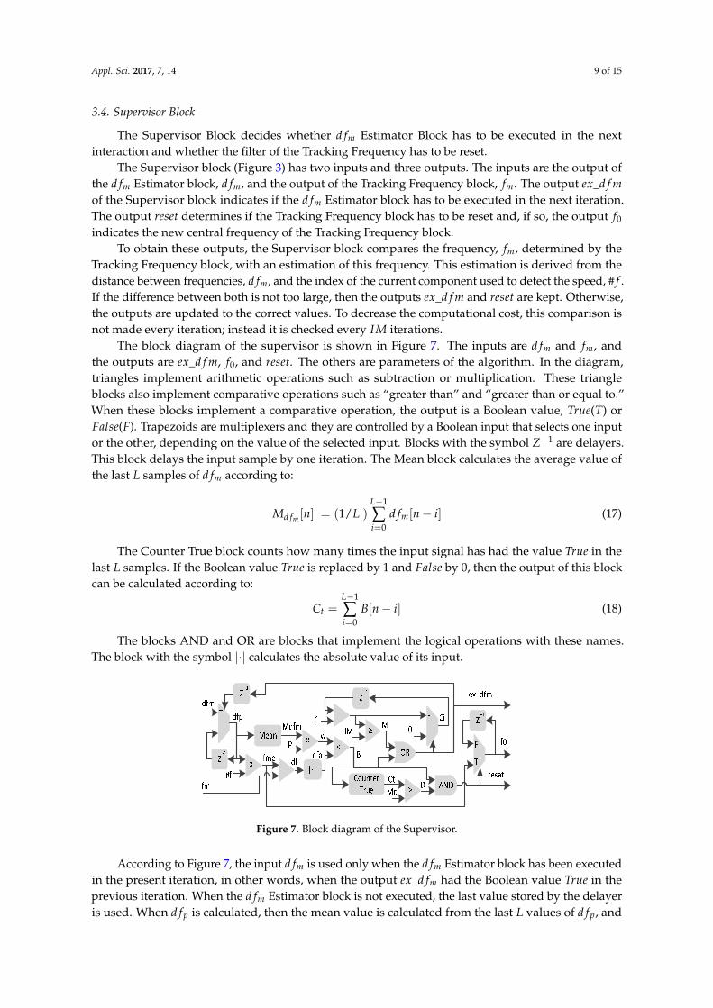
The block diagram of the supervisor is shown in Figure 7. The inputs are d fm and fm, andthe outputs are ex_d f m, f0, and reset. The others are parameters of the algorithm. In the diagram,triangles implement arithmetic operations such as subtraction or multiplication. These triangleblocks also implement comparative operations such as “greater than” and “greater than or equal to.”When these blocks implement a comparative operation, the output is a Boolean value, True(T) orFalse(F). Trapezoids are multiplexers and they are controlled by a Boolean input that selects one inputor the other, depending on the value of the selected input. Blocks with the symbol Z−1 are delayers.This block delays the input sample by one iteration. The Mean block calculates the average value ofthe last L samples of d fm according to:

Md fm [n] = (1/L )L−1

∑i=0

d fm[n− i] (17)

The Counter True block counts how many times the input signal has had the value True in thelast L samples. If the Boolean value True is replaced by 1 and False by 0, then the output of this blockcan be calculated according to:

Ct =L−1

∑i=0

B[n− i] (18)

The blocks AND and OR are blocks that implement the logical operations with these names.The block with the symbol |·| calculates the absolute value of its input.

Appl. Sci. 2016, 7, 14 9 of 14

The Supervisor block (Figure 3) has two inputs and three outputs. The inputs are the output of

the Estimator block, , and the output of the Tracking Frequency block, . The output

_ of the Supervisor block indicates if the Estimator block has to be executed in the next

iteration. The output determines if the Tracking Frequency block has to be reset and, if so, the

output indicates the new central frequency of the Tracking Frequency block.

To obtain these outputs, the Supervisor block compares the frequency, , determined by the

Tracking Frequency block, with an estimation of this frequency. This estimation is derived from the

distance between frequencies, , and the index of the current component used to detect the speed,

# . If the difference between both is not too large, then the outputs _ and are kept.

Otherwise, the outputs are updated to the correct values. To decrease the computational cost, this

comparison is not made every iteration; instead it is checked every iterations.

The block diagram of the supervisor is shown in Figure 7. The inputs are and , and the

outputs are _ , , and . The others are parameters of the algorithm. In the diagram,

triangles implement arithmetic operations such as subtraction or multiplication. These triangle blocks

also implement comparative operations such as “greater than” and “greater than or equal to.” When

these blocks implement a comparative operation, the output is a Boolean value, ( ) or ( ).

Trapezoids are multiplexers and they are controlled by a Boolean input that selects one input or the

other, depending on the value of the selected input. Blocks with the symbol are delayers. This

block delays the input sample by one iteration. The Mean block calculates the average value of the

last samples of according to:

1/ (17)

The Counter True block counts how many times the input signal has had the value in the

last samples. If the Boolean value is replaced by 1 and by 0, then the output of this

block can be calculated according to:

(18)

The blocks AND and OR are blocks that implement the logical operations with these names. The

block with the symbol | | calculates the absolute value of its input.

Figure 7. Block diagram of the Supervisor.

According to Figure 7, the input is used only when the Estimator block has been

executed in the present iteration, in other words, when the output _ had the Boolean value

in the previous iteration. When the Estimator block is not executed, the last value stored

by the delayer is used. When is calculated, then the mean value is calculated from the last

values of , and the estimation of the position of is also determined. This estimation, , is

Figure 7. Block diagram of the Supervisor.

According to Figure 7, the input d fm is used only when the d fm Estimator block has been executedin the present iteration, in other words, when the output ex_d fm had the Boolean value True in theprevious iteration. When the d fm Estimator block is not executed, the last value stored by the delayeris used. When d fp is calculated, then the mean value is calculated from the last L values of d fp, and

Appl. Sci. 2017, 7, 14 10 of 15

the estimation of the position of fm is also determined. This estimation, fme is obtained by multiplyingd fp by # f . The parameter # f is the position or index of the frequency peak used to detect the speed.The estimation of fme is not precise enough to be used to calculate the motor speed. For this reason,the Tracking Frequency block is used to improve precision. When fme has been calculated, the distancebetween fme and fm, named d fa, is calculated. This is done with a subtract block and an absolutevalue block. The maximum allowable distance between both frequencies, w, is obtained by calculatingthe mean value of d fp from the last L values, and multiplying this mean value by the parameter p,p being a value between 0 and 1. When d fa and w are calculated, both values are compared and B iscalculated. B is a Boolean value that indicates when w is lower than d fa. B indicates if the distancebetween fm and the estimation is within the allowable distance. B is used to calculate Ct according toEquation (18). Ct determines how many times the allowable distance between fm and the estimationhas been exceeded in the last L iterations. Next, D is calculated. D indicates if D indicates if Ct is largerthan the maximum allowable number of times the distance can be exceeded, Md. With the values Band D, the reset output is calculated, and it is Ture when both B and D are True. Also, when reset isTrue, the output f0 is updated with the fme value. If reset is False, the value of the previous iterationis kept.

The output ex_d f m is calculated with the values B and Mi. The output ex_d f m is True whenone or both values are True. Mi is True when the total of the counter Ci is bigger than the maximum,IM. The counter Ci is reset to zero when ex_d f m is True, and its count is increased when it is False.The output ex_d fm is True in two situations: (i) when the distance between fm and the estimation fme

is greater than the maximum allowable distance, w; and (ii) when ex_d f m has not been True for thelast IM iterations.

3.5. Converter

The Converter block (Figure 3) calculates the speed of the brushed dc motor, n, using the frequencyfm obtained by the Tracking Frequency block. Both values are related by a linear function according toEquation (9). Because the Tracking Frequency block tracks the component of the current with index # f ,the relation between fm and n will be:

n = fm·60/# f (19)

where n is the motor speed, fm is the output of the Tracking Frequency block, and # f is the index ofthe current component used to detect the motor speed.

4. Experimental Validation

This section describes the experimental procedure for validating the proposed method of motorspeed detection.

4.1. Description of the System

The system used to measure the accuracy of the proposed method was composed of a brushed dcmotor, a current sensor, a data acquisition card, and a computer. Figure 8 shows the experimental setup.

Appl. Sci. 2016, 7, 14 10 of 14

obtained by multiplying by # . The parameter # is the position or index of the frequency peak

used to detect the speed. The estimation of is not precise enough to be used to calculate the motor

speed. For this reason, the Tracking Frequency block is used to improve precision. When has

been calculated, the distance between and , named , is calculated. This is done with a

subtract block and an absolute value block. The maximum allowable distance between both

frequencies, , is obtained by calculating the mean value of from the last values, and

multiplying this mean value by the parameter , being a value between 0 and 1. When and

are calculated, both values are compared and is calculated. is a Boolean value that indicates

when is lower than . indicates if the distance between and the estimation is within the

allowable distance. is used to calculate according to Equation (18). determines how many

times the allowable distance between and the estimation has been exceeded in the last

iterations. Next, is calculated. indicates if is larger than the maximum allowable number of

times the distance can be exceeded, . With the values and , the output is calculated,

and it is when both and are . Also, when is , the output is updated

with the value. If is , the value of the previous iteration is kept.

The output _ is calculated with the values and . The output _ is when

one or both values are . is when the total of the counter is bigger than the

maximum, . The counter is reset to zero when _ is , and its count is increased

when it is . The output _ is in two situations: (i) when the distance between

and the estimation is greater than the maximum allowable distance, ; and (ii) when _

has not been for the last iterations.

3.5. Converter

The Converter block (Figure 3) calculates the speed of the brushed dc motor, , using the

frequency obtained by the Tracking Frequency block. Both values are related by a linear function

according to Equation (9). Because the Tracking Frequency block tracks the component of the current

with index # , the relation between and will be:

60/# (19)

where is the motor speed, is the output of the Tracking Frequency block, and # is the index

of the current component used to detect the motor speed.

4. Experimental Validation

This section describes the experimental procedure for validating the proposed method of motor

speed detection.

4.1. Description of the System

The system used to measure the accuracy of the proposed method was composed of a brushed

dc motor, a current sensor, a data acquisition card, and a computer. Figure 8 shows the experimental

setup.

Figure 8. Scheme of the system. Figure 8. Scheme of the system.

Appl. Sci. 2017, 7, 14 11 of 15

A universal machine set, H-REM-120-CM Universal Laboratory Machine (ULM) from Hampden®

Engineering Corporation (East Longmeadow, MA, USA), was used for the tests. This machine set iscoupled with a swinging frame dc dynamometer. The universal machine stator is composed of 24 slotswith 12-turn coils. The rotor of the universal machine is a 36-slot rotor with a two-pole, full-pitchdc winding composed of 72 four-turn coils connected to 72 commutator segments. This machinecan be connected in many different configurations, such as in single-phase induction, three-phaseinduction, synchronous, and a dc machine with series or shunt excitation. For this work, the machinewas connected with the topology of a brushed dc shunt motor. In this configuration, the motor hasa rating of 1 kW at 110 V.

The current sensor used was an AYA IBP 200:1 (Pulse Electronics, San Diego, CA, USA). This sensorhas a current transformer (CT) connected to a 2 Ω precision resistor (Caddock, Roseburg, OR, USA).The resistor leads convert the current to a voltage signal in order to be able to input it into the dataacquisition system. The current sensor was connected to the armature circuit near the motor brushes,as Figure 8 shows. Note that only the armature current was measured. A current transformer wasintentionally selected because it does not transform the dc current. This selection provides betterprecision in the measurement of the ac component. The data acquisition card used was a NI USB-6356from National Instruments (Austin, TX, USA). It has eight simultaneous analog inputs at a samplerate of 1.25 MS/s/ch, two analog outputs at 3.33 MS/s, and 24 digital I/O. One analog input wasconnected to the current sensor. The data acquisition card was connected to a computer.

The computer used was an ASUS Notebook K72Jk Series (Taipei, Taiwan) with an Intel® Core™ i3CPU M350 processor (Santa Clara, CA, USA), 4 GB RAM, and a 500 GB hard disk. The operating systemwas Windows 7, and the development environment was LabVIEW 2010 from National Instruments(Austin, TX, USA). The computer was configured to work in soft real time, and the data acquisitioncard was configured to acquire samples in a continuous mode.

It was necessary to measure the actual speed to compare the accuracy of the proposed method.The actual speed was measured with an encoder. The encoder used was a Monarch Instrument ACT3 Tachometer/Totalizer/Ratemeter (Amherst, NH, USA). This encoder was configured to output ananalog voltage proportional to the motor speed. The offset value and full scale speed values of theencoder were programmed to values close to the motor operating speed to achieve high resolution inthe speed measurement. The encoder and its connections are not included in Figure 8.

4.2. Data Collection

The motor was monitored in various situations to evaluate the accuracy of the proposed method.As previously described, measurements included the armature current and the real speed of the motor.The sampling rate was 100,000 samples per second (per channel) in continuous mode, Tb was onesecond and the employed window was bounded by fmin = 1000 Hz and fmax = 5000 Hz.

Three tests were performed in different operating modes: constant-speed, slowly changing speed,and rapidly changing speed. The first test involved testing 12 different constant speeds between 2000and 3000 rpm. This speed range was selected because this is the operating range of the tested motor.The second test consisted of slowly changing the motor speed from 2000 rpm to 2900 rpm. The thirdtest consisted of abruptly changing the speed from 2300 rpm to 2400 rpm. Motor speed changes wereaccomplished by changing the motor load and/or the field current.

For the three tests, the mean error and the standard deviation of the error were computed, both inabsolute value (rpm) and in relative value (%).

4.3. Comparison of the Predictions with the Measurements

The results of the first test, the constant-speed test, are shown in Table 1. This table contains,for the twelve tested speeds, the speed of the motor measured by the tachometer and the error in thespeed estimation. The average error and the standard deviation error were less than 1 rpm, and theirrelative values were less than 0.01%.

Appl. Sci. 2017, 7, 14 12 of 15

The results of the second test, the slowly changing speed test, are shown in Figure 9. The figureshows the real speed versus its estimation, and its error. The mean error during this test was 0.2863 rpmand the standard deviation error was 1.2670 rpm.

The results of the third test, the rapidly changing speed test, are shown in Figure 10. The figureshows the real speed versus its estimation, and its error. The mean error during this test was 0.6658 rpmand the standard deviation error was 1.1484 rpm.

Table 1. Speed measurement errors.

Speed (rpm)Average Error Deviation Error

Absolute (rpm) Relative (%) Absolute (rpm) Relative (%)

2004 0.141 0.007 0.319 0.0162103 0.146 0.007 0.425 0.0202204 0.159 0.007 0.402 0.0182297 0.089 0.004 0.286 0.0122400 0.008 0.001 0.188 0.0082500 0.173 0.007 0.214 0.0092603 0.241 0.009 0.371 0.0142705 0.183 0.007 0.380 0.0142803 0.111 0.004 0.224 0.0082913 0.254 0.009 0.114 0.0042998 0.336 0.011 0.112 0.004

Appl. Sci. 2016, 7, 14 12 of 14

The results of the second test, the slowly changing speed test, are shown in Figure 9. The figure

shows the real speed versus its estimation, and its error. The mean error during this test was 0.2863

rpm and the standard deviation error was 1.2670 rpm.

The results of the third test, the rapidly changing speed test, are shown in Figure 10. The figure

shows the real speed versus its estimation, and its error. The mean error during this test was 0.6658

rpm and the standard deviation error was 1.1484 rpm.

Table 1. Speed measurement errors.

Speed (rpm) Average Error Deviation Error

Absolute (rpm) Relative (%) Absolute (rpm) Relative (%) 2004 0.141 0.007 0.319 0.016 2103 0.146 0.007 0.425 0.020 2204 0.159 0.007 0.402 0.018 2297 0.089 0.004 0.286 0.012 2400 0.008 0.001 0.188 0.008 2500 0.173 0.007 0.214 0.009 2603 0.241 0.009 0.371 0.014 2705 0.183 0.007 0.380 0.014 2803 0.111 0.004 0.224 0.008 2913 0.254 0.009 0.114 0.004 2998 0.336 0.011 0.112 0.004

Figure 9. Actual and estimated speed for slow changes in speed.

Figure 10. Actual and estimated speed for fast changes in speed.

The three tests at constant‐speed, slowly changing speed, and rapidly changing speed,

performed between 2000 and 3000 rpm, showed an average error less than 1 rpm and a standard

deviation error less than 1.5 rpm. These results indicate that the proposed method works correctly

for constant speeds, slowly changing speeds, and rapidly changing speeds.

0 50 100 150 2002000

2200

2400

2600

2800

t (s)

(rpm

)

Real SpeedEstimation

0 50 100 150 200

-5

0

5

t(s)

(rp

m)

error

0 5 10 15 20 25 30

2340

2360

2380

2400

2420

t (s)

(rpm

)

0 5 10 15 20 25 30-5

0

5

t (s)

(rpm

)

Error

Real SpeedEstimation

Figure 9. Actual and estimated speed for slow changes in speed.

Appl. Sci. 2016, 7, 14 12 of 14

The results of the second test, the slowly changing speed test, are shown in Figure 9. The figure

shows the real speed versus its estimation, and its error. The mean error during this test was 0.2863

rpm and the standard deviation error was 1.2670 rpm.

The results of the third test, the rapidly changing speed test, are shown in Figure 10. The figure

shows the real speed versus its estimation, and its error. The mean error during this test was 0.6658

rpm and the standard deviation error was 1.1484 rpm.

Table 1. Speed measurement errors.

Speed (rpm) Average Error Deviation Error

Absolute (rpm) Relative (%) Absolute (rpm) Relative (%) 2004 0.141 0.007 0.319 0.016 2103 0.146 0.007 0.425 0.020 2204 0.159 0.007 0.402 0.018 2297 0.089 0.004 0.286 0.012 2400 0.008 0.001 0.188 0.008 2500 0.173 0.007 0.214 0.009 2603 0.241 0.009 0.371 0.014 2705 0.183 0.007 0.380 0.014 2803 0.111 0.004 0.224 0.008 2913 0.254 0.009 0.114 0.004 2998 0.336 0.011 0.112 0.004

Figure 9. Actual and estimated speed for slow changes in speed.

Figure 10. Actual and estimated speed for fast changes in speed.

The three tests at constant‐speed, slowly changing speed, and rapidly changing speed,

performed between 2000 and 3000 rpm, showed an average error less than 1 rpm and a standard

deviation error less than 1.5 rpm. These results indicate that the proposed method works correctly

for constant speeds, slowly changing speeds, and rapidly changing speeds.

0 50 100 150 2002000

2200

2400

2600

2800

t (s)

(rpm

)

Real SpeedEstimation

0 50 100 150 200

-5

0

5

t(s)

(rp

m)

error

0 5 10 15 20 25 30

2340

2360

2380

2400

2420

t (s)

(rpm

)

0 5 10 15 20 25 30-5

0

5

t (s)

(rpm

)

Error

Real SpeedEstimation

Figure 10. Actual and estimated speed for fast changes in speed.

Appl. Sci. 2017, 7, 14 13 of 15

The three tests at constant-speed, slowly changing speed, and rapidly changing speed, performedbetween 2000 and 3000 rpm, showed an average error less than 1 rpm and a standard deviation errorless than 1.5 rpm. These results indicate that the proposed method works correctly for constant speeds,slowly changing speeds, and rapidly changing speeds.

5. Conclusions

This paper has presented a new sensorless method to estimate the speed of brushed dc motorswith a large number of coils, such as in integral horsepower brushed dc motors. The method has thefollowing features:

(1) It is a novel method that cannot be classified in any of the previous existing sensorless groups;it cannot be classified in either the group of methods based on the dynamic model or the groupof methods based on the ripple component. It belongs to a new sensorless group that studies thespectral components of the current and has the advantages of both existing groups.

(2) It requires only the measurement of the current of the brushed dc motor for speed estimation.In contrast, other methods for brushed dc motors with a large number of coils require themeasurements of both current and voltage.

(3) It can be used for brushed dc motors with a large number of coils, such as integral horsepowerbrushed dc motors. In contrast, other methods based on the ripple component that only measurethe current can only be used in brushed dc motors with a low number of coils where the ripplecomponent is big enough.

(4) It achieves a low error in speed estimation in the performed tests. Its average error is less than1 rpm and the standard deviation error is less than 1.5 rpm for speeds between 2000 and 3000 rpmfor an H-REM-120-CM motor configured as a brushed dc motor with shunt configuration.

Author Contributions: The present work was done in three stages. The first stage consisted of the work proposaland article plan, and the second stage consisted of the data acquisition and the data processing. Both thefirst and second stages were carried out by Ernesto Vazquez-Sanchez and Joseph Sottile in Lexington, USA,during a doctoral short-term stay that Ernesto Vazquez-Sanchez conducted at the University of Kentucky.The third stage, which consisted of the article writing, was done collaboratively by the three authors, whileErnesto Vazquez-Sanchez and Jaime Gomez-Gil were at the University of Valladolid, Spain, and while JosephSottile was at the University of Kentucky, USA.

Conflicts of Interest: The authors declare no conflict of interest.

References

1. Sul, S. Control of Electric Machine Drive System, 1st ed.; Wiley-IEEE Press: Piscataway, NJ, USA, 2011.2. Hilairet, M.; Auger, F. Speed sensorless control of a DC-motor via adaptive filters. IET Electr. Power Appl.

2007, 1, 601–610. [CrossRef]3. Chevrel, P.; Siala, S. Robust DC-motor speed control without any mechanical sensor. In Proceedings of the

IEEE International Conference on Control Applications, Hartford, CT, USA, 5–7 October 1997; pp. 244–246.4. Yachiangkam, S.; Prapanavarat, C.; Yungyuen, U.; Po-ngam, S. Speed-sensorless separately excited DC

Motor drive with an adaptive observer. In Proceedings of the IEEE Technical Conference on Computers,Communications, Control and Power Engineering (TENCON 2004), Chiang Mai, Thailand, 21–24 November2004; Volume D, pp. 163–166.

5. Kowal, D.; Patan, M.; Paszke, W.; Romanek, A. Sequential design for model calibration in iterative learningcontrol of DC motor. In Proceedings of the 20th International Conference on Methods and Models inAutomation and Robotics (MMAR), Miedzydroje, Poland, 24–27 August 2015; pp. 794–799.

6. Lobosco, O.S. Modeling and simulation of DC motors in dynamic conditions allowing for the armaturereaction. IEEE Trans. Energy Convers. 1999, 14, 1288–1293. [CrossRef]

7. Bowes, S.R.; Sevinc, A.; Holliday, D. New natural observer applied to speed-sensorless DC servo andinduction motors. IEEE Trans. Ind. Electron. 2004, 51, 1025–1032. [CrossRef]

Appl. Sci. 2017, 7, 14 14 of 15

8. Cupertino, F.; Pellegrino, G.; Giangrande, P.; Salvatore, L. Sensorless Position Control of Permanent-MagnetMotors With Pulsating Current Injection and Compensation of Motor End Effects. IEEE Trans. Ind. Appl.2011, 47, 1371–1379. [CrossRef]

9. Kiyoshi, O.; Yoshihiro, N.; Yoshihisa, H.; Hirokazu, K. High-performance speed control based onan instantaneous speed observer considering the characteristics of a dc chopper in a low speed range.Electr. Eng. Jpn. 2000, 130, 77–87.

10. Castaneda, C.E.; Loukianov, A.G.; Sanchez, E.N.; Castillo-Toledo, B. Discrete-time neural sliding-mode blockcontrol for a DC Motor with controlled flux. IEEE Trans. Ind. Electron. 2012, 59, 1194–1207. [CrossRef]

11. Liu, Z.Z.; Luo, F.L.; Rashid, M.H. Speed nonlinear control of DC motor drive with field weakening. IEEE Trans.Ind. Appl. 2003, 39, 417–423.

12. Scott, J.; McLeish, J.; Round, W.H. Speed control with low armature loss for very small sensorless brushed dcmotors. IEEE Trans. Ind. Electron. 2009, 56, 1223–1229. [CrossRef]

13. Farkas, F.; Halász, S.; Kádár, I. Speed Sensorless Neuro-Fuzzy Controller for Brush type DC Machines.In Proceedings of the 5th International Symposium of Hungarian Researchers on Computational Intelligence,Budapest, Hungray, 11–12 November 2004; pp. 147–158.

14. Weerasooriya, S.; El-Sharkawi, M.A. Identification and control of a DC motor using back-propagation neuralnetworks. IEEE Trans. Energy Convers. 1991, 6, 663–669. [CrossRef]

15. Aydogmus, O.; Talu, M.F. Comparison of Extended-Kalman- and Particle-Filter-Based Sensorless SpeedControl. IEEE Trans. Instrum. Meas. 2012, 61, 402–410. [CrossRef]

16. Razi, R.; Monfared, M. Simple control scheme for single-phase uninterruptible power supply inverters withKalman filter-based estimation of the output voltage. IET Power Electron. 2015, 8, 1817–1824. [CrossRef]

17. Radcliffe, P.; Kumar, D. Sensorless speed measurement for brushed DC motors. IET Power Electron. 2015, 8,2223–2228. [CrossRef]

18. Afjei, E.; Ghomsheh, A.N.; Karami, A. Sensorless speed/position control of brushed DC motor.In Proceedings of the International Aegean Conference on Electrical Machines and Power Electronics(ACEMP’07), Bodrum, Turkey, 10–12 September 2007; pp. 730–732.

19. Sincero, G.C.R.; Cros, J.; Viarouge, P. Arc Models for Simulation of Brush Motor Commutations.IEEE Trans. Magn. 2008, 44, 1518–1521. [CrossRef]

20. Figarella, T.; Jansen, M.H. Brush wear detection by continuous wavelet transform. Mech. Syst. Signal Process.2007, 21, 1212–1222. [CrossRef]

21. Yuan, B.; Hu, Z.; Zhou, Z. Expression of sensorless speed estimation in direct current motor with simplexlap winding. In Proceedings of the IEEE International Conference on Mechatronics and Automation,(ICMA 2007), Harbin, China, 5–8 August 2007; pp. 816–821.

22. Lott, J.; Burke, D. Brushed Motor Position Control Based Upon Back Current Detection. U.S. Patent20060261763 A1, 23 November 2006.

23. Won-Sang, R.; Hye-Jin, L.; Jin Bae, P.; Tae-Sung, Y. Practical Pinch Detection Algorithm for Smart AutomotivePower Window Control Systems. IEEE Trans. Ind. Electr. 2008, 55, 1376–1384.

24. Micke, M.; Sievert, H.; Hachtel, J.; Hertlein, G. Method and Device for Measuring the Rotational Speedof a Pulse-Activated Electric Motor Based on a Frequency of Current Ripples. U.S. Patent 7265538 B2,4 September 2007.

25. Vazquez-Sanchez, E.; Gomez-Gil, J.; Rodriguez-Alvarez, M. Analysis of three methods for sensorless speeddetection in DC motors. In Proceedings of the IEEE International Conference on Power Engineering, Energyand Electrical Drives (POWERENG ‘09), 18–20 March 2009; pp. 117–122.

26. Kessler, E.; Schulter, W. Method for Establishing the Rotational Speed of Mechanically Commutated DCMotors. U.S. Patent 6144179 A, 7 November 2000.

27. Vazquez-Sanchez, E.; Gomez-Gil, J.; Gamazo-Real, J.C.; Diez-Higuera, J.F. A new method for sensorlessestimation of the speed and position in brushed dc motors using support vector machines. IEEE Trans.Ind. Electron. 2012, 59, 1397–1408. [CrossRef]

28. Moller, D.D.; Schneider, P.K.; Canales, S.A. Voltage-Sensitive Oscillator Frequency for Rotor PositionDetection Scheme. U.S. Patent 7352145 B2, 1 April 2008.

29. Toliyat, H.A.; Kliman, G.B. Handbook of Electric Motors; CRC Press: Boca Raton, FL, USA, 2004.30. Chiasson, J. Modeling and High Performance Control of Electric Machines, 1st ed.; Wiley-IEEE Press: Hoboken,

NJ, USA, 2005.

Appl. Sci. 2017, 7, 14 15 of 15

31. Yarlagadda, R.K.R. Analog and Digital Signals and Systems, 1st ed.; Springer Publishing Company,Incorporated: Stillwater, OK, USA, 2009.

32. Egan, W. Phase-Lock Basics, 2nd ed.; Wiley-IEEE Press: Hoboken, NJ, USA, 2007.

© 2016 by the authors; licensee MDPI, Basel, Switzerland. This article is an open accessarticle distributed under the terms and conditions of the Creative Commons Attribution(CC-BY) license (http://creativecommons.org/licenses/by/4.0/).