A New Simple Square Root Option Pricing Model

Antonio Camara & Yaw-Huei Wang

Yaw-Huei WangAssociate Professor

Department of Finance

National Taiwan University

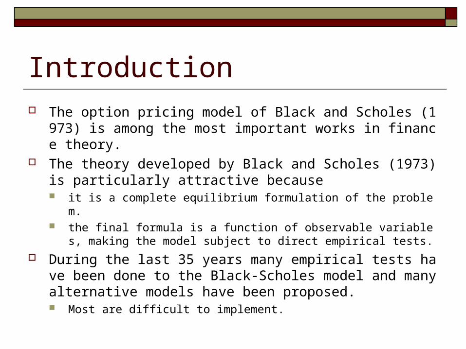
Introduction The option pricing model of Black and Scholes (1973) is amo

ng the most important works in finance theory. The theory developed by Black and Scholes (1973) is particul

arly attractive because it is a complete equilibrium formulation of the problem. the final formula is a function of observable variables, making the mo

del subject to direct empirical tests.

During the last 35 years many empirical tests have been done to the Black-Scholes model and many alternative models have been proposed. Most are difficult to implement.

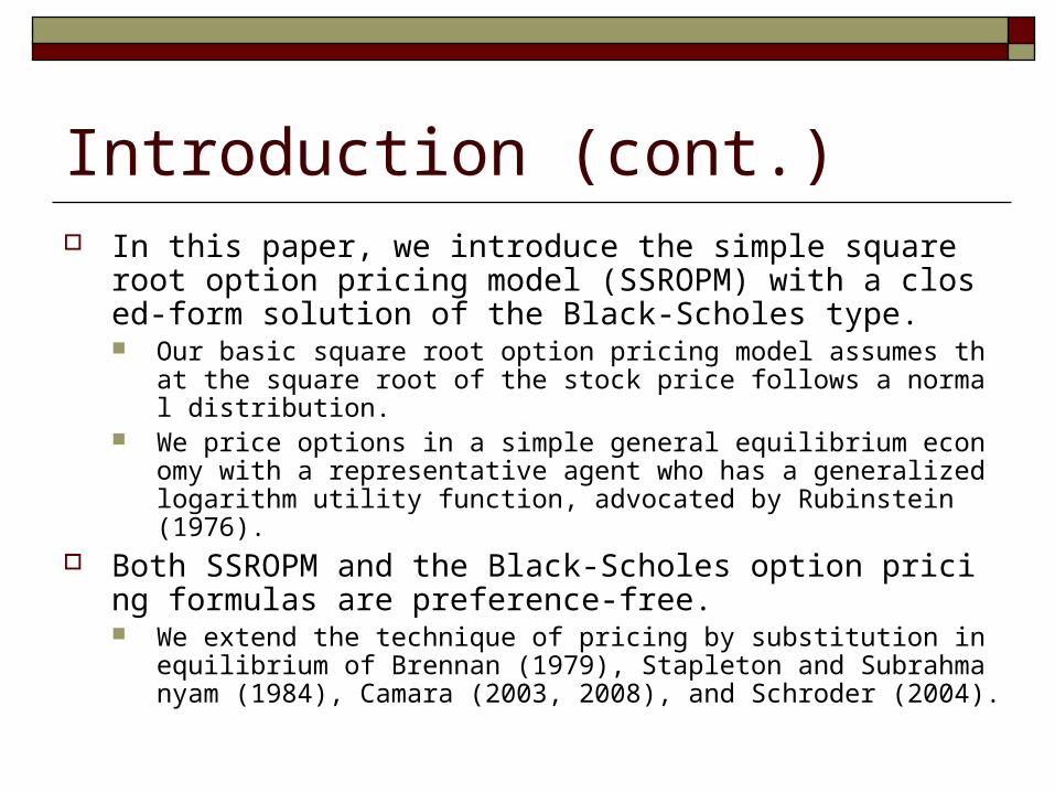
Introduction (cont.) In this paper, we introduce the simple square root option prici

ng model (SSROPM) with a closed-form solution of the Black-Scholes type. Our basic square root option pricing model assumes that the square ro

ot of the stock price follows a normal distribution. We price options in a simple general equilibrium economy with a rep

resentative agent who has a generalized logarithm utility function, advocated by Rubinstein (1976).

Both SSROPM and the Black-Scholes option pricing formulas are preference-free. We extend the technique of pricing by substitution in equilibrium of

Brennan (1979), Stapleton and Subrahmanyam (1984), Camara (2003, 2008), and Schroder (2004).

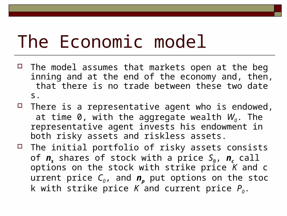
The Economic model The model assumes that markets open at the beginning and at

the end of the economy and, then, that there is no trade between these two dates.

There is a representative agent who is endowed, at time 0, with the aggregate wealth W0. The representative agent invests his endowment in both risky assets and riskless assets.

The initial portfolio of risky assets consists of ns shares of stock with a price S0, nc call options on the stock with strike price K and current price C0, and np put options on the stock with strike price K and current price P0.

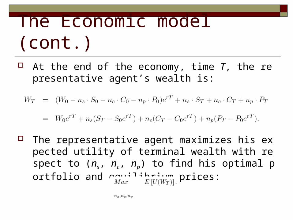
The Economic model (cont.) At the end of the economy, time T, the representative agent’s

wealth is:

The representative agent maximizes his expected utility of terminal wealth with respect to (ns, nc, np) to find his optimal portfolio and equilibrium prices:

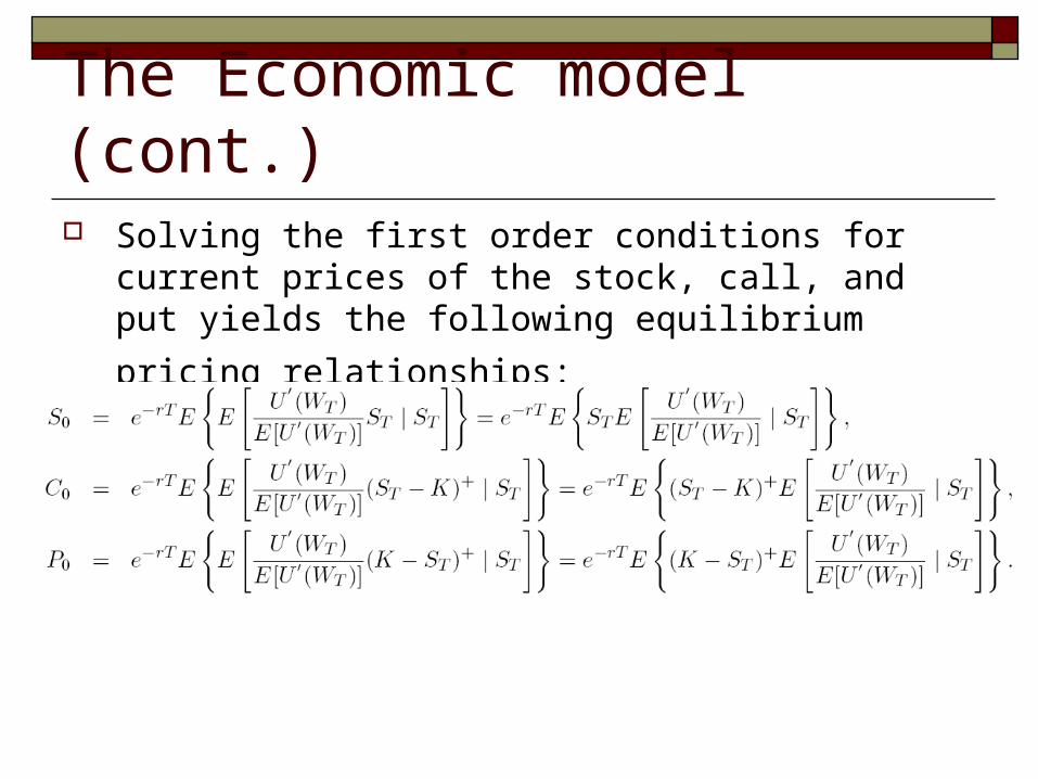
The Economic model (cont.) Solving the first order conditions for current prices of the

stock, call, and put yields the following equilibrium pricing

relationships:

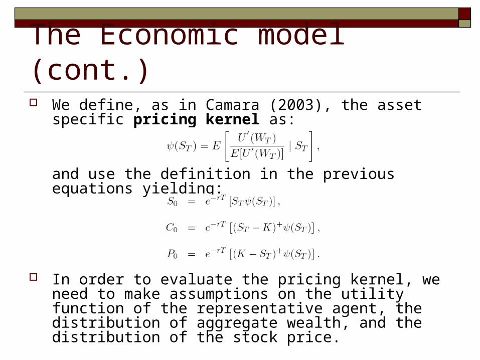
The Economic model (cont.) We define, as in Camara (2003), the asset specific pricing

kernel as:

and use the definition in the previous equations yielding:

In order to evaluate the pricing kernel, we need to make assumptions on the utility function of the representative agent, the distribution of aggregate wealth, and the distribution of the stock price.

The Economic model (cont.)

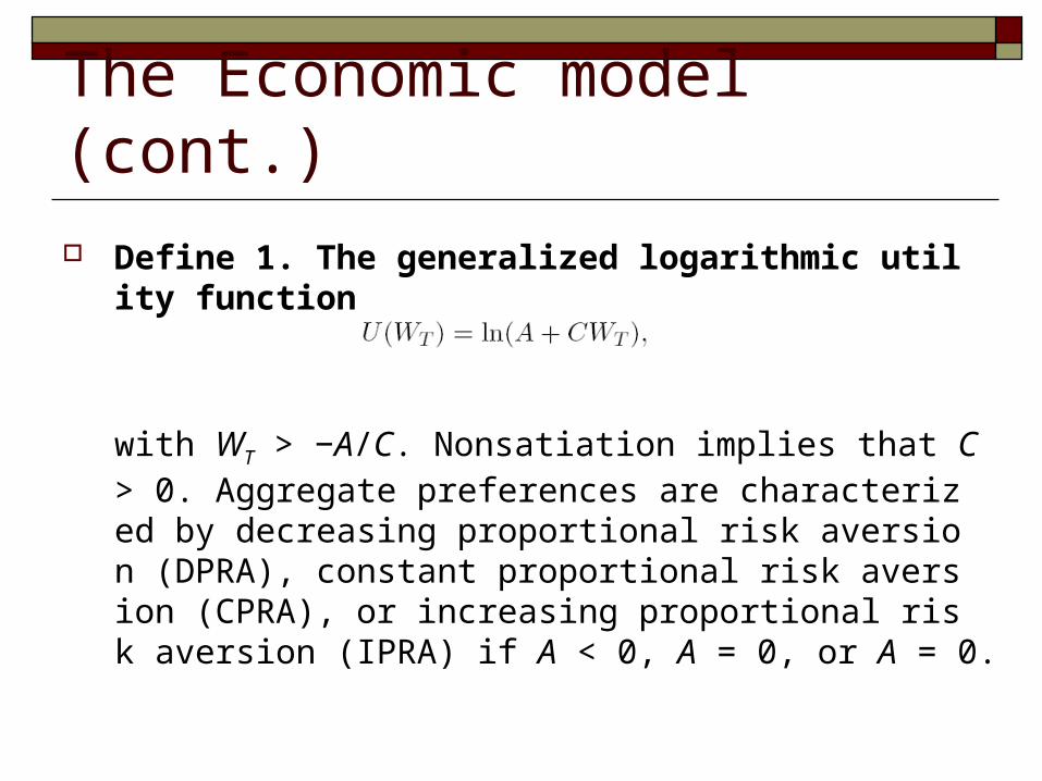
Define 1. The generalized logarithmic utility function

with WT > −A/C. Nonsatiation implies that C > 0. Aggregate preferences are characterized by decreasing proportional risk aversion (DPRA), constant proportional risk aversion (CPRA), or increasing proportional risk aversion (IPRA) if A < 0, A = 0, or A = 0.

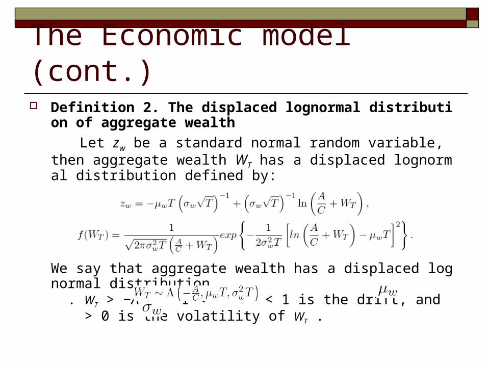
The Economic model (cont.) Definition 2. The displaced lognormal distribution of aggr

egate wealth

Let zw be a standard normal random variable, then aggregate wealth WT has a displaced lognormal distribution defined by:

We say that aggregate wealth has a displaced lognormal distribution . WT > −A/C, −1 < < 1 is the drift, and > 0 is the volatility of WT .

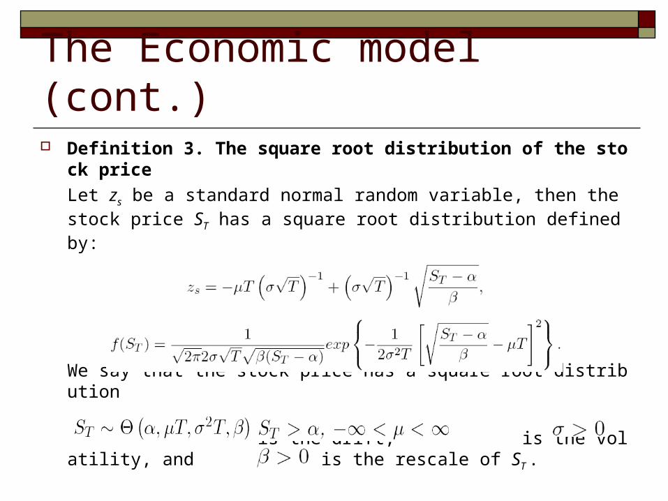
The Economic model (cont.) Definition 3. The square root distribution of the stock pric

e

Let zs be a standard normal random variable, then the stock price ST has a square root distribution defined by:

We say that the stock price has a square root distribution

. is the drift, is the volatility, and is the rescale of ST .

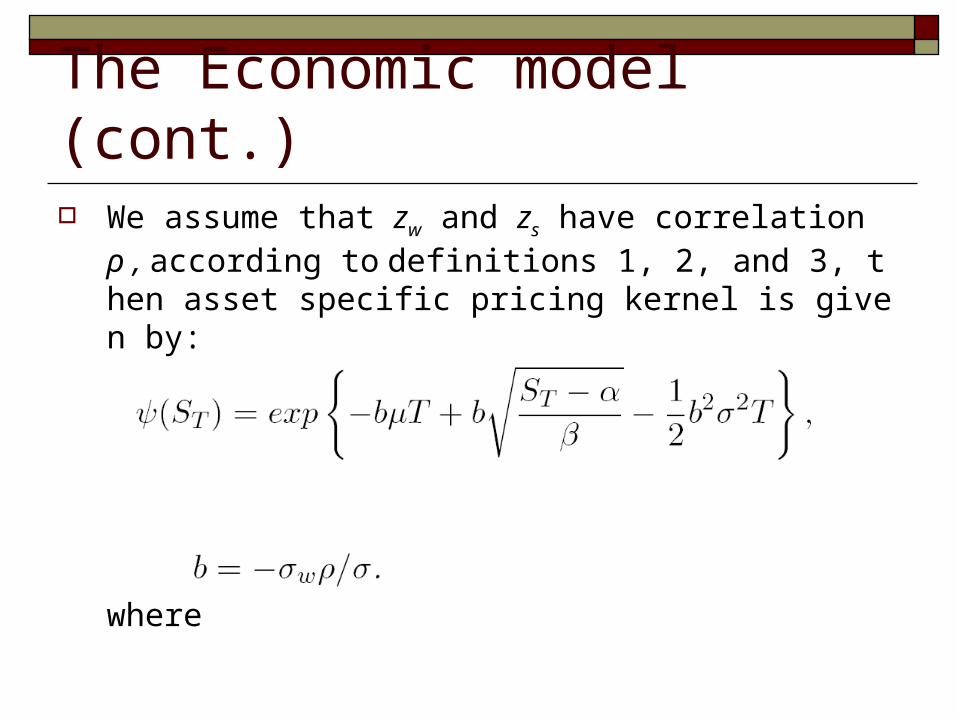
The Economic model (cont.) We assume that zw and zs have correlation ρ , according to def

initions 1, 2, and 3, then asset specific pricing kernel is given by:

where

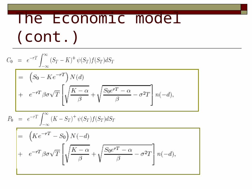
The Economic model (cont.)

The Economic model (cont.)

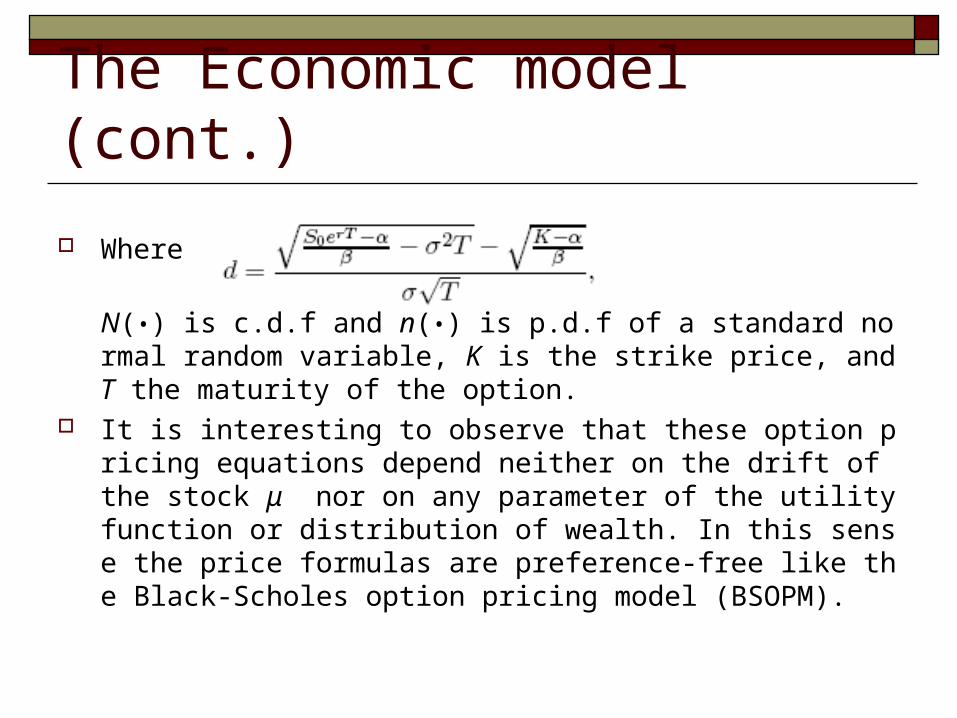
Where

N(•) is c.d.f and n(•) is p.d.f of a standard normal random variable, K is the strike price, and T the maturity of the option.

It is interesting to observe that these option pricing equations depend neither on the drift of the stock μ nor on any parameter of the utility function or distribution of wealth. In this sense the price formulas are preference-free like the Black-Scholes option pricing model (BSOPM).

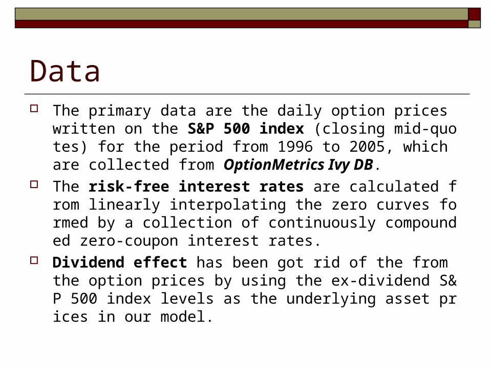
Data The primary data are the daily option prices written on the S

&P 500 index (closing mid-quotes) for the period from 1996 to 2005, which are collected from OptionMetrics Ivy DB.

The risk-free interest rates are calculated from linearly interpolating the zero curves formed by a collection of continuously compounded zero-coupon interest rates.

Dividend effect has been got rid of the from the option prices by using the ex-dividend S&P 500 index levels as the underlying asset prices in our model.

Data (cont.) Only out-of-money options are used since out-of-money

options are usually traded more heavily than in-the-money options.

The option prices are filtered using some additional criteria: Firstly, we exclude those option prices that violate any arbitrage-free

bounds. Secondly, we exclude prices of options with time-to-maturities less

than seven calendar days in order to avoid the liquidity issue imposed on the short-maturity options.

Thirdly, we also ignore those options with prices less than 0.5 as these option prices could be insensitive to the information flow.

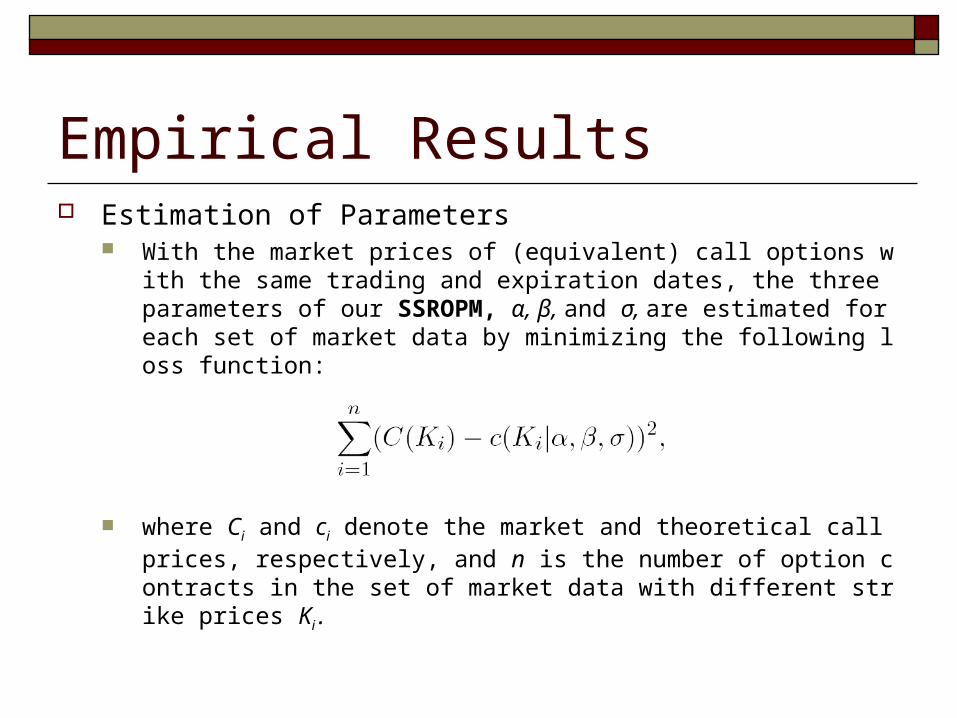
Empirical Results Estimation of Parameters

With the market prices of (equivalent) call options with the same trading and expiration dates, the three parameters of our SSROPM, α, β, and σ, are estimated for each set of market data by minimizing the following loss function:

where Ci and ci denote the market and theoretical call prices, respectively, and n is the number of option contracts in the set of market data with different strike prices Ki .

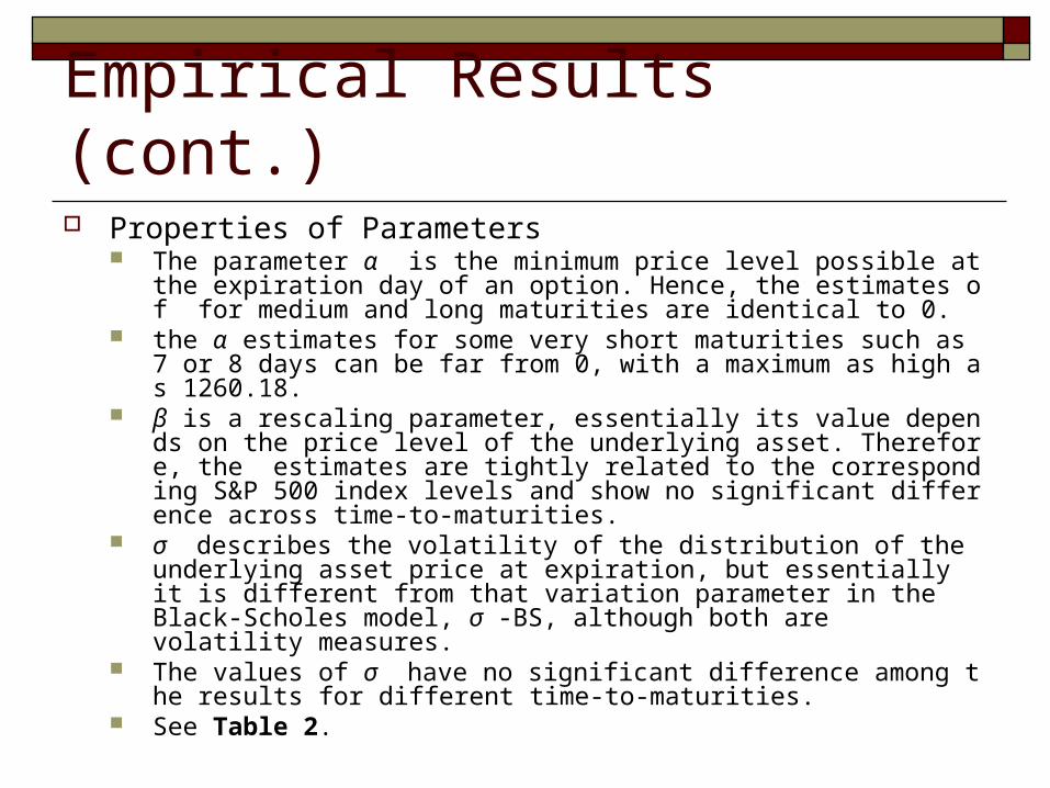
Empirical Results (cont.) Properties of Parameters

The parameter α is the minimum price level possible at the expiration day of an option. Hence, the estimates of for medium and long maturities are identical to 0.

the α estimates for some very short maturities such as 7 or 8 days can be far from 0, with a maximum as high as 1260.18.

β is a rescaling parameter, essentially its value depends on the price level of the underlying asset. Therefore, the estimates are tightly related to the corresponding S&P 500 index levels and show no significant difference across time-to-maturities.

σ describes the volatility of the distribution of the underlying asset price at expiration, but essentially it is different from that variation parameter in the Black-Scholes model, σ -BS, although both are volatility measures.

The values of σ have no significant difference among the results for different time-to-maturities.

See Table 2.

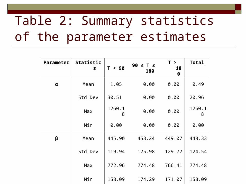
Table 2: Summary statistics of the parameter estimates

Parameter Statistics T < 90 90 ≤ T ≤ 180 T > 180 Total

α Mean 1.05 0.00 0.00 0.49

Std Dev 30.51 0.00 0.00 20.96

Max 1260.18 0.00 0.00 1260.18

Min 0.00 0.00 0.00 0.00

β Mean 445.90 453.24 449.07 448.33

Std Dev 119.94 125.98 129.72 124.54

Max 772.96 774.48 766.41 774.48

Min 158.09 174.29 171.07 158.09

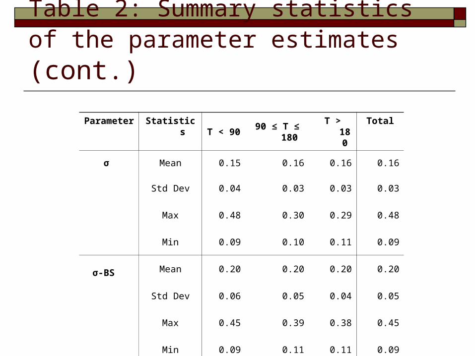
Table 2: Summary statistics of the parameter estimates (cont.)

Parameter Statistics T < 90 90 ≤ T ≤ 180 T > 180 Total

σ Mean 0.15 0.16 0.16 0.16

Std Dev 0.04 0.03 0.03 0.03

Max 0.48 0.30 0.29 0.48

Min 0.09 0.10 0.11 0.09

σ-BS Mean 0.20 0.20 0.20 0.20

Std Dev 0.06 0.05 0.04 0.05

Max 0.45 0.39 0.38 0.45

Min 0.09 0.11 0.11 0.09

Empirical Results (cont.) Fitting Errors of Option Prices

The price fitting errors are measured by the absolute differences between the theoretical and market prices for the SSROPM and Black-Sch

oles model respectively. The errors are also measured in terms of the Black-Scholes implied v

olatility. Regardless of which moenyness and/or time-to-maturity is considere

d, the price fitting errors of SSROPM are much lower than those of the Black-Scholes model. See Table 3.

The results of Wilcoxon’s Signed-Rank Test still strongly support the superiority of SSROPM. See Table 4.

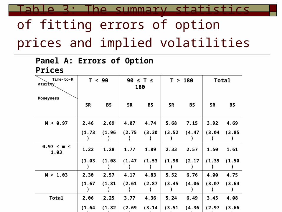
Table 3: The summary statistics of fitting errors

of option prices and implied volatilities Panel A: Errors of Option Prices

Time-to-Maturity

Moneyness

T < 90 90 ≤ T ≤ 180 T > 180 Total

SR BS SR BS SR BS SR BS

M < 0.97 2.46 2.69 4.07 4.74 5.68 7.15 3.92 4.69

(1.73) (1.96) (2.75) (3.30) (3.52) (4.47) (3.04) (3.85)

0.97 ≤ m ≤ 1.03 1.22 1.28 1.77 1.89 2.33 2.57 1.50 1.61

(1.03) (1.08) (1.47) (1.53) (1.98) (2.17) (1.39) (1.50)

M > 1.03 2.30 2.57 4.17 4.83 5.52 6.76 4.00 4.75

(1.67) (1.81) (2.61) (2.87) (3.45) (4.06) (3.07) (3.64)

Total 2.06 2.25 3.77 4.36 5.24 6.49 3.45 4.08

(1.64) (1.82) (2.69) (3.14) (3.51) (4.36) (2.97) (3.66)

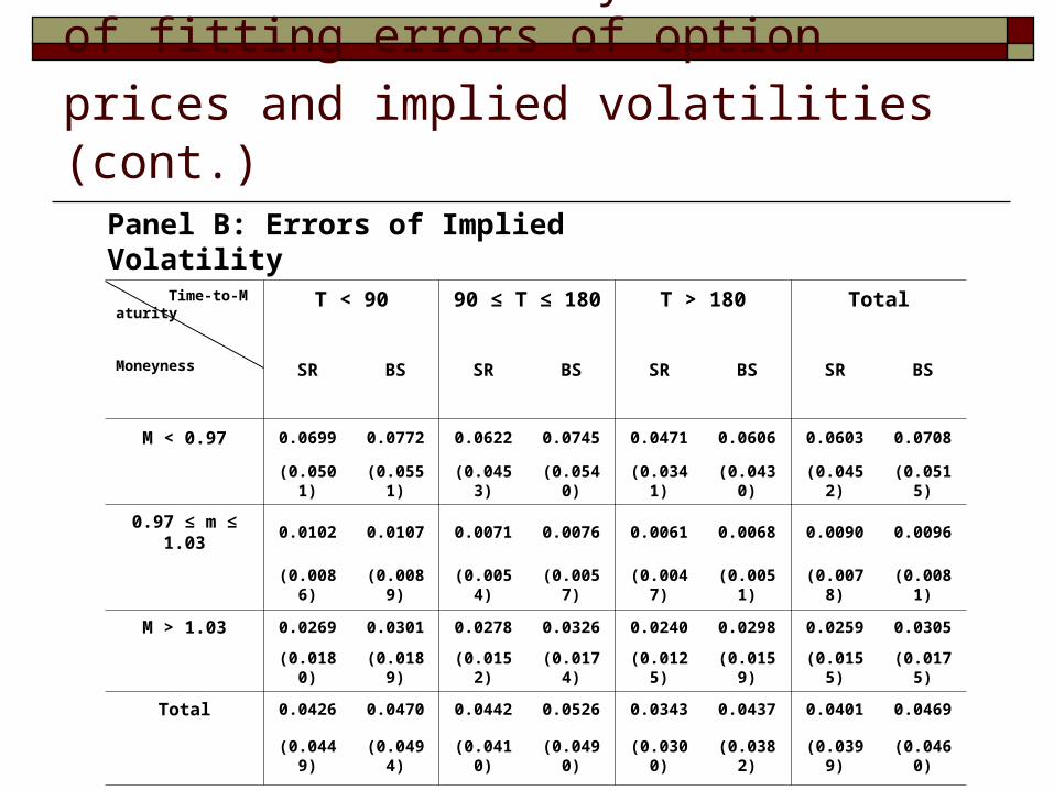
Table 3: The summary statistics of fitting errors

of option prices and implied volatilities (cont.)

Panel B: Errors of Implied Volatility

Time-to-Maturity

Moneyness

T < 90 90 ≤ T ≤ 180 T > 180 Total

SR BS SR BS SR BS SR BS

M < 0.97 0.0699 0.0772 0.0622 0.0745 0.0471 0.0606 0.0603 0.0708

(0.0501) (0.0551) (0.0453) (0.0540) (0.0341) (0.0430) (0.0452) (0.0515)

0.97 ≤ m ≤ 1.03 0.0102 0.0107 0.0071 0.0076 0.0061 0.0068 0.0090 0.0096

(0.0086) (0.0089) (0.0054) (0.0057) (0.0047) (0.0051) (0.0078) (0.0081)

M > 1.03 0.0269 0.0301 0.0278 0.0326 0.0240 0.0298 0.0259 0.0305

(0.0180) (0.0189) (0.0152) (0.0174) (0.0125) (0.0159) (0.0155) (0.0175)

Total 0.0426 0.0470 0.0442 0.0526 0.0343 0.0437 0.0401 0.0469

(0.0449) (0.0494) (0.0410) (0.0490) (0.0300) (0.0382) (0.0399) (0.0460)

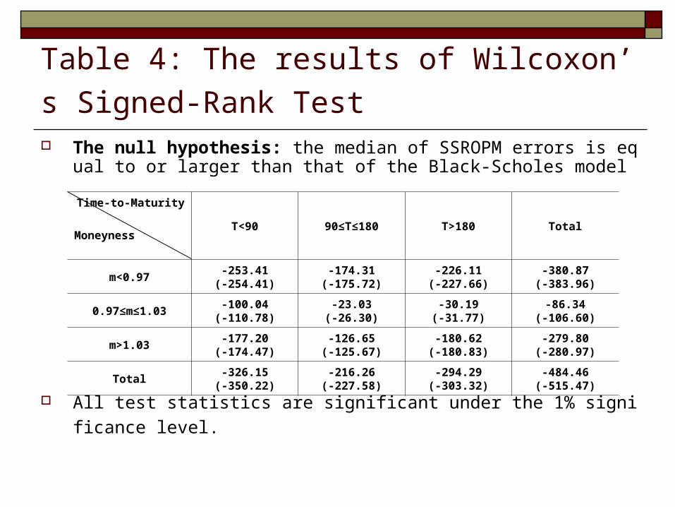
Table 4: The results of Wilcoxon’s Signed-Rank

Test The null hypothesis: the median of SSROPM errors is equal to or larger t

han that of the Black-Scholes model

All test statistics are significant under the 1% significance level.

Time-to-Maturity

MoneynessT<90 90≤T≤180 T>180 Total

m<0.97-253.41

(-254.41)-174.31

(-175.72)-226.11

(-227.66)-380.87

(-383.96)

0.97≤m≤1.03-100.04

(-110.78)-23.03

(-26.30)-30.19

(-31.77)-86.34

(-106.60)

m>1.03-177.20

(-174.47)-126.65

(-125.67)-180.62

(-180.83)-279.80

(-280.97)

Total-326.15

(-350.22)-216.26

(-227.58)-294.29

(-303.32)-484.46

(-515.47)

Empirical Results (cont.) Patterns of Implied Volatility Functions

We select four horizons, 30, 60, 120, and 240 days, to investigate the patterns of implied volatility functions of the SSROPM and the Black-Scholes model.

Firstly, we use the averages of those parameters estimated in the first step as the inputs of the two alternative models.

Secondly, we use the parameter averages to compute the theoretical call prices with various strike prices in terms of moneyness defined by the strike price over the forward price.

Finally, all theoretical prices are converted into Black-Scholes implied volatilities, which are plotted against their moneynesses for the four different time-to-maturities.

See Figure 1.

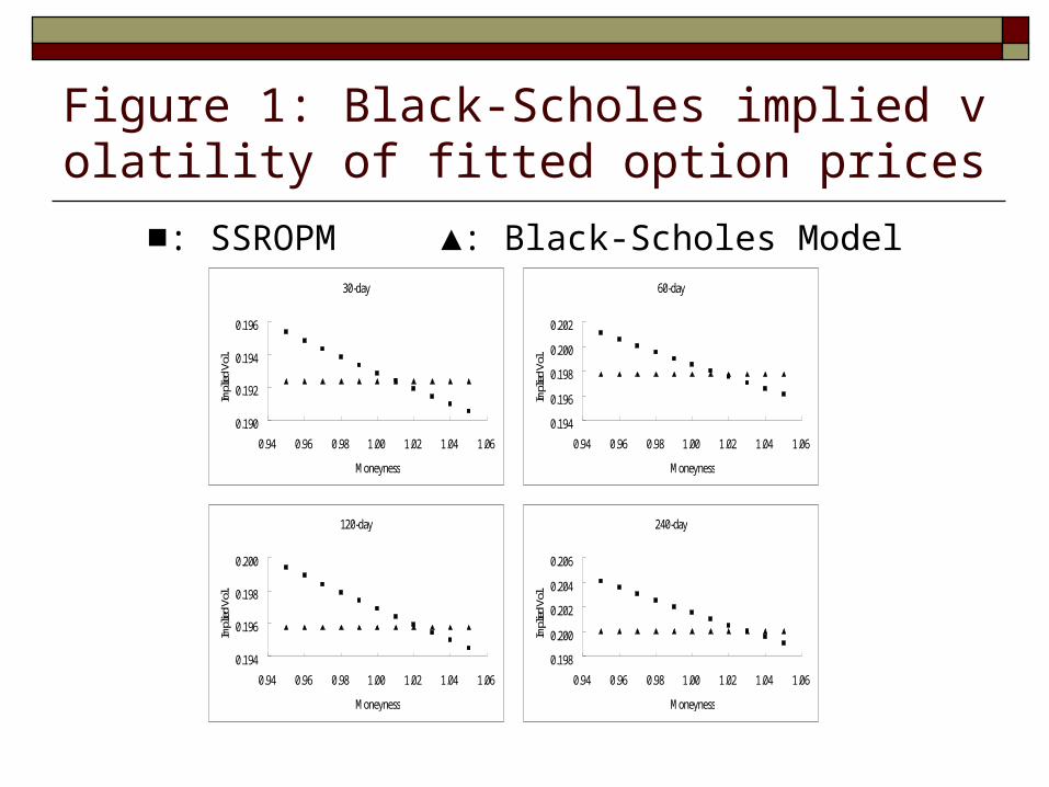
Figure 1: Black-Scholes implied volatility of fitted option prices

■: SSROPM ▲: Black-Scholes Model30-day

0.190

0.192

0.194

0.196

0.94 0.96 0.98 1.00 1.02 1.04 1.06

Moneyness

Impli

ed V

ol.

60-day

0.194

0.196

0.198

0.200

0.202

0.94 0.96 0.98 1.00 1.02 1.04 1.06

Moneyness

Impli

ed V

ol.120-day

0.194

0.196

0.198

0.200

0.94 0.96 0.98 1.00 1.02 1.04 1.06

Moneyness

Impli

ed V

ol.

240-day

0.198

0.200

0.202

0.204

0.206

0.94 0.96 0.98 1.00 1.02 1.04 1.06

Moneyness

Impli

ed V

ol.

Concluding Remarks Rather than assuming that the logarithm of the stock price fol

lows a normal distribution, e.g. Black-Scholes model, we assume that the square root of the stock price follows a normal distribution, and price options in a simple general equilibrium economy with a representative agent who has a generalized logarithmic utility function.

Compared to the Black-Scholes model, our square root option pricing model has two more parameters, but is still easy to implement.

The square root option pricing model produces significantly smaller fitting errors of option prices and generates a negatively sloped implied volatility function.